density driven flow in porous media: how accurate are our models?
DESCRIPTION
Density driven flow in porous media: How accurate are our models?. Wolfgang Kinzelbach Institute for Hydromechanics and Water Resources Engineering Swiss Federal Institute of Technology, Zurich, Switzerland. Contents. Examples of density driven flow in aquifers Equations Formulation - PowerPoint PPT PresentationTRANSCRIPT
Density driven flow in porous media: How accurate are our models?
Wolfgang Kinzelbach
Institute for Hydromechanics and Water Resources Engineering
Swiss Federal Institute of Technology, Zurich, Switzerland

Contents
• Examples of density driven flow in aquifers• Equations
– Formulation– Special features of density driven flows
• Benchmarks– Analytical and exact solutions– Experimental benchmark: Grid convergence– Experimental benchmark: Fingering problem
• Upscaling issues• Conclusions
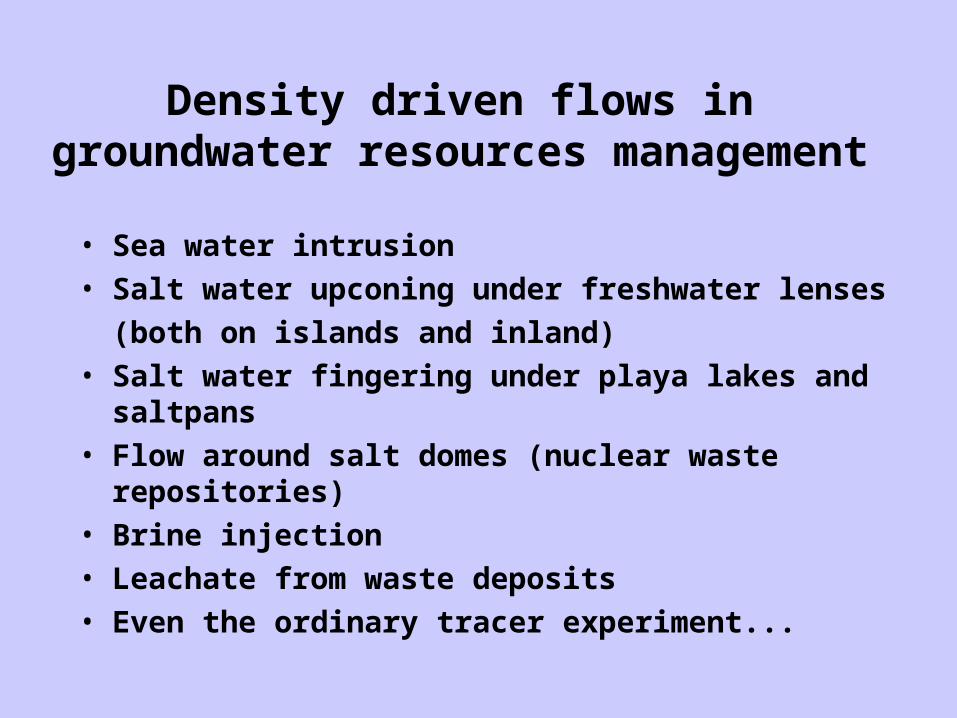
Density driven flows in groundwater resources management
• Sea water intrusion• Salt water upconing under freshwater lenses
(both on islands and inland)• Salt water fingering under playa lakes and saltpans• Flow around salt domes (nuclear waste repositories)• Brine injection• Leachate from waste deposits• Even the ordinary tracer experiment...

Saltwater Intrusion
Salt waterFresh water
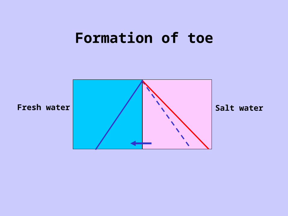
Formation of toe
Fresh water Salt water
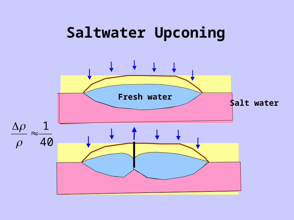
Saltwater Upconing
Salt waterFresh water
40
1

Example: Salt Water Upconing on Wei Zhou Island
Thesis Li Guomin

Upconing
Freshwater Lens
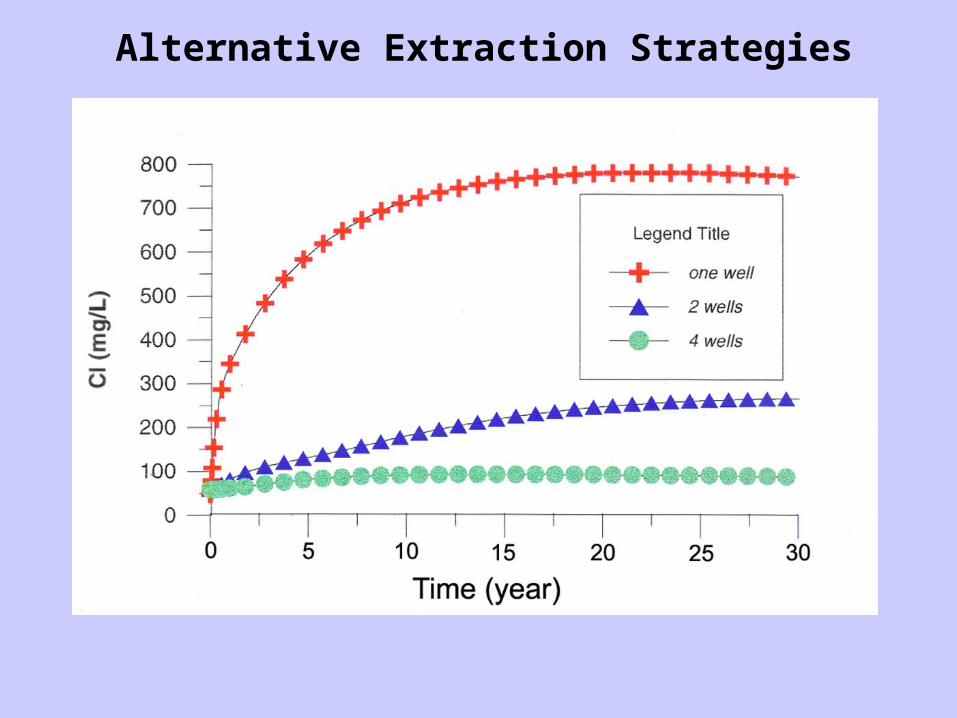
Alternative Extraction Strategies
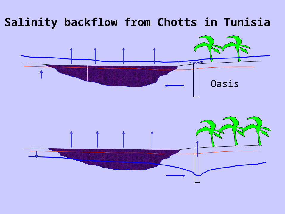
Salinity backflow from Chotts in Tunisia
Oasis
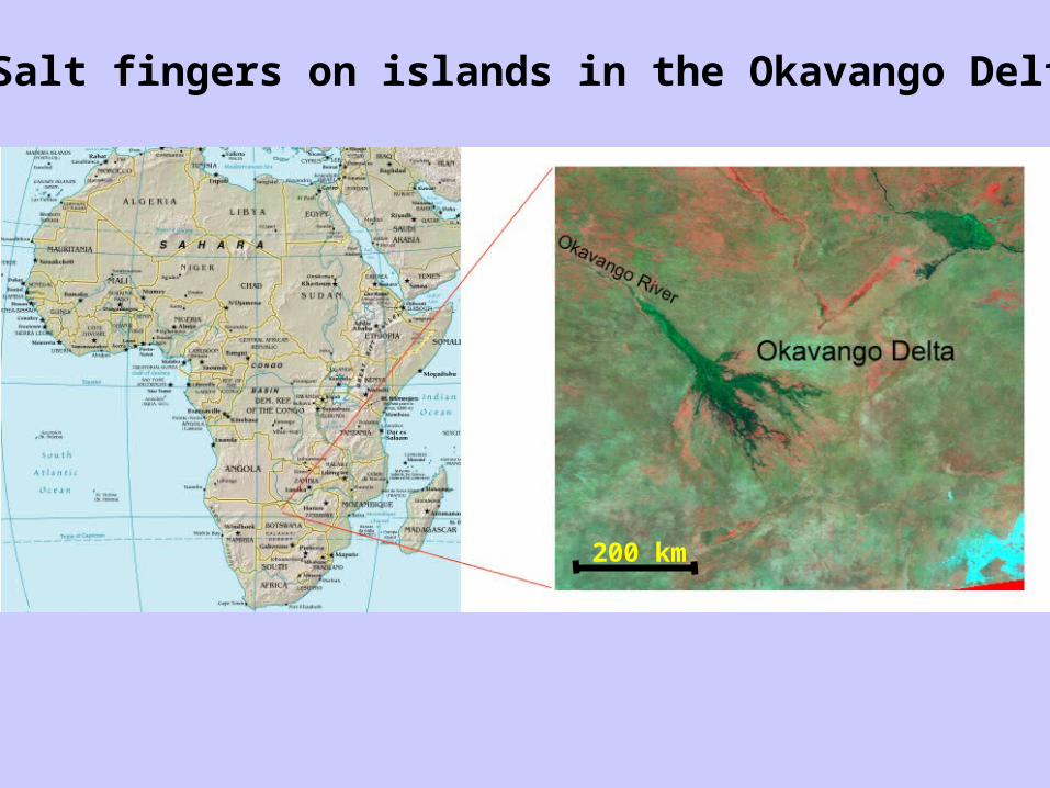
200 km
Salt fingers on islands in the Okavango Delta

Islands and salt crusts in Delta
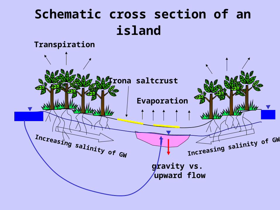
Schematic cross section of an island
Transpiration
Evaporation
Increasing salinity of GW
Trona saltcrust
Increasing salinity of GW
gravity vs. upward flow

Instability on the Islands
ET
f
u
k Number Wooding
Critical Wooding Number:TEM Evaluation
Island-TransectTDS center
(mg/l)TDS layer 2
(mg/l)norm. density
contrast (-)Wooding
No.(-)Thata-1 22425.00 1352.94 0.0147 14.74
Thata-3 9425.00 878.59 0.0060 5.98
Mosupatsela-1 8645.00 1495.31 0.0050 5.00
Mosupatsela-3 5200.00 1803.28 0.0024 2.37
Tshwene-1 19110.00 1135.50 0.0126 12.57
Tshwene-2 19110.00 1135.50 0.0126 12.57
Lebolobolo-1 13000.00 1014.03 0.0084 8.38
Lebolobolo-2 26000.00 1887.59 0.0169 16.86
Lebolobolo-3 7800.00 886.25 0.0048 4.84
Monyopi-1 2665.00 1118.03 0.0011 1.08
Monyopi-2 2665.00 747.22 0.0013 1.34
Atoll-3 15600.00 2172.15 0.0094 9.39
Kwena-1 9750.00 1480.68 0.0058 5.78
Montsana-1 1625.00 367.65 0.0009 0.88
kf= 10-5 m/s, uET=10-8 m/s
0 0.2 0.4 0.6 0.8 1 1.2 1.4 1.6 1.8 20
2
4
6
8
10
12
14
16
18
20
k in units of u/D m-1
Criti
cal W
oodi
ng N
umbe
r
instable
stable
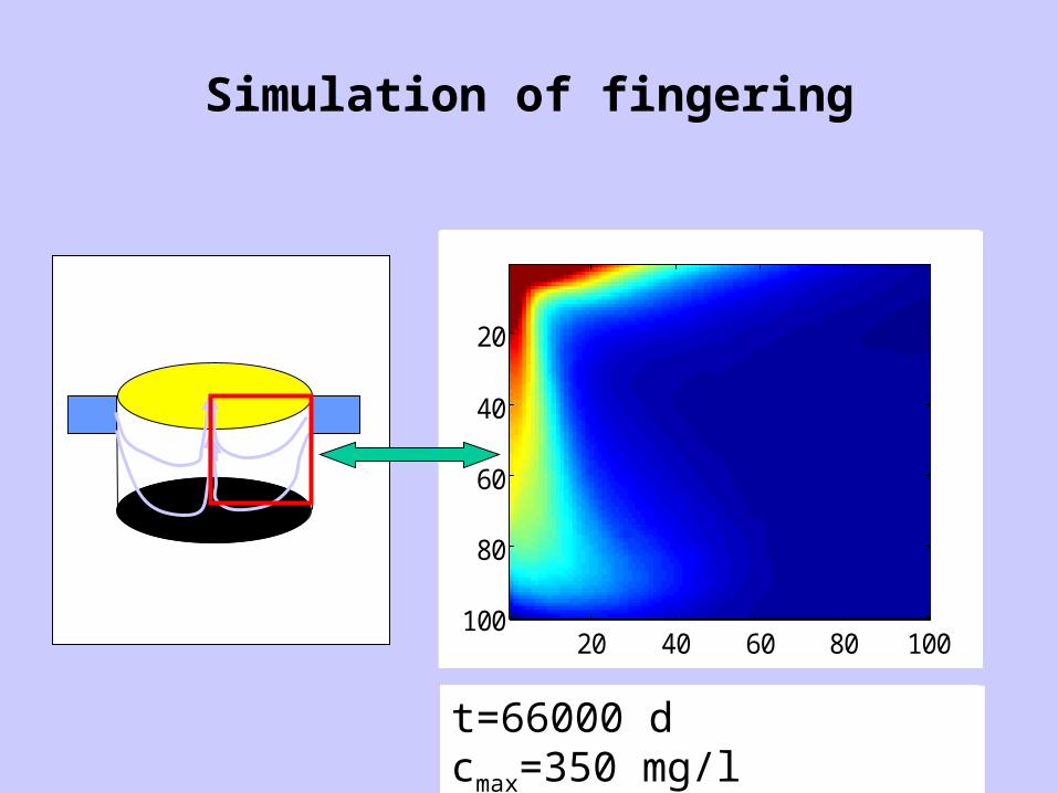
Simulation of fingering
20 40 60 80 100
20
40
60
80
100
t=900 d cmax=11 mg/l
20 40 60 80 100
20
40
60
80
100
t=2900 d cmax=30 mg/l
20 40 60 80 100
20
40
60
80
10020 40 60 80 100
20
40
60
80
100
t=6000 d cmax=54 mg/l
20 40 60 80 100
20
40
60
80
100
t=8500 d cmax=75 mg/l
20 40 60 80 100
20
40
60
80
100
t=12400 d cmax=110 mg/l
20 40 60 80 100
20
40
60
80
100
t=16800 d cmax=235 mg/l
20 40 60 80 100
20
40
60
80
100
t=25000 d cmax=350 mg/l
20 40 60 80 100
20
40
60
80
100
t=32500 d cmax=350 mg/l
20 40 60 80 100
20
40
60
80
100
t=46500 d cmax=350 mg/l
20 40 60 80 100
20
40
60
80
100
t=66000 d cmax=350 mg/l

Flow in the vicinity of a salt dome
Recharge Discharge
Top of salt dome
Salt water -fresh waterinterface
No density difference With density difference
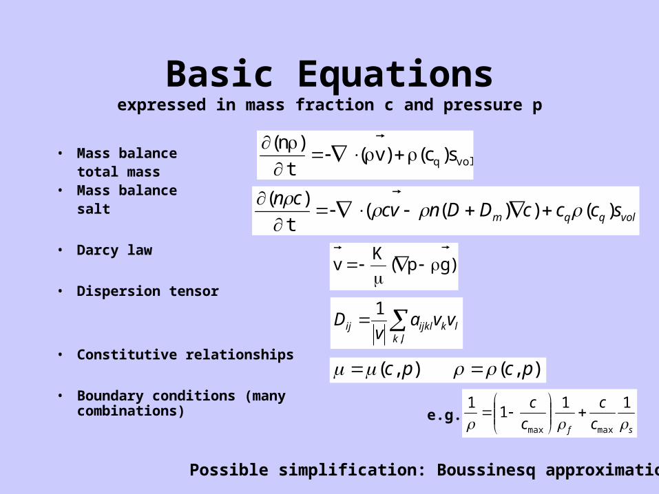
• Mass balance total mass
• Mass balance salt
• Darcy law
• Dispersion tensor
• Constitutive relationships
• Boundary conditions (many combinations)
Basic Equationsexpressed in mass fraction c and pressure p
volq s)c()v(t
)n(
volqqm scccDDnvccn
)())((t
)(
)gp(K
v
lk
lkijklij vvav
D,
1
),(),( pcpc
sf c
c
c
c
11
11
maxmax
e.g.
Possible simplification: Boussinesq approximation
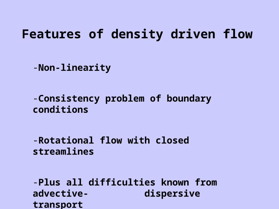
Features of density driven flow
-Non-linearity
-Consistency problem of boundary conditions
-Rotational flow with closed streamlines
-Plus all difficulties known from advective- dispersive transport
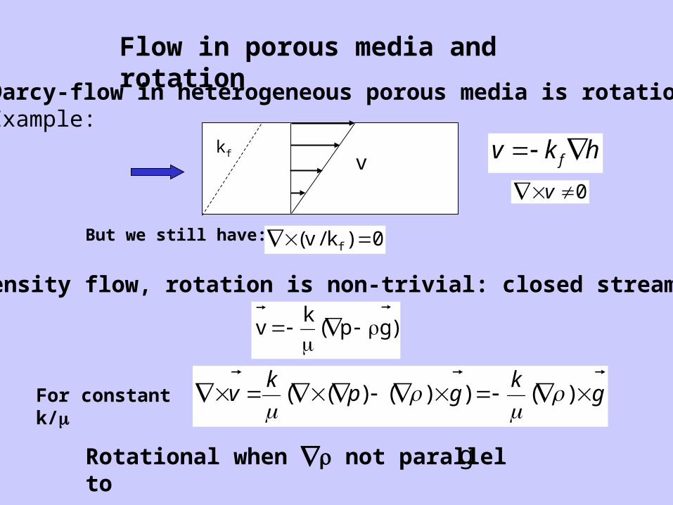
Flow in porous media and rotation
Darcy-flow in heterogeneous porous media is rotationalExample:
)gp(k
v
gk
gpk
v
)())()((
But we still have:
In density flow, rotation is non-trivial: closed streamlines
Rotational when not parallel to g
0)k/v( f
For constant k/
kfv hkv f
0 v
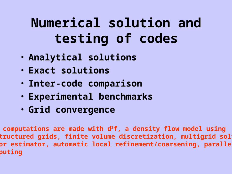
Numerical solution and testing of codes
• Analytical solutions• Exact solutions• Inter-code comparison• Experimental benchmarks• Grid convergence
All computations are made with d3f, a density flow model usingunstructured grids, finite volume discretization, multigrid solver, error estimator, automatic local refinement/coarsening, parallel computing
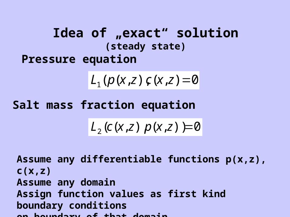
Idea of „exact“ solution(steady state)
Pressure equation
Salt mass fraction equation
0),(),,((1 zxczxpL
0)),(),,((2 zxpzxcL
Assume any differentiable functions p(x,z), c(x,z)Assume any domainAssign function values as first kind boundary conditionson boundary of that domain
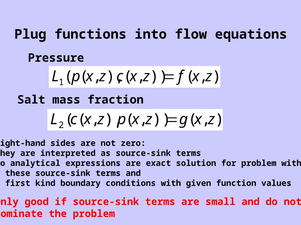
Plug functions into flow equations
Pressure
Salt mass fraction
),()),(),,((1 zxfzxczxpL
),()),(),,((2 zxgzxpzxcL Right-hand sides are not zero: They are interpreted as source-sink termsSo analytical expressions are exact solution for problem with - these source-sink terms and - first kind boundary conditions with given function values
Only good if source-sink terms are small and do not dominate the problem

Analytical expressions for „exact“ solution(steady state)
Pressure
Salt mass fraction
)z)xx()x3(()zzg)(z1()z,x(p ssx0z0
1
222
2
x )zx()z3x(hz2
5.4e1)z,x(c
Values in example tuned to make sources/sinks small: =20, =12, h=.14, =1, 0=1, =1, x=0.1, z=0.02, xs=1, zs=-0.1In PDE: n=1, g=1, k=10, =1, Dm=1, /c=0.1, (c)=0+ /c c=1+0.1c
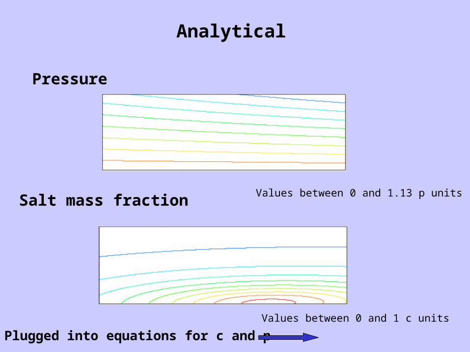
Analytical
Salt mass fraction
Pressure
Values between 0 and 1.13 p units
Values between 0 and 1 c units
Plugged into equations for c and p

Source-sink distributions
Total mass
Salt mass
Red: max. inputTurquoise: 0 input
Red: max. inputLight blue: 0 inputBlue: output
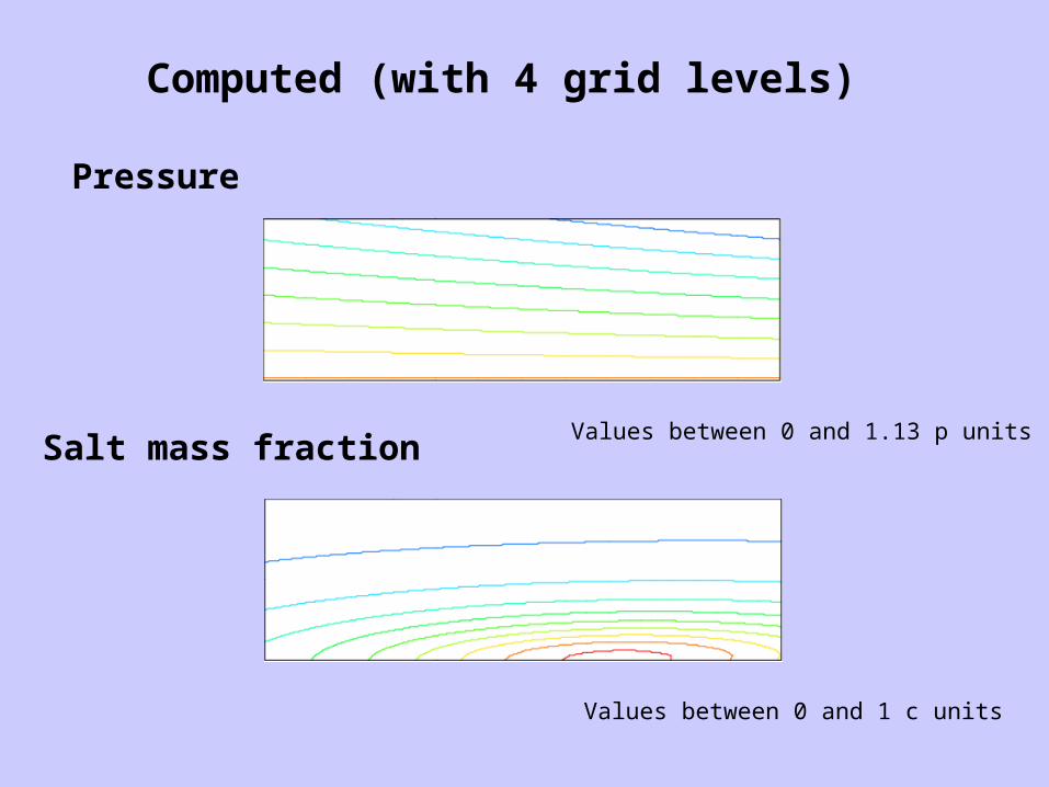
Computed (with 4 grid levels)
Salt mass fraction
Pressure
Values between 0 and 1.13 p units
Values between 0 and 1 c units

Error
Pressure
Salt mass fraction
Red : computed value too large by 0.004 % Blue: computed value too small by 0.005 %
Red : computed value too large by 0.007 %Blue: computed value too small by 0.006 %

Experimental benchmark
• 3D transient experiment in box with simple boundary and initial conditions
• Measurement of concentration distribution in 3D with Nuclear Magnetic Resonance Imaging
• Measurement of breakthrough curves
Drawback: Test of both model equations and mathematics
Way out: Construction of a grid convergent solution inspired by the physical experiments
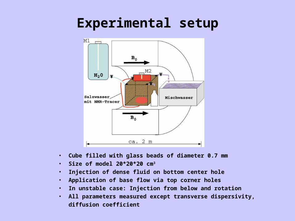
Experimental setup
• Cube filled with glass beads of diameter 0.7 mm• Size of model 20*20*20 cm3
• Injection of dense fluid on bottom center hole• Application of base flow via top corner holes• In unstable case: Injection from below and rotation• All parameters measured except transverse dispersivity,
diffusion coefficient
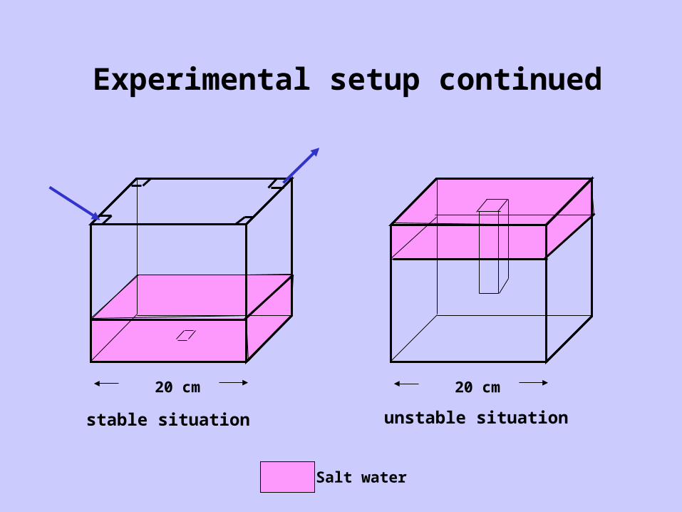
Experimental setup continued
20 cm 20 cm
Salt water
stable situation unstable situation
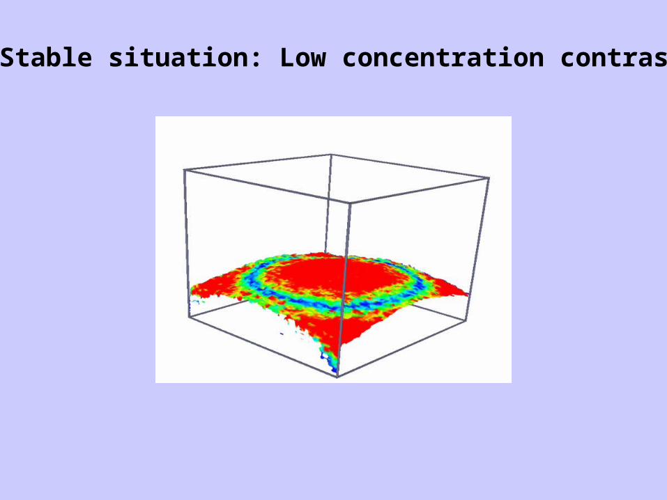
Stable situation: Low concentration contrast
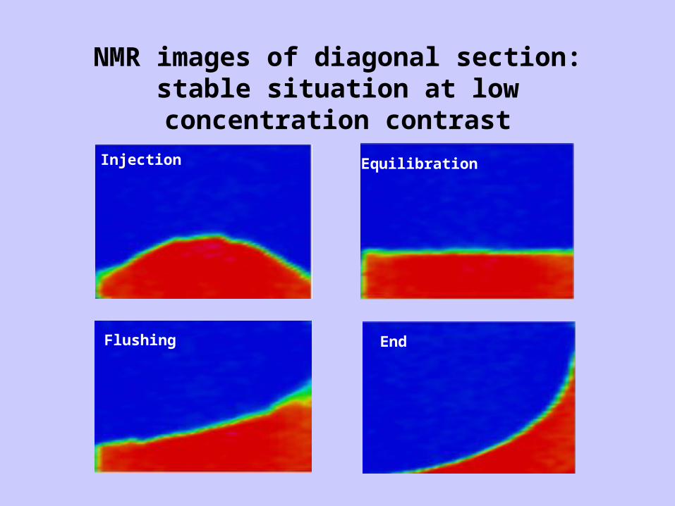
NMR images of diagonal section: stable situation at low concentration contrast
Injection
EndFlushing
Equilibration
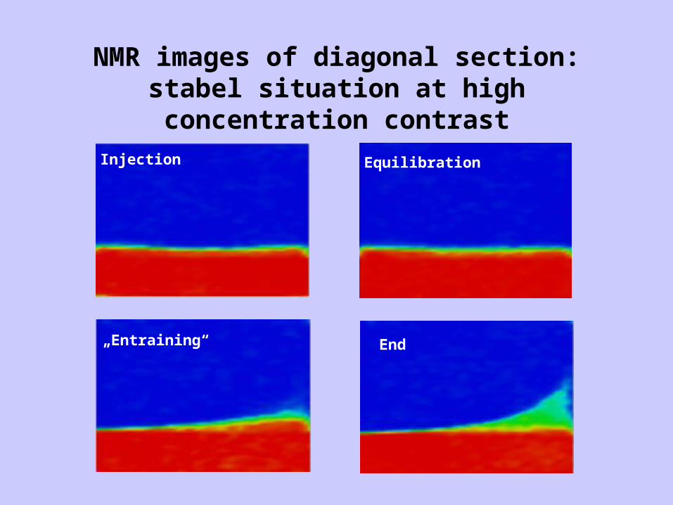
NMR images of diagonal section: stabel situation at high concentration contrast
Injection Equilibration
„Entraining“ End

Two modes
No density contrast Large density contrast
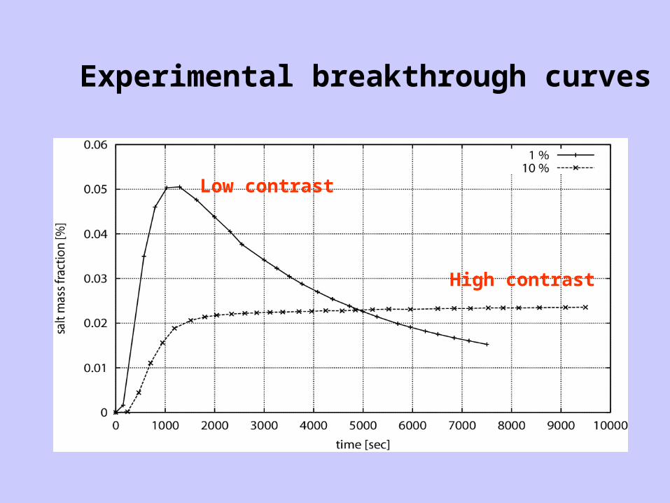
Experimental breakthrough curves
Low contrast
High contrast
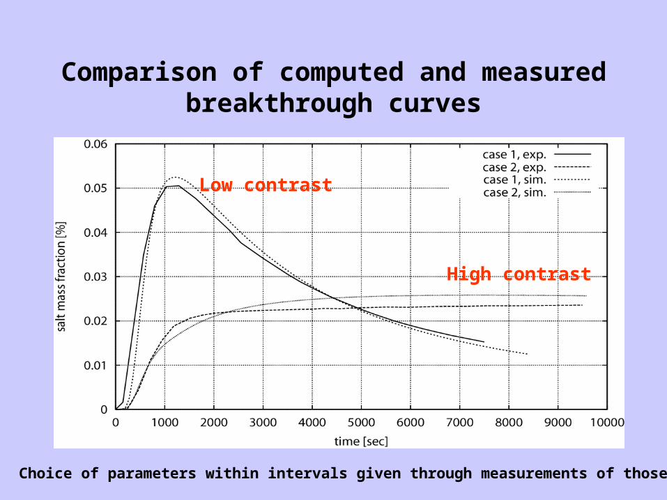
Comparison of computed and measured breakthrough curves
Low contrast
High contrast
Choice of parameters within intervals given through measurements of those

Comparison of concentrations along diagonal sectionLow contrast case, end of experiment
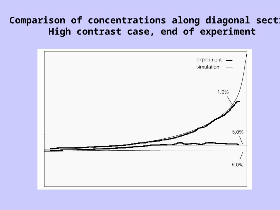
Comparison of concentrations along diagonal sectionHigh contrast case, end of experiment
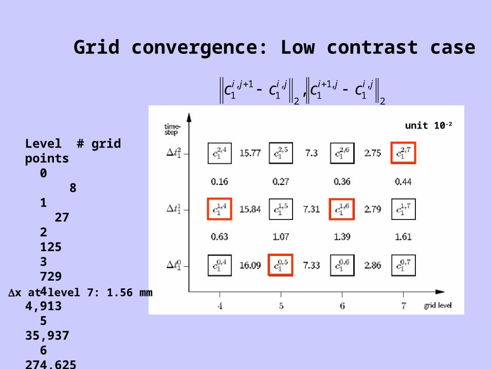
Level # grid points 0 8 1 27 2 125 3 729 4 4,913 5 35,937 6 274,625 7 2,146,689
Grid convergence: Low contrast case
unit 10-2
2
,1
,11
2
,1
1,1 , jijijiji cccc
x at level 7: 1.56 mm

Grid convergence: Low contrast case
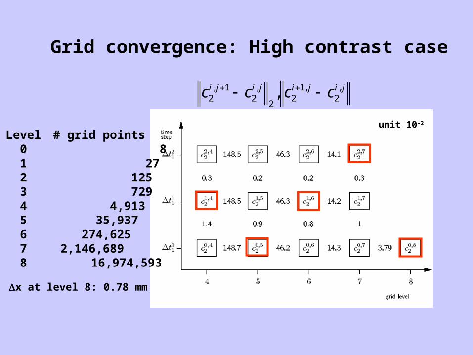
Level # grid points 0 8 1 27 2 125 3 729 4 4,913 5 35,937 6 274,625 7 2,146,689 8 16,974,593
Grid convergence: High contrast case
unit 10-2
jijijiji cccc ,2
,12
2
,2
1,2 ,
x at level 8: 0.78 mm

Grid convergence: High contrast case

Error of grid-convergent solutions
Low contrast
High contrast
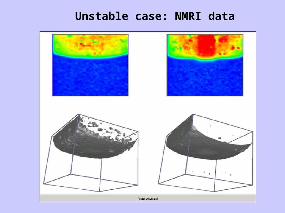
Unstable case: NMRI data

NMRI of vertical and horizontal section: fingering experiment
Vertical section Horizontal section

Fingering: Experiment vs. Computation
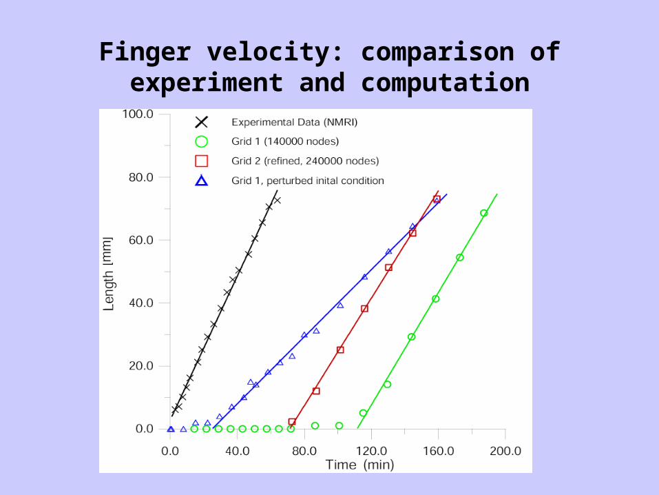
Finger velocity: comparison of experiment and computation

Causes for poor perfomance
• Numerical dispersion smoothes out fingers and eliminates driving force
• Initial perturbance not known well enough• Start of fingers on microlevel, not
represented by continuum equations
Influence of heterogeneity on density flow
• Homogeneous Henry problem
• Heterogeneous Henry problem
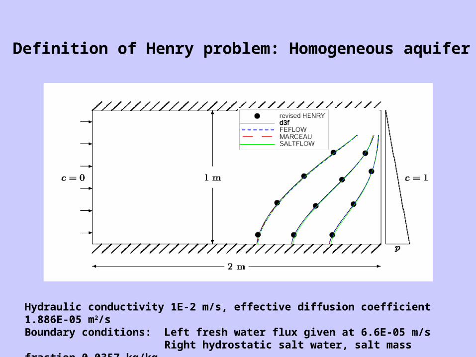
Definition of Henry problem: Homogeneous aquifer
Hydraulic conductivity 1E-2 m/s, effective diffusion coefficient 1.886E-05 m2/sBoundary conditions: Left fresh water flux given at 6.6E-05 m/s
Right hydrostatic salt water, salt mass fraction 0.0357 kg/kg

Solution of Henry problem: Homogeneous aquifer
Relative concentration contours between 0 (left) and 1 (right) in steps of 0.1
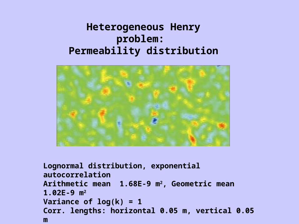
Heterogeneous Henry problem: Permeability distribution
Lognormal distribution, exponential autocorrelationArithmetic mean 1.68E-9 m2, Geometric mean 1.02E-9 m2 Variance of log(k) = 1Corr. lengths: horizontal 0.05 m, vertical 0.05 mRed: 3.5E-08 m2, Blue: 2.6E-11 m2
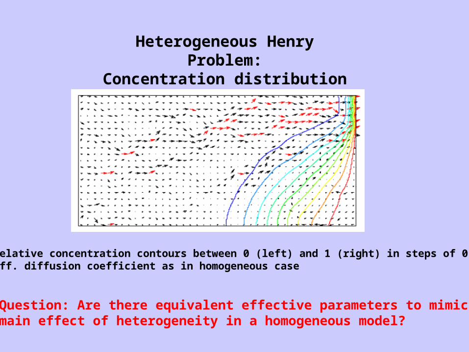
Heterogeneous Henry Problem:Concentration distribution
Relative concentration contours between 0 (left) and 1 (right) in steps of 0.1Eff. diffusion coefficient as in homogeneous case
Question: Are there equivalent effective parameters to mimickmain effect of heterogeneity in a homogeneous model?
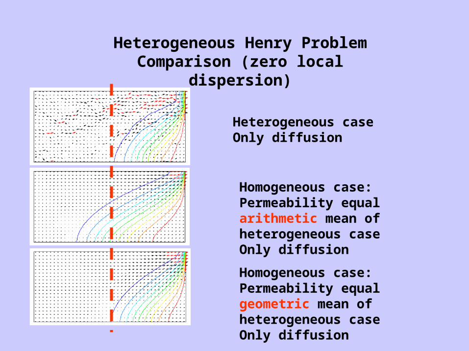
Heterogeneous Henry ProblemComparison (zero local dispersion)
Heterogeneous caseOnly diffusion
Homogeneous case:Permeability equal arithmetic mean of heterogeneous caseOnly diffusion
Homogeneous case:Permeability equal geometric mean of heterogeneous caseOnly diffusion
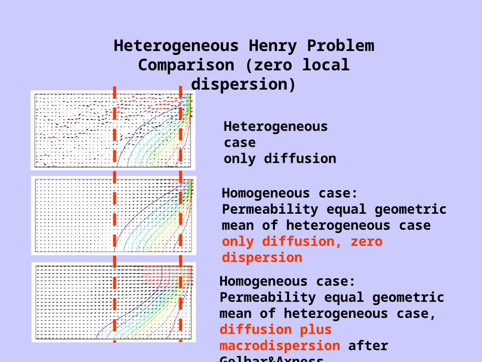
Heterogeneous Henry ProblemComparison (zero local dispersion)
Heterogeneous caseonly diffusion
Homogeneous case:Permeability equal geometric mean of heterogeneous caseonly diffusion, zero dispersion
Homogeneous case:Permeability equal geometric mean of heterogeneous case, diffusion plus macrodispersion after Gelhar&Axness
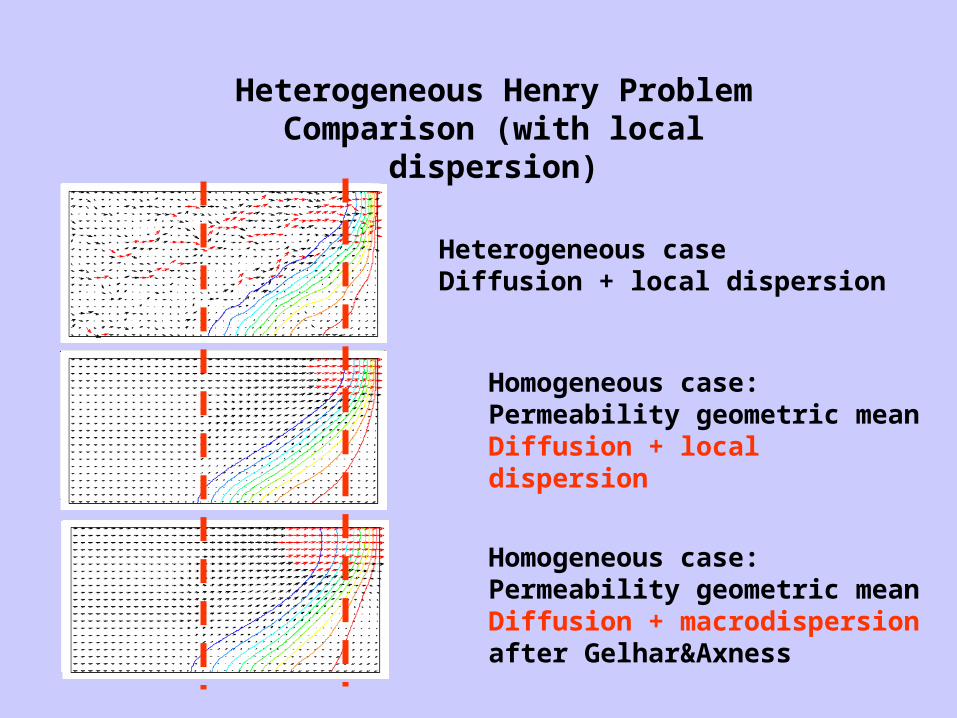
Heterogeneous Henry ProblemComparison (with local dispersion)
Heterogeneous caseDiffusion + local dispersion
Homogeneous case:Permeability geometric mean Diffusion + local dispersion
Homogeneous case:Permeability geometric meanDiffusion + macrodispersion after Gelhar&Axness
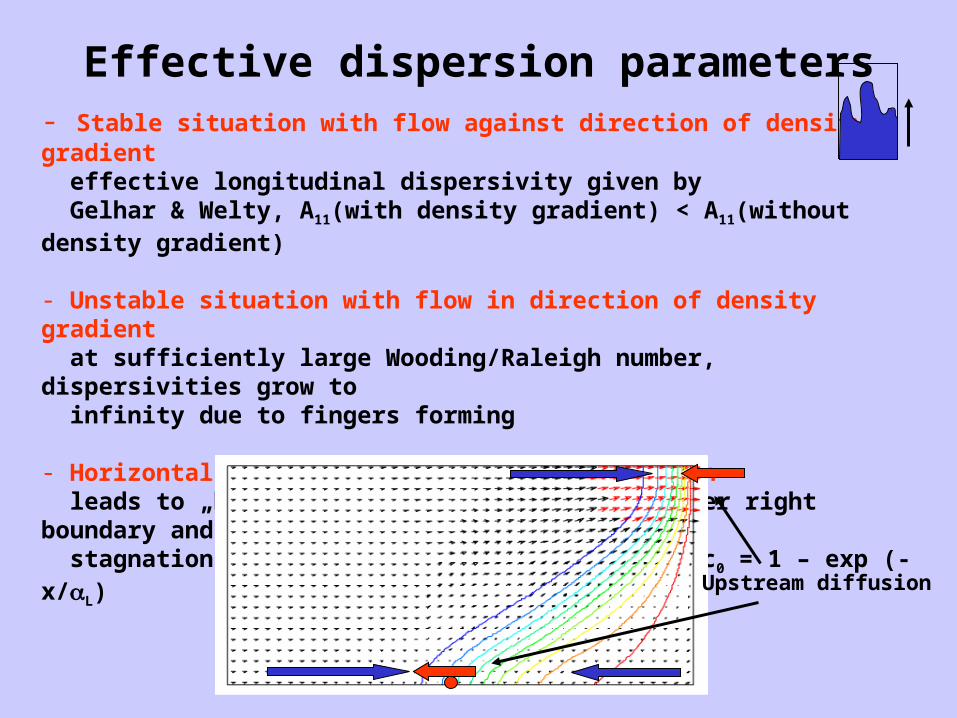
Effective dispersion parameters- Stable situation with flow against direction of density gradient effective longitudinal dispersivity given by Gelhar & Welty, A11(with density gradient) < A11(without density gradient)
- Unstable situation with flow in direction of density gradient at sufficiently large Wooding/Raleigh number, dispersivities grow to infinity due to fingers forming
- Horizontal flow towards a fixed concentration leads to „boundary layer“. Dispersion at upper right boundary and at stagnation point is „upstream diffusion“: c/c0 = 1 – exp (-x/L)
Upstream diffusion
Conclusions
• Density flow of increasing importance in groundwater field
• Tests for reliability of codes are available• Density flow especially with high contrast
numerically demanding: Grid convergence may require millions of nodes
• Numerical simulation of fingering instabilities still inadequate
• Heterogeneities can be handled by effective media approach in situation without fingering
• New numerical methods are in the pipeline