department of aeronautics and astronautics stanford
TRANSCRIPT

d
Department of AERONAUTICS and ASTRONAUTICS
STANFORD UNIVERSITY
OPTIMAL LANDING
OF A HELICOPTER IN AUTOROTATION
(MbSA-C_-177082) OPTI_AL LAH£IMG OF &HELICOPTER IN AU_OROT&_IOB {_tanford Univ.)**
322 p CSCL O|C
_86-2S809
Uacla_
G3/OS 43222
A DISSERTATION
SUBMITTED TO
THE DEPARTMENT OF AERONAUTICS AND ASTRONAUTICS
AND THE COMMITTEE ON GRADUATE STUDIES
OF STANFORD UNIVERSITY
IN PARTIAL FULFILLMENT OF THE REQUIREMENTS
FOR THE DEGREE OF
DOCTOR OF PHILOSOPHY
By
• 11--- '_J ..... '[%J_ T_
July 1985

OPTIMAL LANDING
OF A HELICOPTER IN AUTOROTATION
A DISSERTATION
SUBMITTED TO
THE DEPARTMENT OF AERONAUTICS AND ASTRONAUTICS
AND THE COMMITTEE ON GRADUATE STUDIES
OF STANFORD UNIVERSITY
IN PARTIAL FULFILLMENT OF THE REQUIREMENTS
FOR THE DEGREE OF
DOCTOR OF PHILOSOPHY
By
Allan Yeow-Nam Lee
July 1985

_) 1985
by
Allan Yeow-Nam Lee
ii
L

OPTIMAL LANDING OF A HELICOPTER IN AUTOROTATION
Allan Yeow-Nam Lee, Ph.D.
Stanford University, 1985
Gliding descent in autorotation is a maneuver used by helicopter pilots in case
of engine failure. It requires considerable skill, and since it is seldom practiced, it
is considered quite dangerous. In fact, during certification, a region of low altitude
and low velocity (the H-V restriction zone) is established where it is considered
impossible to make a safe descent.
The landing of a helicopter in autorotation is formulated as a nonlinear op-
timal control problem. A simplified point-mass model of an OH-58A helicopter
is used in the study. The model considers as its states the helicopter vertical and
horizontal velocities, vertical and horizontal displacements (from the point at which
engine-failure occurred), and the rotor angular speed. It provides an empirical ap-
proximation for the induced velocity in the vortex-ring state. The cost function of
the optimal control problem is a weighted sum of the squared horizontal and vertical
components of the helicopter velocity at touchdown. The control (horizontal and
vertical components of the thrust coefficient) required to minimize the cost function
is obtained using nonlinear optimal control theory.
A unique feature in the present problem formulation is the addition of path
inequality constraints on both the control and the state vectors. The control variable
inequality constraint is a reflection of the limitation on the rotor thrust coefficient.

The state variable inequality constraint is an upper bound on the vertical sink-rate
of the helicopter during descent. "Slack" variables are employed to convert these
path inequality constraints into path equality constraints. The resultant two-point
boundary-value problem with path equality constraints is successfully solved using
the Sequential Gradient Restoration Technique.
Optimal trajectories are calculated for entry conditions well within the H-V
restriction curve, with the helicopter initially in hover or in forward flight. Solu-
tions are essentially discontinuous, i.e., they consist of variable subarcs which are
connected at suitable corners. Subarcs are those which satisfy either the Eulerian
equations, the upper bound on the thrust coefficient, or the bound on the maximum
rate of descent. The optimal solutions exhibited similar control techniques as are
used by helicopter pilots in actual autorotational landings. The results indicate the
need to drop the collective pitch immediately after engine failure. During the land-
ing flare phase, the thrust vector is rotated to the rear in order to decelerate the
forward motion of the vehicle. The stored rotational energy of the rotor is traded
for additional thrust to cushion the landing at touchdown. The study indicates
that, subject to pilot acceptability, a substantial reduction could be made in the
H-V restriction zone using optimal control techniques, thus providing a benchmark
for comparisons with other control techniques.
These optimization techniques could also be used to:
(1) help instruct pilots on good autorotation technique.
(2) reduce the risk/time/effort involved in establishing the H-V restriction zones
by flight tests.

(3) provide an objective comparison of the autorotation capabilities of different
helicopter models.
(4) assess the influence of vehicle parameters on autorotation during preliminary
design.
Approved for publication:
By
For Major Department
By
Dean of Graduate Studies and Research
I certify that I have read this thesis and that in my opinion
it is fully adequate, in scope and quality, as a dissertation for the
degree of Doctor of Philosophy.
(Principal Adviser)
I certifythat I have read this thesisand that in my opinion
itisfullyadequate, in scope and quality,as a dissertationfor the
degree of Doctor of Philosophy.
I certifythat I have read this thesisand that in my opinion
itisfullyadequate, in scope and quality,as a dissertationfor the
degree of Doctor of Philosophy.
Approved for the University Committee on Graduate Studies:
Dean of Graduate Studies and Research
iii

Abstract
Gliding descent in autorotation is a maneuver used by helicopter pilots in case
of engine failure. It requires considerable skill, and since it is seldom practiced, it
is considered quite dangerous. In fact, during certification, a region of low altitude
and low velocity (the H-V restriction zone} is established where it is considered
impossible to make a safe descent.
The landing of a helicopter in autorotation is formulated as a nonlinear op-
timal control problem. A simplified point-mass model of an OH-58A helicopter
is used in the study. The model considers as its states the helicopter vertical and
horizontal velocities, vertical and horizontal displacements (from the point at which
engine-failure occurred), and the rotor angular speed. It provides an empirical ap-
proximation for the induced velocity in the vortex-ring state. The cost function of
the optimal control problem is a weighted sum of the squared horizontal and vertical
components of the helicopter velocity at touchdown. The control (horizontal and
vertical components of the thrust coefficient) required to minimize the cost function
is obtained using nonlinear optimal control theo_'.
A unique feature in the present problem formulation is the addition of path
inequality constraints on both the control and the state vectors. The control variable
inequality constraint is a reflection of the limitation on the rotor thrust coefficient.
The state variable inequality constraint is an upper bound on the vertical sink-rate
of the helicopter during descent. "Slack" variables are employed to convert these
path inequality constraints into path equality constraints. The resultant two-point
boundary-value problem with path equality constraints is successfully solved using
the Sequential Gradient Restoration Technique.
iv

Optimal trajectories are calculated for entry conditions well within the H-V
restriction curve, with the helicopter initially in hover or in forward flight. Solu-
tions are essentially discontinuous, i.e., they consist of variable subarcs which are
connected at suitable corners. Subarcs are those which satisfy either the Eulerian
equations, the upper bound on the thrust coefficient, or the bound on the maximum
rate of descent. The optimal solutions exhibited similar control techniques as are
used by helicopter pilots in actual autorotational landings. The results indicate the
need to drop the collective pitch immediately alter engine failure. During the land-
ing flare phase, the thrust vector is rotated to the rear in order to decelerate the
forward motion of the vehicle. The stored rotational energy of the rotor is traded
for additional thrust to cushion the landing at touchdown. The study indicates
that, subject to pilot acceptability, a substantial reduction could be made in the
H-V restriction zone using optimal control techniques, thus providing a benchmark
for comparisons with other control techniques.
These optimization techniques could also be used to:
(l'i :hgJP instruct pilots on good autorotation technique., ,:,_. _ _: _ -_._;
(2)':__h_ _-isk/time/effort ! involved in establishing the H-V restriction zones
by flight tests.
(3) provide an objective comparison of the autorotation capabilities of different
helicopter models.
(4) assess the influence of vehicle parameters on autorotation during preliminary
design.

Acknowledgements
First and foremost, I wish to thank Professor Arthur E. Bryson, Jr. for his help
and friendship. He suggested the research described in this thesis and provided me
with the technical expertise that has made this dissertation possible. He has also
been a constant source of energy and inspiration for me throughout my graduate
study at Stanford University.
I would also like to thank Professors Daniel B. DeBra and John V. Breakwell
for their assistance and guidance during the initial phase of my research.
Special thanks must be given to Senior Research Associate William S. Hind-
son for all the hours of valuable discussions. His experience with operations of
helicopters has helped me to bridge the gap between theory and practice.
I am greatly indebted to my wife, Helen for her endless moral support and her
tireless patience. She was a constant source of joy and inspiration when I needed
it most. To my family, I want to express both my love and gratitude. Without
their unflagging support and encouragement throughout all of my educational ex-
periences, I would never have been able to reach the stage that this dissertation
represents for me.
I also appreciate the encouragement and suggestions offered by many of my
friends. I would particularly like to thank William A. Decker and Dr. Robert
T.N. Chen of NASA Ames Research Center, who contributed to numerous fruitful
technical discussions.
I gratefully acknowledge financial support from the National Aeronautics and
Space Administration under Grant NCC 2-106.
vi

Table of Contents
Abstract . ..........................................................
Page
iv
Acknowledgements .................................................. vi
°°,
List of Figures ...................................................... xm
List of Tables ....................................................... xx
List of._$_'m_ls:_ .. . .......... xxi
Chapter 1. Introduction .............................................. 1
1.1 Background and Motivations of Research ........................ 1
1.2 The Autorotation Maneuver and Related Research ............... 3
1.3 Objectives of Research ........................................ 5
1.4 Outline of Thesis ............................................. 6
Chapter 2. Problem Formulation ...................................... 9
2. l The Need to Simplify ......................................... 9
2.2 Basic Assumptions ........................................... 10
2.3 Equations of Motion .......................................... 13

viii Table of Contents
2.3.1 General Considerations and Coordinate System Used ... 13
2.3.2 Dynamic Equations ................................. 15
2.3.3 The Energ)' Model .................................. 16
2.3.4 Momentum Theory. ................................. 17
2.3.5 Modeling the Induced Velocity ....................... 19
2.3.6 Profile Power and the Blade Element Theory ........... 20
2.3.7 The Ener_' Equation ............................... 22
2.3.8 Kinematical Relations ............................... 25
2.4 Non-Dimensionalization and Scaling ............................ 26
2.5 Cost Function ............................................... 29
2.6 Terminal Constraints and Initial Conditions ..................... 30
2.7 Path Constraints ............................................. 31
2.8 Further Time Normalization ................................... 32
2.9 Final Form of Helicopter Optimization Problem .................. 33
Chapter 3. Numerical Optimization Techniques ......................... 35
3.1 Related Research ............................................ 35
3.2 Combined Function and Parameter Optimization Algorithm ....... 40
Example Problems ...................................... 49
(1) Specified Control Law Problem ........................ 49
(2) Optimal Landing of a Helicopter in Hover ............... 51
3.3 Sequential Gradient Restoration Technique ...................... 56
3.3.1 First Order Conditions .............................. 58
3.3.2 Approximate Methods .............................. 59
3.3.3 The Sequential Gradient Restoration Algorithm ........ 60
3.3.4 Desired Properties in the SGR Process ................ 61
3.3.5 The First Variations ................................ 62

Table of Contents ix
3.3.6 Gradient Phase .................................... 63
3.3.7 Solution Technique in the Gradient Phase ............. 65
3.3.8 Gradient Stepsize ................................... 68
3.3.9 Restoration Phase .................................. 68
3.3. ! 0 Special Variations ................................. 70
3.3.11 Solution Technique in the Restoration Phase .......... 72
3.3.12 Restoration Stepsize ............................... 73
3.3.13 SummaD" of the SGR Algorithm .................... 7.!
3.3.14 Example Problem ................................. 75
3.4 Neighboring Extremal with Path Constraints .................... 80
3.4.1 Problem Formulation ............................... 85
3.4.2 Solution by Backward Sweep Method .................. 86
3.4.3 Example Problems .................................. 88
3.4.4 Conclusions ........................................ 108
Chapter 4. Optimal Solutions and their Interpretations .................. 111
4,t Descriptions of Test.Vehicle ................................... 112
4.1.1 Height-Velocity Restriction Curves .................... 114
4.2 Ener_" Considerations ........................................ 118
4.3 Autorotation Landing Techniques Used by Pilots ................. 120
4.4 Optimal Landing of a Helicopter Initially in Hover ............... 123
4.4.1 A Pure Vertical Descent Path ........................ 125
4.4.2 Interpretations of Optimal C.ontrol Results ............. 128
4.4.3 Comparison with Flight Data ........................ 136
4.4.4 Effects of Entry Height .............................. 142
4.4.5 Most Critical Entry Height .......................... 146
4.5 Optimal Landing of a Helicopter in Forward Flight ............... 147

x Table of Contents
4.5.1
4.5.2
4.5.3
4.5.4
4.5.5
Flight Program ..................................... 150
Interpretation of Results ............................ 153
Comparison with Flight Data ........................ 158
Effects of Entry Height .............................. 167
Effects of Entry Speed .............................. 172
4.5.6 Best Endurance Speed .............................. 177
4.6 Optimal Descent of a Helicopter with a Bound on Vertical Sink Rate 179
4.6.1 Optimal Landing of a Helicopter with a Descent
Velocity Bound ..................................... 184
4.6.2 Comparison Between Results Obtained With and
and Without the Descent Velocity Bound .............. 191
4.6.3 Some Generalizations ............................... 199
4.6.4 Effects of Perturbed Initial and Terminal Conditions .... 199
4.6.5 General Conclusions ................................ 213
Chapter 5. Summary and Recommendations for Further Research ......... 215
5.1 Conclusions ................................................. 215
5.2 Recommendations for Further Research ......................... 218
References .......................................................... 221
Appendix A. Verification of Point Mass Helicopter Model ................ 229
A.1 Introduction ................................................ 229
A.2 Analysis .................................................... 231
A.3 Comparison of Computed Results with Flight Data .............. 233
A.4 Conclusions ................................................. 242
Appendix B. Supporting Analysis ..................................... 243
B.1 Introduction ................................................ 243

Table of Contents xi
B.2 Determination of (I"1)¢ ....................................... 244
B.3 Expressions for Of/OU, Of/O._ and af/a_ ..................... 24G
B.4 Expressions for OS/c_U ....................................... 248
B.5 Expressions/or I and a(/a£ I .......................... 249
B.6 Determination of the Collective Pitch Setting, 0_s ................ 249
Appendix C. Example Problems Solved Using the CPF Algorrthm ........ 251
C.I Example Problems ........................................... 2.51
Problem (1) Minimum Time/Energy Control ............... 251
Problem (2) Specified Control Law Problem ................ 253
Problem (3) Brachistochrone Problem ..................... 254
Appendix D. Generalized Transversality Condition ...................... 256
D.1 Introduction ................................................ 256
D.2 Proof ...................................................... 258
D.3 Conclusion .................................................. 261
Appendb_.=E'.::=_finitions of Matrices Used In Section (3.4) ................ 263
•E: I .liil;_ction ................................................. 263
El2 E_x_r'esSions for HI) .......................................... 263
E.3 Expressions for 5"{ ) .......................................... 266
E.4 Expressions for Aii .......................................... 267
E.5 Expressions for Cq .......................................... 267
Appendix F. Iterative Solution for TPBVPs with Integral Path Constraints . 269
F.1 Problem Formulation ......................................... 269
F.2 Solution Method ............................................. 272
F.3 Iterative Procedure ........................................... 274
Appendix G. Example Problems Solved Using the SGR Technique ......... 278

xii Table of Contents
G.I Bounded Brachistochrone Problem ............................. 278
G.2 Bounded Control of Double Integrator Plant .................... 281
G.3 A Geodesic Problem ......................................... 284
G.4 Bounded Time Rate of Change of State ........................ 287

List of Figures
Figure 1.1.1
Figure 1.1.2
Figure 2.2.1
Figure 2.3.2
Page
Typical Height-Velocity Envelope ......................... 2
Emergency Autorotation Cause Related Factors ............ 4
A Comparison of Computed Sink-rate with Experimental
Results of Reference [18] ................................. 12
Coordinate System Used ................................. 14
Velocity Parameter .fs with xrl and z-2 .. 21
Example Optimal Control Problem ........................ 52
Variation of Induced Velocity Parameter fl with II .......... 53
Flowchart of the Sequential Gradient Restoration Technique .. 76
Neighboring Optimal feedback Law ....................... 89
Feedback Gains In Example {l) ........................... 94
Nominal and Perturbed Results in Example (i) ............. 96
Comparison of Exact Results with Those from Feedback
Figure 3.2.1
Figure 3.2.2
Figure 3.3.3
Figure 3.4.4
Figure 3.4.5
Figure 3.4.6
Figure 3.4.7
Fignre_z3.4. ,i Force Balance Diagram .................................. 23

xiv List of Figures
Figure 3.4.8
Figure 3.4.9
Figure 3.4.10
Figure 3.4.11
Figure 3.4.12
Figure 3.4.13
Figure 3.4.14
Figure 4.1.1
Figure 4.1.2
Figure 4.3.3
Figure 4.4.4
Figure 4.4.5
Figure 4.4.6
Figure 4.4.7
Law in Example (1} ..................................... 97
Feedback Gains in Example (2} ........................... 100
Nominal and Perturbed (Initial Conditions) Results in
Example (2} ............................................ 102
Comparison of Exact Results with those from Feedback Law
in Example (2) ........................................ 104
Nominal and Perturbed (Terminal Condition) Results in
Example (2) ........................................... 10G
Comparison of Exact Results with those from Feedback Law
in Example (2) ........................................ 107
Nominal and Perturbed (Initial and Terminal Conditions)
Results in Example {2} ................................. 109
Comparison of Exact Results with those from Feedback Law
in Example (2} ........................................ 110
Experimental High Energs.' Rotor System {HERS) ........... 113
OH-58A Maximum Performance Height-Velocity Restriction
Curves ................................................ 117
Variations of Energy Terms in Phases of an Autorotational
Landing of a Helicopter .................................. 124
Entry Height of a ltelicopter with Power Loss in Hover ...... 129
Optimal Time Variations of Thrust Coefficient and Collective
Pitch Control, h0 = 100 feet .......... : ................... 131
Optimal Time Variations of Vertical Height and Vertical
Sink Rate [Case (3) h0 = 100 feet] ........................ 133
Optimal Time Variation of Rotor RPM .................... 134

List of Figures xv
Figure 4.4.8
Figure 4.4.9
Figure 4.4.10
Figure 4.4.11
Figure 4.4.12
145
Figure 4.4.13
Figure 4.4.14
Figure 4.5.15
Figure 4.5.16
Variation of Induced Velocity with Rate of Descent .......... 13.5
Comparison of Flight Data with Optimal Results
: Collective Pitch Control ................................ 139
Comparison of Flight Data with Optimal Results
: Rotor Speed ......................................... 140
Time Variations of Collective Pitch Control at Different
Entry Heights ......................................... 144
Time Variation of Thrust Coefficient from Different Entry Height
Time Variations of Rotor Speed at Different Entry Height ... 148
Variation of Terminal Rotor Speed with Entry Height ...... 149
Comparison of HERS Test Results with Standard OH-58A
Helicopter ............................................ 151
(H-V} Entry Conditions ................................ 152
Figure 4.5.17 Optimal Time Variations of Thrust Coefficient and Collective
;_ :_:,::_:_:__:Fttch Con rol ......................................... 155.......... %,. _, .......... _y.._, _,_
F_re4.5.18 Optimal Time Variations of Horizontal and Vertical Velocity 156
Figure 4.5.19 Optimal Time Variations of Rotor RPM and Helicopter's
Altitude .............................................. 157
Figure 4.5.20
Figure 4.5.21
Effects of Rearward (Nose-Up) Cyclic Flare ............... 159
Comparison of Flight Data with Optimal Results
• Collective Pitch Control ............................... 162
Figure 4.5.22 Comparison of Flight Data with Optimal Results
: Rotor RPM ................................... "_"....... 11U'II
Figure 4.5.23 Comparison of Flight Data with Optimal Results

xvi List of Figures
Figure 4.5.24
Figure 4.5.25
Figure 4.5.26
Figure 4.5.27
Figure 4.5.28
Figure 4.5.29
Figure 4.5.30
Figure 4.5.31
Figure 4.5.32
Figure 4.5.33
Figure 4.5.34
Figure 4.5.35
Figure 4.6.36
Figure 4.6.37
: Flight Trajectory ..................................... 166
Flight Data for Autorotation Landing [12]
[Entry Condition : 125 feet, 45 Knots] ................... 168
Computed Optimal Program for Autorotation Landing
[ Entry Condition : 100 feet, 38 Knots ] ................... 179
Variations of Thrust Coefficient with Entry Heights
[ Entry Speed : 8-12 Knots ] ............................ 170
Variations of Horizontal and Vertical Thrust Components
with Entry Height [ Entry Speed : 8-12 Knots ] ............ 173
Optimal Time Histories of Forward Speed at dfferent
Entry Heights [ Entry Speed : 8-12 Knots ] ............... 174
Variations of Thrust Coefficients with Entry Speed
[EntD' Height : 100 feet] ............................... 175
Variations of Horizontal and Vertical Thrust Components
with Entry Speed [ Entry Height : 100 feet ] .............. 176
Variation of Forward Speed with Entry Speed at an Entry
Height of 100 feet ...................................... 178
Variation of Power with Forward Speed ................... 180
Variation of Steady Rate of Descent with Forward Speed
of an OH-58A Helicopter ................................ 181
Time Variations of Rotor Speed [ Entry Speed : 8-12 Knots ] 182
Time Variations of Rotor Speed [ Entry. Height : lO0 feet ] .. 183
Time Rate of Change of Descent Velocity With a [VD]m6,
Bound ................................................ 185
Time Variation of Descent Velocity with Different Values of
[Vg]m6_ ............................................... 186

List of Figures ×vii
Figure 4.6.38 Variation of Steady Autorotative Sink-Rate of the HERS
with Forward Airspeed ................................. 187
Figure 4.6.39 Time Variations of the Thrust Coefficient and its Horizontal
and Vertical Components ............................... 189
Figure 4.6.40 Time Variation of the Collective Pitch With a [VD],,,az Bound 190
Figure 4.6.41 Time Variations of the Thrust Coefficient With and Without
a [Vz_],,,oz Bound ....................................... 192
Figure 4.6.42 Time Variation of the Descent Velocity and the Optimal
Flight Profile .......................................... 195
Figure 4.6.43 Time Variations of the Forward Speed and the Rotor RPM 196
Figure 4.6.44 Comparison of the Time Variations of the Descent Velocity
With and Without a [VD],naz Bound ..................... 197
Figure 4.6.45 Comparison of the Time Variations of the Forward Speed and
Rotor RPM With and Without a [VD],,,az Bound .......... 198
Figure 4.6.46 i2 versus V D Plot showing Segments of the Optimal Control
I [: :::_" ": _ _, _1 _ _ _ _ , Scheme ............................................... 200
Figure 4.fiA7 Comparisons of Optimal Results Obtained at Two Different
Entry Speeds .......................................... 202
Figure 4.6.48 Comparisons of Optimal Results Obtained at Two Different
Entry Speeds .......................................... 203
Figure 4.6.49 Comparisons of Optimal Results Obtained at Two Different
Entry Speeds .......................................... 204
Figure 4.6.50 Comparisons of Optimal Results Obtained With and Without
a Horizontal Distance Constraint ........................ 205
Figure 4.6.51 Comparisons of Optimal Results Obtained With and Without
a Horizontal Distance Constraint ........................ 206

xviii List of Figures
Figure 4.6.52
Figure 4.6.53
Figure 4.6.54
Figure 4.6.55
Figure 4.6.56
Figure 4.6.57
Figure A.I.1
Figure A.3.2
Figure A.3.3
Figure A.3.4
Figure A.3.5
Figure F.3.1
Figure G. 1.1
Figure G.2.2
Figure G.3.3
Comparisons of Optimal Results Obtained With and Without
a Horizontal Distance Constraint ........................ 207
Optimal Results Obtained With a Horizontal Distance
Constraint ............................................ 208
Comparisons of Optimal Results Obtained at Two Different
Entry Altitudes ........................................ 209
Comparisons of Optimal Results Obtained at Two Different
Entry Altitudes ........................................ 210
Comparisons of Optimal Results Obtained at Two Different
Entry Altitudes ........................................ 21 l
Optimal Results Obtained at the Perturbed Entrs' Altitude 212
Stead)' Autorotational Sink Rate of the Standard OH-58A
Helicopter ............................................. 230
Effect of Parasite Drag on Steady State Sink Rate of Standard
OH-58A Helicopter ..................................... 238
Effect of Profile Drag on Steady State Sink Rate of Standard
OH-58A helicopter ..................................... 239
A Comparison of Computed Sink Rate with Experimental
Results of Reference (18) ................................ 240
Variation of Sink Rate With Rotor Speed at a Constant Forward
Speed of 45 Knots ...................................... 241
An lterative Procedure to Find 6_ ........................ 277
Bounded Brachistochrone Problem ....................... 282
Bounded Control of _ Plant ............................. 285
A Geodesic Problem .................................... 288

List of Figures xix
Figure G.4.4 Bounded Time Rate of Change of State Control ............ 291

List of Tables
Table 4.1.1
Table 4.4.2
Table 4.4.3
Table 4.5.4
Table 4.6.5
Table A.2.1
Table A.2.2
Table A.2.3
Table A.2.4
Table A.2.5
Page
System Parameters Used in Optimal Control Study .......... 115
Conditions Used in Comparison of Calculated Results
With Flight Data [12: .................................... 138
Comparison of Optima] Results With Flight Data ........... 143
Flight Test Conditions ................................... 161
Summary of Results Obtained With and Without
Descenl Velocity Bound .................................. 214
System Parameters ...................................... 232
Variation of Steady State Sink Rate With For_-ard Speed at
Constant Rotor Speed of 354 RPM Ife = 16 ft 2, 6e = 0.0087 ] 234
Variation of Steady State Sink Rate With Forward Speed at
Constant Rotor Speed of 354 RPM [ Constant ]'e = 16 ]'t 2 ] .. 235
Variation of Steady State Sink Rate With Forward Speed at
Constant Rotor Speed of 354 RPM [ 6, - 0.0087 ] ........... 236
Variation of Steady State Sink Rate With Rotor Speed at
Constant For_'ard Speed of 45 Knots ...................... 237
List of Symbols
a
A
A())
B(_)
C
C
" _0:
c_
c.
c,
D
Rotor blade two-dimensional lift curve slope
Rotor disk area, _rR _
A function defined in Equation (13) of Section (3.3)
A function defined in Equation (13) of Section (3.3)
Rotor blade chord
A vector defined in Equation (13) of Section (3.3)
Rotor blade section drag coefficient (at zero lift)
No ndimensional parameter defined in Equation
(37) of Section (2.4)
Equivalent profile drag coefficient
Rotor torque coefficient
Rotor thrust coefficient
Rotor stall limit
Horizontal thrust coefficient
Vertical thrust coefficient
Helicopter parasite drag
Nondimensional horizontal distance defined in

xxii List of Symbols
A
h
1
g
go
h
ho
H
In]
hi
I
h
IR
J
io
,Kind
ko
Equation (51) of Section (2.6)
Helicopter equivalent flat plate area
Ground effect factor in induced velocity
Induced velocity parameter
Nondimensional parameter defined in Equation
(37) of Section (2.4)
Acceleration due to gravity
A vector defined by Equations (22) and (23) of
Section (3.2)
Nondimensional parameter defined in Equation
(37) of Section (2.4)
Helicopter vertical displacement
Height at which engine of the helicopter fails
Hamiltonian function
A matrix defined in Equation (11) of Section (3.4)
Nondimensional vertical distance defined in
Equation (51) of Section (2.6)
Optimal control cost function
Rotor blade flap inertia
Total rotor rotational inertia, Nlb
Augmented cost function
Nondimensional parameter defined in Equation (37)
of Section (2.4)
Empirical factor in the induced velcoity
Nondimensional parameter defined in Equation (37)
of Section (2.4)

List of Symbols xxiii
[K](}
K.E.
/;
m
_o
n
N
/V
ns
P
P
IF]
PM
po
/'s
P.E.
q
q
Q
Diagonal gain matrix
Kinetic energy of a helicopter
Integral cost function
Helicopter mass
Order of the control vector [7
Nondimensional parameter defined in Equation (37)
of Section (2.4)
Order of the state vector _"
Number of blades
Current iteration number
Stall parameter
Order of the unknown parameter vector
Feasibility condition
A matrix defined in Equation (11) of Section (3.4)
Induced power
Momentum Power
Nondimensional parameter defined in Equation (37)
of Section (2.4)
Profile power
Power required on the main rotor to generate lift,
propulsive thrust and to overcome blade profile drag
Power supplied by the engine
Potential energy of a helicopter
Order of the terminal constraint vector
Rotor torque
Optimality condition

xxiv List of Symbols
[Q]
[Q;j]
r
r{i)
R
[R]
R.E.
g
IS]
t
T
IT]
T.E.
TPP
t_
ui, i = 1,...,4
6
fi0
V
V
tO
W
Z
A matrix defined in Equation (11) of Section (3.4)
A matrix defined by Equation (24) of Section (3.2)
Order of the equality constraint vector ,_
A scalar defined in Equation (6a) of Section (3.2)
Rotor blade radius
A matrix defined in Equation (11) of Section (3.4)
Rotational energy of a helicopter
Equality constraint vector
A "square-root" matrix defined in Equation (17) of
Section (3.2)
Time
Rotor thrust
A matrix defined in Equation (11) of Section (3.4)
Total energy of a helicopter
Tip Path Plane of the rotor disk
Horizontal component of helicopter velocity
Normalized control components
Control vector
Nondimensional parameter defined in Equation (49)
of Section (2.6)
Helicopter flight path velocity
Normalized vertical sink rate of a helicopter
Vertical component of helicopter velocity
Helicopter gross weight, m9
Weighting factor in the cost function
Helicopter horizontal displacement
List of Symbols xxv
_2
Normalized state components
State vector
Nondimensional parameter defined in Equation (15)
of Section (2.3)
Nondimensional parameter defined in Equation (16)
of Section (2.3)
Greek Symbols
0
875
....... IA]
P
P
//
//h
¢
A
P
Angle between the rotor thrust vector and the
vertical
Rotor Lock number
Angle between the helicopter's flight path velocity
from horizontal
Rotor collective pitch angle at 75 percent chord
Rotor inflow ratio (tip-path plane refernece)
Lagrange multiplier variable vector
Neighboring optimal feedback gain m_trix
Rotor advance ratio (tip-path plane refernece)
Lagrange multiplier
Rotor induced velocity
Induced velocity at hover
Terminal cost function
Augmented terminal cost function
Terminal constraint vector
Air density

xxvi List of Symbols
_7
1"
T
f}
Notations
Lagrange multiplier variable vector
Rotor solidity ratio
Induced velocity time lag, seconds
Normalized time defined in Equation (28) of
Section (2.4)
Terminal value of r
Rotor angular speed
Nominal angular speed of the rotor
Normalized time defined in Equation (55)
of Section (2.8)
Unknown parameter vector
[1
[A]tB!
[AlIBI[el
(-)1
[l
N[A](_)
6(.)
()'
()_
4(.)
Matrix notation
a[Al/aiB]
where [A] [B] and [C] are either scalar or matrix
Value of (-) evaluated at 1" - 1
Transpose of a matrix [ ]
Weighted norm function defined in Equation (15a)
of Section (3.2), BI"[A]]_
First variation of (-)
Differentiation with respect to normalized time _"
Differentiation with respect to normalized time
Perturbation of (.); see Equations (11) and (12)
of Section (3.3)

List of Symbols xxvii
a,tta]
Varied function of (.); see Equations (11) and (12)
of Section (3.3)
Determinant of matrix [A]

Chapter 1
Introduction
§I.I Background and Motivations of Rese_
The unique autorotation capability of the helicopter is an inherent safety feature
which is heavily relied upon during power failure emergencies. However, the au-
torotation maneuver, which places great demands on pilot skill, is an unfamiliar
_::_t he!ico_ pilots. The vulnerability to power failure has received re-
ne_:_:-_'_rest:_ateiy:_due to the increased mil|tary tactical emphasis on nap-of-earth
(NOE) operations which require helicopter flight within the restricted areas of the
height-velocity curve.
Fig. (1.1.1) shows a typical height-velocity restriction diagram. The "avoid _ area
of this curve defines a region of height and speed combinations from which a given
helicopter, operated by a pilot of Saverage _ skill_ cannot make a safe landing should
the power source fail. Outside of the avoid area, the pilot has sufficient leeway to
bld, Lll_ LI_I_/.II, _,/.IU, d, zl _,l..,,¢g;s.L w_.,, u.A,a,,u.,.uo._a.,. ""'_'"IL _,J .....................
sink rate at touch down, and thus accomplish a safe landing.

2 I.Introduction
SO¢
tM
wtb
I
200
IOO
0 10 _0 )0 eO S4 llO
V|_OCITY - I¢_01'11
1o
]Figure I.I.I Typical height-velocityenvelope

1.2 The Autorot at ion .Maneuver and Related Research 3
While the frequency of emergency autorotative landings has decreased over the past
several years due to improvements in the reliability and maintenance of helicopter
engines, the percentage of unsuccessful landings resulting from emergency autoro-
tations has remained high. United States Army Safety Center accident statistics
reveal that at least 27 percent of all autorotative landings involving single engine
helicopters result in some degree of vehicle damage or personnel injury [ Reference
1]. Fig. (1.1.2) shows that most of these emergency landings are related to engine
failure.
§1.2 The Autorotation Maneuver and Related Research
The transient dynamics and control of a helicopter after engine failure have been
studied both analytically !2,3!. and experimentally !4-10. The immediate and obvi-
ous effects of power loss are rotor rpm decay and out-of-trim rotational accelerations
(notably, left yaw). From the standpoint of minimizing rotor rpm decay, the collec-
tive pitch must be reduced immediately. This is especially true when collective pitch
_d:.co_quen_ _.._,_elare high. Heavy weight, high altitude, hover and vertical
_b _ tl_e _tca:! conditions.
Typically, the maneuver of the helicopter, from pilot recognition of engine failure
to touchdown, can be divided into three phases. The entry phase consists mainly of
the arresting angular motion of the vehicle and main-rotor rpm decay. During the
steady-state descent phase, air flows upward through the rotor disk. The increase
in angle of attack on the rotor blades offsets the reduction in the collective pitch
angle. Total aerodynamic force is increased and inclined forward so equilibrium is
established. Potential energy of the vehicle can also be traded for kinetic energy in
order to attain desired steady-state descent airspeed that correspond to minimum
sink rate or minimum descent angle.

4 1. Introduction
(AVI[mAG|O POrt AM-I.UM-I.0N.O. ¢Y 71. ¢Y 81l
]Figure 1.1.2 Emergency autorotation cause related factors

1.2 The Autorotation Maneuver and Related Research
To perform the final phase of an autorotative landing, the pilot must reduce airspeed
and sink rate just before touchdown. Both of these actions can be accomplished by
moving the pilot's cyclic control stick to the rear. The rearward oriented rotor disk
allows a larger volume of air to flow through it, resulting in an increase in the total
lifting force. The increased aft-directed thrust will reduce both the airspeed and
sink rate. Kinetic energy of the vehicle has been converted into lift (in the forms of
profile and induced power losses), as well as rotor energy. Finally, the collective is
raised to convert the stored rotor energy into lift which further cushions the landing.
Various methods and devices have been proposed to improve helicopter autorota-
tional characteristics. One passive autorotation augmentation concept is to store
energy in the helicopter main rotor by using blades with high inertia. Flight demon-
stration of the concept, the High Energy Rotor System (HERS), was conducted by
Bell Helicopter and documented in references [11,12]. In addition to reducing the
H-V restriction curves, the HERS can also provide increased maneuverability and
performance. However, the high payload weight penalty makes HERS unattractive
for all single engine helicopters.
Active autorotation augmentation concepts have also been explored. References
11;13 and 14] list tip jets, flywheel and auxiliary turbines as the three most promising
concepts that can provide an additional source of energy to the system with payload
weight penalty of only 3 to 8 percent. Based upon simulation results, these authors
conclude that the autorotative characteristics of single engine helicopter can be
substantially improved.
In comparison with the concepts of active energy addition and passive energy stor-
age, the concept of optimal control management as a means of improving autoro-
tation characteristics of a helicopter has received relatively little attention. Here,

6 I. Introduction
improved autorotation performance is achieved only by the management of available
energy. No supplemental energy is used.
Johnson '15' used nonlinear optimal control theory to study the autorotative descent
and landing of a helicopter in hover. He found that the optimal descent is purely
vertical. A comparison of the optimal control procedure with flight tests showed
sufficient correlation to verify the basic features of the mathematical model used.
§1.3 Objectives of Research
The primary objective of the research is to study the possible reduction in height-
velocity restrictions for the autorotational landing of a helicopter using optimal
control techniques.
A secondary objective is to develop numerical optimization algorithms that incor-
porate the practical constraints that are involved in executing the maneuver.
§1.4 Outline of Thesis
In Chapter 2, the control of a helicopter after engine failure is formulated as an
optimal control problem using a simplified point mass model representing an OH-
58A helicopter equipped with high inertia blades. The formulation contains path
inequality constraints, reflecting limitations on the rotor thrust coefficient and vet-o
tical sink rates acceptable to pilots.
In Chapter 3 the numerical optimization algorithms used to solve the problems
posed in Chapter 2 are described.

1.4 Outline of Thesis
In Chapter 4, results obtained for optimal autorotative landings of the modeled
helicopter with entry conditions both inside and outside of the height-velocity re-
striction curve are presented. These results are compared with those obtained from
the HERS flight tests 112, that used a similar helicopter to the one modeled for the
research.
Finally, in Chapter 5 we discuss the potential usefulness of the optimal procedure
in the reduction; or even elimination, of the height-velocity restriction curve. Areas
of further research are also recommended.
The major contribution of this research is in the formulation of a general optimal
autorotative descent problem with path inequality constraints, reflecting limitations
on the thrust coefficient and vertical sink rate. This problem was successfully solved
using the Sequential Gradient Restoration (SGR) technique.
In the course of the research, the potential usefulness of two other numerical op-
timization techniques was identified and algorithms developed. The Combined
Parameter and Function (CPF) optimization algorithm extends the capability of
FCNOPT [161 to include an unknown parameter vector in the formulation of the
optimal control problem. The algorithm SECOND computes neighboring feedback
control laws for optimal control problems with path equality constraints.
In addition to its potential usefulness in the reduction of height- velocity restriction
for helicopter flight, the optimal control procedure can also be used for:
(1) assessing the influence of basic parameters on the helicopter autorotation
characteristics during the preliminary design process;
(2) reducing the time and risk involved in the establishment of the I-I-V restric-
tion curves during the helicopter certification process;

8 1. Introduction
and (3) providing an objective comparison of the autorotation capability of
different helicopter designs.

Chapter 2
Problem
Formulation
In this chapter, the landing of a helicopter afterengine failureis formulated as a
dynamic optimization problem. The assumptions made in the derivation of the
dynamic model are stated first.The cost function of the optimal control problem
is formulated as a weighted sum of the square of sink rate and forward speed at
touchdown. Path inequality constraints,reflectinglimitationson the thrust coeffi-
cient and sink rate, are then introduced. Finally,the end conditions are added to
§2.1 The Need to Simplify
The solution of a high-order nonlinear optimal control problem is a difficulttask.
Practical engineering problems, likethis one, need to be simplifiedbefore current
optimization techniques can be applied. Practicalconsiderations suggest the use of
an approximate mathematical model of low order which can describe the dynamic
system within some tolerabledegree of error. Solutions obtained from a simplified
model of the system often provide a good physical understanding of the problem.
More accurate models can then be used, ifnecessary, to include secondary effects
which were ignored in the simplifiedmodel.
10 2. Problem Formulation
§2.2 Basic Assumptions
We simplify the problem here by :
(A) considering only motion in a vertical plane:
(B) using a point mass model:
(C) using a simplified induced velocity model where:
(1) dynamics of induced velocity are neglected:
(2) triangular induced velocity distribution is assumed over the rotor disk:
(3) an empirical determination of induced velocity in the vortex ring
stale is used;
(D) modeling power losses as follows:
(1) compressibility and tail rotor power losses have been neglected;
(2) parasite drag of the fuselage is modeled as an equivalent flat plate area;
(3) mean profile drag coefficient is assumed constant and independent of the
angle of attack on the rotor's blades.
(4) ground effect is neglected;
(E) neglecting winds and variations in air density.
Motion in a vertical plane was assumed to keep the number of state variable lowo
for the optimization codes. Extension of the point-mass model to three-dimensional
motions would be straight forward and would include two additional states (heading
angle and lateral position), and two additional controls (lateral component of thrust
coefficient and yawrate).
2.2 Basic Assumptions 11
Justification of assumption (B) is made through a comparison of the experimentally
determined steady state sink rate of an OH-58A helicopter in autorotation :121 with
that computed using the point mass model (cf. Appendix A). Figure (2.2.1) shows
that the computed steady" state sink rate falls between the upper and lower bounds
of the experimentally determined data. Therefore the neglected pitching motion
of the helicopter in the point mass model does not enter the dynamic performance
equations in a significant way.
The modeling of induced velocity for a helicopter operating in the vortex ring state
is a difficult task. The approximate formula given by Johnson 1151, based upon
experimental results obtained by Washizu et al 117], is used in the present research
work. Since the vortex ring state is a condition with high induced power loss, it is
avoided during autorotation in any" event. The error introduced by the approxima-
tion should be minimal.
No attempt has been made to incorporate an equation to describe the time rate
of change of induced velocity. A simple first order inflow lag was developed in
relies :19_'0:: and}could be used to refine the present formulation.
It is welt known that the power required to hover near the ground is less than that
required for hover out of ground effect [21]. However, this performance benefit of
operating near the ground diminishes rapidly as the airspeed increases [22]. Ground-
based simulator experiments on the control of a helicopter after engine failure and
autorotation landings have shown only a minor role played by ground effect in the
overall autorotational performance of a helicopter [23]. Ground effect is therefore
neglected in the present study.
Finally, it is difficult to include the effect of atmospheric disturbances in an open-
loop optimal control problem. However, neighboring feedback control laws could

12 2. Problem Formulation
ORIGINAL PA_ Ib
OF. POOR QUALITY
I
I
_!
i!|
I
|
*_ o °*'***'° "**
\'_"'_... _:"__
: compu_:ed da_:a
Io i. ,o e. o. _o ,oPOIqWAMO OPliI[O (IKNOTO)
]Figure 2.2.1 A comparison of computed sink rate with
experimental resultsof Reference (18)

2.3 Equations of Motion 13
be computed along the nominal optimal path, to convert the open-loop solution
into closed-loop feedback laws. Deterministic effects of steady wind could easily be
incorporated in the model.
§2.3 Equations of Motion
2.3.1 General Considerations and Coordinate System Used.
The problem considered here is to find the controls after engine failure to arrive at
the ground with acceptably small forward and vertical velocity. The helicopter is
assumed to be in equilibrium level flight at the time of engine failure, with rotor
speed n, forward speed u, and height h0.
It is convenient to define the aircraft position from the point of engine failure by
the coordinates h and x in the vertical and horizontal direction respectively. Fig.
(2.3.2) shows the coordinate system used. The point at which the engine fails is
therefore h= O, and h= ho is the ground.
,. ,' , ..
Va_ous' choices of eot_rol variables are possible. One choice is the rotor thrust
coefficient CT, and the angle the thrust vector makes with the vertical a. Since a
is not well defined when CT becomes very small, and in anticipation of the small
value of CT when the collective pitch is lowered after engine failure, it is preferable
to express the problem in terms of the vertical and horizontal components of CT:
CT, = CT cos a,
CT, = CT sin a.
(1)
The collective pitch control required to obtain this thrust may then be obtained
from blade element theory as in [24]:

14 2. Problem Formulation
ver¢lcal x 0
I
x , .....
W=mg
DEFINITIONS
0
T
D
W
X
h
V
0
O_
Point at which engine fails
Rotor thrust (lb.wt.)
Parasite drag (lb. wt.)
Weight of helicopter (lb. we.)
Horizontal distance from point of engine failure(_t.)
Vertical distance from point of engine failure(ft.)
Velocity of helicopter (ft/sec.)
Horizontal component of V (ft/sec.)
Vertical component of V (ft/sec.)
Angle which V makes wi_.h the horizon (rad.)
Angle between _'.hrust vIH=tor and vertical (rad.)
Figure 2.3.2 Coordinate system used

2.3 Equations of Motion 15
where 0_5 is the rotor collectivepitch angle at 75 percent span, while o and a are
the rotor solidityratio and rotor blade two dimensional liftcurve slope respectively.
The quantities p and A are respectivelythe advance and inflow ratiosdefined in the
tip path plane. With reference to Fig. (2.3.2),the advance ratio p and inflowratio
A are defined as follows:
_coso + wsino/2"--
aRttsina- wcosa + v
A=f_R
Here w is the vertical velocity, and u is the forward velocity of the helicopter with
respect to the inertial frame. 12 is the rotor angular velocity, and v is the induced
velocity of the rotor disk. Note that A is defined positive in the positive direction-_ .,- . •
o_i_::Wh_i# is, d$__ :positive in the negative direction of x.
It is not possible to obtain the longitudinal cyclic pitch control from CT and a
without considering the helicopter pitch attitude, and the rotor flapping also. But
the sign and magnitude of CTz provides information about the orientation of the
rotor disk in space.
2.3.2 Dynamic Equations.
With reference to Fig. (2.3.2) , vertical and horizontal force balances give:
rn@ = rag- Tcosa-e Dsin0,
rnfi= Tsino - Dcos0,
(3)

16 2. Problem Formulation
Here T is the rotor thrust. The helicopter parasite drag D is defined by an equivalent
fiat plate area fe as:
1
D= ov h,1
(4)
The angle 0 which the resultant velocity vector V makes with the horizontal can be
eliminated from equation (2) by the relationships:
sin 8 -_/tl 2 -r W2
UCOS 0 --
V/u 2 -k- w 2
(5)
:Note that 8 is undefined when both u and u, approach zero. However, the corre-
sponding components of parasite drag in the vertical and horizontal direction al_o
approach zero under these conditions:
1DsinO= _pfewv/_ 2-ru, 2_0
1
Dcos0 = 2 ore u X/t_ 2 -:- w 2 ----, 0
(6)
2.3.3 The Energy Model.
A unique characteristic of the helicopter, as opposed to a fixed wing aircraft, is in
its ability to store energy in the main rotor. The main rotor will accelerate when
the torque supplied by the engine exceeds the torque required on the main rotor
shaft. The torque balance equation can be expressed simply as:
1Rfi = -Q,
= -[p(Tr R2)(flR) _R] Cv.
(6Q)
(6b)

2.3 Equations of Motion 17
and the energy balance equation of the rotor system is given by:
IR = Ps -- PR (7)
Here IR is the total rotational inertia of the rotor system and CQ is the torque
coefficient. It can be shown that the torque coefficient CQ is the same as the power
coefficient Cp [24:. Therefore, we can substitute Cp into equation (6b) for the
torque balance equation. Ps is the power supplied by the engine and available on
the main rotor shaft, after losses associated with driving the tail rotor, gearboxes,
etc. have been deducted. In the event of complete engine failure, power supplied
to the main rotor is reduced to zero (in fact, shaft power may even be negative
due to mechanical losses or residual tail-rotor profile losses, etc.). PR is the power
required on the main rotor shaft to generate lift and propulsive thrust, and also to
overcome blade profile drag. The induced power (associated with the generation
of thrust) and propulsive power (power required to overcome parasite drag on the
fuselage and to accelerate the helicopter forward) can be computed using momentum
i i.:,'- : _ on the toCov blades be obtained blade element theory._ :_,..............._.......... must by
2.3.4 Momentum Theory.
In the momentum theory approximation, the rotor affects only the air passing
through the rotor disc. As the air flows through the rotor disc it experiences a
velocity increase tY perpendicular to the disc (the induced velocity). The thrust
generated by the rotor is equal to the rate at which momentum is imparted to the
flOW:
f = -p R Iv - (8)
since the total velocity imparted to the air flowing through the disc is 2z7 (cf. [25!).

18 2. Problem Formulation
The momentum power, which is the sum of the induced and propulsive powers is
simply the rate at which energy is transmitted to the air due to the helicopter flight.
It is the scalar product of the thrust and the resultant velocity of the flow through
the actuator disk:
PM = T" (V - _) (9)
The first term in equation (9), Pp = T- I7, represents propulsive power. This is the
power required to accelerate or to climb against parasite drag. The term is negative
in autorotative flight. The rotor is then like a windmill, extracting energy from the
air as it sweeps through it.
The second term, Pt = -T" P, represents the induced power required to produce
thrust. It is always positive since the induced velocity vector is always oriented in
a direction opposite to the thrust generated.
,Momentum theory cannot account for induced power inefficiencies such as tip loss
(similar to a rotor with reduced blade size) and those due to non-uniform inflow
distribution. A tip loss factor of 0.97 has generally been assumed in helicopter
research and has been neglected in the present work for simplicity.
For a given thrust, a uniform inflow distribution minimizes the induced power loss.
A non-uniform inflow distribution raises the induced power by a factor of/Qn4 and
the actual induced power requirement becomes:
P, = -Km¢l T" _ (10)
where Kind is the ratio of non-uniform inflow to uniform inflow induced power
requirements. For a triangular downwash distribution, Km_ is given by } (_)3, or
approximately 1.13.

2.3 Equations of Motion 19
2.3.5 Modeling the Induced Velocity.
The induced velocity, v is approximated by. Johnson rtl5_ as:
rf/- P = KmdVh fl fG. (11)
where the symbols are defined below.
The ground effect factor fG is taken to be unity in the present study.
constant, approximated by i191:
0.21T--
l,XI no
r is a time
(12)
no is the nominal angular speed of the rotor and is on the order of 37.0 rad/sec for
OH-58A helicopters. A is the inflow ratio which is of the order of 0.04 (for example,
Ahot, er=0.039). The value of r calculated using equation (12) is on the order of 0.14
seconds and may be neglected in our analysis.
v_ is a reference velocity defined by:
= R2n2(-_-) (13)
Finally, the induced velocity parameter fl is defined as the ratio of the actual
induced velocity to the reference velocity defined in equation (13). For the deter-
mination of ]1, the following expression is used [15]:
z.0/V/(t_+ (t, ÷ f_)2), If (2_,+ 3)2÷ t] > 1.0,fl[ _1(0.3732_ + 0.598_ - 1.991), otherwise.
(14)

20 2. Problem Formulation
where the parameters xl and _2 are defined as follow:
•T2 =
u sin _ - u, cos
b, h
t/sin o -- t/' COS O
t/ COSO -- wsinQ
/I h
COS _r _ W sin o_
(15)
(16)
The first expression for fl is the familiar momentum theory result. The second
expression is an empirical approximation for the vortex-ring state (where the mo-
mentum theory breaks down). The region of roughness in the vortex-ring state is
defined approximately by (2_1 - 3) _ + _I _< 1.0 '17. An approximate three dimen-
sional picture of the variation of f! with xl and t_ is given in Fig. (2.3.3).
2.3.6 Profile Power and the Blade Element Theory.
Accurate descriptions of the profile power require extensive wind tunnel tests to
determine the effects of thrust coefficient, advance ratio, and angle of attack of
the rotor's blades on rotor performance. However, in hover and level unaccelerated
flight, a limited power series expansion of the profile drag coefficient in terms of mean
blade lift coefficient and advance ratio offers a convenient although approximate
description of the profile power requirement.
Following simple blade element theory, the profile power is traditionally referred to
by an equivalent profile drag coefficient:
P_o = C_o p _rR 2 (f_R)3 (17)

2.3 Equations of Motion 21
r
VORTEX RING STATE
m
X 2
Figure 2.3.S Variation of induced velocity parameterfs
with zl and _2

22 2. Problem Formulation
The factor Cp, o is the equivalent profile drag coefficient which may be approximated
by 1241:
z (6crcmo= §at.d(1-" --o )2)(1-4"6p2) (18)
where Cd is the mean profile coefficient of the rotor's blades. With the assumed use
of the NACA 0012 Airfoil on the main rotor's blades of an OH-58A helicopter, the
value of _d may be taken as 0.0087 24 _ With values of # and err of the order of* a
0.15 and 0.06 respectively, both squared terms in equation (18) have been neglected.
This is acceptable, as the profile power usually represents a small part of the total
power requirement for helicopters.
2.3.7 The Energy Equation.
The total power required on the main rotor shaft is obtained by adding the mo-
mentum and profile powers together:
PR = PM + P_'o
= f.17- K,.df._+ Ppro (19)
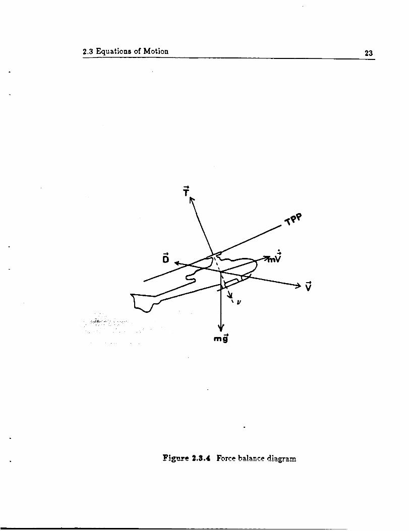
We next consider the force balance equation of the helicopter in accelerated forward
flight (see Fig. (2.3.4)):
L
,_v= f+ rag+ b
therefore rnV-V = ]F. 17 ,_ mr. 17 -r/). I7
(2o)
(21)
note that:
and
-- d(_m V V = _ mV 2) (22)
• d
rag. 17 = -d5 (mgH) (23)
2.3 Equations of Motion 23
T
--4,
V

24 2. Problem Formulation
where H is the height of the helicopter measured in a direction opposite to that of
_" from an arbitrary datum.
By suitably combining equations (7). (19). (21). (22) and (23) and introducing the
fuselage parasite power as :
Ppa,a = - D. V
1
2 pl'3fe (24)
(where fe is defined in equation (4)), the time rate of change of the total energy is
obtained :
d (rngH --- lrnI'2 + llRfl2 ) = Ps - (P, + Pmo * P_ra). (25)dt 2 2
and the corresponding torque balance equation is :
IRfi= -Q,
= --!p(rr R2)(f'IR)2R: Cp.
where Cp is given by:
(25a)
1
Cp = -80_d - CT A, (25b)
This energy conservation equation corresponds to the principle that any excess
power supplied by the engines that is not dissipated by the helicopter is stored as
internal potential, kinetic or rotational energy. Obviously, the internal energy level
of the helicopter can only increase if the engine power supplied on the main rotor
shaft exceeds the total power required. This excess power may be used to climb, to
accelerate, or to increase rotor speed.
Conversely, in the event of engine failure, the total power or energy will decrease
at a rate which depends on the helicopter's airspeed, main rotor thrust, angle of

2.4 Non-dimensionalization and Scaling 25
attack and rotor RPM. The pilot's task during autorotative flight is mainly one
of :Energy Management. This can be achieved through control of the thrust
vector during descent with the desired result that the aircraft can be landed at a
desired (achievable) location with small vertical and forward speeds. At the same
time, during the deceleration phase, the pilot must prevent the main rotor from
overspeeding which would lead to unacceptable blade centrifugal stresses. This
task is by no means easy.
2.3.8 Kinematical Relations.
The kinematical relations needed in the formulation of the optimal control problem
are given simply by :
_:--U
(26)
(27)
Note that these relations are coupled only one way to the dynamical relations. Since
h = _: is a hard terminal constraint on the optimal control problem, equation (26)
is al_s r_t_clecl in i_ formulation. Equation (27) may however be removed, unless
there is also a hard Constraint on the terminal horizontal distance (as in the case
where the helicopter is forced to land at a particular spot, perhaps due to terrain
considerations). The removal of equation (27) will reduce the order of the problem
and will facilitate the numerical solution. Information on the horizontal distance
travelled may be obtained through the forward integration of equation (27) after
the optima] time history of the forward speed has been found.
§2.4 Non-dimenslonalization and Scaling

26 2. Problem Formulation
The efficiency and rate of convergence of numerical optimization methods depends
critically on the scales used for the variables invoh'ed. This is especially true in
nonlinear problems "26 I. A "well scaled" problem is one in which similar changes
in the variables lead to similar changes in the cost function. Now consider a typical
situation where the engine of the helicopter fails while it is cruising at a forward
speed of 40 Knots and at an altitude of 400 ft . The magnitude of the thrust
coefficient CT used just before engine failure is of the order of 0.003. Rotor speed
before engine failure is 354 rpm The different units used by the state/control
variables, and the range of magnitude that these variables will assume in subsequent
autorotative descent flight, clearly indicates the need to normalize and to scale.
The equations of motion may be non-dimensionalized using the quantities no and
R. Here fl0 is the nominal angular speed of the rotor before engine failure and R
is the radius of the helicopter's rotor. Scaling factors of 10, 100 etc. are used for
convenience. Non-dimensionalized and scaled quantities for the time, states, and
controls used in the analysis are defined as follow:
(a) Normalized time:
r = t, (2s).1-b-6
Hence, one unit of r corresponds to about 16 rotations of the rotor.
From here onward, the notation ( )_ will be used to represent differentiation with
d 100 d()'- - (28a)
dr f_o dt
(b) Normalized states:
W
x, = (o.olnoR), (20)
respect to the normalized time r, where:

2.4 Non-dimensionalization and Scaling 27
and
u
=2 = (0.0]n0R), (30)
• 3= (_o), (31)h
•_= (1--_), (32)2"
•5 = (1-5_). (33)
(c) Normalized controls:
therefore :
u_ = ]03cr,, (34)
u2 = ]o3cT=, (35):
lo_cr = (.= + _=2)_. (36)
The effects of these normalizations are first to convert the time, state and control
variables into dimensionless quantities, and second to scale them so that they all
have order of magnitude one.
If in addition, we also define the following dimensionless constants for the system:
:f i ¸_,¸ , , 104g
go = no;_---_
10p_rR 3rn 0 --
m
20rR 2
pTrR sio-
10IR
co = _Oed(lO 3)
K=nd
I,o= o.o1(_)
(37)
The resultant dimensionless equations of motion are then given by:

28 2. Problem Formulation
(a) Dynamical relations (see equations (3) and (7)):
zl _ = go - mo(_)x32 -_ ]zl\":tl 2 -- x2_),
x2' = rno(u2x32 - ]x2X/X_ 2 -- x22) •
z3' = -ioz32(co + Av/ul 2 _ u22).
(39)
(40)
(40)
(b) Kinematical relations (see equations (26) and (27)):
2:4 r = 0.1Zl,
Ix5 = O.lx2.
(41)
(42)
(c) Supporting expressions:
(el) the inflow and advance ratios are (see equations (2a)):
tl sin o -- W COS Ot 1/
Rfl Rfl'
.T2tl 2 -- ZlU 1= 0.01
,T3\/Ul 2 _- U2 2
u cosa + wsina
= Rfl '
,Z2ttl -'t- z] u 2= 0.01
X3k,/Ul 2 _- U22
+ kofl(ul _ "r u2_) }. (43)
(44)
(c2) the induced velocity parameter h (see equations (14)-(16)):
X2u 2 -- 21U l5:1 = P0 (45)
xs(ul 2 + uz2) _-'`:r2Ul % 2:11/2
e2 = p0 (46)23(ttl 2 -+- U22) s--'`
where once again, the value of the induced velocity parameter .[1, is determined
from the expressions given in equation (14):
2.6 Terminal Constraints and Initial Conditions 29
t
h = 1"0/\/(22 + (_1 + fl)2),
• , (0.373_ - 0.59s_I- 1.991).if (2t] -_ 3) 2 _ 2_ _> 1.0;
otherwise.
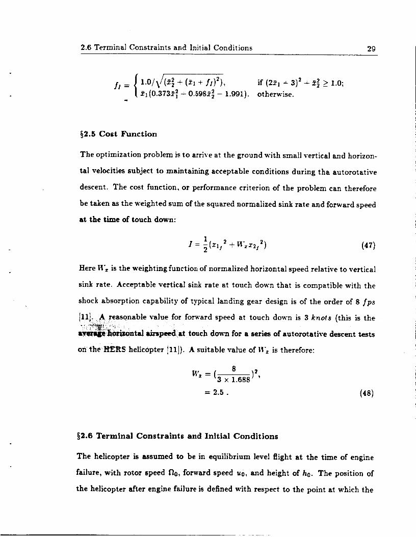
§2.5 Cost Function
The optimization problem is to arrive at the ground with small vertical and horizon-
tal velocities subject to maintaining acceptable conditions during tha autorotative
descent. The cost function, or performance criterion of the problem can therefore
be taken as the weighted sum of the squared normalized sink rate and forward speed
at the time of touch down:
1 2 2
1= _(x]j + _;z2j ) (4T)
Here lYz is the weighting function of normalized horizontal speed relative to vertical
sink rate. Acceptable vertical sink rate at touch down that is compatible with the
shock absorption capability of typical landing gear design is of the order of 8 fps
[1!]:. reasonable value for forward speed at touch down is 3 knots (this is the,--. ..... .
=__:__ta] airspeed:at touch down for a series of autorotative descent tests
on the HERS helicopter i11]). A suitable value of Wz is therefore:
8
"; = (3 × 1.6ss )2'
= 2.5. (4s)
§2.6 Terminal Constraints and Initial Conditions
The helicopter is assumed to be in equilibrium level flight at the time of engine
failure, with rotor speed Go, forward speed u0, and height of h0. The position of
the helicopter after engine failure is defined with respect to the point at which the

30 2. Problem Formulation
enginefailure occurred. The coordinat(, systemusedis defined in Fig. (2.3.2)where
h is measured in the downward direction. Therefore, the initial conditions of the
state variables are:
2"10 = O,
3:20 = UO-
z3o = 1, (49)
X40 = 0,
and xs0 = 0
where fi0 is defined to be (_).u
The terminal constraints of the optimization problem include:
Z4l = hi,
xs t = it].
(so)
where:
hi - ho10R'
dld!- IOR"
(51)
Note that, while the first equation of (50) is always needed, the second equation is
used only when there is a hard constraint on the terminal horizontal distance (to
land at a horizontal distance of d! ft away from the point at which engine failure
occurred).
§2.7 Path Constraints
The equivalent profile drag coefficient of the rotor (Cpro, as defined in equation (18)
) increases sharply when the thrust coefficient exceeds the rotor stall limit (_)aatt.
The immediate effect of this increase in profile drag is a drop in the rotor speed. This

2.8 Further Time Normalization 31
drop in rprn causes an increase in the- angle of attack on the rotor's blades and will
ultimately lead to rotor stall and the instability associated with it. This limitation
on the thrust coefficient requires a path inequality constraint in the optimal control
problem.
A typical value of (-Qr-),tat t for the OH-58A helicopter is 0.15. This value is used. 8.
in the present study. The path inequality constraint, and its non-dimensionalized
form are:
( ),,.u>
or 7.2 > v/ul _ + u2_ (52)
where:
(103CT).talt = 103( CT ),tatl xo,0
= 103 x0.15 ×0.048,
= 7.2.
(53)
This inequality constraint can be converted to a path equality constraint as shown
Since (_T.) 2 _>(ul _ + u22)
where C'Toisequal to 7.2.
therefore C'_-0- (ul2 + u22) - u32 = 0. (54)
where _3 is a "slack variable" or artificial control that has been introduced to convert
the inequality constraint into an equality constraint.
The upper bound on the vertical sink rate as an additional path inequality constraint
will be discussed in Section (3.3).

32 2. Problem Formulation
§2.8 Further Time Normalization
The optimal control problem that has been posed thus far is one with an unspecified
terminal time r1. The problem may be converted into one with specified terminal
time through the following (further) normalization of the dimensionless time r:
7
,, = - (55)rf
The transformation (55) converts the independent variable from r to ( where ,¢ now
varies from 0 to 1. This transformation introduces into the problem an additional
unknown parameter 7! that has to be optimally selected. We shall from here onward
denote the differentiation with respect to _ by:
( )v d
= rz( )'. (56)
§2.9 Final Form of Helicopter Optimization Problem
We are now in a position to write down the final form of the helicopter optimization
problem, Let:
2 = (zl x= z3 =:4 zs) T,
6 = (_ _= _3)r,
_= (r_).
(57)
(58)
(59)
denote the state, control, and unknown parameter vectors of the problem.

2.9 Final Form of Helicopter Optimization Problem 33
The problem is to find [_(_) and ff t,o minimize:
1 2x = _(zll * _;x2s 2) = _(-_s), (60)
subject to :
(1) equations of motion ( _v = f):
xJv = _s(go - mo("Iz3 2 - fx_ \ 'x12 -_ zF)),
x_ v = rlrno(uzx32 - ]x2_;.'x]2 + x22),
z3v = -rlio z3=(co + _x/ul _ + u2_),
z4 v = O.lrlzl,
z5 v = O.lrlz z.
(61)
(2) the initial condition of._ is given by:
-_o = (o, _0,1, o, o) r.
(3) pa_iequality Constraint (S(.X,U,_) = 0 ):
(62)
(u_= + u_2) - ( (u_* + u22)) = - u3z = o. (63)
(4) terminal constraints (t_(._l,_) = 0):
(64)
In the next chapter, a gradient-type numerical optimization technique that can be
used to solve this problem is described in detail. It requires the calculation ofaO
34 2. Problem Formulation
- of (1,,3 matrix), oo (1_5(5x3 matrix), 03_°/-(5×5 matrix), _ (5_,1 matrix), _
or: (2 x 5 matrix) Detailed expressions of these matrices are given inmatrix ) and _
Appendix (B).

Chapter 3
Numerical
Optimization Techniques
In the previous chapter, the landing of a helicopter after engine failure was for-
mulated as a nonlinear optimal control problem with path equality constraints.
Numerical optimization algorithms that can be used to solve this problem are de-
scribed in this chapter.
This chapter begins with a revie,a" of algorithms for solving optimal programming
problems with bounded controls and 'or states. A combined function and parameter
optimization algorithm is then described. It is an extension of the ordinary gradient-
type numerical algorithm (FCNOPT) [16], to handle the presence of an unknown
parameter vector. In Section (3.3), we describe the Sequential Gradient Restoration
algorithm which can be used to solve optimization problems with nondifferentialo.
path equality constraints. Several transformation techniques are then presented
that convert problems with path inequality constraints to problem with equality
constraints. The chapter ends with a description of an algorithm that can be used
to compute neighboring feedback control laws for optimization problems with path
equality constraints.

36 3. Numerical Optimization Techniques
§3.1 Algorithms for Problems with Bounded Controls and/or States
One of the earliest attempts at numerical solution of optimal programming prob-
lems with control or state inequality constraints was made by Bryson et al [27-28.
see also chapter 3 of 29. Necessary conditions for extremal solutions to program-
ming problems with an inequality constraint on a function of the control or state
variables were given. It was shown that, in general, certain terms must be added
to the Hamihonian function during the interval in which the solution curve lies
on the constraint boundary. Furthermore, for inequality constraint functions not
explicitly involving the control variable, one or more functions of the state and time
must satis_" equality constraints at the beginning (the entry corner) of a constraint
boundary interval. The Lagrange multiplier functions are not uniquely defined on
state constraints. In the work reported in Reference 28, a modified version of the
steepest-ascent technique was used in the numerical solution of two atmospheric
entry trajectory problems. An advantage of the method is that improvements in
the control program are not required for the period on the constraint boundary,
making possible a more rapid convergence towards the optimal program. However.
the method requires prior assumptions concerning the number and location of the
junction points.
Inequality constraints on functions of control and/or state variables have also been
treated by several investigators through the use of integral penalty functions [31-331 .
One such scheme [31-321 uses an auxiliary state variable which is the integral of a
quadratic measure of the violation of the inequality constraint, which is brought as
close to zero as is necessary to provide a satisfactorily small violation of inequality
constraint. Rate of convergence to a satisfactory solution is usually slow [29].
McGill [33] developed a generalized Newton-Raphson algorithm based upon essen-

3.1 Algorithms for Problem_ with Bounded Controls and/or States 37
tially the same idea of reducing the constraint problem to an unconstrained one
by the introduction of an additional state. His approach does not require assump-
tions as to the number and location of junction points. Computational experience
with one example problem (a modified version of the classical brachistochrone prob-
lem) suggests that it may be useful for obtaining solutions to the class of nonlinear
problems with bounds on the state space.
In an extension of the work given in references [27-281,Speyer and Bryson [341
gave a new set of necessary conditions for solution of an optimal programming
problem with a statevariableinequalityconstraint.Itwas shown that unconstrained
arcs must satisfy certain "tangency _ constraints; namely, these arcs must haw
zero values of the state variable constraint function and all of its time derivatives
that do not involve the control function, at both the entry and exit corners of
the constrained arc. These conditions are satisfied automatically if the necessary
conditions of reference [27] are used. However, if one uses the "direct-adjoining"
approach of reference f 1t35_, explicit use must be made of the tangency constraints
at both corners.
L: , ¢ .
_. refe_nce 136: ,. Mehra et a] showed that some of the difficulties associated with
nonlinear programming problems with state variable inequality constraints and sin-
gular arcs arise due to the exclusive use of control variables as the independent
variables in the search procedure. They proposed a conjugate-gradient algorithm
which based its choice of independent variables on the problem constraints. This
choice could result in different combinations of state and control variables as inde-
pendent variables along different parts of the trajectory. Four numerical examples
were successfully solved using this approach. Two of the solved problems had a state
variable inequality constraint and the other two had singular arcs. The inequality
constraint and singular arcs were handled in a regular fashion without explicit use

38 3. Numerical Optimization Techniques
of extra necessaryconditions of optimality. This is considered to be a special feature
and an advantage of the method.
In reference [3T_, Maurer e_ al distinguish between two main cases of optimal pro-
gramming problems with bounded state variables, depending on whether the control
variable appears nonlinearly or linearly. The distinction arises naturally from the
fact that a nonlinear optimal control in the first class must be continuous at the
junctions between the interior arcs and boundary arcs, whereas any linear optimal
control in the second class is discontinuous in general. Maurer et al exploited the
fact that the optimal control in the first case must be continuous and satisfy a
suitable augmented Two-Point Boundary-Value Problem (TPBVP). This consists
of the basic two-point boundary-value problem of the Maximum principle, and of
additional differential equations and boundary conditions constructed in such a
way that all the necessary conditions are automatically fulfilled by the solution.
The TPBVP's encountered were solved using the method of multiple shooting [38 I.
Three numerical examples were solved to illustrate the efficiency of the algorithm.
Once again, predetermination of the number and sequence of subarcs of the optimal
solution has to be made prior to the initialization of the algorithm.
Most of the above mentioned methods suffer from the following disadvantages:
(1) it is not known a priori, whether there will be more than one joining of
unconstrained and constrained arcs, and where in time these joining will
occur;
(2) the discontinuities in the Lagrange variables at the junctions of the
unconstrained and constrained arcs are, a priori, unknown, and have
to be guessed and iterated upon.

3.1 Algorithms for Problems with Bounded Controls and/'or States 39
To overcome these difficulties, Jacobson et a] 1391 suggested the use of a different
approach. A device suggested by Valentine was used to transform a control problem
with a state variable inequality constraint into an unconstrained one of increased
dimension. With a pth order state variable inequality constraint, it can be shown
that in the transformed unconstrained problem; the pth time derivative of the
slack variable becomes the new control variable. One feature of the transformed
problem is that any guessed nominal control results in a feasible state trajectory,
i.e., the inequality constraint is automatically satisfied. A second feature is that the
transformed problem exhibits singular arcs which correspond, in the original state
constrained problem, to arcs lying along the state constraint boundary.
However, a major difficuhy arises with Jacobson's approach when the number of
state bounds {r) does not equal the dimension of the control vector (rn). In partic-
ular, if m < r_ then one cannot express u as functions of the r slack variables unless
some of these variables are dependent upon each other. Thus one cannot use the
appropriate time derivative of the r slack variables as independent new controls.
Twq___ples without the above difficulty were given in [39 I.
In_d of _in$ the control u in the original problem formulation by appropriate
slack variables and its time derivatives, one can enforce the state/control bound
by the addition of path equality constraints to the original problem. These path
equality constraints are again obtained by the use of Valentine's device on path
inequality constraints. In this way, nonlinear optimal programming problems with
path inequality constraints can be transformed into ones with nondifferential path
equality constraints.
The solution to this class of problems with path equality constraints differs from the
solution without the constraints. The usual approach of backward integration of

40 3..Numerical Optimization Techniques
the adjoint-equations and forward integration of the equations of motion cannot be
employed here. This is due to the fact that the computation of the Lagrange mul-
tiplier p-(t) (associated with the path constraints if) over the time interval requires
the simultaneous solution of both the adjoint-equations and the equations of mo-
tion. Because of the coupling, the total system must be integrated simultaneously
in either the forward or backward direction. One way of solving the coupled, non-
linear, two-point boundary-value problem is by the Method of Particular Solutions
given in references 140-41
Miele et al !42 I. at about the same time as Jacobson, developed a Sequential Gra-
dient Restoration algorithm for the solution of optimal control problems with path
equality constraints. The algorithm made use of the method of particular solutions
of i401-i41i. Both the feasibility as well as the efficiency of the algorithm were il-
lustrated through the solutions of example problems given in 142 and other related
papers 143-45'. The approach taken in the present work on the optimal autorotation
trajectory of a helicopter is to combine these two mathematical tools (the Valen-
tine's device and the Method of Particular Solutions for the solution of a nonlinear
TPBVP) for the solution of the constrained optimization problem posed in Section
(2.9). The Sequential Gradient Restoration method is described in greater detail in
Section (3.3).
§3.2 Combined Function and Parameter Optimization Algorithm
Direct analytical solutions of dynamical optimization problems are only possible
when the system equations, the performance index, and the constraints of the prob-
lem are very simple. One of the more reliable methods for the numerical solution of
the dynamical optimization problem is the steepest-descent gradient method [301.
The method is characterized by iterative steps for improving estimates of the con-

3.2 Combined Function and Parameter Optimization Algorithm 41
trol history, u(t), so as to come closer to satisfying the optimality conditions and
the boundary conditions. First-order gradient methods usually show great improve-
ments in the first few iterations but have poor convergence characteristics as the
optimal solution is approached. Second-order gradient methods have excellent con-
vergence characteristics as the optimal solution is approached but may have starting
difficulties associated with picking a "convex _ nominal solution !291. Variable Step-
size Gradient methods can improve the convergence characteristics of the first-order
gradient methods through the optimal selection of step-size at each iteration step.
Further information on the variable step-size gradient algorithm can be obtained
from r :.i26_
In this section, we wish to extend the gradient algorithm for function optimization
problems [16: so that it is capable of solving optimal control problems that also have
an unknown parameter vector. We assume that there are no inequality constraints,
that the initial time and state are fixed, and that functions of some of the state
variables and unknown parameters are specified at a given or an unspecified terminal
time. Thus we wish to consider the following optimization problem:
_0 t!_,_
),
= given,
and g(_f, if) = O.
(1)
Here _(n x 1), _(m × 1), and _7(p × 1) are the state, control and the unknown
parameter vectors. _(q x 1) are the terminal constraints of the problem. If the
end-time tl of the problem is unspecified, the problem may be converted to one
with a specified end-time through the use of the following transformation:
t
tl(xa)

42 3. Numerical Optimization Techniques
The independent variable is now r which varies from 0 to 1 (therefore the subscript
"1" in equation (1) denotes terminal condition). The final time t! is included as
one of the components of zT. ]_ and f are replaced by L = t/fL and f = tlf.
If we adjoin the system differential equations and the terminal constraints to the
performance index I with multiplier function A(t)(n , 1) and multiplier/z(q × 1)
respectively, we get:
j = (¢ ÷ .r_,)_ ÷ [L-_ _r(f _ _)!d_. (2)
Now consider the variation in J due to variations in both the control and parameter
vectors:
fO6J = (-A T + Cz)l_xl + [ H_dr + (¢_)I]$_
+ [Hu_fi" + (Hz + AT)_e;dr,
(3)
where for convenience, we have defined scalar functions H (the Hamiltonian func-
tion) and ¢ as given below:
(4)
Therefore, first-order necessary conditions for the extremal solution are given by
the following relations:
A T "- --/']z ,
and
_1T= (¢_)1,
H,.= 0,
dr + (¢n)1 = 0.-
(5)
In the special case when the unknown parameter _ contains the unspecified ter-
minal time, the corresponding component in the last equation in (5) becomes the
transversality condition of the classical literature (cf. Appendix D).

3.2 Combined Function and Parameter Optimization Algorithm 43
Equations (1) and (5) contain all the conditions needed in the solutions of _(r) (n _,
1), _'(r) (rn × 1), ,_(r) (n × 1), _(p × 1) and _(q × 1).
Various methods have been suggested for the solution of this two-point boundary-
value problem. The method used here may be termed the Impulse Response method
[29].
The method involves making initial guesses for both the control time histoD" E(r)
and the unknown parameter _. The dynamic equations are integrated forward us-
ing the given initial conditions. In general: the terminal conditions are not satisfied.
To make improvements in the feasibility condition, we consider the following (q_ 1)
impulse response functions H_ {fl, where i = 0,1,... ,q. Note that Hu(°)(r) repre-
sents the variation in the cost function due to a unit impulse (Dirac Function) in 5ff
at time r, while holding _(0) and _7constant and satisfying the dynamic equations.
Similarly, Hu(i)(r) where i = 1,...,q corresponds to variations in the terminal con-
straints V7 due to a unit impulse in 5ff at time r. These impulse response functions
_eli_'en by the following expression:
.... HJ't(T) = rtOZ,,(r) i_t_)T- _ A(r), (e)
where
r(i)= _1 if i=0; (6a)t 0 ifi _ 0.
for i = 0,1,...,q. The influence functions A(i)(r) are determined from the backward
integrations of the following adjoint equations using the time histories of ._ (r), E (r)
and the value of • from the forward integrations:
A(,I= -r(;)L,(r) - [_l'l]rf,(r), (7)

44 3. Numerical Optimization Techniques
where
¢0 = ¢(£/,_) (9)
In this way, the (q- 1) impulse response functions Hu b), where i = 0,1,...,q, for the
current iteration, can be computed.
The quantities if_ tt, O)(r) dr 4- (¢,_),!, where j = 0A,....q represent the variations
in either the performance index or terminal constraints due to a unit changes in
the elements of zY, while holding £(0) and ff constant and satis_'ing the dynamic
equation.
Therefore variations in the cost function and the terminal constraints due to small
variations in the control histories _ff(r) and the parameters 6ff axe given by the
following relations:
/0' /0l6J = H_(°)6_(_)dT-_ ! H.(°)(,)d_ ÷ (¢o).?_. (10)
and
/oI Jo'6t-'3 = H-C;)(r) 6ffdr ÷ [ H,(J)(r) dr - (t'3), 6='', (11)
where j = 1, .... q
If we adjoin equation (11) to (10) with q Lagrange multipliers p,, where i = 1,...,q,
we have:
q
6J = 6J + _ u,6¢,,
S=I
= [H,,(°) + _,Hu(i)]dfffdr
i=1
l q 1
z.,/._=1
q
i=l
(12)

3.2 Combined Function and Parameter Optimization Algorithm 45
If we wish to obtain the largest change in 63, we would calculate the gradients
H, (i) and [f01H,(i)(r)dr + (t_,),] (i = 0,1,...,q) and then direct 6_ and dSff opposite
to their respective gradients as follow:
/0' '/0'6_= -K_,_ H_C°)d_+ (_o)_- _.,( _'Id_+ (_,).)ir,i=I
'/o' ' /o'-- -K_,I (H_,'°l)rd_-_(,_,o)_r + _.,( (H.'O)rd_ ÷ (e,)_r)i, (13)t=l
where K,r is a (p Y p) diagonal gain matrix that controls the stepsize of $ff.
Similarly,
,=l
(14)
where K= is an (m × m) diagonal gain matrix that controls the stepsize of _ff.
When we make these choices in _ and 6if, the predicted variation in the augmented
performance index J _ d - V'qz--t=l tz,_,,, is:
'/o' ' /o'6J = -._-_ : (Hr(°)) Tdr + (tb0)_ r + _/_,( (H_(')) rdr -_ (tS,)_r)i
t=l
[1 ..=: :,,.. ¢o_.r-. q (15)'":::!i;f"-.to --If.,:In,,! "_ E#iCH" {O)T]dr <-O.
i=l
Here the weighted norm-function NK( ) is defined as:
(15a)
Similarly, the substitutions of equations (13) and (14) into (11) give the following
changes in the terminal constraints:
/o' '/o'_¢j "- - (Hu(Y))Ku(H,,(°))Tdr - Z #i (HuO))K,,(H,,(O) Tdr
i=l
[' ['-r H..(J}dr + (¢,)_}(K.)I (H.(°)) rdr + (¢o). T] (16)'Jo ""Jo
/o'- #i[ H,, (y)dr + (¢y),r](K,,)[ (H,,(O) rdr -_ (t_,),T],
t=l

46 3. Numerical Optimization Techniques
where j = 1,...,q
One way to simpli_" expressions (16) and (17) is to "absorb" K., into Hu (]) and K_
into H_ (J). To do this, we first note that both Ku and K,_, being positive definite
matrices, can be expressed as products of their respective "square-roots":
Ii,r = S,rS,r T ,
Ku = St, Su T •
(17)
Let us define the following quantities"
H_Ol(_)= H (oI(_)S_,
H_')(_)= H_I')(T)S_.(lSa)
where i = 1 .... ,q.
Therefore an expression for/_'u(r) is given by
q
i=l
q
[Y.(_)= H.(_lS. = _(o_(,.)__ .,.F/.(')(,-).t=.]
(lSb)
Similarly, B_{) and (,_{))_ are defined as
_(o)(_) = n lo)(_)s. '
fil_')(r) = H,{')(r)S,_,
(_o), = (_o)_S,,
(_].), = (¢j) s,.
(19)
where i = 1,...,q and j = 1,...,q

!
3.2 Combined Function and Parameter Optimization Algorithm 47
Substitutions of (17)-(19) into (15)-(16) give
' q /0'q
t=l
/o ' /o''H21(_Y_)rd_ Z",_=1
',/o /o- Z O,: H(_Y}dr+ (d3)xl [ (H(i))rdr -f (g.,) T] .
t=l
where j = 1,...,q
(20)
(21)
Equation (21) can be rewritten in a vector-matrix form after the introduction of
the following notation:
6_(q × 1)= (6_21,...,60q)T,
_(q >:1) = (_,l,...,_q)r, (22)
and _(q x 1)-- (gl,...,gq) T.
The ]_h component of _ is given by:
f' ....(.(o.)Tdr-- [fl H_("' drg¢Jo Jo
l
(H(0))Tdr -4- (_0)_ T] (23)
where j = 0,1,...,q
Furthermore, let us define a (q x q) symmetrical matrix Q whose components are
Qtj= Q#,,
._ __ol_.i(i)(_.I{ui))Tdr - if01H{j)dr + (_$),][ fol(/:/{i))Tdr d. (_,) T]. (24)
where (i,j) = 1,-.-, q

48 3. Numerical OptimizatioI: Techniques
Using equations (22)-(24). equation (21) can be written in a more coml,act form:
_J= _- Q6. (25)
If we choose t;O = -t_,,,
evaluated as:
where 0< t <1, the Lagrange multiplier /Y can be
6= -Q-I(V _ t,7) . (26)
If Q-1 exists (the controllability condition, see also Chapter 2 of !29]), we can sub-
sti_ute the value of/7 found in equation (26) into both equations (13) and (14) and
express both bff and bfi" only as functions of the impulse response functions H,, (') (r)
and H, (i)(r) (that have been computed and stored during backward integrations):
jfO 1 q _01_=-s_i (H_°))re_-(_o)_, r-_., (H(:))re_t----I
q
_ = -s_i(,_°))r -_Z '_'"))r]..,t-_t'=l
+ (5,) r],
(27)
For the next iteration, the uses of new trial values
6_-._(r) = ¢_.(_) ÷ bff._-(r).
ff_'-_ = _" -+-b_-,
(2s)
(where N is the current iteration number)
•,,,'ill reduce the value of the performance index and bring the system closer to sat-
isfying the terminal constraints.
After many iterations of the above procedure, all the terminal constraints are sat-
isfied to a prescribed accuracy:

3.2 Combined Function and ParameterOptimization Algorithm 49
for j = 1,...,q, where e_.denotesthe feasibility condition (e.g. e,. = 10-4).
Using this procedure, a feasible path satisfying the constraints is determined. Hob--
ever, the performance index can still be decreased further. The procedure now
concentrates on minimizing the value of the performance index while keeping t'_
within the accuracy of (29). The procedure is repeated until
1 qxi(n °l) r • _<,. (30)!=1
and
7. T q [l"+ (!P0). + Z/z,( (H{i))rd r + (_,)T)] _< '. (31).tO
where _u and e_ represent the optimality conditions (e.g. cu = _ = 10-s).
A numerical algorithm that implements the above procedures has been written.
The procedure is basically an extension of the program FCNOPT by Bryson 116 I.
Example Problems
Tw_le,_licatloas of the Combined Function and Parameter Optimization
Algorithm are gaven here. The first example involves a nonlinear first order system
with a specified control lab-. The second example considers the optimal landing of
a helicopter that is initially in hover.
(I) Specified Control Law Problem [46]
Consider the following optimization problem:
mini = 1 in
subject to the scalar nonlinear differential relation
_-- --Z2 -,- tl .

50 3. Numerical Optimization Techniques
The initial condition is
_(o) = lo.
There is no terminal condition.
In order to exercise the parameter optimizatiobn capability, the control law is spec-
ified to have the following form
?/ = {2.T_
where a is an unknown parameter whose value is to be optimally selected.
t ran s formed problem becomes
rain I = 1 []° 2 Jo ix2-_a2 x2]dt'
The
with the following equation of motion
._= --X2÷ ax,
while the initial condition of x(0) remains unchanged.
The transformed problem now becomes a problem with an unknown parameter a
but without any control. The problem can be solved using the combined function
and parameter algorithm and the optimum value of a found is:
a = -0.10334.
The minimum value of the cost function is:
I = 4.5218.
The value of I is slightly larger than the minimum value when u(t) is open:
Im_'n = 4.5108.
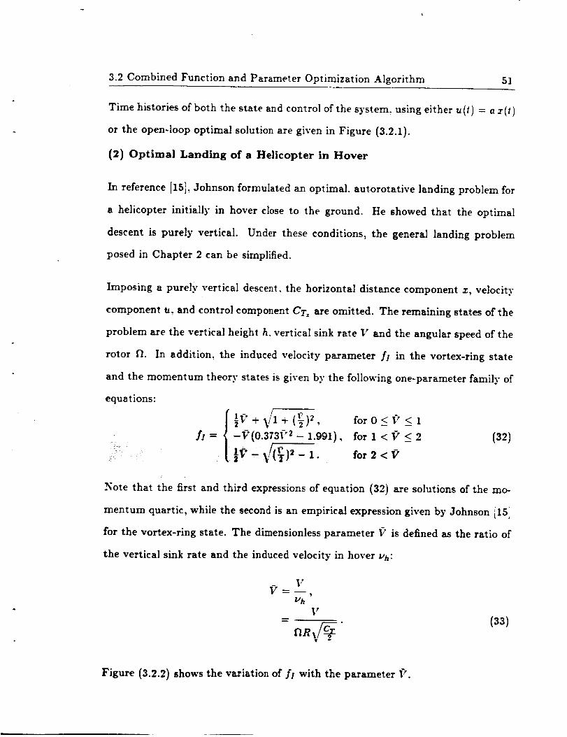
3.2 Combined Function and Parameter Optimization Algorithm 51
Time histories of both the state and control of the system, using either u (t) = e x(t)
or the open-loop optimal solution are given in Figure (3.2.1).
(2) Optimal Landing of a Helicopter in Hover
In reference [15], Johnson formulated an optimal, autorotative landing problem for
a helicopter initially in hover close to the ground. He showed that the optimal
descent is purely vertical. Under these conditions, the general landing problem
posed in Chapter 2 can be simplified.
Imposing a purely vertical descent, the horizontal distance component z, velocity
component u, and control component CT= are omitted. The remaining states of the
problem are the vertical height h. vertical sink rate V and the angular speed of the
rotor f}. In addition, the induced velocity parameter .t"I in the vortex-ring state
and the momentum theory states is given by the following one-parameter family of
equations:
f! = -f'(0.373f "2 - 1.991) for 1 < V < 2/ __
1 for2<,i : 6-- ¥_"
(32)
.Note that the first and third expressions of equation (32) are solutions of the mo-
mentum quartic, while the second is an empirical expression given by Johnson I15]
for the vortex-ring state. The dimensionless parameter I_ is defined as the ratio of
the vertical sink rate and the induced velocity in hover vh:
--- R,
/]hV
m
nR_ c/___ "
(33)
Figure (3.2.2) shows the variation of ,1"1with the parameter fT.

52 3. Numerical Optimization Techniques
!i
"°'l.!' ' '__' II _,_ open- 1 o op
-0 40
-0.20
i I I I
0 0 2 0 4 06 0.0 *.0
I',mi, 141COllIE
IZ 0
,o\\
40 \
0
i ! i 1
--- open- loop• tl = a x
e_•_Ct_'e'i_m_m'•'mm'm• me
OI I I I04 06 08 iO
T,me. MKOnO$
Figure 3.2.1 Example Optimal Control Problem

!
3.2 Combined Function and Parameter Optimization Algorithm 53
wi-
re
Q
4
Figure $.2.2 Variation of Induced Velocity Parameter/! with I7"

54 3. Numerical Optimization Techniques
If we go through the normalization and scaling processes of Section (2.4), the non-
dimensionalized and scaled time, stales and control of the problem are given by the
following relations:_ot
V
x] = (O.Olf_oR),
• 2 = (n--n0),h
ul = IOaCT,.
(34)
In terms of these normalized quantities, the optimal autorotation from hover is
formulated as the minimization of the cost function 1, where
The equations of motion are given by
' mox_uz- foX_Xl = go --
' _ioz221co - ul(-O.O1 zl• 2 = - - l,ov%f_)i, (3s)X2
FX 3 = X 1 .
Here ( )' denotes time differentiation with respect to _ and the dimensionless quan-
tities go, m0, f0. co, and k0 are as defined in Section (2.4) (see equation (37)). The
induced velocity parameter .1"1is a function of 17, which is now given by the following
normalized expression:
XlV = p0_ (35_)X2 V'_I '
where p0 is also defined in Section (2.4).
The optimization problem is constrained at the end-time by the "stopping" condi-
tion:
x3I - hi = o, (36)

3.2 Combined Function and Parameter Optimization Algorithm 55
and the following one-sided path inequality constraint:
_] _<Or.. (37)
Further Time Normalization
Since the end-time of the problem is unspecified, further normalization of the inde-
pendent variable _ is needed. The problem is converted to one with fixed end-time
by the following change of independent variable:
= -, (3s)
The transformation (38) converts the independent variablefrom r to _ where _ now
varies from 0 to 1. This transformation introduces into the problem an additional
unknown parameter fl that must be optimally determined. From here on we shall
denote differentiation with respect to _ by:
()r=d
= _f( )'. (39)
Substitution Technique
The path inequality constraint (37) can be eliminated if we substitute for _] the
new control variable u2, where us is defined as :
ltl --C'T, COS2 it2" (40a)
Final Form of Optimal Autorotation Problem

56 3. Numerical Optimization Techniques
The state, control, and unknown parameter vectors of the problem are:
= (I1 X2 2:3) T,
U= (u2),
e= (TI).
(41)
(42)
(43)
denote the state, control_ and unknown parameter vectors of the problem.
The problem is to find t_(_) and _ to minimize:
1
X= _[xlS] 2 = _('_I)" (44)
subject to:
(1) equations of motion ( gv = f):
• 1v = T1[go- mox22(¢r, co_2u2) - fo_2j,
x2 x- = -rlio x22:c0 + (C'T, c°s_ u2)(-0.01 xl f-_x_ _ k°vCr" cos _2.6):,
:Z3 V : 7"fX 1 .
(45)
(2) the initial condition of ._ is given by:
£o = (0,1,0) r. (46)
(3) terminal constraint (¢(._i,_) = 0 ):
_31- hj. =0 (47)
The optimization problem (41)-(47) is now in a form that can be solved using
the combined function and parameter gradient algorithm. Several other example
applications of the algorithm are given in Appendix C.

3.3 Sequential Gradient Restoration Technique !421 57
§3.3 Sequential Gradient ]Restoration Technique [42]
This section explains the Sequential Gradient Restoration (SGR) method given in
142. The SGR technique is one way that problems with bounded control may be
solved. The technique is employed in the solution of the optimal helicopter landing
problem posed in Section (2.9).
The problem is similar to the one in Section (3.2) except that here we consider
more general path constraints. Specii_cally, we consider the following problem with
unknown parameter vector _ and path equality constraints ,_:
minI,_,_= ¢(_I,_)+ fo_
3-- f(_, if,_,T),
_(0) = given,
_(_,_,_,T) = 0,
d(is, _) = o.
1,(_,_,_,_')d_',
and
(1)
W_e_ ,_{r × 1) a.__ the path equality constraints of the problem. The motivations
f0i' thls formulatmn are:
(1) .Many optimization problems arise directly in the form considered here. i.e.
with path equality constraints.
(2) Problems involving inequality constraints can be converted to the present
scheme through suitable transformations. This statement applies, for
instance, to the following situations:
(a) Problems with bounded controls.
(b) Problem with bounded states.
(c) Problems with bounded time rate of change of state.

i
58 3. Numerical Optimization Techniques
(d) Problems where some bound is imposed on an arbitrarily prescribed
function of the parameters, the control and the time rate of
change of the state.
The transformation techniques employed are of the Valentine-type [41]. The trans-
formation is performed by augmenting the dimension of the control space, with
or without augmentation of the state space. In the process, non-differential path
equality constraints relating the original control and the slack control are produced
that must be satisfied by the solution of the original optimization problem. Four
example problems with bounded control, state or time rate of change of state are
presented in Appendix (G).
3.3.1 First Order Conditions
If we adjoin the system differential equations, the path equality constraints and the
terminal constraints to the performance index I with multiplier functions X(r)(n x
1) and tY(r)(r _ 1); and multiplier ff(q >: 1) respectively, we obtain the following
augmented performance index J
1J = (0 + pr¢) 1 + [I., -+ AT( f - _) .+ ,aT ..q]dr,
/o'= (:x)0-_ (¢- _%)1 + (iT= + n)d_-,
(2)
(3)
where, for convenience, we have defined scalar functions H (the Hamiltonian func-
tion) and ¢ as given below:
n(_,¢,_,_,],r)=L(_,u,_r,r)+ATf(_,¢,_,r)-rpT$(_,¢,_,r), (5)
¢(E/, _,_) = _(_/,,v).uT¢(E/,_). (6)

3.3 Sequential Gradient Restoration Technique i42" 59
Now consider the variation in J due to variations in both the control and the
parameter vectors
6J = (AT_x)0. (-A T- ¢z)16xl - H,rdr-+ (cI,.)]]6_
+ [Hu$ff-_ (H..- ir),SE)dr.
Therefore, first-order necessary conditions of the problem are given by the following
relations:
_= f(_, _',,_,r),
g(_,,_, _, r)=o,.T
= -/-/z,
Hu= 0,
E(0) = given,
(yr)_= (¢z)_,
_(_I,_)=0,
(4)
and O,), -_ lt, dr = O.
Summarizing, we seek functions E(r), _(r), • and multipliers A(r), _r) and p which
satis_' the first order necessary conditions (4).
3.3.2 Approximate Methods
In general, the problem posed in Section (3.3.1)isnonlinear and can only be solved
iteratively.In this connection, we definetwo scalarfunctionals
P = N[_-fldr + NiS]dr + N[(¢)l], (7)Jo Yo
and
/o1 /olQ = N[A+H[]dr + N[Hr]dr + N[ (#r)] + /o I HT dr] + N[(A-{bT)1], (8)

6O 3. NuI_orical Optimization Techniques
where the norm-function .N I I was defined in equation (15a) of Section (3.2).
P and Q are measures of the errors in the constraints and the optimality conditions.
respectively. For the exact optimal solution, one must have
(9)
For an approximation to the optimal solution, one must have
P _< el. (10a)
Q _< (lob)
where cl and _ are small pre-selected numbers.
S.3.3 The Sequential Gradient ]Restoration Algorithm
The Sequential Gradient Restoration algorithm involves a sequence of cycles, where
each cycle has a gradient phase and may or may not have a restoration phase.
The restoration phase is iterative and is started when the inequality (10a) is violated.
In each restoration step, the norm of the variations of the control and the parameter
is minimized, while the constraints are satisfied to first order; this has the effect of
reducing P, i.e. more closely satisfying the feasibility conditions. The restoration
phase is terminated when the inequality (10a) is satisfied.
The gradient phase is started when the inequality (10a) is satisfied. It involves a
single step, which reduces the functional I, while the constraints are satisfied to first
order; this has the effect of reducing Q, i.e. more closely satisfying the optimality
conditions.
The algorithm ends when both inequality (10a) and (10b) are satisfied.

3.3 Sequential Gradient Restoration Technique 421 61
Notation
For steps in the gradient phase or the restoration phase, the following notation is
used: x(r). u(r), _r denote the nominal functions; }(r), fi(r), _r denote the varied
functions, and ,_x(r), __u(r), and _ denote perturbations of z(r), u(r) and r
about the nominal values, i.e.
(11)
_ _ ?T-._ .._'.
(Note the removal of the arrow on top of the symbols for the vectors £, ff and _ in
(11).)
Concerning the functionals I, J and P, the following terminology is used: I, J and
P denote the values associated with the nominal functions; I, J: and ]_ denote the
values associated with the varied functions; and AI, A J, and Ap denote the total
variations of these functionals caused by the perturbations Az(r), Au(r), and ATr,
i.e ..................................................
i_= I + AI,
(]2)
/_= p + Ap.
If the variations appearing in (11) are linear in the stepsize a, (where a > 0 ), they
take the forms
A(,'),
B(r),
Ar_=aC.
(13)
(14)
3.3.4 Desired Properties in the SGR Process

62 3. Numerical Optimization Techniques
The functions A(r), B(r), and C are determined so as to decrease the functional I.
and/or d, and "or P. (A]ternatively, the condition (lOb) on the value of Q can also
be used.) Thus, the following properties are required.
AI< 0,
and .or AJ < 0. (15)
and/or Ap < 0.
In turn. relations (15) can be enforced at every iteration providing the stepsize a is
sufficiently small and the functions A(r). B(r). and C are chosen so tha_
and /or
and/or
61 < 0, (16a)
6 J < 0, (16b)
6 P < 0, (17)
where 6(...) denotes the first variation. Inequalities (16a) and (16b) characterize
the gradient phase, and inequality (17) characterizes the restoration phase.
3.3.5 The First Variations
The first variations of the functionals I, J, and P are
6I=
6J=
6P=2
o'!LzAx+LuAu+L,,Ar]dr+ (¢zAx Cr..ST)l,
I' /o i'[AT + H,!Axdr + H,,Audr -+ [(0,)1 + H1rdr]Ar
](_- .f, Ax- f,,A,_- f,,,_,r)drI)T(A_-
+ 2 sT(SzAx + S,,Au + S,_ATr)dr
+ 2[_T(dy, Ax + ¢,A_r)]l ,
where (6x)o has been assumed zero in the expression for 6J.
(is)

!
3.3 Sequential Gradient Restoration Technique [421 63
3.3.6 Gradient Phase
Suppose that nominal functions x(r), u(r): and 7r satis_'ing (1) are available (a
feasible solution). Let ._(r), fi(r), and _r denote varied functions also satisfying (1).
The varied functions are related to the nominal functions by (11), where Ax(r).
Au(r), and A_r denote the perturbations of x(r), u(r), and r about the nominal
values.
To first order, the perturbations Ax(r). ,Au(r). and Ar must satis_, linearized
constraint relations
A_ -- fxAx -- fu_u -- fxATr = 0,
SzAx + SuAu + S_A_ = O,
(lo)
with the following linearized boundary conditions
[A'X:O : O,
(20)
_ inspection of equation (!8) reveals that 6J can be made negative through the
fo]iow_g e_ce of _variations of the control u and the parameter vector ..
Au = -aHTu ,
(21)A_r = -a [(¢_)1 + H, dr] T.
where o denotes a scaling factor (gradient stepsize). The multipliers A(r), p(r), and
appearing in equation (21) must be consistent with the differential relation
_T = -Hz. (22a)
and the final conditions
= (::b)

64 3. Numerical Optimization Techniques
With the variations defined by (21), the first variation of the augmented functional
(18) becomes
_s = -_Q. (2z)
where Q is the error in the optimality conditions (8), which, with (22), reduces to
f01 cT _1 TQ = .h'_H,,r]dr _ N[( ,)1 _ H,_dr_ . (24)
Since Q > 0, (23) shows that 6J < 0. Hence. for sufficiently small a, the decrease
in the augmented functional J is guaranteed.
To simpli_" the problem, we can make use of the auxiliary variables A(r), B(r)
and C introduced in (13). Using these variables, the linearized relations (19)-(23)
become
A- hA-/.B- f,c = o,(2s)
SzA -r S_,B _ S,_C = O,
with the following boundary conditions
(A)o= 0,(26)
[I_,A "4- I]2.C]l = O.
The special variations are
B = -H T,
= _ 1(¢,,),+ ['CJo
(27)
where once again the multipliers A(r), a(r), and tt satisfy the following differential
relation
i T = -H., (28a)
and the terminal conditions
(_r), = (¢,),. (2sb)

!
3.3 Sequential Gradient Restoration Technique 42
The descent property of the augmented functional (1SJ is
6J = -aQ ,
65
where Q is the error in the optimality condition (24). which reduces to
Q = BTBdr-cTc (29)
We note that the differential system (25)-(28) is linear and nonhomogeneous in the
functions A(r), B(r), and C and the multipliers A(r), p(r), and/_ and can be solved
without assigning a value to the gradient stepsize a. The selection of a is done a
posteriori in such a way that the descent requirement (15-2) (second equation-of
equation (15)) is enforced.
3.3.7 Solution Technique in the Gradient Phase
The usual approach of backward integration of the h-equations and forward inte-
gration of the A-equations cannot be employed with this class of problems since the
¢_m_ion _ pC'r)oyer _he interval 0 < r <_ 1 requires the simultaneous solution
0_'_i'_;the ,X and'A eq_atl0ns. Because of this coupling, the tote] system must
be integrated simultaneously either forward or backward. Forward integration is
chosen here.
Using the Method of Particular Solutions [39-40], the differential system consist-
ing of equations (25), (26-1), (27-1) and (28) may be integrated forward n + p ÷ 1
times. Given
.4 =hA + f.B + f.C, (,,)
(A)0=0, (c)
B -- -H T ,

66 3. Numerical Optimization Techniques
i T = -(L, + ATf, "- pTSz).
(d)
(_)
Substituting equation (d) into (b) and solving for p, we get
. = :s.sri-'(s.A- s,,:_ - s,,:_, s.,c), (f)
which is unique provided
detlS,,S[! :-o.
Therefore a necessary (but not sufficient) condition for the existence of a solution is
that all the components of the path equality constraint vector ff must involve some
components of the control vector ft. If this is not true, time derivative(s) of some of
the constraints have to be taken to involve the control ff in ft. In principle, p may
be eliminated by substituting (f) into (d), and (e) and B may then be eliminated
by substituting (d) into (a).
The initial conditions for the i th forward integration are
(A)o = O,
A,(O) = [6,1,'5,2.... ,6,,, 1r,.
C, -'- [6i(n+l), _,(n-+2) .... ,6i(n_-p}] T ,
(9)
(h)
where i = 1,2,...,[n +p+ 1] and 6tj is the usual Kronecker delta function. Values of
p and B can be computed using equations (f) and (g) respectively. The differential
system:
J = I,A + I.,B + AC,(i)
can then be integrated forward.

3.3 Sequential Gradient Restoration Technique 142 67
The solution of the system is given by
n-p-I
A(_)= __. k,.,,(,-),
I=1
n-p-I
c= zt=l
.-p-I
k,C,, (30)
a(_)= _ k,a,(_).
Here (--.)i is the value of (...) obtained from the i _h iteration. The k, are unknown
coefficients determined from the simultaneous solution of the following equations:
,._, .: .
.-p-I
__. k,(t,:zA,
a-p'-I
t=]
n-,-p-_ 1 ]
z=l
n-p-1
kz=l,z=l
-v'_C,}l = 0,
k,(A,), = (¢r),,
=_ Cr f0 ](f/A,.-$Tp=)dr+C,] [( _)]-_ LTdr:.
(3z)
where we have made use of the function
¢ = Cd-/2T_ ,,
defined earlier in equation (5).
Equation (31) is equivalent to [1 + q + n + p! scalar equations for the solution of
the in + p - 1] unknowns k_ and the q components of the multiplier/2. Using these
C-_-

68 3. Numerical Optimization Techniques
coefficients from equation (31), the solution (30) satisfies the end constraints of (26-
2), (27-2) and (28b). After the constants k, and the components of the multiplier/1
are known, the functions A(r), B(r), and C as well as the multipliers A(r) and p(r)
are computed according to equation (30). In this way, the linear TPBVP is solved.
3.3.8 Gradient Stepsize
The gradient stepsize a is selected in such a way that the following inequality is
satisfied.
< 2(o), (32)
subject to
and
< (33a)
tl > o. (33b)
The last equation in (33b) expresses the need to have the unspecified end-time t!
greater than zero.
Here e3 is a small, preselected number (e.g. e3 = 1). Satisfaction of (32) is guaran-
teed by the descent property of the gradient phase. Satisfaction of (33a) is desirable
in order to limit the constraint violation which is due to the use of the linearized
constraint equations (25)-(26). Satisfaction of (33b) is automatic for problems with
fixed terminal time, and is required in problems where the final time is free.
3.3.9 Restoration Phase
At the end of the gradient phase, the varied functions _(r), fi(r), and _ are known,
and the varied constraint error 15 can be computed with equation (7). In this
connection, two possibilities arise: either (i) Inequality (10a) is satisfied or (ii)
Inequality (10a) is violated.

3.3 Sequential Gradient Restoration Technique 142 69
Case (i) occurs if the equations (1) are linear or if they arc _ nonlinear and the
gradient stepsize is sufficiently small. In this case, the gradient phase is repeated by
employing as nominal functions x(r), tJ(r), and 7r the varied functions ._(r)_ _(r).
and _ of the previous gradient phase.
Case (ii) occurs if the equations (1) are nonlinear and the stepsize is not small.
In this case. prior to repeating the gradient phase, a restoration phase is inserted
in such a way that (a) the constraint error is reduced to a level compatible with
inequality (10a) and (b) the descent property of the augmented functional J is
preserved.
While the gradient phase involves a single step, the restoration is iterative and
hence may involve several steps. This is due to the fact that the constraint equa-
tions (1) are considered only in their linearized form in the restoration phase. For
the first restoration phase, we employ as the nominal functions the varied functions
_(r), fi(r), /r of the previous gradient phase. For any subsequent restoration it-
eration, we employ as nominal functions the varied functions _(r), fi(r), _ of the
_,_s restoration iteratlon.
.Novc conside1" the generic restoration iteration. Let x(r), u(r): _r denote nominal
functions satisfying the initial condition x(0) = given, and let ._(r), fi(r), fr denote
the varied functions also satisfy the initial condition. The varied functions are
related to the nominal functions by (11). To first order, the perturbations Az(r),
A u(r), and ATr must satisfy the linearized constraint equations
A_ -- f, Ax -- f_Au -- I,A_ -k a(& -- f) = O,
(34)$_A:r + S.,Au ÷ $_Az" _ aS = 0,
• , • _66 _6Al. _.pa,v vv AAa_ a66A'_ -_ .......... a7 ............
I =lo = o,(3s)
[¢ Az + ¢,ATr + = 0,

- !
70 3. Numerical Optimization Techniques
where a denotes a scaling factor (restoration stepsize) in the range 0 < a <_ 1. Its
function is to prevent the forcing terms in (34) -(35) from generating variations too
large for the linearized assumptions to hold.
When the variations defined by (34)-(35) are employed, the first variation of the
constraint error (7) becomes (use equation (18-3))
6P = -2aP, (36)
where P is as defined in (7). Since P > 0. equation (36) shows that t;P < 0. Hence,
for a sufficiently small a, the decrease in the constraint error P is guaranteed.
Since equations (34)-(35) admit an infinite number of solutions, the restoration
iteration is not uniquely defined, unless some additional requirement is introduced.
This added requirement is that the restoration be accomplished with the least square
change in the controls and the parameters. Hence we seek the minimum of the
following function
K = [A T :dT + (37)
that also satisfies the linearized constraints (34)-(35).
3.3.10 Special Variations
The problem formulated in Section (3.3.9) is a linear-quadratic Bolza problem in the
calculus of variations. The Au and Ar that minimize (37) subject to the constraints
(34)-(35)are:/_ = -a(._T f. + pT s,,)7",
(3s)
The multipliers ,_(r), p(r), and/_ appearing in equation (38) must be consistent
with the following differential relation
iT = + prS=), (39a)

I
3.3 Sequential Gradient Restoration Technique !42
and the final conditions
(_r)l = (.r_,)1.
71
(3oh)
To simplify, we make use of the auxiliary variables A(r), B(r) and C defined in
(13). Using these variables, the linearized relations (34)-(35) become
A - hA- f,,B-f_C- (_- f)= o,(40)
S_.4 + S_B _ S_C + S = O.
with the following boundary conditions
(_)o=o,
{_.A + _C -__]1 = 0.(4])
The special variations are
B = -(Ar/u -_prSu)r,
C = -[ (Arf. + prsr)d r + (,:r¢,,)]]T(42)
_n the multipliers A(r), p(r), and # satisfy the following differential
relation
_T .___(AT f= -r pr S,.), (43a)
and the terminal conditions
(43b)
We note that the differential system (40)-(43) is linear and nonhomogeneous in the
functions A(r), B(r), and C and the multipliers _(r), p(r), and/a and can be soh-ed
withmat -_signing a value to the gradient stepsize a. The selection of a is done
a posteriori in such a way that the descent requirement (15-2) is enforced. This
property is the same as in the gradient phase.

72 3. Numerical Optimization Techniques
3.3.11 Solution Technique in the Restoration Phase
Once again, because of the coupling due to the presence of p, the total system
must be integrated simultaneously either forward or backward. Using the method
of particular solutions, the differential system consisting of equations (40). (41-1).
(42-1) and (43a) may be integrated forward !n = p + 1! times. Given
A = hA- ruB- f,rC- (_- f),
0 = S_A -_ S,,B - S,_C + S,
(A)o= o.
B = -(/[_ + s[a).
_T = _(_TA + ar S,).
(a)
(b)
(c)
(d)
(e)
Substitution of equation (d) into (b) and solve for p. we get
• T-Ip= !s,s, _ (s,A - s,F_ - s_c -_s). (f)
Note as in the gradient case that the above admits an unique solution providing:
det:S_S[i_ O.
Back substitution of (f) into (d) give
B = -(f[_, Slp). (g)
where p is determined from equation (f).
The initial conditions for the l_h forward integration are as given before (by equation
(h) in the gradient phase). The differential system
A = hA _-I.,B ÷ Ac- (_ - f), (h)
= -(F,_+ sra), (i)

!
3.3 Sequential Gradient Restoration Technique :42 73
can then be integrated forward. The solution of the system is given by equation
(30). The unknown coefficients k,, which differ from those in the gradient phase,
are determined from the simultaneous solution of the following equations:
n-_p" 1
F_,k,:]o't=l
n-. p-I
_ kl=l.
n_p--I
k,(t/zA, + '¢,,_C,), = -(W), ,i=l
n-p--I
Z = [.T(v.)I,.
(EA,- $Tp,)dr + C,] = --[(_.r(_1)]] r
(44)
Equation (44) is equivalent to [1 + q ÷ n _- p] scalar equations for the solution of
the In - p - 1 _ unknown k, and the q components of the multiplier p. Using these
coefficients from equation (31), the solution (30) satisfies the end constraints of (41-
2), (42-2) and (43b). After the constants k, and the components of the multiplier
k_O_::n, the functions A(O" B(r), and C as well as the multipliers A(r) and p(r)._,. :i_:.: =
ar_:i'_ii_puted according'to equation (30). In this way, the linear TPBVP is solved.
3.3.12 Restoration Stepsize
The restoration stepsize is selected in such a way that the following inequality is
satisfied.
/5(a) < P(0), (45)
subject to
t/(o) > 0. (46)
In summary, the restoration stepsize must be chosen so that the above inequality
constraints are satisfied. Should any violation occur, then a smaller value of a must

!
74 3. Numerical Optimization Techniques
be employed and can be obtained, for example, with a bisection process, starting
with a = 1.
3.3.13 Summary of the SGR algorithm
The SGR algorithm has cycles, composed of a gradient phase and (possibly) a
restoration phase. The objective of each cycle is to decrease the functional I, while
the differential and nondifferential constraints are satisfied to the predetermined
accuracy required by (10).
The gradient phase involves a single step, which reduces the functional J. It starts
with nominal functions x(r), u(r), r which satisfy the constraints (1) within the
preselected accuracy (10a). Using these nominal functions, the matrices fz, fu, fx;
Sz, S_, S_ etc. are evaluated at the integration intervals. The TPBVP (25)-(28)
is then solved using the method of particular solutions. The functions A(r), B(r).
C and the multipliers A(r), p(r), /_, are used in turn to compute the corrections
Ax(r), Au(r) and Ar after a suitable value of the stepsize a is found. The varied
functions _(r), fi(r), _ are given by equation (11).
The restoration phase is iterative, hence involves one or more steps: and reduces the
constraint errors to a level required by (10a). The nominal functions x(r), u(r), 7r
are those from the previous gradient phase in the first restoration iteration, or those
from the previous restoration iteration for any subsequent restoration iterations. In
either case, they satisfy the given initial condition x(0).
Using these nominal functions, the matrices fz, f_. Jr; Sz, Su, $_, as well as the
vectors S and [_- fl, are evaluated at the integration intervals. The TPBVP (40)-
(43) is then solved using the method of particular solutions, obtaining the functions
A(r), B(r), C and the multipliers A(r), p(r), and #u, which are used in turn to
compute the corrections Ax(r), Au(r), ATr after a suitable stepsize o has been

i
3.3 Sequential Gradient Restoration Technique 142 75
found. The varied functions _(r). fi(r), _ can then be computed using equation
(11).
The satisfaction of the condition (10b) signals the termination of the process and
the converged solution is given by the varied function _(r), t](r), _ at the end of
the restoration phase.
A flow chart of the SGR algorithm is given in Figure (3.3.3).
3.3.1,1 Example Problem
The example given here is a modification of the autorotation problem that was
formulated in Section (2.9). Here we add an upper bound on the vertical sink rate.
Experience gained from the study on the optimal landing of a helicopter after engine
failure indicates that the optimal control program usually results in an unacceptably
high maximum sink rate. This upper bound on sink rate appears as a state variable
inequality constraint:
which:can be transformed to a path equality constraint by the use of a Valentine-
type slack variable. Since zl denotes the normalized vertical sink rate, we have
Xl- Xlm+X 2 = O, (48)
where x6 is an auxiliary state variable created to convert (47) to (48). Note that
the initial condition of x6 is given by
(4So)
where either the "+" or "-_ sign can be used.

76
OF pOOR C_U_LTtTY"
3. Numerical Optimization Techniques
®
®
(1) StepsLze selection cycle
(2) Restoration cycle
(3) Gradlenl: restora1:lon cycle
(4) Sl:abtlLl:y cycle
l_|gnre 8.8.S Flow Chart of the Sequential Gradient
Restoration Technique

3.3 Sequential Gradient RestoraTion Technique i42
The first time derivative of (48) is
77
Xl l+2x6u4 = 0, (49)
where ( )' denotes time differentiation with respect to the normalized time r. and
124 is an auxiliary control variable defined as
' (50)U4 ---X6.
Since
' mo(ul:r] ÷ + x2_),xl = go - fxl V/X12 (51)
we can substitute (51) into (49) and convert it into the following path equality
constraint that involves the two controls ul and u4:
go - mo(ulx] + fxlv/xl 2 + .2:22) + 2276124 "- O. (52)
The new form of the autorotation optimization problem with vertical sink rate
is _given below. Let
£ = (zl zz z3 z4 zs z6) r, (s3)
0 = (ul _,z,,3 ,_,)r, (54)
,_= %). (55)
denote the augmented state, control, and unknown parameter vectors.
The problem is to find [_(_) and _ to minimize:
1 2
z = _(zll + w_=zs_) = ¢(xs), (56)
subject to :

78 3. Numerical Optimization Techniques
(1) equations of motion ( ._v = f):
• lv = Tj(9o - mo(._zJ + ]z_ \."x_2- x_2)),
_r2v = r/,no(_2zJ - fz2\,'x]2-_ z2_),
z3 v = -rlio x32(co -" AX/_a ; - _22),
X4 V = O.lrfx 1.
(57)
x5 v = 0.1rfx2.
x6 V = r.ftt4.
(2) the initial condition:
20 = (0,_0,1,0,0, _v_T_)r (5s)
(3) path equality constraints (S(X, U, ff) = 0) are:
(_12_ _22)_ ((_2 _ _2_))2_ _32= o.,CT.
go - ,'no(t_ z_ + ]z_ _,/z_2 + z22) - 2z6,_4 = o.
(59)
(4) terminal constraints (W(X/-,rT) = 0) are:
x4! - h I = O,
xsf-d! =0.
(60)
Simplification
Since the computational effort involved in obtaining the optimal control solution
using the SGR algorithm is approximately proportional to the square of the dimen-
sion of the state vector, the optimal landing problem in its "reduced" form is much
preferred.

3.3 Sequential Gradient Restoration Technique 421 79
Since equation (48) is linear in the state _ri. we can find zl in terms of the other
state variables and eliminate it from equations (53)-(60). We first note from (48)
that
:2:1= xlm- z_. (61)
2- (232 Z3 24 /'5 X6) T,
= (_ _2.3.4) r.
,v: (,-j).
Substituting (61) into equations (53)-(60) gives the following reduced problem. Let:
(62)
(63)
(64)
denote the reduced state, control, and unknown parameter vectors of the problem.
The problem is to find U(_) and _ to minimize:
1 2 2I= _[(z]m-z6/) +W,x,12] = ¢(2I), (65)
subject to :
(1) equations of motion ( 2 v =/):
z3v = -rlio z32(co+ _v"u_2_-u22),
x4v = 0.1Tl(x_m- x[),
zs v = O.lrlZ2,
x6 v = flu4.
(66)
The equation of motion for x,, which is not needed in the reduced formulation has
been removed. Note also that the inflow ratio A used in (66) is given by a modified
version of equation (43) (cf. Chapter 2) given below:
A = 0.01[x'u' - (z],.- x_)u,] + kofl("*' + u2')l • (67)
Z3VUl 2 + I/2 2

8O
(2) the initial condition is:
3. Numerical Optimization Techniques
_o = (a0,1,o-o, v_-_) r (6s)
(3) path equality constraint (S(X,U,'E) = O)
(_2 + _2_)_ ((_2, _22))2_ _32= o.,(_r.
2 _./ _ _._)2_ _)_ 2_,,_= o.go- ,_oi,,,=_-/(x,,,, - =62)(=,,.,,
(69)
(4) terminal constraints (v'(X I,E) = 0) are:
x4! - h I = O,
xS ! - d$ = O.
On completion of the optimization process, xl (r) can be recovered from:
=,(,-)= =,,, - 4(T).
(7o)
(71)
Results obtained for this problem are given in Chapter 4.
§3.4 Neighboring Extremal with Path Constraints
The necessary conditions for optimal control problems with path equality con-
straints are given by equations (4)-(6) of the last section. The SGR algorithm
described in that section is one way that such a problem can be solved. However,
this solution is open-loop and even slight changes in the initial or final conditions
require a new computation of the entire control program.
A linear neighboring optimal feedback control scheme was developed by Breakwell,
$peyer, and Bryson for optimal control problems in which the state variables are
subjected to initial and terminal constraints [50 I. Their approach minimizes the

3.4 Neighboring Extremal with Path Constraints 81
second variation of the performance index. Kelley developed a similar feedback
control scheme using the second variation in an accessory minimization formation
[51'. Bryson and Ho 129i utilized a Riccati transformation with a backward sweep
method to obtain the feedback gains needed to approximate neighboring optimal
solution.
In this sub-section, we extend these earlier works to problems which include path
equaliLv constraints, and specifically to problems with both path equality con-
straints S and an unknown parameter vector _. The necessary conditions for this
class of problems are given by equations (4)-(6) of Section (3.3). These necessary
conditions are repeated here for easy reference:
and
:E: f(x,u, lr_ T) ,
_(_,_,_,r) = 0,.T
= -- Hz,
H,, = O,
_'(0) = given,
(F)_ = (¢_)],
_(_1, _)=0,
L(_,)1 "+ tI_dr = 0.
(1)
(2)
Now consider small perturbations from the nominal optimal path produced by small
perturbations in both 8_(0) and 6_. These perturbations give rise to perturbations
8E(r), 6,_(r), 6G(r), 6_r), 8fi and 6_. The relationships among these perturbed
quantities are given by

82 3. Numerical Optimization Techniques
(1) Perturbed differential relations:
(2) Perturbed path equality relations:
H,,z Hu,, Hu_ fu T Su T 6ff -- ,
and
/o' fo- ( H_ti__dr)-= (
(3) End conditions
H..dr]6_
Hr, u6ff dr)- ( fool f,rT'SA dr)- ( fo I s rr r ts _ffd r ) .
6_(0) = specified,
(6_)1 = (t:'z)l(6i)l -(t:_,)lbr: = specified.
(_X)_= (¢.)_(6i)1 - (¢=_)]_ + (_. r)l_.
Note that these relations have been simplified using the following identities:
H=_ = f=T,
H=p= S_r ,
Huz = fu T ,
Sup = Su T ,
(¢,,,)_ = (¢ T)_,
It,r._ = f,r r ,
and H_p = S,r T.
(3)
(4)
(5)
(6)
3.4 Neighboring Extremal with Path Constraints 83
From equation (4), we can solve $ff" and 6/_ in terms of 6_, 5A. and 6r7 as follows:
( I,I6p A2I A22 A23 ._ff
Equation (7) can be substituted into equations (3) and (5) and the result is the
following linear, time-varying differential equation
(")(6_) (C11 Cj2 C13)_,_ (8)A = C23 C22 C23 6
with the integral path constraint
$10 + $116_÷/o
l
(S12 6 )dr = 0. (O)
Here Atj, C,j (/= 1.2 and j = 1,2.3) and $1o-$13 (not to be confused with the path
equality constraints S) are time-varying matrices evaluated on the nominal optimal
path. Detailed expressions of these matrices, as well as those of Huu, Hu_, Hzz,
He_)Hsz and Hsu are given in Appendix (E). Using the resultsgiven in Appendix
(_:_:We can easily establish that -Cll T = C_2 and that both C12 and C21 are
symmetrical matrices.
Note that the system of equations (3)-(6) admits an unique solution providing: (1)
H,_ is non-singular; and (2) $4 (r x r) (= S,, H,,,,-1S,, z) is also non-singular.
The first requirement is the usual convexity condition (or strengthened Legendre-
Clebsch condition). The condition is easily understood from the fact that g(r) is
determined by minimizing the Hamiltonian function (H) with respect to ff while
holding _, ,_ and _ fixed. For a smooth H-function with no constraint on g(r), it
requires that
H,, = O, and Huu > O.

84 3. Numerical Optimization Techniques
The secondrequirement (i.e. 5"4 > 0) can thus be interpreted as a modified form
of the convexity condition for problems with path equality constraints S. Note
that if any of the path equality constraints does not involve some components of
the control vector if, the determinant of SuH_u ] S T j is zero. A necessary (but not
sufficient) condition for the non-singularity of the 54 matrix is hence the involvment
of the control ff in S.
Simplifications
If 0. V, S and f_ are not functions of 77. some simplifications are possible. These
include:
(1) Simplified expressions for some of the S-matrices (of. Appendix (E)):
-l52 = S,,H,,,, H,,,_ ,
S_ = S_o = O,
$11 = (Hu,_ Ss )dr ,
$12 = H,,z + H,,,Ss,
and $13 = H,r,,S7 - fT.
(2) Simplified end-conditions:
6£'(0) = given,
= +
(3) Simplified expressions for H( ):
Since H(£,ff, ff, A,_',r) = L(£,ff, ff, r)+ATf(z,,,lr, r)+pTs(E, ff, r),
therefore Hu = Lu + ATfu + pTsu,
Hz = L_ + AT Iz -4- pT sz ,
H, = L_ + AT /,.

3.4 Neighboring Extremal with Path Constraints 85
m
General expressions of H(.) are given by
With these simplifications, the linear TPBVP (given by equations (6)-(0)) is given
in Section (3.4.1).
3.4.1 Problem Formulation
(")SJ_ = C21 -Cll T C_3 6_(lo)
with the following integral path constraints
$116ff- (SlZ6.r+ S136_)dr = O,
and subjected to the following end conditions
6_(0) = given,
(,5C)_= (¢,),(6=-')_= g;,,,,,,
(_,_)1 "--((I)=z)](6"_')l "}" ('_zr)l _j_'"
3.4.2 Solution by the Backward Sweep Method
6_ and 6_ can be expressed in terms of 6_,, 6fi and _ in the following form (cf.
Chapter (6) of reference [291)
(11)6_ = RT 6_ + Q 6tY + H _ff .

86 3. Numerical Optimization Techniques
Here T(n , n), n(n >_q), P(n 7: p). Q(q _ q) and H(q , p) are matrices that satisfy
the following differential equations:
and
_'= -TC11- C T T- TC12 T-'-C2_ .
= -(C T -,- TC12)R,
1_ = C23 - C T P - T(C12P " C13),
= -RTc12 R,
/I = -RT(c12P- el3 ) •
(12)
The first three relations in equation (12) can be obtained as follows. We first take
the time differentiation of 6_ in equation (11) and substitute into the resultant
equation expressions of 6k and 6_ from equation (10) (noting that both 6fi and 6ff
are constant). The final equation has the form
If the above equation is to be identically true for all $i. _/Y and _, all the ; ] terms
must be zero. Thus, we obtain the first three relations of equation (12).
The last two relations in equation (12) are obtained in a similar way. Here we note
that _ is a constant when we take the time derivative of the second equation in
(11). Substitution into the resultant equation expression for _k from equation (10)
and the expression for _ from equation (11) give the differential relations for Q
and H.
The terminal conditions of the T, R, P, Q and H matrices are obtained in this

3.4 Neighboring Extremal with Path Constraints 87
manner and are given by the following relations:
T(1) = (¢,,)_,
R(1)= (_,r),,
P(1) = (¢,_.), = 0, (13)
Q(1) = O,
and H(1)= (_)1 = O.
Finally, to obtain the neighboring optimal feedback law, we can substitute equation
(11) into equation (7), yielding the following relation:
6_7= -._]6_- A26_- _36_, (14)
The time-varying neighboring optimal feedback gains, A, ( i = 1, 2 and 3) are given
by the following relations:
Al(m × n)= -[All+ Alz(T- RQ-1RT)I,
A2(m × q)= -A,2R Q-', (is)
,__,,_.......,..........and a3(_x p)= -[A,3+ A_(P - R Q-'/_')I.
Equation (14) is a continuous linear feedback law that will produce the desired small
changes in the terminal conditions _f_ starting from the revised initial conditions
of _(0) _- 6_(0). These end-conditions are met in such a way that the performance
index I (and hence J) is minimized. This method constitutes the Neighboring
Optimal Feedback Law.
-1 TIn addition to our earlier mention of the non-singularities of the Huu and S,_Ht, u S_,
matrices, we now note from equation (15) other necessary conditions for a local
minimum in J. These additional necessary conditions are that both
IT - RQ-' R T]

88
and ;P- RQ-1H
be finite for 0 < r < 1.
3. Numerical Optimization Techniques
This is similar to the classical Jacobi condition, or the
condition that no conjugate points exist on the path. If either of these conditions
is violated, for example, IT - RQ-1R T_ approaches infinity, at time r t (where 0 <
r' _< 1)_ it is necessary that certain combinations of the components of EY at time r *
be zero. The set of all possible perturbations is now restricted to a dimension less
than n (the dimension of £). In fact, the path is not a minimum path if it continues
beyond r'.
Note from equation (13) that the matrix Q is identically zero at the terminal time.
All the gain matrices given by equation (13) approach infinity as the end-time
nears. This mathematical singularity can be bypassed if we adopt the strate_" of
"switching-off" the feedback law as the end-time is approached.
The value of 8_ is needed in the neighboring optimal feedback law. This value must
be determined by the simultaneous solution of both the linear TPBVP and path
equality constraints. Appendix (F) gives an iterative procedure that can be used to
find 6_ by taking advantage of the fact that 6_ enters both the differential equation
(10) and its initial condition linearly. A schematic diagram of the neighboring
feedback control is given in Figure (3.4.4).
3.4.3 Example Problems
Two example problems are given here to demonstrate the concept. The first is for
a dynamic optimization problem constrained by a path equality constraint S, but
without the variable parameter vector _. The second example includes both S and
g. The computer code that is used in the following computation is called Program
"SECOND". Furhter information about the computer program can be found in
Appendix (F).

3.4 Neighboring Extremal with Path Constraints 89
k
a,cOO
w_-,_0
r
IH
lib
IIoN
I.
C_
!°l
A
Iv
om

9O 3. Numerical Optimization Techniques
Example Problem (1)
Problem Statement
mini = -yl0
The initial conditions of the problem are
•(o)= o,
y(o)= o,
and the terminal constraint
• (ts) = xf-
The end-time of the problem t I is fixed.
This is a simple two-dimensional problem of transferring between the initial and
final states of a vehicle with a constant velocity V. The objective is to control the
velocity orientation angle 0 in such a way as to maximize y(tl). The problem is
simple enough that analytical solutions for both the optimal control problem and
its neighboring optimal feedback law can be determined as shown below.
(A) Optimal Control Solution

3.4 Neighboring Extremal with Path Constraints- 91
Using standard optimal control techniques (cf.
solution is given by the following relations:
Chapter (2) of [291), the optima]
1
sinO' = (1 -(i--_) 2) ,J
x/
cosO' = (l--_f)
:_'(t) = (_/)
"Vtf"
Therefore the optimal orientation of the velocity vector 0 ° is fixed and is given by
the above expression. The optimal trajectory in space is a straight line and the
problem is well posed only when
Ix! !<_ Vt I.
(B) Ne|ghbor|bg"Opt|mal F_dback Control
The neighboring optimal feedback control law can also be determined in the usual
way (cf. Chapter (6) of [29:). The optimal feedback law is given by the following
equation:
,50' = -A]6_- A26¢.
Here A](1 × 2) and A__(1 x 1) are the feedback gain matrices associated with the
These gain matrices are given bystate and the terminal constraints respectively.
the following relations:
A,- o),
A2-- (-v(,,-:).,.,-).

92 3. Numerical Optimization Techniques
Substitutions of these gain matrices into the feedback law give
60" = -(x.(_ I _ t)sin0.)_ (_'(t: - t)sin0 ")
These "exact" analytical results are used as references for comparison with numer-
ical results.
The above problem can be re-formulated into one with path equality constraint as
follow
Alternative Problem Formulation
mini = -x2(t f)6
-_1 = 2Ul ,
x,2 = 2u2.
The initial conditions of the reformulated problem are the same as those given
before
x, (o) = 0,
• 2(o) = 0,
The terminal constraint is
x(t/) = 1.
The new problem is the same as the original one with V = 2, tf = 1 and xf = 1.
Instead of using the orientation angle 0 as the control, we choose to use the sine

3.4 Neighboring Extremal with Path Constraints 93
and cosine of the same angle as the controls of the problem. That is,
Because of these control definitions, the problem is now constrained by a path
equality constraint
The neighboring optimal feedback law of the problem in its alternative form is solved
using the numerical technique described earlier. The procedure is started with the
solution of the nominal optimization problem and followed by the computations of
the neighboring feedback gain matrices AI and A2. The non-zero components of
these matrices are given in Figure (3.4.5).
These numerically obtained gain matrices should now be compared with those de-
termined analytically. With x I : 1. V = 2: and t! : 1, we have from the analytical
r_i .....
or
and
sin0"=1
cos0" = (_),6z _z!
_o" = -(v_(1 - t)) + (_(1 - t) )"
But since
therefore we have
Ul : COSO,
u2 = sinO.
6ul = ½1_0'.

94 3. Numerical Optimization Techniques
|
!
|
i"
• _000_ • 00000 • 00000 • 0000_ • I_O00
'l'e_o
]Figure 3.4.5 Feedback Gains in Example (1)

3.4 Neighboring Extremal with Path _:onstraims 95
Substitution into the last equation expression for 68" gives us the neighboring op-
tima] feedback law, (_ul , 6u2) T
These results agree with those obtained numerically (see also Figure (3.4.5)). Note
that the magnitudes of these gains approach infinity at the terminal time.
The usefulness of the neighboring optimal feedback law can be confirmed in sev-
eral ways. For example, the initia]and terminal conditions of the nominal control
problem may be "perturbed" simultaneously as follow
z_(o) = o.o-. +o.a ; ,5_(o)= +o.x,
_:2(o)= o.o _ -o.1; _x2(o) = -o.1,
• _(a) = a.o--. +o.9; _(x)= -o.a.
-----__ui|Oa tO this perturbed problem can be obtained numerically using
SECOND:The solution may also be determined analytically using the revised end-
conditions.
Figure (3.4.6) shows the results obtained numerically for both the nominal and the
perturbed problems. The former is obtained using the sequential gradient restora-
tion (SGR) technique while the later by SECOND. It can be seen from these figures
that the neighboring optimal feedback law has predicted substantial changes in both
u] and u2, resulting in large changes in the time history of z] (t) and x2(t).
Both the analytical and numerically computed results for the perturbed problem
are given in Figure (3.4.7). The figure shown indicates excellent agreement.
Example Problem (2)

!
90 3. Numerical Optimization Techniques
J
|
o
m
o* oo o0 oe oe oo oe oo oo
o. oo ee ee 9e_ oo .oe oe eo
|l
• e_ oe oo oe eo oo oe oo oo
JJ=
e
o, aJe oe oe oo oo oe eo oo
: Nominal Path
......... PredLctLona of NeLghborlng Optimal Feodback Lava
Figure 8.4.6 Nominal and Perturbed Results in Example (1)

3.4 Neighboring Extremal with Path Constraints 97
1
|
1
3,
e* om ol @o m@ @o ol ol oo
eo ee o0 oe so @o e@ so oo
||
t
o
s
s
I
1
o* el, o@ go qp_dl_l so o_ so so
o, oo go oe so so o* oe ooou8
: Dtrec= Op_lnLza=lon TechnLquo vl_h rev/sed ond-condLtLons
........ : Predict;Ions st NelghborLng Op_Lm81 Feedback Laws
Figure 8.4.7 Comparison of Exact Results with those from
reeaoacK L,_w .u r_x_mp_e _A)

98 3. Numerical Optimization Techniques
The second example is one with the terminal time unspecified. The problem state-
ment is
mjn I = {u_ -* x_i dt
:i I = 111_
i2 = (',2 - zl).
The initial conditions of the problem are
x,(o) = o, _2(o) = o.
The path constraint is given by the following equation
u_ + x_ = 1.
and the terminal constraints are
_1(tl) = 0.s, x,(tf) = 0.5.
,Note that the problem is linear except for the path constraint. The problem is
designed in such a way that both Huu and [S,,H_1ST! do not vanish for 0 __ t <_ t I.
_(2 × 1). _(2 _ 1)_ _(2 ,. 1) and $(1 × 1) are respectively the state, control, terminal,
and path equality constraint vectors of the problem.
The above problem can be transformed into one with fixed end-time with the fol-
lowing change of independent variable
tT "- --
tl
The independent variable of the problem is now r which varies from 0 to 1.
The transformed problem is
1mini = tIT ,

3.4 Neighboring Extremal with Path Constraints 99
Xl t = tfZt I ,
x2' = tl(u2- Zl).
The initialconditions of the problem are
z_(o) = 0, x2(0) = o.
Here ( )' denotes differentiation with respect to the new independent variable r.
The path constraint is given by the following equation
u22--_xl 2 = 1,
and the terminal constraints are
x,(i) = 0.s, _-2(1)= o.s.
We have introduced in the above process an unknown parameter t! into the problem.
The only Component of the vector ff is hence the unspecified end-time of the problem
t I
The nominal optimization problem is first solved and the neighboring optimal feed-
back gain matrices (A1, Az, 13) in the following feedback law are computed.
Here A1, Az and A3 are (2 × 2), (2 × 2) and (2 × 1) matrices respectively. The
non-zero components of these matrices are given in Figure (3.4.8). Note that (once
again) these gain components approach infinity near the end-time of the problem.
The nominal optimal control problem is being perturbed in the following ways

100 3. Numerical Optimization Techniques
R

3.4 Neighboring Extremal with Path Constraints 101
(1) Perturbed initial conditions
_(0) = (0.05,0.05)r
(2) Perturbed terminal conditions
_j(1) = (0.05,-0.0_) r
(3) Perturbed initial and terminal conditions
_(o) = (-0.03, o.o3)r , $v7(1) = (0,03,-0.03) T .
Since ana]ytical solution of the problem cannot be easily obtained, these problems
with revised end-conditions must be solved by using the SGR technique. The results
obtained in this way are considered to be "exact'. The neighboring optimal feedback
law is then used to solve the same problems. In this way, the accuracy of the results
obtained by using the feedback law can be gauged by a comparison with the "exact"
results.
The time history of both _(r) and if(r) in the nominal control problem are given in
Figure (3.4.9). Those for the perturbed problem with revised initial conditions, as
predicted by the feedback law are given in the same plots. The purpose of showing
these figures is to give some indication of the percentage changes in the state/control
vectors that have occurred due to the revision of the initial conditions.
By using the SGR technique, the end-times of the nominal and perturbed problems
are found to be 0.728 and 0.681 respectively. Therefore the change in the terminal
time t! is
_tl = 0.681 - 0.728 = -0.047

102 3. Numerical Optimization Techniques
ORIGINAL _,_F. IS
OF POOR QUALITY
I=
|
a
IF:
S
O0 • • • 0_ _o=e O_o_ ........uuHDeOlJdb_,/N vtmm
|
i=u, I
• oq oo oo Oo oo, oo oe oo oo
...... .o=&.,&_• _ ......
S
I•
o_ oo oo el o4 oo op oo ooesOagmJ_t,(_OO
: NomJ.n=l Path
......... Pred£c_ons of NetghborLng Opt.tn81 Feed]:)ack Ltv8
Figure 3.4.9 Nominal and Perturbed (initialcondition) Results
in Example (2)

3.4 Neighboring Extremal with Path Constrain_, 103
Using the iterative procedure described in App(1_dix (F), the value of _tl is found
to be -0.045 (with c = 10 -6, see Appendix (F) for definition of e). The computed
bt I is in good agreeement with the "exact" value. Error between these values of
6tl is mainly due to the computational error incurred in the backward integration
of equation (12) and also due to the early' termination of the iterative procedure at
c = I0 -6.
The solutions to the perturbed problem obtained by using the neighboring optimal
feedback law and those obtained directly by using the SGR tecnnique are plotted
together in Figure (3.4.10). These plots shown excellent agreement between results
obtained from the two approaches.
(2) Perturbed terminal conditions
The perturbations of the terminal conditions are $_ = (0.05, -0.05) T. The neigh-
bo_i_ti_ feedback:law is once again used to compute the revised optimal
control program. By using the SGR technique, the end-times of the nominal and
perturbed problems are found to be 0.728 and 0.700 respectively. Therefore the
value of 6t I is given by
6t I = 0.700- 0.728 = -0.028.
Once again the iterative procedure of Appendix (F) is used to estimate the change
in the end-time 6t I and the value computed is -0.0278 (with e = 10-6). This value
agrees well with the "true" value of -0.028.
Since A1, Az and As approach infinity near the end-time, we adopt the strategy
that whenever 6if(r) is larger than a pre-determined amount, the neighboring op-

104 3. Numerical Optimization Techniques
II' II s
i" | °
S So. oe oe o. oo oo oe go oo o, eo oo oo eo oo le oo_ oo--
tJoli0JJJJ VltJg m|itt6_N|
D£re_l: Opt_nlzstlon Technique vlth revised end-conditions
Predictions of Nelgt_orln_ Optimal Feedback Law8
8t f (Direct) - -0.047
8t t (Predicted) m-0.04S
Pigu_re 3.4.10 Comparison of Exact Results with those from
Feedback Law ]n Example (2)

3.4 Neighboring Extrema] with Path Constraints 105
timal feedback law should be turned "off". Figure (3.4.11) shot's the time history
of _(r) and if(r) of/he nominal control problem and those of the perturbed prob-
lem as predicted by the neighboring optimal feedback law. The usefulness of the
neighboring optimal feedback law can once again be confirmed by comparison of
the results obtained by these different approaches. Such a comparison is given in
Figure (3.4.12).
Other than the time history of ul(r), the results given in Figure (3.4.12) shot,
good overall agreement with the "exact" results. The prediction for 6ul(r) is very
good initially but deteriorates as the end-time is near. This error near the end-
time is quite common among neighboring extremal problems with revised terminal _,
conditions. In the present case, the difficulty is compounded by the the fact that
¢_t! has been "inaccurately" determined (6t/(estimated) = -0.0278 as compare with
-0.0280). This small error (-0.0002) in the determination of 6t] is being amplified
b.v the magnitude of A3( ul component ) which becomes very large as the end-time
is approached. Therefore the neighboring optimal feedback law over-estimates the
value of ul by a substantial amount near the end-time. Since A3( u2 component ) is
ident:_ty:::_mrci, the!_mlZimation of us is not being affected by this error in St].
(3) Problem with perturbed initial and terminal conditions
Here the initial conditions are perturbed by 6_(0) = (-0.03_0.03) T while the ter-
minal conditions are perturbed by 6_ = (0.03, -0.03) r. The neighboring optimal
feedback law is used to obtain the optimal program for the perturbed problem.
Using the SGR tecnhique, the end-times of the nominal and perturbed problems
are found to be 0.728 and 0.650 respectively. Therefore the value of _t! is given by
x_. -- n _n _ n "z")_ -- -0.078.
Using the iterative procedure of Appendix (F), the change in the end-times of

106 3. Numerical Optimization Techniques
|s
S
.y
J _P
o0 eo oo oe 4e oo o9 oo ooaoO,alOd_l,JJlO0 _
,j ...... 11,
• . /st "_I S
a •
l= l=oo a
s
s 0"oo el oo el oo oo oB el oo
alOllinSl4_illlt
: Nominal Path
........ : Predlcttons o_ NeLgl_orlnqOptLmsl Feedback T.sv8
Figure 3.4.11 Nominal and Perturbed (terminal condition) Results
in Example (2)

3.4 Neighboring Extremal with Path Constraints 107
OF POOR QUALITY
so0 oo oo 9e oo oo cap oo eo
a /
• oo eo oo eQ oo ee oo uo eo
: DLrec_ Op_LmLzatLon Technique wi_h rovisod end-conditions
........ Predl¢_Lons o5 NeLqll_ov-Ln_l Opl:£mal Feedback taws
6_ 0 (DLroc_) = -0.0280
6t t (PredLctod) = -0 0278
Figure 3.4.12 "Comparison of Exact Results with those from
Feedback Law in Example (2)

108 3. Numerical Optimization Techniques
the nominal and perturbed problems is computed to be -0.077 (with _ = 10-6).
The estimation of _1 is once again good. Figure (3.4.13) shows the time history
for both the nominal control problem and the solution to the perturbed problem
obtained using the neighboring optimal feedback law. Figure (3.4.14) shows the
results obtained for the perturbed problem using either the neighboring optimal
feedback law or the SGR technique. The overall agreement between these results
is good. The cause of the discrepancy found in the time history of ul (r) was given
before.
3.4.4 Conclusions
Neighboring extremal paths for dynamic optimization problems with path equality
constraints and unknown parameter vector were considered in this section. With
certain simplifications, the problem can be reduced to one of solving a linear TPBVP
with integral path equality constraints. The solution technique employed is an
extension of the backward sweep method given in Bryson and Ho (cf. reference
!29:).
Two example problems are solved using a numerical algorithm called SECOND. Ex-
cellent agreement with the _exact" results can be obtained for problems with small
changes in the initial conditions. For cases with changes in the terminal conditions,
the agreement deteriorates when the end-time is approached. This problem near
the end-time is compounded by the multiplication of the small error involved in the
determination of _ and the large feedback gain (As) near the end-time. One prob-
able way of overcoming this problem is to switch from problems with hard terminal
constraints into problems with only soft constraints as the end-time is near. This
idea has not been investigated in depth and is recommended for future research.

3.4 Neighboring Extremal with Path Constraints 109
g
I I
I
I
II
I
I
I
I
jJ
j
r_'°
I I
oe on oo oe go oo op oo ooeooe_t6e,6UO
go go io oe oo oo oB oo go_OR_6L0_O_
l,
II7
• oe oo go oe oo oo o_ oo ooeoOd_06_ltgOSp'Iml
: Nollna! Path
........ : PredlcCLons of Neighboring Optimal-Feedback Lawn
Figure 3.4.13 Nominal and Perturbed (initial and terminal conditions)
Results in Example (2)

110 3. Numerical Optimization Techniques
S
S
Is
S
o_ oo oo o. eo oo o B go go
J
Is
|
l
|g
|
t
I
Jo, go oo oo go oo oe oo oo
a,
I
II
e* oo O_
: DLroc_ Optlmiza_Lon Technique vlth rovLsed end-conditions
........ : Predlct:Lons o_ Nei_]_orlng Op_:Lm81 re4J_=ack Lays
(Stf (DLrec_) = -0.077
8of (Pr,dLct,d) !-0.0"/6
Figure 3.4.14 Comparison of Exact Results with those from
Feedback Law in Example (2)

Chapter 4
Optimal Solutions and
their Interpretations
In this chapter, optimal solutions are obtained for the the helicopter autorotation_
problem without and with the descent velocity bound (cf. Sections (2.9) and (3.3))
using the algorithm developed in Chapter 3.
We begin with a description of an OH-58A helicopter modified with a High Energy
Rotor System (HERS). An autorotation flight test program i121 was conducted
by the Bell Helicopter Company using this helicopter in 1976 !77. The data from
this__i-m':!:_tl_ for comparison with analytical results of this research.
Sect,s:,.(4,2 ) and (4,3) describe the energy management considerations during au-
torotation, and the piloting techniques that were employed during the autorotation
maneuver. These techniques are compared with those associated with the optimal
control schemes.
Optimal solutions obtained for autorotation landings from hover, from forward
flight, and from forward flight with a descent velocity bound are given in Sec-
tions (4.4), (4.5), and (4.6) respectively. These results are presented using plots
^¢ +_,_ .;,-._++ _;=+_,,;,.c ,_+" _ +h_._a+ .-r._q_r_.*_t en|]++rt._vp p_t.e}_+ a_rl Itates of the
helicopter. In each case, the optima] results are interpreted physically and the ad-

112 4. Optimal Solutions and their Interpretations
vantages and disadvantages of the optimal control scheme are discussed. We end
with some general comments on the effectiveness of the algorithms used in solving
dynamic optimization problems with path inequality constraints.
§4.1 Description of Test Vehicle
The helicopter model used in our study of autorotative landings is a point-mass
model of a modified OH-58A, shown in Figure (4.1.1). This helicopter was equipped
with an experimental High Energy Rotor System (HERS). and was constructed by
the Bell Helicopter Textron Company (BHT) as a concept demonstrator. The
inertia of the rotor system was increased by the addition of tip weights in the spar
cavity of the blades (hence the name "High Energy Rotor"). Flight evaluations [12
indicated that the high energy rotor could eliminate the usual height-velocity (H-
V) restriction, and that the rotor kinetic energy could be used to provide transient
power for better maneuverability. This model is used in our study because flight
test data of the helicopter in autorotation are available in references !11 I, !12 i and
1571.
The HERS consists of a two-bladed rotor with a diameter of 35.3 feet which operates
at 354 rpm. The rotor blades have 16 inch chords and were designed so that the
rotational inertia of the rotor system could be varied from the standard OH-58A
inertia to over twice this value. Four external steel doublers were added to carry
the increased centrifugal force. Lock numbers, "_, of 5.43, 3.19, and 2.61, which
correspond to blade inertias lb of 323,550, and 672 slug-ft 2 respectively, were used
in flight tests. The Lock number, "_, of the rotor is defined as
pacR 4
_l -- "[b ' (1)
which isa measure of the ratio of aerodynamic and inertiaforces on the blade.

4.1 Description of Test Vehicle 113
OF POOR QUALITY
Pigure d.l.l Experimental High Energy Rotor System (HERS)

114 4. Optimal Solutions and their Interpretations
Here
p = density of air (slug,/fta),
a = lift curve slope of rotor airfoil (tad -1) ,
c = chord of blades (ft), (2)
R = rotor radius (ft),
Ib = rotational inertia of one blade and hub (slug ft2).
Another quantity, the rotor solidity a, is of importance to the autorotational per-
formance of helicopter. The rotor solidity is defined as the ratio of the total blade
area (NcR for constant chord blades) to the total disk area (TrR2). Therefore. the
rotor solidity is given by the following expression:
Nco = --. (3)
7rR'
where N is the total number of blades per rotor. The solidity of the HERS rotor is
0.048.
A detailed description of the helicopter is given in reference 1561. Table (4.4.1) gives
the values of the model parameters used in the point-mass model of this vehicle
that was developed in Chapter 2.
4.1.1 Height-Velocity Restriction Curves
Most helicopters have a region of operation from which a safe autorotational land-
ing cannot be executed. This area of limited autorotational capability exists for
both single and multiple engine helicopters and is described by the altitude above
the ground and the airspeed. It is commonly illustrated with a height-velocity re-
striction diagram (sometimes refered to as a deadman's curve). The height velocity
restriction curves for the standard OH-58A helicopter, as determined by flight tests
and reported in reference [57], are given in Figure (4.1.2). The two restriction re-
gions indicated in Figure (4.1.2) are typical for conventional helicopters. The low

4.1 Description of Test Vehicle 115
2
3
4
S
6
7
41
SYSTl_ P_TI_.
s
equlvalen_ fla_ pla_e ares (ft z)
g, acceleration duo Co gravity (f_/se¢ 2)m,,
P, air densl_"y (slug/f_ 3)
VALUE USED
24.0
m,,
m. muss of helAcopter (slug)(lb._.)
O, rotor solid£ty
K , induced velocity correc_lon factor
32.17
0.002378
93.16(3000.0)
O. 048
1.13
5.73
17.63
11
8 I_, radius of maln rotor (ft)
(r_)
zo _'.................._,, p,'_ii' drag co,_lc_..t• (NA_ 0012 a_rfotl assumed)
7, rob:or system Lock number
3540
0 0087
2.6
Table 4.1.1 System Parameters Used in Optimal Control Study

116 4. Optimal SolutioJJ_ and their Interpretations
speed region is usually described by three points: the high hover point, the low
hover point, and the knee or the highest speed point. The low speed region of the
I-I-V restriction curve indicates that autorotation from hovering is the most critical
case.
In the restricted high speed region there is insufficient clearance between the tail of
the helicopter and the ground to allow flare to decelerate and control rotor RPM
prior to ground contact. Since we model the helicopter as a point mass, we cannot
s_udy the high speed region. The restricted low speed region is of primary interest
in this work.
The restricted regions of the H-V diagram are traditionally determined by flight test.
Using a build-up technique, the pilot performs a series of simulated engine failures
starting at entry conditions expected to be well outside the restriction regions.
Subsequent entries are made at more critical conditions until the pilot feels a safe
landing could not be performed from conditions more critical than the last. These
tests are performed to establish limits at enough altitude and airspeed combinations
to allow construction of the H-V diagram. A pilot reaction time of two seconds
following engine failure is usually employed, along with landing at groundspeeds of
15 Knots or less.
Another important factor affecting the H-V restriction is the effect of wind. The
published restriction areas are shown for zero wind conditions. The presence of a
headwind when performing an autorotational landing will significantly reduce the
difficulty of the task. Optimal descents of a helicopter from power loss in hover,
as well as those with initial forward speed, are given in subsequent sections of this
chapter for cases with negligible wind effect.
Another factor that affects the restriction region is the technique used to perform the

4.1 Description of Test Vehicle 117
4¢
,0, ._ I I !\
)20
210 _ .
q" 2t0
200
- .\II • i
JII • .
/
0 f Av0 20 40 GO
ALzsi_eed: Im
,ZD80 LO0
Figure 4.1.2 OH-S8A Maximum Performance Height-Velocity
Restriction Curves

I!
118 4. Optimal Solutions and their Interpretations
landings. For the tests reported in reference i12'., the pilot's prhnary objective was
to attain zero rate-of-sink and a safe horizontal speed at touchdown. The technique
was to level the helicopter 1 or 2 feet off the ground with no rate-of-descent and
then gradually sink to the ground as RPM continued to decrease. During this phase
of the maneuver, small amounts of aft cyclic were applied to reduce the horizontal
velocity. This technique yielded consistent zero rate-of-descent touchdowns while
the horizontal velocity varied somewhat.
§4.2 Energy considerations
Consideration of the helicopter energy state aids in understanding the pilot tech-
niques required during an autorotational landing, and also the optimal control solu-
tions given in subsequent sections. After an engine failure, the helicopter has three
sources of energy: (1) the potential energy of altitude, mgH, (2) the kinetic energy
of the flight path velocity, _mll -2, and (3) the rotational energy of the main rotor
IRi2z _. Here we have neglected the small contribution of the tail rotor. Therefore
the total energy (TE) of the helicopter after engine failure is approximately given
by
TE=PE + KE + RE,
(1)1+ lRf , 2= rngH + -2
Not all the energy given in the above equation is available to the pilot. While
it is true that we can make "complete" use of the potential and kinetic energy,
the amount of rotational energy available to the pilot executing an autorotational
landing is limited. This is due to the fact that the rotor must at all times maintain
an angular speed above some minimum value flm,n. Any drop in rotor speed causes
an increase in the angle of attack on the rotor's blades. If not checked, this increase

4.2 Energy considerations 119
in tL,. angle of attack will ultimately lead to stall (first on the retreating blades)
of the rotor and the instability associated with it. The minimum rotor speed _,n,,
defines a bound on the maximum usable rotor energy. The maximum amount of
energy available to the pilot after engine failure is thus given by
Maximum Usable Energy = mgH - lml'_ 1I (12_ 22 - R - (2)
The importance of the various energy- terms in equation (2) varies with both the
(H,V) combination at the time of engine failure and the physical configuration of the
vehicle as represented by the parameters m and IR. For example, the importance of
the potential energy term increases with the altitude H at which power failure oc-
curs. Similarly, the rotational energy" term becomes more important either when the
rotational inertia of the rotor system is increased (such as in the HERS case) or when
the altitude and airspeed at the time of failure decrease. For a given helicopter model
(i.e. (m, IR) = fixed), one can expect the use of different pilot techniques with dif-
ferent (H,V) entry conditions. Similarly, under the same entry condition, pilots will
use somewhat different autorotationa] landing techniques with different helicopter
• (.,j,} ,-alues.
The time rate of change of the total energT of the helicopter in a typical flight
situation is given by equation (25) of Section (2.3):
1 rnV_d (moH + + In n2) Ps (P, + P_o ' P_ta) (3)dt 2
where
Ps = power supplied to rotor shaft,
P, = induced power loss,
P_.o = profile power loss,(4)
P_ra = parasite power loss,

120 4. Optimal Solutions and their Interpretations
where the various power terms are defined in Section (2.3).
Equation (3) expressesthe energy conservation principle according to which any
excesspower supplied by the engines that is not dissipated by the helicopter is
stored as internal potential: kinetic or rotational energy.
In the event of engine failure (i.e. Ps = 0), the total power or energy will decrease
at a rate which depends on the helicopter configuration as defined by airspeed, main
rotor thrust, angle of attack and rotor RPM. The pilot's task when entering power-
off autorotative flight is mainly one of _Energy Management". He has to control
the energy losses such that the total amount of energy used from the time of engine
failure to the final touchdown does not exceed the maximum usable energy (MUE)
of equation (2). This can be achieved through control of the thrust vector during
descent in order to land the aircraft at the correct level attitude with small vertical
and forward speeds. At the same time, during the deceleration phase, the pilot
must prevent the main rotor from overspeeding which would lead to unacceptable
blade centrifugal stresses. This task requires considerable pilot skill.
§4.3 Autorotation Landing Techniques used by Pilots
For the standard OH-58A helicopter, the autorotation technique depends on the
flight condition before engine failure. At low altitude and airspeed, below the knee
of the curve, the pilot technique required for a safe landing is to use increased
collective to reduce the sink rate as the helicopter approaches 10 to 15 feet above
the ground. At about 10 feet above the ground, the fuselage is leveled and collective
is increased as the helicopter settles. At higher airspeeds (still below the airspeed
at the knee) the collective may be reduced somewhat to regain or maintain rotor
RPM while the helicopter is decelerated using a cyclic flare. In these conditions,
the rotor does not enter into a true condition of "autorotation'.

4.3 Autorotation Landing Techniques used by Pilots 121
For higher altitude entries (above the altitude at the knee of the curve), the collective
is reduced and the cyclic moved forward to pitch the nose down in order to gain
some forward airspeed. The objective is to increase airspeed to that required to
build rotor speed during a decelerating flare, usually close to the speed defined by
the knee of the curve. An additional objective of attaining a higher airspeed is
to establish an operating point at the airspeed corresponding to minimum drag.
thereby maximizing the amount of time the pilot has to select and maneuver to a
desired landing area. As the speed increases, altitude rapidly decreases until the
pilot initiates a flare. The purpose of this flare is to first reduce the rate of sink,
second, to reduce the forward airspeed before touchdown; and third, to maintain or
increase rotor RPM. As the helicopter slows down, forward cyclic is applied to level
the fuselage at the proper landing attitude and, simultaneously, the collective is
raised to cushion the landing. The techniques described above are taught to Army
pilots and are described in the OH-58A Flight .Manual [59 I.
From an energy point of view, the maneuver of the helicopter, from pilot recognition
of i._gi_:.fai,b_e _ touchdown, can be divided into three phases; entry, descent,
and flare. The _try phase consists primarily of arresting the RPM decay of the
main rotor by lowering the collective pitch angle. This reduces the induced power
loss P, and established an angle of attack distribution along the blade that results
in aerodynamic autorotative forces that maintain RPM within the desired range.
This is especially critical for entry conditions with large induced power loss such
as when the helicopter is in hover. However, if in hover very near the ground, the
collective can not be lowered and the rotor RPM will decay immediately. Under
these conditions, there will not be a steady-state descent phase, and the pilot must
rely on judicious timing to extract the last available rotor energy to arrest the sink
rate as ground impact approaches.

122 4. Optimal Solutions and their Interpretations
During the stead.v-state descent phase, air flows upward through the rotor di_k.
The increase in angle of attack on the rotor blades offsets the drop in the collective
pitch angle. Total aerodynamic force is increased and inclined forward to establish
equilibrium. The maneuver in this phase typically consists of a longitudinal cyclic
"push over _ to a nose down attitude, followed by acceleration to a desired steady
descent speed (usually from 50 to 75 knots depending on the helicopter and its
gross weight). Given enough altitude, steady-state autorotation at this speed can
be established. Angle of descent is normally 17 to 20 degrees from the horizontal
(compare to 2 or 3 degrees used in powered descent). The center of attention of the
pilot in the steady state phase is on maintaining the equilibrium flight through uses
of the collective and cyclic pitch. In the steady descent phase, some of the potential
energy of the vehicle has been converted into kinetic energ3." of the helicopter fuse-
lage. In effect, the pilot gives up altitude at a controlled rate in return for energy
to maintain the rotor at a constant RPM.
During the flare phase, the pilot must reduce airspeed and sink rate just before
touchdown. Both of these actions can be accomplished by moving the cyclic control
to the rear. The rearward oriented rotor disk (or TPP) allows a larger volume of
air to flow through it, resulting in an increase in the total lifting force. The larger,
rearward pointing thrust will reduce both the airspeed and sink rate. At the same
time, an in-plane force component is created which causes the rotor to accelerate
so that some of the lost RPM can be regained. In this phase, kinetic energy of the
vehicle is converted into rotor energy which, in turn, is used to generate lift. During
the flare, collective control application may be necessary to prevent rotor overspeed
or to slow the vertical descent rate even further. Finally, the collective is raised to
convert the stored rotor energy into lift which further cushions the landing. The
center of attention of the pilot in the touchdown phase is split between the raising

4.4 Optimal landing of a Helicopter Initially in Hover 123m
of ,.he collective to cushion the landing and the leveling of the fuselage. The latter
is performed to avoid striking the tail rotor just prior to touchdown.
The approximate variations of the various energy terms in the entry, steady descent,
and deceleration,;touchdown phases are illustrated in Figure (4.3.3).
§4.4 Optimal landing of a Helicopter Initially in Hover
The optimal descent of a helicopter after power loss in hover was considered by
Johnson [15]. Instead of having a hard bound on the thrust coefficient CT. Johnson '
chose to reflect this limitation on the thrust coefficient in another way. The profile
power loss of the rotor was modified to include a "penalty" term which increases
sharply as the loading is raised above the stall limit:
_'_ C---Z ) N")a atl*pro= -- ( )2÷ i(1÷4.6 2) (4)
i
wh_ii_{_)a,at is the rotor Stab limit and N, is an arbitarily selected large number
(e.g.,J_', =,20).
The last term in the square bracket of (4) is the "penalty _ term. Its function is to
increase the profile power loss manyfold when the loading is above the stall limit.
Its contribution to the profile power loss is insignificant when the rotor operates
below the stall limit.
The main advantage of Johnson's approach is that it avoids the use of path equality
constraints from the constrained optimization problem of Section (2.9). As a result,
an ordinary gradient-type, steepest descent algorithm can be used to solve the

124 4. Optimal Solutions and their Interpretations
01(.0C
Ld
Entry
T[
• be b
R[
SteadyDescent
_Q
LandAng Flare
P[
TouchdovT_
\
_mm
TE : Total [ner_y of the XCelAcopter
p[ : P=tentAal [nerVy of the X4elLcopter
MZ : MAnetA¢ £nergy of the HelAcopter
RE : RotatA=nal Energy of the HelAc=pter'8 Rotor
Figure 4.S.8 Variations of Energy Terms in PhLses of an
Autorotational Landing of a HeUcopter

4.4 Optimal landing of a Helicopter Initially in Hover 125
resultant TPBVP. The disadvantage of the penalty function approach is that the
(cr)stano limit is usually exceeded (b_'. as much as 13 percent) over the last 20 percent
of the trajectory as "ground contact" is approached [15].
4.4.1 A Pure Vertical Descent Path
This section establishes the fact that a pure vertical flight path from power failure in
hover satisfies the first order necessary conditions. (However, the possible existence
of a non-vertical flight path with high entry height is suggested by Figure (4.5.27)
of Section (4.5).) We define a Hamiltonian function H based upon the problem
formulation of Section (2.9).
1--H = Alrgo - mo_,x] - _no/x,_/x,2 _ X22]r!
÷ _2[m0_2_]- _no/x2_/x_2 -__22i (S)
Y • 2 _-r- _3i--Z0X3(C0--. _X/tll 2-r 1122)] -r,_4:0.1Xli
Since neither the Hamihonian function nor the terminal payoff ¢ are functions of
z_ea|_'_ht); wee:an easily establish the fact that A4 is a constant (this is not
true if ground eff_t has been included in the formulation; in which case H will be
a function of height). Knowing this, the Hamiltonian function defined in equation
(5) can be simplified to
±H = _[g0- _o,,,_] - _of_, v% _+ _]r!
"=k _3[--i0.T32(C0 -t- X/UI 2 -_ U22_)] -f" _4[0.IzI] .
(s)
The optimal controls ul and u2 are obtained from the optimality conditions of
H., = o, //._= 0. (7)

126 4. Optimal Solutions and their Interpretations
Using equation (6), these optimality conditions become:
V/Ul -v 1/2 2
X//_I 2 --- 1/2 2
+ A,,_ \/tll _ - u2 2
!
_, + ._,,2 \, t_l 2 -r u2 2
=0,
=0.(s)
From the Euler-Lagrange equations, the partial differential equation of A2 is given
by
A2V = --/'/z2 ,
1_v = -,_,_o]( :"'_' )- ,_,',,o/i,,:_,_- :,'_"r[ X/Xl2 _ 2.2 2
--A31oz_IAx. \/ul 2 + tt22: . (9)
Using the optimality condition of (7), and the Euler-Lagrange equations, the optimal
controls ul and u2 can be solved for simultaneously with the Lagrange multipliers A,
where i = 1,..,3. The analytical solution of the problem cannot be easily obtained.
However, if we guess that the u2 component (i.e. the horizontal component) of the
optimal control [Y(() is zero,
,,_ = o, (lO)
we can proceed to show that the resultant solution of the Lagrange multiplier A2
satisfies the optimality condition of (8-2).
Substitution of (10) into the equation of motion of the normalized forward speed
x2 gives
:_ = _I,_o/_v/:_,_+ _:_, (11)
If we integrate this equation forward (in time _), using the initial condition of x2(0)
= 0 (i.e. hover condition), the result is
x2(¢)=o, for 0<_<a. (12)

4.4 Optima] landing of a Helicopter Initially in Hover 127
Knowing that both u2(() and x2(, c) are zero. the inflow ratio A defined by equation
(43) of Section (2.4) can be simplified to
=-0.01 zl- -_koflx/-_l , (13)23
which is neither a function of u2 nor z2. Also, depending on whether it lies within
the vortex-ring state or the momentum theory state, the induced velocity parameter
fl is given by equation (14) of Section (2.3). Under assumptions (10) and (12), fl
is now only a function of .tl, since z2 is identically zero:
po_'l21 -
:zs .r_] •
;iS= O.
(14)
Using equation (14), we can easily prove that both (fl)t,2 and (fl)z2 are zero.
Therefore. we have from equation (13) that the inflow ratio A is not a function of
either u2 or zs:
(15)
Making use of the fact that both z2(c) and _,=(c) are identically zero in equation
(_)!!i_'i_ foilowing homogeneous differentia] equation in As:
Since the terminal payoff¢_ is not a function ofzs (because zs(_) = 0 for 0 < _ < 1),
the terminal value of A2 is zero. The solution of the homogeneous equation (16) is
therefore
A2(_) = 0, for 0< _< 1. (17)
Finally, back substitution of equations (10), (15-1), and (17) into (8-2) establish the
fact that H. 2 = 0. Therefore the original assumption of u2 = 0 produces conditions

128 4. Optimal Solutions and their Interpretations
that satisfy the optimality condition of Hu_ = 0. Optimal descent of a helicopter
after power loss in hover as formulated in this section is thus a pure vertical flight
path. The same conclusion was reached by Johnson in !15 _.
In practice, a small amount of forward speed is usually required, both to avoid a
vertical descent into the helicopter's own rotor wake, and also to keep the landing
point in sight.
4.4.2 Interpretations of Optimal Control Results
Both flight tests and analysis indicate that an initial forward velocity greatly im-
proves the autorotational characteristics of the helicopter. Therefore optimal control
results are first given for the most critical case of descent from power loss in hover.
This case was found in Section (4.4.1) to involve only a pure vertical descent. With
this knowledge, we can eliminate the states z2 (forward speed) and zs (horizontal
distance), and the control tt2 (horizontal component of the thrust coefficient, Cry)
from the problem formulated in Section (2.9). The simplified problem is given in
Section (3.2) and consists of only three state variables (vertical sink rate, vertical
height, and angular speed of rotor), and one control variable CT, (= Cr).
The simplified problem was solved here using the Sequential Gradient Restoration
Algorithm. The Lock number of the OH-58A helicopter considered is 2.61, which
corresponds to the heaviest blade inertia of 672 slug-ft 2. The entry heights of the
helicopter at the time of power loss, given in Figure (4.4.4), vary from 2,5 to 2,50
feet above ground level (AGL).
Figures (4.4.,5) to (4.4.8) present in detail the optimal solution of power-off descent
from hover from an initial altitude of h0 = 100 feet (Case (3) in Figure (4.4.4)).
The flight time for this case is 4.9 seconds. Figure (4.4.5) gives the collective pitch
control and the thrust coe_cient required as functions of time. Note that the initial

4.4 Optimal landing of a Helicopter Initially in Hover 129
q.4
44O
4O0
320
240
160
8O
+5
4" 4
+ 3
_Y CONDITIONi
ENTRYHEI
1 2 3 ¢ 5
25 50 100 200 250
Figure 4.4.4 Entry Heights of a Helicopter with Power Loss
in Hover

130 4. Optimal Solutions and their Interpretations
value of the thrust coefficient just before engine failure is given by
CT =T
pTrR2(f_R)2 "3000
")" (17.65) 2 (37 ,_ 17.65) 2'0.00_,,78 r,
3.0226, 10 -3 • (is)
Therefore the initial values of c--z. the inflow ratio A. and the collective pitch angleo
(at 75 percent chord) #rs are given by
CT- 0.063,
O
, CT
(19)
= 0.03s9. (20)
07_ -- 6CT 3 Aaa 2
= 7.12 degrees. (21)
The results given in Figure (4.4.5) agree generally with those from reference 1121.
The initial drop in the collective is followed by a gradual increase for flare. In Figure
(4.4.5), the collective flare begins at about one second after engine failure, when the
helicopter is about 80 feet above the ground. Thereafter, the collective pitch starts
to increase, and its rate of change reaches a maximum of 6 degrees per second when
the helicopter is at about the mid-point (in time) of its travel. Because of the hard
bound on the thrust coefficient at (c_a)aatt --- 0.15, the increase in collective pitch
(or the thrust coefficient) levels off towards the end when touchdown is imminent.
The thrust coefficient is on the bound during the last one second of travel when
the helicopter is at about 4 feet above ground level. The results also demonstrate

4.4 Optimal landing of a Helicopter Initially in Hover 131
TiME (ll|O.)
Figure 4.4.g Optimal Time Variations of Thrust Coefficient
and Collective Pitch Control, h0 = 100 feet

132 4. Optimal Solutions and their Interpretations
the effectiveness of the numerical algorithm used in the enforcement of the path
inequality constraint on the thrust coefficient.
Figures (4.4.6) and (4.4.7) show the variations of the vertical height, vertical sink
rate, and the angular speed of the rotor as functions of flight time.
When the rotor starts to descend, the flows inside and outside the slipstream (cre-
ated when the helicopter was in the hovering state) are in opposite directions.
Therefore, from hover to any subsequent windmill brake state, the flow has to first
go through the vortex-ring state. Figure (4.4.8) shows the variation of the induced
velocity with the rate of descent in the various states of the rotor in vertical descent.
The normal hover state and the windmill brake state are well described using mo-
mentum theory because a definite slipstream exists in these states. By convention
( see pp. 99 of reference 1541). the vortex-ring state is defined by P = T(I" - _) >
0 (velocity terms are defined positive in the upward direction), so that the power
extracted from the airstream is less than the induced power loss. The vortex-ring
state is also characterized by large recirculation and high turbulence. The region
with P = T(I" _ v) < 0 is called the turbulent wake state. Here, there is a net
extraction of energy from the airstream. The rotor in this state experiences some
roughness due to turbulence, but nothing like the high vibration in the vortex-ring
state. Note that the empirical fairing in Figure (4.4.7) intersects the ideal autoro-
tation line V 4- v = 0 at l'jlvh = 1.6 (see also Figure (3.2.2)).
In the optimal descent of the helicopter, the rotor is operating in the windmill state
when the vertical sink rate is increasing (except for a brief period immediately
after engine failure). It then operates in the vortex-ring state when the velocity is
decreasing. Maximum rate of descent is of the order of 2200 fprn and occurs when
the helicopter is at about 50 feet above ground level. The touchdown sink rate is

4.4 Optimal landing of a Helicopter Initially in Hover 133
Figure 4.4.8 Optimal Time Variations of Vertical Height and
Vertical Sink Rate [Case (3),ho = 100 feet]

134 4. Optimal Solutions and their I.uterpretatlons
|
ii
o o,8 • 1.6 • • • • 8.• • 4 • •
TIME (liE(:.)
Figure 4.4.7 Optimal Time Variation of Rotor RPM

4.4 Optimal landing of a Helicopter Initially in Hover 135
ORIGINAL PAGE' [S
OF POOR QUALR¥
l_igure (.4.B Variation of Induced Velocity with Rate of Descent [54]

136 4. Optimal Solutions and their Interpretations
of the order of a few feet per second.
Figure (4.4.8) shows the variation of the rotor RPM with the flight time. The initial
rate of the RPM decay is about 7 rpm per second. This low rate is due to the drop in
the collective pitch immediately after power loss. The rate of RPM decay gradually
increases and reaches a rate of 36 rpm per second at touchdown, when rotational
energy stored in the rotor is being traded for more lift to cushion the impact. The
RPM at touchdown is 247, which is about 70 percent of the nominal angular speed.
4.4.3 Comparison with :Flight Data
To investigate the effect of rotor inertia on autorotational landing performance, a
flight test program with more than 100 autorotational entries and landings was
conducted during the HERS flight test programs (cf. [12,57]). Results obtained for
autorotation landings of HERS from power loss in hover are given in Section (2.4)
of reference [121 . An optimal flight path was not flown in these tests, of course.
and in practice_ in order to avoid a vertical descent into the rotor's own wake, some
forward speed and cyclic flare were involved. Nevertheless, a comparison of flight
data with results calculated by the optimal programs will shed some light on the
differences in the piloting techniques involved.
However, there are difficulties associated with these comparisons. First, it is found
that the engine torque involved in these flight tests does not decrease to zero im-
mediately after the throttle is closed to simulate the engine failure. Instead, the
engine torque pressure decays exponentially with a time constant of approximately
one second. Second, the grid camera that was used to record the time history of
the vertical height during these flights covered only up to about 100 feet above the
ground. The initial portion of the maneuver for a simulated engine failure for a
hover at 300 feet altitude was therefore out of the range of the camera. We are

4.4 Optimal landing of a Helicopter Initially in Hover 137
forced to use results from the only other case. which is a low altitude autorotation
from an initial height of 50 feet AGL. Third, there is no record of the vertical sink
rate over time. Finally, for flight tests reported in I12], the pilot's primary objective
was to attain a zero rate of sink at touchdown and to accept any safe horizontal
velocity. The technique used is to level the aircraft 1 or 2 feet off the ground with
no rate of descent. The helicopter then gradually sinks to the ground while small
amounts of aft cyclic are applied to reduce the horizontal velocity. The technique
consistently yield_ a zero rate of descent at touchdown but the flight time is usually
much longer than that calculated from the optimal program.
Because of the second difficulty mentioned above, we only compare results from a
simulated engine failure for a hover at 50 feet AGL. The difference in flight times
obtained from flight data and from calculation make direct comparisons of time
histories of the rotor speed and the collective pitch control meanningless. The
problem can be overcome if we instead use height as the independent variable and
compare plots of rotor speed and collective pitch versus height. Figures (4.4.9)
and (4.4.10)present the resultsofthese comparisons. Table (4.4.2)summarizes-the
c?ndii,_=i_Wh_hi_he comparisons are made.
Figure (_.4:@['corrrpares time histories of the collective pitch calculated by the opti-
mal program (we shall from here onward call it the computed result) and recorded
from flight. The comparison is qualitatively good. Two distinct features emerged
from the comparison. First, relative to the smooth {with an almost uniform increase
in the collective pitch) computed result, the flight data are wavy. Over two intervals
in height, first from 5 to 20 and then from 35 to 45 feet, the recorded collective
pitch remains practically unchanged. The pilot has, perhaps subconsciously divided
the autorotational landing into phases within each of which his center of attention
changes. In the interval from 5 to 20 feet, his concentration is on stopping RPM

138 4. Optimal Solutions and their Interpretations
pOp_Imalrc_ram
EngineSeizure
Gross Weight (lb.) 3000 3048
Rotational Inertia per 672 672blade (slug-f_ 2)
Wind Condition (Knots) O (3
Entry Height (f_.) 50 50
Collective Time O O
Delay (seo.)
Flight Time (see.) 3.8 8.1
Use of Cyclic Pi_ch No Yes
Englne Condition Exponen=ial Decaywi_h one second_ime constant
Table 4.4.2 Conditions Used in Comparison of Calculated
Results with FUght Data [12]

4.4 Optimal landing of a Helicopter Initially in Hover 139
0 /
O : Flight Data [12]
Figure 4.4.9 Comparison of FUght Data with Optimal Results
: Collective Pitch Control
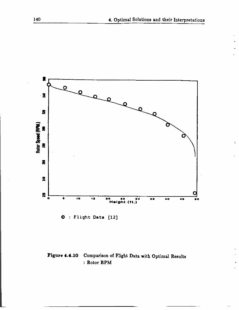
140 4. Optimal Solutions and their Interpretations
I
t
S
mo s s so • s 4 o 4s
I-lel Oht (ft.)
06O
O : Flight Data [12]
Figure 4.4.10 Comparison of Flight Data with Optimal Results
: Rotor RPM

4.4 Optimal landing of a Helicopter Initially in Hover 141
decay by reducing the collective pitch control. When the helicopter is at about
10 feet above the ground (interval from 35 to 45 feet), his attention has shifted
to the use of aft cyclic to reduce both the forward speed and vertical sink rate.
Preparation is made at this stage for the subsequent raising of collective control to
cushion the touchdown. It is in such a rapidly changing, often confusing situation
that an automated control program, which pays attention to "all" aspects of the
landing maneuver, from the begining till the final touchdown, could be of assistance
to inexperienced pilots.
Second, the initial drop in the collective pitch recorded in flight data is only about
two degrees. This is substantially less than the computed result of five degrees.
Thereafter the time history of the collective pitch lies consistently below the com-
puted result. These observations might be explained as follows. In flight tests, the
engine torque does not drop to zero immediately after engine failure. Instead, it
decays exponentially with a 1-second time constant to a level which is 10-15 percent
of the full power output torque. Therefore the residual power available on the rotor
shaft at thebegin_ of the autorotational descent is significant. This may explain
why_::t,he :_al_:_in ¢olleaive pitch is not as much as the computed result. Af-
ter the ]nitiaI'I0we_ting of the collective pitch, the pilot applies a small amount of
forward cyclic to pitch the helicopter nose down and attain about 5 knots ground
speed. This forward motion reduces the induced power consumption of the heli-
copter which explains why recorded data lie consistently below computed results.
The gain obtainable with the use of forward cyclic is of course not without a price.
Aft cyclic must be applied in the landing flare phase of the descent to reduce the
forward speed of the helicopter to zero ground speed at touchdown. In addition
*_, .1_° ;.... _=°A ;._A,w_rt nnwwr ln_ _nr_t.pr] wlt.h thp 11_pn£ raft twelve the tnta]
flight time of the autorotation descent is lengthened.

142 4. Optimal Solutions and their Interpretations
Figure (4.4.10) compares the recorded time history of rotor speed with that calcu-
lated by the optimal program. While one should not look for too much correlation
here, the comparison is surprisingly good. The rotor speed at touchdown is 220
rpm. This value is somewhat lower than the computed result of 268 rprn (see also
Table (4.4.3)). The total amount of energy spent in the optimal program is
Energy Used (Optimal Program)= rngH _ _IR(I2_- f121)
a(672× 2)(372- 2s2) (22)= 3000 x 50--
= 54.3 _ 104 fl.-lb.wt.
This amount is about 24 percent less than that used by the pilot in achieving the
same zero rate of sink at touchdown from a 50 feet hovering throttle chop:
Energy Used (Pilot) = 3000 × 50 + _(672 × 2)(372 232),(23)
= 71.4 × 104 ft.-lb.wt.
4.4.4 Effects of Entry Height
Figure (4.4.11) compares the time history of the collective pitch control calculated
by the optimal program at three different entry heights of 50, 100, and 200 feet.
Since the computed optimal flight time varies with the entry height, we change the
independent variable from time to the normalized time (_), where _ is defined as
= _t, (24)t!
where t! is the flight time. Computed time histories of the thrust coefficient are
compared in Figure (4.4.12)
Figure (4.4.1I)shows that the optimal collectivepitch control program changes with
the entry height. From the 7.2-degree collectivepitch used before engine failure,
the initiaicollectivepitch reduction isin the range of 5-6 degrees for allthe entry

4.4 Optimal landing of a Helicopter Initially in Hover 143
Time of Touchdown (see.)
Max. Rate of Descent (fps.)
Touchdown vertical speed(:ps.)
Rotor
(rpm)Speed at Touchdown
Fligh_Da_a [12]
8.1
15
O
221
Minimum Collective Pitch
(de e®S). ....= ,:
...... _'.'._,i_/i J,,i'ft_; if,,,,i,,_ j,
Touch_wn (degrees)
2.0
14.2
3.8
2O
0
268
14.8
Table 4.4.3 Comparison of Optimal Results with
Flight Data, ho = 50 feet [12]

144 4. Optimal Solutions and their Interpretations
@
@'o
J¢u4,/
O>-,4
AJ
u@
U
15
12
-40
0.25 0.50 0.95 I CX)
Normalized time
ENTRY CONDITION
Drn_z _z_rz' (ft.)
FLIGHT TIME (see.)
2 3 4
50 100 20:3
3.8 4.9 6.1
Figure 41.4.11 Time Variations of Collective Pitch Control
from Different Entry Heights

4.4 Optimal landing of a Helicopter Initlallyin Hover 145
I
U
Su
4_N
t.
O. 16
0.12
0.00
0.04
0
............. _.],_.xP o.,
0 0.25 0.50 0.75 1.00
Normal£zed _Lmo
ENTRY CONDITION 1 2 3
Em'RY Z-_C_T (f=. ] 2S 50 IOO
FLIGHT TIME (sec.) 2.7 3.8 4.9
Figure 41.4.12 Time Variation of Thrust Coefficient
from Different Entry Heights

146 4. Optimal Solutions and their Interpretations
heights considered. The collective i_ lowered to minimize RPM decay. At the lowest
entry height of 50 feet, the collective is immediately raised again after the initial
drop in collective. At the higher entry heights of 100 and 200 feet, the lowered
collective pitch is maintained for some time before it is raised to reduce the rate
of descent. This delay allows a build-up in the rate of descent of the helicopter,
but with the high rotor inertia, subsequent collective increase provides a sufficient
deceleration to allow a safe landing.
4.4.5 Most Critical Entry Height
Figure (4.4.12) shows the time history of the thrust coefficient calculated by the
optimal program at three different entry heights of 25, 50, and 100 feet. The curve
for case (4) (with entry height of 200 feet) lies slightly to the right of that for case
(3) and has been omitted in the interest of clarity.
As the entry height is increased, Figure (4.4.12) shows a corresponding increase
in the amount of (normalized) time that the thrust coefficient spends on its stall
limit. This trend continues till the entry height of 100 feet is reached. Beyond the
_critical" height of 100 feet, any further increase in entry height reduces the time
that the thrust coefficient is on its stall limit. Since prolonged usage of the maximum
available thrust is an indication of an irrevocable extraction of the rotational energy
from the rotor system during the autorotational landing maneuver, the observed
results suggest the existence of a "Most Critical Entry Height" (MCEH). Above
or below this critical height, which in the present case is around 100 feet, the
autorotational landing procedure becomes progressively, easier to execute.
Further confirmation of this hypothesis can be found in the time history of the
rotor angular speed in Figure (4.4.13). Since the rates of descent at touchdown for
all entry heights considered are practically zero, we cannot use them to compare

4.5 Optimal Landing of a I-l_licopter in Forward Flight 147
the criticality of the ]andin_-. However, we have learned from Section (4.4.3) that
the lower the rotor RPM at touchdown, the larger is the amount of energy (of the
helicopter) used in the landing maneuver. One easy way to show the existence of
the MCEH is to plot the rotor speed at touchdown against the corresponding entry
height of the autorotationa] descent. Such a plot is given in Figure (4.4.14).
Figure (4.4.14) shows that the .MCEH (denoted by he,) is at around 100 feet where
the rotor speed at touchdown is a minimum. Therefore the "Most Critical Entry
Condition" is one with engine failure in hover at he,. This conclusion agrees with
flight test results recorded in reference :11 I.
§4.5 Optimal Landing of a Helicopter in Forward Flight
The autorotational landing of a helicopter in forward flight has been formulated as
an optimal control problem in Section (3.3). Unlike the case when power loss occurs
in hover, the present case involves more than a pure vertical descent. As such. we
have to consider the "full state" problem with five states
z] = normalized verticalvelocity,
x2 = normalized horizontal speed.
x3 = normalized rotor speed, (24o)
z4 = normalized vertical height,
zs = normalized horizontal distance.
and two controlsu i = vertical component of thrust,
uz = horizontal component of thrust.
(2s)
If the helicopter is not constrained to land at a particular spot on the ground, the
state xs may be removed from the list in (24). Optimization is then performed on a

148 4. Optimal Solutions and their Interpretations
t_04.;0
360
320
280
24O
2O0
0 0.25 O.SO 0.75 1.00
Normalized time
ENTRY COND IT ION 1 2 3 4u
(ft.) 2s so too 2oo
(see.) 2.7 3.8 4.9 6.1
ENTRY HX!_:CI
ELIG'nVT TIME
]Figure 4.4.13 Time Variations of Rotor Speed at Different
Entry Heights

4.5 Optimal Lauding of a Helicopter in Forward Flight 149
I°IL
7.5 _-
©m 5 --
>
uOc_E 2.5
0
o
oo o
, i * * I J i i J I i , I J I i i l
50 ",00 150
__', '_:_.,+(ft/
_t3
l
|
!IO
Entry Height (ft.)
Ill
Figure 4.4.14 Variations of Terminal Descent Velocity and Rotor
C_^^,.I ,,,;*k 1[_,_,.., l[.l._;,rl_

150 4. Optima] Solutions and their Interpretations
problem with only four states and _wo controls. After the optima] solution has been
computed, information on the horizontal distance (xs) may be recovered through
the forward integration of the kinematical relation:
= (26)
where _ is the normalized flight time.
4.5.1 Flight Program
Once again, the High Energy Rotor System (HERS) described in Section (4.1) is
used as the basis for the analytical model. However, we note in reference [12! that
the highest inertia rotor (with "/= 2.61) allows complete elimination of the height-
velocity restriction curves. For the mid-inertia rotor (with "_ = 3.19), only a small
restricted region remains between 75 to 125 feet altitude with airspeed less than 5
knots. Therefore it is more interesting to investigate optimal landings of the HERS
with its lowest inertia rotor. We have chosen, rather arbitarily, a rotor with Lock
Number 3 of 4.38 which corresponds to a rotor inertia (per blade) of 400 slug-ft 2.
The low-speed height-velocity restrictions for the HERS with rotor inertia at three
different levels are given in Figure (4.5.15) along with the diagram for the standard
OH-58A helicopter.
Entry conditions studied are summarized in Figure (4.5.16). We have chosen to
analyse entry conditions that are within or close to the height-velocity restriction
curve of the HERS with its low-inertia rotor. Note also that entry conditions 1, 2 and
6 are at the same altitude of 100 feet but with different forward speeds. Similarly,
entry conditions 1, 5 and 4 have (approximately) the same forward speed of 8 knots
but are at different entry heights. In this way, effects of both the forward speed and
altitude at entry can be studied. Optimal landings of the HERS studied at these

4.5 Optimal Landing of a Helicopter in Forward Flight 151
400
310
32O
_= 240-14II1:
200,el,14
m 2.60
120
1311- :3020S r.a_4a:d OE-SIA
• ,. / Zb ,i 311 IlUq-fl: ]
\\
f llZltS _ow _er_.a
_. •+J %
J• _ ,I mf i
/
k
\
- 323 81uq-Z_ 2
t +
llZU Nld Zne::£a
/ Zb - SSO 81_q-f_ 2
0 20 40 60 80 100
Ak:speed, kn
l_igure 4.5.15 Comparison of HERS Test Results with Standard OH-SSA [12]
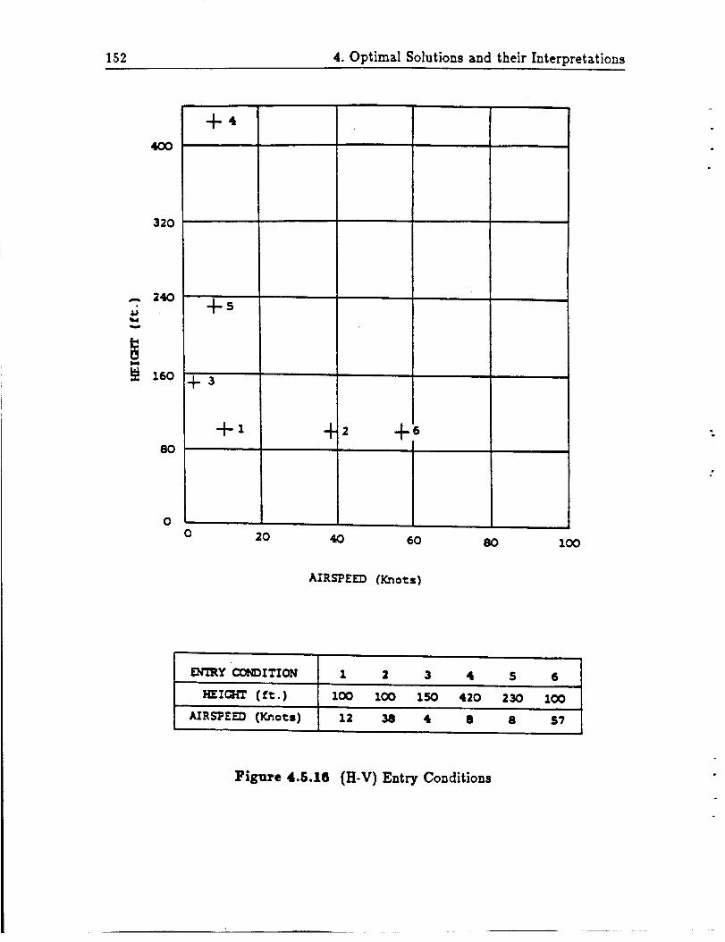
152 4. Optimal Solutions and their Interpretations
400
320
8O
0
4-4
-4-5
!4- s
-+-1 + 2 +6
0 20 40 60 80 100
AIRSPEED (Kno_s)
EN'ERY CONDITION I 2 3 4 S 6
HEICRT (ft.) I00 I00 ISO 420 230 I00
AIRSPEED (Kno_s) 12 38 4 8 8 57
Figure 4.5.16 (H-V) Entry Conditions

4.5 Optimal Landing of a Helicopter in Forward Flight 153
g
entry conditions are with,,ut any terminal constraint on the horizontal distance.
The only exception is entry condition 5, where the helicopter is constrained to land
at various horizontal distances from the point of engine failure.
4.5.2 Interpretation of Results
Figures (4.5.17) to (4.5.19) present in detail the optimal solution of power-off descent
from an altitude of 100 feet and at 12-knots forward speed (entry condition 1 in
Figure (4.5.16)). Figure (4.5.17) gives the collective pitch control and the thrust
coefficient as functions of time. Since the parasite drag on the fuselage of the
helicopter in level flight is small compared with the weight of the vehicle, equation
(18) is still approximately true and the value of the thrust coefficient divided by
the rotor solidity before engine failure is given (approximately) by 0.063.
The induced velocity in level flight can be found from the momentum quartic"
- 2_'p3sin a ÷ _'_z) _ - (T) 2 = 0./p4W
(27)
where the normalized induced velocity (z)) and the normalized flight path velocity. . " •
(¢ ..............• .... .....i green"
B
I/
W
V (2s)
In level flight, the angle which the flight path velocity V makes with the TPP, a,
is approximately zero. Equation (27) can thus be simplified and the value of _ is
given by the following equation

154 4. Optimal Solutions and their Interpretations
The value of the induced velocity at hover, vh. is given by
/; w
b'h _- _/ 2pA '
= 25.38 fps.
(30)
Values ofl-" and _ can then be computed from equa,ions (28-2) and (29) respectively.
Their values aref" = 0.79s.
(31)I) = 0.855.
Therefore the inflow and advance ratios are given by
p = 0.031,
= 0.0332.
(32)
The collective pitch used before engine failure can then be computed from the
following relation3. 2_¢6C__(1÷ _. j_ .o )÷ _(1 - ½.2)
075 :(1- u2÷ _u')
_ 6CT 3 (33)
act 2
--6.63 degrees.
As expected, this value is smaller than the value used in the hover case (7.72 de-
grees).
The optimal solution is similar to that found in the hover case. Initially the collec-
tive is lowered to maintain rotor speed, and nose-down cyclic is used to maintain
airspeed. The results of these control actions are an initial build-up of the verti-
cal sink-rate as well as an increase in the forward airspeed. However, the rate of
RPM decay is being curtailed. In fact, the angular speed of the rotor stabilizes at
around 332 rprn until a rearward, nose-up cyclic flare is used to slow both the rate
of descent and forward airspeed.

4.5 Optimal Landing of a Helicopter in Forward Flight 155
• •.• "l 1o• • ll.tl • ll.ll • 4.11 • •.ll
"rIME (°IiC)
Figure 4.g.lY Optimal Time Vaxiations of Thrust Coe_icient
and CollectivePitch Control

156 4. Optimal Solutions and their Interpretations
i
O
A
|
• • • • 4 • •
TiMe (SlEC)
Figure 4.5.18 Optimal Time Variations of Horizontal and
Vertical Velocity

4.5 Optimal Landing of a Helicopter in Forward Flight 157
o
|
|
W
I
l
It
It
|
0 1 i • 4 •TI_W (OIO)
Figure 4.5.19
• • 4 • •
'T'I MI (111{)
Optimal Time "variations of Rotor RPM and
Helicopter's Altitude

158 4. Optimal Solutions and their Interpretations
Because of the bound on thrust coefficient at (co-q]-) = 0.15, the steady increase in
the collective pitch levels off towards the end when touchdown is imminent. The
thrust coefficient stays on its bound during the last second of the travel when the
helicopter is very near to the ground. Once again, the path inequality constraint on
the thrust coefficient has been effectively enforced by the optimization algorithm.
Nose-up cyclic is initiated 2 seconds after the engine failure when the helicopter is
at about 50 feet above the ground. This occurs later than was the case for hover,
yet there will be sufficient kinetic energy available for the landing flare on account
of the initial forward speed. With a rearward tilt of the TPP, the projected area
of the TPP in the direction perpendicular to the air flow has increased. More air
now flows through the rotor disk. The resultant increase in the angle of attack of
the rotor blades increases the thrust. This effect, together with the steady increase
in the collective pitch, bring about the desired reductions in the forward speed and
rate of descent approaching touchdown.
The time variation of rotor speed is given in Figure (4.5.19). The figure clearly shows
that some of the lost RPM can be regained if a nose-up cyclic flare is initiated with
sufficiently high helicopter forward speed. Effects produced by a rearward (nose-
up)cyclic flare are illustrated in Figure (4.5.20). Because of the increased lift force
(i.e. L >> D in Figure (4.5.20)), the resultant thrust vector R is tilted forward
and produces a net force component in the plane of the rotor's blades. This force
component generates a torque that accelerates the rotor. During the touchdown
phase, the collective is raised to cushion the impact. The rotor speed is reduced to
225 rprn at touchdown, indicative of extracting most of the available rotor energy.
The touchdown is made at a near zero horizontal speed.
4.5.3 Comparison with Flight Data

4.5 Optimal Landing of a Helicopter in Forward Flight 159
Gt
It/II
/,lI//t
!
0
/
//
/
I
/
II
II
I
L : LIFT. D : DItAG, R : ILESt_[,TANT rOR_
V : INDUCED VELOCITY. V: DESCZNT VELOCITY
: PITCH ANGLIr,. OE : ANGLE OF ATTACK. w : ROTOR ItPMI
. Figure 4.5.20 E/Tects of Rearward (Nose-Up) Cyclic Flare

160 4. Optimal Solutions and their Interpretations
In this sub-section, techniques used by pilots are compared with those computed
from the optimal program. We use flight data obtained from a simulated engine
failure of the low-inertia version of the HERS at the "knee" of the height velocity
restriction curve i12. Flight data obtained from this entry condition (with 115 feet
altitude and 45 knots forward speed) are compared with those computed by the
optimal program for the entry condition at 100 feet altitude and 38 knots forward
speed. Therefore, one must note the small differences in both the entry height and
speed when making comparisons. Additionally. because of the strong emphasis on a
zero vertical sink-rate at touchdown, pilots tend to neglect the horizontal component
of the velocity in their landing maneuver (both military and civil criteria permit
this). In this particular case. the touchdown horizontal speed of the helicopter is
20 fps. This pilot priority is quite different from the cost function used in the
formulation of the optimal control problem. Other differences in flight conditions
are summarized in Table (4.5.4).
Because of the difference in flight times obtained from flight data and that from
calculation, direct comparisons of the time histories of the collective pitch and the
rotor angular speed are not meaningful. The previously used technique of converting
the independent variable from time to height is not applicable here because of the
difference in entry heights. Therefore we choose to use the normalized time (_, see
equation (24)) as the independent variable in making comparisons. Figures (4.5.21),
(4.5.22) and (4.5.23) present results of these comparisons.
Figure (4.5.21) compares time histories of the collective pitch calculated by the
optimal program and from flight data. The comparison is qualitatively good. The
most obvious differences in these time histories are the undulating nature of the
flight data, as well as the fact that the collective pitch control used in flight tests
is lower than that calculated. One of the reasons for the observed difference in

4.5 Optimal Landing of a Helicopter in Forward Flight 161
Cross Weigh_ (lb.]
Rotational Iner_Aa perBlade (slug-ft z)
3OOO
4OO
Flight
Data [12]
3040
323
Wlnd Condition (Knots) 0 ¢3
Entry Height (ft.) 100 115
Entry Speed (Knots) 38 45
Collective TAme Delay(sec.] 0 0
Touchdown VerticalSpeed (fps.) 0 0
Touchdown Horizontal
Speed (fps.) 0 20
Rotor Speed a_Touchdown (rpm) 224 280
Flight Time (sec,) 8,7 10.8
Engine Condition
ExponentialDecay withl-second timeconstant
Table 4.5.4 FHght Test Conditions

162 4. Optimal Solutions and their Interpretations
o o.1 o.z o.3 0.4 o.8 o.e 0.7 o.o o.eNormalized Time
//
O Flight Data [12]
Figure 4.S.21 Comparison of Flight Data with Optimal Results
: Collective Pitch Control

4.5 Optimal Landing of a Helicop_or in Forward Flight 163
collective pitch controls is the availability of the residual power to the helicopter
in flight tests. The difference is also partly due to the fact that the touchdown
horizontal speed of the helicopter in the flight test is 20 fps (as compared with the
near zero value in the optimal result). With reference to Figure (4.5.18), we can
see that the calculated vertical sink-rate of the helicopter over the last 1//3 of the
flight time is practically zero. Over the same period of time, the forward speed
of the helicopter is being steadily reduced to its near zero value at touchdown.
Therefore the touchdown condition of the flight test (zero rate of descent and 20
fps forward speed) has been achieved in the optimal program at around 2/3 of the
flight time. If we now compare the value of the computed collective pitch at around
2/3 of the flight time with that from flight data at touchdown, their values become
comparable. Unlike the flight test, the optimal program will not land the helicopter
with high forward speed. Instead it will try to reduce the forward speed to as near
to zero as possible. This is done over the last 1/3 of the flight time where both the
collective pitch and rear cyclic are used to further decelerate the helicopter. The
above reasoning helps to explain the difference in collective pitch controls shown in
Figure (4.5.18).
Figure (4.5.22) compares the recorded time history of the rotor speed with that
calculated by the optimal program. The comparison is again qualitatively good.
Notice that the pilot had placed much greater emphasis on maintaining a constant
rotor RPM than that reflected in the optimal results. Consequently, the collective
pitch is maintained at a minimum for as long as possible. This helps to explain the
discrepancy found in Figure (4.5.22). Since the optimal program decelerates the
forward speed of the vehicle to near zero while flight test to 20 J'ps, the computed
TULUJ- 2[Ik.._iYJ. at _bUU_/IUUI_'II _/D.UUIII, _OU T_TfI_ ID IUtn/_l bll_ll tlll_,t IULIIIU 111 _11_ _I_{:LLI/_I.I
flight test (280 rpm).

164 4. Optimal Solutions and their Interpretations
0
0
\0
\
\
0 Flight Data [12]
Figure 4.5.22 Comparison of Flight Data with Optimal Results
: Rotor RPM

4.5 Optimal Landing of a Helicopter in Forward Flight 165
A comparison of the optimal traj_,c_ory with that found in flight tests is shown in
Figure (4.5.23). Flight data show a 535 ft horizontal distance at touchdown: which
is larger than that from the optimal program (400 ft). The extra distance was used
by the pilot in the reduction of forward speed through the use of cyclic control.
In order to maintain the helicopter at its level attitude for the final touchdown.
only small amount of rearward cyclic was used in the deceleration of the vehicle.
This pilot actions results in a prolonged touchdown and a longer horizontal distance
travelled.
Landing Techniques
The most critical phase of the autorotation descent of a helicopter is the final
approach to a landing flare. Figures (4.5.24) and (4.5.25) show the pilot control
motions and flight profiles from the flight data, and those obtained by the optimal
program, respectively. Both records are for an autorotation entry condition of about
40 to 45 knots airspeed, and level flight at around 100 feet altitude. Superimposed
on the flight profile are reference lines indicating the orientation of the helicopter's
pitch attitude at one-second intervals. Close spacing of the reference lines indicates
a slow maneuver while largerspacing indicatesa fastermaneuver. As the helicopter
ismodelled as a point mass, pitch attitude of the vehicle isnot availablefrom the
optimal program. In Figure (4.5.25),we have substituted for itthe orientation of
the TPP in space. Also, since the longitudinal cycliccannot be determined from
the optimal program, itisnot shown in Figure (4.5.25).
As can be seen from the flight data, a cyclic flare is initiated just below 100 feet
and held to about 20 feet above the ground. This results in a nose-up attitude
^.'_ I Q ..1...... _I'_I_ ,.,..ll,_,_*_,t_ _c _,_._:_ cl_ahtlv rl_-_._o *h,_ R,_.,_ *,_ _-,_v,_n* _._t,_,.
overspeed. Only after reaching about 15 feet does the final collective pull begin. In

166 4. Optimal Solutions and their Interpretations
0 60 100
0 Flight Data [12]
Figure 4.5.23 Comparison of Flight Data with Optimal Results
Flight Trajectory
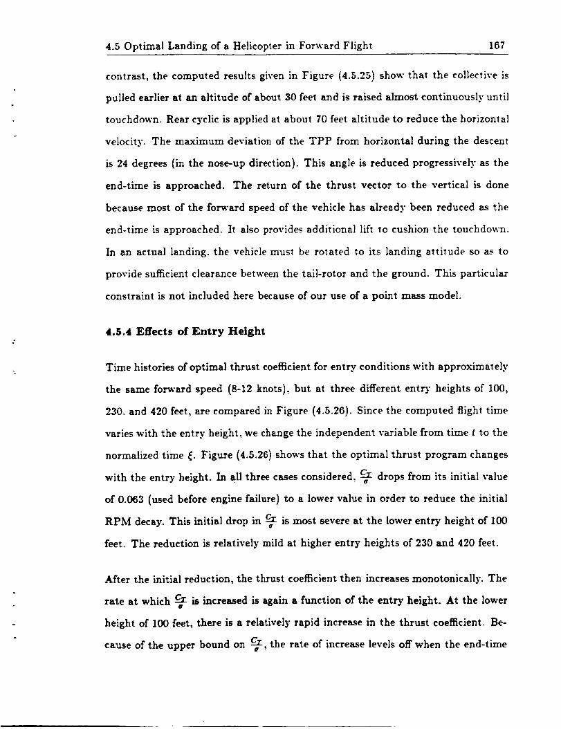
4.5 Optimal Landing of a Helicopter in Forward Flight 167
contrast, the computed results given in Figure (4.5.25) show that the collective is
pulled earlier at an altitude of about 30 feet and is raised almost continuously until
touchdown. Rear cyclic is applied at about 70 feet altitude to reduce the horizontal
velocity. The maximum deviation of the TPP from horizontal during the descent
is 24 degrees (in the nose-up direction). This angle is reduced progressively as the
end-time is approached. The return of the thrust vector to the vertical is done
because most of the forward speed of the vehicle has already been reduced as the
end-time is approached. It also provides additional lift to cushion the touchdown.
In an actual landing, the vehicle must be rotated to its landing attitude so as to
provide sufficient clearance between the tail-rotor and the ground. This particular
constraint is not included here because of our use of a point mass model.
4.5.4 Effects of Entry Height
Time histories of optimal thrust coefficient for entry conditions with approximately
the same forward speed (8-12 knots), but at three different entry heights of 100,
230. and 420 feet, are compared in Figure (4.5.26). Since the computed flight time
varies with the entry height, we change the independent variable from time t to the
normalized time _. Figure (4.5.26) shows that the optimal thrust program changes
with the entry height. In all three cases considered, cr drops from its initial value• G
of 0.063 (used before engine failure) to a lower value in order to reduce the initial
RPM decay. This initial drop in .q.z: is most severe at the lower entry height of 100a
feet. The reduction is relatively mild at higher entry heights of 230 and 420 feet.
After the initial reduction, the thrust coefficient then increases monotonically. The
rate at which cr is increased is again a function of the entry height. At the lowerU
height of 100 feet, there is a relatively rapid increase in the thrust coefficient. Be-
cause of the upper bound on ce-_:, the rate of increase levels off when the end-time

168 4. Optimal Solutions and their Interpretations
e,
0-..4
-..II0e_
U
.IJm
0k4.)
0U
100
80
60
40
2O
m_ mmm mm _'_
0500 400
I ! I I I------Lonqitudina/ Cyclic-----Col,lective
u
_m, 4J
_F
300 200
I/
/
/m eml
14
aJ
4J
==
J_
12' _
100
80
6C
\
40
2O
0500
\
Pitch Attitude
at 1 second intervals
\
400 300 200 100 0
Horizontal Dimtance From Touchdown
Figure 4.5.24 Flight Data for Autorotation Landing [12]
[ Entry Condition : 125 feet, 45 knots ]

4.5 Optimal Landing of a Helicopter in Forward Flight 169
e looQ
g 8o
: 40
o 2o&D
gSO0
-----¢ollecl::Lve
bb_qeo.u
J
....mere _, p _ 'S
/t
//
.Jp,
I/
//
/
II
,i
I
400 300 200 100 0
140
120
100&J
8O6J.1=
.,,4
• 60Z
•_ 40C4
2O
0500
w /'_' aTt tl_ sec°ncl Lnt=erva18
400 300 200 100
Eo_£zontaZ gkltance From Touchdown
0
Figure 4.5.25 Computed Optlmal Program for Autorotation Landing
[ Entry Condition : 100 feet, 38 knots ]

170 4. Optimal Solutions and their Interpretations
O. 16
__ _/___)..ll _=o.:5,retail, _ lid mm ,.,,,,--=. / 1
0.12
! '• 0.0tl
0.04
00 0.33 0.66 1.00
Normalized _lme
ENTRY CONDITION 1 5 4
ENIRY HZICRT (f_.) I00 230 420
ELIGHT TIME (see.) 5.5 9.3 II. 3
Figure 4.5.26 Variations of Thrust Coefticients with Entry Height
[ Entry Speed : 8-12 knots ]

4.5 Optimal Landing of a Helicopter in Forward Flight 171
is approached. The thrust coefficient stays on its stall limit (va-_z-= 0.15) over the
last second of its travel in the optimal control program.
The same trend is followed in cases when engine failure occurs at the higher altitudes
of 230 and 4,20 feet. However, the larger potential energy which is now available to
the helicopter makes it unnecessary to have a large increase in thrust coefficient.
This is because some of the potential energy of the helicopter can be traded for
kinetic energy, and that the same increase in collective pitch produces a larger
thrust at a higher forward speed than at a lower speed. Al._o. throughout the
complete descent process, the stall limit is never reached. These observations agree
with those found in the hover cases. In these cases, a "most critical entry height"
(MCEH) exists from which the autoroational descent is more difficult to execute
than from any other entry heights. This concept of MCEH can be extended to entry
conditions with the same entry speed but different entry heights. As is indicated
in Figure (4.5.26), with approximately the same entry speed of 8-12 knots, the
autorotational landing from the entry height of 100 feet is more difficult to execute
than from any other entry height.
Further insights from the optimal programs can be gained if we resolve the thrust
coefficient into its horizontal and vertical components and plot these thrust compo-
nents against the normalized time. Such a plot is given in Figure (4.5.27). Variation
of CT, with the normalized time is qualitatively similar to that of the thrust co-
efficient shown in Figure (4.5.26). In all three cases considered, the horizontal
component of thrust coefficient is positive for the first half (in time) of the de-
scent, indicative of the use of forward cyclic to accelerate the helicopter to a higher
speed. This forward acceleration, of course, cannot be continued for too long, and
o+ ...... ,_ ,_;,___mo ,.,_- ryellr {_ A_rJlipd to decelerate the helicopter and prepare
it for the final touchdown. Time histories of the forward speeds obtained with such

172 4. Optimal Solutions and their Interpretations
an acceleration/deceleration optimal control program are shown in Figure (4.5.28).
In Figure (4.5.28), the forward speed first increases, reaches a peak at around mid-
time and then decreases to zero at touchdown: the higher the entry height, the
larger the peak speed. The higher forward speed in turn increases the effectiveness
of the rearward (nose-up) cyclic flare (i.e. with negative Cry). This explains why
touchdown is made with progressively- lower Cr value in Figure (4.5.26) as the entry
height is increased.
4.5.5 Effects of Entry Speed
Time histories of optimal thrust coefficient with entry speeds of 12, 38, and 57
knots, all at an entry height of 100 feet, are compared in Figure (4.5.29). Entry
height of 100 feet is selected because of the "criticality" of this height discussed
previously. Optimal time variations of the horizontal and vertical components of
the thrust vector are given in Figure (4.5.30). Time variations of forward speed for
these entry conditions are given in Figure (4.5.31).
Figure (4.5.29) shows the effect that entry speed has on the thrust program. The
time variation of cr in entry condition 1, which is the case considered in SectionG
(4.5.4), consists of an initial drop in c,__, followed immediately by a steady increase
that levels off as the end-time is approached. Variations in cases with higher entry
speeds are qualitatively similar to that of the first case. The higher the entry speed,
the larger is the kinetic energy available to the helicopter in its execution of the
autorotation landing. Since the effectiveness of the rearward cyclic flare increases
with flight path velocity, there is no need for a large increase in collective at the
end of the maneuver for entries with high forward speed. Hover, a condition with
zero forward speed, is therefore the most critical case to execute an autorotation
landing for any given entry height.

4.5 Optimal Landing of a Helicopter in Forward Flight 173
8
CTz
1
5
= 2
._..,,...,.:,,,... . CTx
-2 _,. S
-4 ,
-6
-8
0
• ( • i
0.2 0.4 0.6 0.8 1.0
No_nal£zed time
i
EN'I2Y C_ITI_
t2rray _zcer (tc.)
I S 4
lO0 230 420
S.S 9.3 11.3
Figure 4.5.27 Variations of Horizontal and Vertical Thrust Components
with Entry Height [ Entry Speed: 8-12 knots ]

174 4. Optimal Solutions and their Interpretations
tm
I-el:1I.0
N
0'4
|L-0z
\\\
\
NormalLzed :::Lmo
• i _1::3.8 ICno_s
ENTRY CC_DZTION 1 S •ii
ENTRY I_%CHT (fl:.) %00 230 420
FL_C_T TZZ,_ (8oc.) 5.5 9.3 11.3
|1
Figure 4.5.28 Optimal Time Historiesof Forward Speed at different
Entry Heights [Entry Speed : 8-12 knots ]

4.5 Optimal Landing of a Helicopter in Forward Flight 175
O.16cz/=.)_ -o:_s
O.12 /
! '0.08. _
0.04
00 0.33 0.66 1.00
Normal lzed 1:line
ENI_Y CI_NDITION 1 2 6
ENTRY SPEED (Knots) 12 38 S7
YLI_IT TIME (sot.) 5.5 8.7 10.4
]Figure 4.5.20 Variations of Thrust CoefBclents with Entry Speed
[at Entry Height of I00 feet]

176 4. Optimal Solutions and their Interpretations
t
wm
4J
O
O.,,4qNqu.0
gO
l0
I.
8CTz
6
'o __ . .. .... _ o_---:--
............. " '= "_:':_';" "'--'-'_"_'x- '- " ...o- - " ' z6-2 am,
"_.%.
D
0 0.2 0.4 0.6 0.8 1.0
-4
-6
-8
Nor=alized tl=e
ENTRY _ITZ(:_/ 1 2 6
Dr_¥ SPEED (Kno_:s) 12 38 S7
FLI_-IT T$HE (sot.) S.S 8.7 10.4
Pigure 4.5.30 Vaxiations of Horizontal and Vertical Thrust Components
with Entry Speed [ at Entry Height of 100 feet ]

4.5 Optimal Landing of a Helicopter in Forward Flight 177
An interesting feature of the optimal program is observed in Figure (4.5.30). With
the same entry height of 100 feet, we note the change in the CT_-program with
entry speed. If the forward speed at the time of power loss is relatively low (e.g. 12
knots): forward cyclic must be used to accelerate the helicopter to a higher forward
speed before the aft cyclic is initiated to slow it down for the touchdown. At an
intermediate speed of 38 knots, there is but a brief period of forward acceleration.
At the highest forward speed considered (57 knots), aft cyclic must be applied
immediately after engine failure in order to decelerate the helicopter in time for the
final touchdown. Time variations of forward speeds in these three cases considered
are given in Figure (4.5.31).
4.5.6 Best Endurance Speed
The need to accelerate the helicopter to a higher forward speed when engine failure
occurs at low entry speeds and to decelerate it when power is lost at high speeds
indicates the existence of some intermediate speed at which the helicopter is neither
accelerated nor decelerated. To reduce workload; a pilot might prefer to initiate an
autorotation landing from this speed.
This "preferred" speed can be better understood if we study the effect of forward
speed on the energy consumption of a helicopter in level, powered flight. Total
power consumption is the sum of induced power loss of the rotor, blade profile
power loss, fuselage parasite power loss, and tail rotor power. Tail rotor power and
blade profile power are not strong functions of the forward velocity. In contrast,
induced power loss decreases drastically with increased forward velocity while the
parasite power loss increases with the third power of the forward velocity. Figure
the characteristic "buckeC shape. The speed for best endurance is the speed at

178 4. Optimal Solutions and their Interpretations
g
o
|t_
o!I
O
.............................. :....
• _ ",%
• %
'o
0 1 c_I i.s i 4 c_.e O.e 0 z o_.s O.t
Normalized time
* 1 _nlc:3.8 Knots
[N'_¥ CC_)ITICN
[NTa¥ SPEED (ICnocs)
FLIGHT TIHZ (sec.)
1 2
12 38
5.5 8.7
6
S7
10.4
Figure 4.5.31 Variation of Forward Speed with Entry Speed
at Entry Height of 100 feet

4.6 Optimal Descent of a Helicopter with a bound on Vertical Sinkrate 179
which the power-required curve is at its minimum. Th_ speed for best range, which
is usually slightly higher than the speed for best endurance, is the speed at which
the power-required curve is tangent to a line drawn through the origin. This is also
the point at which the ratio of speed to power (and therefore, of distance to fuel)
is greatest.
In autorotation, steady flight can be achieved only by descending. The rate of
steady autorotative descent is once again a strong function of the forward speed
of the helicopter. Appendix (A) presents a way to compute the rate of steady
descent at different forward speeds. The rate of steady descent in autorotation of
the OH-58A helicopter considered here is shown in Figure (4.5.33). Again, we see
the characteristic "buckeC shape, indicative of some intermediate speed at which
the rate of descent is a minimum. The forward speed with the minimum rate of
descent is the same as the speed for best endurance shown in Figure (4.5.32). This
speed for the OH-58A helicopter is at around 45-50 knots.
From the point of view of energy mangement, the optimal control program tries to
fly the helicopter at a speed which minimizes the power loss. The optimal program
achieves this by accelerating or decelerating the helicopter to a higher or lower
forward speed as the case may be. However, we note that results shown in both
Figures (4.5.32) and (4.5.33) are obtained with the helicopter in a steady state
condition. Since the optimal results are in the transient state, we cannot compare
these optimal results with those shown in the figures directly. Nevertheless, it is
still not too surprising to see that the optimal program has avoided both high and
low forward speed with very high power consumption.
§4.6 Optimal Descent of a Helicopter with a bound on Vertical Sinkrate
In the last section, we presented and interpreted some of the results obtained from

180 4. Optimal Solutions and their Interpretations
kW
200
1200 LCam_mumtn_I_
000 Totld
_ • SPlwe_to
% I
% !
_00 • • Wacm Iwo6_
z'od - - -'<" ...... "....
..... _..... _ ,....__ Tmdrotor ......• 1" i i i.............. i.....
0.1 0.2 0.3 _, 06I
Speed /or _est /
"--Speed for best
j ronge
Speed
Figure 4.5.32 Variation of Power with Forward Speed

4.6 Optimal Descent of a Helicopter with a bound on Vertical Sinkrate 181
2_ i,
_o_,_,_ I Ilotor I_X m 3S4| i i
2000 • _/
A Nq,_2oo I •I I
• CDt Oata of l_te=ence 3.8a_ "--" _, HZU ----
------ FaJ.=Lng ot lqeL'e=ence 18I i J , t ! I
0 20 40 60 80
J_Lzspeed, ]us
100
l, 2000 co.;,c,_c _:,p,;,d -' 4st t, I I I I
_ZGO0
o
.12o0 I. 9 Data of Re_e:ence 18 __..
Q ILElq.q
400
P.aJ.n RoCo= lq_N
Figure 4.5.33 Variation of Steady Rate of Descent with Forward Speed
of an OH-58A Helicopter
ORIGINAL PAGE IS
POOR QUALITY

182 4. Optimal Solutions and their Interpretations
g
o =
0--
0
o • 1 ,;.. o.aJ o., ,;.aJ o.e o.T OoS O.e
Nowma 1 £zed tame
ENTRY CC_ITXCiq 1 $
100 230_Y _mx_ (tt.)
E'LZGtt'I' TZME (8oc.) 5.5 9.3
4
420
11.3
Figure 4.5.34 Time Variations of Rotor Speed
[ Entry Speed : 8-12 knots ]

4.6 Optimal Descent of a Helicopter with a bound on Vertical Sinkrate 183
g
Qo o.I c_.8 O.e c_.4 o.e c_.e c_.y o.e o.e
Normalized time
DFZRY CCt_lTION 1
ENVY SPEED (Kno_:s) 12
FLIGHT TIME (8ec.) S.S
2 6
38 57
8.7 10.4
Figure 4.5.35 Time Variations of Rotor Speed
[ Entry Height : 100 feet ]

184 4. Optimal Solutions and their Interpretations
computations of optimal descents of a helicopter in forward flight. The optimal
descents of the HERS from entry conditions either with a high forward speed or at
a high altitude result in peak rates of descent that are unacceptably high to pilot.
and to overspeeding of the rotor during the rearward cyclic flare.
To remedy this problem, we add an upper bound on the vertical sink-rate of the
helicopter to the optimal landing problem. The new problem, with an additional
state variable inequality constraint is given in Section (3.3). An entry condition
with a 7.7-knot initial speed at an initial altitude of 423 feet was selected for the
present study. This entry condition was used because the optimal descent of the
HERS with this particular entry condition results in unacceptably high peak descent
velocity. Results obtained with the optimal descent of the HERS from this entry
condition and subjected to a descent velocity bound are presented in this section.
4.6.1 Optimal Descent of a Helicopter with a Descent Velocity Bound
If the optimal rate of descent of the helicopter in the unbounded solution exceeds
the upper bound, it is reasonable to assume that the optimal time variation of the
descent velocity in the solution to the new problem will resemble that shown in
Figure (4.6.36). The helicopter starts initially with a zero rate of descent. This rate
then increases, touches and stays on its upper bound for a period of time. Finally.
the rate of descent is reduced so as to allow for a soft touchdown. Typically, this
time variation of the descent velocity consists of three phases. These phases of
entry, steady descent, and landing flare are shown in Figure (4.6.36).
The amount of time that the helicopter spends in each of these phases depends
on the magnitude of the descent velocity bound, [VD]maz" Generally speaking, the
higher the descent velocity bound, the shorter the time spent in the steady descent
phase. As illustrated in Figure (4.6.37), the steady descent phase ceases to exist

4.6 Optimal Descent of a Helicopter with a bound on Vertical Sinkrate 185
U0
0
U
I I
I' IiI I
III !I Im II II II II I
II II II I
Time (seconds)
(1) Entry Phase
(2) Steady Descent Phase
(3) Landing Flare Phase
"_P= positive,dt
[ phase ends with V D = (VD)ma x
: dVD= zero,dt
[ vO = (VD).,,= ]• dVo = negative,• dt
[ phase ends with VD = 0 ]
Pigure 4.6.36 Time Rate of Change of Descent Velocity
with a [VD]m., Bound

186 4. Optimal Solutions and their Interpretations
U0P.4
@
U
...................... [vD],,,.
TAme (seconds)
Medium
Low
(I) High [VDJmez: The variation is essentially that
without a descent velocity bound.
(2) Medium[VD]m,,:The variation consists of the entry,
steady descent and landing flare phases.
(3) Low [VD]m,z: No feasible solution exists in this
case.
Figure 4.6.37 Time Variation of Descent Velocity with
Different Values of [VD],..z

4.6 Optimal Descent of a Helicopter with a bound on Vertical Sinkrate 187
ORIGINAL PAG-:: '_
OF POOR QUALITY
2400
_on8t:_ Roto= IN e 354
8 1100 ,, =D •_
7v
1200 .,era,J i i i I I
• ]Dat8 o£ lbl£ez'ence S<> nzu
Ya£=£ng o£ ]L_e:ence S800 ' "' * _ _ ' '
0 20 40 60 80 100
JU.=speed, kn
1;'iguze 4.6.38 Variation of Steady Autorotative Sink-rate of the HERS
with Forward Ainpeed

188 4. Optimal Solution, and their Interpretations
when the iI'Dimaz-bound is chosen too high. In this ca-e, the variation of the
descent velocity becomes essentially that without the descent velocity bound. The
other extreme is when the :, Djrnaz-t)ouna selected is too low, e.g., at around 1200
fpm. As can be seen from Figure (4.6.38), the horizontal line iUD_,naz = 1200 fpm
does not intersect the curve which shows the variation of the steady autorotative
sink-rate of the HERS with its forward airspeed. Therefore, no feasible control
exists that will allow the helicopter to autorotate at a steady sink-rate of 1200
f prn.
An intermediate value of 1800 fpm was selected as an upper bound on the vertical
sink-rate of the helicopter in autorotative descent. From here on we shall use the
term "nominal case" to represent the autorotative descent of the HERS from an
entry condition with a ?.7-knots forward airspeed, at an initial altitude of 423 feet,
and having a 1800 fprn bound on its vertical sink-rate.
The time variations of the CT, CT,, .q.r_ and the collective pitch for the nominal' a '
case are given in Figure (4.6.39)-(4.6.40). With reference to the CT,-curve, one can
see a natural division of the autorotative landing maneuver into the three phases
mentioned earlier. Similar divisions can also be observed in both the time histories
of the collective pitch and the thrust coefficient.
An approximate Solution of the Cr,
During the steady descent phase, when the sink-rate of the helicopter stays close
to the value [VD]maz, the vertical component of the thrust coefficient CT,, can be
determined using the following approximations. During the steady descent phase,
the time rate of change of the helicopter's sink-rate is near zero. By equating the

4.6 Optimal Descent of a Helicopter with a bound on Vertical Sinkrate 189
ORIGINAL PA_-_ rS
OF POOR QUALITY
• 0., O.• 0.8 04 • O •.O O-_' 0.• O.•
NOill MAt_iZmO 'T'll MI
!
a
• I1.•
Yigure 4.6.39 Time Variations of the Thrust Coefficient and its
Horizontal and Vertical Components

190 4. Optimal Solutions and their Interpretations
l_igure 4.6.40 Time Variation of the Collective Pitch
with a Descent Velocity Bound

4.6 Optimal Descent of a Helicopter with a bound on Vertical Sinkrate 191
LHS of the first equation of Appendix (A) to zero. we obtain
go = u]z3- ]z]\ - x22.(34)
Since -_- = 3.02. f = 0.0306, and magnitudes of both x], x2 and x3 are of the orderm0
equation (34) (i.e., the parasite-drag term, fx] \//_xl2 - x_)of 1. the second term in
may be neglected. Therefore, we obtain the approximate relation:
go- 3.02.
m0 (35)
which can be used to estimate the value of the normalized vertical thrust coefficient
t/1 .
If the angular speed of the main rotor does not vary too much during the steady
descent phase, the normalized rotor speed x3 can be approximated by its mean
value [x31,nea,_. Therefore the approximate value of u] in the steady descent phase
is given by:
Ul "-gO
rrtO(X3)2mean '
3.02
(oo512'= 3.33. (36)
where we have used a value of 0.95 for the average normalized rotor speed ((x3)mea.)
in the steady descent phase (see also Figure (4.6.43)). The computed value of 3.33
for the vertical component of the thrust coefficient in the steady descent phase
agrees well with the value 3.7 found in the optimal solution (see Figure (4.6.41)).
4.6.2 Comparisons between Results Obtained With and Without

192 4. Optimal Solutions and their Interpretations
(_)._.u = o is
• 0.1 e.8 O.I 04 0.0 0.0 O.F O.e @1
it
WITH BOUND
WITHOUT BOUND
Figure 4.6.41 Time Variations of the Thrust Coefficients With and
Without a [Yz>].,.z-Bound
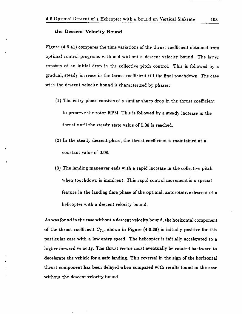
4.6 Optimal Descent of a Helicopter with a bou_Jd on Vertical $inkrate
the Descent Velocity Bound
193
Figure (4.6.41) compares the time variations of the thrust coefficient obtained from
optimal control programs with and without a descent velocity bound. The latter
consists of an initial drop in the collective pitch control. This is followed by a
gradual, steady increase in the thrust coefficient till the final touchdown. The case
with the descent velocity bound is characterized by phases:
(1) The entry phase consists of a similar sharp drop in the thrust coefficient
to preserve the rotor RPM. This is followed by a steady increase in the
thrust until the steady state value of 0.08 is reached.
(2) In the steady descent phase, the thrust coefficient is maintained at a
constant value of 0.08.
(3) The landing maneuver ends with a rapid increase in the collective pitch
when touchdown is imminent. This rapid control movement is a special
feature in the landing flare phase of the optimal, autorotative descent of a
helicopter with a descent velocity bound.
As was found in the case without a descent velocity bound, the horizontal component
of the thrust coefficient CT=, shown in Figure (4.6.39) is initially positive for this
particular case with a low entry speed. The helicopter is initially accelerated to ao
higher forward velocity. The thrust vector must eventually be rotated backward to
decelerate the vehicle for a safe landing. This reversal in the sign of the horizontal
thrust component has been delayed when compared with results found in the case
without the descent velocity bound.

194 4. Optimal Solutions and their Interpretations
The time histories of the descent velocity, forward speed, rotor RPM, as well as
the optimal trajectory obtained for the nominal case are given in Figures (4.6.42)-
(4.6.43).
The time histories of the helicopter's descent velocity obtained from optimal control
programs with and without an upper bound on the descent velocity is compared
in Figure (4.6.44). Those for the helicopter's forward speed and the angular speed
of the main rotor are compared in Figure (4.6.45). It is apparent from Figure
(4.6.44), that "peaking _ of the descent velocity has been effectively suppressed
after the introduction of an upper bound on the descent velocity. To cover the
same vertical distance of 423 feet, the flight time in the case with a [VD]max-bound
has been lengthened. The touchdown time has increased from 11.3 seconds in the
V Icase without the [ D_maz-bound to 16.3 seconds in the case with the bound.
The time variations of the helicopter's forward speed with and without the descent
velocity bound are compared in Figure (4.6.45). These variations are qualitatively
similar. In both cases, the forward speed of the helicopter first increases, reaches a
maximum before it is decreased to near zero at touchdown. The time at which the
maximum forward speed is reached in the case with the descent velocity bound has
been delayed when compares with that without the descent velocity bound. This
is due mainly to the late rotation of the thrust vector to the rearward direction as
explained before.
Differences in the time variations of the main rotor RPM in cases with and without
the [VD]maz-bound are most significant. In the case witlaout the [VD]ma=-bound, the
peak angular speed of the rotor is about 30 percent higher than its nominal value
of 353 rprn. Figure (4.6.45) clearly shows that this "peaking _ in the angular speed
of the rotor has been suppressed as a result of bounding the vertical sink-rate. The

4.6 Optimal Descent of a Helicopter with a bound on Vertical Sinkrate 195
DIIITANGI! (liT)
ItY
41
• 11,8 • • • tO _ll.I 1Q 'ly,
"rlklll (llliO)
Figure 4.0.42 Time Variation of the Descent Velocity and the
Optimal Flight Profile

196 4. Optimal Solutions and their Interpretations
I
t
i"
I
|
I
!
|,|,
I
E
1
lYl
• II.ID • • • wO la.a !1 IT •
?IM II (llllO.)
Pigure 4.6.43 Time Variations of the Forward Speed and the
Rotor RPM

4.6 Optimal Descent of a Helicopter with a bound on Vertical Sinkrate 197
ORIGINAL PAGE !_
OF POOR QUALITY
.l / ",
• T_'l'l ||1_) ,l.l 'l lt.I
•' WITH BOUND
.... WI THOUT BOUND
Fisure 4.6.44 Comparison of the Time Variations of the Descent Velocity
. IV | _1_^,... Awith ,,..n,_ without a L" DJma=-'° ....

198 4. Optimal Solutions a_ndtheir Interpretations
/i///
Q,q e.e e.i • 4 e.@ e.e e,y e.41* o.e
N O Fit M AUl,.m D 1'llMm
ORIGINAL PAGE IS
OF POOR QUALITY
.
_ " p%%
|. ii \_
ll -r_ i// "\
il
|O.11 O.@ • a • • •.6 0.• O*Y 00 • •
NOR MALl _,.lID TIM
WITH BOUND
WITHOUT BOUND
Figure 4.6.45 Comparison of the Time Variations of the Forward Speed
and Rotor RPM with and without a [VD]ma=-Bound

4.6 Optimal Descent of a Helicopter with a bound on Vertical Sinkrate 199
peak value of the angular speed in the nominal case is actually less than the nominal
value. This suggests that the peaking of the rotor RPM found in the solution of the
problem without a descent velocity bound can be eliminated in two different ways.
The overspeeding of the rotor can be removed either directly by the addition of an
inequality constraint on the rotor RPM or indirectly through the use of an upper
bound on the descent velocity.
4.6.3 Some Generalizations
If we impose path inequality constraints on both the descent velocity of the heli-
copter and the angular speed of the main rotor, the time variations of the descent
velocity and the rotor angular speed in the optimal results might look like those
shown in Figure (4.6.46). A plot of the angular speed of the rotor with respect to
the descent velocity of the helicopter in the resultant optimal solution is as shown
in Figure (4.6.46). Depending on values of [VD]rnaz and firnaz, the VD-fl plot might
consist of one or more "corner _ points. In Figure (4.6.46), the entry phase starts
from the initial entry condition (point 0) to the point when the upper bound on
the descent velocity is reached (point 1). Thereafter, the descent velocity is main-
tained at a constant value while the angular speed of the rotor is increased till it
reaches its upper bound lima,, at point 2. The angular speed of the rotor remains
unchange from point 2 to 3 while the descent velocity of the helicopter is dropped.
During this landing flare phase (from point 3 to 4), the descent velocity is being
continuously reduced to its near zero value at touchdown. During the same period
of time, the rotor RPM is also being reduced, indicative of the extraction of the
stored rotational energy to cushion the landing.
4.6.4 Effects of Perturbed Initial or Terminal Conditions
The nominal case considered in the above subsections is with a 7.7-knots forward

200 4. Optimal Solutions and their Interpretations
f_a_ 2 3.....
I
4
Time
3
Time
NONTEASIBLE REGION --_ (VO)MA X
li
=II
0
TOUCHDOWN
Vo --
]Figure 4.6.46 fl versus VD Plot showing Segments of the Optimal
Control Scheme

4.6 Optimal Descent of a Heliropter with a bound on Vertical Sinkrate 201
airspeed and at an initial al_i'ude of 423 feet. To investigate effects that initial
and terminal conditions have on the control scheme, we consider the following three
cases:
(1) The initial airspeed is increased from 7.7 knots to 15 knots.
(2) An additional terminal, horizontal distance constraint of 623 feet is added
to the nominal problem (which is without a terminal distance constraint).
(3) The entry altitude is increased from 423 feet to 460 feet.
Results obtained for the first case are given in Figures (4.6.47)-(4.6.49). Those
obtained for the second case are presented in Figures (4.6.50)-(4.6.53). Results
obtained for the case with a change in the entry height are shown in Figures.(4.6.54)-
(4.6.57).
The optimal results obtained for these three cases agree qualitatively with those
found in the nominal case. In all the cases considered, the path inequality con-
straint on the vertical sink-rate of the helicopter has been effectively enforced by
the optimization algorithm. Since the perturbations in initial and terminal condi-
tions are relatively small, only minor control adjustments are needed to accomodate
these changes. It is also interesting to note that most of these control adjustments
are made in the entry and/or landing flare phases of the descent maneuver. Both
the horizontal and vertical components of the thrust coefficient in the steady descent
phase of the maneuver remain practically unchanged with the perturbed boundary
conditions.
The nominal problem (without a terminal, horizontal distance constraint) has a
touchdown distance of about 560 feet. This horizontal distance has been extended
to 635 feet in the second case. This extension in the horizontal distance has been
achieved by an increase in the forward speed of the helicopter (see Figure (4.6.52)).

202 4. Optimal Solutions and their Interpretations
_"_ / [ORIGINALPAGE_
. /i_'i ,......... I
• "" '_" "',,,o_,,,_,_,o ,M,,,, '_" "" "" '
lid
]
OB O0 Oo O0 O0 OB O0 00
N4_A IdMLIZll O TIll
In£_£ai Forvard Speed : 26 fps
In£_£al Forvard Speed : 13 fps
Figure 4.6.4? Comparisons of Optimal Results Obtained at Two
Different Entry Airspeeds

4.6 Optimal Descent of a Helicopter with a bound on Vertical Sinkrate 203
i /ORIGINAL PAGE IS
O_ Ibll 08 Oe Dill @Q @p 01 00I_lOIlidM ALI&R 0 T_lll
@1 @ll ea @e @@ Oil i_ o6 oQ
NOR*-*ALIZll 0 TIklll
Initial Forward Speed = 26 fps
Initial Forward Speed = 13 fps
Figure 4.6.48 Comparisons of Optimal Results Obtained at Two
Different Entry Airspeeds

204 4. Optimal Solutions and their Interpretations
|
|
D
lie e.. o.. oo eo oe eo et oo eo_o4q MAL.,Js_i 0
1'1
• _lbl 8oo seo 6oo olo •
OJO Y AlqlCl (P'T)
InA_Aal Forward Speed = 26 fps
InA_Aal Forward Speed.= 13 fps
Figure 4.6.49 Comparisons of Optimal Results Obtained at Two
D]fl'erent Entry Airspeeds

4.6 Optimal Descent of a Helicopter with a bound on Vertical Sinkrate 205
ORIGINAL PAGE |$
OF POOR QU#I_ITY
|-
i,i
F
go oo oa 04
J;.. ;L, *' ** ""N(_mI_A O I •
Wi_h Horizon=a1 Distance Cons=rain_ _ 63S feo_
Wi_hou_ Hortzon_al Distance Cons_rain_
l_igure 4.6.50 Comparisons of Optimal Results Obtained With and
Without a Horizontal Distance Constraint

206 4. Optimal Solutions and their Interpretations
I"
| Y;/ \\
• . .. ...,,,:,_. ";, ;_. -, .. ..At 0 e •
Wi_h Horizontal Distance Cons_raln_ at 635 feet
.... W1_hou= Horizontal Dls_ance Cons_raln_
Figure 4.6.51 Comparisons of Optimal Results Obtained With and
Without a Horizontal Distance Constraint

4.6 Optimal Descent of a Helicopter with a bound on Vertical Sinkrate 207
II I ORIGINAL p_GE _,_
,. - \\|' \,
I
I
I
ll I I II II II II go If II II
IklOllldAUllO Tllill
g.
|.
lI4l
• it Ill ll.I Ilil ill Ill alp Ill ill Ill
NOll IdAll.lllO TII_I
With HorAzontal DAstance Cons_raLn_ a_ 635 fee_
------ WA_hou_l{orAzon_al DA$_ance Cons_raAn_
Figure 4.6.52 Comparisons of Optimal Results Obtained With and
Without a Horizontal Distance Constraint

208 4. Optimal Solutions and their Interpretations
Figure 4.6.53 Optimal Results obtained with
a Horizontal Distance Constraint

4.6 Optimal Descent of a Helicopter with a bound on Vertical Sinkrate 209
|
"
/• .Q 0-0 •0 04 06 0• Or 00 O•
_OR _A_la T_
• •_ 00 @l O• aO 00 •t 00 O•NOal_lALllllO TIl_ll
En=ry HeAgh1: z 435 fee=
Entry HeAqhm I,460 fee_
Figure 4.6.54 Comparisons of Optimal Results obtained at Two
Different Entry Altitudes

210 4. Optimal Solutions and their Interpretations
g
D
|.
i!o
61 mm Q8 OQ ol mQ QP 00 00
i_lOIllid ALl| |O
i|
gl*
r!
Qi 011 08 Oe OI) OO gv 4) 0 OO
NC)I_ kiA Lll| D Ttl_6
Entry HeAgh= = 435 feec
En=ry HeAgh_ = 460 fee=
Figure 4.6.55 Comparisons of Optimal Results obtained at Two
Different Entry Altitudes

4.6 Optimal Descent of a HeUcopter with a bound on Vertical Sinkrate 211
ii ORIGINAL PAGE IS ...-. ]
! OF POOR QUALITY/'"_ I
|'1 ._ \ I
:
I:I: I
• •t •l •• ql4 •41 0• •P gO e•
ii i Entry HeAgh_ 8 435 toe_
Entry HeAgh_ - 460 _eo_
Figure 4.6.56 Comparisons of Optimal Results obtained at Two
Different Entry Altitudes

212 4. Optimal Solutions and their Interpretations
|
|
• _•• Do• io• Qo• 8QQ
OIOT AIkIGm |PT)
Figure 4.8.S7 Optimal Results obtained at the
Perturbed Entry Altitude

4.6 Optimal Descent of a Helicopter with a bound on Vertical Sinkrate 213
and by an increase in th_ _ overall flight time of the descent.
profile is shown in Figure (4.6.53).
The resultant flight
A summary of the optimal results obtained in these three cases are given in Table
(4.6.5) together with that found in the nominal case.
4.6.5 General Conclusions
One of the distinct features in the optimal_ autorotative control of a helicopter
with a descent velocity bound is a clear division of the landing maneuver into
phases. These control phases: resemble those practiced by helicopter pilots in their
autorotationa] training. Therefore, this control scheme should be more acceptable
to helicopter pilots.
A second feature of the control scheme is the suppression of the overspeed of the
angular speed of the main rotor during the rearward cyclic flare. The increased
flight time of the autorotational maneuver is an added benefit of putting a bound
on the rate of descent.
One of the major disadvantages of the control scheme considered is the high rate of
collective pitch input observed during the landing flare phase. Another disadvantage
of the control scheme is in the use of a large amount of cyclic pitch during the last
few seconds of the landing maneuver. This will cause a loss of all the ground
references during the final touchdown. However, this will not create too much of a
problem in a practical situation since the helicopter must always be rotated to its
level attitude before a touchdown can be made.
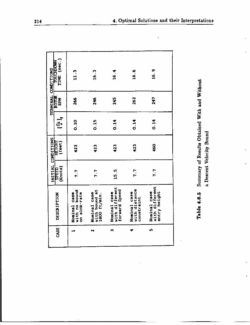
214 4. Optimal Solutionsand theirInterpretations
N N ¢_ N
_i" d d d d d
r_. t_ t_
_-40._ ,--_ 0 ;a ,--_-_ "0 ,_ -,'_
0 .,"__ 0 .,4 0 0 .,,.__0 _ _ _-_U
g

Chapter 5
Conclusions and
Recommendations for Further Research
§5.1 Summary
5.1.1 Adequacy of a Point Mass Model in the Optimal Helicopter Landing
Study
A point-mass model of an OH-5SA helicopter was used in the optimal helicopter
landing study. The states were vertical and horizontal velocities, vertical and hori-
zontal displacements, and the rotor angular speed. The cost function was a weighted
sum of the squared horizontal and vertical components of the helicopter velocity
at touchdown. The controls were horizontal and vertical components of the thrust
coefficient.
Optimal trajectories were calculated for entry conditions well within the H-V restric-
tion curve, with the helicopter initially in hover or in forward flight. The optimal
solutions exhibited control techniques similar to those used by helicopter pilots in
actual autorotational landings. The results confirm the need to drop collective pi_ch
immediately after engine failure. During the landing flare phase, the thrust vector

216 5. Summary an,] Recommendations for Further Research
is rotated to the rear in order to reduce t],_ forward velocity and, just before touch-
down. the stored rotational energy in the rotor is traded for additional thrust to
reduce the vertical velocity. The correlation between flight data and the optimal
results establishes the adequacy of the use of a point mass model in the optimal
helicopter landing study.
5.1.2 The Need for Path Inequality Constraints on Both the Control and
the State Vectors
In order to minimize the cost function defined above, a larger rate of descent and
a larger rotor RPM at the point of flare are desirable. However, a high rate of
descent over a substantial period of time is unacceptable to helicopter pilots, while
a large rotor RPM threatens the structural integrity of the rotor system. A unique
feature of the present formulation is the addition of path inequality constraints
on components of both the control and the state vectors. The control variable
inequality constraint is a reflection of the limited amount of thrust that is available
to the pilot in the autorotational maneuver without stalling the rotor. The state
variable inequality constraint is an upper bound on either the vertical sink rate of
the helicopter or the rotor angular speed during the descent.
With these bounds on the control and the state vectors, the optimal solutions
obtained will realistically reflect the limitations of the helicopter and its pilot. The
optimal solutions consist of subarcs which are connected at suitable corners. The
subarcs are either unconstrained, or are on the upper bound of the thrust coefficient,o
or are on the bound on the vertical sink rate. The results exhibit division of the
landing maneuver into entry, steady descent and landing flare/touchdown phases.
This resembles the techniques taught to helicopter pilots, and so should be more
acceptable to them.

5.1 Summary 217
5.1.3 Comments on the Sequential Gradient Restoration Technique
Slack variables were employed to convert the path inequality constraints men-
tioned above into path equality constraints. The resultant two-point boundary-
value problem with path equality constraints was solved using the Sequential Gra-
dient Restoration Technique. The effectiveness of the SGR technique for problems
with of both control and state variable inequality constraints was demonstrated by
the present study.
In general, the amount of computation involved with the use of the SGR algorithm
is proportional to the square of the dimension of the state vector [42]. Therefore,
the use of by auxiliary states in problems with state variable inequality constraints
increases the computational requirements. In this regard, a transformation tech-
nique for optimal control problems with partially linear state variable inequality
constraints is strongly recommended [43!. The transformation technique takes ad-
vantage of the partial linearity of the state inequality constraint so as to yield a
transformed problem characterized by a new state vector of minimal size. Substan-
tial savings in computer time can be achieved with this transformation technique.
5.1.4 Reduction in the H-V Restriction Curve and Other Potential Ap-
plications
Even though effects of the pilot time delay and other factors have not been taken
into account, the present study indicates that a substantial reduction might be
achievable in the H-V restriction zone using optimal control techniques. Results
computed using the optimal technique thus provide a benchmark for comparisons
with other control techniques. These optimization techniques could also be used to:
(1_ hpl_ i_t1"llct ni]nt$ nn unnd mlltnrntAtinn t_chn_n,l_
(2) reduce the risk/time/effort involved in establishing the H-V restriction

218 5. Summary and Recommendations for Further Research
zones by flight tests.
(3) provide an objective comparison of the autorotation capabilities of
different helicopter models.
(4) assess the influence of vehicle parameters on autorotation during
preliminary design.
§5.2 Recommendations for Further Research
5.2.1 Refinements of the Mathematical Model
The accuracy of studies like this one could be improved by adding the following
refinements to the mathematical model:
(1) induced velocity dynamics (cf. references [151: [19:, [20] and [70:);
(2) ground effect (cf. references [15: and [71]):
(3) variation of the profile drag coefficient with rotor blade angle of
attack (cf. reference [24]);
(4) rigid body dynamics, which would show the effects of pitch
attitude during descent and at touchdown.
These refinements increase the dimension of the state vector (refinements (1) and
(4)) and also the complexity of the analysis (refinements (2) and (3)). They are
considered to be of secondary importance (cf. Section (2.2)), and should be included
only if improvement in the accuracy of the optimal programs is required.
5.2.2 The Effects of the Engine Failure Mode (cf. [5])
The nature of the power reduction transient affects pilot technique and the response
of the helicopter. Common causes of power loss are fuel starvation, fuel control mal-
functions, engine deterioration, and damage from an external source. The transient
nature of the power reduction varies greatly with the cause and directly influences

5.2 Recommendations for Further Research 219
the necessary corrective pilo_ actions. The pr_._ent study considered the most crit-
ical case of a sudden complete power loss: caused as a result of an engine seizure.
disintegration: or drive system failure. It would be of interest to study other "less
critical" cases.
5.2.3 The Effects of Pilot Time Delay (cf. [5])
The term "time delay _ defines the time lag between the instan_ of power loss_ and
the time recovery action is initiated by the pilot. It consists of the recognition time
and the reaction time of the pilot. Therefore, the amount of time delay involved is
a strong function of both the engine failure cues (either audio, visual or kinesthetic
signals) available to the pilot and the experience of the pilot involved.
A time delay on the order of 1.5-2 seconds is typically used in the establishments of
the H-V restriction curves. It is recommended that effects of the pilot time delay on
the autorotational landing of a helicopter from critical flight conditions be studied.
This can be studied through the incorporation of a time delay into the helicopter
landing problem formulated in Section (2.9).
5.2.4 Pilot-in-the-loop Simulation
The importance of pilot-in-the-loop simulations for helicopter research has been
emphasized in references [4, 10, 15 and 65]. The usefulness of simulations in autoro-
tation research has been confirmed in reference [15]. Simulations provide important
information about pilot workload, pilot ability to track a given optimal flightpath.
limitations of hardware involved, and the structural integrity of the vehicle. They
may provide other information, such as whether a particular sink rate or pitch
l"mt_ i_ mer_tmhlo tn hp|it-nntpr nilnt_, l")ztz ,_cn11_lrpr_ frnm fh_ Rieht Eim111_t_n_
and comments from helicopter pilots should be studied carefully and appropriate

220 5. Summary and Recommendations for Further Research
modifications made in the formulation of the optimal h¢.licopter landing problem.
Only through iterative cycles of this kind can a realistic optimal control program
be established and implemented.

References
°
,
.
Graves, J.D., "Methods and Devices to Improve Helicopter Autorotational
Characteristics," USAAVRADCOM-TR-82-D-38, Sep., 1983.
Hansen, K.C., "Single Rotor Helicopter Transient following a Power Failure at
High Speed," presented at the 22nd Annual National Forum of the American
Helicopter Society, 1966.
Jepson, W.D., "Some Considerations of the Landing and Take-Off Characteris-
tics of Twin Engine Helicopters," Journal of American Helicopter Society, Vol.7,
No.4, Oct.,1962.
4. Saunders, G.H., "Safety Column," Rotor and Wing, Jam/Feb., 1976.
5°
.
,
°
Ferreel, K.R., Frederickson, A.C., and Shapley, J.J., "A Flight Test Investi-
gation of Autorotational Performance and Height Velocity Testing of a Single
Main Rotor, Single engine Helicopter," USAAEFA No. 68-25, Mar.,1976.
Segner, D.R., "AH-56A Compound Helicopter Autorotation Characteristics ,"
1972 Report of the Society of Experimental Test Pilots, pp. 29-47.
Buss, M.W., "Sudden Engine Failure Problems of High Performance Attack
Helicopters," 1971 Report of the Society of Experimental Test Pilots, pp. 173-
188.
Davis, J.M., et al, "Study of Tandem Rotor Helicopter Dynamics following
Power Failure at High Speed," USAAVLABS 65 72, Nov., 1965.

222 References
.
10.
II.
12.
13.
14.
15.
16.
17.
18.
19.
Cooper, D.E., et al, "Single Rotor Helicopter Dynamics following Power Failure
at High Speed," USAAVLABS TR 66 30, Jun., 1966.
Watts, J.C., et al, "Engineering Flight Test of AH-IG Helicopter Autorotational
Characteristics," USAASTA-74-10, May, 1974.
Wood, T.L., "High Ener_" Rotor System," presented at the 32nd Annual Na-
tional Forum of the American Helicopter Society, Washington, D.C., May, 1976.
Dooley, L.V,'., and Year)', R.D., "Flight Test Evaluation of the High Inertia
Rotor System ," USARTL-TR-79-9, June,1979.
Pleasant, W.A.,III, and White, G.T.,III, "Status of Improved Autorotative
Landing Research," Journal of American Helicopter Society, Vol. 128 , No.
1, Jan., 1983.
White, G.T., Logan, A.H., and Graves, J.D., "An Evaluation of Helicopter
Autorotation Assist Concepts," presented at the 38th Annual Forum of the
American Helicopter Society, May, 1982.
Johnson, W., "Helicopter Optimal Descent and Landing after Power Loss,"
NASA TM 73,244, May, 1977.
Bryson, A.E., Jr., "FCNOPT Computer Program," Department of Aeronautics
and Astronautics, Guidance and Control Lab., Stanford University, Stanford,
CA 94305.
Washizu, K., Azuma, A., Koo, J., and Oka, T., "Experiments on a Model
Helicopter Rotor Operating in the Vortex Ring State," Journal of Aircraft, Vol.
3, No. 3, May-June, 1966.
Yamakawa, G.M., and Watts, J.C., "Airworthiness and Flight Characteristics
Tests - Production OH-58A Helicopter Unarmed and Armed with XM27EI
Weapon System - Performance," USAAATA Technical Report 68-30, Sep., 1970,
AD875793.
Decker, W.A., et al, "Model Development and the Use of Simulator for Investi-
gating Autorotation," presented at FAA Conference on Helicopter Simulation,

References 223
Atlanta, Georgia, Apr.,1984.
20. Harris, F.D., "Articulated Rotor Blade Flapping Motion at Low Advanced Ra-
tio," J. Am. Helicopter Soc., Vol. 17, Jan. 1972.
21. Hayden J.S., "The Effect of Ground on Helicopter Hovering Power Required,"
presented at the 32 "a Annual National Forum of the American Helicopter So-
ciety, May, 1976.
22. Sheridan, P.F., et al "Aerodynamics of Helicopter Flight near the Ground,"
Paper No. 77.30-04, 33 '4 Annual National Forum of the American Helicopter
Society, Washington, D.C., May, 1977.
23. Private communication with William A. Decker of NASA Ames Research Cen-
ter, Moffet Field, California.
24. Gessow, A., and Myers,G.C., Jr., Aerodynamics of the Helicopter, Frederick
Ungar Publishing Co., New York, 1952.
25. Stepniewski, W.Z., "Rotary Wing Aerodynamics," NASA Contractor Report
3083, Jan., 1979.
26. Jacoby, S.L.S., Iteration Methods for Nonlinear Optimum Problems, Prentice
Hall, Inc., 1972.
27. Bryson, A.E., Jr., Denham, W.F. and Dreyfus, S.E., "Optimal Programming
Problems with Inequality Constraints I: Necessary Conditions for Extremel So-
lutions," A1AA Journal, Vol. l, No. ll, pp. 2544-2550, Nov., 1963.
28. Denham, W.F. and Bryson, A.E., Jr., "Optimal Programming Problems with
Inequality Constraints II: Solution by Steepest-Ascent," AIAA Journal, Vol.2,
No. 1, pp. 25-34, Jan., 1964.
29. Br3'son, A.E., Jr., and Ho, Y.C., Applied Optimal Control, Hemisphere, Wash-
ington, 1975.
30. Bryson, A.E. Jr., and Denham, W.F., "A Steepest-Ascent method for Solving
Optimal Programming Problems," J. of Applied Mechanics, 29, pp. 247-257,
1962.

224 References
31.
32.
33.
Kelley, H.J., "Method of Gradients," Optimization Techniques, edited by' G.
Leitmann, Academic Press Inc., New York, 1962. (Chapter 6)
Kelley, H.J., Falco, M. and Ball, D.J., "Air Vehicle Trajectory, Optimization,"
Symposium on Multivariable System theory, Fall meeting of Society of SIAM,
Cambridge, Mass., 1962.
McGill, R., "Optimal Control, Inequality State Constraints, and the General-
ized Newton Raphson algorithm," J. of SIAM, (Control), Series A, Vol. 3, No.
2, 1965.
34. Speyer, J.L. and Bryson, A.E.,Jr., "Optimal Programming Problems with
Bounded State Space," AIAA Journal, Vol. 6, No. 5, pp. 1488-1491, Aug.,
1968.
35.
36.
Chang, S.S.L., "Optimal Control in Bounded Phase Space," Automatica, Vol.
1, 1963, pp. 55-67; also TR-400-37, Aug., 1961, Department of Electrical Engi-
neering, New York University.
Mehra, R.K and Davis, R.E., "A Generalized Gradient Method for Optimal
Control Problems with Inequality Constraints and Singular Arcs," IEEE Trans-
actions on Automatic Control, Vol. AC-17, No. l, Feb., 1972.
37. Maurer, H. and Gillessen, W., "Application of Multiple Shooting to the Nu-
merical Solution of Optimal Control Problems with Bounded State Varibales,"
Computing 15, pp. 105-126, 1975.
38. Stoer, J., and Bulirsh, R., "Einfuhrung in die Numerische Mathematik II. (Hei-
delberger Traschenbuch 114) Berlin-Heidelberg-New York: Springer 1973.
39. Miele, A., "Method of Particular Solutions for Linear, Two-Point Boundary
Value Problems," Journal of Optimization Theory and Applications, Vol. 2,
No. 4, 1968.
40. Heideman, J., "Use of Method of Particular Solutions in Nonlinear, Two-point,
Boundary" Value Problems," JOTA, Vol. 2, No. 6, 1968.
41. Jacobson, D.H. and Lele, M.M., "A Transformation Technique for Optimal Con-

References 225
42.
43.
44.
45.
46.
47.
48.
49.
50.
trol Problems with a State Variable Inequality Constraint," IEEE Transactions
on Automatic Control, Vol. AC-14, No. 5, Oct., 1969.
Miele, A. et al, "Sequential Gradient-Restoration Algorithm for Optimal Con-
trol Problems with Non-differential Constraints," Journal of Optimization The-
ory" and Applications, Vol. 13, No. 2, 1974.
Miele, A. et al, "A Transformation Technique for Optimal Control Problems
with Partially Linear State Inequality Constraints," Journal of Optimization
Theory and Applications, Vol. 28, No. 2, 1979.
Gonzalez, S. and Miele, A., "Sequential Gradient-Restoration Algorithm for
Optimal Control Problems with General Boundary Conditions," Journal of Op-
timization Theory and Applications, Vol. 26, No. 3, 1978.
Miele, A., "Recent Advances in Gradient Algorithms for Optimal Control Prob-
lems - Survey Paper," Journal of Optimization Theory and Applications, Vol.
17, No. 5/6, 1975.
Sage, A.P. and White, C.C., III, Optimum Systems Control , second edition,
Prentice-Hall, Inc., 1977
Weinreb, A., "Optimal Control with Multiple Bounded Inputs," SUDAAR Re-
port No. 544, Department of Aeronautics and Astronautics, Stanford Univer-
sit)'. Stanford, CA 94395.
Miele, A., et al, "Sequential Gradient Restoration Algorithm for Optimal Con-
trol Problems with Non-differential Constraints," Journal of Optimization The-
ory and Applications, Vol. 13, No.2, 1974.
Miele, A., et al, "Modified Quasilinearization Algorithm for Optimal Control
Problems with Non-differential Constraints, Part I, Theory," Rice University,
Aero-Astronautics Report No. 112, 1973.
Miele, A., et al, "Modified Quasilinearization Algorithm for Optimal Control
Problems with Non-differential Constraints, Part If, Example," Rice University,
Aero-Astronautics Report No. ii3, i973.

226 References
51.
52.
Breakwell, J.V., Speyer, J.L., and Bryson, A.E., Jr., "Optimization and Control
of Nonlinear Systems Using the Second Variation," Journal of SIAM Control,
Series A, Vol. 1, No. 2, 1963, pp. 193-217.
Kelley', H.J., "An Optimal Guidance Approximation Theory," IEEE Transac-
tion on Automatic Control, Oct. 1964, pp.375-380.
53.
54.
55.
Hymns, C.E., Cavin, R.K., III, and Colunga, D., "Neighboring Extremals for
Optimal Control Problems," AIAA Journal, Vol. 11, No. 8, pp. 1101-1109,
August, 1973.
Johnson, W., Helicopter Theory', Princeton University Press, Princeton, New
Jersey, 1980.
Bramwell, A.R.S., Helicopter Dynamics, A. Halsted Press Book, John Wiely
and Sons, New York, 1976.
56.
57.
Wood, T.L., Bull, H., "Safety of Flight Data for the High Energy Rotor System
of Flight Verification Review (SOFVR) Evaluation," Bell Helicopter Textron
Report Number 699-099-051, Fort Worth, Texas, March 1977.
Watts, J.C., Condon, G.W., and Pincavage, J.V., "Height-Velocity Test of the
OH-58A Helicopter," USAASTRA Technical Report Number 69-16, U.S. Army'
Aviation System Test Activity, Edwards Air Force Base, California, June 1971,
AD884973.
58. Operator's Manual, Army' Models UH-ID/H and EH-IH Helicopters, Technical
Manual 55-1520-210-10, Headquarters, Department of the Arm)', Washington,
D.C., May 1979.
59. Operator's Manual, Army Models OH-58A Helicopter, Technical Manual 55-
1520-228-10, Headquarters, Department of the Army', Washington, D.C., Oct.
1970.
0. Operator's Manual, Army Models OH-58C Helicopter, Technical Manual 55-
1520-235-10, Headquarters, Department of the Army, Washington, D.C., April
1978.

References 227
61. Operator's manual, Army Models AH-1S Helicopter, Technical Manual 55-1520-
62.
63.
64.
6.5.
66.
67.
68.
69.
70.
234-10, Headquarters, Department of the Army, Washington, D.C., Nov. 1976.
Training Circular, Rotary. Wing Night Flight, TC 1-28, Headquarters, Depart-
ment of the Army, Washington, D.C.. Feb. 1976.
Field Manual, Rotary Wing Flight, FM 1-51, Headquarters, Department of the
Army, Washington. D.C., April 1979.
Ferreel, K.R., et al, "A Flight Research Investigation of Autorotational Per-
formance and Height Velocity Testing of a Single Main Rotor, Single Engine
Helicopter," USAAEFA Project No. 68-25, US Army Aviation Engineering
Flight Activity, Edwards Air Force Base, California 93523, March 1976.
Benson, G. et al, "Use of Helicopter Flight Simulation for Height-Velocity Test
Predictions and Flight Test Risk Reduction," presented at the 34 th Annual
National Forum of the American Helicopter Society, Washington, D.C., May,
1978.
Shapley, J.J.. et al. "The Development of an Improved Method of Conduct-
ing Height-Velocity Testing on Rotary Wing Aircraft," Journal of American
Helicopter Society. Vol. 15, No. 2, April 1970.
Roesch, P. and Samoni, G., "Applications of Ener_" to the Determination of
Helicopter Flight Paths," Fifth European Rotorcraft and Powered Lift Aircraft
Forum, Amsterdam. The Netherland, September 1979.
Private Communication with Mr. Bill S. Hindson, Senior Research Associate,
Department of Aeronautics and Astronautics, Stanford University, Stanford,
CA 94305.
Talbot, P.D. and Schroers, L.G., "A Simple Method for Estimating Minimum
Autorotative Descent Rate of Single Rotor Helicopters," NASA-TM-78452,
March 1978.
Carpenter, P.J. and Fridovich, B., "Effects of a Rapid Blade-Pitch Increase on
the Thrust and Induced Velocity Response of a Full-Scale Helicopter Rotor,"
NACA-TN-3044, August 1953.

228 References
71. Cheeseman, I.C. and Bennett, W.E., "The Effect of the Ground on :t Helicopter
Rotor in Forward Flight," ARC R and M No. 3021, September 1955.

Appendix A
Verification of
Point Mass Helicopter Model
§A.1 Introduction
A simple point mass helicopter model is used in the study of optima] autorozazive
control of the OH-58A helicopter. It includes the effects of gravity force, main rotor
thrust, parasite drag (on the fuselage) and profile drag (on the rotor blades). The
effects of increased induced power loss when the helicopter operates in the vortex-
ring state have also been included. Secondary effects, such as induced velocity lag.
ground effects etc. have been neglected.
Experimental data describing the steady state sink rate of the standard OH-58A he-
licopter in autorotation are given in References [12,18 I. Fig.(A.l.1) (from Reference
[181) shows the steady autorotationa] sink rate of the standard OH-SSA helicopter
at a constant rotor speed of 354 rpm.. A comparison of these flight data with those
computed by the simplified point mass model is made to establish the validity of
the point mass model, at least in the steady state. The result of such a comparison
is given here.

.,o A. Verification of Point Mass Helicopter Model.°_,1 )
14 IConsttj_l:
Illol:or IUPN - :354
2OOC
.+,.,oo<, _ +%_V'
i g _..o, ._°.,-----" KIIIU "--'' '
--.-- ra_:i.ng of l_te:ence 1880(; i , a i I ] J
0 20 40 SO l0
AA:speed, kn
IO0
• 2000
I I I I I I
.qaAn Iio1=o= IUPN
Fig_are A.I.I Steady Autorotational Sink Rtae of the Standard
OH-58A Helicopter

A.2 Analysis 231
§A.2 Analysis
Table (A.2.1) contains a list of parameters and their values used in the point mass
model. Other than the estimated values of 24 #2 for the equivalent flat plate area
of the fuselage re, and 0.0087 for the mean profile drag coefficient of rotor blades
_eo, all the other values were taken from Reference 18. These two estimated values
were obtained by fitting the flight data for steady sink rate with the steady sink
rate from the point mass model.
In the steady state, the angular speed of the rotor, as well as the forward and
vertical speeds of the helicopter are constant. We can therefore equate the first
three of the five equations of motion derived in Chapter (2) to zero. The resulting
equations are :
go - mo(CTz_. '2 _- fw_c/w 2 -t- u 2) -- 0,
CT,_ '2 - fuV/w 2 + u2 = O,
co - 0.05( CT'_ - Crzw) s* kofl(C_': + C_,)' = O.'.,d
where the definitions of the constants are :
2000g
fro- fl02R ,
2pTr R 3rl20 --
5hf- 47rR 2 ,
prR 5iO--
IOIR '
1 3
co= §oc-a(1o),Kind
ko - : 20_ '
po = o.o5(_).

.232 A. Verification of Point M_s Helicopter Model
s/_.
],
2
3
S
6
7
8
g
],0
11
II ill m
re' o_Avalen_ tla_ plate area (t_ 2)
57. accelera=Aon due to gravA=y (fl:/soc z)I
Po a_r de_s_, (sl_g/t_ 3)
a. ross #t helAcop_er (sluq)
i
O. rot:or aolAdA_/,
K . Lndu¢od velo¢_._."y' ¢oTT'ec1:1on t'a¢_ori i
R, radAus o! uAn re:or (f:)i|
_. no:_.nal _-oc:_" speed (_'l_)
_o. prafAle drag cootfLc_on:(RAe..AOOlZ aArfeL1 assu=ed)
_. ro_or eye:ca Lock n_llDer
VAZ,.UZ US[D
24.0
32.17
0.0023"78
93.16(3000.0)
O. 048
1.13
S.73
17.63I
3S4 .Q
0.008?
2.6
I
Table A.2.1 System Parameters

A.4 Conc]usions 233
These three nonlinear algebraic equations, with their five unknown (u, w, ul, CT,,
and Cy,). must be solved simultaneously. By fixingthe rotor speed at a constant
value of 354 rpm., then for any given value of forward speed, u, the above system
admits an unique solution for w, CT,, and CTz. Alternatively,the airspeed of the
helicopter can be fixed a_ a constant value of 45 Knots and the variation of the
stead)" state sink rate with the rotor rpm. can be studied. Computer programs
have been written to solve these simultaneous nonlinear equations. The resuhs are
given in Tables (A.2.2)-(A.2.5).
§A.3 Comparison of Computed Results with Flight Data
The elects of parasite and profile drag on the steady-state sink rate of the OH-58A
helicopter are given in Figs.(A.3.2) and (A.3.3) respectively. The profound effect of
increased parasite drag at high speed can be seen clearly in Fig.(A.3.2). Fig.(A.3.3)
shows the rise in the stead)" stale sink rate needed to balance the higher profile
power loss as the mean profile drag coemcient is increased.
By trial and error, it was determined that a good fit between the computed and
measured sink rate is obtained with $c0 = 0.0087 and fe = 16.0 ft _. A comparison
of the computed results with the flight data is given in Fig.(A.3.4). The scatter of
the experimental data shown in the figure is possibly due to the variation of the
side-slip angle of the helicopter during the tests. As can be seen, the computed sink
rate falls within the range of the experimental data.
Further confirmation of these results can be obtained by fixing the forward speed
at a constant value of 45 Knots, and computing the steady sink rate at different
rotor speeds. The computed results, plotted in Fig.(A.3.5), compare well with those
found experimentally (see also Fig.(A.l.1)).

234 A. Verification of Point l_Jass Helicopter Model
SFEG:) SZl_n¢: P.A'I'Z(KNOTS) (_M)
15. • 23.383.7.4 2010lg. 3 3.91423.. 2 182523.2 174925. % 3.6832"7.0 3.62829.0 1583.30.g 1S4132.8 1_834.8 1483.36. "7 3.45938.6 3.44240.6 3.42942.5 142144.4 141746.4 1•1748.3 1421SO. 2 142g52.2 1440$4.3. 3.4S456.0 14"7258.0 1494Sg .g 1slg61.9 154863.8 1583.6S.7 161"/67. "7 ].6576g. 6 1"70071 .S 174873. S 1800
(z) (x)
0.0620.O620.0620.O620.062O.O620.0620.0620.0620.0620.0620.0620 06;I0 O620 O620 O620 O620 O620.0620.0620.0620.0620.0620.0620.0620.062O. 0620.0620.04520.061O. 061
0._:0 0.0620.003. 0.O620.003. 0.O620.003. 0.O620.001 0.O620.003. 0.O620.001 O.O6;t0.001 0.O620.001 0.O620.003. 0.0620.001 0.062O.O0;t 0.0620.O02 0.O620.002 0.0620.002 0.0620.002 0.0620.003 0.0620.003 0.0620.003 0.0620.003 0.0620.003 0.0620.004 0.0620.004 0.0620.004 0.0620.004 0.0620.C05 0.062O.COS 0.0620.005 0.0620.006 0.0620.006 0.0620._6 0.062
Table A.2.2 Variations of Steady State Sink Rate With Forward Speed
at Constant Rotor Speed of 354 rpm [ fe = 16 ft 2, 6e = 0.0087 ]

A.4 Conclusions 235
trot (rt D[,.o.oo, t t=o.oos? Dt=o.ozo
O. CO 2801 ,1843 20"74
3.86 2760 2803 2834
7.73 2632 2679 27:13
11.60 2409 2M4 2503.
15.47 2053 2138 320;I
].9.34 1808 1914 1993
23.21 1632 1749 1837
27.08 1505 IS;ill 1721
30.9S 1415 1541 1637
34.81 1352 1M1 1579
38.68 1311 1442 154_
42. $5 1290 1421 15;12
46.42. 1284 1417 ISlg
SO. 29 :.295 1429 1531
54.16 1319 1454 1557
58.03 1359 1494 1598
61.90 1412 1S44 1653
65. "76 1480 1617 1722
69.63 1562 1701 1007
73. SO 1660 1800 1907
Table A.2.$ Variation of Steady State Sink Rate With Forward Speed at
Constant Rotor Speed of 354 rpm [ constant .f. : to It" J

23G A. Verification of Point Mass Helicopter Model
E'A=16.0 E'A=24. O E'A= 32.0
0.00 2843 2835 2805
3.86 2803 2TgS 278T
7. ?3 26Tg 2671, 2663
11.60 2464 2455 244T
15.47 2],38 2134 2131
19.34 ].91.4 1916 2918
23.21 1749 ].757 1"766
2T. 08 1628 1645 2662
30. gS ].541 IS69 259?
34.81 148]. 1Sal ].563
38.68 1442 1.498 1556
42. SS 3.421 14gT 15T6
46.42 14].7 15].7 1621
.r_. 2g 142g 2556 1692
$4.16 1,454 161,6 ],786
$8.03 1494 1695 190g
61. gO ].S4di 2Tgs 2061
65.76 ].6].'7 19].7 2246
6g. 63 ].?01 2063 2468
i 73. SO IlKX) 2335 2733
Table A.2.4 Variation of Steady State Sink Rate With Forward Speed at
Constant Rotor Speed of 354 rpm [ constant 6e = 0.0087 ]

A.4 Conclusions 237
S'?[_:) SINX PATE
300 115S303 117030? 1185310 1201314 1217317 1_33321 1250325 126T328 1284332 1302335 1320339 1339342 1358346 13";?349 ).39?353 ].4),?356 ].431360 ].459363 148036? 15023?0 ].524374 ].54'7376 ].5?038]. ].593385 16).?388 ).642392 ].667395 ].692399 ].?).8402 ].?44406 1771
c':(z)
0.0440.0440.0430.040O. O?S0.0770.0750.074O.0?20 0700 O690 04?0 0460 0450 0430 0420 06].00600.059O. 05?0.0560.0550.0540.0530.0520.05].O.OSO0.049O. 0490.0460.04?
or(x} cr
O. 003 O. 0840.003 O.0440.003 0.04_0.003 O.0800.003 0.0?9O. 003 O. 077O. 0O3 O. O?S0.0O3 O.0?40.0O3 0.O?2O. OO3 O. 0700.003 0.0490.003 0.0480.003 O.0460.0O3 0.0450.C02 0.0430.0o;t 0.0420.002 0.0610.002 0.060O. 002 O.OSgO.O0_t 0.0570.003 0.0560.O02 0.0550.OO2 0.0540.002 0.0530.002 0.0520.002 0.05].0.002 0.0500.00_ O.04g0. O02 0.0490 .O011 0.04410.O02 O.O47
Table A.2.5 Variation of Steady State Sink Rate With Rotor Speed
at Constant Forward Speed of 45 Knots

238 A. Verification of Point Mass Helicopter Model
I
i n
t!|
I• ,O IO IO 40 IO go W'O go
IwO RW AIIID IIPIilID(KNOTll)
Figure A.3.2 Effects of Parasite Drag on Steady State Sink
Rate of Standard OH-58A Helicopter

A.4 Conclusions 239
ORIGINAL PAGE.L_
OF POOR QUALIfy
||
II
• IQ II@ 8@ ,• O• 0• I1'• @O
POAWAMO lIPII II O(K NOTll)
]B'iKuze A.II.$ Effects of Profile Drag on Steady State Sink
Rate of Standard OH-58A Helicopter

240 A. Verification of Point Mass Helicopter Model
ORIGINAL *"_ ....
OF. POOR QUALITY
I
I
!
f , sf S
o
| ._.._. : ¢ompu_,Kl da_a
|• I@ B@ i@ 4@ @@ @@ V@ O@
PoIqWAAO @PllllD (Kl_lOYll)
Pigure A.$.4 A Comp',rison of Computed Sink Rate With
Experimental Results of Rcference [18]

A.4 Conclusions 241
ORIGINAL PAGE 15
OF POOR QUALIFY
I
|
1 1 ,I1|
I
fo=l.6 _2 //
_e=O. 008"7
o
df
,PdJ
/
/
eJ
d
Ids
d
rdl, o 800 880 06Q JdJo 800 600
titOTOA lllnltltO (APl4d)
a_41
Figure A.3.5 Variation of Sink Rate With Rotor Speed at
a Constant Forward Speed of 45 Knots

242 A. Verification of Point Mass Helicopter Model
§A.4 Conclusions
The Flight test data were used to validate the point mass model and also to provide
a basis for establishing values for certain parameters in the model. The confidencei
that can be placed in the results of the optimization programs is considerably en-
hanced.

Appendix B
Supporting Analysis
_B. 1 Introduction
The landingofahelicopter after engine failure has been formulated as an optimal
control problem with a path equality constraint (cf. equations (57-64) in Section
{2.9)). The problem is repeated here for ease of reference:
min I 1o,, 2(='I2 + w'z212) = ¢ (gl ),
= (:1 ===3 =, =5)r,
0 = (-I -2 -s)r,
f= (_/). -
where 0,_ and f are the control ,state and parameter vectors.
subjected to :

244 B. Supporting Analysis
(I) equations of motion { _v = f):
=zv = ,/(go- _('+I=32+/zlx/=12+ =22)),
=2v = ,-/mo(.2=_2-/=_/:12 + z22),
=v = -_'lio =3+(co+ Ax/'+l2 + "+2m),
X4 V = O. lr/zl,
Z$v = 0.I¢/z2.
The initial condition of JC is given by:
J_o=(O, eo, l,O,O) T.
(2) path equality constraint ( g(J_, U, _) = 0):
("I 2 + "+22)_ (('+1_722)21..)2_ "+a2 O.
(3) terminal constraints (_( J_l, ,Y) = 0 ):
In this appendix, detailed expressions for _-_ (5x3 matrix), _ (5x5 matrix),
(5xl matrix), ag a(Ix3 matrix), _ (lx5 matrix) and _ (2x5 matrix) are given.
§B.2 Determination of (+fl)+
The induced velocity parameter j'.r is a function of 4_t and its which in turn are
funtions of "+1, "+2, =1, =2, and =a. J'j' is thus a function of these variables and the
partial derivatives of J'! with respect to "+1,'+2,=1,=2 and =a are given below.

B.2 Determination of (fl)¢ 245
Let us first define 8 and -/as follows:
:_2U2 -- Zlu 1
= zl = _Z3(UI2+ u22_L,, (1):C2UI 4" :_lU2
= _2= poz3(u,2+ u_2-"); (2)
Once again, the value of the induced velocity parameter//, is determined from the
expressions:
1.0/_/(_ 2 + (8 +/_)2), (3)t _(0.373_ 2 + 0.598_12 - 1.991),
If (28 + 3) _ + _ >_ I;
otherwise.
In the region where the momentum theory is applicable, (i.e. when (28 + 3)2+_ _>
1) expressions for fl_ and ft_ are given by the following expressions:
where
z
/z# = (i--__,:), (4)
/,, = (]____z)(p+___). (5)(_+/z)
Z= 1'('I2+ (8 + f_)2),
= -(/3 + fz)fzs. (6)
In the vortex-ring state, the expressions of J'19 and J'l-i are given simply by:
J'l_ = 1.11982+ 0"598"/2 - 1.991,
,fl'l = 1.1968"/.
(7)
(S)
We can then use the chain-rule:
(b)() = hp(8)( ) + b_(_)( ) (9)

246 B. Supporting Analysis
where ( ) stands for =z, us, =z, =2 or =s. To determine (fl){),expressions of
_( ) and 7( ) are therefore needed. These expressions, which are identicalfor both
the vortex-ring and momentum theory states,are as given below:
/_=,= _( p0uz:3(=12 + u2_),L)'
_-2 = +( P0=2=3(=1_+ =22),_)'
_., = -(_),
.a,, = (=3(u12p°+ =_2)z)(-=l - l.su=
P,, = (=3(u12P° )(+== - 1.522+ ,,=2)÷
(]o)
similarly the expressions for 7( ) are given by:
72, = +( p0u2=3(u,2+ ,==_)'-,)'
%= = +( pouz=3(u=_+ ,,=_)'-,)'
7., =-(_),
Po )(+== - 1.5=z_" = (=_(=,2 + ,,22),z
Po
7,2 = (=3(=1_+ ==2)z)(+=l - 1.522
(x2uz + =z==)
(=22+ =22)
)J
!
(I1)
Expressions of (.fZ)=, , (.fZ)_= , (]'Z),= , (.lrz),, and (/Z),, can therefore be computed
using equations (4-II) for either the vortex-ring or momentum theory state. These
resultswillbe needed in equations (12) and (13) in the next two sections.
§B.S to, a[/aO, a[/a,£ ,,,d a[/a

B.3expressionsforOf/nO,af/a: of/o 247
is a (5×3) , .t___ a (5x5) and =I_ a, (5xl) matrix. Detailed expressions of these
matrices are as given in the following sub-sections. An individual element of z
m:_trix is indicated (in the usual way) by its row and column position in the matrix.
An element which is identically zero is not given.
B.a.! Expre.lon. for 0f/a0 .
_is a (5x3) matrix. Non-zero elements of _-_ are given below:
(l, l) = -r/mozs =,
(2,2}= +rlmozs 2,
0.01zl(3,I) = -fSio=3_(
Z3
0.01z2(3, 2) = -r/ioz3_(d
:r3
+ ].skoh(
+ ].5koh(
(12)
UI
(,,l=+ ,,=2)t) + _1"1=+ "2=)l(h)")'u=
1=1=+ ,,2=1,_) + _(,,,= + ,,2=)'=(f,.).,).
B.3.2 Expressions for a,_/a._ .
oASis a (5x5) matrix. Non-zero elements of o_ are given below:
(1,1) = -mor/,f(_/== _+ ==2+
_IZ2 ')t(],2) = -mot//( _/=_=+ ==2
(l, 3) = --2r/m0uzza,
ZlZ2
(2,]) = -_'t/( _/=,=+ =;==),
Z2 2
(2,2) = -,,=o,.//(_/=,2+ =_=+ V=I2+ ==2"(2, 3) = 2r/mou=za,
13,z}= -rs_oz3:Z(-°'°z=_ + _(hl.,(uJ + =2b'=),Z3
I').11! u_ _ ,I13,_)=-r/ioza=(4 ..... " + _(.fl),, 1,,,z + ,,2=1_),
za
(z3)

248 B. Supporting Analysis
(3,3) : -,fio(2co:s + o.o1(=_.=- =,.,1) + ko:dufl + u22),L(2/i+ :3(h).,)),
(4,1) =o.1 V,
(s,2) =o.lr I.
B.3.3 Expressions for cgf/O_.
_-_is a (Sx I matrix). Non-zero elements of flare given below:
(1,1) = go- m0(ul=fl +/:,x/zfl + =a2),
(2, 1) = m0(u_:32 -/=2x/=l 2+ :=2),
(3, 1)= -io zfl(co + ,_/ufl + ,,22),
(4,1) = O.lzl,
(5, 1) = 0.1z2.
(15)
Expressions for the inflow ratio (A) and advance ratio (p) are given by the following
expressions:
A = 0.01(
= 0.01(
=2uz- =lu, :)+ k0/s(ufl + .22)'L,X3'_UI 2 "k U2 2
=3_/,,, 2+ ,_i )"
(16)
The first equation of (16) on A is needed in equation (15). The second expression
on p will be needed in equation (19) of Section (B.6).
§B.4 Expression-, for Off/O_
The path equality constraint S is not a function of either • or _ but only a function
of 0. Expressions for _ and -_ are therefore identically zero. _ is a (Ix3)matrix.

B.6 Determination of Collective pitch setting, 07s 249
Non-zero element of a.¢ are as given below:
(1,]) = 2ulil - 2(ul_ + u22)),
_(ul= + uQ)_(1,2) = 2u2(] - _. ,,,
(1,3) = -2u3.
(iT)
§B.5 Expressions for O0/OX! and 0_/0_!
The terminal cost (_) (a scalar) and the hard terminal constraints (_) (qx I vector)
are usually combined to form a ((q+l)×l) vector _. @ is not a function of either
[_ or _ but only a function of ._/ o_ and o6 o6• o--d _bT are therefore identically zero. _ is
a (3×5) matrix. Non-zero elements of _ are given below:
(l, l) = Zl,
(18)
(3, 5) = 1.
§B.6 Determination of Collective pitch setting, 075
The collective pitch setting required to obtain a given amount of thrust may be
obtained from blade element theory as [241:
075 "-(I + |+,,)
where 07s isthe rotor collectivepitch angle at 75 percent chord, while a and a are
the rotor solidity ratio and rotor blade two dimensional lift curve slope respectively.

250 B. Supporting Analysis
The quantities, _a and ,_ were defined by equations (16) of section (B.3.3). The
collective pitch angle e¢s is therefore given by the following expression:
1 -/j2
s ,,'(l + _1,2)(e_°-,_) + _(l - _ ),_--. qa
1 - p2(19)

Appendix C
Example Problems
Solved Using the CPF Algorithm
In the following section, three examples are described, all pertaining to problems
with an unknown parameter. Problem (1) is a minimum time and energy problem
with an unspecified terminal time. Problem (2) is a specified control law prob-
lem and Problem (3) is the classical Brachistochrone problem. These problems
are solved numerically using the Combined Parameter and Function Optimization
Algorithm developed in Section (3.2).
§C.1 Example Problems
PROBLEM (1) MINIMUM TIME/ENERGY CONTROL
Consider the following minimum time/energy problem:
if0"rain I = t l Q .+ u2dt,,t, -_Z
The equation of motion is given by

252 C. Example Problems Solved Using the (;PF Algorithm
The initial condition is
The terminal condition is
_(o)-- i.
=(ts) =o.
Values of o and _ are chosen to be
B=I.
Initial guesses for u (t) and t I are
,,(t) = o,
tl=l.
for O <_ t <_ t !
The problem is first converted to one with fixed end-time (cf.
Section (3.2)). The transformed problem with a=/_=l is
'/0'mini = t! + u_dr_,,ts -2t I
The independent variable is now r which varies from 0 to 1.
The modified equation of motion is given by
.
=tlu ,
where ( ) now denotes time differentiation with respect to r.
The initial condition of z(O) remains unchanged.
equation (38) of

C.1 Example Problems 253
The transformed problem is one with an unknown parameter t 1. The problem can
be solved using the Combined Parameter and Function optimization algorithm and
the optimum solution found is
l
,,(t) =1
tf =2-3
The minimum value of the cost function is given by
1
I,n,, = 2_ = 1.4141.
PROBLEM (2) SPECIFIED CONTROL LAW PROBLEM
Consider the following optimization problem:
mini = 1 fl2 Jo (z12+ u')dt
subject to the following equations of motion
Initial conditions are
Xl = 2"2 _- 0.01x23
5"2 = -4x1 - 5x2 + 4u.
There is no terminal condition.
The control law is specified to have the following form
tt -- bxl ,
where b is an unknown constant whose value is to be optimally selected. The
transformed problem becomes

254 C. Example Problems Solved Using the CPF Algorithm
minIb = 21[j01
with the following equations of motion
• ÷ b2idt
xl = x2 ÷ 0.01x 3,
x2 = 4xl(b - 1) - 5x2.
while the initial conditions of xl (0) and x2(0) remain unchanged.
The transformed problem is a problem with an unknown parameter b but with-
out any control. The problem can be solved using the Combined Parameter and
Function optimization algorithm and the optimum value of b found is:
b = -0.23387
The minimum valuv of the cost function determined is:
Isoc = 1.14284.
Note that the value of Isoc is (slightly) larger than the minimum value of the original
problem, where u(t) is open, which is:
Imp. = 1.13289.
PROBLEM (3) BRACHISTOCHRONE PROBLEM
Consider the Classical Brachistchrone Problem
rain I "- t l0
The equations of motion are given by

C.1 Example Problems 255
The initial conditions are given by
The terminal condition is given by
•_'1 _- X3 COS 0,
x2 = x3sin0,
&3 = sin 0.
x_(o)=o,
• 2(o)= o,
x3(o)= o.
This problem with an unspecified terminal time can be transformed into one with
t! as the unknown parameter (cf. Problem (1)). The transformed problem can be
solved using the Combined Parameter and Function Optimization Algorithm. The
minimum value of the cost function determined is
Imm = 1.7724
which is very close to the exact solution of %._.
Appendix D
Generalized Transversality Condition
§D.1 Introduction
In the classical calculus of variations problem, we seek to minimize a cost function
3 subject to a set of differential equations and terminal constraints: problem:
minJ,_= ¢_(£I,tl)- f0 ts
£'(0) = given,
and _(_I, tl) = o.
r (_,,z,t)dt,
Here .ff(n x 1), ff(m x 1), and ff(p x 1) are the state, control and parameter vectors.
q_{q x 1) are the terminal constraint functions, t! is the specified or unspecified
end-time of the problem. If t I is unspecified, first-order necessary conditions of
the problem are given by the following relations:

D.1 Introduction 257
and
_= f(i,_,t),
$(0) = given,
i T = - H_ ,
,iT(is) -- (,i>,h_-_:, (I)
H,,= O,
.,,7(is,ts) =o.
(-D-7- -o,_ -,-/l)t___ts
where for convenience, we have defined scalar functions H (the Hamiltonian func-
tion) and • as :
.H(i. _, ._,#)-- L(£_fi-,t) ÷ ATf(_,IZ,t) ,
The last condition in (1) is the so called " transversality condition _ in the classical
literature. It determines the value of the unspecified terminal time, t I.
The above problem with unspecified end-time can be converted into one with fixed
end-time with the following change of independent variable:
tT -- _ .
ts
The transformed problem becomes:
= ¢>_(._s,ts) .-,-[_rain ,,]
12,t/ Jo
(_'- t/l(£,_, tsr),
_(0) = given,
_d _7(_s,ts)= O.
tlL(ff, _, tit )tiT,

258 D. Generalized Transversality Condition
Here ( )' denotes differentiation with respect to the independent variable 7.
The characteristics of the transformed problem are that the end-time is now fixed
at r = 1 but we have introduced into the problem an unknown parameter tl thai
is to be "optimally" selected.
The first-order necessary conditions of the transformed problem are similar to those
given for the original problem. If we define the following "transformed" functions:
;9 TH(i, ff,,(',t/, r) = tlL(i, ff, tit ) + (A) tlf(_,ff, t/r ),
= tl[L(_,ff, t/r)+(_') r f(i, ff, tlr)],
_,(i.f,t/,_')= o(i/;t/)+ (_')r,_(s/,t:).
Here _'(r) and /7' are the Lagrange multiplier function and Lagrange multiplier
associated with the transformed problem.
The necessary conditions are given by the following relations:
(z-')' = tlf(_,ff, t/r ) ,
_,(0) = given,
and
(z) T= -_x,
(zl)r= (_)_,
[-I_ = O,
G(_/,ts)=o,
/o'
(2)
In this appendix we prove that necessary conditions (1) and (2) are equivalent to
each other and that the last equation in (2) is a generalized transversality condition.

D.2 Proof 259
§D.2 Proof
The proof consists of four parts. The first two parts of the proof establish the
facts that A' = ,_ and fit = ft. The last two parts prove that in the special case
when F = tf. the last equation of necessary conditions (2) becomes the classical
transversality condition.
Part (1)
From the optimality condition of (2), we have:
H(_,_,_',t;,_) = o,8
tl_u[L(_,_, rt/)+ (A')rf(e, tT, rt/)] = O.
Since t/is non-zero, we must have:
_iZ(e:_,rtj)_(A')r/(e,_,rtl) = 0 (3)Ou
From the optimality condition of the original problem, we have the following rela-
tion:
a_u = 0_
c_[L(2S,tT,t) ÷ ATf(_,_,t)]= 0
A comparison of equation (3) and (4) leads to the conclusion that:
(4)
_'= _ (4a)
The same conclusion can be reached by comparing the adjoint equation:
_T __ __ Hz,
with _-8 (A')T = -_r=.or
Part (2)

260 D. Generalized Transversa]ity Condition
To prove that _' = /7, we can compare the terminal conditions of the adjoint
equations (i.e. the A-equation and the A'-equation). From Part (1) of the proof, we
have:
(X')r = (_1)r,
= (a¢)_,
= [_(O(_s ,ts) "- (fi_)Tg'(£l,t]) )ir=l
(5)
Whereas the terminal condition of the A-equation is given by
Ar(t = t I) = i_(6(£1,tl)- ur_'(il.tl)l'jt=t I
(6)
a comparison of equation (5) and (6) leads to the conclusion that
-4
p =,7 (6a)
Part (3)
Here, we prove an intermediate result that is needed in part (4). To express f0 ] J_tj
in terms of H, we note that:
But since:
/oI ,._Itjdr = tlH(£,ff, rtl)]dr,
= iH(e, ff, rtl) -+-,t I H(£,ff, rtl)idr,
= [ O Ot,'iH (:L ff, rt s ) ÷ t i-_(H(e, ff, t) )-_l Jdr .Jo
and
tr _ _ _
t IOt
Ot-'-I = r,
dtdr _- _ o
t!
dr

D.3 ConclusionORIGINAL PAGE IS
OF POOR QUALITY 261
Therefore the above equation can be simplified to:
/0 otl OH dt
= _ (H.t )et._ ] [tj 0- t-IJo -_(tHl_,.
= 1--(tH)_,t!
= (H)t=t I .
(7)
This result is needed in the next parl of the proof.
Part (4)
To express (¢tI)1 in terms of (0¢_)t=tj, we note that:
O,i,(¢t,,)1 = (_-/)=],
= [o--_i(¢(._j,tl)- _,%.(il.tl))i,:_,
=1__O'at (¢(_f.t) -- gTw(:_l.t))it=ts .
0¢
= (_-T),=_,,.
(s)
From equations (7) and (S), we obtain the final result:
1(,i,,:)_+ (_',:)d_-,
0¢
= (_-i " H),=,,,
--" O.
(9)
which completes the proof.

2t32 D. Generalized Transversality Condi_ior_
§D.3 Conclusion
In section (D.2). we have proved that the necessary conditions (2) for the general
problem with fixed end-time (r=l) but with an unknown parameter vector (r-)
are equivalent to the necessary conditions (I) for problems withou_ the unknown
parameter vector ffbut with an unspecified end-time Ii. The necessary condition
/0'(_r,)_ - Hr, dr = 0
in equation (2) that determines the value of ff is in effect a more general form of
the classical " transversali_y condition."

Appendix E
Definitions
of Matrices used in Section (3.4)
§E.I Introduction
In Section (3.4), we formulated a linear, time-vaD'ing Two-Poin_ Boundary-_,'alue
Problem with integral path constraints. The problem was formulated in terms of
the matrices S, (where i = 1,...,13), A:_ and C,j where i = 1,2 and j = 1, 2 and
3. These matrices themselves are functions of Huu, H,,,T, Hzz, Huz. Hr.= and H_.
Detailed expressions of S,, A,_, B,j as well as those of Hu,,, Hun, Hzt, Huz, H,_z
and H_u are given in this appendix.
§E.2 Expressions for H( )
Expressions for Huu, Hun, Hzz, Hut, H_z and H,u are given in this section. For
brevity, we assume that the integral payoff L is zero. Cases when L is not zero
can be treated in either of the following ways. The problem may be converted to
one with only terminal payoff by the addition of an auxiliary state whose integral
L:z(p × n) and L,,,(p × m) must be computed and added to the the appropriate H( )

264 E. Definitions of Matrices used in Section (3.4)
matrix. We have also a,sumed here that the path constraints S are not functions
of ft. Genera] expression of H C) is given by the following expression [29]:
a (aH)r
Without the integral payoff L, the Hamihonian function H is given by the following
expression:
H = ATf - pTs
The Huu, H_, Huz, H.z, H_, and Hzz matrices are given by the following expres-
sions: Hutt(m x m)
a T
8= f. rv-., a_S: 82
"'" P._a-G"d'_t=l - i=l J=l
t=l J=l
n.,,,(_ x p)
¢3 TB.. = _(f_ _),
= I=1 1 1
n,,z (,',',× ,',)

E.3 Expressions for $( }
ORIGINAL PAGE IS
OF POOR OUALITY 265
a T sTp)
n 82 . 82S_
t=l J=]
t=l j=l
• " ,_ a,,_a,. + P:a-_a-_,,
• o
"*°
n a _ - c__ S:
• " " _ * O_mnOZn
t= 1 i= ]
n,,(p × .)
a
H,, = _(f[_),
i%'" Oz_,Olhi% Dzz Olrl -.. "=
-- i
H,,,,(px _)
H_ru = (HuTr) r
Hz,(n × n)
Hzz
asTp) ,
i_=1 =a t z"_+ ...
"- : rl _o . : • ^_ - "
symrrletry _ i_'z_ + _P,i=l $=1

266 E. Definitions of Matrices used in Section (3.4)
Here the tirne-varying functions A(r), if(r), ____(f,_)T O_p__(s_)T ___(fu)T aP¥(fu)T '
_(Su) T, and _--i(f,r) T are evaluated on the nominal optimal path.
§E.3 Expressions for S()
The dimensions and detailed expressions of S,, where i = 1,...,13 (note that $9 is
not defined) are given by the following relations:
S1(r x n) = S.H_H,,= - S_.
S2(r × p) = SuH[,_H.; - St,,
S3(r x n)= SuH 2 f[,
&(r×r)=S.H2 s[,
Ss(p x p)= (¢=_)1 + Hx,_dr,
$6(rn x n) H_J(H.. r -= - -S_S4 1S1),
S,;.(rn x n) H_2(fT T -]5'3)= - - S,_ S4 ,
Ss(rn x p)= -H;,,](H,,_- S[$4-'$2),
S,o(,× _)= (¢.,),(_), + (¢_),(_),,
$n(p x n) = H_ + H._S6 - sTs4-1SI,
,..d s,_(p×,,) = H..S=+ I[ - SyS,-'S_.
Note that $1 to 5'4 are defined only when the matrix Huu is non-singular. This
is referred to as the convexity condition (or strengthened Legendre- Clebsch
condition) in calculus of variations. The existence of the matrices $6 to Ss and
S11 to S13 also depends on the non-singularity of both Huu and $4 (= SuHu u-I S,,T ).
The latter condition is in effect a modified form of the convexity condition for
problems with path equality constraints S. It requires that all the path equality

E.5 Expressionsfor C u 267
constraints ff must involve some components of the control vector ff so as to ensure
that det(S4) # O.
§E.4 Expressions for A u
In terms of the matrices St defined in the last section, expressions for A u are given
below :
All(m × .) = &,
An(m × n) = ST,
A13(r × n) = -$4 -1S1,
a21(r x n) = -$4-Is3,
An(rn x p) = Ss,
and A23(r × p) = -S4-IS2.
These expressions for A u are needed in the computations of the neighboring optimal
feedback gains, Ai (where i = 1, 2 and 3) in Section (3.4).
§E.5 Expressions for C u
In terms of the matrices S, defined in section (E.3), expressions of C U are given by
the following relations:
C,,(- × n)= h + AS6,
Cn(n x n)= f.ST,
C,3(n x p) = A + Ass,
c,,(-x .)= -I_..- n..& + sr s4 -' s, ,
c,,(. × .) = _it _ n..s, + srs,-'s_.
and C2a(,,x p)= -1-I,.- H,.S. + sr s4-'s2.

268 E. Definitions of Matrices used in Section (3.4)
These expression_ for Csj are needed in the solution of time- varying Two-Point
Boundary-Value Problem formulated in Section (3.4).

Appendix F
Iterative Solution for TPBVPs
with Integral Path Constraints
In Section (3.4), we consider small deviations from a nominal path produced by
small perturbations in 6_(0) and 6¢. These perturbations give rise to 6_(I"), 6_(r),
6_(_), 6p"(I") and 6_. The perturbed quantities are determined by _ linear, time-
varying Two-Point Boundary-Value Problem (TPBVP) with integral path equality
constraints. The general form of the problem is given by equations (3-6) of Section
(3.4).
When _, t_, S and J', are not functions of f, the TPBVP can be simplified and solved
using the Backward Sweep Method of reference [29]. The resultant neighboring
optimal feedback law has the form
The values of 6f needed in the above feedback law can be obtained from the solution
of integral path equality constraints. An iterative procedure which imbeds the
solution of 6_ in the solution of the TPBVP is described in this appendix.

270 F. ]terative Solution for TPBVPs with Integral Path Constraints
§F.I Problem Formulation
The TPBVP consists of the following differential relations:
ke2z-e. C. _6_J
and path equality constraints
The end-conditions of (1) are
(6_)z = (¢.),(6_)_ = _ren,
(l)
(2)
(3)
Here 6_(r)(rL x 1), 6,_(r)(n x 1) and 6_(p x 1) are variations in the state z(r),
Lagrange multiplier J_(r), and the unknown parameter _ from their nominal values.
The matrices C,j(r) and ,g;(r) are defined in Appendix (E).
Solution of the TPBVP with path equality constraints can be obtained using a
modified form of the backward sweep method. The solution of the problem is given
by the following relations:
6_= Rr 6_+Q6_+ B6_.(4)
where T(n x n), R(n x q), P(n x IP), Q(q x q) and H(q x p) are matrices that satisfy
the following differential equations

F.I Problem Formulation 271
= -TC. - C_ r- TC,2r + c2,,
= -(c_ + TC,2)e,
P = c23- CT e - T(C_=P+ C,3),
¢= -STC,=_,
and H = -RT(CI2P + Cla).
and with the following terminal conditions
T(l) = ((I)=.)],
e(l) = (¢T),,
P(;) = (_.), = o,
Q(l) = o,
and H(1)= (_b,)i= O.
Using these terminal conditions, the matrix time histories can be obtained by back-
ward integrations of the differential equations given above. The task remains to
find the value of 6_ that also satisfies the integral path equality constraints
f0 -"= S;,6_+ (S,26x+ S_a6A)d,= O.
Once determined, 6_ can be used in the neighboring optimum feedback law

272 F. Iterative Solution for TPBVPs with Integral Path Constraints
where the time-v'4rying gains, A_ ( i - 1, 2 and 3) are given by the following relations:
^l(m x n) = -[A_l + Al_(T-/_Q-IRr)],
A2(m × q) = -AI2RQ -1,
and Aa(m x p) = -[AIs + AI2(P - R Q-IH)].
§P.2 Solution method
An iterative procedure can be constructed for the solution of the problem posed in
the last section. We first note from equation (4) that
Therefore the initial conditions needed for the forward integration of equation (1)
are given by the following relations:
(65)0= g/_en,(6)
(6_)0 = [r- RQ-_Rr]0(6_ 0+ [RQ-_]06_+ [P- SO-_H]0_.
If we denote the value of B_ at the i th iteration by 5_,, we can substitute this
value of B_ into equation (6) and integrate equation (1) forward to obtain time
histories of [6_(r)]i and [6,_(r)]i of the i th iteration. These time histories can then
be substituted into equation (2) to obtain the value of l'_ at i th iteration
I'fli = $_[6_1_+ ($_2(rl[6ff(r)]_+ $_3(r)[6,_lr)]i)dr.
If all the components of f_ is less than _, i.e. [ [f_,]j I<_ E, where ./" = I,...,p and
is a small, pre-selected quantity (for example _ - 10-4), then the value of 6_ used
in the present iteration is close enough to the correct value and can be used in the
feedback law. Otherwise, [5_i must be improved to better satisfy path equality
constraints in the next (i.e. (i + l) th) iteration.

F.2 Solution method 273
To construct an iterative procedure, let us define the following vectors/matrices:
F= (6_),
A = \ Ca C_ '
fc, )B = \C23 '
( (6=')0 )c = IT- Rq-UZr]0(6_0+ [Rq-q06,; '
( 0 )D = [p_ sq_ _#]0
Equations (I) and (6) can now be written in more compact forms as follow:
(8)
from which we note that i_ (=6_) enters into both the differential equation and its
initial condition linearly.
Now consider the effect of variation in I_ i.e.
f--. f+A_
(where Af is not small) on the solution of equation (8).
change in _ be
_--. i+Af.
Let the corresponding
If we substitute the last two equations into equation (8), we obtain the following
relation between the A-quantities
af = l(r)af, (9)

274 F. [terative Solution for TPBVPs with Integr_tl Path Constraints
where/It) is a (2_ x p) matrix that satisfiesthe following first-order,linear,time-
vatting differentialequation
] = A(f).f + B(r), (I0)
and with the following initial condition
.f(0) = [DI.
The result given in equation (9) is needed in our subsequent analysis.
§P.8 Iterative Procedure
If we denote the value of f at the i th iteration by 1_, and if p_ does not meet the
path equality constraints, then
£'_i = Slig + ( Sis, $i_) _dr # 0,
To come closer to satisfying the congtraints, we change p_ by Ap_ in our next
iteration. The corresponding change in 17i is given by equation (9). The path
constraints at the (i + 1) t_ iteration are
0 = f]i+1= $_(_ + An} + ( ,S'_2,S_31[_+.f(r)Af,ldr, (Ill
_here AI_ is selected in such a way that path equality constraints at the (i + 1) th
are satisfied exactly.
If we substract the f_i+l- equation from the f_i" equation, we get the following
relation that can be used to solve for AI_:
-_i = [Sll+ (S12,S13}f(rldrl(A_},
therefore AI_' ---KiWi.
(12)

F.3 Iterative Procedure 275
where
_o 1K = [S i + (Sl2,Sl )j'( )dT]-I (13)
Since 511(1"), $12(I"), and $13(I") can be computed (cf. Appendix (E)) and J'(l") is
the solution of equation (I0), the (p x p) gain matrix K can be computed.
Once the value of A_ is computed, the value of _ for the (i + I) th iteration can be
computed as
(14)
The path constraints are satisfied "exactly" if we use this value of _ for the (i + I) th
iteration.
Alternatively, an iterative procedure can be constructed as follow. Here instead of
finding the value of K from equation (13) and using it in the computation of _'+l
for the (i + I) th iteration, we choose to compute the value of l_+l as follow:
= - kill,.
or =(13)
Equation (13) states that the correction that has to be made after the ith iteration
is proportional to the negated value of the constraint violation t_. _'(p x p) is
an arbritarily selected, positive gain matrix. Now instead of meeting the path
constraints in one single step (with substantial amount of calculation in that one
step), we meet them iteratively in several steps. The iterative procedure ends when
the conditions i [_i]j I_ _ for j - l,...,p are met (this also means that the correction
to _ in the next iteration is going to be insignificantly small). A flow chart of this
iterative procedure for the case when p - 1 is shown in Figure (F.3.1).

276 F. IterativeSolutionforTPBVPs with IntegralPath Constraints
Once determined,the v_lue of 6_ can be used in the neighboringoptimal feedback
law and the TPBVP with path equalityconstraintsissolved.

F.3 Iterative Procedure 277
J_sAqlt'_ va1=es "'[
to K and _.(e.g. K =100and e =O.OO2,]
i s 2.,Assume =, val,,ae_or ( 6_1")z.[e.g. ( 6T)a = O)
Znceqrate eq. (l)forward with initial
¢ondLtAons from eq.[6). Obtain tamehAstor'y o_ [_x(l")]_,,rid [SXO')
i I
!Compute the va1_e Iof (_) usAnq eq. (2)
Yes
I
, ,n i i iiO_ut the va_ueo_ (dr),
Obtain tee_ack laws]from eq. (5]
i,|@
ORIGINAL PAGE ISOF POOR QUALITY
[6_11. I
=c6=,,-_Q,
T
l_lgure 1P.$.I An iterative procedure to find 61T

Appendix G
Example Problems
Solved Using the SGR Technique
Four example applications of the Sequential Gradient Restoration Optimization
Algorithm are given in this chapter. Example (1) has a state variable inequality
constraint. Example (2) has a bound on the control. Example (3) is one with
multiple path constraints involving both the state and the control vectors. Lastly,
Example (4) involves a situation where there is a bound on the time rate of change
of one of the states. Whenever necessary, the path inequality constraints are first
converted to equality constraints that involve the controls. The Sequential Gradient
Restoration (SGR) method is then used to solve the optimal control problem with
nondifferentia] constraints.
§G.1 BOUNDED BRACHISTOCHRONE PROBLEM [29]
Consider the following optimization problem:
rain I = t I

G.1 BOUNDED BRACHISTOCHRONE PROBLEM 29 279.:..__
The equations of motion are given by
l? = gsin'),
= V cos'),
= 1" sin'_,
The initial conditions are :
v(0) = 0,
=(0) = 0,
y(0) = 0.
The terminal condition is :
=(tl) = 1.
The minimum time problem is further subjected to a state variable inequality con-
straint of the following form :
x
y< -_+o.2.
The above problem is the same as the one posed in Chapter (3) of Reference 129:_
(pps 119-120) with h = 0.2 and tan0 = ½.
The inequality constraint can be converted into a path constraint with the use of a
Valentine-type auxiliary state z
X z2--+0.2 y = O.2
The initial condition of the auxiliary state z is given by
z(O)= +_ .

280 G. Example Problems Solved Using the SGR Technique
If we take the first time derivative of the path constraint and substitute for k the
dynamic equation of x, we obtain a path equality constraint which involves the
control
lI" Vcos_- sin_-2zu, = O,2
where the auxilliary control w is defined as the time derivative of the auxiliary state
Therefore the transformed problem is given by
x' = tlVcos_,
y' = t lV sin-y,
z I -- t]W,
V' = rig sin's.
Since the end-time ofthe problem is not specified, we have made a change in the
independent variable from t to r where
t
tl
The "new _ independent variable of the problem is now r (which varies from 0 to
1); and ( )_ denotes differentiation with respect to r.
The initial conditions of the transformed problem are
x(o) = o,
y(0) = 0,
z(0) = ÷_0/_.2,
v(0) = 0,
and the terminal condition is
• (1) = I.

G.2 BOUNDED CONTROL OF DOUBLE INTEGRATOR PLANT {291 281
The path equality constraint of the transformed problem is
It' cos'y-Vsin'_-2zw = 02
The minimum-time of this problem for the special case when g = 1 and ! = 1 is
found to be 1.7741. This minimum time ¢_mpares well with that computed using
the formula given in [29 (ty = 1.7795}.
The optimal trajectory of the above problem is given in Figure (G.I.1).
§G.2 BOUNDED CONTROL OF DOUBLE INTEGRATOR PLANT
[_9]
rain I = t/tL
The equations of motion are given by
:/: =- y,
--- U.
The initial conditions are :
z(0) = 0,
y(o)= o.
The terminal conditions are :
•('I)= I,
y(ts)= o.
The minimum-time problem is subjected to a bound on the control u
-l<u<l.

282 G. Example Problems Solved Using the SGR Technique
II 6.1 18 06 eO 0,0 Q_ 06 @.0
X-AXiS
l_igure G.I.1 Bounded Brachistochrone Problem
i

G.3 A GEODESIC PROBLEM i421 283
The above problem is the same as the one posed in Chapter (3) of Reference [291
(pps 112-114). Solution of this optimization problem involves "bang-bang _ control,
i.e. the control "bang" from u = -1 to u = ÷1 and vice versa.
The inequality constraint on the control can be converted into a path equality
constraint with the use of an auxilliary control t'
u2+v2-1 = 0.
Therefore the transformed problem is given by
x I = fly,
yl =tlu.
Once again, since the end-time of the problem is not specified, we have made a
change in the independent variable like the one used in Example (1).
The initial conditions of the transformed problem are
x(0) = 0,
y(0) = 0,
and the terminal conditions are :
x(1) = 1,
y(1) = 0.
The path equality constraint of the transformed problem is
u_+v_-I = O.
The minimum-time of this problem is found numerically to be 2.0041. This mini-
mum time compares well with that obtained analytically (el. [29], t! = 2.0000).

284 G. Example Problems Solved Using the SGR Technique
The "Bang-bang" control of the problem and the optimal trajectory in the distance-
velocity phase-plane is given in Figure (G.2.2).
§(;.3 A GEODESIC PROBLEM [42]
The equations of motion are
min I = t Iu
Z _- tL _ .
The initial conditions are :
x(o) = 1,
v(o) =0,
z(o) =0
The terminal condition are :1
:,:(tl)= v-_'2
v(tl)- v3'3
Here u, v, and w are the components of the velocity vector in a 3-D Cartesian space.
The idea here is to transfer between end points on an ellipsoid, moving at constant
velocity, in minimum time without leaving the surface of the ellipsoid.
Thus, the minimum-time problem is subjected to the following state and control
path equality constraints
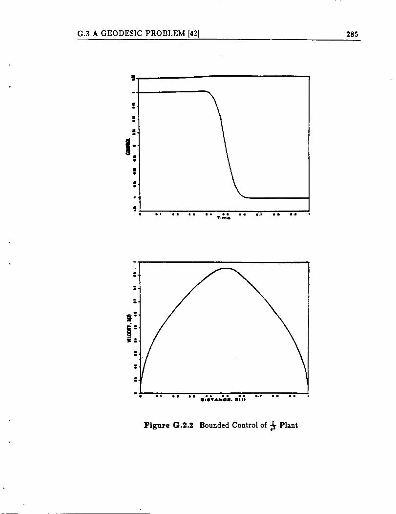
G.3 A GEODESIC PROBLEM [42] 285
S
l-9
• el e8 la ee go •e •.P ol I.gTirol
o
olI.Q o,il ll.ll , • • • • • • ll.lp • • • •
OelJTA;eO•. m¢1)
]Figure G.2.2 Bounded Control of _ Plant

286 G. Example Problems Solved Using the SGR Technique
I/2 .+ V2 + W2 = 1,
y2 Z 2x2÷--÷-- = 1.
4 g
The first constraint states the fact that the magnitude of the velocity is unity. The
second constraint requires that the travel be made on the surface of an ellipsoid
with semiaxes a =1, b =2 and c = 3.
Since the first constraint of the problem is already a path equality constraint, further
transformation is not necessary. If we take the time derivative of the second con-
straint equation and substitute into the resultant equation dynamic relations given
by the equations of motion, we obtain an alternative form of the path equality
constraint
xu q- yt, zw _ 0
4 9
Therefore the tranformed problem is given by
X t =tlu ,
I
y = tfl',
z' = tlu'.
Note the change in the independent variable from t to r for the reason explained
before.
The initial conditions of the transformed problem are
• (0) = 1,
y(0) = o,
z(0) = 0,

G.4 BOUNDED TIME RATE OF CHANGE OF STATE 287
and the terminal conditions are :
1
2y(1)-
3_ _ °
V5
In view of the need to stay on the surface of the ellipsoid at all times, one of the
above three initial and terminal conditions is redundant.
The path equality constraints of the problem are
u 2_- v 2 _ w 2- 1 = 0,
ZWxu ÷ yv _ m = 0
4 9
The minimum-time of this problem is found to be 2.1443. this minimum time com-
pares well with that obtained using the quasilinearization technique of References
[49-50:(tf = 2.1439).
Optimal trajectories in the x - y, x - z and y - z coordinate planes are given in
Figure (G.3.3). Note that the first two trajectories are part of an ellipse while the
last one is a straight line. This result is analogous to the shortest path "great-circle"
travel on the surface of a sphere.
§G.4 BOUNDED TIME RATE OF CHANGE OF STATE
mini = t/ :U
The equations of motion are given by
_: -- it,
= u - z2 - 0.5.

288 G. Example Problems Solved Using the SGR Technique
ORIGINAL PAGE IS
OF POOR QUALITY
ID
I|
!
?
OI It e_ _ t ee tl ee II 0
I11"!
II II tl II It
II_.! •
Figure G.3.3 A Geodesic Problem

G.4 BOUNDED TLME RATE OF CHANGE OF STATE 289
The initial conditions are :
The terminal conditions are :
=(o) = 0,
y(0) = 0.
x(tl) = z.
y(tI) = -._ .
This minimum-time problem is subjected to a bound on the time rate of change of
the state y from below
_>-0.5
The inequality constraint can be converted into a path equality constraint by the
use of the dynamic equation of y. The result is
u2-x 2 >0.
The inequality can be further transformed into a path equality constraint with the
use of an auxiliary control v
t_2 -- X 2 -- V 2 = 0.
Therefore the transformed problem is given by
x I = tlu,
y' = tl(u2 _ =2 _ 0.5).
Note the change in the independent variable from t to r for the reason given before.
The initial conditions of the transformed problem are :
=(o),= o,
y(o)= o,

290 G. Example Problems Solved Using the SGR Technique
and the terminal conditions are :
z(1) = 1,
7ty(1) -
4
The path equality constraint of the transformed problem is
t/2 -- 2: 2- v 2 = O.
The minimum-time of this problem is found to be 1.8191, which compares well
with that computed using the quasilinearization technique of Referene [49-501 and
reported in Reference [481 (t I = 1.8222).
The optimal time history of the state and the control of the problem are given in
Figure (G.4.4). Note that in order to satisfy the bound on the time rate of change
of y, the control u must at all times be larger or equal to x.

G.4 BOUNDED TIME RATE OF CHANGE OF STATE 291
ORIGINAL PAGE IS
POOR QUALITY
f
f"p
,o
• •t •.m 8.• • • • • • • • • • • • •
I1"11k411
Figure G.4.4 Bounded Time-rate-of-change of State Control