Staff Paper Series

Staff Paper P72-28 December 1972

THE MEASUREMENT OF BIASED TECHNICAL CHANGEIN THE MANY FACTORS CASE: U.S. AND

JAPANESE AGRICULUTURE

By

Hans P. Binswanger

Department of Agricultural and Applied Economics

University of MinnesotaInstitute of Agriculture

St. Paul, Minnesota 55108

Staff Paper P72-28 December 1972

.

The Measurement of Biased Technical Change in

the Many Factors Case: U.S. and

Japanese Agriculture

Hans P. Binswanger

Staff Papers are published without any formal review within the Departmentof Agricultural and Applied Economics.

Research Associate, Department of Agricultural and Applied Economics,University of Minnesota. Research for this paper was supported by the

U.S. Agency of International Development first through a grant to theDepartment of Economics of the North Carolina State University andth;n by a grant

The conclusions

to the University of Minnesota Economic Development Center.

do not necessarily reflect the position of the U.S.A.I.D.

THE MEASUREMENT OF BIASED TECHNICAL CHANGE IN THE MANYFACTORS CASE: U.S. AND JAFANESE AGRICULTURE

1. Introduction

This paper presents a way to measure factor saving biases of technical

change, or more generally, of efficiency gains with more than two factors

of production.* The methodology is then applied to the agricultural

sectors of the U. S. (1912-1968) and Japan (1893-1962).

The purpose of measuring biases in two countries is to test the induced

innovation hypothesis at a very basic level: If biases of technical change

are exogenously given by fundamental laws of nature (physics, chemistry

and biology), then we would expect that two countries, which both had

strong factor efficiency growth In agriculture, would have experienced

similar biases during the same time period. If, on the other hand, the

state of the basic sciences does not restrict technological possibilities

as strongly’ as to predetermine biases, economic variables such as factor

prices, rate of interest, and extent of the market will have an influence

on the biases, i.e. the biases will be endogenous. Therefore, we would

expect them to differ in economies where substantial differences in the

economic variables occurred over time.

In another paper (Binswanger 1972) I deal more thoroughly with the

problem of induced innovation as it is discussed in the literature.

That paper will also interpret the series of the biases presented here

*Sato (1970) derived a method to measure biases in the two factor caseusing CES and constant elasticity of derived demand production functions.He applied the method to the U. S. private nonfarm sector.

with respect

will be that

Although the

apply to the

-2-

to the induced innovation hypothesis. The general conclusion

biases are endogenously determined to a very large extent.

methodology used and the induced innovation hypothesis could

economy as a whole, the agricultural sector was chosen because

its product has undergone much less transformation than the output of other

sectors of the economy, so that few measurement problems occur on the output

side. Also a many-factor production process can provide more insight into

the causes of the biases, and last but not least, agriculture provides a

wealth of historic data which might be difficult to find in other industries.

The plan of this paper is as follows: First Hicks (1964) definition

of biases is transformed to a definition in terms of factor shares which

is more easily handled in the many-factor case than Hicks’ definition.

Then the theoretical model

cross sectional estimation

known before biases can be

is derived. The following section deals with

of cost function parameters which have to be

estimated. The last section presents the

derived series

the appendix.

2.

in graphical form with the numerical values included in

Definitions of Hicks Neutrality and Biases

The definitions of biases have been derived to deal with technical

change problems. Technical change is here defined as the development and

adoption of new production techniques. Empirically it is, however, not pos-

sible to determine which part of total increase in factor productivity has been

due to technical change alone (Nelson 1973).Part of the productivity

gains have also been due to education, soil improvements, etc. At present

-3-

it is not possible to measure biases of technical change alone, but only

biases of total factor productivity. Part of these biases are due to

education and other factor quality improvements. Therefore the term

efficiency gains rather than technical change will be used.

Efficiency gains simply mean that the unit isoquant of a production

process shifts closer to the origin. To characterize these shifts as to

biases a particular point on the isoquant has to be considered. Farrell (1957)

has introduced the following useful distinction between economic and

technical efficiency (see figure 1).

Land

“Labor

Figure 1. Technical and Economic Efficiency

-4-

Any point on the unit isoquant such as B or A is technically efficient,

while C is not. For a given set of prices only one point is economically

efficient; unit costs are only minimized at A. The theory of biased

efficiency gains in the Hicksian sense asks how the economically efficient

point moves inwards over time at constant factor price ratio. If it moves

inwards along the ray OA to A’ the efficiency gain is said to be Hicks neutral.

If it moves to A1l the change has been labor saving. More specifically,

efficiency gains are said to be labor saving, labor netural or labor using

depending on whether, at constant factor prices, the labor-land ratio decreases,

stays constant or increases. This definition can be immediately transformed

into a definition in terms of factor shares at constant factor prices.

Efficiency gains are labor saving, labor neutral or labor using according

to whether the labor share decreases, stays constant or increases at constant

factor prices. This definition generalizes easily to

and will lead to one single measure of the biases for

definition in terms of the factor ratios were used it

the many factor case

each factor. If a

would be necessary

to consider n-l factor ratios for each factor to determine biases.

Therefore, the definition in terms of shares is used in the following chapters.

The rate of the factor i bias is measured as:

13i ‘f&i ”~:()+ Hicks f HiIrelative f

“:%:?1 (1) ‘actor prices dt ai Y

i-using

where ctiis the share of factor i in total costs.

-5-

TO cst Lmate biases .tt1s, however, not possible to simply 100Icat

historic factor share changes. The observed share changes have come about

through biased technical change and through ordinary factor substitution

after changes in the prices of the factors. The basic problem is, there--

fore, to sort out to what extent the share changes have been due to

biased technical change and to what extent to price changes. This can

only be done, in a graphic sense, if the curvature of the isoquant is

known. The substitution parameters of the production process have to be

estimated before any biases can be measured. In the following sections

this will be done for the agricultural sector using a cost function to

characterize the production process.

3. Measurement of Biases with a TransSog Cost Function

In my thesis (Binswanger 1973), I first derived a general theory to

measure biases in the many-factor case for arbitrary twice differentialabl.e

production functions. For actual implementation a particular form of the

production function has to be chosen. The production functions considered

were, however, either too restrictive (Cobb-Douglas, CES, constant difference

of elasticities of substitution) or complicated to use (generalized Leontief,

Transcendental Logarithmic production function). In the case of the

Transcendental Logarithmic (Translog) cost function (Christensen,

Jorgensen, and Lau, 1970), the theory simplifies and estimation equations

for its paramters are econometrically convenient. The theory is therefore.

derived directly in terms of this function.

-6-

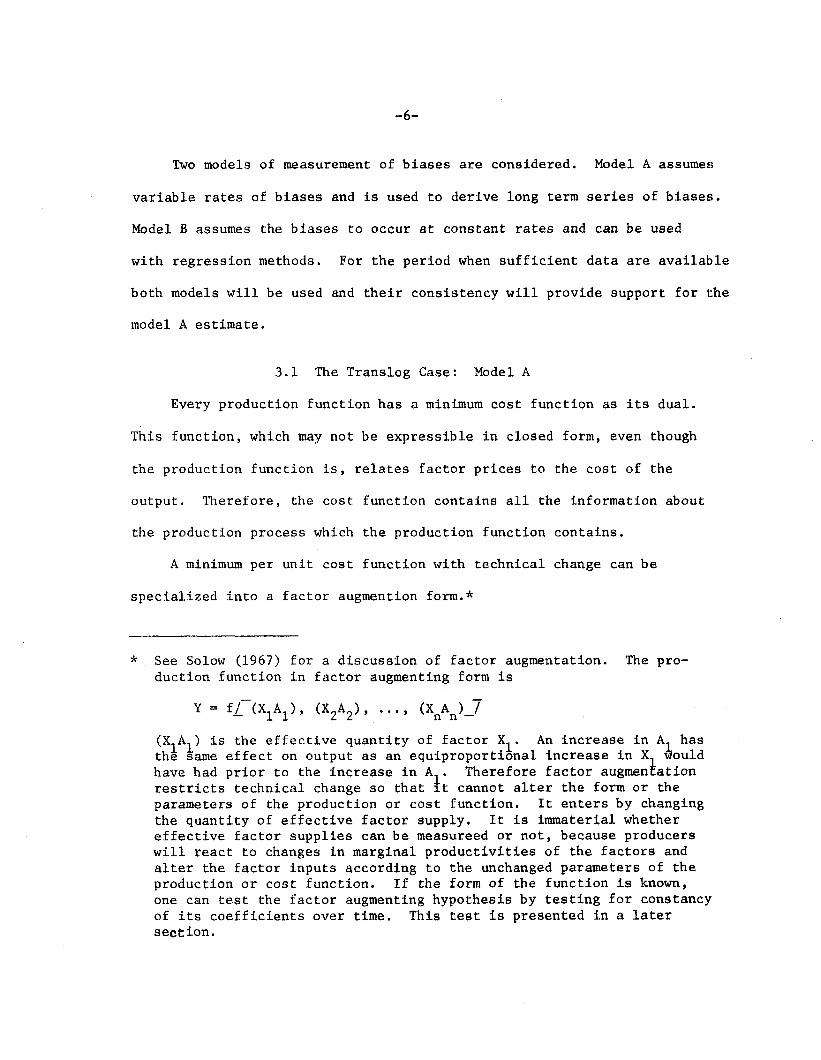
Two

variable

models of measurement of biases are considered. Model A assumes

rates of biases and is used to derive long term series of biases.

Model B assumes the biases to occur at constant rates and can be used

with regression methods. For the period when sufficient data are available

both models will be used and their consistency will provide support for the

model A estimate.

3.1 The Translog Case: Model A

Every production function has a minimum cost function as its dual.

This function, which may not be expressible in closed form, even though

the production function is, relates factor prices to the cost of the

output . Therefore, the cost

the production process which

A minimum per unit cost

function contains all the information about

the production function contains.

function with technical change can be

specialized into a factor augmention form.*

* See Solow (1967) for a discussion of factor augmentation. The pro-duction function in factor augmenting form is

Y = f~–(XIA1), (X2A2), .... (XnAn)_~

(XIA1) is the effective quantity of factor X . An increase in Al hasthe same effect on output as an equiproporti~nal increase in X

kwould

have had prior to the increase in A . Therefore factor augmen ationrestricts technical change so that ~t cannot alter the form or theparameters of the production or cost function. It enters by changing

the quantity of effective factor supply. It is immaterial whethereffective factor supplies can be measureed or not, because producerswill react to changes in marginal productivities of the factors andalter the factor inputs according to the unchanged parameters of theproduction or cost function. If the form of the function is known,one can test the factor augmenting hypothesis by testing for constancyof its coefficients over time. This test is presented in a latersection.

-7-

U= f(W1, W2, .... Wn. T)=+ (~, ~,w

.... n)

‘1 ‘2<

(2)

where U is per unit cost, Wi are the factor prices and Tis a technical change

variable or time. The AIS are augmentation parameters corresponding to the

ones of the dual production function. A proportional change in Ai has the

inverse effect on the unit cost as a proportional change in the factor

price i. As the MP of factor i is uniformly increased, more of it is

substituted for others in exactly the same way as if instead the price of

it had fallen.

Let Ri =wi, the factor price of the augmented factor unit (AiXi).

~

The Translog unit cost function can be written as

(3)

where vo’ ‘i

and yij

are the

the first brackets is a Cobb

parameters of the function. The part within

Douglas function. If the cost function were

Cobb Douglas then the production function would be also (for proof, see

Hanoch, 1970). We therefore can think of the terms in the second bracket

as amendments to the Cobb Douglas function which change the elasticities

of substitution away from one (See equations 28 to 31 below). The functions

allows arbitrary and variable elasticities of substitution among factors.

-8-

The function

In U = In v.

s 1 i near logaritlmes:

+ZVilr]Ri+~ ZZyij lnRi ltl Rj.. .

(4)

i .lJ -

The function can k considered d fdncticmal form in its own rigtlt

or regardcu as a logar-i timlic Taylor series expansion LO the second term

arounci input prices of 1 of an arbitrary twice ciifferentiable cosL functiolr

[Christensen, et al., 1)70]. With the proper set of constraints on its——

para,netcrs i t catI tlwrcfarc de usci as an approxilllation to any one of the

Arloiwl costs at)d producticx) functions. As tl~e sirnpldst example, tne con-

strail~ts for CoIJb Douglas simply set

an approximation to the CLS are more

l-;~e following symmetry coi]straint fKJ

of second cross derivative~ )

Alsu cosis functions are runoqdneous

prices douljle unit costs will double.

complicated [Cilrist.enscn et al., lj713].——

Js for all Tratlslog functions (qudlity

for all i, j, i + j . (j)

of degree one: in prices.” When al 1 factor

It earl be shown tllak tnis ifiplics:

.‘Yi=]i

(6)

IQ measure biases \Ye ndd~ eqdations wilici) expldirl factor 511drc5 ill terrrls of

fdctor prices. TIIe Sl)epard Duality T’ileorc:ll [Iiai)och, lJ)J] gives one of LIIC

fundamental relationships between til(; cost and production fullctiorl unclcr

cost minimization.

au— =Xi.~wi

In augmented units (7) kmms

81J3udwi=Ax=z—=2Ri qq ii-” I

(7)

(8)

, are the factor quanti ticswhere the Z. in the augmented uni t space. ‘rh~

first derivatives of the Trnaslog function, with respect to the log of the

factor prices, arc equal to the s;~ares:

(k/i/Ai)‘31nd _ 3U ~= ‘iRi s ‘ixi

\!iXi _

mi-~”u ~ —v----=ai -ai

Taking these aerivatives9 we have:

,j In ‘{j~i = Vi + L ‘f.

j

Differentiating (10) totally \ve have

I-r

dai = X Yij d in Rj

j==l

(3)

i=l, . . . . Il. (lo)

i=l, . . . . n. (11)

TIIC proportional (log) change of a ratio is the difference of the proportional

changes of i ts numerator and denominator.

n

dai = z yij (d In Wj _ d In Aj) i=l, ● ... n.

j=l

Separating terms and using matrices

I in w....

llnW

(12)

-1o-

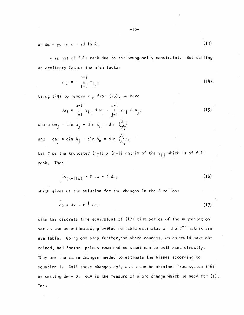
or du=yc.i In d - YJ In A.

y is not of ful 1 rank due to the homogenei ty constraint.

an arbitrary factor tne n’th factor

n-1

Yin = - z Yij”i=l

Using (14) to remove yin from (13), we Ilave

w.wilere dw. = dln il. - din WI] = Jln (

J J &‘n

and dai = dln Ai - dln An = dln (~).

Let r be the truncated (n-

rank. Then

‘a(n-l)xl = r ‘“

“n

(13)

But call irlg

(14)

(15)

) x (n-l) matrix of tile yij which is of full

- r da, (16)

which gives us the solution for tile changes in the A ratios:

da = dW . r-’ da. (17)

With tile discrete

series can be est

available. Going

time equivalent of (17) time

mated, provided reliable est

series of tha augmentation

-1mates of the r matiix are

one step further, the share changes, which would have ob-

tai necl, had factors prices reruained constant can be estimated di rectly.

They are the sl~are ci~anges needed to estimate tile biases according Lo

equation 1. Call these changes dct;~, which can be obtained from system (16)

by setting dw = 0. dci~c is the measure of si]are change which we need for (1).

-11-

(18)

And substi tut’

da:, = - r(j~.

ng da from (17),

du* = &X - I’dw. (19)

According to (19), we can immediately judge tile nature of technical change

for factors i-1, . . . . n-l. Also, since

n: &ti = J,

i=]

we ilave also ttw solution for the n’til factor

n-l ,

da’:= - z da;. (20)n

i=I

Equat

silare

on (12) i]as a nice simplicity to it. To f nd out what the factor

changes viould ilave /)eCiI, i~ad factor prices reiliainecl constant, simply

i=], s.. , 11, (.!1)

(22)

-12-

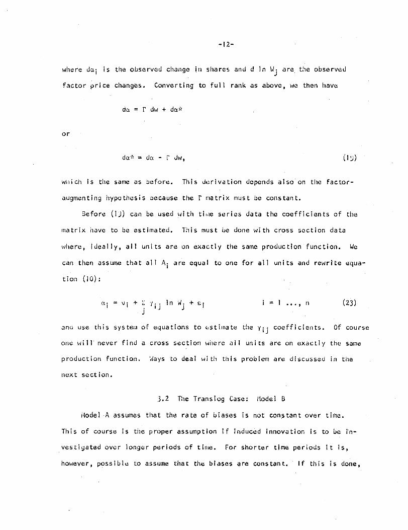
where dC%i is the observed change in shares and d In \/j are the observed

factor price changes. Converting to full rank as above, we then have

do.= r dW + d~+

or

dcI;~ = dfJ - r h,

wiliCh is the same as before. This derivat

augmenting hypothesis because the I’ matrix

Sefore (Ijl) can be used with til,le ser

matrix have to be estimated. This must k

(1!))

on depends also”on the factor-

must be constant.

es data the coefficients of the

done with cross section data

where, ideally, all units are on exactly the same production function. We

can then assume that all Ai are equal to one for all units and rewrite equa-

tion (10):

a. = vi + z .{1

ij InWj+cl i=l . . ..n (23)

j

and use this system of equations to estimate tile Yij coefficients. Of course

one will never find a cross section wiwre all units are on exactly the same

production function. Ways to deal with this problem are discussed in the

next section.

3.2 The Translog Case: Nodel B

i!odel A assumes that the rate of biases is not con,stant over time.

This of course is tile proper assumption if induced innovation is to be in-

vestigated over longer periods of time. For shorter time periods it is,

however, possibie to assume that the biases are constant. If this is done,

-13-

~iasecl technical change at constant exogenous rates can be introduced

in the translog cost function in s similar way in which Christensen

et.ale, (1)70) introduced it into the corresponding production function:

lil u = lnvo+ZvilnWi+l ZZ yijltlWiln Wj

i ij

+vtlnt+wt(lnt)2+l uilnullnt (24)

i

where t stands for time.

Upon differentiation the share equations become:

This is the estimation equation (23) with t

In t (25)

me enter ng as a variable. Wi s

tile constant exogenous rate of factor i bias.

If (25) is used as a regression equatiotl with a tilne series or a com-

bination of cross section and time series, the introduction of time in this

way tii I I ensure tl~at’ biascJ technical change at constant rates will not

bias the estimates of tt~e y. Furtlwrmor-e tile coefficients ii can be usedlj”

;!f;,:to derive another set of price corrected shares series., say Jai which can

be used viith

da’

Of course ti3

gression per

equation (1) to estimate the biases for the particular period:

;~ *= Ui d In t i=l . . . . n. (26)

s moJel cannot be used to extrapolate outside of the s!wrt re-

ed because thcr{ the assumption of a constant exogenous rate

of bias is tenuous,!,

IIowever, t}le consisttincy of tl~e du~” series for the

pcrioti in wllicll b~til IIIOLICIS cal] be used will be of great value to assess the

-14-

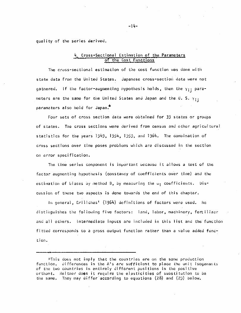
quality of the series derived.

4, Cross-Sectional Estimation of the Parameters

of the Cost Functions

The cross-sectional estimation of the cost function was done with

state data from the United States. Japanese cross-sectiotl data were not

gatnered. If tile factor-augmenting ilypothesis holds, then the yij para-

meters are the same for the United States and Japan and the U. S. “~ij

parameters also hold for Japan.*

Four sets of cross section data were obtained for 39 states or groups

of states. The cross sections were derived from census and other agricultural

statistics for tile years 1949, 1954, lj5j, and 1964. The combination o

cross sections over time poses problcrns which are discussed in the sect

on error specification.

Tile time series component is important uecause it allows a test of

on

the

factor augmenting hypoiiwsis (constancy of coefficients over time) and the

estimation of biases

cuss ion of tnese two

In general, Gri

distinguishes the fo’

by method B, by measuring tile Mi coefficier~ts. Dis-

aspects

i ches 1 (

lowing f

and all others. Intermediate

s done towards the end of this chapter.

964) definitions of factors were used. tie

ve factors: land, labor, machinery, fertilizer

inputs are included in this 1 ist and the function

fitted corresponds to a gross output function rather than a value added func-

tion.

:~This cio~s not imply that the countries are on the same production

function. Differences in the A’s are sufficient to place the unit isogenarlts

of tnc two countries in entirely different positions in the positive

orthant. ideither does it require the elasticities of substitution

tile same. They may differ”according to equations (28) and (25) be

to be

Ow.

-l;-

tist of the data come from published USDA sources. Expenditures On

factors usually arc actual expenditures ai~d, where applicable, irrputecl ex-

penditures for wages of family members interest charges, depreciation and

taxes. Quantity data are derived as price we

units (land and fertilizer) or the sum of ind

(all other) or a combination of tilese methods

gl~tcd indexes of physical

vidually deflated expenditures

(machinery and labor) . The

quantity data were already computed in Fishelson (1969), WIIO used Griiiches

(1364) data with s] ight changes. Expenditure and quantity data are consistent

wi tll each other. The price data were ob&ained by dividing the expenditure

data by the quanti ties.*

Tne estimation equations are as foliows:

‘Z~j 111 Wjk+Cik, i = l.,.n, k= l...m.aik=vi

(27)

j

wilere k is tile k’ th observation unit. They are unaitered if neutral

efficiency differences exist among states or time periods. ideutral differ-

ences would only al ter the intercept V. of tne cost function which drops

out upon differentiation. If ar~y left out factor such as education or

research and extension affects efficiency neutrally, leaving them out of the

estimation equation will not bias tile results.

(Nonneutral efficiency differences among the observational units will

have tile effect tt~at the true ai will differ for each observational unit;

dt equal factor prices shares will not ix equal .;~;~ If such differences

>kThe amount of data transformatior~s performed on this set of data and

on tl}e two sets of time series data discussed below and the diversity of

sources precludes a thorough discussion l~ere. A complete discussion of all

data used can be fourid in 5inswanger (1373)

:~~’qfonneutral efficiency di fferences betvwen 2 states ilnpl ies that

at equai factor prices, they will use factors in differing proportions.Factor shares wiil therefore differ even at equai factor prices

-J/6-

occur among al 1 units, the estimates of the coefficients of (27) will be

biased. tioweve r, if such differences occur only among groups of states,

the proper set of regional dummies will again lead to u~~biased estimators.

While the proper grouping might be q~estioned, dummies for five regions were

therefore included in the regression equations. “I%is should at least

diminisil the problem, iJonneutral differences migtlt arise due to educa-

tional differences, differences in research and extension or differences

in product mix.

If (27) is atifllated ~i~h time series clata, a time trend in tile

estimation equation itiill solve the pr-obletii of biases over tilw as ex-

plained ill Imodel t~ “~ provided the rates of ~)ia5e5 ~

stant during ti~e estimation period. Since tiw per

.lyed r“easonahly con-

od was rather short

(1542-ljL4), this assumption is not unreascx]able.

Liitilin each of the four cross sections, the error ternls of the n-1

estimation equations are not independent, s ince for eacil state the same

variables Iwilictl Inignt affect tile silares in additiorl to the prices were

left Out of t,i~ model. if restrict

are imposed, OLS estimators arc no

that all equations contain tile same

hand side (Tlwil lj71). ~!lL:t-LJfor~,

CJns across equations (y.. = yji)IJ

onger efficient despi te the fact

explanatory variables oIl the rigtlt

ti~c seenlingly unrelated regression

prob]ein applies and Restricted Genera] ized i.cast squares llav~ to i~c appl icd

to all equations silnultaneously (ZeIlner IJ62, ljXiIj).*

$’l-ne Computer Program used was l-riangle Universities Computing Center:Two and Three Stage l-east Squares, kese~rch Triangle Park, :J.C., 1972

(TTLS).

-17-

If all four cross sections are pooled there is an additional problem

of error

problems

test and

strail)ts

interdependence over time. The correct way of I}andling both

would be to specify an equation for each share in each year, tlletl

impose the symmetry and homogeneity constraints and the con-

tllat the y. . pdrdmeters are coIIstaInt over tlrw.IJ

Tlhis excedded

was not possibie.with TTLS.

I-ile follovlillg procedure was therefore adopted: i) l{y~Oti)~Si25 not inv-

olving time concerning the ‘fij Of tile s~iile or differeilt shares equations

were tested in models containing four snares equations using data from a

single cross section only. These tests .~ere also used to decide into which

equation dummies should be include J. 2) The testi,~gof tile constancy of ti~~

yij parameters over timti was done in models containirlg a separate equation

for the salile share in twd cross sections. As an example, to test \dlletller

“]e Yij P aralwwrs of tile labor sharti equation were constailt uver time a

two equation GL$ model containing a labor silare equation for tl]e 1949 data

set arid a labor sl~are equation for t~~e ljjj data set was estimated and a

test performed wnether tile regression coefficients in the two equations were

tne same. ~) The actual estimation Of tne Yij coefficients was LJorle with a

data set wilicr~ cuntai,~ed all four truss sections using a cons~rained GLS

modol containing four snares equations. Trlis procedure took account of error

interdep~l]deilce among Silare equation~ but not of error interdeperidence over

time. Nhile tile resultil~g estimates are unbiased, tiley will not be most

-)8-

efficient ones. Iio txs Ls are per forlned wi th this regression and tlw t-ratios

of tile esciniates are probably overstated.

Tile system to be estimated contains equations fur five expenditure.+

shares. 3uL only four of tilese equations are linearly independent. so

one equation ,las to be dropped. In a statistical saillple lJIe coefficients

estimated wi 1 1 Ilot be t!le same independerit of which cquatiol~ is dropped.

Another quest ioi~ to bd decided is in wnic,l equations Lo include regional

dummies, i.e. for wllicl-r factor to allow b

ences. Theoretical reasoning does l~ut Ile

,~eitiler sljould the estimates of the coeff

the fact Lilat using tests of significance

ascd regional efficiency Jiffer -

p much to makd L!IC above cno ices.

cients be used as guides.

as criteria might lead to

estimation proulems (Wallace and Asilar lj72) , sucn tests ,~ere used,

Despite

sequential

In the

.aDsence of ttleoreticaI justification t(ley are tile only information which is

available. The specification was searcheu Whici) would best satisfy the sym-

metry and Ilorlmguni ty constraints of cIle cost function; i.e. lead to the smallest

relative increase in error SUlilS of squares ,tir~ert i!nposed (smal lest F-ratio) .

Since tnese constraints arc beyond doubt, they call I.w USed to eliminate ccr--

tain specifications. It turned out Lilat on average a model containi[~g the

equations for laIId, labor, Illacnincry anJ fc:rtilizer with regional dummies

in all equations satisfied this criterion Dcst. The homogeneity constraint

was accepted in all four cross sections at tile .0S level. The symmetry con-

straint was only rejected in tile 194j data set. Tile three otl~cr specifica-

tions tried performed less well. TIIe Cobb-Douglas constraint (yij = i.) for

all i,j) \/as dlso tested and rejected in all specifications. Sil~ce the R2

of tilt? singl- equations \vas alwdys ill tl~e ral~~ of .5 to .j, this could be

-i9-

expected. Only if ttle equation i~ad no explanatory power at all could the

constraints be accepted.

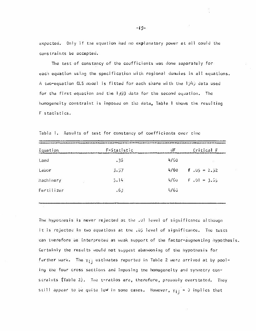
The test of constancy of the coefficients was done separately for

each equation using the specificatiorr witi) regional dummies in all equations.

A two-equation CLS model is fitted for each si~are with the lj4~ data US(

for the first equation and tile 1559 data for the second equation. The

homogeneity constraint is imposed on tllc data, Table I si~ows t;le result

F statistics.

Ta~l~ 1. Results of test for consta~lcy of coefficients over time

d

ng

Ecruation F-Statistic dF Critical F

Land .36 4/Lo

Ldi)Or 3.37 4/60 F .~~ = 2.32

~Ptachinery 3.14 4/6(J F .01 = 3.;j

Fertilizer .63 1+/6~

The hypothesis is never rejected at ti)c .U1 level of significance al tl}oug[l

it is rejected in two equations at tile , uj level of significance. Tne tests

can tl)erefore be interpreted as weak support of t!le factor-augmenting ilypothesis.

Certainly the results would not suggest abandoning of the ilypotnesis for

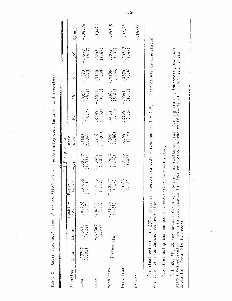
further work. Tile yij estimates reported in Table 2 were arrived at by pool-

ing the four cross sections and imposing the I]omogeneity and symnetry con-

straints ~“~able .?). TIIe t-ratios arc, therefore, pro~ably overstated. Tl~ey

sti 1 1 appcdr to be qui te 10W irl soInc cases. However, Yij = 2 implies that

:1

L:nIc

:

L0.

JP. .-)-

.-

:>ILla

Lc

.Cfc

-J

XI

$-.)

6.-Wm2m’

u -J

.I

.-

--c).=t -C3.n--..4

t

.

.

.I

2L

N

>.- li 0

-.

u

u

1%.3.n

.

Q.E0

L-)(3

Q-

.m u-Q.)cum(f)Uu

TJul

m>~fu

u m-cl

-21-

tIIU correspon~iing partial elasticity of substitution is one, since tile

following relation silip5 b~tki~~tl tile Yij aild t[l~ ‘ij dlld t~l~ T’lij (elasticities

of factor demand) hold (for prqof, see Uinswanger lY73):~:

‘+()’ ii+di2-~i)‘iiUiL

for all i #j

fOr all i #j

Y ,.~ii ‘A+~i -l>

it.I

ulncre CXi are tile factor si~ares. Ti]ere fore, Yij close to zero with

t-ratio is IIOL a ‘tbddl’ result. The yij parameters can be eval uated

(2fi)

(Zj)

(30)

(31)

CM

by look-

ing at tl~c imp] ied elasticities of fdctor demdnd for the diagonal elements

and Lile elasticities of substitutiol~ for t;Ie off-diagonal elements (Tables

3 and

using

lj4j-

4). T!Iey were computed according to equations (28, 2j, 30, and 31),

t:]e unweigi~ted average factor sllarcs of the jj s~ates in the period

Al 1 own Jcilland elas tici ties have the

appears very inelastic. TIIe deloand clast

inputs are larger than I , a fact to keep

correct sign. The delnand for land

cities for machinery and other

il r,lind si n-e it implies that a

rise in ttle corresponding prices will, other things equal, lead to a fall

in Ehe factor snare. Ti)e lower part of Table 3 shows the values of the

‘(Jij is the partial ~lasticity of substitution as defined in Allen

(1~3~~, page ~Jti). ‘lij= ~~i ~~wherc dj is the price Of factor j and Xi

;.JI

tne quantity of factor i.

S;ld~~S used were est

Negative elastic

Corllp I emei~ ts. A

;$lates of i ts coefficients.

ties of substitution ilnply t!~at tile LNO factors Jre

TIIti closest substitute of land is fertilizer , as cIne mignt expect.

Itacilinery also appcarb to i)d a good substitute for land, while labor is

t-lo t . Otiler inputs appear to combine witn land in a?most fixed proportions.

Lauoris uest substitute seems to be other- inputs , and not machinery, as

initially expected. Cul}sidering that ot;~er inputs contain all intermediate

inputs and outside services, the stroi~g substitutability becx)irres more

plausi~le, as intermcJiate inputs substitute for inputs produced with the

use of labor on tile farrll itself. (i{ote tl]at inter-mediate inputs produceu

and consumed on the same farm are neitner inciuded in input nor odtput

statistics.) Also tne substitutability becwecn IaDor and macilinery is still

quite high.

Overall, t~le ~;j estirllates seem to be adequate. iio absurd resul ts were

obtained. To see whettiler error interdependence over time ilad a large in-

fluence on tile estimates, restricted estimates wi tll tlw same model were

also

from

data

sets

obtailwd for each of tile four data sets separately. The estimates

tlie pooled data were colilpared with t!le average estimates for the four

sets individually. The estimates were very close. In particular both

imply complementarily for the same factor pairs except tl~e machinery-

fertilizer pair. TiIe own demand elasticities were very similar except that

::Own elasticities of su~sti tution nave Iittle economic meaning. Theyare simply transforms of tne factor demand elasticities, which explains why

they cannot be infiilitely large. They obey the following addinq up constraint:

(Allen 1938).

-23-

Table 3. Factor demand and cross demand clasti ci tiesa implied in tile

estimated yij and the standard errors around ti~ei r value in

the Cobb-Douglas caseb

Machin- Fert-Landd Labor ery ilizer Other

Estimated Translog valuesc

Land -.3356 .0613 ● 1732 .1062

-

-.0112

(.07) (.07) (.i13)

. ojGG -.jlog .1256 -.0577 .8122(.04) --(ZK)) (.04) (.02)

.1833 .2560 -1.0886 -.d233(.07)

.6733(.08) --’’q’m (.06)

-.0046 .66>0 ,2720 .1053 -1.0417

Cobb-Douglas values for comparisorreLand ~ .3CIOJ .1475 .9356 . 3&52

Labor ● 150: -.65j2 .1475 .3356 .3652

Fertilizer . 150:) .3398 -.3525 . d336 .3652

itacilinery . lsdj . 330s .1475 -.9644 .3652

Other .15i)y ,3008 .1475 .9336 -.G34:

aLaci] element in tile table is tile elasticity of demand for tile input

in tile ro~~ after a price cilange of Llle irlput if] the column. TIIcse elas-ticities arc not syrwnctric.

sE(y.,)‘SE(:lijj =+.

I

C71 . . =IJ

‘~j , “ii = Ui - 1.

-~[+-

Table 4. Estimates of tlw partial elasticities of substitution and

standard errors around la

Machin- Fert-

Land Labor ery ilizer Other

Ldnd -2.225 .2(I4 1.215 2.387 -.031

Labor -~

Fiach i ne rySyrw,le t r

Fertilizer

otillJr-

J28 .851 -1.622 2.224

-7.372 -.672 1.044

L

-26.573 2.>UI

-2.352

Y..au =IJ+l ‘+ (Yii+Qi2 -ai)*

ij 7 ‘ii‘iitij ~i

The elasticities of substitution are symmetric.

other inputs Ilacl an elasticity of

of the four data sets. some of tllc

css than one for tme average estimates

cross elasticities were not very stable

over ttle four salts Iw~lile the staoili ty of tile own elasticities was quite

Cjood .

~. TiJe Empirical !Icasures of- Biases

in Efficiency Gains

Ti~is section prcsenLs tnc derived series of Liascs for tile U.S.

alnd Japan usiilg i[]~del A. It also presents ti~e series of actual factor silares.

Ti)e data for tile U. S. ccm)e from USLA publistled sources. Tne variables are

constructed so tl~at they correspond as closely as possible to the variables

used in tile cross section analysis. Total correspondence vJas, hobfeve’r, not,

acrlievable.

-25-

The Japanese data came from Okawa, ct al. (1965) with the exception

of tne interest rate series ~d~icl} was f~llnd in Ginko (1966). Variables

construction v~as clone to achieve close correspondence v~ith the definitions

used for tile U. S. series. of course, differences in method of data

gathering and some definitional differences prevented exact correspondence.

Tile details of the data are expiained in binswanger (1973).

The basic estimation equation for t,w biases are equations (13)

n-l _~;h = ~ai - ~ dlnw

‘ij J(13)

j=]

;:wnere the u. is tl]e factor share i which would obtain in t!le absence of

I

ordinary factor substi tut ion due Lo price changes, d~i is the actual total

change in share i wnicll includes tt~ effect of tllc price changes. d In \tii

is the proportional c~~ange of the ratio of the price of factor i to the price

of otiler inputs (a choice which is arbitrary). For actual estimation pur-

poses series of three year moving averages of tile shares and tile factor

prices were constructed, TIIeII discrete differences of these moving averages

at four year intervals were taken and used in the discrete change equivalent

A

of (1>). ‘Ti]e ‘(ij were ti]e ones estimatcJ in tile U. S. cross-sectio[t re-

gressions. I t was assur,led ti)ey were ttle same for the whole period and for

Japan.

Equation (12) can be converted il~to a standardized measurement of the

bias for each silare by dividing the si~are changes throucjll the levels of the

actual shares in a base period. This leads to the discrete change equivalent

of equation (1) wllic!l measures tile rate of tile biases.

-26-

add

to

?:ACI

1i saving

Dj = J j 0+ ilicl<s i neutral (1)

a? i using

rlg tllC ai for all 4 year intervals (with Bi of the base period equal

) gives cumulative standardized series of a; as a fraction of tile base

period.

An approach is on

here are simple cost m

y as good as its assumptions. The key assumptions

nimization arid the constancy of tne y. . coefficientsIJ

over tiim and space, Tile former assumption is no problem because it

nei tiler impl ies profi t maxililization nor nonintervention by the government

in goods and factor markets. Only if tile government regulates boti] prices

and quantities of factors of production is tl]ere a big probienl. Quantity

controls alone wi I 1 Lc reflected in corresponding price Changes and vice

versa and therefore wil 1 not disturb tilemeasurements. They may of course

have induced ~iases.

The constancy over time and space is mot-e troublesoiw. Wtlen tested

it ‘was not supported as well as one mig!lc wisil$ But ti”lcre is no way

around the assumption.

Evel~ the con~tai~cy over time assumption is not as restrictive as it

sounds. It Joes Iiot preclude variable elasticity of substitution and of

factor &m3nd. Furthermore these elasticities may I](ive arbitrary values.

Tils approacl] allows for neutral and nonneutral cfficieflcy di ffercnccs bc-

t~(cen tile regions considered. In sliort it does not require countries to be

on tlw same production function. Only the Yjj pararleters of the functions

17avc to be the same.

-27-

The approach is also less restrictive than other approaches used up

to now by allowing the production function to be nonhomogeneous and allow-

ing economies of scale, provided they affect all factors neutrally, It

also uses five factors rather than ? , wt~ich means tilat i t does not impose

a separabi 1 i ty constraint between capital and labor on the one iltllld tile

intermediate inputs on tile other. From tile point of vied of its a.ssurnptions

the approach sIJould cl}erefore k superior ti~an ot:]er known approaches.

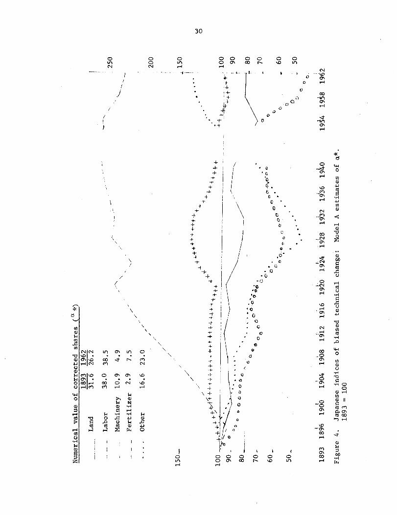
All rcsultil~g seri~s dru prcsC[~Lcd grapilical]y. TIIe corrssponJing

r“juii~erical values are taululated in C112 appendix, Figures 2 and 4 s;]oki

semi logar

(equation

511QW cumu

indicates

tllmic scale. ‘rl~c 510pe 0; eacli of the series is tile Ji rllcasure

1) ,tilicll measur-cs t~le rate of tile bias. Tim series ti~cmselves

ative effects. As an exa(llple, tile fertilizer line in figure 2

tlla i , given tile biases w:licn occurred, the fertilizer snare

would Ilave quadruped 2ct\4een ij12 ,Incl 1J62 Ilad all tlw factor prices re-

mained constant, i.e. , !lad nCJ factCJr Substi ~LJtiOn alOn(J a given production

function occurred. Tl)e rather constant slope of tlw line indicates that

tild rate of tile bias remained fairly constant througi]out the period.

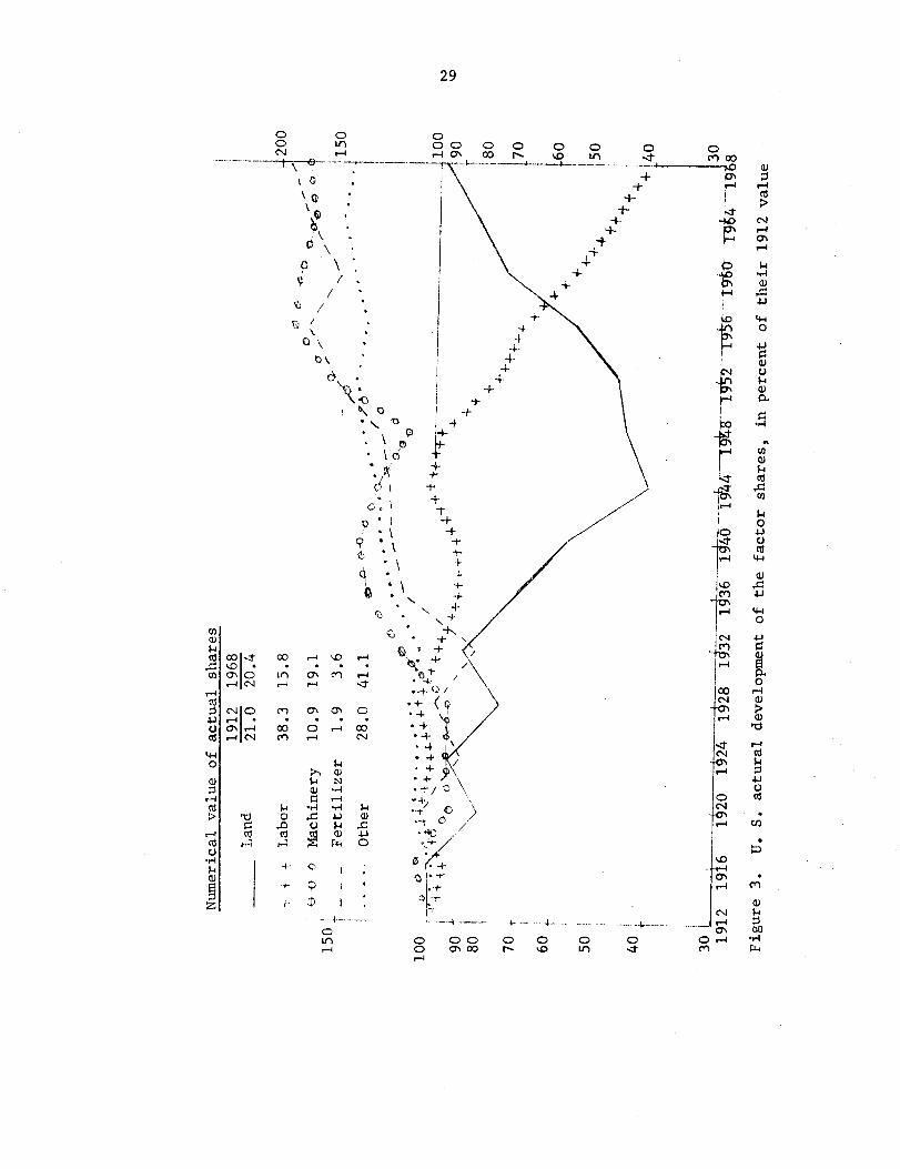
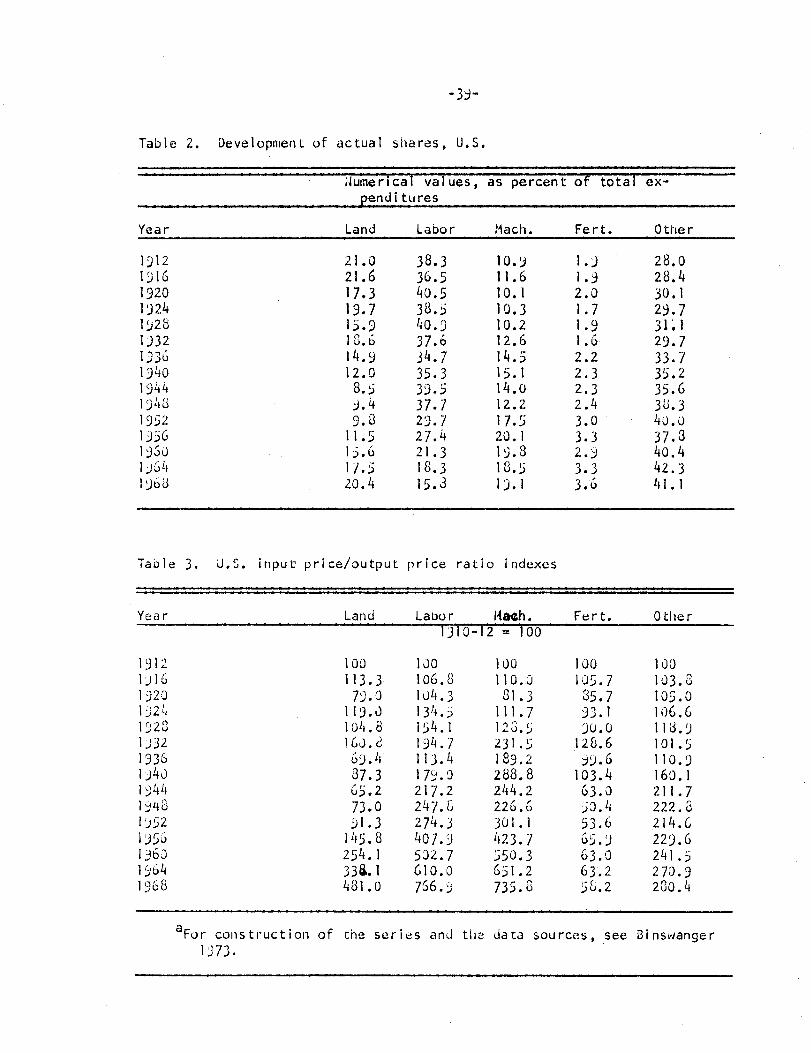
Figures 3 and 5 show tiw actual share movement for tile US and Japan

in the sar;]e sen)iiogarit}mic scale and as a percent of the 1912 vaiue of

tilt? actual si]ares. Tl]e actual share cilal]ges reflect the influence of both

bias and ordinary factor substitution.

According to figure 2 efficiency gains i~~ tile U. S. have Lcen strongly

fertilizer-using and filachi nery-usln!~. At first they have been labor neutral

and then substantially labor saving. Land has first been saved and tiwn used

28

01= ~

.,.. .. ., .,.. I

+

it

1+

ou-l

‘--~PJ

o

___..._ 2-. ....-....-.1;!

o 0 00 0Ocm co

- S“.._”.~~2.. d

“\.............., .

d ..

{) .$ .

.? .

●

{..

●

●

q* 4.

h*a

b. .

M●.

●

b ●

..-

I

g

ikl

l\\

\\I\\

(\

\ 4-”

:“+t/‘\ $

‘\ b,..\ “Q . %1

!+Cl-J

I -d’!

l-n.

com

91:

01:01”

-.

II

I

o 00N 2

00”0Ofmca4

.!-(k!

29

00N

om!4

o00 0Am Zr+: oz.—... .. --$-- --.-.—-—-—L.——+.—.——_

+ l-l

++

“ii4“

+++

+

-------._._ -––y@”

\o;\Q “

.‘O ,b.

J, .

....

.,

.

wo

O-\o\

c?-.

+ \ G+-+

;

!A--4

-4- /“’”-+

:\ +-\ -J-

., -1- /“’” 2uw0

co.

b-ll-l

co.com

$-l

:

3++i-

1+

.-+ -Q/ ‘\ l-l

:

mt-lcdl-is4-J

t%

.tn

1+

o1.+-.+

o -r1’

..._lN+- -- -4---- - .. ..&____ d

00 0 +I=@ m z

.m

i- --4 --—-

0 000 mal!.4

30

. — — —oz o

w N—.. .._. .

1

\

,.~d’

o0

0c1

-+--J-+

.i-+

+-k

-$+++:+-+

-$

+-

-+

-+4

i-

--i-t-

“++

++4-

+-

1 /

i

(‘\,

‘cl‘q0..6.O*0“9 “,v.Q*0.

\,’

0.“0

.5●G

-cl/’

/

\\

\\

\\

\m Cnu) o’”. . . . \cg4r. m

ml

\\

I 1.

I 1“, I 1:

Iou-l$-l

t I {00 0I=@ m

00Ocn zd

--’ ----–-------––-t--------- 1-.—....—~...w

. /cl....._._~ ._.._..._+ g

[’z,’ S‘-----

‘/:

1 “-----.0

// . .

J?o~

0 -.i?-

0 4’

c-&*G’t)0F

+’-1-

+“\+

l’:/+/+-\:\+

%+ki-’/4

t/-/

Q“ ‘. .0.0.

c1c“ “,*

::6+

0. -4

O* -

-} ---+----+--$-~

b

\

\

\

\

i

\

\

\

a3t-u?

wo

c“1+

wo

u

..ccd!2

:

.u-l

-32-

wili le otner inputs experienced neutral efficiency gains over the whole period.

Japanese efficiency gains have been fertilizer-using in a much earlier

period than in tile U. S.. After 1520 they were fertilizer neutral.

Hachinery had a negative overall bias , wl~ich is in strong contrast to the

pos

wh i

U1-1t

tive U. S. bias in machinery. Labor was used until 1528 and then saved

e land had a slight overall negative bids. Other inputs have been saved

1 lj20 and tlusn used.

Another conclusion wilic!l can bc drawn is that biases are very important

forces il~ ti~e deterrnitmtion of factor shares. Of t!le 60% drop in the labor

share in t:Ie U. So between 1344 and lji~ tne labor saving bias accounts for

about 3;% wilereds the direct price influence accounts for the remaining ~5~J

(neglecting any influerrce which the prices might i~ave had in cieterminincj

the biases themselves tilrough induced innovation).

tiow mucn confidence can we have in the quality of the a~( series? “ril is

is a critical question before any interpretative work can be done.

If the estil(mte~ of the yij were really far off, chances would be ti~at

ovsr tl~e long periods involved, whicn include two WorId Wars and the

depression, some strange result would be immediately apparent in the a>t

ser

Siild

Ti]~

es . Such a result might be if one of the ci’~ series became negative.

Ier errors in the (liji’ are of course not ruled out by SUCII cor~siderations.

errors could even be l~rgc enough to r,lake inferences frcxn smal I di rection

cnanges of tile series impossible. That some such errors are present in the

Yij became apparent wilen tlw il~atrix was inverted and estimates of tile series

of augmentation coefficients derived according to (25). These estimates

s:~owed ttle result that tile augmentation coefficient of fertilizer becomes

negative in both the Japanese and tile U. S. case.

-33-

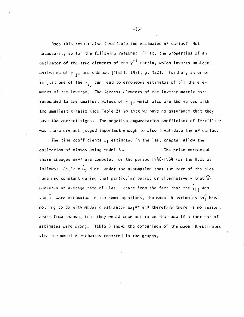
Does tilis result also invalidate the estimated ci;f series? Not

necessari Iy so for the fol lowing reasons: First, the properties of an

estimator of the true elements of the y-1

matrix, which inverts unLiased

estimates of y..IJ$

are unknown [Theil, 1971, p. 322]. Further, an error

in just one of the y..~J

can lead to erroneous estimates of all the ele-

ments of the inverse. The largest elements of the inverse matrix cor-

responded to the smallest values of yij) wnicil also are the values with

Lhe smallest t-ratio (see Table 2) so that we have

Ilave tile correct signs. The negative augmentation

was therefore not judged important enough to also

no assurance that they

coefficient of fertilizer

rival idate tile az~ series.

The time coefficients ~i estimated in tire last chapter allow the

estimation of biases usit~g model 3 , The price corrected

share changes Aa:~~ are computed for the period 1348-

foll~is: d~i~~~ = ii dint under the assumption that

remained constant during

mcdsurcs an average race

,8tile Wi were estimated in

noti~ing to do with model

that particular period or a

964 for the U.S. as

tile rate of the bias

ternatively that fli

of uias. Apart from the fact tilat the ~ij and

the same eciuations, the i!odel A estiulates” Aa~ have

H estimates A~i ):#( an(J therefore tl~ere is no reasOn,

apart from cnancc, tilat they would come out to be the same if either set of

estimates were wrong. Table 5 shows tile comparison of the model B estimates

i.~iti) tne model A estimates reported in tile graphs.

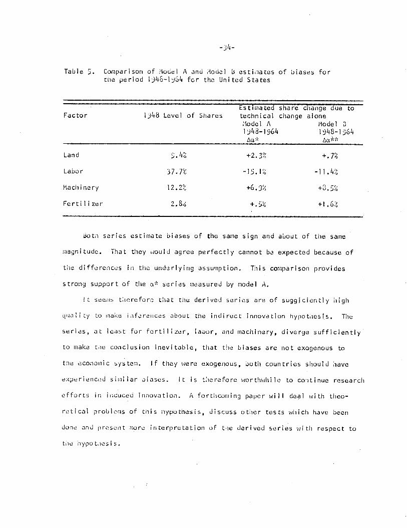
-j4-

Table 5. Comparison of Model A and iiodel b estimates of biases forthe period lj46-lj64 f~r the United States

Estimated share change due toFactor 1348 Levei of Shares technical change alone

Model A !iodel D1248-1964 1948-lj64Aa~ A~;:k

Land ;.42 +2, ~?; +.7%

Labor 37.7% -15.1% -11.42

Fertilizer 2.8A +.~Y; +1.6;<

botn series estimate biases of the same sign and about of the same

lilagnitude. That they would agree perfectly cannot be expected because of

tl~e differences ii) the underlying assumption. This comparison provides

strong support of the a;\ series measured by model A.

I t Seel’!ls t~lcreforc that the derived series are of suggiciently iligh

quali ty to IIIake illfere[]ces about the indirect innovation hypotilesis, The

series, at least for fertilizer, labor, and machinery, diverge sufficiently

to make tile conclusion inevitable, ti)at Ltle biases arc not exogenous to

t:le economic system. If they were exogenous, IWtil countries should have

experienced silni Iar ~iases. [t is t~lcreforc worthwhile to cor~tinue research

efforts in ir-iduced ii~novation. A

rctical problelns of this Ilypothes

done and prcsel)t lmorc interpretat

tile nypoti~csis.

fortl~coming paper will deal with tt)eo-

S, discuss otilcr tests which have been

on of LI]e derived series wi tll respect to

-35-

LIST OF REFERENCES

Allen, R. G. D. 1938. Mathematical analysis for economists. St.

Martin’s Press, Inc., t4ew York.

ikrndt, E. R. and L. R. Christensen, 1971. The translog productionfunction and factor substitution in U. S. manufacturing, 1~2~-lIj68,Unpublished paper presented at the \/inter meetings of the Econo-

metric Society in New Orleans, Louisiana.

Binswanger, Ii. P. 1972. The induced innovation hypothesis reviewed in

the light of some new evidence. Staff paper series #P.72-2~, Depart-ment of Agricultural and Applied Economics, University of Minnesota,

St. Paul, Minn.

Uinswanger, tl.P. 1373. The measurement of biased efficiency gains in U.S.

and Japanese Agriculture to test the induced innovation hypothesis.Unpublished Ph.D. thesis. Department of Economics, North CarolinaState University, Raleigh. University Microfilms, Ann Arbor, Michigan.

Diewert, M. E. 1971. An application of the Shephard duaiity theorem:

A generalized Leontief production function. Journal of Politicai

Economy, 70(3):481-505.

Farrell, M. J. 1957. The Measurement of Production Efficiency, Journal

of tile Royal Statistical Society, Series A, Vol. 120, Part III, p.253-299,

Nadirit if. 1. 1370. Some approaches to the theory and measurement oftotal factor productivity. Journal of Economic Literature, 8(4).

Okaiia, K. et al., eds. 1966. Estimates of long term ecoi~omic statistics

of Japan since 1868. Toyo Keizai Shinposha, Tokyo.

Sate, R. 1579. The estimation of biased technical progress. InternationalEconomic Review, ll(2):17j-207’.

S01OW, R. il. 13G7. Some recent developments in the theory of production.

In Brown (cd.), The theory and empirical analysis of production.NBER, Studies in Income and !Jealth, vol. 31.

T!leil, ii. 1971. Principles of econometrics. Jol]n ililey & sons, Inc.,

:4w YOrk.

Til,lmr, C. P. lJ~~. 011 measuring tcc!lnical efficiency. Food Researc;l

l[ls~i~u~~ St~clics in Agricultur,jl Lconumics, Trade and Development,

J(:Z).

Triai]gle Universities’Computirlg Center. 1372. Program manual for two

and tilrcc stage least squares. ResearcI\ Triangle Park, ;Iortn

Carolina.

Uzawa, H. iji2. Production functions with constant elasticity of substi-

tution. Review of Economic Studies, 30:291 -Z99.

Llal lace, T. il. and V. G. Asilar. 1972. Sequential meti~ods in model construc-

tion. P,eview of Economics and Statistics, 54(2):172-178.

Zellner, A. I)L2. An efficient method of estimating seemingly unreiated

regressions and tests for aggregation bias. Journal of the AmericanStatistical Association, 57:348-368.

Zellner, A. lj63. Estimators for seemingly unrelated regression equa-

tions: Some exact finite sample results. Journal of American

Statistical Association, 58:977-992.

Indices of biases, data on factor shares and data

on prices used to derive the series of biases

-38-

Table 1. U.S. Factor shares adjusbxl for factor price influence: Indices

of biases in technical ci~ange,

Numerical values, as percent of total ex-

Yea r Land Labor Hacho Fert. Other

13521256I960I9641360

21.0 36*3

21.2~~e7

19.6 3Y.32J.LI 39*7Idel 41.412.8 40.3Ic.j 32.516.8 34.316.5 3~,4

17.1 37.2

16.5 29.316.3 30.617.1 27.217.8 25.819.1 25.3

10.9

11.69.310.310.41!+.316.317.616.113.519.723.123.422.423.1

I.jI.&2.1

2. 2

2.72.73.0

;::5.I5.76.56.16.77.2

28.028.729.727.827.4~)+,o

23.327.5

24.226.723.3~3.4

26.1

27.325.3

Standardized, as percent of their 1910-1912 value

lj121516

1920

lj24

ly281332lj36

1940

1)44134819521)56196CIIg641368

100101.1

33.5j5.486.389.7yo.1Jo.178.781,578.777.731.j84.931.1

100

95.6102.6103.’7108.i105.284.Y3j.6

100.337.277.979.971.067.466.1

100106.885.694 ● ~

95.8131.7

150.1

162.1

143.3128,0181.4212.7215.5206.3212.7

10096.51’13.4113.j144.O142.4159.8204.1253.2267.3~58.@

341.8323.3354.4379.3

1w102.6106.199.497.985.4

104.798.386.595.4101.183.633.397.620.4

-39-

Table 2. Development of actual shares, U.S.

iiurrterlcalvalues, as percent of total ex-penditures

Year Land Labor Mache Fert. Other

1312 21.0 38.3 10.9 l.j 28.0lj16 21.6 36.5 11.6 1.9 28.4]y~o 17.3 40.5 10.1 2.0 30.1lj24 19.7 38.5 10.3 1.7 29.7192s IS.g 40.9 10.2 1.91232

310118.6 37.6 12.6 1.6 29.7

lj~~ 14.9 34.7 14.5 2.2 33.71940 12.0 35.3 15.1 2.3 35.21944 6.5 39.5 14.0 2.3 35.61948 37.7 12.2 2.4 32.31952 ;:; 29.7 17.5 40.01J36 1105 27.4 20.1 ;:! 37.31950 15.6 21.3 15.8 2*Y 40.41’JJ1, 1/.5 18.3 18.5 3.3 42.3ljbu 20.4 15.3 12.1 3.6 1}1.1

Taole 3. J.Z. input price/output price ratio indexes

Year Land Labor Maith. Fert. Other1310-12 = 100

1Jo106.8l@+.3

13/+.:)154.1]jl,.~

113.4179.9217.2247.C274.3407.9532.j610.0766.>

100110.081.3

111.7123.5231.5189.2288.8244.2226.6301.111230~

550.36;1.2735.8

100 1 di)105.7 ld3.235.7 105.0jj.1 106.6j~o~ 118.j128.6 10I.Jjg.6 110.9

103.4 160.163.0 211.7;3.4 222.853.6 214.L65.9 223.663.0 241.563.2 270,958,2 280.4

aFor construction of the series and tile data sources, see BinswangerI’J73.

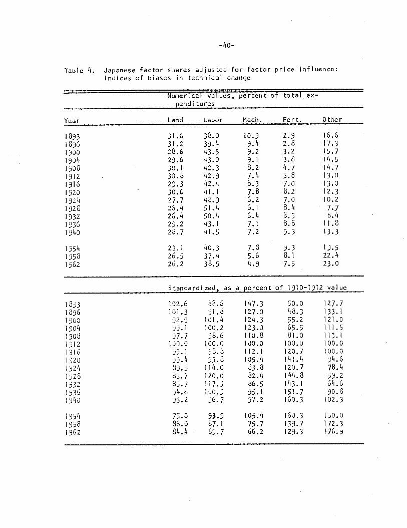
-40-

Table 4. Japanese factor si~ares adjusted for factor price influence:

Indices of biases in technical change

Numeri cal ‘alues$ percent of total ex-

penditures

Year Land Labor Mach. Fert. Other

18j3 31.6 36.0 10.9 2.9 16.61836 31.2 3j.4 9.4 2.3 17.31jiliJ 28.6 43.5 9.2 3.2 15.719J4 23.6 43.0 3.1 2.8 ]4,5

1308 39.1 42.3 8.2 4.7 14.71912 39.3 42.9 7*4 5*8 13.0l~lo 29.3 42.4 8.3 7.0 13.0132il 30.6 41.1 7.8 8.2 12.31314 27.7 48.9 Ge~ 10.21928 26. 4 51.4 6.1 ;:: ;.:193’2 26.4 50.4 6.4 8.3lj36 29.2 43.1 7.1 8.3 11:8134J 28.7 41.5 7.2 3.3 13.3

1354 23.1 40.3 7.8 ;.; 11.51358 26.5 37.4 5.6 22.41562 26.2 38.5 4.9 7:5 23.0

Standardized, as a percent of 1910-1912 value

192.6 88.5101.3 31.832.3 101.4Jj.1 10042

97.7 98.6100.!) 100.0jj.] 58.2j3.4 (J;.8

39.9 114.O85.7 120,085.7 117.5y4.8 100.593.2 36.7

147.3127.0124.3123.0110.8Ido.o112.)

10544!J3.~

82.486.5jjol

97.2

50.043.355.265.581.0100.0120./141.4120.714.t3143.1151.7160.3

127.7133.1121.0111.5113.I100.O100.034.678.453.264.690.8102.3

1354 75.0 93.9 105.4 16(.).3 150.01j58 86.d 87.1 75.7 139.7 172.31362 84.4 89.7 66.2 129.3 176.5

-41-

Table 5. Development of actual shares, Japan

Numerical values, percent Of total ex-pendi tures

Yea r Land Labor Mach. Fert. Other

1833 31.6 38.0 10.9 2.9 16.61&j6 30.1 40.0 9*9 2.7 17.21900 25.8 144.2 9.7 2.6 17.71904 27.5 43.0 9.5 16.91200 27.6 42.7 9.1 ::! 16.61912 28.4 1+2● & 8.5 5.0 15.51916 25. !3 1+207 9.2 6.1 16.1152019241928193219361940

28.022.721.429.825.224. o

11.620.1

40.648.;50.149*343.242, ?

44.741.5

6.77.8

;::8.89.1

10.8

9*3

;:;6.46.37.48.2

7.97.0

15.515.714.615.215.316.5

22.022.1

1 ;;2 20.1 40.4 9.2 6.3 24,4

a For construction of tile series and the data sources, see Binswanger 1973.

Table 6. Japanese input price/output price ratio indexes

Yea r Land Labor Nach. Fert. Other

191@12 = 100

120.6 80.5

112.9 85.4

34.4 gl~o~

99.0 ‘;;.;97.6100.0 [00:()

97*7 111.099.2 105.0]2.7 141.1y3.G ljj.~

IW.3 172.596.4 122.437.4 117.1

143.6129.4124.0120.5110.2100.0113.7102.8Jt;.j93.6

li)5.1~~,~&}*l,

190.8165.2

148.7

127.9118.2

100.0

116.1

;;.f

71:9

73*762.6

79.1

113.0115.3112.9104.8106.1100.0113.499.21:17.7104.2110.71111.1105.6

1954 44.0 113.J ti2.~ 38.2 122./lyj~ 97.2 138.1 79,6 32.3 126.01962 105.1 17U.5 60.j 27.6 116.3

a kor Constructio;l Of the series and the data sources see Binswanger 1973.