1

DEPARTMENT OF CIVIL ENGINEERING

GEETHANJALI COLLEGE OF ENGINEERING & TECHNOLOGY

CHEERYAL (V), KEESARA (M), R.R. DIST. - 501 301

(Affiliated to JNTUH, Approved by AICTE, NEW DELHI, ACCREDITED BY NBA) www.geethanjaliinstitutions.com

2015-2016

MATHEMATICS-II – COURSE FILE

(Subject Code: )

II Year B.TECH. (MECHANICAL ENGINEERING) II Semester

Prepared by Mr. N.NAGI REDDY & Ms M. P. MOLIMOL

2

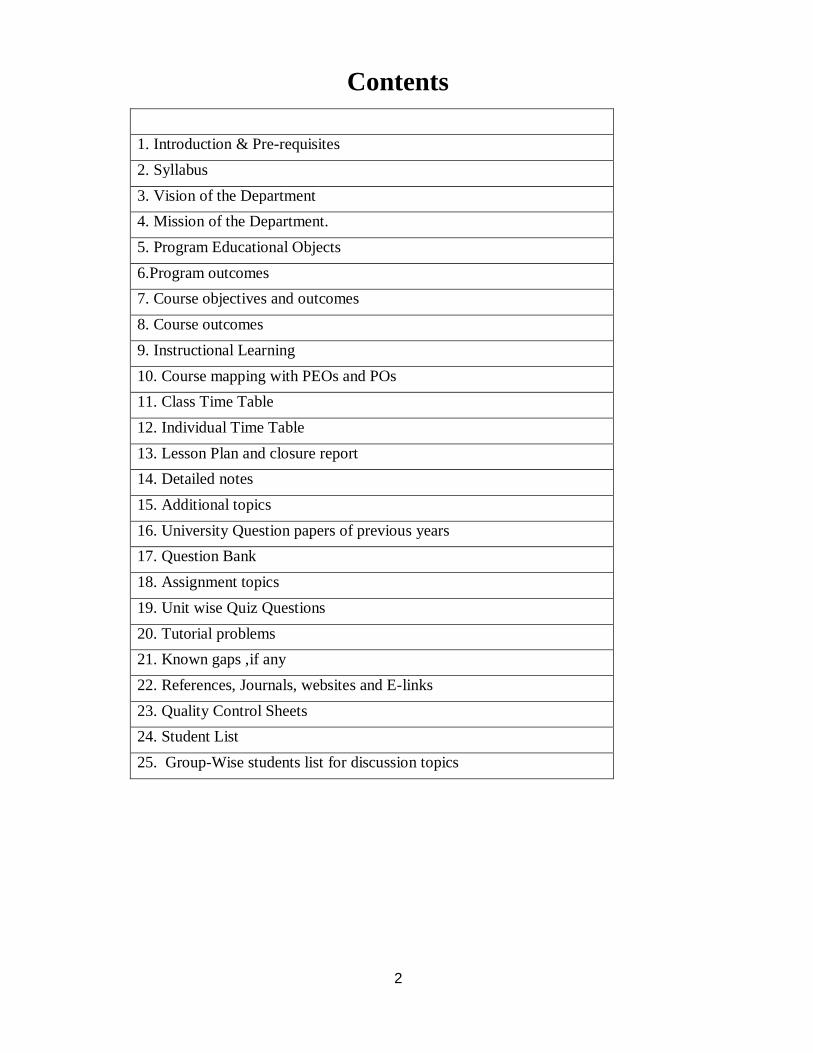
Contents

1. Introduction & Pre-requisites 2. Syllabus 3. Vision of the Department 4. Mission of the Department. 5. Program Educational Objects 6.Program outcomes 7. Course objectives and outcomes 8. Course outcomes 9. Instructional Learning 10. Course mapping with PEOs and POs 11. Class Time Table 12. Individual Time Table 13. Lesson Plan and closure report 14. Detailed notes 15. Additional topics 16. University Question papers of previous years 17. Question Bank 18. Assignment topics 19. Unit wise Quiz Questions 20. Tutorial problems 21. Known gaps ,if any 22. References, Journals, websites and E-links 23. Quality Control Sheets 24. Student List 25. Group-Wise students list for discussion topics

3

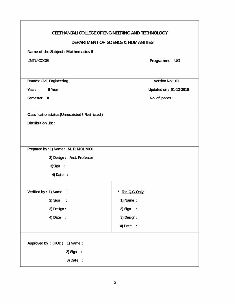
GEETHANJALI COLLEGE OF ENGINEERING AND TECHNOLOGY

DEPARTMENT OF SCIENCE & HUMANITIES

Name of the Subject : Mathematics-II

JNTU CODE: Programme : UG

Branch: Civil Engineering Version No : 01

Year: II Year Updated on : 01-12-2015

Semester: II No. of pages :

Classification status (Unrestricted / Restricted )

Distribution List :

Prepared by : 1) Name : M. P. MOLIMOL

2) Design : Asst. Professor

3)Sign :

4) Date :

Verified by : 1) Name :

2) Sign :

3) Design :

4) Date :

* For Q.C Only.

1) Name :

2) Sign :

3) Design :

4) Date :

Approved by : (HOD ) 1) Name :

2) Sign :

3) Date :

4

1. Introduction to the subject This course is intended to introduce basic principles of fluid mechanics. It is further extended to cover the application of fluid mechanics by the inclusion of fluid machinery especially water turbine and water pumps. Now days the principles of fluid mechanics find wide applications in many situations directly or indirectly. The use of fluid machinery, turbines pumps in general and in power stations in getting as accelerated fill up. Thus there is a great relevance for this course for mechanical technicians. The Mechanical technicians have to deal with large variety of fluids like water, air, steam, ammonia and even plastics. The major emphasis is given for the study of water. However the principle dealt with in this course will be applicable to all incompressible fluids.

Pre-requisites

1. Differentiation

2. Integration

3. Multiple Integrals

4. Beta and Gamma functions

5

2. Syllabus Copy

JAWAHARLAL NEHRU TECHNOLOGICAL UNIVERSITYHYDERABAD II Year B.Tech. ME -II Sem L T/P/D C

4 - /- / - 4

MATHEMATICS - II

UNIT - I Vector Calculus: Vector Calculus: Scalar point function and vector point function, Gradient-

Divergence- Curl and their related properties. Solenoidal and irrotational vectors - finding the

Potential function. Laplacian operator. Line integral - work done - Surface integrals -Volume integral.

Green's Theorem, Stoke's theorem and Gauss's Divergence Theorems (Statement & their

Verification).

UNIT - II: Fourier series and Fourier Transforms: Definition of periodic function. Fourier expansion of

periodic functions in a given interval of length 2 . Determination of Fourier coefficients - Fourier

series of even and odd functions - Fourier series in an arbitrary interval - even and odd periodic

continuation - Half-range Fourier sine and cosine expansions.

Fourier integral theorem - Fourier sine and cosine integrals. Fourier transforms - Fourier sine and

cosine transforms - properties - inverse transforms - Finite Fourier transforms.

UNIT - III: Interpolation and Curve fitting Interpolation: Introduction- Errors in Polynomial Interpolation - Finite differences- Forward

Differences- Backward differences -Central differences - Symbolic relations of symbols. Difference

expressions - Differences of a polynomial-Newton's formulae for interpolation - Gauss Central

Difference Formulae -Interpolation with unevenly spaced points-Lagrange's Interpolation formula.

Curve fitting: Fitting a straight line -Second degree curve-exponential curve-power curve by

method of least squares.

6

UNIT - IV : Numerical techniques Solution of Algebraic and Transcendental Equations and Linear system of equations: Introduction - Graphical interpretation of solution of equations .The Bisection Method - The Method

of False Position - The Iteration Method - Newton-Raphson Method . Solving system of non-

homogeneous equations by L-U Decomposition method (Crout's Method). Jacobi's and Gauss-

Seidel iteration methods.

UNIT - V Numerical Integration and Numerical solutions of differential equations:

Numerical integration - Trapezoidal rule, Simpson's 1/3rd and 3/8 Rule ,

Gauss Legendreone point, two point and three point formulas. Numerical

solution of Ordinary Differential equations: Picard's Method of successive

approximations. Solution by Taylor's series method – Single step

methods-Euler's Method-Euler's modified method, Runge-Kutta (second

and classical fourth order) Methods.

Boundary values & Eigen value problems: Shooting method, Finite difference method and

solving eigen values problems, power method

TEXT BOOKS: 1. Advanced Engineering Mathematics by Kreyszig, John Wiley & Sons.

2. Higher Engineering Mathematics by Dr. B.S. Grewal, Khanna Publishers.

REFERENCES

1. Mathematical Methods by T.K.V. Iyengar, B.Krishna Gandhi &Others, S. Chand.

2. Introductory Methods by Numerical Analysis by S.S. Sastry, PHI Learning Pvt. Ltd.

3. Mathematical Methods by G.Shankar Rao, I.K. International Publications,rdN.Delhi

4. Advanced Engineering Mathematics with MATLAB, Dean G. Duffy, 3 Edi, 2013, CRC Press

Taylor & Francis Group.

5. Mathematics for Engineers and Scientists, Alan Jeffrey, 6ht Edi, 2013, Chapman & Hall/CRC

6. Advanced Engineering Mathematics, Michael Greenberg, Second Edition. Person Education

7 Mathematics For Engineers By K.B.Datta And M.A S.Srinivas, Cengage Publications

7

Websites

1. www.physicsforum.com

2. mathworld.wolfram.com

3. www.intmath.com

4. www.sosmath.com

5. mathforum.org

Journals

1. Numerical Linear Algebra with Applications

2. International Journal for Numerical Methods in Engineering

3 Journal of Inequalities in Pure and Applied Mathematics

4. SIAM Journal of Applied Mathematics

5. Journal of Partial Differential Equations

3. Vision of the Department: The Mechanical Engineering Department strives to be recognized globally for outstanding education and research leading to well-qualified engineers, who are innovative, entrepreneurial and successful in advanced fields of engineering and research.

4. Mission of the Department: Imparting quality education to the students and enhancing their skills to make them globally

competitive mechanical engineers. Maintaining vital, state-of-the-art research facilities to provide its students and faculty with

opportunities to create, interpret, apply and disseminate knowledge. To develop linkages with world class R&D organizations and educational institutions in

India and abroad for excellence in teaching, research and consultancy practices.

5. Program Educational Objectives-PEOs: PEO1. Graduates will have utilized a foundation in engineering and science to improve lives and livelihoods through a successful career in mechanical engineering or other fields. PEO2. Graduates will have become effective collaborators and innovators, leading or participating in efforts to address social, technical and business challenges.

8

PEO3. Graduates will have engaged in life-long learning and professional development through self-study, continuing education or graduate and professional studies in engineering, business, law or medicine.

6. Program Outcomes (PO)

PO 1: An ability to apply knowledge of mathematics, science, and engineering PO 2: An ability to design and conduct experiments, as well as to analyze and interpret data PO 3: An ability to design a system, component, or process to meet desired needs within realistic constraints such as economic, environmental, social, political, ethical, health and safety, manufacturability, and sustainability PO 4: An ability to function on multidisciplinary teams PO 5: An ability to identify, formulate, and solve engineering problems PO 6: An understanding of professional and ethical responsibility. PO 7: An ability to communicate effectively PO 8: The broad education necessary to understand the impact of engineering solutions in a global, economic, environmental, and societal context PO 9: A recognition of the need for, and an ability to engage in life-long learning. PO 10: A knowledge of contemporary issues. PO 11: An ability to use the techniques, skills, and modern engineering tools necessary for engineering practice.

7. Course Objectives:

1. The objective is to find the relation between the variables x and y out of the

given data (x,y).

2. The aim to find such relationships which exactly pass through data or approximately

satisfy the data under the condition of least sum of squares of errors.

3. The aim of numerical methods is to provide systematic methods for solving problems in a

numerical form using the given initial data.

4. This topic deals with methods to find roots of an equation and solving a

differential equation.

5. The numerical methods are important because finding an analytical procedure to solve an

equation may not be always available.

6. In the diverse fields like electrical circuits, electronic communication, mechanical

vibration and structural engineering, periodic functions naturally occur and hence their

properties are very much required.

9

7. Indeed, any periodic and non-periodic function can be best analyzed in one way by

Fourier series and transforms methods.

8. The aim at forming a partial differential equation (PDE) for a function with many

variables and their solution methods. Two important methods for first order PDE's are

learnt. While separation of variables technique is learnt for typical second order PDE's such

as Wave, Heat and Laplace equations.

9. In many Engineering fields the physical quantities involved are vector-valued functions.

Hence the unit aims at the basic properties of vector-valued functions and their applications

to line integrals, surface integrals and volume integrals

8. Course Outcomes:

From a given discrete data, one will be able to predict the value of the data at an intermediate point

and by curve fitting, can find the most appropriate formula for a guessed relation of the data

variables. This method of analysis data helps engineers to understand the system for better

interpretation and decision making

1. After studying this unit one will be able to find a root of a given equation and will be

able to find a numerical solution for a given differential equation.

2. Helps in describing the system by an ODE, if possible. Also, suggests to find the solution as

a first approximation.

3. One will be able to find the expansion of a given function by Fourier series and Fourier

Transform of the function.

4. Helps in phase transformation, Phase change and attenuation of coefficients in

acoustics.

5. After studying this unit, one will be able to find a corresponding Differential Equation for

an unknown function with many independent variables and to find their solution.

6. Most of the problems in physical and engineering applications, problems are highly non-

linear and hence expressing them as DEs'. Hence understanding the nature of the equation

and finding a suitable solution is very much essential.

7. After studying this unit, one will be able to evaluate multiple integrals (line, surface,

volume integrals) and convert line integrals to area integrals and surface integrals to volume

integrals.

10

8. It is an essential requirement for an engineer to understand the behavior of the physical

system.

9. Instructional Learning Outcomes (Unit Wise)

UNIT I: Vector Calculus After the completion of this unit, the students might be able to:

1. Knowledge of the Differential operators divergence, gradient and curl 2. Understand how to calculate angle between the vectors, directional derivative of the

vectors 3. Explain how to find line, surface and volume integrals 4. Explain how to verify Gauss Divergence, Green’s and Stoke’s theorems

UNIT II: Fourier series and Fourier Transforms After the completion of this unit, the students might be able to:

1. Explain Fourier series expansions of functions in different intervals 2. Explain Half-Range Sine and Cosine expansions 3. Explain expansions of Even and Odd functions in different intervals 4. Explain Fourier sine and cosine transformations and its properties 5. Explain inverse and finite Fourier transformations

UNIT III: Interpolation & Curve Fitting

After the completion of this unit, the students might be able to:

1. Explain interpolation formulae for equal intervals and for unequal intervals to construct interpolating polynomials for a given set of data

2. Construct a suitable curve for given set of data points by using method of least squares method

UNIT IV: Numerical Techniques After the completion of this unit, the students might be able to:

1. Explain how to find the approximate roots of Non-Linear Transcendental Equations by applying Numerical Methods

UNIT V: Numerical Integration and Numerical Solution of ODE’s After the completion of this unit, the students might be able to:

1. Explain interpolation formulae for equal intervals and for unequal intervals to construct interpolating polynomials for a given set of data

2. Explain different formulae for numerical integration

11

3. Explain the integration without knowing the actual function 4. Explain how to solve few differential equations that cannot be solved by using analytical

methods. 5. Explain how to solve ODEs by the Numerical Methods

10. Mapping of Course outcomes with Programme outcomes: *When the course outcome weight age is < 40%, it will be given as moderately correlated 1

*When the course outcome weight age is >40%, it will be given as strongly correlated 2 POs 1 2 3 4 5 6 7 8 9 10 11

M

athe

mat

ics-

II

CO 1 2 1 2 1 2 2

CO 2 2 1 1 1 2 1 CO 3

2 1 1 2 1 2 2

CO 4 1 2 1 2 1 1 2 2 2 2 CO 5 2 1 2 2 2 2 2 CO 6 2 1 1 2 1 2 1 2 CO 7

2 2 2 1 2 1 1 1

CO 8 2 2 2 1 2 1 2 1 2 1 1

12

11. Class Timetable

DEPARTMENT OF MECHANICAL ENGINEERING

PROGRAMME : B.TECH. (MECHANICAL ENGINEERING)

SEMESTER: II Year II- SEMESTER

DEPARTMENT OF MECHANICAL ENGINEERING Year/Sem/ II B.Tech II-Sem ME-A ROOM NO : Acad. Yr : 2015-16 WEF: //15

CLASS INCHARGE: Dr. R.Ravi Varma

Time 9.30-10.20

10.20-11.10

11.10-12.00

12.00-12.50

12.50-1.30 1.30-2.20 2.20-3.10 3.10-4.00

Period 1 2 3 4

LU

NC

H

5 6 7 Monday

Tuesday

Wednesday

Thursday

Friday

Saturday

NOTE: “*” Represents Tutorial Classes.

DEPARTMENT OF MECHANICAL ENGINEERING Year/Sem/ II B.Tech II-Sem ME-B ROOM NO : Acad. Yr : 2015-16 WEF: //15

CLASS INCHARGE:

Time 9.30-10.20

10.20-11.10

11.10-12.00

12.00-12.50

12.50-1.30 1.30-2.20 2.20-3.10 3.10-4.00

Period 1 2 3 4

LU

NC

H

5 6 7 Monday

Tuesday

Wednesday

Thursday

Friday

Saturday

NOTE: “*” Represents Tutorial Classes.

13

12. Individual Time Table

Section- II A and II B

Name of the faculty: Load = 10 ; w.e.f.: //15

DEPARTMENT OF MECHANICAL ENGINEERING Year/Sem/ II B.Tech II-Sem ME-A ROOM NO : Acad. Yr : 2015-16 WEF: //15

CLASS INCHARGE:

Time 9.30-10.20

10.20-11.10

11.10-12.00

12.00-12.50

12.50-1.30 1.30-2.20 2.20-

3.10 3.10-4.00

Period 1 2 3 4

LU

NC

H

5 6 7 Monday

Tuesday

Wednesday

Thursday

Friday

Saturday

DEPARTMENT OF MECHANICAL ENGINEERING Year/Sem/ II B.Tech II-Sem ME-B ROOM NO : Acad. Yr : 2015-16 WEF: //15

CLASS INCHARGE:

Time 9.30-10.20

10.20-11.10

11.10-12.00

12.00-12.50

12.50-1.30 1.30-2.20 2.20-

3.10 3.10-4.00

Period 1 2 3 4

LU

NC

H

5 6 7 Monday

Tuesday

Wednesday

Thursday

Friday

Saturday

14

13.Lesson Plan:

Academic Year: 2015-2016 With effect from: 07-12-2015 Name of the Sub: Mathematics-II Dept: Mechanical Engineering Name of the faculty:

S.No.

Unit No

Topic to be covered in one lecture

Regular / Additional

Teaching aids used

LCD/OHP/BB

1

1

Vector Calculus: Scalar point function and vector point

function Regular BB

2 Gradient, Divergence, Curl Regular BB

3 Solenoidal and irrotational

vectors and Finding potential function.

Regular BB

4 Laplacian operator ,Related

properties Regular BB

5 Line integral – work done Regular BB

6 Surface integral Regular BB

7 Volume integral Regular BB

8 Green’s Theorem Regular BB

9 Stoke’s theorem Regular BB

10 Gauss’s Divergence Regular BB

11

2

Fourier series & Fourier Transforms: Definition of

periodic function Additional BB

12 Fourier series expansions in [0 ,2π]

Regular BB

13 Fourier series expansions in [-π ,π]

Regular BB

14 Fourier expansions of discontinuous functions

Regular BB

15 Fourier series of even & odd functions

Regular BB

16 Fourier series in an arbitrary constants

Regular BB

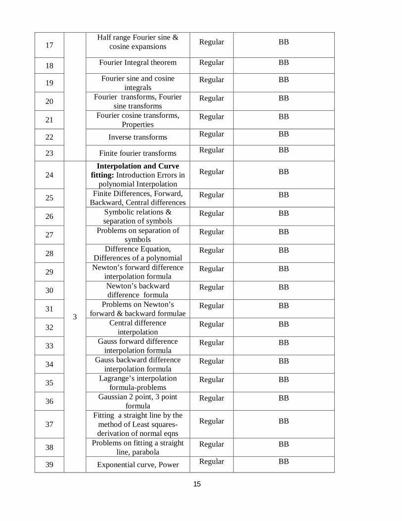
15

17 Half range Fourier sine &

cosine expansions Regular BB

18 Fourier Integral theorem Regular BB

19 Fourier sine and cosine integrals

Regular BB

20 Fourier transforms, Fourier sine transforms

Regular BB

21 Fourier cosine transforms, Properties

Regular BB

22 Inverse transforms Regular BB

23 Finite fourier transforms Regular BB

24

3

Interpolation and Curve fitting: Introduction Errors in

polynomial Interpolation Regular BB

25 Finite Differences, Forward, Backward, Central differences

Regular BB

26 Symbolic relations & separation of symbols

Regular BB

27 Problems on separation of symbols

Regular BB

28 Difference Equation, Differences of a polynomial

Regular BB

29 Newton’s forward difference interpolation formula

Regular BB

30 Newton’s backward difference formula

Regular BB

31 Problems on Newton’s forward & backward formulae

Regular BB

32 Central difference interpolation

Regular BB

33 Gauss forward difference interpolation formula

Regular BB

34 Gauss backward difference interpolation formula

Regular BB

35 Lagrange’s interpolation formula-problems

Regular BB

36 Gaussian 2 point, 3 point formula

Regular BB

37 Fitting a straight line by the

method of Least squares-derivation of normal eqns

Regular BB

38 Problems on fitting a straight line, parabola

Regular BB

39 Exponential curve, Power Regular BB

16

curve

40

4

Numerical techniques: Introduction & Graphical

interpolation of solution of eqns

Regular BB

41 Bisection method, Method of

False position, Iteration method

Regular BB

42 Newton-Raphson method Regular BB

43 Solving of non-homogeneous eqns by LU decomposition-

problems Regular BB

44 Problems on Jacobi’s Regular BB

45 Problems on Gauss-seidel iteration method

Regular BB

46

5

Numerical integration- General quadrature formula

Regular BB

47 Problems on Trapezoidal rule Regular BB

48 Problems on Simpson’s 1/3, 3/8 rules

Regular BB

49 Gauss-Legendre one point,two point

Regular BB

50 And three point formulas Regular BB

51 Numerical Solution of ODE- Taylor’s series method

Regular BB

52 Picard’s method of successive approximations

Regular BB

53 Single step methods Regular BB

54 Euler’s method, Modified Euler’s method

Regular BB

55 Runge-Kutta methods Regular BB

56 Boundary values and Eigen value Problems

Regular BB

57 Shooting Method, Power method

Regular BB

58 Finite difference Method, And solving eigen values problems

Regular BB

17

GUIDELINES: Distribution of periods: No. of classes required to cover JNTUH syllabus : No. of classes required to cover Additional topics : No. of classes required to cover Assignment tests (for every 2 units 1 test) : No. of classes required to cover tutorials : No. of classes required to cover Mid tests : No of classes required to solve University Question papers :

------- Total periods

14. Detailed Notes Hard copy available

15. Additional topics Multiple Integrals

Solving Homogeneous Equations

Initial Value Problems

16. University Question papers of previous year

Code No: 113AA

JAWAHARLAL NEHRU TECHNOLOGICAL UNIVERSITY HYDERABAD

B.Tech II Year II Semester Examinations, December-2014

MATHEMATICS-II

(Common to ME, CHEM, MMT, AE, PTE,CEE)

Time: 3 Hours Max.Marks: 75

Note: The question paper contains two parts A and B.

Part A is compulsory which carries 25 marks. Answer all questions in Part A.

Part B consists of 5 Units. Answer any one full question from each unit.

18

Each question carries 10 marks and may have a, b, c as sub questions.

Part-A

(25 Marks)

1. Find n, if푓 ̅ = 푟 푟̅ is solenoidal. [2M] 2. Find the angle between the surfaces 푥 + 푦 + 푧 = 9 and

푧 = 푥 + 푦 − 3 at the point (2, -1, 2). [3M] 3. If 푓(푥) = 푥 in (-1, 1) then find the Fourier coefficient 푏 . [2M] 4. Write any three properties of Fourier transforms. [3M] 5. Evaluate ∆ [(1 − 푎푥)(1 − 푏푥 )(1 − 푐푥 )(1 − 푑푥 )]. [2M] 6. Write the normal equations to fit a curve 푦 = 푎푒 for the given data by the

Method of least squares. [3M] 7. Define Transcendental equation and give an example. [2M] 8. Write short notes on iteration method to find a root for 푓(푥) = 0. [3M]

9. Define initial value problem and give an example. [2M] 10. Write the finite difference formula for 푦 (푥) and푦 (푥). [3M]

Part- B

(50 Marks)

11. (a) With usual notation of vector calculus, prove that

∇ 푓(푟) = 푓 (푟) + 푓 (푟).

(b) Apply Green’s theorem to evaluate ∮ (푥푦 + 푦 )푑푥 + 푥 푑푦 , where C is the boundary of the area enclosed by the 푥-axis and the upper half of the circle 푥 + 푦 = 푎 .

OR

12.(a) Find the work done by

퐹 = (2푥 − 푦 − 푧)푖 + (푥 + 푦 − 푧)푗 + (3푥 − 2푦 − 5푧)푘 along a curve C in the 푥푦-plane given by푥 + 푦 = 9, 푧 = 0.

(b) Use Gauss divergence theorem, to evaluate

∬ (푥푑푦푑푧 + 푦푑푧푑푥 + 푧푑푥푑푦). Where S is the portion of the plane

푥 + 2푦 + 3푧 = 6. Which lies in the first octant.

13. (a) Expand푓(푥) = 푥푠푖푛푥 as a Fourier series in the interval

0 < 푥 < 2휋.

19

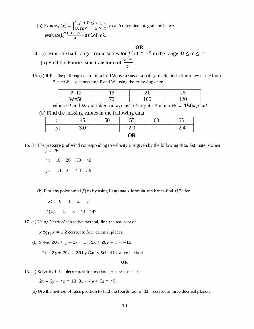
(b) Express푓(푥) = 1, 푓표푟0 ≤ 푥 ≤ 휋0, 푓표푟푥 > 휋 , as a Fourier sine integral and hence

evaluate∫ ( ) sin(푥휆)푑휆.

OR 14. (a) Find the half-range cosine series for 푓(푥) = 푥 in the range 0 ≤ 푥 ≤ 휋.

(b) Find the Fourier sine transform of .

15. (a) If P is the pull required to lift a load W by means of a pulley block, find a linear law of the form 푃 = 푚푊 + 푐 connecting P and W, using the following data:

P=12 15 21 25 W=50 70 100 120

Where P and W are taken in 푘푔.푤푡. Compute P when푊 = 150푘푔.푤푡. (b) Find the missing values in the following data

푥: 45 50 55 60 65 푦: 3.0 - 2.0 - -2.4

OR

16. (a) The pressure 푝 of wind corresponding to velocity 푣 is given by the following data. Estimate 푝 when 푦 = 25.

푣: 10 20 30 40

푝: 1.1 2 4.4 7.9

(b) Find the polynomial 푓(푥) by using Lagrange’s formula and hence find 푓(3) for

푥: 0 1 2 5

푓(푥): 2 3 12 147.

17. (a) Using Newton’s iterative method, find the real root of

푥log 푥 = 1.2 correct to four decimal places.

(b) Solve: 20푥 + 푦 − 2푧 = 17, 3푥 + 20푦 − 푧 = −18,

2푥 − 3푦 + 20푧 = 25 by Gauss-Seidel iterative method.

OR

18. (a) Solve by L-U decomposition method: 푥 + 푦 + 푧 = 9,

2푥 − 3푦 + 4푧 = 13, 3푥 + 4푦 + 5푧 = 40.

(b) Use the method of false position to find the fourth root of 32 correct to three decimal places.

20

19. (a) Using Runge-Kutta method of order 4, find 푦(0.2) for the equation = , 푦(0) = 1. Take

ℎ = 0.2.

(b) A solid of revolution is formed by rotating about the 푥-axis, the lines 푥 = 0 and 푥 = 1 and a curve through the points with the following co-ordinates

푥: 0.00 0.25 0.50 0.75 1.00

푦: 1.0000 0.9896 0.9589 0.9089 0.8415

Estimate the volume of the solid formed using Simpson’s rule.

OR

20. Use power method to find the numerically largest Eigen value and the corresponding Eigen

vector of 퐴 =1 6 11 2 00 0 3

. Find also the least Eigen value and hence the third Eigen value also.

---oo0oo---

17. Question Bank MATHEMATICS-II

Unit-I: Vector calculus

Long Answer Questions:

1. Verify Green’s theorem in the plane for ∫ (푥 − 푥푦 )푑푥 + (푦 − 2푥푦)푑푦 where 푐is a

square with vertices (0,0)(2,0), (2,2), (0,2).

2. Find a unit normal vector to the surface 푧 = 푥 + 푦 at (−1,−2,5).

3. Evaluate by stoke’s theorem ∫∫푐푢푟푙 → .→ .푑푠 where → = 푦 푖 + 푥 푗 − (푥 + 푧) → and s

comprising the planes 푋 = 0,푌 = 0,푌 = 4,푍 = −1.

4. Prove that if → is the position vector of any point in space, then푟 → is irrotational and

solenoidal if푛 = −3

5. i) If → = (5푥푦 − 6푥 ) → + (2푦 − 4푥) → , 푒푣푎푙푢푎푡푒 ∫ → .푑 → along the curve c is xy-

plane 푦 = 푥 from (1,1) to (2,8).

6. Find →− ∇∅ at (1,-1,1) if → = 3푥푦푧 푖 + 2푥푦 푗 − 푥 푦푧푘 and ∅ = 3푥 − 푦푧

7. Show that 퐹 = (2푥푦 + 푧 )푖 + 푥 푗 + 3푥푧 푘 is conservative force field. Find the scalar

potential. Find the work done is moving an object in this field from (1,-2,1) to (3,1,4).

21

8. Verify stoke’s theorem for → = (푦 − 푧 + 2)푖 + (푦푧 + 4)푗 − 푥푧푘 where s is the surface of

the cube x=0, y=0, z=0. X=2, y=2, z=2 above the xy-plane.

9. Find the anlge between the tangent planes to the surface 푥푙표푔푧 = 푦 − 1, 푥 푦 = 2 − 푧 at

the point (1,1,1)

10. Evaluate ∫ → .푁푑푠 where 퐹 = (푥 + 푦 )푖 − 2푥푗 + 2푦푧푘 and s is the surface of the plane

2x+y+2z=6 is the first octant

11. Verify divergence theorem for → = 4푥푖 − 2푦 푗 + 푧 푘 taken over the surface founded by

the region 푥 + 푦 = 4, 푧 = 0푎푛푑푧 = 3

12. Find the work done is moving particle is the force field → = 3푥 푖 + (2푥푧 − 푦)푗 + 3푘 along

the curve 푥 = 4푦, 3푥 = 푧 from x=0 to x=2.

13. Apply stokes theorem to evaluate ∫ ((푥 + 푦)푑푥 + (2푥 − 3)푑푦 + (푦 + 푧)푑푧) where c is the

boundary of the triangle with vertices (2,0,0), (0,3,0)푎푛푑(0,0,6)

14. Evaluate by Green’s theorem ∫ [(푐표푠푥푠푖푛푦 − 2푥푦)푑푥 + 푠푖푛푥푐표푠푦푑푦] where ‘푐’ is the

circle 푥 + 푦 = 1

15. If 퐹⃗ = (5푥푦– 6푥2 )푖 + (2푦 − 4푥)푗 , evaluate∫ 퐹⃗ . 푑푟⃗ along the curve C in xy- plane

푌 = 푥 from (1,1)푡표(2,8).

Short Answer Questions:

1. Define Gradient, divergent and curl of a vector point function. 2. Find the directional derivative of the function 푓 = 푥 – 푦 + 2푧 at the point

푃 = (1,2,3) in the direction of the line PQ where 푄 = (5,0,4). 3. Find the unit normal vector to the surface 푥 + 푦 + 2푧 = 26 at the point (2,2,3). 4. Find the angle of intersection of the spheres 푥 + 푦 + 푧 = 29 & 푥 + 푦 + 푧 +

4푥 − 6푦– 8푧 − 47 = 0. 5. Prove that if 푟⃗ is the position vector of any point in space, and then 푟 푟⃗ is

Irrotational. 6. Show that the vector (푥 − 푦푧)푖 + (푦 – 푧푥)푗 + (푧 – 푥푦)푘 is irrotational 7. Find constants a, b & c if the vector 푓⃗ = (2푥 + 3푦 + 푎푧)푖 + (푏푥 + 2푦 + 3푧)푗 +

(2푥 + 푐푦 + 3푧)푘 is Irrotational. 8. If 퐴⃗ is Irrotational vector, evaluate div ( 퐴⃗ × 푟⃗ ) , where = 푥푖 + 푦푗 + 푧푘. 9. If 푎⃗ = (푥 + 푦 + 푧)푖 + 푗– (푥 + 푦)푘 , then show that 푎⃗ Curl 푎⃗ = 0. 10. Prove that div curl 푓⃗ = 0.

22

11. If 휑1= 푥 푦 & 휑2 = 푥푧 + 푦 , find ∇× (∇φ1×∇ φ2). 12. Find work done in moving particle in the force field 퐹⃗ = 3푥 푖 + (푥푧– 푦)푗 + 푧푘 along

the straight line form (0,0,0)푡표(2,1,3). 13. Find the work done by force 퐹⃗ = (2푦 + 3)푖 + (푧푥)푗 + (푦푧 − 푥)푘 when it moves a

particle from the point (0,0,0)푡표(2,1,1) along the curve 푥 = 2푡 , 푦 = 푡, 푧 = 푡. 14. State Stokes theorem. 15. State Gauss Divergence theorem. 16. State Green’s theorem. 17. Apply the Stokes theorem & show that ∬ 푐푢푟푙퐹⃗ . 푛⃗푑푠⃗ = 0, Where 퐹⃗ is any vector

and 푆 is 푥 + 푦 + 푧 = 1.

UNIT – II: Fourier series and Fourier Transforms

Long Answer Questions:

1. Find a Fourier series to represent 푓(푥) = 푥 in the interval (0,2휋) 2. Find a Fourier series representing 푓(푥) = 0, 0 < 푥 < 2휋 3. Obtain the Fourier series expansion of 푓(푥) given that푓(푥) = (휋 − 푥)2푖푛0 < 푥 < 2휋

and deduce that 1/1 + 1/2 + 1/3 + … … … … = 휋 /6 4. Expand 푓(푥) = 푥. 푠푖푛푥 , 0 < 푥 < 2휋 as a Fourier series

5. Find a Fourier series to represent the function 푓(푥) = 푒 for –휋 < 푥 < 휋 and hence derive

a series for 휋/푠푖푛ℎ휋 6. Write the Dirichlet’s conditions for the existence of Fourier series of a function 푓(푥) in the

interval (훼,훼 + 2휋)

7. Find the Fourier series of the periodic function 푓(푥) = −휋,−휋 < 푥 < 휋푥, 0 < 푥 < 휋

Hence deduce that + + + ⋯… … … . =

8. Obtain Fourier series for

a. 푓(푥) =푥,−휋 < 푥 < 00,0 < 푥 < 휋푥 −

, < 푥 < 휋

9. The intensity of an alternating current after passing through a rectifier is given by

i. 퐼(푥) = 퐼 푠푖푛푥, 0 ≤ 푥 ≤ 휋0,휋 ≤ 푥 ≤ 2휋

ii. where퐼0 is maximum current and the period is 2휋.Express 퐼(푥) as a fourier series

23

10. Expand the function 푓(푥) = 푥 as a Fourier series in [−휋,휋] hence deduce that

a. − + − + ⋯… … … . =

b. + + + ⋯… … … . =

11. Show that + + + + ⋯… … … = 12. Find the Fourier series expansion to represent the function

푓(푥) = 푠푖푛푥 ,−휋 < 푥 < 휋 13. Find the half-range cosine series and sine series for 푓(푥) = 푥 in 0 < 푥 < 휋 hence deduce

that + + + + ⋯… … … = 14. Obtain the Fourier series for 푓(푥) = 푥푠푖푛푥, 0 < 푥 < 휋 and show that

.−

.+

.−

.+ ⋯… … … … … . . = 휋 −

15. Represent the following function by Fourier sine series

푓(푥) = 푥, 0 < 푥 <

, < 푥 < 휋

16. Find the Fourier series expansion for 푓(푥) = 2,−2 < 푥 < 0푥, 0 < 푥 < 2

17. Find the Fourier series to represent 푓(푥) = 푥 − 2푤ℎ푒푛 − 2 ≤ 푥 ≤ 2 18. Find the Fourier series expansion for the function 푓(푥) = 푥 − 푥 푖푛(−1,1)

19. Obtain the Fourier series for the function 푓(푥) = 휋푥,0 ≤ 푥 ≤ 1휋(2− 휋), 1 ≤ 푥 ≤ 2

20. Find the half-range cosine series for the function 푓(푥) = 푘푥,0 ≤ 푥 ≤

푘(푙 − 푥), ≤ 푥 ≤ 푙

Find the sum of the series + + + + ⋯… … … 21. Find the half-range sine series for the function 푓(푥) = 푎푥 + 푏푖푛0 < 푥 < 1 22. Find the half-range cosine series for the function 푓(푥) = 푠푖푛( ) in 0 < 푥 < 푙 23. Find the half-range cosine series for the function 푓(푥) = (푥 − 1) in the interval 0 <

푥 < 1

24

Hence show that ∑( )

∞ =

24. Find the Fourier sine and cosine transform of

푓(푥) = 푥,0 < 푥 < 12 − 푥, 1 < 푥 < 20,푥 > 2

25. Using Fourier Integral show that ∫ λλ

∞ 푠푖푛λπdλ = π Where 푓(푥) = 1, 0 < 푥 < 휋.

26. Evaluate the following using Parseval’s Identity:∫ ( )∞ (푎 > 0)

27.State and prove Fourier Integral theorem

28. Find the Fourier sine and cosine transform of

푓(푥) = 1 − 푥 , |푥| ≤ 10,|푥| ≥ 1

Hence Evaluate (i)∫ 푐표푠 푑푥∞

29. Find the Fourier cosine and sine transforms of 푒 , 푎 > 0 and hence deduce the

Inverse formula.

30. Find the finite Fourier cosine transform of 푓(푥) defind by 푓(푥) = − 푥 + in

0 < 푥 < 휋

Short Answer Questions:

1. Define Periodic function with examples & what the period of푠푖푛2푥 + 3푠푖푛푥 − 4푠푖푛3푥.

2. Define Dirichlet’s condition for Fourier series expansion.

3. Write Fourier series expansion of continuous function 푓(푥) in [0, 2휋] with Euler formulas.

4. Write the Fourier series expansion of the function 푓(푥) = ℎ(푥), 0 < 푥 < 휋푔(푥),휋 < 푥 < 2휋 .

5. Define Even & Odd function. Write Fourier series expansion of even & odd function in [−휋,휋].

6. If 푓(푥) = 푥 in [-휋,휋] then find푎 ,푏 .

25

7. If 푓(푥) = 푒 in [-휋,휋] then find the values of 푎 , 푎 in Fourier series expansion .

8. Define half range sine series & cosine series of the function 푓(푥) in [0,휋].

9. If 푓(푥) = 푥 in [0,휋]푡hen find 푏푛value.

10. Define Fourier series of function 푓(푥) in the intervals [0,2퐿] , [−퐿,퐿].

11. Define half range Fourier sine series & cosine series in the interval [0,퐿].

12. Find 푏 value in the half range Fourier sine series of 푓(푥) = 1 in the interval [0,퐿].

13. Obtain푎 , 푎 values of Half range Fourier cosine series of the function 푓(푥) = 푥 in [0, 1].

14. Find b1 value in half range sine series of 푓(푥) = 푐표푠휋푥 in [0, 1].

15. Define Integral Transform & Fourier transform function, Inverse Transform 푓(푡).

16. State Fourier Integral theorem.

17. Define Fourier cosine & sine Integrals.

18. Define Fourier Integral Transforms in complex forms.

19. Define Fourier cosine & sine Transforms , Inverse Transforms.

20. Define linear property of Fourier Transforms of 푓(푡).

21. State & prove Shifting Theorem of Fourier Transform of 푓(푡).

22. Find Fourier Transform of 푓(푥) defined by 푓(푥) = e ,푎 < 푥 < 푏0, 푥 < 푎푎푛푑푥 > 푏

24. Find Fourier sine & cosine transform of 푥.

25. Find Fourier cosine Transform of 푓(푥) defined by 푓(푥) = 푐표푠푥, 0 < 푥 < 푎0,푥 ≥ 푎

26. Find Fourier sine Transform of 푓(푥) defined by푓(푥) = 푒 .

27. Find Fourier cosine Transform of 푓(푥) defined by 푓(푥) = 푥푒 .

28. State & Prove Parseval’s Identity for Fourier Transforms.

UNIT – III: Interpolation and Curve fitting

Long Answer Questions:

1. Show that ∆ [(1− 푥)(1− 2푥 )(1 − 3푥 )(1− 4푥 )] = 24. 2 10! , if ℎ = 2 2. Find the second difference of the polynomial 푥 − 12푥 + 42푥 − 30푥 + 9 with the

interval of differencing ℎ = 2

26

3. Prove that ∆[푥(푥 + 1)(푥 + 2)(푥 + 3)] = 4(푥 + 1)(푥 + 2)(푥 + 3) , if the interval of differencing is unity

4. Find the missing values in the following table

x 45 50 55 60 65 f(x) 3.0 - 2.0 - -2.4

5. Find 푓(2.5) using Newton forward formula from the following table

6. Find푦(25), given that푦 = 24,푦 = 32, 푦 = 35,푦 = 40, Using Gauss’s forward difference formula

7. Using Gauss’s forward formula, find 푓(22)

x 20 25 30 35 40 45 f(x) 354 332 291 260 231 204

8. Using Gauss backward interpolation formula find 푦(50°42′) given that

x 50 51 52 53 54 y = tan x 1.1918 1.2349 1.2799 1.327 1.3764

9. Using Lagrange’s interpolation formula, find 푦(10) from the following table

x 5 6 9 11 y 12 13 14 16

10. Find the interpolating polynomial 푓(푥)from the table

x 0 1 4 5 f(x) 4 3 24 39

11. Derive normal equations to fit the parabola 푦 = 푎 + 푏푥 + 푐푥

12. Fit a straight line for the following data and compute 푦(3.5)

13. Fit a parabola of the form 푦 = 푎 + 푏푥 + 푐푥 to the following data

x 0 1 2 3 4 5 6 y 0 1 16 81 256 625 1296

x 1 2 3 4 5 6

y 14 33 40 63 76 85

27

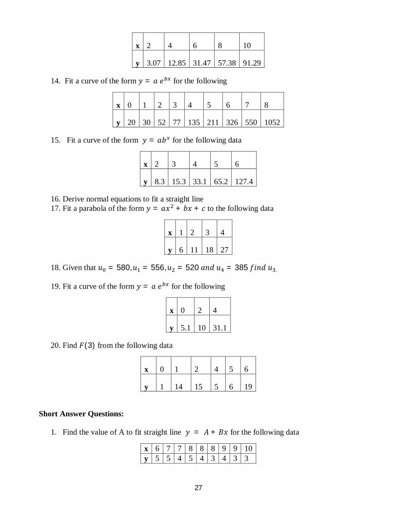
x 2 4 6 8 10

y 3.07 12.85 31.47 57.38 91.29

14. Fit a curve of the form 푦 = 푎푒 for the following

x 0 1 2 3 4 5 6 7 8

y 20 30 52 77 135 211 326 550 1052

15. Fit a curve of the form 푦 = 푎푏 for the following data

x 2 3 4 5 6

y 8.3 15.3 33.1 65.2 127.4

16. Derive normal equations to fit a straight line 17. Fit a parabola of the form 푦 = 푎푥 + 푏푥 + 푐 to the following data

x 1 2 3 4

y 6 11 18 27

18. Given that 푢 = 580,푢 = 556,푢 = 520푎푛푑푢 = 385푓푖푛푑푢 .

19. Fit a curve of the form 푦 = 푎푒 for the following

x 0 2 4

y 5.1 10 31.1

20. Find 퐹(3) from the following data

Short Answer Questions:

1. Find the value of A to fit straight line 푦 = 퐴 + 퐵푥 for the following data

x 6 7 7 8 8 8 9 9 10 y 5 5 4 5 4 3 4 3 3

x 0 1 2 4 5 6

y 1 14 15 5 6 19

28

2. Define Average operator, show that 휇 = (퐸 + 퐸 )

3. Prove that the relations: i) ∆= 훻퐸 = 퐸 4. Evaluate i)∆푐표푠푥 ii)∆푙표푔푓(푥) iii) ∆푡푎푛 푥 5. Evaluate (푓(푥) + 푓(푥 + ℎ)).∆푓(푥) 6. Write Newton’s forward & backward interpolation formulae. 7. Write Gauss forward & backward interpolation formulae. 8. Write Lagrange’s interpolation formula. 9. Find the missing value of the data

x 1 1.4 1.8 2.2 y 3.49 4.82 - 6.5

10. The following table gives a set of values of x & corresponding values of 푦 = 푓(푥)

x 10 15 20 25 30 35 y 19.97 21.51 22.47 23.52 24.65 25.89

Form the forward difference table & write down the values of

∆푓(푥), ∆ 푓(푥), ∆ 푓(푥)&∆ 푓(푥) .

11. Write normal equations to fit a straight. 푦 = 푎 + 푏푥 12. Write normal equations to fit a parabola of the form 푦 = 푎 + 푏푥 + 푐푥

13. Write the normal forms of the curve 푦 = 푎푥 .

14. Write the normal form to fit the curve푦 = 푎푏 . 15. From the following data find the value of a, to fit the straight line of the form

푦 = 푎 + 푏푥,where

x 0 2 5 7 y -1 5 12 20

UNIT – IV: Numerical Techniques Long Answer Questions:

1. Find a real root of the equation 푥푙표푔 푥 = 1.2 which lies between 2푎푛푑3 by bisection method

2. Find the root of the equation2푥– 푙표푔 푥 = 7, which lies between 3.5 and 4by Regula–Falsi method

3. Find the positive root of the equation 푥 = 2푥 + 5 by using iteration method. 4. Using Newton – Rap son method (a) Find square root of a number (b) Find Reciprocal of

a number 5. Find a real root of 푥 −푒 푠푖푛푥 = 1, Using Regula – Falsi method 6. Find an LU decomposition of the matrix A and solve linear system 퐴푋 = 퐵

29

−3 12 −61 −2 20 1 1

푥푦푧

=−337−1

Short Answer Questions:

1. Write Regula falsi method & Newton-Raphson formula.

2. Write the formula to find no. of iterations to find the real root of the given equation in

bisection method.

3. What is the 4푡ℎ iteration to find a real root of an equation 푥 − 4푥 − 9 = 0 using bisection

method

4. Explain Iterative method.

5. What is the 2푛푑iteration in Regula falsi method of the equation2푥– 푙표푔 푥 = 7.

6. What is the 2푛푑 iteration to find reciprocal of 18 using Newton Raphson method.

7. What is diagonally dominant of the given system of linear equations?

8. What is the2푛푑 iteration in Jacobi’s iteration method for the system of equations 3푥 + 푦 −

푧 = 2,푥 + 5푦 + 2푧 = 1, 2푥 − 3푦 + 6푧 = 3.

9. What is the 2nd iteration in Gauss-seidal method for the system of equations 3푥 + 푦 − 푧 =

2, 푥 + 5푦 + 2푧 = 1, 2푥 − 3푦 + 6푧 = 3.

10. Define non Homogeneous system of equations.

11. Find the unit Lower Triangular matrix L from the matrix A =1 2 10 3 12 5 0

12. Find the Upper Triangular matrix U from the matrix A =1 2 10 3 12 5 0

13. What is the necessary sufficient condition for the solution of system of equations in Gauss-

Seidal method?

UNIT – V: Numerical Integration and Numerical Solution of Differential Equations Long Answer Questions:

1. Evaluate ∫(푒 ) 푑푥 in definite interval(0,2), (i) Trapezoidal rule (ii) Simpson’s one –third rule taking ℎ = 0.2

2. Evaluate ∫ ( ) in (0,1) by

(i) Simpson’s one –third rule

30

(ii) Trapezoidal rule 3. Find 푦(0.1), 푧(0.1),푧(0.2) given = 푥 + 푧, = 푥 − 푦 and 푦(0) = 2, 푧(0) = 1 by

using Taylor’s series method 4. Find 푦(0.2) and 푦(0.4) using Taylor’s series method given that = 푥푦 + 1 and

푦(0) = 1 5. Given that = 1 + 푥푦 and푦(0) = 1, Compute 푦(0.1)and 푦(0.2) using Picard’s method

6. Find 푦(0.1) and 푦(0.2)using Range-Kutta 4th order formula given that 푦 ′ = 푥 – 푦 and 푦(0) = 1.

7. Find the solution of = 푥– 푦 at 푥 = 0.4 given 푦 = 1 at 푥 = 0 and ℎ = 0.1 using Milne’s method. Use modified Euler’s method to evaluate 푦(0.1),푦(0.2) and 푦(0.3).

8. If = 2푒 푦 , 푦(0) = 2 find 푦(0.4) using Adam’s predictor corrector formula by calculating 푦(0.1),푦(0.2) and 푦(0.3) using Euler’s modified formula.

9. Find 푦(0.5),푦(1) and 푦(1.5) given that 푦 ′ = 4 − 2푥, 푦(0) = 2 with ℎ = 0.5 using modified Euler’s method.

10. Given that푦 ′ = 푦– 푥, 푦(0) = 2 find 푦(0.2) using Range – kutta method. (take ℎ = 0.1) 11. Use second order method for the solution for the following boundary value

problem 푦 =푥 y+1, 0<x<1, y(0)=1, 푦 (0)=1, y(1)=1 using step length h=0.5? 12. Solve the following boundary value problem with the step length 0.5 and extrapolate

푦 + 4푦 + 3 = 0 with푦(2) = 푦(−1) = 0. 13. Find the Eigen values and corresponding Eigen vectors for the matrix given below

3 2 02 3 00 0 −1

?

Short Answer Questions:

1. Write the formulas for trapezoidal rule, Simpson’s 1/3푟푑 rule & Simpson’s3/8푡ℎ rule.

2. Write the formulas of Taylor’s series to find 푦 , 푦 .

3. Write the formulas in Euler’s, Modified Euler’s method to find 푦

4. Write the formulas of Range kutta methods to find푦 .

5. Write the formulas of predictor-corrector methods

6. Differentiate between initial value problem and boundary value problem for solving the ordinary differential equations?

31

18. Assignment Questions

UNIT-1

16. Verify Green’s theorem in the plane for ∫ (푥 − 푥푦 )푑푥 + (푦 − 2푥푦)푑푦 where c is a square with vertices (0, 0) (2, 0), (2, 2), (0, 2).

17. I) Find a unit normal vector to the surface 푧 = 푥 + 푦 at (-1,-2,5) ii) Evaluate by stroke’s theorem ∫∫푐푢푟푙 → .→ . 푑푠 where → = 푦 푖 + 푥 푗 − (푥 + 푧) → and s comprising the planes X=0, Y=0, Y=4, Z=-1.

18. If → = (5푥푦 − 6푥 )→ + (2푦 − 4푥)→ , 푒푣푎푙푢푎푡푒 ∫ → . 푑 → along the curve c is xy-plane

푦 = 푥 from (1, 1) to (2,8). 19. Show that 퐹 = (2푥푦 + 푧 )푖 + 푥 푗 + 3푥푧 푘 is conservative force field. Find the scalar

potential. Find the work done is moving an object in this field from (1,-2,1) to (3,1,4).

5. i) Find the angle between the tangent planes to the surface 푥푙표푔푧 = 푦 − 1, 푥 푦 =2 − 푧 at the point (1,1,1) ii) Evaluate ∫→ .푁푑푠 where 퐹 = (푥 + 푦 )푖 − 2푥푗 + 2푦푧푘 and s is the surface of the plane 2x+y+2z=6 is the first octant.

UNIT-2

1. Find a Fourier series to represent 푓(푥) = 푥 in the interval (0,2π) . 2. Obtain the Fourier series expansion of 푓(푥) = 푘푥(휋 − 푥) in 0 < 푥 < 2휋 where k is a

constant. 3. Expand 푓(푥) = 푥 − 2 as Fourier series in (-2, 2). 4. Find the half range cosine for the function 푓(푥) = (푥 − 1) in the interval0 < 푥 < 1.

Hence show that ∑( )

∞ = .

5. Find the Fourier series of the periodic function

푓(푥) = −휋, − 휋 < 푥 < 0푥,0 < 푥 < 휋

6. Find the finite Fourier cosine transform of

푓(푥) = 푥, 푖푓0 < 푥 < 휋/2휋 − 푥, 푖푓휋/2 < 푥 < 휋

7. Find the inverse Fourier sine transform f(x) of Fs{푝}= and hence deduce 퐹

32

UNIT-3

1. Find 푓(82) and 푓(97) from the following data :

푥 80 85 90 95 100 푦 = 푓(푥) 5086 5674 6362 7088 7854

2. Find the interpolating polynomial 푓(푥)from the following table

3. Fit a curve of the form fit a curve of the form 푦 = 푎푏 for the following data:

푥 2 3 4 5 6 푦 8.3 15.3 33.1 65.2 127.4

4. Fit a second degree parabola to the following data:

푥 0 1 2 3 4 푦 1.0 1.8 1.3 2.5 6.3

5. Using Lagrange’s interpolation formula, find the value of y corresponding to x=10 from the following table

6. Apply Gauss Forward formula to find f(x) at x=3.5 from the table below

푥 0 1 4 5 푓(푥) 4 3 24 39

푥 5 6 9 11 푓(푥) 12 13 14 16

푥 2 3 4 5 푓(푥) 2.626 3.454 4.784 6.986

33

UNIT-4

1. Solve the system of equations by L U Decomposition method

3푥 + 2푦 + 7푧 = 4; 2푥 + 3푦 + 푧 = 5; 3푥 + 4푦 + 푧 = 7

2. Find a real root of the equation 푥푒 − cos푥 = 0 using Newton – Raphson method. 3. Find a real rot of 푥 − 4푥 + 1 = 0 using Regula-Falsi method.

4. Solve the system of equations by Jacobi’s iteration method and Gauss-Seidel method

20x+y-2z=17; 3x+20y-z=-18; 2x-3y+20z=25

UNIT-5

1. Find 푦(0.1),푦(0.2),푦(0.3) using Taylor’s series method given that 푦 = 푦 + 푥 and 푦(0) = 1.

2. Given 푦 = 푥 + sin푦, 푦(0) = 1. Compute 푦(0.2) and 푦(0.4) with ℎ = 0.2 using Euler’s modified method.

3. Using Runge-Kutta method of fourth order find 푦(0.2)푎푛푑푦(0.4) , given that

= , 푦(0) = 1.

4. Obtain 푦(0.8) using Adam’s predictor –corrector method given that 푦 = 푥 + 푦 and 푦(0) = 1

With ℎ = 0.2 .

5. Solve푦 = 푦 −푥 , 푦(0) = 1by Picard’s method upto fourth approximation. Hence find the values of 푦(0.1),푦(0.2).

6. Solve the system of equations by Jacobi’s iteration method and Gauss-Seidel method

20x+y-2z=17; 3x+20y-z=-18; 2x-3y+20z=25

7. Solve by finite difference method, the boundary value problem 푦 (푥) − 푦(푥) = 2 where 푦(0) = 0 and 푦(1) = 1 taking ℎ = .

8. Find the Eigen values and corresponding Eigen vectors for the matrix given

below3 2 02 3 00 0 −1

?

34

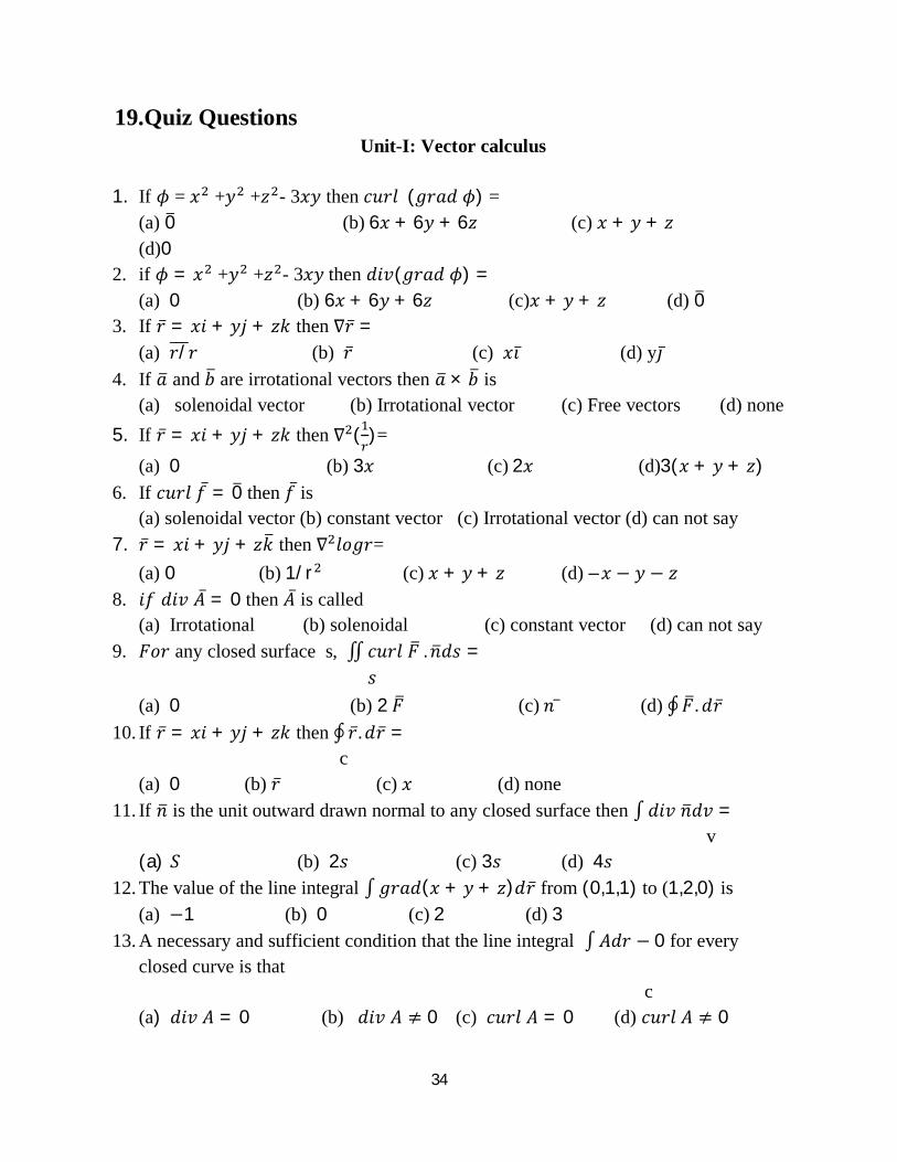
19.Quiz Questions

Unit-I: Vector calculus 1. If 휙 = 푥 +푦 +푧 - 3푥푦 then 푐푢푟푙(푔푟푎푑휙) =

(a) 0 (b) 6푥 + 6푦 + 6푧 (c) 푥 + 푦 + 푧 (d)0

2. if 휙 = 푥 +푦 +푧 - 3푥푦then 푑푖푣(푔푟푎푑휙) = (a) 0 (b) 6푥 + 6푦 + 6푧 (c)푥 + 푦 + 푧 (d) 0

3. If 푟̅ = 푥푖 + 푦푗 + 푧푘 then ∇푟̅ = (a) 푟/푟 (b) 푟̅ (c) 푥횤 ̅ (d) y횥 ̅

4. If 푎 and 푏 are irrotational vectors then 푎 × 푏 is (a) solenoidal vector (b) Irrotational vector (c) Free vectors (d) none

5. If 푟̅ = 푥푖 + 푦푗 + 푧푘 then ∇ ( )= (a) 0 (b) 3푥 (c)2푥 (d)3(푥 + 푦 + 푧)

6. If 푐푢푟푙푓̅ = 0 then 푓 ̅is (a) solenoidal vector (b) constant vector (c) Irrotational vector (d) can not say

7. 푟̅ = 푥푖 + 푦푗 + 푧푘 then ∇ 푙표푔푟= (a) 0 (b) 1/r (c)푥 + 푦 + 푧 (d) – 푥 − 푦 − 푧

8. 푖푓 푑푖푣퐴̅ = 0 then 퐴̅ is called (a) Irrotational (b) solenoidal (c) constant vector (d) can not say

9. 퐹표푟 any closed surface s, ∬푐푢푟푙퐹 .푛푑푠 = 푠 (a) 0 (b) 2퐹 (c)푛 ̅ (d) ∮퐹. 푑푟̅

10. If 푟̅ = 푥푖 + 푦푗 + 푧푘 then ∮ 푟̅.푑푟̅ = c (a) 0 (b) 푟̅ (c) 푥 (d) none

11. If 푛 is the unit outward drawn normal to any closed surface then ∫푑푖푣푛푑푣 = v (a) 푆 (b) 2푠 (c) 3푠 (d) 4푠

12. The value of the line integral ∫푔푟푎푑(푥 + 푦 + 푧)푑푟̅ from (0,1,1) to (1,2,0) is (a) −1 (b) 0 (c) 2 (d) 3

13. A necessary and sufficient condition that the line integral ∫퐴푑푟 − 0 for every closed curve is that c (a)푑푖푣퐴 = 0 (b) 푑푖푣퐴 ≠ 0 (c) 푐푢푟푙퐴 = 0 (d) 푐푢푟푙퐴 ≠ 0

35

14. ∮ 푓∇푓.푑푟̅ = (a) 푓 (b) 2푓 (c) 0 (d) 3푓

15. If 퐹 = 푎푥푖 + 푏푦푗 + 푐푧푘 where a,b,c are constants then ∬퐹.푑푠 where 푆 is the surface of the unit sphere is (a) 0 (b) 휋(푎 + 푏 + 푐) (c) 휋(푎 + 푏 + 푐) (d) 휋 (푎 + 푏 + 푐)

UNIT – II: Fourier Series and Fourier Transforms

1. Conditions for expansion of a function in Fourier series are know _________conditions

2. If 푓(푥) = 푥 in (−푙, 푙)then 푏 =__________

3. If 푓(푥) = 푐표푠푥 in (−휋,휋) then Fourier coefficient 푏 =_______________

4. If 푓(푥) = |푥|in (−휋,휋) then 푎 =______________

5. If 푓(푥) = 푥 in (−푙, 푙)then 푎 =_____________________

6. Fourier series for 푓(푥) = 1− 푥 in (−1,1)is ___________________

7. The half range sine series for 푓(푥) = 1 in (0,휋) is __________________

8. Fourier sine series for 푓(푥) = 푥 in (0,휋) is __________________

9. If 푓(푥) = 푠푖푛푥 in –휋 < 푥 < 휋 then 푎 =________________

10. In Fourier half range cosine series expansion of 푓(푥) in (0,휋)푎 =_____________

11. If 푓(푥) = 푐표푠푥 in –푘 < 푥 < 푘 ,then 푏 =______________

12. If 푓(푥) = 푒 is expanded in half range Fourier cosine series in (0,1) then a0=__________

13. If 푓(푥) = 푥 in 0 < 푥 < 2푘, then 푎 =_______________

14. In Fourier Half range sine series expansion of 푓(푥) in (0,휋) , 푏 ________________

15. In Fourier series expansion of 푓(푥) = 푐표푠ℎ푥 in (−4,4) the Fourier coefficient

a1=_________________

UNIT – III: Interpolation and Curve fitting

1. The relation between E and Δ is __________ 2. 훥[푓(푥)] = ________ 3. Lagrange’s formula is useful for _______ intervals of x

36

4. ________ interpolation formula are useful for equal intervals 5. Gauss Forward interpolation formula is used to interpolate the values of 푦 when 푝 lies

between__________ 6. Gauss Backward interpolation formula is used to interpolate the values of 푦 when 푝 lies

between__________ 7. If 푦 = 푎 + 푎 푥 + 푎 푥 then the third normal eqn by least squares method is ∑푥 푦 =

_________ 8. If푦 = 푎푥 , the first normal equation is ∑푙표푔푦 = _________

9. If 푦 = 푎 + 푏푥 + 푐푥 and 푥 = 0,1,2,3,4 and 푦 = 1,1.8,1.3,2.5,6.3 then the first

normal equation is _________ 10. For the above problem the value of a is__________________.

UNIT – IV: Numerical techniques

Solution of Algebraic and Transcendental Equations and Linear system of equations.

1. The root of 푓(푥) = 푥 − 2푥 − 5 = 0 lies in the interval_________ 2. If f(a) and f(b) have opposite signs and 푎 < 푏 ,then the first approximation to the root of

푓(푥) = 0 by Regula-Falsi method is _________ 3. The order of convergence of Newton –Raphson method is _________ 4. The necessary and sufficient condition that the system of equations 퐴푋 = 퐵is

consistent if________________

5. In the case of bisection method, the convergence is ______________

6. If the first two approximations to the root of 푥푒 − 3 = 0 are 푥0 = 1 and 푥 = 1.5

Then푥 by Regula-Falsi method is __________

7. The condition for the convergence of the method of successive approximation is _______

8. Newton –Raphson formula to find the value of 푁 (i.e qubic root of N) is ___________

9. Newton –Raphson method fails to find root of 푓(푥) = 0 when ______________

10. The order of convergence of Newton –Raphson method is _________

11. If A=LU then A-1 =________

a) U-1L-1 b) (LU)-1 (c)L-1U-1 (d) 1/LU

37

UNIT – V: Numerical Integration and Numerical Solutions of ODE’s

1. Ifℎ = 1/2, ∫ (푥 + 1)푑푥 in definite integral (1,2), by Trapezoidal rule is ____________ 2. The value of ∫ in definite integral (1,10) , by Trapezoidal rule taking 푛 = 4 is ____

3. By Simpson’s one –third rule in definite integral (a, b) of ∫ 푓(푥)푑푥 is __________ 4. Then By Simpson’s one –third rule in definite integral (0,2) of ∫ 푓(푥)푑푥 is ________ 5. If h=1 Simpson’s 3/8 rule in definite integral (1,7) of∫ is __________

6. If ℎ = 1, in definite integral(1,3) of ∫ 푒 푑푥 by Simpson’s 3/8 rule is __________ 7. While evaluating a definite integral by Trapezoidal rule, the accuracy can be increased by

taking __________ 8. By Trapezoidal rule in definite integral (푎, 푏)of ∫ 푓(푥)푑푥 =____________

9. If = 푥 + 푦, 푦(0) = 1&푦 ′(푥) = 1 + 푥 + then by Picard’s method the value of

푦( )(푥) is _______________

10. Using Euler’s method 푦′ = ( – ) ,푦(0) = 1 and ℎ = 0.02 given y1 =____________

11. Range – cute method is a __________ method 12. The first order Range – cute method is ____________ 13. The formula for second order Range – cute method is__________ 14. Adams- Bashforth corrector formula is __________ 15. Which of the following is a step by step method ________

(a) Taylor’s series (b) Picard’s (c) Adams- Bashforth (d) none

16. Which of the following is not a step by step method ________

(a) Euler’s method (b) Modified Euler’s method (c) Taylor’s series method (d) Runge – kutta method of fourth order

17. Which of the following is best for solving initial value problems

(a) Euler’s method (b) Modified Euler’s method

(c) Taylor’s series method (d) Runge – kutta method of fourth order

18. If 푦0 = 1,푦1 = 0.9898,푦2 = 0.9588,푦3 = 0.9088,푦4 = 0.84 and ℎ = 1/4 then the value

In definite integral (0,1)∫ 푦푑푥 by Trapezoidal rule is ___________

38

20. Tutorial Problems

Tutorial sheet-1

1. Evaluate ∬퐹.푛푑푠where 퐹 = 푧푖 + 푥푗 − 3푦 푧푘, where S is the surface of the

cylinder푥 + 푦 = 1in the first octant between 푧 = 0푎푛푑푧 = 2

2. Verify Green’s theorem Evaluate ∫(푥푦 + 푦 )푑푥 + 푥 푑푦 where C is bounded by 푦 = 푥푎푛푑푦 = 푥

3. Find work done by 퐹 = (2푥 − 푦 − 푧)횤̅+ (푥 + 푦 − 푧)횥 ̅+ (3푥 − 2푦 − 5푧)푘 along a curve C in xy-plane given by푥 + 푦 = 4푎푛푑푧 = 0.

4. Find the constants a,b and c if the vector 푓̅ = (2푥 + 3푦 + 푎푧)푖 + (푏푥 + 2푦 + 3푧)푗 + (2푥 + 푐푦 + 3푧)푘 is irrotational.

5. Evaluate by Green’s theorem ∮(푦 − 푠푖푛푥)푑푥 + 푐표푠푥푑푦 where ‘c’ is the triangle enclosed by the lines 푦 = 0, 푥 = 푎푛푑휋푦 = 2푥.

Tutorial sheet-2

1. Find the half-range sine series for the function 푓(푡) = 푡 − 푡 , 푖푛0 < 푡 < 1. 2. Find the Fourier series to represent the function 푓(푥) = |푠푖푛푥| −휋 < 푥 < 휋 3. Find the Fourier sine and cosine transform of 푥 ,푛 > 0.

4. Find the half-range cosine series expansion of the function 푓(푥) =0, 0 ≤ 푥 ≤

푙 − 푥, ≤ 푥 ≤ 푙

5. Expand 푓(푥) = 푒 as Fourier series in the interval (-c, c) 6. Obtain the half range fourier sine series for f(x) =x2 in the range 0<x<Π 7. Obtain cosine and sine series for f(x) =x is the interval 0≤ 푥 ≤ 훱. Hence show that

+ + + ⋯ =

Tutorial sheet-3

1. For x=0,1,2,3,4 and f(x) =1,14,15,5,6 find f(3) using Newton’s interpolation formula 2. Show that ∆ (1− 푥)(1 − 2푥 )(1− 3푥 )(1 − 4푥 ) = 24 × 2 × 10! If h=2. 3. Fit the curve of the form 푦 = 푎푒

4. Using Lagrange’s formula find 푦(6)given

x 3 5 7 9 11

y 6 24 58 108 74

x 77 100 185 239 285 y 2.4 3.4 7 11.1 19.6

39

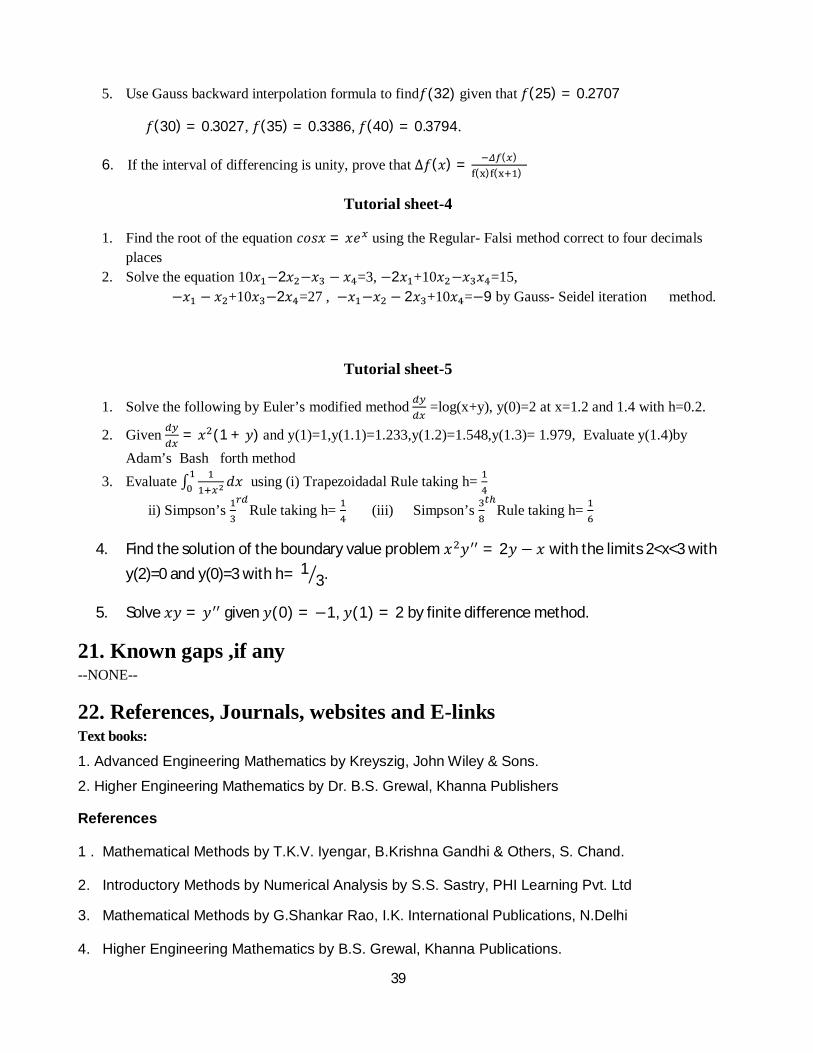
5. Use Gauss backward interpolation formula to find푓(32) given that푓(25) = 0.2707

푓(30) = 0.3027, 푓(35) = 0.3386,푓(40) = 0.3794.

6. If the interval of differencing is unity, prove that ∆푓(푥) = ( )( ) ( )

Tutorial sheet-4

1. Find the root of the equation 푐표푠푥 = 푥푒 using the Regular- Falsi method correct to four decimals places

2. Solve the equation 10푥 −2푥 −푥 − 푥 =3, −2푥 +10푥 −푥 푥 =15, −푥 − 푥 +10푥 −2푥 =27 , −푥 −푥 − 2푥 +10푥 =−9 by Gauss- Seidel iteration method.

Tutorial sheet-5

1. Solve the following by Euler’s modified method =log(x+y), y(0)=2 at x=1.2 and 1.4 with h=0.2.

2. Given = 푥 (1 + 푦) and y(1)=1,y(1.1)=1.233,y(1.2)=1.548,y(1.3)= 1.979, Evaluate y(1.4)by Adam’s Bash forth method

3. Evaluate ∫ 푑푥 using (i) Trapezoidadal Rule taking h=

ii) Simpson’s Rule taking h= (iii) Simpson’s Rule taking h=

4. Find the solution of the boundary value problem 푥 푦 = 2푦 − 푥 with the limits 2<x<3 with y(2)=0 and y(0)=3 with h= 1

3.

5. Solve 푥푦 = 푦 given 푦(0) = −1, 푦(1) = 2 by finite difference method.

21. Known gaps ,if any --NONE--

22. References, Journals, websites and E-links Text books:

1. Advanced Engineering Mathematics by Kreyszig, John Wiley & Sons.

2. Higher Engineering Mathematics by Dr. B.S. Grewal, Khanna Publishers References

1 . Mathematical Methods by T.K.V. Iyengar, B.Krishna Gandhi & Others, S. Chand. 2. Introductory Methods by Numerical Analysis by S.S. Sastry, PHI Learning Pvt. Ltd

3. Mathematical Methods by G.Shankar Rao, I.K. International Publications, N.Delhi 4. Higher Engineering Mathematics by B.S. Grewal, Khanna Publications.

40

5. Mathematical Methods by V. Ravindranath, Etl, Himalaya Publications.

6. Advanced Engineering Mathematics with MATLAB, Dean G.Duffy, 3rd Edi, 2013, CRC Press Taylor & Francis Group.

7. Mathematics for Engineers and Scientists, Alan Jeffrey, 6th Edi. 2013, Chapman & Hall/CRC.

8. Advnaced Engineering Mathematics, Michael Greenberg, Second Edition, Pearson Education.

Journals

1. Numerical Linear Algebra with Applications

2. International Journal for Numerical Methods in Engineering

3 Journal of Inequalities in Pure and Applied Mathematics

4. SIAM Journal of Applied Mathematics

5. Journal of Partial Differential Equations

Websites

1. www.physicsforum.com

2. mathworld.wolfram.com

3. www.intmath.com

4. www.sosmath.com

5. mathforum.org

23. Quality Control Sheets EVALUATION SCHEME:

PARTICULAR WEIGHTAGE MARKS End Examinations 75% 75 Three Sessionals 20% 20 Assignment 5% 5 TEACHER'S ASSESSMENT(TA)* WEIGHTAGE MARKS

*TA will be based on the Assignments given, Unit test Performances and Attendance in the class for a particular student.

41

Model Paper:

GEETHANJALI COLLEGE OF ENGINEERING & TECHNOLOGY Cheeryal (v), Keesara (M), R.R.Dist.-501301.

R13 Model Question Paper-I B.Tech. II-year End Examinations, June 2014

Subject: MATHEMATICS-II Time: 3 hours Max.Marks:75

________________________________________________________________________________________ Note: This question paper contains two parts A and B. Part A is compulsory which carries 25 marks. Answer all questions in Part A. Part B consists of 5 units. Answer any one full question from each unit. Each Question carries 10 marks and may have a, b, c as sub questions.

Part-A (25 Marks) 1. (a) Write normal equations to fit the parabola 푦 = 푎 + 푏푥 + 푐푥 (2M)

(b) Prove that 퐸 = 휇 + 훿 (3M) (c) Find the second iteration using bisection method for푥 − 푥 − 1 = 0. (2M) (d) Find y (0.1) using Euler method given 푦′ = (푥 + 푥푦 )푒 ,푦(0) = 1,ℎ = 0.1. (3M) (e) Find 푎 for the Fourier series for f(x) = 푒 in the interval[0,2휋]. (2M) (f) Write Fourier sine and cosine transforms of f (t). (3M) (g) Write the formulas for trapezoidal rule, Simpson’s 1/3푟푑 rule & Simpson’s3/8푡ℎ rule. (2M) (h) What is the 2푛푑 iteration to find reciprocal of 18 using Newton Raphson method (3M) (i) Show that (∇Φ × ∇Ψ)issolenoidal. (2M) (j)Show that ∇ (r ) = n(n + 1)r (3M)

Part-B (50 Marks) 2. (a) If the interval of differencing is unity

Prove that ∆ [x(x+1) (x+2) (x+3)] = 4(x+1) (x+2) (x+3) (3M)

(b) For x=0,1,2,3,4 and f(x) =1,14,15,5,6 find f(3) using Newton’s interpolation formula. (3M)

(c) A curve passes through the points (0, 18), (1, 10), (3,-18) & (6, 90) find the slope of the curve at x=2. (4M)

(OR) 3. (a) If the interval of differencing is unity. Prove that ∆tan ( ) = 푡푎푛 ( ). (3M)

(b) Fit a second degree parabola to the following data (4M)

X 0 1 2 3 4 y 1 1.8 1.3 2.5 6.3

(c) Fit a straight line to the form y = a + bx for the following data (3M)

42

x 0 5 10 15 20 25 y 12 15 17 22 24 30

4. (a) Find LU decomposition of the matrix A and solve the linear system AX=B (4M)

−3 12 −61 −2 21 1 1

푥푦푧

=−337−1

(b) Find a real root of the equation 푥푒 − 푐표푠푥 = 0 using Newton’s Raphson method. (3M) (c) The velocity v of a particle moving in straight line covers a distance x in time t. They are related as follows: find f '(15). (3M)

(OR)

5. (a) Evaluate ∫ 푑푥 by (i) Trapezoidadal Rule (ii) Simpson’s Rule (iii) Simpson’s Rule (3M) (b) Employ Taylor’s method to obtain approximate value of y at x=0.2 for the differential equation = 2푦 + 3푒 ,푦(0) = 0 (3M)

(c) Given 푦 = 푥(푥 + 푦 )푒 ,푦(0) = 1,find y at x=0.1, 0.2 and 0.3 by Taylor’s series method and Compute y (0.4) using Milni’s method. (4M) 6. (a) Find a Fourier series to represent 푥 − 푥 from 푥 = −휋푡표휋. (3M) (b) Expand 푓(푥) = 푒 as Fourier series in the interval (-c, c) (3M) (c) Expand 푓(푥) = 푥푠푖푛푥 as Fourier series in the interval 0 < 푥 < 2휋 (4M) (OR) 7. (a) Find the following transform of

푓(푥) = 1푓표푟|푥| < 10푓표푟|푥| > 1 Hence Evaluate ∫ 푑푥. (4M)

(b) Find the Fourier sine Transform of . (3M)

(c )Show that 퐹 {푥푓(푥)} = − [퐹 (푝)] (3M) 8. Find 푦(0.5), 푦(1) and 푦(1.5) given that 푦 ′ = 4− 2푥, 푦(0) = 2 with ℎ = 0.5 using modified Euler’s method.

(OR)

9. Use second order method for the solution for the following boundary value problem 푦 =푥 y+1, 0<x<1, y(0)=1, 푦 (0)=1, y(1)=1 using step length h=0.5?

10. (a) Find the angle between the two surfaces 푥 + 푦 + 푧 = 9,푎푛푑푧 = 푥 + 푦 − 3at the point (2,−1, 2) (3M) (b) Find workdone in moving a particle in the force field 푓̅ = 3푥 횤̅+ (2푥푧 − 푦)횥̅+ 푧푘 along the straight line from (0,0,0) to (2,1,3) (3M) (c) Evaluate by Green’s theorem ∮(푦 − 푠푖푛푥)푑푥 + 푐표푠푥푑푦 where ‘c’ is the triangle enclosed by the lines 푦 = 0,푥 = 푎푛푑휋푦 = 2푥. (4M)

(OR) 11. (a) Find work done by 퐹 = (2푥 − 푦 − 푧)횤̅+ (푥 + 푦 − 푧)횥̅+ (3푥 − 2푦 − 5푧)푘 along a curve C in xy-plane given by푥 + 푦 = 4푎푛푑푧 = 0. (3M) (b) Verify Gauss divergence theorem for 2푥 푦횤̅ − 푦 횥̅+ 4푥푧 푘 taken over the region of the

x 0 10 20 30 40

y 45 60 65 54 42

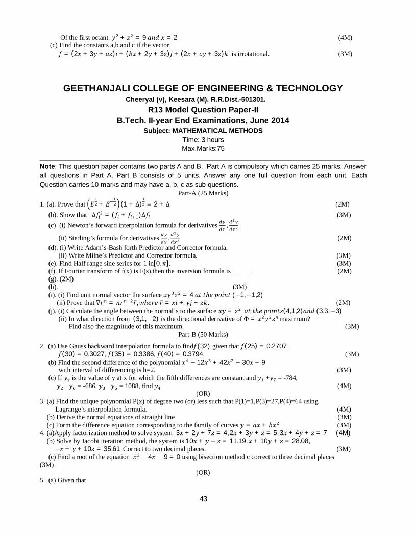
43

Of the first octant 푦 + 푧 = 9푎푛푑푥 = 2 (4M) (c) Find the constants a,b and c if the vector 푓̅ = (2푥 + 3푦 + 푎푧)푖 + (푏푥 + 2푦 + 3푧)푗 + (2푥 + 푐푦 + 3푧)푘 is irrotational. (3M)

GEETHANJALI COLLEGE OF ENGINEERING & TECHNOLOGY Cheeryal (v), Keesara (M), R.R.Dist.-501301.

R13 Model Question Paper-II B.Tech. II-year End Examinations, June 2014

Subject: MATHEMATICAL METHODS Time: 3 hours Max.Marks:75

______________________________________________________________________________________ Note: This question paper contains two parts A and B. Part A is compulsory which carries 25 marks. Answer all questions in Part A. Part B consists of 5 units. Answer any one full question from each unit. Each Question carries 10 marks and may have a, b, c as sub questions.

Part-A (25 Marks) 1. (a). Prove that 퐸 + 퐸 (1 + ∆) = 2 + ∆ (2M) (b). Show that ∆푓 = (푓 + 푓 )∆푓 (3M) (c). (i) Newton’s forward interpolation formula for derivatives ,

(ii) Sterling’s formula for derivatives , (2M) (d). (i) Write Adam’s-Bash forth Predictor and Corrector formula. (ii) Write Milne’s Predictor and Corrector formula. (3M) (e). Find Half range sine series for 1 in[0,휋]. (3M) (f). If Fourier transform of f(x) is F(s),then the inversion formula is______. (2M) (g). (2M) (h). (3M) (i). (i) Find unit normal vector the surface 푥푦 푧 = 4푎푡푡ℎ푒푝표푖푛푡(−1,−1,2) (ii) Prove that ∇푟 = 푛푟 푟̅,푤ℎ푒푟푒푟̅ = 푥푖 + 푦푗 + 푧푘. (2M) (j). (i) Calculate the angle between the normal’s to the surface 푥푦 = 푧 푎푡푡ℎ푒푝표푖푛푡푠(4,1,2)푎푛푑(3,3,−3) (ii) In what direction from (3,1,−2) is the directional derivative of Φ = 푥 푦 푧 maximum? Find also the magnitude of this maximum. (3M)

Part-B (50 Marks)

2. (a) Use Gauss backward interpolation formula to find푓(32) given that푓(25) = 0.2707, 푓(30) = 0.3027, 푓(35) = 0.3386,푓(40) = 0.3794. (3M) (b) Find the second difference of the polynomial 푥 − 12푥 + 42푥 − 30푥 + 9 with interval of differencing is h=2. (3M) (c) If 푦 is the value of y at x for which the fifth differences are constant and 푦 +푦 = -784, 푦 +푦 = -686, 푦 +푦 = 1088, find 푦 (4M)

(OR) 3. (a) Find the unique polynomial P(x) of degree two (or) less such that P(1)=1,P(3)=27,P(4)=64 using Lagrange’s interpolation formula. (4M) (b) Derive the normal equations of straight line (3M) (c) Form the difference equation corresponding to the family of curves 푦 = 푎푥 + 푏푥 (3M) 4. (a)Apply factorization method to solve system 3푥 + 2푦 + 7푧 = 4, 2푥 + 3푦 + 푧 = 5, 3푥 + 4푦 + 푧 = 7(4M) (b) Solve by Jacobi iteration method, the system is 10푥 + 푦 − 푧 = 11.19,푥 + 10푦 + 푧 = 28.08, −푥 + 푦 + 10푧 = 35.61Correct to two decimal places. (3M) (c) Find a root of the equation 푥 − 4푥 − 9 = 0 using bisection method c correct to three decimal places (3M)

(OR) 5. (a) Given that

44

x 1.0 1.1 1.2 1.3 1.4 1.5 1.6 y 7.989 8.403 8.781 9.129 9.451 9.750 10.031

Find , at (i)x=1.1 (ii) x=1.6 (4M)

(b) Evaluate ∫ 푑푥 using (i) Trapezoidadal Rule taking h=

(ii) Simpson’s Rule taking h= (iii) Simpson’s Rule taking h= (3M) (c) Given = 푥 (1 + 푦) and y(1)=1,y(1.1)=1.233,y(1.2)=1.548,y(1.3)= 1.979, Evaluate y(1.4)by Adam’s Bash forth method. (4M) 6. (a) Find the half-range sine series for the function 푓(푡) = 푡 − 푡 , 푖푛0 < 푡 < 1 (3M)

(b) Find the half-range cosine series expansion of the function 푓(푥) =0, 0 ≤ 푥 ≤

푙 − 푥, ≤ 푥 ≤ 푙 (3M)

(c) Find the Fourier series to represent the function 푓(푥) = |푠푖푛푥| −휋 < 푥 < 휋 (4M) (OR) 7. (a) If the Fourier sine transform of 푓(푥) = (0 ≤ 푥 ≤ 휋), 푓푖푛푑푓(푥). (4M) (b) Find the Fourier sine and cosine transform of 푥 ,푛 > 0. (3M) (c ) Find the Fourier Cosine transform of 푒 푐표푠푎푥,푎 > 0 (3M) 8. (a) Solve 푧 = 푝 푥 + 푞 푦푢푠푖푛푔퐶ℎ푎푟푝푖푡푠푚푒푡ℎ표푑 (3M) (b) Solve 3 + 2 = 0,푢(푥, 0) = 4푒 (3M) (c) A tightly stretched string with fixed end points x=0 and x=1 is initially in a position given by 푦 = 푦 푠푖푛 .If it is released from rest from this position, find displacement y(x,t) (4M)

(OR) 9. (a) Solve 푥 − 푦푧) + (푦 − 푥푧) = (푧 − 푥푦 ) (3M) (b) Solve푥 푝 + 푦 푞 = 푧 (3M) (c) Form the partial differential equation by eliminating arbitrary function from 푧 = 푦 + 2푓 + 푙표푔푦 (4M) 10. (a) Evaluate ∬퐹.푛푑푠where 퐹 = 푧푖 + 푥푗 − 3푦 푧푘, where S is the surface of the cylinder 푥 + 푦 = 1in the first octant between 푧 = 0푎푛푑푧 = 2 (3M) (b) Verify Stoke’s theorem for 퐹 = (2푥 − 푦)푖 − 푦푧 푗 − 푦 푧푘 over the upper half of surface of the Sphere푥 + 푦 + 푧 = 1 bounded by the projection of the xy-plane (3M) (c) Find the constants a,b,c so that the vector 퐴̅ = (푥 + 2푦 + 푎푧)푖 + (푏푥 − 3푦 − 푧)푗 + (4푥 + 푐푦 + 2푧)푘 is irrotational and also find Φ so that 퐴̅ = ∇Φ (4M)

(OR) 11. (a) Verify Green’s theorem Evaluate ∫(푥푦 + 푦 )푑푥 + 푥 푑푦 where C is bounded by 푦 = 푥푎푛푑푦 = 푥 (4M) (b) Evaluate ∬퐹.푛푑푠where 퐹 = 4푥푖 − 2푦 푗 − 푧 푘 and S is the surface bounding the region 푥 + 푦 = 4, 푧 = 0푎푛푑푧 = 3. (3M) ( c) Prove that div curl 푓̅ = 0 (3M)

45

GEETHANJALI COLLEGE OF ENGINEERING & TECHNOLOGY

Cheeryal (v), Keesara (M), R.R.Dist.-501301. R13 Model Question Paper-III

B.Tech. II-year End Examinations, June 2014 Subject: MATHEMATICS-II

Time: 3 hours Max.Marks:75

______________________________________________________________________________________ Note: This question paper contains two parts A and B. Part A is compulsory which carries 25 marks. Answer all questions in Part A. Part B consists of 5 units. Answer any one full question from each unit. Each Question carries 10 marks and may have a, b, c as sub questions.

Part-A (25 Marks) 1. (a). Define difference equation. (2M)

(b). Write the Newton’s forward and backward interpolation formulae. (3M) (c). (i) Write Modified Euler’s method formula for 푦1.

(ii) Write Runge - kutta method formula for푦1. (2M)

(d). Write down the formulae for (i) Trapezoidal Rule (ii) Simpson’s 1

3rule (iii) Simpson’s 3

8rule. (3M)

(e). In the Fourier series expansion of 푓(푥) = 푠푖푛푥 in(−Π,Π), then find the value of 푏푛 (2M) (f). Fourier sine integral representation of a function f(x) is? (3M) (g). Solve 푝√푥+푞 푦=√푧. (2M) (h). Solve푝 + 푞 = 1. (3M) (i). If ∅ = log(푥 + 푦 + 푧 ). The find∇∅, (2M)

(j). Find div F and curl F, where 퐹 = 푔푟푎푑(푥 + 푦 + 푧 − 3푥푦푧) (3M)

Part-B (50Marks)

2. (a). Find 푦(25) given that 푦20=24, 푦24=32, 푦28=35, 푦32=40 using Gauss forward difference formula. (3M)

(b). Show that ∆10 (1 − 푥)(1 − 2푥2)(1 − 3푥3)(1 − 4푥4) = 24 × 210 × 10! If h=2. (3M)

(c). Using Lagrange’s formula find 푦(6)given (4M)

x 3 5 7 9 11

y 6 24 58 108 74 (OR)

3. (a). If the interval of differencing is unity, prove that ∆푓(푥) = ( )( ) ( )

(3M)

46

(b) Fit the curve of the form 푦 = 푎푒 (3M)

(c) Fit a Second degree parabolafor the following data (4M)

4. (a). Find the root of the equation 푐표푠푥 = 푥푒 using the Regular- Falsi method correct to four decimals places. (3M)

(b). Solve the equation 10푥1−2푥2−푥3 − 푥4=3, −2푥 +10푥2−푥3푥4=15,

−푥1 − 푥2+10푥3−2푥4=27 , −푥1−푥2 − 2푥3+10푥4=−9 by Gauss- Seidel iteration method. (3M)

(c). Find the maximum and minimum value of y from the following data (4M)

X -2 -1 0 1 2 3 4 Y 2 -0.25 0 -0.25 2 15.75 56

(OR)

5. (a). A solid of revolution is formed by rotating about the x- axis the area between the x-axis , the lines

x=0 and x=1 and a curve through the points with the following co-ordinates

x 0 0.25 0.5 0.75 1.00 y 1.0000 0.9896 0.9589 0.9089 0.8415

Estimate the volume of the solid formed using Simpson’s rule. (3M)

(b). Solve the following by Euler’s modified method =log(x+y), y(0)=2 at x=1.2 and 1.4 with h=0.2. (3M)

(c) Using Runge - kutta method of fourth order, solve 푑푦푑푥

= 푦2−푥2

푦2+푥2 with y(0)=1 at x=0.2 and 0.4 (4M)

6. (a).Using Parseval’s identities , prove that

(i). ∫ (∞0

푑푡

(푎2+푡2)(푏2+푡2 ))=

( ) (ii)∫ 푡2

(푡2+1)2

∞0 = 휋

4 (3M)

(b). Find the Fourier cosine transform of f(x) =푥,0 < 푥 < 1

2 − 푥,1 < 푥 < 20,푥 > 2

(3M)

(c). Find the Fourier sine transform of 푒−|푥|. (4M)

(OR) 7. (a). Show that for –Π<x<Π,푠푖푛푎푥=2푠푖푛푎훱

훱( 푠푖푛푥

1−푎2 − − - ……….) (3M)

x 77 100 185 239 285 y 2.4 3.4 7 11.1 19.6

x 0 1 2 3 4 y 1 1.8 3.3 4.5 6.3

47

(b). Obtain cosine and sine series for f(x) =x is the interval 0≤ 푥 ≤ 훱. Hence show that

1

12 + 1

32 + 1

52 + ⋯ = 훱2

8 (3M)

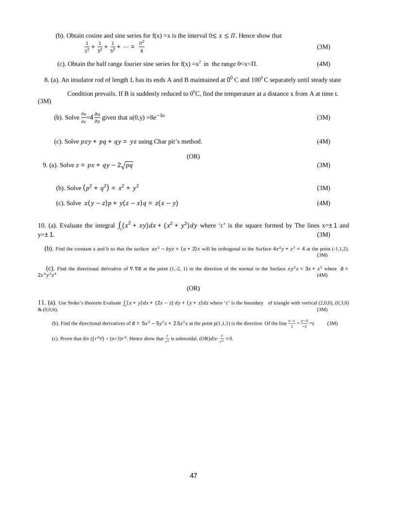
(c). Obtain the half range fourier sine series for f(x) =x2 in the range 0<x<Π. (4M) 8. (a). An insulator rod of length L has its ends A and B maintained at 00 C and 1000 C separately until steady state

Condition prevails. If B is suddenly reduced to 00C, find the temperature at a distance x from A at time t. (3M)

(b). Solve 휕푢휕푥

=4 given that u(0,y) =8푒−3푢 (3M)

(c). Solve 푝푥푦 + 푝푞 + 푞푦 = 푦푧 using Char pit’s method. (4M)

(OR) 9. (a). Solve 푧 = 푝푥 + 푞푦 − 2 푝푞 (3M)

(b). Solve (푝2 + 푞2) = 푥2 + 푦2 (3M) (c). Solve 푥(푦 − 푧)푝 + 푦(푧 − 푥)푞 = 푧(푥 − 푦) (4M)

10. (a). Evaluate the integral ∫(푥2푐 + 푥푦)푑푥 + (푥2 + 푦2)푑푦 where ‘c’ is the square formed by The lines x=±1 and

y=±1. (3M)

(b). Find the constant a and b so that the surface 푎푥 − 푏푦푧 = (푎 + 2)푥 will be orthogonal to the Surface 4푥 푦 + 푧 = 4 at the point (-1,1,2). (3M)

(c). Find the directional derivative of ∇.∇∅ at the point (1,-2, 1) in the direction of the normal to the Surface 푥푦 푧 = 3푥 + 푧 where∅ =2푥 푦 푧 (4M)

(OR)

11. (a). Use Stoke’s theorem Evaluate ∫ (푥 + 푦)푑푥 + (2푥 − 푧) 푑푦 + (푦 + 푧)푑푧 where ‘c’ is the boundary of triangle with vertical (2,0,0), (0,3,0) & (0,0,6). (3M)

(b). Find the directional derivatives of ∅ = 5푥 − 5푦 푧 + 2.5푧 푥 at the point p(1,1,1) is the direction Of the line = =z (3M)

(c). Prove that div ((푟 푟̅) = (n+3)푟 . Hence show that ̅ is solenoidal. (OR)푑푖푣 ̅

=0.

48

25. Student List II-A Section

S.No Roll No Student Name

1 14R11A0301 A SAI AKHIL

2 14R11A0302 A SANDEEP KUMAR

3 14R11A0303 ABHINAY DAULAGHAR

4 14R11A0304 ADIMULAM VENKATA SAI KIRAN

5 14R11A0305 AJAY KUMAR JOSHI

6 14R11A0306 ALLA ANVESH

7 14R11A0307 ARCOT BALRAJ TAHMAIYEE

8 14R11A0308 B VAMSHI BHARADWAJ

9 14R11A0309 BOGAVALLI SRI PAVAN KUMAR

10 14R11A0310 BOLLAVARAM PRASANTH KUMAR REDDY

11 14R11A0311 CHANDAVOLU SRUJAN KUMAR

12 14R11A0312 CHINNA BHEEMAIAH VINOD KUMAR

13 14R11A0313 DAVAN KAUSHIK

14 14R11A0314 G JHUNKAR

15 14R11A0315 G S HARISH

16 14R11A0316 GADDAM NAGA SANTOSH

17 14R11A0317 GUNTI KUMAR

18 14R11A0318 JAKKAM KRANTHI KIRAN

19 14R11A0319 KADAVATH SUMAN

20 14R11A0320 KANDERPALLY RAHUL

21 14R11A0321 KANDHADI BHANU PRAKASH

22 14R11A0322 KARNA KOTI REDDY

23 14R11A0323 KASAVENA ARUN KUMAR

24 14R11A0324 KATTA SHIVA PRASAD REDDY

49

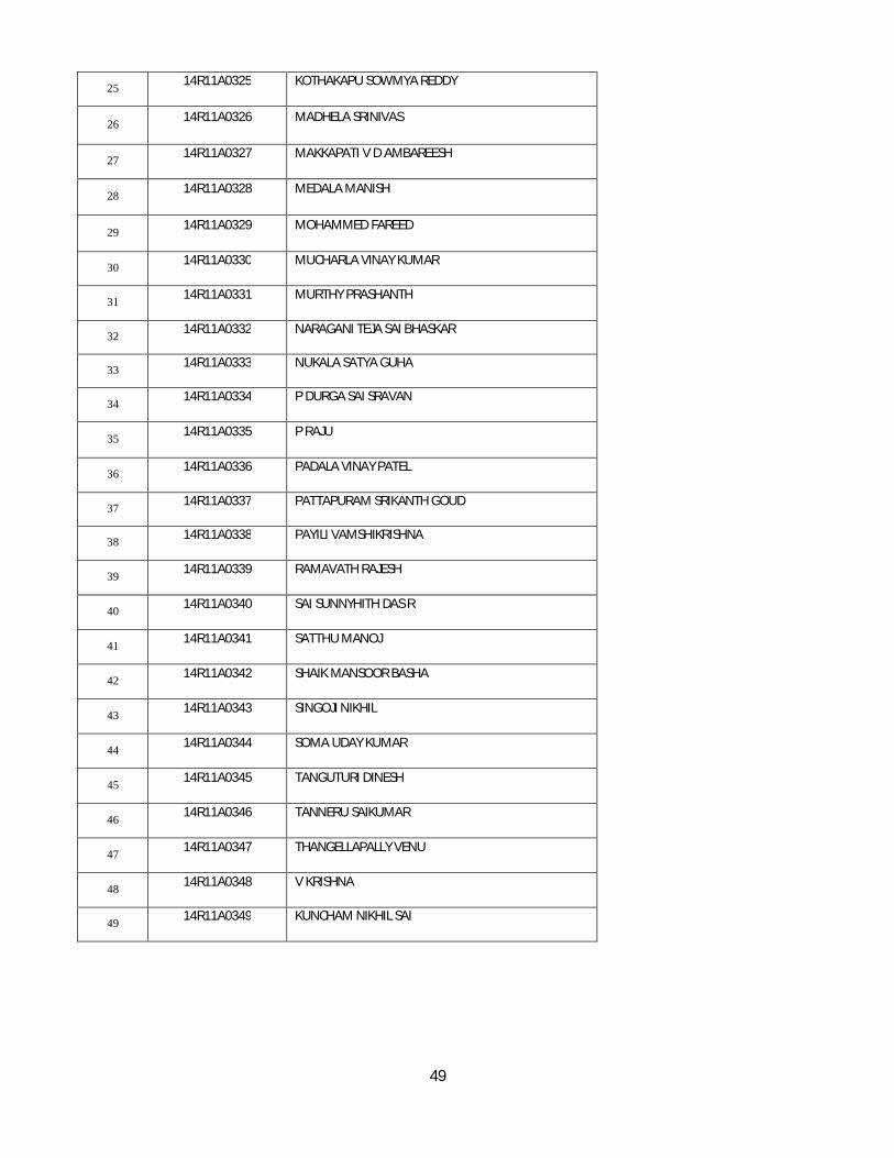
25 14R11A0325 KOTHAKAPU SOWMYA REDDY

26 14R11A0326 MADHELA SRINIVAS

27 14R11A0327 MAKKAPATI V D AMBAREESH

28 14R11A0328 MEDALA MANISH

29 14R11A0329 MOHAMMED FAREED

30 14R11A0330 MUCHARLA VINAY KUMAR

31 14R11A0331 MURTHY PRASHANTH

32 14R11A0332 NARAGANI TEJA SAI BHASKAR

33 14R11A0333 NUKALA SATYA GUHA

34 14R11A0334 P DURGA SAI SRAVAN

35 14R11A0335 P RAJU

36 14R11A0336 PADALA VINAY PATEL

37 14R11A0337 PATTAPURAM SRIKANTH GOUD

38 14R11A0338 PAYILI VAMSHIKRISHNA

39 14R11A0339 RAMAVATH RAJESH

40 14R11A0340 SAI SUNNYHITH DAS R

41 14R11A0341 SATTHU MANOJ

42 14R11A0342 SHAIK MANSOOR BASHA

43 14R11A0343 SINGOJI NIKHIL

44 14R11A0344 SOMA UDAY KUMAR

45 14R11A0345 TANGUTURI DINESH

46 14R11A0346 TANNERU SAIKUMAR

47 14R11A0347 THANGELLAPALLY VENU

48 14R11A0348 V KRISHNA

49 14R11A0349 KUNCHAM NIKHIL SAI

50

II-B-section

S.No Roll No Student Name

1 13R11A03A8 REGU RAJSHEKAR

2 14R11A0351 A DINESH SAGAR

3 14R11A0352 A JANARDHAN

4 14R11A0353 ALLIPURAM VAMSHI KRISHNA

5 14R11A0354 ARDHENDU CHAKRABORTY

6 14R11A0355 ASAPU SAI CHARAN

7 14R11A0356 B SAI KRISHNA

8 14R11A0357 BALE RAGHU RAM

9 14R11A0358 BEERAM PRUHIT

10 14R11A0359 C GAUTHAM

11 14R11A0360 CHADALA NIKHIL KUMAR

12 14R11A0361 CHANDRAIAH VENKATESH

13 14R11A0362 CHILUVERI SOMESHWAR

14 14R11A0363 DARMANOLLA SRINIVASA REDDY

15 14R11A0364 ELLANDULA PRAKASH

16 14R11A0365 G SRIKANTH CHARY

17 14R11A0366 GALLA VAMSI

18 14R11A0367 GUDA ARJUN REDDY

19 14R11A0368 JAGIRAPU SREE HARSHA

20 14R11A0369 K ANIL KUMAR

21 14R11A0370 KILARI RAMU

22 14R11A0371 KOTHAPALLI NAGA SAI PHANI VARMA

23 14R11A0372 KSDK BHARADWAJ

24 14R11A0373 M VENKATESH

25 14R11A0374 MANUPATI SAI PAVAN

51

26 14R11A0375 MEKALA JAYA SAITH REDDY

27 14R11A0376 NAKKA NISHANTH YADAV

28 14R11A0377 NARA MANOJ KUMAR

29 14R11A0378 NAYANI SAI GNANESHWAR

30 14R11A0379 PATHAKOTI SHIVA KUMAR

31 14R11A0380 PRATIK MISHRA

32 14R11A0381 PURAM MANVITH REDDY

33 14R11A0382 R VARUN

34 14R11A0383 REDNAM KOTA RAMA KRISHNA

35 14R11A0384 S JWALA KIRAN

36 14R11A0385 S UMAMAHESHWAR REDDY

37 14R11A0386 SAIKAM SRINIVAS

38 14R11A0387 SAYANI VAMSI KRISHNA

39 14R11A0388 SUMIT KUMAR SINGH

40 14R11A0389 SUVARNA SAI CHANDRA VANEESH

41 14R11A0390 T ANOOPCHANDRAN

42 14R11A0391 T VENKATA SAI NITHIN

43 14R11A0392 THIRUMALA HRUSHIKESH

44 14R11A0393 VARAKALA VISHAL MAI

45 14R11A0394 VINJAMURI SAI VENKATA KRISHNA

46 14R11A0395 VULLIGADDALA ASHOK KUMAR

47 14R11A0396 MAVURAM VAMSHI KRISHNA REDDY

Discussion Topics:

Difference between Initial Value Problems and Boundary Value Problems Applications of Boundary Value Problems and Fourier Series in Heat and Wave Equations Applications of Multiple Integrals in Vector Integral Theorems Interpolation and Extrapolation Analytical and Numerical methods to solve differential equations

52

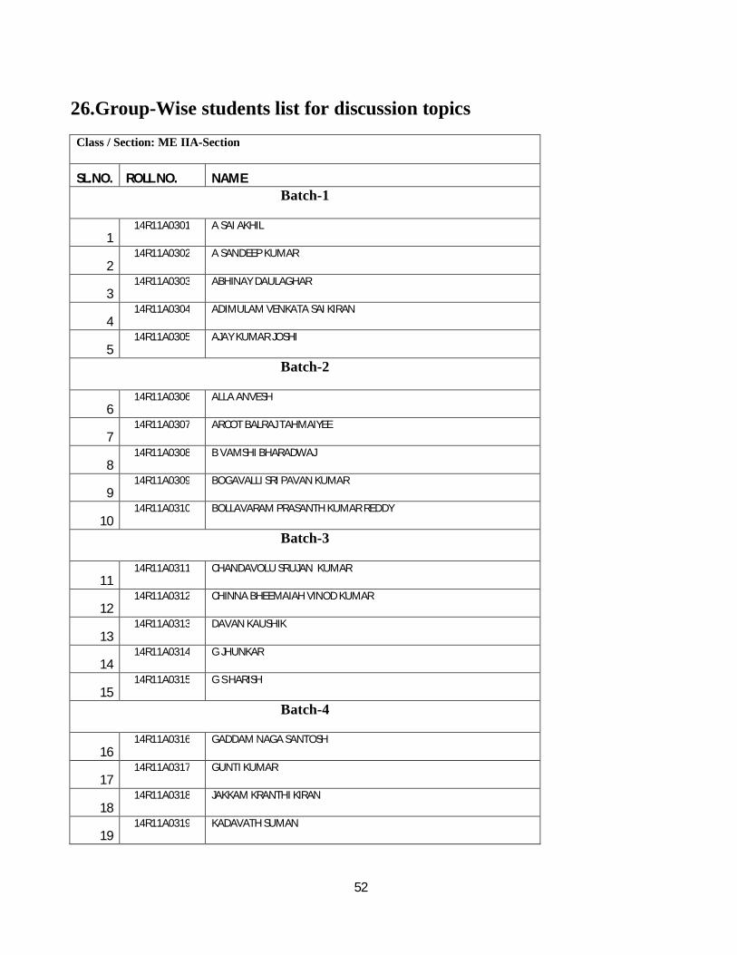
26.Group-Wise students list for discussion topics Class / Section: ME IIA-Section

SL.NO. ROLL NO. NAME Batch-1

1 14R11A0301 A SAI AKHIL

2 14R11A0302 A SANDEEP KUMAR

3 14R11A0303 ABHINAY DAULAGHAR

4 14R11A0304 ADIMULAM VENKATA SAI KIRAN

5 14R11A0305 AJAY KUMAR JOSHI

Batch-2

6 14R11A0306 ALLA ANVESH

7 14R11A0307 ARCOT BALRAJ TAHMAIYEE

8 14R11A0308 B VAMSHI BHARADWAJ

9 14R11A0309 BOGAVALLI SRI PAVAN KUMAR

10 14R11A0310 BOLLAVARAM PRASANTH KUMAR REDDY

Batch-3

11 14R11A0311 CHANDAVOLU SRUJAN KUMAR

12 14R11A0312 CHINNA BHEEMAIAH VINOD KUMAR

13 14R11A0313 DAVAN KAUSHIK

14 14R11A0314 G JHUNKAR

15 14R11A0315 G S HARISH

Batch-4

16 14R11A0316 GADDAM NAGA SANTOSH

17 14R11A0317 GUNTI KUMAR

18 14R11A0318 JAKKAM KRANTHI KIRAN

19 14R11A0319 KADAVATH SUMAN

53

20 14R11A0320 KANDERPALLY RAHUL

Batch-5

21 14R11A0321 KANDHADI BHANU PRAKASH

22 14R11A0322 KARNA KOTI REDDY

23 14R11A0323 KASAVENA ARUN KUMAR

24 14R11A0324 KATTA SHIVA PRASAD REDDY

25 14R11A0325 KOTHAKAPU SOWMYA REDDY

Batch-6

26 14R11A0326 MADHELA SRINIVAS

27 14R11A0327 MAKKAPATI V D AMBAREESH

28 14R11A0328 MEDALA MANISH

29 14R11A0329 MOHAMMED FAREED

30 14R11A0330 MUCHARLA VINAY KUMAR

Batch-7

31 14R11A0331 MURTHY PRASHANTH

32 14R11A0332 NARAGANI TEJA SAI BHASKAR

33 14R11A0333 NUKALA SATYA GUHA

34 14R11A0334 P DURGA SAI SRAVAN

35 14R11A0335 P RAJU

Batch-8

36 14R11A0336 PADALA VINAY PATEL

37 14R11A0337 PATTAPURAM SRIKANTH GOUD

38 14R11A0338 PAYILI VAMSHIKRISHNA

39 14R11A0339 RAMAVATH RAJESH

40 14R11A0340 SAI SUNNYHITH DAS R

Batch-9

41 14R11A0341 SATTHU MANOJ

42 14R11A0342 SHAIK MANSOOR BASHA

54

43 14R11A0343 SINGOJI NIKHIL

44 14R11A0344 SOMA UDAY KUMAR

45 14R11A0345 TANGUTURI DINESH

Batch-10

46 14R11A0346 TANNERU SAIKUMAR

47 14R11A0347 THANGELLAPALLY VENU

48 14R11A0348 V KRISHNA

49 14R11A0349 KUNCHAM NIKHIL SAI

Class / Section: ME IIB-Section

SL.NO. ROLL NO. NAME Batch-1

1 13R11A03A8 REGU RAJSHEKAR

2 14R11A0351 A DINESH SAGAR

3 14R11A0352 A JANARDHAN

4 14R11A0353 ALLIPURAM VAMSHI KRISHNA

5 14R11A0354 ARDHENDU CHAKRABORTY

Batch-2

6 14R11A0355 ASAPU SAI CHARAN

7 14R11A0356 B SAI KRISHNA

8 14R11A0357 BALE RAGHU RAM

9 14R11A0358 BEERAM PRUHIT

10 14R11A0359 C GAUTHAM

Batch-3

11 14R11A0360 CHADALA NIKHIL KUMAR

12 14R11A0361 CHANDRAIAH VENKATESH

13 14R11A0362 CHILUVERI SOMESHWAR

14 14R11A0363 DARMANOLLA SRINIVASA REDDY

55

15 14R11A0364 ELLANDULA PRAKASH

Batch-4

16 14R11A0365 G SRIKANTH CHARY

17 14R11A0366 GALLA VAMSI

18 14R11A0367 GUDA ARJUN REDDY

19 14R11A0368 JAGIRAPU SREE HARSHA

20 14R11A0369 K ANIL KUMAR

Batch-5

21 14R11A0370 KILARI RAMU

22 14R11A0371 KOTHAPALLI NAGA SAI PHANI VARMA

23 14R11A0372 KSDK BHARADWAJ

24 14R11A0373 M VENKATESH

25 14R11A0374 MANUPATI SAI PAVAN

Batch-6

26 14R11A0375 MEKALA JAYA SAITH REDDY

27 14R11A0376 NAKKA NISHANTH YADAV

28 14R11A0377 NARA MANOJ KUMAR

29 14R11A0378 NAYANI SAI GNANESHWAR

30 14R11A0379 PATHAKOTI SHIVA KUMAR

Batch-7

31 14R11A0380 PRATIK MISHRA

32 14R11A0381 PURAM MANVITH REDDY

33 14R11A0382 R VARUN

34 14R11A0383 REDNAM KOTA RAMA KRISHNA

35 14R11A0384 S JWALA KIRAN

Batch-8

36 14R11A0385 S UMAMAHESHWAR REDDY

37 14R11A0386 SAIKAM SRINIVAS

56

38 14R11A0387 SAYANI VAMSI KRISHNA

39 14R11A0388 SUMIT KUMAR SINGH

40 14R11A0389 SUVARNA SAI CHANDRA VANEESH

Batch-9

41 14R11A0390 T ANOOPCHANDRAN

42 14R11A0391 T VENKATA SAI NITHIN

43 14R11A0392 THIRUMALA HRUSHIKESH

44 14R11A0393 VARAKALA VISHAL MAI

45 14R11A0394 VINJAMURI SAI VENKATA KRISHNA

Batch-10

46 14R11A0395 VULLIGADDALA ASHOK KUMAR

47 14R11A0396 MAVURAM VAMSHI KRISHNA REDDY