department of economics and finance chair of theory of finance
TRANSCRIPT

Department of Economics and Finance
Chair of Theory of Finance
PORTFOLIO ALLOCATION AND ESG RATINGS Supervisor Prof. Nicola Borri
Candidate Valeria Chillè
683771 Co-Supervisor Prof. Pierpaolo Benigno
Academic year 2017 – 2018

2
INDEX
1 Introduction ................................................................................................... 4
2 The Dataset ..................................................................................................... 8
2.1 Sample and Setting ..................................................................................................... 8
2.2 The ESG Rating .......................................................................................................... 9
2.2.1 MSCI ESG Rating Methodology ......................................................................... 13
2.3 Statistical Analysis .................................................................................................... 16
3 Factor Analysis ............................................................................................ 32
3.1 Portfolio construction ............................................................................................... 35
3.2 Performance .............................................................................................................. 36
4 Mean - Variance Optimization ................................................................... 50
4.1 Portfolio Optimization: Theory ............................................................................... 50
4.2 Portfolio Optimization: Practice ............................................................................. 55
5 The Market Portfolio(s) .............................................................................. 63
6 Conclusion .................................................................................................... 70
7 References .................................................................................................... 78
8 Appendix ...................................................................................................... 81

3
Abstract This study provides evidence that integrating ESG criteria into factors investment styles leads
to equal or higher expected returns. Factor portfolios composed by high ESG companies yield
equal or higher returns than those composed by low ESG companies and have better risk-
return profiles. The implementation of an optimization model on high ESG stocks causes the
investment universe to be downsized and the “ESG efficient frontier” to be suboptimal with
respect to the “total” one. The ESG investment universe provides efficient investment
solutions characterized by lower variance, investors would be better or worse off with
responsible investments in a mean-variance optimization framework, depending on their
degree of risk aversion and fear of losses. In addition, we examine the market for highly
sustainable stocks. Considering a market weighted index only composed by high ESG stocks
leads to a decrease in volatility and doubles expected returns with respect to the S&P 500
ones.
The ESG data contained herein is the property of MSCI ESG Research LLC. (ESG). ESG, its affiliates and information providers make no warranties with respect to any such data. The ESG data contained herein is used under license and may not be further used, distributed or disseminated without the express written consent of ESG.

4
1 Introduction
The concept of sustainable investing has been discussed throughout the financial field at least
from 1960s. However, while in the 70s many economists like Milton Friedman believed that
only lawmakers and politicians had to care about regulating companies’ sustainability,
nowadays the majority of investment professionals understands the link between
sustainability in broad sense and businesses’ financial success.
In general, the main question about Socially Responsible Investment (SRI) changed from
“why?” to “why not?”, especially following empirical evidence that integrating SRI criteria
into the traditional investment process does not negatively affect profits.
The increased popularity gained by sustainable investments can be outlined looking at United
Nations’ Principles for Responsible Investment (UNPRI) growth in signatories and
investments’ volume through the years; in 2018 the UNPRI had about 2000 signatories, with
assets under management (AUM) amounting to around $80 trillion. Another trend of growth
toward a more sustainable business model can be found analysing the Standard and Poor 500:
while only 20% of its listed companies published sustainability reports in 2011, the number
has increased to 85% just six years later, in 2017 (Coppola, 2018).
ESG investing deviates from the notion of SRI as it is a more comprehensive approach; it
represents the acronym for Environmental, Social and Governance and refers to the three
fundamental factors in measuring the social impact and the sustainability of an investment in
a company. While a SRI process would implement ESG criteria with the aim both of
generating long-term competitive financial returns and a positive impact on society,
Responsible Investing (RI) claims that foregoing ESG factors means disregarding risks and
opportunities that have a material impact on company’s returns, thus they should be taken into
account even by investors whose sole objective is the bottom line1. Although there is an
overlay of social awareness, the key point of ESG evaluation remains financial performance.
Several empirical researches, 2000 studies are just those analysed by Friede et al. (2015) in
their meta-analysis, show that ESG criteria help to better determine the future financial
performance of companies for what concerns both risks and returns. In particular, highly
sustainable companies are deemed to be typically more long-term oriented, with a structured
process for stakeholders engagement and more likely to disclose information.
1 In opposition to SRI’s “triple bottom line”.

5
Our paper is structured as follows: Chapter 2 outlines our data and sample composition, in
Chapter 3 we deal with factor analysis and portfolio construction. Chapter 4 examines
portfolio optimization theory that is then applied to our data and Chapter 5 investigates the
behaviour of three different investment universes: 𝑅! ,𝑅!,!"# ,𝑅!,!" in order to analyse
whether replicating the S&P 500 Index while integrating ESG scores is a more profitable
strategy than just “buying” the Index. Chapter 6 concludes.
Our sample is composed by the companies included in the Standard and Poor 500 Index (S&P
500) during the period from January 31st, 2000 to February 28th, 2018 and all data is intended
as of March 31st, 2018. In Chapter 2 we examine the sources and composition of the dataset,
identifying what are the principal variables on study. In particular, we focus on ESG scores,
explaining MSCI methodology and, more in general, what are the reasons behind responsible
investments. MSCI ESG Ratings are conceived to help investors in the understanding of
ESG-driven opportunities and risks and in the process of integrating these factors into their
portfolio construction and management. Data points collected from public sources, such as
government databases and company disclosures, are analysed in relation to 37 ESG “Key”
issues. The focus is on the intersection between a company’s core business and those industry
issues that can create significant financial risks and opportunities for that company. Firms are
rated on an AAA-CCC scale relative to the standards and performance of their industry peers
and they are systematically monitored and reviewed. The aim of our first statistical analysis
on the whole sample consisting of 1040 cross-sectional objects (stocks) and 218 time series
observations, is to give a panoramic view on the main features of the companies included in
the Index in the last 18 years. The statistics provided on financial variables cover the before
mentioned 18-years time horizon, while the statistics based on ESG scores refer to the period
from December 2006 to February 2018, since ESG ratings are only available to us since 2006.
In this context, firstly, we investigate the composition of the panel in relation to each variable,
and, secondly, we examine the different characteristics of companies classified by mean ESG
score, mean E score, mean S score and mean G score, also studying the industrial sector
breakdown related to each mean ESG score “bucket”.
Chapter 3 investigates combined portfolio strategies, where sustainability aspects are
integrated into classical size, value and momentum portfolios. The aim of this Chapter is to
analyse whether portfolios composed by companies with higher ESG score have been more
profitable than the ones composed by those with lower ESG. We base the construction of

6
those portfolios on two assumptions, first, that the S&P 500 is a good proxy for representing
the whole market, based on the fact that is comprises around 500 stocks amounting to 80%2 of
the total market capitalization of the entire stock market (as of 2018). Secondly, that a fair
game is based on equal starting conditions, that is the main reason behind the choice to
implement factor strategies and then to apply our ESG score strategy on top of them. We want
to aggregate companies with similar features to understand whether any group is
characterized by any trend with respect to the ESG score and whether any strategy is winning
in this framework. The stocks considered for the factor analysis are those effectively included
in the S&P 500 each month during the period from December 2006 to February 2018 (135
time series observations). Stocks are ranked on a monthly rolling basis depending on their
end-of-month market capitalization (size) in descending order, share price-to-book value
(value) in ascending order and momentum in descending order. These portfolios are furtherly
tilted by ESG score: “low” means that a portfolio is made by stocks with ESG score lower
than or equal to 5 within that specific factor decile, whereas “high” means we divide stocks
comprised in a factor decile by our ESG score threshold and only include stocks with score
greater that 5. We chose 5 as threshold instead of 5.7 (that is the score related to the MSCI
“A” final rating) based on the overall distribution of ESG scores across the Index. Mean and
median scores of companies effectively included in the S&P 500 are distributed between 4.4
and 5.4 and 4.2 and 5.4, respectively, through time. Since mean ESG scores for individual
stocks average out at 4.72 we chose to consider as “high” the highest half of BBB stocks (4.3
to 5.7 for MSCI) and all A to AAA stocks, in order to have enough variance when splitting all
deciles.
Chapter 4 explores the impact of ESG scores on mean-variance portfolio selection. While
Markowitz’s (1952, 1959) portfolio optimization structure was based on financial parameters
and investors’ risk aversion, we also introduce ESG scores in order to study whether
discriminating for the degree of sustainability yields portfolios with higher optimal risk-return
profiles. We build two efficient frontiers, one composed by S&P 500 stocks regardless of
their ESG score and the second composed by stocks with ESG score greater than 5. The aim
is to determine whether one strategy is suboptimal with respect to the other and in what cases.
Would investors that currently allocate their capital entirely to the Standard and Poor 500
Index be better off discriminating for ESG scores? If the Index is itself a proxy for the market
portfolio, would investors, in general, be better off by making sustainable investments? The 2 S&P Dow Jones Indices, “Equity, S&P 500 Factsheet”, as of December 31, 2018

7
answers data provide will also suggest whether ESG investors are efficient or not, both in the
long-run (2006 – 2018) and in the short-run (2013 – 2018). Furthermore, we also build an
efficient frontier made of High ESG Portfolios (size, value and momentum from Ch. 3) to
analyse their behaviour both as individual portfolios and combined.
In the end, we classify stocks included in the S&P 500 from 2006 to 2018 in three sets. The
first, 𝑅!, is the one closest to the Index itself since it comprises all stocks that had available
ESG score during the time horizon considered while they were included in the S&P. The
second one, 𝑅!,!"# , only includes stocks that while belonging to the S&P 500 had an ESG
score greater than 5 and 𝑅!,!" is its complementary (ESG score lower than 5). Our purpose is
to aggregate those three sets of stocks both in market-weighted portfolios and in equally
weighted portfolios and compare their returns both among them and versus the S&P 500.
Chapter 5 aims at addressing the question of whether ESG investors can earn higher returns
than traditional ones passively replicating an Index both in the long- and in the short-term.
Moreover, we want to study whether non-financial disclosure and ESG score represent to
investors solid signals of better and longer-lasting future performances.
Finally, Chapter 6 summarizes our main conclusions about all the issues studied.

8
2 The Dataset
Our analysis is carried on the companies comprised in the Standard and Poor 500 Index
(S&P500) during the period from January 31st, 2000 to February 28th, 2018. All data herein is
intended as of March 31st, 2018.
In this Chapter we will go though the sources and composition of our dataset, defining what
are the principal variables on study. Particular attention will be paid to ESG ratings, with the
aim of a clear understanding of their functioning and reasons behind responsible investments.
Especially, we will focus on rating methodology and describe the steps toward the final ESG
rating. Lastly, we will analyse data to investigate whether specific trends characterize our
sample.
2.1 Sample and Setting
The S&P 500 only includes common stock of U.S. companies that, for the index purposes, are
the ones that regularly file a 10-K, have the majority of fixed assets and revenues in the U.S.
and that have primary listing in an eligible U.S. Exchange (such as NASDAQ, NYSE and
Cboe) 3.
The Index (ticker SPX) is a weighted average of individual stock prices and companies’ float-
adjusted market capitalization. Stocks included need to be issued by U.S. large-cap companies
that have market capitalization of $6.1 billions or greater, at least 50% of shares outstanding
available for trading and need also to meet certain eligibility criteria related to financial
viability, liquidity and organizational structure. The S&P 500 is composed by circa 500 stocks
capturing approximately 80% coverage of available market capitalization (as of December
2018) and it is rebalanced quarterly (March, June, September and December)4.
The dataset consists of several variables related to financial and non-financial data with
monthly frequency. The time horizon considered equals 18 years and 1 month starting on
January 31st, 2000 (𝑡!) until February 28th, 2018 (𝑡!"#); hence, there are 218 entries for every
cross-sectional observation for what concerns financial data. On the contrary, data on
sustainability scores (MSCI ratings) are available from December 31st, 2006 until February
3 S&P Dow Jones Indices, “S&P Indices U.S. Methodology”, paragraph on Eligibility Criteria, January 2019 4 S&P Dow Jones Indices, “Equity, S&P 500 Factsheet”, as of December 31, 2018

9
28th, 2018, which means there are 135 time observations for each cross-sectional object. The
total number of subjects that have been included in the S&P 500 amounts to 1040 stocks for
the period under consideration.
In particular, the variables employed to address our analyses are:
• A dummy variable (0-1) that we will name “isconstant” because it indicates whether a
stock was included in the S&P 500 Index in a specific month.
• Market Capitalization expressed in US Dollars ($);
• Cash Flows from Operating activities per share expressed in US Dollars ($);
• Book Value per share expressed in US Dollars ($);
• Price expressed in US Dollars ($);
• A “sector” variable that classifies each company for industry group as of the Global
Industry Classification Standard (GICS) as of March 2018;
• The aggregated 0-10 Weighted Average Key Issue Score supplied by MSCI Inc. (ESG
score);
• The 0-10 MSCI Environmental Pillar Score (E score), the weighted average of
Environmental Key Issues Scores;
• The 0-10 MSCI Social Pillar Score (S score), the weighted average of Social Key Issues
Scores;
• The 0-10 MSCI Governance Pillar Score (G score), the weighted average of Governance
Key Issues Scores.
2.2 The ESG Rating
ESG is the acronym for Environmental, Social and Governance; it refers to the three
fundamental factors in measuring the social impact and the sustainability of an investment in
a company5. Back in 1970 Milton Friedman argued that the social responsibility of a company was to
maximize its own profit and value (1967, 1970), since the management has to address the
environmental impact of their business only to the extent of complying with the law. A
corporation was considered a morally neutral legal construct and the management objective
was meeting shareholder expectations in maximizing their returns on investments. Within
5 Georg Kell (United Nations Global Compact), "Five trends that show corporate responsibility is here to stay", The Guardian, 13 August 2014

10
past decades, the competitive and social context for analysing the three pillars has
dramatically changed, especially for what concerns corporate environmental and social issues,
while the fundamental “G” issues have remained close to those identified by Graham B. &
Dodd D. and by Fisher P. too (Hanson (2013)). Although some analysts may consider the
environmental effects of business activities as mere externalities (hence they would be of
proper concern for lawmakers and regulators rather than corporate managers), we believe
environmental impact issues are undeniably tied to resources’ efficiency, for example, and so
they are directly related to costs and revenues. Social issues can be thought of as indicators
about how well a company relates with a wide range of stakeholders, such as the general
public and media but also its employees and business partners. To finish, broadly speaking,
governance issues investigate whether the company management is well committed and acts
in shareholders’ interests and whether the company is correctly structured and transparent.
The rising interest around this kind of issues displayed around 1960-70s as many faith-based
institutions, colleges and foundations started to better align their investments with their
missions. Their approach was generally known as socially responsible investing (SRI), and it
was mainly concentrated at excluding certain types of products or services that were deemed
contrasting with investors’ values like, for example, alcohol, tobacco and nightclubs for some
religious organization (for example, still today Shariah-compliant investments need to be in
line with the Islamic Principles). More active investors instead, also engaged companies on
broader issues of corporate social and environmental responsibility either directly engaging
with management or through shareholders’ resolution filings and proxy voting.
During time, issues related to investments’ sustainability began being integrated in security
selection processes and the range of environmental, social, and governance issues that had
often been discussed through corporate engagements has been increasingly considered as
material to a company financial success.
Sustainable investing also encompasses the ESG approach, which is more comprehensive and
is the subject the financial field is prominently focusing on now (see Hale (2016)). The three
concepts of environmental, social and corporate governance are also closely related to the
Responsible Investment approach (RI), which subtly differs from Socially responsible
investing6. While SRI is an investment discipline that considers ESG criteria to generate long-
term competitive financial returns and positive impact on society7, RI should be pursued even
6 UNPRI, “What is responsible investment?”, available at https://www.unpri.org/pri/what-is-responsible-investment 7 US SIF, The Forum for Sustainable and Responsible Investment, “SRI Basics”

11
by the investor whose sole objective is the bottom line8, because it claims that foregoing ESG
factors means disregarding risks and opportunities that have a material impact on company’s
returns. Responsible investment aims at incorporating ESG factors into investment decisions,
to better manage risk and generate sustainable, long-term returns9. Although there is an
overlay of social awareness, the key point of ESG evaluation remains financial performance.
Responsible investing can be implemented trough six main strategies:
• Positive selection, the investor actively selects companies in which to invest either
following a defined set of ESG parameters or by the best-in-class method, where a subset
of highly performing ESG compliant companies is chosen for inclusion;
• Activism, investors contribute to the shaping of stakeholders-relevant public policies, for
example, with strategic voting by shareholders in support of a particular issue;
• Engagement, investors initiate constructive dialogues with each invested company in
order to ensure specific improvements;
• Consulting, investors regularly meet the top management in order to discuss about
strategic or governance issues on sight (usually employed by larger institutional
investors);
• Exclusion, investors remove from their investment universe companies or whole sectors
based on specific ESG criteria;
• Integration, investors include ESG information into the investment process, which could
result in making adjustments to asset allocation, selection or on weights.
Impact investing is also a subset of SRI investing and consists of investments made into
companies, organizations, and funds in order to have a beneficial effect on environment or
society alongside a financial return10. Another related type of investing is thematic investing,
which focuses on areas of investment that impact the economy and has environmental or
social intentions (climate change, education, healthcare, etc.). “Green” investing is another
investment category whose focus is centred on companies that improve the environment by
supporting “green” initiatives like clean energy.
Several studies show that ESG criteria help to better determine the future financial
performance of companies for what concerns both risks and returns. In particular, high
sustainability companies are typically more long-term oriented, have structured processes for
8 As opposed to the “triple bottom line”. 9 UNPRI, “What is responsible investment?”. 10 The Global Impact Investing Network (GIIN) , “2017 Annual Impact Investor Survey”.

12
stakeholders engagement and are more likely to disclose non-financial information (see
Eccles et al. (2014)). Between the years of 2013 and 2016 the number of sustainability
reporting instruments and the number of countries employing them has doubled globally11;
moreover, in 2018 the United Nations’ Principles for Responsible Investment had about 2000
signatories, with assets under management (AUM) amounting to around $80 trillion. Another
trend of growth toward a more sustainable business model can be found analysing the
Standard and Poor 500: while only 20% of its listed companies published sustainability
reports in 2011, the number has increased to 85% just six years later, in 2017 (Coppola,
2018). Empirical evidence that ESG and corporate financial performance are highly positively
related over time has been the main driver for growth in interest on firms’ sustainability
performance. Friede et al. (2015) conducted a meta-analysis on 2000 empirical studies
concluding that all rational investors should take into high consideration long-term
responsible investing in order to “harvest the full potential of value-enhancing ESG
factors”12. Also Warren Buffet supports this concept suggesting that, in order to gain a
sustainable competitive advantage, businesses must invest in the three key profitability
components: the environment, communities and their people (Arbex (2012)).
Among investors, the majority of women and younger people tend to be more interested than
others in making sustainable investments, which means these two groups are the most
influential sustainable investors13, notwithstanding the fact that companies still profoundly
underestimate investors’ interest in ESG14. Based of the widely known microeconomic laws
of demand and supply, we expect that in the following years the current gap between
investors’ and companies’ interests will realign, driven by institutional investors need of
satisfying their clients. In the meantime, we can identify as most critical barriers to ESG
integration the lack of comparability across firms, which is caused to the lack of unique and
internationally recognized standards in reporting ESG information; this is one of the major
concerns to make ESG integration more transparent across firms and data providers.
In particular, MSCI ESG Ratings are conceived to help investors in the understanding of
ESG-driven opportunities and risks and in the process of integrating these factors into their
portfolio construction and management. The Research Team assesses data points collected
11 GRI, KPMG, UNEP and The Centre for Corporate Governance in Africa (2016). 12 Friede et al., 2015, p. 227. 13 Morgan Stanley Institute for Sustainable Investing (2015): “Sustainable Signals: The Individual Investor Perspective”. 14 Audience polling conducted during the BofA Merrill Lynch IR Insights Conference on March 22, 2018. A total of 110 respondents.

13
from public sources, such as government databases and company disclosures, across 37 ESG
“Key” issues. The focus is on the intersection between a company’s core business and the
industry issues that can create significant financial risks and opportunities for that company.
Firms are rated on an AAA-CCC scale relative to the standards and performance of their
industry peers and they are systematically monitored and reviewed with new information
reflected in report updates on a weekly basis. Moreover, in-depth company reviews occur at
least annually15.
2.2.1 MSCI ESG Rating Methodology
The sustainability ratings analysed in this paper are provided by MSCI ESG Research LLC, a
subsidiary of MSCI Inc., which has been providing ESG research since 1972. Its Research
Team consists of more than 200 ESG specialists worldwide, including more than 100 ESG
analysts and researchers16; moreover, MSCI ESG Research (MSCI) tools support the United
Nation’s Principles for Responsible Investment (UNPRI) and the United Nation’s
Development Programme Sustainable Development Goals (UNDP SDGs). Through its
services MSCI assesses the ESG impact of more than 6000 global companies and funds and
explores the magnitude of ESG risks and opportunities; the analysts also provide analysis on
potential governance concerns associated with high profile IPOs (like Facebook and Alibaba)
and controversies such as those related to Valeant Pharmaceuticals and Volkswagen. In the
end, the company periodically seeks feedback and opinions from external experts on specific
ESG issue areas through the MSCI ESG Research Thought Leader Council17.
The MSCI ESG rating results from the elaboration of thousands of data points throughout 37
ESG Key Issues. This process attributes a rating from AAA to CCC to companies in relation
to standards and performances of peers belonging to the same industry sector. The rating
process is mainly structured in four phases: Data collection, Analysis and monitoring, Scores
and Weights calculation and definition of final ESG rating.
MSCI collects information on companies through company disclosures, such as 10-K,
sustainability reports and proxy reports, through media sources (more than 1600 media
15 MSCI, ESG Ratings Methodology Executive Summary (2017), available at www. msci.com/esg-ratings 16 MSCI ESG Research (2017), company website, https://www.msci.com, last accessed on January 2019 17 MSCI ESG Research (2018), company website https://www.msci.com/thought-leaders-council, last accessed on January 2019

14
sources are monitored daily, both local and global) and analyses more than 100 specialized
datasets (governments, NGOs, models). In particular, the vast pool of information monitored
counts more than 1000 data points on ESG policies, programs, and performance, data on
65.000 individual directors and 13 years of shareholder meeting results is also considered
(April 2018)18. The data is then aggregated in order to define company exposure to ESG
issues and it is closely monitored. Controversies and governance events are monitored on a
daily basis, communication with issuers improves verification of data accuracy and there is a
thorough quality review process at all stages of rating, including formal committee review.
MSCI analyses Exposure Metrics and Management Metrics. Exposure Metrics address
questions on how and to which extent companies are exposed to each “material” issue;
exposure scores are assessed using indicators like business segments, geographic segments
and company specific indicators and are based on over 80 segment metrics. On the other
hand, Management Metrics aim at understanding how companies manage those key issues
and management score is defined through indicators related to strategy, programs &
initiatives, performance and controversies.
In order to scale the importance issues have on them, companies build a materiality map.
The Global Reporting Initiative (GRI) deems as material those issues with “a direct or
indirect impact on an organization’s ability to create, preserve or erode economic,
environmental and social value for itself, its stakeholders and society at large”19. The
materiality assessment is a tool for identifying and prioritizing the issues that matter most to a
business and its stakeholders enabling a company to decide which corporate social
responsibility (CSR) initiatives to invest in. CSR issues are plotted in terms of two
dimensions: the importance or attractiveness of the issue to stakeholders and the importance
of the issue to the company in terms of the likely influence of the initiative on business
success. The universe of potential material issues is growing in time and stakeholders
expect more corporate action on the most demanding problems and more access and
transparency about sustainability focus chosen20. A similar reasoning can be done talking
about industries; a risk is material to an industry when it is likely that its companies will incur
substantial costs related to the problem, while an opportunity is material when it is likely that
companies in a given industry could make profit on it. The MSCI ESG Rating model focuses 18 MSCI ESG Research (2018), “MSCI ESG Research Methodology”, April 2018 19 Global Reporting Initiative and RobecoSAM, “Defining Materiality. What Matters to Reporters and Investors” 20 SustainAbility, “Materiality and Issue Prioritization”

15
only on issues that are material for each industry and their identification within each industry
is based on a quantitative model that looks at ranges and average values for externalized
impacts21. Once defined, these so-called Key Issues are assigned to each industry and
company; in 2018, 37 ESG Key Issues were identified. To summarise, in the hierarchy of
MSCI Key Issue the three pillars of Environment, Social and Governance represent the
starting point. The Environment pillar is divided into four main themes: climate change,
natural resources, pollution & waste and environmental opportunities. The social pillar is
divided into the themes related to human capital, product liability, stakeholder opposition and
social opportunities. The governance pillar’ subthemes are corporate governance, which
comprises board, pay, ownership and accounting issues, and corporate behaviour.
As penultimate step toward the final rating, the Key Issues that were selected for each GICS
Sub-Industry (8 digits) are weighted for their contribution to the overall rating. Those weights
take into account both the industry contribution, relative to all other industries, to the impact
(negative or positive) on environment or society and the timeline within which that impact is
expected to materialize for companies operating in that industry; for example, a Key Issue
defined as “high impact” and “short-term” would be weighted three times higher than a Key
Issue defined as “low impact” and “long-term”. The Corporate Governance Score is based on
an absolute assessment of a company’s governance and utilizes a 0-10 scale; each company
starts with a “perfect 10” score and incurs in deductions. In any case, each Key Issue typically
accounts for from a minimum of 5% to a maximum of 30% of the total ESG Rating. Key
Issues are aggregated for theme and then for pillar with a weighted average of the underlying
scores and each pillar is given a score between 0, worst, and 10, best.
The last part consists of the construction of the final ESG rating. There are three steps toward
the final ESG rating; the first rating (Weighted Average Key Issue Score) is the weighted
average of the scores assigned to each pillar and ranges between 0 and 10. The second ESG
rating is the Industy-Adjusted Rating (0-10), which means that the previous score is
normalized by industry, with the industry score range being defined taking a three-year rolling
average of the top and bottom scores among the MSCI ACWI Index components on a yearly
basis. The last step consists of transforming the numerical Industry-Adjusted rating into the
final ESG Letter Rating. That last rating goes from AAA to CCC dividing the 0-10 scale into
seven equal parts. 21 MSCI ESG Research (2018), “MSCI ESG Research Methodology”, April 2018

16
2.3 Statistical Analysis
In this paragraph we report some statistical analyses conducted on the whole sample
consisting of 1040 cross-sectional objects (stocks) and 218 time series observations. First of
all, we will investigate the composition of the panel in relation to each variable. Secondly, we
will gain further insights by examining the different characteristics of companies divided by
mean ESG score, mean E score, mean S score and mean G score. Finally, for each mean ESG
score we analyse its sector breakdown.
The variable isconstant equals 1 if a stock belongs to the S&P 500 in that month and 0
otherwise. The mean value of company observations through time represents the percentage
of time they spent in the Index between 2000 and the early 2018, on average. Similarly, the
median highlights whether a company stayed in the Index more than half of the time horizon
considered or less. The analysis of these two measures is useful in order to understand
whether companies are more likely to stay in the S&P 500 after they are once included or not,
and generally how long they stay.
Around 55.9% of the sample median value was less than 0.5, which means that around 55.9%
of stocks were included in the index for less than 9.5 years over 18 years and 1 month under
observation; while, c.ca 44.1% of the sample had median equal to 0.5 or greater.
Figure 2.1: Average Stock Permanence
0 10% 20% 30% 40% 50% 60% 70% 80% 90% 100%Time
0
50
100
150
200
250
300
num
ber o
f obs
erva
tions
17
Moreover, as illustrated in Figure 2.1 above, on average around 22% of the sample stayed in
the index for less than 10% of the time horizon, that is, less than 2 years between 2000 and
2018. As the relative tenure in the S&P increases, the number of stocks decreases, going from
around 10% of the sample having mean permanence between less than 2 years and 3 years
and a half, to around 3.5% of stocks being included for 14.5 to more than 16 years over 18.
What we deem notable is the peak at the other extreme of the graph. Around 25% of stocks
were comprised in the index for 16.3 to 18.1 years. The analysis on average tenure underlines
the dynamic nature of S&P 500, although is also emphasizes that a quarter of companies are
sound enough and have market-cap large enough for being included in the S&P 500 for more
than 15 years.
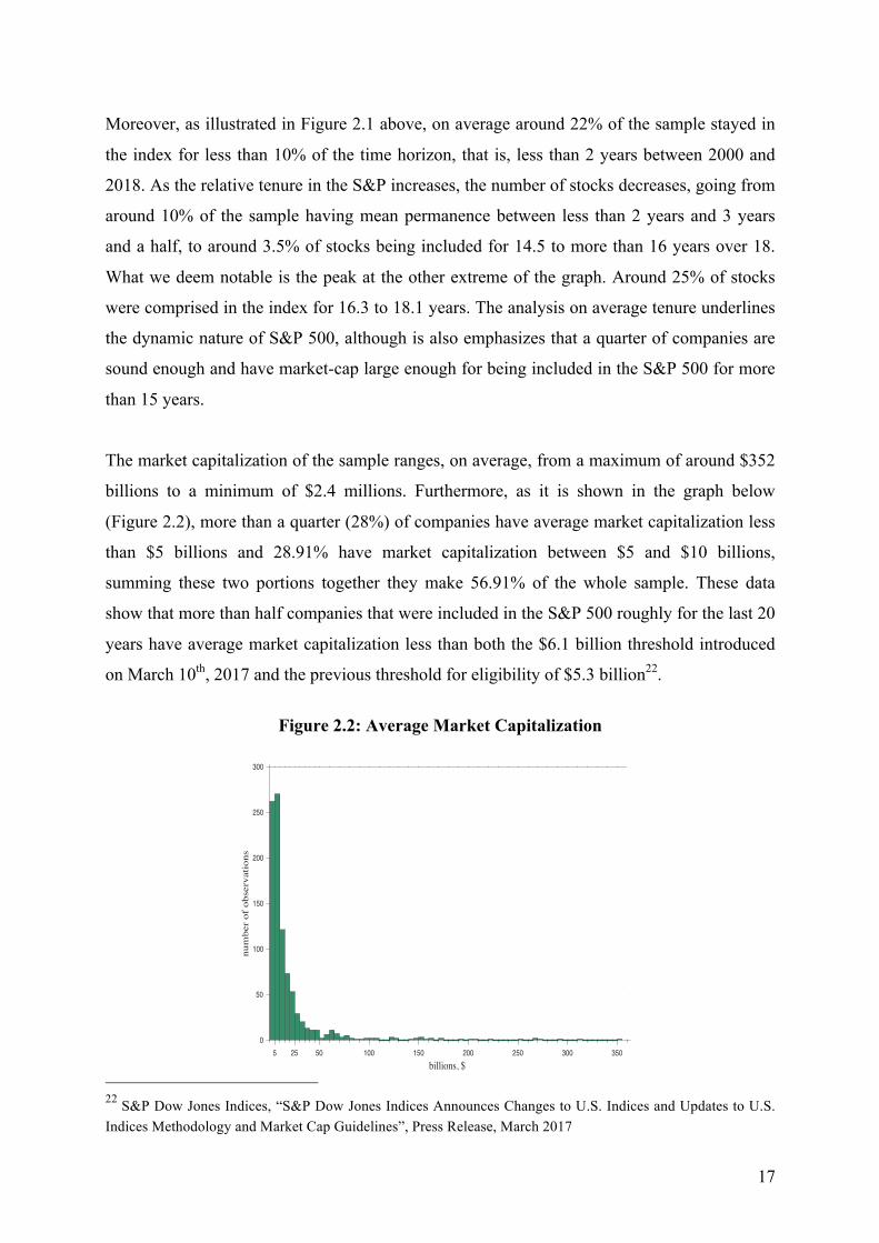
The market capitalization of the sample ranges, on average, from a maximum of around $352
billions to a minimum of $2.4 millions. Furthermore, as it is shown in the graph below
(Figure 2.2), more than a quarter (28%) of companies have average market capitalization less
than $5 billions and 28.91% have market capitalization between $5 and $10 billions,
summing these two portions together they make 56.91% of the whole sample. These data
show that more than half companies that were included in the S&P 500 roughly for the last 20
years have average market capitalization less than both the $6.1 billion threshold introduced
on March 10th, 2017 and the previous threshold for eligibility of $5.3 billion22.
Figure 2.2: Average Market Capitalization
22 S&P Dow Jones Indices, “S&P Dow Jones Indices Announces Changes to U.S. Indices and Updates to U.S. Indices Methodology and Market Cap Guidelines”, Press Release, March 2017
5 25 50 100 150 200 250 300 350billions, $
0
50
100
150
200
250
300
num
ber
of o
bser
vati
ons

18
In particular, 29 companies have average market cap between $0 and $1 billion, 34
companies’ mean value is between $1 and $2 billion, 45 between $2 and $3 billions, 72
between $3 and $4 billions, 82 companies have mean market capitalization between $4 and
$5 billions, only 71 companies over 934 total observations have average market capitalization
between $5 and $6 billion dollars and 63 companies between $6 and $7 billions. This
underlines the fact that around 28% of companies that have been included in the Index during
the period of 2000 to 2018 had mean market capitalization lower than the threshold needed
nowadays for inclusion. Consistently with the analysis on permanence, market capitalization
data points highlight the high turnover rate of companies entering and exiting the S&P 500.
Cash flow from operating activities (CFO) represents the amount of money a company brings
in from its on-going regular business activities; it only focuses on the core business and it is
calculated as earnings before interest and depreciation minus taxes, not taking into account
capital spending or working capital requirements since they could be considered one-time
activities23.
In our sample, we are considering CFO per share; the maximum mean CFO value equals
$50.24, while the median value is higher ($52.34). On the other hand, the minimum mean
value per share amounts to -$17.81 and the minimum median value equals -$26.16.
Over a total of 958 observations, circa 2.5% of the total mean values for cash flow from
operations per share are negative, whether instead companies’ CFO should usually be
positive: if cash flows from operating activities are negative for a long time a business may
struggle, since it is not generating enough cash to pay for its operating activities24.
Moreover, from the graph below (Figure 2.3) it is visible that more than half of our sample
has mean cash flow from operations per share between $0 and $4 dollars and around 85% has
mean CFO per share between 0 and $10 dollars.
23 Ross, S., Westerfield, R., Jaffe, J., “Corporate Finance”, Sixth Edition (2002) 24 Ross, S., Westerfield, R., Jaffe, J., “Corporate Finance”, Sixth Edition (2002)

19
Figure 2.3: Average Cash Flow From Operations per share
Overall, during the period from January 2000 to February 2018, the maximum average value
for CFO per share equals $50.24, while the median value is $52.34; the minimum mean
amount is -$17.81, while the minimum median value equals -$26.16.
We computed the mean and median values of Book Value per share (BV), which is the per-
share accounting equity value of a firm25, for each company belonging to the sample during
the time horizon considered (Figure 2.4).
On average, the maximum value equals $312.2, while the maximum median value equals
$317.1; on the other hand, the minimum mean value is -$48.15 and the minimum median
value equals to -$64.85.
25 Ross, S., Westerfield, R., Jaffe, J., “Corporate Finance”, Sixth Edition (2002)
-20 -10 0 10 20 30 40 50 60US dollars ($)
0
20
40
60
80
100
120
140
160
180
num
ber o
f obs
erva
tions

20
Figure 2.4: Average Book Value per share
The 3.23% of sample companies has negative mean book value per share between January
2000 and February 2018 that is, their liabilities exceed their assets. Negative book value firms
are typically perceived as financially distressed and, although the majority of those firms
survive for a long time, they continue to report negative book value for several years26. A
possible explanation for those many firms in our sample having a book value less than zero
can be found analysing R&D expenditures, as it is studied that they impact book value and
earnings value (see Jan C.-L. and Ou J. A. (2012)) especially in the industries of Health Care,
IT and Consumer Discretionary. Around 56% of our sample book value per share is, on
average, comprised between 0 and $15 dollars. Moreover, more than 80% of companies have
mean Book Value per share between 0 and $35 dollars.
The Global Industry Classification Standard (GICS) was developed in 1999 by S&P Dow
Jones Indices and MSCI. This classification is based on a company’ core business (based on
its accounting) and consists of 11 Sectors, 24 Industry groups, 69 Industries and 158 sub-
industries. During the 18 years under consideration the majority of companies that were
included in the S&P 500 belonged, in median, to the Consumers Discretionary sector. The
comparison of the median company sector to the “last” sector (the sector companies belonged
to on February 2018) in the graph below (Figure 2.5) shows that approximating the sector
value with the median is overall close to the most recent companies’ sector. There are some
26 Ching-Lih Jan and Jane A. Ou (2012) Negative-Book-Value Firms and Their Valuation. Accounting Horizons: March 2012, Vol. 26, No. 1, pp. 91-110.
-50 0 50 100 150 200 250 300 350US dollars ($)
0
50
100
150
200
num
ber o
f obs
erva
tions

21
discrepancies between median and “last” sector especially for what concerns the Consumer
Discretionary and the Information Technology ones. The portion of companies operating in
the consumer discretionary and in the information technology sectors shrank in favour of the
sectors of Health Care, Financials and Real Estate.
Figure 2.5: Sector Breakdown
In general, around 16.2% of companies belonged to the Consumer Discretionary sector, then,
Information Technology has the second biggest stake in the S&P 500 during the period
considered (around 15.14%) followed by Financials (14.6%) and Industrials (11.7%). The
sector in which the lowest number of companies operated is real estate (1.5%) as of the
median; if we take into account the “last” sector record, Real Estate increased by 1.7
percentage points (3.2%), with a decrease in the most numerous sectors.
Average sample prices (Figure 2.6) range from a maximum value of $733.2 dollars per share
to a minimum of $0.28 per share. Even though this seems quite a wide span, it is notable to
report that more than 82% of the sample observations has mean price comprised between 0
and $60.
Energy
Materia
ls
Indus
trials
Consm
er Disc
r.
Consu
mer St.
Health
Care
Financ
ials IT
Commun
icatio
n
Utilities
Real E
state
Sector (GICS)
0
20
40
60
80
100
120
140
160
180
num
ber o
f obs
erva
tions Median Value
Last Record

22
Figure 2.6: Average Share Price
Sample share prices are quite heterogeneous compared both among cross-sectional objects
and in time. In particular, standard deviation of share prices reaches peaks in the region of
thousands; the mean sample standard deviation equals 25.73, while the median equals 15.3.
The strong volatility that affected sample prices can be adduced to the 2007-2008 financial
crisis’ impacts on the market.
Sample mean returns are distributed between a minimum of -10.15% and a maximum average
return of 15.8%. The majority of companies’ average returns is comprised between 0 and 5%,
with around 30% of cross-sectional observation providing mean returns of 1% to 1.5% as
shown in the Figure 2.7 below. The distribution of aggregated mean returns is skewed to the
right and leptokurtic.
Figure 2.7: Average Returns
0 100 200 300 400 500 600 700US dollars ($)
0
20
40
60
80
100
120
140
160
180
200
220
num
ber o
f obs
erva
tions
-10% -5% 0 5% 10% 15%0
50
100
150
200
250
300
num
ber o
f obs
erva
tions
return

23
We also computed skewness and kurtosis for individual cross-sectional observations. The
maximum skewness value is 8.85 while its minimum value equals -3.42. Furthermore, as we
can see from the graph (Scatterplot 1), the majority of observations are centred on zero, that is
characteristic of normal distributions together with a kurtosis around 327. The sample mean
skewness of returns equals 0.49 while the median equals 0.23; 57.2% of observations’
skewness is between -0.5 and 0.5.
Scatterplot 2.1: Skewness and Kurtosis of Returns
The kurtosis of sample returns has maximum value equal to 105.5 and minimum value equal
to 1. As we can see graphically the majority of observations is centred between 4 and 5; the
mean kurtosis among companies’ returns equals 7.97 while the median is 5.2; around 6.3% of
distributions of stock returns in the sample have kurtosis between 3 and 3.5, while the
majority of distributions are leptokurtic.
For what concerns sustainability, there has been a clear shift toward higher scores during
time. The comparison of ESG scores referring to December 2006 (the first month for which
ESG MSCI scores are available) with the ones related to February 2018 (the last entries)
suggests an increase in scores’ plurality and an overall shift toward higher values: in 2006 the
highest ESG score was 8.94 while the lowest was 1.63, while in 2018 the maximum grade
was 9.45 and the minimum was 1.89.
Also Environment and Governance scores experienced an increasing trend through time (0.28
– 8.63 in 2006 to 1.11 – 9.81 in 2018; 0 – 9.5 in 2006 to 1.17 – 9.88 in 2018 respectively),
Social score instead had higher extreme values in 2006.
27 Wooldridge M. J. (2013),: “Introductory Econometrics: A Modern Approach”, Fifth Edition
-4 -2 0 2 4 6 8 10skewness
0
100
200
300
400
500
600
700
800
900
1000
Num
ber o
f Com
pani
es
Skewness of Sample Returns
0 20 40 60 80 100 120kurtosis
0
100
200
300
400
500
600
700
800
900
1000
Num
ber o
f Com
pani
es
Kurtosis of Sample Returns

24
Figure 2.8 illustrates the aggregate observations of companies’ mean ESG scores. In the
specific case of average ESG scores, we can distinguish 7 “buckets”, out of a total of 10, in
which companies are classifies by their grade. The average ESG score ranges from a
minimum value equal to 1.48 to a maximum value of 7.74, similarly, the maximum median
score equals 7.75, while the minimum median value is 0.9.
Figure 2.8: Average ESG Score
Companies aggregated in different score buckets have different characteristics, on average,
with respect to those related to the whole sample. In relation to permanence of stocks in the
S&P 500 (“isconstant”), as the mean ESG score increases also the average time stocks are
included in the Index increases (Table 2.1, Appendix). On average, the companies with mean
ESG score between 1 and 2 stay in the S&P 500 around 40% of the time period considered,
while the ones with mean grade between 7 and 8 stay around the double, 80% of the time
period considered.
Based on the fact that market capitalization magnitude is a fundamental parameter for
eligibility in the S&P 500, we would expect that those companies with largest market
capitalization are the ones that have longer tenure in the Index since they always exceed the
chosen threshold, and, consequently from above, the companies with longer permanence are,
on average, those having highest mean ESG score. Instead, the market capitalization for
companies with lowest mean ESG score equals to $27.8 billions, that is, on average, higher
1 2 3 4 5 6 7 8 9 10ESG Score (MSCI*)
0
50
100
150
200
250
300
num
ber o
f obs
erva
tions
*Reproduced by permission of MSCI ESG Research LLC. ©2018 MSCI ESG Research LLC. All rights reserved.

25
than the values related to buckets 2 to 5, which on the contrary increase gradually. Companies
belonging to bucket 6 have $35.29 billions market capitalization and the 7th bucket almost
doubles that value to $70.30 billions. On the other hand, the median market capitalization
(Table 2.2) is highest for companies in bucket 1 ($15.14 billions). On average, companies
having the largest market capitalization in the sample are the ones with highest ESG rating,
but there is an higher number of large-cap companies having mean ESG score between 1 and
2. The biggest companies pay more attention toward improving their sustainability through
time; however, it is not true that the bigger is the company the higher is the score.
Companies with mean ESG rating between 1 and 2 have, on average $2.88 on cash flow from
operating activities per share, while the ones belonging to the last bucket have on average
$3.89 of cash flow from operations per share. Notwithstanding the overall increase in CFO
per share with respect to the first bucket, there is not a clear pattern of increase, as the peak
value is $4.67 that is the mean value for the companies having rating between 4 and 5. The
same phenomenon also applies to Book Value per share and Price. In both variables there is a
clear increase if we compare the value related to bucket 1 firms with the value in the last one,
but the highest average value is reached in the intermediate bucket, the one comprising
companies with mean ratings between 4 and 5. Book value per share goes from $7.92 in
bucket 1 to $12.72 in bucket 7, with a maximum of $17.69. Average price of companies in
bucket 1 equals $35.33, peaks at $49.56 in bucket 4 and it stays between $50 and $40 for the
higher buckets. Contrarily, returns on average are higher for the companies in bucket 1
(1.93%) than in the last bucket (1.07%) and follow a decreasing pattern.
We also investigated how the disaggregated ratings for Environment, Social and Governance
behave on average in each ESG score bucket; Environment and Social rating have similar
values, even though E mean scores are higher than S mean scores 5/7 times. Both E and S
mean scores for each bucket are in line with the ESG ones’ averages, whereas they are higher
than their own mean values, as reported in Table 2.3 and Table 2.5. This could be due to the
fact that the mean ESG rating goes from 1 to 8, while disaggregated mean scores for
Environment take values from 0 to 10 and for Social are contained between 0 and 9; in the E
case there are two buckets (8 and 9) accounting for 1.31% of the sample that have grade
between 8 and 10, and only 1 bucket (rating 0 to 1) accounting for 0.39% of the sample that
are redistributed over 7 ESG buckets. For the Social side, 0.13% of the sample has average S
score between 0 and 1 and 0.65% of sample observations between 8 and 9. The disaggregated
governance score ranges from 4.22 as mean value for bucket 1 to 6.83 for bucket 7; mean G
score itself has a minimum value equal 1.51 and a maximum 9.52 (Table 2.7), which means it

26
lacks a 0 to 1 rating bucket although presenting both buckets with grades from 8 to 10.
Redistribution of companies with high G rating impacts every mean ESG bucket, especially
the first ones, letting the mean value of governance be flattened throughout aggregated mean
ESG buckets.
Furthermore, companies classified by different mean ESG score also belong to different
industry groups, as illustrated by Graph 2.1 to 2.7 in the Appendix. Bucket 1 companies
operate in the industries of Food, Beverage and Tobacco, of Media and of Materials (Graph
2.1). On the other hand, companies that have mean ESG scores between 7 and 8 belong to the
industries of Utilities, Semiconductors & Semiconductor Equipment, Technology, Hardware
& Equipment, Software & Services, Real Estate and Materials (Graph 2.7).
Companies operating in the Materials’ and Utilities’ industries are present in all buckets and
represent, respectively, 9.3% and 7.7% of the entire sample. Semiconductors &
Semiconductor Equipment, Software & Services, Technology, Hardware & Equipment, as of
the Global Industry Classification Standard (GICS) belong to the same Sector: Information
Technology. The companies operating in this sector have a sound presence in buckets with
higher average ESG score; however, even though their trend is alike, the first two industries
tend to be more concentrated in higher rating buckets, while companies in Technology,
Hardware & Equipment are more spread out.
The Financial Sector comprises Diversified Financials, Banks and Insurances; companies
operating in the Diversified Financials industry are prevalently classified with average ESG
score between 6 to 7, while “banks” are much strongly concentrated in bucket 4. The Real
Estate companies prevalently have intermediate average ESG score. Industries in Capital
Goods have mean rating from 3 to 7 and their presence grows as scores become higher.
Companies in the Automobiles & Components Industry have mean ESG rating between 4 and
7. Companies operating in Food, Beverage and Tobacco industry are well distributed in all
buckets except for the last one. It is also interesting to underline that governance, social and
environmental issues have a different impact on different industries for what concerns both
return on equity and earnings’ risk28. For example, the industries represented by those
companies classified in the last bucket (ESG score between 7 and 8) had the environment as
main driver for return on equity: Materials - environment, Real Estate - environment and
social, Utilities - environment and governance. Whereas IT ROE was mainly related to
governance. In the same way, environment is also the major risk driver for the previous 28 Subramanian for BofA Merrill Lynch (2018), “The ABCs of ESG”, Table 1.

27
industries, except for IT, whose main issues are believed being in the governance and social
areas (see Subramanian (2018)).
The average Environment (E) score ranges from a maximum equal to 9.43 to a minimum of
0.45; the median values are contained in the set 0.3 to 10. In this case, the mean scores are
more diverse among companies, which are classified in 10 buckets as illustrated in Figure 2.9.
Histogram 2.9: Average Environment Score
As for the average ESG score, the variable isconstant follows an increasing trend from bucket
1 to 9; companies in bucket 1, which are now the ones having mean E rating between 0 and 1,
were included in the S&P 500 for 25% of the time period under analysis (Table 2.3).
Companies in bucket 2 (rating 1 to 2) on average stayed in the S&P 500 for around 35% of
the time period considered and this value more than doubles (75%) for companies belonging
to bucket 8 (rating between 7 and 8), reaching 82% in bucket 9. Differently from before,
companies with the highest E rating (9 to 10), on average, are present in the Index for only
6% of time. This could be counterintuitive in some way, however, considering the small
percentage of sample observations (0.26%) the last bucket accounts for we should always
bear in mind there could be not enough variance in the extreme buckets for the mean values to
have an explanatory meaning.
1 2 3 4 5 6 7 8 9 10E Score (MSCI*)
0
20
40
60
80
100
120
140
160
180
200
num
ber o
f obs
erva
tions
*Reproduced by permission of MSCI ESG Research LLC. ©2018 MSCI ESG Research LLC. All rights reserved.

28
Market capitalization’ mean values follow an increasing pattern from bucket 1 to bucket 9 and
then decrease. Companies with mean Environment rating between 0 and 1 have average
market capitalization equal to $5.57 billions, the amount increases up to $20.04 billions for
companies with rating between 5 and 6 and more than doubles at $42.54 billions in the
penultimate bucket. Again, there is a downturn to $6.92 billions for companies with average E
rating between 9 and 10.
For what concerns the Cash flows from operations per share, there is a clear overall growth in
values as we go from the first bucket ($2.59) to the to the last bucket ($5.29), anyway the
pattern is not steady throughout all the buckets.
The average Book value per share is highest form companies with intermediate E mean score:
it starts at $11.85 in bucket 1 and grows up to $18.31 in bucket 5 that is the peak, and then it
decreases to $8.85. As for average ESG aggregated score, buckets with the lowest mean E
score have the lowest price per share ($29.61 for bucket 2 and $33.74 for bucket 1). The stock
price of low-intermediate buckets (from 3 to 6) ranges around $40-$45 and reaches up to
$46.02, while the mean value for the higher buckets peaks at $113.97 (bucket 10). For what
concerns returns, companies in bucket 1 have the highest mean return (2.46%) followed by
those in bucket 10 whose mean overall return equals 1.60%.
Analysing how the S score is distributed among E buckets, we can see from Table 2.3 that
there is a particularly high grade for bucket 1, which, instead of being between 0 and 1 equals
4.42; this is almost equal to the mean rating 4.43 of the bucket 5. The range of mean social
score goes from 2.92 (bucket 2) to 7.26 for bucket 10, this could be interpreted as that the
highest social scores were held by companies with low or intermediate E scores, on average,
flattening a bit the differences in mean S score among E buckets. This is also true for the
Governance mean scores related to E buckets, as their range goes from 4.28 to 6.42. Even
though the difference in governance mean rating among those buckets is not sharp, the high-
intermediate buckets have higher G rating than the low-intermediate ones. In opposition to S
scores, the G score for bucket 10 is the second lowest (4.47) after bucket 1 (4.28).
The average Social (S) score has maximum value of 8.41, while the maximum median value
is 9; on the other hand, the minimum mean value equals 1, while the minimum median value
is 0.

29
Histogram 2.10: Average Social Score
Differently from the two cases discussed above, the average portion of time companies were
included in the index ranges from 9%, which is a lot lower than 39.53% for companies
aggregated by ESG score, to 72% (Table 5), which is lower with respect to maximum tenure
both of companies classified by mean ESG (80.03%) and by mean Environment score (82%).
Companies with average Social score between 0 and 1 were included in the S&P 500 for
around 9% of the time period considered; this amount quadruples in bucket 2 and keeps
increasing up to 72% in bucket 7 (rating 6 to 7), that is the highest value. Companies with
highest average S score were included in the index for circa 66-67% of the time period
considered. Market capitalization ranges from $12.91 billions in bucket 9 to $29.8 billions in
bucket 7 and does not follow a clear path; we could say that the low-intermediate buckets
have lower mean market-cap values compared to the high-intermediate ones overall, except
for bucket 10. CFO per share ranges from $1.81 to $4.38, with the intermediate buckets
having the highest mean values; this pattern is true in all four ways the data is being analysed
(ESG score buckets, E score buckets, S score buckets, G score buckets).
The mean book value per share ranges from $10.77 (bucket 2) to 17.87 (bucket 8), with
companies in the buckets with low-intermediate rating having mean book values lower than
the ones classified into high-intermediate buckets overall, except for bucket 9, which has the
second lowest mean book value. Average price per share reaches its maximum value ($61.69)
1 2 3 4 5 6 7 8 9 10S Score (MSCI*)
0
50
100
150
200
250
300
num
ber o
f obs
erva
tions
*Reproduced by permission of MSCI ESG Research LLC. ©2018 MSCI ESG Research LLC. All rights reserved.

30
in bucket 1 and its lowest value at bucket 2 at $33.78, then it varies between $42 and $54. As
before, average returns are highest for companies with lower average Social score (2.29%)
and in this case companies with lowest returns are the ones having mean S score comprised
between 7 and 8; in general, there is a decreasing trend are S score increases.
The average Environment score related to S rating buckets ranges from 2.72 to 6.36, while the
Governance score ranges from 5.03 to 6.51 (Table 5).
Both mean and median for the Governance score (G) are distributed between 1 and 10
(Histogram 10).
Histogram 2.11: Average Governance Score
Comparing the average G score with E and S ones, it is significant to underline that average
scores comprised between 0 and 1 are missing, differently from the other two cases. G mean
scores appear to be distributed toward higher values, which may be the case considering the
fundamental role that governance covered during time, also before being taken into
consideration for sustainability purposes. The percentage of average permanence in the S&P
500 between the 2000s and 2018 ranges from 13% of companies in bucket 8 to 67% of bucket
5, and has its lowest values in buckets 8 and 9 (may be due to scarce variance inside the
buckets). Average market capitalization follows an overall decreasing trend from bucket 1 to
9, in particular, the average market capitalization of companies that have mean Governance
1 2 3 4 5 6 7 8 9 10G Score (MSCI*)
0
50
100
150
200
250
300
num
ber o
f obs
erva
tions
*Reproduced by permission of MSCI ESG Research LLC. ©2018 MSCI ESG Research LLC. All rights reserved.

31
score between 1 and 2 equals $29.72 billions as reported in Table 7. On the other hand,
companies with governance rating between 8 and 9 have $0.71 billions market-cap and
companies the ones with scores 9 to 10 have market-cap equal to $1.36 billions on average;
however, looking at the median market capitalization that range narrows, with minimum
value equal $1.59 billions and maximum value $9.43 billions. In this case, companies with
the highest G scores have the lowest median market-cap, even though bucket 6 is the one with
highest median market-cap, followed by bucket 1 ($8.22 billions). The differences between
mean and median values suggest that aggregating companies through Governance score
means combining together few companies with very high market-cap and many companies
with lower market capitalization. Average Cash Flow from Operating activities per share
ranges from $0.82 to a maximum of $4.19, and the buckets with higher values are the ones
composed by companies with intermediate governance scores. Mean book value per share is
highest for companies classified in low-intermediate buckets, while median book value per
share follows a clear decreasing path from bucket 1 to 9 values. Returns are higher, on
average, for companies with higher governance mean score (0.97% in bucket 1- 2.03% in
bucket 8). As G score increases, on average, both E and S scores increase in general.
Companies classified by average G score between 0 and 1 have E score equal to 3.67 and S
score equal to 3.22, while those with highest average G score are characterized by E and S
scores amounting to 7.65 and to 5.62 respectively.

32
3 Factor Analysis
The aim of this Chapter is to analyse whether portfolios composed by companies with higher
ESG score have been more profitable than the ones with lower ESG score during the time
period considered. We base the construction of those portfolios on two assumptions, first, that
the S&P 500 is a good proxy for representing the whole market, secondly, that a fair game is
based on equal starting conditions.
The “market portfolio”, as defined by Black, Jensen and Scholes (1972), would represent an
investment in every outstanding asset in proportion to its value. It has long been debated
about how to best proxy the market portfolio for conducting tests on CAPM or on market
efficiency and many empirical studies employed the Standard & Poor 500 for this purpose.
That assumption is backed by the fact that the Index amounts to 80%29 of the total market
capitalization of the entire stock market (as of 2018), that is, it is weighted by a wide number
of market values, much larger than those of other well-known indices as, for example, the
Dow Jones Industrial Average (DJIA). Moreover, the fact that its components are all actively
traded stocks also renders it attractive as market portfolio proxy. On the other hand, it is
important to underline that the companies we consider for our portfolios are those included in
the S&P 500 each month because the great majority of them is large-cap firms ($10 - $100
billions market capitalization typically), which means that even when we talk about small-
cap-firms portfolios (in general firms with $300 million - $2 billion market capitalization),
instead we consider smaller large-cap firms.
Our second assumption refers to the fact that we decided to implement factor-based strategies
and only afterwards we implement our ESG score strategy on top of them. The purpose of
building factor portfolios is to aggregate companies with similar characteristics and to
investigate how ESG score impacts on returns controlling for other variables. Moreover,
considering the rise in ESG investing, to base an investment strategy solely on ESG score
could be misleading causing to overpay for perceived quality. Subramanian (2016) reports
that combining ESG strategies in conjunction with fundamental attributes like valuation,
growth and quality outperformed fundamental strategies alone with lower risk.
The theoretical possibility that factors other than movements in the market portfolio were
needed in order to have a better understanding of future financial performance was recognized
in Asset Pricing Theory at least since Merton (1971, 1973a). One of the most popular 29 S&P Dow Jones Indices, “Equity, S&P 500 Factsheet”, as of December 31, 2018

33
multifactor models is the Fama–French one, which is the subject of several empirical studies.
Fama and French (1996) show how the three-factor model performs in evaluating expected
return puzzles beyond the size and value effects that motivated it. Carhart (1997) extends the
Fama-French three-factor model by including a fourth common risk factor that accounts for
the tendency of firms with positive past returns to produce positive future returns and vice
versa for negative past results. In general, implementing a factor analysis means analysing the
underlying exposures of stocks to identify which factors are providing the best risk-adjusted
returns for investors. A multifactor approach to portfolio construction can smooth returns and
control volatility since factors tend to be relatively uncorrelated from one another and so they
perform under different market conditions and cycles.
In light of those considerations, we created portfolios oriented at targeting the factors of size,
value and momentum following the previous studies conducted by Fama and French (1993)
and Cahrart (1997).
The Size factor refers to a firm’s market capitalization (stock price times shares outstanding).
Historically, portfolios consisting of small-cap stocks exhibit greater returns than portfolios
with large-cap stocks; the intuition is that smaller companies tend to outperform larger ones
rewarding investors for bearing more risks related to illiquidity and high sensitivity to market
movements.
The Value factor aims at capturing excess returns from stocks that have low prices relative to
their fundamental value and it is commonly tracked by price-to-book or price-to-earnings.
Stocks that have market values that are small relative to the accountant’s book value are
called “value stocks”, while the so called “growth stocks” have higher price versus book
value. During time, scholars and investment professionals have argued that value strategies
outperform the market (Graham and Dodd (1934) and Dreman (1977)). These strategies are
based on buying stocks that have low prices relative to earnings, dividends, book assets, or
other measures of fundamental value (see Lakonishok (1991)) and, in particular, Fama and
French (1992) show that stocks with high book/price ratios (BE/ME) earn higher returns.
Further works both extended and refined these results (Rosenberg, Reid, and Lanstein (1984);
Chan, Hamao, and Lakonishok (1991) and Fama and French (1992)).
The Momentum factor is based on the empirical evidence that stocks that have outperformed
in the past tend to exhibit strong future returns and consists of differentiating between stocks
with positive and negative past excess returns. Carhart (1997) calls this additional risk
dimension a price momentum factor and estimates it by computing return over the past 12
34
months skipping the most recent one. Although there are sound economic reasons for these
trends to continue (e.g., company revenues and earnings that continue to grow faster than
expected), it may also be the case that investors periodically underreact to the arrival of new
information (see Chan, Jegadeesh, and Lakonishok (1999)). De Bondt and Thaler (1985,
1987) argue that extreme losers outperform the market over the subsequent several years and
despite significant criticisms (Chan (1988) and Ball and Kothari (1989)), their analysis has
typically stood up to the tests (Chopra, Lakonishok, and Ritter (1992)).
The fundamental step is then addressing the impact of ESG integration on value, size and
momentum strategies.
From investors’ point of view, the ESG framework as it is now structured might be new,
however, the underlying concepts and issues addressed are well known to value investors
since non-financial issues (including corporate culture, employee satisfaction and governance)
play an integral part for fundamental investors to determine the value of a business and derive
investment decisions (see Hanson and Fraser (2013)).
Specifically, Artiach et al. (2010) and Subramanian (2016) demonstrate that there is a strong
link between a firm’ sustainability rating and its size. This positive relation can be attributed
to an increasing investor demand and pressure by shareholders, the general public and media
toward more sustainable business models rather than resulting from genuine internal beliefs-
based decision. Thereon, small firms with a genuine interest in increasing their sustainability
performance that, on the other hand, are restricted by financial and human resources, are in a
disadvantageous position.
For what concerns value and ESG score it is clear that there is a close alignment of the
theoretical underpinnings of value with sustainable investing. The notion of “sustainable”
comprises the concept of the business “being able to continue over the long run”, that is a
crucial concept for value investors with regard to firms’ long-term success. Nevertheless,
fundamental (value) investors and ESG investors’ consensus is prevalently widespread in
Europe and the U.K., whereas U.S. investment managers are more skeptical about the benefits
of sustainable investing (van Duuren et al (2015)).
For what concerns momentum, Kaiser (2018) finds a negative relation between ESG ratings
and momentum; the reason could lie in the fact that momentum is associated to media
coverage (Hillert et al., 2014), which leads companies currently experiencing an upward trend
in returns to pay less attention to their sustainability performance, while stocks that are
currently showing a downward trend increase their sustainability performance to send a

35
positive signal to the market. Consequently, considering that the ESG phenomenon has
experienced a significant increase in popularity only in recent years, the highly rated ESG
stocks may still show low levels of price-return momentum.
3.1 Portfolio construction
The stocks considered for the factor analysis are those effectively included in the S&P 500
each month, for this purpose we built a variable “Nan_isconstant” to obscure all the stocks
that exited the Index each time. In second instance, we implement the three strategies, each
one distinctly from the other two, based on factors: size, value and momentum. We rank
stocks on a monthly rolling basis depending on their end-of-month market capitalization
(size) in descending order, share price-to-book value (value) in ascending order and
momentum in descending order.
Specifically, we rank stocks based on their end-of-month market capitalization, following a
similar procedure as Asness, Moskowitz and Pederson (2013) and MSCI in the definition of
the universe of stocks to include in its global stock indices. For value factor, we sort
individual stocks using as signal the ratio of the end-of-month share price of equity to end-of-
year per share book value of equity, or price-to-book ratio (PBV), that is the per-share inverse
of BE/ME (see Fama and French (1992, 1993) and Lakonishok, Shleifer, and Vishny (1994)),
of the stock. For momentum, we use the common measure of the past 12-month cumulative
simple return on the asset (see Jegadeesh and Titman (1993); Asness (1994); Carhart (1997)
and Grinblatt and Moskowitz (2004)), skipping the most recent month’s return. We skip the
most recent month, which is standard in the momentum literature, in order to avoid the 1-
month reversal in stock returns, which may be related to liquidity or microstructure issues
(Jegadeesh (1990); Lo and MacKinaly (1990); Jegadeesh and Titman (1993); Boudoukh,
Richardson, and Whitelaw (1994); Asness (1994); Grinblatt and Moskowitz (2004)).
After being sorted by factor, data is allocated in 10 clusters composed, ideally30, by 50 stocks
each. This means that, over around 500 stocks we ordered data by factor (three different
orders), we collected returns attached to the ranked stocks and divided them in deciles (10 sets
with a total of 30 sets).
30 The last portfolios (i.e. 9 and 10), especially, may comprise fewer observations than 50 due to either missing data from factors’ variables or because stocks included in the Index are not exactly 500 (for example the number of S&P 500 constituents equalled 505 as of December 2018 but may also be lower) or both.

36
For what concerns size portfolios, stocks are ranked in descending order. In the first portfolio
are present the companies with the highest market capitalization (big), while in the 10th there
are the ones with the lowest market-cap inside the S&P 500 (small). Stocks in value portfolios
are ranked for ascending price-to-book value per share, which means that in the first set there
are stocks with high book value with respect to price, the so called value stocks, while in the
10th portfolio there are growth stocks, the ones characterized by high price versus accounting
equity value. Momentum-ordered portfolio 1 comprises stocks that had the highest return in
the preceding year (skipping the last month), those that are commonly known as winners,
while previous year’s losers are classified in the last sets.
Finally, we apply the ESG score strategy on each of the 10 deciles. The “ESG strategy”
applied consists of additionally sorting stocks by their Weighted Average Key Issue Score,
with threshold score equal 5. Returns of stocks with sustainability rating higher than 5 are
divided from those with rating lower or equal to 5 and returns from the two groups are
aggregated into two equally weighted portfolios for each decile for each factor. We chose 5 as
threshold instead of 5.7 (that is the score related to the MSCI “A” final rating) based on the
overall distribution of ESG scores across the Index. Mean and median scores of S&P 500
companies’ are distributed between 4.4 and 5.4 and 4.2 and 5.4, respectively, through time.
Since mean ESG scores for individual stocks average out at 4.72 we chose to consider the
highest half of BBB stocks (4.3 to 5.7 for MSCI) and all A to AAA stocks, in order to have
enough variance also when splitting the last deciles. Moreover, we chose to integrate ESG
scores on top of our factor strategy in order to take advantage of the financial benefits of
employing full integration, which, together with engagement, is considered the most
beneficial ESG strategy by relevance to investment performance (see Amel-Zadeh and
Serafeim (2018)). Negative screening strategies (we could have excluded sectors or
companies from our sample) are instead the least beneficial and are prominently driven by
ethical considerations rather than from financial ones.
To summarize, we analyse 60 portfolios differentiated first by factor and secondly by ESG
score and monthly rebalanced over a period of 135 months, from December 2006 to February
2018 (Figure 3.1.1 to 3.1.3, Appendix).
3.2 Performance
«Mainstream investors constantly searching for larger returns have come to the conclusion
that a company that considers their material Environmental, Social, and Governance
37
opportunities and risks in their long-term strategies will outperform and outcompete those
firms that do not.» (Coppola L.31 (2018)).
Our factor analysis partially supports this statement. An upfront investment of $100 on
December 2006 would have yielded at most $554 for a size investor, $1180 for a value
investor and $403 for a momentum investor on February 2018 (Figures 3.2.7 to 3.2.9,
Appendix). High ESG Size portfolios had lower annualized returns32 with respect to their low
ESG counterparty during the period 2006 – 2018, while they clearly outperform low ESG
portfolios in the period 2013 – 2018 as reported in Table 3.2.7 (Appendix). In particular,
investing in small-cap high ESG portfolios in the past five years yielded positive returns
while their low ESG counterparty returns were negative. Value investors also would have
earned positive returns from 2013 and less negative returns from 2006 investing in high ESG
portfolios versus low ESG ones, but in general low ESG portfolios outperformed high ESG
ones since growth low ESG stocks yielded higher returns than their high counterparty.
Momentum investors would have been better off investing in high ESG portfolios.
Considering both time horizons high ESG portfolios outperformed low ESG ones, especially,
returns from momentum strategy are all positive, instead portfolio 10 low ESG had negative
returns in the “long-run”. For what concerns strategies, High ESG growth investors during
both periods earned the highest returns with respect to size and momentum investors; while
small-cap investors earned the lowest returns with respect to value and momentum ones in
both periods. Momentum portfolios had lower but more stable and homogeneous returns in
general. Relative to Low ESG portfolios, value-strategy yielded both the highest returns for
growth portfolios but also the most negative ones for value portfolios in the long run, while
small-cap low ESG investors earned the most negative returns in the last 5 years. Also in this
case, momentum investors in both periods earned lower returns that were more stable and
homogeneous and suffered lower losses. Maybe a sector specific framework would have
given sharper results; Subramanian et al. (2016) study that investments based on
Environmental Innovation (scores from Thomson Reuters) would have yielded a 3-year alpha
31 Louis Coppola is the Executive Vice President and co-founder of the Governance and Accountability Institute that is a sustainability consulting, research and advisory firm. G&A is the exclusive Data Partner for Global Reporting Initiative (GRI) for the United States, United Kingdom and Republic of Ireland (as of January 2018). 32 𝐴𝑛𝑛𝑢𝑎𝑙𝑖𝑧𝑒𝑑 𝑟𝑒𝑡𝑢𝑟𝑛 = (1 + 𝐻𝑃𝑅)! − 1 ;
where, holding period returns are calculated as 𝐻𝑃𝑅!!! = $ !"#"$%"&$ !"#$%&$'
= !!!!!!
;
𝑡 = 12/2006 𝑜𝑟 02/2013 ; 𝑡 + 𝑘 = 02/2018 and 𝑥!""# =!"!"#
; 𝑥!"#$ =!"!"
.
(Cochrane, Investment Notes (2006)).

38
of circa 30 percentage points for companies operating in Materials Industry and 20 ppt for
those operating in Energy, while they did not generate any excess returns for Consumer
Sectors’ companies.
Size portfolios comprising companies characterized by high market capitalization also have
higher ESG score, on average, than those composed by lower size companies. The positive
relation
The mean ESG score related to decile 1 (50 companies with average market capitalization of
around $150 billions) equals 5.21 and is the highest one; in general, all first 5 portfolios, that
are those composed by companies characterized by market capitalization higher than $15
billions on average, have higher scores (5.21- 4.9) than the lower 5. The difference in average
score between high and low (but same size) portfolios is wider for the first 5 size deciles (1.79
- 2.32 at maximum), while ranges between 1.90 to 1.98 points for lower market-cap
portfolios.
Furthermore, “big companies” portfolios have higher monthly mean returns versus “small
companies” portfolios. These features also apply after dividing size portfolios by low or high
ESG score. In particular, portfolios have since inception monthly mean returns ranging from a
minimum of -0.7% to a maximum of 1.38% with the “low ESG” outperforming the “high
ESG” in general. For what concerns returns, the 5 top performing portfolios are portfolio 3
low ESG (1.38%), portfolio 2 low ESG (1.36%), portfolio 5 low ESG (1.32%), portfolio 1
low ESG (1.27%) and portfolio 3 high ESG (1.26%); while the 5 worst performing are
portfolio 10 high ESG (-0.7%), portfolio 10 low ESG (-0.5%), portfolio 9 high ESG (0.2%),
portfolio 9 low ESG (0.4%) and v 8 low ESG (0.78%).
Standard deviation of portfolio returns ranges between 0.039 and 0.088. The first 5 high ESG
portfolios (those with higher market capitalization) have less variable returns than their low
ESG score counterparties; this reverses for the last 5 portfolios (those with lower average
market capitalization) as portfolios with lower ESG scores have lower standard deviation of
returns with respect to their counterparties.

39
Figure 3.2.1: Mean – Variance distribution of Size portfolios (2006 – 2018)
Returns from all 20 portfolios are all negatively skewed, except for deciles 6 and 8 high ESG
that have positive skewness equal to 0.1143 and 0.1137 respectively. Low ESG portfolios’
skewness ranges from -0.0047 (decile 10) to a maximum, in absolute terms, of -0.89 (decile
8), while high ESG portfolios have negative skewness ranging from -0.126 to -0.78.
Comparing the two groups’ skewness, the low ESG portfolios have fatter left tails, that is,
their returns distribution is asymmetric and extends towards more negative values, also the
majority of high ESG portfolios have negative skewness, but discriminating by the ESG score
investors can have the possibility to invest in those companies whose returns are positively
skewed, that is, extreme observations are positioned towards the positive end of the
distribution. Kurtosis of low ESG portfolios ranges from 3.87 in portfolio 1 to 7.56 in
portfolio 10; while for high ESG portfolios it ranges from 3.77 to 10.21. As market
capitalization decreases, kurtosis increases, that means there are more outliers in the data. We
can already conclude that our portfolios’ returns are not normally distributed and also the
Jarque-Bera test confirms this is the case.
In order to have a simple and intuitive “cost-benefit” comparison of the risk-return trade-off
of size portfolios with different sustainability scores, we divided average monthly returns by
their standard deviation, computing an “adjusted Sharpe ratio” (Table 3.2.1). This measure
shows how much each portfolio rewards investors for one unit of risk.
0.03 0.04 0.05 0.06 0.07 0.08 0.09Standard deviation
-0.01
-0.005
0
0.005
0.01
0.015
Mea
n re
turn
Scatter - Mean return and Volatility
LOW ESGHIGH ESG

40
Table 3.2.1: “Adjusted Sharpe Ratio” for size portfolios (2006 – 2018)
Portfolio
1
Portfolio
2
Portfolio
3
Portfolio
4
Portfolio
5
Portfolio
6
Portfolio
7
Portfolio
8
Portfolio
9
Portfolio
10
Low
ESG 0.30 0.29 0.30 0.25 0.29 0.25 0.15 0.16 0.07 -0.06
High
ESG 0.27 0.26 0.27 0.26 0.23 0.19 0.21 0.13 0.04 -0.08
In this case it is clear that, also adjusting for risk, size portfolios with lower ESG score had in
general higher returns than those with high ESG scores during the period 2006 to 2018.
Even though based on previous results low ESG portfolios seem to be the winners, statistical
tests do are inconclusive about this issue. We tested whether the differences in mean returns
between low versus high ESG portfolios were significantly different from zero and addressed
the non-normality of distribution by using bootstrapping for computing consistent standard
errors. Neither of the differences was statistically significant at any significance level.
Contrarily as we would expect, value-sorted portfolios composed by companies with higher
price-to-book value (growth stocks) have higher ESG score, on average, than those composed
by lower price-to-book value companies (value stocks) during the period under consideration.
This could be interpreted as that growth stocks were highly priced because of innovations that
could not be still visible in their metrics and part of that “innovation” could be related to
sustainability projects. Moreover, a reason may be intrinsic in the diverse structure of growth
companies versus value ones, if we believe that the majority of growth stocks in this sample
are also “growth companies” and vice versa for value. Growth stocks are expected to grow at
a faster pace than others and companies are not usually expected to pay dividends, since
investors base their profit on capital gains. This way, capital can be reinvested in the firm
more easily because investors will be focused on other key points. Value investors instead
mainly base their profits on dividends, which means that value companies tend to dedicate
some capital to pay dividends losing the opportunities of reinvestment inside the firm.
The average ESG score of value-sorted portfolios ranges between 4.64 (decile 1) and 5.13
(decile 9). The mean score related to decile 9 (companies with average PBV of around 6.34)
equals 5.134 and is the highest one; in general, the last 5 portfolios, those comprising
companies characterized by PBV higher than 4.9 on average, have higher scores (5.134 -
4.913) than the first 5. These features also apply after dividing value-sorted portfolios by low
or high ESG score.

41
Furthermore, our “growth” portfolios have higher monthly mean returns versus “value”
portfolios. Portfolios have monthly mean returns ranging from a minimum of -0.603% to a
maximum of 1.93% with the “low ESG” outperforming the “high ESG” six out of ten times.
The 5 top performing portfolios are portfolio 10 low ESG (1.93%), portfolio 10 high ESG
(1.82%), portfolio 9 high ESG (1.32%), portfolio 9 low ESG (1.51%) and portfolio 8 high
ESG (1.4%); while the 5 worst performing are portfolio 1 low ESG (-0.6%), portfolio 1 high
ESG (-0.5%), portfolio 2 low ESG (0.14%), portfolio 2 high ESG (0.35%) and portfolio 3
high ESG (0.4%).
Standard deviation of portfolio returns ranges between 0.0414 (portfolio 10 low ESG) and
0.0813 (portfolio 1 low ESG). Standard deviation is higher for lower PBV portfolios both for
high ESG and low ESG portfolios and it decreases as PBV increases; moreover, portfolios
with lower ESG scores have lower standard deviation of returns each one with respect to their
high score counterparty.
Figure 3.2.2: Mean – Variance distribution of Value portfolios (2006 – 2018)
The majority of portfolio returns are negatively skewed, except for portfolio 10 low ESG and
portfolios 2 and 5 high ESG that have positive skewness equal to 0.085, 0.224 and 0.385
respectively. Low ESG portfolios’ negative skewness ranges from -0.049 (decile 5) to a
maximum, in absolute terms, of -0.92 (decile 4), while high ESG portfolios have negative
skewness ranging from -0.22 to -0.87. Differently from before, also one low ESG portfolio
(highest PBV, highest decile ESG score) has positive skewness very close to zero while its
counterparty’ skewness is highly negative. In the high ESG portfolios’ group, there are two
portfolios whose third moments are positive; investors can have the possibility to invest in
0.04 0.045 0.05 0.055 0.06 0.065 0.07 0.075 0.08 0.085Standard deviation
-0.01
-0.005
0
0.005
0.01
0.015
0.02
Mea
n re
turn
Scatter - Mean return and Volatility
LOW ESGHIGH ESG

42
those companies whose returns are positively skewed, that is, the probability of outliers being
positive is higher. Kurtosis of low ESG portfolios follows a decreasing path, going from 2.86
(portfolio 10) to 7.095 (portfolio 1), that means there are less outliers in the data referred to
high PBV portfolios; while for high ESG portfolios it ranges from 3.62 to 9.22 but there is not
clear trend depending on PBV. Notably two growth portfolios, one for each group, have
normally distributed returns, portfolio 10 (low) has skewness centred toward zero and kurtosis
close to 3, also returns from portfolio 8 high ESG are normally distributed (skewness -0.31
and kurtosis 3.62).
Adjusting returns for risk there is not a substantial change in favour of high ESG portfolios.
They have a better profile than their low score counterparties four out of ten times, especially
in “value” portfolios as reported in Table 3.2.2.
Table 3.2.2: “Adjusted Sharpe Ratio” for value portfolios (2006 – 2018)
Portfolio
1
Portfolio
2
Portfolio
3
Portfolio
4
Portfolio
5
Portfolio
6
Portfolio
7
Portfolio
8
Portfolio
9
Portfolio
10
Low
ESG -0.08 0.01 0.09 0.11 0.20 0.19 0.28 0.31 0.33 0.45
High
ESG -0.07 0.04 0.06 0.13 0.12 0.18 0.26 0.30 0.34 0.39
As before, the differences in mean returns between low versus high portfolios are not
statistically significant at any significance level for all portfolios.
Momentum portfolios are constructed from deciles composed by stocks ordered by previous
year returns (skipping the last month see Carhart (1997)). Average returns of deciles range
from 42% to -62% and splitting low ESG stocks from high ESG ones does not change the
average portfolios’ returns with respect to their aggregated one. Contrarily from the two cases
above, ESG mean scores are quite similar for every decile, ranging from 4.62 (decile 10) to
4.97 (decile 5), with peaks related to intermediate momentum portfolios. The gap in
sustainability score between high versus low ESG counterparties ranges between 1.93 and
2.13, increasing as momentum decreases. Monthly average returns range between 0.2% and
2%. While Low ESG portfolios’ mean return are low for portfolios 1 and 10 reaching the
highest value at portfolio 6 (1.16%), there is an overall inverse relation between high ESG
portfolios’ return and momentum: returns increase as momentum decreases (return related to

43
portfolio 1 equals 0.78% and return from portfolio 10 amounts to 2%). Also standard
deviation observations seem to have an inverse relation with momentum, that is, portfolios
characterized by higher momentum have lower standard deviation with respect to portfolios
composed by stocks with lower momentum and this applies to both groups of high and low
ESG portfolios. In particular, standard deviation is generally higher for low ESG portfolios
than for their counterparty, except for portfolios 10.
The 5 top performing portfolios, on average, are portfolio 10 high ESG (1.99%), portfolio 8
high ESG (1.23%), portfolio 6 low ESG (1.16%), portfolio 7 high ESG (1.1%) and portfolio 5
low ESG (1.07%); while the 5 worst performing are portfolio 10 low ESG (0.24%), portfolio
1 low ESG (0.705%), portfolio 9 low ESG (0.751%), portfolio 5 high ESG (0.77%) and
portfolio 1 high ESG (0.78%). This ranking, differently from the previous cases, shows that
average monthly returns lead to a different order with respect to monthly compounded returns
as illustrated in Figure 3.2.3 (Appendix). Compounding strongly impacts holding period
returns. Reinvesting capital month after month will yeald a higher percentage than the
nominal one because it takes into account the cumulative effect of a series of returns. The
bigger the capital invested through time, may well yield higher returns but also bitter losses.
Timing matters. The annualized returns’ ranking is 8 high (13.21%), 6 low (13.01%), 5 low
(12.07%), 7 high (11.85%), 6 high (11.47%) as top 5 for performance; while 10 low (-4.82%),
9 low (5.16%), 9 high (6.85%), 1 low (7.09%), 5 high (8.22%) as worst 5.
Figure 3.2.3: Mean – Variance distribution of Momentum portfolios (2006 – 2018)
Distributions of returns are not symmetrical, low ESG portfolios from 1 to 8 have negative
third moment, while portfolios with lowest momentum (9 and 10) are right-skewed. A similar
0.04 0.06 0.08 0.1 0.12 0.14 0.16 0.18Standard deviation
0.002
0.004
0.006
0.008
0.01
0.012
0.014
0.016
0.018
0.02
Mea
n re
turn
Scatter- Mean return and Volatility
LOW ESG PortfoliosHIGH ESG Portfolios

44
pattern applies for the high ESG portfolios: portfolios 1 to 7 are left-tailed, while portfolios 8,
9 and 10 are positively skewed. In general, low ESG portfolios’ returns have distributions
tails that tend toward more negative extreme values with respect to the high score ones. For
both groups kurtosis increases as momentum decreases, ranging between 3.76 and 10.55 for
low ESG portfolios and between 4.13 and 17.11 for high ESG portfolios. This would suggest
that “losers” of the past year have more heterogeneous returns with respect to each other’s
than previous “winners”, causing the distribution to be characterized by more infrequent
extreme deviations. From Jarque-Bera test we infer that only portfolio 1 (low) returns follow
a normal distribution.
Overall, high ESG portfolios outperform low ESG ones and also the risk-return profile of
high ESG portfolios is better than their counterparties’: they reward investors with more
returns for the same unit of risk.
Table 3.2.3: “Adjusted Sharpe Ratio” for momentum portfolios (2006 – 2018)
Portfolio
1
Portfolio
2
Portfolio
3
Portfolio
4
Portfolio
5
Portfolio
6
Portfolio
7
Portfolio
8
Portfolio
9
Portfolio
10
Low
ESG 0.14 0.20 0.18 0.18 0.22 0.22 0.16 0.14 0.09 0.02
High
ESG 0.16 0.21 0.21 0.23 0.16 0.20 0.20 0.20 0.11 0.11
As also analysed in the previous two cases, we computed a t-test with the aim of testing
whether the difference in mean returns for low versus high portfolios was significantly
different from zero. Again, as before, no difference in means was statistically significant at
any significance level.
Changing the time horizon under study to last 5 years (from February 2013 to February
2018), some characteristics of our factor portfolios change accordingly. As we would
imagine, annualized holding period returns are higher in the last 5 years than in the last 12
years and also standard deviation is generally lower; moreover, returns of all factor portfolios
are normally distributed. Taking out the years that have been affected by the financial crisis,
extreme values are less frequent and, in general, more concentrated on the right tail of the
distribution.
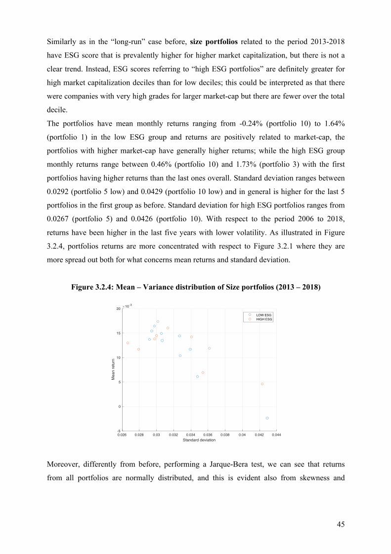
45
Similarly as in the “long-run” case before, size portfolios related to the period 2013-2018
have ESG score that is prevalently higher for higher market capitalization, but there is not a
clear trend. Instead, ESG scores referring to “high ESG portfolios” are definitely greater for
high market capitalization deciles than for low deciles; this could be interpreted as that there
were companies with very high grades for larger market-cap but there are fewer over the total
decile.
The portfolios have mean monthly returns ranging from -0.24% (portfolio 10) to 1.64%
(portfolio 1) in the low ESG group and returns are positively related to market-cap, the
portfolios with higher market-cap have generally higher returns; while the high ESG group
monthly returns range between 0.46% (portfolio 10) and 1.73% (portfolio 3) with the first
portfolios having higher returns than the last ones overall. Standard deviation ranges between
0.0292 (portfolio 5 low) and 0.0429 (portfolio 10 low) and in general is higher for the last 5
portfolios in the first group as before. Standard deviation for high ESG portfolios ranges from
0.0267 (portfolio 5) and 0.0426 (portfolio 10). With respect to the period 2006 to 2018,
returns have been higher in the last five years with lower volatility. As illustrated in Figure
3.2.4, portfolios returns are more concentrated with respect to Figure 3.2.1 where they are
more spread out both for what concerns mean returns and standard deviation.
Figure 3.2.4: Mean – Variance distribution of Size portfolios (2013 – 2018)
Moreover, differently from before, performing a Jarque-Bera test, we can see that returns
from all portfolios are normally distributed, and this is evident also from skewness and
0.026 0.028 0.03 0.032 0.034 0.036 0.038 0.04 0.042 0.044Standard deviation
-5
0
5
10
15
20
Mea
n re
turn
10-3 Scatter - Mean return and Volatility
LOW ESGHIGH ESG

46
kurtosis. Portfolios’ skewness is centred on zero, although in the low ESG score group returns
tend to more negative observations. Kurtosis is around three for all portfolios.
We computed a t-test against the null hypothesis that the difference between returns from low
ESG portfolios and returns from high ESG portfolios comes from a normal distribution with
mean equal to zero and unknown variance. As before, the majority of tests failed to reject the
null hypothesis at any significance level, although in this case the difference in mean returns
of portfolios 10 low versus high was statistically significant at 5% significance level. That
means that during the last five years, investing in small-cap firms with high ESG score
yielded significantly different (higher) returns than investing in small-cap low ESG firms. In
general, also the risk-return profile of high ESG portfolios is better with respect to low ESG
ones.
Table 3.2.4: “Adjusted Sharpe Ratio” for size portfolios (2013 – 2018)
Portfolio
1
Portfolio
2
Portfolio
3
Portfolio
4
Portfolio
5
Portfolio
6
Portfolio
7
Portfolio
8
Portfolio
9
Portfolio
10
Low
ESG 0.55 0.44 0.52 0.49 0.47 0.44 0.34 0.32 0.18 -0.06
High
ESG 0.46 0.51 0.57 0.48 0.49 0.42 0.42 0.33 0.20 0.11
As reported in Table 3.2.4 above, investing in high market-cap companies earns an higher
reward over one unit of risk for low ESG portfolios; this is true also for high ESG portfolios,
although investors can choose to be better off and still invest in small-cap companies
choosing high ESG score ones.
For value portfolios the ESG score increases as price-to-book value increases and ranges
between 4.23 (1) to 4.76 (9). Value-sorted portfolios have mean monthly returns ranging from
0.05% (portfolio 1 low) to 2.11% (portfolio 10 low) and 0.35% (portfolio 1 high) to 1.93%
(portfolio 10 high). In general portfolios with high ESG scores have higher mean returns than
their low score counterparties, especially for the first “value” portfolios. Accordingly, in both
groups standard deviation is higher for the first “value” portfolios and it is generally higher
for the second group (high ESG portfolios). In the above, “long-run” case instead, low ESG

47
portfolios outperformed high ESG ones six out of ten times and “growth” portfolios had more
volatile returns than “value” stock.
Figure 3.2.5: Mean – Variance distribution of value portfolios (2013 – 2018)
Returns of all portfolios are normally distributed, with skewness around zero and kurtosis
around 3. In particular, distributions of low ESG portfolios’ returns have more negative
skewness with respect to high ESG portfolios. With respect to the long-term time horizon,
distribution of mean returns is much more concentrated than before, especially, standard
deviation is around three times smaller now and returns are higher.
The test statistic on the difference between low ESG and high ESG portfolios in mean, failed
to reject the null hypothesis for almost all pairs of portfolios. The only exception was
portfolio 9. The difference between returns from low ESG portfolio 9 and returns from high
ESG portfolio 9 comes from a normal distribution with mean statistically different from zero
at 5% significance level. During the last five years, investing in “growth” portfolios firms
with high ESG score yielded significantly different (higher) returns than investing in
“growth” low ESG firms (1.39% low versus 1.95% high). In general, also the risk-return
profile of high ESG portfolios is better with respect to low ESG ones.
0.028 0.03 0.032 0.034 0.036 0.038 0.04 0.042 0.044 0.046Standard deviation
0
0.005
0.01
0.015
0.02
0.025
Mea
n re
turn
LOW ESGHIGH ESG

48
Table 3.2.5: “Adjusted Sharpe Ratio” for value portfolios (2013 – 2018)
Portfolio
1
Portfolio
2
Portfolio
3
Portfolio
4
Portfolio
5
Portfolio
6
Portfolio
7
Portfolio
8
Portfolio
9
Portfolio
10
Low
ESG 0.01 0.16 0.25 0.28 0.44 0.31 0.49 0.53 0.48 0.64
High
ESG 0.08 0.19 0.27 0.33 0.30 0.33 0.49 0.43 0.68 0.60
The risk-return profile is much better than before. “Value companies” have better risk-
adjusted returns for high ESG than for low ESG portfolios, while the contrary is true for
“growth stocks”.
In contrast with the “long-run” case that was not characterized by a clear trend, momentum
portfolios composed by companies that had scarce returns in the previous year, have lower
aggregated ESG score than previous year “winners”.
Low ESG portfolios had returns ranging between 0.67% (portfolio 10) and 1.21% (portfolio
1), while high ESG portfolios had returns comprised between 1.05% (portfolio 3) and 1.48%
(portfolio 4). Standard deviation of both groups increases as momentum decreases ranging
from 0.0284 (portfolio 2 low) to 0.068 (portfolio 10 low) and from 0.0298 (portfolio 2 high)
to 0.0665 (portfolio 10 high). As illustrated in Figure 3.2.6 below, with respect to the “long-
run” (Figure 3.3) standard deviation almost halved and mean returns distributions shifted
upwards. Last five years mean returns are overall higher with respect to the previous ones,
except for portfolio 10 high ESG that achieved 2% average monthly returns before and equals
to 1.37% in this case.
Figure 3.2.6: Mean – Variance distribution of Momentum portfolios (2013 – 2018)
0.025 0.03 0.035 0.04 0.045 0.05 0.055 0.06 0.065 0.07Standard deviation
0.006
0.007
0.008
0.009
0.01
0.011
0.012
0.013
0.014
0.015
Mea
n re
turn
LOW ESG PortfoliosHIGH ESG Portfolios

49
For what concerns higher moments, skewness is centred around zero and the majority of
portfolios in both groups have distribution tails that tend toward more positive values (slightly
positively skewed) and kurtosis is centred around 3. The measure for risk-return trade-off
relative to 2013-2018, suggests that portfolios composed by low momentum companies that
have high ESG score outperform those with low ESG score. Moreover, also high ESG
portfolios with higher momentum outperform their low ESG counterparties.
Table 3.2.6: “Adjusted Sharpe Ratio” for momentum portfolios (2013 – 2018)
Portfolio
1
Portfolio
2
Portfolio
3
Portfolio
4
Portfolio
5
Portfolio
6
Portfolio
7
Portfolio
8
Portfolio
9
Portfolio
10
Low
ESG 0.36 0.40 0.37 0.38 0.46 0.38 0.35 0.29 0.22 0.10
High
ESG 0.40 0.45 0.35 0.49 0.43 0.38 0.42 0.36 0.24 0.21
Even though returns for the two portfolio groups seem to strongly deviate from each other’s,
their difference in mean is not statistically different. The null hypothesis that difference of
low ESG and high ESG (same momentum decile) portfolios comes from a normal distribution
with mean equal to zero and unknown variance cannot be rejected at any significance level.

50
4 Mean - Variance Optimization
This Chapter explores the impact of ESG scores on mean-variance portfolio optimization.
While Markowitz’s (1952, 1959) portfolio optimization structure is solely based on financial
parameters and investors’ risk aversion, we also introduce ESG scores in order to study
whether discriminating for the degree of sustainability yields portfolios with higher risk-
return profiles. We build two efficient frontiers, one composed by S&P 500 stocks regardless
of their ESG score and the second composed by stocks with ESG score greater than 5. The
aim is to determine whether one strategy is suboptimal with respect to the other and in what
cases. Furthermore, we also build an efficient frontier made of High ESG Portfolios (size,
value and momentum from Ch. 3) to analyse their behaviour both as individual portfolios and
combined.
4.1 Portfolio Optimization: Theory
Prior to 1950, portfolio theory lacked an adequate framework for investments as it did not
consider the effects of diversification when risks are correlated, missed the distinction
between efficient and not efficient portfolios and did not analyse the trade-offs between risk
and return on portfolio as a whole (see Markowitz (1999)). In 1952, both Harry Markowitz
and Andrew D. Roy laid the foundations of what is now called Modern Portfolio Theory: they
theorized about basing portfolio selection on expected return and variance of the entire
portfolio. Especially, Markowitz assumed securities’ projections obey to the same probability
laws as those of random variables; which implies that the expected return of a portfolio is the
weighted average of the expected returns on individual securities and that the variance of
portfolio returns is a function of the variances of securities and the covariance between them,
and their weights in the portfolio. This theory is deemed ground-breaking particularly for two
reasons: it examined how to select assets in order to diversify and to reduce portfolio risk, and
it provided investors with the first rigorous risk measure, which then was further studied by
Markowitz (1959) and Sharpe (1964). In addition, Markowitz (1959), following Von
Neumann and Morgenstern (1944) who were the first to view that choice under uncertainty
may be related to expected utility33, based his analysis on utility maximization and gave a
general solution for the portfolio selection problem: his method allows the calculation of the
33 see Dhrymes (2017).

51
expected return and volatility of a portfolio composed by several securities relying on just
four inputs: the weights for capital to be allocated to each asset, the expected return and
volatility associated with each asset, and the correlation between them. It is fundamental to
take into account correlation coefficients among assets when selecting an investment since,
combining assets or portfolios that have low-positive or negative correlation, investors can
maintain their rate of return while reducing their portfolio risk level. Also, Tobin (1958)
showed that under certain conditions Markowitz's model implies that the process of
investment choice can be divided into two distinct stages: the first consists of choosing a
unique efficient portfolio of risky assets; and the second is about deciding the allocation of
capital between such a portfolio and a single risk-free asset.
If the Markowitz model gave a tremendous contribution to Portfolio Theory, it has not come
without making assumptions referred to investors’ behaviour and without some practical and
theoretical pitfalls. The objective function for a Markowitz investor can be interpreted as a
particular form of the objective function for a general investor, as their utility function only
depends on expected return and risk, whereas, according to basic asset pricing theories, a
general investor wants to maximize utility under some constraints related to consumption
without considering risk-return parameters. Especially, the Markowitz model assumes
investors maximize one-period expected utility, and that their utility curves demonstrate
diminishing marginal utility of wealth. Those utility curves are functions only taking into
account expected return and variance, following the previous assumptions. In general, the
majority of theoretical portfolio selection models assume a quadratic utility function34, that is,
a quadratic function of portfolio returns:
𝑈 𝑅! = 𝑅! − 𝜆𝜎!!
given a portfolio P with return 𝑅! and variance 𝜎!!, and with λ ≥ 0 being the investor-specific
risk-aversion parameter35. The maximization of this function lays at the foundation of mean-
variance analysis and links utility maximization to asset allocation since, given a level of
return, maximizing utility is equivalent to minimizing variance. The model assumes that
investors are efficient and risk averse36, which implies that they prefer higher returns to lower
returns, given the same level of risk and, for a given level of expected return, they prefer less
34 Also our study is based on maximization of a quadratic utility function, with default risk aversion coefficient (λ) equal to 4, if not differently stated 35 see Lhabitant (2007). 36 Higher λ values presuppose an higher degree of risk aversion and vice versa, λ values below zero mean that investors are “risk lovers”.

52
risk to more risk and that they want to allocate their capital in efficient investments (no other
asset or portfolio of assets has higher expected return with same or lower risk and vice versa).
The efficient frontier represents “the set of efficient mean-variance combinations”
(Markowitz (1952)). It is the upward sloping curve that bounds the region containing
portfolios resulting from different asset allocations. Thanks to the benefits of diversification
the efficient frontier is curved with its curvature generally increasing as the number of assets
that compose the investment universe increases and in the case those assets are low or
negatively correlated. Portfolios below the frontier are not efficient because it is possible to
find other portfolios with better risk-return profile, while portfolios above the frontier do not
exist because, they had existed, the efficient frontier would have been shifted accordingly to
include them. Among the “dominant portfolios”, each investor chooses the one which is
tangent to their highest utility curve; considering that risk–return utility functions reflect
individual investor’s expectations, only the investors that have the same utility curve will
conclude the same portfolio choice. No portfolio on the efficient frontier can dominate any
other portfolio on it since they are characterized by different return and risk measures and
expected rates of return increase as risk increases. Furthermore, adding equal increments of
risk going to the right part of the efficient frontier gives diminishing increments of expected
return.
Under these assumptions, the Markowitz approach leads to the so called “mean-variance
optimization model” aimed at finding the optimal weights in an efficient portfolio.
Quantitatively, the process is set as to minimizing variance under two main constraints: the
expected return of the portfolio is the target level chosen by the investor and the sum of the
weights must be equal to 1.
min!
𝜎!!
subject to,
𝑤!𝐸 𝑅! = 𝐸(𝑅∗)!
!!!
;
𝑤! = 1 ;!
!!!
and possibly with 𝑤! ≥ 0 and 𝑖 = 1… 𝑘 .

53
As mentioned before, the model suffers from some drawbacks; some of the abovementioned
assumptions, for example, may not reflect reality. One of the assumptions is that asset returns
follow a normal distribution, whereas in reality, securities may well experience returns that
are more than three standard deviations away from the mean. Moreover, although
Markowitz's theory assumes investors are rational, risk averse price takers who do not take
into account taxes and transaction costs, the market includes irrational, risk-seeking investors
and large market participants who could influence market prices leading to an inefficient
market. Another practical difficulty lays in the estimation of the covariance matrix. The
model has to calculate plenty of combinations: !!!!!
covariances, with 𝑛 be the number of
securities being accounted for. This means that for calculating the covariance matrix of 500
stocks, 124,750.0 covariance estimates are needed. Furthermore, financial literature has
shown there is evidence that efficient portfolios’ composition is often unreasonable, as
portfolios are either too concentrated (causing a lack of diversification) or they allocate big
weights to marginal markets. In addition, efficient portfolios are unstable, indeed, optimal
weights are not unfluctuating: a little change in input parameters like expected returns, can
strongly affect the portfolio final composition (see Reilly and Brown (2012)). For what
concerns expected returns, especially, efficient portfolios are said to be “estimation errors
maximizers”: since estimation error is often large, portfolios selected accordingly to the
Markowitz criterion are not likely to be more efficient than those selected following a Naïve37
strategy.
The major factor that allowed Markowitz portfolio theory to develop into capital market
theory was the introduction of a risk-free asset, that is, an asset with zero variance. The
Capital Allocation Line (CAL) is the investment opportunity set represented by a risky asset
and a risk-free asset.
𝐶𝐴𝐿: 𝐸 𝑅! = 𝑅𝐹𝑅 + 𝜎!𝐸 𝑅! − 𝑅𝐹𝑅
𝜎!
The risk-return relationship holds for every combination of the risk-free asset with any
collection of risky assets. The Capital Market Line (CML), instead, represents a new efficient
37 Naïve portfolio formation strategies are mainly based on qualitative estimations and do not implement optimization models.

54
frontier that combines the Markowitz efficient frontier of risky assets with the ability to invest
in the risk- free security.
𝐶𝑀𝐿: 𝐸 𝑅! = 𝑅𝐹𝑅 + 𝜎!𝐸 𝑅! − 𝑅𝐹𝑅
𝜎!
Portfolio M is called the market portfolio and, by definition, it contains all risky assets held in
the marketplace and receives the highest level of expected return per unit of risk for any
available portfolio of risky assets. The slope of the CML is the maximum risk premium that
investors can expect for each unit of risk they bear. Both return and risk increase in a linear
fashion along the CML and all portfolios composing this line are, so, perfectly correlated.
Since the market portfolio contains all risky assets, it is a completely diversified portfolio,
which means that all risk unique to individual assets in the portfolio is diversified away.
In the last decade, several studies attempted to combine the Markowitz framework with SRI
criteria (see Drut (2010)). In theory, investors choosing to invest only in socially responsible
companies restrict their investment universe and should thus be penalized in a mean-variance
framework. Drut (2010) shows, however, that the additional cost for responsible investing
depends essentially on individual investors’ risk aversion. Ballestero et al. (2012) propose a
“financial-ethical bi-criteria model” and their analysis suggests that ethical investments are
linked to increments in risk exposure. Bilbao-Terol et al. (2012) introduce a goal-
programming model for SRI portfolio selection in order to allow investors to align their
ethical and financial preferences and show that investors’ risk attitudes affect returns’ losses.
Also, Bilbao-Terol et al. (2013) develop a two-stage multi-objective framework for SRI
portfolios’ selection applying a “Hedonic Price Method” and their empirical findings suggest
that the losses in returns associated with sustainable investments are relatively minor for
highly risk-averse investors. Hoang et al. (2016) find that ESG investors are neither efficient nor rational on the basis of
modern portfolio theory. Although ESG investors admit that ESG integration reduces
investment opportunities38, they suggest that the benefits from such integration are greater
than the losses on efficiency since ESG constraint would help eliminating from the
investment universe companies expected to have poor future performance. Contrarily, Hoang
38 Traditional investors argue that the implementation of ESG factors must lead to lower returns because they will have a smaller investment universe. (Hoang et al. (2016)).

55
et al. (2016) find no empirical evidence that the losses on portfolio efficiency are outweighed
by the benefits of ESG integration.
Uncertainty in the input parameters is deemed to be greater for SRI portfolios than for
conventional portfolios based on the fact that Corporate Social Performance (CSP) scores are
price sensitive information thus subject to considerable estimation risks. These features would
affect the selection of an appropriate optimization method for SRI portfolios. Oikonomou et
al. (2018) investigates the impact of the choice of optimization technique when constructing
SRI portfolios finding that the more “formal” optimization approaches (Black-Litterman,
Markowitz and robust estimation) lead to less risky SRI portfolios with superior risk-return
trade-offs than do more simplistic approaches. On the other hand, the use of the formal
approaches also leads to more unstable asset allocations and to lower diversification.
4.2 Portfolio Optimization: Practice
Through this Chapter, our research paper aims at understanding whether introducing ESG
scores in the portfolio optimization structure yields investments with higher risk-return
profiles. Would investors that currently allocate their capital entirely to the Standard and Poor
500 Index be better off discriminating for ESG scores? If the Index is itself a proxy for the
market portfolio, would investors, in general, be better off by making sustainable
investments? The answers data provide will also suggest whether ESG investors are efficient
or not both in the long-run (2006 – 2018) and in the short-run (2013 – 2018)39.
In our optimization analysis we implement the Matlab function Porfolio in order to create a
Portfolio object for mean-variance optimization whose computations are based on the
Markowitz model (1952, 1959)40 and to which we apply further constraints on lower and
upper bounds. Then, we employ the function portalloc to compute the optimal risky
portfolio, and the optimal allocation of funds between the risky portfolio and the risk-free
asset. By optimal risky portfolio (ORP) we mean the portfolio on the efficient frontier that
maximises the slope of the Capital Allocation Line (CAL). The ORP is the portfolio
associated with the highest Sharpe Ratio given the constraints that we put on assets’ weights,
39 Precise time periods related to this two timeframes are delineated in the previous chapter and refer to December 2006 to February 2018 and February 2013 to February 2018 (the last 5 years). 40 Matlab portfolio optimization tools make reference to Chapter 7 of Bodie Z., Kane A. and Marcus A. J. (1993): “Investments”, 2nd Edition. Source: Matlab Bibliography

56
while the optimal final portfolio (OFP) represents the portfolio with the optimal proportion of
funds to be invested in the OPR and in the risk-free asset given the investors’ individual
preferences. We build two efficient frontiers, one composed by S&P 500 stocks regardless of
their ESG score and the second composed by stocks with ESG score greater than 5. The aim
is to determine whether one strategy is suboptimal with respect to the other and in what cases.
Furthermore, we also build an efficient frontier made of High ESG Portfolios (size, value and
momentum from Ch. 3) to analyse their behaviour both as individual portfolios and
combined. In order to accommodate the mathematical needs of the model for computing the
covariance matrix, we sort the data, both assets available to compute the “total” efficient
frontier and those related to high ESG assets (efficient frontier “ESG”), by the number of
missings. In the first case, we are able to include in our investable universe 470 stocks whose
number of missing values ranges from zero to a maximum of 66, which is half of our time
horizon length. In the second instance, we are only able to include 60 stocks out of the 170
having less than 67 missing values since otherwise the covariance between some assets could
not be assessed.
Furthermore, in order to build the efficient frontiers we choose to assign a lower and an upper
bound to the possible weights to be allocated to each stock. For the total frontier we
calculated the actual weights assigned to each stock included in the S&P 500 each month,
while for the ESG frontier we calculated the weights assigned to each asset belonging to the
HIGH Portfolio, also based on market capitalization. The HIGH Portfolio comprises all the
stocks that were included in the S&P 500 every month and that at the same time had ESG
score greater than 5, while the LOW Portfolio represents its complementary. Then, we
compute the medians and maxima for all monthly weights and picked the maximum among
monthly maxima as upper bound and the minimum among the monthly medians as lower
bound. In this way we assure that our portfolios do not suffer from excessive concentration
and that they take advantage of the benefits of diversification, without setting a lower bound
equal to the minimum among minima because this would just lead to a useless increase in
transaction costs. The lower bound for the total portfolio equals 0.0009 and the upper bound
is set to 0.1; the HIGH portfolio lower bound equals 0.002 and the upper bound is set to 0.12
out of a total available amount equal to 1.
Figure 4.2.1 illustrates the results of the mean-variance optimization process described above.
In general, the “total” efficient frontier always lies above the ESG efficient frontier, in
accordance with Drut (2010) and to the majority of traditional investors that claim that the
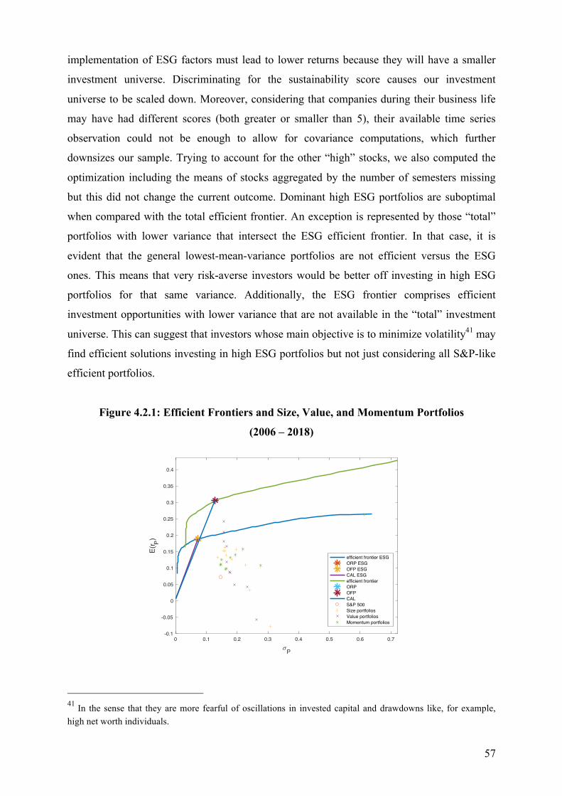
57
implementation of ESG factors must lead to lower returns because they will have a smaller
investment universe. Discriminating for the sustainability score causes our investment
universe to be scaled down. Moreover, considering that companies during their business life
may have had different scores (both greater or smaller than 5), their available time series
observation could not be enough to allow for covariance computations, which further
downsizes our sample. Trying to account for the other “high” stocks, we also computed the
optimization including the means of stocks aggregated by the number of semesters missing
but this did not change the current outcome. Dominant high ESG portfolios are suboptimal
when compared with the total efficient frontier. An exception is represented by those “total”
portfolios with lower variance that intersect the ESG efficient frontier. In that case, it is
evident that the general lowest-mean-variance portfolios are not efficient versus the ESG
ones. This means that very risk-averse investors would be better off investing in high ESG
portfolios for that same variance. Additionally, the ESG frontier comprises efficient
investment opportunities with lower variance that are not available in the “total” investment
universe. This can suggest that investors whose main objective is to minimize volatility41 may
find efficient solutions investing in high ESG portfolios but not just considering all S&P-like
efficient portfolios.
Figure 4.2.1: Efficient Frontiers and Size, Value, and Momentum Portfolios
(2006 – 2018)
41 In the sense that they are more fearful of oscillations in invested capital and drawdowns like, for example, high net worth individuals.
0 0.1 0.2 0.3 0.4 0.5 0.6 0.7
P
-0.1
-0.05
0
0.05
0.1
0.15
0.2
0.25
0.3
0.35
0.4
E(r P)
efficient frontier ESGORP ESGOFP ESGCAL ESGefficient frontierORPOFPCALS&P 500Size portfoliosValue portfoliosMomentum portfolios

58
Based on our investor preferences42, the Capital Allocation Line represents the allocation
between the risk-free asset and a risky portfolio of assets. The optimal risky portfolio on the
high ESG frontier has a better risk-return profile with respect to the total one. The line is
slightly steeper and for the same increase in variance it rewards investors with higher
expected returns. The investment in the ESG risky portfolio yields 2.6 units of return of every
unit of risk, whereas the total risky portfolio yields 2.38 units of return for every unit of risk43.
This is in contrast with Gasser et al. (2017) since their empirical study showed that investors
caring about social responsibility face a statistically significant Sharpe Ratio decrease with
respect to risk-return optimal portfolios. On the other hand, the authors also underline that
optimal portfolios exhibiting a modest social responsibility rating can be attained by
“accepting only a very limited decrease of the resulting portfolio’s Sharpe Ratio”44.
In this investment framework, the optimal weights to assign to the risk-free asset and to the
risky portfolio are 0 and 1, respectively. The Optimal Risky Portfolio and the Optimal Final
Portfolio coincide because the most efficient capital allocation for our investor is to allocate
all their capital to the risky asset to have the optimal risk- return profile.
In addition, Figure 4.2.1 plots together the two efficient frontiers with the annualized
expected return and variance related to the S&P 500 and the 30 portfolios relative to size,
value and momentum strategies with higher ESG score. The S&P 500 is far below both
efficient frontiers and also below their two CALs. This suggests that implementing an
optimization framework using stocks’ expected returns and covariances yields portfolios that
have higher returns for the same level of risk of the Index, which instead allocates capital
weights among its stocks based on market capitalization and regardless of their covariances.
Furthermore, the majority of high ESG portfolios have higher expected returns than the S&P
with the same or very close standard deviation; some portfolios are above the ESG frontier,
halfway to the total one. Those portfolios are more efficient for ESG investors but
suboptimal, like all the others composing the ESG frontier, with respect to the full investment
universe. Notably, no factor portfolio has lower standard deviation than 13.6, which is the
corresponding point to the total ORP; that is, using factor strategies for ESG investments may
yield efficient portfolios but does not allow taking full advantage of the lower variance that
42 This investor chose investment bounds and has a quadratic utility function based on expected return and variance with a risk aversion coefficient (λ) equal to 4. 43 Recall the concept of “Adjusted Sharpe Ratio” of Chapter 3. This measure is now calculated as OFP Return over OFP risk, which, in this case, is the same as ORP Return divided by ORP risk. 44 Gasser S., Rammerstorfer M. and Weinmayer K. (2017): “Markowitz Revisited Social Portfolio Engineering”.

59
characterizes sustainable investments. Moreover, some portfolios are positioned exactly on
the ESG frontier, suggesting that value and momentum strategies yield efficient portfolios.
As already ascertained by literature, risk aversion has a fundamental impact on ESG
investments and their efficency degree. Changing the risk aversion coefficien in our study
affects the choice of both ORP and OFP. Decreasing the risk aversion coefficient λ to 3
causes a decrease in the risk-return relationship as both CALs move toward the right part on
the efficient frontier and the adjusted Sharpe Ratios become 2.344 and 2.45 for the total and
the ESG ORPs respectively. On the other hand, if we increment the risk aversion coefficient
up to 5, both Sharpe Ratios increase becoming 2.643 (total) and 2.893 (ESG). From this
simple experiment, it is clear that ESG investments are strongly influenced by risk aversion,
much more than investments that disregard sustainability. The differences from base (λ = 4)
Sharpe Ratios are -0.039 and -0.14 when we lower the risk aversion and 0.26 and around 0.3
when we increase it, respectively for total and ESG portfolios. We conclude that the more an
investor is risk averse, the more an ESG investment becomes more efficient for him.
Efficiency of ESG investments also depends on the terms to which we allow asset
aggregation. We computed an additional efficient frontier composed by the 30 high ESG
factor portfolios. If our investor decides not to allow short selling and to allocate at least 0 and
at most 0.33 (1/3) of capital on one portfolio, the resulting efficient frontier (“portfolios”)
appears like a portion of the ESG one, as illustrated in Figure 4.2.2. Optimization of factor
portfolios leads to an efficient frontier, which is slightly more efficient than the ESG one from
the ORP onwards but it is strongly suboptimal to the left of the ORP. The Adjusted Sharpe
Ratio of this ORP is 1.15 and the composition of this portfolio is made by 0.44% of portfolio
1 size, 0.48% of portfolio 7 value, 32.78% portfolio 8 value, 33% portfolio 9 value, 33%
portfolio 10 value and 0.3% of portfolio 10 momentum.

60
Figure 4.2.2: Efficient Frontiers, no short selling (2006 – 2018)
Alternatively, if the investor decides not to impose bounds on weights allocation, except no
short selling, the optimization process yields a new frontier (Figure 4.2.3). This second
frontier lies above the ESG one, while becoming suboptimal for portfolios with variance
greater than 40% and for those with variance equal or lower to around 18%. The Optimal
Risky Portfolio would offer to investors 1.2345 units of return for a unit of risk, and would be
composed by 98% of portfolio 10 value and by around 2% of portfolio 9 size.
Figure 4.2.3: Efficient Frontiers, no short selling and no upper bound (2006 – 2018)
0 0.1 0.2 0.3 0.4 0.5 0.6
P
0.05
0.1
0.15
0.2
0.25
0.3
0.35
E(r P)
efficient frontier ESGORP ESGOFP ESGCML ESGefficient frontier portfoliosORP portfoliosOFP portfoliosCML portfoliosefficient frontierORPOFPCML
0 0.05 0.1 0.15 0.2 0.25 0.3 0.35 0.4 0.45 0.5
P
0
0.05
0.1
0.15
0.2
0.25
0.3
0.35
E(r P)
efficient frontier ESGORP ESGOFP ESGCAL ESGefficient frontier portfoliosORP portfoliosOFP portfoliosCAL portfoliosefficient frontierORPOFPCAL

61
Another strategic decision for the investor could be lifting the short selling constraint and just
allow the man-variance optimization to yield the most efficient portfolios while respecting a
lower bound equal to -0.033 (1/30) and an upper bound of 0.33 (1/3). The Optimal Risky
Portfolio achieves 1.48 units of return for a unit of risk and it is composed by 33% of
portfolio 3 size, 12.34 % of portfolio 4 size, around 33% of the portfolios 7 to 10 value, and
1.7% of the portfolio 10 momentum; while shorting all the others. This efficient frontier is
very much closer to the total efficient frontier but still suboptimal to that, as illustrated in
Figure 4.2.4. Combining the factor portfolios we can see no benefits in investing in their
optimized combination for lower values of standard deviation in any of the three cases
analysed.
Figure 4.2.4: Efficient Frontiers, short selling allowed and no upper bound (2006 – 2018)
Until now, the strategic choice of allowing short selling and implementing long-short
positions is the one that yields the most efficient set of portfolios. The three cases above
highlight the fact that in these optimization frameworks growth portfolios are always included
in the ORPs. However, factor investing in general does not “beat” optimized investments
related to the total investment universe, although some of them are much more efficient than
the S&P 500 itself. Which means that screening for high ESG scores could still yield better
risk-adjusted returns than passively replicating or buying the Index.
As stated by previous literature, we find that ESG investors are not efficient, unless they
target investments with standard deviation lower than 4%. High Net Worth Individuals, for
0 0.1 0.2 0.3 0.4 0.5 0.6
P
0
0.05
0.1
0.15
0.2
0.25
0.3
0.35
0.4
E(r P)
efficient frontier ESGORP ESGOFP ESGCAL ESGefficient frontier portfoliosORP portfoliosOFP portfoliosCAL portfoliosefficient frontierORPOFPCAL

62
example, would likely be better off in implementing ESG screenings and mean-variance
optimization in order to choose the less variable investments. Reducing the time horizon to
the last 5 year (2013 – 2018) does not change all the considerations made until now.

63
5 The Market Portfolio(s)
In this Chapter we analyse three indices that refer to three distinct investment universes:
𝑅! ,𝑅!,!"# ,𝑅!,!". Those three indices are composed by all S&P 500 stocks with an ESG
score, all S&P 500 stocks with ESG score greater than 5, and all S&P 500 stocks with ESG
score smaller than 5, respectively. Our purpose is to aggregate those three sets of stocks both
in market-weighted portfolios and in equally weighted portfolios and compare their returns
among them and versus the S&P 500 Index itself. Our aim is to address the question of
whether ESG investors can earn higher returns than traditional ones both in the long- and in
the short-term. Are non-financial disclosure and ESG score signals for investors of better and
longer lasting future performances?
We classify stocks included in the S&P 500 from 2006 to 2018 in three sets. The first, 𝑅!, is
the one closest to the Index itself. 𝑅! comprises all stocks that had available ESG score
during the time horizon considered. The second one, 𝑅!,!"# , only includes stocks that while
being included in the S&P 500 had an ESG score greater than 5 and 𝑅!,!" is its
complementary.
In the first instance we compute market-weighted portfolios relative to those investment
universes, while in the second instance we aggregate stocks in equally weighted portfolios.
As illustrated in Figure 5.1, the monthly returns of the three indices move together in general.
However, during the period from 2008 to 2012, 𝑅!,!" considerably deviated from 𝑅! ;
wherears from 2013 to 2018 𝑅!,!"# had more extreme values with respect to 𝑅!. Deviations
from 𝑅!, which we are considering to describe the behaviour of the general market, mean the
market prominently commoved with the “other” investment set. Since all those indexes are
market weighted, either during 2008-2012 𝑅! , and consequently the S&P 500, mainly
included high ESG scored firms, or, those high ESG companies had a larger market
capitalization thus making a greater impact on the whole index. Similarly, just after 2013 𝑅!
returns prevalently deviated from 𝑅!,!"# . Both reasoning could hold, however, we could
argue that in the period just after the last financial crisis the majority of firms meeting S&P
500 eligibility criteria where those with high ESG rating, while in normal economic periods
more firms with low ESG scores meet the S&P 500 criteria.
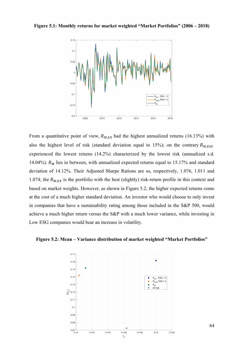
64
Figure 5.1: Monthly returns for market weighted “Market Portfolios” (2006 – 2018)
From a quantitative point of view, 𝑅!,!" had the highest annualized returns (16.13%) with
also the highest level of risk (standard deviation equal to 15%); on the contrary 𝑅!,!"#
experienced the lowest returns (14.2%) characterized by the lowest risk (annualized s.d.
14.04%). 𝑅! lies in between, with annualized expected returns equal to 15.17% and standard
deviation of 14.12%. Their Adjusted Sharpe Rations are so, respectively, 1.076, 1.011 and
1.074; the 𝑅!,!" is the portfolio with the best (slightly) risk-return profile in this context and
based on market weights. However, as shown in Figure 5.2, the higher expected returns come
at the cost of a much higher standard deviation. An investor who would choose to only invest
in companies that have a sustainability rating among those included in the S&P 500, would
achieve a much higher return versus the S&P with a much lower variance, while investing in
Low ESG companies would bear an increase in volatility.
Figure 5.2: Mean – Variance distribution of market weighted “Market Portfolios”
2008 2010 2012 2014 2016 2018-0.2
-0.15
-0.1
-0.05
0
0.05
0.1
0.15
REX ESG 5RESG ESG > 5RM
0.14 0.142 0.144 0.146 0.148 0.15 0.152
p
0.07
0.08
0.09
0.1
0.11
0.12
0.13
0.14
0.15
0.16
0.17
E(r p)
REX ESG 5RESG ESG > 5RMSP 500

65
The S&P 500 yields an annualized expected return of around 7.23% with standard deviation
amounting to 14.63%. Investing in ESG rated companies would have more than doubled the
expected return with lower variance.
Figure 5.3 illustrates the behaviour or both S&P 500 and 𝑅! monthly returns in the long term.
Notably, 𝑅! is always equal or above the S&P 500. This means that distributing invested
capital over ESG rated companies allows the investor to allocate bigger weights on more
profitable companies than it is possible in the S&P 500.
In this case we can say that with respect to the staring investment universe, investors seeking
high ESG portfolios are better off than general investors. The decision to care about the ESG
score yields the double expected return than the S&P 500. Among the ESG rated universes,
less risk-averse investors earn the highest expected returns.
Figure 5.3: Monthly returns of S&P 500 and market weighted 𝑹𝑴 (2006 – 2018)
The second instance consists of computing three equally weighted portfolios from the same
three investment universes as before. The equally weighted portfolio method makes sure that
we analyse the true number of companies that make an impact on each portfolio and it is
illustrated in Figure 5.4.
Compared to before, the monthly returns behave in a much more homogeneous way, without
such extreme peaks. However, it is still visible that in the period 2008–2012 𝑅!,!" deviated
from 𝑅!. It is clear from this, that both reasoning from before apply, although one dominates
2008 2010 2012 2014 2016 2018-0.2
-0.15
-0.1
-0.05
0
0.05
0.1
0.15
S&P 500RM

66
the other. It is true that 𝑅! was prominently composed by High ESG companies, but the
numerical amounts differ slightly. What prominently makes a difference is allocating higher
weights following market capitalization, which means that during this period the S&P 500
included larger companies with high more than low ESG score. Similarly, during the period
from 2015 to 2018 𝑅! prevalently included low ESG companies, deviating from 𝑅!,!"# .
Figure 5.4: Monthly returns for equally weighted “Market Portfolios” (2006 – 2018)
Equally weighted portfolios are characterized by higher standard deviations versus market
weighted ones. Furthermore, in this case 𝑅!,!"# had the highest annualized returns (11.65%)
with instead the lowest level of risk (standard deviation equal to 16.91%); on the contrary
𝑅!,!" experienced the lowest returns (11.05%) charachterized by the highest risk (annualized
s.d. of 17.11%). 𝑅! lies in between, with annualized expected returns equal to 11.23% and
standard deviation of 16.94%. Their Adjusted Sharpe Rations are so, respectively, 0.69, 0.65
and 0.665, with the 𝑅!,!"# having the best risk-return profile.
2008 2010 2012 2014 2016 2018-0.25
-0.2
-0.15
-0.1
-0.05
0
0.05
0.1
0.15
0.2
REX ESG 5RESG ESG > 5RM

67
Figure 5.5: Mean – Variance distribution of equally weighted “Market Portfolios”
The differences between equally and market-weighted portfolios highlight several features of
these investment universes. Volatility in equally weighted portfolios is higher versus volatility
in market weighted ones, and returns are generally higher for the last portfolios than for the
first ones. Assigning the same weights to all securities causes more variability in the portfolio
especially in the 𝑅!,!", which is always the one with the highest standard deviation. On the
other hand, 𝑅!,!"# always has the lowest standard deviation. 𝑅!,!"# returns are those that
experience the least decrease when comparing market weighted and equally weighted
portfolios; this may suggest that high ESG companies have generally higher returns than low
ESG ones, but the companies with largest market capitalization have lower returns in the high
ESG portfolio while they have higher returns with respect to the portfolio mean (or also
median) in the low ESG portfolio; this leads to the low ESG market weighted portfolio
returns dominating the high ESG one, when, instead, the equally weighted high ESG portfolio
dominates the low ESG one. Moreover, in both cases, and especially in the market-weighted
case, 𝑅! standard deviation is closer to the high ESG one; this can suggest that in general
high ESG companies have larger market-cap than low ESG ones but are outnumbered by
many lower sized low ESG companies, except few important exceptions.
Implementing an equally weighted 𝑅!, differently from before, is not always more profitable
than investing in the S&P 500. Even though the expected return is still higher, returns
volatility also increased considerably.
0.145 0.15 0.155 0.16 0.165 0.17 0.175
p
0.07
0.075
0.08
0.085
0.09
0.095
0.1
0.105
0.11
0.115
0.12
E(r p)
REX ESG 5RESG ESG > 5RMSP 500

68
Figure 5.6: Monthly returns of S&P 500 and equally weighted 𝑹𝑴 (2006 – 2018)
We also reproduced our analysis taking into account the last 5 years (2013 – 2018) as time
horizon. Short run computations lead to the same conclusions as for the long run. The
efficient frontier ESG is still suboptimal versus the total one and also the other overall results
referring to the three indices do not differ substantially from those extensively presented
above.
Comparing monthly long-run returns between market weighted and equally weighted
portfolios (Figure 5.7 and 5.8, Appendix) the low ESG market weighted portfolio
outperformed the high ESG one and vice versa in the equally weighted case. Notably, after
reaching the lowest rate of returns in 2009, all portfolios started yielding positive returns in
2010, although the portfolio with the fastest recovery among equally weighted ones was that
composed by high ESG companies, while it also outperformed all the others in general.
Table 5.1: Annualized holding period returns in the long - run
2006 - 2018 𝑹𝑴,𝑬𝑿 𝑹𝑴,𝑬𝑺𝑮 𝑹𝑴 S&P 500
Market Weighted 14.831% 13.068% 14.029% 7.03%
Equal Weighted 9.401% 10.038% 9.641% 7.03%
2008 2010 2012 2014 2016 2018-0.25
-0.2
-0.15
-0.1
-0.05
0
0.05
0.1
0.15
0.2S&P 500RM

69
Table 5.2: Annualized holding period returns in the short - run
2013 - 2018 𝑹𝑴,𝑬𝑿 𝑹𝑴,𝑬𝑺𝑮 𝑹𝑴 S&P 500
Market Weighted 19.104% 18.327% 19.048% 12.399%
Equal Weighted 14.250% 15.574% 14.756% 12.399%
As reported in Tables 5.1 and 5.2, both strategies beat the S&P 500 in the long- run and in the
short- run. Investing $100 either 2006 or in 2013 in one of our market weighted “Market
Portfolios” would mean receiving at least 6 percentage points more in expected returns. While
making the same investment with both a long-term time horizon and a short term one, would
yield at least 2 pp more than investing in the S&P 500. Equally weighted strategies are
optimal after the implementation of high ESG score screening. While market weighted ones
are optimal excluding high ESG rated companies. As previously stated, in general high ESG
companies yield higher returns than low ESG ones, but the biggest high ESG companies to
which market weighted strategies assign most weight yield lower returns that the biggest low
ESG companies. This suggests that the high ESG market is more homogeneous, generally
healthier and characterized by lower volatility.

70
6 Conclusion
From the analysis of our whole panel we can conclude that ESG scores attached to sample
stocks are more influenced by environmental and social scores, on average, than by
governance scores, which are flatter through those buckets. Moreover, stocks with lower
sustainability ratings are characterized by higher returns’ volatility, in all scenarios
(aggregating them by ESG and also by E, S and G scores separately).
Factor portfolios composed by high ESG companies yield equal or higher returns than those
composed by low ESG companies and have better risk-return profiles. While in an
optimization framework scaling down the investment universe in order to consider only ESG
stocks may lead to a suboptimal mean-variance frontier, the ESG investment universe
provides investment solutions characterized by lower variance and better rewards to investors
for bearing the same unit of risk. In addition, considering a market weighted index only
composed by high ESG stocks leads to a decrease in volatility and doubles expected returns
with respect to the S&P 500 ones.
This paper, overall, shows that choosing to take ESG criteria into account is becoming more
and more profitable, as highlighted by our short-term results. Moreover, the mixed evidence
related to long-term results indicates that investors would have been better off with
responsible investments depending on their risk aversion and fear of losses in a mean-
variance optimization framework.
Notwithstanding the fact that applying factor strategies has mixed outcomes related to which
set of portfolios achieves the best risk return trade off, in the long run it would not lead to
statistically significant differences in expected monthly returns.
Furthermore, investors interested in replicating the S&P 500 would have had higher gains
with lower variance investing in high ESG companies within the same investment universe
and would have recovered faster from the financial crisis.
During time companies became more interested in improving their sustainability and
investment managers became keener on recognizing companies’ “intrinsic value” through the
implementation of their material ESG issues’ analysis. Comparing ESG scores referring to
December 2006 with the ones related to February 2018 there is an evident shift toward higher
scores and an increase in their plurality. On average, also Environment and Governance
scores experienced an increasing trend through time, instead, Social scores were higher in
2006. Moreover, companies that had higher average ESG score, during the period studied,

71
also had longer permanence in the S&P 500, and this applies to E score and S score too.
Improvements in business’ sustainability are more important for largest-cap companies;
indeed, these are the ones with highest ESG rating. However, it is not true that the bigger is
the company the higher is the score since the majority of large-cap companies have mean
ESG score between 1 and 2. In the same way, CFO, book value and price per share are higher
for companies with higher mean ESG score, whereas returns are inversely related with
average sustainability scores. The market may have already incorporated high ESG
companies’ greater intrinsic value on their price and has to give higher rewards to investors
choosing to buy low ESG firms in order to compensate them for the higher risk they bear,
since volatility of low ESG companies’ returns is much higher versus that of high ESG
companies. This features also apply to companies aggregated by E score and S score, while G
score buckets have diverse characteristics, for example, returns are higher for higher G scores
companies. Furthermore, companies classified by different mean ESG score also belong to
different industry groups: Bucket 1 companies operate in the industries of Food, Beverage
and Tobacco, of Media and of Materials (Graph 2.1); instead, companies that have mean ESG
scores between 7 and 8 belong to the industries of Utilities, Semiconductors & Semiconductor
Equipment, Technology, Hardware & Equipment, Software & Services, Real Estate and
Materials (Graph 2.7).
From our factor analysis we conclude that investing in our factor portfolios composed by high
ESG stocks is not statistically significantly different from investing in low ESG stocks in the
long term. Contrarily, high ESG portfolios yield better risk-adjusted profits in the short run,
and the differences in factor portfolios’ expected returns are, in some case, statistically
significantly different from zero, favouring sustainable investments.
Size portfolios comprising companies characterized by high market capitalization have higher
ESG score, on average, than those composed by lower size companies. Furthermore, “big
companies” portfolios have higher monthly mean returns versus “small companies” ones and
also the first 5 high ESG portfolios have lower standard deviations of returns than their low
ESG score counterparties; this reverses for the last 5 portfolios. Also adjusting for risk, size
portfolios with lower ESG score have in general higher returns than those with high ESG
scores during the period 2006 to 2018, even though statistical tests are inconclusive on this
point.

72
Long run annualized returns related to High ESG Size portfolios are lower with respect to
their low ESG counterparty.
Value portfolios composed by companies with higher price-to-book value (growth stocks)
have higher ESG score, on average, than those composed by lower price-to-book value
companies (value stocks) in the long run. This counterintuitive result could be caused by the
fact we are building our value portfolios based on stocks already “ordered” by size, as that is
the main eligibility criteria for the S&P 500. In this case, large-cap growth stocks’ high prices
would already incorporate the value of innovations. These “innovations” could not be visible
in companies’ metrics, yet, and could be related to sustainability projects in this context.
Moreover, the diverse structure of growth companies versus value ones also lays in the use of
income: the first ones retain earnings reinvesting them inside the company, which allows
them to have more funds at hand to spend in R&D, innovation and projects; while the last
ones pay them out as dividends, which makes it more demanding to allocate funds to
sustainability projects than to either dividends or to the core business.
Sample growth portfolios have higher monthly mean returns versus value portfolios, with the
low ESG outperforming the high ESG six out of ten times. Volatility is higher for lower PBV
portfolios both for high ESG and low ESG portfolios and it decreases as PBV increases.
Although value investors also would have earned positive returns in the long run and less
negative returns from 2006 investing in high ESG portfolios versus low ESG ones, in general,
low ESG portfolios outperformed high ESG ones since growth low ESG stocks yielded higher
returns.
High ESG portfolios based on momentum outperform low ESG ones and also the risk-return
profile of high ESG portfolios is better than their counterparties’: they reward investors with
more returns for the same unit of risk. There is an overall inverse relation between high ESG
portfolios’ return and momentum: returns increase as momentum decreases (return related to
portfolio 1 equals 0.78% and return from portfolio 10 amounts to 2%). Portfolios
characterized by higher momentum have lower standard deviation with respect to portfolios
composed by stocks with lower momentum and this applies to both groups of high and low
ESG portfolios. In particular, standard deviation is generally higher for low ESG portfolios
than for their counterparty, except for portfolios 10. Momentum investors would have been
better off investing in high ESG portfolios. Considering both time horizons high ESG
portfolios outperforms low ESG ones.

73
Changing the time horizon under examination to the last 5 years (from February 2013 to
February 2018), some characteristics of our factor portfolios change accordingly. As we
would imagine, annualized holding period returns are higher in the last 5 years than in the last
12 years and volatility is lower. Taking out the years that have been affected by the financial
crisis, extreme values are less frequent and, in general, more concentrated on the right tail of
the distribution.
Similarly as in the long run, size portfolios related to the period 2013-2018 have ESG score
that is prevalently higher for higher market capitalization, but there is not a clear trend.
Investing in small-cap firms with high ESG score yielded significantly different (higher)
returns than investing in small-cap low ESG firms. While the majority of tests against the null
hypothesis that the difference between returns from low ESG portfolios and returns from high
ESG portfolio failed to reject the null hypothesis at any significance level, the difference in
mean returns of portfolios 10 low versus 10 high was statistically significant at 5%
significance level. In general, also the risk-return profile of high ESG portfolios is better with
respect to low ESG ones.
Among value portfolios, the ESG score increases as price-to-book value increases and, in
general portfolios with high ESG scores have higher mean returns than their low score
counterparties. In both groups standard deviation is higher for value portfolios and it is
generally higher for high ESG portfolios; in the long-run case, instead, low ESG portfolios
outperformed high ESG ones and growth portfolios had more volatile returns than value ones.
The risk-return profile of high ESG portfolios is better with respect to low ESG ones.
Furthermore, “Value companies” have better risk-adjusted returns for high ESG than for low
ESG portfolios, while the contrary is true for “growth stocks”. The test statistic on the
difference between low ESG and high ESG portfolios in mean, failed to reject the null
hypothesis for almost all pairs of portfolios. The only exception was portfolio 9. The
difference between returns from low ESG portfolio 9 and returns from high ESG portfolio 9 is
statistically different from zero at 5% significance level. During the last five years, investing
in growth portfolios firms with high ESG score yielded significantly different (higher) returns
than investing in “growth” low ESG firms (1.39% low versus 1.95% high).
Momentum portfolios composed by companies that had scarce returns in the previous year,
have lower aggregated ESG score than previous year “winners”. Portfolios composed by
companies that have high ESG score outperform those with low ESG score.
With respect to the “long-run”, last five years mean returns are overall higher with almost half
standard deviation.

74
For what concerns strategies, High ESG growth investors during both periods earned the
highest returns with respect to size and momentum investors; while small-cap investors
earned the lowest returns with respect to value and momentum ones in both periods.
Momentum portfolios had lower but more stable and homogeneous returns in general.
Relative to Low ESG portfolios, value-strategy yielded both the highest returns for growth
portfolios but also the most negative ones for value portfolios in the long run, while small-cap
low ESG investors earned the most negative returns in the last 5 years. Also in this case,
momentum investors in both periods earned lower but more stable returns and suffered less
severe losses.
From the mean-variance optimization analysis of Chapter 4 we conclude that the “total”
efficient frontier is more efficient than the ESG efficient frontier in the majority of cases. This
meets previous studies (see Drut (2010)) claiming that the implementation of ESG factors
leads to less efficient investments, since the investment universe is being scaled down. In our
study, this result could also be caused by the fact we could not include all the available high
ESG stocks due to the presence of missing values.
However, although “dominant” high ESG portfolios are suboptimal when compared with the
“total” ones, those total portfolios that have variance lower than 3.1% represent an exception,
since they intersect the ESG efficient frontier at that point. Investors that are much more risk-
averse would be better-off investing in ESG optimized portfolios when targeting lower
portfolio variance, since the total efficient frontier is suboptimal at that point and does not
provide further investment opportunities from then on. It is clear that ESG investments are
strongly influenced by risk aversion, much more than investments that disregard
sustainability. The differences from base (risk aversion coefficient λ = 4) Sharpe Ratios are -
0.039 and -0.14 when we lower the risk aversion and 0.26 and around 0.3 when we increase
it, respectively for total and ESG portfolios. We conclude that the more an investor is risk
averse, the more an ESG investment becomes the most efficient choice for him.
Moreover, in this context, the optimal risky portfolio on the ESG frontier has a better risk-
return profile with respect to the total one considering it provides our investor with 2.6 units
of return for one unit of risk while the total ORP earns investors 2.38 units of return for the
same risk. This is in contrast with Gasser et al. (2017) whose empirical study shows that
75
caring about social responsibility causes a statistically significant Sharpe Ratio decrease with
respect to risk-return optimal portfolios.
Implementing an optimization framework using stocks’ expected returns and covariance
yields portfolios that have higher returns for the same level of risk of the S&P 500, which
instead allocates capital weights among its stocks based on market capitalization and
regardless of their covariance and lies below both efficient frontiers and their two CALs
(Figure 4.2.1).
Our analysis also shows that implementing factor-based strategies can result in portfolios that
are more efficient that the optimal ESG ones (value and momentum especially) but are still
individually suboptimal versus the total dominant portfolios. Anyway, employing factor
strategies does not allow taking full advantage of the lower variance that characterizes
sustainable investments.
Furthermore, combining the factor portfolios, we can see no benefits in investing in their
optimized combination for lower values of standard deviation in any of the three scenarios
analysed in Chapter 4, even though the strategic choice of allowing short selling and
implementing long-short positions is the one that yields the most efficient set of portfolios
among the three cases.
In these optimization frameworks growth portfolios are always included in the ORPs.
However, factor investing in general does not “beat” optimized investments related to the
total investment universe, although some of them are much more efficient than the S&P 500
itself. Which means that screening for high ESG scores could still yield better risk-adjusted
returns than passively replicating or buying the Index.
In light of these considerations, we find that ESG investors are not efficient, unless they target
investments with standard deviation lower than 3.1 %, both in the long- and in the short-run.
High Net Worth Individuals, for example, would likely be better-off in implementing ESG
screenings and mean-variance optimization in order to choose the less variable investments.
Relative to the analysis on “Market Portfolios”, we find that investing in 𝑅!,!"# , which
means discriminating for stocks with ESG score greater that 5 within the S&P 500 investment
universe, yields higher returns than investing in the Index itself, both aggregating stocks in
equally weighted and market-weighted portfolios. Investors seeking high ESG portfolios are
better off than general investors, whereas, among the ESG rated market-weighted indexes,
less risk-averse investors earn the highest expected returns through 𝑅!,!" . Notably, an

76
investor who would choose to invest in companies that have a sustainability rating among
those included in the S&P 500, would achieve a much higher return versus the S&P with
lower variance, while investing in Low ESG companies would bear an increase in volatility.
On the other hand, implementing an equally weighted 𝑅!, is not always more profitable than
investing in the S&P 500. Even though the expected return is still higher, returns volatility
also increased considerably
From the comparison between equally weighted and market-weighted portfolios we conclude
that high ESG companies have generally higher returns than low ESG ones, but the
companies with largest market capitalization have lower returns in the high ESG portfolio
while they have higher returns with respect to the portfolio mean (or also median) in the low
ESG portfolio; this leads to the low ESG market weighted portfolio returns dominating the
high ESG one, when, instead, the equally weighted high ESG portfolio dominates the low
ESG one. Moreover, in both cases, and especially in the market-weighted case, 𝑅! standard
deviation is closer to the high ESG one; this can suggest that in general high ESG companies
have larger market-cap than low ESG ones but are outnumbered by many lower sized low
ESG companies, except few outliers.
As illustrated in Figures 5.1 and 5.4, during the period from 2008 to 2012 the S&P 500 was
composed by a slightly higher number of high ESG companies, which also had much higher
market capitalization than those with low ESG score. Indeed, 𝑅!,!" considerably deviated
from 𝑅! during that period; whereas from 2013 to 2018 𝑅!,!"# had more extreme values
with respect to 𝑅!. Deviations from 𝑅!, which we are considering to describe the behaviour
of the general market, mean the market prominently commoved with the “other” investment
set and we could argue that in the period during and just after the last financial crisis the
majority of firms meeting S&P 500 eligibility criteria where those with high ESG rating,
while in normal economic periods more firms with low ESG scores meet the S&P 500
criteria. As reported in Tables 5.1 and 5.2, both strategies beat the S&P 500 in the long- run
and in the short- run. Investing $100 either 2006 or in 2013 in one of our market weighted
“Market Portfolios” would mean receiving at least 6 percentage points more in expected
returns. While making the same investment with both a long-term time horizon and a short
term one, would yield at least 2 ppt more than investing in the S&P 500. Equally weighted
strategies more efficient after the implementation of high ESG score screening; while market
weighted ones have the best risk-return profile when excluding high ESG rated companies.
As previously stated, in general high ESG companies yield higher returns than low ESG ones,
but the biggest high ESG companies to which market weighted strategies assign most weight

77
yield lower returns that the biggest low ESG companies. This suggests that the high ESG
market is more homogeneous, generally healthier and characterized by lower volatility.

78
7 References Amel-Zadeh, A. and Serafeim, G. (2018): Why and How Investors Use ESG Information:
Evidence from a Global Survey. In: Financial Analysts Journal, Third Quarter: 1-17. Arbex N. (2012): “2011 sustainability report”. Report, Johns Manville. Artiach T., Lee D., Nelson D. and Walker J. (2010): “The determinants of corporate
sustainability performance”. Accounting & Finance, 50:31–51. Asness, C.S. Moskowitz T. and Pedersen H:, L 2013, 'Value and Momentum Everywhere'
Journal of Finance, vol 68, nr. 3, s. 929- 985. Balkissoon K., Davis B. and Heaps T. (2017): “Performance and Impact: Can ESG Equity
Portfolios Generate Healthier Financial Returns?”, Journal of Environmental Investing 8, no 1, 2017.
Black F., Jensen M. and Scholes M. (1972): “The capital asset pricing model: Some empirical
tests”. Studies in the Theory of Capital Markets, 79-121. Bosch-Badia M. T., Montllor-Serrats J., Tarrazon M. A. (2013): “Corporate Social
Responsibility from Friedman to Porter and Kramer”, Theoretical Economics Letters, Vol.3 No.3A, 2013.
Carhart M. M. (1997): “On Persistence in Mutual Fund Performance.” Journal of Finance 52,
no. 1 (March): 57–82. Chan L., Jegadeesh N. and Lakonishok J. (1995): “Momentum Strategies”. NBER Working
Paper No. 5375. Available at SSRN: https://ssrn.com/abstract=225438 Chan L., Jegadeesh N. and Lakonishok J. (1999): “The Profitability of Momentum
Strategies.” Financial Analysts Journal 55, no. 6 (November/December): 80–90. Ching-Lih J. and Ou J. A. (2012): “Negative-Book-Value Firms and Their Valuation”. In
Accounting Horizons: March 2012, Vol. 26, No. 1, pp. 91-110. Cochrane J. H. (2005): “Asset Pricing”, (Revised Edition), Princeton university press, 2009. Coppola L. (2018): “Eighty one percent of the s&p 500 index companies published corporate
sustainability reports in 2017”. Flash report, Governance & Accountability Institute, May 2018.
Dhrymes P. J. (2017): “Portfolio Theory: Origins, Markowitz and CAPM Based Selection”,
in Portfolio Construction, Measurement, and Efficiency, Springer International Publishing, 2017, pp. 39–48.
Drut B. (2010): "Social responsibility and mean-variance portfolio selection," Working
Papers CEB 10-002.

79
van Duuren E., Plantinga A. and Scholtens B. (2015): “ESG Integration and the Investment Management Process: Fundamental Investing Reinvented”, Journal of Business Ethics 138(3), March 2015
Eccles, R., Ioannou I., and Serafeim G. (2014): “The Impact of Corporate Sustainability on
Organizational Processes and Performance”. In: Management Science 60, no. 11: 2835–2857.
Eccles, R., and Serafeim G. (2013): The Performance Frontier: Innovating for a Sustainable
Strategy. In: Harvard Business Review 91, no. 5: 50–60 Fama, E. F. and French, K. R. (1992): “The Cross-Section of Expected Stock Returns”.
Journal of Finance, 47(2): 427–465. Fama, E. F. and French, K. R. (1995): “Size and Book-to-Market Factors in Earnings and
Returns”. Journal of Finance, 50(1): 131–155. Fama, E. F. and French, K. R. (1996): “Multifactor Explanation of Asset Pricing Anomalies”.
Journal of Finance, 51(1): 55–84. Friede, G., Busch, T., and Bassen, A. (2015). “Esg and financial performance: aggregated
evidence from more than 2000 empirical studies”. Journal of Sustainable Finance & Investment, 5:210–233.
Friedman M. (1970): “The Social Responsibility of Business Is to Increase Its Profits”, New
York Times Magazine, September 13, 1970. Giese G., Lee L.-E., Melas D., Nagy Z., Nishikawa L. (2017): “Foundations of ESG
Investing”. Gasser S., Rammerstorfer M. and Weinmayer K. (2017): “Markowitz Revisited Social
Portfolio Engineering”. European Journal of Operational Research (EJOR) 258 (3), 1181-1190.
GRI, KPMG, UNEP and The Centre for Corporate Governance in Africa (2016): “Carrots and
Sticks: Global trends in sustainability reporting regulation and policy”. GS Sustain (2017): “The PM’s Guide to the ESG Revolution. From article of faith to
mainstream investment tool”. Goldman Sachs. Hale, J. (2016): “The appeal of sustainable investing - amid a demographic shift, more
investors want to have an impact”. Morningstar Magazine. Hanson, D. and Fraser, J. (2013): “Esg investing in Graham & Doddsville”. Journal of
Applied Corporate Finance, 25(3): 20–31. Kaiser L. (2018): “ESG Integration: Value Growth and Momentum”, Paper presented at the
17th Colloquium on Financial Markets, Cologne (Deutschland). Lakonishok, J., Shleifer, A., and Vishny, R. (1994): “Contrarian investment, extrapolation,
and risk”, Journal of Finance, 40(5): 1541–1578.

80
Lhabitant F.-S. (2007): “Handbook of hedge funds”, John Wiley & Sons, 2007. Markowitz H. M. (1959): “Portfolio Selection”, The Journal of Finance, XII (March 1952),
77-91. Markowitz H. M. (1999): “The Early History of Portfolio Theory: 1600-1960”, Financial
Analysts Journal, Vol. 55, No. 4 (Jul. - Aug., 1999), pp. 5-16 MSCI ESG Research (2018): “MSCI ESG Research Methodology”, Executive Summary,
April 2018. Oikonomou I., Platanakis E. and Sutcliffe C. M. (2018): “Socially Responsible Investment
Portfolios: Does the Optimization Process Matter?”, The British Accounting Review, Forthcoming.
Patel K. (2018): “ESG Investing Moves to the Mainstream”, In: In Practice, 2018, Vol. 3, No.
1. Porter M. E., and Van der Linde C. (1995): “Green and Competitive, Ending the Stalemate”,
Harvard Business Review, Vol. 73, No. 5, 1995, pp. 120-121. Reilly F. K., and Brown K. C. (2012): “Analysis of Investments and Management of
Portfolios”, 10th edition, Cengage Ross, S., Westerfield, R., Jaffe, J. (2002): “Corporate Finance”, Sixth Edition. Sharpe W. F. (1960): Capital Asset Prices: A Theory of Market Equilibrium under Conditions
of Risk”, The Journal of Finance, Vol. 19, No. 3 (Sep., 1964), pp. 425-442. Subramanian, S. (2016): “Esg: good companies can make good stocks”, Technical report,
Bank of America Merrill Lynch. Subramanian, S. (2018): “The ABCs of ESG”, Technical report, Bank of America Merrill
Lynch. Tobin J. (1958): "Liquidity Preference as Behavior Towards Risk," The Review of Economic
Studies, XXV (February, 1958), 65-86. Wooldridge M. J. (2013),: “Introductory Econometrics: A Modern Approach”, Fifth Edition. United Nations (2016): United Nations Principle of Responsible Investment. Online available
under https://www.unpri.org/pri/about-the-pri. Last accessed January 2019.

81
8 Appendix
Table 2.1: Mean Values for ESG Rating Buckets (2000 - 2018)
1 - 2 2 - 3 3 - 4 4 - 5 5 - 6 6 - 7 7 - 8
Is Constant 39.53% 47.02% 54.22% 58.53% 65.14% 76.59% 80.03%
Market Capitalization (billion) $27.80 $7.74 $12.05 $21.92 $19.46 $35.29 $70.39
CFO per share $2.88 $3,71 $3,42 $4.67 $3,76 $3.32 $3,89
Book Value per share $7.92 $14.87 $13.30 $17.69 $15.88 $15.48 $12.72
Price per share $35.33 $39.46 $38.83 $49.56 $46.76 $49.43 $42.40
Returns 1.93% 1.46% 1.22% 1.28% 1.34% 1,07% 1,07%
Environment score 1.77 2.25 3,74 4.74 5.69 6.62 7.44
Social score 2.00 2.73 3,59 4.35 5.20 6.23 7.05
Governance score 4.22 4.61 4.69 5.40 5.85 6.21 6.83
Table 2.2: Median Values for ESG Rating Buckets (2000 - 2018)
1 - 2 2 - 3 3 - 4 4 - 5 5 - 6 6 - 7 7 - 8 8 - 9
Is Constant 0% 0% 50% 100% 100% 100% 100% 100%
Market Capitalization (billion) $15.14 $3,58 $4.25 $5.50 $7.24 $9.09 $12.04 $12.43
CFO per share $2.40 $2.62 $2.86 $3.03 $3.16 $3.01 $2.73 $2.11
Book Value per share -$0.51 $2.00 $13.16 $11.23 $12.30 $11.62 $9.16 $11.92
Price per share $24.35 $26.81 $26.02 $28.14 $33,62 $36.25 $31.21 $28.70
Returns 1.40% 1.34% 1.31% 1,07% 1.25% 1.25% 1,09% 0.76%
Environment score 0.30 1,00 2.45 3,54 4.60 5.75 6.50 7.45
Social score 0.95 2.65 3,47 4.33 5.20 6.10 7.20 5.10
Governance score 5.10 3,85 4.19 4.54 5.20 5.60 6.08 7.23

82
Table 2.3: Mean Values for "E" Rating Buckets (2000 - 2018)
0 - 1 1 - 2 2 - 3 3 - 4 4 - 5 5 - 6 6 - 7 7 - 8 8 - 9 9 - 10
Is Constant 25% 35% 50% 52% 61% 66% 64% 75% 82% 6%
Market Capitalization (billion)
$5.57 $6.68 $9.91 $10.39 $17.12 $20.04 $28.02 $56.11 $42.54 $6.92
CFO per share $2.59 $3.15 $4.14 $3,82 $4.17 $3,78 $4.33 $3,73 $4.54 $5.29
Book Value per share $11.85 $12.31 $16.25 $15.12 $18.31 $13,58 $17.39 $16.08 $14.09 $8.85
Price per share $33,74 $29.61 $44.22 $40.23 $41.80 $46.02 $57.95 $48.34 $51.47 $113,9
Returns 2.46% 1.55% 1.19% 1.27% 1.29% 1.29% 1.28% 1.12% 1,08% 1.60%
Environment score 0.72 1.54 2.60 3,53 4.50 5.47 6.43 7.36 8.38 9.29
Social score 4.42 2.92 3,95 4.21 4.43 4.82 4.97 5.15 5.84 7.26
Governance score 4.28 5.28 5.00 5.17 5.45 5.52 5.83 5.50 6.42 4.47
Table 2.4: Median Values for "E" Rating Buckets (2000 - 2018)
0 - 1 1 - 2 2 - 3 3 - 4 4 - 5 5 - 6 6 - 7 7 - 8 8 - 9 9 - 10
Is Constant 0% 100% 0% 100% 100% 100% 100% 100% 100% 0%
Market Capitalization (billion)
$3,64 $5.10 $4.23 $5.95 $6.91 $10.52 $7.92 $11,03 $23,45 $7.62
CFO per share $2.40 $3.03 $3,85 $3.13 $2.76 $3.09 $2.55 $2.74 $4.14 $3.25
Book Value per share $15.40 $13.16 $14.89 $13,95 $10.58 $11.65 $9.76 $9.31 $16.69 $10.97
Price per share $26.13 $27.60 $28.04 $28.45 $27.77 $36.79 $31.92 $39.17 $39.57 $38.26
Returns 1.88% 1.13% 1.17% 1.20% 1.25% 1.10% 1.27% 1.11% 1,06% 0.76%
Environment score 0.40 1.50 2.53 3,46 4.46 5.50 6.40 7.38 8.24 9.35
Social score 3,70 2.50 3,70 4.30 4.40 4.76 5.00 5.15 5.51 7.15
Governance score 5.10 5.10 4.42 5.18 5.20 5.44 5.50 5.54 5.71 5.30

83
Table 2.5: Mean Values for "S" Rating Buckets (2000 - 2018)
0 - 1 1 - 2 2 - 3 3 - 4 4 - 5 5 - 6 6 - 7 7 - 8 8 - 9
Is Constant 9% 36% 52% 58% 61% 64% 72% 66% 67%
Market Capitalization (billion) $21.65 $18.39 $23,95 $14.21 $19.81 $25.37 $29.80 $26.42 $12.91
CFO per share $2.95 $2.68 $3,74 $4.38 $4.07 $3,76 $4.28 $1.81 $3,67
Book Value per share $13.18 $10.77 $13,92 $15.62 $17.11 $15.54 $15.05 $17.87 $12.46
Price per share $61.69 $33,78 $42.00 $44.77 $48.55 $46.23 $43.00 $54.78 $48.35
Returns 2.29% 1.40% 1.36% 1.25% 1.26% 1.32% 1.17% 0.97% 1.22%
Environment score 5.31 2.72 4.35 4.49 4.83 5.29 6.02 6.36 6.09
Social score 1,00 1.46 2.63 3,61 4.50 5.44 6.45 7.36 8.23
Governance score 6.51 5.03 5.20 5.04 5.41 5.68 6.20 5.73 6.40
Table 2.6: Median Values for "S" Rating Buckets (2000 - 2018)
0 - 1 1 - 2 2 - 3 3 - 4 4 - 5 5 - 6 6 - 7 7 - 8 8 - 9 9 - 10
Is Constant 100% 0% 100% 100% 100% 100% 100% 100% 100% 100%
Market Capitalization (billion)
$15.14 $4.01 $7.32 $5.78 $6.61 $9.61 $9.24 $13.15 $12.60 $18.86
CFO per share $2.65 $2.13 $3.34 $2.98 $3.03 $3.02 $2.99 $3.08 $2.49 $2.92
Book Value per share $6.79 $12.20 $11.93 $11.27 $12.77 $9.96 $11.88 $11.80 $12.59 $11,01
Price per share $28.26 $21,09 $33,62 $29.31 $31.62 $34.31 $31.21 $38.56 $48.69 $27.78
Returns 1.97% 1.25% 1.13% 1.15% 1.26% 1,09% 1.52% 0.85% 1.19% 1.29%
Environment score 3.10 3,80 4.35 4.17 4.76 5.42 5.86 5.98 6.00 5.17
Social score 0.70 1.10 2.43 3,60 4.50 5.39 6.35 7.48 8.30 -
Governance score 5.10 5.20 5.03 4.85 5.30 5.44 5.85 6.00 6.47 5.66

84
Table 2.7: Mean Values for "G" Rating Buckets (2000 - 2018)
1 - 2 2 - 3 3 - 4 4 - 5 5 - 6 6 - 7 7 - 8 8 - 9 9 - 10
Is Constant 41% 53% 49% 58% 67% 65% 48% 13% 27%
Market Capitalization (billion)
$29.72 $18.14 $25.30 $20.94 $22.74 $17.57 $22.71 $0.71 $1.36
CFO per share $2.00 $3,69 $3,80 $4.06 $4.07 $4.19 $3.06 $0.82 $2.99
Book Value per share $17.60 $19.24 $12.27 $18.87 $15.65 $15.87 $10.87 $6.90 $10.33
Price per share $18.92 $41.28 $54.32 $47.25 $47.34 $45.57 $33.19 $10.76 $29.31
Returns 0.97% 1.45% 1.39% 1.23% 1.23% 1.28% 1.30% 2.03% 1.11%
Environment score 3,67 4.25 4.27 4.82 4.96 5.19 5.19 4.48 7.65
Social score 3.22 3,81 4.16 4.31 4.57 4.89 5.21 4.92 5.62
Governance score 1.51 2.67 3,61 4.54 5.52 6.42 7.38 8.51 9.52
Table 2.8: Median Values for "G" Rating Buckets (2000 - 2018)
1 - 2 2 - 3 3 - 4 4 - 5 5 - 6 6 - 7 7 - 8 8 - 9 9 - 10
Is Constant 0% 0% 0% 100% 100% 100% 100% 0% 0%
Market Capitalization (billion) $8.22 $5.80 $5.48 $6.89 $7.59 $9.43 $7.15 $1.59 $2.23
CFO per share $2.84 $2.68 $2.49 $2.97 $3.26 $3.10 $2.24 $2.42 $2.55
Book Value per share $19.25 $14.27 $10.06 $11.40 $11.76 $12.77 $7.01 $7.66 $10.53
Price per share $18.71 $29.10 $30.93 $33,63 $35.13 $32.08 $26.91 $8.90 $26.14
Returns 0.64% 1,01% 1.12% 1.25% 1.19% 1.27% 1.12% 0.08% 0.76%
Environment score 4.30 4.33 4.24 4.55 4.95 5.50 5.60 6.10 6.70
Social score 2.90 3,65 3,78 4.12 4.57 4.92 5.30 5.00 5.75
Governance score 1.76 2.60 3,50 4.50 5.40 6.23 7.30 8.50 10.00

85
Graph 2.1: Industry Breakdown, mean ESG rating 1 to 2 (2000 - 2018)
Graph 2.2: Industry Breakdown, mean ESG rating 2 to 3 (2000 - 2018)
0 0.5 1 1.5 2 2.5 3Observations
EnergyMaterials
Capital GoodsCommercial Services & Supplies
TransportationAutomobiles & Components
Consumer Durables & ApparelConsumer Services
MediaRetailing
Food & Staples RetailingFood, Beverage & Tobacco
Household & Personal ProductsHealth Care
Pharmaceuticals, Biotechnology & Life SciencesBanks
Diversified FinancialsInsurance
Real EstateSoftware & Services
Technology Hardware & EquipmentSemiconductors
TelecommunicationUtilities
Indu
stry
Gro
up (G
ICS)
0 1 2 3 4 5Observations
EnergyMaterials
Capital GoodsCommercial Services & Supplies
TransportationAutomobiles & Components
Consumer Durables & ApparelConsumer Services
MediaRetailing
Food & Staples RetailingFood, Beverage & Tobacco
Household & Personal ProductsHealth Care
Pharmaceuticals, Biotechnology & Life SciencesBanks
Diversified FinancialsInsurance
Real EstateSoftware & Services
Technology Hardware & EquipmentSemiconductors
TelecommunicationUtilities
Indu
stry
Gro
up (G
ICS)

86
Graph 2.3: Industry Breakdown, mean ESG rating 3 to 4 (2000 - 2018)
Graph 2.4: Industry Breakdown, mean ESG rating 4 to 5 (2000 - 2018)
0 5 10 15 20Observations
EnergyMaterials
Capital GoodsCommercial Services & Supplies
TransportationAutomobiles & Components
Consumer Durables & ApparelConsumer Services
MediaRetailing
Food & Staples RetailingFood, Beverage & Tobacco
Household & Personal ProductsHealth Care
Pharmaceuticals, Biotechnology & Life SciencesBanks
Diversified FinancialsInsurance
Real EstateSoftware & Services
Technology Hardware & EquipmentSemiconductors
TelecommunicationUtilities
Indu
stry
Gro
up (G
ICS)

87
Graph 2.5: Industry Breakdown, mean ESG rating 5 to 6 (2000 - 2018)
Graph 2.6: Industry Breakdown, mean ESG rating 6 to 7 (2000 - 2018)
0 5 10 15 20Observations
EnergyMaterials
Capital GoodsCommercial Services & Supplies
TransportationAutomobiles & Components
Consumer Durables & ApparelConsumer Services
MediaRetailing
Food & Staples RetailingFood, Beverage & Tobacco
Household & Personal ProductsHealth Care
Pharmaceuticals, Biotechnology & Life SciencesBanks
Diversified FinancialsInsurance
Real EstateSoftware & Services
Technology Hardware & EquipmentSemiconductors
TelecommunicationUtilities
Indu
stry
Gro
up (G
ICS)
0 2 4 6 8 10Observations
EnergyMaterials
Capital GoodsCommercial Services & Supplies
TransportationAutomobiles & Components
Consumer Durables & ApparelConsumer Services
MediaRetailing
Food & Staples RetailingFood, Beverage & Tobacco
Household & Personal ProductsHealth Care
Pharmaceuticals, Biotechnology & Life SciencesBanks
Diversified FinancialsInsurance
Real EstateSoftware & Services
Technology Hardware & EquipmentSemiconductors
TelecommunicationUtilities
Indu
stry
Gro
up (G
ICS)

88
Graph 2.7: Industry Breakdown, mean ESG rating 7 to 8 (2000 - 2018)
0 1 2 3 4Observations
EnergyMaterials
Capital GoodsCommercial Services & Supplies
TransportationAutomobiles & Components
Consumer Durables & ApparelConsumer Services
MediaRetailing
Food & Staples RetailingFood, Beverage & Tobacco
Household & Personal ProductsHealth Care
Pharmaceuticals, Biotechnology & Life SciencesBanks
Diversified FinancialsInsurance
Real EstateSoftware & Services
Technology Hardware & EquipmentSemiconductors
TelecommunicationUtilities
Indu
stry
Gro
up (G
ICS)
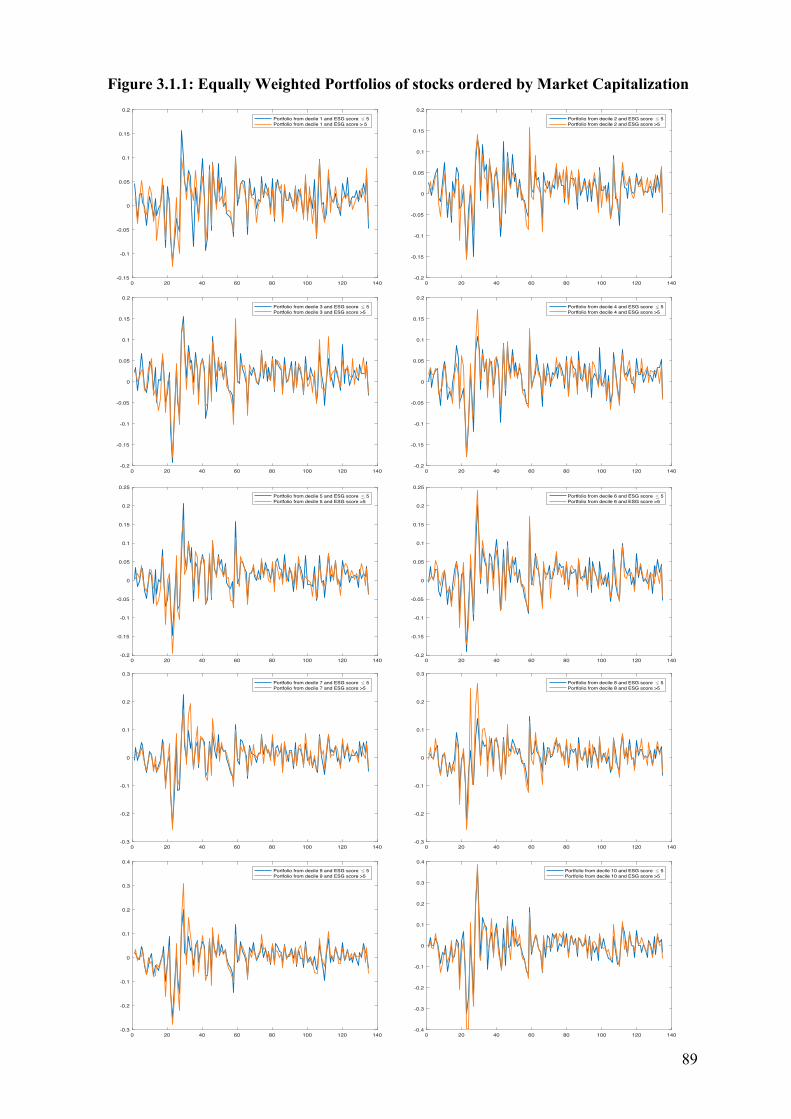
89
Figure 3.1.1: Equally Weighted Portfolios of stocks ordered by Market Capitalization
0 20 40 60 80 100 120 140-0.4
-0.3
-0.2
-0.1
0
0.1
0.2
0.3
0.4Portfolio from decile 10 and ESG score 5Portfolio from decile 10 and ESG score >5
0 20 40 60 80 100 120 140-0.3
-0.2
-0.1
0
0.1
0.2
0.3
0.4Portfolio from decile 9 and ESG score 5Portfolio from decile 9 and ESG score >5
0 20 40 60 80 100 120 140-0.3
-0.2
-0.1
0
0.1
0.2
0.3Portfolio from decile 8 and ESG score 5Portfolio from decile 8 and ESG score >5
0 20 40 60 80 100 120 140-0.3
-0.2
-0.1
0
0.1
0.2
0.3Portfolio from decile 7 and ESG score 5Portfolio from decile 7 and ESG score >5
0 20 40 60 80 100 120 140-0.2
-0.15
-0.1
-0.05
0
0.05
0.1
0.15
0.2
0.25Portfolio from decile 6 and ESG score 5Portfolio from decile 6 and ESG score >5
0 20 40 60 80 100 120 140-0.2
-0.15
-0.1
-0.05
0
0.05
0.1
0.15
0.2
0.25Portfolio from decile 5 and ESG score 5Portfolio from decile 5 and ESG score >5
0 20 40 60 80 100 120 140-0.2
-0.15
-0.1
-0.05
0
0.05
0.1
0.15
0.2Portfolio from decile 4 and ESG score 5Portfolio from decile 4 and ESG score >5
0 20 40 60 80 100 120 140-0.2
-0.15
-0.1
-0.05
0
0.05
0.1
0.15
0.2Portfolio from decile 3 and ESG score 5Portfolio from decile 3 and ESG score >5
0 20 40 60 80 100 120 140-0.2
-0.15
-0.1
-0.05
0
0.05
0.1
0.15
0.2Portfolio from decile 2 and ESG score 5Portfolio from decile 2 and ESG score >5
0 20 40 60 80 100 120 140-0.15
-0.1
-0.05
0
0.05
0.1
0.15
0.2Portfolio from decile 1 and ESG score 5Portfolio from decile 1 and ESG score > 5

90
Figure 3.1.2: Equally Weighted Portfolios of stocks ordered by Price to Book Value
0 20 40 60 80 100 120 140-0.2
-0.15
-0.1
-0.05
0
0.05
0.1
0.15
0.2Portfolio from decile 10 and ESG score 5Portfolio from decile 10 and ESG score >5
0 20 40 60 80 100 120 140-0.2
-0.15
-0.1
-0.05
0
0.05
0.1
0.15
0.2Portfolio from decile 9 and ESG score v 5Portfolio from decile 9 and ESG score >5
0 20 40 60 80 100 120 140-0.2
-0.15
-0.1
-0.05
0
0.05
0.1
0.15
0.2Portfolio from decile 8 and ESG score 5Portfolio from decile 8 and ESG score >5
0 20 40 60 80 100 120 140-0.2
-0.15
-0.1
-0.05
0
0.05
0.1
0.15
0.2Portfolio from decile 7 and ESG score 5Portfolio from decile 7 and ESG score >5
0 20 40 60 80 100 120 140-0.2
-0.15
-0.1
-0.05
0
0.05
0.1
0.15
0.2Portfolio from decile 6 and ESG score 5Portfolio from decile 6 and ESG score >5
0 20 40 60 80 100 120 140-0.25
-0.2
-0.15
-0.1
-0.05
0
0.05
0.1
0.15
0.2
0.25Portfolio from decile 5 and ESG score 5Portfolio from decile 5 and ESG score >5
0 20 40 60 80 100 120 140-0.3
-0.2
-0.1
0
0.1
0.2
0.3Portfolio from decile 4 and ESG score 5Portfolio from decile 4 and ESG score >5
0 20 40 60 80 100 120 140-0.3
-0.25
-0.2
-0.15
-0.1
-0.05
0
0.05
0.1
0.15
0.2Portfolio from decile 3 and ESG score 5Portfolio from decile 3 and ESG score >5
0 20 40 60 80 100 120 140-0.4
-0.3
-0.2
-0.1
0
0.1
0.2
0.3Portfolio from decile 2 and ESG score 5Portfolio from decile 2 and ESG score >5
0 20 40 60 80 100 120 140-0.4
-0.3
-0.2
-0.1
0
0.1
0.2
0.3
0.4Portfolio from decile 1 and ESG score 5Portfolio from decile 1 and ESG score >5

91
Figure 3.1.3: Equally Weighted Portfolios of stocks ordered by Momentum
0 20 40 60 80 100 120 140-0.4
-0.2
0
0.2
0.4
0.6
0.8
1Portfolio from decile 10 and ESG score 5Portfolio from decile 10 and ESG score >5
0 20 40 60 80 100 120 140-0.3
-0.2
-0.1
0
0.1
0.2
0.3Portfolio from decile 9 and ESG score 5Portfolio from decile 9 and ESG score >5
0 20 40 60 80 100 120 140-0.25
-0.2
-0.15
-0.1
-0.05
0
0.05
0.1
0.15
0.2
0.25Portfolio from decile 8 and ESG score 5Portfolio from decile 8 and ESG score >5
0 20 40 60 80 100 120 140-0.25
-0.2
-0.15
-0.1
-0.05
0
0.05
0.1
0.15
0.2Portfolio from decile 7 and ESG score 5Portfolio from decile 7 and ESG score >5
0 20 40 60 80 100 120 140-0.25
-0.2
-0.15
-0.1
-0.05
0
0.05
0.1
0.15
0.2Portfolio from decile 6 and ESG score 5Portfolio from decile 6 and ESG score >5
0 20 40 60 80 100 120 140-0.25
-0.2
-0.15
-0.1
-0.05
0
0.05
0.1
0.15Portfolio from decile 5 and ESG score 5Portfolio from decile 5 and ESG score >5
0 20 40 60 80 100 120 140-0.2
-0.15
-0.1
-0.05
0
0.05
0.1
0.15Portfolio from decile 4 and ESG score 5Portfolio from decile 4 and ESG score >5
0 20 40 60 80 100 120 140-0.2
-0.15
-0.1
-0.05
0
0.05
0.1
0.15
0.2
0.25Portfolio from decile 3 and ESG score 5Portfolio from decile 3 and ESG score >5
0 20 40 60 80 100 120 140-0.3
-0.2
-0.1
0
0.1
0.2
0.3
0.4Portfolio from decile 2 and ESG score 5Portfolio from decile 2 and ESG score >5
0 20 40 60 80 100 120 140-0.3
-0.2
-0.1
0
0.1
0.2
0.3Portfolio from decile 1 and ESG score 5Portfolio from decile 1 and ESG score >5

92
Figure 3.2.7: Multiperiod Returns of Market-cap-sorted Portfolios (2006 – 2018)
Figure 3.2.8: Multiperiod Returns of Price to Book Value-sorted Portfolios (2006 – 2018)
Figure 3.2.9: Multiperiod Returns of Momentum-sorted Portfolios (2006 – 2018)

93
Table 3.2.7: Annualized Holding Period Returns of Size, Value and Momentum Portfolios from 2006 and from 2013
Size Value Momentum
2006 2013 2006 2013 2006 2013
Hig
h E
sg
Portfolio 1 12.29% 18.43% -9.19% 3.15% 8.31% 19.10%
Portfolio 2 13,74% 21.27% 1.48% 5.15% 9.78% 18.60%
Portfolio 3 14.77% 23.28% 2.92% 7.80% 9.93% 15.00%
Portfolio 4 13,80% 19.01% 7.18% 12.42% 11.29% 19.88%
Portfolio 5 12.39% 16.28% 6.83% 11.22% 8.22% 15.02%
Portfolio 6 10.77% 13,58% 10.33% 13.01% 11.47% 14.16%
Portfolio 7 13.32% 18.06% 15.04% 21.15% 11.85% 16.72%
Portfolio 8 8.16% 13,56% 16.83% 19.53% 13.21% 15.41%
Portfolio 9 0.33% 8.16% 19.44% 27.27% 6.85% 8.29%
Portfolio 10 -12.7% 2.23% 22.68% 27.03% 8.40% 8.17%
Low
ESG
Portfolio 1 15.17% 22.51% -10.82% -0.32% 7.09% 15.62%
Portfolio 2 16.11% 17.17% -0.94% 5.83% 9.27% 14.79%
Portfolio 3 16.44% 19.71% 5.15% 9.41% 8.81% 15.68%
Portfolio 4 12.83% 19.65% 6.13% 9.26% 9.09% 14.08%
Portfolio 5 15.72% 15.96% 13.18% 18.42% 12.07% 17.48%
Portfolio 6 14.50% 16.89% 10.70% 13.02% 13.01% 16.66%
Portfolio 7 8.20% 15.53% 16.54% 18.48% 9.49% 13,63%
Portfolio 8 8.12% 12.06% 17.47% 20.96% 8.62% 11.12%
Portfolio 9 2.85% 6.20% 18.41% 17.61% 5.16% 8.52%
Portfolio 10 -9.51% -3.12% 24.53% 29.10% -4.82% 6.73%

94
Figure 5.7: Multiperiod Returns of Equally weighted “Market Portfolios”
(2006 – 2018)
Figure 5.8: Multiperiod Returns of Equally weighted “Market Portfolios”
(2006 – 2018)

95
Figure 5.9: Multiperiod Returns of Equally weighted “Market Portfolios”
(2013 – 2018)
Figure 5.10: Multiperiod Returns of Equally weighted “Market Portfolios”
(2013 – 2018)

96
PORTFOLIO ALLOCATION AND ESG RATINGS:
SUMMARY
1 Introduction
The concept of sustainable investing has been discussed throughout the financial field at least
from 1960s. However, while in the 70s many economists like Milton Friedman believed that
only lawmakers and politicians had to care about regulating companies’ sustainability,
nowadays the majority of investment professionals understands the link between
sustainability in broad sense and businesses’ financial success.
In general, the main question about Socially Responsible Investment (SRI) has changed from
“why?” to “why not?” following empirical evidence that integrating SRI criteria into the
traditional investment process does not negatively affect profits, usually.
The increased popularity gained by sustainable investments can be outlined looking at United
Nations’ Principles for Responsible Investment (UNPRI) growth in signatories and
investments’ volume through the years; in 2018 the UNPRI had about 2000 signatories, with
assets under management (AUM) amounting to around $80 trillion. Another trend of growth
toward a more sustainable business model can be found analysing the Standard and Poor 500:
while only 20% of its listed companies published sustainability reports in 2011, the number
has increased to 85% just six years later, in 2017 (Coppola, 2018).
ESG investing deviates from the notion of SRI as it is a more comprehensive approach; it
represents the acronym for Environmental, Social and Governance and refers to the three
fundamental factors in measuring the social impact and the sustainability of an investment in
a company. While SRI process would implement ESG criteria with the aim both of generating
long-term competitive financial returns and a positive impact on society, Responsible
Investing (RI) claims that foregoing ESG factors means disregarding risks and opportunities
that have a material impact on company’s returns, thus they should be taken into account even
by investors whose sole objective is the bottom line45. Although there is an overlay of social
awareness, the key point of ESG evaluation remains financial performance. Several empirical
researches, 2000 studies are just those analysed by Friede et al. (2015) in their meta-analysis,
show that ESG criteria help to better determine the future financial performance of companies
for what concerns both risks and returns. In particular, highly sustainable companies are
45 In opposition to SRI’s “triple bottom line”.

97
deemed to be typically more long-term oriented, with a structured process for stakeholders
engagement and more likely to disclose information.
Our paper is structured as follows: Chapter 2 outlines sample composition and settings, in
Chapter 3 we deal with factor analysis and portfolio construction and in Chapter 4 we go
through portfolio optimization theory and we apply it on our data. Chapter 5 investigates the
behaviour of three different investment universes: 𝑅! ,𝑅!,!"# ,𝑅!,!" and Chapter 6
concludes.
2 The Dataset
Our analysis is carried on the companies comprised in the Standard and Poor 500 Index
(S&P500) during the period from January 31st, 2000 to February 28th, 2018. All data herein is
intended as of March 31st, 2018.
The dataset consists of several variables related to financial and non-financial data with
monthly frequency. The time horizon considered equals 18 years and 1 month starting on
January 31st, 2000 (𝑡!) until February 28th, 2018 (𝑡!"#); hence, there are 218 entries for every
cross-sectional observation for what concerns financial data. On the contrary, data on
sustainability scores (MSCI ratings) are available from December 31st, 2006 until February
28th, 2018, which means there are 135 time observations for each cross-sectional object.
In particular, the variables employed to address our analyses are:
• A dummy variable (0-1) that we will name “isconstant” because it indicates whether a
stock was included in the S&P 500 Index in a specific month.
• Market Capitalization expressed in US Dollars ($);
• Cash Flows from Operating activities per share expressed in US Dollars ($);
• Book Value per share expressed in US Dollars ($);
• Price expressed in US Dollars ($);
• A “sector” variable that classifies each company for industry group as of the Global
Industry Classification Standard (GICS) as of March 2018;
• The aggregated 0-10 Weighted Average Key Issue Score supplied by MSCI Inc. (ESG
score);
• The 0-10 MSCI Environmental Pillar Score (E score), the weighted average of
Environmental Key Issues Scores;

98
• The 0-10 MSCI Social Pillar Score (S score), the weighted average of Social Key Issues
Scores;
• The 0-10 MSCI Governance Pillar Score (G score), the weighted average of Governance
Key Issues Scores.
MSCI ESG Ratings are conceived to help investors in the understanding of ESG-driven
opportunities and risks and in the process of integrating these factors into their portfolio
construction and management. Data points collected from public sources, such as government
databases and company disclosures, are analysed in relation to 37 ESG “Key” issues. The
focus is on the intersection between a company’s core business and those industry issues that
can create significant financial risks and opportunities for that company. Firms are rated on an
AAA-CCC scale relative to the standards and performance of their industry peers and they are
systematically monitored and reviewed.
Within past decades, the competitive and social context for analysing the three pillars has
dramatically changed, especially for what concerns corporate environmental and social issues,
while the fundamental “G” issues have remained close to those identified by Graham B. &
Dodd D. and by Fisher P. too (Hanson (2013)). Sustainable investing also encompasses the
ESG approach, which is more comprehensive and is the subject the financial field is
prominently focusing on now (see Hale (2016)). The three concepts of environmental, social
and corporate governance are also closely related to the Responsible Investment approach
(RI), which subtly differs from Socially responsible investing46. While SRI is an investment
discipline that considers ESG criteria to generate long-term competitive financial returns and
positive impact on society47, RI should be pursued even by the investor whose sole objective
is the bottom line48, because it claims that foregoing ESG factors means disregarding risks
and opportunities that have a material impact on company’s returns. Responsible investment
aims at incorporating ESG factors into investment decisions, to better manage risk and
generate sustainable, long-term returns49. Although there is an overlay of social awareness,
the key point of ESG evaluation remains financial performance.
Several studies show that ESG criteria help to better determine the future financial
performance of companies for what concerns both risks and returns. In particular, high
46 UNPRI, “What is responsible investment?”, available at https://www.unpri.org/pri/what-is-responsible-investment 47 US SIF, The Forum for Sustainable and Responsible Investment, “SRI Basics” 48 As opposed to the “triple bottom line”. 49 UNPRI, “What is responsible investment?”.

99
sustainability companies are typically more long-term oriented, have structured processes for
stakeholders engagement and are more likely to disclose non-financial information (see
Eccles et al. (2014)). In 2018 the United Nations’ Principles for Responsible Investment had
about 2000 signatories, with assets under management (AUM) amounting to around $80
trillion. Another trend of growth toward a more sustainable business model can be found
analysing the Standard and Poor 500: while only 20% of its listed companies published
sustainability reports in 2011, the number has increased to 85% just six years later, in 2017
(Coppola, 2018). Empirical evidence that ESG and corporate financial performance are highly
positively related over time has been the main driver for growth in interest on firms’
sustainability performance. Friede et al. (2015) conducted a meta-analysis on 2000 empirical
studies concluding that all rational investors should take into high consideration long-term
responsible investing in order to “harvest the full potential of value-enhancing ESG
factors”50. Also Warren Buffet supports this concept suggesting that, in order to gain a
sustainable competitive advantage, businesses must invest in the three key profitability
components: the environment, communities and their people (Arbex (2012)).
From statistical analysis on the whole sample we find that 25% of the 1040 stocks were
included in the S&P 500 for 16.3 to 18.1 years between 2000 and 2018. Moreover, 28% of
companies have average market capitalization less than $5 billions, more than half of our
sample has mean cash flow from operations per share between $0 and $4 dollars and around
56% of our sample book value per share is, on average, comprised between 0 and $15 dollars.
During the 18 years under consideration the biggest stake of companies that were included in
the S&P 500 belonged, in median, to the Consumers Discretionary sector. The portion of
companies operating in the consumer discretionary and in the information technology sectors
shrank in favour of the sectors of Health Care, Financials and Real Estate. More than 82% of
the sample observations has mean price comprised between 0 and $60 and are quite
heterogeneous compared both among cross-sectional objects and in time. The majority of
companies’ average returns is comprised between 0 and 5%, with around 30% of cross-
sectional observation providing mean returns of 1% to 1.5% as shown in the Figure 2.7
below. The distribution of aggregated mean returns is skewed to the right and leptokurtic.
During time companies became more interested in improving their sustainability and
investment managers became keener on recognizing companies’ “intrinsic value” through the 50 Friede et al., 2015, p. 227.

100
implementation of their material ESG issues’ analysis. Comparing ESG scores referring to
December 2006 with the ones related to February 2018 there is an evident shift toward higher
scores and an increase in their plurality. On average, also Environment and Governance
scores experienced an increasing trend through time, instead, Social scores were higher in
2006. Moreover, companies that had higher average ESG score, during the period studied,
also had longer permanence in the S&P 500, and this applies to E score and S score too.
Improvements in business’ sustainability are more important for largest-cap companies;
indeed, these are the ones with highest ESG rating. However, it is not true that the bigger is
the company the higher is the score since the majority of large-cap companies have mean
ESG score between 1 and 2. In the same way, CFO, book value and price per share are higher
for companies with higher mean ESG score, whereas returns are inversely related with
average sustainability scores. The market may have already incorporated high ESG
companies’ greater intrinsic value on their price and has to give higher rewards to investors
choosing to buy low ESG firms in order to compensate them for the higher risk they bear,
since volatility of low ESG companies’ returns is much higher versus that of high ESG
companies. This features also apply to companies aggregated by E score and S score, while G
score buckets have diverse characteristics, for example, returns are higher for higher G scores
companies. Furthermore, companies classified by different mean ESG score also belong to
different industry groups: Bucket 1 companies operate in the industries of Food, Beverage
and Tobacco, of Media and of Materials (Graph 2.1); instead, companies that have mean ESG
scores between 7 and 8 belong to the industries of Utilities, Semiconductors & Semiconductor
Equipment, Technology, Hardware & Equipment, Software & Services, Real Estate and
Materials (Graph 2.7).
3 Factor Analysis
The aim of this Chapter is to analyse whether portfolios composed by companies with higher
ESG score have been more profitable than the ones with lower ESG score during the time
period considered. We base the construction of those portfolios on two assumptions, first, that
the S&P 500 is a good proxy for representing the whole market, secondly, that a fair game is
based on equal starting conditions.
The “market portfolio”, as defined by Black, Jensen and Scholes (1972), would represent an
investment in every outstanding asset in proportion to its value. That assumption is backed by

101
the fact that the Index amounts to 80%51 of the total market capitalization of the entire stock
market (as of 2018), that is, it is weighted by a wide number of market values. Moreover, the
fact that its components are all actively traded stocks also renders it attractive as market
portfolio proxy.
Our second assumption refers to the fact that we decided to implement factor-based strategies
and only afterwards we implement our ESG score strategy on top of them. The purpose of
building factor portfolios is to aggregate companies with similar characteristics and to
investigate how ESG score impacts on returns controlling for other variables. Moreover,
considering the rise in ESG investing, to base an investment strategy solely on ESG score
could be misleading causing to overpay for perceived quality. Subramanian (2016) reports
that combining ESG strategies in conjunction with fundamental attributes like valuation,
growth and quality outperformed fundamental strategies alone with lower risk.
In light of those considerations, we created portfolios oriented at targeting the factors of size,
value and momentum following the previous studies conducted by Fama and French (1993)
and Cahrart (1997).
The Size factor refers to a firm’s market capitalization (stock price times shares outstanding).
Historically, portfolios consisting of small-cap stocks exhibit greater returns than portfolios
with large-cap stocks; the intuition is that smaller companies tend to outperform larger ones
rewarding investors for bearing more risks related to illiquidity and high sensitivity to market
movements. The Value factor aims at capturing excess returns from stocks that have low
prices relative to their fundamental value and it is commonly tracked by price-to-book or
price-to-earnings. “Value stocks” are those that have market values that are small relative to
the accountant’s book value, while the so called “growth stocks” have higher price versus
book value. During time, scholars and investment professionals have argued that value
strategies outperform the market (Graham and Dodd (1934) and Dreman (1977)). These
strategies are based on buying stocks that have low prices relative to earnings, dividends,
book assets, or other measures of fundamental value (see Lakonishok (1991)) and, in
particular, Fama and French (1992) show that stocks with high book/price ratios (BE/ME)
earn higher returns. Further works both extended and refined these results (Rosenberg, Reid,
and Lanstein (1984); Chan, Hamao, and Lakonishok (1991) and Fama and French (1992)).
The Momentum factor is based on the empirical evidence that stocks that have outperformed
in the past tend to exhibit strong future returns and consists of differentiating between stocks
with positive and negative excess returns in the recent past. Carhart (1997) calls this 51 S&P Dow Jones Indices, “Equity, S&P 500 Factsheet”, as of December 31, 2018

102
additional risk dimension a price momentum factor and estimates it by computing return over
the past 12 months skipping the most recent one. Although there are sound economic reasons
for these trends to continue (e.g., company revenues and earnings that continue to grow faster
than expected), it may also be the case that investors periodically underreact to the arrival of
new information (see Chan, Jegadeesh, and Lakonishok (1999)). De Bondt and Thaler (1985,
1987) argue that extreme losers outperform the market over the subsequent several years and
despite significant criticisms (Chan (1988) and Ball and Kothari (1989)), their analysis has
typically stood up to the tests (Chopra, Lakonishok, and Ritter (1992)).
The stocks considered for the factor analysis are those effectively included in the S&P 500
each month, for this purpose we built a variable “Nan_isconstant” to obscure all the stocks
that exited the Index each time. In second instance, we implement the three strategies, each
one distinctly from the other two, based on factors: size, value and momentum. We rank
stocks on a monthly rolling basis depending on their end-of-month market capitalization
(size) in descending order, share price-to-book value (value) in ascending order and
momentum in descending order.
After being sorted by factor, data is allocated in 10 clusters composed, ideally52, by 50 stocks
each. This means that, over around 500 stocks we ordered data by factor (three different
orders), we collected returns attached to the ranked stocks and divided them in deciles (10 sets
with a total of 30 sets).
For what concerns size portfolios, stocks are ranked in descending order. In the first portfolio
are present the companies with the highest market capitalization (big), while in the 10th there
are the ones with the lowest market-cap inside the S&P 500 (small). Stocks in value portfolios
are ranked for ascending price-to-book value per share, which means that in the first set there
are stocks with high book value with respect to price, the so called value stocks, while in the
10th portfolio there are growth stocks, the ones characterized by high price versus accounting
equity value. Momentum-ordered portfolio 1 comprises stocks that had the highest return in
the preceding year (skipping the last month), those that are commonly known as winners,
while previous year’s losers are classified in the last sets.
Finally, we apply the ESG score strategy on each of the 10 deciles. The “ESG strategy”
applied consists of additionally sorting stocks by their Weighted Average Key Issue Score,
with threshold score equal 5. Returns of stocks with sustainability rating higher than 5 are 52 The last portfolios (i.e. 9 and 10), especially, may comprise fewer observations than 50 due to either missing data from factors’ variables or because stocks included in the Index are not exactly 500 (for example the number of S&P 500 constituents equalled 505 as of December 2018 but may also be lower) or both.

103
divided from those with rating lower or equal to 5 and returns from the two groups are
aggregated into two equally weighted portfolios for each decile for each factor. We chose 5 as
threshold instead of 5.7 (that is the score related to the MSCI “A” final rating) based on the
overall distribution of ESG scores across the Index. Mean and median scores of S&P 500
companies’ are distributed between 4.4 and 5.4 and 4.2 and 5.4, respectively, through time.
Since mean ESG scores for individual stocks average out at 4.72 we chose to consider the
highest half of BBB stocks (4.3 to 5.7 for MSCI) and all A to AAA stocks, in order to have
enough variance also when splitting the last deciles. Moreover, we chose to integrate ESG
scores on top of our factor strategy in order to take advantage of the financial benefits of
employing full integration, which, together with engagement, is considered the most
beneficial ESG strategy by relevance to investment performance (see Amel-Zadeh and
Serafeim (2018)).
An upfront investment of $100 on December 2006 would have yielded at most $554 for a size
investor, $1180 for a value investor and $403 for a momentum investor on February 2018
(Figures 3.2.7 to 3.2.9, Appendix). High ESG Size portfolios had lower annualized returns
with respect to their low ESG counterparty during the period 2006 – 2018, while they clearly
outperform low ESG portfolios in the period 2013 – 2018 as reported in Table 3.2.7
(Appendix). In particular, investing in small-cap high ESG portfolios in the past five years
yielded positive returns while their low ESG counterparty returns were negative. Value
investors also would have earned positive returns from 2013 and less negative returns from
2006 investing in high ESG portfolios versus low ESG ones, but in general low ESG
portfolios outperformed high ESG ones since growth low ESG stocks yielded higher returns
than their high counterparty. Momentum investors would have been better off investing in
high ESG portfolios. Considering both time horizons high ESG portfolios outperformed low
ESG ones, especially, returns from momentum strategy are all positive, instead portfolio 10
low ESG had negative returns in the “long-run”. For what concerns strategies, High ESG
growth investors during both periods earned the highest returns with respect to size and
momentum investors; while small-cap investors earned the lowest returns with respect to
value and momentum ones in both periods. Momentum portfolios had lower but more stable
and homogeneous returns in general. Relative to Low ESG portfolios, value-strategy yielded
both the highest returns for growth portfolios but also the most negative ones for value
portfolios in the long run, while small-cap low ESG investors earned the most negative
returns in the last 5 years. Also in this case, momentum investors in both periods earned lower

104
returns that were more stable and homogeneous and suffered lower losses. Maybe a sector
specific framework would have given sharper results; Subramanian et al. (2016) study that
investments based on Environmental Innovation (scores from Thomson Reuters) would have
yielded a 3-year alpha of circa 30 percentage points for companies operating in Materials
Industry and 20 ppt for those operating in Energy, while they did not generate any excess
returns for Consumer Sectors’ companies.
4 Mean - Variance Optimization
While Markowitz’s (1952, 1959) portfolio optimization structure was solely based on
financial parameters and investors’ risk aversion, we also introduce ESG scores in order to
study whether discriminating for the degree of sustainability yields portfolios with higher
risk-return profiles.
Prior to 1950, portfolio theory lacked an adequate framework for investments as it did not
consider the effects of diversification when risks are correlated, missed the distinction
between efficient and not efficient portfolios and did not analyse the trade-offs between risk
and return on portfolio as a whole (see Markowitz (1999)). In 1952, both Harry Markowitz
and Andrew D. Roy laid the foundations of what is now called Modern Portfolio Theory: they
theorized about basing portfolio selection on expected return and variance of the entire
portfolio. Especially, Markowitz assumed securities’ projections obey to the same probability
laws as those of random variables; which implies that the expected return of a portfolio is the
weighted average of the expected returns on individual securities and that the variance of
portfolio returns is a function of the variances of securities and the covariance between them,
and their weights in the portfolio.
In our optimization analysis we implement the Matlab function Porfolio in order to create a
Portfolio object for mean-variance optimization whose computations are based on the
Markowitz model (1952, 1959)53 and to which we apply further constraints on lower and
upper bounds. Then, we employ the function portalloc to compute the optimal risky
portfolio, and the optimal allocation of funds between the risky portfolio and the risk-free
asset. By optimal risky portfolio (ORP) we mean the portfolio on the efficient frontier that
53 Matlab portfolio optimization tools make reference to Chapter 7 of Bodie Z., Kane A. and Marcus A. J. (1993): “Investments”, 2nd Edition. Source: Matlab Bibliography
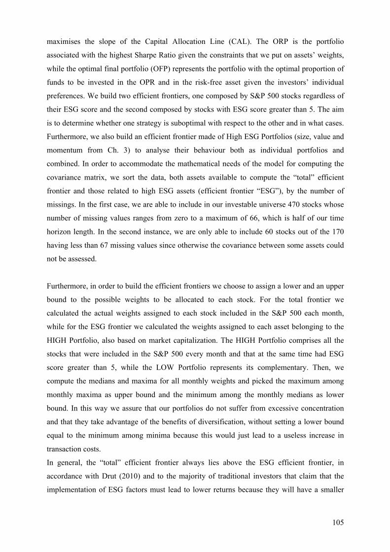
105
maximises the slope of the Capital Allocation Line (CAL). The ORP is the portfolio
associated with the highest Sharpe Ratio given the constraints that we put on assets’ weights,
while the optimal final portfolio (OFP) represents the portfolio with the optimal proportion of
funds to be invested in the OPR and in the risk-free asset given the investors’ individual
preferences. We build two efficient frontiers, one composed by S&P 500 stocks regardless of
their ESG score and the second composed by stocks with ESG score greater than 5. The aim
is to determine whether one strategy is suboptimal with respect to the other and in what cases.
Furthermore, we also build an efficient frontier made of High ESG Portfolios (size, value and
momentum from Ch. 3) to analyse their behaviour both as individual portfolios and
combined. In order to accommodate the mathematical needs of the model for computing the
covariance matrix, we sort the data, both assets available to compute the “total” efficient
frontier and those related to high ESG assets (efficient frontier “ESG”), by the number of
missings. In the first case, we are able to include in our investable universe 470 stocks whose
number of missing values ranges from zero to a maximum of 66, which is half of our time
horizon length. In the second instance, we are only able to include 60 stocks out of the 170
having less than 67 missing values since otherwise the covariance between some assets could
not be assessed.
Furthermore, in order to build the efficient frontiers we choose to assign a lower and an upper
bound to the possible weights to be allocated to each stock. For the total frontier we
calculated the actual weights assigned to each stock included in the S&P 500 each month,
while for the ESG frontier we calculated the weights assigned to each asset belonging to the
HIGH Portfolio, also based on market capitalization. The HIGH Portfolio comprises all the
stocks that were included in the S&P 500 every month and that at the same time had ESG
score greater than 5, while the LOW Portfolio represents its complementary. Then, we
compute the medians and maxima for all monthly weights and picked the maximum among
monthly maxima as upper bound and the minimum among the monthly medians as lower
bound. In this way we assure that our portfolios do not suffer from excessive concentration
and that they take advantage of the benefits of diversification, without setting a lower bound
equal to the minimum among minima because this would just lead to a useless increase in
transaction costs.
In general, the “total” efficient frontier always lies above the ESG efficient frontier, in
accordance with Drut (2010) and to the majority of traditional investors that claim that the
implementation of ESG factors must lead to lower returns because they will have a smaller

106
investment universe. Discriminating for the sustainability score causes our investment
universe to be scaled down. Moreover, considering that companies during their business life
may have had different scores (both greater or smaller than 5), their available time series
observation could not be enough to allow for covariance computations, which further
downsizes our sample. Trying to account for the other “high” stocks, we also computed the
optimization including the means of stocks aggregated by the number of semesters missing
but this did not change the current outcome. Dominant high ESG portfolios are suboptimal
when compared with the total efficient frontier. An exception is represented by those “total”
portfolios with lower variance that intersect the ESG efficient frontier. In that case, it is
evident that the general lowest-mean-variance portfolios are not efficient versus the ESG
ones. This means that very risk-averse investors would be better off investing in high ESG
portfolios for that same variance. Additionally, the ESG frontier comprises efficient
investment opportunities with lower variance that are not available in the “total” investment
universe. This can suggest that investors whose main objective is to minimize volatility54 may
find efficient solutions investing in high ESG portfolios but not just considering all S&P-like
efficient portfolios.
Based on our investor preferences55, the Capital Allocation Line represents the allocation
between the risk-free asset and a risky portfolio of assets. The optimal risky portfolio on the
high ESG frontier has a better risk-return profile with respect to the total one. The line is
slightly steeper and for the same increase in variance it rewards investors with higher
expected returns. The investment in the ESG risky portfolio yields 2.6 units of return of every
unit of risk, whereas the total risky portfolio yields 2.38 units of return for every unit of risk56.
The S&P 500 is far below both efficient frontiers and also below their two CALs. This
suggests that implementing an optimization framework using stocks’ expected returns and
covariances yields portfolios that have higher returns for the same level of risk of the Index,
which instead allocates capital weights among its stocks based on market capitalization and
regardless of their covariances. Furthermore, the majority of high ESG portfolios have higher
expected returns than the S&P with the same or very close standard deviation; some
portfolios are above the ESG frontier, halfway to the total one. Those portfolios are more
54 In the sense that they are more fearful of oscillations in invested capital and drawdowns like, for example, high net worth individuals. 55 This investor chose investment bounds and has a quadratic utility function based on expected return and variance with a risk aversion coefficient (λ) equal to 4. 56 Recall the concept of “Adjusted Sharpe Ratio” of Chapter 3. This measure is now calculated as OFP Return over OFP risk, which, in this case, is the same as ORP Return divided by ORP risk.

107
efficient for ESG investors but suboptimal, like all the others composing the ESG frontier,
with respect to the full investment universe. Notably, no factor portfolio has lower standard
deviation than 13.6, which is the corresponding point to the total ORP; that is, using factor
strategies for ESG investments may yield efficient portfolios but does not allow taking full
advantage of the lower variance that characterizes sustainable investments. Moreover, some
portfolios are positioned exactly on the ESG frontier, suggesting that value and momentum
strategies yield efficient portfolios.
We computed an additional efficient frontier composed by the 30 high ESG factor portfolios.
If our investor decides not to allow short selling and to allocate at least 0 and at most 0.33
(1/3) of capital on one portfolio, the resulting efficient frontier (“portfolios”) appears like a
portion of the ESG one, as illustrated in Figure 4.2.2. Optimization of factor portfolios leads
to an efficient frontier, which is slightly more efficient than the ESG one from the ORP
onwards but it is strongly suboptimal to the left of the ORP.
Alternatively, if the investor decides not to impose bounds on weights allocation, except no
short selling, the optimization process yields a new frontier (Figure 4.2.3). This second
frontier lies above the ESG one, while becoming suboptimal for portfolios with variance
greater than 40% and for those with variance equal or lower to around 18%.
Another strategic decision for the investor could be lifting the short selling constraint and just
allow the man-variance optimization to yield the most efficient portfolios while respecting a
lower bound equal to -0.033 (1/30) and an upper bound of 0.33 (1/3).
Combining the factor portfolios we can see no benefits in investing in their optimized
combination for lower values of standard deviation in any of the three cases analysed.
Until now, the strategic choice of allowing short selling and implementing long-short
positions is the one that yields the most efficient set of portfolios. The three cases above
highlight the fact that in these optimization frameworks growth portfolios are always included
in the ORPs. However, factor investing in general does not “beat” optimized investments
related to the total investment universe, although some of them are much more efficient than
the S&P 500 itself. Which means that screening for high ESG scores could still yield better
risk-adjusted returns than passively replicating or buying the Index.
As stated by previous literature, we find that ESG investors are not efficient, unless they
target investments with standard deviation lower than 4%. High Net Worth Individuals, for
example, would likely be better off in implementing ESG screenings and mean-variance

108
optimization in order to choose the less variable investments. Reducing the time horizon to
the last 5 year (2013 – 2018) does not change all the considerations made until now.
5 The Market Portfolio(s)
In this Chapter we analyse three indices that refer to three distinct investment universes:
𝑅! ,𝑅!,!"# ,𝑅!,!". Those three indices are composed by all S&P 500 stocks with an ESG
score, all S&P 500 stocks with ESG score greater than 5, and all S&P 500 stocks with ESG
score smaller than 5, respectively. Our purpose is to aggregate those three sets of stocks both
in market-weighted portfolios and in equally weighted portfolios and compare their returns
among them and versus the S&P 500 Index itself. Our aim is to address the question of
whether ESG investors can earn higher returns than traditional ones both in the long- and in
the short-term. Are non-financial disclosure and ESG score signals for investors of better and
longer lasting future performances?
As illustrated in Figure 5.1, the monthly returns of the indices move together in general.
However, during the period from 2008 to 2012, 𝑅!,!" considerably deviated from 𝑅! ;
wherears from 2013 to 2018 𝑅!,!"# had more extreme values with respect to 𝑅!. Deviations
from 𝑅!, which we are considering to describe the behaviour of the general market, mean the
market prominently commoved with the “other” investment set. Since all those indexes are
market weighted, either during 2008-2012 𝑅! , and consequently the S&P 500, mainly
included high ESG scored firms, or, those high ESG companies had a larger market
capitalization thus making a greater impact on the whole index. Similarly, just after 2013 𝑅!
returns prevalently deviated from 𝑅!,!"# . Both reasoning could hold, however, we could
argue that in the period just after the last financial crisis the majority of firms meeting S&P
500 eligibility criteria where those with high ESG rating, while in normal economic periods
more firms with low ESG scores meet the S&P 500 criteria.
𝑅!,!" had the highest annualized returns (16.13%) with also the highest level of risk
(standard deviation equal to 15%); on the contrary 𝑅!,!"# experienced the lowest returns
(14.2%) characterized by the lowest risk (annualized s.d. 14.04%). 𝑅! lies in between, with
annualized expected returns equal to 15.17% and standard deviation of 14.12%. Their
Adjusted Sharpe Rations are so, respectively, 1.076, 1.011 and 1.074; the 𝑅!,!" is the
portfolio with the best (slightly) risk-return profile in this context and based on market
weights. However, as shown in Figure 5.2, the higher expected returns come at the cost of a
much higher standard deviation. An investor who would choose to only invest in companies

109
that have a sustainability rating among those included in the S&P 500, would achieve a much
higher return versus the S&P with a much lower variance, while investing in Low ESG
companies would bear an increase in volatility. 𝑅! is always equal or above the S&P 500.
This means that distributing invested capital over ESG rated companies allows the investor to
allocate bigger weights on more profitable companies than it is possible in the S&P 500.
In this case we can say that with respect to the staring investment universe, investors seeking
high ESG portfolios are better off than general investors. The decision to care about the ESG
score yields the double expected return than the S&P 500. Among the ESG rated universes,
less risk-averse investors earn the highest expected returns.
The second instance consists of computing three equally weighted portfolios from the same
three investment universes as before. The equally weighted portfolio method makes sure that
we analyse the true number of companies that make an impact on each portfolio and it is
illustrated in Figure 5.4. It is true that 𝑅! was prominently composed by High ESG
companies, but the numerical amounts differ slightly. What prominently makes a difference is
allocating higher weights following market capitalization, which means that during this
period the S&P 500 included larger companies with high more than low ESG score.
Similarly, during the period from 2015 to 2018 𝑅! prevalently included low ESG companies,
deviating from 𝑅!,!"# .
Equally weighted portfolios are characterized by higher standard deviations versus market
weighted ones. Furthermore, in this case 𝑅!,!"# had the highest annualized returns (11.65%)
with instead the lowest level of risk (standard deviation equal to 16.91%); on the contrary
𝑅!,!" experienced the lowest returns (11.05%) charachterized by the highest risk (annualized
s.d. of 17.11%). 𝑅! lies in between, with annualized expected returns equal to 11.23% and
standard deviation of 16.94%. Their Adjusted Sharpe Rations are so, respectively, 0.69, 0.65
and 0.665, with the 𝑅!,!"# having the best risk-return profile. Volatility in equally weighted
portfolios is higher versus volatility in market weighted ones, and returns are generally higher
for the last portfolios than for the first ones. Assigning the same weights to all securities
causes more variability in the portfolio especially in the 𝑅!,!", which is always the one with
the highest standard deviation. On the other hand, 𝑅!,!"# always has the lowest standard
deviation. 𝑅!,!"# returns are those that experience the least decrease when comparing market
weighted and equally weighted portfolios; this may suggest that high ESG companies have
generally higher returns than low ESG ones, but the companies with largest market
capitalization have lower returns in the high ESG portfolio while they have higher returns

110
with respect to the portfolio mean (or also median) in the low ESG portfolio; this leads to the
low ESG market weighted portfolio returns dominating the high ESG one, when, instead, the
equally weighted high ESG portfolio dominates the low ESG one. Moreover, in both cases,
and especially in the market-weighted case, 𝑅! standard deviation is closer to the high ESG
one; this can suggest that in general high ESG companies have larger market-cap than low
ESG ones but are outnumbered by many lower sized low ESG companies, except few
important exceptions.
Comparing monthly long-run returns between market weighted and equally weighted
portfolios (Figure 5.7 and 5.8, Appendix) the low ESG market weighted portfolio
outperformed the high ESG one and vice versa in the equally weighted case. Notably, after
reaching the lowest rate of returns in 2009, all portfolios started yielding positive returns in
2010, although the portfolio with the fastest recovery among equally weighted ones was that
composed by high ESG companies, while it also outperformed all the others in general.
Investing $100 either 2006 or in 2013 in one of our market weighted “Market Portfolios”
would mean receiving at least 6 percentage points more in expected returns. While making
the same investment with both a long-term time horizon and a short term one, would yield at
least 2 pp more than investing in the S&P 500. Equally weighted strategies are optimal after
the implementation of high ESG score screening. While market weighted ones are optimal
excluding high ESG rated companies. As previously stated, in general high ESG companies
yield higher returns than low ESG ones, but the biggest high ESG companies to which market
weighted strategies assign most weight yield lower returns that the biggest low ESG
companies. This suggests that the high ESG market is more homogeneous, generally healthier
and characterized by lower volatility.
6 Conclusion
From the analysis of our whole panel we can conclude that ESG scores attached to sample
stocks are more influenced by environmental and social scores, on average, than by
governance scores, which are flatter through those buckets. Moreover, stocks with lower
sustainability ratings are characterized by higher returns’ volatility, in all scenarios
(aggregating them by ESG and also by E, S and G scores separately).
Factor portfolios composed by high ESG companies yield equal or higher returns than those
composed by low ESG companies and have better risk-return profiles. While in an
optimization framework scaling down the investment universe in order to consider only ESG

111
stocks may lead to a suboptimal mean-variance frontier, the ESG investment universe
provides investment solutions characterized by lower variance and better rewards to investors
for bearing the same unit of risk. In addition, considering a market weighted index only
composed by high ESG stocks leads to a decrease in volatility and doubles expected returns
with respect to the S&P 500 ones.
This paper, overall, shows that choosing to take ESG criteria into account is becoming more
and more profitable, as highlighted by our short-term results. Moreover, the mixed evidence
related to long-term results indicates that investors would have been better off with
responsible investments depending on their risk aversion and fear of losses in a mean-
variance optimization framework.
Notwithstanding the fact that applying factor strategies has mixed outcomes related to which
set of portfolios achieves the best risk return trade off, in the long run it would not lead to
statistically significant differences in expected monthly returns.
Furthermore, investors interested in replicating the S&P 500 would have had higher gains
with lower variance investing in high ESG companies within the same investment universe
and would have recovered faster from the financial crisis.
During time companies became more interested in improving their sustainability and
investment managers became keener on recognizing companies’ “intrinsic value” through the
implementation of their material ESG issues’ analysis. Comparing ESG scores referring to
December 2006 with the ones related to February 2018 there is an evident shift toward higher
scores and an increase in their plurality. On average, also Environment and Governance
scores experienced an increasing trend through time, instead, Social scores were higher in
2006. Moreover, companies that had higher average ESG score, during the period studied,
also had longer permanence in the S&P 500, and this applies to E score and S score too.
Improvements in business’ sustainability are more important for largest-cap companies;
indeed, these are the ones with highest ESG rating. However, it is not true that the bigger is
the company the higher is the score since the majority of large-cap companies have mean
ESG score between 1 and 2. In the same way, CFO, book value and price per share are higher
for companies with higher mean ESG score, whereas returns are inversely related with
average sustainability scores. The market may have already incorporated high ESG
companies’ greater intrinsic value on their price and has to give higher rewards to investors
choosing to buy low ESG firms in order to compensate them for the higher risk they bear,
since volatility of low ESG companies’ returns is much higher versus that of high ESG

112
companies. This features also apply to companies aggregated by E score and S score, while G
score buckets have diverse characteristics, for example, returns are higher for higher G scores
companies. Furthermore, companies classified by different mean ESG score also belong to
different industry groups: Bucket 1 companies operate in the industries of Food, Beverage
and Tobacco, of Media and of Materials (Graph 2.1); instead, companies that have mean ESG
scores between 7 and 8 belong to the industries of Utilities, Semiconductors & Semiconductor
Equipment, Technology, Hardware & Equipment, Software & Services, Real Estate and
Materials (Graph 2.7).
From our factor analysis we conclude that investing in our factor portfolios composed by high
ESG stocks is not statistically significantly different from investing in low ESG stocks in the
long term. Contrarily, high ESG portfolios yield better risk-adjusted profits in the short run,
and the differences in factor portfolios’ expected returns are, in some case, statistically
significantly different from zero, favouring sustainable investments.
Size portfolios comprising companies characterized by high market capitalization have higher
ESG score, on average, than those composed by lower size companies. Furthermore, “big
companies” portfolios have higher monthly mean returns versus “small companies” ones and
also the first 5 high ESG portfolios have lower standard deviations of returns than their low
ESG score counterparties; this reverses for the last 5 portfolios. Also adjusting for risk, size
portfolios with lower ESG score have in general higher returns than those with high ESG
scores during the period 2006 to 2018, even though statistical tests are inconclusive on this
point.
Long run annualized returns related to High ESG Size portfolios are lower with respect to
their low ESG counterparty.
Value portfolios composed by companies with higher price-to-book value (growth stocks)
have higher ESG score, on average, than those composed by lower price-to-book value
companies (value stocks) in the long run. This counterintuitive result could be caused by the
fact we are building our value portfolios based on stocks already “ordered” by size, as that is
the main eligibility criteria for the S&P 500. In this case, large-cap growth stocks’ high prices
would already incorporate the value of innovations. These “innovations” could not be visible
in companies’ metrics, yet, and could be related to sustainability projects in this context.
Moreover, the diverse structure of growth companies versus value ones also lays in the use of
income: the first ones retain earnings reinvesting them inside the company, which allows

113
them to have more funds at hand to spend in R&D, innovation and projects; while the last
ones pay them out as dividends, which makes it more demanding to allocate funds to
sustainability projects than to either dividends or to the core business.
Sample growth portfolios have higher monthly mean returns versus value portfolios, with the
low ESG outperforming the high ESG six out of ten times. Volatility is higher for lower PBV
portfolios both for high ESG and low ESG portfolios and it decreases as PBV increases.
Although value investors also would have earned positive returns in the long run and less
negative returns from 2006 investing in high ESG portfolios versus low ESG ones, in general,
low ESG portfolios outperformed high ESG ones since growth low ESG stocks yielded higher
returns.
High ESG portfolios based on momentum outperform low ESG ones and also the risk-return
profile of high ESG portfolios is better than their counterparties’: they reward investors with
more returns for the same unit of risk. There is an overall inverse relation between high ESG
portfolios’ return and momentum: returns increase as momentum decreases (return related to
portfolio 1 equals 0.78% and return from portfolio 10 amounts to 2%). Portfolios
characterized by higher momentum have lower standard deviation with respect to portfolios
composed by stocks with lower momentum and this applies to both groups of high and low
ESG portfolios. In particular, standard deviation is generally higher for low ESG portfolios
than for their counterparty, except for portfolios 10. Momentum investors would have been
better off investing in high ESG portfolios. Considering both time horizons high ESG
portfolios outperforms low ESG ones.
Changing the time horizon under examination to the last 5 years (from February 2013 to
February 2018), some characteristics of our factor portfolios change accordingly. As we
would imagine, annualized holding period returns are higher in the last 5 years than in the last
12 years and volatility is lower. Taking out the years that have been affected by the financial
crisis, extreme values are less frequent and, in general, more concentrated on the right tail of
the distribution.
Similarly as in the long run, size portfolios related to the period 2013-2018 have ESG score
that is prevalently higher for higher market capitalization, but there is not a clear trend.
Investing in small-cap firms with high ESG score yielded significantly different (higher)
returns than investing in small-cap low ESG firms. While the majority of tests against the null
hypothesis that the difference between returns from low ESG portfolios and returns from high
ESG portfolio failed to reject the null hypothesis at any significance level, the difference in
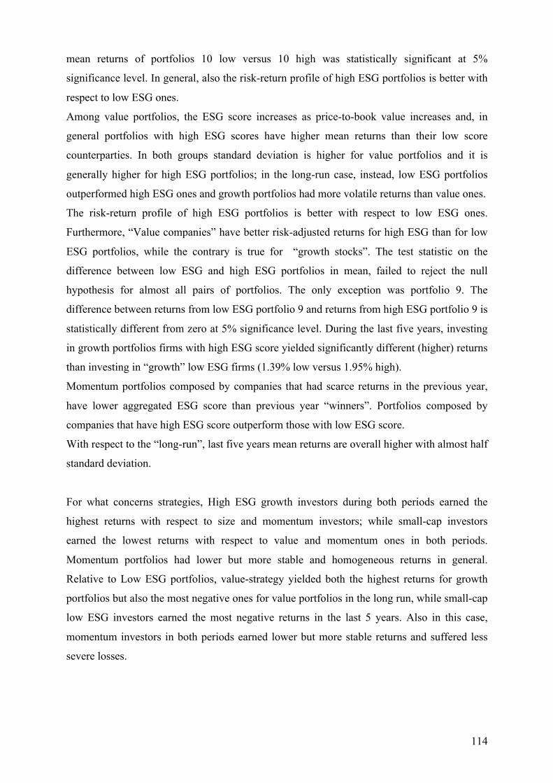
114
mean returns of portfolios 10 low versus 10 high was statistically significant at 5%
significance level. In general, also the risk-return profile of high ESG portfolios is better with
respect to low ESG ones.
Among value portfolios, the ESG score increases as price-to-book value increases and, in
general portfolios with high ESG scores have higher mean returns than their low score
counterparties. In both groups standard deviation is higher for value portfolios and it is
generally higher for high ESG portfolios; in the long-run case, instead, low ESG portfolios
outperformed high ESG ones and growth portfolios had more volatile returns than value ones.
The risk-return profile of high ESG portfolios is better with respect to low ESG ones.
Furthermore, “Value companies” have better risk-adjusted returns for high ESG than for low
ESG portfolios, while the contrary is true for “growth stocks”. The test statistic on the
difference between low ESG and high ESG portfolios in mean, failed to reject the null
hypothesis for almost all pairs of portfolios. The only exception was portfolio 9. The
difference between returns from low ESG portfolio 9 and returns from high ESG portfolio 9 is
statistically different from zero at 5% significance level. During the last five years, investing
in growth portfolios firms with high ESG score yielded significantly different (higher) returns
than investing in “growth” low ESG firms (1.39% low versus 1.95% high).
Momentum portfolios composed by companies that had scarce returns in the previous year,
have lower aggregated ESG score than previous year “winners”. Portfolios composed by
companies that have high ESG score outperform those with low ESG score.
With respect to the “long-run”, last five years mean returns are overall higher with almost half
standard deviation.
For what concerns strategies, High ESG growth investors during both periods earned the
highest returns with respect to size and momentum investors; while small-cap investors
earned the lowest returns with respect to value and momentum ones in both periods.
Momentum portfolios had lower but more stable and homogeneous returns in general.
Relative to Low ESG portfolios, value-strategy yielded both the highest returns for growth
portfolios but also the most negative ones for value portfolios in the long run, while small-cap
low ESG investors earned the most negative returns in the last 5 years. Also in this case,
momentum investors in both periods earned lower but more stable returns and suffered less
severe losses.

115
From the mean-variance optimization analysis of Chapter 4 we conclude that the “total”
efficient frontier is more efficient than the ESG efficient frontier in the majority of cases. This
meets previous studies (see Drut (2010)) claiming that the implementation of ESG factors
leads to less efficient investments, since the investment universe is being scaled down. In our
study, this result could also be caused by the fact we could not include all the available high
ESG stocks due to the presence of missing values.
However, although “dominant” high ESG portfolios are suboptimal when compared with the
“total” ones, those total portfolios that have variance lower than 3.1% represent an exception,
since they intersect the ESG efficient frontier at that point. Investors that are much more risk-
averse would be better-off investing in ESG optimized portfolios when targeting lower
portfolio variance, since the total efficient frontier is suboptimal at that point and does not
provide further investment opportunities from then on. It is clear that ESG investments are
strongly influenced by risk aversion, much more than investments that disregard
sustainability. The differences from base (risk aversion coefficient λ = 4) Sharpe Ratios are -
0.039 and -0.14 when we lower the risk aversion and 0.26 and around 0.3 when we increase
it, respectively for total and ESG portfolios. We conclude that the more an investor is risk
averse, the more an ESG investment becomes the most efficient choice for him.
Moreover, in this context, the optimal risky portfolio on the ESG frontier has a better risk-
return profile with respect to the total one considering it provides our investor with 2.6 units
of return for one unit of risk while the total ORP earns investors 2.38 units of return for the
same risk. This is in contrast with Gasser et al. (2017) whose empirical study shows that
caring about social responsibility causes a statistically significant Sharpe Ratio decrease with
respect to risk-return optimal portfolios.
Implementing an optimization framework using stocks’ expected returns and covariance
yields portfolios that have higher returns for the same level of risk of the S&P 500, which
instead allocates capital weights among its stocks based on market capitalization and
regardless of their covariance and lies below both efficient frontiers and their two CALs
(Figure 4.2.1).
Our analysis also shows that implementing factor-based strategies can result in portfolios that
are more efficient that the optimal ESG ones (value and momentum especially) but are still
individually suboptimal versus the total dominant portfolios. Anyway, employing factor
strategies does not allow taking full advantage of the lower variance that characterizes
sustainable investments.

116
Furthermore, combining the factor portfolios, we can see no benefits in investing in their
optimized combination for lower values of standard deviation in any of the three scenarios
analysed in Chapter 4, even though the strategic choice of allowing short selling and
implementing long-short positions is the one that yields the most efficient set of portfolios
among the three cases.
In these optimization frameworks growth portfolios are always included in the ORPs.
However, factor investing in general does not “beat” optimized investments related to the
total investment universe, although some of them are much more efficient than the S&P 500
itself. Which means that screening for high ESG scores could still yield better risk-adjusted
returns than passively replicating or buying the Index.
In light of these considerations, we find that ESG investors are not efficient, unless they target
investments with standard deviation lower than 3.1 %, both in the long- and in the short-run.
High Net Worth Individuals, for example, would likely be better-off in implementing ESG
screenings and mean-variance optimization in order to choose the less variable investments.
Relative to the analysis on “Market Portfolios”, we find that investing in 𝑅!,!"# , which
means discriminating for stocks with ESG score greater that 5 within the S&P 500 investment
universe, yields higher returns than investing in the Index itself, both aggregating stocks in
equally weighted and market-weighted portfolios. Investors seeking high ESG portfolios are
better off than general investors, whereas, among the ESG rated market-weighted indexes,
less risk-averse investors earn the highest expected returns through 𝑅!,!" . Notably, an
investor who would choose to invest in companies that have a sustainability rating among
those included in the S&P 500, would achieve a much higher return versus the S&P with
lower variance, while investing in Low ESG companies would bear an increase in volatility.
On the other hand, implementing an equally weighted 𝑅!, is not always more profitable than
investing in the S&P 500. Even though the expected return is still higher, returns volatility
also increased considerably
From the comparison between equally weighted and market-weighted portfolios we conclude
that high ESG companies have generally higher returns than low ESG ones, but the
companies with largest market capitalization have lower returns in the high ESG portfolio
while they have higher returns with respect to the portfolio mean (or also median) in the low
ESG portfolio; this leads to the low ESG market weighted portfolio returns dominating the
high ESG one, when, instead, the equally weighted high ESG portfolio dominates the low

117
ESG one. Moreover, in both cases, and especially in the market-weighted case, 𝑅! standard
deviation is closer to the high ESG one; this can suggest that in general high ESG companies
have larger market-cap than low ESG ones but are outnumbered by many lower sized low
ESG companies, except few outliers.
As illustrated in Figures 4.3.1 and 4.3.4, during the period from 2008 to 2012 the S&P 500
was composed by a slightly higher number of high ESG companies, which also had much
higher market capitalization than those with low ESG score. Indeed, 𝑅!,!" considerably
deviated from 𝑅! during that period; whereas from 2013 to 2018 𝑅!,!!! had more extreme
values with respect to 𝑅!. Deviations from 𝑅!, which we are considering to describe the
behaviour of the general market, mean the market prominently commoved with the “other”
investment set and we could argue that in the period during and just after the last financial
crisis the majority of firms meeting S&P 500 eligibility criteria where those with high ESG
rating, while in normal economic periods more firms with low ESG scores meet the S&P 500
criteria. As reported in Tables 4.3.1 and 4.3.2, both strategies beat the S&P 500 in the long-
run and in the short- run. Investing $100 either 2006 or in 2013 in one of our market weighted
“Market Portfolios” would mean receiving at least 6 percentage points more in expected
returns. While making the same investment with both a long-term time horizon and a short
term one, would yield at least 2 ppt more than investing in the S&P 500. Equally weighted
strategies more efficient after the implementation of high ESG score screening; while market
weighted ones have the best risk-return profile when excluding high ESG rated companies.
As previously stated, in general high ESG companies yield higher returns than low ESG ones,
but the biggest high ESG companies to which market weighted strategies assign most weight
yield lower returns that the biggest low ESG companies. This suggests that the high ESG
market is more homogeneous, generally healthier and characterized by lower volatility.