Department of Economics

Trinity College Dublin, Ireland

Day 1: Getting Started

Getting StartedContents:

1. An Introduction to Stata2. Creating do files3. Creating log files4. Commands to get you started5. Opening, sorting and merging data files6. Cleaning data7. Descriptive Statistics

1. An Introduction to Stata

Starting Stata:Start Programs Stata Stata SE 8

Description of package:• Menu bar• Tool bar• Command Window• Results Window• Variables Window• Review Window• Data Browser• Data Editor• Do file editor

Projects are easiest to manage if you record all of your work in a ‘do-file’

Typing doedit or clicking the do editor button opens an empty do-file. A do file is saved with extension .do

To run a series of commands saved in a do-file under filename.do, type:

do filename.do

To run only a selection of command lines in a do-file, highlight them and click the “run” button inside the open do file.

2. Creating do-files

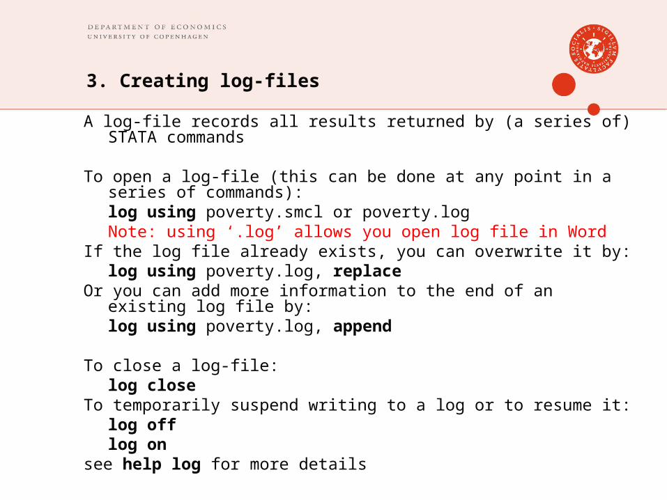
A log-file records all results returned by (a series of) STATA commands

To open a log-file (this can be done at any point in a series of commands):

log using poverty.smcl or poverty.logNote: using ‘.log’ allows you open log file in Word

If the log file already exists, you can overwrite it by:log using poverty.log, replace

Or you can add more information to the end of an existing log file by:

log using poverty.log, append

To close a log-file:log close

To temporarily suspend writing to a log or to resume it:log offlog on

see help log for more details

3. Creating log-files

4. Commands to get you started

• clear removes all data from memory

• set memory instructs Stata to create space to store data• no; data in memory would be lost

• op sys refuses to provide memory

• set maxvar maximum number of variables

• set matsize maximum number of variables that can be included in a model

• When to use these commands:• no room to add more observations

• no room to add more variables

• query memory or memory displays current memory and data settings

• Use , permanently to add changes permanently

• cd “file location” directs STATA to the path on your PC where your data are stored

STATA usually displays results by screenfulls. A key needs to be touched to make the rest of a command continue. By typing:

set more off

in the beginning of the do-file, you avoid this. Set more off makes the programme run screen after screen. Turn it on again by:

set more on

“More” can also be set to equal a certain number x, the program will then run window after window, pausing each time for x seconds between them

4. Commands to get you started

STATA will stop automatically if a command is entered incorrectly

In some cases you may prefer for STATA to continue, even if an error is made. For example, if you ask STATA to start a new log file and there is already a log file open it will stop running the do-file

To instruct STATA to continue with the do-file use the command capture

So instead oflog close

Usecapture log close

4. Commands to get you started

CommentingTo keep track of what is contained in the do-file, start a do-file

by assigning a title, the date it was produced or changed, by whom it was created, which datasets are used, and other relevant information which will make it easier for the do-file to be used later by yourself or by someone else.

Comments written between /* comment */ will be ignored by STATA and not executed. A whole line can be ignored by typing an asterisk in front:

* the next command shows averages of rural consumption:

sum consumption if rural==1 /* urban cons. is shown in descriptive table */

4. Commands to get you started

1. Open the do-file “Day1.do” stored on your desktop

2. Write your name and the date in the title box

3. Clear all data from Stata’s memory

4. Set Stata up so that 200 megabytes of RAM is allocated to store the data

5. Set the path to “C:\Data”

6. Open a new log file called “Day1.log”

EXERCISE ONE

5. Opening, sorting and organising data files

• Open a Stata dataset: use filename.dta [, clear]

• Save a Stata file: save filename.dta [, replace]

• browse: allows you view the data

• describe [varlist]: lists and describes variables

• Numeric variables

• String variables

• codebook [varlist]: stats and other information

• inspect [varlist]: more statistical information

• count [varlist]: counts the number of observations that satisfy a specified condition

• sort [varlist]: sorts data in ascending order of varlist

• gsort [varlist]: same as sort but allows you specify whether in ascending or descending order (use ‘+’ or ‘-’)

• erase datafile.dta: permanently erases a data file from your computer

5. Opening, sorting and organising data files

• keep [varlist]: keeps the variables listed and drops all other variables in the data set

• drop [varlist]: drops the variables listed from the data set

• if varname==#

’=’ means assign a value

’==’ means check whether a variable has a specific value

• Merging Data:• Both files have to be in Stata format• Both have to have at least one of the same variables

the identifies each observation• This variable should be sorted in the same way

merge identifier list using filename

• Use tab _merge to check merged data• _merge=1 if the observation is only present in the

master dataset• _merge=2 if the observation is only present in the

incoming dataset• _merge=3 if the observation is present in both

datasets

5. Opening, sorting and organising data files

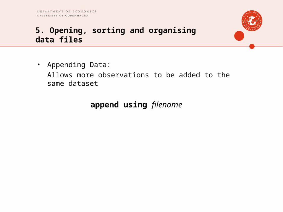
• Appending Data:Allows more observations to be added to the same dataset

append using filename

5. Opening, sorting and organising data files

1. Open the data file “Day1.dta”2. ‘count’ the number of observations in the data set3. Use the ‘describe’ command to review the data in memory4. Use the ‘codebook’ command to review the data in memory5. Use the ‘inspect’ command to produce detailed information on the

structure of the variables in your dataset, i.e., the number of negative and zero values, the number of missing values etc.

6. Open the individual data file “individual.dta”7. Keep observations on the household head8. Sort by household and save as “temp1.dta”9. Open “Day1.dta” and merge with “temp1.dta”10.Tabulate the variable ‘_merge’ and then drop it11.Erase the data file “temp1.dta”12.Set the sample (samp_report==1)13.Sort by household and save changes to “Day1.dta”

EXERCISE TWO

6. Cleaning data

• label variable varname Assigns label to varname

• label values varname valuename Assigns values to varnameFor example:

categorical variables

• label define valuename codes Defines the value labels

• label data “……” Labels the actual data

• label list Lists all the labels stored

6. Cleaning data

generate variable=value generates a variable with a specified value for each observation.

generate var2=var1 replicates a variable already in the dataset

(for editing later for example)

generate var2=var1-var0 creates a new variable that is some function of other variables in the

dataset

6. Cleaning data

replace variable=value changes the value of a variable for each observation

Note: usually specified with an ‘if’ command to selectively change variable valuesreplace variable=value if var1==10

This would mean that you would only replace the value of the variable in cases where var1 takes a value of 10

Other operators can also be used such as, ‘>’ or ‘<’ or ‘>=’ or ‘<=’

OR and AND commands can also be used

The AND command is given by ‘&’:replace variable=value if var1<=10 & var2>5

The OR command is given by ‘|’:replace variable=value if var1==10 | var1==11

’!=’ means not equal to!

7. Descriptive Statistics

summarize varlist: Summary statistics for all variables in varlist , detail: displays additional stats

By Options:

• by varname, sort: summarize varlist

If already sorted by varname no need for ’sort’ option

• bysort varname: summarize varlist

• summarize varlist if varname==#

Saved Results:

return list: Lists the results saved by Stata

’=’ means assign a value

’==’ means check whether a variable has a specific value

7. Descriptive Statistics

Tables of Summary Statistics

tabstat varname: Displays table of summary stats

Options:• allows you specify statistics: stats(mean sd)• by: for two way tables• missing: show number of missing observations

7. Descriptive Statistics

Tabulate

tab varname or tab1 varnames: Gives frequencies for varname(s)

tab2 varname1 varname 2: Gives two way frequencies

Options:• nolabel for numeric values instead of value labels• missing to display missing values• plot for graphical comparison• summarize for summary statistics

8. Graphs

• graph twoway scatterplots, line plots etc.

• graph matrix scatterplot matrices

• graph bar bar charts

• graph pie pie charts

8. Graphs

Bar charts:graph bar (stat) varname, over(catvar)

draws bar chart of a statistic, stat, of varname for a categorical variable given by catvar.

Default for stat is the meanSearch help graph bar for all options

Pie charts:graph pie varname

Saving/Printing graphs:graph save graphname filename.gph

graph print

Most surveys have one or more of the following design characteristics:• sampling or probability weights• stratification• clustering

Data are assumed to be representative:• for the whole population they are drawn from • for certain groups (regions or other than geographically determined

groups)

Not taking into account the design of the survey could entail that the results returned by STATA commands such as summarise, mean, regress, … only reflect characteristics of the collected data (sample) but not the larger population they are representative off.

=> inaccurate or biased results

9. Applying weights

Example: some groups which are of particular interest to the researcher or which are of particular ease to collect data for, might have been oversampled. Oversampling = share in the sample does not reflect true share in the actual population the oversampled are part of. Oversampling => can cause a difference between the sample statistics (point estimates and/or standard errors) and the population statistics.

In order to retrieve the accurate population statistics from the sample, the exact characteristics of the sample (such as how it was designed, stratified, clustered, how observations were drawn) have to be known and taken into account.

How to make sure that the descriptive statistics we report are describing the population rather than the sample?

• “manually” by including weights or cluster options • STATA survey commands

9. Applying weights

Assume we have a simple random sample of n observations drawn from a population of size N, the variable of interest is x, with observations xi running from 1 to n.

In the case of simple random design, the sample mean is the correct estimator of the population mean:

BUT! Most surveys do not use a simple random design but different households have different probabilities of being selected into the sample in which case the sample means will be biased estimators of the population means.

In order to calculate correct statistics, observations need to be reweighted: those that are underrepresented will be weighted up and those that are overrepresented will be weighted down.

1

1

n

ii

x n x

9. Applying weights

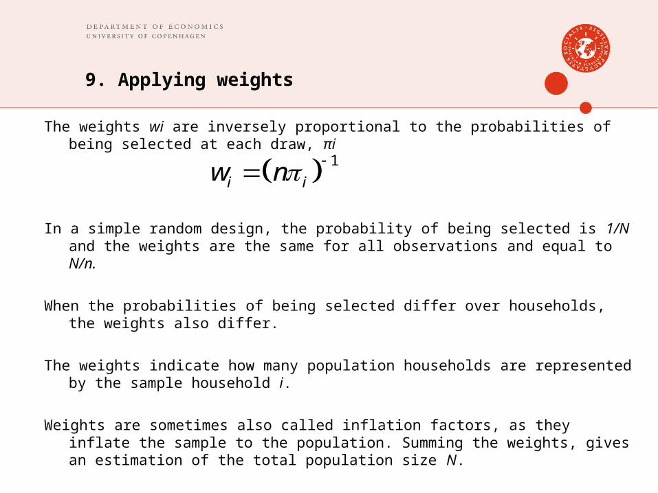
The weights wi are inversely proportional to the probabilities of being selected at each draw, πi

In a simple random design, the probability of being selected is 1/N and the weights are the same for all observations and equal to N/n.

When the probabilities of being selected differ over households, the weights also differ.

The weights indicate how many population households are represented by the sample household i.

Weights are sometimes also called inflation factors, as they inflate the sample to the population. Summing the weights, gives an estimation of the total population size N.

1

i iw n

9. Applying weights

The probability weighted mean is equal to the estimated total divided by the estimated population size:

This can be rewritten as:

Where the weights are normalised to add up to one:

1 1

/n n

w i i ii i

x w x w

w i ix v x

1

/n

i i kk

v w w

9. Applying weights

So where we fail to correct for the weighting of the sample, we will get biased estimators of the population parameters.

The same holds when calculating statistics for each subgroup of the population such as regions, rural/urban areas, men/women, etc.

In STATA we can correct for weighting by explicitly including the variable that holds the weights between square brackets at the end of a command (see help weight)

command vars [w=weight]

you can also specify the type of weights you want to use:pweights=probability weights (typically used for samples)aweights=analytical weightsfweights=frequency weights

command vars [pw=weight]

9. Applying weights

Household weights versus population weights.

Often we are interested not in household means but in means per person. For example, from a household level dataset we would like to know the proportion of poor people rather than the proportion of poor households, or we would like to know the proportion of poor people by sex or age.

In this case we would need to use population weights rather than household weights. To arrive at the correct weights, we need to multiply the household weights by the household size. The total of these weights is an estimate of the total population (rather than of the total number of households as described before).

9. Applying weights

1. Run the command line in the do-file that creates food expenditure quintiles

2. Run the command lines in the do-file that labels this variable and assigns value labels

3. Run the command lines in the do-file that tabulate this variable with and without weights and think about what you observe

4. A number of dummy variables have to be created for Table 1.1. They are

• malehead – the sex of the household head• kinh – ethnicity of the household head• viet – head of household speaks Vietnamese• vietmain – Vietnamese is the main language of the head of household• classpoor – household is classified as poor by the authorities

Create a 0-1 indicator variable for each of these and label each variable as appropriate. A number of prompts and hints are given in the do-file

EXERCISE THREE

5. Replicate Table 1.1 and Figure 1.1 from the 2006 report using the 2008 data (Hint: don’t forget to use weights)

6. Run the commands in the do-file that create the variables ‘suppchout’ and ‘bornhere’. Pay particular attention to the notes on the difference between these variables in 2008 compared with 2006

7. Replicate Table 1.2 from the 2006 report using the 2008 data8. Run the commands in the do-file that create the variables ‘eduhead’

and ‘profhead’9. Replicate Table 1.3 from the 2006 report using the 2008 data10.Run the commands in the do-file that create the variable ‘disprimary’11.Create the following 0-1 dummy variables:

• dislowsec – distance to lower secondary school• disuppsec – distance to upper secondary school• dispcoffice – distance to people’s committee office

12.Replicate Table 1.4 from the 2006 report using the 2008 data

EXERCISE THREE

13. Run the commands in the do-file that create Figures 1.2 and 1.3 What do these figures tell you? How do they compare to 2006?

14. Replicate Figures 1.4 and 1.5 from the 2006 report using the 2008 data

15. Close the log file and save your changes to the do-file “Day1.do”

EXERCISE THREE