department of economics working paper 2005
TRANSCRIPT

DEPARTMENT OF ECONOMICS
WORKING PAPER
2005
Department of Economics Tufts University
Medford, MA 02155 (617) 627 – 3560
http://ase.tufts.edu/econ

Understanding Why Universal Service Obligations May Be Unnecessary: The Private Development of Local Internet Access Markets1
Tom Downes
Department of Economics Tufts University
Medford, MA 02155 E-mail: [email protected]
and Shane Greenstein
Kellogg Graduate School of Management Northwestern University Evanston, IL 60208-2013
E-mail: [email protected]
July 2005 Abstract: This study analyzes the geographic spread of commercial Internet Service Providers (ISPs), the leading suppliers of Internet access. The geographic spread of ISPs is a key consideration in U.S. policy for universal access. We examine the Fall of 1998, a time of minimal government subsidy, when inexpensive access was synonymous with a local telephone call to an ISP. Population size and location in a metropolitan statistical area were the single most important determinants of entry, but their effects on national, regional and local firms differed, especially on the margin. The thresholds for entry were remarkably low for local firms. Universal service in less densely-populated areas was largely a function of investment decisions by ISPs with local focus. There was little trace of the early imprint of government subsidies for Internet access at major U.S. universities. Keywords: Internet; Universal service; Geographic diffusion; Telecommunications
1This study was funded by the Institute for Government and Public Affairs at the University of Illinois and by a Mellon Small Grant in the Economics of Information at the Council on Library Resources. We appreciate comments from Amy Almeida, Tim Bresnahan, Linda Garcia, Zvi Griliches, Kristina McElheran, Scott Marcus, Padmanabhan Srinagesh, Pablo Spiller, Dan Spulber, Scott Stern, John Walsh, Wes Cohen, and many seminar participants. Howard Berkson, Heather Radach, Holly Gill, Helen Connolly, and Joshua Hyman provided excellent research assistance at various stages. We would especially like to thank Angelique Augereau for her extraordinary research assistance in the final stages. The authors take responsibility for all remaining errors.


Universal Access and Local Commercial Internet Markets Page 1
I. Overview
Through a series of decisions in the 1980s and early 90s, policy makers in the
Department of Defense and the National Science Foundation (NSF) decided to privatize
investment for TPC/IP infrastructure, effectively commercializing the Internet. For most of the
1990s, the Internet developed through largely private, uncoordinated, and market-oriented
investment.1 Enough time has now passed to understand what transpired after privatization. In
this paper we analyze an unintended outcome: commercial Internet access firms in the U.S.
almost achieved a public policy ideal: universal geographic coverage.
This study analyzes the geographic spread of commercial Internet Service Providers
(ISPs), the leading suppliers of Internet access. The geographic spread of ISPs was, and still is, a
key consideration in U.S. policy for universal access. While all consumers had access to the
Internet at some price, the key questions for public policy concerned the condition of small and
medium adopters, who care about inexpensively acquiring access.2 In this era inexpensive was
synonymous with a local telephone call to an ISP. Hence, the number of commercial ISPs
accessible via a local phone call determined whether a competitive, commercial Internet was
readily available to a community.
We measure economic determinants of ISP availability. We construct and analyze a
comprehensive measure of the number of suppliers for every county in the U.S. More
specifically, we characterize the determinants of the location of over 60,000 dial-up access points
(i.e., "points of presence" or POPs in industry parlance) offered by commercial ISPs in the Fall
of 1998 in every county in the United States. We build an econometric model for predicting the
1These policies are well known. For summaries, see Webach (1997), Greenstein (2001), Cannon (2001), and Mowery and Simcoe (2002). 2This theme resonates throughout the literature. See e.g., Cherry and Wildman (1999), Compaine and Weinraub (1997), Compaine (2001), Drake (1995), Garcia (1996), Garcia and Gorenflo (1997), Kalil (1995), National Academy of Engineering (1995), National Research Council (1996), Strover (2001), Strover, Oden and Inagaki (2002), or Werbach (1997).

Universal Access and Local Commercial Internet Markets Page 2
density of suppliers. Our model measures several factors: the importance of economies of scale,
pre-existing demographic features of an area, pre-existing infrastructure for other
communications technologies, and spillovers from universities.
Fall of 1998 was a good time for analyzing the determinants of the geographic coverage
of ISPs. By this point, the industry's structure was no longer changing every month. Most of the
leading firms had been in the ISP market for a few years, making it possible to document their
strategies, behavior, and commercial achievement. More to the point, the geographic dispersion
of access and conditions of supply were similar throughout most of 1998. This arose despite
continued entry and exit, as well as some hints of -- but little movement towards -- consolidation
of ownership of supply.
Fall of 1998 was also an interesting date in the economic history of the Internet access
network. First, we believe we are viewing geographic coverage with only moderate
concentration of supply and without significant inter-modal competition. During our snapshot of
the industry, AOL’s leadership was not yet solidified. The AOL-CompuServe merger occurred
just prior to our snapshot, while the AOL-Time Warner merger came a couple years later. In
addition, this date preceded any significant rollout of broadband access over cable or phone lines
to U.S. homes.
Perhaps most important, we believe the period of our analysis provides the best set of
conditions for learning what the market would do with minimal government subsidy. Our
snapshot preceded the full implementation of Internet II and the E-Rate program. The NSF
largely coordinated the former program, a private/public partnership to move academic and
research infrastructure to the next generation of technology. The Federal Communications
Commission (FCC) administered the latter, a two billion dollar federal program authorized in the
1996 Telecom Act. This program was held up by court challenges during our snapshot, but

Universal Access and Local Commercial Internet Markets Page 3
eventually subsidized delivery of Internet access to individuals living in low-density areas and in
poor communities. In other words, government subsidies accelerated after the Fall of 1998.
In previous research (Downes and Greenstein, 2002), we showed that the US market can
be analyzed as thousands of local markets. These markets consisted of small, geographically
dispersed local providers for Internet access. In addition, a number of national firms provided
access over extremely wide and geographically dispersed areas. In this paper we focus on
understanding how variation in economic factors produced different competitive conditions. Our
key findings are:
- Population size and location in a metropolitan statistical area were the single most
important determinants of entry, but their effects on national, regional and local firms
differed, especially on the margin. The thresholds for entry were remarkably low for
local firms.
- Universal service in less densely-populated areas was largely a function of
investment decisions by ISPs with local focus. National firms did not play a
significant role in bringing access to the U.S. population in less densely-populated
areas. If national and local firms differed in the quality of services provided, then
marginal adopters experienced differentials in access.
- Other important attractors for ISPs included the demographic make-up of a
residential and business population and the pre-existing infrastructure of the area. For
national firms these factors were of substantially less importance than population and
urban location. The location of local firms was much more sensitive to factors other
than population and presence in an MSA.
- By 1998, there was still a small trace of the early imprint of the government
subsidies for Internet access at major U.S. universities. However, the early growth of

Universal Access and Local Commercial Internet Markets Page 4
ISPs largely diminished the importance of the presence of a research university.
There was also a small effect from the presence of nearby infrastructure that lowered
the costs of opening a small ISP, such as highways and rail lines, along which
backbone was laid.
Throughout the paper, we are careful to distinguish between the factors that are quasi-
permanent, such as the geographic patterns of density, and those that are idiosyncratic to this
technology, such as the identities of suppliers. We try to determine if the quasi-permanent or
idiosyncratic factors helped achieve near-universal geographic access with very little government
involvement. This distinction continues to elicit interest. The targeting of subsidies, if any,
depends critically on understanding when privately funded access services achieve near-
universal geographic access and when they do not.
More recent research continues to find select patterns of demographic and geographic
inertia in the deployment and use of Internet access technologies, even among recent access
technologies such as broadband over cable modem service or DSL over telephone lines
(Grubesic, 2005; Flamm, 2005; Hu and Prieger, 2005). The same people in the same places – for
example, in the Appalachian region – continue to face problematic circumstances with regard to
access. Dial-up ISP service was the first example of an Internet technology to manifest this type
of pattern. Understanding this pattern provides a useful perspective on similar patterns today.
The remainder of this paper begins with some background about ISPs. In the section that
follows, we state several open research questions. The fourth section of the paper provides a
description of the econometric model; the data are described in the fifth and sixth sections. In
the seventh section, we analyze the estimates, and we close the paper with a discussion of the
implications of our results.

Universal Access and Local Commercial Internet Markets Page 5
II. ISPs and Geographic Coverage
We focus on firms that provided dial-up service which enabled a user to employ an
Internet browser. Browser development occurred at about the same time as the final
implementation of policies by the NSF to commercialize the Internet and at the same time as the
widespread adoption and development of WWW (World-Wide Web) technology. Furthermore,
we make no distinction between firms that began as on-line information providers, computer
companies, telecommunications carriers, or entrepreneurial ventures. As long as a firm provided
commercial Internet access as a backbone or a downstream provider, this firm is an ISP in our
study.
The presence of ISPs within a local call area determined a user's access to inexpensive
Internet service. The cost of this phone call depended on state regulations defining the size of the
local calling area, as well as both state and federal regulations defining the costs of long-distance
calling (Nicholas, 2000). Non-toll local areas were typically between ten and twenty miles,
depending on state-specific policies for urban and rural charges. Consequently, from a user’s
perspective, the market structure for low-cost access was defined over a small geographic region.
The number of ISPs in the geographic region in which non-toll calls could be made determined
the density of supply of low-cost access to Internet services within any given small geographic
region.
The geographic reach and coverage of an ISP is best understood as one of several
important dimensions of firm strategy. Geographic coverage was determined in conjunction
with choices for value-added services, scale, performance and price. More to the point, ISPs
displayed much heterogeneity in their underlying capital and equipment structures, indicative of

Universal Access and Local Commercial Internet Markets Page 6
experimentation in these investments and organizations.3 ISPs made strategic choices regarding
the scale of service, the quality of the hardware and software associated with offering
connections, the value-added services to offer in conjunction with access, the geographic scope
of the enterprise, and the pricing of product lines. Not surprisingly, ISPs also made different
choices about the sizes and features of areas to cover.
A local, independent ISP required a modem farm, one or more servers to handle
registering and other traffic functions, and a connection to the Internet backbone.4 Higher-
quality components were optional, but were essential for serving most business customers.
High-speed connections to the backbone were expensive, as were fast modems. Facilities
needed to be monitored, either remotely or in person, by an employee or ISP owner/operator.
Local telephone firms had some options to use their existing capital and configure their network
architecture to receive and carry calls. Additional services, such as web-hosting and network
maintenance for businesses, were also costly. All these decisions influenced the quality of the
service the customers’ experienced, ultimately influencing the revenues and profitability of the
business (Maloff, 1997).
National ISPs also differed in their choices of target customer and target area for service.
Some targeted only business users, providing them with value-added services such as web
hosting. In this business model, dial-up access might have been a necessary complement to the
other, more profitable services offered. Other national ISPs focused on residential customers and
on a different set of value-added services, such as appropriate chat rooms or an array of easy-to-
use bulletin boards. Still others seemed to do a bit of everything, targeting both business and
residential use. Substantial price variation survived in this market, depending on the value-added
3This theme arises in many industry reports and analyses. See e.g., Maloff Group International, Inc. (1997), the Economist (1997), Greenstein (2000), or Augereau and Greenstein (2001). 4For example, see the description in Kalakota and Whinston (1996), Lieda (1997), and the accumulated discussion on http://www.amazing.com/isp/ .

Universal Access and Local Commercial Internet Markets Page 7
services offered in conjunction with dial-up service and on other factors associated with degrees
of differentiation.
These different strategies influenced the geographic focus of providers. ISPs who sought
to provide national service tended to maintain points of presence (POPs) in all large and many
moderately-sized cities in the U.S., covering a high fraction of the population and potential travel
destinations. Some local ISPs targeted niche markets in urban areas that the national ISPs failed
to address, seeking to attract those users requiring a “local” component or customized technical
service. National firms potentially brought with them the same capabilities in all localities.
Local firms were dependent on various local characteristics such as labor markets, the quality of
existing infrastructure and educational institutions, and the initiative of stake-holders in the
community. Local firms had the potential advantage, however, of being able to tailor their
services to local demand. Thus, our expectation was that, while population and presence in an
urban area would be the principal determinants of the location pattern of national ISPs, variation
in local conditions would explain much more of the variation in the location of local ISPs.
III. Research Questions
We are hesitant to presume very much about the specific features of firm behavior and
market equilibrium in a young market, particularly for purposes of estimating firm entry and exit.
Rather, we borrow from the spirit of the economics literature on firm entry, as applied in many
other markets for local services (e.g., Bresnahan and Reiss, 1991; Downes and Greenstein,
1996). While this literature does not provide very firm predictions about what factors influence
the entry of access providers, it does emphasize several common themes for framing hypotheses
about the economic determinants of the scope and nature of geographic coverage.
We focus on two of these themes. First, we analyze what conditions created highly-

Universal Access and Local Commercial Internet Markets Page 8
competitive areas or less-competitive ones. For reasons already noted, virtually all major urban
areas attracted some combination of local and national firms (Downes and Greenstein, 2002).
We are less certain about the nature of entry in areas outside of central urban centers. Thus, one
of our research goals is to characterize the factors influencing entry in less dense circumstances.
Second, we describe the factors that contribute to variations in the entry behavior of different
types of providers. We do this because we expect these firms to be responsive to different
economic incentives and to offer different services. We hypothesize that this will help clarify
how these differences shaped the nature of entry in less-dense circumstances.
We consider several theories about determinants of supply:
Economics of scale and presence in an MSA: Network-access providers grew by
adding POPs. A sufficient amount of revenue must justify expending the costs of maintaining
the POP. Hence, we expect small populations to support fewer POPs. We expect higher
population densities, which were prevalent in urban areas, to be easier to serve.
Pre-existing investment and demand: By 1998, personal computers could be found in
42.1% of U.S. households. In 26.2% of households, at least one member of the household used
the Internet at home (Newburger, 2001). Households with computers tended to have higher
incomes, to have heads who were better educated, and to be non-minority.5 We expect such
demographic features to have influenced the presence of Internet suppliers.
Local communication-intensive activities and infrastructure: Internet technology was
complementary to existing local communications infrastructure, both in use and in supply.
Internet access vendors often targeted business users, many of whom were already users of
computing and communications infrastructure. A large and developed infrastructure and labor
market had grown in many localities, tailored to the presence of communications-intensive or
5See e.g., Kridel et al. (1999), Goolsbee and Klenow (2002), National Telecommunications Information Administration (1999, 2000), and Fairlee (2004).

Universal Access and Local Commercial Internet Markets Page 9
computing-intensive business users (Greenstein, Lizardo, and Spiller, 2003). Therefore, we
develop and test several measures of the presence of related infrastructure for other
communications activity, such as the presence of major telephone companies or other factors that
promoted the presence of backbone lines.
The imprint of the origins of the Internet: The presence of a nearby university might
have influenced the demand for Internet service, because universities acted as substitute
suppliers for some potential users. In addition, universities were also an important source of
potential supply of entrepreneurs to start businesses that supplied Internet access. In this study,
we analyze whether these origins for the Internet continued to influence its geographic dispersion
a few years into commercialization.
State regulation: States differed in their regulations for interconnection and local calling
plans. Though the 1996 Telecommunications Act standardized some of these rules across
localities, there were still significant differences as of 1998. While it is difficult to measure
directly the influence of these regulatory factors, they may influence many of the locations in the
same state. Thus, we utilize state-specific effects to control for variation in the effects of state
regulation.
IV. Modeling Approach
We assume that the entrepreneurs who contemplated forming ISPs came from two
groups, either the national firms who were developing national ISP brands or from a set of local
individuals directly interested in providing Internet access to a local area. In each period the
number of observed entrants (or successful entrepreneurs) was the sum of many decisions by
potential entrants about whether to enter a particular region. In general, we presume little about
this decision process. Our working hypothesis is that local economic factors shaped entry.

Universal Access and Local Commercial Internet Markets Page 10
A precise measure of local competition requires detailed information about which
connections between telephone switches are local calls, about the characteristics of the
residences/businesses served by each switch, and about the locations of the POPs of every ISP.
This type of data is difficult to assemble at a comprehensive level. Our strategy is to come close
by constructing approximate measures of competition from a census about POPs and then
matching it to US Census data about areas. This will lead to an approximate measure of how
many ISPs provided service in certain sufficiently-small geographic areas. This approximation is
adequate to allow us to infer which factors induced or discouraged entry.
We will infer firm presence from a census of every commercial POP in every county in
the U.S. Let i stand for type of ISP (e.g., local, national) in county j. Let Nji be the number of
ISPs of type i in county j.
Let Xj be the set of variables describing characteristics of county j that potentially
influenced the location pattern of ISPs. These include measures of factors that encouraged
supply, such as population levels and density, pre-existing features of demand and local
infrastructure, the presence of universities, and state dummies.
Neighboring areas also contributed to potential supply. For example, consumers in
county j could get low cost access from a supplier in an urban county next door that had many
already-present suppliers. Assume there were Hj counties contiguous to county j and let Xh, h =
1,2,..., Hj, be the set of variables describing characteristics of contiguous county h. These factors
should have induced supply in that county, to be sure, and also possibly influenced the behavior
of potential suppliers for county j.
We assume the distribution for Nji is Poisson with mean λj
i, which takes the form
(1) λji = exp[Xjβi + Σ h ∈ Hj exp(-αιdjh)(Xhγi)] .
Here, Xjβi measures the influence of factors within county j, while Xhγi measures the influence of

Universal Access and Local Commercial Internet Markets Page 11
factors within counties surrounding county j. We let djh be the distance between counties j and h.
We weight by distance as a way of examining directly the geographic scope of the influence of
the characteristics of neighboring counties factors. As in Bresnahan and Reiss (1991) and
Downes and Greenstein (1996), we do not presume to know what neighboring factors were
relevant to entrants. This specification permits us flexibly and parsimoniously to allow the
characteristics of neighboring counties to have influenced the extent of entry in county j. The
larger are the αi (the coefficients on distance), the less important were the characteristics of
neighboring counties.
If the numbers of ISPs of each type i in county j are independent Poisson random
variables, then the log of the likelihood function is:
(2) ℓ = ∑i,j P(Nji = nj
i) = ∑i,j [-λji + nj
iln(λji) – ln(nj
i!)]
Minimizing ℓ provides estimates of the parameters in (1).
If the distribution of the number of entrants has been correctly specified, minimizing (2)
generates efficient parameter estimates. Cameron and Trivedi (1986) argue that economic data
typically violate the restriction implicit in the Poisson that the mean and the variance are equal.
If the data exhibit over-dispersion, estimates generated by minimizing (2) continue to be
consistent as long as the mean number of ISPs is correctly specified (Gourieroux, Monfort, and
Troghon, 1984). Appropriate corrections to the standard errors can be made using the formulas
for robust standard errors given in Cameron and Trivedi (1986).6
This method has several strengths. First, the endogenous variables are skewed and non-
negative but most of the observations concentrate at small countable numbers, appropriate for a 6An alternative approach is to use an explicit distribution in which the mean and variance are not equal. The most common distribution for this purpose is the negative binomial. If the assumptions underlying the negative binomial specification are valid, a simple test can be implemented to determine if it is appropriate to impose the equality of mean and variance restriction implicit in the Poisson specification. The risk, however, is inconsistent estimates if the negative binomial specification is invalid. Since we have no particular reason to believe the negative binomial specification is more appropriate than other possible distributional assumptions, we have chosen instead to estimate the basic Poisson model and correct the standard errors.

Universal Access and Local Commercial Internet Markets Page 12
count data approach such as this. Second, we need a single method to summarize the
determinants of observations with small counts (e.g., no or a small number of entrants in most
rural counties of the U.S.) and large counts (e.g., major cities). This approach does this quite
easily and without excessive sensitivity to the outlying observations. Third, the specification
provides a flexible approach for examining the importance of neighboring geographic features,
the key measurement issue whenever the geographic scope of the market is difficult to define
precisely, ex ante.
In addition, this method allows us to explore the possibility that different types of ISPs
had different objectives or that the competitive environment facing national and local firms
might have differed. For example, Dinlersoz (2004) found that the location pattern of retail
alcoholic beverage stores in California was consistent with a dominant firms-competitive fringe
model. In the ISP context, such a model might be appropriate for urban markets, where the
dominant firms were the national ISPs and the locals formed the competitive fringe. Dinlersoz
showed that, in the dominant firms-competitive fringe model, there would be differences across
firm type in the effects of the determinants of the location pattern.
We test for evidence of differences in the determinants of location patterns by testing the
null hypothesis that the βi, αi, and γi are the same for all types. The test is only suggestive of
differences driven by the supply-side of the market; differences in these parameters could result
from differences in the effects of demand-side determinants of the location pattern.
V. Data
Data sources and construction: In the Fall of 1998, the authors surveyed every
compilation of ISPs on the Internet. Only a few of these compilations were found to be
comprehensive, systematic, and regularly updated in response to entry and exit. This study's data

Universal Access and Local Commercial Internet Markets Page 13
combine a count of the ISP dial-in list from August/September of 1998 in thedirectory and a
count of the backbone dial-in list for October of Boardwatch magazine.7 This choice was made
because the thedirectory ISP list contained the most comprehensive cataloguing of the locations
of POPs maintained by all ISPs except the national backbone providers, for which Boardwatch
contained a superior survey of locations.
For many of the tables below, the key question will be the following: how many suppliers
had POPs in a market? When the city of a dial-in phone number was listed by an ISP, we used
that to infer the presence of a POP.8 When it was in doubt, the area code and prefix of the dial-in
POP were compared to lists of the locations of local switches with these area-codes and prefixes.
Then we used the location of the local switch to infer location. If this failed to locate the POP,
which happened for small ISPs that only provided information about their office and nothing
about the size of their dial-up network, then the voice dial-in number for the ISP was used as an
indicator of location.9 Finally, to enhance a variety of marketing and performance goals, some
ISPs maintained two or more POPs in the same location; in such cases, we counted this as one
firm presence.
On final count, the merged set contained over 65,000 phone numbers which served as
dial-in POPs. Applying the above procedures resulted in a total of 6,000 ISPs. Of 3,109 counties,
over three-quarters were associated with just over four or more firms. Of the total number of
ISPs, approximately half were ISPs for which we had only a single phone number.
7Incomplete historical versions of these lists posted at http://www.archive.org/ provide a sense of the data utilized in this study. Our data set includes POPs found in the ISP section of thedirectory (http://www.thedirectory.org/)and excludes POPs found in bulletin boards. Our data set also includes POPs for ISPs listed in the Boardwatch backbone section. 8When a city is part of two counties and the phone number did not resolve the ambiguity, the phone number was counted as part of the county in which the city has the greatest share of its land. 9This last procedure mostly resulted in an increase in the number of firms we cover, not a substantial change in the geographic scope of the coverage of ISPs. It did, however, help identify entry of ISPs in a few small rural areas.

Universal Access and Local Commercial Internet Markets Page 14
Strengths and Weaknesses. Our procedure for establishing the location of POPs will
produce flawed information about entry only if it generates sampling error which correlates with
geography. We have taken several steps to quantify and, if necessary, correct any biases that the
procedure may have imparted. We checked our data against very detailed maps of the U.S. and
standard name/places references.10 We also checked our data against multiple sources. In
addition, though we avoided all apparent measurement error, we adopted statistical procedures to
correct for any measurement error we may have inadvertently induced. Overall, we found no
evidence of any error in the coverage of small commercial ISPs. 11
This approach has several potential weaknesses. It provides no information about the
market shares of suppliers in specific locations, nor about their quality. For reasons noted above,
the absence of information on market share is not problematic, given the timing of our data.
Second, while we cannot measure quality, we are aware of related work that has found some
differences in the quality of local, regional, and national firms.12 By separately examining the
location pattern of different types of providers, we can look indirectly at variation in quality.
Our procedure may create the impression that there had been less ISP entry than had
actually occurred in new suburbs in counties that bordered on dense, urban counties. New
suburbs frequently used the telephone exchange of existing cities. Unless the ISP specifically
named this new suburb in the bordering county as a targeted area, our procedures will not count
10Sometimes an ISP would not provide clear indications about the extent of its coverage. However, in most cases we could infer coverage from other supplemental information. Our largest problems arose in the suburbs of recently growing cities. When these suburbs approached and crossed county boundaries, it became increasing difficult to attribute a supplier to a distinct area with full confidence. In such instances, we normally attributed the ISP to the area with the highest population. Also, some ISPs used common names to refer to their area of coverage, though the common name could literally refer to multiple different places in a region – such as a lake community, forest area, valley settlement or resort/vacation complex. With careful triangulation of several sources of data we could often attribute the ISP to the appropriate area. The default in a handful of instances was to attribute it to the most-populated areas. 11 The Foundation for Rural Service publishes membership directories for hundreds of rural cooperative telephone companies. The 1998 directory portrayed fairly widespread support of Internet access by rural telephone firms. Our findings did not qualitatively change when we integrated this information into our database, suggesting that our first two sources were comprehensive. 12 See, e.g., Nicholas (2000), Greenstein (2001), Strover (2001), or Strover, Oden and Nagoki (2002).

Universal Access and Local Commercial Internet Markets Page 15
the ISP's presence in that new suburb.13 Our best control for this potential bias is our definition
of the market for an ISP as a county and its nearby neighbors.
Finally, our procedure offers only a snapshot of the industry. A snapshot could be
problematic for a new industry if the industry’s geographic coverage patterns changed
frequently. Aware of this potential issue from the outset, we tracked the geographic
developments in the industry every six months for two consecutive years (Downes and
Greenstein, 2002). We observed big changes in the geographic patterns of coverage between
1996 and 1997, but comparatively little between Fall of 1997 and Spring of 1998. We found
almost no change between Spring of 1998 and Fall of 1998, by which time new entry had
slowed. We chose Fall of 1998 after noting its stability. Results for Spring 1998 do not differ
qualitatively.
We reaffirmed this decision in retrospect as we took note of a few changes in the
market.14 The implementation of the E-rate program began on a large scale in 1999. This
program, along with the AOL-Time Warner merger a year later, altered the expectations for the
industry’s growth. Hence, in retrospect, we view Spring and Fall 1998 as the closest the ISP
industry ever got to a stable equilibrium that occurred with minimal government intervention.
Definitions: In all tables below, national ISPs are defined as firms that maintain POPs in
more than 25 states. Local firms are present in three or fewer counties. We classify the remainder
as regional ISPs.
13A similar and related bias arises when a county’s boundaries and a city’s boundaries are roughly equivalent, even when the neighboring county contains part of the suburbs of the city. In this situation, many ISPs that serve the neighboring county will be located within the city’s boundary. 14This time period also is coincident with comparative stability in firm strategy. By this time, virtually every firm had implemented flat-rate pricing as one of its options, and sometimes as its only option. In addition, AOL had since recovered from its mismanagement of the introduction of flat-rate pricing. As it turned out, the next major experiment in business models (largely in 1999) came from the introduction of so-called “free” ISPs. Their entry did not alter geographic coverage much because virtually all of these firms were national in scope and initially made contracts to use existing infrastructure operated by others.

Universal Access and Local Commercial Internet Markets Page 16
We only examine commercial ISPs, excluding firms such as bulletin boards, the primary
business of which was providing downloadable text or software without Internet access. Both
thedirectory and Boardwatch tried to distinguish between bulletin boards and ISPs, where the
former might have consisted of a server and modems while the latter provided WWW access,
FTP, e-mail, and often much more.15
Both sources for data eschewed listing university enterprises that acted as ISPs for
students and faculty. This is less worrisome than it seems, since commercial ISPs provided over
90 percent of household access in 1998 (Clement, 1998; NTIA, 1999). In addition, commercial
ISPs gravitated towards the same locations as universities. This study's procedure, therefore, will
likely pick up the presence of ISP access at remotely-situated educational institutions unless the
amount of traffic outside the university was too small to have induced commercial entry. We also
control for the presence of different types of universities, so if different types of universities
substituted for commercial firms, our statistical procedures should capture this.
The tables below provide a broad description of county features. Population numbers
come from 1998 U.S. Bureau of the Census estimates. We labeled a county as urban when the
Census Bureau gave it an MSA designation, which is the broadest indicator of an urban
settlement in the region and includes about a quarter of the counties in the United States. The
data pertain to all states except Hawaii and Alaska.16 These data also include the District of
Columbia, which is treated as another county. Throughout this study, county definitions
correspond to standard U.S. Census county definitions. This results in a total of 3,109 counties.
15Extensive double-checking verified that thedirectory and Boardwatch were careful about the distinction between an ISP and a bulletin board. No bulletin boards were ISPs, and they were appropriately not classified as an ISP. 16Alaska and Hawaii are excluded because the geography and related statistics are so unusual. We have, however, estimated the specifications presented below including all usable observations from Alaska and Hawaii. None of the conclusions are changed when these observations are included.

Universal Access and Local Commercial Internet Markets Page 17
VI The Geographic Scope of ISPs in Fall of 1998
The summary of the nature of ISP coverage can be found in Table 1. This table provides
a summary of our endogenous variable.17 Table 1 is organized by counties in the continental
U.S. In calculating these summary statistics, we accounted for the presence of ISPs in nearby
counties.18 Specifically, we used as the unit of observation a county together with all other
counties with a geographic center within 30 miles of the geographic center of the central county.
We chose 30 miles to create this market definition because this was within the first mileage band
for a long-distance call in most rural areas.19 See Downes and Greenstein (2002) for more
detailed discussion of these issues, where we considered a variety of procedures for a sample
taken a year earlier and concluded that this procedure was superior.
Of the 3,109 counties, 229 did not contain a single POP supported by any ISP in its
county or in any nearby county, 121 had only one, 203 had only two, and 126 had only three.
These counties tended to contain a small part of the population. Just over three percent of the
U.S. population lived in counties with three or fewer ISPs nearby. As evidence that low (high)
entry was predominantly a rural (urban) phenomenon, almost ninety-seven percent (1,317 out of
1,360) of the counties with ten or fewer suppliers were rural.
In Table 1, we also indicate which markets were served by only local, regional or
national suppliers. The most common occurrence (which was a rural country) was that a market
was entirely supplied by local or regional ISPs. Rarely, if ever, were markets with few providers
entirely supplied by national ISPs. In fact, of the 3,109 counties in our data set, 1,458 counties
17For more extensive discussion of the geographic scope of ISP coverage, see Downes and Greenstein (2002). 18To do this we use the U.S. Bureau of the Census's CONTIGUOUS COUNTY FILE, 1991: UNITED STATES. 19In Downes and Greenstein (2002), we experimented with a number of different definitions of the market. We began by using the counties themselves as the unit of observation. We found that this definition failed to account for the fact that counties with little entry frequently border on competitive markets. We also tried calculating the influence of all neighboring counties without distinguishing by their distance, but found that this was far too inclusive of neighboring counties, the populations of which could not be linked by local phone calls.

Universal Access and Local Commercial Internet Markets Page 18
were not within 30 miles of a national provider, 473 were not within 30 miles of a regional
provider, and 660 were not within 30 miles of a local ISP.20
Table 1 also gives information on the types of providers in markets with few entrants. Of
the 121 with only one supplier in this county and nearby counties, 49 were served by a local ISP,
68 were served by a regional ISP, and 4 were served by a national ISP. Of the 203 with two
suppliers in this county and nearby counties, 72 had only local suppliers, 99 had only regional,
and 5 had only national. The predominance of local and regional suppliers in less competitive
markets also held in markets with three or four total suppliers. Once the number of entrants got
past about five or six in a county and nearby area, then residents likely had a choice from at least
one national ISP, as well as additional local and regional suppliers.
The other columns of Table 1 show the population that lived in the counties with only
one type of supplier. Just under 3.28 million people lived in counties with only local ISPs. Just
over 5.03 million lived in counties with only regional suppliers. Just under 0.28 million lived in
counties with only national providers. Further, about 10.19 percent of the population resided in
counties in which no national ISP was present in the market. If national, regional and local firms
provided different qualities of service, and if the national firms were better, then Table 1 is
evidence that the presence of an ISP might not have been sufficient to infer similar access in both
urban and rural areas.
To illustrate these points, we provide Figure 1, which shows all the counties with at least
one national provider. Counties shaded in black have at least one national provider, and counties
shaded in gray have only local or regional providers. The figure shows clearly that national firms
were present primarily in the major urban areas. In the areas with the least entry, predominantly
rural counties, no national firm had entered.
20These were not mutually exclusive. Many of the counties without a local ISP were the same counties without a regional or national ISP.

Universal Access and Local Commercial Internet Markets Page 19
To characterize the sources of variation in entry across counties, we collected data about
the local areas. Table 2 presents descriptive statistics for our econometric model.
Population: We included measures of the population at the county level, as noted above.
This accounted for economies of scale. We also included a dummy variable for whether a county
was designated as part of an urban area, capturing the notion that density alone lowered costs of
provision.
Pre-existing demand: We included measures of the population that correlated with those
found in measures of the demand for PCs, which might have induced entry of suppliers in order
to meet potential demand or provided potential entrepreneurs for opening ISPs.21 We included
measures of the age and education distributions of the population. To control both for the level
and the distribution of income in each county, we included median family income in 1999 as
well as the percent of families with incomes under $25,000 and over $75,000.
Recent research, particularly Fairlee (2004), has documented racial/ethnic differences in
access to the Internet. Fairlee noted that, even after accounting for differences in income,
education, and occupation, large racial/ethnic differences in Internet access remain, conditional
on computer ownership. Fairlee went on to argue that, while price differences probably do not
explain remaining gaps, racial differences in access to the Internet could. To explore that
possibility, we included as controls the percent of each county’s population that is African-
American, Native American, Hispanic, and Asian-American. In addition, given Fairlee’s
suggestion that occupation could influence demand for Internet access, we included as a control
the percent of each county’s population employed in occupations classified as professional.
Location communication infrastructure: We looked at features of the workforce from
which ISPs drew their employees so as to examine factors that either raised costs to suppliers or 21We also attempted to utilize direct measures of the fraction of the population that adopted PCs. We found that available data (from the CPS supplement) only sufficiently sampled major urban areas, forcing us to exclude too many observations from our analysis.

Universal Access and Local Commercial Internet Markets Page 20
induced entry to meet demand. As a result, we included the percent of the county’s workforce
employed in professional occupations and the wages for workers in the computer services sector
and in the business services sector. Suppression due to privacy restrictions meant that
observations on the percent of the workforce employed in professional occupations and on wages
were missing for a number of smaller counties. As a result, we also present results that excluded
the workforce composition and wage variables.22
Since there should be spillovers from the business computing community in the supply of
technical talent, we also constructed a measure of the scale of the business computing
community: the number of large-scale computing sites per capita. We also have dummy
variables for whether the primary provider of local voice services was a descendant of the Bell
companies or GTE, who were presumed to provide more advanced infrastructure than
independent phone companies.
Finally, conversations with those in the industry suggested that the backbone needed for
high-quality communications was more easily routed to communities near major highways and
railroad lines, since the necessary cables could be laid along these highways or railroads. To
determine if ISP presence was influenced by the pre-existing layout of transportation
infrastructure, we used as controls dummy variables that indicate whether a limited access
highway or major railroad lines passes through the county. We created these variables from the
classification of transportation infrastructure present in the Tiger Line files produced by the U.S.
Census Bureau.
The Imprint of the origins of the Internet: We also constructed measures of total
enrollment and enrollment in technical disciplines at local post-secondary institutions. We 22If data on one of the wage variables was missing for a county, that county was excluded from the estimation of any model that included that wage variable. We needed, however, to make it possible for counties with missing data to be included in the set from which contiguous counties are selected. To do that, we assigned each county with missing wage data the state average for that wage. Similarly, we assigned each county with missing data on the county’s workforce employed in professional occupations a value of zero for that percent.

Universal Access and Local Commercial Internet Markets Page 21
divided post-secondary institutions into four types, based on their Carnegie classifications. Type
1 are institutions that grant PhDs. Type 2 are institutions that grant degrees above a Bachelors,
but not PhDs. Type 3 are institutions that grant bachelor degrees. All other institutions fall into
the remaining classification. These institutions might have served as a source of demand or local
supply of entrepreneurs for potential ISPs.
VII. The determinants of geographic presence
Table 3 presents estimates of a model that uses the total number of ISPs as the dependent
variable and includes no controls for contiguous county characteristics. The estimates in Table 4
are of parameters of a model that continues to use total ISP presence as the dependent variable
but adds contiguous county characteristics. In addition to the controls described above, we also
included state dummies as controls for variation in state regulatory influences and in other
economic determinants that were common across the state.
To determine whether the estimates in Tables 3 or 4 are preferred, we tested the null
hypothesis that the coefficients on the characteristics of the neighboring counties were jointly
equal to zero. For the specification implied by Model 1, the F-statistic corresponding to this null
is 121.42, allowing us to reject the hypothesis at the 1 percent level.23 The coefficient on distance
in Model 1 in Table 4 implies that the characteristics of a neighboring county with its center 30
miles from the center of the county of interest are given a weight equal to 78.33 percent of the
county of interest.
In Tables 5A, 5B, 6A, and 6B, we present estimates of variants of the models in Tables 3
and 4 in which we allow for differences in the equilibrium location pattern of local and national
23We were also able to reject the null for the specifications implied by Models 2, 3, and 4.

Universal Access and Local Commercial Internet Markets Page 22
ISPs.24 Using these models, we tested for similarities of coefficients between national and local
firms. We easily rejected the hypothesis that they had equal sensitivity to the exogenous
variables.25
For each of the count models that we estimated, we performed a goodness of fit test. In
every case, we were able to reject the null hypothesis that the parameters of the model were
jointly equal to zero.26 A comparison of actual and predicted numbers confirms that these
models generally do a good job fitting the data. Figure 2 plots actual number of ISPs against
predicted numbers for the Model 1 in Table 3. The dominance of observations at or near zero is
apparent from the figure. The figure also reveals the fact that this model tends to over-predict for
counties with few ISPs and under-predict for counties with moderate numbers of entrants. We
improve on this fit by distinguishing between types of entrants. Figure 3 plots actual number of
entrants against predicted numbers which sum across specifications that distinguish between
national, regional and local ISPs but do not incorporate contiguous county information. Here we
see the model tends to predict better in areas where there are few entrants.
Economics of scale and population density: All estimates show that entry was sensitive
to population levels. The total number of ISPs increased as population increases. This is
consistent with the presence of economies of scale at the point of presence. That said, the effect
of population was relatively small, once we accounted for the other determinants of ISP location.
For example, the estimates of Model 1 in Table 4 indicate that, all else equal, the elasticity of the
24The effects of the determinants of the location pattern of regional providers differed significantly from the impact of the location pattern of both local and national providers. Since, however, the qualitative effects of the determinants were, for the most part, very similar to their effects on the location pattern of local providers, we did not include estimates for the regional providers. These estimates are available from the authors. 25For example, when no controls for contiguous county information were included, the Wald test statistic that corresponds to the null of equality of the coefficients on all variables except for the state dummies in Model 1 in Tables 5A and 5B took on the value of 187.64. Since there were 25 degrees of freedom, we could easily reject the null hypothesis at the 1 percent level. 26For example, for Model 1 in Table 3, the value of the test statistic was 39,464.29. Since the statistic has a chi-squared distribution with 3,036 degrees of freedom, we could reject the null at the one-percent level.

Universal Access and Local Commercial Internet Markets Page 23
mean number of ISPs with respect to population was 0.014 for a county with the mean
population.27 We interpret this as an estimate of size alone. That said, we have clearly found
ISPs in areas with small populations, so this motivates further investigation of the result.
There are interesting differences between different types of firms in the elasticity of the
mean number of ISPs with respect to population. This elasticity was more than twice as large for
local firms in comparison to national or regional firms. This is consistent with Table 1, where
local firms entered at lower population levels than did national firms.
While the total number of ISPs in a county was unrelated to the population of contiguous
counties, more local ISPs were located in those counties for which the populations of contiguous
counties were larger. Even for local ISPs, however, the contribution of population in a
contiguous county was small. For example, for local ISPs, the elasticity of the mean number of
ISPs with respect to population in a contiguous county with 100,000 residents was 0.0069, while
the elasticity of the mean number of local ISPs with respect to own population was 0.029 if the
county had 100,000 residents.
Population levels largely accounted for the greater presence of local firms in low- density
areas. In addition, local firms displayed lower profitability thresholds. To be sure, the differences
between the local and national providers in the coefficients on population have multiple
interpretations. For example, these differences are consistent with lower costs for local providers
or, because of differences in preferences, local ISPs’ willingness to suffer lower profits in order
to provide local service.28
27Let Xj
k be the kth element of Xj. Then the elasticity of the mean number of ISPs of type i in county j (λji) with
respect to Xjk is βikXj
k. For contiguous-district characteristics, the elasticity of the mean number of ISPs with respect
to the kth element of Xhk for contiguous county h is e
-αidjh
(Xhkγik).
28This is also in keeping with the norms of rural telephony, where local firms deliberately provide new services with public goods features or local regulators cross-subsidize their delivery.

Universal Access and Local Commercial Internet Markets Page 24
Related differences arose in the coefficients on the dummy variable indicating location in
an MSA. The results of Model 1 in Table 6A imply that, all else equal, counties classified as
urban attracted over 886.5 percent more national firms than non-urban counties. While this
result is consistent with lower costs of provision in areas of higher density, such an explanation
for this estimated effect would be consistent with similar responsiveness from local and regional
firms, which we did not find. Urban counties only saw 53.3 percent more local firms. Hence, we
think that this finding arose due to difference in objectives or due to the type of dominant firm-
competitive fringe dynamics discussed in Dinlersoz (2004). For example, many national firms
provided national service to traveling business customers, so they provided POPs in the urban
centers that were the most common travel destinations. Local firms had no motive to open their
own facilities.29
Since population and density are highly correlated in cross-sectional data, it is often
difficult to infer which one is responsible for inducing entry. These results suggest that density,
not population, was the more important of the two factors. If population were of independent
importance, then the elasticity of the mean number of ISPs with respect to population would be
substantially larger. But these estimates imply that extremely large changes in population were
needed to induce differences in the number of vendors. On the other hand, presence in an MSA,
independent of population, induced substantive entry, particularly of national providers.30
29By this point in the evolution of business practices among ISPs, it was possible for a local firm to arrange to “rent” phone numbers in major cities from other national backbone firms, such as Sprint. With such renting a local ISP could provide its business customers with options when they left their local area (Boardwatch, 1998). 30The estimated coefficients on the MSA dummy variables are likely to provide an imperfect picture of the role of density, since there was significant variation across metropolitan areas in density. Some of that variation would be absorbed by the demographic and infrastructure factors and by the state dummy variables, if there was variation across states in the density of MSAs. Some variation in density would, however, go unexplained. The most likely outcome is that the coefficient on density understates the full impact of density on ISP location. For example, in areas like New York County (Manhattan), certain neighborhoods would have density in excess of the density of the county. If the ISPs in New York County located nearest to these neighborhoods, the role of density could never be estimated using county-level data.

Universal Access and Local Commercial Internet Markets Page 25
Pre-existing investment and demand: While population and location in an MSA can
explain a portion of the variability across counties in the presence of ISPs, our estimates imply
that there clearly was more to the diffusion of Internet infrastructure than population or density.
Since there was substantial variation in ISP presence in the Fall of 1998, differences in the
demographics of counties and in the infrastructure that was related to ISP presence must explain
the large variation in supply conditions across localities.
The entry of ISPs was especially responsive to the presence of white collar workers. For
a county with the mean percent of the population in professional employment, the elasticity of
the mean number of ISPs with respect to this measure was 2.01. This type of sensitivity was
strong across all the types of ISPs, though it was especially high for the national firms. The
coincidence of this variable with the presence of college graduates in the population might
explain the surprising result that ISP presence was not significantly related to percentage of
college graduates but was higher in those counties with higher percents who finished high school
but not college. Education mattered, but not as much as the composition of employment in a
county.
The strong correlation of median family income with the percent of the population in
professional employment might also help explain the negative and significant relationship
between median family income and the number of ISPs present in a county. The coefficient
gives the impact of a $10,000 increase in median family income, holding constant the percent of
families in the county who had incomes in the upper and lower tails of the income distribution.
In other words, if one county had a higher median family income and had a larger percentage of
families with incomes over $75,000 than did a comparison county, the higher-income county
would typically have more ISPs. That conclusion is attributable to the facts that more ISPs were
located in counties with higher percentages of families with income above $75,000 and that the

Universal Access and Local Commercial Internet Markets Page 26
coefficient on the percent of families with incomes over $75,000 is relatively larger than the
coefficient on median family income. The elasticity of the mean number of ISPs with respect to
family income was -3.13, while the elasticity with respect to the percent of families with incomes
over $75,000 was 1.78.
The impact of an increase in the percent of families with incomes below $25,000 was
generally insignificant. Only for local providers was there ever a significant relationship
between the number of ISPs and the percent of families with incomes below $25,000. For these
providers, an increase in the percent of families in the lower end of the income distribution had
an effect in the opposite direction of the effect of an increase in the percent of families in the
upper tail.
Generally, the relationship between ISP presence and a county’s age composition makes
intuitive sense. Increases in the percent of the population 22 to 29 – and concomitant reductions
in the population under 18 – increased the presence of ISPs. This result is unsurprising, since
individuals 22 and 29 were heavy Internet users. Increases in the relative size of two groups who
made less use of the Internet, those 30 to 39 years and those 40 to 64 years, reduced ISP
presence. Again, these results seem plausible. What seems implausible, however, is our finding
that relative growth of the percent over 64 years was associated with more ISP presence.
Explaining this result is difficult, particularly since every survey shows that Internet use was
lower for the oldest population in the U.S. But what every survey also shows was that growth of
Internet use was most rapid in the over 64 group. Possibly ISPs were responding to this reality
and to the fact that those over 64 acquired Internet access for themselves and not for someone
else in their family.
Our results indicate that the digital divide between race and ethnic groups could not be
explained by less presence of ISPs in counties with larger minority populations. In fact, we find

Universal Access and Local Commercial Internet Markets Page 27
that there were significantly more ISPs in counties with larger percents African-American and
Hispanic, holding all else constant.
Local communication-intensive activities and infrastructure: The presence of local
infrastructure had a consequence for the development of the commercial access industry. While
individually, the economic importance of each of the infrastructure elements was comparatively
small, in most counties the cumulative impact of infrastructure was larger than the impact of
population and presence in an MSA.
The estimates on the regional Bell and GTE dummies are positive in all cases, with the
GTE dummy being the smaller of the two. While digital switches were largely diffused
everywhere by this time, there were still some rural areas not served by a regional Bell or GTE
where no such upgrade had been made (Greenstein, Lizardo and Spiller, 2002; Shampine, 2001).
Thus, it is not surprising that the presence of the technical sophistication of the major providers
seemed to induce entry.
This effect, however, was probably not attributable to infrastructure alone. In addition,
any asymmetric treatment of local phone companies by state regulators would be picked up by
these two dummy variables as long as the asymmetry was common across states. For example,
ISPs’ difficulties interconnecting with regional Bell companies, which were are usually the
largest incumbent local exchange carriers in a state, might have received more scrutiny than
interconnection with GTE. In turn, GTE’s actions might have received more scrutiny than other
independent firms.31
31 For example, Mini (2001) carefully documents that Competitive Local Exchange Companies had very different experiences depending on whether they were interconnecting with Regional Bell Operating Companies, GTE, or independent telecommunications firms. RBOCs often developed interconnection agreements and policies as part of the quid-pro-quo with the FCC, who sought to disallow entry into long-distance markets until the RBOCs complied with a series of tests for opening up their local markets (Shiman and Rosenwercel, 2002). In contrast, the non-RBOC incumbents simply made interconnection agreements, if they made any at all, under the guidance of the state regulatory commissions.

Universal Access and Local Commercial Internet Markets Page 28
The coefficient on the number of large-scale computer sites per capita indicates that the
presence of a technically sophisticated business computing population encouraged entry. In all
cases, however, these influences were comparatively small. The coefficient on the regional Bell
dummy in Model 1 in Table 4 indicates that those counties that had been served by a regional
Bell company had 80.4 percent more ISPs than did counties not served by a regional Bell
company. Similarly, the elasticity of the mean number of ISPs with respect to the number of
mainframe sites per 100,000 people was 0.0994. The implication is that infrastructure variation
would only generate substantive differences in counties where the supply was already low for
other reasons. In other words, the presence of a relatively-sophisticated plant in a low-density
location did induce a bit of entry, particularly when it was supported by one of the major
telephone companies.
The presence of highways and rail lines also played an interesting role in fostering entry.
The estimates of Model 1 in Table 4 imply that, all else equal, counties in which at least one
limited access highway was present had 25.47 percent more ISPs than did counties with no
limited access highways. The difference between national and local firms is especially
interesting. While the coefficients on the limited access highway and major rail line indicator
variables are consistently positive in Table 6A, they are never statistically significant. Thus, the
presence of these transportation features had no impact on the geographical dispersion of
national ISPs. The results in Table 6B imply, however, that significantly more local ISPs were
located in counties with limited access highways and with major rail lines. For example, the
estimates of Model 1 in that table imply that counties in which at least one limited access
highway was present had 35.1 percent more local ISPs than did counties with no limited access
highways and that counties in which at least major rail line was present had 43.41 percent more
ISPs than did counties with no major rail lines. Since these transportation features were

Universal Access and Local Commercial Internet Markets Page 29
ubiquitous in high-density areas, where the national firms predominated, it is not that surprising
that the geographic dispersion of the national firms was unrelated to the presence of these
features. What is notable is boost these transportation features provided in low-density areas
where local firms accounted for most of the entry.
The influence of local wages for technically-sophisticated employees differed across the
different types of ISPs. More local firms were located in counties with higher wages for
business services or computer services workers, though the magnitude of the relationship was
small. For example, the estimates of Model 4 in Table 5B imply the elasticity of the mean
number of ISPs with respect to the mean weekly wage in computer services was 0.0034. In
addition, the entry of national ISPs was unrelated to either of the wage measures. For none of
the providers do we see the expected relationship, fewer ISPs present in those counties where the
cost of labor was likely to be higher. This counterintuitive result is probably attributable in part
to the fact that labor costs were a small portion of the total costs of setting up and operating an
access point. In addition, all else equal, wages of workers in computer services and other related
fields would tend to be higher in those markets where there is more demand for all computer
services, including Internet access. Thus, the wage variation we observe may proxy for
unmeasured differences in demand.
The imprint of the origins of the Internet: Did federal subsidies for the Internet
influence the presence of commercial firms in the Fall of 1998? We find some evidence of this
imprint, but the effects were small.
In counties with a Carnegie 1 presence, the number of ISPs declined as per-capita
enrollment at a Carnegie 1 institution increases. The estimates in Tables 5A and 5B and in
Tables 6A and 6B reveal that the effect of Carnegie 1 enrollment was concentrated among the

Universal Access and Local Commercial Internet Markets Page 30
national ISPs. Further, even for the national ISPs, only when Carnegie 1 enrollment was quite
large was the impact of economic importance.
The limited impact of the presence of Carnegie 1 institutions and the absence of any
impact of the presence of Carnegie 2 and 3 institutions run counter to the popular wisdom that
diffusion of Internet access was influenced by the presence of access that had been built with
federal subsidies. Nonetheless, we do not want to suggest that this popular wisdom is an urban
myth. Rather, we infer that commercial firms had largely diffused around the country by 1998,
overwhelming the imprint of university subsidies on cross-sectional supply and entry.32 Further,
the negative relationship between a county’s Carnegie 1 enrollment and the presence of national
ISPs in that county is consistent with the view that the national firms viewed the large research
universities that had been primary beneficiaries of federal subsidies as competitors.
State regulation: While states differed in the regulations for interconnection and local
calling plans, no measures of these differences in regulation exist. Since we expected regulatory
differences to matter, we included state dummies in our specification. We could not, however,
disentangle the effects of regulatory differences from other unmeasured factors that were
correlated within a state. Hence, the coefficients on our state dummies do not provide much
useful information on the causes of these systematic interstate differences.
Here we give a brief summary of the estimated coefficients on the state dummies
associated with Model 1 in Table 3. The baseline was Wyoming, a state with relatively low ISP
presence per county. This made most of the coefficients for the state dummies positive. All else
equal, counties in California, Connecticut, Delaware, Maine, Massachusetts, Nevada, New
Hampshire, New Jersey, Ohio, Oregon, Pennsylvania, Vermont, Washington, and West Virginia
had significantly more ISPs than did counties in Wyoming. Counties in Georgia, South Dakota, 32It is our impression that this finding is partly a result of the timing of our survey. The industry is full of examples of suppliers located next to major universities just as commercialization ensued. It appears that commercial entry was so swift and so large that any such effect was largely eliminated by the Fall of 1998.

Universal Access and Local Commercial Internet Markets Page 31
and Virginia had significantly fewer. In both Nevada and Vermont, the number of ISPs in the
state's counties was over 200 percent higher than the number in the counties in Wyoming, all else
equal. In South Dakota, the total number of ISPs in the state's counties was over 200 percent
lower than the number in the counties in Wyoming, all else equal.
VIII Discussion
Precursor episodes of communications network development offer a useful contrast to the
diffusion of low-cost Internet access. During the first two decades of telephony in the U.S., the
technology and commercial business co-evolved, largely under the single coordinating hand of
the Bell companies (Weiman, 2000; Mueller, 1997). The new voice network was a radical
technical and organizational departure from the existing telegraph network, eventually
competing with it. Geographic dispersion occurred gradually and over many decades, both under
Bell direction and, also, after the emergence of competition after the expiration of the Bell
patents.
In contrast, Internet technology incubated under government supervision for over two
decades prior to commercialization. This incubation, arguably, made it ripe for immediate use by
many vendors (Greenstein, 2000; Mowery and Simcoe, 2002). During the first few years the
Internet was a complement to existing communications technology and generated greater use of
the existing voice network. Overall, the most common access mode, dial-up Internet services,
was a retrofit on top of telephones and required incremental investment by users of personal
computers. The most common provider was not an incumbent local telephone firm at first, but
eventually these firms also became involved in supply, resulting in large mix of different types of
providers by 1998.

Universal Access and Local Commercial Internet Markets Page 32
Such technical maturity and complementarity did not guarantee widespread diffusion, but
this propitious combination of features did enable low-cost private investment and development.
Furthermore, at the time of commercialization, the technology was such that there were limited
economies of scale for an ISP that operated few POPs. Hence, the presence of access in
comparatively small towns, which initially were ignored by national firms, became feasible for
local and independent ISPs, who were the dominant providers in such areas. Only a few years
after commercialization, only a small fraction of the country did not have a local provider
(Downes and Greenstein, 2002).
Yet, even with these circumstances there were some places that did not attract much
entry. The places that lacked access had features that drove up cost, such as low density, lack of
major highway or railway for carrying backbone, and the absence of investments in other IT
infrastructure that supported a labor market for technical talent. In addition, extremely
unfavorable demographics contributed to lack of demand, which naturally led to less entry. In
this sense we conclude that, in this era, the supply of Internet access was largely a function of
local economic factors that tend not to change rapidly.
We think this experience is informative about policies for network development in the
absence of government subsidy. Targeted subsidies should not go to areas where private
suppliers would amply and competitively supply access services. Our findings would emphasize
lack of encouraging demographics (e.g., age, education or income), discouraging infrastructure
conditions (e.g., lack of major roads or pre-existing labor markets), and other cost related issues
associated with providing Internet access in low density areas. Interestingly, we found that
nearby presence of a higher educational institution was not relevant. We also emphasize that the
presence of a few (but not all) favorable factors was sufficient to induce some entry in this era.
Lack of entry required the majority of these factors to be unfavorable.

Universal Access and Local Commercial Internet Markets Page 33
Two factors in the dial-up era seem unique. Our findings depended on the low economies
of scale in dial-up access. Broadband access technologies do not exhibit such low economies of
scale. In addition, our findings emphasize the distinctly different roles played by local and
national firms. Local ISPs are less prevalent in the diffusion of broadband technologies. Both of
these factors raise troubling questions today.
The provision of universal service in the dial-up era was a decentralized and
uncoordinated affair. In the less densely-populated areas of the country, national firms were less
likely to supply access than were their local or regional counterparts, who, according to our
estimates, were far less sensitive to the population, density, and infrastructure of a prospective
market. In addition, our estimates indicate that, in choosing locations, national firms placed
more weight than did local firms on the age structure, adult education level, and employment
composition of a county’s population. National firms appeared to conclude that less-populated
areas were not sufficiently profitable, while local firms appeared to conclude something quite
different. Hence, hard-to-serve areas only got access if one or more of thousands of local
entrepreneurs and business decision makers in different localities decided to open an ISP.
This comparison between local and national ISPs also raises questions about the quality
of provision in less-dense areas. If local firms did not provide similar products as national firms,
then users in low-density areas may have experienced lower quality than that found in urban
areas. To be sure, some local ISPs in small towns offered high-quality service, more attention,
and product tailored to local needs. But there is mounting evidence that some local suppliers
upgraded their equipment more slowly (Augereau and Greenstein, 2001), provided narrower
arrays of frontier services (Greenstein, 2000), and limited their services to only business users
(Nicholas, 2002; Strover, 2001). Such behavior would have consequences for local economic

Universal Access and Local Commercial Internet Markets Page 34
growth, as well as for the achievement of educational and social objectives of public policies for
widening access to underserved populations.
The comparative success of local firms in this instance places great weight on the ease
with which a wide set of decision makers in a wide set of environments embedded TCP/IP
technology in their investments. This emphasis is particularly striking in comparison to the low
sensitivity of entry to the presence of a university. Universities did not play a large role with
localized geographic spillovers, as was seen in other new technologies. More to the point, if
universities did do so, the local effects were overwhelmed by commercial entry within a few
years.
In retrospect, the most significant role for the university was its place as a laboratory for
developing, refining, and expanding use of TCP/IP applications, as well as teaching a generation
of students in the 1990s how to use basic technologies, such as email and browsing (Goldfarb,
2005). Because it suited their low budgets, student-staffed environment and minimal needs,
university IT administrators eventually developed a technology with low-economies of scale and
strong complementarities with the existing infrastructure. These features helped produce a
highly mobile technology, one that was not limited much by geographically local information
flows, labor markets, supply conditions or other local conditions.

Universal Access and Local Commercial Internet Markets Page 35
References Augereau, Angelique. and Greenstein, Shane, 2001, “The Need for Speed in Emerging Communications Markets: Upgrades to Advanced Technology at Internet Service Providers,” International Journal of Industrial Organization, v19, pp 1085-1102. Bresnahan, Timothy F. and Peter C. Reiss. 1991. Entry and Competition in Concentrated Markets. Journal of Political Economy 99 (5): 977–1009. Boardwatch, 1997, March/April Directory of Internet Service Providers, (Boardwatch, Littleton, CO). Cannon, Robert, 2001, “Where Internet Service Providers and Telephone Companies Compete: A Guide to the Computer Inquiries, Enhanced Service Providers, and Information Service Providers,” In (eds) Benjamin Compaine and Shane Greenstein, Communications Policy in Transition: The Internet and Beyond. MIT Press: Cambridge. Pp. 3-34. Cameron, A. and Trivedi, P., 1986, “Econometric Models Based on Count Data: Comparisons and Applications of Some Estimators and Tests,” Journal of Applied Econometrics, Vol 1, pp 29-53. Cherry, B. A., and Wildman, S. S., 1999, Review of Federal Universal Service Policy in the United States, in: B. A. Cherry, S. S. Wildman, and A. S. Hammond, IV (Editors), Making Universal Service Policy: Enhancing the Process Through Multidisciplinary Evaluation (Lawrence Erlbaum Associates, Hillsdale, NJ). Clemente, P. C., 1998, The State of the Net: The New Frontier (McGraw-Hill, New York). Compaine, B., and Weinraub, M., 1997, “Universal Access to Online Services: an Examination of the Issue,” Telecommunications Policy 21(1), 15-33. Compaine, B., 2001, “Re-examining the Digital Divide,” in: B. Compaine and S. M. Greenstein (Editors), Communications Policy in Transition: The Internet and Beyond (MIT Press, Cambridge, MA). Dinlersoz, E.M., 2004, “Firm Organization and the Structure of Retail Markets,” Journal of Economics and Management Strategy, 13(2), 207-240. Downes, T., and S. Greenstein, 1996, “Understanding the Supply Decisions of Non-Profits: Modeling the Location of Private Schools,” Rand Journal of Economics.27 (2), pp 365-390. Downes, T.; and S. Greenstein, 2002, “Universal Access and Local Internet Markets in the U.S.” Research Policy, 31, pp. 1035-1052. Drake, W., 1995, The New Information Infrastructure: Strategies for U.S. Policy (The Twentieth Century Fund Press, New York). Fairlee, R.W., 2004, “Race and the Digital Divide,” Contributions to Economic Analysis and

Universal Access and Local Commercial Internet Markets Page 36
Policy, 3(1), Article 15. Flamm, Ken, 2005, “The Role of Economics, Demographics, and State Policy in Broadband Availability,” Presented at Internet Use in the Americas, CIDE, Mexico City, Mexico, June. Garcia, D. L., 1996, "Who? What? Where? A Look at Internet Deployment in Rural America," Rural Telecommunications, November/December, 25-29. Garcia, D. L. and Gorenflo, N., 1997, “Best Practices for Rural Internet Deployment: The Implications for Universal Service Policy,” Mimeo, presented at the Telecommunications Policy Research Conference, September 1997. Goldfarb, Avi, 2005, “The (Teaching) Role of Universities in the Diffusion of the Internet” mimeo, University of Toronto, http://www.rotman.utoronto.ca/~agoldfarb/. Goolsbee and Klenow, 2002, “Evidence on Learning and Network Externalities in the Diffusion of Home Computers,” Journal of Law and Economics, 45, October, 371-343. Grubesic, T., 2005, “A Spatial Taxonomy of Broadband Regions in the United States,” Presented at Internet Use in the Americas, CIDE, Mexico City, Mexico, June. Gourieroux, C., Monfort, A, and Trognon, A., 1984, “Pseudo Maximum Likelihood Methods: Theory,” Econometric Vol 52, pp 681-700. Greenstein, S. M., 2001, “Commercialization of the Internet: The Interaction of Public Policy and Private Actions,” in: A. Jaffe, J. Lerner and S. Stern (Editors), Innovation, Policy and the Economy (MIT Press, Cambridge, MA). Greenstein, Shane, Mercedes Lizardo and Pablo Spiller, 2003, “The Evolution of Advanced Large Scale Information Infrastructure in the United States,” in (ed.) Allan Shampine, Down to the Wire: Studies in the Diffusion and Regulation of Telecommunications Technologies, Nova Press. Pp. 3-36. Hu, W., Prieger, J., 2005, “New Estimates of Broadband Entry and Demand,” Presented at Internet Use in the Americas, CIDE, Mexico City, June. Kalil, T., 1995, Public Policy and the National Information Infrastructure, Business Economics 30(4), 15-20. Kridel, D., Rappaport, P., and Taylor, L., 1999, “An Econometric Model of the Demand for Access to the Internet,” in (eds) D. Loomis and L. Taylor, The Future of the Telecommunications Industry: Forecasting and Demand Analysis, Kluwer Academic Publishers. Leida, Brett, 1997, “A Cost Model of Internet Service Providers: Implications for Internet Telephony and Yield Management,” Masters Thesis, Departments of Electrical Engineering and Computer Science, the Technology and Policy Program, MIT, Cambridge Ma. Maloff Group International, Inc., 1997, 1996-1997 Internet Access Providers Marketplace

Universal Access and Local Commercial Internet Markets Page 37
Analysis (Maloff Group International, Inc., Dexter, MO). Mini, Federico. 2001. “The Role of Incentives for Opening Monopoly Markets: Comparing GTE and BOC Cooperation with Local Entrants.” Journal of Industrial Economics 49 (3): 379–413. Mowery, D.C., and T.S. Simcoe, 2002, "The Origins and Evolution of the Internet," in (eds) B. Steil, D. Victor, and R. Nelson, Technological Innovation and Economic Performance: Princeton University Press, pp. 229-264. Mueller, M. J., 1997, Universal Service: Competition, Interconnection, and Monopoly in the Making of the American Telephone System (MIT Press, Cambridge, MA). National Academy of Engineering, 1995, Revolution in the U.S. Information Infrastructure (National Academy Press, Washington, D.C.). National Research Council, 1996, The Unpredictable Certainty: Information Infrastructure Through 2000 (National Academy Press, Washington, D.C.). National Telecommunications and Information Administration, 1999, Falling Through The Net: Defining the Digital Divide (U.S. Department of Commerce, Washington, D.C.) (http://www.ntia.doc.gov/ntiahome/fttn99/contents.html) National Telecommunications and Information Administration, 2000, Falling Through the Net: Towards Digital Inclusion, A Report on Americans' Access to Technology Tools (U.S. Department of Commerce, Washington, D.C.) (http://search.ntia.doc.gov/pdf/fttn00.pdf) Newburger, E.C., 2001, “Home Computers and Internet Use in the United States: August 2000,” U.S. Department of Commerce, U.S. Census Bureau, Economics and Statistics Administration, Current Population Reports, P23-207. Nicholas, Kyle. H., 2000, “Stronger then Barbed Wire: How Geo-Policy Barriers Constrict Rural Internet Access,” in (eds) Lorrie Faith Cranor and Shane Greenstein, Communications Policy and Information Technology: Promises, Problems, Prospects, MIT Press, Cambridge, MA. Pp. 299-316. Shampine, Alan, 2001, “Determinants of the Diffusion of U.S. Digital Telecommunications,” Journal of Evolutionary Economics, iss.11, pp. 249-261. Shiman, Daniel, and Jessica Rosenworcel. 2002.. “Assessing the Effectiveness of Section 271 Five Years After the Telecommunications Act of 1996,” In Communications Policy and Information Technology: Promises, Problems and Prospects, ed. Lorrie Cranor and Shane Greenstein, pp 183-216, Cambridge, MA: MIT Press. Strover, S., 2001, “Rural Internet Connectivity,” Telecommunications Policy 25(5). Strover, S, Michael Oden and Nobuya Inagaki. 2002. “Telecommunications and Rural Economies: Findings from the Appalachian Region,” In Communication Policy and Information

Universal Access and Local Commercial Internet Markets Page 38
Technology: Promises, Problems, Prospects, eds. Lorrie Faith Cranor and Shane Greenstein, Cambridge, MA: MIT Press. The Economist, 1997, “Internet Service Providers, Making a Business of the Bit Buffet,” The Economist, March 8. U.S. Department of Commerce, Bureau of the Census, 1992, CONTIGUOUS COUNTY FILE, 1991: U.S. (Inter-university Consortium for Political and Social Research, Ann Arbor, MI). Weiman, D. F., 2000, “Building Universal Service in the Early Bell System: The Reciprocal Development of Regional Urban Systems and Long Distance Telephone Networks,” in: W. Sundstrom (Editor), History Matters: Economic Growth, Technology and Population (MIT Press, Cambridge, MA). Werbach, K., 1997, Digital Tornado: The Internet and Telecommunications Policy, Federal Communications Commission, Office of Planning and Policy Working Paper 29 (Federal Communications Commission, Washington, D.C.).

Universal Access and Local Commercial Internet Markets Page 39

Universal Access and Local Commercial Internet Markets Page 40

Universal Access and Local Commercial Internet Markets Page 41
Table 1 Summary Statistics - Number of ISPs in County by Type
Variable Number of Counties
Mean Standard Deviation
Minimum Maximum
Number of Local ISPs 3109 1.8559 5.8211 0.0000 162.0000
Number of Regional ISPs 3109 2.1866 5.3043 0.0000 59.0000
Number of National ISPs 3109 10.7414 35.1913 0.0000 171.0000
Total Number of ISPs 3109 14.7838 42.5318 0.0000 392.0000
Number of ISPs in the Market by Type of ISP Market Definition: County of Residence and All Counties Within 30 Miles
Number of ISPs in Market
Number of Counties
Number of Counties Local Only
Popula- tion Local Only1
Number of Counties Regional Only
Popula- tion Regional Only1
Number of Counties National Only
Popula-tion National Only1
0 229 . . . . . . 1 121 49 467,248 68 755,512 4 23,7822
203 72 1,116,30
7 991,302,04
0 5 116,9723 126 22 385,180 39 492,560 0 04 173 22 677,831 51 732,401 1 27,0065 92 8 164,268 15 182,876 0 06 124 7 218,754 19 231,534 1 110,0897 67 2 86,446 11 211,640 0 08 89 2 59,964 17 359,895 0 09 72 2 103,237 13 152,367 0 010 64 0 0 5 52,955 0 011-15 281 0 0 17 336,735 0 016-20 168 0 0 6 120,365 0 021 or more 1,300 0 0 4 102,412 0 0Total
3,109 186 3,279,23
5 3645,033,29
2 11 277,849 Note: 1) For the calculations in these columns, the county of residence is treated as the unit of observation.
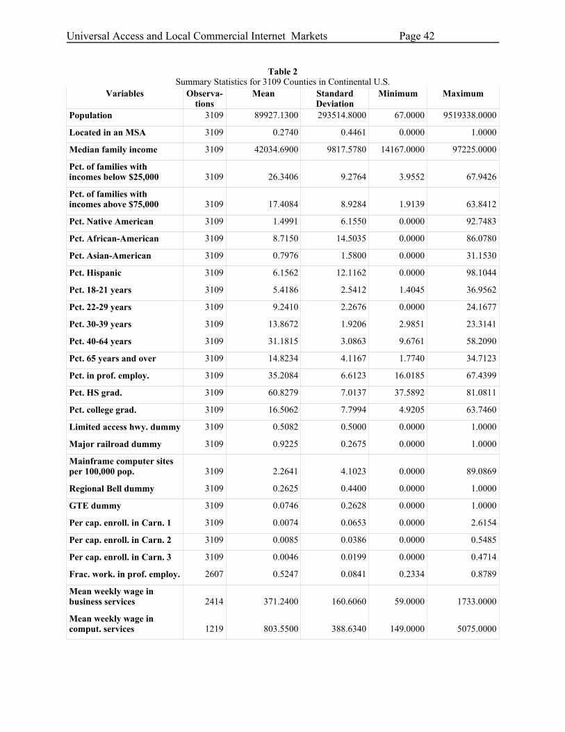
Universal Access and Local Commercial Internet Markets Page 42
Table 2 Summary Statistics for 3109 Counties in Continental U.S.
Variables Observa- tions
Mean Standard Deviation
Minimum Maximum
Population 3109 89927.1300 293514.8000 67.0000 9519338.0000
Located in an MSA 3109 0.2740 0.4461 0.0000 1.0000
Median family income 3109 42034.6900 9817.5780 14167.0000 97225.0000
Pct. of families with incomes below $25,000 3109 26.3406 9.2764 3.9552 67.9426
Pct. of families with incomes above $75,000 3109 17.4084 8.9284 1.9139 63.8412
Pct. Native American 3109 1.4991 6.1550 0.0000 92.7483
Pct. African-American 3109 8.7150 14.5035 0.0000 86.0780
Pct. Asian-American 3109 0.7976 1.5800 0.0000 31.1530
Pct. Hispanic 3109 6.1562 12.1162 0.0000 98.1044
Pct. 18-21 years 3109 5.4186 2.5412 1.4045 36.9562
Pct. 22-29 years 3109 9.2410 2.2676 0.0000 24.1677
Pct. 30-39 years 3109 13.8672 1.9206 2.9851 23.3141
Pct. 40-64 years 3109 31.1815 3.0863 9.6761 58.2090
Pct. 65 years and over 3109 14.8234 4.1167 1.7740 34.7123
Pct. in prof. employ. 3109 35.2084 6.6123 16.0185 67.4399
Pct. HS grad. 3109 60.8279 7.0137 37.5892 81.0811
Pct. college grad. 3109 16.5062 7.7994 4.9205 63.7460
Limited access hwy. dummy 3109 0.5082 0.5000 0.0000 1.0000
Major railroad dummy 3109 0.9225 0.2675 0.0000 1.0000
Mainframe computer sites per 100,000 pop. 3109 2.2641 4.1023 0.0000 89.0869
Regional Bell dummy 3109 0.2625 0.4400 0.0000 1.0000
GTE dummy 3109 0.0746 0.2628 0.0000 1.0000
Per cap. enroll. in Carn. 1 3109 0.0074 0.0653 0.0000 2.6154
Per cap. enroll. in Carn. 2 3109 0.0085 0.0386 0.0000 0.5485
Per cap. enroll. in Carn. 3 3109 0.0046 0.0199 0.0000 0.4714
Frac. work. in prof. employ. 2607 0.5247 0.0841 0.2334 0.8789
Mean weekly wage in business services 2414 371.2400 160.6060 59.0000 1733.0000
Mean weekly wage in comput. services 1219 803.5500 388.6340 149.0000 5075.0000
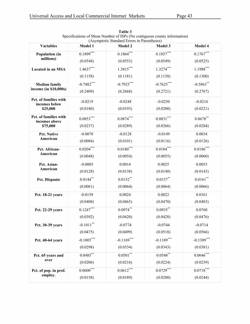
Universal Access and Local Commercial Internet Markets Page 43
Table 3 Specifications of Mean Number of ISPs (No contiguous county information)
(Asymptotic Standard Errors in Parentheses) Variables Model 1 Model 2 Model 3 Model 4
Population (in millions)
0.1899***
(0.0548)
0.1864***
(0.0553)
0.1857***
(0.0549)
0.1767***
(0.0525)
Located in an MSA 1.4637***
(0.1158)
1.3815***
(0.1181)
1.3274***
(0.1158)
1.1988***
(0.1300)
Median family income (in $10,000s)
-0.7482***
(0.2409)
-0.7925***
(0.2668)
-0.7625***
(0.2721)
-0.5863**
(0.2767)
Pct. of families with incomes below
$25,000
-0.0219
(0.0180)
-0.0248
(0.0193)
-0.0250
(0.0200)
-0.0216
(0.0221)
Pct. of families with incomes above
$75,000
0.0853***
(0.0237)
0.0874***
(0.0289)
0.0831***
(0.0266)
0.0678**
(0.0284)
Pct. Native American
-0.0070
(0.0084)
-0.0128
(0.0101)
-0.0149
(0.0116)
0.0034
(0.0126)
Pct. African-American
0.0204***
(0.0048)
0.0180***
(0.0054)
0.0184***
(0.0055)
0.0186***
(0.0060)
Pct. Asian-American
-0.0005
(0.0128)
0.0014
(0.0138)
0.0025
(0.0140)
0.0053
(0.0143)
Pct. Hispanic
0.0144**
(0.0061)
0.0152**
(0.0064)
0.0157**
(0.0064)
0.0161**
(0.0066)
Pct. 18-21 years -0.0159
(0.0408)
0.0024
(0.0465)
0.0022
(0.0470)
0.0161
(0.0483)
Pct. 22-29 years 0.1247***
(0.0392)
0.0974**
(0.0420)
0.0935**
(0.0428)
0.0760
(0.0476)
Pct. 30-39 years -0.1011**
(0.0475)
-0.0774
(0.0499)
-0.0744
(0.0518)
-0.0714
(0.0566)
Pct. 40-64 years -0.1005***
(0.0298)
-0.1169***
(0.0334)
-0.1189***
(0.0343)
-0.1309***
(0.0381)
Pct. 65 years and over
0.0485**
(0.0206)
0.0501**
(0.0216)
0.0548**
(0.0224)
0.0646***
(0.0239)
Pct. of pop. in prof. employ.
0.0600***
(0.0158)
0.0612***
(0.0189)
0.0729***
(0.0200)
0.0718***
(0.0244)

Universal Access and Local Commercial Internet Markets Page 44
Variables Model 1 Model 2 Model 3 Model 4
Pct. HS grad. 0.0495***
(0.0139)
0.0543***
(0.0146)
0.0526***
(0.0152)
0.0442***
(0.0169)
Pct. college grad. 0.0146
(0.0183)
0.0146
(0.0192)
0.0065
(0.0200)
-0.0019
(0.0231)
Limited access hwy. dummy
0.4014***
(0.1253)
0.4337***
(0.1268)
0.3839***
(0.1287)
0.2899*
(0.1639)
Major railroad dummy
0.2813
(0.2699)
0.2695
(0.3389)
0.2682
(0.3707)
0.5729
(0.5420)
Mainframe computer sites per
100,000 pop.
0.0461***
(0.0069)
0.0532***
(0.0090)
0.0525***
(0.0093)
0.0541***
(0.0104)
Regional Bell dummy
0.7076***
(0.1085)
0.6586***
(0.1109)
0.6290***
(0.1101)
0.5612***
(0.1207)
GTE dummy 0.4185***
(0.1343)
0.3686***
(0.1382)
0.3429**
(0.1377)
0.2725*
(0.1472)
Enrollment in Carnegie 1 per
capita
-2.8431*
(1.5018)
-3.4035*
(1.7747)
-3.2290*
(1.7592)
-3.8488**
(1.6778)
Enrollment in Carnegie 2 per
capita
-0.2247
(1.4113)
-0.8494
(1.6052)
-0.8695
(1.5873)
-1.0239
(1.6289)
Enrollment in Carnegie 3 per
capita
-2.4846
(2.3314)
-3.4351
(2.4547)
-3.9075
(2.5576)
-5.7717**
(2.9152)
Fraction of workers in prof. employment
0.5026
(0.7411)
0.6291
(0.7494)
0.7627
(0.8160)
Mean weekly wage in business services
(in $10000s)
-0.1565
(2.6084)
Mean weekly wage in comput. services
(in $10000s)
1.0638
(1.0261)
Value of pseudo-likelihood -23407.1600 -21865.0240 -21094.7060 -17706.5580
Observations 3109 2607 2171 1143
Notes: * Significant at 10 percent level. ** Significant at 5 percent level. *** Significant at 1 percent level.

Universal Access and Local Commercial Internet Markets Page 45
Table 4 Specifications of Mean Number of ISPs (Contiguous county information)
(Asymptotic Standard Errors in Parentheses) Variables Model 1 Model 2 Model 3 Model 4
Coefficients on Home County Characteristics
Population (in millions)
0.1512***
(0.0485)
0.1520***
(0.0518)
0.1466***
(0.0513)
0.1329***
(0.0502)
Located in an MSA 1.4194***
(0.1180)
1.2990***
(0.1187)
1.2472***
(0.1168)
1.1122***
(0.1255)
Median family income (in $10,000s)
-0.7435***
(0.2170)
-0.7955***
(0.2362)
-0.8031***
(0.2423)
-0.6751***
(0.2589)
Pct. of families with incomes below
$25,000
0.0110
(0.0193)
0.0207
(0.0202)
0.0240
(0.0207)
0.0245
(0.0235)
Pct. of families with incomes above
$75,000
0.1023***
(0.0232)
0.1081***
(0.0252)
0.1095***
(0.0262)
0.1080***
(0.0297)
Pct. Native American
-0.0192*
(0.0112)
-0.0147
(0.0118)
-0.0197
(0.0148)
0.0107
(0.0130)
Pct. African-American
0.0307***
(0.0054)
0.0265***
(0.0058)
0.0264***
(0.0058)
0.0259***
(0.0063)
Pct. Asian-American
0.0077
(0.0147)
0.0101
(0.0158)
0.0138
(0.0172)
0.0288
(0.0176)
Pct. Hispanic
0.0282***
(0.0069)
0.0260***
(0.0072)
0.0262***
(0.0071)
0.0232***
(0.0074)
Pct. 18-21 years 0.0053
(0.0411)
0.0016
(0.0470)
0.0005
(0.0468)
0.0073
(0.0488)
Pct. 22-29 years 0.1642***
(0.0372)
0.1472***
(0.0409)
0.1412***
(0.0419)
0.1406***
(0.0479)
Pct. 30-39 years -0.0509
(0.0493)
-0.0512
(0.0495)
-0.0549
(0.0507)
-0.0739
(0.0560)
Pct. 40-64 years -0.0490
(0.0319)
-0.0709**
(0.0340)
-0.0735**
(0.0350)
-0.0861**
(0.0383)
Pct. 65 years and over
0.0806***
(0.0220)
0.0692***
(0.0226)
0.0718***
(0.0232)
0.0743***
(0.0249)
Pct. of pop. in prof. employ.
0.0571***
(0.0169)
0.0579***
(0.0206)
0.0691***
(0.0219)
0.0638**
(0.0263)
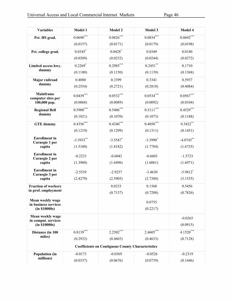
Universal Access and Local Commercial Internet Markets Page 46
Variables Model 1 Model 2 Model 3 Model 4
Pct. HS grad. 0.0690***
(0.0157)
0.0826***
(0.0171)
0.0834***
(0.0179)
0.0692***
(0.0198)
Pct. college grad. 0.0345*
(0.0209)
0.0428*
(0.0232)
0.0349
(0.0244)
0.0180
(0.0272)
Limited access hwy. dummy
0.2269*
(0.1180)
0.2985***
(0.1150)
0.2451**
(0.1139)
0.1710
(0.1368)
Major railroad dummy
0.4080
(0.2554)
0.3399
(0.2721)
0.3341
(0.2818)
0.5937
(0.4084)
Mainframe computer sites per
100,000 pop.
0.0439***
(0.0068)
0.0532***
(0.0089)
0.0534***
(0.0092)
0.0567***
(0.0104)
Regional Bell dummy
0.5900***
(0.1021)
0.5406***
(0.1070)
0.5111***
(0.1073)
0.4529***
(0.1188)
GTE dummy 0.4356***
(0.1219)
0.4240***
(0.1299)
0.4050***
(0.1311)
0.3422**
(0.1451)
Enrollment in Carnegie 1 per
capita
-3.3933**
(1.5180)
-3.5547*
(1.8182)
-3.3990*
(1.7784)
-4.0745**
(1.6735)
Enrollment in Carnegie 2 per
capita
-0.2223
(1.3960)
-0.6042
(1.6496)
-0.6603
(1.6061)
-1.5723
(1.6971)
Enrollment in Carnegie 3 per
capita
-2.5539
(2.4279)
-2.9257
(2.5905)
-3.4630
(2.7380)
-5.9812*
(3.1535)
Fraction of workers in prof. employment
0.0233
(0.7137)
0.1560
(0.7208)
0.5456
(0.7826)
Mean weekly wage in business services
(in $10000s)
0.0755
(0.2217)
Mean weekly wage in comput. services
(in $10000s)
-0.0265
(0.0915)
Distance (in 100 miles)
0.8139***
(0.2932)
2.2502***
(0.4603)
2.4605***
(0.4633)
4.1520***
(0.7128)
Coefficients on Contiguous County Characteristics
Population (in millions)
-0.0173
(0.0337)
-0.0369
(0.0676)
-0.0526
(0.0739)
-0.2319
(0.1446)

Universal Access and Local Commercial Internet Markets Page 47
Variables Model 1 Model 2 Model 3 Model 4
Located in an MSA 0.0162
(0.0535)
0.0953
(0.0841)
0.1053
(0.0899)
0.2660*
(0.1438)
Median family income(in $10,000s)
-0.0530
(0.1164)
-0.1214
(0.1652)
-0.1130
(0.1777)
-0.1304
(0.2540)
Pct. of families with incomes below
$25,000
-0.0171**
(0.0071)
-0.0259**
(0.0109)
-0.0260**
(0.0116)
-0.0332*
(0.0186)
Pct. of families with incomes above
$75,000
0.0016
(0.0103)
0.0056
(0.0151)
0.0042
(0.0163)
-0.0026
(0.0263)
Pct. Native American
0.0125**
(0.0059)
0.0188*
(0.0100)
0.0231**
(0.0114)
0.0577**
(0.0272)
Pct. African-American
-0.0049***
(0.0017)
-0.0064**
(0.0026)
-0.0069**
(0.0028)
-0.0074
(0.0046)
Pct. Asian-American
-0.0110
(0.0079)
-0.0078
(0.0109)
-0.0061
(0.0116)
0.0107
(0.0183)
Pct. Hispanic
-0.0046*
(0.0024)
-0.0051
(0.0037)
-0.0051
(0.0039)
-0.0016
(0.0064)
Pct. 18-21 years -0.0002
(0.0184)
-0.0013
(0.0276)
-0.0054
(0.0290)
-0.0185
(0.0475)
Pct. 22-29 years -0.0383**
(0.0195)
-0.0628**
(0.0289)
-0.0716**
(0.0311)
-0.1098**
(0.0487)
Pct. 30-39 years 0.0179
(0.0217)
0.0419
(0.0346)
0.0502
(0.0368)
0.0879
(0.0586)
Pct. 40-64 years -0.0146
(0.0120)
-0.0261
(0.0200)
-0.0322
(0.0217)
-0.0571
(0.0368)
Pct. 65 years and over
-0.0087
(0.0096)
-0.0098
(0.0156)
-0.0112
(0.0167)
-0.0158
(0.0275)
Pct. of pop. in prof. employ.
-0.0046
(0.0064)
-0.0093
(0.0104)
-0.0088
(0.0115)
-0.0061
(0.0200)
Pct. HS grad. -0.0132**
(0.0067)
-0.0216**
(0.0105)
-0.0222**
(0.0112)
-0.0298
(0.0186)
Pct. college grad. -0.0121
(0.0075)
-0.0176
(0.0117)
-0.0177
(0.0126)
-0.0235
(0.0211)

Universal Access and Local Commercial Internet Markets Page 48
Variables Model 1 Model 2 Model 3 Model 4
Limited access hwy. dummy
-0.0188
(0.0458)
-0.0243
(0.0714)
-0.0304
(0.0776)
-0.1031
(0.1293)
Major railroad dummy
-0.0105
(0.1005)
-0.1260
(0.1670)
-0.1415
(0.1821)
-0.2165
(0.3582)
Mainframe computer sites per
100,000 pop.
-0.0105
(0.0086)
-0.0104
(0.0138)
-0.0095
(0.0144)
-0.0085
(0.0232)
Regional Bell dummy
-0.0367
(0.0515)
-0.0539
(0.0754)
-0.0587
(0.0802)
-0.1220
(0.1215)
GTE dummy -0.0370
(0.0693)
-0.0958
(0.1046)
-0.1131
(0.1138)
-0.2008
(0.1793)
Enrollment in Carnegie 1 per
capita
-0.5622
(0.4901)
-0.8223
(0.6550)
-0.8002
(0.5973)
-1.2917
(1.3022)
Enrollment in Carnegie 2 per
capita
0.7558
(0.6626)
1.1374
(0.9527)
-1.3936
(0.9796)
-1.5544
(1.8025)
Enrollment in Carnegie 3 per
capita
2.7836**
(1.2663)
4.5314**
(1.8939)
5.3497***
(2.0538)
9.5765**
(3.9831)
Fraction of workers in prof. employment
-0.1777
(0.1547)
-0.2130
(0.1671)
-0.3120
(0.2857)
Mean weekly wage in business services
(in $10000s)
-0.0619
(0.2920)
Mean weekly wage in comput. services
(in $10000s)
-0.2428*
(0.1425)
Value of pseudo-likelihood -19626.3001 -18191.7352 -17351.9018 -14009.2264
Observations 3109 2607 2171 1143
Notes: * Significant at 10 percent level. ** Significant at 5 percent level. *** Significant at 1 percent level.

Universal Access and Local Commercial Internet Markets Page 49
Table 5A Specifications of Mean Number of National ISPs (No contiguous county information)
(Asymptotic Standard Errors in Parentheses) Variables Model 1 Model 2 Model 3 Model 4
Population (in millions)
0.1727***
(0.0658)
0.1679**
(0.0664)
0.1681**
(0.0663)
0.1591**
(0.0651)
Located in an MSA 2.3745***
(0.2441)
2.1922***
(0.2354)
2.0880***
(0.2253)
1.7524***
(0.2227)
Median family income (in $10,000s)
-0.8721***
(0.3289)
-0.8844**
(0.3520)
-0.8574**
(0.3542)
-0.6642*
(0.3488)
Pct. of families with incomes below
$25,000
-0.0313
(0.0263)
-0.0350
(0.0274)
-0.0358
(0.0279)
-0.0348
(0.0284)
Pct. of families with incomes above
$75,000
0.0890***
(0.0330)
0.0883**
(0.0348)
0.0841**
(0.0351)
0.0618*
(0.0356)
Pct. Native American
-0.0217
(0.0174)
-0.0292
(0.0193)
-0.0328
(0.0218)
-0.0039
(0.0195)
Pct. African-American
0.0216***
(0.0066)
0.0171**
(0.0073)
0.0176**
(0.0074)
0.0174**
(0.0076)
Pct. Asian-American
0.0114
(0.0177)
0.0132
(0.0189)
0.0143
(0.0191)
0.0141
(0.0187)
Pct. Hispanic
0.0164**
(0.0078)
0.0173**
(0.0078)
0.0170**
(0.0078)
0.0157**
(0.0079)
Pct. 18-21 years -0.0062
(0.0562)
0.0179
(0.0623)
0.0165
(0.0618)
0.0167
(0.0610)
Pct. 22-29 years 0.1094**
(0.0549)
0.0776
(0.0580)
0.0760
(0.0582)
0.0582
(0.0601)
Pct. 30-39 years -0.1505**
(0.0702)
-0.1225*
(0.0727)
-0.1194
(0.0747)
-0.1103
(0.0738)
Pct. 40-64 years -0.1464***
(0.0430)
-0.1723***
(0.0470)
-0.1714***
(0.0477)
-0.1755***
(0.0494)
Pct. 65 years and over
0.0501*
(0.0282)
0.0511*
(0.0288)
0.0545*
(0.0296)
0.0624**
(0.0298)
Pct. of pop. in prof. employ.
0.0862***
(0.0240)
0.0826***
(0.0274)
0.0920***
(0.0282)
0.0875***
(0.0311)

Universal Access and Local Commercial Internet Markets Page 50
Variables Model 1 Model 2 Model 3 Model 4
Pct. HS grad. 0.0564***
(0.0198)
0.0622***
(0.0204)
0.0591***
(0.0207)
0.0450**
(0.0212)
Pct. college grad. 0.0082
(0.0266)
0.0098
(0.0272)
0.0026
(0.0277)
-0.0052
(0.0293)
Limited access hwy. dummy
0.5444***
(0.2401)
0.6030**
(0.2437)
0.5378**
(0.2387)
0.3824
(0.2486)
Major railroad dummy
0.6093
(0.5791)
0.7340
(0.7642)
0.7382
(0.7958)
0.7752
(0.8768)
Mainframe computer sites per
100,000 pop.
0.0571***
(0.0087)
0.0660***
(0.0125)
0.0649***
(0.0129)
0.0625***
(0.0135)
Regional Bell dummy
0.8380***
(0.1626)
0.7679***
(0.1602)
0.7397***
(0.1581)
0.6109***
(0.1563)
GTE dummy 0.5396***
(0.1928)
0.4655**
(0.1935)
0.4405**
(0.1914)
0.2956
(0.1884)
Enrollment in Carnegie 1 per
capita
-3.8363**
(1.9321)
-4.8914**
(2.2714)
-4.7068**
(2.2194)
-4.6320**
(2.1277)
Enrollment in Carnegie 2 per
capita
-0.2955
(1.9545)
-1.3534
(2.1760)
-1.3890
(2.1258)
-1.1714
(2.0960)
Enrollment in Carnegie 3 per
capita
-3.1011
(3.3654)
-4.6740
(3.5603)
-5.0273
(3.5612)
-6.0338
(3.6764)
Fraction of workers in prof. employment
0.9999
(1.0131)
1.0952
(1.0101)
1.1589
(1.0240)
Mean weekly wage in business services
(in $10000s)
-0.5518
(3.5514)
Mean weekly wage in comput. services
(in $10000s)
1.1248
(1.3064)
Value of pseudo-likelihood -22223.9714 -21139.6770 -20850.0510 -18641.5990
Observations 3109 2607 2171 1143
Notes: * Significant at 10 percent level. ** Significant at 5 percent level. *** Significant at 1 percent level.

Universal Access and Local Commercial Internet Markets Page 51
Table 5B Specifications of Mean Number of Local ISPs (No contiguous county information)
(Asymptotic Standard Errors in Parentheses) Variables Model 1 Model 2 Model 3 Model 4
Population (in millions)
0.3280***
(0.0400)
0.3234***
(0.0395)
0.3228***
(0.0387)
0.3162***
(0.0366)
Located in an MSA 0.5206***
(0.0653)
0.4837***
(0.0677)
0.4465***
(0.0667)
0.3349***
(0.0769)
Median family income (in $10,000s)
-0.4918***
(0.1521)
-0.5308***
(0.1611)
-0.4840***
(0.1636)
-0.3468*
(0.1788)
Pct. of families with incomes below
$25,000
-0.0314***
(0.0118)
-0.0306**
(0.0125)
-0.0289**
(0.0130)
-0.0216
(0.0156)
Pct. of families with incomes above
$75,000
0.0688***
(0.0152)
0.0695***
(0.0163)
0.0621***
(0.0166)
0.0547***
(0.0189)
Pct. Native American
-0.0006
(0.0073)
-0.0009
(0.0090)
-0.0008
(0.0096)
0.0173**
(0.0074)
Pct. African-American
0.0155***
(0.0032)
0.0172***
(0.0034)
0.0171***
(0.0034)
0.0208***
(0.0038)
Pct. Asian-American
0.0131
(0.0106)
0.0129
(0.0108)
0.0110
(0.0107)
0.0118
(0.0106)
Pct. Hispanic
0.0161***
(0.0056)
0.0193***
(0.0057)
0.0203***
(0.0056)
0.0234***
(0.0057)
Pct. 18-21 years -0.0714**
(0.0288)
-0.0615**
(0.0275)
-0.0630**
(0.0274)
-0.0337
(0.0323)
Pct. 22-29 years 0.1394***
(0.0258)
0.1369***
(0.0277)
0.1358***
(0.0280)
0.1588***
(0.0339)
Pct. 30-39 years -0.0362
(0.0324)
-0.0179
(0.0350)
-0.0236
(0.0365)
-0.0221
(0.0410)
Pct. 40-64 years -0.0452**
(0.0199)
-0.0330
(0.0225)
-0.0379
(0.0234)
-0.0208
(0.0266)
Pct. 65 years and over
0.0374***
(0.0145)
0.0415***
(0.0159)
0.0444***
(0.0163)
0.0653***
(0.0180)
Pct. of pop. in prof. employ.
0.0226**
(0.0111)
0.0369***
(0.0133)
0.0526***
(0.0147)
0.0702***
(0.0192)
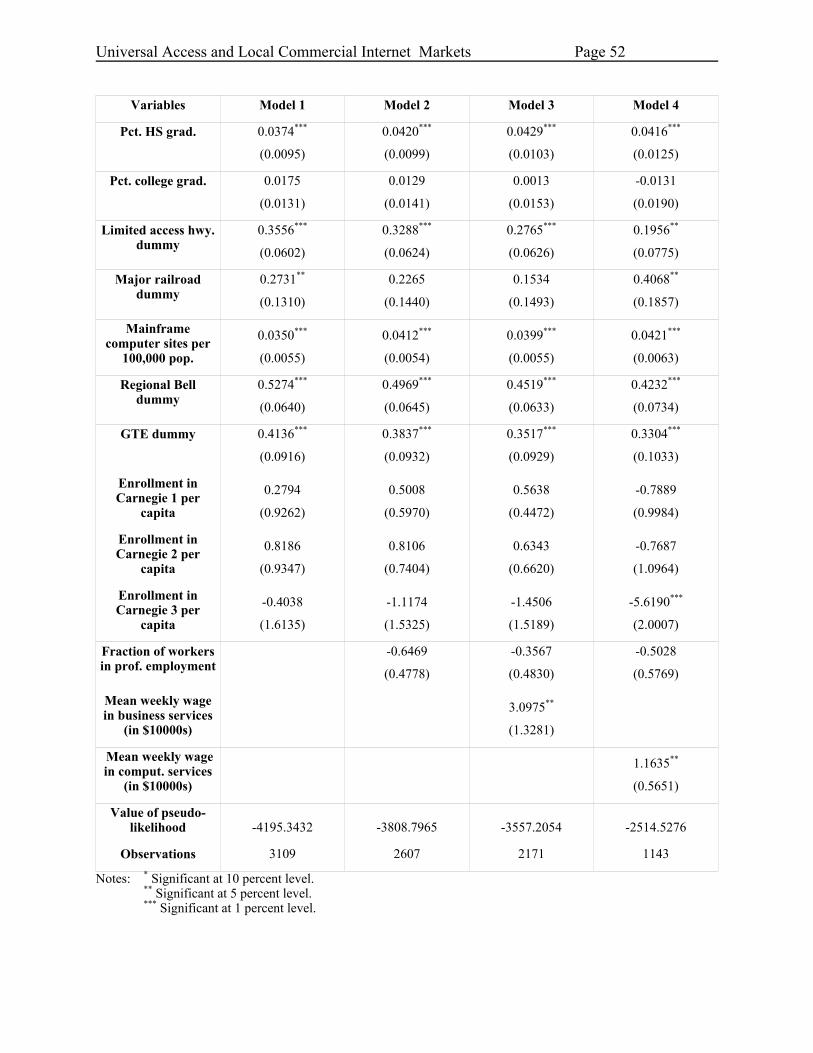
Universal Access and Local Commercial Internet Markets Page 52
Variables Model 1 Model 2 Model 3 Model 4
Pct. HS grad. 0.0374***
(0.0095)
0.0420***
(0.0099)
0.0429***
(0.0103)
0.0416***
(0.0125)
Pct. college grad. 0.0175
(0.0131)
0.0129
(0.0141)
0.0013
(0.0153)
-0.0131
(0.0190)
Limited access hwy. dummy
0.3556***
(0.0602)
0.3288***
(0.0624)
0.2765***
(0.0626)
0.1956**
(0.0775)
Major railroad dummy
0.2731**
(0.1310)
0.2265
(0.1440)
0.1534
(0.1493)
0.4068**
(0.1857)
Mainframe computer sites per
100,000 pop.
0.0350***
(0.0055)
0.0412***
(0.0054)
0.0399***
(0.0055)
0.0421***
(0.0063)
Regional Bell dummy
0.5274***
(0.0640)
0.4969***
(0.0645)
0.4519***
(0.0633)
0.4232***
(0.0734)
GTE dummy 0.4136***
(0.0916)
0.3837***
(0.0932)
0.3517***
(0.0929)
0.3304***
(0.1033)
Enrollment in Carnegie 1 per
capita
0.2794
(0.9262)
0.5008
(0.5970)
0.5638
(0.4472)
-0.7889
(0.9984)
Enrollment in Carnegie 2 per
capita
0.8186
(0.9347)
0.8106
(0.7404)
0.6343
(0.6620)
-0.7687
(1.0964)
Enrollment in Carnegie 3 per
capita
-0.4038
(1.6135)
-1.1174
(1.5325)
-1.4506
(1.5189)
-5.6190***
(2.0007)
Fraction of workers in prof. employment
-0.6469
(0.4778)
-0.3567
(0.4830)
-0.5028
(0.5769)
Mean weekly wage in business services
(in $10000s)
3.0975**
(1.3281)
Mean weekly wage in comput. services
(in $10000s)
1.1635**
(0.5651)
Value of pseudo-likelihood -4195.3432 -3808.7965 -3557.2054 -2514.5276
Observations 3109 2607 2171 1143
Notes: * Significant at 10 percent level. ** Significant at 5 percent level. *** Significant at 1 percent level.

Universal Access and Local Commercial Internet Markets Page 53
Table 6A Specifications of Mean Number of National ISPs (Contiguous county information)
(Asymptotic Standard Errors in Parentheses) Variables Model 1 Model 2 Model 3 Model 4
Coefficients on Home County Characteristics
Population (in millions)
0.1357**
(0.0670)
0.1391**
(0.0672)
0.1354**
(0.0665)
0.1226*
(0.0648)
Located in an MSA 2.2890***
(0.2448)
2.1067***
(0.2366)
2.0136***
(0.2256)
1.6604***
(0.2109)
Median family income (in $10,000s)
-1.0525***
(0.3092)
-1.0084***
(0.3267)
-1.0101***
(0.3272)
-0.8085**
(0.3309)
Pct. of families with incomes below
$25,000
0.0147
(0.0290)
0.0206
(0.0296)
0.0216
(0.0297)
0.0174
(0.0310)
Pct. of families with incomes above
$75,000
0.1436***
(0.0339)
0.1386***
(0.0358)
0.1354***
(0.0361)
0.1229***
(0.0379)
Pct. Native American
-0.0389**
(0.0196)
-0.0437*
(0.0246)
-0.0552
(0.0355)
0.0041
(0.0264)
Pct. African-American
0.0327***
(0.0074)
0.0279***
(0.0078)
0.0272***
(0.0079)
0.0273***
(0.0081)
Pct. Asian-American
0.0250
(0.0220)
0.0186
(0.0228)
0.0183
(0.0242)
0.0286
(0.0233)
Pct. Hispanic
0.0237***
(0.0092)
0.0239**
(0.0099)
0.0237**
(0.0100)
0.0207**
(0.0101)
Pct. 18-21 years -0.0206
(0.0607)
0.0003
(0.0701)
-0.0636
(0.0679)
0.0086
(0.0662)
Pct. 22-29 years 0.1723***
(0.0578)
0.1563**
(0.0612)
0.1470**
(0.0617)
0.1424**
(0.0627)
Pct. 30-39 years -0.1286*
(0.0721)
-0.1047
(0.0751)
-0.1137
(0.0757)
-0.1138
(0.0775)
Pct. 40-64 years -0.1266***
(0.0457)
-0.1365***
(0.0508)
-0.1427***
(0.0525)
-0.1442***
(0.0527)
Pct. 65 years and over
0.0656**
(0.0313)
0.0675**
(0.0323)
0.0662**
(0.0333)
0.0738**
(0.0331)
Pct. of pop. in prof. employ.
0.0821***
(0.0276)
0.0797**
(0.0314)
0.0897***
(0.0321)
0.0854**
(0.0353)

Universal Access and Local Commercial Internet Markets Page 54
Variables Model 1 Model 2 Model 3 Model 4
Pct. HS grad. 0.0824***
(0.0238)
0.0918***
(0.0254)
0.0920***
(0.0260)
0.0658**
(0.0265)
Pct. college grad. 0.0282
(0.0334)
0.0328
(0.0347)
0.0258
(0.0355)
0.0031
(0.0363)
Limited access hwy. dummy
0.3214
(0.2032)
0.3956*
(0.2062)
0.3228
(0.1987)
0.1999
(0.2028)
Major railroad dummy
0.6524
(0.5267)
0.6174
(0.5853)
0.6410
(0.5899)
0.7088
(0.6511)
Mainframe computer sites per
100,000 pop.
0.0568***
(0.0098)
0.0656***
(0.0130)
0.0651***
(0.0130)
0.0654***
(0.0137)
Regional Bell dummy
0.7189***
(0.1589)
0.6432***
(0.1606)
0.6057***
(0.1600)
0.4666***
(0.1568)
GTE dummy 0.6543***
(0.1910)
0.5886***
(0.1933)
0.5617***
(0.1932)
0.4060**
(0.1916)
Enrollment in Carnegie 1 per
capita
-4.7148**
(2.1464)
-5.1191**
(2.5553)
-4.8050**
(2.4161)
-5.4144**
(2.2344)
Enrollment in Carnegie 2 per
capita
-0.8700
(2.1390)
-1.3845
(2.3911)
-1.2595
(2.2567)
-2.2055
(2.2465)
Enrollment in Carnegie 3 per
capita
-4.2488
(4.2499)
-4.8668
(4.3227)
-4.8631
(4.2739)
-7.6275*
(4.3402)
Fraction of workers in prof. employment
0.3857
(1.0155)
0.5933
(1.0157)
0.8181
(1.0233)
Mean weekly wage in business services
(in $10000s)
0.2663
(0.3266)
Mean weekly wage in comput. services
(in $10000s)
0.0078
(0.1240)
Distance (in 100 miles)
3.0342***
(0.4237)
2.8704***
(0.3772)
2.8725***
(0.3643)
3.1477***
(0.3855)
Coefficients on Contiguous County Characteristics
Population (in millions)
-0.2855*
(0.1566)
-0.2295
(0.1428)
-0.2258
(0.1434)
-0.2752*
(0.1544)

Universal Access and Local Commercial Internet Markets Page 55
Variables Model 1 Model 2 Model 3 Model 4
Located in an MSA 0.1755
(0.1332)
0.2086
(0.1342)
0.2066
(0.1332)
0.2209
(0.1378)
Median family income(in $10,000s)
-0.0252
(0.2619)
-0.0288
(0.2611)
-0.0050
(0.2673)
0.0273
(0.2808)
Pct. of families with incomes below
$25,000
-0.0362**
(0.0174)
-0.0344**
(0.0172)
-0.0334**
(0.0170)
-0.0286
(0.0185)
Pct. of families with incomes above
$75,000
-0.0135
(0.0252)
-0.0105
(0.0246)
-0.0133
(0.0249)
-0.0174
(0.0271)
Pct. Native American
0.0401**
(0.0159)
0.0408***
(0.0158)
0.0425**
(0.0175)
0.0502**
(0.0206)
Pct. African-American
-0.0046
(0.0041)
-0.0047
(0.0041)
-0.0050
(0.0041)
-0.0047
(0.0043)
Pct. Asian-American
0.0026
(0.0187)
0.0028
(0.0178)
0.0025
(0.0180)
0.0142
(0.0190)
Pct. Hispanic
-0.0017
(0.0060)
-0.0011
(0.0060)
-0.0011
(0.0060)
0.0008
(0.0065)
Pct. 18-21 years 0.0217
(0.0555)
0.0342
(0.0552)
0.0256
(0.0543)
0.0279
(0.0601)
Pct. 22-29 years -0.0674
(0.0491)
-0.0900*
(0.0473)
-0.0944**
(0.0476)
-0.1086**
(0.0505)
Pct. 30-39 years 0.0542
(0.0551)
0.0886
(0.0546)
0.0877
(0.0539)
0.1107*
(0.0590)
Pct. 40-64 years -0.0385
(0.0325)
-0.0342
(0.0340)
-0.0369
(0.0337)
-0.0396
(0.0372)
Pct. 65 years and over
-0.0026
(0.0257)
0.0051
(0.0259)
0.0108
(0.0260)
0.0072
(0.0280)
Pct. of pop. in prof. employ.
-0.0060
(0.0182)
-0.0084
(0.0175)
-0.0080
(0.0180)
-0.0005
(0.0197)
Pct. HS grad. -0.0277
(0.0172)
-0.0277
(0.0168)
-0.0274
(0.0168)
-0.0250
(0.0182)
Pct. college grad. -0.0215
(0.0199)
-0.0234
(0.0196)
-0.0237
(0.0196)
-0.0252
(0.0214)

Universal Access and Local Commercial Internet Markets Page 56
Variables Model 1 Model 2 Model 3 Model 4
Limited access hwy. dummy
-0.0222
(0.1185)
-0.0482
(0.1153)
-0.0455
(0.1176)
-0.0728
(0.1302)
Major railroad dummy
-0.2424
(0.3070)
-0.1447
(0.3141)
-0.1340
(0.3093)
-0.0738
(0.3434)
Mainframe computer sites per
100,000 pop.
-0.0152
(0.0216)
-0.0079
(0.0205)
-0.0072
(0.0203)
-0.0080
(0.0224)
Regional Bell dummy
-0.1623
(0.1247)
-0.1227
(0.1199)
-0.1156
(0.1206)
-0.1120
(0.1257)
GTE dummy -0.2024
(0.1696)
-0.1980
(0.1669)
-0.1955
(0.1685)
-0.1763
(0.1740)
Enrollment in Carnegie 1 per
capita
-3.1624
(2.3996)
-2.5033
(2.2379)
-2.1211
(2.1188)
-2.3026
(2.4278)
Enrollment in Carnegie 2 per
capita
0.1081
(2.2618)
-0.5132
(2.1344)
1.0437
(2.0704)
1.2444
(2.3058)
Enrollment in Carnegie 3 per
capita
8.4871**
(3.5586)
7.6732**
(3.4930)
8.2020**
(3.5196)
9.2399**
(4.1378)
Fraction of workers in prof. employment
-0.2113
(0.2458)
-0.2278
(0.2446)
-0.2514
(0.2630)
Mean weekly wage in business services
(in $10000s)
0.0637
(0.4136)
Mean weekly wage in comput. services
(in $10000s)
-0.2317*
(0.1359)
Value of pseudo-likelihood -17754.0768 -16840.5412 -16502.7077 -14424.1332
Observations 3109 2607 2171 1143
Notes: * Significant at 10 percent level. ** Significant at 5 percent level. *** Significant at 1 percent level.
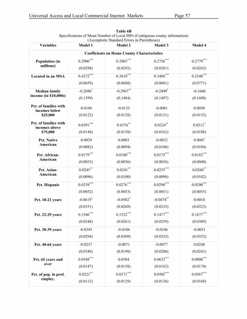
Universal Access and Local Commercial Internet Markets Page 57
Table 6B Specifications of Mean Number of Local ISPs (Contiguous county information)
(Asymptotic Standard Errors in Parentheses) Variables Model 1 Model 2 Model 3 Model 4
Coefficients on Home County Characteristics
Population (in millions)
0.2900***
(0.0298)
0.2803***
(0.0292)
0.2756***
(0.0281)
0.2779***
(0.0262)
Located in an MSA 0.4272***
(0.0659)
0.3810***
(0.0688)
0.3486***
(0.0681)
0.2540***
(0.0771)
Median family income (in $10,000s)
-0.2696*
(0.1399)
-0.2967**
(0.1484)
-0.2499*
(0.1497)
-0.1660
(0.1608)
Pct. of families with incomes below
$25,000
-0.0186
(0.0122)
-0.0125
(0.0128)
-0.0081
(0.0131)
0.0050
(0.0152)
Pct. of families with incomes above
$75,000
0.0391***
(0.0148)
0.0376**
(0.0158)
0.0324**
(0.0162)
0.0312*
(0.0188)
Pct. Native American
-0.0029
(0.0082)
0.0003
(0.0094)
-0.0032
(0.0106)
0.0047
(0.0104)
Pct. African-American
0.0179***
(0.0033)
0.0180***
(0.0036)
0.0175***
(0.0036)
0.0183***
(0.0040)
Pct. Asian-American
0.0245**
(0.0096)
0.0241**
(0.0100)
0.0255***
(0.0098)
0.0260**
(0.0102)
Pct. Hispanic
0.0239***
(0.0052)
0.0276***
(0.0053)
0.0290***
(0.0051)
0.0290***
(0.0055)
Pct. 18-21 years -0.0619*
(0.0351)
-0.0502*
(0.0268)
-0.0478**
(0.0235)
0.0010
(0.0323)
Pct. 22-29 years 0.1546***
(0.0248)
0.1522***
(0.0261)
0.1477***
(0.0259)
0.1677***
(0.0309)
Pct. 30-39 years -0.0345
(0.0294)
-0.0106
(0.0309)
-0.0106
(0.0325)
-0.0031
(0.0352)
Pct. 40-64 years -0.0237
(0.0186)
-0.0071
(0.0198)
-0.0077
(0.0206)
0.0248
(0.0241)
Pct. 65 years and over
0.0548***
(0.0147)
0.0584
(0.0158)
0.0623***
(0.0162)
0.0800***
(0.0174)
Pct. of pop. in prof. employ.
0.0221**
(0.0112)
0.0371***
(0.0129)
0.0505***
(0.0136)
0.0567***
(0.0168)

Universal Access and Local Commercial Internet Markets Page 58
Variables Model 1 Model 2 Model 3 Model 4
Pct. HS grad. 0.0457***
(0.0103)
0.0543***
(0.0108)
0.0560***
(0.0110)
0.0584***
(0.0129)
Pct. college grad. 0.0358***
(0.0128)
0.0340**
(0.0137)
0.0231
(0.0142)
0.0176
(0.0168)
Limited access hwy. dummy
0.3008***
(0.0633)
0.2882***
(0.0658)
0.2552***
(0.0652)
0.1721**
(0.0775)
Major railroad dummy
0.3605***
(0.1270)
0.3041**
(0.1392)
0.2008
(0.1409)
0.5258***
(0.1739)
Mainframe computer sites per
100,000 pop.
0.0359***
(0.0051)
0.0432***
(0.0046)
0.0429***
(0.0046)
0.0485***
(0.0052)
Regional Bell dummy
0.4465***
(0.0607)
0.4332***
(0.0624)
0.3962***
(0.0608)
0.3939***
(0.0690)
GTE dummy 0.3688***
(0.0855)
0.3548***
(0.0864)
0.3372***
(0.0865)
0.3758***
(0.0943)
Enrollment in Carnegie 1 per
capita
0.0775
(1.5349)
0.4124
(0.9089)
0.5616
(0.5518)
-1.2809
(1.2926)
Enrollment in Carnegie 2 per
capita
0.7411
(1.3463)
0.7914
(0.9104)
0.6202
(0.6967)
-1.1764
(1.1939)
Enrollment in Carnegie 3 per
capita
0.1052
(1.7670)
-0.4002
(1.4206)
-0.7066
(1.3695)
-5.8614***
(1.9931)
Fraction of workers in prof. employment
-0.6901
(0.4433)
-0.5008
(0.4495)
0.5391
(0.5394)
Mean weekly wage in business services
(in $10000s)
0.2645*
(0.1488)
Mean weekly wage in comput. services
(in $10000s)
0.0424
(0.0618)
Distance (in 100 miles)
0.2991
(0.2169)
0.3549
(0.2245)
0.3792
(0.2339)
0.5776**
(0.2462)
Coefficients on Contiguous County Characteristics
Population (in millions)
0.0751***
(0.0221)
0.0685***
(0.0214)
0.0675***
(0.0208)
0.0767***
(0.0219)

Universal Access and Local Commercial Internet Markets Page 59
Variables Model 1 Model 2 Model 3 Model 4
Located in an MSA 0.0741**
(0.0317)
0.0733**
(0.0324)
0.0760**
(0.0332)
0.0895**
(0.0382)
Median family income(in $10,000s)
-0.1901***
(0.0656)
-0.2028***
(0.0685)
-0.1671**
(0.0702)
-0.1881**
(0.0802)
Pct. of families with incomes below
$25,000
-0.0034
(0.0038)
-0.0047
(0.0040)
-0.0026
(0.0041)
-0.0010
(0.0047)
Pct. of families with incomes above
$75,000
0.0177***
(0.0064)
0.0194***
(0.0068)
0.0166**
(0.0069)
0.0194**
(0.0083)
Pct. Native American
-0.0018
(0.0251)
-0.0023
(0.0027)
-0.0014
(0.0028)
-0.0008
(0.0036)
Pct. African-American
-0.0053***
(0.0010)
-0.0052***
(0.0011)
-0.0050***
(0.0011)
-0.0040***
(0.0012)
Pct. Asian-American
-0.0017
(0.0042)
-0.0017
(0.0042)
0.0005
(0.0044)
-0.0009
(0.0048)
Pct. Hispanic
-0.0053***
(0.0015)
-0.0054***
(0.0015)
-0.0052***
(0.0014)
-0.0052***
(0.0017)
Pct. 18-21 years -0.0126
(0.0114)
-0.0161
(0.0119)
-0.0189
(0.0121)
-0.0092
(0.0145)
Pct. 22-29 years -0.0310***
(0.0114)
-0.0349***
(0.0116)
-0.0376***
(0.0116)
-0.0536***
(0.0139)
Pct. 30-39 years 0.0012
(0.0112)
-0.0039
(0.0119)
-0.0032
(0.0120)
0.0104
(0.0146)
Pct. 40-64 years -0.0128*
(0.0067)
-0.0179**
(0.0073)
-0.0201***
(0.0076)
-0.0296***
(0.0092)
Pct. 65 years and over
-0.0180***
(0.0054)
-0.0206***
(0.0059)
-0.0216***
(0.0059)
-0.0201***
(0.0072)
Pct. of pop. in prof. employ.
-0.0088**
(0.0039)
-0.0085**
(0.0041)
-0.0058
(0.0040)
-0.0050
(0.0048)
Pct. HS grad. -0.0019
(0.0034)
-0.0025
(0.0037)
-0.0019
(0.0036)
0.0001
(0.0045)
Pct. college grad. 0.0006
(0.0047)
-0.0001
(0.0049)
0.0002
(0.0049)
0.0002
(0.0057)

Universal Access and Local Commercial Internet Markets Page 60
Variables Model 1 Model 2 Model 3 Model 4
Limited access hwy. dummy
-0.0108
(0.0266)
-0.0208
(0.0277)
-0.0324
(0.0277)
-0.0651**
(0.0330)
Major railroad dummy
-0.0175
(0.0536)
-0.0218
(0.0591)
-0.0198
(0.0593)
0.0360
(0.0749)
Mainframe computer sites per
100,000 pop.
-0.0030
(0.0045)
-0.0024
(0.0045)
-0.0016
(0.0043)
0.0018
(0.0047)
Regional Bell dummy
0.0442
(0.0281)
0.0433
(0.0289)
0.0405
(0.0284)
0.0306
(0.0322)
GTE dummy 0.0236
(0.0400)
0.0087
(0.0411)
-0.0064
(0.0429)
-0.0500
(0.0488)
Enrollment in Carnegie 1 per
capita
0.0602
(0.3226)
0.1130
(0.3023)
0.1742
(0.2798)
-0.3249
(0.4116)
Enrollment in Carnegie 2 per
capita
0.1204
(0.4635)
0.1538
(0.4694)
0.0326
(0.4812)
-0.3432
(0.5888)
Enrollment in Carnegie 3 per
capita
-0.6846
(0.7511)
-0.7958
(0.7675)
-0.6973
(0.7693)
-0.8838
(0.9253)
Fraction of workers in prof. employment
0.0171
(0.0632)
-0.0284
(0.0645)
-0.0275
(0.0727)
Mean weekly wage in business services
(in $10000s)
-0.1527*
(0.0881)
Mean weekly wage in comput. services
(in $10000s)
-0.0718
(0.0454)
Value of pseudo-likelihood -3954.7979 -3580.2231 -3332.3023 -2301.0526
Observations 3109 2607 2171 1143
Notes: * Significant at 10 percent level. ** Significant at 5 percent level. *** Significant at 1 percent level.

WORKING PAPER SERIES 2005 http://ase.tufts.edu/econ/papers/papers.html
2005-01 EGGLESTON, Karen, Keqin RAO and Jian WANG; “From Plan
to Market in the Health Sector? China's Experience.”
2005-02 SHIMSHACK Jay; “Are Mercury Advisories Effective?
Information, Education, and Fish Consumption.”
2005-03 KIM, Henry and Jinill KIM; “Welfare Effects of Tax Policy in
Open Economies: Stabilization and Cooperation.”
2005-04 KIM, Henry, Jinill KIM and Robert KOLLMANN; “Applying
Perturbation Methods to Incomplete Market Models with
Exogenous Borrowing Constraints.”
2005-05 KIM, Henry, Jinill KIM, Ernst SCHAUMBURG and Christopher
A. SIMS; “Calculating and Using Second Order Accurate
Solutions of Discrete Time Dynamic Equilibrium Models.”
2005-06 KIM, Henry, Soyoung KIM and Yunjong WANG; “International
Capital Flows and Boom-Bust Cycles in the Asia Pacific Region.”
2005-07 KIM, Henry, Soyoung KIM and Yunjong WANG; “Fear of
Floating in East Asia.”
2005-08 SCHMIDHEINY, Kurt; “How Fiscal Decentralization Flattens
Progressive Taxes.”
2005-09 SCHMIDHEINY, Kurt; “Segregation from Local Income Taxation
When Households Differ in Both Preferences and Incomes.”

2005-10 DURLAUF, Steven N., Andros KOURTELLOS, and Chih Ming
TAN; “How Robust Are the Linkages between Religiosity and
Economic Growth?”
2005-11 KEELY, Louise C. and Chih Ming TAN; “Understanding
Preferences For Income Redistribution.”
2005-12 TAN, Chih Ming; “No One True Path: Uncovering the Interplay
between Geography, Institutions, and Fractionalization in
Economic Development.”
2005-13 IOANNIDES, Yannis and Esteban ROSSI-HANSBERG; “Urban
Growth.”
2005-14 PATERSON, Robert W. and Jeffrey E. ZABEL; “The Effects of
Critical Habitat Designation on Housing Supply: An Analysis of
California Housing Construction Activity.”
2005-15 KEELY, Louise C. and Chih Ming TAN; “Understanding
Divergent Views on Redistribution Policy in the United States.”
2005-16 DOWNES, Tom and Shane GREENSTEIN; “Understanding Why
Universal Service Obligations May Be Unnecessary: The Private
Development of Local Internet Access Markets.”
2005-17 CALVO-ARMENGOL, Antoni and Yannis M. IOANNIDES;
“Social Networks in Labor Markets.”
2005-18 IOANNIDES, Yannis M.; “Random Graphs and Social Networks:
An Economics Perspective.”
2005-19 METCALF, Gilbert E.; “Tax Reform and Environmental
Taxation.”
2005-20 DURLAUF, Steven N., Andros KOURTELLOS, and Chih Ming
TAN; “Empirics of Growth and Development.”
2005-21 IOANNIDES, Yannis M. and Adriaan R. SOETEVENT; “Social
Networking and Individual Outcomes Beyond the Mean Field
Case.”

2005-22 CHISHOLM, Darlene and George NORMAN; “When to Exit a
Product: Evidence from the U.S. Motion-Pictures Exhibition
Market.”
2005-23 CHISHOLM, Darlene C., Margaret S. McMILLAN and George
NORMAN; “Product Differentiation and Film Programming
Choice: Do First-Run Movie Theatres Show the Same Films?”