CHAPTER 1

INTRODUCTION

1.1 Background

The term ‘network’ refers to the means to tie together various resources so that they may

operate as a group, thus realizing the benefits of numbers and communications in such a

group [1, p.12]. In the context of computers, a network is a combination of

interconnected equipment and programs used for moving information between points

(nodes) in the network where it may be generated, stored, or used in what ever fashion is

deemed appropriate.

Kanem et al. [2] has averred that the current state of the art in the design of computer

networks is based on experience, that the usual approach is to evaluate a network from

similar type systems without basing the evaluation on any network performance data, and

then purchase the highest performing equipment that the project funds will support. It has

also been argued by Torab and Kanem [3] that the design of switched Ethernet networks

is highly based on experience and heuristics and that experience has shown that, the

network is just installed, switches randomly placed as the need arises without any load

analysis and load computation. There are usually no performance specifications to be

met, and this approach, frequently leads to expensive systems that fail to satisfy end users

in terms of speed in uploading and downloading of information. This speed of uploading

and downloading of information challenge was the reason that motivated the research of

Abiona who stated in [4, p.10] with respect to the network at the Obafemi Awolowo

University, Ile-Ife, Nigeria, that access to the Internet is very slow at certain times of the

day and sometimes impossible. Also, response times slow down and performance drops,

leading to the frustration of users. Therefore, it became necessary to critically examine

the network and improve access to the Internet. According to Gallo and Wilder [5], in a

network, the arrival of information in real-time to the destination point at a specified time

is a critical issue. It is the contention of this work that, this observed problem is a

common feature with most installed local area networks, as it has also been observed at

Covenant University, Ota, Nigeria. According to Song in [6], although a lot of work has

1

been done, there exists few fundamental research works on the time behavior of switched

Ethernet networks. In the view of Fowler and Leland in [7], there are times when a

network appears to be more congestion-prone than at other times, and that small errors in

the engineering of local area networks can incur dramatic penalties in packet loss and/or

packet delay. Falaki and Sorensen [8] has once averred that, there have always been a

need for a basic understanding of the causes of communication delays in distributed

systems on a local area network (LAN).

It has also been pointed out by Elbaum and Sidi in [9] that, the issue of network

topological design evaluation criteria is not quite clear, and that there is, therefore, the

need to provide analytic basis for the design of network topology and making network

device choices. But Kanem et al.[2], Bertsekas and Gallager [10, p.149], Gerd [11,

p.204], Kamal [12] have argued that one of the most important performance measures of

a data network is the average delay required to deliver a packet from origin to

destination; and this delay depends on the characteristics of the network [10, p149].

According to Mann and Terplan [13, p.74], the most common network performance

measures are cost, delay and reliability. Reiser [14] has averred that, the two most

important network performance measures are delay and maximum throughput. Cruz [15]

has also argued that, the parameters of interest in packet switched networks include

delay, buffer allocation, and throughput. However, Elbaum and Sidi [9] have proposed

the following three topological design evaluation criteria:

1. Traffic-related criterion. This traffic criterion deals with traffic locality.

2. Delay-related criterion. The minimum average network delay reflects the average

delay between all pairs of users in the network, and the maximum access time (the

maximum average delay) between any pair of users.

3. Cost-related criterion. The equipment price and the maintenance cost can be of

great significance. This cost can be normalized to be expressed in terms of cost

per bit of messages across the network, and be included in any other complicated

criterion.

2

Gerd [11, p.287] has also stated that, when conceiving any type of network, whether

long-haul, or local, the network designer has available a set of switches, transmission

lines, repeaters, nodal equipment and terminals with known performance ratings; the

design problem is to arrange these equipment in such a way that a given set of traffic

requirements are met at the lowest cost. This he stated, is known as network optimization

within a given cost constraint; and that the main parameters for network optimization are

throughput, delay and reliability. It is apparent so far, that an important criterion for

evaluating a network is network delay. Delay is the elapsed time for a packet to be passed

from the sender through the network to the receiver [16]. There are three common types

of network delay; namely, total network delay, average network delay and end-to-end

delay [14]. The total network delay is the sum of the total average link delay, the total

average nodal delay and the total average propagation delay [13, p.88]. The average delay

of the whole network is the weighted sum of the average path delays [17]. The concept of

end-to-end is used as a relative comparison with hop-by-hop, as data transmission seldom

occurs only between two adjacent nodes, but via a path which may include many

intermediate nodes. End-To-End delay is, therefore, the sum of the delays experienced at

each hop from the source to the destination [17], it is the delay required to deliver a

packet from a source to a destination [18]. The average end-to-end delay time is the

weighted combination of all end-to-end delay times.

Mann and Terplan in [13, p.26] have argued that, in certain real-time applications,

network designers must know the time needed to transfer data from one node of the

network to another; while Cruz in [15] pointed out that, deterministic guarantees on

network delay are useful engineering quantities. Krommenacker, Rondeau and Divoux

[19] have also averred that the inter-connections between different switches in a switched

Ethernet network must be studied, as a bad management of the network cabling plan can

generate bottlenecks and can slow down the network traffic.

1.2 Statement of the Problem

There has been a strong trend away from shared medium (in the most recent case, the use

of Ethernet hubs) in Ethernet LANs in favor of switched Ethernet LANs installations [20,

3

p.102]. But local area networks designs in practice are based on heuristics and

experience. In fact, in many cases, no network design is carried out, but only network

installation (network cabling and node/equipment placements) [2], [3]. According to

Ferguson and Huston [16], one of the causes of poor quality of service within the Internet

is localized instances of substandard network engineering that is incapable of carrying

high traffic loads. There is the need for deterministic guarantees on delays when

designing switched local area networks; this is because, these delays are useful

engineering quantities in integrated services networks, as there is obviously a relationship

between the delay suffered in a network and packet loss probability [15]. In the view of

Bersekas and Gallagar [10, p.510], voice, video and an increasing variety of data sessions

require upper bounds on delay and lower bounds on loss rate. Martin, Minet and Laurent

[21] have also contended that, if the maximum delay between two nodes of a network is

not known, it is impossible to provide a deterministic guarantee of worst case response

times of packets’ flows in the network. Ingvaldsen, Klovning and Wilkens [22] have also

asserted that collaborative multimedia applications are becoming mainstream business

tools; that useful work can only be performed if the subjective quality of the application

is adequate, that this subjective quality is influenced by many factors, including the end-

system and network performance, and that end-to-end delay has been identified as a

significant parameter affecting the users’ satisfaction with the application. Trulove has

averred in [23, p.142] that the LAN technologies in widespread use today – Ethernet, Fast

Ethernet, FDDI and Token Ring were not designed with the needs of real-time voice and

video in mind. These technologies provide ‘best effort’ delivery of data packets, and

offers no guarantees about how long delivery will take place; but interactive real-time

voice and video communications over LANs require the delivery of steady stream of

packets with guaranteed end-to-end delay. Clark and Hamilton [24, p.13] have also

reported that, ‘debates rage over Ethernet performance measures’. According to these

authors, network administrators focus on the question, ‘what is the average loading that

should be supported on a network?’ They went on to suggest that the answer really

depends upon your users’ applications needs; that is, at what point do users complain? In

their opinion, it is the point at which it is most inconvenient for the network administrator

to do anything about it.

4

Therefore, this research work was motivated by the following network issues: network

end-to-end delay and the capability of a network to transfer a required amount of

information in a specified time. Network switches cannot just be placed and installed in a

switched Ethernet LAN without any formalism for appropriately specifying the switches,

as Bersekas and Gallager have argued in [10, p.339] that, the speed of a network is

limited by the electronic processing at the nodes of the network. Mann and Terplan have

also averred in [13, p.49] that, the two factors that determine the capacity of a node are

the processor speed and the amount of memory in the node. They went further to argue

that, nodes should be sized so that they are adequate to support current and future traffic

flows. This is because, if a node’s capacity is too small, or the traffic flows are too high,

the node utilization and traffic processing times will increase correspondingly and hence,

the delay which a packet will suffer in the network will also increase.

Network hosts cannot also continue to be added to a network indiscriminately, as Bolot

[18] have argued that end-to-end delay depends on the time of day, and that at certain

times of the day, more users are logged on to the network, leading to an increase in end-

to-end delay. Mohammed et al. [25], Forouzan [26, p.876] have also expressed the view

that, there is a limit on the number of hosts that can be attached to a single network; and,

the size of the geographical area that a single network can serve.

How, therefore, should appropriate number of switches for any switched Ethernet LAN

be determined? And how should the capacities of the switches be determined? Also, what

is the optimum number of hosts for any network configuration, since beyond a certain

point, network end-to-end delay become unacceptable?

1.3 Aims and Objectives of the Research

In this research work, we seek to achieve the following aims:

1. Develop formal methodologies for the design of switched Ethernet LANs that,

addresses the problems of overall topological design of such LANs, so that the end-to-

end delay between any two nodes is always below a threshold. That is, we want to be

5

able to provide an upper bound on the time for any packet to transit from one end node to

another end node in any switched Ethernet LAN.

2. Develop a procedure with which network design engineers can generate optimum

network designs in terms of installed network switches and attached number of hosts;

putting into consideration, the need for upper-bounded end-to-end delays.

The objectives of this research work are to:

1. Develop a model of a packet switch with which the maximum delay for a packet to

cross any N-port packet switch can be calculated;

2. Develop an algorithm that can be used to carry out the placements and specifications

of the switches in any switched Ethernet LAN;

3. Characterize the bounded capacities of switched Ethernet LANs in terms of the number

of hosts that can be connected;

4. Develop a general framework for the design of switched Ethernet LANs based on

achieved objectives (1), (2), and (3); culminating ultimately, in the development of a

software application package for the design of switched Ethernet LANs.

1.4 Research Methodology

According to Cruz [15], a communication network can be represented as the

interconnection of fundamental building blocks called network elements, and he went on

to propose temporal properties including: output burstiness and maximum delay for a

number of network elements. End-To-End delay depends on the path taken by a packet in

transiting from a source node to a destination node [18]. Modeling the network internal

nodes and adding some assumptions on the arrival process of packets to the nodes, one

can use simple queuing formulas to estimate the delay times associated with each

network node; based on the network topology, the delay times are then combined to

compute the end-to-end delay times for the entire network [3]. Moreover, modeling the

traffic entering a network or network node as a stochastic process (this has largely been

the case in the literature), for example as a Bernoulli or Poisson process has some

shortcomings. These short comings includes the fact that exact analysis is often

intractable for realistic models [15], [14]; stochastic description of arrivals only give an

6

estimation of the arrival of messages [27], [28]. Also, arrivals in stochastic approaches

are not known to be definite; for example, the widely used Poisson arrivals in Ethernet

LANs was faulted in [8]. Instead, the hyper-exponential and Weilbull arrivals were

proposed based on the experiments that were carried out in the work. Cruz in [15]

therefore, proposed a deterministic approach to modeling the traffic entering a network or

a network node. In this modeling approach, it is assumed that the ‘entering traffic’ is

‘unknown’ but satisfies certain ‘regularity constraints’. The constraints considered here,

have the effect of limiting the traffic traveling on any given link in the network, hence

Cruz called it the ‘burstiness constraint’ and he went on to use it to characterize the traffic

flowing at any point in a network. The proposition roughly speaking is that, if the traffic

entering a network is not too bursty, then the traffic flowing in the network is also, not

too bursty. The method, therefore, consists in deriving the burstiness constraints satisfied

by traffic flowing at different points in the network. Stated differently, this approach

(called the network calculus approach) which was introduced by Cruz in [15] and

extended in [29] only assumes that the number of bytes sent on the network links does

not exceed an arrival curve value (traditionally, this is the leaky bucket value). As pointed

out by Anurag, Manjunath and Kuri in [20, p.15] network calculus is used for the end-to-

end deterministic analysis of the performance of flows in networks, and for the design of

worst-case performance guarantees. The research methodology that was adopted in this

work in order to achieve the research objectives, therefore, includes the following:

1. Extensive review of related literature.

2. A general representative model of a packet switch using elementary components

such as receive buffers, multiplexers, constant delay element, first-in-first-out

(FIFO) queue defined, analyzed and characterized by Cruz in [15] was obtained.

3. The network traffic arriving at a switch was modeled using the arrival curve

approach.

4. Tree-based model was used to determine a switched LAN’s end-to-end delays.

5. An algorithm was developed that can be used to optimally design any switched

Ethernet LAN.

7

6. The bounded capacities of switched LANs with respect to the number of hosts

that can be connected, was determined.

7. The algorithm that was developed in (5) was validated by carrying out a real

(practical) local area network design example.

1.5 Contributions of this Research Work to Knowledge

The following are the contributions of this research work to the advancement of

knowledge:

1. Novel packet switch model and switched (Ethernet) LAN maximum end-to-end

delays determination methodology were developed and validated in this work.

Although researchers have proposed some Ethernet packet switch models in the

literature, in efforts at solving the delay problem of switched Ethernet networks,

we have found that these models have not put into consideration two factors that

lead to packet delays in a switch – the simultaneous arrival of packets at more

than one input port, all destined for the same output port and the arrival of burst

traffic destined for an output port. Our maximum delay packet switch model is,

therefore, unique in that we have put into consideration, these two factors. More

importantly, our methodology (the switched Ethernet LANs maximum end-to-end

delays determination methodology) is very unique, as to the best of our,

knowledge, researchers have not previously considered this perspective in

attempts at solving the switched Ethernet LANs end-to-end delays problem.

2. A formal method for designing upper-bounded end-to-end delay switched

(Ethernet) LANs using the model and methodology developed in (1) was also

developed in this work. This method for designing upper-bounded end-to-end

delay switched LANs will make it possible for network ‘design’ engineers to

design fast-response, switched (Ethernet) LANs. This is quite a unique

development, as with our method, the days when network ‘design’ engineers only

have to position switches of arbitrary capacities in any desired position are

numbered, as switches will now be selected and positioned based on an algorithm

that was developed from clear cut mathematical formulations.

8

3. This work has also shown for the first time that, the maximum queuing delay of a

packet switch is indeed the ratio of the maximum amount of traffic that can arrive

in a burst at an output port of the switch to the capacity of the link (data rate of the

media) that is attached to the port.

4. It was revealed also, in this work (and this was clearly shown from first

principles) that, the widely held notion in literature as regards origin-destination

pairs of hosts enumeration for end-to-end delay computation purposes appears to

be wrong in the context of switched local area networks. We have shown for the

first time, how this enumeration should be done.

5. Generally, we have been able to provide fundamental insights into the nature, and

causes of end-to-end delays in switched local area networks.

1.6 Organization of the rest of the Thesis

The rest of the thesis is organized as follows. Chapter 2 deals with a brief review of

related literature and an extensive treatment of theoretical concepts underlying this

research work. The derivation of a maximum delay model of a packet switch is reported

in Chapter 3. In Chapter 4, the development of a novel methodology for enumerating all

the end-to-end delays of any switched local area network and of designing such networks

is presented. Chapter 5 deals with the evaluation of the maximum delay model of a

packet switch that was derived in Chapter 3, and the development of a switched local area

network design algorithm. This chapter also reports a practical illustrative example of the

switched local area network design methodology that was developed in Chapter 4.

Chapter 6 completes the thesis with conclusions and recommendations.

9

CHAPTER 2

LITERATURE REVIEW AND RELATED THEORETICAL CONCEPTS

2.1 Introduction

The rapid establishments of standards relating to Local Area Networks (LANs), coupled

with the development by major semi-conductor manufacturers of inexpensive chipsets for

interfacing computers to them has resulted in LANs forming the basis of almost all

commercial, research and university data communication networks. As the applications

of LANs has grown, so is, the demands on them in terms of throughput and reliability

[30, p.308]. The literature on LANs (particularly switched Ethernet LANs) is almost in a

flux. However, a common challenge that has been confronting researchers for a long time

now is how to tackle the problem of slow response of local area networks. Slow response

of such networks means packets flows from one host (origin host) to another host

(destination host) takes longer time than is necessary for comfort at certain times of the

day. Switched networks (for example, switched Ethernet LANs) were quite recent

developments by the computer networking community in attempts at solving this slow

response challenge. While the introduction of switched networks have reduced

considerably this slow response (and hence long delay) problem, it has not completely

eliminated it. This has elicited researches into switched networks in efforts at totally

eliminating this problem. These researches have been said to be important in the present

dispensation because of the deployment and/or the increased necessity to deploy real-

time applications on these networks. In the next and succeeding sections, a few of these

research works and theoretical concepts that are important for an understanding of the

problem of this research work and of the solutions approaches adopted are discussed.

2.2 Some works on Switched Local Area Networks

Kanem et al. in [2] described a methodology which was extended in Kanem and Torab

[3] for the design and analysis of switched networks in control system environments. But

the method is based on expected (average) information flow rates between end nodes and

an M/D/1 queuing system model of a packet switch. As we shall indicate in this work,

researchers (for example [15], [20]) have suggested a move from stochastic approaches to

10

deterministic approaches in the analysis and estimation of the traffic arrivals and flows in

communication networks because of the inherent advantages of deterministic approaches

over stochastic approaches.

Georges, Divoux and Rondeau in [28] proposed and evaluated three switch architecture

models using the elementary components proposed and analyzed by Cruz in [15].

According to this paper, modeling an Ethernet packet switch requires a good knowledge

of the internal technologies of such switches; but we find the three proposals: 2-

demultiplexers at the input connected by channels to 2-multiplexers at the output, 1-

multiplexer at the input connected by a channel to 1-demultiplexer at the output, and 1-

multiplexer at the input connected by a FIFO queue to 1-demultiplexer at the output as

not being descriptive enough of the sub-functions that take place inside a packet switch.

Georges, Divoux and Rondeau in [27] reported a study of the performance of switched

Ethernet networks for connecting plant level devices in an industrial environment with

respect to support for real-time communications. This work used the network calculus

approach to derive maximum end-to-end delay expressions for switched Ethernet

networks. But the system of equations that resulted from the application of the

methodology that was described in the paper to a one switch, three hosts network is so

large and complex that, it was even stated in the paper that ‘the equation system which

describes such a small network shows that for a more complex architecture, the

dimension of the system will increase roughly proportionally.’ In fact, the system of

equations for increasingly complex networks will be increasingly incomprehensible. The

practical utility of the methodology that is presented in this work appears to be doubtful.

It looks like the complexity of the resulting model system of equations, even for a one

switch, three hosts network is as a result of a wrong application of the burstiness

evolution concept enunciated by Cruz in [29].

In Georges, Krommenacker, and Divoux [31], a method based on genetic algorithm for

designing switched architectures was described, and a method based on network calculus

to evaluate (based on maximum end-to-end delay) the resulting architecture obtained by

using genetic algorithm was also described. But the challenge of the proposed genetic

11

algorithm is its utility for practical engineering work. Moreover, as we shall show in this

work, the origin-destination traffic matrix approach for all hosts to be connected to the

switched network analysis method which was used in the paper appears to be wrong.

Krommenacker, Rondeau and Divoux [19] presented a spectral algorithm method for

defining the cabling plan for switched Ethernet networks. The problem with the method

that was described in this paper is also its practical engineering utility.

Jasperneite and Ifak [32] studied the performance of switched Ethernet networks at the

control level within a factory communications system with a view to using such networks

to support real-time communications. This work is a study which is on-going, and gave

no practical engineering implications and/or applications. Kakanakov et al. in [33]

presented a simulation scenario for the performance evaluation of switched Ethernet as a

communication infrastructure in factory control systems’ networks. This work is also a

study which is on-going, and it gave no practical engineering implications and/or

applications. Costa, Netto and Pereira in [34] aimed to evaluate in time dependent

environment, the utilization of switched Ethernets and of traffic differentiation

mechanisms introduced in IEEE 802.1D/Q standards. The paper reported results that led

it to conclude that, the aggregate use of switched networks and traffic differentiation

mechanism represents a promising technology for real time systems. A realistic delay

estimation method was described in the paper, but it did not consider the nature of end-to-

end delays of switched LANs; which is that there is a particular number of origin-

destination pairs that must be worked out as we shall show in this work. It merely

considered the estimation of the maximum end-to-end delay of an origin-destination path.

It can be seen that works on switched Ethernet networks in the literature have mostly

been carried out in the context of industrial control network environments, because of the

inherent necessity for real-time communication in these environments in meeting the

delay constraints of the applications that are usually deployed. But as it has been pointed

out in Chapter 1 of this work, the need to have networks that meet the delay requirements

of applications is not limited to industrial environments. Our methodology therefore, took

a general perspective of switched Ethernet local area networks; that is, our method can be

12

applied to switched Ethernet networks, not withstanding the environment of deployment.

Moreover, there does not, seem yet, methods in literature with tangible practical utility;

this is one of the challenges that our work sought to overcome.

2.3 Data Communication Networks, Switched Ethernet Local Area Networks and the Network Delay Problem

A data communication network has been defined as a set of communication links for

interconnecting a collection of terminals, computers, telephones, printers, or other types

of data-communication or data-handling devices and it resulted from a convergence of

two technologies – computers and telecommunication [11, p.2]. Generally, any data

communication network can be classified into one of three categories: a Local Area

Network (LAN), which is a network that can span a single building or campus; a

Metropolitan Area Network (MAN), which is a network that can span a single city and

Wide Area Network (WAN), which is a network that can span sites in multiple cities,

countries, or continents [35, p. 201]. LANs have also been categorized as networks

covering on the order of a square kilometre or less [10, p. 4]. Local Area Networks made

a dramatic entry into the communications scene in the late 1970s and early 1980s [11,

p.2], [10, p.13] and the rapid rise and popularity of LANs were as a result of the dramatic

advances in integrated circuit technology that allowed a small computer chip in the 1980s

to have the same processing capabilities of a room-sized computer of the 1950s; this

allowed computers to become smaller and less expensive, while they simultaneously

became more powerful and versatile [11, p.2]. A LAN operates at the bottom two layers

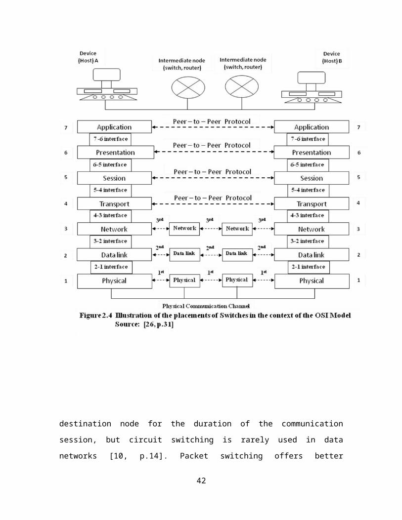
of the Open System Interconnection (OSI) model – the physical layer and the data-link

layer [11, p.55] and is shown in relation to the IEEE family of protocols in Figure 2.1.

The manner in which the nodes of a network are geometrically arranged and connected is

known as the topology of the network and local area networks are commonly

characterized in terms of their topology [11, p.146]. The topology of a network defines

the logical and /or physical configuration of the network components [10, p.50]; it is a

graphical description of the arrangement of different network components and their

interconnections [3].

13

Figure 2.1 IEEE family of protocols with respect to ISO OSI model layers 1 and 2 Adapted from: [11, p.55]

14

Upper Layer

Data Link Layer

Physical Layer

Upper Layers

Logic Link Control (LLC)

802.3 MAC e.g Ethernet MAC

802.4 MAC e.g Token Bus MAC

802.5 MAC e.g. Token Ring MAC

802.6 MAC e.g. MANs MAC ...

Ethernet Physical Layer (Several)

Token Bus Physical Layer

Token Ring Physical Layer

MAN Physical Layer ...

Scope of IEEE 802

Medium Access Control (MAC)

Transmission Medium Transmission Medium

IEEE StandardOSI Model

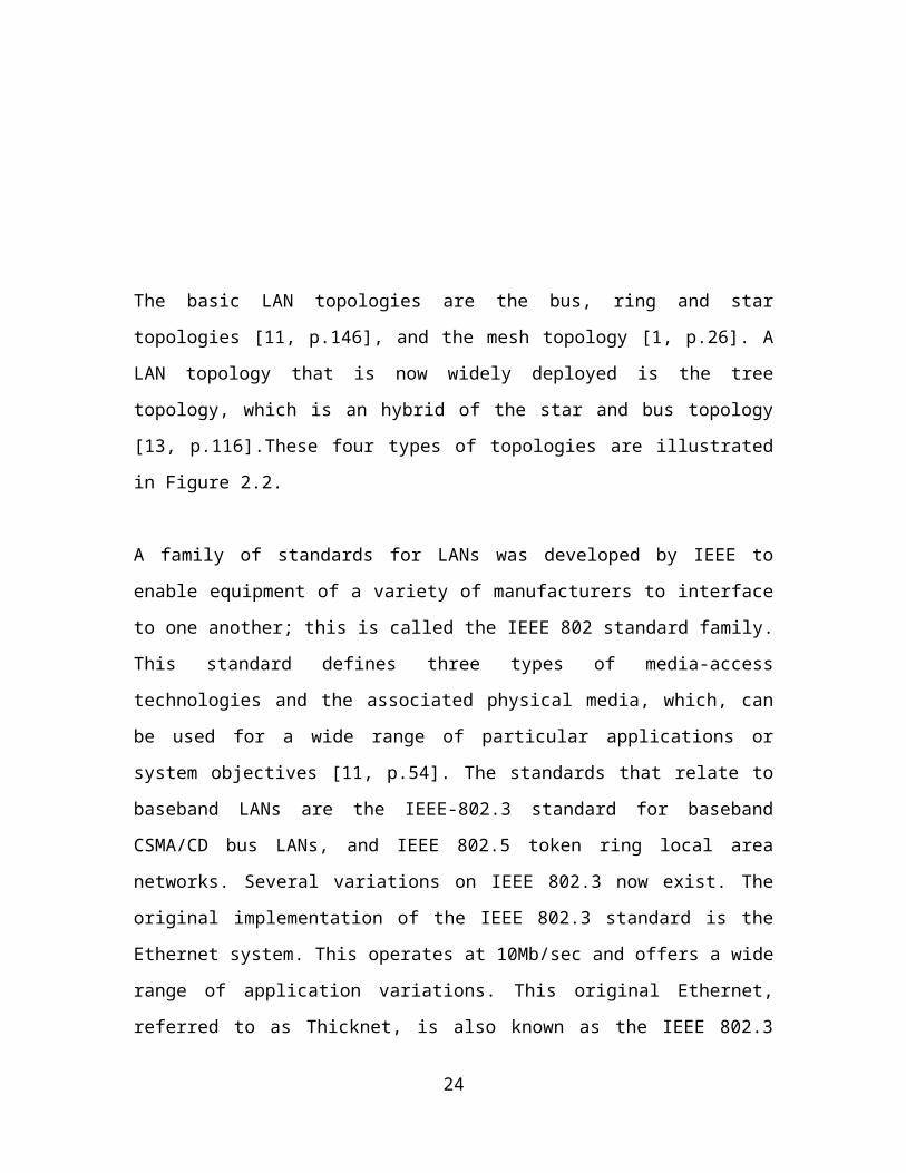
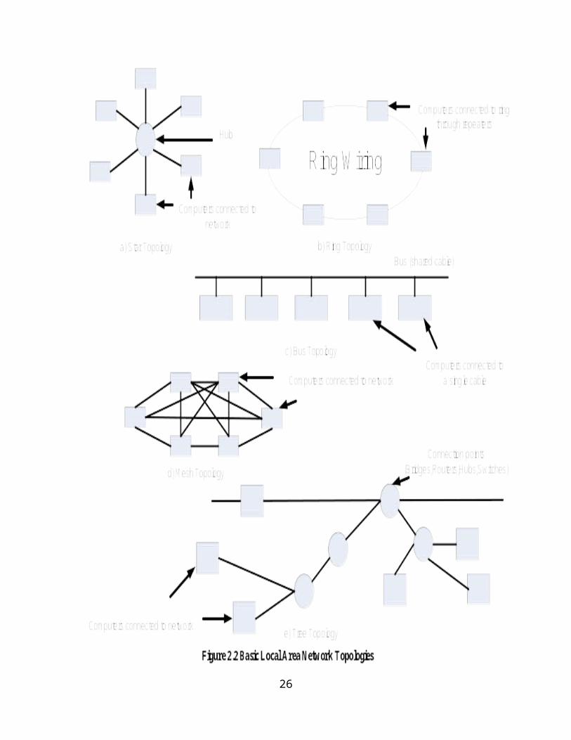
The basic LAN topologies are the bus, ring and star topologies [11, p.146], and the mesh

topology [1, p.26]. A LAN topology that is now widely deployed is the tree topology,

which is an hybrid of the star and bus topology [13, p.116].These four types of topologies

are illustrated in Figure 2.2.

A family of standards for LANs was developed by IEEE to enable equipment of a variety

of manufacturers to interface to one another; this is called the IEEE 802 standard family.

This standard defines three types of media-access technologies and the associated

physical media, which, can be used for a wide range of particular applications or system

objectives [11, p.54]. The standards that relate to baseband LANs are the IEEE-802.3

standard for baseband CSMA/CD bus LANs, and IEEE 802.5 token ring local area

networks. Several variations on IEEE 802.3 now exist. The original implementation of

the IEEE 802.3 standard is the Ethernet system. This operates at 10Mb/sec and offers a

wide range of application variations. This original Ethernet, referred to as Thicknet, is

also known as the IEEE 802.3 Type 10-Base-5 standard. A more limited abbreviated

version of the original Ethernet is known as Thinnet or Cheapernet or IEEE 802.3 Type

10-Base-2 standard. Thinnet also operates at 10Mb/sec, but uses a thinner, less expensive

coaxial cable for interconnecting stations such as personal computers and workstations. A

third variation originated from Star LAN, which was developed by AT&T, and, uses,

unshielded twisted-pair cable, which is often already installed in office buildings for

telephone lines [11, p.364], [36, p.220], and the first version was formally known as

IEEE 802.3 Type 10-Base-T. There has been other versions of the twisted pair Ethernet –

Fast Ethernet (100-Base-T or IEEE 802.3u), Gigabit Ethernet (1000-Base-T or IEEE

802.3z). Instead of a shared medium, twisted pair Ethernet wiring scheme uses an

electronic device known as a hub in place of a shared cable. Electronic components in the

hub emulate a physical cable, making the entire system operate like a conventional

Ethernet, as the collisions now takes place inside the hub rather than the connecting

cables [35, p.149].

Ethernet, in its original implementation, is a branching broadcast communication system

for carrying data packets among locally distributed computing stations. The thicknet,

15

16

thinnet and hub-based twisted-pair Ethernet are all shared-medium networks [6]. That is,

traditional Ethernet (which these three types of Ethernet represents), in which all hosts

compete for the same bandwidth is called shared Ethernet.

The use of Carrier Sense Multiple Access with Collision Detection (CSMA/CD) protocol

that controls access of all the interconnected stations to the common shared medium

results in a non deterministic access delay, since after every collision, a station waits a

random delay before it retransmits [18]. The probability of collision depends on the

number of stations in a collision domain and the network load [6], [27]. Moreover, the

number of stations attached to a shared-medium Ethernet LAN cannot be increased

indefinitely; as eventually, the traffic generated by the stations will approach the limit of

the shared transmission medium [37, p.433]. One traditional way to decrease the collision

probability is to reduce the size of the collision domain by forming micro-segments

separated by bridges [6]. This is where switches come in, as functionally, switches can be

considered as multi-port bridges [6], [38].

A Switched Ethernet is an Ethernet/802.3 LAN that uses switches to connect individual

nodes or segments. On switched Ethernet networks where nodes are directly connected to

switches with full-duplex links, the communications become point-to-point. That is, a

switched Ethernet/802.3 LAN isolates network traffic between sending and receiving

nodes. In this configuration, switches break up collision domains into small groups of

devices, effectively reducing the number of collisions [6], [27]. Furthermore, with micro-

segmentation with full-duplex links, each device is isolated in its own segment in full-

duplex mode and has the entire port throughput for its own use; collisions are, therefore,

eliminated [32]. The CSMA/CD protocol does not therefore, play any role in switched

Ethernet networks [20, p.102]. The collision problem is thus shifted to congestion in

switches [2], [6], [27]. This is, because, switched Ethernet transforms traditional

Ethernet/802.3 LAN from broadcast technology to a point-to-point technology. The

congestion in such switches is a function of their loading (number of hosts connected)

[27]; in fact, loading increases as more people log on to a network [8], and congestion

occurs when the users of the network collectively demand more resources than the

17

network can offer [10, p.27]. The performance of switched Ethernet networks should

therefore, be evaluated by analyzing the congestion in switches [3], [27]. In other words,

the delay performance of switched Ethernet local area networks can be evaluated by

analyzing the congestion in switches. This is one of the research directions that was

pursued in this work. We sought to establish deterministic bounds for the end-to-end

delays that are inherent in switched Ethernet local area networks by evaluating the

congestion in switches. Trulove in [23, p.143] made this point very succinct when he

stated that ‘LAN switching has done much to overcome the limitations of shared LANs’.

However, despite the vast increase in bandwidth provision per user that this represents

over and above a shared LAN scenario, there is still contention in the network leading to

unacceptable delay characteristics. For example, multiple users connected to a switch

may demand file transfers from several servers connected via 100 Mb/sec Fast Ethernet

to the backbone. Each Server may send a burst of packets that temporarily overwhelms

the Fast Ethernet uplink to the wiring closet. A queue will form in the backbone switch

that is driving this link, and any voice or video packet being sent to the same wiring

closet will have to wait their turn behind the data packets in this queue. The resultant

delays will compromise the perceived quality of the voice or video transmission.

2.4 Delays in Computer Networks

One fundamental characteristics of a packet-switched network is the delay required to

deliver a packet from a source to a destination [18]. Each packet generated by a source is

routed to the destination via a sequence of intermediate nodes; the end-to-end delay is

thus the sum of the delays experienced at each hop on the way to the destination [18].

Each such delay in turn consists of two components [17], [18], [10, p.150];

- a fixed component which includes:

i. the transmission delay at the node,

ii. the propagation delay on the link to the next node,

- a variable component which includes:

i. the processing delay at the node,

ii. the queuing delay at the node.

18

Transmission delay is the time required to transmit a packet [11, p.110], it is the time

between when the first bit and the last bit are transmitted [10, p.150]. For example, a 100

kb/sec transmitter needs 0.1seconds to send out a 10,000 bit message block [11, p.110].

For an Ethernet packet switch, the transmission delay will be a function of the output

ports’ (and hence on the attached lines) bit rates.

Propagation delay is the time between when the last bit is transmitted at the head node of

a link and the time when the last bit is received at the tail node [10, p.150], it is the time

needed for a transmitted bit to reach the destination station [11, p.110]. This time depends

on the physical distance between transmitter and receiver, on the physical characteristics

of the link, and is independent on the traffic carried by the link [10, p.150], [11, p.110].

Processing delay is the time required for nodal equipment to perform the necessary

processing and switching [35, p.244] of data (packets in packet switched networks) at a

node [11, p.110], [10, p.150]. Included here are error detection and address recognition,

and transfer of packet to the output queue [11, p.110]. The processing delay is

independent of the amount of traffic arriving at a node if computation power is not a

limiting resource, otherwise, in queuing models of nodes, a separate processing queue

must be included [10, p.150].

Queuing delay is the time between when the packet is assigned to a queue for

transmission and when it starts being transmitted; during this time, the packet waits while

other packets in the transmission queue are transmitted [10, p.150]. The queuing delay

has the most adverse effect on packet delay in a switched network. According to Song

[6], in a fully switched Ethernet, there is only one equipment (station or switch) per

switch port; and in case wire speed, full-duplex switches are used, the end-to-end delay

can be minimized by decreasing at maximum, the message buffering (queuing); as any

frame traveling through the switches in its path from origin to destination without

experiencing any buffering (queuing) has the minimum end-to-end delay. Queuing delay

builds up at the output port of a switch because, the port may receive packet from several

input ports; that is, packets from several input ports that arrive simultaneously may be

19

destined for the same output port [20, p.121]. If input and output links are of equal speed,

and if only one input link feeds an output link, then a packet arriving at the input will

never find another packet in service and hence, will not experience queuing delay.

Message buffering occurs whenever the output port cannot forward all input messages at

a time and this corresponds to burst traffic arrival; the analysis of buffering delay

therefore, depends on a knowledge of the input traffic patterns [6], [40]. According to

Anurag, Manjunath and Kuri in [20, p.538], the queuing delay and the loss probabilities

in the input or output queue of input queued or output queued switches are important

performance measures for a switch and are functions of:

- switching capacity,

- packet buffer sizes, and

- the packet arrival process.

Two other types of delays identified by [11 p.240] are the waiting time at the buffers

associated with the source and destination stations and the processing delays at these

stations; this was called thinking time in [32]. But these are usually not part of end-to-end

delay (see previous definition of end-to-end delay), since in a way, by simply having

hosts of high buffer and processing capacities, delays associated with the host stations

can be minimized. Moreover, the capacities of host stations are not part of the factors that

are put into consideration when engineering local area networks. As argued by Costa,

Netto and Pereira in [34], the message processing time consumed in source and

destination hosts is not included in the calculation of end-to-end delay because these

times are not directly related to the physical conditions of the network. Access delays

occur when a number of hosts share a medium, and hence may wait in turns to use the

medium [35, p.244]; but this delay does not apply to switched networks.

While propagation and switching delays are often negligible, queuing delay is not [10

p.15], [39], [27]; propagation delay is in general, small compared to queuing and

transmission delays [13, p.90]. Inter-nodal propagation delay is negligible for local area

networks [13, p.247], [11, p.110]; propagation delays are neglected in delay computation

20

even in wide area networks because of its negligibility [10, p.15]. We therefore,

neglected propagation delays in our end-to-end delay computation in this work.

2.4.1 End-To-End Delay in Switched Ethernet Local Area Networks

Ethernet was originally designed to function as a physical bus, but nowadays, almost all

Ethernet installations consist of physical star. Tree local area networks can be seen as

multi-level star local area networks [11, p.372], [30, p.254]. A tree is a connected graph

that has no cycles [41, p.43], [42, p.131], while a graph is a mathematical structure

consisting of two finite sets V and E. The elements of V are called the vertices (or nodes)

and the elements of E are called edges; with each edge having a set of one or two vertices

associated with it, which are called its end points [3], [41, p.2], [42, p.123]. In the context

of switched computer networks, a graph consists of transmission lines (links)

interconnected by nodes (switches) [2], [3], [37, p.234]. The operational part of a

switched Ethernet network and a large number of Asynchronous Transfer Mode (ATM)

networks configurations are examples of networks with tree topology, since in a tree

topology, there is a single path between all pair of nodes [13, p. 50]. Tree networks

therefore, are networks with unique communication paths between any two nodes, with

packets from source nodes traveling along predetermined fixed routes to reach the

destination nodes [3]. But the throughput (and hence the delay) of an Ethernet LAN is a

function of the workload [38], and the workload depends on the number of stations

connected to the network [6]. But the end-to-end delays of switched Ethernet LANs

depend on the number of level of switches below the root node (switch) and on the

number of end nodes (hosts) [28]. But Falaki and Sorensen [8], Abiona [4] have argued

that the loading on a network increases as the number of people logged on to the network

increases; and this leads to an increase in end-to-end delay [2], [3], [28]. Also, Jasperneite

and Ifak [32] have listed the system parameters that affect the real-time capabilities (that

is, the ability to operate within a specified end-to-end delay limit) of switched Ethernet

networks as among others, the following:

1. Number of stations, N,

2. The stations communication profiles,

3. The number of switches, K,

21

4. Link capacity, C (10, 100, 1000, 10,000) Mb/sec,

5. Packet scheduling strategy of the transit system (switches) and the stations,

6. The thinking time (TTH), within stations (the thinking time comprises the

processing time for communications request within the stations).

The traffic accepted into a network will experience an average delay per packet that will

depend on the routes taken by the packets [10, p.366]. The minimum average network

delay is the average delay between all pairs of users in the network [9]. We will use this

idea to calculate the maximum average network delay in this work.

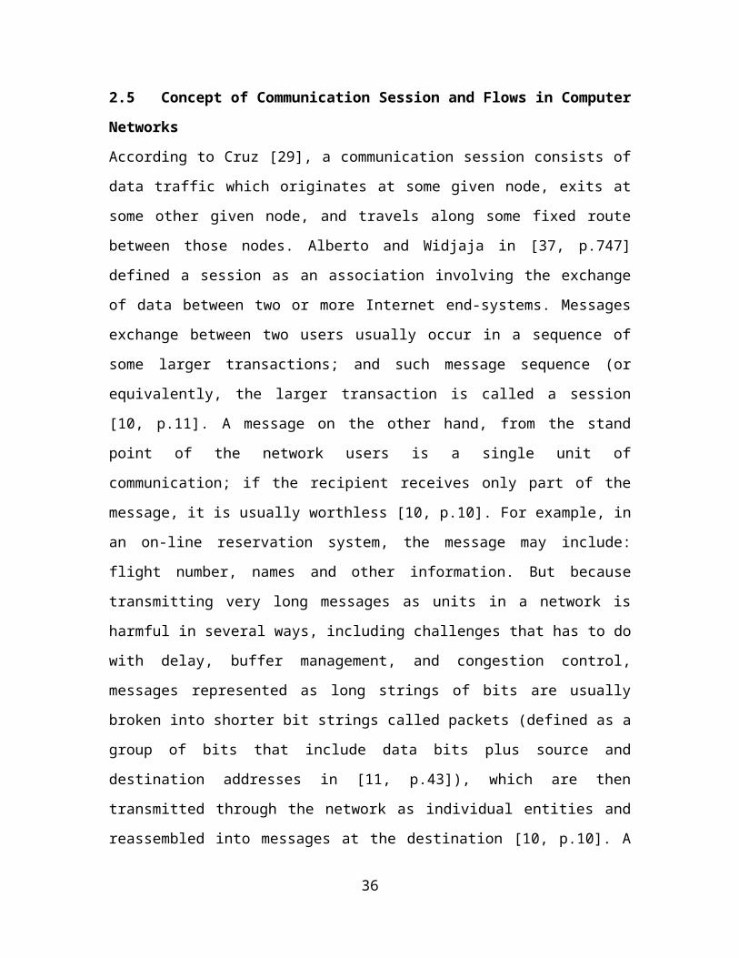
2.5 Concept of Communication Session and Flows in Computer Networks

According to Cruz [29], a communication session consists of data traffic which originates

at some given node, exits at some other given node, and travels along some fixed route

between those nodes. Alberto and Widjaja in [37, p.747] defined a session as an

association involving the exchange of data between two or more Internet end-systems.

Messages exchange between two users usually occur in a sequence of some larger

transactions; and such message sequence (or equivalently, the larger transaction is called

a session [10, p.11]. A message on the other hand, from the stand point of the network

users is a single unit of communication; if the recipient receives only part of the message,

it is usually worthless [10, p.10]. For example, in an on-line reservation system, the

message may include: flight number, names and other information. But because

transmitting very long messages as units in a network is harmful in several ways,

including challenges that has to do with delay, buffer management, and congestion

control, messages represented as long strings of bits are usually broken into shorter bit

strings called packets (defined as a group of bits that include data bits plus source and

destination addresses in [11, p.43]), which are then transmitted through the network as

individual entities and reassembled into messages at the destination [10, p.10]. A traffic

stream therefore, consists of a collection of packets that can be of variable length [15].

Bertsekas and Gallager [10, p.12], therefore, contends that a network exists to provide

communication for a varying set of sessions and within each session, messages of some

22

random length distribution arrive at random times according to some random process.

They further listed the following as the gross characteristics of sessions:

1. Message arrival rate and variability of arrivals; typical arrival rates for sessions

vary from zero to more than enough to saturate the network. Simple models for

the variability of arrivals include; Poisson arrivals, deterministic arrivals, and

uniformly distributed arrivals.

2. Session holding time; sometimes (as with electronic mail), a session is initiated

for a single message, while other sessions may last for a working day or even

permanently [20, p.45].

3. Expected message length and distribution; typical message length vary roughly

from a few bits to a few gigabits, with long file and graphics transfer at the high

end. Simple models for length distribution include an exponentially decaying

probability density, a uniform probability density between some minimum and

maximum, and fixed length.

4. Allowable delay; there may be some maximum allowable delay, and delay is

sometimes of interest on a message basis, and sometimes in the flow model, on a

bit basis.

5. Reliability; for some applications, all messages must be delivered error free.

6. Message and Packet ordering; the packets within a message must either be

maintained in the correct order going through the network, or restored to the

correct order at some point.

With respect to traffic modeling considerations in order to determine end-to-end packet

delay, items 1 to 4 are usually the main issues for consideration. Cruz in [15], [29]

referred to a communication session as a flow. In computer communication networks,

flows can represent either the total amount of information, or the rate of information flow

between any two nodes of a network [2], [3]. Specifically in a LAN, routers and switches

direct traffic by forwarding data packets between nodes (hosts) according to a routing

scheme; edge nodes (hosts) connected directly to routers or switches are called origin or

destination nodes (hosts) [43]. An edge node (host) is usually both an origin and a

23

destination, depending on the direction of the traffic; the set of traffic between all pairs of

origins and destinations is conventionally called a traffic matrix [43], [9].

2.6 Switching in Computer Networks

A switch can be defined as a device that sits at the junction of two or more links and

moves the flow unit between them to allow the sharing of these links among a large

number of users; a switch makes it possible to replace transmission links with a device

that can switch flow between the links [20, p.34]. In summary, a switch forwards or

switch flows. Other functions of a switch may include; the exchange of information about

the network and switch conditions, the calculation of routes to different destinations in

the network [20, p.35]. Figure 2.3 shows a block diagram view of a switch.

In a LAN, switches direct traffic by forwarding data packets between nodes according to

a routing scheme [43]. The concept of switching or Medium Access Control (MAC)

bridging was introduced in standard IEEE 802.1 in 1993, and expanded in 1998 by the

definition of additional capabilities in bridged LANs; the aim is to provide additional

capabilities so as to support the transmission of time critical information in a LAN

environment [44], [32]. A switched network, therefore, consists of a series of inter-linked

nodes called switches; switches are devices capable of creating temporary connections

between two or more devices linked to the switch [26, p.213]. Switches operate in the

first three layers of the OSI reference model. While a local area network switch is

essentially a layer 2 entity, there are now layer 3 switches that function in the network

layer (they perform the functions of routers outside the 802 network cloud). Figure 2.4

illustrates the placement of switches in the context of the OSI reference model.

Two approaches exist for transmitting traffic for various sessions within a subnet: circuit

switching and store-and-forward switching [10, p.14]. There are also two different types

of switches with respect to communication networks: circuit switches and packet

switches. While circuit switches are used in circuit multiplexed networks, packet

switches are used in packet multiplexed networks [20, p.34], [37, p.234]. In circuit

switching, a path is created from the transmitting node through the network to the

24

25

26

destination node for the duration of the communication session, but circuit switching is

rarely used in data networks [10, p.14]. Packet switching offers better bandwidth sharing

and is less costly to implement than circuit switching [17].

A packet is a variable length block of information up to some specified maximum size

[37, p.14]; it is a self-contained parcel of data sent across a computer network, with each

packet containing a header that identifies the sender and recipient, and a payload area that

contains the data being sent [35, p.666]. User messages that do not fit into a single packet

are segmented and transmitted using multiple packets and are transferred from packet

switch to packet switch until they are delivered at the destination [37, p.15]. A packet

switch performs essentially two main functions: routing and forwarding [37, p.511].

Packet switching, therefore, is an offshoot of message switching in which an entire

message hop from node to node; at each node, the entire message is received, inspected

for errors, and temporarily stored in secondary storage until a link to the next node is

available [11, p.114], [10, p.16]; and they are both called store and forward switching in

which no communication path is created for a session [11, p.114], [10, p.16]. Rather,

when a packet (or message) arrives at a switching node on its path to the destination

node, it waits in a queue for its turn to be transmitted on the next link in its path (usually,

a packet or message is transmitted on the next link using the full transmission rate of the

link) [10, p.16]. Packet switching essentially overcomes the long transmission delays

inherent in transmitting entire messages from hop to hop [11, p.115] and was pioneered

by the ARPANET (Advanced Research Project Agency Network) experiment [14].

Virtual circuit-switching (routing) is store-and-forward switching in which a particular

path is set up when a session is initiated and maintained during the life of the session.

This is like circuit switching in the sense of using a fixed path; but it is virtual in the

sense that, the capacity of each link is shared by the sessions using that link on a demand

basis rather than by fixed allocations [10, p.16]. Dynamic routing (or datagram routing) is

store-and-forward switching in which each packet finds its own path through the network

according to the current information available at the nodes visited; virtual circuit routing

is generally used in practice in data networks [10, p.17].

27

Reiser in [14] put the packet-switching concepts more succinctly when he averred that,

the basic packet-switching protocol entails the following:

- messages are broken into packets,

- to each packet is added a header which contains among other information, the

destination address,

- at each intermediate node, a table look-up is made which yields the address of the

link next on the packet’s route, and

- at the destination, the message is reassembled and routed to the receiving process.

Routes are defined by entries in the node’s routing table. Protocols differ by the way

these tables are maintained. The simplest case is one of fixed routes, with the possibility

of back-up routes to be used in case of link or node failures. More elaborate schemes try

to adapt routes to changes in the traffic pattern, with the optimization of some cost

measures in mind; a well known example of an adaptive protocol is the ARPANET

routing algorithm [14]. The Ethernet switch like the router, the bridge, and the cell switch

in ATM networks is a packet switch [20, p.35], [37, p.433]. A packet switching network

therefore, is any communication network that accepts and delivers individual packets of

information [35, p.666]. Therefore, switched Ethernet networks have the following

attributes:

- they are switched networks,

- they have collision-free communication links,

- they operate in packet-switched mode,

- they have a fixed routing strategy (because of the spanning tree algorithm that are

employed in these networks).

2.6.1 Classification of Packet Switches according to Switching Structure (Switching Fabric)

To model a packet switch, the switching structure (fabric) implemented in the switch

must be known and reflected in the model. The switching fabric of a switch is the

element of the switch which controls the port to which each packet is forwarded [20,

p.596].

28

Common elementary switching structures (fabric) that can be used to build small- and

medium-capacity switches having a small number of ports are: the shared-medium

(single bus) switching fabric, the shared memory switching fabric, and the cross-bar

switching fabric [20, p.597], [27], [6]. These switching fabrics results in shared-medium

switches, shared memory switches and cross-bar switches. A brief description of these

three types of switches (explained in [20, p.597- 599]) is now presented so that the reason

for the choice of the switching fabric that is adopted in this work will be clear.

i. The Shared-Medium Switches

This type of switch has a switching fabric that is based on a broadcast bus (much like the

bus in bus-based Ethernet LANs, except that the bus spans a very small area – usually a

small chip or at most the backplane of the switching system). This is illustrated in Figure

2.5. The input interfaces write to and read from the bus. At any time, only one device can

write to the bus. Hence, there is the need for a bus control logic to arbitrate access to the

bus.

The input interface extracts the packet from the input link, performs a route look-up

(either through the forwarding table stored in its cache or by consulting a central

processor), inserts a header on the packet to identify its output port and service class, and

then transmits the packet on the shared medium. Only the target output(s) read the packet

from the bus and place it on the output queue. A shared-medium switch is, therefore, an

output – queued switch with all the attendant advantages and limitations. According to

Anurag, Manjunath and Kuri in [20, p.599], a large number of low-capacity packet

switches in the Internet are based on the shared-medium switch over the backplane bus of

a computer. Multicasting and broadcasting are very straight forward in this switch.

The transfer rate on the bus must be greater than the sum of the input link rates (a high

input link rates sum implies a wider bus or more number of bits) which is difficult to

implement and is, therefore, a disadvantage [20, p.599]. The shared-medium switch also

requires that the maximum memory transfer rate be at least equal to the sum of the

29

transmission rates of the input links and the transmission rates of the corresponding

outputs.

30

ii. The Crossbar Switches

These are also known as space division switches. An NxN crossbar has N2 cross-points at

the junctions of the input and output lines, and each junction has a cross-point switch. A

4x4 crossbar switch is shown in Figure 2.6. If there is an output conflict in a crossbar

packet switch, only one of the packets is transferred to the destination. Thus, the basic

crossbar switch is an input-queued switch, with queues maintained at the inputs and the

cross-points activated such that at any time, one output is receiving packets from only

one input. It is also not necessary that the input be connected to only one output at any

time, as depending on the electrical characteristics of the input interface, up to N-outputs

can be connected to an input at the same time; thus, performing a multicast and broadcast

is straight forward in a crossbar switch.

iii. The Shared-Memory Switches

The shared-memory switching fabric is shown in Figure 2.7. In its most basic form, it

consists of a dual-ported memory; a write port for writing by the input interfaces and a

read port for reading by the output interfaces. The input interface extracts the packet from

the input link and determines the output port for the packets by consulting a forwarding

table. The information is used by the memory controller to control the location where the

packet is enqueued in the shared memory. The memory controller also determines the

location from which the output interfaces read their packets. Internally, the shared-

memory is organized into N-separate queues, one for each output port. It is not necessary

that the buffer for an output queue be from contiguous locations.

The following are two important attributes of shared-memory switching fabrics.

- The transfer rate of the memory should be at least twice the sum of the input line

rates.

31

- The memory controller should be able to process N input packets in one packet

arrival time to determine their destinations and hence their storage location in

memory.

32

It should be noted that while in a shared-medium switch, all the output queues are usually

separate, in a shared-memory switch, this need not be the case; that is, the total memory

in the switch need not be strictly partitioned among the N-outputs; the allocation is

dynamically done [6]. According to Song [6], the shared memory architecture is based on

rapid simultaneous multiple access by all ports and that in this situation, a packet entering

the switch is stored in memory, the packet forwarding is performed by an ASIC

(Application Specific Integrated Circuit) engine which looks up the destination MAC

address in the forwarding table, finds it and sends the packet to the appropriate output

port. Output buffering is used instead of input buffering, hence it avoids HOL (head-of-

line) blocking. Output overflow is minimized by using a shared-memory queuing, since

the buffer size is dynamically allocated; in fact all output buffers share the same global

memory, reducing thus, the buffer overflow compared to the per-port queuing [6]. The

shared-memory switching fabric is the most implemented in small packet switches that

are used in local area networks [27], [28]. We, therefore, in our maximum delay packet

switch model assumed a shared-memory switching fabric.

2.6.2 Packets/Frames Forwarding Methods in Switches

There are four packet forwarding methods that a switch can use: store-and-forward, cut-

through, fragment free, and adaptive switching [6]. In store-and-forward switching, the

switch buffers, and, typically performs checksum on each frame before forwarding it; in

other words, it waits until the entire packet is received before processing it [20, p.35]. A

cut-through switch reads only up to the frames hardware address before starting to

forward it. There is no error checking with this method. The transmission on the output

port could start before the entire packet is received on the input port. Cut-through

switches have very small latency, but they can forward malformed packets because the

CRC (Cyclic Redundancy Check) is calculated after forwarding [32]. The advantages of

cut-through switching are limited, and it is rarely implemented in practice [20, p.35].

33

Fragment free method of forwarding packets attempts to retain the benefits of both ‘store

and forward’ and ‘cut-through’ methods. This way, the frame always reaches its intended

destination. Adaptive switching is a method of automatically switching between the other

three modes.

34

2.7 Ethernet Technology and Standards for Local Area Networks

Ethernet is the most widely used LAN technology for the following reasons [40]:

- technology maturity,

- very low priced product,

- reliability and stability of technology,

- large bandwidths (10 Mbps, 100 Mbps, 1Gbps, 10 Gbps),

- deterministic network access delay (for switched Ethernet with full-duplex links),

- availability of priority handling features (IEEE 802.1p), which provides a basic

mechanism for supporting real-time communications,

- broadcast traffic isolation, scalability and enhanced security by configuring the

network in terms of VLAN (Virtual LAN),

- reliability improved by deploying Spanning Tree Protocol (STP) on redundant

paths,

- deployment facility with wireless LAN (WLAN), that is, IEEE 802.11 LAN,

- de facto standard supporting many widely spread upper stacks (IP and socket-

based UDP and TCP) for file transfer (FTP), remote login or virtual terminal

(telnet), network management (SNMP), Web-based access (HTTP), email

(SMTP), and allows the integration of many Commercial Off-The Shelf (COTS)

API and middle wares.

In addition, no special staff training is needed since almost all network engineers know

Ethernet and Internet related higher layer protocols very well. Importantly, approximately

85 percent of the world’s LAN-connected personal computers (PCs) and workstations use

Ethernet.

Therefore, switched Ethernet is more and more now being considered as an attractive

technology for supporting time-constrained communications [27], [28], [40]; and

currently, Ethernet is the most common underlying network technology that IP runs on

[37, p.586]

35

2.7.1 Ethernet Frame Formats

In the original Ethernet frame defined by Xerox, after the source’s MAC address, two

bytes (2 octets) follow to indicate to the receiver the correct layer 3 protocol to which the

packet belongs. For example, if the packet belongs to IP, then the type field value is

0×0800. The following list shows several common protocols and their associated type

values.

Protocol Hex Type Value

IP 0800

ARP 0806

Novel IPX 8137

Apple Talk 809B

Banyan Vines 0BAD

802.3 0000-05DC

Following the type value, the receiver expects to see additional protocol headers. For

example, if the value indicates that the packet is IP, the receiver expects to decode IP

headers next.

IEEE defined an alternative frame format. In this format, there is no type field, but packet

length follows the source address. A receiver recognizes that a packet follows 802.3

formats rather than Ethernet formats by the value of the 2-byte field following the source

MAC address. If the value falls within 0×0000 and 0×05DC (1500 decimal), the value

indicates length; protocol type values begin after 0×05DC. Figure 2.8 shows the extended

Ethernet frame format (with IEEE 802.1Q field).

36

2.7.2 IEEE 802 Standards for Local Area Networks

The following are the IEEE standards for local area networks:

- 802.1; this standard deals with interfacing the LAN protocols to higher layers; for

example, the 802.1s standard for Multiple Spanning Tree (MST) Protocol.

- 802.2; this is the data link control standard, very similar to HDLC (High-level

Data Link Control).

37

- 802.3; this is the medium access control (MAC) standard, referring to CSMA/CD

- system.

- 802.4; this is the medium access control (MAC) standard, referring to token bus

system.

- 802.5; this is the medium access control (MAC) standard, referring to token ring

system.

- 802.6; this is the medium access control (MAC) standard referring to Distributed

Queue Dual Bus (DQDB) system which is standardized for metropolitan area

networks (MANs). DQDB systems have a fixed frame length of 53 bytes and

hence, compatible with ATM.

The 802.3 standard is essentially the same as Ethernet, using unslotted persistent

CSMA/CD with binary exponential back-off [10, p.320]. There is also the FDDI (fiber

distributed data interface), which is a 100 Mbps token ring that uses fiber optics as the

transmission medium. Because of the high speed and relative insensitivity to physical

size, FDDI was planned to be used as backbone for slower LANs and for metropolitan

area networks (MANs). And then there is the IEEE 802.11 standard for WLAN (Wireless

Local Area Networks) also called WiFi (Wireless Fidelity). The IEEE 802.12 standard is

known as Demand Priority (100 VG –Any LAN) standard. There is also the IEEE 802.15

which is the standard for wireless personal area network (PAN); the PAN is a wireless

network that is located within a room or a hall. An example of the implementation of the

protocol defined by 802.15 is Bluetooth. Bluetooth is a wireless LAN technology which

was started as a project by the Ericsson Company, designed to connect devices of

different functions such as telephones, notebooks, computers (desktop and laptop),

cameras, printers and others. A Bluetooth LAN is an ad-hoc (formed spontaneously)

network. IEEE 802.16 standard is defined for wireless local-loop. It is also called

WiMax. There is the new IEEE 802.20 for Mobile Broadband Wireless Access

(MBWA).

2.7.3 Ethernet switches and the spanning tree algorithm

38

Ethernet switches are multi-port transparent bridges for interconnecting stations using

Ethernet links [37, p.466]. A bridge interconnects multiple LANs to form a bridged LAN

or extended LAN; while a bridge is termed transparent for the fact that, stations are

completely unaware of the presence of bridges in the network. Therefore, introducing a

bridge does not require the stations to be reconfigured.

The process in bridge learning (of a network it is connected to) works as long as the

network does not contain any loops – meaning that there is only one path between any

two LANs. In practice however, loops may be created accidentally or intentionally to

increase redundancy. Unfortunately, loops can be disastrous during the learning process,

as each frame from the flooding triggers the next flood of frames, eventually causing a

broadcast storm and bringing down the whole network.

To remove loops from a network, the IEEE 802.1 committee specified an algorithm

called the spanning tree algorithm. If we represent a network with a graph, a spanning

tree maintains the connectivity of the graph by including each node in the graph, but

removing all possible loops; this is done by automatically disabling certain bridges. It is

based on an algorithm invented by Radia Perlman while working for Digital Equipment

Corporation. The Spanning Tree Protocol (STP) is an OSI layer 2 protocol which ensures

a loop-free topology for any bridged LAN [45]. Ethernet switches support the Spanning

Tree Algorithm and Protocol (IEEE 802.1D Standard); a tree is called a spanning tree

since it connects (spans) all the end nodes in the network [2]. An extended version of the

IEEE 802.1D standard is the IEEE 802.1W or the rapid spanning tree protocol.

2.8 Modeling of Switched Local Area Networks

Models are set of rules or formulas which try to represent the behavior of a given

phenomenon [46]. A model is an abstraction of a system that, extracts out the important

items and their interactions [1, p.2]. Models provide a tool for users to define a system

and its problem in a concise fashion, they are general description of systems, are typically

developed based on theoretical laws and principles and are only as good as the

information put into them [1, p.2]. The basic notion is that, a model is a modeler’s

39

subjective view of the system; the view defines what is important, what the purpose is,

details, boundaries [1, p.3]. Modeling a system is easier and typically better, if [1, p.2]:

- physical laws are available that can be used to describe them,

- pictorial representation can be made to provide better understanding of the model,

- the system’s inputs, elements, and outputs are of manageable magnitude.

2.8.1 Elementary Network Components that were incorporated into the Packet Switch Model

This section discusses the elementary network components that were used for modeling

the packet switch and is based on the work of Cruz in [15].

i. The Constant Delay Line

The constant delay line is a network element with a single input stream and a single

output stream. The operation is defined by a single parameter D. All data which arrive in

the input stream exit on the output stream exactly D seconds later; that is, each packet is

delayed a fixed constant time before it is moved out. Thus, if Rin represents the rate of the

input stream, and Rout represents the rate of the output stream, then,

Rout (t) = Rin (t-D) for all t

The maximum delay of a delay line is obviously D. The delay line can be used to model

propagation delays in communication links. In addition, it can be used in conjunction

with other elements to model devices that do not process data instantaneously. The

constant delay line is illustrated in Figure 2.9.

The routing latency in a packet switch could be modeled by applying a burst-delay

service curve δT(t), which is equivalent to adding a constant delay T [27]. Figure 2.10a

40

41

shows the input and output curves of the guaranteed delay element, while Figure 2.10b

shows the curve of the burst-delay function.

ii. The Receiver Buffer

The receiver buffer is a network element with a single input stream and a single output

stream. The input stream arrives on a link with a finite transmission, rate, say C. The

42

output stream exits on a link with infinite transmission rate. The receiver buffer simply

outputs the data that arrives on the input link in First-Come-First-Served (FCFS) order.

The data packet exits the receive buffer instantaneously at the time instant when it is

completely transmitted to the receive buffer on the input link. That is, the receive buffer

does not output a packet until the last bit of the packet has been received; at which time,

it now outputs the packet. The receive buffer is employed to model situations in which

cut-through switching is not used; but, in which store-and-forward switching is used.

If Lk = length in bits of packet k that starts transmission on the input link at time Sk, then

tk = Sk + Lk /C for all k,

where, tk = time at which the kth packet starts exiting the receive buffer.

Obviously, the maximum delay of any data bit passing through this network element is

upper bounded by L/C, and the backlog in the receive buffer is obviously bounded by L.

The receiver buffer is a useful network element for modeling network nodes which must

completely receive a packet before the packet commences exit from the node. For

example, the receiver buffer is a convenient network modeling element in a data

communication network node that performs error correction on data packets before

placing them in a queue. In addition, the receive buffer is useful for devices in which the

input links have smaller transmission rates than the output links. The receive buffer is

illustrated in Figure 2.11.

43

iii. The First-Come-First-Served multiplexer (FCFS MUX)

The multiplexer (FCFS MUX) has two or more input links and a single output link. The

function of the FCFS MUX is to merge the streams arriving on the input links onto the

output link. That is, it multiplexes two or more input streams together onto a single

output stream. The output link has maximum transmission rate Cout and the input links

have maximum transmission rates Ci , i = 1,2,3,…,N. It is normally assumed that C i ≥ Cout

for i = 1, 2, 3,…,N. An illustration of the FCFS MUX is shown in Figure 2.12.

44

iv. First-In-First-Out (FIFO) Queue

The FIFO queue can be viewed as a degenerate form of FCFS multiplexer. The FIFO

queue has one input link and one output link. The input link has transmission capacity C in

and the output link has transmission capacity Cout. The FIFO is defined simply as follows.

Data that arrives on the input link is transmitted on the output link in FCFS order as soon

as possible at the transmission rate Cout. For example, if a packet begins to arrive at time t0

and if no backlog exists inside the FIFO at time t0, then the packet also commences

transmission on the output link at time t0. We assume that Cin ≥ Cout so that this is

possible. If Cin were less than Cout, then this would be impossible to do, as the FIFO

would ‘run out’ of data to transmit immediately following time t0 before the packet could

be transmitted at rate Cout.

Suppose that the rate of the input stream to the FIFO queue is given as Rin(t),

If the size of the backlog inside the FIFO queue at time t is given by WCout (Rin)(t); the jth

packet which arrives at time Sj must wait for all the current backlog and this backlog gets

transmitted at rate Cout. It follows that the jth packet commences exit from the FIFO queue

at time tj = Sj + dj, where,

(2.1)

= time spent by the jth packet in the FIFO queue before being transmitted at rate Cout.

The FIFO queue is illustrated in Figure 2.13. The following are Cruz’s [15] inputs and

outputs rates specifications for the network elements that were used in this work.

45

46

1. Receive Buffer: Input rate = Ci buffer

Output rate = Co buffer

Co buffer >> Ci buffer

2. Constant Delay Line: Input rate = Rin(t)DL

Output rate = Rout(t)DL

47

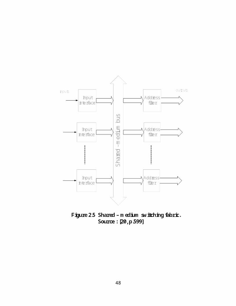
Rout(t)DL = Rin(t - D)DL

3. FCFS MUX: Input rate = Ci MUX, i = 1, 2,…., N

Output rate = Co MUX

Ci MUX ≥ Co MUX

4. FIFO Queue: Input rate = Ci QU

Output rate = Co QU

Ci QU ≥ Co QU

It is to be noted that all rates are in bits/sec

2.8.2 Approaches to Modeling Traffic Flows in Communication Networks: Network Calculus versus Traditional Queuing Theory

To determine the end-to-end response time of flows in communication networks, two

general approaches can be used: stochastic approaches or deterministic approaches.

Stochastic approaches consist in determining the mean behavior of the considered

network, leading to mean statistical or probabilistic end-to-end response times; while

deterministic approaches are based on a worst-case analysis of the network behavior,

leading to worst-case end-to-end response times [21], [27]. This is because, stochastic

processes are processes with events that can be described by probability functions; while

a deterministic process is a process whose behavior is certain and completely known.

Network calculus is a deterministic approach to modeling network entities and flows.

The advantages of the Network Calculus over the Traditional Queuing Theory can be put

in the following more compact form [44], [10, p.149], [14].

Network Calculus

1. Network calculus basically considers networks of service nodes and packets’

flows between the nodes.

2. Network calculus involves bounded constraints on packets arrivals and services.

48

3. These bounded constraints allow bounds on the packets’ delays and work

backlogs to be derived, which can be used to quantify real-time network behavior.

4. The packets arrival processes in network calculus are described with the aid of

arrival curves, which quantify constraints on the number of packets or the number

of bits of a packet flow in a time interval at a service node.

Traditional Queuing Theory

1. Traditional queuing theory deals with stochastic processes and probability

distributions.

2. Traditional queuing theory normally yields mean values and perhaps quantiles of

distributions.

3. The derivations of these mean values and quantiles of distributions are often

difficult.

4. Upper bounds on end-to-end delays may not exist or be computable.

Generally, the deterministic methodology which the network calculus represents

considers the worst case performance of the network and, therefore, yields conservative

results [20, p. 127]. Network calculus has traditionally been used for scheduling and

traffic regulation problems in order to improve Quality of Service (QoS); but it is now

more and more being used to study switched Ethernet networks (for example, [27], [28],

[44], [47]). Network calculus enables one to obtain upper-bounded delay for each of the

network elements proposed by Cruz in [15]; to obtain the maximum end-to-end delay of a

complete, switched communication system, we must, add the different upper bounded

delays [31]. Network calculus can be used to engineer Internet networks [44]. In end-to-

end deterministic network calculus approach, input processes are characterized via

envelops, network elements are characterized via service curves, and it is useful for the

engineering of networks if worst-case guarantees are required [20, p.252].

2.8.3 Network Traffic Modeling – the Arrival Curve approach

The delays experienced by packets of a given packet stream at a link or switch, depends

on the pattern of arrivals in the stream (arriving instants and the number of bits in the

49

arriving packets) and in the case of a link, on the way the link transmits packets from the

stream (the link may be shared in some way between two or more packet streams). To

analyze such situations, we use mathematical models that are variously called traffic

models, congestion models, or queuing models [20, p.120].

The modeling of network traffic is traditionally done using stochastic models [27], [10,

p.149]; for example, Bernoulli arrival process was assumed in [6]. But in order to

guarantee bounded end-to-end delay for any traffic flow, the traffic itself has to be

bounded [28]. This is where the arrival curve concept of traffic arrivals to a system is

important. In integrated service networks (ATM and other integrated service internet), the

concept of arrival curves is used to provide guarantees to data flows [48, p.7]. In this

approach (arrival curve), the traffic is unknown, but it is assumed that its arrival satisfies

a time constraint. Generally, this means that the quantity of data that has arrived before

time t will not be more than the arrival curve value at time t. The constraints are normally

specified by a regulation method; for example, the leaky bucket controller (regulation).

2.8.3.1 Leaky Bucket Controller

The arrival curve concept can be viewed as an abstraction of the regulation algorithm,

and the most common example of traffic regulation algorithm is the leaky bucket

algorithm, which has an arrival curve given by the following equation [49];

b(t) = σ + ρt for t > 0,

which means that no more than σ data units can be sent at once and the long-term rate is

ρ. The arrival curve, therefore, bounds traffic and denotes the largest amount of traffic

allowed to be sent in a given time interval [49], [10, p.512]. A leaky bucket controller

according to Le Boudec and Thiran [48, p.10] is a device that analyses the data on a flow

as follows. There is a pool (bucket) of fluid of size σ. The bucket is initially empty. The

bucket has a hole and leaks at a rate, ρ units of fluid per second when it is not empty.

Data from the flow R(t) has to pour into the bucket an amount of fluid equal to the

amount of data that will make the bucket to be full. Data that would cause the bucket to

overflow is declared as non-conformant (it would not pour into the bucket) otherwise, the

data is declared as conformant. The leaky bucket scheme is used to regulate the

50

burstiness of transmitted traffic [10, p.911]. Figure 2.14 illustrates the operation of the

leaky bucket regulator.

In ATM systems, non-conformant data is either discarded, tagged with low priority for

loss (“red” cells) or can be put in a buffer (buffered leaky bucket controller); with the

Integrated Services Internet, non-conformant data is in principle, not marked, but simply

passed as ‘best effort’ traffic (namely, normal IP traffic) [48, p.10]. A similar concept to

the leaky bucket concept is the token bucket controller. While the leaky bucket algorithm

shapes bursty traffic into fixed-rate traffic by averaging the data rate, the token bucket

algorithm allows bursty traffic at a regulated maximum rate [26, p.779].

2.8.3.2 Straight line Equation as an Affine arrival curve

It is a well known fact in elementary mathematics that y = mx represents a straight line

through the origin (y being on the vertical axis and x on the horizontal axis), with

gradient or slope m. y = mx + c is obtained by adding the value c to the y-coordinate at

every point of y = mx thus getting a line parallel to the original one; hence, it represents

a straight line with gradient m, with the value c most easily seen as the value of y

corresponding to x = 0.

We can see from Figure 2.15a that, y1 = c + Z1, y2 = c + Z2, and y3 = c + Z3; and that Z1,

Z2, and Z3 depends on the length of the intervals x1-x0, x2-x0, and x3-x0. Also, from Figure

2.15b, we can see that y = σ + ρt, where,

ρ = gradient of the straight line

=

51

52

2.8.3.3 Traffic Stream Characterization

In the network calculus approach for describing network traffic, a traffic stream (which is

a collection of packets that can be of variable length [15]) or flow is described by a wide-

sense increasing function r(t). The function r is wide-sense increasing if and only if r(s) ≤

r(t) for all s ≤ t. We represent a traffic stream as follows: for any t > 0,

53

is the amount of bits seen in the flow in the interval [0, t]. R(s) is

called the rate function of the traffic stream [48, p.4], [15]; it is the instantaneous rate of

traffic from the stream at time s. By convention, we take r(0) = 0 [48, p.4].

Also, in this traffic modeling approach, for any y ≥ x,

represents the amount of traffic seen in the flow in the time interval [x, y].

We note explicitly that the interval of integration is a closed interval.

2.8.4 Definition of Burstiness Constraint

Given ρ ≥ 0 and σ ≥ 0, we write R ~ (σ, ρ) if and only if for all x, y satisfying y ≥ x, there

holds;

(2.2)

Thus, if R ~ (σ, ρ), there is an upper bound on the amount of traffic contained in any

interval [x, y] that is equal to a constant σ plus a quantity that is proportional to the length

of the interval. The constant of proportionality ρ determines an upper bound to the long-

term average rate of traffic flow, if such an average rate exists. For a fixed value of ρ, the

term σ allows for some burstiness.

From (2.2), another interpretation of the constraint R ~ (σ, ρ) is that;

(2.3)

or

(2.4)

Therefore, a useful interpretation of the constraint R ~ (σ, ρ) is as follows [15]: for any

function R and a constant ρ > 0, define the function Wρ(R) for all times by Eq. (2.5).

, -∞ < t < ∞

(2.5)

54

Clearly, from (2.3) and (2.4), Wρ(R)(t) ≤ σ for all t if and only if R ~ (σ, ρ). Wρ(R)(t) is

the size of the backlog; that is, the amount of unfinished work at time t in a work-

conserving system which accepts data at a rate described by the rate function R and

transmits the data at rate ρ while there is data to be transmitted (work to be done).

2.8.4.1 Characterization of a Traffic Stream by Burstiness Constraint

The burstiness constraint for a given traffic stream characterizes the traffic stream in the

following way [15]. Given any positive number ρ, there exists a number σ (which is

possibly infinite) such that, if the traffic is fed to a server that works at rate ρ while there

is work to be done, the size of the backlog will never be larger than σ. σ is therefore, a

measure of the burstiness of the traffic entering a network; a large σ means the traffic is

very bursty [10, p.512]

Backlog means the average number of packets seen (waiting for service) by an arriving

packet to a queue. The backlog of a system is the amount of bits that are held inside the

system; if the system is a single buffer, the backlog is the queue length; if the system is

more complex, then the backlog is the number of bits in transit, assuming that we can

observe the input and output simultaneously [48, p.5].

2.8.4.2 Bursty Traffic and Network Delays

The class of message flows that satisfies the condition that, the amount of traffic in an

interval is upper bounded by an affine function of the length of the interval has been

found to be a useful class of models for traffic on internal links in networks that have to

handle bursty traffic [50], and bursty traffic is one of the causes of congestion in a

network [26, p.763]. Congestion in a network may occur if the load on the network (the

number of packets sent to the network) is greater than the capacity of the network (the

number of packets a network can handle) [26, p.763]. Fundamentally, congestion occurs

when the users of a network collectively demand more resources than the network

(including the destination sites) has to offer [10, p.27], and congestion leads to delays

[10, p.27]. Bursty traffic sessions, therefore, generally lead to large delays in networks

55

[10, p.511]; the delay suffered in a switch by an arriving packet increases as the

burstiness of the traffic going into the switch increases [28].

2.8.5 Graph Models in Switched Networks

To bring the power of mathematics on real-world problems, one must first model the

problem mathematically; graphs are remarkably versatile tools for modeling [41, p.7].

The topology of a network is a graphical representation of different network components

and their interconnections [2], [3]. As networks grow in size and complexity, more

powerful, yet flexible models are needed to capture the important aspects of network

topology. A network graph model is such an effective tool that can easily be applied to

several topology related analysis problems [2], [3]. A network consists of a graph of

transmission lines (links) interconnected by nodes (switches). In computer networks

where computing elements are interconnected by switching elements, switching elements

are regarded as nodes while computing elements are regarded as hosts. Figure 2.16a

illustrates a switch and 4 hosts and the equivalent graph model; while Figure 2.16b

illustrates 3 switches and 8 hosts and the equivalent graph model.

In switched Ethernet networks, traffic can often be regarded as a set of packet flows from

a group of source nodes to a group of destination nodes [3]. It is instructive to note that

the direction of a link in the graph model of a switched network is not related to the

direction of traffic flow across the link. In fact, all links are half-duplex or full duplex

Ethernet segments carrying traffic in both directions. One can think of the link direction

as a way of characterizing the hierarchical structure of the network. Starting from any

node in the graph, and following the link directions, we pass through switches of lower

and lower hierarchy until we reach a network end node [2], [3]. The delay times across a

network can be estimated by computing the delay time for each switch device as a

function of its offered load, and combining the delay times based on the graph model to

generate the end-to-end delay times. Assuming a store-and-forward operation for all

switches, the communication delay time between two end nodes is found by adding the

56

1 2 3 4 1 2 3 41 432 5 6 7 8

1 2 3 4 5 78

6

Figure 2.16a Illustration of 1-switch and 4-hosts and the equivalent graph model

Figure 2.16b Illustration of 3-switches and 8-hosts and the equivalent graph model

queuing time for the switches on the connecting path and the appropriate number of

transmission (forwarding) times [2], [17].

57

2.8.5.1 Network Graphs and the Spanning Tree Algorithm

A graph G which consists of a non-empty set V called a set of nodes or vertices or points,

a set E (which is a set of edges of the graph) and a mapping from a set of edges E to a set

of pairs of elements of V can be represented as [41, p.2], [42, p.123]:

G = (V, E)

(2.6)

An edge between two vertices creates a connection in two opposite directions at once;

assigning a direction makes one of these senses forward and the other backward [41, p.3].

In a line drawing, the choice of forward direction is indicated by placing an arrow on an

edge. Any two nodes which are connected by an edge of a graph are called adjacent

nodes. In a graph G = (V, E), an edge which is directed from one node to another is called

a directed edge. An edge which has no specific direction is called an undirected edge. A

graph in which all edges are directed is called a directed graph or digraph. A cycle in a

graph is a sequence of vertices v0, v1,…,vk such that vi-1 vi is an edge for i= 1, 2,…,k, the

first and last vertices are the same and no other vertices (or edges) are repeated [42,

p.142].

A graph in which every edge is undirected is called an undirected graph. An edge is said

to be incident on the nodes Vi and Vj. An edge of a graph which joins a node to itself is

called a loop. A graph which contains some parallel edges is called a multi-graph, while

that without parallel edges is called a simple graph. A simple digraph which does not

have any cycle is called acyclic [1], [41, p.74], [42, p.142].

An acyclic graph is called a forest [41, p.74]. A weighted graph is a graph in which each

edge is assigned a number called its edge weight [41, p.176]. In a directed graph, for any

node V, the number of edges which have V as their initial node is called the out-degree of

58

node V, the number of edges which have V as their terminal node is called the in-degree

of node V. The sum of the out-degree and the in-degree is called total degree. An isolated

node is any node in which the total degree is equal to zero. A null graph is any graph

having only isolated nodes. A graph G = (V, E) is a tree if G is connected and acyclic [42,

p.142], [10, p.388], [1]. A connected graph is one in which there exists a path between

every pair of vertices in the graph [41, p.74], [42, p.142].

A rooted tree is a tree in which one vertex is distinguished and called the root of the tree;

vertices immediately below a vertex V are called the children of V [42, p.143], [51,

p.302]. The node at the top of the tree is called the root and in some sense, the root is the

greatest element of the tree [51, p.300]. Vertices at the bottom of the tree (those with no

child or children) are called the leaves [42, p.143], [51, p.302]. Vertices other than the

root or the leaves are called internal vertices, and a null tree is a tree with no vertices [42,

p.143]. Trees combine the advantages of two other structures: ordered array and linked

list; for a collection of nodes and edges to be called a tree, there must be one (and only

one) path from the root node to any other node [51, p.300].

An m-ary tree (m ≥ 2) is a rooted tree in which every vertex has m or fewer children; a

complete m-aray tree is an m-ary tree in which every internal vertex has exactly m

children and all leaves have the same depth; for m = 2, we have a binary or complete

binary tree [41, p.127].

A spanning tree for a graph G is a tree constructed from the edges of G which includes all

the vertices of G [10, p.388], [42, p.143]. A minimum weight spanning tree (MST for

short) is a spanning tree with minimum sum of arc weights [10, p.390]. The minimal

spanning tree algorithm produces a spanning tree of minimal total weight in a weighted

connected graph [42, p.143].

A systematic visit (visiting in a specified order) of each vertex of a tree is called tree

transversal [41, p.132], [51, p.302], and this produces a global ordering of the vertices of

a tree [41, p.132]. Trees can be transversed pre-order, post-order, in-order [41, p.132],

59

[51, p.317], [52, p.230], and level-order [41, p.132]. While pre-order, post-order, and in-

order transversals are used for transversing binary trees, the last type of transversal (level-

order) can be used to transverse binary and non-binary trees [41, p.132]. The level-order

of an ordered tree is a listing of the vertices in the top-to-bottom, left-to-right order of a

standard plane drawing of the tree [41, p.132]. It should be noted that the tree diagrams

resulting from switched Ethernet LANs may not necessarily be binary.

In the context of switched networks, a directed graph (digraph) G = (V, E) is defined as a

set V of vertices or nodes, and a set E of directed links; each directed link is an ordered

pair of nodes (i, j), where i is called the source or initial node and j is called the sink or

terminal node [3]. A path P of length q is an ordered set of q distinct links P = (E 1, E2,

…,Eq) with E1 = (i0, i1), E2 = (i1, i2),…,Eq = (iq-1, iq). All links of a path are of the same

direction and each link Er has one common end-point with Er-1, and a second common

end-point with Er+1. Nodes i0 and iq are called the initial and terminal nodes, respectively.

A loop (also called circuit) is a special path with coinciding initial and final nodes. To

remove loops from a network, the IEEE 802.1 committee specified an algorithm called

the spanning tree algorithm [21, p.472]. If we represent a network with a graph, the

spanning tree maintains the connectivity of the graph by including each node in the

graph, but removing all possible loops [37, p.472].

Many switched networks, however, have the basic property that there is a unique

communication path between any two nodes of the operational part of the network,

therefore, it seems that a graph model of the operational network should not have a circuit

[3]. In switched Ethernet networks, paths are determined by the spanning tree algorithm;

therefore, the graph representing this class of networks are, trees, since they can have no

circuits [27]. We assume that the root of the tree is the top of the tree. An arc weight

represents the communication cost of a message along the arc in either direction, and the

total spanning tree weight represents the cost of broadcasting a message to all nodes

along the spanning tree [10, p.390].

2.9 Quality of Service (QoS) in Switched Ethernet Networks

60

Data communication using computer networks and the general Internet is today provided

by IP technology using a unique type of service called ‘Best Effort’. But with the

appearance of time-sensitive applications, and the more and more ubiquitous use of the

Internet as a working tool, congestion and uncertainties in delay and delay variation have

led to a degradation of the quality of response of applications [53]. Quality of Service

(QoS) is a generic term which takes into account several techniques and strategies that

could assure applications and users a predictable service from the network and other

components involved [53]. Enabling QoS on a network implies the definition of QoS and

the deployment of various mechanisms, including scheduling, control admission,

shaping, control on routing latency/performance and resource planning; all these

techniques are aimed at providing an end-to-end QoS for selected traffic [53]. Service

quality can be expressed as a combination of network-imposed delay, jitter, bandwidth

and reliability [16], [53]. QoS problem has two perspectives: network perspective and

application/user perspective [54]. Basically, two common possibilities exist in order to

guarantee a certain QoS as required by the users of a network: either, one can use

resource reservation or alternatively, one could rely on prioritization combined with

additional control. In the context of the Internet, the resource reservation approach is

reflected by, for example, the IntServ proposal and the prioritization approach is inherent

in the DiffServ [55].

QoS does not refer to achieved services; instead, it is the ability to guarantee a certain

level of performance to a data flow; for example, a required bit rate, delay, jitter, packet

dropping probability or bit error rate may be guaranteed [56]. It ensures some

performance in explicit application requirements – some resources such as channels and

memory are reserved [27]. An alternative and disputable definition of QoS used

especially in application layer services such as telephony and streaming video is a metric

that reflects or predicts the subjectively experienced quality, otherwise called ‘Quality of

Experience (QoE)’, ‘User Perceived Performance’, or ‘the degree of satisfaction of the

user’ [56].

61

The Ethernet protocol is an OSI model layer 2 protocol [27]. But in the layer 2 of the OSI

model, no quality of service (QoS) can be managed, only classification of service (CoS)

is available. However, the CoS mechanism only provides a better service for critical

applications, it does not explicitly guarantee that specific needs will be satisfied [27],

[57]. This is unlike the upper layers where there are transport protocols like the resource

reservation protocol (RSVP) which rely on the quality of service (QoS) functionality

implemented in routers [27]. The standard 802.1p is the IEEE standard (released in

September, 1998) that enables LAN switches and other devices (for example, bridges and

hubs) to prioritize traffic into one of eight classes [58]. According to Trulove in [23], the

802.1p is concerned with ‘Traffic Class Expediting’ in LAN switches. It is usually

associated with two other IEEE 802.1 specifications – 802.1D (spanning tree protocol)

and 802.1Q (VLAN tagging). The IEEE 802.1 Internetworking Task Force Group

developed a set of enhancements to the basic MAC services provided in a Bridged Local

Area network (switching in LAN). As a supplement to the original IEEE MAC Bridges

standard, IEEE.1D-1990 (802.1D-ORIGINAL), the updated IEEE 802.1D-1998 (802.1D)

proposes differentiated traffic class queuing in switches. The IEEE 802.1Q specification

extends the capabilities of Ethernet/802.3 media to carry a traffic class indicator or ‘user-

priority’ field within data frames. Class 7, the highest priority is reserved for network

control data such as Open Shortest Path First (OSPF) and Routing Information Protocol

(RIP) table updates. Classes 6 and 5 can be used for voice, video, and other delay

sensitive traffic. Classes 4 through 1 address streaming data applications and loss-tolerant

traffic such as File Transfer Protocol (FTP). Class 0, the default class is a ‘best-effort’

class. In conjunction with the 802.1Q specification for VLAN tagging, 802.1 paved the

way for standards-based multi-vendor grade of service (GoS) [58].

The scope of 802.1p is limited to a LAN. Once the packet crosses to a layer 3 device, the

802.1p tag is removed; but it can be mapped to a layer 3 equivalent information, for

example in the Type of Service (ToS) byte of the IP header [53]. Because of the eight

priority classes that are possible as a result of the 802.1p standard, LAN devices like

switches are expected to handle the traffic according to 802.1p priority by means of

appropriate queuing mechanisms. Traffic will be scheduled on aggregate; for example, all

62

video streams will be processed within a single queue. Problems, however, arise if there

are many streams to be handled within the same priority, especially when real-time

constraints are hard [57].

This problem can be better understood when we note how a switch operates in a switched

LAN under the 802.1p standard as enunciated by Trulove in [23]. In this context, the

LAN switch needs to implement a queue scheduling algorithm that gives preference to

the high priority queues on outgoing ports and by this means, it is hoped that real-time

voice and video can be carried over the LAN without incurring unacceptable delays

during periods of heavy data traffic. But this will not completely solve the packet delay

problem of switched LANs. For example, it does not address the situation where there

may be several contending packets of the same class all destined for the same output port

(as noted in [57]) and/or burst of frames can arrive before another frame, with both

arrivals destined for the same output port, but belonging to different traffic streams. This

delay problem can be seen from the fact that installed switched Ethernet LANs without

real-time applications deployment are very slow at most times of the day and are faster at

night. This was part of the problem we sought to solve in this work.

2.10 Methods of Studying Engineering Systems

A system can be defined as a collection of entities that act and interact together toward

the accomplishment of some logical end [59, p.3]. It is a unified group of objects united

to perform some set functions [1, p.3]. The different ways by which engineering systems

can be studied has been outlined by Law and Kelton in [59, p.4] as shown in Figure 2.17.

Once a mathematical model has been built for a system, it must then be experimented to

see how it can be used to answer the questions of interest about the system it is supposed

to represent [59, p.4]. If the model is simple enough, it may be possible to work with its

relationships and quantities to get an exact analytical solution. For example, if d = vt,

where d = distance (m), v = velocity (m/s) and t = time (seconds), then if we know the

distance to be traveled, and the velocity, we can work with the model d = vt to get t =

as the time required. This is a very simple, closed form solution obtainable with just

63

paper and pencil. However, many systems are highly complex, so that valid mathematical

models of them are themselves complex, precluding any possibility of an analytical

solution. In this case, the model must be studied by means of simulation, that is,

numerically exercising the model for the inputs in question to see how they affect the

output measures of performance [59, p.4]. We were guided by Figure 2.17 in developing

solutions to the problems of this research work.

64

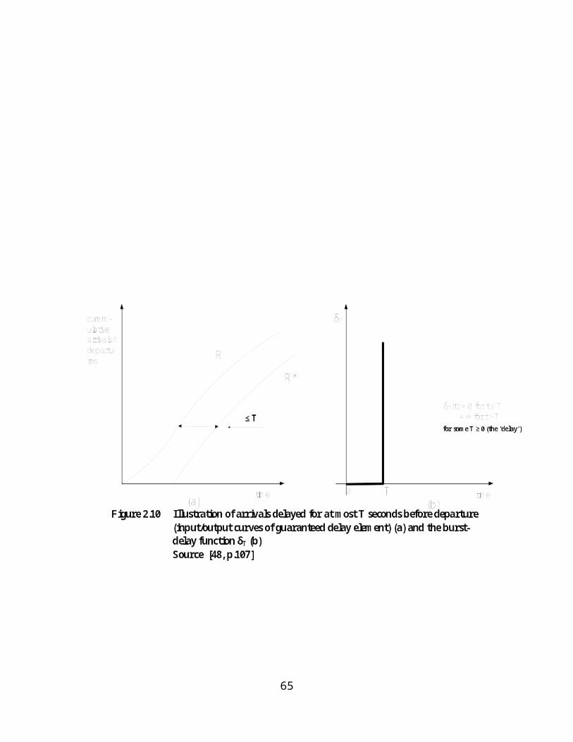
65

System

Experiment with actual system Experiment with a model of the system

Physical model Mathematical model

Analytical solution Simulation

Figure 2.17 Different Ways to Study an Engineering System [59, p. 4]

CHAPTER 3

MAXIMUM DELAY ETHERNET PACKET SWITCH MODEL DERIVATION

3.1 Introduction

To model a switched network, one must represent the behavior of the internal network

devices (the switches), their interconnections and the traffic supported by the

communication system [27]. In our attempt to model switched Ethernet local area

networks for the purpose of computing maximum end-to-end delays, network calculus

and graph-based approaches are adopted. This modeling direction is adopted in this work

for the following reasons. Firstly, the network calculus introduced by Cruz in [15] and

extended in [29] only assumes that the number of bytes sent on the network links does

not exceed an arrival curve (traditionally, the leaky bucket arrival curve [27], [20, p.179],

[48, p.10]) and the network calculus applied to switched networks, enables one to

determine the frames/packets maximum end-to-end delays; unlike common stochastic

approaches that assume Bernoulli, Poisson etc. arrival of packets which gives only

probabilistic estimation of the arrival of messages. Secondly, the network calculus would

enable us to model the Ethernet switch by assembling elementary components such as

multiplexers, constant delay lines, receive buffers whose temporal properties were

derived in [15].

3.2 Internal Structure of a Packet Switch from Delay Point of View

According to Song in [6], the total delay introduced by a switch is composed of the

following:

- the switching latency (traffic classification according to IEEE 802.1p mapping

table, DAD (destination address) look-up and switch set-up time),

- the frame forwarding latency, which depends on the forwarding mode and,

eventually, on the frame length, if the store-and-forward mode is used, and

- the buffering delay when the frame is queued.

In this partitioning of the total delay of a switch, it was explained that the switching

latency is a fixed value which depends on the switch performance, and is often provided

66

Switch

by the switch vendors (typically, about 10μs). This view is supported by Elbaum and Sidi

in [9], where they stated that the delay due to look-up, that is, the look-up time, can be

assumed to be fixed for any packet passing a bridge (we note that a packet switch is a

multi-port bridge). The forwarding delay can be obtained if the mode (for example, store-

and-forward) in which the switch is running is known. The buffering delay depends on a

knowledge of the input traffic pattern and a frame traveling through switches in its path

without experiencing any buffering has the minimum delay. This view can indeed aid one

to structurally partition (with respect to latency or delay) a switch into three components;

these are:

- the component responsible for incurring switching latency,

- the component responsible for incurring frame-forwarding latency, and

- the component responsible for incurring buffering delay.

In a fashion almost similar to [6], but in this case the attempt was on an actual structural

partitioning (partitioning based on actual positioning of the switch internal components),

Georges, Divourx, and Rondeau in [27], [28] decomposed the architecture of a switch

into three main components, these are: the queuing subsystem, the switching mechanism

implementation, and the switching fabric. While the queuing subsystem refers to the

buffering and congestion mechanisms located in the switch (congestion management is

required when multiple input ports contend for the same output port within the switch

[28]), the switching mechanism implementation refers to the decision-making process

within the switch (how and where a switching decision is made). The switching fabric on

its own is the path that data take to move from input ports to output ports. In order to be

able to calculate the maximum delay encountered by a packet in crossing an Ethernet

packet switch, the model in Figure 3.1 was proposed in [27], [28].

R1(t) is the arrival rate in bits/sec of traffic stream into port 1, while C in is an input port

rate in bits/sec. There is a multiplexer that merges the input streams (switches streams in

succession) in to a First-In-First-Out (FIFO) queue; then a demultiplexer separates the

traffic stream, which then moves into FIFO queues at the output ports of the switch. C is

the switch’s internal transfer rate; Cout is an output port rate, while R1*(t) is the departure

67

68

rate of traffic stream 1, all in bits/sec. The switch model of Figure 3.1 does not seem to

give a good functional decomposition of a packet switch.

Song [6] modeled the Ethernet packet switch as shown in Figure 3.2. This switch model

appears to have depicted more realistically, the actual operation of a packet switch than

the model in Figure 3.1. It has a CPU connected to input lines and feeding output ports

buffers that are connected to output lines. The CPU performs the scheduling and

switching of in-coming packets. The challenge with this model is ‘how does one model

mathematically, the CPU (including how it schedules and switches packets)’. Shown in

Figure 3.3 is another model of an Ethernet packet switch by Song et al. [40]. This is a

much better model of an Ethernet packet switch. It inherently reflects a better functional

decomposition of such a switch. It has input buffers for storing packets extracted from the

transmission medium, the switching subsystem for switching packets to output buffers

(these buffers are part of random access memory that are assigned to output ports) ready

to be placed on the transmission mediums that are attached to the output ports.

In our attempt to arrive at an appropriate functional decomposition (and hence modeling

paradigm) of a packet switch to be adopted in this work for calculating the maximum

delay of an Ethernet packet when crossing such a switch, we will look at the description

of a patented packet switch as reported in US Patent number 5889776 [60].

The switch is described as comprising of the following:

- a central processor

- a switching fabric consisting of the following:

i. a number of packet processing channels

ii. each channel has one buffer and media access controller (MAC)

- an N x N switch circuit

- a connectivity module or network interface

69

70

The following points were highlighted in relation to the operation of the switch.

- the operation of the switch system is controlled by the central processor,

71

- generally, a packet signal is processed in the MAC, so that only the data being

transmitted is retrieved,

- the buffer in the switch fabric provides a tentative holding place for the data to be

moved eventually to the designated destination specified in the data.

3.3 Packet Switch Functional and Structural Partitioning and Modeling

In our attempt to arrive at a maximum delay model of a packet switch and hence, an

equivalent mathematical expression, we need to consider very well how a packet switch

operates. Figure 3.4 is an illustration of the underlying concepts of a switch. Electronic

circuits in the switch provide each computer with the illusion of a separate LAN segment

connected to other LAN segments by bridges [35, p.120]. In this figure, it can be seen

that it is possible for a packet from any computer that is attached to port 1, a packet from

any computer that is attached to port 2, and a packet from any computer that is attached

to port 3 to arrive simultaneously or almost simultaneously and are all destined for port 4

(since switch ports are bidirectional and input/output paired). Then each of the packets 1,

2, and 3 say, will now be sent to any computer (a server machine for example) that is

attached to port 4 by the switching mechanism of the switch one after the other (this is

what is called congestion in switches [27], [6], [2]). Note that the first thing that is done

is to queue each of the packets in the output buffer of port 4 in either first-come-first-

served (FCFS) order, in the case when one packet header is detected before that of

another packet, or in the case where the headers of packets 1, 2, and 3 are detected

simultaneously, by using what is generally called ‘best effort’ scheduling or what Cruz in

[15] referred to as ‘ties are resolved arbitrarily’. It is obvious that one of the packets out

of packets 1, 2, and 3 will have to wait for the other two packets to be sent to the

computer that is attached to port 4 before it will be sent. This exposition is supported by

Song in [6] who argued that, in an N-port switch, all N-input ports (we think it should be

N-1 input ports, since a packet from a port cannot be destined for itself) may be

contending for the same output port. Therefore, it can be seen that the maximum delay

which this packet will incur in this switch will be a function of the maximum congestion

72

in the switch, and this maximum congestion will depend on the number of ports in the

switch. The more the packets in a queue that are met by an arriving packet, the longer,

73

will be the delay experienced by that packet. The queue of packets is called the backlog

and could be seen as the congestion value of the network component (switch); thus, the

upper bounded delay value for a component (switch) will depend on the maximum

backlog expression [27]. Song in [6] has also averred that, the buffering delay in a switch

when a frame (packet) is queued, depends on a knowledge, of the input traffic pattern and

that a frame traveling through switches in its path without experiencing any buffering has

the minimum delay. Our packet switch maximum delay model derivation will, therefore,

be done putting into consideration, these two obvious maximum congestion scenarios.

3.3.1 Functional Requirements for Delay Modeling of a Packet Switch

The main components of a packet switch as reported by different works are largely

similar (see for example [37, p.511], [20, p.537, p.35]. These are in addition to the views

on the functional decomposition of packet switches that we have previously described.

But the functional decomposition as presented by Anurag, Manjunath and Kuri in [20,

p.35] is more detailed and more illuminating. This is shown in Figure 3.5. In this

decomposition, a line interface extracts the packet from the input link by appropriately

identifying the boundaries of the bits and of the packets. An input processor then extracts

the header, and an associated forwarding engine performs a route look-up using the

header information by consulting a routing table to determine the output link. In a multi-

service network, the service type of the packet is also determined at this stage to

determine the type of service that the packet is to be provided. The type of service

determines the scheduling of the packet transmission on the output link and the drop

priority during periods of congestion. If it is possible to send the packet to the output port

immediately, it is queued and scheduled to be moved to the output port according to its

service type. The switch fabric next moves the packet to the output queue. An output

processor determines queue position and schedules its transmission on the output link.

Finally, the packet is transmitted on the output link by the output line interface. From the

74

Figure 3.5 The components of a packet switch Source: [20, p.35]

diagram, it can be seen that the control and signaling block interacts with all the other

packet processing blocks in the switch.

75

Since we are concerned with the modeling of a packet (Ethernet packet) switch in order

to be able to calculate the maximum delay incurred by an Ethernet packet when crossing

such a switch, we note that, Ethernet switches are simply multi-port transparent bridges

for interconnecting stations using Ethernet links; and in such switches, each input port

buffers incoming transmissions, the incoming frames are examined and transferred to the

appropriate output ports with each output port implementing the MAC protocol to

transmit frames [37, p.433]. But it has been argued in [28] that a switch model must

include the centralized arbitration notion of the switching fabric, so that the simultaneous

switching of two or more input ports to their output ports is possible.

Giving due consideration to our discussions and illustrations of the different views of the

functional decomposition of a packet switch, it can be deduced that there is a

commonality of opinions that can be aggregated in order to model such a switch, more

specifically, an Ethernet packet switch. A packet switch generally, therefore, has the

following functional components:

1. an input buffer where bit streams (packets) extracted from the transmission media

are stored,

2. a switching fabric; the switching fabric consists of a number of packet processing

channels which incurs frame routing latency,

3. a frame processing channel buffers which are associated with each output port,

which is also called the queuing subsystem that refers to the buffering and

congestion mechanisms that is located in the switch, and

4. the switching mechanism implementation; which refers to the decision-making

process within the switch (how and where a switching decision is made), which is

reflected as the controlling and signaling functions in Figure 3.5.

With a basic knowledge of embedded systems design and implementation, it is apparent

that functional component number 4 is the processor and its associated firmware that is

embedded in the switch to perform bit stream (packet) extraction, packet header

examination, output port determination and frame forwarding to destination output port.

It is necessary to put into consideration one other delay of a data packet in a packet

76

switch. This is the frame transmission delay. The transmission delay is the time between

when the first and last bits of the packet are transmitted after the packets that an arriving

packet met in the queue (output buffer) has been transmitted.

3.4 Maximum Delay Model of a Packet Switch

A switch is a complex system which introduces different mechanisms and different

technologies [27], [28]. Some researchers have modeled a packet switch as a black box

(for example [44]); the service curve notion defined in [48, p.18] was also used in [44] to

describe the service offered by a switch to packets that are arriving to it. We have also

previously presented some models of an Ethernet packet switch by different researchers.

Shown in Figure 3.6 is our maximum delay model of a packet switch. We will proceed in

the next few sections to describe the model and derive its mathematical equivalent.

3.4.1 Description of the Maximum Delay Model

Our maximum delay packet switch model is based on the following delays/latencies;

1. packet (frame) forwarding latency,

2. packet (frame) routing latency,

3. queuing delay,

4. packet (frame) transmission delay and,

5. concurrent arrival of packets (frames) delay.

So the maximum delay which a packet will suffer in a packet switch is given by:

Maximum Packet Delay = Maximum Forwarding (Store and Forward) Latency +

Maximum Routing (Switching) Latency + Maximum Delay as a result of concurrent

arrival of packets + Maximum Queuing Delay + Maximum Transmission Delay

(3.1)

All these delays/latencies have been explained in the previous discussions, but we

emphasize the concurrent arrivals of packets/frames delay which have been mentioned by

77

some researchers in the literature, but we have not seen any work where an attempt was

made to include it in a delay model of a packet switch. According to Christensen et al.

78

[61], if two stations try to transmit to the same station at exactly the same time, then one

of the stations will get through, while the other will be temporarily buffered in the switch.

There will be periods of times when several stations will try to transmit to the same

station, thus, resulting in multiple frames being buffered. We have, therefore, reinforced

our previous explanations of the necessity of this delay in an upper-bounded delay model

of a packet switch. It should be noted that, so far, we have used the words

packet(s)/frame(s) inter-changeably in this work; however, according to RFC 1122 (see

[62]) frames refer to the entire message from the data link (layer 2) header information

through and including the user data; while packets exclude layer 2 headers and only

include the IP header (layer 3 protocol header) through and including user data.

In the model that is shown in Figure 3.6, there are N-1 (where N is the number of ports in

the switch) receive buffers, representing the input buffering at each of the input ports of

packet switches. Christensen et al. [61] emphasized the need for input buffering in LAN

switches when they averred that, a LAN switch must ensure that frames from two or

more simultaneously transmitting workstations are not lost due to contention (they can be

contending for the same output port) within the switch; LAN switches, therefore, usually

contain both input and output ports buffering. The time spent in the receive buffer is the

frame forwarding latency which was proposed by Song in [6]. Since we assumed a store-

and-forward packet switch, then all the bits of the packet will be received before it will be

sent to the output port. According to Cruz [15], the receive buffer is a useful network

element for modeling network nodes which must completely receive a packet before the

packet commences exit from the node; it is used to model situations where cut-through

switching is not employed (that is, situations where store-and-forward switching is used).

This is the basis for our using it to model the store-and-forward operations at the input

ports of a packet switch.

Next, there are N-1 constant delay lines. These constant delay lines are each used to

model the routing (switching) latency of a packet in the switch. As averred by Cruz in

[15], the constant delay line is a useful network element which can be used to model

propagation delays in communication links; in addition, it can be used in conjunction

79

with other elements to model devices that do not process data instantaneously. This is the

basis for our using it to model the routing (switching) latency in a packet switch. This

modeling approach finds support with Georges, Divoux and Rondeau who asserted in

[27] that the routing latency in a packet switch could be modeled by applying a burst-

delay service curve δT(t), which is equivalent to adding a constant delay T. We have also

used the constant delay line to model the delay suffered by one or more packets in a

packet switch when two or more packets arrive at input ports simultaneously, and all of

these arriving packets are destined for the same output port. When two packets arrive

simultaneously at two input ports, but both of them are destined for the same output port,

one of them is delayed for a fixed constant time (T seconds) before it is sent to the output

port.

In the model, we then have a set of constant delay lines between the first set of constant

delay lines and the FCFS MUX (first-come, first-serve multiplexer). The first port (port

1) has no other constant delay line (except the constant delay line that is used to model

routing or switching latency). The second port (port 2) has one constant delay line, the

third port has two constant delay lines, and so on up to the (N-1) th port that has N-2

constant delay lines between the constant delay line that models the routing (switching)

latency and the FCFS MUX. These set of constant delay lines are necessary because, the

switch model is a maximum packet delay model; that is, we are developing a model of a

packet switch that will give us the maximum delay that any data packet will ever suffer

inside the switch.

These constant delay lines, therefore, model a part of the packet switch maximum delay

as follows (recall Cruz’s [15] exposition on the use of the constant delay line). It is

known that N-1 data packets can arrive simultaneously at N-1 input ports all destined for

the Nth output port (recall that a host that is attached to the N th port cannot have traffic

destined for itself). Therefore, one will have to be the first to be sent to the output port.

We have assumed that the data packet that arrived at port 1 is the first to be sent to the

port N; therefore, it suffers no delay. Then the packet that arrived at port 2 is the next to

be sent to the output port N, therefore, it suffers one delay (represented by the one

80

constant delay line). The packet that arrived at port 3 is the next to be sent to output port

N, therefore, it suffers two delays (represented by the two constant delay lines), and so on

up to the packet that arrived at port N-1 being the next to be sent to output port N,

therefore, it suffers N-2 delays (which is represented by N-2 constant delay lines).

The next component in this model is the FCFS MUX (first come, first serve multiplexer).

The multiplexer has two or more input links and a single output link. The function of the

MUX is to merge the streams arriving on the input links onto the output link. That is, it

multiplexes two or more input streams together onto a single output stream. It is included

in the model to indicate the fact that, data packets can arrive at different input ports

(represented by the inputs of the multiplexer), but all of them are destined for the same

output port (represented by the output of the multiplexer).

FIFO (first-in, first-out) Queue is the next component in the model. It is used to model

the output queuing in packet switches. If a data packet arrives at the input port, after the

packet header has been checked to know its destination address, it is switched (routed) to

the output port corresponding to the destination address by the switching fabric. If there

are other data packets waiting in the queue of the output port to be transmitted on the

transmission line, it has to wait for the transmission of these other data packets before

being transmitted. The FCFS MUX together with the FIFO Queue is called packet

multiplexer (this is because, apart from multiplexing data packets from multiple inputs

onto a single output, data multiplexers contain buffers for queuing data packets).

The last component in the maximum delay model is a unit that models the transmission

delay in a switch (that is, the delay between when the first bit of a packet is placed on the

transmission line that is attached to the output port and when the last bit of the packet is

placed on the same transmission line).

3.4.2 Mathematical Model of the Maximum Delay Packet Switch

81

Having described the maximum delay model of a packet switch, in this section, an

equivalent mathematical model will be obtained. This will be achieved by modeling

mathematically, each of the components in the maximum delay model; and by adding

together these mathematical models, we would obtain the equivalent mathematical model

for the whole switch. We note explicitly here that, from the explanations that we have

previously made, it is the packet that arrives at the (N-1)th input port that will suffer the

maximum delay in the switch.

3.4.2.1 Receive Buffer

As was explained by Anurag, Manjunath and Kuri in [20, p.121], a packet of length L-

bits arriving over a link of bit rate C, will start arriving at time t and will finish arriving at

time t + . Cruz [15] has also stated that, the backlog in the receive buffer is bounded by

L (where L is the maximum length in bits of a data packet), and that the

maximum delay of any data packet passing through the receive buffer is upper-bounded

by:

Dbuffer = (secs)

(3.2)

where Dbuffer = maximum delay experienced by a data packet in passing through

the receive buffer,

L = maximum length in bits of a data packet,

Ci = transmission rate in bits/sec of the input channel (line).

But the maximum packet size of the extended Ethernet packet = 1530 bytes (8-bytes

preamble + 18-bytes header + 1500 data bytes + 4-bytes CRC). We use the maximum

packet size because, we are seeking to establish an upper bound delay, and hence, there is

the need to maximally load the switch.

3.4.2.2 Constant Delay Line

82

We had earlier stated that our switch model is based on the shared-memory switching

fabric, which is the most commonly implemented switching fabric for local area network

switches [27]. In this type of switch, the packets transfer rate of the switching fabric is

usually at least twice the sum of the input line rates [6], [20, p.600].

Therefore, assuming that there are N ports with input line rates x1, x2, x3,…,xN in bps (bits

per second) = speeds of the connected mediums to input ports 1, 2, 3,…,N of the switch =

input rates (ci’s) of the receive buffers; if SFTR = switching fabric transfer rate, then,

SFTR [2×(x1+x2+x3+ …….+xN)]bps

which, taking the lower bound, gives;

SFTR = [2× ( c1+c2+c3+ …….+cN)]bps

= [2× ( )] bps

(3.3)

But Cruz in [15] contends that the operation of a constant delay line is described by a

single parameter D, and that all data that arrive in the input stream exit in the output

stream exactly D seconds later. We can then say that one packet delay time in seconds is:

D (secs) =

=

Then the delay D in seconds of a packet in a constant delay line becomes:

D (secs) =

(3.4)

Since the arriving (N-1)th packet will suffer N-2 constant delay times in our model, we

then have:

83

DCDT (secs) = (N-2) ×

(3.5)

where DCDT = maximum delay suffered by a data packet in the switch as a

result of N-1 constant delay times,

N = the number of I/O ports in the switch,

L = maximum length in bits of a data packet.

The ci’s are the input rates of the receive buffers.

For example, ci , i = 1, 2, 3, ………., N for an Ethernet packet switch would be:

10 Mbps Ethernet rate

100 Mbps Ethernet rate (Fast Ethernet)

1000 Mbps Ethernet rate (Gigabit Ethernet)

We note here that, the transfer rate is now the output rate (Co buffer) of the receive buffer,

and the value (to be obtained from Eq. (3.3)) would be in agreement with Cruz’s [15]

specification, which (noting that Ci buffer is the input rate of the receive buffer) is;

Co buffer >> Ci buffer

3.4.2.3 First-Come-First-Served Multiplexer (FCFS MUX)

The multiplexer merges two or more input data streams on an output link [37, p.341],

[20, p.120]. Our multiplexer is bufferless. Anurag, Manjunath and Kuri in [20, p.231] has

once used the bufferless multiplexer concept in multiplexer analysis. We adopt the notion

in this work that output contention resolution (packet scheduling policy) along with

output buffering (used for output queuing), both in the switch is called packet multiplexer

[20, p.120]. Packets, therefore, do not suffer delay in our FCFS MUX. The delay that is

supposed to be suffered by packets in the FCFS MUX is represented by the succeeding

FIFO Queuing delay. According to Alberto and Widjaja in [37, p.557], the buffer

occupancy of a system at a given time instant determines the delay that will be

experienced by a byte that arrives at that instant, since the occupancy is exactly the

number of bytes that need to be transmitted before the arriving byte is transmitted.

84

3.4.2.4 First-In-First-Out (FIFO) Queue

We had earlier stated that, if R ~ (σ, ρ),

where R = the rate function of a traffic stream,

ρ > 0 is an upper bound on the long-term average rate of the traffic flow,

σ ≥ 0 is the burstiness constraint of the traffic flow (and also the maximum amount of

data that can arrive in a burst), then the function Wρ(R) was defined for all times by Cruz

in [15] as follows:

Wρ(R)(t) =

(3.6)

where Wρ(R)(t) = size of the backlog (that is, the amount of unfinished work) at time t in

a work-conserving system, which, accepts data at a rate described by the rate function R,

and transmits data at the rate ρ while there is work to be done (data to be transmitted).

We note that our switch model is based on output buffering which is what is implemented

in switches, as it eliminates head-of-line (HOL) blocking [6], [27]. Since one of the

causes of buffering delays in switches is the arrival of burst traffic during which periods,

the output port cannot forward all arrived packets in the same time period [6], [63], it

may be necessary to have a knowledge of the input traffic pattern in order to be able to

estimate the buffering delay [6], [40]. Also, according to Cruz in [15], the transmission

delays for packets entering a given node are correlated with the arrival process for

packets entering that node. It can also be seen in the switch model that of all the elements

contained in it, arrival of burst traffic can only build up backlogs in the FIFO queue (this

we can deduce from our explanations of the operations of the network elements). It has

also been asserted severally (for example in [6], [27]) that the main bottleneck to better

delay performance of switches is queuing delays. Hence, an arriving packet to a FIFO

queue has to wait for the backlog in the queue to be zero before it will be forwarded on

the output link at rate Cout, where,

Cout = bit rate of the output link (switch port).

From Eq. (3.6), the backlog inside the queue at time t is given as:

85

Wcout(R)(t) = (3.7)

where Rin(t) = rate function of the incoming traffic stream at time t.

We had previously stated with respect to the FIFO queue that in [15], it is given that;

(3.8)

and

(3.9)

where, Sj = time at which the jth packet starts arriving at the FIFO queue,

dj = time spent by the jth packet in the FIFO queue before being transmitted at rate Cout,

= maximum delay of the jth packet in the FIFO queue,

tj = time at which the jth packet commences exit from the FIFO queue.

Putting (3.7) into (3.8), we have:

(3.10)

Since our intention in this model is to provide a maximum bound on the queuing delay

(that is, dj), the challenge here is, how do we determine the interval [s, s j] for which dj is

maximum? This will have to correspond to the maximum burst traffic arrival period of

the incoming traffic. But Cout is fixed, this is because, the FIFO queue is a degenerate

FCFS MUX [15], and we assume that the FCFS MUX is work-conserving; that is, if B(t)

is the backlog at time t, and B(t)>0 at any instant of time t, then, Rout(t) = Cout [15]. So

definitely, the interval [s, sj] where dj is maximum only depends on the arrival process of

the traffic Rin(t). This is illustrated in Figure 3.7. The data rate of traffic arrival in the time

interval t4 is equal to the data rate of traffic arrival in the time interval t3 and is greater

than the data rate of traffic arrival in the time interval t2 which is greater than the data rate

of traffic arrival in the time interval t1.

86

Therefore, if we assume that t1 = t2 = t3 = t4, it follows that the amount of data that will be

in the queue as a result of the traffic that arrived during t4 is equal to the amount of data

87

that will be in the queue as a result of the traffic that arrived during t3 and is greater than

the amount of data that will be in the queue as a result of data traffic that arrived during t2,

which will be greater than the amount of data that will be in the queue as a result of data

traffic that arrived during t1 . Hence, any data packet that arrives to the queue at the time

immediately following the end of time interval t4 or t3 would have met, more, backlog and

hence, experienced more delay than any data packet that arrives at the time immediately

following the end of time interval t2, this same reasoning also applies to time interval t1.

We now proceed to determine a possible traffic arrival interval where d j, would be

maximum. Recall that Rin is the rate function of the incoming traffic stream;

is the amount of traffic that have arrived in the closed interval [s, sj].

Given σ ≥ 0, and ρ ≥ 0, we write R in ~ (σ, ρ), if and only if for all s, s j satisfying sj ≥ s,

there holds:

(3.11)

where σ = the maximum amount of traffic that can arrive in a burst, and,

ρ = the long term average rate of traffic arrivals.

Similarly, if b is any function defined in the non-negative reals, and R in ~ b, we can write

[15], [27]:

b(t) = σ + ρt

(3.12)

where b(t) is an affine arrival curve which we have previously illustrated.

In consonance with the description of the physical layer switch system in [60]; that the

switching circuit of a switch establishes a link between two ports specified by the source

address and the destination address that is received from the status look-up table, we can

then take into account, the internal bus (the bus connecting the receive buffer to the

output buffer) capacity (transfer rate). If this is C bits/sec, then the affine function (Eq.

(3.12)) can be completed with an inequality constraint:

88

b(t) ≤ Ct

(3.13)

This inequality constraint idea was introduced by Georges, Divoux and Rondeau in [27]

in relation to the communication link feeding a switch. The inequality relationship

represented by (3.13) means that, the arrival of data to the output buffers cannot be

greater than the internal bus capacity through which the data will flow.

Eq. (3.12) can now be completed with the inequality constraint (3.13) as:

(3.14)

We can now write out the amount of data that have arrived in the interval [sj, s] for all

sj ≥ s as:

(3.15)

From Eq. (3.14), if Ct < σ + ρt, then

b(t) = Ct and (3.16)

(3.17)

and if , then

b(t) = σ + ρt and t >

(3.18)

(3.19)

Eqs. (3.17) and (3.19) then give us two possible arrival rates: C, the internal bus capacity

and ρ, a long term average rate (both are in bits/sec).

89

But the maximum burst size has been defined as the maximum length of time that a data

traffic flows at the peak rate [26, p.762], [37, p.551]; we, therefore, ignore Eq. (3.19)

which deals with average rate. Eq. (3.15) can now be written (taking the upper bound of

the inequality) as:

(3.20)

Eq. (3.10) now becomes:

(3.21)

To determine the maximum length of time or max [sj – s] that the incoming traffic flows

at the peak rate, we note that, the upper bound of the inequality of (3.15) implies,

either

(3.22)

or

(3.23)

that is C(sj - s) = σ + ρ(sj – s)

(3.24)

or sj – s =

(3.25)

= maximum length of time at which the traffic flows at the peak rate.

We can now re-write Eq. (3.21) as:

=

(3.26)

= maximum delay in seconds incurred by the jth packet in crossing the FIFO queue.

90

We note here again that σ is the maximum amount of traffic (in bits) that can arrive in a

burst to the FIFO Queue. But we had earlier stated that ρ is the rate at which a work-

conserving system that accepts data at a rate described by the rate function R, transmits

the data while there is data to be transmitted [15]. We can explain this concept in this

simple way. Consider a work-conserving system as shown in Figure 3.8, which receives

data at a rate described by R(t) (the rate at different times are different as illustrated by

Figure 3.7), and issues out traffic at a constant rate Cout.

Consider also, a communication session between the traffic source and the work-

conserving system. It is easy to see that the traffic that arrives to the work-conserving

system during the communication session (including burst traffic arrivals) would

eventually be issued out by the system over time, at, rate Cout. It is easy to see also, that,

Cout represent the average rate of traffic arrivals to the work-conserving system during the

communication session.

Consider that the communication session has four (4) intervals with different rate

functions [t0 to just before t1] with rate function R1(t), [t1 to just before t2] with rate

function R2(t), [t2 to just before t3] with rate function R3(t), and [t3 to just before t4] with

rate function R4(t) (which can appropriately be illustrated as we did in Figure 3.7). Then,

This idea (output port issuing rate equals average rate of traffic arrivals) was amply

illustrated by Sven, Ales, and Stanislav in [63] as shown in Figure 3.9. In the words of

Costa, Netto and Pereira in [34], the queuing delay experienced by packets arriving at a

switch varies, since the packets that might have arrived in the output queue before any

arriving packet is not fixed; it depends on the patterns of arrivals at any time.

Therefore, taking ρ as Cout, Eq. (3.26) becomes:

91

(3.27)

where,

d j = maximum delay in seconds incurred by the jth packet in crossing the FIFO Queue,

σ = maximum amount of data traffic that can arrive in a burst in bits,

Cout = bit rate of the output link (switch port) in bits per second (bps).

92

93

Eq. (3.27) is in agreement with the assertion (with respect to a router) by Sven, Ales and

Stanislav in [63], that since the output queue of a router is emptied at the nominal link

capacity, an hypothesis can be made that, the size of a packet burst in bits measured on a

router’s output port divided by the nominal physical link capacity is the upper limit of

delay added to the queue build-up by the packet burst. We have, however, shown beyond

this hypothesis that Eq. (3.27) actually characterizes the maximum delay suffered by a

packet at the output queue of the output port of a packet switch.

3.4.2.5 Transmission Delay

According to Kanem et al. [2], Reiser [14], Gerd [11, p.169] for all arriving instants, the

delay experienced by a message upon arrival at a queuing system is composed of the

message’s own service time plus the backlog ‘seen’ upon arrival. Bersekas and Gallager

[10, p.149] contends that among the delays which a packet suffers in a network is the

transmission delay, which is the time between when the first and last bits of the packet

are transmitted after the backlog of packets met at a queue by the packet has been

transmitted. A fourth component of our model, therefore, is the transmission delay. The

maximum transmission delay that can be suffered by an arriving packet is obviously the

ratio of the maximum size that can be assumed by the packet to the transmission speed of

the output port (channel). According to Alberto and Widjaja [37, p.416], if

L = length of frame in bits, R = full rate of medium that connects to the output port of a node in bits/sec,

then, the time to transmit the frame at full rate = secs

Therefore, if;

Dmaxtrans = maximum transmission delay of a packet in the switch in seconds,

L = maximum length of a packet in bits,

94

Cout = transmission speed of the output port (link) in bits/sec, then;

Dmaxtrans = secs

(3.28)

Having derived the maximum delay expressions for each of the components in Eq. (3.1),

we can now proceed to insert these maximum delay expressions into this equation.

Therefore, if we replace Ci in Eq. (3.2) by CN-1 (since we have assumed that the data

packet that arrived in port N-1 will suffer the maximum delay – it is the last to be

forwarded to the output port N), we have:

Dmax (seconds) = + + (N-2) × + +

In the context of Figure 3.6, the packet that arrives on port 1 suffers one constant delay

(the time to switch the packet); the packet that arrives on port 2 suffers two constant

delays (the time it waited for packet that arrived on port 1 to be switched plus the time for

itself to be switched); the packet that arrives on port 3 suffers three constant delays (the

time it waited for the packets that arrived on ports 1 and 2 to be switched plus the time

for itself to be switched); therefore,

Dmax (seconds) = + (N-1) × + + (3.29)

where,

Dmax = maximum delay in seconds for a packet to cross any N-port packet switch,

N = No of input/output ports,

Ci, i = 1, 2, 3,…,N = bit rates of ports 1, 2, 3,…,N in bps,

= channel (for example, Ethernet) rates of input ports in bps,

Cout = bit rate of the Nth output link in bps,

= output port (line) rate of the Nth port (the destination of the other N-1 input

traffics)

CN-1 = bit rate of the (N-1)th input port in bps,

95

L = maximum length in bits of a data (for example, Ethernet) packet,

σ = maximum amount of traffic in bits that can arrive in a burst.

3.4.2.6 Determination of σ (the maximum amount of traffic that can arrive in a burst)The parameter σ has been defined as the maximum amount of data traffic that can arrive

in a burst [15], [10, p.512]. But there is no general agreement in literature on how to

characterize bursty traffic (how do we assign a numerical value to σ?). For example,

Sven, Ales and Stanislav [63] have asserted that metrics for traffic burstiness have not yet

been defined, and that methods to monitor traffic burstiness are not well understood.

Ryousei et al. [ 64 ] has also averred that there is no consensus on a quantitative

definition of data traffic burstiness. But Sven, Ales and Stanislav contends in [63] that

network traffic tends to be bursty for a number of reasons, including: protocol design,

user behavior and traffic aggregation; while Khalil and Sun [65] has asserted that, traffic

generated within token ring and Ethernet local area networks are very bursty due to the

widespread use of distributed applications (for example, distributed file systems and

distributed databases) and high-speed computers capable of transmitting large amount of

data in a very short period of time.

What is quite clear to researchers of computer network traffic and the performance effect

of such traffic on the networks is that, bursty traffic is quite critical to the performance of

computer networks. For example, Forouzan [26, p.763] asserted that although the peak

data rate is a critical value for any network, it can usually be ignored if the duration of the

peak value is very short. For example, if the data is flowing steadily at a rate of 1Mbps

with a sudden peak rate value of 2Mbps for just 1ms, the network probably can handle

the situation. However, if the peak data rate lasts for 60ms, then this may be a problem

for the network.

Bersekas and Gallagar [10, p.15] has posited with respect to circuit-switched networks

that, communication sessions for which λT<<1 are usually referred to as bursty sessions;

96

where λ = message inter-arrival rate in messages per second, and T = allowable expected

delay from message arrival at a source to delivery at the destination in seconds. Sven,

Ales and Stanislav [63] defined a bursty traffic as a sequence of consecutive packets with

inter-frame gaps not greater than some specified parameter, while the inter-frame gap

before and after this sequence of packets is greater than this specified parameter. The fact

that the ‘specified parameter’ has been defined in terms of ‘inter-frame’ gap means that it

is a function of time. The challenge with this definition is that, how will this ‘parameter’

be specified? This paper went on to suggest that, ‘it can be supposed that, an inter-frame

gap that is so small that no valid packet can fit into it (including the minimum possible

inter-frame gaps before and after the packet) means that the packet in question is a

continuation of a burst (the packet in question is part of the bursty part of the traffic

stream)’. This definition was attractive to this very work because, the main purpose of the

work was to ‘monitor live network traffic’ and use the observed traffic patterns to attempt

to characterize ‘traffic bursts’. But this definition does not seem to be amenable for the

analytical quantification of traffic bursts.

Ryousei Takano et al. [64] contend that, bursty traffic is characterized as traffic in which

short-term bandwidth exceeds the available bandwidth of the path; and that, if the bursty

traffic exceeds the available bandwidth of the path, packets are queued at the router or

switch at the entry point (the entry node) of the path and may cause excessive queuing

delay and packet losses. It is, therefore, important to detect the relationship that exists

between burstiness and performance factors (for example, delay) and apply this

information in traffic engineering and network planning [64]. According to Bolot [18],

bursty periods are periods with many packets of small inter-arrival times; small in

relation to the mean inter-arrival time of the traffic stream. A sequence of packets in

bursts was called ‘a flight’ in [64]. Moreover, because of the excessive queuing delay and

packet losses caused by bursty traffic in networks, many researchers have proposed the

need for modeling traffic burstiness and burstiness mitigation schemes [64].

Despite the several definitions of ‘traffic in bursts’ in the literature, it has not yet been

possible to predict by any means that, from the on-set of a communication session, that

97

this is the maximum and/or this is the minimum of traffic bursts that is possible in the

communication session. The difficulties in assigning a value to σ is quite apparent from

the fact that, researchers like Georges, Divoux and Rondeau [27], Song et al. [40] used

the Ethernet frame length as the value for σ in their work. But can it be rightly asserted

that the maximum amount of traffic that can arrive in a burst to a switch in a switched

Ethernet network is one Ethernet packet length? This does not seem to agree with

literature. But we do know that arriving bursty traffic to a network node (switch, router)

causes queuing delay at the node, and may cause packet losses at the node once the buffer

in the node is full. This idea can be used to attempt to assign a value to the maximum

amount of traffic that can arrive in a burst at a network switch.

According to Medhi [66, p.49], delay systems are systems with infinite capacity; that

make all arrivals to be able to join the system and are, therefore, not lost (they are,

therefore, called lossless systems); whereas, lossy systems have finite capacities, and,

therefore, arrivals are lost when the system is full. Le Boudec and Thiran [48, p.18]

contend that, when the buffer size of a node is so large that overflow is not possible, then

we have a lossless system.

In this context, Ryousei et al. in [64] defined burstiness as the queue size of a virtual

bottleneck buffer. This definition was premised on the fact that, packets are queued when

there is a bottleneck and that the difference between arrival and service rates is reflected

in queue length; that is, the amount of data that is stored at the buffer before the

bottleneck. A similar concept is the bottleneck bandwidth of a network. Paxson [67] has

posited that, a fundamental property of a network is a bottleneck bandwidth, which sets

the upper limit on how quickly the network can deliver the sender’s data to the receiver.

This queue size of a virtual bottleneck buffer definition of burstiness seems to be

attractive to us in this work. We, therefore, propose that σ, the maximum amount of

‘traffic in burst’ that can arrive at a switch in any communication session will have to be

a certain minimum installed read/write memory capacity of that switch. This proposition

agrees with the burstiness constraint characterization of network traffic in [15]; which

was explained in this way. Given any positive number ρ, there exists a (possibly infinite)

98

number σp such that, if the traffic is fed to a server that works at a rate ρ while there is

work to be done (that is, the server does not go on vacation), the size of the backlog

(unprocessed data traffic met by an arriving packet) will never be larger than σp. Thus, σp

is a measure of the maximum delay which an arriving packet will experience before

entering into service.

Fortunately, one of the specifications which switch manufacturers state for their product

is the installed read/write memory capacity (see Appendix B for some typical Ethernet

switch specifications). We now proceed to give further reasons to support our proposal.

According to Georges, Divoux and Rondeau [27], in the context of implementing real-

time protocols used for data transmission, σ and ρ could be determined by using the

parameters of these protocols. The paper then went on to suggest that as an example, in

the Resource Reservation Protocol (RSVP), booking some memory in the switches

corresponds to the determination of σ. But we will recall that our maximum delay model

of a packet switch (Figure 3.6) is based on two factors that may lead to an arriving packet

suffering a maximum delay in the switch. These factors are:

i. Packets from N – 1 input lines may arrive simultaneously at the N – 1 input

ports, all destined for the same output port. A good example is when a number

of users are simultaneously attempting to access a server, assuming that

Ethernet cable capacity and node-to-node distance specifications (which are

usually constants for a given network technology) are strictly adhered to

during network installation.

ii. One or more of the traffic streams may be bursty, for reasons which we had

earlier stated.

The memory of the switch, which is actually a number of FIFO buffers assigned to each

of the output ports of the switch (we will recall that our switch model is based on output

buffering, which is the most widely implemented type of buffering [6], [27], [28])

corresponds to the maximum amount of traffic that can arrive in a burst. This number of

FIFO output buffers (of which the switch memory is composed) are usually assigned

dynamically and they can all be assigned to a single output port (the only port for which

the traffic from the other N – 1 input ports are destined). This dynamic assignment is

99

usually possible with the use of, for example, the linked-list data storage structure.

Linked-list can be used to implement other storage structures such as stacks, queues [51,

p.146]. The memory available in a switch is normally logically divided into a number of

fixed-sized units called buffers; buffer management involves passing a pointer for a free

buffer to the memory controller so that a new packet is received and by passing the

pointer of a full buffer to the chip set for onward transmission (forwarding) of packets.

This passing of memory pointer is usually between the output port management software

and the switch protocol entity software and is usually carried out via a set of queues.

Figure 3.10a is an illustration of a linked storage structure.

A linked list is a set of items where each item is part of a node that also contains a link to

another node; we normally think of linked lists as implementing a sequential arrangement

of a set of items [52, p.90]. Linked storage representation usually provides a way of

linking two or more spaces together. Linked lists are basic data structures where each

item contains the information that is needed to get to the next item. Figure 3.10a shows

the memory spaces split into two; with a space (FIFO buffers) for storing arriving

packets, and the other space containing the address of its neighbor. The linked-list

structure of the used memory spaces is shown in Figure 3.10b. In principle, a linked-list

could be cyclic and the sequence could be infinite, but most often, system designers work

with lists that correspond to a simple sequential arrangement of a finite set of items,

adopting one of the following conventions [52, p.91]:

i. it is a null link that points to no node,

ii. it refers to a dummy node that contains no item,

iii. it refers back to the first node, making it a circular list.

Any traffic burst that is more than the switch read/write memory capacity will lead to the

dropping (loss) of some packets; in this situation, the system becomes a lossy (loss)

system. In their work, Song et el. [40] assumed that each output buffer of a switch is of

infinite capacity, because according to them, as it is in practice, all output buffers

dynamically share the same RAM (random access memory) zone.

100

This infinite output buffer capacity assumption is attractive for the fact that, it makes the

switch to be lossless for all traffic arrival situations. But in practice, no switch

manufacturer specifies the read/write (RAM) memory capacity of its switch as infinite.

101

But we need a practical situation that can be applied in real computer networks’ designs;

hence we adopt the recommendations of RFC (Request For Comments) 2544 in [68] by

the IETF (Internet Engineering Task Force). It was made under its Device Under Test

(DUT) recommendations to switch (and other similar devices like router manufacturers).

This document discusses and defines a number of tests that may be used to describe the

performance of network interconnecting devices. In addition to defining the tests, the

document also describes specific formats for reporting the results of the tests.

In this document, the following are stated;

Bursty Traffic. It is convenient to measure the DUT performance under steady-state

load, but this is an unrealistic way to gauge the functionality of the DUT, since actual

network traffic normally consists of bursts of frames. Tests should be performed with

traffic consisting of repeated bursts of frames.

Objective. The objective of the test is to determine the minimum interval between bursts

which the DUT can process with no frame loss. During each test, the number of frames in

each burst is held constant and the inter-burst interval is varied. Tests should be run with

burst sizes of 16, 64, 256, and 1024 frames.

In this work, therefore, we used the average of these four recommended burst sizes; that

is, the parameter σ was taken as:

Ethernet frames = 340 Ethernet frames.

102

CHAPTER 4

SWITCHED LOCAL AREA NETWORKS’ END-TO-END DELAY MODELING

AND CAPACITY DETERMINATION

4.1 Introduction

The path transversed by a packet through a network can be modeled as a sequence of

queuing systems [3], [37, p.539]; this is illustrated in Figure 4.1. The dashed arrows show

packets from other flows that may ‘interfere’ with the packet of interest in the sense of

contending for buffers and transmission along the path. It should be noted that these

interfering flows may enter at one node and depart at some later node, since they belong

to different origin-destination pairs and follow different paths through the network. The

performance experienced by a packet along the path is the accumulation of the

performances experienced along the N queuing systems; for example, the total end-to-end

delay is the sum of the individual delays experienced at each system [37, p.539]. If we

can guarantee that the delay at each system can be kept below some upper bound, then

the end-to-end delay can be kept below the sum of the upper bounds [37, p.540].

Having, therefore, derived a maximum packet delay model for an N-port packet switch,

the question then arises: to what use can this maximum delay switch model be put in our

efforts at solving the end-to-end delay problem of switched Ethernet local area networks?

We had earlier shown from literature (see for example [37, p.540]) that it is very

necessary to upper bound the end-to-end packet delay of switched computer networks, in

fact, of networks in general. The reason is that, if the end-to-end packet delay of a given

network is upper bounded, then under no network loading condition will a packet’s end-

to-end delay exceed the upper bound. Also, to determine the maximum end-to-end delay

from origin to destination of a switched communication system, we must add the

different maximum delays at each switch from origin to destination of a path. [3], [37,

p.539].

103

It is, therefore, easy to see that, using our maximum packet delay model for an N-port

packet switch, we can calculate the maximum end-to-end delay of a packet from origin to

104

destination if we know the number of switches on its route from origin to destination. But

actual switched networks (for example, switched Ethernet local area networks) have

complex topologies when compared to Figure 4.1. Figure 4.2 is an example of a switched

Ethernet LAN. It consists of 8 hosts numbered H1, H2,…,H7 and H8, 6 switches numbered

S1, S2,…,S6 and 1 Router (R).

It can be seen from this figure that, at any point in time, H1 can be communicating with

any other host in the LAN, or can be downloading contents from or uploading contents to

the Internet. This can be the situation with any other host in the LAN. We, therefore, have

in our hands, a complex situation of possible inter-host, host-to-Internet, Internet-to-host

data traffic scenarios. How do we now calculate a packet’s end-to-end delay in this type

of situation? Moreover, we ask the following complementary questions, ‘how do we now

dimension (properly rate) the switches in the LAN?’ Or can we just place any switch at

any point without any basis for switch rating as network installers usually do? Also, can

we continue to add hosts to the network without any metrics, despite the fact that a

number of researchers (some have previously been cited in this work) have argued that

end-to-end delay becomes unacceptable after a certain number of hosts?

4.2 End-To-End Delays Determination Methodology

We proceed in this section, to develop an end-to-end (maximum end-to-end) delay

determination methodology for switched LANs, while in a subsequent section, it is

shown that the concept of origin-destination pairs (with respect to the end nodes or hosts

that are attached to a switched LAN) when computing end-to-end delays as enunciated by

some researchers (for example [2], [3], [19]) does not seem to be correct.

Consider again the hypothetical switched LAN shown in Figure 4.2, which has 8 end

nodes (hosts) and that is connected to a wide area network (WAN) – either the corporate

WAN of an organization or the Internet or both. We would assume that it is connected to

the Internet since it is difficult to find an organization, no matter how small whose LAN

is not connected to the Internet these days. However, our solution methodology works for

105

any switched LAN, whether it is a standalone LAN or it is connected to the Internet

alone,

106

or to the corporate WAN alone or to both the corporate WAN and the Internet as is

illustrated in Annexure A (attached at the end of this report) which was extracted from

[69].

Each of the hosts can be a source (sending) or a sink (receiving) of traffic; in this

situation, we take the Internet as a fictitious host that is also a source or a sink of data

traffic. In case this LAN is also connected to a corporate WAN, then we would also

model the WAN as a fictitious host that is a source or sink of data traffic. It is important

to note at this point that the router is also a ‘switching node’. In the context of this

explanation, we redraw Figure 4.2 as Figure 4.3, where we now take the Internet as a

fictitious host H1, the next host as H2 and so on until we get to the last host Hk (we

enumerate the hosts in an anticlockwise direction), where k (k = 9 in Figure 4.3) is the

number of hosts in the switched local area network.

We can see that Figure 4.3 is a tree, in which we take the first switch (a router in this

case) as the root node. We label the switches (taking the router as the first switch) using

level-order transversal, which is a listing of the switches in the top-to-bottom, left-to-right

order of a standard plane drawing of the tree.

For packet switched [10, p.366], random access [14], lossless [10, p.366], [14] networks,

offered load = throughput

but,

throughput

therefore,

offered load =

107

For any origin-destination pair of nodes (hosts),

108

time taken to effect the transfer = delay from origin node (host) to destination node (host)

maximum time to effect the transfer = maximum delay from origin host to destination

host

maximum time to effect the transfer from origin host to destination host = maximum time

(delay) through the 1st switch + maximum time (delay) through the 2nd switch +…+

maximum time (delay) through the nth switch on the origin-destination path.

If an external site presents to the origin-destination path (route) Z packets every second

(loading or offered load),

it presents 1 packet every seconds.

Since for a lossless system,

offered load = throughput,

maximum time to effect the transfer of 1 packet = maximum delay from origin to

destination of 1 packet

= maximum time (delay) through 1st

switch + maximum time (delay) through 2nd switch +…+ maximum time (delay) through

nth switch ≤ (4.1)

where n = the number of switches in the origin-destination path (route).

The ≤ inequality symbol in (4.1) implies that seconds is an upper bound on end-to-end

delay for the origin-destination pair of hosts. Above seconds, we will have a lossy path.

We can also rationalize the preceding idea in this way. Consider an origin-destination

pair of hosts that are involved in a communication session.

Assume that X Mbits/sec = maximum Ethernet port transfer rate of a host,

= packets/sec.

= Z packets/sec, say

or it transfers 1 packet every seconds.

109

The minimum Ethernet packet length should be used because, this will give us the

maximum packets/sec (maximum loading) and hence, it will give us an upper bounded

delay situation. Therefore, for a lossless system, each packet should cross all the switches

in its path from origin-to-destination in seconds.

This idea was succinctly expressed by Bersekas and Gallagar in [10, p.511]; where it was

stated that, a strict implementation of a communication session’s rate of r packets/sec

would be to admit 1 packet every seconds.

As an example, for hosts (workstations), X could be 10Mbps (megabits per second) or the

basic Ethernet rate, 100Mbps (Fast Ethernet rate). For Servers, X could be 1,000Mbps

(Gigabit Ethernet rate).

4.3 End-To-End Delay Model of Switched Local Area Networks

Consider a network that has two (2) hosts connected by a switch as shown in Figure 4.4.

We can see that either of the hosts will be sending data traffic to the other host or

receiving data traffic from it; therefore, we will have the traffic matrix shown in (4.2)

(4.2)

12 is Host1 sending data traffic to Host2 and Host2 receiving data traffic from Host1;

similarly, 21 is Host2 sending data traffic to Host1, and Host1 receiving the data traffic.

11 is Host1 sending data traffic to itself (which is not possible); and 22 is Host 2 sending

data traffic to itself (which is also not possible). Therefore, the diagonal entries are not

necessary, but we retain them so that we can get a clear picture of the network traffic

matrix; the diagonal entries are hence, crossed out. But we can see from Figure 4.4 that

end-to-end delay in the direction from Host1 to Host2 is the same as the end-to-end delay

from Host2 to Host1; so for a two (2) hosts network, we have 1 end-to-end delay since:

end-to-end delay 12 = end-to-end delay 21 .

110

Consider also, a network that has three (3) hosts. There are more than one way of

connecting the hosts. It may be through a switch or through multiple switches (this again

111

can have multiple configurations). We illustrate just two of the configurations in Figures

4.5 and 4.6. We should emphasize at this point that, in our illustrations (Figures 4.3, 4.5

and 4.6) and indeed in any LAN installation, one or more of the hosts may be a server or

servers (for example, file server, web server); but for the purpose of our analysis, we

regard all connected end devices (computing devices, printing devices and others) as

hosts.

Whatever be the configuration (connection) of the three hosts network does not matter;

what is important in the context of our analysis is that, Host1 can either be sending traffic

to Host2 or receiving traffic from Host2, it can either be sending traffic to Host 3 or

receiving traffic from Host3. The same scenario holds for Host2 and Host3. We therefore,

have the traffic matrix for a three (3) hosts connected through two (2) switches network

as shown in (4.3).

(4.3)

Following our previous explanations, we cross out the diagonal entries. Also, since the

traffic from Host1 to Host2 will cross the same number of switches from origin to

destination as the traffic from Host2 to Host1, it follows that,

end-to-end delay 12 = end-to-end delay 21

similarly,

end-to-end delay 13 = end-to-end delay 31

end-to-end delay 23 = end-to-end delay 32

Therefore, for a three (3) host network, we have 3 end-to-end delays

By following the preceding explanations, we can proceed to write out the traffic matrix

for a four (4) hosts network as shown in (4.4).

112

(4.4)

113

origin-destination 1

origin-destination 2

origin-destination 3

By a similar reasoning, we can see that for a four (4) hosts network, we have 6 end-to-

end delays; for a five (5) hosts network, we have 10 end-to-end delays, for a six (6) hosts

network, we have 15 end-to-end delays. We have been able to come-up with a closed-

form relation for finding the number of end-to-end delays (number of origin-destination

pairs) to be used with (4.1). In (4.1), we considered only one (1) origin-destination pair of

two (2) hosts involved in a communication session.

If p = number of end-to-end delays (number of origin-destination pairs) to be used with

(4.1),

k = number of end nodes (hosts) in a switched local area network, then,

p =

(4.5)

For example, if k=2,

p = = = 1

if k=3,

p =

= = (3 -1) + (3 – 2) = 2+1 = 3

if k=4,

p =

= = (4 -1) + (4-2) + (4-3) = 3+2+1 = 6

if k=5,

114

origin-destination 6 origin-destination 5 origin-destination 4

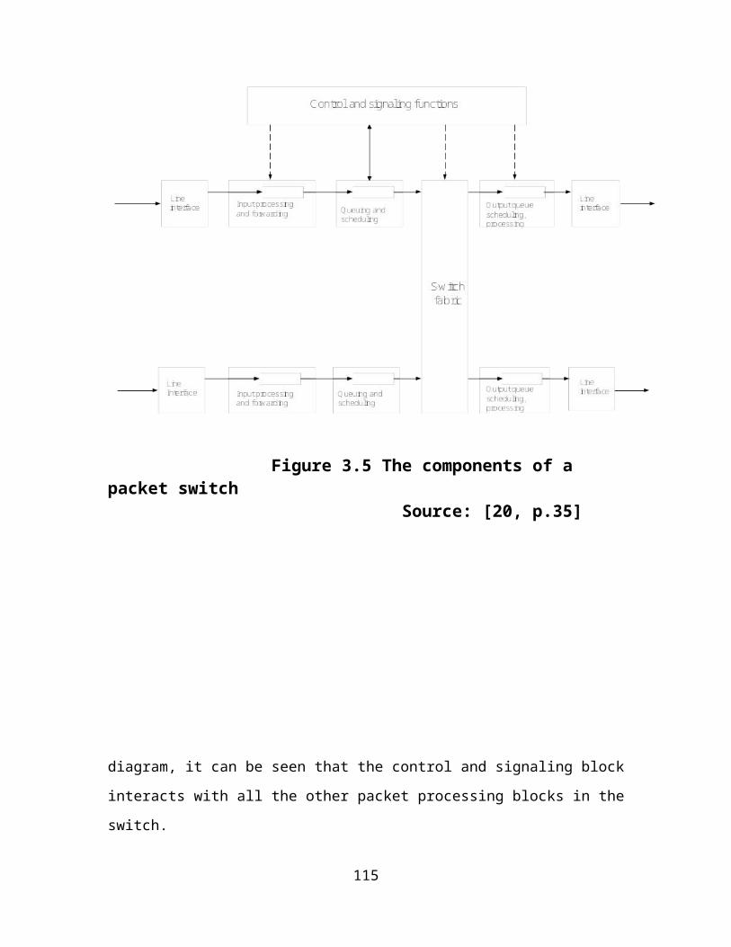
p =

= = (5 -1) + (5-2) + (5-3) + (5- 4) = 4+3+2+1 = 10

So no matter the number of hosts in the LAN, we can calculate the number of end-to-end

delays (number of origin host to destination host delays) to be used with (4.1). It is

instructive to note that, all the hosts in a LAN with k hosts appeared in the lower diagonal

of the traffic matrix (which is the only useful part for our use) k-1 times either as origin

host or as destination host.

4.3.1 Derivation of Switched Local Area Networks’ End-To-End Delay Model and End-To-End Delays Enumeration Methodology

Using the ideas that were developed in Section 4.2, consider again the network shown in

Figure 4.3. We can see that if host H2 is in a communication session with host H3, packets

flow will only cross one switch (S3). If host H2 is in a communication session with host

H5, packets flow will cross three switches (S3, S2 and S4); if host H2 is in a communication

session with host H9, packet flows will cross five switches (S3, S2, S1, S5, and S7). If host

H8 is downloading from or uploading to the Internet (H1), packets flow will cross three

switches (S1, S5, and S7). We can make the same enumeration for other host-to-host and

host-to-Internet communications.

No matter the number of end nodes (hosts) in a switched local area network, we can write

(4.1) for all desired (as given by Eq. (4.5)) origin-destination pairs. We illustrate this

point with the three (3) hosts, two (2) switches LAN shown in Figure 4.6.

Since the application of Eq. (4.5) gives us 3 origin-destination pairs; and from (4.3), the 3

origin-destination pairs are 1-2, 1-3, and 2-3. From Figure 4.6, therefore, the three origin-

destination equations (using inequality (4.1) which has an upper bound of ) are:

For the 1-2 origin-destination pair of hosts, we have;

115

maximum time to transfer 1 packet from host 1 to host 2 (maximum end-to-end delay) =

maximum time (delay) through switch 1 =

(4.6)

For the 1-3 origin-destination pair of hosts, we have;

maximum time to transfer 1 packet from host 1 to host 3 (maximum end-to-end delay) =

maximum time (delay) through switch 1+

maximum time (delay) through switch 2 =

(4.7)

For the 2-3 origin-destination pair of hosts, we have;

maximum time to transfer 1 packet from host 2 to host 3 (maximum end-to-end delay) =

maximum time (delay) through switch 1+

maximum time (delay) through switch 2 =

(4.8)

where Z1, Z2, and Z3 are the Ethernet port transfer rates in packets per second of any of

the two hosts that are involved in a communication session in (4.6), (4.7), and (4.8)

respectively.

We now proceed to write out (4.6), (4.7), and (4.8) together in matrix form as:

= ×

(4.9)

116

where an entry in the bit matrix is 1 if a packet from or to any of the hosts at either end in

the origin-destination path (the maximum end-to-end delay entry of the maximum end-to-

end delay column vector) crosses the corresponding switch in transiting from origin host

to destination host; the entry is 0, if the packet does not cross the switch.

We can re-write (4.9) as:

= ×

(4.10)

Where a11 = a21 = a22 = a31 = a32 = 1 and a12 = 0

Matrix Eq. (4.10) can be written for any switched local area network, with any arbitrary

number of m switches and k hosts.

Let y1, y2, y3,…,yp-1, yp represent origin-destination pair1 maximum end-to-end delay,

origin-destination pair 2 maximum end-to-end delay, origin-destination pair 3 maximum

end-to-end delay,…, origin-destination pair p-1 maximum end-to-end delay and origin-

destination pair p maximum end-to-end delay, respectively.

Also, let x1, x2, x3,…, xm-1, xm represent the maximum delay of any data packet through

switch 1, the maximum delay of any data packet through switch 2, the maximum delay of

any data packet through switch 3,…, the maximum delay of any data packet through

switch m-1, the maximum delay of any data packet through switch m respectively, then

matrix Eq. (4.10) can be written for any switched local area network as:

117

= ×

(4.11)

Carrying out matrix multiplication of the right hand side of (4.11), results in the

following system of linear equations:

y1 = a11x1 + a12x2 + …+ a1m-1xm-1 + a1mxm

y2 = a21x1 + a22x2 + …+ a2m-1xm-1 + a2mxm

y3 = a31x1 + a32x2 + …+a3m-1xm-1 + a3mxm (4.12)

…………………………………………..

………………………………………….

yp-1 = ap-11x1 + ap-12x2 + …+ ap-1m-1xm-1 + ap-1mxm

yp = ap1x1 + ap2x2 + …+ apm-1xm-1 + apmxm

where y1= , y2= , …,yp = and x1, x2, x3,…,xm-1, xm are the unknowns,

m = number of switches in the local area network,

aij = 1/0, i = 1,2,3,…,p; j = 1,2,3,…,m are elements of the path bit matrix for the whole

network.

aij = 1, if a data packet transversing origin-destination i passes through switch j,

aij = 0, if a data packet transversing origin-destination i does not pass through switch j.

p = the LAN’s number of origin-destination pairs of hosts, which is given by Eq. (4.5).

Put in compact form, matrix Eq. (4.11) can be written as:

118

y = AX

(4.13)

Where A is a p×m matrix whose elements are the coefficients matrix of (4.11).

X = (x1, x2, x3,…,xm-1, xm) is a 1×m column vector

y = (y1, y2, y3,…,yp-1, yp) is a 1×p column vector

On the surface, the systems of equations (Eq. (4.11) and Eq. (4.12)) seem to support the

notion that there is an origin-destination pairs traffic matrix with respect to end-to-end

delay computation for all the hosts that are attached to a switched LAN as enunciated (we

think, not correctly) in [2], [3], [9], [19]. For example, Elbaum and Sidi [9] defined

minimum average network delay as the average delay between all pairs of users in the

network; and in [2], the average end-to-end delay time for a switched LAN is defined

with respect to the average traffic between end node i and end node j and the average

delay between these nodes as the weighted combination of all end-to-end delay times. We

have gone through all these hog so as to show that we have not just arrived at this

conclusion without any basis. We now explain why this notion does not seem to be

correct when applied to switched LANs.

If we look at (4.9), we see that rows 2 and 3 of the bit matrix have the same type of

entries; indeed a21 = a31 and a22 = a32 in relation to (4.10). This will make the set of vectors

resulting from (4.12) to be linearly dependent. If we write out (4.12) for this system, we

have;

y1 = a11x1 + a12x2

(4.14a)

y2 = a21x1 + a22x2

(4.14b)

y3 = a31x1 + a32x2

(4.14c)

The reason for the linear dependence of the system of equations in (4.14) is that, if we

look at the network of Figure 4.6, for host H1 to communicate with host H3, and vice

119

versa, data packets will transit through switch S1 and switch S2; the same thing as when

host H2 is to communicate with host H3 or H3 with H2. Therefore, the maximum delays of

a data packet in switches S1 and S2 for the two communication sessions are the same;

hence, the similarity of the entries in rows 2 and 3 of the end-to-end paths bit matrix in

(4.9).

We now illustrate this fact further with a network that is more elaborate than the network

of Figure 4.6. Consider the network shown in Figure 4.7. Using the methodology that we

have previously explained, the resulting traffic matrix for this network is shown in (4.15).

(4.15)

We have 28 end-to-end delays as can be confirmed by using Eq. (4.5).

If y1, y2, y3,…, y28 represent origin-destination pair 1 maximum end-to-end delay, origin-

destination pair 2 maximum end-to-end delay, origin-destination pair 3 maximum end-to-

end delay,…, origin-destination pair 28 maximum end-to-end delay and x1, x2, x3,…, x8

represent the maximum delay of any data packet through switch 1, the maximum delay of

any data packet through switch 2, the maximum delay of any data packet through switch

3,…, the maximum delay of any data packet through switch 8 respectively, then we can

write out (4.13) for this network as is shown in (4.16).

120

Figure 4.7 An hypothetical three (3) switches, eight (8) hosts switched LAN

121

= ×

(4.16)

We can now insert the bits into (4.16) according to whether;

aij = 1, if a data packet transversing origin-destination i passes through switch j,

aij = 0, if a data packet transversing origin-destination i does not pass through switch j.

122

We then have (4.17).

= ×

(4.17)

123

From (4.17), it can be seen that rows 1, 2 and 3 of the origin-destination paths bit matrix

have similar entries; rows 4, 5, 6, 7, 8, 9, 11, 12, 13, 16, 17 and 18 have similar entries,

rows 10, 14, 15, 19, 20, and 21 have similar entries, rows 22, 23, and 24 have similar

entries, and rows 25, 26, 27 and 28 have similar entries; this will make the set of vectors

resulting from (4.17) to be linearly dependent.

In the words of Kreyszig in [70, p.332], ‘what is the point of linear independence and

dependence?’ And he provided the following answer: ‘well, from a linearly dependent set

of vectors, we may often omit vectors that are linear combination of others until we are

finally left with a linearly independent subset of the ‘really essential’ vectors, which can

no longer be expressed linearly in terms of each other’ [70, p.332]. Therefore, if we

eliminate the linearly dependent set of vectors in (4.17), some of the yi’s will vanish,

meaning that the communication paths of some of the hosts (origin-destination pairs of

hosts) will vanish. This is because, as we have previously explained, packets traveling

between two end hosts will suffer maximum delays in the same set of switches along

their end-to-end paths. This proves the fact (and we are proposing a new theorem) that

there is no origin-destination pairs traffic matrix with respect to end-to-end delays

computation for all the hosts that are attached to a switched LAN.

This theorem shows that, for any switched LAN, we cannot simply enumerate the hosts

that are attached to the LAN in order to calculate all origin-destination end-to-end delays.

How then do we enumerate all the (necessary) end-to-end delays of a switched LAN? If

we look at Figure 4.7, for host H1 to communicate with host H8, the data packets must go

through switches S2 and S1. The same thing happens if either host H2 or H3 wants to

communicate with host H8. And hosts H1, H2, and H3 cannot simultaneously communi-

cate with host H8; packets must wait for their turn (in switches) to be sent to host H8. On

the other hand, an host that is attached to switch S2 can be communicating with H8

simultaneously as another host that is attached to switch S2 which is communicating with

an host that is attached to switch S3. This means that, no matter the number of hosts that

are attached to switch S2 or the number of hosts that are attached to switch S1 for

example, we only have one end-to-end delay (and hence, one maximum end-to-end

124

delay) between the hosts that are attached to switch S2 and the hosts that are attached to

switch S1. We can therefore, aggregate all the hosts that are attached to any of the

switches in a switched LAN as shown in Figure 4.8 for maximum delay computation

purposes.

125

S1

HA

S2

S3

HB

HC

Figure 4.8 A Switched LAN, with the hosts that are attached to switches S1, S2, and S3 aggregated as HA, HB and HC respectively.

Then if all the hosts that are attached to any switch in a switched LAN simultaneously

have packets that are destined for another (the same) host in the LAN, we have a

maximum switch delay situation (as the offered load to a network or network device is

the aggregate sum of the data packet rates presented to the network or network device

[11, p.203]). This maximum switch delay situation can be seen as one of the reasons for

the difficulty in uploading/downloading to/from the Internet at certain times of the day

when many users that are attached to the LAN are trying to upload and download at the

same time. We will use these ideas to develop a methodology for designing upper-

bounded delay switched Ethernet local area networks.

Consider Figure 4.8; let us assume that switches S1, S2, and S3, will be placed by the

network designer (installer) as a result of the number of hosts and the locations of the

hosts in a new LAN installation. We have been able to deduce that, if;

m = the number of switches in the LAN,

p = the number of maximum end-to-end delays required for the design of an upper

delay bounded switched LAN,

then,

p =

(4.18)

Here, m =3, therefore,

p =

= (3-0)+(3-1)+(3-2)

= 3+2+1 = 6 maximum end-to-end delays.

126

We now use Figure 4.8 to illustrate how to enumerate the maximum end-to-end delays

for any switched LAN. Our method (algorithm) for this enumeration which we call,

‘right-most, pre-order transversal’ (method of growing the spanning tree of the switches

in any switched Ethernet LAN) has two steps:

1. Process the root switch,

2. Transverse the right-most, sub-tree pre-order, until all the switches have been

processed.

Performing ‘left-most, pre-order transversal’ (the opposite of ‘right-most, pre-order

transversal’) results in the same solution. The important thing is that, both methods

cannot be mixed for the same LAN design process.

Using the right-most, pre-order transversal, the required end-to-end delays are

enumerated as follows (we take switch S1 as the root switch).

1. Switch S1 is placed as shown in Figure 4.9a.

2. Next, place switch S2 and connect S1 to S2. This is shown in Figure 4.9b.

Now, for any host that is attached to switch S1 to communicate with any host that is

attached to switch S2, data packets will experience delay in switch S1 and switch S2 and

vice versa; this is 1 end-to-end delay.

(delay in S1 + delay in S2) = 1 end-to-end delay

3. Next, place switch S3 and connect to already placed switches as shown in Figure 4.9c.

Again, for any host that is attached to switch S1 to communicate with any host that is

attached to switch S3, the data packets will experience delays in switch S1, switch S2, and

switch S3; this is 1 end-to-end delay.

(delay in S1 + delay in S2 + delay in S3) = 1 end-to-end delay

127

Also, for any host that is attached to switch S2 to communicate with any host that is

attached to switch S3, the data packets will experience delays in switch S2 and switch S3;

this is one end-to-end delay.

(delay in S2 + delay in S3) = 1 end-to-end delay

Figure 4.9a Switch S1 is placed

Figure 4.9b Switches S1 and S2 are placed and connected together

Figure 4.9c Switches S1, S2 and S3 are placed and connected together

128

S1

S2

S2

S2

S3

S1

Figure 4.9d Illustration of 1 end-to-end delay through switch S2

We now have 3 end-to-end delays already. It can also be seen that, for any host that is

attached to switch S2 to communicate with another host that is attached to the same

switch S2, data packets will experience delay only in switch S2; this is 1 end-to-end delay.

This is illustrated in Figure 4.9d for hosts H1 and H2.

We have a similar situation if any host that is attached to switch S3 wants to communicate

with another host that is attached to the same switch S3. This is similarly the case with

hosts that are attached to switch S1 (although Figure 4.7 shows that only one host (H8) is

attached to switch 1 – which is just for illustration purpose). These three situations gives

us 3 end-to-end delays, which added to the previous end-to-end delays gives us a total of

6 end-to-end delays, which is what is obtained by applying Eq. (4.18).

While the network shown in Figure 4.7 is quite simple, our method of enumerating the

end-to-end delays and of computing these end-to-end delays works for any switched local

area network, no matter how complex it is. We now illustrate the methodology with the

hypothetical switched local area network that is shown in Figure 4.10, without going into

detailed description.

Basically, as we had previously explained, associated with each of the switches S1, S2, S3,

S4, S5, S6, S7, and S8 is an end-to-end delay as a result of an host that is attached to a

switch wanting to communicate with another host that is attached to the same switch.

This gives us 8 end-to-end delays. We now apply our right-most, pre-order transversal

method to the network.

129H2

S2H1 H2

1. Switch S1 is placed.

2. Switch S2 is placed and connected to it; there is 1 end-to-end delay between switch S1

and switch S2.

(delay in S1 + delay in S2) = 1 end-to-end delay

130

3. Switch S3 is now connected to switch S2; there is 1 end-to-end delay between switch S2

and switch S3.

(delay in S2 + delay in S3) = 1 end-to-end delay

There is another end-to-end delay between switch S1 and switch S3.

(delay in S1 + delay in S2 + delay in S3) = 1 end-to-end delay

4. Switch S4 is now connected to switch S2; there is an end-to-end

delay between switches S2 and S4.

(delay in S2 + delay in S4) = 1 end-to-end delay

There is an end-to-end delay between switches S3 and S4.

(delay in S3 + delay in S2 + delay in S4) = 1 end-to-end delay

There is another end-to-end delay between switches S1 and S4.

(delay in S1 + delay in S2 + delay in S4) = 1 end-to-end delay

By similarly adding switches S5, S6, S7 and S8 in that order to the network, we have the

following end-to-end delays.

5. When switch S5 is connected to switch S2.

(delay in S2 + delay in S5) = 1 end-to-end delay

(delay in S4 + delay in S2 + delay in S5) = 1 end-to-end delay

(delay in S3 + delay in S2 + delay in S5) = 1 end-to-end delay

(delay in S1 + delay in S2 + delay in S5) = 1 end-to-end delay

131

6. When switch S6 is connected to switch S1.

(delay in S1 + delay in S6) = 1 end-to-end delay

(delay in S2 + delay in S1 + delay in S6) = 1 end-to-end delay

(delay in S3 + delay in S2 + delay in S1 + delay in S6) = 1 end-to-end delay

(delay in S4 + delay in S2 + delay in S1 + delay in S6) = 1 end-to-end delay

(delay in S5 + delay in S2 + delay in S1 + delay in S6) = 1 end-to-end delay

7. When switch S7 is connected to switch S6.

(delay in S6 + delay in S7) = 1 end-to-end delay

(delay in S1 + delay in S6 + delay in S7) = 1 end-to-end delay

(delay in S2 + delay in S1 + delay in S6 + delay in S7) = 1 end-to-end delay

(delay in S3 + delay in S2 + delay in S1 + delay in S6 + delay in S7) = 1 end-to-end delay

(delay in S4 + delay in S2 + delay in S1 + delay in S6 + delay in S7) = 1 end-to-end delay

(delay in S5 + delay in S2 + delay in S1 + delay in S6 + delay in S7) = 1 end-to-end delay

8. When switch S8 is connected to switch S1

(delay in S1 + delay in S8) = 1 end-to-end delay

(delay in S2 + delay in S1 + delay in S8) = 1 end-to-end delay

(delay in S3 + delay in S2 + delay in S1 + delay in S8) = 1 end-to-end delay

(delay in S4 + delay in S2 + delay in S1 + delay in S8) = 1 end-to-end delay

(delay in S5 + delay in S2 + delay in S1 + delay in S8) = 1 end-to-end delay

(delay in S6 + delay in S1 + delay in S8) = 1 end-to-end delay

(delay in S7 + delay in S6 + delay in S1 + delay in S8) = 1 end-to-end delay

We have systematically enumerated all the inherent end-to-end delays of this LAN. The

total end-to-end delays = 8+1+2+3+4+5+6+7= 36 which is what is obtained by applying

Eq. (4.18). Eq. (4.18) can therefore, be used as a check to ensure that all the end-to-end

delays that are inherent in any switched local area network have been systematically

enumerated using our right-most, pre-order transversal method.

132

Having explained our methodology for enumerating all the end-to-end delays that are

inherent in any switched local area network, we now proceed to explain how to use the

notion of maximum (upper-bounded) end-to-end delay to design high quality switched

local area networks. We use the network shown in Figure 4.8 as an example (but the

methodology is the same for any switched local area network, no matter how complex it

is). We write down all the inherent end-to-end delays for Figure 4.8.

end-to-end delay 1-1 = time for a data packet to cross S1 for any host that is attached to

switch 1 that is communicating with another host that is attached to the same switch 1.

end-to-end delay 2-2 = time for a data packet to cross S2 for any host that is attached to

switch 2 that is communicating with another host that is attached to the same switch 2.

end-to-end delay 3-3 = time for a data packet to cross S3 for any host that is attached to

switch 3 that is communicating with another host that is attached to the same switch 3.

end-to-end delay 1-2 = time for any data packet to cross S1 + the time for the same data

packet to cross S2 for any host that is attached to switch 1 that is communicating with

another host that is attached to switch 2.

end-to-end delay 2-3 = time for any data packet to cross S2 + the time for the same data

packet to cross S3 for any host that is attached to switch 2 that is communicating with

another host that is attached to switch 3.

end-to-end delay 1-2-3 = time for any data packet to cross S1 + the time for the same data

packet to cross S2 + the time for the same data packet to cross S3 for any host that is

attached to switch 1 that is communicating with another host that is attached to switch 3.

Assuming that the;

maximum time for any data packet to cross S1 = x1 seconds

maximum time for any data packet to cross S2 = x2 seconds

133

maximum time for any data packet to cross S3 = x3 seconds

Then,

maximum end-to-end delay 1-1 = x1 seconds

maximum end-to-end delay 2-2 = x2 seconds

maximum end-to-end delay 3-3 = x3 seconds

maximum end-to-end delay 1-2 = (x1 + x2) seconds

maximum end-to-end delay 2-3 = (x2 + x3) seconds

maximum end-to-end delay 1-2-3 = (x1 + x2 + x3) seconds

the average of the maximum end-to-end delays of the whole network is therefore,

= seconds

Therefore, if t1= maximum end-to-end delay 1, t2= maximum end-to-end delay 2, t3=

maximum end-to-end delay 3,…, tp= maximum end-to-end delay p, respectively,

and Davmax = average of the maximum end-to-end delays of the whole network,

where p = number of end-to-end delays inherent in the switched LAN, then,

Davmax = seconds (4.19)

Eq. (4.19) is similar (but specified with respect to an opposite frame of reference) to the

network delay performance measure defined in [9]. In this paper, it was stated that the

minimum average network delay is the average delay between all pairs of users in the

network. What we think is meant here is that, the minimum average network delay is the

average of the minimum end-to-end delay between all pairs of users in the network.

Correspondingly therefore, the maximum average network delay is the average of the

maximum end-to-end delay between all pairs of users in the network. But we have

previously shown in this work that, for a switched local area network, it is wrong to

enumerate all the users (hosts) that are attached to the network for the purpose of end-to-

end (for example, average end-to-end) delay computation.

134

We are, thus, able to know whether this average of the maximum end-to-end delays of

the whole network is less than the maximum end-to-end delay that can be tolerated by

any application that is to be deployed on this network. If it is less than, then we have

designed an efficient network; if it is more than, then we can iteratively choose switches

of higher capacity (high switching fabric data transfer rate) and hence, low switching

latency (delay). Using the maximum end-to-end delay specification of an application in

this methodology finds support with the view of Metzler in [71] that ‘the latency of any

network has a major impact on the applications that can be deployed in the network’.

Moreover, Georges, Divoux and Rondeau has stated in [27] with respect to switched

Ethernet networks in an industrial environment that, the network calculus is used to

determine the upper-bounded end-to-end delays of each packet; and that, if all the end-to-

end delays are less than the time-cycle of the programmable controllers, then the network

organization (switches placements) is in accordance with the application constraint.

This method of specifying the switches in a switched LAN also finds agreement in the

switched network design problem formulation by Reiser in [14]; which, stated in words,

is ‘design the switched network under maximum loading condition, such that the average

network delay is less than or equal to a given delay bound’. Another way of looking at

this switched LAN design methodology is to state the network design problem in this

way: ‘can we specify and arrange the switches in a switched LAN such that the

maximum of the maximum (max-max) end-to-end delays of the LAN is less than the

maximum tolerable delay of the applications to be deployed in the network?’

With respect to the switched LAN shown in Figure 4.10, assuming that the maximum

time for any data packet to cross Si = xi seconds, for i = 1, 2,…,8, then, the maximum

end-to-end delay for all the end-to-end delays that we have previously enumerated can be

computed; we can then go on to compute Davmax, the average of the maximum end-to-

end delays of the whole network.

135

Moreover, we propose in this work, a generic maximum end-to-end delay matrix for

switched local area networks (which we call the Eyinagho-Falaki maximum end-to-end

delay matrix for switched local area networks). If,

n = the number of switches in any switched local area network,

metedir = maximum end-to-end delay between any host that is attached to switch i and

any host that is attached to switch r,

meted11 = maximum end-to-end delay between any two hosts that are attached to switch1,

meted22 = maximum end-to-end delay between any two hosts that are attached to switch

2,…, metednn = maximum end-to-end delay between any two hosts that are attached to

switch n, respectively, then the Eyinagho-Falaki maximum end-to-end delay matrix (with

associated switched local area network’s switches) is the lower triangular matrix (it can

also be formulated in terms of the upper triangular matrix) given by (4.20).

(4.20)

If we know the maximum delay of a packet through each and every one of the switches in

any switched local area network (these delays can be obtained by using Eq. (3.29)); with

the aid of (4.20), it is not difficult to write a program that computes a switched local area

network’s maximum end-to-end delays.

4.4 Specification of the Switches in a Switched Local Area Network

It should by now be clear that the switched LAN’s design problem is the problem of

specifying all the switches in the network so that either the average maximum (average of

max) end-to-end delay for the whole network is upper bounded or the maximum of the

maximum (max. of max.) end-to-end delays is upper bounded; and these should be

136

bounded above by the maximum of the delay constraints that we desire to be imposed on

the network. For example, if the maximum of the end-to-end delay constraints of the

applications to be deployed on the network is 3 seconds, while the max of max end-to-

end delays of the network is 2 seconds, it implies that the network under all operating

situations will be able to transmit packets from an origin host to a destination host within

the time limits imposed by the applications. This is the only way to ensure a high quality

best-effort network. A best-effort network does not support quality of service; an

alternative to complex QoS control mechanisms is to provide high quality

communication over a best-effort network by over-provisioning the capacity so that it is

sufficient for the expected peak traffic load [56]. Tananbeum in [72, p.398] expressed

this idea in this way: one of the techniques for achieving QoS is over-provisioning; this

technique seeks to provide so much router (switch) capacity, buffer space and the packets

just fly through easily, and that as time goes on and designers have a better idea of how

much is enough, this technique may even become practical [72, p.399]. This is the

technique that we are pursuing in this work: formalized, practical method of designing

switched Ethernet local area networks, with a view to meeting particular delay

constraints.

4.5 Specification of the Switching Fabric Transfer Rates of the Switches in a Switched Local Area Network

One of the common specifications for packet switches by switch manufacturers is the

switching fabric packet transfer rate from the buffers of the input ports to the buffers of

the output ports of the switches. And our work is to select all the switches in a switched

LAN such that each of their switching fabric transfer rate is not below a minimum, while

respecting the end-to-end delay constraints that we have previously explained. The

minimum switching fabric transfer rate (SFTRMIN) of a shared memory packet switch was

obtained as Eq. (3.3), which is restated in the context of this subsection as Eq. (4.21).

SFTRMIN = bits/sec

(4.21)

where, Ci = data rate of switch input port i in bits/sec.

137

Knowing the input ports transfer rates of an Ethernet packet switch; that is, the C is, i = 1,

2, 3,…,N, where N is the number of ports in the switch, we can calculate this minimum

switching fabric transfer rate of the switch.

4.6 Estimating the Read/Write Memory Capacities of the Switches in a Switched Local Area Network

We know that σ is the maximum amount of data traffic that can arrive in a burst in bits.

But RFC 2544 [68] recommends the use of 16, 64, 256 and1024 frames, respectively, as

the maximum amount of traffic that can arrive in a burst (σ in our model) for DUTs

(Device Under Test) burstability or burst test (the burst test assesses the buffering

capacity of a switch; it measures the maximum number of frames that are received at full

line rate before a frame is lost [73]). We can, therefore, use any of these burst sizes to

have a rough estimate of the minimum amount of read/write memory (RAM) capacities

of the switches in a switched LAN; but since this work is an initial research effort, we

decided to use the average of these four values as our value for σ.

The minimum amount of read/write memory capacities for the switches in the switched

(Ethernet) LAN = σ×maximum length of an Ethernet frame (L)

Since L= 1530 bytes, the minimum read/write memory capacity (RWMEMCAPMIN) for a

switch is given by;

RWMEMCAPMIN = (σ×1530×8) bits (4.22)

4.7 Determining the Maximum Number of Hosts that can be attached to a Switched Local Area Network

From our discussions so far, it should be clear now that the real bottleneck to the delay

performance of switches in switched LANs is the queuing delay in the switches. If a

switch has N input/output ports, with hosts attached to (N−1) ports (the N th port is used to

connect the switch to other switches in the LAN), then, if the hosts that are attached to

the switch simultaneously have packets that are destined for another (the same) host in

the LAN, then, we have a maximum switch delay situation (as the offered load to a

network or network device is the aggregate sum of the data packet rates presented to the

138

network or network device [11, p.203]). It, therefore, follows that, based on the upper

bounded delay network design methodology, the number of hosts that can be attached to

a switch is only limited by the number of I/O ports that the switch has minus one.

Therefore, if,

m = number of switches in an upper delay bounded designed switched LAN,

Nj = number of I/O ports in upper delay bounded specified switch j,

h = the number of hosts that can be connected to the LAN, then.

h = (4.23)

(N-1) hosts can be connected to a switch because the N th host cannot have packets

destined for itself. The difference between a non-upper delay bounded designed switched

LAN having m switches with each switch having N I/O ports and an upper delay

bounded designed switched LAN having m switches with each switch having N ports is

that, all packets are sure to move from an origin host to a destination host within the time

bound of the network, and hence, users are not likely to have experiences of a sluggish

network in the latter case. This is unlike the former case in which packets may not be

moving from origin hosts to destination hosts within a time bound, and hence, users are

likely to have experiences of a sluggish network. Eq. (4.23) finds support with the

contention in [74] that the number of users that can be supported by a local area network

is limited by the physical number of ports available in the switches.

4.8 Determining a Switched Local Area Network’s Downlink and Uplink rates for Internet access

It is generally known that the common challenge with most LANs that are connected to

the Internet is the difficulty in downloading and uploading of contents at certain times of

the day. The worst-case scenario for any LAN should, be, when either all the hosts that

are attached to the network are simultaneously sending traffic to, or receiving traffic from

the Internet at their maximum rates. In between these two extremes are situations

whereby, some hosts are sources of traffic to the Internet and some hosts are sinks to

Internet traffic. But we have shown that, as far as end-to-end delay is concerned, we do

139

not enumerate origin-destination pairs with respect to hosts; but that, this enumeration

should be done, with respect to the switches in the network. We will use this idea to

explain how to properly specify a switched LANs downlink and uplink rates for Internet

access.

Bersakas and Gallager has averred in [10, p.440] that, if γ is the total arrival rate into a

network, then there is a given input flow for each origin-destination pair and γ is the sum

of these. The same notion was expressed in [14] where it was stated that, if;

λ = total arrival rate to a network (network loading) in bits/sec, then,

(4.24)

where λ(r) = arrival rate of route r

R = the number of routes in the network.

Gerd in [11, p.195] has also stated that if γs is the arrival rate in messages per second

associated with path s, then the total arrival rate (γ) to the whole network is:

(4.25)

where n = the number of paths in the network.

The idea underlining Eqs. (4.24) and (4.25) is illustrated in Figure 4.11 for the case of a

switched LAN. It could be seen in this figure that, switches on paths s say, of one origin-

destination traffic may also be on path i = 1,2,…,m, i ≠ s of other origin-destination

traffic. Since in our model the Internet is a fictitious host which is the source of traffic to

the LAN, we consider the worst case scenario in which all the hosts in the LAN are

simultaneously downloading (what we are going to explain also apply to the situation in

which all the hosts are simultaneously uploading). If we look at Figure 4.7, we can

assume that the Internet as a fictitious host (a source of traffic) is attached to switch 1.

140

γ2 γ2

γm γm

.

.

.

.

.

.

.

. Switched LAN

γ1 γ1

Switch 1 is, therefore, our router that is connected to the Internet access device, for

example, a VSAT (Very Small Aperture Terminal). This is illustrated in Figure 4.12.

Of the six (6) end-to-end delays, we extract the end-to-end delays in which S1 is the

source node, while another switch is the destination node. These are:

(delay in S1 + delay in S2) = 1 end-to-end delay

In which S1 is the source node and S2 is the destination node.

(delay in S1 + delay in S2 + delay in S3) = 1 end-to-end delay

In which S1 is the source node with traffic flowing through S2, while S3 is the destination

node.

141

Internet Access Device(for example,VSAT)

Other Switches on Path 1

Arrival rate to the network from the Internet

γ

Destination Switch

Destination Switch

Destination Switch

OtherSwitches on Path 2

OtherSwitches on Path m

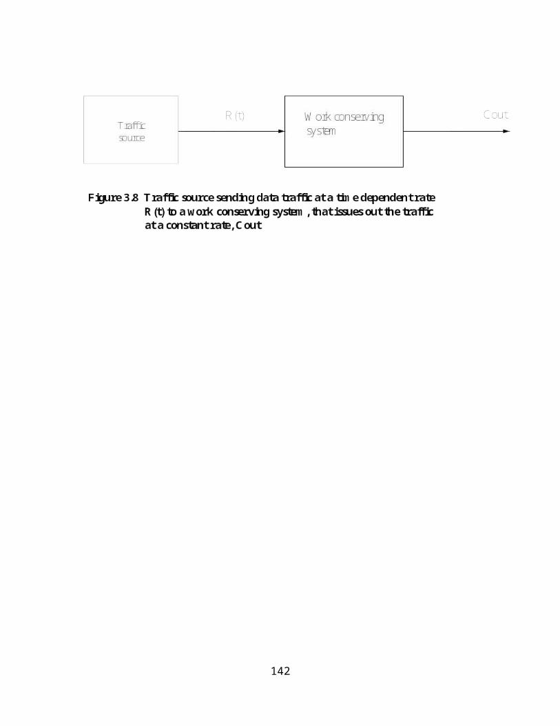
142

S1(Router)

S2

S3

Internet (fictitious host)

Figure 4.11 Illustration of the division of traffic arrivals to a Switched LAN into m paths, with the arrival rate on path i being γi, i= 1,2,....,m

Figure 4.12 The switches in a Switched LAN, with the hosts left out and the Internet as a fictitious host (S1 is a router)

In relation to Eqs. (4.24) and (4.25), we see that there are two origin-destination pairs (or

paths) through which traffic flow from the Internet through the network. If the bandwidth

of each path is Z Mbps, say, then for pleasurable download by the users (hosts) that are

attached to the network, the theoretical downlink rate for Internet access should be 2Z

Mbps. Similarly, the theoretical uplink rate for pleasurable upload is 2Z Mbps (since in

the uplink, S2 and S3 will be source nodes, while S1 will be the destination node).

Likewise, with respect to Figure 4.10, taking S1 as the switch (router) that is attached to

the Internet access device (VSAT), we find (from the enumerated 36 origin-destination

end-to-end delays) that, there are 7 paths in which S1 is the source of traffic, while, the

other 7 switches are the destinations of traffic. Similarly, there are 7 paths in which S 1 is

the destination of traffic, while, the other 7 switches are the sources of traffic (these can

be seen in the context of Figure 4.11). Therefore, for pleasurable downloading and

uploading by the users (hosts) that are attached to the network, the theoretical downlink

and uplink rates for Internet access should be 7Z Mbps, where Z Mbps is the bandwidth

of each path. From the preceding discussion, it can be seen that if,

Zi = bandwidth of the ith origin-destination path in bits/sec,

143

q = the number of origin-destination paths, with the switch (router) that is attached to the

Internet access device as the source node, the theoretical downlink and uplink rates

(DLULRATES) of the Internet access device (for example VSAT) for pleasurable uploading

and downloading of Internet traffic should be;

DLULRATES = bits/sec.

(4.26)

It can be seen that q is equal to the number of switches in the switched LAN minus the

switch (or router) that is connected to the Internet access device (VSAT). For a path with

more than one inter-switching node rates, the bandwidth of the path Z i, should be taken as

the (rate) bandwidth of the smallest inter-switching node media in order to avoid

congestions on some links and queue build-ups on some switches.

This is, therefore, an empirical method for specifying the downlink and uplink rates of

the Internet access device of any switched local area network. This method finds support

with the assertion of Oppenheiner in [75, p.47], that, by increasing the bandwidth on a

WAN circuit, you decrease queue length and hence, the queuing delay is decreased (it has

previously been asserted and shown in this work that the queuing delay is the bottleneck

delay in switching devices).

144

CHAPTER 5

EVALUATION OF PACKET SWITCH MODEL AND AN APPLICATION EXAMPLE

5.1 Introduction

The contention in this work that the ‘N-port maximum delay packet switch model’

developed in the penultimate chapter (Figure 3.6 and Eq. (3.29)) is indeed what the term

in quotes suggests, must be adequately substantiated. In the first place, a packet switch is

a packet switch – that is, the functionalities and operation of packet switches are largely

the same as have been shown from literature. Their differences which are mainly in the

choice of switching fabric implementation and in the type of buffering employed (input,

output, or input and output) were also clearly explained using literature. The fact that we

are concerned in this work with the Ethernet packet switch only suggests that our data

unit or packet type is the Ethernet packet; this can be reflected in the model by using the

maximum length (L) of an Ethernet packet in the resulting mathematical model (Eq.

(3.29)). We have clearly explained how all the functionalities of a packet switch that

contribute to delays in the switch have been reflected in the model. While explaining this

145

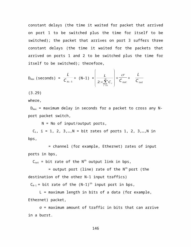
model, and deriving its mathematical equivalent, we indicated at every step, how the

notion of ‘maximum delay’ has been reflected in both Figure 3.6 and Eq. (3.29).

But the challenge that arises in the context of this work is ‘how good is our maximum

delay model?’ In other words, is there an optimum upper-bound delay by which we can

measure our upper-delay bounded model? According to Adegbenro in [76], issues that

have to do with making comparisons are undoubtedly difficult tasks; they are difficult

because, the framework on which a comparison is based must be clearly defined,

otherwise, the whole exercise may be meaningless. This is because, the more acceptable

this framework is, the more acceptable the result of the comparison is likely to be. We

agree no much less with this assertion and indeed, we were in a big dilemma about how

to resolve this issue. This is because, the area of research which this work delved into is

relatively new, is evolving and with no discernable procedural standards for now.

We have, however, shown from literature that there is the need to know the maximum

end-to-end delay that the packets transiting a switched LAN can ever experience; and that

by using such an upper-bounded end-to-end delay to specify and select the switches for

such a LAN, the users whose workstations (hosts) are attached to such a network will

always have pleasurable experiences when logged on to the network. Some researchers

(for example Abiona [4], Georges, Divoux and Rondeau [27]) have attempted to solve

this problem by using network simulation software packages such as OPNET Modeler,

NS-2 (Network Simulator-2), Comnet 111 to model network components in order to be

able to carry out performance comparisons. Georges, Divoux and Rondeau in [27] used

the Comnet 111 to model a 1-switch and 3-hosts network and the upper-bounded end-to-

end delay values obtained with the simulator was compared to the upper-bounded end-to-

end delay values that were computed by using the algorithm that was proposed in the

paper. But the values that were obtained by using the network simulator differed widely

from the values that were computed using the algorithm. Hence, we may then ask the

next pertinent question: how good are the values that are obtained by using network

simulators – since, different experimental values are obtained by using different network

simulators even for the same experimental platform? This assertion was emphasized in

146

[77] where it was stated that ‘breach of credibility’ by studies that are based on network

simulation tools has been reported in the literature. This is due to the fact that network

simulators are normally supposed to be used as network management and performance

prediction tools.

In the context of this work, therefore, if a network simulator package is adopted to model

an Ethernet packet switch, how good will the upper-bounded delay value that will be

obtained using the simulator be? This question no doubt is difficult to answer for the time

being as things are in this research area, as there are no specifications for ‘maximum

switch delays’ by which comparisons can be made. Therefore, we decided on a simple

ingenious ‘practical’ way to validate the ‘goodness’ of our model in this work; and

incidentally, this ingenious practical method showed that values (for example, delay

values) obtained by using network simulators can be very misleading; which, therefore,

supports the ‘breach of credibility’ by network simulators that have been reported in

literature as asserted in [77]. This simple practical validation of our maximum delay

packet switch model is what is reported in the next section of this chapter.

Subsequently, we will describe the development of our switched LAN design algorithm,

and illustrate (by means of an installed switched LAN example), the design of a switched

Ethernet LAN using this algorithm. Researchers (for example, Georges, Divoux and

Rondeau [27], [28], Krommenacker, Rondeau, and Divoux [19], Kanem, Torab, Cooper

and Custodi [2], Torab and Kamen [3]) demonstrated the utility of their proposed

switched Ethernet network design methodology by using an ‘illustrative example’. We

will use the Covenant University College of Science and Technology (CST) building

local area network as an example to illustrate the switched LAN design algorithm. The

essence for this is to be able to compare the specifications for the placed switches that are

obtained using this design algorithm (methodology) with the actual installed switches

and, therefore, make informed inferences.

5.2 Evaluation by Comparison of Upper-Bounded Delay Packet Switch Models

147

We will use the 100 Mbps channel rate, which is almost now the basic standard for LAN

workstation access (Fast Ethernet); as the 10 Mbps access rate which was the standard

when there was almost no multimedia traffic in the 802 LANs is almost now, no longer

used. Also, the maximum size of an Ethernet frame (the extended Ethernet frame which

is 1530 bytes) will be used. Typical maximum delay values for the model represented by

Eq. (3.29) are:

(The components of the extended Ethernet frame are shown in Figure 2.8, and the

maximum size of this frame is = 7+1+6+6+4+2+1500+4 =1530 bytes = 1530×8 bits =

12240 bits)

i. Forwarding Delay (FWD) = secs.

where L = 12240 bits,

CN−1 = 100×106 bps

therefore,

FWD =

= 12240 × 10-8secs

= 0.12240 ms

ii. Routing or Switching Delay (RSD) = secs.

We assume here that the switch is a Super Stack 11 Ethernet Switch 3900 (we will

use this switch through out in this section as the basis for our evaluation) by 3Com

Corporation. It is a 24 ports switch.

where L = 12240 bits,

Ci = 100×106 bps

N= 24

therefore,

RSD =

148

=

= 255 ×10-8secs

= 0.00255 ms

iii. Simultaneous Arrivals of packets Delay (SAD) = (N-2) × secs.

SAD = (N-2) ×RSD = (24-2) ×RSD

= 22 ×0.00255ms

= 0.05610 ms

iv. Frame Transmission Delay (FTD) = secs.

where L = 12240 bits,

Cout = 100×106 bps

therefore,

FTD =

= 12240 × 10-8secs

= 0.12240 ms

v. Queuing Delay (QD) = secs.

To calculate the maximum queuing delay that is possible, we had previously noted the

recommendations that are contained in RFC 2544 [68] with respect to burstability tests.

This RFC recommended burst sizes of 16, 64, 256, and 1024 frames. Recall that we

decided to use the average of these values in this work. We now present sample

maximum queuing delays using these five (5) values (the four recommended by RFC

2544 plus the average of these four values).

For 16 Ethernet frames,

σ = 16×1530×8 = 195,840 bits

149

QD =

=

= 195, 840×10-8

= 0.001958 secs. = 1.958 ms

For 64 Ethernet frames,

σ = 64×1530×8 = 783,360 bits

QD =

=

= 783, 360×10-8

= 0.007834 secs. = 7.834 ms

For 256 Ethernet frames,

σ = 256×1530×8 = 3,133,440 bits

QD =

=

= 3,133,440×10-8

= 0.031334 secs. = 31.334 ms

For 1024 Ethernet frames,

σ = 1024×1530×8 = 3,133,440 bits

QD =

=

= 12,533,760×10-8

= 0.125338secs. = 125.338 ms

150

Using the average of these values, that is 340 Ethernet frames,

σ = 340×1530×8 = 4,161,600 bits

QD =

=

= 4,161,600×10-8

= 0.041616secs. = 41.616 ms

It can be seen that while burst sizes of 16 and 64 Ethernet frame lengths will result to

very small queuing delays, a burst size of 256 Ethernet frame lengths will result to a

moderate queuing delay, and a burst size of 1024 Ethernet frame lengths will result to a

very large queuing delay. The mean of these four values will result to a queuing delay of

approximately 41.62ms (which is also moderate). It is, therefore, not out of place to use

the mean of the four values in this work.

Therefore, adding i + ii + iii + iv + v, we have the maximum delay of this Ethernet packet

switch model as:

Dmax = 0.12240ms + 0.00255ms + 0.05610ms + 0.12240ms + 41.616ms

= 41.91945 ms

42 ms

Here, it can be seen that, if an arriving packet to the switch does not meet any packet in

the queue, and particularly, if there is no burst traffic that has previously arrived in the

queue before this arriving packet, the switch delay would be i + ii + iii + iv. The delay D

in this situation will be:

D = 0.12240ms + 0.00255ms + 0.05610ms + 0.12240ms

= 0.3035 ms

This shows that the queuing delay is the bottleneck delay in a packet switch as has been

previously noted. We now make a comparison of this model value with literature values

and make informed inference.

151

5.2.1 Model Validation

It has not been easy coming across values for maximum packet switch delay in literature.

But Georges, Divoux, and Rondeau reported in [27], that the maximum delay value

obtained with the maximum delay Ethernet packet switch model reported in the paper is

3080 μs or 3.080 ms; while the COMNET 111 simulation software package gave a

maximum delay value of 450 μs or 0.450 ms. Which of the three (the model that is

represented by Eq. (3.29), the model in [27], or the value given by COMNET 111 as

reported in [27]) results can be said to be the better result? We will now use a typical

practical switched Ethernet LAN installation scenario in literature for this comparison.

5.2.1.1 Selecting an Appropriate Upper Bound Delay

Metzler [71] has averred that instead of managing applications (in the context of

application response time) in a monolithic fashion, the task of application management

must be decomposed into sub-tasks. According to this paper, one option is for an IT

(Information Technology) organization to decompose applications management into a

network component and a compute component. Assuming, therefore, that the IT

organization has a target response time for the application, it can then assign a maximum

amount of delay for the network and a maximum amount of delay for the compute

infrastructure; the IT organization must now ensure that it can manage its network and its

compute infrastructure to meet these delay goals. This paper also went on to suggest that,

when deploying a wired or wireless WAN, it is necessary to support the latency

requirement of the most demanding application; and that many common applications

require a sustained average latency of 150 ms or less in order to function properly. It was

further averred in this paper that the ITU recommends that voice should have a one-way

latency of 150 ms or less; and that the latency requirements of voice and video is similar

to the latency requirements of applications like ERP (Enterprises Resource Planning) – an

average sustainable latency of 150 ms or less. Appendix D1 shows ITU-T

Recommendation Y.1541 [78] network QoS definitions and network performance

objectives. In [79], it was stated that voice traffic end-to-end delay requirements should

152

be between 150 ms and 200 ms maximum for one-way and a round-trip maximum of

between 300 ms and 400 ms. Also in [80], it was stated that one-way end-to-end delay for

voice and video packets should be maximum of 150 ms. In the view of Nielson in [81],

- 100 ms is the maximum delay before a user no longer feels that a network is

reacting instantaneously,

- 1 second is the maximum delay before a user’s flow of thought is interrupted, and

- 10 seconds is the maximum delay before the user loses focus on the current

dialog.

This view is in concurrence with IETF RFC 2815: Integrated Services Mappings on IEEE

802 Networks [82] (see Appendix D2). It can be seen from this recommendation that the

highest delay bound for IEEE 802 networks (the switched Ethernet LAN is an example of

an IEEE 802 network) is 100 ms. It is necessary to state all these literature facts as it

relates to applications’ upper-bound delay in order to show that opinions on these issues

are largely similar.

From the foregoing, two values are prevalent in literature as applications end-to-end

delay bounds – 150 ms and 100 ms. In this context, therefore, we now make a

comparison of the three maximum packet switch delay values that were previously stated.

i. The maximum delay value in [27]. This value is 3.080 ms. Using the 150 ms

end-to-end application delay bound, it will mean that between two hosts (one,

the origin host and the other, the destination host) there can be =

48.7 49 switches

Using the 100 ms end-to-end application delay bound, it will mean that between two

hosts (one, the origin host and the other, the destination host) there can be =

32.5 33 switches

ii. The maximum delay value provided by COMNET 111 as reported in [27].

This value is 0.450 ms. Using the 150 ms end-to-end application delay bound,

153

it will mean that between two hosts (one, the origin host and the other, the

destination host) there can be = 333 switches

Using the 100 ms end-to-end application delay bound, it will mean that between two

hosts (one, the origin host and the other, the destination host) there can be =

222 switches

iii. The maximum delay value provided by the model represented by Eq. (3.29).

This value is 42 ms. Using the 150 ms end-to-end application delay bound, it

will mean that between two hosts (one, the origin host and the other, the

destination host) there can be = 3.57 4 switches

Using the 100 ms end-to-end application delay bound, it will mean that between two

hosts (one, the origin host and the other, the destination host) there can be = 2.4,

rounded up to 3 switches.

Figure 5.1 shows a manufacturer’s (Square D) [83] pictorial installation guide, for the

installation of the Model SDM 5DE 100, Class 1400 Ethernet packet switch. This is

included in the manufacturer’s installation bulletin. It is stated in the bulletin that

switches can be concatenated between devices (hosts) as long as the path between hosts

does not exceed four (4) switches and five (5) cable runs. This manufacturer was kind

enough to provide this data to network installers; as manufacturers of Ethernet packet

switches seldom do this. From the information provided by this manufacturer, it can be

seen that in practical terms, our model is close to reality (and it is therefore, validated). In

fact, we can say with utmost assuredness that the model in [27] and the value provided by

COMNET 111 as reported in [27] are very unrealistic as maximum delay bound for an

Ethernet packet switch.

5.3 Application

5.3.1 Switched Local Area Networks Design Steps

154

Reiser in [14] has once averred that, the packet switched network design specification

may be to obtain load values such that the mean network delay remains below a given

bound, and, therefore, formulated the following mathematical programming problem:

max

subject to ≤ t0

where λ = arrival rate to the network (network loading),

= average delay of the whole network,

t0 = a given delay bound.

155

Figure 5.1 A typical concatenation of multiple switches; manufacturer’s instruction: additional switches can be used as long as the path between network devices (hosts) does not exceed four switches and five cables

Modeling the network internal nodes by simple queuing systems and adding some

assumptions on the arrival process of packets to these nodes, one can use simple queuing

formulas to estimate the delay time associated with each network node; based on the

network topology, these delay times are then combined to compute the end-to-end delay

times for the entire network [2], [3]. This overtly simplified method may be the only

156

possible approach to many practical design problems [3]. Therefore, according to Kanem

et al. [2], the steps in the design of switched computer networks are:

1. Specification of the number of end nodes, that is, the number of nodes to be

connected to the network, and the physical locations of the end nodes,

2. Specification of the likely maximum information flow rate from end node to end

node for all end nodes to be connected to the network.

Given the number of end nodes, the location of the end nodes, and the maximum

information flow rates aij from end node i to end node j, the problem is to design a

network that has, among others, an acceptable performance. As in many cases (for

example, [2], [9], [39]) the network performance parameter of interest is the average

network delay. And according to Kanem et al. [2], the average end-to-end delay of a

switched Ethernet local area network is the weighted combination of all end-to-end delay

times. But the challenge with the method proposed in this work for the computation of

the average end-to-end delay of a switched Ethernet local area network is that it was

assumed that there is a known average traffic flow Iij, say, from end node i to end node j

for all end nodes in the network instead of using the maximum information flow rate

from end node i to end node j as was enunciated in the paper. However, assumptions are

difficult to standardize, and they are, therefore, not good for engineering works.

We adopt in this work, the average of the network maximum end-to-end delays

specification. That is, the switched Ethernet local area network design objective is to

design the network with an average maximum end-to-end delay that is below an upper

bound, this upper bound being determined by the maximum delay constraints

(requirements) of the applications to be deployed in the network.

5.3.2 Development of Switched Local Area Networks Design Algorithm

We now proceed to develop our switched local area networks design algorithm. The

developed algorithm would subsequently be used to automate the process of designing

switched Ethernet local area networks. The network in Figure 4.10 (see page 130) would

be used to develop this design algorithm.

157

We had earlier explained (see Section 4.3.1, page 135) that, assuming the maximum time

for any data packet to cross Si = xi seconds, for i = 1, 2,…8, then, associated with each of

the switches S1, S2, S3, S4, S5, S6, S7, and S8, is a maximum end-to-end delay of x1

seconds, x2 seconds, x3 seconds, x4 seconds, x5 seconds, x6 seconds, x7 seconds, and x8

seconds, respectively. We now list all the other maximum end-to-end delays as each of

the switches is being placed.

When S2 is placed, the maximum end-to-end delay is:

x2 + x1

When S3 is placed, the maximum end-to-end delays are:

x3 + x2

x3 + x2 + x1

When S4 is placed, the maximum end-to-end delays are:

x4 + x2

x4 + x2 + x1

x4 + x2 + x3

When S5 is placed, the maximum end-to-end delays are:

x5 + x2

x5 + x2 + x1

x5 + x2 + x3

x5 + x2 + x4

When S6 is placed, the maximum end-to-end delays are:

x6 + x1

x6 + x1 + x2

x6 + x1 + x2 + x3

x6 + x1 + x2 + x4

x6 + x1 + x2 + x5

When S7 is placed, the maximum end-to-end delays are:

x7 + x6

x7 + x6 + x1

158

x7 + x6 + x1 + x2

x7 + x6 + x1 + x2 + x3

x7 + x6 + x1 + x2 + x4

x7 + x6 + x1 + x2 + x5

When S8 is placed, the maximum end-to-end delays are:

x8 + x1

x8 + x1 + x2

x8 + x1 + x2 + x3

x8 + x1 + x2 + x4

x8 + x1 + x2 + x5

x8 + x1 + x6

x8 + x1 + x6 + x7

where all the maximum end-to-end delays enumerated above are in seconds.

Therefore, the following steps can be followed in attempts at automating the maximum

end-to-end delays enumeration process.

STEP 1.

Place S1

STEP 2.

Place S2 and connect to S1

additional end-to-end delays = 1 = no of switch already in the network

switch already in the network is; S1

S2 is attached to S1

1st maximum end-to-end delay is x2 + x1

S2 is the beginning switch AND S1 is the ending switch OR S2 is the ending switch AND

S1 is the beginning switch

the maximum end-to-end delay is: MAX END-TO-END DELAY 1-2

STEP 3.

159

Place S3 and connect to S2

additional end-to-end delays = 2 = no of switches already in the network

switches already in the network are; S1 and S2

S3 is attached to S2

1st maximum end-to-end delay is x3 + x2

S3 is the beginning switch AND S2 is the ending switch OR S3 is the ending switch AND

S2 is the beginning switch

the maximum end-to-end delay is: MAX END-TO-END DELAY 2-3

2nd maximum end-to-end delay is x3 + x2 + x1

S3 is the beginning switch AND S1 is the ending switch OR S3 is the ending switch AND

S1 is the beginning switch

since S3 is attached to S2,

the maximum end-to-end delay is: MAX END-TO-END DELAY 1-3 = MAX END-TO-

END DELAY 3 + MAX END-TO-END DELAY 1-2

STEP 4.

Place S4 and connect to S2

additional end-to-end delays = 3 = no of switches already in the network

switches already in the network are; S1, S2, and S3

S4 is attached to S2

1st maximum end-to-end delay is x4 + x2

S4 is the beginning switch AND S2 is the ending switch OR S4 is the ending switch AND

S2 is the beginning switch

the maximum end-to-end delay is: MAX END-TO-END DELAY 2-4

2nd maximum end-to-end delay is x4 + x2 + x1

S4 is the beginning switch AND S1 is the ending switch OR S4 is the ending switch AND

S1 is the beginning switch

since S4 is attached to S2,

the maximum end-to-end delay is: MAX END-TO-END DELAY 1-4 = MAX END-TO-

END DELAY 4+ MAX END-TO-END DELAY 1-2

160

3rd maximum end-to-end delay is x4 + x2 + x3

S4 is the beginning switch AND S3 is the ending switch OR S4 is the ending switch AND

S3 is the beginning switch

since S4 is attached to S2,

the maximum end-to-end delay is: MAX END-TO-END DELAY 3-4 = MAX END-TO-

END DELAY 4 + MAX END-TO-END DELAY 3-2

STEP 5.

Place S5 and connect to S2

additional end-to-end delays = 4 = no of switches already in the network

switches already in the network are; S1, S2, S3, and S4

S5 is attached to S2

1st maximum end-to-end delay is x5 + x2

S5 is the beginning switch AND S2 is the ending switch OR S5 is the ending switch AND

S2 is the beginning switch

the maximum end-to-end delay is: MAX END-TO-END DELAY 2-5

2nd maximum end-to-end delay is x5 + x2 + x1

S5 is the beginning switch AND S1 is the ending switch OR S5 is the ending switch AND

S1 is the beginning switch

since S5 is attached to S2,

the maximum end-to-end delay is: MAX END-TO-END DELAY 1-5 = MAX END-TO-

END DELAY 5 + MAX END-TO-END DELAY 1-2

3rd maximum end-to-end delay is x5 + x2 + x3

S5 is the beginning switch AND S3 is the ending switch OR S5 is the ending switch AND

S3 is the beginning switch

since S5 is attached to S2,

161

the maximum end-to-end delay is: MAX END-TO-END DELAY 3-5 = MAX END-TO-

END DELAY 5 + MAX END-TO-END DELAY 3-2

4th maximum end-to-end delay is x5 + x2 + x4

S5 is the beginning switch AND S4 is the ending switch OR S5 is the ending switch AND

S4 is the beginning switch

since S5 is attached to S2,

the maximum end-to-end delay is: MAX END-TO-END DELAY 4-5 = MAX END-TO-

END DELAY 5 + MAX END-TO-END DELAY 4-2

STEP 6.

Place S6 and connect to S1

additional end-to-end delays = 5 = no of switches already in the network

switches already in the network are; S1, S2, S3, S4, and S5

S6 is attached to S1

1st maximum end-to-end delay is x6 + x1

S6 is the beginning switch AND S1 is the ending switch OR S6 is the ending switch AND

S1 is the beginning switch

the maximum end-to-end delay is: MAX END-TO-END DELAY 1-6

2nd maximum end-to-end delay is x6 + x1 + x2

S6 is the beginning switch AND S2 is the ending switch OR S6 is the ending switch AND

S2 is the beginning switch

since S6 is attached to S1,

the maximum end-to-end delay is: MAX END-TO-END DELAY 2-6 = MAX END-TO-

END DELAY 6 + MAX END-TO-END DELAY 1-2

3rd maximum end-to-end delay is x6 + x1 + x2 + x3

S6 is the beginning switch AND S3 is the ending switch OR S6 is the ending switch AND

S3 is the beginning switch

since S6 is attached to S1,

162

the maximum end-to-end delay is: MAX END-TO-END DELAY 3-6 = MAX END-TO-

END DELAY 6 + MAX END-TO-END DELAY 1-3

4th maximum end-to-end delay is x6 + x1 + x2 + x4

S6 is the beginning switch AND S4 is the ending switch OR S6 is the ending switch AND

S4 is the beginning switch

since S6 is attached to S1,

the maximum end-to-end delay is: MAX END-TO-END DELAY 4-6 = MAX END-TO-

END DELAY 6 + MAX END-TO-END DELAY 1-4

5th maximum end-to-end delay is x6 + x1 + x2 + x4

S6 is the beginning switch AND S5 is the ending switch OR S6 is the ending switch AND

S5 is the beginning switch

since S6 is attached to S1,

the maximum end-to-end delay is: MAX END-TO-END DELAY 5-6 = MAX END-TO-

END DELAY 6 + MAX END-TO-END DELAY 1-5

STEP 7.

Place S7 and connect to S6

additional end-to-end delays = 6 = no of switches already in the network

switches already in the network are; S1, S2, S3, S4, S5 and S6

S7 is attached to S6

1st maximum end-to-end delay is x7 + x6

S7 is the beginning switch AND S6 is the ending switch OR S7 is the ending switch AND

S6 is the beginning switch

the maximum end-to-end delay is: MAX END-TO-END DELAY 6-7

2nd maximum end-to-end delay is x7 + x6 + x1

S7 is the beginning switch AND S1 is the ending switch OR S7 is the ending switch AND

S1 is the beginning switch

since S7 is attached to S6,

163

the maximum end-to-end delay is: MAX END-TO-END DELAY 1-7 = MAX END-TO-

END DELAY 7 + MAX END-TO-END DELAY 1-6

3rd maximum end-to-end delay is x7 + x6 + x1 + x2

S7 is the beginning switch AND S2 is the ending switch OR S7 is the ending switch AND

S2 is the beginning switch

since S7 is attached to S6,

the maximum end-to-end delay is: MAX END-TO-END DELAY 2-7 = MAX END-TO-

END DELAY 7 + MAX END-TO-END DELAY 2-6

4th maximum end-to-end delay is x7 + x6 + x1 + x2 + x3

S7 is the beginning switch AND S3 is the ending switch OR S7 is the ending switch AND

S3 is the beginning switch

since S7 is attached to S6,

the maximum end-to-end delay is: MAX END-TO-END DELAY 3-7 = MAX END-TO-

END DELAY 7 + MAX END-TO-END DELAY 3-6

5th maximum end-to-end delay is x7 + x6 + x1 + x2 + x4

S7 is the beginning switch AND S4 is the ending switch OR S7 is the ending switch AND

S4 is the beginning switch

since S7 is attached to S6,

the maximum end-to-end delay is: MAX END-TO-END DELAY 4-7 = MAX END-TO-

END DELAY 7 + MAX END-TO-END DELAY 4-6

6th maximum end-to-end delay is x7 + x6 + x1 + x2 + x5

S7 is the beginning switch AND S5 is the ending switch OR S7 is the ending switch AND

S5 is the beginning switch

since S7 is attached to S6,

the maximum end-to-end delay is: MAX END-TO-END DELAY 5-7 = MAX END-TO-

END DELAY 7 + MAX END-TO-END DELAY 5-6

164

STEP 8.

Place S8 and connect to S1

additional end-to-end delays = 7 = no of switches already in the network

switches already in the network are; S1, S2, S3, S4, S5, S6 and S7

S8 is attached to S1

1st maximum end-to-end delay is x8 + x1

S8 is the beginning switch AND S1 is the ending switch OR S8 is the ending switch AND

S1 is the beginning switch

the maximum end-to-end delay is: MAX END-TO-END DELAY 1-8

2nd maximum end-to-end delay is x8 + x1 + x2

S8 is the beginning switch AND S2 is the ending switch OR S8 is the ending switch AND

S2 is the beginning switch

since S8 is attached to S1,

the maximum end-to-end delay is: MAX END-TO-END DELAY 2-8 = MAX END-TO-

END DELAY 8 + MAX END-TO-END DELAY 2-1

3rd maximum end-to-end delay is x8 + x1 + x2 + x3

S8 is the beginning switch AND S3 is the ending switch OR S8 is the ending switch AND

S3 is the beginning switch

since S8 is attached to S1,

the maximum end-to-end delay is: MAX END-TO-END DELAY 3-8 = MAX END-TO-

END DELAY 8 + MAX END-TO-END DELAY 3-1

4th maximum end-to-end delay is x8 + x1 + x2 + x4

S8 is the beginning switch AND S4 is the ending switch OR S8 is the ending switch AND

S4 is the beginning switch

since S8 is attached to S1,

the maximum end-to-end delay is: MAX END-TO-END DELAY 4-8 = MAX END-TO-

END DELAY 8 + MAX END-TO-END DELAY 4-1

165

5th maximum end-to-end delay is x8 + x1 + x2 + x5

S8 is the beginning switch AND S5 is the ending switch OR S8 is the ending switch AND

S5 is the beginning switch

since S8 is attached to S1,

the maximum end-to-end delay is: MAX END-TO-END DELAY 5-8 = MAX END-TO-

END DELAY 8 + MAX END-TO-END DELAY 5-1

6th maximum end-to-end delay is x8 + x1 + x6

S8 is the beginning switch AND S6 is the ending switch OR S8 is the ending switch AND

S6 is the beginning switch

since S8 is attached to S1,

the maximum end-to-end delay is: MAX END-TO-END DELAY 6-8 = MAX END-TO-

END DELAY 8 + MAX END-TO-END DELAY 6-1

7th maximum end-to-end delay is x8 + x1 + x6 + x7

S8 is the beginning switch AND S7 is the ending switch OR S8 is the ending switch AND

S7 is the beginning switch

since S8 is attached to S1,

the maximum end-to-end delay is: MAX END-TO-END DELAY 7-8 = MAX END-TO-

END DELAY 8 + MAX END-TO-END DELAY 7-1

5.3.2.1 The Upper-Delay Bounded Switched Local Area Networks Design Algorithm

The upper-delay bounded switched network design algorithm is as follows:

1. Produce an undirected graph drawing of the network with the switches as the

nodes (the hosts are excluded from the drawing).

2. Use the right-most pre-order transversal method to number the switches; Si, i = 1,

2, 3,…,m, where m = the number of switches in the LAN.

3. Use the maximum delay model for an N-port switch to calculate the maximum

end-to-end delay for switches Si, i = 1, 2, 3,…,m.

maximum end-to-end delay for switch 1(S1) = MAX END-TO-END DELAY 1

maximum end-to-end delay for switch 2(S2) = MAX END-TO-END DELAY 2

166

……………………………………………………………………………………..

……………………………………………………………………………………..

……………………………………………………………………………………..

maximum end-to-end delay for switch m(Sm) = MAX END-TO-END DELAY m

4. Placement of switches and computation of the maximum end-to-end delays in the

switched LAN

a. Place switch 1(S1)

b. For i = 2, 3, 4,…,m, Do

Place switch i (Si)

Assuming Si is attached to Sr, and q switches have already been placed,

then there are:

q = i −1 additional maximum end-to-end delays;

the additional maximum end-to-end delays are given by:

c. MAX END-TO-END DELAY ir = Si + Sr

d. MAX END-TO-END DELAY ij = Si + Srj; j = 1, 2, 3,…,q ≠ r

Si = MAX END-TO-END DELAY i (maximum end-to-end delay for

switch i)

Sr = MAX END-TO-END DELAY r (maximum end-to-end delay for

switch r)

Srj = MAX END-TO-END DELAY rj (maximum end-to-end delay of the

switches on origin-destination path r-j)

e. Calculate the network average maximum end-to-end delay; NETWK

AVR-MAX END-TO-END DELAY

f. Calculate the network maximum of the maximum end-to-end delays;

MAX-MAX END-TO-END DELAYS

g. Compare (e) or (f) with maximum delay requirements of the applications

to be deployed in the network

h. If either (e) or (f) is more than the maximum delay requirements of the

applications to be deployed in the network, upgrade switches and/or some

inter-switch links to higher capacities/rates in order to make (e) or (f) to be

167

less than the maximum delay requirements of the applications to be

deployed in the network.

Putting into consideration the fact that pseudo-programs and flow-charts contain similar

information [84, p.199], we present in the next section, the general program specification

for Switched Local Area Networks design (pseudo-program); in flow-chart form, this is

shown in Figure 5.2. Other details of program specification are shown in Figures 5.3 to

5.8 (because they are flow-charts, Figures 5.2 to 5.8 are attached to the end of this

report).

5.3.2.2 Pseudo-program for Switched Local Area Networks Design

begin;

read in the number of switches (m) in the switched LAN and calculate the LAN’s

number of maximum end-to-end delays (p) (flow-chart shown in Figure 5.3);

read in the parameters for calculating the maximum delay of an Ethernet packet

through each of the switches in the LAN; calculate and output all the maximum

delays of the switches (flow-chart shown in Figure 5.4);

for each placed switch in the LAN using the right-most, transversal algorithm,

determine and calculate all the maximum end-to-end delays of the switched LAN

(flow-chart shown in Figure 5.5);

read in the maximum delay constraint of the applications to be deployed in the

switched LAN (applimax delay);

calculate and output the average of the maximum end-to-end delays of the

switched LAN (flow-chart shown in Figure 5.6);

determine and output all the maximum end-to-end delays that are greater than

applimax delay for the purpose of adjusting media rates and the capacities of

switches; output the switched LAN’s maximum of maximum end-to-end delays

(flow-chart shown in Figure 5.7);

adjust particular inter-switch media rates and the capacities of particular switches so

that all maximum end-to-end delays are less than applimax delay, by using

information on the LAN’s maximum end-to-end delays that are greater than

168

applimax delay (flow-chart shown in Figure 5.8);

end

5.3.3 Illustrative Example of Switched Local Area Network Design

5.3.3.1 Computation of Maximum End-To-End Delays

We will use the Covenant University’s College of Science and Technology (CST)

building local area network (LAN) to illustrate the use of the models, algorithms and

methodologies that have been developed and explained in Chapters 3 and 4 and the

preceding sections of this chapter. The CST LAN is attached to the end of this report as

Annexure B. It has eight switches and one router. One of the switches (CISCO 3550) is

serving as a backbone switch to six other CISCO 2950 switches. A seventh CISCO 2950

switch connects the CISCO 2600 router and the CISCO 3550 switch (we think this

seventh switch – CISCO 2950 is redundant).The DVB is a Digital Video Broadcasting

device for receiving digital video signals. The router is CISCO 2600 which connects to

the VSAT terminal through a Radyme Comstream modem. Six of the CISCO 2950

switches are used to network the users’ hosts that are located in CST building. Figure 5.9

shows the LAN redrawn, with the attached hosts excluded from the drawing; this is in

accordance with the fact that the number of end-to-end delays in a switched LAN is only

dependent on the number of switches in the LAN. We note also, that a router is a

switching device, which, in the context of a switched LAN, will be taken as one of the

switches. Shown in Figure 5.10 is Figure 5.9 redrawn with the VSAT terminal, DVB

receiver and the modem excluded. The router is S1 in Figure 5.10, since it attaches to the

VSAT through the modem.

169

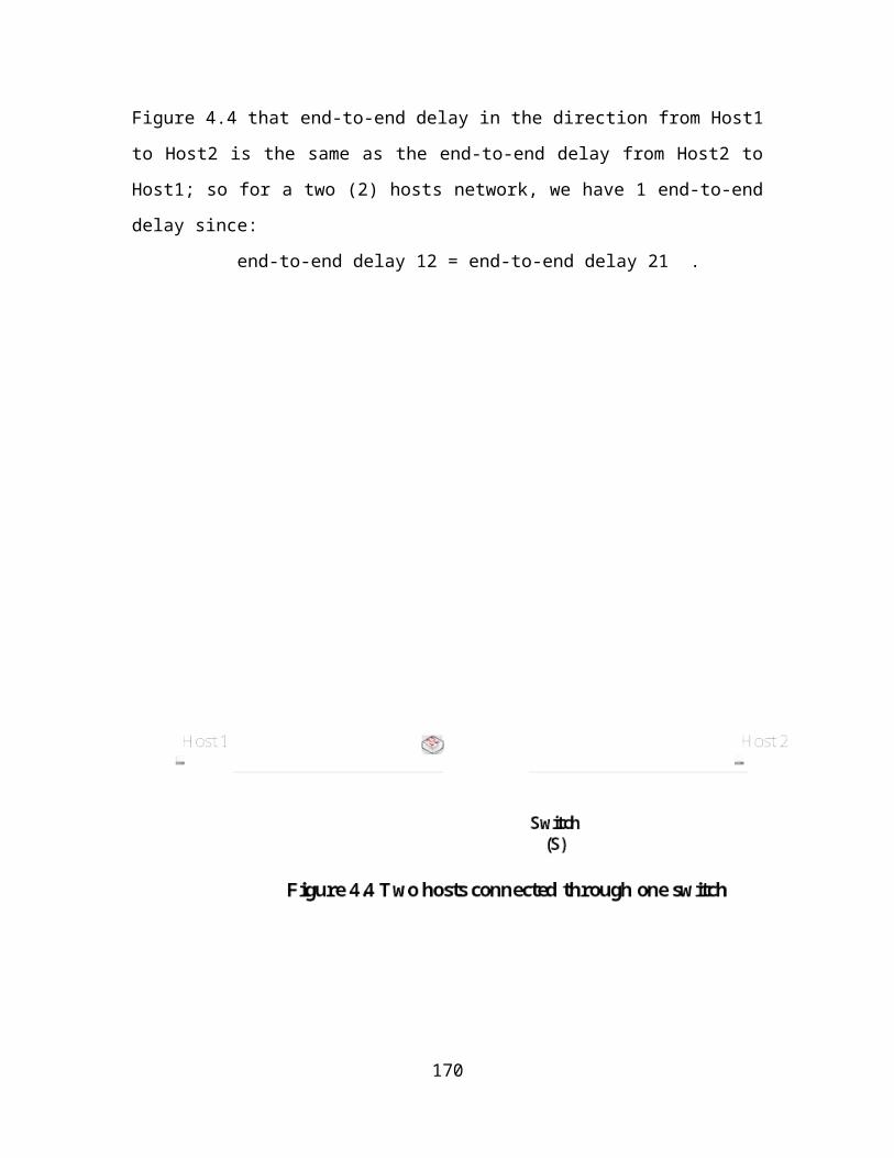
Figure 5.9 Covenant University CST Building LAN (excluding users’ hosts that are attached to the LAN)

170

VSATDVBReceiver

ModemCISCO2600Router

CISCO 3550 Switch

CISCO2950Switch

CISCO2950Switch

CISCO2950Switch

CISCO2950Switch

CISCO2950Switch

CISCO2950Switch

CISCO2950Switch

We now use our methodology to enumerate all the end-to-end delays in this LAN,

specify all the switches and router, and specify the up-link and down-link rates of the

Internet access device (VSAT); with a view to comparing the values obtained with the

actual values of these installed devices. The following are the illustrative procedures.

Label the switches and router using the right-most, pre-order transversal (this is

reflected in Figure 5.10).

For this LAN,

m = 9 = the number of switches in the LAN,

p, the number of maximum end-to-end delays required for the design of an upper

delay bounded LAN is given by Eq. (4.18) as;

p =

= (9-0)+(9-1)+(9-2)+(9-3)+(9-4)+(9-5)+(9-6)+(9-7) +(9-8)

= 9+8+7+6+5+4+3+2+1

= 45 maximum end-to-end delays

Assuming the maximum time for any data packet to cross Si = xi seconds, for i = 1, 2,

…,9,

then, associated with each of the switches S1, S2, S3, S4, S5, S6, S7, S8, and S9, is a

maximum end-to-end delay of x1(t1), x2(t2), x3(t3), x4(t4), x5(t5), x6(t6), x7(t7), x8(t8), and

x9(t9) respectively. We now list all the other maximum end-to-end delays as each of the

switches is being placed.

When S2 is placed, the maximum end-to-end delay is:

x2 + x1 = t10

When S3 is placed, the maximum end-to-end delays are:

x3 + x2 = t11

x3 + x2 + x1 = t12

171

Figure 5.10 Covenant University CST Building LAN (with only switching devices – router and switches)

172

Switch (S3)

Switch (S2)

Router (S1)

Switch (S9)

Switch (S5)

Switch (S4)

Switch (S7)

Switch (S8)

Switch (S6)

When S4 is placed, the maximum end-to-end delays are:

x4 + x3 = t13

x4 + x3 + x2 = t14

x4 + x3 + x2 + x1 = t15

When S5 is placed, the maximum end-to-end delays are:

x5 + x3 = t16

x5 + x3 + x2 = t17

x5 + x3 + x4 = t18

x5 + x3 + x2 + x1 = t19

When S6 is placed, the maximum end-to-end delays are:

x6 + x3 = t20

x6 + x3 + x2 = t21

x6 + x3 + x4 = t22

x6 + x3 + x5 = t23

x6 + x3 + x2 + x1 = t24

When S7 is placed, the maximum end-to-end delays are:

x7 + x3 = t25

x7 + x3 + x2 = t26

x7 + x3 + x4 = t27

x7 + x3 + x5 = t28

x7 + x3 + x6 = t29

x7 + x3 + x2 + x1 = t30

When S8 is placed, the maximum end-to-end delays are:

x8 + x3 = t31

x8 + x3 + x2 = t32

x8 + x3 + x4 = t33

x8 + x3 + x5 = t34

x8 + x3 + x6 = t35

x8 + x3 + x7 = t36

x8 + x3 + x2 + x1 = t37

When S9 is placed, the maximum end-to-end delays are:

173

x9 + x3 = t38

x9 + x3 + x2 = t39

x9 + x3 + x4 = t40

x9 + x3 + x5 = t41

x9 + x3 + x6= t42

x9 + x3 + x7 = t43

x9 + x3 + x8 = t44

x9 + x3 + x2 + x1 = t45

where t1, t2, t3,…,t44, t45 are the maximum end-to-end delays of this switched LAN.

In the LAN at Covenant University’s CST building shown in Figure 5.10, S2, S4, S5, S6,

S7, S8, and S9 are CISCO 2950 switches, S3 is a CISCO 3550 switch while S1 is a CISCO

2600 router. The 2950 is a 24-port switch, the 3550 is a 48-port switch, while the router

has 2 onboard LAN ports. We now proceed to calculate the maximum delay of an

Ethernet packet through each of these devices using the model of Eq. (3.29).

If,

D2950max = the maximum delay of an Ethernet packet in the CISCO 2950 switch,

D3550max = the maximum delay of an Ethernet packet in the CISCO 3550 switch, and

D2600max = the maximum delay of an Ethernet packet in the CISCO 2600 router,

we use the previous computation which was performed for the 24 ports Super Stack 11

Ethernet switch 3900 by 3Com Corporation for the CISCO 2950 switch (since they are

both 24 ports switches); this would imply that the maximum delay of an Ethernet packet

in the CISCO 2950 switch is:

D2950max = 0.12240ms + 0.00255ms + 0.05610ms + 0.12240ms + 41.616ms

= 41.91945 ms

42 ms

This is the maximum delay for switches S2(x2) seconds, S4(x4) seconds, S5(x5) seconds,

S6(x6) seconds, S7(x7) seconds, S8(x8) seconds, and S9(x9) seconds.

174

Since the CISCO 3550 switch has 48 ports, the routing or switching delay (RSD) and the

simultaneous arrivals of packets delay are computed as follows.

Routing or Switching delay (RSD) = secs.

where L = 12240 bits,

Ci = 100×106 bps

N= 48

therefore,

RSD =

=

= 127.5 ×10-8secs

= 0.00128 ms

Simultaneous arrivals of packets delay (SAD) = (N-2)× secs.

SAD = (N-2) ×RSD = (48-2)×RSD

= 46 ×0.00128ms

= 0.0589 ms

Therefore,

D3550max = 0.12240ms + 0.00128ms + 0.05890ms + 0.12240ms + 41.616ms

= 41.92ms

= 42 ms

This is the maximum delay for switch S3(x3 seconds).

The CISCO 2600 router has 2 onboard LAN ports (since it is an access router, see [85]),

the routing or switching delay (RSD) and the simultaneous arrivals of packets delay are

computed as follows.

175

Routing or Switching delay (RSD) = secs.

where L = 12240 bits,

Ci = 100×106 bps

N= 2

therefore,

RSD =

=

= 3060 ×10-8secs

= 0.0306 ms

Simultaneous arrivals of packets delay (SAD) = (N-2)× secs.

SAD = (N-2) ×RSD = (2-2)×RSD

= 0

Therefore,

D3550max = 0.12240ms + 0.0306ms + 0.12240ms + 41.616ms

= 41.89 ms

= 42 ms

This is the maximum delay for router or S1(x1) seconds.

The different maximum end-to-end delays in milliseconds are, therefore, t1= 42, t2= 42,

t3= 42, t4= 42, t5= 42, t6= 42, t7= 42, t8= 42, t9= 42

t10 = x2 + x1= 42 + 42= 82

t11 = x3 + x2 = 42 + 42= 82

t12 = x3 + x2 + x1= 42 +42 + 42 = 126

t13 = x4 + x3 = 42 + 42= 82

t14 = x4 + x3 + x2 = 42 +42 + 42 = 126

t15 = x4 + x3 + x2 + x1 = 42 +42 + 42 + 42 = 168

176

t16 = x5 + x3 = 42 + 42= 82

t17 = x5 + x3 + x2 = 42 +42 + 42 = 126

t18 = x5 + x3 + x4 = 42 +42 + 42 = 126

t19 = x5 + x3 + x2 + x1 = 42 +42 + 42 + 42 = 168

t20 = x6 + x3 = 42 + 42= 82

t21 = x6 + x3 + x2 = 42 +42 + 42 = 126

t22 = x6 + x3 + x4 = 42 +42 + 42 = 126

t23 = x6 + x3 + x5 = 42 +42 + 42 = 126

t24 = x6 + x3 + x2 + x1 = 42 +42 + 42 + 42 = 168

t25 = x7 + x3 = 42 + 42 = 82

t26 = x7 + x3 + x2 = 42 +42 + 42 = 126

t27 = x7 + x3 + x4 = 42 +42 + 42 = 126

t28 = x7 + x3 + x5 = 42 +42 + 42 = 126

t29 = x7 + x3 + x6 = 42 +42 + 42 = 126

t30 = x7 + x3 + x2 + x1 = 42 +42 + 42 + 42 = 168

t31 = x8 + x3 = 42 + 42 = 82

t32 = x8 + x3 + x2 = 42 +42 + 42 = 126

t33 = x8 + x3 + x4 = 42 +42 + 42 = 126

t34 = x8 + x3 + x5 = 42 +42 + 42 = 126

t35 = x8 + x3 + x6 = 42 +42 + 42 = 126

t36 = x8 + x3 + x7 = 42 +42 + 42 = 126

t37 = x8 + x3 + x2 + x1 = 42 +42 + 42 + 42 = 168

t38 = x9 + x3 = 42 + 42 = 82

t39 = x9 + x3 + x2 = 42 +42 + 42 = 126

t40 = x9 + x3 + x4 = 42 +42 + 42 = 126

t41 = x9 + x3 + x5 = 42 +42 + 42 = 126

t42 = x9 + x3 + x6 = 42 +42 + 42 = 126

t43 = x9 + x3 + x7 = 42 +42 + 42 = 126

t44 = x9 + x3 + x8 = 42 +42 + 42 = 126

t45 = x9 + x3 + x2 + x1 = 42 +42 + 42 + 42 = 168

From Eq. (4.19), the average maximum end-to-end delay = Davmax

177

= seconds

= ms

= 107 ms

From the above computations, the contention (for example in [74] and also shown in this

work) that the number of hosts that can be attached to a switched LAN is only limited by

the number of I/O ports available on the switches that are attached to the LAN is

justified; as it can be seen that the total maximum delay through a 24 port switch is

approximately the same as the total maximum delay through a 48 ports switch. The

bottleneck delay in switches is, therefore, the queuing delay.

Also, if we take the view expressed by Nielson in [81], that 100 ms is the maximum

delay before a user no longer feels that a network is reacting instantaneously, then the

switches’ placements in Covenant University’s CST building LAN (in the context of

Intranet) has not been properly done. This is because, there are end-to-end delays that are

much more than100 ms. Therefore, users at both ends of these origin-destination paths

will not have pleasurable experiences when-ever they are logged on to the network and

the network is heavily loaded and utilized.

5.3.3.2 Minimum Switching Fabric Transfer Rates Computation

From Eq. (4.21), the minimum switching fabric transfer rate (SFTRMIN) is given by;

SFTRMIN = bits/sec

For the CISCO 2950 switch,

N = 24, Ci = 100×106 bits/sec therefore,

SFTRMIN = bits/sec

= 2×24×100×106 bits/sec

= 48×108 bits/sec = 4.8 Gbps

178

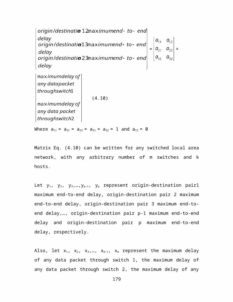
The specification for the CISCO 2950-24 in [86] is,

Switching fabric transfer rate (SFTR) = 8.8 Gbps

Therefore, this switch meets the minimum theoretical switching fabric transfer rate

desired.

For the CISCO 3550 switch,

N = 48, Ci = 100×106 bits/sec therefore,

SFTRMIN = bits/sec

=2×48×100×106 bits/sec

=96×108 bits/sec = 9.6 Gbps

The specification for the CISCO 3550 in [87] is,

Switching fabric transfer rate (SFTR) = 13.6 Gbps

Therefore, this switch meets the minimum theoretical switching fabric transfer rate

desired.

For the CISCO 2600 router,

N = 2, Ci = 100×106 bits/sec therefore,

SFTRMIN = bits/sec

=2×2×100×106 bits/sec

=400×106 bits/sec = 400 Mbps

The minimum Packet Transfer Rate (PTR) specification for the CISCO series 2600 router

in [85] is,

PTR = 15 kpps (kilo packets per second) = 183.6 Mbps

179

The minimum PTR specification for this router is not up to the theoretical minimum that

is desired; therefore, it is necessary to upgrade this router if packet queues are not to be

building up in it.

5.3.3.3 Estimating the Read/Write (RAM) Memory Capacities of the Switches and Router

From Eq. (4.22), the minimum read/write (RAM) capacity (RWMEMCAPMIN) for the

switches and router is given by;

RWMEMCAPMIN = (σ×1530×8) bits

where σ = the maximum amount of traffic that can arrive in a burst.

Since in this work σ is taken as 340 Ethernet frames, it means σ for all the three devices

(CISCO 2950 switch, CISCO 3550 switch and CISCO 2600 router) is;

RWMEMCAPMIN = (σ×1530×8) bits

= 340×1530×8 bits

= 4,161,600 bits

= 4.161 Mb

From CISCO specifications,

for CISCO 2950,

Read/Write Memory (RWM) shared by all ports is 8 Mb in size,

for CISCO 3550,

Read/Write Memory (RWM) shared by all ports is 4 Mb in size,

for CISCO 2600,

The minimum system memory for the CISCO series 2600 router is 4 Mb.

Therefore, it is reasonable to infer that there is not likely to be packet losses with the

arrival of burst traffic to these devices.

180

5.3.3.4 Determining the Maximum Number of Hosts that can be attached to the Switched Ethernet Local Area Network

It has previously been asserted in this work (page 138) that, if,

m = number of switches in an upper delay bounded designed switched LAN,

Nj = number of I/O ports in upper delay bounded specified switch j, then,

h, the number of hosts that can be connected to the LAN is given by Eq. (4.23) as:

h =

It is apparent from this equation that, the number of hosts that can be attached to a

switched LAN is only upper bounded by the number of I/O ports in the switches. This is

affirmed in [87].

5.3.3.5 Determining the Switched Ethernet Local Area Network’s Downlink and Uplink Rates for Internet access

We had previously shown that, for pleasurable uploading and downloading of Internet

traffic, the downlink and uplink rates (DLULRATES) of the Internet access device (for

example VSAT) is given by Eq. (4.26); where q is the number of origin-destination paths

in which the switch (or router) that is attached to the Internet access device is the only

source node or it is the only destination node and it (q) is also equal to the number of

switches in the switched LAN minus the switch (or router) that is attached to the Internet

access device.

From Annexure B, and Figures 5.9 and 5.10, it can be seen that q is equal to 7. Therefore,

if we take Zi as 100 Mbps, Eq. (4.26) gives;

DLULRATES = bits/sec

= 7×100×106 Mbps

= 700 Mbps.

CHAPTER 6

181

SUMMARY OF MAJOR FINDINGS, CONCLUSIONS AND RECOMMENDATIONS

6.1 Summary of Major Findings

1. This work has for the first time shown (by using network calculus concepts) that, the

maximum queuing delay of a packet switching device is indeed the ratio of the maximum

amount of traffic that can arrive in a burst at an output port of the device to the capacity

of the link (data rate of the media) that is attached to the port.

2. Novel Ethernet packet switch model and switched Ethernet LAN maximum end-to-

end delays determination methodology were developed and validated (the former by

practically comparing the model’s maximum delay value with values that were obtained

from literature and the latter, by applying the methodology to an existing switched LAN

installation) in this work. Although researchers have proposed some Ethernet packet

switch models in literature in efforts at solving the delay problem of switched Ethernet

networks, we have found that these models have not put into consideration, two factors

that contribute to packet delays in a switch – the simultaneous arrival of packets at more

than one input port, all destined for the same output port and the arrival of burst traffic

destined for an output port. Our maximum delay packet switch model is, therefore,

unique in that we have put into consideration, these two factors. More importantly, our

methodology (the switched Ethernet LANs maximum end-to-end delays determination

methodology) is particularly very unique, as to the best of our knowledge researchers

have not previously considered this perspective in attempts at solving the switched

Ethernet networks end-to-end delay problem.

3. This work has also revealed (and this was clearly shown from first principles) that, the

widely held notion in literature as regards origin-destination pairs of hosts enumeration

for end-to-end delay computation purposes appears to be wrong in the context of

switched local area networks. We have shown for the first time, how this enumeration

should be done. The need to report this discovery and the end-to-end delays enumeration

methodology led to two initial papers [88], [89] from this work.

182

4. A formal method for designing upper-bounded end-to-end delay switched Ethernet

LANs using the model and methodology that were developed in (2) was developed in this

work. This method for designing upper-bounded end-to-end delay switched LANs will

make it possible for network ‘design’ engineers to design fast-response, switched

Ethernet LANs. This is quite a unique development, as with our methodology, the days

when network ‘design’ engineers only have to position switches of arbitrary capacities in

any desired position are numbered; as switches will now be selected and positioned based

on an algorithm that was developed from clear cut mathematical formulations.

5. It has also been empirically shown in this work that the number of hosts that can be

attached to any switched LAN is actually bounded by the number of ports in the switches

of which the LAN is composed.

6.2 Conclusions

The following major conclusions have been made from the findings of this study:

1. The predominant cause of delay (sluggishness) in switched LANs is the queuing

delay, and not the number of users that are connected to the LAN. The fact that the

network becomes slow as more users are logged on to the network is as a result of the

flow of bursty traffic (uploading and downloading of high-bit rates and bandwidth

consuming applications).

2. In the context of (1) above, the solution as have been shown in this work is to limit the

number of switches between all origin-destination hosts, and/or to upgrade certain inter-

switch media to higher bit-rates media.

6.3 Recommendations

In the context of the major findings of this work, and the conclusions that have been

arrived at, the following recommendations are deemed desirable:

1. It is recommended that for any switched Ethernet LAN design, there should be at most

three (3) inter-host switches between any two hosts. For switch placements that need to

183

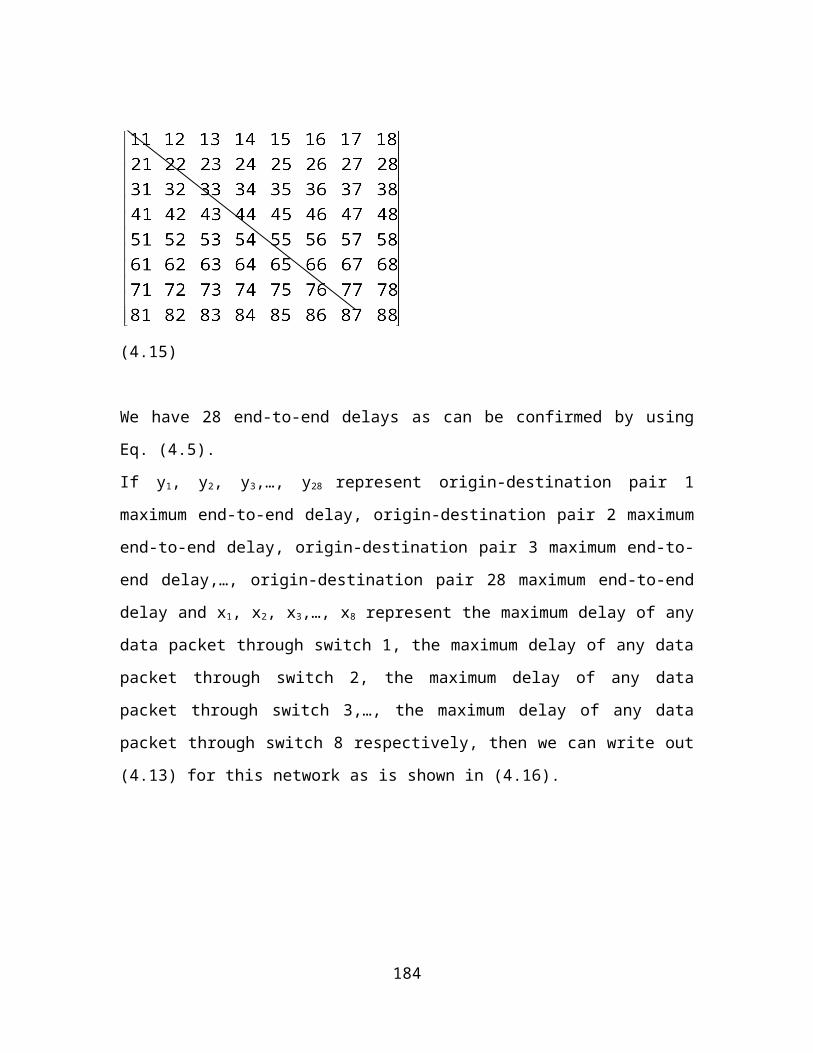
exceed this value, higher data rate media (in this case gigabits/sec media) should be used.

That is, if it is necessary to connect two hosts in any switched Ethernet LAN by more

than three switches, between the 3rd and 4th switches, the 4th and 5th switches and so on,

higher data rate media should be used; always of course, the media originating from

servers should be of gigabits/sec. capacity. This is in consonance with one of the

recommendations in [61], where it was stated that; in client-server computing

environment, a single station, the server, is often the target or source for most of the

traffic from and to a large number of client workstations; for such configurations, a

higher bandwidth (fat pipe) attachment is needed for the server. For example, a single

100 Mbps Fast Ethernet port can be used to attach a file-server that is accessed by a

multitude of 10 Mbps Ethernet workstations, with the client workstations attached to the

switch via 10 Mbps ports.

2. Therefore, when a server or another switch is in the down stream of an output port

loading more traffic on the trunk link, to reduce the buffering delay, it may be necessary

to put more bandwidth on such a trunk link by deploying one or more solutions, for

example, trunk link aggregation or 1 Gbps link or 10 Gbps link.

3. In the context of the Covenant University CST building LAN, Switch S2 (CISCO

2950) is redundant; hence, it is a bottleneck to pleasurable Internet sessions (uploading

and downloading of information). Therefore, it should be removed, as it is only

increasing end-to-end delays of some paths by 42ms.

4. Still on the Covenant University CST building LAN, the CISCO 2600 router should

be removed, since the CISCO 3550 switch performs both layers 2 and 3 functions; that is,

it performs the layer 3 functions of the CISCO 2600 router.

6.3.1 Suggestions for Further Studies

184

Some problems’ areas were discovered in the course of this research work. Our further

efforts and in fact the efforts of other interested researchers, would be/could be geared

towards finding solutions to these problem areas. These include:

1. Determining a value for σ. The most pressing challenge that was encountered in this

work is obviously determining a value for σ (the maximum amount of traffic that can

arrive to a switch in a burst). This is presently an area of very intense research activity. In

fact, it is the, believe here that, coming out with an empirically validated value for σ (or

how to determine σ) will be a major breakthrough to the Internet and Networking

research community.

2. Introduction of weighting function(s) in the end-to-end delay models. The need to

introduce weighting function(s) in the end-to-end delays computations for the purpose of

calculating the average network end-to-end delay is very imperative. This is because, the

end-to-end paths of a switched LAN are of different lengths (the number of switches

between pairs of hosts are different).

3. The need to introduce cost variables in determining the optimal Internet access device

input and output rates. This should include the cost of bandwidth and of wasted time due

to slow access to the Internet when bandwidth is inadequate.

4. There may also be the need to introduce in the maximum delay packet switch model

proposed in this work, some mechanisms of IEEE 802.1p and IEEE 802.1D. That is,

there may be the need for the inclusion of the prioritization and differentiation of packets

mechanisms in the switch model.

REFERENCES

185

[1] Fortier, P. and Desrochers, G. (1999), “Modeling and Analysis of Local Area Networks”, CRC Press, New York, USA

[2] Kanem, E., Torab, P., Cooper, K., and Custodi, G. (1999), “Design and Analysis of Packet Switched Networks for Control Systems”, Proceedings1999 IEEE Conference on Decision and Control, Phoenix, AZ, pp. 4460-4465

[3] Torab, P. and Kanem, E. (1999), “Load Analysis of Packet Switched Networks in Control Systems”, Proceedings 25th Annual Conference of the IEEE Industrial Electronics Society, San Jose, CA, vol. 3, pp.1222 - 1227

[4] Abiona, O. (2005), “Development of a Framework for Optimizing Access to WAN Resources”, Ph.D Computer Science Thesis, Obafemi Awolowo University, Ile-Ife, Nigeria

[5] Gallo, A. and Wilder, R. (1981), “Performance Measurement of Data Communication Systems with Emphasis on Open System Interconnections (OSI)”, Proceedings 8th= IEEE Annual Symposium on Computer Architecture, Minneapolis, USA, May 12-14, pp.149-161

[6] Song, Y. (2001), “Time Constrained Communication over Switched Ethernet”, Proceedings IFAC International Conference on Fieldbus Systems and their Application, Nancy, France, pp. 152-169

[7] Fowler, H. and Leland, W. (1991), ”Local Area Network Traffic Characteristics, with implications for Broadband Network Congestion Management”, IEEE Journal on Selected Areas in Communications, vol. 9, issue. 7, pp.1139-1149

[8] Falaki, S. and Sorensen, S. (1992), ”Traffic Measurements on a Local Area Computer Network”, Butterworth Heinemann Computer Communications Journal, vol. 15, no. 3, pp.192-197

[9] Elbaum, R. and Sidi, M. (1996), “Topological Design of Local Area Networks using Genetic Algorithms”, IEEE/ACM Transactions on Networking, vol.4, no. 5, pp. 766-778

[10] Bertsekas, D. and Gallager, R. (1992), “Data Networks”, Prentice-Hall, Englewood Cliffs, USA

[11] Gerd, K. (1989), “Local Area Networks”, McGraw-Hill Book Co., New-York, USA

[12] Kamal, E. (1987), “Star Local Area Networks: A Performance Study”, IEEE Transactions on Computers, vol. C-36, no. 4, pp.483-499

[13] Mann, R. and Terplan, K. (1999), “Network Design: Management and Technical Perspectives”, CRC Press Ltd, New-York, USA

[14] Reiser, M. (1982), “Performance Evaluation of Data Communications Systems”, Proceedings of the 1982 IEEE Conference, vol. 70, no. 2, pp.171-194

[15] Cruz, R. (1991) (a), “A Calculus for Network Delay, Part 1: Network Elements in

186

Isolation”, IEEE Transactions on Information Theory, vol. 37, no.1, pp.114-131

[16] Ferguson, P. and Huston, G. (2009), “Quality of Service in the Internet: Facts, Fiction or Compromise?” Available: http://eprints.kfupm.edu.sa (20-08-2009)

[17] Ming-Yang, X., Rong, L. and Huimin, C.(2004), “Predicting Internet End-to-End Delay: An Overview”, Proceedings of the IEEE 36th South Eastern Symposium on Information Systems Theory, pp. 210 - 214

[18] Bolot, J. (1993), “Characterizing End-to-End Packet Delay and Loss in the Internet”, Journal of High-Speed Networks, vol.2, no. 3, pp. 305-323

[19] Krommenacker, N., Rondeau, E, and Divoux, T. (2001), “Study of Algorithms to Define the Cabling Plan of Switched Ethernet for Real-Time Applications”, Proceedings of the 8th IEEE International Conference on Emerging Technologies and Factory Communications, Antibes, pp.223-230

[20] Anurag, K., Manjunath, D. and Kuri, J. (2004), “Communication Networking: An Analytical Approach”, Morgan Kaufmann Publishers, San Francisco, USA

[21] Martin, S., Minet, P. and Laurent, G. (2005), “End-To-End Response Time with Fixed Priority Scheduling: Trajectory Approach Versus Holistic Approach”, International Journal of Communication Systems, vol. 18, pp.37-56

[22] Ingvaldsen, T., Klovning, E., and Wilkins, M. (2000), “Determining the Causes of End-to-End Delay in CSCW Applications”, Computer Communication, vol. 23, issue 3, pp.219-232

[23] Trulove J., (2000), “Broadband Networking”, CRC Press, Boca Raton, Florida, USA

[24] Clark, K. and Hamilton, K. (1999), “CISCO LAN Switching”, CISCO Press, Indianapolis, Indiana, USA

[25] Muhammed, I., Asif, S., Syed, S., and Khaled, M. (2009) “Performance Analysis of Switches in High Speed LAN”, 2009 ASEE Northeast Section Conference, University of Bridgeport, Connecticut, pp.1-6

[26] Forouzan, B. (2008), “Data Communications and Networking”, 4th Edition, Tata McGraw-Hill Limited, New Delhi, India

[27] Georges, J., Divoux, T. and Rondeau, E. (2005), “Confronting the Performances of Switched Ethernet Network with Industrial Constraints by using Network Calculus”, International Journal of Communications Systems, vol.18, pp. 877-903

[28] Georges. J., Divoux, T. and Rondeau, E. (2003), “Comparison of Switched Ethernet Architecture Models”, Proceedings IEEE Conference on Emerging Technologies and Factory Automation, Lisbon, Portugal, pp. 375-382

[29] Cruz, R. (1991) (b), “A Calculus for Network Delay, Part 2: Network Analysis”, IEEE Transactions on Information Theory, vol. 37, no.1, pp.132-141[30] Halsall, F. (1992), “Data Communications, Computer Networks and Open

187

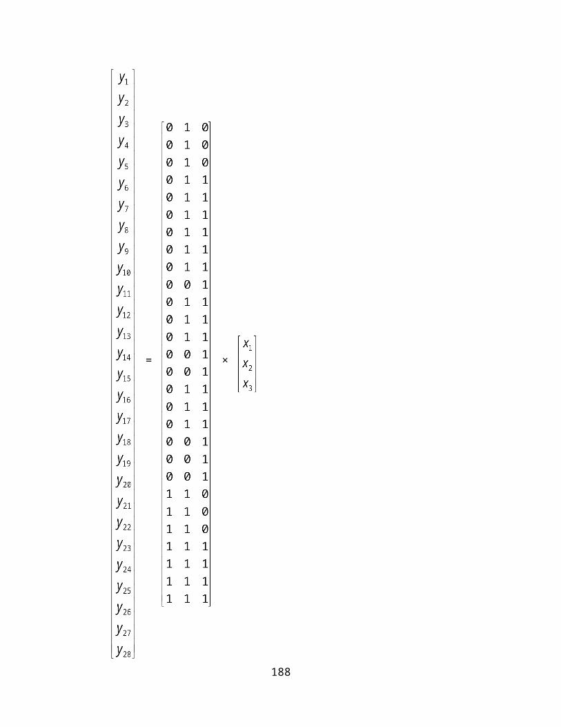
Systems”, Addison-Wesley Publishers, Workinghan, England

[31] Georges J., Krommenacker, N., Divoux, T. (2006), “A Design Process of Switched Ethernet Architectures According to Real-Time Application Constraints”, Engineering Applications of Artificial Intelligence, vol.19, issue 3, pp.335-344

[32] Jasperneite, J. and Ifak, N. (2001), “Switched Ethernet for Factory Communication”, Proceedings 8th IEEE International Conference on Emerging Technologies and Factory Automation (ETFA 2001), Antibes, France, pp.205-212

[33] Kakanakov, N., Shopov, M., Spasov, G. and Hristev, H. (2007), “Performance Evaluation of Switched Ethernet as a Communication Media in Controller Networks”, Proceedings International Conference on Computer Systems and Technologies (Compusys. Tech. 07), pp.9.2-9.7

[34] Costa P., Netto J., and Pereira, C. (2004), “Analysis of Traffic Differentiation on Switched Ethernet”, Proceedings of the International Workshop on Real-Time Networks Available: http://www.ieeta.pt/lse/rtn2004/preprints (20-08-2009)

[35] Comer, D. (2004), “Computer Networks and Intranets with Internet Applications”, Pearson Prentice Hall, New Jersey, USA

[36] Michael, D. and Richard, R. (2003), “Computer Communications and Data Networks for Computer Scientists and Engineers”, 2nd edition, Pearson Prentice Hall, Essex, England

[37] Alberto, L. and Widjaja, I. (2004), “Communications Networks: Fundamental Concepts and Key Architectures”, McGraw Hill, New-York, USA

[38] Bejerano, Y., Breithart, Y., Garofalakis, M. and Rastogi, R. (2003), “Physical Topology Discovery for Large Multi-Subnet Networks”, IEEE Transactions on Networking, vol. 3, no. 6, pp.342-352

[39] Ersoy, C. and Panwar, S. (1993), “Topological Design of Interconnected LAN/MAN Networks”, IEEE Journal on Selected Areas in Communications, vol.11, no.8, pp.1172-1182

[40] Song Y., Koubaa A., Simonot F., and Li Lorraine F. (2002), “Switched Ethernet for Real-Time Industrial Communication: Modeling and Message Buffering Delay Evaluation”, 4th IEEE International Workshop on Factory Communication Systems, Vasteras, Sweden, pp.27-35

[41] Gross, L. and Yellen, J. (2006) “Graph Theory and Its Applications”, 2nd Edition, Chapman and Hall, New-York, USA

[42] Haggarty, R. (2002), “Discrete Mathematics for Computing”, Pearson Education Ltd, Essex, England

[43] Jin C., Drew D., Scott V., and Bin Y.(2000), “Time-Varying Network Tomography: Router Link Data”, Journal of the American Statistical Association: Application and Case Studies, vol. 95, no. 452, pp.1063-1075

188

[44] Jasperneite, J., Neumann, P., Theis, M., and Watson, K. (2002), “Deterministic Real-Time Communication with Switched Ethernet”, 4th IEEE International Workshop on Factory Communication Systems, Vasteras, Sweden, pp.11-18

[45] “Spanning Tree Protocol”, Available: http://en.wikipedia.org/wiki/spanning tree protocol (10-09-2009)

[46] “Robust Mathematical Modeling”, Available: http://pagespersoorange.fr/ scmsa/RMM/robust (23-04-2008)

[47] Georges, J., Rondeau, E. and Divoux, T. (2002), “Evaluation of Switched Ethernet in an Industrial Context using the Network Calculus”, 4th IEEE International Workshop on Factory Communication Systems, Vasteras, Sweden, pp.19-26

[48] Le Boudec, J. and Thiran, P. (2004), “Network Calculus: Theory of Deterministic Queuing Systems for the Internet”, Springer, Verlag

[49] Krishna, P., Jens, S. and Ralf, S. (2004), “Network Calculus meets Queuing Theory: A Simulation-based Approach to Bounded Queues”, Proceedings of the 12th IEEE International Workshop on Quality of Service (IWQoS 2004), Montreal, Canada, pp.114-118

[50] Anantharam, V. (1993), “An Approach to the Design of High-Speed Networks for Bursty Traffic”, Proceedings of the 32nd IEEE Conference onDecision and Control, San Antonio, Texas, pp.1678-1679

[51] Lafore, R. (1999), “Data Structures and Algorithms in 24 Hours”, SAMS Publishing, Indiana, USA

[52] Sadgewick, R. (2006), “Algorithms in C”, 3rd Edition, Addison-Wesley Publishing, New York, USA

[53] Mauro, C., Pierre, C., Afrodite, S., and Nicolas, S. (2009), “Project SEQUIN – Final Document on Definition of Quality of Service”, Available: http://archive-dante.net/upload/pdf/SEQ-01-030. (17-08-2009)

[54] White paper by Technical University of Cluj, Napoca (2009), “Wireless LAN Medium Access Techniques: QoS Perspective”,

Available: http://whitepapers.techrepublic.com/abstract (17-08-2009)

[55] Wollingger, B., Wolf, J., and Le Grand, G. (2005), “Improving Node Behaviour in a QoS Control Environment by means of Load-Dependent Resource Redistributions in LANs”, International Journal of Communication Systems, vol. 18, pp.373-394

[56] “Quality of Service”, Available: http://en.wikipedia.org/wiki/Quality-of-Service (20-08-2009)

[57] Koubaa, A., Jarraya, A., and Song, Y. (2009), “SBM Protocol for Providing Real- Time QoS in Ethernet LAN” Available: http://www.dei.isep.ipp.pt/akoubaapublications (03-04-2009)

[58] “Your Dictionary.Com”,Available: http://www.yourdictionary.com/telecom/802.1p (20-08-2009)

189

[59] Law, A. and Kelton, D. (2003), “Simulation Modeling and Analysis”, 3rd Edition,Tata McGrawHill, New-Delhi, India

[60] “Physical Layer Switch System for Ethernet Local Area Communication System; US Patent No. 5889776”, Available: http://www.freepatentsonline.com/5889776. (10-11-2008)

[61] Christensen, K., Hass, L., Noel, F. and Stole, N. (1995), “Local Area Networks – Evolving from Shared to Switched Access”, IBM Systems Journal, pp.347-374

[62] “RFC 1122 on Requirements for Internet Hosts—Communication Layers”, Available: http;//www.ietf.org/rfc/rfc1122 (20-08-2009)

[63] Sven, U., Ales, F., and Stanislav, H. (2008), “Quantification of Traffic Burstiness with MAPI Middleware”, Proceedings 2008 CESNET (Czech Educational and Scientific Network) Conference, Prague, Czech Republic, pp.13-22

[64] Ryousei, T., Yuetsu, K., Tomohiro, K., Motohiko, M., and Fumihiro, O. (2006), “Real Time Burstiness Measurement”, Proceedings PFLDnet 2006 Conference, Nara, Japan, pp.109-115

[65] Khalil, K. and Sun, Y. (1992), “The Effect of Bursty Traffic on the Performance of Local Area Networks”, Proceedings IEEE Global Telecommunications Conference (GLOBECOM), Orlando, Florida, USA, pp.597-603

[66] Medhi, J. (2003), “Stochastic Models in Queuing Theory”, 2nd Edition, Academic Press, Elsevier Science, Orlando, Florida, USA

[67] Paxson, V. (1999), “End-to-End Internet Packet Dynamics”, IEEE/ACM Transactions on Networking, vol. 7, no. 3, pp.277-292

[68] “Request For Comments 2544”, Available: http://www.ietf.org/rfc/rfc 2544 (20-08-2009)

[69] 3 Com Technical Paper, “Layer 3 Switching: An Introduction”, Available: http://www.pulsewan.com/data101/pdfs/layer3_switching (23-05-2009)

[70] Kreyzig, E. (2003), “Advanced Engineering Mathematics”, 8th Edition, John Wiley and Sons, New York, USA

[71] Metzler, J. (2009), “A LAN Perspective on Wireless WAN Requirements”, Available: http://www.ashtonmetzler.com/Apps_Paper (24-06-2009)

[72] Tanenbaum, A. (2006), “Computer Networks”, 4th Edition, Prentice-Hall of India Private Limited, New Delhi, India

[73] “RFC 2544: How it helps Qualify a Carrier Ethernet Network”, Available: http://documents.exfo.com/appnotes/anote 183 (15-03-2009)

[74] “IP Multicast Best Practices for Enterprises Customers”, Available: http://www.cisco.com/application/pdf/en/US/guest (24-06-2009)

[75] Oppenheiner, P.(2004), “Top-Down Network Design”, Prentice Hall, New-York, USA

190

[76] Adegbenro, O. (1986), “LSI-Oriented Residue Arithmetic Circuits and their Application in the Implementation of a Digital Signal Processor”, A Dissertation for the Degree of Doctor of Engineering , Department of Electronic Engineering, Faculty of Engineering Graduate Division, Tohoku University, Sendai, Japan

[77] Gilberto, F., Marcos, P., Emmanuel, J., Martin, F. and Martin, J. (2009), “OPNET Modeler and Ns-2: Comparing the Accuracy of Network Simulators for Packet – Level Analysis using a Network Test bed”, Available: http://genie.iitd.ernet.in/ns/weas (20-08-2009)

[78] “Y.1541-QOSM—Y1541 QoS Model for Networks Using Y.1541 QoS Classes”, Available: http://tools.ietf.org/html/draft-ietf-nsis-y1541-qs (15-03-2009)

[79] “Voice Over Packet: An Assessment of Voice Performance in Packet Networks”, White Paper by Nortel Networks, Available: http://www.nortel.com/products/library/collateral (15-07-2009)

[80] “Technical Requirements for CISCO QoS Certified Metro Networks”, White Paper on Metro-Ethernet, Available: http://www.ciso.com/en/US/solutions/collateral (15-07-2009)

[81] Nielson, J. (2009), “Designing Web Usability”, Available: http://www.amazon.com/Designing-Web-Usability-Jakob-Nielson/dp (15-07-2009)

[82] “Integrated Services Mappings on IEEE 802 Networks”, Available: http://tools.ietf.org/html/rfc2815 (20-08-2009)

[83] “Square D® Ethernet Switch Model SDM 5DE 100 Installation and Illustration Bulletin”, Available: www.us.Square D®

(03-02-2009)

[84] Lawrie, M.(1985) “Foundations of Programming with Pascal”, Ellis Horwood Ltd, West Sussex, England

[85] “Cisco 2600 Series System Specification”, http://www.onsiteaustine.com/whitepapers/cisco%202600.pdf (09-08-2009) Available: http://www.cisco.com/en/US/products/collateral/router (09-08-2009)

[86] “Cisco 2950 Series Switch Specification”, Available: http://www.cisco.com/en/US/products/hw/switches (09-08-2009)

[87] “Cisco 3550 Series Switch Specification”, Available: http://www.cisco.com/en/US/products/collateral/switches (09-08-2009)

[88] Eyinagho, M. O., Falaki, S. O. and Atayero, A. A., “Revisiting the Notion of Origin-Destination Traffic Matrix of the Hosts that are attached to a Switched Local Area Network” (accepted paper), The World Congress on Engineering and Computer Science 2010, San Francisco, 20-22 October, 2010

[89] Eyinagho, M. O., Falaki, S. O. and Atayero, A. A., “Determination of the End-To- End Delays in any Switched Local Area Network” (accepted paper), International Journal of Electrical and Computer Sciences (in press)

191

[90] “Request For Comments 2285”, Available: http://www.faq.org/rfcs/rfc 2285.(20-04-2009)

[91] “Request For Comments 1944”, Available: http://rfc.tstsrc.org/rfc/rfc 1944 (20-04-2009)

192

193

194

195

196

197

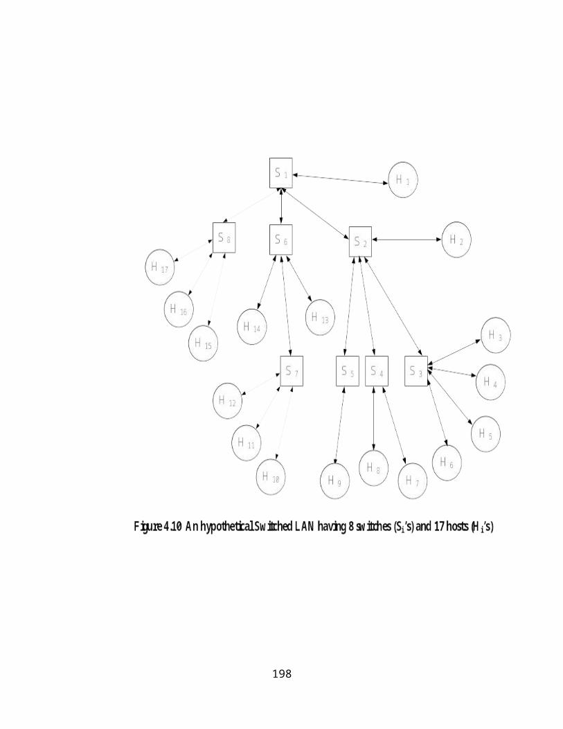
198

199

APPENDIX A

RFC 2285 – Benchmarking terminology for LAN switching devices. Source [90]

Burst: A sequence of frames transmitted with the minimum legal inter-frame gap.

Burst Size: The number of frames in a burst; burst size can range from one to infinity,

there is no theoretical limit to burst size.

Measurement Units: No of N-octet frames.

Inter-burst gap (IBG); This is the interval between two bursts.

Bidirectional traffic are inherently bursty, since interfaces share their time between

receiving and transmitting frames.

Measurement units:

- nanoseconds

- microseconds

- milliseconds

- seconds

Loads; the rates at which traffic is offered to any DUT (Device Under Test) or SUT

(System Under Test).

Offered Load; the number of frames per second that an external source can be observed

or measured to transmit to a SUT/DUT for forwarding to a specified output interface or

interfaces.

200

Maximum Offered Load (MOL); is the highest number of frames per second that an

external source can be observed or measured to transmit to a SUT/DUT for forwarding to

a specified output interface or interfaces.

Maximum Frame Rate (MFR); is the maximum frame rates that should be used when

testing LAN connections should be the listed theoretical maximum rate for the frame size

on the media [91].

201

APPENDIX B

Some typical Ethernet Packet Switch Specification Data

1. ISCOM 2009 Managed L2 Access Ethernet Switch;

Features

Forwarding mode: Store and Forward

Maximum Frame Size: 1632 Bytes

Port Rate Limiting: Based on ingress and egress

of each port, ranging from 63 Kbps

to 100 Kbps

Specification

Performance: Switching fabric; 1.8 Gbps

Capacity: 32 MB SDRAM, 4 MB flash,

128 KB switch buffer, 8 KB MAC

address, 255 IGMP groups

VLAN IEEE 802.1Q support: Up to 4 output queues IEEE 801.1p

Priority

QoS and ALL: diffServe and IP TOS

2. CISCO Catalyst 2900 Fast Ethernet Switch;

Key Features

Data Transfer Rate: 1000 Mbps

Installed Memory: 16 Mbps

Networking Connection Type: IEEE 802.3, Fast Ethernet, IEEE

802.3u, IEEE 802.1d, Ethernet

Networking Ports: 24 ports

202

APPENDIX C

Definition of Linear Independence and Dependence [70, p.336]

p vectors x(1), x(2), ……..,x(p) (with n components each) are linearly independent if the

matrix with row vectors x(1), x(2), ……..,x(p) has rank p; they are linearly dependent if the

rank is less than p. Since each of the P vectors has n components, that matrix, call it A,

has p rows and n columns; and if n < p, then by the preceding assertion, rank A ≤ n < p.

Therefore, p vectors with n < p components are always linearly dependent.

203

APPENDIX D

D.1 Y.1541: IP Network QoS Definitions and Network Performance

Objectives

Class Network Performance Parameter Targeted Applications

(network delay) objectives

0 100ms Real-time, highly interactive;

for example, VOIP, Video Con-

ferencing

1 400ms Real-time, highly interactive;

for example, VOIP, Video Con-

ferencing

2 100ms Transaction data, highly

interactive (for example,

signaling)

3 400ms Transaction data, highly

interactive

4 1 second Low-loss only(short transactions,

bulk data, video streaming

5 U (unspecified) Traditional applications of default

IP networks.

D.2 RFC 2815: Inter-Serv Mappings on IEEE 802 Networks

User-Priority (Class of Service) Service

0 Default, assumed to be Best Effort

1 Reserved, less than ‘Best Effort’

2 Reserved

3 Reserved

4 Delay Sensitive, no bound

5 Delay Sensitive, 100ms bound

6 Delay Sensitive, 10ms bound

204

7 Network Control

205