Title Page

Title:

Conjunctive Management of Surface-Groundwater Resources by coupling a hybrid Wavelet-

ANFIS/ Fuzzy C-means (FCM) Clustering Model with Particle Swarm Optimization (PSO):

Application to the Miandarband Plain, Iran

Author names and affiliations

Mohammad Zare, Manfred Koch

Department of Geohydraulics and Engineering Hydrology, University of Kassel.

Kurt Woltersstr. 3,

34109 Kassel,

Germany

Email : mzare896@gmail.com

Conjunctive Management of Surface-Groundwater Resources by coupling a hybrid

Wavelet-ANFIS/ Fuzzy C-means (FCM) Clustering Model with Particle Swarm

Optimization (PSO): Application to the Miandarband Plain, Iran

Abstract

Conjunctive management of surface-groundwater resources systems by means of mathematical

optimization-simulation techniques becomes an important issue for sustainable water resources

development, namely in water scarce regions. In this study, the particle swarm optimization (PSO)

method has been coupled with a hybrid Wavelet/ANFIS- fuzzy C-means (FCM) simulation model to

determine the optimal agricultural irrigation water allocation in the Miandarband plain, western Iran.

Firstly the optimal amount of conveyed water (CW) from the Gavoshan dam into the plain is determined

by constrained PSO. The constraints are the long-term minimum monthly exceedance streamflows that

are estimated for different exceedance probabilities – with an 70% value found to best reflect the average

annual river inflow of 3.4 m3/s into the dam – using two-parameter Weibull distribution as well as the

classical Weibull non-parametric plotting position method. Then, based on the politically prioritized

proportions of the dam’s allocated water for domestic, environmental and agricultural uses, as well as

the share of the plain for agriculture, the optimal monthly CW available for the plain (=112 MCM/a) is

obtained. However, the subsequent estimation of the irrigation water request (IWR) (= 265.8

MCM/a) calculated by the FAO-56 method and using empirical crop coefficients of the present

agricultural pattern in the plain indicates that there is an irrigation water deficit of 153.1 MCM/a

that must be made up by groundwater withdrawal (GW) in a way that neither waterlogging nor severe

drop condition in groundwater level (GL) will occur. The latter are then calculated by the hybrid

Wavelet/ANFIS (FCM) model, with good performance indicators R2 and RMSE equal to 0.98 and 0.21m

and 0.94 and 0.31m in the testing and training phases, respectively. Finally, PSO and the hybrid model

are coupled to simulate the GL- fluctuations – with the above GL-constraints - under conjunctive use

of the optimal surface (CW) and groundwater resources (GW) in the Miandarband plain. In conclusion,

the innovative coupled simulation/optimization model turns out to be a very useful tool for optimal and

sustainable conjunctive management of surface-groundwater resources in an irrigation area.

Keywords: Conjunctive surface-groundwater management; hybrid Wavelet/ANFIS-FCM model; particle

swarm optimization; irrigation water requirement Miandarband plain; Iran.

1. Introduction

Changing hydrological conditions occurring in arid and semi-arid regions, owing mostly to

phenomena of climate change, that affect rainfall temporally and spatially, as well as the

increasing exploitation of surface and groundwater resources have caused fundamental

variations in the surface water flow regimes and severe drops of groundwater levels in many

regions of the world (Fink and Koch, 2010; Koch, 2008). Responding appropriately to the

usually growing water demands - not to the least due to the increasing population in the

countries that are mostly affected by such events - under these threatening situations,

necessitates the use of the techniques of integrated water resources management more than ever

before. The main priority of the latter is to find suitable methods and models in order to simulate

the optimal use of the available and dwindling water resources.

Decision making and planning for the prediction of future water-affecting events and

conditions can effectively only be realized by deterministic or stochastic numerical models

(Zare and Koch, 2016a). Appropriate models and algorithms such as conceptual models,

artificial intelligence models (ANN), evolutionary algorithms, swarm Intelligence and fuzzy

logic have been developed and used in many research projects of conjunctive management of

surface-groundwater resources in recent years. The combination of these models and algorithms

has led to an increased accuracy in the modeling of water resources allocation problems (Peralta

et al., 2014; Das et al., 2015; Mani et al., 2016).

Raman and Chandramouli (1996) used ANN for inferring optimal release rules, conditioned

on initial storage, inflows, and demands for the Aliyar reservoir in Tamil Nadu, India. Results

of a deterministic DP model for the reservoir for 20 years of bimonthly data serve as a training

set for the artificial neural network. The training of an ANN is an optimization process, usually

performed by a gradient-type back propagation procedure which determines the values of the

weights on all interconnections that best explain the input-output relationships between the

neurons of the ANN. Singh (2014) emphasized the need for an appropriate conjunctive

management of water resources, i.e. surface and groundwater, for agricultural irrigation

purposes, as this methodology is not only useful for water storage problems, but reduces also

the environmental degradation in the irrigated areas. Safavi and Enteshari (2016) presented a

simulation/optimization model for conjunctive use of surface-groundwater resources in the

Najafabad plain, Iran, using ANN and an ant colony optimization were used in their study. They

showed that the conjunctive management model modified the water allocation temporally

which enhances the water use efficiency.

All these studies indicate that by combining a simulation and optimization model, suitable

results for conjunctive surface-groundwater management can be obtained. In the simulation

phase, Artificial Intelligence- (AI) methods, such as ANFIS and FFNN, have been found to

be flexible and useful methods (Zare and Koch, 2016b), however, AI is facing problems

when the hydrological time series are non-stationary. To overcome this problem, signal-

processing methods, like wavelet-tools may be combined with AI- models.

In this study, the Wavelet-ANFIS model based on a powerful unsupervised algorithm,

which organizes the data into groups, based on similarities within the ANFIS- model, will be

used for modeling conjunctive surface-groundwater use in the Miandarband plain, western Iran,

whose major water supply comes from the Gavoshan dam. The algorithm uses a Fuzzy C-

means (FCM) clustering method, i.e. the whole procedure may be called a Wavelet-

ANFIS/FCM, which has been applied in a previous study of Zare and Koch (2017) for the

simulation of groundwater level fluctuations in that area. Moreover, for the solution of the

constrained optimization problem, Particle Swarm Optimization (PSO) will be applied to get

the optimal release of conveyed water (CW) from the dam to the agricultural lands of the

Miandarband plain.

2. Study area

The Miandarband plain is located in the Kermanshah province, western Iran. The plain is

geographically limited in the North by the Gharal and Baluch mountains and in the South by

the Gharasoo river and has a surface area of about 300km2 (see Fig. 1). Because of the rather

dry climate of Iran, with an average annual precipitation of only ~250mm/a, likewise to that in

the lower part of the Miandarband plain, most of the surface water in the plain comes from head

waters - with the major river being the Razavar river - originating in the northern mountain

range, where the annual precipitation is ~435mm/a (Zare and Koch, 2016c). The plain is

endowed, in addition, by ample groundwater resources and has, with the construction of an

irrigation and drainage network become one of the high potential areas for crop production of

Iran in recent years, not to the least due to the water from the Gavoshan dam constructed in

1988. In that year, an irrigation water management plan was conceived by the ministry of

power and ministry of agriculture, which was further adjusted in 1995 when the present day

cultivation pattern (see Table 4) was established. This irrigation plan plays a crucial role in the

effective use of the available water resources (Zare and Koch, 2014), as it is estimated that

90% of the available water resources in the Miandarband plain are spent for agriculture

(Anonymous, 2001).

The Gavoshan dam, located on the Gaveh-rood river, has a dam height of 123 m, a crest

length of 650 m and a reservoir volume of 550 MCM (Mahboubi et al., 2007). As mentioned,

the major purpose of this dam is to convey about 176.2 MCM/year of surface water into the

Miandarband plain for agricultural irrigation.

Fig. 1. The Miandarband plain and Gavoshan Dam, western Iran

3. Material and methods

3.1. Data

With the Gavoshan reservoir, the major surface water resource for the water supply of the

Miandarband plain, information on its inflow is indispensable for the later optimization of the

conjunctive surface-groundwater management. To that avail, monthly stream flow into the

dam, measured from October 1957 to September 2016 (Fig. 2), will be analyzed further in terms

of its exceedance probability of minimum discharge.

As illustrated in Fig. 2, whereas the mean long-term monthly stream flow of the Gaveh-

rood river is equal to 6.64 m3/sec, it has decreased to 3.41 and 3.37 m3/sec in the last 10 and 5

years, respectively. This significant reduction may be related to changing hydrological

conditions occurring in arid and semi-arid regions (climate changing phenomena that affect

rainfall temporally and spatially), as well to the increasing exploitation of surface and

groundwater resources in the upstream areas of the dam.

Fig. 2. Time series of monthly Gaveh-rood discharge, i.e. dam inflow

The two panels of Fig. 3 show the annual percental allocation the total dam-released water

by water users (left panel), as well as the further geographic allocation of the agricultural share

of water, as advocated by Iran’s Ministry of Power. With an annual share of 79%, agricultural

development is the main objective of dam construction. Out of this 79% the share of water

conveyed into the Miandarband plain proper is only 62% which amounts to about 50% of the

dam’s total water release.

Moreover, Table 1 lists the average absolute monthly allocations of the dam’s water to the

users/geographical regions. These numbers will enter the later optimization analysis which is

carried out for each month of the year separately.

Fig. 3 Left panel: Annual percentage of total water allocation from the Gavoshan reservoir by water- users. Right

panel: Annual geographic distribution of the water allocated for agriculture alone.

Table 1. Recommended monthly water release from the Gavoshan dam for different allocation purposes, i.e

domestic, environmental and agricultural, with the latter portion further distributed geographically. Usage (MCM) Oct Nov Dec Jan Feb Mar Apr May Jun Jul Aug Sep Sum

Domestic 3.9 3.9 4.2 5 5.9 7.3 8.4 8.4 7.5 6 4.6 4.1 69.2

Environmental 0.3 0 1 1.4 2 4.1 6.9 2.5 1.2 0 0 0 19.4

Agricultural

Khamesan 0.8 0.5 0.3 0.1 0.3 0.5 0.9 1 1.2 1.4 1.5 1.3 9.8

Bilevar 5.7 2.3 0.3 0.1 0 0 0.4 4.3 14.3 18.3 14.2 8.4 68.3

Miandarband 10.2 1.4 0 0.6 0 0.5 7 28 48 41.5 23.8 15.2 176.2

Water right 5.2 3.1 0.7 0 0 0 0 0.7 3.9 5.4 5.4 5.4 29.8

Sum 26.1 11.2 6.5 7.2 8.2 12.4 23.6 44.9 76.1 72.6 49.5 34.4 372.7

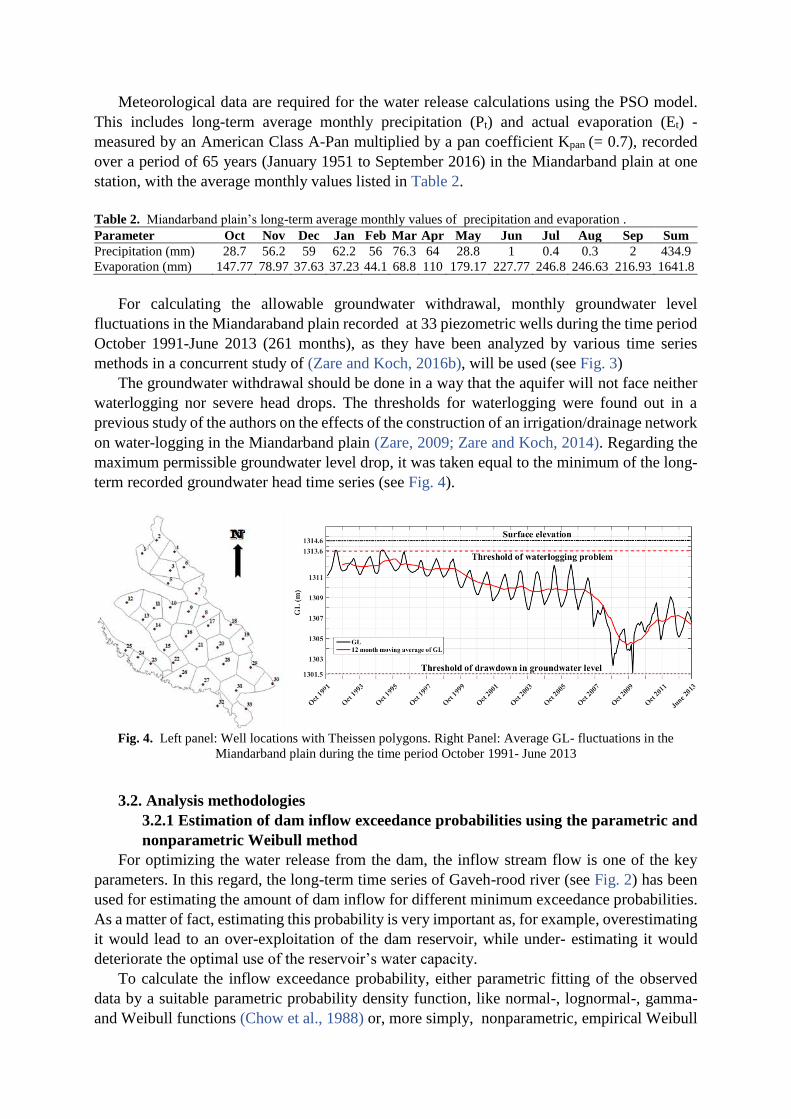
Meteorological data are required for the water release calculations using the PSO model.

This includes long-term average monthly precipitation (Pt) and actual evaporation (Et) -

measured by an American Class A-Pan multiplied by a pan coefficient Kpan (= 0.7), recorded

over a period of 65 years (January 1951 to September 2016) in the Miandarband plain at one

station, with the average monthly values listed in Table 2.

Table 2. Miandarband plain’s long-term average monthly values of precipitation and evaporation . Parameter Oct Nov Dec Jan Feb Mar Apr May Jun Jul Aug Sep Sum

Precipitation (mm) 28.7 56.2 59 62.2 56 76.3 64 28.8 1 0.4 0.3 2 434.9

Evaporation (mm) 147.77 78.97 37.63 37.23 44.1 68.8 110 179.17 227.77 246.8 246.63 216.93 1641.8

For calculating the allowable groundwater withdrawal, monthly groundwater level

fluctuations in the Miandaraband plain recorded at 33 piezometric wells during the time period

October 1991-June 2013 (261 months), as they have been analyzed by various time series

methods in a concurrent study of (Zare and Koch, 2016b), will be used (see Fig. 3)

The groundwater withdrawal should be done in a way that the aquifer will not face neither

waterlogging nor severe head drops. The thresholds for waterlogging were found out in a

previous study of the authors on the effects of the construction of an irrigation/drainage network

on water-logging in the Miandarband plain (Zare, 2009; Zare and Koch, 2014). Regarding the

maximum permissible groundwater level drop, it was taken equal to the minimum of the long-

term recorded groundwater head time series (see Fig. 4).

Fig. 4. Left panel: Well locations with Theissen polygons. Right Panel: Average GL- fluctuations in the

Miandarband plain during the time period October 1991- June 2013

3.2. Analysis methodologies

3.2.1 Estimation of dam inflow exceedance probabilities using the parametric and

nonparametric Weibull method

For optimizing the water release from the dam, the inflow stream flow is one of the key

parameters. In this regard, the long-term time series of Gaveh-rood river (see Fig. 2) has been

used for estimating the amount of dam inflow for different minimum exceedance probabilities.

As a matter of fact, estimating this probability is very important as, for example, overestimating

it would lead to an over-exploitation of the dam reservoir, while under- estimating it would

deteriorate the optimal use of the reservoir’s water capacity.

To calculate the inflow exceedance probability, either parametric fitting of the observed

data by a suitable parametric probability density function, like normal-, lognormal-, gamma-

and Weibull functions (Chow et al., 1988) or, more simply, nonparametric, empirical Weibull

(1939) ranking (plotting positions) can be used. There have been a lot of discussions for quite

some time in the hydrological literature on the appropriateness of the classical Weibull- and /

modified plotting position methods for calculating exceedance probabilities, respective, return

periods, and the jury on the proper plotting positions is still out ( Cunnane, 1978; Hirsch, 1987;

Chow et al., 1988). For this reason, both methods are used and compared in the present study.

For the parametric method a two-parameter Weibull density distribution (Pook and

Laboratory, 1984), given by

𝑓(𝑥|𝛼, 𝛽) =𝛽

𝛼(

𝑥

𝛼)𝛽−1𝑒−(𝑥/𝛼)𝛽

(1)

where α and β are shape and scale parameters, respectively, has been fitted to the observed

dam inflow for each month of the year during the observation period (1957-2016), using

nonlinear maximum likelihood estimation (MLE).

Exceedence probability discharges Q(pe) are then defined from the quantiles Q for a given

exceedance probability pe =1-pc, where pc is the predefined non-exceedence probability, given

by the ratio of the area underneath the fitted Weibull-function between Q=0 to Q(pc) to the total

area (usually normalized to one).

The second, simpler method used in general extreme value statistical hydrology, namely,

for the estimation of return periods, used here, consists in the application of the nonparametric

empirical Weibull (1939) plotting position approach. In this method the monthly stream flows

are ranked in ascending order and the minimum exceedance probability 𝑝(𝑥𝑖) is calculated

by the empirical plotting position (Agbede and Abiona, 2012):

𝑝(𝑥𝑖) =𝑚

𝑁+1 , (2)

where m is the rank of data 𝑥𝑖; and N is the sample size (=59), the number of years. As

mentioned above, modifications of this plotting position method have been proposed, but their

usefulness is not always clear (Chow et al., 1988).

3.2.2 Optimization methodology for water release from the Gavoshan dam.

3.2.2.1 Formulation of the constrained optimization problem

For finding the optimal monthly water release from the Gavoshan dam, using constrained

optimization methods, the objective function and the constraints must be determined first. In

this study, the constrained optimization problem is stated as follows:

min 𝑍 = ∑ ((𝑅𝑡 − 𝑅𝑟𝑒𝑐)/𝑅𝑚𝑎𝑥)212𝑖=1 + 𝑃𝐹 (3)

subject to

𝑅𝑡 = 𝑆𝑡 − 𝑆𝑡+1 + 𝑄𝑡 − 𝐿𝑡 𝑡 = 1,2, … ,12 (4)

𝑆𝑚𝑖𝑛 ≤ 𝑆𝑡 ≤ 𝑆𝑚𝑎𝑥 (5)

𝑅𝑚𝑖𝑛 ≤ 𝑅𝑡 ≤ 𝑅𝑚𝑎𝑥, (6)

where Z is the objective function; 𝑅𝑡 is the water release from the Gavoshan dam in month

t; 𝑅𝑟𝑒𝑐 is the recommended release as advocated by Iran’s Minstry of Power (Table 1); 𝑅𝑚𝑎𝑥

is the maximum release which is equal to 76.1 MCM; 𝑅𝑚𝑖𝑛 is equal to 0. PF is the penalty

function which is determined by the continuity equation which in discretized form is equal

to ∑ (𝑆12𝑡=1 𝑡+1

− 𝑆𝑡 − 𝑄𝑡 + 𝑅𝑡 + 𝐿𝑡); S is the storage volume; 𝑄𝑡 is the dam inflow; 𝑆𝑚𝑖𝑛is the

dead volume of the constructed dam which is equal to 35.07 MCM; 𝑆𝑚𝑎𝑥 is the reservoir

volume at normal level, equal to 504.25 MCM; 𝐿𝑡 is the difference between evaporation (𝐸𝑡)

and precipitation (𝑃𝑡) whose average monthly values are listed in Table 2.

To calculate the volume of 𝐿𝑡, the following area – storage equations has been used:

𝐿𝑡 = (𝐸𝑡 − 𝑃𝑡) ∗ 𝐴𝑡̅̅ ̅ (7)

with

𝐴𝑡̅̅ ̅ = 0.5 ∗ (𝐴𝑡 + 𝐴𝑡+1) (8)

and

𝐴𝑡 = 𝑎𝑆𝑡 + 𝑏 (9)

where 𝐴𝑡̅̅ ̅ is the average of two consecutive months and 𝑎 and 𝑏 are linear regression

coefficients found by least squares regression (see Fig. 5).

Fig. 5 Area-storage values with fitted linear regression line

3.2.2.2 Solution of the optimization problem by Particle Swarm Optimization (PSO)

To solve the constrained optimization problem formulated above, particle swarm

optimization (PSO) is employed. PSO is a population-based stochastic optimization technique,

which is derived from social behaviors of animals or insects. It was invented by Kennedy and

Eberhart (1995). The PSO belongs to the group of so-called derivative-free optimization

methods, similar to evolutionary methods like the genetic algorithm (GA) or the shuffled

complex evolution algorithm, whose most appealing feature is that they look for a global

minimum of an objective function, unlike most gradient (derivative) methods, which obtain

only local minima.

In the PSO algorithm the data are introduced as particles (there is no need to encoding and

decoding like as in GA) and these particles move around in the function space with updated

internal velocities to finally converge to the best solution (Rao and Savsani, 2012). More

specifically, the particles are spread in the search space and each particle keeps tracks of its

coordinates in this space to find the best solution. For every particle in its position the objective

function is calculated, then, by combining information of the present and previous position, the

best solution up to the present iteration step is obtained, called the personal best (pBest). Each

particle's movement is influenced by its pBest known position, but is at the same time guided

towards the best known positions from other particles in the population, the global best (gBest).

By means of updating the velocities in the directions of personal and global best solutions, PSO

searches iteratively the optimum objective function (Gill et al., 2006).

In the PSO each particle has five properties: a) position (xi); b) objective function value at

xi; c) velocity (vi); d) the pBest position (xi, best); and e) objective function value at gBest xi, best.

The equations that describe the behavior of particles in PSO are (Robinson and Rahmat-Samii,

2004):

𝑣𝑖(𝑡 + 1) = 𝑤𝑣𝑖(𝑡) + 𝑐1𝑟1(𝑥𝑖,𝑏𝑒𝑠𝑡(𝑡) − 𝑥𝑖(𝑡)) + 𝑐2𝑟2(𝑥𝑔𝑏𝑒𝑠𝑡(𝑡) − 𝑥𝑖(𝑡)) (10)

𝑥𝑖(𝑡 + 1) = 𝑥𝑖(𝑡) + 𝑣𝑖(𝑡 + 1) (11)

where w is the inertia coefficient of velocity at time t (𝑣𝑖(𝑡)) which is equal to 1 in the

first iteration, with a damping of 0.99 for the next iterations; 𝑟1 and 𝑟2 are random functions

which generate uniformly distributed random numbers between 0 and 1; 𝑐1 = 2 is a factor

determining the influences of memory of best position of particle 𝑥𝑖,𝑏𝑒𝑠𝑡(𝑡) and 𝑐2 = 2 is a

factor determining the influences of the other particles, i.e. 𝑐1 and 𝑐2 which are between 0 and

2, move the particle in direction of personal and global best (xgbest(t)) solution;

xi(t + 1) and vi(t + 1) are position and velocity in (t+1), respectively (see Fig. 6).

In the present PSO-application of the optimal dam water release, the number of swarm

particles Npop is equal to 100 and the maximum number of iterations is set to Nmax =1000,

although the actual number of iterations turns out to be much less (between 100 and 350) (see

Fig. 16, to be discussed later). All initial values have been taken following the

recommendations of Clerc and Kennedy (2002), where it was found that the final results are

not sensitive to ±20% changes of the coefficients 𝑐1, 𝑐2 in Eq. 10. In addition, because the

inertia weight changes by the damping factor 0.99 in each iteration, the acceleration becomes

smaller and smaller as the number of iterations increases, so that the particle just converges to

its pBest and gBest.

Fig. 6 Optimization search strategy in thePSO algorithm

3.3. Calculation of allowable groundwater withdrawal by coupling of a hybrid

Wavelet-ANFIS/ fuzzy C-means (FCM) clustering model with PSO

3.3.1 Formulation of groundwater level output-input function

To study the effects of groundwater withdrawal as well as of the conveyed water from the

Gavoshan Dam on the groundwater levels in the study area, a hybrid Wavelet- Adaptive Neuro-

Fuzzy Inference System (ANFIS) model based on fuzzy C-means (FCM) clustering developed

by Zare and Koch (2017) in conjunction has been used.

The hybrid Wavelet-ANFIS/ fuzzy C-means (FCM) clustering model is a data- driven input-

output prediction model (Zare and Koch, 2017), wherefore the groundwater level at time t is

assumed to be a function of CW and the water deficit from the irrigation water requirement

(IWR) – which is supposed to be equal to the groundwater withdrawal (GW) –, i.e.:

𝐺𝐿𝑡 = 𝑓(𝐶𝑊𝑡 , 𝐺𝑊𝑡) (12)

The water for the agricultural activities in the Miandarband flood plain has been conveyed

from the Gavoshan Dam since October 2007 (Fig. 7).

Fig. 7. Recommended and conveyed water from the Gavoshan Dam into the Miandarband plain during the time

of the operation of the irrigation network (2007-2014)

The hybrid model consists in fact of three separate tools, namely, discrete wavelet

transform/ multiresolution analysis (DWT/MRA), fuzzy C-means (FCM) clustering and

ANFIS (Zare and Koch, 2017) which are described in the following subsections.

3.3.2 Multiresolution analysis of input data using the discrete wavelet transform

Wavelet analysis of a time series is an extension of the classical Fourier analysis, inasmuch

that, unlike the latter, it allows also for a location in time of the frequency content of a time-

signal, which for that reason may also then be non-stationary. In practical applications, one

distinguishes usually between the continuous wavelet transform (CWT) used for depicting 2D

time- frequency (or its inverse, the scale) scalograms of a time- series and its discrete

counterpart, the DWT, used mainly for the approximation of high-frequency signals at different

lower frequency levels, i.e. doing some kind of low-pass (resolution) filtering (see Zare and

Koch, 2017, for details).

The DWT of a time series of x(t) is defined as (Percival and Walden, 2006):

𝐷𝑊𝑇𝑗,𝑘(𝑡) = 2−𝑗/2 ∫ 𝑥(𝑡) 𝜓 (𝑡− 𝑏𝑘

𝑎𝑗) 𝑑𝑡

+∞

−∞, 𝑗, 𝑘 𝜖 𝑍, (13)

where aj = 2j is the scale (i.e. inverse of frequency) (dilatated/compressed), bk = k 2j is the

shift (translate) parameter, and 𝜓(𝑡) is the mother wavelet, i.e. 𝜓𝑗,𝑘(𝑡) are the scaled and

shiftet daughter wavelets.

In the case that the mother wavelet 𝜓𝑗,𝑘(𝑡) belongs to a so-called tight frame of wavelet

classes, 𝜓𝑗,𝑘(𝑡) forms a complete and orthonormal basis, so that the signal x(t) can be

reconstructed by the classical formula

𝑥(𝑡) = ∑ < 𝑥(𝑡), 𝜓𝑗,𝑘(𝑡) > | 𝜓𝑗,𝑘(𝑡) >𝑗,𝑘 = ∑ 𝐷𝑊𝑇𝑗,𝑘(𝑡) | 𝜓𝑗,𝑘(𝑡) >𝑗,𝑘 . (14)

This equation is the basis of the multiresolution analysis (MRA) (Mallat, 1989), For the

𝜓𝑗,𝑘(𝑡) to be admissible, i.e. orthonormal, in the MRA, it must satisfy the two-scale property:

𝜓(𝑡) = √2 ∑ 𝑔(𝑛)𝜓(2𝑡 − 𝑛)𝑛 , (15)

i.e. the width and the location of the wavelet function at a scale j+1 are half of that at scale

j. As such, the wavelet function 𝜓𝑗,𝑘(𝑡) can be understood as a series of high / band pass filters,

or a filter bank, with filter coefficients g(n) and which covers the whole frequency range of the

signal, starting from the Nyquist sampling frequency (the lowest scale ) down to a minimum

frequency (highest scale). However, as the scale cannot go up infinitely, because the signal is

time-limited or finite, the scale range is limited at a maximum j, leaving a remainder (with the

lowest frequency) of the signal unresolved. This is where the so-called scaling function 𝜙(𝑡)

comes into play, which is defined similar to the wavelet function 𝜓(𝑡), but derived from a father

wavelet, orthonormal to the former and obeying also the two-scale property:

𝜙(𝑡) = √2 ∑ ℎ(𝑛)𝜙(2𝑡 − 𝑛)𝑛 (16)

where ℎ(𝑛) are the filter coefficients, which now describes a low-pass filter. Because of the

orthonormality of 𝜓(𝑡) and 𝜙(𝑡), the filter coefficients h(n) and g(n) are related to each other

(mirror filter):

𝑔(𝑚 − 1 − 𝑛) = (−1)𝑛ℎ(𝑛), 𝑚: 𝑓𝑖𝑙𝑡𝑒𝑟 𝑙𝑒𝑛𝑔𝑡ℎ (17)

The scaling function 𝜙𝑗,𝑘(𝑡) at scale j thus covers the lower part of the spectrum of the

signal x(t), not yet attained by the that scale j.

Using the fundamental decomposition Eq. 14 over the finite range of scales and shift times,

one obtains the equation for the complete decomposition of the signal x(t), for scales up to jmax:

𝑥(𝑡) = ∑ < 𝑥(𝑡), 𝜙𝑗𝑚𝑎𝑥,𝑘(𝑡) > | 𝜙𝑗𝑚𝑎𝑥,𝑘(𝑡) >𝑘 + ∑ < 𝑥(𝑡), 𝜓(𝑡)𝑗,𝑘(𝑡) > |𝜓𝑗,𝑘(𝑡) >𝑗𝑚𝑎𝑥𝑗,𝑘 , (18)

where the expansion coefficients (projections) 𝑎𝑗,𝑘 =< 𝑥(𝑡), 𝜙𝑗,𝑘(𝑡) > and

𝑑𝑗,𝑘 =< 𝑥(𝑡), 𝜓𝑗,𝑘(𝑡) > have also the 2-scale property, i.e. can be computed recursively as:

𝑎𝑗,𝑘 = ∑ ℎ(𝑛 − 2𝑘)𝑎𝑗−1,𝑛𝑛 & 𝑑𝑗,𝑘 = ∑ 𝑔(𝑛 − 2𝑘)𝑎𝑗−1,𝑛𝑛 (19)

The first sum in Eq. 18 describes the coarse, high scale (low frequency) component of x(t),

generated by the low-pass scaling function 𝜙𝑗,𝑘(𝑡) , i.e. represents the Ajmax - approximation of

the signal at the highest decomposition level. The second sum consists of the low-scale, high

frequency details Dj of the signal, generated by the high-frequency / band pass wavelet

functions 𝜓𝑗,𝑘(𝑡) (j=1,..,jmax). Thus, Eq. 18 can also be written as

𝑥(𝑡) = 𝐴𝑗𝑚𝑎𝑥 + 𝐷1 + 𝐷2. . +. . 𝐷𝑗𝑚𝑎𝑥 (20)

By applying Eqs. 18 or 20 recursively for different maximum scale levels (j =1,..,jmax),

the multiresolution decomposition of the signal x(t) at that level, consisting of the

approximation 𝐴𝑗 and the detail 𝐷𝑗 at that level is computed. In the subsequent step j+1 this

approximation 𝐴𝑗 is further decomposed into 𝐴𝑗+1 and 𝐷𝑗+1, and so on, until level jmax is

reached, with the low-frequency remainder of the signal then described by the term Ajmax.

Practically, the MRA by means of the DWT is performed by so-called subband coding

(Vetterli and Herley, 1992), which consists in running the signal x(t) through a cascade of

high/band- and low-pass digital filters, defined by the dyadically (power of 2) dilated and

shifted wavelet- and scaling- functions, respectively, and subsequent down-sampling of the

time series also by a factor of 2, due to the fact that the low-pass filtered series at level j+1 has

only half the frequency-bandwidth of the original one at level j. This methodology results in a

natural adaptation of the resolution of the filter wherefore the number of digital flops in the

evaluation of the filtering (convolution) equation at the next higher scale is halved, making

subband coding computationally extremely efficient. It should be noted that filtering of signals

with subband coding of cascade filters has an even longer history in signal processing than

wavelets, and the latter in the form of the DWT represents only a special variant of it (Mallat,

1989).

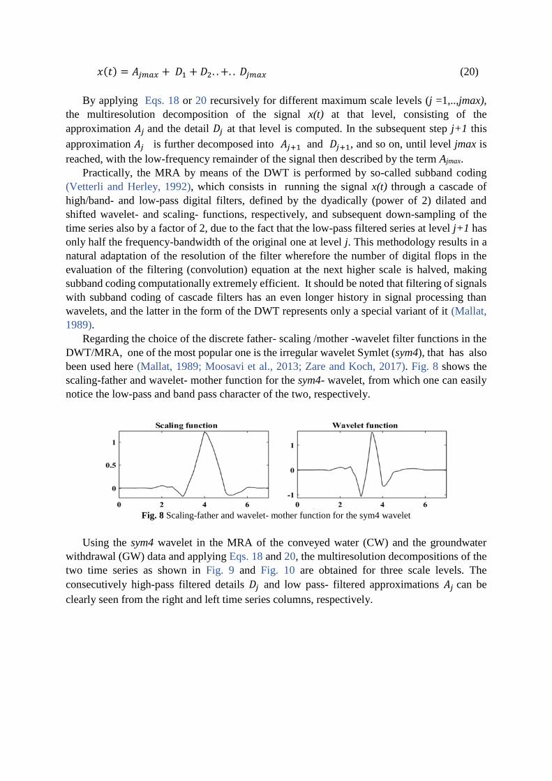
Regarding the choice of the discrete father- scaling /mother -wavelet filter functions in the

DWT/MRA, one of the most popular one is the irregular wavelet Symlet (sym4), that has also

been used here (Mallat, 1989; Moosavi et al., 2013; Zare and Koch, 2017). Fig. 8 shows the

scaling-father and wavelet- mother function for the sym4- wavelet, from which one can easily

notice the low-pass and band pass character of the two, respectively.

Fig. 8 Scaling-father and wavelet- mother function for the sym4 wavelet

Using the sym4 wavelet in the MRA of the conveyed water (CW) and the groundwater

withdrawal (GW) data and applying Eqs. 18 and 20, the multiresolution decompositions of the

two time series as shown in Fig. 9 and Fig. 10 are obtained for three scale levels. The

consecutively high-pass filtered details 𝐷𝑗 and low pass- filtered approximations 𝐴𝑗 can be

clearly seen from the right and left time series columns, respectively.

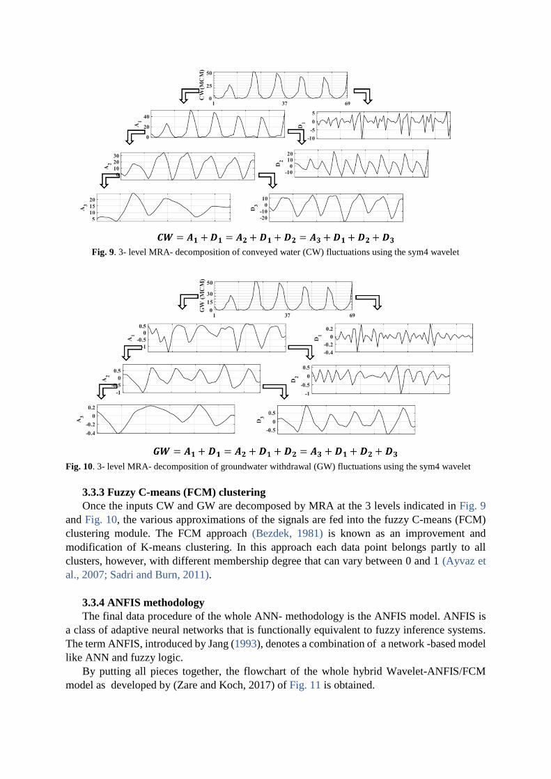
Fig. 9. 3- level MRA- decomposition of conveyed water (CW) fluctuations using the sym4 wavelet

Fig. 10. 3- level MRA- decomposition of groundwater withdrawal (GW) fluctuations using the sym4 wavelet

3.3.3 Fuzzy C-means (FCM) clustering

Once the inputs CW and GW are decomposed by MRA at the 3 levels indicated in Fig. 9

and Fig. 10, the various approximations of the signals are fed into the fuzzy C-means (FCM)

clustering module. The FCM approach (Bezdek, 1981) is known as an improvement and

modification of K-means clustering. In this approach each data point belongs partly to all

clusters, however, with different membership degree that can vary between 0 and 1 (Ayvaz et

al., 2007; Sadri and Burn, 2011).

3.3.4 ANFIS methodology

The final data procedure of the whole ANN- methodology is the ANFIS model. ANFIS is

a class of adaptive neural networks that is functionally equivalent to fuzzy inference systems.

The term ANFIS, introduced by Jang (1993), denotes a combination of a network -based model

like ANN and fuzzy logic.

By putting all pieces together, the flowchart of the whole hybrid Wavelet-ANFIS/FCM

model as developed by (Zare and Koch, 2017) of Fig. 11 is obtained.

Fig. 11 Sketch of the hybrid Wavelet-ANFIS/FCM model

3.4. Coupling of the hybrid Wavelet-ANFIS/FCM model with PSO for conjunctive

management of surface-groundwater resources in the study area

Fig. 4 illustrates how the hybrid Wavelet-ANFIS/FCM model is coupled with the PSO for

calculating the required groundwater withdrawal GW as the difference between IWR and the

optimal PSO- computed conveyed water (CW) from the dam into the plain, while ensuring that

groundwater levels (GL) stay within an acceptable range.

Fig. 12 Flowchart of coupling of the hybrid model with PSO for computation of groundwater levels as a

function of required groundwater withdrawal and optimally conveyed water in the study region

Firstly, the hybrid Wavelet-ANFIS/ fuzzy C-means (FCM) clustering model is trained and

tested in the usual way, wherefore from a total of 69 monthly observed values of GL and CW

in the common record time window between October 2007 and June 2013, 48 months (70%)

are used for training and 21 months (30%) for testing.

If the results of the trained and tested hybrid model are accurate, secondly, new inputs

including the optimal monthly CW and the required groundwater withdrawal GW - equal to the

water deficit between IWR and the optimal CW – is introduced as new predictors into the

trained hybrid model to get the GL for each month. The latter are then checked for respecting

the upper water-logging and the lower threshold limits. If the former is violated, i.e. GL

increases above the waterlogging threshold, GW must be increased and the excessive water can

be conveyed to the domestic water network of Kermanshah, the biggest city in western Iran. In

contrast, if the GL falls below the minimum (maximally allowable drawdown) level, GW

should be decreased and irrigation policies under crop water stress should be adopted. An

alternative option would be to change the cultivation pattern, i.e. planting crops that have less

water demand.

4. Results and discussion

4.1. Estimation of dam inflow exceedance probabilities using two-parameter Weibull

distribution and Weibull non-parametric plotting position methods

As mentioned in Section 3.2.1 exceedance probabilities of the Gavoshan dam’s inflow are

calculated by the two-parameter Weibull distribution as well as the non-parametric Weibull

plotting position method. This has been done for the mean recorded data for each month of the

year over the observation period (October 1957 to September 2016).

Regarding the Weibull distribution method, its shape (α) and scale (β) parameters have been

determined by nonlinear maximum likelihood estimation (MLE). The results are shown for

each month in Fig. 13. The figure illustrates clearly that the dam inflow during the rainy season

– from January to June – is higher than during the dry season for most of the years, with the

peak values occurring in April, whereas in September and October the Gaveh-rood river is

almost drying up, especially, during the last decade, when the study area faced several

meteorological drought conditions.

Fig. 13. Histograms of inflow to the Gavoshan dam for each month of the year, fitted by Weibull- density

function, with shape and scale parameters as indicated.

Exceedance inflow discharges Q(p) for different probabilities p are then computed in this

method from the corresponding quantiles of the fitted Weibull distribution. The results are

shown by the smooth lines in Fig. 14. Also plotted in the figure are the discrete points of the

discharge exceedance probabilities obtained with the second, nonparametric empirical Weibull

(1939) plotting position approach. One may notice that the plotting positions of the latter

method are mostly lying on the Weibull probability curve, with some differences arising mainly

in the minimum flow tails, which are less of interest here.

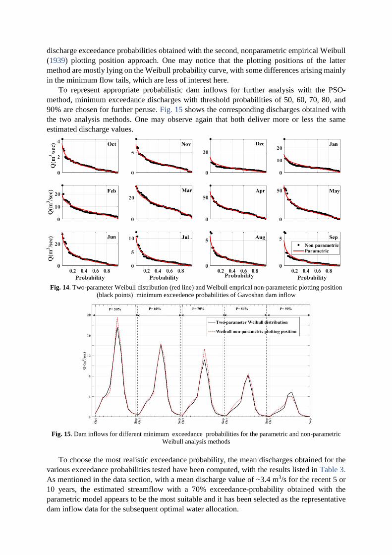
To represent appropriate probabilistic dam inflows for further analysis with the PSO-

method, minimum exceedance discharges with threshold probabilities of 50, 60, 70, 80, and

90% are chosen for further peruse. Fig. 15 shows the corresponding discharges obtained with

the two analysis methods. One may observe again that both deliver more or less the same

estimated discharge values.

Fig. 14. Two-parameter Weibull distribution (red line) and Weibull emprical non-parameteric plotting position

(black points) minimum exceedence probabilities of Gavoshan dam inflow

Fig. 15. Dam inflows for different minimum exceedance probabilities for the parametric and non-parametric

Weibull analysis methods

To choose the most realistic exceedance probability, the mean discharges obtained for the

various exceedance probabilities tested have been computed, with the results listed in Table 3.

As mentioned in the data section, with a mean discharge value of ~3.4 m3/s for the recent 5 or

10 years, the estimated streamflow with a 70% exceedance-probability obtained with the

parametric model appears to be the most suitable and it has been selected as the representative

dam inflow data for the subsequent optimal water allocation.

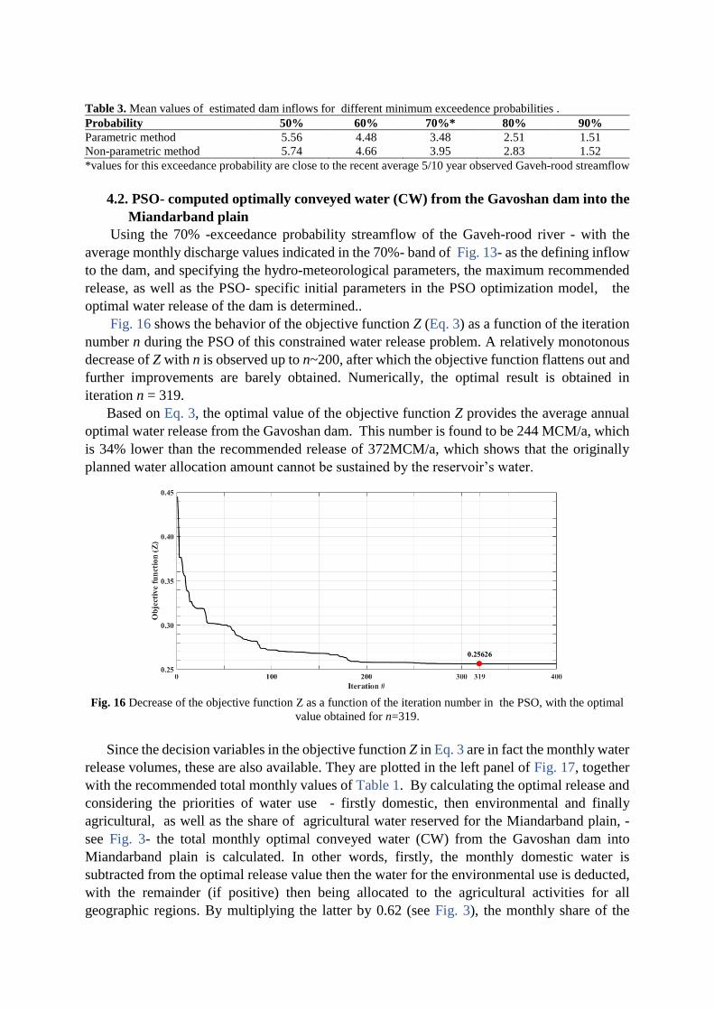
Table 3. Mean values of estimated dam inflows for different minimum exceedence probabilities .

Probability 50% 60% 70%* 80% 90%

Parametric method 5.56 4.48 3.48 2.51 1.51

Non-parametric method 5.74 4.66 3.95 2.83 1.52

*values for this exceedance probability are close to the recent average 5/10 year observed Gaveh-rood streamflow

4.2. PSO- computed optimally conveyed water (CW) from the Gavoshan dam into the

Miandarband plain

Using the 70% -exceedance probability streamflow of the Gaveh-rood river - with the

average monthly discharge values indicated in the 70%- band of Fig. 13- as the defining inflow

to the dam, and specifying the hydro-meteorological parameters, the maximum recommended

release, as well as the PSO- specific initial parameters in the PSO optimization model, the

optimal water release of the dam is determined..

Fig. 16 shows the behavior of the objective function Z (Eq. 3) as a function of the iteration

number n during the PSO of this constrained water release problem. A relatively monotonous

decrease of Z with n is observed up to n~200, after which the objective function flattens out and

further improvements are barely obtained. Numerically, the optimal result is obtained in

iteration n = 319.

Based on Eq. 3, the optimal value of the objective function Z provides the average annual

optimal water release from the Gavoshan dam. This number is found to be 244 MCM/a, which

is 34% lower than the recommended release of 372MCM/a, which shows that the originally

planned water allocation amount cannot be sustained by the reservoir’s water.

Fig. 16 Decrease of the objective function Z as a function of the iteration number in the PSO, with the optimal

value obtained for n=319.

Since the decision variables in the objective function Z in Eq. 3 are in fact the monthly water

release volumes, these are also available. They are plotted in the left panel of Fig. 17, together

with the recommended total monthly values of Table 1. By calculating the optimal release and

considering the priorities of water use - firstly domestic, then environmental and finally

agricultural, as well as the share of agricultural water reserved for the Miandarband plain, -

see Fig. 3- the total monthly optimal conveyed water (CW) from the Gavoshan dam into

Miandarband plain is calculated. In other words, firstly, the monthly domestic water is

subtracted from the optimal release value then the water for the environmental use is deducted,

with the remainder (if positive) then being allocated to the agricultural activities for all

geographic regions. By multiplying the latter by 0.62 (see Fig. 3), the monthly share of the

Miandarband irrigation and drainage network is finally determined. The results are shown in

the right panel of Fig. 17.

Fig. 17 (right panel) illustrates that for none of the months in the year the optimal water

released from the dam is sufficient to sustain the irrigation water originally recommended for

the agricultural activities in the Miandarband plain. In fact, between November and April no

water at all is available for the plain, as it is all allocated to domestic and environmental uses.

For the other months of late spring and summer which is the growing season for most of the

crops cultivated in the plain (see following section) about 50-70% of the water recommended

can be satisfied by the water conveyed (CW) from the dam. Integrated over the whole year, the

totally recommended irrigation water (RIW) for the plain amounts to 176.2 MCM/a, whereas

the water available from the dam is only 112.7MCM/a, i.e. there is a CW- deficit of 63.5MCM/a

in the plain which must be made up from groundwater (see following section).

Fig. 17 Left panel: Optimal and recommended monthly water release from the Gavoshan Dam. Right panel:

Recommended and optimally conveyed water (CW) into the Miandarband plain, proper.

4.3. Conjunctive management of surface-groundwater resources using the PSO-

Hybrid Wavelet-ANFIS/FCM model

4.3.1. Computation of the irrigation water deficit (IWR)

The results of the previous section indicate that the PSO- computed optimal amount of

surface water conveyed (CW) by the Gavoshan dam into the Miandarband plain cannot satisfy

the amount of irrigation water recommended originally (in year 1993) by Iran’s Ministry of

Power. The water difference to satisfy the crop needs in the plain can only be supplied from

groundwater resources which, by nature of the very dry climate in that part of the world with

low precipitation and high evapotranspiration (see Table 2), ergo low aquifer recharge, may

themselves not be sustainable neither in the long run. To overcome this problem, an appropriate

surface- groundwater conjunctive management strategy for the Miandarband plain is inevitable.

This task is carried out by firstly determining the irrigation water requirement (IWR) of all

crops supposed to be cultivated in the plain based on the original agricultural development plan

of 1993, which is listed in Table 4.

Table 4 Cultivation pattern and percentage of cultivated area (~200 km2) in the Miandarband plain.

Crop Area (km2) Crop Area (km2) Crop Area (km2)

Wheat 53.8 Clover 11.6 Apple 4

Alfalfa 27 Dry beans 11.5 Water melon 3.8

Barely 26.8 Chick beans 11.5 Tomato 3.8

Sweet corn 13.4 Sugar beet 9.6 Soybean 3.8

Field corn 11.6 Grape 4 Sun flower 3.8

It must be emphasized that this IWR should not be confounded with the originally

recommended volume of irrigation water (RIW) for the Miandarband plain of 176.2 MCM/a,

and as the former had not yet been calculated at that time, it has been done by (Zare and Koch,

2016c), wherefore IWR is defined as the difference between the total crop evapotranspiration

ETc during the growth season and the input precipitation P, multiplied by an irrigation network

efficiency factor e. ETc was computed using the FAO-56 Penman-Monteith method with

empirical crop coefficients Kc (Allen et al., 1998). For further details see (Zare and Koch,

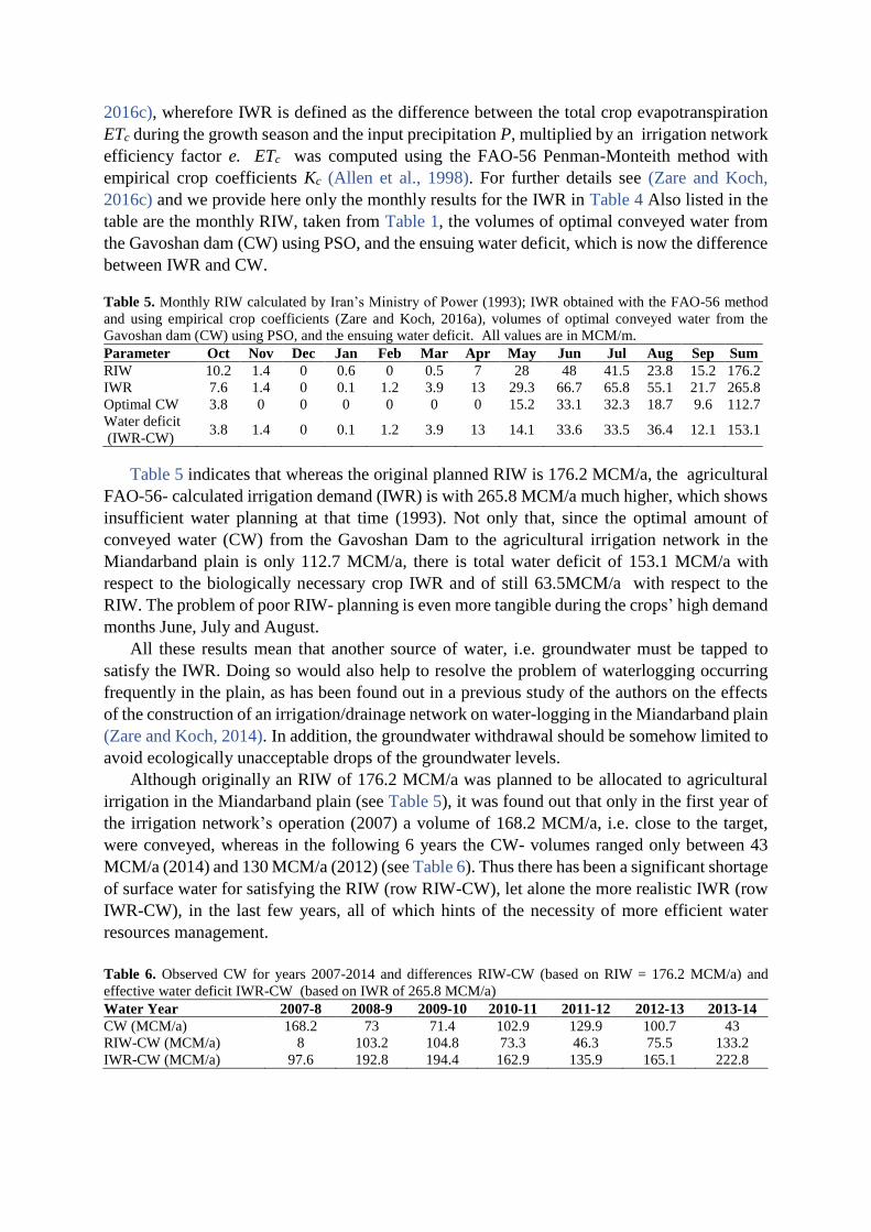
2016c) and we provide here only the monthly results for the IWR in Table 4 Also listed in the

table are the monthly RIW, taken from Table 1, the volumes of optimal conveyed water from

the Gavoshan dam (CW) using PSO, and the ensuing water deficit, which is now the difference

between IWR and CW.

Table 5. Monthly RIW calculated by Iran’s Ministry of Power (1993); IWR obtained with the FAO-56 method

and using empirical crop coefficients (Zare and Koch, 2016a), volumes of optimal conveyed water from the

Gavoshan dam (CW) using PSO, and the ensuing water deficit. All values are in MCM/m.

Parameter Oct Nov Dec Jan Feb Mar Apr May Jun Jul Aug Sep Sum

RIW 10.2 1.4 0 0.6 0 0.5 7 28 48 41.5 23.8 15.2 176.2

IWR 7.6 1.4 0 0.1 1.2 3.9 13 29.3 66.7 65.8 55.1 21.7 265.8

Optimal CW 3.8 0 0 0 0 0 0 15.2 33.1 32.3 18.7 9.6 112.7

Water deficit

(IWR-CW) 3.8 1.4 0 0.1 1.2 3.9 13 14.1 33.6 33.5 36.4 12.1 153.1

Table 5 indicates that whereas the original planned RIW is 176.2 MCM/a, the agricultural

FAO-56- calculated irrigation demand (IWR) is with 265.8 MCM/a much higher, which shows

insufficient water planning at that time (1993). Not only that, since the optimal amount of

conveyed water (CW) from the Gavoshan Dam to the agricultural irrigation network in the

Miandarband plain is only 112.7 MCM/a, there is total water deficit of 153.1 MCM/a with

respect to the biologically necessary crop IWR and of still 63.5MCM/a with respect to the

RIW. The problem of poor RIW- planning is even more tangible during the crops’ high demand

months June, July and August.

All these results mean that another source of water, i.e. groundwater must be tapped to

satisfy the IWR. Doing so would also help to resolve the problem of waterlogging occurring

frequently in the plain, as has been found out in a previous study of the authors on the effects

of the construction of an irrigation/drainage network on water-logging in the Miandarband plain

(Zare and Koch, 2014). In addition, the groundwater withdrawal should be somehow limited to

avoid ecologically unacceptable drops of the groundwater levels.

Although originally an RIW of 176.2 MCM/a was planned to be allocated to agricultural

irrigation in the Miandarband plain (see Table 5), it was found out that only in the first year of

the irrigation network’s operation (2007) a volume of 168.2 MCM/a, i.e. close to the target,

were conveyed, whereas in the following 6 years the CW- volumes ranged only between 43

MCM/a (2014) and 130 MCM/a (2012) (see Table 6). Thus there has been a significant shortage

of surface water for satisfying the RIW (row RIW-CW), let alone the more realistic IWR (row

IWR-CW), in the last few years, all of which hints of the necessity of more efficient water

resources management.

Table 6. Observed CW for years 2007-2014 and differences RIW-CW (based on RIW = 176.2 MCM/a) and

effective water deficit IWR-CW (based on IWR of 265.8 MCM/a)

Water Year 2007-8 2008-9 2009-10 2010-11 2011-12 2012-13 2013-14

CW (MCM/a) 168.2 73 71.4 102.9 129.9 100.7 43

RIW-CW (MCM/a) 8 103.2 104.8 73.3 46.3 75.5 133.2

IWR-CW (MCM/a) 97.6 192.8 194.4 162.9 135.9 165.1 222.8

4.3.2. Groundwater pumping induced head fluctuations estimated by the hybrid

Wavelet-ANFIS/FCM model

The effective agricultural water difference IWR-CW in Table 6 must be made up by

groundwater withdrawal (GW). However, the latter should be done in a way that the plain will

neither face groundwater levels (GL) too high, leading to waterlogging, nor drops too low.

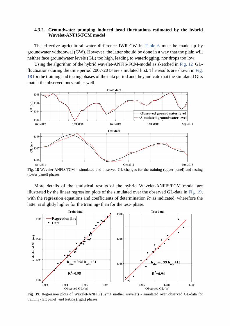
Using the algorithm of the hybrid wavelet-ANFIS/FCM-model as sketched in Fig. 12 GL-

fluctuations during the time period 2007-2013 are simulated first. The results are shown in Fig.

18 for the training and testing phases of the data period and they indicate that the simulated GLs

match the observed ones rather well.

Fig. 18 Wavelet-ANFIS/FCM – simulated and observed GL-changes for the training (upper panel) and testing

(lower panel) phases.

More details of the statistical results of the hybrid Wavelet-ANFIS/FCM model are

illustrated by the linear regression plots of the simulated over the observed GL-data in Fig. 19,

with the regression equations and coefficients of determination R2 as indicated, wherefore the

latter is slightly higher for the training- than for the test- phase.

Fig. 19. Regression plots of Wavelet-ANFIS (Sym4 mother wavelet) - simulated over observed GL-data for

training (left panel) and testing (right) phases

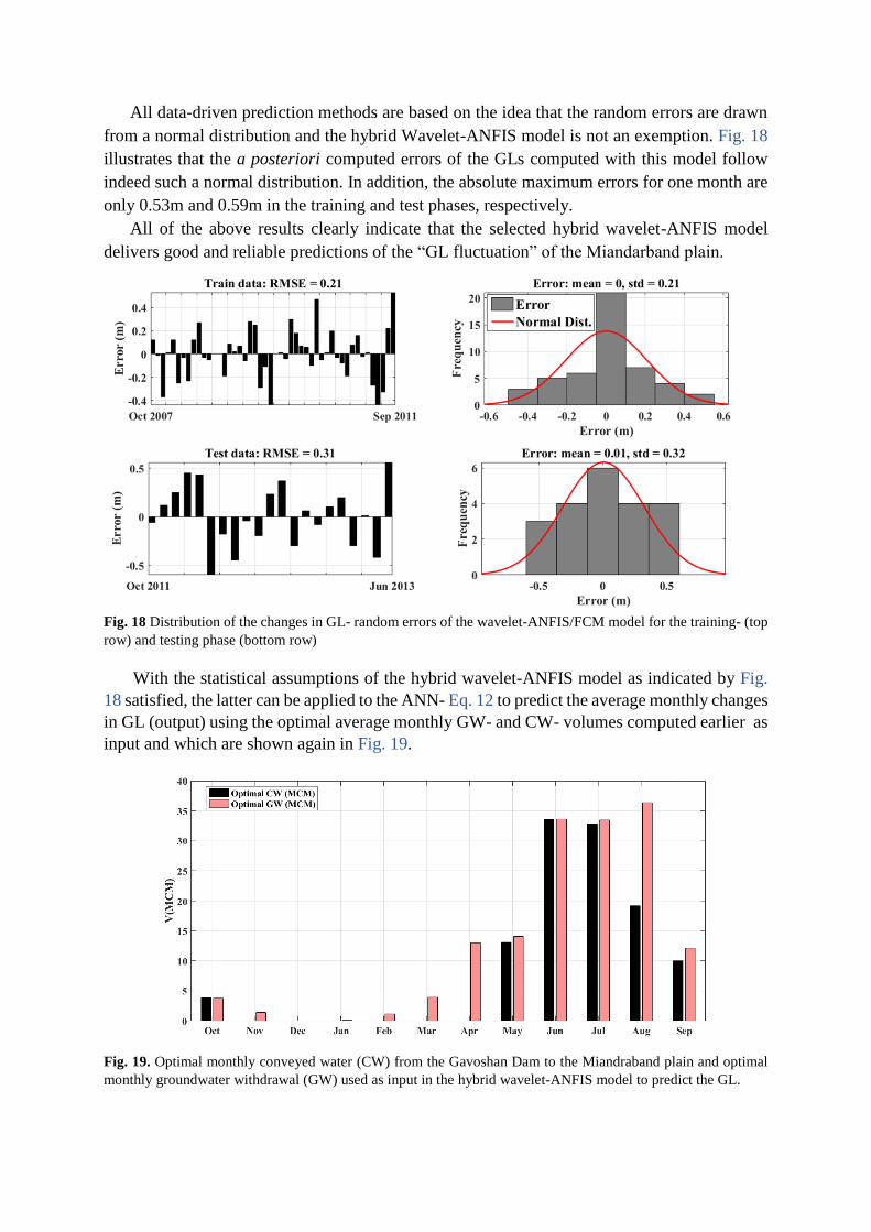
All data-driven prediction methods are based on the idea that the random errors are drawn

from a normal distribution and the hybrid Wavelet-ANFIS model is not an exemption. Fig. 18

illustrates that the a posteriori computed errors of the GLs computed with this model follow

indeed such a normal distribution. In addition, the absolute maximum errors for one month are

only 0.53m and 0.59m in the training and test phases, respectively.

All of the above results clearly indicate that the selected hybrid wavelet-ANFIS model

delivers good and reliable predictions of the “GL fluctuation” of the Miandarband plain.

Fig. 18 Distribution of the changes in GL- random errors of the wavelet-ANFIS/FCM model for the training- (top

row) and testing phase (bottom row)

With the statistical assumptions of the hybrid wavelet-ANFIS model as indicated by Fig.

18 satisfied, the latter can be applied to the ANN- Eq. 12 to predict the average monthly changes

in GL (output) using the optimal average monthly GW- and CW- volumes computed earlier as

input and which are shown again in Fig. 19.

Fig. 19. Optimal monthly conveyed water (CW) from the Gavoshan Dam to the Miandraband plain and optimal

monthly groundwater withdrawal (GW) used as input in the hybrid wavelet-ANFIS model to predict the GL.

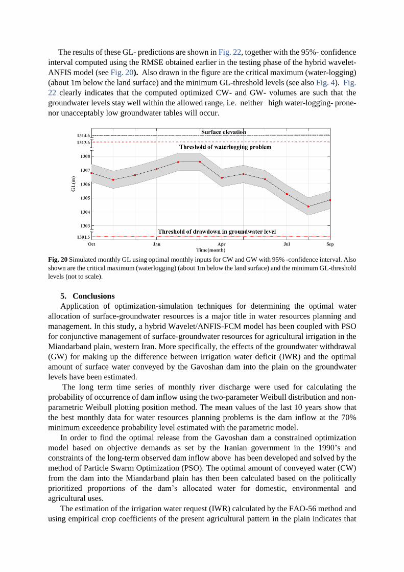
The results of these GL- predictions are shown in Fig. 22, together with the 95%- confidence

interval computed using the RMSE obtained earlier in the testing phase of the hybrid wavelet-

ANFIS model (see Fig. 20). Also drawn in the figure are the critical maximum (water-logging)

(about 1m below the land surface) and the minimum GL-threshold levels (see also Fig. 4). Fig.

22 clearly indicates that the computed optimized CW- and GW- volumes are such that the

groundwater levels stay well within the allowed range, i.e. neither high water-logging- prone-

nor unacceptably low groundwater tables will occur.

Fig. 20 Simulated monthly GL using optimal monthly inputs for CW and GW with 95% -confidence interval. Also

shown are the critical maximum (waterlogging) (about 1m below the land surface) and the minimum GL-threshold

levels (not to scale).

5. Conclusions

Application of optimization-simulation techniques for determining the optimal water

allocation of surface-groundwater resources is a major title in water resources planning and

management. In this study, a hybrid Wavelet/ANFIS-FCM model has been coupled with PSO

for conjunctive management of surface-groundwater resources for agricultural irrigation in the

Miandarband plain, western Iran. More specifically, the effects of the groundwater withdrawal

(GW) for making up the difference between irrigation water deficit (IWR) and the optimal

amount of surface water conveyed by the Gavoshan dam into the plain on the groundwater

levels have been estimated.

The long term time series of monthly river discharge were used for calculating the

probability of occurrence of dam inflow using the two-parameter Weibull distribution and non-

parametric Weibull plotting position method. The mean values of the last 10 years show that

the best monthly data for water resources planning problems is the dam inflow at the 70%

minimum exceedence probability level estimated with the parametric model.

In order to find the optimal release from the Gavoshan dam a constrained optimization

model based on objective demands as set by the Iranian government in the 1990’s and

constraints of the long-term observed dam inflow above has been developed and solved by the

method of Particle Swarm Optimization (PSO). The optimal amount of conveyed water (CW)

from the dam into the Miandarband plain has then been calculated based on the politically

prioritized proportions of the dam’s allocated water for domestic, environmental and

agricultural uses.

The estimation of the irrigation water request (IWR) calculated by the FAO-56 method and

using empirical crop coefficients of the present agricultural pattern in the plain indicates that

the original recommended irrigation water request (RIW) has been extremely underestimated

and both cannot be satisfied by neither the observed nor the optimal CW. Therefore, this

irrigation water deficit must be made up for by groundwater withdrawal (GW), however, at the

risk of unacceptable changes in the groundwater levels (GL).

Using the hybrid Wavelet-ANFIS/FCM model, monthly groundwater levels (GL) are

functionally connected to the monthly observed CW as well as to the estimated GW (equal to

the surface water deficit) and this input-output relationship trained and tested. The statistical

analysis of the training and testing results shows that the hybrid model works appropriately.

In the final step optimal CW and corresponding GW are used as input predictors in the

trained hybrid model to get corresponding GL. The latter are then checked if they violate either

the upper water-logging threshold or the lower limit of a too severe drop of the groundwater

table. If so, the GW must be adjusted accordingly in an iterative process which, in turn, means

am associated alteration of the conjunctive surface-groundwater management in the plain.

However the results obtained so far do not hint of such a possibility, as the groundwater levels

computed under optimal conditions stay well within the given bounds.

In conclusion, the innovative coupled hybrid Wavelet-ANFIS/FCM- PSO model developed

here reveals itself to be a helpful tool for developing efficient conjunctive surface-groundwater

resources management systems, in particular, when there is a lack of data, and/or when the

physical processes of surface-groundwater interactions are not completely understood, so that

deterministic physical models are barely applicable.

References

Agbede, A.O., Abiona, O., 2012. Plotting Position Probability Fittings to Lagos Metropolitan

Precipitation: Hydrological Tools for Hydraulic Structures Design in Flood Control. International

Journal of Pure and Applied Sciences and Technology. 10, 6.

Allen, R.G., Pereira, L.S., Raes, D., Smith, M., 1998. Crop evapotranspiration-Guidelines for computing

crop water requirements-FAO Irrigation and drainage paper 56. FAO, Rome 300, D05109.

Anonymous, 2001. Miandarband and Bilekvar irrigation and drainage network, final report. Mahab

Ghods Co, (in Farsi).

Ayvaz, M.T., Karahan, H., Aral, M.M., 2007. Aquifer parameter and zone structure estimation using

kernel-based fuzzy c-means clustering and genetic algorithm. Journal of Hydrology 343, 240-253.

Bezdek, J.C., 1981. Pattern recognition with fuzzy objective function algorithms. New York (N.Y.) :

Plenum press.

Chow, V.T., Maidment, D.R., Mays, L.W., 1988. Applied Hydrology. McGraw-Hill.

Clerc, M., Kennedy, J., 2002. The particle swarm - explosion, stability, and convergence in a

multidimensional complex space. IEEE Transactions on Evolutionary Computation 6, 58-73.

Cunnane, C., 1978. Unbiased plotting positions — A review. Journal of Hydrology 37, 205-222.

Das, B., Singh, A., Panda, S.N., Yasuda, H., 2015. Optimal land and water resources allocation policies

for sustainable irrigated agriculture. Land Use Policy 42, 527-537.

Fink, G., Koch, M., 2010. Climate Change Effects on the Water Balance in the Fulda Catchment,

Germany, during the 21st Century., Symposium on "Sustainable Water Resources Management and

Climate Change Adaptation", Nakhon Pathom University, Thailand.

Gill, M.K., Kaheil, Y.H., Khalil, A., McKee, M., Bastidas, L., 2006. Multiobjective particle swarm

optimization for parameter estimation in hydrology. Water Resources Research 42, n/a-n/a.

Hirsch, R.M., 1987. Probability plotting position formulas for flood records with historical information.

Journal of Hydrology 96, 185-199.

Jang, J.S.R., 1993. ANFIS: Adaptive-Network-based Fuzzy Inference Systems. IEEE Transactions on

Systems, Man and Cybernetics. 23, 665-685.

Kennedy, J., Eberhart, R., 1995. Particle swarm optimization, Neural Networks, 1995. Proceedings.,

IEEE International Conference on, pp. 1942-1948 vol.1944.

Koch, M., 2008. Challenges for future sustainable water resources management in the face of climate

change., 1st NPRU Academic Conference., Nakhon Pathom University, Thailand.

Mahboubi, A.R., Aminpour, M., Kazempour, S., 2007. Finite element modeling and back analysis of

Gavoshan dam during construction and pondage intervals, 5th International Conference on Dam

Engineering., 14-16 Feb., Lisbon, Portugal.

Mallat, S.G., 1989. A theory for multiresolution signal decomposition: the wavelet representation. IEEE

Transactions on Pattern Analysis and Machine Intelligence 11, 674-693.

Mani, A., Tsai, F.T.C., Kao, S.-C., Naz, B.S., Ashfaq, M., Rastogi, D., 2016. Conjunctive management

of surface and groundwater resources under projected future climate change scenarios. Journal of

Hydrology 540, 397-411.

Moosavi, V., Vafakhah, M., Shirmohammadi, B., Behnia, N., 2013. A Wavelet-ANFIS Hybrid Model

for Groundwater Level Forecasting for Different Prediction Periods. Water Resources Management 27,

1301-1321.

Peralta, R.C., Forghani, A., Fayad, H., 2014. Multiobjective genetic algorithm conjunctive use

optimization for production, cost, and energy with dynamic return flow. Journal of Hydrology 511, 776-

785.

Percival, D.B., Walden, A.T., 2006. Wavelet Methods for Time Series Analysis. Cambridge University

Press, London.

Pook, L.P., Laboratory, N.E., 1984. Approximation of Two Parameter Weibull Distribution by Rayleigh

Distributions for Fatigue Testing. National Engineering Laboratory.

Raman, H., Chandramouli, V., 1996. Deriving a General Operating Policy for Reservoirs Using Neural

Network.

Rao, R.V., Savsani, V.J., 2012. Mechanical Design Optimization Using Advanced Optimization

Techniques. Springer Publishing Company, Incorporated.

Robinson, J., Rahmat-Samii, Y., 2004. Particle swarm optimization in electromagnetics. IEEE

Transactions on Antennas and Propagation 52, 397-407.

Sadri, S., Burn, D.H., 2011. A Fuzzy C-Means approach for regionalization using a bivariate

homogeneity and discordancy approach. Journal of Hydrology 401, 231-239.

Safavi, H.R., Enteshari, S., 2016. Conjunctive use of surface and ground water resources using the ant

system optimization. Agricultural Water Management 173, 23-34.

Singh, A., 2014. Conjunctive use of water resources for sustainable irrigated agriculture. Journal of

Hydrology 519, Part B, 1688-1697.

Vetterli, M., Herley, C., 1992. Wavelets and filter banks: theory and design. IEEE Transactions on

Signal Processing 40, 2207-2232.

Zare, M., 2009. Study effects of constructing Gavoshan dam's irrigation and drainage network on ground

water of Miandarband plain, using conceptual, mathematical model GMS 6.5, Department of Water

Engineering Razi university of Kermanshah, Kermanshah, Iran, p. 139. (In Farsi).

Zare, M., Koch, M., 2014. 3D- groundwater flow modeling of the possible effects of the construction of

an irrigation/drainage network on water-logging in the Miandarband plain, Iran. Basic Research Journal

of Soil and Environmental Science 2, 29-39.

Zare, M., Koch, M., 2016a. Integrating Spatial Multi Criteria Decision Making (SMCDM) with

Geographic Information Systems (GIS) for determining the most suitable areas for artificial

groundwater recharge, in: Erpicum, S., Dewals, B., Archambeau, P., Pirotton, M. (Eds.), Sustainable

Hydraulics in the Era of Global Change: Proceedings of the 4th IAHR Europe Congress (Liege,

Belgium, 27-29 July 2016). CRC Press, 2016, Taylor & Francis Group, London,, pp. 108-117.

Zare, M., Koch, M., 2016b. Using ANN and ANFIS Models for simulating and predicting Groundwater

Level Fluctuations in the Miandarband Plain, Iran, 4th IAHR Europe Congress, Liege, Belgium.

Zare, M., Koch, M., 2016c. Computation of the Irrigation Water Demand in the Miandarband Plain,

Iran, using FAO-56- and Satellite- estimated Crop Coefficients International Conference of

Multidisciplinary Approaches on UN Sustainable Development Goals, Bangkok, Thailand.

Zare, M., Koch, M., 2017. Groundwater level fluctuations simulation and prediction by ANFIS- and

hybrid Wavelet-ANFIS/ fuzzy C-means (FCM) clustering models: Application to the Miandarband

plain. Submitted to Journal of Hydro-environment Research.