department of information ... - university of trento
TRANSCRIPT
PhD Dissertation
January 2016
International Doctorate School in
Information and Communication Technologies
Department of Information Engineering and Computer Science
University of Trento
RECOVERING THE SIGHT TO BLIND PEOPLE IN INDOOR ENVIRONMENTS
WITH SMART TECHNOLOGIES
Mohamed Lamine Mekhalfi
Advisor: Prof. Farid Melgani, University of Trento

ii

iii
Words cannot thank them enough, I would just extend profound thanks to
Particularly my supervisor Dr. Farid Melgani for the immense academic as well as moral supports.
My internship hosts at ALISR Lab: Dr. Y. Bazi, Dr N. Alajlan, Dr H. Alhichri, Dr. N. Ammour,
Dr.Mohammad alrahhal, Dr. Esam Alhakimi.
My M.Sc. supervisor Dr. Redha Benzid, who had provided a tremendous assistance,
My M.Sc. teacher Dr. Nabil Benoudjit.
My friends Waqar, Thomas, Luca, Atta, Maqsood, Mojtaba, Minh, Kashif and the list is way too long…
As well as anyone who helped the cause of this work in any possible way.

iv
Abstract
The methodologies presented in this thesis address the problem of blind people rehabilitation
through assistive technologies. In overall terms, the basic and principal needs that a blind indi-
vidual might be concerned with can be confined to two components, namely (i) naviga-
tion/obstacle avoidance, and (ii) object recognition. Having a close look at the literature, it
seems clear that the former category has been devoted the biggest concern with respect to the
latter one. Moreover, the few contributions on the second concern tend to approach the recogni-
tion task on a single predefined class of objects. Furthermore, both needs, to the best of our
knowledge, have not been embedded into a single prototype. In this respect, we put forth in this
thesis two main contributions. The first and main one tackles the issue of object recognition for
the blind, in which we propose a ‘coarse recognition’ approach that proceeds by detecting ob-
jects in bulk rather than focusing on a single class. Thus, the underlying insight of the coarse
recognition is to list the bunch of objects that likely exist in a camera-shot image (acquired by
the blind individual with an opportune interface, e.g., voice recognition synthesis-based sup-
port), regardless of their position in the scene. It thus trades the computational time with object
information details as to lessen the processing constraints. As for the second contribution, we
further incorporate the recognition algorithm, along with an implemented navigation system that
is supplied with a laser-based obstacle avoidance module. Evaluated on image datasets acquired
in indoor environments, the recognition schemes have exhibited, with little to mild disparities
with respect to one another, interesting results in terms of either recognition rates or processing
gap. On the other hand, the navigation system has been assessed in an indoor site and has re-
vealed plausible performance and flexibility with respect to the usual blind people’s mobility
speed. A thorough experimental analysis is hereby provided alongside laying the foundations for
potential future research lines, including object recognition in outdoor environments.

v
vi
Contents
Chapter 1. Introduction and Thesis Overview 1.1. Context .................................................................................................................................................. 2
1.2. Problems ................................................................................................................................................ 2
1.3. Thesis Objective, Solutions And Organization ..................................................................................... 4
1.4. References ............................................................................................................................................. 5
Chapter 2. Coarse Scene Description Via Image Multilabeling
2.1. Coarse Image Description Concept ....................................................................................................... 9
2.2. Local Feature-Based Image Representation ......................................................................................... 10
2.2.1. Scale Invariant Feature Transform Coarse Description (SCD) ................................................. 10
2.2.2. Bag of Words Coarse Description (BOWCD) ......................................................................... 14
2.3. Global Feature-Based Image Representation ..................................................................................... 16
2.3.1. Principal Component Analysis Coarse Description (PCACD) ................................................ 16
2.3.2. Compressed Sensing ................................................................................................................ 17
2.3.2.1. Compressed Sensing Theory ............................................................................................ 17
2.3.2.2. CS-Based Image Representation ...................................................................................... 18
2.3.2.3. Gaussian Process Regression ........................................................................................... 19
2.3.2.4. Semantic Similarity for Image Multilabeling ................................................................... 21
2.3.3. Multiresolution Random Projections Coarse Description (MRPCD) ...................................... 22
2.3.3.1. Random Projections Concept ........................................................................................... 22
2.3.3.2. Random Projections for Image Representation ................................................................ 23
2.4. References ........................................................................................................................................... 26
Chapter 3. Experimental Validation
3.1. Dataset Description ............................................................................................................................. 30
3.2. Results and Discussion ....................................................................................................................... 31
Chapter 4. Assisted Navigation and Scene Understanding for Blind Individuals in Indoor
Sites
4.1. Introduction ......................................................................................................................................... 60
4.2. Proposed Prototype .............................................................................................................................. 62
4.3. Guidance System ................................................................................................................................. 62
4.3.1. Egomotion Module .................................................................................................................. 62
4.3.2. Path Planning Module .............................................................................................................. 64
4.3.3. Obstacle Detection Module ...................................................................................................... 64
4.4. Recognition System ............................................................................................................................. 65

vii
4.5. Prototype Illustration ........................................................................................................................... 65
4.6. References ........................................................................................................................................... 68
Chapter 5. Preliminary Feasibility Study in Outdoor Recognition Scenarios
5.1. Introduction ......................................................................................................................................... 72
5.2. Experimental Setup ............................................................................................................................. 73
5.3. References ........................................................................................................................................... 78
Chapter 6. Conclusion .......................................................................................................................... 80

viii
List of Tables
TABLE 2. 1. THE SET OF MULTIRESOLUTION RANDOM PROJECTION FILTERS.
TABLE 3. 1. CONFUSION MATRIX FOR THE COMPUTATION OF THE SPECIFICITY
AND SENSITIVITY ACCURACIES.
TABLE 3. 2. CLASSIFICATION ACCURACIES OF THE SCD SCHEME IN TERMS OF K
VALUES FOR ALL DATASETS.
TABLE 3. 3. PER-CLASS OVERALL CLASSIFICATION ACCURACIES ACHIEVED ON
ALL DATASETS BY MEANS OF THE SCD METHOD FOR K=1.
TABLE 3. 4. CLASSIFICATION ACCURACIES OF THE BOWCD SCHEME IN TERMS OF
K VALUES FOR ALL DATASETS.
TABLE 3. 5. PER-CLASS OVERALL CLASSIFICATION ACCURACIES ACHIEVED ON
ALL DATASETS BY MEANS OF THE BOWCD METHOD FOR K=1.
TABLE 3. 6. CLASSIFICATION ACCURACIES OF THE PCACD SCHEME IN TERMS OF K
VALUES FOR ALL DATASETS.
TABLE 3. 7. PER-CLASS OVERALL CLASSIFICATION ACCURACIES ACHIEVED ON
ALL DATASETS BY MEANS OF THE PCACD METHOD FOR K=1.
TABLE 3. 8. RESULTS OF PROPOSED STRATEGIES OBTAINED ON DATASET 1, BY
VARYING IMAGE RESOLUTION AND K (NUMBER OF MULTILABELING IMAGES)
VALUE.
TABLE 3. 9. PER-CLASS CLASSIFICATION ACCURACIES ACHIEVED ON DATASET 1
BY: EDCS METHOD (K=1 AND 1/10 RATIO), SSCS METHOD (K=3 AND 1/2 RATIO).
TABLE 3. 10. RESULTS OF PROPOSED STRATEGIES OBTAINED ON DATASET 2, BY
VARYING IMAGE RESOLUTION AND K (NUMBER OF MULTILABELING IMAGES)
VALUE.
TABLE 3. 11. PER-CLASS CLASSIFICATION ACCURACIES ACHIEVED ON DATASET 2
BY: EDCS METHOD (K=1 AND 1/2 RATIO), SSCS METHOD (K=3 AND 1/2 RATIO).
TABLE 3. 12. RESULTS OF PROPOSED STRATEGIES OBTAINED ON DATASET 3, BY
VARYING IMAGE RESOLUTION AND K (NUMBER OF MULTILABELING IMAGES)
VALUE.
TABLE 3. 13. PER-CLASS CLASSIFICATION ACCURACIES ACHIEVED ON DATASET 3
BY: EDCS METHOD (K=1 AND 1 RATIO), SSCS METHOD (K=5 AND 1 RATIO).
TABLE 3. 14. RESULTS OF PROPOSED STRATEGIES OBTAINED ON DATASET 4, BY
VARYING IMAGE RESOLUTION AND K (NUMBER OF MULTILABELING IMAGES)
VALUE.
TABLE 3. 15. PER-CLASS CLASSIFICATION ACCURACIES ACHIEVED ON DATASET 4
BY: EDCS METHOD (K=1 AND 1 RATIO), SSCS METHOD (K=1 AND 1 RATIO).
TABLE 3. 16. CLASSIFICATION RESULTS ON ALL DATASETS BY MEANS OF MRPCD
FOR A RESOLUTION RATIO OF 1.

ix
TABLE 3. 17. CLASSIFICATION RESULTS ON ALL DATASETS BY MEAN SOF MRPCD
FOR A RESOLUTION RATIO OF ½.
TABLE 3. 18. CLASSIFICATION RESULTS ON ALL DATASETS BY MEAN SOF MRPCD
FOR A RESOLUTION RATIO OF 1/5.
TABLE 3. 19. CLASSIFICATION RESULTS ON ALL DATASETS BY MEAN SOF MRPCD
FOR A RESOLUTION RATIO OF 1/10.
TABLE 3. 20. PER-CLASS OVERALL CLASSIFICATION ACCURACIES ACHIEVED ON
ALL DATASETS BY MEANS OF THE MRPCD METHOD FOR A RESOLUTION RATIO OF
1/10.
TABLE 3. 21. COMPARISON OF ALL CLASSIFICATION STRATEGIES ON ALL
DATASETS. FOR THE SCD, BOWCD, AND THE PCACD, THE ACCURACIES
CORRESPOND TO K =1. FOR HE SSCS STRATEGY THE VALUES OF K AND THE
RESOLUTION RATIO WERE (3, ½), (3, 1/2), (5, 1), AND (1,1) FOR THE CONSIDERED
DATASETS, RESPECTIVELY. FOR THE MRPCD, THE RESOLUTION RATION
CORRESPONDS TO 1/10.
TABLE 3. 22. OVERALL PROCESSING TIME PER IMAGE WITH RESPECT TO ALL
STRATEGIES.
TABLE 4. 1. VOCABULARY OF THE PROTOTYPE.
TABLE 5. 1. CLASSIFICATION STRATEGIES ON OUTDOOR DATASET. FOR THE
BOWCD, A CODEBOOK SIZE OF 300 CENTROIDS WAS USED. FOR HE SSCS AND THE
MRPCD, THE VALUE OF THE RESOLUTION RATIO WAS 1/10, AND (1,1) FOR, THE
RESOLUTION RATIOS WERE SET TO 1/10.

x
List of Figures
Figure. 2. 1. Illustration of the coarse image description concept
Figure. 2. 2. Pipeline of the image multilabeling approach
Figure. 2. 3. Routinr for binary descriptor construction.
Figure. 2. 4. Operational phase of the SIFT-based coarse image description (SCD) strategy.
Figure. 2. 5. Example depicting SIFT keypoints extaction.
Figure. 2. 6. Codebook construction in the BOW representation strategy.
Figure. 2. 7. BOW image signature generation procedure.
Figure. 2. 8. BOW image multilabeling strategy.
Figure. 2. 9. BOW image signature example.
Figure. 2. 10. PCA image representation example.
Figure. 2. 11. Proposed CS-based image representation.
Figure. 2. 12. Example of a CS-based image representation.
Figure. 2. 13. Flowchart of the proposed SSCS image multilabeling strategy.
Figure. 2. 14. Diagram outlining the RP-based image representation
Figure. 2. 15. Two samples of each projection template sorted from top to bottom according to the
resolution. Top templates refer to resolutions of half the image size. Bottom templates refer to
regions of one pixel. Black color indicates the -1 whilst the grey color refers to +1
Figure. 2. 16. RP image representaion example.
Figure. 3. 1. From topmost row to lowermost, three instances of: dataset1, dataset1, dataset 3, and
dataset 4, respectively.
Figure. 3. 2. Three multilabeling examples from Dataset 1 by means of the SCD.
Figure. 3. 3. Three multilabeling examples from Dataset 2 by means of the SCD.
Figure. 3. 4. Three multilabeling examples from Dataset 3 by means of the SCD.
Figure. 3. 5. Three multilabeling examples from Dataset 4 by means of the SCD.
Figure. 3. 6. Three multilabeling examples from Dataset 1 by means of the BOWCD.
Figure. 3. 7. Three multilabeling examples from Dataset 2 by means of the BOWCD.
Figure. 3. 8. Three multilabeling examples from Dataset 3 by means of the BOWCD.
Figure. 3. 9. Three multilabeling examples from Dataset 4 by means of the BOWCD.
Figure. 3. 10. Three multilabeling examples from Dataset 1 by means of the PCACD.
Figure. 3. 11. Three multilabeling examples from Dataset 2 by means of the PCACD.
Figure. 3. 12. Three multilabeling examples from Dataset 3 by means of the PCACD.
Figure. 3. 13. Three multilabeling examples from Dataset 4 by means of the PCACD.

xi
Figure. 3. 14. Three multilabeling examples from Dataset 1 by means of the SSCS.
Figure. 3. 15. Three multilabeling examples from Dataset 2 by means of the SSCS.
Figure. 3. 16. Three multilabeling examples from Dataset 3 by means of the SSCS.
Figure. 3. 17. Three multilabeling examples from Dataset 4 by means of the SSCS.
Figure. 3. 18. Three multilabeling examples from Dataset 1 by means of the RPCS.
Figure. 3. 19. Three multilabeling examples from Dataset 2 by means of the RPCS.
Figure. 3. 20. Three multilabeling examples from Dataset 3 by means of the RPCS.
Figure. 3. 21. Three multilabeling examples from Dataset 4 by means of the RPCS.
Figure 4. 1. Block diagram and interconnections of the developed prototype.
Figure 4. 2. Ultimate path extraction out of Voronoi diagram.
Figure 4. 3. URG-04LX-UG01 laser sensor.
Figure 4. 4. Illustration of the hardware components of the prototype.
Figure 4. 5. Example depicting the guidance system interface.
Figure. 5. 1. Google map defining the outdoor dataset acquisition points (red pins) in the city of
Trento.
Figure. 5. 2. per-class overall classification accuracies achieved on outdoor dataset by means of
the BOWCD method.
Figure. 5. 3. per-class overall classification accuracies achieved on outdoor dataset by means of
the PCACD method.
Figure. 5. 4. per-class overall classification accuracies achieved on outdoor dataset by means of
the SSCS method for a resolution ratio of 1/10 and for k=5.
Figure. 5. 5. per-class overall classification accuracies achieved on outdoor dataset by means of
the MRPCD method for a resolution ratio of 1/10.
Figure. 5. 6. Multilabeling examples by means of the BOWCD, PCACD, SSCS, and MRPCD,
respectively from top-line to bottom-line.

xii

xiii
Glossary
SIFT: scale invariant feature transform
BOW: bag of visual words
PCA: principal component analysis
CS: Compressive sensing
RP: Random projections
MRP: Multiresolution random projection
SCD: SIFT coarse description
BOWCD: bag of visual words coarse description
PCACD: principal component analysis coarse description
SSCS: Semantic similarity compressed sensing
EDCS: Euclidean distance compressed sensing
MRPCD: Multiresolution random projection coarse description
DOG: difference of Gaussian
GP: Gaussian process
GPR: Gaussian process regression
SURF: speeded up robust feature
SEN: Sensitivity
SPE: Specificity
STD: Standard deviation
AVG: Average
CNN: Convolutional neural network

xiv

Chapter I
Introduction and Thesis Overview

Chapter I. Introduction and Thesis Overview
2
1.1. Context
As of August 2014, the estimates of the World Health Organization (WHO) reported that 39 million
people worldwide are blind, and 246 millions have low vision varying between severe and moderate cases
[1]. In geographical Europe alone, an average of 1 in 30 Europeans experience sight loss [2]. Particularly
in Italy, according the Italian union of the blind and partially sighted (Unione Italiana dei Ciechi), a total
of 129.220 individuals suffer from vision disability. That accounts for a 0.22 % of the country’s popula-
tion [3].
A recent revision of visual impairment definitions in the international statistical classification of dis-
eases, carried out in 2006, has revealed that visual acuity and performance are categorized according to
one of the following four levels, namely normal vision, moderate, severe, and blindness [1].
Blindness is posed as the inability to see. The leading causes of chronic blindness include cataract,
glaucoma, age-related macular degeneration, corneal opacities, diabetic retinopathy, trachoma, and eye
conditions in children (e.g. caused by vitamin A deficiency) [1].
Undoubtedly, either partial or full vision loss have their unpleasing psychological, social, as well as
economic ramifications. A research conducted on a bunch of 18 blind and partially sighted adults from
the east coast of Scotland, highlighted that participants experienced reduced mental health and decreased
social functioning as a result of sight loss. The findings further added that participants shared common
socio-emotional issues during transition from sight to blindness [4].
In his TEDx talk entitled ‘How I use sonar to navigate the world’, Daniel Kish, himself a blind per-
son and an expert in human echolocation as well as the President of World Access for the Blind organiza-
tion, indicated: ‘it’s impressions about blindness that are far more threatening to blind people than the
blindness itself’ [5]. This statement underscores the profound psychological reflections that might be
raised by visual impairment.
Berthold Lowenfeld, a psychologist, and a renowned advocate for the blind, hypothesized that blind-
ness imposes 3 basic limitations on an individual: (1) a limited range and variety of experiences; (2) a
limited ability to get around; (3) a limited control of the environment and the self in relation to it [6]. As a
matter of fact, visually impaired children and young adults exhibit a sense of immaturity as compared to
their sighted peers, which is due to the lack of adequate socialization opportunities. They usually have a
tendency to be more socially isolated or to have feelings of loneliness and detachment [7].
Aimed at exploring the economic influence exerted by blindness and visual impairment on the US
budget, a study concluded that these disorders were significantly associated with higher medical care ex-
penditures, a greater number of informal care days, and a decrease in health utility. The home care com-
ponent of expenditures was most affected by blindness [8]. Furthermore, the average unemployment rate
of blind and partially sighted persons of working age is over 75 percent [2].
These warning figures/facts call for an urgent need to spend any possible effort and work on all lev-
els in order to improve the quality of life for people with vision disability, or at least to reduce its conse-
quences.
In spite of the remarkable social and healthcare efforts being dedicated to cope with vision disability,
the big prospective leap to full sight recovery has not yet been met. Nonetheless, assistive technologies
can meet the challenge and provide a significant help towards the achievement of such an objective with a
certain success.
In pursuit of satisfying the needs of visually disabled people and promote better conditions for them,
several designs and prototypes have been put forth in the last years. From an overall perspective, the
overwhelming majority can be framed according to two mainstreams. The first one addresses the mobili-
ty/navigation concern while affording the possibility to avoid potential obstacles. The second endeavor is
confined to recognizing the nature of nearby obstacles.
1.2. Problems
Considering both mobility and recognition aspects, various contributions, oftentimes referred to as
electronic travel aids (ETAs), have been put forth in the literature. Regarding the navigation issue, which
has been devoted the biggest part of interest as compared to the recognition aspect, different contributions
have been carried out, and generally the mainstream makes use of ultrasonic sensors as a means for sens-
ing close-by obstacles. In which case, some sort of signal or beam is sent and subsequently received back

Chapter I. Introduction and Thesis Overview
3
and the duration consumed between both processes defined as time of flight (TOF) is exploited, as pro-
posed for instance in [9], which poses a guide-cane consisting of a round housing, wheelbase and a han-
dle. The housing is surrounded by ten ultrasonic sensors, eight of which are placed on the frontal side and
spaced by 15° so that to cover a wide sensed area of 120°, and the other two sensors are located on the
edgewise for side-objects detection (doors, walls, etc…). The user can use a mini joystick to control the
preferred direction and push the cane through in order to inspect the area. In case any obstacle is present,
it will be detected by the sensors and an obstacle avoidance algorithm (embedded in a computer) esti-
mates an alternative obstacle-free path and steers the cane through, which results in a force felt by the us-
er on the handle. A somehow similar concept called NavBelt was also presented in [10]. In this work, the
ultrasonic sensors are integrated on a worn belt and spaced by 15°. The information about the context in
front of the user is carried within the reflected signal and is processed within a portable computer. The
outcome result is relayed to the user by means of earphones. The distance to objects is represented by the
pitch and volume of the generated sound (i.e., the shorter the distance, the higher the pitch and volume).
As an attempt to facilitate the use and inclose more comfort, a wearable smart clothing prototype has been
designed in [11]. The model is equipped with a microcontroller, ultrasonic sensors, as well as indicating
vibrators. The sensors take charge of sensing the area of concern, whilst the neuro-fuzzy-based controller
serves for detecting the obstacle’s position (left, right, and front) and provides navigational tips such as
turn left, turn right. An analogous work has also been proposed in [12]. Another study [13], provides an
ultrasonic-based navigation aid for the blind, permitting him/her to explore the route within 6 meters
ahead via ultrasonic sensors placed on the shoulders as well as on a guide cane. The underlying idea is
that the sensors emit a pulse, which in case of an obstacle if any, is reflected back, and the time between
emission and reception (i.e., time of flight) defines the distance of the reflecting object. The indication is
carried out to the user by means of two vibrators (also mounted on his/her shoulders), and vocally for
guiding the cane. The control of all the process is attributed to a microcontroller. However, the main
drawbacks of such devices are their size on the one hand and their power consumption on the other hand,
which reduce their suitability for daily use by a visually impaired individual. Other navigation aids ex-
ploit the Global Positioning System (GPS) to determine the blind user’s location and instruct him along
his path [14] [15]. Such assistive devices may be useful and accurate for estimating the user’s location,
but cannot tackle the issue of object avoidance.
As for the recognition aspect, relatively few contributions could be found in the literature and are
mostly computer-vision-based. In [16] for instance, a banknote recognition system for the blind was pro-
posed. It relies basically on the well-known Speeded-Up Robust Features (SURF). Diego et al. [17] sug-
gested a supported supermarket shopping, which incorporates navigational tips for the blind person
through RFID technology, and camera-based product recognition via QR codes placed on the shelves.
Another product barcodes detection as well as reading was developed in [18]. In Pan et al. [19], a travel
assistant was proposed. It takes advantage of the text zones depicted in the frontal side of buses (at bus
stops) for further extraction of information related to line number and the coming bus. The system pro-
cesses a given image acquired by a portable-camera and then notifies the outcome to the user vocally. In
another computer vision-based contribution [20], assisted indoor staircases detection (within 1 to 5 meters
ahead) was suggested. Also proposed in [21] is an algorithm intended to help visually impaired people to
detect as well as read text encountered in natural scenes. Yang et al. [22] proposed to assist blind persons
to detect doors in unfamiliar environments. Assisted indoor scene understanding through indoor signage
detection and recognition was also considered in [23], through the use of the popular Scale Invariant Fea-
ture Transform (i.e., SIFT features).
Accordingly, from the state-of-the-art reported so far, it is possible to make out that object detection
and/or recognition for the blinds is approached in a class-specific manner. In other words, all the contri-
butions tend to emphasize on the recognition of one specific category of objects. Such strategy (i.e., fo-
cusing the interest on one class of objects), despite its effectiveness, conveys useful but limited infor-
mation for the blind person. By contrast, extending the interest to recognizing multiple different objects at
once can be looked at as an alternative approach to make the recognition task more generalized and in-
formative. It is also aiming at bringing closer the indoor scene description to the blind person, yet foster-
ing his/her imagination. This is, however, not an easily achievable task due to the number of algorithms
that would be invoked simultaneously (in case of setting up one algorithm per specific object), and may
result in an unwanted high processing overcharge, thus making a real time or even a quasi-real time im-
plementation infeasible.
Chapter I. Introduction and Thesis Overview
4
In the general computer vision literature, several works dealing with multi-object recognition can be
found [24]-[28]. In [24], for instance, a novel approach for semantic image segmentation is investigated.
The proposed scheme relies on a learned model, which derives benefits from newly proposed features,
termed texture-layout filters, incorporating texture, layout, and context information. Presented in [25] is a
scalable multi-class detector, in which a shared discriminative codebook of feature appearances is jointly
trained for all object classes. Subsequently, a taxonomy of object classes is built based on the learned
sharing distributions of features among classes, which is thereupon taken as a means to lessen the cost of
multi-class object detection. Following a scheme that combines local representations with region segmen-
tation and template matching, in [26], an algorithm for classifying images containing multiple objects is
presented. A generative model-based object recognition is proposed in [27]. It makes use of a codebook
derived from edge based features. In [28], the authors introduce an object recognition approach which
starts from a bottom-up image segmentation and analyzes the multiple segmentation levels of the image.
To sum up, three main points are to be highlighted. The first one recalls the fact that object recogni-
tion for the blind and visually impaired, as compared to assistive mobility, has not been fairly addressed
in the literature. The second one is that, to the best of our knowledge so far, amongst the tight list of assis-
tive object recognition contributions, multi-object recognition has not been subjected in the literature.
Third, in order to address the previous point, one might suggest tailoring the typical multi-object recogni-
tion algorithms such as the ones conducted earlier. This resort, however, poses a major computational is-
sue, making such algorithms thereby not particularly adapted to the context of blind assistance because of
tight time processing requirements.
1.3. Thesis Objective, Solutions and Organization
As pointed out in the previous subsection, (i) a scarce attention has been paid with respect to assis-
tive object recognition for the blind and visually disabled individuals, and furthermore (ii) assistive multi-
object recognition, as yet, has not been posed. On these points, the scope of this dissertation is principally
focused on providing solutions on assistive multi-object recognition in indoor environments. Neverthe-
less, we further push the perspective towards (i) addressing the same concern outdoor spaces, and (ii) in-
corporating the proposed multi-object recognition solution(s) into a complete prototype that accommo-
dates a navigation system as well.
The recognition model posed in this thesis accommodates a portable chest-mounted camera, which is
used by the blind person to grab the indoor scene, which is afterwards forwarded to a processing unit, say
a laptop or a tablet, on which the proposed multi-object algorithms are embedded. The outcome of the
processing device is further communicated to the user through an audible voice via earphones.
As hinted earlier, multi-object recognition for the blind is not an easy task to accomplish as it is con-
strained by real-time, or at least near-real time, processing requirements. In other terms, the blind individ-
ual needs an adequate description of the objects encountered in a given indoor site ‘in a brief processing
span’, and this does not seem to be satisfied if common multi-object recognition algorithms are employed.
In this respect, we introduce in this dissertation a concept termed ‘coarse scene description’, which con-
sists of listing/multilabeling the objects that most likely exist in the indoor scene regardless their position
across the indoor site, which renders the processing requirements manageable as detailed further in this
thesis. The image multilabeling process basically exploits and opportune library holding a set of labelled
training images that serve as exemplary instances to multilabel a target test images (acquired by the blind
user). Yet, the multilabeling process boils down to an image similarity regard, in which the test image in-
herits the objects of the closest training samples.
Having devoted this first chapter to cover the different corners of the topic and drawing a complete
picture of the problem and its surroundings. The next chapter puts forth all the proposed five multilabel-
ing schemes. Precisely, the first method takes advantage of the Scale Invariant Feature Transform (SIFT)
[29], which is a renowned algorithm in computer vision meant to deduce a bunch of salient keypoints out
of a given image. In this way, the issue similarity assessment between two generic images would be shift-
ed to keypoint correspondence check. In other words, the closest images shall score a high keypoints cor-
respondences. Despite its efficiency, the SIFT algorithm is known to consume a rather long processing
time when comparing numerous images. To cope with that, a second alternative, named Bag of Words
(BOW) [30], is posed. The BOW model consists of gathering the ensemble of keypoints extracted out of a
considered image into a fixed-length signature. This is achieved by the mediation of a so-called codebook
of words, which are a diminished set of keypoints derived from the library’s training images and clustered

Chapter I. Introduction and Thesis Overview
5
down to a certain number (i.e., which is the size of the codebook as well as the final signature alike). The
third scheme is confined to the well-known Principal Component Analysis (PCA) [31], an algorithm that
serves for deducing a number of eigenimages, from the covariance matrix formed by the training images,
and make use of them as a basis to project a given generic image, which ends up by producing a concise
representation of that very image. The fourth strategy derives benefits from the compressed sensing (CS)
theory [32], which has been posed as a powerful signal reconstruction tool in information theory. CS has
been employed in our work as a tool to generate a compact representation of the images dealt with, which
is reflected on the processing burden as detailed further in the third chapter. Additionally, CS has been
further coupled with a Gaussian Process Regression model [33], as to estimate the final list of objects
comprised in the test image. The last method is based on a Multiresolution Random Projection (MRP),
which is an extension of the basic Random Projection (RP) algorithm [34]. The underlying idea of RP is
to cast a given image, supposedly converted into a vector, onto a matrix of random entries whose number
of columns defines the final size of the RP representation pertaining to the input image. Noteworthy is
that, as pointed out in the experimental chapter, the RP has incurred a significant processing time-wise
jump as compared to the other methods.
The remainder of this dissertation is outlined as follows. Chapter 2 details the pipeline underlying the
coarse image description alongside all the multilabeling algorithms. Chapter 3 conducts the experimental
setup and discusses the numerical findings. Chapter 4 describes the ultimate recognition-navigation proto-
type. Chapter 6 addresses outdoor objects recognition and reports preliminary results. Chapter 7 con-
cludes the thesis and paves the way for future ameliorations.
This dissertation has been written supposing that the Reader is familiar with the basic concepts re-
garding the image processing, computer vision and pattern recognition fields. Otherwise, the Reader is
recommended to consult the references which are appended in this dissertation. They are useful to give a
complete and well-structured overview about the topics discussed throughout the manuscript. The follow-
ing chapters have been written in such a way to be independent between each other to give to the Readers
the possibility to read only the chapter/s of interest, without loss of information.
1.4. References
[1] http://www.who.int/
[2] http://www.euroblind.org/resources/information/#details
[3] http://www.uiciechi.it/servizi/riviste/TestoRiv.asp?id_art=16598
[4] M.Thurston, A. Thurston, J. McLeod, “Socio-emotional effects of the transition from sight to blind-
ness”, British Journal of Visual Impairment, vol. 28. no. 2, pp. 90-112, 2010.
[5] https://www.ted.com/talks/daniel_kish_how_i_use_sonar_to_navigate_the_world?language=en
[6] T. D. Wachs, R. Sheehan, Assessment of young developmentally disabled children, Springer Science
& Business Media, 2013.
[7] D. W. Tuttle, N. R. Tuttle, Self-esteem and adjusting with blindness: The process of responding to
life's demands. Charles C Thomas Publisher, 2004.
[8] K. D. Frick, E. W. Gower, J. H. Kempen, J. L. Wolff, “Economic impact of visual impairment and
blindness in the United States”. Archives of Ophthalmology, vol. 125. no. 4, pp. 544-550, 2007.
[9] I. Ulrich, J. Borenstein, ‘’The guideCane-applying mobile robot technologies to assist the visually im-
paired‘’, IEEE Transactions on Systems, Man, and Cybernetics—Part A: Systems and Humans, vol.
31, no. 02, pp. 131 - 136, 2001.
[10] S. Shoval, J. Borenstein, Y. Koren, ‘’The Navbelt-Acomputerized travel aid for the blind based on
mobile robotics technology‘’, IEEE Transactions on Biomedical Engineering, vol. 45, no. 11, pp. 1376
– 1386, 1998.

Chapter I. Introduction and Thesis Overview
6
[11] S. K. Bahadir, V. Koncar, F. Kalaoglu, ‘’Wearable obstacle detection system fully integrated to tex-
tile structures for visually impaired people‘’, Sensors and Actuators A: Physical, vol. 179, pp. 297–
311, 2012.
[12] B. S. Shin, C. S. Lim, ‘’Obstacle detection and avoidance system for visually impaired people‘’,
Second International Workshop on Haptic and Audio Interaction Design HAID, 2007, pp. 78-85.
[13] M. B. Salah, M. Bettayeb, A. Larbi, ‘’A navigation aid for blind people‘’, Journal of Intelligent &
Robotic Systems, vol. 64, pp. 387-400, 2011.
[14] A. Brilhault, K. Slim, O. Gutierrez, P. Truillet, C. Jouffrais, “Fusion of artificial vision and GPS to
improve blind pedestrian positioning” IEEE International Conference on New Technologies, Mobility
and Security (NTMS), pp. 1-5, 2011.
[15] S. Chumkamon, P. Tuvaphanthaphiphat, P. Keeratiwintakorn, “A blind navigation system using
RFID for indoor environments”, International Conference on Electrical Engineering/Electronics,
Computer, Telecommunications and Information Technology, vol. 2, pp. 765-768. 2008.
[16] F. M. Hasanuzzaman, X. Yang, Y. Tian,”Robust and effective component-based banknote recogni-
tion for the blind” IEEE Transactions on Systems, Man, and Cybernetics, Part C: Applications and
Reviews, vol. 42, no. 6, pp. 1021-1030, 2012.
[17] D. López-de-Ipiña, T. Lorido, U. López, “BlindShopping: Enabling accessible shopping for visually
impaired people through mobile technologies”, Toward Useful Services for Elderly and People with
Disabilities, pp. 266-270, 2011.
[18] E. Tekin, J. M. Coughlan, “An algorithm enabling blind users to find and read barcodes”, IEEE
Workshop on Applications of Computer Vision, pp. 1-8, 2009.
[19] H. Pan, C. Yi, Y. Tian, “A primary travelling assistant system of bus detection and recognition for
visually impaired people”, IEEE International Conference on Multimedia and Expo (ICMEW), pp. 1-6
, 2013.
[20] T. J. J. Tang, W. L. D. Lui, W. H. Li, “Plane-based detection of staircases using inverse depth” Aus-
tralasian Conference on Robotics and Automation, 2012.
[21] X. Chen, A. L. Yuille, “Detecting and reading text in natural scenes”, IEEE Conference on Computer
Vision and Pattern Recognition, vol. 2, pp. II-366, 2004.
[22] X. Yang, Y. Tian, “Robust door detection in unfamiliar environments by combining edge and corner
features” IEEE Conference on Computer Vision and Pattern Recognition, pp. 57-64, 2010.
[23] S. Wang, Y. Tian, “Camera-Based signage detection and recognition for blind persons”, Computers
Helping People with Special Needs, pp. 17-24, 2012.
[24] J. Shotton, J. Winn, C. Rother, and A. Criminisi, “Textonboost for Image Understanding: Multi-
Class object Recognition and Segmentation by Jointly Modeling Texture, Layout, and Context”, Int.
Journ. Computer Vision, vol. 81, no. 1, pp. 2-23, 2009.
[25] N. Razavi, J. Gall, L. Van Gool, “Scalable multi-class object detection”, IEEE Conference on Com-
puter Vision and Pattern Recognition, pp. 1505-1512, 2011.
[26] T. Deselaers, D. Keysers, R. Paredes, E. Vidal, H. Ney, “Local representations for multi-object
recognition”, Pattern Recognition, pp. 305-312, 2003.
[27] K. Mikolajczyk, B. Leibe, B. Schiele, “Multiple object class detection with a generative model”
IEEE Conference on Computer Vision and Pattern Recognition, pp. 26-36, 2006.

Chapter I. Introduction and Thesis Overview
7
[28] C. Pantofaru, C. Schmid, M. Hebert, “Object recognition by integrating multiple image segmenta-
tions”, European Conference on Computer Vision, pp. 481-494, 2008.
[29] Lowe, D. G, “Object recognition from local scale-invariant features”, IEEE international conference
on Computer vision, vol. 2, pp. 1150-1157.
[30] Zhang, Y., Jin, R., & Zhou, Z. H, “Understanding bag-of-words model: a statistical framework”, In-
ternational Journal of Machine Learning and Cybernetics, vol. 1, pp. 43-52.
[31] I. Jolliffe, Principal component analysis, John Wiley & Sons, 2002.
[32] D. L. Donoho, “Compressed sensing”, IEEE Transactions on Information Theory, vol. 5. no. 24, pp.
1289-1306.
[33] C. E, Rasmussen, Gaussian processes for machine learning, 2006.
[34] D. Achlioptas, “Database-friendly random projections: Johnson-Lindenstrauss with binary coins”,
Journal of computer and System Sciences, vol. 66. No. 4, 671-687.

Chapter II
Coarse Scene Description Via Image
Multilabeling

Chapter 2. Coarse Scene Description Via Image Multilabeling
9
2.1. Coarse Image Description Concept
As hinted in the introdution chapter, instaead of emphasizing the scope to recognize a single
particular object, the purpose in this work is to ‘coarsely’ describe a given camera-grabbed image of an
indoor scene, whose description consists of checking the presence/absence of different objects of interest
(determined a priori) and turns out to convey the list of the objects that are most likely present in the
indoor scene regardless of their position within the image. The basic flowchart of the whole process is
shown in Fig. 2. 1.
Figure. 2. 1. Illustration of the coarse image description concept
The reason behind such a framework is to enrich the perception and broaden the imagination of the
blind individual regarding his/her surrounding environment.
The proposed image multilabeling process is depicted in Fig. 2. 2.
Figure. 2. 2. Pipeline of the image multilabeling approach

Chapter 2. Coarse Scene Description Via Image Multilabeling
10
The underlying insight is to compare the considered query image (i.e., camera-shot image) with an
entire set of training images that are captured and stored offline along with their associated binary
descriptors, which encode their content as illustrated in Fig. 2. 3. The binary descriptors of the k most
similar images are considered for successive fusion in order to multilabel the given query image. This
fusion step, which aims at achieving better robustness in the decision process, is based on the simple
majority-based vote applied on the k most similar images (i.e., an object is detected in the query image
only if, amongst the k training images, it exists once for k=1, at least twice for k=3, and at least thrice for
k=5). For that purpose, each training image in the library earns its own binary multilabeling vector (or
simply image descriptor), which feeds the fusion operator. The routine for establishing such vector for a
given training image is to visually check the existence of each object within a predefined list in the image.
If an object exists within a given depth range ahead, assessed by visual inspection of the considered
training image (e.g., 4 meters), then a ‘1’ is assigned to its associated bin in the vector, otherwise a ‘0’
value is retained as reported in Fig. 2. 3. Another paramount requirement, is to acquire an inclusive
training ensemble (i.e., the set of training images shall cover the predefined list of objects). Additionally,
Different acquisition conditions, such as illumination, scale, and rotation, have to be considered.
Figure. 2. 3. Routinr for binary descriptor construction.
As aforesaid, the underlying idea for multilabeling a given query image is to fuse the content of the
most similar training images in the library. Hence, the way the matching is performed represents a
decisive part. This implies the adoption of two main ingredients: 1) a suitable image representation; and
2) a similarity measure. In this context, we propose in this work five different strategies that can be
framed under two main categories according the feature extraction technique opted for. The first category,
derives its image representation from local feature-based techniques. Whilst the second trend encloses
global feature-based representation. The key-distinction between both is that the former one goes into
image details at pixel level to build the feature set, whereas the latter one takes the image as a whole to
produce its representation, as detailed further in what follows.
2.2. Local Feature-Based Image Representation
2.2.1. Scale Invariant Feature Transform Coarse Description (SCD):
Suitable image representation is a critical aspect in our work since it should fulfill accuracy and
computation time requirements. For such purpose, we first considered simple and traditional image
comparison methods [1]-[2]. They however provided unsatisfactory results (by yielding around 30% of
accuracy in the best cases). This is explained by the fact that the images dealt with contain lots of objects
and structural details, additionally to scale and illumination changes that might significantly affect the
matching process. Accordingly, it was important to resort to more sophisticated image representation
strategies capable to tackle the issues of scale, rotation and illumination changes. To date, various image
characterization methods have been proposed in the literature such as: scale-invariant feature transform
(SIFT) [3], gradient location and orientation histogram (GLOH), shape context [4], spin images [5],
Chapter 2. Coarse Scene Description Via Image Multilabeling
11
steerable filters [6], and differential invariants [7]. They are typically based on the extraction of
histograms which describe the local properties of points of interest in the considered image. The main
differences between them lie in the kind of information conveyed by the local histograms (e.g. intensity,
intensity gradients, edge point locations and orientations) and the dimension of the descriptor. An
interesting comparative study is proposed in [8], where it is shown that SIFT descriptors perform amongst
the best. In this work, we will rely on the SIFT algorithm proposed by Lowe, [3], in order to localize and
characterize the keypoints in a given image.
The process used to produce the SIFT features is composed mainly by four steps. The first step is
devoted to the identification of possible locations which are invariant to scale changes. This objective is
carried out by searching for stable points across various possible scales of a scale space properly created
by convolving the image I with a variable scale Gaussian filter:
( ) ( )
(
) (2.1)
where ‘*’ is the convolution operator and a scale factor.
The detection of stable locations is done by identifying scale-space extrema in the difference-of-
Gaussian (DoG) function convolved with the original image:
( ) ( ) ( ) (2.2)
where is a constant multiplicative factor which separates the new image scale from the original
image. To identify which points will become possible keypoints, each pixel in the DoG is compared with
the 8 neighbors at the same scale and with the other 18 neighbors of the two neighbor scales. A pixel is
called keypoint if it is larger or smaller than all the other 26 neighbors. The points getting extremum in
the DoG are then classified as candidate locations. DoG function is sensitive to noise and edges, hence a
careful procedure to reject points with low contrast and poorly localized along the edges is necessary.
This improvement is done considering the Taylor expansion of the scale-space function and shifting the
( ) so that the origin is at the sample point:
( )
(2.3)
where D and its derivatives are evaluated at the sample point and ( ) is the offset from
this point. The location of the extremum is determined by taking the derivative of this function with
respect to X and setting it to zero, giving:
(
)
(2.4)
If then it means that the extremum lies closer to a different sample point. In this case, the
interpolation is performed. If we substitute equation (2.4) into (2.3), we obtain a function useful to
determine the points with low contrast and reject them:
( )
(2.5)
The locations with a | ( )| smaller than a predefined threshold are discarded.
The DoG produces a strong response along the edges, but the locations along the edges are poorly
determined and could be unstable even with small amount of noise. So, a threshold to discard the points
poorly defined is essential. Usually a poorly defined peak in the DoG has large principal curvature across
the edge and small curvature in the perpendicular direction. The principal curvatures are computed from a
2×2 Hessian matrix H estimated at the location and scale of the keypoint:
(
) (2.6)

Chapter 2. Coarse Scene Description Via Image Multilabeling
12
The derivatives are estimated by taking differences of neighboring sample points. The eigenvalues of
H are proportional to the principal curvatures of D. Let be the eigenvalue with the largest magnitude
and be the smallest one. We can compute the sum and the product of the eigenvalues from the trace and
from the determinant of H:
( ) (2.7)
( ) ( ) (2.8)
Let r be the ratio between the largest eigenvalue and the smallest one, then:
( )
( ) ( )
( )
( )
(2.9)
To check that the ratio of principal curvatures is below some threshold, we need to check whether
( )
( ) ( )
(2.10)
A set of scale-invariant points is now detected, but as we stated before we need locations invariant
also to the rotation point of view and this goal is reached by assigning to each point a consistent local
orientation. The scale of the keypoint is used to select the Gaussian smoothed image L with the closest
scale, so that all computations are performed in a scale-invariant manner. For each image sample ( ) at this scale, the gradient magnitude ( ) and the orientation ( ) are evaluated using pixel
differences:
( ) √( ( ) ( )) ( ( ) ( )) (2.11)
( ) ( ( ) ( )
( ) ( )) (2.12)
A region around a sample point is considered and an orientation histogram is created. This histogram
is composed by 36 bins in order to cover all the 360 degrees of orientation (each bin holds 10 degrees).
Each sample added to the histogram is weighted by its gradient magnitude and by Gaussian-weighted
circular window. The highest peak of the histogram is detected and together with the peaks within the
80% of the main peak is used to create a keypoint with that orientation.
In the last step of the method proposed by Lowe, at each keypoint, a vector is assigned which
contains image gradients to give further invariance, especially with respect to the remaining variations
(i.e., change in illumination and 3D viewpoint), at the selected locations. The gradient magnitude and the
orientation at each location are computed in a region around the keypoint location to create the keypoint
descriptor. These computed values are weighted by a Gaussian window. They are then accumulated into
orientation histograms summarizing the contents over 4×4 subregions, with the length of each arrow
corresponding to the sum of the gradient magnitudes near that direction within the region. The descriptor
is formed as a vector, which is made up by the values of all the orientation histogram entries.
We will adopt the common 4×4 array of histograms with 8 orientation bins, which means that the
feature descriptor will be composed of 4×4×8=128 features. Finally, the descriptor is normalized to unit
length to reduce the effects of illumination change. Any change in contrast in a pixel value multiplied by
a constant will multiply gradients by the same constant, so this contrast change is cancelled by vector
normalization. As mentioned above, all descriptors are extracted for each image and stored offline.
Given a query image and a training image from the library, the proposed SIFT-based coarse image
description (SCD) strategy evaluates their resemblance basing on a matching score that is aggregated by

Chapter 2. Coarse Scene Description Via Image Multilabeling
13
counting the number of matching keypoints between them. In more details, for each keypoint in the first
image, the two nearest neighbors (in the SIFT space) from the second image are identified according to
the Euclidean distance. If the distance to the 1st nearest neighbor multiplied by a predefined value is
smaller than the distance to the 2nd nearest neighbor, the matching score is increased by 1. This is
repeated for all the keypoints of the first image.
Since our interest is to pick up the k most similar images from the library to the query image, we
compute its matching scores against all the training images (their stored SIFT descriptors) and keep the k
images with the highest scores (see Fig. 2. 4.). In this way, the query image is multilabeled by fusing the k
binary descriptors corresponding to the k images with highest matching scores. The fusion is implemented
through the simple winner-takes-all rule (i.e., majority rule). Fig. 2. 5. Gives an example of SIFT
keypoints extraction out of an image.
Figure. 2. 4. Operational phase of the SIFT-based coarse image description (SCD) strategy.
Figure. 2. 5. Example depicting SIFT keypoints extaction.
Input Image SIFT keypoints
100 200 300 400 500 600
50
100
150
200
250
300
350
400
450
SIFT
Keypoints

Chapter 2. Coarse Scene Description Via Image Multilabeling
14
2.2.2. Bag of Words Coarse Description (BOWCD)
Since the idea of our approach is based upon computing the similarity between the query image and
each of the library images, it is expected that the SCD, despite its expected efficiency, may incur in a
substantial processing time, which may not fulfill the time requirement of the application. Therefore, it is
important to resort to a technique which can cope with this issue. A formulation of the image
representation problem under a bag of words (BOW) model could be an interesting solution to drastically
reduce the computation time by passing from a full SIFT to a SIFT-BOW representation. Indeed, BOW
operates as an image representation model intended to map the set of features extracted from the image
itself into a fixed size histogram of visual words [9]. In more details, all SIFT descriptors of all training
images are first collected. Then, a codebook is generated by applying the K-means clustering algorithm
[10]. This allows to define K centroids in the SIFT space, where each centroid represents a single word of
the bag (see Fig. 2. 6.).
Figure. 2. 6. Codebook construction in the BOW representation strategy.
The set of training images of the library is thus substituted by a compact codebook. With this last,
each query image initially represented by numerous SIFT descriptors will be represented by a compact
BOW histogram (signature) which will gather the number of times each word appears in the query image
(by assigning each keypoint descriptor to the closest centroid). The BOW signatures are generated out of
all the training images collected to form the offline library.
Given a query image, first, all its SIFT descriptors are extracted. Then, each SIFT descriptor is
matched to the closest codeword (i.e., the closest among the K centroids in the SIFT space). The bin (of
the BOW histogram) associated to that codeword is incremented by one. The end of this process leads to
a compact K-bin BOW histogram (signature) representing the original image (see Fig. 2. 7).

Chapter 2. Coarse Scene Description Via Image Multilabeling
15
Figure. 2. 7. BOW image signature generation procedure.
For obtaining the k most resembling training images, we first compute the distances between the
BOW histogram of the query image and all the BOW histograms stored in the library. Then, we consider
the k images having the best scores as illustrated in Fig. 2. 8. These images refer to the k smallest
Euclidean distances to the test histogram. Fig. 2. 9. provides an instance of BOW image representation.
Figure. 2. 8. BOW image multilabeling strategy.
Figure. 2. 9. BOW image signature example.
Test image
50 100 150 200 250 3000
2
4
6
8
10
12
14
16
18
20
BOW Histogram

Chapter 2. Coarse Scene Description Via Image Multilabeling
16
2.3. Global Feature-Based Image Representation
2.3.1. Principal Component Analysis Coarse Description (PCACD)
The principal component analysis (PCA) has been successfully applied to solve various problems
such as face recognition [12] and data compression [13]. Its underlying concept is to transform linearly
the data under analysis according to the eigenvectors of the related covariance matrix, resulting thus in so-
called principal components (PCs). PCs are ranked according to their variability (information content)
[14]. In the following, we describe the proposed application of PCA under a scene recognition
perspective.
Given the library of training images and a query image, PCA is aimed at identifying which image of
the library appears the closest to the query image. The main steps for doing so are concisely formulated as
follows:
Step 1: Given p training images of size h×w, convert each of them to a vector of size hw and arrange all
the vectors in a global matrix T so that each column represents a training image vector. Thus, the size of T
is hw×p.
Step 2: Compute the centered matrix A of T by subtracting the mean image from each column of T.
Step 3: Since the size of the related covariance matrix C=A·At can be very large (hw×hw), first compute
the eigenvectors Vi (i=1, 2…, p) from the matrix given by At·A, i.e.,
At·A Vi = i Vi (2.13)
where i is the eigenvalue associated with Vi.
Step 4: By introducing A on both sides of (13):
A·At·A Vi = i A·Vi (2.14)
the desired eigenvectors Ei of C (i=1, 2…, p) are simply given by:
Ei = A Vi (2.15)
Step 5: Construct a library of p eigenimages EIi by projecting the centered training images collected in A
onto the eigenvector directions:
EIi = At·Ei (2.16)
Therefore, in the eigenimage representation strategy, instead of computing the similarity between the
query image and the training images transformed in the SIFT or BOW spaces, the similarity computation
will be performed between the eigenprojected query image and the library of training eigenimages EI.
At the operational stage, when a query image is generated, it is first converted to a vector of size hw
and centered by subtracting the mean training image. Let Q be the resulting vector. Then, it is projected
along the eigenvectors computed in (15), namely:
Et·Q = PQ (2.17)
where E is a hw×p matrix collecting the p eigenvectors Ei and PQ denotes a p-dimensional vector
representing the eigenprojection of Q.
In order to find the k closest eigenimages, the Euclidean distance is computed between PQ and each
eigenimage EIi (i=1, 2,…, p). The k eigenimages which exhibit the lowest distances are picked up.
Afterwards, multilabeling is performed as formerly described in the SCD strategy. An example of PCA-
based image representation is shown in Fig. 2. 10.

Chapter 2. Coarse Scene Description Via Image Multilabeling
17
Figure. 2. 10. PCA image representation example.
2.3.2. Compressed Sensing
As aforesaid, the way the matching is performed represents a decisive part. This implies the adoption
of two main ingredients: 1) a suitable image representation; and 2) a similarity measure. Regarding the
former ingredient, there is a need for an appropriate tool to represent the images dealt with in a compact
way for being able to achieve fast image analysis. Among recent possible compact representations is the
compressive sensing (CS) theory [15]-[16], which has gained an outstanding position and become a
significant tool in the signal processing community. In the following, we will respectively provide
foundational details outlining the main CS concepts, and describe how it is exploited in our work for
compact image representation.
The second ingredient to be adopted for image matching is the similarity measure. Unlike the
matching process adopted in the previous strategies, in this strategy however, we will interpret the term
‘similarity’ in two different ways. The first one, termed Euclidean distance coarse description (EDCS),
refers to the distance between two images in a given image domain representation, which in our case is
the CS coefficient domain. For measuring the distance, we will make use of the well-known Euclidean
distance. The second strategy, named semantic similarity coarse description (SSCS), of interpretation
consists to compare the images in a semantic domain. This means that two images are semantically close
if they contain the same objects, regardless of the apparent image resemblance. To that end, we propose a
semantic-based framework for quantifying the similarity between images. Its underlying idea is to go
through a semantic similarity predictor, learned a priori on a set of training images to predict the extent up
to which two given images are semantically close. Among the variety of existing predictors, we will take
advantage of the Gaussian process (GP) regression model because of its good generalization capability
and short processing time. In the next subsections, more details about the CS theory, the GP regression
and the proposed semantic similarity prediction are provided, respectively.
2.3.2.1. Compressed Sensing Theory
Compressed sensing, also known as compressive sampling, compressed sensing or sparse sampling,
was recently introduced by Donoho [15] and Candès [16]. CS theory aims at recovering an unknown
sparse signal from a small set of linear projections. By exploiting this new and important result, it is
possible to obtain equivalent or better representations by using less information compared with traditional
methods (i.e., lower sampling rate or smaller data size). CS has been proved to be a powerful tool for
several applications, such as acquisition, representation, regularization in inverse problem, feature
extraction and compression of high-dimensional signals, and applied in different research fields such as
signal processing, object recognition, data mining, and bioinformatics [17]. In these fields, CS has been
adopted to cope with several tasks like recognition [18]-[20], image super-resolution [21],
segmentation [22], denoising [23], inpainting and reconstruction [24]-[25], and classification [26]. Note
that images are a special case of signals which hold a natural sparse representation, with respect to fixed
bases, also called dictionary (i.e.: Fourier, wavelet) [27].
Compressive sensing a thus way to obtain a sparse representation of a signal. It relies on the idea to
exploit redundancy (if any) in the signals [28]- [29]. Usually signals like images are sparse, as they
contain, in some representation domain, many coefficients close to or equal to zero. The fundamental idea
Query Image
0 10 20 30 40 50 60 70-6
-4
-2
0
2
4
6
8x 10
8 Eigenprojection

Chapter 2. Coarse Scene Description Via Image Multilabeling
18
of the CS theory is the ability to recover with relatively few measurements by solving the
following L0-minimization problem:
‖ ‖ , (2.18)
where is a dictionary with a certain number of atoms (which in our case, are images converted into
vectors), is the input image (converted into vector) which can be represented as a sparse linear
combination of these atoms, is the set of coefficients intended as a compact CS-based representation for
the input image . The minimization of ‖ ‖ , the L0-norm, corresponds to the maximization of the
number of zeros in , following this formulation: ‖ ‖ { }. Equation (2.18) represents a NP-
hard problem, which means that it is computationally infeasible to solve. Following the discussion of
Candès and Tao [36], it is possible to simplify the evaluation of (1) in a relatively easy linear
programming solution. They demonstrate that, under some reasonable assumptions, minimizing L1-norm
is equivalent to minimizing L0-norm, which is defined as ‖ ‖ ∑ | | . Accordingly, it is possible to
rewrite equation (2.18) as:
‖ ‖ . (2.19)
In the literature, there exist several algorithms for solving optimization problems similar to the one
expressed in equation (2.19). In the following, we briefly introduce an effective algorithm called
stagewise orthogonal matching pursuit (StOMP) [29], which will be used in our work. By contrast to the
basic orthogonal matching pursuit (OMP) algorithm, StOMP involves many coefficients at each stage
(iteration) while in OMP only one coefficient can be involved. Additionally, StOMP runs over a fixed
number of stages, whereas OMP may take numerous iterations. Hence, StOMP was preferred in our work
on account of its fast computation capability.
2.3.2.2. CS-Based Image Representation
The use of the CS theory for image representation in our work is thus motivated by its capability to
concisely represent a given image. For such purpose, a bunch of learning images representing the
indoor environment of interest is first acquired. All images (if in RGB format) are converted in grayscale
and into vectors. Their column-wise concatenation forms the dictionary D (composed of atoms).
Given a query image V, its compact representation (whose dimension is reduced to the number of
learning images) is achieved by means of the procedure summarized below:
Step 1: Consider an initial solution , an initial residual , a stage counter s set to 1, and
an index sequence denoted as T1,…,Ts, which contains the locations of the non-zeros in .
Step 2: Compute the inner product between the current residual and the considered dictionary :
(2.20)
Step 3: Perform a hard thresholding in order to find out the significant non-zeros in by searching
for the locations corresponding to the ‘large coordinates’ :
{ ( ) } (2.21)
where represents a formal noise level, and is a threshold parameter taking values in the range
.
Step 4: Merge the selected coordinates with the previous support:
(2.22)
Step 5: Project the vector on the columns of that correspond to the previously updated Ts. This
yields a new approximation :

Chapter 2. Coarse Scene Description Via Image Multilabeling
19
( ) ( )
(2.23)
Step 6: Update the residual according to Step 7: Check whether a stopping condition (e.g., smax=10) is met. If so, is considered as the
final solution. Otherwise, the stage counter is incremented and the next-stage process is repeated
starting from Step 2.
The procedure for generating the vector of CS coefficients is illustrated in Fig. 2. 11. Fig. 2. 12.
Depicts a CS representation example.
Figure. 2. 11. Proposed CS-based image representation.
Figure. 2. 12. Example of a CS-based image representation.
2.3.2.3. Gaussian Process Regression
According to the GP formulation [30]-[32], the learning of a machine is expressed in terms of a
Bayesian estimation problem, where the parameters of the machine are assumed to be random variables
Test image
5 10 15 20 25 30 35 40 45 500
0.05
0.1
0.15
0.2
0.25
0.3
0.35
0.4
CS representation

Chapter 2. Coarse Scene Description Via Image Multilabeling
20
which are a-priori jointly drawn from a Gaussian distribution. In greater detail, let us consider
{ }
a matrix of input data representing our N training images and where represents a vector
of processed features, namely the CS coefficients associated with the i-th training image.
Let also denote { }
as the corresponding output target vector, which collects the desired
semantic similarity values (between the considered reference image and all the training images). The aim
of GP regression is to infer from the set of training samples { } the function ( ) so that ( ) This can be done by formulating the Bayesian estimation problem directly in the function space
view. The observed values y of the function to model are considered as the sum of a latent function f and
a noise component , where:
{ ( )} (2.24)
And
( ) (2.25)
Equation (2.24) means that a Gaussian process GP{ } is assumed over the latent function f, i.e., this
last is a collection of random variables, any finite number of which follow a joint Gaussian distribution
[31]. ( ) is the covariance matrix, which is built by means of a covariance (kernel) function
computed on all the training sample pairs. Equation (2.25) states that a Gaussian distribution with zero
mean and variance is supposed for the entries of the noise vector with each entry drawn
independently from the others (I represents the identity matrix). Because of the statistical independence
between the latent function f and the noise component , the noisy observations y are also modeled with a
GP, i.e.
( ( ) ) (2.26)
Or equivalently:
( | ) ( ( ) ) (2.27)
In the inference process, the best estimation of the output value associated with an unknown
sample is given by:
| { | } ∫ ( | ) (2.28)
From (2.28), it is clear that, for finding the output value estimate, the knowledge of the predictive
distribution ( | ) is required. For this purpose, the joint distribution of the known observations y
and the desired function value should be first derived. Thanks to the assumption of a GP over y and to
the marginalization property of GPs, this joint distribution is Gaussian. The desired predictive distribution
can be derived simply by conditioning the joint one to the noisy observations y and takes the following
expression:
( | ) ( ) (2.29)
where:
[ ( )
] (2.30)
( )
[ ( ) ] (2.31)
These are the key equations in the GP regression approach. Two important information can be
retrieved from them: i) the mean , which represents the best output value estimate for the considered
sample according to equation (2.29) and depends on the covariance matrix ( ), the kernel distances
between training and test samples the noise variance and the training observations ; and ii) the
variance which expresses a confidence measure associated by the model to the output. A central role
in the GP regression model is played by the covariance function ( ) as it embeds the geometrical

Chapter 2. Coarse Scene Description Via Image Multilabeling
21
structure of the training samples. Through it, it is possible to define the prior knowledge about the output
function ( ). In this paper, we shall consider the following Matérn covariance function [31]:
( ) [ √ | |
] [
√ | |
] (2.32)
For this covariance function, the hyperparameter vector is given by ʘ=[l, θ0]. Such vector can be
determined empirically by cross-validation or by using an independent set of labeled samples called
validation samples. As an alternative, as it will be done in this work, the intrinsic nature of GPs allows a
Bayesian treatment for the estimation of ʘ. For such purpose, one may resort to the type II maximum
likelihood (ML-II) estimation procedure. It consists in the maximization of the marginal likelihood with
respect to ʘ, that is the integral of the likelihood times the prior:
( | ) ( | ) ∫ ( | ) ( | ) (2.33)
with the marginalization over the latent function f. Under a GP regression modeling, both the prior
and the likelihood follow Gaussian distributions. After some manipulations, it is possible to show that the
log marginal likelihood can be written as [31]:
( | )
( ( )
)
| ( )
|
( ) (2.34)
As it can be seen, equation (2.34) is the sum of three terms. The first is the only one that involves the
target observations. It represents the capability of the model to fit the data. The second one is the model
complexity penalty while the third term is normalization constant. From an implementation viewpoint,
this maximization problem can easily be solved by a gradient-based search routine [31].
2.3.2.4. Semantic Similarity for Image Multilabeling
Given two images and together with their corresponding binary descriptors and , we define
the quantity as the semantic similarity between and . In particular, this measure expresses the
ratio inclusion of in , that is the number of objects of (represented as ones in ) present also in
(i.e., still represented as ones in ). Hence, the larger the the (semantically) closer to .
Mathematically, it is expressed by:
∑ ( ) ( )
∑ ( )
(2. 35)
The multilabeling process based on the semantic similarity prediction is articulated over two phases:
Training phase: First, compute the values between all couples of training images.
Then, train as many GP regressors as the number of training images (i.e., N). Each GP regressor will
be learned to predict , that is the semantic similarity between a given generic image and the
training image to which the GP regressor is associated. The supervised training of the p-th predictor is
performed by giving: i) in input the CS coefficients corresponding to each training image ; and ii) in
output as target the values (between the reference image and each training image ).
Operational phase: Feed each GP predictor with the CS coefficient vector of the query image to
estimate all values, i.e., the similarity between and each training images .
Subsequently, the process finalizes by picking up the k binary descriptors associated with the training
images corresponding to the k highest values for successive fusion, and infer the multilabeling of the
query image as explained earlier. Fig. 2. 13, illustrates the semantic similarity compressive sensing
(SSCS) strategy.

Chapter 2. Coarse Scene Description Via Image Multilabeling
22
Figure. 2. 13. Flowchart of the proposed SSCS image multilabeling strategy.
2.3.3. Multiresolution Random Projections Coarse Description (MRPCD)
2.3.3.1. Random Projections Concept
As said earlier, in order to satisfy near-real-time standards in terms of processing loads, a compact
image representation paradigm needs to be opted for. Yes, besides the strategies we have posed so far, we
also suggest to make use of image domentionality reduction as a means to narrow the processing burden.
With regards to the literature, several techniques meant for dimensionality reduction have been presented
such as for instance principal component analysis (PCA) [PCA], and linear discriminant analysis (LDA)
[33]. The underlying idea of the PCA is to construct a set of linearly uncorrelated vectors, called principal
components, based on their eigenvalues. The bunch of principal components, being less than or equal to
the number of original vectors in the data, are then used as a basis to represent the data in hand. LDA is a
method that searches for the best basis vectors (features) among the data for further separation into one or
more classes. However, such dimensionality reduction methods may draw low performances as the
original set of data is projected onto a subspace that does not guarantee the best discriminatory
representation. In other terms, the vectors that maximize the variance don not necessarily maximize
information content. Moreover, they require a training stage in order to produce the basis vectors, which
often need to be regenerated once the data has been modified (i.e., data-dependent). A recently emerged
technique, namely RP, has shown powerful assets for dimensionality reduction while holding a data-
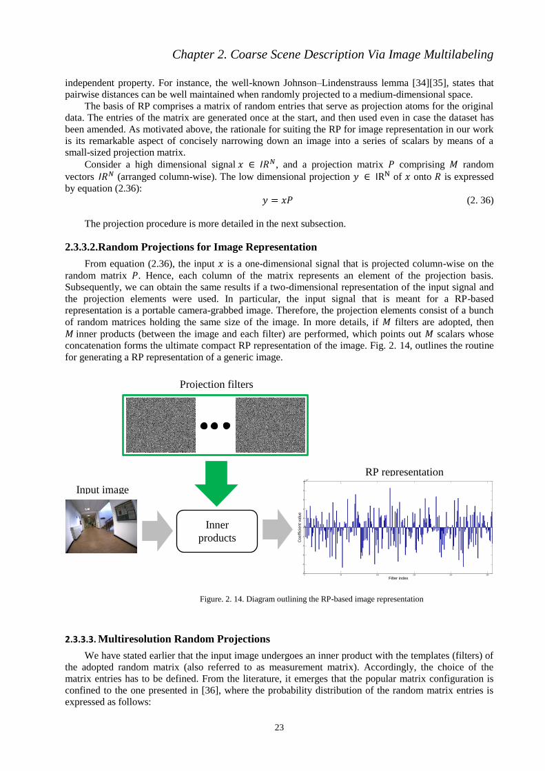
Chapter 2. Coarse Scene Description Via Image Multilabeling
23
independent property. For instance, the well-known Johnson–Lindenstrauss lemma [34][35], states that
pairwise distances can be well maintained when randomly projected to a medium-dimensional space.
The basis of RP comprises a matrix of random entries that serve as projection atoms for the original
data. The entries of the matrix are generated once at the start, and then used even in case the dataset has
been amended. As motivated above, the rationale for suiting the RP for image representation in our work
is its remarkable aspect of concisely narrowing down an image into a series of scalars by means of a
small-sized projection matrix.
Consider a high dimensional signal , and a projection matrix comprising random
vectors (arranged column-wise). The low dimensional projection of onto is expressed
by equation (2.36):
(2. 36)
The projection procedure is more detailed in the next subsection.
2.3.3.2.Random Projections for Image Representation
From equation (2.36), the input is a one-dimensional signal that is projected column-wise on the
random matrix . Hence, each column of the matrix represents an element of the projection basis.
Subsequently, we can obtain the same results if a two-dimensional representation of the input signal and
the projection elements were used. In particular, the input signal that is meant for a RP-based
representation is a portable camera-grabbed image. Therefore, the projection elements consist of a bunch
of random matrices holding the same size of the image. In more details, if filters are adopted, then
inner products (between the image and each filter) are performed, which points out scalars whose
concatenation forms the ultimate compact RP representation of the image. Fig. 2. 14, outlines the routine
for generating a RP representation of a generic image.
Figure. 2. 14. Diagram outlining the RP-based image representation
2.3.3.3. Multiresolution Random Projections
We have stated earlier that the input image undergoes an inner product with the templates (filters) of
the adopted random matrix (also referred to as measurement matrix). Accordingly, the choice of the
matrix entries has to be defined. From the literature, it emerges that the popular matrix configuration is
confined to the one presented in [36], where the probability distribution of the random matrix entries is
expressed as follows:
Input image
Projection filters
Inner
products
0 50 100 150 200 250-5
-4
-3
-2
-1
0
1
2
3
4
5x 10
4
Filter index
Co
eff
icie
nt
va
lue
RP representation

Chapter 2. Coarse Scene Description Via Image Multilabeling
24
( ) √ {
( )
(2. 37)
Where the indices and point to the lines and columns of the random matrix . Thus, two popular
particular cases that are used the most in the literature are given by and [37-39]. In the case
of , two thirds of the projection templates entries would be null, which causes the elimination of
of the input image pixels. Such information loss is not in the favor of our application as all the pixels
of the images play a major role. Whereas if is set to unity, the projection matrix would then exhibit a
uniform distribution of +1 and -1, which actually serves our application as it randomly captures the
gradients at different positions over the input image. In this paper, the value of is set to one, the
respective uniform distribution is conducted hereunder:
( ) {
(2. 38)
As to thoroughly analyze the images across different scales, we propose in this work a
multiresolution random projection (MRP) of the input image. Multiresolution concept is meant to further
analyze a given signal/image at different scales. Hence, the aim is to capture richer information and cover
finer details regarding the addressed signal/image. Examples of multiresolution include for instance scene
classification [40] [41], and texture analysis [42].
The MRP method consists of casting the input image onto a set of multiresolution random templates
generated according to equation (2.38) with different patterns that vary gradually. In particular, assuming
the images are of size m x n, then the first template of the projection matrix consists of four regions of
size (m/2) x (n/2) each. The assignment of +1 and -1 is done according to equation (2.38). The next
template consists of either +1 or -1-filled up regions of size (m/4) x (n/4). The size of the regions degrades
progressively until the smallest sized region is reached, that is a single pixel of the image, where the
pixels of the image take the values +1 or -1. In our work, the images consist of a resolution of 640x480.
Eight multiresolution levels were adopted for generating the templates. The region size as well as the
number of the respective templates are listed in Table 2. 1. Fig. 2. 15, depicts two samples of each
template. Fig. 2. 16, illustrates an example of RP image representation.
TABLE 2. 1. THE SET OF MULTIRESOLUTION RANDOM PROJECTION FILTERS.
Region size Number of templates
240x320 2
120x160 5
60x80 10
30x40 20
15x20 30
5x10 40
3x5 50
1x1 100
Total 257

Chapter 2. Coarse Scene Description Via Image Multilabeling
25
Figure. 2. 15. Two samples of each projection template sorted from top to bottom according to the resolution. Top templates refer
to resolutions of half the image size. Bottom templates refer to regions of one pixel. Black color indicates the -1 whilst the grey
color refers to +1
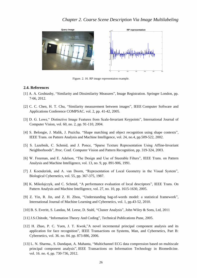
Chapter 2. Coarse Scene Description Via Image Multilabeling
26
Figure. 2. 16. RP image representaion example.
2.4. References
[1] A. A. Goshtasby, “Similarity and Dissimilarity Measures”, Image Registration. Springer London, pp.
7-66, 2012.
[2] C. C. Chen, H. T. Chu, “Similarity measurement between images”, IEEE Computer Software and
Applications Conference COMPSAC. vol. 2, pp. 41-42, 2005.
[3] D. G. Lowe,“ Distinctive Image Features from Scale-Invariant Keypoints”, International Journal of
Computer Vision, vol. 60, no. 2, pp. 91-110, 2004.
[4] S. Belongie, J. Malik, J. Puzicha. “Shape matching and object recognition using shape contexts”,
IEEE Trans. on Pattern Analysis and Machine Intelligence, vol. 24, no.4, pp.509-522, 2002.
[5] S. Lazebnik, C. Schmid, and J. Ponce, “Sparse Texture Representation Using Affine-Invariant
Neighborhoods”, Proc. Conf. Computer Vision and Pattern Recognition, pp. 319-324, 2003.
[6] W. Freeman, and E. Adelson, “The Design and Use of Steerable Filters”, IEEE Trans. on Pattern
Analysis and Machine Intelligence, vol. 13, no. 9, pp. 891-906, 1991.
[7] J. Koenderink, and A. van Doorn, “Representation of Local Geometry in the Visual System”,
Biological Cybernetics, vol. 55, pp. 367-375, 1987.
[8] K. Mikolajczyk, and C. Schmid, “A performance evaluation of local descriptors”, IEEE Trans. On
Pattern Analysis and Machine Intelligence, vol. 27, no. 10, pp. 1615-1630, 2005.
[9] Z. Yin, R. Jin, and Z. H. Zhou, “Understanding bag-of-words model: a statistical framework”,
International Journal of Machine Learning and Cybernetics, vol. 1, pp.43-52, 2010.
[10] B. S. Everitt, S. Landau, M. Leese, D. Stahl, “Cluster Analysis”, John Wiley & Sons, Ltd, 2011
[11] J.S.Chitode, “Information Theory And Coding”, Technical Publications Pune, 2005.
[12] H. Zhao, P. C. Yuen, J. T. Kwok,”A novel incremental principal component analysis and its
application for face recognition”, IEEE Transactions on Systems, Man, and Cybernetics, Part B:
Cybernetics, vol. 36. no. 04. pp. 873-886, 2006.
[13] L. N. Sharma., S. Dandapat, A. Mahanta, “Multichannel ECG data compression based on multiscale
principal component analysis”, IEEE Transactions on Information Technology in Biomedicine.
vol. 16. no. 4, pp. 730-736, 2012.
Query Image
0 50 100 150 200 250 300-6
-4
-2
0
2
4
6
8x 10
4 RP representation

Chapter 2. Coarse Scene Description Via Image Multilabeling
27
[14] L. Jolliffe, “Principal component analysis”, John Wiley & Sons, Ltd, 2005.
[15] D. L. Donoho, “Compressed Sensing”, IEEE Trans. Inf. Theory, vol. 52, no. 4, pp. 1289-1306, 2006.
[16] E. J. Candès, J. Romberg, T. Tao, “Robust Uncertainty Principle-Exact Signal Reconstruction from
Highly Incomplete Frequency Information”, IEEE Trans. Inf. Theory, vol. 52, no. 2, pp. 489-509,
[17] M. Aharon, M. Elad, A. Bruckstein, “K-SVD: An algorithm for designing overcomplete dictionaries
for sparse representation”, IEEE Trans. on Signal Processing, vol. 54, no.11, pp. 4311-4322, 2006.
[18] J. Wright, A. Yang, A. Ganesh, S. Sastry, Y. MA, “Robust Face Recognition via Sparse
Representation”, IEEE Trans. Pattern Anal. Mach. Intell., vol. 30, no. 2, pp. 210-227, 2009.
[19] V.M. Patel, R. Chellappa, ”Sparse representations, compressive sensing and dictionaries for pattern
recognition”, Proceeding in Asian Conference on Pattern Recognition (ACPR), pp. 325-329, 2011.
[20] A. Morelli Andrés, S. Padovani, M. Tepper. “Face recognition on partially occluded images using
compressed sensing”, Pattern Recognition Letters, vol. 36, pp. 235-242, 2014.
[21] J. Yang, J. Wright, T. Huang and Y. Ma, “Image Super-Resolution Via Sparse Representations”,
IEEE Trans. on Image Process., vol. 19, no. 11, pp. 2861-2873, 2010.
[22] S. Rao, R. Tron, R. Vidal, Y. Ma, “Motion Segmentation via Robust Subspace Separation in the
Presence of Outlying, Incomplete, and Corrupted Trajectories”, IEEE Trans. Pattern Anal. Mach.
Intell., vol. 32, no. 10, pp. 1832-1845, 2008.
[23] J. Mairal, M. Elad and G. Sapiro, “Sparse Representation for Color Image Restoration”, IEEE Trans.
Image Process, vol. 17, no. 1, pp. 53-69, 2008.
[24] B. Shen, W. Hu, Y. Zhang and Y.-J. Zhang, “Image Inpainting via Sparse Representation”, IEEE
ICASSP, pp. 697-700, 2009.
[25] L. Lorenzi, F. Melgani, and G. Mercier, “Missing Area Reconstruction in Multispectral Images
Under a Compressive Sensing Perspective”, IEEE Trans. Geosci. and Remote Sens., vol. 51, no. 7,
pp. 3998-4008, July 2013.
[26] A. Quattoni, M. Collins and T. Darrell, “Transfer Learning for Image Classification with Sparse
Prototype Representation”, IEEE Conference on Computer Vision and Pattern Recognition (CVPR),
pp. 1-8, 2008.
[27] J. Wright, Y. Ma, J. Mairal, G. Sapiro, T.S. Huang, and S. Yan, “Sparse Representation for
Computer Vision and Pattern Recognition”, Proc. of the IEEE, vol. 98, no. 6, Jun. 2010.
[28] E. J. Candès, T. Tao, “Decoding by Linear Programming”, IEEE Trans. Inform. Theory, vol. 51, no.
12, pp. 4203-4215, Dec. 2005.
[29] D. L. Donoho, Y. Tsaig, , I. Drori, , J. L. Starck, “Sparse solution of underdetermined systems of
linear equations by stagewise orthogonal matching pursuit”, IEEE Trans. Information Theory, vol.
58, no. 2, pp. 1094-1121, 2012.
[30] C. K.Williams, D. Barber, “Bayesian classification with Gaussian processes”, IEEE Trans. Pattern
Anal. Mach. Intell., vol. 20, no.12, pp. 1342-1351, 1998.

Chapter 2. Coarse Scene Description Via Image Multilabeling
28
[31] C. Rasmussen, C.K.I. Williams, “Gaussian process for machine learning”, The MIT press, 2006.
[32] Y. Bazi, F. Melgani, “Gaussian Process approach to remote sensing image classification”, IEEE
Trans. Geosci. and Remote Sens., vol. 48, pp.186-197, 2010.
[33] X. Shu, Y. Gao and H. Lu, “Efficient linear discriminant analysis with locality preserving for face
recognition”, Pattern Recognition, vol. 45, no. 5, pp. 1892-1898, 2012.
[34] E. Candes and T. Tao, “Near-Optimal Signal Recovery From Random Projections: Universal
Encoding Strategies”, IEEE Trans. Inform. Theory, vol. 52, no. 12, pp. 5406-5425, 2006.
[35] W.B. Johnson and J. Lindenstrauss, “Extension of Lipschitz Mapping into a Hilbert Space”, Proc.
Conf. Modern Analysis and Probability, pp. 189-206, 1984.
[36] P. Li, T. J. Hastie, and K. W. Church, “Very sparse random projections”, in Proc. 12th ACM
SIGKDD Int. Conf. Knowl. Disc. Data Mining, 2006, pp. 287–296.
[37] J. Wang, Geometric structure of high-dimensional data and dimensionality reduction. Beijing:
Springer, 2012.
[38] E. Bingham and H. Mannila, “Random Projection in Dimensionality Reduction: Applications to
Image and Text Data”, Proc. ACM SIGKDD Int’l Conf. Knowledge Discovery and Data Mining, pp.
245- 250, 2001.
[39] D. Achlioptas, “Database-friendly random projections: Johnson-Lindenstrauss with binary coins”,
Journal of Computer and System Sciences, vol. 66, no. 4, pp. 671-687, 2003.
[40] L. Zhou, Z. Zhou and D. Hu, “Scene classification using multi-resolution low-level feature
combination”, Neurocomputing, vol. 122, pp. 284-297, 2013.
[41] L. Zhou, Z. Zhou and D. Hu, “Scene classification using a multi-resolution bag-of-features model”,
Pattern Recognition, vol. 46, no. 1, pp. 424-433, 2013.
[42] J. Florindo and O. Bruno, “Texture analysis by multi-resolution fractal descriptors”, Expert Systems
with Applications, vol. 40, no. 10, pp. 4022-4028, 2013.

Chapter III
Experimental Validation

Chapter 3. Experimental Validation
30
3.1. Dataset Description
The evaluation of the presented image multilabeling approach was performed on four different
datasets (the input images of all datasets consist in a resolution of 640x480). The first two datasets
(dataset 1 and dataset 2) were acquired in two separate indoor locations at the University of Trento, Italy.
The acquisition was run by means of a chest-mounted CMOS camera from the IDS Imaging Development
Systems, model UI-1240LE-C-HQ with KOWA LM4NCL lens, carried by a wearable lightweight vest as
illustrated in Fig. 3. 1. This last shows the multisensor prototype on which we are working for both
guiding blind people and helping them in recognizing objects in indoor sites (Please refer to chapter 4 for
further details). The method for the recognition part, which is described in this chapter, is exploited on
demand, that is the user has access to the recognition function only when he desires it through a vocal
instruction. The names of the objects identified within the image extracted from the video stream at the
moment of the vocal instruction are communicated by speech synthesis. Work is in progress to integrate
all the developed algorithms in the prototype. Back to this work, it is also noteworthy that the images
acquired by the portable camera were not compensated for barrel distortion, as our method handles the
images as a whole and does not extract any feature from the images.
Dataset 1 contains a total of 130 images, which was split into 58 training images, and 72 for testing
purposes. Dataset 2 holds 131 images, divided into 61 images for training, and 70 images for testing.
As noted above, a list of objects of interest must be predefined. Thereupon, we have selected the
objects deemed to be the most important ones across the considered indoor environments. Regarding
dataset 1, 15 objects were considered as follows:
‘External Window’, ‘Board’, ‘Table’, ‘External Door’, ‘Stair Door’, ‘Access Control Reader’,
‘Office’, ‘Pillar’, ‘Display Screen’, ‘People’, ‘ATM’, ‘Chairs’, ‘Bins’, ‘Internal Door’, and ‘Elevator’.
As for dataset 2, the list was the following:
‘Stairs’, ‘Heater’, ‘Corridor’, ‘Board’, ‘Laboratories’, ‘Bins’, ‘Office’, ‘People’, ‘Pillar’, ‘Elevator’,
‘Reception’, ‘Chairs’, ‘Self Service’, ‘External Door’, and ‘Display Screen’.
The second two datasets (dataset 3 and dataset 4) were shot at two separate indoor locations at the
University of King Saud, Saudi Arabia, by means of a Samsung Note 3 smartphone. Dataset 3
accommodates 161 training and 159 test images for a total of 320 images. The list of objects is set as
follows:
‘Pillar’, ‘Fire extinguisher/hose’, ‘Trash can’, ‘Chairs’, ‘External Door’, ‘Hallway’, ’Self-service’,
‘Reception’, ’Didactic service machine’, ‘Display Screen’, ‘Board’, ‘Stairs’, ‘Elevator’, ‘Laboratory’,
‘Internal Door’.
Dataset 4 comprises 174 images consisting of 86 training and 88 testing images, and the object list
contains:
‘Board’, ‘Fire extinguisher’, ‘Trash cans’, ‘Chairs’, ‘External door’, ‘didactic service machine’,
‘Self-service’, ‘Reception’, ‘Cafeteria’, ‘Display screen’, ‘Pillar’, ‘Stairs’, ‘Elevator’, ‘Prayer room’,
‘Internal door’.
It is noteworthy that the training images for all datasets were selected in such a way to cover all the
predefined objects in the considered indoor environment. Fig. 3.1. depicts sample images from each
dataset.
For all training images of each dataset, and for each of the proposed strategies (SCD, BOWCD,
PCACD, EDCS, SSCS, MRPCD), we extracted the respective image representations as described in the
previous chapter and stored them in a library alongside the training binary descriptors.

Chapter 3. Experimental Validation
31
Figure. 3. 1. From topmost row to lowermost, three instances of: dataset1, dataset1, dataset 3, and dataset 4, respectively.
As for the learning images, which are exploited to develop the CS dictionary, we made use of 51, 54,
59, and 74 images with regards to Dataset 1, Dataset 2, Dataset 3, and Dataset 4, respectively.
3.2. Results and Discussion
Regarding the accuracy assessment, we compute accuracies by comparing the output vectors
(estimated list of objects given by the multilabel vectors) of the test (query) images to the true multilabel
vectors. In particular, we rely on two well-known accuracy measures, namely sensitivity and specificity,
which are expressed as follows:
True PositivesSensitivity
True Positives False Negatives
(3.1)

Chapter 3. Experimental Validation
32
True NegativesSpecificity
True Negatives False Positives
(3.2)
The annotations mentioned in the previous two equations are clarified in Table 3. 1. In the following,
the acronyms SEN and SPE will be used for sensitivity and specificity accuracies, which underline the
accuracies of true positives (existing objects) and true negatives (non- existing objects), respectively.
TABLE 3. 1. CONFUSION MATRIX FOR THE COMPUTATION OF THE SPECIFICITY AND
SENSITIVITY ACCURACIES.
Real label \ Estimated label 0 1
0 True Negative False Positive
1 False Negative True Positive
Since the BOWCD strategy undergoes an iterative K-means clustering algorithm, we performed the
experiments 10 times for this strategy, each time with a different random clustering initialization. The
accuracies of BOWCD reported in the following are averaged over the ten trials. Hereby, tables (from
3.2. to 3.20) summarize the classification results for all datasets regarding all the proposed strategies.
Let’s consider for instance the results pointed out by the first three schemes (SCD, BOWCD, and the
PCACD), whose outcomes are reported in Tables 3.2. to 3.7. In particular, we first interpret the effect of
the value of the number of training images (k) on the accuracies. For the three strategies, the results
suggest that the value of k does not impact much on the specificity, while it does on the sensitivity. This
is explained by the fact that the k closest images may appear very different, and thus convey disagreeing
lists of objects. A motivation for this disagreement can be found in the way our library has been
constructed. Indeed, we used relatively few training images to represent the entire environment. A
significant number of training images, sufficient enough to cover all the indoor spots, would lead to an
increase of correlation between the training images and hence to a higher likelihood of getting k closest
images in better compatibility to each other, increasing thereby the fusion effectiveness. However, the
drawback of increasing the size of the library is the computational time, which may become unacceptable
for an application like the one targeted in this work. Therefore, for our datasets, it emerges that the most
appropriate value is k=1. In particular, for the first dataset, the best strategy is SCD (SEN=84.64% and
SPE=91.02%), followed by BOWCD (72.73 % and 88.38%) and PCACD (70.79% and 80.69%). For the
second dataset, the best one is still SCD (91.36% and 95.78%), followed by BOWCD (85.09% and
93.88%) and PCACD (76.36% and 91.09%), the third dataset scored its best under the SCD (89.79% and
97.90%), followed by BOWCD (83.74% and 96.66%) and PCACD (71.49% and 92.02%), and finally the
fourth dataset reporting the highest porformance by means of the SCD (88.84% and 95.92%), then
BOWCD (77.60% and 92.96%), and PCACD (71.49% and 92.02%).
As for the third method, we recall the point that it encompasses two strategies for image
comparison, an Euclidean distance in the CS representation space, and a semantic similarity measure as
detailed in the previous chapter. A worth mentioning fact is that the resolution of the images has a direct
influence on the processing time (in particular, in the CS representation phase). Therefore, we have
analyzed its impact by running the experiments on four different resolution ratios. The first one is set to
the unity (thus, keeping the original 640×480 resolution), the second ratio was set to the half (320×240
image size), the third one equals to one fifth (128×96), and the last one was fixed to one tenth (64×48).
The results corresponding to the combination of the k values and the image resolutions regarding both
EDCS and SSCS strategies are summarized in Tables 3.8 to 3.15. Observing the results, it comes out that,
in overall terms, both the semantic similarity-based compressed sensing (SSCS) and Euclidean distance-
based compressed sensing (EDCS) methods perform nearly equivalently for k=1 on an average over the
SEN and SPE accuracies. However, the SSCS strategy yields a better sensitivity while the EDCS shows a
better specificity. For the other k values, the SSCS outperforms. This is explained by the fact that the
EDCS relies on measuring the similarity of the CS coefficients, yet measuring the apparent similarity
between the images, which is likely to guarantee the query image actually resembles to the first closest
image from the library (for k=1). However, by raising the value of k to 3 and 5, the library images tend to
Chapter 3. Experimental Validation
33
be dissimilar to the query image, which results in a lower performance (in particular, the sensitivity). The
rationale behind such accuracy decrease can, as aforesaid, be referred to the limited number of library
images. In other terms, for every indoor scenery, there are few representative images within the library.
Increasing such number would certainly promote a better correlation between the k considered library
images and uplift the probability of having objects in common, and hence boost the fusion process but at
the cost of a larger processing load. On the other hand, such phenomenon is not observed with the SSCS
strategy since similarity computation is performed not in the image domain but in the semantic one.
Moreover, it tends to be more balanced between the sensitivity and the specificity, which is not the case
with the former strategy. The result differences between the datasets can be refered to the reason that the
structure and the quantity of the objects composing their images, in addition to the physical dimensions of
the indoor spaces, are different. In general, the SSCS, in spite of the small-size library, behaves better
than the EDCS given that it performs the multilabeling process more efficiently. This is because image
similarity assessment in the semantic domain appears more straightforward to infer than in the image
domain which is more sensitive to image acquisition condition issues. As for the behavior of the GP
regressors, it can be drawn that the obtained results are very satisfactory despite that only few training
images are used.
Moving to the last MRPCD strategy, given that the higher the resolution the more time is consumed
whilst in the projection step (i.e., the inner product) as the RP templates have the same size of the input
image. Therefore, we adopt the same image resolution scenarios undersaken in the SSCD strategy.
Provided that the projection matrix comprises random +1 and -1 distributions, we have taken the average
accuracies over ten runs (each run performed with a different set of random projections). The matching
step has been achieved by means of the cosine distance as it pointed out slight improvements with respect
to the basic Euclidean distance.
We initiate the experimental evaluation by checking the efficiency of a multiresolution RP as
compared to a regular state-of-the-art multiresolution strategy (i.e., where the projection filters consist of
a resolution of one pixel). Therefore, we further launched the experiments by means of 257 RP templates
(which is the total number of multiresolution templates as stated in the previous chapter) of a 1x1 region
size. The average accuracies over ten runs are reported in Tables 3.16. to 3.19. The results clearly point
out the valuable increase incurred by the multiresolution RP over the ordinary RP scenario, which
indicates the capacity of the MRP in investigating further scales of the considered images.
From the reported results, it appears clearly that the presented MRP algorithm points out its best at a
resolution ration of 1/10 regarding all the datasets. This might trace back to the point that decaying the
image resolution diminishes the small details as well as the size of the objects while maintaining the
backgrounds and the large surfaces/objects. In other terms, the tiny details can be considered as outlier
noise, hence reducing the resolution fades that noise and keeps the dominating spectral content of the
images, which is essential for the comparison as validated by the results.
Considering the best case scenario with respect to all strategies, we provide in Table 3.21 a
comparison of yielded accuracies on all datasets.Having a close look at the outcomes, it emerges that the
SCD and the BOWCD methods exhibit relatively higher accuracies (particularly, the SEN), which is
raionale as both strategies rely on the SIFT keypoints space for image representation, which is likely to
preserve the most prominent image content into salient keypoints, raising thereby the efficiency of image
matching, that leads to accurate multilabeling. On the other end, the remaining three strategies do not go
into a pixel-level investiation but treat a onsidered image as whole, which might be subject to overlook
some essential spectral details. On the whole, the SCD outperforms all the other schemes, followed by the
BOWCD, then the PCACD and MRPCD that perform almost equivalently and lastly the CSCD. We also
report the overall (average over all datasets) processing time per image in Table 3. 22. It comes out that
the MRPCD is, by far, much faster than the remaining methods, the PCACD comes second with less than
a second per image, then the BOWCD followed by the PCACD. The SCD, however, cosumes as much as
2.5 min per image, which makes it inappropriate in real-time implementations. Ultimately, considering
the recognition accuracy on the one hand and the processing span on the other, one might tend to deem
the MRPCD and the BOWCD as the most adequate accuracy-time-balanced options. For the sake of
illustration, three multilabeling examples are depicted in the upcoming figures. The examples for all
methods depic the quesry camera-grabed images and their closest thre neighbours from the library, the
objects list however, was derived from the closest training image (k=1), except for the RPCD where only
the depiction of the closest neighbour is shown. It is yet to point out the fact that, even though the

Chapter 3. Experimental Validation
34
libraries hold a limited set of images as compared to the broadness of the adressed indoor sites, the closest
images exhibit a certain similarity with the quesry samples, and as mentioned earlier a denser training
library is bound to bridge the gaps (i.e., the semantic gap with regards to the SSCD and the spectral gap
regarding the remaining strategies) between he test and the training images.
Finally, worth addressing is the behavioir of the BOWCD with respect to different codebook sizes,
we have performed the experiments considering different cases and found out that a codebook of 250 or
300 words yields the best rates, yet a fixed size of 300 centroids was adopted. On the other hand, we have
conducted further experiments considring illumination changes, and found out that the results are not
impacted, which is reasonable as we are dealing with images of inddor sites what are supplied with
artificial lights,. In other words the objects are exposed to artificial illumination with constant intensity,
the outdoor illumination has therefore no impact on the objects reflectance.
TABLE 3. 2. CLASSIFICATION ACCURACIES OF THE SCD SCHEME IN TERMS OF k VALUES
FOR ALL DATASETS.
Dataset1 Dataset2 Dataset3 Dataset4
k=1 SEN 84.64 91.36 89.79 88.84
SPE 91.02 95.78 97.90 95.92
AVG 87.83 93.57 93.84 92.38
k=3 SEN 83.52 90.45 81.94 80.58
SPE 91.76 95.06 97.10 95.36
AVG 87.64 92.75 89.52 87.97
k=5 SEN 77.15 86.36 72.77 70.66
SPE 92.13 93.01 97.40 95.18
AVG 84.64 89.68 85.08 82.92
TABLE 3. 3. PER-CLASS OVERALL CLASSIFICATION ACCURACIES ACHIEVED ON ALL
DATASETS BY MEANS OF THE SCD METHOD FOR k=1.
1 2 3 4 5 6 7 8 9 10 11 12 13 14 15
Ds1 94.44 83.33 98.61 90.28 84.72 98.61 86.11 86.11 86.11 94.44 95.83 81.94 87.50 80.56 93.06
Ds2 98.57 97.14 94.29 84.29 95.71 91.43 94.29 90.00 98.57 98.57 91.43 97.14 95.71 97.14 98.57
Ds3 99.37 92.45 95.60 96.23 96.23 94.34 98.11 100.00 98.74 98.74 97.48 96.23 100.00 100.00 85.53
Ds4 85.23 89.77 94.32 89.77 92.05 96.59 95.45 96.59 98.86 98.86 100.00 100.00 98.86 95.45 87.50
TABLE 3. 4. CLASSIFICATION ACCURACIES OF THE BOWCD SCHEME IN TERMS OF k
VALUES FOR ALL DATASETS.
Dataset1 Dataset2 Dataset3 Dataset4
k=1 SEN 72.73 85.09 83.74 77.60
SPE 88.38 93.88 96.66 92.96
AVG 80.55 89.48 90.2 85.28
k=3 SEN 65.96 80.18 75.16 60.29
SPE 90.09 94.39 95.93 93.09
AVG 78.02 87.28 85.54 76.69
k=5 SEN 60.90 75.05 70.26 50.04
SPE 90.38 94.37 96.07 93.64
AVG 75.64 84.71 83.16 71.84

Chapter 3. Experimental Validation
35
TABLE 3. 5. PER-CLASS OVERALL CLASSIFICATION ACCURACIES ACHIEVED ON ALL
DATASETS BY MEANS OF THE BOWCD METHOD FOR k=1.
1 2 3 4 5 6 7 8 9 10 11 12 13 14 15
Ds1 93.06 70.83 98.61 76.39 70.83 97.22 81.94 76.39 87.50 95.83 91.67 75.00 80.56 72.22 95.83
Ds2 98.57 90.00 90.00 77.14 92.86 84.29 88.57 85.71 97.14 100.00 91.43 97.14 92.86 94.29 97.14
Ds3 97.48 88.68 91.19 90.57 96.23 93.71 96.23 99.37 98.11 95.60 94.34 95.60 97.48 100.00 82.39
Ds4 75.00 82.95 79.55 82.95 88.64 89.77 86.36 96.59 95.45 90.91 98.86 98.86 96.59 93.18 76.14
TABLE 3. 6. CLASSIFICATION ACCURACIES OF THE PCACD SCHEME IN TERMS OF k
VALUES FOR ALL DATASETS.
Dataset1 Dataset2 Dataset3 Dataset4
k=1 SEN 70.79 76.36 70.16 71.49
SPE 80.69 91.08 94.06 92.02
AVG 75.74 83.72 82.11 81.75
k=3 SEN 67.79 66.36 63.35 57.02
SPE 81.80 90.00 93.71 93.41
AVG 74.795 78.18 78.53 75.21
k=5 SEN 65.54 62.27 52.62 42.98
SPE 81.67 91.57 94.21 93.41
AVG 73.60 76.92 73.41 68.19
TABLE 3. 7. PER-CLASS OVERALL CLASSIFICATION ACCURACIES ACHIEVED ON ALL
DATASETS BY MEANS OF THE PCACD METHOD FOR k=1.
1 2 3 4 5 6 7 8 9 10 11 12 13 14 15
Ds1 76.39 58.33 94.44 80.56 79.17 93.06 70.83 63.89 80.56 95.83 88.89 72.22 69.44 63.89 86.11
Ds2 94.29 75.71 84.29 74.29 84.29 77.14 87.14 90.00 95.71 97.14 90.00 94.29 92.86 92.86 90.00
Ds3 96.86 81.13 91.82 84.91 90.57 76.73 91.82 96.23 96.86 94.97 89.31 89.31 98.74 99.37 74.84
Ds4 71.59 81.82 94.32 80.68 88.64 95.45 88.64 90.91 97.73 92.05 95.45 88.64 95.45 92.05 70.45
TABLE 3. 8. RESULTS OF PROPOSED STRATEGIES OBTAINED ON DATASET 1, BY VARYING
IMAGE RESOLUTION AND K (NUMBER OF MULTILABELING IMAGES) VALUE.
SSCS
(Semantic similarity compressed sensing)
EDCS
(Euclidean distance compressed sensing)
Ratio 1/10 1/5 1/2 1 1/10 1/5 1/2 1
k=1 SEN 80.89 81.64 79.77 79.77 71.53 70.41 69.66 69.66
SPE 68.14
67.40 66.91 66.54 79.33
79.82
79.82
80.19
AVG 74.51 74.52 73.34 73.15 75.43 75.115 74.74 74.92
k=3 SEN 78.65 78.65 80.52 80.14 65.91 66.66 67.41 68.53
SPE 69.86
69.61 69.74 69.37 81.54
80.93
81.42
81.91
AVG 74.25 74.13 75.13 74.75 73.72 73.79 74.41 75.22
k=5 SEN 76.02 76.77 76.02 75.65 67.41 67.79 67.79 68.16
SPE 71.09
70.60 70.47 70.72 82.41
81.91
81.79
82.04
AVG 73.55 73.68 73.24 73.18 74.91 74.85 74.79 75.1
TABLE 3. 9. PER-CLASS CLASSIFICATION ACCURACIES ACHIEVED ON DATASET 1 BY:
EDCS METHOD (K=1 AND 1/10 RATIO), SSCS METHOD (K=3 AND 1/2 RATIO).
1 2 3 4 5 6 7 8 9 10 11 12 13 14 15
EDCS 77.77 61.11 93.05 75 77.77 90.27 75 66.66 77.77 95.83 91.66 65.27 66.66 59.72 87.50
SSCS 58.33 59.72 91.66 69.44 63.88 90.27 44.44 54.16 90.27 95.83 87.50 38.88 72.22 73.61 88.88
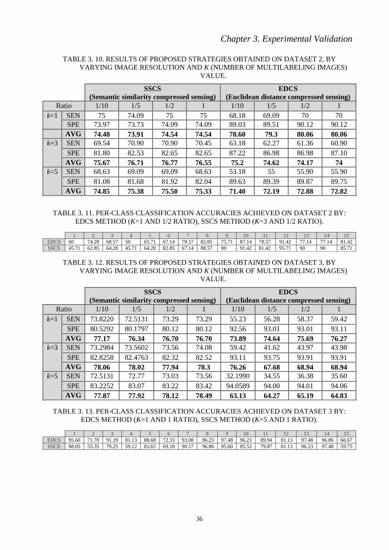
Chapter 3. Experimental Validation
36
TABLE 3. 10. RESULTS OF PROPOSED STRATEGIES OBTAINED ON DATASET 2, BY
VARYING IMAGE RESOLUTION AND K (NUMBER OF MULTILABELING IMAGES)
VALUE.
SSCS
(Semantic similarity compressed sensing)
EDCS
(Euclidean distance compressed sensing)
Ratio 1/10 1/5 1/2 1 1/10 1/5 1/2 1
k=1 SEN 75 74.09 75 75 68.18 69.09 70 70
SPE 73.97 73.73 74.09 74.09 89.03 89.51 90.12 90.12
AVG 74.48 73.91 74.54 74.54 78.60 79.3 80.06 80.06
k=3 SEN 69.54 70.90 70.90 70.45 63.18 62.27 61.36 60.90
SPE 81.80 82.53
82.65 82.65 87.22 86.98 86.98 87.10
AVG 75.67 76.71 76.77 76.55 75.2 74.62 74.17 74
k=5 SEN 68.63 69.09 69.09 68.63 53.18 55 55.90 55.90
SPE 81.08 81.68
81.92 82.04 89.63 89.39 89.87 89.75
AVG 74.85 75.38 75.50 75.33 71.40 72.19 72.88 72.82
TABLE 3. 11. PER-CLASS CLASSIFICATION ACCURACIES ACHIEVED ON DATASET 2 BY:
EDCS METHOD (K=1 AND 1/2 RATIO), SSCS METHOD (K=3 AND 1/2 RATIO).
1 2 3 4 5 6 7 8 9 10 11 12 13 14 15
EDCS 60 74.28 68.57 50 65.71 67.14 78.57 82.85 75.71 87.14 78.57 91.42 77.14 77.14 81.42
SSCS 45.71 62.85 64.28 45.71 64.28 82.85 67.14 88.57 80 91.42 81.42 95.71 90 90 85.71
TABLE 3. 12. RESULTS OF PROPOSED STRATEGIES OBTAINED ON DATASET 3, BY
VARYING IMAGE RESOLUTION AND K (NUMBER OF MULTILABELING IMAGES)
VALUE.
SSCS
(Semantic similarity compressed sensing)
EDCS
(Euclidean distance compressed sensing)
Ratio 1/10 1/5 1/2 1 1/10 1/5 1/2 1
k=1 SEN 73.8220 72.5131 73.29 73.29 55.23 56.28 58.37 59.42
SPE 80.5292 80.1797 80.12 80.12 92.56 93.01 93.01 93.11
AVG 77.17 76.34 76.70 76.70 73.89 74.64 75.69 76.27
k=3 SEN 73.2984 73.5602 73.56 74.08 59.42 41.62 43.97 43.98
SPE 82.8258 82.4763 82.32 82.52 93.11 93.75 93.91 93.91
AVG 78.06 78.02 77.94 78.3 76.26 67.68 68.94 68.94
k=5 SEN 72.5131 72.77 73.03 73.56 32.1990 34.55 36.38 35.60
SPE 83.2252 83.07 83.22 83.42 94.0589 94.00 94.01 94.06
AVG 77.87 77.92 78.12 78.49 63.13 64.27 65.19 64.83
TABLE 3. 13. PER-CLASS CLASSIFICATION ACCURACIES ACHIEVED ON DATASET 3 BY:
EDCS METHOD (K=1 AND 1 RATIO), SSCS METHOD (K=5 AND 1 RATIO).
1 2 3 4 5 6 7 8 9 10 11 12 13 14 15
EDCS 95.60 71.70 91.19 81.13 88.68 72.33 93.08 96.23 97.48 96.23 89.94 81.13 97.48 96.86 66.67
SSCS 88.05 55.35 79.25 59.12 83.65 69.18 90.57 96.86 95.60 85.53 79.87 81.13 96.23 97.48 59.75
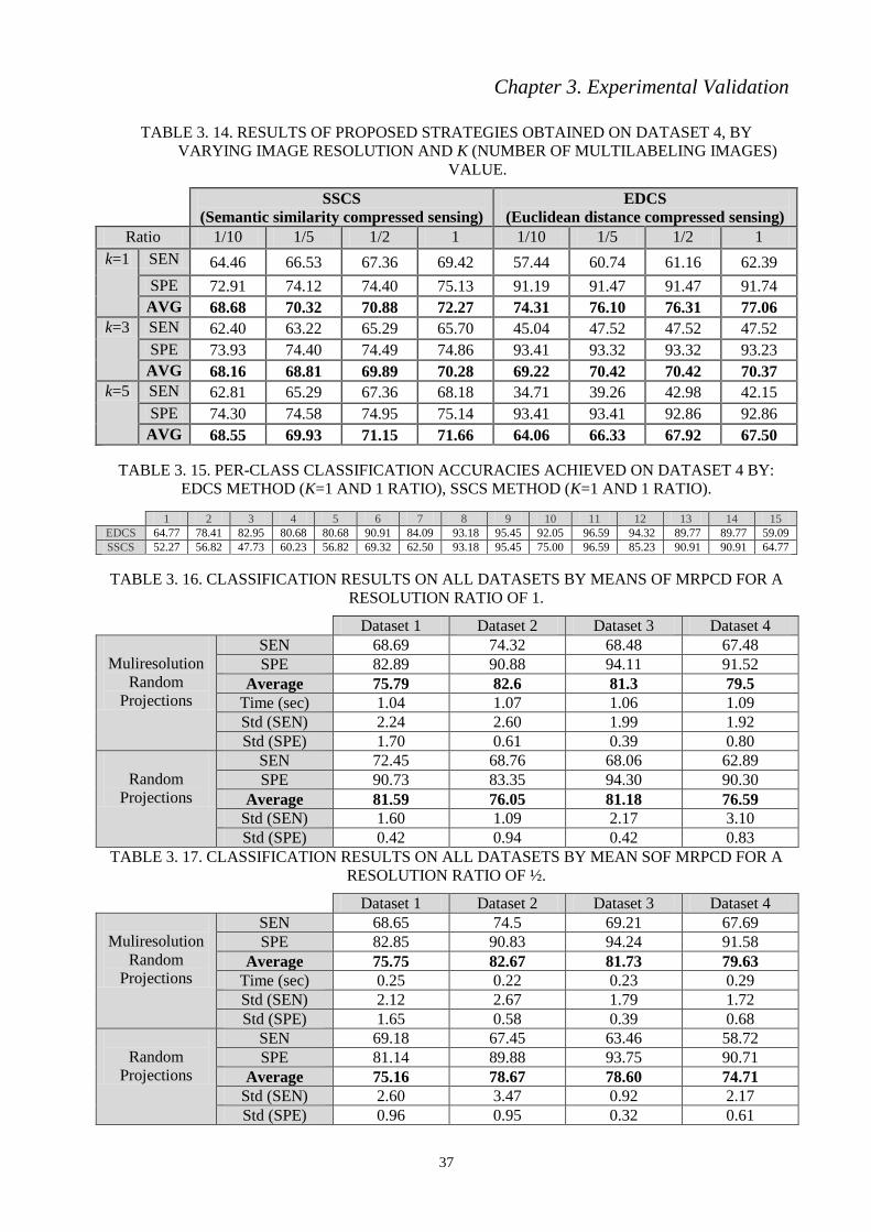
Chapter 3. Experimental Validation
37
TABLE 3. 14. RESULTS OF PROPOSED STRATEGIES OBTAINED ON DATASET 4, BY
VARYING IMAGE RESOLUTION AND K (NUMBER OF MULTILABELING IMAGES)
VALUE.
SSCS
(Semantic similarity compressed sensing)
EDCS
(Euclidean distance compressed sensing)
Ratio 1/10 1/5 1/2 1 1/10 1/5 1/2 1
k=1 SEN 64.46 66.53 67.36 69.42 57.44 60.74 61.16 62.39
SPE 72.91 74.12 74.40 75.13 91.19 91.47 91.47 91.74
AVG 68.68 70.32 70.88 72.27 74.31 76.10 76.31 77.06
k=3 SEN 62.40 63.22 65.29 65.70 45.04 47.52 47.52 47.52
SPE 73.93 74.40 74.49 74.86 93.41 93.32 93.32 93.23
AVG 68.16 68.81 69.89 70.28 69.22 70.42 70.42 70.37
k=5 SEN 62.81 65.29 67.36 68.18 34.71 39.26 42.98 42.15
SPE 74.30 74.58 74.95 75.14 93.41 93.41 92.86 92.86
AVG 68.55 69.93 71.15 71.66 64.06 66.33 67.92 67.50
TABLE 3. 15. PER-CLASS CLASSIFICATION ACCURACIES ACHIEVED ON DATASET 4 BY:
EDCS METHOD (K=1 AND 1 RATIO), SSCS METHOD (K=1 AND 1 RATIO).
1 2 3 4 5 6 7 8 9 10 11 12 13 14 15
EDCS 64.77 78.41 82.95 80.68 80.68 90.91 84.09 93.18 95.45 92.05 96.59 94.32 89.77 89.77 59.09
SSCS 52.27 56.82 47.73 60.23 56.82 69.32 62.50 93.18 95.45 75.00 96.59 85.23 90.91 90.91 64.77
TABLE 3. 16. CLASSIFICATION RESULTS ON ALL DATASETS BY MEANS OF MRPCD FOR A
RESOLUTION RATIO OF 1.
Dataset 1 Dataset 2 Dataset 3 Dataset 4
Muliresolution
Random
Projections
SEN 68.69 74.32 68.48 67.48
SPE 82.89 90.88 94.11 91.52
Average 75.79 82.6 81.3 79.5
Time (sec) 1.04 1.07 1.06 1.09
Std (SEN) 2.24 2.60 1.99 1.92
Std (SPE) 1.70 0.61 0.39 0.80
Random
Projections
SEN 72.45 68.76 68.06 62.89
SPE 90.73 83.35 94.30 90.30
Average 81.59 76.05 81.18 76.59
Std (SEN) 1.60 1.09 2.17 3.10
Std (SPE) 0.42 0.94 0.42 0.83
TABLE 3. 17. CLASSIFICATION RESULTS ON ALL DATASETS BY MEAN SOF MRPCD FOR A
RESOLUTION RATIO OF ½.
Dataset 1 Dataset 2 Dataset 3 Dataset 4
Muliresolution
Random
Projections
SEN 68.65 74.5 69.21 67.69
SPE 82.85 90.83 94.24 91.58
Average 75.75 82.67 81.73 79.63
Time (sec) 0.25 0.22 0.23 0.29
Std (SEN) 2.12 2.67 1.79 1.72
Std (SPE) 1.65 0.58 0.39 0.68
Random
Projections
SEN 69.18 67.45 63.46 58.72
SPE 81.14 89.88 93.75 90.71
Average 75.16 78.67 78.60 74.71
Std (SEN) 2.60 3.47 0.92 2.17
Std (SPE) 0.96 0.95 0.32 0.61

Chapter 3. Experimental Validation
38
TABLE 3. 18. CLASSIFICATION RESULTS ON ALL DATASETS BY MEAN SOF MRPCD FOR A
RESOLUTION RATIO OF 1/5.
Dataset 1 Dataset 2 Dataset 3 Dataset 4
Muliresolution
Random
Projections
SEN 68.84 75.86 70.42 69.55
SPE 82.77 91.08 94.54 91.73
Average 75.8 83.47 82.48 80.64
Time (sec) 0.056 0.056 0.061 0.061
Std (SEN) 2.43 2.17 1.63 1.92
Std (SPE) 1.63 0.53 0.35 0.78
Random
Projections
SEN 70.07 64.63 64.63 57.15
SPE 80.12 93.89 93.89 90.35
Average 75.10 79.26 79.26 73.75
Std (SEN) 2.20 1.98 1.71 2.10
Std (SPE) 0.96 0.72 0.37 0.73
TABLE 3. 19. CLASSIFICATION RESULTS ON ALL DATASETS BY MEAN SOF MRPCD FOR A
RESOLUTION RATIO OF 1/10.
Dataset 1 Dataset 2 Dataset 3 Dataset 4
Muliresolution
Random
Projections
SEN 71.16 77.18 71.65 70
SPE 83.2 91.41 94.81 92.33
Average 77.18 84.3 83.23 81.16
Time (sec) 0.037 0.037 0.035 0.037
Std (SEN) 2.32 2.32 1.49 1.90
Std (SPE) 0.78 0.49 0.31 0.73
Random
Projections
SEN 70.60 67.77 65.16 61.32
SPE 80.92 89.75 94.15 90.73
Average 75.76 78.76 79.65 76.03
Std (SEN) 1.04 2.32 1.68 2.54
Std (SPE) 1.16 0.47 0.23 0.59
TABLE 3. 20. PER-CLASS OVERALL CLASSIFICATION ACCURACIES ACHIEVED ON ALL
DATASETS BY MEANS OF THE MRPCD METHOD FOR A RESOLUTION RATIO OF 1/10.
1 2 3 4 5 6 7 8 9 10 11 12 13 14 15
Ds1 81.91 67.87 93.30 79.37 80.53 92.18 78.86 67.87 79.85 95.27 89.56 77.07 78.17 69.01 84.85
Ds2 90.14 80.29 83.86 76.71 86.86 77.71 89.29 85.71 94.00 96.29 91.57 97.00 90.71 93.43 92.86
Ds3 96.54 80.31 92.58 86.29 91.57 81.70 92.20 97.55 96.42 96.23 90.00 88.68 97.74 99.18 79.50
Ds4 73.18 81.70 89.55 85.34 84.55 94.32 88.75 93.98 95.34 90.34 97.73 91.36 92.95 89.32 75.11

Chapter 3. Experimental Validation
39
TABLE 3. 21. COMPARISON OF ALL CLASSIFICATION STRATEGIES ON ALL DATASETS.
FOR THE SCD, BOWCD, AND THE PCACD, THE ACCURACIES CORRESPOND TO K =1. FOR
HE SSCS STRATEGY THE VALUES OF K AND THE RESOLUTION RATIO WERE (3, ½), (3, 1/2),
(5, 1), AND (1,1) FOR THE CONSIDERED DATASETS, RESPECTIVELY. FOR THE MRPCD, THE
RESOLUTION RATION CORRESPONDS TO 1/10.
Dataset1 Dataset2 Dataset3 Dataset4 Overall
SCD SEN 84.64 91.36 89.79 88.84 88.66
SPE 91.02 95.78 97.90 95.92 95.16
AVG 87.83 93.57 93.84 92.38 91.91
BOWCD
SEN 72.73 85.09 83.74 77.60 79.79
SPE 88.38 93.88 96.66 92.96 92.97
AVG 80.55 89.48 90.2 85.28 86.38
PCACD
SEN 70.79 76.36 70.16 71.49 72.20
SPE 80.69 91.08 94.06 92.02 89.46
AVG 75.74 83.72 82.11 81.75 80.83
SSCS
SEN 80.52 70.90 73.56 69.42 73.60
SPE 69.74 82.65 83.42 75.13 77.74
AVG 75.13 76.77 78.49 72.27 75.67
MRPCD
SEN 71.16 77.18 71.65 70 72.50
SPE 83.2 91.41 94.81 92.33 90.44
AVG 77.18 84.3 83.23 81.16 81.47
TABLE 3. 22. OVERALL PROCESSING TIME PER IMAGE WITH RESPECT TO ALL
STRATEGIES.
Scheme SCD BOWCD PCACD SSCS MRPCD
Time/Image 2.5 min 0.71 sec 0.65 sec 1.18 sec 0.036 sec

Chapter 3. Experimental Validation
40
Figure. 3. 2. Three multilabeling examples from Dataset 1 by means of the SCD.
Query image 1st Closest image
Predicted objects: 'External Window', 'Board', 'Table', 'External Door', 'Access Control Reader',
2nd Closest image 3rd Closest image
Query image 1st Closest image
Predicted objects:'Internal Door', Elevator',
2nd Closest image 3rd Closest image
Query image 1st Closest image
Predicted objects:'Office', 'Pillar', 'Display Screen', 'Chairs',
2nd Closest image 3rd Closest image

Chapter 3. Experimental Validation
41
Figure. 3. 3. Three multilabeling examples from Dataset 2 by means of the SCD.
Query image 1st Closest image
Predicted objects: 'Heater', 'Corridor', 'Board', 'Office',
2nd Closest image 3rd Closest image
Query image 1st Closest image
Predicted objects: 'Stairs', 'Board', 'Pillar', 'Elevator',
2nd Closest image 3rd Closest image
Query image 1st Closest image
Predicted objects: 'Corridor', 'Board', 'Laboratories', 'Bins',
2nd Closest image 3rd Closest image

Chapter 3. Experimental Validation
42
Figure. 3. 4. Three multilabeling examples from Dataset 3 by means of the SCD.
Query image 1st Closest image
Predicted objects:'Chairs', 'Self service', 'Internal Door',
2nd Closest image 3rd Closest image
Query image 1st Closest image
Predicted objects:'Chairs', 'Didactic service machine',
2nd Closest image 3rd Closest image
Query image 1st Closest image
Predicted objects:'Chairs', 'Reception',
2nd Closest image 3rd Closest image

Chapter 3. Experimental Validation
43
Figure. 3. 5. Three multilabeling examples from Dataset 4 by means of the SCD.
Query image 1st Closest image
Predicted objects:'Trash cans', 'Chairs', 'External door',
2nd Closest image 3rd Closest image
Query image 1st Closest image
Predicted objects:'Elevator',
2nd Closest image 3rd Closest image
Query image 1st Closest image
Predicted objects:'Board', 'Trash cans', 'didactic service machine', 'Self service',
2nd Closest image 3rd Closest image

Chapter 3. Experimental Validation
44
Figure. 3. 6. Three multilabeling examples from Dataset 1 by means of the BOWCD.
Query image 1st closest image
Predicted objects:'Office', 'Pillar', 'Display Screen', 'Chairs',
2nd closest image 3rd closest image
Query image 1st closest image
Predicted objects:'Board', 'Pillar', 'ATM',
2nd closest image 3rd closest image
Query image 1st closest image
Predicted objects:'Board', 'Stair Door', 'Office', 'Display Screen', 'Internal Door',
2nd closest image 3rd closest image

Chapter 3. Experimental Validation
45
Figure. 3. 7. Three multilabeling examples from Dataset 2 by means of the BOWCD.
Query image 1st closest image
Predicted objects: 'Stairs', 'Heater', 'Corridor', 'Board',
2nd closest image 3rd closest image
Query image 1st closest image
Predicted objects: 'Stairs', 'Board', 'Pillar', 'Elevator',
2nd closest image 3rd closest image
Query image 1st closest image
Predicted objects: 'Board', 'Reception', 'Display screen',
2nd closest image 3rd closest image
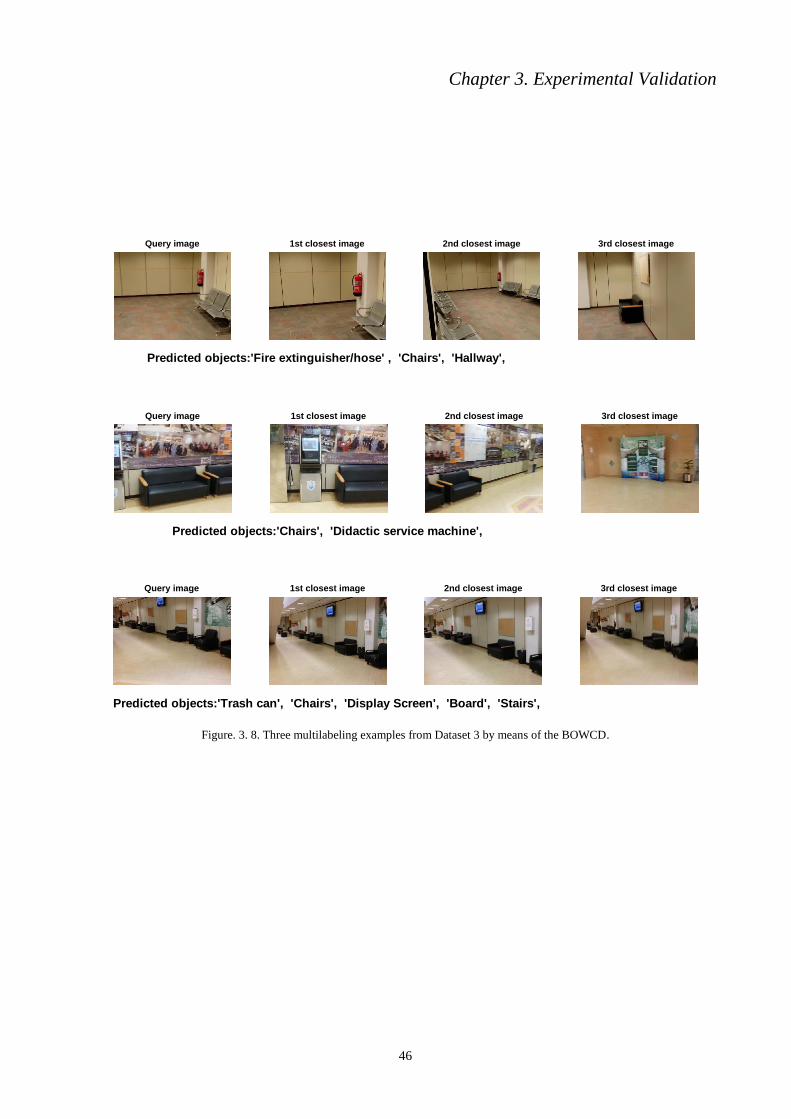
Chapter 3. Experimental Validation
46
Figure. 3. 8. Three multilabeling examples from Dataset 3 by means of the BOWCD.
Query image 1st closest image
Predicted objects:'Fire extinguisher/hose' , 'Chairs', 'Hallway',
2nd closest image 3rd closest image
Query image 1st closest image
Predicted objects:'Chairs', 'Didactic service machine',
2nd closest image 3rd closest image
Query image 1st closest image
Predicted objects:'Trash can', 'Chairs', 'Display Screen', 'Board', 'Stairs',
2nd closest image 3rd closest image

Chapter 3. Experimental Validation
47
Figure. 3. 9. Three multilabeling examples from Dataset 4 by means of the BOWCD.
Query image 1st closest image
Predicted objects:'Board', 'Stairs',
2nd closest image 3rd closest image
Query image 1st closest image
Predicted objects:'Trash cans', 'Chairs', 'External door',
2nd closest image 3rd closest image
Query image 1st closest image
Predicted objects:'Chairs', 'Self service', 'Internal door',
2nd closest image 3rd closest image

Chapter 3. Experimental Validation
48
Figure. 3. 10. Three multilabeling examples from Dataset 1 by means of the PCACD.
Query Image 1st Closest Image
Predicted objects:'External Door', 'Stair Door',
2nd Closest Image 3rd Closest Image
Query Image 1st Closest Image
Predicted objects:'Office', 'Pillar', 'Chairs', 'Bins', 'Internal Door',
2nd Closest Image 3rd Closest Image
Query Image 1st Closest Image
Predicted objects:'Board', 'Office', 'Pillar', 'ATM', 'Chairs', 'Internal Door',
2nd Closest Image 3rd Closest Image

Chapter 3. Experimental Validation
49
Figure. 3. 11. Three multilabeling examples from Dataset 2 by means of the PCACD.
Query Image 1st Closest Image
Predicted objects: 'Board', 'Pillar', 'Reception', 'Display screen',
2nd Closest Image 3rd Closest Image
Query Image 1st Closest Image
Predicted objects: 'Stairs', 'Board', 'Pillar', 'Elevator',
2nd Closest Image 3rd Closest Image
Query Image 1st Closest Image
Predicted objects: 'Heater', 'Corridor', 'Board', 'Laboratories', 'Office',
2nd Closest Image 3rd Closest Image

Chapter 3. Experimental Validation
50
Figure. 3. 12. Three multilabeling examples from Dataset 3 by means of the PCACD.
Query Image 1st Closest Image
Predicted objects:'Fire extinguisher/hose' , 'Hallway', 'Internal Door',
2nd Closest Image 3rd Closest Image
Query Image 1st Closest Image
Predicted objects:'Fire extinguisher/hose' , 'Chairs', 'Board',
2nd Closest Image 3rd Closest Image
Query Image 1st Closest Image
Predicted objects:'Pillar', 'Fire extinguisher/hose' , 'Chairs', 'External Door',
2nd Closest Image 3rd Closest Image

Chapter 3. Experimental Validation
51
Figure. 3. 13. Three multilabeling examples from Dataset 4 by means of the PCACD.
Query Image 1st Closest Image
Predicted objects:'Fire extinguisher', 'Trash cans', 'Chairs', 'Display screen', 'Internal door',
2nd Closest Image 3rd Closest Image
Query Image 1st Closest Image
Predicted objects:'Chairs', 'Internal door',
2nd Closest Image 3rd Closest Image
Query Image 1st Closest Image
Predicted objects:'Self service', 'Internal door',
2nd Closest Image 3rd Closest Image

Chapter 3. Experimental Validation
52
Figure. 3. 14. Three multilabeling examples from Dataset 1 by means of the SSCS.
Test image Closest image
Predicted objects:'Board', 'Office', 'Pillar', 'Display Screen', 'Chairs', 'Bins', 'Internal Door',
2nd Closest image 3rd Closest image
Test image Closest image
Predicted objects:'External Door', 'Stair Door', 'Internal Door',
2nd Closest image 3rd Closest image
Test image Closest image
Predicted objects:'Board', 'Office', 'Pillar', 'ATM', 'Chairs', 'Internal Door',
2nd Closest image 3rd Closest image
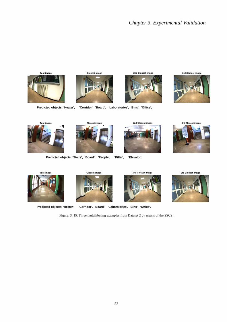
Chapter 3. Experimental Validation
53
Figure. 3. 15. Three multilabeling examples from Dataset 2 by means of the SSCS.
Test image Closest image
Predicted objects: 'Heater', 'Corridor', 'Board', 'Laboratories', 'Bins', 'Office',
2nd Closest image 3rd Closest image
Test image Closest image
Predicted objects: 'Stairs', 'Board', 'People', 'Pillar', 'Elevator',
2nd Closest image 3rd Closest image
Test image Closest image
Predicted objects: 'Heater', 'Corridor', 'Board', 'Laboratories', 'Bins', 'Office',
2nd Closest image 3rd Closest image
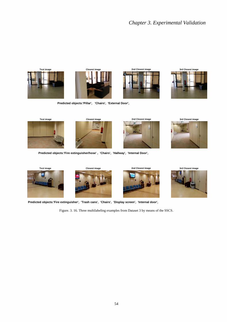
Chapter 3. Experimental Validation
54
Figure. 3. 16. Three multilabeling examples from Dataset 3 by means of the SSCS.
Test image Closest image
Predicted objects:'Pillar', 'Chairs', 'External Door',
2nd Closest image 3rd Closest image
Test image Closest image
Predicted objects:'Fire extinguisher/hose' , 'Chairs', 'Hallway', 'Internal Door',
2nd Closest image 3rd Closest image
Test image Closest image
Predicted objects:'Fire extinguisher', 'Trash cans', 'Chairs', 'Display screen', 'Internal door',
2nd Closest image 3rd Closest image

Chapter 3. Experimental Validation
55
Figure. 3. 17. Three multilabeling examples from Dataset 4 by means of the SSCS.
Test image Closest image
Predicted objects:'Board', 'Fire extinguisher', 'Trash cans', 'Chairs', 'External door', 'Display screen',
2nd Closest image 3rd Closest image
Test image Closest image
Predicted objects:'Board', 'Trash cans', 'didactic service machine', 'Self service', 'Internal door',
2nd Closest image 3rd Closest image
Test image Closest image
Predicted objects:'Board', 'Fire extinguisher', 'Stairs', 'Internal door',
2nd Closest image 3rd Closest image

Chapter 3. Experimental Validation
56
Figure. 3. 18. Three multilabeling examples from Dataset 1 by means of the RPCS.
Query Image
Predicted objects: 'External Window', 'Board', 'Table', 'Access Control Reader',
Closest Image
Query Image
Predicted objects:'External Door', 'Stair Door',
Closest Image
Query Image
Predicted objects:'Board', 'Office', 'Pillar', 'Chairs', 'Bins', 'Internal Door',
Closest Image

Chapter 3. Experimental Validation
57
Figure. 3. 19. Three multilabeling examples from Dataset 2 by means of the RPCS.
Query Image
Predicted objects: 'Heater', 'Corridor',
Closest Image
Query Image
Predicted objects: 'Corridor', 'Board', 'Laboratories', 'Bins',
Closest Image
Query Image
Predicted objects: 'Corridor', 'Board', 'Bins', 'Self Service', 'External Door',
Closest Image

Chapter 3. Experimental Validation
58
Figure. 3. 20. Three multilabeling examples from Dataset 3 by means of the RPCS.
Query Image
Predicted objects:'Chairs', 'Didactic service machine',
Closest Image
Query Image
Predicted objects:'Trash can', 'Chairs', 'Display Screen', 'Board', 'Stairs',
Closest Image
Query Image
Predicted objects:'Fire extinguisher/hose' , 'Chairs', 'Board',
Closest Image
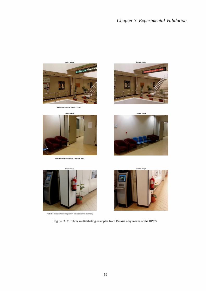
Chapter 3. Experimental Validation
59
Figure. 3. 21. Three multilabeling examples from Dataset 4 by means of the RPCS.
Query Image
Predicted objects:'Board', 'Stairs',
Closest Image
Query Image
Predicted objects:'Chairs', 'Internal door',
Closest Image
Query Image
Predicted objects:'Fire extinguisher', 'didactic service machine',
Closest Image

Chapter IV
Joint Navigation and Scene Understanding
for Blind Individuals in Indoor Sites

Chapter 4. Assisted Navig. and Scene Underst. for Blind Individ. in Ind. Sites
61
4.1. Introduction
Visual disability is one of the most serious troubles that may afflict an individual. Despite the fact
that 80 percent of all visual impairment is claimed to be preventable and even curable, still
blindness/partial-sight represent a serious problem worldwide [1](WHO). Besides the great efforts spent
in medicine, neuro-science and biotechnologies to find an ultimate solution to such problems,
technologies can provide tools to support those people by providing basic functionalities such as the
ability to navigate and recognize their entourage independently, to improve their quality of life and allow
better integration into the society. This objective is ambitious but not out-of-reach, thanks to the recent
technological advances.
In pursuit of satisfying the needs of visually disabled people and promote better conditions for them,
several designs have been put forth in the last years. From an overall perspective, they can be framed into
two mainstreams. The former addresses the guidance/navigation concern, while affording the possibility
to avoid potential obstacles. The latter is focused on recognizing the nature of nearby moving/static
obstacles. Considering both aspects, various contributions have been suggested, often referred to as
electronic travel aids (ETAs) [2] (Capi & Toda, 2011) [3] (Tian & Arditi, 2010) [4] (Chen, Dong, &
Wang, 2010) [5] (Loomis, Golledge, Klatzky, 1998) [6] (Ganz, Grandhi, Wilson, Mullett, 2010) [7]
(Simpson, LoPresti, Hayashi, Guo, Ding, Ammer, Sharma, Cooper, 2005). In [8] (Nanayakkara, Shilkrot,
& Maes, 2012), an autonomous device, called EyeRing, has been presented. It comprises a finger-worn
ring equipped with a VGA mini camera and an on/off switch, as well as an android mobile application.
The user is required to turn the switch on, then the camera captures the scene and carries it on to the
mobile phone via Bluetooth for further computer vision-based processing. Depending on the chosen mode
(e.g., object, color, or currency), which is verbally selectable by the user, a vocal statement is output by
the mobile application through a TTS (Text-To-Speech) module. The notable features of the designed
instrument are the ease-of-use and lightweight. Proposed in [9], is a guide-cane consisting of a round
housing, wheelbase and a handle. The housing is surrounded by ten ultrasonic sensors, eight of which are
placed on the frontal side and spaced by 15° so that to cover a wide sensed area of 120°, while the
remaining two are located on the edgewise for side-objects detection (doors, walls, etc…). The user can
use a mini joystick to control the preferred direction and push the cane through in order to inspect the
area. When an obstacle is detected by the sensors, an embedded obstacle avoidance algorithm is launched
to estimate an alternative obstacle-free path. The feedback to the user is given by steering the cane
through, which results in a force felt by the user on the handle. A somehow similar concept, called
NavBelt, was also presented in [10] (Shoval, Borenstein, & Koren, 1998). In this work, the ultrasonic
sensors are integrated on a worn belt and spaced by 15°. The information about the context in front of the
user is carried within the reflected signal and is processed within a portable computer. The outcome of the
analysis is relayed to the user by means of earphones. The distance to objects is represented by the pitch
and volume of the generated sound (i.e., the shorter the distance, the higher the pitch and volume). As an
attempt to facilitate the use and bring more comfort, a wearable smart clothing prototype has been
designed in [11] (Bahadir, Koncar, & Kalaoglu, 1998). The model is equipped with a microcontroller,
ultrasonic sensors, as well as indicating vibrators. The sensors explore the area of concern, whilst a neuro-
fuzzy-based controller detects the obstacle position (left, right, and front), and provides navigation tips
such as “turn left”,or “turn right”. A similar approach is also proposed in [12] (Shin & Lim, 2007).
Another study [13] (Bousbia-Salah, Bettayeb, & Larbi, 2011), provides an ultrasonic-based navigation aid
for the blind, permitting him/her to explore the route within 6 meters ahead via ultrasonic sensors placed
on the shoulders as well as on a guide cane. The underlying idea is that the sensors emit a pulse, which in
case of an obstacle is reflected back: the time between emission and reception (time of flight) allows
estimating the distance of the obstacle. The indication is carried to the user by means of two vibrators
(also mounted on his/her shoulders), and verbally for guiding the cane. The control of all the process is
attributed to a microcontroller. In [14] (Lee, Kang, Lee, 2008), the authors propose a different approach
including many tasks. In particular, the proposed system contains the following modules: object
detection, pedestrian recognition, ultrasonic-based object distance sensing, and a positioning system
through the GPS (Global Positioning System). Object detection module generates a disparity image,
which is processed in the object recognition module using support vector machines (SVM). The classifier
is trained on vertical silhouette and takes charge of face detection. Text recognition is also included and is
achieved using a commercial engine. The main drawback is that the above modules are run sequentially.
Another design was considered in [15] (Scalise, Primiani, Russo, Shahu, Di Mattia, De Leo, Cerri, 2012).

Chapter 4. Assisted Navig. and Scene Underst. for Blind Individ. in Ind. Sites
62
In that paper, a new electromagnetic concept for obstacle detection was introduced, based on the idea of
scanning the frontal area through a wideband antenna, emitting an electromagnetic wave. The presence of
an obstacle generates a reflection of the signal, which is amplified and analyzed to assess the distance of
the reflecting object. The presence of objects has been achieved at a signal-to-noise ratio (SNR) within
10-23 dB. Robot-based assistance for visually impaired has also received attention [16] (Kulyukin,
Gharpure, Nicholson, & Osborne, 2006) [17] (Kim, Yi, 2008). Robots can perform many assistive tasks
for people with vision disability such as navigation guidance, handling various household duties,
providing medical care, entertainment and rehabilitation. In order to effectively assist blind and low
vision people in an interactive and team-based way, and to improve the acceptance and usability of these
technologies, assistive robots must be able to recognize the current activity that the human is engaged in,
the task and goal context of the current activity, as well as be able to estimate how the human is
performing and whether assistance is required and appropriate in the current setting. Social assistive
robots, which may be particularly expensive, must also ensure the physical safety of the human users with
whom they share their workspace. Banknote recognition for the blind has also been addressed in [18]
(Hasanuzzaman, Yang, & Tian, 2012), where the Speeded-Up Robust Features (SURF) have been
employed. A supermarket shopping scenario has been treated in [19] (López-de-Ipiña, Lorido, López,
2011). In this work, Radio-frequency identification (RFID) has been used as a means for localization and
navigation, while product recognition has been performed by reading QR codes through a portable
camera. Product barcodes detection and reading has also been suggested in [20] (Tekin, Coughlan, 2009).
In another work [21] (Pan, Yi, & Tian, 2013), a portable camera-based design for bus line-number
detection was considered as a travel assistant. Staircase detection in indoor environments was proposed in
[22] (Tang, Lui, Li, 2012). In [23] (Chen & Yuille, 2004), the authors suggest assistive text reading in
natural scenes. RFID technology was also exploited for bus detection at public bus stations as to further
ease blind people mobility [24] (Al Kalbani, Suwailam, Al Yafai, Al Abri, Awadalla, 2015). Another
worth-noting contribution was proposed in [25] (Kulkarni & Bhurchandi, 2015). It consists of a device
designed for facilitating e-book reading for blind individuals via a built-in Braille script. The device was
claimed to be handy and at an affordable cost. Another work, which considers clothes color as well as
pattern recognition as a means of facilitating recognition capabilities of blind people, was put forth in [26]
(Thilagavathi, 2015). It combines three kinds of features, which are further fed into a SVM classifier as a
decision making paradigm. In [27] (Neto & Fonseca, 2014), assistive text reading was propounded. Its
underlying idea is to acquire the text zones by means of a camera, and afterwards exploit optical character
recognition capabilities to recognize the text and forward it to a text-to-speech engine as to deliver a vocal
feedback.
Overall, although the current literature proposes several interesting technologies to address specific
guidance or recognition problems for the blind, there is still a remarkable lack of integrated solutions able
to provide a usable “sight substitute”. In this context, we propose in this paper a new design that
incorporates guidance and recognition capabilities into a single prototype. These two needs, as observed
throughout the literature, have very scarcely (just one previous work to the best of our knowledge) been
coupled together. The tool is designed for indoor use, and is fully based on computer-vision technologies.
The components of the system include a portable camera attached to a wearable jacket, a processing unit,
and a headset for commands/feedback. The navigation system is launched as soon as the prototype is
powered on, and keeps instructing the blind person whenever he/she moves across the indoor
environment. In order to avoid information flooding, the recognition system is activated upon request of
the user. The prototype was implemented and tested in an indoor environment, showing good
performance in terms of both navigation and recognition accuracy.
The rest of this paper is structured as follows. Section 2 provides an overview of the prototype
architecture. In Section 3, the functioning of the guidance system and its modules are reported in detail.
Section 4 describes how the recognition task is performed. Section 5 illustrates the operational use of the
prototype in a real indoor environment. Finally, conclusions are drawn in Section 6.
4.2. Proposed Prototype
The proposed prototype accommodates two complementary units: (i) a guidance system, and (ii) a
recognition system. The former works online and takes charge of guiding the blind person through the
indoor environment from his/her current location and leading him/her to the desired destination, while
allowing avoiding static as well as moving obstacles. By contrast, the latter works on demand. The whole

Chapter 4. Assisted Navig. and Scene Underst. for Blind Individ. in Ind. Sites
63
prototype is based on computer vision and machine learning techniques. The inputs of the prototype
include:
A speech recognition module, which acquires verbal instructions from the headset and serves for
determining the command of the user, e.g., to launch for instance the recognition system, or to in-
dicate a desired target location for the guidance module.
A laser sensor whose task is to provide information about the distance to encountered obstacles, if
any.
A set of patterns (markers) as well as their associated coordinates within the indoor environment.
This set is used as a ground truth for determining the user’s location, as explained later.
An inertial measurement unit (IMU sensor), used to reinforce the egomotion module, in particular
by getting a reliable measurement of the user orientation within the indoor space.
A dataset including a bunch of images to be utilized in the recognition module as detailed in the
following.
A portable camera (a CMOS camera from the IDS Imaging Development Systems, model UI-
1240LE-C-HQ with KOWA LM4NCL lens) utilized for capturing the scene and forwarding the
shots to either the navigation or the recognition units.
An ego-motion module for estimating the current position of the user, based on coupling two key
information, namely (i) the marker-based estimated spatial coordinates within the indoor envi-
ronment, and (ii) the user’s orientation from the IMU sensor.
A path planning module, which receives (i) the user’s location from the egomotion module, and
(ii) the distance to potential obstacles from the laser sensor, and calculates a safe path for the user
to walk through.
A speech synthesis module to convert the output of both guidance and recognition units into au-
dio feedback.
All the modules are implemented on a portable processing unit carried by the user (a laptop in our
case). The overall architecture is depicted in Fig. 4. 1
The various modules are described in detail in the following sections.
4.3. Guidance System
The guidance system embodies three main modules, namely (i) an egomotion module whose
function is to estimate the user’s current position within the indoor environment, (ii) a path planning
module that serves for estimating an obstacle-free path from the current location (automatically detected
by the egomotion module) and the desired destination (provided by the user through a verbal command
among a list of predefined potential destinations in the environment), and (iii) an obstacle detection
module, which provides information about the possible presence of unforeseen obstacles along the path
(e.g., people, objects), and sends it to the path planning module in order to avoid obstruction.
4.3.1. Egomotion Module
In order to estimate the user’s current position (within the environment), we implemented a
positioning technique based on pattern matching. The underlying idea is that a set of markers is placed at
selected locations over the indoor environment. The markers employed in this work are the Aruco
markers [28] (Fusiello, 2008), which represent a 7x7 grid where the internal 5x5 white/black cells
formulate the code and the outer black bordure represents the frame. The process consists of detecting the
markers prior to proceeding with the recognition, both procedures are detailed in [29] (Brunner) and [30]
(Aruco), respectively. Since the markers, along with their spatial coordinates, are stored in the portable
processing unit, the camera position can be calculated at every step by triangulating the point of view,
based on the back-projection of visible markers. The portable camera, while walking, captures the
surrounding area and sends the stream to the processing unit, which in turn detects the markers in the
scene and uses them to estimate the camera pose as detailed in [28] (Fusiello, 2008).

Chapter 4. Assisted Navig. and Scene Underst. for Blind Individ. in Ind. Sites
64
As the guidance operates in a continuous manner, so does the egomotion module, which generates
the position and orientation estimates. If at some point no markers are detected, a Kalman filter is used to
perform a dead reckoning based on previous positioning and current IMU measurements [31] (Grimble,
1994). The output of the egomotion (i.e., the estimated spatial position of the camera within the indoor
space) is finally fed to the path planning module.
Figure 4. 1. Block diagram and interconnections of the developed prototype.
4.3.2. Path Planning Module
In order to track the motion of the user within the environment and plan the path to destination, we
use a CAD map of the site as shown in Fig. 4. 2. Thus, the user as well as the temporary obstacles
detected by the system can be placed on the map and monitored on the screen. The role of the path
planning module is to steer the blind from his/her current position all the way to his desired destination
within the indoor space, by computing the safest (collision-free) path. It thus collects the desired

Chapter 4. Assisted Navig. and Scene Underst. for Blind Individ. in Ind. Sites
65
destination from the voice command unit and the initial location from the egomotion module, and defines
a preliminary path. As long as the user proceeds along the path, the current location and the presence of
unexpected obstacles are continuously monitored using egomotion and obstacle detection modules, and
the remaining path is updated accordingly.
As far as the definition of the path is concerned, the algorithm works as follows:
Firstly, we highlight the areas within the environment across which the user might walk.
Then, we create a skeleton of the highlighted walkable area as explained further (see red curve on
Fig. 4. 2.). The skeleton provides the pieces of trajectory that ensure maximum distance from ob-
stacles.
Finally, we select the set of skeleton segments that provides the safest path between the current
position and the final destination.
In order to create the skeleton, we use of the Voronoi diagram, which generates an ensemble of cells
around a set of seeds (i.e., points that are provided a-priori), where each cell includes the nearby points
around the respective closest seed [32] (Okabe, Boots, Sugihara, Chiu, 2009). In our work, we adopt the
boundaries of the fixed obstacles (pillars, walls, etc.) lying across the indoor space as starting seeds. An
example of Voronoi diagram is depicted on Fig. 4. 2.
Afterwards, the points corresponding to the current and the desired locations are linked to the closest
nearby cells (based on the Euclidean distance) as shown in Fig. 4. 2. Finally, the safest path (green route
on Fig. 4. 2.) is computed by means of the Dijkstra's algorithm [33] (Dijkstra, 1959). The ultimate
trajectory is highlighted in green in Fig. 4. 2.
4.3.3. Obstacle Detection Module
The obstacles that might be encountered along the way could be either static (walls, pillars, furniture)
or moving (mostly pedestrians). Their locations within the environment are pivotal for the path planning
module as to alert the user while instructing him/her. Static obstacles are typically part of the map (except
for objects that can be temporarily moved), so that their coordinates can be stored beforehand. Moving
obstacles instead need to be monitored online while walking. Accordingly, in our prototype we opted for
a laser sensor-based obstacle detection. Precisely, a URG-04LX-UG01 time-of-flight laser scan is
employed (Fig. 4. 3.), due to its remarkably small size, high precision, lightweight, and low power
consumption. The distance to the object (if any) as well as its angulation (rough information about the
object shape) obtained from the laser scan are then communicated to the path planning module, which
exploit them to localize the moving obstacle in the CAD map of the site and then locally (in the
neighborhood of the obstacle) update the safest path before steering the user.
Figure 4. 2. Ultimate path extraction out of Voronoi diagram.

Chapter 4. Assisted Navig. and Scene Underst. for Blind Individ. in Ind. Sites
66
Figure 4. 3. URG-04LX-UG01 laser sensor.
4.4. Recognition System
As for the recognition system, the SSCD described in the previous chapter has been implemented
considering an image resolution of 1/10. The reader is referred to Chapter 3 for further details.
4.5. Prototype Illustration
We experimented the prototype in an indoor open-access space at the University of Trento, Italy.
This space represents an interesting but at the same time challenging public indoor environment. It is
composed of long and relatively large corridors, offices, classrooms, as well as numerous objects
typically found in such environments (e.g., advertisement boards, chairs, ATM). In the following, we
illustrate how the prototype behaves in such environment, and in particular its guidance and recognition
systems.
As stated before, the prototype includes a portable camera mounted on a lightweight and rigid jacket
worn by the user, and USB-connected to the processing unit (currently, a simple laptop). Once the
application is launched, all the offline-stored information regarding both the recognition and the
navigation systems are loaded. From that point on, the application is under the voice control of the user.
The predefined verbal commands, system instructions and information are listed in Table 4. 1.
An image illustrating the prototype is provided in Fig. 4. 4. Examples of the markers (employed for
positioning) can be seen in the image (attached to the walls).
For greater detail, we provide a demonstrative example in Fig. 4. 5., which shows some screen shots
of the application. In this example, the user requests ‘Reception’ as a destination by uttering the voice
command ‘Go to Reception’, which is interpreted by the speech recognition module and fed into the path
planning module for further guidance. In Fig. 4. 5., four instances of the guidance process are illustrated
(the chronological order goes from left to right, and from top to bottom). As shown, the black command
prompt highlights the voice tips derived out of the estimated route (by the path planning module) such as
‘go left’, ‘go right’…etc, as well as the user’s command at the beginning of the process. As recommended
by a local association of blind people, a voice tip is released by the system only when a change in the
walking direction is suggested. This modality has been found important in order not to overload the user
with a redundant flow of similar voice instructions. Finally, upon arrival to the desired destination, the
prototype informs the users.
Fig. 4. 5. depicts also (rightmost images) a virtual environment emulating the real movement of the
user within the indoor space. The user is symbolized by a black silhouette, with which two lines are
associated. The blue line shows the current user’s orientation, while the green one points to the
destination (estimated by the path planning module). The red dot represents the final destination, while
the red curve highlights the estimated safest path. The interface also includes the markers displayed as
thick lines lying on the walls in different locations across the environment. In this experiment, we have
considered five predefined destinations (Reception, Didactic Office, Elevator, Toilet, and Classroom).
The list can be obviously customized by adding other desired locations within the indoor site.
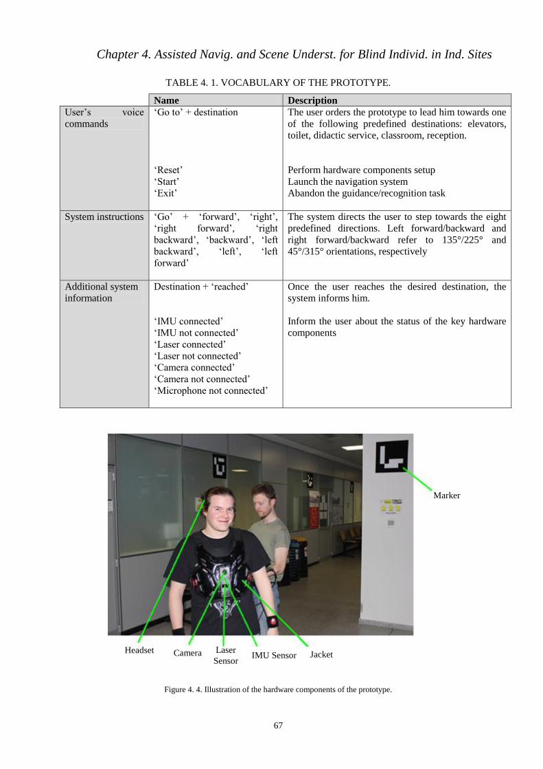
Chapter 4. Assisted Navig. and Scene Underst. for Blind Individ. in Ind. Sites
67
TABLE 4. 1. VOCABULARY OF THE PROTOTYPE.
Name Description
User’s voice
commands
‘Go to’ + destination
‘Reset’
‘Start’
‘Exit’
The user orders the prototype to lead him towards one
of the following predefined destinations: elevators,
toilet, didactic service, classroom, reception.
Perform hardware components setup
Launch the navigation system
Abandon the guidance/recognition task
System instructions ‘Go’ + ‘forward’, ‘right’,
‘right forward’, ‘right
backward’, ‘backward’, ‘left
backward’, ‘left’, ‘left
forward’
The system directs the user to step towards the eight
predefined directions. Left forward/backward and
right forward/backward refer to 135°/225° and
45°/315° orientations, respectively
Additional system
information
Destination + ‘reached’
‘IMU connected’
‘IMU not connected’
‘Laser connected’
‘Laser not connected’
‘Camera connected’
‘Camera not connected’
‘Microphone not connected’
Once the user reaches the desired destination, the
system informs him.
Inform the user about the status of the key hardware
components
Figure 4. 4. Illustration of the hardware components of the prototype.
Marker
Jacket IMU Sensor Laser
Sensor Camera Headset

Chapter 4. Assisted Navig. and Scene Underst. for Blind Individ. in Ind. Sites
68
Figure 4. 5. Example depicting the guidance system interface.
Noteworthy is that the experiments were run on a Dell laptop, incorporating an i5 Intel processor
with a 4Gb memory. The processing and instruction speed has shown a sound compatibility with an
ordinary blind user’s motion. The accuracy of the egomotion and path planning modules can be
considered satisfactory with regard to the various trials we performed within the test site. The main issue
found, though not critical, is the piecewise nature of the computed safest path which sometimes may
appear not compatible with an expected naturally curved path.
4.6. References
[1] Available at: http://www.who.int/mediacentre/factsheets/fs282/en/
[2] G. Capi, H. Toda, “A new robotic system to assist visually impaired people”, IEEE RO-MAN, pp.
259-263, 2011.
[3] Y. Tian, C. Yi, A. Arditi, “Improving computer vision-based indoor wayfinding for blind persons with
context information”, Computers Helping People with Special Needs, Springer Berlin Heidelberg, pp.
255-262, 2010.
[4] J. Chen, Z. Li, M. Dong, X. Wang, ‘’Blind Path Identification System Design Base on RFID‘’, IEEE
International Conference on Electrical and Control Engineering, 2010, pp. 548 – 551.
[5] J. M. Loomis, R. G. Golledge, , R. L. Klatzky, “Navigation system for the blind: Auditory display
modes and guidance”, Presence: Teleoperators and Virtual Environments, vol. 7, no. 2, pp. 193-203,
1998.
[6] A. Ganz, S. R. Gandhi, C. Wilson, G. Mullett, ‘’INSIGHT: RFID and Bluetooth Enabled Automated
Space for the Blind and Visually Impaired‘’, 32nd Annual International Conference of the IEEE
EMBS, 2010, pp. 331 - 334.

Chapter 4. Assisted Navig. and Scene Underst. for Blind Individ. in Ind. Sites
69
[7] R. Simpson, E. LoPresti, S. Hayashi, S. Guo, D. Ding, W. Ammer, V. Sharma, R. Cooper, ‘’A proto-
type power assist wheelchair that provides for obstacle detection and avoidance for those with visual
impairments‘’, Journal of NeuroEngineering and Rehabilitation, vol. 2, no. 30, 2005.
[8] S. Nanayakkara, R. Shilkrot, P. Maes, ‘’EyeRing: A Finger-Worn Assistant‘’, CHI Conference on
Human Factors in Computing Systems CHI, 2012, pp. 1961-1966.
[9] I. Ulrich, J. Borenstein, ‘’The guideCane-applying mobile robot technologies to assist the visually im-
paired‘’, IEEE TRANSACTIONS ON SYSTEMS, MAN, AND CYBERNETICS—PART A: SYS-
TEMS AND HUMANS, vol. 31, no. 02, pp. 131 - 136, 2001.
[10] S. Shoval, J. Borenstein, Y. Koren, ‘’The Navbelt-Acomputerized travel aid for the blind based on
mobile robotics technology‘’, IEEE Transactions on Biomedical Engineering, vol. 45, no. 11, pp. 1376
– 1386, 1998.
[11] S. K. Bahadir, V. Koncar, F. Kalaoglu, ‘’Wearable obstacle detection system fully integrated to tex-
tile structures for visually impaired people‘’, Sensors and Actuators A: Physical, vol. 179, pp. 297–
311, 2012.
[12] B. S. Shin, C. S. Lim, ‘’Obstacle detection and avoidance system for visually impaired people‘’,
Second International Workshop on Haptic and Audio Interaction Design HAID, 2007, pp. 78-85.
[13] M. B. Salah, M. Bettayeb, A. Larbi, ‘’A navigation aid for blind people‘’, Journal of Intelligent &
Robotic Systems, vol. 64, pp. 387-400, 2011.
[14] S. W. lee, S. kang, S. W. lee, ‘’A walking guidance system for visually impaired‘’, International
Journal of Pattern Recognition and Artificial Intelligence, vol. 22. no. 06, pp. 1171-1186, 2008.
[15] L. Scalise, et al, ‘’Experimental investigation of EM obstacle detection for visually impaired users. A
comparison with ultrasonic sensing‘’, IEEE TRANSACTIONS ON INSTRUMENTATION AND
MEASUREMENT, vol. 61. no. 11, pp. 3047 - 3057, 2012.
[16] V. Kulyukin, C. Gharpure, J. Nicholson, G. Osborne, ‘’Robot-assisted wayfinding for the visually
impaired in structured indoor environments‘’, Autonomous Robots, Vol. 21, no. 1 , pp. 29-41, 2006.
[17] D. Y. Kim, K. Y. Yi, “A user-steered guide robot for the blind”, IEEE International Conference
on Robotics and Biomimetics, pp. 114-119, 2009.
[18] F. M. Hasanuzzaman, X. Yang, Y. Tian,"Robust and effective component-based banknote recogni-
tion for the blind," Systems, Man, and Cybernetics, Part C: Applications and Reviews, IEEE Transac-
tions on, vol. 42, no. 6, pp. 1021-1030, 2012.
[19] D. López-de-Ipiña, T. Lorido, U. López, "BlindShopping: Enabling accessible shopping for visually
impaired people through mobile technologies," Toward Useful Services for Elderly and People with
Disabilities, pp. 266-270, 2011.
[20] E. Tekin, J. M. Coughlan, "An algorithm enabling blind users to find and read barcodes," Applica-
tions of Computer Vision (WACV), Workshop on, pp. 1-8, 2009.
[21] H. Pan, C. Yi, Y. Tian, "A primary travelling assistant system of bus detection and recognition for
visually impaired people,"Multimedia and Expo Workshops (ICMEW), IEEE International Confer-
ence on, pp. 1-6 , 2013.

Chapter 4. Assisted Navig. and Scene Underst. for Blind Individ. in Ind. Sites
70
[22] T. J. J. Tang, W. L. D. Lui, W. H. Li, "Plane-based detection of staircases using inverse depth,"
ACRA, 2012.
[23] X. Chen, A. L. Yuille, , "Detecting and reading text in natural scenes, " Computer Vision and Pattern
Recognition CVPR. Proceedings of the 2004 IEEE Computer Society Conference on. vol. 2, pp. II-
366, 2004.
[24] J. Al Kalbani, R. B. Suwailam, A. Al Yafai, D. Al Abri, M. Awadalla, “Bus detection system for
blind people using RFID”, 8th IEEE GCC Conference and Exhibition (GCCCE), pp. 1-6, 2015.
[25] A. Kulkarni, K. Bhurchandi, “Low Cost E-Book Reading Device for Blind People”, IEEE Interna-
tional Conference on Computing Communication Control and Automation (ICCUBEA), pp. 516-520,
2015.
[26] B. Thilagavathi, “Recognizing clothes patterns and colours for blind people using neural network”,
IEEE International Conference on Innovations in Information, Embedded and Communication Sys-
tems (ICIIECS), pp. 1-5, 2015.
[27] R. Neto, N. Fonseca, “Camera reading for blind people”, Procedia Technology, vol. 16, pp. 1200-
1209, 2014.
[28] Fusiello, A. (2008). Visione computazionale. Appunti delle lezioni. Pubblicato a cura dell’autore.
[29] J. Brunner, "ArUco: a minimal library for Augmented Reality applications based on OpenCv,"
[Online]. Available at: http://www.uco.es/investiga/grupos/ava/node/26.
[30] Available at: http://iplimage.com/blog/create-markers-aruco/
[31] M. J. Grimble, Robust industrial control: optimal design approach for polynomial systems. Prentice-
Hall, Inc, 1994.
[32] A. Okabe, B. Boots, K. Sugihara, S. N. Chiu, Spatial tessellations: concepts and applications of Vo-
ronoi diagrams. John Wiley & Sons, 2009.
[33] E. W. Dijkstra, “A note on two problems in connexion with graphs”, Numerische mathematik, vol. 1,
no. 1, pp. 269-271, 1959.

Chapter V
Preliminary Feasibility Study in Outdoor
Recognition Scenarios

Chapter 5. Preliminary Feasibility Study in Outdoor Recognition Scenarios
72
5.1. Introduction
In the introduction chapter, we have stressed the role smart technologies can play in service of blind
people rehabilitation, with a particular focus on the indoor-based context. Another yet worth tackling but
more challenging problem is the development of supportive methodologies able to aid blind individuals in
outdoor environments.
Up to date, different attempts have been set forth in the literature. Similarly to the indoor-based con-
cepts, outdoor contributions generally stem as a two-sided regard, enfolding the two formerly claimed
concerns, namely navigation and recognition. Considering the navigation aspect, several works have been
accumulated so far, which were made mention of in the previous chapters. With respect to the recognition
part, however, still there is much to do as a little attention has been paid. For instance, the work presented
in [1], intends to facilitate the task of bus detection for blind people. The system accommodates two sub
modules; the first one is implemented inside the bus and serves for detecting nearby bus stops and subse-
quently alerting the blind persons aboard, it also counts the number of blind people in local bus stops if
any, and informs the bus driver; the second module is implemented at bus stations and takes charge of de-
tecting the upcoming buses while keeping the blind individuals in the station updated. Another travel as-
sistant system was presented in [2]. It takes advantage of the text zones depicted in the frontal side of
buses (at bus stops) for further extraction of information related to bus line number. The system processes
a given image acquired by a portable-camera and then notifies the outcome to the user vocally. In [3], as-
sistive text reading from complex backgrounds was put forth. The algorithm mainly consists of two tasks,
namely (i) text localization, and (ii) text reading from the localized zones. The former task was achieved
by learning gradient features of stroke orientations and distributions of edge pixels by means of an Ada-
boost model. Afterwards, the latter task is performed by off-the-shelf optical character recognition (OCR)
software and subsequently transformed into an audible output. The algorithm was assessed in the context
of the ICDAR 2003 competition and further on a dataset collected by 10 blind persons, and has been
proven effective. In another work [4], stairs, pedestrian crosswalks, and traffic signs detection was tackled
by means of an RGB-D (i.e., Red, Green, Blue, and Depth information) image-based method. Departing
from the fact that crosswalks, as stairs, are characterized by a parallel-lines-like structure, Hough trans-
form was applied on the RGB channels as to extract those forming lines, which are coupled with depth
information and later fed into a support vector machine classifier (SVM) for a final decision whether the
input conveys stairs or crosswalks. In the former case, another SVM classifier is employed to tell the in-
clination of the stairs (i.e., upstairs or downstairs). The status (i.e., red or non-red) of traffic lights nearby
the crosswalks was determined by another SVM classifier learned on HOG (i.e., histogram of oriented
gradient) features extracted from the input RGB image. The design was evaluated on an outdoor dataset
and pointed out interesting outcomes. The proposal suggested in [5] considers a different recognition con-
cern, instead of recognizing definite objects, the algorithm is meant to recognize blind user’s situation in
outdoor places, where the term ‘situation’ refers to the entity of the spot/location where the blind user is
standing. The considered situations account for three types, namely sidewalk, roadway, and intersection.
Mainly, the scheme’s pipeline encompasses three steps. In a first step, regions of interest (ROIs) underlin-
ing the boundaries lying between the sidewalks and roadways are extracted by means of Canny edge de-
tector and Hough transform. In a second step, features (Fourier transform) are extracted from the ROIs
and injected into SVMs for further training. Lastly, in operational phase, the trained SVMs are applied to
a given input image to decide the situation’s class. Another contribution, suggested in [6] designed an al-
gorithm for outdoor scene description, the description consists of attributing a single label (e.g., door in
front of building) to a given query image. The labeling was performed by considering a majority vote
amongst the k closest labeled training images from an already prepared library, where image representa-
tion was achieved through GIST features, whilst KNN classifier was used for the matching process. In
this respect, outdoor object recognition in the context of blind rehabilitation has notpaid much attention to
the multiobject concern.
On this point, in the future expansion of the scope of this thesis, we intend to focus on outdoor mul-
tiobject recognition. Thus far, we have highlighted the pivotal need to holistically describe indoor scenes,
and we conducted trending contributions from the literature. We recall the fact that, in indoor sites, the
challenge encompasses two requirements, namely (i) adequate recognition efficacy, constrained by (ii)
short processing time, as to closely meet (at least near) real-time requirements. Subsequently, the chal-
lenge inflates and becomes harder to address while tackling the same concern (i.e., coarse description) in
outdoor environments, due to diverse reasons such as:

Chapter 5. Preliminary Feasibility Study in Outdoor Recognition Scenarios
73
(i) The high number of objects likely to appear in outdoor scenes.
(ii) The heterogeneity of objects, particularly the ones that belong to the same class, in terms of
shape (e.g., different types of trees might reflect different shapes and sizes), color (e.g.,
onroad vehicles drastically differ often by color, and less often by size).
(iii) The scale-change tends to be harder as the camera’s frontal field of view expands while
switching from indoor to outdoor.
(iv) The weather condition changes, expressed within the illumination of the shot images (in in-
door sites, the lighting is artificial and thus poses less problems as its intensity is kept under
control).
(v) The mobility of different objects, particularly vehicles, might cause blurred out images,
which does not serve the cause of this work.
In this chapter, apart from the SCD strategy which was proposed as a best case scenario exemplary
that needs further investigation with what concerns the processing time, we run the remaining strategies
in the outdoor context and assess their efficiency under the challenges mentioned above. We further pave
the way for potential future considerations as to bridge the gaps underlining these strategies.
5.2. Experimental Setup
The experimental evaluation with respect to outdoor environments will be conducted on a dataset of
images acquired at different locations across the city of Trento located in the Trentino-Alto Adige region.
The locations were selected based on their importance as well as the density of people frequenting them.
For the sake of clarity, we provide a Google map highlighting those locations (Fig. 5.1). The dataset ini-
tially comprises one thousand images, which were split up into training and testing subsets (i.e., 500
each). As for the predefined list of objects, a long initial list has been prepared. However, upon consulta-
tion of a visually impaired person, the list was narrowed down to a total of 26 objects, as follows:
People, Building, Bar(s), Monument(s), Chairs/Benches, Green ground, Vehicle(s), Stairs, Walk path
/ Sidewalk, Fence / Wall, Tree(s) / Plant(s), Garbage can(s), Bus stop, Crosswalk, River, Roundabout,
Pole(s) / Pillar(s), Shop(s), Supermarket(s), Pound/Birds, Underpass, Bridge, Railroad, Admiration build-
ing, Church, Traffic signs.
In addition to the aforementioned challenges, in the outdoor case, the size of the dataset (number of
training images) expands roughly nine or ten times with respect to the indoor datasets addressed before.
On what concerns the SSCS, a dictionary for representing the images by way of CS has to be allocated.
Therefore, a total of 58 images were used to develop the CS dictionary, which gives rise of image repre-
sentations of the same size.
The classification results are reported in Table. 5. 1. In particular, for the SSCS and the MRPCD, we
opted for an images resolution of 1/10 (which was thought of as the optimal choice for a large dataset).
From the table, it is to deduce that, despite the challenges noted above, satisfactory results can be
yielded in the outdoor scenario. It is also to mention the observation that SEN, similarly to the indoor
case, is still higher that SPE, except for the SSCS scheme where the opposite is observed, which can be
interpreted by the reason that, in outdoor spaces, the images are likely to have in common at least few ob-
jects amongst the long predefined list (e.g., such as sidewalk, buildings, and vehicles, which appear in
many images), which is further reflected in a high SEN metric, which also recalls the expectation men-
tioned in the previous chapters, that a high number of training images is likely to lift the object co-
occurrence amongst the k images, which renders the recognition accuracy higher.
Considering the average between SEN and SPE, the best result was pointed out by the BOWCD
method, followed respectively by the SSCD, the PCACD, and the MRPCD with somewhat close efficien-
cies, which once again underlines the fact that local keypoint-based image representation still outperforms
global holistic-based ones for the reason that richer information is ought to be gathered by way of work-
ing at pixel-level than at image level.
Regarding the behavior of the methodologies under different k values, the best outcomes can be
gained by considering the sole nearest neighbor from the library, except for the SSCD that scores the
highest at k=5, which shows that the concept of cooperative object detection makes more sense under the
semantic approach for the reason pointed out earlier.

Chapter 5. Preliminary Feasibility Study in Outdoor Recognition Scenarios
74
Figure. 5. 1. Google map defining the outdoor dataset acquisition points (red pins) in the city of Trento.
Regarding the behavior of the methodologies under different k values, the best outcomes can be
gained by considering the sole nearest neighbor from the library, except for the SSCD that scores the
highest at k=5, which shows that the concept of cooperative object detection makes more sense under the
semantic approach for the reason pointed out earlier.
Concerning the processing time, on the other hand, the methods exhibit some raise with respect to
the indoor case. A massive increase, however, has been incurred by the PCACD, which renders it disqual-
ified as it is very dataset size-dependent. The MRPCD, however, preserves its property of being remarka-
bly fast but still less accurate than the BOWCD. On the whole, a tradeoff between the accuracy and the
processing time would tell that the BOWCD emerges as a potential applicable paradigm.
In sum, we believe that both the BOWCD and the MRPCD lay the ground for potential future cus-
tomization as detailed in the next chapter. For the sake of demonstration, per-class classification accura-
cies are given by the subsequent figures (Fig. 5. 2. to Fig. 5. 5.). Besides, outdoor image multilabeling in-
stances, for k=3, are depicted in the figures that follow.

Chapter 5. Preliminary Feasibility Study in Outdoor Recognition Scenarios
75
TABLE 5. 1. CLASSIFICATION STRATEGIES ON OUTDOOR DATASET. FOR THE BOWCD, A
CODEBOOK SIZE OF 300 CENTROIDS WAS USED. FOR HE SSCS and the MRPCD, THE VALUE
OF THE RESOLUTION RATIO Was 1/10, AND (1,1) For, THE RESOLUTION RATIOS WERE SET
TO 1/10.
k=1 k=3 k=5 Proc. Time (Sec/Image)
BOWCD
SEN 81.80 78.74 75.75
1.6 SPE 92.90 93.18 92.89
AVG 87.595 85.79 84.4
PCACD
SEN 68.72 65.63 65.16
37 SPE 89.22 91.33 91.84
AVG 78.97 78.48 78.5
SSCS
SEN 88.12 87.97 87.06
2.6 SPE 65.20 68.83 72.73
AVG 76.66 78.41 79.9
MRPCD
SEN 66.71 - -
0.044 SPE 88.28 - -
AVG 77.495
- -
Figure. 5. 2. per-class overall classification accuracies achieved on outdoor dataset by means of the BOWCD method.

Chapter 5. Preliminary Feasibility Study in Outdoor Recognition Scenarios
76
Figure. 5. 3. per-class overall classification accuracies achieved on outdoor dataset by means of the PCACD method.
Figure. 5. 4. per-class overall classification accuracies achieved on outdoor dataset by means of the SSCS method for a resolu-
tion ratio of 1/10 and for k=5.
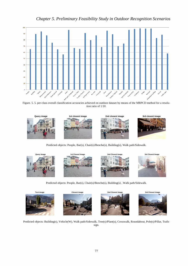
Chapter 5. Preliminary Feasibility Study in Outdoor Recognition Scenarios
77
Figure. 5. 5. per-class overall classification accuracies achieved on outdoor dataset by means of the MRPCD method for a resolu-
tion ratio of 1/10.
Predicted objects: People, Bar(s), Chair(s)/Benche(s), Building(s), Walk path/Sidewalk.
Predicted objects: People, Bar(s), Chair(s)/Benche(s), Building(s) , Walk path/Sidewalk.
Predicted objects: Building(s), Vehicle(W), Walk path/Sidewalk, Tree(s)/Plant(s), Crosswalk, Roundabout, Pole(s)/Pillar, Trafic
sign.
Query image 1st closest image
Predicted objects:'People', 'Bar(s)', 'Chair(s)/Benche(s)', 'Building(s)', 'Walk path / Sidewalk', 'Tree(s) / Plant(s)'
2nd closest image 3rd closest image
Query Image 1st Closest Image
Predicted objects:'People', 'Bar(s)', 'Monument(s)', 'Chair(s)/Benche(s)', 'Building(s)', 'Stair(s)', 'Walk path / Sidewalk', 'Church'
2nd Closest Image 3rd Closest Image
Test image
Predicted objects:'People', 'Bar(s)', 'Building(s)', 'Green ground', 'Vehicle(s)', 'Walk path / Sidewalk', 'Fence / Wall', 'Tree(s) / Plant(s)', 'Crosswalk', 'Roundabout', 'Pole(s) / Pillar(s)', 'Traffic sign'
Closest image 2nd Closest image 3rd Closest image

Chapter 5. Preliminary Feasibility Study in Outdoor Recognition Scenarios
78
Predicted objects: Building(s), Walk path/Sidewalk, Fence/Wall, Tree(s)/Plant(s), Pole(s)/Pillar, Trafic sign.
Figure. 5. 6. Multilabeling examples by means of the BOWCD, PCACD, SSCS, and MRPCD, respectively
from top-line to bottom-line.
5.3.References
[1] J. Al Kalbani, R. B. Suwailam, A. Al Yafai, D. Al Abri, M. Awadalla, “Bus detection system for blind
people using RFID”, 8th IEEE GCC Conference and Exhibition (GCCCE), pp. 1-6, 2015.
[2] H. Pan, C. Yi, Y. Tian, "A primary travelling assistant system of bus detection and recognition for
visually impaired people,"Multimedia and Expo Workshops (ICMEW), IEEE International Confer-
ence on, pp. 1-6 , 2013.
[3] C. Yi, Y. Tian, “Assistive text reading from complex background for blind persons”, Camera-Based
Document Analysis and Recognition, pp. 15-28, 2012.
[4] S. Wang, H. Pan, C. Zhang, Y. Tian, “RGB-D image-based detection of stairs, pedestrian crosswalks
and traffic signs”, Journal of Visual Communication and Image Representation, vol. 25. no. 2, pp.
263-272, 2014.
[5] J. Hwang, K. T. Kim, E. Y. Kim, “Outdoor situation recognition using support vector machine for the
blind and the visually impaired”, PRICAI 2012: Trends in Artificial Intelligence, pp. 124-132, 2012.
[6] Q. H. Nguyen, T. H. Tran, “Scene description for visually impaired in outdoor environment”, IEEE
International Conference on Advanced Technologies for Communications (ATC), pp. 398-403, 2013.
Query Image Closest Image
Predicted objects:'Building(s)', 'Walk path / Sidewalk', 'Fence / Wall', 'Tree(s) / Plant(s)', 'Pole(s) / Pillar(s)', 'Traffic sign'

Chapter VI
Conclusion
Chapter 6. Conclusion
80
In this thesis, the problem of blind people assistance through smart technologies has been covered.
The dissertation detailed various elements of a prototype meant to aid blind individuals to (i) navigate,
while offering the capability of obstacle avoidance, in indoor environments, and (ii) mainly recognize fa-
miliar objects. A key-contribution to be noted is to embed both the navigation as well as the recognition
aspects into a single prototype, which as a matter of fact, is scarcely addressed in the literature. The main
scope of the thesis, however, emphasized on the recognition side as it has been paid less attention with
respect to the navigation issue. Putting the problem object recognition on the one hand, and the short pro-
cessing requirements constraining the targeted application on the other, it seems rather hard to meet both
ends together as (i) numerous objects might appear in the indoor site, and (ii) adopting traditional recogni-
tion paradigms as to proceed with the recognition of all those objects is prohibitively demanding. Depart-
ing from this fact, we have introduced a simple but efficient way to bulk-recognize objects in indoor
spaces at minimal costs. Hereafter, we provide highlights underlining all the proposed object recognition
strategies. For further details, we direct the reader to the respective chapters.
In Chapter 1, we provide an introduction into the topic by referencing leading works in the literature.
We listed the main contributions on the navigation issue, some of which convey similar concepts (e.g.,
wearable, ultrasonic…etc). Then we stressed the fact that the navigation concern has been devoted the
biggest part in the literature and that more effort need to be exerted with what relates to the recognition
part. On this latter, we have surveyed the most popular works in the field and have pointed out the clear
fact that the state-of-the-art for the blind has a tendency to focus on the recognition of single class of ob-
jects, which we believe is less informative and needs to be widened towards Multiobject recognition.
Thus, we introduced the concept of coarse description in Chapter 2, which basically aims to detect multi-
ple objects at once in brief processing span. In this context, coarse description consists in developing a set
of training images multilabeled beforehand, and then label a given query image (basically a camera-shot
image) in a collaborative manner (majority-based vote) between the closest training images. This process
leads to a final (agreed-upon) list of objects that likely appear in the indoor spot. On this point, five strat-
egies were suggested to tackle two distinct problems, namely image representation, and representation
comparison. The first method (SCD) is based on the traditional SIFT features and has proven efficient but
significantly slow. To overcome the processing requirements of SIFT, the well-known Bag of Visual
Words (BOWCD) was undertaken, which indeed exhibited fast performance whilst maintaining reasona-
bly close efficiency. The third method makes use of the PCA as to extract concise representations, and
has shown promising results but somewhat failed (in terms of processing time) when applied large da-
tasets. A different image matching concept was put forth in the fourth strategy (SSCD), where the similar-
ity was assessed from a semantic perspective. The last strategy is rather simple but much faster than the
other schemes. It is based on generating random projections of the images and matching them by means
of the cosine distance.
In Chapter 3, we investigated the behaviour of all the strategies in the indoor scenario. Different per-
formances have been obtained where the SCD method emerged as the most efficient but the slowest. The
MRPCD was the fastest but a little less than the BOW method for instance. This latter, however, has
shown an interesting time-accuracy trade off.
In Chapter 4, we detailed the complete prototype that incorporates both the recognition and the navi-
gation modules. The prototype is wearable and fully computer vision-based.
In Chapter 5, we evaluate the different multilabeling strategies (except the SCD) for future imple-
mentations in outdoor contexts. In this respect, the PCA consumed much more time than in the indoor
case, which leaves the BOW and the MRP as the ultimate potential implementations, that if they benefit
from future customizations may lead to meet our expectations.
In this regard, we suggest future proposals to invest in the following directions:
The MRPCD emerged as the fastest and the closest to real-time processing standards. Thereupon,
we believe it can be further boosted by projecting only interesting local areas within the image in-
stead of projecting the entire image onto the random filters. In other words, a pre-processing step
aimed at determining salient regions of interest (ROIs) from a considered image, is involved. On
this point, we propose to make use of either Harris corner detector salient [1] or keypoint detec-
tors (without proceeding with descriptors construction) such as SIFT [2] or SURF (speeded-up
robust features) [3], which are ought to point out numerous potential interesting points distributed
at different coordinates across the image. Afterwards, we consider a squared random projection
window centred around each previously produced keypoint. By projecting the local spatial re-

Chapter 6. Conclusion
81
gions onto the claimed RP window at all locations, we obtain as many scalars as the number of
keypoints, which thereafter allows us to construct a histogram by aggregating the occurrences of
all the scalars into a single vector. Hence, by adopting several, say N, window sizes, N histo-
grams shall be generated. The final step to take is to find an appropriate way to fuse these histo-
grams (e.g., the simplest and fastest way would be a linear sum) into a final fixed-size image rep-
resentation. The other challenging part of the task is to adequately match the representations,
especially in the challenging case where they convey significant sparsity. The task becomes even
harder to tackle if some bins in the histogram exhibit a sense of prevalence over the others. This
particularly deserves a careful investigation in the future.
The main goal aimed at in this work is to coarsely list the objects spotted at indoor sites. Another
yet worth investigating aspect is to infer the location of a certain object amongst the outcome list
of the multilabeling algorithm. That is the procedure becomes a ‘coarse-to-fine’ approach, where
the coarse task is addressed by one of the implemented algorithms so far, and the fine recognition
may be tackled by relevant state-of-the-art algorithms. The fine recognition can be considered as
a post-processing to be performed upon request of the blind person who can select an object from
the generated coarse list. This, again, is likely to be gained at the cost of further processing re-
quirements.
Another pivotal concern is the fact that the predefined list of objects to be recognized presumes
that all the objects are alike in terms of visual as well as semantic importance. The matter of the
fact, as also pointed out upon a meeting with a blind person, is that not all objects have the same
beneficial value (i.e., some objects have to be designated more attention than others). Ultimately,
we came to the conclusion that weighting the objects while embedding the weight values into the
multilabeling process shall satisfy the aforesaid concern.
The ultimate and potentially most promising direction to adopt, is to make use of the Convolu-
tional Neural Network (CNN) [4], which is an instance of artificial neural networks that has
gained a wide focus, particularly in the last few years, due to the abundance of powerful pro-
cessing facilities. CNNs have been proven effective in diverse computer vision, pattern recogni-
tion, and multimedia applications. They include obstacle detection [5], quality assessment [6],
face recognition [7], object classification [8], and scene classification [9]. In this respect, we be-
lieve that CNNs can be successfully tailored to the coarse description problem. Therefore, our
current endeavour is to adequately take advantage of CNNs particularly in the context of outdoor
coarse description.
6.1. References
[1] F. Bellavia, T. Domenico, C. Valenti. “Improving Harris corner selection strategy”, IET Computer
Vision, vol. 5, no. 2, pp. 87-96, 2011.
[2] D. G. Lowe, “Object recognition from local scale-invariant features”, International Conference on
Computer Vision. pp. 1150–1157. 1999.
[3] B. Herbert, T. Tinne, V. G. Luc, “SURF: Speeded Up Robust Features”, European Conference on
Computer vision, pp. 404-417, 2006.
[4] S. Haykin, B. Kosko., “Gradient-based learning applied to document recognition”, Intelligent Signal
Processing: Wiley-IEEE Press, pp. 306-351, 2009.
[5] H. Yu, H.Ruxia, H. XiaoLei, W. Zhengyou, “Obstacle Detection with Deep Convolutional Neural
Network” IEEE International Symposium on Computational Intelligence and Design (ISCID), vol. 1, pp.
265-268, 2013.
[6] P. Le Callet, C. Viard-Gaudin, D. Barba, “A convolutional neural network approach for objective
video quality assessment”, IEEE Transactions on Neural Networks, 17(5), pp. 1316-1327, 2006.
[7] S. Lawrence, C. L. Giles, A. C. Tsoi, A. D. Back, “Face recognition: A convolutional neural-network
approach”, IEEE Transactions on Neural Networks, vol. 8, no.1, pp. 98-113, 1997.

Chapter 6. Conclusion
82
[8] Z. Dong, Y. Wu, M. Pei, Y. Jia, “Vehicle Type Classification Using a Semisupervised Convolutional
Neural Network”, IEEE Transactions on Intelligent Transportation Systems, vol. 16, no. 4, pp. 2247 –
2256, 2015.
[9] F. P. S. Luus, B. P. Salmon, F. van den Bergh, B. T. J. Maharaj, “Multiview Deep Learning for Land-
Use Classification”, IEEE Geoscience and Remote Sensing Letters, vol. 12, no. 12, pp. 2448-2452, 2015.

Acknowledgments
The Authors would like to thank A. Vedaldi and B. Fulkerson for the supply of VLFeat software [1],
D. Donoho and Y. Tsaig for providing the SparseLab toolbox [2], as well as C. E. Rasmussen and K. I.
Williams for supplying the GPC software [3], which were used in the context of this paper. Likewise,
The Authors would like to thank the local Trento’s Sec-tion of the Italian Union of Blind and Visually
Impaired People for the availability and useful feedbacks.
References:
[1] A. Vedaldi and B. Fulkerson, VLFeat platform. [Online]. Available: http://www.vlfeat.org/index.html.
[2] Available at: http://sparselab.stanford.edu
[3] C. E. Rasmussen and K. I. Williams, Gaussian Process Soft-ware. [Online]. Available at: http://www.Gaussianprocess.org/gpml/code/matlab/doc/

Relevant List of Publications achieved during PhD activity
Journal Papers:
[J1] M. L. Mekhalfi , F. Melgani, Y. Bazi, , N. Alajlan, “Toward an assisted indoor scene perception for blind people with image multilabeling strategies”, Expert Systems with Applications, vol. 42, no. 6, pp. 2907-2918, 2015.
[J2] M. L. Mekhalfi , F. Melgani, Y. Bazi, , N. Alajlan, “A Compressive Sensing Approach to Describe Indoor Scenes for Blind People”, IEEE Transactions on Circuits and Systems for Video Technology, vol. 25, no. 7, pp. 1246 – 1257, 2015.
[J3] M. L. Mekhalfi , F. Melgani , A. Zeggada , F. G. B. DE Natale ,M. A.-M. Salem , A. Khamis. “Recovering the Sight to Blind People in Indoor Environments with Smart Technologies”, Expert Systems with Applications, vol. 46, pp. 129-138, 2016.
[J4] M. L. Mekhalfi , F. Melgani, Y. Bazi, , N. Alajlan, “Indoor Scene Description for Blind People with Multiresolution Random Projections”, In submission.
Conference Proceedings:
[C1] M. L. Mekhalfi, F. Melgani, M. A.-Megeed Salem, A. Khamis, “A Fast and Comprehensive Indoor Scene Understanding Approach for Blind People”, International Conference on Computational Intelligence, Communication Systems and Networks (CICSyN2014), Tetovo, Macedonia, pp. 1-5, 2014.
[C2] M. L. Mekhalfi, F. Melgani, P. Calanca, F. G. B. De Natale, M. A.-Megeed Salem, A. Khamis, “An Indoor Guidance System for Blind People”, International Conference on Industry Academia Collaboration IAC, Cairo, Egypt, pp. 1-6, 2014.
[C3] M. L. Mekhalfi, Farid Melgani, M. A.-M. Salem, A. Khamis, S. Malek, A. Zeggada, “A SIFT-GPR Multi-Class Indoor Object Recognition Method for Visually Impaired People”, International Conference on Industry Academia Collaboration IAC, Cairo, Egypt, pp. 1-4, 2015.
