SCHOOL OF PHYSICS AND ASTRONOMY

FIRST YEAR LABORATORY

PX 1223 Introductory Practical Physics II

(Supplemental Lab Book)

Academic Year 2016 - 2017

NAME: Lab group:

1

Welcome to the 1st year laboratory, Introductory Practical Physics II, module PX1223 in the spring semester. You will need to bring this manual with you to every laboratory session, as it contains the description of the new list of experiments that you undertake in this semester. It is designed as a supplement to your existing lab manual, and does not duplicate essential information contained in the manual you received for PX1123. You are still expected to have pre-read each relevant section prior to coming to your weekly laboratory session and to have written your Risk Assessment and Aims. If you cannot find the information that you are looking for, please ask any member of the teaching team - your Lab Supervisor, the demonstrators or the module organizer (Dr Phil Buckle, room S/1.24). Lab Supervisor: Contact email: Demonstrators:

2

1 Contents

1 Contents ....................................................................................................................... 2

2 Introduction and logistics of the 1st year laboratory .................................................. 3

2.1 Organisation and administration of the laboratory ............................................ 3

2.1.1 Introduction ................................................................................................... 3

2.1.2 Attendance ..................................................................................................... 3

2.1.3 Submission of coursework. ............................................................................ 3

2.2 Assessment of practical work .............................................................................. 4

2.2.1 The feedback you should expect to receive .................................................. 4

2.2.2 Decile level descriptors .................................................................................. 5

2.2.3 Notes on decile level descriptors ................................................................... 6

2.3 Formal reports of experiments ........................................................................... 7

2.3.1 The process of report submission and assessment ....................................... 7

3 Experiments ................................................................................................................. 8

3.1 Time table and list of experiments ...................................................................... 8

3.2 Checklist ............................................................................................................... 9

3.3 Experiment 12: Optical Diffraction ................................................................... 10

3.4 Experiment 13: Propogation of Sound in Gases. .............................................. 14

3.5 Experiment 14: Microwaves ............................................................................. 17

3.6 Experiment 15: Variation of Resistance with Temperature. ............................. 24

3.7 Experiment 16: Resistive and reactive impedances in RC circuits .................... 28

3.8 Experiment 17: Radiation from a Hot Body ...................................................... 37

3.9 Experiment 18: Report writing feedback ......................................................... 40

3.10 Experiment 19: Computer Error Simulations and Analysis .............................. 41

3.11 Experiment 20: Group Easter Challenge - The strength of paper .................... 47

4 Error propagation: A reminder of the general case................................................... 48

5 Lab Diary checklist...................................................................................................... 50

6 Formal report checklist .............................................................................................. 50

3

2 Introduction and logistics of the 1st year laboratory

2.1 Organisation and administration of the laboratory

2.1.1 Introduction

There are 9 laboratory sessions in the spring semester (no lab in week 1 and no formal lab in week 11). They are designed to continue on from the foundation in the first semester. ie:-

1. To provide familiarity and build confidence with a range of apparatus. 2. To provide training in how to perform experiments and teach you the techniques

of scientific measurement. 3. To give you practise in recording your observations and efficiently

communicating your findings to others. 4. To demonstrate theoretical ideas in physics, which you will encounter in your

lecture courses. 5. To understand the important role of experimental physics

2.1.2 Attendance

Class Times. Labs run from 13:30 to 17:30 on Monday, Tuesday and Thursday afternoons. Students will in general be assigned the same laboratory afternoon as the autumn semester, however to make numbers more even and therefore comfortable there will be a limited number of people being moved between sessions. Attendance at Laboratories. Experimental physics forms an important part of all degree programmes offered by the School of Physics and Astronomy and is a requirement for Institute of Physics accreditation. Attendance at all scheduled laboratory classes is compulsory. Unscheduled absence from laboratories will lead to loss of marks and possibly failure of the module. It is not always possible to offer summer resits in laboratory-based modules (see UG Student Handbook Appendix 1).

2.1.3 Submission of coursework.

As with the autumn semester this module is assessed 100% through continual assessment (in the form of lab diaries and formal reports). Deadlines are final and late submission will be awarded zero marks without exception. Coursework is submitted in the same two ways as the first semester, either through the “post boxes” near the General Office or electronically through Learning Central. Major pieces of writing (e.g. your formal laboratory report) are submitted electronically to Turnitin, an electronic system which helps identify plagiarism.

4

2.2 Assessment of practical work

Assessment will follow the same process as the autumn semester Each experiment and each report will be marked out of 20 in accordance with the scheme: 16+ = exceptionally good, contains good physicists’ reasoning; 14+ = very good solid performance; 12+ = good performance which could be improved; 10+ = competent performance but with some key omissions; 8+ = bare pass; 7- = fail. Your final module mark (see Undergraduate Handbook) will be made up as follows: Formal report 33.3% Experimental lab diaries 66.7% (Please see PX1123 for more information on Assessment Criterial used in marking).

2.2.1 The feedback you should expect to receive

You will receive feedback on each of your Lab Diary submissions on a weekly basis. This feedback will be in the form of a single mark out of 20 with additional written notes to guide you on things you didn’t achieve and improvements you could consider. The demonstrators will return your work to you personally, thus giving the further opportunity for verbal feedback and for you to ask questions. At any time, you can ask the Lab Supervisor for justification of the mark awarded or where you could improve. Bare in mind that a mark of 14/20 or better is a first-class degree performance whilst one of less than 8/20 represents a fail. Your markers will base this mark on the Decile Level Descriptors provided in Table 1. These describe how well the required task must be performed in order to obtain a certain range of marks. This method is commonly used in University assessment where there is no model answer and independence is to be encouraged. Note that this system considers “lapses” in two types: “major” and “minor” (also considered in Table 2). It is worth paying attention to these, as marks of 70% or greater cannot be awarded in the presence of major lapses. Your individual marks will be recorded on Learning Central for you to review. It is your responsibility to check that they have been recorded correctly and to contact the Module Organizer if that is not the case. Formal reports are marked at the end of semester and a Report and Feedback Sheet will be given back to you to give a thorough justification for the % mark received. The expectation is then on YOU to read, understand and use the feedback received in order to improve your future performance.

5

2.2.2 Decile level descriptors

Table 1. The descriptors and descriptions used in assessing reports and diaries

Decile range

Descriptors Level Descriptions

90-100% Outstanding The assessed work is as good as could reasonably be expected from a student at this level. It is uniformly-excellent in meeting the task specifications. It contains no major lapses and very few (if any) minor lapses.

80-89% Excellent Work of very high quality, but not quite as good as could reasonably be expected from a student at this level. It is uniformly very good and sometimes excellent in meeting the task specifications. It contains no major lapses and few minor lapses.

70-79% Very good Taken as a whole the work is very good in meeting the task specification. It contains no major lapses but does contain a number of minor lapses.

60-69% Good Taken as a whole the work is good in meeting the task specifications. It may contain a small number of major and minor lapses, or no major lapses but significant minor lapses.

50-59% Satisfactory Satisfactory work taken as a whole. It is likely to show significant variability in meeting the task specifications. It is likely to contain a number of major and minor lapses.

40-49% Pass Adequate work taken as a whole. It is likely to have significant deficiencies in meeting the task specifications. It is likely that the work will reveal substantial gaps in understanding and have significant major and minor lapses.

30-39% Fail Insufficient relevant content, serious errors/omissions/lapses.

20-29% Insufficient Little relevant content, extensive errors/omissions/lapses.

10-19% Unsatisfactory Very little relevant content, extensive errors/omissions/lapses.

0-9% Poor Essentially no relevant content, extensive errors/omissions/lapses.

Some notes on the above are present on the following page.

6

2.2.3 Notes on decile level descriptors

Major Lapses The level descriptions above indicate that in order to award a mark greater than 70% (i.e. of 1st class standard) there should be no “major lapses”. Major lapses are therefore important in determining the mark awarded and are listed in Table 2. Table 2 Common major lapses in diaries and reports

Diaries Reports

From task description From task description

No, or highly inappropriate, risk assessment.

Significant deviation from the format and structure explained in the support available in Learning Central.

Content is illegible (neatness per se is not a requirement).

Report is not electronically generated.

Content cannot be easily followed or understood.

Lapses that might be major depending on circumstances

Lacking clarity and succinctness. Obvious (e.g. numerical) mistakes in principle result(s).

Lacking in appropriate experimental observations.

Substantial gaps in understanding.

Lack of appropriate data analysis. Lack of proper error consideration. Lack of appropriate error analysis.

Lack of concluding remarks.

It should be appreciated that major lapses are, in general, not a restriction of marks over and above those defined in the task*. For example, a diary with “content that is illegible” will not represent a good record of the experiment performed. The point of including the term in the descriptors is to help authors and markers in thinking about and checking reports and diaries. *An exception applied to diaries: “No, or highly inappropriate, risk assessment” is considered a major lapse since safety is important. However, the presence of a risk assessment is not worth (up to) 30%.

7

2.3 Formal reports of experiments

The formal report for PX1223 is due in at 4pm on the Friday of teaching week 11 of the spring semester.

2.3.1 The process of report submission and assessment

Reports are submitted via Turnitin whose plagiarism* checking is later supplemented by that of the markers.

Reports are assigned to the 3 lab supervisors to mark.

Markers read and annotate the scripts, fill in the “Report Mark and Feedback Sheet” and decide on marks for each section.

Markers then perform a reality check on the mark; again by comparing their view of the report against the decile level descriptors, before applying any necessary adjustments. This check is designed to pick up double awards/penalties that can occur when using mark sheets (due to the sections not being entirely independent).

When all reports have been marked the Module Organizer and all Lab Supervisors meet and moderate the marks: by comparing the averages for different markers and experiments and second marking a selection of reports.

* Check your student handbook for guidance: although data analysis can be done as pairs it is advisable to not exchange reports once the writing process begins.

8

3 Experiments

3.1 Time table and list of experiments

Week Experiment Title Spring Semester (PX1223) 1 Free Week 2-8

12

Optical Diffraction

(see list) 13 14 15 16 17 18

Propogation of Sound in Gases. Microwaves Variation of Resistance with Temperature. Resistive and reactive impedances in RC circuits Radiation from a Hot Body Report writing feedback

9 19 Computer Error Simulations and Analysis 10 11

20 21

Group Easter Challenge - The strength of paper Formal Report writing – no experiments.

9

3.2 Checklist

BEFORE THE LAB SESSION

Read through the notes on the experiment that you will be doing BEFORE coming to the practical class. You will be expected to have read all the introductory notes and refreshed yourself of any knowledge of the subject taught in school

Think about the safety considerations that there might be associated with the practical, having read through the lab notes. Write a Risk Assessment before coming into the lab, to be discussed with your demonstrator at the start of the session.

Read carefully through any additional sections that might be useful in Section III – eg. use of electronic equipment, statistics., and also the diary checklist given at the end of this manual.

Write an Aims statement before coming into the lab, so that you understand the basics of what you are about to peform.

DURING THE LAB SESSION

On turning up to the lab, listen carefully to any briefing that is given by your demonstrator: he/she will give you tips on how to do the experiment as well as detailing any safety considerations relevant to your experiment.Amend your risk assessment, if required.

Check that the size of any quantities that you have been asked to derive/calculate are sensible - ie. are they the right order of magnitude?

Read through your account of your experiment before handing it in, checking that you have included errors/error calculations, that you are quoting numbers to the correct number of significant figures and that you have included units.

Staple/attach any loose paper (eg. graphs, computer print-outs, questionnaires etc.) into your lab book.

10

3.3 Experiment 12: Optical Diffraction

Safety Aspects: You must take great care when using the laser to avoid damage to your eyes. In no circumstances must you look along the main beam. You must also take care that specularly reflected beams do not enter your eye when you are adjusting the various components. Check with a demonstrator before starting the experiment. Before coming to the lab, remind yourself about optical diffraction. Use an A level reference or read some of Chapter 36 (p990) of The Wiley Plus “Principles of Physics”.

Outline In optics, Fraunhofer (or far-field) diffraction is a form of wave diffraction that occurs when field waves are passed through an aperture or slit. In this experiment you will study quantitatively and qualitatively various diffracting objects and their diffraction patterns, by using a laser as a source of monochromatic light and a series of apertures, aligned on an optical bench.

Experimental skills

Using a HeNe laser, and taking relevant safety considerations.

Careful experimental alignment and set-up using an optical bench.

Making use of observations and trial/survey experiments (as mentioned in Experiment 3) prior to taking detailed measurements.

Wider Applications

Any real optical system (a microscope, a telescope, a camera) contains finite sized components and apertures. These give rise to diffraction effects and fundamentally limit the obtainable resolution of any optical device. (There may be other optical imperfections too, such as scratches or misalignment.)

Thus, the resolution of a given instrument is proportional to the size of its objective, and inversely proportional to the wavelength of the light being observed.

An optical system with the ability to produce images with angular resolution as good as the instrument's theoretical limit is said to be diffraction limited. In astronomy, a diffraction-limited observation is achievable with space-based telescopes, of suitable size.

11

Introduction Diffraction is the name given to the modification of a wavefront as it passes through some region in which there is a diffracting object. The object is usually an obstacle or an aperture in an opaque sheet of material. Huygens’ Principle postulates that all points on the modified wavefront act as secondary sources of radiation. According to Figure 1, at any point P beyond the object the secondary waves superpose, or interfere, to give a resulting disturbance which is characteristic of the diffracting object. This resulting disturbance is usually referred to as the diffraction pattern of the object, although interference pattern would be a better name.

Figure 1: Diffraction through a slit

The form of the diffraction pattern also depends on the distance, D, of the observation plane from the object. Diffraction effects can be divided conveniently into two categories. (1) Near-field, or Fresnel diffraction, for which D is fairly small

(2) Far-field, or Fraunhofer diffraction, for which D >> a 2 , where a is the size of

diffracting unit and is the wavelength of the scattered radiation. In this experiment you will be concerned only with Fraunhofer diffraction effects. The experiment consists of studying, either quantitatively or qualitatively or both, various diffracting objects and their diffraction patterns.

Experimental set-up and adjustment of the apparatus The laser - The source of radiation is a 1 mW helium-neon (HeNe) laser which emits a coherent beam of light of approximately 4 mm2 cross-sectional area. Switch on the laser and adjust it so that the beam is travelling parallel to the longitudinal axis of the optical bench. Make a crude adjustment first by standing back and using your eye to judge how parallel the the axis of the laser is to the optical bench. Then, fine adjustment can be made by checking the beam position on a piece of white card as it is moved along the optical bench. Hold the white card in one of the holders provided and check that the beam strikes the card at the same point, which may be marked with a cross, wherever along the bench it is. Make adjustments using the vertical and

12

transverse fine adjustment knobs on the laser baseplate. Don’t spend too much time doing this; if you’re having trouble, talk to a demonstrator. Objects and holder Mount the three-jaw slide holder in a saddle positioned close to the laser. You are provided with a series of mounted 2” x 2” slides, etched into which are various diffracting objects. These slides are unprotected and must only be handled by their edges to avoid damage.

Diffacting object(s) SLIDE 1 One-dimensional diffraction grating.

SLIDE 2 Double slits

SLIDE 3 A series of single slits of different widths.

SLIDE 4 Two-dimensional diffraction grating. SLIDE 5 One-dimensional diffraction grating

Measurement of the width of the central peak Place slide 3 in the slide holder and mount it close to the laser at one end of the bench. Adjust it horizontally until the light is passing through slit C and displaying a clear diffraction pattern on the wall. Always look along the bench, away from the laser when making adjustments.

Measure the distance, D, between the slide and the wall. Observe the pattern on the wall and sketch it, to scale, in your lab book. Is the pattern what you expect? What is the diffracting object? Accurately measure the width of the central peak, W. The peak width W is given by: W = Kan, (1) where K depends on D and , and a is the width of the slit (Figure 6.1). Repeat this measurement for slits D, E, F and G. Compare the width of the central peak with the slit widths, which are given inm, on the packet containing the slides. (Record all

measurements in metres!) Rearrange equation [1] so that a plot of W as a function of a will give you a straight line graph and, using appropriate graph paper, plot a graph to find the integer n. What do you think is the relationship between K, D and ? (Hint: use dimensional analysis to work it out and then refer to the literature to check the correct equation.) Determination of the wavelength of the laser light Now use SLIDE 1 to obtain the diffraction pattern as illustrated in Figure 2. Using the travelling microscope and the Rayleigh mean method (if in doubt, ask a demonstrator), determine the repeat distance d of this one-dimensional grating. Place the slide in the slide holder so that the grating is illuminated by the laser and the diffracted beams lie approximately in a horizontal plane. Maximise the size of this pattern so that you can

13

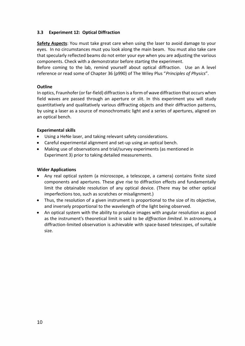
easily determine the zeroth order (centre) and as many higher orders as possible. Sketch and describe the pattern. Now, by careful experimental measurement it should be possible to determine the wavelength of the laser light. The wavelength of the light from the laser is given by

m

d msin

, (2)

where the angle θm is indicated in Figure 2

Figure 2: Defining d and θm

Because θm is small, D

mxmm

)(tansin , and [2] becomes

m

mx

D

d )( (3)

Note x(m) is the distance between the centre of the pattern and the mth diffraction spot. Rearrange the equation to plot a suitable straight line graph in order to determine , the wavelength of the HeNe laser. Check that your answer is sensible! Two dimensional grating

SLIDE 4, is a two-dimensional diffraction grating. Use any convenient diffraction method to find the ratio of the repeat distances in the two principal directions. Remember to sketch your observations and discuss.

14

3.4 Experiment 13: Propogation of Sound in Gases.

Note: This experiment is performed in the dark room. SAFETY ASPECTS: MAKE SURE THAT THE ROOM FAN IS SWITCHED TO EXTRACT AND IS WORKING. Outline The speed of sound is commonly used to refer specifically to the speed of sound waves in air, although the speed of sound can be measured in virtually any substance and will vary. The speed of sound in other gases will be dependent on the compressibility, density and temperature of the media. You will investigate these dependencies by studying the sound waves set up in various gases contained in a gas cavity. Experimental skills Observation of longitudinal waves. Understand the use of a microphone as an acoustic to electric transducer. Hence using an oscilloscope to study non-electrical waves. Careful use of gases and gas cylinders. Wider Applications In dry air at 20°C, the speed of sound is 343 metres per second. This equates to 1,236 kilometres per hour, or about one kilometer in three seconds. The speed of sound in air is referred to as Mach 1 by aerospace professionals (i.e the ratio of air speed to local speed of sound =1). The physics of sound propogation, reflection and detection is used extensively for underwater locating (SONAR), robot navigation, atmospheric investigations and medical imaging (Ultrasound). The high speed of sound is responsible for the amusing "Donald Duck" voice which occurs when someone has breathed in helium from a balloon!

15

Introduction The speed of propagation of a sound disturbance in a gas depends upon the speed of the atoms or molecules that make up the gas, even though the movement of the atoms or molecules is localised. The r.m.s. speed of molecules of mass m in a gas at Kelvin-scale temperature T is given by;

2

1

21

2 3

m

kTc ,

where k is the Boltzmann constant. The sound is not propagated exactly at the speed

c2

1

2 but at 2

1

3

times it, where is the ratio of the principal heat capacities of the

gas. Thus

Csound =2

1

m

kT (1)

Measurement of Csound for known T and m therefore enables to be determined1. In this experiment the speed of sound in gaseous argon, air (mainly nitrogen) and carbon dioxide is measured by analysing the standing waves in a cavity.

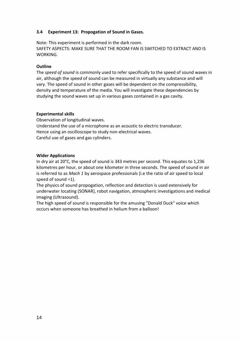
Experiment Apparatus The standing wave cavity is shown schematically in Figure 1.

Figure 1: Standing wave cavity

The loudspeaker, driven from an oscillator, directs sound into the tube; standing waves are obtained by adjustment of the piston and detected by the microphone insert at the end of the tube. The output from the microphone is amplified and displayed on the oscilloscope. Ensure that the amplifier is turned off when you have finished this experiment. Consider and write down the relationship between the length of the tube and the wavelength of sound for standing waves in closed and open tubes. Revise these expressions having considered this material using reference 2 or another source. Should you treat your equipment as having two closed ends or one open and one closed? Why?

16

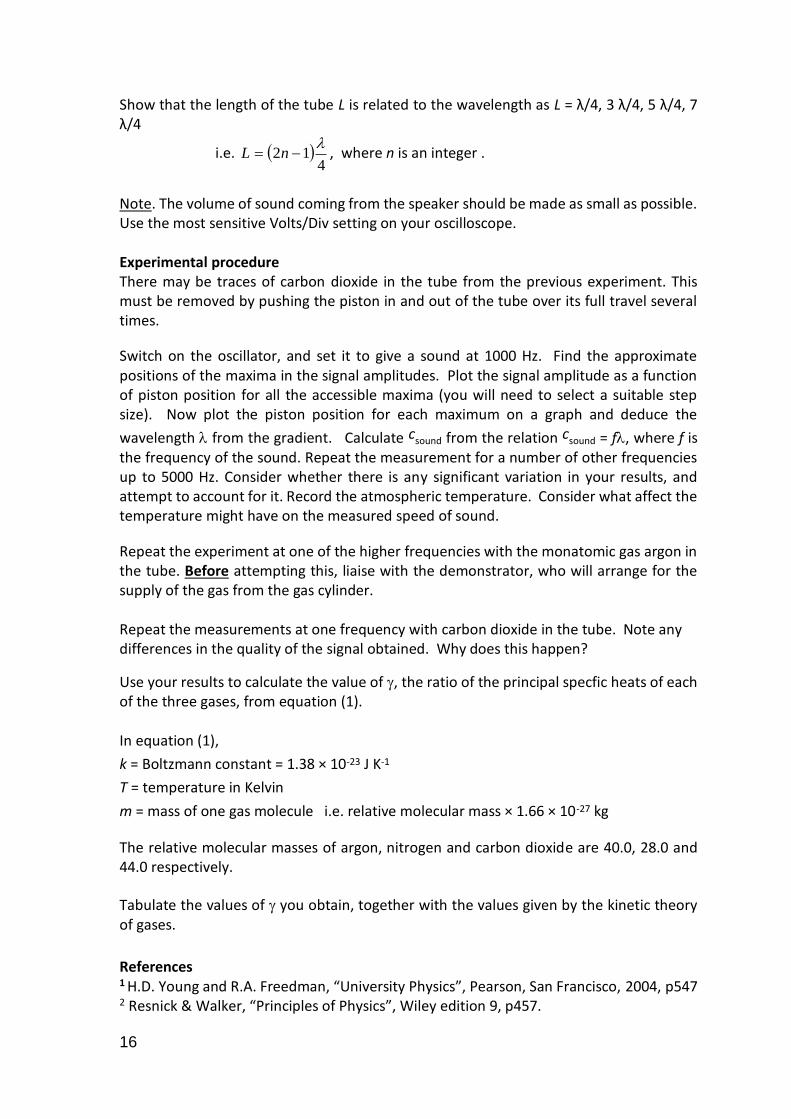
Show that the length of the tube L is related to the wavelength as L = λ/4, 3 λ/4, 5 λ/4, 7 λ/4

i.e. 4

12

nL , where n is an integer .

Note. The volume of sound coming from the speaker should be made as small as possible. Use the most sensitive Volts/Div setting on your oscilloscope. Experimental procedure There may be traces of carbon dioxide in the tube from the previous experiment. This must be removed by pushing the piston in and out of the tube over its full travel several times.

Switch on the oscillator, and set it to give a sound at 1000 Hz. Find the approximate positions of the maxima in the signal amplitudes. Plot the signal amplitude as a function of piston position for all the accessible maxima (you will need to select a suitable step size). Now plot the piston position for each maximum on a graph and deduce the

wavelength from the gradient. Calculate csound from the relation csound = f, where f is the frequency of the sound. Repeat the measurement for a number of other frequencies up to 5000 Hz. Consider whether there is any significant variation in your results, and attempt to account for it. Record the atmospheric temperature. Consider what affect the temperature might have on the measured speed of sound.

Repeat the experiment at one of the higher frequencies with the monatomic gas argon in the tube. Before attempting this, liaise with the demonstrator, who will arrange for the supply of the gas from the gas cylinder. Repeat the measurements at one frequency with carbon dioxide in the tube. Note any differences in the quality of the signal obtained. Why does this happen?

Use your results to calculate the value of , the ratio of the principal specfic heats of each of the three gases, from equation (1). In equation (1),

k = Boltzmann constant = 1.38 × 10-23 J K-1

T = temperature in Kelvin

m = mass of one gas molecule i.e. relative molecular mass × 1.66 × 10-27 kg

The relative molecular masses of argon, nitrogen and carbon dioxide are 40.0, 28.0 and 44.0 respectively.

Tabulate the values of you obtain, together with the values given by the kinetic theory of gases.

References 1 H.D. Young and R.A. Freedman, “University Physics”, Pearson, San Francisco, 2004, p547 2 Resnick & Walker, “Principles of Physics”, Wiley edition 9, p457.

17

3.5 Experiment 14: Microwaves

Safety

Although the microwave power used in this experiment is very low students should take care not to look directly into the source when it is switched on.

The resistor mounted on the back of the transmitter does get hot after extended use.

Outline The properties of waves in general and electromagnetic waves in particular are examined by using microwaves of wavelength ~2.8 cm. The properties examined include polarization, diffraction and interference. The interference experiments are similar to those performed with visible light at much shorter wavelengths (and sound with similar wavelengths). However, the macroscopic wavelength of microwaves is exploited to reveal behaviour not readily accessible at short wavelengths, in particular phase changes on reflection and edge diffraction effects.

Experimental skills

Experience of handling microwave radiation, sources and detectors.

Experience of polarized electromagnetic radiation.

Wider Applications

Microwave radiation is used in communications, astronomy, radar and cooking. Mobile phones use two frequency bands at ~ 950 MHz and ~18850 MHz. Astronomy - the cosmic microwave background radiation peaks at λ= 1.9 mm. Microwave ovens use a frequency of 2.45 GHz wavelength of 12.2 cm. The oscillating electric field interacts with the electric dipole in water molecules so that they rotate, have more energy and so get “hotter”. Since water molecules in solid form cannot rotate ice is an inefficient absorber of microwave radiation.

The manipulation of polarization is an important way to exploit electromagnetic radiation. This is not restricted to plane polarization. For example “circularly” polarized light is exploited in the latest 3D films shown at cinemas.

Electromagnetic radiation detection is common to many branches of physics. For example with an array of detectors similar to the ones used here and some optics astronomical imaging becomes possible – this is a very active research area within this School.

18

Introduction The name “microwave” is generally given to that part of the electromagnetic spectrum with wavelengths in the approximate range 1mm - 100 cm (10-3-1 m). This compares with the visible region with wavelengths of 4 to 8 x 10-7 m. Microwaves therefore have a wavelength which is >20,000 times longer than light waves. Because of this difference it is easier in many cases to demonstrate the wave properties of electromagnetic radiation using microwaves.

Electromagnetic Waves An electromagnetic wave is a transverse variation of electric and magnetic fields as shown

in figure 1 and travels through space with the velocity of light (3 x 108 m s-1). Because it is a transverse wave it can be “polarized”, meaning that there is a definite orientation for their oscillations. As shown in Figure 1 an electromagnetic wave is composed of electric and magnetic fields oscillating at right angles. The direction of polarization is defined to be the direction in which the electric field is vibrating. (This is an arbitrary matter; the magnetic field could equally well have been chosen to define the direction of polarization). Plane polarized radiation means that the electric field (or the magnetic field) oscillates in one direction only.

Figure 1 The electric and magnetic fields in an electromagnetic wave. E is the electric field strength, B the

magnetic flux density. The wave propagates with a velocity of 3 x 108 m s-1

.

The microwave transmitter provided emits monochromatic plane polarized radiation. A normal light source is a mixture of many different directions of polarization so that its average polarization is zero.

An electric field is defined in terms of both an amplitude and direction and is therefore a vector. It is useful to think of polarized radiation in terms of vectors. The detectors of (microwave) electromagnetic radiation used in this experiment are polarization sensitive (some are not). In this case the relative orientation of the transmitter (and electric field) and the detector (receiver) is important and is illustrated in Figure 2.

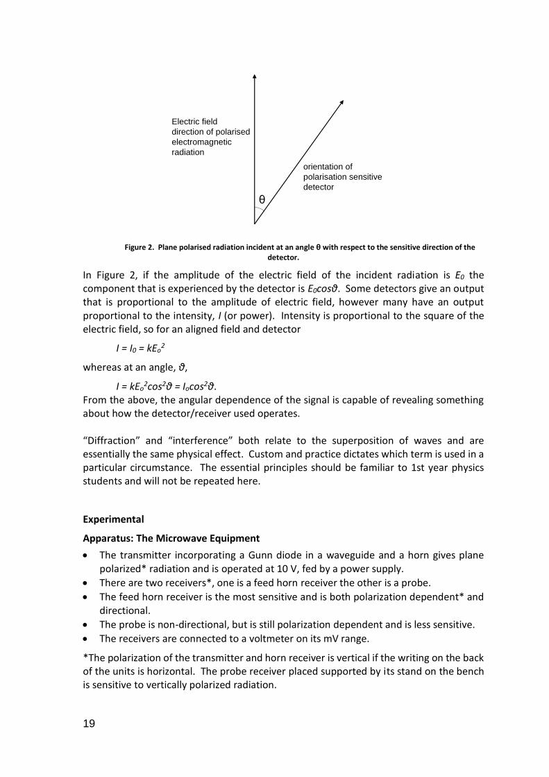
19

Figure 2. Plane polarised radiation incident at an angle θ with respect to the sensitive direction of the

detector.

In Figure 2, if the amplitude of the electric field of the incident radiation is E0 the component that is experienced by the detector is E0cosθ. Some detectors give an output that is proportional to the amplitude of electric field, however many have an output proportional to the intensity, I (or power). Intensity is proportional to the square of the electric field, so for an aligned field and detector

I = I0 = kEo2

whereas at an angle, θ,

I = kEo2cos2θ = Iocos2θ.

From the above, the angular dependence of the signal is capable of revealing something about how the detector/receiver used operates. “Diffraction” and “interference” both relate to the superposition of waves and are essentially the same physical effect. Custom and practice dictates which term is used in a particular circumstance. The essential principles should be familiar to 1st year physics students and will not be repeated here.

Experimental

Apparatus: The Microwave Equipment

The transmitter incorporating a Gunn diode in a waveguide and a horn gives plane polarized* radiation and is operated at 10 V, fed by a power supply.

There are two receivers*, one is a feed horn receiver the other is a probe.

The feed horn receiver is the most sensitive and is both polarization dependent* and directional.

The probe is non-directional, but is still polarization dependent and is less sensitive.

The receivers are connected to a voltmeter on its mV range.

*The polarization of the transmitter and horn receiver is vertical if the writing on the back of the units is horizontal. The probe receiver placed supported by its stand on the bench is sensitive to vertically polarized radiation.

θ

Electric field

direction of polarised

electromagnetic

radiation

orientation of

polarisation sensitive

detector

20

Important:

Reminder: Do not look into the transmitter when it is turned on.

Neither receiver should be placed nearer than 10 cm from the transmitter.

Stray reflections are a big problem when undertaking microwave experiments. To minimise these, the experiment should be carried out on the top level of the bench and all objects (bags, hands and arms etc) should be kept out of the beam whilst taking measurements.

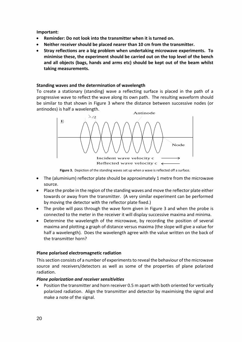
Standing waves and the determination of wavelength To create a stationary (standing) wave a reflecting surface is placed in the path of a progressive wave to reflect the wave along its own path. The resulting waveform should be similar to that shown in Figure 3 where the distance between successive nodes (or antinodes) is half a wavelength.

Node

Antinode

Incident wave velocity c

Reflected wave velocity c

E_

/2

Figure 3. Depiction of the standing waves set up when a wave is reflected off a surface.

The (aluminium) reflector plate should be approximately 1 metre from the microwave source.

Place the probe in the region of the standing waves and move the reflector plate either towards or away from the transmitter. (A very similar experiment can be performed by moving the detector with the reflector plate fixed.)

The probe will pass through the wave form given in Figure 3 and when the probe is connected to the meter in the receiver it will display successive maxima and minima.

Determine the wavelength of the microwave, by recording the position of several maxima and plotting a graph of distance versus maxima (the slope will give a value for half a wavelength). Does the wavelength agree with the value written on the back of the transmitter horn?

Plane polarised electromagnetic radiation

This section consists of a number of experiments to reveal the behaviour of the microwave source and receivers/detectors as well as some of the properties of plane polarized radiation.

Plane polarization and receiver sensitivities

Position the transmitter and horn receiver 0.5 m apart with both oriented for vertically polarized radiation. Align the transmitter and detector by maximising the signal and make a note of the signal.

21

The polarization of the emitted radiation and polarized sensitivity of the receiver can be demonstrated by rotating the transmitter through 90o. Find the minimum possible signal and record it.

Repeat for the probe receiver and compare the properties of the two receivers.

Return the transmitter and horn to their vertical position. Place the large metal grid between the two, rotate it and observe the variation in the received signal. What effect does the grid have? Why?

Detection of polarized radiation: angular dependence Either by using the metal grid or by rotation of the transmitter, deduce the dependence of the measured power on the angle of polarization. (This may be quite tricky.)

Find a suitable way of measuring the angle of rotation and vary this in 15 degree steps from 0 o to 180 o. Record the measured signal.

Tabulate the signal measurements along with the expected values for cosθ and cos2θ dependencies. What do the results imply?

Demonstration of interference effects

This part of the experiment builds up a microwave analogue of the single slit optical interference experiments. By concentrating on the straight through beam the experiment complements optical diffraction experiments. The general arrangement is shown in Figure 4.

Figure 4. Schematic of the experimental arrangement for interference from a single slit (the transmitter is shown relatively much closer to the slit than is required)

The experiment is performed in four parts whilst keeping the distance between the front of the transmitter and the plane AA’ constant (at ~0.6 m). This will allow all results to be compared.

(i) No slits in place This section gives an indication of the spread of microwaves emitted from the source.

Position a 1 m rule on the bench top to provide an indication of position in the AA’ plane.

transmitter

x

A

A'

to meter on

receiver

22

Moving the probe in 2 cm steps between measurements, take 8 measurements either side of the centre line, i.e. 17 measurements in all.

Plot the data. Note: The graph shows the distribution of microwave power in the “beam” emitted from the transmitter.

(ii) Single slit: variable slit width probe fixed in straight through position This section investigates the effect of slit width on the straight through beam.

Position the two large plates equidistant from the front of the transmitter and the plane AA’, with a slit width of 3 cm.

Keeping the centre of the slit on the line between transmitter and probe, take measurements as the separation of the plates (width of the slit) is increased in 2 cm steps up to ~21 cm and then in 1 cm steps up to ~35 cm.

Plot the data and compare with (i).

Note: The above results have all the hallmarks of interference.

(iii) Single plate: variable plate position, probe fixed in straight through position This section seeks to provide an explanation for the results found in (ii).

Position one large plate as above but with one of its edges directly in the line of sight between the source and the detector. Make a note of this position and then move it across a further 5 cm to obscure the detector.

From this starting position take readings as the probe is moved out of the beam. Take readings every ~2 cm for the first 10 cm and every 1 cm for the final 10 cm (20 cm movement in total). (You can always add more readings if you need to.)

Plot the data and consider whether two such single plates can explain the results in (ii).

Note: There is very little scattering of radiation behind the plate.

The origin of interference If all has gone well, the two plate/single slit the interference behaviour of the straight through beam can now be understood to arise from the addition of the effect of two single plates. The single plate behaviour is better considered to be an example of “straight edge diffraction” where the straight through beam from the emitter interferes with a secondary source of radiation reflected from the edge of the plate. As the plate is moved away from the centre line the path difference, between the straight through and reflected beams, increases. From this argument it might be expected that the first turning point, corresponding to a path difference of λ/2 (phase difference of π), would be a minimum, whereas clearly it is a maximum. This is explained by the reflection at the edge producing a (negative) phase shift in the re-emitted radiation.

If you have time, use Pythagoras theorem to determine the phase shift** caused by reflection at the edge. See Appendix at end.

** A simple reflection (as in 2.2) would be expected to result in a -π phase shift, however with this geometry the Gouy effect is reported to result in a further -π/4 phase shift giving a total of -3π/4.

(iv) Single slit diffraction pattern: fixed width This section seeks to illustrate the fundamental equivalence of light and microwaves by generating a (familiar) single slit diffraction pattern.

23

Position the two large plates as in (ii) but with a separation of 11 cm.

Moving the probe in 2 cm steps between measurements, take 8 measurements either side of the centre line, i.e. 17 measurements in all.

Plot the data and compare the first minimum with its expected position (given λ = 2.8 cm).

(Note: Here due to diffraction, minima are expected at n = d.sin, where d is the slit width.)

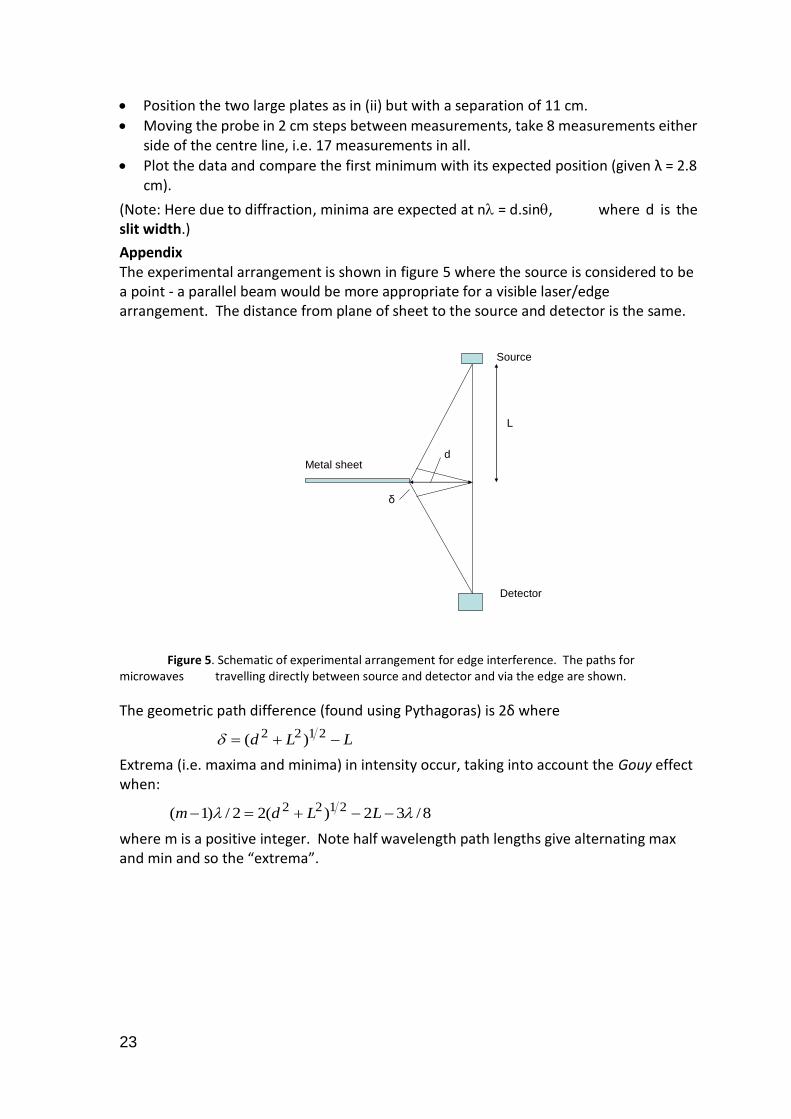
Appendix The experimental arrangement is shown in figure 5 where the source is considered to be a point - a parallel beam would be more appropriate for a visible laser/edge arrangement. The distance from plane of sheet to the source and detector is the same.

Figure 5. Schematic of experimental arrangement for edge interference. The paths for microwaves travelling directly between source and detector and via the edge are shown.

The geometric path difference (found using Pythagoras) is 2δ where

LLd 2122 )( Extrema (i.e. maxima and minima) in intensity occur, taking into account the Gouy effect when:

8/32)(22/)1( 2122 LLdm where m is a positive integer. Note half wavelength path lengths give alternating max and min and so the “extrema”.

Detector

Metal sheet

Source

L

d

δ

24

3.6 Experiment 15: Variation of Resistance with Temperature.

Safety Aspects: In this experiment you will use the cryogen liquid nitrogen (boiling point 77.3K). Please ensure that you read the safety precautions, write a risk assessment AND seek the assistance of a demonstrator before using this. SAFETY PRECAUTIONS IN THE HANDLING OF LIQUID NlTROGEN Avoid contact with the fluid, and therefore avoid splashing of the liquid when transferring it from one vessel to another. Remember that when filling a "warm" dewar, excessive boil-off occurs and therefore a slow and careful transfer is necessary. Do not permit the liquid to become trapped in an unvented system. If you do not wear spectacles, safety glasses (which are provided) must be worn when liquid nitrogen is being transferred from one vessel to another. FIRST AID If liquid nitrogen contacts the skin, flush the affected area with water. If any visible ''burn" results contact a member of staff.

Outline All materials can be broadly separated into 3 classes, according to their electrical resistance; metals, insulators and semiconductors. This resistance to the flow of charge is temperature dependent but the dependence is not the same for all material classes, because of the physical processes involved. In this experiment you will determine the behaviour of electrical resistance as a function of temperature for a metal and a semiconductor. You will confirm the linearity or otherwise of these behaviours.

Experimental skills

Ability to keep a clear head and organize a one-off experiment, paying careful attention to safety aspects.

Make and record simultaneous measurements of a number of time-varying quantities.

Determine realistic errors in these quantities and combine them.

Gain experience of liquid cryogens.

Fit measured data to linear, polynomial and logarithmic expressions.

Wider Applications

Many branches of physics and its applications involve the study and use of materials at cryogenic temperatures (those below ~ 150K). By understanding the temperature dependence of material behaviour, we can use it to our advantage.

Modern imaging and communication systems rely on the sensitive, noiseless and reproducible detection and transfer of electrical information. This is often achived by using cooled semiconductor devices.

Some materials become superconducting at cryogenic temperatures (i.e a temperature somewhat above absolute zero). This phenomenon has found application in Medical imaging (MRI scanners depend on the huge magnetic fields achievable only by using superconducting coils); Astronomical imaging (superconducting detectors are used to count 13 billion year old photons) and transport (MAGLEV trains).

25

Introduction In this experiment you will investigate the variation of the resistance of: 1) a semiconductor (a thermistor); 2) a metal (copper) in the temperature range from ~ 120 - 290 K. For a metal the following equation (1) describes the linear behaviour of resistance R with temperature T.

R(T)= R273(1 + (T-273)) , (1) Where R(T) is the resistance at temperature T (in Kelvin), R273 is the resistance at 273K

and is a constant known as the temperature coefficient of resistance, which depends on the material being considered and will vary slightly with the reference temperature (273K here). However the behaviour may be more closely described by a 2nd order polynomial fit.

RT = R273 {1 + (T-273) + (T-273) 2}, (2)

where is another constant. For a typical intrinsic semiconductor the electrical resistance obeys an exponential relationship with temperature. It takes the form of equation (3) . RT = a eb/T , (3) where RT is the resistance at T and a and b are constants. By using equations (1), (2) and (3), you are to find suitable graphical ways to verify or disprove these relationships. You may use Excel (or another plotting package familiar to you) to plot your data, BUT remember to take care with axes, apply suitable error bars and think about what your results mean. Experiment Apparatus The metal you will test is in the form of a coil of fine wire. The semiconductor is a thermistor. Both of these are attached to the top of a copper rod. They are held in good thermal contact with it by a low-temperature varnish. The temperature of the specimens can be reduced by immersing the copper rod to various depths in liquid nitrogen, which boils at 77.3 K. The liquid nitrogen is poured into a Dewar flask contained in the box which supports the copper-rod assembly. The liquid-nitrogen level is gradually increased by adding liquid nitrogen through the funnel. An insulating cap is provided which, when placed over the top of the rod, thermally isolates the specimens from the surroundings and allows their temperature to fall to a value determined by the depth of immersion of the rod in the liquid nitrogen.

26

The temperature of the specimens is measured with a thermocouple. This consists of two junctions of dissimilar metals arranged as shown in Figure 1. If the two junctions are at different temperatures an e.m.f. is generated which, to a good approximation, is proportional to the temperature difference between the two junctions. By calibrating such a thermocouple, temperature differences can be determined by voltage measurements and these can be used to measure temperature if one standard junction is held at a well-defined fixed temperature.

Figure 1: Representation of back-to-back thermocouple junctions and circuit

In this experiment we use a copper-constantan thermocouple. One junction of this is embedded with the specimens in the varnish; the other, the standard, is kept at 77.3 K by immersion in liquid nitrogen contained in a separate Dewar flask. You will calibrate the thermocouple with the standard junction in liquid nitrogen while that attached to the metal rod remains at room temperature. The resistances of the copper and thermistor are read from multimeters suitably connected. The voltage across the thermocouple is also read by a multimeter. Ensure you can read all 3 scales simultaneously. Calibration of the thermocouple Connect a multimeter to the appropriate thermocouple terminals on top of the rod. Immerse the free junction in liquid nitrogen and record a voltage. Take another voltage reading when the junction is at room temperature. You can now calibrate the thermocouple scale by assuming that the voltage is linearly related to temperature difference. (This is not strictly true but will suffice for our purposes.) Check your calibration with a demonstrator and ensure that you know how to use the thermocouple as a thermometer for the rest of the experiment. Resistance measurements The magnitudes of the coil and thermistor resistances will be determined using multimeters set to the ohms range. Measure RC (the resistance of the copper coil) and RTh (the resistance of the thermistor)

at room temperature.

27

Place the insulating cap on top of the rod and start to add liquid nitrogen through the funnel. Note the readings on the 3 multimeters (thermocouple voltage, Rc and RTh).

Gradually add more liquid nitrogen and repeat .The object of the experiment is to obtain as many measurements of Rc and RT as possible over as wide a temperature range as

possible. Remember to ensure that you have a simple diagram of your apparatus that would allow you to set the experiment up again. Experimental Notes

You must work quickly and efficiently if you are to obtain sufficient experimental points on the graphs

Handle the Dewar flasks carefully.

DO NOT touch the copper rod when it has been immersed in liquid nitrogen. If you do, you may freeze to the cold metal and give yourself a severe burn

You will find that there will be little change in temperature of the coil and the thermistor when liquid nitrogen is added initially, but take care not to add too much liquid nitrogen at any one time or a large temperature drop may result. Once the rod has been cooled, it is not easy to raise the temperature again in the course of the experiment. This is a one hit expereiment!

The lowest temperature you are likely to reach will be at best ~ 120 K.

Make notes in your lab diaries of anything that happens during the experiment, e.g. where you note a change of range on the multimeter.

Make a note in your lab diary of the specific pieces of equipment that you have used.

Data analysis Plot suitable graphs of your data and investigate the validity of equations (1) and (2) for

the metal and equation (3) for the thermistor. Finding values of , , a and b. You may use a computer package (Excel is recommended) to fit the equations but be careful to check your axes, show error information and quote gradients and results to a sensible number of significant figures. Does the variation of resistance in a metal vary linearly with temperature? Which equation gives the best fit to the data? What do you notice about the variation for a semiconductor? Is the exponential fit of equation (3) good enough? How might the experiment, errors in the data, or your experimental method be improved?

28

3.7 Experiment 16: Resistive and reactive impedances in RC circuits

Outline

An introduction to an oscilloscope and to electrical circuits

An introduction to the behaviour of time varying electronic signals in electronic circuits involving both reactive and resistive impedances, using a series combination of a resistor and a capacitor.

The investigation uses an oscilloscope to examine voltage signals for the capacitor coupled/high pass filter arrangement. This allows the frequency dependence of the phase angle between current and voltage and the filter performance to be found.

Experimental Skills

Reinforcement of the use of coaxial leads and circuit construction with breadboards.

Reinforcement of the use of oscilloscopes for measuring time varying electrical signals.

Introduction of oscilloscope techniques for measuring the phase differences between signals in both Y-t and XY modes.

Wider Applications

Resistor-capacitors combinations are widely used in electronic circuits as frequency filters to let through (or pass) either low or high frequency signals, i.e. as low or high pass filters respectively.

With inductors in “LCR circuits”, resonance behaviour can occur described by mathematics that is analogous to mechanical forced, damped oscillatory systems: This behaviour is extensively covered in 1st year maths and in 2nd year physics labs. These tuning circuits are what was at the core of the wireless (radio) communication revolution.

The visualisation of orthogonal oscillating signals, as seen during this experiment with the oscilloscope in XY mode, has very close parallels with the different possible polarisation of light: the analogies of linear, circular and elliptically polarised light are all produced in this experiment.

29

1 Introduction Capacitors, like resistors “impede” current flow, although not in the same way:

A steady voltage applied to a capacitor causes a charge to build up on the plates of a capacitor eventually preventing further current flow, whilst alternating currents can flow on and off the plates; hence low frequency signals are impeded but high frequency signals are not.

Whereas resistors heat up and so dissipate electrical power (I2R) capacitors do not: hence their impedance is said to be “reactive” rather than “resistive” (this is the same for inductors whose impedance is also reactive).

Whereas current and voltage are in-phase across a resistor they are 90° out of phase across capacitors (and inductors).

It is the frequency dependence in alternating current (ac) circuits that has lead to capacitors being widely used in electronic circuits. In analogue filter networks, they help remove high frequency signals from dc power supplies or remove unwanted direct current (dc) voltages from ac signals. In resonant circuits they can be used to ‘pick up’ particular frequencies.

1.1 Impedances of resistors and capacitors The above considerations lead to a distinction: the general term for something that impedes current flow is called an “impedance” (Z); whereas the impedances of capacitors (and inductors) are called reactive (X) and of resistors are called resistive (R). In all cases impedances are measured in ohms and current and voltage are related by

𝐼 =

𝑉

𝑍 [1]

In addition, of particular relevance here is that the total impedance of a circuit containing series combination of a resistor (R) and a capacitor (XC) is given by: 𝑍 = 𝑅 + 𝑋𝐶 [2]

Resistors: A reminder is probably not needed however, the relationship between the current I through and voltage V across a resistor is I = V/R. If the voltage is varying sinusoidally (i.e. 𝑉 = 𝑉0𝑠𝑖𝑛𝜔𝑡, where 𝜔(= 2𝜋𝑓) is the angular frequency) then:

𝐼 =

𝑉0𝑠𝑖𝑛𝜔𝑡

𝑅 [3]

Hence current and voltage are in phase.

Capacitors: The equation that describes the behaviour of capacitors is 𝑄 = 𝐶𝑉 where Q is the charge on the plates of the capacitor and C is the constant of proportionality to the voltage across it and is known as its capacitance. In a similar fashion to a resistor the magnitude of the charge on the capacitor varies in phase with the voltage. However, here it is the phase difference between current and voltage that is of interest.

Current is given by

𝐼 =

𝑑𝑄

𝑑𝑡= 𝐶

𝑑𝑉

𝑑𝑡= 𝐶𝑉0𝜔𝑐𝑜𝑠𝜔𝑡 [4]

30

Hence the current leads the voltage by 90° and the magnitude of the reactance is given by

|𝑋𝐶| =|𝑉|

|𝐼|=

|𝑉0𝑠𝑖𝑛𝜔𝑡|

|𝐶𝑉0𝜔𝑐𝑜𝑠𝜔𝑡|=1

𝜔𝐶 [5]

i.e. the reactance of a capacitor decreases with increasing frequency.

1.2 Series RC circuit theory. Capacitors and resistors often occur in circuits together. In these “RC circuits” the capacitive reactance and resistance combine to produce an overall circuit. The study of current and voltage in a series combination of a resistor and a capacitor is the subject of this experiment. Consider a sinusoidally varying voltage source connected to a resistor and capacitor in series as shown in figure 1. The instantaneous voltage across both components must equal the input voltage and the instantaneous current at all parts of the circuit must be the same hence equation [6]

𝑉𝑖𝑛 = 𝑉𝑅 + 𝑉𝐶 = 𝐼(𝑅 + 𝑋𝐶) [6]

Figure 1 Series combination of a resistor and capacitor and the voltages across them.

However, due to the phase differences the voltage across each component peaks at different times and therefore it is incorrect to add their amplitudes. To understand and express what is happening it is useful to make use of complex number representations. An Argand diagram of impedance, Z as shown in Figure 2.

R

C

VR

VC

Vin

31

Figure 2 Argand diagram (similar to phasor diagram) for the impedance of a series RC circuit. The angle 𝜙 is the phase

angle difference between current and input voltage, Vin.

The resistive impedance, R is on the real axis as current and voltage are in phase (experimentally this is very important – measuring the voltage across any resistor gives the phase of the current and, if R is known, its magnitude).

By contrast the reactive impedance of the capacitor is given by:

𝑋𝐶 = −𝑗

𝜔𝐶 [7]

in order to be consistent with the current (which is the same at all parts of the circuit) leading the voltage across the capacitor by 90°.

Using equation 2 the impedance of the series combination of R and C is 𝑍𝑡𝑜𝑡 = 𝑅 −𝑗

𝜔𝐶

The magnitude of the total impedance is given by |𝑍𝑡𝑜𝑡| = √𝑅2 + (

1

𝜔𝐶)2

R

ImZ

-j/ωC

Ztot

=R-j/ωC

ReZ φ

32

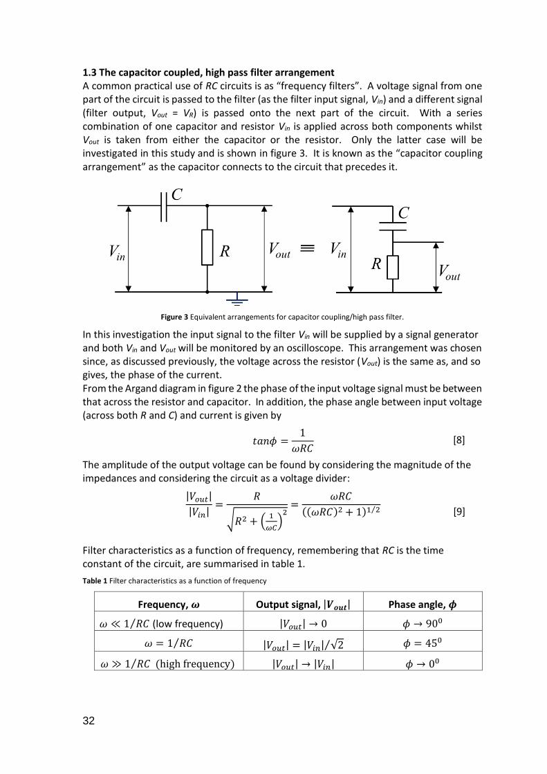
1.3 The capacitor coupled, high pass filter arrangement A common practical use of RC circuits is as “frequency filters”. A voltage signal from one part of the circuit is passed to the filter (as the filter input signal, Vin) and a different signal (filter output, Vout = VR) is passed onto the next part of the circuit. With a series combination of one capacitor and resistor Vin is applied across both components whilst Vout is taken from either the capacitor or the resistor. Only the latter case will be investigated in this study and is shown in figure 3. It is known as the “capacitor coupling arrangement” as the capacitor connects to the circuit that precedes it.

Figure 3 Equivalent arrangements for capacitor coupling/high pass filter.

In this investigation the input signal to the filter Vin will be supplied by a signal generator and both Vin and Vout will be monitored by an oscilloscope. This arrangement was chosen since, as discussed previously, the voltage across the resistor (Vout) is the same as, and so gives, the phase of the current. From the Argand diagram in figure 2 the phase of the input voltage signal must be between that across the resistor and capacitor. In addition, the phase angle between input voltage (across both R and C) and current is given by

𝑡𝑎𝑛𝜙 =1

𝜔𝑅𝐶 [8]

The amplitude of the output voltage can be found by considering the magnitude of the impedances and considering the circuit as a voltage divider: |𝑉𝑜𝑢𝑡|

|𝑉𝑖𝑛|=

𝑅

√𝑅2 + (1

𝜔𝐶)2=

𝜔𝑅𝐶

((𝜔𝑅𝐶)2 + 1)1 2⁄

[9]

Filter characteristics as a function of frequency, remembering that RC is the time constant of the circuit, are summarised in table 1.

Table 1 Filter characteristics as a function of frequency

Frequency, 𝝎 Output signal, |𝑽𝒐𝒖𝒕| Phase angle, 𝝓

𝜔 ≪ 1 𝑅𝐶⁄ (low frequency) |𝑉𝑜𝑢𝑡| → 0 𝜙 → 900

𝜔 = 1 𝑅𝐶⁄ |𝑉𝑜𝑢𝑡| = |𝑉𝑖𝑛| √2⁄ 𝜙 = 450

𝜔 ≫ 1 𝑅𝐶⁄ (high frequency) |𝑉𝑜𝑢𝑡| → |𝑉𝑖𝑛| 𝜙 → 00

33

At low frequencies the impedance of the capacitor dominates and most of the input voltage is dropped across it, whereas at high frequencies the reverse is true. This is why the arrangement is known as a high pass filter: the input signal is only passed on faithfully (i.e. without attenuation) at high frequencies.

Aside: A “tweeter” is the loudspeaker in audio systems that is designed to generate high frequency sound (f > 2 kHz typically). High pass filters very similar to the one measured here are used to ensure that only the high frequencies are delivered to the tweeter.

2 Experimental

Using the prototype board, assemble the circuit in Figure 3 making use of three coaxial leads and connector posts and ensuring that:

When connecting jump leads to the 4 mm posts ensure that some bare wire protrudes from the post: a common cause of poor connections is pinching down on the wires’ insulation.

The earth of the three coaxial leads join at the same post (otherwise they will short out voltage signals).

The input and output signals are taken to Ch1 and Ch2 of the oscilloscope respectively.

The function generator is set to sine wave and its “dc offset” is turned off.

The capacitor and resistor provided have nominal values of 0.022 F and 4.3 kΩ respectively. However, measure the resistor value with a multi-meter and use this later to find the value of the capacitor (the quoted tolerance on the value given is 10%).

With the circuit made up, get used to operating the oscilloscope. Reminder: a summary version of how to use the oscilloscope can be found in background notes. But to start:

Turn on the oscilloscope and when the GW Instek banner has disappeared press “Save/Recall” then select “Default Setup” and finally press “Autoset”.

Or you could simply press “Autoset” – but this may (if you are very unlucky) remember unsuitable previous conditions.

Now:

Adjust the signal generator to set an input signal (dc offset in off position) with a peak to peak amplitude of ~3 V.

Use the vertical adjustments on Ch1 and 2 so that they are both at 0V (the position appears at the bottom left of the trace as they are being adjusted) to make phase and signal changes more obvious.

Check that the circuit is working as expected, i.e. that as the input signal frequency is varied the output signal size and phase vary roughly as described at the end of section 1.3.

Note: the same circuit arrangement will be used for all subsequent measurements. If you are unsure that it is working correctly check with a demonstrator.

2.1 Measuring the filter characteristics With the set up as above, and with the time base and y scales adjusted as appropriate perform measurements of frequency, f (and so period, T=1/f), Vin (although this isn’t

34

adjusted it may drift so measure it), Vout and the lead or lag of one oscillation against the other, dT (and so the phase offset 𝜙).

Note: 𝜙 = 360𝑑𝑇

𝑇 degrees (or 2𝜋

𝑑𝑇

𝑇 radians)

As 1 period, T, corresponds to 1 cycle, 360°, 2π radians.

Do this as a function of frequency (take ~10 readings in the range 200 Hz to 8000 Hz) recording the results in a suitable table.

Most measurements are made by the oscilloscope and can be read from its display using its “measure” facility (use peak to peak amplitudes for voltages), but for dT use the two X cursors (and then convert to radians or degrees as required). It will be necessary to toggle between “cursor” and “measure”.

Make plots of phase angle and |𝑉𝑜𝑢𝑡|/|𝑉𝑖𝑛| versus frequency, use these to find the condition 𝜔 = 1 𝑅𝐶⁄ and so determine the value of the capacitance (see table 1).

Using the phase angle data plot a suitable straight line graph (see equation 8), use this to determine the capacitance and compare the value with that above.

2.2 Using the oscilloscope XY mode for determination of filter characteristics. Here the x axis is not time dependent, instead one of the two channel inputs produces x deflections and the other y. This mode will be used to repeat the measurements of the previous section, but first some explanation.

The movement of the spot on the screen is then described by

𝑥 = 𝐴𝑠𝑖𝑛(𝜔𝑡); 𝑦 = 𝐵𝑠𝑖𝑛(𝜔𝑡 − 𝜙) [10]

where is the phase angle between the 2 inputs. In general this represents an ellipse, as shown in Figure 4, although depending on the phase angle the ellipse may appear when in-phase as a straight line through to, with A = B and 90° out of phase, a perfect circle. Such plots are known as Lissajous plots or figures.

Figure 4: Elliptical trace for the measurement of phase angle. Also shown dotted are straight line (𝜙=0) and circular

(𝜙 = 90°, 𝐴 = 𝐵) traces.

Understanding the XY mode To understand what you are seeing do the following (you will almost certainly need to get help from a demonstrator to get you started here):

35

Sketch one period of a time varying sine wave and a cosine wave, both of amplitude 1, in your diary. On both mark 10 reasonably evenly time spaced points and number these from 0 to 9 (point at start and end of cycle numbered 0 and 9 respectively).

Draw an XY plot with scales -1 to +1 in both X and Y. On this and for the case when both X and Y vary sinusoidally, plot out the time progression of the display using the numbers 0 to 9 as markers (rather than x’s or o’s). This is a Lissajous figure for the case of signals of the same frequency and in phase.

Repeat for X a sine wave and Y a cosine wave. This is the case of X and Y 90° out of phase. Using the time progression note whether the resulting (hopefully circular) trace was drawn out in a clockwise or anticlockwise sense.

Analysis of plots such as figure 4 (to find both |𝑽𝒐𝒖𝒕|/|𝑽𝒊𝒏| and 𝝓).

To find 𝜙 the line y = 0 (passing through A’,N’,O,N and A) through the ellipse is considered.

We have

𝑦 = 𝐵𝑠𝑖𝑛(𝜔𝑡 − 𝜙); So that 𝜔𝑡 = 𝜙 [11]

Hence 𝑥 = 𝐴𝑠𝑖𝑛(𝜔𝑡) = 𝐴𝑠𝑖𝑛𝜙 = 𝑁 = |𝑁′| [12]

And 𝑠𝑖𝑛𝜙 =𝑁

𝐴=𝑁𝑁′

𝐴𝐴′ [13]

Here AA' is the difference length between the two extreme x values of the ellipse, and NN' is the length given by the intersection of the ellipse with the x axis. Using the cursors it is more convenient to obtain these from the oscilloscope trace than N and A.

If the input signal (Vin) to a circuit (here the signal from the signal generator) is applied to channel 1 (X) and the output signal (Vout) from the circuit (here from across the resistor) to channel 2 then from figure 4 we have:

|𝑉𝑜𝑢𝑡|

|𝑉𝑖𝑛|=𝐵

𝐴=𝑌𝑝𝑝

𝑋𝑝𝑝=𝐶ℎ2𝑝𝑝

𝐶ℎ1𝑝𝑝

Where the pp subscript indicates peak to peak amplitude as the oscilloscope finds in its “measure” mode.

Measurements

To put the scope in XY mode press the “menu” button under horizontal and then select

XY.

Make measurements of |𝑉𝑜𝑢𝑡|/|𝑉𝑖𝑛|and phase offset 𝜙 versus frequency.

Add this data to your earlier plots ($2.1) of phase angle and |𝑉𝑜𝑢𝑡|/|𝑉𝑖𝑛| versus frequency and comment on the agreement.

3 Conclusions

As part of your concluding remarks consider the relative merits of the different methods

for measuring phase offsets and determining C.

36

Appendix: Complex number treatment of output voltage across the resistor

We are dealing with a potential divider circuit in which (using complex ohm’s law)

𝑉𝑖𝑛 = 𝐼 (𝑅 −𝑗

𝜔𝐶)

And, since the current must be the same in all parts of the circuit

𝐼 =𝑉𝑜𝑢𝑡𝑅=

𝑉𝑖𝑛

(𝑅 −𝑗

𝜔𝐶)

Rearranged this gives

𝑉𝑜𝑢𝑡 = 𝐼𝑅 =𝑉𝑖𝑛𝑅

(𝑅 −𝑗

𝜔𝐶)=

𝑉𝑖𝑛𝑅

(𝑅 −𝑗

𝜔𝐶).(𝑅 +

𝑗

𝜔𝐶)

(𝑅 +𝑗

𝜔𝐶)=𝑉𝑖𝑛𝑅 (𝑅 +

𝑗

𝜔𝐶)

(𝑅2 + (1

𝜔𝐶)2)

The amplitude of the output (usually of most interest) is given by:

|𝑉𝑜𝑢𝑡| = (𝑉𝑜𝑢𝑡𝑉𝑜𝑢𝑡∗ )1 2⁄ =

(

(𝑉𝑖𝑛𝑅)

2 (𝑅2 +1

𝜔2𝐶2)

(𝑅2 + (1

𝜔𝐶)2)2

)

1 2⁄

=𝑉𝑖𝑛𝑅

(𝑅2 + (1

𝜔𝐶)2)1 2⁄

=𝑉𝑖𝑛𝜔𝑅𝐶

((𝜔𝑅𝐶)2 + 1)1 2⁄

Phasor diagrams

These are an alternative to the Argand diagram of figure 1 to represent such time

varying voltages and currents and are used in Halliday and Resnick (chapters 16 and 31).

Figures may appear very similar to figure 2, however, the vectors rotates anticlockwise

with constant angular velocity corresponding to the angular frequency of the quantity

involved. The length of the vectors is equal to the amplitude of the quantity and the

instantaneous value of a quantity is represented by the projection onto the vertical axis.

37

3.8 Experiment 17: Radiation from a Hot Body

Outline A body (a light bulb filament) is heated by passing an electrical current through it. Knowing the voltage and current and something about the filament it is possible to determine the energy lost as a function of its temperature. This very simple experiment provides a good introduction to electrical circuits and measuring techniques, the manipulation of equations into a suitable form for analysis and the introduction of logarithmic plots in determining so-called power law dependencies. The physics in this experiment is not covered in lecture courses in autumn semester but will appear in the spring (in PX0201 and PX0202).

Introduction

A body at an absolute temperature T (T(K) = T(oC) + 273) placed in a vacuum will lose heat by radiation. Assuming there are no radiation sources surrounding the body, the body would eventually cool down to absolute zero (T=0 Kelvin). The rate of loss of heat by

radiation for a body placed in a vacuum is proportional to T4. For a perfect emitter (or black body)

𝑊 = 𝜎𝐴𝑇4 (1)

where A is the area of the radiating surface of the body (in m ), is Stefan's constant (5.6

x 10-8 W m-2 K-4 ) and W is the rate of heat loss of the body (in watt). The above equation is called the Stefan-Boltzmann law. In practice, most bodies cannot be considered as perfect emitters and the Stefan-Boltzmann equation has to be written

𝑊 = 𝜀𝜎𝐴𝑇4 (2)

where the emissivity factor is a number less than unity (and which depends upon the material). However, the surroundings have an ambient temperature T0 and so the net

rate of heat loss of the body is given by the difference at which it loses heat by radiation and absorbs heat from its surroundings by radiation, so that,

𝑊 = 𝜀𝜎𝐴(𝑇4 − 𝑇04) (3)

Eventually, if no energy is supplied to the body to make up for the radiative heat loss, the body will cool down until at T T 0 dynamic equilibrium exists in which energy is

continually being exchanged with the surroundings, but the net heat loss is zero.

Experiment Note: There is a lot of number crunching at the end of this experiment so it is important to carry out the measurements efficiently.

In this experiment, the energy radiated from the tungsten filament of a small electric light bulb is measured as a function of temperature. This is done by passing a current through the filament, waiting until the temperature of the filament has stabilised, and then measuring both the current I through the filament and the voltage V across it. (Note that the filament is not in thermal equilibrium with its surroundings since its temperature is always higher than that of the surroundings (ie T T

0 , except when no current flows.

However it is in a steady state, in which the power supplied to the filament by the power

38

supply is exactly equal to the radiative heat loss, so that the temperature is constant and measurements can easily be made).

The power dissipated in the bulb can be found from the voltage V across it and the current I through it:

𝑊 = 𝐼𝑉 (4)

The temperature of the filament can be found using the formula,

𝑅 = 𝑅0[1 + 𝛼(𝑇 − 𝑇0)] (5)

where R0 is the value of the resistance R of the filament at room temperature T0 and is

the average temperature coefficient of resistance (= 0.0053 K-1 for tungsten). By measuring R (using R = V/I) it is easy to calculate T.

The above information is then used to check the relation, equation (1).

Method

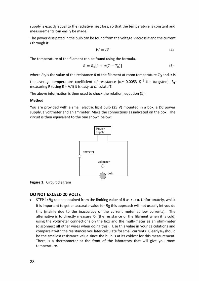
You are provided with a small electric light bulb (25 V) mounted in a box, a DC power supply, a voltmeter and an ammeter. Make the connections as indicated on the box. The circuit is then equivalent to the one shown below:

Powersupply

voltmeter

ammeter

bulb

Figure 1. Circuit diagram

DO NOT EXCEED 20 VOLTs STEP 1: R0 can be obtained from the limiting value of R as I 0. Unfortunately, whilst

it is important to get an accurate value for R0 this approach will not usually let you do

this (mainly due to the inaccuracy of the current meter at low currents). The alternative is to directly measure R0 (the resistance of the filament when it is cold) using the voltmeter connections on the box and the multi-meter as an ohm-meter (disconnect all other wires when doing this). Use this value in your calculations and compare it with the resistances you later calculate for small currents. Clearly R0 should be the smallest resistance value since the bulb is at its coldest for this measurement. There is a thermometer at the front of the laboratory that will give you room temperature.

39

STEP 2: Take readings of V and I (the expected maximum current is ~75 mA = 0.075 A). You should tabulate your data, including columns for I and V data and calculated values of power W (=I.V), resistance R (=V/I), temperature T (in Kelvin), T4 and T4 - T0

4. Making sure that V DOES NOT EXCEED 20 volts, take readings in ~2 V steps up to 20 V. Note - when you change the temperature of the filament let the system reach equilibrium before taking a reading. In addition, note the conditions under which the filament starts to glow so that you can estimate the temperature of the filament at this point.

STEP 3: Tabulate values of log10W and log10T and plot a graph of log10W versus log10T. If W T n then a log-log plot should produce a straight line of gradient n* (see “maths”

below). From your graph find n (and its error) to see if a T4 dependence is observed. Try to explain any discrepancy.

Note: In the following analysis you will not be required to work out errors as there is unlikely to be sufficient time.

STEP 4: Plot W versus T4 - T04. Using equation 3, calculate the total surface area A of

the filament (assume that = 0.1). Note there will be a systematic error introduced here if the temperature dependence isn’t T4.

*Maths

If we have 𝑊 = 𝑘𝑇𝑛

Taking log10 of both sides log10𝑊 = log10(𝑘𝑇𝑛) = log10𝑇

𝑛 = log10𝑘 = 𝑛log10𝑇 + log10𝑘

so a graph of log10W against log10T will be a straight line of slope n.

40

3.9 Experiment 18: Report writing feedback

Aim: This session is primarily to provide you with feedback for your formal report that you submitted before Christmas. You will sit with the session supervisor and go through feedback.

However it is also a chance to see what is involved in assessment of reports by actually having a chance to peer review a number of examples as an exercise, and then in your small peer group will be able to discuss the issues associated with good science communication and why certain conventions adopted by scientists are important.

41

3.10 Experiment 19: Computer Error Simulations and Analysis

Outline The autumn semester introduced random errors (from repeated measurement and from straight line graphs) and the propagation of errors (through techniques of partial differentials and adding in “quadrature”). Having used these concepts for a while, this session revisits the underlying concepts using new and existing Python computing skills.

Experimental (and computing) skills

Understanding the statistical analysis of data.

Use of statistical computing tools.

Wider Applications This experiment illustrates the unseen statistics behind all practical physics

In advanced applications the statistical analysis of data is all handled by computers.

This section explores the nature of least squares fitting and provides an introduction

to alternative numerical approaches.

Introduction The experiment “Statistics of experimental data (Gaussian Distribution)” performed during the autumn semester (PX1123) introduced you to some of the underlying foundations of the analysis of random errors. Here the subject is revisited. But, by making use of a computer (and Python programming), to both generate and analyse data much faster progress can be made. After reconsidering the error associated with repeated measurements of a single point, the session moves on to consider the treatment of error propagation (the combination of errors) and the “least squares” analysis of straight line data.

Session 1. Evolution of errors with repeated measurement with a normal distribution.

2. Error propagation (making sense of adding in quadrature)

3. The statistics of straight line graphs

Quick Reminder: the nature of experimental measurements (see section III.2 of PX1123 lab manual for full treatments)

Repeated measurements usually result in a normal distribution around a mean value.

With a reasonably large number of repeats “standard errors” represent the

uncertainty in determined values.

For y(x) when x is varied the data points can be considered as very similar to repeats

with the points distributed above and below the “best fit line”.

Experiments It will be a good idea to have access to the website during the course of the session. This should be one of your “favourites” but if it is not:

https://alexandria.astro.cf.ac.uk/Joomla-python/ Quick Python reminder – relevant syntax is present in week 2 and 3 (Arrays, Vector Algebra and Graph Plotting) of the taught computing course.

42

Normal/Gaussian statistics of repeated measurements Section 2.1 will be based on the simulation of repeated measurements of two timed events, A and B both measured with a stopwatch. Suppose that:

For the sake of the simulations the true values of A and B are 2.0 s and 3.0 s exactly.

The standard deviation* that characterises both measurements is 0.2 s.

*The standard deviation parameterises the spread in values that are obtained and so is also said to characterise (parameterise) the precision of the measurement.

Distributions for A and B The first step is to create arrays of points for A and B randomly generated from ideal normal distributions. The first point in each array then corresponds to the first measurement etc. Provided these arrays are only created once the subsequent analysis can be cross compared. To achieve this arrays for A and B will be created in the Spyder console. This does not exclude creating programmes in the editor because they can (and are normally) executed in the console and so can call on arrays that exist there.

Creating arrays This will be done using the normal() function. As given in the object explorer the defaults for this are:

normal(loc=0,scale = 1.0,size =1 value)

where loc is the mean value of the distribution, scale is the standard deviation and size is the number of points.

Do the following:

Create n = 1000 point arrays for A and B (labelled as A and B)

Create and print out a single (20 bin is appropriate) histogram including both A and B

and comment on the range of values for each and any overlap between the

distributions.

Perform a statistical analysis of A to find the mean, standard deviation and standard

error.

Transfer these to the editor and save the code as a (very) simple programme – it is

worth it as it will be used a few times today. Since this runs in the “Console” it can

call on the A array generated earlier. Do not write a function to generate A in the

programme as this will overwrite it.

Change the array name in the programme to analyse the B array.

Consider the appropriate parameter to use as the errors in A and B, state their values

(with errors – as usual) and state whether they agree with the accepted/known

values of A and B.

Error propagation (adding in quadrature) Students have been required to combine errors based on the outcomes of partial differentiation (which hopefully makes sense) and addition in quadrature (which hasn’t yet been justified). The aim here is to justify the addition in quadrature.

43

The addition and multiplication of two values (A and B) will be considered and their errors will be taken to be their standard deviations. (A large number of points (n) will be used so standard errors are more appropriate however since the two are linked by a factor of (n-1)0.5 this will not affect the interpretation or error propagation).

Addition of A and B (Sum, S=A+B) Reminder: error propagation for P = A + B

Partial differentiation gives 𝜕𝑆

𝜕𝐴= 1 and

𝜕𝑆

𝜕𝐵= 1

Or 𝜕𝑆 = 𝜕𝐴 and 𝜕𝑆 = 𝜕𝐵 Combining the 𝜕𝑃 (or ΔP) contributions in quadrature gives the familiar

(∆𝑆)2 = (∆𝐴)2 + (∆𝐵)2

Here a distribution of n (=1000) measurements of S = A + B will be generated, i.e. the first value of S is the first measurement of A is added to the first of B and generally for the ith term Si = Ai +Bi. In this way some errors/deviations from the true value will reinforce positively or negatively and some will tend to cancel. This is as would be expected in a real experiment.

Add the arrays A and B together to create the S array.

Plot a histogram and perform a statistical analysis of S to find its mean and standard

deviation.

Compare the mean of S with the expected value and its standard deviation with the

error in S calculated (in the usual way) using the standard deviations in A and B as

their errors.

Multiplication of A and B (product, P = AB) Reminder: error propagation for P = AB

Partial differentiation gives 𝜕𝑃

𝜕𝐴= 𝐵 and

𝜕𝑃

𝜕𝐵= 𝐴

Or 𝜕𝑃 = 𝐵𝜕𝐴 and 𝜕𝑃 = 𝐴𝜕𝐵 Combining the 𝜕𝑃 (or ΔP) contributions in quadrature

(∆𝑃)2 = (𝐵∆𝐴)2 + (𝐴∆𝐵)2 Dividing by P2 = (AB)2 gives the familiar

(∆𝑃

𝑃)2

= (∆𝐴

𝐴)2

+ (∆𝐵

𝐵)2

Here a distribution of n (=1000) measurements of P = AB will be generated, i.e. the first value of P is the first measurement of A is multiplied with the first of B and generally for the ith term Si = Ai.Bi. Again, some errors/deviations from the true value will reinforce positively or negatively and some will tend to cancel.

Use the same arrays for A and B as before.

Multiply the A and B arrays together to produce P.

Plot a histogram and perform a statistical analysis of P to find its mean and standard

deviation.

44

Compare the mean of S with the expected value and its standard deviation with the

error in S calculated in the usual way.

Evolution of mean standard deviation and standard error The aim here is to illustrate the difference between standard deviation and standard error and their suitability in representing the random error in measurements.

The A array of 1000 points generated at the start of this section will again be used and should not be overwritten. The approach will mimic an experiment in which the number of measurements is gradually increased and the mean, standard deviation and standard error evolve.

The Python programme written earlier needs to be modified to perform the analysis in this section. To do this elegantly requires the use of “For loops” which is scheduled for week 7 (but subject to change). Depending on proficiency (and perhaps confidence) students may use loops (a) or stick to a simpler sampling strategy (b).

For both strategies it will be necessary to sample (or return) parts of the array A, a sequence that always starts with the first value. This skill was addressed in week 3 of the computing course. Start by testing that you can sample the array correctly.

(a) Simple sampling strategy

Transfer the code to sample the array to your existing programme and test that it

performs correctly (eg by examining the mean of a small number of points).

Next run the program to analyse the first 5, 10, 20, 50, 100, 200, 500, 1000 points.

Plot a graph of (mean value – 2), +/- standard deviation and standard error on the y –

axis and number of samples (measurements) on the x-axis. (+/- are plotted here to

represent possible error ranges).

Consider and describe the evolution with number of measurements.

(b) Advanced strategy (using For loops)

By using a For loop it is possible to sample and analyse each measurement from 2 to

1000 points and see the evolution in much finer detail.

However, do not attempt this approach unless you are proficient in the use of loops.

Consider and describe the evolution with number of measurements.

Straight line graphs Laboratory and computing courses have introduced the analytical method of finding the “least squares” best fit (and associated errors) to straight line (linear) data. Although this has been used it has not yet been examined in detail. To do this the “Hooke’s law data”, given in Table 1, used in the computing module will be used as an example data set.

Mass (x_data)/kg Length (y_data)/m

0 0.055

0.1 0.074

0.2 0.089

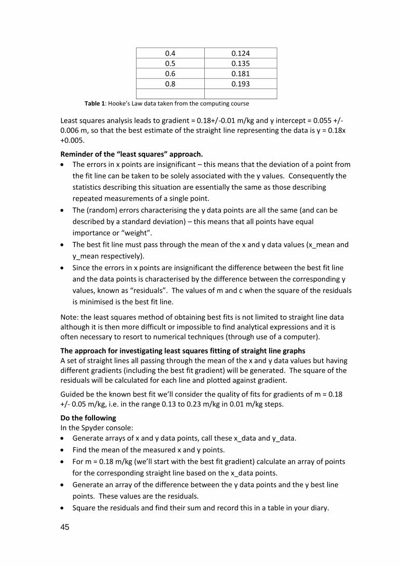
45

0.4 0.124 0.5 0.135

0.6 0.181

0.8 0.193

Table 1: Hooke’s Law data taken from the computing course

Least squares analysis leads to gradient = 0.18+/-0.01 m/kg and y intercept = 0.055 +/- 0.006 m, so that the best estimate of the straight line representing the data is y = 0.18x +0.005.

Reminder of the “least squares” approach.

The errors in x points are insignificant – this means that the deviation of a point from

the fit line can be taken to be solely associated with the y values. Consequently the

statistics describing this situation are essentially the same as those describing

repeated measurements of a single point.

The (random) errors characterising the y data points are all the same (and can be

described by a standard deviation) – this means that all points have equal

importance or “weight”.

The best fit line must pass through the mean of the x and y data values (x_mean and

y_mean respectively).

Since the errors in x points are insignificant the difference between the best fit line

and the data points is characterised by the difference between the corresponding y

values, known as “residuals”. The values of m and c when the square of the residuals

is minimised is the best fit line.

Note: the least squares method of obtaining best fits is not limited to straight line data although it is then more difficult or impossible to find analytical expressions and it is often necessary to resort to numerical techniques (through use of a computer).

The approach for investigating least squares fitting of straight line graphs A set of straight lines all passing through the mean of the x and y data values but having different gradients (including the best fit gradient) will be generated. The square of the residuals will be calculated for each line and plotted against gradient.

Guided be the known best fit we’ll consider the quality of fits for gradients of m = 0.18 +/- 0.05 m/kg, i.e. in the range 0.13 to 0.23 m/kg in 0.01 m/kg steps.

Do the following In the Spyder console:

Generate arrays of x and y data points, call these x_data and y_data.

Find the mean of the measured x and y points.

For m = 0.18 m/kg (we’ll start with the best fit gradient) calculate an array of points

for the corresponding straight line based on the x_data points.

Generate an array of the difference between the y data points and the y best line

points. These values are the residuals.

Square the residuals and find their sum and record this in a table in your diary.

46

Transfer the working code to the editor to create and save a little programme.

Repeat* the calculation for all the required gradients.

Plot a graph of sums of the squares of residuals versus gradient.

Describe its form.

* This could also be done using a loop.

47

3.11 Experiment 20: Group Easter Challenge - The strength of paper

? You will be assigned into a group for one lab session where you will undertake a team task. This will, like Rube Goldberg, be a competitive test against your fellow students.

48

4 Error propagation: A reminder of the general case

The problem here is to find the overall change of a function due to (small) changes in its component parts. The answer can be found using calculus, if a value z is a function of x and y, (i.e. z = f(x,y)) partial differentiation can be used to find the effect of a small change in either x or y. (Partial differentiation is taught in the first year and the process is essentially one of differentiating with respect to (w.r.t.) one variable whilst holding all the others constant).

The partial differential of z with respect to x (holding y constant) is given by xz so that

the change in z (i.e. Δz )due to a small change in x (i.e. Δx) is:

xx

zz

[3]

There is a similar expression for changes in z due to changes in y and the total change in z, i.e. the “total differential” is then given by

yy

zx

x

zz

[4]

The above equation concerns two variables but clearly the number of terms on the right hand side would increase to match the number of variables in an arbitrary function. Even so, Δz in the above equation cannot be used as the combined error arising from the errors, Δx and Δy, in x and y respectively. The reason is that in the above equation the signs of both the derivatives and the errors are important. As presented then the signs of multiple terms (2 here) could lead to the situation where two large but opposite contributions cancel each other, resulting in an underestimated error.

One way to resolve this issue would be to add the magnitudes of the terms on the rhs of the equation. However, this is equivalent to having the errors contribution due to x and y always reinforcing each other which is not realistic either. Instead, the conventional solution is to square all of the terms, i.e.:

22

22

2)( yy

zx

x

zz

[5]

Δz in this equation is the overall error. The resulting errors are realistic and are often said to have been combined in “quadrature” (quadrature is often used to mean squaring).

Example. Resistance, R = f(V,I) = V/I.

The aim is to show how the overall error for resistance is found using the values and errors for voltage and current. First consider the total derivative

II

RV

V

RI

I

VV

II

I

RV

V

RR

2

1

Rearranging I

I

V

V

R

R

49

Squaring each term 222

I

I

V

V

R

R

This methodology used here for a quotient can be used generally and the more common results are given in the next section

50

5 Lab Diary checklist

Date Experiment Title and Number Risk Analysis Brief Introduction Brief description of what you did and how you did it Results (indicating errors in readings) Graphs (where applicable) Error calculations Final statement of results with errors Discussion/Conclusion (including a comparison with accepted results if applicable)

6 Formal report checklist

Date Experiment Title and Number Abstract Introduction Method Results: Use graphs – and don’t forget to describe them. Indication of how errors were determined Final results with errors Discussion Conclusion (including a comparison with accepted results if applicable) Use Appendices if necessary A risk assessment is unnecessary.