department of statistics s.k.n. college of agriculture jobner

DEPARTMENT OF STATISTICS

S.K.N. College of Agriculture Jobner

Practical Manual STAT-4211

2013-14

Dr K.N. Gupta Dr B.K. Sharma

Dr Pratibha Manohar Suresh Kr Sharma

Name_______________________ Semester____________________

STAT 4211 Syllabus Credit 3(2+1)

Deptt of Statistics, SKNCOA, Jobner

Theory:

Introduction: Definition of statistics by Seligman and Horac Secrist. Aims, Scope and limitation of statistics. Classification: Definition and its type (According to attributes and class intervals). Measures of central tendency: A.M., G.M., H.M. median, mode, Properties of A.M. Merits, demerits and uses of above measures. Dispersion: range, M.D., Q.D., S.D., variance and c.v., Merits and demerits of above measures. Correlation and regression: scatter diagram, Karl pearson’s correlation coefficient, Simple linear regression; regression lines and their fitting, properties of correlation and regression coefficients. Probability and simple problems based on probability. Test of significance; Null and alternative hypothesis, two types of errors, level of significance, critical region, d.f. standard normal deviate test and students. t-test for single mean and difference between two means, paired t-test. Test of significance of correlation and regression coefficients. Chisquare test for Goodness of fit and fortesting independence of attributes, Yates correlation (No mathematical derivatives).

Practical:

Preparation of frequency table of quantitative data. Computation of A.M. for raw data and frequency distribution by direct method and short cut method. Computation of G.M. and H.M. for raw data and frequency distribution. Computation of median and mode for raw data and frequency distribution. Computation of median and mode for raw data and frequency distribution. Computation of M.D.; Q.D. for raw data and frequency distribution. Computation of S.D> and C.V. for raw data and frequency distribution. Computation of correlation coefficient. Estimation of regression lines, t & S.N.D. test for single mean and difference between two means, paired t-test. Test of significance of correlation and regression coefficients. Chisquare test for Goodness of fit & test of independence in 2x2 contingency table and mxn contingency table.

CONTENTS

STAT-4211

S. No. Practical Date of Submission

Signature of Teacher

1. Classification of data 2. Arithmetic Mean

3. Geometric and Harmonic Mean

4. Median and Mode 5. Range and Quartile Deviation

6. Standard Deviation and Coefficient of Variation

7. Product Moment Correlation Coefficient

8. Estimation of Lines of Regression

9. Large Sample Test (SND test) 10. t-test

11. Test of Significance for

Correlation Coefficient & Regression Coefficient

12. Chi-Square Test ( 2χ Test)

13. Finding Logarithms and Antilogarithms

14. Excel Statistical Functions

STAT 4211 Practical 1 Classification of Data


Q. 1. Prepare a discrete frequency distribution from the following data giving marks obtained by 50 students out of a total of 10 marks.

4 6 8 7 5 2 4 6 4 2

8 5 4 1 2 0 5 4 6 1

0 5 7 6 8 2 4 3 7 9

7 6 4 8 3 2 5 7 6 3

4 8 5 9 7 5 6 3 1 1

Sol. The required discrete frequency distribution shall be as follows:

Marks Tally Marks (number of students)

Frequency

0

1

2

3

4

5

6

7

8

9

Total

Q. 2. The weight of 60 apples (in gms) picked out at random from consignment are as follows.

106, 107, 76, 82, 109, 107, 115, 93, 150, 95, 123, 125, 111, 92, 86, 70, 126, 68, 130, 152, 139, 119, 115, 128, 100, 160, 84, 99, 113, 158, 112, 140, 136, 123, 90, 115, 98, 110, 78, 90, 107, 81, 75, 84, 104, 110, 80, 118, 82, 75, 61, 76, 78, 65, 88, 87, 68, 74, 76, 82.

Arrange the data in a frequency table using equal class interval (inclusive method) as 60-69, 70-79, 80-89……………………………………………..

STAT 4211 Practical 1 Classification of Data


Sol. The classification of weights of apples shall be as under:

S. No. Classes Tally Marks Frequency 1 60-69 2 70-79 3 80-89 4 90-99 5 100-109 6 110-119 7 120-129 8 130-139 9 140-149 10 150-159 11 160-169

Q.3. The marks of 50 students in statistics obtained out of 100 are as given below:

Marks

8 26 54 49 28 28 40 54 68 63

50 72 28 65 37 38 26 56 40 28

50 36 31 42 10 11 26 23 40 40

40 36 40 12 19 16 33 16 26 28

50 54 51 13 03 58 15 06 00 15

Classify the data in the frequency table using equal class interval as 0-10, 10-20, …,70-80.

Sol. The Classification of data shall be as under:

S. No. Classes of Marks Tally Marks Frequency Cumulative Frequency

STAT 4211 Practical 2 Arithmetic Mean


Q. 1. Calculate A.M. of the following frequency distribution giving number of seeds per pod for 29 pods using (a) Direct Method, (b) Short cut Method.

No. of seeds per pod (x):

11 12 13 14 15 16

No. of pods (f) 3 7 8 5 2 4

Sol. The required discrete frequency distribution shall be as follows:

(a) Direct Method S. No. No. of seeds (x) No. of pods (f) fx 1 2 3 4 5 6 Total

fxX

N= =∑

(b) By short cut method Let 13A =

S. No. No. of seeds (x) No. of pods (f) d X A= − Fd 1 2 3 4 5 6 Total

fd

X AN

= + =∑

Q.2. Calculate A.M. for the following distribution by step deviation method:

Class Interval 0-99 100-199

200-299 300-399

400-499

500-599

600-699

700-799

Frequency 10 54 184 264 246 40 1 1



Sol. Take 349.5A =

Class Interval f Mid-value x x Adh−

= fd

0-99 10 100-199 54 200-299 184 300-399 264 400-499 246 500-599 40 600-699 1 700-799 1 Total N=

fdX A h

N

= + × =

∑

Q.3. The Average age of 20 students in a class is 15 years and the average age of 30 students in the other class is 18 years. Find the average age of the 50 students of the two classes taken together. Sol.

1 1 2 2

1 2

N X N XXN N

+=

+

Here 1N =

2N =

1X =

2X =

There fore X = Q.4. The average marks of 100 students (consisting of 60 boys and 40 girls) in a class is 50. The average marks of 60 boys is 60. Find the average marks of 40 girls of the same class. Sol.

1 1 2 2

1 2

N X N XXN N

+=

+



Here 1N =

2N =

1X =

X = There fore 2X =

Q.5. Average marks of 80 students is 40. Later it was discovered that a score of 54 was misread as 64. Find correct mean of 80 students. Sol. Incorrect sum NX = Correct sum NX − Incorrect value + Correct value = X =

STAT 4211 Practical 3 Geometric and Harmonic Mean


Q. 1. Find G.M. of 133, 141, 125, 173, 182.

x log x 133 141 125 173 182 n = log x =∑

1. . log logG M anti xn = ∑

=

Q.2. Calculate G.M. for the following discrete distribution:

Marks 5 15 25 35 45 Number of Students 5 7 15 25 8

Sol.

Marks x log x Number of students f .logf x

5 15 25 35 45

Total N = logf x =∑

1. . log logG M anti f xn = ∑

=

Q.3. Calculate G.M. for the following distribution:



Class 0-10 10-20 20-30 30-40 40-50 Frequency 1 2 3 4 5

Sol.

Class Interval Mid-value x log x f logf x

0-10 10 10-20 54 20-30 184 30-40 264 40-50 246 N= logf x∑

G.M.= Q.4. Calculate H.M. for the following frequency distribution:

Height of plant (cm): 5 15 25 35 45 Number of Plants: 4 6 10 7 3 Sol.

x

f

1x

1fx

5

15 25 35

45

N= 1fx

=

∑

. .1

NH Mf

x

= =

∑



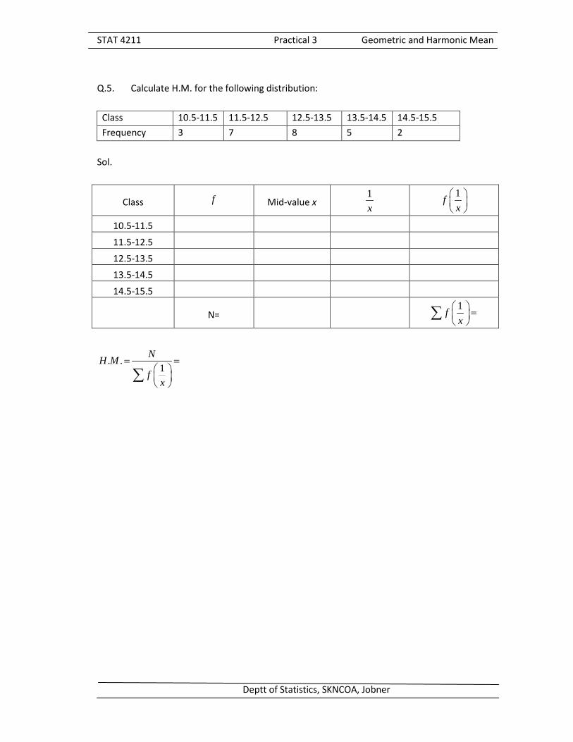
Q.5. Calculate H.M. for the following distribution:

Class 10.5-11.5 11.5-12.5 12.5-13.5 13.5-14.5 14.5-15.5 Frequency 3 7 8 5 2

Sol.

Class f

Mid-value x 1x

1fx

10.5-11.5

11.5-12.5 12.5-13.5 13.5-14.5

14.5-15.5

N= 1fx

=

∑

. .1

NH Mf

x

= =

∑

STAT 4211 Practical 4 Median and Mode


Q. 1. Find Mode, Median, 1 4,Q D and 70P for the following series

a) 11, 12, 14, 12, 13, 11, 14, 12, 13, 16, 13 b) 9, 6, 10, 8, 7, 9, 10, 6, 8, 11 Sol. a) Mode = Maximum value =

Median Arrange the series in ascending order of magnitude 11, 11, 12, 12, 12, 13, 13, 13, 14, 14, 16 n =

Median = Value of 1

2

thn +

term = th term

=

1Q = Value of 1

4

thn +

term =

4D = Value of 14

10

thn +

term =

=

70P = Value of 170

100

thn +

term=

b) Mode = Maximum value = Median: Arrange the series in ascending order of magnitude n = Median =

1Q =

4D =

70P =

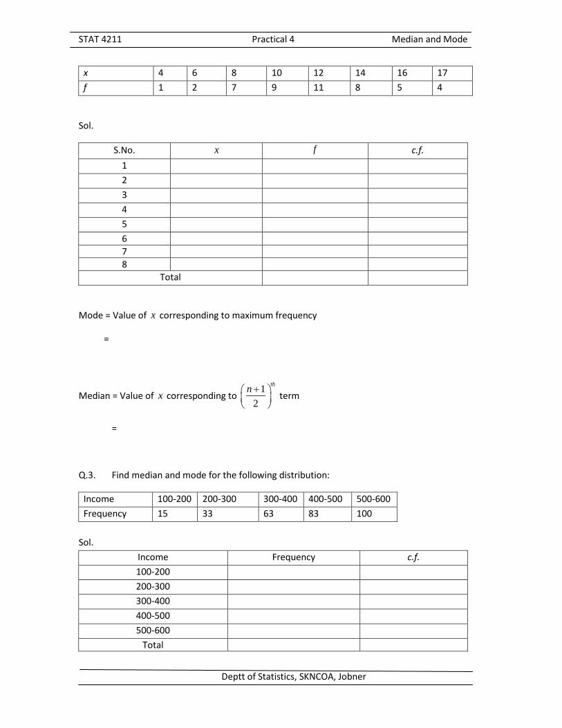
Q.2. Find the Mode and Median for the following distribution



x 4 6 8 10 12 14 16 17 f 1 2 7 9 11 8 5 4

Sol.

S.No. x f c.f.

1 2 3 4 5 6 7 8

Total

Mode = Value of x corresponding to maximum frequency

=

Median = Value of x corresponding to 1

2

thn +

term

=

Q.3. Find median and mode for the following distribution:

Income 100-200 200-300 300-400 400-500 500-600 Frequency 15 33 63 83 100

Sol.

Income Frequency c.f.

100-200 200-300 300-400 400-500 500-600

Total



Median Median class is

Median 12N C

l hf

− = + ×

= Mode Model Class is

Mode 1 01

1 0 22f fl h

f f f −

= + × − −

=

Q.4. Compute mode of the distribution by grouping method

Marks 0-5 5-10 10-15 15-20 20-25 25-30 30-35 35-40 40-45 Number of Students

29 195 241 117 52 10 6 3 2

Sol.

Marks Frequencies (1)

(2) (3) (4) (5) (6)

0-5

5-10 10-15

15-20 20-25 25-30

30-35 35-40

40-45



Analysis Table Column Number

Class Intervals Having Maximum Frequency

1 2 3 4 5 6

Total

Model class =

Mode = 1 01

1 0 12f fl h

f f f −

+ × − −

=

STAT 4211 Practical 5 Range and Quartile Deviation


Q. 1. From the following data, find

a) Range and coefficient of range b) Quartile deviation and coefficient of Quartile deviation

Month 1 2 3 4 5 6 7 8 9 10 11 12 Sales’ 1000 Rs 78 80 80 82 82 84 84 86 86 88 88 90 Sol. a) Range = L S− =

Coefficient of Range = L SL S−

=+

b) The values are already arranged in ascending order of magnitude

1Q = Value of 1

4

thn +

term =

3Q = Value of 134

thn +

term =

Q.D. = 3 1

2Q Q−

=

Coefficient of Q.D. = 3 1

3 1

Q QQ Q

−+

=

=

Q.2. Calculate range, coefficient of range, Q.D. and Coefficient of Q.D. from the following data

Weight 60 61 62 63 65 70 75 80 No. of workers 1 3 5 7 10 3 1 1

Sol.



Weight in Kg Frequency Cumulative Frequency

60 1 61 3 62 5 63 7 65 10 70 3 75 1 80 1

1Q = Size of ( )1 14

thN + item

= Size of

=

1Q = Size of ( )3 14

thN + item

= Size of

=

Q.D. = 3 1

2Q Q−

=


3 1

Q QQ Q

−+

=

Range = L S− =

Coefficient of Range = L SL S−

=+

Q.3. Calculate Q.D. and its relative coefficient from the following data

Marks 0-10 10-20 20-30 30-40 40-50 50-60 60-70 70-80 80-90 No. of Students 11 18 25 28 30 33 22 15 22



Sol. S.No. Marks Frequency c.f.

1 2 3 4 5 6 7 8 9

First Quartile Class

= Value of 4

thN item

=

1 14N c

Q l hf

−= + ×

=

Third Quartile Class

= Value of 34

thN Item

=

3 1

34N c

Q l hf

−= + ×

=

Q.D. = 3 1

2Q Q−

=


3 1

Q QQ Q

−+

=

Q.4. Calculate M.D. from mean and median of the following data

Height (inches) 60 61 62 63 64 65 66 67 68 No. of Children 2 0 15 29 25 12 10 4 3



Sol. Step 1

Height (inches) Frequency f c.f. f x 60 2 61 0 62 15 63 29 64 25 65 12 66 10 67 4 68 3

Total 100

Median = Size of ( )1 thN + item

= Step 2

M.D. from Median = f x Median

N−∑

=

Height (inches)

f X Me− f X Me− ( )X X− ( )f X X−

1 2 3 4 5 6

Mean = fX

N∑

M.D. from Mean = f x xN−∑

=



Q. 5. Compute M.D. about median and its coefficient for the following data

Class 5-10 10-15 15-20 20-25 25-30 30-35 Frequency 8 17 30 26 12 7 Sol.

Class f c.f. Mid x X Me− f X Me−

5-10 8 10-15 17 15-20 30 20-25 26 25-30 12 30-35 7 Total

Median Class =

Median = 12N c h

lf

− × +

=

M.D. = ( )f x MeN−∑

=

Coefficient of M.D. =. .M D

Median

=

STAT 4211 Practical 6 Standard Deviation and Coefficient of Variation


Q. 1. Calculate the S.D. from the following data

Size of item 6 7 8 9 10 11 12 Frequency 3 6 9 13 8 5 4

Sol.

Size of item X

Frequency f f X X X− ( )2

X X− ( )2f X X−

6 3 7 6 8 9 9 13

10 8 11 5 12 4

Total

A.M. = fX

N=∑

S.D. ( )2

f X XN−

= =

Q.2. Calculate S.D. of the following data

Asc 0-10 10-20 20-30 30-40 40-50 50-60 60-70 No. of persons 15 15 23 13 10 5 10

Sol.

Direct Method

Asc Frequency f Mid X f X ( )X X− ( )2X X− ( )2

f X X−

0-10 15 10-20 15 20-30 23 30-40 13 40-50 10 50-60 5 60-70 10 Total



A.M. = fX

N=∑

S.D. ( )2

f X XN−

= =

Step Deviation Method:

Asc Frequency f Mid x 45

10Xd −

= fd 2fd

0-10 15 10-20 15 20-30 23 30-40 13 40-50 10 50-60 5 60-70 10 Total

22

. .fd fd

S D hXN N

= −

∑ ∑

=

=

Q.3. For a group of 50 male workers the mean and the S.D. of their daily wages are rs 63 and Rs 9 respectively. For a group of 40 female workers these are Rs 54 and Rs 6 respectively. Find the S.D. for the combined group of 90 workers

Sol. The mean of combined group is

1 1 2 212

1 2

n X n XXn n+

=+

= S.D. of combined group is



( ) ( )2 2 2 21 1 2 2 1 1 2 22

121 2

n n n d n dn n

σ σσ

+ + +=

+

1 12 1d X X= − =

2 12 2d X X= − =

212σ =

Q.4. From some financial statistics it is found that the monthly average electric charges were Rs 2460 and S.D. Rs 120. The monthly average direct wages were Rs 42000 and S.D. Rs 1200. State which is more consistent

Sol. Electric Charges Direct Wages

Mean 2460 42,000 S.D. 120 1200

C.V. for Electric charges = 100xσ×

=

C.V. for Direct Wages = 100xσ×

The C.V. of ___________________ is less series is consistent.

STAT 4211 Practical 7 Product Moment Correlation Coefficient


Q. 1. Calculate the correlation coefficient for the following data of scores awarded to 10 children for intelligence ratio (IR) and Arithmetic ratio (AR) by direct method and change of origin method.

Child 1 2 3 4 5 6 7 8 9 10 I.R. 105 104 101 99 100 98 96 93 92 102 A.R. 101 103 98 96 95 104 92 97 93 100

Sol. Intelligence ratio IR = X Arithmetic ratio AR = Y a) Direct Method:-

X Y 2X 2Y XY 105 101 104 103 101 98 99 96 100 95 98 104 96 92 93 97 92 93 102 100

( )( )

( ) ( )2 2

2 2

X YXY

NrX Y

X YN N

−=

− −

=

=

∑ ∑∑

∑ ∑∑ ∑

b) Change of Origin Method

Let 100u X= −

95v Y= −



X Y 100u X= − 95v Y= − 2u 2v uv 105 101 104 103 101 98 99 96 100 95 98 104 96 92 93 97 92 93 102 100

( )( )

( ) ( )2 2

2 2

u vuv

Nru v

u vN N

−=

− −

=

=

∑ ∑∑

∑ ∑∑ ∑

Q.2. For the following data calculate the value of coefficient of correlation (r).

2

2

425 13255

630 9075

20 19870

i i i

i i

i

x x y

y x

N y

= =

= =

= =

∑ ∑∑ ∑

∑

Sol.

r =

r =



Q. 3 Calculate the coefficient of correlation between ages of husband and age of wife for 10 pairs.

Pair No. 1 2 3 4 5 6 7 8 9 10 Age of Husband (Yrs)

23 27 28 29 30 31 33 35 36 39

Age of Wife (Yrs)

18 22 26 24 29 27 30 36 30 32

Sol.

Let age of husband = X

Age of wife = Y

X Y 2X 2Y XY 23 18 27 22 28 26 29 24 30 29 31 27 33 30 35 36 36 30 39 32

( )( )

( ) ( )2 2

2 2

X YXY

NrX Y

X YN N

−=

− −

=

=

∑ ∑∑

∑ ∑∑ ∑

STAT 4211 Practical 8 Estimation of Lines of Regression


Q.1. Given the following data on two variables.

Series X Series Y Mean 18 100 S.D. 14 20

Coefficient of correlation = +0.80

Find out the most probable value of Y if 70X = and the most probable value of X if 9.0Y =

Sol. Regression line Y on X

( )YXY Y b X X= + −

YYX

X

b r σσ

=

=

Y = For 70X = Y = Regression line X on Y

( )

( )XY

XY

X X b Y Y

X X b Y Y

− = −

= + −

XXY

Y

b r σσ

=

=

X =

For 9Y = X =

Q.2. From the following data, determine the two regression equations by using method of least squares X 2 4 5 8 6 Y 5 9 8 10 7 Also find the S.E. of estimates of two regression lines



Sol.

X Y 2X 2Y XY 2 5 4 9 5 8 8 10 6 7

Let the regression line of Y on X is Y a bX= + (1) Normal equations are

Y na b X= +∑ ∑ (2)

2XY a X b X= +∑ ∑ ∑ (3)

From Equation (2) and (3), we get the values of a and b as

a⇒ = b = Putting these values in (1), the regression equation Y on X is Regression equation X on Y X c dY= +

X nc b Y= +∑ ∑ (4)

2XY c Y d Y= +∑ ∑ ∑ (5)

c⇒ =



d = S.E. of regression line Y on X is

2

YX

Y a Y b XYS

n− −

= ∑ ∑ ∑

=

S.E. of regression line X on Y is 2

XY

X c X d XYS

n− −

= ∑ ∑ ∑

= Q.3. In a partially destroyed laboratory records of an analysis of correlation data the following results only are lesible Variance of X is 9 Regression equations are 8 10 66 0X Y− + = And 40 18 214X Y− = then, find

i. The mean value of X and Y ii. The S.D. of Y and

iii. The coefficient of correlation between X and Y

Sol.

Mean value of X and Y are obtained by solving two regression equation

8 10 66 0

40 18 214 0

X Y

X Y

− + =

− − =

So X = and Y =



Let regression equation of X and Y is 40 18 214X Y− =

Let regression equation Y on X is 8 10 66 0X Y− + =

So YXb =

XYb =

YX XYr b b= ± ×

=

Again

XXY

Y

b r σσ

=

Yσ =

Q.4. Find YXb and XYb and equations of two regression lines for the following basis of

observations on X and Y

X 18 19 20 21 22 23 24 25 26 27 Y 17 17 18 18 18 19 19 20 21 22

Sol

X Y 2X 2Y XY



( )( )( )22YX

n XY X Yb

n X X

−=

−

∑ ∑ ∑∑ ∑

=

( )( )( )22XY

n XY X Yb

n Y Y

−=

−

∑ ∑ ∑∑ ∑

=

Regression equation of X and Y is

( )XYX X b Y Y− = −

Regression equation Y on X is

( )YXY Y b X X− = −

STAT 4211 Practical 9 Large Sample Test (SND test)


Q.1. In order to know the effect of electric current on the growth of wheat seedlings, 400 pairs of plant of wheat were grown in similar plots and one member of each pair was electrically treated. The mean difference in heights of the treated and untreated plants was found to be 0.8 cm with a S.D. of 0.20 cm. Does the electric current exercise any effect on the growth of the wheat plants?

Sol.

0H : the electric current has no effect on the growth of wheat plants i.e. 0H =

1H :

under 0H

/x

znµ

σ−

=

Here x = µ =

σ = n =

z =

=

tabz at 0.05α = is 1.96 so Q. 2. A certain sugar manufacturing process produces 20.5 units of sugar per hour with a variance of 2.0 units. A new manufacturing process is evolved which being quite expensive can be accepted if production of sugar can be increased to an average of 21.0 units per hour. In order to decide its acceptability, 50 new manufacturing machines are tested. These produce on an average 21.5 units of sugar per hour. On the basis of these date suggest if the change to the new process can be justified. Sol.

0 :H µ =



1 :H µ <

under 0H

/x

znµ

σ−

=

x = µ = σ = n = z =

0.5 1.645tα= = Therefore Q. 3. The mean staple length determined by taking 100 samples from each of the two lots of cotton was as follows : Lot A: 25.4 0.8± mm Lot B: 26.8 0.7± mm Do the lots differ significantly in their mean staple length? Sol.

0 :H

1 :H

Under 0H

1 2

2 21 2

1 2

x xz

s sn n

−=

+

1x =

2x =

S.E. of 11

1

0.8sxn

= =

S.E. of 2x =

1n =



2n =

calz =

0.05 1.96zα= = So Q.4. A random sample of 500 house-holds in a city showed an average annual consumption of 15 kg of brand A coffee with a s.d. of 2 kg. Another sample of 400 households showed an average consumption of 13 kg of brand B with a s.d. of 3 kg. For a significance level of 1%, a marketing research agency wishes to judge the claims of each brand being the market leader. Sol.

0H :

1H :

Under 0H

2 2

B A

A B

A B

x xz

S Sn n

−=

+

where

Bx =

Ax =

Aς =

Bς =

an =

bn = So

z =

So

STAT 4211 Practical 10 t-test


Q.1. A certain type of rats show a mean gain in weight of 66 g during the first 6 months of life. Twelve rats were fed a particular diet from birth until age 6 months, and the following weight gains were observed.

5.5, 6.2, 5.4, 5.8, 6.5, 6.4, 6.0, 6.2, 5.9, 6.7, 6.2, 6.1

Is there reason to believe at the 5% level of significance that the diet causes a decreases in the amount of weight gained?

Sol.

0H :

1H : 6.5µ <

under 0H :

/x

ts n

µ−=

Where

2

2 211

ii

ii

xs x

n n

= − −

∑∑

Sample observations ix 2ix

5.5 2ς = = =

ixx

n= =∑

ix =∑ 2ix =∑

2s =



t =

calt =

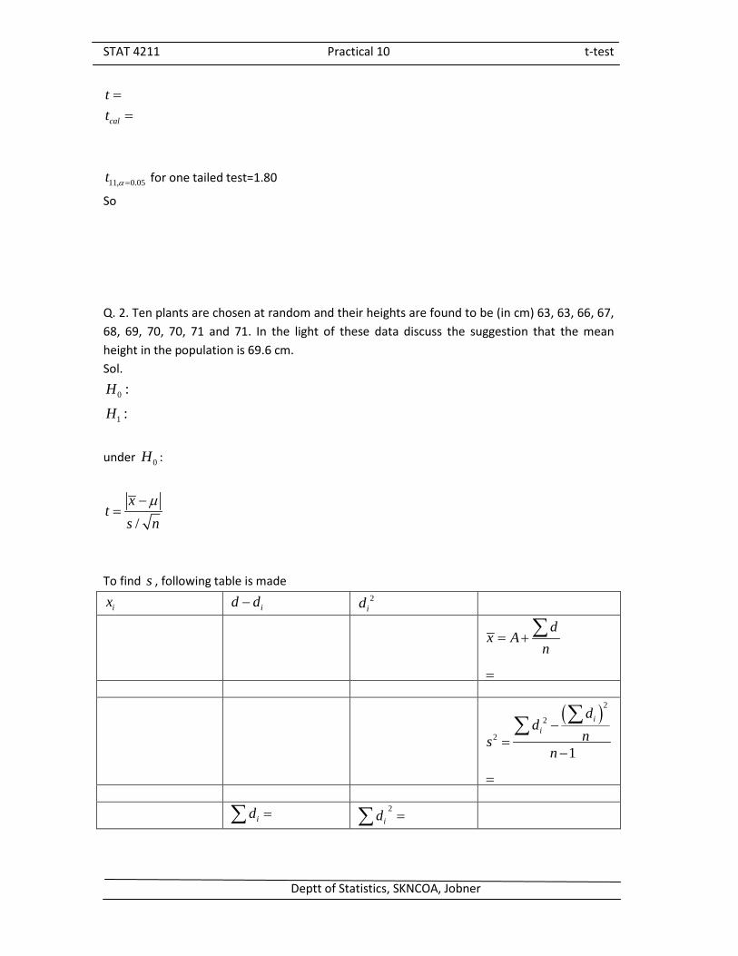
11, 0.05t α= for one tailed test=1.80

So Q. 2. Ten plants are chosen at random and their heights are found to be (in cm) 63, 63, 66, 67, 68, 69, 70, 70, 71 and 71. In the light of these data discuss the suggestion that the mean height in the population is 69.6 cm. Sol.

0 :H

1 :H

under 0H :

/x

ts n

µ−=

To find s , following table is made

ix id d− 2id

dx A

n= +

=

∑

( )2

2

2

1

ii

dd

nsn

−=

−

=

∑∑

id =∑ 2id =∑



2s =

calt = =

9,0.05 2.262t =

So Q. 3. For a random sample of 10 pigs, fed on a diet A, the increases in weights in a certain period were : 10 6 16 17 13 12 8 14 15 9 lbs. For another random sample of 12 pigs, fed on the diet B, the increases in weights in the same period were : 7 13 22 15 12 14 18 8 21 23 10 17 lbs. Find, if the two samples are significantly different regarding the effect of diet. Given that for

d.f. ( )ν = 20, 22, 24 the 5 percent values of t are respectively 2.09, 2.07, 2.06.

Sol.

0H :

1H :

Under 0H :

( )1 2

1 2

1 1x x

ts

n n

−=

+

Where ( ) ( )2 221 1 2 2

1 2

12

s x x x xn n

= − + − + − ∑



Sample 1 Sample 2 S.No.

1x ( )21 1x x− S.No.

2x ( )22 2x x−

1 2 3 4 5 6 7 8 9 10

1n = 1x∑ ( )21 1x x−∑ 2 12n = 2x∑ ( )2

2 2x x−∑

11

1

xx

n= =∑

22

2

xx

n= =∑

( ) ( )2 221 1 2 2

1 2

12

s x x x xn n

= − + − + − ∑

( )1 2

1 2

1 1x x

ts

n n

−=

+

=

0.05,20 2.09t =



So Q. 4. The respiration rates per minute in nine cases of one group and seven cases of the other group of persons are noted below. Is there any significant difference in the observation of the two groups?

Respiration rate Group A 23 22 20 24 16 17 18 19 21 Group B 24 21 20 18 17 19 21 Sol.

0H :

1H :

Under 0H :

1 2

1 2

1 1x x

ts

n n

−=

+

Where ( ) ( )2 221 1 2 2

1 2

12

s x x x xn n

= − + − + − ∑

Sample 1 Sample 2 S.No.

1x ( )21 1x x− S.No.

2x ( )22 2x x−

1 2 3 4 5 6 7 8 9 10

1n = 1x∑ ( )21 1x x−∑ 2 12n = 2x∑ ( )2

2 2x x−∑



11

1

xx

n= =∑

22

2

xx

n= =∑

( ) ( )2 221 1 2 2

1 2

12

s x x x xn n

= − + − + − ∑

( )1 2

1 2

1 1x x

ts

n n

−=

+

=

0.05,14t =

So Q. 5. In a field experiment with two varieties of wheat grown in seven pairs plots, the following yields were obtained ;

Variety A Yield in

A 15 14 12 15 16 11 13

B 11 11 13 12 13 10 12

From the above data compute the mean difference standard deviation of the difference and ‘t’. What is the reasonable inference about the population mean difference? Sol.

0H :



1H :

S.No. Yield of A ( ix ) Yield of B ( iy ) Difference

i i id x y= −

2id

1 2 3 4 5 6 7 Total

id∑ 2id∑

idd

n= =∑

( )2

2

2

1

ii

dd

nsn

−= =

−

∑∑

=

/dt

s n= =

=

0.05,6t =

So



Q. 6 Ten students were examined in statistics. The same ten students were again examined after coaching them for a month by a similar test. The marks obtained by students are given below.

Students Marks in test

Before Coaching After Coaching

1 2 3 4 5 6 7 8 9 10

7 8 4 9 6 5 8 9 4 7

6 6 6 9 7 4 8 7 3 8

Can it be concluded on the basis of these marks that the students have benefitted themselves by this coaching. Sol.

0H :

1H :

S.No. Before Cochin

ix After Cochin iy id 2

id

1 2 3 4 5 6 7 8 9 10 Total

id =∑ 2id =∑



idd

n= =∑

( )2

2

2

1

ii

dd

nsn

−= =

−

∑∑

= =

under 0H

/dt

nς= =

=

0.05,9 1.83t =

So

STAT 4211 Practical 11 Test of significance for Correlation Coefficient & Regression Coefficient


Q.1. From a pair of 18 values the value of the correlation coefficient ' 'r was calculated as 0.60. Test its significance.

Sol.

0H :

1H : 65µ <

under 0H :

2

21

r ntr−

=−

=

0.05,16 2.12t =

So

Q. 2. From the following data calculate S.E. of YXb and XYb and also test their significance

2 210, 40, 50, 270, 300, 250, 0.83, 1YX XYn X Y X Y XY b b= = = = = = = + =∑ ∑ ∑ ∑ ∑

Sol.

( )

( )

( )

2

22

2. .2YX

xyy

xS E b

n x

−

= −

∑∑ ∑∑

Where

( ) ( )222 2 X

x x x XN

= − = −

=

∑∑ ∑ ∑

( ) ( )222 2 Y

y y y YN

= − = − ∑∑ ∑ ∑



=

( )( )X Yxy XY

N= − ∑ ∑∑ ∑

=

S.E. ( )YXb =

Also 2YX

xyb

x= =∑∑

( ). .YX

YX

btS E b

=

=

0.05,8 2.306.t =

Also 2XY

xyb

y= ∑∑

( )

( )

( )

2

22

2. .2XY

xyx

yS E b

n y

−

= −

∑∑ ∑∑

= =



( ). .XY

XY

btS E b

=

= Q. 3. From 15 plots of cotton, the number of plants per plot (X) and the corresponding yield (Y) were recorded and the following quantities obtained

( ) ( )

( )( )

2 2175.6, 79.6

102.4, 11, 6.4

X X Y Y

X X Y Y X Y

− = − =

− − = = =

∑ ∑

∑

Calculate the regression yield on the number of plants and its test of significance. What will be equation of regression line. Sol. Let Y is dependent variable X is independent variable i.e. no. of plants/plot

( )( )( )2YX

X X Y Yb

X X

− −=

−

∑∑

= Regression line is

( )YXY Y b X X− = −

Or

( )YXY Y b X X= + −

0H : 0β =

under 0H :



( ). .YX

YX

btS E b

=

( ) ( )2

. .2 .

Y XY XYX

X

SS b SS E bn S S−

=−

where

( )2YSS Y Y= −∑

( )2

XSS X X= −∑ t =

0.05,13 2.160t =

So

2

21

r ntr−

=−

=

0.05,16 2.12t =

So

STAT 4211 Practical 12 Chi-Square Test ( 2χ Test )


Q. 1. Calculate the value of 2χ from the following data and test its significance

iO 40 36 19 2 0 2 1

iE 37 37 18 6 2 0 0

Sol.

0H The discrepancy between 'iE s and 'iO s is not significant

S.No. iO

iE

i iO E−

( )2i i

i

O EE−

1 40 37

2 36 37

3 19 18

4 2 6

5 0 2

6 2 0

7 1 0

Total

2calχ =

( )20.05 5 11.07χ =



Therefore Q. 2. The theory predicts that the proportion of beans in the four groups A, B, C and D should be 9 : 3 : 3 : 1. In an experiment among 1600 beans, the numbers in the four groups were 882,

313, 287 and 118. Does the experimental results support the theory: ( 2χ for 3 d.f. at 5% level

= 7.815). Sol.

0H :

1H :

Under 0H , the expected frequencies are

As 9 3 3 1 16+ + + =

19 1600

16E = × =

23 1600

16E = × =

3E =

4E =

Now we have

iO iE i iO E− ( )2i i

i

O EE−

882 313 287 118 Total

2calχ =

20.05,9 16.92χ =



therefore Q. 3. In a public preference survey, the people interviewed were classified as follows according to their opinion regarding intercaste-marriage and their age :

Opinion Age in years

19-25

26-35 36-55 Over 55

Unconditional support :

76 125 96 10

Conditional support :

69 117 126 17

Indifference : 14 27 35 4

Conditional opposition :

60 168 210 46

Examine whether and in what way opinion regarding intercaste marriage changes with age? Sol.

0H : the drug does not have any significant effect

S. No.


i

O EE−

1 2 3 4 5 6 Total

( )22 i i

i

O EE

χ−

=∑

=



20.05,3 7.815χ =

So Q.4. To test the efficiency of a new medicine, a controlled experiment was conducted where in 150 patients were administered the new medicine and 100 other patient were not given the medicine. The patients were monitored and the results were obtained as : Cured Condition worse No effect Total Given the medicine

100 20 30 150

Not given the medicine

60 15 25 100

Total 160 35 55 250 Sol.

0H : there is no association between ___________

1H :


i

O EE−

2calχ =

( )20.05 2 5.99χ =

Hence



Q. 5. In an experiment on the immunization of goats from Anthrax, the following results were obtained. Derive your inference on the efficiency of the vaccine : Dead Survived Totals Inoculated 2 10 12 Not inoculated 6 6 12 Totals: 8 16 24 Sol.

0H : the vaccination has no effect on the survival of goats from Antrax

1H :

Under 0H

( )( )( )( )

2

2 2Nad bc

a b a c b d c d

µχ

− − =+ + + +

=

20.05,1 3.841χ =

Hence

STAT 4211 Practical 13 Finding Logarithms and Antilogaritmhs


We begin by reviewing some of the laws of logarithms. For this exercise, note that

10log logx x= then

1. log log logab a b= +

2. log log loga a bb

= −

3. log logba b a= 4. log10 1=

Using the log table, find the following logarithms

(a) log1.72 (b) log6.39 (c) log9.45

Ans. 0.2355 0.8055 0.9754

Write numbers as a product of some number between 1 and 10 and 10 to some power.

(a) 8568300300 5.68300300 10= ×

(b) 40.0003865 3.865 10−= ×

This helps because we can only find logarithms of numbers between 1 and 9.99.

Using the log table, find the following logarithms.

(a) 6log1720000 log1.72 log10 0.2355 6= + = + Next we switch to find antilogs Using log table find the following antilogs

(a) log0.8407 6.93anti = (b) log0.5453 3.51anti =

Using the antilog table, we can only find antilogs of numbers between 0 and 0.9996. To find antilog of any number, we write that number as

(whole number)+(number between 0 and 0.9996)

(a) { }3log(3.8407) log(3 0.8407) 10 log(0.8407) 6930anti anti anti= + = =

(b) ( ) ( ) ( ){ }2log 1.4547 log 2 0.5453 10 log 0.5453 0.0351anti anti anti−− = − + = =

STAT 4211 Practical 14 EXCEL: CORRELATION & REGRESSION EXAMPLE


EXCEL: CORRELATION & REGRESSION EXAMPLE

1. DATA

2. STATISTICS

Summary Output

Regression Statistics

Multiple R 0.316228

R Square 0.1

Adjusted R Square -0.35

Standard Error 4.242641

Observations 4

ANOVA

df SS MS F Significant F

Regression 1 4 4 0.222222 0.683772

Residual 2 36 18

Total 3 40

ID X Y

A .00 .00

B .00 6.00

C 8.00 2.00

D 8.00 8.00



Coefficient S.E. t Stat P-value Lower 95% Upper 95%

Intercept 3 3 1 0.42265 -9.90797 15.90797

X 0.25 0.53033 0.471405 0.683772 -2.03183 2.531828

3. GRAPH

1. ENTERING THE DATA

Enter the scores in the worksheet as such:

X Y

.00 .00

.00 6.00

8.00 2.00

8.00 8.00

X and Y will be the two variables that we want to find correlation.

0123456789

0 2 4 6 8 10

Gra

des

on Q

uiz

Hours of Practice



2. COMPUTING THE STATISTICS

1. Go to Insert and select function wizard button fx, select the Statistical category, select CORREL, and click Next.

2. Enter the range A2:A5 in the array 1 box. You can also click and drag over the range for X instead of entering manually.

3. Enter the range B2:B5 in the array 2 box. You can also click and drag over the range for Y instead of entering manually.

4. Click Finish and an r of .31 is returned. 5. In the Main Menu Bar, click on Tools – Data Analysis. 6. In the Data Analysis window, select Regression and click OK. 7. Input Y range: Enter $B$1:$B$5 or drag over the cells of Y. 8. Input X range: Enter $A$1:$A$5 or drag over the cells of X. 9. Labels should be checked because we include the variable names in cells A1 and B1. These

labels will be used in the output. 10. Constant is Zero is not checked because we do not want to force the regression line

through the origin. 11. Confidence Level is checked and a value of 90 is entered int eh space to the right of

Confidence Level. If it is not checked, the default value of 95% will be utilized, and we will see the 95% boundaries reported twice in the regression output.

12. Type $C$1 for Output options. 13. Residuals refer to the difference between the actual Y data points and the Y values

predicted by the regression equation. We did not ask for any output in this section. 14. Normal Probability will generate a chart of normal probabilities. We did not select this

output. 15. Click OK and the output shown above will be generated.

3. GRAPHING THE DATA

Excel’s Chart Wizard provides an efficient way to produce a scatterplot of two variables. The procedure will not work, however, unless the two variables are adjacent to each other in the worksheet.

1. Click on the Insert on the Menu bar, select Chart and select As New Sheet. 2. Click and drag over the range of numerical values in columns A and B. 3. Select XY(Scatter) and click Next. 4. Select Format 3 and click next. 5. Select Data Series in Columns, and Use First 1 columns for X Data, 0 Rows for Legend Text.

Then Click Next. 6. Specify the legend, chart title, X-axis title, and Y-axis title in the dialog box. 7. The completed scatterplpot is shown at the top of this page. 8. To add the regression line simply click on one of the data points on the chart with the left

mouse button. Square handles will appear on all the points. Now click the right mouse button, a menu will appear. Select the Add Trendline command.

9. Select the right group (Group 1) and click OK.



EDITING THE GRAPH

Often the graph will not appear exactly as you wish. However, it's easy to change colors, markers, axes, etc.

Using the mouse, move the cursor anywhere on the graph you want to edit and double click.

A new window will appear and you can make your own changes on the graph.

department of statistics s.k.n. college of agriculture jobner

Documents