department of the interior u.s. geological … · technique to similar problems in soil mechanics...
TRANSCRIPT
DEPARTMENT OF THE INTERIOR
U.S. GEOLOGICAL SURVEY
A Study of Flow Development in Mass Movements
of Granular Materials
by
G. B. Crosta1 , P.S. Powers 1 , and W.Z. Savage1
Open-File Report 91-383
This report is preliminary and has not been reviewed for conformity with U.S. Geological Survey editorial standards. Any use of trade, product, or firm names is for descriptive purposes only and does not imply endorsement by the U.S. Government.
Golden, Colorado
1991

CONTENTS
Page
Introduction ........................... 1Theory of plasticity ....................... 1Solution for extrusion of a perfectly plastic material ...... 8Experimental theory and methodology ................ 11Description of the experimental technique ............. 12Description of typical features in the flow experiments ...... 20
Confined experiments .................... 20Unconfined experiments ................... 30Mass balance ........................ 38
Comparison of the experimental results with theoreticalsolutions ............................ 41
Discussion of applicability of the plasticity solutions ...... 62Conclusions ............................ 63References ............................ 65
ILLUSTRATIONS
Figure 1. Base friction model .................. 132. Sketch representing the dimensions of the experimental
apparatus ...................... 153. Weighing zone definition scheme. Subdivision of the
material, for unconfined experiments, in 5 different volumes to obtain a mass balance (discharge and rate of growth) ................... 21
4. Subdivision of the plastic region and location ofthe dead zone .................... 22
5. Sketch representing the plastic region, limiting boundaries and the adopted reference system (compare with fig. 4) ................ 22
6. Rigid plug boundary for a confined experiment withsand and a funnel-shaped obstacle .......... 24
7. Rigid plug boundary for a confined experiment on flour and an extrusion ratio of three. Dead zones and velocity discontinuities are also visible .... 24
8. A, Confined experiment (24 in. wide channel, extrusion ratio = 3) on sand showing the main velocity discontinuities and core flow; fl, main lateral discontinuities reaching the free surface in a confined experiment on sand (12 in. wide channel, extrusion ratio = 3); C, Development of lateral discontinuities and formation of a conical depression at the free surface in a confined experiment on sand with funnel- shaped obstacle and a 12 in. wide channel ...... 25

9. Development of a conical depression in a confined sandexperiment ...................... 27
10. Draw ellipse model (Janelid and Kvapil, 1966) ..... 2711. Rigid plug boundary and well-developed dead zones in
a confined flour experiment ............. 2712. Confined flour experiment showing the first stage in the
development of the dead zones and some well-developed velocity discontinuities ............... 28
13. Confined flour experiment showing the final stage of dead zone evolution with sheared, compacted, and rigid zones ..................... 29
14. A, Confined flour experiment showing the dead zoneformation near an obstacle positioned in the middleof the channel; fl, identification of some dead zonefeatures for finite, large deformations in a confinedexperiment on flour; C, confined experiment in sand witha central obstacle. Notice the same features observedin the two previous figures ............. 31
15. Vertical distribution of the horizontal velocityobserved in a 2 in. thick experiment conducted onflour ........................ 32
16. Unconfined experiment in flour; the main features areshown in the figure ................. 33
17. A 9 Unconfined flour experiment showing semicircular steps (in plane view) in the first stage of development of a dead zone; fl,sets of fractures developed during the final stage of dead zone development ............ 33
18. Longitudinal cross section of a dead zone in an unconfinedexperiment on flour (flow from right to left) .... 35
19. Fractures and bulging dead zones in the proximity of thechannel orifice (extrusion ratio =1.5) ....... 35
20. A, Transversal cross section, upstream of the orifice, looking downstream. Steps in the blue chalk layers were caused by the differential velocities inside the shear zones; B 9 transversal cross section, downstream from the orifice. Steps in the blue chalk are visible under the lateral levees ............... 36
21. Unconfined sand experiment showing the bulged dead zones and the groove indicating the origin of the lateral levees (ER = 3) ................... 37
22. A, Systems of velocity discontinuities that reach the free surface in an unconfined experiment on sand; fl, evolution of the conical depression induced by the action of the velocity discontinuities. The rigid core is also shown .................. 37
23. A, Systems of curved strike-slip faults (or reverse faults), tension cracks, and fractures inside the flour; B 9 detail of the system of fractures, tension cracks, and strike- slip faults (or reverse faults) developed in the rear part of the material ................. 39
24. Velocity discontinuities generated by the backward-pushing action of a central obstacle (1st and 2nd show the order of formation) ................. 39
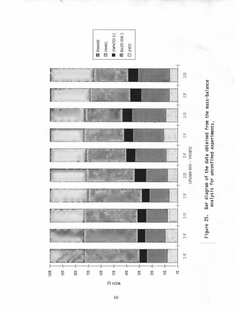
25. Bar diagram of the data obtained from the mass-balanceanalysis for unconfined experiments ......... 40
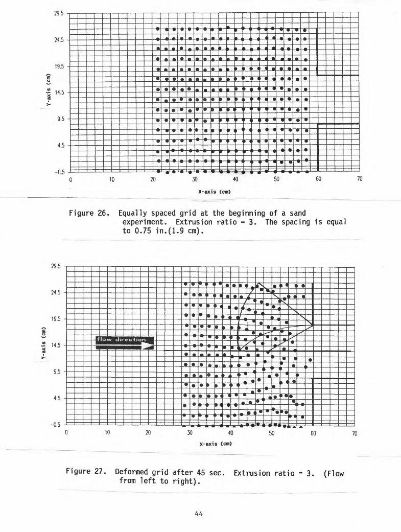
26. Equally spaced grid at the beginning of a sandexperiment. Extrusion ratio = 3. The spacing is equalto 0.75 in.(1.9 cm) ................. 44
27. Deformed grid after 45 sec. Extrusion ratio =3. (Flowfrom left to right) ................. 44
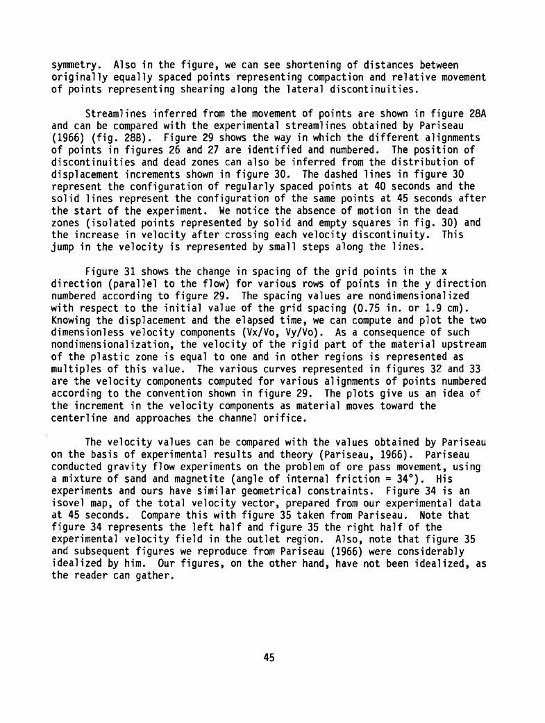
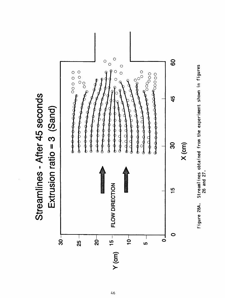
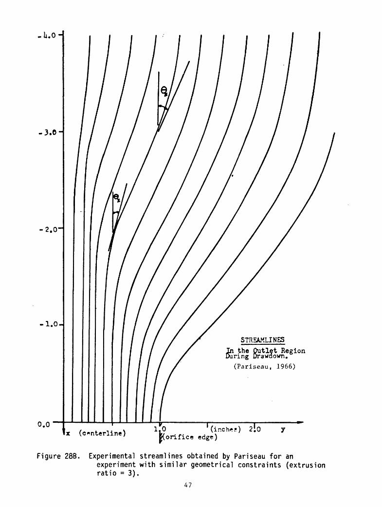
28. A, Streamlines obtained from the experiment shown infigures 26 and 27; B, experimental streamlines obtained by Pariseau for an experiment with similar geometrical constraints (extrusion ratio =3) .......... 46, 47
29. Grid identification numbering scheme .......... 4830. Distribution of displacement increments. Plot of 5 rows
of points from two consecutive images. Dashed lines: position after 40 sec.; solid lines: position after 45 sec. ....................... 49
31. Plot of the variation of the grid spacing vs. x. Thespacing values are nondimensionalized ........ 49
32. Plot of Vx/Vo vs. y. The X values in the legend indicate the number of the row of points, from the origin toward the orifice ..................... 50
33. Plot of Vy/Vo vs. x. The Y values in the legend indicate the number of the row of points counting upward from the origin ...................... 50
34. Isovels map of the total velocity vector after 45 sec from the beginning of the experiment. Only one half of the plastic region is represented. All the velocity values are dimensionless .......... 51
35. Isovels map reproduced from Pariseau's work (1966) for geometric conditions similar to those shown in figures 26-32 ........................ 51
36. A, X-strain rate component (after 30 sec); B 9 Y-strain component (after 30 sec); C, XY-shear strain components (after 30 sec) .............. 53, 54
37. A t Principal stress characteristic field reconstructed from experimental data (after 30 sec); B, idealized principal stress characteristic field from Pariseau (1966) ........................ 55
38. A, Velocity field reconstructed from experimental data (after 30 sec) for <J> = 0°; /?, idealized velocity field from Pariseau (1966) for 4> = 0° ........ 56

39. A, Velocity characteristic field reconstructed from experimental data (after 30 sec) for <J> = 44°; B 9 idealized velocity field from Pariseau (1966) for * = 34° ..................... 57
40. A, Theoretical characteristic field (directions of maximum and minimum shear stresses) for a purely cohesive material with minimum friction along the channel sides; fl, theoretical velocity field for a purely cohesive material with minimum friction along the channel sides ................ 58, 59
41. A 9 Theoretical characteristic field (directions of maximum and minimum shear stresses) for a purely cohesive material with maximum friction along the channel sides; fl, theoretical velocity field for a purely cohesive material with maximum friction along the channel sides ................ 60, 61
TABLES
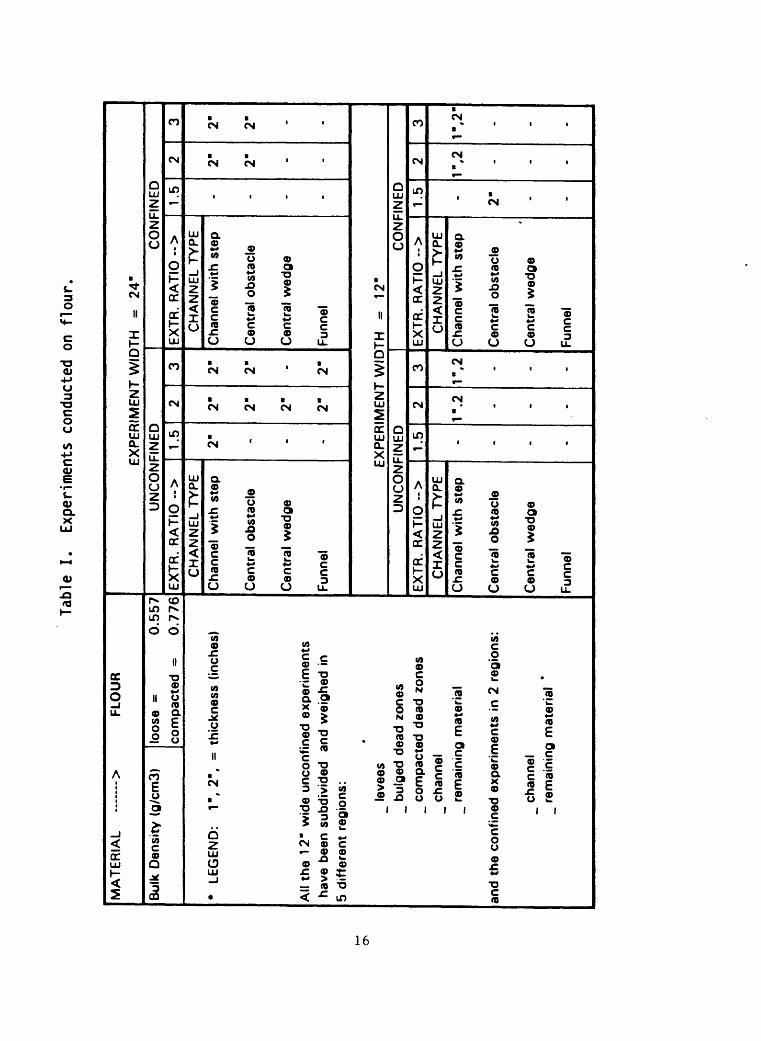
Table I. Experiments conducted on flour ........... 16II. Experiments conducted on sand ........... 17
III. Grain-size analysis for the sand .......... 18IV. Bulk density values computed for unconfined and
confined experiments on sand ........... 19V. Bulk density values computed for unconfined and
confined experiments on flour .......... 19VI. Rate of growth for levees and dead zones and
discharge through the channel unconfined andconfined experiments on flour .......... 42
VII. Rate of growth for levees and dead zones anddischarge through the channel unconfined andconfined experiments on sand ........... 42
A STUDY OF FLOW DEVELOPMENT IN MASS MOVEMENTS OF GRANULAR MATERIALS
by
G.B. Crosta, P.S. Powers, and W.Z. Savage
INTRODUCTION
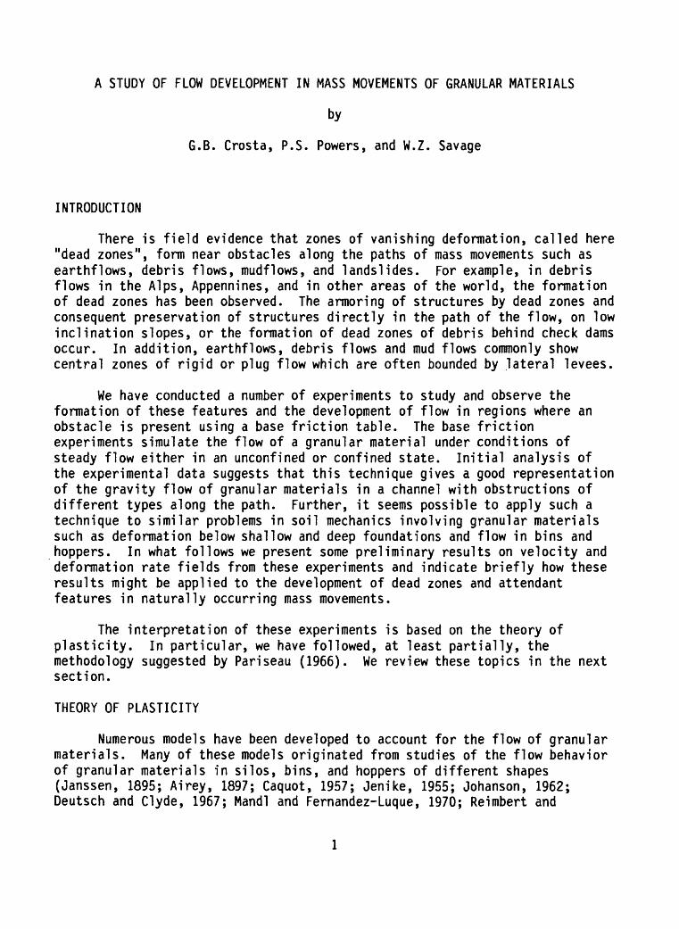
There is field evidence that zones of vanishing deformation, called here "dead zones", form near obstacles along the paths of mass movements such as earthflows, debris flows, mudflows, and landslides. For example, in debris flows in the Alps, Appennines, and in other areas of the world, the formation of dead zones has been observed. The armoring of structures by dead zones and consequent preservation of structures directly in the path of the flow, on low inclination slopes, or the formation of dead zones of debris behind check dams occur. In addition, earthflows, debris flows and mud flows commonly show central zones of rigid or plug flow which are often bounded by lateral levees.
We have conducted a number of experiments to study and observe the formation of these features and the development of flow in regions where an obstacle is present using a base friction table. The base friction experiments simulate the flow of a granular material under conditions of steady flow either in an unconfined or confined state. Initial analysis of the experimental data suggests that this technique gives a good representation of the gravity flow of granular materials in a channel with obstructions of different types along the path. Further, it seems possible to apply such a technique to similar problems in soil mechanics involving granular materials such as deformation below shallow and deep foundations and flow in bins and hoppers. In what follows we present some preliminary results on velocity and deformation rate fields from these experiments and indicate briefly how these results might be applied to the development of dead zones and attendant features in naturally occurring mass movements.
The interpretation of these experiments is based on the theory of plasticity. In particular, we have followed, at least partially, the methodology suggested by Pariseau (1966). We review these topics in the next section.
THEORY OF PLASTICITY
Numerous models have been developed to account for the flow of granular materials. Many of these models originated from studies of the flow behavior of granular materials in silos, bins, and hoppers of different shapes (Janssen, 1895; Airey, 1897; Caquot, 1957; Jenike, 1955; Johanson, 1962; Deutsch and Clyde, 1967; Mandl and Fernandez-Luque, 1970; Reimbert and
Reimbert, 1976; Drescher, 1976; Drescher et al., 1978), or flow of broken rock in mining operations (O'Callaghan, 1960), sublevel caving (Kvapil, 1965), ore pass movement (Pariseau, 1966), or with tectonic faulting (Ode, 1960; Crans and Mandl, 1981) and gravitational sliding of loose or slightly consolidated sediments (Sokolovski, 1960; Szczepinski, 1972; Bruckl and Scheidegger, 1973; Savage and Smith, 1986). These referenced authors have found that the theory of plasticity adequately describes the gravitationally driven flow of cohesive and frictional materials when the flow is steady and the medium behaves like a homogeneous and isotropic continuum.
The plasticity of granular materials differs from the plasticity of metals. These differences occur because the relationships between stress and strain rate, the flow rules, are more complicated for granular materials. This complexity can, in.part, be attributed to the mechanical properties of granular materials and to difficulties encountered in the observation of experiments. It is well known that increasing the confining pressure causes an increase in the strength of a granular material. Thus, when dealing with granular materials it is necessary to replace the Von Mises yield condition, adopted in perfect plasticity, with a yield condition that explicitly takes into account the hydrostatic pressure. As noted by Drescher (1976), flow rules for granular materials can be divided in two main categories: associated flow (Drucker and Prager, 1952; Hill, 1950; Shield, 1953, 1954; Jenike and Shield, 1959; Rowe, 1962; Roscoe et al., 1963; Schofield and Wroth, 1968; Roscoe, 1970) or non-associated flow (Geniev, 1958; De Jong, 1959; Spencer, 1964; Drescher, 1976; Mandl and Fernandez-Luque, 1970). The first, associated flow, postulates coaxiality of the tensors of stress and strain increment. The second, non-associated flow, takes the two tensors to be non- coaxial. Since one of the aims of our research is to compare experimentally developed velocity fields with theoretical velocity fields, we will discuss these aspects of plasticity in greater detail in this section.
The theory of plasticity represents a necessary extension of the theory of elasticity and is concerned with the analysis of stresses and strains in materials in the plastic range. The theory seeks to establish relationships between stress and strain rate which adequately describe the observed deformation under complex stress states. A fundamental principal of plasticity theory is that if the stress at a point in an elastic material exceeds the material strength at that point, then the material will fail and flow inviscidly. Due to the inviscid nature of the motion, there is no relation between stress and rate of deformation, the time variable does not enter into the stress-strain formulation, and thus we can speak of strain rates in terms of strain increments.
In a flowing material the stresses must satisfy the three equations of motion, which, in the static or quasi-static case, reduce to the equations of equilibrium written in cartesian tensor notation as:
'i-
ax,. +FTO (l)
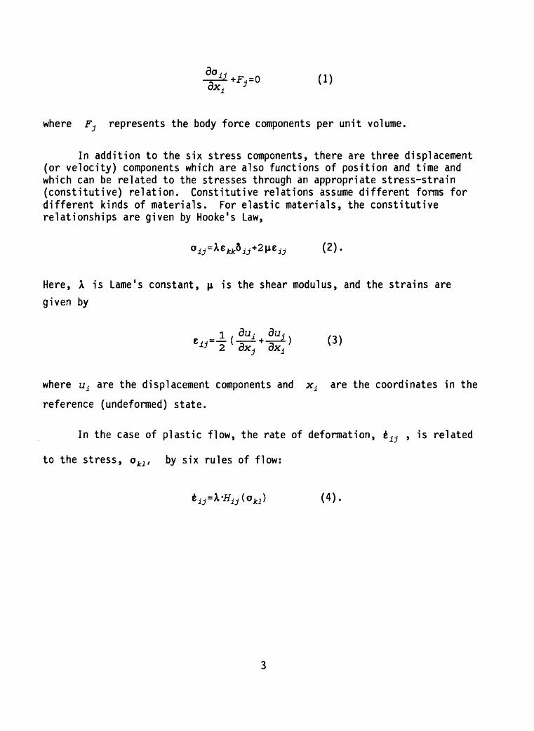
where FJ represents the body force components per unit volume.
In addition to the six stress components, there are three displacement (or velocity) components which are also functions of position and time and which can be related to the stresses through an appropriate stress-strain (constitutive) relation. Constitutive relations assume different forms for different kinds of materials. For elastic materials, the constitutive relationships are given by Hooke's Law,
(2)-
Here, A, is Lame's constant, p. is the shear modulus, and the strains are given by
where ud are the displacement components and xi are the coordinates in the
reference (undeformed) state.
In the case of plastic flow, the rate of deformation, t ±j , is related
to the stress, o^, by six rules of flow:
tii=l,'Hii(ou ) (4).
Here the plastic strain rates are given by,
*
A is a non-vanishing scalar function of time and space, x^ is the
coordinate in the undeformed state, and Hi:j is a known function of material
properties.
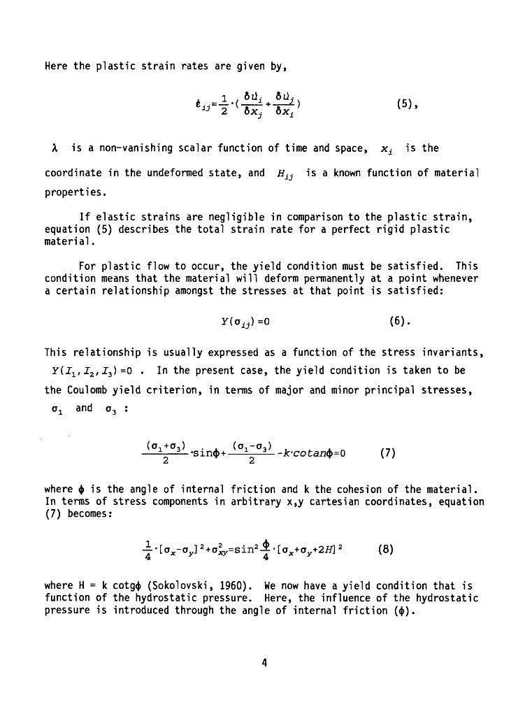
If elastic strains are negligible in comparison to the plastic strain, equation (5) describes the total strain rate for a perfect rigid plastic material.
For plastic flow to occur, the yield condition must be satisfied. Thiscondition means that the material will deform permanently at a point whenevera certain relationship amongst the stresses at that point is satisfied:
ir (oi ,)=0 (6).i J *
This relationship is usually expressed as a function of the stress invariants,
Y(Iit J2 , J3 ) =0 . In the present case, the yield condition is taken to be
the Coulomb yield criterion, in terms of major and minor principal stresses, a, and o, :
A i-3 , ^ A tt\ -sin<l>+ i i -k-cotan$=Q (7)
where <J> is the angle of internal friction and k the cohesion of the material. In terms of stress components in arbitrary x,y cartesian coordinates, equation (7) becomes:
(8)
where H = k cotg<|> (Sokolovski, 1960). We now have a yield condition that isfunction of the hydrostatic pressure. Here, the influence of the hydrostaticpressure is introduced through the angle of internal friction (<|>).
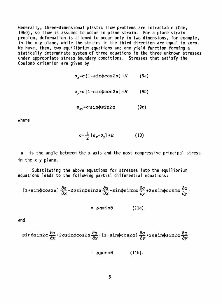
Generally, three-dimensional plastic flow problems are intractable (Ode, 1960), so flow is assumed to occur in plane strain. For a plane strain problem, deformation is allowed to occur only in two dimensions, for example, in the x-y plane, while the strains in the third direction are equal to zero. We have, then, two equilibrium equations and one yield function forming a statically determinate system of three equations in the three unknown stresses under appropriate stress boundary conditions. Stresses that satisfy the Coulomb criterion are given by
ox=o [l+sin<|>cos2a] +H (9a)
oy=o [l-sin<|>cos2a] +H (9b)
(9c)
where
0 = Ji [ox+0y] +H (10)
a is the angle between the x-axis and the most compressive principal stress in the x-y plane.
Substituting the above equations for stresses into the equilibrium equations leads to the following partial differential equations:
[l+sin<bcos2a] ----- ax ax ay ay
= pgsinQ (lla)
and
-a- + [l-sind>cos2a] --- ax ax oy dy
= pgcosQ (Hb).
Here, for gravitational body force, p is the density, g is the gravitational
acceleration, and 6 is the angle between the horizontal and the ground surface. This result yields two equations for the four derivatives
^r- 1 ^r- 1 ^- 1 ^- We can add two more equations, the equations of the dx oy ox oy
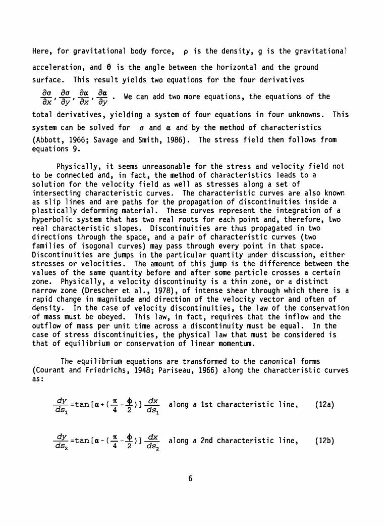
total derivatives, yielding a system of four equations in four unknowns. This system can be solved for o and a and by the method of characteristics(Abbott, 1966; Savage and Smith, 1986). The stress field then follows from equations 9.
Physically, it seems unreasonable for the stress and velocity field not to be connected and, in fact, the method of characteristics leads to a solution for the velocity field as well as stresses along a set of intersecting characteristic curves. The characteristic curves are also known as slip lines and are paths for the propagation of discontinuities inside a plastically deforming material. These curves represent the integration of a hyperbolic system that has two real roots for each point and, therefore, two real characteristic slopes. Discontinuities are thus propagated in two directions through the space, and a pair of characteristic curves (two families of isogonal curves) may pass through every point in that space. Discontinuities are jumps in the particular quantity under discussion, either stresses or velocities. The amount of this jump is the difference between the values of the same quantity before and after some particle crosses a certain zone. Physically, a velocity discontinuity is a thin zone, or a distinct narrow zone (Drescher et al., 1978), of intense shear through which there is a rapid change in magnitude and direction of the velocity vector and often of density. In the case of velocity discontinuities, the law of the conservation of mass must be obeyed. This law, in fact, requires that the inflow and the outflow of mass per unit time across a discontinuity must be equal. In the case of stress discontinuities, the physical law that must be considered is that of equilibrium or conservation of linear momentum.
The equilibrium equations are transformed to the canonical forms (Courant and Friedrichs, 1948; Pariseau, 1966) along the characteristic curves as:
^L=tan[a+( --£)] -- along a 1st characteristic line, (12a)
^l=tan[a-( -- £)]-^- along a 2nd characteristic line, (12b)ds2 4 2 as2

+2o'tain$-^--Ki -^-=Q along a 1st characteristic line, (12c)
2 --=Q along a 2nd characteristic line, (12d)ds2 ds2
where the independent parameters sif s2 represent arc lengths, respectively,
along the 1st and 2nd characteristic curves. The two coefficients, kif k2 ,
introduced in the system are:
-Fy-cos (a-n) ][cos<|>cos (a+u.) ]
a+u) -F-cos ([cos<|)cos (a~
where JA=[ --] , and Fx,Fy represent the body force components:rr
Fy=pg-cosQ
The solution of this system, for a gravity flow problem, is complicated by the introduction of the body forces acting in the material. As an approximation, we can neglect the body forces in the case that (Pariseau, 1966):
where pg is the specific weight of the material, L is the typical depth,and k the cohesion. If this holds, one can ignore the contribution of the body force terms in the analysis of steady flow of granular materials. On the other hand, if the materials are cohesion!ess, body force terms must not be ignored in modeling the experimental flow.
SOLUTION FOR EXTRUSION OF A PERFECTLY PLASTIC MATERIAL
When <i , as would be the case in the flow of highly cohesiveK.
frictional materials, the gravity terms ( kit k2 ) can be neglected and the
governing system of equations reduces to:
-4)3-^- along a 1st characteristic line, (16a) 4 2 cte-
ds2 4 2 as2along a 2nd characteristic line, (16b)
along a 1st characteristic line, (16c)
-2o-tan<|>-^-=0 along a 2nd characteristic line (16d).ds2 ds2
In fact, as Pariseau (1966) shows, gravity flows of such materials can be treated approximately by integration of the above equations. In addition, for materials where 4> is small, or equal to zero, the governing system of equations reduces to:
] - along a 1st characteristic line, (17a) 4 ds-
ds2 4 ds2- 3 - along a 2nd characteristic line, (17b)
_J_
-^ =0 along a 1st characteristic line, (17c)
_j_=0 along a 2nd characteristic line (17d).
ds2
8
These are the governing equations for the case of a purely cohesive material, a Von Mises material which has the yield criterion:
A. [0x-0 ]2+ 0^=;c 2 (18)
This criterion can be obtained from the Coulomb yield criterion by making 4> 0. Solving this system according to the method of characteristics outlined above (Abbott, 1966), we obtain the characteristic directions:
) (19)
o
Thus, we can see that due to the absence of friction, the directions of the maximum and minimum shear lines, respectively called 1st and 2ndcharacteristic lines, in the x-y plane, are obtained with rotations of ± 45with respect to the principal directions of stress. These are the characteristic relationships adopted in metal plasticity (Hill, 1950; Prager and Hodge, 1951; Thomsen et al., 1966). Hill (1950) demonstrated that the plastic equations are hyperbolic and that, for this kind of material, the characteristics of stress and velocity coincide, and therefore only two distinct characteristic directions can be found at each point, and the resulting lines are called sliplines.
Integrating along each characteristic, we determine the Riemann invariants:
c+2ka= constant along a 1st characteristic line, (20a) and
o-2ka= constant along a 2nd characteristic line (20b)
For a Von Mises material, only maximum shearing stresses exist along characteristic lines and the normal stress is equal to the mean stress. Hence, no extension can take place along slip lines and, thus,
du =0 (21a)ds1
and
dv =0 (21b)ds2
These last equations can be written in terms of a as Geiringer's equations (Hill, 1950):
du-vda=Q along a 1st characteristic line (22a)
and
dv-uda=Q along a 2nd characteristic line (22b).
Expressions for the stress components in x and y, which satisfy the yield
condition in terms of o and a , are
ax=a-k-cos2a (23a),
ay=a+k*cos2a (23b),
(23c)
where o = *[ox+oy] .^
A number of numerical techniques, based on geometrical theorems, have been used to solve the characteristic equations for stress and velocity fields. Such theorems and numerical techniques are discussed in detail in textbooks on plasticity (Hill, 1950; Prager and Hodge, 1951; Sokolovski, 1960; Thomsen et al., 1966). We give here only a brief summary of the geometrical theorems.
The two fundamental theorems are called Hencky's theorems. The first theorem states that the angle between the tangents to one family of slip- lines, at the intersection with the slip-lines of a second family, is constant along the length of the slip-lines of the first family. It is clear that if a segment of a slip-line is straight, then all the corresponding sections of any other line of the same family are also straight. Then, according to the Riemann invariants and Geiringer's equations (equations 20 and 21), if one family of slip-lines is straight, the hydrostatic pressure and the total velocity are constant along each line of that family. The second theorem
10

states that as we travel along a slip-line, the radii of curvature of the slip-lines of the other family at the points of intersection change by the distance traveled. The numerical solution of the system of characteristic equations is obtained by a step-by-step numerical integration along the slip- lines, by replacing the derivatives by the tangents or finite differences. The computation starts from curves along which the boundary conditions are given and proceeds to points which discretize the space inside the region of plastic flow limited by the boundary curves the region of influence. In order to solve the problem, the nature of the boundary conditions is the most important factor. Generally, three types of boundary problems can arise. The first is the Cauchy problem, when all the variables are known on a curve not coincident with a characteristic. The second is the Gourset or Riemann problem, in which the variables are known at two points of two different intersecting characteristic lines. The last is the mixed boundary problem, where one slip-line is given together with a curve along which a is known (e.g., the centerline or the walls in an extrusion problem).
EXPERIMENTAL THEORY AND METHODOLOGY
Since this study is concerned with gravity-driven flow of granular material, the first problem was to choose a way to simulate this kind of flow in the laboratory. Gravity-driven flow can be simulated in three different ways: by using an inclined plane, a centrifuge apparatus, or a base friction table.
For these experiments, material flow is realized by means of a base friction table. In rock mechanics, this apparatus is commonly used to simulate gravity-induced defonnation of solids, but here, the base friction table is used to simulate the flow of loose granular materials against obstructions. These materials are either nearly frictionless or cohesionless, are either confined or unconfined, and brought as nearly as possible to steady-state flow conditions in which inertial forces are absent. The apparatus consists of an electric motor, two rollers, and a rubber belt. The motor can be connected by means of a rubber belt to five pulleys of different sizes which permit five different velocities. The largest pulley, which gives the slowest velocity (0.18in/s = 0.46 cm/s), has been employed in our experiments.
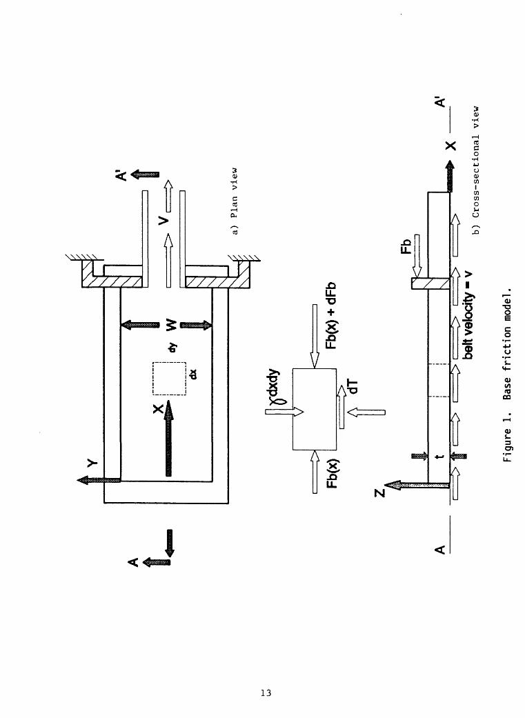
Before describing the experimental technique, it is useful to review briefly the theory of the base friction table (Hoek, 1971; Bray and Goodman, 1981). The fundamental idea is that the base friction table simulates the action of gravity in a two-dimensional physical model by means of the drag force acting along the base of the physical model. These forces are the combined result of the belt movement, under the model, and the contrasting action of a fixed obstacle.
11
Physically, the drag force created by the belt along the base of the model is resisted by the base friction force, Fb, (see fig. 1) acting in the horizontal (xy) plane of the model. The increment of the drag, dT, under a small slice, dx, of material is:
tdxdy (24)
where \ib is the coefficient of friction between the model and the moving
belt, Y 1S the unit weight, and t is the thickness of the physical model.
Under gravity, the body force acting on an element is :
dF^tdxdy (25).
Comparing the last two equations, the analogy between the action of gravity
and drag force, proportionally related by \Lb , is clear and so the validity
of the experimental technique follows. For a model of uniform width (w), the base friction force at "depth" x is:
where p is a confining pressure applied on the upper surface of the model (Egger, 1979).
DESCRIPTION OF THE EXPERIMENTAL TECHNIQUE
One aim of this experimental research is the generation of data for comparison with the theoretical solutions to be presented below for the flow of granular materials in plane strain conditions. Another aim is the study of the development of morphological features, both in confined and unconfined conditions. A final aim is to check the validity of the adopted experimental technique for the study of gravity-driven flow of granular materials. In particular, the comparison with theoretical solutions involves the collection of experimental velocity data to reconstruct velocity characteristics and the principal stress field. Different experimental techniques have been adopted in studies of gravity flow of bulk materials.
12
Fb(x)
dx
V
A1
Wc>
a) Plan view
Fb(x) +
dFb
"-1
I
1 1
t i
i*
i i
T \
Fb"
^ff-
^
belt
velo
city
- v
b) Cross-sectional
view
Figu
re 1.
Base f
rict
ion
model.

Generally, a variety of particle tracking techniques phosphorescent powder (Pariseau, 1966), X-ray with small lead balls (Drescher et al., 1978), labeled markers inserted in the material (Li Yenge, 1980) have been used to follow the movement of material (sand, mixtures of sand with copper or magnetite, glass spheres, small angular rock fragments, etc.) inside bins or hoppers of different shapes.
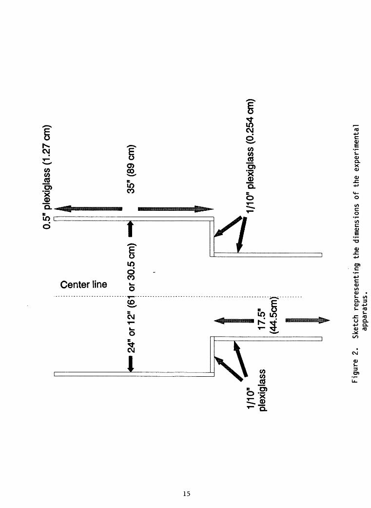
The original base friction apparatus designed for rock mechanics simulations, at the University of Colorado (Boulder), has been modified to satisfy our requirements. Two channels of different widths (12 and 24 in. or 30.5 and 61 cm for 41 in. or 104 cm of length) (fig. 2) and a series of obstacles were prepared to simulate narrowing along the path (with normal or inclined sides) and obstructions in the middle of the main channel (normal or inclined). The narrowing of the channel is described below by means of the ratio between the width upstream and the width downstream of the obstruction (the extrusion ratio). In the experiments, three values of the extrusion ratio (E.R. in Tables I and II) were used: 1.5, 2, and 3. The apparatus was also modified by the addition of a thick (0.5 in. or 1.27 cm) plexiglass plate to constrain the material from dilatation in the vertical direction (z-axis) and to simulate plane (confined) flow conditions.
The experiments were carried out with two types of dry granular material: flour (to simulate a cohesive, frictionless material) and sand (a frictional-conesionless material) (see Table I and II). The former was simple white cooking flour, small enough to pass through the 100 sieve (0.149 mm) but larger than a 200 sieve mesh (0.074 mm). The uniformity of the sand is represented in the grain-size plot (U = uniformity coefficient = 1.75) (see Table III). Angles of friction were measured, by means of a direct shear test, for the materials and the contact surface between sand or flour and plexiglass. The angles of internal friction were 40°-44° for the sand and 10°-14° for the flour. The friction angle for the contact between sand and plexiglass was 30° and less than 10° for the contact between flour and plexiglass. The material was placed on the conveyor without any particular technique and the bulk densities, obtained using the known weight and volume, were always in a restricted range (see Table IV and V).
The particle tracking technique, for the confined experiments, consisted of spraying black paint through a peg-board to create small dots and using white or black spray paint, respectively, on sand and flour to draw regularly spaced transversal lines. The size of the mesh constituting the grid was different: 1 in. (2.54 cm) and 3/4 in. (1.9 cm), respectively, for a 24 and a 12 in. wide channel. The paint used in this operation was of the flat type to avoid increasing the moisture content of the material. In the unconfined experiments, the grid was generated by indenting the material surface with a plastic grid (eggshell form). This gave a square mesh of 0.6 in. (1.5 cm) spacing. In this way, a series of regular straight grooves were created.
14
0.5"
ple
xigl
ass
(1.2
7 cm
)
24"
or 1
2" (6
1 or
30.
5 cm
)
1/10
" pl
exig
lass
17.5
"
(44.
5cm
)
O o> I o>
35"
(89
cm)
1/10
" pl
exig
lass
(0.
254
cm)
Figure 2
. Sk
etch
rep
rese
ntin
g th
e dimensions o
f the
expe
rime
ntal
apparatus.
Tabl
e I.
Expe
rime
nts
conducted
on f
lour.
MA
TE
RIA
L - >
F
LOU
R
Bul
k D
ensi
ty (
g/cm
3)
loos
e =
0.5
57
com
pact
ed
= 0.7
76
* LE
GE
ND
: 1"
, 2",
=
thic
knes
s (in
ches
)
All
the
1 2"
wid
e un
conf
ined
exp
erim
ents
have
bee
n su
bdiv
ided
an
d w
eigh
ed i
n5
diff
ere
nt
regi
ons:
leve
es_
bulg
ed d
ead
zone
s_
com
pact
ed d
ead
zone
sch
anne
l_
rem
aini
ng m
ater
ial
and
the
conf
ined
exp
erim
ents
in
2 re
gion
s:
_ ch
anne
l_
rem
aini
ng m
ater
ial
EX
PE
RIM
EN
T W
IDT
H
= 2
4"
UN
CO
NF
INE
D
EX
TR
. R
AT
IO -
->
CH
AN
NE
L TY
PE
Cha
nnel
with
ste
p
Cen
tral
obs
tacl
e
Cen
tral
wed
ge
Fun
nel
1.5
2" - - -
2 2"
2"
2"
2"
3 2"
2" . 2"
CO
NF
INE
D
EX
TR.
RA
TIO
-->
CH
AN
NE
L T
YP
E
Cha
nnel
with
ste
p
Cen
tral
obs
tacl
e
Cen
tral
wed
ge
Funn
el
1.5 - - - -
2 2"
2" . -
3 2"
2" - -
EX
PE
RIM
EN
T W
IDT
H
=
12"
UN
CO
NF
INE
D
EX
TR
. R
AT
IO -
->
CH
AN
NE
L TY
PE
Cha
nnel
with
ste
p
Cen
tral
ob
sta
cle
Cen
tral
wedge
Fun
nel
1.5 - - - *
2
1".
2 - - *
3
r,2 - .
CO
NFI
NE
DE
XTR
. R
AT
IO -
->
CH
AN
NE
L T
YP
E
Cha
nnel
with
ste
p
Cen
tral
obs
tacl
e
Cen
tral
wed
ge
Funn
el
1.5 - 2" -
2
1",
2 - .
3
1-,
2"
- . *

Table
II.
Expe
rime
nts
conducted
on s
and.
MA
TE
RIA
L
----
- ->
S
AN
D
Bul
k D
ensi
ty (
g/cm
3)
loos
e =
1 .3
47co
mpa
cted
=
1 .4
92
* LE
GE
ND
: 1"
, 2
",
= t
hick
ness
(in
ches
)
All
the
1 2"
wid
e un
conf
ined
exp
erim
ents
have
bee
n su
bdiv
ided
an
d w
eigh
ed i
n5
diffe
rent
reg
ions
:
leve
esbu
lged
dea
d zo
nes
com
pact
ed d
ead
zone
sch
anne
l_
rem
aini
ng m
ater
ial
and
the
conf
ined
exp
erim
ents
in
2 re
gion
s:
chan
nel
_ re
mai
ning
mat
eria
l
PILE
: ob
stac
le 1
4"
long
pla
ced
insi
deth
e m
ater
ial
EX
PE
RIM
EN
T W
IDT
H
= 24"
UN
CO
NF
INE
D
EX
TR
. R
AT
IO -
>
CH
AN
NE
L T
YP
E
Cha
nnel
with
ste
p
Cen
tral
obs
tacl
e
Cen
tral
wed
ge
Funn
el
1.5 - - . -
2 2"
2"
2" 2"
3 2" 2" . -
CO
NF
INE
D
EX
TR
. R
AT
IO -
->
CH
AN
NE
L T
YP
E
Cha
nnel
with
ste
p
Cen
tral
obs
tacl
e
Cen
tral
wed
ge
Funn
el
1.5 - - . -
2 2"
2"
2"
2"
3 2"
2" . 2"
EX
PE
RIM
EN
T W
IDT
H
=
12"
UN
CO
NF
INE
D
EX
TR
. R
AT
IO -
->
CH
AN
NE
L T
YP
E
Cha
nnel
with
ste
p
Cen
tral
obs
tacl
e
Cen
tral
wed
ge
Funn
el
1.5 - - - -
2
1",
2 - - -
3
1",
2 - - -
CO
NFI
NE
DE
XT
R.
RA
TIO
->
CH
AN
NE
L T
YP
E
Cha
nnel
with
ste
p
Cen
tral
obs
tacl
e
Cen
tral
wed
ge
Fun
nel
Pile
1.5 - - - - 1"
2
1",
2
2" - 1" -
3
1",
2"
2" - - -
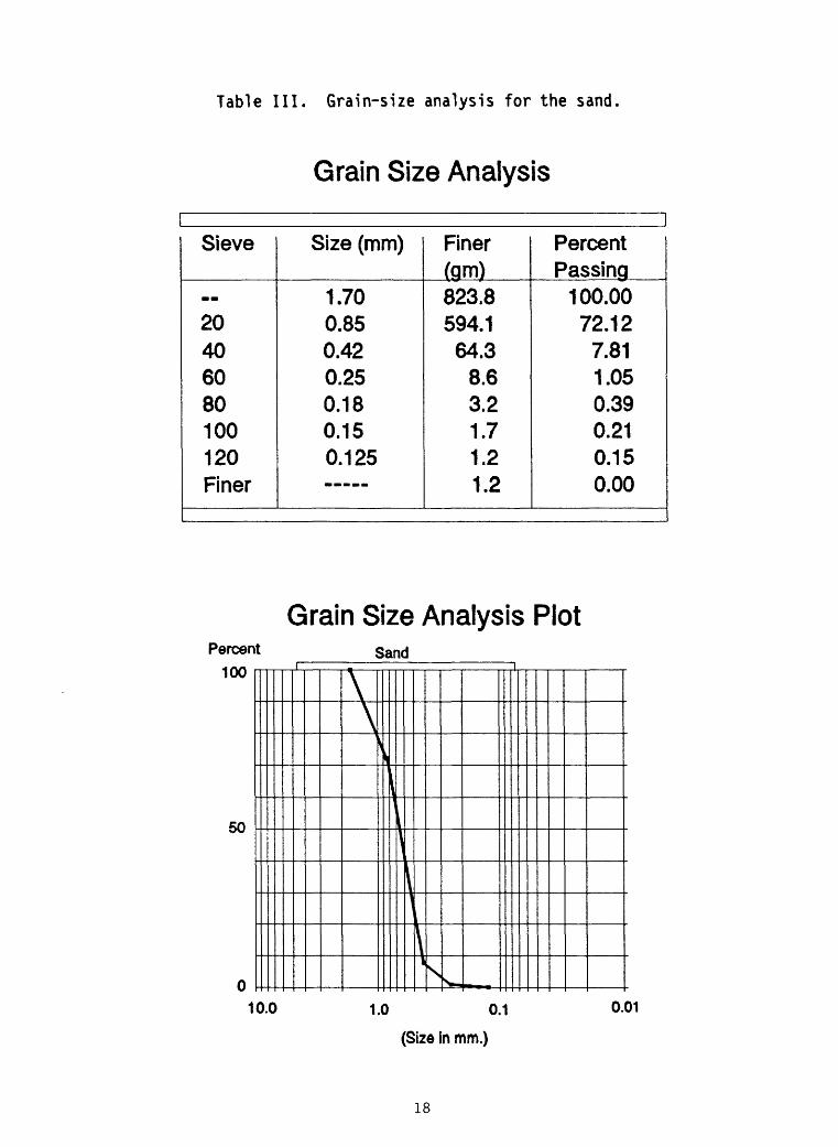
Table III. Grain-size analysis for the sand.
Grain Size Analysis
Sieve
..20406080100120Finer
Size (mm)
1.700.850.420.250.180.150.125.....
Finer(grn)823.8594.164.3
8.63.21.71.21.2
Percent Passing
100.0072.12
7.811.050.390.210.150.00
Grain Size Analysis PlotPercent
100 -
v»
n .
iS
\̂
arI
^tK
II
i
|IsSB, i -
Vi
10.0 1.0 0.1
(Size in mm.)
0.01
18
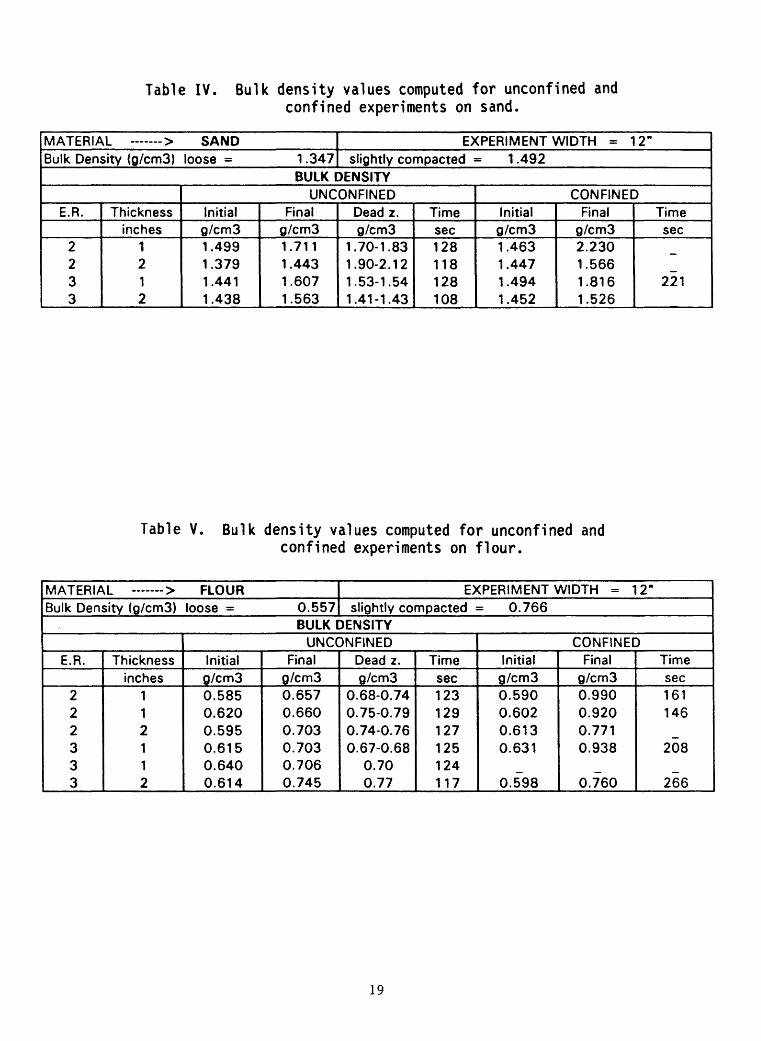
Table IV. Bulk density values computed for unconfined and confined experiments on sand.
IVIM 1 CniMU ** OMWLS
Bulk Density (g/cm3) loose = 1 .347cyvrcniivicix i vviuin i z.
slightly compacted = 1 .492BULK DENSITY
E.R.
2 2 3 3
Thicknessinches
1 2 1 2
UNCONFINEDInitialg/cm31.499 1.379 1.441 1.438
Finalg/cm31.711 1.443 1.607 1.563
Dead z.g/cm3
1.70-1.83 1.90-2.12 1.53-1.54 1.41-1.43
Timesec128 118 128 108
CONFINEDInitialg/cm31.463 1.447 1.494 1.452
Finalg/cm32.230 1.566 1.816 1.526
Timesec
221
Table V. Bulk density values computed for unconfined and confined experiments on flour.
MM i cniML * ruuun
Bulk Density (g/cm3) loose = 0.557CA.rcniivicix i vviuin i^
slightly compacted = 0.766BULK DENSITY
E.R.
222333
Thicknessinches
112112
UNCONFINEDInitialg/cm30.5850.6200.5950.6150.6400.614
Finalg/cm30.6570.6600.7030.7030.7060.745
Dead z.g/cm3
0.68-0.740.75-0.790.74-0.760.67-0.68
0.700.77
Timesec123129127125124117
CONFINEDInitialg/cm30.5900.6020.6130.631
0.598
Finalg/cm30.9900.9200.7710.938
0.760
Timesec161146
208
266
19

These grooves persisted for the duration of the experiments and could be made visible by illuminating the surface at a low angle.
To obtain information on mass balance, weighing was carried out on both types of experiments. For purposes of weighing, material of the confined experiments was subdivided into two volumes. Material passing through the inside of the narrow channel and material remaining behind or upstream of the obstruction were weighed separately. In the case of the unconfined experiments, the material was weighed in 5 regions (fig. 3) in the bulged dead zones, in the compacted dead zones, in the levees, in the channel, and in material remaining behind the obstruction. The separation of bulged and compacted dead zones and of levees and channel material is represented by the plane of original thickness (t) in figure 3. During weighing, the various regions were separated by thin (<0.1 in. or <0.254 cm) plexiglass sheets.
Another variable introduced in the experiments was the thickness of the material to evaluate its influence on the velocity distribution in the horizontal x-y plane as well as in the vertical x-z plane. Two thickness values were adopted: 1 and 2 in. (2.54 and 5.08 cm).
To maximize the information from the experiments, all experiments were filmed with a video camera, which stores images in a digital format. To avoid strong optical distortion, we used the maximum possible distance between video camera and material. By means of a graphic board, we were able to capture images from the video camera to a computer. These images were then digitized directly on a computer screen by means of a program written for this purpose. In addition to the video tapes, 35 mm pictures were taken with a reflex camera during all the experiments.
DESCRIPTION OF TYPICAL FEATURES IN THE FLOW EXPERIMENTS
Features typical of gravity flow of granular material, as reported in many experimental studies (Johanson, 1962; Pariseau, 1966; Ladanyi and Hoyaux, 1969; Drescher, 1976; Drescher et al., 1978; Li Yenge, 1980) can be recognized from careful examination of the results of the experiments. Further, some of the observed features can be compared to the features described in structural geology experiments (Hubbert, 1951) and soil mechanics experiments (Sylwestrowicz, 1953). In the following, we summarize these features considering separately the confined and unconfined experiments.
Confined experiments
The first feature to appear, a few seconds after initiation of belt movement, is the boundary between the plastic zone (regions A and B in figs. 4 and 5) and the rigid plug (region C) represented by line d-g in figure 5. The plastic zone consists of two fans upstream of the step or obstacle in the flow
20

Wei
ghin
g Zo
ne D
efin
ition
Sch
eme
Bulged dea
d zo
ne
Levee
FLO
W D
IRE
CTI
ON
Con
veyo
r Be
lt
Fixe
d di
stan
ce
from
the
obst
acle
Com
pact
ed
Dea
d Zo
ne
Leve
e
Rem
aini
ng
i -,
,
mat
eria
l j
Cha
nnel
FLO
W D
IRE
CTI
ON
Leve
e
XC
ompa
cted
Dea
d Zo
ne
Figu
re 3
. We
ighi
ng z
one
definition s
chem
e.
Subd
ivis
ion
of t
he m
ater
ial,
fo
r un
conf
ined
exp
erim
ents
, in 5
dif
fere
nt v
olumes t
o ob
tain
a m
ass
bala
nce
(discharge a
nd rate o
f gr
owth
).
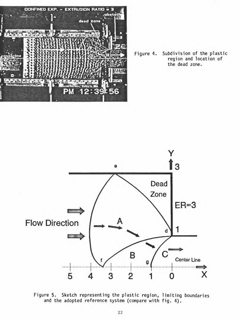
Figure 4. Subdivision of the plastic region and location of the dead zone.
e
Flow Direction
ER=3
Figure 5. Sketch representing the plastic region, limiting boundaries and the adopted reference system (compare with fig. 4).
22
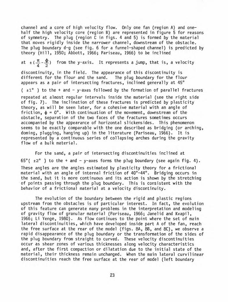
channel and a core of high velocity flow. Only one fan (region A) and one- half the high velocity core (region B) are represented in figure 5 for reasons of symmetry. The plug (region C in figs. 4 and 5) is formed by the material that moves rigidly inside the narrower channel, downstream of the obstacle. The plug boundary d-g (see fig. 6 for a funnel-shaped channel) is predicted by theory (Hill, 1950; Abbott, 1966; Pariseau, 1966) to be inclined
at ±( -£) from the y-axis. It represents a jump, that is, a velocity4 ^
discontinuity, in the field. The appearance of this discontinuity isdifferent for the flour and the sand. The plug boundary for the flourappears as a pair of intersecting fractures, inclined generally at 45°
( ±1° ) to the + and - y-axes followed by the formation of parallel fracturesrepeated at almost regular intervals inside the material (see the right side of fig. 7). The inclination of these fractures is predicted by plasticity theory, as will be seen later, for a cohesive material with an angle of friction, 4> = 0°. With continuation of the movement, downstream of the obstacle, separation of the two faces of the fractures sometimes occurs accompanied by the appearance of horizontal slickensides. This phenomenon seems to be exactly comparable with the one described as bridging (or arching, doming, plugging, hanging up) in the literature (Pariseau, 1966). It is represented by a continuous series of collapsing arches during the gravity flow of a bulk material.
For the sand, a pair of intersecting discontinuities inclined at
65°( ±2° ) to the + and - y-axes forms the plug boundary (see again fig. 4).
These angles are the angles estimated by plasticity theory for a frictional material with an angle of internal friction of 40°-44°. Bridging occurs in the sand, but it is more continuous and its action is shown by the stretching of points passing through the plug boundary. This is consistent with the behavior of a frictional material at a velocity discontinuity.
The evolution of the boundary between the rigid and plastic regions upstream from the obstacles is of particular interest. In fact, the evolution of this feature can generate many problems in the interpretation and modeling of gravity flow of granular material (Pariseau, 1966; Jane!id and Kvapil, 1966; Li Yenge, 1980). As flow continues to the point where the set of main lateral discontinuities, which have developed inside part A of the fan, reach the free surface at the rear of the model (figs. 8A, 8B, and 8C), we observe a rapid disappearance of the plug boundary or the transformation of the sides of the plug boundary from straight to curved. These velocity discontinuities occur as shear zones of various thicknesses along velocity characteristics and, after the first compaction or dilatation due to the initial state of the material, their thickness remain unchanged. When the main lateral curvilinear discontinuities reach the free surface at the rear of model (left boundary
23

Figure 6. Rigid plug boundary for a confined experiment with sand and a funnel-shaped obstacle.
rigid plug boundaries transported into the narrow/ channel
Figure 7. Rigid plug boundary for a confined experiment on flour and anextrusion ratio of three. Dead zones and velocity discontinuities are also visible. _____________________
24
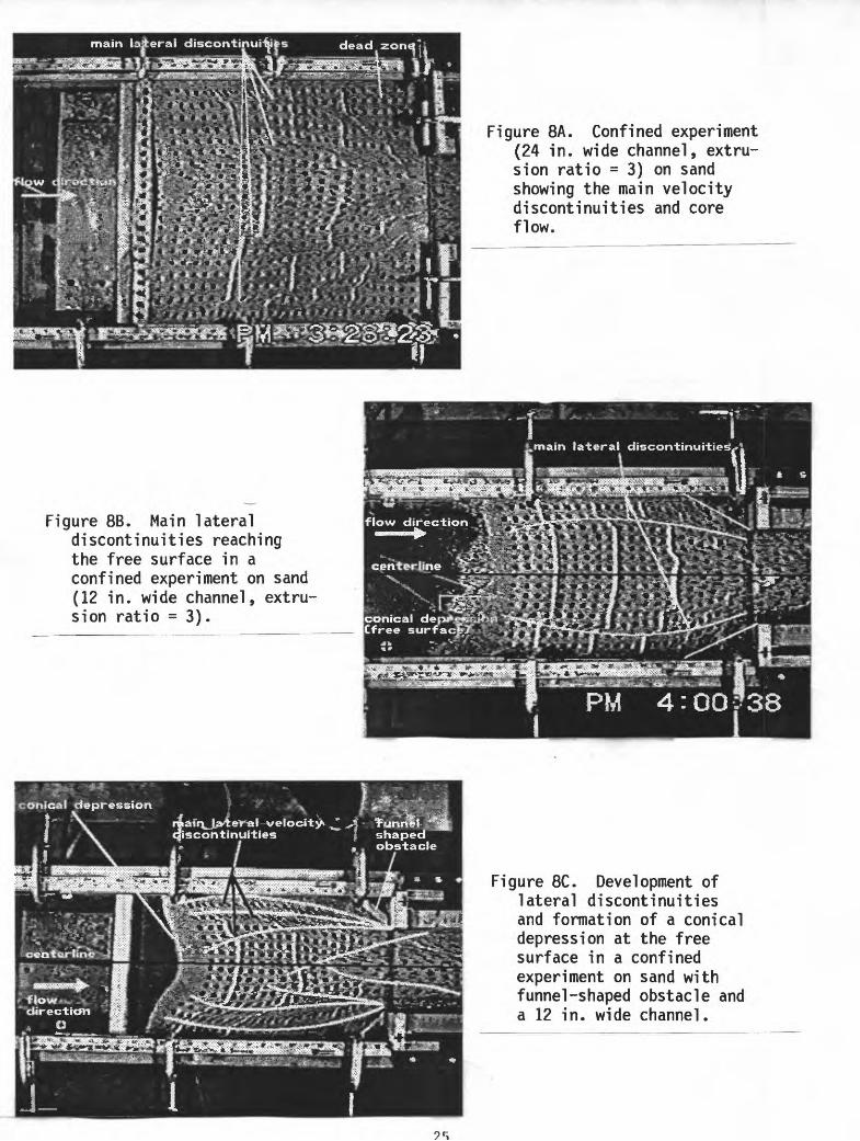
Figure 8A. Confined experiment (24 in. wide channel, extru sion ratio = 3) on sand showing the main velocity discontinuities and core flow.
Figure 8B. Main lateral discontinuities reaching the free surface in a confined experiment on sand (12 in. wide channel, extru sion ratio = 3).
Figure 8C. Development of lateral discontinuities and formation of a conical depression at the free surface in a confined experiment on sand with funnel-shaped obstacle and a 12 in. wide channel.
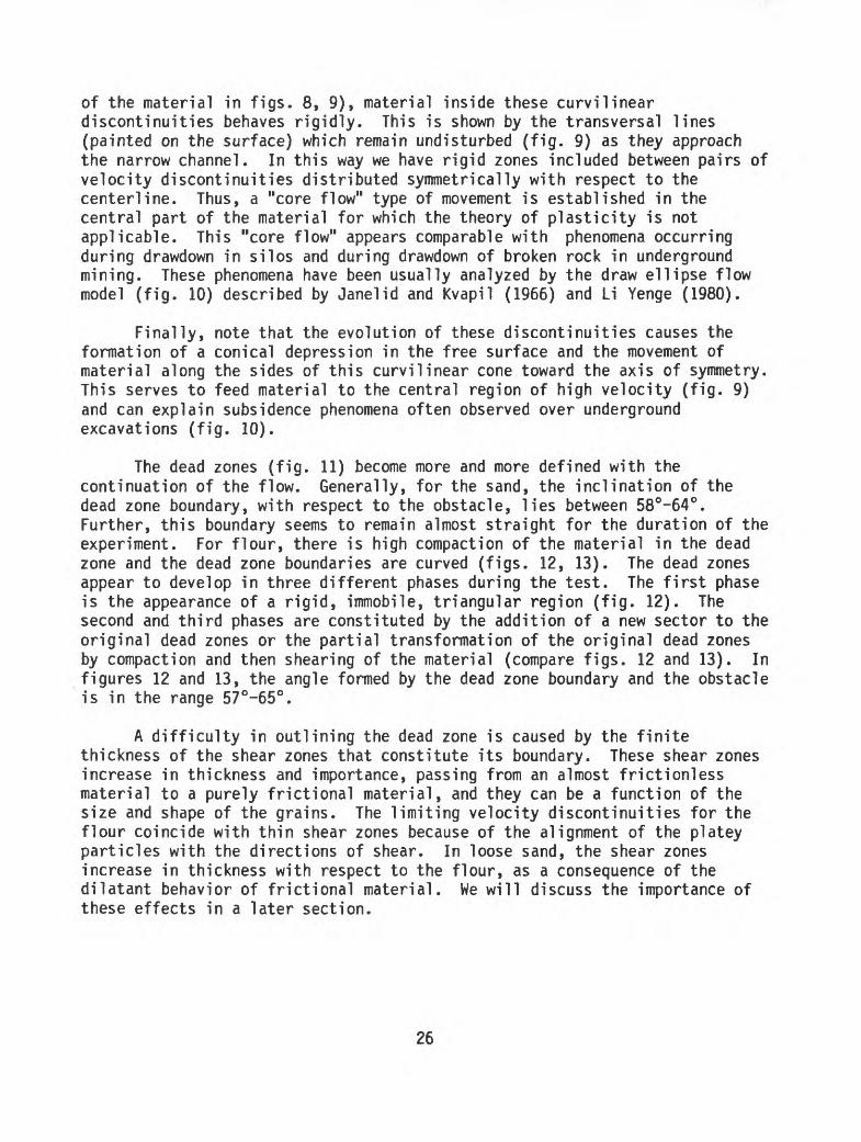
of the material in figs. 8, 9), material inside these curvilinear discontinuities behaves rigidly. This is shown by the transversal lines (painted on the surface) which remain undisturbed (fig. 9) as they approach the narrow channel. In this way we have rigid zones included between pairs of velocity discontinuities distributed symmetrically with respect to the centerline. Thus, a "core flow" type of movement is established in the central part of the material for which the theory of plasticity is not applicable. This "core flow" appears comparable with phenomena occurring during drawdown in silos and during drawdown of broken rock in underground mining. These phenomena have been usually analyzed by the draw ellipse flow model (fig. 10) described by Janelid and Kvapil (1966) and Li Yenge (1980).
Finally, note that the evolution of these discontinuities causes the formation of a conical depression in the free surface and the movement of material along the sides of this curvilinear cone toward the axis of symmetry. This serves to feed material to the central region of high velocity (fig. 9) and can explain subsidence phenomena often observed over underground excavations (fig. 10).
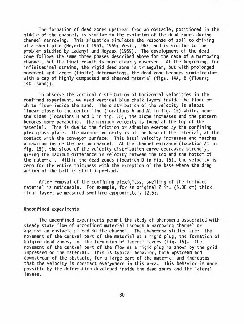
The dead zones (fig. 11) become more and more defined with the continuation of the flow. Generally, for the sand, the inclination of the dead zone boundary, with respect to the obstacle, lies between 58°-64°. Further, this boundary seems to remain almost straight for the duration of the experiment. For flour, there is high compaction of the material in the dead zone and the dead zone boundaries are curved (figs. 12, 13). The dead zones appear to develop in three different phases during the test. The first phase is the appearance of a rigid, immobile, triangular region (fig. 12). The second and third phases are constituted by the addition of a new sector to the original dead zones or the partial transformation of the original dead zones by compaction and then shearing of the material (compare figs. 12 and 13). In figures 12 and 13, the angle formed by the dead zone boundary and the obstacle is in the range 57°-65°.
A difficulty in outlining the dead zone is caused by the finite thickness of the shear zones that constitute its boundary. These shear zones increase in thickness and importance, passing from an almost frictionless material to a purely frictional material, and they can be a function of the size and shape of the grains. The limiting velocity discontinuities for the flour coincide with thin shear zones because of the alignment of the platey particles with the directions of shear. In loose sand, the shear zones increase in thickness with respect to the flour, as a consequence of the dilatant behavior of frictional material. We will discuss the importance of these effects in a later section.
26
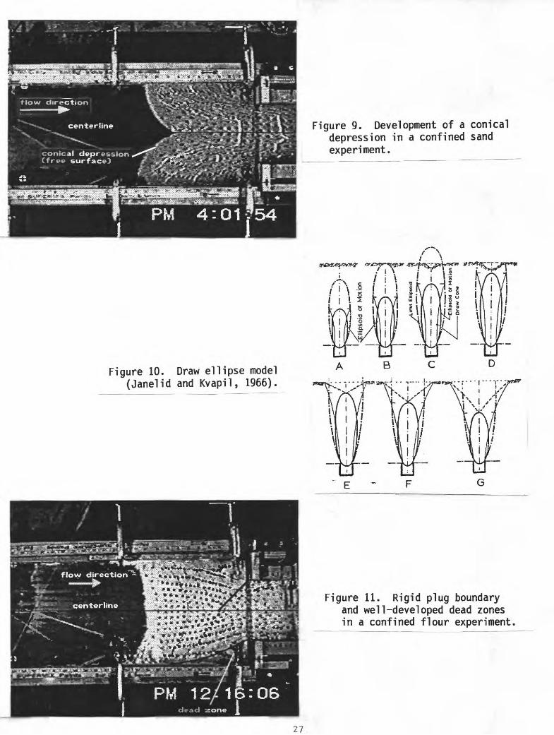
Figure 10. Draw ellipse model (Janelid and Kvapil, 1966).
Figure 9. Development of a conical depression in a confined sand experiment.
Figure 11. Rigid plug boundary and we11-developed dead zones in a confined flour experiment,

Figure 12. Confined flour experiment showing the first stage in the development of the dead zones and some we11-developed velocity discontinuities.
28
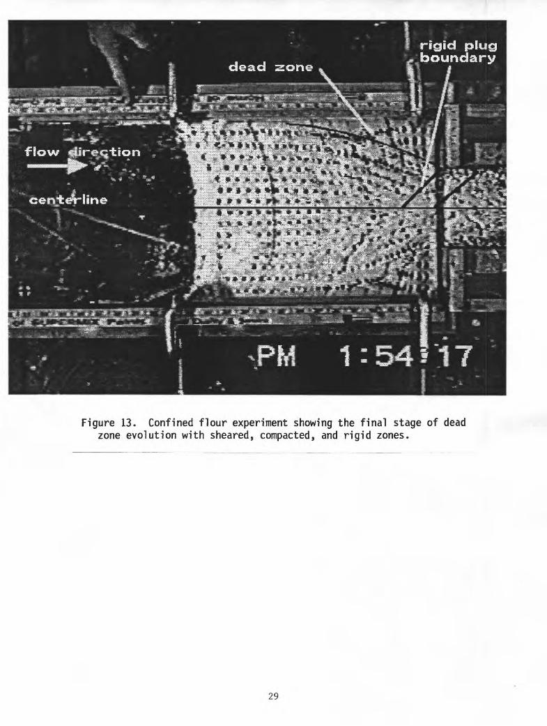
Figure 13. Confined flour experiment showing the final stage of dead zone evolution with sheared, compacted, and rigid zones.
29
The formation of dead zones upstream from an obstacle, positioned in the middle of the channel, is similar to the evolution of the dead zones during channel narrowing. This situation simulates the response of soil to driving of a sheet pile (Meyerhoff 1951, 1959; Vesic, 1967) and is similar to the problem studied by Ladanyi and Hoyaux (1969). The development of the dead zone follows the same three phases described above for the case of a narrowing channel, but the final result is more clearly observed. At the beginning, for infinitesimal strains, the rigid dead zone is triangular, but with prolonged movement and larger (finite) deformations, the dead zone becomes semicircular with a cap of highly compacted and sheared material (figs. 14A, B (flour); 14C (sand)).
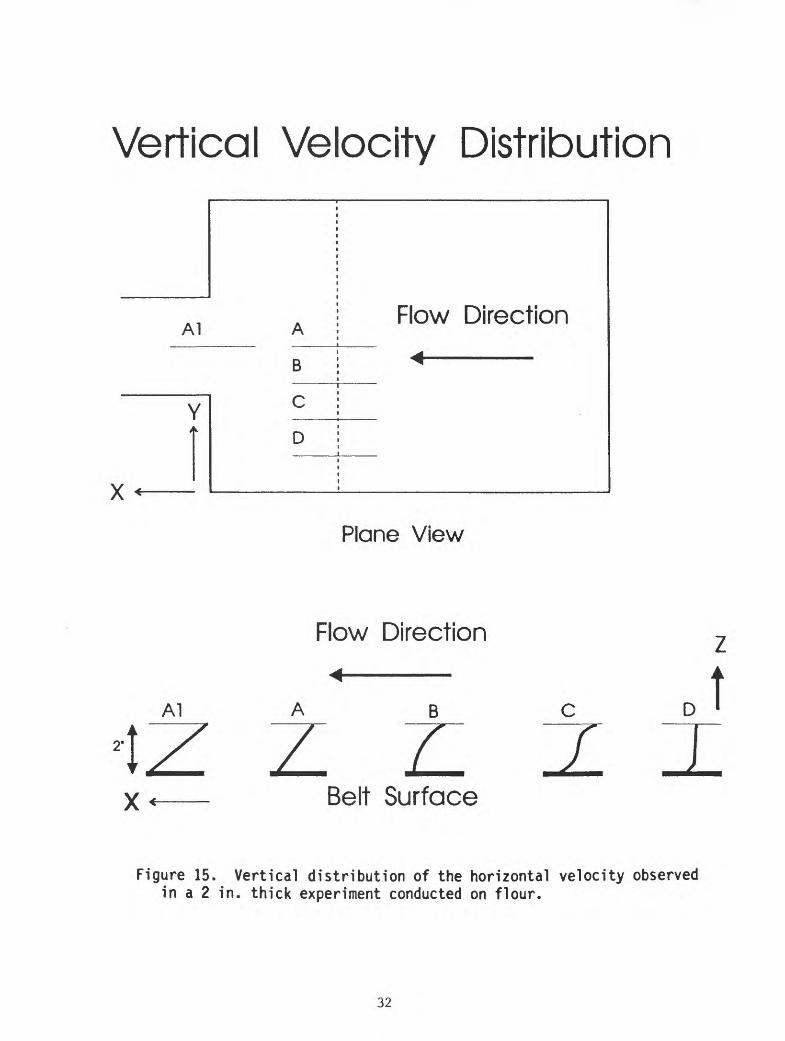
To observe the vertical distribution of horizontal velocities in the confined experiment, we used vertical blue chalk layers inside the flour or white flour inside the sand. The distribution of the velocity is almost linear close to the center line (locations A and Al in fig. 15) while, near the sides (locations B and C in fig. 15), the slope increases and the pattern becomes more parabolic. The minimum velocity is found at the top of the material. This is due to the friction or adhesion exerted by the confining plexiglass plate. The maximum velocity is at the base of the material, at the contact with the conveyor surface. This basal velocity increases and reaches a maximum inside the narrow channel. At the channel entrance (location Al in fig. 15), the slope of the velocity distribution curve decreases strongly, giving the maximum difference in velocity between the top and the bottom of the material. Within the dead zones (location D in fig. 15), the velocity is zero for the entire thickness with the exception of the base where the drag action of the belt is still important.
After removal of the confining plexiglass, swelling of the included material is noticeable. For example, for an original 2 in. (5.08 cm) thick flour layer, we measured swelling approximately 12.5%.
Unconfined experiments
The unconfined experiments permit the study of phenomena associated with steady state flow of unconfined material through a narrowing channel or against an obstacle placed in the channel. The phenomena studied are: the movement of the central part of the material as a rigid plug, the formation of bulging dead zones, and the formation of lateral levees (fig. 16). The movement of the central part of the flow as a rigid plug is shown by the grid inpressed on the material. This is typical behavior, both upstream and downstream of the obstacle, for a large part of the material and indicates that the velocity is constant everywhere in this area. This behavior is made possible by the deformation developed inside the dead zones and the lateral levees.
30
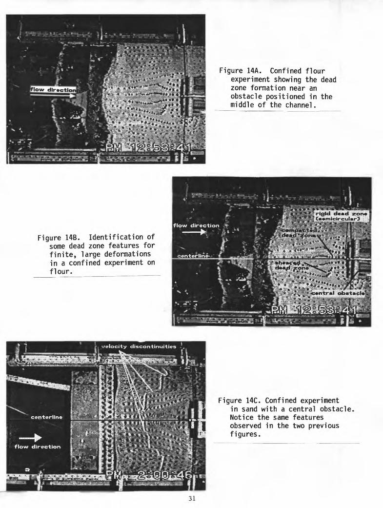
Figure 14A. Confined flour experiment showing the dead zone formation near an obstacle positioned in the middle of the channel.
Figure 14B. Identification of some dead zone features for finite, large deformations in a confined experiment on flour.
rigid dead zohi CB*rriicirculaiO
Figure 14C. Confined experiment in sand with a central obstacle, Notice the same features observed in the two previous figures.
31
Vertical Velocity Distribution
X
Al
Y
B
C
D
Flow Direction
Plane View
Al
2'
Flow Direction
B
Z L. J-Belt Surface
D t
Figure 15. Vertical distribution of the horizontal velocity observed in a 2 in. thick experiment conducted on flour.
32
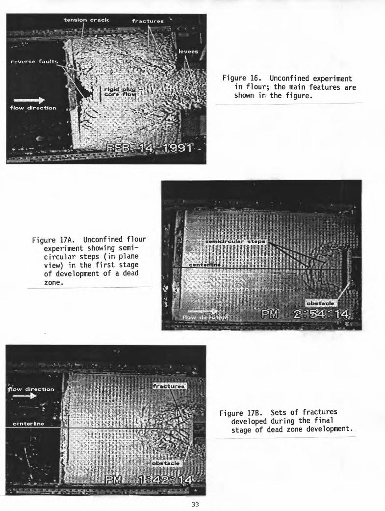
Figure 16. Unconfined experiment in flour; the main features are shown in the figure.
Figure 17A. Unconfined flour experiment showing semi circular steps (in plane view) in the first stage of development of a dead zone.
Figure 17B. Sets of fractures developed during the final stage of dead zone development,
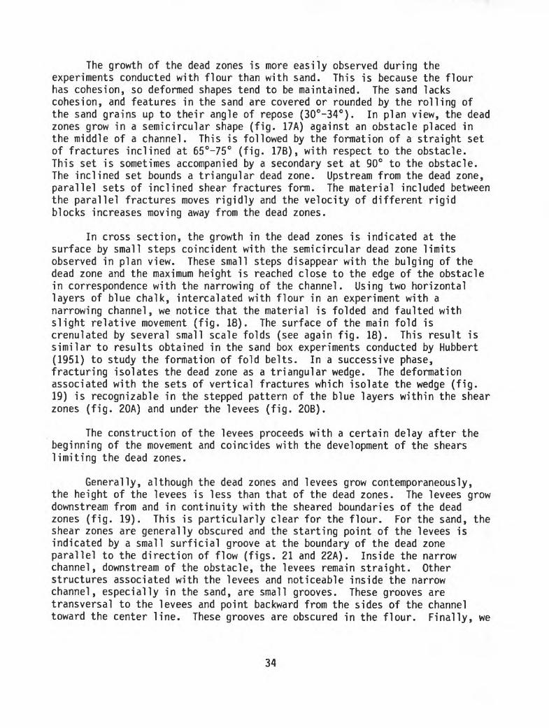
The growth of the dead zones is more easily observed during the experiments conducted with flour than with sand. This is because the flour has cohesion, so deformed shapes tend to be maintained. The sand lacks cohesion, and features in the sand are covered or rounded by the rolling of the sand grains up to their angle of repose (30°-34°). In plan view, the dead zones grow in a semicircular shape (fig. 17A) against an obstacle placed in the middle of a channel. This is followed by the formation of a straight set of fractures inclined at 65°-75° (fig. 17B), with respect to the obstacle. This set is sometimes accompanied by a secondary set at 90° to the obstacle. The inclined set bounds a triangular dead zone. Upstream from the dead zone, parallel sets of inclined shear fractures form. The material included between the parallel fractures moves rigidly and the velocity of different rigid blocks increases moving away from the dead zones.
In cross section, the growth in the dead zones is indicated at the surface by small steps coincident with the semicircular dead zone limits observed in plan view. These small steps disappear with the bulging of the dead zone and the maximum height is reached close to the edge of the obstacle in correspondence with the narrowing of the channel. Using two horizontal layers of blue chalk, intercalated with flour in an experiment with a narrowing channel, we notice that the material is folded and faulted with slight relative movement (fig. 18). The surface of the main fold is crenulated by several small scale folds (see again fig. 18). This result is similar to results obtained in the sand box experiments conducted by Hubbert (1951) to study the formation of fold belts. In a successive phase, fracturing isolates the dead zone as a triangular wedge. The deformation associated with the sets of vertical fractures which isolate the wedge (fig. 19) is recognizable in the stepped pattern of the blue layers within the shear zones (fig. 20A) and under the levees (fig. 20B).
The construction of the levees proceeds with a certain delay after the beginning of the movement and coincides with the development of the shears limiting the dead zones.
Generally, although the dead zones and levees grow contemporaneously, the height of the levees is less than that of the dead zones. The levees grow downstream from and in continuity with the sheared boundaries of the dead zones (fig. 19). This is particularly clear for the flour. For the sand, the shear zones are generally obscured and the starting point of the levees is indicated by a small surficial groove at the boundary of the dead zone parallel to the direction of flow (figs. 21 and 22A). Inside the narrow channel, downstream of the obstacle, the levees remain straight. Other structures associated with the levees and noticeable inside the narrow channel, especially in the sand, are small grooves. These grooves are transversal to the levees and point backward from the sides of the channel toward the center line. These grooves are obscured in the flour. Finally, we
34
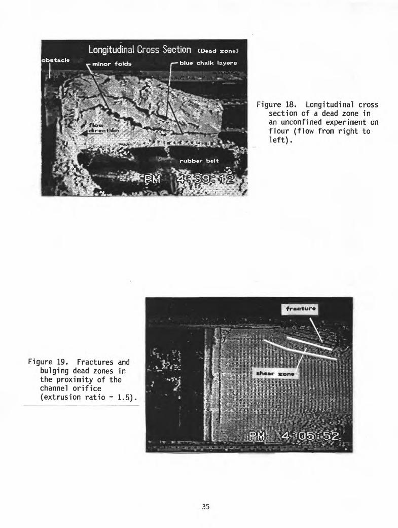
Figure 18. Longitudinal cross section of a dead zone in an unconfined experiment on flour (flow from right to left).
Figure 19. Fractures and bulging dead zones in the proximity of the channel orifice (extrusion ratio = 1.5).
35
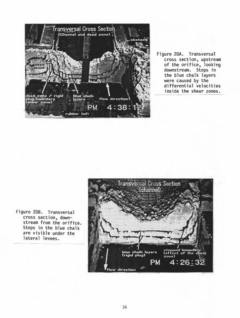
Figure 20A. Transversal cross section, upstream of the orifice, looking downstream. Steps in the blue chalk layers were caused by the differential velocities inside the shear zones.
Figure 20B. Transversal cross section, down stream from the orifice, Steps in the blue chalk are visible under the lateral levees.
36
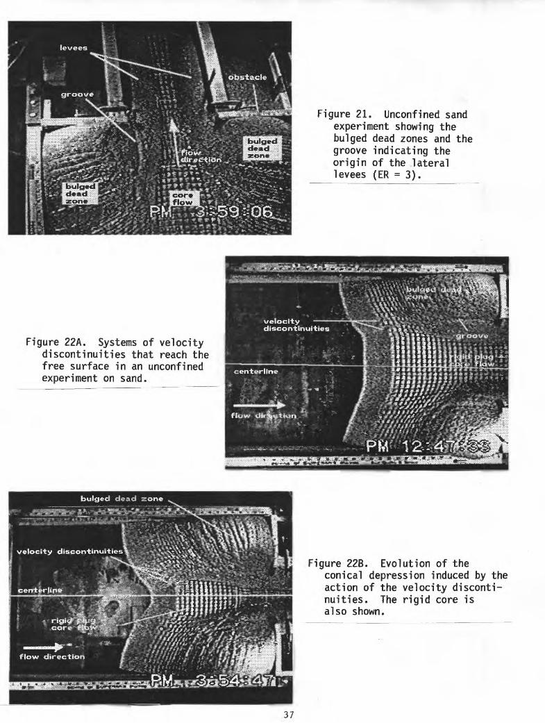
Figure 21. Unconfined sand experiment showing the bulged dead zones and the groove indicating the origin of the lateral levees (ER = 3).
Figure 22A. Systems of velocity discontinuities that reach the free surface in an unconfined experiment on sand.
Figure 22B. Evolution of theconical depression induced by the action of the velocity disconti nuities. The rigid core is also shown.

observed that the levees are usually larger in the case of a funnel-shaped channel. This may be due to the presence of a smaller dead zone together with a larger bulging zone than occurs when the channel narrows by a step.
If the experiments proceed for enough time, there is a point at which the fast central rigid core reaches the rear limit of the material and tension cracks and reverse faults develop (figs. 23A and B (flour); figs. 22A and B (sand)). The reverse faults have the same curvilinear shape as the discontinuities described in the confined experiments and bound the central rigid plug from the obstacle to the rear.
In the case of a central obstacle the most important features are the reverse faults which depart from the edge of the obstacle. These discontinuities are inclined at the beginning of their formation and become normal to the obstacle with the continuation of the movement (see fig. 24, where these discontinuities are labeled 1st and 2nd to show the order of formation). The discontinuities are comparable to the features described in the case of a narrowing channel because of symmetry. Their development is followed by the development of normal faults subdividing the wedge of material pushed backward. These results are similar to results obtained by Sanford (1959) on the problem of deformation of a sedimentary cover overlaying an uplifted or downdropped rigid crystalline block.
Mass balance
We have also evaluated the mass balances involved in the experiments. To do this, the material both in the confined and unconfined experiments, was separated in different regions (fig. 3) and the separated material was weighed. The results, some of which were repeated to check their validity and reproducibility, are reported in figure 25 where the percentage in weight is plotted against the extrusion ratio, the thickness, and the type of material. In figure 25, for example, 3.IF represents an extrusion ratio of three and a 1 in. thick layer of flour. Compacted dead zones, as defined previously, have vertical thicknesses equal to the original vertical thickness of the material. It is evident that the type of material and the thickness have no influence on the mass balance while the extrusion ratio controls the size of both bulged and compacted dead zones. The quantity of material stored in these regions increases and that passing through the channel decreases, respectively, with increasing extrusion ratio. Thus, as the outflow channel narrows, more material will be stored in the dead zones.
Using the appropriate computed volumes for each region, the computation of the bulk density was carried out, for the confined and unconfined experiments, at the beginning of the test, before any deformation takes place, and at the end of the test on the material remaining in the channel. The bulk density of the compacted dead zone has been computed in the case of the
38
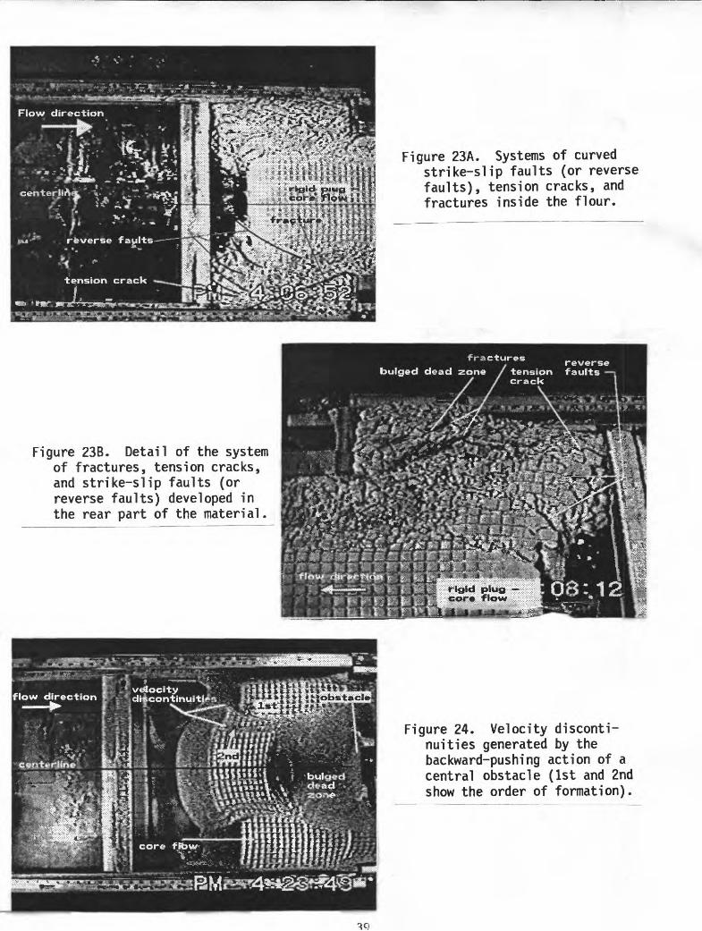
Figure 23A. Systems of curved strike-slip faults (or reverse faults), tension cracks, and fractures inside the flour.
Figure 23B. Detail of the system of fractures, tension cracks, and strike-slip faults (or reverse faults) developed in the rear part of the material.
rigid plug cor* flow
Figure 24. Velocity disconti nuities generated by the backward-pushing action of a central obstacle (1st and 2nd show the order of formation).
100%
90%
70%
--
50%
--
40%
--
30%
--
20%
--
10%
--
0%
N
C
HANN
EL
C
OMPA
CTED
D.Z.
O B
ULGE
D DE
AD Z
.
H L
EVEE
S
2.1F
2.1F
2.1S
2.2F
2.2S
3.1F
3.1F
EXTR
USIO
N RA
TIO -
THI
CKNE
SS
3.1S
3.2F
3.2S
Figure 2
5.
Bar
diag
ram
of t
he d
ata
obta
ined
from
the
mass
-bal
ance
analysis for
unconfined e
xperiments.
unconfined experiments. The results are given in Tables IV and V. Note the inverse relationship between the thickness of the material and the bulk density at the end of the confined experiments. In other words, for the confined test, the material in the thinner layer is more compacted.
The time duration is the time necessary for the same final material configuration to be reached in each similar experiment. This final configuration is obtained by stopping the experiments at a fixed distance from the obstacle. A distance of 8.5 in. (21.6 cm) has been chosen because it leaves the dead zones undisturbed. Considering the total time duration of each weighed experiment, we tried to obtain the discharge or the rate of growth of the dead zones and levees for different materials, extrusion ratios, and thicknesses (Tables VI and VII). In general, we notice a decrease in the duration of the experiment with increasing thickness. Further, we notice that for flour and sand, different relationships exist between the rate of growth of the dead zones, rate of growth of the levees, and the discharge of material passing through the channel (all measured in g/sec).
COMPARISON OF THE EXPERIMENTAL RESULTS WITH THEORETICAL SOLUTIONS
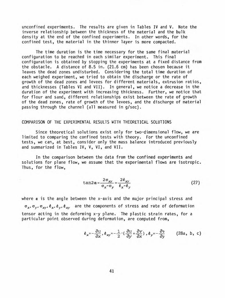
Since theoretical solutions exist only for two-dimensional flow, we are limited to comparing the confined tests with theory. For the unconfined tests, we can, at best, consider only the mass balance introduced previously and summarized in Tables IV, V, VI, and VII.
In the comparison between the data from the confined experiments and solutions for plane flow, we assume that the experimental flows are isotropic Thus, for the flow,
(27)
where a is the angle between the x-axis and the major principal stress and
ox , oy , o^,, tx , ty , t^ are the components of stress and rate of deformation
tensor acting in the deforming x-y plane. The plastic strain rates, for a particular point observed during deformation, are computed from,
b dy dx r y By , D,
41
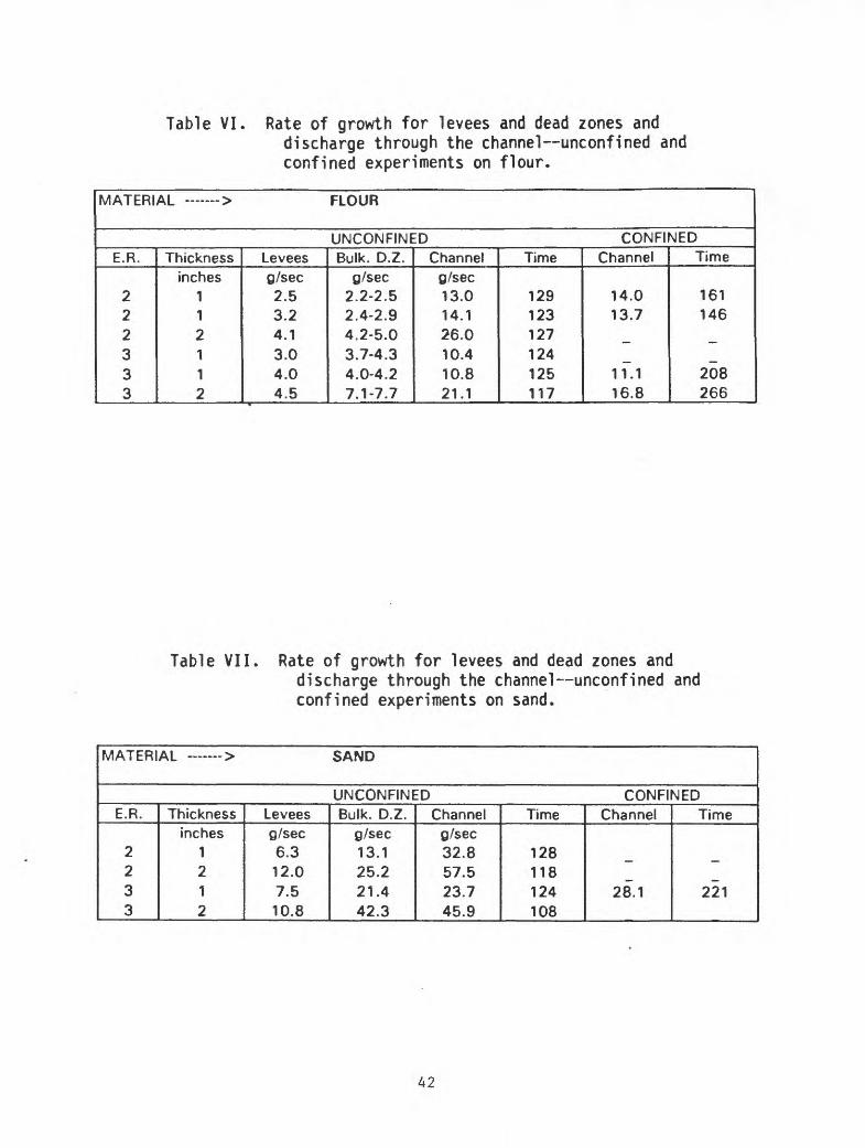
Table VI. Rate of growth for levees and dead zones anddischarge through the channel unconfined and confined experiments on flour.
MATERI Al >r^ ̂ ^ FLOUR
UNCONFINED CONFINEDE.R.
222333
Thicknessinches
112112
Leveesg/sec2.53.24.13.04.04.5
Bulk. D.Z.g/sec
2.2-2.52.4-2.94.2-5.03.7-4.34.0-4.27.1-7.7
Channelg/sec13.014.126.010.410.821.1
Time
129123127124125117
Channel
14.013.7
11.116.8
Time
161146
208266
Table VII. Rate of growth for levees and dead zones anddischarge through the channel unconfined and confined experiments on sand.
IVIAA 1 Cr\IAM_ -^ OAM1IU
UNCONFINED CONFINEDE.R.
2233
Thicknessinches
1212
Leveesg/sec6.312.07.510.8
Bulk. D.Z.g/sec13.125.221.442.3
Channelg/sec32.857.523.745.9
Time
128118124108
Channel
28.1
Time
221
where u and v represent the components of velocity acting in the x-y direction, respectively, while the z-components are all equal to zero as a consequence of the plane strain conditions. The negative signs are due to the adoption of the soil mechanics sign convention, considering compression and contraction as positive. Substituting the strain rate equations in the condition of isotropy gives:
tan2a= . (29).
This relationship shows that the velocity field, u = u(x,y) and v = v(x,y), and, hence the strain rate field obtained from the experiments can be used to reconstruct the field for the principal strain rate and stress directions. Additionally, we can obtain the sliplines since the sliplines are inclined at
an angle ^=±(JL--i) with respect to the major principal stress.~r £»
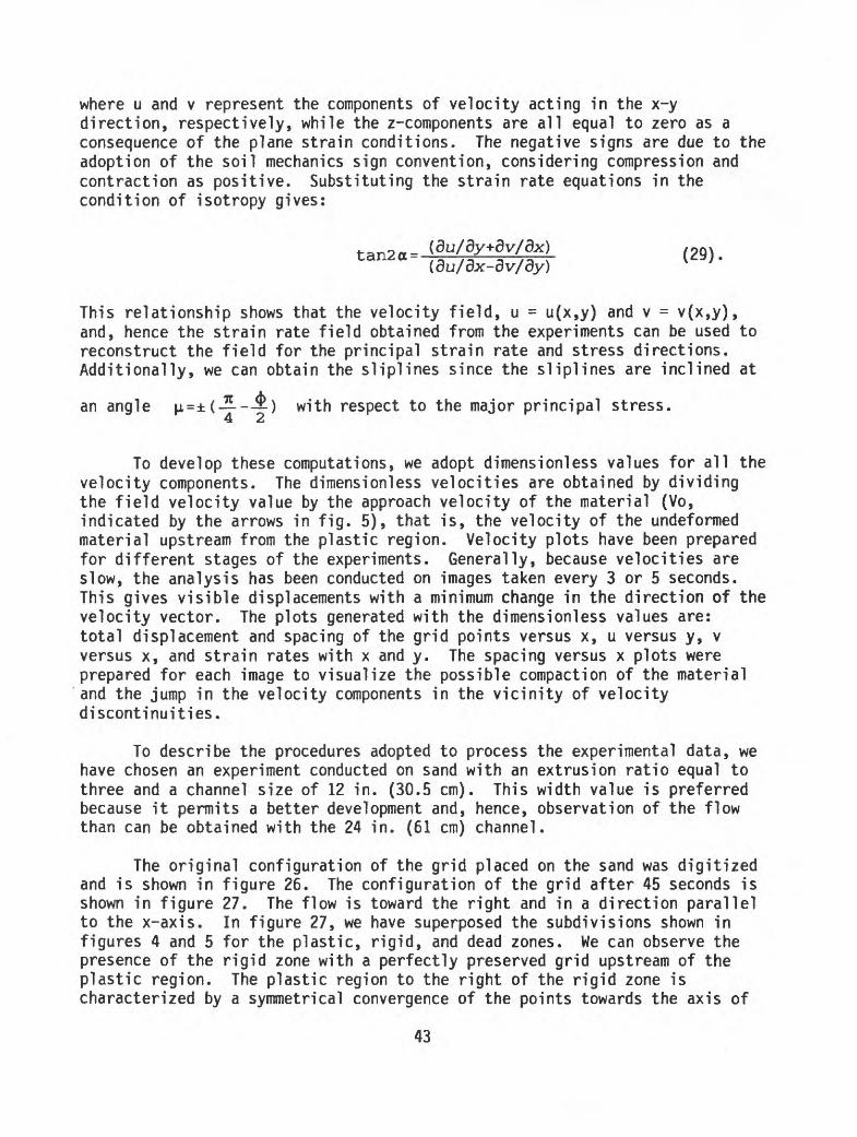
To develop these computations, we adopt dimensionless values for all the velocity components. The dimensionless velocities are obtained by dividing the field velocity value by the approach velocity of the material (Vo, indicated by the arrows in fig. 5), that is, the velocity of the undeformed material upstream from the plastic region. Velocity plots have been prepared for different stages of the experiments. Generally, because velocities are slow, the analysis has been conducted on images taken every 3 or 5 seconds. This gives visible displacements with a minimum change in the direction of the velocity vector. The plots generated with the dimensionless values are: total displacement and spacing of the grid points versus x, u versus y, v versus x, and strain rates with x and y. The spacing versus x plots were prepared for each image to visualize the possible compaction of the material and the jump in the velocity components in the vicinity of velocity discontinuities.
To describe the procedures adopted to process the experimental data, we have chosen an experiment conducted on sand with an extrusion ratio equal to three and a channel size of 12 in. (30.5 cm). This width value is preferred because it permits a better development and, hence, observation of the flow than can be obtained with the 24 in. (61 cm) channel.
The original configuration of the grid placed on the sand was digitized and is shown in figure 26. The configuration of the grid after 45 seconds is shown in figure 27. The flow is toward the right and in a direction parallel to the x-axis. In figure 27, we have superposed the subdivisions shown in figures 4 and 5 for the plastic, rigid, and dead zones. We can observe the presence of the rigid zone with a perfectly preserved grid upstream of the plastic region. The plastic region to the right of the rigid zone is characterized by a symmetrical convergence of the points towards the axis of
43
29.5
24.5
19.5
9.5
4.5
-0.5
10 20 30 40 50 60 70
X-axis (cm)
Figure 26. Equally spaced grid at the beginning of a sandexperiment. Extrusion ratio = 3. The spacing is equal to 0.75 in.(1.9 cm).
29.5
24.5
19.5
9.5
4.5
-0.5
10
41 «
JLJ
<» »
F1F
JLJ
n\
ft-lL
r*»
s
20 30 40
X-axis (cm)
50 60 70
Figure 27. Deformed grid after 45 sec. Extrusion ratio = 3. (Flow from left to right).
symmetry. Also in the figure, we can see shortening of distances between originally equally spaced points representing compaction and relative movement of points representing shearing along the lateral discontinuities.
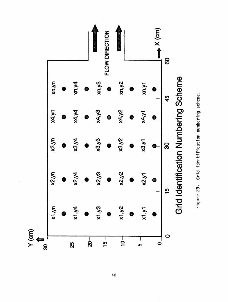
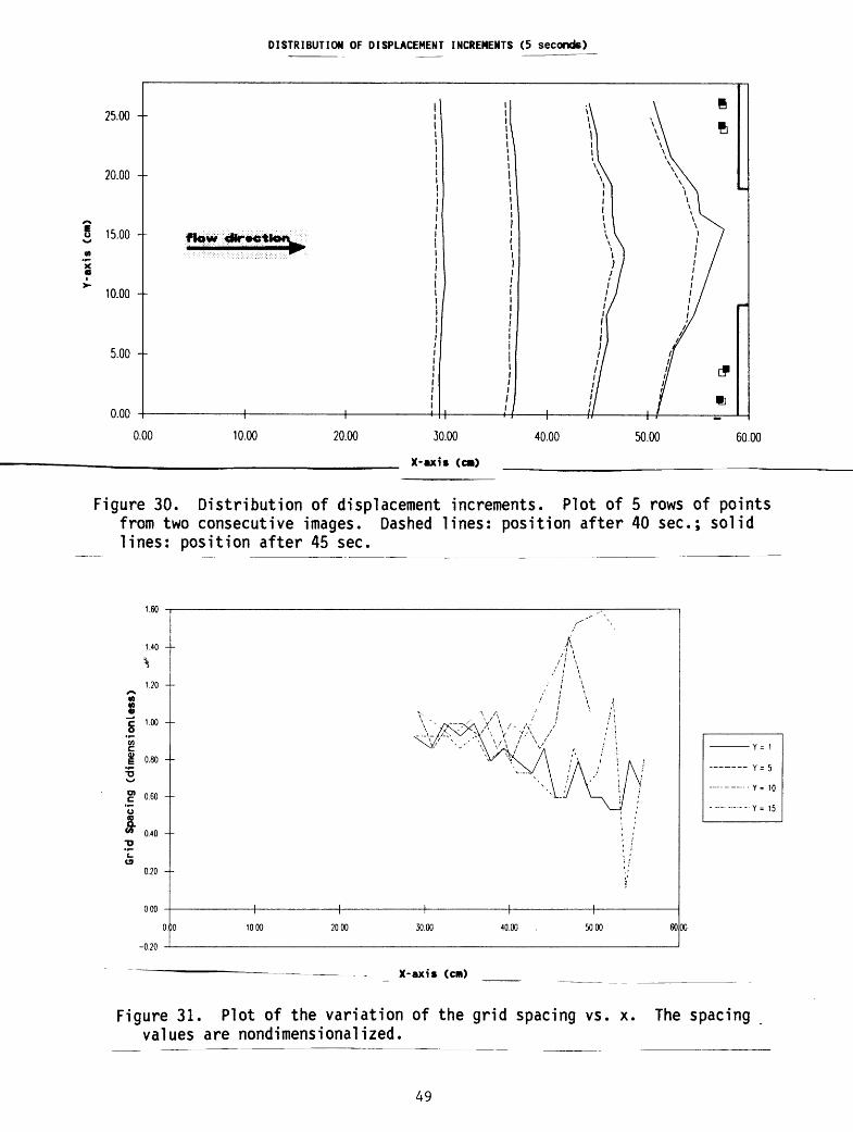
Streamlines inferred from the movement of points are shown in figure 28A and can be compared with the experimental streamlines obtained by Pariseau (1966) (fig. 28B). Figure 29 shows the way in which the different alignments of points in figures 26 and 27 are identified and numbered. The position of discontinuities and dead zones can also be inferred from the distribution of displacement increments shown in figure 30. The dashed lines in figure 30 represent the configuration of regularly spaced points at 40 seconds and the solid lines represent the configuration of the same points at 45 seconds after the start of the experiment. We notice the absence of motion in the dead zones (isolated points represented by solid and empty squares in fig. 30) and the increase in velocity after crossing each velocity discontinuity. This jump in the velocity is represented by small steps along the lines.
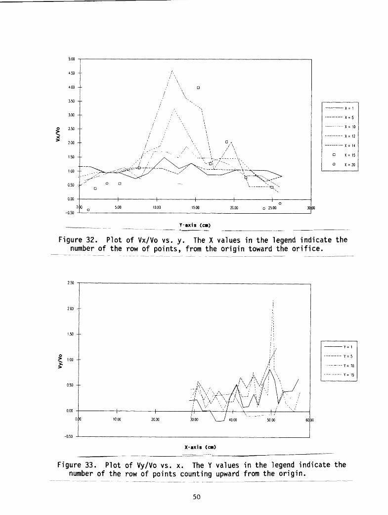
Figure 31 shows the change in spacing of the grid points in the x direction (parallel to the flow) for various rows of points in the y direction numbered according to figure 29. The spacing values are nondimensionalized with respect to the initial value of the grid spacing (0.75 in. or 1.9 cm). Knowing the displacement and the elapsed time, we can compute and plot the two dimensionless velocity components (Vx/Vo, Vy/Vo). As a consequence of such nondimensionalization, the velocity of the rigid part of the material upstream of the plastic zone is equal to one and in other regions is represented as multiples of this value. The various curves represented in figures 32 and 33 are the velocity components computed for various alignments of points numbered according to the convention shown in figure 29. The plots give us an idea of the increment in the velocity components as material moves toward the centerline and approaches the channel orifice.
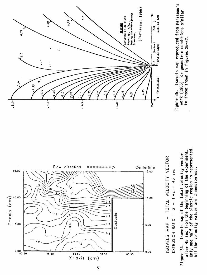
The velocity values can be compared with the values obtained by Pariseau on the basis of experimental results and theory (Pariseau, 1966). Pariseau conducted gravity flow experiments on the problem of ore pass movement, using a mixture of sand and magnetite (angle of internal friction = 34°). His experiments and ours have similar geometrical constraints. Figure 34 is an isovel map, of the total velocity vector, prepared from our experimental data at 45 seconds. Compare this with figure 35 taken from Pariseau. Note that figure 34 represents the left half and figure 35 the right half of the experimental velocity field in the outlet region. Also, note that figure 35 and subsequent figures we reproduce from Pariseau (1966) were considerably idealized by him. Our figures, on the other hand, have not been idealized, as the reader can gather.
45
Y(c
m)
30-
25 20 15 10-
Str
eam
lines
- A
fter 4
5 se
cond
s E
xtru
sion
rat
io =
3 (
San
d)
FLO
W D
IRE
CTI
ON
1530
X(cm)
4560
Figu
re 2
8A.
Stre
amli
nes
obtained f
rom
the
experiment s
hown in
fig
ures
26
and 2
7.
-U.o-
-3.C-1
-2.0-
-1.0-
0.0
STREAMLINESIn the Outlet Region During Drawdown.
(Pariseau, 1966)
x (c*nterline) ,w ' (inch*?)2iO fc(orifice edge)
Figure 28B. Experimental streamlines obtained by Pariseau for anexperiment with similar geometrical constraints (extrusion ratio = 3).
47
00
Y(c
m)
30
B
25 -
£.*
J 20
-
15-
10-
0
x1,y
n
x1,y
4
*
x1,y
3
* x1,y
2
© x1,y
1
©
x2,y
n
*
x2,y
4
x2,y
3
9
x2,y
2
©
x2,y
1
I
x3,y
n
*
x3,y
4
x3,y
3
9
x3,y
2 x3
,y1 f
x4,y
n xn
,yn
«A
V
x4,y
4 xn
,y4
x4,y
3 Xn
,y3
^^^
@
A
FLO
W D
IRE
CT
ION
x4,y
2 xn
,v2
Bi^
®|
©
A
x4,y
1 xn
,y1
©
( ©
__ ̂ y f/^rn
jB
M^ s
\ \\
sll\
0 15
30
45
60
Grid
Ide
ntifi
catio
n N
umbe
ring
Sch
eme
Figu
re 2
9.
Grid
id
enti
fica
tion
numbering s
cheme.
DISTRIBUTION OF DISPLACEMENT INCREMENTS (5 seconds)
25.00 --
20.00 --
15.00 --
10.00 --
5.00 --
0.00
0.00 10.00 20.00 30.00
X-axis (CM)
40.00 50.00 60.00
Figure 30. Distribution of displacement increments. Plot of 5 rows of points from two consecutive images. Dashed lines: position after 40 sec.; solid lines: position after 45 sec.
1.60
1.40
\
1.20 --^x
I 1 -°° -
I 0.80 -- 5
c 0.60 --u&"* 0.40 --
(90.20 --
000
-0.20
1000 2000 30.00 40.00 5000 6000
X-axis (cm)
Figure 31. Plot of the variation of the grid spacing vs. x values are nondimensionalized.
The spacing
49
X = 5
X= 10
X= 12
X= 14
X= 15
X = 20
3000-0.50
Y-axis (cm)
Figure 32. Plot of Vx/Vo vs. y. The X values in the legend indicate the number of the row of points, from the origin toward the orifice.
X-axis (cm)
Figure 33. Plot of Vy/Vo vs. x. The Y values in the legend indicate the number of the row of points counting upward from the origin.
50
Y-a
xis
(c
m)
ISO
VE
LS
M
AP
-
TO
TA
L
VE
LO
CIT
Y
VE
CT
OR
EX
TR
US
ION
R
ATI
O
=
3 -
TIM
E
=
45
se
c
Fig
ure
34
. Is
ove
ls
map
of
the to
tal
ve
locity ve
ctor
aft
er
45
sec
from
the
begin
nin
g o
f th
e
expe
rimen
t. O
nly
one
ha
lf o
f th
e pla
stic
regio
n
is
repr
esen
ted
All
the ve
locity
valu
es
are
dim
en
sio
nle
ss.
u.o
-
-3.0
-
- 2
.0-
- 1.0
-
0.0
-
ISO
VEL
3 C
onto
urs
of
Rel
ativ
eV
eloci
ty,
V/V
0 ,
Dur
ing
St*p
-«*i
c«t$
t«fc
4j
Dra
wdo
wn.
z (c
»nU
rlin
«)
(Pariseau, 1966)
(will
at 3
.0)
Figu
re 3
5.
Isov
els
map
repr
oduc
ed f
rom
Pari
seau
's
work (1
966)
fo
r ge
omet
ric
cond
itio
ns s
imil
ar
to t
hose
sho
wn in
figures 2
6-32
.
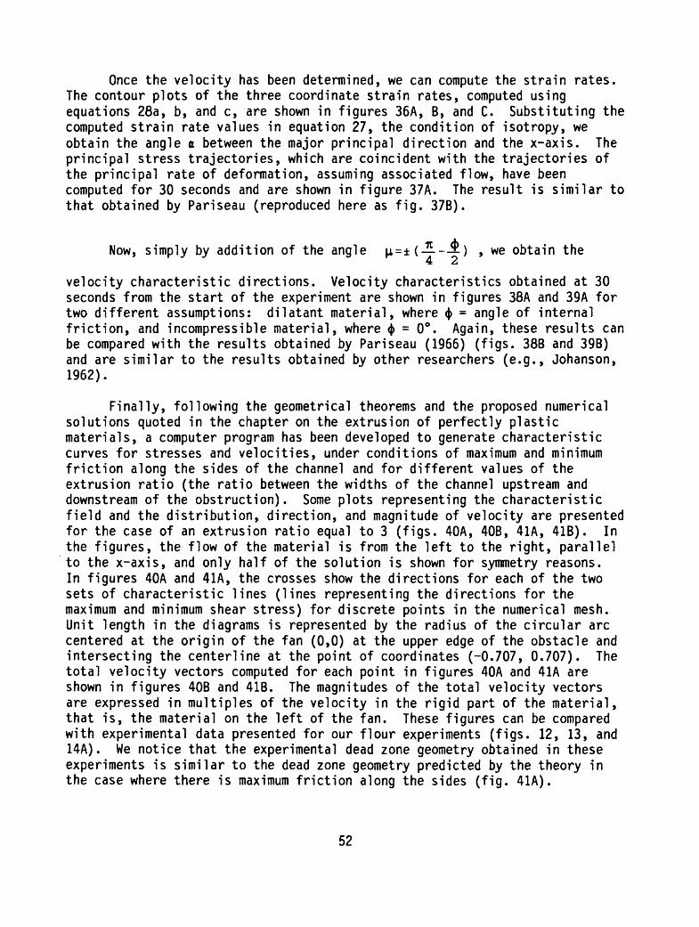
Once the velocity has been determined, we can compute the strain rates. The contour plots of the three coordinate strain rates, computed using equations 28a, b, and c, are shown in figures 36A, B, and C. Substituting the computed strain rate values in equation 27, the condition of isotropy, we obtain the angle a between the major principal direction and the x-axis. The principal stress trajectories, which are coincident with the trajectories of the principal rate of deformation, assuming associated flow, have been computed for 30 seconds and are shown in figure 37A. The result is similar to that obtained by Pariseau (reproduced here as fig. 37B).
Now, simply by addition of the angle |i=± (JL--i) , we obtain the4 2
velocity characteristic directions. Velocity characteristics obtained at 30 seconds from the start of the experiment are shown in figures 38A and 39A for two different assumptions: dilatant material, where <)> = angle of internal friction, and incompressible material, where <)> = 0°. Again, these results can be compared with the results obtained by Pariseau (1966) (figs. 38B and 39B) and are similar to the results obtained by other researchers (e.g., Johanson, 1962).
Finally, following the geometrical theorems and the proposed numerical solutions quoted in the chapter on the extrusion of perfectly plastic materials, a computer program has been developed to generate characteristic curves for stresses and velocities, under conditions of maximum and minimum friction along the sides of the channel and for different values of the extrusion ratio (the ratio between the widths of the channel upstream and downstream of the obstruction). Some plots representing the characteristic field and the distribution, direction, and magnitude of velocity are presented for the case of an extrusion ratio equal to 3 (figs. 40A, 40B, 41A, 41B). In the figures, the flow of the material is from the left to the right, parallel to the x-axis, and only half of the solution is shown for symmetry reasons. In figures 40A and 41A, the crosses show the directions for each of the two sets of characteristic lines (lines representing the directions for the maximum and minimum shear stress) for discrete points in the numerical mesh. Unit length in the diagrams is represented by the radius of the circular arc centered at the origin of the fan (0,0) at the upper edge of the obstacle and intersecting the center!ine at the point of coordinates (-0.707, 0.707). The total velocity vectors computed for each point in figures 40A and 41A are shown in figures 40B and 41B. The magnitudes of the total velocity vectors are expressed in multiples of the velocity in the rigid part of the material, that is, the material on the left of the fan. These figures can be compared with experimental data presented for our flour experiments (figs. 12, 13, and 14A). We notice that the experimental dead zone geometry obtained in these experiments is similar to the dead zone geometry predicted by the theory in the case where there is maximum friction along the sides (fig. 41A).
52
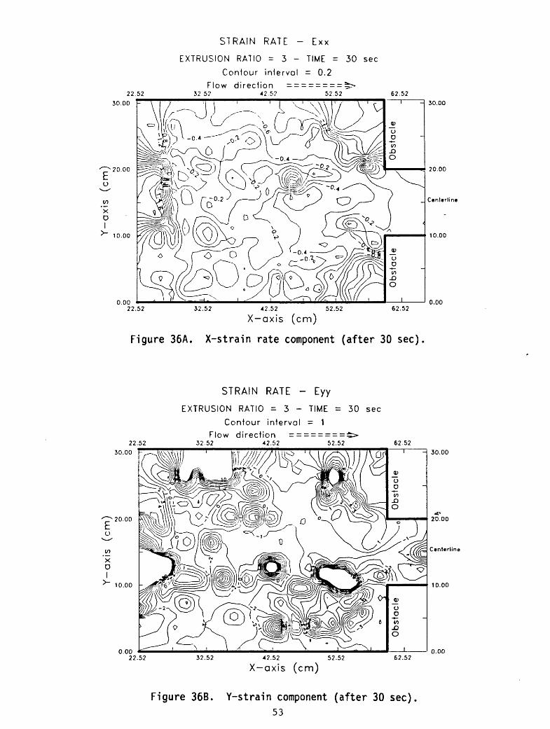
STRAIN RATE - Exx
EXTRUSION RATIO = 3 - TIME = 30 sec
Contour interval = 0.2
22.52
30.00 -
Flow direction32 5? 42.5? 52.52 62.52
20.00
10.00
- 30.00
20.00
_ Centerline
10.00
0.0022.52 32.52 42.52 52.52
X axis (cm)62.52
Figure 36A. X-strain rate component (after 30 sec)
STRAIN RATE - Eyy
EXTRUSION RATIO = 3 - TIME = 30 sec
Contour interval = 1
22.52
30.00 -
Flow direction32.52 42.52 52.52 62.52
- 30.00
20.00
10.00 -
0.00
Cenierline
10.00
22.52 32.52 42.52 52.52
X-axis (cm)62.52
0.00
Figure 36B. Y-strain component (after 30 sec).53

ST
RA
IN
RA
TE -
Exy
EX
TR
US
ION
R
ATI
O
=
3 -
TIM
E
=
30
sec
Co
nto
ur
inte
rval
=
1F
low
d
ire
cti
on
=
= =
= =
= =
=32
.52
42.5
2 52
.52
62.5
2
0.0
0
^
30.0
0
20.0
0
Cen
terl
ine
10
.00
0.0
022
.52
32.5
242
.52
52.5
2
X-a
xis
(c
m)
62.5
2
Figure 3
6C.
XY-shear s
train
components (after 3
0 se
c).
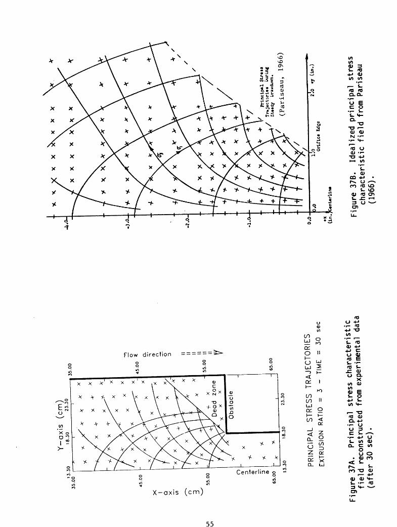
Y-a
xis
(c
m)
13
.30
1
8.3
0
23.3
035.0
035
.00
45.0
0
X I a x
55
.00
65.0
0
13
.30
18.3
0 23
.30
PR
INC
IPA
L
ST
RE
SS
T
RA
JEC
TO
RIE
S
EX
TRU
SIO
N
RAT
IO
= 3
- TI
ME
=
30
sec
Figure 3
7A.
Prin
cipa
l st
ress
cha
ract
eris
tic
field
reconstr
ucte
d fr
om e
xperimen
tal
data
(a
fter 3
0 se
c).
Pri
nci
pal
Str
ts»
Lur
ing
/
Trfcjecta
Sttidy
L
(Pariseau, 1966)
2lo
Ort
fict
Ld
gc
K«ntt
rlin
«
Figu
re 3
7B.
Idealized
prin
cipa
l stress
charac
teri
stic
field f
rom
Pari
seau
(1966).
Y-a
xis
(c
m)
18.3
0 23
. JO
35.0
0
- 4
5.0
0
55
.00
65.0
0
- .30
- 6
5.0
0
18.3
023
.30
VE
LO
CIT
Y
CH
AR
AC
TE
RIS
TIC
S
EX
TR
US
ION
R
ATI
O
=
3 -
TIM
E
=
30
sec
Phi
=
0
degre
es
Figu
re 3
8A.
Velo
city
field
reconstructed
from
exp
erim
enta
l da
ta (after 3
0 se
c)
for
<J> =
0°.
An
lrp
«rl
»«
nt«
l N
etw
ork
ot
Ort
hofo
ul
Vel
oci
ty C
hara
cte
rist
ic!
Dur
ing
£t«*
djr
Dra
wdo
wn.
-1.0
0.0
Figure 3
8B.
Idea
lize
d ve
loci
ty f
ield
fr
om P
aris
eau
(196
6) for
<J> =
0°.
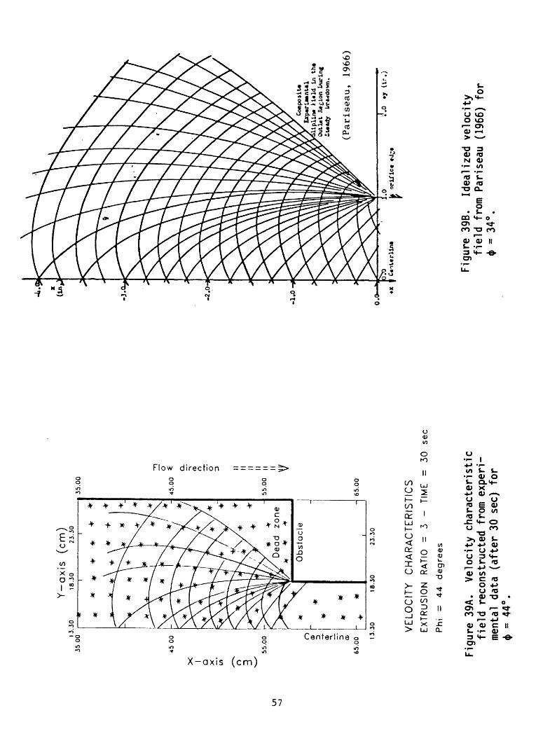
Ui
Y-a
xis
(c
m)
13.3
0 18
.30
23.3
0 35
.00
, *
r
45 0
0
55
.00
35.0
0
45
.00
0.
- 55.00
65.0
0
-
13.3
0
- 65.00
18
.30
23
.30
VE
LO
CIT
Y
CH
AR
AC
TE
RIS
TIC
S
EX
TRU
SIO
N
RAT
IO
= 3
- TI
ME
=
30
sec
Phi
=
44
degre
es
Figu
re 3
9A.
Velocity c
haracteristic
fiel
d re
cons
truc
ted
from
experi
mental
da
ta (a
fter
30
sec)
for
> =
44°.
-1.0
llpli
iw
>i«
ld
in
th«
Out
let
Reg
ion
Lru
ring
U
raw
dow
n.
(ir.)
Figure 3
9B.
Idealized
velo
city
fiel
d fr
om P
ariseau
(196
6) for
+ =
34°.
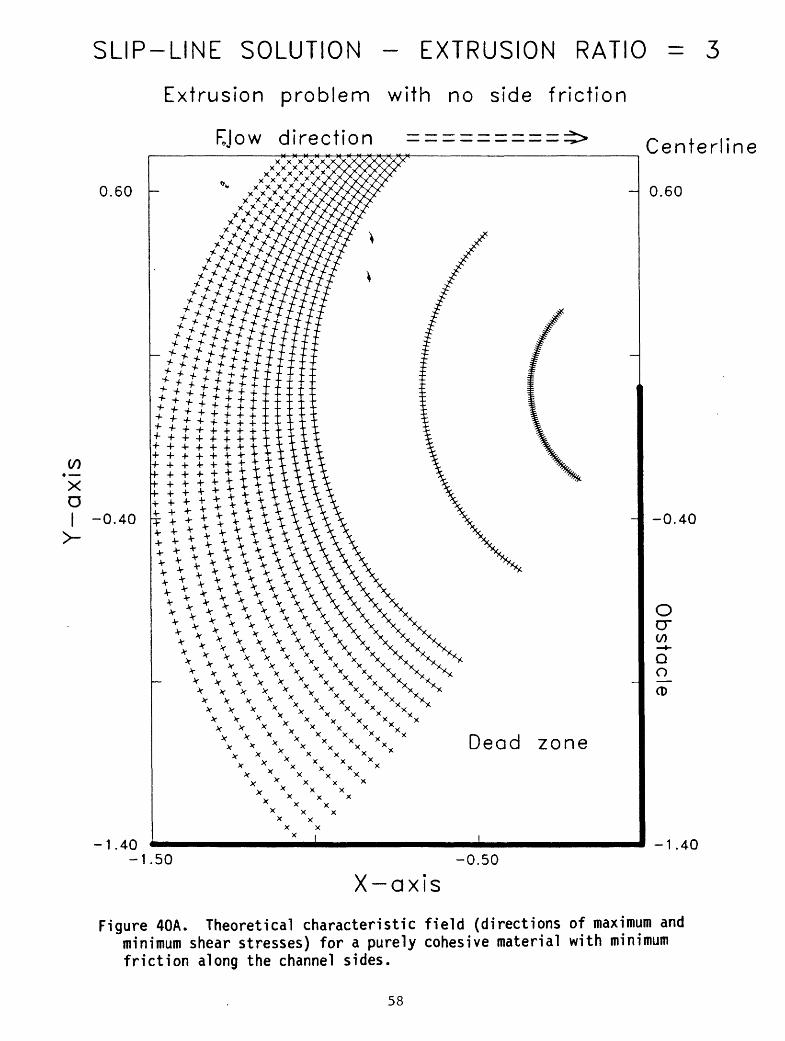
SLIP-LINE SOLUTION EXTRUSION RATIO = 3
Extrusion problem with no side friction
fvjow direction
0.60 -
XD| -0.40
-1.40 -1.40-1.50 -0.50
X-axis
Figure 40A. Theoretical characteristic field (directions of maximum and minimum shear stresses) for a purely cohesive material with minimum friction along the channel sides.
58
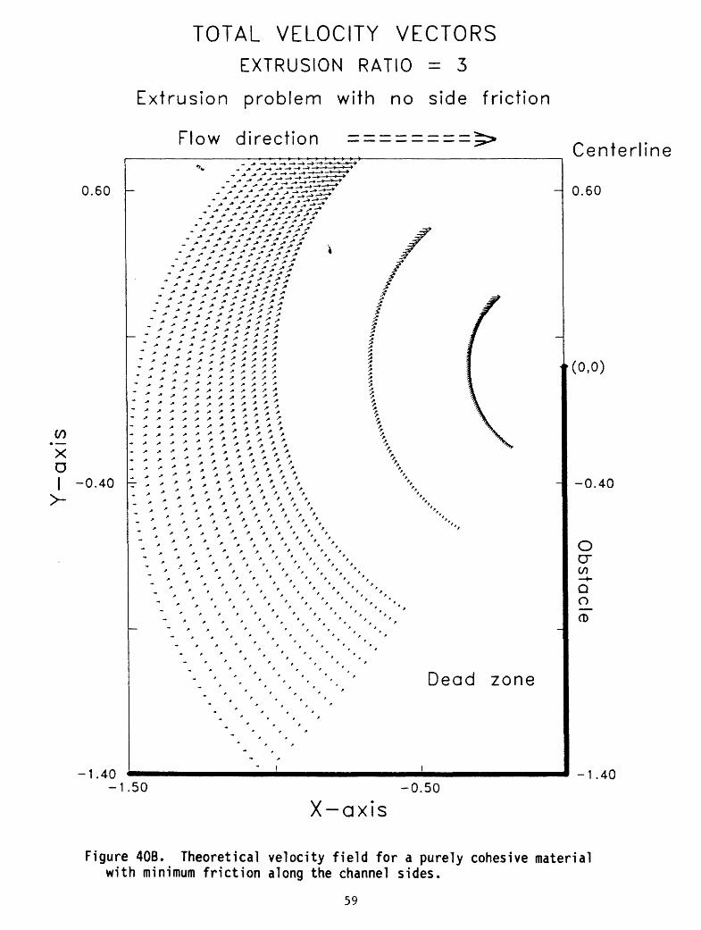
TOTAL VELOCITY VECTORSEXTRUSION RATIO = 3
Extrusion problem with no side friction
Flow direction = = = = = = = =
0.60
00
XO| -0.40
-1.40
- **<':*;*;*;7,' :; -///// "'"''"''i'
f r / '
Dead zone
-1.50 -0.50
X-axis
Centerline
0.60
(0,0)
-0.40
OcrCOQ~
O
-1.40
Figure 40B. Theoretical velocity field for a purely cohesive material with minimum friction along the channel sides.
59

SL
IP-L
INE
S
OLU
TIO
N -
EX
TR
US
ION
R
ATI
O
=
3
CO X D
Extr
usio
n
pro
ble
m
with
m
axim
um
si
de
fr
iction
Flo
w
direction
= =
= =
= =
0.6
0
-
Ce
nte
rlin
e
0.60
-0.4
0
-
1.4
0 -3
- -0
.40
-1.4
00
5-2
.05
-1.0
5 0
.05
X-a
xis
Figu
re 4
1A.
Th
eore
tica
l ch
arac
teri
stic
fi
eld
(d
irec
tio
ns
of
max
imum
and
m
inim
um s
hear
str
esse
s)
for
a pu
rely
coh
esiv
e m
ater
ial
with
max
imum
fr
icti
on
al
ong
the
chan
nel
side
s.
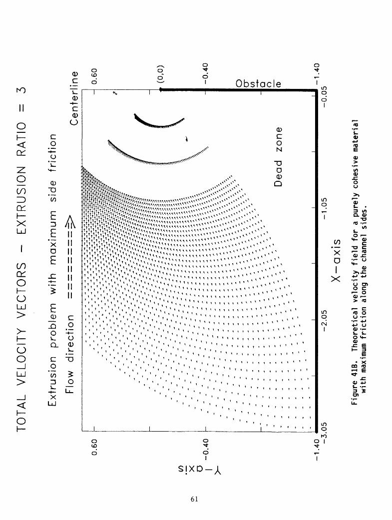
TO
TA
L V
ELO
CIT
Y
VE
CT
OR
S -
EX
TR
US
ION
R
ATI
O
=
3
0.6
0
X D-0
.40
-1.4
0 -3.0
5
Extr
usio
n
pro
ble
m
with
m
axim
um
si
de
fric
tion
Flo
w
direction
===
= =
Ce
nte
rlin
e
Dead
zon
e
-2.0
51.0
5
X-a
xis
0.60
(0,0
)
-0.40
O cr CO o"
o_ CD" -1.4
0-0
.05
Figure 4
1B.
Theoretical
velocity f
ield
for
a p
urel
y co
hesi
ve m
ater
ial
with
max
imum f
riction
along
the
chan
nel
side
s.
DISCUSSION OF APPLICABILITY OF THE PLASTICITY SOLUTIONS
In modeling the flow, we have assumed homogeneity and isotropy of material and unbreakability of the grains. Most importantly, we have assumed that principal strain rate and principal stress axes are coincident during flow. We have seen that this gives good agreement between experimentally and theoretically determined principal stress orientations (figs. 37A and B).
Since we have assumed an associated flow rule, we expect that the volume of the deforming material will increase during confined flow when 4> > 0 (Savage and Smith, 1986). However, we have seen that the thickness of shear zones remain constant for the duration of our experiments. In addition, our velocity field for sand shown in figure 34 is comparable to the velocity field from Pariseau for a similar material (fig. 35). Also, our experimental streamline field in figure 28A and Pariseau 's experimental streamline field in figure 28B are comparable. Pariseau (1966) and Pariseau and Pfleider (1969) found a disagreement between the theoretical velocity and streamline field, computed using the angle of internal friction of the material, and their experimental velocity field and streamlines. Repeating the computation using a value of internal friction of zero, the incompressibility condition, they found better agreement between the theoretical and experimental velocity and streamline fields. Since figures 28A (for streamlines), 34 (for velocities for our sand experiment), 28B (for streamlines), and 35 (for velocities from Pariseau) are similar, we can infer that our experimental velocity data should be modeled by taking 4> = angle of internal friction to be zero. Indeed, although a detailed comparison has not yet been made between velocities obtained from the flour experiments and the theoretical extrusion velocities for a perfectly plastic material, we do see similarities even though the flour angle of friction average is 12°.
Experimentally, as in the experiments described above, it has been observed that all materials, after contraction or dilatation during the initial phases of deformation, depending on the original density, approach a critical state during which deformation occurs at constant volume (cv) (Castro, 1969; Poulos, 1981). For this reason, Houlsby and Wroth (1980) assume that intensely sheared zones and adjacent rigid zones have different
properties. They take $=$peak ,v*Q in the rigid zones
and ^Hw^ea*' v=0 tne intensely sheared zones where v is the angle of
dilatation. As mentioned above, Pariseau (1966) arrived at a similar solution by reconstructing the stress and velocity fields from experimental data and concluded that the best approximation of such data through the theory is obtained using a value of 4> = 0.
62
Another consequence of using an associated flow rule and, hence, coaxiality of principal directions of strain rate and stress (Pollaczek- Geiringer, 1930; Shield, 1953, 1954; Davis, 1968; Roscoe, 1970) is that a velocity discontinuity may only occur on a velocity characteristic. This means that no extension can occur along a velocity discontinuity. Houlsby and Wroth (1980) present a classification of kinematic discontinuities and discuss the inextensibility requirement. They prove that the inextensibility requirement for a velocity discontinuity, in its direction of development, is unnecessary. An important example where the strain discontinuity must be considered inextensional, in order to satisfy the compatibility requirements, is the case for contact with a rigid zone or a dead zone (region of no movement and deformation). Previous authors derived this inextensibility condition, applied at any velocity discontinuity, on the bases of various and often invalid assumptions. For example, Prager and Hodge (1951) assumed that the velocity variations along the discontinuity must be negligible as compared to those across it. In this way, Prager and Hodge (1951) neglect the fact that the presence of velocity gradients inside discontinuities will cause the deviation of the velocity discontinuities from the characteristics.
In any ideal plastic analysis, the approach is the same as the approach used for a limit analysis and, as a consequence, the material is considered to be everywhere at yield at the same instant. As we have seen from describing the experiments, this behavior is improbable. It is more probable that only some portions of the material will reach the failure condition contemporaneously and, for a certain interval of time, growth of the plastic region will occur in a quasi-static manner with negligible accelerations up to a condition of steady state. Furthermore, even if the material behaves like a plastic material, the theory does not insure that all the sliplines will be activated. What is actually observed during the experiments is the development of only some velocity discontinuities due to the activation of a small number of sliplines. This situation can be compared and perhaps analyzed by the theory of formation of shear bands for frictional materials (Rudnicki and Rice, 1975; Molenkamp, 1985). In fact, physically, the real situation is one in which some rigid parts slide relative to each other because of the presence of these few velocity discontinuities (De Jong, 1959; Pariseau, 1966; Drescher, 1976; Drescher et al., 1978).
CONCLUSIONS
We have seen that there are qualitative similarities between the confined experiments and plane plastic flow of bulk materials. These similarities are seen in the development of the theoretically predicted regions A and B (the regions of plastic flow) and the development of region C (the rigid plug) in channel flow (figs. 4 and 5). Of course, these observed similarities are limited to velocities, velocity discontinuities, and deformations, since we did not measure stresses inside the materials.
63
Certain aspects of the experimental confined flow are exactly predicted by the theory. For example, the boundary between regions B and C; the rigid plug boundary is 45° for flour and 60°-65° for sand. Also, the observed orientations of the shear zones which form the boundary between the dead zones and the plastic fan in channel flow are those predicted by the theory. For the flour, this boundary is curved and becomes tangent upstream with the channel sides. This behavior is predicted for extrusion flow of a cohesive plastic material in the case where the walls of the channel are frictional (figs. 41A and 41B; Thomsen et al., 1966). Another important feature is the formation of compacted, sheared, and rigid dead zones in the confined experiments.
Also, for sand and flour, the experimentally determined velocities are in qualitative agreement with those determined theoretically. For the flour, the velocities are similar to those determined by the solution for extrusion of cohesive materials through a narrowing channel. For the sand, the experimental velocities compare with those computed by Pariseau (1966) using classical plasticity theory for frictional materials and adopting the incompressibility condition.
For the unconfined flow, many of the features observed have natural analogues. Some, such as the zones of vanishing deformation (dead zones), which form near obstacles, lateral levees, and the movement of central parts of landslides as rigid regions bounded by shear zones, have been reported in the landslide literature (Fleming and Johnson, 1989; Crandell and Varnes, 1961). Many of these features have also been observed for glaciers (Nye, 1951, 1957, 1973; Coll ins, 1970).
We have also observed features in the experiments that presumably have natural analogues but have yet to be observed in the field. For example, the evolution of features such as the main lateral discontinuities (figs. 8A, 8B, and 8C), the development of faulting within the dead zones (fig. 19), and rates of levee growth (Tables VI and VII) in natural mass movements should be measured and compared with the experimental data.
Finally, certain refinements should be considered in future experimental and theoretical work. For example, load cells should be incorporated for direct measurement of pressure along the sides of the channel and in the front of the obstacles. A finer grid should be used for better resolution of velocities and a mechanical deposition technique should be used to obtain a more uniform starting density for the material used in the experiments. Also, methods should be developed to reduce effects of compaction during the experiments and to accomplish continuous feeding of the material during the experiments. This last refinement would eliminate the effects of the free surface at the rear of the model and allow experiments of greater duration to be conducted. Theoretical refinements should include the development and application of constitutive equations, which properly describe the
64
relationships between stress and strain rate as well as the development of discrete zones of shear and attendant phenomena within the deforming material.
REFERENCES
Abbott, M.B., 1966, An introduction to the method of characteristics: New York, American Elsevier, 243 p.
Airey, W., 1897, Theory of silos: London, Institution of Civil Engineers, Minutes of Proceedings, v. 31, p. 347-358.
Bray, J.W., and Goodman, R.E., 1981, The theory of base friction models: International Journal for Rock Mechanics and Mining Science, v. 18, p. 453-468.
Bruckl, E., and Scheidegger, A.E., 1973, Application of the theory ofplasticity to slow mud flows: Geotechnique, v. 23, no. 1, p. 101-107.
Caquot, A., 1957, La pression dans les silos in Proceedings, 4th International Conference on Soil Mechanics and Foundation Engineering, London: Butterworths Scientific Publications, 1958 eds., vol. Ill, p. 191-195.
Castro, G., 1969, Liquefaction of sands: Cambridge, Massachusetts, Harvard University, Harvard Soil Mechanics Series No. 81, January 1969, 112 p.
Collins, I.F., 1970, A slip-line field analysis of the deformation at theconfluence of two glacier streams: Journal of Glaciology, v. 9, no. 56, p. 169-193.
Courant, R., and Friedrichs, K., 1948, Supersonic flow and shock waves: New York, Interscience.
Crandell, D.R., and Varnes, D.J., 1961, Movement of the Slumgullion earthflow near Lake City, Colorado: U.S. Geological Survey Professional Paper 424-B, paper 57, p. B136-B139.
Crans, W., and Mandl, G., 1981, On the theory of growth faulting; Pt. lib, Genesis of the "unit": Journal of Petroleum Geology, v. 3, no. 3, p. 333-355.
Davis, E.H., 1968, Theories of plasticity and failure of soil masses, in Lee, I.K., ed., Soil Mechanics Selected Topics: London, Butterworths, p. 341-380.
65
De Jong, G. de Josselin, 1959, Statics and kinematics in the failable zone of a granular material: Delft, Amsterdam, Uitgenerij Waltman, Ph.D. thesis, 119 p.
Deutsch, G.P., and Clyde, D.H., 1967, Flow and pressure of granular materials in silos: Proceedings of the American Society of Civil Engineers, Journal of Engineering Mechanics Division, v. 93, p. 103-125.
Drescher, A., 1976, An experimental investigation of flow rules for granular materials using optically sensitive glass particles: Geotechnique, v. 26, no. 4, p. 591-601.
Drescher, A., Cousens, T.W., and Bransby, P.L., 1978, Kinematics of the mass flow of granular material through a plane hopper: Geotechnique, v. 28, no. 1, p. 27-42.
Drucker, D.C., and Prager, W., 1952, Soil mechanics and plastic analysis or limit design: Quarterly of Applied Mathematics, v. 10, no. 2, p. 157-165.
Egger, P., 1979, A new development in the base friction technique:Proceedings, Symposium on Physical-Geomechanical Models, ISMES, Bergamo, Italy.
Fleming, R.W., and Johnson, A.M., 1989, Structures associated with strike-slip faults that bound landslide elements: Engineering Geology, v. 27, p. 39-114.
Geniev, G.A., 1958, Questions on the dynamics of granular media (in Russian): Moscow, Akad. Str. Arch.
Hill, R., 1950, The mathematical theory of plasticity: Oxford University Press, 355 p.
Hoek, E., 1971, Rock Engineering (Inaugural lecture): London, Imperial College, Univsity of London.
Houlsby, G.T., and Wroth, C.P., 1980, Strain and displacement discontinuities in soil: Journal of Engineering Mechanics Division, v. 106, p. 753-771.
Hubbert, M.K., 1951, Mechanical basis for certain familiar geologicalstructures: Geological Society of America Bulletin, v. 62, p. 355.
Janelid, I., and Kvapil, R., 1966, Sublevel caving: International Journal for Rock Mechanics and Mining Sciences, v. 3, p. 129-153.
66
Janssen, H.A., 1895, On the pressure of grain in silos: Institute of Civil Engineers, v. 124, p. 553-555.
Jenike, A.M., 1955, How to keep solids flowing in bins and hoppers: Engineering and Mining Journal, v. 156, no. 3a, p. 83-85.
Jenike, A.M., and Shield, R.T., 1959, On the plastic flow of Coulomb solids beyond original failure: Journal of Applied Mechanics, v. 27, p. 599- 602.
Johanson, J.R., 1962, Stress and velocity fields in gravity flow of bulk solids: University of Utah, 170 p.
Kvapil, R., 1965, Gravity flow of granular materials in hoppers and bins:International Journal for Rock Mechanics and Mining Sciences, v. 2, p. 25-41, p. 277-304.
Ladanyi, B., and Hoyaux, B., 1969, A study of trap door problems in a granular mass: Canadian Geotechnical Journal, v. 6, p. 1-15.
Li Yenge, I., 1980, Analysis of bulk flow of materials under gravity caving process. Part I: Sublevel caving in relation to flow in bins and bunkers: Colorado School of Mines Quarterly, Vol. 75, October 1980, no. 4, 45 p.
Mandl, G., and Fernandez-Luque, R., 1970, Fully developed plastic shear flow of granular materials: Geotechnique, v. 20, no. 3, p. 277-307.
Meyerhof, G.G., 1951, The ultimate bearing capacity of foundations: Geotechnique, v. 2, p. 301-332.
Meyerhof, G.G., 1959, Compaction of sands and bearing capacity of piles: Proceedings, American Society of Civil Engineers, Journal of Soil Mechanics Foundations Division, v. 85, SM6, p. 1-29.
Molenkamp, F., 1985, Comparison of frictional material models with respect to shear band initiation: Geotechnique, v. 35, no. 2, p. 127-143.
Nye, J.F., 1951, The flow of glaciers and ice-sheets as a problem inplasticity: Proceedings, Royal Society, Series A, v. 207, no. 1091, p. 554-572.
Nye, J.F., 1957, The distribution of stress and velocity in glaciers and ice- sheets: Proceedings, Royal Society, Series A, v. 239, no. 1216, p. 113-133.
67
Nye, J.F., 1973, The motion of ice past obstacles, in Whalley, E., Jones, S.J., and Gold, L.W., eds., Physics and chemistry of ice: Ottawa, Canada, Royal Society of Canada, p. 387-394.
O'Callaghan, J.R., 1960, Internal flow in moving beds of granular material: Journal of Agricultural Engineering Research, no. 5, p. 200-217.
Ode, H., 1960, Faulting as a velocity discontinuity in plastic deformation, in Griggs, D., and Handin, J., eds., Rock Deformation: Journal, Geologic Society of America, Memoir 79, p. 293-321.
Pariseau, W.G., 1966, The gravity induced movement of materials in ore passes analyzed as a problem in Coulomb plasticity: University of Minnesota, Ph.D. thesis, 218 p.
Pariseau, W.G., and Pfleider, E.P., 1969, Soil plasticity and the movement of material in ore passes: ASME Transactions, p. 42-56.
Pollaczek-Geiringer, v.H., 1930, Beitrag zum vollstandigen ebenenplastizitatsproblem: 3rd International Congress of Applied Mechanics, Stockholm, Sweden, v. 2, p. 185-190.
Poulos, S.J., 1981, The steady state of deformation: Proceedings, American Society of Civil Engineers, Journal of Geotechnical Engineering Division, v. 107, p. 553-562.
Prager, W., and Hodge, P.G., 1951, Theory of perfectly plastic solids: New York, Dover Publics., 264 p.
Reimbert, M., and Reimbert, A., 1976, Silos: Theory and Practice, Trans Tech Publications, 1st Ed., 239 p.
Roscoe, K.H., 1970, The influence of strains in soil mechanics: Geotechnique, v. 20, no. 2, p. 129-170. (Tenth Rankine Lecture)
Roscoe K.H, Schofield, A.M., and Thurairajah, A., 1963, Yielding of clays in states wetter then critical: Geotechnique, v. 13, no. 3, p. 211-240.
Rowe, P.M., 1962, The stress dilatancy relation for static equilibrium on an assembly of particles in contact: Proceedings, Royal Society, Series A, v. 269, p. 500-567.
Rudnicki, J.W., and Rice, J.R., 1975, Conditions for the localization of deformation in pressure-sensitive dilatant materials: Journal of Mechanics and Physics Solids, v. 23, p. 371-394.
68
Sanford, A.R., 1959, Analytical and experimental study of simple geologic structures: Geologic Society of America Bulletin, v. 70, p. 19-52.
Savage, W.Z., and Smith, W.K., 1986, A model for the plastic flow oflandslides: U.S. Geological Survey Professional Paper 1385, 32 p.
Schofield, A.N., and Wroth, L.P., 1968, Critical state soil mechanics: London, McGraw-Hill, 310 p.
Shield, R.T., 1953, Mixed boundary value problems in soil mechanics: Quarterly of Applied Mathematics, v. 11, p. 61-75.
Shield, R.T., 1954, Stress and velocity fields in soil mechanics: Journal of Mathematics and Physics, v. XXXIII, no. 2, p. 144-156.
Sokolovski, V.V., 1960, Statics of soil media: London, Butterworths Scientific Publications.
Spencer, A.J.M., 1964, A theory of the kinematics of ideal soils under plain strain conditions: Journal of Mechanics and Physics Solids, v. 12, p. 337-351.
Sylwestrowicz, W., 1953, Experimental investigation of the behavior of soil under a punch or footing: Journal of Mechanics and Physics Solids, v. 1, p. 258-264.
Szczepinski, W., 1972, On the motion of flat landslides and avalanches treated as a problem in plasticity: Warsaw, Architectural Mechanics Stosowonej, v. 24, no. 5-6, p. 919-930.
Thomsen, E.G., Yang, C.T., and Kobayashi, S., 1966, Mechanics of plasticdeformation in metal processing: New York, The MacMillan Co., 485 p.
Vesic, A.S., 1967, Ultimate loads and settlements of deep foundations in sands: Symposium on Bearing Capacity and Settlement of Foundations, Duke University, Durham, North Carolina, 1965, p. 53-68.
69