Institutionen för systemteknikDepartment of Electrical Engineering

Examensarbete

Performance of Cooperative Relay Protocols overan Audio Channel

Examensarbete utfört i Kommunikationssytemvid Tekniska högskolan i Linköping

av

Thomas Wärme

LiTH-ISY-EX--09/4267--SE

Linköping 2009

Department of Electrical Engineering Linköpings tekniska högskolaLinköpings universitet Linköpings universitetSE-581 83 Linköping, Sweden 581 83 Linköping

Performance of Cooperative Relay Protocols overan Audio Channel

Examensarbete utfört i Kommunikationssytemvid Tekniska högskolan i Linköping

av

Thomas Wärme

LiTH-ISY-EX--09/4267--SE

Handledare: Erik G. LarssonCommunication Systems, ISY, LiU

Examinator: Danyo DanevCommunication Systems, ISY, LiU

Linköping, 26 May, 2009

Avdelning, InstitutionDivision, Department

Communication SystemsDepartment of Electrical EngineeringLinköpings universitetSE-581 83 Linköping, Sweden

DatumDate

2009-05-26

SpråkLanguage

¤ Svenska/Swedish¤ Engelska/English

¤

£

RapporttypReport category

¤ Licentiatavhandling¤ Examensarbete¤ C-uppsats¤ D-uppsats¤ Övrig rapport¤

£

URL för elektronisk versionhttp://www.commsys.isy.liu.sehttp://urn.kb.se/resolve?urn=urn:nbn:se:liu:diva-19629

ISBN—

ISRNLiTH-ISY-EX--09/4267--SE

Serietitel och serienummerTitle of series, numbering

ISSN—

TitelTitle

Prestanda för Cooperativa Relayprotokoll över AudiokanalPerformance of Cooperative Relay Protocols over an Audio Channel

FörfattareAuthor

Thomas Wärme

SammanfattningAbstract

In wireless transmissions the communication is often degraded by random fades,noise and other performance reducing phenomena. One way of improving thestability and reducing the error rates is to use relaying techniques where severalnodes cooperate in a transmission between two of them.

This thesis analyzes some of the available Decode-and-Forward relayingschemes for wireless transmission. The investigated schemes are conventionalrepetition coding, partial repetition coding and non-collaborative direct transmission.I have developed a three-node communication system using an audio channel totest the performance of repetition coding and direct transmission. This audiocommunication system can also be used to demonstrate some basic phenomena inwireless transmissions and how different scenarios change the performance of thecommunication. A theoretical performance analysis and computer simulations ofthe schemes performance over a Rayleigh fading channel are done as a basis forcomparison. As a result we see that in the audio communication system repetitioncoding actually degrades the performance, compared to direct transmission, whenusing a relatively slow data rate in comparison to the speed of the fading in theaudio channel.

NyckelordKeywords Relay, Cooperative Transmission, Wireless Transmission, Audio Channel

AbstractIn wireless transmissions the communication is often degraded by randomfades, noise and other performance reducing phenomena. One way of im-proving the stability and reducing the error rates is to use relaying tech-niques where several nodes cooperate in a transmission between two ofthem.

This thesis analyzes some of the available Decode-and-Forward relayingschemes for wireless transmission. The investigated schemes are conven-tional repetition coding, partial repetition coding and non-collaborativedirect transmission. I have developed a three-node communication sys-tem using an audio channel to test the performance of repetition codingand direct transmission. This audio communication system can also beused to demonstrate some basic phenomena in wireless transmissions andhow different scenarios change the performance of the communication. Atheoretical performance analysis and computer simulations of the schemesperformance over a Rayleigh fading channel are done as a basis for compar-ison. As a result we see that in the audio communication system repetitioncoding actually degrades the performance, compared to direct transmis-sion, when using a relatively slow data rate in comparison to the speed ofthe fading in the audio channel.

v

Acknowledgments

I would like to thank my supervisor Erik G. Larsson, my examinator DanyoDanev, Mikael Olofsson and the others at Communication Systems, LiU,for all the help and input. I want to thank my opponent Fredrik Anderssonand also my better half Joksie Biesemans for proofreading.

vii

Contents

1 Introduction 11.1 Background . . . . . . . . . . . . . . . . . . . . . . . . . . . 11.2 Purpose of the Project . . . . . . . . . . . . . . . . . . . . . 21.3 Delimitations . . . . . . . . . . . . . . . . . . . . . . . . . . 21.4 Thesis Layout . . . . . . . . . . . . . . . . . . . . . . . . . . 3

2 Relays in Wireless Networks 52.1 Potential Applications of Relaying . . . . . . . . . . . . . . 62.2 Cooperative Diversity . . . . . . . . . . . . . . . . . . . . . 72.3 Combination Methods . . . . . . . . . . . . . . . . . . . . . 72.4 Performance Measures . . . . . . . . . . . . . . . . . . . . . 8

3 Transmission Schemes for DF Relaying 113.1 Transmission Protocol . . . . . . . . . . . . . . . . . . . . . 113.2 Channel Model . . . . . . . . . . . . . . . . . . . . . . . . . 123.3 Direct Transmission . . . . . . . . . . . . . . . . . . . . . . 133.4 Repetition Coding . . . . . . . . . . . . . . . . . . . . . . . 143.5 Partial Repetition Coding . . . . . . . . . . . . . . . . . . . 15

4 Computer Simulations 174.1 How the Simulations were performed . . . . . . . . . . . . . 184.2 Simulation Results . . . . . . . . . . . . . . . . . . . . . . . 18

5 Audio Communication System 215.1 System Requirements . . . . . . . . . . . . . . . . . . . . . 215.2 System Design . . . . . . . . . . . . . . . . . . . . . . . . . 22

5.2.1 The Data Acquisition Toolbox . . . . . . . . . . . . 225.2.2 Coding and Modulation . . . . . . . . . . . . . . . . 245.2.3 Design Choices . . . . . . . . . . . . . . . . . . . . . 245.2.4 Time Synchronization . . . . . . . . . . . . . . . . . 26

5.3 The Audio Channel . . . . . . . . . . . . . . . . . . . . . . . 26

ix

x Contents

5.4 Testbench Setup . . . . . . . . . . . . . . . . . . . . . . . . 285.5 Test Results . . . . . . . . . . . . . . . . . . . . . . . . . . . 29

6 Analysis and Conclusions 336.1 Comparisons . . . . . . . . . . . . . . . . . . . . . . . . . . 336.2 Analysis . . . . . . . . . . . . . . . . . . . . . . . . . . . . . 336.3 Conclusions . . . . . . . . . . . . . . . . . . . . . . . . . . . 346.4 Future Work . . . . . . . . . . . . . . . . . . . . . . . . . . 35

Bibliography 37

A Matlab code - Source 39A.1 source.m . . . . . . . . . . . . . . . . . . . . . . . . . . . . . 39A.2 DLsource.m . . . . . . . . . . . . . . . . . . . . . . . . . . . 40A.3 RCsource.m . . . . . . . . . . . . . . . . . . . . . . . . . . . 41A.4 PRsource.m . . . . . . . . . . . . . . . . . . . . . . . . . . . 42A.5 bfskmod.m . . . . . . . . . . . . . . . . . . . . . . . . . . . 44A.6 code-hamming.m . . . . . . . . . . . . . . . . . . . . . . . . 44

B Matlab Code - Relay 46B.1 relay.m . . . . . . . . . . . . . . . . . . . . . . . . . . . . . . 46B.2 RCrelay.m . . . . . . . . . . . . . . . . . . . . . . . . . . . . 47B.3 PRrelay.m . . . . . . . . . . . . . . . . . . . . . . . . . . . . 49B.4 bfskdemod.m . . . . . . . . . . . . . . . . . . . . . . . . . . 52B.5 decode-hamming.m . . . . . . . . . . . . . . . . . . . . . . . 52B.6 errorcheck.m . . . . . . . . . . . . . . . . . . . . . . . . . . 54

C Matlab Code - Destination 56C.1 destination.m . . . . . . . . . . . . . . . . . . . . . . . . . . 56C.2 DLdestination.m . . . . . . . . . . . . . . . . . . . . . . . . 57C.3 RCdestination.m . . . . . . . . . . . . . . . . . . . . . . . . 59C.4 PRdestination.m . . . . . . . . . . . . . . . . . . . . . . . . 61C.5 bfsk-softdemod . . . . . . . . . . . . . . . . . . . . . . . . . 63C.6 bfsk-harddemod . . . . . . . . . . . . . . . . . . . . . . . . . 64C.7 combine.m . . . . . . . . . . . . . . . . . . . . . . . . . . . . 64C.8 synchronize.m . . . . . . . . . . . . . . . . . . . . . . . . . . 65C.9 truncate.m . . . . . . . . . . . . . . . . . . . . . . . . . . . 66C.10 truncate-start.m . . . . . . . . . . . . . . . . . . . . . . . . 67C.11 errorcalc.m . . . . . . . . . . . . . . . . . . . . . . . . . . . 68

Chapter 1

Introduction

1.1 BackgroundIn wireless transmissions a large problem is the unavoidable fades intro-duced in the channel due to multiple path propagation of the signals. Tra-ditionally, relays have been used to extend the range of wireless commu-nication systems [7] but as the research into cooperative transmission hasgained a lot of interest in the last few years it has proved to be a very inter-esting concept to also improve the performance as well as to save energy.This interest is justified as cooperative transmission schemes in many casescan increase the performance of a communication system, by increasing thediversity and thereby counteracting fading, without notably increasing thecomplexity. The basic concept is to make use of additional nodes in thenetwork when transmitting from a source to a destination. These addi-tional nodes that help to improve the performance of transmission betweenother nodes are called relays and I will start by presenting an example ofusage.

Example 1.1In a cellular network, with several mobile nodes in one area, a specific node,A, wants to transmit a message, msg, to a nearby base station, B. Othermobile units that are idle at the moment, meaning that they have time andpower to spare without affecting their own interests, might overhear thatA is trying to transmit msg to B. They can then act as relays and assistin the communication by forwarding msg to B, who then receives severalcopies of msg coming from different nodes in the network and the risk ofmsg not being delivered correctly to B is very low. If the link between Aand B is in a bad state the message might otherwise not be delivered at

1

2 Introduction

all. This could be done in an ad-hoc fashion so that A later on could actas a relay to help and improve the communication between other nodes.

The theoretical parts of this thesis are largely based on the work of Ma-jid Nasiri Khormuji and Erik G. Larsson [1] [4] in which the performanceof several Decode-and-Forward, DF, relaying schemes in a Rayleigh fadingchannel are presented.

1.2 Purpose of the Project

The starting point of this thesis was to investigate the performance of re-laying schemes and incorporate them into an audio communication systemfor demonstration purposes. The schemes to analyze were non-collaborativedirect transmission and the cooperative schemes repetition coding and par-tial repetition coding. The scheme partial repetition coding was recentlyproposed in [1] and the performance of all these schemes in a Rayleighfading channel has also been derived and shown in [1] in closed form asanalytical expressions along with simulation results to support them. I wasto construct a testbed environment, with three computers as nodes, usingan audio-channel to get test results about these schemes under the influ-ence of controlled disturbances. The software that I develop to operatethis audio communication system should also be able to demonstrate somebasic phenomena in wireless transmissions and to show the impact that dif-ferent scenarios have on the performance of the communication. The goalhas been to get results about the performance of the schemes and aboutcooperative transmission in general compared to direct transmission whenusing an audio-channel.

1.3 Delimitations

There are two main categories of relaying protocols, Amplify-and-Forward,AF, and Decode-and-Forward, DF. This thesis is limited to only investi-gating DF relaying protocols and only setups using one single relay. I havelimited the study to only investigating the schemes direct transmission,repetition coding and partial repetition coding. I will not investigate theeffects of different hardware setups because one setup is enough for thepurpose of comparing the communication schemes.

1.4 Thesis Layout 3

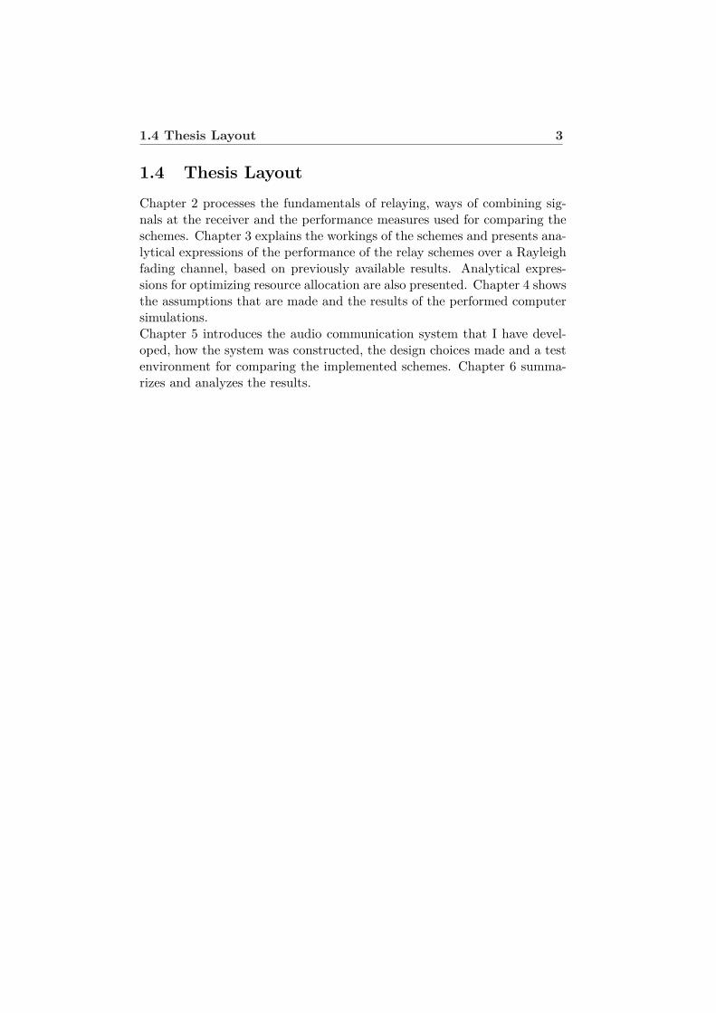
1.4 Thesis LayoutChapter 2 processes the fundamentals of relaying, ways of combining sig-nals at the receiver and the performance measures used for comparing theschemes. Chapter 3 explains the workings of the schemes and presents ana-lytical expressions of the performance of the relay schemes over a Rayleighfading channel, based on previously available results. Analytical expres-sions for optimizing resource allocation are also presented. Chapter 4 showsthe assumptions that are made and the results of the performed computersimulations.Chapter 5 introduces the audio communication system that I have devel-oped, how the system was constructed, the design choices made and a testenvironment for comparing the implemented schemes. Chapter 6 summa-rizes and analyzes the results.

Chapter 2

Relays in Wireless Networks

It lies in the nature of wireless transmission that information is broadcastedand that anyone with the right equipment can listen in. This fact canbe used to lower the error rates between a transmitting source and theintended destination by letting one or several extra nodes, relays, assist inthe communication.The wireless channel is often haunted by random variations in the strengthof the received signal. The phenomenon is refered to as fading and itoccurs when transmission is maintained through a number of stochasticreflections [3]. This continuously changes the quality of the channel andthe reliability of the communication. By letting a signal pass through extranodes, that listen to the transmitted signal and forward it to its intendeddestination, the signal takes several routes from the original source to thefinal destination. The source and the assisting relays usually share accessto the same channel through time division by using separate time slots.The separate links between each of the nodes are influenced by individualdistortion, independent of each other, and the improvement we get is thatif the direct link from the source to the destination is in a bad state, thesignal may still be delivered correctly via another node. When a signaltakes multiple paths from its source to its destination this often translatesinto diversity gains [1] which are discussed in section 2.2. The nodes thatassist in the transmission are called relays. From here on I assume thatwe are working with one single relay and a basic layout of the three-noderelay setup can be seen in Fig. 2.1. For short we can call the source, relayand destination S, R and D. When one single relay is used, D receives twocopies of the messages transmitted by S. One version that comes directlyfrom S and one version that has passed through R.

5

6 Relays in Wireless Networks

S

R

D

Time slot 1 Time slot 2

Figure 2.1. Basic setup of the three-node relay channel. S is the source, R is therelay and D is the destination

Relaying protocols can be divided into the two main categories Amplify-and-Forward protocols, AF, and Decode-and-Forward protocols, DF. InAF, the relay simply amplifies the received signals and re-transmits them.In DF, the relay only re-transmits a received message if it has been ableto successfully decode it first. The relay then has the option to re-encodemessages in a different channel code than the original messages were codedin and error correction can be performed at the relay as well. AlthoughDF relaying can be very efficient in some cases it is very much relies on thecapacity of the link between S and R. The relay only forwards a messageif it has been perfectly decoded and a poor link between S and R thereforeleaves R unused at times and direct transmission, not using the relay atall, could be a better option [5].

2.1 Potential Applications of Relaying

The concept of relaying can be incorporated into most wireless networks.Fixed relays could be implemented in cellular networks to assist mobilephones in their up and down links. This would bring the benefits ofMultiple-Input Multiple-Output, MIMO, resulting in diversity gains as adistributed MIMO system, without the practical constraint of having sev-eral antennas in the mobile unit. Conventional MIMO demands a lot ofpower and is therefore not well suited for mobile applications, where energyconsumption is a big concern. Another advantage in relay-based systems,that make them suited for mobile applications, is their resistance to shadowfading, which occurs when large obstacles block the signal path. This isthanks to the fact that the placement of the relay is not restricted in spaceto being at the same place as the transmitter or receiver. When the trans-

2.2 Cooperative Diversity 7

mission path between two nodes is obstructed, the information could stillflow through another path. Other potential applications could be wirelesssensor networks and coginitive radio networks [1] [7].

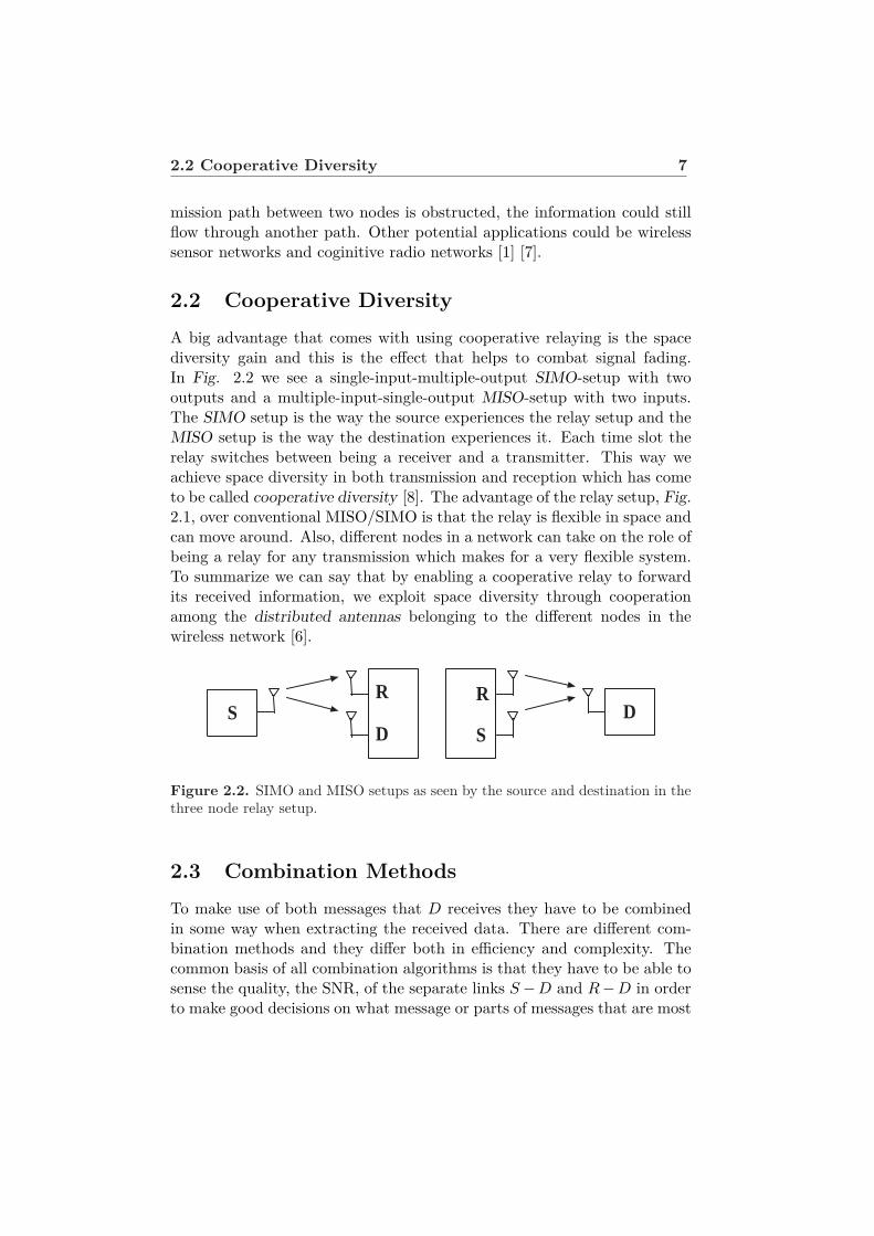
2.2 Cooperative DiversityA big advantage that comes with using cooperative relaying is the spacediversity gain and this is the effect that helps to combat signal fading.In Fig. 2.2 we see a single-input-multiple-output SIMO-setup with twooutputs and a multiple-input-single-output MISO-setup with two inputs.The SIMO setup is the way the source experiences the relay setup and theMISO setup is the way the destination experiences it. Each time slot therelay switches between being a receiver and a transmitter. This way weachieve space diversity in both transmission and reception which has cometo be called cooperative diversity [8]. The advantage of the relay setup, Fig.2.1, over conventional MISO/SIMO is that the relay is flexible in space andcan move around. Also, different nodes in a network can take on the role ofbeing a relay for any transmission which makes for a very flexible system.To summarize we can say that by enabling a cooperative relay to forwardits received information, we exploit space diversity through cooperationamong the distributed antennas belonging to the different nodes in thewireless network [6].

S R

D D

R

S

Figure 2.2. SIMO and MISO setups as seen by the source and destination in thethree node relay setup.

2.3 Combination MethodsTo make use of both messages that D receives they have to be combinedin some way when extracting the received data. There are different com-bination methods and they differ both in efficiency and complexity. Thecommon basis of all combination algorithms is that they have to be able tosense the quality, the SNR, of the separate links S−D and R−D in orderto make good decisions on what message or parts of messages that are most

8 Relays in Wireless Networks

likely not to have been corrupted during transmission. The most simpleand straight-forward way is Selection Combining, SC, which only uses oneof the received messages and ignores the other one. SC only chooses to usethe message coming from the diversity branch that has the highest instan-taneous SNR [2].A superior method is Maximum Ratio Combining, MRC, which combinesboth received messages, each weighted with a gain factor proportional tothe SNR of that link. To be optimal the gain factors should be chosen tomaximize the SNR of the combined message [2]. If the relay uses a differ-ent channel code than the source the destination cannot simply merge themessages as they are but has to use code combining which is very computa-tionally expensive. In the audio communication system that I have designedI always use the same channel code for the S−D and R−D links becausethen the combination process at the destination can be implemented withan MRC combiner.

2.4 Performance MeasuresThere are many ways of measuring the performance of a wireless link. Oneway is to calculate the bit-error-rate, BER, which denotes the number ofbits of a received message that differ from the transmitted message dividedby the total number of transmitted bits (i.e. the probability of a bit to beincorrectly received). I use the BER measurement when testing the audiocommunication system in chapter 5.Another way of measuring performance is to look at the probability of thechannel being in outage, Pout, which occurs during fades in the signal am-plitude over the channel as seen in Fig. 2.3. For the computer simulationsin chapter 4, the Pout measurement is used to compare the different relayingschemes. Setting β [bits per channel use] as the target spectral efficiencya link is said to be in outage when the instantaneously achievable spectralefficiency of that link is less than β. The outage probability shows howoften the destination can successfully decode a packet transmitted with afixed rate β bits per channel uses [1].The probability of outage is defined as

Pout = Pr{Outage} = Pr{R < β}

where R is the achievable rate obtained by a given scheme [1].

2.4 Performance Measures 9

Figure 2.3. Signal amplitude fluctuations at the receiver when transmitting overa Rayleigh Fading channel

Chapter 3

Transmission Schemes forDF Relaying

There are many transmission schemes for cooperative transmission de-scribed in the literature and I will analyze a few of them. A transmissionscheme is a set of rules on how the communication is to be done. Ruleson how to use and divide the available space, time and power between thenodes taking part in a transmission and also how channel codes should in-teract and other choices that form the basis for the transmission.In this chapter the schemes direct transmission, repetition coding and par-tial repetition coding are explained. A Rayleigh fading channel modelis presented and analytical expressions for the outage probabilities of theschemes for this model are presented on a closed form. Also expressionsfor optimizing the power and time allocation are presented. All of theanalytical expressions of finite SNR performance and for optimization ofresource allocation presented here are derived in [1] and I refer the readerwho is interested in the calculations leading up to these expressions to thiswork. A plot of the Pout for the relaying schemes based on the analyticalexpressions presented here can be seen in Fig. 4.1, as a comparison to thesimulation results presented in Chapter 4, plotted on a logarithmic scale asfunctions of the SNR.

3.1 Transmission ProtocolThere are two possible setups for the medium access, full-duplex and half-duplex. In a full-duplex setup the relay is able to transmit and receivesimultaneously on the same frequency which in practice, if possible, is com-

11

12 Transmission Schemes for DF Relaying

plicated. I consider the simpler setup of a half-duplex relaying system inwhich the relay can not transmit and receive simultaneously, for both thecomputer simulations and the audio system tests. This is accomplishedby using time division so that reception and transmission is done in non-overlapping time slots.Assume, for all schemes, that the total energy per packet is E = PT =PsTs+PrTr where P is the average transmit power and T is the total num-ber of channel uses available per packet. We have a three-node channelwhere transmission takes place in two phases. In the first phase S trans-mits a packet using Ts channel uses and power Ps while both R and Dlisten. In the second phase, if the relay has successfully decoded the re-ceived packet, it re-encodes the packet and re-transmits it using Tr = T−Tschannel uses and power Pr. If decoding at R fails it remains silent. Thedifferences between the relaying schemes lie in the distribution of transmitpower and channel uses between S and R. By letting all available transmitpower and channel uses be used by S any scheme reduces to direct trans-mission, leaving R unused.

3.2 Channel ModelConsider a time frame of length T which is divided into two parts, Ts = δTand Tr = (1− δ)T . δ ∈ [0.5, 1] is a coefficient that shows how much of thetotal available channel uses are used by the source. During the first timeslot, Ts, the source transmits a block of data s[n] while the relay and thedestination listen to the transmitted signal. Then during the second timeslot, Tr, the relay transmits a processed form of the received data, sr[n],after decoding and re-encoding it. In the nth time slot the received signals,ysr and ysd, at the relay and at the destination can be described by thefollowing channel model:

ysr[n] = hsrs[n] + zr[n] (3.1)ysd[n] = hsds[n] + zd[n] (3.2)

and in the (n + 1)th time slot the relay transmits the signal sr and thedestination receives yrd according to the model

yrd[n+ 1] = hrdsr[n+ 1] + zd[n+ 1], (3.3)

Here hsr, hsd and hrd denote the channel gains of the links and they captureboth the effects of path loss, shadowing and frequency non selective fading

3.3 Direct Transmission 13

[1]. The added variables zr[n], zd[n] and zd[n+ 1] denote the receiver noiseand other forms of interference. They can be modeled as zero-mean, mu-tually independent Gaussian random variables with unit variances N0 = 1.The channel between the nodes are modeled as quasi-static Rayleigh fad-ing, quasi-static meaning that the gain is constant during the transmissionof one block. Let

αij = |hij |2

N0, i ∈ {s, r}, j ∈ {r, d}

where hij is the channel gain from node i to node j. Then the receivedSNR for link i − j equals Piαij and it is exponentially distributed withmean Piγij where

γij = E|hij |2

3.3 Direct TransmissionIn direct transmission, DT, the relay is not taking part in the communica-tion, as can be seen in Fig. 3.1. Therefore all available power and time isused by the source and δ = 1 so that Ps = P , Ts = T , Pr = 0 and Tr = 0.Since DT only uses the direct link, S − D, the scheme is in outage when

S

R

D

Time slot 1 T

Figure 3.1. Network Schematic for Direct Transmission.

that link is in outage and the probability of outage for DT over a Rayleighfading channel is then given by:

Pout = Pr{αsd < 2β − 1P} = 1− exp(1− 2β

γsdP) = 2β − 1

γsdP+O( 1

P 2 ) (3.4)

No diversity is achieved since there is only one transmitting and one receiv-ing node.

14 Transmission Schemes for DF Relaying

3.4 Repetition Coding

In repetition coding, RC, all three nodes are taking part in the communi-cation, as can be seen in Fig. 3.2. The total number of available channeluses are divided into two equal parts so that δ = 0.5⇒ Ts = Tr = T

2 . Thetransmit power however does not have to be equally distributed between Sand R as long as it sums up to Ps +Pr = 2P giving a total signal energy ofE = PsTs +PrTr = (Ps +Pr)T2 = PT which is the same as for DT. DuringTs the source transmits and the relay and destination listen. During Tr therelay repeats the information, if has been successful in decoding it, and thedestination listens. Since the channel uses are divided equally between thesource and the relay it is possible for the relay to repeat all the data trans-mitted by the source. The destination can then use SC or MRC on wholemessages to combine them. Only MRC is considered as the combinationmethod here because it performs better than SC.In the collaborative schemes, RC and PR, the messages travel two separatepaths to the destination. For these schemes to be in outage the direct link,S−D, and at least one of the links that include the relay, S−R or R−D,must be in outage at the same time. The probability of outage for RC ina Rayleigh fading channel is then given by:

Pout = (22β − 1)2 1γsdPs

[ 1γsrPs

+ 12γrdPr

]+O( 1

P 3 ) (3.5)

Repetition Coding provides a diversity of order two.

S

R

D

Time slot 1 Time slot 2

T /2 T /2

Figure 3.2. Network Schematic for Repetition Coding.

For the conventional repetition coding scheme the only design choices arePs and Pr and from Eq. 3.5 we see that, by dropping the O( 1

P 3 ), a goodchoice of Ps and Pr, that minimizes the outage probability, is obtained by

3.5 Partial Repetition Coding 15

minimizingJ(Ps, Pr) = 1

γsrP 2s

+ 12γrdPsPr

(3.6)

under the limitations that Ps + Pr = 2P , 0 ≤ Ps ≤ 2P and 0 ≤ Pr ≤ 2P .

3.5 Partial Repetition CodingIn partial repetition coding, PR, the available channel uses do not have tobe equally divided between S and R. Since R uses the same channel codeas S it can not repeat all the data it receives if Tr < Ts. With Ts = δTand Tr = (1 − δ)T the relay only retransmits a fraction 1−δ

δ of the datait receives and discards the rest, where 0.5 < δ < 1. The transmit poweris shared by S and R under the constraint that δPs + (1 − δ)Pr = P sothat the total energy used is E = PsTs + PrTr = δTPs + (1− δ)TPr = PTwhich is the same as for the other schemes. So for the partial repetition

Figure 3.3. Network Schematic for Partial Repetition Coding.

scheme D receives full packets from S and parts of the packets from R andmessage combining has to be done separately for the common parts of thepackets and the parts only received from the source. MRC can be usedfor the common parts of the packets and the parts only received from thesource needs no processing since it has nothing to be combined with. Asfor RC the scheme is in outage when the link S−D and at least one of thelinks S−R or R−D are in outage. The probability of outage in a Rayleighfading channel is then given by:

Pout = (1−2βs )2

γsrγsdP 2s

+ 1−2βs−0.5(1−2βs)2+ 1−δ2−3δ (22βs−2βr )

γrdγsdPrPs+O( 1

P 3 ), δ 6= 23

Pout = (1−21.5β)2

γsrγsdP 2s

+ 1−21.5β−0.5(1−21.5β)2+1.5 ln(2)β23β

γrdγsdPrPs+O( 1

P 3 ), δ = 23

(3.7)

16 Transmission Schemes for DF Relaying

where βs = βδ and βr = β

1−δ . Partial Repetition Coding also provides adiversity of order two.When optimizing the resource allocation for PR δ is also a variable and weget an optimization problem with three parameters. From Eq. 3.7 we seethat a good choice of Ps, Pr and δ, that minimize the outage probability, isobtained by minimizing

J(Ps, Pr, δ) = (1− 2βs)2

γsrP 2s

+1− 2βs − 0.5(1− 2βs)2 + 1−δ

2−3δ (22βs − 2βr)γrdPrPs

(3.8)

under the limitations that 0.5 < δ < 1, 0 ≤ Ps ≤ Pδ , 0 ≤ Pr ≤ P

1−δ andδPs + (1− δ)Pr = P .

Chapter 4

Computer Simulations

I have done a performance analysis of the relaying schemes by runningMonte Carlo simulations in matlab. A Monte Carlo simulation, MC sim-ulation, is used to evaluate expressions that include stochastic variables.Evaluating such an expression will give a different result every time becauseof its stochastic properties and an MC-simulation evaluates this expressionseveral times to calculate a mean value. This estimated mean value is in-creasingly reliable as the number of evaluations increase. When simulatingcommunication schemes it is the channel properties that vary in time andthe strength of the received signal can be modeled with a certain distri-bution. In these simulations it is assumed that the channel is quasi-staticRayleigh fading and the signal strength at the receiver is then exponentiallydistributed. Assume a log-distance path loss model for the channel

γij = 1dαij

where α is the path loss exponent and dij is the normalized distance fromnode i to node j. The choice of path loss exponent, α, depends on thedesired path loss model but is typically chosen as 2 < α < 4. I chooseα = 4 which represents a dense urban area with some obstacles that de-grade the communication [1]. We can see from Eq. 3.6 and Eq. 3.8 thatwhen assuming the same channel distribution between all nodes the nor-malized distances between S, R and D control the optimal choice of energydistribution since γij is determined by dij .From section 3.2 we have that the received SNR for link i → j is ex-ponentially distributed with the mean Piγij = Pi

dαij. For this simulation

the normalized distances between the nodes S, R and D are chosen asdsd = dsr = 1 and drd = 0.1 so that the relay is quite close to the des-tination. An optimized time distribution for the PR scheme is chosen as

17

18 Computer Simulations

δ = 0.83 meaning that 83% of the available channel uses are used by thesource and only 17% of each transmitted block is repeated by the relay.The choice of δ = 0.83 for this setup was found through trial-and-errortests for varying values of δ. The average transmit power of S and R arefor simplicity chosen as Ps = Pr.

4.1 How the Simulations were performedThe target spectral efficiency is chosen to be β = 3 bits per channel usesfor this simulation. I run MC-simulations until 200 outages has occurredper SNR point for SNR ranging from 0 to 40 dB. The simulations arebased on the Pout according to equations in chapter 3 and those expressionswere derived under the assumption of MRC being used as the combinationmethod at D.

4.2 Simulation ResultsIn Fig. 4.1 the results of the MC-simulation can be seen as the dashedcurves, plotted as functions of the SNR. They are shown in the high-SNRregime because that is where the best results can be achieved when an-alyzing relaying protocols. That is because in the high-SNR regime thedata rates are mainly limited by interference as opposed to in the low-SNRregime where the influence of channel noise prevails, and hence the gainfrom cooperation is reduced [5]. Also in Fig. 4.1, seen as solid lines, are theasymptotes of the theoretical curves for the schemes in the same setup, asa comparison. We can see that the cooperative schemes achieve full diver-sity, i.e., the outage probability decays proportional to 1/SNR2 whereas itdecays as 1/SNR for the DL scheme [8].

4.2 Simulation Results 19

Figure 4.1. Theoretical and MC-simulated outage probabilities for the schemesdirect transmission, repetition coding and partial repetition coding. The solidlines are the asymptotes of the analytical expressions without the O( 1

P 3 )-term.The dashed lines are the simulation results. Plot made with dsd = dsr = 1,drd = 0.1, β = 3, α = 4 and δ = 0.83.

Chapter 5

Audio CommunicationSystem

To test the performance of the transmission schemes over an audio channelI have developed programs to be used by three computers acting as source,relay and destination in a three-node audio communication setup. Withthese programs you can transmit data between computers using differenttransmission schemes and then measure the performance of the schemesby calculating the BER after transmissions. The system was developedin Matlab and has been embedded into a Matlab GUI for easy usabilitywithout knowledge about the system design details. All code is included inAppendix A-C. The system is meant to be used as an intuitive demonstra-tion of the principles of cooperative transmission and to show some basicconcepts and phenomena that are typical for wireless communication.

5.1 System Requirements

These programs work on any OS running Matlab version 7.0 or later. Mat-lab has to have the Data Acquisition Toolbox version 2.7 or later in orderto control the computers sound card. The hardware needed is a microphonefor the source computer, a pair of speakers for the destination computerand, for running the cooperative schemes, a relay computer with a mi-crophone and a pair of speakers. The system has proven to work fine oncomputers with a 1.7 GHz processor and 512 MB RAM.

21

22 Audio Communication System

5.2 System DesignThe programs, running on all three computers, control and monitor thewhole transmission process. When starting a transmission the user choosesbetween different transmission schemes, what channel code to use and whatdata to transmit. Fig. 5.1 shows the GUI of the source program andthe GUIs for the relay and destination programs look similar. After atransmission is finished the relay and destination programs will display thelength of the received data, how many errors, if any, that occurred duringtransmission for the separate links S −R, S −D, R−D and the BER forthe combined final estimate. When starting a transmission it is assumedthat all three computers agree beforehand on what transmission schemeand channel code to use and the source and relay programs need to knowwhat data is being transmitted to have something to compare the receiveddata with in the error calculations.

Figure 5.1. Matlab GUI for the source computer in the audio communicationsystem.

5.2.1 The Data Acquisition ToolboxThe data acquisition toolbox, DAQ toolbox, in matlab helps to interactwith hardware in the computer and is a very useful tool when workingwith input to and output from a computer. With the DAQ toolbox we cancreate analog input objects and analog output objects and configure themto be connected to inputs and outputs of a computers sound card. This

5.2 System Design 23

way signals can be output from matlab to the speakers and the input froma microphone can be recorded into matlab in real-time. A block schematicof a direct transmission between two computers can be seen in Fig. 5.2.The source program encodes a vector of binary data, that it has been toldto transmit, according to the users choice of coding and then modulatesthe data into a signal that is stored in the stack of an analog output object.When this object is activated the contents of its stack flows to the outputof the sound card, at a predetermined rate, and the speakers play thesignal stored on the stack. The relay program has both an analog inputobject connected to the sound cards input and an analog output objectconnected to the sound cards output. It switches between the two anduses the input object to record a signal in the time slots where the sourceprogram is transmitting and then uses the output object to transmit inthe following time slot. After recording a signal in the first time slot therelay program demodulates and decodes the signal to retrieve the originalbinary data of that block. If decoding is successful it re-encodes the data,modulates it and then puts it on the stack of the analog output object to betransmitted in the next time slot. The destination program only needs ananalog input object to record the whole received transmission, coming fromthe sound card. After a transmission is completed the destination programhas a recording that contains the signals transmitted by both the sourceand the relay. The original vector of binary data can then be retrievedby first combining the signals or by looking at them separately and thendemodulate and decode them.

Coding Modulation DAQ

De-coding De-modulation DAQ

Channel

Binary data Input

Binary data Output Sound

Card

Sound Card

MATLAB

MATLAB

Figure 5.2. Block diagram of the system for direct transmission from the sourceto the destination.

24 Audio Communication System

5.2.2 Coding and Modulation

The modulation method used is non-coherent binary frequency shift keying,BFSK, using two distinct carrier frequencies to denote binary 1 and 0. Thecarrier frequencies used are fc1 = 1100Hz and fc2 = 1300Hz which arereasonable frequencies for audio transmission and lie in a frequency regionwhere the speakers and microphones work well. With BFSK modulationeach symbol represents a single bit of data and I use 200 samples of acosine, of frequency fc1 or fc2, to represent each symbol in the modulatedsignal. Using a non-coherent modulation technique simplifies the receiverbecause knowledge about the phase of the signal is not required in thedemodulation process. Due to shifting of the phase during transmissioncoherent detection can become troublesome. Demodulation is done usinga simple fast fourier transform, FFT, which is an approximation of thediscrete fourier transform, DFT. The FFT algorithm is used separatelyon parts of a received signal to extract the frequency information of thesymbols in those parts. The demodulation process looks at those parts forfrequency peaks at fc1 and fc2 to determine what data was received.The system is designed with the option of using an error correcting blockcode. Block codes split the data, that is to be transmitted, into blocksof k symbols and add check symbols to each block to get correspondingcodewords of length n > k. These check symbols can then be used inthe decoding of the blocks at the receiver to correct errors that may haveoccurred during transmission [2]. I have chosen to use a hamming (7, 4)block code, that is k = 4 and n = 7, because of its simple implementationinto the system and because the blocks in each time slot consist of sevenbits. When using this hamming code one error per four transmitted bitscan be corrected at the cost of having to transmit 7

4 = 1.75 times as manysymbols than when transmitting uncoded data.

5.2.3 Design Choices

For the cooperative schemes, when the relay is taking part in the communi-cation, time is divided into time slots giving the source and the relay accessto the channel every other time slot. The data that is to be transmitted istherefore divided into blocks, where one block is transmitted by the sourcein one time slot and the relay forwards that block in the following timeslot and the process is repeated until all the data is transmitted. I havechosen to use a block length of seven symbols per block for my tests butthis value can easily be varied. Transmission is done at the rate of 8000samples per second and recording is done at the same sample frequency.

5.2 System Design 25

0 0.2 0.4 0.6 0.8 10

1

2

3

Time [s]

Source BlockRelay BlockGuard Band

Figure 5.3. Placement of guard intervals between the transmission time slots ofS and R for the cooperative schemes. The boxes represent the slots where S andR are permitted to transmit.

Using 200 samples of a cosine to represent each symbol results in a bit rateof 40 bits/s for DL transmission. For the cooperative schemes the bit rateis naturally cut in half because every block of data is transmitted twice,both by S and R in non-overlapping timeslots. But because of guard bandsinserted between the transmission time slots of S and R for the coopera-tive schemes, see Fig. 5.3, the bit rate actually drops to about 13 bits/s.These guard bands are required to give the relay time to process its receivedsignals before its time slot for re-transmission occurs. These guard bandsalso gives D a clear distinction between the transmissions from S and Rand give room for good reception even if the synchronization is a bit off.When using hamming coding these bit rates drop to about 22.9 bits/s forDL transmission and 7.4 bits/s for the cooperative schemes.

Coding Scheme Data rate [bits/s]Uncoded DL 40Uncoded Coop 13Hamming DL 22.9Hamming Coop 7.4

Table 5.1. Data rates for transmission in the audio communication system. Coopdenotes both the RC and PR schemes.

At the destinationMRC is used to combine the messages. First the receivedsignal is demodulated into a matrix of soft demodulated symbols containingthe frequency information of the signals from both S and R and then thesevalues are combined withMRC before the hard-decision demodulation, thatresults in a final binary estimate of the received signal, is done. For MRC

26 Audio Communication System

to work well we have to have knowledge about the SNR of the separatelinks at all times in order to choose good gain factors and make use of thevariation in link quality. This estimation process of the SNR of the separatelinks needs more work and does not work optimally.

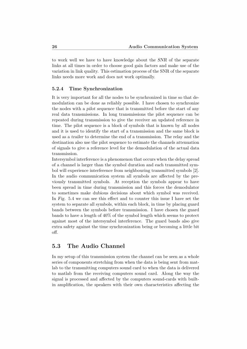
5.2.4 Time SynchronizationIt is very important for all the nodes to be synchronized in time so that de-modulation can be done as reliably possible. I have chosen to synchronizethe nodes with a pilot sequence that is transmitted before the start of anyreal data transmissions. In long transmissions the pilot sequence can berepeated during transmission to give the receiver an updated reference intime. The pilot sequence is a block of symbols that is known by all nodesand it is used to identify the start of a transmission and the same block isused as a trailer to determine the end of a transmission. The relay and thedestination also use the pilot sequence to estimate the channels attenuationof signals to give a reference level for the demodulation of the actual datatransmission.Intersymbol interference is a phenomenon that occurs when the delay spreadof a channel is larger than the symbol duration and each transmitted sym-bol will experience interference from neighbouring transmitted symbols [2].In the audio communication system all symbols are affected by the pre-viously transmitted symbols. At reception the symbols appear to havebeen spread in time during transmission and this forces the demodulatorto sometimes make dubious decisions about which symbol was received.In Fig. 5.4 we can see this effect and to counter this issue I have set thesystem to separate all symbols, within each block, in time by placing guardbands between the symbols before transmission. I have chosen the guardbands to have a length of 40% of the symbol length which seems to protectagainst most of the intersymbol interference. The guard bands also giveextra safety against the time synchronization being or becoming a little bitoff.

5.3 The Audio ChannelIn my setup of this transmission system the channel can be seen as a wholeseries of components stretching from when the data is being sent from mat-lab to the transmitting computers sound card to when the data is deliveredto matlab from the receiving computers sound card. Along the way thesignal is processed and affected by the computers sound-cards with built-in amplification, the speakers with their own characteristics affecting the

5.3 The Audio Channel 27

produced audio signal, the effects of the actual channel and the propertiesof the recording microphone. The signal recorded by the microphone isa distorted version of the signal transmitted from the speakers, affectedby multiple path propagation, echoes, and random background noise aswell as more controllable audio disturbances such as people talking in thebackground. The audio transmissions multiple path propagation yields animpulse response that is a sum of delayed attenuated impulses dependingon the acoustic properties of the room that the transmission is being per-formed in. We can assume the channel to be linear within normal signalstrengths and also to be time invariant, as long as the environment is notphysically changing during transmission. A DC-component and other lowfrequency distortions appear in the received signals but do not degrade theperformance since the communication is done in the 1100 − 1300Hz re-gion. The signals produced by the speakers have a time delay spread that

0 0.01 0.02 0.03 0.04 0.05−0.8

−0.6

−0.4

−0.2

0

0.2

0.4

0.6

0.8

1

Time [s]

Figure 5.4. The received signal of two consecutive symbols transmitted over theaudio channel. The boxes show where the transmitter is active and between theboxes are guard intervals.

is larger than the symbol duration because of the physical limitations ofthe speakers themselves. It is impossible for the speakers to go from play-ing to being completely quiet instantaneously. Combined with the effectsof multiple path propagation we get a quite large time delay spread forthe channel which can lead to intersymbol interference. Fig. 5.4 shows arecevied signal from when two consecutive symbols were transmitted overthe audio channel in my test setup, with the transmission bands and guardbands marked. We can clearly see the channels delay spread and why theintroduction of guard bands is necessary.

28 Audio Communication System

5.4 Testbench Setup

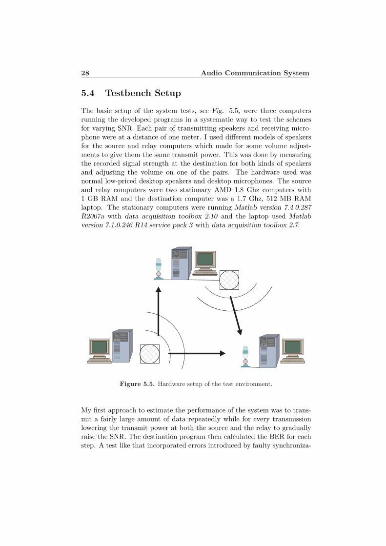
The basic setup of the system tests, see Fig. 5.5, were three computersrunning the developed programs in a systematic way to test the schemesfor varying SNR. Each pair of transmitting speakers and receiving micro-phone were at a distance of one meter. I used different models of speakersfor the source and relay computers which made for some volume adjust-ments to give them the same transmit power. This was done by measuringthe recorded signal strength at the destination for both kinds of speakersand adjusting the volume on one of the pairs. The hardware used wasnormal low-priced desktop speakers and desktop microphones. The sourceand relay computers were two stationary AMD 1.8 Ghz computers with1 GB RAM and the destination computer was a 1.7 Ghz, 512 MB RAMlaptop. The stationary computers were running Matlab version 7.4.0.287R2007a with data acquisition toolbox 2.10 and the laptop used Matlabversion 7.1.0.246 R14 service pack 3 with data acquisition toolbox 2.7.�� ��

Figure 5.5. Hardware setup of the test environment.

My first approach to estimate the performance of the system was to trans-mit a fairly large amount of data repeatedly while for every transmissionlowering the transmit power at both the source and the relay to graduallyraise the SNR. The destination program then calculated the BER for eachstep. A test like that incorporated errors introduced by faulty synchroniza-

5.5 Test Results 29

tion into the results and when varying the transmit signal power over alarge interval the receivers sometimes had problems adapting to the largedifferences in signal energy between the first and the last transmission. Thisproved to give very erratic results and another test method was needed.The next idea, that proved to give more stable results, was to first transmita large chunk of data through the relay system and then save the wholerecorded signal at the destination, which included the signals from boththe source and the relay, and then varying the SNR of that received signalbefore demodulating and decoding. Truncating this received signal to makesure that the synchronization was satisfactory I could then save that syn-chronized recorded signal to run several tests on without worrying aboutsynchronization errors. To vary the SNR I added white Gaussian noise tothe signal varying the power of the noise to change the SNR step by step.This way of testing saves time as the actual audio transmission is not nec-essary for each SNR value and that made for much faster tests. In this testsetup it is possible to vary the SNR separately for the S −D and R − Dlinks, to test different scenarios, but the properties of the S − R link cannot be altered once the initial transmission is recorded at D. This methodof testing was used to achieve the test results for the DL and RC schemesthat are presented in Fig. 5.6 and Fig. 5.7. I used BER as the performancemeasure and for the RC scheme I calculated the BER for both the S −Dand R−D links as well as for the MRC combined final estimate at D.

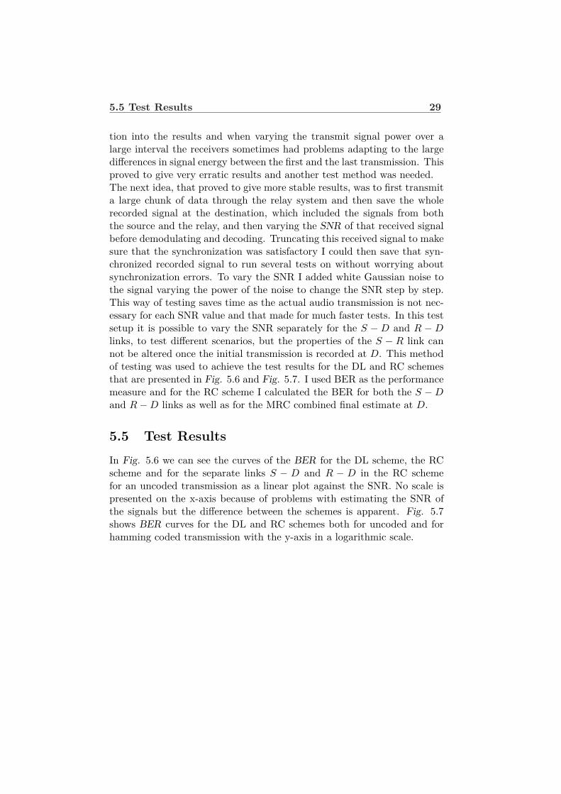
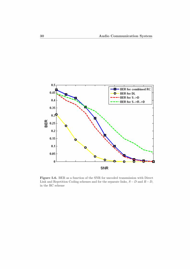
5.5 Test ResultsIn Fig. 5.6 we can see the curves of the BER for the DL scheme, the RCscheme and for the separate links S − D and R − D in the RC schemefor an uncoded transmission as a linear plot against the SNR. No scale ispresented on the x-axis because of problems with estimating the SNR ofthe signals but the difference between the schemes is apparent. Fig. 5.7shows BER curves for the DL and RC schemes both for uncoded and forhamming coded transmission with the y-axis in a logarithmic scale.

30 Audio Communication System

Figure 5.6. BER as a function of the SNR for uncoded transmission with DirectLink and Repetition Coding schemes and for the separate links, S−D and R−D,in the RC scheme

5.5 Test Results 31

Figure 5.7. BER as a function of the SNR for uncoded and hamming coded trans-mission with Repetition Coding and Direct Link schemes, plotted in a logarithmicscale.

Chapter 6

Analysis and Conclusions

6.1 ComparisonsIt is not really possible to compare the results from the MC-simulations inchapter 4 with the results from the audio system tests in chapter 5 becausethe assumptions and the test setups are very different. Comparisons canhowever be made between the schemes for each of the tests separately.The MC simulations show results that align very well with the asymptotesof the analytical expressions, see Fig. 4.1, and we see that the cooperativeschemes achieve a diversity order of two which leads to steeper slopes inthe logarithmic plots of the Pout. For high SNR we then see that RC andPR outperform DL and we can also see that PR provides a power gain ofabout 8dB over RC for the assumed situation.The results of the audio communication system tests show that DL trans-mission, not using the relay at all, actually gives a better performance thanRC and in Fig. 5.7 we can see that my implementation of the RC schemegives a consistently higher BER than the DL scheme. The hamming codedtransmissions, as can be expected, give better performance results than theuncoded transmissions for both the DL and RC schemes and this improve-ment seems to grow as the SNR increases.

6.2 AnalysisTo get the advantages of relaying it is very important for the destination tohave good knowledge about the SNR of the separate links S−D and R−Din order for the combination process to work well. When fades occur in thedifferent transmission paths, S−D and R−D, they are unlikely to occur atthe same time instant in the separate paths and MRC combining can then

33

34 Analysis and Conclusions

make use of the high-SNR parts of each signal and reduce the probabilityof errors in the final estimate of the transmitted data. As the conditions ofthe links change the MRC combiner has to be able to adapt and change thegain factors used when combining the signals from the source and the relay,otherwise the combiner will not know which link provides the most reliablesignal and could, in a worst case scenario, cause an incorrect data estimatewhen a correctly received signal was available. Due to problems with esti-mating the SNR of the links, while running the system, the implementationof the MRC in the audio communication system is far from optimal andthis could be one of the reasons that we see RC being outperformed by DL.I also believe that, although it very much exists in the audio channel, fadingis not a big problem for the system. This could be explained by the useof guard bands between each transmitted symbol and having a slow datarate over the channel compared to the speed of the fading. This reducessome of the possible gain from using relaying techniques. If there is no biggain from using relaying in the audio communication system, an apparentrisk is that a sub-optimally implemented relaying scheme introduces moreerrors than it counteracts and that the simpler non-cooperative DL schemeworks better.

6.3 Conclusions

I have constructed an audio communication system to be used by two orthree computers and implemented relaying schemes into the system to testtheir performance over an audio channel. Monte Carlo simulations showedthe gain that relaying schemes can achieve compared to direct link transmis-sion under the right circumstances. We saw that different relaying schemes,that divide the available time and transmit power differently between thesource and the relay, yield different performance and that partial repetitioncoding can give a large improvement over conventional repetition coding.However, there are very many parameters and design choices that all havean effect on the performance of communication. The distances betweennodes, the data rate of transmission, block length, channel codes and otherdesign choices all affect the performance and it is very hard to draw generalconclusions about the schemes. In the audio communication system the RCscheme did not show the improvement over DL transmission that was ex-pected. This, however, says little about the scheme itself and more aboutthe situation with the audio channel, my implementation of the schemesinto the audio communication system and how the tests were performed.

6.4 Future Work 35

Audio channels are rarely or never used in real applications because of ex-tensive interference, short transmission ranges and because it makes alot ofnoise. A reason for using an audio channel in this thesis was that it requiredno special equipment and to design a communication system working overthe channel you encounter the same kind of design choices and have to takethe same basic problems into consideration as for other types of wirelesscommunication. My audio communication system can give an intuitive un-derstanding of wireless communication and the advantages and drawbacksof different types of coding, modulation and the use of relays. It is wellsuited for further development and possible use in laborations for basiccommunication courses at the university to let students investigate and seehow different setups and design choices change the performance of wirelesscommunication.

6.4 Future WorkThe programs for the source, relay and destination computers, that controlthe audio communication system, are developed in a block manner so thatadditional coding algorithms and communication schemes easily can beadded to the system without altering the basic framework. Parts of thesystem, such as combination algorithms or synchronization techniques canalso be further developed separately. Some examples of interesting futuredevelopment that I have not had time to implement could be

• Improvement of the combination algorithm.

• Adding more coding algorithms and making the length of block codesscalable.

• Adding additional modulation techniques.

• Performing more tests with other setups and other parameter choices.

• Adding functionality for transmitting files from disk.

• Adding re-transmission functionality for incorrectly received blocks.

Bibliography

[1] M. N. Khormuji, Relaying Protocols for Wireless Networks, Licenciatethesis, Royal Institute of Technology, Stockholm, Sweden, 2008

[2] J. Zander, B. Slimane and L. Ahlin, Principles of Wireless Communi-cations., Studentlitteratur, 2006

[3] M. Olofsson, T. Ericson, R. Forchheimer and U. Henriksson, Ba-sic Telecommunication. Department of Electrical Engineering, LiU,Linköping, 2006

[4] M. N. Khormuji and E. G. Larsson, ’Finite-SNR Analysis and Opti-mization of DF Relaying over slow fading channels’, submitted to IEEETransactions on Vehicular Technology, 2009

[5] editor, Mohamed Ibnkahla, Adaptive Signal Processing in WirelessCommunications. CRC Press, Tayler and Francis Group, LLC, 2009

[6] Q. Zhang, J. Jia and J. Zhang, ’Cooperative Relay to Improve Diver-sity in Cognitive Radio Networks’, IEEE Communications magazineFeb 2009, Vol. 47, No. 2, 111-117

[7] W. Chin, Y. Qian and G. Giambene ’Advances in Cooperative andRelay Communications’ IEEE Communications magazine Feb 2009,Vol. 47, No. 2, 100-101.

[8] J. N. Laneman, D. N. C. Tse and G. W. Wornell, ’Cooperative Diver-sity in Wireless Networks: Efficient Protocols and Outage Behavior’IEEE Transactions on Information Theory Dec 2004, Vol. 50, No.12

37

Appendix A

Matlab code - Source

A.1 source.m

1 function source ( scheme , data , hamming , d e l t a )2 % syntax : source ( scheme , time , hamming , d e l t a )3 % Cal l ed by sourceGUI .m to run the s e l e c t e d re l ay ing−scheme with4 % s e l e c t e d parameters .5 % Written By : Thomas Wärme67 clc ;8 %Parameters−−−−−−−−−−−−−−−−−−−−−−−−−−−−−−−−−−−−−−−−−−−−−−−−−−−9 F=8000; %Channel ra t e [ sampels / s ]

10 Ns=200; %Sampels per symbol11 Nf=7; %Symbols per frame12 Ampl=2; %Ampl i f i ca t i on Factor1314 f c1 =1300; %Carr ier f r e q ; b inary 015 f c2 =1100; %Carr ier f r e q ; b inary 11617 %Ki l l any open DAQ−ob j e c t s−−−−−−−−−−−−−−−−−−−−−−−−−−−−−−−−−−−−18 openDAQ=daqf ind ;19 for i =1: length (openDAQ)20 stop (openDAQ( i ) ) ;21 delete (openDAQ( i ) ) ;22 end2324 % Check t ha t input data i s binary−−−−−−−−−−−−−−−−−−−−−−−−−−−−−25 for i =1: length ( data )26 i f not ( data ( i )==0 | data ( i )==1)27 fpr intf ( ’ Error ! Input data i s not binary ! \ n ’ )28 return29 end30 end31

39

40 Matlab code - Source

32 % Run the chosen scheme−−−−−−−−−−−−−−−−−−−−−−−−−−−−−−−−−−−−−−−33 i f strcmp ( scheme , ’DL ’ )34 DLsource ( data , hamming , fc1 , fc2 , F , Ns , Ampl) ;35 end36 i f strcmp ( scheme , ’RC’ )37 RCsource ( data , hamming , fc1 , fc2 , F , Ns , Nf , Ampl) ;38 end39 i f strcmp ( scheme , ’PR ’ )40 PRsource ( data , hamming , fc1 , fc2 , F , Ns , Nf , Ampl , d e l t a ) ;41 end4243 %Ki l l any open DAQ−ob j e c t s−−−−−−−−−−−−−−−−−−−−−−−−−−−−−−−−−−−−44 openDAQ=daqf ind ;45 for i =1: length (openDAQ)46 stop (openDAQ( i ) ) ;47 delete (openDAQ( i ) ) ;48 end49 end

A.2 DLsource.m

1 function DLsource ( data , hamming , fc1 , fc2 , F , Ns , Ampl)2 % syntax : DLsource ( data , hamming , fc1 , fc2 , F, Ns , Ampl)3 % Transmits data over Audio−channel wi th BFSK−modulation us ing4 % ca r r i e r f r e q u en c i e s f c1 and fc2 , sample ra t e F, Ns samples / b i t5 % and amp l i f i c a t i o n f a c t o r Ampl . Using hamming=1 g i v e s hamming6 % coded transmiss ion , hamming=0 g i v e s uncoded t ransmiss ion .7 % Input ’ data ’ as a b inary row vec to r .8 % Written By : Thomas Wärme9

10 fpr intf ( ’ D i rec t Link Transmission−−−−−−−−−−−−−−−−−−−−−−−−\n ’ )11 %Coding−−−−−−−−−−−−−−−−−−−−−−−−−−−−−−−−−−−−−−−−−−−−−−−−−−−−−−12 i f hamming==113 cdata=code_hamming ( data ) ;14 else15 cdata=data ;16 end1718 %Ins e r t synchron i za t ion−sequences−−−−−−−−−−−−−−−−−−−−−−−−−−−−−19 pn=[1 1 1 0 0 1 1 1 ] ;20 cdata=[pn , cdata , pn ] ;2122 %Modulation BFSK−−−−−−−−−−−−−−−−−−−−−−−−−−−−−−−−−−−−−−−−−−−−−−23 data_mod=bfskmod ( cdata , fc1 , fc2 , Ns , Ampl) ;2425 % Transmission−−−−−−−−−−−−−−−−−−−−−−−−−−−−−−−−−−−−−−−−−−−−−−−26 ao=analogoutput ( ’ winsound ’ ) ; %Create analog output o b j e c t27 addchannel ( ao , [ 1 2 ] ) ; %Add two channe l s28 set ( ao , ’ SampleRate ’ , F) ; %Output F sampels / s29 putdata ( ao , [ data_mod data_mod ] ) ; %Enqueue modulated data

A.3 RCsource.m 41

3031 fpr intf ( ’Number o f b i t s to Transmit : ’ ) ;32 disp ( length ( data ) ) ;33 i f hamming==134 fpr intf ( ’Number o f hamming coded b i t s to transmit : ’ ) ;35 disp ( length ( cdata )−2∗length (pn) ) ;36 end37 fpr intf ( ’ Estimated Time f o r Transmiss ion [ s ] : ’ ) ;38 disp ( ( get ( ao , ’ s amp l e sava i l ab l e ’ ) −16∗200)/F) ;3940 set ( ao , ’ TriggerType ’ , ’ Immediate ’ ) ; %Trigger immediate ly41 s t a r t ( ao ) ; %Act i va t e hardware and DAQ−engine42 wait ( ao , 120 ) ; %Wait f o r output to f i n i s h [max 2 min ]4344 fpr intf ( ’ Transmiss ion Complete . \ n ’ ) ;45 end

A.3 RCsource.m

1 function RCsource ( data , hamming , fc1 , fc2 , F , Ns , Nf , Ampl)2 % syntax : RCsource ( data , hamming , fc1 , fc2 , F, Ns , Nf , Ampl)3 % Transmits data over Audio−channel wi th BFSK−modulation and4 % Repe t i t i on Coding Cooperat ive t ransmiss ion scheme .5 % Transmission uses c a r r i e r f r e q u en c i e s f c1 and fc2 , sample6 % ra te F, Ns samples / b i t , b l o c k s i z e Nf and amp l i f i c a t i o n7 % fa c t o r Ampl . Using hamming=1 g i v e s hamming coded8 % transmiss ion , hamming=0 g i v e s uncoded t ransmiss ion .9 % Input ’ data ’ as a b inary row vec t o r .

10 % Written By : Thomas Wärme1112 fpr intf ( ’ Repet i t i on Coding Transmission−−−−−−−−−−−−−−−−−−−\n ’ )13 %Coding−−−−−−−−−−−−−−−−−−−−−−−−−−−−−−−−−−−−−−−−−−−−−−−−−−−−14 i f hamming==115 cdata=code_hamming ( data ) ;16 else17 cdata=data ;18 end1920 %Ins e r t synchron i za t ion−sequences−−−−−−−−−−−−−−−−−−−−−−−−−−21 pn=[1 1 1 0 0 1 1 ] ;22 cdata=[pn , cdata , pn ] ;2324 %Modulation BFSK−−−−−−−−−−−−−−−−−−−−−−−−−−−−−−−−−−−−−−−−−−−25 data_mod=bfskmod ( cdata , fc1 , fc2 , Ns , Ampl) ;2627 %Block separat ion−−−−−−−−−−−−−−−−−−−−−−−−−−−−−−−−−−−−−−−−−−28 block_L=Nf∗Ns ; %Samples per b l o c k29 space=zeros ( block_L+Ns∗8 ,1) ; %Inc l two 4∗Ns guard i n t e r v a l s30 data_spaced=space ;31

42 Matlab code - Source

32 while length (data_mod)>block_L33 data_spaced=[data_spaced ; data_mod ( 1 : block_L ) ; space ] ;34 data_mod=data_mod( block_L+1:end) ;35 end36 data_spaced=[data_spaced ; data_mod ; space ] ;3738 % Printouts−−−−−−−−−−−−−−−−−−−−−−−−−−−−−−−−−−−−−−−−−−−−−−3940 i f hamming==141 fpr intf ( ’Number o f b i t s be f o r e coding : ’ )42 disp ( length ( data ) )43 fpr intf ( ’Number o f hamming coded b i t s to transmit : ’ ) ;44 disp ( length ( cdata )−2∗Nf )45 else46 fpr intf ( ’Number o f uncoded b i t s to transmit : ’ )47 disp ( length ( data ) )48 end4950 fpr intf ( ’Number o f b locks to transmit : ’ ) ;51 disp ( ce i l ( ( length ( cdata )−2∗Nf ) /Nf ) )5253 % Transmission−−−−−−−−−−−−−−−−−−−−−−−−−−−−−−−−−−−−−−−−−−54 ao = analogoutput ( ’ winsound ’ ) ; %Create analog output o b j e c t55 addchannel ( ao , [ 1 2 ] ) ; %Add two channe l s56 set ( ao , ’ SampleRate ’ , F) ; %Output F sampels / s57 set ( ao , ’ TriggerType ’ , ’ Immediate ’ ) ;58 putdata ( ao , [ data_spaced data_spaced ] ) ; %Enque modulated data5960 fpr intf ( ’ Estimated Time f o r Transmiss ion [ s ] : ’ ) ;61 disp ( ( get ( ao , ’ s amp l e sava i l ab l e ’ )−6400)/F)6263 s t a r t ( ao ) ; %Act i va t e s hardware and DAQ−engine .64 wait ( ao , 120 ) ; %Wait f o r output to f i n i s h or max o f 2 minutes .6566 fpr intf ( ’ Transmiss ion Completed . \ n ’ ) ;67 end

A.4 PRsource.m

1 function PRsource ( data , hamming , fc1 , fc2 ,F , Ns , Nf ,Ampl , d e l t a )2 % syntax : PRsource ( data , hamming , fc1 , fc2 ,F,Ns , Nf ,Ampl , d e l t a )3 % Transmits data over Audio−channel wi th BFSK−modulation and4 % Par t i a l Repe t i t i on Coding Cooperat ive t ransmiss ion scheme .5 % Transmission uses c a r r i e r f r e qu en c i e s f c1 and fc2 , sample6 % ra te F, Ns samples / b i t , b l o c k s i z e Nf and amp l i f i c a t i o n f a c t o r7 % Ampl . ’ d e l t a ’ v a r i e s the coopera t ion l e v e l . Using hamming=18 % g i v e s hamming coded transmiss ion , hamming=0 g i v e s uncoded9 % transmiss ion . Input ’ data ’ as a b inary row vec t o r .

10 % Written By : Thomas Wärme11

A.4 PRsource.m 43

12 fpr intf ( ’ Pa r t i a l Repet i t i on Coding Transmission−−−−−−−−−−−\n ’ )13 %Coding−−−−−−−−−−−−−−−−−−−−−−−−−−−−−−−−−−−−−−−−−−−−−−−−−−−−−−−14 i f hamming==115 cdata=code_hamming ( data ) ;16 else17 cdata=data ;18 end1920 %Ins e r t synchron i za t ion−sequences−−−−−−−−−−−−−−−−−−−−−−−−−−−−−21 pn=[1 1 1 0 0 1 1 ] ;22 cdata=[pn , cdata , pn ] ;2324 %Modulation BFSK−−−−−−−−−−−−−−−−−−−−−−−−−−−−−−−−−−−−−−−−−−−−−−25 data_mod=bfskmod ( cdata , fc1 , fc2 , Ns , Ampl) ;2627 %Block separat ion−−−−−−−−−−−−−−−−−−−−−−−−−−−−−−−−−−−−−−−−−−−−28 Frame_L=Nf∗Ns ;29 space=zeros (Frame_L+Ns∗8 ,1) ; %Inc l two 4∗Ns guard i n t e r v a l s30 data_spaced=space ;3132 while length (data_mod)>Frame_L33 data_spaced=[data_spaced ; data_mod ( 1 : Frame_L) ; space ] ;34 data_mod=data_mod(Frame_L+1:end) ;35 end3637 data_spaced=[data_spaced ; data_mod ; space ] ;3839 % Printouts−−−−−−−−−−−−−−−−−−−−−−−−−−−−−−−−−−−−−−−−−−−−−−−−−−40 i f hamming==141 fpr intf ( ’Number o f b i t s be f o r e coding : ’ )42 disp ( length ( data ) )43 fpr intf ( ’Number o f hamming coded b i t s to transmit : ’ ) ;44 disp ( length ( cdata )−2∗Nf )45 else46 fpr intf ( ’Number o f uncoded b i t s to transmit : ’ )47 disp ( length ( data ) )48 end4950 fpr intf ( ’Number o f b locks to transmit : ’ ) ;51 disp ( ce i l ( ( length ( cdata )−2∗Nf ) /Nf ) )5253 % Transmission−−−−−−−−−−−−−−−−−−−−−−−−−−−−−−−−−−−−−−−−−−−−−−−54 ao = analogoutput ( ’ winsound ’ ) ; %Create analog output o b j e c t55 addchannel ( ao , [ 1 2 ] ) ; %Add two channe l s56 set ( ao , ’ SampleRate ’ , F) ; %Output F sampels / s57 set ( ao , ’ TriggerType ’ , ’ Immediate ’ ) ;58 putdata ( ao , [ data_spaced data_spaced ] ) ; %Enque modulated data5960 fpr intf ( ’ Estimated Time f o r Transmiss ion [ s ] : ’ ) ;61 disp ( ( get ( ao , ’ s amp l e sava i l ab l e ’ )−6400)/F)

44 Matlab code - Source

6263 s t a r t ( ao ) ; %Act i va t e s hardware and DAQ−engine .64 wait ( ao , 120 ) ; %Wait f o r output to f i n i s h or max o f 2 minutes .6566 fpr intf ( ’ Transmiss ion Completed . \ n ’ ) ;67 end

A.5 bfskmod.m

1 function bfskdata = bfskmod ( data , fc1 , fc2 , Ns , Ampl)2 % syntax : b f dkda ta = bfskmod ( data , fc1 , fc2 , Ns , Ampl)3 % BFSK−modulation o f a b inary data vec t o r " data " wi th4 % amp l i f i c a t i o n f a c t o r Ampl and c a r r i e r f r e q u en c i e s5 % fc1 and fc2 . Returns a modulated s i g n a l wi th 2006 % samples per b i t i n c l u d i n g guard i n t e r v a l s between b i t s .7 % Written By : Thomas Wärme 2009−02−1289 t=linspace ( 0 , 1 , 0 . 6∗Ns) ;

1011 s0=Ampl∗cos (2∗pi∗ f c 1 ∗ t ) ; %Binary 012 s1=Ampl∗cos (2∗pi∗ f c 2 ∗ t ) ; %Binary 113 guard=zeros ( 0 . 2∗Ns , 1 ) ; %Guard Band1415 bfskdata = [ ] ;16 for i = 1 : length ( data )17 i f data ( i ) == 018 bfskdata=[ bfskdata ; guard ; s0 ’ ; guard ] ;19 end20 i f data ( i ) == 121 bfskdata=[ bfskdata ; guard ; s1 ’ ; guard ] ;22 end23 end2425 end

A.6 code-hamming.m

1 function cdata=code_hamming ( data )2 % syntax : coded_data = hamming( data )3 % Codes a s i n g l e row binary vec t o r ’ data ’4 % with a (7 ,4) hamming−code .5 % Written By : Thomas Wärme 2009−02−2167 %Div ides the data in t o a matrix wi th rowleng th 4 .8 rowdata = [ ] ;9 for i =1: length ( data ) /4

10 rowdata ( i , 1 : 4 )=data ( 1 : 4 ) ;11 data=data ( 5 : end) ;12 end

A.6 code-hamming.m 45

1314 G= [ [ 0 , 1 , 1 ; 1 , 0 , 1 ; 1 , 1 , 0 ; 1 , 1 , 1 ] , eye (4 ) ] ;15 prod=Mod2MatMul( rowdata ,G) ;1617 %Switch back to s i n g l e row vec t o r18 [ rows c o l s ]= s ize (prod ) ;19 cdata = [ ] ;20 for i =1: rows21 cdata=[ cdata , prod ( i , 1 : 7 ) ] ;22 end23 end2425 %−−−−−−−−−−−−−−−−−−−−−−−−−−−−−−−−−−−−−−−−−−−−−−−−−−−−2627 function out=Mod2MatMul(matr1 , matr2 )28 %Finds a modulo 2 based matrix product o f b inary matr ices2930 [ r1 , c1 ]= s ize (matr1 ) ;31 [ r2 , c2 ]= s ize (matr2 ) ;32 i f c1~=r233 ’Non Matching Matr ices ’ ;34 else35 out=zeros ( r1 , c2 ) ;36 for i =1: r137 for j =1: c238 for k=1: c139 out ( i , j )=xor ( out ( i , j ) ,matr1 ( i , k ) ∗matr2 (k , j ) ) ;40 end41 end42 end43 end44 end

Appendix B

Matlab Code - Relay

The Relay Computer also uses bfskmod.m and code-hamming.m seen inAppendix A.5 and Appendix A.6.

B.1 relay.m

1 function r e l ayed=re l ay ( scheme , comp_data , hamming , d e l t a )2 %syntax : r e l a yed=re l a y ( scheme , comp_data , hamming , d e l t a )3 % Written By : Thomas Wärme45 clc ;6 %Parameters−−−−−−−−−−−−−−−−−−−−−−−−−−−−−−−−−−−−−−−−−−−−−−−−7 F=8000; %Channel ra t e [ sampels / s ]8 Ns=200; %Sampel per symbol9 Nf=7; %Symbols per frame

10 Ampl=2; %Ampl i f i ca t i on Factor1112 f c1 =1300; %Carr ier f r e q 1= binary 013 f c2 =1100; %Carr ier f r e q 2= binary 11415 i f hamming==016 time=10+round( length ( comp_data ) /11) ;17 else18 time=10+round( length ( comp_data ) /11/4∗7) ;19 end2021 %Run s e l e c t e d scheme−−−−−−−−−−−−−−−−−−−−−−−−−−−−−−−−−−−−−−−22 i f strcmp ( scheme , ’RC’ )23 r e l ayed=RCrelay ( time , comp_data , hamming , fc1 , fc2 ,F , Ns , Nf ,Ampl) ;24 end2526 i f strcmp ( scheme , ’PR ’ )

46

B.2 RCrelay.m 47

27 re l ayed=PRrelay ( time , comp_data , hamming , fc1 , fc2 ,F , Ns , Nf ,Ampl ,d e l t a ) ;

28 end293031 %Stop and De le te any open DAQ−ob j e c t s−−−−−−−−−−−−−−−−−−−−−32 openDAQ=daqf ind ;33 for i =1: length (openDAQ)34 stop (openDAQ( i ) ) ;35 delete (openDAQ( i ) ) ;36 end37 end

B.2 RCrelay.m

1 function r e l ayed=RCrelay ( time , comp_data , hamming , fc1 , fc2 ,F , Ns , Nf ,Ampl)

2 % syntax : r e l a yed=RCrelay ( time , comp_data , hamming , fc1 , fc2 ,F,Ns , Nf,Ampl)

3 % Records data from the Audio−channel dur ing " time " [ s ] wi th4 % BFSK−demodulat ion . Re−modulation o f the s i g n a l and5 % re−t ransmiss ion .6 % Written By : Thomas Wärme78 clc ;9 %Parameters−−−−−−−−−−−−−−−−−−−−−−−−−−−−−−−−−−−−−−−−−−−−−−−−−−

10 G=800; %Guard Frame Length [ samples ]11 T=Ns∗Nf ; %Transmit/Recieve Frame Length [ samples ]12 re l ayed = [ ] ; %I n i t i a t e v e c t o r f o r r e l ayed b i t s .13 runs=1; %Sta r t va lue f o r number o f r e l a y runs14 relay_ok=1; %I n i t i a t e re lay_ok as 11516 %I n i t i a t e Input−−−−−−−−−−−−−−−−−−−−−−−−−−−−−−−−−−−−−−−−−−−−−−17 a i = analog input ( ’ winsound ’ ) ; %Create analog input o b j e c t18 addchannel ( ai , 1) ; %Add one channel19 a i . SampleRate=F; %Sampelrate [ samples / s ]20 a i . SamplesPerTrigger=time∗F; %Sampels per t r i g g e r21 a i . TriggerType=’ Immediate ’ ; %Trigger immediate ly a f t e r s t a r t2223 %I n i t i a t e Output−−−−−−−−−−−−−−−−−−−−−−−−−−−−−−−−−−−−−−−−−−−−−24 ao = analogoutput ( ’ winsound ’ ) ; %Create analog output o b j e c t25 addchannel ( ao , [ 1 2 ] ) ; %Add two channe l s26 ao . SampleRate=F; %Output ra t e [ sampels / s ]27 ao . TriggerType=’ Immediate ’ ; %Trigger immediate ly a f t e r s t a r t2829 %Detect S t a r t sequence and Synchronize−−−−−−−−−−−−−−−−−−−−−−30 s t a r t ( a i )31 fpr intf ( ’Waiting f o r s i g n a l . . . \ n ’ )32 sensedata=getdata ( ai , Ns) ;33 chunk=(abs ( f f t ( sensedata ( 1 : Ns) ) ) ) ;

48 Matlab Code - Relay

34 s i gna l_ l im i t=sum(abs ( chunk (21 : 4 0 ) ) ) /20 ;3536 % Detect p i l o t sequence37 while chunk (50)<5∗ s i gna l_ l im i t38 sensedata=peekdata ( ai , Ns) ;39 chunk=(abs ( f f t ( sensedata ( 1 : Ns) ) ) ) ;40 end4142 av a i l=a i . SamplesAvai lable ;43 pre_data=peekdata ( ai , a v a i l ) ;44 f l u shda ta ( a i ) ;45 pre_data=pre_data (end−800:end) ;4647 % Synchronize s t a r t48 chunk=(abs ( f f t ( pre_data ( 1 : 2 00 ) ) ) ) ;49 l im i t=5∗sum( chunk (11 : 4 0 ) ) /30 ;50 while chunk (50)<l im i t51 pre_data=pre_data ( 1 0 :end) ;52 i f length ( pre_data )>20053 chunk=(abs ( f f t ( pre_data ( 1 : 2 00 ) ) ) ) ;54 else55 return ;56 end57 end58 over s t ep=length ( pre_data )−200+20;59 sync_frame=getdata ( ai ,T+T+2∗G−over s t ep ) ; %#ok<NASGU>6061 %Sta r t Relaying Loop−−−−−−−−−−−−−−−−−−−−−−−−−−−−−−−−−−−−−−−−−62 fpr intf ( ’ S i gna l detected , s t a r t i n g r e l ay ! \ n ’ )63 while runs <100 & relay_ok==1 %#ok<AND2>64 indata=getdata ( ai , T) ;65 %Demodulation66 [ b lockskat tn demod_ok]=bfskdemod ( s i gna l_ l im i t , indata , Ns) ;67 i f b lockskat tn==[5 5 5 5 5 5 5 ] %#ok<BDSCA>68 relay_ok=0;69 end70 i f demod_ok==1 && relay_ok==171 i f hamming==172 decoded=decode_hamming ( b lockskat tn ) ;73 r e l ayed=[ re layed , decoded ] ;74 reencoded=code_hamming ( decoded ) ;75 data_mod=bfskmod ( reencoded , fc1 , fc2 , Ns , Ampl) ;76 else77 re l ayed=[ re layed , b lockskat tn ] ;78 data_mod=bfskmod ( blockskattn , fc1 , fc2 , Ns , Ampl) ;79 end80 putdata ( ao , [ data_mod data_mod ] ) ;81 s t a r t ( ao )82 else83 re l ayed=[ re layed , 5∗ ones (1 , 7 ) ] ;

B.3 PRrelay.m 49

84 break ;85 end86 guard=getdata ( ai , 2∗G+T) ; %#ok<NASGU>87 runs=runs+1;88 end8990 i f hamming==191 re l ayed=re l ayed ( 1 : end−11) ;92 else93 re l ayed=re l ayed ( 1 : end−14) ;94 end9596 %Aftermath−−−−−−−−−−−−−−−−−−−−−−−−−−−−−−−−−−−−−−−−−−−−−−−−−−−97 fpr intf ( ’ Relaying Finnished . \ n ’ )98 fpr intf ( ’−−−−−−−−−−−−−−−−−−−−−−−−−−−−−−−−−−−−−−−−−−−−−−−−−\n ’ )99 i f hamming==1100 fpr intf ( ’Number o f Blocks Relayed : ’ )101 disp ( length ( r e l ayed ) /Nf /4∗7)102 fpr intf ( ’Number o f Hamming−coded Bi t s Relayed : ’ ) ;103 disp ( length ( r e l ayed ) /4∗7)104 else105 fpr intf ( ’Number o f Blocks Relayed : ’ )106 disp ( length ( r e l ayed ) /Nf )107 fpr intf ( ’Number o f Uncoded Bi t s Relayed : ’ )108 disp ( length ( r e l ayed ) )109 end110 fpr intf ( ’−−−−−−−−−−−−−−−−−−−−−−−−−−−−−−−−−−−−−−−−−−−−−−−−−\n ’ )111112 % BER−c a l c u l a t i on−−−−−−−−−−−−−−−−−−−−−−−−−−−−−−−−−−−−−−−−−−−−113 e r ro r check ( re layed , comp_data ) ;114 end

B.3 PRrelay.m

1 function r e l ayed=PRrelay ( time , comp_data , hamming , fc1 , fc2 ,F , Ns , Nf ,Ampl , d e l t a )

2 % syntax : r e l a yed=RCrelay ( time , comp_data , hamming , fc1 , fc2 ,F,Ns , Nf,Ampl , d e l t a )

3 % Records data from the Audio−channel dur ing " time " [ s ] wi th4 % BFSK−demodulat ion . Re−modulation o f the s i g n a l and5 % re−t ransmiss ion .6 % Written By : Thomas Wärme78 clc ;9 %Parameters−−−−−−−−−−−−−−−−−−−−−−−−−−−−−−−−−−−−−−−−−−−−−−−−−−−

10 G=800; %Guard Frame Length [ samples ]11 T=Ns∗Nf ; %Transmit/Recieve Frame Length [ samples ]12 re l ayed = [ ] ; %I n i t i a t e v e c t o r f o r r e l ayed b i t s .13 runs=1; %Sta r t va lue f o r number o f r e l a y runs14 relay_ok=1; %I n i t i a t e r e l a y i n g a c t i v e

50 Matlab Code - Relay

15 dL=round((1− de l t a ) ∗Nf ∗2) ; %Length o f data to r e l a y1617 %I n i t i a t e Input−−−−−−−−−−−−−−−−−−−−−−−−−−−−−−−−−−−−−−−−−−−−−−−18 a i = analog input ( ’ winsound ’ ) ; %Create analog input o b j e c t19 addchannel ( ai , 1) ; %Add one channel20 a i . SampleRate=F; %Sampelrate [ samples / s ]21 a i . SamplesPerTrigger=time∗F; %Sampels per t r i g g e r22 a i . TriggerType=’ Immediate ’ ; %Trigger immediate ly a f t e r s t a r t2324 %I n i t i a t e Output−−−−−−−−−−−−−−−−−−−−−−−−−−−−−−−−−−−−−−−−−−−−−25 ao = analogoutput ( ’ winsound ’ ) ; %Create analog output o b j e c t26 addchannel ( ao , [ 1 2 ] ) ; %Add two channe l s27 ao . SampleRate=F; %Output ra t e [ sampels / s ]28 ao . TriggerType=’ Immediate ’ ; %Trigger immediate ly a f t e r s t a r t2930 %Detect S t a r t sequence and Synchronize−−−−−−−−−−−−−−−−−−−−−−31 s t a r t ( a i )32 fpr intf ( ’Waiting f o r s i g n a l . . . \ n ’ )33 sensedata=getdata ( ai , Ns) ;34 chunk=(abs ( f f t ( sensedata ( 1 : Ns) ) ) ) ;35 s i gna l_ l im i t=sum(abs ( chunk (21 : 4 0 ) ) ) /20 ;3637 % Detect p i l o t sequence38 while chunk (50)<5∗ s i gna l_ l im i t39 sensedata=peekdata ( ai , Ns) ;40 chunk=(abs ( f f t ( sensedata ( 1 : Ns) ) ) ) ;41 end42 fpr intf ( ’ Synchron izat ion Sequence I d e n t i f i e d \n ’ )43 a v a i l=a i . SamplesAvai lable ;44 pre_data=peekdata ( ai , a v a i l ) ;45 f l u shda ta ( a i ) ;46 pre_data=pre_data (end−800:end) ;4748 % Synchronize s t a r t49 chunk=(abs ( f f t ( pre_data ( 1 : 2 00 ) ) ) ) ;50 l im i t=5∗sum( chunk (11 : 4 0 ) ) /30 ;51 while chunk (50)<l im i t52 pre_data=pre_data ( 1 0 :end) ;53 i f length ( pre_data )>20054 chunk=(abs ( f f t ( pre_data ( 1 : 2 00 ) ) ) ) ;55 else56 return ;57 end58 end59 over s t ep=length ( pre_data )−200+20;60 sync_frame=getdata ( ai ,T+T+2∗G−over s t ep ) ; %#ok<NASGU>6162 %Sta r t Relaying Loop−−−−−−−−−−−−−−−−−−−−−−−−−−−−−−−−−−−−−−−−−63 fpr intf ( ’ S i gna l detected , s t a r t i n g r e l ay ! \ n ’ )64 while runs<50 & relay_ok==1 %#ok<AND2>

B.3 PRrelay.m 51

65 indata=getdata ( ai , T) ;66 %Demodulation67 [ b lockskat tn demod_ok]=bfskdemod ( s i gna l_ l im i t , indata , Ns) ;68 i f b lockskat tn==[5 5 5 5 5 5 5 ] %#ok<BDSCA>69 relay_ok=0;70 end71 i f demod_ok==1 && relay_ok==172 i f hamming==173 decoded=decode_hamming ( b lockskat tn ) ;74 r e l ayed=[ re layed , decoded ] ;75 reencoded=code_hamming ( decoded ) ;76 data_mod=bfskmod ( reencoded ( 1 : dL) , fc1 , fc2 , Ns ,Ampl) ;77 else78 re l ayed=[ re layed , b lockskat tn ] ;79 data_mod=bfskmod ( b lockskat tn ( 1 : dL) , fc1 , fc2 , Ns ,Ampl) ;80 data_mod=[data_mod ; zeros (Ns∗(Nf−dL) ,1 ) ] ;81 end82 putdata ( ao , [ data_mod data_mod ] ) ;83 s t a r t ( ao )84 else85 re l ayed=[ re layed , 5∗ ones (1 , Nf ) ] ;86 break ;87 end88 guard=getdata ( ai , 2∗G+T) ; %#ok<NASGU>89 runs=runs+1;90 end9192 i f hamming==193 re l ayed=re l ayed ( 1 : end−11) ;94 else95 re l ayed=re l ayed ( 1 : end−14) ;96 end9798 %Aftermath−−−−−−−−−−−−−−−−−−−−−−−−−−−−−−−−−−−−−−−−−−−−−−−−−−99100 fpr intf ( ’ Relaying Finnished . \ n ’ )101 fpr intf ( ’−−−−−−−−−−−−−−−−−−−−−−−−−−−−−−−−−−−−−−−−−−−−−−−−\n ’ )102 fpr intf ( ’ Cooperation Leve l [ percentage ] : ’ )103 disp (round(200∗(1− de l t a ) ) ) ;104 i f hamming==1105 fpr intf ( ’Number o f Blocks Recieved : ’ )106 disp ( length ( r e l ayed ) /Nf /4∗7)107 fpr intf ( ’Number o f Hamming Coded Bi t s Recieved : ’ ) ;108 disp ( length ( r e l ayed ) /4∗7)109 fpr intf ( ’Number o f Hamming Coded Bi t s Relayed : ’ )110 disp ( length ( r e l ayed ) /Nf/4∗7∗dL)111 else112 fpr intf ( ’Number o f Blocks Recieved : ’ )113 disp ( length ( r e l ayed ) /Nf )114 fpr intf ( ’Number o f Uncoded Bi t s Recieved : ’ )

52 Matlab Code - Relay

115 disp ( length ( r e l ayed ) )116 fpr intf ( ’Number o f Uncoded Bi t s Relayed : ’ )117 disp ( length ( r e l ayed ) /Nf∗dL)118 end119 fpr intf ( ’−−−−−−−−−−−−−−−−−−−−−−−−−−−−−−−−−−−−−−−−−−−−−−−\n ’ )120121 % BER−c a l c u l a t i on−−−−−−−−−−−−−−−−−−−−−−−−−−−−−−−−−−−−−−−−−−122 e r ro r check ( re layed , comp_data ) ;123 end

B.4 bfskdemod.m

1 function [ demodulated demod_ok ] = bfskdemod ( l im i t , indata , Ns)2 % syntax : [ demodulated demod_ok ] = bfskdemod ( l im i t , indata , Ns)3 % BFSK−demodulat ion o f recorded s i g n a l . Returns a es t imated4 % binary data vec t o r ’ demodulated ’ and ’demod_ok ’ which shows5 % i f a l l b i t s were decoded s u c c e s s f u l l y or not .6 % Written By : Thomas Wärme 2009−02−1278 L=f loor ( length ( indata ) /(Ns) ) ; %Number o f symbols in input9 demodulated = [ ] ; %I n i t i a t e demodulated output v e c t o r

10 demod_ok=1;1112 for i = 1 :L13 i f length ( indata ( ( i ∗Ns−Ns)+1:end) )>Ns14 symbol=indata ( ( i ∗Ns−Ns)+1: i ∗Ns) ;15 else16 p i e c e=indata (1+( i ∗Ns−Ns) : end) ;17 symbol=[ p i e c e zeros (1 , Ns−length ( p i e c e ) ) ] ;18 end1920 S=abs ( f f t ( symbol ) ) ;2122 i f S (50)>S (16) && S(50)>5∗ l im i t23 demodulated ( i )=1;24 end25 i f S (16)>S (50) && S(16)>5∗ l im i t26 demodulated ( i )=0;27 end28 i f S (50)<5∗ l im i t && S(16)<5∗ l im i t29 demodulated ( i )=5;30 demod_ok=0;31 end32 end33 end

B.5 decode-hamming.m

1 function decoded = decode_hamming ( indata )

B.5 decode-hamming.m 53

2 % syntax : decoded_data=decode_hamming ( indata )3 % Decodes s i n g l e row vec to r ’ data ’ coded wi th hamming (7 ,4)−code4 % Written By : Thomas Wärme 2009−02−2156 %Switch in t o matrix o f row l en g t h 7 .7 recieved_row = [ ] ;8 for i =1: length ( indata ) /79 recieved_row ( i , 1 : 7 )=indata ( 1 : 7 ) ;

10 indata=indata ( 8 : end) ;11 end1213 H=[eye (3 ) , t ranspose ( [ 0 , 1 , 1 ; 1 , 0 , 1 ; 1 , 1 , 0 ; 1 , 1 , 1 ] ) ] ;14 %Ca l cu l a t e the Syndromes15 Syndromes=Mod2MatMul( recieved_row ,H’ ) ;16 %Error Correct ion17 decoded7bit=xor ( e r r o rpa t t e rn ( Syndromes ) , recieved_row ) ;18 decoded4bit=decoded7bit ( : , [ 4 , 5 , 6 , 7 ] ) ; %Remove the pa r i t y b i t s1920 %Switch back to s i n g l e row vec t o r21 [ rows c o l s ]= s ize ( decoded4bit ) ; %#ok<NASGU>22 decoded = [ ] ;23 for i =1: rows24 decoded=[decoded , decoded4bit ( i , 1 : 4 ) ] ;25 end26 end2728 %−−−−−−−−−−−−−−−−−−−−−−−−−−−−−−−−−−−−−−−−−−−−−−−−−−−−−−−−−−−−29 function out=Mod2MatMul(matr1 , matr2 )30 % syntax : product=Mod2MatMul(matr1 , matr2 )31 % Finds a modulo 2 based matrix product o f b inary matr ices3233 [ r1 , c1 ]= s ize (matr1 ) ;34 [ r2 , c2 ]= s ize (matr2 ) ;35 i f c1~=r236 ’Non Matching Matr ices ’ ;37 else38 out=zeros ( r1 , c2 ) ;39 for i =1: r140 for j =1: c241 for k=1: c142 out ( i , j )=xor ( out ( i , j ) ,matr1 ( i , k ) ∗matr2 (k , j ) ) ;43 end44 end45 end46 end47 end4849 %−−−−−−−−−−−−−−−−−−−−−−−−−−−−−−−−−−−−−−−−−−−−−−−−−−−−−−−−−−−50 function out=e r r o rpa t t e rn ( syndrome )51 % func t i on to ge t the error pa t t e rn g iven the syndrome

54 Matlab Code - Relay

52 % Works on ly f o r p a r i t y check matrix53 % H=[eye (3) , t ranspose ( [ 0 , 1 , 1 ; 1 , 0 , 1 ; 1 , 1 , 0 ; 1 , 1 , 1 ] ) ] ;5455 r=s ize ( syndrome , 1 ) ;56 out=zeros ( r , 7 ) ;57 for i =1: r58 i f sum(xor ( syndrome ( i , : ) , [ 0 , 0 , 0 ] ) )==059 out ( i , : ) = [ 0 , 0 , 0 , 0 , 0 , 0 , 0 ] ;60 end61 i f sum(xor ( syndrome ( i , : ) , [ 0 , 0 , 1 ] ) )==062 out ( i , : ) = [ 0 , 0 , 1 , 0 , 0 , 0 , 0 ] ;63 end64 i f sum(xor ( syndrome ( i , : ) , [ 0 , 1 , 0 ] ) )==065 out ( i , : ) = [ 0 , 1 , 0 , 0 , 0 , 0 , 0 ] ;66 end67 i f sum(xor ( syndrome ( i , : ) , [ 0 , 1 , 1 ] ) )==068 out ( i , : ) = [ 0 , 0 , 0 , 1 , 0 , 0 , 0 ] ;69 end70 i f sum(xor ( syndrome ( i , : ) , [ 1 , 0 , 0 ] ) )==071 out ( i , : ) = [ 1 , 0 , 0 , 0 , 0 , 0 , 0 ] ;72 end73 i f sum(xor ( syndrome ( i , : ) , [ 1 , 0 , 1 ] ) )==074 out ( i , : ) = [ 0 , 0 , 0 , 0 , 1 , 0 , 0 ] ;75 end76 i f sum(xor ( syndrome ( i , : ) , [ 1 , 1 , 0 ] ) )==077 out ( i , : ) = [ 0 , 0 , 0 , 0 , 0 , 1 , 0 ] ;78 end79 i f sum(xor ( syndrome ( i , : ) , [ 1 , 1 , 1 ] ) )==080 out ( i , : ) = [ 0 , 0 , 0 , 0 , 0 , 0 , 1 ] ;81 end82 end83 end

B.6 errorcheck.m

1 function e r ro r check ( re layed , comp_data )2 % syntax : e r rorcheck ( re layed , comp_data )3 % Performs error checks wi th ’ comp_data ’ as the r e f e r ence o f4 % transmi ted data and d i s p l a y s the r e s u l t s .5 % Written By : Thomas Wärme 2009−03−0567 L_relayed=length ( r e l ayed ) ;8 L_comp=length ( comp_data ) ;9

10 i f L_relayed==L_comp11 i f r e l ayed==comp_data ;12 b i t e r r o r s =0;13 fpr intf ( ’BER f o r S−−>R S igna l : ’ )14 disp ( b i t e r r o r s )15 fpr intf ( ’ Relaying Suc c e s f u l ! \ n ’ ) ;

B.6 errorcheck.m 55

16 else17 b i t e r r o r s =0;18 for i =1:L_relayed19 i f not ( r e l ayed ( i )==comp_data ( i ) )20 b i t e r r o r s=b i t e r r o r s +1;21 end22 end23 fpr intf ( ’BER f o r S−−>R S igna l : ’ )24 disp ( b i t e r r o r s /L_relayed )25 fpr intf ( ’ Relaying Fa i l u r e ! \ n ’ ) ;26 end27 else28 fpr intf ( ’ Relaying Fa i l u r e ! \ n ’ ) ;29 fpr intf ( ’ Recieved data i s o f wrong length . \ n ’ ) ;30 end31 end

Appendix C

Matlab Code - Destination

The Destination Computer also uses bfskdemod.m and decode-hamming.mseen in Appendix B.4 and Appendix B.5.

C.1 destination.m

1 function r e c i e v ed=de s t i n a t i on ( scheme , comp_data , hamming , d e l t a )2 %syntax : r e c i e v ed=de s t i n a t i o n ( scheme , comp_data , hamming , d e l t a )3 % Written By : Thomas Wärme45 clc ;6 %Parameters−−−−−−−−−−−−−−−−−−−−−−−−−−−−−−−−−−−−−−−−−−−−−−−−−−−−7 F=8000; %Channel ra t e [ sampels / s ]8 Ns=200; %Sampel per symbol9 Nf=7; %Symbols per frame

10 f c1 =1300; %Carr ier f r e q 1= binary 011 f c2 =1100; %Carr ier f r e q 2= binary 11213 i f hamming==014 time=5+round( length ( comp_data ) /11) ;15 else16 time=5+round( length ( comp_data ) /11/4∗7) ;17 end1819 %Ki l l open DAQ−o b j e c t s20 openDAQ=daqf ind ;21 for i =1: length (openDAQ)22 stop (openDAQ( i ) ) ;23 delete (openDAQ( i ) ) ;24 end2526 i f strcmp ( scheme , ’DL ’ )27 time=2+length ( comp_data ) /8 ;

56

C.2 DLdestination.m 57

28 r e c i e v ed=DLdest inat ion ( time , comp_data , hamming , fc1 , fc2 ,F , Ns ,Nf ) ;

29 end3031 i f strcmp ( scheme , ’RC’ )32 r e c i e v ed=RCdest inat ion ( time , comp_data , hamming , fc1 , fc2 ,F , Ns ,

Nf ) ;33 end3435 i f strcmp ( scheme , ’PR ’ )36 r e c i e v ed=PRdest inat ion ( time , comp_data , hamming , . . .37 fc1 , fc2 , F , Ns , Nf , d e l t a ) ;38 end39 end

C.2 DLdestination.m

1 function decoded=DLdest inat ion ( time , comp_data , hamming , fc1 , fc2 ,F ,Ns , Nf )

2 % syntax : decoded=DLdest inat ion ( time , comp_dat , hamming , fc1 , fc2 ,F,Ns , Nf )

3 % Written By : Thomas Wärme 2009−02−1245 %Input−−−−−−−−−−−−−−−−−−−−−−−−−−−−−−−−−−−−−−−−−−−−−−−−−−−−−6 a i=analog input ( ’ winsound ’ ) ; %Create analog input o b j e c t7 addchannel ( ai , 1) ; %Add one channel8 a i . SampleRate = F; %Sample ra t e [ sampels / s ]9 a i . SamplesPerTrigger = F∗ time ; %Sampels per t r i g g e r

10 a i . TriggerType = ’ Immediate ’ ; %Trigger immediate ly a t s t a r t1112 fpr intf ( ’ Recording from channel . . . \ n ’ ) ;13 s t a r t ( a i )14 [ rec_s igna l , t ] = getdata ( a i ) ;15 fpr intf ( ’ Post−pro c e s s i ng . . \ n ’ ) ;1617 % Truncate recording−−−−−−−−−−−−−−−−−−−−−−−−−−−−−−−−−−−−−−18 trunc_data=truncate ( r e c_s i gna l ) ;1920 % Check sync−sequences−−−−−−−−−−−−−−−−−−−−−−−−−−−−−−−−−−−−21 [ synced avg_f ]= synchron i ze ( trunc_data , 8) ;22 i f length ( synced )<40023 decoded = [ ] ;24 return ;25 end2627 % Demodulation−−−−−−−−−−−−−−−−−−−−−−−−−−−−−−−−−−−−−−−−−−−−28 s i g_es t=bfskdemod ( avg_f , synced ) ;2930 % Truncate t a i l −−−−−−−−−−−−−−−−−−−−−−−−−−−−−−−−−−−−−−−−−−−31 ta i l_ok=0;

58 Matlab Code - Destination

32 while ta i l_ok==033 i f s i g_es t (end−7:end)==[1 1 1 0 0 1 1 1 ]34 ta i l_ok=1;35 end36 s i g_es t=s ig_es t ( 1 : end−1) ;37 end38 s i g_es t=s ig_es t ( 1 : end−7) ;3940 % Decoding−−−−−−−−−−−−−−−−−−−−−−−−−−−−−−−−−−−−−−−−−−−−−−−−41 i f hamming==142 decoded=decode_hamming ( s i g_es t ) ;43 fpr intf ( ’−−−−−−−−−−−−−−−−−−−−−−−−−−−−−−−−−−−−−−−−−−\n ’ )44 fpr intf ( ’Number o f r e c i e v ed hamming−coded b i t s : ’ ) ;45 disp ( length ( s i g_es t ) ) ;46 fpr intf ( ’Number o f b i t s a f t e r decoding : ’ ) ;47 disp ( length ( decoded ) ) ;48 else49 decoded=s ig_es t ;50 fpr intf ( ’−−−−−−−−−−−−−−−−−−−−−−−−−−−−−−−−−−−−−−−−−−\n ’ )51 fpr intf ( ’Number o f r e c i e v ed uncoded b i t s : ’ ) ;52 disp ( length ( decoded ) ) ;53 end5455 % Aftermath−−−−−−−−−−−−−−−−−−−−−−−−−−−−−−−−−−−−−−−−−−−−−−−−5657 BER_DL=e r r o r c a l c ( decoded , comp_data ) ;58 fpr intf ( ’−−−−−−−−−−−−−−−−−−−−−−−−−−−−−−−−−−−−−−−−−−−−−−−\n ’ )59 fpr intf ( ’BER f o r Di rec t Link Transmiss ion : ’ )60 disp (BER_DL)6162 i f BER_DL==063 fpr intf ( ’ Transmiss ion Suc c e s f u l ! \ n ’ )64 else65 fpr intf ( ’ Transmiss ion Fa i l ed ! \ n ’ )66 end6768 figure (2 )69 subplot ( 3 , 1 , 1 )70 stem( decoded )71 t i t l e ( ’ Recieved data ’ )72 subplot ( 3 , 1 , 2 )73 stem( comp_data )74 t i t l e ( ’ Or i g i na l Transmiss ion ’ )75 i f length ( comp_data )==length ( decoded )76 subplot ( 3 , 1 , 3 )77 stem( comp_data−decoded , ’ r ’ )78 t i t l e ( ’ Errors ( i f any ) ’ )79 end80 end

C.3 RCdestination.m 59

C.3 RCdestination.m

1 function combined_est=RCdest inat ion ( time , comp_data , hamming , fc1 ,fc2 ,F , Ns , Nf )

2 % Written By : Thomas Wärme 2009−02−1234 % Recieve−−−−−−−−−−−−−−−−−−−−−−−−−−−−−−−−−−−−−−−−−−−−−−−−−−−5 a i = analog input ( ’ winsound ’ ) ; %Create analog input o b j e c t6 addchannel ( ai , 1) ; %Add one channel7 a i . SampleRate = F; %Sampels/ s8 a i . SamplesPerTrigger = F∗ time ; %Sampels per t r i g g e r9 a i . TriggerType = ’ Immediate ’ ; %Trigger immediate ly a f t e r

s t a r t1011 fpr intf ( ’ Recording from Channel . . . \ n ’ )12 s t a r t ( a i )13 [ rec_s igna l , t ]= getdata ( a i ) ;14 fpr intf ( ’ Post−pro c e s s i ng . . \ n ’ )1516 % Truncate recording−−−−−−−−−−−−−−−−−−−−−−−−−−−−−−−−−−−−−−−−17 trunc_data=truncate ( r e c_s i gna l ) ;18 i f length ( trunc_data )<100019 combined_est = [ ] ;20 return ;21 end2223 % Channel e s t ima t ion and remove p i l o t−−−−−−−−−−−−−−−−−−−−−−−−24 pilot_chunk=abs ( f f t ( trunc_data ( 1 : Ns) ) ) ;25 l im i t=sum( pi lot_chunk (21 : 4 0 ) ) /20 ;26 data=trunc_data (4440 :end) ;27 Source_soft = [ ] ;28 Relay_soft = [ ] ;2930 % So f t Decis ion Demodulation−−−−−−−−−−−−−−−−−−−−−−−−−−−−−−−−−31 while length ( data )>60003233 Source_block=data ( 1 : Nf∗Ns) ;34 s o f t b l o c k=bfsk_softdemod ( l im i t , Source_block , Nf ) ;35 Source_soft=[ Source_soft , s o f t b l o c k ] ;36 data=data (1801 :end) ;3738 [ Relay_block trunc_ok ]= truncate_star t ( l im i t , data (1 : 2600 ) ) ;39 i f trunc_ok==140 Relay_block=Relay_block ( 1 : Nf∗Ns) ;41 s o f t b l o c k=bfsk_softdemod ( l im i t , Relay_block , Nf ) ;42 Relay_soft=[Relay_soft , s o f t b l o c k ] ;43 else44 Relay_soft=[Relay_soft , zeros (Nf , 2 ) ] ;45 end46 data=data (2601 :end) ;

60 Matlab Code - Destination

4748 end4950 % Combining−−−−−−−−−−−−−−−−−−−−−−−−−−−−−−−−−−−−−−−−−−−−−−−−−−−51 combined_soft=combine ( Source_soft , Relay_soft , 1) ;5253 % Hard Decis ion Demodulation−−−−−−−−−−−−−−−−−−−−−−−−−−−−−−−−−−54 combined_hard=bfsk_harddemod ( combined_soft ) ;55 relay_hard=bfsk_harddemod ( Relay_soft ) ;56 source_hard=bfsk_harddemod ( Source_soft ) ;5758 % Decoding−−−−−−−−−−−−−−−−−−−−−−−−−−−−−−−−−−−−−−−−−−−−−−−−−−−−59 i f hamming==160 source_est=decode_hamming ( source_hard ) ;61 re lay_es t=decode_hamming ( relay_hard ) ;62 combined_est=decode_hamming ( combined_hard ) ;63 fpr intf ( ’−−−−−−−−−−−−−−−−−−−−−−−−−−−−−−−−−−−−−−−−−−−−−\n ’ )64 fpr intf ( ’Number o f r e c i e v ed b locks : ’ )65 disp ( length ( combined_hard ) /7) ;66 fpr intf ( ’Number o f r e c i e v ed hamming−coded b i t s : ’ ) ;67 disp ( length ( combined_hard ) ) ;68 fpr intf ( ’Number o f b i t s a f t e r decoding : ’ ) ;69 disp ( length ( combined_est ) ) ;70 else71 combined_est=combined_hard ;72 re lay_es t=relay_hard ;73 source_est=source_hard ;74 fpr intf ( ’−−−−−−−−−−−−−−−−−−−−−−−−−−−−−−−−−−−−−−−−−−−−−\n ’ )75 fpr intf ( ’Number o f r e c i e v ed b locks : ’ )76 disp ( length ( combined_est ) /7) ;77 fpr intf ( ’Number o f r e c i e v ed uncoded b i t s : ’ ) ;78 disp ( length ( combined_est ) ) ;79 end8081 % Aftermath−−−−−−−−−−−−−−−−−−−−−−−−−−−−−−−−−−−−−−−−−−−−−−−−−−8283 BER_source=e r r o r c a l c ( source_est , comp_data ) ;84 BER_relay=e r r o r c a l c ( re lay_est , comp_data ) ;85 BER_combined=e r r o r c a l c ( combined_est , comp_data ) ;86 fpr intf ( ’−−−−−−−−−−−−−−−−−−−−−−−−−−−−−−−−−−−−−−−−−−−−−−−−\n ’ )87 fpr intf ( ’BER f o r S−−>D S igna l : ’ )88 disp (BER_source )89 fpr intf ( ’BER f o r S−−>R−−>D S igna l : ’ )90 disp (BER_relay )91 fpr intf ( ’BER f o r Combined S igna l : ’ )92 disp (BER_combined)9394 i f BER_combined==095 fpr intf ( ’ Transmiss ion Suc c e s f u l ! \ n ’ )96 else

C.4 PRdestination.m 61

97 fpr intf ( ’ Transmiss ion Fa i l ed ! \ n ’ )98 end99100 f igure (2 )101 subplot ( 3 , 1 , 1 )102 stem( combined_est )103 t i t l e ( ’ Recieved Data at Des t inat i on ’ )104 subplot ( 3 , 1 , 2 )105 stem( comp_data )106 t i t l e ( ’ Transmitted Data from Source ’ )107 i f length ( comp_data )==length ( combined_est )108 subplot ( 3 , 1 , 3 )109 stem( comp_data−combined_est , ’ r ’ )110 t i t l e ( ’ Errors ( i f any ) ’ )111 end112 end

C.4 PRdestination.m

1 function combined_est=PRdest inat ion ( time , comp_data , hamming , fc1 ,fc2 ,F , Ns , Nf , d e l t a )

2 % Written By : Thomas Wärme 2009−02−1234 dL=round((1− de l t a ) ∗Nf ∗2) ; %Length o f r e l a y ed data56 % Recieve−−−−−−−−−−−−−−−−−−−−−−−−−−−−−−−−−−−−−−−−−−−−−−−−−−−−−7 a i = analog input ( ’ winsound ’ ) ; %Create analog input o b j e c t8 addchannel ( ai , 1) ; %Add one channel9 a i . SampleRate = F; %Sampels/ s

10 a i . SamplesPerTrigger = F∗ time ; %Sampels per t r i g g e r11 a i . TriggerType = ’ Immediate ’ ; %Trigger immed . a f t e r s t a r t1213 fpr intf ( ’ Recording from Channel . . . \ n ’ )14 s t a r t ( a i )15 [ rec_s igna l , t ] = getdata ( a i ) ;16 fpr intf ( ’ Post−pro c e s s i ng . . \ n ’ )1718 % Truncate recording−−−−−−−−−−−−−−−−−−−−−−−−−−−−−−−−−−−−−−−−−−19 trunc_data=truncate ( r e c_s i gna l ) ;2021 % Channel e s t ima t ion and remove p i l o t−−−−−−−−−−−−−−−−−−−−−−−−−22 pilot_chunk=abs ( f f t ( trunc_data ( 1 : Ns) ) ) ;23 l im i t=sum( pi lot_chunk (21 : 4 0 ) ) /20 ;24 data=trunc_data (4400 :end) ;25 Source_soft = [ ] ;26 Relay_soft = [ ] ;2728 % So f t Decis ion Demodulation−−−−−−−−−−−−−−−−−−−−−−−−−−−−−−−−−−29 while length ( data )>600030

62 Matlab Code - Destination

31 Source_block=data ( 1 : Nf∗Ns) ;32 s o f t b l o c k=bfsk_softdemod ( l im i t , Source_block , Nf ) ;33 Source_soft=[ Source_soft , s o f t b l o c k ] ;34 data=data (1600 :end) ;3536 [ Relay_block trunc_ok ]= truncate_star t ( l im i t , data (1 : 2800 ) ) ;37 i f trunc_ok==138 Relay_block=Relay_block ( 1 : Nf∗Ns) ;39 s o f t b l o c k=bfsk_softdemod ( l im i t , Relay_block , Nf ) ;40 s o f t b l o c k (dL+1:end , : ) =0;41 Relay_soft=[Relay_soft , s o f t b l o c k ] ;42 else43 Relay_soft=[Relay_soft , zeros (Nf , 2 ) ] ;44 end45 data=data (2801 :end) ;46 end474849 % Combining−−−−−−−−−−−−−−−−−−−−−−−−−−−−−−−−−−−−−−−−−−−−−−−−−−−50 combined_soft=combine ( Source_soft , Relay_soft , 1) ;5152 % Hard Decis ion Demodulation−−−−−−−−−−−−−−−−−−−−−−−−−−−−−−−−−−53 combined_hard=bfsk_harddemod ( combined_soft ) ;54 relay_hard=bfsk_harddemod ( Relay_soft ) ;55 source_hard=bfsk_harddemod ( Source_soft ) ;5657 % Decoding−−−−−−−−−−−−−−−−−−−−−−−−−−−−−−−−−−−−−−−−−−−−−−−−−−−−58 fpr intf ( ’−−−−−−−−−−−−−−−−−−−−−−−−−−−−−−−−−−−−−−−−−−−−−−−−−\n ’ )59 fpr intf ( ’ Cooperation Level [ percentage ] : ’ )60 disp (round(200∗(1− de l t a ) ) ) ;61 i f hamming==162 combined_est=decode_hamming ( combined_hard ) ;63 re lay_es t=decode_hamming ( relay_hard ) ;64 source_est=decode_hamming ( source_hard ) ;65 fpr intf ( ’Number o f Recieved Hamming Coded Bi t s : ’ ) ;66 disp ( length ( combined_hard ) ) ;67 fpr intf ( ’Number o f Bi t s a f t e r Decoding : ’ ) ;68 disp ( length ( combined_est ) ) ;69 else70 combined_est=combined_hard ;71 re lay_es t=relay_hard ;72 source_est=source_hard ;73 fpr intf ( ’Number o f Recieved Uncoded Bi t s : ’ ) ;74 disp ( length ( combined_est ) ) ;75 fpr intf ( ’Number o f Recieved Bi t s from Source : ’ )76 disp ( length ( source_est ) )77 fpr intf ( ’Number o f Recieved Bi t s from Relay : ’ )78 disp ( length ( r e l ay_es t ) )79 end80 fpr intf ( ’−−−−−−−−−−−−−−−−−−−−−−−−−−−−−−−−−−−−−−−−−−−−−−−−−\n ’ )

C.5 bfsk-softdemod 63

8182 % Aftermath−−−−−−−−−−−−−−−−−−−−−−−−−−−−−−−−−−−−−−−−−−−−−−−−−−8384 BER_source=e r r o r c a l c ( source_est , comp_data ) ;85 fpr intf ( ’BER f o r S−−>D S igna l : ’ )86 disp (BER_source )8788 i f length ( r e l ay_est )>089 comp_data_PR= [ ] ;90 comp_data_P=comp_data ;91 while length (comp_data_P)>692 comp_data_PR=[comp_data_PR , comp_data_P ( 1 : dL) ] ;93 comp_data_P=comp_data_P ( 8 : end) ;94 end95 BER_relay=e r r o r c a l c ( re lay_est , comp_data_PR) ;9697 i f hamming==098 fpr intf ( ’BER f o r S−−>R−−>D S igna l : ’ )99 disp (BER_relay )100 end101 end102103 BER_combined=e r r o r c a l c ( combined_est , comp_data ) ;104 fpr intf ( ’BER f o r Combined S igna l : ’ )105 disp (BER_combined)106107 i f BER_combined==0108 fpr intf ( ’ Transmiss ion Suc c e s f u l ! \ n ’ )109 else110 fpr intf ( ’ Transmiss ion Fa i l ed ! \ n ’ )111 end112113 f igure (2 )114 subplot ( 3 , 1 , 1 )115 stem( combined_est )116 t i t l e ( ’Combined S igna l ’ )117 subplot ( 3 , 1 , 2 )118 stem( comp_data )119 t i t l e ( ’ Or i g i na l S i gna l ’ )120 subplot ( 3 , 1 , 3 )121 i f length ( comp_data )==length ( combined_est )122 stem( comp_data−combined_est , ’ r ’ )123 t i t l e ( ’ Errors ( i f any ) ’ )124 end125 end

C.5 bfsk-softdemod

1 function soft_demodulated=bfsk_softdemod ( s igna lmede l , indata , Nf )2 % syntax : sof t_demodulated=bfsk_sof tdemod ( s igna lmede l , indata , Nf )

64 Matlab Code - Destination

3 % BFSK−demodulat ion o f cont inous s i g n a l t h a t has been sampled4 % and saved . Returns a matrix o f f requency va l u e s f o r the two5 % ca r r i e r f r e q u en c i e s a f t e r s o f t−de c i s i on demodulat ion .6 % Indata i s the r e c i e v ed sampled s i g n a l .7 % Written by Thomas Wärme.89 Ns=200; %symbol l e n g t h [ samples ]

10 soft_demodulated=zeros (Nf , 2 ) ; %so f t demodulated data to output1112 for i = 1 : Nf13 i f length ( indata ( ( i ∗Ns−Ns)+1:end) )>Ns14 symbol=indata ( ( i ∗Ns−Ns)+1: i ∗Ns) ;15 else16 snutt=indata (1+( i ∗Ns−Ns) : end) ;17 symbol=[ snutt zeros (1 , Ns−length ( snutt ) ) ] ;18 end19 S=abs ( f f t ( symbol ) ) ;2021 soft_demodulated ( i , 1 )=S (16) ;22 soft_demodulated ( i , 2 )=S (50) ;23 end24 end

C.6 bfsk-harddemod

1 function hard_data = bfsk_harddemod ( soft_data )2 % syntax : hard_data = bfsk_harddemod ( so f t_data )3 % Returns a b inary vec t o r a f t e r hard−de c i s i on demodulat ion .4 % Written by Thomas Wärme.56 S=s ize ( soft_data ) ;7 rows=S (1) ; %number o f rows in so f t_data8 c o l s=S (2) ; %number o f c o l s in so f t_data9 hard_data = [ ] ;

1011 for i =1:2 : c o l s12 for j =1: rows13 i f soft_data ( j , i )>soft_data ( j , i +1)14 hard_data=[hard_data , 0 ] ;15 end16 i f soft_data ( j , i )<soft_data ( j , i +1)17 hard_data=[hard_data , 1 ] ;18 end19 end20 end21 end

C.7 combine.m

C.8 synchronize.m 65

1 function combined_est=combine ( Source_soft , Relay_soft , method )2 % syntax : comined_est=combine ( source_sof t , Relay_soft , method )3 % Combines two matr ices o f s o f t symbols and ou tpu t s a matrix o f4 % the same s i z e as the l a r g e s t input matrix . I f s i z e o f inpu t s5 % d i f f e r the sma l l e s t matrix w i l l g e t added zeros to make them6 % equa l l e n g t h .7 % Written by Thomas Wärme.89 Relay_L=s ize ( Relay_soft ) ;

10 Source_L=s ize ( Source_soft ) ;1112 % Gain f a c t o r s f o r the MRC combining . [To do : Base on r e l . SNR! ]13 k1=1;14 k2=2−k1 ;1516 % Se l e c t i o n Combining−−−−−−−−−−−−−−−−−−−−−−−−−−−−−−−−−−−−−−−−−−17 i f method==018 %Choose the channel wi th the h i g h e s t SNR! [ Not working ]19 combined_est=Source_soft ;20 return ;21 end2223 % Maximum Ratio Combining−−−−−−−−−−−−−−−−−−−−−−−−−−−−−−−−−−−−−−24 i f method==125 i f Relay_L (2)>Source_L (2)26 Source_soft=[ Source_soft , zeros ( Source_L (1) , Relay_L (2)−

Source_L (2) ) ] ;27 end28 i f Source_L (2)>Relay_L (2)29 Relay_soft=[Relay_soft , zeros (Relay_L (1) , Source_L (2)−

Relay_L (2) ) ] ;30 end31 combined_est=(k1∗Source_soft+k2∗Relay_soft ) . / 2 ;32 end33 end

C.8 synchronize.m

1 function [ out recpower ]= synchron i ze ( in , sync_length )2 % syntax [ output avg_pow]= synchron i ze ( trunc_input , sync_length )3 % Checks i f the sync−b l o c k s are c o r r e c t l y r e c i e v ed and then4 % removes them . sync_length shou ld be g iven as the l e n g t h o f5 % the sync−b l o c k [ b i t s ] . Based on sync−b l o c k s c a l c u l a t e s the6 % average r e c i e v ed s i g n a l power .7 % Written By : Thomas Wärme89 Ns=200; %# samples per b i t .

1011 %f p r i n t f ( ’START Sync−sequence :\n ’ ) ;12 pn_start=bfskdemod (0 , in ( 1 : sync_length ∗Ns) ) ;

66 Matlab Code - Destination

1314 part_power=0;15 %Ca l cu l a t e average r e v i e c ed power16 for i =1: sync_length17 pn_bit=abs ( f f t ( in ( (Ns∗ i−Ns)+1: i ∗Ns) ) ) ;18 part_power=part_power+sum( pn_bit ( 1 : 1 00 ) ) ;19 end2021 recpower=part_power /(100∗ sync_length ) ;222324 %Remove s t a r t sync−b l o c k from the r e c i e v ed s i g n a l25 out=in ( sync_length ∗Ns+1:end) ;2627 i f pn_start==[1 1 1 0 0 1 1 1 ]28 fpr intf ( ’ Synchron izat ion OK.\ n ’ )29 else30 fpr intf ( ’ Error in the synchron i za t i on sequences ! \ n ’ ) ;31 out = [ ] ;32 end33 end

C.9 truncate.m

1 function t runcated_s igna l = truncate ( indata )2 % syntax : t runca t ed_s i gna l=t runca te ( s i g n a l )3 % Truncate s i g n a l in the s t a r t and end .4 % Sync−sequence b e f o r e and a f t e r t ransmiss ion .5 % Written By : Thomas Wärme 2009−02−1267 % Truncate s t a r t−−−−−−−−−−−−−−−−−−−−−−−−−−−−−−−−−−−−−−−−−−−8 chunk=(abs ( f f t ( indata ( 1 : 2 00 ) ) ) ) ;9 while chunk (50)<10∗sum( chunk (21 : 4 0 ) ) /20 %Look f o r sync

10 indata=indata ( 5 0 :end) ;11 i f length ( indata )>20012 chunk=(abs ( f f t ( indata ( 1 : 2 00 ) ) ) ) ;13 else14 fpr intf ( ’No synchron i za t i on sequence detec ted . \ n ’ ) ;15 fpr intf ( ’No data r e c i e v ed \n ’ )16 t runcated_s igna l = [ ] ;17 return18 end19 end20 chunk_old=chunk ;21 indata=indata ( 4 : end) ;22 chunk=abs ( f f t ( indata ( 1 : 2 00 ) ) ) ;23 while sum( chunk_old ( 48 : 5 2 ) )<sum( chunk (48 : 5 2 ) ) %Small s t e p s24 chunk_old=chunk ;25 indata=indata ( 4 : end) ;26 chunk=(abs ( f f t ( indata ( 1 : 2 00 ) ) ) ) ;

C.10 truncate-start.m 67

27 end2829 % Truncate end−−−−−−−−−−−−−−−−−−−−−−−−−−−−−−−−−−−−−−−−−−−−30 chunk=abs ( f f t ( indata (end−199:end) ) ) ;31 while chunk (50)<10∗sum( chunk (21 : 4 0 ) ) /2032 indata=indata ( 1 : end−50) ;33 i f length ( indata )>20034 chunk=abs ( f f t ( indata (end−199:end) ) ) ;35 else36 fpr intf ( ’The Recieved S igna l makes no sense . \ n ’ ) ;37 fpr intf ( ’No data r e c i e v ed \n ’ )38 t runcated_s igna l = [ ] ;39 return40 end41 end42 chunk_old=chunk ;43 indata=indata ( 1 : end−4) ;44 chunk=abs ( f f t ( indata (end−199:end) ) ) ;45 while sum( chunk_old ( 48 : 5 2 ) )<sum( chunk (48 : 5 2 ) ) %Small s t e p s46 chunk_old=chunk ;47 indata=indata ( 1 : end−4) ;48 chunk=abs ( f f t ( indata (end−199:end) ) ) ;49 end5051 truncated_s igna l=indata ;52 end

C.10 truncate-start.m

1 function [ t runcated trunc_ok ] = truncate_star t ( l im i t , indata )2 % syntax : [ t runc_sig trnc_ok ] = t runca t e_s ta r t ( l im i t , s i g n a l )3 % Truncate s i g n a l in the s t a r t and end .4 % Synkron i s e r ing s s ekvens f ö r e sändning och e f t e r sändning5 % Written By : Thomas Wärme 2009−02−1267 trunc_ok=1;89 i f length ( indata )<201

10 trunc_ok=0;11 truncated = [ 0 ] ;12 return ;13 end1415 % Truncate s t a r t16 chunk=abs ( f f t ( indata ( 1 : 2 00 ) ) ) ;17 while chunk (50)<10∗ l im i t && chunk (16)<10∗ l im i t18 indata=indata ( 2 0 :end) ;19 i f length ( indata )>160020 chunk=abs ( f f t ( indata ( 1 : 2 00 ) ) ) ;21 else

68 Matlab Code - Destination

22 trunc_ok=0;23 truncated = [ 0 ] ;24 return ;25 end26 end2728 %Move sma l l s t e p s u n t i l p e r f e c t match29 chunk_old=chunk ;30 indata=indata ( 4 : end) ;31 chunk=abs ( f f t ( indata ( 1 : 2 00 ) ) ) ;3233 while sum( chunk_old ( 48 : 5 2 ) )<sum( chunk (48 : 5 2 ) )34 chunk_old=chunk ;35 indata=indata ( 4 : end) ;36 chunk=abs ( f f t ( indata ( 1 : 2 00 ) ) ) ;37 end3839 %trunca ted=indata ;40 truncated=indata (100 :end) ;4142 end

C.11 errorcalc.m

1 function ber = e r r o r c a l c ( decod_skattn , comp_data )2 % syntax : ber = e r r o r c a l c ( s i g n a l s k a t t n , comp_data )3 % Written By : Thomas Wärme45 Ls=length ( decod_skattn ) ;6 Lj=length ( comp_data ) ;7 b i t e r r o r s =0;89 i f Ls==Lj

10 i f decod_skattn==comp_data ;11 b i t e r r o r s =0;12 else13 for i =1:Lj14 i f not ( decod_skattn ( i )==comp_data ( i ) )15 b i t e r r o r s=b i t e r r o r s +1;16 end17 end18 end19 end2021 i f Ls<Lj22 decod_skattn=[decod_skattn , 5∗ ones (1 , Lj−Ls ) ] ;23 for i =1:Lj24 i f not ( decod_skattn ( i )==comp_data ( i ) )25 b i t e r r o r s=b i t e r r o r s +1;26 end

C.11 errorcalc.m 69

27 end28 end2930 i f Ls>Lj31 decod_skattn=decod_skattn ( 1 : Lj ) ;32 b i t e r r o r s=Ls−Lj ;33 for i =1:Lj34 i f not ( decod_skattn ( i )==comp_data ( i ) )35 b i t e r r o r s=b i t e r r o r s +1;36 end37 end38 end3940 ber=b i t e r r o r s /Lj ;4142 end

UpphovsrättDetta dokument hålls tillgängligt på Internet — eller dess framtida ersättare —under 25 år från publiceringsdatum under förutsättning att inga extraordinäraomständigheter uppstår.

Tillgång till dokumentet innebär tillstånd för var och en att läsa, ladda ner,skriva ut enstaka kopior för enskilt bruk och att använda det oförändrat för icke-kommersiell forskning och för undervisning. Överföring av upphovsrätten vid ensenare tidpunkt kan inte upphäva detta tillstånd. All annan användning av doku-mentet kräver upphovsmannens medgivande. För att garantera äktheten, säker-heten och tillgängligheten finns det lösningar av teknisk och administrativ art.

Upphovsmannens ideella rätt innefattar rätt att bli nämnd som upphovsmani den omfattning som god sed kräver vid användning av dokumentet på ovan be-skrivna sätt samt skydd mot att dokumentet ändras eller presenteras i sådan formeller i sådant sammanhang som är kränkande för upphovsmannens litterära ellerkonstnärliga anseende eller egenart.

För ytterligare information om Linköping University Electronic Press se för-lagets hemsida http://www.ep.liu.se/

CopyrightThe publishers will keep this document online on the Internet — or its possi-ble replacement — for a period of 25 years from the date of publication barringexceptional circumstances.

The online availability of the document implies a permanent permission foranyone to read, to download, to print out single copies for his/her own use andto use it unchanged for any non-commercial research and educational purpose.Subsequent transfers of copyright cannot revoke this permission. All other uses ofthe document are conditional on the consent of the copyright owner. The publisherhas taken technical and administrative measures to assure authenticity, securityand accessibility.

According to intellectual property law the author has the right to be mentionedwhen his/her work is accessed as described above and to be protected againstinfringement.

For additional information about the Linköping University Electronic Pressand its procedures for publication and for assurance of document integrity, pleaserefer to its www home page: http://www.ep.liu.se/

c© Thomas Wärme