dependence modelling of operational risk with special
TRANSCRIPT

Technische Universitat Munchen
Department of Mathematics
Dependence modelling of operational riskwith special focus on multivariate compound
Poisson processes
Master Thesis
by
Jixuan Wang
Supervisor: Prof. Dr. Claudia Kluppelberg
Advisor: Prof. Dr. Matthias Fischer
(cooperation with the Bayerische Landesbank)
Submission date: 25.06.2018

I hereby declare that this thesis is my own work and that no other sources have been
used except those clearly indicated and referenced.
Garching, 25.06.2018

Acknowledgement
On this occasion, I would like to thank Prof. Claudia Kluppelberg and Prof. Matthias
Fischer for offering me the opportunity of writing my master thesis at the Chair of Mathe-
matical Statistics of the Technical University of Munich and at the Bayerische Landesbank
(BayernLB) simultaneously. Despite his tight working schedule, Prof. Matthias Fischer al-
ways took time to advise me and to give constructive suggestions. On the other hand,
Prof. Claudia Kluppelberg answered all my questions in great detail and even visited me
to share her valuable expertise.
Furthermore, I am grateful for the real-world operational loss data provided by the Bay-
ernLB and the patient of Dr. Christian Dietz for thorough discussions on the data char-
acteristics. Last but not least, I would like to thank my good friend and fellow student
Christina Zou, with whom I shared the joy in mathematics during the last years and who
introduced me into the fascinating topic of operational risk at first.

Abstract
Operational risk measurement has become an important research area for the financial
industry in recent years. In order to accurately estimate the required capital reserves as
well as to obtain a deeper understanding into this complex risk category, an appropri-
ately specified dependence model for loss incidents attributed to different risk factors and
business units is indispensable. Hence the current thesis is dedicated to exploring various
proposals for dependence modelling in operational risk, and subsequently focusing on a
straightforward to apply, yet flexible enough approach based on compound Poisson pro-
cesses and Levy copulas. Similar to the rationale of ordinary copulas, the Levy measure
of a multivariate Levy process is fully characterised by its marginal components and the
associated Levy copula. Besides an in-depth theoretical treatment of bivariate models,
extensive simulation and real application examples are provided.

Contents
1 Introduction 1
1.1 Outline of the thesis . . . . . . . . . . . . . . . . . . . . . . . . . . . . . . 2
1.2 A literature review of dependence modelling . . . . . . . . . . . . . . . . . 2
1.2.1 Inter-cell frequency dependence . . . . . . . . . . . . . . . . . . . . 5
1.2.2 Inter-cell severity dependence . . . . . . . . . . . . . . . . . . . . . 8
1.2.3 Inter-cell aggregate loss dependence . . . . . . . . . . . . . . . . . . 9
1.2.4 Inter-cell frequency and severity dependence . . . . . . . . . . . . . 12
1.2.5 Intra-cell dependence . . . . . . . . . . . . . . . . . . . . . . . . . . 13
1.2.6 Inter- and intra-cell dependence . . . . . . . . . . . . . . . . . . . . 15
2 Preliminaries 19
2.1 From Levy processes to compound Poisson processes. . . . . . . . . . . . . 19
2.2 Tail integrals and Levy copulas . . . . . . . . . . . . . . . . . . . . . . . . 23
3 Dependence modelling via compound Poisson processes and Levy cop-
ulas 30
3.1 A multivariate compound Poisson model for operational risk . . . . . . . . 30
3.2 Detailed analysis of bivariate compound Poisson models . . . . . . . . . . . 31
3.2.1 Construction and properties . . . . . . . . . . . . . . . . . . . . . . 32
3.2.2 A useful decomposition . . . . . . . . . . . . . . . . . . . . . . . . . 35
3.2.3 Attainable range of frequency correlation . . . . . . . . . . . . . . . 41
3.2.4 Examples of bivariate Levy copulas . . . . . . . . . . . . . . . . . . 43
3.3 Maximum likelihood estimation of bivariate compound Poisson models . . 46
3.3.1 MLE under a continuous observation scheme . . . . . . . . . . . . . 46
3.3.2 MLE under a discrete observation scheme . . . . . . . . . . . . . . 49
3.3.3 Implication of rescaled observation time unit . . . . . . . . . . . . . 52
4 Estimation of operational risk measures 55
4.1 Analytical approximation of operational risk measures . . . . . . . . . . . . 57
4.1.1 The one-dimensional case . . . . . . . . . . . . . . . . . . . . . . . 57
4.1.2 The multidimensional case . . . . . . . . . . . . . . . . . . . . . . . 59
4.2 A closed-form expression for the overall loss severity in bivariate compound
Poisson models . . . . . . . . . . . . . . . . . . . . . . . . . . . . . . . . . 63
4.3 Discussions and extensions . . . . . . . . . . . . . . . . . . . . . . . . . . . 72
5 Simulation study 75
i

CONTENTS ii
5.1 A flexible algorithm for sampling from bivariate compound Poisson models 75
5.2 Assessment of maximum likelihood estimates . . . . . . . . . . . . . . . . . 79
5.3 Approaches for dependence model examination . . . . . . . . . . . . . . . . 83
5.4 Sensitivity of operational risk measures to model components . . . . . . . . 94
6 Real data application 109
6.1 Danish reinsurance claim dataset . . . . . . . . . . . . . . . . . . . . . . . 109
6.2 Operational risk datasets . . . . . . . . . . . . . . . . . . . . . . . . . . . . 115
6.2.1 Internal data . . . . . . . . . . . . . . . . . . . . . . . . . . . . . . 115
6.2.2 External data . . . . . . . . . . . . . . . . . . . . . . . . . . . . . . 115
7 Conclusion and outlook 135
A Categorisation of operational losses 137
B Characterisation of distribution tails 139
C Results of simulation study 141
Bibliography 158

Chapter 1
Introduction
Operational risk belongs to one of the three primary risk types encountered in the finance
industry. The other two categories are market and credit risk, respectively. The commonly
recognised definition of operational risk was first introduced in the second of the Basel
Accords1, which constitute the most important international regulatory framework for
financial institutions and are issued by the Basel Committee on Banking Supervision.
Accordingly, operational risk is the risk of loss resulting from inadequate or failed internal
processes, people and systems or from external events, including legal risk2 but excluding
strategic and reputational risk. This definition is preserved in the latest finalisation of the
Basel III framework from December 20173.
Despite the increasing attention devoted to operational risk management, the financial
sector continues suffering from significant losses due to operational failures. Alone in
2017, for example, the ten largest operational losses worldwide exceeded $11.6 billion
as reported by [Ris18a]. The largest loss was caused by fraudulent transactions at the
Brazilian development bank totalling $2.52 billion. Secondly, employees at the Shoko
Chukin Bank in Japan improperly granted $2.39 billion of loans by falsifying approval
documents. In third place, the U.S. Securities and Exchange Commission brought charges
against the Woodbridge Group of Companies with running a $1.22 billion Ponzi scheme.
Besides the rare events cited above, operational losses of smaller but still considerable
sizes do occur at every financial institute, not least because of the progresses made in
financial technology and the increasing complexity and interdependence of operations
in the corresponding industry. This concern emphasises the importance of operational
risk quantifications and reliable estimation methods for sufficient capital reserves against
potential incidents. Hence in the present work we put our focus on dependence modelling
for operational losses, which should be part of any solid operational risk model. First,
a brief outline of the thesis is provided in Section 1.1, as well as an overview of various
approaches for capturing dependence in Section 1.2, before the main approach based on
1See [Ban06].2As explained in [Ban06], legal risk includes, but is not limited to, exposure to fines, penalties, or
punitive damages resulting from supervisory actions, as well as private settlements.3See [Ban17].
1

CHAPTER 1. INTRODUCTION 2
compound Poisson processes and Levy copulas is discussed in the subsequent chapters.
1.1 Outline of the thesis
The remaining chapters of this thesis are structured as follows. To begin with, Chapter 2
reviews the definition and essential properties of Levy processes and their associated Levy
measures. Most importantly, a version of Sklar’s theorem for Levy copulas is explained
in detail, which builds the theoretical foundation for the multivariate dependence model
introduced in Chapter 3. The marginal components of our dependence model are given
by the familiar compound Poisson processes originating from actuarial risk theory. In
order to demonstrate how Levy copulas simultaneously shape frequency and severity
interdependence among the marginal processes, the features of a bivariate model are
explored in detail and illustrated through examples. Going one step further, the estimation
of such a dependence model is enabled by specifying the corresponding likelihood function.
As more accurate risk exposure calculations constitute a major incentive of dependence
modelling, Chapter 4 is devoted to presenting closed-form risk measure approximations
for high confidence levels. The restrictions when generalising univariate results to higher
dimensions and some potential extensions are discussed as well. The sensitivity of risk
measure estimations towards different model components is addressed in Chapter 5, where
the quality of maximum likelihood estimates and various approaches to assessing the
goodness of fitted dependence structures are also investigated by means of simulation.
Drawing on real-world loss data, Chapter 6 exemplifies our modelling approach by pro-
viding the entire procedure of verifying model assumptions, estimating model parameters
and evaluating the reasonableness of obtained models. The possible insufficiency of loss
observations within a single financial institute and the incorporation of external loss in-
formation are briefly covered as well. Finally, concluding remarks and directions for future
research follow in Chapter 7.
1.2 A literature review of dependence modelling
According to the currently effective Basel requirements for the quantitative modelling of
operational risk, activities within a financial institute are divided into eight business lines,
each of them exposed to seven potential loss event types. For a detailed description of
the categorisation we refer to Appendix A. Hence there are 56 different combinations of
business line and event type, usually called risk cells. The determination of operational
risk capital is built upon the explicit estimation of frequency and severity distributions for
losses assigned to each risk cell. This method is often referred to as the loss distribution
approach.
Owing to the individual data availability and business organisation, financial institutes
may deviate from the matrix of 56 risk cells and adopt a substructure of it for statistical

CHAPTER 1. INTRODUCTION 3
modelling. Therefore, let d denote the number of risk cells being generally considered.
Inspired by the classical actuarial risk theory, the aggregate loss amount up to time t in
risk cell i ∈ 1, . . . , d is given by a compound stochastic process
Si(t) =
Ni(t)∑k=1
Xik, t ≥ 0, (1.1)
where Ni(t) denotes the loss frequency process with starting value Ni(0) = 0 and Xik,
k ≥ 1, are random positive loss severities from a continuous distribution. The probability
of no loss occurring until time t is given by P(Si(t) = 0) = P(Ni(t) = 0). Under the
standard assumption, the individual losses Xik within the same risk cell i are i.i.d. with
distribution function FXi satisfying FXi(0) = 0 and are independent from the number of
losses Ni(t).
The overall operational loss process of a financial institute is obtained by summing up
over all d risk cells, that is,
S+(t) =d∑i=1
Si(t), t ≥ 0. (1.2)
In order to estimate the necessary capital reserves against future losses, the risk mea-
sure value at risk (VaR) is typically applied. More precisely, we introduce the following
definition.
Definition 1.1 (Operational VaR).
Let Gi,t(x) = P(Si(t) ≤ x) denote the distribution function of the aggregate loss Si(t) in
risk cell i ∈ 1, . . . , d. Then the stand-alone operational VaR of risk cell i until time t at
confidence level α ∈ (0, 1) is the α-quantile of Si(t) and given by the generalised inverse
VaRi,t(α) = G←i,t(α) = inf x ∈ R |Gi,t(x) ≥ α . (1.3)
Accordingly, the distribution function of S+(t) is denoted by G+,t(x) and the overall
operational VaR of a financial institution until time t at level α ∈ (0, 1) is defined as
VaR+,t(α) = G←+,t(α) = inf x ∈ R |G+,t(x) ≥ α . (1.4)
The standard risk measure specified by the Basel Committee is the VaR at level 99.9%
for a one-year holding period4. In other words, the value of VaR+,1(99.9%) is to calculate,
when assuming the time scaling t = 1 corresponds to one calender year. However, even the
compound distribution Gi,1 of a single risk cell generally does not possess a closed-form
expression, let alone the distribution G+,1 of the overall loss process, which further involves
the dependence structure among the d risk cells. For this reason, financial institutions
are requested to add up the stand-alone measures VaRi,1(99.9%), i ∈ 1, . . . , d, for
4Paragraph 667 of [Ban06] states “... Whatever approach is used, a bank must demonstrate that its
operational risk measure meets a soundness standard comparable to that of the internal ratings-based
approach for credit risk, (i.e. comparable to a one year holding period and a 99.9th percentile confidence
interval).”

CHAPTER 1. INTRODUCTION 4
calculating the overall capital reserve, unless they can provide a well-founded dependence
model for the risk cells5.
The provision of simple accumulation may be due to the fact that for any subadditive risk
measure the summation of all stand-alone measures represents an upper bound for the
same risk measure directly applied to the sum S+. However, it is well-known that VaR
lacks subadditivity and its potential superadditivity is particularly pronounced in case of
heavy-tailed severity distributions which are commonly encountered in operational risk
context. Theoretical explanations for the latter can be found in [BK08] and [CEN06], as
well as for empirical evidences we refer to [CA08], [GFA09] and [MPY11].
Moreover, the assumption of the equivalence between VaR+ and∑d
i=1 VaRi corresponds
to the implicit adoption of perfectly positive dependence among the aggregate losses
S1, . . . , Sd, as been proved in Proposition 7.20 in [MFE15], for instance. In contrast, empir-
ical studies show that the dependence between aggregate losses is generally rather weak.
For example, [CA08] examines international operational losses collected by the ORX6
consortium and finds Kendall’s rank correlations among the losses, aggregated either at
business line or at event type level, commonly less than 0.2 and rarely exceeding 0.4. Sim-
ilarly, study of the Italian DIPO7 database by [BCP14] results in empirical Kendall’s τ
values ranging from −0.14 to 0.30. Further examples can be found in [Cha+04], [FVG08],
[Gia+08] and [GFA09], where the authors study anonymised loss data from individual
banks.
In summary, the simple addition of stand-alone VaRs could either over- or underestimate
the true overall risk exposure and the comonotonic scenario among different risk cells is
seen unjustified in reality. Therefore, a strong incentive to explicitly model dependence
structures arises and a fruitful research on this issue emerges both in academia and prac-
tice. The latter gives the ground for the literature review in the current section.
At this point it should also be noticed that a new non-model based method, the stan-
dardised approach, is introduced in the recently published finalisation of the Basel III
framework8. From the 1st of January 2022 on, the standardised approach shall replace
all existing methodologies for measuring minimum operational risk capital requirements
under Pillar I of the Basel standards. The new approach is supposed to improve the
comparability and simplicity of operational risk capital calculations. On the other hand,
concerns have been raised that a non-model based approach cannot sufficiently respect
the complexity and firm-specific characteristics of operational losses and hence lacks risk
sensitivity, for example as reported in [Coo18] and [Ris18b]. As a result, it is expected
5Paragraph 669(d) of [Ban06] states “Risk measures for different operational risk estimates must be
added for purposes of calculating the regulatory minimum capital requirement. However, the bank may be
permitted to use internally determined correlations in operational risk losses across individual operational
risk estimates, provided it can demonstrate to the satisfaction of the national supervisor that its systems
for determining correlations are sound, implemented with integrity, and take into account the uncertainty
surrounding any such correlation estimates ....”6Operational Riskdata eXchange Association.7Database Italiano delle Perdite Operative.8See [Ban17].

CHAPTER 1. INTRODUCTION 5
that sophisticated approaches based on mathematical modelling would retain their impor-
tance as well as be employed for assessing economic capital and Pillar II capital support.
Furthermore, a reasonable dependence model should not only contribute to an accurate
assessment of regulatory capital, but also improve the understanding of the overall opera-
tional risk structure within financial institutions and support risk management procedures.
The objective of the subsequent sections is to explore different approaches of relaxing
the perfect dependence assumption among the d risk cells as well as the independence
assumption of loss counts and loss sizes within a single risk cell. We do not strive for a full
treatment of all possible dependence models, as that would fill a separate textbook. Instead
we highlight the state-of-the-art techniques and summarise some practical experiences
with operational loss data. In order to give the overview a clear structure, we subdivide
all dependence concepts as follows:
(1) inter-cell dependence based on frequencies N1(t), . . . , Nd(t),
(2) inter-cell dependence based on severities X1k, . . . , Xdk,
(3) inter-cell dependence based on aggregate losses S1(t), . . . , Sd(t),
(4) inter-cell dependence based on frequencies N1(t), . . . , Nd(t) and on severities
X1k, . . . , Xdk,
(5) intra-cell dependence introduced between frequency Ni(t) and severities Xik for risk
cell i ∈ 1, . . . , d,
(6) both inter- and intra-cell dependence.
For notational convenience, whenever the observation time horizon is regarded as fixed,
for example at t = 1, we may omit the time index t from the notations introduced in (1.1)-
(1.4). From a mathematical perspective, the total loss process of risk cell i ∈ 1, . . . , dthen reduces to a compound random variable Si, represented as a sum of Ni random single
losses.
1.2.1 Inter-cell frequency dependence
One of the most popular methods is to characterise the dependence structure among the
frequencies of different risk cells via parametric copulas. Let CN : [0, 1]d → [0, 1] be a d-
variate copula and let FNi denote the distribution function of the loss frequency Ni in risk
cell i ∈ 1, . . . d. Then a joint distribution FN of N = (N1, . . . , Nd)> can be constructed
by
FN(n1, . . . , nd) = CN (FN1(n1), . . . , FNd(nd)) , (n1, . . . , nd)> ∈ Nd
0. (1.5)
Commonly utilised candidates for the marginal distribution FNi are the Poisson distribu-
tion and the negative binomial distribution, where the latter can be seen as the randomi-
sation of the Poisson parameter through a gamma distribution and hence accounts for

CHAPTER 1. INTRODUCTION 6
over-dispersion. However, with regard to VaR estimations, the difference between Poisson
and negative binomial distributed frequencies can be negligible as theoretically shown in
[BK05] as well as empirically observed by [AK07] and [Val09].
The theoretical foundation of (1.5) is provided by the well-known Sklar’s theorem. Since
the copula CN can be chosen arbitrarily, the current approach allows for both positive
and negative dependence among N1, . . . , Nd. Nevertheless, we would like to mention the
dependence structure of N1, . . . , Nd is not solely determined by the copula, which follows
from the non-uniqueness of copula for discrete random variables. Consequently, drawing
inference for the parameters of the copula CN could be tricky.
In order to circumvent the above difficulty, [SV14] employs the idea of “jittering” for mod-
elling multivariate insurance claim numbers, which can be readily applied in operational
risk context as well. The discrete frequencies N1, . . . , Nd are jittered by subtracting an
independent standard uniform random variable from each of them, such that the usual
maximum likelihood inference for continuous distributions can be carried out. Rank-based
dependence measures, such as Kendall’s τ , are preserved within the jittering procedure.
Another variation of frequency dependence modelling via copulas is proposed by [WSZ16],
in which mutual information from the entropy framework is utilised as the correlation
parameters for a Gaussian copula. The mutual information I(Ni, Nj) between two random
variables Ni and Nj, i 6= j, measures the information of Ni contained in Nj and vice versa.
It is symmetric among its two arguments and can be calculated through
I(Ni, Nj) = H(Nj)−H(Nj|Ni) = H(Ni)−H(Ni|Nj)
= H(Ni) +H(Nj)−H(Ni, Nj),
where H(Ni) and H(Nj) denote the entropy of Ni and Nj, respectively, H(Nj|Ni) and
H(Ni|Nj) are the conditional entropy, and H(Ni, Nj) is the joint entropy. The value of
I(Ni, Nj) is always non-negative and equals to zero if and only if Ni and Nj are indepen-
dent. Hence the mutual information between Ni and Nj can be considered as a measure
of dependence between these variables. As the correlation parameters in a Gaussian cop-
ula have to lie in the interval [0, 1], the global correlation coefficient is introduced as a
standardised version of mutual information and it is given by
ρIij =√
1− exp[−2I(Ni, Nj)]. (1.6)
The authors of [WSZ16] apply the above method to calculate the operational risk capital
charge for the overall Chinese banking industry.
An alternative to utilising copulas is to directly specify the joint distribution of N as a
d-variate mixed Poisson distribution. More precisely, the authors of [Bad+14] and [Tan16]
adopt a multivariate Erlang mixture with a common scale parameter as the mixing dis-
tribution, such that the random vector N follows a d-variate Pascal mixture distribution,
that is, a negative binomial distribution with a positive integer shape parameter. All
parameters are estimated by an expectation maximisation (EM) algorithm, whose M-
step converges to a unique global maximum and is supposed to outperform copula-based
estimations in high dimension.

CHAPTER 1. INTRODUCTION 7
In addition, the issue of left-truncated severities is addressed, as often only losses exceeding
certain recording thresholds c1, . . . , cd are collected in practice. If the loss frequency of risk
cell i is redefined as N reci =
∑Nik=1 1Xik>ci, then the joint distribution of N rec
1 , . . . , N recd
still belongs to the class of multivariate Pascal mixtures with modified scale parameters.
Moreover, in case that loss severities are discretised and satisfy the standard independent
assumption as detailed after (1.1), the joint distribution of the aggregate losses S1, . . . , Sdconstitutes a compound negative binomial distribution and possesses a closed-form ex-
pression. Hence VaR calculations can be carried out through Panjer’s recursion instead
of Monte Carlo simulation. As numerical illustration, the above procedure is applied to
the operational loss data of a North American financial institution comprising eight risk
cells.
Another adaptation of Poisson mixtures to characterising multivariate loss frequencies is
proposed in the lecture notes [Sch17] about an extension of the CreditRisk+ framework.
Interestingly, the industry model CreditRisk+ from the world of credit risk management
actually stems from actuarial mathematics and is now in turn utilised to analyse oper-
ational risk, whose basic model assumptions are also based upon actuarial risk theory
as already indicated. More specifically, obligors and non-idiosyncratic risk factors from
the extended CreditRisk+ model are interpreted in the operational risk setting as busi-
ness lines and event types, respectively. Furthermore, the evaluation of compound loss
distributions and VaRs can be achieved via a variation of Panjer’s recursion.
Besides specifying the joint distribution of N1, . . . , Nd either directly or via copulas, inter-
cell frequency dependence can also be replicated through a common shock structure. More
precisely, losses of different risk cells are considered to be related to a series of underly-
ing independent common shocks, such as electric failures, internal miscommunications or
cybersecurity breaches. In particular, consider m independent Poisson random variables
N1, . . . , Nm with positive rate parameters λ1, . . . , λm, respectively. Each of these random
variables represents an underlying process which can be assigned to one or more risk cells
and the assignment is recorded in the indicator variables
δij =
1, shock j has an impact on cell i,
0, otherwise,i ∈ 1, . . . , d, j ∈ 1, . . . ,m.
Then the observable frequency Ni of risk cell i has the expression
Ni =m∑j=1
δijNj,
and is also Poisson distributed with mean λi =∑m
j=1 δijλj. Note that only positive cor-
relations between frequencies can be captured through this approach and an empirical
support is provided by [FRS04], in which the authors observed a high number of external
fraud events in case of increasing occurrence of internal fraud events.
In terms of parameter estimation, [PRT02] suggests a two-step procedure. First, the pa-
rameter λi of the observable frequency Ni, i ∈ 1, . . . , d, is estimated by its empirical
mean, which is equivalent to the maximum likelihood estimate (MLE) in the current Pois-
son case. In the second step, the underlying intensities λj, j ∈ 1, . . . ,m, are computed

CHAPTER 1. INTRODUCTION 8
as the solution of a constrained quadratic optimisation problem. The objective function is
defined as the difference between the empirical and the theoretical covariance matrices in
Frobenius norm, under the constraints of non-negative Poisson parameters and matching
with the estimators from the first step. The property of equal mean and variance of a
Poisson distribution is essential for the formulation of the optimisation problem.
A more flexible dependence structure is obtained through replacing the indicator variables
by Bernoulli random variables Bij ∼ Ber(pij), i ∈ 1, . . . , d, j ∈ 1, . . . ,m. Then
common shock j causes with probability pij ∈ [0, 1] a loss in risk cell j. Furthermore, the
authors of [LM03] advocate taking into account dependent severities caused by the same
common shock in a similar manner.
We conclude this section about inter-cell frequency dependence by a brief discussion of
its influence on the implied dependence strength among the compound losses S1, . . . , Sd.
Different investigations of real loss data, for example of a French bank by [FRS04], a
German bank by [AK07] and an Italian bank by [Bee05], show that even with strong
frequency correlations the implied correlations between S1, . . . , Sd are rather weak, as
long as loss severities are assumed being independent. This phenomenon is argued to be
particularly true for heavy-tailed severity distributions, which are commonly encountered
in operational risk and dominate any frequency dependence structures. Of course, this
observation also has an important implication for the overall risk measure VaR+, and its
value is expected to resemble the case of independent compound losses S1, . . . , Sd despite
potentially varying frequency correlations.
1.2.2 Inter-cell severity dependence
Obviously, a dependence structure among the single loss sizes from different risk cells
can also be calibrated by means of parametric copulas. A real-life application is provided
by [GH12], in which the authors in particular use pair-copula constructions to estimate
the capital requirement for the French semi-cooperative banking group Caisse d’Epargne
based upon its historical loss data. Both nested Archimedean and D-vine architectures
are fitted to the ten risk cells being considered, whereas the bivariate building blocks are
chosen from the Gumbel, Clayton, Frank, Galambos, Husler-Reiss and Tawn copulas. All
compound loss distributions are built as a convolution with Poisson frequency, although
the authors have also tested alternative frequency distributions such as the binomial and
the negative binomial ones, and conclude the VaR estimates are insensitive to the choice
of frequency distributions.
In the above example, the method of semi-parametric pseudo maximum likelihood esti-
mation (PMLE) is employed to fit the copula parameters. In order to clarify terms, we
briefly recall the three most common methods for copula estimation, as this also plays a
relevant role in the subsequent sections.
The first method is of course the classical MLE, whereby the joint density is maximised
simultaneously with respect to both the copula and the marginal distribution parameters.

CHAPTER 1. INTRODUCTION 9
Hence this method is often referred to as the full parametric MLE and presents the com-
putationally most expensive one. In order to reduce computational complexity, especially
in higher dimensions, the next two approaches both rely on the idea of separating the
margins from the copula estimation. Depending on how the marginal distributions are
treated, one differentiates between the inference function for margins (IFM) technique
and the aforementioned PMLE.
The IFM is often called stepwise parametric as the marginal distributions and the copula
are estimated parametrically in two successive steps. Firstly, the parameters of the margins
are estimated via MLE. Then the marginal parameters are considered as fixed and plugged
into the joint likelihood of the copula and the margins, which is maximised solely with
respect to the copula parameter in the second step. Equivalently, the second step can be
interpreted as maximising the copula density based on the so-called pseudo copula data,
which are obtained through applying the estimated marginal distribution functions to the
original observed loss data.
In contrast, the PMLE is called semi-parametric, as empirical marginal distribution func-
tions are computed in the first stage and utilised to transform original data into pseudo
copula data in the second stage. One rationale for this procedure is to avoid potential
parametric restrictions on the margins when estimating the dependence structure, which
is of course only sensible if sufficient loss data are available to ensure a good approxi-
mation through empirical distribution functions. Under mild regularity conditions on the
copula family, the copula parameter estimate is shown by [GGR95] to be asymptotically
normal.
1.2.3 Inter-cell aggregate loss dependence
As discussed at the end of Section 1.2.1, pure frequency dependence modelling may only
result in a very limited range of aggregate loss dependence, hence another popular ap-
proach is to directly consider a dependence structure at the level of the compound losses
S1, . . . , Sd.
A straightforward way for this purpose is again by means of parametric copulas. As before,
let Gi, i ∈ 1, . . . , d, denote the distribution function of the compound loss in risk cell i,
and let CS : [0, 1]d → [0, 1] be a d-variate copula. Then the expression
G(x1, . . . , xd) = CS (G1(x1), . . . , Gd(xd)) , (x1, . . . , xd)> ∈ Rd
+,
specifies a joint distribution G of S = (S1, . . . , Sd)>. Note that the marginal distributions
Gi, i ∈ 1, . . . , d, are calculated by compounding the severity distribution via the fre-
quency of the corresponding cell, whereas the standard independent assumptions following
(1.1) hold. Common choices for fitting loss frequency include the Poisson, the negative
binomial and the geometric distributions. In order to take rare loss occurrence in certain
risk cells into account, a zero-inflated version of the aforementioned distributions can be
considered. With respect to loss severity, the gamma distribution, the Weibull distribu-
tion, the lognormal distribution, the Pareto distribution as well as the generalised Pareto

CHAPTER 1. INTRODUCTION 10
distribution (GPD) are widely employed.
As already stated, the compound distributions usually do not have a closed-form expres-
sion and have to be accessed via recursion or simulation. Furthermore, in order to obtain
a sufficiently large sample for copula parameter estimation, loss data are often aggregated
on a quarterly or monthly basis, although the VaR estimate with respect to the annual
loss amount is of primary interest for capital reserves. The implicit assumption made here
is the dependence structure over a one-year time horizon corresponds to that of shorter
periods.
The current copula approach is followed by many literature sources and we summarise
below some variations worthy of mentioning. Instead of fitting a plain distribution to
loss severities, [CR04] and [GFA09] utilise a spliced distribution with lognormal body
and GPD tail. The theoretical foundation to this originates from extreme value theory
(EVT), in which the well-known Pickands-Balkema-de Haan theorem ensures that the
excess distribution over a high threshold can be well approximated through a GPD for
all commonly encountered distribution functions. Similarly, the authors of [Gia+08] use
a variation of heavy-tailed α-stable distributions to model the body of loss severities
and both symmetric and skewed Student’s t copulas to model dependence among the
compound losses.
The application of EVT is further elaborated by [ABF12] such that the upper tail of
a t copula is substituted by the upper tail of a multivariate GPD copula in a continu-
ous way. The result constitutes a well-defined copula which is supposed to capture the
heavy-tailed nature of operational losses more adequately. The authors exemplify their
approach by an analysis of the SAS OpRisk Global Data, which is an external database
containing worldwide publicly reported operational losses. For ease of model calibration,
the thresholds chosen for the marginal spliced distributions are also used for estimating
the spliced copula.
An alternative to maximum likelihood based methods is suggested in [Ang+09], where
an EM algorithm is employed for frequency and severity parameter estimation in case of
left truncated loss data. An empirical illustration is provided by evaluating the external
dataset from the company OpVantage, in which losses exceeding $1 million are collected
from public sources. Apart from this, the authors of [Val09] adopt a Bayesian model for
analysing the losses of an anonymous bank, as they argue Bayesian statistics are in par-
ticular suitable when dealing with scarce operational risk data and incorporating prior
information brought by experts. Parameters of both the marginal distributions as well
as the Gaussian and Student’s t copulas are computed via Markov chain Monte Carlo
(MCMC) methods. A further utilisation of Gaussian and t copulas is incorporated by
[PG09] into a graphical model. More precisely, each node in the graph represents the
random total loss for a combination of business line and event type. The joint distri-
bution of nodes within a connected subgraph is then formed via a copula whereas the
interdependence between connected subgraphs is subject to hyper Markov properties.
On the other hand, the authors of [BCP14] extend the current copula approach by explic-
itly modelling potential zero observations in certain risk cells, as the non-occurrence of

CHAPTER 1. INTRODUCTION 11
losses should also convey information about dependence characteristics. For this purpose,
a Bernoulli random variable Bi is introduced for each risk cell i ∈ 1, . . . , d and has the
interpretation
Bi =
1, if no loss occurs in cell i,
0, otherwise.
If S+i denotes the strictly positive and continuous part of the total loss Si in risk cell i,
then the total loss can be expressed as Si = (1− Bi)S+i ≥ 0. Additionally, let pB denote
the multivariate probability mass function of B = (B1, . . . , Bd)> and let b = (b1, . . . , bd)
>
be a realisation of B. Then we introduce D(b) = i ∈ 1, . . . , d | bi = 0 as the set of all
indices, for which the corresponding component of b is equal to 0. The |D(b)|-dimensional
density of S+i | i ∈ D(b), is denoted by gS+
i | i∈D(b). By assuming the non-occurrence of
losses is independent from the distribution of strictly positive losses, the joint density of
the total losses S1, . . . , Sd can be written as
gB,S(b, x) = pB(b)gS|B(x|b) = pB(b)gS+i | i∈D(b)(xi, i ∈ D(b)), b ∈ 0, 1d, x ∈ Rd
+.
In this way, the dependence modelling of zero losses is separated from the dependence
modelling of strictly positive losses. Whereas the latter has already been extensively dis-
cussed in the current section, in principle any d-variate copula can also be used to calibrate
the joint distribution of B. However, the authors recommend elliptical copulas for reason
of computational efficiency and exemplify the proposed model by analysing the aforemen-
tioned DIPO data from Italian banks.
Another analysis of the DIPO database is conducted in [MPY11] and the authors examine
the impact of different fitted copulas on the overall risk capital estimate VaR+,1(99.9%).
The dependence structure is calibrated based upon losses aggregated monthly and accord-
ing to event type. Considered copulas include the elliptical as well as the Archimedean
families. Simulation-based VaR+,1(99.9%) estimates under a copula model are found to
be up to 30% higher than the value obtained through simply adding up the stand-alone
estimates VaRi,1(99.9%), i ∈ 1, . . . , d. Nonetheless, the authors argue that the observed
increase in VaR estimates is attributed to two reasons, that is, the potential superaddi-
tivity of the VaR measure on the one hand and the possibly insufficient number of Monte
Carlo iterations on the other hand. In order to disentangle the two effects to a certain
degree, theoretical asymptotic bounds for VaRs are computed under the assumption of
different underlying copulas and any resulting estimates outside the bounds should be
caused by the simulation setting and are discarded.
To conclude the copula approach to modelling aggregate loss dependence, we would like
to mention a few more literature references including [Cha+08], [EP08] and [Li+14a],
as well as the observation described in [FVG08] and [Val09], that heavy-tailed marginal
severity distributions have a much larger impact on the VaR estimation outcome than the
specific choice of copula. Furthermore, differences between the Poisson and the negative
binomial distribution for frequency calibration are found to be insignificant.
Without utilising copulas, the authors of [Li+14b] combine the variance-covariance ap-
proach, known from market risk management, with the concept of mutual information

CHAPTER 1. INTRODUCTION 12
in order to assess the operational risk capital for the Chinese banking industry. The sug-
gested procedure consists of two stages. First, the stand-alone measures VaRi,1(99.9%),
i ∈ 1, . . . , d, are estimated based on simulated annual losses. Second, the linear corre-
lation coefficients in the common variance-covariance method are replaced by the global
correlation coefficients introduced in (1.6) and the overall VaR estimate is calculated
through
VaR+,1(99.9%) =
√√√√ d∑i=1
d∑j=1
VaRi,1(99.9%)ρIijVaRj,1(99.9%).
As the global correlation coefficients are supposed to capture both linear and non-linear
dependence across risk cells, they are considered to be superior to their liner counter-
parts. The authors also argue that the simple adaptation of linear correlation may lead
to underestimation of VaR values.
1.2.4 Inter-cell frequency and severity dependence
The proposal of [EP08] is to model inter-cell dependence in frequency and in severity both
via parametric copulas, respectively. In addition, the authors discuss the issue of possibly
different resulting VaR estimations caused by differently designed risk cells, for example,
either aggregated across business lines or across event types. By means of simulation they
conclude that the discrepancy of the VaR+,1(99.9%) estimates is more sensitive to the
interdependence among severities than to the interdependence among frequencies, and
generally decreases with increasing dependence governed by the fitted copulas. Moreover,
the Gaussian copula is found to yield a reduction of all quantile estimates compared to
the Gumbel copula which allows for asymptotic upper tail dependence.
Alternatively, the joint distribution of the k-th severities from different cells can be speci-
fied via a mixed distribution instead of copulas, as this was already presented for the pure
frequency dependence modelling through a Poisson mixture in Section 1.2.1. Following
the idea of [Res08], the marginal severities comply with exponential distributions sharing
a gamma distributed random variable as parameter, such that the joint severity has a
multivariate Pareto distribution. Furthermore, frequency and severities within one cell
are still assumed to be independent and the joint frequency follows a multivariate nega-
tive binomial distribution as the result of a Poisson mixture also with gamma distributed
parameters.
By utilising the notion of point processes, one can explicitly characterise dependence
between the k-th severities, between the k-th event inter-arrival times or between the
k-th event times of different risk cells. Clearly, for this purpose the time component in the
compound sum expression (1.1) is assumed to progress in a continuous manner. Following
the approach in [CEN06], the frequency process Ni(t) of risk cell i ∈ 1, . . . , d with rate
parameter λi > 0 is formulated as a Poisson point process. Given a fixed time interval [0, T ]
and a risk cell i, let NTi be a Poisson random variable with mean λiT and independent
from i.i.d. random variables Tik, k ≥ 1, distributed according to the uniform distribution

CHAPTER 1. INTRODUCTION 13
on [0, T ]. Then the frequency process of risk cell i can be written as the random sum
Ni(t) =∑NT
ik=1 1Tik≤t for t ∈ [0, T ].
Hence the random variables Tik, k ≥ 1, precisely correspond to the loss arrival times of
cell i and two kinds of elementary dependence structures under the current model setting
are the following. On the one hand, the joint distribution of the arrival times T1k, . . . , Tdkcan be specified via a d-variate copula. This construction is interpreted as the presence of
a common underlying effect causing losses in different risk cells at different times. On the
other hand, a copula dependence structure can be imposed among the total counts of losses
NT1 , . . . , N
Td in the interval [0, T ]. These two constructions are exemplified in [CEN06] with
a Frank copula which allows for both positive and negative dependence. In addition, the
above two construction methods can be combined with each other via superposition and
thinning of different Poisson processes. In order to also take dependence between loss
severities into account, the random variables Tik are extended to 2-dimensional random
vectors (Tik, Xik)> for k ≥ 1 and i ∈ 1, . . . , d.
1.2.5 Intra-cell dependence
In the current section the risk cell index i ∈ 1, . . . , d is suppressed, as we solely consider
dependence characterisations within one risk cell whose model components constitute the
compound sum expression given by (1.1).
In the appendix of [FRS04], a simple concept is adopted for modelling the dependence
between loss frequency N and loss severities Xk, k ≥ 1. The Poisson distribution is cho-
sen for frequency and the lognormal distribution for severity. Furthermore, let (µ, σ2)>
denote the lognormal parameters and let λ be the Poisson parameter estimated under
the standard independence assumption between N and Xk, k ≥ 1. Next, the indepen-
dence assumption is relaxed by introducing a weight parameter c ∈ [0, 1] which represents
the proportion of the mean and the variance of the logarithm of Xk explained by N .
More precisely, the conditional distribution of Xk given N is specified through a lognor-
mal distribution with logarithmic mean µ(N) = (1 − c)µ + cµλN and standard deviation
σ2(N) = (1− c)σ2 + cσ2
λN . Hence conditional on N , the severities Xk, k ≥ 1, are indepen-
dent, whereas the parameter c controls the dependence strength between frequency and
severity.
On the other hand, the authors of [GCX17] directly model the parameters µ, σ2 and
λ as random variables. Then a dependence structure is imposed by fitting either a 3-
dimensional Gaussian or Student’s t copula to the random distribution parameters. The
authors illustrate their model calibration and VaR estimation procedure by using simu-
lated and publicly available financial market losses, which contain remarkably more data
points than common operational risk datasets. Hence the performance of the proposed
methodology in operational risk context is subject to further research.
As mentioned previously, a compound random sum of form (1.1) is one of the prime
components appearing in actuarial models. Therefore, below we also include several de-

CHAPTER 1. INTRODUCTION 14
pendence concepts which are originally proposed for modelling non-life insurance claims
and have potential application possibilities for modelling operational risk losses. A further
reason for this treatment is that the dependence between loss frequency and loss severity
in operational risk management has been by far not as extensively studied as in non-life
insurance context.
The first approach we consider is a joint regression model whose margins are given by
univariate generalised linear models (GLM) and then linked together via a copula. As
suggested in [Cza+12], the loss number N is characterised by a Poisson GLM
N ∼ Poi(λ) with ln(λ) = ln(e) + z>α,
and the average loss size X = 1N
∑Nk=1 Xk by a gamma GLM
X ∼ Gamma(µ, ν2) with ln(µ) = z>β,
where z denotes the covariate vector, the offset e gives the known time length in which loss
events occur, and the parameter ν is assumed to be known as well. A bivariate Gaussian
copula with a single correlation parameter ρ is used to reflect the dependence between X
and N . The unknown parameters α, β and ρ are estimated through a maximisation by
parts (MBP) algorithm which is originally developed by [SFK05]. More precisely, the log-
likelihood function is decomposed as l(α, β, ρ) = lm(α, β) + lc(α, β, ρ). The first summand
lm is independent of ρ and its maximisation provides an initial estimate for the marginal
parameters (α, β)>. Then the second summand lc is used to estimate the copula parameter
ρ as well as to update the estimate for (α, β)>. In other words, the overall log-likelihood
l is maximised by iteratively updating the estimators for (α, β)> and ρ.
The more recent publication [Kra+13] extends the above approach by considering
Archimedean copulas to connect the marginal GLMs and by utilising the likelihood ratio
test of Vuong for the selection of copula families.
A further approach involving GLMs, but without employing copulas, is proposed by
[GGS16]. This approach shares similarity with the one presented at the beginning of
the current section and treats the loss frequency N as a covariate in the GLM for the
average loss size X. If hN and hX denote the link function for N and X, respectively,
whereas the remaining notations stay the same, then the marginal GLMs can be written
as
λ = E[N |z] = h−1N (z>α) and µθ = E[X|N, z] = h−1
X(z>β + θN). (1.7)
Hence the parameter θ ∈ R controls the degree of dependence between N and X. Besides
the covariate vector z describing fixed effects, the authors of [Jeo+17] extend (1.7) by
adding a multivariate normally distributed covariate R to capture random effects.
Clearly, all previous stated dependence concepts based on GLMs need to be transferred
with care when applying to operational risk data. First, the characterisation of the severity
distribution highly relies on its expectation, which is certainly not sufficient in case of
heavy-tailed operational losses. Moreover, the specification of covariates in operational risk

CHAPTER 1. INTRODUCTION 15
context is not as straightforward as in non-life insurance, in which rating factors serve as
a natural choice. Nevertheless, potential impacts of economic and political environments
as well as firm-specific factors on operational loss events have been reported in empirical
studies and some initial work has been done in incorporating covariates into operational
risk modelling. For more details we refer to Section 1.2.6 where more dependence concepts
directly related to operational risk are presented.
The last proposal accounting for intra-cell dependence is found in [AT06] and [CMM10],
for which the time component in the compound sum (1.1) is not considered as fixed but
continuously evolving. In other words, the frequency component N(t) is represented by
a homogeneous Poisson process and the aggregate loss S(t) accordingly by a compound
Poisson process. In order to overcome the potential inconvenience when fitting a copula
with discrete margins, the authors suggest to impose a copula between the single loss
amount and its corresponding inter-arrival time instead of the loss number itself. Note that
the inter-arrival times are i.i.d. exponential random variables under the current Poisson
assumption. Besides the commonly used elliptical and Archimedean families, the Farlie-
Gumbel-Morgenstern copula
C(u1, u2) = u1u2 + θu1u2(1− u1)(1− u2), (u1, u2)> ∈ [0, 1]2,
with a single parameter θ ∈ [−1, 1] is highlighted due to its simplicity and tractability.
This copula includes the independence copula for θ = 0, as well as allows for both positive
and negative dependence. Numerical examples in [CMM10] show that the dependence
parameter θ has a significant impact on the ruin measures in actuarial context, so to
expect a similar effect when estimating VaR in operational risk.
1.2.6 Inter- and intra-cell dependence
Of course, a model respecting both inter- and intra-cell dependence can be constructed
by appropriately combining the concepts from Sections 1.2.1-1.2.4 with those from Sec-
tion 1.2.5. Hence, below we shall focus on dependence models inherently developed for
both inter- and intra-cell dependence.
Structural models with common factors, already widely applied in credit risk management,
can also be adopted for modelling dependence in operational risk. For this purpose, the
time component is treated in a discrete fashion, that is, t ≥ 1 represents time periods of
equal length, usually in annul units. Then the dependence among loss frequencies Ni(t),
i ∈ 1, . . . , d, and loss severities Xik(t), k ≥ 1, is in particular driven by their common
dependence on a set of risk factors which are modelled stochastically and may change in
the course of time.
As illustration we consider a one-factor model based on Gaussian copulas as suggested
in Chapter 12.5 of [CPS15]. Let Ω(t) denote the common factor, Wi(t) the idiosyncratic
component of Ni(t), and Vik(t) the idiosyncratic component of Xik(t), respectively, and
assume they are all independent random variables from the standard normal distribution.
As noted before, the frequency distribution of risk cell i is given by FNi and the severity

CHAPTER 1. INTRODUCTION 16
distribution by FXi . If Φ denotes the distribution function of a standard normal random
variable, then a one-factor model can be constructed as follows,
Ni(t) = F−1Ni
(Φ(Ni(t))) with Ni(t) = ρNiΩ(t) +√
1− ρ2NiWi(t),
Xik(t) = F−1Xi
(Φ(Xik(t))) with Xik(t) = ρXiΩ(t) +√
1− ρ2XiVik(t),
for k ∈ 1, . . . Ni(t) and i ∈ 1, . . . d. Hence given Ω(t), the frequencies and severities
are independent, but unconditionally they are dependent if the corresponding correlation
coefficients ρNi and ρXi are non-zero.
From another perspective, the proposed one-factor model can also be used to identify
dependent risk cells based on whether the corresponding coefficients ρNi and ρXi are close
to zero. The obtained knowledge may help to calibrate more sophisticated dependence
models. Furthermore, the extension to incorporating more than one common factor is
readily achieved by assuming the joint distribution of Ω1(t), . . . ,ΩJ(t) to be a multivariate
normal distribution with zero means, unit variances, and some correlation matrix. Another
modification is found in [MY09] where the authors consider Archimedean copulas instead
of a Gaussian dependence structure.
Usually, the common factors are interpreted as macroeconomic variables as well as certain
internal factors of each individual bank. Some factors are typically considered to affect
frequencies only, for example system automations, some to affect severities only, for exam-
ple changes in the legal environment, and some to affect both frequencies and severities,
for example system security. Empirical evidence of such dependence is reported, amongst
others, in [AB07], [Moo11], [CJY11] and [PP16].
The authors of [AB07] examine a sample of financial intermediaries and conclude that
factors such as GDP, unemployment, equity indices, interest rates, foreign exchange rates,
and changes in the regulatory environment have a considerable influence on operational
risk. In addition, an analysis of the relationship between the unemployment rate and the
operational loss events at American firms is carried out in [Moo11]. The results show a
significant positive association between the unemployment rate and the loss severity on
the one hand and an insignificant relation to the loss frequency on the other hand.
Apart from that, the sensitivity of operational risk with respect to firm-internal factors
is explored in the empirical study [CJY11] based on the Algo FIRST database9, which
is an external database comprising publicly known loss events mainly occurred in North
America. The loss incidence is found to be positively correlated with equity volatility,
credit risk, a high number of anti-takeover provisions, and CEOs with a large amount of
option and bonus-based compensation relative to salary. Moreover, quantifiable measures
of the internal situation of a firm, such as capital ratios and number of employees, are
identified to play a role in loss severities resulting from the event types of internal fraud
or improper business and market practice by the more recent study [PP16], where the
authors perform a multiple regression analysis on the OffSchOR10 database containing
9Provided by the company Algorithmics at the time of the empirical study. Today Algorithmics is
acquired by IBM.10Offentliche Schadenfalle OpRisk, provided by the Association of German Public Banks.

CHAPTER 1. INTRODUCTION 17
loss events occurred in German-speaking countries and culled from public sources.
Instead of imposing a dependence structure among the frequency and severity variables
themselves, dependence can also be characterised by treating their underlying distribution
parameters as random and modelling the corresponding joint distribution via a copula.
The logic behind this is similar to that for the previous model based on common factors,
that is, the distribution parameters are not constant but rather changing stochastically
and jointly driven by the regulatory and economic environment or certain firm charac-
teristics. With regard to actually fitting a model, [PSW09] advocates the use of Bayesian
inference methodology which further allows for combining internal data, external data and
expert opinions in the estimation procedure. The authors apply slice sampling, a special
MCMC simulation algorithm, to obtain samples from the resulting posterior distribution
and to estimate the model parameters.
As already indicated, dependence between severities and frequencies of different risk cells,
as well as within one cell, can be achieved by explicitly incorporating covariates into
a model. To this end, recall from EVT the peaks over threshold (POT) technique for
characterising extreme loss events. The excesses of i.i.d. or stationary loss severities over
a high threshold are independent GPD random variables and the excess times constitute
a Poisson process. In order to properly depict the trends and uncertainties due to various
external and internal factors which may be present in operational risk data, the classical
POT method is modified by [CEN06] such that the GPD shape and scale parameters,
as well as the Poisson intensity parameter, are dependent on time and covariates. More
precisely, a smooth function is employed to describe the time dependence, an indicator
function for the mapping to a certain risk cell, and a discontinuity indicator to capture a
significant increase in loss frequency observed in the studied anonymised real loss data.
The discontinuity in loss numbers is attributed to the often encountered reporting bias
in operational risk, as loss events have been more frequently as well as more accurately
recorded after the strengthening of regulations in the latest years.
The more recent publication [CEH16] by the same main author formalises the incorpora-
tion of covariates as a semi-parametric generalised additive model for location, scale, and
shape (GAMLSS), that is,
h(θ) = z>θ βθ +J∑j=1
hθ,j(zθ,j),
where θ is either the Poisson parameter, the GPD scale parameter or the GPD shape
parameter; h is a monotonic link function; zθ is a vector of linear predictors and βθ their
corresponding coefficients; zθ,j is the j-th non-linear predictor for θ and hθ,j a smooth
function, for example composed of cubic splines. The proposed methodology is applied
both to simulated data and to an external database provided by Willis Professional Risks
containing losses collected from public media.
Going even one step further, the above model is extended by [Ham+16] to a so-called
Markov-switching GAMLSS. Motivation for this extension is that the effect of a covariate
may vary according to the state of unobservable environmental and economic factors.

CHAPTER 1. INTRODUCTION 18
Hence, the model components βθ and hθ,j, j ∈ 1, . . . , J, are allowed to evolve over
time and governed by an unobservable Markov chain. The applicability of the proposed
approach is illustrated by fitting a model to the real losses resulting from external frauds
and occurred at the Italian bank UniCredit. For computational simplicity, the authors
utilise a stationary two-state model and assume the Markov chain that drives the vary-
ing dependence on covariates to be identical for frequency and severity. The estimation
procedure is based on a forward recursion and the maximisation of a penalised likelihood
function. Incorporated covariates include the percentage of revenue coming from fees, the
Italian unemployment rate and the VIX index as a measure for market volatility.

Chapter 2
Preliminaries
The objective of this chapter is to prepare the theoretical ground for the upcoming de-
pendence model for operational risk. In Section 2.1, the multivariate compound Poisson
process is formally introduced as a special case of the more general class of Levy processes.
We present some of its essential properties which should be useful in future chapters. Fur-
thermore, the notion of Levy copulas is defined in Section 2.2 and shall be utilised to
characterise the dependence structure among the marginal processes. As the theoretical
framework of Levy processes and Levy copulas is quite comprehensive in its full length,
and the current thesis rather focuses on their application in operational risk, we provide
shortened proofs with adequate references in this chapter. Nonetheless, we detail the in-
centive of each selected theorem and proposition, as well as illustrate the new concept of
dependence modelling via Levy copulas by means of various examples and highlight their
similarities and distinctions in comparison to ordinary copulas.
2.1 From Levy processes to compound Poisson pro-
cesses.
Definition 2.1 (Levy Process).
Let (Ω,F ,P) be a probability space. A cadlag1 stochastic process S(t), t ≥ 0, on (Ω,F ,P)
with values in Rd and S(0) = 0 a.s. is called a Levy process if it satisfies the following
properties:
(1) for all n ∈ N and every increasing sequence of times 0 ≤ t0 < · · · < tn < ∞, the
increments S(t0), S(t1)− S(t0), . . . , S(tn)− S(tn−1) are independent,
(2) for all h ≥ 0 the distribution of S(t+ h)− S(t) is independent of t ≥ 0,
1The acronym cadlag comes from the French “continue a droite, limite a gauche”, which translates to
“right-continuous with left limits”. Although the cadlag assumption does not have to be imposed on the
definition of Levy processes, every Levy process has a unique modification satisfying the cadlag property.
Hence we assume the cadlag property without loss of generality.
19
CHAPTER 2. PRELIMINARIES 20
(3) the process S(t), t ≥ 0, is continuous in probability, which means for all ε > 0 there
holds limh→0
P(|S(t+ h)− S(t)| ≥ ε) = 0.
An important subclass of Levy processes are compound Poisson processes, which con-
tribute as the foundation of the dependence model later on.
Definition 2.2 (Compound Poisson process (CPP)).
Let N(t), t ≥ 0, be a homogeneous Poisson process with intensity parameter λ > 0 and let
Xk, k ≥ 1, be i.i.d. random variables in Rd with distribution function F . Assume further
the process N(t) is independent from Xk for all k ≥ 1, and the distribution F of the latter
has no atom at zero. Then a d-dimensional compound Poisson process S(t), t ≥ 0, with
intensity λ and jump size distribution F is a stochastic process given by
S(t) =
N(t)∑k=1
Xk, t ≥ 0.
For notational convenience we summarise the key ingredients of a compound Poisson
process into the abbreviation S(t) ∼ CPP(λ, F ).
Proposition 2.3. A stochastic process S(t), t ≥ 0, is a compound Poisson process if and
only if it is a Levy process and its sample paths are piecewise constant functions.
Proof. See Chapter 3, Proposition 3.3 in [CT04].
Proposition 2.4 (Characteristic function of compound Poisson processes).
Let S(t) ∼ CPP(λ, F ) be a compound Poisson process on Rd. Then its characteristic
function has the representation
E[ei〈u,S(t)〉] = exp
λt
∫Rd
(ei〈u,x〉 − 1
)F (dx)
, u ∈ Rd. (2.1)
Proof. Let φX(u) =∫Rd e
i〈u,x〉F (dx) denote the common characteristic function of the
i.i.d. jump sizes Xk, k ≥ 1, of S(t). Then for any n ∈ N, the characteristic function of the
sum∑n
k=1 Xk is given by φnX(u). By the tower property of conditional expectation and
the independence between N(t) and Xk for all k ≥ 1, we calculate
E[ei〈u,S(t)〉] = E
Ei⟨u, N(t)∑
k=1
Xk
⟩∣∣∣∣∣∣N(t)
=∞∑n=1
E
[i
⟨u,
n∑k=1
Xk
⟩]P (N(t) = n)
=∞∑n=1
φnX(u)e−λt(λt)n
n!= exp λt(φX(u)− 1)
= exp
λt
∫Rd
(ei〈u,x〉 − 1
)F (dx)
.

CHAPTER 2. PRELIMINARIES 21
Comparing (2.1) to the characteristic function expλt(eiu − 1) of a Poisson process,
we see that a compound Poisson process S(t) can be interpreted as the superposition
of independent Poisson processes with the same intensity λ, but different jump sizes
determined by the distribution function F . In other words, the total intensity of jump
sizes in the interval [x, x+ dx] is given by λF (dx). This gives rise to the introduction of a
new measure Π(·) = λF (·) on (Rd,B(Rd)). Note that for simplicity we use the notation F
both for the distribution as well as for the distribution function of the jump sizes. Hence
formula (2.1) can be rewritten as
E[ei〈u,S(t)〉] = exp
t
∫Rd
(ei〈u,x〉 − 1
)Π(dx)
, u ∈ Rd. (2.2)
The above formula is a special case of the so-called Levy-Khinchin representation for
Levy processes and the measure Π is the corresponding Levy measure having the formal
definition:
Definition 2.5 (Levy measure).
Let S(t), t ≥ 0, be a Levy process on Rd and let ∆S(t) = S(t) − S(t−) denote its jump
at time point t. The measure ν on Rd \ 0 defined by
ν(B) = E [ # ∆S(t) ∈ B | t ∈ [0, 1] ∧ ∆S(t) 6= 0 ] , B ∈ B(Rd \ 0),
is called the Levy measure of S(t).
Hence the Levy measure ν(B) of a Borel set B is the expected number of non-trivial
jumps per unit time interval with size in B. It is easy to verify that the above definition is
indeed in accordance with our derivation of the measure Π(·) = λF (·) for the special case
of compound Poisson processes. Recall the Poisson process N(t) has up to time t = 1 a
finite expected number of jumps equal to its intensity parameter λ and it is independent
from the jump sizes Xk for all k ≥ 1. Moreover, all non-trivial jumps of S(t) are fully
characterized by the distribution function F of Xk, k ≥ 1, and the latter are a.s. non-zero.
The distribution of a general Levy process is also uniquely determined by its characteristic
function, which is given by the Levy-Khinchin formula:
Theorem 2.6 (Levy-Khinchin formula for Levy processes).
Let S(t), t ≥ 0, be a Levy process on Rd. Then there exist
(1) a positive definite matrix A ∈ Rd×d,
(2) a Radon measure2 ν on Rd \ 0 satisfying the conditions∫|x|≤1|x|2ν(dx) <∞ and∫
|x|≥1ν(dx) <∞,
(3) and a vector γ ∈ Rd,
2Let E be a subset of Rd. A Radon measure on (E,B(E)) is a measure µ such that µ(B) < ∞ for
every compact measurable set B ∈ B(E).

CHAPTER 2. PRELIMINARIES 22
such that the characteristic function of S(t) has the representation
E[ei〈u,S(t)〉] = etΨ(u), u ∈ Rd
with Ψ(u) = −1
2〈u,Au〉+ i〈γ, u〉+
∫Rd
(ei〈u,x〉 − 1− i〈u, x〉1|x|≤1
)ν(dx).
The triplet (A, ν, γ) is called the characteristic triplet of the process S(t).
Proof. See Chapter 3, Theorem 3.1 in [CT04].
As before, the measure ν is referred to as the Levy measure. The Levy-Khinchin rep-
resentation induces that a Levy process is fully determined by its characteristic triplet.
In case of a compound Poisson process S(t) ∼ CPP(λ, F ), we have seen that its Levy
measure is given by ν(·) = Π(·) = λF (·). Furthermore, it is easy to verify that the charac-
teristic function (2.1) coincides with the Levy-Khinchin formula if we choose A = 0 and
γ =∫|x|≤1
xΠ(dx).
In addition, the class of Levy processes is invariant under linear transformations:
Theorem 2.7. Let S(t), t ≥ 0, be a Levy process on Rd with characteristic triplet (A, ν, γ)
and let M be an m× d matrix. Then S(t) = MS(t), t ≥ 0, is a Levy process on Rm with
characteristic triplet (A, ν, γ) specified through
A = MAM>,
ν(B) = ν(x |Mx ∈ B), B ∈ B(Rm),
γ = Mγ +
∫Rm
x(1|x|≤1(x)− 1D(x)
)ν(dx), (2.3)
where D = My | y ∈ Rd ∧ |y| ≤ 1 is the image of a closed unit ball in Rd under M .
Proof. See Chapter 4, Theorem 4.1 in [CT04].
In particular, the above theorem implies the margins of a Levy measure can be com-
puted in an analogous manner to the margins of a probability measure. The margins of
a Levy measure ν can be seen as the one-dimensional Levy measures associated with the
marginal processes S1(t), . . . , Sd(t) of S(t). For example, the first marginal process S1(t)
is obtained by setting M equal to the first standard basis vector (1, 0 . . . , 0)>. Then its
one-dimensional Levy measure ν1(B) is given by
ν1(B) = ν(B × (−∞,∞)× · · · × (−∞,∞))
for any Borel set B ∈ B(R \ 0). Levy measures of the remaining marginal processes are
computed in a similar way.
Furthermore, we deduce that the margins of a multivariate compound Poisson process
are themselves univariate compound Poisson processes. As already mentioned, the i-th
marginal process can be accessed by setting M to the i-th standard basis vector. Then

CHAPTER 2. PRELIMINARIES 23
the corresponding marginal Levy measure Πi is simply given by the projection of Π onto
the i-th component. Due to the elementary choice of M , the second summand in (2.3)
vanishes and only the term γi =∫|x|≤1
xiΠ(dx) =∫|x|≤1
xΠi(dx) remains. By inserting the
triplet (0,Πi, γi) into the Levy-Khinchin formula, we see that the i-th marginal process
indeed has the characteristic function of a one-dimensional compound Poisson process.
Similarly, it can be shown that the sum of an arbitrary subset of the margins constitutes
a compound Poisson process as well.
2.2 Tail integrals and Levy copulas
When modelling the dependence structure of multivariate Levy processes, a natural ap-
proach is by transferring the concept of copulas for random vectors to a dependence
concept for Levy processes. The dependence among the margins, or more precisely, the
dependence among the marginal jumps, of a multivariate Levy process can be charac-
terised by the so-called Levy copulas, which have many common properties with the
ordinary copulas, but are defined on a different domain. In order to distinguish between
the two copula concepts, in the sequel we shall refer to copulas for random variables
as ordinary copulas and use the regular capital letter C for notation. Copulas for Levy
processes shall be referred to as Levy copulas and denoted by the calligraphic letter C.
The notion of Levy copula was first introduced in 2003 by Tankov in [Tan03] for Levy
processes only admitting positive jumps. Shortly thereafter, in [KT06] Kallsen and Tankov
presented an extension for Levy processes with possibly negative jumps. In the following
we shall concentrate on the theory for Levy copulas and Levy measures supported on
[0,∞]d, as the main application of this dependence concept in the present thesis is the
modelling of positive loss amounts in operational risk.
In order to formally define a Levy copula, at first we need to review the notion of d-
increasing functions. For this purpose, we denote a half-open interval in (−∞,∞]d by
(a, b] = (a1, b1]× · · · × (ad, bd],
where the vectors a = (a1, . . . , ad)> and b = (b1, . . . , bd)
> satisfy the property ai ≤ bifor all i ∈ 1, . . . d. We are interested in the behaviour of functions on these half-open
intervals.
Definition 2.8 (F -volume and d-increasing functions).
Let D ⊂ (−∞,∞]d be a non-empty set and F : D → (−∞,∞] a d-variate function. The
F -volume of an half-open interval (a, b] in D is defined as
VF ((a, b]) =2∑
j1=1
· · ·2∑
jd=1
(−1)j1+···+jd F (u1j1 , . . . , udjd)
with ui1 = ai and ui2 = bi for all i ∈ 1, . . . d. The function F is called d-increasing if
the F-volume VF ((a, b]) is non-negative for all half-open intervals (a, b] in D.

CHAPTER 2. PRELIMINARIES 24
In other words, the F -volume is the sum of function values at each vertice of the d-
dimensional interval (a, b], whereby a vertice contributes with positive sign, if an even
number of its components belongs to the vector a, and with negative sign otherwise.
Note that a d-variate probability function F always satisfies the d-increasing property, as
the corresponding F -volume VF ((a, b]) just reflects the respective probability measure of
(a, b]. In the two-dimensional case, the F -volume reduces to the measure of a rectangle
(a1, b1]× (a2, b2] given by
VF ((a, b]) = F (b1, b2)− F (a1, b2)− F (b1, a2) + F (a1, a2).
Definition 2.9 (Positive Levy copulas).
A d-dimensional Levy copula for Levy processes with positive jumps, or for short, a positive
Levy copula, is a function C : [0,∞]d → [0,∞] such that
(1) C is grounded, which means C(u1, . . . , ud) = 0 if ui = 0 for at least one i ∈ 1, . . . d,
(2) C is d-increasing,
(3) C has uniform margins, that is, Ci(ui) = C(∞, . . . ,∞, ui,∞ . . . ,∞) = ui for all
i ∈ 1, . . . d and ui ∈ [0,∞].
Similarly to ordinary copulas, Levy copulas are Lipschitz continuous with Lipschitz con-
stant equal to one:
Lemma 2.10. Let C : [0,∞]d → [0,∞] be a Levy copula. Then for every (u1, . . . , ud)>
and (v1, . . . , vd)> ∈ [0,∞)d it holds that
|C(u1, . . . , ud)− C(v1, . . . , vd)| ≤d∑i=1
|ui − vi| .
Proof. See Lemma 3.2 in [KT06].
In particular, this smooth property of Levy copulas allows us to exchange the copula C
with limit-taking of its arguments in subsequent sections.
Before we state the main theorem for the interaction between Levy copulas and Levy
processes, which is an analogue to Sklar’s theorem on ordinary copulas, we shall think a
little more about the appropriate input arguments for a Levy copula. Recall that ordinary
copulas are introduced on the basis of distribution functions associated with probability
measures, and Levy measures play the same role for the jumps of Levy processes as
probability measures for random variables. Therefore, an appropriate input argument
for Levy copulas must be built upon the Levy measure and the following notion of tail
integrals evolves.
Definition 2.11 (Tail integral of Levy processes).
Let ν be a Levy measure on [0,∞)d\0. Its tail integral is a function ν : [0,∞]d → [0,∞]

CHAPTER 2. PRELIMINARIES 25
defined as
ν(x1, . . . , xd) =
0, if xi =∞ for at least one i ∈ 1, . . . d,ν([x1,∞)× · · · × [xd,∞)) if (x1, . . . , xd)
> ∈ [0,∞)d \ 0,∞ if (x1, . . . , xd)
> = 0.
As the Levy measure ν is a Radon measure, its tail integral ν is finite except at zero. In
addition, the i-th margin of the tail integral ν is given by
νi(xi) = ν(0, . . . , 0, xi, 0, . . . , 0), xi > 0,
which corresponds to the tail integral of the i-th marginal Levy measure νi, that is,
νi(xi) = νi([xi,∞)).
The following theorem parallelises the dependence characterisation through copulas on
the level of Levy processes and the role of distribution functions in the ordinary Sklar’s
theorem is now played by tail integrals.
Theorem 2.12 (Sklar’s theorem for Levy processes).
(a) Let ν denote the tail integral of a Levy process on [0,∞)d and let ν1, . . . , νd be the
tail integrals of its components. Then a Levy copula C : [0,∞]d → [0,∞] exists such
that for all (x1, . . . , xd)> ∈ [0,∞]d the relation
ν(x1, . . . , xd) = C(ν1(x1), . . . , νd(xd)) (2.4)
holds. If the marginal tail integrals ν1, . . . , νd are continuous, then the Levy copula
C is unique. Otherwise it is unique on the product of the range of the marginal tail
integrals.
(b) Conversely, if C is a d-dimensional Levy copula and ν1, . . . , νd are tail integrals
of one-dimensional Levy measures, then the function ν defined by (2.4) is the tail
integral of a Levy process on [0,∞)d having marginal tail integrals ν1, . . . , νd.
Proof. See Theorem 3.1 an well as Theorem 3.4 in [Tan03].
The above theorem shows that Levy copulas connect multidimensional tail integrals to
their margins in the same way as ordinary copulas connect multivariate probability dis-
tribution functions to their margins. Furthermore, the role of Levy copulas is twofold.
First, they provide a complete characterisation of the possible dependence structures for
the jump part of multidimensional Levy processes. Second, Levy copulas enable the con-
struction of a multidimensional Levy process from a given collection of one-dimensional
Levy processes complying with a particular dependence structure.
Hereinafter we give several examples of Levy copulas and see how some of them can
actually be constructed from ordinary copulas. Of course, one fundamental dependence
structure is the independence case and to this we need at first the following criterion
characterising independent Levy processes.

CHAPTER 2. PRELIMINARIES 26
Lemma 2.13 (Independence of Levy processes).
Let S(t) = (S1(t), . . . , Sd(t))> be a Levy process on [0,∞)d such that its characteristic
triplet has the form (0, ν, γ). Then its margins S1(t), . . . , Sd(t) are independent if and
only if ν is completely supported by the coordinate axes, which means for any Borel set
B ∈ B([0,∞)d \ 0) it holds that
ν(B) = ν1(B1) + · · ·+ νd(Bd),
where for every i ∈ 1, . . . , d the measure νi is the Levy measure belonging to the marginal
process Si(t) and Bi = xi | (0, . . . , 0, xi, 0, . . . , 0) ∈ B is the projection of the set B onto
the i-th coordinate axis.
Proof. The independence of a Levy process translates to that its marginal processes never
jump at the same time. Both directions of the statement in Lemma 2.13 can be shown
by elementary manipulations of the characteristic function, that is, the Levy-Khinchin
representation of S(t). See also Lemma 4.1 in [Tan03].
Given a Levy process S(t) with discontinuous marginal tail integrals, there might be more
than one Levy copula satisfying equation (2.4) in Sklar’s theorem for Levy copulas. In
general, we say C is the or a Levy copula of a process S(t), if together with the tail integrals
equation (2.4) is fulfilled. In this sense we can derive one possible copula corresponding
to Levy processes with independent margins:
Proposition 2.14 (Independence Levy copula).
Let S(t) = (S1(t), . . . , Sd(t))> be a Levy process on [0,∞)d such that its characteristic
triplet has the form (0, ν, γ). Then the marginal processes S1(t), . . . , Sd(t) of S(t) are
independent if and only if its Levy copula (or one of them if there are many) is given by
C⊥(u1, . . . , ud) = u11u2=∞,...,ud=∞ + · · ·+ ud1u1=∞,...,ud−1=∞.
Proof. As the tail integrals ν1, . . . , νd are finite except at zero, Lemma 2.13 implies the
marginal processes S1(t), . . . , Sd(t) are independent if and only if the tail integral ν of
S(t) has the form
ν(x1, . . . , xd) = ν1(x1)1x2=0,...,xd=0 + · · ·+ νd(xd)1x1=0,...,xd−1=0.
Then the assertion directly follows from Sklar’s theorem for Levy processes.
Besides independent margins, another important basis dependence structure is the com-
plete dependence case. To this we proceed as before and specify first the notion of complete
dependence for Levy processes. In the second step the corresponding Levy copula will be
computed.
Definition 2.15 (Complete dependence of Levy processes).
(a) A subset E of [0,∞)d is called increasing if two arbitrary and different vectors
a = (a1, . . . , ad)> and b = (b1, . . . , bd)
> in E satisfy either ai < bi for all i ∈ 1, . . . d,or ai > bi for all i ∈ 1, . . . d.

CHAPTER 2. PRELIMINARIES 27
(b) Let S(t) = (S1(t), . . . , Sd(t))> be a Levy process on [0,∞)d. Its jumps are called
completely dependent or comonotonic, if an increasing set E ⊂ [0,∞)d \ 0 exists
such that every non-trivial jump ∆S(t) = S(t)− S(t−) 6= 0 of S(t) belongs to E.
Proposition 2.16 (Complete dependence Levy copula).
Let S(t) = (S1(t), . . . , Sd(t))> be a Levy process on [0,∞)d. If its jumps are completely
dependent, then a possible Levy copula of S(t) has the form
C‖(u1, . . . , ud) = min(u1, . . . , ud).
Conversely, if all marginal tail integrals of S(t) are continuous and the Levy copula of
S(t) is given by C‖, then the jumps of S(t) are completely dependent.
Proof. According to Definition 2.15, the jumps of S(t) are completely dependent if and
only if an increasing set E ⊂ [0,∞)d \ 0 exists such that the Levy measure ν of S(t)
is concentrated on E. Then the assertion follows from the property of increasing sets
and Sklar’s theorem for Levy processes. For more details also see Proposition 4.3 in
[Tan03].
Note that the complete dependence Levy copula C‖ has the same form as the ordi-
nary comonotonicity copula, under which a random vector has perfectly positive de-
pendent components. On the other hand, the ordinary independence copula is given by
C⊥(u1, . . . , ud) =∏d
i=1 ui and has an entirely different structure than the independence
Levy copula. This is due to the fact that the independence concept defined for Levy
processes is different from the stochastically independence underlying random vectors,
whereas both the ordinary and the Levy version of the comotonicity copula are based on
the idea that the marginal components are almost surely strictly increasing functions of
each other.
Encouraged by the class of ordinary copulas known as Archimedean copulas, an analo-
gous class of Archimedean Levy copulas can be constructed from the so-called generator
functions:
Proposition 2.17 (Archimedean Levy copulas).
Let φ : [0,∞] → [0,∞] be a strictly decreasing continuous function such that φ(0) = ∞and φ(∞) = 0. Furthermore, suppose the inverse function φ−1 has derivatives up to order
d on (0,∞) and satisfies the condition (−1)d ddφ−1(x)dxd
≥ 0. Then the d-dimensional function
C : [0,∞]d → [0,∞] defined through
C(u1, . . . , ud) = φ−1(φ(u1) + · · ·+ φ(ud)) (2.5)
is a positive Levy copula.
Proof. The statement can be shown by verifying the three defining properties of a Levy
copula given in Definition 2.9. For more details see also Proposition 4.5 in [Tan03].

CHAPTER 2. PRELIMINARIES 28
Recall that ordinary Archimedean copulas have the same defining structure as (2.5),
whereas the generator function must satisfy equivalent conditions besides possessing a
different domain. Writing ψ for a valid generator of an ordinary Archimedean copula, it
maps [0, 1] onto [0,∞] with ψ(1) = 0. For comparison, the generator functions of some
common Archimedean copula families are summarised in Table 2.13.
Copula family Ordinary generator ψ(u) Levy generator φ(u)
Clayton u−θ − 1, θ > 0 u−θ, θ > 0
Gumbel (− lnu)θ, θ ≥ 1 [ln(u+ 1)]−θ, θ > 0
Ali-Mikhail-Haq ln(
1−θu
+ θ), θ ∈ [−1, 1) ln
(1−θu
+ 1), θ ∈ [−1, 1)
Table 2.1: Comparison of Archimedean generators for ordinary and Levy copulas.
The Clayton Levy copula was already introduced in the fundamental work [Tan03] of Levy
copulas by Tankov and hence has the longest history among the Archimedean families.
Similar to its ordinary counterpart, the Clayton Levy copula has the convenient properties
that it is governed by a single parameter and comprises the complete dependence copula
for θ ↑ ∞ as well as the independence copula for θ ↓ 0 as limiting cases. Since in practice
often only a limited amount of data are available for the estimation of a dependence model,
it is not surprising that the one-parametric Clayton family with a wide range of possible
dependence strength counts to the most commonly used Levy copulas. Its application in
operational risk context will be demonstrated in the upcoming chapters. For examples in
other practical fields, the interested readers are referred to [MM13] for modelling spark
spreads on energy markets, to [LDD16] for maintenance optimisation, and to [Okh16] for
VaR calculation of portfolios constructed on classic stocks as well as on cryptocurrencies.
We conclude this theoretical chapter with a method of constructing Levy copulas from
ordinary ones.
Proposition 2.18. Let C : [0, 1]d → [0, 1] be an ordinary copula and f : [0, 1]→ [0,∞] a
strictly increasing function with f(0) = 0, f(1) = ∞, and non-negative derivatives up to
order d on (0, 1). Then the function C : [0,∞]d → [0,∞] defined as
C(u1, . . . , ud) = f(C(f−1(u1), . . . , f−1(ud)
))(2.6)
is a positive Levy copula.
Proof. The properties of groundedness and uniform margins can be established through
simple calculations. For the d-increasingness of C we refer to Theorem 5.1 in [Tan04].
As many parametric families of ordinary copulas have been well studied, Proposition 2.18
substantially enlarges the available families of Levy copulas. Hereinafter we call any func-
3The representation of the Gumbel and Ali-Mikhail-Haq Levy generators is found in [BB11], primarily
used to optimise insurance portfolios.

CHAPTER 2. PRELIMINARIES 29
tion f satisfying the required conditions a construction function. Because we mainly con-
centrate on two-dimensional compound Poisson processes later on, some examples of f in
order to define a valid bivariate Levy copula are given by
f(x) =x
1− x,
f(x) = − ln(1− x),
and f(x) = (x−θ − 1)−1θ , θ > 0.
For illustration, consider the ordinary independence copula C(u1, u2) = u1u2 and the
construction function f(x) = x1−x . By applying formula (2.6) we obtain the Levy copula
C(u1, u2) = u1u2u1+u2+1
which assembles the Ali-Mikhail-Haq Levy copula with parameter
θ = 0 as given in Table 2.1.

Chapter 3
Dependence modelling via compound
Poisson processes and Levy copulas
Being well prepared by the previous chapter, we now are able to establish a multivariate
model based on compound Poisson processes and Levy copulas. After introducing the
model definition in Section 3.1, Section 3.2 works out the properties of a bivariate process
in detail, and the impact of Levy copulas on both frequency and severity interdependence
becomes clear. Thereafter, the associated likelihood function, either under a continuous
or a discrete observation scheme, is provided and proved in Section 3.3. As a result, MLE
of our dependence model is made possible and the behaviour of its resulting estimators
will be studied in Chapter 5 under various distribution assumptions.
3.1 A multivariate compound Poisson model for op-
erational risk
In line with the loss distribution approach introduced in Section 1.2, let us consider a
financial institution maintaining d operational risk cells. Moreover, suppose a sufficient
degree of homogeneity within each risk class is ensured such that the losses allocated to
the same cell may be reasonably assumed as i.i.d and the corresponding loss frequency
may be described by a homogeneous Poisson process. Then justified by Theorem 2.12, the
dependence characterisation among the d risk cells can be detached from the modelling of
the marginal processes. More specifically, we follow the approach of [BK10] and formalise
the subsequent multivariate model.
Definition 3.1 (Multivariate compound Poisson model).
(a) Marginal cell processes: The aggregate loss amount in each risk cell i ∈ 1, . . . , dis given by a one-dimensional compound Poisson process
Si(t) =
Ni(t)∑k=1
Xik, t ≥ 0,
30

CHAPTER 3. DEPENDENCE MODELLING VIA CPPS AND LEVY COPULAS 31
where Ni(t) is a homogeneous Poisson process with intensity parameter λi > 0 and
Xik, k ≥ 1, are i.i.d. single losses following an absolutely continuous distribution
function FXi with FXi(0) = 0. The loss frequency process Ni(t) is independent of
the loss severities Xik for all k ≥ 1.
(b) Dependence structure: For i ∈ 1, . . . , d, let Πi : [0,∞]→ [0,∞] denote the tail
integral associated with the marginal process Si(t), and let C : [0,∞]d → [0,∞] be
a Levy copula. Then the d-variate tail integral defined by
Π(x1, . . . , xd) = C(Π1(x1), . . . ,Πd(xd)), (x1, . . . , xd)> ∈ [0,∞]d, (3.1)
constitutes the tail integral of the d-dimensional compound Poisson process
S(t) = (S1(t), . . . , Sd(t))>, t ≥ 0.
(c) The overall loss process: The overall loss process is given by the one-dimensional
compound Poisson process
S+(t) =d∑i=1
Si(t), t ≥ 0.
There are several convenient properties of the above model worth mentioning. First,
under the assumption of absolutely continuous severity distributions, the tail integral
of the marginal process Si(t) ∼ CPP(λi, FXi), i ∈ 1, . . . , d, is simply given by
Πi(xi) = λiFXi(xi) for xi > 0. Second, as a consequence of Part (b) in Theorem 2.12,
the d-dimensional process S(t) = (S1(t), . . . , Sd(t))> defined via the tail integral in equa-
tion (3.1) indeed forms a compound Poisson process. Last but not least, due to the in-
variance of compound Poisson processes under linear transformations as detailed in The-
orem 2.7, the overall loss process S+(t) constitutes itself a univariate compound Poisson
process with tail integral
Π+(x) = Π(
(x1, . . . , xd)> ∈ [0,∞)d \ 0
∣∣x1 + · · ·+ xd ≥ x), x ≥ 0. (3.2)
On the whole, Definition 3.1 presents a flexible model for characterising operational loss
events, which can be readily built by taking any collection of d one-dimensional compound
Poisson processes and linking them together via an arbitrary Levy copula.
3.2 Detailed analysis of bivariate compound Poisson
models
In this section we focus on bivariate compound Poisson models and give an in-depth
analysis of their properties. One reason for this is to become familiar with the concept of
dependence modelling through Levy copulas, as in a low-dimensional setting we can break
down the relationships between the different model components in a detailed manner.
Another reason is that models of higher dimension are often most easily built based upon
bivariate processes.

CHAPTER 3. DEPENDENCE MODELLING VIA CPPS AND LEVY COPULAS 32
3.2.1 Construction and properties
In line with Definition 3.1, a bivariate compound Poisson model is specified through
S(t) = (S1(t), S2(t))> =
N1(t)∑j=1
X1j,
N2(t)∑l=1
X2l
> , t ≥ 0, (3.3)
where N1(t) and N2(t) denote the marginal frequency processes, and X1j as well as X2l
are the marginal loss severities in the first and the second risk cell, respectively. On the
other hand, the two-dimensional compound Poisson process S(t) has by Definition 2.2
a representation through a single Poisson frequency process N(t), t ≥ 0, and i.i.d. non-
negative bivariate loss severities, that is,
S(t) =
N(t)∑h=1
Yh =
N(t)∑h=1
(Y1h, Y2h)>, t ≥ 0. (3.4)
Note that the components Y1h and Y2h of the bivariate losses are not the same as the
univariate marginal losses X1j and X2l from equation (3.3). Bear in mind not to confuse
them with each other and their relation will be developed in the course of this section.
We assume the dependence structure of the bivariate compound Poisson model, that is, the
dependence between the marginal processes S1(t) and S2(t), is given by a Levy copula C.
Furthermore, the dependence between the margins of the bivariate losses Yh = (Y1h, Y2h)>,
h ≥ 1, shall comply with an ordinary survival copula Cs. Recall that a survival copula
connects the marginal survival distributions to the joint survival distribution and the
following lemma holds as a direct consequence of Sklar’s theorem for ordinary copulas.
Lemma 3.2 (Sklar’s theorem for survival functions).
Let F : Rd → [0, 1] be a d-variate survival function and let F 1, . . . , F d : R→ [0, 1] be the
corresponding marginal survival functions. Then an ordinary copula C : [0, 1]d → [0, 1]
exists such that for all (x1, . . . , xd)> ∈ Rd there holds
F (x1, . . . , xd) = C(F 1(x1), . . . , F d(xd)). (3.5)
Conversely, if C is an ordinary copula and F 1, . . . , F d are univariate survival func-
tions, then the function F defined by (3.5) is a d-variate survival function with margins
F 1, . . . , F d. The link between F and C is one-to-one if all survival functions F 1, . . . , F d
are continuous, otherwise C is unique on the product of the range of the marginal survival
functions.
On the other hand, a Levy copula operates on the level of tail integrals, which are closely
linked to the severity distribution tails, that is, the survival functions. Hence it is a
natural question whether there is a tangible relationship between the Levy copula C and
the survival copula Cs. Before we state the result shortly, we shall first take a closer look
at the domain of the survival copula Cs.

CHAPTER 3. DEPENDENCE MODELLING VIA CPPS AND LEVY COPULAS 33
Assume the i.i.d. loss vectors Yh = (Y1h, Y2h)>, h ≥ 1, have a common distribution function
FY , and let Y = (Y1, Y2)> be a generic random vector with this distribution. In other
words, FY (x1, x2) = P(Y1 ≤ x1, Y2 ≤ x2) holds for (x1, x2)> ∈ [0,∞)2. The marginal laws
shall be denoted by FYi , i ∈ 1, 2, and the corresponding survival functions are given by
F Yi(xi) = 1− FYi(xi) = P(Yi > xi), xi ≥ 0, i ∈ 1, 2.
Although the distribution function FY is not allowed to have an atom at zero by Defini-
tion 2.2 of compound Poisson processes, the marginal distributions FY1 and FY2 can have
positive measure at zero, for which we write
pi = P(Yi = 0) = FYi(0) ∈ [0, 1), i ∈ 1, 2.
If we, in addition, assume the distribution of Y is absolutely continuous everywhere except
at zero, then the marginal survival functions F Y1 and F Y2 have the range [0, 1 − p1] and
[0, 1− p2], respectively. As a consequence, given the marginal survival functions F Y1 and
F Y2 , every survival copula Cs for Y is unique on the rectangle [0, 1− p1]× [0, 1− p2].
Following the above notations, the subsequent relationship between the Levy copula C
and the survival copula Cs can be derived.
Proposition 3.3. Assume the Poisson frequency process in representation (3.4) of S(t)
has an intensity parameter λ > 0 and the bivariate single loss distribution FY is absolutely
continuous everywhere except at zero. Then for all (u1, u2)> ∈ [0, 1− p1]× [0, 1− p2], the
Levy copula C and the survival copula Cs satisfy the equation
λCs(u1, u2) = C(λu1, λu2). (3.6)
Proof. Recall from Chapter 2 that for (x1, x2)> ∈ [0,∞)2 \ 0 the tail integral of the
bivariate compound Poisson process S(t) = (S1(t), S2(t))> is given by
Π(x1, x2) = λP(Y1 ≥ x1, Y2 ≥ x2).
Thus the marginal tail integral Π1 of Π, which also constitutes the tail integral of the
marginal process S1(t), can be computed from Π for x1 > 0 as
Π1(x1) = Π(x1, 0) = λP(Y1 ≥ x1, Y2 ≥ 0) = λP(Y1 > x1) = λF Y1(x1), (3.7)
where we have used that Y1 is absolutely continuous on (0,∞) and Y2 is completely
supported by [0,∞). The tail integral of the marginal process S2(t) is obtained in an
analogous manner and given by Π2(x2) = λF Y2(x2) for x2 > 0.
Now we use Sklar’s theorem for survival functions as well as Sklar’s theorem for Levy
processes to verify the claimed relationship between the survival copula Cs and the Levy
copula C. First, it follows from Sklar’s theorem for Levy processes that the tail integral
Π has the representation
Π(x1, x2) = C(Π1(x1),Π2(x2)) = C(λF Y1(x1), λF Y2(x2)), (x1, x2)> ∈ (0,∞)2. (3.8)

CHAPTER 3. DEPENDENCE MODELLING VIA CPPS AND LEVY COPULAS 34
On the other hand, the tail integral Π(x1, x2) can be expressed by means of the joint
survival function of Y = (Y1, Y2)> through
Π(x1, x2) = λP(Y2 ≥ x2, Y2 ≥ x2) = λF Y (x1, x2), (x1, x2)> ∈ (0,∞)2, (3.9)
as by assumption the distribution of Y is absolutely continuous except at zero. Next we
apply Sklar’s theorem for survival functions with the survival copula Cs for Y and obtain
F Y (x1, x2) = Cs(F Y1(x1), F Y2(x2)), (x1, x2)> ∈ (0,∞)2. (3.10)
Putting everything together, from equations (3.8)-(3.10) it follows that
λCs(F Y1(x1), F Y2(x2)) = C(λF Y1(x1), λF Y2(x2)), (x1, x2)> ∈ (0,∞)2.
Then by setting u1 = F Y1(x1) and u2 = F Y2(x2), we have verified equation (3.6) for
(u1, u2)> ∈ (0, 1 − p1) × (0, 1 − p2). Furthermore, the validity of (3.6) can be extended
onto the domain of [0, 1− p1]× [0, 1− p2] by the continuity of the survival copula Cs as
well as the Levy copula C.
In view of the above proposition, it would be false to conclude that the relevant domain of
the Levy copula C associated with a bivariate compound Poisson process is solely given by
the set [0, λ(1−p1)]×[0, λ(1−p2)]. According to Theorem 2.12, the Levy copula is unique on
the range product of the marginal tail integrals. Note the relationship Πi(xi) = λF Yi(xi),
i ∈ 1, 2, only holds for xi > 0, as the tail integral at zero is always fixed as infinity
by Definition 2.11. Therefore, the Levv copula C is actually unique on the domain of
([0, λ(1−p1)]∪∞)× ([0, λ(1−p2)]∪∞). Nevertheless, with regard to the estimation
of C, for example, its behaviour on the sets [0, λ(1 − p1)] × ∞, ∞ × [0, λ(1 − p2)]
and ∞ × ∞ is of minor interest. This is due to the fact that a valid Levy copula
must have uniform margins, meaning that C(u1,∞) = u1 for every u1 ∈ [0,∞], and
similarly, C(∞, u2) = u2 for every u2 ∈ [0,∞]. Hence the behaviour of C outside the range
[0, λ(1− p1)]× [0, λ(1− p2)] does not contribute to the understanding of the dependence
structure between the marginal processes. As a result, in the case of a bivariate compound
Poisson model we assume the relevant domain of the corresponding Levy copula is given
by the rectangle [0, λ(1− p1)]× [0, λ(1− p2)] in the sequel.
As promised at the beginning of the present section, now we are going to derive the
relationship between the bivariate losses Yh = (Y1h, Y2h)>, h ≥ 1, and the univariate
losses X1j, j ≥ 1, and X2l, l ≥ 1, of the marginal processes S1(t) and S2(t), respectively.
More precisely, we assume representation (3.4) of the bivariate compound Poisson process
S(t) to be known, that is, the intensity parameter λ > 0 of the Poisson frequency process
and the bivariate single loss distribution FY shall be given. Based upon these information,
we want to find the parameters behind representation (3.3) of S(t).
For simplicity of notation, we again consult a generic random vector Y = (Y1, Y2)> with
distribution function FY . As already mentioned, the marginal distributions FYi , i ∈ 1, 2,can have positive measure at zero. On the other hand, by Definition 2.2 the single losses
of the one-dimensional compound Poisson processes Si(t), i ∈ 1, 2, must not have an

CHAPTER 3. DEPENDENCE MODELLING VIA CPPS AND LEVY COPULAS 35
atom at zero. As a result, it is a natural approach to introduce two new random variables
X1 and X2 only taking the non-zero values of Y1 and Y2, respectively:
X1d
:= Y1 |Y1 > 0 and X2d
:= Y2 |Y2 > 0.
Recall the definition of the constants pi = P(Yi = 0), i ∈ 1, 2. Then the distribution
function FXi of Xi, i ∈ 1, 2, is computed for xi ≥ 0 as
FXi(xi) = P(Xi ≤ xi) = P(Yi ≤ xi |Yi > 0) (3.11)
=P(0 < Yi ≤ xi)
P(Yi > 0)=
P(Yi ≤ xi)− P(Yi = 0)
1− P(Yi = 0)=
FYi(xi)− pi1− pi
.
Now we claim that the single loss distributions of the marginal compound Poisson pro-
cesses Si(t) are exactly given by FXi , i ∈ 1, 2, and the intensities of the underlying
marginal Poisson processes can be calculated by
λi = λ(1− pi) > 0, i ∈ 1, 2. (3.12)
To see this, we make use of the uniqueness of the characteristic function for Si(t),
i ∈ 1, 2. From Section 2.1 we know the characteristic function of the one-dimensional
compound Poisson process Si(t) is fully determined by its associated Levy measure Πi,
which has a one-to-one relationship to the tail integral Πi. In (3.7) we have already estab-
lished that the tail integrals are given by Πi(xi) = λF Yi(xi), i ∈ 1, 2. In order to obtain
a representation through FXi instead of F Yi , we first utilise the previous calculation (3.11)
and solve for FYi(xi), that is,
FYi(xi) = (1− pi)FXi(xi) + pi, i ∈ 1, 2.
Then the survival functions of Yi, i ∈ 1, 2, can be expressed in terms of the survival
functions of Xi, i ∈ 1, 2, respectively:
F Yi(xi) = (1− pi)FXi(xi), i ∈ 1, 2. (3.13)
Consequently, together with the definition of λi = λ(1− pi), i ∈ 1, 2, it follows that
Πi(xi) = λF Yi(xi) = λ(1− pi)FXi(xi) = λiFXi(xi), i ∈ 1, 2.
Note the distributions of Xi, i ∈ 1, 2, have by definition no atom at zero. Therefore,
due to the specific form of the characteristic function of compound Poisson processes and
the uniqueness of characteristic functions, the marginal process Si(t) must have FXi as
severity distribution and λi as frequency intensity parameter for i ∈ 1, 2.
3.2.2 A useful decomposition
The following decomposition lemma proves itself to be especially useful for the estimation
and simulation of a bivariate compound Poisson model. Its theoretical background can be
found in Section 5.5 of [CT04] and its proof is partially inspired by [Boc08].

CHAPTER 3. DEPENDENCE MODELLING VIA CPPS AND LEVY COPULAS 36
Lemma 3.4 (Decomposition of a bivariate compound Poisson model).
Let S(t) = (S1(t), S2(t))>, t ≥ 0, be a bivariate compound Poisson model in accordance
with Definition 3.1 and let the dependence structure between its margins be given by a
Levy copula C. The marginal frequency processes Ni(t), i ∈ 1, 2, shall have intensity
parameters λi > 0, i ∈ 1, 2, and the marginal severity distribution functions are given
by FXi, i ∈ 1, 2. Then the following holds:
(a) Each marginal loss process Si(t), i ∈ 1, 2, can be decomposed into the sum of two
compound Poisson processes S⊥i (t) and S‖i (t) with the representation
S1(t) = S⊥1 (t) + S‖1(t) =
N⊥1 (t)∑j=1
X⊥1j +
N‖(t)∑k=1
X‖1k, t ≥ 0, (3.14)
S2(t) = S⊥2 (t) + S‖2(t) =
N⊥2 (t)∑l=1
X⊥2l +
N‖(t)∑k=1
X‖2k, t ≥ 0, (3.15)
where the one-dimensional processes S⊥1 (t) and S⊥2 (t) describe the losses exclusively
occurring in risk cell one and risk cell two, respectively, and the bivariate process
S‖(t) = (S‖1(t), S
‖2(t))> describes the simultaneous losses of both cells. The corre-
sponding frequency processes are denoted by N⊥1 (t), N⊥2 (t) and N‖(t), the corre-
sponding single losses by X⊥1j, X⊥2l and X
‖k = (X
‖1k, X
‖2k)>. Moreover, the processes
S⊥1 (t), S⊥2 (t) and S‖(t) are independent from each other.
(b) The intensity parameter of the common loss frequency process N‖(t) is explicitly
given by
λ‖ = C(λ1, λ2).
Subsequently, the intensities of the individual frequency processes N⊥1 (t) and N⊥2 (t)
are calculated as
λ⊥1 = λ1 − λ‖ and λ⊥2 = λ2 − λ‖.
Moreover, the joint survival function of the common severities (X‖1k, X
‖2k)>, k ≥ 1,
can be expressed in terms of the Levy copula C as
F‖(x1, x2) =
1
λ‖C(λ1FX1(x1), λ2FX2(x2)), (x1, x2)> ∈ [0,∞)2. (3.16)
Accordingly, the survival functions of the individual severities X⊥1j, j ≥ 1, and X⊥2l ,
l ≥ 1, are given by
F⊥1 (x1) =
1
λ⊥1
[λ1FX1(x1)− C(λ1FX1(x1), λ2)
], x1 ≥ 0,
and F⊥2 (x2) =
1
λ⊥2
[λ2FX2(x2)− C(λ1, λ2FX2(x2))
], x2 ≥ 0,
respectively.

CHAPTER 3. DEPENDENCE MODELLING VIA CPPS AND LEVY COPULAS 37
Proof. A straightforward proof is based on the decomposition of the Levy measure Π
associated with the process S(t) = (S1(t), S2(t))>.
(a) By Definition 2.5, the Levy measure Π(B) of a Borel set B ∈ B([0,∞)2 \ 0) is
the expected number of non-trivial losses per time unit with size in B, which can
be formalised for the bivariate case as
Π(B) = E [ # (∆S1(t),∆S2(t)) ∈ B | t ∈ [0, 1] ∧ (∆S1(t) 6= 0 ∨∆S2(t) 6= 0) ] .
Among the non-trivial losses with size in B we differentiate between the losses with
a non-zero entry in the first dimension, the losses with a non-zero entry in the
second dimension, and finally the losses with non-zero entries in both dimensions.
Accordingly, the measure Π(B) can be split into
Π(B) = Π⊥1 (B) + Π⊥2 (B) + Π‖(B),
where the three summands are given by
Π⊥1 (B) = E [ # (∆S1(t), 0) ∈ B | t ∈ [0, 1] ∧ ∆S1(t) 6= 0 ] ,
Π⊥2 (B) = E [ # (0, ∆S2(t)) ∈ B | t ∈ [0, 1] ∧ ∆S2(t) 6= 0 ]
and Π‖(B) = E [ # (∆S1(t),∆S2(t)) ∈ B | t ∈ [0, 1] ∧ (∆S1(t) 6= 0 ∧∆S2(t) 6= 0) ] .
By introducing the notations B1 = x1 | (x1, 0) ∈ B and B2 = x2 | (0, x2) ∈ B,the measures Π⊥1 and Π⊥2 can be replaced by their one-dimensional projections:
Π⊥1 (B1) = Π⊥1 (B) = Π(B1 × 0),Π⊥2 (B2) = Π⊥2 (B) = Π(0 ×B2).
Note the three measures Π⊥1 , Π⊥2 and Π‖ are well-defined Levy measures according to
Definition 2.5. Recall the characteristic function of S(t) has a representation through
an integral with respect to Π as given in (2.2). Together with the decomposition of
Π stated above, we obtain for arbitrary u = (u1, u2)> ∈ R2 that
E[ei〈u,S(t)〉] = E
[eiu1S1(t)+iu2S2(t)
]= exp
t
∫ ∞0
∫ ∞0
(eiu1x1+iu2x2 − 1
)Π(dx1 × dx2)
= exp
t
∫ ∞0
∫ ∞0
(eiu1x1+iu2x2 − 1
)(Π⊥1 + Π⊥2 + Π‖)(dx1 × dx2)
= exp
t
∫ ∞0
(eiu1x1 − 1
)Π⊥1 (dx1)
exp
t
∫ ∞0
(eiu2x2 − 1
)Π⊥2 (dx2)
exp
t
∫ ∞0
∫ ∞0
(eiu1x1+iu2x2 − 1
)Π‖(dx1 × dx2)
, (3.17)
where for the last equality we have used the fact that the measures Π⊥1 and Π⊥2are solely supported by the sets (x1, 0) |x1 ∈ [0,∞) and (0, x2) |x2 ∈ [0,∞),respectively. Hence the corresponding integrals reduce to one-dimensional integrals
with respect to the measures Π⊥1 and Π⊥2 .

CHAPTER 3. DEPENDENCE MODELLING VIA CPPS AND LEVY COPULAS 38
Now observe that each of the three integrals in (3.17) has the form of the character-
istic function of a compound Poisson process as given in (2.2). The corresponding
Levy measures are given by the one-dimensional measures Π⊥1 , Π⊥2 , and the two-
dimensional measure Π‖, respectively. On these grounds, we first introduce a uni-
variate compound Poisson process S⊥1 (t) determined by the measure Π⊥1 , which only
records losses in the first risk cell, when no loss occurs in the second cell at the same
time. Conversely, let S⊥2 (t) denote the compound Poisson process determined by Π⊥2 ,
and it only records losses in cell two, when no loss occurs in cell one. Hence in the
sequel we call S⊥1 (t) and S⊥2 (t) the independent parts of S(t). On the other hand, the
third integral in (3.17) corresponds to a two-dimensional compound Poisson process
having the Levy measure Π‖. We denote this process by S‖(t) = (S‖1(t), S
‖2(t))> and
call it the dependent part of S(t), as S‖(t) describes the simultaneous losses in both
risk cells.
Up to now we have established the decomposition of (S1(t), S2(t))> as given in (3.14)
and (3.15). Only the independence between the processes S⊥1 (t), S⊥2 (t), and S‖(t)
remains to be shown. But this is easy to see when we once again look at the product
of the three integrals in (3.17) and recall that the characteristic function of the
sum of independent random variables is given by the product of the characteristic
functions of the single random variables.
(b) As the marginal severity distributions FX1 and FX2 are absolutely continuous by
assumption, the marginal intensity parameters can be recovered from the corre-
sponding marginal tail integrals through
λ1 = limx1↓0
λ1FX1(x1) = limx1↓0
Π1(x1) (3.18)
and λ2 = limx2↓0
λ2FX2(x2) = limx2↓0
Π2(x2). (3.19)
On the other hand, we can utilise the decomposition of the Levy measure Π, as this
was explained in Part (a) of the proof, in order to obtain another representation of
the tail integrals Π1 and Π2. More precisely, it holds for x1 > 0 that
Π1(x1) = Π(x1, 0) = Π([x1,∞)× [0,∞))
= Π([x1,∞)× 0) + Π([x1,∞)× (0,∞))
= Π⊥1 ([x1,∞)) + limx2↓0
Π‖([x1,∞)× [x2,∞))
= Π⊥1 (x1) + lim
x2↓0Π‖(x1, x2)
= Π⊥1 (x1) + lim
x2↓0C(Π1(x1),Π2(x2)), (3.20)
whereby we have used the continuity of the Levy measure Π‖ on its support (0,∞)2
and its coincidence with the measure Π in the same domain, so that Sklar’s theorem
for Levy processes applies and the second summand in the last line is replaced by a
representation through the Levy copula C and the marginal tail integrals. Next, by
taking the limit x1 ↓ 0 on both sides of the equation and the continuity of the Levy

CHAPTER 3. DEPENDENCE MODELLING VIA CPPS AND LEVY COPULAS 39
copula C, we obtain
limx1↓0
Π1(x1) = limx1↓0
Π⊥1 (x1) + lim
x1,x2↓0C(Π1(x1),Π2(x2))
= limx1↓0
Π⊥1 (x1) + C(lim
x1↓0Π1(x1), lim
x2↓0Π2(x2)).
Together with (3.18) and (3.19), it follows that
λ1 = limx1↓0
Π⊥1 (x1) + C(λ1, λ2).
Similarly, the intensity parameter λ2 associated with the marginal process S2(t) can
be decomposed into
λ2 = limx2↓0
Π⊥2 (x2) + C(λ1, λ2).
Now we set λ‖ = C(λ1, λ2) and convince ourselves that λ‖ is indeed the parameter
of the Poisson process underlying the bivariate dependence part S‖(t) of S(t). This
follows from the fact that, by construction, the Levy measure Π‖ of the bivariate
compound Poisson process S‖(t) is only supported by (0,∞)2. Therefore, the inten-
sity parameter λ‖ can be actually computed by taking the limit of the corresponding
tail integral limx1,x2↓0 Π‖(x1, x2), which results in the above definition of λ‖. Further-
more, the frequency parameters of the univariate independent loss processes S⊥1 (t)
and S⊥2 (t) are given by
λ⊥1 = limx1↓0
Π⊥1 (x1) = λ1 − C(λ1, λ2)
and λ⊥2 = limx2↓0
Π⊥2 (x2) = λ2 − C(λ1, λ2).
Finally, only the expressions for the survival functions of the independent as well as
the dependent single losses remain to be shown. Again, note the Levy measure Π‖
is completely supported by (0,∞)2, thus the survival function F‖
can be retrieved
from the corresponding tail integral Π‖
for (x1, x2)> ∈ [0,∞)2, that is,
F‖(x1, x2) =
1
λ‖Π‖(x1, x2) =
1
λ‖C(Π1(x1),Π2(x2))
=1
λ‖C(λ1FX1(x1), λ2FX2(x2)).
Likewise, in order to compute the severity survival function F⊥1 underlying the
independent marginal process S⊥1 (t), we replace the tail integrals in equation (3.20)
by the corresponding products of intensity parameter and survival function, yielding
λ1FX1(x1) = λ⊥1 F⊥1 (x1) + lim
x2↓0C(λ1FX1(x1), λ2FX2(x2))
= λ⊥1 F⊥1 (x1) + C(λ1FX1(x1), λ2), x1 ≥ 0.
Then by simply rearranging the terms, the claimed representation of the survival
function F⊥1 follows. The severity survival function F
⊥2 of the independent loss pro-
cess S⊥2 (t) is computed in an analogous manner.

CHAPTER 3. DEPENDENCE MODELLING VIA CPPS AND LEVY COPULAS 40
Let X‖ = (X‖1 , X
‖2 )> be a generic random vector having the same distribution as the
dependent severities X‖ = (X‖1k, X
‖2k)>, k ≥ 1. Given formula (3.16) of the joint survival
function, the marginal survival functions can be calculated as
F‖1(x1) = lim
x2↓0F‖(x1, x2) =
1
λ‖C(λ1FX1(x1), λ2), x1 ≥ 0, (3.21)
and F‖2(x2) = lim
x1↓0F‖(x1, x2) =
1
λ‖C(λ1, λ2FX2(x2)), x2 ≥ 0. (3.22)
By construction, X‖ has absolutely continuous margins. As a direct consequence of Sklar’s
theorem for survival functions, there exists a unique survival copula C‖s : [0, 1]2 → [0, 1]
satisfying
F‖(x1, x2) = C‖s (F
‖1(x1), F
‖2(x2)), (x1, x2)> ∈ [0,∞)2. (3.23)
At this point it is understandable to ask for the relationship between the survival copula
C‖s of the dependent severities X‖ and the survival copula Cs of the severity vector Y
introduced in Section 3.2.1. For this purpose, we utilise the relationship between Cs and
the Levy copula C established in Proposition 3.3 and calculate
λ‖ = C(λ1, λ2) = λCs(λ1λ
−1, λ2λ−1).
According to equation (3.12), the product λiλ−1 is given by 1− pi for i ∈ 1, 2, whereby
the constant pi is the probability of the marginal variable Yi attaining the value zero.
Hence we further rewrite λ‖ as
λ‖ = λCs(1− p1, 1− p2) = λCs(F Y1(0), F Y2(0)) = λF Y (0, 0). (3.24)
Similarly, it holds that
C(λ1FX1(x1), λ2FX2(x2)) = λCs(λ1λ−1FX1(x1), λ2λ
−1FX2(x2))
= λCs((1− p1)FX1(x1), (1− p2)FX2(x2))
= λCs(F Y1(x1), F Y2(x2))
= λF Y (x1, x2),
and
C(λ1FX1(x1), λ2) = λCs(F Y1(x1), F Y2(0)) = λF Y (x1, 0),
C(λ1, λ2FX2(x2)) = λCs(F Y1(0), F Y2(x2)) = λF Y (0, x2),
where we have used relation (3.13) between the survival functions of Yi and Xi with
i ∈ 1, 2, respectively. Putting things together, the joint survival function of X‖ can be
rewritten as
F‖(x1, x2) =
1
λ‖C(λ1FX1(x1), λ2FX2(x2)) =
F Y (x1, x2)
F Y (0, 0),

CHAPTER 3. DEPENDENCE MODELLING VIA CPPS AND LEVY COPULAS 41
and the corresponding marginal survival functions are given by
F‖1(x1) =
1
λ‖C(λ1FX1(x1), λ2) =
F Y (x1, 0)
F Y (0, 0)
and F‖2(x2) =
1
λ‖C(λ1, λ2FX2(x2)) =
F Y (0, x2)
F Y (0, 0).
As a result, the marginal severities X‖1 and X
‖2 have the same distribution as the condi-
tional random variables
X‖1
d:= Y1 |Y1, Y2 > 0 and X
‖2
d:= Y2 |Y1, Y2 > 0,
respectively. Hence the survival copula C‖s of X‖ = (X
‖1 , X
‖2 )> must comply with
F Y (x1, x2)
F Y (0, 0)= C‖s
(F Y (x1, 0)
F Y (0, 0),F Y (0, x2)
F Y (0, 0)
).
As already explained, the survival copula Cs of Y = (Y1, Y2)> is only unique on the
rectangle [0, 1−p1]×[0, 1−p2], as the marginal distributions FY1 and FY2 may have an atom
at zero. Therefore, by viewing the random variables X‖1 and X
‖2 as the conditional version
of Y1 and Y2 on the requirement Y1, Y2 > 0, the survival copula C‖s of X‖ = (X
‖1 , X
‖2 )> is
precisely the normalised version of Cs onto the unit square [0, 1]2.
Unfortunately, there is no general closed-form expression characterising the copula C‖s
in relation to the ordinary survival copula Cs or to the Levy copula C. Only in the
special case of Archimedean Levy copulas of the form C(u1, u2) = φ−1[φ(u1) + φ(u2)],
elementary manipulations of equation (3.23) show that C‖s has a representation in terms
of the generator function φ as
C‖s (u1, u2) =1
λ‖φ−1
[φ(λ‖u1) + φ(λ‖u2)− φ(λ‖)
](3.25)
for (u1, u2)> ∈ [0, 1]2. In particular, expression (3.25) is independent of the time t as well
as the marginal severity distributions FX1 and FX2 .
3.2.3 Attainable range of frequency correlation
It is worth taking a moment to think about the attainable values of the frequency param-
eter λ‖ underlying the dependent loss process S‖(t) and the implication thereof for the
dependence structure within a bivariate model, when assuming the marginal frequency
parameters λ1 and λ2 are already given. As the independent loss intensities are calculated
as the difference λ⊥i = λi − λ‖ for i ∈ 1, 2, which must be non-negative, it is natural to
restrain λ‖ to the range of
0 ≤ λ‖ ≤ minλ1, λ2. (3.26)
Intuitively speaking, the case of λ‖ = 0 implies that losses in the two risk cells never occur
at the same time and this reflects the understanding of independence in the framework of

CHAPTER 3. DEPENDENCE MODELLING VIA CPPS AND LEVY COPULAS 42
Levy processes. In the other extreme case of λ‖ = minλ1, λ2, the expected number of
simultaneous losses in a time interval is equal to the expected number of losses in the risk
cell with the lower frequency parameter during the same period. The latter presents the
strongest possible frequency dependence in a bivariate compound Poisson model. From a
more theoretical point of view, from Lemma 3.4 we already know the value of λ‖ directly
depends on the underlying Levy copula and is given by the formula λ‖ = C(λ1, λ2). Now
recall from Chapter 2 the definition of the independence and the complete dependence
Levy copula. The application of these two special copulas results in
C⊥(λ1, λ2) = 0 and C‖(λ1, λ2) = minλ1, λ2,
respectively. Therefore, the theoretical result matches our natural understanding of de-
pendence and independence in compound Poisson models. Going one step further, it is
easy to verify that all well-defined Levy copulas C indeed provide a value of λ‖ within
the bounds given in (3.26). The lower bound is trivial as all positive Levy copulas are
functions onto [0,∞]. The upper bound is more interesting and can be shown by utilising
Proposition 3.3 as follows:
λ‖ = C(λ1, λ2) = λCs(λ1λ
−1, λ2λ−1)≤ λmin
λ1λ
−1, λ2λ−1,
where for the last equation we have used the upper Frechet-Hoeffding bound for ordinary
copulas. Therefore, the upper bound in (3.26) is precisely attained if the survival copula
Cs of the bivariate losses (Y1h, Y2h)>, h ≥ 1, is given by the ordinary comonotonic copula
and if λ = maxλ1, λ2 holds. The latter translates to the situation where the expected
number λ of the bivariate losses, which may have one component equal to zero but not
both, is equal to the expected total number of losses in the risk cell with the higher
frequency parameter. This is just an equivalent interpretation of the greatest possible
positive dependence between the two risk cells and once again we see how the two concepts
of dependence characterisation through C and Cs fit together.
As already indicated in Section 1.2, one of the popular approaches for dependence mod-
elling in operational risk is to incorporate a dependence structure among the frequency
distributions or processes of different risk cells. Hence for comparison purpose, we state be-
low the implied Pearson’s correlation coefficient between the marginal Poisson frequency
processes N1(t) and N2(t) in terms of the parameters λ‖, λ1 and λ2. Since at any time
point t the frequency count Ni(t), i ∈ 1, 2, is Poisson distributed with parameter λit,
its variance is simply given by Var[Ni(t)] = λit. Moreover, by utilising the decomposition
Ni(t) = N⊥i (t) +N‖(t) from Lemma 3.4, the covariance can be calculated through
Cov[N1(t), N2(t)]
= Cov[N⊥1 (t) +N‖(t), N⊥2 (t) +N‖(t)]
= Cov[N⊥1 (t), N⊥2 (t)] + Cov[N⊥1 (t), N‖(t)] + Cov[N⊥2 (t), N‖(t)] + Cov[N‖(t), N‖(t)].
Because the processes N⊥1 (t), N⊥2 (t) and N‖(t) are mutually independent, only the last
summand remains and it is equal to Var[N‖(t)] = λ‖t. Altogether we obtain the correlation
coefficient
Corr[N1(t), N2(t)] =Cov[N1(t), N2(t)]√VarN1(t)
√VarN2(t)
=λ‖√λ1λ2
.

CHAPTER 3. DEPENDENCE MODELLING VIA CPPS AND LEVY COPULAS 43
In particular, the correlation is independent of t and can only attain non-negative values.
3.2.4 Examples of bivariate Levy copulas
At the end of Chapter 2 we have already listed some examples of Archimedean Levy
copulas. In the current section, we want to enlarge our toolbox and introduce several more
parametric families of Levy copulas. As the focus currently lies on the case of bivariate
compound Poisson models, we state below the copulas in their bivariate form.
In Lemma 3.4 we have seen how dependence in both frequency and severity is influenced
by the underlying Levy copula. Of course, this modelling scheme shall also cover the
special case in which the components of the common losses X‖k = (X
‖1k, X
‖2k)>, k ≥ 1, are
independent, whereas dependence between the marginal frequencies is allowed. This gives
rise to the pure common shock Levy copula introduced by [ACW11].
Example 3.5 (Pure common shock Levy copula).
A pure common shock Levy copula is specified through the marginal Poisson intensity
parameters λ1, λ2 ≥ 0 and a third parameter 0 ≤ θ ≤ minλ−11 , λ−1
2 adjusting the
strength in frequency dependence. For any (u1, u2)> ∈ [0,∞]2, the Levy copula has the
form
C(u1, u2) = θminu1, λ1minu2, λ2+ (u1 − θλ2 minu1, λ1)1u2=∞ + (u2 − θλ1 minu2, λ2)1u1=∞.
The pure common shock Levy copula is indeed a well-defined positive Levy copula, as it
satisfies all three necessary properties therefore from Definition 2.9. By Lemma 3.4, the
intensity parameter λ‖ underlying the dependent loss process S‖(t) can be calculated as
λ‖ = C(λ1, λ2) = θλ1λ2. Hence the full possible range of frequency dependence given in
(3.26) is attainable through varying the parameter θ between 0 and minλ−11 , λ−1
2 . Fur-
thermore, the survival copula C‖s associated with the dependent losses X
‖k = (X
‖1k, X
‖2k)>,
k ≥ 1, can be explicitly derived from its defining equation (3.23) and is simply given by
the ordinary independence copula C‖s (u1, u2) = u1u2. This shows the Levy copula model
is a very general concept and encompasses certain inter-cell frequency dependence models
introduced in Section 1.2.
Besides the named Archimedean Levy generators presented in Table 2.1, there are three
more Levy copulas of Archimedean type encountered in literature, for example see
[ACW11], [BL07] and [Ket12].
Example 3.6 (More Archimedean Levy copulas).
(1) Generated by φ(u) =(eθu − 1
)−1with θ > 0:
C(u1, u2) =1
θln
[(1
eθu1 − 1+
1
eθu2 − 1
)−1
+ 1
].

CHAPTER 3. DEPENDENCE MODELLING VIA CPPS AND LEVY COPULAS 44
(2) Generated by φ(u) = (eu − 1)−θ with θ > 0:
C(u1, u2) = ln
( 1
(eu1 − 1)θ+
1
(eu2 − 1)θ
)− 1θ
+ 1
.(3) Generated by φ(u) = exp(u−θ)− 1 with θ > 0:
C(u1, u2) =[ln(exp(u−θ1 ) + exp(u−θ2 )− 1
)]− 1θ .
The third example is sometimes called the complementary Gumbel Levy copula, as its
generator is the inverse function of the generator for the Gumbel Levy copula, when
reparameterising θ to θ−1 in either formulation.
At this point is should be noticed that the full range of frequency dependence given
in (3.26) cannot be attained by all introduced Levy copulas. More specifically, the
Archimedean family in Example 3.6 (1) does not approach the independence Levy copula
C⊥ as its parameter θ tends to zero, but instead the limit limθ↓0
C(u1, u2) = u1u2u1+u2
holds.
Nonetheless, this Levy copula approaches the complete dependence Levy copula C‖ for
θ ↑ ∞. Furthermore, the Ali-Mikhail-Haq Levy copula from Table 2.1 tends to neither
of the extreme dependence structures for limiting values of its parameter θ. In contrast,
the limit relations limθ↓−1
C(u1, u2) = u1u22+u1+u2
and limθ↑1
C(u1, u2) = u1u2u1+u2
hold. On the other
hand, the Clayton, the Gumbel, the complementary Gumbel and the second Levy copula
in Example 3.6 approach the independence copula as their corresponding parameter falls
down to zero, as well as tend to the complete dependence copula as the parameter rises
up to infinity.
Obviously, all so far presented copulas satisfy the symmetry property C(u1, u2) = C(u2, u1)
for arbitrary (u1, u2)> ∈ [0,∞]2. However, it is desirable to capture potential asymmetric
dependence structures between the marginal processes as well. Hence we introduce the
following skewed Levy copula from [MM13] with three parameters.
Example 3.7 (Skewed Clayton Levy copula).
Given parameters θ > 0, ω > 0, and 0 < κ ≤ θ + 1, the function C : [0,∞]2 → [0,∞]
defined as
C(u1, u2) =[(ωu−κ2 + 1
)u−θ1 + u−θ2
]− 1θ .
is a valid Levy copula.
Figure 3.1 illustrates two Clayton Levy copulas with different asymmetry degree compared
to a symmetric Clayton Levy copula with the same parameter θ. The density plots in the
bottom panel are especially informative with respect to demonstrating the diverse induced
dependence structures. Note that small values of u1 and u2 correspond to large loss sizes
in the compound Poisson setting, since severity survival functions enter as arguments into
the Levy copula. Hence all three copulas depicted in Figure 3.1 share the feature that the

CHAPTER 3. DEPENDENCE MODELLING VIA CPPS AND LEVY COPULAS 45
u1
010
2030
4050u2
0
10
20
3040
50
Copula
0
10
20
30
40
u1
010203040
50u2
0 10 2030
4050
Copula density
0
1
2
3
4
5
(a) Symmetric Clayton Levy copula
with θ = 15.
u1
010
2030
4050u2
0
10
20
3040
50
Copula
0
10
20
30
40
u1
010203040
50u2
0 10 2030
4050
Copula density
0.0
0.2
0.4
0.6
0.8
(b) Skewed Clayton Levy copula
with θ = 15, ω = 15 and κ = 0.05.
u1
010
2030
4050u2
0
10
20
3040
50
Copula
0
10
20
30
u1
010203040
50u2
0 10 2030
4050
Copula density
0.0
0.5
1.0
(c) Skewed Clayton Levy copula
with θ = 15, ω = 100 and κ = 0.05.
Figure 3.1: Comparison of symmetric and skewed Clayton Levy copulas with increasing asym-
metry from left to right. Top panel: copula function. Bottom panel: copula density.
induced loss severities tend to be simultaneously large in both risk cells, as the density
is increasingly concentrated on small u1 and u2. On the other hand, for the same value
of u1 the density under a skewed copula is more concentrated on smaller values of u2 in
comparison to the symmetric copula. As a result, the same loss size in the first component
is more likely to be accompanied by a larger loss in the second component.
We complete our example list of bivariate Levy copulas by constructing two elliptical
Levy copulas from their ordinary counterparts in the spirit of Proposition 2.18.
Example 3.8 (Elliptical Levy copulas).
Let f be a construction function satisfying the properties specified in Proposition 2.18.
(1) The Gaussian Levy copula is given by
C(u1, u2) = f Φ2
(Φ−1 f−1(u1), Φ−1 f−1(u2) ; ρ
),
where Φ(u) denotes the distribution function of the standard univariate normal
distribution and Φ2(u1, u2; ρ) is the bivariate normal distribution function with zero
means, unit variances and correlation ρ.
(2) Similarly, the Student’s t Levy copula is constructed as
C(u1, u2) = f T2
(T −1ν f−1(u1), T −1
ν f−1(u2) ; ν, ρ),
where Tν(u) is the distribution function of the standard univariate t distribution
with ν degrees of freedom and T2(u1, u2; ν, ρ) represents the bivariate t distribution
function with ν degrees of freedom, zero means, unit variances and correlation ρ.

CHAPTER 3. DEPENDENCE MODELLING VIA CPPS AND LEVY COPULAS 46
3.3 Maximum likelihood estimation of bivariate com-
pound Poisson models
Under the assumption of parametric Levy copulas and absolutely continuous marginal
severity distributions, the likelihood function of a bivariate compound Poisson model
S(t) = (S1(t), S2(t))>, t ≥ 0, can be derived with the help of Lemma 3.4. In Section 3.3.1
we first treat the case of a continuous observation scheme. That is, given a fixed time
interval [0, T ], the size and the occurrence time of all losses are known accurately. Con-
sequently, all recorded single losses can be assigned either to the dependent part S‖(t) of
the process S(t), or to one of the independent parts S⊥1 (t) and S⊥2 (t), respectively. On the
other hand, if the loss times are only known up to a short period, for example within one
week, then we speak of a discrete observation scheme and the corresponding estimation
method is presented in Section 3.3.2.
To begin with, we have to clarify the parameters to be estimated under the assumption of
a bivariate compound Poisson model. First, we want to obtain the intensity parameters
λi > 0, i ∈ 1, 2, of the marginal Poisson frequency processes. Next, let fXi(xi; θi)
denote the marginal severity density of risk cell i, i ∈ 1, 2, where θi represents the
corresponding parameter vector to be estimated. Finally, the parameter θC of the Levy
copula C(u1, u2; θC) is of interest as well.
3.3.1 MLE under a continuous observation scheme
For now suppose we can gather the following information from the observed data:
• the observation interval [0, T ],
• the number n⊥1 of losses occurred in risk cell one without losses occurring in risk
cell two at the same time, and similarly, the number n⊥2 of the independent losses
in risk cell two,
• the number n‖ of losses simultaneously occurred in both risk cells and thus belonging
to the bivariate dependent process S‖(t),
• the univariate severities x⊥11, . . . , x⊥1n⊥1
attributed to the independent process S⊥1 (t)
and the univariate severities x⊥21, . . . , x⊥2n⊥2
attributed to the independent process
S⊥2 (t),
• the bivariate loss severities (x‖11, x
‖21)>, . . . , (x
‖1n‖, x‖2n‖
)> attributed to the dependent
process S‖(t).
In order to apply MLE, we first specify the likelihood function:
Theorem 3.9 (Likelihood function under a continuous observation scheme).
Consider a parametric bivariate compound Poisson model as described above and assume

CHAPTER 3. DEPENDENCE MODELLING VIA CPPS AND LEVY COPULAS 47
for all (u1, u2)> ∈ (0, λ1)× (0, λ2) the density ∂2
∂u1∂u2C(u1, u2; θC) of the Levy copula exists.
Furthermore, let λ‖θC
= C(λ1, λ2; θC) denote the frequency parameter of the common losses
which depends on the copula parameter θC. Accordingly, the frequency parameters of the
individual losses are given by λ⊥iθC = λi − λ‖θC, i ∈ 1, 2. Then the likelihood function of
the bivariate compound Poisson model is computed as
L(λ1, λ2, θ1, θ2, θC) (3.27)
= (λ1)n⊥1 e−λ⊥1θCT
n⊥1∏j=1
[fX1(x
⊥1j; θ1)
(1− ∂
∂u1
C(u1, λ2; θC)
∣∣∣∣u1=λ1FX1(x⊥1j ;θ1)
)]
× (λ2)n⊥2 e−λ⊥2θCT
n⊥2∏l=1
[fX2(x
⊥2l; θ2)
(1− ∂
∂u2
C(λ1, u2; θC)
∣∣∣∣u2=λ2FX2(x⊥2l;θ2)
)]
× (λ1λ2)n‖e−λ‖θCT
n‖∏k=1
[fX1(x
‖1k; θ1)fX2(x
‖2k; θ2)
∂2
∂u1∂u2
C(u1, u2; θC)
∣∣∣∣u1=λ1FX1(x‖1k;θ1),u2=λ2FX2
(x‖2k;θ2)
].
Proof. The likelihood function mainly draws upon the decomposition of S = (S1, S2)>
into the three independent compound Poisson processes S⊥1 , S⊥2 and S‖ made possible
by Lemma 3.4. Let LS⊥i (λ⊥iθC , θi, θC), i ∈ 1, 2, denote the likelihood corresponding to
the process S⊥i , and let LS‖(λ‖θC, θ1, θ2, θC) denote the likelihood of S‖. Then the joint
likelihood is readily given by the product
L(λ1, λ2, θ1, θ2, θC) = LS⊥1 (λ⊥1θC , θ1, θC)LS⊥2 (λ⊥2θC , θ2, θC)LS‖(λ‖θC, θ1, θ2, θC).
The likelihood function of a compound Poisson process observed over a fixed period [0, T ]
is well studied and its general form can be found at the beginning of Chapter 6, Section 4
in [BR80], for example. Here we explain the derivation of LS⊥1 in detail and state the
similar results for LS⊥2 as well as for LS‖ later on.
By construction of the model, the losses x⊥11, . . . , x⊥1n⊥1
attributed to the process S⊥1 took
place according to a homogeneous Poisson process with intensity λ⊥1θC . If t⊥1,1, . . . , t⊥1,n⊥1
are the time points at which the losses occurred, the inter-arrival times t⊥1,j − t⊥1,j−1 with
j = 1, . . . , n⊥1 and t⊥1,0 = 0 are i.i.d. according to the exponential distribution with den-
sity f(t) = λ⊥1θCe−λ⊥1θC t. Therefore, the Poisson frequency part of S⊥1 contributes to the
likelihood through
e−λ⊥1θC
(T−t⊥
1,n⊥1
) n⊥1∏j=1
[λ⊥1θCe
−λ⊥1θC(t⊥1,j−t⊥1,j−1)]
=(λ⊥1θC
)n⊥1 e−λ⊥1θCT ,whereby the first factor on the left side of the equation is the probability that no more
losses occurred after x⊥1n⊥1
until the end of the observation period [0, T ]. With regard to
the severity part of S⊥1 , we make use of the survival function F⊥1 (x1) specified in Part (b)
of Lemma 3.4 and obtain the lose size density as
f⊥1 (x1) = − ∂
∂x1
F⊥1 (x1) (3.28)

CHAPTER 3. DEPENDENCE MODELLING VIA CPPS AND LEVY COPULAS 48
= − ∂
∂x1
((λ⊥1θC
)−1 [λ1FX1(x1; θ1)− C(λ1FX1(x1; θ1), λ2; θC)
])=(λ⊥1θC
)−1λ1fX1(x1; θ1)
(1− ∂
∂u1
C(u1, λ2; θC)
∣∣∣∣u1=λ1FX1(x1;θ1)
).
Putting the severity and frequency parts of S⊥1 together, we arrive at its likelihood function
LS⊥1 (λ⊥1θC , θ1, θC) =(λ⊥1θC
)n⊥1 e−λ⊥1θCT n⊥1∏j=1
f⊥1 (x⊥1j),
which reflects the second line of (3.27) after rearranging the terms. By symmetry, the
likelihood LS⊥2 associated with the process S⊥2 is exactly given by the third line of (3.27).
Only the likelihood LS‖ of the bivariate compound Poisson process S‖ = (S‖1 , S
‖2)> remains
to be determined. As its frequency component follows a homogeneous Poisson process with
intensity λ‖θC
, the corresponding likelihood can be derived in the same manner as above.
To obtain the density of the bivariate loss sizes, we utilise their joint survival function
F‖(x1, x2) from Part (b) of Lemma 3.4 and calculate the twofold partial derivative
f ‖(x1, x2) =∂2
∂x1∂x2
F‖(x1, x2) (3.29)
=∂2
∂x1∂x2
[(λ‖θC
)−1C(λ1FX1(x1; θ1), λ2FX2(x2; θ2); θC
)]= (λ
‖θC
)−1λ1λ2fX1(x1; θ1)fX2(x2; θ2)∂2
∂u1∂u2
C (u1, u2; θC)|u1=λ1FX1(x1;θ1),u2=λ2FX2
(x2;θ2) .
As a result, the likelihood function of the bivariate process S‖ is given by
LS‖(λ‖θC, θ1, θ2, θC) =
(λ‖θC
)n‖e−λ‖θCT
n‖∏k=1
f ‖(x‖1k, x
‖2k),
After simple reformulation, the likelihood LS‖ resembles the last line of equation (3.27)
and this completes the proof.
In view of the practical estimation of the parameters (λ1, λ2, θ1, θ2, θC)> underlying a
bivariate compound Poisson model S(t) = (S1(t), S2(t))>, there are two common ap-
proaches. The first one is the full maximum likelihood method, requiring the maximisation
of L(λ1, λ2, θ1, θ2, θC) with respect to all its arguments simultaneously. Mostly this results
in a highly non-trivial optimisation problem, given the typically large dimension of the
parameter vector (λ1, λ2, θ1, θ2, θC)>. As operational losses are known for possessing high
skewness, high kurtosis and a heavy tail, their characterisation often involves distribution
families with at least two parameters. Hence the components θ1 and θ2 already account
for four dimensions.
Nevertheless, the full MLE is appealing due to the typically expected convenient properties
of its resulting estimates. Under mild regularity conditions on the random information

CHAPTER 3. DEPENDENCE MODELLING VIA CPPS AND LEVY COPULAS 49
matrix, [Swe80] shows that maximum likelihood estimators are weakly consistent and
asymptotically normal for the observation horizon T approaching infinity. In addition,
the subsequent publication [Swe83] by the same author supplements that the estimators
are efficient in the sense of having asymptotically maximum probability of concentration
in convex symmetric sets around the true parameter values. For more details on the
existence, uniqueness and asymptotic properties of maximum likelihood estimates for
stochastic processes we refer to Chapter 8 in [KS97].
The second approach resembles the IFM method, which is originally developed for the
estimation of multivariate models based upon ordinary copulas. Its main idea relies on the
decomposition of the joint distribution into marginal laws and copula, in order to overcome
the numerical problems associated with the full MLE. The IFM concept consists of the
following two steps:
(1) The marginal compound Poisson processes S1(t) and S2(t) are estimated separately.
For each i ∈ 1, 2, an estimate for the marginal parameter vector (λi, θi)> is ob-
tained by maximising the marginal likelihood function
LSi(λi, θi) = (λi)n⊥i +n‖ e−λiT
n⊥i∏j=1
fXi(x⊥ij; θi)
n‖∏k=1
fXi(x‖ik; θi)
and by utilising all observed losses x⊥i1, . . . , x⊥in⊥i
;x‖i1, . . . , x
‖in‖
occurred in the corre-
sponding risk cell i. The resulting parameters shall be denoted by (λ1, λ2, θ1, θ2)>.
(2) The marginal estimators are considered as fixed and plugged into the likelihood
function L(λ1, λ2, θ1, θ2, θC) given in Theorem 3.9. Then the likelihood is maximised
as a function solely of the Levy copula parameter θC and this ultimately yields the
estimate θC.
Clearly, the resulting estimates of the full MLE and the IFM method most likely differ from
each other. The striking advantage of the latter is the reduction of numerical complexity.
As the joint likelihood is maximised only over the copula parameter in the second step, a
Levy copula family with more than one parameter could be imposed to capture complexer
dependence characteristics such as asymmetry. Certainly, it is also possible to combine
the two concepts, for example by using the estimators obtained through IFM as starting
values of a full maximum likelihood procedure. Another approach of taking the advantage
of both methods is to first choose a copula family from various potentially suitable Levy
copulas via IFM, then apply the full MLE to finalise the parameter estimation. Last but
not least, the likelihood function as detailed in Theorem 3.9 can be utilised within a
Bayesian estimation scheme as well, in which expert knowledge is incorporated in form of
prior distributions.
3.3.2 MLE under a discrete observation scheme
In practice, it is not unusual that operational losses are only reported on a weekly or
even a monthly basis, and we shall call this the reporting period in the sequel. Against

CHAPTER 3. DEPENDENCE MODELLING VIA CPPS AND LEVY COPULAS 50
this background, within one reporting period the dependent losses (X‖1k, X
‖2k)> cannot be
distinguished from the independent losses X⊥1j and X⊥2l , respectively, although all loss sizes
are documented exactly. As a result, the likelihood function given in Theorem 3.9 cannot
be applied and a new estimation method is needed.
Following the proposal by [Vel12], suppose the entire observation horizon [0, T ] consists
of n reporting periods with equal length. In other words, the bivariate compound Poisson
model S(t) = (S1(t), S2(t))> shall be observed over an equidistant grid
0 = t0 < t1 < · · · < tn = T with ts − ts−1 = ∆t =T
n, s ∈ 1, . . . , n.
Moreover, losses from disjoint reporting periods are assumed to be too far apart to be
caused by common reasons. Similar to Theorem 3.9, if the Levy copula C is continuously
differentiable of second order on (0, λ1) × (0, λ2), then a closed-form likelihood function
for S(t) can be derived based upon the maximum loss sizes within each reporting period.
Hence assume the following loss data are available:
• the number nis of losses occurred in risk cell i, i ∈ 1, 2, and within the reporting
period (ts, ts−1], s ∈ 1, . . . , n,
• the maximum loss amount xis in risk cell i, i ∈ 1, 2, and within the reporting
period (ts, ts−1], s ∈ 1, . . . , n.
Let the corresponding random variables be denoted by Nis and Mis with i ∈ 1, 2 and
s ∈ 1, . . . , n, respectively. Because the compound Poisson process S(t) has independent
and stationary increments, whose distribution only depends on the length of the interval,
the random vectors (N1s, N2s,M1s,M2s)> are i.i.d. for s ∈ 1, . . . , n. Therefore, the
overall likelihood can be factorised into
LD(λ1, λ2, θ1, θ2, θC) =n∏s=1
LDn1s,n2s,x1s,x2s(λ1, λ2, θ1, θ2, θC),
whereby LDn1s,n2s,x1s,x2sis the likelihood attributed to the reporting period (ts, ts−1] and
evaluated at the corresponding observation. Of course, the likelihood of each reporting
period has the same form and we write LDn1,n2,x1,x2for simpler notation. In order to make
LDn1,n2,x1,x2tangible, we differentiate between four cases of the possible value (n1, n2)>
which the frequency vector (N1s, N2s)> can take:
LDn1,n2,x1,x2= H0,0(∞,∞)1n1=0,n2=0 +
∂
∂x1
Hn1,0(x1,∞)1n1>0,n2=0
+∂
∂x2
H0,n2(∞, x2)1n1=0,n2>0 +∂2
∂x1∂x2
Hn1,n2(x1, x2)1n1>0,n2>0,
where the function Hn1,n2(x1, x2) denotes the joint distribution of the maximum loss
amounts (M1s,M2s)> with given frequency values:
Hn1,n2(x1, x2) = P(N1s = n1, N2s = n2,M1s ≤ x1,M2s ≤ x2).

CHAPTER 3. DEPENDENCE MODELLING VIA CPPS AND LEVY COPULAS 51
In accordance with Lemma 3.4, the frequency random variable Nis can be decomposed
into
Nis = N⊥is +N‖s , i ∈ 1, 2, s ∈ 1, . . . , n,
with N⊥is = N⊥i (ts) − N⊥i (ts−1) and N‖s = N‖(ts) − N⊥(ts−1). Note that in contrast to
Nis, the values of N⊥is and N‖s cannot be observed under the current time discretisation
assumption. Nevertheless, the consideration of the latter is essential in order to compute
Hn1,n2(x1, x2). Again let λ‖ := λ‖θC
denote the frequency parameter of the dependent loss
process S‖ which depends on the copula parameter θC. Moreover, the frequency parameter
of the independent loss process S⊥i is computed as λ⊥i = λi − λ‖ for i ∈ 1, 2. Then the
random variables N⊥1s, N⊥2s and N
‖s are independently Poisson distributed with parameters
λ⊥1 ∆t, λ⊥2 ∆t and λ‖∆t, respectively.
On the severity side, the maximum loss amounts can be expressed through
Mis = maxM⊥is ,M
‖is, i ∈ 1, 2, s ∈ 1, . . . , n,
where M⊥is denotes the maximum of losses occurred in the interval (ts, ts−1] and attributed
to the independent loss process S⊥i , and M‖is is the maximum of losses occurred in the
same time interval but attributed to the marginal dependent loss process S‖i . Similar to
the discretised frequency process, the maxima M⊥is and M
‖is cannot be observed directly,
but their consideration is necessary for deriving the likelihood. Furthermore, recall the
general fact that the maximum Mm of i.i.d. random variables X1, . . . , Xm with distribution
function F satisfies P(Mm ≤ x) = Fm(x).
In view of the independence between the three partial processes S⊥1 , S⊥2 and S‖, as well
as the independence between frequency and severity, it follows for the simplest case of
n1 = n2 = 0 that
H0,0(∞,∞) = P(N1s = 0, N2s = 0) = P(N⊥1s = 0, N⊥2s = 0, N‖s = 0) = e−(λ⊥1 +λ⊥2 +λ‖)∆t.
If n1 > 0 and n2 = 0, then the joint distribution takes the form
Hn1,0(x1,∞) = P(N1s = n1, N2s = 0,M1s ≤ x1)
= P(N⊥1s = n1, N⊥2s = 0, N‖s = 0,M⊥
1s ≤ x1)
= P(N⊥1s = n1, N⊥2s = 0, N‖s = 0)P(M⊥
1s ≤ x1|N⊥1s = n1)
=(λ⊥1 ∆t)n1
n1!e−(λ⊥1 +λ⊥2 +λ‖)∆t
[F⊥1 (x1)
]n1.
Thus its partial derivative with respect to x1 is given by
∂
∂x1
Hn1,0(x1,∞) =(λ⊥1 ∆t)n1
n1!e−(λ⊥1 +λ⊥2 +λ‖)∆tn1
[F⊥1 (x1)
]n1−1f⊥1 (x1),
whereas the density f⊥1 (x1) is already calculated in (3.28) during the derivation of the
likelihood under a continuous observation scheme. Due to symmetry, the case of n1 = 0
and n2 > 0 follows by an analogous calculation, resulting in
∂
∂x2
H0,n2(∞, x2) =(λ⊥2 ∆t)n2
n2!e−(λ⊥1 +λ⊥2 +λ‖)∆tn2
[F⊥2 (x2)
]n2−1f⊥2 (x2).

CHAPTER 3. DEPENDENCE MODELLING VIA CPPS AND LEVY COPULAS 52
For the last case of n1 > 0 and n2 > 0, the joint distribution is split into a sum by
exploiting all the possible values n‖ the dependent loss frequency N‖s can take:
Hn1,n2(x1, x2) =
minn1,n2∑n‖=0
P(N⊥1s = n1 − n‖, N⊥2s = n2 − n‖, N‖s = n‖,M1s ≤ x1,M2s ≤ x2),
where each summand is further computed through
P(N⊥1s = n1 − n‖, N⊥2s = n2 − n‖, N‖s = n‖,M⊥1s ≤ x1,M
⊥2s ≤ x2,M
‖1s ≤ x1,M
‖2s ≤ x2)
= P(N⊥1s = n1 − n‖, N⊥2s = n2 − n‖, N‖s = n‖)
× P(M⊥1s ≤ x1|N⊥1s = n1 − n‖)P(M⊥
2s ≤ x2|N⊥2s = n2 − n‖)P(M‖1s ≤ x1,M
‖2s ≤ x2|N‖s = n‖)
=(λ⊥1 ∆t)n1−n‖
(n1 − n‖)!e−λ
⊥1 ∆t (λ⊥2 ∆t)n2−n‖
(n2 − n‖)!e−λ
⊥2 ∆t (λ‖∆t)n
‖
n‖!e−λ
‖∆t
×[F⊥1 (x1)
]n1−n‖ [F⊥2 (x2)
]n2−n‖ [F ‖(x1, x2)
]n‖.
Then the twofold partial derivative of Hn1,n2(x1, x2) can be calculated by the product rule
and in a similar manner to (3.28). The details are omitted here as they are rather lengthy
and do not provide deeper insights into the subject.
In conclusion, all components of the likelihood function LD under the discrete observa-
tion scheme are specified. According to [Vel12], the function LD converges to the like-
lihood under the continuous observation scheme given in Theorem 3.9 as the number
n of the reporting periods approaches infinity. Furthermore, just as in the already dis-
cussed continuous case, the practical estimation of the parameters (λ1, λ2, θ1, θ2, θC)> can
be achieved via either the full maximum likelihood method or the IFM approach. The
latter is particularly appealing under the discrete observation scheme, as in the first step
of the IFM approach all single loss sizes can be used to determine the parameters (λ1, θ1)>
and (λ2, θ2)> underlying the marginal processes. In comparison, the joint maximisation
of LD(λ1, λ2, θ1, θ2, θC) with respect to all entries only makes use of the number of losses
and the maximum loss sizes within each reporting period.
3.3.3 Implication of rescaled observation time unit
So far we have assumed the expected number of the marginal losses in one time unit is
given by λi, i ∈ 1, 2, without explicitly defining the length of one time unit. As the risk
measure currently specified by authority is the VaR for a one-year holding period, it is
natural to consider one year as one time unit. However, for different reasons one may be
interested in a dependence model based on alternative time units. Suppose the new time
unit is the old one rescaled with a positive constant c−1, for instance c = 4, in case we
switch from yearly to quarterly modelling. If the Levy copula under the old time unit is
given by C(u1, u2; θC), then [BL07] ensures that the Levy copula C under the new time
unit can be derived from the old one through
C(u1, u2; θC) = c−1C(cu1, cu2; θC), (u1, u2)> ∈ [0,∞]2. (3.30)

CHAPTER 3. DEPENDENCE MODELLING VIA CPPS AND LEVY COPULAS 53
Note the above equation not only holds for bivariate Poisson models, but also for general
Levy processes in higher dimension. Hereinafter, we establish the relation between C and C
by verifying that the corresponding likelihood functions L and L according to Theorem 3.9
indeed attain maximum at the same parameter values.
As the parameters θ1 and θ2 underlying the severity distributions remain unchanged under
the new time unit, they are omitted below for simpler notation. The same principle applies
to the copula parameter θC. On the other hand, the rescaled marginal intensities are given
by λi = c−1λi, i ∈ 1, 2, owing to properties of homogeneous Poisson processes. So the
new intensity of the dependent losses can be calculated through
λ‖ = C(λ1, λ2) = c−1C(λ1, λ2) = c−1λ‖
and it is a rescaling of λ‖ as expected. The intensity of the independent loss process S⊥ifollows as λ⊥i = c−1λ⊥i for i ∈ 1, 2. Furthermore, the loss data used for estimation,
as they were described at the beginning of Section 3.3.1, stay the same, besides the
corresponding observation interval is adjusted to [0, T ] = [0, cT ].
As usual, it is more convenient to maximise the log-likelihood function instead of the
likelihood function itself. Hence we apply the logarithm to the likelihood function under
the rescaled time unit and obtain
ln L(λ1, λ2)
= n⊥1 ln λ1 − λ⊥1 T +
n⊥1∑j=1
ln fX1(x⊥1j) +
n⊥1∑j=1
ln
(1− ∂
∂u1
C(u1, λ2)
∣∣∣∣u1=λ1FX1(x⊥1j)
)
+ n⊥2 ln λ2 − λ⊥2 T +
n⊥2∑l=1
ln fX2(x⊥2l) +
n⊥2∑l=1
ln
(1− ∂
∂u2
C(λ1, u2)
∣∣∣∣u2=λ2FX2(x⊥2l)
)
+ n‖ ln(λ1λ2)− λ‖T +n‖∑k=1
[ln fX1(x
‖1k) + ln fX2(x
‖2k)]
+n‖∑k=1
ln∂2
∂u1∂u2
C(u1, u2)
∣∣∣∣u1=λ1FX1
(x‖1k),u2=λ2FX2
(x‖2k)
.
The partial derivatives of C can be calculated as
∂
∂uiC(u1, u2) =
∂
∂viC(v1, v2)
∣∣∣∣v1=cu1,v2=cu2
, i ∈ 1, 2,
and similarly, the density has the representation
∂2
∂u1∂u2
C(u1, u2) = c∂2
∂v1∂v2
C(v1, v2)
∣∣∣∣v1=cu1,v2=cu2
.
Putting everything together, the log-likelihood under the new time unit satisfies
ln L(λ1, λ2)

CHAPTER 3. DEPENDENCE MODELLING VIA CPPS AND LEVY COPULAS 54
= n⊥1 ln(c−1λ1)− λ⊥1 T +
n⊥1∑j=1
ln fX1(x⊥1j) +
n⊥1∑j=1
ln
(1− ∂
∂v1
C(v1, λ2)
∣∣∣∣v1=λ1FX1(x⊥1j)
)
+ n⊥2 ln(c−1λ2)− λ⊥2 T +
n⊥2∑l=1
ln fX2(x⊥2l) +
n⊥2∑l=1
ln
(1− ∂
∂v2
C(λ1, v2)
∣∣∣∣v2=λ2FX2(x⊥2l)
)
+ n‖ ln(c−2λ1λ2)− λ‖T +n‖∑k=1
[ln fX1(x
‖1k) + ln fX2(x
‖2k)]
+n‖∑k=1
ln
(c
∂2
∂v1∂v2
C(v1, v2)
∣∣∣∣v1=λ1FX1(x‖1k),v2=λ2FX2
(x‖2k)
)= −(n⊥1 + n⊥2 + n‖) ln c + lnL(λ1, λ2)
In conclusion, the log-likelihood function ln L only differs from the original one lnL by
a constant and their maximisation would deliver equivalent results. Hence the parame-
ters under the rescaled time unit can be retrieved by properly rescaling the maximum
likelihood estimates under the original time unit.
Furthermore, this is an appropriate occasion to introduce the class of homogeneous Levy
copulas. A Levy copula is called homogeneous of order one, if it satisfies the property
C(u1, u2) = c−1C(cu1, cu2)
for all (u1, u2)> ∈ [0,∞]2 and for any constant c > 0. By comparing the above equation
to formula (3.30) for the Levy copula after modifying the time unit by a constant, we
immediately conclude that homogeneous Levy copulas are invariant under time rescal-
ing. Prominent examples of this special copula class are the complete dependence, the
independence and the Clayton Levy copulas.

Chapter 4
Estimation of operational risk
measures
As already explained in Chapter 1, a key objective of modelling operational risk is to assess
the required capital reserves in a financial institution against potential future losses. Under
the current industry standards, the core principle of capital charge estimation is the VaR
for a one-year ahead time horizon and measured based upon the distribution G+ of the
overall loss process S+ =∑d
i=1 Si. A precise mathematical characterisation of operational
VaR was introduced in Definition 1.1 under the general loss distribution approach, which
of course equally applies to our dependence model built upon a d-dimensional compound
Poisson process as detailed in Definition 3.1.
Besides VaR, the most popular alternative risk measure is given by expected shortfall
(ES). In contrast to VaR, ES constitutes a coherent risk measure and in particular sat-
isfies the subadditive property. The latter reflects the natural intuition of diversification
benefit, that is, the risk exposure calculated based on the aggregate loss distribution across
independent risk cells should not be larger than the sum of risk exposures calculated for
each cell alone. Moreover, ES does not only state the threshold but also the expected
size of potential severe losses, provided that the threshold is exceeded. Hence it is more
conservative than the VaR at the same confidence level. However, the risk measure ES is
only well-defined if the underlying distribution possesses finite expectation, which is not
always the case regarding the heavy-tailed property of operational risk losses. In an anal-
ogous manner to Definition 1.1 for operational VaR, we make the concept of ES precise
in the current context of operational risk.
Definition 4.1 (Operational ES).
Assume the aggregate loss Si(t) of risk cell i ∈ 1, . . . , d has finite expectation for t ≥ 0.
Then the stand-lone operational ES of risk cell i until time t ≥ 0 at confidence level
α ∈ (0, 1) is defined as
ESi,t(α) =1
1− α
∫ 1
α
VaRi,t(α)dα.
Accordingly, the total operational ES of a financial institution until time t ≥ 0 at level
55

CHAPTER 4. ESTIMATION OF OPERATIONAL RISK MEASURES 56
α ∈ (0, 1) is specified through
ES+,t(α) =1
1− α
∫ 1
α
VaR+,t(α)dα.
Furthermore, ES belongs as a special case to the so-called spectral risk measures (SRMs),
which build a more general coherent class of risk measures in quantitative finance and is
first considered in [TW12] to quantify operational risk. Given a non-negative and non-
decreasing weight function φ : [0, 1] → R satisfying the normalisation∫ 1
0φ(s)ds = 1, a
SRM can be specified as
SRMφ =
∫ 1
0
φ(s)VaR(s) ds.
The function φ is referred to as an admissible risk spectrum and its non-decreasing prop-
erty ensures that the weight attached to a higher quantile being no less than it attached
to a lower one. In addition, the more risk averse the user of a SRM is, the more steeply the
weight φ rises. Hence on the contrary to VaR, SRMs allow for individual risk attitudes in
operational risk exposure estimations. In order to formulate asymptotic results with re-
spect to the confidence level α, we restrict our attention below to a subclass of admissible
risk spectra, which assign non-decreasing weights to the largest (1−α)% losses, and zero
weight to the remaining smaller quantiles. This consideration is also reasonable in the
sense that both banks and regulators are mainly concerned with the severest loss sizes.
For any admissible risk spectrum φ as introduced above, the transformation
φ∗(s) =1
1− αφ
(1− 1− s
1− α
)1[α,1](s). (4.1)
constitutes a family of rescaled admissible risk spectra. Obviously, ES can be characterised
as a SRM with φ(s) = 11−α1[α,1)(s). Now we can define the operational SRMs for a financial
institution comprising d risk cells.
Definition 4.2 (Operational SRM).
Let φ∗ : [α, 1] → R denote an admissible risk spectrum as detailed in (4.1) and assume
the aggregate loss Si(t) of risk cell i ∈ 1, . . . , d has finite expectation for t ≥ 0. Then
the stand-alone operational SRM associated with φ∗ at confidence level α ∈ (0, 1) and
over period [0, t] is given by
SRMφ∗
i,t (α) =
∫ 1
α
φ∗(α)VaRi,t(α) dα
for risk cell i. Moreover, the total operational SRM of a financial institution until time
t ≥ 0 at level α ∈ (0, 1) has the representation
SRMφ∗
+,t(α) =
∫ 1
α
φ∗(α)VaR+,t(α) dα.
For most choices of severity and frequency distributions, the distribution G+ of the overall
loss process S+ does not possess an analytically evaluable formula. As a result, banks often

CHAPTER 4. ESTIMATION OF OPERATIONAL RISK MEASURES 57
resort to simulation methods in order to estimate operational risk measures. Nonetheless,
as both regulatory and economic capital calculations are based on very high quantiles,
typically at least of significance level α = 99.9%, a natural estimation approach is via
asymptotic tail approximations. More precisely, we would like to represent the risk mea-
sures at high confidence levels through a closed-form expression in terms of the single
loss distributions FXi , i ∈ 1, . . . , d. The result for VaR in the univariate case is already
commonly applied in practice and well-known under the name single-loss approximation
(SLA). Going one step further, the employment of Levy copulas proves itself to be par-
ticularly convenient in generalising SLA to the multidimensional case, that is, the joint
estimation of VaR+, ES+ or SRMφ∗
+ for d risk cells.
In Section 4.1.1 and 4.1.2, the most relevant approximation results for the uni- and mul-
tivariate cases are briefly reviewed, respectively. We shall spare the proofs and refer the
interested readers to [BK10] for detailed information on operational VaR, to [BU09] for
ES, and to [TW12] for SRM. Then in Section 4.2, we make use of the compound Poisson
property of the overall loss process S+ and derive an analytical expression for the as-
sociated severity distribution F+ in the two-dimensional setting. The implications out of
this for the overall risk measure estimation is explored as well. Eventually, Section 4.3 dis-
cusses potential improvements and extensions of the previous results. In order to state the
asymptotic relation limx→∞
f(x)g(x)
= 1 between two functions f and g via a simpler notation,
we introduce in this chapter the expression f(x) ∼ g(x) as x→∞.
4.1 Analytical approximation of operational risk
measures
4.1.1 The one-dimensional case
First we recall risk measure approximations in the univariate case, that is, for a single
risk cell i ∈ 1, . . . , d, whose structure is characterised by a compound Poisson process
Si(t) ∼ CPP(λi, FXi) as detailed in Part (a) of Definition 3.1. As we focus on one risk cell
in the current section, the subscript i is omitted for ease of notation.
For the sake of completeness, we point out that in the one-dimensional setting, the sub-
sequent asymptotic results do not only hold for compound Poisson processes, but also for
more general compound distributions based on alternative frequency components. More
precisely, the frequency process N(t), t ≥ 0, can be relaxed to a counting process with
values in N0, which constitutes a cadlag process with piecewise constant trajectories and
sample paths moving by jump size of plus one.
Due to the independence between frequency and severity, the aggregate loss distribution
function can be written as
Gt(x) = P(S(t) ≤ x)

CHAPTER 4. ESTIMATION OF OPERATIONAL RISK MEASURES 58
=∞∑n=0
P(N(t) = n)P(S(t) ≤ x|N(t) = n)
=∞∑n=0
P(N(t) = n)F n∗X (x), t ≥ 0, x ≥ 0,
where F n∗X denotes the n-fold convolution of the severity distribution FX with the spe-
cial case F 0∗X (x) = 1[0,∞). Under weak regularity conditions, the far out right tail of the
compound distribution Gt, which is crucial for the determination of operational risk mea-
sures at high confidence levels, is related to the severity distribution FX via the following
theorem from [EKM97].
Theorem 4.3 (Aggregate loss distribution in the subexponential case).
If the severity distribution FX is subexponential and for fixed t > 0 the frequency process
N(t) satisfies the condition
∞∑n=0
(1 + ε)n P(N(t) = n) < ∞ (4.2)
for some ε > 0, then the aggregate loss distribution Gt is subexponential with asymptotic
tail behaviour
Gt(x) ∼ E[N(t)]FX(x), x→∞. (4.3)
It is also shown in [EKM97] that condition (4.2) is fulfilled by the Poisson and the negative
binomial frequency processes, which constitute the two most popular frequency modelling
choices among financial institutions.
In contrast to the relaxation with respect to frequency, for the subsequent asymptotic
statements to apply we strengthen the loss severity to the class of subexponential distri-
butions denoted by S. For a formal definition of S and the related classes of regularly vary-
ing distributions R as well as rapidly varying distributions R∞, we refer to Appendix B.
Nonetheless, owing to the heavy-tailed nature of operational losses, the assumption of
subexponential severities does not present a substantial restriction in practice. The at-
tribute subexponential refers to the fact that the tail of a distribution in S decays more
slowly than any exponential tail. Important examples include the Weibull distribution
with shape parameter less than one, the lognormal distribution and the Pareto distri-
bution, which are already widely applied in the operational risk context as indicated in
Section 1.2.
Given relation (4.3), it is straightforward to derive asymptotic estimations for operational
VaR, ES and SRM valid at a high confidence level α near one. Although we have ac-
knowledged ES being a special case of SRM, we separately state the approximations for
ES in the subsequent theorems due to its prominent popularity after VaR in practical
implementations.
Theorem 4.4 (Operational risk measures for a single risk cell).
Consider a one-dimensional loss process as detailed in Theorem 3.1, Part (a), and let

CHAPTER 4. ESTIMATION OF OPERATIONAL RISK MEASURES 59
the conditions of Theorem 4.3 be satisfied with FX ∈ S ∩ (R ∪R∞). Then the following
approximations hold:
(a) The stand-alone VaR admits the asymptotic approximation
VaRt(α) ∼ F←X
(1− 1− α
E[N(t)]
), α→ 1. (4.4)
(b) Assume further the severity distribution has a regularly varying tail FX ∈ R−γ with
γ > 1, then an approximation for the operational ES can be specified as
ESt(α) ∼ γ
γ − 1VaRt(α), α→ 1.
(c) Let φ∗ be an admissible risk spectrum as introduced in (4.1) and let its unscaled
equivalence satisfy for all s > 1 the condition φ(1 − s−1) ≤ ηs−γ−1+1−ε with some
η > 0 and ε > 0. Then under the same assumption for the loss severity FX as in
Part (b), the asymptotic SRM with respect to φ∗ has the form
SRMφ∗
t (α) ∼ k(γ, φ)VaRt(α), α→ 1,
with the constant k(γ, φ) =∫∞
1sγ−1−2 φ(1− s−1) ds.
Consequently, operational VaR, ES and SRM at high confidence levels are mainly deter-
mined by the tail of the severity distribution and the frequency expectation. As capital
reserve quantification based on risk measures is of primary relevance for financial institu-
tions, tail severity modelling should be paid with the highest attention.
Besides ES, a commonly encountered SRM with a risk spectrum satisfying the condition
in Part (c) of the above theorem can be derived from the constant absolute risk aversion
utility function with the Arrow-Pratt coefficient A. The corresponding weighting function
is given by φ(s) = Ae−A(1−s)
1−e−A , which is capable of reflecting the risk aversion of an individual
financial institution.
4.1.2 The multidimensional case
The current section is attributed to risk measure estimations for a bank consisting of d risk
cells, whose dependence structure is modelled by a d-variate compound Poisson process
as detailed in Definition 3.1. Clearly, the individual VaRi, ESi and SRMi of each risk
cell i ∈ 1, . . . , d can be separately approximated by the formulas from Theorem 4.4,
if the marginal loss severities belong to the class S ∩ (R ∪ R∞). However, the Levy
copula characterising the interdependence among the risk cells plays an essential role
in the estimation of the overall risk measures VaR+, ES+ and SRM+ with respect to
the loss process S+. As already explained after the model specification in Section 3.1, the
overall loss process S+ itself constitutes a one-dimensional compound Poisson process with

CHAPTER 4. ESTIMATION OF OPERATIONAL RISK MEASURES 60
tail integral Π+ given by equation (3.2). Accordingly, the Poisson frequency parameter
underlying S+ is computed through
λ+ = limx↓0
Π+(x),
and the corresponding severity distribution follows as
F+(x) = 1− F+(x) = 1− λ−1+ Π+(x), x ≥ 0. (4.5)
Obviously, dependence modelling by means of Levy copulas requires the underlying mar-
gins to be Levy processes. Hence in contrast to the univariate case, hereafter we exclusively
consider compound Poisson processes, which are the only Levy process with piecewise con-
stant sample paths as stated by Proposition 2.3. In order not to disturb the reading flow,
we postpone the reasoning why the popular alternative of negative binomial frequency
process does not suit in the multivariate setting to the last section of this chapter.
Unfortunately, a universally applicable closed-form approximation for arbitrary Levy cop-
ulas and marginal severities is not available. Notwithstanding, asymptotic VaR+, ES+ and
SRM+ representations in terms of Poisson frequency parameters and marginal severity
distributions do exist for certain special cases, which shall be presented below and cover
a quite substantial range of operational loss situations in practice.
First, we state the results for the important cases of independence and complete positive
dependence, which may serve as benchmark values for the impact of dependence structures
on risk exposures, provided the marginal parameters have been appropriately estimated
and are regarded as fixed. If the dependence structure is described by the independence
Levy copula C⊥ from Proposition 2.14, then the entire mass of the Levy measure Π
associated with the d-variate compound Poisson process S = (S1, . . . , Sd)> is concentrated
on the coordinate axes and losses from different risk cells almost surely never occur at
the same time. Hence expression (3.2) for the tail integral of the overall loss process S+
simplifies to Π+(x) =∑d
i=1 Πi(x) for x ≥ 0.
Theorem 4.5 (Operational risk measures for independent cells).
If the dependence structure of a d-dimensional compound Poisson model is given by the
independence Levy copula, then the frequency parameter and the severity distribution of
the overall loss process S+ can be explicitly calculated as
λ+ =d∑i=1
λi and F+(x) =1
λ+
d∑i=1
λiFXi(x), x ≥ 0,
respectively. Furthermore, suppose FX1 ∈ S ∩ (R∪R∞) holds and a constant ci ≥ 0 exists
for each risk cell i ∈ 2, . . . , d, such that FXi(x) ∼ ciFX1(x) as x→∞. Then by setting
c = λ1 +∑d
i=2 ciλi, the risk measures related to S+ are approximated as follows:
(a) The total VaR is asymptotically equivalent to a high quantile of the severity distri-
bution FX1 and satisfies
VaR+,t(α) ∼ F←+
(1− 1− α
λ+t
)∼ F←X1
(1− 1− α
ct
), α→ 1.

CHAPTER 4. ESTIMATION OF OPERATIONAL RISK MEASURES 61
(b) Assume the distribution tail FX1 is regularly varying with tail index γ1 > 1, then
the total ES behaves asymptotically as in the one-dimensional case, that is,
ES+,t(α) ∼ γ1
γ1 − 1VaR+,t(α), α→ 1.
(c) If φ∗ denotes an admissible risk spectrum fulfilling the conditions in Part (c) of
Theorem 4.4, and the marginal severity of risk cell one satisfies the same condition
FX1 ∈ R−γ1 with γ1 > 1 as in Part (b), then we obtain for the total SRM with
respect to φ∗ the approximation
SRMφ∗
+,t(α) ∼ k(γ1, φ)VaR+,t(α), α→ 1,
with k(γ1, φ) =∫∞
1sγ−11 −2 φ(1− s−1) ds.
On the other hand, if the marginal cell processes S1, . . . , Sd are completely positively
dependent, then losses always occur simultaneously across all d risk cells. Therefore, the
expected number of losses per unit time is equal in all cells and the intensity parameter λ+
of the overall loss process S+ is readily provided by λ+ = λ1 = · · · = λd. Furthermore,
the utilisation of the complete dependence Levy copula C‖ as specified in Proposition 2.16
implies the entire mass of the Levy measure Π is concentrated on(x1, . . . , xd)
> ∈ [0,∞)d∣∣Π1(x1) = · · · = Πd(xd)
=
(x1, . . . , xd)> ∈ [0,∞)d
∣∣FX1(x1) = · · · = FXd(xd).
Theorem 4.6 (Operational risk measures for completely dependent cells).
Assume the dependence structure of a d-dimensional compound Poisson model is given by
the complete dependence Levy copula. If all marginal severity distributions FX1 , . . . , FXdare strictly increasing, the function h(x) = x +
∑di=2 F
−1Xi
(FX1(x)) is well-defined and
invertible for x ≥ 0. Then the severity distribution associated with S+ has the closed-form
tail
F+(x) = FX1(h−1(x)), x ≥ 0.
Furthermore, if F+ ∈ S ∩ (R ∪ R∞) holds, then Theorem 4.4 applies and enables the
following approximations:
(a) The VaR of the overall loss precess S+ asymptotically equals the sum of the stand-
alone VaRs, that is,
VaR+,t(α) ∼ h
[F−1X1
(1− 1− α
λ+t
)]∼
d∑i=1
VaRi,t(α), α→ 1.
(b) Further, assume all marginal severity distributions possess a finite expectation, then
the total ES can be similarly approximated by
ES+,t(α) ∼d∑i=1
ESi,t(α), α→ 1.

CHAPTER 4. ESTIMATION OF OPERATIONAL RISK MEASURES 62
(c) Let φ∗ be an admissible risk spectrum satisfying the conditions in Part (c) of The-
orem 4.4. Then under the same assumption as in Part (b) for marginal severities,
the total SRM with respect to φ∗ is asymptotically given by the sum
SRMφ∗
+,t(α) ∼d∑i=1
SRMφ∗
i,t (α), α→ 1.
The above result is in line with our claim in Section 1.2 that the simple summation of
the stand-alone measures VaRi, i ∈ 1, . . . d, implicitly assumes complete dependence
among all risk cells. However, [BK08] demonstrates that in case of extremely heavy-tailed
losses, for example characterised by a Pareto distribution with tail index less than one
and thus infinite expectation, the sum of individual VaRs is smaller than the overall VaR+
calculated based on the independence Levy copula. Hence the intuition of diversification
benefit through independent risk cells must be treated with caution in the heavy-tailed
situation. This shall be further illustrated in Section 5.4 with the help of simulated loss
data.
The last special case is more pronounced by the constellation of marginal severities rather
than the Levy copula. More precisely, the losses in one risk cell shall possess a regularly
varying distribution tail and dominate the losses in all other cells, whereas the dependence
structure among the risk cells can be arbitrary.
Theorem 4.7 (Operational risk measures in case of one dominating cell).
Without loss of generality, assume FX1 ∈ R−γ1 for some γ1 > 0. Moreover, let γ > γ1
and suppose the γ-th moment of the severity distribution in all other cells i ∈ 2, . . . , d is
finite. Then regardless of the dependence structure between the risk cells, the asymptotic
equivalence
G+,t(x) ∼ E[N1(t)]FX1(x), x→∞,
holds and we obtain the following risk measure estimations:
(a) The VaR of the overall loss process S+ is asymptotically dominated by the stand-
alone VaR of the first cell, that is,
VaR+,t(α) ∼ VaR1,t(α), α→ 1.
(b) Assume further the severity distribution FX1 has a tail index γ1 > 1, then the total
ES satisfies a similar approximation
ES+,t(α) ∼ γ1
γ1 − 1F←X1
(1− 1− α
E[N1(t)]
)∼ ES1,t(α), α→ 1.
(c) Let φ∗ be an admissible risk spectrum complying with the conditions in Part (c) of
Theorem 4.4. Under the same requirement FX1 ∈ R−γ1 with γ1 > 1 as in Part (b),
CHAPTER 4. ESTIMATION OF OPERATIONAL RISK MEASURES 63
the overall SRM with respect to φ∗ is asymptotically equivalent to the SRM of risk
cell one, that is,
SRMφ∗
+,t(α) ∼ k(γ1, φ)F←X1
(1− 1− α
E[N1(t)]
)∼ SRMφ∗
1,t(α), α→ 1,
with k(γ1, φ) =∫∞
1sγ−11 −2 φ(1− s−1) ds.
Note that the above theorem has an exceptional wide range of applicability, as it does not
only hold for dependence modelling via Levy copulas, but also for arbitrary dependence
concepts between the marginal compound Poisson process. However, in the latter case the
overall loss process S+ is not necessarily a compound Poisson one itself.
4.2 A closed-form expression for the overall loss
severity in bivariate compound Poisson models
In this section we exploit the fact that S+(t) ∼ CPP(λ+, F+) constitutes itself a one-
dimensional compound Poisson process and derive analytical expressions for λ+ as well as
F+ in a bivariate setting. First, recall equation (3.2) which links the tail integral Π+ asso-
ciated with S+(t) to the Levy measure Π of the bivariate process S(t) = (S1(t), S2(t))>,
that is,
Π+(x) = Π(
(x1, x2)> ∈ [0,∞)2 \ 0∣∣x1 + x2 ≥ x
), x ≥ 0. (4.6)
Moreover, the two-dimensional model can be written according to equation (3.4) as a
random sum S(t) =∑N(t)
h=1 (Y1h, Y2h)> of i.i.d. loss severities with bivariate distribution
function FY , which are compounded via a homogeneous Poisson process N(t) with inten-
sity λ > 0. As already explained after Definition 2.5 of Levy measure and via a slight
abuse of notation, the measure Π(·) is readily given by λFY (·), where FY (·) shall rep-
resent the underlying probability law of a generic random bivariate loss Y = (Y1, Y2)>.
As the probability distribution of Y has by definition of compound Poisson processes no
atom at zero, the entire mass of the Levy measure Π is exhausted by taking the limit
λ+ = limx↓0
Π+(x). Hence we immediately conclude that the frequency parameter λ+ must
be equal to the frequency parameter λ of the bivariate process S(t) ∼ CPP(λ, FY ).
In fact, as a jump of the process S(t) almost surely manifests itself in a loss of at least
one of its two components, the overall loss process admits a representation
S+(t) =
N(t)∑h=1
Y1h + Y2h, t ≥ 0.
In line with the Levy measure interpretation (4.6), this yields the survival function of the
overall loss severity distribution as
F+(x) = P(Y1 + Y2 > x), x ≥ 0. (4.7)

CHAPTER 4. ESTIMATION OF OPERATIONAL RISK MEASURES 64
On the other hand, the associated Levy measure Π+ as stated in (4.6) can be decomposed
into the following three parts:
Π+(x) = Π(
(x1, 0)> ∈ [0,∞)× 0∣∣x1 ≥ x
)+ Π
((0, x2)> ∈ 0 × [0,∞)
∣∣x2 ≥ x)
+ Π(
(x1, x2)> ∈ (0,∞)2∣∣x1 + x2 ≥ x
)= Π
⊥1 (x) + Π
⊥2 (x) + Π
‖+(x), (4.8)
where for the last line we have employed the notation from the proof of Lemma 3.4. By
taking limit on both sides of the above equation, we arrive at another representation of
the overall loss frequency as
λ+ = limx↓0
Π+(x) = limx↓0
Π⊥1 (x) + lim
x↓0Π⊥2 (x) + lim
x↓0Π‖+(x)
= λ⊥1 + λ⊥2 + λ‖
= (λ1 − λ‖) + (λ2 − λ‖) + λ‖
= λ1 + λ2 − λ‖, (4.9)
where λ1 and λ2 denote the frequency parameters of the marginal processes S1(t) and
S2(t), respectively. Recall that the parameters λi, i ∈ 1, 2, are linked to the bivariate
loss severities (Y1, Y2)> through λi = λF Yi(0). In addition, equation (3.24) connects the
Poisson frequency λ‖ to the joint survival function F Y via
λ‖ = λF Y (0, 0) = λ(F Y1(0) + F Y2(0) + FY (0, 0)− 1
)= λ1 + λ2 − λ
as FY (0, 0) = 0. By substituting the above expression for λ‖ into equation (4.9), we obtain
once again the identity λ+ = λ and everything fits together.
Now we turn our attention to deriving a representation of the overall loss severity F+ in
terms of the marginal compound Poisson processes Si(t) ∼ CPP(λi, FXi), i ∈ 1, 2, and
the Levy copula C. It is already stated in (4.5) that the associated survival function F+
can be retrieved from the tail integral as
F+(x) =Π+(x)
λ+
=Π⊥1 (x) + Π
⊥2 (x) + Π
‖+(x)
λ1 + λ2 − λ‖, (4.10)
where for the second equality we have used decomposition (4.8) for Π+ and decomposi-
tion (4.9) for λ+, respectively. From Part (b) of Lemma 3.4 we know the independent tail
integrals can be written as
Π⊥1 (x) = λ⊥1 F
⊥1 (x) = λ1FX1(x)− C(λ1FX1(x), λ2),
Π⊥2 (x) = λ⊥2 F
⊥2 (x) = λ2FX2(x)− C(λ1, λ2FX2(x)),
and the intensity parameter corresponding to the dependent Levy measure Π‖ can be
calculated from the Levy copula as λ‖ = C(λ1, λ2). As a result, the Levy measure Π‖+

CHAPTER 4. ESTIMATION OF OPERATIONAL RISK MEASURES 65
remains the only unknown term in the last fraction of equation (4.10). As Π‖+ precisely
describes the common loss severities (X‖1 , X
‖2 )> with distribution function F ‖, we compute
Π‖+(x) = Π‖
((x1, x2)> ∈ (0,∞)2
∣∣x1 + x2 ≥ x)
= λ‖ P(X‖1 +X
‖2 ≥ x)
= λ‖∫ ∞
0
P(X‖2 ≥ x− z|X‖1 = z)F
‖1 (dz)
= λ‖∫ x
0
P(X‖2 ≥ x− z|X‖1 = z)F
‖1 (dz) + λ‖
∫ ∞x
F‖1 (dz)
= λ‖∫ x
0
F‖2|1(x− z|z)f
‖1 (z)dz + λ‖
∫ ∞x
f‖1 (z)dz,
where F‖2|1(x2|x1) denotes the conditional distribution of the second component X
‖2 given
the first one X‖1 . We continue with the calculation of this conditional distribution by limit
considerations, that is,
F‖2|1(x2|x1) = lim
h↓0P(X
‖2 > x2 |x1 < X
‖1 ≤ x1 + h) = lim
h↓0
P(x1 < X‖1 ≤ x1 + h,X
‖2 > x2)
P(x1 < X‖1 ≤ x1 + h)
= limh↓0
F‖(x1, x2)− F ‖(x1 + h, x2)
F‖1 (x1 + h)− F ‖1 (x1)
= − ∂
∂x1
F‖(x1, x2)
1
f‖1 (x1)
.
We have already deduced expressions for F‖(x1, x2) and F
‖1(x1) in terms of the Levy
copula in (3.16) and (3.21), which allow to proceed with the corresponding derivatives
∂
∂x1
F‖(x1, x2) =
∂
∂x1
[(λ‖)−1
C(λ1FX1(x1), λ2FX2(x2)
)]= −
(λ‖)−1
λ1fX1(x1)∂
∂u1
C(u1, λ2FX2(x2)
)∣∣∣∣u1=λ1FX1
(x1)
and
f‖1 (x1) = − ∂
∂x1
F‖1(x1) = − ∂
∂x1
[(λ‖)−1
C(λ1FX1(x1), λ2
)]=(λ‖)−1
λ1fX1(x1)∂
∂u1
C (u1, λ2)
∣∣∣∣u1=λ1FX1
(x1)
,
respectively. Hence overall we obtain the identity
F‖2|1(x2|x1) =
∂∂u1
C(u1, λ2FX2(x2)
)∣∣∣u1=λ1FX1
(x1)
∂∂u1
C (u1, λ2)∣∣∣u1=λ1FX1
(x1)
. (4.11)
All in all, we are able to express every component in expression (4.10) for the overall
loss severity F+ through the Levy copula C as well as the marginal Poisson parameters
λi and severity distributions FXi , i ∈ 1, 2. Given observed loss data, the associated

CHAPTER 4. ESTIMATION OF OPERATIONAL RISK MEASURES 66
parameters of the latter can be easily estimated within a maximum likelihood scheme as
introduced in Section 3.3. Hence in the current bivariate setting we have an analytical
access to the severity distribution F+. In view of risk measure calculations based on
the overall loss process S+(t) ∼ CPP(λ+, F+), simulation methods can be reduced to
directly sampling from a Poisson frequency process with intensity λ+ and the univariate
severity distribution F+. In other words, simulation of entire paths of the bivariate process
S(t) = (S1(t), S2(t))> is not required.
In particular, if the severity distribution F+ belongs to the class S ∩ (R ∪ R∞), we can
apply Theorem 4.4 to asymptotically estimate risk measures at high confidence levels, such
that no simulation is necessary at all. Clearly, in practice it is not always straightforward
to determine whether the distribution tail F+ is subexponential or even regularly varying.
Note in (4.7) we established the identity F+(x) = P(Y1 +Y2 > x). Although generally the
marginal severity distributions FX1 and FX2 are estimated and thus their heavy-tailedness
is known, the corresponding property can often be inferred for FY1 and FY2 as well. Recall
the tail equivalence F Yi = (1− pi)FXi for pi ∈ [0, 1) and i ∈ 1, 2, as this was derived in
(3.13). As the classes S and R−γ, γ ≥ 0, are each closed with respect to tail equivalence,
subexponentiality or the regularly varying property of Xi results in the same asymptotic
tail behaviour for Yi.
Similarly to the setting in Theorem 4.7, the regularly varying characteristic of F+ can be
deduced in case of one cell dominance. Without loss of generality, assume FX1 ∈ R−γ1 for
some γ1 > 0 and it shall dominate the severity tail FX2 , that is,
limx→∞
FX1(xt)
FX1(x)= t−γ1 , t > 0, and lim
x→∞
FX2(x)
FX1(x)= 0 (4.12)
hold. As just explained, the associated distribution tails F Y1 and F Y2 are simply a rescaled
version of FX1 and FX2 , respectively. Hence the same relation (4.12) applies to the
distributions of the random variables Y1 and Y2. For arbitrary x > 0, the probability
P(Y1 + Y2 > x) is bounded from above by the sum P(Y1 > x(1− ε)) + P(Y2 > xε) for any
ε ∈ (0, 1). Together with (4.12), this yields the asymptotic estimation
lim supx→∞
P(Y1 + Y2 > x)
P(Y1 > x)≤ lim
x→∞
P(Y1 > x(1− ε))P(Y1 > x)
+ limx→∞
P(Y2 > xε)
P(Y1 > x)= (1− ε)−γ1 .
On the other hand, P(Y1 + Y2 > x) is bounded from below by P(Y1 > x(1 + ε)), which
leads to
lim infx→∞
P(Y1 + Y2 > x)
P(Y1 > x)≥ lim
x→∞
P(Y1 > x(1 + ε))
P(Y1 > x)= (1 + ε)−γ1 .
By letting ε→ 0, we obtain from the above inequalities the asymptotic equality
limx→∞
F+
(x)
F Y1(x)= lim
x→∞
P(Y1 + Y2 > x)
P(Y1 > x)= 1.
In other words, the distribution tail F+ is asymptotically equivalent to the dominating
severity tail of the first risk cell and hence lies in the class R−γ1 as well.

CHAPTER 4. ESTIMATION OF OPERATIONAL RISK MEASURES 67
However, subexponentiality of marginal severities does not in general imply subexponen-
tiality of F+. The far out right tail behaviour of F+ must be carefully examined in each
particular constellation of marginal distributions and dependence structures. For more
details on the heavy-tailedness of the sum of subexponential random variables, we refer
the interested readers to [EG80] as well as the more recent publications [GN06], [GT09],
[KT08] and [KA09].
We close the current section with some visualisations of the decomposition of a bivariate
compound Poisson model S = (S1, S2)> into its two individual loss processes S⊥1 , S⊥2 , and
one common loss process S‖ = (S‖1 , S
‖2)>. The corresponding Levy measures are denoted
by Π⊥1 , Π⊥2 , and Π‖ as before. Clearly, the relative weight of each process compared to the
entire measure Π directly depends on the underlying Levy copula. As detailed in (4.9),
the total mass of Π is finite and given by the Poisson intensity λ+ = λ.
Figure 4.1 shows the contribution of the partial measures Π⊥1 , Π⊥2 and Π‖ for three different
one-parametric Levy copula families. In each subfigure, the relative weights of the partial
measures are plotted as a function of the copula parameter θ, whereby the marginal Levy
measures Π1 = Π⊥1 + Π‖1 and Π2 = Π⊥2 + Π
‖2 are fixed to have a total mass of 15 and 20,
respectively. Note that the induced dependence strength between the marginal processes
increases with the value of θ for each of the three selected copula families. Hence all
subfigures have in common that the contribution of the simultaneous loss part Π‖ grows
from near zero in the almost independent case with small θ to the most possibly dependent
case with an absolute weight of 15, resulting in a relative weight of 1520
= 0.75. However,
the growth rate is obviously different across the selected copulas. The Levy copula from
Example 3.6 exhibits the sharpest increase, whereas the dependence strength rises quite
smoothly in case of the Gumbel Levy copula. On the other hand, the contribution of the
individual loss part Π⊥1 is fully exhausted by the common loss part for large values of θ,
thus drops down to zero in all subfigures. In contrast, the individual loss part Π⊥2 retains
a relative weight of 20−1520
= 0.25 even in the strongest dependent situation.
0.00
0.25
0.50
0.75
1.00
0 10 20 30 40 50
θ
Re
lative
we
igh
t
Dep. part of Π Indep. part of Π1 Indep. part of Π2
(a) Clayton Levy copula.
0.00
0.25
0.50
0.75
1.00
0 10 20 30 40 50
θ
Re
lative
we
igh
t
Dep. part of Π Indep. part of Π1 Indep. part of Π2
(b) Gumbel Levy copula.
0.00
0.25
0.50
0.75
1.00
0 1 2 3 4 5
θ
Re
lative
we
igh
t
Dep. part of Π Indep. part of Π1 Indep. part of Π2
(c) Levy copula in Example 3.6 (2).
Figure 4.1: Relative weights of the partial Levy measures Π⊥1 , Π⊥2 and Π‖ with respect to the
Levy copula parameter θ.

CHAPTER 4. ESTIMATION OF OPERATIONAL RISK MEASURES 68
0 20 40 60 80
020
4060
0.9 0.98 0.9950.997 0.9990.95 0.99 0.996 0.998
0.9
0.98
0.995
0.997
0.999
0.95
0.99
0.996
0.998
X1
X2
solely cell 1 solely cell 2
(a) λ‖ = 0.
0.9
0.95
0.98
0.99
0.995 0.996
0.997
0.998
0.999
0 20 40 60
020
4060
0.9 0.98 0.995 0.9990.95 0.99 0.998
0.9
0.98
0.9950.997
0.999
0.95
0.99
0.996
0.998
X1
X2
common loss solely cell 1 solely cell 2
(b) λ‖ = 3.
0.9
0.95
0.98
0.99
0.995 0.996
0.997
0.998
0.999
0 20 40 60 80
020
4060
0.9 0.9990.995
0.90.9950.999
X1
X2
common loss solely cell 1 solely cell 2
(c) λ‖ = 7.
0.9
0.95
0.98
0.99
0.995 0.996
0.997
0.998
0.999
0 10 20 30 40 50 60
010
2030
4050
60
0.999
0.999
X1
X2
common loss solely cell 1 solely cell 2
(d) λ‖ = 9.9.
Figure 4.2: Simulation from the bivariate Clayton Levy copula with different dependence
strength. Theoretical quantile contour lines are superimposed on simulated single loss severi-
ties.

CHAPTER 4. ESTIMATION OF OPERATIONAL RISK MEASURES 69
0 20 40 60 80
020
4060
0.9 0.98 0.9950.997 0.9990.95 0.99 0.996 0.998
0.9
0.98
0.995
0.997
0.999
0.95
0.99
0.996
0.998
X1
X2
solely cell 1 solely cell 2
(a) λ‖ = 0.
0.9
0.95
0.98
0.99
0.995 0.996
0.997
0.998
0.999
0 10 20 30 40 50 60 70
010
2030
4050
6070
0.9 0.9950.9990.98 0.997
0.9
0.98
0.9950.997
0.999
0.9
X1
X2
common loss solely cell 1 solely cell 2
(b) λ‖ = 3.
0.9
0.95
0.98
0.99
0.995 0.996
0.997
0.998
0.999
0 10 20 30 40 50 60
010
2030
4050
0.90.9990.995
0.90.9950.999
X1
X2
common loss solely cell 1 solely cell 2
(c) λ‖ = 7.
0.98
0.9
9
0.995 0.996
0.9
97
0.998 0.999
0 50 100 150
020
4060
8010
012
014
0
0.9 0.98 0.9950.997 0.9990.95 0.99 0.996 0.998
0.9
0.98
0.995
0.997
0.999
0.95
0.99
0.996
0.998
X1
X2
common loss solely cell 1 solely cell 2
(d) λ‖ = 9.9.
Figure 4.3: Simulation from the bivariate Gumbel Levy copula with different dependence
strength. Theoretical quantile contour lines are superimposed on simulated single loss severi-
ties.

CHAPTER 4. ESTIMATION OF OPERATIONAL RISK MEASURES 70
0 20 40 60 80
020
4060
0.9 0.98 0.9950.997 0.9990.95 0.99 0.996 0.998
0.9
0.98
0.995
0.997
0.999
0.95
0.99
0.996
0.998
X1
X2
solely cell 1 solely cell 2
(a) λ‖ = 0.
0.98
0.99
0.995
0.996
0.998 0.999
0 10 20 30 40 50 60
010
2030
4050
60
0.9 0.98 0.995 0.997 0.9990.95 0.99 0.996 0.998
0.9
0.98
0.995
0.997
0.999
0.95
0.99
0.996
0.998
X1
X2
common loss solely cell 1 solely cell 2
(b) λ‖ = 3.
0.9
0.95
0.98 0.99 0.995
0.996
0.997
0.998 0.999
0 10 20 30 40 50 60 70
010
2030
4050
60
0.9 0.98 0.9950.997 0.9990.95 0.99 0.996 0.998
0.9
0.98
0.995
0.997
0.999
0.95
0.99
0.996
0.998
X1
X2
common loss solely cell 1 solely cell 2
(c) λ‖ = 7.
0.9
0.95
0.98
0.99
0.995 0.996
0.997
0.998
0.999
0 20 40 60
020
4060
0.999
0.999
X1
X2
common loss solely cell 1 solely cell 2
(d) λ‖ = 9.9.
Figure 4.4: Simulation from the bivariate Levy copula in Example 3.6 (2) with different de-
pendence strength. Theoretical quantile contour lines are superimposed on simulated single loss
severities.

CHAPTER 4. ESTIMATION OF OPERATIONAL RISK MEASURES 71
Going one step further, Figures 4.2-4.4 illustrate the interplay between the two individual
loss processes S⊥1 , S⊥2 , and the common loss process S‖ = (S‖1 , S
‖2)> in view of quan-
tile estimations. The latter of course plays an important role in operational risk measure
calculations. In order to highlight the impact of the dependence structure rather than
the marginal parameters, in all figures the two single cell processes are assumed to have
an identical Poisson intensity of 10 and a heavy-tailed Weibull severity distribution with
shape parameter 0.5 and scale parameter 1. Additionally, as to make a comparison across
different copula families reasonable to some extent, we select three different absolute
weights of the simultaneous loss part Π‖, which are readily given by the correspond-
ing Poisson intensities λ‖ = 3, 7, 9.9, representing weak, medium and high dependence
strength. Then we calculate the resulting copula parameters for the Clayton, the Gumbel
and the Levy copula from Example 3.6 (2), and simulate loss data over a period of [0, 80]
for each combination of copula families and dependence levels.
Note that the Poisson intensity parameter precisely reflects the expected number of the
associated single losses in a time unit, hence the simulated individual loss severities X⊥1and X⊥2 , as well as the common loss severities (X
‖1 , X
‖2 )>, have an approximately equal
sample size for the same value of λ‖ across all selected copula families, respectively. Fur-
thermore, we draw the theoretical contour lines corresponding to each of the three types
of loss severities, in order to illustrate how different dependence structures may have an
impact on quantile estimations. As severe loss events are of primary concern in operational
risk management, the contour line at level α associated with the bivariate loss severities
is calculated such that the survival probability P(X‖1 > x1, X
‖2 > x2) is equal to 1− α.
In all three Figures 4.2-4.4, the independence case is depicted in the upper left corner as
a benchmark situation. We observe that the contour lines associated with the individual
loss severities X⊥1 and X⊥2 show a decreasing trend with growing overall weight of the
simultaneous loss part Π‖ for all three copula families, with a single exception given by
the high dependence case induced by the Gumbel Levy copula. On the other hand, the
contour lines associated with the bivariate common loss severities (X‖1 , X
‖2 )> exhibit an in-
teresting convex shape in the low and medium dependence cases for the Levy copula from
Example 3.6 (2). In contrast, the contour lines derived from the Clayton and the Gumbel
Levy copulas have similar concave shapes. Nevertheless, the bivariate contour lines ap-
proach in the strongest dependent case the rectangle shape induced by the comonotonic
copula across all three investigated copula families. On the whole, Figures 4.2-4.4 allow
for interesting insights into the contribution of each partial processes S⊥1 , S⊥2 , and S‖ to
the overall quantiles under different assumptions of dependence structures. Thereby, the
contribution of each set of contour lines is reflected by the relative weight of the associated
Levy measure Π⊥1 , Π⊥2 or Π‖, which is itself determined by the underlying Levy copula
and already illustrated in Figure 4.1.

CHAPTER 4. ESTIMATION OF OPERATIONAL RISK MEASURES 72
4.3 Discussions and extensions
In comparison to the simulation approaches for risk measure estimations, the closed-
form asymptotic results in Section 4.1 allow for more transparent sensitivity statements
with respect to different model components, are straightforward to implement, and of
course offer less time-consuming calculations. Therefore, it is not surprising that different
refinements of such analytical formulas have gained great attention in both academia
and practice. Since equation (4.4) can be interpreted as that one single severe loss event
instead of the accumulation of small events determines the overall risk exposure, such
asymptotic results are often called single-loss approximations (SLAs) in operational risk.
For instance, [BS06] derives an improved approximation for the case of large frequency
expectation combined with severity random variables having finite expectation, that is,
the loss severities are not extremely heavy-tailed. Despite the important role of the biggest
single loss at a very high quantile level, expression (4.4) could underestimate the real risk
exposure, as medium sized losses also contribute to the total VaR with a not negligible
amount in this particular constellation. As a result, the authors of [BS06] add to equa-
tion (4.4) the product of severity mean and frequency mean subtracted by one, which
is known as mean correction. Later on, the SLA is further refined in [Deg10], where the
author not only differentiates between finite and infinite severity expectations, but also
suggests distinct asymptotic expressions depending on the value of the tail index γ. The
incentive of his refinements originates from analysing the relative error of the standard
approximation (4.4) by the theory of second-oder subexponentiality.
To give a research example from the industry, [Opd14] and [Opd17] by the same author
account for the potential divergence caused by the approximation of [Deg10] for the case of
a tail index γ close to one. More precisely, the non-divergent approximation for γ exactly at
one is used as an anchor to cross over the divergence zone by means of linear interpolation.
Inspired by this idea, the authors of the R package OpVaR (cf. [Zou+18]) apply monotonic
cubic spline interpolations to circumvent the divergence problem, whereby the author of
the current thesis contributes to its implementation. Furthermore, we refer to Chapter 8 in
the monograph [PS15] for a comprehensive overview of SLA refinements with theoretical
deviations and detailed proofs.
Besides univariate considerations, the concept of multivariate subexponentiality also con-
stitutes an active field of study and may be utilised to obtain alternative operational
risk measure estimations. To illustrate this, we briefly discuss an analogous result to
Theorem 4.3 for the two-dimensional case. As before, let X1 and X2 denote the sever-
ity random variables in the first and the second risk cell, respectively. Their partial
sums are given by Sn1 =∑n
j X1j and Sn2 =∑n
l X2l, whose joint distribution function
is defined as F n∗X (x1, x2) = P(Sn1 ≤ x1, S
n2 ≤ x2) for (x1, x2)> ∈ [0,∞)>. We write
F n∗X (x1, x2) for the corresponding survival function. Similarly to the one-dimensional case,
the joint distribution G of the random sum (S1 =∑N
j X1j, S2 =∑N
l X2l)>, obtained
by compounding the loss severities with a discrete random variable N , has the form
G(x1, x2) =∑∞
n=0 P(N = n)F n∗X (x1, x2). If the marginal severity distributions FX1 and
FX2 are subexponential, then the n-fold convolution satisfies according to [DOV07] the

CHAPTER 4. ESTIMATION OF OPERATIONAL RISK MEASURES 73
approximation F n∗X (x1, x2) ∼ nFX(x1, x2) as the minimum of x1 and x2 tends to in-
finity. Furthermore, in case of N fulfilling condition (4.2), the asymptotic equivalence
G(x1, x2) ∼ E[N ]FX(x1, x2) holds under the same limit taking. Note here the asymptotic
tail probability of the random vector (S1, S2)> is derived solely based on univariate subex-
ponential assumptions about FX1 and FX2 . We mention the reference [CR92] and the more
recent publication [OMS06] for alternative statements relying on the subexponentiality of
the bivariate joint distribution FX .
As promised at the beginning of Section 4.1.2, we dedicate the last part of this chapter
to explaining the inadequacy of negative binomial processes as the frequency component
in a multivariate model based on Levy copulas. To begin with, the motivation of utilis-
ing a negative binomial process NNB(t), t ≥ 0, comes from its ability of incorporating
over-dispersion in loss counts. That is, the loss frequency has greater variance than its
expectation. On the contrary, the loss number NP (t) up to time t described by a homo-
geneous Poisson process with intensity λ > 0 has equal mean and variance given by λt.
Nevertheless, the negative binomial process is closely related to the Poisson one. More
specifically, consider a Poisson process NP (t), t ≥ 0, whose intensity parameter is not
constant any more, but becomes a gamma random variable Λ, which is independent from
NP (t) and has the density
f(λ) =ba
Γ(a)λa−1e−bλ, λ > 0.
Then the probability mass function can be calculated for arbitrary n ∈ N0 as
P(NP (t) = n) =
∫ ∞0
P(NP (t) = n | Λ = λ)f(λ) dλ =
∫ ∞0
e−λt(λt)n
n!f(λ) dλ
=
(a+ n− 1
n
)(b
b+ t
)a(t
b+ t
)n,
which precisely reflects the probability P(NNB(t) = n) of a negative binomial process
with parameters a, b > 0. For t ≥ 0, it has expectation E[NNB(t)] = ab−1t and variance
Var[NNB(t)] = (1 + b−1t)E[NNB(t)] > E[NNB(t)].
However, if we compound i.i.d. random losses Xn, n ≥ 1, via NNB, the resulting compound
negative binomial process does not belong to the class of Levy processes. The most simple
way to see this is by recalling Proposition 2.3. Namely, a compound negative binomial
process constitutes a stochastic process with piecewise constant sample paths, but the
only Levy process with this property is provided by the compound Poisson process as
specified in Definition 2.2. To further underline this, as well as to explicitly demonstrate
the infeasibility of combining negative binomial loss frequencies with Levy copulas, we
show the condition of independent and stationary increments for being a Levy process is
violated by NNB.
Amongst others, the author of [Lu14] attempts to characterise NNB itself as a compound
Poisson process with logarithmic jump distributions. More precisely, let M(t) denote a
Poisson random variable with mean −a ln(
bb+t
)and let L(t) be a logarithmically dis-
CHAPTER 4. ESTIMATION OF OPERATIONAL RISK MEASURES 74
tributed random variable with probability mass function
P(L(t) = n) = −(
tb+t
)nn ln
(bb+t
) , n ∈ N. (4.13)
Then the negative binomial random variable NNB(t) indeed admits the representation
NNB(t) =∑M(t)
k=1 Lk(t) as a Poisson random sum with each summand Lk(t) having the
logarithmic distribution specified in (4.13). However, we immediately observe that the
associated Poisson process M(t), t ≥ 0, is not homogeneous, as its intensity −a ln(
bb+t
)does not provide a linear function of t. In addition, [Lu14] argues that the aggregate loss
process of a single risk cell with negative binomial frequency NNB(t) could be expressed
through
S(t) =
NNB(t)∑n=1
Xn =
M(t)∑k=1
Lk(t)∑n=1
Xn
, t ≥ 0,
which shall be interpreted as a compound Poisson process with frequency M(t) and sever-
ities∑Lk(t)
n=1 Xn, k ≥ 1. Still, neither the distribution of the increment∑Lk(t)
n=1 Xn is inde-
pendent of the time t.
In conclusion, although a compound negative binomial process can be written in the form
of a Poisson random sum, neither the compounding frequency process is a homogeneous
Poisson one, nor the i.i.d. property of the corresponding summands is provided. On the
other hand, the fundamental idea behind Levy copulas is that they operate on the domain
of time-independent Levy measures, such that a dependence structure between marginal
Levy processes can be solely specified through a Levy copula and stays invariant against
the course of time. As a result, the marginal homogeneous Poisson frequency processes in
our dependence model as detailed in Definition 3.1 cannot be replaced by negative bino-
mial ones offhand, and the multivariate asymptotic risk measure approximations relying
on Levy copulas do not apply to compound negative binomial processes. Of course, one can
connect univariate compound negative binomial processes by means of ordinary copulas
instead. However, this would request more model parameters in comparison to a com-
pound Poisson model based on Levy copulas, such that its practicability is questionable
in view of generally scarce operational risk data. Last but not least, note that the fre-
quency component enters the analytical estimation formulas both in the one-dimensional
case treated in Section 4.1.1 and in the multidimensional case treated in Section 4.1.2 only
with its expectation instead of variance. Therefore, the potential benefit of modelling over-
dispersion by utilising negative binomial frequency processes is in fact insignificant with
regard to risk measure calculations.

Chapter 5
Simulation study
After having presented the theory of dependence modelling and risk measure estimations
based on Levy copulas, the current chapter aims at demonstrating the practical imple-
mentation by means of simulation. First, an algorithm for sampling from an arbitrary
bivariate compound Poisson model is introduced in Section 5.1. This allows generating
loss data as input for MLE procedures, whose goodness is assessed in Section 5.2 for
various parameterisations of marginal components and dependence structures. Next, Sec-
tion 5.3 explores potential concepts for evaluating the fit of an estimated model. Since
accurate and stable capital reserve estimations are of primary interest for financial insti-
tutions, Section 5.4 studies the sensitivity of risk measure values towards different model
components as well as the considered confidence level α. Last but not least, the conse-
quences of dependence structure misspecification on risk exposure outcomes are studied
within a simulation example at the end of this chapter.
5.1 A flexible algorithm for sampling from bivariate
compound Poisson models
Losses characterised through a bivariate compound Poisson model S(t) = (S1(t), S2(t))>
can be simulated by decomposing S(t) into its three independent partial processes S⊥1 (t),
S⊥2 (t) and S‖(t). Then a sample path of S(t) in a prescribed time interval [0, T ] is obtained
by recombining the losses simulated from the partial processes. The notations applied in
the algorithm description below coincide with those introduced in Section 3.2.2.
Algorithm 5.1 (Simulation of a bivariate compound Poisson model).
Input: a time horizon T , marginal Poisson intensity parameters λ1 and λ2, marginal
severity distributions FX1 and FX2, and a Levy copula C.
Output: loss occurrence times and loss severities of a bivariate compound Poisson model.
Step 1: Calculate the Poisson parameter of the dependent process S‖ as λ‖ = C(λ1, λ2) and
the Poisson parameters of the independent processes S⊥i as λ⊥i = λi−λ‖, i ∈ 1, 2.
75

CHAPTER 5. SIMULATION STUDY 76
Step 2: Simulate three independent Poisson distributed random variables N‖ ∼ Poi(λ‖T )
and N⊥i ∼ Poi(λ⊥i T ), i ∈ 1, 2, as the number of losses belonging to S‖ and S⊥i ,
i ∈ 1, 2, respectively.
Step 3: Simulate independent random variables Γ⊥1j, j = 1, . . . , N⊥1 , from the Unif [0, T ]-
distribution as the loss arrival times of the process S⊥1 . Similarly, the loss arrival
times of the process S⊥2 are obtained through generation of independent random
variables Γ⊥2l, l = 1, . . . , N⊥2 , from the Unif [0, T ]-distribution as well.
Step 4: Simulate independent random variables Γ‖k, k = 1, . . . , N‖, from the Unif [0, T ]-
distribution as the occurrence times of the bivariate losses attributed to S‖.
Step 5: Simulate independent random variables U1j, j = 1, . . . , N⊥1 ; U2l, l = 1, . . . , N⊥2 ,
from the Unif [0, 1]-distribution. Then the loss severities attributed to the process
S⊥1 are given by F⊥←1 (U1j), j = 1, . . . , N⊥1 , and the loss severities attributed to the
process S⊥2 by F⊥←2 (U2l), l = 1, . . . , N⊥2 .
Step 6: Simulate independent random variables V1k and V2k, k = 1, . . . , N‖, from the
Unif [0, 1]-distribution. If F‖2|1(x2|x1) denotes the conditional distribution of the sec-
ond component given the first one of a bivariate dependent loss, then the loss sever-
ities belonging to the process S‖ are given by(F‖←1 (V1k), F
‖←2|1 (V2k|F ‖←1 (V1k))
)>,
k = 1, . . . , N‖.
Clearly, if the interest only lies in the accrued loss amounts up to time point T rather
than the chronological loss development, Step 3 and Step 4 of the above algorithm can be
omitted. However, the loss arrival times are necessary for obtaining the entire trajectory
of S(t) = (S1(t), S2(t))>. Based on the simulation output, the bivariate trajectory up to
time T is constructed through
S1(t) =
N⊥1∑j=1
F⊥←1 (U1j)1Γ⊥1j≤t +N‖∑k=1
F‖←1 (V1k)1Γ‖k≤t
and S2(t) =
N⊥2∑l=1
F⊥←2 (U2l)1Γ⊥2l≤t +N‖∑k=1
F‖←2|1 (V2k|F ‖←1 (V1k))1Γ‖k≤t
for t ∈ [0, T ]. Algorithm 5.1 mainly resembles the procedure proposed by [EK10] and its
validity directly follows from Lemma 3.4. Only the following two aspects need some expla-
nation. First, for a homogeneous Poisson process N(t) it is well-known that conditionally
on the number N(T ) = n of jumps up to time point T , the jump times in the interval [0, T ]
are distributed like the order statistics of a sample of size n from the uniform distribution
on [0, T ]. Therefore, Step 3 and Step 4 of Algorithm 5.1 simulate the loss arrival times of
S(t) up to the given time horizon T correctly.
Second, the generation of loss severities in Step 5 and Step 6 follows from the commonly
applied probability integral transform. Depending on the particular marginal distributions
and the Levy copula, the inverses F⊥←1 , F⊥←2 , F‖←1 and F
‖←2|1 are computed either via

CHAPTER 5. SIMULATION STUDY 77
numerical methods or directly, provided that the corresponding distribution functions can
be analytically inverted. In particular, the conditional distribution F‖2|1 can be retrieved in
different ways and this constitutes the main deviation of Algorithm 5.1 from the procedure
in [EK10]. The latter suggests to make use of the survival copula C‖s underlying the
dependent loss severities introduced in (3.23), as the survival function of F‖2|1 takes the
form F‖2|1(x2|x1) = ∂
∂u1C‖s (u1, F
‖2(x2))
∣∣∣u1=F
‖1(x1)
. However, this approach is only feasible if
the ordinary copula C‖s is known in closed form, which is not always the case as already
explained at the end of Section 3.2.2.
On the contrary, Step 6 of Algorithm 5.1 does not specify a particular requirement on
the copula C‖s , indicating the calculation of F
‖←2|1 should be carried out in the most ap-
propriate way depending on the underlying marginal distributions and the Levy copula.
More precisely, equation (4.11) provides a general expression of the corresponding survival
distribution F‖2|1, which only depends on the input parameters of Algorithm 5.1, that is,
the marginal distributions and the Levy copula C itself. We illustrate this idea by giving
the subsequent example based on the Clayton Levy family.
Example 5.2. By plugging the generator function φ(u) = u−θ, θ > 0, of the Clayton Levy
copula from Table 2.1 into expression (3.25) for C‖s in the case of underlying Archimedean
Levy copulas, we find out that the survival copula C‖s is readily given by the ordinary
Clayton copula
C‖s (u1, u2) = (u−θ1 + u−θ2 − 1)−1θ .
Its partial derivative with respect to the first entry is given by
∂
∂u1
C‖s (u1, u2) =
[1 +
(u1
u2
)θ− uθ1
]− 1θ−1
. (5.1)
Furthermore, the marginal survival functions of the bivariate dependent losses (X‖1 , X
‖2 )>
have already been computed in equations (3.21)-(3.22) for a general Levy copula. In the
current Clayton setting they take the form
F‖1(x1) =
1
λ‖C(λ1FX1(x1), λ2) =
1
λ‖
[λ−θ1 F
−θX1
(x1) + λ−θ2
]− 1θ
(5.2)
and F‖2(x2) =
1
λ‖C(λ1, λ2FX2(x2)) =
1
λ‖
[λ−θ1 + λ−θ2 F
−θX2
(x2)]− 1
θ. (5.3)
Then the conditional distribution F‖2|1(x2|x1) can be obtained through expressing the
corresponding survival function in terms of C‖s , that is, we insert equations (5.2)-(5.3)
into (5.1) and calculate
F‖2|1(x2|x1) =
∂
∂u1
C‖s (u1, F‖2(x2))
∣∣∣u1=F
‖1(x1)
=
[1 +
λ−θ1 + λ−θ2 F−θX2
(x2)
λ−θ1 F−θX1
(x1) + λ−θ2
− (λ‖)−θ
λ−θ1 F−θX1
(x1) + λ−θ2
]− 1θ−1
.

CHAPTER 5. SIMULATION STUDY 78
Now recall the Poisson frequency parameter of the common loss severities (X‖1 , X
‖2 )> is
related to the Levy copula as λ‖ = C(λ1, λ2) =(λ−θ1 + λ−θ2
)− 1θ , which further simplifies
the above equation to
F‖2|1(x2|x1) =
[λ−θ1 F
−θX1
(x1) + λ−θ2 F−θX2
(x2)
λ−θ1 F−θX1
(x1) + λ−θ2
]− 1θ−1
. (5.4)
On the other hand, we can represent F‖2|1(x2|x1) without utilising C
‖s , but directly via the
Levy copula C itself. For this purpose, we first need the partial derivative of the Clayton
Levy copula
∂
∂u1
C(u1, u2) =
[1 +
(u1
u2
)θ]− 1θ−1
,
then the conditional distribution follows from equation (4.11) as
F‖2|1(x2|x1) =
∂∂u1
C(u1, λ2FX2(x2)
)∣∣∣u1=λ1FX1
(x1)
∂∂u1
C (u1, λ2)∣∣∣u1=λ1FX1
(x1)
=
[1 +
(λ1FX1
(x1)
λ2FX2(x2)
)θ]− 1θ−1
[1 +
(λ1FX1
(x1)
λ2
)θ]− 1θ−1
=
[1 + λθ1F
θ
X1(x1)λ−θ2 F
−θX2
(x2)
1 + λθ1Fθ
X1(x1)λ−θ2
]− 1θ−1
.
Hence by expanding both the numerator and denominator of the inner fraction in
the above equation with λ−θ1 F−θX1
(x1), once again we arrive at the same expression for
F‖2|1(x2|x1) as detailed in (5.4).
Going one step further, assume the marginal severity in risk cell i ∈ 1, 2 follows a
heavy-tailed GPD(ξi, βi) distribution with zero location parameter, shape ξi > 0 and
scale βi > 0. The corresponding survival function thus has the form
FXi(xi) =
(1 + ξi
xiβi
)− 1ξi
, xi > 0. (5.5)
Then the conditional survival function F‖2|1(x2|x1) can be explicitly stated as
F‖2|1(x2|x1) =
λ−θ1
(1 + ξ1
x1β1
) θξ1 + λ−θ2
(1 + ξ2
x2β2
) θξ2
λ−θ1
(1 + ξ1
x1β1
) θξ1 + λ−θ2
− 1θ−1
.
In conclusion, we demonstrated in Example 5.2 that different computations of the condi-
tional distribution F‖2|1 indeed result in the same representation. In addition, by choosing
the Clayton Levy copula and marginal severity distributions of a comparably simple form,

CHAPTER 5. SIMULATION STUDY 79
the conditional distribution F‖2|1(x2|x1) can be analytically inverted as a function of x2
for given x1. This convenient property of the Clayton family admittedly explains its pop-
ularity in literature. On the other hand, As equation (4.11) is free of the ordinary survival
copula C‖s , it is of particular importance when simulating from a Levy copula with un-
known C‖s , or when the partial derivative of C
‖s is more elaborate to calculate than the
partial derivative of C.
5.2 Assessment of maximum likelihood estimates
In this section we investigate the quality of obtained estimates for a bivariate compound
Poisson model via maximising the likelihood function from Theorem 3.9. The analysis
relies on simulated sample paths by employing Algorithm 5.1. To begin with, the simula-
tion procedure shall be explained. In order to make our results also relevant to practition-
ers, we choose three commonly applied severity distributions in the context of operation
risk to sample from and thus to produce observations for MLE. With shape parameter
a ∈ (0, 1) and scale parameter b > 0, the Weibull distribution is heavy-tailed and denoted
by Weib(a, b). Its distribution function has the form
F (x) = 1− exp[−(xb
)a], x > 0. (5.6)
Another popular subexponential distribution is given by the lognormal distribution with
two parameters µ ∈ R and σ > 0. If Φ denotes the standard normal distribution function,
then the lognormal distribution function has the representation
F (x) = Φ
(lnx− µ
σ
), x > 0,
and we utilise the abbreviation LN (µ, σ). The last selected severity distribution is the
GPD and its survival function is already specified in (5.5). The consideration of this
distribution is twofold. First, a GPD with shape parameter ξ > 0 covers the ordinary
Pareto distribution and possesses an even broader parameter space. Second and as already
indicated in Section 1.2, the GPD appears as the limiting distribution for loss severities
over a high threshold in the POT technique from EVT. Since operational risk measures
at high confidence levels are mainly determined by severe loss events, models based on
GPD provide a natural choice.
In addition, all parameter values are chosen in such a way that they belong to a realistic
range for characterising operational risk losses. The details are summarised in Table 5.1
and Table 5.2.
In view of observation horizons, we consider one year as one time unit, as to be consistent
with the typical capital charge calculations based on yearly aggregate loss amounts. As
Paragraph 672 of the Basel document [Ban06] prescribes a minimum five-year observation
period for internal loss data, we set the shortest interval length in our simulation study to
be T = 5 as well. Loss data from even shorter periods cannot support reliable estimates

CHAPTER 5. SIMULATION STUDY 80
Cell 1 Cell 2
Weib(a1 = 0.16, b1 = 4000) Weib(a2 = 0.19, b2 = 5000)
LN (µ1 = 10.3, σ1 = 1.8) LN (µ2 = 9.8, σ2 = 1.4)
GPD(ξ1 = 1.5, β1 = 6000) GPD(ξ2 = 1.3, β2 = 5000)
GPD(ξ1 = 0.9, β1 = 6000) GPD(ξ2 = 0.9, β2 = 6000)
Table 5.1: Marginal severity distributions from the same distribution class and utilised in the
sampling and estimation procedure for the assessment of MLE.
Cell 1 Cell 2
LN (µ1 = 10.3, σ1 = 1.8) Weib(a2 = 0.19, b2 = 5000)
Weib(a1 = 0.19, b1 = 5000) GPD(ξ2 = 1.3, β2 = 5000)
LN (µ1 = 10.3, σ1 = 1.8) GPD(ξ2 = 1.3, β2 = 5000)
Table 5.2: Marginal severity distributions from different distribution classes and utilised in the
sampling and estimation procedure for the assessment of MLE.
in general. Moreover, we choose two longer periods of T = 10 and T = 20 to judge the
potential improvements in parameter estimates owing to an increased sample size.
Furthermore, the marginal Poisson parameters are set to be λ1 = 40 and λ2 = 45,
which reflect reasonable frequencies of loss events observed on a yearly basis. As to make
the comparison between different Levy copula families possible to some extent, we fix
the expected yearly number of simultaneous losses in the two risk cells at three levels
λ‖ = 5, 24, 38. Then we select three different copula families, the Clayton and the Gumbel
ones from Table 2.1, as well as the Archimedean copula from Example 3.6 (2). One reason
for this choice of copula families is purely technical, as they are all capable to produce the
desired value of λ‖, which is not the general case for arbitrary Levy copulas as explained
after Example 3.6. The second reason is that we have seen in Figures 4.2-4.4 how the
three chosen families reveal different severity dependence structures, even when frequency
correlation is fixed at the same value. Hence it is worthwhile to explore whether the latter
has an impact on the behaviour of MLE as well.
For each of the selected copula families, we calculate the implied copula parameter θ and
the results are displayed in Table 5.3.
λ‖ = 5 λ‖ = 24 λ‖ = 38
Clayton θClay,low = 0.3242 θClay,med = 1.2212 θClay,high = 7.0519
Gumbel θGumb,low = 0.9317 θGumb,med = 4.3951 θGumb,high = 26.8980
Example 3.6 (2) θArch,low = 0.0185 θArch,med = 0.0377 θArch,high = 0.1746
Table 5.3: Levy copula parameters utilised in the sampling and estimation procedure for the
assessment of MLE.

CHAPTER 5. SIMULATION STUDY 81
0
1
2
3
0.00 0.05 0.10 0.15 0.20 0.25
time t
Com
poun
d lo
ss S
1 an
d S
2
Cell 1
Cell 2
0.0
0.1
0.2
0.3
0.4
0.00 0.05 0.10 0.15 0.20 0.25
time t
Sin
gle
loss
X1
0.0
0.5
1.0
1.5
0.00 0.05 0.10 0.15 0.20 0.25
time t
Sin
gle
loss
X2
Low dependence strength with θ = 0.9317
0.0
0.5
1.0
0.00 0.05 0.10 0.15 0.20 0.25
time t
Com
poun
d lo
ss S
1 an
d S
2
Cell 1
Cell 2
0.0
0.2
0.4
0.6
0.00 0.05 0.10 0.15 0.20 0.25
time t
Sin
gle
loss
X1
0.0
0.2
0.4
0.6
0.8
0.00 0.05 0.10 0.15 0.20 0.25
time t
Sin
gle
loss
X2
Medium dependence strength with θ = 4.3951
0
1
2
3
4
0.00 0.05 0.10 0.15 0.20 0.25
time t
Com
poun
d lo
ss S
1 an
d S
2
Cell 1
Cell 2
0.0
0.5
1.0
1.5
2.0
0.00 0.05 0.10 0.15 0.20 0.25
time t
Sin
gle
loss
X1
0.0
0.5
1.0
1.5
2.0
0.00 0.05 0.10 0.15 0.20 0.25
time t
Sin
gle
loss
X2
High dependence strength with θ = 26.8980
Figure 5.1: Simulation of three bivariate compound Poisson models based on the Gumbel Levy
family with different dependence strength. The left panel shows the sample paths of the com-
pound loss processes, whereas the right panel presents the same paths as marked point processes.
The marginal frequency parameters are given by λ1 = 40, λ2 = 45, and the severity distributions
by the GPD with identical parameters ξ1 = ξ2 = 0.9, β1 = β2 = 6000 for both risk cells.

CHAPTER 5. SIMULATION STUDY 82
In order to evaluate the performance of MLE, we simulate 100 sample paths of a bi-
variate compound Poisson model for each combination of Levy copulas from Table 5.3
and marginal severities from Table 5.1 over T = 20 years. The marginal severities from
different distribution classes provided by Table 5.2 are only combined with the Clayton
Levy family. Then the marginal frequency and severity parameters as well as the copula
parameter are estimated for each sample path by utilising the obtained loss data from the
first 5 years, the first 10 years and in the end all 20 years, respectively.
To illustrate the simulation scheme, Figure 5.1 depicts simulated trajectories of three
bivariate compound Poisson models based on the Gumbel Levy family for different de-
pendence strength as offered in Table 5.3. The underlying severity distributions are given
by the GPD with identical parameters for both risk cells from Table 5.1. For a clear vi-
sualisation, all loss amounts are shown in 10,000 unit and only the time period [0, 0.25] is
presented. In the weak dependence case with the smallest value of the copula parameter θ,
loss occurrence times of the two risk cells tend to avoid each other and the single loss sizes
appear independent. With increasing value of θ, we clearly see more joint loss occurrences
of the two risk cells and large losses from different cells tend to accompany each other as
well.
The scatter plots in Figure 5.2 compare the single losses simultaneously occurred in the
two risk cells and those solely attributed to one risk cell in more detail. The underlying
model parameters are the same as for Figure 5.1, with the exception that the observation
period is extended to T = 10. The findings from Figure 5.1 are confirmed, as more and
more joint losses concentrate near the diagonal line with increasing dependence strength.
In contrast, the individual losses on the axes decrease in number and reveal a narrower
range from the left to the right in Figure 5.2. Moreover, the right subfigure indicates upper
0
5
10
15
0 5 10 15
Single loss X1
Sin
gle
loss
X2
solely cell 1 solely cell 2 common loss
Low dependence
0
5
10
15
0 5 10 15
Single loss X1
Sin
gle
loss
X2
solely cell 1 solely cell 2 common loss
Medium dependence
0
5
10
15
0 5 10 15
Single loss X1
Sin
gle
loss
X2
solely cell 1 solely cell 2 common loss
High dependence
Figure 5.2: Simulation of three bivariate compound Poisson models based on the Gumbel Levy
family with different dependence strength. The single loss sizes up to time horizon T = 10
are depicted in logarithmic scale. The marginal frequency parameters are given by λ1 = 40,
λ2 = 45, and the severity distributions by the GPD with identical parameters ξ1 = ξ2 = 0.9,
β1 = β2 = 6000 for both risk cells.

CHAPTER 5. SIMULATION STUDY 83
tail dependence in the bivariate common losses, as well as all severe large losses are the
bivariate ones in the upper right corner rather than the univariate ones on the axes.
In order to evaluate the goodness of the obtained estimators, different performance mea-
sures are calculated. For space reasons, we relocate the detailed results in tabular format
into Appendix C and summarise at this point the main findings. The MLE procedure
achieves equally good results, independent of the particular combination of Levy copula
families and marginal distributions. The mean relative bias based on 20-year observations
rarely exceeds 1% across all model constellations. Moreover, no systematic under- or over-
estimation of any parameter is identified, as the estimated biases appear evenly positively
and negatively spread out near zero.
Concerning the parameter θ of the Levy copula being the main interest in dependence
modelling, the box plot in Figure 5.3 illustrates estimated relative biases of this essential
parameter for all considered copula families. The true parameter values can be read off
from Table 5.3 and the estimators are calculated based on losses observed up to the
shortest time horizon of T = 5. We see that this minimum observation period prescribed
in the Basel framework is already sufficient to obtain estimators of reasonable quality.
Moreover, all performance measures exhibit satisfactory improvements with extended ob-
servation horizons. For illustration, Figure 5.4 demonstrates the estimation results based
on the Clayton Levy copula with lognormal severity in risk cell one and GPD severity
in risk cell two. With increasing number of observation years, the height of the boxes
for all model parameters narrows significantly. As the importance of operational risk has
been seriously recognised since its incorporation into the Basel regulations, reliable loss
data from a period of approximately 10 years are already common practice among finan-
cial institutions. Hence we expect our simulation scenarios to reflect realistic performance
of MLE when applied in practice. Although we only visualise the relative bias, other
utilised performance measures provide similar interpretations and all details are reported
in Appendix C.
5.3 Approaches for dependence model examination
In contrast to the univariate setting or dependence modelling via ordinary copulas, no
standard procedures for goodness of fit examinations exist for dependence models based on
Levy copulas. For this reason, in the current section we investigate the ability of potential
diagnostic tools, mainly by means of graphical inspections, in order to assess the fit of
a bivariate compound Poisson model. Once again we consider all possible combinations
of marginal severity distributions and Levy copula families as detailed in Table 5.1 and
Table 5.3, respectively. Note all parameter values are selected in such a way that they
belong to reasonable scenarios for operational risk in practice. After having convinced
ourselves of the reliable behaviour of MLE, now we sample only one path from each
feasible bivariate model and explore below several visualisation techniques applied to
these observations.

CHAPTER 5. SIMULATION STUDY 84
−0.25
0.00
0.25
0.50
θClay θGumb θArch
Rel
ativ
e bi
as Dependence
Low
Medium
High
Figure 5.3: Comparison regarding relative bias of estimated copula parameters for three Levy
copula families. The MLE is performed based on marginal frequency intensities of λ1 = 40,
λ2 = 45, and marginal GPD severities with identical parameters ξ1 = ξ2 = 0.9, β1 = β2 = 6000
for both risk cells. The observation time horizon is given by T = 5 and the true copula parameters
can be read off from Table 5.3.
−0.2
−0.1
0.0
0.1
0.2
0.3
λ1 λ2 µ1 σ1 ξ2 β2 θClay
Rel
ativ
e bi
as Year
5
10
20
Figure 5.4: Relative bias of parameter estimates for a bivariate Clayton dependence model based
on simulated observations of up to three different time horizons. The true marginal frequency
intensities are given by λ1 = 40, λ2 = 45, the severity distributions by LN (µ1 = 10.3, σ1 = 1.8),
GPD(ξ2 = 1.3, β2 = 5000), and the Levy copula parameter by θClay,high = 7.0519.
CHAPTER 5. SIMULATION STUDY 85
Inspired by the important role of empirical distribution functions in standard goodness
of fit techniques, we introduce hereafter the counterpart for tail integrals. Recall from
Definition 2.5 and Definition 2.11 that the tail integral associated with a Levy measure
has the intuitive interpretation as the expected number of losses per unit time which
exceed a certain loss amount in each risk cell. Therefore, the tail integral Π⊥1 associated
with the loss process S⊥1 (t) solely attributed to the first risk cell has the characterisation
Π⊥1 (x1) = E [ # (∆S1(t), 0) | t ∈ [0, 1] ∧ ∆S1(t) ≥ x1 ] , x1 ≥ 0,
and it can be naturally approximated by
Π⊥T,1(x1) =
1
T
N⊥1 (T )∑j=1
1X⊥1j≥x1 =1
T
N(T )∑h=1
1Y1h≥x1,Y2h=0,
where we follow the notations from Chapter 3. The stationary and independent properties
of the increments of S⊥1 (t) as a Levy process ensure that the same loss behaviour is to
be expected over each unit time interval up to the observation horizon T , hence the
standardisation by dividing through T is justified. The tail integral Π⊥2 describing the
individual losses of risk cell two is defined and estimated in an analogous manner. Finally,
the bivariate joint tail integral Π‖
is estimated for arbitrary (x1, x2)> ∈ (0,∞)2 as
Π‖T (x1, x2) =
1
T
N‖(T )∑k=1
1X‖1k≥x1,X‖2k≥x2
=1
T
N(T )∑h=1
1Y1h≥x1,Y2h≥x2,
and its first marginal component Π‖1 can be approximated through
Π‖T,1(x1) =
1
T
N‖(T )∑k=1
1X‖1k≥x1=
1
T
N(T )∑h=1
1Y1h≥x1,Y2h>0.
The second marginal component Π‖2 is treated similarly.
Note the tail integrals Π⊥i and Π
‖i , i ∈ 1, 2, comprise information about both the
marginal processes and the dependence structure, as this was manifested in Section 3.2.2
where they were expressed in terms of the marginal Poisson frequencies, the marginal
severity distributions and the Levy copula. Therefore, we believe the comparison between
the theoretical and empirical versions of tail integrals could contribute to the quality
assessment of a fitted dependence model.
Figures 5.5-5.7 illustrate the comparison of empirical and theoretical tail integrals,
whereby the underlying bivariate compound Poisson model is based on the Clayton Levy
family with different dependence strength as detailed in Table 5.3, and the marginal
Weibull severities with parameters from Table 5.1. Although the marginal Poisson inten-
sities are fixed at λ1 = 40 and λ2 = 45 across all three depicted models, the Poisson
intensity of the common loss process S‖ = (S‖1 , S
‖2)> is given by λ‖ = 5 in Figure 5.5, by
λ‖ = 24 in Figure 5.6 and by λ‖ = 38 in Figure 5.7. Recall from Section 3.2.2 that λ‖

CHAPTER 5. SIMULATION STUDY 86
0.5
1.5
2
2.5
3
3.5
4
4.5
0 10 20 30 40
010
2030
40
T = 5
u1
u 2
1
2
3
4
5
6
7
empiricaltheoretical 0.5
1.5
2
2.5
3
3.5
4
4.5
0 10 20 30 40
010
2030
40
T = 10
u1
u 2
0.5 1
1.5
2 2.5
3
3.5 4
4.5
5
empiricaltheoretical 0.5
1.5
2
2.5
3
3.5
4
4.5
0 10 20 30 40
010
2030
40
T = 20
u1
u 2
0.5 1
1.5
2
2.5
3
3.5
4
4.5
5
5.5
empiricaltheoretical
0.0e+00 1.0e+07 2.0e+07
05
1015
2025
3035
Tail
inte
gral
Indep. part of Π1
empiricaltheoretical
0e+00 1e+07 2e+07 3e+07 4e+07
05
1015
2025
3035
Tail
inte
gral
Indep. part of Π1
empiricaltheoretical
0e+00 2e+07 4e+07 6e+07 8e+07 1e+08
05
1015
2025
3035
Tail
inte
gral
Indep. part of Π1
empiricaltheoretical
0.0e+00 5.0e+06 1.0e+07 1.5e+07
010
2030
40
Tail
inte
gral
Indep. part of Π2
empiricaltheoretical
0.0e+00 5.0e+06 1.0e+07 1.5e+07
010
2030
40
Tail
inte
gral
Indep. part of Π2
empiricaltheoretical
0.0e+00 5.0e+06 1.0e+07 1.5e+07 2.0e+07
010
2030
40
Tail
inte
gral
Indep. part of Π2
empiricaltheoretical
0e+00 2e+07 4e+07 6e+07 8e+07 1e+08
02
46
Tail
inte
gral
Dep. part of Π1
empiricaltheoretical
0e+00 2e+07 4e+07 6e+07 8e+07 1e+08
01
23
45
Tail
inte
gral
Dep. part of Π1
empiricaltheoretical
0.0e+00 4.0e+08 8.0e+08 1.2e+09
01
23
45
6
Tail
inte
gral
Dep. part of Π1
empiricaltheoretical
0.0e+00 1.0e+07 2.0e+07
02
46
Tail
inte
gral
Dep. part of Π2
empiricaltheoretical
0.0e+00 1.0e+07 2.0e+07
01
23
45
Tail
inte
gral
Dep. part of Π2
empiricaltheoretical
0e+00 2e+07 4e+07 6e+07 8e+07 1e+08
01
23
45
6
Tail
inte
gral
Dep. part of Π2
empiricaltheoretical
Figure 5.5: First row: contour lines of the sample Levy copula compared with the theoretical
Clayton one with low dependence strength characterised by θClay,low = 0.3242. Second to last
rows: empirical tail integrals Π⊥1 , Π
⊥2 , Π
‖1 and Π
‖2 compared with their theoretical counterparts.

CHAPTER 5. SIMULATION STUDY 87
2
6
10
12
14
16
18
20
22
0 10 20 30 40
010
2030
40
T = 5
u1
u 2
2 4
6 8
10 12
14
16
18
20
22
24
26
empiricaltheoretical
2
6
10
12
14
16
18
20
22
0 10 20 30 40
010
2030
40
T = 10
u1
u 2
2 4
6 8
10 12
14
16
18
20
22
24
empiricaltheoretical
2
6
10
12
14
16
18
20
22
0 10 20 30 40
010
2030
40
T = 20
u1
u 2
2 4
6 8
10
12
14
16
18
20
22
empiricaltheoretical
0 20000 40000 60000 80000 120000
05
1015
Tail
inte
gral
Indep. part of Π1
empiricaltheoretical
0e+00 1e+05 2e+05 3e+05 4e+05
05
1015
Tail
inte
gral
Indep. part of Π1
empiricaltheoretical
0e+00 2e+05 4e+05 6e+05 8e+05 1e+06
05
1015
Tail
inte
gral
Indep. part of Π1
empiricaltheoretical
0 500000 1000000 1500000
05
1015
20
Tail
inte
gral
Indep. part of Π2
empiricaltheoretical
0 500000 1000000 1500000
05
1015
20
Tail
inte
gral
Indep. part of Π2
empiricaltheoretical
0 500000 1000000 1500000
05
1015
20
Tail
inte
gral
Indep. part of Π2
empiricaltheoretical
0.0e+00 5.0e+08 1.0e+09 1.5e+09
05
1015
2025
Tail
inte
gral
Dep. part of Π1
empiricaltheoretical
0.0e+00 5.0e+08 1.0e+09 1.5e+09
05
1015
2025
Tail
inte
gral
Dep. part of Π1
empiricaltheoretical
0.0e+00 5.0e+08 1.0e+09 1.5e+09
05
1015
2025
Tail
inte
gral
Dep. part of Π1
empiricaltheoretical
0.0e+00 1.0e+08 2.0e+08 3.0e+08
05
1015
2025
Tail
inte
gral
Dep. part of Π2
empiricaltheoretical
0.0e+00 1.0e+08 2.0e+08 3.0e+08
05
1015
2025
Tail
inte
gral
Dep. part of Π2
empiricaltheoretical
0.0e+00 1.0e+08 2.0e+08 3.0e+08
05
1015
2025
Tail
inte
gral
Dep. part of Π2
empiricaltheoretical
Figure 5.6: First row: contour lines of the sample Levy copula compared with the theoretical
Clayton one with medium dependence strength characterised by θClay,med = 1.2212. Second to
last rows: empirical tail integrals Π⊥1 , Π
⊥2 , Π
‖1 and Π
‖2 compared with their theoretical counter-
parts.

CHAPTER 5. SIMULATION STUDY 88
5
10
15
20
25
30
35
0 10 20 30 40
010
2030
40
T = 5
u1
u 2
5
10
15
20
25 30
empiricaltheoretical
5
10
15
20
25
30
35
0 10 20 30 40
010
2030
40
T = 10
u1
u 2
5
10
15
20
25 30
empiricaltheoretical
5
10
15
20
25
30
35
0 10 20 30 40
010
2030
40
T = 20
u1
u 2
5
10
15
20
25
30
empiricaltheoretical
0 1 2 3 4
0.0
0.5
1.0
1.5
Tail
inte
gral
Indep. part of Π1
empiricaltheoretical
0 1 2 3 4
0.0
0.5
1.0
1.5
Tail
inte
gral
Indep. part of Π1
empiricaltheoretical
0 1 2 3 4
0.0
0.5
1.0
1.5
2.0
Tail
inte
gral
Indep. part of Π1
empiricaltheoretical
0 500 1000 1500
01
23
45
67
Tail
inte
gral
Indep. part of Π2
empiricaltheoretical
0 500 1000 1500
01
23
45
67
Tail
inte
gral
Indep. part of Π2
empiricaltheoretical
0 500 1000 1500
01
23
45
67
Tail
inte
gral
Indep. part of Π2
empiricaltheoretical
0.0e+00 4.0e+07 8.0e+07 1.2e+08
010
2030
Tail
inte
gral
Dep. part of Π1
empiricaltheoretical
0.0e+00 1.0e+08 2.0e+08 3.0e+08
010
2030
Tail
inte
gral
Dep. part of Π1
empiricaltheoretical
0e+00 2e+08 4e+08 6e+08
010
2030
Tail
inte
gral
Dep. part of Π1
empiricaltheoretical
0.0e+00 1.0e+07 2.0e+07 3.0e+07
010
2030
Tail
inte
gral
Dep. part of Π2
empiricaltheoretical
0e+00 2e+07 4e+07 6e+07 8e+07
010
2030
Tail
inte
gral
Dep. part of Π2
empiricaltheoretical
0e+00 2e+07 4e+07 6e+07 8e+07 1e+08
010
2030
Tail
inte
gral
Dep. part of Π2
empiricaltheoretical
Figure 5.7: First row: contour lines of the sample Levy copula compared with the theoretical
Clayton one with high dependence strength characterised by θClay,high = 7.0519. Second to last
rows: empirical tail integrals Π⊥1 , Π
⊥2 , Π
‖1 and Π
‖2 compared with their theoretical counterparts.

CHAPTER 5. SIMULATION STUDY 89
is equal to the entire mass of the Levy measure Π‖ and precisely expresses the average
number of the bivariate loss severities X‖ = (X‖1 , X
‖2 )> in a unit time interval. Moreover,
Figure 4.1 has already indicated that λ‖ is a monotone function of the copula parameter
θ under the current Clayton family. Hence the percentage expected number of common
losses related to the different θ used are roughly 6%, 39%, and 81%.
As expected, all three Figures 5.5-5.7 have in common that the accordance between the
empirical and theoretical integrals improves significantly with increasing observation hori-
zon T , as more data points become available. Note that the observations up to time T = 20
include those from the shorter periods, as to enable a consistent comparison. However,
the empirical version of the tail integrals Π‖i , i ∈ 1, 2, attributed to the common loss
process does not provide satisfactory agreement with their theoretical counterparts for all
considered time horizons in the last two lines of Figure 5.5. This is due to the fact that the
average number of simultaneous losses in the weak dependence setting is insufficient to
draw conclusions about the model fit based on the corresponding empirical tail integrals.
Similar observations and interpretations can be made for the poor fit of the individual
tail integral Π⊥1 in the high dependence case as displayed in the second line of Figure 5.7.
Beyond that, in the top panel of Figures 5.5-5.7 we compare contour plots of empirical
and theoretical Levy copulas. The empirical version of a Levy copula up to observation
horizon T is naturally defined as the bivariate function satisfying
ΠT (x1, x2) = CT (ΠT,1(x1), ΠT,2(x2)),
where the marginal tail integrals are estimated similarly to above via
ΠT,i(xi) =1
T
N⊥i (T )∑j=1
1X⊥ij≥xi +1
T
N‖(T )∑k=1
1X‖ik≥xi=
1
T
N(T )∑h=1
1Yih≥xi, i ∈ 1, 2.
Since the highest average number of bivariate loss severities is offered under the strong
dependence induced by the largest Clayton Levy copula parameter θ, the best accordance
between the theoretical and empirical contour lines are offered by Figure 5.7. On the
0 500000 1000000 1500000 2000000
020
4060
80
Tail
inte
gral
Π+
empiricaltheoretical
T = 5
0 500000 1000000 1500000 2000000
020
4060
80
Tail
inte
gral
Π+
empiricaltheoretical
T = 10
0.0e+00 4.0e+06 8.0e+06 1.2e+07
020
4060
80
Tail
inte
gral
Π+
empiricaltheoretical
T = 20
Figure 5.8: Comparison of the empirical tail integral Π+ associated with the overall loss process
S+ with its theoretical counterpart up to three different observation horizons. The underlying
Levy copula is from Example 3.6 (2) with θArch,low = 0.0185.

CHAPTER 5. SIMULATION STUDY 90
contrary, under the weak dependence as depicted in Figure 5.5, the empirical contour
lines exhibit significant deviations from the theoretical ones even up to the remotest time
horizon. The kinks in the empirical copulas indicate that too few observations are present
to properly assess the quality of the fitted dependence model.
At this point it should be mentioned that similar behaviours of the empirical copula
contours and tail integrals as shown in Figures 5.5-5.7 have been observed during our
simulation study across different model constellations, although we only picture the Clay-
ton Levy copula with Weibull marginal severities for illustration purpose. To conclude,
the visualisation techniques based on empirical copulas and tail integrals cannot be fully
trusted when assessing the fit of a dependence model, as their accordance with the the-
oretical counterparts appears unsatisfactorily even though the observations are sampled
from the model with the true parameter values.
Since the consideration of the individual tail integrals Π⊥i and Π
‖i , i ∈ 1, 2, provides
inconclusive results, we introduce one more visualisation option related to the tail integral
Π+ describing the overall loss process S+ = S1 +S2. Its theoretical representation is stated
in equation (4.6) and the empirical equivalence can be naturally written as
ΠT,+(x) =1
T
N⊥1 (T )∑j=1
1X⊥1j≥x +1
T
N⊥2 (T )∑l=1
1X⊥2l≥x+
1
T
N‖(T )∑k=1
1X‖1k+X‖2k≥x
=1
T
N(T )∑h=1
1Y1h+Y2h≥x, x ≥ 0.
Figure 5.8 illustrates the fit of the theoretical tail integral Π+ to the empirical estimates.
The underlying Levy copula is chosen from Example 3.6 (2) with the parameter indicating
weak dependence from Table 5.3. In contrast to Figures 5.5-5.7, the tail integrals Π+ and
ΠT,+ show satisfying agreement with each other for all considered time horizons. This
is mainly due to the fact that Π+ comprises information in both the individual and
simultaneous loss part, hence enables robuster estimates compared to the individual tail
integrals Π⊥i and Π
‖i with i ∈ 1, 2.
As the Levy copula contributes as the most interesting part in a dependence model rather
than the marginal distributions, we consider one more potential approach to evaluating the
model fit featuring the empirical Levy copula CT based on observations up to the time
horizon T . It is established in [BV13] that with T approaching infinity, the difference
between CT and the true Levy copula C is asymptotically normally distributed. More
precisely, the scaled difference√T (CT (x1, x2) − C(x1, x2)) converges for fixed (x1, x2)>
to a centred normal random variable whose variance is given by the true copula value
C(x1, x2). However, an observation period of near infinite length can never be encountered
in practice. Hence it is worthwhile to examine whether the above asymptotic result already
applies to our selected finite and realistic time horizons T = 5, 10, 20.
For this purpose, we choose four different vectors (x1, x2)> and evaluate the Clayton
Levy family implying low, medium and high dependence strength at these points. The
obtained values shall reflect the asymptotic variance of the estimates and are summarised

CHAPTER 5. SIMULATION STUDY 91
(x1, x2)> → (4, 4)> (7, 7)> (3, 5)> (4, 7)>
T Mean Var Mean Var Mean Var Mean Var
θClay,low = 0.3242
5 0.0123 0.5140 -0.0418 0.8980 0.0073 0.4841 -0.0308 0.6525
10 -0.0307 0.4513 -0.0787 0.8182 -0.0282 0.4406 -0.0524 0.6076
20 -0.0126 0.4967 -0.0657 0.8800 -0.0154 0.4818 -0.0275 0.6433
θClay,med = 1.2212
5 0.0503 2.4272 0.0354 4.4901 0.0181 2.1789 0.0281 3.0617
10 0.0900 2.1549 0.0039 4.4181 0.0901 2.0340 0.0562 2.8621
20 -0.0032 2.1805 -0.0710 4.1218 0.0142 2.0170 -0.0318 2.8573
θClay,high = 7.0519
5 0.0127 3.7603 0.0960 6.1495 0.0076 3.3063 0.0466 4.2187
10 0.0072 3.9051 0.1249 6.6045 -0.0246 3.2095 0.0577 4.3848
20 0.0039 3.3818 0.0882 6.2391 -0.0187 2.8765 0.0315 3.7646
Table 5.4: Sample mean and variance of the standardised estimates√T (CT (x1, x2)− C(x1, x2))
for the Clayton Levy copula with different dependence strengths and evaluated up to different
time horizons T .
(x1, x2)> → (4, 4)> (7, 7)> (3, 5)> (4, 7)>
θClay,low = 0.3242 0.4717 0.8255 0.4519 0.6162
θClay,med = 1.2212 2.2675 3.9682 2.1111 2.8622
θClay,high = 7.0519 3.6255 6.3447 2.9886 3.9892
Table 5.5: Clayton Levy copula of three dependence strengths evaluated at four different points.
in Table 5.5. Then for each considered Levy copula, we sample 500 times from the cor-
responding compound Poisson model and calculate the empirical copula values up to
different time horizons. Table 5.4 reports the mean and variance of the standardised es-
timates√T (CT (x1, x2) − C(x1, x2)). Generally, we observe that the theoretical variances
are well reproduced for all combinations of various dependence levels, selected points and
time horizons. The sample means offer small absolute values around zero, indifferent to
the length of the observation period. On the other hand, the sample variances based
on 10-year data approach the theoretical asymptotic variances visibly better than only
relying on 5-year data. However, no significant improvement is recognised when further
extending the time horizon to 20 years.
In order to judge the performance of the normal approximation apart from the bias and
variance, Figure 5.9 depicts quantile-quantile plots (Q-Q plots) for the case of strong
dependence. The fine agreement between the empirical and theoretical quantiles confirms
that the finite sample properties are indeed satisfying. From a statistical point of view, our
small simulation study reveals the potential of constructing goodness of fit tests for Levy
copulas based on the asymptotic normal results. Note that also the covariance structure
on the range of the copula must be taken into consideration when constructing such
hypothesis tests.
Last but not least, if the ordinary copula C‖ associated with the bivariate loss severities
(X‖1 , X
‖2 )> is known in closed form, as this is satisfied by the Archimedean Levy family,
and a sufficiently large sample size of bivariate loss observations is available, then goodness
of fit tests and model selection criteria for ordinary copulas can also be used to assess the

CHAPTER 5. SIMULATION STUDY 92
(4,4)
−5.0
−2.5
0.0
2.5
5.0
−6 −3 0 3 6
Theoretical normal quantiles
Em
piric
al q
uant
iles
T = 5
(4,4)
−3
0
3
6
−6 −3 0 3 6
Theoretical normal quantiles
Em
piric
al q
uant
iles
T = 10
(4,4)
−6
−3
0
3
6
−6 −3 0 3 6
Theoretical normal quantiles
Em
piric
al q
uant
iles
T = 20
(7,7)
−4
0
4
8
−5 0 5
Theoretical normal quantiles
Em
piric
al q
uant
iles
(7,7)
−5
0
5
−5 0 5
Theoretical normal quantiles
Em
piric
al q
uant
iles
(7,7)
−5
0
5
−5 0 5
Theoretical normal quantilesE
mpi
rical
qua
ntile
s
(3,5)
−4
−2
0
2
4
6
−3 0 3
Theoretical normal quantiles
Em
piric
al q
uant
iles
(3,5)
−3
0
3
−3 0 3
Theoretical normal quantiles
Em
piric
al q
uant
iles
(3,5)
−6
−3
0
3
−3 0 3
Theoretical normal quantiles
Em
piric
al q
uant
iles
(4,7)
−5.0
−2.5
0.0
2.5
5.0
−4 0 4
Theoretical normal quantiles
Em
piric
al q
uant
iles
(4,7)
−4
0
4
−4 0 4
Theoretical normal quantiles
Em
piric
al q
uant
iles
(4,7)
−6
−3
0
3
6
−4 0 4
Theoretical normal quantiles
Em
piric
al q
uant
iles
Figure 5.9: Q-Q plots of the standardised estimates√T (CT (x1, x2)− C(x1, x2)) with respect to
asymptotic theoretical normal distributions. The underlying Levy copula is given by the Clayton
family with parameter θClay,high = 7.0519 and the evaluation point (x1, x2)> is shown as label
in the top left corner in each subfigure.

CHAPTER 5. SIMULATION STUDY 93
0.0 0.2 0.4 0.6 0.8 1.0
0.0
0.2
0.4
0.6
0.8
1.0
u1
u 2
u10.2 0.4 0.6 0.8u2
0.2
0.4
0.6
0.8
Copula density
10
20
30
u10.2 0.4 0.6 0.8
u2
0.2
0.4
0.6
0.8Copula cdf
0.2
0.4
0.6
0.8
0.0 0.2 0.4 0.6 0.8 1.0
0.0
0.2
0.4
0.6
0.8
1.0
u1
u 2
u10.2 0.4 0.6 0.8
u2
0.2
0.4
0.6
0.8
Copula density
20
40
60
80
100
u10.2 0.4 0.6 0.8u2
0.2
0.4
0.6
0.8Copula cdf
0.2
0.4
0.6
0.8
0.0 0.2 0.4 0.6 0.8 1.0
0.0
0.2
0.4
0.6
0.8
1.0
u1
u 2
u10.2 0.4 0.6 0.8
u2
0.2
0.4
0.6
0.8Copula density 2
4
6
u10.2 0.4 0.6 0.8
u2
0.2
0.4
0.6
0.8
Copula cdf 0.2
0.4
0.6
0.8
Figure 5.10: Illustration of the ordinary copula C‖ associated with the bivariate common loss
severities (X‖1 , X
‖2 )> induced by the Clayton (first row), the Gumbel (middle row) and the
Archimedean Levy family from Example 3.6 (2) (last row). The underlying Levy copula param-
eters are given by θClay,med = 1.2212, θGumb,med = 4.3951 and θArch,med = 0.0377, respectively.
The left column shows bivariate losses (X‖1 , X
‖2 )> in copula scale, the middle column presents
the density of C‖ and the right column the copula function itself.

CHAPTER 5. SIMULATION STUDY 94
fit of dependence structures. By way of illustration, a scatter plot of bivariate losses, a
copula density plot and a copula distribution plot are shown in Figure 5.10 for all three
selected Levy copula families in the medium dependence case. The copula density and
distribution functions are derived from expression (3.25) for the corresponding survival
copula C‖s .
As the bivariate Archimedean Levy family is symmetric in its two arguments, all induced
ordinary copulas C‖ in Figure 5.10 are symmetric with respect to the positive diagonal
as well. Furthermore, recall Example 5.2 states that the survival copula C‖s implied by
the Clayton Levy copula is precisely its ordinary Clayton counterpart. This explains the
obvious upper tail dependence indicated by both the scatter and the density plot in the
top panel. In addition, the ordinary copula C‖ induced by the Gumbel Levy copula shows
a similar positive dependence trend as well as upper tail dependence to the Clayton one.
On the contrary, the copula C‖ underlying the Levy family from Example 3.6 (2) shows
countermonotonic behaviour among the simultaneous losses of both risk cells.
In conclusion, our observations on the implied ordinary copulas C‖ underline the fact that
Levy copulas simultaneously model the interdependence among frequencies and sever-
ities. Despite the identical frequency correlation behind all illustrated Levy copulas in
Figure 5.10, the bivariate loss severities reveal fairly different dependence patterns.
5.4 Sensitivity of operational risk measures to model
components
Whereas the asymptotic sensitivity of operational VaR, ES and SRM to the different
components of a compound Poisson model can be directly deduced via the analytic ap-
proximations from Section 4.1.2 in the special cases of independence, complete dependence
and one-cell dominance, the more general situation has to be studied by means of simula-
tion. Hence in the current section we introduce several bivariate model constellations for
which no asymptotic results exist and explore the impact of varying dependence strength
as well as marginal distributions on the value of operational risk measures.
For reasons of comparability across difference models and of computational effort, we fix
the marginal frequency parameters at λ1 = λ2 = 10. This choice of identical marginal Pois-
son intensities also allows for incorporating the completely positive dependence as detailed
before Theorem 4.6. Furthermore, all estimated risk measure values and the corresponding
confidence intervals are based on two million Monte Carlo iterations, where we employ
Algorithm 5.1 for obtaining a sample path from a bivariate compound Poisson model.
Nonetheless, some closed-form asymptotic approximations provided by Section 4.1.2 are
also taken into consideration when appropriate and serve as benchmark outcomes.
The first model family we consider is built upon heavy-tailed Weibull distributions whose
distribution function is specified in equation (5.6). The corresponding parameter values
are given by X1 ∼Weib(a1 = 0.5, b1 = 2) and X2 ∼Weib(a2 = 0.5, b2 = 1). Although the

CHAPTER 5. SIMULATION STUDY 95
limit limx→∞
FX2(x)
FX1(x)
= 0 holds, that is, the far out right distribution tail of the second risk
cell is dominated by the first cell, we cannot apply the analytical results in Theorem 4.7.
This is due to the fact that a Weibull distribution tail is not regularly varying.
In order to examine the sensitivity of risk measures with respect to the dependence struc-
ture, we choose the Clayton Levy family as specified in Table 2.1 and plot estimated VaR
as well ES values as a function of the dependence parameter θClay in Figure 5.11. Recall
that the Clayton family approaches the independence Levy copula as θClay ↓ 0 and the
complete dependence Levy copula as θClay ↑ ∞, whereas the right limit θClay = 250 in
Figure 5.11 can be considered as fairly close to the complete dependence situation. First,
we observe that the overall risk measures VaR+ and ES+ exhibit a similar development
0 50 100 150 200 250
100
150
200
250
300
350
θClay
Ann
ual V
aR
0 50 100 150 200 250
150
250
350
450
α=99.9%, overallα=99.9%, cell 1α=99.9%, cell 2α=99.8%, overallα=99.8%, cell 1α=99.8%, cell 2α=99.95%, overallα=99.95%, cell 1α=99.95%, cell 2
θClay
Ann
ual E
S
Figure 5.11: Sensitivity of risk measure estimates to the Clayton Levy copula parameter at
three different confidence levels α. The underlying marginal severity distributions are given by
Weib(a1 = 0.5, b1 = 2) and Weib(a2 = 0.5, b2 = 1).
0.9980 0.9985 0.9990 0.9995 1.0000
100
200
300
400
Confidence level α
Ann
ual r
isk
0.9980 0.9985 0.9990 0.9995 1.0000
10
02
00
30
04
00
50
06
00
Confidence level α
An
nu
al r
isk
VaR, overallVaR, cell 1VaR, cell 2VaR 95% CI, overallVaR 95% CI, cell 1VaR 95% CI, cell 2ES, overallES, cell 1ES, cell 2
Figure 5.12: Risk measure estimates induced by the Gumbel Levy family for two different de-
pendence strengths: θGumb = 0.13 (left) and θGumb = 17.09 (right). The underlying marginal
severity distributions are given by Weib(a1 = 0.5, b1 = 2) and Weib(a2 = 0.5, b2 = 1).

CHAPTER 5. SIMULATION STUDY 96
with increasing θClay across all three depicted confidence levels α. Moreover, both VaR+
and ES+ have smaller values in the independence case than in the approximately complete
dependence case. However, the latter does not constitute an upper bound for the overall
risk exposure, as all yellow curves rise sharply up to a peak at roughly θClay = 15, then
fall smoothly down towards the complete dependence case.
On the other hand, the stand-alone risk measure estimates are independent of the depen-
dence structure as expected. All green and blue lines in Figure 5.11 stay constant with
respect to the copula parameter θClay and indicate the correctness of our simulation pro-
cedure. Furthermore, the annual VaR1,1(α) of the first cell is twice as high as the annual
VaR2,1(α) of the second cell for each of the three confidence levels α. This coincides with
the asymptotic result according to Theorem 4.4, as the risk measures can be approximated
by VaR1,1(α) ∼ 2[ln(0.1− 0.1α)]2 and VaR2,1(α) ∼ [ln(0.1− 0.1α)]2, respectively.
Since financial institutions often consider not only α = 99.9% for regulatory requirements,
but also a broader range of quantile levels for internal business steering, Figure 5.12
visualises the sensitivity of VaR and ES with respect to α. Whereas the risk exposure
exhibits a slow increase up to around α = 99.9% and then exponentially increases in
the left panel for weak dependence, the steep increase occurs at a higher level of roughly
α = 99.95% in the right panel for stronger dependence. Furthermore, the 95% confidence
intervals (CIs) for VaR are quite narrow in both figures, suggesting our sample size of two
million is sufficiently large.
Having examined a model example with rapidly varying marginal severities, now we move
on to the regularly varying case. More precisely, we assume for both risk cells a stan-
dardised GPD with zero location and unit scale parameters β1 = β2 = 1. However, the
shape parameters are set differently to ξ1 = 1 and ξ2 = 0.8. The core idea behind this
severity construction is that the key component of a GPD is its shape parameter, which
determines the heavy-tailedness of the distribution alone and the corresponding tail index
is readily given by γ = ξ−1. In contrast, random variables in practical applications can
be easily rescaled to have standardised location and scale parameters, which should not
distort our simulation results below. The practice relevance of GPDs has already been
discussed in Section 1.2 as well as in Section 5.2.
The severity distribution of the first risk cell has infinite expectation and dominates the
severity distribution of the second cell. In other words, the current setting satisfies the
precondition of Theorem 4.7. Hence not surprisingly, the overall VaR+ estimate is quite
robust against various choices of Levy copulas as demonstrated in Figure 5.13. The left
subfigure compares two Clayton models with difference dependence strength, whereas
the right subfigure features the Clayton, the Gumbel and the Archimedean family from
Example 3.6 (2). The dependence parameter of the latter is abbreviated as θArch in all
subsequent illustrations. In particular, the parameters of the Levy copulas underlying the
right subfigure are chosen in such a way that the frequency correlation is identical across
all three dependence models and given by 0.3. Furthermore, as stated in Theorem 4.7,
the overall VaR+ can be approximated by the stand-alone VaR1 of the dominating risk
cell. Both graphs in Figure 5.13 reveal that this analytical result indeed works reasonable
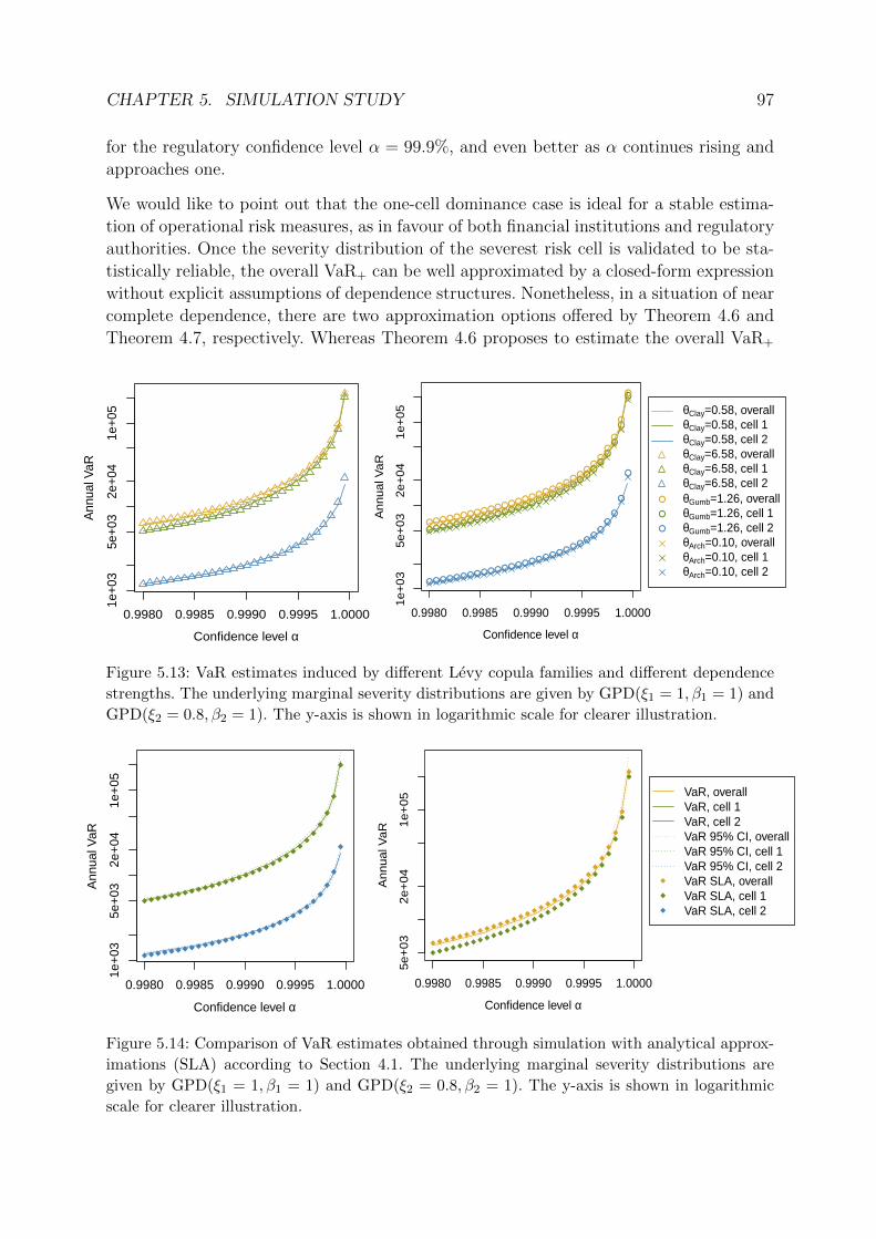
CHAPTER 5. SIMULATION STUDY 97
for the regulatory confidence level α = 99.9%, and even better as α continues rising and
approaches one.
We would like to point out that the one-cell dominance case is ideal for a stable estima-
tion of operational risk measures, as in favour of both financial institutions and regulatory
authorities. Once the severity distribution of the severest risk cell is validated to be sta-
tistically reliable, the overall VaR+ can be well approximated by a closed-form expression
without explicit assumptions of dependence structures. Nonetheless, in a situation of near
complete dependence, there are two approximation options offered by Theorem 4.6 and
Theorem 4.7, respectively. Whereas Theorem 4.6 proposes to estimate the overall VaR+
0.9980 0.9985 0.9990 0.9995 1.0000
1e+0
35e
+03
2e+0
41e
+05
Confidence level α
Ann
ual V
aR
0.9980 0.9985 0.9990 0.9995 1.0000
1e
+0
35
e+
03
2e
+0
41
e+
05
θClay=0.58, overallθClay=0.58, cell 1θClay=0.58, cell 2θClay=6.58, overallθClay=6.58, cell 1θClay=6.58, cell 2θGumb=1.26, overallθGumb=1.26, cell 1θGumb=1.26, cell 2θArch=0.10, overallθArch=0.10, cell 1θArch=0.10, cell 2
Confidence level α
An
nua
l Va
R
Figure 5.13: VaR estimates induced by different Levy copula families and different dependence
strengths. The underlying marginal severity distributions are given by GPD(ξ1 = 1, β1 = 1) and
GPD(ξ2 = 0.8, β2 = 1). The y-axis is shown in logarithmic scale for clearer illustration.
0.9980 0.9985 0.9990 0.9995 1.0000
1e+
035e
+03
2e+
041e
+05
Confidence level α
Ann
ual V
aR
0.9980 0.9985 0.9990 0.9995 1.0000
5e
+0
32
e+
04
1e
+0
5 VaR, overallVaR, cell 1VaR, cell 2VaR 95% CI, overallVaR 95% CI, cell 1VaR 95% CI, cell 2VaR SLA, overallVaR SLA, cell 1VaR SLA, cell 2
Confidence level α
An
nua
l Va
R
Figure 5.14: Comparison of VaR estimates obtained through simulation with analytical approx-
imations (SLA) according to Section 4.1. The underlying marginal severity distributions are
given by GPD(ξ1 = 1, β1 = 1) and GPD(ξ2 = 0.8, β2 = 1). The y-axis is shown in logarithmic
scale for clearer illustration.

CHAPTER 5. SIMULATION STUDY 98
as the sum of the stand-alone VaR values, Theorem 4.7 suggests the approximation via
the dominating marginal severity as just explained. In order to find out the more accurate
method, the right panel of Figure 5.14 compares the two discussed estimation choices. The
underlying data are drawn from a bivariate model based on the Clayton Levy copula with
θClay = 320. Up to a significance level around α = 99.95%, only the summation estimate
lies within the 95% CI of the simulated result, and should therefore be preferred to the
approximation through VaR1. However, the difference becomes increasingly negligible for
higher values of α. In addition, the accuracy of the stand-alone estimates VaR1 and VaR2
are confirmed by the left panel in Figure 5.14, as the analytical approximations lie within
the 95% CI regardless the target confidence level α.
After having discussed the one-cell dominance situation in detail, now we consider a bal-
anced severity design. That is, the marginal severities are assumed to follow a standardised
GPD with identical shape parameters. Note that no closed-form risk measure approxima-
tions exist for arbitrary dependence structures in this setting, except for the independence
and the complete dependence Levy copulas. We first investigate a finite expectation case
and Figure 5.15 presents estimated VaR values for ξ1 = ξ2 = 0.8. The parameters of the
underlying Levy copulas in each of the two subgraphs are precisely the same as in Fig-
ure 5.13. In contrast to Figure 5.13, Figure 5.15 clearly shows that the overall VaR+ based
on the total loss aggregated across both risk cells has varying values for different copula
families and dependence strength. In other words, risk measures in a balanced severity
design are sensitive to the dependence structure. Hence the Levy copula family as well
as the dependence parameter must be modelled carefully in order to obtain accurate risk
measure estimates. Nonetheless, the stand-alone VaR values in Figure 5.15 are unaffected
by the concrete Levy copula, as all estimates stay within the 95% confidence interval with
respect to the Clayton family with θClay = 0.58.
In the right panel of Figure 5.15, the Gumbel Levy copula results in higher VaR+ estimates
0.9980 0.9985 0.9990 0.9995 1.0000
1000
5000
2000
050
000
Confidence level α
Ann
ual V
aR
0.9980 0.9985 0.9990 0.9995 1.0000
1000
5000
2000
050
000
θClay=0.58, overallθClay=0.58, cell 1θClay=0.58, overall, 95% CIθClay=0.58, cell 1, 95% CIθClay=6.58, overallθClay=6.58, cell 1θGumb=1.26, overallθGumb=1.26, cell 1θArch=0.10, overallθArch=0.10, cell 1
Confidence level α
Ann
ual V
aR
Figure 5.15: VaR estimates induced by different Levy copula families and different dependence
strengths. The marginal components have a common GPD with ξ1 = ξ2 = 0.8 and β1 = β2 = 1
as severity distribution, hence only the results for the first risk cell are depicted. The y-axis is
shown in logarithmic scale for clearer illustration.

CHAPTER 5. SIMULATION STUDY 99
than the Clayton family, and the Archimedean family from Example 3.6 (2) offers the
smallest estimates for all depicted confidence levels α. However, this is not in general the
case. The common frequency correlation of the three copula families is changed from 0.3 as
in Figure 5.15 to 0.001 in the left panel of Figure 5.16, and further modified to 0.99 in the
right panel of Figure 5.16. For comparison purpose, the analytical approximations under
the independence and the complete dependence assumptions are drawn as well. Whereas
all three copula families provide nearly identical VaR+ estimates with the independence
copula in the left subfigure, the Clayton family generates the highest VaR+ estimates in the
right subfigure, followed by the Archimedean Levy copula from 3.6 (2), which generates
almost the same estimates as the complete dependence Levy copula. Furthermore, the
overall ES+ estimates are visualised for the same selected Levy copulas in Figure 5.17.
Once again we notice the sensitivity of ES+ towards different dependence structures and
its steep increase with growing confidence level α.
In Figure 5.16, the overall VaR+ estimate in the independence case is smaller than that
under the complete dependence Levy copula. However, it is already argued in [BK08]
that subadditivity of VaR can be violated under heavy-tailed severity distributions. More
precisely, the authors compare overall VaR+ approximations for GPD severities with dif-
ferent shape parameters by employing Theorem 4.5 and Theorem 4.6, respectively. They
conclude that in the finite expectation situation, that is, for ξ1 = ξ2 < 1, the complete
dependence Levy copula indeed produces a higher VaR+ value than the independence
one. On the other hand, subadditivity is violated for infinite expectation models with
ξ1 = ξ2 > 1. Moreover, VaR+ estimates in these two special dependence situations coin-
cide for ξ1 = ξ2 = 1.
Within our simulation study, we extend the results in [BK08] by incorporating a medium
0.9980 0.9985 0.9990 0.9995 1.0000
2000
5000
2000
050
000
θClay=0.10θClay=0.10, 95% CIθGumb=0.13θArch=0.05
Confidence level α
Ann
ual V
aR
0.9980 0.9985 0.9990 0.9995 1.0000
10
00
20
00
50
00
20
00
05
00
00
θClay=69θClay=69, 95% CIθGumb=182θArch=6.9
Indep. overallCompl. Dep. overall
Confidence level α
An
nu
al V
aR
Figure 5.16: Overall VaR+ estimates induced by different Levy copula families and different
dependence strengths. The analytical approximations for the independence and the complete
dependence cases according to Section 4.1.2 are also depicted for comparison purpose. The
marginal components have a common GPD with ξ1 = ξ2 = 0.8 and β1 = β2 = 1 as severity
distribution and the y-axis is shown in logarithmic scale for clearer illustration.

CHAPTER 5. SIMULATION STUDY 100
0.9980 0.9985 0.9990 0.9995 1.0000
1e+
045e
+04
2e+
05
θClay=0.10θGumb=0.13θArch=0.05θClay=0.58θGumb=1.26θArch=0.10
Confidence level α
Ann
ual E
S
0.9980 0.9985 0.9990 0.9995 1.0000
1e+0
42e
+04
5e+0
41e
+05
2e+0
5
θClay=6.58θGumb=17.09θArch=0.69θClay=69θGumb=182θArch=6.9
Confidence level α
Ann
ual E
S
Figure 5.17: Overall ES+ estimates induced by different Levy copula families and different de-
pendence strengths. The marginal components have a common GPD with ξ1 = ξ2 = 0.8 and
β1 = β2 = 1 as severity distribution and the y-axis is shown in logarithmic scale for clearer
illustration.
dependence structure and evaluate a broader range of potential interesting confidence
levels α ∈ [99.8%, 100%). In order to make the results across different copula families
comparable to a certain degree, the copula parameters in all four subgraphs of Figure 5.18
are determined via introducing an equal frequency correlation of 0.5.
For finite marginal severity expectations with ξ1 = ξ2 = 0.8 shown in the top left corner,
the complete dependence Levy copula indeed provides a higher value than the indepen-
dence one for all depicted quantile levels. However, the overall VaR+ estimate associated
with the Gumbel family exhibits an even larger value up to roughly α = 99.95%. Hence
the complete dependence VaR+ cannot be regarded as an upper bond for risk measure
estimations even if the severities are not extremely heavy-tailed and have finite expecta-
tions. In the threshold case of ξ1 = ξ2 = 1 shown in the top right corner, the VaR+ values
not only coincide in both ends of the dependence spectrum, but also across the three
considered copula families with a medium dependence strength. Note that the VaR+ esti-
mates under different dependence assumptions all lie within the 95% CI associated with
the Clayton family for each quantile level α. Finally, the independence VaR+ estimate
exceeds the complete dependence one in both pictures of the bottom panel. Interestingly,
now the Archimedean family from Example 3.6 (2) provides the highest overall VaR+
estimates rather than the Gumbel family as in the top left subgraph. In addition, the
VaR+ values produced by the three selected copula families indicate a more significant
deviation from each other as ξ1 = ξ2 grows from 1.2 in bottom left to 1.5 in bottom right
and thus is more far off the threshold one.
Beyond that, we emphasize that the heavy-tailedness of severity distributions plays a
much more crucial role in view of risk measure calculations in comparison to frequency
correlations. Although the latter is set equally at 0.5 for all subfigures, the obtained
overall VaR+ values exhibit obvious deviations. To further illustrate this, Figure 5.19

CHAPTER 5. SIMULATION STUDY 101
0.9980 0.9985 0.9990 0.9995 1.0000
20
00
50
00
10
00
05
00
00
ξ1=ξ2=0.8
Confidence level α
An
nu
al V
aR
0.9980 0.9985 0.9990 0.9995 1.0000
1e
+0
45
e+
04
2e
+0
5
ClayClay 95% CIGumbArchIndep. overallCompl. Dep. overall
ξ1=ξ2=1
Confidence level α
An
nu
al V
aR
0.9980 0.9985 0.9990 0.9995 1.0000
5e
+0
42
e+
05
1e
+0
65
e+
06
ξ1=ξ2=1,2
Confidence level α
An
nu
al V
aR
0.9980 0.9985 0.9990 0.9995 1.0000
5e
+0
55
e+
06
5e
+0
7
ClayClay 95% CIGumbArchIndep. overallCompl. Dep. overall
ξ1=ξ2=1.5
Confidence level α
An
nu
al V
aR
Figure 5.18: Overall VaR+ estimates under varying shape parameters ξ1 = ξ2 of the marginal
generalised Pareto severity distributions. The scale parameters are set identically at β1 = β2 = 1
in all subfigures. The different Levy copula families are specified to have a common frequency
correlation of 0.5 and the corresponding parameters are given by θClay = 1.00, θGumb = 2.38 and
θArch = 0.14. The analytical approximations for the independence and the complete dependence
cases according to Section 4.1.2 are also depicted for comparison purpose. The y-axis is shown
in logarithmic scale for clearer illustration.

CHAPTER 5. SIMULATION STUDY 102
plots the estimated VaR+ as a function against the shape parameter ξ1 = ξ2 of the
marginal GPD severities. Both the four different significant levels α corresponding to the
four subgraphs and the GPD shape parameters in the x-axis belong to a realistic range
for practical applications. The underlying Levy copulas are characterised by the same
dependence parameters as in Figure 5.18. As the graphs reveal an upwards linear trend
with logarithmically scaled y-axis, we immediately conclude that the overall VaR+ grows
at an exponential rate with increasing ξ1 = ξ2. This pattern is consistent across all depicted
confidence levels and dependence structures. Contrarily, the sensitivity of VaR+ towards
the different copula families is much less pronounced. Nonetheless, the Gumbel family
provides the highest risk measure estimate for the smallest considered shape parameter
ξ1 = ξ2 = 0.6, and is overtaken by the Archimedean family from Example 3.6 (2), as
ξ1 = ξ2 rises to 1.5.
0.6 0.8 1.0 1.2 1.4
5e+0
25e
+03
5e+0
45e
+05
α=99.8%
ξ1=ξ2
Ann
ual V
aR
0.6 0.8 1.0 1.2 1.4
5e+0
25e
+03
5e+0
45e
+05
ClayGumbArch
α=99.85%
ξ1=ξ2
Ann
ual V
aR
0.6 0.8 1.0 1.2 1.4
5e+0
25e
+03
5e+0
45e
+05
α=99.9%
ξ1=ξ2
Ann
ual V
aR
0.6 0.8 1.0 1.2 1.4
1e+0
31e
+04
1e+0
51e
+06
ClayGumbArch
α=99.95%
ξ1=ξ2
Ann
ual V
aR
Figure 5.19: Overall VaR+ estimates for four different confidence levels α and as a function of
the shape parameter ξ1 = ξ2 underlying the marginal generalised Pareto severity distributions.
The scale parameters are set identically at β1 = β2 = 1. The different Levy copula families are
specified to have a common frequency correlation of 0.5 and the corresponding parameters are
given by θClay = 1.00, θGumb = 2.38 and θArch = 0.14. The y-axis is shown in logarithmic scale
for clearer illustration.
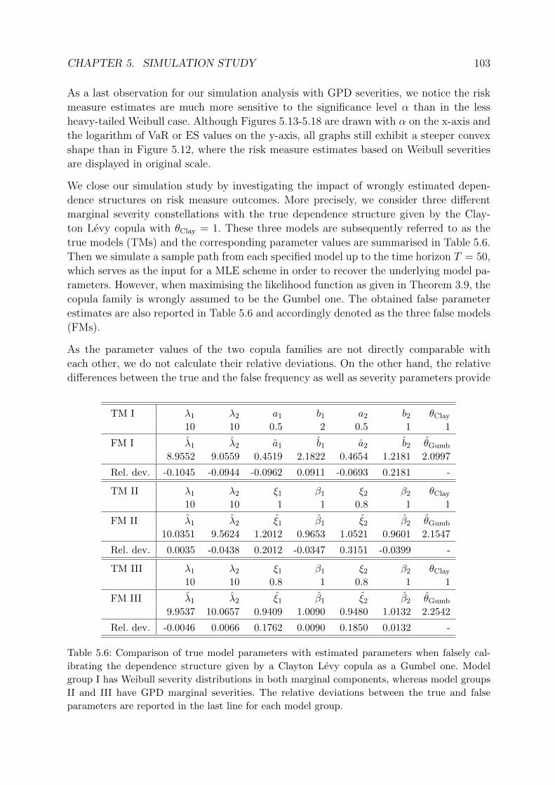
CHAPTER 5. SIMULATION STUDY 103
As a last observation for our simulation analysis with GPD severities, we notice the risk
measure estimates are much more sensitive to the significance level α than in the less
heavy-tailed Weibull case. Although Figures 5.13-5.18 are drawn with α on the x-axis and
the logarithm of VaR or ES values on the y-axis, all graphs still exhibit a steeper convex
shape than in Figure 5.12, where the risk measure estimates based on Weibull severities
are displayed in original scale.
We close our simulation study by investigating the impact of wrongly estimated depen-
dence structures on risk measure outcomes. More precisely, we consider three different
marginal severity constellations with the true dependence structure given by the Clay-
ton Levy copula with θClay = 1. These three models are subsequently referred to as the
true models (TMs) and the corresponding parameter values are summarised in Table 5.6.
Then we simulate a sample path from each specified model up to the time horizon T = 50,
which serves as the input for a MLE scheme in order to recover the underlying model pa-
rameters. However, when maximising the likelihood function as given in Theorem 3.9, the
copula family is wrongly assumed to be the Gumbel one. The obtained false parameter
estimates are also reported in Table 5.6 and accordingly denoted as the three false models
(FMs).
As the parameter values of the two copula families are not directly comparable with
each other, we do not calculate their relative deviations. On the other hand, the relative
differences between the true and the false frequency as well as severity parameters provide
TM I λ1 λ2 a1 b1 a2 b2 θClay
10 10 0.5 2 0.5 1 1
FM I λ1 λ2 a1 b1 a2 b2 θGumb
8.9552 9.0559 0.4519 2.1822 0.4654 1.2181 2.0997
Rel. dev. -0.1045 -0.0944 -0.0962 0.0911 -0.0693 0.2181 -
TM II λ1 λ2 ξ1 β1 ξ2 β2 θClay
10 10 1 1 0.8 1 1
FM II λ1 λ2 ξ1 β1 ξ2 β2 θGumb
10.0351 9.5624 1.2012 0.9653 1.0521 0.9601 2.1547
Rel. dev. 0.0035 -0.0438 0.2012 -0.0347 0.3151 -0.0399 -
TM III λ1 λ2 ξ1 β1 ξ2 β2 θClay
10 10 0.8 1 0.8 1 1
FM III λ1 λ2 ξ1 β1 ξ2 β2 θGumb
9.9537 10.0657 0.9409 1.0090 0.9480 1.0132 2.2542
Rel. dev. -0.0046 0.0066 0.1762 0.0090 0.1850 0.0132 -
Table 5.6: Comparison of true model parameters with estimated parameters when falsely cal-
ibrating the dependence structure given by a Clayton Levy copula as a Gumbel one. Model
group I has Weibull severity distributions in both marginal components, whereas model groups
II and III have GPD marginal severities. The relative deviations between the true and false
parameters are reported in the last line for each model group.

CHAPTER 5. SIMULATION STUDY 104
some interesting observations. Concerning the Poisson intensities λ1 and λ2, their relative
deviations in model groups II and III with regularly varying GPD severities are much
smaller than in model group I with rapidly varying Weibull severities. Moreover, the
imprecision of the estimated Weibull parameters is of approximately the same magnitude
as the frequency estimates in the first model group. Unfortunately, the shape parameter
estimates in model groups II and III, which constitute the most important component of
a GPD, exhibit the largest relative deviations from their true values. Hence we expect the
impact on risk measure computations is also more significant than with Weibull severities,
which shall be examined shortly below. In contrast, the less essential scale parameter β
of a GPD is estimated with a higher accuracy in false models II and III, as their relative
deviations can be as small as one tenth of the relative deviations associated with the shape
parameter ξ.
Nonetheless, the one-cell dominance design in true model II and the balanced severity de-
sign in true model III seem to be preserved despite the misspecification of the dependence
structure. The estimate ξ1 in false model II is significantly higher than ξ2, such that losses
in the first risk cell are more heavy-tailed than in the second one. On the other hand,
0
20
40
0 10 20 30 40 50
Single loss X1
Sin
gle
loss
X2
True model I
0
200
400
0 200 400 600
Single loss X1
Sin
gle
loss
X2
True model II
0
25
50
75
0 100 200
Single loss X1
Sin
gle
loss
X2
True model III
0
10
20
30
0 20 40 60
Single loss X1
Sin
gle
loss
X2
solely cell 1 solely cell 2 common loss
False model I
0
100
200
0 100 200 300
Single loss X1
Sin
gle
loss
X2
solely cell 1 solely cell 2 common loss
False model II
0
100
200
0 50 100 150 200
Single loss X1
Sin
gle
loss
X2
solely cell 1 solely cell 2 common loss
False model III
Figure 5.20: Comparison of loss severities sampled from the true models with the false models
when wrongly calibrating the dependence structure given by a Clayton Levy copula as a Gum-
bel one. Both the underlying marginal distribution parameters and the copula parameters are
reported in Table 5.6.

CHAPTER 5. SIMULATION STUDY 105
the false estimates ξ1 and ξ2 for model III are nearly identical and indicate comparable
marginal loss severities. Also note that model groups II and III have in common that the
wrongly estimated shape parameters are bigger than their true values, which is expected
to result in an overestimation of risk measures.
For illustration purpose, a scatter plot of simulated loss data is displayed in Figure 5.20
for each true and false model. The message we aim for is that the misspecification of
Levy copula families may not be easily identified by visualising the induced single loss
severities, as the point clouds of the false models do not show obviously dissimilar patterns
in comparison to their real counterparts.
Now we turn to evaluating the impact of inappropriately estimated dependence models
on risk measure values, which presents the most relevant issue in view of capital reserve
calculations. To this end, both absolute and relative deviations in VaR and ES estimates,
the latter if well-defined, are depicted for each of the three model groups in Figures 5.21-
5.23, respectively. Moreover, the obtained risk measure estimates themselves are reported
in Table 5.7 for VaR and in Table 5.8 for ES at certain selected confidence levels.
In addition, Table 5.9 exemplarily compares the 95% CIs of VaR estimates between the
true and the false models. The associated significance level is given by α = 99.9%, which
constitutes the most commonly applied one for regulatory capital requirements. In none of
the three model groups, the two CIs are overlapping, indicating massive deviations of risk
measure estimates due to model misspecification. The distance between the lower bound
99.8% 99.825% 99.85% 99.875% 99.9% 99.925% 99.95% 99.975%
TM I 293.24 299.83 307.69 317.91 329.88 346.09 371.03 413.75
FM I 458.40 470.91 485.15 504.14 527.95 557.42 604.15 689.45
TM II 6114.28 7024.06 8158.79 9753.91 12155.24 15578.86 22987.83 43047.23
FM II 30357.06 35517.04 42420.06 51586.96 66902.62 94416.58 147197.03 331672.21
TM III 2280.72 2519.75 2824.67 3210.19 3808.20 4778.93 6546.95 10946.34
FM III 6756.80 7648.88 8804.43 10459.16 12961.90 17236.27 25947.85 50918.40
Table 5.7: Comparison of total VaR+ estimates for one time unit based on the true models with
the false models when wrongly calibrating the dependence structure given by a Clayton Levy
copula as a Gumbel one. Both the underlying marginal distribution parameters and the copula
parameters can be read off from Table 5.6.
99.8% 99.825% 99.85% 99.875% 99.9% 99.925% 99.95% 99.975%
TM I 350.33 358.03 367.12 378.03 391.56 409.57 435.57 481.69
FM I 567.16 581.78 599.10 620.02 646.18 680.97 732.23 823.03
TM III 9222.02 10197.15 11451.31 13142.19 15555.15 19326.75 26191.16 44099.64
FM III 41714.22 46647.17 53054.11 61744.94 74286.60 94088.19 130679.58 225453.85
Table 5.8: Comparison of total ES+ estimates for one time unit based on the true models with
the false models when wrongly calibrating the dependence structure given by a Clayton Levy
copula as a Gumbel one. Both the underlying marginal distribution parameters and the copula
parameters can be read off from Table 5.6.

CHAPTER 5. SIMULATION STUDY 106
TM 95% CI FM 95% CI
I [327.82, 332.58] I [523.39, 532.14]
II [11675.19, 12597.54] II [63631.70, 70579.16]
III [3680.11, 3948.98] III [12384.29, 13554.24]
Table 5.9: Comparison of 95% CIs associated with the overall VaR+(99.9%) estimates based
on the true models with the false models when wrongly calibrating the dependence structure
given by a Clayton Levy copula as a Gumbel one. Both the underlying marginal distribution
parameters and the copula parameters can be read off from Table 5.6.
of the overestimating CI and the upper bound of the true CI is the largest in model group
II with the most heavy-tailed severity distributions, whereas the lower bound of the CI
based on the false model is five times as high as the upper bound of the true CI.
Concerning the first model group with marginal Weibull severities depicted in Figure 5.21,
the absolute deviations exhibit an increasing curve with respect to rising confidence level
α for both VaR and ES, as well as for both the stand-alone and the overall values based
on the total loss amount of the two risk cells. As shown by the right panel, the relative
deviations in ES reveal a similarly smooth, but steeper upwards trend than the absolute
deviations. However, the relative deviations in VaR have much more kinks and reveal an
even sharper increase as α approaches one.
In model group II, the true marginal severity of risk cell one and the falsely estimated
severities of both cells indicate an infinite expectation, hence only the resulting deviations
in VaR are displayed in Figure 5.22. Interestingly, both the absolute and the relative
differences in the overall VaR+ estimates are similar to that of the dominating first cell,
which has a more heavy-tailed GPD severity than the second cell in both the real and the
wrong model. Whereas the second risk cell results in the lowest absolute deviations across
0.9980 0.9985 0.9990 0.9995 1.0000
10
02
00
30
04
00
Confidence level α
Ab
solu
te d
evia
tion
0.9980 0.9985 0.9990 0.9995 1.0000
0.55
0.60
0.65
0.70
VaR, overallVaR, cell 1VaR, cell 2ES, overallES, cell 1ES, cell 2
Confidence level α
Rel
ativ
e de
viat
ion
Figure 5.21: Absolute and relative deviations in risk measure estimates between the true and
the false models of model group I. Both the underlying marginal distribution parameters and
the copula parameters can be read off from Table 5.6.

CHAPTER 5. SIMULATION STUDY 107
all depicted significance levels α, it surpasses the overall VaR+ and the individual VaR1
of the first cell in terms of relative deviations. Although the y-axis in the left subfigure is
shown in logarithmic scale, the graph still possesses an upwards convex trend, indicating
that risk measure deviations grow at least exponentially with respect to α. Furthermore,
the growth rate is much more dramatic than in the less heavy-tailed case with Weibull
severities in Figure 5.21, where the y-axis is shown in original scale. This feature is similar
to our previous observation by comparing Figures 5.13-5.18 with Figure 5.12.
Figure 5.23 illustrates the deviation in VaR and ES estimates for model group III. Re-
call that the underlying true model has a balanced severity design, whereby the falsely
estimated shape parameters of the two risk cells have a similar value as well. Hence the
0.9980 0.9985 0.9990 0.9995 1.0000
5e+
032e
+04
1e+
055e
+05
2e+
06
Confidence level α
Abs
olut
e de
viat
ion
0.9980 0.9985 0.9990 0.9995 1.0000
46
810
1214
16
VaR, overallVaR, cell 1VaR, cell 2
Confidence level α
Rel
ativ
e de
viat
ion
Figure 5.22: Absolute and relative deviations in risk measure estimates between the true and
the false models of model group II. Both the underlying marginal distribution parameters and
the copula parameters can be read off from Table 5.6. The y-axis of the left subfigure is shown
in logarithmic scale for clearer illustration.
0.9980 0.9985 0.9990 0.9995 1.0000
010
0000
2000
0030
0000
Confidence level α
Abs
olut
e de
viat
ion
0.9980 0.9985 0.9990 0.9995 1.0000
2.0
2.5
3.0
3.5
4.0
VaR, overallVaR, cell 1VaR, cell 2ES, overallES, cell 1ES, cell 2
Confidence level α
Rel
ativ
e de
viat
ion
Figure 5.23: Absolute and relative deviations in risk measure estimates between the true and
the false models of model group III. Both the underlying marginal distribution parameters and
the copula parameters can be read off from Table 5.6.

CHAPTER 5. SIMULATION STUDY 108
absolute deviations in the stand-alone risk measures have similar outcomes across the two
cells, and are about half the size compared to the deviation in the overall estimates VaR+
and ES+. However, the relative deviations in the overall risk measure outcomes are rather
close to those for the second risk cell. Beyond that, ES estimates offer a much smoother
increase with respect to the significance level α than VaR estimates in terms of relative
deviations.
Last but not least, all three considered model groups have in common that the deviations
in risk measure outcomes increase with growing confidence level α, whereas the growth
rate depends on the heavy-tailedness of the underlying severity distributions. In addition,
the ES deviations have a higher value than the corresponding VaR differences from both
the absolute and the relative viewpoint. As already indicated within the examination of
the discrepancies between the true and the false model parameters, the risk measures cal-
culated based on all three false models overestimate their real values. This is not surprising
since the scale parameters of the Weibull distributions and the shape parameters of the
GPDs in the false models are estimated larger than their real counterparts, respectively.
Thus the resulting loss severities have a heavier right distribution tail. To conclude, the
misspecification of dependence structure by a wrongly selected Levy copula family can
cause inaccurate marginal parameter estimates as well as have an undesired impact on
risk measure calculations.

Chapter 6
Real data application
In this chapter we apply our dependence modelling approach based on compound Poisson
processes and Levy copulas to three different real-life datasets. To clarify, the application
example presented in Section 6.1 deals with the well-known Danish insurance claim data
rather than operational loss events. The reason for this is that publicly accessible and
high-quality sources of operational risk data are not yet available. The reluctance of the
financial industry to share their sensitive loss information is naturally understandable.
Nonetheless, we would like to exemplify our estimation methodology based on a freely
available data sample, such that every modelling step and illustration can be provided
in detail, as well as be tried out by interested readers. As a result, the Danish fire loss
claims, which possess the same heavy-tailed distribution properties as commonly observed
among operational risk incidents, seem to be the ideal choice. The multivariate version
of this dataset can be found either in the package “CASdatasets” (containing various
actuarial datasets) or “fitdistrplus” (developed for parametric distribution fitting) within
the statistical software environment R.
In Section 6.2, both an internal and an external dataset kindly provided by the Bayerische
Landesbank (BayernLB) are introduced. On the basis of these real operational loss events,
we demonstrate the entire procedure from exploring potential dependence patterns, veri-
fying model assumptions, applying MLE as detailed in Section 3.3, assessing model fit by
means tested within the simulation study from Section 5.3, and finally to estimating risk
measures via both simulation and approximation methods from Chapter 4.
6.1 Danish reinsurance claim dataset
The Danish insurance data were collected at the Copenhagen Reinsurance and consist
of fire losses exceeding one million Danish Krone (mDKK) over the period from 1980 to
1990. Each claim is divided into a loss amount of the building coverage, of the contents
coverage and of the profit coverage. As the last loss category rarely exhibits a non-zero
entry, below we focus on the loss history of building and contents, which is potentially
109

CHAPTER 6. REAL DATA APPLICATION 110
suitable for a bivariate compound Poisson model as detailed in Definition 3.1.
In order to give our modelling approach a clear structure, we briefly state the three
major steps to be followed. First we verify whether the marginal components, that is, the
building and the contents claim processes, can be reasonably described by a homogeneous
compound Poisson process, respectively. If this condition is satisfied, then we apply MLE
by employing the likelihood function from Theorem 3.9 to fit dependence models based
upon alternative Levy copulas. Finally, we compare the fitted models by means of different
diagnostic plots.
To begin with, we consider one calendar year as one time unit such that the overall
observation horizon is given by T = 11. If the marginal claim series follow a homogeneous
compound Poisson process, then the corresponding claim inter-arrival times should be
i.i.d. exponentially distributed random variables. Figure 6.1 examines the exponential
nature of the inter-arrival times of building and contents losses, respectively. The estimated
autocorrelations shown in the top panel fairly lie within the 95% confidence interval,
except for one spike in the building series. In the bottom panel, the empirical quantiles are
plotted against the theoretical ones of an exponential distribution, whose rate parameter
is estimated by the sample mean of the gaps between two loss arrivals. Apart from the
discrete nature of empirical observations, the theoretical and empirical quantiles agree
0.00
0.25
0.50
0.75
1.00
0 10 20 30
Lag
AC
F
Building
0.00
0.25
0.50
0.75
1.00
0 10 20
Lag
AC
F
Contents
0.00
0.02
0.04
0.06
0.00 0.02 0.04 0.06
Theoretical exponential quantiles
Em
piric
al q
uant
iles
0.00
0.03
0.06
0.09
0.00 0.05 0.10
Theoretical exponential quantiles
Em
piric
al q
uant
iles
Figure 6.1: Top panel: autocorrelation functions (acfs) of marginal claim inter-arrival times. Bot-
tom panel: Q-Q plots of the corresponding empirical quantiles against the theoretical exponential
quantiles with an estimated rate parameter 108.53 for building and 49.92 for contents.

CHAPTER 6. REAL DATA APPLICATION 111
well on the positive diagonal line. Overall, there is no evidence against i.i.d. exponential
claim arrival times for both the building and the contents loss processes.
Now we turn to characterising the marginal loss severities. Since the Parato-type behaviour
of the fire losses in the current dataset is already well-known and the reporting limit of
one mDKK provides a natural threshold, two GPDs with identical location parameter
µi = 1 for the two margins i ∈ 1, 2 seem to be an appropriate choice. The associated
distribution tails have the form (1 + ξix−µiβi
)−ξ−1i with shape ξi and scale βi. The shape
and scale parameters are estimated by means of MLE. In order to assess the GPD fit, we
calculate for each loss observation x of marginal component i ∈ 1, 2 the corresponding
residual value ξ−1i ln(1+ ξi
x−1
βi) based on estimated parameters. If the original observations
follow a GPD(ξi, βi, µi), then the residuals should be i.i.d. and follow a standard expo-
nential distribution. In addition, the residuals have a finite second moment in contrast to
the original GPD random variables with a shape parameter larger than or equal to 0.5.
Therefore, we inspect the independence among loss severities via calculating the sample
autocorrelation function based on the residuals, which is presented in the top panel of
Figure 6.2. Furthermore, the bottom panel illustrates the match between the empirical
and the theoretical exponential quantiles. Similar to the interpretation of Figure 6.1 for
0.00
0.25
0.50
0.75
1.00
0 5 10 15 20
Lag
AC
F
Building
0.00
0.25
0.50
0.75
1.00
0 5 10 15 20
Lag
AC
F
Contents
0
2
4
6
8
0 2 4 6
Theoretical exponential quantiles
Em
piric
al q
uant
iles
0
2
4
6
0 2 4 6
Theoretical exponential quantiles
Em
piric
al q
uant
iles
Figure 6.2: Top panel: acfs of residual values calculated from the marginal GPD fits to the loss
amounts under the building and the contents coverage, respectively. The estimated parameters
are given by ξ1 = 0.4525, β1 = 1.0655 for building and ξ2 = 0.6877, β2 = 1.3015 for con-
tents. Bottom panel: Q-Q plots of the corresponding empirical quantiles against the theoretical
standard exponential quantiles.

CHAPTER 6. REAL DATA APPLICATION 112
the inter-arrival times, we conclude that both building and contents claim amounts can
be reasonably modelled by the GPD. Note we have also examined alternative heavy-tailed
distributions not depicted here, and none of them can compete with the GPD fit.
After approving the marginal compound Poisson assumptions, now we aim at capturing
the interdependence between the building and the contents loss processes by means of
Levy copulas. The potential candidates include the Clayton and the Gumbel families from
Table 2.1, the Archimedean copula from Example 3.6 (2), as well as the complementary
Gumbel Levy copula from the same example. As the occurrence dates of all claim events
are known exactly, we apply MLE under a continuous observation scheme as explained in
Section 3.3.1. In practical implementations the corresponding log-likelihood function lnLis maximised for numerical stability, and its maximum value together with the obtained
estimates is summarised in Table 6.1 for different Levy copulas.
λ1 λ2 ξ1 β1 ξ2 β2 θ max. lnLClayton 107.0989 49.2377 0.5373 1.0255 0.8110 1.2863 0.8503 1265.91
Gumbel 107.1765 50.7052 0.7466 0.9548 1.1371 1.2344 3.3625 1228.66
Example 3.6 (2) 112.5945 66.9301 0.9390 1.6044 1.6451 2.1026 0.0373 734.36
Comp. Gumbel 107.6742 50.0968 0.6717 0.9589 0.9055 1.2755 0.8448 1254.22
Table 6.1: Maximum likelihood estimates obtained by maximising the likelihood function in
Theorem 3.9 for selected Levy copula families. Note the copula parameter estimate θ is not
directly comparable across different copula families.
From Table 6.1, we immediately see that the dependence model characterised by the
Archimedean Levy copula of Example 3.6 (2) offers the lowest value of maximised log-
likelihood function, which indicates its infeasibility with respect to the fire loss data. In
order to draw a more comprehensive comparison between the fitted models, we employ
the concept of empirical tail integrals introduced in Section 5.3. Figure 6.3 visualises their
conformity with the theoretical counterparts calculated based on the estimated model
parameters. The independent partial Levy measure Π⊥1 is associated with the claims solely
attributed to the building category. Similarly, the Levy measure Π⊥2 describes contents
claims without resulting in building losses. Claims attributed to both coverage categories
are described by the dependent partial Levy measure Π‖ = (Π‖1,Π
‖2)>.
In line with the maximised log-likelihood function values in Table 6.1, the fitted tail
integrals based on the Archimedean Levy copula from Example 3.6 (2) exhibit a poor fit to
the sample version in all four subfigures. On the other hand, the Clayton, the Gumbel and
its complementary family reveal equally good agreements for the individual tail integrals
Π⊥1 and Π
⊥2 . However, the behaviour of the common tail integral Π
‖= (Π
‖1,Π
‖2)> cannot
be properly reproduced by any of the fitted models. Only the Clayton one, which also
achieves the highest maximised log-likelihood value in Table 6.1, seems to perform slightly
better than the other copulas. Our observation of Figure 6.3 constitutes no surprise, as
the estimated copula parameters in Table 6.1 fall into the range from low to medium
dependence strength as studied in Section 5.3. Recall Figures 5.5-5.6 where the empirical
tail integrals deviate from their theoretical equivalences due to the lack of strictly positive

CHAPTER 6. REAL DATA APPLICATION 113
bivariate observations, even though the underlying data are sampled from the model with
the true parameter values.
As the model suitability of the Clayton, the Gumbel and the complementary Levy copulas
cannot be fully distinguished by exploring the tail integrals in Figure 6.3, we further
compare in Figure 6.4 Q-Q plots for the individual loss severities solely attributed to the
building or to the contents category, respectively. The theoretical quantiles are calculated
based on the corresponding survival functions F⊥1 and F
⊥2 as specified in Lemma 3.4,
Part (b). We observe deviations from the straight diagonal line in the upper quantile area
of different magnitudes.
Moreover, the observed bivariate loss severities related to both the building and the con-
tents coverage are transformed to copula scale and displayed in the upper left corner of
Figure 6.5. The point cloud suggests near independence between the marginal components
with a slight scarcity of points in the top left and bottom right corner, respectively. As
the Archimedean Levy copula from Example 3.6 (2) rather implies a countermonotonic
relationship as revealed in the lower panel of Figure 5.10, it does not provide an appro-
priate fit to the fire losses. Besides the scatter plot, Figure 6.5 also presents a contour
plot featuring the empirical Levy copula as well as the three more promising fitted copula
families. Once again, the sample version does not exhibit a satisfactory overlap with any
0 5 10 15
020
4060
Tail
inte
gral
Indep. part of Π1
empiricalClaytonGumbelArchComp.Gumbel
0 5 10 15
05
1015
20
Tail
inte
gral
Indep. part of Π2
empiricalClaytonGumbelArchComp.Gumbel
0 50 100 150
010
2030
4050
60
Tail
inte
gral
Dep. part of Π1
empiricalClaytonGumbelArchComp.Gumbel
0 20 40 60 80 100 120
010
2030
4050
60
Tail
inte
gral
Dep. part of Π2
empiricalClaytonGumbelArchComp.Gumbel
Figure 6.3: Comparison of sample tail integrals with their theoretical counterparts calcu-
lated based on different fitted Levy copula families. The abbreviation “Arch” refers to the
Archimedean Levy copula from Example 3.6 (2).

CHAPTER 6. REAL DATA APPLICATION 114
0 5 10 15
05
1015
Theoretical quantiles
Em
piric
al q
uant
iles
0 5 10 15
05
1015
Theoretical quantiles
Em
piric
al q
uant
iles
0 5 10 15
05
1015
Theoretical quantiles
Em
piric
al q
uant
iles
0 5 10 15
05
1015
Theoretical quantiles
Em
piric
al q
uant
iles
0 5 10 15
05
1015
Theoretical quantiles
Em
piric
al q
uant
iles
0 5 10 15
05
1015
Theoretical quantiles
Em
piric
al q
uant
iles
Figure 6.4: Q-Q plots of loss severities solely attributed to the building coverage (top section)
and solely attributed to the contents coverage (bottom section). The left column is obtained
from the estimated Clayton Levy copula, the middle column from the Gumbel Levy copula, and
the right column from the complementary Gumbel Levy copula.
of the theoretical counterparts owing to the current low dependence setting, similar to the
reason explained before with respect to the tail integrals attributed to the common loss
process. Nonetheless, the Gumbel Levy copula with the lowest maximised log-likelihood
value after the Archimedean Levy copula from Example 3.6 (2) shows the largest devi-
ation from the empirical contour lines. Finally, a perspective plot in the lower panel of
Figure 6.5 illustrates from two different angles the shape of the theoretical Levy copula,
displayed as a 3D surface, in comparison to the sample version displayed as a 3D his-
togram. Although we only depict the Clayton case, similar visualisations can be obtained
from other copula families.
At the end we notice that the Danish insurance loss data are also analysed by means
of bivariate compound Poisson models under a continuous observation scheme in [EK10]
as well as under a discrete observation scheme in [Vel12]. However, in both references
only the Clayton Levy family is taken into consideration and the single losses are fitted
in logarithmic scale by Weibull distributions. Hence, the current thesis contributes to
the formalisation of the entire procedure of estimating a multivariate compound Poisson
model, that is, from verifying the marginal compound Poisson assumptions to evaluating
the fitted models based on different Levy copulas via various diagnostic tools. Moreover,
we model the loss severities in their original instead of logarithmic scale such that the
obtained model can be directly utilised for operational risk measure calculations and thus
is comparable with the real operational risk data introduced below.

CHAPTER 6. REAL DATA APPLICATION 115
0.0 0.2 0.4 0.6 0.8 1.0
0.0
0.2
0.4
0.6
0.8
1.0
u1
u 2
(a) Scatter plot of losses attributed
to both the building and the contents
coverage in copula scale.
5
10
15
20
25 30
0 20 40 60 80 100
010
2030
4050
5
10
15
20
25
30
5
10
15
20
25
30
5
10
15
20
25
30
u1
u 2
empiricalClaytonGumbelComp.Gumbel
(b) Comparison of contour lines of the
sample Levy copula with different fit-
ted copula families.
u1
2040
60
80
100
u2
1020
3040
Copula
51015202530
u1
2040
6080
100
u210
2030
40
Copula
51015202530
(c) Comparison of sample Levy copula (yellow 3D histogram) with fitted Clayton
Levy copula (grey 3D surface).
Figure 6.5: Examination of fitted dependence models for the Danish fire losses.
6.2 Operational risk datasets
6.2.1 Internal data
It is not allowed to publish the data, but the full analysis has been made available to the
supervisor and advisor.
6.2.2 External data
It is not allowed to publish the data, but the full analysis has been made available to the
supervisors and advisor.

Chapter 7
Conclusion and outlook
Justified by Sklar’s theorem for Levy processes, a multivariate dependence model for op-
erational risk loss events can be readily constructed by combining marginal compound
Poisson processes through a suitable Levy copula. The current thesis contributes to this
not yet commonly known dependence concept by a detailed analysis of its model compo-
nents in Chapter 3, highlighting its potential for asymptotic risk measure approximations
in Chapter 4, investigating the quality of maximum likelihood estimators, the goodness of
fitted dependence structures and the sensitivity of risk measure estimates in Chapter 5.
Furthermore, Chapter 6 puts all previously introduced methodologies at work, whereby
dependence models built upon various Levy copulas are estimated and subsequently ex-
amined based on real loss data. In this way we hope to gain confidence in the applicability
of our modelling approach also from operational risk practitioners.
In comparison to the most alternative dependence modelling techniques summarised in
Section 1.2, the multivariate model based on Levy copulas exhibits several advantages.
First, the dependence structure specification can be separated from the marginal process
characterisation in an analogous manner to utilising ordinary copulas. The severity model
of each risk cell may be chosen from any appropriate distributions, or parameterised as a
spliced one with different body and tail distribution families, such that the heterogeneity
of losses attributed to different causes or business units is respected. On the other hand,
various parametric Levy copula families as well as the extreme cases of independence and
complete dependence Levy copulas are available to be selected.
Second, both frequency and severity dependence are controlled by the same Levy copula
in a calibrated model, such that relatively few parameters are required. In addition, as
Levy copulas operate on the domain of time-independent Levy measures, the dependence
characterisation stays valid as the loss occurrence progresses in the course of time. In
general, the latter does not hold when imposing interdependence among compound Pois-
son processes via ordinary copulas, which may result in the necessity of complexer model
structures with more variables. The parameter parsimony of Levy copula models despite
their flexibility is especially valuable with regard to the scarcity of reliable operational risk
data compared to market or credit risk information. Moreover, the employment of Levy
135

CHAPTER 7. CONCLUSION AND OUTLOOK 136
copulas enables to generalise the already well-known univariate SLA for subexponential
loss severities to higher dimensions. The appeal of closed-form risk exposure estimations
by contrast with simulation methods does not have to be reiterated.
Notwithstanding, the convenient property of integrating frequency and severity depen-
dence into one single concept may also pose a limitation of Levy copulas. Furthermore,
dependence in the sense of Levy measures is only defined for simultaneously occurring
loss events, which might oversimplify real loss situations. Hence possible extensions of
the current model or its combination with alternative dependence concepts constitute an
interesting subject for future research. Beyond that, the issue of incorporating external
data into dependence modelling and risk exposure assessment is briefly addressed at the
end of Chapter 6. Since operational loss incidents of a financial institution are not least
shaped by its individual procedure and control system, the challenge of rescaling external
loss events with respect to representativity is evident. However, the sample size of inter-
nal observations is usually insufficient to support robust risk measure calculations at the
generally high target quantile levels. As a result, it is indispensable to include external
information into internal model calibration and validation schemes.
The growing participation in data consortia certainly confirms the awareness of financial
institutions for sound operational risk quantifications. At the same time, a downturn
in loss frequency or loss magnitude cannot be expected owing to the increasing global
network of business activities and the advances made in information technology, such
that operational risk exposures may become more diverse and complicated. Therefore, the
incentive of implementing adequate dependence models goes far beyond the fulfilment of
regulatory capital requirements, and should constitute an essential element of any risk
management strategy at financial institutions. Finally, we emphasise that the assessment
of the plausibility and the interpretation of a model are at least as important as fitting
the model itself. Of course, all model assumptions and specifications must be periodically
verified by analysts in practice and adjusted to actual loss experience where appropriate.

Appendix A
Categorisation of operational losses
Table A.1: Definition of business lines according to Annex 8 of [Ban06].
Business line Explanation
Corporate Finance Mergers and acquisitions, underwriting, privatisations, securitisation, re-
search, debt (government, high yield), equity, syndications, IPO, secondary
private placements
Trading & Sales Fixed income, equity, foreign exchanges, commodities, credit, funding, own
position securities, lending and repos, brokerage, debt, prime brokerage
Retail Banking Retail lending and deposits, banking services, trust and estates; Private
lending and deposits, banking services, trust and Retail Banking estates,
investment advice; Merchant/commercial/corporate cards, private labels
and retail
Commercial Banking Project finance, real estate, export finance, trade finance, factoring, leasing,
lending, guarantees, bills of exchange
Payment and Settlement Payments and collections, funds transfer, clearing and settlement
Agency Services Escrow, depository receipts, securities lending (customers) corporate ac-
tions; Issuer and paying agents
Asset Management Pooled, segregated, retail, institutional, closed, open, private equity
Retail Brokerage Execution and full service
137

APPENDIX A. CATEGORISATION OF OPERATIONAL LOSSES 138
Table A.2: Definition of event types according to Annex 9 of [Ban06].
Event type Explanation
Internal fraud Losses due to acts of a type intended to de-
fraud, misappropriate property or circumvent regu-
lations, the law or company policy, excluding diver-
sity/discrimination events, which involves at least one
internal party
External fraud Losses due to acts of a type intended to defraud, mis-
appropriate property or circumvent the law, by a third
party
Employment Practices and Workplace Safety Losses arising from acts inconsistent with employ-
ment, health or safety laws or agreements, from pay-
ment of personal injury claims, or from diversity /
discrimination events
Clients, Products & Business Practices Losses arising from an unintentional or negligent fail-
ure to meet a professional obligation to specific clients
(including fiduciary and suitability requirements), or
from the nature or design of a product.
Damage to Physical Assets Losses arising from loss or damage to physical assets
from natural disaster or other events.
Business disruption and system failures Losses arising from disruption of business or system
failures
Execution, Delivery & Process Management Losses from failed transaction processing or process
management, from relations with trade counterparties
and vendors

Appendix B
Characterisation of distribution tails
In order to make the heavy-tailed property of operational risk losses precise, we sum-
marise the main notions utilised in this thesis for characterising heavy-tailed probability
distributions. For further discussions of the subsequent definitions we refer to Appendix 3
of [EKM97], which is a classic textbook for extreme events modelling.
Definition B.1 (Subexponential distribution function).
Let F be a distribution function with support (0,∞) and let F n∗ denote its n-fold con-
volution. If the asymptotic relation
limx→∞
F n∗(x)
F (x)= n, n ≥ 2, (B.1)
holds, then F is called subexponential and written as F ∈ S.
From relation (B.1) the following more intuitive characterisation of subexponentiality can
be derived:
limx→∞
P(X1 + · · ·+Xn > x)
P(maxX1, . . . , Xn > x)= 1, n ≥ 2.
Hence the distribution tail of the partial sum of n i.i.d. subexponential random variables
has the same order of magnitude as the tail of the maximum among them. In other words,
a severe overall loss amount is more probably owing to a single extreme loss rather than
to accumulated small losses.
An important subclass of subexponential distributions comprises distributions whose far
out right tail behaves like a power function:
Definition B.2 (Regularly varying distribution tail).
Let F be a distribution function with support (0,∞). If for some γ ≥ 0 the distribution
tail F satisfies the condition
limx→∞
F (xt)
F (x)= t−γ, t > 0,
139

APPENDIX B. CHARACTERISATION OF DISTRIBUTION TAILS 140
then F is said to be regularly varying with index −γ and denoted by F ∈ R−γ. The
quantity γ is often referred to as the tail index of F and we write R = ∪γ≥0R−γ.
Note that the k-th power moment of a random variable with F ∈ R−γ only exists for
k < γ. A prominent example of a regularly varying distribution is given by the Pareto
distribution. On the other hand, the heavy-tailed Weibull distribution and the lognormal
distribution are subexponential but not regularly varying. Their tails decay faster than
the tails in R, but more slowly than any exponential tail. Hence a third distribution tail
characterisation is needed:
Definition B.3 (Rapidly varying distribution tail).
Let F be a distribution function with support (0,∞). If the asymptotic relation
limx→∞
F (xt)
F (x)=
0, t > 1,
∞, 0 < t < 1,
holds, then F is called rapidly varying and denoted by F ∈ R∞.
In contrast to random variables with distribution tail in R, all power moments of a
distribution with rapidly varying tail exist and are finite.

Appendix C
Results of simulation study
In the current section we present the simulation results for Section 5.2, where the quality of
obtained maximum likelihood estimates (MLEs) for a bivariate compound Poisson model
based on Levy copulas is investigated. First, the utilised performance measures shall be
explained.
Let δ be either a parameter of the marginal Poisson frequency distributions, a parameter
of the marginal severity distributions, or a Levy copula parameter. A simple criterion
for the goodness of its estimator δ is given by the bias, which is defined as the expected
difference between δ and δ. In our study, the bias is estimated by the difference between
the empirical mean and the true parameter value. In order to make the obtained results for
parameter values of different scales comparable, the mean relative bias (MRB) is reported
in the subsequent tables. The latter expresses the bias as a percentage of the true value
and is estimated by
MRB =1
δM
M∑m=1
δm − δ,
where M = 100 denotes the number of replications for each considered compound Poisson
model in our simulation scheme.
A common accuracy measure is called the mean squared error (MSE), which is defined as
MSE[δ] = E[(δ − δ)2] and reflects the dispersion of the estimates around the true value.
In particular, the MSE incorporates the concept of both bias and precision as it satisfies
the decomposition MSE[δ] = Var[δ] + Bias[δ]2. Small variance and little bias thus lead to
a highly accurate estimator. Since the MSE squares all differences, it does not have the
same scale as the parameter δ. Hence we take the square root of the MSE, yielding the
root mean squared error (RMSE) which is on the same scale as δ. In order to compare
estimates across different model components, we again divide this measure by the true
parameter value and obtain the relative RMSE (RRMSE). The corresponding empirical
version is calculated as
RRMSE =1
δ
√√√√ 1
M
M∑m=1
(δm − δ)2.
141

APPENDIX C. RESULTS OF SIMULATION STUDY 142
Since both the MSE and RMSE are calculated using squared differences, they could be
dominated by outlying estimates far away from the true value δ. To avoid this potential
problem of outliers, we also consider the absolute value of the difference between δ and
δ as a more robust measure for accuracy. The latter is commonly known as the mean
absolute error (MAE) and its relative version is estimated as
RMAE =1
δM
M∑m=1
| δm − δ | .
After having presented the relevant performance measures, the subsequent tables sum-
marise the results from our simulation procedure as detailed in Section 5.2.

APPENDIX C. RESULTS OF SIMULATION STUDY 143
Table C.1: Performance measures based on 100 MLEs for the parameters of a bivariate compound
Poisson model built upon the Clayton Levy copula with different dependence strength (Top section:
low dependence with true value θClay,low = 0.3242; Middle section: medium dependence with true value
θClay,med = 1.2212; Bottom section: high dependence with true value θClay,high = 7.0519), and each for
the time horizon of T = 5, 10, 20 years. The true marginal frequency parameters are given by λ1 = 40,
λ2 = 45, and the severity distributions by LN (µ1 = 10.3, σ1 = 1.8), Weib(a2 = 0.19, b2 = 5000).
T λ1 λ2 µ1 σ1 a2 b2 θClay,low
Mean
5 40.2124 45.6848 10.3202 1.7744 0.1914 5407.0411 0.3284
10 40.0461 45.3387 10.3149 1.7813 0.1904 5127.2845 0.3262
20 39.9180 45.1435 10.3191 1.7921 0.1905 5048.6349 0.3254
MRB
5 0.0053 0.0152 0.0020 -0.0142 0.0075 0.0814 0.0128
10 0.0012 0.0075 0.0014 -0.0104 0.0022 0.0255 0.0059
20 -0.0021 0.0032 0.0019 -0.0044 0.0026 0.0097 0.0034
RMAE
5 0.0534 0.0539 0.0116 0.0399 0.0438 0.3323 0.0696
10 0.0426 0.0362 0.0069 0.0306 0.0274 0.2198 0.0432
20 0.0297 0.0258 0.0047 0.0213 0.0187 0.1529 0.0290
RRMSE
5 0.0638 0.0649 0.0139 0.0494 0.0538 0.4257 0.0853
10 0.0504 0.0451 0.0085 0.0370 0.0344 0.2767 0.0548
20 0.0366 0.0318 0.0059 0.0261 0.0239 0.1944 0.0390
T λ1 λ2 µ1 σ1 a2 b2 θClay,med
Mean
5 39.9567 44.1770 10.2798 1.7835 0.1919 5180.8075 1.2131
10 40.1726 44.5516 10.2856 1.7943 0.1905 5132.0707 1.2242
20 40.0598 44.8498 10.2975 1.7956 0.1898 5013.3640 1.2242
MRB
5 -0.0011 -0.0183 -0.0020 -0.0092 0.0103 0.0362 -0.0066
10 0.0043 -0.0100 -0.0014 -0.0032 0.0028 0.0264 0.0024
20 0.0015 -0.0033 -0.0002 -0.0025 -0.0009 0.0027 0.0025
RMAE
5 0.0593 0.0537 0.0102 0.0329 0.0347 0.2811 0.0654
10 0.0397 0.0391 0.0067 0.0223 0.0237 0.2066 0.0501
20 0.0317 0.0280 0.0044 0.0167 0.0170 0.1536 0.0340
RRMSE
5 0.0765 0.0700 0.0126 0.0425 0.0446 0.3732 0.0835
10 0.0508 0.0500 0.0079 0.0289 0.0302 0.2630 0.0627
20 0.0384 0.0351 0.0056 0.0210 0.0222 0.1888 0.0426
T λ1 λ2 µ1 σ1 a2 b2 θClay,high
Mean
5 39.9308 44.8135 10.2898 1.7864 0.1918 5187.7130 7.0323
10 39.8997 44.7082 10.2979 1.7909 0.1915 5215.4336 7.0942
20 39.9578 44.8283 10.2977 1.7937 0.1910 5153.2642 7.0786
MRB
5 -0.0017 -0.0041 -0.0010 -0.0076 0.0093 0.0375 -0.0028
10 -0.0025 -0.0065 -0.0002 -0.0051 0.0077 0.0431 0.0060
20 -0.0011 -0.0038 -0.0002 -0.0035 0.0052 0.0307 0.0038
RMAE
5 0.0551 0.0500 0.0090 0.0307 0.0270 0.2979 0.0628
10 0.0374 0.0373 0.0068 0.0230 0.0183 0.2071 0.0495
20 0.0265 0.0261 0.0054 0.0158 0.0149 0.1653 0.0361
RRMSE
5 0.0696 0.0644 0.0113 0.0378 0.0337 0.3969 0.0799
10 0.0475 0.0468 0.0084 0.0285 0.0233 0.2778 0.0627
20 0.0329 0.0328 0.0068 0.0197 0.0187 0.2097 0.0443

APPENDIX C. RESULTS OF SIMULATION STUDY 144
Table C.2: Performance measures based on 100 MLEs for the parameters of a bivariate compound
Poisson model built upon the Clayton Levy copula with different dependence strength (Top section:
low dependence with true value θClay,low = 0.3242; Middle section: medium dependence with true value
θClay,med = 1.2212; Bottom section: high dependence with true value θClay,high = 7.0519), and each for
the time horizon of T = 5, 10, 20 years. The true marginal frequency parameters are given by λ1 = 40,
λ2 = 45, and the severity distributions by Weib(a1 = 0.19, b1 = 5000), GPD(ξ2 = 1.3, β2 = 5000).
T λ1 λ2 a1 b1 ξ2 β2 θClay,low
Mean
5 39.7284 44.4946 0.1919 5632.4421 1.2921 5093.9403 0.3210
10 39.9099 44.7353 0.1907 5401.0427 1.2920 5051.7121 0.3248
20 40.2513 44.7989 0.1909 5188.9437 1.2863 5058.2948 0.3251
MRB
5 -0.0068 -0.0112 0.0099 0.1265 -0.0061 0.0188 -0.0100
10 -0.0023 -0.0059 0.0035 0.0802 -0.0062 0.0103 0.0018
20 0.0063 -0.0045 0.0046 0.0378 -0.0105 0.0117 0.0028
RMAE
5 0.0614 0.0526 0.0459 0.3410 0.0805 0.1323 0.0665
10 0.0440 0.0347 0.0303 0.2100 0.0600 0.0887 0.0425
20 0.0298 0.0206 0.0236 0.1352 0.0446 0.0606 0.0310
RRMSE
5 0.0802 0.0632 0.0570 0.4727 0.1046 0.1671 0.0829
10 0.0572 0.0417 0.0364 0.2749 0.0773 0.1104 0.0547
20 0.0366 0.0248 0.0285 0.1797 0.0558 0.0795 0.0391
T λ1 λ2 a1 b1 ξ2 β2 θClay,med
Mean
5 39.9592 44.6513 0.1902 5408.7682 1.3018 4940.3094 1.2130
10 39.7005 44.5764 0.1897 5014.7597 1.3022 4899.4134 1.2104
20 39.9328 44.7790 0.1900 5088.0564 1.3072 4945.4481 1.2213
MRB
5 -0.0010 -0.0077 0.0009 0.0818 0.0014 -0.0119 -0.0067
10 -0.0075 -0.0094 -0.0013 0.0030 0.0017 -0.0201 -0.0088
20 -0.0017 -0.0049 -0.0000 0.0176 0.0055 -0.0109 0.0001
RMAE
5 0.0568 0.0477 0.0386 0.3704 0.0786 0.1043 0.0640
10 0.0403 0.0347 0.0243 0.2125 0.0631 0.0720 0.0487
20 0.0246 0.0261 0.0163 0.1487 0.0418 0.0478 0.0323
RRMSE
5 0.0701 0.0605 0.0480 0.5060 0.0998 0.1272 0.0780
10 0.0525 0.0445 0.0304 0.2901 0.0777 0.0853 0.0589
20 0.0327 0.0323 0.0200 0.1907 0.0534 0.0623 0.0401
T λ1 λ2 a1 b1 ξ2 β2 θClay,high
Mean
5 39.0748 44.0593 0.1920 5663.4055 1.3002 5145.6403 7.1948
10 39.3702 44.4336 0.1907 5315.3628 1.3030 5057.1749 7.1242
20 39.6745 44.6520 0.1903 5328.1002 1.3111 5053.1263 7.1247
MRB
5 -0.0231 -0.0209 0.0105 0.1327 0.0002 0.0291 0.0203
10 -0.0157 -0.0126 0.0036 0.0631 0.0023 0.0114 0.0103
20 -0.0081 -0.0077 0.0014 0.0656 0.0086 0.0106 0.0103
RMAE
5 0.0576 0.0526 0.0311 0.3176 0.0671 0.0938 0.0780
10 0.0389 0.0345 0.0209 0.1944 0.0437 0.0707 0.0530
20 0.0285 0.0256 0.0147 0.1544 0.0380 0.0471 0.0345
RRMSE
5 0.0720 0.0651 0.0391 0.3971 0.0848 0.1173 0.0999
10 0.0485 0.0433 0.0258 0.2476 0.0567 0.0898 0.0669
20 0.0353 0.0326 0.0188 0.1922 0.0479 0.0599 0.0446

APPENDIX C. RESULTS OF SIMULATION STUDY 145
Table C.3: Performance measures based on 100 MLEs for the parameters of a bivariate compound
Poisson model built upon the Clayton Levy copula with different dependence strength (Top section:
low dependence with true value θClay,low = 0.3242; Middle section: medium dependence with true value
θClay,med = 1.2212; Bottom section: high dependence with true value θClay,high = 7.0519), and each for
the time horizon of T = 5, 10, 20 years. The true marginal frequency parameters are given by λ1 = 40,
λ2 = 45, and the severity distributions by LN (µ1 = 10.3, σ1 = 1.8), GPD(ξ2 = 1.3, β2 = 5000).
T λ1 λ2 µ1 σ1 ξ2 β2 θClay,low
Mean
5 39.8686 45.1355 10.3061 1.7881 1.2873 5133.8954 0.3248
10 40.0596 44.8414 10.2987 1.7896 1.2770 5099.1410 0.3218
20 39.7667 44.9224 10.2985 1.7963 1.2773 5092.6631 0.3234
MRB
5 -0.0033 0.0030 0.0006 -0.0066 -0.0098 0.0268 0.0016
10 0.0015 -0.0035 -0.0001 -0.0058 -0.0177 0.0198 -0.0076
20 -0.0058 -0.0017 -0.0001 -0.0021 -0.0175 0.0185 -0.0025
RMAE
5 0.0524 0.0529 0.0108 0.0342 0.0912 0.1280 0.0791
10 0.0393 0.0363 0.0073 0.0272 0.0679 0.0824 0.0499
20 0.0279 0.0248 0.0041 0.0177 0.0459 0.0615 0.0357
RRMSE
5 0.0657 0.0682 0.0132 0.0433 0.1121 0.1563 0.0999
10 0.0485 0.0480 0.0086 0.0340 0.0835 0.1065 0.0635
20 0.0349 0.0312 0.0050 0.0213 0.0584 0.0785 0.0454
T λ1 λ2 µ1 σ1 ξ2 β2 θClay,med
Mean
5 39.8461 44.4483 10.3084 1.7873 1.3070 5063.4838 1.2288
10 40.0318 44.7946 10.3034 1.7951 1.3126 5013.9403 1.2287
20 39.9473 44.8117 10.3018 1.8014 1.3058 5004.9352 1.2234
MRB
5 -0.0038 -0.0123 0.0008 -0.0071 0.0054 0.0127 0.0062
10 0.0008 -0.0046 0.0003 -0.0027 0.0097 0.0028 0.0062
20 -0.0013 -0.0042 0.0002 0.0008 0.0045 0.0010 0.0018
RMAE
5 0.0547 0.0535 0.0092 0.0370 0.0788 0.1149 0.0601
10 0.0359 0.0350 0.0067 0.0269 0.0517 0.0734 0.0445
20 0.0275 0.0289 0.0044 0.0179 0.0421 0.0532 0.0342
RRMSE
5 0.0700 0.0663 0.0119 0.0464 0.1003 0.1565 0.0777
10 0.0463 0.0457 0.0087 0.0337 0.0681 0.0951 0.0553
20 0.0335 0.0364 0.0058 0.0219 0.0501 0.0682 0.0429
T λ1 λ2 µ1 σ1 ξ2 β2 θClay,high
Mean
5 39.1453 44.2740 10.2870 1.7974 1.2900 4947.2790 7.0393
10 39.3099 44.3939 10.2915 1.7974 1.2937 4949.5253 7.0344
20 39.6911 44.7503 10.2958 1.8015 1.3013 4961.7985 7.0235
MRB
5 -0.0214 -0.0161 -0.0013 -0.0015 -0.0077 -0.0105 -0.0018
10 -0.0173 -0.0135 -0.0008 -0.0015 -0.0049 -0.0101 -0.0025
20 -0.0077 -0.0055 -0.0004 0.0008 0.0010 -0.0076 -0.0040
RMAE
5 0.0527 0.0522 0.0096 0.0350 0.0764 0.0970 0.0696
10 0.0387 0.0375 0.0067 0.0246 0.0508 0.0632 0.0497
20 0.0282 0.0252 0.0053 0.0179 0.0337 0.0533 0.0353
RRMSE
5 0.0672 0.0637 0.0117 0.0455 0.0949 0.1171 0.0892
10 0.0501 0.0475 0.0082 0.0320 0.0644 0.0774 0.0619
20 0.0346 0.0309 0.0064 0.0226 0.0433 0.0629 0.0427

APPENDIX C. RESULTS OF SIMULATION STUDY 146
Table C.4: Performance measures based on 100 MLEs for the parameters of a bivariate compound
Poisson model built upon the Clayton Levy copula with different dependence strength (Top section:
low dependence with true value θClay,low = 0.3242; Middle section: medium dependence with true value
θClay,med = 1.2212; Bottom section: high dependence with true value θClay,high = 7.0519), and each for
the time horizon of T = 5, 10, 20 years. The true marginal frequency parameters are given by λ1 = 40,
λ2 = 45, and the severity distributions by Weib(a1 = 0.16, b1 = 4000), Weib(a2 = 0.19, b2 = 5000).
T λ1 λ2 a1 b1 a2 b2 θClay,low
Mean
5 39.4263 45.1948 0.1615 4809.1522 0.1911 5687.2657 0.3289
10 39.8423 45.2273 0.1615 4361.6227 0.1902 5339.0626 0.3272
20 39.8868 45.2191 0.1605 4171.9963 0.1906 5180.3028 0.3264
MRB
5 -0.0143 0.0043 0.0091 0.2023 0.0058 0.1375 0.0145
10 -0.0039 0.0051 0.0095 0.0904 0.0009 0.0678 0.0089
20 -0.0028 0.0049 0.0031 0.0430 0.0030 0.0361 0.0065
RMAE
5 0.0516 0.0487 0.0451 0.4410 0.0403 0.3671 0.0675
10 0.0382 0.0358 0.0318 0.2875 0.0309 0.2185 0.0488
20 0.0281 0.0237 0.0222 0.2020 0.0182 0.1332 0.0334
RRMSE
5 0.0635 0.0606 0.0558 0.6125 0.0496 0.4794 0.0840
10 0.0483 0.0441 0.0413 0.3767 0.0366 0.2786 0.0600
20 0.0350 0.0305 0.0293 0.2486 0.0227 0.1716 0.0423
T λ1 λ2 a1 b1 a2 b2 θClay,med
Mean
5 39.8399 45.2654 0.1613 4197.9251 0.1908 5156.4578 1.2241
10 40.0144 45.1698 0.1606 4101.4673 0.1909 5178.6554 1.2179
20 40.2196 45.3155 0.1599 4050.1897 0.1909 5122.6918 1.2188
MRB
5 -0.0040 0.0059 0.0084 0.0495 0.0043 0.0313 0.0024
10 0.0004 0.0038 0.0037 0.0254 0.0046 0.0357 -0.0027
20 0.0055 0.0070 -0.0004 0.0125 0.0050 0.0245 -0.0020
RMAE
5 0.0540 0.0489 0.0383 0.3289 0.0389 0.2904 0.0626
10 0.0381 0.0401 0.0245 0.2413 0.0294 0.1959 0.0429
20 0.0274 0.0298 0.0168 0.1807 0.0209 0.1318 0.0315
RRMSE
5 0.0666 0.0603 0.0476 0.4301 0.0491 0.3561 0.0762
10 0.0483 0.0516 0.0319 0.3181 0.0346 0.2482 0.0530
20 0.0355 0.0367 0.0218 0.2287 0.0257 0.1720 0.0377
T λ1 λ2 a1 b1 a2 b2 θClay,high
Mean
5 40.3741 45.3980 0.1611 4281.1287 0.1912 5174.3061 7.0648
10 40.1756 45.1960 0.1605 4150.7013 0.1902 5050.7024 7.1111
20 40.2173 45.2234 0.1601 4050.7317 0.1899 4996.3067 7.0878
MRB
5 0.0094 0.0088 0.0070 0.0703 0.0061 0.0349 0.0018
10 0.0044 0.0044 0.0032 0.0377 0.0009 0.0101 0.0084
20 0.0054 0.0050 0.0008 0.0127 -0.0007 -0.0007 0.0051
RMAE
5 0.0553 0.0517 0.0256 0.3774 0.0315 0.2912 0.0674
10 0.0351 0.0337 0.0193 0.2508 0.0198 0.1883 0.0576
20 0.0274 0.0251 0.0144 0.1788 0.0156 0.1380 0.0380
RRMSE
5 0.0685 0.0630 0.0329 0.5088 0.0394 0.3787 0.0888
10 0.0438 0.0411 0.0232 0.3416 0.0254 0.2553 0.0714
20 0.0338 0.0316 0.0176 0.2242 0.0197 0.1784 0.0479

APPENDIX C. RESULTS OF SIMULATION STUDY 147
Table C.5: Performance measures based on 100 MLEs for the parameters of a bivariate compound
Poisson model built upon the Clayton Levy copula with different dependence strength (Top section:
low dependence with true value θClay,low = 0.3242; Middle section: medium dependence with true value
θClay,med = 1.2212; Bottom section: high dependence with true value θClay,high = 7.0519), and each for
the time horizon of T = 5, 10, 20 years. The true marginal frequency parameters are given by λ1 = 40,
λ2 = 45, and the severity distributions by LN (µ1 = 10.3, σ1 = 1.8), LN (µ2 = 9.8, σ2 = 1.4).
T λ1 λ2 µ1 σ1 µ2 σ2 θClay,low
Mean
5 39.9164 44.9538 10.3100 1.7975 9.7996 1.4027 0.3243
10 39.9262 44.9793 10.3103 1.7943 9.7980 1.4035 0.3251
20 39.9969 45.1528 10.3010 1.7920 9.8027 1.4040 0.3238
MRB
5 -0.0021 -0.0010 0.0010 -0.0014 -0.0000 0.0019 0.0002
10 -0.0018 -0.0005 0.0010 -0.0032 -0.0002 0.0025 0.0027
20 -0.0001 0.0034 0.0001 -0.0044 0.0003 0.0029 -0.0013
RMAE
5 0.0519 0.0505 0.0096 0.0390 0.0079 0.0426 0.0634
10 0.0358 0.0356 0.0063 0.0253 0.0057 0.0259 0.0461
20 0.0260 0.0271 0.0049 0.0182 0.0039 0.0171 0.0323
RRMSE
5 0.0671 0.0669 0.0121 0.0496 0.0099 0.0519 0.0797
10 0.0452 0.0457 0.0081 0.0309 0.0071 0.0345 0.0581
20 0.0322 0.0329 0.0063 0.0235 0.0046 0.0216 0.0414
T λ1 λ2 µ1 σ1 µ2 σ2 θClay,med
Mean
5 39.7469 44.6879 10.3087 1.7844 9.8170 1.3908 1.2182
10 39.9191 44.8704 10.3056 1.7867 9.8082 1.3959 1.2170
20 39.9989 44.7628 10.3034 1.7937 9.8003 1.3988 1.2188
MRB
5 -0.0063 -0.0069 0.0008 -0.0087 0.0017 -0.0066 -0.0024
10 -0.0020 -0.0029 0.0005 -0.0074 0.0008 -0.0029 -0.0034
20 -0.0000 -0.0053 0.0003 -0.0035 0.0000 -0.0009 -0.0020
RMAE
5 0.0500 0.0527 0.0091 0.0381 0.0076 0.0326 0.0598
10 0.0345 0.0372 0.0069 0.0256 0.0056 0.0228 0.0401
20 0.0263 0.0254 0.0053 0.0180 0.0041 0.0175 0.0311
RRMSE
5 0.0645 0.0662 0.0120 0.0455 0.0095 0.0397 0.0790
10 0.0450 0.0465 0.0086 0.0317 0.0071 0.0281 0.0497
20 0.0320 0.0310 0.0067 0.0223 0.0052 0.0207 0.0366
T λ1 λ2 µ1 σ1 µ2 σ2 θClay,high
Mean
5 40.4191 45.6044 10.2911 1.7912 9.7902 1.3961 7.0370
10 40.4015 45.4730 10.2984 1.7971 9.7976 1.3999 7.0508
20 40.1179 45.2114 10.3061 1.7966 9.8011 1.3991 7.0650
MRB
5 0.0105 0.0134 -0.0009 -0.0049 -0.0010 -0.0028 -0.0021
10 0.0100 0.0105 -0.0002 -0.0016 -0.0002 -0.0001 -0.0002
20 0.0029 0.0047 0.0006 -0.0019 0.0001 -0.0006 0.0019
RMAE
5 0.0555 0.0488 0.0095 0.0295 0.0078 0.0307 0.0729
10 0.0386 0.0352 0.0071 0.0194 0.0053 0.0215 0.0516
20 0.0292 0.0272 0.0050 0.0148 0.0038 0.0154 0.0361
RRMSE
5 0.0714 0.0630 0.0116 0.0362 0.0099 0.0366 0.0933
10 0.0484 0.0443 0.0086 0.0241 0.0068 0.0259 0.0646
20 0.0363 0.0345 0.0062 0.0181 0.0047 0.0201 0.0462

APPENDIX C. RESULTS OF SIMULATION STUDY 148
Table C.6: Performance measures based on 100 MLEs for the parameters of a bivariate compound
Poisson model built upon the Clayton Levy copula with different dependence strength (Top section:
low dependence with true value θClay,low = 0.3242; Middle section: medium dependence with true value
θClay,med = 1.2212; Bottom section: high dependence with true value θClay,high = 7.0519), and each for
the time horizon of T = 5, 10, 20 years. The true marginal frequency parameters are given by λ1 = 40,
λ2 = 45, and the severity distributions by GPD(ξ1 = 1.5, β1 = 6000), GPD(ξ2 = 1.3, β2 = 5000).
T λ1 λ2 ξ1 β1 ξ2 β2 θClay,low
Mean
5 39.4806 44.9344 1.4527 6075.8581 1.2809 5016.4564 0.3139
10 39.9064 44.9220 1.4882 6053.7551 1.2952 4977.6855 0.3190
20 40.1449 45.0540 1.4895 6019.4580 1.2896 5030.6567 0.3212
MRB
5 -0.0130 -0.0015 -0.0316 0.0126 -0.0147 0.0033 -0.0318
10 -0.0023 -0.0017 -0.0078 0.0090 -0.0037 -0.0045 -0.0162
20 0.0036 0.0012 -0.0070 0.0032 -0.0080 0.0061 -0.0095
RMAE
5 0.0659 0.0531 0.0844 0.1065 0.0910 0.1302 0.0733
10 0.0363 0.0387 0.0686 0.0852 0.0646 0.0871 0.0510
20 0.0301 0.0256 0.0513 0.0601 0.0453 0.0522 0.0407
RRMSE
5 0.0790 0.0676 0.1040 0.1307 0.1124 0.1660 0.0955
10 0.0442 0.0485 0.0822 0.1035 0.0791 0.1107 0.0617
20 0.0362 0.0325 0.0620 0.0762 0.0543 0.0681 0.0503
T λ1 λ2 ξ1 β1 ξ2 β2 θClay,med
Mean
5 40.2708 44.8805 1.4971 6074.1477 1.2964 5030.7057 1.2304
10 39.9647 44.6188 1.4883 6101.4901 1.3029 4979.2258 1.2275
20 40.0979 44.7993 1.4925 6008.4340 1.2929 5024.6935 1.2259
MRB
5 0.0068 -0.0027 -0.0020 0.0124 -0.0027 0.0061 0.0075
10 -0.0009 -0.0085 -0.0078 0.0169 0.0022 -0.0042 0.0051
20 0.0024 -0.0045 -0.0050 0.0014 -0.0055 0.0049 0.0039
RMAE
5 0.0540 0.0501 0.0789 0.1122 0.0821 0.1142 0.0716
10 0.0426 0.0348 0.0545 0.0892 0.0564 0.0806 0.0424
20 0.0302 0.0249 0.0389 0.0647 0.0401 0.0517 0.0323
RRMSE
5 0.0725 0.0636 0.1018 0.1353 0.1042 0.1444 0.0880
10 0.0543 0.0437 0.0682 0.1147 0.0702 0.1000 0.0562
20 0.0388 0.0323 0.0484 0.0805 0.0500 0.0656 0.0403
T λ1 λ2 ξ1 β1 ξ2 β2 θClay,high
Mean
5 40.1587 45.2055 1.4715 6102.6530 1.2719 5081.5584 7.1509
10 40.1376 45.0229 1.4793 6040.4492 1.2789 5078.1190 7.0773
20 39.9179 44.8596 1.4822 6025.7559 1.2831 5050.1588 7.0820
MRB
5 0.0040 0.0046 -0.0190 0.0171 -0.0216 0.0163 0.0140
10 0.0034 0.0005 -0.0138 0.0067 -0.0162 0.0156 0.0036
20 -0.0021 -0.0031 -0.0119 0.0043 -0.0130 0.0100 0.0043
RMAE
5 0.0492 0.0431 0.0645 0.1000 0.0666 0.0897 0.0647
10 0.0354 0.0326 0.0414 0.0650 0.0452 0.0611 0.0394
20 0.0277 0.0277 0.0307 0.0449 0.0334 0.0429 0.0316
RRMSE
5 0.0620 0.0556 0.0814 0.1247 0.0833 0.1139 0.0796
10 0.0451 0.0415 0.0515 0.0796 0.0552 0.0774 0.0536
20 0.0346 0.0346 0.0383 0.0582 0.0406 0.0519 0.0384

APPENDIX C. RESULTS OF SIMULATION STUDY 149
Table C.7: Performance measures based on 100 MLEs for the parameters of a bivariate compound
Poisson model built upon the Clayton Levy copula with different dependence strength (Top section:
low dependence with true value θClay,low = 0.3242; Middle section: medium dependence with true value
θClay,med = 1.2212; Bottom section: high dependence with true value θClay,high = 7.0519), and each for
the time horizon of T = 5, 10, 20 years. The true marginal frequency parameters are given by λ1 = 40,
λ2 = 45, and the severity distributions by GPD(ξ1 = 0.9, β1 = 6000), GPD(ξ2 = 0.9, β2 = 6000).
T λ1 λ2 ξ1 β1 ξ2 β2 θClay,low
Mean
5 39.6000 44.9858 0.9056 6169.0486 0.8814 6198.6746 0.3270
10 39.7663 45.1606 0.9013 6110.6873 0.8979 6112.7971 0.3259
20 39.8128 45.0460 0.8956 6079.5861 0.8983 6058.4359 0.3258
MRB
5 -0.0100 -0.0003 0.0062 0.0282 -0.0206 0.0331 0.0085
10 -0.0058 0.0036 0.0015 0.0184 -0.0024 0.0188 0.0049
20 -0.0047 0.0010 -0.0049 0.0133 -0.0019 0.0097 0.0047
RMAE
5 0.0553 0.0463 0.1092 0.1234 0.1200 0.1053 0.0616
10 0.0362 0.0324 0.0730 0.0907 0.0791 0.0707 0.0434
20 0.0293 0.0214 0.0535 0.0602 0.0574 0.0509 0.0318
RRMSE
5 0.0681 0.0579 0.1436 0.1530 0.1554 0.1302 0.0791
10 0.0465 0.0403 0.0905 0.1101 0.1019 0.0885 0.0547
20 0.0367 0.0273 0.0660 0.0732 0.0737 0.0619 0.0412
T λ1 λ2 ξ1 β1 ξ2 β2 θClay,med
Mean
5 40.4259 45.1548 0.9022 6081.2606 0.8983 6110.7307 1.2363
10 40.2095 44.9877 0.9072 5979.5402 0.9091 6017.7748 1.2307
20 40.1766 45.0691 0.9065 5940.8229 0.9116 5974.4792 1.2262
MRB
5 0.0106 0.0034 0.0025 0.0135 -0.0018 0.0185 0.0124
10 0.0052 -0.0003 0.0080 -0.0034 0.0101 0.0030 0.0078
20 0.0044 0.0015 0.0072 -0.0099 0.0129 -0.0043 0.0041
RMAE
5 0.0656 0.0553 0.0893 0.0903 0.0900 0.0915 0.0594
10 0.0430 0.0352 0.0677 0.0701 0.0697 0.0665 0.0435
20 0.0309 0.0303 0.0520 0.0505 0.0490 0.0453 0.0302
RRMSE
5 0.0789 0.0722 0.1146 0.1104 0.1062 0.1151 0.0752
10 0.0521 0.0476 0.0854 0.0871 0.0876 0.0819 0.0554
20 0.0384 0.0370 0.0652 0.0611 0.0638 0.0560 0.0375
T λ1 λ2 ξ1 β1 ξ2 β2 θClay,high
Mean
5 40.7235 45.6070 0.8854 6110.4527 0.8860 6166.9081 7.1168
10 40.1786 45.2457 0.8919 6097.7207 0.8943 6080.3753 7.1054
20 40.1925 45.3117 0.8936 6034.8480 0.8948 6006.7217 7.0586
MRB
5 0.0181 0.0135 -0.0162 0.0184 -0.0156 0.0278 0.0092
10 0.0045 0.0055 -0.0090 0.0163 -0.0063 0.0134 0.0076
20 0.0048 0.0069 -0.0071 0.0058 -0.0057 0.0011 0.0010
RMAE
5 0.0531 0.0493 0.0937 0.0975 0.0903 0.1001 0.0750
10 0.0363 0.0334 0.0651 0.0593 0.0633 0.0600 0.0487
20 0.0279 0.0282 0.0435 0.0409 0.0417 0.0399 0.0341
RRMSE
5 0.0682 0.0630 0.1119 0.1207 0.1061 0.1233 0.0918
10 0.0469 0.0454 0.0804 0.0741 0.0773 0.0747 0.0597
20 0.0350 0.0344 0.0543 0.0510 0.0519 0.0512 0.0417

APPENDIX C. RESULTS OF SIMULATION STUDY 150
Table C.8: Performance measures based on 100 MLEs for the parameters of a bivariate compound
Poisson model built upon the Gumbel Levy copula with different dependence strength (Top section: low
dependence with true value θGumb,low = 0.9317; Middle section: medium dependence with true value
θGumb,med = 4.3951; Bottom section: high dependence with true value θGumb,high = 26.8980), and each
for the time horizon of T = 5, 10, 20 years. The true marginal frequency parameters are given by λ1 = 40,
λ2 = 45, and the severity distributions by Weib(a1 = 0.16, b1 = 4000), Weib(a2 = 0.19, b2 = 5000).
T λ1 λ2 a1 b1 a2 b2 θGumb,low
Mean
5 40.2164 44.6700 0.1610 4320.0109 0.1933 5772.8305 0.9195
10 40.2581 44.9302 0.1617 4169.4294 0.1921 5436.4003 0.9265
20 40.0259 44.7941 0.1608 4152.3709 0.1905 5144.2345 0.9321
MRB
5 0.0054 -0.0073 0.0060 0.0800 0.0174 0.1546 -0.0131
10 0.0065 -0.0016 0.0104 0.0424 0.0111 0.0873 -0.0056
20 0.0006 -0.0046 0.0053 0.0381 0.0027 0.0288 0.0004
RMAE
5 0.0527 0.0612 0.0439 0.3591 0.0451 0.3214 0.0921
10 0.0343 0.0410 0.0328 0.2775 0.0299 0.2059 0.0623
20 0.0287 0.0305 0.0197 0.1904 0.0194 0.1403 0.0486
RRMSE
5 0.0656 0.0760 0.0538 0.5006 0.0554 0.4388 0.1182
10 0.0430 0.0502 0.0407 0.3569 0.0373 0.2673 0.0780
20 0.0355 0.0373 0.0251 0.2463 0.0236 0.1790 0.0617
T λ1 λ2 a1 b1 a2 b2 θGumb,med
Mean
5 40.2316 45.0689 0.1609 4292.3140 0.1917 5374.2003 4.4070
10 39.9582 44.9934 0.1601 4117.0492 0.1911 5149.1394 4.4032
20 39.8848 44.8213 0.1602 4054.5263 0.1909 5160.2550 4.3889
MRB
5 0.0058 0.0015 0.0054 0.0731 0.0090 0.0748 0.0027
10 -0.0010 -0.0001 0.0004 0.0293 0.0056 0.0298 0.0019
20 -0.0029 -0.0040 0.0009 0.0136 0.0047 0.0321 -0.0014
RMAE
5 0.0553 0.0537 0.0373 0.3516 0.0311 0.3023 0.0757
10 0.0395 0.0355 0.0257 0.2448 0.0223 0.1837 0.0505
20 0.0266 0.0261 0.0173 0.1738 0.0150 0.1439 0.0373
RRMSE
5 0.0698 0.0643 0.0455 0.4757 0.0403 0.3742 0.0937
10 0.0480 0.0479 0.0320 0.3201 0.0265 0.2322 0.0666
20 0.0351 0.0342 0.0211 0.2145 0.0189 0.1749 0.0455
T λ1 λ2 a1 b1 a2 b2 θGumb,high
Mean
5 39.5735 44.4862 0.1611 4361.8710 0.1913 5295.9069 27.3544
10 39.6912 44.7412 0.1605 4181.0857 0.1904 5111.8820 27.0513
20 39.9180 44.9589 0.1604 4163.8795 0.1904 5136.0205 27.0818
MRB
5 -0.0107 -0.0114 0.0071 0.0905 0.0067 0.0592 0.0170
10 -0.0077 -0.0058 0.0033 0.0453 0.0023 0.0224 0.0057
20 -0.0021 -0.0009 0.0024 0.0410 0.0019 0.0272 0.0068
RMAE
5 0.0573 0.0585 0.0285 0.3683 0.0295 0.2688 0.0814
10 0.0452 0.0452 0.0204 0.2591 0.0194 0.1981 0.0529
20 0.0323 0.0310 0.0146 0.1750 0.0143 0.1456 0.0392
RRMSE
5 0.0698 0.0711 0.0354 0.4827 0.0367 0.3717 0.1009
10 0.0571 0.0555 0.0245 0.3297 0.0253 0.2567 0.0647
20 0.0407 0.0389 0.0179 0.2212 0.0181 0.1740 0.0481

APPENDIX C. RESULTS OF SIMULATION STUDY 151
Table C.9: Performance measures based on 100 MLEs for the parameters of a bivariate compound
Poisson model built upon the Gumbel Levy copula with different dependence strength (Top section: low
dependence with true value θGumb,low = 0.9317; Middle section: medium dependence with true value
θGumb,med = 4.3951; Bottom section: high dependence with true value θGumb,high = 26.8980), and each
for the time horizon of T = 5, 10, 20 years. The true marginal frequency parameters are given by λ1 = 40,
λ2 = 45, and the severity distributions by LN (µ1 = 10.3, σ1 = 1.8), LN (µ2 = 9.8, σ2 = 1.4).
T λ1 λ2 µ1 σ1 µ2 σ2 θGumb,low
Mean
5 39.9114 45.0306 10.2825 1.7873 9.7971 1.3967 0.9244
10 39.9733 44.9614 10.2893 1.7907 9.8030 1.4011 0.9267
20 39.9813 45.0108 10.2933 1.7965 9.8022 1.4024 0.9270
MRB
5 -0.0022 0.0007 -0.0017 -0.0071 -0.0003 -0.0024 -0.0079
10 -0.0007 -0.0009 -0.0010 -0.0052 0.0003 0.0008 -0.0054
20 -0.0005 0.0002 -0.0007 -0.0019 0.0002 0.0017 -0.0051
RMAE
5 0.0553 0.0509 0.0089 0.0363 0.0079 0.0313 0.0871
10 0.0369 0.0376 0.0069 0.0283 0.0060 0.0256 0.0612
20 0.0263 0.0265 0.0048 0.0206 0.0042 0.0184 0.0467
RRMSE
5 0.0691 0.0632 0.0109 0.0466 0.0101 0.0399 0.1073
10 0.0457 0.0470 0.0085 0.0358 0.0072 0.0322 0.0779
20 0.0329 0.0333 0.0059 0.0257 0.0051 0.0223 0.0581
T λ1 λ2 µ1 σ1 µ2 σ2 θGumb,med
Mean
5 39.6337 44.5268 10.2866 1.7912 9.7896 1.3914 4.3207
10 39.8199 44.9170 10.3117 1.7960 9.8003 1.4016 4.4197
20 40.0314 45.0300 10.3086 1.8034 9.8095 1.4002 4.4266
MRB
5 -0.0092 -0.0105 -0.0013 -0.0049 -0.0011 -0.0062 -0.0169
10 -0.0045 -0.0018 0.0011 -0.0022 0.0000 0.0011 0.0056
20 0.0008 0.0007 0.0008 0.0019 0.0010 0.0001 0.0072
RMAE
5 0.0656 0.0548 0.0109 0.0246 0.0074 0.0277 0.0896
10 0.0455 0.0394 0.0083 0.0195 0.0054 0.0198 0.0621
20 0.0273 0.0250 0.0052 0.0130 0.0040 0.0130 0.0422
RRMSE
5 0.0829 0.0686 0.0142 0.0307 0.0096 0.0367 0.1140
10 0.0571 0.0485 0.0101 0.0250 0.0069 0.0250 0.0785
20 0.0342 0.0327 0.0065 0.0160 0.0052 0.0170 0.0541
T λ1 λ2 µ1 σ1 µ2 σ2 θGumb,high
Mean
5 40.2213 45.1986 10.3040 1.8021 9.8055 1.4013 27.4689
10 40.3078 45.2557 10.3072 1.8000 9.8079 1.3997 27.3196
20 40.1482 45.0565 10.3095 1.8027 9.8087 1.4021 27.2211
MRB
5 0.0055 0.0044 0.0004 0.0012 0.0006 0.0010 0.0212
10 0.0077 0.0057 0.0007 0.0000 0.0008 -0.0002 0.0157
20 0.0037 0.0013 0.0009 0.0015 0.0009 0.0015 0.0120
RMAE
5 0.0584 0.0534 0.0094 0.0255 0.0082 0.0253 0.0837
10 0.0391 0.0364 0.0056 0.0197 0.0048 0.0200 0.0516
20 0.0257 0.0247 0.0042 0.0132 0.0036 0.0135 0.0363
RRMSE
5 0.0710 0.0666 0.0115 0.0310 0.0100 0.0308 0.1037
10 0.0493 0.0473 0.0072 0.0254 0.0064 0.0262 0.0683
20 0.0327 0.0309 0.0053 0.0168 0.0044 0.0174 0.0472

APPENDIX C. RESULTS OF SIMULATION STUDY 152
Table C.10: Performance measures based on 100 MLEs for the parameters of a bivariate compound
Poisson model built upon the Gumbel Levy copula with different dependence strength (Top section: low
dependence with true value θGumb,low = 0.9317; Middle section: medium dependence with true value
θGumb,med = 4.3951; Bottom section: high dependence with true value θGumb,high = 26.8980), and each
for the time horizon of T = 5, 10, 20 years. The true marginal frequency parameters are given by λ1 = 40,
λ2 = 45, and the severity distributions by GPD(ξ1 = 1.5, β1 = 6000), GPD(ξ2 = 1.3, β2 = 5000).
T λ1 λ2 ξ1 β1 ξ2 β2 θGumb,low
Mean
5 39.5429 44.5132 1.4697 6283.6742 1.2766 5199.1889 0.9345
10 39.6504 44.8438 1.4888 6154.7059 1.2906 5025.6624 0.9325
20 39.9579 44.9658 1.4890 6084.3774 1.2990 5041.8845 0.9352
MRB
5 -0.0114 -0.0108 -0.0202 0.0473 -0.0180 0.0398 0.0029
10 -0.0087 -0.0035 -0.0074 0.0258 -0.0072 0.0051 0.0008
20 -0.0011 -0.0008 -0.0073 0.0141 -0.0007 0.0084 0.0037
RMAE
5 0.0594 0.0495 0.0785 0.1307 0.0878 0.1436 0.0934
10 0.0397 0.0360 0.0545 0.0804 0.0590 0.0860 0.0628
20 0.0290 0.0254 0.0441 0.0614 0.0356 0.0518 0.0367
RRMSE
5 0.0742 0.0634 0.1038 0.1691 0.1177 0.1849 0.1134
10 0.0490 0.0477 0.0713 0.1106 0.0763 0.1044 0.0757
20 0.0368 0.0324 0.0535 0.0795 0.0469 0.0652 0.0452
T λ1 λ2 ξ1 β1 ξ2 β2 θGumb,med
Mean
5 40.0266 45.2881 1.4884 6080.6771 1.2812 4999.4044 4.3864
10 39.8682 44.9094 1.4887 6081.3711 1.2816 5033.7814 4.3765
20 39.9360 44.9620 1.4951 6068.2213 1.2934 5015.7577 4.3901
MRB
5 0.0007 0.0064 -0.0077 0.0134 -0.0144 -0.0001 -0.0020
10 -0.0033 -0.0020 -0.0075 0.0136 -0.0141 0.0068 -0.0042
20 -0.0016 -0.0008 -0.0032 0.0114 -0.0050 0.0032 -0.0011
RMAE
5 0.0518 0.0529 0.0644 0.1009 0.0650 0.0935 0.0649
10 0.0369 0.0364 0.0443 0.0839 0.0448 0.0754 0.0482
20 0.0268 0.0248 0.0307 0.0569 0.0305 0.0480 0.0354
RRMSE
5 0.0628 0.0652 0.0788 0.1262 0.0789 0.1132 0.0811
10 0.0443 0.0444 0.0575 0.1040 0.0558 0.0945 0.0625
20 0.0324 0.0311 0.0375 0.0699 0.0389 0.0612 0.0440
T λ1 λ2 ξ1 β1 ξ2 β2 θGumb,high
Mean
5 40.0846 45.1240 1.4894 6022.6879 1.2887 5027.8557 27.3753
10 40.0602 44.9990 1.4913 5989.0825 1.2897 5023.4766 26.9650
20 39.9138 44.9331 1.4947 6002.2036 1.2947 4996.1381 26.9584
MRB
5 0.0021 0.0028 -0.0071 0.0038 -0.0087 0.0056 0.0177
10 0.0015 -0.0000 -0.0058 -0.0018 -0.0079 0.0047 0.0025
20 -0.0022 -0.0015 -0.0035 0.0004 -0.0041 -0.0008 0.0022
RMAE
5 0.0526 0.0520 0.0692 0.1001 0.0682 0.0766 0.0857
10 0.0359 0.0359 0.0454 0.0747 0.0452 0.0647 0.0559
20 0.0272 0.0276 0.0291 0.0456 0.0290 0.0416 0.0374
RRMSE
5 0.0637 0.0623 0.0856 0.1159 0.0839 0.0946 0.1034
10 0.0462 0.0457 0.0583 0.0926 0.0577 0.0806 0.0701
20 0.0344 0.0348 0.0375 0.0573 0.0377 0.0535 0.0461

APPENDIX C. RESULTS OF SIMULATION STUDY 153
Table C.11: Performance measures based on 100 MLEs for the parameters of a bivariate compound
Poisson model built upon the Gumbel Levy copula with different dependence strength (Top section: low
dependence with true value θGumb,low = 0.9317; Middle section: medium dependence with true value
θGumb,med = 4.3951; Bottom section: high dependence with true value θGumb,high = 26.8980), and each
for the time horizon of T = 5, 10, 20 years. The true marginal frequency parameters are given by λ1 = 40,
λ2 = 45, and the severity distributions by GPD(ξ1 = 0.9, β1 = 6000), GPD(ξ2 = 0.9, β2 = 6000).
T λ1 λ2 ξ1 β1 ξ2 β2 θGumb,low
Mean
5 39.8841 45.0753 0.9180 5981.8488 0.9020 6082.4192 0.9447
10 39.8080 45.0409 0.8995 6026.0918 0.8876 6097.8865 0.9333
20 39.8961 45.1428 0.9043 6033.0511 0.8984 6005.1707 0.9358
MRB
5 -0.0029 0.0017 0.0200 -0.0030 0.0022 0.0137 0.0139
10 -0.0048 0.0009 -0.0006 0.0043 -0.0137 0.0163 0.0017
20 -0.0026 0.0032 0.0048 0.0055 -0.0018 0.0009 0.0044
RMAE
5 0.0545 0.0540 0.1129 0.1002 0.0892 0.1014 0.0990
10 0.0363 0.0402 0.0734 0.0732 0.0722 0.0752 0.0669
20 0.0267 0.0277 0.0505 0.0563 0.0466 0.0479 0.0455
RRMSE
5 0.0681 0.0676 0.1405 0.1270 0.1167 0.1245 0.1223
10 0.0456 0.0477 0.0931 0.0983 0.0875 0.0922 0.0816
20 0.0324 0.0338 0.0632 0.0695 0.0560 0.0586 0.0563
T λ1 λ2 ξ1 β1 ξ2 β2 θGumb,med
Mean
5 40.1506 45.4965 0.8863 6193.1889 0.8920 6018.4122 4.4285
10 40.0179 45.3504 0.8950 6097.5172 0.9039 5915.6334 4.4074
20 40.1153 45.0880 0.8974 6018.5176 0.9025 5960.7398 4.4089
MRB
5 0.0038 0.0110 -0.0152 0.0322 -0.0089 0.0031 0.0076
10 0.0004 0.0078 -0.0056 0.0163 0.0043 -0.0141 0.0028
20 0.0029 0.0020 -0.0029 0.0031 0.0027 -0.0065 0.0031
RMAE
5 0.0539 0.0502 0.0774 0.0971 0.0788 0.0972 0.0627
10 0.0430 0.0353 0.0574 0.0697 0.0555 0.0696 0.0510
20 0.0288 0.0250 0.0421 0.0466 0.0386 0.0494 0.0369
RRMSE
5 0.0692 0.0658 0.0957 0.1174 0.0995 0.1179 0.0803
10 0.0538 0.0467 0.0734 0.0871 0.0689 0.0834 0.0619
20 0.0365 0.0333 0.0528 0.0614 0.0496 0.0611 0.0465
T λ1 λ2 ξ1 β1 ξ2 β2 θGumb,high
Mean
5 39.7476 44.5191 0.8940 5991.1450 0.8921 6062.3819 27.0920
10 39.9985 44.8812 0.8948 6002.7881 0.8936 6050.9067 26.9045
20 39.8976 44.8008 0.8947 5996.2052 0.8940 6022.5115 26.7872
MRB
5 -0.0063 -0.0107 -0.0066 -0.0015 -0.0088 0.0104 0.0072
10 -0.0000 -0.0026 -0.0058 0.0005 -0.0071 0.0085 0.0002
20 -0.0026 -0.0044 -0.0058 -0.0006 -0.0067 0.0038 -0.0041
RMAE
5 0.0534 0.0514 0.0700 0.0745 0.0690 0.0845 0.0765
10 0.0326 0.0326 0.0529 0.0514 0.0544 0.0584 0.0560
20 0.0228 0.0234 0.0398 0.0372 0.0400 0.0414 0.0403
RRMSE
5 0.0664 0.0626 0.0853 0.0969 0.0839 0.1051 0.1053
10 0.0402 0.0408 0.0669 0.0647 0.0682 0.0740 0.0715
20 0.0272 0.0288 0.0489 0.0481 0.0488 0.0537 0.0501

APPENDIX C. RESULTS OF SIMULATION STUDY 154
Table C.12: Performance measures based on 100 MLEs for the parameters of a bivariate compound
Poisson model built upon the Levy copula in Example 3.6 (2) with different dependence strength (Top
section: low dependence with true value θArch,low = 0.0185; Middle section: medium dependence with true
value θArch,med = 0.0377; Bottom section: high dependence with true value θArch,high = 0.1746), and each
for the time horizon of T = 5, 10, 20 years. The true marginal frequency parameters are given by λ1 = 40,
λ2 = 45, and the severity distributions by Weib(a1 = 0.16, b1 = 4000), Weib(a2 = 0.19, b2 = 5000).
T λ1 λ2 a1 b1 a2 b2 θArch,low
Mean
5 39.6449 45.0026 0.1601 4157.9074 0.1908 5080.3731 0.0186
10 39.7272 45.2021 0.1603 4002.9639 0.1904 5110.5558 0.0186
20 40.1143 45.1632 0.1597 3991.4773 0.1898 4985.5159 0.0185
MRB
5 -0.0089 0.0001 0.0004 0.0395 0.0040 0.0161 0.0073
10 -0.0068 0.0045 0.0021 0.0007 0.0020 0.0221 0.0030
20 0.0029 0.0036 -0.0021 -0.0021 -0.0013 -0.0029 -0.0017
RMAE
5 0.0524 0.0532 0.0460 0.3468 0.0391 0.2580 0.0387
10 0.0415 0.0373 0.0320 0.2533 0.0269 0.1962 0.0283
20 0.0278 0.0270 0.0220 0.1707 0.0178 0.1374 0.0200
RRMSE
5 0.0663 0.0661 0.0593 0.4414 0.0496 0.3225 0.0493
10 0.0504 0.0476 0.0389 0.3182 0.0353 0.2780 0.0348
20 0.0353 0.0341 0.0289 0.2153 0.0222 0.1825 0.0250
T λ1 λ2 a1 b1 a2 b2 θArch,med
Mean
5 39.9833 44.5070 0.1607 4231.5093 0.1922 5278.5295 0.0382
10 39.9394 44.7173 0.1603 4100.0270 0.1912 5213.6351 0.0380
20 40.0007 44.7869 0.1600 4010.7836 0.1906 4992.8627 0.0379
MRB
5 -0.0004 -0.0110 0.0043 0.0579 0.0114 0.0557 0.0126
10 -0.0015 -0.0063 0.0019 0.0250 0.0062 0.0427 0.0065
20 0.0000 -0.0047 0.0002 0.0027 0.0029 -0.0014 0.0059
RMAE
5 0.0460 0.0478 0.0398 0.3000 0.0367 0.2645 0.0480
10 0.0310 0.0319 0.0299 0.2229 0.0244 0.1793 0.0293
20 0.0240 0.0244 0.0208 0.1391 0.0181 0.1221 0.0224
RRMSE
5 0.0578 0.0589 0.0518 0.3885 0.0470 0.3513 0.0579
10 0.0390 0.0392 0.0375 0.2752 0.0298 0.2289 0.0382
20 0.0305 0.0309 0.0258 0.1737 0.0227 0.1597 0.0286
T λ1 λ2 a1 b1 a2 b2 θArch,high
Mean
5 40.0766 45.0151 0.1605 4225.7601 0.1911 5132.7539 0.1749
10 40.2806 45.3051 0.1604 4108.0894 0.1904 4959.7071 0.1741
20 40.1242 45.1105 0.1601 4002.7443 0.1902 4953.2431 0.1739
MRB
5 0.0019 0.0003 0.0033 0.0564 0.0056 0.0266 0.0019
10 0.0070 0.0068 0.0023 0.0270 0.0023 -0.0081 -0.0026
20 0.0031 0.0025 0.0004 0.0007 0.0010 -0.0094 -0.0038
RMAE
5 0.0596 0.0573 0.0390 0.2936 0.0353 0.2384 0.0640
10 0.0366 0.0336 0.0306 0.2193 0.0257 0.1627 0.0445
20 0.0277 0.0255 0.0214 0.1487 0.0202 0.1069 0.0329
RRMSE
5 0.0720 0.0712 0.0485 0.3755 0.0457 0.3148 0.0793
10 0.0466 0.0448 0.0378 0.2731 0.0323 0.2035 0.0553
20 0.0336 0.0327 0.0265 0.1862 0.0243 0.1357 0.0408

APPENDIX C. RESULTS OF SIMULATION STUDY 155
Table C.13: Performance measures based on 100 MLEs for the parameters of a bivariate compound
Poisson model built upon the Levy copula in Example 3.6 (2) with different dependence strength (Top
section: low dependence with true value θArch,low = 0.0185; Middle section: medium dependence with
true value θArch,med = 0.0377; Bottom section: high dependence with true value θArch,high = 0.1746), and
each for the time horizon of T = 5, 10, 20 years. The true marginal frequency parameters are given by
λ1 = 40, λ2 = 45, and the severity distributions by LN (µ1 = 10.3, σ1 = 1.8), LN (µ2 = 9.8, σ2 = 1.4).
T λ1 λ2 µ1 σ1 µ2 σ2 θArch,low
Mean
5 40.4752 44.5744 10.2871 1.8019 9.8001 1.3982 0.0185
10 40.1440 44.6219 10.2922 1.7962 9.8064 1.3903 0.0186
20 40.1887 44.9048 10.2933 1.7965 9.8058 1.3971 0.0185
MRB
5 0.0119 -0.0095 -0.0013 0.0011 0.0000 -0.0013 0.0021
10 0.0036 -0.0084 -0.0008 -0.0021 0.0007 -0.0069 0.0023
20 0.0047 -0.0021 -0.0007 -0.0019 0.0006 -0.0021 -0.0010
RMAE
5 0.0712 0.0469 0.0095 0.0362 0.0073 0.0397 0.0412
10 0.0436 0.0353 0.0058 0.0278 0.0058 0.0255 0.0282
20 0.0312 0.0254 0.0044 0.0202 0.0038 0.0180 0.0207
RRMSE
5 0.0880 0.0595 0.0122 0.0436 0.0090 0.0496 0.0498
10 0.0540 0.0445 0.0075 0.0345 0.0071 0.0314 0.0348
20 0.0377 0.0322 0.0055 0.0256 0.0046 0.0219 0.0260
T λ1 λ2 µ1 σ1 µ2 σ2 θArch,med
Mean
5 40.2352 45.5970 10.2898 1.7950 9.8029 1.3991 0.0375
10 40.2857 45.2729 10.2990 1.7975 9.8029 1.4002 0.0375
20 40.0939 45.0183 10.2991 1.7997 9.8024 1.4008 0.0377
MRB
5 0.0059 0.0133 -0.0010 -0.0028 0.0003 -0.0007 -0.0050
10 0.0071 0.0061 -0.0001 -0.0014 0.0003 0.0001 -0.0057
20 0.0023 0.0004 -0.0001 -0.0002 0.0002 0.0005 -0.0012
RMAE
5 0.0531 0.0436 0.0076 0.0383 0.0062 0.0292 0.0461
10 0.0376 0.0329 0.0051 0.0258 0.0042 0.0230 0.0334
20 0.0266 0.0217 0.0037 0.0182 0.0032 0.0182 0.0234
RRMSE
5 0.0675 0.0557 0.0094 0.0453 0.0081 0.0371 0.0585
10 0.0483 0.0426 0.0064 0.0327 0.0055 0.0283 0.0419
20 0.0331 0.0278 0.0048 0.0225 0.0042 0.0222 0.0298
T λ1 λ2 µ1 σ1 µ2 σ2 θArch,high
Mean
5 39.8654 44.9796 10.3113 1.7785 9.7985 1.3988 0.1757
10 39.8484 44.9057 10.3054 1.7954 9.7995 1.3993 0.1757
20 39.8770 44.8999 10.3038 1.7967 9.7966 1.3984 0.1757
MRB
5 -0.0034 -0.0005 0.0011 -0.0119 -0.0002 -0.0009 0.0062
10 -0.0038 -0.0021 0.0005 -0.0025 -0.0001 -0.0005 0.0066
20 -0.0031 -0.0022 0.0004 -0.0018 -0.0003 -0.0011 0.0063
RMAE
5 0.0578 0.0569 0.0074 0.0331 0.0059 0.0340 0.0670
10 0.0423 0.0390 0.0054 0.0224 0.0040 0.0233 0.0484
20 0.0270 0.0256 0.0038 0.0155 0.0029 0.0162 0.0328
RRMSE
5 0.0709 0.0686 0.0094 0.0423 0.0072 0.0431 0.0817
10 0.0526 0.0490 0.0069 0.0277 0.0050 0.0295 0.0609
20 0.0354 0.0327 0.0047 0.0192 0.0036 0.0204 0.0420

APPENDIX C. RESULTS OF SIMULATION STUDY 156
Table C.14: Performance measures based on 100 MLEs for the parameters of a bivariate compound
Poisson model built upon the Levy copula in Example 3.6 (2) with different dependence strength (Top
section: low dependence with true value θArch,low = 0.0185; Middle section: medium dependence with true
value θArch,med = 0.0377; Bottom section: high dependence with true value θArch,high = 0.1746), and each
for the time horizon of T = 5, 10, 20 years. The true marginal frequency parameters are given by λ1 = 40,
λ2 = 45, and the severity distributions by GPD(ξ1 = 1.5, β1 = 6000), GPD(ξ2 = 1.3, β2 = 5000).
T λ1 λ2 ξ1 β1 ξ2 β2 θArch,low
Mean
5 40.0761 45.3860 1.4976 6090.5952 1.2755 5144.7178 0.0185
10 39.9029 45.0736 1.5060 6036.8552 1.2914 5036.5174 0.0185
20 39.9969 45.0559 1.5040 6025.7539 1.2990 5002.2732 0.0185
MRB
5 0.0019 0.0086 -0.0016 0.0151 -0.0189 0.0289 -0.0026
10 -0.0024 0.0016 0.0040 0.0061 -0.0066 0.0073 0.0011
20 -0.0001 0.0012 0.0026 0.0043 -0.0008 0.0005 0.0005
RMAE
5 0.0540 0.0561 0.0983 0.1289 0.1030 0.1211 0.0480
10 0.0395 0.0405 0.0673 0.0886 0.0688 0.0822 0.0306
20 0.0297 0.0264 0.0446 0.0587 0.0502 0.0580 0.0194
RRMSE
5 0.0726 0.0713 0.1211 0.1531 0.1307 0.1481 0.0595
10 0.0525 0.0508 0.0810 0.1121 0.0903 0.1018 0.0372
20 0.0375 0.0336 0.0573 0.0731 0.0627 0.0732 0.0259
T λ1 λ2 ξ1 β1 ξ2 β2 θArch,med
Mean
5 40.0785 45.0461 1.4893 6114.3703 1.2846 5012.7072 0.0379
10 40.1351 45.0233 1.4911 6033.6682 1.2966 4991.4238 0.0378
20 40.0593 44.9183 1.5029 6001.6752 1.2962 5025.8983 0.0378
MRB
5 0.0020 0.0010 -0.0071 0.0191 -0.0119 0.0025 0.0049
10 0.0034 0.0005 -0.0059 0.0056 -0.0026 -0.0017 0.0020
20 0.0015 -0.0018 0.0019 0.0003 -0.0029 0.0052 0.0012
RMAE
5 0.0536 0.0462 0.0820 0.1154 0.0829 0.1106 0.0488
10 0.0346 0.0331 0.0553 0.0846 0.0649 0.0709 0.0346
20 0.0253 0.0252 0.0365 0.0496 0.0448 0.0573 0.0258
RRMSE
5 0.0652 0.0567 0.1032 0.1428 0.1056 0.1437 0.0628
10 0.0444 0.0413 0.0688 0.1038 0.0809 0.0915 0.0422
20 0.0313 0.0304 0.0453 0.0630 0.0565 0.0696 0.0311
T λ1 λ2 ξ1 β1 ξ2 β2 θArch,high
Mean
5 40.1190 45.2840 1.5026 6245.7079 1.2914 5085.2836 0.1750
10 40.0096 45.0911 1.5071 6117.4158 1.2905 5048.0774 0.1750
20 39.9587 45.0179 1.5091 6047.9958 1.2980 5021.2755 0.1748
MRB
5 0.0030 0.0063 0.0018 0.0410 -0.0066 0.0171 0.0027
10 0.0002 0.0020 0.0047 0.0196 -0.0073 0.0096 0.0026
20 -0.0010 0.0004 0.0061 0.0080 -0.0016 0.0043 0.0016
RMAE
5 0.0487 0.0470 0.0855 0.1131 0.0788 0.0909 0.0694
10 0.0350 0.0330 0.0599 0.0745 0.0535 0.0567 0.0505
20 0.0271 0.0259 0.0407 0.0471 0.0387 0.0450 0.0380
RRMSE
5 0.0614 0.0581 0.1027 0.1409 0.0970 0.1174 0.0848
10 0.0416 0.0405 0.0748 0.0935 0.0674 0.0721 0.0608
20 0.0341 0.0318 0.0521 0.0614 0.0489 0.0574 0.0471

APPENDIX C. RESULTS OF SIMULATION STUDY 157
Table C.15: Performance measures based on 100 MLEs for the parameters of a bivariate compound
Poisson model built upon the Levy copula in Example 3.6 (2) with different dependence strength (Top
section: low dependence with true value θArch,low = 0.0185; Middle section: medium dependence with true
value θArch,med = 0.0377; Bottom section: high dependence with true value θArch,high = 0.1746), and each
for the time horizon of T = 5, 10, 20 years. The true marginal frequency parameters are given by λ1 = 40,
λ2 = 45, and the severity distributions by GPD(ξ1 = 0.9, β1 = 6000), GPD(ξ2 = 0.9, β2 = 6000).
T λ1 λ2 ξ1 β1 ξ2 β2 θArch,low
Mean
5 39.9680 45.2377 0.8780 6121.3737 0.8920 6058.0105 0.0185
10 39.9527 45.5691 0.8904 6074.9159 0.8877 6066.2244 0.0184
20 39.9034 45.3661 0.8993 5992.0966 0.8915 6030.5225 0.0185
MRB
5 -0.0008 0.0053 -0.0244 0.0202 -0.0089 0.0097 -0.0013
10 -0.0012 0.0126 -0.0106 0.0125 -0.0137 0.0110 -0.0052
20 -0.0024 0.0081 -0.0008 -0.0013 -0.0095 0.0051 -0.0023
RMAE
5 0.0487 0.0506 0.1222 0.1035 0.1055 0.0907 0.0375
10 0.0408 0.0395 0.0824 0.0745 0.0797 0.0697 0.0296
20 0.0283 0.0265 0.0655 0.0469 0.0529 0.0395 0.0219
RRMSE
5 0.0609 0.0624 0.1549 0.1266 0.1295 0.1115 0.0464
10 0.0501 0.0485 0.1010 0.0940 0.1002 0.0824 0.0356
20 0.0350 0.0333 0.0788 0.0588 0.0657 0.0496 0.0266
T λ1 λ2 ξ1 β1 ξ2 β2 θArch,med
Mean
5 39.9966 45.0280 0.8903 5969.0081 0.8713 6203.1752 0.0379
10 39.8900 44.9662 0.8937 5990.2169 0.8815 6103.9991 0.0379
20 39.8081 44.8546 0.8977 5994.6307 0.8906 6044.2956 0.0379
MRB
5 -0.0001 0.0006 -0.0108 -0.0052 -0.0319 0.0339 0.0058
10 -0.0027 -0.0008 -0.0069 -0.0016 -0.0206 0.0173 0.0048
20 -0.0048 -0.0032 -0.0026 -0.0009 -0.0105 0.0074 0.0054
RMAE
5 0.0479 0.0449 0.1058 0.0911 0.0990 0.1013 0.0467
10 0.0354 0.0360 0.0797 0.0608 0.0653 0.0703 0.0332
20 0.0227 0.0250 0.0521 0.0434 0.0549 0.0523 0.0221
RRMSE
5 0.0593 0.0578 0.1339 0.1135 0.1249 0.1281 0.0588
10 0.0443 0.0455 0.0947 0.0737 0.0837 0.0883 0.0400
20 0.0286 0.0310 0.0655 0.0545 0.0658 0.0635 0.0288
T λ1 λ2 ξ1 β1 ξ2 β2 θArch,high
Mean
5 40.3363 45.5008 0.9001 6001.3233 0.8904 5994.5807 0.1759
10 40.3000 45.2965 0.9063 5948.6131 0.9026 5968.4655 0.1752
20 40.1984 45.1913 0.9096 5955.9315 0.9029 5965.2039 0.1745
MRB
5 0.0084 0.0111 0.0001 0.0002 -0.0106 -0.0009 0.0074
10 0.0075 0.0066 0.0070 -0.0086 0.0028 -0.0053 0.0036
20 0.0050 0.0043 0.0107 -0.0073 0.0032 -0.0058 -0.0007
RMAE
5 0.0576 0.0571 0.1059 0.0858 0.1206 0.0961 0.0708
10 0.0381 0.0369 0.0769 0.0633 0.0777 0.0642 0.0478
20 0.0263 0.0255 0.0553 0.0472 0.0598 0.0413 0.0323
RRMSE
5 0.0720 0.0719 0.1333 0.1098 0.1492 0.1193 0.0913
10 0.0472 0.0445 0.0978 0.0783 0.0996 0.0806 0.0592
20 0.0337 0.0331 0.0676 0.0581 0.0759 0.0514 0.0396

Bibliography
[AT06] Hansjorg Albrecher and Jef L. Teugels. “Exponential behavior in the presence
of dependence in risk theory”. In: Journal of Applied Probability 43.1 (2006),
pp. 257–273.
[AB07] Linda Allen and Turan G. Bali. “Cyclicality in catastrophic and operational
risk measurements”. In: Journal of Banking & Finance 31.4 (2007), pp. 1191–
1235.
[Ang+09] Carla Angela, Rossella Bisignani, Giovanni Masala, and Marco Micocci. “Ad-
vanced operational risk modelling in banks and insurance companies”. In:
Investment Management and Financial Innovations 6.3 (2009), pp. 73–83.
[AK07] Falko Aue and Michael Kalkbrener. LDA at work. Working paper. Risk Ana-
lytics & Instruments, Risk and Capital Management, Deutsche Bank AG,
2007. url: http : / / kalkbrener . at / Selected _ publications _ files /
AueKalkbrener06.pdf.
[ABF12] Stefan Aulbach, Verena Bayer, and Michael Falk. “A multivariate piecing-
together approach with an application to operational loss data”. In: Bernoulli
18.2 (2012), pp. 455–475.
[ACW11] Benjamin Avanzi, Luke C. Cassar, and Bernard Wong. “Modelling depen-
dence in insurance claims processes with Levy copulas”. In: ASTIN Bulletin
41.2 (2011), pp. 575–609.
[Bad+14] Andrei L. Badescu, Lan Gong, X. Sheldon Lin, and Dameng Tang. “Modeling
correlated frequencies with application in operational risk management”. In:
The Journal of Operational Risk 10.1 (2014), pp. 1–43.
[Ban06] Basel Committee on Banking Supervision. International convergence of cap-
ital measurement and capital standards, a revised framework. Bank for In-
ternational Settlements, June 2006. url: https://www.bis.org/publ/
bcbs128.htm.
[Ban17] Basel Committee on Banking Supervision. Basel III: finalising post-crisis re-
forms. Bank for International Settlements, Dec. 2017. url: https://www.
bis.org/bcbs/publ/d424.htm.
[BL07] Ole E. Barndorff-Nielsen and Alexander M. Lindner. “Levy copulas: dynamics
and transforms of Upsilon-type”. In: Scandinavian Journal of Statistics 34
(2007), pp. 298–316.
158

BIBLIOGRAPHY 159
[BR80] Ishwar V. Basawa and B.L.S. Prakasa Rao. Statistical inference for stochastic
processes. Academic Press Inc., 1980.
[BB11] Nicole Bauerle and Anja Blatter. “Optimal control and dependence modeling
of insurance portfolios with Levy dynamics”. In: Insurance: Mathematics and
Economics 48 (2011), pp. 398–405.
[Bee05] Marco Bee. Copula-based multivariate models with applications to risk man-
agement and insurance. Working paper. Department of Economics, Univer-
sity of Trento, 2005. url: https://papers.ssrn.com/sol3/papers.cfm?
abstract_id=795964.
[BU09] Francesca Biagini and Sascha Ulmer. “Asymptotics for operational risk quan-
tified with expected shortfall”. In: ASTIN Bulletin 39.2 (2009), pp. 735–752.
[Boc08] Klaus Bocker. “Quantifying risk: modelling and estimation”. PhD thesis. De-
partment of Mathematics, Technical University of Munich, 2008. url: https:
//mediatum.ub.tum.de/node?id=676423.
[BK05] Klaus Bocker and Claudia Kluppelberg. “Operational VaR: a closed-form
approximation”. In: RISK Magazine (2005), pp. 90–93.
[BK08] Klaus Bocker and Claudia Kluppelberg. Modelling and measuring multivari-
ate operational risk with Levy copulas. Working paper. Risk Analytics and
Methods, UniCredit Group; Center for Mathematical Sciences, Munich Uni-
versity of Technology, 2008. url: https://mediatum.ub.tum.de/node?id=
1072574.
[BK10] Klaus Bocker and Claudia Kluppelberg. “Multivariate models for operational
risk”. In: Quantitative Finance 10.8 (2010), pp. 855–869.
[BS06] Klaus Bocker and Jacob Sprittulla. “Operational VAR: meaningful means”.
In: RISK Magazine (2006), pp. 96–98.
[BCP14] Eike C. Brechmann, Claudia Czado, and Sandra Paterlini. “Flexible depen-
dence modeling of operational risk losses and its impact on total capital
requirements”. In: Journal of Banking & Finance 40 (2014), pp. 271–285.
[BV13] Axel Bucher and Mathias Vetter. “Nonparametric inference on Levy measures
and copulas”. In: The Annals of Statistics 41.3 (2013), pp. 1485–1515.
[Cha+04] Ariane Chapelle, Yves Crama, Georges Hubner, and Jean-Philippe Peters.
Basel II and operational risk: implications for risk measurement and manage-
ment in the financial sector. Conference. National Bank of Belgium conference
on “Efficiency and Stability in an Evolving Financial System”, May 17–18,
2004. url: https://papers.ssrn.com/sol3/papers.cfm?abstract_id=
1691592.
[Cha+08] Ariane Chapelle, Yves Crama, Georges Hubner, and Jean-Philippe Peters.
“Practical methods for measuring and managing operational risk in the fi-
nancial sector: a clinical study”. In: Journal of Banking & Finance 32 (2008),
pp. 1049–1061.
BIBLIOGRAPHY 160
[CEH16] Valerie Chavez-Demoulin, Paul Embrechts, and Marius Hofert. “An extreme
value approach for modeling operational risk losses depending on covariates”.
In: The Journal of Risk and Insurance 83.3 (2016), pp. 735–776.
[CEN06] Valerie Chavez-Demoulin, Paul Embrechts, and Johanna Neslehova. “Quan-
titative models for operational risk: extremes, dependence and aggregation”.
In: Journal of Banking & Finance 30.10 (2006), pp. 2635–2658.
[CJY11] Anna Chernobai, Philippe Jorion, and Fan Yu. “The determinants of op-
erational risk in U.S. financial institutions”. In: Journal of Financial and
Quantitative Analysis 46.6 (2011), pp. 1683–1725.
[CR04] Annalisa Di Clemente and Claudio Romano. “A copula-extreme value the-
ory approach for modelling operational risk”. In: Operational risk modelling
and analysis: theory and practice. Ed. by Marcelo Cruz. Risk Books, 2004,
pp. 189–208.
[CR92] Daren B.H. Cline and Sidney I. Resnick. “Multivariate subexponential distri-
butions”. In: Stochastic Processes and their Applications 42 (1992), pp. 49–
72.
[CT04] Rama Cont and Peter Tankov. Financial modelling with jump processes.
Chapman & Hall/CRC, 2004.
[Coo18] KPMG International Cooperative. Basel 4: the way ahead, operational risk,
the new standardised approach. Feb. 21, 2018. url: https://assets.kpmg.
com/content/dam/kpmg/xx/pdf/2018/02/basel-4-the-way-ahead.pdf
(visited on 04/08/2018).
[CA08] Eric Cope and Gianluca Antonini. “Observed correlations and dependencies
among operational losses in the ORX consortium database”. In: The Journal
of Operational Risk 3.4 (2008), pp. 47–74.
[CMM10] Helene Cossette, Etienne Marceau, and Fouad Marri. “Analysis of ruin mea-
sures for the classical compound Poisson risk model with dependence”. In:
Scandinavian Actuarial Journal 3 (2010), pp. 221–245.
[CPS15] Marcelo G. Cruz, Gareth W. Peters, and Pavel V. Shevchenko. Fundamental
aspects of operational risk and insurance analytics: a handbook of operational
risk. John Wiley & Sons, Inc., 2015.
[Cza+12] Claudia Czado, Rainer Kastenmeier, Eike C. Brechmann, and Aleksey Min.
“A mixed copula model for insurance claims and claim sizes”. In: Scandina-
vian Actuarial Journal 4 (2012), pp. 278–305.
[DOV07] D. J. Daley, Edward Omey, and Rein Vesilo. “The tail behaviour of a random
sum of subexponential random variables and vectors”. In: Extremes 10 (2007),
pp. 21–39.
[Deg10] Matthias Degen. “The calculation of minimum regulatory capital using single-
loss approximations”. In: The Journal of Operational Risk 5.4 (2010), pp. 3–
17.

BIBLIOGRAPHY 161
[EG80] Paul Embrechts and Charles M. Goldie. “On closure and factorization proper-
ties of subexponential and related distributions”. In: Journal of the Australian
Mathematical Society 29.2 (1980), pp. 243–256.
[EKM97] Paul Embrechts, Claudia Kluppelberg, and Thomas Mikosch. Modelling ex-
tremal events for insurance and finance. Springer-Verlag, 1997.
[EP08] Paul Embrechts and Giovanni Puccetti. “Aggregating risk across matrix
structured loss data: the case of operational risk”. In: The Journal of Op-
erational Risk 3.2 (2008), pp. 29–44.
[EK10] Habib Esmaeili and Claudia Kluppelberg. “Parameter estimation of a bivari-
ate compound Poisson process”. In: Insurance: Mathematics and Economics
47 (2010), pp. 224–233.
[FVG08] Dean Fantazzini, Luciana Dalla Valle, and Paolo Giudici. “Copulae and oper-
ational risks”. In: International Journal of Risk Assessment and Management
9.3 (2008), pp. 238–257.
[FRS04] Antoine Frachot, Thierry Roncalli, and Eric Salomon. The correlation prob-
lem in operational risk. Working paper. Groupe de Recherche Operationnelle,
Group Risk Management, Credit Agricole SA, 2004. url: https://papers.
ssrn.com/sol3/papers.cfm?abstract_id=1032594.
[GGS16] Jose Garrido, Christian Genest, and Juliana Schulz. “Generalized linear mod-
els for dependent frequency and severity of insurance claims”. In: Insurance:
Mathematics and Economics 70 (2016), pp. 205–215.
[GN06] Jaap Geluk and Kai W. Ng. “Tail behaviour of negatively associated heavy-
tailed sums”. In: Journal of Applied Probability 43.2 (2006), pp. 587–593.
[GT09] Jaap Geluk and Qihe Tang. “Asymptotic tail probabilities of sums of depen-
dent subexponential random variables”. In: Journal of Theoretical Probability
22 (2009), pp. 871–882.
[GGR95] Christian Genest, Kilani Ghoudi, and Louis-Paul Rivest. “A semiparametric
estimation procedure of dependence parameters in multivariate families of
distributions”. In: Biometrika 82.3 (1995), pp. 543–552.
[Gia+08] Rosella Giacometti, Svetlozar Rachev, Anna Chernobai, and Marida Bertoc-
chi. “Aggregation issues in operational risk”. In: The Journal of Operational
Risk 3.3 (2008), pp. 3–23.
[GFA09] Elise Gourier, Walter Farkas, and Donato Abbate. “Operational risk quan-
tification using extreme value theory and copulas: from theory to practice”.
In: Journal of Operational Risk 4.3 (2009), pp. 1–24.
[GH12] Dominique Guegan and Bertrand K. Hassani. Multivariate VaRs for oper-
ational risk capital computation: a vine structure approach. Working paper.
Documents de travail du Centre d’Economie de la Sorbonne, July 17, 2012.
url: https://www.inderscienceonline.com/doi/full/10.1504/IJRAM.
2013.057104.

BIBLIOGRAPHY 162
[GCX17] Sabyasachi Guharay, K. C. Chang, and Jie Xu. Flexible estimation of risk
metric using copula model for the joint severity-frequency loss framework.
Conference. 20th International Conference on Information Fusion, July 10–
13, 2017. url: https://ieeexplore.ieee.org/document/8009872/.
[Ham+16] Julien Hambuckers, Thomas Kneib, Roland Langrock, and A. Sohn. A
Markov-switching generalized additive model for compound Poisson processes,
with applications to operational losses models. Working paper. Georg-August-
Universitat Gottingen, Bielefeld University, Sept. 21, 2016. url: https://
www.uni-goettingen.de/de/12_hambuckers_09_2016/549704.html.
[Jeo+17] Himchan Jeong, Emiliano A. Valdez, Jae Youn Ahn, and Sojung Park. Gen-
eralized linear mixed models for dependent compound risk models. Working
paper. University of Connecticut, Ewha Womans University, Seoul National
University, Sept. 15, 2017. url: https://ssrn.com/abstract=3045360.
[Kal+11] Malaak Kallache, Mathieu Vrac, Philippe Naveau, and Paul-Antoine
Michelangeli. “Nonstationary probabilistic downscaling of extreme precipi-
tation”. In: Journal of Geophysical Research 116 (2011).
[KT06] Jan Kallsen and Peter Tankov. “Characterization of dependence of multidi-
mensional Levy processes using Levy copulas”. In: Journal of Multivariate
Analysis 97 (2006), pp. 1551–1572.
[Ket12] Paul C. Kettler. Levy-copula-driven financial processes. Working pa-
per. Catrıona Research Foundation, 2012. url: http : / / www .
paulcarlislekettler.net/docs/LCDFP.pdf.
[KT08] Bangwon Ko and Qihe Tang. “Sums of dependent nonnegative random vari-
ables with subexponential tails”. In: Journal of Applied Probability 45.1
(2008), pp. 85–94.
[KA09] Dominik Kortschak and Hansjorg Albrecher. “Asymptotic results for the sum
of dependent non-identically distributed random variables”. In: Methodology
and Computing in Applied Probability 11.3 (2009), pp. 279–306.
[Kra+13] Nicole Kramer, Eike C. Brechmann, Daniel Silvestrini, and Claudia Czado.
“Total loss estimation using copula-based regression models”. In: Insurance:
Mathematics and Economics 53 (2013), pp. 829–839.
[KS97] Uwe Kuchler and Michael Sørensen. Exponential families of stochastic pro-
cesses. Springer-Verlag, 1997.
[LDD16] Heping Li, Estelle Deloux, and Laurence Dieulle. “A condition-based main-
tenance policy for multi-component systems with Levy copulas dependence”.
In: Reliability Engineering and System Safety 149 (2016), pp. 44–55.
[Li+14a] Jianping Li, Xiaoqian Zhu, Jianming Chen, Lijun Gao, Jichuang Feng, Deng-
sheng Wu, and Xiaolei Sun. “Operational risk aggregation across business
lines based on frequency dependence and loss dependence”. In: Mathematical
Problems in Engineering (2014), Article ID 404208.

BIBLIOGRAPHY 163
[Li+14b] Jianping Li, Xiaoqian Zhu, Yongjia Xie, Jianming Chen, Lijun Gao, Jichuang
Feng, and Wujiang Shi. “The mutual-information-based variance-covariance
approach: an application to operational risk aggregation in Chinese banking”.
In: Journal of Operational Risk 9.3 (2014), pp. 3–19.
[LM03] Filip Lindskog and Alexander J. Mcneil. “Common Poisson shock models:
applications to insurance and credit risk modelling”. In: ASTIN Bulletin 33.2
(2003), pp. 209–238.
[Lu14] Zhaoyang Lu. “Asymptotic results for over-dispersed operational risk by us-
ing the asymptotic expansion method”. In: Journal of Systems Science and
Complexity 3 (2014), pp. 524–536.
[MFE15] Alexander J. McNeil, Rudiger Frey, and Paul Embrechts. Quantitative risk
management: concepts, techniques and tools. Revised edition. Princeton Uni-
versity Press, 2015.
[MM13] Thilo Meyer-Brandis and Michael Morgan. “A dynamic Levy-copula model
for the spark spread”. In: Quantitative Energy Finance. Ed. by Fred Espen
Benth, Valery A. Kholodnyi, and Peter Laurence. Springer, 2013, pp. 237–
257.
[MVL09] Paul-Antoine Michelangeli, Mathieu Vrac, and Harilaos Loukos. “Probabilis-
tic downscaling approaches: application to wind cumulative distribution func-
tions”. In: Geophysical Research Letters 36 (2009).
[MPY11] Stefan Mittnik, Sandra Paterlini, and Tina Yener. Operational-risk depen-
dencies and the determination of risk capital. Working paper 3. Center for
Quantitative Risk Analysis (CEQURA), Department of Statistics, Univer-
sity of Munich, 2011. url: https://papers.ssrn.com/sol3/papers.cfm?
abstract_id=1905600.
[MY09] Stefan Mittnik and Tina Yener. Estimating operational risk capital for cor-
related, rare events. Working paper 1. Center for Quantitative Risk Analy-
sis (CEQURA), Department of Statistics, University of Munich, 2009. url:
http://www.cequra.uni-muenchen.de/download/cequra_wp_01.pdf.
[Moo11] Imad Moosa. “Operational risk as a function of the state of the economy”.
In: Economic Modelling 28 (2011), pp. 2137–2142.
[Okh16] Ostap Okhrin. “Levy copulae for financial returns”. In: Dependence Modeling
4 (2016), pp. 288–305.
[OMS06] Edward Omey, Fermin Mallor, and Javier Santos. “Multivariate subexpo-
nential distributions and random sums of random vectors”. In: Advances in
Applied Probability 38.4 (2006), pp. 1028–1046.
[Opd14] John Douglas Opdyke. Estimating operational risk capital with greater accu-
racy, precision, and robustness. Working paper. Operational Risk Modeling,
Quantitative Methods Group, GE Capital, 2014. url: https://arxiv.org/
abs/1406.0389.

BIBLIOGRAPHY 164
[Opd17] John Douglas Opdyke. Fast, accurate, straightforward extreme quantiles of
compound loss distributions. Working paper. Operational Risk Modeling,
Quantitative Methods Group, GE Capital, 2017. url: https://arxiv.org/
abs/1610.03718.
[PS15] Gareth W. Peters and Pavel V. Shevchenko. Advances in heavy tailed risk
modeling. A handbook of operational risk. John Wiley & Sons, Inc., 2015.
[PSW09] Gareth W. Peters, Pavel V. Shevchenko, and Mario V. Wuthrich. “Dynamic
operational risk: modeling dependence and combining different sources of
information”. In: The Journal of Operational Risk 4.2 (2009), pp. 69–104.
[PG09] Danae Politou and Paolo Giudici. “Modelling operational risk losses with
graphical models and copula functions”. In: Methodology and Computing in
Applied Probability 11.1 (2009), pp. 65–93.
[PRT02] Miro R. Powojowski, Diane Reynolds, and Hans J.H. Tuenter. “Depen-
dent events and operational risk”. In: ALGO Research Quarterly 5.2 (2002),
pp. 65–73.
[PP16] Jorg Prokop and Suren Pakhchanyan. Determinants of internal fraud and
improper business or market practices in financial institutions. Working pa-
per. Department of Business Administration, Economics, Law, Finance, and
Banking, University of Oldenburg, 2016.
[Res08] Ganna Reshetar. Dependence of operational losses and the capital at risk.
Working paper. Swiss Banking Institute, University of Zurich, Jan. 7, 2008.
url: https : / / papers . ssrn . com / sol3 / papers . cfm ? abstract _ id =
1081256.
[Ris18a] Risk.net. Top 10 op risk losses of 2017: crisis-era fines abate. Jan. 16, 2018.
url: https://www.risk.net/comment/5384771/top- 10- op- risk-
losses-of-2017-crisis-era-fines-abate (visited on 03/16/2018).
[Ris18b] Steve Marlin Risk.net. Op risk modelling to survive move to SMA. Feb. 8,
2018. url: https://www.risk.net/risk-management/5403881/op-risk-
modelling-to-survive-move-to-sma (visited on 04/08/2018).
[Sch17] Uwe Schmock. Modelling dependent credit risks with extensions of
CreditRisk+ and application to operational risk. Lecture notes. Institute for
Stochastics and Mathematical Methods in Economics, Vienna University of
Technology, Mar. 28, 2017. url: https://fam.tuwien.ac.at/~schmock/
notes/ExtensionsCreditRiskPlus.pdf.
[SV14] Peng Shi and Emiliano A. Valdez. “Multivariate negative binomial models
for insurance claim counts”. In: Insurance: Mathematics and Economics 55
(2014), pp. 18–29.
[SFK05] Peter X.-K. Song, Yanquin Fan, and John D. Kalbfleish. “Maximization by
parts in likelihood inference”. In: Journal of the American Statistical Associ-
ation 100.472 (2005), pp. 1145–1167.

BIBLIOGRAPHY 165
[Swe80] Trevor J. Sweeting. “Uniform asymptotic normality of the maximum likeli-
hood estimator”. In: The Annals of Statistics 8.6 (1980), pp. 1375–1381.
[Swe83] Trevor J. Sweeting. “On estimator efficiency in stochastic processes”. In:
Stochastic Processes and their Applications 15.1 (1983), pp. 93–98.
[Tan16] Dameng Tang. “Applications of Pascal mixture models to insurance and risk
management”. PhD thesis. Graduate Department of Statistical Sciences, Uni-
versity of Toronto, 2016. url: https://tspace.library.utoronto.ca/
bitstream/1807/73218/1/Tang_Dameng_201606_PhD_thesis.pdf.
[Tan03] Peter Tankov. Dependence structure of spectrally positive multidimensional
Levy processes. Working paper. Centre de Mathematiques Appliquees, 2003.
url: http://www.proba.jussieu.fr/pageperso/tankov/.
[Tan04] Peter Tankov. “Levy processes in finance: inverse problems and dependence
modelling”. PhD thesis. Ecole polytechnique, Mathematiques Appliquees,
2004. url: https://pastel.archives- ouvertes.fr/tel- 00007944/
document.
[TW12] Bin Tong and Chongfeng Wu. “Asymptotics for operational risk quantified
with a spectral risk measure”. In: Journal of Operational Risk 7.3 (2012),
pp. 91–116.
[Val09] Luciana Dalla Valle. “Bayesian copulae distributions, with application to
operational risk management”. In: Methodology and Computing in Applied
Probability 11.1 (2009), pp. 95–115.
[Vel12] J. L. van Velsen. Parameter estimation of a Levy copula of a discretely ob-
served bivariate compound Poisson process with an application to operational
risk modelling. Working paper. EC Modelling, Duisenberg school of finance,
2012. url: https://arxiv.org/pdf/1212.0092.pdf.
[WSZ16] Wenzhou Wang, Limeng Shi, and Xiaoqian Zhu. “Operational risk aggrega-
tion based on business line dependence: a mutual information approach”. In:
Discrete Dynamics in Nature and Society (2016), Article ID 6546318.
[Zou+18] Christina Zou, Marius Pfeuffer, Matthias Fischer, Kristina Dehler, Nicole
Derfuss, Benedikt Graswald, Linda Moestel, Jixuan Wang, and Leonie Wicht.
OpVaR: Statistical methods for modeling operational risk. R package version
1.0.5. 2018. url: https://CRAN.R-project.org/package=OpVaR.