PHYSICAL REVIEW A 89, 032120 (2014)

Derivation of quantum theory from Feynman’s rules

Philip Goyal*

University at Albany (SUNY), Albany, New York 12222, USA(Received 18 November 2013; published 20 March 2014)

Feynman’s formulation of quantum theory is remarkable in its combination of formal simplicity andcomputational power. However, as a formulation of the abstract structure of quantum theory, it is incompleteas it does not account for most of the fundamental mathematical structure of the standard von Neumann–Diracformalism such as the unitary evolution of quantum states. In this paper, we show how to reconstruct the entiretyof the finite-dimensional quantum formalism starting from Feynman’s rules with the aid of a single physicalpostulate, the no-disturbance postulate. This postulate states that a particular class of measurements have noeffect on the outcome probabilities of subsequent measurements performed. We also show how it is possible toderive both the amplitude rule for composite systems of distinguishable subsystems and Dirac’s amplitude-actionrule, each from a single elementary and natural assumption, by making use of the fact that these assumptionsmust be consistent with Feynman’s rules.

DOI: 10.1103/PhysRevA.89.032120 PACS number(s): 03.65.Ca

I. INTRODUCTION

The mathematical formalism of quantum theory has numer-ous structural features, such as its use of complex numbers,whose physical basis has long been regarded as obscure. Inrecent years, there has been a growing interest in derivingthese features from compelling physical principles inspired byan informational perspective on physical processes [1–4]. Thepurpose of such derivation is to better understand the differ-ences between quantum and classical physics, to establish therange of validity of the various parts of the quantum formalism,and to identify physical principles whose validity might extendbeyond quantum theory itself. Substantial progress has nowbeen made, both in deriving much of the quantum formalismfrom physical principles [5–13], and in identifying physicalprinciples that account for some of the nonclassical featuresof quantum physics [14,15].

Almost without exception, the above-mentioned attempts tounderstand the quantum formalism have focused their attentionon the standard Dirac–von Neumann formalism. However,Feynman’s formulation of quantum theory provides a strik-ingly different representation of quantum physics [16,17], andthis raises the important question of whether we may be ableto gain valuable insights by deriving quantum theory fromFeynman’s perspective.

Perhaps the most remarkable feature of Feynman’s formu-lation is its formal simplicity. The simplicity is achieved bydispensing with the notion of the state of a system and withoperators that represent measurements and temporal evolutionor symmetry transformations. Instead, the primary notionis that of a transition of a system from one measurementoutcome, obtained at some time, to another measurementoutcome, obtained at some other time; and a complex-valuedamplitude is associated with each transition. Feynman’sabstract formalism for individual systems consists of what weshall refer to as Feynman’s rules [16]. These rules, summarizedin Fig. 3, stipulate how amplitudes associated with giventransitions of a system are combined to yield amplitudes of

*pgoyal@albany.edu

more complex transitions of that system, and how probabilitiesare computed from amplitudes.

As Feynman observed, the rules for combining amplitudesbear a striking resemblance to the rules of probability theory[16,17]. In previous work [10], we seized on this observa-tion to derive Feynman’s rules using a method similar tothat used by Cox to derive the rules of probability theoryfrom Boolean algebra [18,19]. Our derivation provides aparticularly clear understanding of why complex numbersare such a fundamental part of the mathematical structureof quantum theory, and provides a precise understanding ofthe relationship between Feynman’s rules and probabilitytheory [20].

Feynman’s rules, however, do not, by themselves, constitutea complete formulation of quantum theory. Most importantly,they do not account for most of the fundamental mathematicalstructure of the standard von Neumann–Dirac formalism[21,22]. For example, a basic property of the standardformalism is that state evolution is unitary, but this propertydoes not follow from Feynman’s rules. While it is true thatFeynman’s rules imply unitarity given the form of the classicalaction and Dirac’s amplitude-action rule [16,23], unitarity doesnot follow as a direct consequence of Feynman’s rules alone,a problem of which Feynman was aware [24]. Not only isthis unsatisfactory on a theoretical level, it is particularlyproblematic since a corresponding classical action does notalways exist for a quantum system [17], and even when onedoes exist, a mathematically rigorous proof of unitarity on thebasis of Feynman’s path integral, assuming a general form forthe action, is highly nontrivial [23].

Even more fundamentally, the notion of a quantum stateitself does not follow naturally from Feynman’s rules. Contraryto what is asserted in Refs. [16,17], one cannot simply assumethat the state of a system consists of the amplitudes to obtainthe possible outcomes of a given measurement irrespectiveof the prior history of the system, for two reasons. First, onecannot exclude the possibility that the system is entangled withanother system, and is therefore in a mixed state rather than apure state. Second, before these amplitudes can be declared toconstitute the state of the system, one must establish that theseamplitudes suffice to compute the outcome probabilities of not

1050-2947/2014/89(3)/032120(12) 032120-1 ©2014 American Physical Society

PHILIP GOYAL PHYSICAL REVIEW A 89, 032120 (2014)

just the given measurement but of any measurement that couldbe performed on the system.

Thus, in order to complete the derivation of quantum theoryfrom the Feynman perspective, it is essential to discover whatphysical ideas are needed in order to derive the standardquantum formalism given Feynman’s rules for individualsystems. In this paper, we show that a single physical idea,formalized in the no-disturbance postulate, suffices. Thispostulate states that a particular class of measurements—which we refer to as trivial measurements—have no effecton the outcome probabilities of subsequent measurements. Atrivial measurement has a single outcome, this outcome havingbeen obtained by coarse-graining over all of the outcomes of anatomic, repeatable measurement (see Sec. II A for definitionsof these terms). For example, a Stern-Gerlach measurementwith but a single detector which registers all outgoing systemsis a trivial measurement.

The no-disturbance postulate formalizes a key differencebetween classical and quantum physics. In quantum physics,a trivial measurement is nondisturbing. However, in classicalphysics, a trivial measurement is generally disturbing. Forexample, consider a trivial Stern-Gerlach measurement witha single coarse-grained outcome obtained by coarse-grainingover two atomic outcomes. From a classical point of view,it is a fact of the matter that the system passed throughone of the atomic outcomes, even though the coarse-grainedoutcome was not capable of registering this fact. As we showin Sec. III A, this classical inference leads to a change in theoutcome probabilities of subsequent measurements.

One can understand the no-disturbance postulate quitenaturally as follows. From an information-theoretic point ofview, it is the gain of information about a quantum systemthat is ultimately responsible for the disturbance of its state[25]. From this viewpoint, it seems eminently plausible that,conversely, there should exist measurements that provideno useful information which do not disturb the state [26].Informally, one might say that, if a measurement provides noinformation, then it need not disturb the state of the system[27]. Since a trivial measurement has only one outcome, onegains no information (in the sense of Shannon information)about which outcome was obtained on learning the outcomeof the measurement. This is similar to ones predicamenton learning that a two-headed coin has landed heads. Theno-disturbance postulate asserts that trivial measurements aresuch nondisturbing, noninformative measurements.

Since the no-disturbance postulate exposes a fundamentaldifference between classical and quantum physics, it is anexcellent candidate to take as a physical postulate in derivingquantum theory. Indeed, we have previously employed aspecial case of this postulate in our derivation of Feynman’srules [10], and a very similar idea has more recently beenemployed in Ref. [28] to derive interesting results regardingthe state space of general probabilistic theories.

As mentioned above, Feynman’s rules concern a givenquantum system, so that additional rules must be given ifone wishes to treat composite systems of distinguishableor indistinguishable subsystems. A particularly attractivefeature of these rules is their formal simplicity. In Ref. [17],the amplitude rules for such composite systems are sim-ply postulated, presumably having been extracted from the

standard formalism. In this paper, we show that the rulefor composite systems of distinguishable subsystems canin fact be derived from a simple composition postulate onthe condition that Feynman’s rules for individual systemsare valid. The composition postulate simply posits that theamplitude of a transition of a composite system consistingof two noninteracting subsystems is a continuous functionof the amplitudes of the respective subsystem transitions.Remarkably, the rule for assigning amplitudes to compositesystems is uniquely determined by the requirement that theamplitude assignment to the composite system be consistentwith Feynman’s rules for assigning amplitudes to individualsystems. This rule immediately gives rise to the tensor productrule in the standard quantum formalism. The derivation ofthe symmetrization postulate, which is needed to describecomposite systems consisting of indistinguishable subsystems,is detailed elsewhere [29].

Finally, a striking feature of Feynman’s formulation is itsremarkably direct connection to the Lagrangian formulationof classical physics. More precisely, when a series of tran-sitions of a quantum system in configuration space is wellapproximated by a continuous trajectory of the correspondingclassical system, Dirac’s amplitude-action rule associates theamplitude eiS/� to the series of transitions, where S is the actionof the corresponding classical trajectory [30]. It is this rulefrom which much of the computational power of Feynman’srules derives, allowing, for example, the derivation of theSchrodinger equation [16] and quantum electrodynamics [31].Dirac obtained this rule on the basis of a detailed analogybetween transformations in quantum theory and contacttransformations in the Lagrangian formulation of classicalmechanics. However, given the fundamental importance ofthis classical-quantum connection, a simpler and more directderivation is desirable. Here, using only elementary propertiesof the action, we provide a simple and direct derivation of thisrule on the simple assumption that the amplitude of a path inconfiguration space is a continuous function of its classicalaction.

The work described here significantly improves uponprevious attempts to address many of the above-mentionedissues. In particular, a previous attempt to derive unitarityfrom Feynman’s rules makes appeal to the Hilbert space norm,which itself must be independently justified [32]. In contrast,our derivation rests entirely on the no-disturbance postulate.Similarly, two previous derivations of the rule for compositesystems of distinguishable subsystems implicitly assume thatthe functional relationships involved are complex analytic,an assumption which significantly detracts from the physicaltransparency of the derivations [33,34]. We are able to avoidsuch assumptions.

The results given here have implications for many issueswhich have been raised in the literature. For example, arecurrent question is whether linear temporal evolution canbe replaced with nonlinear temporal evolution [35–39]. Suchreplacement has a variety of motivations, such as the desire toincorporate the quantum measurement process into the usualtemporal evolution of a quantum state, or to solve the blackhole information paradox [40]. Such work has led to attemptsto explore whether, taking certain other parts of the quantumformalism as a given, one can derive linearity or unitarity

032120-2

DERIVATION OF QUANTUM THEORY FROM FEYNMAN’s RULES PHYSICAL REVIEW A 89, 032120 (2014)

from a physical principle such as the requirement that thereis no instantaneous signaling between separated subsystems[41–43]. Our earlier derivation of Feynman’s rules, togetherwith the present derivation of unitarity from the no-disturbancepostulate, shows that the linearity and unitarity of temporalevolution is very basic to the structure of quantum theory,and cannot be replaced with nonlinear deterministic evolution,even in a manner that is barely experimentally perceptible,without undermining the entire edifice. Furthermore, sinceour derivation of unitarity depends only on no-disturbance,and not on any postulate that refers to the behavior (such asno instantaneous signaling) of composite systems, our resultshows that such behavior, contrary to that which is suggestedby some previous work [41–43], is not necessary to understandunitarity.

The remainder of the paper is organized as follows. InSec. II, we summarize the experimental framework andnotation presented in Ref. [10], extend the framework todeal with composite systems, and summarize Feynman’s rulesin operational language. In Sec. III, we formulate the no-disturbance postulate, and use this to systematically introducethe notion of a quantum state, show that states evolve unitarily,and show that repeatable measurements are represented byHermitian operators. In Sec. IV, we introduce a compositionoperator, formulate its symmetry relations, and show, viathe composition postulate, that these lead to the amplituderule for composite systems. Finally, in Sec. V, we deriveDirac’s amplitude-action rule. We conclude in Sec. VI witha discussion of the results and their broader implications.

II. BACKGROUND AND NOTATION

A. Experimental framework

An experimental setup is defined by specifying a source ofphysical systems, a sequence of measurements to be performedon a system in each run of the experiment, and the interactionsbetween the system and its environment which occur betweenthe measurements (see the example in Fig. 1). In a run ofan experiment, a physical system from the source passesthrough a sequence of measurements L,M,N, . . . , which

source

L M N

FIG. 1. Schematic representation of a Stern-Gerlach experimentperformed on silver atoms. A silver atom from a source (an evapora-tor) is subject to a sequence of measurements, each of which yieldsone of two possible outcomes registered by nonabsorbing wire-loopdetectors. Between measurements, the atoms interact with a uniformmagnetic field. A run of the experiment yields outcomes �,m,n of themeasurements L,M,N performed at times t1,t2,t3, respectively. Theprobability distribution over the outcomes of M given an outcome ofL is observed to be independent of any interactions the system hadprior to L, a property to which we refer as closure.

respectively yield outcomes �,m,n, . . . at times t1,t2,t3, . . . .These outcomes are summarized in the measurement sequence[�,m,n, . . . ]. In between these measurements, the system mayundergo interactions with the environment. We shall label thepossible outcomes of a measurement M as m,m′,m′′,m′′′, . . .as far as is needed in each case.

Over many runs of the experiment, the experimenter willobserve the frequencies of the various possible measurementsequences, from which the experimenter can estimate theprobability associated with each sequence. The probabilityP (A) associated with sequence A = [�,m,n, . . . ] is definedas the probability of obtaining outcomes m,n, . . . conditionalupon obtaining �,

P (A) = Pr(m,n, . . . | �). (1)

A particular outcome of a measurement is either atomicor coarse-grained. An atomic outcome is one that cannotbe more finely divided in the sense that the detector whoseoutput corresponds to the outcome cannot be subdividedinto smaller detectors whose outputs correspond to two ormore outcomes. An example of atomic outcomes are the twopossible outcomes of a Stern-Gerlach measurement performedon a silver atom. A coarse-grained outcome is one that doesnot differentiate between two or more outcomes, an examplebeing a Stern-Gerlach measurement where a detector’s fieldof sensitivity encompasses the fields of sensitivity of twodetectors, each of which corresponds to a different atomicoutcome. Abstractly, if a measurement has an outcome whichis a coarse-graining of the outcomes labeled m and m′ ofmeasurement M, the outcome is labeled (m,m′), and thisnotational convention naturally extends to coarse-graining ofmore than two atomic outcomes. In general, if all of thepossible outcomes of a measurement are atomic, we shallcall the measurement itself atomic. Otherwise, we say it is acoarse-grained measurement. A coarse-grained measurementwith but a single outcome is called a trivial measurement asits outcome provides us with no more information than thefact that the measurement has detected a system at a particulartime.

As explained in Refs. [10,44], the measurements andinteractions which can be employed in a given experiment mustsatisfy certain conditions if they are to lead to a well-definedtheoretical model. The measurements that are employed in anexperimental setup must be repeatable, come from the samemeasurement set M, or be coarsened versions of measure-ments drawn from this set; and the first measurement in eachexperiment must be atomic. These conditions ensure that (i) allthe measurements are probing the same aspect (say, the spinbehavior) of the system, and (ii) the outcome probabilities ofall measurements except the first are independent of the historyof the system prior to the experiment, a property we refer to asclosure. Similarly, interactions that occur in the period of timebetween measurements are selected from a set I of possibleinteractions. These interactions preserve closure when theyact on the given system between any two measurements inM. For the operational definitions of sets M and I, andfurther discussion of the above conditions, we refer the readerto Ref. [10].

032120-3

PHILIP GOYAL PHYSICAL REVIEW A 89, 032120 (2014)

mm2m1

1

m1

n1

2

m2

n2

×

n

m1

1

m1

n1

2

n2

×

n

(m2,m2) (m,m )

(a)

(b)

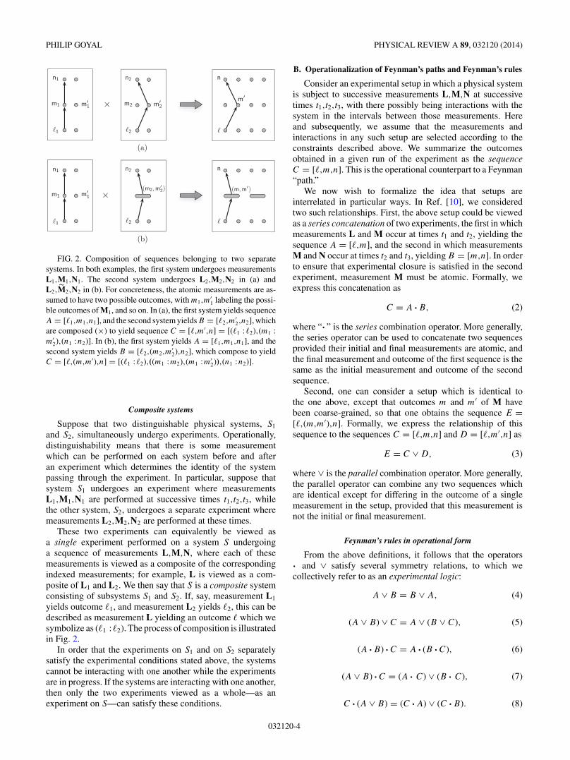
FIG. 2. Composition of sequences belonging to two separatesystems. In both examples, the first system undergoes measurementsL1,M1,N1. The second system undergoes L2,M2,N2 in (a) andL2,M2,N2 in (b). For concreteness, the atomic measurements are as-sumed to have two possible outcomes, with m1,m

′1 labeling the possi-

ble outcomes of M1, and so on. In (a), the first system yields sequenceA = [�1,m1,n1], and the second system yields B = [�2,m

′2,n2], which

are composed (×) to yield sequence C = [�,m′,n] = [(�1 :�2),(m1 :m′

2),(n1 :n2)]. In (b), the first system yields A = [�1,m1,n1], and thesecond system yields B = [�2,(m2,m

′2),n2], which compose to yield

C = [�,(m,m′),n] = [(�1 :�2),((m1 :m2),(m1 :m′2)),(n1 :n2)].

Composite systems

Suppose that two distinguishable physical systems, S1

and S2, simultaneously undergo experiments. Operationally,distinguishability means that there is some measurementwhich can be performed on each system before and afteran experiment which determines the identity of the systempassing through the experiment. In particular, suppose thatsystem S1 undergoes an experiment where measurementsL1,M1,N1 are performed at successive times t1,t2,t3, whilethe other system, S2, undergoes a separate experiment wheremeasurements L2,M2,N2 are performed at these times.

These two experiments can equivalently be viewed asa single experiment performed on a system S undergoinga sequence of measurements L,M,N, where each of thesemeasurements is viewed as a composite of the correspondingindexed measurements; for example, L is viewed as a com-posite of L1 and L2. We then say that S is a composite systemconsisting of subsystems S1 and S2. If, say, measurement L1

yields outcome �1, and measurement L2 yields �2, this can bedescribed as measurement L yielding an outcome � which wesymbolize as (�1 :�2). The process of composition is illustratedin Fig. 2.

In order that the experiments on S1 and on S2 separatelysatisfy the experimental conditions stated above, the systemscannot be interacting with one another while the experimentsare in progress. If the systems are interacting with one another,then only the two experiments viewed as a whole—as anexperiment on S—can satisfy these conditions.

B. Operationalization of Feynman’s paths and Feynman’s rules

Consider an experimental setup in which a physical systemis subject to successive measurements L,M,N at successivetimes t1,t2,t3, with there possibly being interactions with thesystem in the intervals between those measurements. Hereand subsequently, we assume that the measurements andinteractions in any such setup are selected according to theconstraints described above. We summarize the outcomesobtained in a given run of the experiment as the sequenceC = [�,m,n]. This is the operational counterpart to a Feynman“path.”

We now wish to formalize the idea that setups areinterrelated in particular ways. In Ref. [10], we consideredtwo such relationships. First, the above setup could be viewedas a series concatenation of two experiments, the first in whichmeasurements L and M occur at times t1 and t2, yielding thesequence A = [�,m], and the second in which measurementsM and N occur at times t2 and t3, yielding B = [m,n]. In orderto ensure that experimental closure is satisfied in the secondexperiment, measurement M must be atomic. Formally, weexpress this concatenation as

C = A · B, (2)

where “· ” is the series combination operator. More generally,the series operator can be used to concatenate two sequencesprovided their initial and final measurements are atomic, andthe final measurement and outcome of the first sequence is thesame as the initial measurement and outcome of the secondsequence.

Second, one can consider a setup which is identical tothe one above, except that outcomes m and m′ of M havebeen coarse-grained, so that one obtains the sequence E =[�,(m,m′),n]. Formally, we express the relationship of thissequence to the sequences C = [�,m,n] and D = [�,m′,n] as

E = C ∨ D, (3)

where ∨ is the parallel combination operator. More generally,the parallel operator can combine any two sequences whichare identical except for differing in the outcome of a singlemeasurement in the setup, provided that this measurement isnot the initial or final measurement.

Feynman’s rules in operational form

From the above definitions, it follows that the operators· and ∨ satisfy several symmetry relations, to which wecollectively refer to as an experimental logic:

A ∨ B = B ∨ A, (4)

(A ∨ B) ∨ C = A ∨ (B ∨ C), (5)

(A ·B) · C = A · (B · C), (6)

(A ∨ B) · C = (A · C) ∨ (B · C), (7)

C · (A ∨ B) = (C · A) ∨ (C ·B). (8)

032120-4

DERIVATION OF QUANTUM THEORY FROM FEYNMAN’s RULES PHYSICAL REVIEW A 89, 032120 (2014)

v(m, m )

m

n n n

m

A B A ∨ B

a b a + b

m m

n

m

n

A

B

A · B

.a

b a · b

A

m

n

Pr(m, n| ) = |a|2

a

(a)

(b)

(c)

FIG. 3. (Color online) Feynman’s rules for individual systems,expressed in operational terms. In each case, the sequence namesare denoted A,B, . . . , while their amplitudes are denoted a,b, . . . .(a) Sum rule: z(A ∨ B) = z(A) + z(B). (b) Product rule: z(A · B) =z(A) z(B). (c) Probability rule: Pr(m,n | � = |a2|).

In Ref. [10], it is shown that Feynman’s rules are the uniquepair-valued representation of this logic consistent with a fewadditional assumptions. Writing z(X) for the complex-valuedamplitude that represents sequence X, one finds (see Fig. 3)

z(A ∨ B) = z(A) + z(B) (amplitude sum rule)

z(A ·B) = z(A) z(B) (amplitude product rule)

P (A) = |z(A)|2 (probability rule)

These are Feynman’s rules for measurements on individualquantum systems.

III. STATE FORMULATION OF QUANTUM THEORY

In the standard, von Neumann–Dirac formulation of quan-tum theory, one describes a system by specifying its state at aparticular time. Temporal evolution of the system is then rep-resented by a unitary operator, and repeatable measurementsmade on the system are represented by Hermitian operators.When the states of the subsystems of a composite system aregiven, the state of the composite system is the tensor product ofthe subsystem states. In this section, starting from Feynman’s

L

N

L

N

M

n

m

n

FIG. 4. No-disturbance postulate. Left: A system undergoesmeasurement L at time t , followed by N at time t ′. For illustration,each measurement has two possible outcomes. The sequence ofoutcomes [�,n] has associated probability Pr(n | �). Right: Trivialmeasurement M, with single outcome m, occurs between L and N.By the no-disturbance postulate, M has no effect on the probabilityof outcome n given �.

rules and the composite systems rule (derived in Sec. IV),we derive these features with the aid of the no-disturbancepostulate.

A. No-disturbance postulate

The no-disturbance postulate asserts that a trivial measure-ment (as defined in Sec. II A) has no effect on the outcomeprobabilities of subsequent measurements. For example, inthe arrangement shown in Fig. 4, if the trivial measurementM, with single outcome m = (m,m′), is inserted betweenmeasurements L and N, the probability of outcome n given� is unaffected. That is,

Pr(n | �; M) = Pr(n | �), (9)

where M in the conditional on the left-hand side indicates thatthe arrangement containing M is the one under consideration.

The no-disturbance postulate can be regarded as capturingthe essential departure of quantum physics from the mode ofthinking embodied in classical physics. The key point is that,from the classical point of view, if outcome m is obtained, onewould assert that it is a fact of the matter that the systemwent either through the field of sensitivity of the detectorcorresponding to outcome m or through that correspondingto m′, even though neither was, in fact, observed. To see theconsequences of this assertion, let us consider the special casewhere L is repeated at time t ′, where t ′ is immediately after t sothat the system undergoes no appreciable temporal evolutionin the interim (see Fig. 5). For clarity, we denote outcome �

of measurement L at t ′ by �. Now, according to the classicalassertion,

Pr(� | �; M) = Pr(�,m | �) + Pr(�,m′ | �)

= Pr(m | �) Pr(� | m,�) + Pr(m′ | �) Pr(� | m′,�)

= Pr(m | �) Pr(� | m) + Pr(m′ | �) Pr(� | m′),

where we have used the sum and product rules of probabilitytheory in the first two lines, and closure in the third. If wenow assume that transition probabilities are symmetric (an as-sumption that is independently well supported by experiment),then Pr(� | m) = Pr(m | �) and Pr(� | m′) = Pr(m′ | �). Setting

032120-5

PHILIP GOYAL PHYSICAL REVIEW A 89, 032120 (2014)

L

M

ˆ

L

Mm

Lˆ

L

m m

α

α 1−α

1−α

FIG. 5. (Color online) Disturbance of repeatability. Left: A sys-tem undergoes measurement L at time t , and again immediatelyafterwards at t ′, with trivial measurement M in between. Sincemeasurement L is a repeatable measurement, the no-disturbancepostulate implies that it will yield the same outcome at t ′ as at t ,even though M is present. Right: From a classical point of view,the occurrence of m = (m,m′) implies that either outcome m or m′

occurred, but was not observed. The transition probabilities are asindicated, assuming that transition probabilities are symmetric. Fromthese probabilities, it follows that repeatability is disturbed by Munless α is 0 or 1.

α = Pr(m | �) and noting that Pr(m | �) + Pr(m′ | �) = 1,

Pr(� | �; M) = Pr(m | �) Pr(m | �) + Pr(m′ | �) Pr(m′ | �)

= α2 + (1 − α)2.

Since L is a repeatable measurement, Pr(� | �; M) should beunity. But, for this to be possible, α2 + (1 − α)2 = 1, whichcannot hold true unless α is 0 or 1. Therefore, repeatabilitycannot be preserved by the insertion of M except in the specialcase where one of the outcomes m or m′ is certain to occur. Thatis, on the classical assertion that the occurrence of outcome m

implies that either outcome m or m′ in fact occurs, insertionof M will, in general, disturb repeatability of L. Conversely,if the no-disturbance postulate is true, one must conclude thatthe classical assertion is, in general, false.

B. Quantum states

We operationally define the mathematical representationof the physical state of a system at any given time asthat mathematical object which enables one to compute theoutcome probabilities of any measurement (chosen from agiven measurement set M) performed upon the system at thattime.

First, suppose that a system is prepared at time t usingmeasurement L, and that measurement M is subsequentlyperformed upon it at time t ′. Here, and subsequently, weassume that all measurements belong to the same measurementset, and each have N possible outcomes. We label the j thoutcome of measurement M as m(j ), where j ∈ {1,2, . . . ,N},and the outcomes of other measurements similarly.

Suppose that measurement L yields outcome �(i). In orderto compute the transition probabilities Pr(m(j )| �(i)) for everyj , it suffices to know the amplitude vector v = (v1, . . . ,vN )whose j th component is the amplitude of the sequence[�(i),m(j )]. Then, Pr(m(j )| �(i)) = |vj |2. Since the outcomes ofM are mutually exclusive and exhaustive, |v|2 = ∑

j |vj |2 =1. Insofar as calculating the outcome probabilities of Mperformed at t ′, the object v suffices.

v2

T12

∨

v2 T12

v1 T11

v1 = v1 T11 + v2 T12

L

N

L

N

M

L

N

v1

T11

M

L

N

M

(1)

n(1)

(1)

n(1)

m

FIG. 6. (Color online) Left: A system undergoes measurement Lat time t , followed by N at time t ′, yielding sequence [�(1),n(1)].Middle: If trivial measurement M occurs immediately prior to N,then, by the no-disturbance postulate, it has no effect on the outcomeprobabilities of N. Hence, the probability Pr(n(1) | �(1)) = |v1|2. Right:From the amplitude sum rule, v1 = v1T11 + v2T12 = (Tv)1.

Second, suppose that, at time t ′, instead of M, we wishto perform measurement N, and to compute its outcomeprobabilities. To do so, we now make use of the no-disturbancepostulate, according to which we can insert the trivial form ofmeasurement M, which we denote M, prior to measurement N,without changing the outcome probabilities of N. We insert Mimmediately prior to N in order that the system undergoesno appreciable temporal evolution between M and N (seeFig. 6). We can now compute the outcome probabilities of N inthe modified arrangement instead. Now, in this arrangement,the sequence [�(i),m,n(k)], where m ≡ (m(1), . . . ,m(N)), can bedecomposed as

[�(i),m,n(k)] =∨j

[�(i),m(j ),n(k)] (10)

=∨j

[�(i),m(j )] · [m(j ),n(k)], (11)

where∨

indicates parallel combination. Hence, given theamplitudes Tkj of the sequences [m(j ),n(k)], the amplitude sumand product rules imply that the amplitude vk of sequence[�(i),m,n(k)] is

vk =∑

j

vjTkj = (Tv)k, (12)

where T is a matrix with components Tkj . Since the sys-tem undergoes no appreciable temporal evolution betweenmeasurement M and N, the matrix T captures precisely therelationship between M and N. We shall refer to it as thetransformation matrix from M to N. Hence, the transitionprobability

Pr(m,n(k)| �(i)) = |(Tv)k|2. (13)

032120-6

DERIVATION OF QUANTUM THEORY FROM FEYNMAN’s RULES PHYSICAL REVIEW A 89, 032120 (2014)

Using the product rule of probability theory,

Pr(m,n(k) | �(i)) = Pr(n(k)| �(i)) Pr(m | n(k),�(i)), (14)

and noting that Pr(m | n(k),�(i)) = 1, we obtain

Pr(n(k)| �(i)) = |(Tv)k|2. (15)

This statement holds for the modified experiment in which Moccurs. But, by the nondisturbance postulate, it also holds truefor the original experiment.

Thus, the object v, which is specified with respect to M,not only allows one to compute the outcome probabilities ofM, but also to compute the outcome probabilities of any othermeasurement, N, provided one is given the transformationmatrix T from M to N. Therefore, from the operational pointof view stated earlier, v represents the state of the system attime t ′.

C. Representation of measurements

Since the outcomes of N are mutually exclusive andexhaustive, Eq. (15) becomes∑

k

Pr(n(k)| �(i)) =∑

k

|(Tv)k|2 = 1, (16)

which implies that |Tv|2 = 1. But v can be freely varied byvarying the initial measurement L, its outcome �(i), and theinteraction with the system in the interval [t,t ′]. Therefore, thetransformation matrix T, which connects M to N, is unitary.

To determine the states that can be prepared by measure-ment N, we use the fact that, since N is repeatable, if a systemis prepared at time t using measurement N with outcomen(q), the same outcome is obtained when the measurementis immediately repeated. Therefore, using Eq. (15), the stateuq that is prepared must be such that

Pr(n(k)| n(q)) = |(Tuq)k|2 = δqk, (17)

which implies that uq = (Tq1, . . . ,TqN )† up to a predictivelyirrelevant overall phase. In terms of the uq , one can writevk = u†

kv, so that Eq. (15) becomes

Pr(n(k)| �(i)) = |u†kv|2, (18)

which is the Born rule with uk and v specified with respectto M. Therefore, measurement N can be characterized interms of the uq , which form an orthonormal basis of CN .Alternatively, as is more conventional, we can represent N interms of the Hermitian matrix N = ∑

q aququ†q , where aq is

the value associated with outcome n(q).In the special case where measurement N is the same as

M, it follows from the repeatability of measurements thatPr(m(k)| m(j )) = δjk . Therefore the transformation matrix T′

that relates M to itself has the property that T ′kj = δkj e

iφk ,where the φk are phases. Now, the states u′

q = (T ′q1, . . . ,T

′qN )†

prepared by M are predictively relevant only via Eq. (18),whose result is insensitive to the values of the φk . Therefore,without loss of generality, the φk can all be set to zero, so thatT′ reduces to the identity matrix I. Hence, measurement M isrepresented by a diagonal Hermitian matrix, M.

D. Relationship between representations

Thus far, we have specified the state of the system vand the states uk that are prepared by measurement N, withrespect to measurement M. Suppose that we were insteadto represent these states as v′ and u′

k with respect to someother measurement M′. The no-disturbance postulate canthen be used to relate the new representation to the oldrepresentation by completely coarse-graining measurement M′and inserting measurement M immediately afterwards. If astate is represented by v′ with respect to measurement M′, andV is the transformation matrix from M′ to M, then

vi =∑

j

v′jVij = (Vv′)i , (19)

so that v = Vv′. Since V is unitary, this can be inverted togive v′ = V†v. Similarly u′

k = V†uk , which implies that theHermitian operator N′ that represents N with respect to M′, isgiven by V†NV.

If measurement M′ is represented with respect to Mby Hermitian matrix M′ with eigenvectors wi , then thetransformation matrix V has components Vij = (wj )i .

E. Unitary representation of temporal evolution

Suppose that a system is prepared using measurement Lat time t , and then undergoes measurement M at time t ′.Immediately prior to measurement M, the system is in statev. Suppose now that measurement M is completely coarse-grained, and an additional measurement M is performed attime t ′′ > t ′. In this arrangement, the sequence [�(i),m,m(k)]can be decomposed as

[�(i),m,m(k)] =∨j

[�(i),m(j )] · [m(j ),m(k)]. (20)

The temporal evolution of the system in interval [t ′,t ′′] isrepresented by the amplitudes Ukj of the sequences [m(j ),m(k)].The amplitude sum and product rules accordingly imply thatthe amplitude vk of sequence [�(i),m,m(k)] is

vk =∑

j

vjUkj = (Uv)k. (21)

Therefore, the state of the system v immediately prior to thelast measurement is

v = Uv. (22)

Now, the initial state v can be arbitrarily varied, but the statesv and v are normalized. Therefore, U is unitary.

Since temporal evolution from t ′ to t ′′ is represented byU, temporal evolution from t ′′ to t ′ is represented by U†.Therefore, if we denote the temporal inverse of the sequenceA as A−1, then

z(A−1) = z∗(A), (23)

to which we shall refer as the amplitude temporal inversionrule.

F. Composite systems

At time t , system S1 is prepared by measurement L1 withoutcome �1, and S2 by measurement L2 with outcome �2.Suppose that these systems evolve without interacting with

032120-7

PHILIP GOYAL PHYSICAL REVIEW A 89, 032120 (2014)

one another until time t ′, at which point they are measured,respectively, by M1 and M2, which respectively have N1,N2

possible outcomes, m(j )1 and m

(k)2 with j ∈ {1, . . . ,N1} and

k ∈ {1, . . . ,N2}. Then the components of the respective statesv′ and v′′ of the systems immediately prior to t ′ are given by

v′j = z

([�1,m

(j )1

])and v′′

k = z([

�2,m(k)2

]). (24)

Viewed as a single system S, the system is preparedby measurement L with outcome (�1 :�2), and subsequentlyundergoes measurement M with N1N2 possible outcomes(m(j )

1 :m(k)2 ). With respect to M, the components of the state of

the system v immediately prior to M is given by

v(i−1)N2+j = z([

(�1 :�2),(m

(j )1 :m(k)

2

)]). (25)

But, by the composite systems rule, Eq. (44), which we shallderive in Sec. IV,

z([

(�1 :�2),(m

(j )1 :m(k)

2

)]) = z([

�1,m(j )1

])z([

�2,m(k)2

]),

(26)so that v(i−1)N2+j = v′

j v′′k . Hence,

v = v′ ⊗ v′′. (27)

G. Summary

In summary, we have derived the following:(i) If a system is prepared by some measurement L at time

t , then its state at time t ′ immediately prior to measurement Nis given by vector v with respect to reference measurement M.

(ii) Measurement N is represented by Hermitian operatorN = ∑

q aququ†q , where the uq , also specified with respect

to M, are the states prepared by N. When performed on thesystem in state v, the probability of the kth outcome of N isgiven by Pr(n(k)| v) = |u†

kv|2.(iii) If the reference measurement is changed to M′, then the

state v′ of the system with respect to M′ is given by v′ = V†v,where V is the unitary transformation matrix from M′ to M.

(iv) The state v evolves unitarily in the time betweenmeasurements.

(v) If the two subsystems of a composite system are in statesv′ and v′′, then the composite system is in state v = v′ ⊗ v′′.

Collectively, this set of statements is equivalent tovon Neumann’s postulates for finite-dimensional quantumsystems.

IV. COMPOSITE SYSTEMS

A. Composition operator and its symmetries

Suppose that one physical system, denoted S1, undergoesan experiment involving measurements L1,M1,N1 at suc-cessive times t1,t2,t3, while another system, S2, undergoesan experiment where the measurements L2,M2,N2 at thesesame times. The measurements on S1 yield the outcomesequence A = [�1,m1,n1], while the measurements on S2

yield B = [�2,m2,n2]. As described earlier, in Sec. II A, onecan also describe the situation by saying that measurementsL, M, and N are performed on the composite system S,yielding the sequence C = [(�1 :�2),(m1 :m2),(n1 :n2)]. Wenow symbolize the relationship between A, B, and C bydefining a binary operator ×, the composition operator, which

here acts on A and B to generate the sequence

C = A × B. (28)

Generally, the operator × combines any two sequences of thesame length, each obtained from a different experiment ondifferent physical systems where each measurement in oneexperiment occurs at the same time as one measurement in theother experiment.

From the definition just given, it follows that × isassociative. To see this, consider the three sequences A =[�1,m1], B = [�2,m2], and C = [�3,m3], obtained from threedifferent experiments satisfying the condition just statedabove. We can then combine these to yield the sequenceD = [(�1 :�2 :�3),(m1 :m2 :m3)] in two different ways, eitheras A × (B × C) or as (A × B) × C. Hence,

A × (B × C) = (A × B) × C. (29)

Similar considerations show that × also satisfies the followingsymmetry relations involving the operators ∨ and · :

(A · B) × (C · D) = (A × C) · (B × D), (30)

A × (B ∨ C) = (A × B) ∨ (A × C), (31)

(A ∨ B) × C = (A × C) ∨ (B × C). (32)

The cross-multiplicativity and left-distributivity propertiesexpressed in Eqs. (30) and (31) are illustrated in Figs. 7 and 8,respectively.

B. Composite systems rule

If systems S1 and S2 are noninteracting, we postulate that,in Eq. (28), the amplitude c of sequence C is determined bythe amplitudes a,b of the sequences A,B, so that

c = F (a,b), (33)

where F is some continuous complex-valued function to bedetermined. This is the composition postulate, given whichEqs. (29), (30), (31), and (32), respectively, imply

F (a,F (b,c)) = F (F (a,b),c), (34)

F (ab,cd) = F (a,c) F (b,d), (35)

F (a,b + c) = F (a,b) + F (a,c), (36)

F (a + b,c) = F (a,c) + F (b,c). (37)

We can now solve these for F . Due to the cross-multiplicativityequation, Eq. (35),

F (u,v) = F (u × 1,1 × v) = F (u,1) F (1,v). (38)

To determine the form of F (u,1), we use the right-distributivityand cross-multiplicativity equations, Eqs. (37) and (35),respectively, to obtain

F (u1 + u2,1) = F (u1,1) + F (u2,1), (39a)

F (u1u2,1) = F (u1,1) F (u2,1). (39b)

032120-8

DERIVATION OF QUANTUM THEORY FROM FEYNMAN’s RULES PHYSICAL REVIEW A 89, 032120 (2014)

.

.

1

m1

n1

2

m2

n2

x

A · B

C · D

.

A

B D

C

(A · B) × (C · D)

A × C

B × D

(A × C) · (B × D)

A C

x

x

B

D

1 2

m2m1

n2n1

1 2

m2m1

m2m1

n2n1

FIG. 7. (Color online) Illustration of the cross-multiplicativity property. The composite sequence [(�1 :�2),(m1 :m2),(n1 :n2)] can beobtained by combining the sequences A = [�1,m1], B = [m1,n1], C = [�2,m2], and D = [m2,n2] in two different ways, as shown, yieldingthe cross-multiplicativity relation (A · B) × (C ·D) = (A × C) · (B × D), which is Eq. (30).

Writing f (z) = F (z,1), these two equations can be written asa pair of functional equations,

f (z1 + z2) = f (z1) + f (z2), (40a)

f (z1z2) = f (z1) f (z2), (40b)

whose continuous solutions in the domain |z| � 1 are f (z) =z, f (z) = z∗, or f (z) = 0 (see the Appendix). The zerosolution implies F (u,v) = 0 for all u,v, and is therefore

inadmissible. Therefore,

F (u,1) ={

u (41a)

u∗. (41b)

To eliminate the possibility F (u,1) = u∗ we make use of theassociativity equation, Eq. (34), which implies

F (u,F (1,1)) = F (F (u,1),1). (42)

1

m1

n1

2

n2

x

A × C

A C

1 2

m1

n2n1

(m2,m2)

A × (B ∨ C)

A

(A × B) ∨ (A × C)

1 2

m2m1

n2n1

1 2

m1

n2n1

v m2

B ∨ C

(m2, m2)

v

A × B

B C

x

A B

x

FIG. 8. (Color online) Illustration of left-distributivity of × over ∨. The composite sequence [(�1,�2),(m1 : (m2,m′2)),(n1,n2)] can be

obtained by combining the sequences A = [�1,m1,n1], B = [�2,m2,n2], and C = [�2,m′2,n2] in two different ways, as shown, yielding the

relation A × (B ∨ C) = (A × B) ∨ (A × C), which is Eq. (31).

032120-9

PHILIP GOYAL PHYSICAL REVIEW A 89, 032120 (2014)

Now, from the cross-multiplicativity equation, Eq. (35),F (u × 1,v × 1) = F (u,v) F (1,1), which implies F (1,1) = 1since the zero solution for F (u,v) is inadmissible. Therefore,Eq. (42) becomes

F (u,1) = F (F (u,1),1). (43)

But this is incompatible with F (u,1) = u∗ since u∗ =F (u,1) �= F (F (u,1),1) = F (u∗,1) = u. We are therefore leftwith F (u,1) = u, which is compatible with Eq. (43). Aparallel argument establishes that F (1,v) = v. Therefore, fromEq. (38),

F (u,v) = uv. (44)

This is the amplitude rule for distinguishable, noninteractingcomposite systems. We refer to it as the composite system rule.

V. DERIVATION OF DIRAC’S AMPLITUDE-ACTION RULE

Consider a quantum system that is subject to positionmeasurements at successive times. Suppose that the intervalsbetween these successive times are sufficiently small thatthe resulting measurement sequence is well approximatedby a continuous classical trajectory (or simply “path”) ofthe same system as treated according to the framework ofclassical physics. Dirac’s amplitude-action rule asserts thatthe amplitude associated with the measurement sequence isgiven by eiS/�, where S is the classical action associated withthe corresponding classical path. We now derive the form ofthis rule up to � from two elementary properties of the classicalaction:

Additivity. If sequence C = A · B, then SC = SA + SB ,where SX is the classical action of the path correspondingto sequence X.

Inversion. The action SA−1 associated with sequence A−1 is−SA.Our assumption is that the amplitude z(A) of sequence A, withcorresponding classical action SA, is given by f (SA), where f

is a continuous, complex-valued function.The additivity and inversion properties of the classical

action induce two functional equations in f . First, theamplitude z(C) of sequence C = A · B can be computed in twoways (see Fig. 9), either using the action additivity property,

z(C) = f (SC) = f (SA + SB),

or using the amplitude product rule,

z(C) = z(A) z(B) = f (SA)f (SB),

so that

f (x + y) = f (x)f (y). (45)

Second, the amplitude z(A−1) of sequence A−1 can becomputed either using the amplitude temporal inversion rule,Eq. (23),

z(A−1) = z∗(A) = f ∗(SA),

or using the action inversion property,

z(A−1) = f (SA−1 ) = f (−SA),

SA

SB

SA+SB

action

additivity of

f(SA)

f(SB)

f(SA+SB)

f(SA)·f(SB)amplitude

product rule

f f

FIG. 9. (Color online) The amplitude of the path C = A · B canbe obtained from the classical actions SA,SB of paths A,B intwo different ways: (i) obtain the action SC = SA + SB , whosecorresponding amplitude is f (SA + SB ); and (ii) use f to obtain theamplitudes f (A),f (B) and then compose these to obtain amplitudef (SA)f (SB ). Hence, f (SA + SB ) = f (SA)f (SB ).

so that

f ∗(x) = f (−x). (46)

We can solve Eq. (45) by writing f (x) = R(x)ei�(x), withR,� real, to obtain, for integer n,

R(x + y) = R(x)R(y), (47)

�(x + y) = �(x) + �(y) + 2πn. (48)

The second equation can be transformed via �(x) = �(x) +2πn to give

�(x + y) = �(x) + �(y). (49)

Equations (47) and (49) are two of Cauchy’s standard functionequations, with general solutions R(x) = eβx and �(x) = αx,where α,β ∈ R [45]. Hence, �(x) = αx − 2πn, and

f (x) = eβxeiαx. (50)

But Eq. (46) then implies that β = 0. Therefore,

z(A) = eiαSA, (51)

where the constant α has dimensions of �−1. This is Dirac’s

amplitude-action rule up to �.

VI. DISCUSSION

In this paper, we have shown that it is possible to system-atically build Feynman’s rules into a complete formulation offinite-dimensional quantum theory. The key physical ingre-dient in this process has been the no-disturbance postulate,which expresses the singularly nonclassical fact that a trivialmeasurement does not disturb the outcome probabilities of

032120-10

DERIVATION OF QUANTUM THEORY FROM FEYNMAN’s RULES PHYSICAL REVIEW A 89, 032120 (2014)

subsequent measurements on the system. This postulate allowsus to introduce the concept of the state of a system ina systematic way, and to prove the unitarity of temporalevolution and the Hermiticity of measurement operators. Wehave also derived the composite system rule and Dirac’samplitude-action rule, each from a single elementary andnatural assumption, by making use of the fact that theseassumptions must be consistent with Feynman’s rules.

The work described here, in concert with our earlier deriva-tion of Feynman’s rules, constitutes a complete derivation ofthe finite-dimensional quantum formalism. The derivation hasa number of important implications for our understandingof quantum theory in addition to those mentioned in theIntroduction.

First, most other attempts to derive the quantum formalismfrom physically motivated postulates (such as [5,11,46]) de-pend upon postulates (such as purifiability [11] or local tomog-raphy [5,46]) that concern the behavior of composite systemsin order to derive the quantum formalism for individualsystems. This tends to suggest that the behavior of compositesystems is in some sense fundamental to the structure of thequantum formalism. However, in the present derivation, thereis no such dependency. Instead, we have shown that it ispossible to derive the formalism for individual systems withoutassumptions that overtly concern composite systems, and thento derive the rule for composite systems on the basis of a simpleassumption merely by requiring consistency with the formal-ism for individual systems. Therefore, the present derivationstrongly implies that the behavior of composite systems is asecondary feature of quantum theory, not a primary one.

Second, one of the most remarkable features of Feynman’sformulation of quantum theory is the absence of a stateconcept, and the absence of any distinction between dynamics,on the one hand, and the relationship between measurements,on the other. We have shown here that these features can berecovered, but at the cost of an additional physical postulatewhich has nontrivial physical content.

Finally, we have shown that Dirac’s amplitude-action rulefollows from elementary properties of the classical actionvia the simple assumption that the amplitude of a sequenceis determined by the corresponding action. In contrast withDirac’s argument, our approach does not depend on theparticular form of the classical Lagrangian or on the existenceor form of Lagrange’s equations of motion, but only on twoelementary properties (additivity, inversion) of the action.Hence, we have shown that Dirac’s rule has a very generalvalidity, and arises as soon as one attempts to establish a

quantitative connection between the notion of action in theLagrangian formulation of classical mechanics, and the notionof amplitude in Feynman’s formulation of quantum theory.

We conclude with two open questions. First, is theno-disturbance postulate related in any way with otherinformational ideas that have been proposed, such as inRefs. [11,47,48]? Second, is there a direct, general pathfrom Dirac’s amplitude-action rule to the unitary formexp(−iHt/�) of the temporal evolution operator?

ACKNOWLEDGMENT

This publication was made possible, in part, through thesupport of a grant from the John Templeton Foundation.

APPENDIX: SOLUTION OF A PAIR OFFUNCTIONAL EQUATIONS

We solve Eqs. (40a) and (40b) with the aid of one ofCauchy’s standard functional equations,

h(x1 + x2) = h(x1) + h(x2), (A1)

where h is a real function and x1,x2 ∈ R. Its continuoussolution is h(x) = ax with a ∈ R [45].

Setting z1 + z2 = x + iy, with x,y ∈ R, in Eq. (40a) gives

f (x + iy) = f (x) + f (iy).

Applying Eq. (40a) again on f (x1 + x2) and f (iy1 + iy2) thenimplies

f (x1 + x2) = f (x1) + f (x2),

f (iy1 + iy2) = f (iy1) + f (iy2).

The real and imaginary parts of both of these equations eachhave the form of Eq. (A1), and therefore have solutions

f (x) = αx and f (iy) = βy

with α,β ∈ C, so that

f (x + iy) = αx + βy. (A2)

From Eq. (40b),

f (1 · 1) = f (1)f (1) and f (i · i) = f (i)f (i),

which, due to Eq. (A2), imply

α = α2 and −α = β2.

These have solutions (α,β) = (0,0), (1,i), and (1, − i), whichcorrespond to f (z) = 0, f (z) = z, and f (z) = z∗.

[1] J. A. Wheeler, in Foundations of Quantum Mechanics in theLight of New Technology: Proceedings of the 3rd InternationalSymposium (Physical Society of Japan, Tokyo, 1990).

[2] A. Zeilinger, Found. Phys. 29, 631 (1999).[3] C. A. Fuchs, in Quantum Theory: Reconsideration of Founda-

tions, edited by A. Khrennikov (Vaxjo University Press, Vaxjo,Sweden, 2002), pp. 463–543.

[4] A. Grinbaum, Br. J. Philos. Sci. 58, 387 (2007).

[5] L. Hardy, arXiv:quant-ph/0101012.[6] R. Clifton, J. Bub, and H. Halvorson, Found. Phys. 33, 1561

(2003).[7] G. M. D’Ariano, in Foundations of Probability and Physics, 4,

edited by A. Y. K. G. Adenier and C. A. Fuchs (AIP, New York,2007), p. 79.

[8] P. Goyal, New J. Phys. 12, 023012 (2010).[9] M. Reginatto, Phys. Rev. A 58, 1775 (1998).

032120-11

PHILIP GOYAL PHYSICAL REVIEW A 89, 032120 (2014)

[10] P. Goyal, K. H. Knuth, and J. Skilling, Phys. Rev. A 81, 022109(2010).

[11] G. Chiribella, G. M. D’Ariano, and P. Perinotti, Phys. Rev. A84, 012311 (2011).

[12] L. Masanes and M. Muller, New J. Phys. 13, 063001(2011).

[13] B. Dakic and C. Brukner, in Deep Beauty: Understanding theQuantum World through Mathematical Innovation, edited by H.Halvorson (Cambridge University Press, Cambridge, 2011), pp.365–392.

[14] J. Barrett, Phys. Rev. A 75, 032304 (2007).[15] M. Pawłowski, T. Paterek, D. Kaszlikowski, V. Scarani,

A. Winter, and M. Zukowski, Nature (London) 461, 1101(2009).

[16] R. P. Feynman, Rev. Mod. Phys. 20, 367 (1948).[17] R. P. Feynman and A. R. Hibbs, Quantum Mechanics and Path

Integrals, 1st ed. (McGraw-Hill, New York, 1965).[18] R. T. Cox, Am. J. Phys. 14, 1 (1946).[19] R. T. Cox, The Algebra of Probable Inference (The Johns

Hopkins University Press, Baltimore, 1961).[20] P. Goyal and K. H. Knuth, Symmetry 3, 171 (2011).[21] P. A. M. Dirac, Principles of Quantum Mechanics, 1st ed.

(Oxford University Press, New York, 1930).[22] J. von Neumann, Mathematical Foundations of Quantum Me-

chanics (Princeton University Press, Princeton, NJ, 1955).[23] G. Johnson and M. L. Lapidus, The Feynman Integral and

Feynman’s Operational Calculus (Oxford University Press, NewYork, 2000).

[24] In Ref. [16], Sec. 11, Feynman states, “One of the most importantcharacteristics of quantum mechanics is its invariance underunitary transformations.... Of course, the present formulation,being equivalent to ordinary formulations, can be mathemati-cally demonstrated to be invariant under these transformations.

However, it has not been formulated in such a way that it isphysically obvious that it is invariant.”

[25] C. A. Fuchs and A. Peres, Phys. Rev. A 53, 2038 (1996).[26] I am grateful to Paulo Perinotti for suggesting this point of view.[27] One cannot rule out measurements that provide no useful

information and yet still disturb the state.[28] C. Pfister and S. Wehner, Nat. Commun. 4, 1851 (2013).[29] P. Goyal, arXiv:1309.0478.[30] P. A. M. Dirac, Phys. Z. Sowjetunion 3, 64 (1933).[31] R. P. Feynman, Phys. Rev. 76, 769 (1949).[32] A. Caticha, Found. Phys. 30, 227 (2000).[33] Y. Tikochinsky, Phys. Rev. A 37, 3553 (1988).[34] A. Caticha, Phys. Rev. A 57, 1572 (1998).[35] P. Pearle, Phys. Rev. D 13, 857 (1976).[36] I. Bialynicki-Birula and J. Mycielski, Ann. Phys. 100, 62 (1976).[37] A. Shimony, Phys. Rev. A 20, 394 (1979).[38] S. Weinberg, Phys. Rev. Lett. 62, 485 (1989).[39] S. Weinberg, Ann. Phys. (N.Y.) 194, 336 (1989).[40] S. B. Giddings, arXiv:hep-th/9508151.[41] C. Simon, V. Buzek, and N. Gisin, Phys. Rev. Lett. 87, 170405

(2001).[42] M. Ferrero, D. Salgado, and J. L. Sanchez-Gomez, Phys. Rev.

A 70, 014101 (2004).[43] M. Ferrero, D. Salgado, and J. L. Sanchez-Gomez, Phys. Rev.

A 73, 034304 (2006).[44] P. Goyal, Phys. Rev. A 78, 052120 (2008).[45] J. Aczel, Lectures on Functional Equations and their Applica-

tion (Academic Press, New York, 1966).[46] L. Hardy, in Quantum Theory: Informational Foundations and

Foils, edited by G. Chiribella and R. Spekkens (unpublished),arXiv:1303.1538.

[47] C. Brukner and A. Zeilinger, Phys. Rev. Lett. 83, 3354 (1999).[48] C. Brukner and A. Zeilinger, Found. Phys. 39, 677 (2009).

032120-12