derivatives introduction to option pricing andré farber solvay business school university of...

DerivativesIntroduction to option pricing

André Farber

Solvay Business School

University of Brussels

Derivatives 07 Pricing options |2April 19, 2023

Forward/Futures: Review

• Forward contract = portfolio

– asset (stock, bond, index)

– borrowing

• Value f = value of portfolio

f = S - PV(K)

Based on absence of arbitrage opportunities

• 4 inputs:

• Spot price (adjusted for “dividends” )

• Delivery price

• Maturity

• Interest rate

• Expected future price not required


Options

• Standard options

– Call, put

– European, American

• Exotic options (non standard)

– More complex payoff (ex: Asian)

– Exercise opportunities (ex: Bermudian)


Option Valuation Models: Key ingredients

• Model of the behavior of spot price

new variable: volatility

• Technique: create a synthetic option

• No arbitrage

• Value determination

– closed form solution (Black Merton Scholes)

– numerical technique


Model of the behavior of spot price

• Geometric Brownian motion

– continuous time, continuous stock prices

• Binomial

– discrete time, discrete stock prices

– approximation of geometric Brownian motion


Creation of synthetic option

• Geometric Brownian motion

– requires advanced calculus (Ito’s lemna)

• Binomial

– based on elementary algebra


Options: the family tree

Black Merton Scholes (1973)

Analyticalmodels

Numericalmodels

Analyticalapproximation

models

Term structuremodels

B & SMerton

BinomialTrinomial

Finite differenceMonte Carlo

EuropeanOption

EuropeanAmerican

Option

AmericanOption

Options onBonds &

Interest Rates

AnalyticalNumerical


Modelling stock price behaviour

• Consider a small time interval t: S = St+t - St

• 2 components of S:– drift : E(S) = S t [ = expected return (per year)]

– volatility:S/S = E(S/S) + random variable (rv)

• Expected value E(rv) = 0

• Variance proportional to t

– Var(rv) = ² t Standard deviation = t– rv = Normal (0, t)– = Normal (0,t)– = z z :

Normal (0,t)– = t : Normal(0,1)

z independent of past values (Markov process)


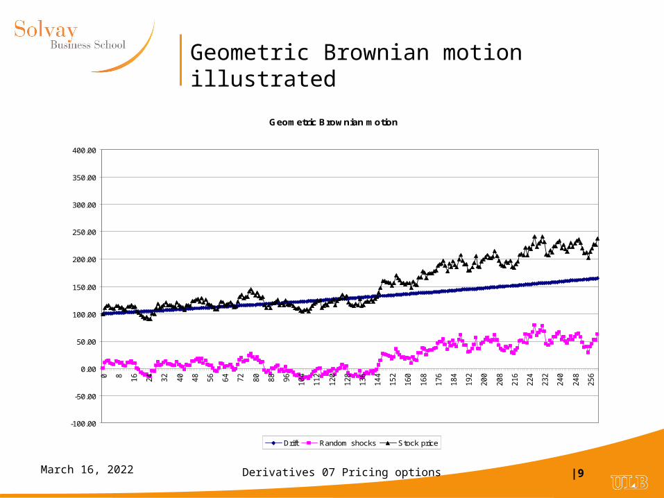
Geometric Brownian motion illustrated

Geometric Brownian motion

-100.00

-50.00

0.00

50.00

100.00

150.00

200.00

250.00

300.00

350.00

400.00

0 8 16

24

32

40

48

56

64

72

80

88

96

104

112

120

128

136

144

152

160

168

176

184

192

200

208

216

224

232

240

248

256

Drift Random shocks Stock price


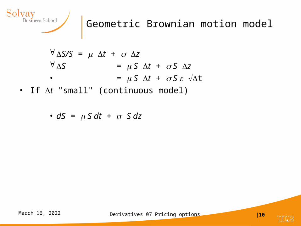
Geometric Brownian motion model

S/S = t + z S = S t + S z

• = S t + S t

• If t "small" (continuous model)

• dS = S dt + S dz


Binomial representation of the geometric Brownian

• u, d and q are choosen to reproduce the drift and the volatility of the underlying process:

• Drift:

• Volatility:

• Cox, Ross, Rubinstein’s solution:

•

S

uS

dS

q

1-q

teu u

d1

du

deq

t

tSeSdqqSu )1(

tSSedSquqS t 2222222 )()1(


Binomial process: Example

• dS = 0.15 S dt + 0.30 S dz ( = 15%, = 30%)

• Consider a binomial representation with t = 0.5

u = 1.2363, d = 0.8089, q = 0.6293

• Time 0 0.5 1 1.5 2 2.5• 28,883• 23,362• 18,897 18,897• 15,285 15,285• 12,363 12,363 12,363• 10,000 10,000 10,000• 8,089 8,089 8,089• 6,543 6,543• 5,292 5,292• 4,280• 3,462


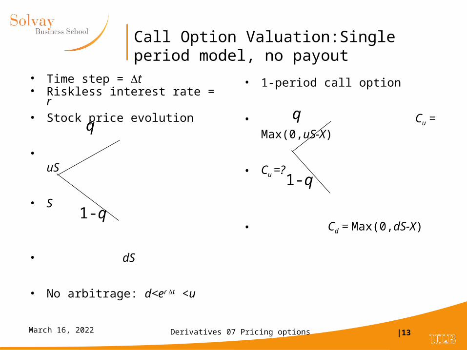
Call Option Valuation:Single period model, no payout

• Time step = t• Riskless interest rate = r • Stock price evolution

• uS

• S

• dS

• No arbitrage: d<er t <u

• 1-period call option

• Cu = Max(0,uS-X)

• Cu =?

• Cd = Max(0,dS-X)

q

1-q

q

1-q


Option valuation: Basic idea

• Basic idea underlying the analysis of derivative securities

• Can be decomposed into basic components possibility of creating a synthetic identical security

• by combining:

• - Underlying asset

• - Borrowing / lending

Value of derivative = value of components


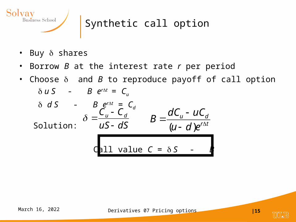
Synthetic call option

• Buy shares

• Borrow B at the interest rate r per period

• Choose and B to reproduce payoff of call option

u S - B ert = Cu

d S - B ert = Cd

Solution:

Call value C = S - B

dSuS

CC du

trdu

edu

uCdCB

)(


Call value: Another interpretation

Call value C = S - B

• In this formula:

+ : long position (buy, invest)

- : short position (sell borrow)

B = S - C

Interpretation:

Buying shares and selling one call is equivalent to a riskless investment.


Binomial valuation: Example

• Data

• S = 100

• Interest rate (cc) = 5%

• Volatility = 30%

• Strike price X = 100, • Maturity =1 month (t = 0.0833)

• u = 1.0905 d = 0.9170

• uS = 109.05 Cu = 9.05

• dS = 91.70 Cd = 0

= 0.5216

• B = 47.64

• Call value= 0.5216x100 - 47.64

• =4.53


1-period binomial formula

• Cash value = S - B

• Substitue values for and B and simplify:

• C = [ pCu + (1-p)Cd ]/ ert where p = (ert - d)/(u-d)

• As 0< p<1, p can be interpreted as a probability

• p is the “risk-neutral probability”: the probability such that the expected return on any asset is equal to the riskless interest rate


Risk neutral valuation

• There is no risk premium in the formula attitude toward risk of investors are irrelevant for valuing the option

Valuation can be achieved by assuming a risk neutral world

• In a risk neutral world : Expected return = risk free interest rate What are the probabilities of u and d in such a world ?

p u + (1 - p) d = ert

Solving for p:p = (ert - d)/(u-d)• Conclusion : in binomial pricing formula, p = probability of an upward

movement in a risk neutral world


Mutiperiod extension: European option

u²SuS

S udS

dS

d²S

• Recursive method (European and American options)

Value option at maturityWork backward through the tree.

Apply 1-period binomial formula at each node

• Risk neutral discounting(European options only)

Value option at maturityDiscount expected future value

(risk neutral) at the riskfree interest rate


Multiperiod valuation: Example

• Data

• S = 100

• Interest rate (cc) = 5%

• Volatility = 30%

• European call option:

• Strike price X = 100,

• Maturity =2 months

• Binomial model: 2 steps

• Time step t = 0.0833

• u = 1.0905 d = 0.9170

• p = 0.5024

0 1 2 Risk neutral probability118.91 p²= 18.91 0.2524

109.05 9.46

100.00 100.00 2p(1-p)= 4.73 0.00 0.5000

91.70 0.00

84.10 (1-p)²= 0.00 0.2476

Risk neutral expected value = 4.77Call value = 4.77 e-.05(.1667) = 4.73


From binomial to Black Scholes

• Consider:

• European option

• on non dividend paying stock

• constant volatility

• constant interest rate

• Limiting case of binomial model as t0

Stock price

Timet T


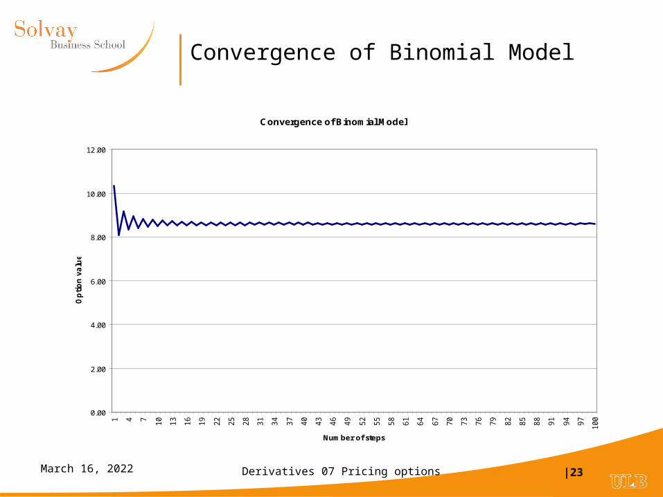
Convergence of Binomial Model

Convergence of Binomial Model

0.00

2.00

4.00

6.00

8.00

10.00

12.00

1 4 7 10

13

16

19

22

25

28

31

34

37

40

43

46

49

52

55

58

61

64

67

70

73

76

79

82

85

88

91

94

97

100

Number of steps

Op

tio

n v

alu

e


Black Scholes formula

• European call option:

• C = S N(d1) - K e-r(T-t) N(d2)

• N(x) = cumulative probability distribution function for a standardized normal variable

• European put option:

• P= K e-r(T-t) N(-d2) - S N(-d1)

• or use Put-Call Parity

tTtT

KeS

dtTr

5.0)ln( )(

1

tTdd 12


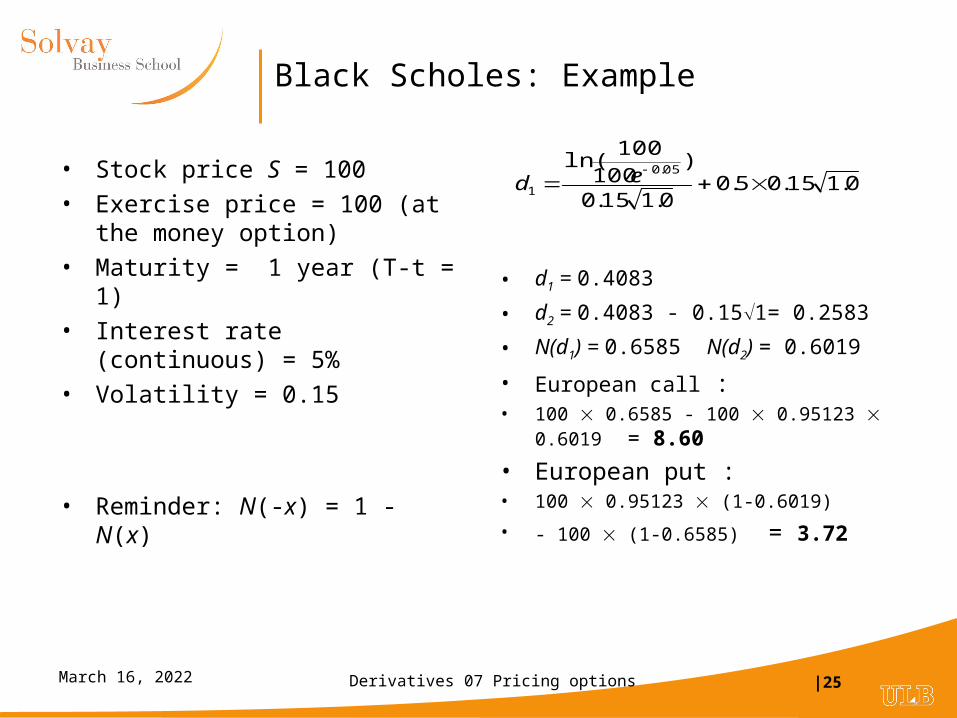
Black Scholes: Example

• Stock price S = 100

• Exercise price = 100 (at the money option)

• Maturity = 1 year (T-t = 1)

• Interest rate (continuous) = 5%

• Volatility = 0.15

• Reminder: N(-x) = 1 - N(x)

• d1 = 0.4083

• d2 = 0.4083 - 0.151= 0.2583

• N(d1) = 0.6585 N(d2) = 0.6019

• European call : • 100 0.6585 - 100 0.95123 0.6019 =

8.60

• European put : • 100 0.95123 (1-0.6019)

• - 100 (1-0.6585) = 3.72

0.115.05.00.115.0

)100

100ln( 05.0

1 ed


Black Scholes differential equation: Assumptions

• S follows a geometric Brownian motion:dS = µS dt + S dz

• Volatility constant

• No dividend payment (until maturity of option)

• Continuous market

• Perfect capital markets

• Short sales possible

• No transaction costs, no taxes

• Constant interest rate


Black-Scholes illustrated

0

50

100

150

200

250

0 10 20 30 40 50 60 70 80 90 100 110 120 130 140 150 160 170 180 190 200

Action Option Valeur intrinséque

Lower boundIntrinsic value Max(0,S-K)

Upper boundStock price

derivatives introduction to option pricing andré farber solvay business school university of...

Documents

s t t s t

s t s t

pricing options

s t s z

t z s

options standard options

s dt s dz slide

t varrv