describing the distribution of income: guidelines for
TRANSCRIPT

Describing the Distribution of Income:Guidelines for Effective Analysis
by Mikal Skuterud (FLS), Marc Frenette (BLMA), Preston Poon
Income Statistics DivisionJean Talon Building, Ottawa, K1A 0T6
Telephone: 613 951-7355
This paper represents the views of the authors and does not necessarily reflect the opinions of Statistics Canada.
Catalogue no. 75F0002MIE — No. 010
Research Paper
Income research paper series
ISSN: 1707-2840
ISBN: 0-662-38380-X

How to obtain more information
Specific inquiries about this product and related statistics or services should be directed to Client Services, IncomeStatistics Division, Statistics Canada, Ottawa, Ontario, K1A 0T6 ((613) 951-7355; (888) 297-7355; [email protected]).
For information on the wide range of data available from Statistics Canada, you can contact us by calling one of ourtoll-free numbers. You can also contact us by e-mail or by visiting our Web site.
National inquiries line 1 800 263-1136
National telecommunications device for the hearing impaired 1 800 363-7629
Depository Services Program inquiries 1 800 700-1033
Fax line for Depository Services Program 1 800 889-9734
E-mail inquiries [email protected]
Web site www.statcan.ca
Ordering and subscription information
This product, Catalogue no. 75F0002MIE2004010, is available on Internet free. Users can obtain single issuesat: http://www.statcan.ca/cgi-bin/downpub/research.cgi.
Standards of service to the public
Statistics Canada is committed to serving its clients in a prompt, reliable and courteous manner and in the officiallanguage of their choice. To this end, the Agency has developed standards of service which its employees observein serving its clients. To obtain a copy of these service standards, please contact Statistics Canada toll free at 1 800263-1136.

Statistics CanadaIncome Statistics Division
Describing the Distribution of Income:Guidelines for Effective Analysis
Note of appreciation
Canada owes the success of its statistical system to a long-standing partnership between StatisticsCanada, the citizens of Canada, its businesses, governments and other institutions. Accurate andtimely statistical information could not be produced without their continued cooperation and goodwill.
Published by authority of the Minister responsible for Statistics Canada
© Minister of Industry, 2004
All rights reserved. No part of this publication may be reproduced, stored in a retrieval system ortransmitted in any form or by any means, electronic, mechanical, photocopying, recording or otherwisewithout prior written permission from Licence Services, Marketing Division, Statistics Canada, Ottawa,Ontario, Canada K1A 0T6.
October 2004
Catalogue no. 75F0002MIE2004010
Frequency: Irregular
Ottawa
La version française de cette publication est disponible sur demande (n° 75F0002MIF au catalogue).
Income research paper series
ISSN: 1707-2840
ISBN: 0-662-38380-X

Abstract: Describing the distribution of income: Guidelines for Effective Analysis
This document offers a set of guidelines for effective analysis of income distributions. In doing so, it focuses on the basic intuition of the concepts and techniques instead of the equations and technical details. The hope is that this emphasis will make the guide accessible to a wider audience which includes both data analysts interested in doing their own quantitative analysis and non-specialists interested in obtaining a complete and accurate understanding of how income is distributed in the Canadian population. The fundamental challenge in producing a document such as this is that income distributions are not easily summarized using single measures which can be presented in neat statistical tables. Rather, effective analysis depends on consideration of many different measures that emphasize various features of the distribution. Nonetheless, from the perspective of a statistical agency, having standard measures is important. Besides assuring that statistics are comparable over time, between jurisdictions, and even between the statistical agency’s own data sources, standards allow for the dissemination of regular and timely indicators that data consumers can come to expect and interpret with minimal effort. In light of these considerations, this document proposes the use of a standard analytical approach, but one that emphasizes the use of multiple measures that highlight different features of the distribution. Although most of the guidelines suggested in this document are equally applicable to analyses of specific sources, this document is primarily concerned with the distribution of income from all sources. Finally, in attempting to capture economic well being this document focuses on the income of families, as opposed to individuals.

TABLES OF CONTENT
1. Introduction......................................................................................................... 6 2. Defining family income ...................................................................................... 8
2.1. Defining families ......................................................................................... 8 2.2. Defining income........................................................................................... 9 2.3. Equivalence scales ..................................................................................... 11 2.4. Unit of analysis .......................................................................................... 14
3. Describing the Distribution of Family Income ................................................. 15 3.1. The distribution.......................................................................................... 15 3.2. Central tendency of the distribution........................................................... 17 3.3. Concepts of Inequality, Polarization and Low Income.............................. 18 3.4. Measuring Income Inequality .................................................................... 20 3.5. Measuring Income Polarization ................................................................. 24 3.6. Measuring Low Income ............................................................................. 25 3.7. Supplementary Measures of Low Income ................................................. 28
4. Summary ........................................................................................................... 29 Appendix............................................................................................................... 39

Statistics Canada 6 75F0002MIE - 2004010
1. Introduction When Statistics Canada released their first results from the 2001 Canadian Census on employment earnings and family income, the numbers that captured the most media headlines were those pointing to a growing gap between the top and bottom ends of the distributions. Why is there so much interest in how income is distributed in the Canadian population? There are at least three reasons for this interest. First, there is a belief that income provides an indicator of the economic well being of Canadians. For some observers, an important question is whether economic well being in Canada is distributed in a way that is consistent with their personal values of equity and fairness or their beliefs that everyone in the population has an economic right to a basic standard of living. Second, some observers may believe that the way income is distributed is related to other economic outcomes. For example, a reduction in income inequality, perhaps through more progressive tax rates, may weaken incentives for capital investment or reduce the number of hours that individuals choose to work. Or income losses that are concentrated at the bottom end of the distribution may be perceived as resulting in a rise in poverty and greater disparities in the opportunities of Canada’s children.1 Third, based on their values of fairness and equity and beliefs about the broader economic effects of income distributions, government policymakers are likely to have notions of what are more and less ideal distributions. For them, updated information on the distribution of income provides justification for adjusting policy levers, such as tax rates and government transfer payments, to shift the distribution closer to its ideal. Despite the tremendous interest in the distribution of income in the Canadian population, there is no standard approach to quantitatively describing it. This document offers a set of guidelines for effective analysis of income distributions. In doing so, it focuses on the basic intuition of the concepts and techniques instead of the equations and technical details. The hope is that this emphasis will make the guide accessible to a wider audience which includes both data analysts interested in doing their own quantitative analysis and non-specialists interested in obtaining a complete and accurate understanding of how income is distributed in the Canadian population. The fundamental challenge in producing a document such as this is that income distributions are not easily summarized using single measures which can be presented in neat statistical tables. Rather, effective analysis depends on consideration of many different measures that emphasize various features of the distribution. For example, in examining whether the incomes of Canadian families 1. A classic research question in the economics literature is the relation between economic development and income inequality within nations. This relation was formalized by Simon Kuznets in what has become known as the Kuznets curve. See “Economic Growth and Income Inequality,” American Economic Review (March 1955). More recently, Bell and Freeman examine how the level of wage inequality might affect the number of weekly hours that people work. See “The Incentive for Working Hard: Explaining Hours Worked Differences in the US and Germany,” Labour Economics 8(2): 181-202.

Statistics Canada 7 75F0002MIE - 2004010
increased or decreased between the 1991 and 2001 Censuses, the analytical result depends critically on what measure is used to summarize the central tendency of incomes. If we use average income the data suggest a highly significant increase, but if median incomes are compared there was essentially no change over the decade. In this case we would clearly not want to limit our analysis to a single “standard” measure. Nonetheless, from the perspective of a statistical agency, having standard measures is important. Besides assuring that statistics are comparable over time, between jurisdictions, and even between the statistical agency’s own data sources, standards allow for the dissemination of regular and timely indicators that data consumers can come to expect and interpret with minimal effort. In light of these considerations, this document proposes the use of a standard analytical approach, but one that emphasizes the use of multiple measures that highlight different features of the distribution. In examining the distribution of income, we are typically interested in knowing something about how economic well being varies between the individuals in a population. Since economic well being depends on income from all sources, including employment earnings, investment income and government transfer payments, we will not want to limit our analyses of income distributions to income from particular sources. There may however be situations when our interests are more specific. In these cases, we may want to focus on particular sources, such as wages and salaries. Although most of the guidelines suggested in this document are equally applicable to analyses of specific sources, this document is primarily concerned with the distribution of income from all sources. Finally, in attempting to capture economic well being this document focuses on the income of families, as opposed to individuals. Why? One reason is that incomes and expenditures are typically shared within families - often between individuals with very different amounts of personal income. So the fact that an individual in the population has no personal income - such as is the case for most children in the Canadian population - tells us nothing about their economic well being. Another reason is that many costs of living, such as the cost of heating a home, have a fixed component, in the sense that they do not increase proportionally with family size. As a result, two individuals with the equal personal incomes may enjoy very different levels of economic well being, depending on whether or not, and with how many people, they share these costs. By adjusting family incomes by the size of families we are able to construct income measures that reflect these shared expenditures. The remainder of the document is organized as follows. In Section 2 alternative definitions of “family” and “income” are considered to arrive at a preferred definition that best captures the economic well being of individuals in the population. Section 3 begins by illustrating the distribution of Canadian family income in 1999 using data from the Survey of Labour Income Dynamics (SLID).

Statistics Canada 8 75F0002MIE - 2004010
It then explores alternative measures of the distribution with an emphasis on the conceptual distinction between measuring income inequality, income polarization, and low income. The remainder of the third section is concerned with how best to measure these different features of the income distribution. Finally, the guidelines are summarized in Section 4 and a framework for effective analysis of income distributions is presented. 2. Defining family income If what we are interested in is the distribution of economic well being in the population, then our focus should be on family income from all sources, as opposed to the incomes of individuals or income from particular sources. Unfortunately, determining what definitions of “family” and “income” best capture the income and expenditures that determine economic well being is not entirely straightforward. In this section we provide guidelines for defining family income and then consider the challenges of comparing incomes between families of different sizes. 2.1. Defining families A useful starting point in defining families is to begin with what is often referred to as a “nuclear family” or the “immediate family.” Statistics Canada refers to this notion of families as census family.2 The current standard definition of census family includes married couples and common-law couples with and without children, and lone parents with children. All members of a census family must share a common dwelling. Furthermore, census family children can not have their own spouse or child living in the same dwelling. Although one would expect most of the sharing of economic resources and living costs to occur within census families, one can think of many situations in which they will be shared more widely. For example, parents often provide their children with loans or allowances while they are living away from home at university and grandparents sometimes help their married children with payments on their mortgages. Ideally we want a definition of family that also captures these types of transfers. At least some, such as allowances for students at university, are captured by defining “dwelling” as “usual place of residence.” Unfortunately, it is not always clear to survey respondents what is meant by “usual.” Moreover, much income and expenditure sharing occurs between individuals who have different permanent residences. In most data sources on income it is impossible to identify family relations between individuals who do not share a permanent residence.
2. Prior to the 1941 Census, the definition of family was based on the concept of a housekeeping unit in which people ate and slept under the same roof. The notion of “nuclear family” was introduced in the 1941 Census. In 1956, Statistics Canada added a broader definition of families, called “economic families” and to distinguish it from the existing definition of families, the more restricted structure has since that time been referred to as “census family.”

Statistics Canada 9 75F0002MIE - 2004010
It is however possible to extend the census family definition to include all related individuals who share a dwelling. This is what Statistics Canada refers to as the economic family. Specifically, an economic family is defined as a group of two or more persons who live in the same dwelling and are related to each other by blood, marriage, common-law or adoption. Examples of economic families include two cousins living together, and an uncle who lives with his sister’s census family. By definition, all persons who are members of a common census family are also members of the same economic family. Since we believe that incomes and living costs are often shared within dwellings beyond the census family unit, for the purpose of analyzing income distributions the economic family structure is preferred to the census family structure. Strictly speaking, economic families must have at least two members. Persons who are not in an economic family are called unattached individuals. An unattached individual is a person living either alone or with others to whom he or she is unrelated, such as a roommate or lodger. The total of economic families and unattached individuals is often referred to as “economic families composed of one or more persons.” If the goal of examining family income is to describe the overall level of economic well being in the population, then it is important to focus on economic families composed of one or more persons. This is because more than ten percent of Canadians are unattached individuals, and their incomes may be very different from the rest of the population. 2.2. Defining income On the surface, the concept of income appears to be a straightforward indicator of economic well being. In practice, however, it is often confused with other, closely related, concepts. First and foremost among these are earnings. Earnings are simply one source of income – that which is derived from employment. It therefore includes wages and salaries, as well as net income from self-employment. Although most people obtain the largest share of their income from work, there are of course many other possible sources of income. Income must also be distinguished from wealth. The wealth of a family is the value of its assets, which is the value of a “stock”. A family’s income, on the other hand, is the value of a “flow” of money generated over a given period, which can be added to the stock or used for consumption. In some sense, economic well being is a function of both wealth and income. For example, an individual who owns two cars, everything else being the same, probably enjoys greater economic well being than a person who owns only one. However, this is true only if both cars are actually used. In this sense, what really matters for

Statistics Canada 10 75F0002MIE - 2004010
economic well being is consumption.3 In order to consume an individual must have liquidity which might involve selling assets or wealth and converting them to a flow. For this reason economic well being is arguably more closely related to income than wealth. In this document, we focus on three measures of income: market income, total income, and after-tax income. The equations below define these three measures of income: 1) Market income = earnings + other market income 2) Total income = market income + government transfer income 3) After-tax income = total income – income taxes paid Market income includes earnings plus other market income, which comprises investment income, pension income, alimony income, and other taxable income. Total income is the sum of market income and government transfer income. Government transfer income includes income from the Child Tax Benefit, Old Age Security and Guaranteed Income Supplement/Spousal Allowance, Social Assistance and Provincial Income Supplements, Employment Insurance Benefits, Worker’s Compensation Benefits, Canada/Quebec Pension Plan Benefits, and the Goods and Services Tax Credit. After-tax income is total income minus federal and provincial income taxes paid. As a measure of economic well being, after-tax income is arguably preferable to market or total income since it better reflects the income available to a family for consumption. However, this raises the question of why other taxes, such as property taxes, should not similarly be subtracted from total income. It could even be argued that income net of all non-discretionary expenditures best reflects economic well-being. So perhaps costs such as union dues and child-care expenses should also be subtracted. The problem with these even narrower definitions of income is they assume that these additional taxes and expenditures do not influence the consumption of families and therefore their economic well-being. But perhaps paying higher property taxes provides more or better public services. We would then clearly want to include property tax payments in our income measure intended to capture economic well-being. To the extent that higher income taxes also raise consumption of public goods and services (and this consumption is not accounted for in government transfer payments), we would probably also not want to subtract income tax from total income. The position that
3. There is, in fact, a school of thought among economists that believes we should be focusing on the distribution of consumption and consumption inequality rather than the distribution of income. For example, in his popular book “The Analysis of Household Surveys” Angus Deaton states: “It is not necessary to subscribe to the permanent income or life-cycle hypothesis to believe that consumption, rather than income, is the better indicator of household living standards, or to recognize that households take steps to smooth consumption over time.”

Statistics Canada 11 75F0002MIE - 2004010
after-tax income best reflects the economic well-being of families therefore rests, at least in part, on the belief that consumption, and economic well-being, do not tend to rise with the amount of income taxes paid. Indeed, this is one implication of a progressive income tax structure. It is also true that in the context of other research questions, analysts may want to focus on narrower definitions of income such as the distribution of market income or total income. For example, in examining the role of technological change in raising wage inequality between high and low-skilled workers an analyst might opt to abstract from the effects of government transfer payments and income taxes by focusing on market income. 2.3. Equivalence scales Families come in different sizes. In studying the economic well being of individuals in families, this introduces two issues. First, if we assume that the benefits derived from family income are always divided equally between family members, then it must be true that for the same level of family income, individuals in smaller families are better off than individuals in larger ones. But how much better off are they? Can we realistically assume that someone in a family that is half the size enjoys twice the economic well being? Second, when reporting statistics on family income should we be counting families or the individuals in these families. In other words, “what is the appropriate unit of analysis?” In this subsection we address the first issue. The following subsection addresses the second. Since we rarely observe how family income is divided between individuals within families, we are typically forced to assume that in all families, the benefits of family income are distributed equally. This implies that for a given level of family income, individuals in smaller families enjoy greater economic well being than individuals in larger families. The simplest way of accounting for this difference is to create a “per-capita” measure of family income by dividing family income by the number of members in the family. For example, a family of 4 with a total income of $100,000 has a per-capita income of $25,000, just as a childless couple with a combined income of $50,000 does. The problem with this simple per-capita measure of individual economic well being is that it fails to account for cost savings that come from living in larger families. A simple example will illustrate why this is important. Consider a single woman living alone with an income level of $40,000. Now imagine that she becomes married and her husband, who has no income, moves in with her. Our simple per-capita measure of economic well being would imply that the woman’s income is effectively now $20,000 instead of $40,000. When we consider consumption expenditures like food and clothing, it is probably quite accurate that her expenditures will double so her economic well being is effectively cut in half. However, other types of expenditures are unlikely to double. For example, the

Statistics Canada 12 75F0002MIE - 2004010
costs of heating a home are for the most part fixed and do not tend to increase proportionally with the family size. Similarly, rent and mortgage payments, electricity costs, property maintenance costs, and furniture costs are unlikely to double when family size doubles. In fact, it might even be the case that food costs increase less than proportionally if unit food costs are lower on larger quantities of food purchased or if additional family members tend to be children who normally need fewer calories. The point of this example is that by increasing the size of the family, expenses are expected to increase in order to maintain the same level of economic well being for each member, but not necessarily at the same rate as the increase in family size. This is often referred to as the economies of scale associated with larger families. When we simply divide family income by family size, we ignore economies of scale and thereby understate the economic well being of individuals in larger families. A preferred approach to estimating economic well being is to weight family members beyond the first by less than 1 when constructing per-capita income. The difficulty is knowing how much additional income is needed to maintain a constant level of economic well being as a family’s size increases beyond 1. Certainly, family living costs must increase with each additional family member, but the amount that it rises by should not become larger with each additional member, since we believe that additional members cost less than previous ones. The rule for determining the rate at which the denominator in our per-capita measure rises is referred to as an equivalence scale – since adjusted incomes are made “equivalent” between individuals living in families of different sizes. The resulting income is often referred to as equivalent income. There are many equivalence scales in use in the economics literature, as well as considerable debate about which captures economic well being best.4 One popular approach consists of counting the first person as 1, the second person as 0.4 if an adult and 0.3 otherwise, and all other members as 0.3. A similar, yet more computationally convenient equivalence scale uses the square root of family size. It can be quite easily verified that the two measures are almost identical for families with fewer than six members and very similar for families with fewer than eight members. Whichever equivalence scale one uses, the main drawback encountered is the difficulty of interpreting equivalent income. Most people know what is meant by an average family income of $80,000. Many of the same people will be much less at ease in interpreting the result that average equivalent family income is $50,000. However, it is undoubtedly more meaningful to compare family incomes adjusted
4. For a discussion of the degree of disagreement about what is the correct equivalence scale see B. Buhmann, L. Rainwater, G.Schmaus and T. Smeeding, “Equivalence Scales, Well-Being, Inequality, and Poverty: Sensitivity Estimates Across Ten Countries Using the Luxembourg Income Study (LIS) Database,” Review of Income and Wealth, 1988, pp.115-42. For an excellent discussion of the conceptual history of equivalence scales see J. Nelson, “Household Equivalence Scales: Theory versus Policy?” Journal of Labor Economics, 1993, pp. 471-93.
Statistics Canada 13 75F0002MIE - 2004010
for family size than to compare the total incomes of families of different sizes. Working with equivalent income is particularly important when income distributions are compared over time or across different populations and family structures are changing through time or vary between populations. In fact, equivalent incomes have a logical interpretation that once established as a standard practice and presented together with unadjusted incomes should not present insurmountable challenges for non-specialists. A straightforward and intuitive way of interpreting equivalent incomes is to recognize that equivalence scales never adjust the incomes of unattached individuals. Equivalent incomes can then be thought of as the economic well being that an individual living without any relatives would derive from that level of income. So for example, using the square root of family size equivalence scale, an individual living in a family of 4 with $100,000 in total family income, should be thought of as having the same level of economic well being as an unattached individual with $50,000 in total income (since the square root of 4 is 2 and $100,000 divided by 2 is $50,000). An alternative approach to reporting actual dollar value incomes which accounts for families of different sizes is to report the trends separately for families of different sizes. For example, we might consider the distribution of income among couples with one child and then separately the distribution of income among unattached individuals. Although this is useful for revealing differences in economic well being between individuals living in different family types, it does not allow for analyses of how income is distributed in the entire population. The overall distribution not only depends on how incomes vary between individuals living in families of similar sizes, but also on how they vary between individuals living in families of different sizes. To capture all of this variation we need to consider the entire population together, which can only be done properly by adjusting actual incomes using an equivalence scale. Given the importance of family size in determining living costs and therefore economic well being, it can be argued that perhaps incomes should be combined at the level of the household, and not the economic family - after all, even unrelated people who live together gain from the sharing of living expenses. Anyone who has searched for a roommate to help pay the bills is aware of these gains. Arguably, we should then be using household income to capture economic well being. Indeed, much of the academic literature on income inequality is concerned with household, not family, income.5 Due to subtle differences in how
5. A quick search on Econlit, a popular database of academic publications in the field of economics, reveals that the vast majority of research on income inequality is concerned with the distribution of household incomes.

Statistics Canada 14 75F0002MIE - 2004010
national statistical agencies define families, it is also the case that international comparisons are usually only possible using household income.6 Despite these advantages of household income, there are probably many situations in which the household structure assumes too much income sharing. For example, unrelated friends living together with very unequal amounts of personal income, in most cases, probably enjoy very different levels of economic well being. To the extent that these types of living arrangements are common, combining the incomes of all individuals within households will serve to underestimate variation in economic well being in the population. From this perspective, economic family income is a preferred indicator of economic well being and is the measure used in this document. However, in situations where the data only allow for the identification of census families and households, such as is the case with tax data, household income is clearly preferred to census family income, which assumes too little income sharing and too little cost sharing. 2.4. Unit of analysis Since it is the level of family income that matters most for economic well being, one might argue that aggregate income statistics should be presented at the level of the family, not the individual. A simple example illustrates why this reasoning yields an inappropriate measure of economic well being. This complication is particularly relevant in populations where there are large differences in family size. Consider a population consisting of only two families, where the first family has 10 members and the second 1. Suppose the equivalent income of everyone in the first family is $10,000 and the individual that comprises the second family has no income. What is the average equivalent income in the population? If we count families it is $5,000 ($10,000 plus $0 divided by 2 families). However, 10 out of 11 individuals in the population are enjoying equivalent incomes of $10,000. If we count persons, average equivalent income is $9,091 ($10,000 multiplied by 10 and divided by 11 persons). Clearly, counting persons yields a measure of average family income that reflects more accurately average economic well being in the population.
6. Based in part on the reasoning of improved international comparability, the Canberra Group, an international group of experts on income statistics who met between December 1996 and May 2000 to develop standards on the production of income statistics, recommended that “household … be adopted as the basic statistical unit for income distribution analysis.” They also recommended that “for distributional analysis, income should be adjusted to take account of household size using equivalence scales.” For the final report and recommendations of the group see Expert Group on Household Income Statistics: The Canberra Group, Final Report and Recommendations, Statistics Canada, STC-4936E.

Statistics Canada 15 75F0002MIE - 2004010
3. Describing the Distribution of Family Income Having defined family income and made adjustments for the number of individuals within families who share this income, it is possible to explore the distribution of income in the overall population. The objective of this section is to provide readers with guidelines for how best to describe this distribution. Of particular importance in the discussion that follows is the distinction between income inequality, income polarization, and low income. To aid in the readability of the technical details of this section, the 1999 Survey of Labour and Income Dynamics (SLID) is employed throughout. Consistent with the considerations of the previous section, the variable of interest is equivalent economic family income. This variable is defined for every individual in our sample by dividing actual income by the square root of family size. Sampling weights are also employed in all the estimates so that the results can be interpreted as being representative of the Canadian population. Finally, in order to provide readers with a sense of how the measures vary between distributions, all the results are produced separately for each of the three income measures defined in section 2.2. 3.1. The distribution Before calculating particular statistics used to describe the various features of the income distribution, it is worth first considering its overall shape. This is best done by graphically illustrating the distribution. The simplest technique for doing this is through the use of a histogram. A histogram is a special type of bar graph in which the vertical distances of the bars represent the distribution of a population across some variable of interest that is grouped into fixed intervals. Figure 1 presents histograms of the distribution of equivalent market income, equivalent total income, and equivalent after-tax income. The heights of the bars in all three charts should be interpreted as indicating the fraction of the population whose equivalent income falls within the range indicated on the horizontal axis. For example, the histogram of market income in the upper-left-hand corner reveals that close to 20 percent of the population had equivalent incomes in 1999 between $0 and $10,000. Roughly another 17 percent had equivalent incomes between $10,000 and $20,000. Over the full range of income, the vertical heights of the bars will add up to 1. However, each of the charts in figure 1 are only drawn over the range from $0 to $120,000 so that in each case the vertical heights add up to slightly less than 1.7
7. In the market income figure, 0.11 percent have equivalent incomes below $0 and 0.52 percent have equivalent incomes above $120,000. Together this means 0.63 percent of the population falls outside of the income range $0 to $120,000. The combined shares missing from the total income and after-tax income charts are even less – 0.57 percent and 0.25 percent respectively.

Statistics Canada 16 75F0002MIE - 2004010
Comparison of the market income and total income charts reveals that the main effect of government transfers is to reduce the fraction of individuals with equivalent incomes below $10,000. Whereas close to 20 percent of individuals had market incomes below $10,000, less than 10 percent have total incomes below $10,000. This is entirely consistent with the notion that government transfers, which include social assistance programs, unemployment insurance and the Canada Pension Plan, are disproportionately concentrated among Canadian families with the lowest labour market earnings. With a smaller share of the population with income below $10,000 there must be a larger fraction at some other range of distribution. Comparison of the market and total income charts reveals that government transfers serve mostly to increase the fraction of individuals with equivalent incomes in the $10,000 to $40,000 range.8 Comparison of the total and after-tax income histograms illustrates the effect of the income taxes on the distribution of income. The most obvious difference between the two distributions is the increase in the fraction of individuals with equivalent after-tax income in the $10,000 to $30,000 range. Based on total income, only slightly more than 40 percent of individuals fall in this range. In contrast, more than 50 percent of individuals fall in this range based on after-tax income. The fraction with incomes below $10,000 is essentially identical in the two charts suggesting that income taxes have little impact on the incomes of families at the lowest end of the distribution. Comparison of the total and after-tax income charts does however reveal an offsetting reduction in the fraction of individuals with incomes above $40,000. A more effective technique for making comparisons between distributions is to plot them together in a single chart. Unfortunately, this is difficult to do using histograms as taller bars will tend to hide shorter bars – think of overlaying the three charts in figure 1. A solution is to compare lines drawn by connecting the peaks of the histogram bars. By increasing the number of income intervals in the histograms the lines connecting the peaks become smoother and begin to look
8. In interpreting the differences between the market, total and income distributions as the effects of income taxes and government transfers it is important to note that we are ignoring possible behavioural responses to taxes and transfers. In this sense we are only identifying the “first-order effects” of these programs. Identifying the “second-order effects” is much more difficult as it requires us to estimate, for example, what the actual market income distribution would look like if there truly were no income taxes or government transfers. Simply subtracting taxes and transfers from the after-tax incomes that we observe in the data is probably not a good estimate of this “counterfactual” distribution.

Statistics Canada 17 75F0002MIE - 2004010
more like asymmetric bell-shaped curves. Figure 2 presents smoothed versions of the histograms in figure 1.9 By comparing the histograms in figure 1 to their smoothed counterparts in figure 2, it should be clear that the latter are simply smoothed versions of the former. The main difference is the unit of measurement used to measure the vertical axis. In the histograms the heights of the bars indicate the fraction of the population with incomes within a given range. In contrast, the height of the smoothed distributions – the “density” of the distribution – indicates the probability that someone in the population will have income of a particular value. So whereas the heights of the bars in figure 1 will add up to 1, in figure 2 it is the areas under the curves that add up to 1. Since the distributions in figure 2 are simply smoothed histograms, the interpretation of the differences between them is identical to the discussion above. Once again, the main effect of government transfer is to reduce the share of the population, or the “density”, with incomes close to $0. Comparing the market and total income distributions there is more density at all incomes above $10,000 (roughly the point where the two curves cross). However, most of the increased density is very clearly in the $10,000 and $40,000 range. Figure 2 also reveals in a more transparent way the effect of income taxes on the distribution of equivalent income. Comparison of the total and after-tax income distributions reveals clearly that the main effect of income taxes is to reduce the density between roughly $36,000 (the point where the curves cross) and $80,000. This decrease in density is offset by a substantial increase between $10,000 and $36,000. 3.2. Central tendency of the distribution Once the overall shape of the income distribution has been illustrated, it is natural to consider what the central tendency of the distribution is. By far the two most common measures of central tendency used to describe income distributions are the mean and median. The mean is the statistical term for what is popularly known as the average. It is calculated by adding up the individual incomes of everyone in the population and dividing by the size of that population. The
9. The smoothing technique used in Figure 2 is to estimate kernel density functions. The basic idea behind this smoothing technique is rather than evaluate the fraction of individuals falling within fixed income intervals, the kernel density estimates are evaluated at particular values of income. However, whereas histograms simply count the number of individuals over a given interval giving equal weight to all individuals in that range, the kernel approach counts the numbers of individuals in the vicinity of that value, but gives decreasing weight to individuals further from the particular income value being evaluated. An alternative approach to smoothing is to make a distributional assumption and estimate the parameters of that distribution. The advantage of kernel density estimators is they do not rely on distributional assumptions and are in that sense nonparametric. For a more detailed description of univariate kernel density estimation see B.W. Silverman, Density Estimation for Statistics and Data Analysis, London: Chapman & Hall, 1986.
Statistics Canada 18 75F0002MIE - 2004010
median, on the other hand, is the income level that falls exactly in the middle of the distribution. It is calculated by sorting the population by their incomes and finding the income level where exactly one-half of the population have higher incomes and one-half have lower incomes. Table 1 reports means and medians of the three income distributions illustrated in figure 2. Mean market income is greater than mean after-tax income, but lower than mean total income. These differences reflect the addition of government transfers to total income and the subtraction of income taxes from after-tax income. Not surprisingly, the same pattern emerges when median incomes are compared between the three income measurements. What is more interesting is that in all three distributions the mean is substantially larger than the median. By definition, 50 percent of the population has incomes below the median. However, in all cases the percentage of the population with incomes below the mean is close to 60 percent (indicated in the second row of table 1). What explains this difference? The reason is that the income distributions in figure 2 are highly skewed. Skewness is a statistical measure of how symmetric the distribution is. In all three distributions in figure 2 the upper half of the distribution is much more spread out than the bottom half. The size of the tails at the high end of the distribution determines how much the mean income exceeds the median income. Ideally, a measure of central tendency should provide some indication of the income of the “typical” person in the population. Although there is no precise definition of “typical” in this context, it is difficult to justify using a measure that close to 60 percent of the population fall below. Since the median is not sensitive to asymmetries in the distribution it is a preferred measure of the central tendency of income distributions. Nonetheless, the mean of the distribution still contains valuable information. In comparing family incomes in the 1991 and 2001 Censuses, the median indicates no improvement through the 1990s, whereas the mean suggests substantial gains. Together these results imply that while incomes were stagnant in the middle of the distribution, increases were experienced by some families at either the lower or upper ends of the distribution. Further examination of the distribution reveals that the gains were concentrated at the top end of the distribution. In this case, it is clearly beneficial to have information on both the median and the mean. 3.3. Concepts of Inequality, Polarization and Low Income If we believe that equivalent family income provides a measure of the economic well being of individuals then an obvious question is how equal or unequal these incomes are in the population. Of particular interest might be how income inequality in Canada has changed over time, perhaps with a focus on the effect of new government transfer programs or changes in marginal tax rates. Or

Statistics Canada 19 75F0002MIE - 2004010
alternatively, we might be interested in how the level of income inequality in Canada compares with levels in other countries with different labour markets, government transfer programs or income tax rates. Assuming measures exist that allow us to put actual values on the amount of inequality, we might then also ask questions about how inequality is related to other economic outcomes such as number of weekly hours that people work, the amount of business investment, or even crime rates. Unfortunately, it is not obvious how income inequality should be measured. An important part of the complication involves the conceptual question of what inequality means. One approach to formalizing the concept of inequality is to begin with a set of conditions, or “axioms”, that we think a reasonable measure of inequality should satisfy.10 An example of such an axiom is that measured inequality should depend only on the shape of the income distribution and not its location. For example, shifting the entire distribution to the right by giving everyone in the population an additional $1,000, should raise mean income by $1,000, but have no effect on measured inequality. By adding more axioms, the number of possible measures is reduced. Unfortunately, it turns out that the set of axioms that economists widely agree upon, do not reduce the possibilities to a single measure. A perfectly reasonable notion of inequality, which is the notion of inequality most economists have in mind when they discuss inequality, is how the total income of a country is divided between the individuals in it. Perfect equality would exist if everyone in the population accounted for an equal share of the total income and perfect inequality would exist if a single individual accounted for all the income. Since the measure that this notion leads to always satisfies any reasonable set of axioms, this is the notion of inequality on which the vast majority of the economics literature is based. Although often confused, this notion of income inequality is quite different from the concept of income polarization.11 The concept of polarization is instead concerned with the notion of a “disappearing middle class”. This issue has received considerable attention from economists interested in the effects of technological advancements that are believed to have resulted in a bifurcation of labour markets into high-skill and low-skill workers.12 In terms of the density
10. This approach to choosing between a set of measures was first applied to inequality measures by A.B. Atkinson. See A.B. Atkinson, “On Measurement of Inequality,” Journal of Economic Theory 2, 1970. 11. Wolfson demonstrates this distinction graphically by considering two transfers of income from two ends of an income distribution which leaves overall mean income unchanged. See “When Inequities Diverge,” American Economic Review 84(2): 353-58. 12. This possibility is referred to as “skill-biased technological change” in the economics literature and has been widely identified as the cause of the rising wage inequality in the U.S. that was observed through the 1980s. See for example Berman, Bound and Griliches “Changes in the Demand for Skilled Labor within US Manufacturing: Evidence from the Annual Survey of Manufacturers,” Quarterly Journal of Economics 109(2): 367-97.

Statistics Canada 20 75F0002MIE - 2004010
functions in figure 2, a more polarized distribution would be one with more density in the upper and lower tails of the distribution and less in the middle. The important point is that a distribution that is more unequal in the sense discussed above, is not necessarily more polarized, and vice-versa. Indeed, it is possible for income polarization to rise at the same time as income inequality is declining. The appendix describes a simple example which illustrates this possibility. A third feature of the income distribution which receives considerable attention is the fraction of the population with low income. Researchers and policy-makers interested in low-income measures are typically concerned with the extent to which individuals in the population are living in poverty. Unfortunately, defining poverty is far from straightforward. Perhaps the most contentious issue is whether poverty should be measured using an absolute income cutoff, which identifies what is needed for some basic level of subsistence, or whether it should be a relative measure, which evaluates what share of the population have incomes that are substantially below the “typical” in the population. The distinction between absolute and relative measures of low-income is important because it is possible that rates of low income measured in the absolute sense increase over time while over the same period of time those measured in the relative sense decrease. Due to this conceptual difficulty in defining poverty, Statistics Canada refers to these measures as low-income rates instead of poverty rates.13 In what follows we consider several measures of low income and make no attempt to argue that any one of these measures is preferred over any other. 3.4. Measuring Income Inequality In measuring the amount of income inequality exhibited by a particular distribution of income, we are trying to quantify how unequally the total income, obtained by adding up the personal incomes of all the individuals in the population, is divided in the population. A useful starting point for producing such a measure is to arrange or sort the population in ascending order of their incomes and divide them into equal sized groups. The general statistical term for these equal sized groups is quantiles, although there are more specific names given to groupings of particular sizes. For example, when the population is divided into 5 equal sized groups the groups are called quintiles; when there are 10 groups they are called deciles; and when there are 20 groups they are called vingtiles. Having divided the population into these groups we can then compare incomes of those in higher quantiles to those in lower quantiles. In table 2 we divide the three distributions in figure 2 into income deciles and present income ranges within each decile. The upper left-hand corner of this table indicates that 10 percent of the population have equivalent market incomes below $3,368. The 10 percent of individuals with the next highest market incomes all fall in the $3,369 to $10,325 range. Individuals in the highest decile have market 13. See Ivan Fellegi, “On Poverty and Low-Income,” for Statistics Canada’s position on the interpretation of low income rates as poverty rates.

Statistics Canada 21 75F0002MIE - 2004010
incomes that exceed $59,927. In contrast, when we divide the population into deciles according to their equivalent after-tax income the maximum equivalent income in the lowest decile is $11,564, while the minimum income in the highest decile is $47,794.14 With higher incomes at the low end and lower incomes at the high end, it certainly appears that after-tax income is less unequally distributed than market income. Is total income also less unequally distributed than market income? Comparing the first and second columns we find a higher maximum total income of the lowest decile, but also a higher minimum of the highest decile. How should we then go about determining if market income is more unequally distributed than total income? Clearly what is needed is a measure of income inequality which quantifies the level of inequality in a single value. This is what economists and statisticians refer to as a scalar measure of inequality. The simplest possibility is to simply take mean incomes within quantiles and then evaluate the ratios of mean incomes between higher and lower quantiles. In table 3 we present mean incomes for the income deciles defined in table 2. Consistent with our discussion above, we find that the mean market income of the lowest decile is lower than both its mean after-tax and mean total income. For the highest decile, on the other hand, mean market income is greater than mean after-tax income but less than mean total income. In table 4 we present four different ratios of these means. In the first row we divide the mean income of the 10th decile by the mean income of the 1st. The resulting value is 141.19 which can be interpreted as: for every $1 belonging to the 10 percent of individuals in the population with the lowest equivalent market incomes, the 10 percent with the highest have $141.19. The same ratio based on the after-tax incomes of these two deciles is substantially lower at $8.82, as is the ratio based on total income - $11.62. In fact, all four ratios presented in table 4 suggest that market income is more unequally distributed than total income and after-tax income. The differences between total and after-tax income are however less pronounced. Although all four ratios suggest similar rankings of inequality across the income definitions, it is theoretically possible that these ratios taken at different points in the distribution do not agree. An additional complication is that these ratios will fail to capture changes in the distribution of income within quantiles. For example, suppose some fraction of the individuals with the highest incomes in the 1st decile were forced to give $1 each to a fund that was distributed equally among the same fraction of individuals with the lowest incomes in the 1st decile. Since the total income and number of individuals in the 1st decile would be unchanged, the mean income of the 1st decile and the 10th/1st mean income ratio would also be unchanged. However, according to any reasonable definition of inequality there would have been a reduction in inequality. In this respect, we prefer a scalar
14. It is important to keep in mind that the individuals in the first market income decile may not be exactly the same individuals that are in the lowest after-tax income decile. Depending on how individuals are taxed and how much they receive in government transfers it is entirely possible for them to switch between deciles when we change our definition of income.

Statistics Canada 22 75F0002MIE - 2004010
measure that takes into account the complete distribution of income and is able to capture these types of incomes transfers that have no effect on the mean.15 It is widely accepted among economists that the “gold-standard” for measuring income inequality is the Lorenz curve. The Lorenz notion of inequality directly quantifies how the total income of the economy is divided across the distribution. In table 5 we present Lorenz income shares for the same deciles presented in tables 2 and 3. The correct interpretation of the upper left-hand number is that the 10 percent of individuals with the lowest equivalent market incomes together account for 0.2 percent of the combined equivalent incomes of all individuals in the population. In contrast, the 10 percent of individuals with the highest market incomes account for 28.0 percent of the total income. Rather than evaluate these income shares for particular quantiles, such as the deciles above, Lorenz curves plot the shares over the entire distribution of income. Figure 3 presents Lorenz curves using each of the three definitions of income. Once again, the population of individuals are sorted in ascending order of their incomes. Moving left to right along the horizontal axis the height of the Lorenz curve indicates what share of the total income is accounted for by the share of the population with the lowest incomes. Perfect equality means all individuals have equal incomes, which must mean that the 20 percent of individuals who happen to fall at the top of the sorted order account for exactly 20 percent of the total income; the bottom 40 percent of the population accounts for 40 percent of the income; the bottom 60 percent accounts for 60 percent of the income; and so on across the entire distribution. Graphically, the Lorenz curve for the distribution exhibiting perfect equality then appears as a straight line running from the bottom left-hand corner of the graph to the top right-hand corner. In general, the 20 percent of individuals with the lowest incomes will tend to account for less than 20 percent of all income, so that Lorenz curves of actual income distributions will tend to lie below the curve exhibiting perfect equality. The further below the line of perfect equality these curves lay, the more unequal the distribution of income. So once again we find after-tax income is less unequally distributed than total income, which in turn is less unequally distributed than market income. Moreover, the distance between the curves suggests that government transfers do more to reduce income inequality than do income taxes. Although Lorenz curves are widely considered to be the “gold-standard” of inequality measures, they still do not to provide us with a scalar measure of inequality. This is a problem because it is possible for two distributions to produce Lorenz curves that intersect. In these situations we will be unable to conclude whether one distribution is more unequally distributed than another.
15. The complication of mean-preserving transfers of income dates back to Dalton (1920), but has more recently been used as an axiom to evaluate various income inequality measures by Love and Wolfson (1976). See Hugh Dalton, “The Measurement of Inequalities of Incomes,” Economic Journal, 1920 and Roger Love and Michael Wolfson, “Income Inequality: Statistical Methodology and Canadian Illustrations,” Statistics Canada, Catalogue no. 13-559.

Statistics Canada 23 75F0002MIE - 2004010
Figure 4 illustrates a situation in which the Lorenz curves cross. The first Lorenz curve (with the dashed line) is estimated for a hypothetical distribution of income in which 50 individuals have $0.00 and 50 individuals have $1.00. The perfectly horizontal Lorenz curve up to 0.5 share of the population reflects the fact that the 50 percent of the population with the lowest incomes account for 0 percent of the combined income of the population. The second Lorenz curve (with the dashed-dotted line) is estimated for another hypothetical distribution in which 75 individuals have $0.15 and 25 individuals have $1.55. The question of interest is which of these distributions of $50 is more unequal. Unlike the comparisons of market, total and after-tax income, in this case one curve does not fall below the other over the entire distribution of income. It is therefore ambiguous which is more unequally distributed. In table 6 we present three common scalar measures of income inequality found in the economics literature. We estimate the level of income inequality using each of these measures and each of our three definitions of income. The Gini coefficient, shown in the first row of table 6, is by far the most widely recognized and used measure of income inequality. Its calculation is very closely related to the estimation of Lorenz curves. Basically it evaluates the level of inequality by calculating the area between the Lorenz curve and the line of perfect inequality. The larger this area is, the greater the amount of inequality. Since intersecting Lorenz curves almost always have different areas between them and the line of perfect equality, the Gini coefficient almost always allows us to reach unambiguous conclusions. In terms of the intersecting Lorenz curves in figure 4, since area A is common to the areas under both curves, the question is simply whether area B is greater than area C. If it is, then according to the Gini measure the first distribution is more unequally distributed than the second. In this particular case it turns out that area B is slightly smaller than area C, so the second distribution is more unequally distributed than the first. Since the area between the Lorenz curve and the line of perfect equality must always be between 0 and 0.5, in practice the Gini coefficient is calculated by dividing the area by 0.5 so as to give us a measure that is always between 0 and 1.16 Given that the market income Lorenz curve always appears to lie below the total income curve, which in turn always lies below the after-tax curve, the ranking of the estimated Gini coefficients in table 6 is not surprising. A common criticism of the Gini measure of inequality is that in comparing distributions it may fail to capture important differences at the upper and lower ends of the distributions. To address this issue two other scalar measures of inequality are sometimes presented together with the Gini coefficient. The first is the squared coefficient of variation which is relatively more sensitive to differences in the upper end of the income distribution. The second is the
16. For formulas of all three scalar inequality measures see Wolfson, Michael, “Stasis and Change: Income Inequality in Canada, 1965-1983,” Review of Income and Wealth, December, 1986.

Statistics Canada 24 75F0002MIE - 2004010
exponential measure which is relatively more sensitive to differences in the lower end of the income distribution. It turns out that if these two measures and the Gini coefficient all move in the same direction when comparing two distributions, then it is unlikely that the underlying Lorenz curves intersect. However, if any two of the three measures move in opposite directions then it must be the case that the underlying Lorenz curves intersect. From table 5 we see that the squared coefficient of variation ordering of inequality across our three measures of income is identical to that of the Gini coefficient. After-tax income is least unequally distributed, followed by total income and market income. However, the ordering implied by the exponential measure is different. Although market income continues to be more unequally distributed than total income, the exponential measure suggests that after-tax income is more unequally distributed than total income. Is it possible that income taxes actually serve to increase inequality? This disagreement across measures implies that the Lorenz curves illustrated in figure 4 do in fact intersect at some point. Closer examination of the data reveals that at the very lowest levels of income the Lorenz curves for total income and after-tax income do in fact cross. Due to the scale of figure 4 this crossing of the Lorenz curves is not apparent graphically. As a result of the exponential measure’s sensitivity to the bottom end of the distribution, it actually implies a very slight increase in inequality when we go from total income to after-tax income. These results emphasize the importance of not restricting analyses of income inequality to a single measure of inequality like the Gini coefficient. 3.5. Measuring Income Polarization As discussed above, inequality and polarization are conceptually distinct. To measure polarization we need a measure that quantifies the fraction of individuals, or density, that falls in the middle of the income distribution. The most straightforward approach to doing this is to measure what proportion of the population has incomes which fall between some multiple and fraction of the median income. The first row of table 7 presents estimates of the share falling between 75 percent and 150 percent of the median. The fact that the bounds are not symmetric around the median is intended to capture the skewness of the upper tail of the income distribution. Based on equivalent market income this share is 35.7 percent; for total income it is 42.5 percent; and for after-tax income it is 47.9 percent. This measure then suggests that both government transfers and the income-tax system serve to reduce polarization. This result is not surprising given the distributions illustrated in figure 3. The second row of table 7 defines middle class more widely and evaluates the share of the population whose incomes are between 60 and 225 percent of the median. The resulting measures, which necessarily imply greater polarization, do not suggest a different ordering across the income types. Once again, the tax and transfer systems appear to increase the size of the “middle class”.

Statistics Canada 25 75F0002MIE - 2004010
The problem with these simple density measures of polarization is that, in a similar way to the decile ratios in table 4, they require the analyst to make ad-hoc decisions about the points where the distribution should be evaluated. Implicitly, this requires that the analyst define what is meant by “middle class”. A preferred approach is to construct a scalar measure of polarization which takes into account the entire distribution. The polarization coefficient is an example of such a measure that in a similar way to the Gini coefficient can be defined graphically using Lorenz curves.17 Once again, we find that the distribution of market income is more polarized than the total income distribution, which in turn is more polarized than the distribution of after-tax income. Although our inequality and polarization measures suggest a similar ordering of distributions, different distributions may not as the example in the appendix illustrates. For this reason we think it is important to evaluate measures of both inequality and polarization when evaluating income distributions, whether the comparisons are between different populations at a point in time or a given population over time. 3.6. Measuring Low Income The basic technique for constructing low income rates is more straightforward than measuring either income inequality or income polarization. The basic strategy is simply to choose a level of income below which families are thought to be “substantially worse off than the average” and then calculate fraction of the population, who live in families with incomes below this level.18 The difficulty is not in this basic approach, but rather in deciding what the cutoff should be. Of particular difficulty is deciding whether the cutoff should be defined in a way that captures the income needed to pay for some absolute level of subsistence or whether it should be defined relative to the incomes of others in the population. In Canada there are currently several important measures of low income in use, each with their own history, strengths and weaknesses. In this document we briefly review three low income measures: low income cutoffs (LICOs), low income measures (LIMs), and the market basket measure (MBM). The LICOs, first published in 1967, are by far Statistics Canada’s most established and widely recognized approach to estimating low-income cutoffs. The approach is essentially to estimate an income threshold at which families are expected to spend 20 percentage points more than the average family on food, shelter and clothing. The first set of published LICOs used the 1959 Family and
17. See Michael Wolfson, “When Inequities Diverge,” American Economic Review 84(2): 353-58, for a more detailed exposition of the derivation of the polarization coefficient. 18. For Statistics Canada’s official position on the estimation of low-income rates, see Ivan Fellegi, “On Poverty and Low Income,” Statistics Canada, Catalogue no. 13F0027XIE, 1997. The term “substantially below the average” is taken directly from this document.

Statistics Canada 26 75F0002MIE - 2004010
Expenditure Survey (FAMEX) to estimate five different cutoffs varying between families of size one to five. These thresholds were then compared to family income from Statistics Canada’s major income survey, the Survey of Consumer Finances (SCF), to produce low income rates. Thirty-seven years later Statistics Canada continues to use precisely this approach to construct LICOs, with the exception that now cutoffs vary by 7 family sizes and 5 different populations of the area of residence. This additional variability is intended to capture differences in the cost of living between rural and urban areas. The most up-to-date LICOs are based on the 1992 FAMEX.19 Using these data, figure 5 illustrates how a LICO is calculated. Each dot in the chart represents a family of four living somewhere in Canada in an urban area with a population between 30,000 and 99,999. The placement of each dot along the horizontal axis indicates the family’s after-tax income (unadjusted for family size) and the height of the dot indicates the percentage of the family’s after-tax income that is spent on food, shelter and clothing. Using these data, the mean share of after-tax family income spent on necessities is calculated. In 1992 this share was 43.6 percent, which is shown graphically as a horizontal straight line. The LICO approach then estimates the after-tax income level where families in Canada are expected to spend 20 percentage points more than the average on these necessities. This is done using a technique called regression analysis.20 The main advantage of using the LICOs to describe the incidence of low income is their long history. Statistics Canada has produced low income cutoffs using the LICO methodology since the 1960s, providing readily available data which span a long period of time and are therefore useful for monitoring trends over time. Another advantage of the LICO is its hybrid approach incorporating both relative and absolute comparisons in family income. The relationship between income and the proportion spent on the necessities of food, shelter and clothing is at the heart of LICO cutoffs, which is a unique approach to measuring low income. In the year that these expenditure shares are calculated, the LICO is a purely relative measure – a family’s spending is relative to average spending on necessities
19. The LICOs were rebased every four to six years corresponding with a new FAMEX survey. In fact, the LICOs were rebased in 1969, 1978, 1986 and finally in 1992. The only FAMEX year that the LICOs were not rebased was 1982 because the differences between 1978 and 1982 were not significant enough to justify a break in the time series. 20. The basic idea of regression analysis is to estimate the line that best captures the variation in the dots plotted in figure 5. The simplest form of regression analysis restricts the possible choices of lines to those that are perfectly straight. However, in this case it is clear from the pattern of the dots that a straight line will do a poor job of explaining the variation. The reason is that not only does the proportion of after-tax income devoted to necessities tend to fall as family income increases, but the decline in the proportion tends to decrease as family income becomes larger. For this reason, a line with some curvature is instead estimated, which is shown in the figure. Our estimate of the after-tax income level at which a family spends 20 percentage points more than the average on food, shelter and clothing is then simply the location on the horizontal axis where our estimated regression line crosses 63.6 percent on the vertical axis. In this case, this occurs at $21,300.

Statistics Canada 27 75F0002MIE - 2004010
among all families in Canada. However, annual updating to adjust for price inflation introduces an absolute dimension to the LICOs. The most common criticism of the LICOs is that they do not adequately account for geographical differences since the cutoffs are based on the population of the area of residence of families and family size only. As such, only one cutoff is derived for all large urban areas with a population greater than 500,000, although we know the cost of necessities can vary substantially between large cities in Canada. Other criticisms have focused on the complexity of the technique used to estimate the cutoffs and the broad definition of necessities.21 For the purpose of making international comparisons, the LIM is the most commonly used low-income measure. Statistics Canada has been publishing LIMs since 1991. The LIM is defined simply as half of the median family income in the population, where family incomes have been adjusted using an equivalence scale. LIMs are particularly convenient for making international comparisons for two reasons. First, estimating the cutoff requires only data on family incomes within a country and not on expenditures. Second, the cutoffs are constructed relative to the median within each country so that there is no need to adjust cutoffs using exchange rate or purchasing power indexes as would be necessary to make meaningful comparisons of absolute levels of income between countries. Their downside is, of course, that they are highly relative measures in the sense that the resulting low-income rates depend only on the shape of the income distribution and not on its location. In comparing LIMS between two income distributions, it is theoretically possible that the first distribution exhibits more low income than the second, even if nobody in the second distribution has higher income than the individual with the lowest income in the first distribution. A third approach is Human Resources and Skills Development Canada’s MBM. In contrast to the LIM, the MBM is an absolute measure of low income built around the cost of a basket of goods and services that would allow a family to: eat a nutritious diet; buy clothing for work and social occasions; house themselves in their community; satisfy basic transportation needs for work, school, shopping and community activities; and pay for other necessary expenses. Constructing the MBM cutoffs involves identifying a basket of goods for particular family types and using price data to evaluate the cost of these baskets in various geographic areas. Once the cost of the basket has been established, a family is considered to be above the MBM line if it has enough income to purchase the basket and below the line if it does not. Rather than simply using the after-tax income of the family for this comparison, MBM low-income rates are constructed using a measure of family income that subtracts many other non-discretionary expenditures besides income taxes, such as the employee portion of payroll taxes, union and
21. See Evans and Wolfson , “Statistics Canada’s Low Income Cutoffs Methodological Concerns and Possibilities” and Cotton, Webber and Saint-Pierre, “Should the Low Income Cutoffs be updated? A Discussion Paper” for more details.

Statistics Canada 28 75F0002MIE - 2004010
professional dues, child care costs, and out-of-pocket costs medical costs. The resulting measure of family income is referred to as MBM disposable income. Arguably, MBM low-income rates have a clearer interpretation than those based on LICOs and from the perspective of an absolute notion of poverty may provide a more meaningful measure. However, it is far from obvious exactly what should be included in the baskets used to construct the income thresholds. Moreover, in constructing disposable income it is far from obvious what costs should be deducted. Consider two families with identical market incomes who choose to spend very different amounts on child care because they value quality of care differently. In subtracting child care costs from family income, it is possible that the MBM measure identifies only the family receiving better child care as being in low income. This is clearly a problem if the economic well being of families depends on the well being of their children. Table 8 presents low-income rates for the three distributions illustrated in figures 1 and 2. Since the MBM relies on more detailed expenditure data than are available in the SLID, these rates are not reported. Further, since Statistics Canada does not estimate LICOs based on family market income, low-income rates using the LICO are only reported for total and after-tax income. The results indicate that the rates using the LIM and LICO are fairly close given the substantially different methodologies on which they are based. For example, using LICOs and total income, the data suggest 15.8 percent of individuals were living in families with low income in 1999. The comparable rate using the LIM is 17.4 percent. In addition, both approaches imply a lower incidence of low income in the after-tax distribution than in the total income distribution. Nonetheless, given different income distributions it is possible that these measures diverge substantially. 3.7. Supplementary Measures of Low Income Just as axioms have been used to help analysts choose between measures of income inequality, the relative usefulness of measures of low income can be evaluated using an axiomatic approach.22 A widely accepted axiom in the context of low income measures is the transfer axiom, which states that a transfer of income from a family in low income to one above the low-income cutoff should always result in an increase in the low income measure. Since all low-income rates are simply counts of the number of individuals living below the cutoffs, expressed as percentages of the population, they do not satisfy the transfer axiom. In response to this shortcoming of low income rates, supplemental measures of low income have been proposed. The most widely used and recognized low-income measure that is sensitive to small income changes among low-income families is the low-income gap. Once a low-income cutoff is determined, the low-income gap is constructed by computing by how much, on average, the incomes 22. See A. Sen, “Poverty: An Ordinal Approach to Measurement,” Econometrica 44, 219-31, 1976 for an axiomatic approach to evaluating low income measures.

Statistics Canada 29 75F0002MIE - 2004010
of those in low income fall below the cutoff. Rather than present the gap as a dollar value, the mean gap is divided by the cutoff to give a proportion. Using the LIM cutoff based on market income, table 8 shows a low-income gap of 0.596. So on average the market incomes of the 25.5 percent families in low income fell below the low income cutoff by 60 percent of the cutoff. The second and third columns of table 8 show that the average gaps drop significantly as a result of government transfers and income taxes. In both cases the mean gap is nearly one-half of that based on market incomes. The low-income gap is arguably also not an ideal measure of low income. The reason is that it does not depend on the number of individuals in low income. Imagine transferring income between families whose incomes are above the low-income cutoff, so that some of them end up with incomes that fall below the cutoff by exactly the amount of the low-income gap. This would certainly raise the incidence of low income, but it would have no effect on the low-income gap. In an effort to address this concern, an additional measure called low-income intensity has been proposed, which is a function of both the low-income rate and low-income gap. Specifically, low-income intensity is calculated by multiplying together the low-income rate, the low-income gap, and 1 plus the Gini coefficient of the distribution of low-income gaps in the population (where everybody above the cutoff is assigned a gap of 0 instead of something positive). So, for example, in the case of the LIM based on market income, low-income intensity is equal to 0.278 which is simply the product of 0.255 (the rate), 0.596 (the mean gap among families in low income), and 1 plus 0.828 (the Gini coefficient of the gap among all families). Interestingly, the ordering of low income between the three income variables evaluated in table 8 varies somewhat depending on what measure is used. Specifically, the low-income rates and the low-income intensity measure imply less low income in the distribution of after-tax distribution than in the total income distribution. However, the low-income gap is slightly higher in the after-tax distribution than in the total income distribution. Once again, these results emphasize the importance of using multiple measures that reflect different features of the income distribution. Just as the analysis of income inequality should not rest solely on Gini coefficients, effective analysis of low income depends on consideration of multiple measures. 4. Summary Analyzing the distribution of income and how it has changed over time continues to be of great interest to social scientists, government policymakers, and the general public. Despite this, there is no standard approach to describing it. If the purpose of the analysis is to capture how economic well being varies between individuals in the population, this document argues that the focus should be on family, not personal income. Moreover, it is preferable to define families broadly so as to capture sharing of economic resources beyond the census (or nuclear)

Statistics Canada 30 75F0002MIE - 2004010
family unit and the economies of scale of larger families. This document also emphasizes the importance of including unattached individuals, who comprise roughly one-tenth of the Canadian population. Specifically, it is suggested that family income be defined using economic families of size one or more. Finally, in general it is preferable to focus on after-tax income as it reflects the income available to the family for consumption better than either market or total income. Of course, comparing incomes across families of different sizes is potentially misleading. To this end, it is proposed that income be adjusted using an equivalence scale, so as to make incomes approximately “equivalent” across families of different sizes. This approach addresses the fact that to maintain the same level of economic well being, additional persons in a family imply added costs, but per-person costs tend to decline with each additional person. Although several measures are available, for the sake of computational simplicity, the approach followed in this document is to divide actual family income by the square root of family size. Another issue that relates to the variation in family size is the question of how to calculate aggregate income statistics. In particular, should we count families or persons? We have argued with the help of a simple example that counting families is potentially misleading in that average income measures do not necessarily reflect the average level of income among persons in the economy, especially if there are large differences in family size. Having defined family income and adjusted for family size, it is possible to explore the distribution of income in the overall population. In this document we began with a graphical exploration of the overall distribution of equivalent income in the population. Through the use of a smoothing technique we were able to make direct comparisons between the distributions of market, total and after-tax income. We believe that this initial exploration is critical for effective analysis as it provides the “big picture” which can reveal important differences between distributions which might otherwise be overlooked. These differences can then be used to motivate more focused analyses emphasizing particular features of the distribution. In analysing the features of the income distribution, we paid close attention to the distinction between measuring income inequality, income polarization and low income. In each case a variety of measures were offered and the relative advantages and disadvantages of each were discussed. Rather than recommend using particular measures, throughout this discussion we have emphasized the importance of combining different measures that are more or less sensitive to different regions of the distribution. It is likely that statistics on the distribution of income in the Canadian population will continue to be closely watched in future releases of income data. Producing accurate and consistent statistics that can be compared over time and with other

Statistics Canada 31 75F0002MIE - 2004010
countries requires that income distributions be described and analysed using a standard approach. This document describes such an approach. We believe that this approach, which emphasizes the basic intuition of distributional analysis, is accessible to specialists and non-specialists alike.

Statistics Canada 32 75F0002MIE - 2004010
0.1
.2.3
Frac
tion
0 20,000 40,000 60,000 80,000 100,000
Market Income
0.1
.2.3
Frac
tion
0 20,000 40,000 60,000 80,000 100,000
Total Income
0.1
.2.3
Frac
tion
0 20,000 40,000 60,000 80,000 100,000
After-tax Income
Survey of Labour and Income Dynamics, 1999Figure 1: Histograms of equivalent income
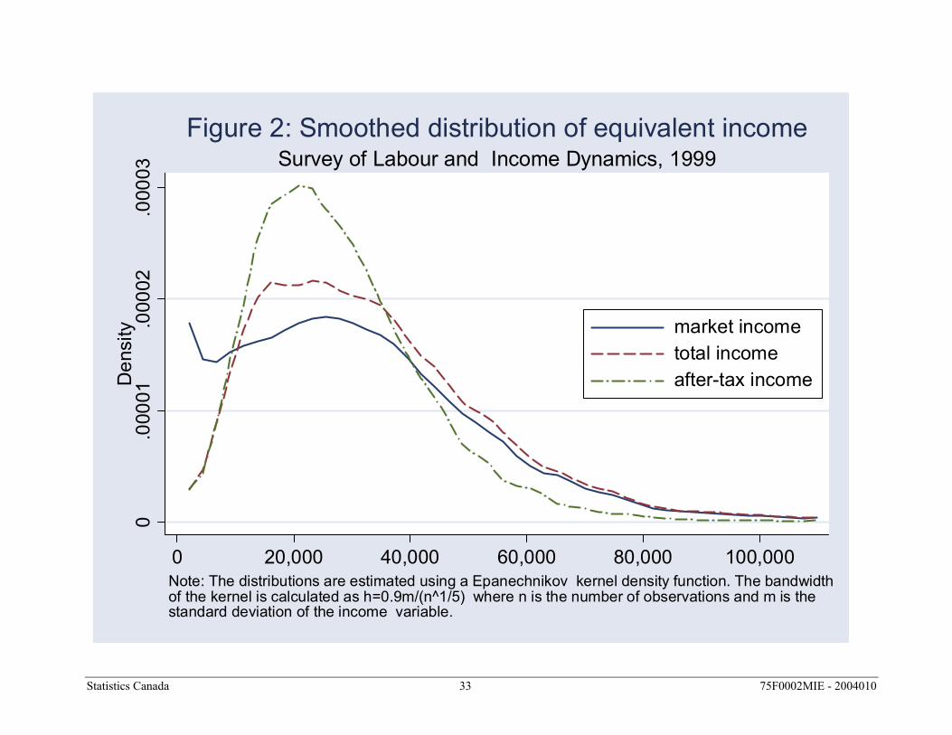
Statistics Canada 33 75F0002MIE - 2004010
0.0
0001
.000
02.0
0003
Den
sity
0 20,000 40,000 60,000 80,000 100,000
market incometotal incomeafter-tax income
Note: The distributions are estimated using a Epanechnikov kernel density function. The bandwidthof the kernel is calculated as h=0.9m/(n^1/5) where n is the number of observations and m is thestandard deviation of the income variable.
Survey of Labour and Income Dynamics, 1999Figure 2: Smoothed distribution of equivalent income

Statistics Canada 34 75F0002MIE - 2004010
0.2
.4.6
.81
Sha
re o
f Inc
ome
0 .2 .4 .6 .8 1Share of Population
market incometotal incomeafter-tax incomeperfect equality
Survey of Labour and Income Dynamics, 1999Figure 3: Lorenz Curves

Statistics Canada 35 75F0002MIE - 2004010
A
B
C
0.2
.4.6
.81
Sha
re o
f Inc
ome
0 .2 .4 .6 .8 1Share of Population
50 have $0.00, 50 have $1.0075 have $0.15, 25 have $1.55perfect equality
Figure 4: Intersecting Lorenz Curves

Statistics Canada 36 75F0002MIE - 2004010
P=63.6%
LICO = $21,300
avg spending = 43.6%
0%
20%
40%
60%
80%
100%
$0 $20,000 $40,000 $60,000 $80,000 $100,000 $120,000After-tax Income
% spent on food, shelter, clothing
20 pp
Figure 5: Estimating low-income cutoffs.

Statistics Canada 37 75F0002MIE - 2004010
Table 1: Mean and median adult-equivalent income. Market income Total income After-tax income Mean 31,731 35,558 28,706 Percentage below 57.3 59.5 58.1 Median 27,660 30,848 25,788 Percentage below 50.0 50.0 50.0 Table 2: Adult-equivalent income deciles. Decile Market income Total income After-tax income 1 Less than 3,368 Less than 11,863 Less than 11,564 2 3,368 - 10,325 11,863 - 16,618 11,564 - 15,560 3 10,325 - 16,500 16,618 - 21,410 15,560 - 18,942 4 16,500 - 22,261 21,410 - 25,930 18,942 - 22,307 5 22,261 - 27,660 25,930 - 30,848 22,307 - 25,788 6 27,660 - 33,358 30,848 - 35,864 25,788 - 29,524 7 33,358 - 39,387 35,864 - 41,766 29,524 - 33,749 8 39,387 - 47,453 41,766 - 49,481 33,794 - 39,237 9 47,453 - 59,927 49,481 - 61,905 39,237 - 47,794 10 Greater than 59,927 Greater than 61,905 Greater than 47,794 Table 3: Mean adult-equivalent income by decile. Decile Market income Total income After-tax income 1 629 7,767 7,417 2 6,973 14,334 13,699 3 13,447 18,979 17,294 4 19,447 23,672 20,686 5 24,968 28,366 23,986 6 30,453 33,307 27,577 7 36,301 38,636 31,529 8 43,207 45,327 36,343 9 53,082 54,920 43,148 10 88,811 90,271 65,390 Table 4: Ratio of decile means of adult-equivalent income. Decile ratio Market income Total income After-tax income 10th/1st 141.19 11.62 8.82 9th/2nd 7.61 3.83 3.15 8th/3rd 3.21 2.39 2.10 7th/4th 1.87 1.63 1.52

Statistics Canada 38 75F0002MIE - 2004010
Table 5: Share of total adult-equivalent income by decile. Decile Market income Total income After-tax income 1 0.002 0.022 0.026 2 0.022 0.040 0.048 3 0.042 0.053 0.060 4 0.061 0.067 0.072 5 0.079 0.080 0.084 6 0.096 0.094 0.096 7 0.114 0.109 0.110 8 0.136 0.127 0.127 9 0.167 0.154 0.150 10 0.280 0.254 0.228 Table 6: Scalar measures of income inequality. Measure Market income Total income After-tax income Gini coefficient 0.425 0.348 0.306 Coefficient of variation 1.006 0.736 0.449 Exponential 0.469 0.437 0.454 Table 7: Measures of income polarization. Measure Market income Total income After-tax income (Percent of median) 75-125 0.357 0.425 0.479 60-225 0.608 0.694 0.755 Polarization coefficient 0.372 0.296 0.257 Table 8: Measures of low income. Measure Market income Total income After-tax income LICO - 0.158 0.116 LIM 0.255 0.174 0.127 MBM - - - Low-income gap (based on LIM)
0.596 0.332 0.344
Gini coefficient of gap (based on LIM)
0.828 0.900 0.932
Low-income intensity (based on LIM)
0.278 0.110 0.085

Statistics Canada 39 75F0002MIE - 2004010
Appendix Distinguishing Income Inequality and Income Polarization As a simple example of this possibility consider the hypothetical economy described in the table below. There are only 6 individuals in this economy and we have information on the incomes of each individual at two different points in time. In period 1 person 1 has an equivalent income of $1; person 2 has $2; person 3 has $3; and so on to person 6 who has $6. Suppose that at the end of period 1 person 3 is required to give $1 to person 1 and person 6 is required to give $1 to person 4. As a result of these transfers of income, in period 2 persons 1, 2 and 3 each have $2 and persons 4, 5 and 6 each have $5. Time 1 Time 2 Person Income Share of Total Person Income Share of
Total 1 1 1/21 = 0.048 1 2 2/21 = 0.095 2 2 2/21 = 0.095 2 2 2/21 = 0.095 3 3 3/21 = 0.143 3 2 2/21 = 0.095 4 4 4/21 = 0.190 4 5 5/21 = 0.238 5 5 5/21 = 0.238 5 5 5/21 = 0.238 6 6 6/21 = 0.279 6 5 5/21 = 0.238 Which of these two distributions is more polarized? Clearly any reasonable measure of polarization would identify time period 2 as being more polarized. Indeed, the polarization coefficient is 0.432 in time 2 and 0.300 in time 1. Is income also more unequally distributed in time 2? According to the Lorenz measure of inequality it is not. Clearly, at all points of the income distribution the Lorenz curve for time 1 lies below or right on top of the Lorenz curve for time 2. So income is more polarized in time 2, but is more unequally distributed in time 1.