Descriptive Statistics

Univariate Statistics

Chi Square

ANOVA

Summarization of a collection of data in a clear and understandable way

the most basic form of statistics lays the foundation for all statistical knowledge

Descriptive Statistics

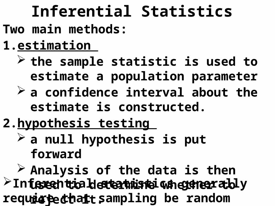
Inferential StatisticsTwo main methods: 1. estimation

the sample statistic is used to estimate a population parameter

a confidence interval about the estimate is constructed.

2. hypothesis testing a null hypothesis is put forward Analysis of the data is then used to

determine whether to reject it.Inferential statistics generally require that sampling be random

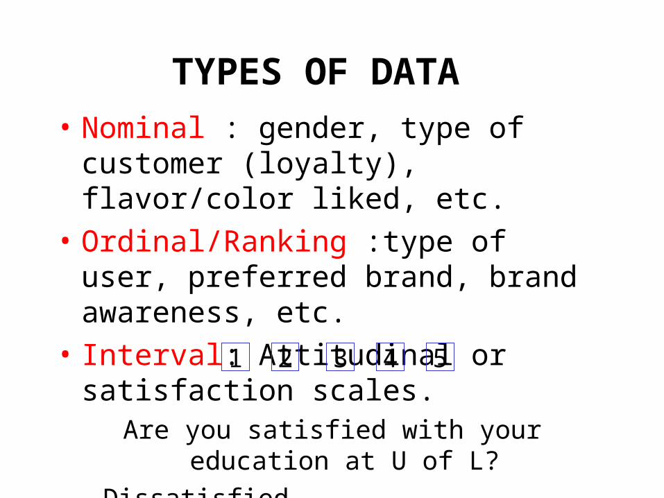
• Nominal : gender, type of customer (loyalty), flavor/color liked, etc.

• Ordinal/Ranking :type of user, preferred brand, brand awareness, etc.

• Interval: Attitudinal or satisfaction scales. Are you satisfied with your education at U of L?

Dissatisfied Satisfied

• Ratio: Income, price willing to pay, age, etc.

TYPES OF DATA

3 4 521

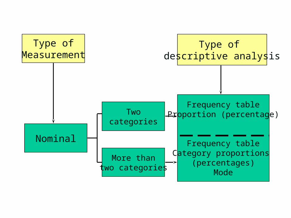
Type ofMeasurement

Nominal

Twocategories

More thantwo categories

Frequency tableProportion (percentage)

Frequency tableCategory proportions

(percentages)Mode

Type of descriptive analysis

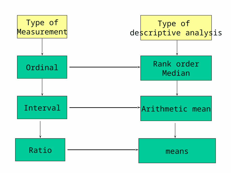
Ratio means

Type ofMeasurement

Type of descriptive analysis

Ordinal Rank orderMedian

Interval Arithmetic mean

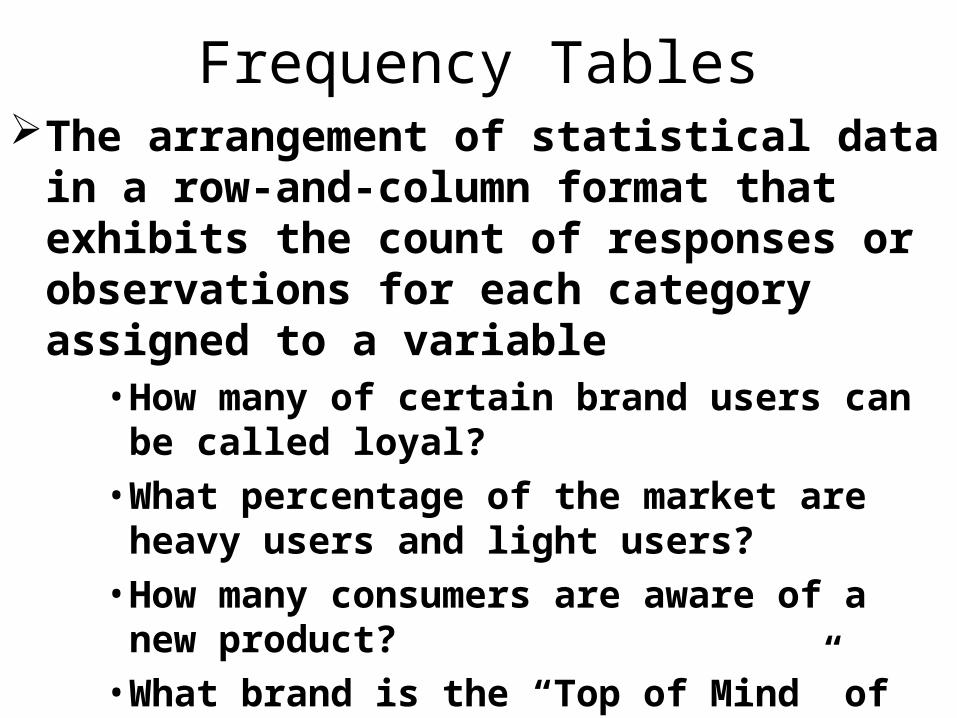
The arrangement of statistical data in a row-and-column format that exhibits the count of responses or observations for each category assigned to a variable

• How many of certain brand users can be called loyal?

• What percentage of the market are heavy users and light users?

• How many consumers are aware of a new product?• What brand is the “Top of Mind” of the market?

Frequency Tables

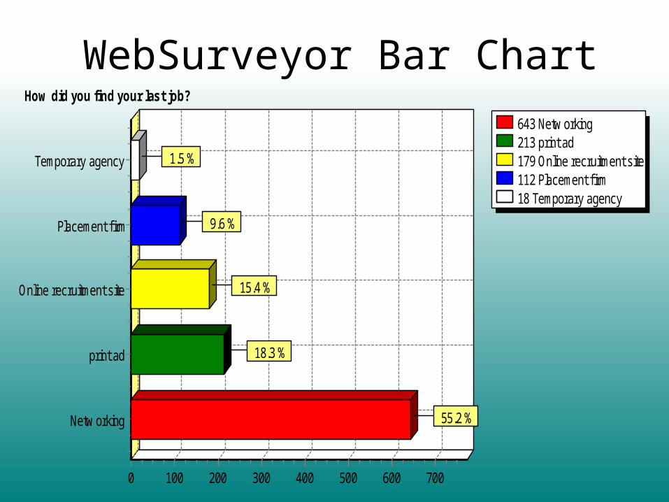
643 Netw orking213 print ad179 Online recruitment site112 Placement f irm18 Temporary agency

How did you find your last job?

7006005004003002001000

Netw orking

print ad

Online recruitment site

Placement f irm

Temporary agency

55.2 %

18.3 %

15.4 %

9.6 %

1.5 %

WebSurveyor Bar Chart

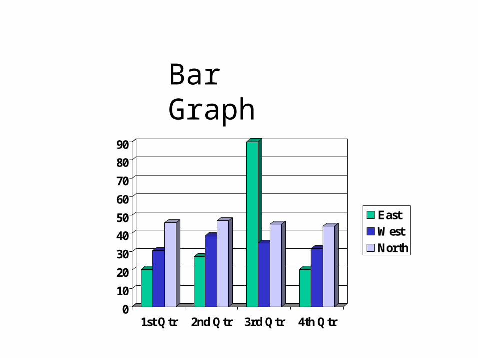
0

10

20

30

40

50

60

70

80

90

1st Qtr 2nd Qtr 3rd Qtr 4th Qtr

EastWestNorth

Bar Graph

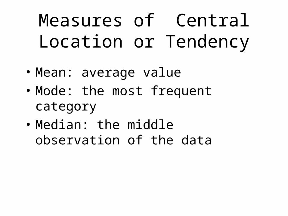
• Mean: average value

• Mode: the most frequent category

• Median: the middle observation of the data

Measures of Central Location or Tendency

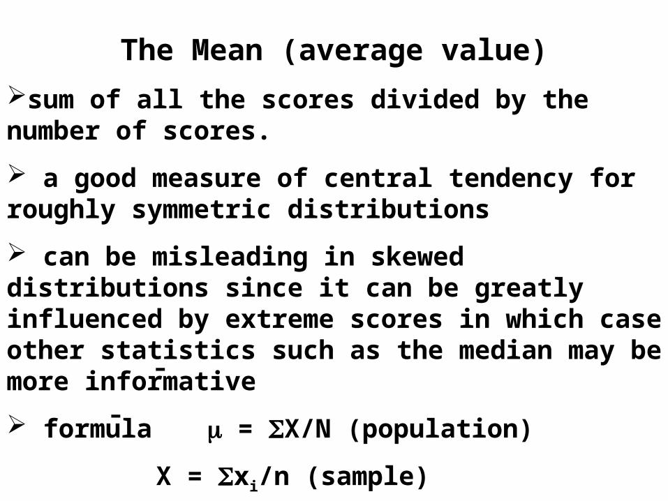
The Mean (average value)

sum of all the scores divided by the number of scores.

a good measure of central tendency for roughly symmetric distributions

can be misleading in skewed distributions since it can be greatly influenced by extreme scores in which case other statistics such as the median may be more informative

formula = X/N (population)

X = xi/n (sample)

where /X is the population/sample mean

and N/n is the number of scores.

¯

¯

Mode the most frequent category

users 25%non-users 75%

Advantages: • meaning is obvious• the only measure of central tendency that can be used with nominal data.

Disadvantages• many distributions have more than one mode, i.e. are "multimodal• greatly subject to sample fluctuations • therefore not recommended to be used as the only measure of central tendency.

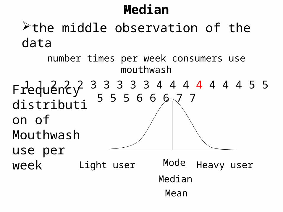
Medianthe middle observation of the data

number times per week consumers use mouthwash

1 1 2 2 2 3 3 3 3 3 4 4 4 4 4 4 4 5 5 5 5 5 6 6 6 7 7

Frequency distribution of Mouthwash use per week

Heavy userLight user Mode

Median

Mean

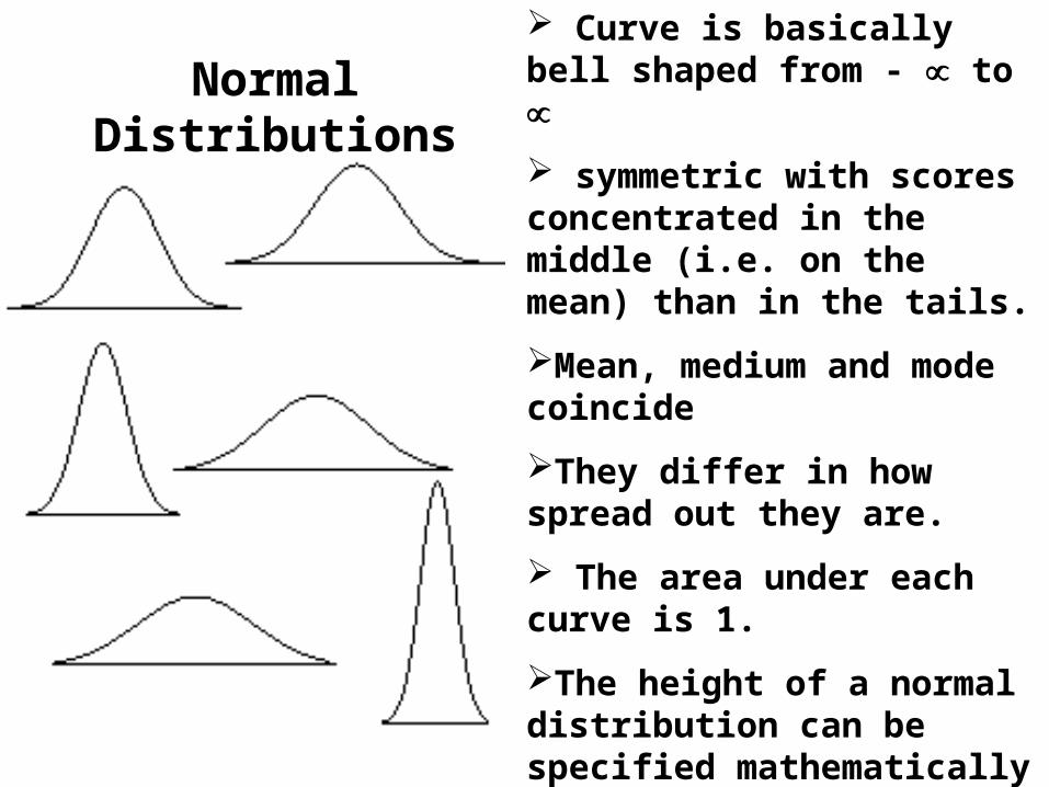
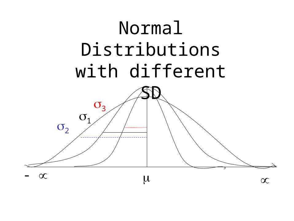
Normal Distributions Curve is basically bell shaped from - to

symmetric with scores concentrated in the middle (i.e. on the mean) than in the tails.

Mean, medium and mode coincide

They differ in how spread out they are.

The area under each curve is 1.

The height of a normal distribution can be specified mathematically in terms of two parameters: the mean () and the standard deviation ().

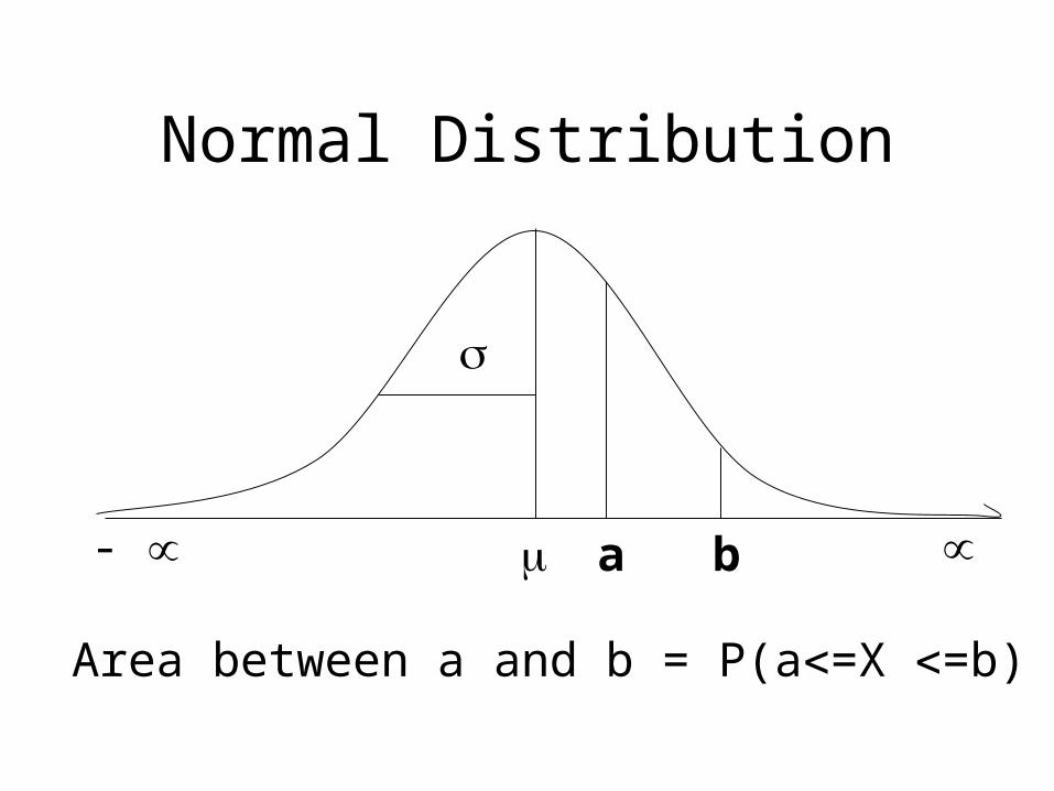
Normal Distribution

- a b

Area between a and b = P(a=X =b)

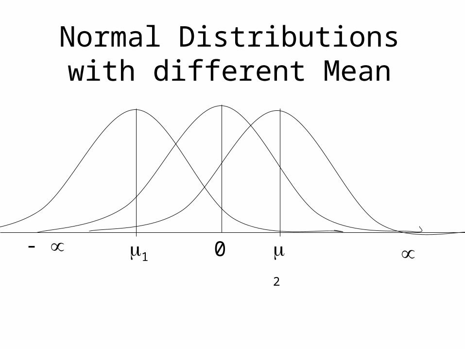
Normal Distributions with different Mean

0- 1 2

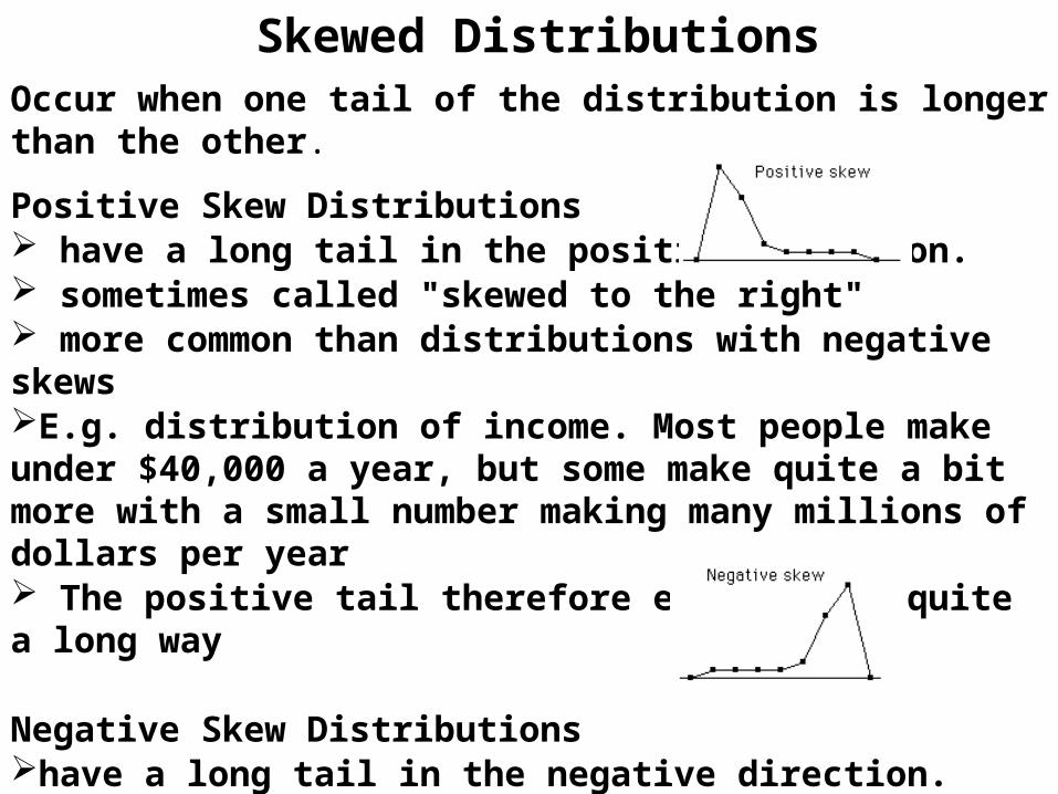
Occur when one tail of the distribution is longer than the other.

Positive Skew Distributions have a long tail in the positive direction. sometimes called "skewed to the right" more common than distributions with negative skews E.g. distribution of income. Most people make under $40,000 a year, but some make quite a bit more with a small number making many millions of dollars per year The positive tail therefore extends out quite a long way

Negative Skew Distributionshave a long tail in the negative direction. called "skewed to the left." negative tail stops at zero

Skewed Distributions

• Minimum, Maximum, and Range

• Variance

• Standard Deviation

Measures of Dispersion or Variability

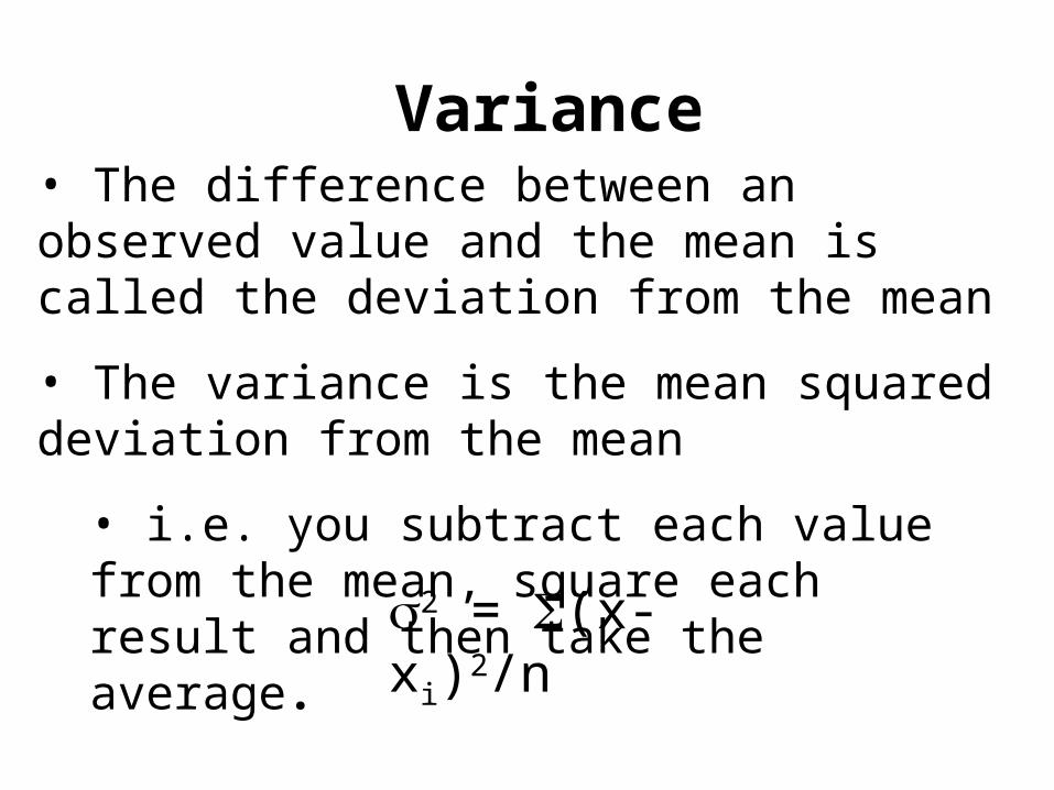
Variance• The difference between an observed value and the mean is called the deviation from the mean

• The variance is the mean squared deviation from the mean

• i.e. you subtract each value from the mean, square each result and then take the average.

• Because it is squared it can never be negative

2 = (x- xi)2/n¯

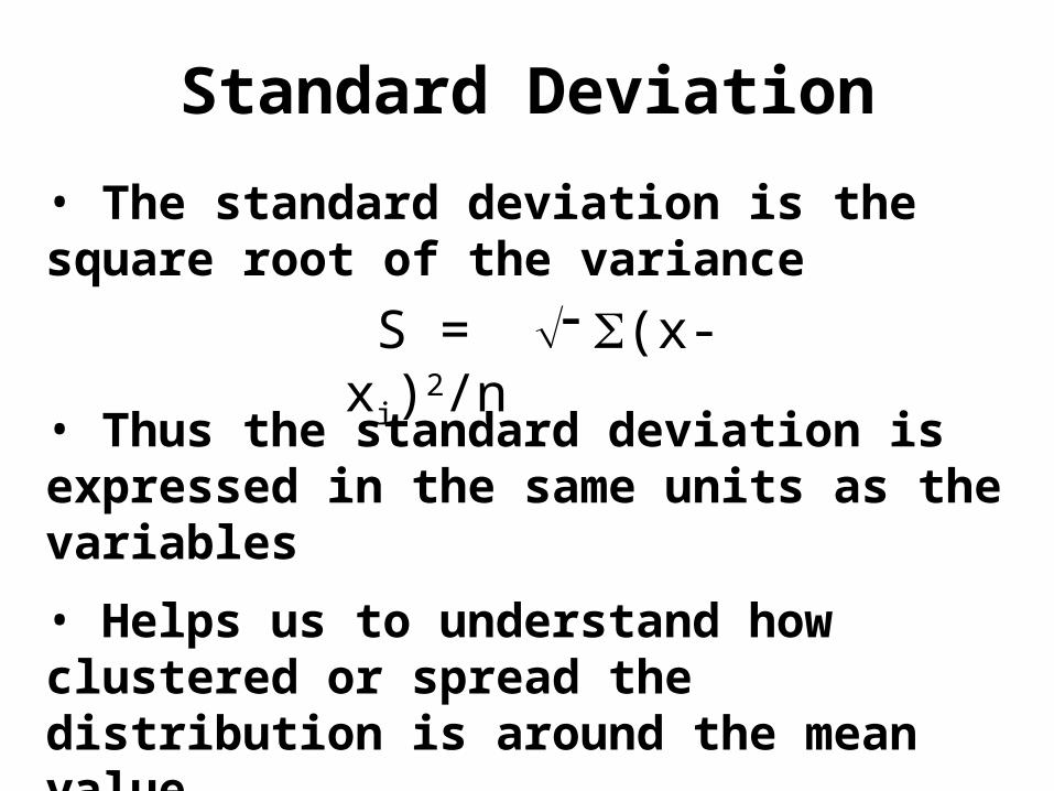
• The standard deviation is the square root of the variance

• Thus the standard deviation is expressed in the same units as the variables

• Helps us to understand how clustered or spread the distribution is around the mean value.

Standard Deviation

S = (x- xi)2/n¯

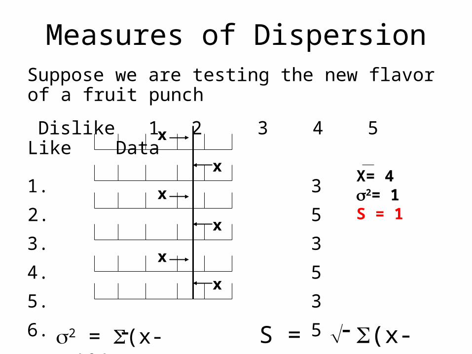
Measures of DispersionSuppose we are testing the new flavor of a fruit punch

Dislike 1 2 3 4 5 Like Data

1. 3

2. 5

3. 3

4. 5

5. 3

6. 5

x

x

x

x

x

x

X= 42= 1S = 1

2 = (x- xi)2/n¯ S = (x- xi)2/n¯

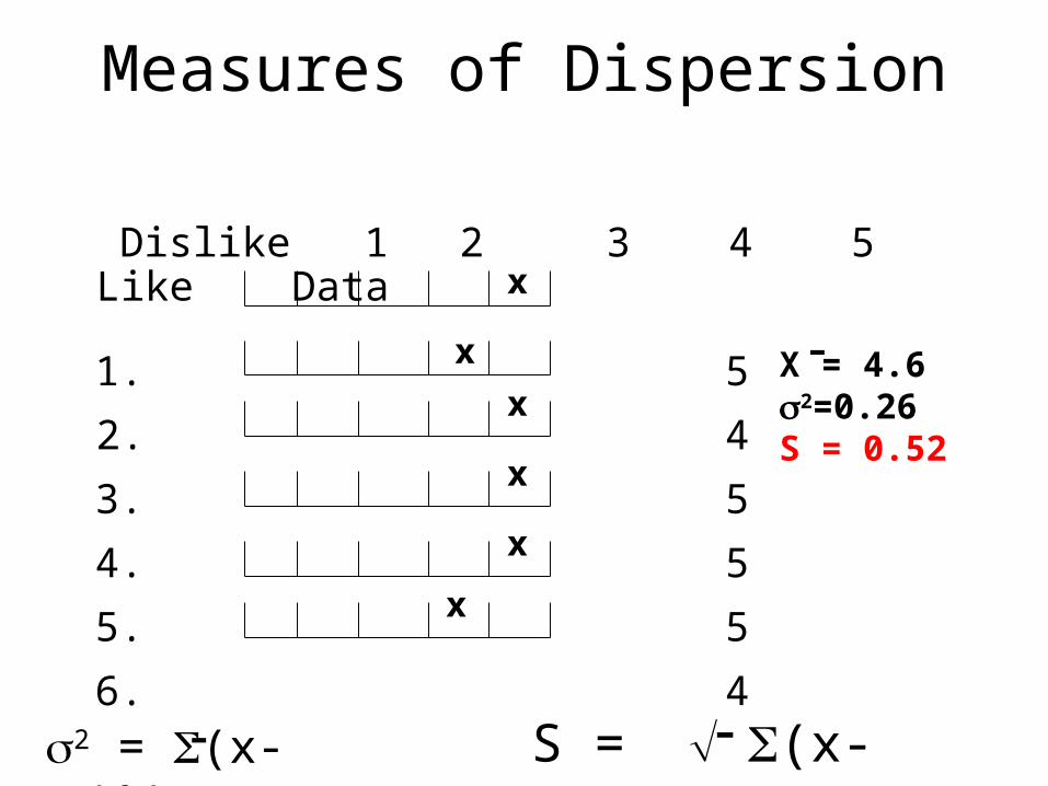
Measures of Dispersion

Dislike 1 2 3 4 5 Like Data

1. 5

2. 4

3. 5

4. 5

5. 5

6. 4

x

x

x

x

x

xX = 4.62=0.26S = 0.52

2 = (x- xi)2/n¯ S = (x- xi)2/n¯

¯

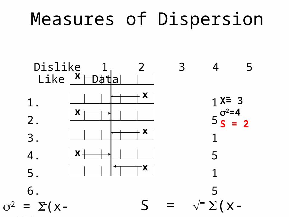
Measures of Dispersion

Dislike 1 2 3 4 5 Like Data

1. 1

2. 5

3. 1

4. 5

5. 1

6. 5

x

x

x

x

x

x

X= 32=4S = 2

2 = (x- xi)2/n¯ S = (x- xi)2/n¯

¯

-

12

3

Normal Distributions with different SD

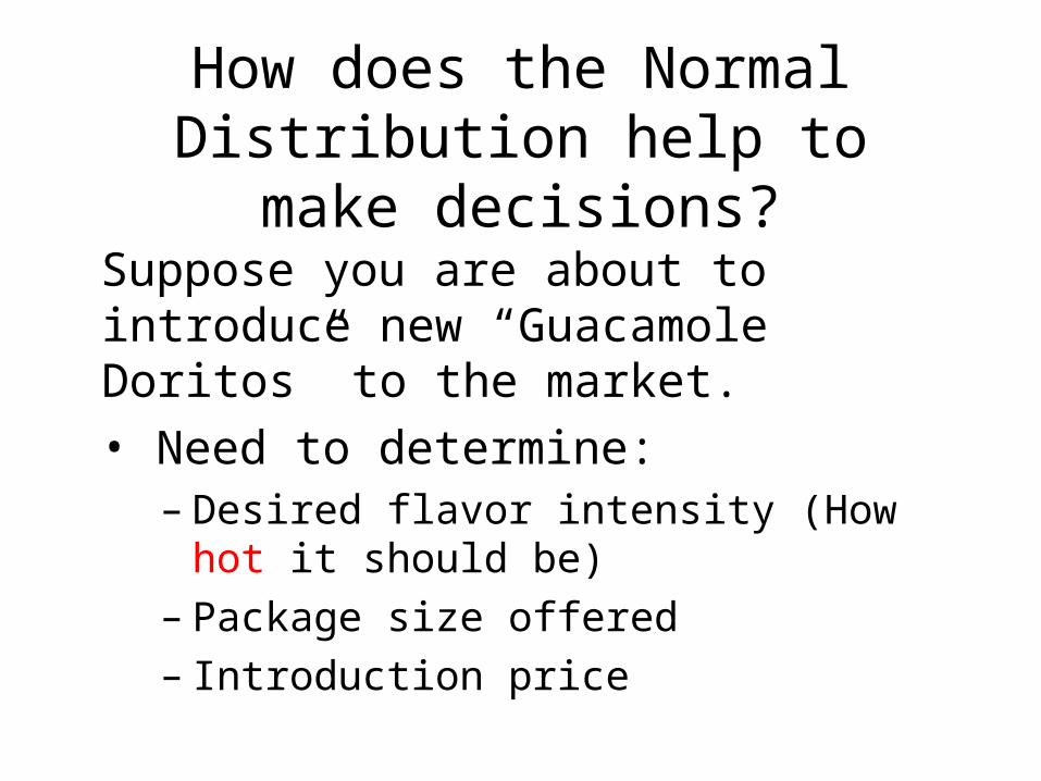
How does the Normal Distribution help to make decisions?

Suppose you are about to introduce new “Guacamole Doritos” to the market.

• Need to determine:– Desired flavor intensity (How hot it should be)– Package size offered– Introduction price

• What do you do in order to answer your questions?

ASK THE CONSUMER

• How?

TAKE A SAMPLE

• How can you be sure that what you conclude on the sample would be true for the whole population?

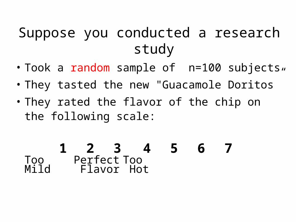
Suppose you conducted a research study• Took a random sample of n=100 subjects

• They tasted the new "Guacamole Doritos”

• They rated the flavor of the chip on the following scale:

Too Perfect Too Mild Flavor Hot

1 2 3 4 5 6 7

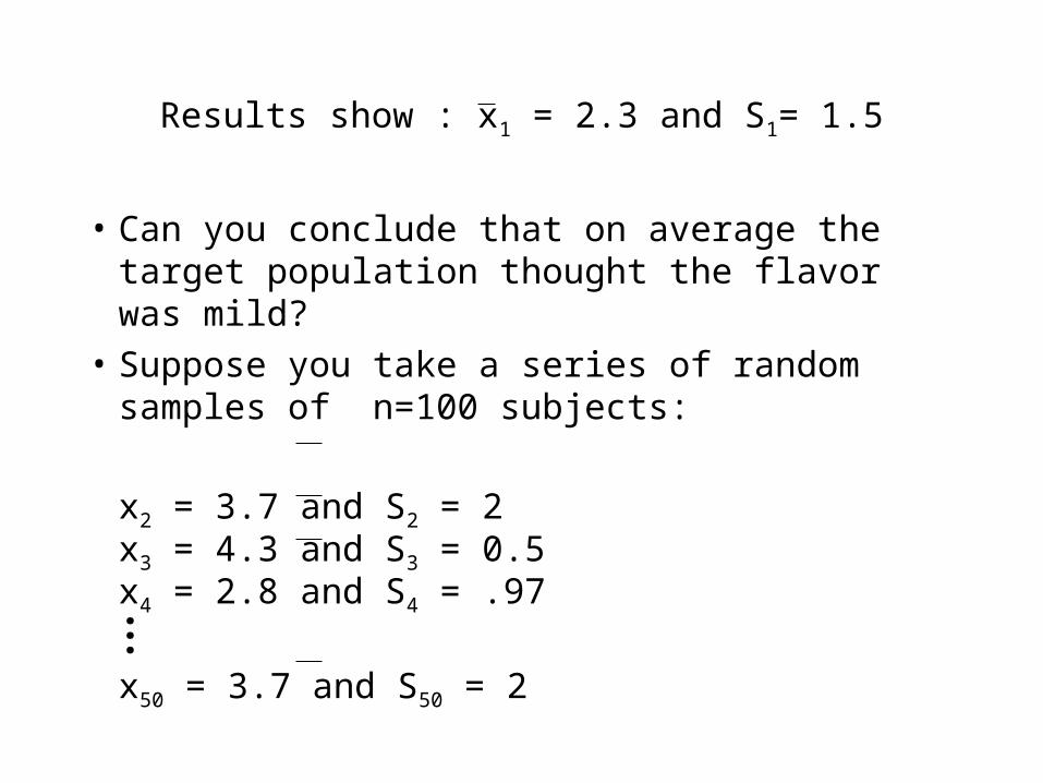
Results show : x1 = 2.3 and S1= 1.5

• Can you conclude that on average the target population thought the flavor was mild?

• Suppose you take a series of random samples of n=100 subjects:

x2 = 3.7 and S2 = 2x3 = 4.3 and S3 = 0.5x4 = 2.8 and S4 = .97...x50 = 3.7 and S50 = 2

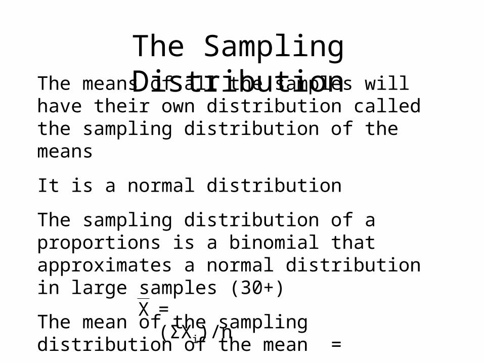
The Sampling DistributionThe means of all the samples will have their own distribution called the sampling distribution of the means

It is a normal distribution

The sampling distribution of a proportions is a binomial that approximates a normal distribution in large samples (30+)

The mean of the sampling distribution of the mean =

It equals the population parameter

X = (ΣXi)/n

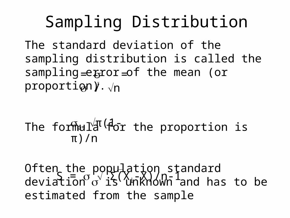
Sampling DistributionThe standard deviation of the sampling distribution is called the sampling error of the mean (or proportion).

The formula for the proportion is

Often the population standard deviation is unknown and has to be estimated from the sample

= = / nX

p= π(1-π)/n

S = Σ(Xi-X)/n-1

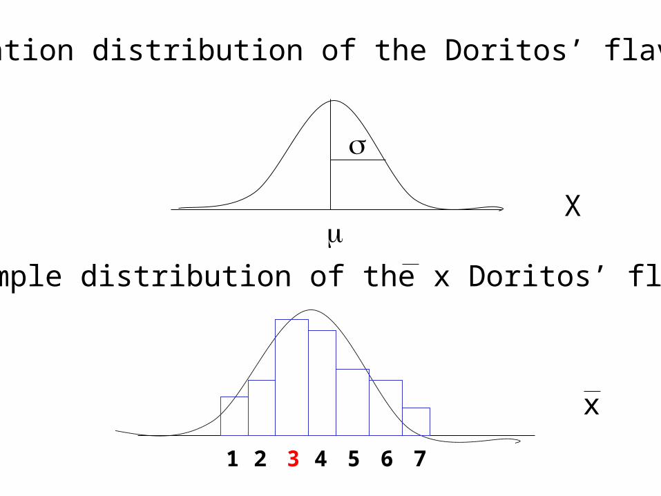
Population distribution of the Doritos’ flavor (X)

Sample distribution of the x Doritos’ flavor

x

X

1 2 3 4 5 6 7

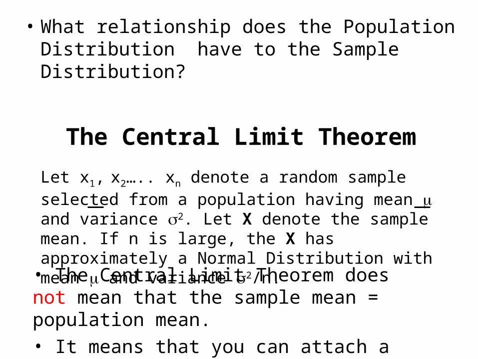
• What relationship does the Population Distribution have to the Sample Distribution?

The Central Limit Theorem

Let x1, x2….. xn denote a random sample selected from a population having mean and variance 2. Let X denote the sample mean. If n is large, the X has approximately a Normal Distribution with mean and variance 2/n.

• The Central Limit Theorem does not mean that the sample mean = population mean. • It means that you can attach a probability to that value and decide.

Interpretation• The process of making pertinent inferences

and drawing conclusions

• concerning the meaning and implications of a research investigation

• You do not need to know the population distribution in order to take decisions.

• In order to draw conclusions n must be “big enough.”

• How big?, it DEPENDS

Univariate Statistics

• Test of statistical significance

• Hypothesis testing one variable at a time

• Hypothesis• Unproven proposition• Supposition that tentatively explains certain

facts or phenomena• Assumption about nature of the world

What is a Hypothesis Test?

• It is used when we want to make inferences about a population.

• Generally we have a particular theory, or hypothesis, about certain events like:– The average age of our regular customers– The average money spent per week on fast food

restaurants– The percentage of unsatisfied customers of our

store.

Basic Concepts

• The hypothesis the researcher wants to test is called the alternative hypothesis H1.

• The opposite of the alternative hypothesis us the null hypothesis H0 (the status quo)(no difference between the

sample and the population, or between samples).

• The objective is to DISPROVE the null hypothesis.

• The Significance Level is the Critical probability of choosing between the null hypothesis and the alternative hypothesis

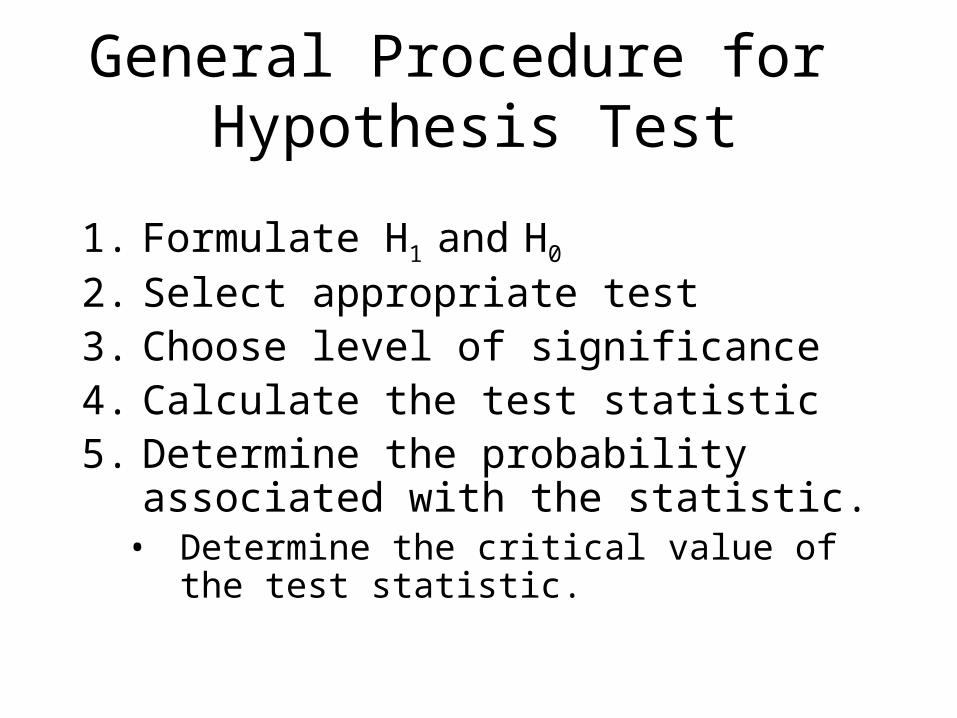
General Procedure for Hypothesis Test

1. Formulate H1 and H0

2. Select appropriate test3. Choose level of significance4. Calculate the test statistic5. Determine the probability associated with

the statistic.• Determine the critical value of the test

statistic.

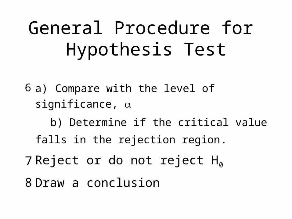
General Procedure for Hypothesis Test

6 a) Compare with the level of significance,

b) Determine if the critical value falls in the

rejection region.

7 Reject or do not reject H0

8 Draw a conclusion

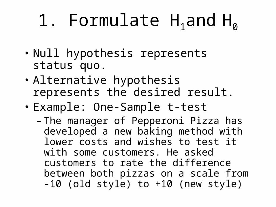
1. Formulate H1and H0

• Null hypothesis represents status quo.• Alternative hypothesis represents the

desired result.• Example: One-Sample t-test

– The manager of Pepperoni Pizza has developed a new baking method with lower costs and wishes to test it with some customers. He asked customers to rate the difference between both pizzas on a scale from -10 (old style) to +10 (new style)

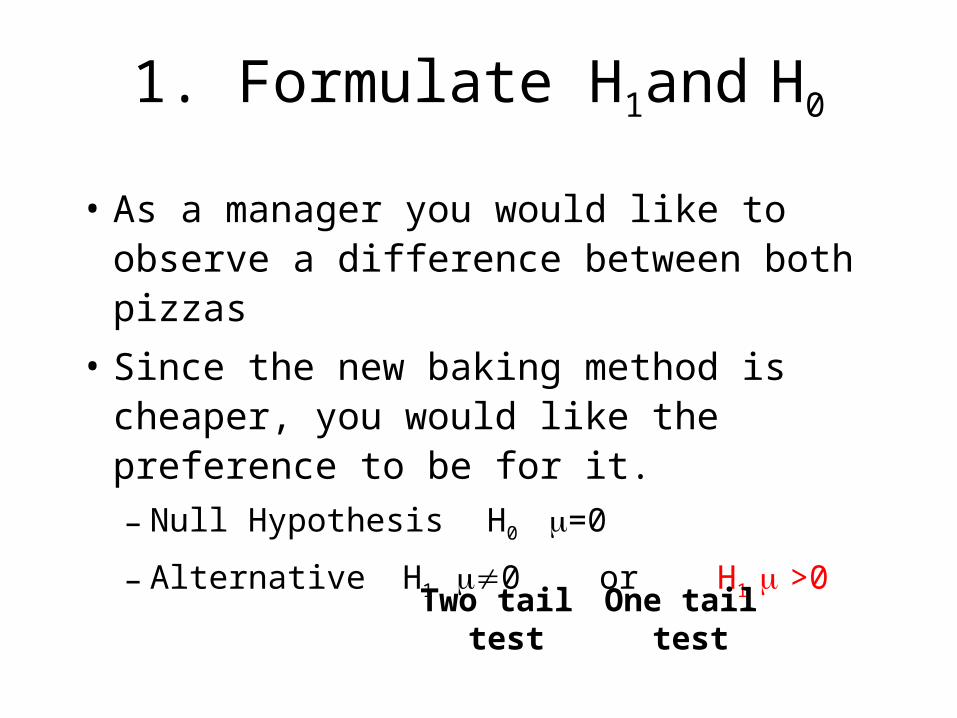
1. Formulate H1and H0

• As a manager you would like to observe a difference between both pizzas

• Since the new baking method is cheaper, you would like the preference to be for it.

– Null Hypothesis H0 =0

– Alternative H1 0 or H1 >0

Two tail test

One tail test

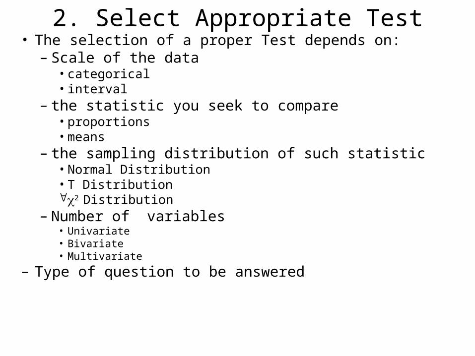
• The selection of a proper Test depends on:– Scale of the data

• categorical• interval

– the statistic you seek to compare• proportions• means

– the sampling distribution of such statistic• Normal Distribution• T Distribution2 Distribution

– Number of variables• Univariate• Bivariate• Multivariate

– Type of question to be answered

2. Select Appropriate Test

3. Choose Level of Significance• Whenever we draw inferences about a population, there is a risk

that an incorrect conclusion will be reached

• The significance level states the probability of incorrectly

rejecting H0. This error is commonly known as Type I error, and

we denote the significance level as .

• Significance Level selected is typically .05 or .01

– In our example the Type I error would be rejecting the null hypothesis

that the pizzas are equal, when they really are perceived equal by the

customers of the entire population.

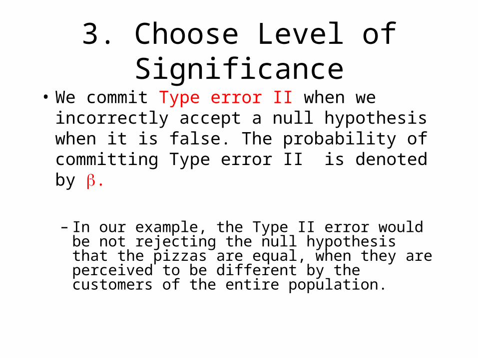
3. Choose Level of Significance

• We commit Type error II when we incorrectly accept a null hypothesis when it is false. The probability of committing Type error II is denoted by .

– In our example, the Type II error would be not rejecting the null hypothesis that the pizzas are equal, when they are perceived to be different by the customers of the entire population.

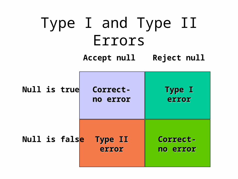
Accept null Reject null

Null is true

Null is false

Correct-Correct-no errorno error

Type IType Ierrorerror

Type IIType IIerrorerror

Correct-Correct-no errorno error

Type I and Type II Errors

Which is worse?

• Both are serious, but traditionally Type I error has been considered more serious, that’s why the objective of hypothesis testing is to reject H0 only when there is enough evidence that supports it.

• Therefore, we choose to be as small as possible without compromising .

• Increasing the sample size for a given α will decrease β

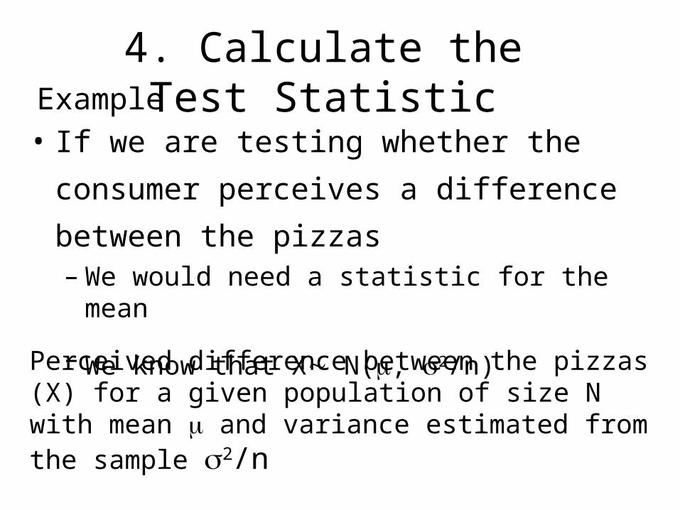
• If we are testing whether the consumer

perceives a difference between the pizzas– We would need a statistic for the mean

– We know that X N(, 2/n)

Perceived difference between the pizzas (X) for a given population of size N with mean and variance estimated from the sample 2/n

Example

4. Calculate the Test Statistic

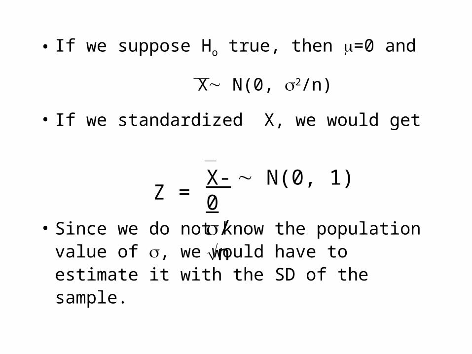
• If we suppose Ho true, then =0 and

X N(0, 2/n) • If we standardized X, we would get

• Since we do not know the population value of , we would have to estimate it with the SD of the sample.

N(0, 1) X- 0/nZ =

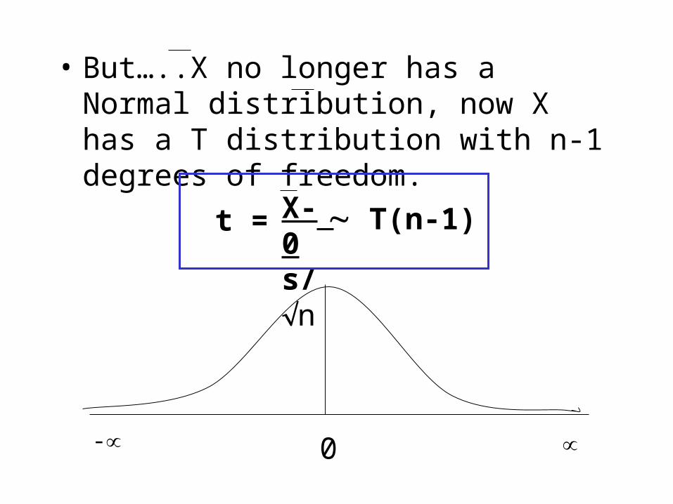
• But…..X no longer has a Normal distribution, now X has a T distribution with n-1 degrees of freedom.

t = X- 0s/n

T(n-1)

0-

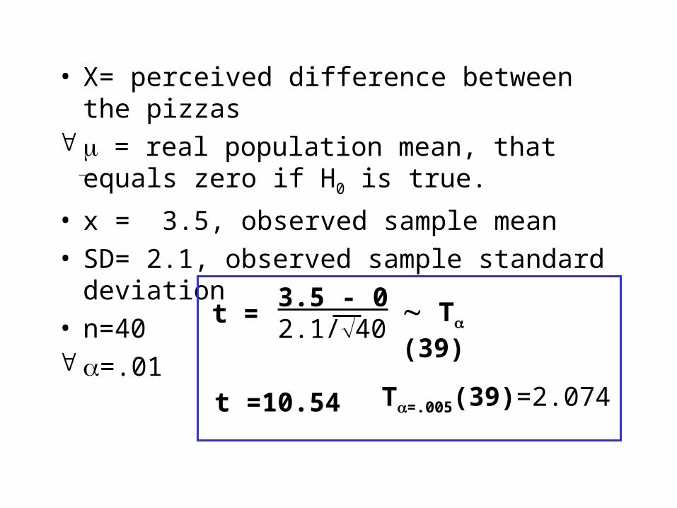
• X= perceived difference between the pizzas = real population mean, that equals zero if H0 is

true.• x = 3.5, observed sample mean• SD= 2.1, observed sample standard deviation• n=40 =.01 t =

3.5 - 02.1/40

T (39)

t =10.54 T=.005(39)=2.074

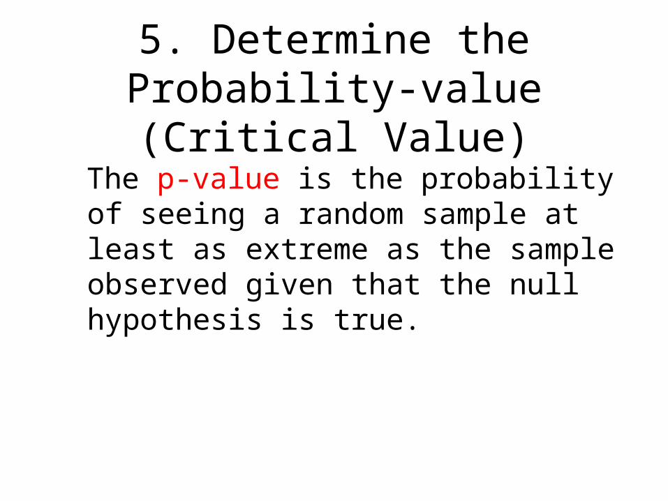
5. Determine the Probability-value (Critical Value)

The p-value is the probability of seeing a random sample at least as extreme as the sample observed given that the null hypothesis is true.

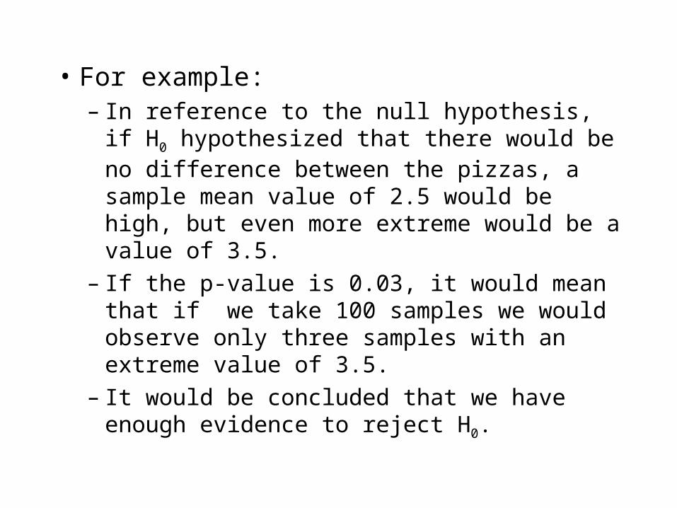
• For example:– In reference to the null hypothesis, if H0

hypothesized that there would be no difference between the pizzas, a sample mean value of 2.5 would be high, but even more extreme would be a value of 3.5.

– If the p-value is 0.03, it would mean that if we take 100 samples we would observe only three samples with an extreme value of 3.5.

– It would be concluded that we have enough evidence to reject H0.

0 10.542.074-2.074

/2/2

1-

Reject H0 Reject H0

Do not Reject H0

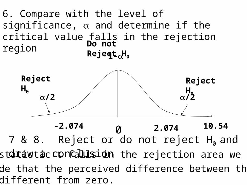
6. Compare with the level of significance, and determine if the critical value falls in the rejection region

Since the statistic t falls in the rejection area we reject Ho

and conclude that the perceived difference between the pizzas is different from zero.

7 & 8. Reject or do not reject H0 and draw a conclusion

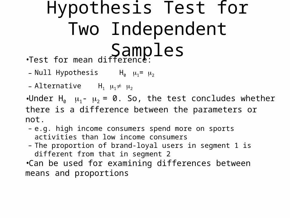
Hypothesis Test for Two Independent Samples

•Test for mean difference:

– Null Hypothesis H0 1= 2

– Alternative H1 1 2

•Under H0 1- 2 = 0. So, the test concludes whether there is a difference between the parameters or not.– e.g. high income consumers spend more on sports activities than low

income consumers– The proportion of brand-loyal users in segment 1 is different from that in

segment 2•Can be used for examining differences between means and proportions

Test for Means Difference

• Suppose X measures the preference for a mouthwash flavor (cool mint) on a scale from 1-dislike to 5-like

• We want to know if the flavor preference is

different between the type of user (heavy or

light) H0: H= L

H1: H L

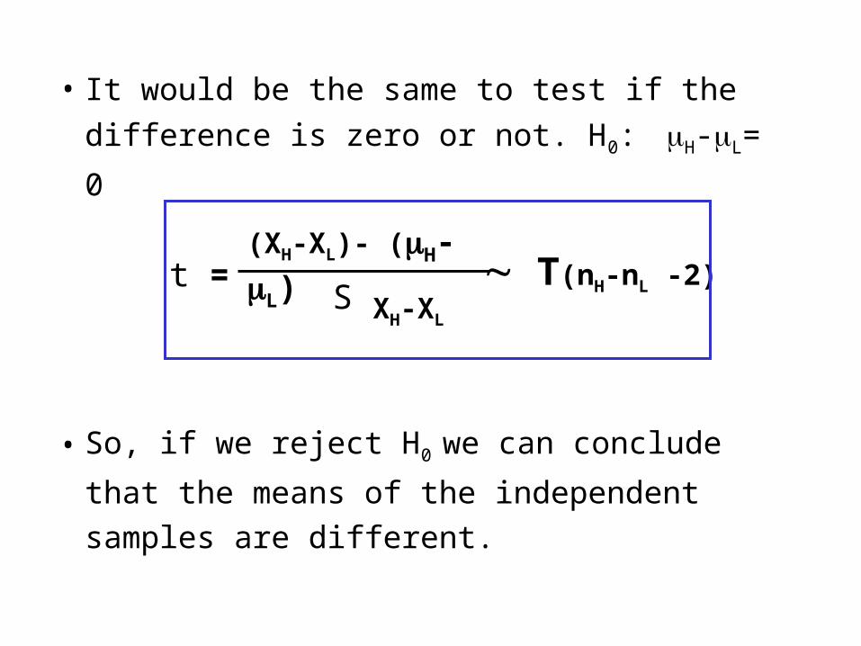
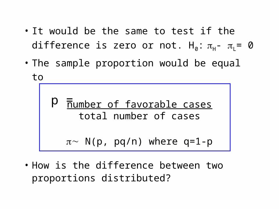
• It would be the same to test if the difference is

zero or not. H0: H-L= 0

• So, if we reject H0 we can conclude that the

means of the independent samples are

different.

t = S XH-XL

(XH-XL)- (H-L) T(nH-nL -2)

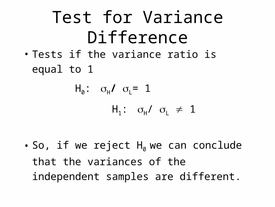
Test for Variance Difference

• Tests if the variance ratio is equal to 1

H0: H/ L= 1

H1: H/ L 1

• So, if we reject H0 we can conclude that the

variances of the independent samples are

different.

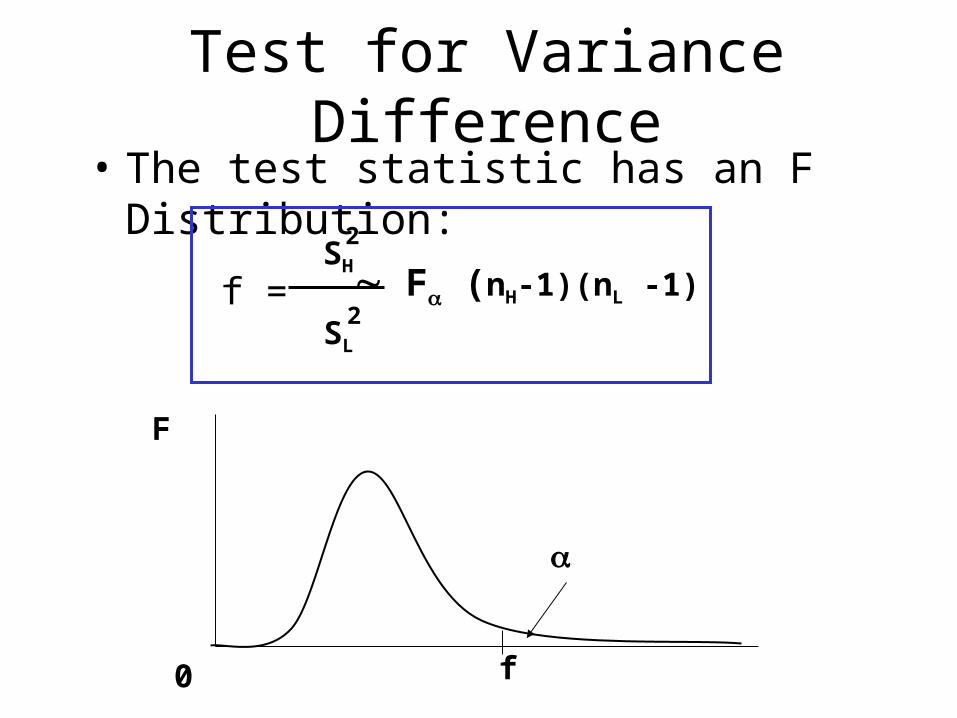
Test for Variance Difference• The test statistic has an F Distribution:

f =SH

2

SL

2 F (nH-1)(nL -1)

0

F

f

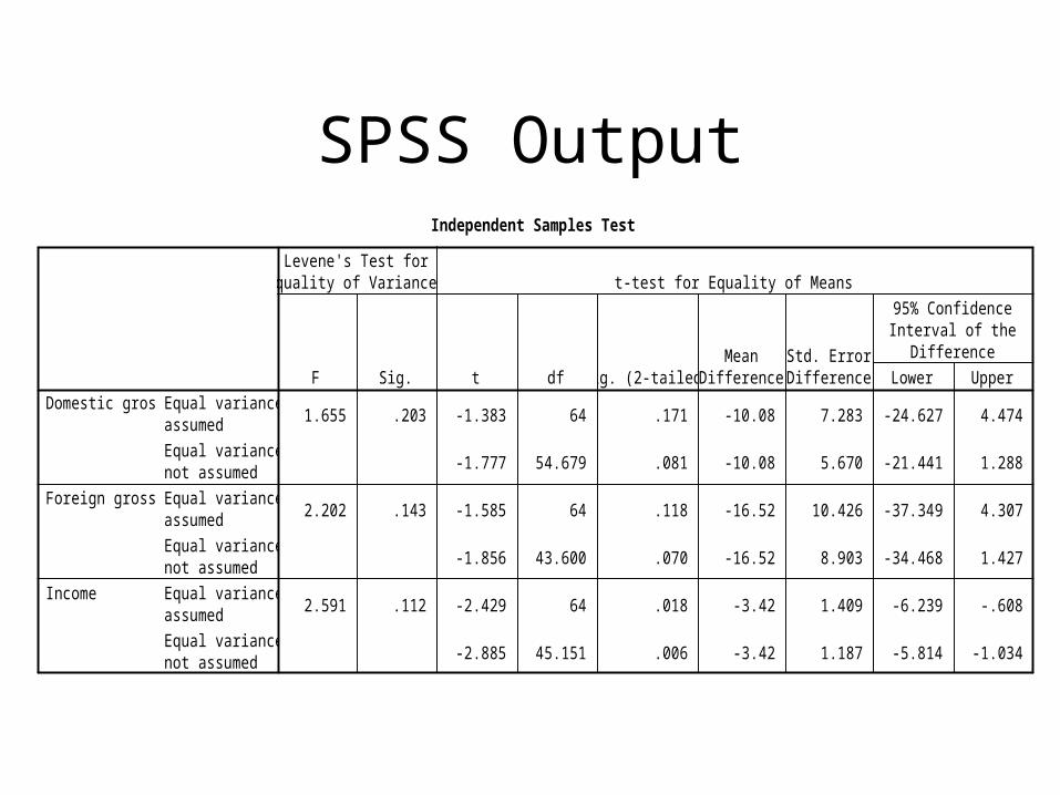
SPSS OutputIndependent Samples Test

1.655 .203 -1.383 64 .171 -10.08 7.283 -24.627 4.474

-1.777 54.679 .081 -10.08 5.670 -21.441 1.288

2.202 .143 -1.585 64 .118 -16.52 10.426 -37.349 4.307

-1.856 43.600 .070 -16.52 8.903 -34.468 1.427

2.591 .112 -2.429 64 .018 -3.42 1.409 -6.239 -.608

-2.885 45.151 .006 -3.42 1.187 -5.814 -1.034

Equal variancesassumed

Equal variancesnot assumed

Equal variancesassumed

Equal variancesnot assumed

Equal variancesassumed

Equal variancesnot assumed

Domestic gross

Foreign gross

Income

F Sig.

Levene's Test forEquality of Variances

t df Sig. (2-tailed)Mean

DifferenceStd. ErrorDifference Lower Upper

95% ConfidenceInterval of the

Difference

t-test for Equality of Means

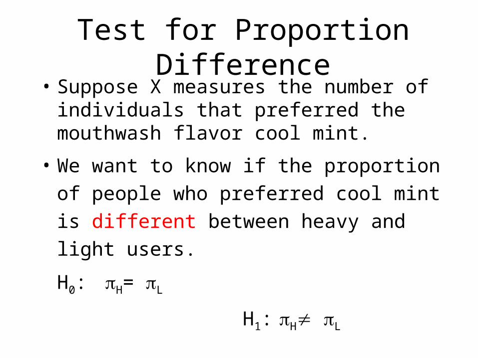
Test for Proportion Difference• Suppose X measures the number of

individuals that preferred the mouthwash flavor cool mint.

• We want to know if the proportion of people

who preferred cool mint is different between

heavy and light users.

H0: H= L

H1: H L

• It would be the same to test if the difference

is zero or not. H0: H- L= 0

• The sample proportion would be equal to

number of favorable casestotal number of cases

N(p, pq/n) where q=1-p

• How is the difference between two proportions distributed?

p =

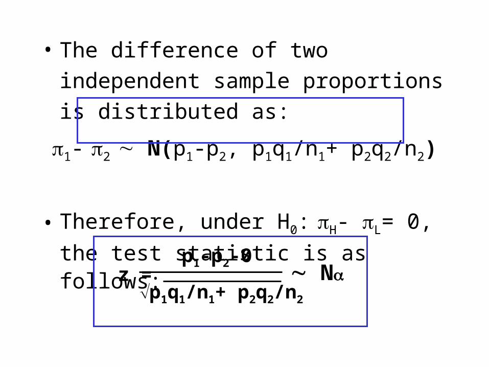
• The difference of two independent sample

proportions is distributed as:

1- 2 N(p1-p2, p1q1/n1+ p2q2/n2)

• Therefore, under H0: H- L= 0, the test

statistic is as follows:

z =

p1-p2-0 Np1q1/n1+ p2q2/n2

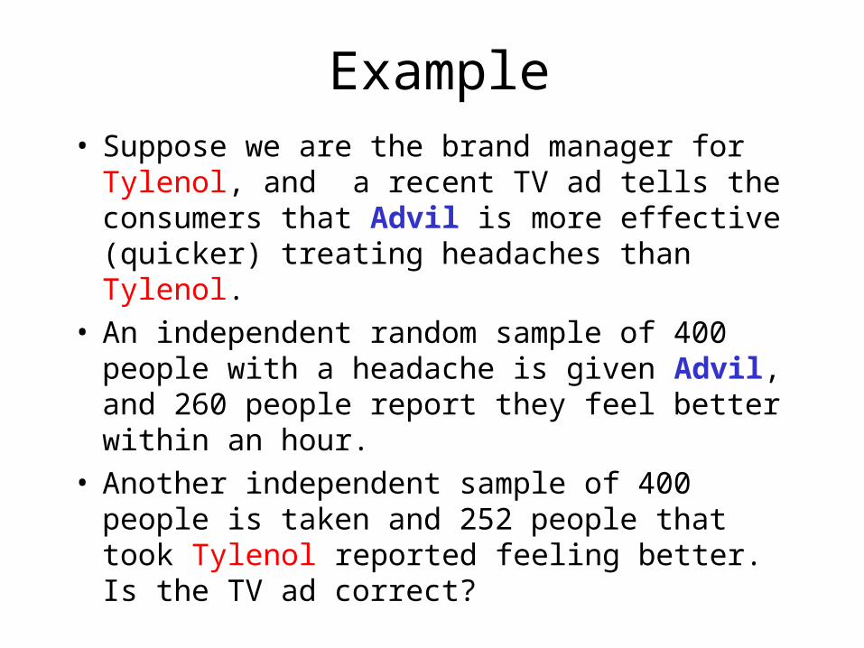
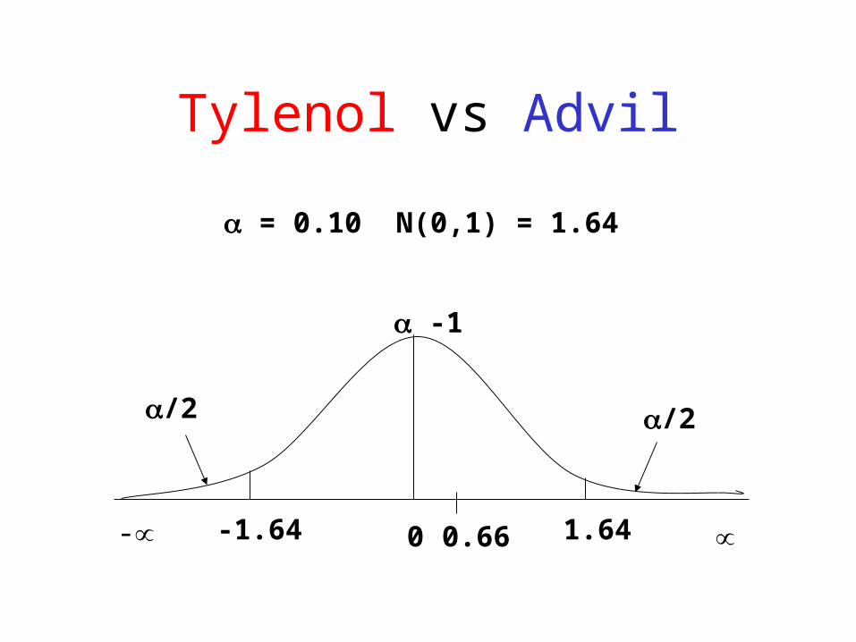
Example• Suppose we are the brand manager for Tylenol,

and a recent TV ad tells the consumers that Advil is more effective (quicker) treating headaches than Tylenol.

• An independent random sample of 400 people with a headache is given Advil, and 260 people report they feel better within an hour.

• Another independent sample of 400 people is taken and 252 people that took Tylenol reported feeling better. Is the TV ad correct?

Tylenol vs Advil

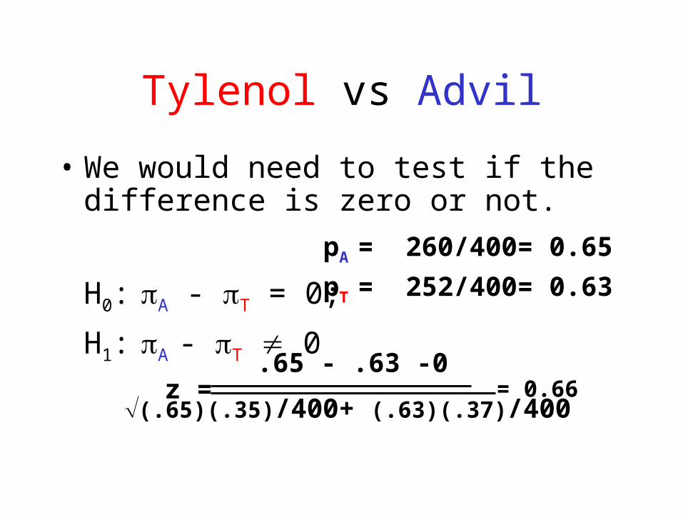
• We would need to test if the difference is zero or not.

H0: A - T = 0;

H1: A - T 0

z =

.65 - .63 -0

(.65)(.35)/400+ (.63)(.37)/400= 0.66

pA = 260/400= 0.65

pT = 252/400= 0.63

Tylenol vs Advil

- 0 0.66

= 0.10 N(0,1) = 1.64

1.64-1.64

/2/2

-1

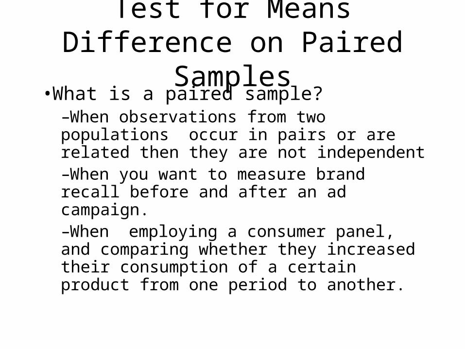
Test for Means Difference on Paired Samples

•What is a paired sample?–When observations from two populations occur in pairs or are related then they are not independent–When you want to measure brand recall before and after an ad campaign.–When employing a consumer panel, and comparing whether they increased their consumption of a certain product from one period to another.

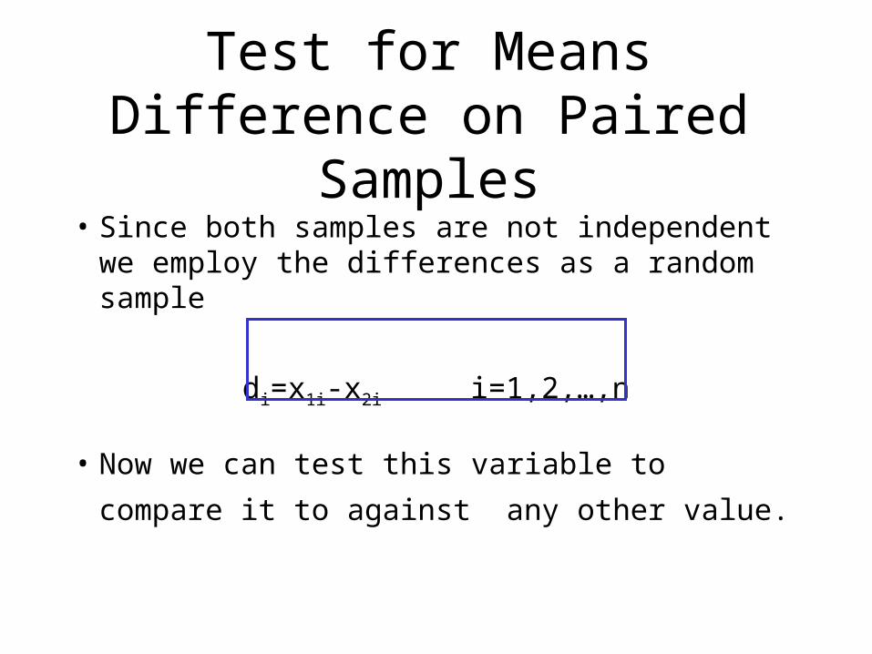
• Since both samples are not independent we employ the differences as a random sample

di=x1i-x2i i=1,2,…,n

• Now we can test this variable to compare it

to against any other value.

Test for Means Difference on Paired Samples

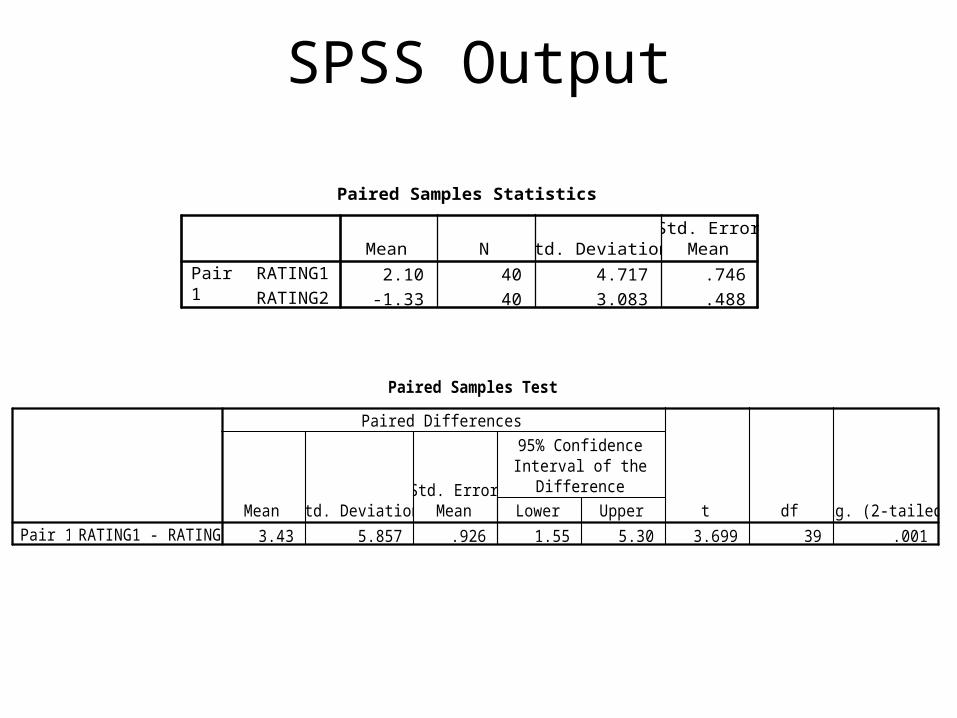
SPSS Output

Paired Samples Statistics

2.10 40 4.717 .746

-1.33 40 3.083 .488

RATING1

RATING2

Pair1

Mean N Std. DeviationStd. Error

Mean

Paired Samples Test

3.43 5.857 .926 1.55 5.30 3.699 39 .001RATING1 - RATING2Pair 1Mean Std. Deviation

Std. ErrorMean Lower Upper

95% ConfidenceInterval of the

Difference

Paired Differences

t df Sig. (2-tailed)

Cross Tabulation

and Chi Square Test

for Independence

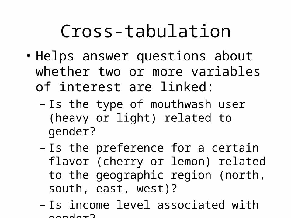
Cross-tabulation• Helps answer questions about whether two

or more variables of interest are linked:– Is the type of mouthwash user (heavy or light)

related to gender?– Is the preference for a certain flavor (cherry or

lemon) related to the geographic region (north, south, east, west)?

– Is income level associated with gender?

• Cross-tabulation determines association not causality.

• The variable being studied is called the dependent variable or response variable.

• A variable that influences the dependent variable is called independent variable.

Dependent and Independent Variables

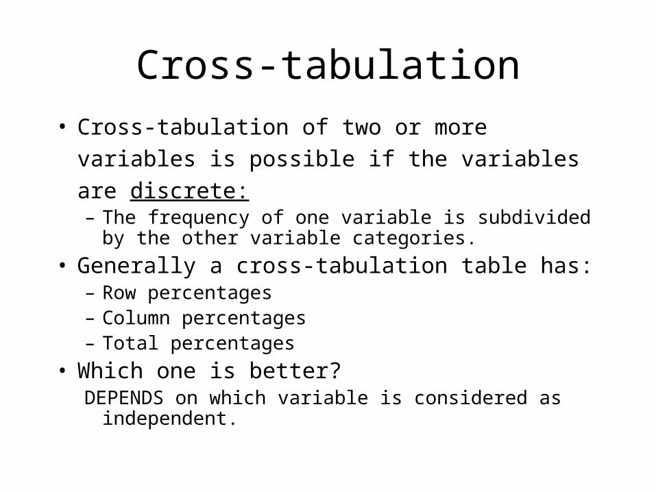
Cross-tabulation

• Cross-tabulation of two or more variables is

possible if the variables are discrete:– The frequency of one variable is subdivided by the

other variable categories.

• Generally a cross-tabulation table has:– Row percentages– Column percentages– Total percentages

• Which one is better?DEPENDS on which variable is considered as

independent.

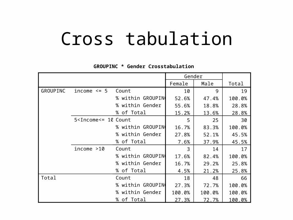
Cross tabulationGROUPINC * Gender Crosstabulation

10 9 19

52.6% 47.4% 100.0%

55.6% 18.8% 28.8%

15.2% 13.6% 28.8%

5 25 30

16.7% 83.3% 100.0%

27.8% 52.1% 45.5%

7.6% 37.9% 45.5%

3 14 17

17.6% 82.4% 100.0%

16.7% 29.2% 25.8%

4.5% 21.2% 25.8%

18 48 66

27.3% 72.7% 100.0%

100.0% 100.0% 100.0%

27.3% 72.7% 100.0%

Count

% within GROUPINC

% within Gender

% of Total

Count

% within GROUPINC

% within Gender

% of Total

Count

% within GROUPINC

% within Gender

% of Total

Count

% within GROUPINC

% within Gender

% of Total

income <= 5

5<Income<= 10

income >10

GROUPINC

Total

Female Male

Gender

Total

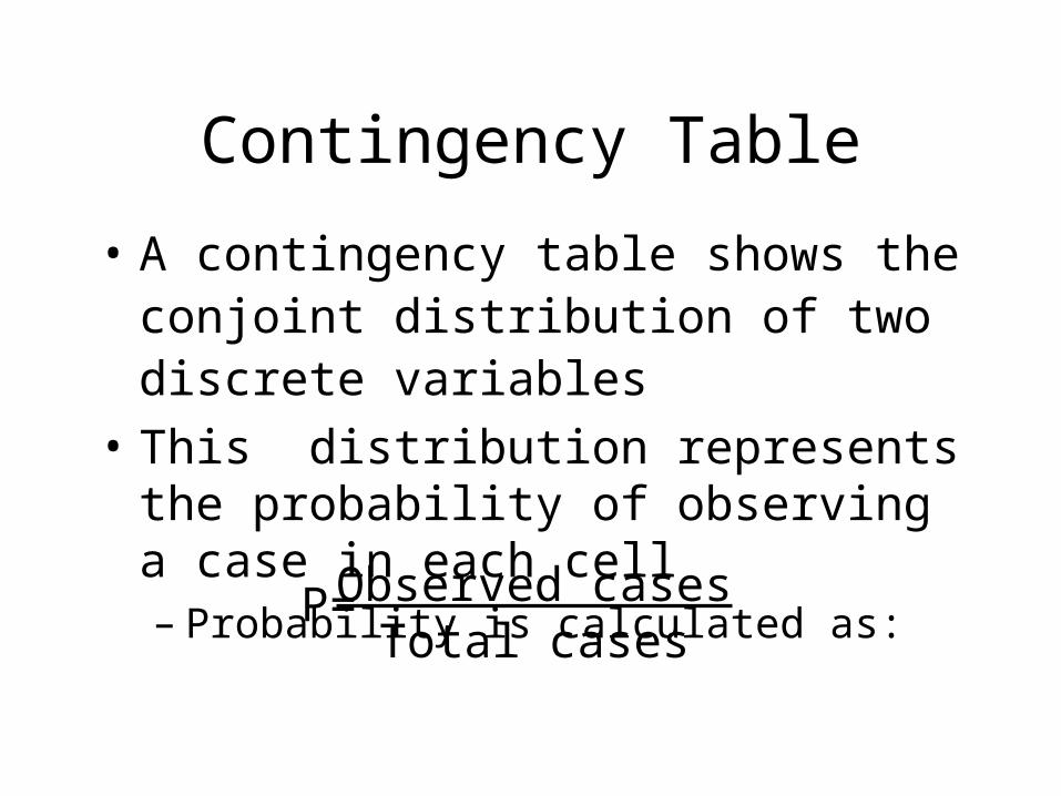
• A contingency table shows the conjoint distribution of two discrete variables

• This distribution represents the probability of observing a case in each cell– Probability is calculated as:

Contingency Table

Observed casesTotal cases

P=

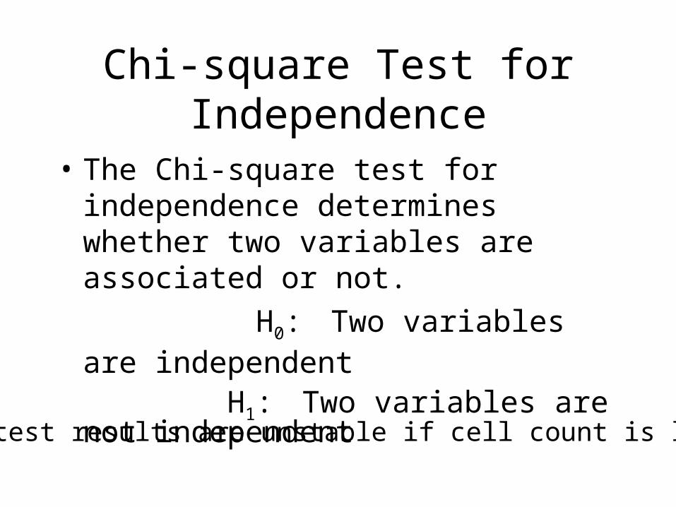
Chi-square Test for Independence

• The Chi-square test for independence determines whether two variables are associated or not.

H0: Two variables are independent

H1: Two variables are not independent

Chi-square test results are unstable if cell count is lower than 5

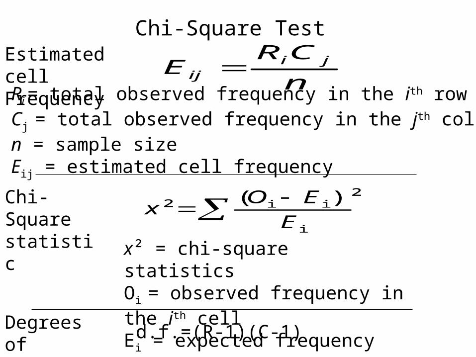
x² = chi-square statisticsOi = observed frequency in the ith cellEi = expected frequency on the ith cell

i

ii )²( ²

E

EOx

n

CRE ji

ij Ri = total observed frequency in the ith rowCj = total observed frequency in the jth columnn = sample sizeEij = estimated cell frequency

Estimated cell Frequency

Chi-Square statistic

Chi-Square Test

Degrees of Freedom

d.f.=(R-1)(C-1)

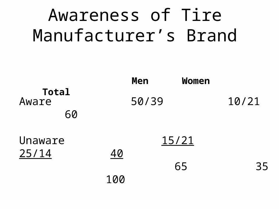
Aware 50/39 10/21 60

Unaware 15/21 25/14 40 65 35 100

Men Women Total

Awareness of Tire Manufacturer’s Brand

21

)2110(

39

)3950( 222

X

14

)1425(

26

)2615( 22

Chi-Square Test: Differences Among Groups Example

161.22

643.8654.4762.5102.32

2

1)12)(12(..

)1)(1(..

fd

CRfd

X2 with 1 d.f. at .05 critical value = 3.84

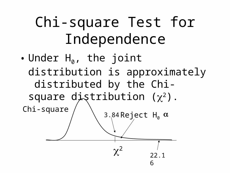
Chi-square Test for Independence

• Under H0, the joint distribution is approximately distributed by the Chi-square distribution (2).

2

Reject H0 Chi-square

3.84

22.16

Analysis of Variance

(ANOVA)

What is an ANOVA?• One-way ANOVA stands for Analysis of

Variance

• Purpose:– Extends the test for mean difference between

two independent samples to multiple samples.– Employed to analyze the effects of

manipulations (independent variables) on a random variable (dependent).

Definitions

• Dependent variable: the variable we are trying to explain, also known as response variable (Y).

• Independent variable: also known as explanatory variables (X).

Therefore, we would like to study whether the independent variable has an effect on the variability of the dependent variable

Continuous Dependent variable

One Independent Variable

Binary

t Test

One or More Independent Variable

Categorical Categorical and Continuous

Continuous

ANOVA ANCOVA Regression

One Factor More than one Factor

One-Way ANOVA N-Way

ANOVA

What does ANOVA tests?

H0 1= 2 = 3 …..= n

H1 1 2 3 ….. n

• The null hypothesis tests whether the mean of all the independent samples is equal

• The alternative hypothesis specifies that all the means are not equal

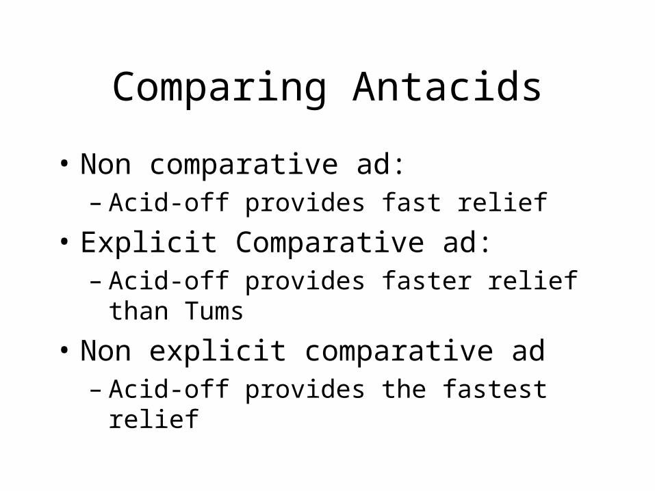
Comparing Antacids

• Non comparative ad:– Acid-off provides fast relief

• Explicit Comparative ad:– Acid-off provides faster relief than Tums

• Non explicit comparative ad– Acid-off provides the fastest relief

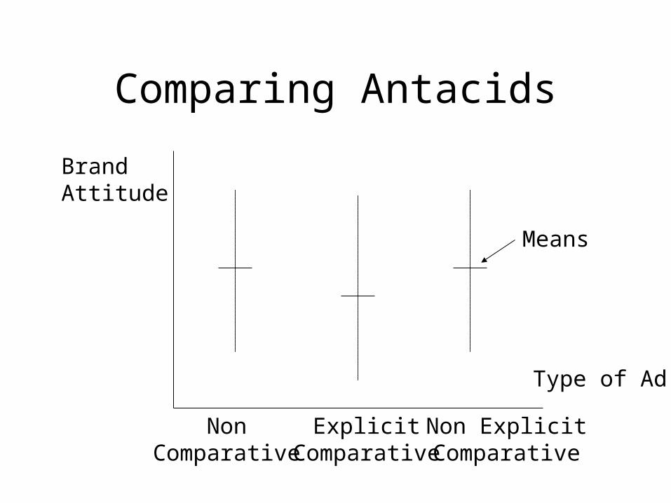
Comparing Antacids

BrandAttitude

Type of Ad

NonComparative

ExplicitComparative

Non ExplicitComparative

Means

Comparing Antacids

BrandAttitude

Type of Ad

NonComparative

ExplicitComparative

Non ExplicitComparative

Means

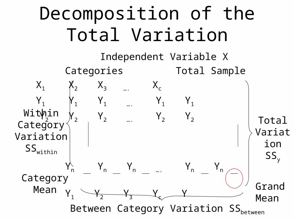
Independent Variable X

Categories Total Sample

X1 X2 X3 …. Xc

Y1 Y1 Y1 …. Y1 Y1

Y2 Y2 Y2 …. Y2 Y2

Yn Yn Yn …. Yn Yn

Y1 Y2 Y3 Yc Y

Decomposition of the Total Variation

TotalVariatio

nSSy

Between Category Variation SSbetween

CategoryMean

WithinCategoryVariation

SSwithin

GrandMean

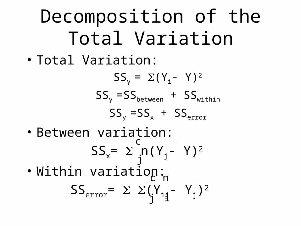
Decomposition of the Total Variation

• Total Variation:SSy = (Yi- Y)2

SSy =SSbetween + SSwithin

SSy =SSx + SSerror

• Between variation:

SSx= n(Yj- Y)2

• Within variation:

SSerror= (Yij- Yj)2

c

j

j i

c n

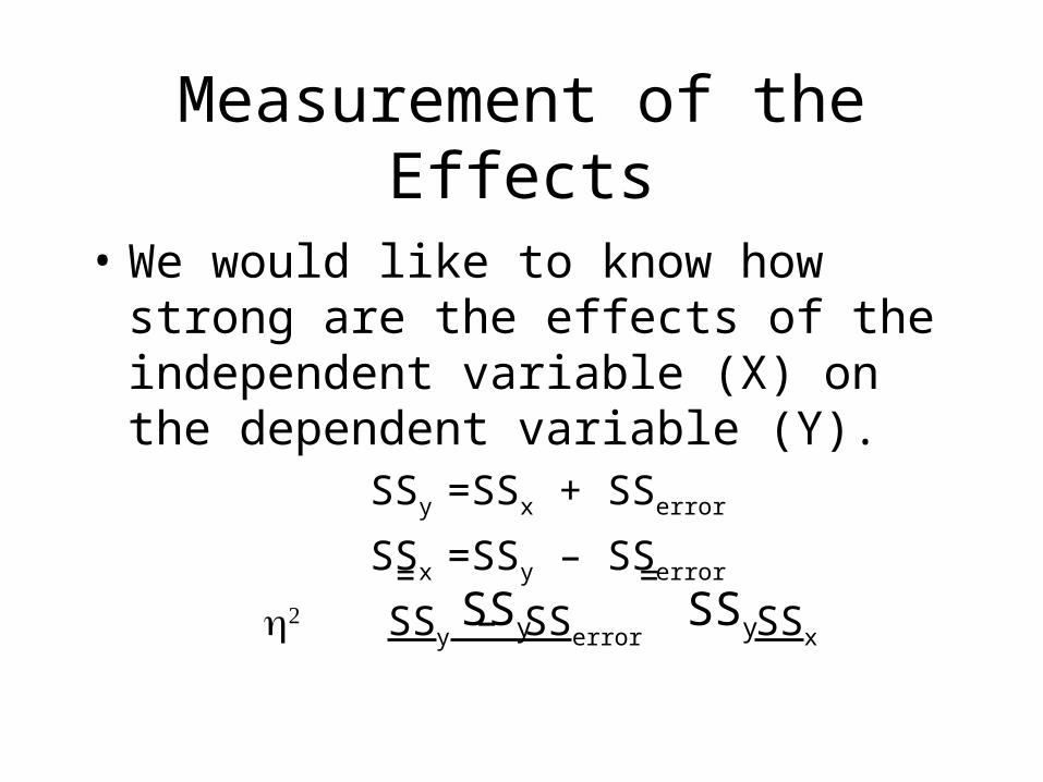
Measurement of the Effects

• We would like to know how strong are the effects of the independent variable (X) on the dependent variable (Y).

SSy =SSx + SSerror

SSx =SSy – SSerror

SSy – SSerror SSx

SSy

= = SSy

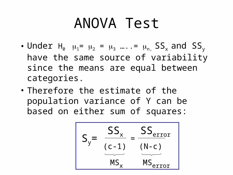
ANOVA Test

• Under H0 1= 2 = 3 …..= n, SSx and SSy have the same source of variability since the means are equal between categories.

• Therefore the estimate of the population variance of Y can be based on either sum of squares:

Sy=SSx SSerror

(c-1) (N-c)=

MSx MSerror

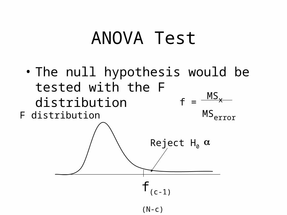
ANOVA Test

• The null hypothesis would be tested with the F distribution

f(c-1)(N-c)

Reject H0

F distributionf =

MSx

MSerror