desiccant cooling analysis simulation software, energy, cost and …325808/fulltext01.pdf ·...
TRANSCRIPT

I
Master Program in Energy Systems Examiner: Bahram Moshfegh Supervisor: Bahram Moshfegh
DEPARTMENT OF BUILDING, ENERGY AND ENVIRONMENTAL ENGINEERING
Desiccant Cooling Analysis Simulation software, energy, cost and environmental
analysis of desiccant cooling system
Juan Artieda Urrutia
June 2010
Master’s Thesis in Energy Systems

II

III
Preface
I would like to start this report by thanking all the people that made this project possible,
starting with my thesis supervisor, Bahram Moshfegh, for offering me the possibility to
conduct a research work in such an interesting field, and without whom this project
would not have been possible.
I am also very grateful to the people in the department of Energy Systems in the
University of Linköping, for their advice and constructive criticism that help me improve
my work considerably, and especially Inger-Lise Svensson for their help and assistance.
Finally, I would like to thank the University of Gävle for the help and resources provided
during the course of this project and of the Master Program.

IV

V
Summary
Desiccant cooling is a technology that, based on a open psychrometric cycle, is able to
provide cooling using heat as the main energy carrier. This technology uses a
considerably smaller amount of electricity than refrigerators based on the vapor-
compression cycle, which is an electricity driven cycle. Electricity is often more
expensive than other types of energy and has CO2 emissions associated with its
generation , so desiccant cooling has the potential of achieving both economic and
environmental benefits.
In addition to this, the heat the desiccant cooling cycle needs to work can be supplied at
relative low temperatures, so it can use heat coming from the district heating grid, from a
solar collector or even waste heat coming from industries.
The system which will be studied in this report is a desiccant cooling system based on the
model designed by the company Munters AB. The systems relies on several components:
a desiccant rotor, a rotary heat exchanger two evaporative humidifiers and two heating
coils. It is a flexible system that is able to provide cooling in summer and heat during
winter.
This study performs a deep economic and environmental analysis of the desiccant cooling
systems, comparing it with traditional vapor compression based systems:
In order to achieve this objective a user-friendly software was created, called the DCSS –
Desiccant Cooling Simulation Software – that simulates the operation of the system
during a year and performs automatically all the necessary calculations.
This study demonstrates that economic savings up to 54% percent can be achieved in the
running costs of desiccant cooling systems when compared to traditional compressor
cooling systems, and reductions up to39% in the CO2 emissions. It also demonstrates that
desiccant cooling is more appropriate in dry climate zones with low latent heat generation
gains.
In addition to that, the DSCC software created will help further studies about the physical,
economic and environmental feasibility of installing desiccant cooling systems in
different locations.

VI
Key words
Desiccant cooling, energy analysis, cost analysis, COP, CO2 emissions, waste heat, solar
energy, district heating.

VII

VIII
Contents page
1 INTRODUCTION .................................................................................................... 1
2 PURPOSE .............................................................................................................. 3
3 METHODOLOGY .................................................................................................... 5
4 DESCRIPTION OF THE SYSTEM ............................................................................... 7
4.1 COMPONENTS OF THE SYSTEM ................................................................................... 7
4.1.1 MCC DesiCool Wheel ....................................................................................... 7
4.1.2 VVX heat exchanger ...................................................................................... 10
4.1.3 Humidifiers .................................................................................................... 11
4.1.4 Heater ............................................................................................................ 11
4.2 OPERATION OF THE SYSTEM ..................................................................................... 12
4.2.1 Refrigeration Mode 1 – Direct Evaporative Cooling – ................................... 13
4.2.2 Refrigeration Mode 2 – Indirect Evaporative Cooling – ................................ 14
4.2.3 Refrigeration Mode 3 – Desiccant & Evaporative Cooling – ......................... 15
4.2.4 Heating Mode 1 – Heat recovery with MCC heat exchanger – ..................... 18
4.2.5 Heating Mode 2 – Heat recovery with MCC & VVX heat exchangers – ......... 19
4.2.6 Heating Mode 3 – Heat recovery with MCC & VVX heat exchangers & After
heating – .................................................................................................................... 20
5 DESCRIPTION OF THE PROGRAM ......................................................................... 23
5.1 PROGRAM INPUTS .................................................................................................. 24
5.2 ALGORITHM .......................................................................................................... 26
5.2.1 Level I - Psychrometrics ................................................................................. 26
5.2.2 Level II – Process Level – ................................................................................ 29
5.2.3 Level III – System Level – ................................................................................ 33
5.3 OUTPUT ............................................................................................................... 37
5.3.1 Data Outputs. ................................................................................................ 37

IX
5.3.2 Graphical Outputs: ........................................................................................ 40
6 RESULTS ............................................................................................................. 43
6.1 OVERALL PERFORMANCE OF THE SYSTEM ................................................................... 43
6.2 RESULTS OF THE SIMULATIONS ................................................................................ 45
6.2.1 Arlanda & District Heating ............................................................................ 45
6.2.2 Simulation 2: Arlanda & Waste Heat/Solar Energy ...................................... 50
6.2.3 Simulation 3 – Madrid & Natural Gas – ........................................................ 52
6.2.4 Simulation 4 – Madrid & Solar Energy/Waste Heat – .................................. 55
7 DISCUSSION ........................................................................................................ 59
8 CONCLUSIONS .................................................................................................... 63
9 REFERENCES ....................................................................................................... 65
10 APPENDIX I: DETAILED RESULTS OF THE SIMULATIONS ....................................... 69
10.1 RESULTS FOR SIMULATION 1 – ARLANDA – ................................................................ 69
10.2 RESULTS FOR SIMULATION 2 – ARLANDA & WASTE HEAT/SOLAR ENERGY – ................... 71
10.3 RESULTS FOR SIMULATION 3 – MADRID & NG – ........................................................ 72
10.4 RESULTS FOR SIMULATION 4 – MADRID & SOLAR ENERGY/ WASTE HEAT ....................... 74
11 APPENDIX II: TABLE OF SYMBOLS ....................................................................... 75
12 APPENDIX III: LIST OF M-FUNCTIONS AND DESCRIPTION..................................... 77
13 APPENDIX IV: USER’S GUIDE ............................................................................... 81
13.1 MAIN WINDOW .................................................................................................... 81
13.2 FILE MENU: .......................................................................................................... 84
13.3 INPUT MENU ......................................................................................................... 84
13.4 GRAPH MENU....................................................................................................... 85

X
List of Figures
Figure 1: Components of the DesiCool system ................................................................... 7
Figure 2:Desiccant Wheel [7] .............................................................................................. 8
Figure 3: Humidifier .......................................................................................................... 11
Figure 4. Heater ................................................................................................................. 12
Figure 5: Characteristic points of the psychrometric process............................................ 12
Figure 6: Refrigeration Mode 1 – Direct Evaporative Cooling - ...................................... 13
Figure 7: Refrigeration Mode 2 – Indirect Evaporative Cooling – ................................... 14
Figure 8: Refrigeration Mode 3 – Adsorption & Evaporative Cooling – .......................... 16
Figure 9: Heating Mode 1 – Heat recovery with MCC heat exchanger – ......................... 19
Figure 10: Heating Mode 2 – Heat recovery with MCC & VVX heat exchangers – ........ 19
Figure 11: Heating Mode 2 – Heat recovery with MCC & VVX heat exchangers –with
humidification ................................................................................................................... 20
Figure 12: 6.2.6 Heating Mode 3 – Heat recovery with MCC & VVX heat exchangers
& After heating – with humidification .............................................................................. 21
Figure 13: Schema of the inputs and outputs of the application ....................................... 23
Figure 14: Direct approach ................................................................................................ 31
Figure 15: Iterative approach ............................................................................................ 31
Figure 16: Flow chart diagram of the mode selection process .......................................... 33
Figure 17: Schema of the system used for comparing ...................................................... 39
Figure 18: Overall performance of the system for RH=30% ............................................ 44
Figure 19: Overall performance of the system for different outdoor relative humidities . 44
Figure 20: VVX and MCC dependency on the outdoor temperature and relative humidity
........................................................................................................................................... 45
Figure 21: Annual Energy Analysis for Arlanda ............................................................... 47
Figure 22: Annual Cost Analysis for Simulation 1 ........................................................... 48
Figure 23: Monthly Cost Analysis for Simualtion1 .......................................................... 49
Figure 24: CO2 emissions for Simulation 1 ....................................................................... 50

XI
Figure 25: Annual Cost analysis for Simulation 2 ............................................................ 51
Figure 26:Monthly Cost Analysis for Simulation 2 .......................................................... 51
Figure 27: Annual Energy Analysis for Madrid ............................................................... 52
Figure 28: Annual Cost Analysis for Simulation 3 ........................................................... 54
Figure 29: Monthly Cost Analysis for Simulation 3 ......................................................... 54
Figure 30: CO2 emissions for Simulation 3 ...................................................................... 55
Figure 31: Annual Cost Analysis for Simulation 4 ........................................................... 56
Figure 32: Annual Cost Analysis for Simulation 4 ........................................................... 57
Figure 33: CO2 emissions for Simulation 4 ...................................................................... 57
Figure 34: Main Window Lay-Out ................................................................................... 83
Figure 35: File menu ......................................................................................................... 84
Figure 36: Load File Dialog .............................................................................................. 84
Figure 37: Save File Dialog .............................................................................................. 84
Figure 38: Input Menu ...................................................................................................... 84
Figure 39:System parameters input dialog ....................................................................... 85
Figure 40: Cost information input dialog .......................................................................... 85
Figure 41: Simulation time input dialog ........................................................................... 85
Figure 42: Graph Menu ..................................................................................................... 85
Figure 43: Duration Diagram ............................................................................................ 86
Figure 44: Annual Energy Gaph ....................................................................................... 86
Figure 45:Monthly Energy Graph ..................................................................................... 86
Figure 46:Annual Cost Graph ........................................................................................... 86
Figure 47:Monthly Cost Graph ......................................................................................... 86
Figure 48:Efficiency Graph .............................................................................................. 86
Figure 49: Overall Performance Graph ............................................................................. 87
Figure 50:Environmental Graph ....................................................................................... 87

XII
List of tables
Table 1: Adsorbent Characteristics ..................................................................................... 9
Table 2: Case function for the Level I of code .................................................................. 27
Table 3: q-Matrix .............................................................................................................. 32
Table 4: Schema of the transfer from the A-matrix to the q-matrix .................................. 34
Table 5: Power used by the system ................................................................................... 35
Table 6: CO2 emissions associated with heat and power generation ................................. 38
Table 7: Simulation 1 inputs ............................................................................................. 46
Table 8: Annual Energy Analysis for Arlanda .................................................................. 46
Table 9: Annual Cost Analysis for Simulation 1 ............................................................... 47
Table 10: CO2 emissions for the DesiCool and compressor cooling system in Arlanda ... 49
Table 11: Annual Cost Analysis for Simulation 2 ............................................................. 50
Table 12: Annual Energy Analysis for Madrid ................................................................. 52
Table 13: Natural Gas Prices in Spain[17] ........................................................................ 53
Table 14:Annual Cost Analysis for Simulation 3 .............................................................. 53
Table 15: CO2 emissions for the DesiCool and compressor cooling system in Madrid .... 55
Table 16: Annual Cost Analysis for Simulation 4 ............................................................. 56
Table 17: Results of the simulations ................................................................................. 60
Table 18: Monthly Energy Analysis for Simulation 1 – DesiCool System ....................... 69
Table 19: Monthly Energy Analysis for Simulation 1 – Compressor cooling system ...... 69
Table 20: : Monthly Cost Analysis for Simulation 1 – DesiCool System ......................... 70
Table 21: Monthly Cost Analysis for Simulation 1 – Compressor Cooling System ......... 70
Table 22: Monthly Cost Analysis for simulation 1 – Desicool – ...................................... 71
Table 23: Monthly Cost Analysis for simulation 1 – Compressor Cooling System – ...... 71
Table 24: Monthly Energy Analysis for Simulation 3 – Desicool – ................................. 72
Table 25: Monthly Energy Analysis for Simulation 3 – Compressor Cooling System – .. 72
Table 26: Monthly Cost Analysis for Simulation 3 – Desicool – ..................................... 73

XIII
Table 27: Monthly Cost Analysis for Simulation 3 – Compressor Cooling System – ..... 73
Table 28: Monthly Cost Analysis for Simulation 4 – Desicool – ..................................... 74
Table 29: Monthly Cost Analysis for Simulation 4 – Compressor Cooling System – ..... 74
Table 30: Table of equivalences of symbols ..................................................................... 76
Table 31: List of M-functions and description ................................................................. 79
Table 32: Main window elements and description ........................................................... 82


1
1 Introduction
The need for heating and cooling in a building has been satisfied over the years in
different ways.
Traditionally, only systems based on the reverse-Rankine vapor-compression cycle have
been used to provide cooling in both residential and commercial buildings. This type of
system is characterized by the use of a great amount of electricity by its compressor.
However, electricity is a very high quality form of energy that should be used only in
electricity specific processes, since it is often more expensive than other types of energy
and has CO2 emissions associated with its generation. [1].
Many different types of systems with a lower electricity demand have been developed
lately, such as absorption systems, direct and indirect evaporative cooling systems or
cooling with chilled surfaces. The true economic and environmental potential of these
technologies comes out when they are combined with renewable energy sources, such as
solar energy. However, the range of applicability of most of this technologies is not as
wide as the traditional compressor cycles. [2]
The system studied in this thesis, is a desiccant cooling system based on a device created
by the Swedish company Munters, called DesiCool system. This device is able to provide
cool air using a considerably smaller amount of electricity, thanks to the fact that it does
not use a compressor to work. Instead of it, it cools the air in several steps, taking
advantage of an open psychrometric cycle and using heat as the main energy carrier.
The system does not need very high temperature heat to work, usually about 55ºC, so it
can come from a variety of sources, like district heating, solar energy or waste heat. This
possibility enhances even more its environmental and economical advantages.
In addition to this, the system does not use any kind of refrigerants, which usually contain
CFCs and cause environmental problems; nor dangerous absorbent substances such Li-Br.
Desiccant cooling devices are flexible systems that can also provide warm air in winter,
acting as a heat recovery system. Thanks to the two rotating heat exchangers they have,
that recovery efficiencies as high as 90% can be achieved. Another advantage is that the
supply and the exhaust air do not mix, so a 100% of fresh air is supplied to the room.
A great deal of desiccant cooling devices have been installed successfully in several
locations around the globe, leading to very remarkable savings in energy and electricity.
For instance, a DesiCool system was installed by the German supermarket chain Globus

2
in its facility in Saarlouis, southern Germany. As a result, savings of 20% were achieved,
meaning that the system has a payback period of 3 years. [3].
Another Desicool system was installed by the Swedish company Sandvik AB in Sandvik
Wernshausen's new production hall and has led to up to 45% savings in energy running
costs, which mean a total of 88,200€ per year. [4].
A good example of how DesiCool system can be combined with solar thermal energy is
the installation of a DesiCool system and solar panels in the new offices in Denmark of
the energy company named Fyn. As a result, a reduction of 60% (for cooling and
ventilation) was achieved, compared with conventional ventilation systems [5].
The environmental benefits of desiccant cooling systems has also lead to many
governmental plans designed to demonstrate their advantages. That is the case, for
example, of the five pilot rotary desiccant cooling systems, installed in Mataró (Spain),
Freiburg (Germany), Lisbon (Portugal), Hartberg (Austria), and Waalwijk (Netherlands).
which are within Task 25 on ‘‘Solar Assisted Air Conditioning of Buildings’’ of the Solar
Heating & Cooling Program of the International Energy Agency [6].
Desiccant cooling is a mature technology, which has both important economic and
environmental benefits, but which also needs further studies in order to achieve its true
potential

3
2 Purpose
The aim of this thesis is to perform a deep energy and cost analysis of desiccant cooling
systems. This analysis will include:
• A complete description of the components of the system and how they work in
the different modes of operation.
• A cost estimation of the system during a year, supposing it is installed in different
climate zones.
• A comparison between the system and other alternatives heating and cooling
devices such as compression cooling systems.
This report will estimate and quantify the amount of electricity than can be saved using
this system compared to compression cooling systems, as well as its economic and
environmental repercussions, in terms of money and kg of CO2 emissions that can be
saved.
It will also determine the most important system parameters and climate characteristics
that affect the performance of the system, which will help point out the climate zones for
which desiccant cooling systems are suitable.

4

5
3 Methodology
Desiccant cooling systems are complex devices that are able to provide the desired
conditions for the supplied air by means of several psychrometric processes that take
place in the air. The outdoor air conditions are constantly changing so, in order to
calculate the cost of the system for a whole year, a great deal of calculations are needed.
This is the reason why the only reasonable approach to the problem is to program a
software that would make all this calculations repeatedly.
A software named DSCC – Desiccant Cooling Simulation Software – was created in
order to perform the calculations mentioned above hour by hour during a whole year, and
to calculate the desired results .
In order to achieve the objectives described in the previous section, the overall project
comprised the following phases:
• Research about the system operation for all of its different modes. This phase
implies a detailed comprehension of all the psychrometric changes that take place
in each phase
• Determination of the variables, equations and parameters that will define the
problem.
• Research about the parameters that are needed to describe the system.
• Programming of the first models to simulate the system.
• Extensive validation of the model. Checking if the program works correctly for
all the temperature and other air characteristics considered. Comparison with
empirical data.
• Corrections of the previous program and revalidation.
• Running of the model for several locations.
• Analysis of the results.
.

6

7
4 Description of the system
Munters’ DesiCool is a flexible HVAC system that is able to provide both cooling in
summer and heating in winter. In order to do that, the incoming air undergoes several
phases during which its psychrometric properties, such as temperature or relative
humidity, change.
Although the way the system works during winter differs significantly from the way it
works in summer, the same components are used . In section 4.1, the components of the
system will be explained, as well as the different parameters that characterize their
performance. Section 4.14.2 will give details on how those components work together to
achieve the desired results in the different operation modes.
4.1 Components of the system
In this section, we take a closer look to the components of the system that make it
possible. The following figure, shows the most important parts of the DesiCool system.
Figure 1: Components of the DesiCool system [7]
4.1.1 MCC DesiCool Wheel
The MCC DesiCool wheel is the core of the DesiCool system. It is also known as
sorption rotor/wheel, desiccant rotor/wheel, honeycomb rotor/wheel and drying
rotor/wheel.
8
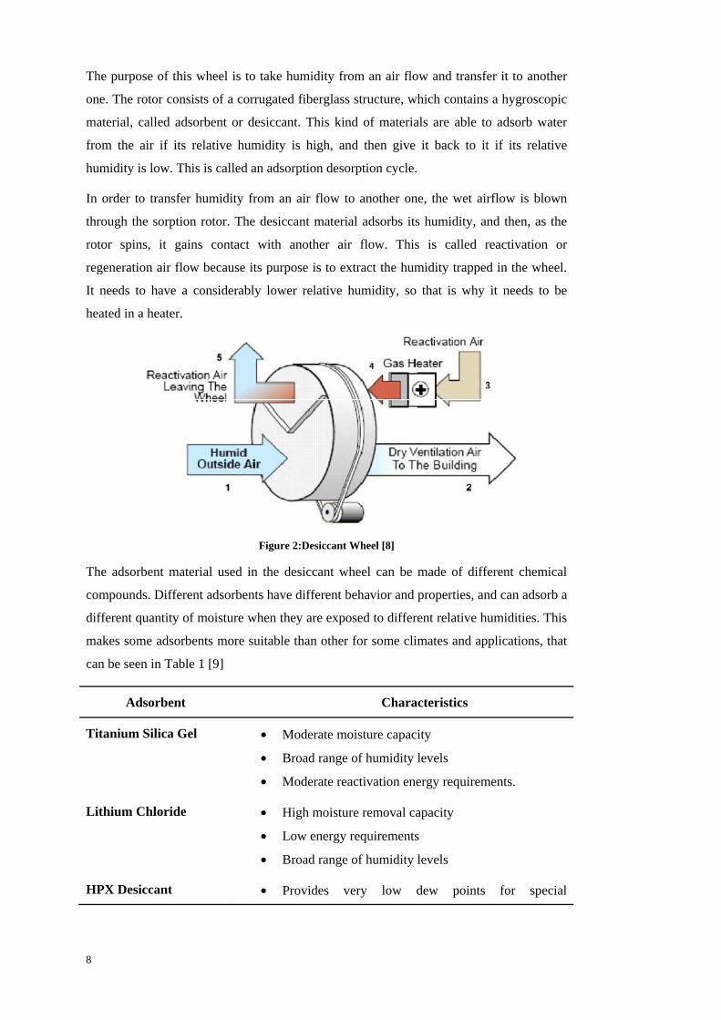
The purpose of this wheel is to take humidity from an air flow and transfer it to another
one. The rotor consists of a corrugated fiberglass structure, which contains a hygroscopic
material, called adsorbent or desiccant. This kind of materials are able to adsorb water
from the air if its relative humidity is high, and then give it back to it if its relative
humidity is low. This is called an adsorption desorption cycle.
In order to transfer humidity from an air flow to another one, the wet airflow is blown
through the sorption rotor. The desiccant material adsorbs its humidity, and then, as the
rotor spins, it gains contact with another air flow. This is called reactivation or
regeneration air flow because its purpose is to extract the humidity trapped in the wheel.
It needs to have a considerably lower relative humidity, so that is why it needs to be
heated in a heater.
Figure 2:Desiccant Wheel [8]
The adsorbent material used in the desiccant wheel can be made of different chemical
compounds. Different adsorbents have different behavior and properties, and can adsorb a
different quantity of moisture when they are exposed to different relative humidities. This
makes some adsorbents more suitable than other for some climates and applications, that
can be seen in Table 1 [9]
Adsorbent Characteristics
Titanium Silica Gel • Moderate moisture capacity
• Broad range of humidity levels
• Moderate reactivation energy requirements.
Lithium Chloride • High moisture removal capacity
• Low energy requirements
• Broad range of humidity levels
HPX Desiccant • Provides very low dew points for special

9
applications.
HCR Desiccant • Use low temperature air for reactivation. Most common for desiccant cooling
Molecular Sieve • It is able to remove moisture from very dry environments (rh<10%),
• High energy for reactivation
Table 1: Adsorbent Characteristics
The MCC wheel in the DesiCool system uses the HCR desiccant, which is an adsorbent
material patented by Munters whose main feature consists of the low regeneration
temperatures it needs to work.
The MCC wheel not only transfers humidity, but it also transfers heat from one of the air
flows to the other. Depending on its velocity, it has two different modes of operation:
Low rotation velocity
When the spinning velocity is low, (below 10 rph), the rotor acts then as a humidity
exchanger, taking humidity from one of the air flows and giving it to the other. There are
many definitions of efficiencies for the operation of a desiccant wheel, which depend on
many parameters such as the inlet temperature, the reactivation temperature, the wheel
velocity, etc.
The following efficiencies were taken in order to determine the performance of the
system, since their value is approximately constant for the studied temperature interval, as
demonstrated by Pahlavanzadeh and Mandegari [8].
• Regeneration Efficiency: expresses the relation between the amount of heat of the
water adsorbed by the wheel, and the heat needed for the regeneration. It takes
the following expression:
( 1)
where is the latent vaporization heat of water, and the specific
humidity of the air before and after the wheel, and and the enthalpy before
and after the regeneration heater.
• Adiabatic efficiency: the process that takes place in the desiccant wheel is almost
adiabatic. The deviation from the adiabatic process is characterized by the
adiabatic efficiency, which is defined as:
10
1 2 ( 2)
Where and are respectively the enthalpies of the air before and after the wheel.
High rotation velocity
When the spinning velocity is high, (above 10 rpm), a great deal of heat is also extracted
from the hot air flow and stored in the wheel as sensible heat, and then released to the
cold air flow. In this mode, both heat and moisture will be transferred from one air flow
to the other. Two parameters are needed to characterize its behavior:
• Temperature efficiency: is defined the same way as for a traditional rotational
heat exchanger:
( 3)
• Humidity efficiency: is defined in a similar way, using humidity contents instead
of temperatures:
( 4)
4.1.2 VVX heat exchanger
The VVX heat exchanger, called in the picture Thermal Wheel, is a sensible heat rotary
heat exchanger. It consists of several densely packaged aluminum sheets constantly
rotating. When the wheel rotates, the aluminum sheets gain contact with the hot air and as
a result its temperature rises. After that, as it rotates, it gains contact with the cold air flow
and releases the heat it had stored.
Rotary heat exchangers have the important advantage that they achieve very high
efficiencies without mixing the airflows, so that the contaminants in the exhaust air are
not recirculated back in.
Its most important parameter is the temperature efficiency, which is defined the same way
as for the MCC heat exchanger.
( 5)
This kind of wheel is only able to transfer sensible heat, not latent heat, meaning that
humidity is not exchanged between airflows.

11
4.1.3 Humidifiers
There are two humidifiers in the DesiCool system, one in the supply air flow and the
other in the exhaust air flow.
The purpose of the humidifier is to increase the humidity of the air and cool it down. It is
a process in which the air comes into contact with liquid water, and part of it evaporates
in the air. The heat used to evaporate this water is taken from the air, so its temperature is
reduced.
In order to do so, the humidifiers used by the DesiCool system consist of a very porous
material called pad, which is kept constantly wet with the help of a recirculation system
and a pump. The contact area between the air and the water is very big (500 m2 of contact
surface per m3 ) so very high efficiencies are achieved. [7]
Figure 3: Humidifier [7]
The main advantage of this kind of humidifiers is that they have a very high efficiency,
and there are no aerosols involved, so it does not use CFDs, which are harmful for the
environment. Another advantage is that there is no possibility for bacteria to grow and at
the same time it acts as a filter for the air, since the particles suspended in the air are
trapped in the water and drained away.
In addition to this, it is a self-cleaning and very long lasting system.
4.1.4 Heater
There are two heaters, one in the supply air flow, which acts as an after heater when the
temperature of the supply air has not reached the desired temperature, and another one in

12
the exhaust air flow, whose mission is to heat up the reactivation air so that its relative
humidity is low enough and the desiccant wheel can work properly.
Figure 4. Heater
The heater consists of a net of very small pipes filled with hot water. As the air passes
across the heater, the heat from the water is released in the air. The system can work with
relative low water temperatures, so the source of the heat can be very different, such as
district heating, solar energy or waste heat.
This kind of heaters have a very high efficiency, a low pressure drop and a long life.
4.2 Operation of the system
The DesiCool system is a flexible device that can provide both heating and cooling. The
desired supply air conditions are achieved in different ways, depending on the outdoor air
properties and the user needs.
This section will explain the different psychrometric cycles that are used. The DesiCool
system can work in six different modes, so there are six different cycles.
The cycles consist of several process, which take place in the different components of the
system, which were explained in the previous section. After each of the processes, the
psychrometric properties of the air change. In order to provide a better description of the
different cycles. Figure 5 shows where the different states are physically located in the
device.
Figure 5: Characteristic points of the psychrometric process [7]
13
4.2.1 Refrigeration Mode 1 – Direct Evaporative Cooling –
This mode of refrigeration is used when there is a need for cooling, but the outdoor air
temperature and its relative humidity is not too high.
The process is simple, water is sprayed over the incoming air in the first humidifier, so
that its temperature falls and its relative humidity increases. This is kind of process is
called evaporative cooling, and it is based on the fact that the energy content in the air can
be separated in two: sensible heat, that represents the energy in the air due to its
temperature, and latent heat, that is the energy needed to prevent the water in the air from
condensing.
During this process, when the air comes into contact with the water, heat is taken from
the air to evaporate the water. The sensible heat of the air is thus converted into latent
heat, making its temperature fall.
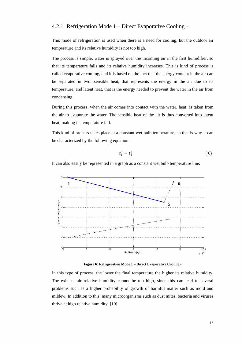
This kind of process takes place at a constant wet bulb temperature, so that is why it can
be characterized by the following equation:
( 6)
It can also easily be represented in a graph as a constant wet bulb temperature line:
Figure 6: Refrigeration Mode 1 – Direct Evaporative Cooling -
In this type of process, the lower the final temperature the higher its relative humidity.
The exhaust air relative humidity cannot be too high, since this can lead to several
problems such as a higher probability of growth of harmful matter such as mold and
mildew. In addition to this, many microorganisms such as dust mites, bacteria and viruses
thrive at high relative humidity. [10]
1
5
6

14
For this reason, there must be a maximum allowed relative humidity level, | ,
beyond which the air cannot be humidified. If the air needs to be cooled down below this
levels, another refrigerating mode should be used.
4.2.2 Refrigeration Mode 2 – Indirect Evaporative Cooling –
When direct evaporative cooling is not enough to achieve the desired conditions, the
DesiCool system switches to the Indirect Evaporative Cooling mode.
In this mode, the supply air is first cooled down in the VVX heat exchanger and then
humidified, so that its temperature falls until it reaches the target temperature. In the
VVX heat exchanger, heat is taken from the supply air flow and it is released to the
exhaust air flow. This is only possible if the temperature of the exhaust air is lower than
the temperature of the supply air. That is the reason why the exhaust air must be cooled
down in the second humidifier.
The following figure shows the process in a psychrometric diagram:
Figure 7: Refrigeration Mode 2 – Indirect Evaporative Cooling –
The vertical yellow line to the left represents the changes in the supply air that take place
in the heat exchanger. The other yellow line corresponds to the changes in the exhaust air.
In this process, there is no exchange of humidity between the two air flows, so the total
water content in the air remains constant. This leads to the following equations:
( 7)
( 8)
1=2
3
4=5
68-10
7
15
In addition to this, the energy gained by the exhaust air flow equals the energy gained by
the supply air flow, considering the heat losses to the surroundings negligible.
( 9)
Another important equation that characterizes this process is the temperature efficiency of
the heat exchanger, which is defined as:
(10)
The blue oblique lines represent both humidifiers. These are humidification adiabatic
processes that have been explained in the previous sections. During these processes, the
wet bulb temperature remains constant and can be defined by the following equations:
(11)
(12)
4.2.3 Refrigeration Mode 3 – Desiccant & Evaporative Cooling –
In order for the VVX to be able to work properly, the exhaust air temperature must be
always a few degrees below the supply air temperature. The magnitude of this
temperature difference is determined by the VVX efficiency.
For this reason, in this mode the exhaust air is also cooled down in the humidifier like in
the previous case. However, the saturation line acts as a physical limit beyond which the
air cannot be cooled. Once the saturation conditions are achieved, the moisture content of
the air cannot be increased, since the water in the air would condensate, and the air cannot
be cooled down further. The adsorption cooling mode starts when this limit is reached.
In this mode, given that the exhaust air cannot be cooled beyond saturation, the supply air
is heated instead. This way, the temperature difference between both air flow will be
enough to exchange the desired amount of heat.
The whole process can be seen in the following figure:

16
Figure 8: Refrigeration Mode 3 – Adsorption & Evaporative Cooling –
The temperature of the supply air is increased with the help of the MCC wheel. This rotor
is able to extract humidity from the supply air flow and release it to the exhaust airflow.
This is an almost adiabatic process, which is characterized by the adiabatic efficiency
explained in Section 4.1.1:
2 (13)
The total amount of moisture that will be extracted from the air will be determined by the
temperature the air has to reach in order to lose the desired amount of heat in the VVX
heat exchanger. Because of that, the efficiency of the VVX heat exchanger will have a
direct repercussion on the amount of humidity that should be extracted.
(14)
Once the air has been dehumidified, it can release heat to the exhaust airflow, in the VVX
heat exchanger. The equations that rule this process are the same as in the previous mode:
(15)
Since the air has been dehumidified, it can be easily cooled down again in the humidifier.
The air will be humidified until the desired dry-bulb temperature is achieved. This
process takes place at constant wet-bulb temperature .
(16)
1
3
4=5
6
10
7
8
9
2

17
The exhaust airflow, as in the previous mode, will be refrigerated as much as it is possible
in the humidifier:
(17)
The exhaust air flow gains now all the heat that was released by the supply air flow in the
VVX heat exchanger. It follows the equations:
(18)
(19)
After the VVX heat exchanger, the air must be heated in the reactivation heater. This is a
crucial process for the MCC heat exchanger to work properly. The MCC heat exchanger
is able to transfer moisture from one airflow to another only if the relative humidity of the
air flow from which the moisture is being extracted is considerably higher than the
relative humidity of the airflow that will receive this moisture.
In order to achieve the necessary relative humidity, the air must be heated in the so called
reactivation process. This is a heating process, during which the total moisture content of
the air remains constant, and the relative humidity falls.
(20)
The heat needed in the reactivation will be determined by the amount of humidity that
was extracted from the supply airflow in the dehumidification process, and it will depend
on the regeneration efficiency defined in section 4.1.1
(21)
Finally, the exhaust air will receive all the moisture that has been taken from the supply
air, according to the following equation:
(22)
The process will also take place in an almost adiabatic way. 2 (23)

18
4.2.4 Heating Mode 1 – Heat recovery with MCC heat exchanger –
The heating modes start when the outdoor temperature is below the desired supply
temperature. When the difference between both temperatures is not too high, it is possible
to recover all the necessary heat from the exhaust airflow using only the MCC heat
exchanger.
The process is simple and similar to any heat recovery system with a rotational heat
exchanger, but the MCC heat exchanger has the additional feature of being able to
transfer not only sensible heat, but also latent heat thanks to the hygroscopic
characteristics of the rotor.
Two important conservation equation will be followed:
On the one hand, all the energy that is given by one of the air flows will be gained by the
other one (energy conservation):
(24)
On the other hand, all the water that has been extracted from one of the air flows will be
given to the other one (mass conservation):
(25)
In addition to this equations, both the temperature and the humidity efficiencies will
characterize the process:
(26)
(27)
In the case of the MCC rotor, both efficiencies have the same value which is equal to 75%
[11]. This is the reason why the process is represented by a straight line in the figure:

19
Figure 9: Heating Mode 1 – Heat recovery with MCC heat exchanger –
4.2.5 Heating Mode 2 – Heat recovery with MCC & VVX heat
exchangers –
When the outdoor temperature is too low for the MCC rotor to provide enough heat
recovery, the VVX rotor starts working. The yellow lines in the following figure illustrate
the process carried out by the VVX:
Figure 10: Heating Mode 2 – Heat recovery with MCC & VVX heat exchangers –
The VVX heat exchanger cannot transfer humidity, so only sensible heat will be
exchanged.
(28)
In addition to this equation, the energy conservation equation and the heat exchanger
efficiency will characterize the process:
1
2-5
6-9
10
1
2
6-7
10
3-5
8-9

20
(29)
(30)
The efficiency of the VVX will be controlled and adjusted to achieve the desired supply
air conditions.
Since the outdoor air is heated in the VVX heat exchanger without any moisture transfer,
the relative humidity of the supply air decreases. If the relative humidity of the supply air
is too low, it may lead to discomfort and health problems, such as irritated skin or dry
eyes. [12]. In addition to this, other problems may occur such as shrinkage of wood floors
and furniture, cracking of paint on wood trim and static electricity discharges. [13].
Should the relative humidity of the supply air be below the minimum, | the
humidifier will work. It will humidify the air until the minimum level of relative humidity
is reached. As in the rest of humidification processes, the wet-bulb temperature is
constant:
(31)
Figure 11: Heating Mode 2 – Heat recovery with MCC & VVX heat exchangers –with humidification
4.2.6 Heating Mode 3 – Heat recovery with MCC & VVX heat
exchangers & After heating –
For very cold outdoor conditions, it is impossible to achieve the desired supply air
temperature simply by recovering heat from the exhaust air. There must be an additional
1 2
6-7
10
3
8-9
4-5

21
source of heat that raises the supply air temperature up to its target level. This process
takes place with help of a heating coil.
There is no moisture transfer during this process, so the equation 32 is followed:
(32)
As in the previous mode, the process can take place with or without humidification,
depending on the resulting exhaust air relative humidity. The after heating process is
depicted by the red line that goes from point 4 to point 5 in the following figure:
Figure 12: 6.2.6Heating Mode 3 – Heat recovery with MCC & VVX heat exchangers & After heating – with humidification
1
2
6-7
10
3
8-9
4
5

22

23
5 Description of the program
One of the most important phases in this project is the development of the software that
will help analyze the system and obtain results. The programming language that was
decided to use was Matlab, thanks to its high performance as a numerical solver.
The program main objective consists of generating several files containing information
about the energy used by the system, its costs and other relevant parameters of the
operation of the DesiCool system throughout a year. In order to be able to perform these
calculations, a file containing the climate information of a given location needs to be
provided, as well as different user defined variables such as some system parameters and
the costs.
The following figure schematizes the inputs and outputs of the program.
Figure 13: Schema of the inputs and outputs of the application
The next sections will take a closer look at the program inputs and outputs, and at how
the algorithm performs the calculations. A brief user’s guide of the program can be found
in Appendix IV.

24
5.1 Program inputs
The aim of the program is to perform an energy and a cost analysis of the DesiCool
system in different locations. Because of that, the user will have to specify certain
information about the system parameters, the cost of the different energy sources, as well
as a file containing climate information. A detailed explanation of these inputs is given
below:
Climate information file.
A file containing the hourly climate information of a given location must be supplied to
the program. It has to be a .txt file, in which the first three columns must be:
- Hour
- Outdoor temperature [ºC]
- Outdoor relative humidity [%]
Files from different locations in the world can be downloaded from
http://www.equaonline.com/iceuser/
Supply air conditions.
The temperature of the supply air will determine the cooling power of the system. The
temperature cannot be either too cold or too hot, given that it would provoke discomfort.
In addition to the temperature, the maximum, and minimum allowed relative humidity for
the supply air, | and | respectively, must be specified by the user, since too
dry or too wet air conditions can cause several problems to the building and its occupants
[12].
Room air conditions.
The room temperature and its relative humidity will depend on the Internal Heat
Generation characteristic of the building. It is determined by the user as a temperature
increase ∆ and a moisture content increase ∆ with respect to the supply air.
Cost information.
The program will calculate the cost of the system during a year, so it will need
information about the cost of the different energy sources the system uses. The following
information will be required to the user:
- Electricity price. This represents the average price in SEK per kWh of
electricity used. It should include both the amount paid per kWh to the
electricity supplier and the transmission fee per kWh paid to the grid owner.

25
- Water price: It is the price per m3 of water paid to the water supplier.
- Heat price: given that the price per kWh of heat supplied by a district heating
company is usually different in summer and winter, two different prices must
be defined. If waste heat or solar energy is used instead of district heating, the
price of heat should be 0. In case a fuel boiler is used, the heat price should
be calculated as the fuel price divided by the boiler efficiency.
- Electricity power price: the amount of power used by the DesiCool system
will affect the total need of power of the building, and therefore the power
fee paid to the grid owner. This term represents the price per kW paid to the
grid owner.
- Heat power price: the subscription fee paid to the district heating supplier
depends on the maximum heat that can be delivered to the building. This
term represents the price paid to the district heating supplier per kW of heat.
The calculation of the power fee in the district heating tariff is different for
each district heating company. In this study, the power fee is calculated as the
product of the heat power price and the average power use during the 60
hours with a highest district heating demand.
System parameters.
The parameters of the DesiCool system are fixed values, that depend on the system
characteristics and cannot be modified. However, it was decided to let the user specify the
value of the different parameters to be able to simulate the performance of desiccant
cooling systems of different manufacturers. In addition to this, this feature will allow the
user to evaluate the impact of the modification of the different parameters in the overall
performance of the system. The default values correspond to the actual values of the
DesiCool system and were asked to the system manufacturer [11] or estimated form the
empirical results..
The following parameters can be defined by the user and were explained in Section 4.1:
- VVX Maximum Temperature Efficiency, [%]
- MCC Maximum Temperature Efficiency, [%]
- MCC Maximum Humidity Efficiency, [%]
- MCC Regeneration Efficiency, [%]
- MCC Adiabatic Efficiency [%]
Simulation information.

26
The simulation does not need to be run 24 hours a day 7 days a week, since the
ventilation system might be only working during the operating hours, in offices, factories
and other non-residential buildings.
The algorithm will only compute the data between the starting hour and the end hour, and
will automatically exclude week-ends.
5.2 Algorithm
All the functions that constitute the program and that transform the inputs into the
required outputs are classified in three different levels of code:
• Level I -Psychrometrics Level. This part of the program will be able to calculate
all the psychrometric properties of a state, given two psychrometric variables. For
example, given the dry-bulb temperature and the relative humidity of a state, it
will calculate the water content, the wet-bulb temperature and the enthalpy for
that state.
• Level II - Process Level. This level will simulate the operation of the system both
in cooling and heating modes, for given outside supply and exhaust air
characteristics.
• Level III – System Level it will make the calculations in the system level for a
whole year. It will read the outdoor air characteristics for a given location during
a year, and will calculate all the parameters needed. After that, it will sum up the
results, so that it can provide a general idea of the total cost of the system during
a year.
A list of all the functions with a brief description of them and the level of code to which
they belong can be found in Appendix III.
5.2.1 Level I - Psychrometrics
All the thermodynamic properties of a given state of wet air can be determined with two
independent variables. This can be visualized with the help of the psychrometric diagram,
in which all the properties of the air can be determine knowing two different
psychrometric properties.
The aim of this level of code is to calculate all the psychrometrics properties of the air,
given two of them. The properties that are taken into account are only those which will be
needed for the accomplishment of the purpose of this thesis. This variables are:
• Dry bulb temperature [°C]

27
• Relative humidity
• Water content [kg/kg]
• Wet-bulb temperature [°C]
• Enthalpy. [kJ/kg]
• Pressure [Pa]
The input variables can be any two variables among the first five variables described
above, and the output variables will be the other three. Since there are multiple
combinations of input and output variables, several cases have been taken into account.
Each case is a function, which has two air properties as input variables and the other three
as output variables:
Name of the function Input Variables Output variables
Case_1 t, ϕ W, t*, h
Case_2 W, t* t, ϕ, h
Case_3 t, t* Φ, W, h
Case_4 W, h t, ϕ, t*
Case_5 ϕ, W t, t*, h
Case_6 t, W t*, ϕ, h
Case_7 ϕ, t* t, W, h
Table 2: Case function for the Level I of code
Another important property of the moist air is its total pressure, p. Although a total
pressure drop of around 250 Pa [11] takes place in the system, it can be ignored when
calculating the thermodynamic properties given that its influence in the results of the
calculations is minimal. This is why the pressure, p, has been considered a global variable
common to all the different working states.
The relationship between all these variables is defined by a set of equations described in
the ASHRAE Handbook of Fundamentals [14]. To illustrate the process of calculating the
different properties, below it is explained how the wet bulb temperature, the relative
humidity and the enthalpy are calculated when the dry-bulb temperature and the moisture
content are known (Case_6). The rest of the cases work in a similar way, using the same
set of equations, but in a different order and with other independent variables.
The first variable that is calculated is the relative humidity. The relative humidity is
defined as the relation between the partial pressure of water vapor in moist air, ,and
the pressure of saturated pure water, :

28
, (33)
Both properties must be calculated before. The pressure of saturated pure water, , is a
function of the absolute dry-bulb temperature, T, given by the following empirical
formula:
For a temperature range -100ºC<t<0ºC, the saturation pressure over ice is:
5.674 5359 03 6.392 524 7 00 9.677 843 0 – 03 6.221 570 1 07 2.074 782 5 09 9.484 024 0 13 4.163 501 9 00
(34)
The saturation pressure over liquid water, for a temperature range of 0ºC<t<200ºC
5.800 220 6 03 1.391 499 3 00 4.864 023 9 02 4.176 476 8 05 1.445 209 3 08 6.545 967 3 00
(35)
On the other hand the partial pressure of water vapor in moist air, , is a function of the
humidity ratio of moist air (also called water content), W, and the total pressure, p. The
value of can be worked out from the following equation:

29
0.621 945 (36)
The relation between W, t and t* is given by the following equations:
If t<0ºC 2830 0.24 1.0062830 1.86 2.1 (37)
If t>0ºC 2501 2.326 1.0062501 1.86 4.186 (38)
Where is the humidity ratio at saturation at thermodynamic wet-bulb temperature,
and can be calculated using instead of in equation 36. In order to work out the
value of t*, the numerical solver fsolve implemented in Matlab was used.
The only remaining property that must be calculated is the enthalpy of the moist air. It is
easily calculated as a function of the temperature and the humidity ratio as described
below:
1.006 2501 1.86 (39)
5.2.2 Level II – Process Level –
This level of code is in charge of calculating all the relevant properties of every state of
the whole process. In order to accomplish that purpose, this level of code takes advantage
of the system equations which were explain in Section 6.2.The set of process equations,
as it was explained before, differs from one mode of operation to another. Because of that,
there is a different function for each of the modes.
Although the steps followed by each of the functions are different, there is a common
approach to all of them. Generally speaking, all the process level functions work the
following way:
• Two input psychrometric variables of one or several points are read by the
program.
• The Level-I of code calculates the other three remaining variables.
• The system equations take these values and calculate two psychrometric
properties of another point.
• The process is repeated until all the points have been computed.

30
It can be easily understood taking the Cooling Mode 2 as an example:
• First, the program reads the T and the relative humidity of the outdoor (Point 1)
and supply air (Point 5)
• The Level-I of code is called to calculate the W, t* and h of these points.
• In this case, the MCC rotor and the after heater are not working so Point 1 =
Point 2 and Point 4=Point 5.
• In the VVX heat exchanger there is no exchange of humidity so: . This
is one of the system equations. In the humidifier the wet bulb temperature is
constant so .
• Now that two psychrometric properties are known for the point 3, and , the
Level I of code can be called again to determine the rest of the properties.
Cooling mode 2 can be solved directly, meaning that the equations can be solved one
after the other, and the different states can be determined without taking any assumption
or without needing to solve a system of equation. This also happens for cooling mode 1
and heating mode 1.
However, cooling mode 3, and heating modes 2 and 3 are defined by a system of
equations that cannot be solved directly, since the psychrometric properties of the
different states are mutually dependent. In order to solve these equations, an iterative
approach using the Matlab built-in numerical solver fsolve was used.
The iterative approach works the following way:
• First, the psychrometric properties of the states that are well defined are
determined (Point 1, Point 5 and Point 6)
• Since it is impossible to determine the rest of the states with this information,
point 2 properties are given random values.
• The rest of the points can now be determined using this information
• Once all the psychrometric properties of all the states are known, Point 2 is
recalculated using the remaining equations. An error variable is calculated as the
difference between the assumed value for Point 2 and the calculated value.
• This process is repeated using the numerical solver fsolve, until the error is
smaller than the tolerance defined.
The iterative method used for cooling mode 3 and heating modes 2 and 3 is defined by a
function which has the same name as the mode function, preceded by the word iterate.
For example, for cooling_mode3, the iterative solver is called iterate_cooling_mode3,
and it is a subfunction that belongs to the same M-file as cooling_mode3.
31
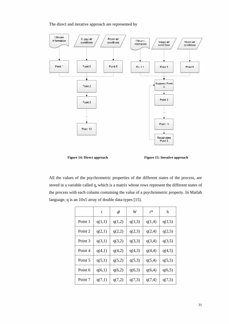
The direct and iterative approach are represented by
Figure 14: Direct approach
Figure 15: Iterative approach
All the values of the psychrometric properties of the different states of the process, are
stored in a variable called q, which is a matrix whose rows represent the different states of
the process with each column containing the value of a psychrometric property. In Matlab
language, q is an 10x5 array of double data-types [15].
t ϕ W t* h
Point 1 q(1,1) q(1,2) q(1,3) q(1,4) q(1,5)
Point 2 q(2,1) q(2,2) q(2,3) q(2,4) q(2,5)
Point 3 q(3,1) q(3,2) q(3,3) q(3,4) q(3,5)
Point 4 q(4,1) q(4,2) q(4,3) q(4,4) q(4,5)
Point 5 q(5,1) q(5,2) q(5,3) q(5,4) q(5,5)
Point 6 q(6,1) q(6,2) q(6,3) q(6,4) q(6,5)
Point 7 q(7,1) q(7,2) q(7,3) q(7,4) q(7,5)

32
Point 8 q(8,1) q(8,2) q(8,3) q(8,4) q(8,5)
Point 9 q(9,1) q(9,2) q(9,3) q(9,4) q(9,5)
Point 10 q(10,1) q(10,2) q(10,3) q(10,4) q(10,5)
Table 3: q-Matrix
Level II of code is also in charge of changing from one operating mode to another. Figure
16 illustrates the flow diagram of the process:
First, the outdoor temperature, is compared with the supply air temperature, , to
determine if the outdoor air needs to be heated or cooled.
1. If the air needs to be heated, the algorithm will start with heating mode 1. After
all the states have been determined, the program will calculate the efficiency of
the MCC wheel that is needed to achieve these states. If the efficiency turns out
to be higher than the maximum possible MCC efficiency introduced by the user,
the program will switch to mode 2. If it is not, the next level of code starts
working.
2. After heating mode 2 has been executed, the VVX efficiency is also compared to
the maximum VVX efficiency. If it is higher, the next mode will start. It may also
happen that condensation occurs in the heat exchanger; in that case, the next
heating mode will also start.
3. Then, heating mode 3 starts. After it has determined the properties of all the
states of the process, Level III of code is in charge of storing the results and
jumping to the next operating hour.
If, on the contrary, the air needs to be refrigerated, the algorithm will start with cooling
mode 1.
1. The properties of the supply air will be calculated as if the desired supply air
temperature could be reached simply by humidification. If the relative humidity
of the supply air temperature turns out to be higher than the maximum relative
humidity for the supply air flow entered by the user, cooling mode 2 will start.
2. After all the states have been determined by mode 2, the VVX efficiency will be
computed. If it is higher than the maximum, mode 3 will start. The program also
checks if the humidifier is asked to dehumidify the air flow, which is physically
impossible. This might happen because the maximum relative humidity is higher
than the relative humidity achieved for point 3. In case this happens, mode 3 will
also start.

33
3. If cooling mode 3 is called, it will calculate the properties of all the states and the
next level of code will be executed.
Figure 16: Flow chart diagram of the mode selection process
5.2.3 Level III – System Level –
Given all the information produced by the previous level of code, this level performs the
necessary calculations to obtain interesting data about the process, such as the heat or the
water needed, or the overall coefficient of performance, COP.
Once all these values have been calculated for each operating hour throughout a year, the
program will consolidate the results in to monthly or yearly information, that will be
useful for the technicians that will evaluate the potential savings of installing the
DesiCool system in a certain location.
All the data will be stored in a global variable called A, a matrix in which each row
contains the relevant information of each hour of the year. The algorithm will not
compute and skip the data concerning non-operating hours, so these rows will be filled

34
with zeros. The A-matrix will contain as many rows as hours in the year, approximately
8700, and as may columns as relevant information that will be collected,66.
Below it is explained the information that is stored in each column of the matrix and how
it is calculated:
Column 1: Hour
Contains information about the hour of the simulation, starting with 0 on 1st January 2000
at 00:00 am.
Column 2: Date
Contains information about the date and hour of the simulation. The data is stored in the
form of Matlab numerical representations of dates, which is a decimal number which
Matlab is able to interpret as a date. The date is calculated by adding the number of hours
to the base date, which is 1st January 2000 at 00:00 am.
Columns 3 to 52 : Psychrometric properties
The data stored in the q-matrix is now transferred to the A-matrix. Since all the
information contained by the q-matrix deals with the same hour, they must be stored only
in one row of the A-matrix.
Col 3 Col 4 Col 5 Col 6 Col 7 Col 8 Col 9 … … Col 52
… …
Table 4: Schema of the transfer from the A-matrix to the q-matrix
Column 53: Heat provided in the after heating process [kW]
In heating mode 3, the air needs to be heated after it has recovered all the possible heat
from the exhaust air. The total heat can be calculated as the mass flow by the temperature
difference.
(40)
Column 54: Heat provided in the reactivation process [kW]
During the desiccant cooling mode, the exhaust air needs to be reactivated, in other words,
it needs to be heated so that its relative humidity decreases. It is calculated in a similar
way to the previous case.
(41)

35
Column 55: Water provided to the supplied air [m3/h]
The water supplied to the incoming air by the humidifier is calculated as the mass flow by
the water content difference. The result, which would be in kg/s, must be multiplied by
3600 and divided by the density of water to obtain the value in m3/h.
3600 / (42)
Column 56: Water provided to the exhaust air [m3/h]
Similar to the previous case, this time for the second humidifier.
3600 / (43)
Column 57: Heat power
The power of the total heating coils that are present in the DesiCool system is equal to
400 kW.
Column 58: Electricity used
In order to be able to calculate the exact amount of electricity that is being used at each
moment, it would be necessary to do extensive calculations including the pressure drop
that takes place in each of the components, which depends, for example on the velocity of
the heat exchangers.
As a simplification, the average power used by the system is calculated as the 65% of the
maximum power of the DesiCool system, supplied by the manufacturer. This percentage
was estimated based on empiric data about the performance of the DesiCool system.
Air Flow [m3/s] Power
Supply Air Fan [kW]
Power Exhaust Air Fan [kW]
Total Power [kW]
Avg Power [kW]
2.2 4 4 8 5,2 2.9 5,5 5,5 11 7,15 3.6 5,5 7,5 13 8,45 4.8 7,5 11 18,5 12 5.2 7,5 11 18,5 12 6.3 11 11 22 14,3 8.0 11 15 26 16,9
10.0 15 18,5 33,5 21,8
Table 5: Power used by the system
Column 59: Cooling Power.

36
The cooling capacity is defined as the amount of heat that is taken from the room. It will
be equal to the difference between the amount of heat that leaves the room with the
exhaust air flow, and the amount of heat that it is provided to the room with the supply air
flow.
Δ 1.2 (44)
Column 60: Cost of heat
The cost of the heat actually used by the system is simply calculated as the multiplication
of the cost per kWh of district heating by the total amount of heat used by the process,
including both reactivation and after heating:
For winter hours:
_ (45)
For summer hours:
_ (46)
Column 61: Cost of water
The cost of the water is calculated multiplying the cost per m3 of water by the total
amount of water used by both humidifiers:
(47)
Column 62: Cost of electricity
It is determined as the cost per kWh by the amount of electricity, in kWh, consumed each
hour.
(48)
Column 63: VVX efficiency
The VVX efficiency is a global value that has been calculated by the Level II of code,
and it is stored now in the 63rd position.
Column 64: MCC efficiency
It is also a global variable calculated by the previous level of code, stored in the 64th
position.
Column 65: COPheat

37
The Coefficient of Performance, COP, is defined as the supplied output divided by the
required input. In this case, the supplied output will be the amount of heat removed from
the room, which has been calculated in Column 59. As it uses two type of energy carriers,
heat and electricity, two different COPs can be calculated. The COP in terms of heat
considers the required input as the total amount of heat supplied to the system:
| 5954 (49)
It must be pointed out that, most of the operating modes do not require any heat, since in
the refrigerating modes 1 and 2 the cooling effect is obtained through evaporative cooling
and does not require any heat. In these cases, the COP will have an infinite value. When
the results are exported from Matlab to Excel, Excel automatically converts this infinite
value to the maximum possible integer in simple precision. The COP is only defined in
the refrigerating modes.
Column 66: COPelectricity
The COP can be calculated considering the electricity as the required input. In that case,
the following formula will be applied:
| 5958 (50)
5.3 Output
Once the simulation has finished, the program will generate several reports and graphical
outputs, that will provide useful information about the performance of the system.
5.3.1 Data Outputs.
The program will generate an excel file when the simulation is finished and the user
presses the button save. This file will contain three different sheets:
• General: this sheet reflects all the information contained in the A-matrix. It
consists of an extensive collection of data for all the hours of the simulation.
• Energy Analysis: it adds up all the hourly data about the energy use and
calculates the total for each month. After that, it adds up again the results for each
month and calculates the total for the year.

38
It will create a table with the months in each column and the following
information in the rows:
o Heat used for after heating [kWh/year]
o Heat used for regeneration [kWh/year]
o Use of electricity [kWh/year]
• Costs Analysis: like in the previous case, it calculates the total cost of each of the
different resources used by the system in a monthly basis. All the results are in
SEK or in the currency used in the cost input window. These resources are:
o Heat Cost [SEK/year]
o Water Cost [SEK/year]
o Electricity Cost [SEK/year]
o Heat Power Cost [SEK/year]
o Electricity Power Cost [SEK/year]
o Maintenance Cost [SEK/year]
• Environmental Analysis: this sheet contains information about the CO2 emissions
associated with the operation of the system throughout a year. Since the system
uses two different type of energy carriers, heat and electricity, the following table
was used to account for their emissions.
CO2 emissions associated with electricity generation
Swedish electricity mix 10 kg/MWh
Nordic electricity mix 58/kg/MWh
Using coal condensing as marginal source 890 kg/MWh
CO2 emissions associated with heat generation
Waste Heat/Solar Heat 0 kg/MWh
District heating (Swedish Mix) 11 kg/MWh
Natural Gas 230kg/MWh
Table 6: CO2 emissions associated with heat and power generation
There are two different approaches to account for the CO2 emissions that can be
saved. Using the Swedish electricity mix to calculate the CO2 savings, it
represents that the electricity that has been saved, has been generated using the
same percentage of each of the different energy sources used for electricity
generation in Sweden (mostly nuclear and hydropower). The Nordic electricity
mix represents a similar concept but for the average of the Scandinavian

39
countries. However, most countries, including the Nordic countries, use coal
condensing plants as a marginal source, meaning that it is the last energy source
that it is used in order to meet the demand. For that reason, lowering the demand
– reducing the electricity use – would directly reduce the amount of energy
generated by coal condensing plants. As a result, the savings in CO2 emissions
can be accounted as if all the electricity was generated using coal condensing
plants. [1]
The CO2 emissions associated with the use of heat depend on how the heat has
been generated. If the heat comes from a renewable source, such as solar or waste
energy, the CO2 emission associated with it will be obviously zero. If the heat is
provided by district heating, its emissions will depend on how that heat has been
generated. In this study, it has been calculated using the Swedish district heating
mix, with has a value of 11 kg CO2/MWh heat. As most of the heat distributed in
Sweden by district heating grids is generated in biomass plants, the amount of
CO2 absorbed by the trees and other plants used as biofuel during its life is
equivalent to the CO2 released when they are burnt, so the emissions are quite
low.
If the heat is generated by a natural gas burner, the amount of emission per kWh
of heat provided is: 230kg/MWh [16].
Comparison with a compressor cooling system
In addition to the results for the desiccant cooling system, the program calculates the
same information for a compressor cooling system. The system considered has the same
components as the DesiCool system, with the only difference that cooling is provided by
a cooling coil, belonging to a compressor cooling system.
Figure 17: Schema of the system used for comparing
The calculations of the energy and cost for this system are performed the following way:
40
• Heating Mode: the energy and cost are the same as for the DesiCool system,
since both systems work in the same way.
• Cooling Mode: this system is based on a compressor cooling system, so there is
no need for reactivation heat. Instead of it, the electricity used by the compressor
should be included. It is calculated as the sensible heat cooled down, divided by
the COP of the system.
1.006 (51)
The COP for compression cooling system varies between 2-3 and in this study a
COP value of 3 has been used.
The total electricity used by the whole system is simply calculated as the addition
of the electricity used by the compressor and the one needed to drive the fans.
(52)
It is important to bear in mind that most of the HVAC with rotational heat exchangers
only have one, which transfers sensible heat, instead of two, like the DesiCool system.
The results for this kind of system can be easily obtained by setting the efficiency of the
MCC to zero and repeating the simulation.
5.3.2 Graphical Outputs:
The program can generate the following type of graphs:
Duration diagram:
The diagram shows the outdoor temperature sorted in ascending order, and other relevant
temperatures of intermediate states of the process also sorted according to this order.
The purpose of this diagram is to illustrate how the temperature changes in different
states of the process, as well as to represent the amount of energy that each of the
component of process provides or recovers. The energy is proportional to the area
between lines.
Energy Graphs:
The information calculated in the Energy Analysis sheet is displayed in two different
graphs: a pie graph showing the annual analysis and a bar graph showing the monthly
analysis
Cost Graphs:

41
It generates the same graphs as in the previous case, but concerning the Cost Analysis.
Efficiency Graphs:
The efficiency of the VVX heat exchanger and of the MCC rotor constantly changes and
adapts itself to supply the amount of heat necessary. In addition to this, the heat for
regeneration and after heating also changes, depending on several parameters, such as the
outdoor temperature and relative humidity, the supply temperature and the internal heat
generation of sensible and latent heat.
In order to illustrate how the system works, two different graphs are plotted:
• VVX and MCC efficiencies graph:
For a given supply temperature and internal heat generation, the efficiency of the
VVX and MCC wheels will only depend on the outdoor temperature and relative
humidity. Two three-dimensional graphs are plotted, where the efficiencies are in the
z-axis, and the outdoor temperature and relative humidity on the xy plane.
This graphs are created using the Matlab function surf, which creates a surface
interpolating the data from the simulation.
• Over-all performance graph:
This graph represents the normalized values of the VVX efficiency, the MCC
efficiency, the after heating heat and the reactivation heat, for different relative
humidities, varying from 10% to 90%.
This is calculated as a cut of both previous graphs by a vertical plane of constant
relative humidity. Its aim is to show the performance of the system for all outdoor
temperatures, for a fixed outdoor relative humidity.
Environmental graph
It consists of a bar graph, representing the total amount of CO2 emissions for both the
desiccant cooling system and the compressor cooling system. The amount of
emissions represented has been calculated considering that the electricity has been
generated in coal condensing plants and that the heat comes from a renewable source.

42

43
6 Results
In this section, several simulations have been conducted in different locations in order to
determine the possible profitability of the system, using different heat sources such as
district heating and solar energy.
In addition to that, the system was run for all the possible combinations of temperature
and relative humidity for the outdoor air. This way, the overall performance of the system
was determined for all possible types of climates. These results will help point out the
climates for which this kind of system is suitable and economically feasible.
6.1 Overall performance of the system
In order to determine the overall performance of the system and to validate the
mathematical model created, the model was run for all the possible combinations of
outdoor temperature and relative humidity.
A virtual climate file was created, containing all the possible combinations of temperature
and relative humidity, with an outdoor temperature range going from -30ºC to 40 ºC and a
relative humidity range going from 0 to 100%.
The supply temperature was chosen to be 15ºC, with a maximum relative humidity of 80%
and a minimum of 20%. The ∆ and ∆ were respectively 7ºC and 0.2 g/kg.
Figure 18 shows how the efficiencies of the MCC and VVX and the after heating and
regeneration heat vary with the outdoor temperature for a fixed relative humidity of 30%.
They are normalized values, meaning that they have been divided by its maximum.
It can be seen how the different modes of operation of the system and in which
temperature intervals they occur.

44
Figure 18: Overall performance of the system for RH=30%
The performance of the system has also a strong dependence on the outdoor relative
humidity. Figure 19 contains the same information as Figure 18, but for different relative
humidities varying from 10% to 90%. It shows how the different modes start operating at
different outdoor temperatures, depending on the outdoor relative humidity.
Figure 19: Overall performance of the system for different outdoor relative humidities
The dependence of the performance of the system on the outdoor temperature and relative
humidity is also illustrated in Figure 20, where the efficiencies of the VVX and MCC are

45
plotted in three-dimensional graphs. It can be easily seen that, the higher the relative
humidity, the sooner both heat exchangers start working to provide desiccant cooling.
Figure 20: VVX and MCC dependency on the outdoor temperature and relative humidity
6.2 Results of the Simulations
Once the model was validated and its performance was deeply analyzed, several
simulations were conducted in order to quantify the potential savings of installing the
system in different locations.
Two different locations were chosen, Arlanda (Sweden) and Madrid (Spain), which were
considered as representative of the northern and southern European climates respectively.
6.2.1 Arlanda & District Heating
Table 7 shows the inputs that were introduced in the program. It should be noted that two
different supply air temperatures and sensible heat gain, ∆ , were introduced for summer
and winter conditions. This was done in order to model the higher internal heat
generation that takes place in summer, mainly due to a higher solar irradiation. The latent
heat gain, on the other hand is set to constant value.

46
The system with which the desiccant system was compared was similar to the one
described in Section 7.3, with the only difference of having just one sensible heat
exchanger.
Supply Air Conditions System Parameters
Supply Air T :Jan-Mar & Nov-Dec:
18ºC VVX Efficiency: 75%
Supply Air T :Apr-Oct: 15ºC MCC Temperature Efficiency: 65%
Supply Air Max Rel. Hum: 80% MCC Humidity efficiency: 65%
Supply Air Min. Rel Hum: 20% Regeneration Efficiency: 35%
Adiabatic Efficiency: 95%
Sensible & Latent Heat Generation Costs ∆ Jan-Mar & Nov-Dec: 4ºC Electricity cost [SEK/kWh]: 1 ∆ Apr-Oct: 7ºC Tap water price [SEK/m3] 16 ∆ 0.2 g/kg Heat Cost Winter (Jan-Mar & Nov-Dec) [SEK/kWh]:
0.7
Air flow 10 m3/s Heat Cost Summer (Apr-Oct) [SEK/kWh]:
0.3
Simulation time 8-20 Electricity Power Price [SEK/kW]: 400
Heat Power Price [SEK/kW] 400
Table 7: Simulation 1 inputs
After the simulation had finished, the results showed in Table 8 were obtained, which can
be graphically seen in Figure 21:
DESICOOL SYSTEM COMPRESSOR COOLING SYSTEM
Heat after heating [kWh/year] 4700 32100 Heat regeneration [kWh/year] 67500 0 Electricity [kWh/year] 68200 90700
Total [kWh/year] 140400 122800
Table 8: Annual Energy Analysis for Arlanda

47
The total amount of energy used by the DesiCool System is 140,400 kWh/year and
122,800 kWh for the compressor cooling system. Although the amount of energy used by
the desiccant cooling system is higher, the following differences should be noticed:
• The amount of electricity used by the desiccant cooling system is considerably
smaller than the amount of electricity used by the compressor cooling system.
This is due to electricity used to drive the compressor.
• The DesiCool system uses a considerable smaller amount of heat in the after
heating, 4700 kWh vs. 32100 kWh used by the traditional system, as a result of
having one extra heat exchanger (MCC wheel)
Figure 21: Annual Energy Analysis for Arlanda
A cost analysis was also performed with the help of the software created. The cost data
used for all the different sources can be found in Table 7, and the results of analysis in
Table 9 and Figure 22.
DESICOOL SYSTEM
COMPRESSOR COOLING SYSTEM
Heat Cost [SEK/year] 25300 22500 Water Cost [SEK/year] 1600 200 Electricity Cost [SEK/year] 68200 82100 Heat Power Cost [SEK/year] 11400 34100 Electricity Power Cost [SEK/year] 8700 20100 Maintenance Cost [SEK/year] 13000 41000
Total [SEK/year] 128200 200000
Table 9: Annual Cost Analysis for Simulation 1
0
20000
40000
60000
80000
100000
120000
140000
160000
DESICOOL SYSTEM COMPRESSOR COOLING SYSTEM
kWh
Annual Energy Analysis
Electricity [kW]
Heat regeneration [kW]

48
Figure 22: Annual Cost Analysis for Simulation 1
Whereas the compressor cooling system has a total operative cost of 200,000 SEK per
year, the DesiCool system has a cost of 128,200 SEK. The total saving is 71,800 SEK per
year, which represents a 36% of the total cost.
It should be noted that:
• Although the total amount of heat used by the DesiCool system is higher than the
one used by the compressor cooling system, as seen in Table 8, the total cost for
heat is very similar. This is due to the fact that most of the heat used by the
DesiCool system is employed for the regeneration process in summer, when the
district heating prices are lower; whereas the heat used by the traditional system
is used in the after heating process in winter, when district heating prices are
higher.
• The lower electricity use of the DesiCool system leads to type of savings: lower
cost of the actual electricity used and also lower cost of the power fee paid to the
distribution company, since the average and the peak power of the compressor
cooling system is also higher.
• The maintenance cost of the DesiCool system is also smaller, given that the
compressor of the traditional systems has a lower life cycle.
Figure 23 shows the cost of the DesiCool system (bars) and of the compressor system
(area) in a monthly basis. It can be seen that the cost of the DesiCool system is smaller
than the one of the compressor system for every month, even in July, when the need for
regeneration heat is higher.
0
50000
100000
150000
200000
250000
DESICOOL SYSTEM COMPRESSOR COOLING SYSTEM
SEK
Annual Cost Analysis
Maintenance Cost
Electricity Power Cost
Heat Power Cost
Electricity Cost
Water Cost
Heat Cost
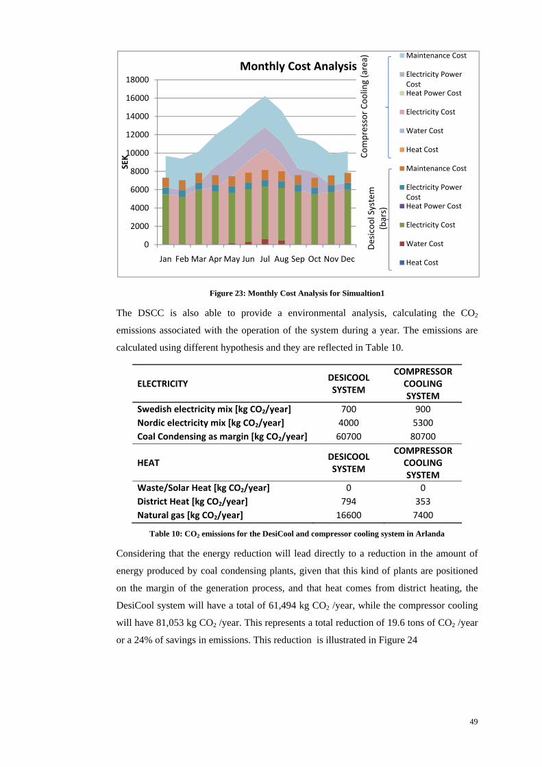
49
Figure 23: Monthly Cost Analysis for Simualtion1
The DSCC is also able to provide a environmental analysis, calculating the CO2
emissions associated with the operation of the system during a year. The emissions are
calculated using different hypothesis and they are reflected in Table 10.
ELECTRICITY DESICOOL SYSTEM
COMPRESSOR COOLING SYSTEM
Swedish electricity mix [kg CO2/year] 700 900 Nordic electricity mix [kg CO2/year] 4000 5300 Coal Condensing as margin [kg CO2/year] 60700 80700
HEAT DESICOOL SYSTEM
COMPRESSOR COOLING SYSTEM
Waste/Solar Heat [kg CO2/year] 0 0 District Heat [kg CO2/year] 794 353 Natural gas [kg CO2/year] 16600 7400
Table 10: CO2 emissions for the DesiCool and compressor cooling system in Arlanda
Considering that the energy reduction will lead directly to a reduction in the amount of
energy produced by coal condensing plants, given that this kind of plants are positioned
on the margin of the generation process, and that heat comes from district heating, the
DesiCool system will have a total of 61,494 kg CO2 /year, while the compressor cooling
will have 81,053 kg CO2 /year. This represents a total reduction of 19.6 tons of CO2 /year
or a 24% of savings in emissions. This reduction is illustrated in Figure 24
0
2000
4000
6000
8000
10000
12000
14000
16000
18000
Jan Feb Mar Apr May Jun Jul Aug Sep Oct Nov Dec
SEK
Monthly Cost AnalysisMaintenance Cost
Electricity Power CostHeat Power Cost
Electricity Cost
Water Cost
Heat Cost
Maintenance Cost
Electricity Power CostHeat Power Cost
Electricity Cost
Water Cost
Heat Cost
Des
icoo
lSys
tem
(b
ars)
Com
pres
sor
Cool
ing
(are
a)
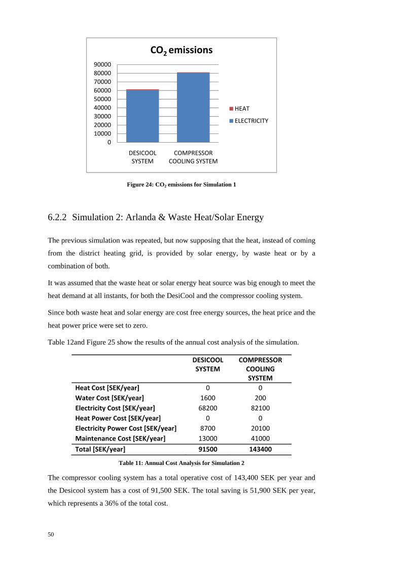
50
Figure 24: CO2 emissions for Simulation 1
6.2.2 Simulation 2: Arlanda & Waste Heat/Solar Energy
The previous simulation was repeated, but now supposing that the heat, instead of coming
from the district heating grid, is provided by solar energy, by waste heat or by a
combination of both.
It was assumed that the waste heat or solar energy heat source was big enough to meet the
heat demand at all instants, for both the DesiCool and the compressor cooling system.
Since both waste heat and solar energy are cost free energy sources, the heat price and the
heat power price were set to zero.
Table 12and Figure 25 show the results of the annual cost analysis of the simulation.
DESICOOL SYSTEM
COMPRESSOR COOLING SYSTEM
Heat Cost [SEK/year] 0 0 Water Cost [SEK/year] 1600 200 Electricity Cost [SEK/year] 68200 82100 Heat Power Cost [SEK/year] 0 0 Electricity Power Cost [SEK/year] 8700 20100 Maintenance Cost [SEK/year] 13000 41000
Total [SEK/year] 91500 143400
Table 11: Annual Cost Analysis for Simulation 2
The compressor cooling system has a total operative cost of 143,400 SEK per year and
the Desicool system has a cost of 91,500 SEK. The total saving is 51,900 SEK per year,
which represents a 36% of the total cost.
0100002000030000400005000060000700008000090000
DESICOOL SYSTEM
COMPRESSOR COOLING SYSTEM
CO2 emissions
HEAT
ELECTRICITY

51
Figure 25: Annual Cost analysis for Simulation 2
Given that there is no cost for heat, the savings come from the reduced use of electricity,
as well as the lower maintenance cost. Figure 26 shows how most of the savings take
place in summer, where the electricity used by the compressor system increases.
Figure 26:Monthly Cost Analysis for Simulation 2
The results of the environmental analysis can be seen in Table 10, in the previous case.
However, in this case, since the heat comes from a renewable energy source, it has no
emissions associated with it, being the total emissions for the DesiCool system 60,700 kg
CO2/year, and for the compressor system 80,700 kg CO2/year. This represents a reduction
of 20 tons of CO2/year, which is a 25% reduction of the total emissions.
0
20000
40000
60000
80000
100000
120000
140000
160000
DESICOOL SYSTEM COMPRESSOR COOLING SYSTEM
SEK
Annual Cost Analysis
Maintenance Cost
Electricity Power CostHeat Power Cost
Electricity Cost
Water Cost
0
2000
4000
6000
8000
10000
12000
14000
16000
18000
Jan Feb Mar Apr May Jun Jul Aug Sep Oct Nov Dec
SEK
Monthly Cost Analysis Maintenance Cost
Electricity Power CostHeat Power Cost
Electricity Cost
Water Cost
Heat Cost
Maintenance Cost
Electricity Power CostHeat Power Cost
Electricity Cost
Water Cost
Com
pres
sor
Cool
ing
(are
a)
Des
icoo
lSys
tem
(b
ars)
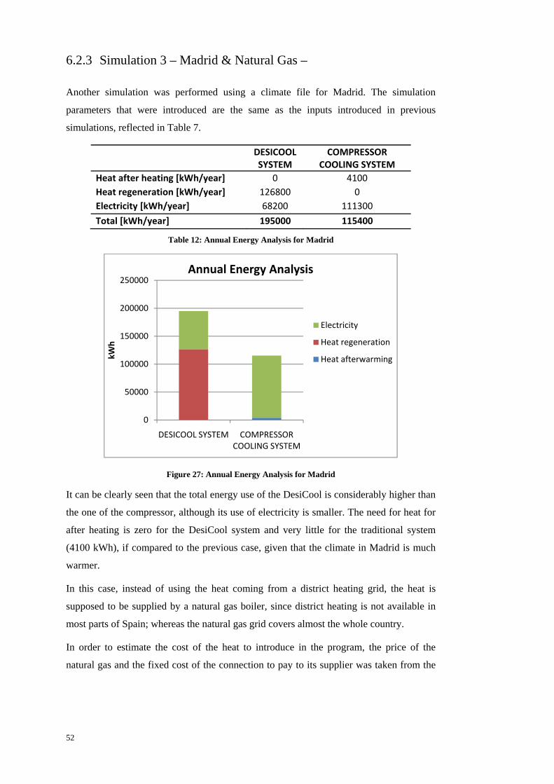
52
6.2.3 Simulation 3 – Madrid & Natural Gas –
Another simulation was performed using a climate file for Madrid. The simulation
parameters that were introduced are the same as the inputs introduced in previous
simulations, reflected in Table 7.
DESICOOL SYSTEM
COMPRESSOR COOLING SYSTEM
Heat after heating [kWh/year] 0 4100 Heat regeneration [kWh/year] 126800 0 Electricity [kWh/year] 68200 111300
Total [kWh/year] 195000 115400
Table 12: Annual Energy Analysis for Madrid
Figure 27: Annual Energy Analysis for Madrid
It can be clearly seen that the total energy use of the DesiCool is considerably higher than
the one of the compressor, although its use of electricity is smaller. The need for heat for
after heating is zero for the DesiCool system and very little for the traditional system
(4100 kWh), if compared to the previous case, given that the climate in Madrid is much
warmer.
In this case, instead of using the heat coming from a district heating grid, the heat is
supposed to be supplied by a natural gas boiler, since district heating is not available in
most parts of Spain; whereas the natural gas grid covers almost the whole country.
In order to estimate the cost of the heat to introduce in the program, the price of the
natural gas and the fixed cost of the connection to pay to its supplier was taken from the
0
50000
100000
150000
200000
250000
DESICOOL SYSTEM COMPRESSOR COOLING SYSTEM
kWh
Annual Energy Analysis
Electricity
Heat regeneration
Heat afterwarming

53
most important NG end-costumer supplier company in Spain –Gas Natural Fenosa – . An
extract of its tariff is shown in Table 13.
Tariff Name Energy Use [kWh/year]
Fixed Cost [€/month] Variable Cost [€/kWh]
Básica <5000 3,90 0,04444219
Supra >100000 66,48 0,038596
Table 13: Natural Gas Prices in Spain [17]
Once the price per kWh of gas is known, the price of the heat is calculated as the price
per kWh of gas divided by the boiler efficiency. It has been taken a standard efficiency
for a NG boiler of 90% [18].
A conversion rate of 1€=10 SEK was used to convert the prices to SEK in order to
facilitate the comparison. A price of . . 0.49 / was used for the
Compressor System and a price of . . 0.43 / for the DesiCool system. The
price for the gas for the compressor system is higher than the one for DesiCool, given that
the gas company has a cheaper tariff for bigger costumers, i.e. with higher gas
consumption.
The results can be seen in Table 14 and in Figure 28.
DESICOOL SYSTEM
COMPRESSOR COOLING SYSTEM
Heat Cost [SEK/year] 77000 2000 Water Cost [SEK/year] 4400 0 Electricity Cost [SEK/year] 68200 124200 Heat Power Cost [SEK/year] 8000 500 Electricity Power Cost [SEK/year] 8700 39400 Maintenance Cost [SEK/year] 13000 41000
Total [SEK/year] 179300 207100
Table 14:Annual Cost Analysis for Simulation 3
The total operational annual cost is equal to 179,300 SEK for the DesiCool system and
207,100 SEK for the vapor compression system. Which means a total saving of 25,600
SEK per year, and a relative reduction of 13%. This reduction is considerably smaller
than in the previous cases, mainly due to a higher price for heat.

54
Figure 28: Annual Cost Analysis for Simulation 3
The monthly cost analysis can be seen in Figure 29. It should be noticed that, during
August, which is the hottest month, the price of the DesiCool system is higher than the
price for the compressor based system. This is due to the fact that the high outdoor
temperatures require very high regeneration temperatures, and thus a great deal of heat.
Figure 29: Monthly Cost Analysis for Simulation 3
As for the environmental analysis, Table 15 shows the CO2 emissions associated with the
operation of the desiccant cooling system and a standard compressor cooling system
throughout a year.
0
50000
100000
150000
200000
250000
DESICOOL SYSTEM COMPRESSOR COOLING SYSTEM
SEK
Annual Cost Analysis
Maintenance Cost
Electricity Power CostHeat Power Cost
Electricity Cost
Water Cost
0
5000
10000
15000
20000
25000
30000
35000
40000
Jan Feb Mar Apr May Jun Jul Aug Sep Oct Nov Dec
SEK
Monthly Cost AnalysisMaintenance CostElectricity Power CostHeat Power Cost
Electricity Cost
Water Cost
Heat Cost
Maintenance Cost
Com
pres
soD
esic
ool
Syst
em
(bar
s)

55
ELECTRICITY DESICOOL SYSTEM
COMPRESSOR COOLING SYSTEM
Swedish electricity mix [kg CO2/year] 680 1110 Nordic electricity mix [kg CO2/year] 3960 6450 Coal Condensing as margin [kg CO2/year] 60700 99020 HEAT DESICOOL
SYSTEM COMPRESSOR
COOLING SYSTEM Waste\Solar Heat [kg CO2/year] 0 0 District Heat [kg CO2/year] 1399 45 Natural gas [kg CO2/year] 29160 940
Table 15: CO2 emissions for the DesiCool and compressor cooling system in Madrid
Considering that coal condensing is used on the margin of the electricity generation and,
that heat is generated in a natural gas furnace, the total emissions for the DesiCool system
will be 89,860 kg CO2/year and for the compressor cooling system 99,960 kg CO2/year.
The total reduction per year will be 10,100 kg CO2 which represents a 10%.
Figure 30: CO2 emissions for Simulation 3
6.2.4 Simulation 4 – Madrid & Solar Energy/Waste Heat –
This simulation has as aim to determine the potential benefits of the DesiCool system in
Madrid, supposing the heat comes from a solar energy or waste heat source. It was
assumed that the waste heat energy or the solar energy can meet the demands of heat in
the regeneration process. This assumption should be verified for each company, since it
depends on the characteristics and amount of the waste heat generated by them; or in the
solar radiation and characteristics of the installation.
0
20000
40000
60000
80000
100000
120000
DESICOOL SYSTEM
COMPRESSOR COOLING SYSTEM
CO2 emissions
HEAT
ELECTRICITY

56
The price for heat was therefore set to zero, and the results can be seen in Table 16 and
Figure 29.
DESICOOL SYSTEM
COMPRESSOR COOLING SYSTEM
Heat Cost [SEK/year] 0 0
Water Cost [SEK/year] 4400 0 Electricity Cost [SEK/year] 68200 124000 Heat Power Cost [SEK/year] 0 0 Electricity Power Cost [SEK/year] 8700 39400 Maintenance Cost [SEK/year] 13000 41000
Total [SEK/year] 94300 204400
Table 16: Annual Cost Analysis for Simulation 4
The total annual saving in this case is 110,100 SEK/year, which is approximately a 54%
of the total energy used.
Figure 31: Annual Cost Analysis for Simulation 4
Figure 32 shows how most part of the savings take place during the summer months,
when the outdoor temperature is higher and the electricity used by the compressor system
is higher.
0
50000
100000
150000
200000
250000
DESICOOL SYSTEM COMPRESSOR COOLING SYSTEM
SEK
Annual Cost Analysis
Maintenance Cost
Electricity Power Cost
Heat Power Cost
Electricity Cost
Water Cost
Heat Cost

57
Figure 32: Annual Cost Analysis for Simulation 4
As for the environmental analysis, the results are the same as in the previous simulation
and they can be seen in Table 15. However, this time the heat comes from solar energy or
waste heat, and it has therefore no emissions associated with its generation. Figure 33
shows the potential CO2 reduction.
Figure 33: CO2 emissions for Simulation 4
The DesiCool system emits 60,700 kg CO2 /year while the traditional system
approximately 99,020 kg CO2 /year. The use of the DesiCool system leads thus to a
reduction of 38,320 kg CO2 /year which means a 39% reduction of the CO2 emissions.
0
5000
10000
15000
20000
25000
30000
Jan Feb Mar Apr May Jun Jul Aug Sep Oct Nov Dec
SEK
Monthly Cost AnalysisMaintenance CostElectricity Power CostHeat Power Cost
Electricity Cost
Water Cost
Heat Cost
Maintenance Cost
Com
pres
soD
esic
ool
Syst
em
(bar
s)
0
20000
40000
60000
80000
100000
120000
DESICOOL SYSTEM
COMPRESSOR COOLING SYSTEM
CO2 emissions
HEAT
ELECTRICITY

58

59
7 Discussion
The main objective of this thesis was the development of an hourly-based simulation
software that would help describe the performance and quantify the potential savings of a
desiccant cooling system in different locations around the world. This objective has been
achieved with the creation of the Desiccant Cooling Simulation Software – DCSS –, a
Matlab software able to perform the calculations mentioned above.
One of the most important features of the DCSS is that it uses an hourly-based approach.
Unlike other simulation approaches, that only perform the simulation for a typical day in
winter and a typical day in summer, such as the model used by Halliday, Beggs and Sleig
[19], the DCSS performs all the calculations for every operating hour in the year. The
main advantage of this approach it that it allows to take into account all the different
operating modes of the system, and have a more realistic estimation of the costs and of
the performance of the system.
Another characteristic of the DCSS is that it has been programmed so that it uses the
minimum regeneration temperature needed for each case. The regeneration temperature is
calculated as the lowest amount needed to obtain the desired level of dehumidification.
This approach is different to the one used by other authors, such as Wurtz, Maalouf, Mora,
& Allard, [20], that consider a constant regeneration temperature. The use of a varying
regeneration temperature allows a better estimation of the minimal costs of the system.
The DCSS approach also differs from the one taken by Camargo, Godoy, & Ebinuma in
the design of the simulation software for desiccant cooling systems SYSREAD [21]. In
this software, the regeneration temperatures are known and will determine the supply air
conditions, unlike in the DCSS system, in which the user decides the supply air
conditions and the regeneration characteristics will be automatically calculated.
The performance of the Desiccant Cooling Simulation Software – DCSS – has been
validated against the empirical data provided by the system manufacturer [22]. The
system performance illustrated in Figure 18 perfectly matches the performance diagram
provided by the manufacturer.
In addition to this, the cost analysis performed for the system in Arlanda, in Simulation 1
obtains very similar results to the study performed by the company [22].
It can be seen that, for all the simulations that were carried out, the DesiCool system
grants important savings in both economic and environmental terms, as reflected in Table
17.

60
Simulation Location Energy Source Percentage Savings
CO2 reduction
1 Arlanda District Heating 36% 24%
2 Arlanda Solar/Waste Energy 36% 25%
3 Madrid Natural Gas 13% 10%
4 Madrid Solar/Waste Energy 54% 39%
Table 17: Results of the simulations
The savings achieved by the use of the DesiCool system come from different sources:
• In heating mode:
The use of the MCC wheel as heat exchanger, allows to save a great deal of after heating
energy since, in combination with the VVX wheel, the system achieves an overall
regeneration efficiency above 90%.
In addition to this, as it also transfers humidity from one air flow to the other, the need of
humidification of the supply airflow when the outdoor temperatures are very low is
considerably reduced.
This feature is particularly important in cold climates, such as in northern Europe, where
the heat used in the after heating process represents a considerable amount of the energy
budget.
• In cooling mode:
The lower price of heat than of electricity is the main advantage that desiccant cooling
has over the traditional systems. Simulation 3, where natural gas is used to provide heat
to the system in Madrid, has shown that a higher price for heat makes the system less
attractive when compared to a traditional systems, obtaining only a 13% of savings.
Simulations 1 and 2, as well as the analysis of the overall performance of the system have
shown that the heat needed for regeneration is smaller in climates with not too high
outdoor temperatures and not too big latent heat gains, such as the climate in Scandinavia.
This is one of the reasons why this system is quite spread in Scandinavia, as stated by
Mavroudaki, P. [23]

61
In dry climates, the temperature range in which the direct and indirect evaporative
cooling modes operate is wider, as demonstrated in Figure 19 and Figure 20, meaning
that, since there is no use of heat at all, the cost will be considerably smaller. In addition
to this, the latent heat gains in this type of climates tend to be smaller, so the heat needed
for regeneration will also be smaller.
This facts corroborates early studies such as the study performed by Smith, Hwang, &
Dougall, in which the feasabiliy of dessicant cooling systems in the US was analysed.
The study concluded that desiccant cooling was specially appropiate in climates with low
heat gains, such as New Mexico [24]. Another study carried out a similar analysis for
southern European climates, and also concluded that the system was appropriate for
locations with low latent heat gains, such as Madrid or Lisbon, whereas places with very
big latent heat gains, especially in the Mediterranean coast line, were not so appropriate
[23] .
It can be seen as well that the lowest operating costs are achieved when the system uses a
cost-free source of heat, such as solar energy or waste heat. In this study, it has been
assumed that the amount of heat as well as its temperature is sufficient to satisfy the
demand of heat by the system at all times. However, it should be pointed out that specific
studies should be carried out for each building and location, since it may happen that in
some moments the need for heat exceeds the available heat.
The information contained in the sheet “General” of the Excel output can be used to
determine the amount of heat needed and compare it with the quantity of heat available .It
can also be used to determine the size of the solar collectors needed to meet the heat
demand at any time, or to determine if an additional source of heat, such a natural gas
furnace, is needed as back-up.
It is clear from the results of the simulations that desiccant cooling is a technology with
great economic and environmental potential benefits, which are even bigger when this
technology is combined with solar energy and waste heat.

62
63
8 Conclusions
The creation of a software that simulates the performance of a desiccant cooling system
has been developed successfully. The following conclusions can be extracted:
1. The mathematical model and the results it withdraws have been compared and
validated with the empirical data, supplied by the manufacturer, about the
performance of the system.
2. The software uses an hourly-based approach, which provides a better estimation
of the performance of the system and which adapts better to the characteristics of
the climates of different locations than other software.
3. The program also performs time dependent energy and cost calculations, which
will facilitate the evaluation of the potential of the system in different buildings
and locations.
4. The graphical outputs allow to easily interpret the data and withdraw conclusions.
The simulations performed in different locations have lead also to the following
conclusions about the potential of desiccant cooling technologies:
5. The system studied gives to substantial savings when compared to traditional
HVAC systems, both in winter and in summer.
6. The maximum possible savings are achieved when the system is combined with
solar energy or waste energy; although the combination with district heating also
leads to important budget reductions.
7. Desiccant cooling technology is especially well suited for dry climates and
buildings with low latent heat gains.
During the creation of the software, some simplifications were taken and some
interesting development paths were discovered, such as the ones described below:
8. The DCSS simulates the performance of the desiccant wheel considering its
efficiency remains constant. Although this simplification leads to good results,
the possible combination of the DCSS software with software that simulates the
behavior of different desiccant wheels, usually provided by desiccant wheel
manufacturers, would lead to a better estimation of the results. In addition to this,
it would help determine the applicability of different desiccant wheels and
adsorptive materials in different climates.
9. The DCSS software allows the user to manually introduce the sensible and the
latent heat gain for the building. A good expansion of the software in a further

64
development face would consist of making it compatible with building simulation
software such as IDA. This feature would make easier for the user to perform
simulations in different buildings, without the need of having to determine the
latent and sensible heat gains for each period and having to manually introduce it.

65
9 References
[1] Louise Trygg and Björn G. Karlsson, "Industrial DSM in a deregulated European
electricity market—a case study of 11 plants in Sweden," Energy Policy, vol. 33, no.
11, pp. 1445-1459, July 2005.
[2] G.A. Florides, S.A. Tassou, S.A. Kalogirou, and L.C. Wrobel, "Review of solar and
low energy cooling technologies for buildings," Renewable and Sustainable Energy
Reviews, no. 6, pp. 557–572, 2002.
[3] Munters AB. (2008, November) Supermarket saves 20% energy with DesiCool.
[Online]. http://www.munters.se/sv/se/nyheter/Division-Avfuktning/E-
news/November-08/3/
[4] Munters AB. (2009, August) Sandvik Wernshausen is saving 45% on energy using
DesiCool instead ofconventional air conditioning. [Online].
http://www.muntersglobal.com/upload/Case%20studies/Sandvik%20Wernshausen%
20r1.pdf
[5] Nicolai Østergaard. (2009, April) Solar thermal cooling office. [Online].
http://www.munters.se/sv/se/nyheter/Division-Avfuktning/E-news/April-2009/4/
[6] D. La, Y.J. Dai, Y. Li, R.Z. Wang, and T.S. Ge, "Technical development of rotary
desiccant dehumidification and air conditioning: A Review," Renewable and
Sustainable Energy Reviews, vol. 14, pp. 130–147, 2010.
[7] Anne Marie Lenning. (2009, September) Ventilationskursurs. [Online].
http://www.energitjenesten.dk/files/resource_11/Downloads/091008%20Ventilation
skursus/091008_Ventilationskursus%20Energitjenesten_Anne%20Marie%20Lennin
g_DesiCool.pdf
[8] H. Pahlavanzadeh and M. Ali Mandegari, "Introduction of a new definition for
effectiveness of desiccant wheels," Energy, vol. 34, no. 6, pp. 797-803, June 2009.
[9] Munters AB. Dehumidification Units and Systems. Company Brochure. [Online].
http://www.munters.us/upload/Case%20studies/Dehumidification%20Units%20and
%20Systems.pdf
66
[10] Faye C. McQuiston, Jerald D. Parker, and Jeffrey D. Spitler, Heating, Ventilating,
and Air Conditioning. Analysis and Design., 6th ed.: Wiley.
[11] Personnel of Dehumidification Divsion at Munters. (2010, April) Information asked
through e-mail.
[12] M. Maroni, B. Seifert, and T. Lindvall, Indoor Air Quality. Amsterdam: Air Quality
Monographs, 1995.
[13] Joseph Lstiburek, "Systems engineer approach to development of advanced
residential buildings," in Healthy Indoor Environments, Austin (Texas), 2002.
[14] ASHRAE, "Psychometrics," in ASHRAE Handbook of Fundamentals. Atlanta, 2009,
pp. 1.1 -1.16.
[15] Stephen J Chapman, Matlab programming for engineers. Independence, KY:
Thomson, 2004.
[16] Association Française du Gaz. Le gaz naturel - Une energie essentielle pour
atteindre le Facteur 4. [Online].
http://www.afgaz.fr/upload/banque/plaquette_afg_gaz_naturel_et_CO2.pdf
[17] Gas Natural - Fenosa. (2010) Natural Gas Tariff brochure. [Online].
http://portal.gasnatural.com/servlet/ContentServer?gnpage=1-71-
1¢ralassetname=1-71-1-1-0-0-0
[18] Lennox. (2010) GWB9-IH Boiler Brochure. [Online].
http://www.lennox.com/products/boilers/GWB9-IH/#
[19] S. P. Halliday, C. B. Beggs, and P. A. Sleigh., "The use of solar desiccant cooling in
the UK: a feasibility study," Applied Thermal Engineering, vol. 22, pp. 1327–1338,
2002.
[20] Etienne Wurtz, Chadi Maalouf, Laurent Mora, and Francis Allard, "Parametric of a
solar desiccant cooling system using the SIMSPARK environment," in Building
Simulation 2005 Ninth International IBPSA Conference, Montréal, 2005, pp. 1369-
1376.

67
[21] J. R. Camargo, Jr. E. Godoy, and C. D. Ebinuma, "An evaporative and desiccant
cooling system for air conditioning in humid climates," Journal of the Brazilian
Society of Mechanical, pp. 1678-5878, 2005.
[22] Munters, DesiCool - information.
[23] P. Mavroudaki, C.B. Beggs, P.A. Sleigh, and S.P. Halliday, "The potential for solar
powered single-stage desiccant cooling in southern Europe," Applied Thermal
Engineering, vol. 22, pp. 1129-1140, 2002.
[24] R.R. Smith, C.C. Hwang, and R.S. Dougall, "Modelling of a solar-assisted desiccant
air conditioner for a residential building," Energy, no. 19 (6), pp. 679-691, 1994.

68
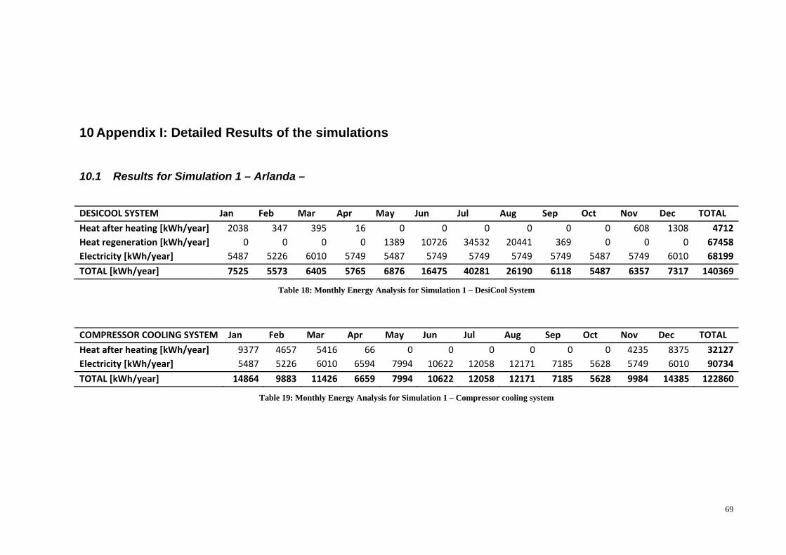
69
10 Appendix I: Detailed Results of the simulations
10.1 Results for Simulation 1 – Arlanda –
DESICOOL SYSTEM Jan Feb Mar Apr May Jun Jul Aug Sep Oct Nov Dec TOTAL
Heat after heating [kWh/year] 2038 347 395 16 0 0 0 0 0 0 608 1308 4712 Heat regeneration [kWh/year] 0 0 0 0 1389 10726 34532 20441 369 0 0 0 67458 Electricity [kWh/year] 5487 5226 6010 5749 5487 5749 5749 5749 5749 5487 5749 6010 68199
TOTAL [kWh/year] 7525 5573 6405 5765 6876 16475 40281 26190 6118 5487 6357 7317 140369
Table 18: Monthly Energy Analysis for Simulation 1 – DesiCool System
COMPRESSOR COOLING SYSTEM Jan Feb Mar Apr May Jun Jul Aug Sep Oct Nov Dec TOTAL
Heat after heating [kWh/year] 9377 4657 5416 66 0 0 0 0 0 0 4235 8375 32127 Electricity [kWh/year] 5487 5226 6010 6594 7994 10622 12058 12171 7185 5628 5749 6010 90734
TOTAL [kWh/year] 14864 9883 11426 6659 7994 10622 12058 12171 7185 5628 9984 14385 122860
Table 19: Monthly Energy Analysis for Simulation 1 – Compressor cooling system
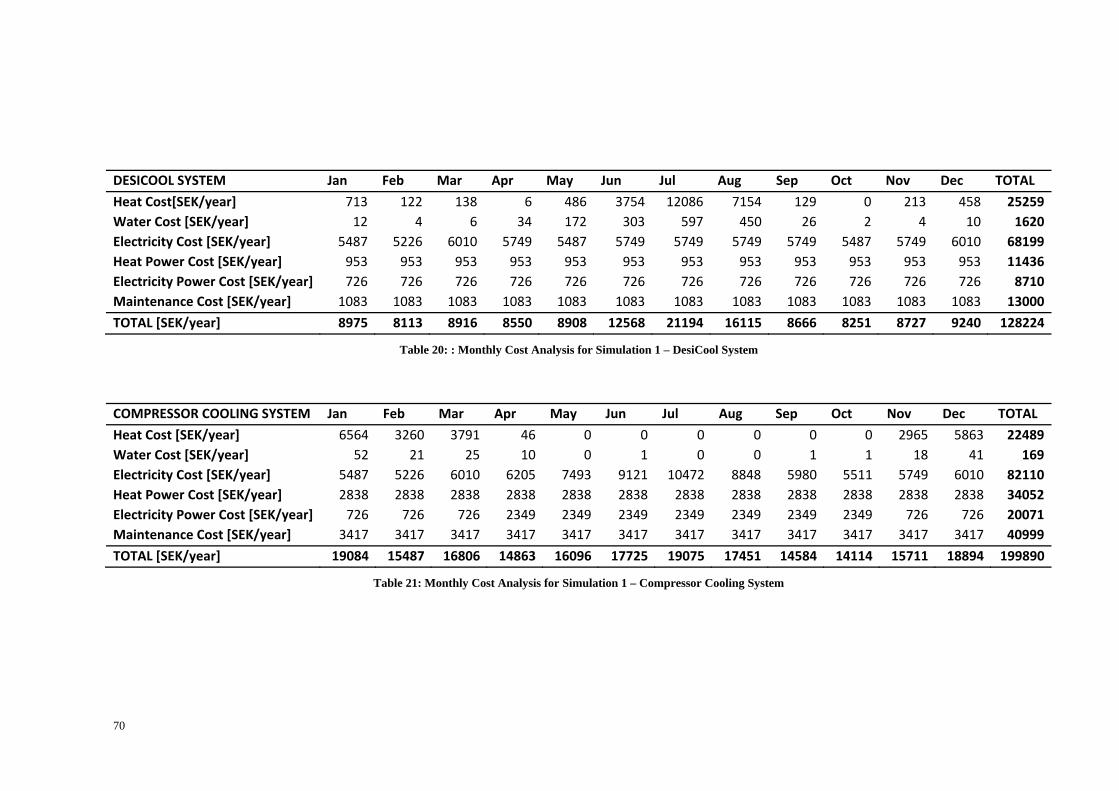
70
DESICOOL SYSTEM Jan Feb Mar Apr May Jun Jul Aug Sep Oct Nov Dec TOTAL
Heat Cost[SEK/year] 713 122 138 6 486 3754 12086 7154 129 0 213 458 25259 Water Cost [SEK/year] 12 4 6 34 172 303 597 450 26 2 4 10 1620 Electricity Cost [SEK/year] 5487 5226 6010 5749 5487 5749 5749 5749 5749 5487 5749 6010 68199 Heat Power Cost [SEK/year] 953 953 953 953 953 953 953 953 953 953 953 953 11436 Electricity Power Cost [SEK/year] 726 726 726 726 726 726 726 726 726 726 726 726 8710 Maintenance Cost [SEK/year] 1083 1083 1083 1083 1083 1083 1083 1083 1083 1083 1083 1083 13000
TOTAL [SEK/year] 8975 8113 8916 8550 8908 12568 21194 16115 8666 8251 8727 9240 128224
Table 20: : Monthly Cost Analysis for Simulation 1 – DesiCool System
COMPRESSOR COOLING SYSTEM Jan Feb Mar Apr May Jun Jul Aug Sep Oct Nov Dec TOTAL
Heat Cost [SEK/year] 6564 3260 3791 46 0 0 0 0 0 0 2965 5863 22489 Water Cost [SEK/year] 52 21 25 10 0 1 0 0 1 1 18 41 169 Electricity Cost [SEK/year] 5487 5226 6010 6205 7493 9121 10472 8848 5980 5511 5749 6010 82110 Heat Power Cost [SEK/year] 2838 2838 2838 2838 2838 2838 2838 2838 2838 2838 2838 2838 34052 Electricity Power Cost [SEK/year] 726 726 726 2349 2349 2349 2349 2349 2349 2349 726 726 20071 Maintenance Cost [SEK/year] 3417 3417 3417 3417 3417 3417 3417 3417 3417 3417 3417 3417 40999
TOTAL [SEK/year] 19084 15487 16806 14863 16096 17725 19075 17451 14584 14114 15711 18894 199890
Table 21: Monthly Cost Analysis for Simulation 1 – Compressor Cooling System

71
10.2 Results for Simulation 2 – Arlanda & Waste Heat/Solar Energy –
DESICOOL SYSTEM Jan Feb Mar Apr May Jun Jul Aug Sep Oct Nov Dec TOTAL
Heat Cost [SEK/year] 0 0 0 0 0 0 0 0 0 0 0 0 0 Water Cost [SEK/year] 12 4 6 34 172 303 597 450 26 2 4 10 1620 Electricity Cost [SEK/year] 5487 5226 6010 5749 5487 5749 5749 5749 5749 5487 5749 6010 68199 Heat Power Cost [SEK/year] 0 0 0 0 0 0 0 0 0 0 0 0 0 Electricity Power Cost [SEK/year] 726 726 726 726 726 726 726 726 726 726 726 726 8710 Maintenance Cost [SEK/year] 1083 1083 1083 1083 1083 1083 1083 1083 1083 1083 1083 1083 13000
TOTAL [SEK/year] 7309 7039 7825 7592 7469 7861 8155 8007 7584 7298 7561 7829 91529
Table 22: Monthly Cost Analysis for simulation 1 – Desicool –
COMPRESSOR COOLING SYSTEM Jan Feb Mar Apr May Jun Jul Aug Sep Oct Nov Dec TOTAL
Heat Cost [SEK/year] 0 0 0 0 0 0 0 0 0 0 0 0 0 Water Cost [SEK/year] 52 21 25 10 0 1 0 0 1 1 18 41 169 Electricity Cost [SEK/year] 5487 5226 6010 6205 7493 9121 10472 8848 5980 5511 5749 6010 82110 Heat Power Cost [SEK/year] 0 0 0 0 0 0 0 0 0 0 0 0 0 Electricity Power Cost [SEK/year] 726 726 726 2349 2349 2349 2349 2349 2349 2349 726 726 20071 Maintenance Cost [SEK/year] 3417 3417 3417 3417 3417 3417 3417 3417 3417 3417 3417 3417 40999
TOTAL [SEK/year] 9682 9389 10177 11980 13258 14887 16237 14613 11746 11277 9909 10194 143350
Table 23: Monthly Cost Analysis for simulation 1 – Compressor Cooling System –

72
10.3 Results for Simulation 3 – Madrid & NG –
DESICOOL SYSTEM Jan Feb Mar Apr May Jun Jul Aug Sep Oct Nov Dec TOTAL
Heat after heating [kWh/year] 0 0 0 0 0 0 0 0 0 0 0 0 0 Heat regeneration [kWh/year] 0 0 0 3333 8136 20423 33655 34882 18736 7562 72 0 126799 Electricity [kWh/year] 5487 5226 6010 5749 5487 5749 5749 5749 5749 5487 5749 6010 68199
TOTAL [kWh/year] 5487 5226 6010 9081 13624 26171 39404 40631 24485 13049 5821 6010 194998
Table 24: Monthly Energy Analysis for Simulation 3 – Desicool –
COMPRESSOR COOLING SYSTEM Jan Feb Mar Apr May Jun Jul Aug Sep Oct Nov Dec TOTAL
Heat after heating [kWh/year] 1422 786 510 0 0 0 0 0 0 0 465 902 4084 Electricity [kWh/year] 5487 5226 6332 8960 11177 12622 13129 13044 12791 10163 6320 6010 111260
TOTAL [kWh/year] 6909 6012 6841 8960 11177 12622 13129 13044 12791 10163 6785 6912 115344
Table 25: Monthly Energy Analysis for Simulation 3 – Compressor Cooling System –

73
DESICOOL SYSTEM Jan Feb Mar Apr May Jun Jul Aug Sep Oct Nov Dec TOTAL
Heat Cost [SEK/year] 0 0 0 1131 2369 11578 18922 26066 12916 3962 57 0 77000 Water Cost [SEK/year] 0 0 13 165 526 712 918 948 744 339 8 0 4373 Electricity Cost [SEK/year] 5487 5226 6010 5749 5487 5749 5749 5749 5749 5487 5749 6010 68199 Heat Power Cost [SEK/year] 665 665 665 665 665 665 665 665 665 665 665 665 7978 Electricity Power Cost [SEK/year] 726 726 726 726 726 726 726 726 726 726 726 726 8710 Maintenance Cost [SEK/year] 1083 1083 1083 1083 1083 1083 1083 1083 1083 1083 1083 1083 13000
TOTAL [SEK/year] 7962 7700 8497 9519 10856 20512 28063 35236 21883 12262 8287 8484 179260
Table 26: Monthly Cost Analysis for Simulation 3 – Desicool –
COMPRESSOR COOLING SYSTEM Jan Feb Mar Apr May Jun Jul Aug Sep Oct Nov Dec TOTAL
Heat Cost [SEK/year] 697 385 250 0 0 0 0 0 0 0 228 442 2001 Water Cost [SEK/year] 11 0 9 0 1 2 0 0 1 2 1 1 27 Electricity Cost [SEK/year] 5487 5226 6193 7912 11015 14872 19859 19694 13844 8107 5984 6010 124203 Heat Power Cost [SEK/year] 39 39 39 39 39 39 39 39 39 39 39 39 468 Electricity Power Cost [SEK/year] 726 726 4133 4133 4133 4133 4133 4133 4133 4133 4133 726 39373 Maintenance Cost [SEK/year] 3417 3417 3417 3417 3417 3417 3417 3417 3417 3417 3417 3417 40999
TOTAL [SEK/year] 10376 9793 14040 15501 18604 22462 27447 27283 21433 15698 13801 10634 207071
Table 27: Monthly Cost Analysis for Simulation 3 – Compressor Cooling System –
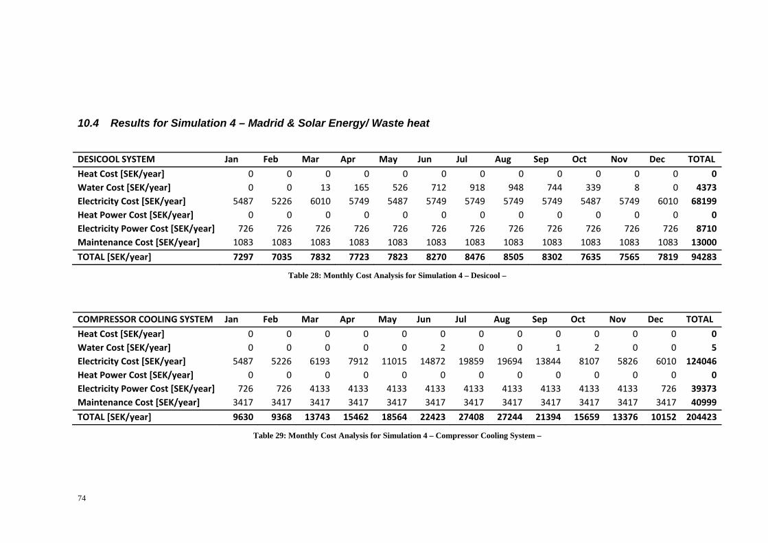
74
10.4 Results for Simulation 4 – Madrid & Solar Energy/ Waste heat
DESICOOL SYSTEM Jan Feb Mar Apr May Jun Jul Aug Sep Oct Nov Dec TOTAL
Heat Cost [SEK/year] 0 0 0 0 0 0 0 0 0 0 0 0 0 Water Cost [SEK/year] 0 0 13 165 526 712 918 948 744 339 8 0 4373 Electricity Cost [SEK/year] 5487 5226 6010 5749 5487 5749 5749 5749 5749 5487 5749 6010 68199 Heat Power Cost [SEK/year] 0 0 0 0 0 0 0 0 0 0 0 0 0 Electricity Power Cost [SEK/year] 726 726 726 726 726 726 726 726 726 726 726 726 8710 Maintenance Cost [SEK/year] 1083 1083 1083 1083 1083 1083 1083 1083 1083 1083 1083 1083 13000
TOTAL [SEK/year] 7297 7035 7832 7723 7823 8270 8476 8505 8302 7635 7565 7819 94283
Table 28: Monthly Cost Analysis for Simulation 4 – Desicool –
COMPRESSOR COOLING SYSTEM Jan Feb Mar Apr May Jun Jul Aug Sep Oct Nov Dec TOTAL
Heat Cost [SEK/year] 0 0 0 0 0 0 0 0 0 0 0 0 0 Water Cost [SEK/year] 0 0 0 0 0 2 0 0 1 2 0 0 5 Electricity Cost [SEK/year] 5487 5226 6193 7912 11015 14872 19859 19694 13844 8107 5826 6010 124046 Heat Power Cost [SEK/year] 0 0 0 0 0 0 0 0 0 0 0 0 0 Electricity Power Cost [SEK/year] 726 726 4133 4133 4133 4133 4133 4133 4133 4133 4133 726 39373 Maintenance Cost [SEK/year] 3417 3417 3417 3417 3417 3417 3417 3417 3417 3417 3417 3417 40999
TOTAL [SEK/year] 9630 9368 13743 15462 18564 22423 27408 27244 21394 15659 13376 10152 204423
Table 29: Monthly Cost Analysis for Simulation 4 – Compressor Cooling System –

75
11 Appendix II: Table of symbols
The following table shows equivalence between the symbols used to represent variables
and parameters in the report and those used in the programming code:
Symbol used in the report
Symbol used in the code Description
REG_EFF Regeneration efficiency
AD_EFF Adiabatic efficiency
TEFF_MCC Temperature efficiency for the MCC wheel
WEFF_MCC Humidity efficiency for the MCC wheel
EFF_VVX Temperature efficiency for the VVX wheel
| MAX_ TEFF_MCC Maximum Temperature efficiency for the MCC wheel
| MAX_ WEFF_MCC Maximum Humidity efficiency for the MCC wheel | MAX_ EFF_VVX Maximum Temperature efficiency for the VVX wheel
t Dry-bulb temperature
rh Relative Humidity
W Humidity content
twb Wet-bulb temperature
h Enthalpy
pw Partial pressure of water
pws Partial pressure of water at saturation
p Atmospheric pressure
T1 Outdoor temperature
FI1 Outdoor relative humidity
DT Temperature gain in the room
DW Humidity gain in the room

76
T5 Supply air temperature
| MAX_FI5 Maximum relative humidity allowed for the supply air
| MIN_FI5 Minimum relative humidity allowed for the supply air
FLOW Air flow in cubic meters per hour
C(1) Cost per kWh of electricity
C(2) Cost per cubic meter of water
C(3) Cost per kWh of heat in winter
C(4) Cost per kWh of heat in summer
C(5) Cost per kW of electricity power
C(6) Cost per kW of heat power
Table 30: Table of equivalences of symbols

77
12 Appendix III: List of M-functions and description
MAIN FUNCTION
Desicool Main function. It contains all the functions associated with all
the callbacks of the elements in the figure
LEVEL I
Psychrometrics Functions
Eq_6 (t) Equations 34 and 35 in the report. (5 and 6 in ASHRAE). It
calculates given T.
Eq_38(W) Equation 36 in the report, 38 in ASHRAE. Calculates
given
Eq_35(t,twb) Equations 37 and 38 of the report, 35 and 37 in ASHRAE
Eq_32(t,W) Equation 39 in the report, 32 in ASHRAE. It calculates the
enthalpy.
Eq_24(pw,pws) Equation 33 in the report. It calculates
Eq_22(W,pw) Equation 36 in the report, 22 in ASHRAE. Calculates
given
Case Functions
Case_1
See Table 2 …
Case_7
LEVEL II
General Functions
calculate() It executes the flow diagram in Figure 16. It writes the q-
matrix in the window and calls the plot function to plot the
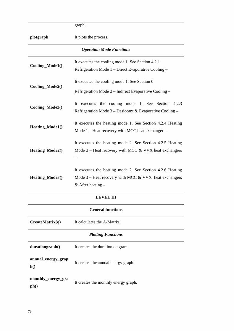
78
graph.
plotgraph It plots the process.
Operation Mode Functions
Cooling_Mode1() It executes the cooling mode 1. See Section 4.2.1
Refrigeration Mode 1 – Direct Evaporative Cooling –
Cooling_Mode2() It executes the cooling mode 1. See Section 0
Refrigeration Mode 2 – Indirect Evaporative Cooling –
Cooling_Mode3() It executes the cooling mode 1. See Section 4.2.3
Refrigeration Mode 3 – Desiccant & Evaporative Cooling –
Heating_Mode1() It executes the heating mode 1. See Section 4.2.4 Heating
Mode 1 – Heat recovery with MCC heat exchanger –
Heating_Mode2()
It executes the heating mode 2. See Section 4.2.5 Heating
Mode 2 – Heat recovery with MCC & VVX heat exchangers
–
Heating_Mode3()
It executes the heating mode 2. See Section 4.2.6 Heating
Mode 3 – Heat recovery with MCC & VVX heat exchangers
& After heating –
LEVEL III
General functions
CreateMatrix(q) It calculates the A-Matrix.
Plotting Functions
durationgraph() It creates the duration diagram.
annual_energy_grap
h() It creates the annual energy graph.
monthly_energy_gra
ph() It creates the monthly energy graph.

79
piegraph() It creates the annual cost graph.
monthlygraph() It creates the monthly cost graph.
efficiencygraph() It creates the VVX and MCC efficiency graphs.
efficiency_and_heat_
graph() It creates the overall performance graph.
environmental_graph
() It creates the environmental analysis graph
Table 31: List of M-functions and description

80
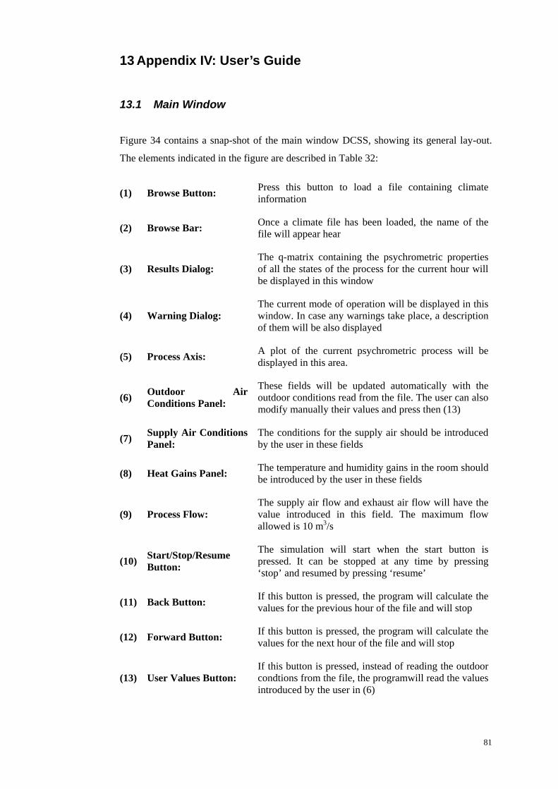
81
13 Appendix IV: User’s Guide
13.1 Main Window
Figure 34 contains a snap-shot of the main window DCSS, showing its general lay-out.
The elements indicated in the figure are described in Table 32:
(1) Browse Button: Press this button to load a file containing climate information
(2) Browse Bar: Once a climate file has been loaded, the name of the file will appear hear
(3) Results Dialog: The q-matrix containing the psychrometric properties of all the states of the process for the current hour will be displayed in this window
(4) Warning Dialog: The current mode of operation will be displayed in this window. In case any warnings take place, a description of them will be also displayed
(5) Process Axis: A plot of the current psychrometric process will be displayed in this area.
(6) Outdoor Air Conditions Panel:
These fields will be updated automatically with the outdoor conditions read from the file. The user can also modify manually their values and press then (13)
(7) Supply Air Conditions Panel:
The conditions for the supply air should be introduced by the user in these fields
(8) Heat Gains Panel: The temperature and humidity gains in the room should be introduced by the user in these fields
(9) Process Flow: The supply air flow and exhaust air flow will have the value introduced in this field. The maximum flow allowed is 10 m3/s
(10) Start/Stop/Resume Button:
The simulation will start when the start button is pressed. It can be stopped at any time by pressing ‘stop’ and resumed by pressing ‘resume’
(11) Back Button: If this button is pressed, the program will calculate the values for the previous hour of the file and will stop
(12) Forward Button: If this button is pressed, the program will calculate the values for the next hour of the file and will stop
(13) User Values Button: If this button is pressed, instead of reading the outdoor condtions from the file, the programwill read the values introduced by the user in (6)
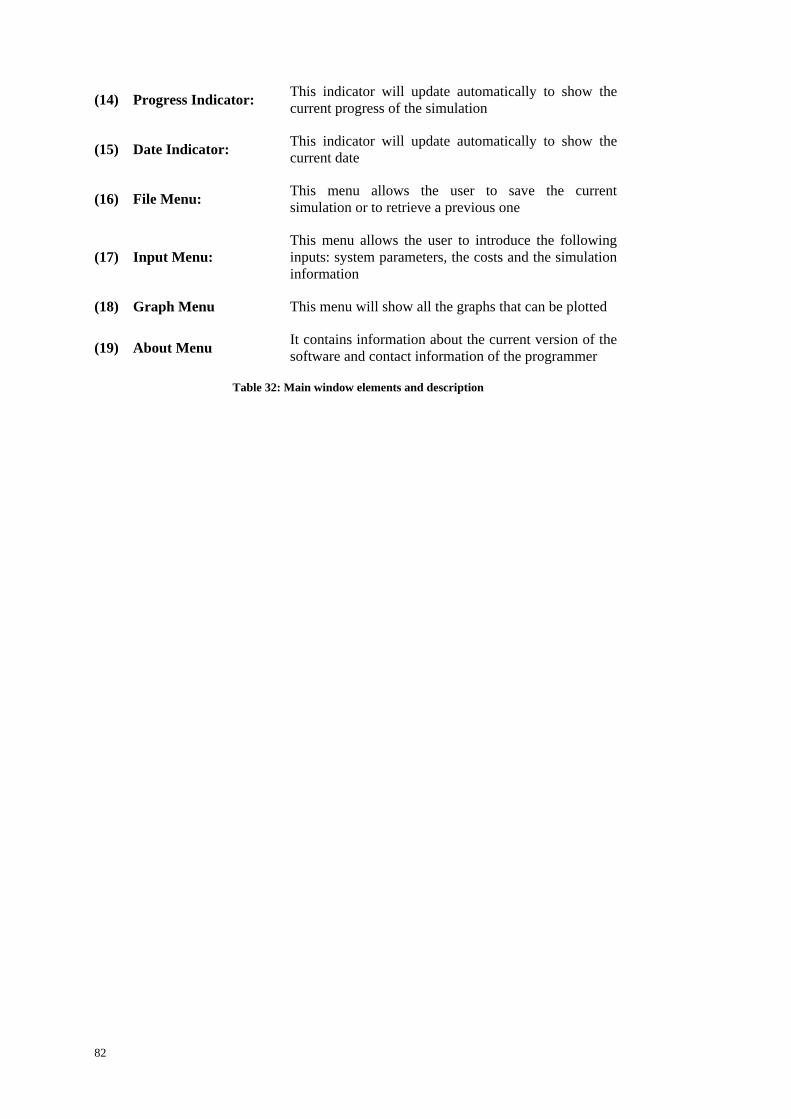
82
(14) Progress Indicator: This indicator will update automatically to show the current progress of the simulation
(15) Date Indicator: This indicator will update automatically to show the current date
(16) File Menu: This menu allows the user to save the current simulation or to retrieve a previous one
(17) Input Menu: This menu allows the user to introduce the following inputs: system parameters, the costs and the simulation information
(18) Graph Menu This menu will show all the graphs that can be plotted
(19) About Menu It contains information about the current version of the software and contact information of the programmer
Table 32: Main window elements and description

83
Figure 34: Main Window Lay-Out
(1) (2)
(3)
(4)
(5) (6) (7)
(8)
(9)
(10) (11) (12) (13) (14) (15)
(16) (17) (18) (19)

84
13.2 File Menu:
When the mouse is passed over the file menu, the menu shown in Figure 35 will pop-up:
Figure 35: File menu
The open function will allow the user to retrieve a simulation that has been previously
saved, and the save button will allow the user to save the current simulation. Standard
windows dialogs like the ones shown in Figure 36and Figure 37 will be used:
Figure 36: Load File Dialog
Figure 37: Save File Dialog
13.3 Input menu
Figure 38 shows the input menu, which will let the user introduce information about the
system parameters, the cost of the different resources and the simulation time.
Figure 38: Input Menu
When this fields are pressed, the input dialogs shown in

85
Figure 39:System parameters input dialog
Figure 40: Cost information input dialog
Figure 41: Simulation time input dialog
13.4 Graph Menu
The graph menu in Figure 42 will allow the user to plot different graphic outputs:
Figure 42: Graph Menu
Figure 43 to Figure 50 show all the possible graph outputs of the DCSS. The pictures will
appear in a Matlab window, that allows the user to edit and customize the graphs. The
figures can be later saved using different extensions, such as .fig, which is the extension
used for Matlab figures, and also standard image extensions like .bmp and .jpg

86
Figure 43: Duration Diagram
Figure 44: Annual Energy Gaph
Figure 45:Monthly Energy Graph
Figure 46:Annual Cost Graph
Figure 47:Monthly Cost Graph
Figure 48:Efficiency Graph

87
Figure 49: Overall Performance Graph Figure 50:Environmental Graph