design and analysis of a 3-dimensional cluster
TRANSCRIPT

DESIGN AND ANALYSIS OF A 3-DIMENSIONAL CLUSTER
MULTICOMPUTER ARCHITECTURE USING OPTICAL
INTERCONNECTION FOR PETAFLOP COMPUTING
A Dissertation
by
EKPE APIA OKORAFOR
Submitted to the Office of Graduate Studies ofTexas A&M University
in partial fulfillment of the requirements for the degree of
DOCTOR OF PHILOSOPHY
December 2005
Major Subject: Computer Engineering

DESIGN AND ANALYSIS OF A 3-DIMENSIONAL CLUSTER
MULTICOMPUTER ARCHITECTURE USING OPTICAL
INTERCONNECTION FOR PETAFLOP COMPUTING
A Dissertation
by
EKPE APIA OKORAFOR
Submitted to the Office of Graduate Studies ofTexas A&M University
in partial fulfillment of the requirements for the degree of
DOCTOR OF PHILOSOPHY
Approved by:
Chair of Committee, Gwan S. ChoiCommittee Members, Duncan M. Walker
Henry F. TaylorSunil P. Khatri
Head of Department, Costas N. Georghiades
December 2005
Major Subject: Computer Engineering

iii
ABSTRACT
Design and Analysis of a 3-Dimensional Cluster Multicomputer Architecture Using
Optical Interconnection for PetaFLOP Computing. (December 2005)
Ekpe Apia Okorafor, B.E., University of Nigeria;
M.S., Texas A&M University
Chair of Advisory Committee: Dr. Gwan Choi
In this dissertation, the design and analyses of an extremely scalable distributed
multicomputer architecture, using optical interconnects, that has the potential to
deliver in the order of petaFLOP performance is presented in detail. The design
takes advantage of optical technologies, harnessing the features inherent in optics,
to produce a 3D stack that implements efficiently a large, fully connected system of
nodes forming a true 3D architecture. To adopt optics in large-scale multiproces-
sor cluster systems, efficient routing and scheduling techniques are needed. To this
end, novel self-routing strategies for all-optical packet switched networks and on-line
scheduling methods that can result in collision free communication and achieve real
time operation in high-speed multiprocessor systems are proposed. The system is de-
signed to allow failed/faulty nodes to stay in place without appreciable performance
degradation. The approach is to develop a dynamic communication environment that
will be able to effectively adapt and evolve with a high density of missing units or
nodes. A joint CPU/bandwidth controller that maximizes the resource allocation in
this dynamic computing environment is introduced with an objective to optimize the
distributed cluster architecture, preventing performance/system degradation in the
presence of failed/faulty nodes. A thorough analysis, feasibility study and description

iv
of the characteristics of a 3-Dimensional multicomputer system capable of achieving
100 teraFLOP performance is discussed in detail. Included in this dissertation is
throughput analysis of the routing schemes, using methods from discrete-time queu-
ing systems and computer simulation results for the different proposed algorithms. A
prototype of the 3D architecture proposed is built and a test bed developed to obtain
experimental results to further prove the feasibility of the design, validate initial as-
sumptions, algorithms, simulations and the optimized distributed resource allocation
scheme. Finally, as a prelude to further research, an efficient data routing strategy
for highly scalable distributed mobile multiprocessor networks is introduced.

v
To my loving wife, Unoma, and my beautiful daughter, Chisom.

vi
ACKNOWLEDGMENTS
I am indeed indebted to many people in the course of producing this dissertation.
First, I would like to express my thanks to Dr. Mi Lu, who gave me the opportunity,
initial guidance and support to pursue my graduate studies here at Texas A&M
University. Her directives provided me with a clear insight and understanding of the
initial problems I tackled in producing this dissertation.
Next, I would like to acknowledge the members of my committee, Dr. Gwan Choi,
Dr. Hank Walker, Dr. Henry Taylor & Dr. Sunil Khatri. Together they inspired
me to achieve excellence in research. The many discussions and collaborations have
really paid off. Their great insight and understanding of related subject matters have
had a profound impact on me. The road to success in a PhD program in part rests
on the support and guidance from one’s committee members, and I was blessed to
have the best.
I had the opportunity to work on many projects that resulted in both conference
and journal papers while interning at IBM, at the Almaden and Watson facilities. I
want to thank Claudio Fleiner, Richard Garner and Wilfried Wilcke at the Almaden
Research Center. At the Watson Center, many thanks to Jeremy Silber, Dimitrios
Pendarakis and Laura Wynter.
To my parents and siblings, I just want to say thanks, I made it. Last, but
certainly not the least, my wife, Unoma, who has to put up with me. Thanks, baby,
you are the best. I give God Almighty all the glory. Thank you Lord for the many
blessings in my life.

vii
TABLE OF CONTENTS
CHAPTER Page
I INTRODUCTION . . . . . . . . . . . . . . . . . . . . . . . . . . 1
A. Problem Definition . . . . . . . . . . . . . . . . . . . . . . 2
1. Architecture and Optical Implementation . . . . . . . 4
2. Routing and Scheduling . . . . . . . . . . . . . . . . . 4
3. Fault Tolerance and Adaptability . . . . . . . . . . . . 6
4. System Optimization and Performance . . . . . . . . . 7
B. Objectives . . . . . . . . . . . . . . . . . . . . . . . . . . . 8
C. Current Status . . . . . . . . . . . . . . . . . . . . . . . . 9
II ARCHITECTURE AND OPTICAL IMPLEMENTATION . . . 15
A. Basic Architecture . . . . . . . . . . . . . . . . . . . . . . 15
1. Basic Building Block . . . . . . . . . . . . . . . . . . . 16
2. 3D System . . . . . . . . . . . . . . . . . . . . . . . . 18
B. 100 TeraFLOP Performance: A Case Study . . . . . . . . 20
1. Feasibility Analysis for Optical Components . . . . . . 20
a. Free Space Optical Coupler Interface . . . . . . . 21
b. Optical Transmitters/Receivers . . . . . . . . . . 22
c. Power . . . . . . . . . . . . . . . . . . . . . . . . 22
d. Guided Planar Optical Interconnect . . . . . . . . 22
C. Analysis of the Optical Interconnection Network . . . . . . 23
1. Modeling the Free-space Optical Interconnect . . . . . 23
a. Cross-talk and Transmission Efficiency . . . . . . 24
b. Bit Error Rate . . . . . . . . . . . . . . . . . . . 24
c. Simulation Results and Discussion . . . . . . . . . 25
2. Modeling the POF Guided Planar Optical Interconnect 26
a. Cross-talk and Transmission Efficiency . . . . . . 27
b. Simulation Results and Discussion . . . . . . . . . 29
D. Performance Evaluation . . . . . . . . . . . . . . . . . . . 30
1. Implementation of Compute/Communication In-
tensive Algorithm . . . . . . . . . . . . . . . . . . . . 30
2. Comparing the Single-hop and Multi-hop Commu-
nication Methods . . . . . . . . . . . . . . . . . . . . . 32

viii
CHAPTER Page
III ALL-OPTICAL ROUTING . . . . . . . . . . . . . . . . . . . . 34
A. The Self-routing Scheme . . . . . . . . . . . . . . . . . . . 35
1. Node Structure and Address . . . . . . . . . . . . . . 37
2. Routing . . . . . . . . . . . . . . . . . . . . . . . . . . 39
B. Optical Implementation . . . . . . . . . . . . . . . . . . . 41
C. Analytical Model . . . . . . . . . . . . . . . . . . . . . . . 43
1. Average Packet Hop Count and Throughput . . . . . 44
2. Packet Loss Probability . . . . . . . . . . . . . . . . . 46
D. Simulation Results . . . . . . . . . . . . . . . . . . . . . . 48
E. Conclusion . . . . . . . . . . . . . . . . . . . . . . . . . . . 50
IV MESSAGE SCHEDULING . . . . . . . . . . . . . . . . . . . . . 52
A. System Model . . . . . . . . . . . . . . . . . . . . . . . . . 54
B. Scheduling Algorithm . . . . . . . . . . . . . . . . . . . . . 56
1. Control Frame Ordering . . . . . . . . . . . . . . . . . 57
2. Data and Control Frame Ordering . . . . . . . . . . . 58
3. Multiple Data and Control Frame Ordering . . . . . . 59
4. Multiple Data and Control Frame Ordering with
Multicast Partition . . . . . . . . . . . . . . . . . . . . 60
C. Simulation Results . . . . . . . . . . . . . . . . . . . . . . 61
V FAULT TOLERANCE . . . . . . . . . . . . . . . . . . . . . . . 67
A. Percolation in Large Systems . . . . . . . . . . . . . . . . . 71
B. Percolation Routing with Optical Interconnectivity . . . . 74
1. Address Formulation, Path Setup, and Channel
Assignment . . . . . . . . . . . . . . . . . . . . . . . . 76
2. Routing Algorithms . . . . . . . . . . . . . . . . . . . 78
a. Notation . . . . . . . . . . . . . . . . . . . . . . . 78
b. Dimension order routing (XYZ routing) . . . . . . 80
c. Probability-based percolation random routing . . 83
C. Feasibility of Optical Implementation . . . . . . . . . . . . 86
D. Simulation Results . . . . . . . . . . . . . . . . . . . . . . 89
VI SYSTEM OPTIMIZATION AND PERFORMANCE . . . . . . 95
A. Overview of Related Work . . . . . . . . . . . . . . . . . . 98
B. Experimental Design . . . . . . . . . . . . . . . . . . . . . 100
1. Bandwidth Policing . . . . . . . . . . . . . . . . . . . 100
2. CPU Monitoring . . . . . . . . . . . . . . . . . . . . . 102

ix
CHAPTER Page
3. Bandwidth Monitoring . . . . . . . . . . . . 103 4. Controller . . . . . . . . . . . . . . . . 104
C. Experimental Procedure and Results . . . . . . . . . . 105 1. Experimental Procedures . . . . . . . . . . . . 106
a. Linux Scheduler Priority (nice) . . . . . . . . 107 b. Class-based Kernel Resource Manager (CKRM) . . 107 c. Autonomic Traffic Management System (ATM) . . 108
2. Experimental Results . . . . . . . . . . . . . 108 D. Conclusion and Future Work . . . . . . . . . . . . . 113
VII ROUTING IN MOBILE MULTICOMPUTER NETWORK - A CASE STUDY . . . . . . . . . . . . . . . . . . . . . . 116
A. The System Model . . . . . . . . . . . . . . . 120
1. Network Partition Scheme . . . . . . . . . . . 121 2. Node Addressing . . . . . . . . . . . . . 122 3. Node Community Update . . . . . . . . . . . 124 4. Location Inquiry . . . . . . . . . . . . . . 127
B. Distributed Mobile Data Routing . . . . . . . . . . 128 1. Path Setup . . . . . . . . . . . . . . . . 128 2. Path Hand-over . . . . . . . . . . . . . . 131 3. Predictive Data Routing . . . . . . . . . . . . 132
C. Analysis . . . . . . . . . . . . . . . . . . 133 1. Analysis for Optimal Partitioning . . . . . . . . . 133 2. Analysis for Delay Improvement . . . . . . . . . 135
D. Simulation Results . . . . . . . . . . . . . . . 136 E. Conclusion . . . . . . . . . . . . . . . . . . 139
VIII CONCLUSION . . . . . . . . . . . . . . . . . . 140 REFERENCES AND LINKS . . . . . . . . . . . . . . . . . . 142 APPENDIX A . . . . . . . . . . . . . . . . . . . . . . . 156 APPENDIX B . . . . . . . . . . . . . . . . . . . . . . . 158 VITA . . . . . . . . . . . . . . . . . . . . . . . . . . 160

x
LIST OF TABLES
TABLE Page
I Optimized Parameters . . . . . . . . . . . . . . . . . . . . . . . . . . 27
II Characteristics of Sources/Detectors . . . . . . . . . . . . . . . . . . 28
III Simulation Parameters for the All-Optical Packet Routing Subsystem 90
xi
LIST OF FIGURES
FIGURE Page
1 Diagram showing basic node structure with FSOI couplers capable
of gigahertz communication . . . . . . . . . . . . . . . . . . . . . . . 16
2 Diagram showing logical interconnection within each node . . . . . . 17
3 Schematic diagram of each PE . . . . . . . . . . . . . . . . . . . . . 18
4 3D 4x4x4 mesh interconnection network using optical interconnect . 19
5 Optical link assembly with built-in redundancy . . . . . . . . . . . . 21
6 Channel density as interconnection length is increased . . . . . . . . 25
7 Transmission efficiency of the free-space of lens with different focal
numbers . . . . . . . . . . . . . . . . . . . . . . . . . . . . . . . . . . 26
8 The plot of BER as a function of the angular tilt . . . . . . . . . . . 26
9 The plot of BER as a function of the laser power . . . . . . . . . . . 27
10 Transmission of the POF based guided-wave interconnect using a
VCSEL . . . . . . . . . . . . . . . . . . . . . . . . . . . . . . . . . . 30
11 Jacobi iteration . . . . . . . . . . . . . . . . . . . . . . . . . . . . . . 31
12 Ratio of single-hop to multi-hop raw bandwidth-per-link against
network size for a 3D mesh . . . . . . . . . . . . . . . . . . . . . . . 33
13 Two field address structure . . . . . . . . . . . . . . . . . . . . . . . 36
14 A 48-node 3-D network . . . . . . . . . . . . . . . . . . . . . . . . . 37
15 The node structure . . . . . . . . . . . . . . . . . . . . . . . . . . . . 38
16 Diagram to illustrate output link options . . . . . . . . . . . . . . . . 39
17 Data routing illustration . . . . . . . . . . . . . . . . . . . . . . . . . 40

xii
FIGURE Page
18 Packet address illustration . . . . . . . . . . . . . . . . . . . . . . . . 41
19 Temporal snapshot of (a) programming (b) & (c) processing stages . 42
20 Phase matching diagram . . . . . . . . . . . . . . . . . . . . . . . . . 43
21 Average hop count for 48-node network topology . . . . . . . . . . . 48
22 Average hop count for 48-node network topology under higher loads . 49
23 Packet loss probability for a 48-node topology . . . . . . . . . . . . . 49
24 Node throughput for a 48-node topology . . . . . . . . . . . . . . . . 50
25 Diagram to illustrate output link options . . . . . . . . . . . . . . . . 54
26 Operational system cycles . . . . . . . . . . . . . . . . . . . . . . . . 55
27 Plot of average packet delay versus arrival rate per node . . . . . . . 64
28 Plots showing average packet delay versus multicast rate . . . . . . . 65
29 Throughput versus arrival rate per node . . . . . . . . . . . . . . . . 66
30 3-dimensional mesh network with failed nodes depicted as white nodes 72
31 Diagram showing min-cut in both 2- and 3-dimension . . . . . . . . . 73
32 Two field address structure . . . . . . . . . . . . . . . . . . . . . . . 75
33 Distribution of link loading on traffic model for 0% . . . . . . . . . . 86
34 Distribution of link loading on traffic model for 50% . . . . . . . . . 87
35 Block diagram of header recognition subsystem using OTDM . . . . 88
36 Bit format of the OTDM packet . . . . . . . . . . . . . . . . . . . . 88
37 Bit format of the OTDM packet . . . . . . . . . . . . . . . . . . . . 89
38 Channel width . . . . . . . . . . . . . . . . . . . . . . . . . . . . . . 91

xiii
FIGURE Page
39 Network latency for a 10x10x10 3D mesh network with arbitrary
fixed message size under uniform random traffic . . . . . . . . . . . . 92
40 Effect of faulty node degree on saturation throughput . . . . . . . . . 92
41 Effect of faulty node degree on worse case loading . . . . . . . . . . . 93
42 Average number of hot spots . . . . . . . . . . . . . . . . . . . . . . 94
43 CPU utilization measured using each of the 3 management schemes:
nice, CKRM, and ATM for varying processing levels. Each scheme
is represented by two lines for the two tasks, and the target CPU
utilizations are indicated by the dotted lines labeled “targets” . . . . 109
44 Bandwidth Utilization measured using each of the 3 management
schemes: nice, CKRM, and ATM for varying processing levels.
Each scheme is represented by two lines corresponding to the two tasks.110
45 Standard deviation of CPU utilization . . . . . . . . . . . . . . . . . 112
46 Standard deviation of bandwidth utilization . . . . . . . . . . . . . . 112
47 Graphical illustration of network showing only two levels . . . . . . . 120
48 Illustration of the hexagonal tree structure . . . . . . . . . . . . . . . 122
49 Illustration of network-layout showing levels of the partition hierarchy 123
50 Comparison between rectangle and hexagonal packing . . . . . . . . 133
51 Comparing the control signal delay of SEEK and different regular
topologies . . . . . . . . . . . . . . . . . . . . . . . . . . . . . . . . . 137
52 Effect of reservation techniques on control signal delay . . . . . . . . 137
53 Comparing the average packet delay of SEEK and other topologies . 138
54 Effects of predictive routing on average packet delay using SEEK . . 138

1
CHAPTER I
INTRODUCTION
In this dissertation, the design and analysis of an extremely scalable distributed mul-
ticomputer architecture using optical interconnects that has the potential to deliver
in the order of petaFLOP (1015 floating point operations per second) performance is
presented in detail. The design takes advantage of optical technologies, harnessing
the features inherent in optics, to produce a 3D stack that implements efficiently
a large, fully connected system of nodes forming a true 3D architecture. To adopt
optics in large-scale multiprocessor cluster systems, efficient routing and scheduling
techniques are needed.
To this end, novel self-routing strategies for all-optical packet switched networks,
and on-line scheduling methods that can result in collision free communication and
achieve real time operation in high-speed multiprocessor systems are proposed. The
system is designed to allow failed/faulty nodes stay in place without appreciable per-
formance degradation. The approach will be to develop a dynamic communication
environment that will be able to efficiently adapt and evolve with a high density of
missing units or nodes. A joint CPU/bandwidth controller that maximizes the re-
source allocation in this dynamic computing environment is introduced with an objec-
tive to optimize the distributed cluster architecture, preventing performance/system
degradation in the presence of failed/faulty nodes.
A thorough analysis and feasibility study is done for a 100 teraFLOP perfor-
mance and description of the characteristics of the proposed hardware components is
outlined. __________
This dissertation follows the style and format of the Journal of Optical Networking.

2
Included in this dissertation will be throughput analysis of the routing schemes,
using methods from discrete-time queuing systems and computer simulation results
for the different proposed algorithms. A prototype of the 3D architecture proposed
is built and a test bed developed to obtain experimental results to further prove
the feasibility of the design, validate initial assumptions, algorithms, simulations and
the optimized distributed resource allocation scheme. Finally, as a prelude to fur-
ther research, an efficient data routing strategy for highly scalable distributed mobile
multiprocessor networks is introduced.
A. Problem Definition
Some of the serious issues faced by the designers of large-scale computers or computing
systems include the following in order of importance;
• Inter-processor communication is a bottleneck
• System management is too complex
• Wide range of scalability
• System acquisition cost, and
• Environmental issues (floor space, power, cooling and noise)
The architecture and subsequently, computer system proposed in this dissertation
will improve on all these metrics simultaneously. The problems or issues dealt with
in this dissertation can be broadly grouped into four main categories:
1. Architecture and Optical Implementation
2. Routing and Scheduling

3
3. Fault Tolerance and Adaptability
4. System Optimization and Performance
This classification is by no means exhaustive and perhaps not exlusively authori-
tative. However, it is the authors opinion that these broad categories which form the
basis of the research, will provide readers and computer designers some understanding
of the problems, and offer possible solutions to these problems, faced in large-scale
computer networks and systems.
The current trend in multi-computer network design is to pack nodes more
densely in such a manner as to efficiently distribute computing resources and intercon-
nect uniformly in three-dimensional space. This has led to a remarkable improvement
in communication performance, scalability and density. Ultimately, the demand for
ever-greater performance by many computation problems pushes the boundaries for
the development of such large-scale supercomputers. PetaFLOP performance are re-
quired by many applications and they include real-time image processing, artificial
intelligence, real-time processing of databases, weather modeling, simulation of neural
networks, simulation of physical and biological phenomena, etc.
The functions of such large-scale petaFLOP-performance computer architecture
will include data acquisition and transmission, data processing, data management
and storage. These functions necessitate a large-scale, cost-effective computing and
storage capability to handle the extensive requirements for simulations and analysis
of massive amounts of data. They rely on advanced, emerging information technolo-
gies to create combinations of hardware and software, which will achieve unprece-
dented increases in numerical processing through parallel computation. However, the
main cause for the difficulty in managing and designing such large systems is the
proliferation of too many building blocks such as processors, disk arrays, switches,

4
communication protocols, etc. This leads to a combinatorial explosion complexity.
1. Architecture and Optical Implementation
From the foregoing, the issue of scalability of such large-scale petaFLOP-performance
computer cannot be over-emphasized. Massively parallel systems are required to scale
in the sense that their performance should be proportional to the number of nodes.
Unfortunately, unlimited scalability is not theoretically possible and worse still even
harder to achieve practically beyond some order of magnitude in the number of nodes.
The performance objectives of supercomputers is hindered because of the difficulties
associated with developing low complexity, high-bisection bandwidth, and low-latency
interconnection networks to connect thousands of nodes while still keeping the system
scalable.
It is desirable to have low-dimensional massively parallel computers with full-
connectivity in each direction. It is also desirable to make use of a topology that has
an extremely small diameter and average inter-node distance, and a large bisection
width. The utmost flexibility in exploiting parallelism is afforded by a topology with
diameter equal to one, where each processor can directly communicate with any other
processor. The most useful properties of a parallel processor interconnection network
are high bandwidth (scaling directly with the number of processors), low latency, no
arbitration delay, and non-blocking communication. It is apparent that the electronic
implementation of such a large-scale system is very difficult. Hence, the need to
investigate the feasibility of using optics instead.
2. Routing and Scheduling
Traditional optical communication systems are impaired by the severe drawbacks
imposed by Photonic-Electronic signal conversions at intermediate nodes. All optical

5
switching and routing can remove such bottleneck, maximizing link capacity and
network transparency. Decoding addresses optically in real time allows us to design
a self-routing scheme, break the 10Gb/s interconnection speed barrier, and eliminate
the need for wire connections. Speeds of up to 100Gb/s are possible if both the
header and payload remain in the optical domain. Terabytes or petabytes memory
capacity can be achieved in the dense cluster of computer systems. Free space optical
interconnects combined with the ability to perform all optical routing has broad
applications in highly scalable massively parallel systems, neural networks, optical
and quantum computing, optical Ethernet, LAN, ultra fast signal processing, and
super high speed switches for broadband communication.
There are two ways of communication in photonic networks. It can either be
Circuit Switched or Packet Switched communication. In circuit switched networks,
dedicated links are established between communicating nodes. In contrast, for packet
switched networks, packets are sent across the network like the postal system. The
packet switched network has the potential to provide better efficiency and lower cost
when compared to the circuit switched network, as the number of nodes in the network
increases, for ideal conditions. However, because of the OEO (i.e. Optical-Electrical-
Optical) conversion, unnecessary delays and losses are introduced degrading the per-
formance.
To take advantage of the enormous potential of single-hop WDM networks, effi-
cient access protocols and scheduling algorithms [1-3] are needed to allocate and man-
age the system resources. These protocol and algorithms have to meet the communi-
cation and computation constraints. In such mode of communication, a reservation-
based technique is employed for scheduling. Scheduling algorithms can be broken
down into two distinct stages, a channel assignment stage and a packet/message or-
dering stage. The assignment stage involves selecting an appropriate channel for

6
message transfer. It may also involve establishing a time slot for the transfer. The
ordering stage deals primarily with arranging the messages in a particular order ready
for transmission. The assignment stage has been researched extensively; however the
ordering aspect has not received as much attention.
There are three main communication traffic types, unicast, multicast and broad-
cast, based on the number of intended receivers. The individual traffic types have
received a great deal of attention [4-8]. A unicast packet has only one destination
address; a multicast packet has two or more destination addresses, while a broadcast
packet is intended for all the receiver nodes in the network. The obvious problems
include source and destination address conflicts of data packets. This has the effect of
causing large data delays and degrading throughput. It then becomes important to
device a way to schedule these different packets so that conflicts and collisions can be
avoided. A collision occurs when two or more transmitters access the same channel at
the same time, while a conflict occurs when two or more transmitting nodes transmit
to a single receiver on different channels at the same time.
3. Fault Tolerance and Adaptability
As noted earlier, the current trend in multi-computer network design is to pack nodes
more densely in such a manner as to efficiently distribute computing resources and
interconnect uniformly in three-dimensional space. A direct consequence of these
trends is that as these computing devices and their accessories get cheaper, smaller
and faster, users demand more of these units to be packed in as small a space as
possible. Herein lies a potential problem - the percolation problem, that deals with
the ability of a system as a whole to continue its functions with some of its components
missing or faulty. As individual nodes in a multicomputer system get smaller and the
packing gets denser, it becomes less desirable to try to fix problems that occur in

7
individual nodes or accessories. Any attempt to fix a problem with a node may result
in making problems worse in the system as a whole. A notion widely shared by large-
scale computer system designers is that human error when carrying out maintenance
or repair results in so much loss or down time and is usually quite expensive. The
problem then is to design a system that is able to function adequately in the presence
of failed nodes.
4. System Optimization and Performance
With the design of such large scale systems, it is expected that neither the comput-
ing nor the communication subsystem become the bottleneck. A novel autonomic
control system for high performance stream processing systems is proposed. The sys-
tem uses bandwidth controls on incoming or outgoing streams to achieve a desired
resource utilization balance among a set of concurrently executing stream processing
tasks. An objective is to show that CPU prioritization and allocation mechanisms in
schedulers and virtual machine managers are not sufficient to control such I/O-centric
applications, and to present an autonomic bandwidth control system that adaptively
adjusts incoming and outgoing traffic rates to achieve target CPU utilizations.
The system learns the bandwidth rate necessary to meet the CPU utilization ob-
jectives using a stochastic nonlinear optimization, and detects changes in the stream
processing applications that require bandwidth adjustment. The Linux implementa-
tion is lightweight, has low overhead, and is capable of effectively managing stream
processing applications.

8
B. Objectives
This dissertation aims at introducing an extremely scalable multicomputer architec-
ture that has the potential to deliver in the order of petaFLOP performance utilizing
optical interconnects. The architecture should be robust and fault-tolerant even with
a high degree of failed nodes. The objectives are as follows:
1. Propose an interconnection network that has an extremely high connectivity and
reduced packaging complexity in a large scale distributed cluster environment
2. Control combinatorial explosion of complexity by encapsulating complexity
within physical building blocks or nodes
3. Realize petaFLOP performance by solving the scalability and bandwidth issues
associated with such large scale systems
4. Analyze the different MAC protocols, routing and flow control techniques and
come up with the best suited for optimal performance
5. Evaluate the interconnection network in terms of fault tolerance and adaptabil-
ity in an environment with high degree of missing or faulty nodes
6. Setup an experimental test bed to derive and analyze performance results
7. Optimize the system by developing a joint CPU/bandwidth controller to effi-
ciently allocate resources in this highly dynamic environment
8. Finally, discuss the analytical, simulation and experimental results to prove the
feasibility of our design

9
C. Current Status
This section, with the objectives stated above and the classes of problems identi-
fied, outlines some research done in some of those areas, focusing on the existing
methods, the strengths and weakness of each method, the hardness to overcome the
insufficiencies and the basis of our approach.
Many interconnection networks have been proposed for the design of massively
parallel computers, including hypercubes [9], meshes and tori [10]. Others include fat
trees and enhanced meshes. Amongst these, the hypercube has been researched more
intensively because of its good topological properties and high interconnectivity. The
difficulty posed by the extremely high VLSI complexity incurred, due to very high
communication channels needed to implement these interconnection networks, has
continued to hinder the use of these topologies to achieve large-scale computer sys-
tems. The high VLSI complexity problem is obviously unbearable for any scalability.
According to [11], metal interconnects have reached their physical limits and
have become a limiting factor because of power, delays and density considerations.
The idea of optical interconnection of very large-scale integration (VLSI) electronic
was proposed and analyzed in [12]. This no doubt was the start of the field of optical
interconnects. Many advances have been made in the field of optical interconnects to
date. Engineering analysis has showed specific energy dissipation benefits of optical
interconnect [13, 14]. It is becoming increasingly clear to silicon semiconductor indus-
try that electrical interconnects are beginning to run into serious scaling limitations.
As an electrical line is scaled down on all three dimensions, its resistive-capacitive
time constant does not change. This is an undesirable quality, since the wires do
not scale to keep up with the transistors. Optical interconnects avoid this problem
altogether because they do not have the resistive loss physics that gives rise to this
10
phenomenon. In recent years, extremely fast photonic networks are being developed
that have the potential to support very large bandwidth interconnections, with an
extraordinarily quick response time and very low latency.
Significant progress both at the device and sub-system levels has been made
in Free-Space Optical Interconnects (FSOI) to the point where FSOI can now be
considered in computing hardware at the board to board interconnect level [15]. Opto-
Electronic (OE) devices including Vertical Cavity Surface Emitting Laser (VCSELs),
light modulators, and detectors have now been developed to the point that they
can enable high speed and high density FSOI [16-18]. It is important to note here
that recent attempts to connect boxes or computer systems with FSOI links have
proven practical [19]. System boards usually run at some fraction of the processor
clock, usually about half. In the next few years, we would expect the off-board
communication to approach 10 GHz. Signals have to be routed at 10 GHz over a
small distance at 2.5 or 1.8 V cycles. Cross-talk and reflections on electrical lines have
been identified as major problems. It is well known that VCSEL links can provide
the interconnection bandwidth thereby replacing the current large edge connectors.
This will improve system noise margins because cross-talk and ground noise coupling
become more difficult to control in traditional connectors as edge rates increase.
Sophisticated CAD tools for free-space optical systems are already in development
[20].
From the foregoing, an interconnection network that utilizes free-space and guided
wave optical technology because of its increased connectivity and reduced packaging
complexity is proposed. A 3-dimensional mesh interconnection is considered for this
design. As the number of nodes in a mesh-connected multicomputer increases, the
chance of failures also increases. The complex nature of networks also makes them
vulnerable to disturbances, which can be either deliberate or accidental. Therefore it

11
is so important that the network have the ability to tolerate failures especially in the
communication subsystem.
Many routing schemes have been proposed including Deflection [21-23], Store-
and-Forward [24] and Hot Potato routing algorithms [25-27]. These routing controls
either require complex optical routing control or internal output buffers. There will
also be some latency issues particularly where wavelength conversion is required. In
terms of logic devices, optics is still in its infancy compared to electronics. Self-
routing schemes require less complex routing control. Some work has been done
to deal with the current shortcomings of using optics in packet switched networks.
Self-routing schemes have been applied to regular topologies like the hypercubes,
meshes and Manhattan Street networks in the electronic domain. In [28] a self-
routing scheme is introduced but requires routing tables, hence not really practical
for large multiprocessor systems implemented using optics. The OEO conversions
become a bottleneck that limits the performance.
To circumvent this bottleneck, researchers are working on optical packet switched
networks [29]. Such networks are very difficult to implement, especially in dealing
with contentions at the switch. Two ways to deal with contentions at the switch
include Optical Buffering and Deflection Routing. In deflection routing, a packet
is sent to a different output because of contention at its destined port. This mode
results in some delay but it is much cheaper than keeping a packet in an optical
buffer. Practical optical buffers are not yet readily available compared to electronic
buffers [30]. Optical buffering can be achieved through the use of fiber delay lines
[31]. This approach however, is not appropriate for multiprocessor systems but suited
more for long distance type communication. In order to delay a single packet for 5
ms it requires over a kilometer of fiber [32].
A scheme introduced for an arbitrary topology [33] does not require a lookup

12
table, but need single bit processing only. It can also be adapted for use in hierar-
chical networks. However, as the number of nodes in the system increases, the node
addresses can become extremely large causing a lot of overhead. This overhead is sig-
nificant compared to the payload in multiprocessor systems, which typically assume
short fixed message sizes.
In this dissertation, a proposal is made for a self-routing all-optical packet switch-
ing scheme to be applied to multiprocessor systems with a 3D mesh topology. This
technique can also be applied to an architecture that supports point-to-multicast com-
munication. The proposed scheme does not require lookup tables; instead a source
node runs an algorithm that establishes a preferred route and its alternative. It
also circumvents the use of output optical buffers and bit-by-bit processing of header
information, by substituting with real-time address header decoding suitable for high-
speed multiprocessor systems.
Some algorithms developed for scheduling are classified as either non-partitioning
[34] or partitioning [35, 36]. In the non-partitioning schemes, the multi-destination
packets are transmitted to all the intended receiver nodes simultaneously. The prob-
lem here lies in the fact that some receiver nodes may not be available at the time
of transmission. On the other hand, with the partitioning algorithms, the multi-
destination packets can be transmitted in two or more steps to accommodate those
receivers not available in the initial transmission. However, if the number of transmis-
sions of these multi-destination packets is large, the WDM scheme is underutilized.
The maximum-destination-scheduling algorithm [36] attempts to remedy this prob-
lem. If these multi-destination packets are scheduled first, then it means that a lot
more data packets are prevented from being transmitted.
A priority based scheduling algorithm [37] in which the transmission of multicast
packets with more destination address overlap is postponed has been proposed. The

13
scheme is applied to a system with fixed transmitters and tunable receivers. However,
this method requires that each node maintain some global information. This is not
practical for multiprocessor systems with many nodes, as the memory requirement
becomes a bottleneck.
In this dissertation, a proposal is made for a scheduling algorithm suitable for
multiprocessor systems. A set of reservation-based schemes for scheduling fixed-length
messages consisting of mixed packet types in single-hop, WDM interconnection net-
work is evaluated. In order to reduce the packet delay, the method incorporates
the scheme where multi-destination packets are accorded lower priority than unicast
packets. Priority is also accorded to multi-destination packets with less destination
overlap. The algorithm is designed to prevent starvation, a case whereby a packet is
indefinitely postponed, by servicing messages in batches. The methos method uses
both time and wavelength division multiplexing and will be suitable for distributed
real-time systems that require very high performance. In the scheme, both the trans-
mitter and receiver of a node are tunable.
Prior to producing this dissertation, no previous work has been done in the area
of optimizing both CPU and bandwidth allocation concurrently in a dynamic, dis-
tributed computing environment. There is an appreciable amount of work done in
the area of fair scheduling, load balancing and resource management in maximizing
either CPU utilization or bandwidth allocation, but typically not both at the same
time. Control mechanisms in software are relatively new and more interest will be
shown to this area. In [38], the authors introduce a feedback-control-based resource
manager that allows a computer system allocate resources based on the perceived
progress of the application. Applications are broken into threads, and each thread
feeds into a buffer. By monitoring the buffer and keeping the buffer half full, resources
are allocated or dispatched continuously with feedback control. The idea of feedback

14
control and progress based scheduling introduced here is novel however, each resource
is treated separately. Optimizing one resource in isolation does not necessarily lead
to optimizing resource utilization in the whole system, especially when more than one
application is running. Some work has also been done in the area of co-scheduling.
In [39], buffered co-scheduling is introduced as a new methodology for multitasking
parallel jobs on a distributed system, while [40] is a design that alleviates the ineffi-
ciencies of gang scheduling by using flexible co-scheduling, in an attempt to improving
resource utilization. An area addressed in this context is the dependencies between
different applications executing on different nodes. In other words, application A
running on node N1 requires communication with application B, running on another
node, N2. This results in a very complex scheduling problem across multiple nodes.
The model designed will be slightly different in that an assumption that each
application runs on two communicating nodes (i.e., it is a client-server application)
but do not look at cross dependencies between different applications is made. This fits
more the model of processing continuous streams. From the review of these papers
and the work done, it appears that they still do not explicitly look at bandwidth
differentiation mechanisms for influencing the progress of different applications. Much
work has been done at packet level scheduling however, the progress of some tasks
may not be measured in terms of bits/second, but rather at the application layer, for
example, in frames/second when the application is video streams.
15
CHAPTER II
ARCHITECTURE AND OPTICAL IMPLEMENTATION
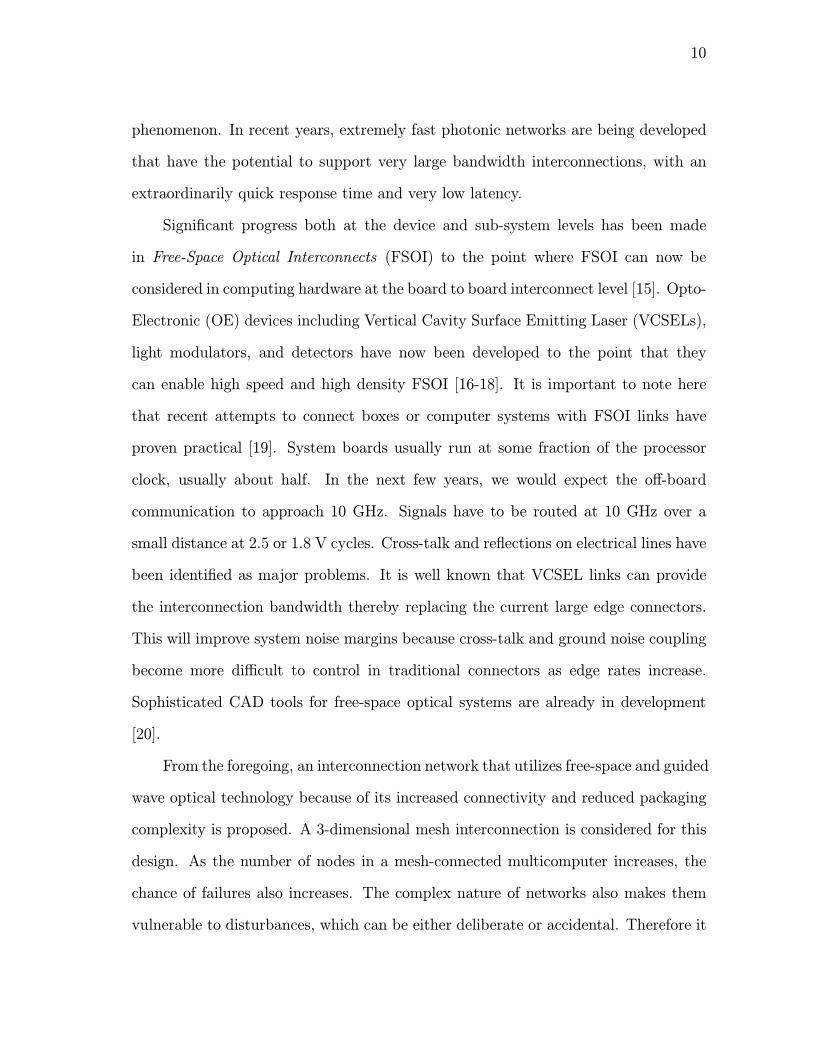
This chapter outlines an overview of the initial design of the extremely scalable su-
percomputer that has the potential to deliver in the order of petaFLOP performance,
mentioned in the previous chapter. The design takes advantage of free-space opti-
cal technologies, harnessing the features inherent in optics, to produce a 3D stack
that implements efficiently a large, fully connected system of nodes forming a true
3D mesh. Each node is a complete computer system with both compute and stor-
age units, and six communication interfaces to the optical medium. This packaging
greatly improves density and communication performance. The system is designed to
allow failed nodes stay in place without appreciable performance degradation. The
case study for 100 teraFLOP performance is investigated in detail and a descrip-
tion of the characteristics of the proposed hardware used for the design. Results on
performance based on the implementation of an important algorithmic kernel and
simulation results comparing two approaches in the optical interconnection design
will be presented.
A. Basic Architecture
The architecture encompasses a 3D optical interconnection network. The basic node
architecture has the capability to circumvent the need for optical-electrical-optical
OEO conversion at the node-to-node interface. In the next subsection, the structure
of the basic building block and the issues relating to the implementation are presented.
This 3D structure is a true mesh with each node connected to six nearest neighbors.

16
Fig. 1. Diagram showing basic node structure with FSOI couplers capable of gigahertz
communication
1. Basic Building Block
The basic design takes advantage of free-space optics technology to produce a fully
connected scalable node unit. The following design concept is strictly adhered to; high
density and low packaging complexity, reliable, low-cost yet powerful, and above all a
robust interconnection network. A root cause for the staggering difficulty of managing
large systems is the proliferation of too many building blocks such as processors, disk
arrays, switches, communication protocols, etc. [41]. Accordingly, this has lead
to combinatorial explosion of complexity. In this design, encapsulating complexity
within the basic building blocks or nodes controls this explosion. These nodes have
well defined hardware and software interfaces. The basic shape of our node is a cube
with six sides.
Figure 1 shows the basic node structure in our design. All nodes have six sides
as in a cube structure. On each side is an optical coupler capable of gigahertz com-
munication. Internally, each node consists of 8 multiprocessor units coupled to the
optical highway as shown in Figure 2.
Each node consists of 8 CMOS PEs with optical trasmitters and receivers as
the only means of external high-speed data communication. Each PE in the node
has its own local memory. Packets passing through a node can be transparent to
the electronic components and as such routed by the optical switch without any

17
Fig. 2. Diagram showing logical interconnection within each node
OEO conversions. Each processor unit is interfaced with optical transmitter/receiver
modules and attached wave guide for inter-processor data transfer. The wave guide
provides single hop inter-processor communication. The wave guide is then coupled
to an 8-port optical switch. This switch routes data to the respective node interface
coupler for external node communication. The destination address for a data transfer
is decoded in real time. Using n distinct wavelength (n colors), each processor is able
to transmit to and receive from all other processors in the node. WDM techniques are
employed for inter-processor communication within a node. Each CPU is assigned a
unique transmitting wavelength λn.
Figure 3 is a schematic of the design concept of each processor. Each PE in-
cludes two CPUs with L1 and L2 cache connected by a high-speed multiport optical
switch. The switch connects to an on-chip shared L3 cache and multiple high-speed
optical ports. The thermal management of the electrical CMOS and optical ports are
separated. The optical port interfaces, decode and multiplex signals for all-optical
routing. The interface consists of low-power VCSEL transmitters, photodetector re-
ceivers and the optical interface. Each optical port is capable of sustaining 40GB/s
(320 Gb/s) data throughput in each direction. Each PE has 8 of such optical ports.
One is dedicated to local main memory, another for inter-chip communication and
the remaining six are for external IO.

18
Fig. 3. Schematic diagram of each PE
As mentioned earlier, encapsulating complexity within the basic building blocks
or nodes controls the combinatorial explosion of complexity. The scalability of the
system is depends on availability of network bandwidth. The bisection bandwidth of
the 8-port optical switch in each PE is 640 GB/s (5.12 Tb/s). The result of this design
is a set of high-performance encapsulated processors serviced by high-bandwidth optic
interconnects that form the basic building block of the 3D system.
2. 3D System
As stated earlier, each node is made up of 8 PEs all connected via guided, planar
optical interconnect. The nodes need to communicate with each other, other nodes
and also with the external world. Two very important considerations in a design
of this nature are power and cooling, however, these will not be discussed in this
dissertation, as it is beyond the scope. A network which links all the nodes into a
true 3D mesh realizes the communication is shown in Figure 4.
This physical architecture leads to very high system density. An important in-

19
Fig. 4. 3D 4x4x4 mesh interconnection network using optical interconnect
novation is the elimination of cables and connectors, and instead substituted with
free-space optical couplers. This undoubtedly leads to remarkably improved commu-
nication hardware cost/performance (magnitudes greater than 100 Gb/s per interface)
compared to conventional, centralized switch solutions. This architecture is able to
scale extensively while delivering a large amount of bandwidth. It is important to
emphasize that the quest for teraFLOP computing begins by solving the scalability
and bandwidth issues.
Recall that each processor unit has 6 optical ports for external communication.
Each of these ports is capable of sustaining 320 Gb/s data throughput in each direc-
tion. Each of these ports is also optically coupled to the specified node interface. The
free-space optical coupler attached to each face of the node is capable of sustaining 40
GB/s (320 Gb/s) data throughput in each direction. If we assume the communication
frequency fc for each PE is about 1GHz (2 Gb/s). The guided planar optical intercon-
nect should be able to sustain 16 Gb/s data throughput in each direction. Similarly,
each node optical interface has to sustain this data rate. Obviously, this is quite lower
than the capacity of the interface and indeed the guided planar optical interconnect.
The number of processors in a node can be increased up to the bandwidth capacity
of the inter-processor link. However, due to power and thermal considerations, there

20
will be a limit to how many processors can be packed in a certain volume of space.
B. 100 TeraFLOP Performance: A Case Study
Innovative circuit design using 0.1-m CMOS technology have produced clock speeds in
GHz. The resulting peak performance of a single processor is about 10 gigaFLOPS.
Thus for 100 teraFLOPS performance, we need approximately 10,000 processors.
Each node in our design with multiple processors is capable of peak performance
n10 gigaFLOPS, where n = 8, we have 80 gigaFLOPS. For such massively parallel
systems to be viable, the physical volume and the size must be reasonably small. In
addition, the communication capabilities should match closely those of computation.
In order words, I/O performance should not be the bottleneck that affects the overall
performance of such systems. It was stated earlier that the use of optics and optical
technology will certainly increase the bandwidth potential but also eliminate the need
for wire. This leads to a dense array of processors in a very small volume, precisely
what we want to achieve. The system thus far described, is also scalable in both
architecture and optical technology based on the values stated, and therefore further
performance improvement is possible, should the need arise. An n x n x n 3D mesh
has a total of 8n3 processors. Since each processor is capable of 10 gigaFLOPS, to
achieve 100 teraFLOPS or more we need at least 10,000 processors. This gives a
value of n = 11. In the next few subsections, the feasibility analysis for the optical
components in this design is undertaken.
1. Feasibility Analysis for Optical Components
The analysis is done for the 3D mesh architecture made up of 1331 (11 x 11 x 11)
nodes. This gives a performance of roughly 106.5 teraFLOPS. The optical link an-

21
VCSEL array Transmitter lens
Free-space
Receiver lens PD array
Opto-mechanicalComponents foralignment
PML array
Node interface
VCSEL array Transmitter lens
Free-space
Receiver lens PD array
Opto-mechanicalComponents foralignment
PML array
Node interface
Fig. 5. Optical link assembly with built-in redundancy
alyzed is integrated in a bi-directional free-space interconnect between two adjacent
faces of two nodes, separated by a distance ranging from 0 to 25 cm. This system
is able to sustain a 1-mm lateral misalignment, and a 10 angular misalignment be-
tween the adjacent faces. The system uses VCSELs arrays and photodetectors (PDs).
The design incorporates optical coupler interfaces, transmitters/receivers, power con-
sumption, and the optical planer wave-guide.
a. Free Space Optical Coupler Interface
As stated earlier each FSOI is capable of sustaining 320 Gb/s. FSOI can provide high
bandwidth with no physical contact, however it suffers from poor tolerance to mis-
alignment. Therefore, a key implementation objective is to use an active alignment
scheme in conjunction with an optimized optical design. The optical link is imple-
mented using both passive and active alignment techniques. The system is aligned
mechanically under no lateral misalignment. When misalignment is introduced, re-
dundancy is used to guarantee proper optical performance. A schematic of the optical
link is shown in Figure 5.

22
b. Optical Transmitters/Receivers
The optical system provides a maximum power coupling efficiency between a (2 x
4) array of single-mode 960-nm 3-m diameter VCSELs with 250-m pitch, and (2 x
4) array of 70-m diameter PDs with a 125-m, under any degree of lateral or angular
misalignment within the specified limits. Each VCSEL in the array emits -2.22 dBm
of optical power. In [14], the performance of single- and multimode VCSELs intended
for high capacity free space optical interconnects at 10 Gb/s is presented. The receiver
sensibility at about 2 Gb/s results in a requirement of at least -25 dBm of optical
power. The optical link system for the transmitter consists of a planar microlens
(PML) array to collimate the VCSELs and a macrolens to relay beams. The receiver
part of the link uses only macroptics.
c. Power
As already mentioned each VCSEL in the array emits -2.22 dBm of optical power.
Each node transmits information to each of the 1330 other nodes in the system via
approximately 48 = (6 x 8) dedicated VCSELs, and radiates, on the average, 1330 x
48 x -2.22 dBm = 14W of optical power.
d. Guided Planar Optical Interconnect
Plastic optical fibers (POFs) are used as the optical pathways within a node. POFs
are preferred over glass fibers because of their lower cost, their smaller bending radius
and their large numerical aperture (NA). The pitch of the POFs is designed to match
that of the active devices (250-m). These optical pathways have been fabricated using
Toray’s PGR-FB125 fiber. In [15], an interconnect demonstrator using multimode
POF fiber ribbon is presented. The fiber is butt-coupled to the VCSEls and detectors.

23
The light from each processor is coupled into the POF.
To connect all the PEs, an (8 x 8) POF arrays (pitched at 250 mm in the two
dimensions) is developed. The optical pathways for connecting the different PEs
have been fabricated. They consist of two arrays of (8 x 8) POF ribbons. The optical
pathway in GigaLink uses an approach where 1-D arrays of POF-fiber plates are
stacked, which makes it easier to manufacture.
C. Analysis of the Optical Interconnection Network
This section presents some results of the analysis, simulation, and feasibility study
for the optical interconnection network of the design.
1. Modeling the Free-space Optical Interconnect
Contrary to the guided-wave approach, where the diameters of the POFs limit the
maximum channel density of the optical intra-MCM interconnects, the free-space
bridge has the advantage that there are no major technological fabrication limitations
for small lenslet diameters at different focal lengths. The only design consideration
is to make the diameters of the lenslets smaller than the channel pitch. This means
that the free-space approach has the potential advantage of being scalable because
lower lens diameters imply higher channel densities and consequently higher total
throughputs. The minimum lens diameter for each interconnection length L, will
be determined by the diffraction of the VCSEL beam, which has a waist w0 and a
divergence θ. From the minimum lens diameter we can then calculate the maximum
channel density as a function of the distance traveled in the optical path box (OPB),
assuming that the pitch of the channels equals the lens diameter.

24
a. Cross-talk and Transmission Efficiency
Assume that in the middle of the OPB (at z = 0) the beam waist is w’(0)= w’0 then
the beam radius at the lens (z = Lmax/2 = L) is given w’(L) = w0 1 = λ2L2
π2w 40.
Now apply the rule that the laser beam must always be smaller than 2/3 of the
lens diameter so that more than 99% optical energy throughput through the lenses is
achieved and cross-talk is absent in the system, we also have that w’(L) = θlens3and
L = πλ
w 20θ2lens
9− w 4
0.
Calculate the beam waist w0 such that the optical interconnection distance L is
maximum. For δLδw0
= 0 we find w0 =θlens3√2and Lmax = 2L =
πλ
θ2lens9So due to diffraction
of the laser beam the minimum lens diameter θlens lens for an interconnection length
L is limited to
θlens3λ
πLmax (2.1)
b. Bit Error Rate
The bit error rate (BER) indicates the required source power and signal-to-noise levels
necessary to achieve a desired signal fidelity, and represents an important measure of
system performance. With Gaussian statistics we find that the probability of error
(PE) is given by
PE ≡ 1
(2πQ)1/2e−Q
2/2 (2.2)
where Q is a normalized number that qualifies the quantity of the current signal.
To achieve a BER of 10-17, Q = 8.5.

25
Fig. 6. Channel density as interconnection length is increased
c. Simulation Results and Discussion
Figure 6 shows calculated results for the allowed channel density as a function of
the interconnection length in the design using an 8 x 2 array of VCSELs. Using
the earlier derived expression (1), the minimum lens diameter to achieve at least
99% transmission efficiency while avoiding cross-talk is approximately 130 μm with
wavelength (λ = 960 nm).
Next, the transmission efficiency of the optical interconnection system (the ratio
between the powers of the emitted light and the light impinging on the detector area)
is calculated for different focal numbers of the lens and for different working distances
between the sides of two adjacent communicating nodes. The results are shown in
Figure 7.
The angular tilt of the optical beam presents a major constraint in our design.
Proper alignment of the optical system is of utmost importance. A value of 0.10
optimizes the system, whereas a larger angular tilt will require an increase in the lens
radius, and other system dimensions as a consequence. It is impractical to compensate
for the tilt by increasing the laser power due to the exponential nature of the curve.
In Figure 8, the BER for a laser power of 5mW as a function of the angular tilt

26
Fig. 7. Transmission efficiency of the free-space of lens with different focal numbers
is shown, while the BER as a function of laser power is shown in Figure 9. Some of
the optimized parameters in the design are shown in table I.
0
-10
-20
-30
-40
-500.1 0.12 0.14 0.16 0.18
Angular Tilt (degrees)
Log
10(B
ER
)
0.08
0
-10
-20
-30
-40
-500.1 0.12 0.14 0.16 0.18
10
0.08
0
-10
-20
-30
-40
-500.1 0.12 0.14 0.16 0.18
Angular Tilt (degrees)
Log
10(B
ER
)
0.08
0
-10
-20
-30
-40
-500.1 0.12 0.14 0.16 0.18
10
0.08
Fig. 8. The plot of BER as a function of the angular tilt
2. Modeling the POF Guided Planar Optical Interconnect
For modeling purposes, the interconnection block is schematically divided into two
main parts: the emitter side and the receiver side. This allows one to investigate the
two optical sub-systems on efficiency, cross-talk and tolerances individually. Listed
in table II, are the parameters that affect the cross-talk and the efficiency. The
characteristics of the VCSEL sources and of the InP photo-detectors can also be

27
Fig. 9. The plot of BER as a function of the laser power
found in table II. Considered here are small diameter POFs with a core diameter of
120 m and a device pitch of 250 m.
Table I. Optimized Parameters
Maximum efficiency % 98.7
Focal number 2.9
Propagation distance (μm) 1550
Allignment tolerance (degrees) 0.1
Reflective power loss (dB/cm) 0.25
Wavelength (μm) 0.96
Detector diameter (μm) 130
Q parameter of receiver 8.5 for a BER of 10−17
RMS current noise by receiver (nA) 789.6
a. Cross-talk and Transmission Efficiency
It is important to derive an analytic expression for the maximum working distance
Lmax from the emitter or receiver to the POF, below which no cross-talk between
neighboring fibers will occur. Lmax is given by 2.3 at the emitter side and by 2.4

28
Table II. Characteristics of Sources/Detectors
VCSEL POF Detector
Substrate thickness (μm) 150 150
Diameter (μm) dsource = 7 120 ddet = 75
NA θFWHM = 12o 0.25
Pitch (μm) 250
Working distance L L
at the receiver side. Here θ represents the divergence angle θFWHM of the micro-
emitters as long as θFWHM is smaller than the acceptance angle of the POF. If the
latter condition is not satisfied θ takes the value of the acceptance angle θPOF of the
POF:
Lmax =P − d source
2− D
2
tan θ(2.3)
where dsource = dsource + 2T tan(arcsinsin θFWHM
ηGaAs)
Lmax =P − d source
2− D
2
tan θPOF(2.4)
where dsource = dsource + 2T tan(arcsinNAηInP
)
where, P = pitch of the devices, ddet, dsource = diameter of the active area of the
detector and source, D = diameter of POF, NA = numerical aperture of POF, θPOF
= acceptance angle of the POF, T = substrate thickness, ηGaAs, ηInP = index of
refraction, θFWHM = FWHM angle of the emitter
and
θ = θPOF if θPOF > θFWHM
θ = θFWHM if θPOF < θFWHM

29
To study the transmission efficiency of the POF-based interconnect as a function
of the working distance L, both the emitter and detector module via ray tracing and
radiometric calculations, are simulated using the photonics design software SOLSTIS.
When simulating the emitter side, the VCSEL is modeled with a user-defined source
featuring a circular geometry with a uniform emittance distribution. The assumption
is made regarding the intensity to have a revolution angular distribution. A Gaussian
angular intensity distribution is also assumed. Next, the coupling efficiencies of both
sources for the different POFs are calculated. In a next step the receiver side is
simulated to calculate how much of the light emerging from the POF impinges on the
detector area. Here again, a user-defined source models the light that is coupled out
of the POF. Multiplying the values of the coupling efficiencies of both the emitter and
receiver side for an identical working distance L then gives the transmission efficiency
of the optical interconnection system for this working distance.
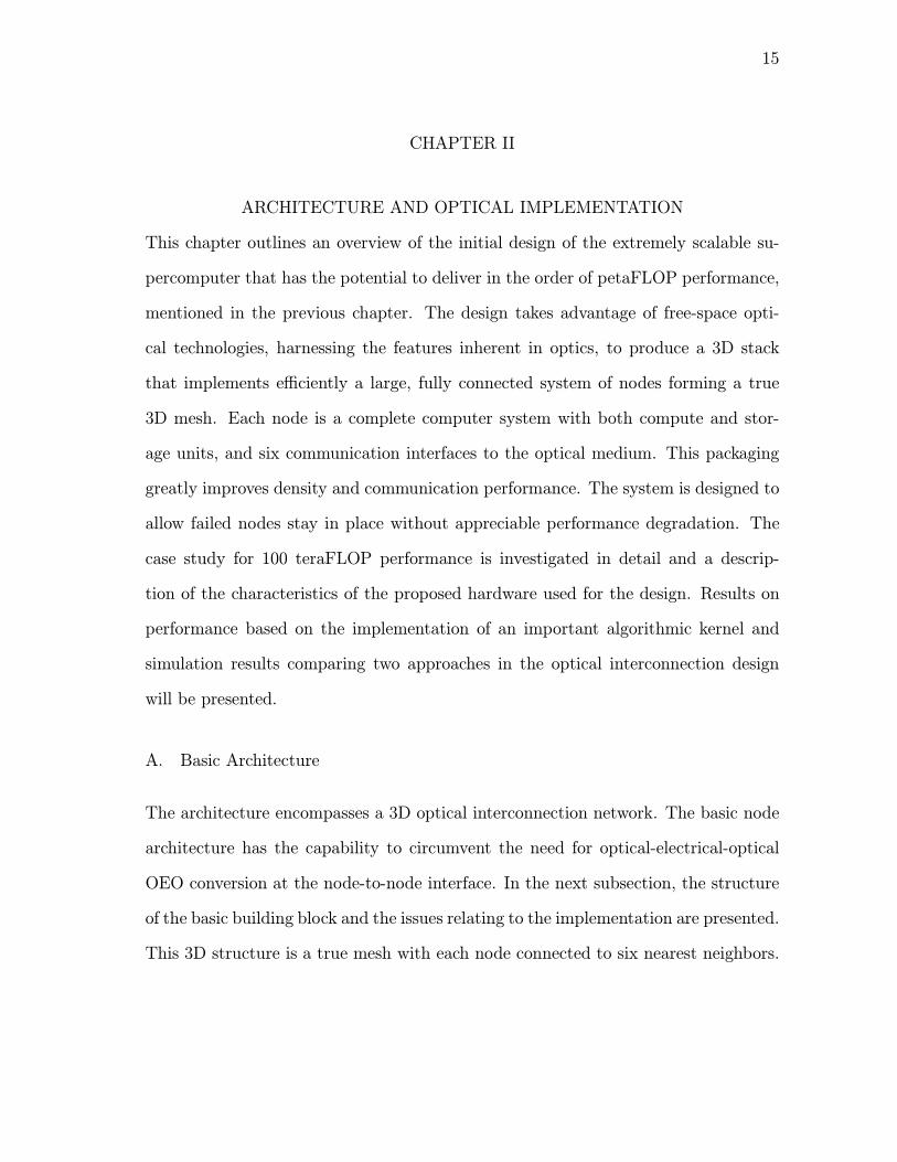
b. Simulation Results and Discussion
Figure 10 shows the results of the transmission efficiency for two combinations of the
diameter and the NA of the POF as a function of the distance between the POF and
the emitter or receiver.
Observe that the NA of the fiber used does not affect the coupling efficiency at
the emitter side because of the small divergence angle of the laser. This means that a
fiber with a smaller NA and diameter can be used with the result being an improved
coupling efficiency at the detector side and a more relaxed cross-talk condition.
30
Fig. 10. Transmission of the POF based guided-wave interconnect using a VCSEL
D. Performance Evaluation
In evaluating the performance of this design, the communication and computational
capabilities of the system is investigated. The relative raw bandwidth available to
the network links in the context of the network topology. The later is achieved by
comparing the single-hop and the multi-hop modes of communication. In the single-
hop approach, the signal in the communication link between source and destination
remains in the optical domain, while in the multi-hop case, the signal undergoes
optical-electrical conversion and vice versa at the intermediate nodes between source
and destination.
1. Implementation of Compute/Communication Intensive Algorithm
The efficient implementation of application algorithms on the proposed system is vital
for its success. A kernel frequently encountered in scientific codes is used to examine
the performance of the design. Some of these computation kernels include; SAXPY,

31
A(N,N,N), B(N,N,N)do K=2,N-1do J=2,N-1do I=2,N-1A(I,J,K) = C*(B(I-1,J,K)+B(I+1,J,K)+
B(I,J-1,K)+B(I,J+1,K)+B(I,J,K-1)+B(I,J,K+1))
A(N,N,N), B(N,N,N)do K=2,N-1do J=2,N-1do I=2,N-1A(I,J,K) = C*(B(I-1,J,K)+B(I+1,J,K)+
B(I,J-1,K)+B(I,J+1,K)+B(I,J,K-1)+B(I,J,K+1))
Fig. 11. Jacobi iteration
Large Stride Vector Fetch and Store, Irregular Scatter/Gather, 3D Jacobi Kernel, 3D
Jacobi Kernel with large local computation, and Tree-matching.
The 3D Jacobi kernel which is a class of kernels known as Edge-based “stencil-
op” loops shown in Figure 11. These kernels are characterized by large ratio of
work to data, and colored edge concurrency (local communication). The potential
architectural stresspoints are the inter-node bandwidth and the load/store bandwidth.
For the implementation, let n = 108.
The 3D Jacobi kernel with a problem size (N = 1000) is executed. This com-
putation is a convolution-and-reduction operation applied for all values of C for a
given A. The corresponding sum of B terms is computed only once for each A. The
number of iterations involving all indices I, J, and K is larger than the number of
PEs, so the loops are distrubuted among all the PEs. Thus, each PE performs ψ =
(10003/10648), which is approximately 93915 iterations involving these loops. For a
given (I, J, K), a PE performs:
• Five additions involving six elements from B, resulting in 5C additions
• One multiplication involving C, and one addition involving the result of themultiplication and the previous value of A(I, J, K). These are performed C2
times.
From the foregoing, each node performs a total of (5C + C )ψ additions and C2ψ

32
multiplications. Data transfer is facilitated by mapping the arrays A and B onto the
processors in our 3D mesh topology. This is achieved by partitioning the 3D (I, J,
K) grid for mapping onto the logical 3D mesh.
The execution time of the algorithm is given by
T = 2Tm + td + tc + (5C + 2C2)
ψ
5tc + td (2.5)
where tm is the inter-PE propagation delay (1/1GHz = 1ns), tc the CPU speed
(1/2GHz = 0.5ns), td the memory speed (1/1.5GHz = 0.67ns). The denominator is
the speedup resulting from using PEs with 5 FPUs. Assume C = 5, then the execution
time for the algorithm is T = 704.36 μs. The amount of parallelism available in the
algorithm is 10003 x (5C + 2C2) = 75 x 109 operations. The execution rate therefore
is 106.48 teraFLOPS, which is remarkably close to the peak rate of 106.5 teraFLOPS.
2. Comparing the Single-hop and Multi-hop Communication Methods
The aggregate bandwidth is defined as
B = LT [L
i=1
1
B(mi)]−1 (2.6)
where L = number of transceiver groups (each node has 6 groups), B(m) is the
bandwidth of a single channel, and T is the total number of transceivers. Each node
in the topology has 6 neighbors. Assume n = number of nodes, and use, L = Lsh = 6
to evaluate the single-hop bandwidth, while L = Lmh = 6+ 2(3√n− 1) for the multi-
hop bandwidth. The ratio of the single-hop bandwidth-per-link to the multiple-hop
bandwidth-per-link in the design is plotted and results are shown in Figure 12.
The ratio Lmh:Lsh is the idealized ratio where the aggregate bandwidth of the
interface is fixed. For small network sizes, the modeled ratios are relatively close to

33
0
2
4
6
8
10
12
14
16
18
020
040
060
080
0
Number of nodes
Rat
io o
f ban
dwid
th-p
er-li
nk (
sing
le-
hop/
mul
ti-h
op)
0
2
4
6
8
10
12
14
16
18
010
00-
--
-
Lmh :LshEqual powerEqual number
0
2
4
6
8
10
12
14
16
18
020
040
060
080
0
Number of nodes
Rat
io o
f ban
dwid
th-p
er-li
nk (
sing
le-
hop/
mul
ti-h
op)
0
2
4
6
8
10
12
14
16
18
010
00-
--
-
Lmh :LshEqual powerEqual number
Lmh :LshEqual powerEqual number
Fig. 12. Ratio of single-hop to multi-hop raw bandwidth-per-link against network size
for a 3D mesh
the Lmh:Lsh, however, as the network size increases, the three curves begin to deviate
quite clearly. The single-hop performance is better than that of the multi-hop case
due in part to the difference in the number of links that share each optical interface.
To summerize, the design described so far is suitable and feasible for very high
performance computing. The system is characterized by immense bisection band-
width, scalabilty, and low interconnect complexity. This design meets all the per-
formance objectives earlier on outlined. The design is able to control combinatorial
explosion of complexity by encapsulating complexity within the basic building blocks
or nodes. Optical interconnection will be an inevitable solution to the bandwidth
needs anticipated in the quest for petaFLOP performance. Analyses of the optical
interconnection network as well as performance result for an important algorithmic
kernel were employed to further support the claim that this design achieves outstand-
ing performance.

34
CHAPTER III
ALL-OPTICAL ROUTING
In large multiprocessor systems such as massively parallel computers, interprocessor
communication is increasingly becoming the bottleneck that limits the performance
of such supercomputing systems [42, 43]. In recent years, extremely fast photonic
networks are being developed that have the potential to support very large bandwidth
interconnections, with an extraordinarily quick response time and very low latency
[44, 45]. To adapt such photonic networks for use in multiprocessor systems, routing
schemes that do not require sophisticated processing of the optical data is required.
In this chapter, a novel self-routing technique for all-optical packet switched net-
works for the multiprocessor system presented in Chapter II, with real-time processing
of the header is introduced. In Chapter II, a 3-D hierarchical regular topology was
proposed. This type of topology results in a greater degree of freedom in design and
a relaxation of the design constraints thereby achieving better routing performance
as shown by results. The approach discussed in this chapter aims at resolving con-
tentions at the nodes, eliminating the need for buffering in the optical domain and
reducing the overhead associated with address decoding. The scheme is designed to
support point-to-multicast transmissions.
The proposed scheme also eliminates the need for lookup tables. Despite the fact
that memory requirements for a lookup tables is no longer of major consequence, even
for a network of significantly large number of nodes, this can have significant effect
in an all optical type network. This arises from the fact that, at each intermediate
node, an OEO (Optical-Electrical-Optical) conversion has to be performed in order to
carry out the lookup operation to determine the next hop. The conversions that have
to take place at each intermediate node will undoubtedly degrade the performance,

35
defeating the goal of using optics.
Optical logic is still in its infancy and so designs that involve complex logic in
decoding header information will not achieve the expected improvements in routing
performance. The goal is to harness the features inherent in optics in the design to
achieve decoding, data directional capability and contention resolution in real time.
In this design, the need for optical buffering is eliminated, which is clearly unsuitable
for large multiprocessor systems, by aggressively reducing the probabilities of data
contentions and unavailability of outgoing links at each intermediate node.
Multicasting without packet replication is done, by encoding in the header the
routing that services the multicast group. This technique is unique to this design
and demonstrates the dynamic nature of this self-routing scheme. In summary, this
is a network that is self-routing, all optical in nature with no optical buffers, is
hierarchical with a 3-D structure, and is able to route data without OEO conversions
in real time. The network has a distributed control and supports point-to-multicast
communication. This design will find applications in massively parallel machines,
neural networks, optical and quantum computing, network servers and local Area
Networks (LANs) just to mention a few.
A. The Self-routing Scheme
In the scheme, the path between two nodes is provided with an alternative path.
These two paths can be switched back and forth depending on the availability of
output links at each intermediate node. An address encodes a unique path from
source to destination. For each node, three situations are observed when a packet
reaches that node. The packet is (1) destined for the node, (2) not destined for the
node, or (3) destined for the node and also other nodes (multicast group). In the

36
P (Preferred)
A (Alternate)
Intermediate nodes 1 2 n
+ + + + + + +- - - - - -
+ + + + + +- - - - -- -
. . .
Fig. 13. Two field address structure
first case the address of the packet matches that of the node. In the second case
the packet address does not match that of the node. In the last case, the node
address is a member of the set of addresses encoded in the packet address. A packet
is encapsulated in layers of Address Markers corresponding to the action taken at
an intermediate node. After each marker is traversed, it is striped from the address
exposing the next marker. It becomes obvious that the last marker of a packet will be
the destination node or the last destination in a multicast group. Our scheme ensures
that the path chosen will traverse all the nodes belonging to a multicast group.
These markers may be defined on a per-destination basis, on a source/destination
pair basis, or on a per-flow basis. However, we acknowledge that being a self-routing
scheme, it is difficult to implement congestion control and traffic engineering. For
each destination address, each intermediate node has a preferred output link and an
alternative output link should the preferred link be unavailable. If an alternative
output link is taken, then the address markers have to change accordingly. In this
design, an address is made up of two fields as shown in Figure 13. At each node, the
preferred output link is always chosen. This corresponds to field P. If, however, an
alternative link A is taken then the field to which the link belongs to becomes the
preferred field P.

37
Fig. 14. A 48-node 3-D network
1. Node Structure and Address
The network considered consists of N nodes. The links associated with each node are
space invariant links and bi-directional. As an illustration, a 48-node network is shown
in Figure 14. As already mentioned, the address of the destination node(s) encodes
the routing instructions at each intermediate node. The address of a destination node
obtained from a source node may defer from that of another source node. This is
because the route to a node from two other nodes may be different. The process of
defining the address of a destination node or nodes can be divided into three sub-
problems.
The first sub-problem is to determine the intermediate nodes needed from source
to destination(s). The second is to determine the primary outgoing links at each
intermediate node. Assume that for a source-destination pair, the shortest path is
chosen. This means that the destination address has to encode information about
the intermediate nodes and the outgoing link in each node in the shortest path. The
intermediate links for a source-destination pair can be found by running Dijkstra’s

38
To lower plane
To Upper plane
To nodes on the same plane
Fig. 15. The node structure
shortest-path algorithm. For multicast packets, a number of path routing algorithms
are available. However, the constraint lies in not having the header extremely large
or complicated, and considering only optical real-time decoding with small overhead.
Either a Minimum Spanning Tree (MST) or a Minimum Rectilinear Steiner Tree
(MRST) approach can be adopted in determining the intermediate nodes and outgo-
ing links. Thirdly, deflection alternative(s) have to be established at each intermediate
node. This process has to be done such that loops are avoided. In [46], an algorithm
for loopless deflection is studied and presented.
Figure 15 shows the node structure considered. As already mentioned this self-
routing scheme should support a 3-D structure. Each node is represented by a three-
turple N(i,j,k). The subscripts i and j identify a node on a plane, where i represents
the row index and j represents the column index. Subscript k, is associated with
the plane number. On a plane, a node has four bi-directional links. Two links are
available for communication across planes. Incoming packets have three options for
outgoing links. The packets can either (1) remain on the same axis as the entry, (2)
move along a perpendicular direction along the horizontal plane or (3) move along a
perpendicular direction in the vertical plane. An illustration is shown in Figure 16.
A destination address basically represents an action taken at each intermediate
node. The action taken directs a packet to the appropriate output link. A node

39
(1)
Axis of entry
(2)
(3)
Y-axis
Z-axisX-axis
HorizontalPlane
VerticalPlane
Fig. 16. Diagram to illustrate output link options
knows that the packet has arrived at the destination if no further action is to be
taken in the case of a unicast packet. This means that the structure of an address
for a packet while remaining unchanged throughout the transport process will illicit
different actions at different nodes. The action is processed in real time. The node
identifies an address and on the fly directs the packet to one of its output links. If
the primary link is unavailable, the alternate link is chosen.
2. Routing
When a packet arrives at a node prior to the transport over the network, the processor
identifies if the packet is a unicast or multicast packet. If it is a unicast packet, the
processor runs the shortest-path algorithm to establish the primary and alternative
routes at each intermediate node. This information is then encoded and attached onto
the header. The header will typically precede the payload. As already mentioned,
the address of the destination will encode routing instructions at each intermediate
node. For a multicast packet, the processor runs either the MST or MSRT algorithms
to establish the primary and alternative routes as before. Consider the transmission
of a packet from node A111 to node B232 illustrated in Figure 17.
As shown in Figure 17, there are a number of shortest paths from node A to node

40
(111)
(112)
(212)
(222)
(232)
(132)
(122)
(121)
(131) (231)
Fig. 17. Data routing illustration
B. From the figure, node A has a choice of three outgoing links that would satisfy
the shortest path condition. Shown are three of the paths that have exclusive links
from source to destination. Any of the paths is chosen at random as the primary
route. The alternative route is established on a node by node basis depending on the
primary path chosen. At each intermediate node, an alternative output link is chosen
should the primary link become unavailable at an intermediate node. Consider that
path (111-112-122-132-232) is chosen as the primary path P. The processor chooses
an alternative link that still satisfies the shortest distance condition on a node by
node basis. It does this by routing the packet to a nearest node belonging to one
of the earlier established shortest routes from source to destination. So in this case,
if the primary outgoing link in, say, node 112 is not available, then the packet is
routed to node 212. Node 212 belongs to path (111-211-212-222-232). In a likewise
manner, if the primary outgoing link in node 132 is not available, the packet is routed
to node 131. At the least, two additional intermediate nodes are traversed if the
outgoing link between an intermediate node and the destination is unavailable. It is

41
P (Preferred)
A (Alternate)
Intermediate nodes 1 2 n
112 232132
131 231212 222 232
. . .
122
232
Fig. 18. Packet address illustration
worth mentioning again that looping and backtracking are not allowed in this scheme.
From the foregoing the address from node 111 to node 232 is shown in Figure 18.
As shown in the diagram, the address is obtained by providing an alternative
outgoing link for all intermediate nodes in the preferred path.
B. Optical Implementation
Optical implementation of our routing scheme is based on the following:
• Ability to decode optical data in real time
• Data directional capability and
• Contention detection/resolution.
Each node has an array of six receivers corresponding to the six available output
links. These receivers are tuned to six different wavelengths with no tuning capabil-
ities. The receiving node is able to receive messages simultaneously on all six links.
Each node also has a tunable transmitter, able to tune to all six wavelengths. The
wavelengths are not exclusively associated with a particular output link. Wavelength
Division Multiplexing WDM scheme to be applied with our self-routing method has
been extensively researched and as such will not be discussed here, due to the space
limit.
Recently, a demonstration has been done of address header decoding using an
erbium doped insulating crystal (Er:YSO) [47]. The crystal was programmed to recog-

42
Er:YSO
Crystal
Primary (A)AddressPulse
Alternate (B)AddressPulse Primary (A)
DirectionPulse
Alternate (B)DirectionPulse
XA
Xadd
XB
Er:YSO
CrystalXH
Header Encoded withPrimary Address
Header Encoded withAlternate Address
Er:YSO
CrystalStimulated Echo
Stimulated Echo
ASEX
BSEX
XA
XA
XB
XB
(a)
(b)
(c)
Fig. 19. Temporal snapshot of (a) programming (b) & (c) processing stages
nize biphase-coded address headers and to decode an arbitrary sequence of headers.
This result is spatially discriminated optical output pulses. Each of these output
pulses in turn is used to route the combined header and data packet in real time. Ac-
cording to [47], the address header decoding was performed in two stages. The first
stage involves programming the crystal with a distinct spatial-spectral holographic
grating for each address header by the application of a pair of optical programming
pulses. An illustration is shown in Figure 19. This grating is stored utilizing the
absorption property of the Er:YSO spectral hole-burning material. It is worth men-
tioning that independent gratings at other adjacent wavelengths in the absorption
profile can be stored with the application of wavelength division multiplexing.

43
The second stage involves header processing. The headers are propagated along
the normal direction, where each header generates stimulated photon-echo output
signals following interaction with each stored grating. The direction of each combined
header and data is predicted by the phase-matching conditions
This is illustrated in Figure 20. The shape of the simulated echo is determined
by the cross correlation of the header pulse with the convolution of the address and
direction-programming pulse stored in each grating.
ASEX
BSEX
XH
-Xadd
-Xadd
XA
XB
Fig. 20. Phase matching diagram
C. Analytical Model
A theoretical model for evaluating the performance of the network is proposed in this
section. In [48-50], results were obtained for queuing-based models of regular network
topologies. While these present an insight to the problem dealt with the design of
the network considered here, they are not applicable being that the network attempts
to eliminate message buffering. The objective is to come up with some method of
determining the maximum throughput achievable under uniform load, the average
number of hops made by a packet from source to destination, and the packet loss
probabilities.

44
1. Average Packet Hop Count and Throughput
Assume that all links are similar and are accorded equal status. Assume also that
traffic generation follows a Poisson process. The packets are considered to be all of
the same size, that is, of fixed length t seconds. The arrival rate is defined as the
average number of packets that enter the network in a unit of time. In a network of
N nodes, the total number of links N x L, where L represents the number of incoming
(outgoing) links per node.
The performance of the network depends on the availability of outgoing links.
Therefore a very important consideration is how busy a link is, or put in other words,
the probability that a link is not available as an outgoing link. If δ is defined as
the average number of links traveled by a packet from source to destination, the
probability that a given link is not available is described by the following relationship:
P(prob)αδλ
NL(3.1)
P is the same for all the links because the network is regular, and the aim is to
derive a method of calculating δ as a function of P and by further solving a system of
equations, derive δ as a function of λ. Since the routing decision at any intermediate
node does not depend on the routing history of the packet, the routing operation can
be taken as an element in a Markovian chain. Suppose Nd denotes the destination
node, then the expected number of intermediate nodes to be traversed from a certain
node Ni on its way to Nd is Ei.
Ei = 1 +L
j=1
PjEXj (3.2)
where Pj is the probability that the packet will be routed via the output port j,
and xj is the index of the link connected to Ni via that port. The probabilities Pj

45
are determined by the routing function at the source node Ns. The average number
of links traversed by a packet in the network with N nodes can be calculated given
the values E1,..., EN−1 as:
δ =N−1i=1 Ei
N − 1 (3.3)
The three equations generated so far can be solved in an iterative process to
obtain δ as a function of λ. The procedure is as follows:
1. Set P = 0.
2. Solve the linear set of 3.2 to calculate E1,..., EN .
3. Calculate δ using 3.3
4. A new value for P is obtained from 3.1, go back to 2.
In step 3, a sequence of δi’s is generated for the approximations of δ. The
implication here is that if the sequence converges then it means that λ is below the
saturation point and that
δ = limx→∞ δn (3.4)
This then gives the average packet hop count. In calculating the maximum
throughput achievable, note that the number of inputs/outputs at the node (d = 6).
Define U as the link utilization, then the admissible load at each node is given by:
λaccept =dU
δ(3.5)

46
2. Packet Loss Probability
In evaluating the packet loss probability, note that the network is asynchronous. The
arrival rate λijk of the packets traversing a particular link λijk is a summation of all
the packet arrivals that will pass through the link λijk. The arrival rate also depends
on the Pijk. The probability that a packet encounters contention at link ijk is equal
to the probability that the link is busy:
Pijk =t
E[T ](3.6)
where E[T], the expected cycle time, between two consecutive packet departures
is found by adding the expected time till the next packet arrival with the expected
packet transmission time:
E[T ] =1
λijk+ t (3.7)
According to this implementation, the following types of links depending on
whether the link is on the primary path from source to destination(s) or is an alternate
link to the destination:
1. Link lsp is on the primary path and is directly connected to the source, in which
case the arrival rate is lsp.
2. Link lip is on the primary path but is not directly connected to the source, in
which case the arrival rate is lip consisting of all the packets directed through
that node.
3. Link lsa is the alternate link for the primary link and is directly connected to
the source, in which case the arrival rate is λsdPsd, Psd being the probability
that the packet experiences contention at the source node.

47
4. Link lia is the alternate link for the primary link and is connected to an in-
termediate node, in which case the arrival rate is λia, made up of all the load
experiencing contention in the primary link.
From the foregoing, a number of equations to determine the arrival rates for each
node and hence Pijk can be derived.
λTotal = λsp (lijk = lsp) (3.8)
λTotal =i
λip(1− Pip) (lijk = lip) (3.9)
λTotal =i
λip(1− Pip) ((lijk = lia (lijk = lsp)) (3.10)
λTotal = λsaPsp (lijk = lsa) (3.11)
λTotal =i
λip(1− Pip)Pid ((lijk = lia (lijk = lip)) (3.12)
The packet loss probability is a measure of the performance of the network. A
packet is lost if both the primary and alternate links are not available. Consider the
transmission of a packet from source to destination, two routes can be distinguished,
a primary route and the alternate route. Therefore, the packet loss probability is
given by:
Ploss = PspPsa + (1− Psp)Pip(loss) + Psp(1− Psa)Pia(loss) (3.13)
The equation above is for a source destination pair. We note that destination
here may refer to the last node in a multicast group. The total packet loss probability
for the system is found by taking an average of the packet losses for each such source-
destination pair.

48
10
1.5
2
2.5
3.0
3.5
4
Average Hop Count for 48 nodes
0.1 0.2 0.3 0.4 0.5 0.6 0.7 0.8 0.9 1
Load (Erlang)
AnalysisManhattan StreetProposed 3-D
Ave
rage
Hop
Co
unt
Fig. 21. Average hop count for 48-node network topology
D. Simulation Results
In this section, the self-routing method in the 48-node network topology shown in
Figure 14 is evaluated. The 3-D network consists of bi-directional links in which the
nodal degree is equal to six. The packets are assumed to have fixed lengths of 384 bits.
With a transmission rate of 10Gb/s, packet arrival follows a Poisson process, with
uniform traffic distribution over the entire network. We compare the results obtained
from analysis and that obtained using a regular Manhattan street architecture against
our proposed 3-D structure to show the performance of the self-routing scheme.
Figure 21 shows the average hop count as a function of load for a 48-node net-
work. It is observed that the proposed 3-D structure has better average hop count
performance than the Manhattan street topology. In Figure 22, the average hop count
for higher network loads in the 48-node network is plotted. For the Manhattan street
topology, as the load increases, the average hop count increases, indicating that more
packets are being deflected and successfully reaching the destinations. However, as

49
Fig. 22. Average hop count for 48-node network topology under higher loads
the load is further increased, deflection starts to lead to packet loss, and consequently
a drop in the number of successful packet transmissions. Hence, the average hop
count reduces. The proposed 3-D structure exhibits similar characteristics, however
there are more successful packet transmissions as the load is increased.
Fig. 23. Packet loss probability for a 48-node topology

50
Throughput (48 nodes)
Load (Erlang)
Thro
ugh
put
AnalysisManhattan StreetProposed 3-D
0 0.1 0.2 0.3 0.4 0.5 0.6 0.7 0.8 0.9 10
0.2
0.4
0.6
0.8
1
Fig. 24. Node throughput for a 48-node topology
Figure 23 shows the packet loss probability as a function of load. It is observed
that the 3-D structure offers significantly low packet loss probabilities than the Man-
hattan street network. It suffices to say that from the result, a higher nodal degree
means that more nodes have alternative link options. This is very important since
only loopless packet routing is considered.
Finally, in Figure 24, node throughput is shown as a function link utilization.
A maximum of 0.6 packet/time/node is obtained by analysis, while 0.67, and 0.74
packet/time/node are the corresponding maximums for the Manhattan street and
proposed 3-D structure respectively.
E. Conclusion
A self-routing scheme for an all-optical packet switched network has been introduced.
This scheme resolves contentions and avoids the need for optical buffers. Optical real
time header data processing is applied to reduce the overhead associated with address
decoding. The need for optical buffers is eliminated and while avoiding looping of

51
optical packets. A general analytical model, which can be applied to a wide range of
packet switched schemes and on a wide range of topologies, was developed to evaluate
our routing scheme. The scheme assumes that there is only one alternative link for
every primary link in the case of contention, however, this can be modified so that
more alternatives are established for each primary link at the time of address encoding.
More research would be needed to encode a large amount of information corresponding
to the different link alternatives without degrading the performance of the routing
scheme. It is shown that with a higher node degree, the self-routing scheme provides
better performance. Specifically, the 3-D structure provides lower average hop count,
lower packet loss probability and much better node throughput than the Manhattan
Street topology. At high loads, the 3-D structure appears to be more reliable in
successfully transmitting packets from source to destination in a loopless environment.
In this design, a network type more suited to high-speed multiprocessors is achieved.
The design is self-routing and all optical in nature. It circumvents the need for OEO
conversions, optical buffers and looping. The proposed design supports point-to-
multicast communication and provides real time optical header decoding. Lookup
tables are not needed to make routing decisions, while still achieving a distributed
control. In summary, this self-routing scheme achieves all the objectives set earlier
and provides the needed reliability and performance in high-speed multiprocessor
computing environment.

52
CHAPTER IV
MESSAGE SCHEDULING
Network performance for a single-hop WDM network deteriorates due to packet colli-
sions that occur in both source and destination nodes. These collisions can also occur
in both the control and data channels as in the case where reservation techniques
are adopted. In order to reduce these collisions and maximize bandwidth utiliza-
tion, an on-line scheduling method that can result in collision free communication
and achieve real time operation in high-speed multiprocessor systems is presented.
The method proposed can be easily adapted to other network types employing opti-
cal interconnects. A throughput analysis of the scheme is done using methods from
discrete-time queuing systems and use computer simulation results to compare the
different variations of the scheduling algorithm.
The message scheduling method outlined in this chapter, efficiently utilizes the
enormous bandwidth potential optical interconnects and Wavelength Division Mul-
tiplexing (WDM) techniques provide in computer network communication. This
method is unique because it allows the transmission schedule to be staggered in time
and space with provision for on-line packet arrivals and mixed packets types (unicast,
multicast and broadcast). It is topology independent. Access to each data channel
is controlled by a priority based cluster scheme that optimizes bandwidth utilization
while minimizing packet delay.
The basic idea of the proposed scheduling method is to show that the data packet
sequencing has a profound effect on network traffic performance and, surprisingly, it
has not received much attention. Accordingly, results show that efficient message or-
dering in the data scheduling stage of the Routing and Wavelength Allocation (RWA)
process, can better effectively utilize the enormous bandwidth potential available in

53
optics. These results consequently lead to a remarkable improved throughput perfor-
mance and lower average packet delay.
In this chapter, the problem of on-line scheduling of mixed packet transmissions
in single-hop Wavelength Division Multiplexing (WDM) multiprocessor systems is
examined, where for each node both the data receivers and transmitters are tun-
able. WDM is an effective way to utilize the large bandwidth of optics. In WDM,
multiple messages can be transmitted in parallel on separate channels. In single-hop
communication, all nodes can reach any other node directly. This means that the
transmitted data are not passed through any intermediate routing stages and remain
in optical form all the way from the source node to the destination node. Single-hop
architectures employing WDM [51-53] have been proposed thereby.
To take advantage of the enormous potential of single-hop WDM networks, effi-
cient access protocols and scheduling algorithms are needed to allocate and manage
the system resources. These protocol and algorithms have to meet the communication
and computation constraints. In such mode of communication, a reservation-based
technique is employed for scheduling.
Scheduling algorithms can be broken down into two distinct stages, a channel
assignment stage and a packet/message ordering stage. The assignment stage involves
selecting an appropriate channel for message transfer. It may also involve establishing
a time slot for the transfer. The ordering stage deals primarily with arranging the
messages in a particular order ready for transmission. The assignment stage has
been researched extensively, however the ordering aspect has not received as much
attention.

54
OpticalStar
Coupler
Node 1
Node 2
Node 3
Node 4
Node N
.
.
.
Fig. 25. Diagram to illustrate output link options
A. System Model
The network described consists of N nodes optically coupled using a passive star
coupler shown in Figure 25. Each node consists of a fixed tuned transmitter and
receiver (FT-FR), a control channel (CC) access, and a tunable transmitter and
receiver (TT-TR) for data channel access. Accordingly, based on Mukerjee taxonomy
[51], the network can be classified as a single-hop system with CC-FT-FR-TT-TR.
There are λ numbers of channels available for data transfer. The bandwidth is divided
into λ + 1 channels, where N ≥ λ. Each node has a queue length determined
by design. The length l of the queue determines the number of messages that a
transmitting node is allowed to broadcast control information about. The following
are assumed:
1. that the data packets are of fixed sizes
2. that one time slot is the time to transmit a data packet
3. clock synchronization over all channels
Node communication involves two cycles. The first cycle is called the control
cycle (CTRC). In this cycle, the schedule for data transmission is established and
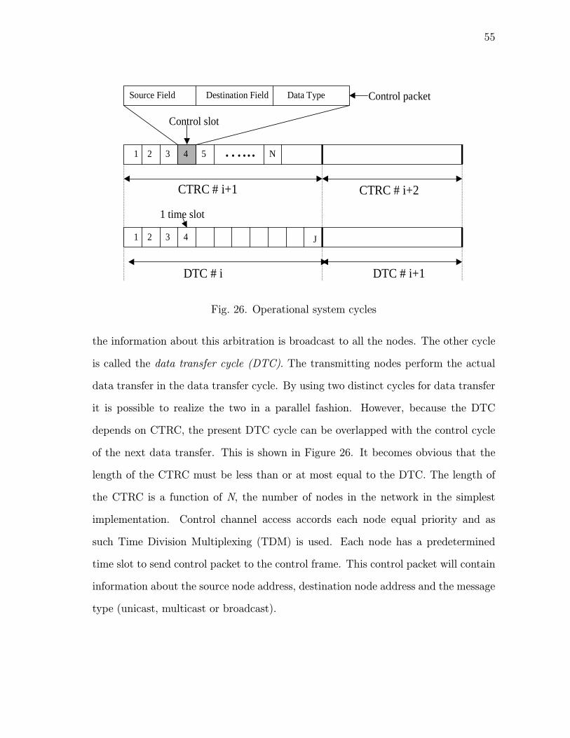
55
…...
Source Field Destination Field Data Type
CTRC # i+1
Control slot
Control packet
1 2 3 4 5 N
1 2 3 4 J
1 time slot
DTC # i
CTRC # i+2
DTC # i+1
Fig. 26. Operational system cycles
the information about this arbitration is broadcast to all the nodes. The other cycle
is called the data transfer cycle (DTC). The transmitting nodes perform the actual
data transfer in the data transfer cycle. By using two distinct cycles for data transfer
it is possible to realize the two in a parallel fashion. However, because the DTC
depends on CTRC, the present DTC cycle can be overlapped with the control cycle
of the next data transfer. This is shown in Figure 26. It becomes obvious that the
length of the CTRC must be less than or at most equal to the DTC. The length of
the CTRC is a function of N, the number of nodes in the network in the simplest
implementation. Control channel access accords each node equal priority and as
such Time Division Multiplexing (TDM) is used. Each node has a predetermined
time slot to send control packet to the control frame. This control packet will contain
information about the source node address, destination node address and the message
type (unicast, multicast or broadcast).

56
B. Scheduling Algorithm
The basic algorithm consists of three steps:
1. Each node transmits a control packet
2. Each node separately runs the distributed scheduling algorithm
3. The nodes transmit and receive data packets
Having mentioned earlier that the allocation of wavelength in the scheduling
process has received a lot of research, the focus will be on message ordering or se-
quencing of messages for transmission. In this approach, the message-ordering algo-
rithm is independent of the allocation algorithm. The way in which the contents of
the control packets are calculated and incoming messages and buffers are handled has
a profound effect on the network characteristics and performance.
There are two instances where message ordering can take place based on the
priorities chosen. The first instant occurs in the source node and the other is in the
control packets. This means that an algorithm can be deployed to the source nodes
intermittently to order the messages accordingly before control information is sent
to the control packet. It also becomes possible to modify the control information in
the control packet to effect a more globally optimized ordering to reduce delay, avoid
collisions and starvation, and improve performance.
A number of different scheduling schemes are obtained depending on whether
message ordering is done at
• the source node
• the control frame or
• both at the source node and at the control frame

57
Other variations that occur depend on whether single or multiple message control
information is transmitted to the control packet and the priority scheme adopted. In
the following subsections, some of the variations and characteristics will be discussed.
1. Control Frame Ordering
In the above scheme, there is no message ordering at the source node as the name
indicates. The messages arriving at the queues of each node are maintained in a
strictly First-Come-First-Serve (FCFS) fashion. During its scheduled time slot, a
transmitting node transmits control information about the message at the head of its
queue. This information will contain the message destination(s). After the control
frame has received all the control information from all the N nodes, the message-
ordering algorithm is invoked to sort the message according to unicast, multicast and
broadcast packet types.
Unicast packets are accorded the highest priority while the broadcast packets
have the lowest. After the sorting is accomplished and the order of message trans-
mission is determined, the time of transmission and channels are allocated according
to the wavelength allocation algorithm employed. At the completion of the control
cycle (ordering + allocation), the transmitting and receiving nodes know on which
channel to tune to and at what time to do this.
This scheme does not lead to starvation because the messages are serviced in
batches. Each batch of messages, consisting of all the currently arriving messages
of each source node, is completed before another set can be serviced. This scheme
allows one message per node to be transmitted in the DTC. It may not lead to a
very efficient utilization of the resources available, because an equal opportunity is
given to all nodes to transmit data regardless of whether each node has data to be
transmitted or not. It works well with nodes without queues where at most one

58
message is represented at the source node.
Analysis:
Consider λ number of data channels for N number of nodes. If all the data
packets at the front of the N source node queue are all unicast messages with exactly
non-overlapping destinations, then the lower bound on how many time slots in a DTC
required to complete the data transfer of the N packets is given by TCF = N/λ .
If all the packets are broadcast messages, which is the upper bound, then TCF = N.
It then implies that N ≥ TCF ≥ N/λ . The DTC length can either be fixed as the
time it takes to transmit N broadcast packets, or make the DTC variable depending
on the message composition. If there are U unicast, M multicast, and B broadcast
data packets in the control frame then:
TCF ≈ U/λ + tM +B (4.1)
where t is a positive value in the range 1 ≥ t > 0.
2. Data and Control Frame Ordering
As the name suggests, in this scheme, the data is sorted at two instances. The first is
at the source node and the other at the control packet. This scheme obviously requires
that the source nodes maintain a queue for arriving messages. As the messages arrive,
the priority scheme adopted, in our case a unicast packet scheduled first and broadcast
packets last, is strictly adhered to. Consequently, at each instant in time, the message
with the highest priority is always at the head of the queue. During its pre-allocated
time slot, a node sends control information about the message to the control frame.
The message-ordering algorithm is invoked after receipt of all control packets, and
the scheduling proceeds just like in the previous scheme.

59
The scheme will obviously lead to starvation, since there is a high probability that
the messages with higher priority will keep on arriving and as such delay indefinitely
the chances that multicast or broadcast messages will be transmitted. The arriving
unicast messages are automatically put at the head of the message queue. To remedy
this effect, a window is associated with a batch of packets. This batch of packets
must be serviced before another set of packets is included in the window.
3. Multiple Data and Control Frame Ordering
In the previous two schemes the control packet sent to the control frame contains
information about only one message. In the current approach, the control packet will
include information for multiple messages. In addition, each node utilizes the priority-
based algorithm earlier mentioned to order the messages in its queue. It is expected
that not all nodes will have a message packet at the time of control information
transmission, while in some cases very few nodes will. At other times almost all
the nodes will, and in the worst case scenario, all the nodes have a message to be
transmitted. To address this unbalance and unpredictable traffic flow of messages,
control information for multiple messages per node could be transmitted in the control
packet. Ordering is done once when all the control packets have been received. The
ordering algorithm sorts all the messages and imposes a sequence based on the priority
scheme discussed.
This scheme like the first one discussed does not lead to starvation since each
batch is serviced before another set is serviced. This approach is an attempt to
globally optimize the scheduling algorithm. The length of the service queue (LSQ)
determines the number of messages scheduled to be transmitted at once. It is expected
that as LSQ increases, the scheduling algorithm becomes more efficient. A large LSQ
means that the scheduling time is increased, however, there is a reduction in the

60
number of times the scheduling algorithm is needed.
Analysis: The maximum number of messages represented in the control frame
is LSQ x N, and as previously stated the DTC is increased and on the average, the
DTC has a time lapse:
TMDCF ≈ LSQ( U/λ + tM +B) (4.2)
4. Multiple Data and Control Frame Ordering with Multicast Partition
In the previous schemes, the multicast packets have been treated collectively as having
the same priority. In this scheme, the multicast packets are also accorded priority
based on the number of overlapped receiver nodes. A multicast packet with fewer
destinations has a higher priority than the one with more destinations. Sorting of the
multicast packets in this fashion enables the scheduling of some unicast packets at the
same time as multicast packets provided there is no overlap of destination address.
This highly optimizes network efficiency and reduces message delay.
As in the previous method, the control packet contains multiple message packet
information for each source node intending to transmit data in the next DTC.
Analysis: In the last scheme, the DTC had a time lapse, TMDCF ≈ LSQ( U/λ +tM +B). In this section, a more accurate representation of T is obtained, assuming
the worst case scenario. The worst case include the following:
• The queues are full with data packets
• All the nodes are involved in transmitting messages
If m is defined as the number of non-overlapping destinations observed in a batch
of unicast messages, then the number of data slots required in a DTC is:

61
TU = U/λ(m
u) (4.3)
Each multicast packet can be modeled as k unicast packets emanating from a
single destination. Here k represents the number of destinations for each multicast
packet. It is obvious 0 < k < N. Within each multicast packet, there is obviously no
destination overlap.
There are M multicast packets, and each will independently take one time slot
in the DTC. At most, M time slots are needed.
TM = dmax if dmax < M (4.4)
TM =M else (4.5)
Some of the multicast packets will have destination overlaps. Define di as the
number of destination overlaps observed for each destination in a multicast packet
as compared to others in the control frame. In other words, for each destination in
a multicast packet in the control frame, d represents the number of other multicast
packets having the same destination. The maximum number of non-unique destina-
tions observed amongst the multicast packets in the control frame dmax determines
the number of time slots required to transmit the M multicast packets. From the
foregoing, the number of time slots required is calculated as follows:
TDTC = TU + TM + TB = U/λ(m
u) + dmax +B (4.6)
C. Simulation Results
Results are obtained for the average message delay and throughput by computer
simulation. The average message delay is defined as the time it takes a packet arriving

62
at the queue of a transmitting node to be transmitted to all its destination nodes.
The throughput is defined as the number of messages that get to its destination per
time slot. Each packet is equally likely destined to any of the nodes and the message
arrivals follow a Bernoulli process with a rate βin. ρM is defined as the percentage
of all messages belonging to the multicast group and δ[M] as the average number of
destination addresses of a multicast message. The four strategies described earlier
are identified using the acronyms: CF = Control Frame, DCF = Data and Control
Frame, MDCF = Multiple Data and Control Frame, and MDCFMP = Multiple Data
and Control Frame with Multicast Partitioning. The tuning times are assumed to be
negligible.
The results obtained for the average packet delay as a function of the arrival
rates is shown in Figure 27. For the simulation, shown are results for a network of
48 nodes (N=48), ρM is set to 0.5, while δ[M] = 6. The results are also shown for
number of channels l = 16, 32, 48.
From Figure 27, observed that the best performance is obtained when the MD-
CFMP scheme is implemented. By prioritizing the transmission of the different pack-
ets, there is a decrease in the number of packets prevented from transmission. With
the ability to transmit control information for multiple packets, the frequency of in-
voking the scheduling algorithm reduces, thereby increasing efficiency, minimizing
bandwidth latency while globally optimizing the performance. The multicast parti-
tion enables the overlap of multicast packets that do not have destination conflicts.
The results clearly show that the MDCFMP scheme achieves lower delays as the
arrival rates increase.
Shown in Figure 28, is the effect of the ratio of multicast packets to the average
packet delay. The results are obtained for bin = 0.125, 0.175. As evident from
the results, the MDCFMP scheme maintains a lower average packet delay as the
63
percentage of the multicast packets is increased. In the other schemes where multicast
partition is not allowed, each multicast packet is treated as a broadcast packet and
hence, no other packets can be scheduled in the same time slot.
In Figure 29, the results of throughput as a function of arrival rate per node
is shown. More packets are able to be transmitted using the MDCFMP scheme
because there is packet prioritizing, global optimization, and multicast partitioning.
The bandwidth is much more efficiently utilized and network latency is lower.
The basic idea of the proposed scheduling method underscores the profound
effect and remarkable improvement data packet sequencing has on network traffic
performance. The surprise that it has not received much attention, was only assuaged
by the fact that optics in computer communication is still in a relatively early stage.
From analysis and results, efficient message ordering in the data scheduling stage
of the Routing and Wavelength Allocation (RWA) process, effectively utilizes the
enormous bandwidth potential available in optics.
Four possible variations on the proposed algorithm for scheduling mixed packet
types has been described. Prioritizing the transmission of the packets, with the ability
to send multiple data control information and utilizing multicast partitions, improves
the performance of the algorithm significantly. It was shown through computer simu-
lations that the algorithm utilizing the MDCFMP scheme can decrease the number of
data packets prevented from transmission, reduce the average delay, improve through-
put performance and completely prevent starvation. This technique is easily adapted
to suit any optical network type and is topology independent.

64
Average packet delay versus arrival rate per node� = 16
Arrival rate per node
Ave
rage
pac
ket d
elay
(tim
e sl
ots)
CFDCFMDCFMDCFMP
0.04 0.08 0.12 0.16 0.20 0.24
0
5
10
15
20
25
Average packet delay versus arrival rate per node� = 16
Arrival rate per node
Ave
rage
pac
ket d
elay
(tim
e sl
ots)
CFDCFMDCFMDCFMP
0.04 0.08 0.12 0.16 0.20 0.24
0
5
10
15
20
25
Average packet delay versus arrival rate per node� = 32
Arrival rate per node
Ave
rage
pac
ket de
lay
(tim
e sl
ots)
CFDCFMDCFMDCFMP
0.05 0.10 0.15 0.20 0.25
0
5
10
15
20
25
Average packet delay versus arrival rate per node� = 32
Arrival rate per node
Ave
rage
pac
ket de
lay
(tim
e sl
ots)
CFDCFMDCFMDCFMP
0.05 0.10 0.15 0.20 0.25
0
5
10
15
20
25
Average packet delay versus arrival rate per node� = 48
Arrival rate per node
Ave
rage
pac
ket d
elay
(tim
e sl
ots)
CFDCFMDCFMDCFMP
0.06 0.12 0.18 0.24 0.30
0
5
10
15
20
25
Average packet delay versus arrival rate per node� = 48
Arrival rate per node
Ave
rage
pac
ket d
elay
(tim
e sl
ots)
CFDCFMDCFMDCFMP
0.06 0.12 0.18 0.24 0.30
0
5
10
15
20
25
Fig. 27. Plot of average packet delay versus arrival rate per node

65
Average packet delay versus multicast rateßin = 0.125
Percentage of multicast packets (x10)
Ave
rage
pac
ket d
elay
(tim
e sl
ots)
CFDCFMDCFMDCFMP
10
2
4
6
8
10
2 3 4 5 6 7 8
Average packet delay versus multicast rateßin = 0.125
Percentage of multicast packets (x10)
Ave
rage
pac
ket d
elay
(tim
e sl
ots)
CFDCFMDCFMDCFMP
10
2
4
6
8
10
2 3 4 5 6 7 8
Average packet delay versus multicast rate
Percentage of multicast packets (x10)
Ave
rage
pac
ket d
elay
(tim
e sl
ots)
CFDCFMDCFMDCFMP
1 2 3 4 5 6 7 80
5
10
15
20
25
ßin = 0.175Average packet delay versus multicast rate
Percentage of multicast packets (x10)
Ave
rage
pac
ket d
elay
(tim
e sl
ots)
CFDCFMDCFMDCFMP
1 2 3 4 5 6 7 80
5
10
15
20
25
ßin = 0.175
Fig. 28. Plots showing average packet delay versus multicast rate

66
Throughput versus arrival rate per node� = 16
Arrival rate per node
Thr
ough
put (
# of
pac
kets
per
time
slot
s) CFDCFMDCFMDCFMP
0.05 0.10 0.15 0.20 0.25 0.30
0
2
4
6
8
10
12
14
16
Throughput versus arrival rate per node� = 16
Arrival rate per node
Thr
ough
put (
# of
pac
kets
per
time
slot
s) CFDCFMDCFMDCFMP
0.05 0.10 0.15 0.20 0.25 0.30
0
2
4
6
8
10
12
14
16
Throughput versus arrival rate per node� = 32
Arrival rate per node
Thr
ough
put (#
of p
acke
tspe
r tim
e sl
ots) CF
DCFMDCFMDCFMP
0.05 0.10 0.15 0.20 0.25 0.30
0
5
10
15
20
25
30
Throughput versus arrival rate per node� = 32
Arrival rate per node
Thr
ough
put (#
of p
acke
tspe
r tim
e sl
ots) CF
DCFMDCFMDCFMP
0.05 0.10 0.15 0.20 0.25 0.30
0
5
10
15
20
25
30
Throughput versus arrival rate per node� = 48
Arrival rate per node
Thr
ough
put (
# of
pac
kets
per
time
slot
s) CFDCFMDCFMDCFMP
0.05 0.10 0.15 0.20 0.25 0.30
0
10
20
30
40
50
Throughput versus arrival rate per node� = 48
Arrival rate per node
Thr
ough
put (
# of
pac
kets
per
time
slot
s) CFDCFMDCFMDCFMP
0.05 0.10 0.15 0.20 0.25 0.30
0
10
20
30
40
50
Fig. 29. Throughput versus arrival rate per node

67
CHAPTER V
FAULT TOLERANCE
This chapter investigates the network communication behavior of the three-dimensional
(3D) multicomputer system using optical interconnection. In this environment, faulty
nodes are left in place, a concept called fail-in-place. This is called the percolation
problem in which various amounts of missing nodes fixed in position in the network
may have a dramatic effect on the networks ability to transport data effectively. As
the number of failed nodes increases, data have to be rerouted through intermedi-
ate nodes creating potential hot spots. These hot spots become the bottleneck that
degrades performance.
The ability to absorb rerouted data without ejecting it from the network is critical
in massively parallel computing systems. Optical technology is a promising solution
for internode communication with extraordinarily quick response time supporting
enormous bandwidth. To adopt it in multiprocessor systems, efficient routing tech-
niques are needed. We adapt self-routing strategies for all-optical packet routing in
3D mesh networks and investigate the percolation properties. To achieve percola-
tion routing, the features inherent in optics are incorporated to achieve decoding and
routing capability in real time.
The objective is to develop a dynamic communication environment that adapts
and evolves with a high density of missing units or nodes, and by employing analytical,
experimental, and simulation methods, show that optical interconnection in this dense
3D system reduces considerably this percolation problem.
Interprocessor communication has become one of the most important issues af-
fecting system performance. The topology, the communication medium, and the
routing algorithm all have a great effect on network performance. While the routing

68
algorithm and topology decide the path between two nodes involved in a one-to-one
communication, the medium determines the volume and speed with which the rout-
ing can be accomplished. The current trend in multicomputer network design is to
pack nodes more densely for efficient distribution of computing resources and uniform
interconnection in 3D space. This has led to improved communication performance,
scalability, and density.
This trend toward placing more and more computing devices, accessories, power
supplies, and the data communications linking these devices into ever smaller spaces
has created a new and quite interesting percolation problem. The percolation problem
deals with the ability of a system as a whole to continue its functions with some of
its components missing or faulty. As individual nodes in a system get smaller and
the packing gets denser, it becomes less desirable to try to fix problems that occur in
individual nodes or accessories. Any attempt to fix a problem with a node may result
in making problems worse in the system as a whole. It then becomes increasingly
important to leave these nodes in the system, a concept referred to as “fail-inplace”.
Many recent multicomputers and multiprocessors [54-57] use grid topology based
on the mesh-connected topology [58, 59]. Mesh-connected topologies, also called k-
ary ndimensional meshes, have an n-dimensional grid structure with k nodes in each
dimension such that every node is connected to two other nodes in each dimension by
direct communication. Mesh-connected topologies include n-dimensional meshes, tori,
and hypercubes. In large multicomputer systems, exchanging data at high speeds is
increasingly becoming the bottleneck that limits the performance of such large-scale
systems [60-63]. This creates the need to investigate new physical approaches to
dense and high-speed interconnections at various levels of a system interconnection
hierarchy. In recent years, extremely fast photonic networks have been developed
that have the potential to support large bandwidth interconnections, with an extra-

69
ordinarily quick response time and low latency. However, the business model that
enables optics to invade telecommunication as the medium of choice for communica-
tion is not applicable in computer systems. This has the effect of limiting the use of
optical components in modern computing systems because of the high cost of optical
devices.
Optics and optical interconnects present some solutions that can potentially ad-
dress the increasingly complex communication requirements for multicomputer sys-
tems [64-66]. Time- and wavelength-division multiplexing are techniques employed
in optical communication to increase the number of connections that can be simul-
taneously established in a network. This has the effect of reducing the frequency
of control operations and thus limited network control overhead. Two approaches
are used to establish sourcedestination connections. One approach called link multi-
plexing establishes connection on more than one communication link, possibly using
different channels on each link. Conversely, path multiplexing uses the same channel
on each of the links.
Several routing strategies that work in the presence of failed nodes for the mesh
topology have been proposed in the literature [67-71]. The simplest routing algo-
rithms are deterministic (oblivious) and define a single path between the source and
destination. A message must wait for each busy channel in the path to become
available. On the other hand, adaptive routing algorithms support multiple paths
between the source and destination. Adaptive routing algorithms are either minimal
or nonminimal. Minimal routing algorithms allow only shortest paths to be chosen,
while nonminimal routing algorithms also allow longer paths. An adaptive routing
algorithm is fully adaptive if it does not impose any restriction on the selection of non-
faulty profitable links, and is partially adaptive otherwise. Therefore, a fully adaptive
algorithm can exploit all alternative optimal paths to well disperse local congestion,

70
thus outperforming deterministic and partially adaptive algorithms. While most of
these approaches are local-information-based (knowledge of only neighbor status),
others are global-information-based. Local-information-based routing does not yield
the shortest possible path in the presence of failures because insufficient informa-
tion is available when the routing decisions are made. On the other hand, while
global-information-based routing can achieve optimal or near routing, its overhead in
maintaining up-to-date fault information at all network nodes is usually quite high.
The main challenge is to devise a simple and effective way of efficiently routing infor-
mation in a system that has a high degree of failed nodes that can be implemented
using optical interconnection devices with limited global fault information.
Several header-processing systems have been proposed that can be used to im-
plement an all-optical routing [72, 73]. In [72] an all-optical header processing using
a terahertz optical asymmetric demultiplexer (TOAD) is demonstrated that has a bit
rate of 250 Gbit/s. This TOAD-based header recognition operates at low energy and
allows photonic integration. A disadvantage with this approach is that the control
pulse has to be synchronized with the header bits. To circumvent this, in [74] an
asynchronous multioutput all-optical header processing technique based on the two-
pulse correlation principle in a semiconductor laser amplifier in a loop optical mirror
configuration (SLALOM) is presented. This concept was employed in an all-optical
packet switch [75]. One disadvantage though in [74] is that the SLALOM configura-
tion is too large to allow photonic integration. In the implementation of an optical
interconnection network that supports a percolation routing in a multicomputer sys-
tem operating under the fail-in-place condition, a dual-output header differentiation
scheme that will allow a synchronous operation suited to photonic integration is pro-
posed. The model proposed is an all-optical time-division-multiplexed transmission
based on TOAD. Optical time-division multiplexing (OTDM) is an alternative to

71
WDM for future networks that utilize a single wavelength at high (> 100 Gbit/s)
data rates [76, 77].
In OTDM networks many signals are combined before being transmitted with a
single wavelength. Each signal from a lower-bit-rate source is broken up into many
segments (slots), each having short duration and multiplexed in a rotating repeating
sequence (i.e., round-robin fashion) onto a high bit-rate transmission line. The use
of short-duration (soliton) pulses allows information to be transmitted at very high
bit rates (> 100 Gbit/s). An asset of OTDM is its flexibility; the scheme allows for
variation in the number of signals being sent along the line and constantly adjusts
the time intervals to make optimum use of the available bandwidth. Consequently,
it is believed that OTDM networks are excellent candidates for meeting the future
system requirements for massive ultrafast networks [78-80].
A. Percolation in Large Systems
The percolation theory as it describes computing with a faulty array of processors
has been introduced in [81], while [82] looks at this phenomenon in large storage
systems. In our context, percolation deals with the effects of varying the richness of
interconnections present in a random system. The basic idea of percolation is the
existence of a sharp transition at which the long-range connectivity of the system
disappears (or, going the other way, appears). This transition occurs abruptly when
some generalized density in this system reaches a critical value (percolation thresh-
old). The percolation transition makes percolation a natural model for describing
a diversity of phenomena. The percolation model is described as one with failures
modeled as complete elimination of both data and communication in a node. The
central idea is that various amounts of missing elements fixed in position in a network

72
Fig. 30. 3-dimensional mesh network with failed nodes depicted as white nodes
may have a dramatic effect on the networks ability to transport material, and in our
case, information. Figure 30 is an illustration of a network with failed nodes. Every
node in the network has a direct network connection with all its six neighbors. For
nodes located on the surface of the network or adjacent to failed nodes, the number
of neighbors is obviously less than six. An important definition is the percolation
threshold, which is a fraction of lattice elements, or in our case, good nodes, below
which all the nodes remaining are connected to one another only as small clusters,
not enough to span the whole structure or network. So if a node fails, availability
requires that the repair be accomplished quickly. However, in a large system, trying
to repair a bad node may ultimately introduce more problems, hence the fail-in-place
concept. This means that in a cluster of nodes, there will increasingly be nodes that
fail and are allowed to remain in place in order to reduce maintenance cost and avoid
the introduction of more problems due to human error. In such an environment, the
connectivity, bandwidth and data path lengths among others are adversely affected.
Increasing the number of failures will drastically degrade the performance by
creating hot spots and discontinuities in the network. As the number of failed nodes
increases, we expect that the overall bandwidth will decrease. This decrease in band-

73
Fig. 31. Diagram showing min-cut in both 2- and 3-dimension
width is due to fewer paths becoming available because traffic is rerouted around
failed nodes. This also has the effect of creating hot spots. As a consequence, with
half the nodes in operation, the bandwidth for data traffic is only 10% of the initial
value. To see the effect of faulty nodes on overall bandwidth, we can calculate the
maximum number of parallel paths that exist connecting opposite faces of an array
with faulty nodes. Figure 31 shows the min-cut in both two-dimensional (2D) and
3D site percolation as a function of the fraction of good nodes. We define the min-cut
as the smallest fraction of links that must be cut by a continuous, but not necessarily
flat, surface passing normal to one axis of either a 2D or 3D lattice.
This graph is obtained by an algebraic analysis of a worst-case measure of overall
bandwidth reduction due to node failure. Actual observed bandwidth may be even
lower because of hot spots in the message traffic. As seen in the graph, when the
number of faulty nodes is half the total number of bricks, the relative bandwidth
available is reduced to 10% in the 3D site percolation. The increase in path length
due to avoiding failed nodes is not particularly significant in this design. The increase

74
becomes large when the number of faulty nodes is close to the percolation threshold.
As mentioned above, considered here is a design with 50% or more good nodes.
B. Percolation Routing with Optical Interconnectivity
In this section the percolation routing in a 3D mesh adaptable for optical interconnec-
tion networks is examined. The proposed scheme is based on the concept of limited
global fault information and eliminates the need for lookup tables. Limited global
information, means that individual nodes know which, if any, of its neighbors are
faulty. This model is also known as the one-step local information model. As men-
tioned, a fault means that its entire communication links are faulty. The emphasis is
not so much the dynamic nature of the faults that occur in the system, but how well
the system as a whole handles steady-state faults in a fail-in-place environment.
The size of a lookup table for a network of a significantly large number of nodes
presents a challenge to large-scale network design. The lookup times for such large
address spaces are of the order of micro- or milliseconds. In addition to the large
lookup times, an OEO (opticalelectricaloptical) conversion has to be performed in or-
der to carry out the lookup operation to determine the next hop in an optical system.
The conversions that have to take place at each intermediate node will undoubtedly
degrade the performance, and as such, the goal of using optics in the first place is de-
feated. However, since optical logic is still in its infancy, designs that involve complex
logic in decoding header information will not achieve the expected improvements in
routing performance. The features inherent in optics are harnessed to achieve header
recognition and decoding, data routing capability, and contention resolution in real
time in this design. In the design the need for optical buffering is eliminated, which is
clearly unsuitable for large multiprocessor systems, by aggressively reducing the prob-

75
In te r m e d ia te n o d e s
s rc d e s t
s rc d e s t
p 1 p 2 p 3 p 4 p 5 p 6 p 7 p 8 p 9
a 1 a 2 a 3 a 4 a 5 a 6 a 7 a 8 a 9
P r e fe r r e d
A lte r n a te
In te r m e d ia te n o d e s
s rc d e s t
s rc d e s t
p 1 p 2 p 3 p 4 p 5 p 6 p 7 p 8 p 9
a 1 a 2 a 3 a 4 a 5 a 6 a 7 a 8 a 9
P r e fe r r e d
A lte r n a te
Fig. 32. Two field address structure
abilities of data contentions and unavailability of outgoing links at each intermediate
node.
In this implementatione, the path P between two nodes, source S and destina-
tion D, is provided with an alternative path A. Consequently, every primary link is
provided with an alternate physical one. These two paths can be switched back and
forth depending on the availability of output links at each intermediate node. An
address encodes a unique path from S to D. A packet is encapsulated in layers of
address markers corresponding to the action taken at an intermediate node i. After
each marker is traversed, it is stripped from the address exposing the next marker.
These markers may be defined on a per-destination basis, on an S-D pair basis, or on
a per-flow basis. However, in a self-routing scheme it is difficult to implement conges-
tion control and traffic engineering. For each destination address, each intermediate
node has a preferred output link and an alternativeoutput link should the preferred
link be unavailable. If an alternative output link is taken, then the address markers
have to change accordingly. In this design, an address is made up of two fields as
shown in Figure 32. At each node, the preferred output link is always chosen. This
corresponds to field P. If, however, an alternative link is taken then the field to which
the link belongs becomes the preferred field.
Every node in a 3D mesh has a direct network connection with all six of its neigh-
bors. The exceptions are the nodes on the surface of the mesh and those adjacent

76
failed nodes. The process of routing data from source to destination can be done in
three phases. The first phase is to determine the primary and alternative intermediate
nodes between source and destination and thereby forming the address. An address
basically represents an action taken at each intermediate node. The action taken
directs a packet to the appropriate output link. This means that the structure of
an address for a packet while remaining unchanged throughout the transport process
will illicit different actions at different nodes. The action is processed in real time.
The node identifies an address and on the fly directs the packet to one of its output
links. If the primary link is unavailable, the alternate link is chosen. The second in-
volves path setup by assigning channels to each of the primary outgoing links at each
intermediate node. Since we consider optical real-time decoding with little overhead,
the header should not be extremely large or complicated. The destination address
has information about the intermediate nodes, while these intermediate nodes make
decisions on assigning channels to the outgoing link used to get to the next interme-
diate node. Third, the data are sent out by the source. As already mentioned, this
self-routing scheme should support a 3D structure. Each node is represented by a
3-tuple N(x,y, z), which completely describes the position of a node in a 3D mesh.
1. Address Formulation, Path Setup, and Channel Assignment
Given a source node S = (xs, ys, zs) and a destination nodeD = (xd, yd, zd), ADDR =
(S, i2, ..., in−1, D) is defined as the set of address to give minimal distance routing,
where i represent the intermediate links between the source and destination nodes,
n number of nodes and there are n-1 intermediate links. The primary route address
ADDRP = (S, i2, ..., in−1,D) and alternate route addressADDRA = (S, i2, ..., in−1, D)
are chosen from a set of equally unique routes that satisfy the following conditions:

77
1. ADDRP ADDRA = {S,D}
2. ADDRP {ix}&ADDRA {ix} [where x = (2,3, . . . ,n-1)]; have only one of the(x,y, z) coordinates differing by only one in Hamming distance, a well known
concept in channel coding is used.
Condition 1 means that no intermediate node address belongs to both the pre-
ferred and alternate node address set except the source and destination addresses. In
condition 2, the Hamming distance, a well known concept in channel coding is used.
Let a and b be two binary sequences or coordinates in space of the same length.
The Hamming distance between these two addresses is the number of symbols that
disagree. To further illustrate, an example is given. If the third intermediate node of
the preferred address is (2,3,4), the set of possible options for the alternate address
will be (1,3,4), (3,3,4), (2,2,4), (2,4,4), (2,3,3), (2,3,5). These obviously correspond
to the six nearest neighbors. The conditions mentioned above try to guarantee that
the minimal path length feasible is maintained when the alternate path is taken and
in most cases only an additional link is traversed in the event that a link is faulty,
especially near the destination. However, as the number of faults increases in the net-
work, the path length will invariably increase. The scheme proposed is best described
as a nonminimal adaptive routing scheme based on limited global information.
Having determined the intermediate nodes/links needed for data transfer, the
sender S sends a header flit that contains information on the primary and alternate
intermediate nodes (links) needed for the data transfer [ADDRP = (S, i2, ..., in−1,D)
and ADDRA = (S, i2, ..., in−1, D)]. Each intermediate node has the task of assigning
unused channels on the appropriate outgoing links. A hold state is placed on any
channel assigned. If the header flit is successfully transmitted to the destination D,
the sender S then sends the data preceded by the control flit that contains information

78
on the intermediate routes with channel assignments. A channel is released only when
the final flit of data passes through it. In this implementation, the path setup/channel
assignment phase is overlapped with data transfer. The data lags behind to give time
for the intermediate nodes to assign and place a hold on the appropriate channels.
In the next subsections, the different strategies in the algorithm used to perform
percolation routing is outlined. Emphasis is placed on the feasibility of implementing
the algorithm using optical devices.
2. Routing Algorithms
In a 3D mesh array or nodes, there may exist up to six first hops that lead to a shortest
path to a distant node. Two natural ways of selecting one of the alternative first steps
for routing exist. The first follows a predetermined rule, and the second is random.
The predetermined rule is traditionally used in nonadaptive mesh routing. However,
the random rule is likely to cope with high levels of failed nodes more gracefully. In
what follows, we describe these two approaches of the routing methodology.
a. Notation
Given a source node S = (xs, ys, zs), and a destination node D = (xd, yd, zd), Cs,d is
defined as the smallest cube that includes both S and D. Without faulty nodes, the
algorithm will find a path from Sto D within Cs,d. It is worth mentioning that Cs,d
is not unique for an S-D pair.With S as our focal point, let all the nodes n in Cs,d be
labeled nx,y,z, where (x, y, z) represent the x, y, z coordinates in space. In the XYZ
rule, a canonical ordering, the approach is to always move first in the x direction if
possible, then in the y direction if possible, then in the z direction. The pair of nodes
S-D is represented as (sx,y,z, dx,y,z). If the number of virtual channels is C, then the
algorithm finds for each S-D pair an allocation Ci that is free. Links are defined links

79
as follows:
lx ∈ L(x0, x1, ..., x|d−s|) = LX , (5.1)
ly ∈ L(y0, y1, ..., y|d−s|) = LY , (5.2)
lz ∈ L(z0, z1, ..., z|d−s|) = LZ. (5.3)
The value |d−s| represents the number of intermediate nodes between the source anddestination. Thus, a path from S to D is represented as path (S−D) = {LX , LY , LZ}.Consequently, a channel allocation for an S-D pair is denoted by an integer value
channel ± alloc(LX , LY , LZ). B channel is used to represent a set of blocked channelsthat exist on the links that make up the path (S-D). To simplify the notation, two
states, f = current state, and h = next state are defined.
η = sy if θ = x = dx,
η = sz if θ = y = dy,
η = sx if θ = z = dz.
First, the XYZ routing for path and link multiplexing is discussed and then an
adaptation for faulty nodes implemented using optical devices.
Algorithm 1 (XYZ rule (No faults, path multiplexing))
Inputs: (S-D)pair, channel alloc(sx,y,z, dx,y,z), B channel
Output: XYZ routing
begin
initialize channel alloc(sx,y,z, dx,y,z) = null for all links;
for( each S-D pair requesting connection) do
path(sx,y,z, dx,y,z) = {null} and Bchannel = {null};x = sx;

80
while(ϕ = dϕ) do
add lϕ to path(sx,y,z, dx,y,z) and ϕ = ϕ+ 1;
if ϕ = dϕ, break; then ϕ = η;
if η = z = dz, break;
end while
B channel = B channel channel alloc(sx,y,z, dx, y, z)
channel = (n /∈ B channel) && (n < C)
for (every link {LX , LY , LZ} in path (sx,y,z, dx,y,z)) doset C(sx,y,z, dx,y,z) = channel;
channel alloc(sx,y,z, dx,y,z) = channel alloc(sx,y,z, dx,y,z) {channel};end for
end for
end
b. Dimension order routing (XYZ routing)
In the path-multiplexing algorithm above (Algorithm 1), channels are not assigned to
connections as the path is constructed. Information about the channel availability is
obtained first before a channel is assigned to a path. As a consequence, if a channel is
not available in the preferred route from source to destination, a longer route may have
to be taken, and data could be ejected from the network or some delay incurred while
waiting for channel availability. Link multiplexing is better suited to alleviate this
constraint. Therefore, the algorithm above can be modified by eliminating “channel”
and “B channel” as shown in Algorithm 2 below.
The next step is to take a closer look at the percolation routing of the XYZ rule.
As mentioned above, Cs,d is not unique for an S-D pair. This property enables the

81
system to circumvent faulty nodes or links by implementation of the algorithm for the
alternate path. Information about the failed link is obtained during the path setup
phase. It is important to note that link failure is different from link unavailability.
The consequence being that link unavailability is transient and not permanent, so the
information is treated as such. The differentiation between link failure and unavail-
ability is done at the hardware sense level. The objective of the routing algorithm will
be to minimize the number of additional steps needed to circumvent a faulty node.
The heuristic percolation routing follows the XYZ rule, albeit only loosely. If a fault
is detected in the x-axis, move a step in the y-axis toward the destination node. The
same rule applies to faults in both y- and z-axes. In both cases move in the z and
x axes respectively. This method is described as cyclic-XYZ rule, where ψ denotes a
faulty link.
Algorithm 2 (XYZ rule (No faults, link multiplexing))
Inputs: (S-D)pair, channel alloc(sx,y,z, dx,y,z), B channel
Output: XYZ routing
begin
initialize channel alloc(sx,y,z, dx,y,z) = null for all links;
for( each S-D pair requesting connection) do
path(sx,y,z, dx,y,z) = {null} and Bchannel = {null};x = sx;
while(ϕ = dϕ) do
add lϕ to path(sx,y,z, dx,y,z) and ϕ = ϕ+ 1;
channel alloc(lϕ) = channel alloc(lϕ) + 1;
if ϕ = dϕ, break; then ϕ = η;
end while

82
end for
end
Algorithm 3 (XYZ rule (Pecolation))
Inputs: (S-D)pair, channel alloc(sx,y,z, dx,y,z), B channel
Output: XYZ routing
begin
initialize channel alloc(sx,y,z, dx,y,z) = null for all links;
for( each S-D pair requesting connection) do
path(sx,y,z, dx,y,z) = {null} and Bchannel = {null};x = sx;
while(ϕ = dϕ) do
if (lϕ = ψ)
add lϕ to path(sx,y,z, dx,y,z) and ϕ = ϕ+ 1;
channel alloc(lϕ) = channel alloc(lϕ) + 1;
else
ϕ = η and add lϕ to path(sx,y,z, dx,y,z);
channel alloc(lϕ) = channel alloc(lϕ) + 1;
if ϕ = dϕ, break; then ϕ = η;
end if
end while
end for
end

83
c. Probability-based percolation random routing
In this approach each intermediate node determines the next step on the basis of
its current position, calculated probability of success, and the destination address.
The current node chooses a next step in order to produce a minimal path to the
destination. Routing at each node is based on a calculated probability vector P =
(P1N , ..., Pn
N). Each intermediate node determines a set of faulty neighbors and
updates its faulty set Fx,y,z. With this it calculates the probability vector P1. It then
performs an exchange with its neighbors to determine the rest of the vector elements,
PlN , for all (n ≥ l ≥ 2). PlN represents the probability that a destination at distance
l(x,y,z) cannot be reached from the current node N(x,y,z) using a minimal path due to
a faulty intermediate node. In summary, each node runs the following basic steps of
this algorithm:
• Determine Fx,y,z of unreachable neighbors; compute probability vector P =
(P1N , ..., Pn
N) based on Fx,y,z and exchanged information from neighbors.
• Determine primary and alternate route to destination based on probability vec-tor and encode information in header and data flits.
A path is faulty if it includes at least one faulty or unreachable node. Since
there are at most six neighbors to each node and f is defined as the number of faulty
neighbors, then
P1N = f/6 (5.4)
If QlN(i)
is defined as the probability of reaching a destination at distance l from N
via its neighbor N (i), then the probability P1N , l ≥ 2, can be expressed as
P1N =
6
i=1
(1−QlN(i)
) (5.5)

84
where,
QlN(i)
= 0 if node N(i) is faulty
QlN(i)
= 16(1−QlN(i−1)
) otherwise
After the probability vector P1N is determined, a source node S selects two paths
at random that have the least P1N . The source node then encodes these two addresses
onto the header and data flits as the primary and alternate addresses. See Algorithm
4.
Algorithm 4 (Random rule (Pecolation))
Inputs: (S-D)pair, f, channel alloc(sx,y,z, dx,y,z)
Output: Random pecolation routing
begin
initialize channel alloc(sx,y,z, dx,y,z) = null for all links;
for( each S-D pair requesting connection) do
path(sx,y,z, dx,y,z) = {null};P1
N = f
6; /* determine the probability vector */
for(l = 2 to n) do
PlN = 1;
for(i = l to n) do
if(N (i) is faulty)
QlN(i)
= 0;
else
QlN(i)
= 16(1−Ql−lN(i)
);
PlN = Pl
n(1−QlN(i)
);
end for

85
end for
Randomly select two minimal routes based on least PlN ;
Encode primary and alternate address: ADDRP ADDRA = {S,D};while (N = D) do
if(lN(P ) = ψ) /* lN(P ) denotes primary link on current node */
add lN(P ) to path(sx,y,x, dx,y,z);
channel alloc(lN(P )) = channel alloc(lN) + 1;
else
lN(P ) = lN(A) and add lN(P ) to path(sx,y,x, dx,y,z);
channel alloc(lN(A)) = channel alloc(lN) + 1;
end while
end for
end
To show how these two approaches perform in various degrees of number of failed
nodes, a traffic model is defined. In the traffic model, each node is either a compute
node or a storage node.We have an nnn network, with n = 10. Of the 1000 nodes,
100 are compute nodes. Each compute node reads data from all the storage nodes,
performs some specified computation on the collected data, and writes the result to
all the storage nodes. Next, for each storage node, its data are mirrored to another
node in the network. An acknowledgement is also returned to the original compute
node. The idea is to generate as much traffic as possible to every node. The compute
nodes are distributed uniformly throughout the whole network. This traffic model is
simulated using various degrees of failed nodes. The traffic model for both types of
routing rules is simulated. Of particular interest is in understanding the hot spots
that form under load. The performance of the network is more adversely affected by

86
Fig. 33. Distribution of link loading on traffic model for 0%
the bottlenecks and worst-case loadings rather than the average loadings. Single link
failures are not considered, rather, a node failure means that all six outgoing links
are no longer available for routing.
Figure 33 shows that with all the nodes working, the predetermined rule produces
a highly regular and balanced arrangement. By contrast, the random routing scheme
produces a tail of heavily loaded buffers when all nodes are working. However, as the
number of failed nodes increases, the random routing scheme is progressively better
than the predetermined case up to 50% as shown in Figure 34.
C. Feasibility of Optical Implementation
For a practical implementation of the all-optical header processing system utilized
in devising an all-optical packet switch, the header processor should be scalable,
have low power consumption, be high speed, and be photonic integrated on a chip.
In particular, scalability defines the capacity of the header processor to recognize a
large amount of header information and eventually to update the system easily to

87
Fig. 34. Distribution of link loading on traffic model for 50%
recognize more headers. High-speed operation is required for matching the line rate
of the optical transmission system so that no bottleneck is generated. Low power
consumption and photonic integration guarantee largescale production, low cost, and
integration with other functionalities on the same chip. Optical implementation of
our routing scheme is based on the following:
• Address recognition
• Ability to decode optical data in real time
• Generation of switching control signal
• Contention detection/resolution
In this section the feasibility of implementing this routing scheme and the ability
to accomplish all the goals stated above is demonstrated. The architecture is based
on a system that has as its inputs an OTDM packet containing header and payload

88
OTDMPacket
Generator
AWGNChannel
OTDMRouter
Filter1 Detector1
Filter2 Detector2
Node interface
Link 1(Primary)
Link 2(Alternate)
Fig. 35. Block diagram of header recognition subsystem using OTDM
information. Figure 35 shows a block diagram of the simulated OTDM transmission
system. It consists of an OTDM packet generator, additive white Gaussian noise
(AWGN) channel, optical router, matched filter, and detector. Figure 36 shows the
format of two consecutive packets at the output from the OTDM packet generator.
Framing bits indicate the interpacket boundaries thereby providing a synchronization
mechanism. The address bits indicate the destination port to which the payload
information is routed. A value of 1 (0) results in the payload information being routed
to link 1 (link 2) of the OTDM router. To demonstrate all-optical address recognition
and single-bit self-routing, a single node of the OTDM router is constructed from two
TOADs.
Fig. 36. Bit format of the OTDM packet

89
Buffer
TOAD #1(decode address)
TOAD #2(route data)
BeamSplitterData
1X2
Output link 1
Output link 2
Control signal Control signal
Buffer
TOAD #1(decode address)
TOAD #2(route data)
BeamSplitterData
1X2
Output link 1
Output link 2
Control signal Control signal
Fig. 37. Bit format of the OTDM packet
As shown in Figure 37, the switching node consists of an all-optically controlled
routing switch (TOAD #2 with ∆x = Tc/2, where T = 20ps is the width of switching
window), an ultrafast controller (TOAD #1 with ∆x = Tc/2, where T is the width
of the window equals the duration of the address bit), and a buffer. The ultrafast
controller all-optically sets the states of the routing switch (TOAD #2) in a switched
or unswitched state, and the optical buffer matches the delays of the input packet to
the processing delay of the routing controller [32].
When an OTDM data signal enters the node, the clock, which is an orthogonal
polarization signal, is separated from the optical packet by use of a polarization beam
splitter and then used as the control signal of TOAD #1. A portion of the packet is
split off and sent to TOAD #1 before entering the buffer. TOAD #1 reads the packet
destination address bit and uses it as the optical routing control for the routing switch
(TOAD #2). In a single bit routing scheme, packets with address bit of value 1 are
routed to output link 1, while packets with an address bit of value 0 are routed to
output link 2. Thus photonic packets are self-routed through an all-optical ultrafast
switch without the need for optoelectronic conversion.
D. Simulation Results
This section presents simulation results for the 3D mesh in a fail-in-place situation
with varied amounts of failed nodes. The simulator is a 10,000-line C++ program

90
Table III. Simulation Parameters for the All-Optical Packet Routing Subsystem
Bit period 4ps
Control pulse width FWHM 2ps
Control pulse wavelength 1550nm
Data signal width FWHM 2ps
Data signal wavelength 1550nm
SOA length 300μm
SOA active area 0.2 e−12m2
SOA carrier density 1024m−3
SOA confinement factor 0.30
SOA position ∆x 2ps
capable of modeling multicomputer nodes, routing, and interconnection network prop-
erties already discussed in the preceding sections. We compare the results of both
electrical and optical interconnects using the same topology but based on their known
properties for various degrees of faulty nodes, to show the strength of our routing
methodology. The following parameters and values listed in Table III are used in
modeling the optical header decoding and routing subsystem.
The electrical interconnection network is modeled using the gigabit Ethernet
specifications approved by the IEEE 802.3z Gigabit Task Force in 1996. Throughput,
packet transmission delay (or network latency), and worst-case loading effects for
various degrees of faulty nodes are used as the indices of performance. The two net-
works are driven with the following traffic loads: uniform random traffic, saturation
traffic, and hot-spot traffic. In uniform random traffic mode, every node generates
messages with exponentially distributed arrival times and uniformly distributed des-
tination nodes. Figure 38 shows the channel width for both types of interconnects as

91
Channel width
0
20
40
60
80
100
120
140
160
180
2 3 4 5 6
dimension, n
chan
nel w
idth
, bit
s/ch
anne
lelec
optics
Fig. 38. Channel width
a function of dimension. Optics has a wider channel in all cases. As shown in Figure
39, optical interconnects achieve lower latency and are closer to achieving constant
minimal network latency for various degrees of faulty nodes for a 3D mesh.
Figure 40 illustrates the effect of faulty node degree on saturation throughput for
both electrical and optical interconnection networks. The destination nodes for each
source are uniformly distributed, and fully adaptive routing is used. Each source is
constantly injecting a message into the network. This is done to maintain 100to keep
the network saturated. The figure shows that the optical interconnection network
achieves a much higher saturation throughput and is less affected by the number of
faulty nodes. Both interconnection networks have high bisection bandwidth and a
large number of routing options; however, as the number of faulty nodes increases, the
number of routing options decreases. This decrease is more apparent in the electrical
case owing to its smaller network link capacity.
In hot-spot traffic, the network is over saturated. The idea is to identify bottle-
necks and worst-case loading in an effort to understand the hot spots that form under

92
Network latency (10x10x10)
0
50
100
150
200
250
300
350
400
0.5 0.55 0.6 0.65 0.7 0.75 0.8 0.85 0.9 0.95 1
fraction of good nodes
netw
ork
late
ncy.
ns
elec
optics
Fig. 39. Network latency for a 10x10x10 3D mesh network with arbitrary fixed message
size under uniform random traffic
Fig. 40. Effect of faulty node degree on saturation throughput

93
Worse-case loading
0
200
400
600
800
1000
1200
0.5
0.55 0.6
0.65 0.7
0.75 0.
8
0.85 0.9
0.9
5 1
fraction of good nodes
mes
sag
es p
er li
nk (a
rbitr
ary
unit
s)
elec
optics
Fig. 41. Effect of faulty node degree on worse case loading
this traffic mode. The next set of figures show curves for worst-case loading. The hot
nodes (bottlenecks) will increasingly have to deal with a lot more load being diverted
through them as the number of faulty nodes increases. In Figure 41 the maximum
number of packets passing per unit time is plotted as the degree of faulty nodes is
increased for both electrical and optical networks. Figure 42 shows the number of hot
spots created for a worst-case loading as the number of faulty nodes is increased for
both electrical and optical cases. The result shows that with optical interconnects,
the number of hot spots created is relatively small compared with electrical. As a
consequence, more routing options are available, resulting in an increased throughput
and a balanced load distribution.
In a large system, there will increasingly be nodes that fail and are allowed to
remain in place. Using simulation analysis it has been shown that bandwidth is the
most critical factor affected by the so-called fail-in-place problem. Optical intercon-
nection is the solution to this bandwidth need created by the percolation problem
that exists in large computing systems. A routing strategy for alloptical packet-
switched networks that harnesses the features inherent in optics to achieve header

94
Worse-case loading
0
50
100
150
200
250
300
350
0.5 0.55 0.
60.
65 0.7
0.75 0.
80.
85 0.9
0.95 1
fraction of good nodes
aver
age
num
ber
of h
ot s
pots
elec
optics
Fig. 42. Average number of hot spots
recognition/decoding and data routing in real time was presented. Analytical study
and simulations have been used to examine the feasibility of such a network. A sim-
ple OTDM system model based on the optical router developed in [83] is presented.
The model successfully recognizes the address bits and routes the data at speeds up
to 0.25 Tbit/s. The all-optical communication system overcomes the bottleneck of
optoelectronic conversion because of its ultrafast switching capability. This commu-
nication environment is able to adapt and evolve with a high density of missing units
or nodes.

95
CHAPTER VI
SYSTEM OPTIMIZATION AND PERFORMANCE
A novel autonomic control system for high performance stream processing systems is
presented suited for large scale systems described in this dissertation. The system,
“Automomic Traffic Management” (ATM), uses bandwidth controls on incoming or
outgoing streams to achieve a desired resource utilization balance among a set of
concurrently executing stream processing tasks. The objective is to show that CPU
prioritization and allocation mechanisms in schedulers and virtual machine managers
are not sufficient to control such I/O-centric applications, and present an autonomic
bandwidth control system that adaptively adjusts incoming and outgoing traffic rates
to achieve target CPU utilizations. The system learns the bandwidth rate necessary
to meet the CPU utilization objectives using a stochastic nonlinear optimization, and
detects changes in the stream processing applications that require bandwidth adjust-
ment. The Linux implementation designed here is lightweight, has low overhead, and
is capable of effectively managing stream processing applications.
In modern distributed processing systems, system resources such as processing
cycles, memory, and interconnection bandwidth must be carefully managed for effi-
cient operation. Cost and reliability benefits have driven consolidation of formerly
isolated server applications into fewer physical machines, while I/O subsystems (such
as memory, storage, and network) have increasingly replaced processors as the bot-
tleneck of many important classes of workload. The semiconductor industrys shift to
multi-core processors and multi-processor systems makes it all the more important,
and difficult, to keep processing units supplied with the data they require. As grid
and on-demand computing become more prevalent, system resources must be shared
not only among many applications, but among many organizations with different

96
workloads, service level requirements, and contracts. Whether managing a single
server or an entire cluster, effective management of system resources is critical to
achieving desired application performance levels. While substantial prior work exists
on independently managing processing resources (processor usage) and networking
resources (bandwidth), little attention has been given to understanding the complex
relationship between the two or managing them jointly. Furthermore, the currently
prevailing solution to resource management in high performance computing and grid
clusters is to carefully control the processor usage of different tasks, and ignore en-
tirely the bandwidth used by each task. This approach is reasonable when intercon-
nection bandwidth is overprovisioned to the point that the network can keep pace
with processors demands for data, and thus the processors are the bottleneck that
limits throughput. However, with extremely bandwidth-intensive applications (e.g.
high-rate stream processing) or when network resources are scarce or prohibitively
expensive (e.g. in global-scale grid computing), such overprovisioning is not practi-
cal. In such applications network bandwidth must be considered to be as important
as, and sometimes even more important than, processing power.
Traditional CPU scheduling algorithms can fail to achieve their goals when CPU
is not really the bottleneck resource. For example, without any bandwidth control,
some processes may consume more than their fair share of bandwidth, thus “starving”
other (potentially more important) processes to the point where they cannot utilize
their allocated CPU share. The ideal CPU utilization targets may be a three to one
ratio, but a CPU scheduler would not enforce any bandwidth restriction, and that
task may take up 90% of the CPU. Or, with TCP or similar flow control mechanisms,
each task may receive an equal bandwidth share. Either way, failure to allocate
or prioritize access to network resources can counteract careful allocation of CPU
shares. This network allocation problem differs from traditional network congestion

97
control, however. Traditional network QoS solutions require system administrators
and/or application developers to provide a characterization of the traffic generated
by the applications and the corresponding network resource requirements, such as
link bandwidth and network buffers. The commonly used leaky (or token) bucket
model characterizes a network traffic source by its average bit rate (the bucket rate)
and its maximum burst size (the bucket depth). Such a characterization may only be
possible in very static and predictable environments. In real-life distributed systems,
where multiple external factors affect application performance, apriori traffic charac-
terization is inevitably imprecise and burdensome for the system administrator. This
is even more the case for emerging distributed computing paradigms such as grid and
on demand computing where the system has to provide QoS to applications which
are unknown and even outside the control of the system operator.
There is therefore a clear need for systemmanagement solutions that autonomously
monitor applications progress, in terms of meeting quality objectives, with respect
to their use of system resources, thus learning the implicit relationship between the
two. Such a solution is described in this paper. Specifically, a system for autonomic
management of network resources to effect the desired balance between concurrently
executing processes on a stream processing node is presented. This system is capa-
ble of maintaining this balance with or without the presence of explicit perprocess
CPU allocation mechanisms (e.g. processor sharing between LPAR partitions[84],
VMWare images[85], or CPU-allocating schedulers such as CKRM[86]). In systems
without per-process CPU allocation mechanisms, such as a stock Linux kernel, our
management system is able to autonomously determine the appropriate data rate
for each process to achieve its CPU target and allocate the corresponding amount of
network resources. Even in systems equipped with per-process CPU allocation mech-
anisms, our autonomic traffic management system ensures that less important tasks

98
dont starve more important tasks of bandwidth. We anticipate that current trends
in distributed systems will make it increasingly important to carefully monitor appli-
cation performance and link it with resource utilization requirements and allocation.
Furthermore, systems should be able to cope with disparate and quickly changing
loads and resource requirements. The analysis presented here is an important step in
this direction.
A. Overview of Related Work
In this section discussion will be based on prior work that is related to management
of distributed stream processing systems. The problem of providing network QoS via
bandwidth reservation, scheduling and policing has been extensively researched over
the past years. The main focus of this work [87-90] has been to study mechanisms
that, given an appropriate traffic characterization, can guarantee high efficiency sta-
tistical multiplexing while ensuring the requested levels of QoS (or limiting violations
thereof). The traffic parameters (such as leaky bucket rate and size) along with the
negotiated QoS can be thought of as a contract between the user and the network.
This work underlined part of the work of the Internet Engineering Task Force Inte-
grated Services (IntServ) [91, 92] and Differentiated Services (DiffServ) [93] working
groups. One common shortcoming of these approaches is that they rely on accurate
characterization of the traffic streams entering the network. While this assumption
might have been true for a small set of well known applications, it is clearly not
applicable in todays heterogenous, on demand computing envirornment, where the
traffic generated by an application and the relation to CPU resource availability is
not know in advance. Additionally, as already pointed out, this work does not link
the allocation of network bandwidth with CPU processing utilization. Still, the tech-

99
niques developed to allocate and police bandwidth allocation domain can be used as
a building block in the 3D multicomputer control system.
Substantial amount of work in managing distributed applications has been car-
ried in the domain of operating systems. This work focuses on intelligent scheduling
of different tasks across different nodes, prioritization and allocation of CPU, mem-
ory and disk resources. Typically the network is assumed to be of sufficient capacity
that it can be considered infinite. The authors in [94, 95] consider the interaction
of traffic with the network and propose using a simple feedback mechanism based
on local buffer occupancy levels to control the progress of different processes. Load
balancing [96] has been also used to asign different nodes in a cluster to different
processes requiring processing. It relies on individual nodes to periodically send state
(processing load and resource availability) measurements to a gateway node that
then determines the appropriate job dispatch policy. Prior research in multimedia
and stream processing systems is also relevant to our work; multimedia applications
have often been developed with build-in adaptation mechanisms to handle network
or system congestion. [97] describes application-level quality adaptation techniques.
[98] presents adaptive mechanisms for real-time applications that adjust resource allo-
cation if there is risk of failure to satisfy timing constraints. Transcoding of web page
multimedia objects based on the available bandwidth is used in [99] to provide service
differentiation across different clients. Abeni and Buttazzo in [100] propose a frame-
work for dynamically allocating CPU resources to tasks whose execution times are
not know apriori. The motivation for learning the tasks CPU requirements is similar
to the work presented here; however the authors consider only the CPU bandwidth
and not that of the network and do not address the dependency between the utiliza-
tion of multiple resources. A multiple-resource utilization prediction model, based on
autocorrelation and cross correlation between two resources (e.g., CPU and memory)

100
is presented in [101]. This work presents a novel model for predicting the joint utiliza-
tion requirements of different resources but does not address how to achieve a desired
operating point from a system management perspective. Among more recent system
management tools, VMware [85], creates virtual machines (VMs) on x86 architecture
systems. It partitions a single physical system into logical compartments, each run-
ning its own copy of operating system and applications and, thus, giving the illusion
of a separate system. While such separation is an effective way for managing different
applications requirements, the granularity of the different VMs is quite coarse and not
very well suited for individual stream processing applications. In addition, creating
and management of different VMs entails substantial overhead, of the order of 2-20%,
depending on the application, product and experimental setting [85], substantially
more than the 0.2-0.5% that our system exhibits.
B. Experimental Design
This section details the system architecture of the Autonomic Traffic Manager sys-
tem. The system is designed to be compatible with standard Linux kernels and
legacy applications, so no modification of either the kernel or the applications under
management is necessary.
1. Bandwidth Policing
The bandwidth policing component uses Linuxs tc command (part of the iproute2
package to enforce the bandwidth allocations decided by the controller. tc (short
for “traffic control”) is a user-space Linux application that allows a user (with root
privileges) to configure a set of packet queues, traffic classes, and traffic shapers that
reside in the Linux kernel and control the handling of incoming and outgoing packets.

101
tc supports a range of packet filters for classifying traffic, queueing disciplines for
scheduling packet processing and an efficient mechanism for controlling traffic rates.
In this dissertation, only policing of the rate of incoming traffic will be considered.
While iproute2 has a variety of scheduling and shaping mechanisms for outgoing
traffic, it is quite limited in its ability to handle incoming traffic. While outgoing
packets may be queued and scheduled for later transmission, incoming packets must
be policed, i.e., delivered or dropped without delay (recent iproute2 releases now
support queueing of incoming traffic). In the first realization of this scheme, emphasis
will be on making use of the policing functionality only, which simplifies the system
and increases compatibility. Since the policing functionality is available for both
incoming and outgoing traffic, these methods are applicable to traffic either entering
or leaving the host.
The bandwidth policing module finds the ports in use by the processes being
managed using netstat. It then creates tc filters that match packets addressed to
those ports (or, equivalently for outgoing traffic, packets coming from those ports).
To detect new port numbers, netstat may be run periodically. Otherwise it need
be executed only when a process initially comes under management. tc implements
policing using a “token bucket filter”. The “bucket” is conceptually a container for
tokens which arrive at a specified rate. When a packet of size x bytes arrives at
the policing filter, it tries to remove x tokens from the bucket. If the bucket does
not contain x tokens, the packet is dropped. The two most important settings of
a token bucket filter are its fill rate and its size. The fill rate determines the maxi-
mum sustainable throughput. The bucket size determines the amount of “burstiness”
that is allowed in the packet flow: a burst of packets can be delivered immediately
(temporarily exceeding the token fill rate) if there are enough tokens accumulated
in the bucket. Sizing of the bucket is important for efficient operation, as a cer-

102
tain amount of burstiness is unavoidable. At a minimum, the bucket size must hold
enough tokens to deliver a single maximum-size packet, and also large enough to
deliver the number of bytes per timer tick that corresponds to the desired policing
rate. The former condition requires bucketsize > MTU , and the latter requires
bucketsize(bits) ≥ rate(bps)/clockfrequency (using the default Linux clock tick res-olution of 10ms, this translates to bucketsize(bits) ≥ rate(bps)/100). In practice, thebucket size must be somewhat larger than these lower bound requirements to achieve
the desired maximum rate. However, larger bucket sizes allow more bursty traffic,
which can make the system more difficult to control. It was determined that setting
the bucket size to a (small) fixed multiple of the minimal bucket size ensured that
traffic can reach the target rate without allowing very large bursts.
At each iteration of the control algorithm a new bandwidth allocation vector
is computed and passed to the bandwidth policing module which sets new policing
rates and bucket sizes. It should be noted that the current implementation of tc does
not allow rates on existing filters to be changed; therefore, at each iteration, existing
filters must be deleted and replaced with new ones at the desired rate. This limitation
presents another challenge in choosing bucket sizes: when initialized, each bucket is
full of tokens, and thus each filter can immediately emit a burst of packets equal
to the bucket size. Experiments showed that the heuristic for setting small bucket
sizes appears to mitigate this effect. Additionally, there is a short time between the
deletion of a filter and the creation of a new one where packets might be subject to
no rate control, but in practice no significant effect was observed.
2. CPU Monitoring
ATM attempts to set bandwidth allocations so as to maximize a system quality of
service (QoS) metric. In order to do so, a monitoring component that periodically

103
recalculates the value of the chosen QoS metric is utilized. Ideally, QoS measurement
should be accurate, inexpensive, and meaningful down to a short time scale. For
the results described in this dissertation, the goal was to achieve a given target CPU
utilization vector, and our QoS metric is derived from the squared distance of the
observed operating point from that vector. Specifically, at each iteration. j, seek to
minimize:
E[f j(b)] =1
2Ei=1...n
(ti − Cij(bi))2 = 1
2E t− Cj(b) 2
=1
2t− Cj(b) 2
. (6.1)
The function 6.1 must be optimized subject to constraints on the control variable,
b. That is, impose the following set of constraints:
b ∈ B := {b|i=1...n
1 ≥ bi ≥ 0, i = 1...n}. (6.2)
The input target CPU levels, ti, i = 1...n, satisfy 1 ≥ i=1...n ti. bi is the
bandwidth allocation for process i and Cji(bi) is the corresponding CPU utilization
at iteration j.
CPU utilization is read from Linux’s /proc virtual filesystem, which provides the
number of CPU ticks used for each process and by the system as a whole. For any
given interval, the ratio of ticks used by a process to the total provides the fractional
CPU utilization (regardless of the number of CPUs). This metric is inexpensive to
obtain, and accurate for polling frequencies down to tenths of a second.
3. Bandwidth Monitoring
In addition to creating and deleting filters for policing streams, tc allows a user to
query a filter for some basic information: bytes delivered, packets delivered, and
packets dropped. Bytes delivered statistic is used to monitor the amount of traffic
associated with each process under management. The measured traffic rate usually

104
differs from the allocated rate, even when an application attempts to use the full
amount of bandwidth allocated to it. This difference is attributed to transient effects
caused from filter creation/deletion (see section 3.1), TCP rate control, and approxi-
mations by the rate control filters. These short terms variations make it difficult to
use the measured bandwidth in this adaptation algorithm, so only measured band-
width is used to determine whether or not an application is attempting to utilize
all the bandwidth allocated to it. Thus, small changes in the measured bandwidth
are not taken to indicate changes in an applications CPU/bandwidth function; how-
ever, when the measured bandwidth is considerably less than the allocated, it is used
as an indication that the application is not capable of utilizing the full bandwidth
allocation.
4. Controller
The controller uses input from the bandwidth and CPU monitoring components to
iteratively adjust the bandwidth policing levels until the CPU resources are shared in
the desired proportion. Good controller design is critical, since the system is inher-
ently difficult to control, each iteration is potentially expensive given that it perturbes
the operating point, and poorly-chosen bandwidth policing levels can significantly de-
crease the efficiency and endanger the stability of the computing processes. Critical
requirements in the controller design are stability, low overhead and minimum number
of steps to convergence.
Additionally, the controller has to be able to cope with noisy input variables.
In particular, CPU utilization is subject to significant noise levels; this can be due
to the granularity of the Linux kernel scheduler. For example, if CPU utilization is
measured over a period shorter than a complete scheduler epoch, the measurement
will overstate the CPU share of the processes that have already run while understating

105
the share of those that have not yet run. The next CPU utilization measurement will
likely over/understate different sets of processes. This noise can be decreased by
measuring CPU utilization over longer measurement periods, somewhat decreasing
the responsiveness of the control. Other sources of CPU utilization noise are harder
to control, such as the periodic execution of various system services and any other
processes not under direct management.
More important than random noise in CPU utilization, however, is the fact that
processes can exhibit different relationships between bandwidth use and CPU utiliza-
tion over time. This relationship can change quite rapidly and quite often, as a process
handling of incoming traffic may be entirely dependent on the content of the data.
To address this problem, the controller has a mechanism outside the usual adaptation
algorithm that recognizes a fundamental shift in the bandwidth/CPU relationship,
and triggers a reset of the learning and control algorithm. Some processes may ex-
hibit totally unpredictable behavior with no meaningful statistical mean, in which
case the autonomic traffic manager would not be able to make meaningful decisions,
but the controller can effectively manage samples of several real-world processes with
data-dependent processing times.
The controller problem is formulated as a non-linear stochastic optimization
problem. Details of the optimization formulation and the approach to solving it
can be found in [102]
C. Experimental Procedure and Results
To evaluate the performance of ATM, a series of experiments was setup, to both
compare it against other existing alternatives and evaluate how well it can work in
conjunction with these mechanisms. In this section, a comparison is made on the

106
ATMs ability to achieve and maintain a desired CPU allocation with attempts to
reach the same allocation using two alternative mechanisms: process priorities in
the Linux 2.6 kernel scheduler, and CPU allocation with the “Class-based Kernel
Resource Manager” (CKRM) patch. Experiments are then conducted to evaluate
how well ATM performs when operating in conjunction with CKRM.
1. Experimental Procedures
The goal in the experiments is to maintain a target 3:1 ratio of processing allocation
between two instances of the same stream processing application, each instance re-
ceiving a separate stream of input data over a shared 100Mbit local area network. Of
interest is in experimenting with applications that exhibit different bandwidth and
CPU resource requirement profiles, from low bandwidth, very CPU intensive to those
requiring high bandwidth but relatively low CPU. A synthetic stream processing ap-
plication is created, that can be tuned to model a wide spectrum of applications with
different CPU/bandwidth requirements. It achieves this by having a configuration ar-
gument that specifies the number of (numerical) computation loops (i.e. operations)
to execute for each kilobyte-sized block of incoming data. Each of the management
mechanisms is configured (manually, in the case of nice levels, automatically in the
case of CKRM and ATM) to get as close as possible to the 3:1 ratio target of CPU
utilization. The observed CPU utilization and incoming bandwidth is recorded for
at least 3 minutes for each test case, and repeated for each management mechanism.
This procedure is repeated for several different settings of the data processing appli-
cations argument (number of loops per 1Kb of data). This gives a complete picture
of the effectiveness of the different management mechanisms across a wide range of
stream-processing applications, varying from high to low bandwidth intensity. To
reduce noise in measurements due to background processing, the maximum CPU

107
targets are limited to 75% and 20%, reserving at least 5% for system processes.
a. Linux Scheduler Priority (nice)
In a stock Linux kernel, the sole mechanism for influencing the relative cpu allocation
of running tasks is adjustment of scheduling priorities (also known as nice levels,
in reference to the Linux nice command, which allows a ‘‘nice’’ user to depriori-
tize their own tasks and a priveleged user to prioritize tasks). The kernel scheduler
uses these priorities to determine both the precedence of and the timeslice given to
each task in every scheduling epoch. The nice levels range from -20 to 19, with
-20 being the highest priority. The kernel adjusts the nice level by an interactivity
bonus/penalty ranging from -5 to +5, depending on whether a program usually sleeps
waiting for some input (bonus) or usually runs (penalty).
The process for managing CPU allocation using scheduler priorities involves man-
ually searching for the pair of priorities for the two running tasks that result in CPU
utilizations closest to the targets. For lower values of the processing loops per kilobyte
of data, even the most extreme pair of priorities (-20 and 19) were not able to reach
the desired CPU targets. In such cases the results obtained with these minimum and
maximum priorities are shown.
b. Class-based Kernel Resource Manager (CKRM)
CKRM is a patch to the Linux kernel that allows “Class-based Kernel Resource Man-
agement”. Through a psuedo filesystem, users can create classes, assign running tasks
to them, and set CPU sharing allocations of each class. The process for managing
CPU allocation using CKRM involves putting each task in a separate class, then set-
ting the CPU share guarantees (which is also used as a weight for CPU sharing) to
the desired targets. As previously mentioned, the sum of the two targets is allowed

108
to be at most 95% of the CPU. Leaving less than 5%of the CPU available for system
tasks and the monitoring components leaves the system unresponsive and potentially
unstable.
c. Autonomic Traffic Management System (ATM)
ATM can be launched by any user with sudo priveleges to run the kernel network
QoS controller tc. It accepts arguments specifying the names or pids of the tasks to
be controlled, and the desired CPU targets.
The system is configured to sample CPU usage every second, and to use 5 of
these samples per iteration. In such a configuration, the system may change the
bandwidth allocation to a task at most once every five seconds, though in actuality
it rapidly converges on an allocation and maintains it unless the system is disturbed.
2. Experimental Results
Figure 43 shows the CPU utilizations achieved by the tested management schemes
under a range of per-kilobyte processing levels ranging from 0 to 80 loops per kilobyte.
The dotted lines labeled “targets” show the target levels of CPU utilization the
desired levels to be achieved using each of the tested mechanisms.
As a note, ATM is consistently closest to the target levels across the entire
spectrum of processing load. The difference is most remarkable when processing load
per unit bandwidth is low, i.e., for very bandwidth intensive applications. In the range
between 0 and 20 processing loops per kilobyte, neither nice nor CKRM are capable
of achieving any differentiation at all between the two tasks, let alone the desired 3:1
ratio. nice begins showing the ability to effect differentiation above 20 loops/KB,
and reaches the target differentiation at about 50 loops/KB. CKRM shows very little
differentiation below 40 loops/KB, and reaches the targets at about 60 loops/KB.

109
Fig. 43. CPU utilization measured using each of the 3 management schemes: nice,
CKRM, and ATM for varying processing levels. Each scheme is represented
by two lines for the two tasks, and the target CPU utilizations are indicated
by the dotted lines labeled “targets”
Note also that nice and CKRM are unable to achieve differentiation in the case of
low CPU/high bandwidth intensity applications because the processing tasks receive
data via TCP/IP over a shared link, and the TCP/IP stack does not explicitly favor
tasks of higher nice priority or larger CKRM CPU allocation. Thus TCP/IP tends to
equalize the bandwidth allocated to each of the two tasks unless another mechanism
is used to explicitly control this allocation, which is exactly what ATM does.
For cases with 60 loops/KB and above, all three mechanisms are able to maintain
the system at target levels (note that nice and CKRM converge on CPU utilizations
slightly above the targets, since they will redistribute any unused CPU time above
the 95% allocated). As the loop count increases, tasks become increasingly CPU
dependent, and pure CPU-allocation scheduling schemes can successfully maintain

110
the desired balance, while management by pure bandwidth-allocation schemes such
as ATM become more difficult. Nevertheless, ATM is quite capable of reaching CPU
targets in separate trials with up to 10,000 processing loops/KB.
Figure 44 shows the bandwidth utilization measured during the tests. Similar
to the CPU utilization graphs, it is observed that nice and CKRM do not achieve
any meaningful differentiation between the two tasks for loops/KB values below 20.
Bandwidth differentiation closely parallels CPU differentiation: nice shows some
differentiation above 20 and converges with ATM at 50, while CKRM shows differ-
entiation above 30 and converges to ATM and nice at 60.
Fig. 44. Bandwidth Utilization measured using each of the 3 management schemes:
nice, CKRM, and ATM for varying processing levels. Each scheme is repre-
sented by two lines corresponding to the two tasks.
The bandwidth utilization lines for ATM are essentially flat for the section of

111
the line between 0 and 40 loops/KB, reflecting the fact that targets increase in direct
proportion to the number of instructions per KB. Above 50 loops/KB, the CPU is fully
utilized, so increasing the loops/KB variable leads to linear decrease in the bandwidth.
The ATM bandwidth utilizations are very near the ideal, as can be observed from the
fact that nice and CKRM converge on ATMs bandwidth utilization once they reach
the targets.
Figure 45 shows the standard deviation of all samples taken during all trials
of nice, CKRM, and ATM. The predominant feature of the graph is a large peak
demonstrated by nice in the range between 20 and 60 operations per kilobyte. Recall
that this range corresponds exactly to the region where nice transitions from achiev-
ing no differentiation between tasks to achieving the full targeted differentiation. In
fact, during experimentation it was noticed that nice was producing very unstable
system operation in this range around 40 operations per kilobyte, with both CPU
utilization and bandwidth usage oscillating quite violently. This may be the result
of interaction between the Linux scheduler giving priority and larger timeslices to a
task while TCP/IP detects higher losses on that tasks link, and repeatedly throttles
it down (via its dramatic multiplicative decrease algorithm).
CKRM exhibits standard deviation which increases roughly linearly from 0 to
50 operations per kilobyte, then drops near zero at 60 operations per kilobyte and
thereafter. ATM, in comparison, shows standard deviation roughly flat across all
operations/KB, demonstrating that it is not very sensitive to the ratio of bandwidth
to CPU. For 0 to 50 operations per kilobyte, ATM exhibits similar or less variance
around the CPU targets than either nice or CKRM. Both CKRM and nice perform
very well when tasks are sufficiently CPU-centric: with 60 or more operations per
kilobyte, nice and CKRM exhibit less variance than ATM.
Figure 46 shows the standard deviation of the bandwidth used across all samples
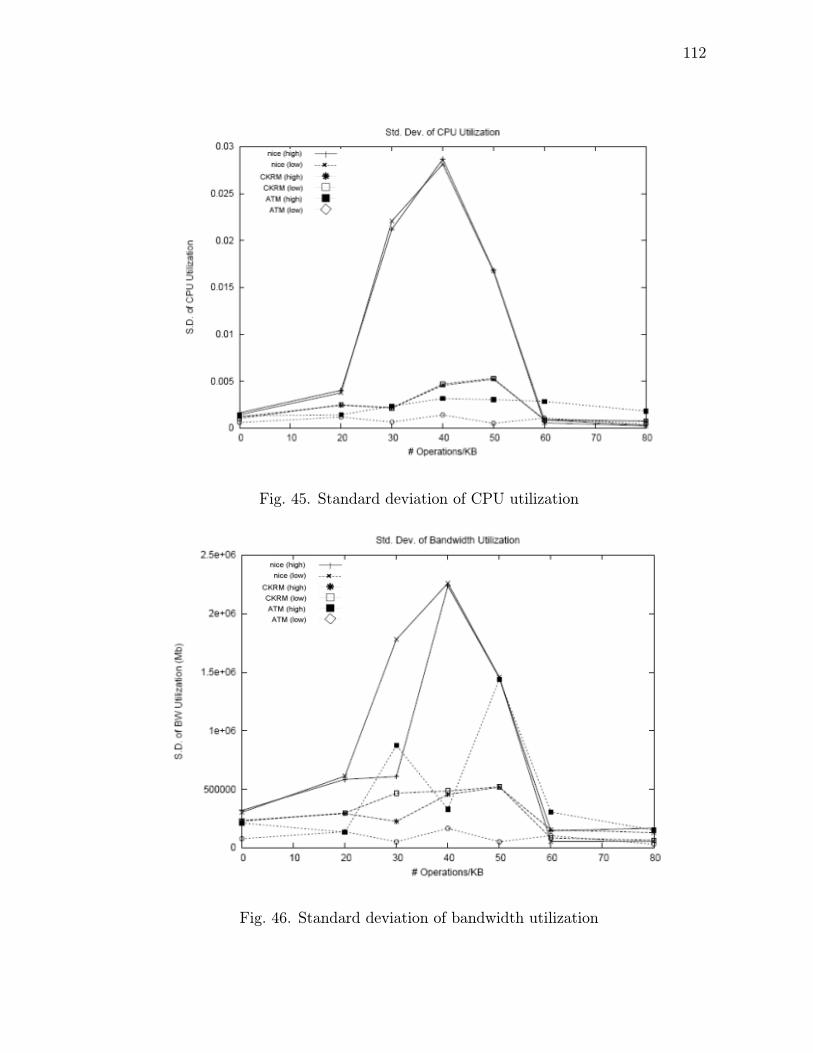
112
Fig. 45. Standard deviation of CPU utilization
Fig. 46. Standard deviation of bandwidth utilization

113
for each trial. Similar to Figure 45, we observe that nice exhibits relatively large
variance in the region between 20 and 60 operations per kilobyte. ATM displays
differing variance in different trials, at times quite high for the higher priority tasks
bandwidth, but consistently lowest of the group for the lower priority tasks band-
width. The former observation is attributed to ATMs bandwidth search mechanism,
which likely had to adjust bandwidth allocation rapidly to maintain the desired CPU
levels in this challenging operating region. In observing ATM at work, it is observed
that often, system tasks can “steal” CPU from the stream processing tasks (since
ATM, unlike nice and CKRM, does not directly control CPU scheduling). This is
consistent with the observation of low variance in the low priority task under ATM,
since it is less likely to have CPU share stolen by system tasks, and ATM can lock in
a specific bandwidth and maintain that allocation for long periods of time.
D. Conclusions and Future Work
Efficient operation of distributed and parallel computing applications depends on
efficient management of multiple resources such as CPU, system memory and link
bandwidth. While substantial work exists on independently managing system (CPU,
memory) and networking resources, little attention has been given to the complex
dependencies between utilization of processing and network bandwidth resources. As
this design shows this link is a critical piece of system management tools, especially in
the case of high bandwidth stream processing applications, for which existing system
management tools based on CPU-prioritization schemes are inadequate.
To address these shortcomings, a system that seeks to achieve system manage-
ment objectives by explicitly considering the relationship between the bandwidth
allocated to an application and its corresponding utilization of processing resources

114
has been developed. By controlling the bandwidth allocation vector across different
applications, the systen is driven towards a desired CPU utilization vector. Effective
operation of this system has been demonstrated for a wide-range of applications, from
CPU intensive to bandwidth-intensive.
The results demonstrate that weighted and prioritized CPU scheduling are not
sufficient to achieve meaningful control over high-rate stream processing operations,
and that our Autonomic Traffic Management system can achieve such control over
both high-rate (low operations/ unit of bandwidth) and low-rate (high operations/unit
bandwidth) stream processing tasks. ATM controls CPU utilization indirectly by
setting the bandwidth to (or from) each processing tasks, and so must learn the
relationship between the bandwidth and CPU resources used by each task, while
simultaneously effecting the desired control output. Despite this algorithmic com-
plexity of ATM, when compared to simple weighted CPU sharing (e.g. nice and
CKRM), ATM achieves accuracy consistency comparable to nice and CKRM for
low-rate stream processing applications, and maintains this performance with the
high-rate stream processing tasks that nice and CKRM cannot handle. Further-
more, it achieves this will notably low overhead. An attempt was made to run both
ATM and CKRM simultaneously, with no corindation between the two, and found
that the combination did not perform as well as ATM alone. Specifically, ATM seems
to experience higher variability and slightly less differentiation in the presence of
CKRM than in isolation. With ATMs ability to control highly bandwidth-centric
tasks and CKRMs ability to control CPU-oriented tasks, using the two in concert, or
dynamically choosing between them, should enable improved control across the full
spectrum of stream processing tasks, and with other types of processes as well.
Further consideration will be given to the design of a generalized resource con-
troller with the ability to allocate and prioritize tasks use of multiple resources (CPU,
115
bandwidth, and others). It is anticipated that there will be gains made by managing
multiple resources in a single framework above and beyond those we achieved here
by controlling different resources via entirely isolated mechanisms. Improvements
will be made on this autonomic traffic management system, getting closer to the
goal of increased performance in real-world systems with significant noise, changing
bandwidth/ CPU usage relationships, and complex interactions.

116
CHAPTER VII
ROUTING IN MOBILE MULTICOMPUTER NETWORK - A CASE STUDY
The advances made recently in the areas of network and computer technology have
given rise to an explosion of mobile computing devices and development of mobile
computing environment. A very important issue in data routing in mobile com-
puting involves managing or tracking of the locations of the computing devices. A
scalable distributed network imposes another level of difficulty, as this involves dy-
namic location management techniques. In this chapter a novel scheme called SEEK
(Spatial Embedded Environment Knowledge) is presented to efficiently route data
while performing location management dynamically for a scalable distributed mobile
multiprocessor network.
The idea is to use some of the communication and routing techniques developed
in previous chapters and adapt these to suite a mobile environment. The first novel
idea introduced is using age parameter to elect non-static location servers in each local
partition. The term location server is used loosely, since the nodes in the network
have equal likelihood of assuming the role of a location server. A more appropriate
name will be Elected Location Manager. Secondly, the method incorporates a new
idea for efficient path set-up for data transfer during the location inquiry and update
steps. Third, this algorithm takes into account the dynamic nature of intermediate
nodes, where nodes may also be moving during data routing.
The diversities in distributed mobile multiprocessor network mean that the net-
works are built with no fixed infrastructure. The nodes have to establish communi-
cation with each other without the services of a centralized switch. Traffic modeling
in such a system is nondeterministic with nodes having diverse mobility patterns. In
order to route data from a source to its destination(s), a host (mobile or static) needs

117
to know the address of the destination(s) at the least.
Some important problems associated with mobile computing on a large scale are
non-trivial. First, the tracking of nodes in a mobile network expends the limited
resources, such as bandwidth and power. Thus, the goal of a location management
scheme will be to optimize the update and query operations, so as to minimize the cost
of location tracking. Secondly, routing of data as a consequence involves establishing
a communication path between source and destination and getting data across the
link to the destination. In a mobile network, where singlehop communication may
not be enough to get data from source node x to destination node y, the cost of
path setup and the mobility of the intermediate routing nodes must be taken into
consideration. Hence, the objective will be to minimize the cost of path setup for
data transfer and eliminate link failures due to the mobility of intermediate nodes,
involved in data transfer.
Mobile networks depend on location servers to hold a list of nodes within a geo-
graphical area. These servers are usually assumed to be static [103-105]. However, for
a large network with many nodes, it becomes impractical to assume that in every par-
tition, a location server exists. This would make it more difficult to achieve scalablity.
The source x has to know the address of the destination y before any transactions
can take place. Assume that every node knows its geographical location by use of
GPS devices. Due to the mobility of nodes, the problem here is that for any node
x, its static address or identification has no relation to its physical location due to
mobility. Address for any node y has to be obtained with only the static address or
identification of y. Node x or y or both could be mobile, as such location update will
have to continue even after the initial handshake, during the course of data exchange.
Some work has been done in the area of Location Management for mobile dis-
tributed computing. Far less work has been done in the area of data routing for such

118
systems that takes advantage of the proposed location management schemes. In [104]
a hierarchical location management scheme is proposed that divide a network into
areas, where each area has at least one router. It achieves good results, however, the
mobility of the location servers is not discussed and it assumes that within an area,
there must exist a location server. The data packets destined for an area has to be
routed through this location server, constituting a bottleneck. In another approach
[106], the location databases hold location storage and retrieval information while an
assumption is made that these databases form an interconnection network with no
clear description on how this routing is achieved. However, the servers are assumed
to be static, which does not solve the problem of scalability. In [107], the authors
suggest a decentralized location service, in which nodes create region with similar IDs
and designate one node as the location server. The obvious problems inherent with
such a scheme lie in mobility. To find a location server, a node needs to scan an entire
network. Also, It is likely that both node and original server may move, and this is
not addressed. What happens if a new node enters the region, is not addressed either
in the paper.
Another insight to the mobility issues is found in the work of [103], in which the
authors propose a distributed location management. It has the attributes of being
distributed, scales well and meets certain mobility challenges. The address structure
is hierarchical, so it achieves address encapsulation. However, the scheme makes
use of location servers, without taking into account the mobility of such servers and
assumes that in the network partitions, there are no areas without a location server.
The cost of having dedicated location servers in each partition as the number of
partition increase will certainly prove to be enormous.
In this chapter, a novel scheme to address the issue of static location servers in
location management is presented. A data routing scheme that takes into account the

119
mobility of the communicating nodes and that of intermediate routing nodes during
data transfer is also presented.
First, a unique addressing scheme is introduced that is hierarchical and exploits
locality. This leads to the address of a node dynamically changing as it moves through
different virtual communities. Next, the SEEK set of algorithms are presented, that
perform the function of location management and data routing by establishing par-
titions of nodes to which nodes are locally identified. With the partitioning concept
only a few nodes need to be updated when a node moves. To further improve perfor-
mance, location accuracy is prioritized, so that only a small number of nodes need to
have an accurate location update. This greatly reduces the amount of resources ex-
pended in mobility tracking. Third, age is used as a parameter to determine partition
location managers in this dynamic environment. Fourth, the data routing strategy
incorporated in the location inquiry/update stage is introduced. This design takes
into account the mobility of both the communicating nodes and intermediate nodes
involved in data transfer. With this method, there is a significant reduction in delays
caused by routing data through the location managers. A further reduction in delays
is achieved by applying a novel concept called predictive data routing. This uses a
probability model to predict the location of destination nodes. Finally, some theoret-
ical analysis to show the complexity of this scheme is presented along with computer
simulations to show the performance.
The outcome of this approach is such that the mobility of the location servers
and mobility of the intermediate routing nodes are taken into account. Furthermore,
location prediction methods are applied to prevent data loss and enhance packet
routing in the case where all nodes are in motion.

120
Fig. 47. Graphical illustration of network showing only two levels
A. The System Model
In the proposed scheme, a tree structure is used to implement a hierarchy, in which
leaf nodes of the tree are the zero-level cells or level-0 partition. The tree structure
enables scalability of the network and reduces the overhead control message borne by
each cell. We show later by mathematical modeling and theoretical considerations
the upper bound on the complexity of our scheme.
In this dissertation, cell structures identical and hexagon-shaped as in wireless
cell phone structures are adopted. Hexagons have been shown to be optimal shape
in a 2D space for cell packing [108]. This proof is described in a later section. A
graphical illustration of this network is shown in Figure 47.
The mobile network is modeled on a flat two-dimensional plane physically, called
the “network area”. The cells are assumed to be non-overlapping and cover the
network area contiguously. Each node in the network can be in one and only one of
the partitions at any given time. The partitioning scheme is hierarchical and so the
addressing scheme harnesses this feature. The goal is to achieve the following:

121
• Partition the network into a hierarchy of regular 6-sided polygons to minimizethe average signaling cost registration
• Achieve address compression using a hierarchical approach
1. Network Partition Scheme
Below are some definitions.
Definition:
1. A minimum partition (hexagon) is called a level-0 partition.
2. A level-n partition consists of seven level-(n-1) partition cells, grouped together
to form another hexagonal area.
It is assumed that within a level-0 partition, the power requirements will be met,
i.e., single hop communication will be guaranteed at the least. In this scheme, the
network area is partitioned, adopting hexagonal-shaped cell structures. The center
of the network area is identified, shown in the Figure 48, as the Locus of Network
Trajectory (LocusNT). This locus is also going to be the center of a hexagon. The
LocusNt is surrounded by six other hexagons on its six sides. The result is a 7-leaf
tree structure used to implement a hierarchy, in which leaf nodes of the tree are the
level-zero partition cells. The tree structure enables scalability of the network, (ie the
network is allowed to grow) and reduces the overhead control message borne by each
cell. An illustration is given in Figure 48.
The dimensions of the base hexagon will depend on the design specifications,
which include power requirements of the nodes, so that the diameter of hexagon does
not exceed range of transmission of every node in the network. The physical partition
layout in Figure 49 shows an example of partitioning for a four-level network.
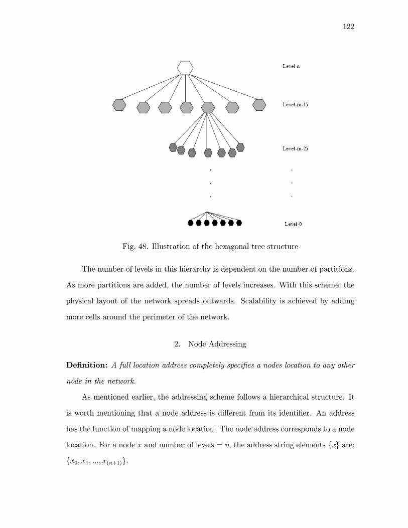
122
Fig. 48. Illustration of the hexagonal tree structure
The number of levels in this hierarchy is dependent on the number of partitions.
As more partitions are added, the number of levels increases. With this scheme, the
physical layout of the network spreads outwards. Scalability is achieved by adding
more cells around the perimeter of the network.
2. Node Addressing
Definition: A full location address completely specifies a nodes location to any other
node in the network.
As mentioned earlier, the addressing scheme follows a hierarchical structure. It
is worth mentioning that a node address is different from its identifier. An address
has the function of mapping a node location. The node address corresponds to a node
location. For a node x and number of levels = n, the address string elements {x} are:{x0, x1, ..., x(n+1)}.
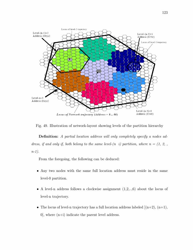
123
Fig. 49. Illustration of network-layout showing levels of the partition hierarchy
Definition: A partial location address will only completely specify a nodes ad-
dress, if and only if, both belong to the same level-(n i) partition, where n = (1, 2, ,
n-1).
From the foregoing, the following can be deduced:
• Any two nodes with the same full location address must reside in the samelevel-0 partition.
• A level-n address follows a clockwise assignment (1,2,..,6) about the locus of
level-n trajectory.
• The locus of level-n trajectory has a full location address labeled [(n+2), (n+1),0], where (n+i) indicate the parent level address.

124
Consider Figure 493, there are three levels. The locusNT has address [0, 0, 0, 0].
Each level-0 partition has full address [x3, x2, x1, x0]. Two nodes in the same level-0
partition will have the same location address. If the nodes are in different partitions,
then the extent of which their location address differs depends on which common
parent level they share in the hierarchy.
3. Node Community Update
A mobile node may leave its current location (partition) and enter another partition.
The elected location manager is updated each time this happens. If a node enters
or moves away from a partition, it sends this information to the location manager.
Assume that a node is able to determine the boundaries corresponding to the loca-
tion address. The location server updates its list and broadcasts this information to
all the nodes within the level-0 partition. Every node then updates its list. This
is necessary to enable communication amongst nodes in a cell, without reference to
the location manager in that cell. A different approach might be to have only the
location manager keep a member list and perform all the updates without broadcast-
ing. However, apart from maximizing network resources in the case of inquiry and
update, another important factor is delay. If two nodes in the same level-0 partition
need to communicate, the sender has to send the inquiry to the location manager.
The location manager becomes the bottleneck, and consequently leads to delays. In
this implementation, SEEK- (location entry) and SEEK - (location exit) algorithm
are used to achieve the node community update.
Algorithm 5 (SEEK - (Location Entry))
begin
SEEK (addr(x), id(x), node age, counter);

125
set counter = 0;
for each level-0 partition do
reset node age = 0;
start counter;
node age = counter;
for (i = 0, i < 3, i++) do
send ping packet to addr[000];
if ack packet is received then
send id(x) to addr[000];
addr(x) = memlist + 1;
addr[000] broadcasts id(x) & addr(x);
break;
else
set addr(x) = addr[000];
end
end
end
end
In location entry, when a node enters a new partition, it sends a ping packet
to address [000]. This is usually reserved for the location manager. If an ack is not
received after a specified wait time, the node retransmits the ping packet. Retrans-
mission is done three times to make sure that the partition is empty. If no ack is
received after the third ping, the node assumes the partition is empty and assigned
address [000] to itself. If however, an ack is received, the node sends its node-id to

126
the location manager.
In location exit, a node also sends a ping packet to the location manager, and the
process of updating and broadcasting is repeated. If however, the location manager
is the node exiting, it checks to see if address [001] exists in its list. If this address
exists, it hands over the member list to the node with address [001]. If this node is
non-existent, the member list is discarded.
Algorithm 6 (SEEK - (Location Exit))
begin
SEEK (addr(x), id(x), new list, old list);
for each level-0 partition do
send addr(x) to addr [000];
if addr(x) == addr[000] then
if addr[001]==NULL then ;
return 0 ;
else send memlist to addr[001];
end;
else
addr[000] updates memlist;
new list = old list - addr(x);
broadcast new list;
end
end
end

127
4. Location Inquiry
A node sends a query to its location manager only when the requested node iden-
tification is not within the level-0 partition member list. When a location manager
in level-0, receives an address inquiry from a member node, it resends this request
to the level-1 location manager. A location manager in level-n partition (where
n = 1, 2, ..., n) on receiving an address inquiry from one of the level-(n − 1) loca-tion managers, redirects this query to the other (n − 1) sibling location managers.These sibling location managers propagate this inquiry down to the level-0 location
managers that check their member list. If there is a match, an “ack” is sent back
with the address to the level-n location manager. The level-n location manager, then
forwards the address to the level-(n-1) manager that sent the inquiry . The level-n
location manager also broadcasts a “stop-query” packet, to signal that a match was
found. If matches are not found in the member lists of the level-0 location managers
that have root at the level-n location manager, the query is the sent to the level-
(n+1) location manager and the process is repeated until a match is found. A formal
description of the location inquiry is shown in Table 3.
Algorithm 7 (SEEK - (Location Inquiry))
begin
SEEK (id(x-inquiry), addr(x));
node(y) sends id(x-inquiry) to addr[000];
while(level-n is not level-0) do
send id(x-inquiry) to other level-n addr[000] ;
if id(x-inquiry) is in memlist do
send ack/addr(x) packet to query addr[000];
query addr[000] broadcast stop-query packet;

128
send addr(x) to node(y) or level-(n-1) addr[000];
else
send id(x-inquiry) to level-(n+1) addr[000];
end
end
end
B. Distributed Mobile Data Routing
The main objectives outlined are first, to complete the path setup for the data transfer
at the same time as the location inquiry step. Second, address the issue of mobility
of the intermediate nodes involved in data transfer, and third, apply predictive data
routing as a method of reducing delays and control overhead. The types of data
considered here will typically be of large size take quite some time to transfer like
a continuous data transfer, e.g., streaming video/audio. This scheme differs from
other schemes in that the path setup step is done at the same time as the destination
address inquiry step. The location managers are not dedicated router nodes for data
transfer, and so are not bottlenecks. Data transfer follows a flat topology, while
location management makes use of a hierarchical topology.
1. Path Setup
Data routing follows a packet switched approach. Packet switch networks have been
researched extensively and is well understood. However, mobility of the communicat-
ing nodes and indeed the intermediate routing nodes still posses some challenge in a
distributed mobile network.

129
As mentioned earlier, if a node wants to communicate with another node, it ob-
tains the address using the location inquiry technique earlier outlined. A node address
specifies the node location. Here, a description of how the path setup is incorporated
in the location inquiry step is outlined. When the destination node receives a location
query packet, the path setup commences. The destination node runs the algorithm to
determine how many hops it would take to establish communication with the source
based on the address and power transmission range. This is basically a backward
reservation technique. It then sends a request-for-reservation packet to the location
manager or level-0 location manager. This request-for-reservation packet contains
the destination address. The level-0 location manager then transmits this packet to
a level-1 location manager that broadcasts this request-for-reservation packet in the
reverse direction of data propagation. Any node along this direction of propagation
but not in the same cell or level-0 partition as either the destination node or source
node can respond to this request and send an ack packet to its location manager.
The location manager attaches the address location of the intermediate node in the
ack/address packet being propagated to the source. This process continues up and
down the hierarchy until the ack/address packet gets to the source node. The result
is that the acknowledgement packet from the destination node to the sender will con-
tain the addresses of all intermediate nodes reserved by the level-n location managers
during the course of location inquiry. Data transfer commences when this ack/address
packet is received from the destination node. A formal description of the path setup
is shown in Table 4.
Algorithm 8 (SEEK - (Path setup))
begin
SEEK (addr(*), addr(x), request-for-reservation, node(*);

130
node(x) receives id(x-inquiry) from addr[000];
attach addr(x) to request-for-reservation packet;
send request-for-reservation packet to addr[000];
set switch = 0;
transmit packet to level -1 addr[000];
while(level-n is not level-0) do
if switch = 0 do
send request-for-reservation packet to
other level-(n-1) addr[000];
if level-(n-1)==level-0 do
if (partition is a long direction of propagation
& not source node address) do;
assign node* = intermediate routing node;
attach addr(*) to request-for-reservation packet;
switch = 1;
send to level-n;
else
send request-for-reservation packet to source node;
end
else
send packet to level-(n-i) addr[000]
(i = 2, 3,..., (n- 1));
end
else
send packet to level-(n+1) addr[000];

131
end
end
end
Once data transfer is initiated, all the nodes involved in the data transfer refresh
the location addresses intermittently. This is a necessary step, to avoid link failure due
to node mobility. The data transfer and location address refresh does not include any
of the location managers. In the next section, the issue of mobility of the intermediate
nodes is addressed.
2. Packet Hand-over
During data transfer, an intermediate may move away from the path of optimal
data transfer or out of range of communication. In such a case, the link may be
broken and hence data transfer aborted, or the need may arise to route through
another intermediate node. To accommodate this we propose a Hand-over scheme,
to accommodate this problem. In a previous section, we described a SEEK- (location
exit) algorithm. In the algorithm, a node updates its location manager. If this
node is currently involved in a data transfer, it also sends the updated version of
the list of nodes involved it the data transfer. The location manager then re-assigns
another node to take over the data transfer. The location manager also modifies
the header information containing the list of addresses of the nodes involved in the
data transfer to reflect the change. It then propagates this information to the source
node. The source node and all subsequent intermediate nodes that receive this header
information attach it to the data packets. Automatically, a hand-over is achieved.

132
3. Predictive Data Routing
In predictive data routing, a source node assumes that the last known address of
the destination is still the current location address. In this case both nodes must
have communicated in the past. This approach has the overall result of reducing the
frequency of location inquiry and consequently an improvement on delay. Analysis on
delay improvement is given in Section 4. By applying predictive methods, a source
node does destination location address inquiry only if it has no record of having
communicated with the destination node in the past. In our design, we assume that
this memory requirement will not be significant for any of the nodes.
This form of routing is based on the observation that on the average a node
will communicate with a destination node more than once before the destination
node leaves its cell. In this regard, the source node is able to perform forward path
reservation. The source node is able to do this because it assumes the destination
node address has not changed. If the forward path reservation does not complete its
task in a given time frame, the normal source initiated destination address inquiry
and backward reservation is prompted.
When the destination receives the req packet from the source in forward reserva-
tion, it sends an ack packet via the intermediate nodes. This reduces the delay and
bottleneck imposed by routing this ack through the location managers.
For fault tolerant purposes, this approach also proves to be most efficient. If a
path in data routing fails due to intermediate node mobility, forward reservation is
initiated as mentioned above.

133
Fig. 50. Comparison between rectangle and hexagonal packing
C. Analysis
In this section, some analytical results on the complexity of the proposed scheme and
some theoretical bounds on performance are presented. First, a proof to show that
the optimal partitioning for a 2D space is the hexagon.
1. Analysis for Optimal Partitioning
Theorem 1: Optimal sampling in 2D results in the hexagonal or interlaced sampling :
Proof:

134
This is shown by comparing interlaced hexagonal partitioning to the commonly
used rectangular partitions [103]. Consider the partitioning of the space as a sampling
operation and the operation of assigning nodes in the space to a given partition as
analogous to 2D quantization. Then, compare this problem to one of optimal vector
quantization sampling in 2D [108]. Figure 50 shows the rectangular sampling, with
a sampling period of T , while the hexagonal sampling has a sample period of T on
the x-axis and (T2 = (3)T1)/2 on the y-axis. The indices (x, y) is mapped onto the
sampling grid as
⎛⎜⎜⎝ ShxShy
⎞⎟⎟⎠ = Vhex⎛⎜⎜⎝ xy
⎞⎟⎟⎠ and⎛⎜⎜⎝ SrxSry
⎞⎟⎟⎠ = Vrect⎛⎜⎜⎝ xy
⎞⎟⎟⎠Assuming that both methods have the same sampling period T on the x-axis,
the matrix conveniently describes this 2D sampling
Vrect =
⎛⎜⎜⎝ T 0
0 T
⎞⎟⎟⎠ and Vhex =⎛⎜⎜⎝ T 0
T/2 (√3T )/2
⎞⎟⎟⎠Sampling density is proportional to 1
detV. By taking ratios,
detVrect
detVhex=
√3
3= 0.866 (7.1)
From this it is evident that hexagonal sampling requires 13.4% fewer samples than
rectangular sampling. This is a well-known result in communication that hexagonal
partitioning is the most efficient partition of a 2D space.
Theorem 2: The upper bound for delay for any request is twice the depth of tree
multiplied by maximum time delay for single hop.
Proof:

135
The hierarchical hexagonal partitioning may be represented as a 7-leaf tree-
partitioning scheme. To describe a fast algorithm for computing request path, we
consider recursive partitioning in which subdivision is recursively done, until the
leave nodes, i.e. the smallest hexagonal cells of the space are reached. If there are
m such cells, then we attain a level J tree where J = 2log7(n) . The number of
hops for a request from one node in the network to any other node is then upper-
bounded by 2J . This is true, since in the worst case scenario, requests between cells
that are farthest apart have to ascend to the over-all level J location manager, be-
fore descending again to the level- 0 node. If it takes a maximum time delay of δ
for a single hop, then 2Jδ ≥ delay for any request. This scheme presents a savingsof 7/4% over the commonly used rectangular schemes with dyadic block structures.
Each node has a total of J location servers (in hierarchy) and this represents 13.4%
fewer location managers, than in the rectangular dyadic structure proposed in [103].
Thus this scheme yields improved delays for requests.
2. Analysis for Delay Improvement
Theorem 3: The forward path reservation algorithm yields 50% delay improvement
Proof:
This is intuitive since the source node is not required to first wait for the ack
packets from the destination notes before transmission commences. For example, for
a 3-hop transmission route, the source node has to wait 12 time slots with the regular
transmission scheme before he commences transmission. This is first used to find the
destination node using location managers, and then to reserve. For the forward path
reservation, he waits only 6 time slots.

136
D. Simulation Results
The simulations are implemented using OPNET network simulator. Each nodes trans-
mission range is assumed to have a radius of 4s0 where sn is the length of a side of
the level-n hexagonal cell, s0 = 100m, the network area is a level-2 hexagon with s2
= 1400m. The nodes move randomly using a 1D Brownian model. 50 nodes are used,
all assumed to be uniformly distributed over the entire network. The duration of each
data stream is set to 5 seconds. All buffers are assumed to have infinite size, so that
delays are only due to location management, path reservation and mobility of nodes.
The following metrics are used for comparison and analysis.
1. Control signal delay: this is the average time delay needed to obtain a destina-
tion address before transfer.
2. Reservation scheme: either source initiated (backward reservation) or destina-
tion initiated (forward reservation).
3. Average packet delay: is defined as the time it takes a packet arriving at the
queue of a transmitting node to be transmitted to all its destination nodes.
Figure 51 illustrates the control signal delay comparison. The total number of
nodes is varied from 0 to 100 per simulation time. The result shows that a hierarchical
scheme performs better. In Figure 52, the effect of having either backward or forward
reservation is shown. Figure 53 shows the average packet delay as speed of nodes
is varied, while Figure 54 illustrates the effect of applying predictive routing using
SEEK algorithm.

137
Fig. 51. Comparing the control signal delay of SEEK and different regular topologies
Fig. 52. Effect of reservation techniques on control signal delay

138
Fig. 53. Comparing the average packet delay of SEEK and other topologies
Fig. 54. Effects of predictive routing on average packet delay using SEEK

139
E. Conclusion
In this chapter, a novel scheme to efficiently route data while performing location
management in a mobile multiprocessor network was presented. The scheme uses
a hierarchical addressing and hexagonal partitioning structure. This approach elim-
inates the need for static location servers and takes into account the mobility of
intermediate routing nodes to minimize packet delays. It was demonstrated that the
method is fault tolerant and scalable. Theoretical and experimental analysis was
offered to show the good performance of this design.

140
CHAPTER VIII
CONCLUSION
The ever-increasing quest for higher performance has made current multi-computer
systems exceedingly complex. This complexity lies in both hardware and software
systems, making it difficult, if not impossible, to further improve total system perfor-
mance. Furthermore, overall complexity is driving up design, development, implemen-
tation, and testing costs while decreasing system reliability. The primary motivation
of this research was to discover novel approaches to improve performance and in-
crease the capabilities of modern multi-computer systems without unduly increasing
the complexity faced by computer architects, software developers and communication
interconnection network and topologies.
The approach in this dissertation first has been to understand and predict the
changes in trends, requirements and underlying technology, then extrapolate the cur-
rent evolutionary path, identify possible paradigm shifts that can drastically simplify,
improve and expand the system, and test these hypotheses by developing a working
prototype within the current constraints. The assumption is made that building real
systems is critical in conducting credible systems research. In many instances, the
discrepancies between a theoretical paper design and a feasible design can only be
delineated or revealed by implementing a prototype. This prototype was designed to
undergo stress analysis under real world situations. The research approach encom-
passed scalable designs both in hardware and software. The underlying philosophy
used in producing this dissertation was to work closely with industry leaders in re-
search and development. It is hoped that this study will aid in understanding with
an objective to give realistic feedback to short and long term projections in large-
scale supercomputer designs capable of petaFLOP and beyond. To this end novel

141
approaches involving optical interconnects, classical and quantum computer designs,
electro-optical integration, etc., have formed the basis of this research.
The design and analyses of an extremely scalable distributed multicomputer ar-
chitecture using optical interconnects that has the potential to deliver in the order
of petaFLOP (1015 floating point operations per second) performance was presented
in detail. The design takes advantage of optical technologies, harnessing the fea-
tures inherent in optics, to produce a 3D stack that implements efficiently a large,
fully connected system of nodes forming a true 3D architecture. To adopt optics in
large-scale multiprocessor cluster systems, efficient routing and scheduling techniques
are needed. To this end, novel self-routing strategies for all-optical packet switched
networks, and on-line scheduling methods that can result in collision free commu-
nication and achieve real time operation in high-speed multiprocessor systems were
proposed. The system was designed to allow failed/faulty nodes stay in place with-
out appreciable performance degradation. The approach was to develop a dynamic
communication environment that will be able to effectively adapt and evolve with
a high density of missing units or nodes. A joint CPU/bandwidth controller that
maximizes the resource allocation in this dynamic computing environment was intro-
duced with an objective to optimize the distributed cluster architecture, preventing
performance/system degradation in the presence of failed/faulty nodes.

142
REFERENCES AND LINKS
[1] H. Zang, J. P. Jue, L. Sahasrabuddhe, R. Ramamurthy, and B. Mukherjee, ``Dy-
namic Lightpath Establishment in Wavelength-Routed WDM Networks," IEEE
Communications Magazine 39(9), 100-108 (2001).
[2] H. Zang, J. P. Jue, and B. Mukherjee, ``Capacity Allocation and Contention
Resolution in a Photonic Slot Routing All-Optical WDM Mesh Network,"
IEEE/OSA Journal of Lightwave Technology 18(12), 1728-1741 (2000).
[3] K. Lu, J. P. Jue, G. Xiao, and I. Chlamtac, ``Intermediate-Node Initiated Reser-
vation (IIR): A New Signaling Scheme for Wavelength-Routed Networks," IEEE
Journal on Selected Areas in Communications 21(8), 1285-1294 (2003).
[4] B. Hamidzadeh, M. Maode, and M. Hamdi, ``Message Sequencing Techniques
for On-Line Scheduling in WDM Networks," IEEE/OSA Journal of Lightwave
Technology 17(8), 1309-1319 (1999).
[5] T. Kitamura, M. Iizuka, M. Sakuta, Y. Nishino, and I. Sasase, ``New Parti-
tion Scheduling Algorithm by Prioritizing the Transmission of Multicast Packets
with Less Destination Address Overlap in WDM Single-Hop Networks," in Pro-
ceedings of the IEEE Global Telecommunications Conference, GLOBECOM '01,
(IEEE 2001), pp. 1469 -1473.
[6] J. E. M. Perea Martins and A. G. Neto, ``Simulation and Analysis of a Collision-
less Optical Interconnection Network," in Proceedings of the SBT/IEEE Int'l
Telecomm. Symposium, (IEEE 1998), pp. 120-125.
[7] B. Dasgupta and M. A. Palis, ``Provable Good Algorithms for Transmission

143
scheduling in WDMOptical Networks,” Journal of Parallel and Distributed Com-
puting 57, 345-357 (1999).
[8] E. Modiano, “Unscheduled Multicasts in WDMBroadcast-and-Select Networks,”
In Proceedings of the IEEE/Infocom ’98, (IEEE 1998) 1, 86-93.
[9] C. L. Seitz, “Concurrent VLSI Architectures,” IEEE Trans. On Computers C-
33(12), 1247-1265 (1984).
[10] W. J. Dally and C. L. Seitz, “The Torus Routing Chip,” Journal of Parallel and
Distributed Computing 1, 187-196 (1986).
[11] W. J. Dally, “Network and Processor Architectures for Message-driven Comput-
ers,” VLSI and Parallel Computation, R. Suaya, G. Birtwistle (Eds.), (Morgan
Kaufmann, Los Altos, CA, 1990), pp. 140-222.
[12] J. W. Goodman, F. J. Leonberger, S. C. Kung, and R. A. Athale, “Optical
Interconnections for VLSI Systems,” IEEE 72(7), 850-866, (1984).
[13] M. R. Feldman, S. C. Esener, C. C. Guest, and S. H. Lee, “Comparison Between
Optical and Electrical Interconnects Based on Power and Speed Considerations,”
Appl. Opt. 27, 1742-1751, (1988).
[14] D. A. B. Miller, “Optics for Low-energy Communication Inside Digital Proces-
sors: Quantum Detectors, Sources, and Modulators as Efficient Impedance Con-
verters,” Opt. Lett. 14, 146-148, (1989).
[15] S. Esener and P. Marchand, “Present and Future Needs of Free-Space Optical
Interconnects,” in Proceedings of the IPDPSWorkshop, (IPDPS 2000), pp. 1104-
1109.

144
[16] R. A. Morgan, J. Bristow, M. Hibbs-Brenner, J. Nohava, S. Bounnak, et al, “Ver-
tical Cavity Surface Emitting Lasers for Spaceborne Photonic Interconnects,” in
Proceedings of the SPIE - The International Society for Optical Engineering,
(Photonics for Space Environments IV), SPIE 2811 232-242 (1996).
[17] A. V. Kishnamoorthy, L. M. F. Chirovsky, W. H. Hobson, R. E. Leibenguth,
S. P. Hui, et al., “Vertical-Cavity Surface-Emitting Lasers Flip-chip Bonded to
Gigabit-per-Second CMOS Circuits,” IEEE Phot. Tech. Lett. 11(1), 128-130,
(1999).
[18] A. V. Krishnamoorthy, “Applications of Opto-electronic VLSI Technologies,”
Int. Journal Optoelectron 12(4), 155161, (1998).
[19] D. J. Goodwill, “Free-space Optical Interconnect for Terabit Network Elements,”
in Proceedings of the Optics in Computing Conference, (Snowmass CO, April
1999).
[20] S. P. Levitan, T. P. Kurzweg, P. J. Marchand, M. A. Rempel, D. M. Chiarulli, et
al., “Chatoyant: A Computer-aided Design Tool for Free-space Optoelectronic
Systems,” Applied Optics 37(26), 6078-6092, (1998).
[21] N. F. Maxemchuk, “Comparison of Deflection and Store-and-Forward Techniques
in the Manhattan Street and Shuffle-Exchange Networks,” INFOCOM 89 3, 800-
809, (1989).
[22] A. Choudhoury and V. Li, “Performance Analysis of Deflection Routing in the
Manhattan Street Network,” IEEE ICC’91 3, 1659-1665, (1991).
[23] T. Robertazzi and A. Lazar, “Deflection Strategies for the Manhattan Street
Network,” IEEE ICC’91 3, 1652-1658, (1991).

145
[24] N. F. Maxemchuk, “Routing in the Manhattan Street Network,” IEEE Trans.
on Communications 35(5), 503-512, (1987).
[25] A. S. Acampora and S. I. A. Shah, “ Multihop Lightwave Networks: A Compar-
ison of Store-and Forward and Hot-Potato Routing,” IEEE Trans. on Commu-
nications 40(6), 1082-1090, (1992).
[26] F. Forghieri, A. Bononi and P. Prucnal, “Analysis and Comparison of Hot-Potato
and Single Buffer Deflection Routing in Very High Bit Rate Optical Mesh Net-
works,” IEEE Trans. on Communications 43(1), 88-98, (1995).
[27] J. Brassil, A. Choudhoury and N. Maxemchuk, “The Manhattan Street Network:
A High Performance, Highly Reliable Metropolitan Area Network,” Computer
Networks and ISDN Systems 26, 841-858, (1994).
[28] F. Chevalier, D. Cotter and D. Harle, “Performance of a Novel Control and
Routing Strategy for a Manhattan Street Network,” in 15th IEE UK Teletraffic
Symposium, (Durham, UK, 1998).
[29] X. C. Yuan, V. O. K. Li, C. Y. Li and P. K. A. Wai, “A Novel Self-routing
Scheme for All-optical Packet Switched Networks with Arbitrary Topology,”
IEEE ICC’01, 7, 2155-2159, (2001).
[30] V. W. S. Chan, K. L. Hall, E. Modiano and K. A. Rauschenbach, “Architectures
and Technologies for High-speed Optical Data Networks,” Journal of Lightwave
Technology 16(12), 2146-2168, (1998).
[31] I. Chlamtac, A. Fumagalli and L. G. Kazovsky, “CORD: Contention Resolution
by Delay Lines,” IEEE Journal on Selected Areas in Communications, 14(5),
1014-1029, (1996).

146
[32] J. P. Jue, “An Algorithm for Loopless Deflection in Photonic Packet-Switched
Networks,” IEEE ICC ’02, New York, 5, 2776-2780, (2002).
[33] X. C. Yuan, V. O. K. Li, C. Y. Li and P. K. A. Wai, “A Novel Self-routing
Scheme for All-optical Packet Switched Networks with Arbitrary Topology,”
IEEE ICC’01 7, 2155-2159, (2001).
[34] M. S. Borella and B. Murkherjee, “A Reservation-Based Multicasting Protocol
for WDM Local Lightwave Networks,” in Proceedings of the IEEE ICC’95, pp.
1277-1281.
[35] J. P. Jue and B. Mukherjee, “The Advantages of Partitioning Multicast Trans-
missions in a Single- Hop Optical WDM Network,” in Proceedings of the IEEE
ICC’97, pp. 247-431.
[36] H. Lin and C. Wang, “Minimizing the Number of Multicast Transmissions in
Single-Hop WDM Networks,” in Proceedings of the IEEE ICC2000, pp. 1645-
1649.
[37] T. Kitamura, M. Iizuka, M. Sakuta, Y. Nishino, and I. Sasase, “New Parti-
tion Scheduling Algorithm by Prioritizing the Transmission of Multicast Packets
with Less Destination Address Overlap in WDM Single-Hop Networks,” in Pro-
ceedings of the IEEE Global Telecommunications Conference, GLOBECOM ’01,
pp.1469 -1473.
[38] D. Steer, M. H. Shor, A. Goel, J. Walpole, and C. Pu, “Control and Modeling
Issues in Computer Operating Systems: Resource Management for Real-rate
Computer Applications,” In Proceedings of 39th IEEE Conference on Decision
and Control (CDC), (December 2000).

147
[39] F. Petrini and W. Feng, “Buffered Coscheduling: A New Methodology for Mul-
titasking Parallel Jobs on Distributed Systems,” in Proceedings of the Inter-
national Parallel and Distributed Processing Symposium (IPDPS 2000), (April
2003).
[40] E. Frachtenberg, D. G. Feitelson, F. Petrini, and J. Fernandez, “Flexible
Coscheduling: Mitigating Load Imbalance and Improving Utilization of Hetero-
geneous Resources,” in Proceedings of the International Parallel and Distributed
Proceesing Symposium (IPDPS 2000), (April 2003).
[41] W. W. Wilcke, S. Kirkpatrick, R. B. Garner and H. Huels, “Percolation in Dense
Storage Arrays,” Physica A 314(1-4), 220-229, (2002).
[42] T. M. Pinkston, “Design Considerations for Optical Interconnects in Parallel
Computers,” in Proceedings of the First International Workshop on Massively
Parallel Processing Using Optical Interconnects, (April 1994), pp. 306-322.
[43] H. J. Siegel, “Interconnection Networks for Large Scale Parallel Processing,”
(McGraw-Hill, 1990).
[44] S. W. Seo, K. Bergman and P. R. Prucnal, “Transparent Optical Networks with
Time-Division Multiplexing,” IEEE Journal Selected Areas in Communication
14(5), 1039-1052, (1996).
[45] D. Cotter, J. K. Lucek and D. Marcenac, “Ultra-high Bit Rate Networking:
From the Trans-Continental Backbone to the Desktop,” IEEE Communications
Magazine 35(4), 90-95, (1997).
[46] J. P. Jue, “An Algorithm for Loopless Deflection in Photonic Packet-Switched
Networks,” in Proceedings of the IEEE ICC ’02, (2002), pp. 2776-2780.

148
[47] T. L. Harris, Y. Sun and R. L. Cone, “Demonstration of Real-time Address
Header Decoding for Optical Data Routing at 1536nm,” Optical Letters 23(8),
636-638, (1998).
[48] W. Dally and C. Seitz, “Deadlock-free Message Routing in Multiprocessor Inter-
connection Networks” IEEE Trans. on Computers 36(5), 547-553, (1987).
[49] S. Dandamudi, Hierarchical Hypercube Multicomputer Interconnection Net-
works, (Ellis Horwood, 1991).
[50] S. Dandamudi and D. Eager,“Hierarchical Interconnection Networks for Multi-
computer Systems,” IEEE Trans. on Computers 39(6), 786-797, (1990).
[51] B. Mukherjee, “WDM-based Local Lightwave Networks- Part I: Single-Hop Sys-
tems,” IEEE Network 6(3), 12-27, (1992).
[52] B. Mukherjee, “WDM-based Local Lightwave Networks- Part II: Multi-Hop Sys-
tems,” IEEE Network 6(4), 20-32, (1992).
[53] K. Bogineni, K. M. Sivalingam, and P. W. Dowd, “Low-Complexity Multiple Ac-
cess Protocols for Wavelength Division Multiplexed Photonic Networks,” IEEE
Journal on Communication 11(4), 590-603, (1993).
[54] K. Davis, A. Hoisie1, G. Johnson, D. J. Kerbyson, M. Lang, et al., “A Perfor-
mance and Scalability Analysis of the BlueGene/L Architecture,” in Proceed-
ings of the High Performance Computing, Networking and Storage Conference,
SC2004, PA, (2004).
[55] N. R. Adiga, G. Almasi, G.S. Almasi, Y. Aridor, R. Barik, et al., “An Overview
of the BlueGene/L Supercomputer,” in Proceedings of the SC2002, (2002).

149
[56] Cray Research Inc., Cray T3D System Architecture Overview, (1993).
[57] Intel Corporation, Paragon XP/S Product Overview, (1991).
[58] W. J. Dally, “The J-machine: System Support for Actors,” Knowledge-Based
Concurrent Computing, Hewitt and Agha eds., (MIT Press, 1989).
[59] R. K. Koeninger, M. Furtney, and M. Walker, “A Shared Memory MPP from
Cray Research,” Digital Technical Journal 6(2), 8-21, (1994).
[60] A. V. Krishnamoorthy and D. A. B. Miller, “Firehose Architectures for Free-
space Optically Interconnected VLSI Circuits,” Journal of Parallel and Distrib-
uted Computing 41(1), 109-114, (1997).
[61] P. J. Marchand, A. V. Krishnamoorthy, G. I. Yayla, S. C. Esener and U. Efron,
“Optically Augmented 3-D computer: System Technology and Architecture,”
Journal of Parallel Distributed Computing Special Issue on Optical Interconnects
41(1), 20-35, (1997).
[62] G. A. Betzos, P. A. Mitkas, “Performance Evaluation of Massively Parallel
Processing Architectures with Three-dimensional Optical Interconnections,” Ap-
plied Optics 37(2), 315-25, (1998).
[63] J. W. Goodman, F. J. Leonberger, S. C. Kung, and R. A. Athale, “Optical
Interconnections for VLSI Systems,” IEEE 72(7), 850-866, (1984).
[64] D. A. B. Miller, “Rationale and Challenges for Optical Interconnects to Elec-
tronic Chips,” IEEE 88, 728-749, (2000).
[65] S. Esener and P. Marchand, “Present and Future Needs of Free-Space Optical
Interconnects,” in Proceedings of the IPDPS Workshop, (2000), pp. 1104-1109.

150
[66] D. J. Goodwill, “Free-space Optical Interconnect for Terabit Network Elements,”
Proc. Optics in Computing Conference, (Snowmass CO, April 1999).
[67] B. F. Almohammad and B. Bose, “Fault-tolerant Communication Algorithms in
Toroidal Networks,” IEEE Trans. Parallel & Distributed Systems 10, 976-983,
(1999).
[68] J. Wu, “A Fault-tolerant Adaptive and Minimal Routing Approach in 3D
Meshes,” IEEE Trans. of Parallel and Dist. Systems 11(2), 149-159, (2000).
[69] Z. Jiang and J. Wu, “A Limited-global Fault Information Model for Dynamic
Routing in 3D Meshes,” in Proceedings of the Second IEEE International Sym-
posium on Network Computing and Applications NCA (2003), pp. 333-340.
[70] H. Shen, F. Chin, and Y. Pan, “Efficient Fault-tolerant Routing in Multi-hop
Optical WDM Networks,” IEEE Trans. on Parallel & Distributed Systems 10,
1012-1025, (1999).
[71] C. Ho and L. Stockmeyer, “A New Approach to Fault-Tolerant Wormhole Rout-
ing for Mesh-Connected Parallel Computers,” IEEE Trans. on Computers 53,
427-438, (2004).
[72] I. Glesk, K. I. Kang, and P. R. Prucnal, “All-optical Address Recognition and
Self-routing in a 250 Gbit/s Packet Switched Network,” Electron. Lett. 30, 1322-
1323, (1994).
[73] A. E. Willne, D. Gurkan, A. B. Sahin, J. E. McGeehan, and M. C. Hauer, “All-
optical Address Recognition for Optically-assisted Routing in Next-generation
Optical Networks,” IEEE Commun. Mag. 41(5), 3844, (2003).

151
[74] N. Calabretta, Y. Liu, H. de Waardt, M. T. Hill, G. D. Khoe, and H. J. S. Dorren,
“Multipleoutput All-optical Header Processing Technique Based on Two-pulse
Correlation Principle,” Electron. Lett. 37, 1238-1240, (2001).
[75] M. T. Hill, A. Srivatsa, N. Calabretta, Y. Liu, H. deWaardt, G. D. Khoe, and
H. J. S. Dorren, “1x2 optical packet switch using all-optical header processing,”
Electron. Lett. 37, 774-775, (2001).
[76] P. Toliver, I. Glesk, R. J. Runser, K. L. Deng, B. Y. Yu, and P. R. Prucnal, “Rout-
ing of 100Gb/s Words in a Packet-switched Optical Networking Demonstration
(POND) Node,” Journal of Lightwave Technology 16, 2169-2180, (1998).
[77] K. L. Deng, R. J. Runser, P. Toliver, C. Coldwell, D. Zhou, I. Glesk, and P.
R. Prucnal, “Demonstration of Highly Scalable 100Gbit/s OTDM Computer
Interconnect with Rapid Interchannel Switching Capability,” Electron. Lett. 34,
2418-2419, (1998).
[78] G. Castanon, “Optical Packet Switching with Multiple Path Routing,” Computer
Networks 32, 653-662, (2000).
[79] H. Shi and J. Lin, “Theoretical Analysis on Polarization Deviation and Switch
Window Optimization in Nonlinear Optical Loop Mirror Demultiplexer,” Journal
of Lightwave Technology 17, 2572-2576, (1999).
[80] L. Tangjun, P. Cuizhu, and Z. Yucheng, “Study on improving the performance
of OTDM device,” IEEE Photon. Technol. Lett. 11, 1389-1383, (1999).
[81] T. R. Mathies, “Percolation Theory and Computing with Faulty Arrays of
Processors,” in Proceedings of the Third Annual Symposium on Discrete Al-
gorithms (SODA), (1992), pp. 100-103.

152
[82] W. W. Wilcke, S. Kirkpatrick, R. B. Garner and H. Huels, “Percolation in Dense
Storage Arrays,” Physica A 314(1-4), 220-229, (2002).
[83] R. Gao, Z. Ghassemlooy , G. Swift and P. Ball, “Simulation of All- Optical Time
Division Multiplexed Router”, SPIE Photonics West, (San Jose, 2001).
[84] IBM “LPAR: Dynamic Logical Partitioning, An IBM Virtualization Engine Sys-
tems Technology,” (2004), http://www-1.ibm.com/servers/eserver/iseries/lpar/.
[85] T. Deane, G. Haff and J.Enuice, “VMware on the March,” Research Note, Illu-
minata, Inc., (2004), http://www.vmware.com/pdf/illuminata.pdf.
[86] Sourceforge “Class-based Kernel Resource Management (CKRM),” (2004),
http://ckrm.sourceforge.net/.
[87] R. Cruz,“A Calculus for Network Delay, Part II: Network Analysis,” IEEE Trans-
actions on Information Theory 37, 132-141, (1991).
[88] R. Guerin, H. Ahmadi, and M. Naghshineh, “Equivalent Capacity and Its Ap-
plication to Bandwidth Allocation in High-Speed Networks,” IEEE Journal on
Selected Areas in Communications 9(7), 968-981, (1991).
[89] L. Georgiadis, R. Gurin, V. Peris, K.N. Sivarajan, “Efficient Network QoS Pro-
visioning Based on per Node Traffic Shaping,” in Proceedings of the IEEE IN-
FOCOM Transactions on Networking, (1996), pp. 102-110.
[90] E. Knightly and H. Zhang, “D-BIND: An Accurate Traffic Model for Providing
QoS Guarantees to VBR Traffic,” IEEE/ACM Transactions on Networking 5(2),
219-231, (1997).
[91] R. Braden, D. Clark, S. Shenker, “Integrated Services in the Internet Architec-
ture: An Overview,”Request for Comments - RFC 1633, (1994).

153
[92] E. Crawley, Ed., L. Berger, S. Berson, F. Baker, M. Borden, J. Krawczyk, “A
Framework for Integrated Services and RSVP over ATM,” Request for Comments
- RFC 2382, (1998).
[93] K. Nichols, V. Jacobson, L. Zhang, “A Two-bit Differentiated Services Architec-
ture for the Internet,” Request for Comments - RFC 2638, (1999).
[94] A. Goel, M. H. Shor, J. Walpole, D. C. Steere, and C. Pu, “Using feedback control
for a network and CPU resource management application,” in Proceedings of the
2001 American Control Conference ACC (2001), pp. 2974-2980.
[95] D. Steere, M.H. Shor, A. Goel, J. Walpole, C. Pu, “Control and modeling issues
in computer operating systems: resource management for real-rate computer ap-
plications,” in Proceedings of the 39th IEEE Conference on Decision and Control
CDC2000 (Sydney, Australia, 2000).
[96] J. Guo and L. N. Bhuyan, “Load Sharing in a Transcoding Cluster,” in Proceed-
ings of the Distributed Computing IWDC 2918, pp. 330-339, (2003).
[97] A. Fox, “Adapting to Network and Client Variability via On-Demand Dynamic
Distillation,” in Proceedings of the Seventh Intl. Conf. on Arch. Support for
Programming Languages and Operating Systems (ASPLOS-VII), Cambridge,
MA, 1996.
[98] D. Rosu, K. Schwan, S. Yalamanchili, R. Jha, “On Adaptive Resource Allocation
for Complex Real-time Applications,” in Proceedings of the 18th IEEE Real-
Time Systems Symposium (RTSS 97), December 1997.
[99] S. Chandra, C. S.Ellis, and A. Vahdat, “Application-Level Differentiated Multi-
media Web Services Using Quality Aware Transcoding,” IEEE Special Issue on

154
QOS in the Internet, (2000).
[100] L. Abeni, G.C. Buttazzo, “Adaptive Bandwidth Reservation for Multimedia
Computing,” in Proceedings of the 6th International Conference on Real- Time
and Embedded Computing Systems and Applications (RTCSA), 1999.
[101] J. Liang, K. Nahrstedt and Y. Zhou, “Adaptive Multi-Resource Prediction
in Distributed Resource Sharing Environment,” in Proceedings of the Fourth
IEEE/ACM Symposium on Cluster Computing and the Grid (CCGrid04),
Chicago, IL, April, 2004.
[102] E. Okorafor, D. Pendarakis, J. Silber and L. Wynter, “DIRAC: A Distributed
Interface for Adaptive Network Resource Allocation and Application Control,”
unpublished manuscript, Department of Computer Engineering, Texas A&M
University, College Station.
[103] Y. Xue, B. Li, and K. Nahrstedt, “A Scalable Location Management Scheme
in Mobile Ad-hoc Networks,” in Proceedings of the IEEE Conference on Local
Computer Networks - LCN’2001, (2001), pp. 102-111.
[104] H. Hagino, T. Hara, M. Tsukamoto, S. Nishio, and J. Okui, “A Location Man-
agement Method using Network Hierarchies,” in Proceedings of the IEEE Pacific
Rim Conference on Communications, Computers and Signal Processing, (1997),
pp. 243-246.
[105] R. Subrata, and A. Y. Zomaya, “Location Management in Mobile Comput-
ing,” In Proc. ACS/IEEE International Conference on Computer Systems and
Applications, (2001), pp. 287-289.

155
[106] Z. J. Haas, and B. Liang, “Ad Hoc Mobility Management with Uniform Quorum
Systems,” IEEE/ACM Transactions on Networking 7(2), 228-240, (1999).
[107] J. Li, J. Jannotti, D. Cuoto, D. R. Karger, and R. Morris, “A Scalable Location
Service for Geographic Ad Hoc Routing,” In Proc. Sixth Annual International
Conf. on Mobile Computing and Networking (MOBICOM00), (2000), pp. 120-
130.
[108] A. Lundmark, N. Wardstromer, and H. Li,“Hierarchical Subsampling Giving
Fractal Regions,” IEEE Trans. on Image Processing 10(1), pp. 167-173, (2001).

156
APPENDIX A
NOTATION
Aapp Applications running in a node
N Number of nodes
λn n distinct wavelengths
L Length
w Waist of VCSEL
θ Divergence angle
NA Numerical Aperture
T Execution time of any process
tm Inter-PE propagation delay
tc CPU speed
td Memory speed
N(i,j,k) Three-turple representation of a node in a 3D mesh
Ns Source node
Ni Intermediate node
Nd Destination node
Ei Expected number of intermediate nodes
P Preferred data routing path
A Alternate data routing path
P(prob) Probability
Ploss Packet loss probability
δ Average number of of links
U Link Utilization
λi,j,k Packet arrival rates

157
TCF Number of times lots to complete a data transfer for CF algorithm
TMDCF Number of times lots to complete a data transfer for MDCF algorithm
TDTC Number of times lots to complete a data transfer for DTC algorithm
TMDCFMP Number of time slots to complete a data transfer for MDCFMP algorithm
βin Rate given for a Bernoulli process
LSQ The length of a service queue
S Source
D Destination
ADDRp Primary address
ADDRA Alternate address
Ci Number of virtual channels
Bchannel A set of channels reserved from source to destination
ti Target input CPU levels
bi Bandwidth allocation for process i
Cji(bi) CPU utilization for iteration j

158
APPENDIX B
ACRONYMS
AON All-Optical Network
ATM Autonomic Traffic Management
BER Bit Error Rate
CKRM Class Based Kernel Resource Manager
CPU Central Processing Unit
FLOP Floating Point Operations
FSOI Free Space Optical Interconnects
I/O Input/Output
LAN Local Area Network
MAC Media Access Control
MST Minimum Spanning Tree
MRST Minimum Rectilinear Steiner Tree
NA Numerical Aperture
OEO Optical-Electrical-Optical
OPB Optical Path Box
OTDM Optical Time Division Multiplexing
SEEK Spatial Embedded Environment Knowledge
PE Probability of Error
PML Planar Microlens
POF Plastic Optical Fiber
SLALOM Semiconductor Laser Amplifier in a Loop Mirror

159
TDM Time Division Multiplexing
TOAD Terahertz Optical Asymmetric Demultiplexer
V CSEL Vertical Cavity Surface Emitting Laser
V LSI Very Large Scale Integration
WDM Wavelength Division Multiplexing
RWA Routing & Wavelength Allocation
DTC Data Transfer Cycle
FCFS First-Come-First-Serve

160
VITA
Ekpe Apia Okorafor received the B.E. in electronic and computer engineering
from the University of Nigeria in 1996, the M.S. and Ph.D. in electrical and computer
engineering from Texas A&M University in 2001 and 2005 respectively.
While at Texas A&M, he was a Graduate Research Assistant. He co-authored
a number of conference and journal papers, including a best paper entry. He was a
receipient of the departmental scholarship and several academic achievement awards.
He has worked in different research labs, including IBM.
His research interests are in the areas of optical interconnection networks, mas-
sively parallel and distributed computing, high speed computer network systems, grid
computing, mobile computing and computer architecture.
Permanent Address:
209 Rugen Lane
College Station, TX 77845
USA
The typist for this thesis was Ekpe Apia Okorafor.