design and comparison of pmasynrm versus pmsm for …
TRANSCRIPT
INOM EXAMENSARBETE ENERGI OCH MILJÖ,AVANCERAD NIVÅ, 30 HP
, STOCKHOLM SVERIGE 2018
Design and comparison of PMaSynRM versus PMSM for pumping applications
VIKTOR BRIGGNER
KTHSKOLAN FÖR ELEKTROTEKNIK OCH DATAVETENSKAP

TRITA TRITA-EECS-EX-2018:496
www.kth.se

Design and comparison of PMaSynRM versus PMSM forpumping applications
VIKTOR BRIGGNER
Master of Science Thesis in Electrical Energy Conversionat the School of Electrical Engineering and Computer Science
KTH Royal Institute of TechnologyStockholm, Sweden, August 2018.
Supervisors: Tanja Hedberg and Øystein KrogenExaminer: Oskar Wallmark
TRITA-EECS-EX-2018:496

Design and comparison of PMaSynRM versus PMSM for pumping applicationsVIKTOR BRIGGNER
c� VIKTOR BRIGGNER, 2018.
School of Electrical Engineering and Computer ScienceDepartment of Electric Power Engineering and Energy SystemsKungliga Tekniska hogskolanSE–100 44 StockholmSweden

Abstract
This master thesis aimed to design a permanent magnet assisted synchronous reluctancemachine (PMaSynRM) rotor for pump applications which were to be implemented inan existing Induction Machine stator. The machine were to be compared with a similarpermanent magnet synchronous machine (PMSM) with similar torque production in termsof cost and performance.
This thesis goes through the theory of the Synchronous Reluctance Machine andthe Permanent Magnet assistance. A rotor was designed by utilizing existing design ap-proaches and simulation of performance by use of finite element analysis. A demagneti-zation study was conducted on the added permanent magnets in order to investigate thefeasiblity of the design.
The final design of the PMaSynRM was thereafter compared to the equivalentsurface-mounted PMSM in terms of performance and cost. The performance parameterswas torque production, torque ripple, efficiency and power factor. Due to the lower torquedensity of the PMaSynRM, for equal torque production the PMSM had a 40% shorterlamination stack than the PMaSynRM.
The economic evaluation resulted in that when utilizing ferrite magnets in the PMa-SynRM it became slightly cheaper than the PMSM, up to 20%. However, due to the fluc-tuating prices of NdFeB magnets, there exist breakpoints below which the PMaSynRM isin fact more expensive than the PMSM or where the price reduction of the PMaSynRMis not worth the extra length of the motor. However, it was shown that the PMaSynRMis very insensitive to magnet price fluctuations and thereby proved to be a more securechoice than the PMSM
Keywords: Demagnetization, economic evaluation, permanent magnet assistance,synchronous reluctance machine.
ii
Sammanfattning
Detta examensarbete avsag att designa en rotor till en permanentmagnetsassisteradsynkron reluktansmaskin (PMaSynRM) for pumpapplikationer, vilken skulle implement-eras i en befintlig asynkronmaskin (IM) stator. Maskinen jamfordes ekonomiskt och pre-standamassigt med en liknande synkronmaskin med permanentmagneter (PMSM) medjamforbar vridmomentsproduktion.
Uppsatsen avhandlar teorin bakom synkrona reluktansmaskiner och konceptet kringpermanentmagnetassistans. Rotorn designades genom anvandandet av befintliga design-metoder och simulering genom finit elementanalys (FEA). En avmagnetiseringsstudieutfordes pa de adderade magneterna for att undersoka rimligheten kring designen
Den slutgiltiga designen av PMaSynRMen jamfordes darefter mot den jamlikaPMSMen i termer om prestanda och kostnad. De undersokta prestandaparameterarna varvridmoment, vridmomentsrippel, verkningsgrad och effektfaktor. Eftersom vridmoments-densiteten i en PMaSynRM ar lagre an hos en PMSM sa visade sig PMSMen ha en 40%kortare lamineringskropp an PMaSynRMen vid jamnlik vridmomentsproduktion.
Den ekonomiska utvarderingen resulterade i att vid anvandandet av ferritmagneteri PMaSynRMen sa blev den nagot billigare an PMSMen, upp till 20%. Pa grund av fluk-tuerande priser hos NdFeB magneter, sa finns det brytpunkter dar PMaSynRMen faktisktblir dyrare an PMSMen eller da kostnadsreduktionen for PMaSynRMen kan bedomas attvara for lag med tanke pa den okade langden och vridmomentsrippel. Daremot visadesdet att PMaSynRMen ar valdigt okanslig for prisvariationer och darfor visades vara ettkostnadsmassigt tryggare val an PMSMen.
Nyckelord: Avmagnetisering, ekonomisk utvardering, permanentmagnetassistans,synkron reuktansmaskin.
iii

Acknowledgements
This master thesis has been carried out at the department of Research and Developmentfor electrical motors at Xylem Water Solutions in Stockholm, Sweden.
I would like to thank Xylem Water Solutions for giving me the opportunity to do mymaster thesis for them and for the great experience that it has entailed. I would especiallylike to thank Tanja Hedberg and Øystein Krogen for their supervision and help throughoutthe duration of the project. Furthermore would I like to thank my co-workers at XylemWater Solutions for making my stay there even more enjoyable with their company.
I would also like to express a special thanks to Associate Professor Oskar Wallmark forsparking my interest in electrical machines and for inspiring me to pursue this field of en-gineering. Additionally I would like to thank him for acting as my examiner for this thesis.
I also want to give thanks to all of my friends here in Stockholm who has made myyears at KTH unforgettable to say the least. Thank you for all the memories and for yourfriendship. Even if we eventually find ourselves in different parts of the world, I knowthat we will always stay in touch.
Finally, I would like to give my deepest gratitude to my parents and my sister who alwayshave supported me and helped me whenever I needed it. I would also like to especiallythank my girlfriend, Saga Kubulenso, for her never-ending patience with me when mystudies has gotten the best of me and for always being there for me no matter what. Thankyou so much.
Viktor BriggnerStockholm, SwedenAugust 2018
iv

Contents
Abstract ii
Sammanfattning iii
Acknowledgements iv
Contents v
Acronyms 1
Nomenclature 3
1 Introduction 61.1 Background and objectives . . . . . . . . . . . . . . . . . . . . . . . . . 61.2 Thesis outline . . . . . . . . . . . . . . . . . . . . . . . . . . . . . . . . 8
2 Synchronous Reluctance Machine and Permanent Magnet assistance 92.1 Concept of reluctance torque . . . . . . . . . . . . . . . . . . . . . . . . 92.2 Synchronous reluctance machine . . . . . . . . . . . . . . . . . . . . . . 10
2.2.1 Definition of axes . . . . . . . . . . . . . . . . . . . . . . . . . . 112.2.2 Governing equations . . . . . . . . . . . . . . . . . . . . . . . . 12
2.3 Saliency and performance . . . . . . . . . . . . . . . . . . . . . . . . . . 152.4 Iron saturation . . . . . . . . . . . . . . . . . . . . . . . . . . . . . . . . 172.5 Permanent magnet assistance . . . . . . . . . . . . . . . . . . . . . . . . 17
2.5.1 PM flux magnitude . . . . . . . . . . . . . . . . . . . . . . . . . 202.6 Geometry and performance of PMaSynRM . . . . . . . . . . . . . . . . 21
2.6.1 Parameterization of PMaSynRM . . . . . . . . . . . . . . . . . . 212.6.2 Insulation ratios . . . . . . . . . . . . . . . . . . . . . . . . . . . 232.6.3 Number of flux barriers . . . . . . . . . . . . . . . . . . . . . . . 232.6.4 Torque ripple and rotor slots . . . . . . . . . . . . . . . . . . . . 242.6.5 Air-gap length . . . . . . . . . . . . . . . . . . . . . . . . . . . 252.6.6 Radial and tangential ribs . . . . . . . . . . . . . . . . . . . . . . 25
v

Contents
2.6.7 Magnet dimensions and placement . . . . . . . . . . . . . . . . . 282.6.8 Stator and rotor steel . . . . . . . . . . . . . . . . . . . . . . . . 29
2.7 Permanent magnets . . . . . . . . . . . . . . . . . . . . . . . . . . . . . 302.7.1 Demagnetization . . . . . . . . . . . . . . . . . . . . . . . . . . 31
2.8 Theoretical foundation of design approach . . . . . . . . . . . . . . . . . 322.8.1 Rotor barrier end angles . . . . . . . . . . . . . . . . . . . . . . 332.8.2 d/q-axis MMF and barrier sizing . . . . . . . . . . . . . . . . . . 33
3 Method of analysis 373.1 Modeling . . . . . . . . . . . . . . . . . . . . . . . . . . . . . . . . . . 37
3.1.1 Performance parameters . . . . . . . . . . . . . . . . . . . . . . 373.2 Initial dimensions and target PMSM . . . . . . . . . . . . . . . . . . . . 38
3.2.1 Stator selection for PMaSynRM . . . . . . . . . . . . . . . . . . 393.2.2 Target PMSM . . . . . . . . . . . . . . . . . . . . . . . . . . . . 39
3.3 Design procedure . . . . . . . . . . . . . . . . . . . . . . . . . . . . . . 403.3.1 Parametric study . . . . . . . . . . . . . . . . . . . . . . . . . . 413.3.2 SynRM base-line design . . . . . . . . . . . . . . . . . . . . . . 42
3.4 SynRM design . . . . . . . . . . . . . . . . . . . . . . . . . . . . . . . 433.4.1 Insulation ratios . . . . . . . . . . . . . . . . . . . . . . . . . . . 433.4.2 Air-gap . . . . . . . . . . . . . . . . . . . . . . . . . . . . . . . 443.4.3 Rotor barrier end angles . . . . . . . . . . . . . . . . . . . . . . 443.4.4 Choice of barriers . . . . . . . . . . . . . . . . . . . . . . . . . . 453.4.5 Radial ribs . . . . . . . . . . . . . . . . . . . . . . . . . . . . . 45
3.5 PMaSynRM design . . . . . . . . . . . . . . . . . . . . . . . . . . . . . 453.5.1 Magnet sizes . . . . . . . . . . . . . . . . . . . . . . . . . . . . 463.5.2 Steel grade . . . . . . . . . . . . . . . . . . . . . . . . . . . . . 463.5.3 Demagnetization . . . . . . . . . . . . . . . . . . . . . . . . . . 47
3.6 Performance comparison and economic analysis . . . . . . . . . . . . . . 473.6.1 Comparing the machines . . . . . . . . . . . . . . . . . . . . . . 47
4 Results 504.1 Rotor design . . . . . . . . . . . . . . . . . . . . . . . . . . . . . . . . . 50
4.1.1 q-axis insulation ratio . . . . . . . . . . . . . . . . . . . . . . . . 504.1.2 d-axis insulation ratio . . . . . . . . . . . . . . . . . . . . . . . . 514.1.3 Air-gap . . . . . . . . . . . . . . . . . . . . . . . . . . . . . . . 524.1.4 Rotor barrier end angles . . . . . . . . . . . . . . . . . . . . . . 544.1.5 Radial ribs . . . . . . . . . . . . . . . . . . . . . . . . . . . . . 554.1.6 Final SynRM rotor geometry . . . . . . . . . . . . . . . . . . . . 57
4.2 PMaSynRM design . . . . . . . . . . . . . . . . . . . . . . . . . . . . . 594.2.1 Magnet addition . . . . . . . . . . . . . . . . . . . . . . . . . . 594.2.2 Without magnet in outermost barrier . . . . . . . . . . . . . . . . 59
vi

Contents
4.2.3 NdFeB . . . . . . . . . . . . . . . . . . . . . . . . . . . . . . . 604.2.4 Steel types . . . . . . . . . . . . . . . . . . . . . . . . . . . . . 61
4.3 Demagnetization . . . . . . . . . . . . . . . . . . . . . . . . . . . . . . 614.4 PMSM versus PMaSynRM . . . . . . . . . . . . . . . . . . . . . . . . . 66
4.4.1 Performance comparison . . . . . . . . . . . . . . . . . . . . . . 664.4.2 Cost comparison . . . . . . . . . . . . . . . . . . . . . . . . . . 66
5 Conclusions and discussion 715.1 Performance of PMaSynRM . . . . . . . . . . . . . . . . . . . . . . . . 715.2 Economic feasibility of PMaSynRM . . . . . . . . . . . . . . . . . . . . 725.3 Future work . . . . . . . . . . . . . . . . . . . . . . . . . . . . . . . . . 73
A General calculations 74A.1 Derivation of expression for IPF . . . . . . . . . . . . . . . . . . . . . . 74A.2 Center of gravity of rotor segments . . . . . . . . . . . . . . . . . . . . . 75
B Data sheets 77B.1 Steel . . . . . . . . . . . . . . . . . . . . . . . . . . . . . . . . . . . . . 77
B.1.1 M400-50A . . . . . . . . . . . . . . . . . . . . . . . . . . . . . 78B.1.2 M600-50A . . . . . . . . . . . . . . . . . . . . . . . . . . . . . 79B.1.3 M800-50A . . . . . . . . . . . . . . . . . . . . . . . . . . . . . 80
B.2 Magnets . . . . . . . . . . . . . . . . . . . . . . . . . . . . . . . . . . . 81B.2.1 Ferrite . . . . . . . . . . . . . . . . . . . . . . . . . . . . . . . . 82B.2.2 NdFeB - N33EH . . . . . . . . . . . . . . . . . . . . . . . . . . 83
C Results 84C.1 Demagnetization . . . . . . . . . . . . . . . . . . . . . . . . . . . . . . 84
References 87
vii
Acronyms
Notation Description PageList
ALA axially laminated anisotropy 11
CSPR constant power speed range 11
FEA finite element analysis 7, 21FFT fast fourier transform 38FSCW fractional slot concentrated winding 40
IM induction machine 6IPF internal power factor 15IPMSM interior PM synchronous machine 11
LSPM line start PMSM 7
MOOA multi-objective optimization algorithms 73MTPA maximum torque per ampere 16MTPkVA maximum torque per kVA 15
NdFeB neodymium-iron-boron 6
PF power factor 15PM permanent magnet 10PMaSynRM permanent magnet assisted synchronous machine 7PMSM permanent magnet synchronous machine 6
SP salient pole 11SynRM synchronous reluctance machine 7, 9
TLA transversally laminated anisotropy 11
1

Acronyms
Notation Description PageList
VFD variable frequency drive 7
2

Nomenclature
Notation Description PageList
AFe
Area of rotor segments 27e Complex valued emf 12vs Complex valued stator voltage 12B
r
Remanent flux density 30Fc
Centrifugal force acting on the rotor material 26fd,i
Average MMF seen by the i:th iron segment dueto sinusoidal d-axis MMF
34
fq,i
Average MMF seen by the i:th iron segment dueto sinusoidal q-axis MMF
34
�fq,i
Average q-axis MMF difference across the i:thflux barrier
35
g Air-gap length 25H
c
Coercivity 30H
c,b
Normal coercivity 31H
c,i
Intrinsic coercivity 31H
k
Value of magnetic field at the knee of the intrinsiccurve
31
ic Complex valued iron loss current 12i Complex valued stator current vector after iron
losses12
id
d-axis stator current 13Im Magnetic polarization 31iq
q-axis stator current 13Is
Magnitude of current vector in dq-frame 16is Complex valued stator current vector in dq-frame 12kmag,a
Magnet fill factor for center barrier 46kmag,b
Magnet fill factor for barrier arms 46kw,d
Insulation ratio in d-axis 21Ld
d-axis inductance 14
3

Nomenclature
Notation Description PageList
Wk,q
Height of barrier k in q-axis 21Lq
d-axis inductance 14Lstk
Stack length of the machine 26nr
Number of rotor barrier slots per pole 24ns
Number of stator slots per pole 24p Number of poles 13ps
Stator slot pitch 23R1 Rotor radius 35R
c
Equivalent iron loss resistance 12R
G
Center of gravity of rotor segments 27R
s
Stator resistance 12R1 Shaft radius 35Sh,q
Height of iron segment h in q-axis 21✓b,k
Rotor barrier end angle of barrier k 21vd
d-axis stator voltage 13vq
d-axis stator voltage 13kw,q
Insulation ratio in q-axis 21W
k,d
Height of barrier k in d-axis 21w
ma,i
Width of barriers placed in center of flux barrier 28w
mb,i
Width of barriers placed in arms of flux barrier 28w
r,i
Width of radial ribs 26w
t,i
Width of tangential ribs 26w
tooth
Stator tooth width 23
↵i
Angle between flux barrier arm and center of fluxbarrier
21
↵m
Rotor slot pitch angle 33� Torque angle 13�s
Rotor slot displacement angle 33� Load angle 13⌘ Machine efficiency 38� Current angle from d-axis 13⌫rib
Safety factor for dimensioning of radial barrierribs
26
!e
Electrical angular frequency 12!m
Mechanical angular rotor frequency 27' Power factor angle 13'i
Internal power factor angle 13
4

Nomenclature
Notation Description PageList
Complex valued flux linkage in dq-frame 12 d
d-axis flux linkage 13 PM
Permanent magnet flux linkage 18 q
q-axis flux linkage 13⇢lam
Steel mass density 27�r
Tensile strength of steel lamination 26⌧em
Electromagnetic torque 13⌧PM
PM torque 19⌧rel
Reluctance torque 19⇠ Saliency ratio 15
5

Chapter 1
Introduction
1.1 Background and objectives
Electrical machines is an ever-present piece of equipment found in numerous industrialand household applications. In fact, it is estimated that the energy usage by electricalmachines correspond to approximately 40% of the total electrical power consumption inindustrialized countries and up to 65% of the industrial energy consumption. Addition-ally, in the EU approximately 22% of the energy consumed by electrical machines usedin industry found its usage for pumping applications [1, 2]. Therefore, an increase in effi-ciency of these machines would turn out to be hugely important in the strive for reducingoverall energy consumption in the world.
The vast majority of the electrical machines on the market today are inductionmachines (IMs). In Sweden it has been estimated that 90 % of all electrical machinesof power ratings between 0.75-375 kW are IMs [3]. These machines have a relativelypoor power factor and efficiency compared to permanent magnet synchronous machine(PMSM), keeping power rating and pole numbers equal. However, the main benefit ofthe IM is the sheer simplicity and reliability of the machine and its long history in indus-trial applications. It can be line-started without the need for any power electronic drivesand doesn’t have any magnetic components which are expensive and are at risk of beingdemagnetized.
However, as the price of power electronics continue to decline [4], synchronousmachine-based drives increase in popularity. This because synchronous machines are eas-ier to control and generally has a higher or comparable torque density and higher effi-ciency compared to IMs [5]. Furthermore, in order to keep the power ratings, and thuscosts, of the power electronic components down for these drives, the power factor plays asignificant role when evaluating these kinds of machines.
High-efficiency PMSMs utilize rare-earth magnets such as neodymium-iron-boron(NdFeB) magnets which are not only relatively expensive compared to non rare-earthmagnets but also pose with quite poor price-stability as shown over the last few years
6
1.1. Background and objectives
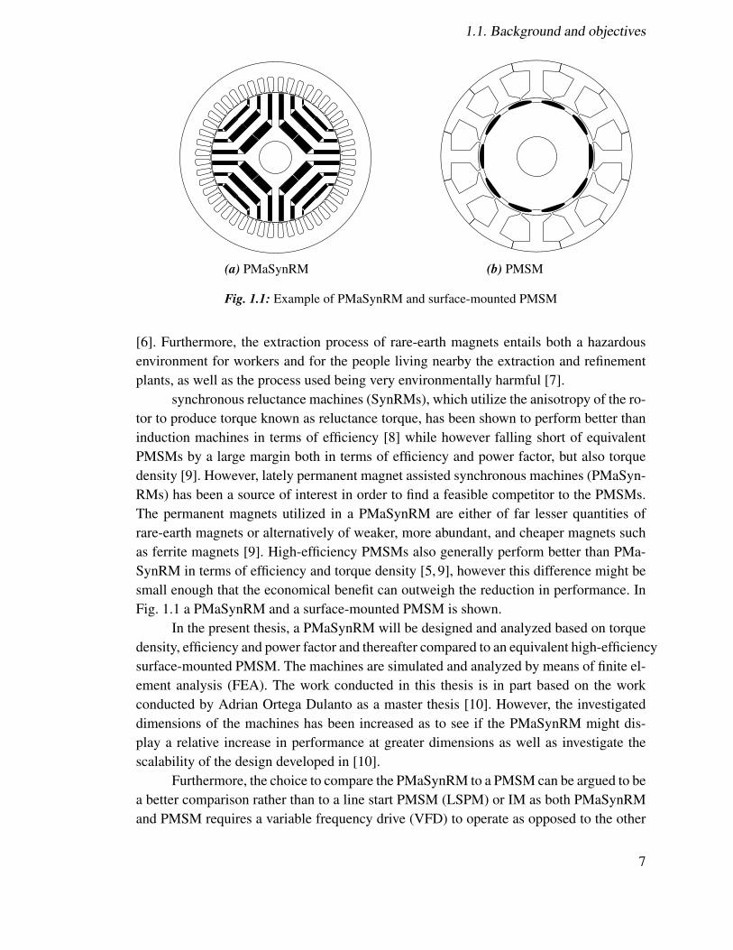
(a) PMaSynRM (b) PMSM
Fig. 1.1: Example of PMaSynRM and surface-mounted PMSM
[6]. Furthermore, the extraction process of rare-earth magnets entails both a hazardousenvironment for workers and for the people living nearby the extraction and refinementplants, as well as the process used being very environmentally harmful [7].
synchronous reluctance machines (SynRMs), which utilize the anisotropy of the ro-tor to produce torque known as reluctance torque, has been shown to perform better thaninduction machines in terms of efficiency [8] while however falling short of equivalentPMSMs by a large margin both in terms of efficiency and power factor, but also torquedensity [9]. However, lately permanent magnet assisted synchronous machines (PMaSyn-RMs) has been a source of interest in order to find a feasible competitor to the PMSMs.The permanent magnets utilized in a PMaSynRM are either of far lesser quantities ofrare-earth magnets or alternatively of weaker, more abundant, and cheaper magnets suchas ferrite magnets [9]. High-efficiency PMSMs also generally perform better than PMa-SynRM in terms of efficiency and torque density [5, 9], however this difference might besmall enough that the economical benefit can outweigh the reduction in performance. InFig. 1.1 a PMaSynRM and a surface-mounted PMSM is shown.
In the present thesis, a PMaSynRM will be designed and analyzed based on torquedensity, efficiency and power factor and thereafter compared to an equivalent high-efficiencysurface-mounted PMSM. The machines are simulated and analyzed by means of finite el-ement analysis (FEA). The work conducted in this thesis is in part based on the workconducted by Adrian Ortega Dulanto as a master thesis [10]. However, the investigateddimensions of the machines has been increased as to see if the PMaSynRM might dis-play a relative increase in performance at greater dimensions as well as investigate thescalability of the design developed in [10].
Furthermore, the choice to compare the PMaSynRM to a PMSM can be argued to bea better comparison rather than to a line start PMSM (LSPM) or IM as both PMaSynRMand PMSM requires a variable frequency drive (VFD) to operate as opposed to the other
7
1.2. Thesis outline
two and therefore their applications are more similar.
1.2 Thesis outline
The thesis consist of 5 chapters and will hold the following structure
• Chapter 1: Introduction, background and justification of the thesis
• Chapter 2: Theoretical foundation of PMaSynRM design and analysis
• Chapter 3: Description of the analysis and design process
• Chapter 4: Results and comparison of the developed PMaSynRM and PMSM
• Chapter 5: Conclusions and discussions regarding further work
8

Chapter 2
Synchronous Reluctance Machine andPermanent Magnet assistance
As was briefly stated in Chapter 1 the synchronous reluctance machine (SynRM) andPMaSynRM relied on the anisotropy of the rotor in order to produce torque. In this chapterthe theory of the SynRM will be discussed and how utilizing magnets to further improvethe operation of SynRM influence the operation, thus producing a PMaSynRM.
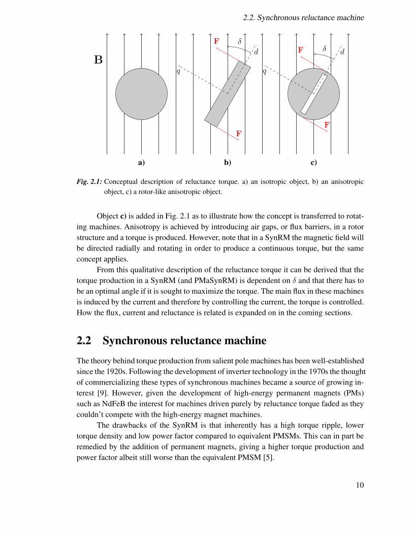
2.1 Concept of reluctance torque
Reluctance torque relies on, as the name would suggest, the reluctance of an object. Morespecifically, it relies on the difference in reluctance in different directions. This differ-ence means that depending on the how the object is placed in a magnetic field relativeto the direction of the field, different magnetic behaviour is displayed, i.e. the specimenis anisotropic. This anisotropy is easiest achieved by altering the geometry of a magneticmaterial specimen. The torque produced is dependent on the interaction of the specimenand an applied magnetic field. By defining an object-orientated coordinate system, withthe direct (d) axis aligned with the lowest reluctance and the quadrature (q) axis along thepath of highest reluctance we can begin to define the torque produced.
To illustrate this, assume that the anisotropic specimen is subjected to a homoge-neous magnetic field and there is an angle between the d-axis of the specimen and themagnetic field. This angle means that a distortion in the field is introduced and hence thecurl of the field will be non-zero. This in turn creates a force which does not cancel outand hence a torque is produced. In Fig. 2.1 object a) is completely isotropic and thus dis-plays equal reluctance in all directions in the plane of the magnetic field B and thereforeno torque is exerted on it and consequently it remains unaffected by the field. However,object b) is anisotropic with an angle to the field and therefore experience a net torque.The angle � is known as the load angle and it is the angle which determines the magnitudeof the torque since the system always aim to keep � equal to zero [11].
9
2.2. Synchronous reluctance machine
B
a) b) c)
F
F
F
F
d
q
�
d
q
�
Fig. 2.1: Conceptual description of reluctance torque. a) an isotropic object, b) an anisotropicobject, c) a rotor-like anisotropic object.
Object c) is added in Fig. 2.1 as to illustrate how the concept is transferred to rotat-ing machines. Anisotropy is achieved by introducing air gaps, or flux barriers, in a rotorstructure and a torque is produced. However, note that in a SynRM the magnetic field willbe directed radially and rotating in order to produce a continuous torque, but the sameconcept applies.
From this qualitative description of the reluctance torque it can be derived that thetorque production in a SynRM (and PMaSynRM) is dependent on � and that there has tobe an optimal angle if it is sought to maximize the torque. The main flux in these machinesis induced by the current and therefore by controlling the current, the torque is controlled.How the flux, current and reluctance is related is expanded on in the coming sections.
2.2 Synchronous reluctance machine
The theory behind torque production from salient pole machines has been well-establishedsince the 1920s. Following the development of inverter technology in the 1970s the thoughtof commercializing these types of synchronous machines became a source of growing in-terest [9]. However, given the development of high-energy permanent magnets (PMs)such as NdFeB the interest for machines driven purely by reluctance torque faded as theycouldn’t compete with the high-energy magnet machines.
The drawbacks of the SynRM is that inherently has a high torque ripple, lowertorque density and low power factor compared to equivalent PMSMs. This can in part beremedied by the addition of permanent magnets, giving a higher torque production andpower factor albeit still worse than the equivalent PMSM [5].
10
2.2. Synchronous reluctance machine
The main advantage of the SynRM when compared to a PMSM is generally thelower price range as it doesn’t utilize expensive rare-earth magnets. However, there aremore advantages over the PMSM of the SynRM and PMaSynRM as outlined in [9] and[12]. To name a few we have
• The SynRM is not as vulnerable to short-circuit conditions as the lack of magnetsmeans that no current is induced.
• The constant power speed range (CSPR) is very good for SynRM and especiallyPMaSynRM
• The rotor saliency provides with easy rotor position detection at stand-still
The design of the SynRM rotor as it looks today is still conceptually based on thework done by Kostko in 1923 where the rotor is divided into different segments withflux barriers in order to achieve a high saliency [9, 13] as seen in Fig. 2.2b and c. Salientpole machines can be constructed in a few different ways. First, there is the conventionalsalient pole (SP) rotor, the axially laminated anisotropy (ALA) rotor and the transversallylaminated anisotropy (TLA) rotor [14] and these types can be seen in Fig. 2.2.
However, the SP design configuration has been shown to be sub-optimal for SynRMdrives and is more suitable for wound rotor synchronous machines. The ALA is moretheoretically appealing and is believed to be able to provide a higher saliency ratio than theTLA configuration. However, the TLA configuration is much easier to mass produce as itutilizes the same punching and assembly procedure as traditional electrical machines [15]and therefore will be the focus of this thesis.
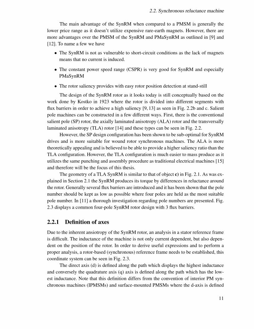
The geometry of a TLA SynRM is similar to that of object c) in Fig. 2.1. As was ex-plained in Section 2.1 the SynRM produces its torque by differences in reluctance aroundthe rotor. Generally several flux barriers are introduced and it has been shown that the polenumber should be kept as low as possible where four poles are held as the most suitablepole number. In [11] a thorough investigation regarding pole numbers are presented. Fig.2.3 displays a common four-pole SynRM rotor design with 3 flux barriers.
2.2.1 Definition of axes
Due to the inherent ansiotropy of the SynRM rotor, an analysis in a stator reference frameis difficult. The inductance of the machine is not only current dependent, but also depen-dent on the position of the rotor. In order to derive useful expressions and to perform aproper analysis, a rotor-based (synchronous) reference frame needs to be established, thiscoordinate system can be seen in Fig. 2.3.
The direct axis (d) is defined along the path which displays the highest inductanceand conversely the quadrature axis (q) axis is defined along the path which has the low-est inductance. Note that this definition differs from the convention of interior PM syn-chronous machines (IPMSMs) and surface-mounted PMSMs where the d-axis is defined
11

2.2. Synchronous reluctance machine
Fig. 2.2: Different rotor designs for rotor saliency. a) Conventional salient pole. b) Axially lami-nated anisotropy. c) Transversally laminated anisotropy. From [14]
along the flux from the PM, this distinction will prove important when discussing perma-nent magnet assistance since the consequence will be that the axes are reversed in termsof permanent magnet flux.
2.2.2 Governing equations
A model over the SynRM can be formulated in accordance with the equivalent circuitseen in Fig. 2.4 [16], where all bold-faced quantities are complex-valued. is the fluxlinkage of the machine, vs is the stator voltage, is is the stator current, i is the current notcontributing to the iron losses, ic is the iron loss current, R
s
is the stator resistance, Rc
isthe equivalent iron loss resistance and !
e
is the angular frequency. Here e represents theemf as
e =
d
dt+ j!
e
(2.1)
Neglecting iron losses, the dynamics of the synchronous machine in dq-frame canbe described by
12
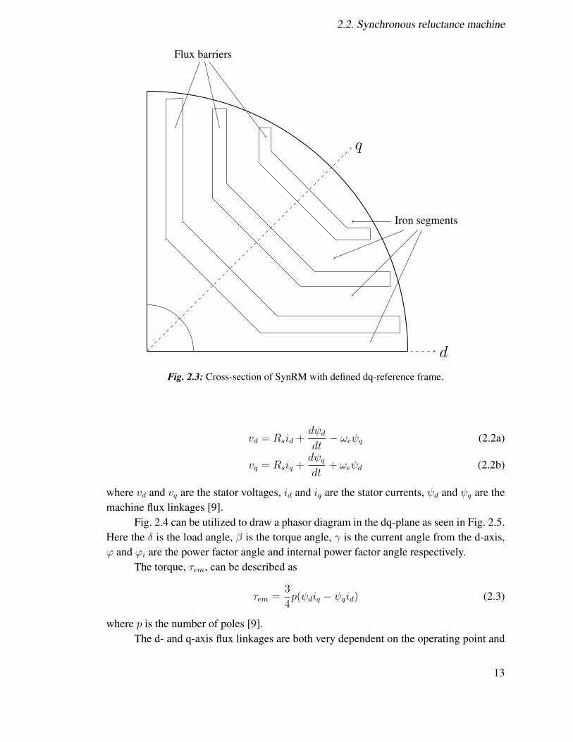
2.2. Synchronous reluctance machine
q
d
Flux barriers
Iron segments
Fig. 2.3: Cross-section of SynRM with defined dq-reference frame.
vd
= Rs
id
+
d d
dt� !
e
q
(2.2a)
vq
= Rs
iq
+
d q
dt+ !
e
d
(2.2b)
where vd
and vq
are the stator voltages, id
and iq
are the stator currents, d
and q
are themachine flux linkages [9].
Fig. 2.4 can be utilized to draw a phasor diagram in the dq-plane as seen in Fig. 2.5.Here the � is the load angle, � is the torque angle, � is the current angle from the d-axis,' and '
i
are the power factor angle and internal power factor angle respectively.The torque, ⌧
em
, can be described as
⌧em
=
3
4
p( d
iq
� q
id
) (2.3)
where p is the number of poles [9].The d- and q-axis flux linkages are both very dependent on the operating point and
13

2.2. Synchronous reluctance machine
Rs is
Rce
ic
�+
j!e i
Ld
dtvs
Fig. 2.4: Circuit diagram including iron losses.
q
d
vs
e
iiq
id
is ic
Ld
id
jLq
iq
Rs
iq
j!e
Ld
id
Rs
id
�!e
Lq
iq
�
�
�
'i
'
Fig. 2.5: Phasor diagram for SynRM.
experience cross-coupling from currents in the adjacent axis [9, 11], i.e.( d
= d
(id
, iq
)
q
= q
(id
, iq
)
(2.4)
This cross-coupling occurs since the q-axis current cause a flux component in the d-axisand vise verse. This not only contributes to the total flux in the respective axis but it alsoaffect the saturation level of the iron in the respective axes. Hence, when rewriting theflux linkages as current times inductances it is very important to note that the inductances(L
d
, Lq
) are indeed not constant [9, 11]( d
= Ld
(id
, iq
)id
q
= Lq
(id
, iq
)iq
(2.5)
14

2.3. Saliency and performance
Note that this definition of the inductances is a simplification and for a more thor-ough discussion see Chapter 4 in [9]. Note also that the inductances includes not onlymagnetizing inductances but also the leakage inductances, which are not significantly in-fluenced by the aforementioned cross-coupling and saturation [16].
2.3 Saliency and performance
The saliency ratio, ⇠ is of great significance for the performance of the SynRM. Thesaliency ratio is defined as
⇠ =Ld
Lq
(2.6)
and in a SynRM, ⇠ generally do not exceed values much higher than 10 [9].Consider the phasor diagram in Fig. 2.5. The following relationships hold for the
defined angles⇡
2
+ � = � + 'i
(2.7)
� = � + � (2.8)
Utilizing these relationships we find that we can write the internal power factor (IPF) as
IPF = cos'i
= cos
⇣⇡2
+ � � �⌘=
⇠ � 1r⇠2
1
sin
2 �+
1
cos
2 �
(2.9)
for the derivation of this expression refer to Appendix A.1. And thus, it becomes obviousthat the saliency ratio influences the IPF heavily, as seen in Fig. 2.6 where the it is plottedfor different values of ⇠ as a function of the current vector angle. It is important to notethat IPF is not the same thing as power factor (PF) but they are, however, related anda high value of IPF leads to a high value of PF since the difference between these twoare only governed by R
s
and Rc
which can be verified by looking at Fig. 2.5 and Fig.2.4. Therefore, IPF is discussed here as it is quite straightforward to derive an analyticalexpression from current angle and saliency.
From equation (2.9) it is obvious that for any given value of ⇠ there exist a valueof the current vector angle which allows for the optimal IPF. It can be shown that this
occurs when tan � =
p⇠ and then the IPF is equal to
⇠ � 1
⇠ + 1
. This operating point is often
called maximum torque per kVA (MTPkVA) [16] and thus correspond to the operatingpoint when the least amount of reactive power is required by the supply.
With the definition of flux in equation (2.5) and dropping the parentheses for sim-plicity we find that equation (2.3) can be rewritten as
15

2.3. Saliency and performance
0 10 20 30 40 50 60 70 80 90
0
0.1
0.2
0.3
0.4
0.5
0.6
0.7
0.8
0.9
1
� [deg]
IPF
⇠=2⇠=5⇠=10⇠=15⇠=20⇠=100
Fig. 2.6: IPF as function of current angle for different values of ⇠.
⌧em
=
3
4
p(Ld
� Lq
)id
iq
(2.10)
Thus, the torque is proportional to the difference in inductance between the twoaxes. It is interesting to note that while the IPF is governed by the saliency ratio, thetorque production is dependent on the saliency difference. Even though these parametersare related, it can prove difficult to maximize both parameters simultaneously when de-veloping a rotor design [10]. This is due to the non-linear dependency of d- and q-axisinductances on the rotor geometry [17].
Another conflict occurs when operating a SynRM and it becomes apparent whenrewriting equation (2.10) utilizing the phasor quantities presented in Fig. 2.5 in steadystate, i.e.
⌧em
=
3
4
p(Ld
� Lq
)I2s
sin 2� (2.11)
where Is
is the stator current magnitude in steady state. Here we see that for given (con-stant) inductances and current magnitude, the maximum torque is achieved for a currentvector angle of 45 degrees. This operating point is referred to as maximum torque perampere (MTPA). Again, looking at Fig. 2.6 we see that this current vector angle does notcoincide with the angle which maximizes the IPF for moderately high values of ⇠.
16

2.4. Iron saturation
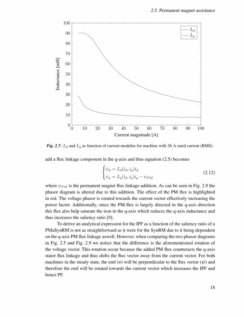
It should also be noted that saturation affect both the inductance difference andsaliency ratio such that in reality ⇠ and inductance difference decrease with increasingcurrent, which affect both the torque production and power factor. The effect of iron sat-uration will be expanded upon below.
2.4 Iron saturation
As has been stated above the performance of SynRMs and PMaSynRMs is affected bythe saturation of the iron. The most prominent effect of this is that the inductances changeas a function of current level. This in turn contributes to a different behaviour in terms oftorque and PF between low and high levels of current. In Fig. 2.7 the two inductances areplotted as functions of the applied current modulus. Since the d-axis is defined along thepath of lowest reluctance and therefore the path which contains the greatest amount of ironit is quite straightforward to understand that it is also affected by the saturation to a greaterextent. In fact, to saturate the q-axis is desirable because it allows for ⇠ and the inductancedifference to increase. However, the decreased values of L
d
results in undesirable effects.As the torque is proportional to the inductance difference it becomes obvious that
the torque does not vary with the square of the current level when considering saturation.The saturation of the iron leads to a shift towards higher values of optimal current vectorangle for maximum torque (MTPA) as the current increases. The same tendencies canbe seen when analyzing the PF curve. Saturation implies that ⇠ decrease in value forgreater current levels. Again, referring to Fig. 2.6 we see that as ⇠ decrease, so does theinternal power factor and therefore the power factor. However, some saturation effectsactually benefits the PF when operating in the maximum torque (MTPA) operating pointas discussed in [18]. This was attributed to the fact that the current angle for maximizedpower factor (MTPkVA) and MTPA current angle values were shifted closer together andthereby resulting in a higher PF.
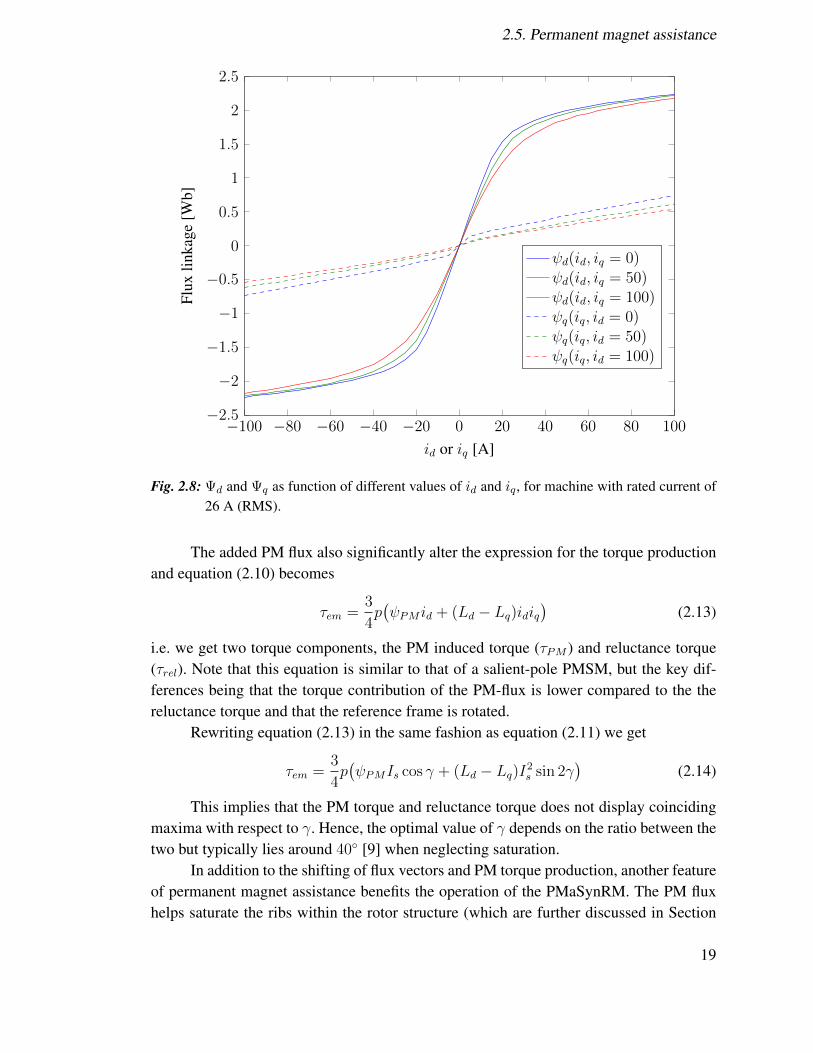
Moreover, as was stated previously the d- and q-axis inductances are not only de-pendent on the d- and q-axis currents respectively but cross-saturation also occurs to vary-ing degrees. In Fig. 2.8 the flux is plotted against different values of i
d
and iq
. Here wesee difference in flux when the opposite axis current is non-zero.
2.5 Permanent magnet assistance
Reviewing Fig. 2.6 we see that in order to for an ordinary SynRM to have a IPF greaterthan 0.9 a saliency ratio beyond 20 is needed, which is an unrealistic value [16]. There-fore, in order to make the SynRM feasible compared to PMSMs some modifications needto be done. Such a modification is to add magnets in the rotor barriers, thus making aPMaSynRM. This addition slightly alters the characteristics of the machine. The magnets
17
2.5. Permanent magnet assistance
0 10 20 30 40 50 60 70 80 90 100
0
10
20
30
40
50
60
70
80
90
100
Current magnitude [A]
Indu
ctan
ce[m
H]
Ld
Lq
Fig. 2.7: Ld
and Lq
as function of current modulus for machine with 26 A rated current (RMS).
add a flux linkage component in the q-axis and thus equation (2.5) becomes( d
= Ld
(id
, iq
)id
q
= Lq
(id
, iq
)iq
� PM
(2.12)
where PM
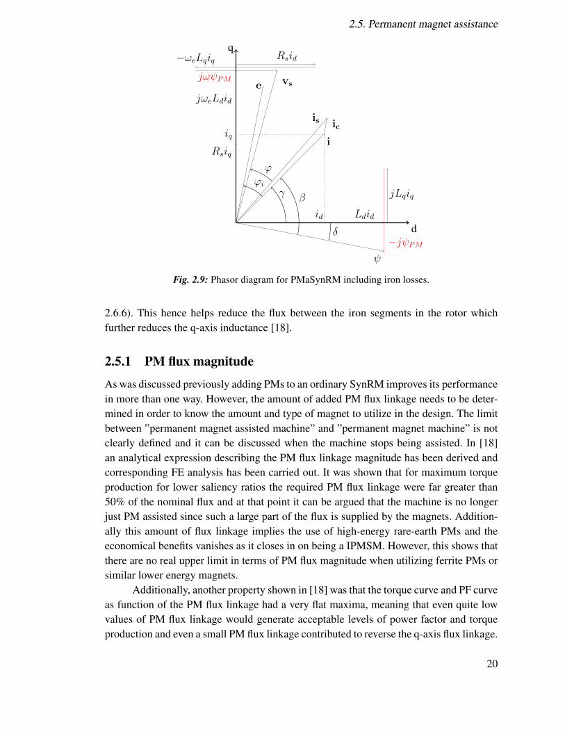
is the permanent magnet flux linkage addition. As can be seen in Fig. 2.9 thephasor diagram is altered due to this addition. The effect of the PM flux is highlightedin red. The voltage phasor is rotated towards the current vector effectively increasing thepower factor. Additionally, since the PM-flux is largely directed in the q-axis directionthis flux also help saturate the iron in the q-axis which reduces the q-axis inductance andthus increases the saliency ratio [9].
To derive an analytical expression for the IPF as a function of the saliency ratio of aPMaSynRM is not as straightforward as it were for the SynRM due to it being dependenton the q-axis PM flux linkage aswell. However, when comparing the two phasor diagramsin Fig. 2.5 and Fig. 2.9 we notice that the difference is the aforementioned rotation ofthe voltage vector. This rotation occur because the added PM flux counteracts the q-axisstator flux linkage and thus shifts the flux vector away from the current vector. For bothmachines in the steady state, the emf (e) will be perpendicular to the flux vector ( ) andtherefore the emf will be rotated towards the current vector which increases the IPF andhence PF.
18
2.5. Permanent magnet assistance
�100 �80 �60 �40 �20 0 20 40 60 80 100
�2.5
�2
�1.5
�1
�0.5
0
0.5
1
1.5
2
2.5
id
or iq
[A]
Flux
linka
ge[W
b]
d
(id
, iq
= 0)
d
(id
, iq
= 50)
d
(id
, iq
= 100)
q
(iq
, id
= 0)
q
(iq
, id
= 50)
q
(iq
, id
= 100)
Fig. 2.8: d
and q
as function of different values of id
and iq
, for machine with rated current of26 A (RMS).
The added PM flux also significantly alter the expression for the torque productionand equation (2.10) becomes
⌧em
=
3
4
p� PM
id
+ (Ld
� Lq
)id
iq
�(2.13)
i.e. we get two torque components, the PM induced torque (⌧PM
) and reluctance torque(⌧
rel
). Note that this equation is similar to that of a salient-pole PMSM, but the key dif-ferences being that the torque contribution of the PM-flux is lower compared to the thereluctance torque and that the reference frame is rotated.
Rewriting equation (2.13) in the same fashion as equation (2.11) we get
⌧em
=
3
4
p� PM
Is
cos � + (Ld
� Lq
)I2s
sin 2��
(2.14)
This implies that the PM torque and reluctance torque does not display coincidingmaxima with respect to �. Hence, the optimal value of � depends on the ratio between thetwo but typically lies around 40
� [9] when neglecting saturation.In addition to the shifting of flux vectors and PM torque production, another feature
of permanent magnet assistance benefits the operation of the PMaSynRM. The PM fluxhelps saturate the ribs within the rotor structure (which are further discussed in Section
19
2.5. Permanent magnet assistance
q
d
vse
iiq
id
is ic
Ld
id
jLq
iq
�j PM
Rs
iq
j!e
Ld
id
Rs
id�!
e
Lq
iq
j! PM
�
� �
'i
'
Fig. 2.9: Phasor diagram for PMaSynRM including iron losses.
2.6.6). This hence helps reduce the flux between the iron segments in the rotor whichfurther reduces the q-axis inductance [18].
2.5.1 PM flux magnitude
As was discussed previously adding PMs to an ordinary SynRM improves its performancein more than one way. However, the amount of added PM flux linkage needs to be deter-mined in order to know the amount and type of magnet to utilize in the design. The limitbetween ”permanent magnet assisted machine” and ”permanent magnet machine” is notclearly defined and it can be discussed when the machine stops being assisted. In [18]an analytical expression describing the PM flux linkage magnitude has been derived andcorresponding FE analysis has been carried out. It was shown that for maximum torqueproduction for lower saliency ratios the required PM flux linkage were far greater than50% of the nominal flux and at that point it can be argued that the machine is no longerjust PM assisted since such a large part of the flux is supplied by the magnets. Addition-ally this amount of flux linkage implies the use of high-energy rare-earth PMs and theeconomical benefits vanishes as it closes in on being a IPMSM. However, this shows thatthere are no real upper limit in terms of PM flux magnitude when utilizing ferrite PMs orsimilar lower energy magnets.
Additionally, another property shown in [18] was that the torque curve and PF curveas function of the PM flux linkage had a very flat maxima, meaning that even quite lowvalues of PM flux linkage would generate acceptable levels of power factor and torqueproduction and even a small PM flux linkage contributed to reverse the q-axis flux linkage.
20

2.6. Geometry and performance of PMaSynRM
In fact, it is stated in [18] that the PM flux should be in the vicinity of 25-35% of thenominal flux. This also implies that ferrite PMs might be sufficient in order to reach thedesired operating point.
2.6 Geometry and performance of PMaSynRM
The geometry of a SynRM rotor is inherently complex and as the operation of this ma-chine depends on the saliency of the rotor, it is of utmost importance that the geometry iswell defined in terms of parameters to analyze. Due to the complexity and non-linearity ofthese machines, it is very difficult and of questionable use to derive an analytical model ofthe machine and optimize. Instead, it is better to combine analytical expressions which de-termines some key geometrical parameters and thereafter conduct the performance analy-sis utilizing computer-aided finite element analysis (FEA) as is done in [11], [19] and [10].The parameterization in this thesis is based on the work conducted in [15] and [11] andits theoretical relevance is expanded upon in Section 2.8.
2.6.1 Parameterization of PMaSynRM
In order to properly describe the rotor of the PMaSynRM it is crucial to define the ge-ometry through comprehensible parameters. In Fig. 2.10 a pole of a PMaSynRM rotorwith 3 barriers is shown. This parameterization follows that conducted in papers suchas [15], [19].
• The barrier height of barrier k is described by Wk,q
in the q-direction and Wk,d
inthe d-direction.
• The height of the iron segment h between barriers is described in the q-direction asSh,q
• The angle that the barrier k makes at the periphery of the rotor with the d-axis isdefined as ✓
b,k
• The angle between flux barrier arm and center of flux barrier is defined as ↵i
Often, the q-axis position of a rotor barrier along the q-axis is of interest. The dis-tance to the n:th barrier is defined as
D0,n =
nX
h=1
Sh,q
+
n�1X
k=1
Wk,q
(2.15)
Furthermore, in order to give an indication as to how much air versus iron there is inthe rotor in both the q- and d-direction the insulation ratios k
w,q
and kw,d
are qualitatively
21

2.6. Geometry and performance of PMaSynRM
Rsh
R1
✓b,1
✓b,2
✓b,3
S1,q
S2,q
S3,q
S4,q
W1,q
W2,q
W3,q
W1,d
W2,d
W3,d↵1
↵2
↵3
Fig. 2.10: Parameterization of PMaSynRM rotor.
defined as
kw,q
=
Amount of airAmount of iron
����q�axis
(2.16)
kw,d
=
Amount of airAmount of iron
����d�axis
(2.17)
which gives that a value below 1 of these ratios means that there is more iron than air inthe respective direction and conversely a value above 1 means that there is more air thaniron. Note that the path of calculation for the q-axis is easily defined along the axis. Forthe d-axis it is a somewhat more complicated. The expressions for the insulation ratiosare given in Section 2.8.
22

2.6. Geometry and performance of PMaSynRM
2.6.2 Insulation ratios
The aforementioned insulation ratios have a great influence on the torque production aswell as the power factor. The reason of this is most easily explained by the fact that theseratios determine the reluctance of the machine. This, in turn, affects the flux linkage insidethe machine and therefore the saturation level of the iron and thus the inductance is altered.More air introduced in the q-axis direction lowers the q-axis inductance, thus allowingfor increasing the inductance difference and saliency ratio. Therefore it is common tooptimize the insulation ratio in terms of torque production. However, the relationship ofthe insulation ratios are not linear towards either ⇠ or inductance difference (for fixedvalues of � and current). It can be shown that there exist an optimum in terms of k
w,q
andkw,d
when it comes to inductance difference and saliency ratio [11, 20]. These optimumvalues does not necessarily coincide and therefore a design trade-off has to be made interms of power factor and torque production. Furthermore, an upper limit of the rotorinsulation ratios has been suggested, which is related to the stator insulation ratio. Thisvalue is described by
kw,s
=
ps
� wtooth
ps
(2.18)
where ps
is the stator slot pitch and wtooth
is the stator tooth width. It is desirable to choosethe q-axis insulation ratio of the rotor to a value close to or below the value of k
w,s
[9,15].This is true since the insulation ratios in large determines the flux density magnitude inthe stator and rotor and hence the saturation levels in rotor and stator. Therefore, if k
w,q
<
kw,s
the stator teeth experience a greater saturation flux than the rotor and conversely ifkw,q
> kw,s
is true the opposite applies. This affects the flux linkage magnitudes at highercurrent levels and therefore the torque production. This was shown in [9] and there it wasconcluded that a lower value for k
w,q
was preferable to a higher in terms of flux linkageand torque production. Following the same reasoning, it can be concluded that the d-axisinsulation ratio k
w,d
should be equal or less than the value of kw,q
, i.e. the amount of ironin the d-axis should be higher than in the q-axis [15, 21].
2.6.3 Number of flux barriers
While it can be shown that the insulation ratios mostly govern the torque production thenumber of flux barriers also impacts the performance of the SynRM. Generally speaking,a greater amount of flux barriers has a positive impact on both torque production andpower factor. However, when it comes to aspects such as torque ripple the interactionbetween stator and rotor is of great importance and therefore the number of barriers willhave a great influence on these parameters [10,15,19,22], albeit there are no simple rulesfor how many are optimal.
The choice of number of barriers is non-trivial and a simple analytical expressionis difficult to derive. However, in order to minimize the torque ripple a general rule was
23

2.6. Geometry and performance of PMaSynRM
presented in [23] as
nr
= ns
± 4 (2.19)
where nr
is the number of rotor barrier slots per pole and ns
is the number of stator slotsper pole. Whether the equation should be treated with a plus or a minus is determined bythe feasibility of the structure albeit it is stated that +4 generates better results.
In [22] a thorough analysis of the behavior of different numbers of stator slots andbarriers is presented. There it was derived that different number of stator slots performat its best for different number of rotor barriers For instance was it shown that for a 48slot machine, torque production was maximized for 4 or 6 number of barriers whereasefficiency was maximized for 4 barriers and torque ripple was minimized for 6 barriers.Whereas in [10] it was determined that for the 36 slot machine 3 barriers generated theoverall best performance in terms of torque production and power factor.
2.6.4 Torque ripple and rotor slots
High torque ripple is an inherent problem that plagues the SynRM and other machinessuch as IPMSMs [24]. It has already been determined that the interaction between statorand rotor influences the performance of the machine and most importantly the torqueripple. Therefore it becomes obvious that the positioning of the rotor barrier ends, or rotorbarrier slots, impacts the operation of the machine.
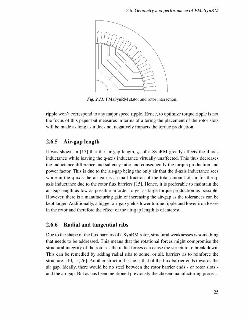
The ripple that occurs in a SynRM is due to the variation in reluctance that occurwhen a rotor slot passes a stator slot [19, 23–25]. Therefore, it is of interest to place therotor slots such that the torque ripple is minimized. A great deal of research has beenmade in the field of reducing the torque ripple of these types of machines. Torque ripplereduction can be achieved in a variety of ways. The method discussed above presentedin [23] focuses on equally distributed rotor slots along the circumference and focus moreon number of barriers rather than the placement of the rotor slots, [25] discusses thepossibility of asymmetrically placed stator slot openings as a means of combating torqueripple, and [24] proposes asymmetrically shifting the rotor slots between every other orseveral laminations. A rule of thumb is presented in [19], where it is stated that the rotorbarrier should be placed such that when one of the two barrier slots enters below a statorslot, the other barrier slot should enter below a stator tooth. Fig. 2.11 illustrates how thestator and rotor slots can be aligned. In this case the innermost barrier might be properlyaligned since the top slot it is about to pass below a stator slot while the right slot is aboutto pass below a tooth. However, the middle barrier is more problematic since both slotsare situated below the middle of both teeth which cause discrepancies in reluctance andthereby torque ripple.
However, for pumping applications torque ripple is not a serious issue as the loadtorque typically is proportional to the square of the rotor speed, and therefore the torque
24
2.6. Geometry and performance of PMaSynRM
Fig. 2.11: PMaSynRM stator and rotor interaction.
ripple won’t correspond to any major speed ripple. Hence, to optimize torque ripple is notthe focus of this paper but measures in terms of altering the placement of the rotor slotswill be made as long as it does not negatively impacts the torque production.
2.6.5 Air-gap length
It was shown in [17] that the air-gap length, g, of a SynRM greatly affects the d-axisinductance while leaving the q-axis inductance virtually unaffected. This thus decreasesthe inductance difference and saliency ratio and consequently the torque production andpower factor. This is due to the air-gap being the only air that the d-axis inductance seeswhile in the q-axis the air-gap is a small fraction of the total amount of air for the q-axis inductance due to the rotor flux barriers [15]. Hence, it is preferable to maintain theair-gap length as low as possible in order to get as large torque production as possible.However, there is a manufacturing gain of increasing the air-gap as the tolerances can bekept larger. Additionally, a bigger air-gap yields lower torque ripple and lower iron lossesin the rotor and therefore the effect of the air-gap length is of interest.
2.6.6 Radial and tangential ribs
Due to the shape of the flux barriers of a SynRM rotor, structural weaknesses is somethingthat needs to be addressed. This means that the rotational forces might compromise thestructural integrity of the rotor as the radial forces can cause the structure to break down.This can be remedied by adding radial ribs to some, or all, barriers as to reinforce thestructure. [10, 15, 26]. Another structural issue is that of the flux barrier ends towards theair gap. Ideally, there would be no steel between the rotor barrier ends - or rotor slots -and the air gap. But as has been mentioned previously the chosen manufacturing process,
25

2.6. Geometry and performance of PMaSynRM
wr,1
wr,2
wr,3
wt,1
wt,2
wt,3
Fig. 2.12: Illustration of radial and tangential ribs in SynRM.
TLA, means that the rotor is punched and therefore require a continuous sheet of metal.The width of this rib is in part determined by the tolerance of the punching machine, butalso by the expected tangential forces from torque ripple or load variations. However, thecalculation of the thickness of the tangential ribs are determined to be outside of the scopeof this project. In Fig. 2.12, these ribs are illustrated, and the parameters describing thewidths defined, w
r,i
is the widths of the radial ribs and wt,i
is the width of the tangentialribs.
Not all machines require radial ribs and it is rather a question of size of the rotor,radial positioning of the flux barriers, and maximum allowable speed of the machinewhich determines the need and widths of them. The width of the radial ribs can calculatedby diving the rotor into i segments and calculate the rotational force exerted on eachsegment [26]. This is done as
wr,i
= ⌫rib
Fc,i
�r
Lstk
(2.20)
where Fc
is the centrifugal force acting on the rotor, �r
is the tensile strength of thematerial, L
stk
is the total stack length of the rotor and ⌫rib
is a safety factor usually in the
26
2.6. Geometry and performance of PMaSynRM
D0,1
D0,2
D0,3
1 2 3
Fig. 2.13: Areas for radial rib calculation.
range between 2 and 3 [26]. The centrifugal force can be calculated as
Fc,i
= ⇢lam
!2m
RG,i
AFe,i
Lstk
(2.21)
where AFe
is the area of the relevant rotor segment, RG
is the center of gravity of therotor segment, !
m
is the mechanical angular frequency of the rotor and ⇢lam
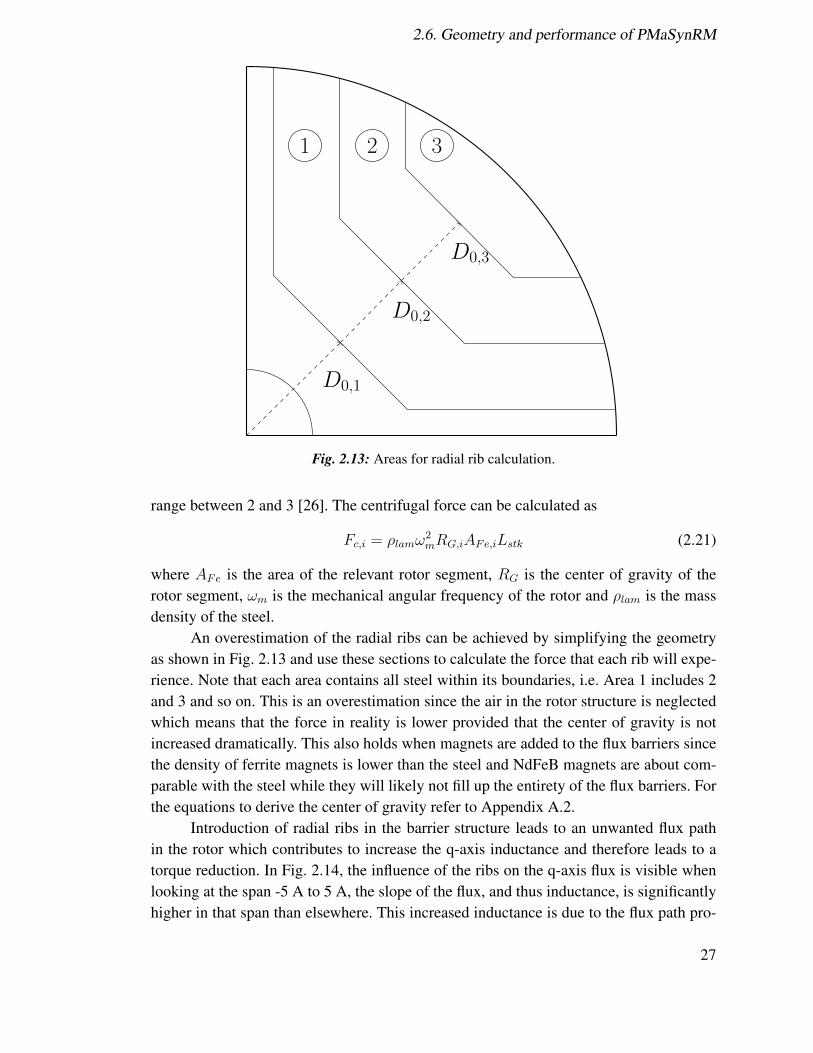
is the massdensity of the steel.
An overestimation of the radial ribs can be achieved by simplifying the geometryas shown in Fig. 2.13 and use these sections to calculate the force that each rib will expe-rience. Note that each area contains all steel within its boundaries, i.e. Area 1 includes 2and 3 and so on. This is an overestimation since the air in the rotor structure is neglectedwhich means that the force in reality is lower provided that the center of gravity is notincreased dramatically. This also holds when magnets are added to the flux barriers sincethe density of ferrite magnets is lower than the steel and NdFeB magnets are about com-parable with the steel while they will likely not fill up the entirety of the flux barriers. Forthe equations to derive the center of gravity refer to Appendix A.2.
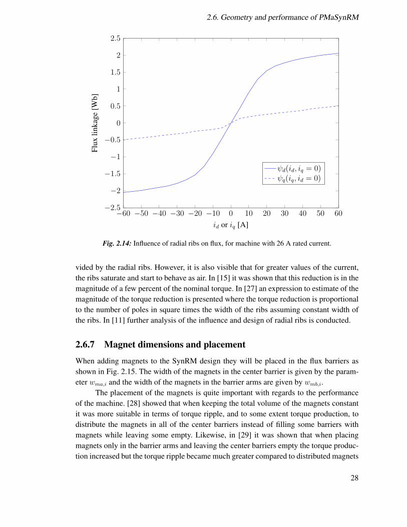
Introduction of radial ribs in the barrier structure leads to an unwanted flux pathin the rotor which contributes to increase the q-axis inductance and therefore leads to atorque reduction. In Fig. 2.14, the influence of the ribs on the q-axis flux is visible whenlooking at the span -5 A to 5 A, the slope of the flux, and thus inductance, is significantlyhigher in that span than elsewhere. This increased inductance is due to the flux path pro-
27
2.6. Geometry and performance of PMaSynRM
�60 �50 �40 �30 �20 �10 0 10 20 30 40 50 60
�2.5
�2
�1.5
�1
�0.5
0
0.5
1
1.5
2
2.5
id
or iq
[A]
Flux
linka
ge[W
b]
d
(id
, iq
= 0)
q
(iq
, id
= 0)
Fig. 2.14: Influence of radial ribs on flux, for machine with 26 A rated current.
vided by the radial ribs. However, it is also visible that for greater values of the current,the ribs saturate and start to behave as air. In [15] it was shown that this reduction is in themagnitude of a few percent of the nominal torque. In [27] an expression to estimate of themagnitude of the torque reduction is presented where the torque reduction is proportionalto the number of poles in square times the width of the ribs assuming constant width ofthe ribs. In [11] further analysis of the influence and design of radial ribs is conducted.
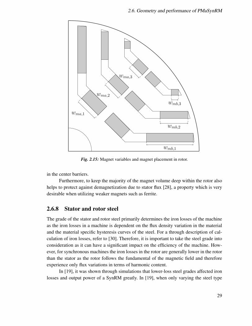
2.6.7 Magnet dimensions and placement
When adding magnets to the SynRM design they will be placed in the flux barriers asshown in Fig. 2.15. The width of the magnets in the center barrier is given by the param-eter w
ma,i
and the width of the magnets in the barrier arms are given by wmb,i
.The placement of the magnets is quite important with regards to the performance
of the machine. [28] showed that when keeping the total volume of the magnets constantit was more suitable in terms of torque ripple, and to some extent torque production, todistribute the magnets in all of the center barriers instead of filling some barriers withmagnets while leaving some empty. Likewise, in [29] it was shown that when placingmagnets only in the barrier arms and leaving the center barriers empty the torque produc-tion increased but the torque ripple became much greater compared to distributed magnets
28
2.6. Geometry and performance of PMaSynRM
wma,1
wma,2
wma,3
wmb,1
wmb,2
wmb,3
Fig. 2.15: Magnet variables and magnet placement in rotor.
in the center barriers.Furthermore, to keep the majority of the magnet volume deep within the rotor also
helps to protect against demagnetization due to stator flux [28], a property which is verydesirable when utilizing weaker magnets such as ferrite.
2.6.8 Stator and rotor steel
The grade of the stator and rotor steel primarily determines the iron losses of the machineas the iron losses in a machine is dependent on the flux density variation in the materialand the material specific hysteresis curves of the steel. For a through description of cal-culation of iron losses, refer to [30]. Therefore, it is important to take the steel grade intoconsideration as it can have a significant impact on the efficiency of the machine. How-ever, for synchronous machines the iron losses in the rotor are generally lower in the rotorthan the stator as the rotor follows the fundamental of the magnetic field and thereforeexperience only flux variations in terms of harmonic content.
In [19], it was shown through simulations that lower-loss steel grades affected ironlosses and output power of a SynRM greatly. In [19], when only varying the steel type
29

2.7. Permanent magnets
Hc
Br
H
B
Fig. 2.16: Typical B-H curve for a hard magnetic material.
for a machine in the range of 12 kW output power, the efficiency saw an increase of 9percentage units between the lowest and highest loss steel grade. At the same time, theoutput power increased by 8 percent when using the low loss grade steel compared to thehigher loss grade.
2.7 Permanent magnets
Magnetic materials are in general characterized by the hysteresis loop of the B-H curvewhich describes how the magnetic flux density varies when an external magnetic fieldis applied. A magnetic material is largely defined by the remanent flux density, B
r
, andthe coercivity, H
c
. Br
defines the flux density in the material when no external H-fieldis applied and H
c
describes the H-field required in order to bring the flux density insidethe material to zero. Magnetic materials can be divided into two major groups, hard andsoft magnetic materials. Hard magnetic materials are defined by large values of B
r
andH
c
while soft magnetic materials have lower values [31,32]. Fig. 2.16 illustrates a typicalcurve for a hard magnetic material.
Permanent magnets are hard magnetic materials and are, as the name suggests,permanently magnetized. This magnetization, M, relates to the magnetic flux density as[32]
B = µ0(H+M) (2.22)
30

2.7. Permanent magnets
Hc,b
Hc,i
Br
H
B or Im
Fig. 2.17: Typical normal (dashed) and intrisic (line) curve for permanent magnet.
2.7.1 Demagnetization
Typically, permanent magnets do not lose its magnetization when the flux density is re-duced to zero, i.e. when the coercivity is reached. Utilizing the above stated relationshipone can define the magnetic polarization, Im, as
Im = µ0M = B� µ0H (2.23)
Both Im and B can be plotted in the same graph as is done in Fig. 2.17. The Im-Hplot is often referred to as the intrinsic curve and the B-H plot is called normal curve.In these plots two coercivities appear, the intrinsic and normal coercivity H
c,i
and Hc,b
.Analogous to the definition of H
c
, Hc,i
is the value at which the magnetization is forcedto zero and beyond this point the magnetization will start to shift polarity [31]. Note thatH
c,b
= Hc
as defined previously.Demagnetization of the permanent magnet occurs when the magnetic field intensity
approaches the intrinsic coercivity. In fact, when the magnetic field passes the value closeto the knee of the intrinsic curve partial demagnetization start to occur. For most practicalsituations in electrical machines, only the second quadrant of the hysteresis loops are ofinterest. One can define the magnetic field knee value in the second quadrant as H
k
andwhen that value is exceeded and thereafter reduced to below that value again, the magne-tization of the magnet will be reduced and therefore also the remanent flux density. It canbe shown that when H
k
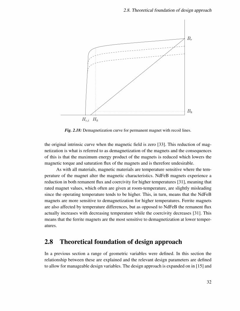
is exceeded, the new intrinsic curve follows the so called recoillines shown in Fig. 2.18. The slope of the recoil lines are similar to that of the slope of
31
2.8. Theoretical foundation of design approach
Hk
Hc,i
Bk
Br
Fig. 2.18: Demagnetization curve for permanent magnet with recoil lines.
the original intrinsic curve when the magnetic field is zero [33]. This reduction of mag-netization is what is referred to as demagnetization of the magnets and the consequencesof this is that the maximum energy product of the magnets is reduced which lowers themagnetic torque and saturation flux of the magnets and is therefore undesirable.
As with all materials, magnetic materials are temperature sensitive where the tem-perature of the magnet alter the magnetic characteristics. NdFeB magnets experience areduction in both remanent flux and coercivity for higher temperatures [31], meaning thatrated magnet values, which often are given at room-temperature, are slightly misleadingsince the operating temperature tends to be higher. This, in turn, means that the NdFeBmagnets are more sensitive to demagnetization for higher temperatures. Ferrite magnetsare also affected by temperature differences, but as opposed to NdFeB the remanent fluxactually increases with decreasing temperature while the coercivity decreases [31]. Thismeans that the ferrite magnets are the most sensitive to demagnetization at lower temper-atures.
2.8 Theoretical foundation of design approach
In a previous section a range of geometric variables were defined. In this section therelationship between these are explained and the relevant design parameters are definedto allow for manageable design variables. The design approach is expanded on in [15] and
32
2.8. Theoretical foundation of design approach
it relies on a number of key assumptions which are
• Saturation effects are neglected
• Stator slotting effects are neglected
• Magnetic scalar potential drop in the iron is neglected
• The stator winding is assumed to be ideal
• Distribution effects of the MMF is disregarded
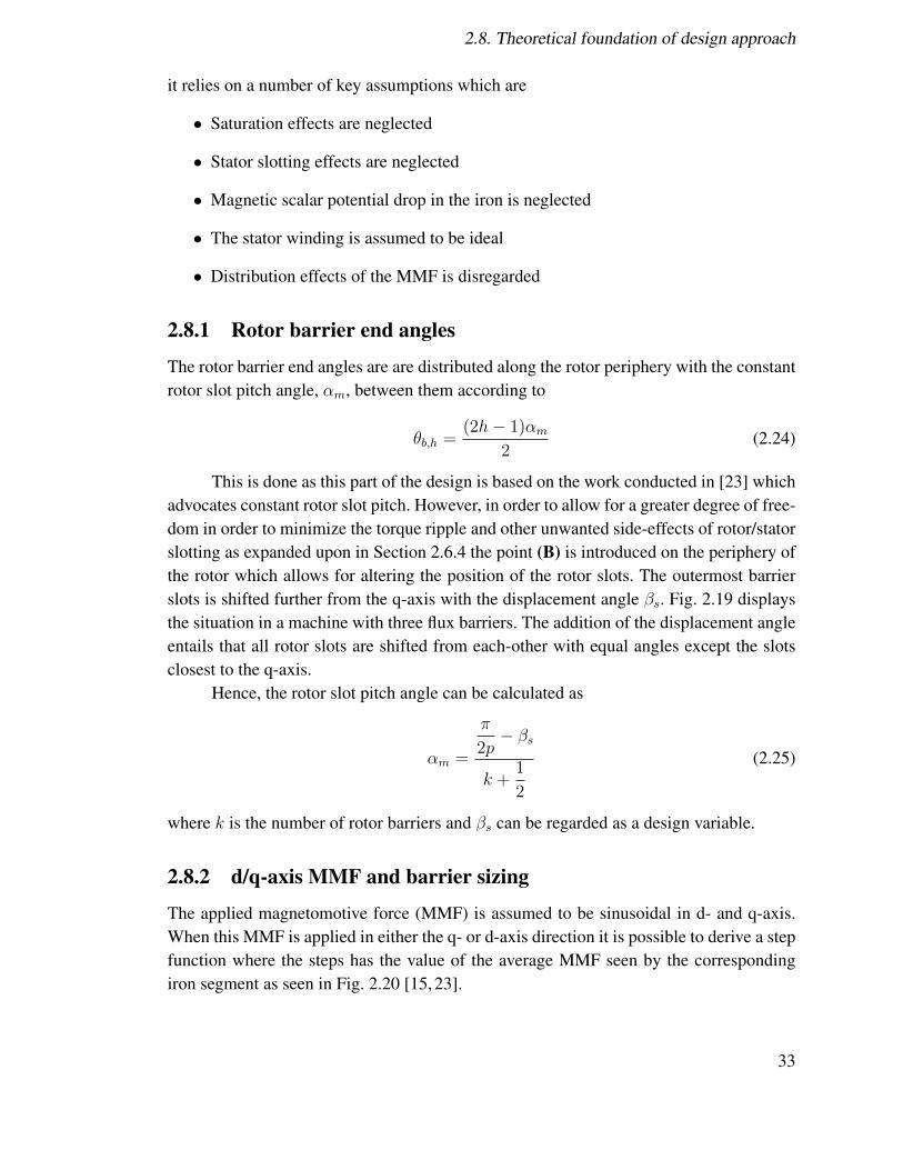
2.8.1 Rotor barrier end angles
The rotor barrier end angles are are distributed along the rotor periphery with the constantrotor slot pitch angle, ↵
m
, between them according to
✓b,h
=
(2h� 1)↵m
2
(2.24)
This is done as this part of the design is based on the work conducted in [23] whichadvocates constant rotor slot pitch. However, in order to allow for a greater degree of free-dom in order to minimize the torque ripple and other unwanted side-effects of rotor/statorslotting as expanded upon in Section 2.6.4 the point (B) is introduced on the periphery ofthe rotor which allows for altering the position of the rotor slots. The outermost barrierslots is shifted further from the q-axis with the displacement angle �
s
. Fig. 2.19 displaysthe situation in a machine with three flux barriers. The addition of the displacement angleentails that all rotor slots are shifted from each-other with equal angles except the slotsclosest to the q-axis.
Hence, the rotor slot pitch angle can be calculated as
↵m
=
⇡
2p� �
s
k +
1
2
(2.25)
where k is the number of rotor barriers and �s
can be regarded as a design variable.
2.8.2 d/q-axis MMF and barrier sizing
The applied magnetomotive force (MMF) is assumed to be sinusoidal in d- and q-axis.When this MMF is applied in either the q- or d-axis direction it is possible to derive a stepfunction where the steps has the value of the average MMF seen by the correspondingiron segment as seen in Fig. 2.20 [15, 23].
33
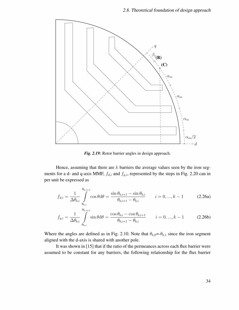
2.8. Theoretical foundation of design approach
q
d
↵m/2
↵m
↵m
↵m
(C)(B)
�s
Fig. 2.19: Rotor barrier angles in design approach.
Hence, assuming that there are k barriers the average values seen by the iron seg-ments for a d- and q-axis MMF, f
d,i
and fq,i
, represented by the steps in Fig. 2.20 can inper unit be expressed as
fd,i
=
1
�✓b,i
✓b,i+1Z
✓b,i
cos ✓d✓ =sin ✓
b,i+1 � sin ✓b,i
✓b,i+1 � ✓
b,i
i = 0, ..., k � 1 (2.26a)
fq,i
=
1
�✓b,i
✓b,i+1Z
✓b,i
sin ✓d✓ =cos ✓
b,i
� cos ✓b,i+1
✓b,i+1 � ✓
b,i
i = 0, ..., k � 1 (2.26b)
Where the angles are defined as in Fig. 2.10. Note that ✓b,0=-✓
b,1 since the iron segmentaligned with the d-axis is shared with another pole.
It was shown in [15] that if the ratio of the permeances across each flux barrier wereassumed to be constant for any barriers, the following relationship for the flux barrier
34

2.8. Theoretical foundation of design approach
0 10 20 30 40
0
0.5
1
Rotor periphery angle
q-axis MMF
0 10 20 30 40
0
0.5
1
Rotor periphery angle
d-axis MMF
Fig. 2.20: Sinusoidal MMF as function rotor periphery, sinusoidal and averaged step function.
widths in the q-axis direction applied
Wi,q
Wj,q
=
�f
q,i
�fq,j
!2
(2.27)
where i and j denotes any barriers in the structure and �fq,i
is the difference in q-axisMMF across the i:th flux barrier. Note here that other assumptions can be made withregards to the permeance ratio which would lead to other relationships, however the con-stant permeance ratio was utilized as this would allow for a sinusoidal flux distribution inthe air gap [15].
However, if there are k barriers we find that equations (2.27) only gives k � 1
equations. Recalling from previous section, the insulation ratio is defined as the ratiobetween air and iron in the different directions. Hence, in order to complete the system ofequations we define the following relationship
kX
h=1
Wh,q
=
(R1 �Rsh
)
1 +
1
kw,q
(2.28)
where R1 and R1 are the rotor radius and shaft radius respectively, as seen in Fig. 2.10.Furthermore, in order to allow for a near-constant flux density in each iron segment
the iron segment width was set to be proportional to the average d-axis MMF seen by thesegment according to
2S1,q
S2,q=
fd,1
fd,2
(2.29a)
Si,q
S(i+1),q=
fd,i
fd,(i+1)
i = 2, ..., k (2.29b)
where the first equation is a product of the angle definition in equation (2.26a).
35

2.8. Theoretical foundation of design approach
Similarly as with (2.27) we have k + 1 unknowns and k equations and in the samefashion we define the last equation from k
w,q
according to
k+1X
h=1
Sh,q
=
(R1 �Rsh
)
1 + kw,q
(2.30)
The d-axis flux barrier widths are determined by assuming them to be proportionalto their corresponding q-axis widths as
Wi,d
W(i+1),d=
Wi,q
W(i+1),qi = 1, ..., k � 1 (2.31)
Once again we find the system of equations to be under-determined with k � 1
equations and k unknowns. However, the path along which to calculate the d-axis insula-tion ratio is defined by introducing a point (C) on the rotor periphery as seen in Fig. 2.19.Point (C) is defined as point (B) if �
s
=
↵m
2
. In [15] point (C) is said to be positionedon the ”conventional path” meaning defined as if �
s
was not variable. Therefore, the in-sulation ratio in the d-axis is calculated from point (C) along the dashed line in Fig. 2.19towards the d-axis. With this in place it is possible to define the last equation to completethe equation system corresponding to equation (2.29a) as
kX
h=1
Wh,d
=
R1 sin (⇡
2p� 3↵0
m
4
)
1 +
1
kw,d
(2.32)
where ↵m
is the angle derived from equation (2.25) if �s
= ↵m
/2 and has the value⇡
2p(k + 1)
Hence, the rotor flux barrier placement and geometry of the SynRM is defined bythe three input variables k
w,q
, kw,d
and �s
. It is important to note here that the displacementangle affects each individual barrier width and which barrier is the thickest, this becomesobvious when looking at the above equations and this should be kept in mind when alter-ing �
s
such that no barrier becomes unfeasible. Note also that this design approach onlyfully defines the rotor geometry if the barrier arm angles ↵
i
are defined as constant orconsidered known (see Fig. 2.10).
36
Chapter 3
Method of analysis
In this chapter, the design process is expanded upon based on the theory described inthe previous chapter. The parametric study is explained and assumptions are justified.Additionally, the economic evaluation is expanded upon.
3.1 Modeling
The machines, both PMaSynRM and PMSM, were modelled utilizing the finite elementsoftware FLUX. All models created were verified utilizing the analytical/finite elementsoftware SPEED which provides a lesser accuracy at a much faster computational time.When simulating in FLUX, all models were calculated with imposed pure sinusoidal cur-rent.
3.1.1 Performance parameters
The performance of the machines was evaluated based on four key indicators at the speed1500 RPM. These were
• Average torque
• Torque ripple
• Power factor
• Efficency
Average torque production of a machine is the most obvious and crucial indicatoras, for a given speed, it indicates the power output of the machine and shows how muchload the machine can handle. The average torque calculated over the span of one elec-trical period since over that period the rotor will see all possible rotor/stator slot relativepositions.
37

3.2. Initial dimensions and target PMSM
The torque ripple is another important aspect in terms of operation. While not a keyfactor for pumping applications, as stated earlier, it is an undesirable aspect which shouldbe minimized if possible The torque ripple is calculated as the peak-peak torque ripple,given in percent of the average torque.
The power factor is another important factor to control as a high power factor of themotor can keep the VFD at lower rating and thereby reduce costs. In FLUX, it is possibleto add the end-winding inductances to the model, this in turn allows for the possibilityof retrieving the voltage as seen from the motor terminals from the time-derivative of theflux. The fundamental voltage and angle was retrieved via FFT and since the current anglewas known, the power factor could be calculated.
The efficiency is an important factor since it determines how great the losses of themachine is. It is calculated according to its definition as
⌘ =
Pmech
PMech
+ PIron
+ PMagn
+ PFric
+ PCu
(3.1)
where ⌘ is the efficiency. PMech
is the mechanical output power, PMagn
is the losses inthe magnets, P
Fric
is the frictional losses from bearings and such, PCu
is the copperlosses in the stator winding. The iron losses are a sum of three parts, namely P
hyst
, Peddy
and Pstray
which correspond to the hysteresis losses, eddy current losses and stray lossesrespectively.
The hysteresis and eddy losses were calculated by use of a built-in function inFLUX, which utilizes the Loss Surface (LS) model. The accuracy of the LS model is quitegood and can handle complex sinusoidal waveforms, but do require prior knowledge ofthe material [34]. The hysteresis model utilized by the LS model is expanded upon in [35].The stray losses, which are very difficult to predict analytically, were assumed constantfor all simulations. Therefore, based on data on stray losses from the utilized IM stator theSynRM/PMaSynRM stray losses were set to be equal to 140 W. Similarly, for the PMSMthe stray losses were assumed to be 80 W.
Furthermore, the magnet losses in the PMaSynRM was assumed to be zero due tothe fact that the magnets would be mostly be buried in the rotor while the losses in thesurface mounted magnets on the PMSM were calculated in FLUX. The frictional losseswere based on the data from the IM and assumed equal for both the PMaSynRM and thePMSM and was set to 50 W.
3.2 Initial dimensions and target PMSM
The aim of this thesis was to investigate the possible economic gain of utilizing a PMa-SynRM for certain applications instead of a surface-mounted PMSM and to test this onlarger machines than in [10]. Therefore, the outer diameter of the machines was definedto be 250 mm which is greater than the dimensions utilized in [10] and corresponded to
38

3.2. Initial dimensions and target PMSM
the largest PM machine available at Xylem.Based on the design algorithm defined in Chapter 2, a parametric study was con-
ducted in order to derive the PMaSynRM rotor. The influence of the design parameterswere analyzed and the best overall performance for each design parameters was kept forthe final design.
3.2.1 Stator selection for PMaSynRM
To begin with the design procedure of the PMaSynRM, some target values needed tobe defined. In analogy with [10], a standard IM stator were utilized such that only therotor was to be designed. The stator utilized for the PMaSynRM had the dimensions andwinding data given in Table 3.1. Since it was assumed that the stator and rotor of thePMaSynRM are punched from the same sheet of steel, both stator and rotor are assumedto have the same steel grade throughout this thesis.
Table 3.1: Data for PMaSynRM
Number of slots 48Outer diameter [mm] 250
Length [mm] 262Number of turns 9
Number of parallel strands 10Strand diameter [mm] 0.9
End-winding inductance [mH] 0.34Stator steel grade M800-50
The current was set to a rated value of 26 A as this was the rated value for theintended IM and provided a suitable current density value which corresponded to whatwas found in literature [30] and the experience at Xylem.
3.2.2 Target PMSM
The PMSM used for comparison was based on an existing model developed by Xylem.However, since the torque density for a PMaSynRM is lower than for a PMSM, the origi-nal sizing of the PMSM would be wrong in terms of torque production. Instead, the lengthof the machine was adjusted after the design of the PMaSynRM was finished such thatthe torque in the MTPA operating point of the PMSM matched that of the PMaSynRM.The relevant end-winding inductance and stator resistance for the adjusted length wascalculated with the software SPEED. A cross-section of the PMSM can be seen in Fig.3.1. As can be seen, the PMSM had 12 slots and 10 poles and the stator was divided
39

3.3. Design procedure
Fig. 3.1: Cross-section of target PMSM.
up into segments. This is because it was of the type fractional slot concentrated wind-ing (FSCW), and in this case it thus has single-tooth windings which gives it a very lowleakage inductance.
The primary rated parameters of the PMSM can be seen in Table 3.2
Table 3.2: Preliminary PMSM parameters
Outer radius [mm] 250Rated current [A] 44Number of poles 10Number of slots 12Number of turns 24
Number of parallel strands 7End-winding inductance [mH] 0.042
Stator steel grade M600-50Rotor steel grade M800-50
3.3 Design procedure
The design procedure utilized in this paper is based on the algorithm outlined in [15]as it provided a good theoretical foundation and also was the procedure followed in the
40
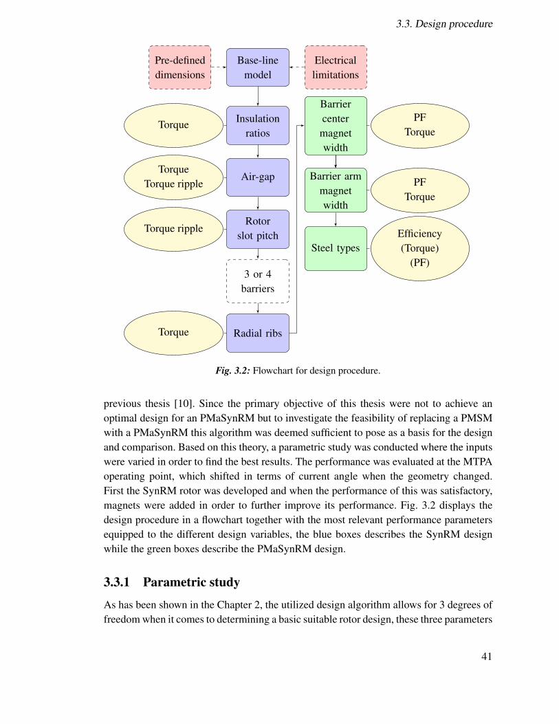
3.3. Design procedure
Base-linemodel
Pre-defineddimensions
Electricallimitations
Insulationratios
Torque
Air-gapTorque
Torque ripple
Rotorslot pitch
Torque ripple
3 or 4barriers
Radial ribsTorque
Barriercenter
magnetwidth
PFTorque
Barrier armmagnetwidth
PFTorque
Steel typesEfficiency(Torque)
(PF)
Fig. 3.2: Flowchart for design procedure.
previous thesis [10]. Since the primary objective of this thesis were not to achieve anoptimal design for an PMaSynRM but to investigate the feasibility of replacing a PMSMwith a PMaSynRM this algorithm was deemed sufficient to pose as a basis for the designand comparison. Based on this theory, a parametric study was conducted where the inputswere varied in order to find the best results. The performance was evaluated at the MTPAoperating point, which shifted in terms of current angle when the geometry changed.First the SynRM rotor was developed and when the performance of this was satisfactory,magnets were added in order to further improve its performance. Fig. 3.2 displays thedesign procedure in a flowchart together with the most relevant performance parametersequipped to the different design variables, the blue boxes describes the SynRM designwhile the green boxes describe the PMaSynRM design.
3.3.1 Parametric study
As has been shown in the Chapter 2, the utilized design algorithm allows for 3 degrees offreedom when it comes to determining a basic suitable rotor design, these three parameters
41

3.3. Design procedure
were
• q-axis insulation ratio, kw,q
• d-axis insulation ratio, kw,d
• Rotor slot displacement angle, �s
These three parameters were deemed sufficient to determine a basic design of aSynRM-rotor. However, more aspects needed to be considered in order to derive a finishedPMaSynRM rotor design such as
• Air-gap length, g
• Radial rib width, wr,i
• Magnet widths, wma,i
and wm,b
The study was conducted and the performance was primarily operationalized fromthe torque production, as the torque density of the PMaSynRM generally is lower than thePMSM and the most important factor for pumping applications. However, other aspectsof the machine was also taken into consideration and were torque ripple, power factor andefficiency.
3.3.2 SynRM base-line design
In order to initiate the design procedure a starting point needed to be defined. Given thediscussion regarding the number of barriers it was determined that two different designswere to be developed initially, one with three barriers and one with four barriers, andthen compared as to which one displayed the best performance. The pole number of themachine was set to be four, following the discussion in Section 2.2.
Hence, initial guesses needed to be made with regards to the input values in orderto have a design starting point where non-swept values were given a default value.
Additionally, some values were out of the scope of the analysis and assigned a fixedvalue. These values were
• The angle ↵i
between barrier arm and center part of barrier (see Fig. 2.10) was tobe kept constant at 135� as it simplified the analysis and was shown to be suitablein [11].
• The tangential ribs were kept constant at 1 mm as their influence was out of thescope of the analysis and kept at the minimum allowable tolerance from the manu-facturer at 1 mm
The two base-line designs were based on the same input-values and can be seen inTable 3.3. Note that the base-line value for �
s
was 5.625� for three barriers and 4.5� forfour barriers.
42
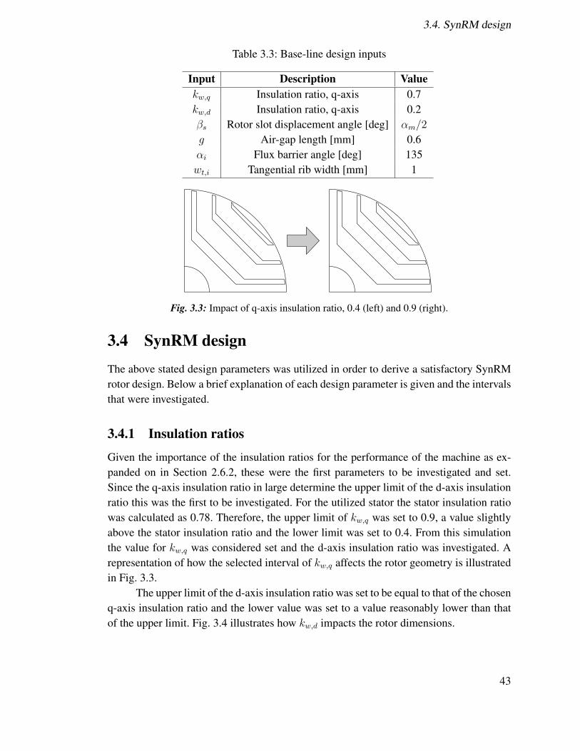
3.4. SynRM design
Table 3.3: Base-line design inputs
Input Description Valuekw,q
Insulation ratio, q-axis 0.7kw,d
Insulation ratio, q-axis 0.2�s
Rotor slot displacement angle [deg] ↵m
/2
g Air-gap length [mm] 0.6↵i
Flux barrier angle [deg] 135w
t,i
Tangential rib width [mm] 1
Fig. 3.3: Impact of q-axis insulation ratio, 0.4 (left) and 0.9 (right).
3.4 SynRM design
The above stated design parameters was utilized in order to derive a satisfactory SynRMrotor design. Below a brief explanation of each design parameter is given and the intervalsthat were investigated.
3.4.1 Insulation ratios
Given the importance of the insulation ratios for the performance of the machine as ex-panded on in Section 2.6.2, these were the first parameters to be investigated and set.Since the q-axis insulation ratio in large determine the upper limit of the d-axis insulationratio this was the first to be investigated. For the utilized stator the stator insulation ratiowas calculated as 0.78. Therefore, the upper limit of k
w,q
was set to 0.9, a value slightlyabove the stator insulation ratio and the lower limit was set to 0.4. From this simulationthe value for k
w,q
was considered set and the d-axis insulation ratio was investigated. Arepresentation of how the selected interval of k
w,q
affects the rotor geometry is illustratedin Fig. 3.3.
The upper limit of the d-axis insulation ratio was set to be equal to that of the chosenq-axis insulation ratio and the lower value was set to a value reasonably lower than thatof the upper limit. Fig. 3.4 illustrates how k
w,d
impacts the rotor dimensions.
43
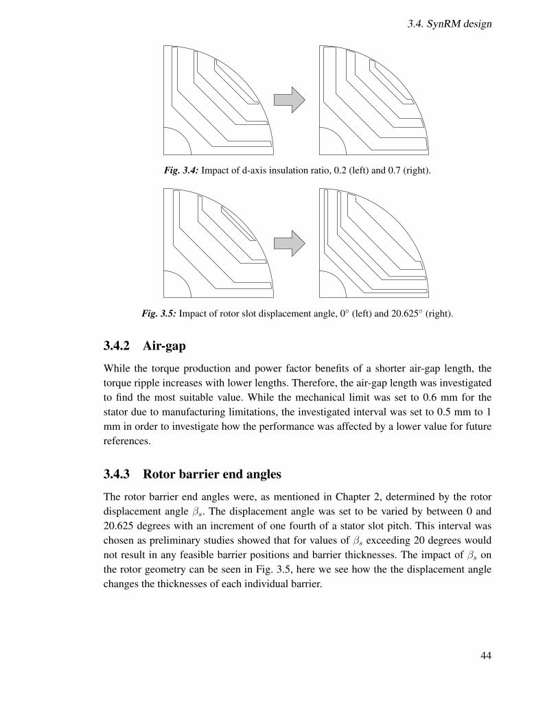
3.4. SynRM design
Fig. 3.4: Impact of d-axis insulation ratio, 0.2 (left) and 0.7 (right).
Fig. 3.5: Impact of rotor slot displacement angle, 0� (left) and 20.625� (right).
3.4.2 Air-gap
While the torque production and power factor benefits of a shorter air-gap length, thetorque ripple increases with lower lengths. Therefore, the air-gap length was investigatedto find the most suitable value. While the mechanical limit was set to 0.6 mm for thestator due to manufacturing limitations, the investigated interval was set to 0.5 mm to 1mm in order to investigate how the performance was affected by a lower value for futurereferences.
3.4.3 Rotor barrier end angles
The rotor barrier end angles were, as mentioned in Chapter 2, determined by the rotordisplacement angle �
s
. The displacement angle was set to be varied by between 0 and20.625 degrees with an increment of one fourth of a stator slot pitch. This interval waschosen as preliminary studies showed that for values of �
s
exceeding 20 degrees wouldnot result in any feasible barrier positions and barrier thicknesses. The impact of �
s
onthe rotor geometry can be seen in Fig. 3.5, here we see how the the displacement anglechanges the thicknesses of each individual barrier.
44
3.5. PMaSynRM design
3.4.4 Choice of barriers
After the aforementioned parameter investigations given previously in this section, it wasassumed that enough data on whether three or four barriers was the best choice in terms ofperformance. Therefore, it was determined sufficient to only investigate one design whenadding PMs, radial ribs and such.
3.4.5 Radial ribs
It was expected that introducing the radial ribs in the flux barrier structure would corre-spond to a decrease in torque and therefore it was deemed desirable to keep the ribs assmall as possible. However, in the manufacturing process the punching does not allow forsmall ribs. As the case with the tangential ribs, the minimum size of the radial ribs wasdeemed to be 1 mm based on previous experience.
As stated above, the ribs were desirable to keep as small as possible, the safetyfactor was put in place in order to ensure that the ribs do not break as that would havedevastating consequences. The sizes of the radial ribs that were tested was calculatedbased on equation (2.20) utilizing different values on the safety factor ⌫ with restrictionson the minimum size due to the manufacturing aspects. This analysis was made in orderto see how much of a detrimental effect the ribs would have depending on their thickness.However, given the overestimation of applied force to the rotor segments sufficiently smallribs was neglected as it could be assumed that it was not necessary. Hence, the limitationswere set to be
• No ribs were allowed to be thinner than 1 mm due to manufacturing limitations
• Any calculated rib size smaller than 0.2 mm were neglected and no ribs was utilizedin that barrier
The values for the safety factor to be utilized was set to be ⌫ = {1.5, 2, 2.5, 3}where the 1.5 value was motivated by the overestimation of the rib sizes.
3.5 PMaSynRM design
Two different types of magnets were used in the simulations of the PMaSynRM, oneferrite magnet and one NdFeB. The ferrite magnet data was supplied by NORDMAG,without specified grade standard, and the NdFeB was the grade N33EH. The characteris-tics of the two magnets are summarized in Table 3.4 and the data-sheets can be seen inAppendix B.2.
45
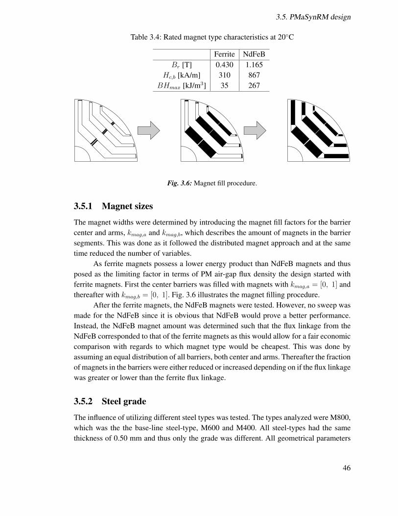
3.5. PMaSynRM design
Table 3.4: Rated magnet type characteristics at 20�C
Ferrite NdFeBB
r
[T] 0.430 1.165H
c,b
[kA/m] 310 867BH
max
[kJ/m3] 35 267
Fig. 3.6: Magnet fill procedure.
3.5.1 Magnet sizes
The magnet widths were determined by introducing the magnet fill factors for the barriercenter and arms, k
mag,a
and kmag,b
, which describes the amount of magnets in the barriersegments. This was done as it followed the distributed magnet approach and at the sametime reduced the number of variables.
As ferrite magnets possess a lower energy product than NdFeB magnets and thusposed as the limiting factor in terms of PM air-gap flux density the design started withferrite magnets. First the center barriers was filled with magnets with k
mag,a
= [0, 1] andthereafter with k
mag,b
= [0, 1]. Fig. 3.6 illustrates the magnet filling procedure.After the ferrite magnets, the NdFeB magnets were tested. However, no sweep was
made for the NdFeB since it is obvious that NdFeB would prove a better performance.Instead, the NdFeB magnet amount was determined such that the flux linkage from theNdFeB corresponded to that of the ferrite magnets as this would allow for a fair economiccomparison with regards to which magnet type would be cheapest. This was done byassuming an equal distribution of all barriers, both center and arms. Thereafter the fractionof magnets in the barriers were either reduced or increased depending on if the flux linkagewas greater or lower than the ferrite flux linkage.
3.5.2 Steel grade
The influence of utilizing different steel types was tested. The types analyzed were M800,which was the the base-line steel-type, M600 and M400. All steel-types had the samethickness of 0.50 mm and thus only the grade was different. All geometrical parameters
46

3.6. Performance comparison and economic analysis
were kept constant. For datasheets of the steels refer to Appendix B.1.
3.5.3 Demagnetization
In order to investigate demagnetization of the different magnets, the demagnetizationmodel as described in Section 2.7.1 was utilized in a built-in macro in FLUX where itreduces the remanent flux when H
k
was exceeded. The threshold for any part of the mag-net being considered demagnetized was set to be 90% of the nominal remanent flux andafter the simulation the fraction of each magnet that violated that threshold was calculated.
In order to aptly account for as many demagnetization scenarios as possible thecurrent was set to be 1, 1.5, 2 and 2.5 times the nominal current levels. 2.5 was chosento be the upper limit because the drives normally utilized for machines of the intendedpurpose has a current limit of around two times the nominal current.
Furthermore, the current angle also influences the demagnetization as the stator fluxshould counteract the magnetization of the magnets. Since the magnets are magnetized indifferent directions, different current angles were tested. Preliminary tests showed thatthe most detrimental current angles were in the span 70 to 110 degrees. While these arenot commonplace current angles, it is important to take them into consideration sincethe motor is intended for pumping applications which might lead to unintended cloggingwhich abruptly stops the machine and these angles might occur for short periods of time.
The demagnetization was tested at an operating temperature at which the magnetswas most at risk for experience demagnetization. For the ferrite magnets, this was deter-mined to be at 0�C which was deemed the lowest feasible magnet temperature given astart-up sequence in cold water. For the NdFeB the maximum operating temperature wasset to 120�C.
3.6 Performance comparison and economic analysis
The intended purpose of the developed PMaSynRM was to pose as a more cost-effectivealternative for the applications of a surface-mounted PMSM, where a power electronicdrive was utilized for speed control. Therefore, it was important to compare these twotypes of machines in order to investigate whether or not the developed PMaSynRM werecomparable to the PMSM.
3.6.1 Comparing the machines
The performance comparison was conducted based on equal torque production as thespatial requirements for the intended application was not of great concern. Since the twomachines displayed different behaviour in terms of torque production and power fac-tor related to current angle, the performance comparison was made based on the torque
47

3.6. Performance comparison and economic analysis
production curves as function of current angle at rated current in order to assess the char-acteristics of the machines. The machines were run at 1500 RPM. Any speed range testsalong with high-speed analysis was not deemed to be of great importance as the speedrange is in part limited by the DC link voltage which for this thesis was not a constraint.Field-weakening operation was not of great relevance as the load torque for pumping ap-plications tend to increase with the square of the rotational speed, and therefore to someextent impractical in CPSR.
The economic analysis were made based on material costs and some productioncosts of the stators due to the differences in production methods between the two ma-chines. The costs of the machines are an important factor in this assessment as it com-bined with the performance of the machines will help determine for which applicationsthe PMaSynRM is feasible.
For the economic analysis the following assumptions are made
• The PMaSynRM stator and rotor was assumed to be punched from a single sheetof steel and excess steel is considered waste. The total steel usage thus is a squarewith sides equal to the outer diameter of the machine.
• The PMSM stator segments are smaller and easier to punch and the shape of thesegments allows for less waste and therefore was calculated by assuming that arectangular segment with one side as wide as a stator segment and one side 50%longer than one stator segment has space for two stator segment as exemplified inFig. 3.7
• The PMSM rotor is assumed to be punched from a single sheet of steel, given theconsumed material equal to the square of the diameter of the rotor.
• Only the cost per weight of the magnets were considered without taking the press-ing, cutting or transport of the magnets into consideration.
• Only the manufacturing costs of the stators were taken into consideration as therotors are manufactured by a third party and thereby the manufacturing cost is diffi-cult to estimate. Furthermore, the greatest difference manufacturing-wise is deemedto be located to the stator. The manufacturing costs was given by the economics de-partment at Xylem.
As magnets corresponded to a significant part of the cost of a machine, which is es-pecially true when NdFeB magnets were utilized, and given the fluctuating nature of thesetypes of magnet, it was investigated if there occurred any breaking points with regards tothe NdFeB machines and the ferrite PMaSynRM.
In this thesis, given the sensitive nature of material pricing, all costs was given inper unit (pu) cost as opposed to real currency. The base cost was set to be the ferrite PMa-SynRM with the steel M800-50A and magnet price in the middle of the given interval.
48
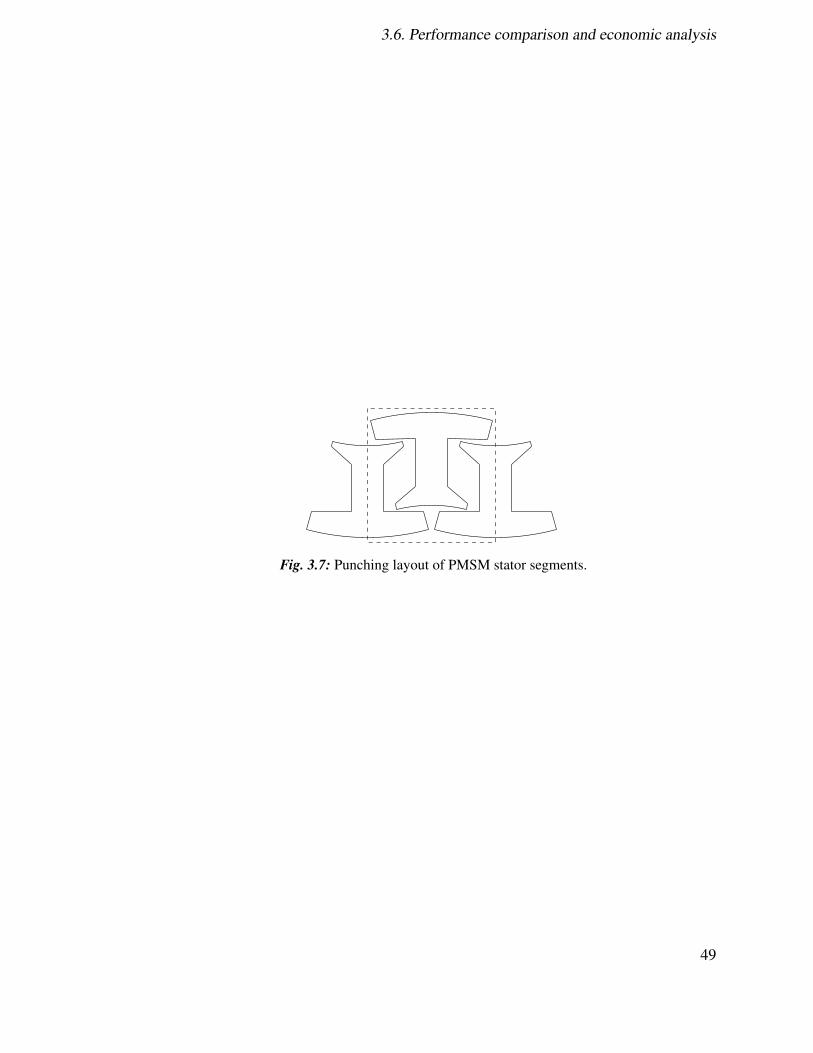
3.6. Performance comparison and economic analysis
Fig. 3.7: Punching layout of PMSM stator segments.
49

Chapter 4
Results
In this chapter, all the results are presented. All relevant plots and figures are given anddiscussed to some extent. The values which were carried over are given and the finaldesign is displayed.
4.1 Rotor design
As was described in Chapter 3, the design process was divided up into several parts wherethe result from the previous simulations were added on to the baseline design. In thissection, the results from this analysis will be described.
4.1.1 q-axis insulation ratio
The q-axis insulation ratio was varied between 0.4 and 0.9, utilizing all base-line valuesas seen in Table 4.1.
Table 4.1: Simulation parameters for kw,q
kw,q
kw,d
g �s
Variable Baseline Baseline Baseline
In Fig. 4.1 the results for torque, torque ripple, power factor and efficiency can beseen respectively. It is useful to note that the torque doesn’t vary particularly much overthis interval, which can be attributed to the fact that the interval was too narrow to see thedetrimental effects of too low or too high values, and only the maxima was achieved.
We can also note that in terms of torque and power factor, the four barrier designdisplayed better performance than three barriers whilst generally displaying worse perfor-mance in terms of torque ripple. However, the torque ripple wasn’t the key performanceindicator for k
w,q
since the ripple was shown to be mostly governed by the location ofthe rotor barrier ends. Thus, the optimum values for both barriers were deemed to be
50
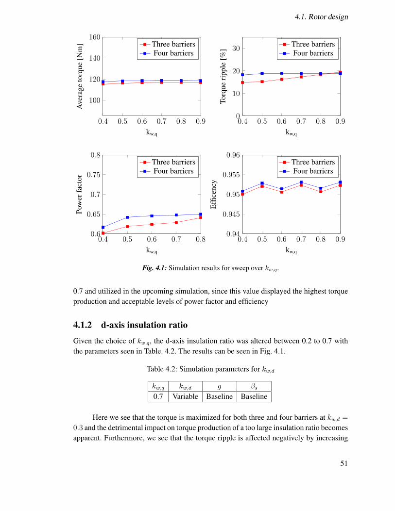
4.1. Rotor design
0.4 0.5 0.6 0.7 0.8 0.9
100
120
140
160
kw,q
Ave
rage
torq
ue[N
m] Three barriers
Four barriers
0.4 0.5 0.6 0.7 0.8 0.90
10
20
30
kw,q
Torq
uerip
ple
[%]
Three barriersFour barriers
0.4 0.5 0.6 0.7 0.80.6
0.65
0.7
0.75
0.8
kw,q
Pow
erfa
ctor
Three barriersFour barriers
0.4 0.5 0.6 0.7 0.8 0.90.94
0.945
0.95
0.955
0.96
kw,q
Effic
ency
Three barriersFour barriers
Fig. 4.1: Simulation results for sweep over kw,q
.
0.7 and utilized in the upcoming simulation, since this value displayed the highest torqueproduction and acceptable levels of power factor and efficiency
4.1.2 d-axis insulation ratio
Given the choice of kw,q
, the d-axis insulation ratio was altered between 0.2 to 0.7 withthe parameters seen in Table. 4.2. The results can be seen in Fig. 4.1.
Table 4.2: Simulation parameters for kw,d
kw,q
kw,d
g �s
0.7 Variable Baseline Baseline
Here we see that the torque is maximized for both three and four barriers at kw,d
=
0.3 and the detrimental impact on torque production of a too large insulation ratio becomesapparent. Furthermore, we see that the torque ripple is affected negatively by increasing
51

4.1. Rotor design
0.2 0.3 0.4 0.5 0.6 0.7
100
120
140
160
kw,d
Ave
rage
torq
ue[N
m] Three barriers
Four barriers
0.2 0.3 0.4 0.5 0.6 0.70
10
20
30
kw,d
Torq
uerip
ple
[%]
Three barriersFour barriers
0.2 0.3 0.4 0.5 0.6 0.70.6
0.65
0.7
0.75
0.8
kw,d
Pow
erfa
ctor
Three barriersFour barriers
0.2 0.3 0.4 0.5 0.6 0.70.94
0.945
0.95
0.955
0.96
kw,d
Effic
ency
Three barriersFour barriers
Fig. 4.2: Simulation results for sweep over kw,d
.
insulation ratio. Once again, torque ripple wasn’t the key performance indicator for theinsulation ratio and since the increase in ripple is so low for the optimal value for torquethe slight increase is allowed. The same thing applies to the power factor, the maxima forboth power factors are situated at k
w,d
= 0.5 but since the variation is so small, especiallyfor the four barrier configuration this non-optimal value is allowed. Furthermore, we seethat the efficiency is negatively affected by increasing insulation ratio for four barrierswhile higher values affect the efficiency negatively for three barriers. This can probablybe attributed to increased rotor saturation, which also can explain the decrease in torqueproduction for greater values of k
w,d
.
4.1.3 Air-gap
The input data for the air-gap sweep is given in Table 4.3. The air-gap sweep was con-ducted between 0.4 mm to 1 mm. As can be seen from Fig. 4.3, the torque productiondeclines almost linearly with the air-gap length. Also, as expected the power factor re-duces greatly. The efficiency declines, most likely as a product of the reduced mechanical
52

4.1. Rotor design
0.4 0.6 0.8 1
100
120
140
160
Air-gap length [mm]
Ave
rage
torq
ue[N
m] Three barriers
Four barriers
0.4 0.6 0.8 1
0
10
20
30
Air-gap length [mm]
Torq
uerip
ple
[%]
Three barriersFour barriers
0.4 0.6 0.8 1
0.5
0.6
0.7
0.8
Air-gap length [mm]
Pow
erfa
ctor
Three barriersFour barriers
0.4 0.6 0.8 1
0.92
0.94
0.96
Air-gap length [mm]
Effic
ency
Three barriersFour barriers
Fig. 4.3: Simulation results for sweep over g.
power. The torque ripple reduction is quite modest considering the drastic reduction oftorque production. Thus, it is visible that it is imperative to maintain the air-gap as shortas possible and a value below 0.6 mm would be beneficial. Given the steep decline of thetorque production and the low decrease in torque ripple, the minimum allowable air-gapheight was chosen, i.e. g = 0.6 mm.
Table 4.3: Simulation parameters for g
kw,q
kw,d
g �s
0.7 0.3 Variable Baseline
53
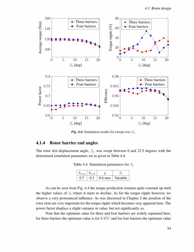
4.1. Rotor design
0 5 10 15 20
100
120
140
160
�s
[deg]
Ave
rage
torq
ue[N
m] Three barriers
Four barriers
0 5 10 15 20
0
20
40
60
80
�s
[deg]
Torq
uerip
ple
[%] Three barriers
Four barriers
0 5 10 15 20
0.6
0.65
0.7
0.75
0.8
�s
[deg]
Pow
erfa
ctor
Three barriersFour barriers
0 5 10 15 20
0.94
0.945
0.95
0.955
0.96
�s
[deg]
Effic
ency
Three barriersFour barriers
Fig. 4.4: Simulation results for sweep over �s
.
4.1.4 Rotor barrier end angles
The rotor slot displacement angle, �s
, was swept between 0 and 22.5 degrees with thedetermined simulation parameters set as given in Table 4.4.
Table 4.4: Simulation parameters for �s
kw,q
kw,d
g �s
0.7 0.3 0.6 mm Variable
As can be seen from Fig. 4.4 the torque production remains quite constant up untilthe higher values of �
s
where it starts to decline. As for the torque ripple however, weobserve a very pronounced influence. As was discussed in Chapter 2 the position of therotor slots are very important for the torque ripple which becomes very apparent here. Thepower factor displays a slight variance in value, but not significantly so.
Note that the optimum value for three and four barriers are widely separated here,for three barriers the optimum value is for 9.375� and for four barriers the optimum value
54

4.1. Rotor design
was 0
� when considering both torque production and torque ripple. These differeces inrotor angles are reasonable since the actual rotor slot positions are different for the samevalue of �
s
. With previous simulations, the basic SynRM design is concluded with theperformance as seen in Table. 4.5.
Table 4.5: Performance for best preliminary 3 and 4 barrier design
3 barriers 4 barriersTorque 117.56 119.96
Torque ripple 10.32 6.85Power factor 0.649 0.650
Efficiency 0.952 0.953
After these simulations it could be concluded that for this 48 slot stator, four bar-riers were the best performing configuration in all regards. This resulted in the choice ofcontinuing the simulations with only the four-barrier alternative with the design parametervalues which can be seen in Table. 4.6
Table 4.6: Basic design parameters for four-barrier SynRM rotor
kw,q
kw,d
g �s
0.7 0.3 0.6 mm 0�
4.1.5 Radial ribs
The geometry from the previous simulations was used to calculate the rib-sizes for theradial ribs following the restrictions described in Chapter 2. The resulting values can beseen in Table. 4.7. The constraints set on the ribs with the minimum size affected all ribssizes indicated by an asterisk giving an over-dimensioning of the two middle ribs and aunder-dimensioning of the outer barrier.
Table 4.7: Radial rib sizes for different values of safety factors
Safety factor, ⌫ wr,1 [mm] w
r,2 [mm] wr,3 [mm] w
r,4 [mm]1.5 1.4986 1.0000* 1.0000* 0*2 1.9981 1.1797 1.0000* 0*
2.5 2.4976 1.4747 1.0000* 0*3 2.9971 1.7696 1.0000* 0*
The results can be seen in Fig.4.5. As expected, the torque production is affected bythe introduction of ribs and we also see a decrease in power factor. The torque reduction
55
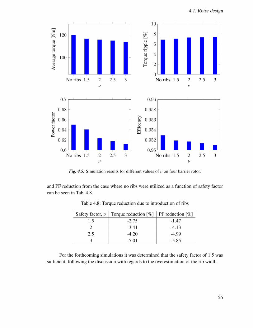
4.1. Rotor design
No ribs 1.5 2 2.5 3
100
120
⌫
Ave
rage
torq
ue[N
m]
No ribs 1.5 2 2.5 30
2
4
6
8
10
⌫
Torq
uerip
ple
[%]
No ribs 1.5 2 2.5 30.6
0.62
0.64
0.66
0.68
0.7
⌫
Pow
erfa
ctor
No ribs 1.5 2 2.5 30.95
0.952
0.954
0.956
0.958
0.96
⌫
Effic
ency
Fig. 4.5: Simulation results for different values of ⌫ on four barrier rotor.
and PF reduction from the case where no ribs were utilized as a function of safety factorcan be seen in Tab. 4.8.
Table 4.8: Torque reduction due to introduction of ribs
Safety factor, ⌫ Torque reduction [%] PF reduction [%]1.5 -2.75 -1.472 -3.41 -4.13
2.5 -4.20 -4.993 -5.01 -5.85
For the forthcoming simulations it was determined that the safety factor of 1.5 wassufficient, following the discussion with regards to the overestimation of the rib width.
56

4.1. Rotor design
Fig. 4.6: Final design of SynRM rotor.
4.1.6 Final SynRM rotor geometry
With the above conducted analysis, the rotor design corresponding to the SynRM-designcan be regarded as set. The final design can be seen in Fig. 4.6 and corresponding rotordimensions can be seen in Table. 4.9. It can be seen that the outermost barrier becamequite small, only 1.25 millimeters. This might cause difficulties to add magnets to thatbarrier, which will be discussed further in the next section.
57
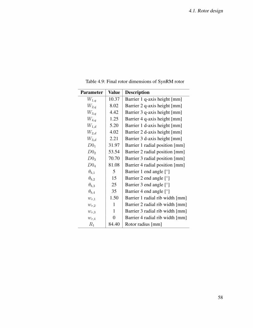
4.1. Rotor design
Table 4.9: Final rotor dimensions of SynRM rotor
Parameter Value DescriptionW1,q 10.37 Barrier 1 q-axis height [mm]W2,q 8.02 Barrier 2 q-axis height [mm]W3,q 4.42 Barrier 3 q-axis height [mm]W4,q 1.25 Barrier 4 q-axis height [mm]W1,d 5.20 Barrier 1 d-axis height [mm]W2,d 4.02 Barrier 2 d-axis height [mm]W3,d 2.21 Barrier 3 d-axis height [mm]D01 31.97 Barrier 1 radial position [mm]D02 53.54 Barrier 2 radial position [mm]D03 70.70 Barrier 3 radial position [mm]D04 81.08 Barrier 4 radial position [mm]✓b,1 5 Barrier 1 end angle [�]✓b,2 15 Barrier 2 end angle [�]✓b,3 25 Barrier 3 end angle [�]✓b,4 35 Barrier 4 end angle [�]
wr,1 1.50 Barrier 1 radial rib width [mm]
wr,2 1 Barrier 2 radial rib width [mm]
wr,3 1 Barrier 3 radial rib width [mm]
wr,4 0 Barrier 4 radial rib width [mm]R1 84.40 Rotor radius [mm]
58
4.2. PMaSynRM design
4.2 PMaSynRM design
With the rotor design complete, the magnets were ready to be added. First, the ferritePM addition was simulated, thereafter the NdFeB magnet amount was calculated andsimulated. Additionally, the effects of leaving the outer barrier empty was investigated.Last, the influence of utilizing different types of steel was analyzed.
4.2.1 Magnet addition
As stated in Chapter 3, the center barriers was filled with ferrite magnets and when thiswas done the barrier arms were filled. In Fig. 4.7, the center barrier data can be seen.As expected, the torque production and power factor experience a great increase. Thetorque increases from 118 Nm to 143 Nm and the power factor goes from 0.64 to 0.79.The torque ripple remains constant between 10-11 % for all values except the last whereit goes down to 8.5%. However, looking at the numerical values we see that the torqueripple maintains a value between 11.5-14.5 Nm. From this data the choice fell quite easilyon completely filling the center barriers with magnets.
Next the barrier arms were filled with magnets, with all barrier centers filled withmagnets. The results can be seen in Fig. 4.8. Here we see that the torque goes from 143Nm to 157 Nm while the power factor goes from 0.79 to 0.85. Interestingly, the torqueripple reduces until 60 % of the arms are filled and thereafter it increases. However, thesevalues are not deemed to be worrisome given the application and therefore the entirelyfilled barrier arm was chosen to define the final design of the rotor.
And thus, with the magnets in place the ferrite PM flux of the machine correspondedto 40% of the nominal flux, a value which was in acceptable agreement with the discussionwith regards to the magnitude of PM flux.
4.2.2 Without magnet in outermost barrier
The final design of the rotor resulted in a quite small outer barrier (1.25 mm thick) asseen in Table 4.9. Even though it might be possible to add ferrite magnets to this barrierafter discussion with the supplier it would result in very many small magnets since themanufacturing process does not allow for magnet dimensions where one side is muchlarger than the others for those dimensions. Therefore, the impact of leaving that barrierfilled with air was investigated. The results can be seen in Table. 4.10 where it is comparedto the entirely magnet-filled rotor.
Here we see that the torque reduction is around 2 Nm while the torque ripple alsodecrease slightly and the other values are left virtually unaffected. Hence, it has beenshown that if it proves unpractical to add magnets to the outermost barrier the performancereduction is within reasonable values.
59

4.2. PMaSynRM design
0 0.2 0.4 0.6 0.8 1
100
120
140
160
Fraction of center barrier filled
Ave
rage
torq
ue[N
m]
0 0.2 0.4 0.6 0.8 1
0
10
20
30
Fraction of center barrier filled
Torq
uerip
ple
[%]
0 0.2 0.4 0.6 0.8 1
0.6
0.7
0.8
0.9
Fraction of center barrier filled
Pow
erfa
ctor
0 0.2 0.4 0.6 0.8 1
0.95
0.955
0.96
0.965
0.97
Fraction of center barrier filled
Effic
ency
Fig. 4.7: Simulation data when adding magnets to center barrier.
4.2.3 NdFeB
The NdFeB magnets were filled in all barriers including the outermost, as that topologywould provide the base for the economic calculations. The tolerance for the NdFeB fluxlinkage versus the ferrite flux linkage was 1%. The magnet fill factor for the center barrier,kmag,a
, was set to 0.4 while for the barrier arms, kmag,b
was set to 0.3625. The results ofthe simulations can be seen in Table. 4.11
It is quite noticeable that the torque production is lower for the NdFeB, while thetorque ripple is higher. This can probably be attributed to the distribution of the magnets inthe barriers and the fact that the magnet flux does not affect all parts of the iron segmentsin the same way since there are large portions of air in the flux barriers with NdFeBmagnets in the rotor. However, these results were deemed to be sufficient as basis forthe economic comparison since the performance of the two machines are similar to eachother.
60

4.3. Demagnetization
0 0.2 0.4 0.6 0.8 1
100
120
140
160
Fraction of center barrier filled
Ave
rage
torq
ue[N
m]
0 0.2 0.4 0.6 0.8 1
0
10
20
30
Fraction of center barrier filled
Torq
uerip
ple
[%]
0 0.2 0.4 0.6 0.8 1
0.6
0.7
0.8
0.9
Fraction of center barrier filled
Pow
erfa
ctor
0 0.2 0.4 0.6 0.8 1
0.95
0.955
0.96
0.965
0.97
Fraction of center barrier filled
Effic
ency
Fig. 4.8: Simulation data when adding magnets to barrier arms.
4.2.4 Steel types
The different steel-types tested were M800, M600 and M400. The results of the simula-tions can be seen in Table 4.12.
As can be seen, the torque production actually decrease as the steel grade improves.However, we see that the power factor does get affected by the steel grade. This can prob-ably be attributed to the steel grades yielding different inductances and having slightlydifferent B-H curves and saturation levels which affected the d-q inductance differenceas well as the saliency ratio. Additionally, while the output mechanical power slightly de-crease, so does the iron losses leaving the efficiency largely unaffected to any significantnumber.
4.3 Demagnetization
The demagnetization was studied for a variety of current magnitudes and angles. The basisfor this simulation was the ferrite rotor with all barriers filled. The current levels analyzed
61
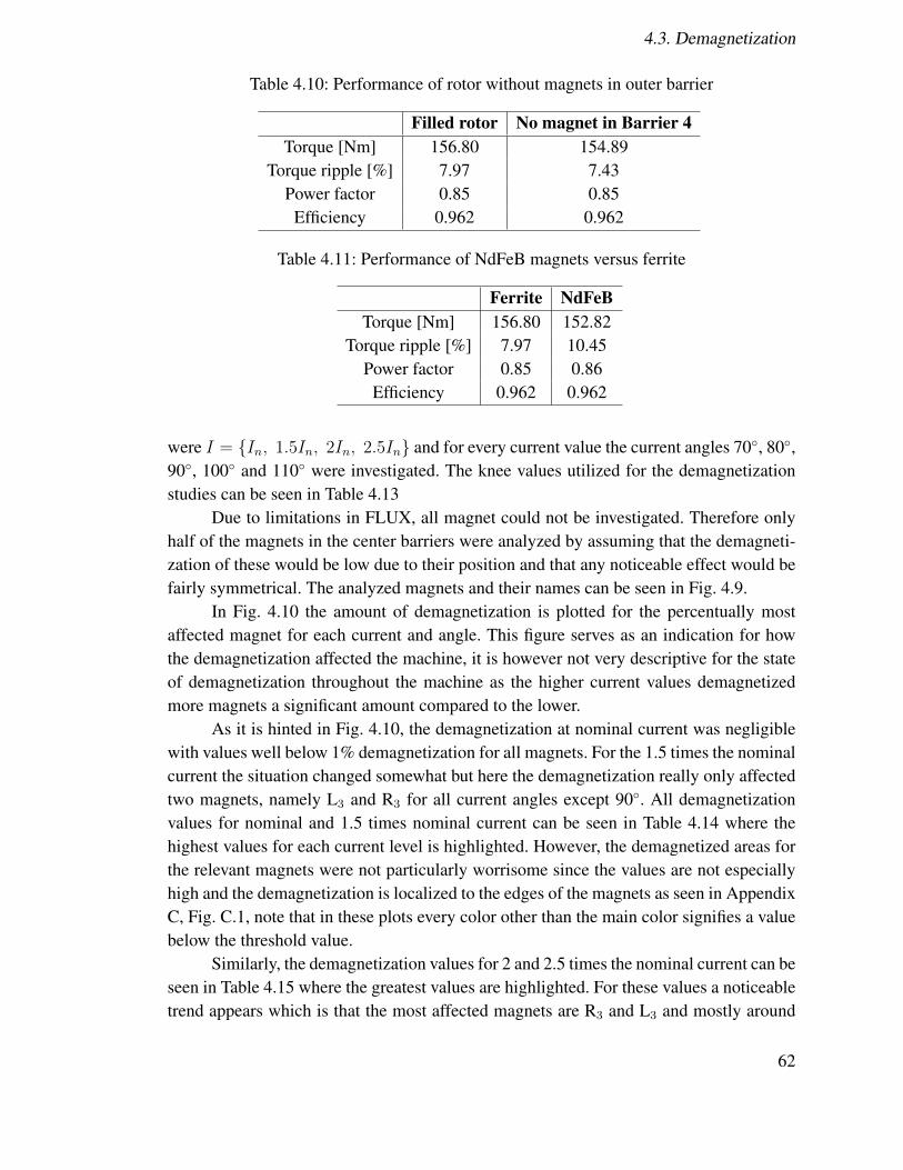
4.3. Demagnetization
Table 4.10: Performance of rotor without magnets in outer barrier
Filled rotor No magnet in Barrier 4Torque [Nm] 156.80 154.89
Torque ripple [%] 7.97 7.43Power factor 0.85 0.85
Efficiency 0.962 0.962
Table 4.11: Performance of NdFeB magnets versus ferrite
Ferrite NdFeBTorque [Nm] 156.80 152.82
Torque ripple [%] 7.97 10.45Power factor 0.85 0.86
Efficiency 0.962 0.962
were I = {In
, 1.5In
, 2In
, 2.5In
} and for every current value the current angles 70�, 80�,90�, 100� and 110� were investigated. The knee values utilized for the demagnetizationstudies can be seen in Table 4.13
Due to limitations in FLUX, all magnet could not be investigated. Therefore onlyhalf of the magnets in the center barriers were analyzed by assuming that the demagneti-zation of these would be low due to their position and that any noticeable effect would befairly symmetrical. The analyzed magnets and their names can be seen in Fig. 4.9.
In Fig. 4.10 the amount of demagnetization is plotted for the percentually mostaffected magnet for each current and angle. This figure serves as an indication for howthe demagnetization affected the machine, it is however not very descriptive for the stateof demagnetization throughout the machine as the higher current values demagnetizedmore magnets a significant amount compared to the lower.
As it is hinted in Fig. 4.10, the demagnetization at nominal current was negligiblewith values well below 1% demagnetization for all magnets. For the 1.5 times the nominalcurrent the situation changed somewhat but here the demagnetization really only affectedtwo magnets, namely L3 and R3 for all current angles except 90�. All demagnetizationvalues for nominal and 1.5 times nominal current can be seen in Table 4.14 where thehighest values for each current level is highlighted. However, the demagnetized areas forthe relevant magnets were not particularly worrisome since the values are not especiallyhigh and the demagnetization is localized to the edges of the magnets as seen in AppendixC, Fig. C.1, note that in these plots every color other than the main color signifies a valuebelow the threshold value.
Similarly, the demagnetization values for 2 and 2.5 times the nominal current can beseen in Table 4.15 where the greatest values are highlighted. For these values a noticeabletrend appears which is that the most affected magnets are R3 and L3 and mostly around
62

4.3. Demagnetization
Table 4.12: Performance for different steel grades
M800-50 M600-50 M400-50Torque [Nm] 156.80 156.00 153.99
Torque ripple [%] 7.97 8.04 7.93Power factor 0.852 0.896 0.899
Efficiency 0.962 0.962 0.968Rotor iron losses (only hysteresis and eddy) [W] 103.4 99.2 93.8Stator iron losses (only hysteresis and eddy) [W] 211.2 209.7 205.4
Table 4.13: Magnet demagnetization values
Ferrite NdFeBB
r
[T] 0.45 1.025H
k
[kA/m] 360 1195
100� for R3 and 70� for L3. This is reasonable since R3 and L3 are positioned such that thestator flux direction is mostly counteracting the remanent flux of the magnets. Similarly,it can be noticed that the demagnetization for barriers 2 and 1 increases with the angulardistance from 90�. Additionally we see that the center barriers are well protected from de-magnetization as was stated in Chapter 2. For these two values, the demagnetization beganto be significant. However, utilizing the same argument as earlier, the demagnetization for2 times the nominal current was deemed to be insignificant for producing a noticeableperformance reduction. For 2.5 times the nominal current, however, the demagnetizationof especially barrier 3 and 2 begin to be of significant magnitude. The demagnetizationfor these two current levels can be seen in Appendix C, Fig. C.2.
A similar analysis were conducted on the NdFeB rotor aswell, and as expectedalmost no demagnetization occurred as can be seen in Table. 4.16 where only the highestcurrent is displayed. The low demagnetization can be easily explained by the high valuesof both remanent flux and coercive force that characterizes the NdFeB magnets.
63
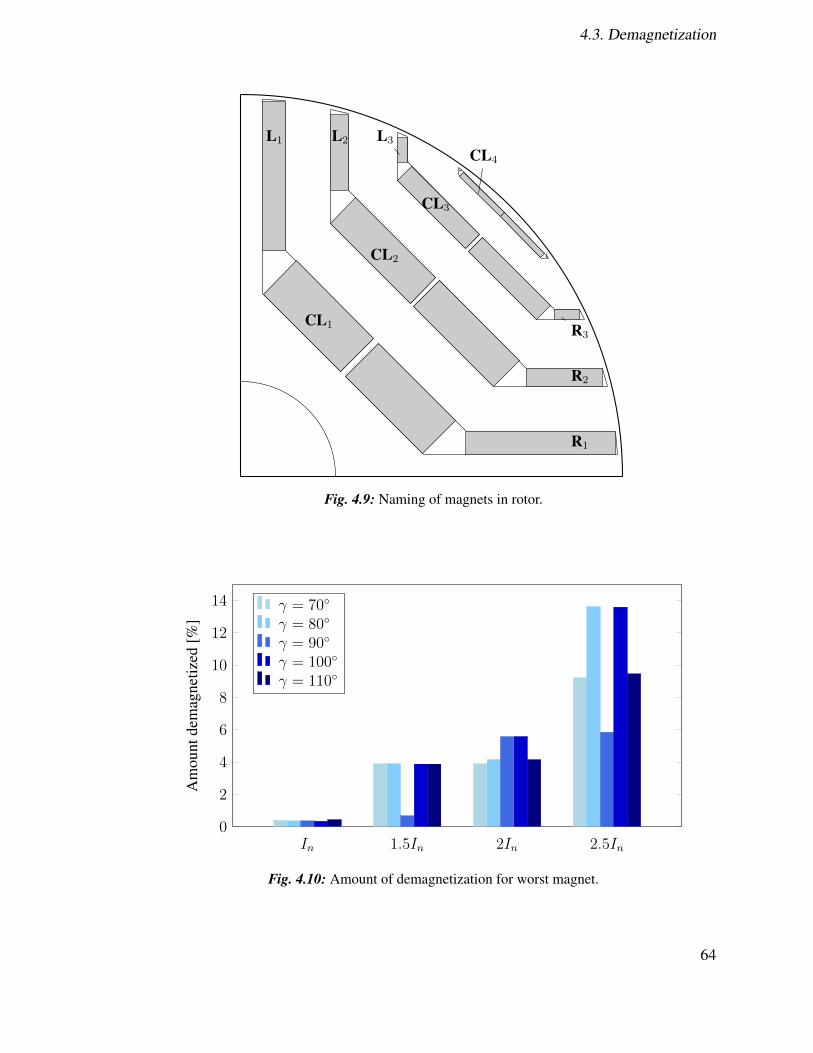
4.3. Demagnetization
CL1
CL2
CL3
CL4
L1 L2 L3
R1
R2
R3
Fig. 4.9: Naming of magnets in rotor.
In
1.5In
2In
2.5In
0
2
4
6
8
10
12
14
Am
ount
dem
agne
tized
[%]
� = 70
�
� = 80
�
� = 90
�
� = 100
�
� = 110
�
Fig. 4.10: Amount of demagnetization for worst magnet.
64

4.3. Demagnetization
Table 4.14: Percent of ferrite magnet demagnetized below 0.41 T for In
and 1.5In
Current In
1.5In
Angle 70� 80� 90� 100� 110� 70� 80� 90� 100� 110�
L1 0.39 0.29 0.00 0.02 0.05 1.05 0.77 0.31 0.19 0.36L2 0.35 0.35 0.35 0.12 0.00 1.45 1.45 0.35 0.12 0.25L3 0.00 0.00 0.00 0.00 0.00 3.89 3.89 0.00 0.00 0.00R1 0.06 0.02 0.00 0.26 0.43 0.40 0.26 0.32 0.91 1.07R2 0.00 0.11 0.33 0.33 0.33 0.35 0.45 0.67 1.73 2.08R3 0.00 0.00 0.00 0.00 0.00 0.00 0.00 0.00 3.88 3.88CL1 0.00 0.00 0.00 0.00 0.00 0.00 0.00 0.00 0.00 0.00CL2 0.00 0.00 0.00 0.00 0.00 0.00 0.00 0.00 0.00 0.00CL3 0.00 0.00 0.00 0.00 0.00 0.00 0.00 0.00 0.00 0.00CL4 0.00 0.00 0.00 0.00 0.00 0.00 0.00 0.00 0.00 0.00
Table 4.15: Percent of ferrite magnet demagnetized below 0.41 T for 2In
and 2.5In
Current 2In
2.5In
Angle 70� 80� 90� 100� 110� 70� 80� 90� 100� 110�
L1 1.35 1.26 0.65 0.60 0.93 2.14 1.56 1.07 0.98 1.50L2 2.14 2.14 0.70 0.97 0.85 3.74 3.03 1.91 2.07 2.08L3 3.89 4.15 4.15 0.26 0.26 9.20 13.61 5.84 3.02 5.49R1 0.92 0.66 0.62 1.22 1.48 1.58 1.04 1.31 1.64 2.38R2 0.84 0.95 0.77 2.18 2.08 2.07 1.73 2.18 4.06 4.06R3 1.70 1.70 5.57 5.57 4.14 5.76 4.10 5.83 13.59 9.45CL1 0.00 0.00 0.00 0.00 0.00 0.00 0.00 0.00 0.00 0.00CL2 0.00 0.00 0.00 0.00 0.00 0.02 0.02 0.02 0.02 0.02CL3 0.00 0.00 0.00 0.00 0.00 0.00 0.00 0.00 0.00 0.00CL4 0.00 0.00 0.00 0.00 0.36 0.00 0.00 0.98 0.98 0.98
Table 4.16: Percent of NdFeB magnet demagnetized below 0.9 T
Current 2.5In
Angle 80� 90� 100� 110�
L1 0 0 0 0L2 0.3221 0 0 0L3 0 0 0 0R1 0 0 0 0R2 0 0 0.3273 0.3273R3 0 0 0 0
65

4.4. PMSM versus PMaSynRM
4.4 PMSM versus PMaSynRM
The finished design of the PMaSynRM was compared to the PMSM in terms of bothperformance and economic parameters. Below the results of the simulations conductedon both PMaSynRM and PMSM is presented along with the calculations of the cost ofboth machines.
4.4.1 Performance comparison
When it comes to comparing the two machines in terms of performance, there are nostraight-forward method to do this. Table 4.17 displays the results of the simulations atMTPA for both machines. We see that the torque production of the PMSM was slightlyhigher than the PMaSynRM but within a reasonable range. The torque ripple of the PMSMwas as expected significantly lower than the PMaSynRM. The efficiency of the PMSMbecame slightly higher than the PMaSynRM.
Table 4.17: Performance of PMaSynRM versus PMSM at MTPA
PMaSynRM PMSMTorque [Nm] 156.80 163.03
Torque ripple [%] 7.97 1.19Efficiency 0.962 0.966
In Fig. 4.11 the torque and power factor of the machines are plotted as function ofthe current vector angle. We see that the PMaSynRM maximum torque (MTPA operatingpoint) occurs at about 47� while the PMSM occurs at about 0�, even though none of themachines display any particularly good power factor values at this point it is interestingto note that the PMaSynRM in fact has a better value at this point. Both machines dis-play a peak PF (MTPkVA operating point) of very close to 1. However, it is worth notingthat none of these operating points pose with a particularly high torque value. However,it is very noticeable that the PF-curve is much flatter for the PMSM than for the PMa-SynRM, meaning that for most torque values in these charts the PMSM is better than thePMaSynRM.
4.4.2 Cost comparison
The cost of the machines was calculated in terms of material costs and production costsof the stators. The price in pu of the materials are given in Table 4.18. The PMSM andPMaSynRM utilized different types of copper wire and thereby they obtained differentprices.
The magnet material price of NdFeB were given in the span of 0.17-0.34 pu, andfor ferrite magnets about a factor of 10 lower meaning 0.017-0.034 pu. Setting the magnet
66

4.4. PMSM versus PMaSynRM
0 20 40 60 80
0
20
40
60
80
100
120
140
160
0
0.2
0.4
0.6
0.8
1
� [deg]
Torq
ue[N
m]
Pow
erFa
ctor
(a) PMaSynRM
0 20 40 60 80
0
20
40
60
80
100
120
140
160
0
0.2
0.4
0.6
0.8
1
� [deg]
Torq
ue[N
m]
Pow
erFa
ctor
(b) PMSM
Fig. 4.11: Torque and power factor as function of current vector angle �.
67
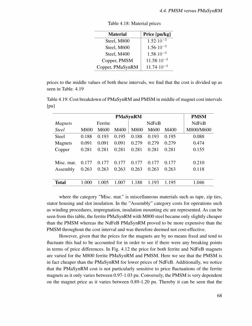
4.4. PMSM versus PMaSynRM
Table 4.18: Material prices
Material Price [pu/kg]Steel, M800 1.52·10�3
Steel, M600 1.56·10�3
Steel, M400 1.58·10�3
Copper, PMSM 11.58·10�3
Copper, PMaSynRM 11.74·10�3
prices to the middle values of both these intervals, we find that the cost is divided up asseen in Table. 4.19
Table 4.19: Cost breakdown of PMaSynRM and PMSM in middle of magnet cost intervals[pu]
PMaSynRM PMSMMagnets Ferrite NdFeB NdFeBSteel M800 M600 M400 M800 M600 M400 M800/M600Steel 0.188 0.193 0.195 0.188 0.193 0.195 0.088Magnets 0.091 0.091 0.091 0.279 0.279 0.279 0.474Copper 0.281 0.281 0.281 0.281 0.281 0.281 0.155
Misc. mat. 0.177 0.177 0.177 0.177 0.177 0.177 0.210Assembly 0.263 0.263 0.263 0.263 0.263 0.263 0.118
Total 1.000 1.005 1.007 1.188 1.193 1.195 1.046
where the category ”Misc. mat.” is miscellaneous materials such as tape, zip ties,stator housing and slot insulation. In the ”Assembly” category costs for operations suchas winding procedures, impregnation, insulation mounting etc are represented. As can beseen from this table, the ferrite PMaSynRM with M800 steel became only slightly cheaperthan the PMSM whereas the NdFeB PMaSynRM proved to be more expensive than thePMSM throughout the cost interval and was therefore deemed not cost-effective.
However, given that the prices for the magnets are by no means fixed and tend tofluctuate this had to be accounted for in order to see if there were any breaking pointsin terms of price differences. In Fig. 4.12 the price for both ferrite and NdFeB magnetsare varied for the M800 ferrite PMaSynRM and PMSM. Here we see that the PMSM isin fact cheaper than the PMaSynRM for lower prices of NdFeB. Additionally, we noticethat the PMaSynRM cost is not particularly sensitive to price fluctuations of the ferritemagnets as it only varies between 0.97-1.03 pu. Conversely, the PMSM is very dependenton the magnet price as it varies between 0.89-1.20 pu. Thereby it can be seen that the
68

4.4. PMSM versus PMaSynRM
0.1722 0.2066 0.2410 0.2755 0.3099 0.34430.6
0.8
1
1.2
1.4
NdFeB price [pu/kg]
Tota
lpric
e[p
u]
PMaSynRMPMSM
0.01722 0.02066 0.02410 0.02755 0.03099 0.03443Ferrite price [pu/kg]
Fig. 4.12: PMaSynRM and PMSM cost as function of magnet costs.
breaking point occurs somewhere around an NdFeB price of 0.23 pu, depending on thecost of the ferrite magnets. If the price of ferrite and NdFeB would follow each-other,the PMaSynRM proves to be 14% cheaper than the PMSM at the maximum of the priceinterval. If ferrite would be at its cheapest and NdFeB at its most expensive, the PMa-SynRM would be almost 20% cheaper than the PMSM. On the other hand, if it were tobe the other way around, that NdFeB is at its cheapest and ferrite at its most expensive thePMaSynRM would actually be 16% more expensive than the PMSM.
However, it is interesting to note that these prices are mostly due to the higherproduction cost of the stator utilized for the PMaSynRM. As seen in Table 4.19, the costof assembly for the PMaSynRM stator is almost double that of the PMSM which is animportant factor. Related to this, in Table. 4.20 a cost breakdown in percent for eachmachine is given when the magnets are at their most expensive. The magnets in the PMSM
Table 4.20: Cost breakdown for PMaSynRM and PMSM at peak magnet price [%]
PMaSynRM PMSMSteel 18.77 8.41
Magnets 9.09 45.35Copper 28.11 14.80
Misc. mat. 17.68 20.12Assembly 26.34 11.32
correspond to almost half of the total cost of the machine in contrast to only 9% for the
69

4.4. PMSM versus PMaSynRM
PMaSynRM. For the PMaSynRM, the significant cost could be found mainly in the copperusage and assembly cost. The copper cost is reasonable since the long end-windings andlonger motor adds to the overall cost.
The assembly is an interesting aspect to analyze, due to the PMSM having a single-tooth winding with stator segments rather than a stator plate allows for much cheaperassembly and winding cost.
70
Chapter 5
Conclusions and discussion
5.1 Performance of PMaSynRM
In this thesis it were shown that the performance of the PMaSynRM could compete withthe PMSM in terms of performance. However, the PMaSynRM was about 40% longer instack length than the PMSM at approximately equal torque production. For certain appli-cations, the requirements on volume and weight are not particularly harsh and thereforethe machines are readily interchangeable. It was shown that changing the steel grade didnot have a significant impact on the performance of the PMaSynRM, and the torque pro-duction actually declined for better grades. It was shown that the maximum current levelfor the PMaSynRM operating in cold conditions should be limited to approximately twotimes times the rated current in order to avoid demagnetization.
Furthermore, the PMaSynRM has a better power factor than the PMSM at theMTPA operating point. Assuming that both machines operate at the MTPA operatingpoint and display equal active power consumption, this means that the kVA-rating of thepower electronic drive can be lower for the PMaSynRM, which is preferable from aneconomic point of view.
Additionally, the torque ripple is lower for the PMSM than the PMaSynRM, yield-ing in another selling point on behalf for the PMSM if the application is sensitive to suchbehaviour. However, as has already been stated this is not the case for pumping applica-tions.
Hence, it can be concluded that in terms of torque production and efficiency thePMaSynRM can pose as a viable alternative to the PMSM if the demands on machinelength and torque ripple are not especially rigid.
Furthermore, it must be mentioned that the iron loss calculations and hence theefficiency is the parameter which pose as greatest uncertainty as the stray losses are notcalculated through FEA, but are added as assumptions.
71

5.2. Economic feasibility of PMaSynRM
5.2 Economic feasibility of PMaSynRM
Following the economic analysis conducted in this report we were able to find that theferrite-based PMaSynRM was cheaper than the corresponding PMSM with NdFeB mag-nets, given that the NdFeB price was high enough, whereas it would not be economicallyfeasible to utilize NdFeB magnets in the PMaSynRM.
It was shown that the PMaSynRM would not be particularly sensitive to fluctuationsin the ferrite magnet price as opposed to the PMSM which could fluctuate 35% in cost.It was shown that the PMSM could actually become cheaper than the ferrite PMaSynRMwhen the cost of NdFeB was low enough. This combined with the better performance andlower volume of the PMSM means that it was a better choice when NdFeB magnets arecheap. However, if one seeks to develop a machine which is robust towards magnet pricefluctuations the ferrite PMaSynRM proved to be a very good alternative as the magnetprice didn’t correspond to a significant part of the machine price and varied vary littlewhen changing the ferrite cost.
The price of the assembly is a significant factor in the cost calculations which areunaffected by material prices. The cost of assembly shift the overall cost of the machine,independent of different material prices. If the PMaSynRM stator could be manufacturedin such a way that the price is reduced, the overall savings of the PMaSynRM comparedto the PMSM would be greater.
Had the price of each machine only depended on the steel, copper and magnets theprice outlook would have differed greatly. If that would have been the case, the machineswould have had the same price when the magnet prices were at the lower end of the priceinterval. Furthermore, the cost reduction of utilizing the PMaSynRM when both magnetswere at their most expensive would have been 30% along with the best-case scenario withNdFeB in the expensive end of the interval and ferrite in the cheaper end which wouldhave yielded the PMaSynRM to be 40% cheaper.
The discrepancy in the assembly cost can be attributed to the difference in assemblyprocedure. For instance, the stator laminations for the PMaSynRM are punched in as asolid part whereas the PMSM is assembled as segments which is possible to do since thePMSM is a single-tooth FSCW that allows each stator segment to be wound individuallybefore insertion into the stator house in contrast to how the PMaSynRM is wound whichis more complicated. Additionally, the copper cables differ to a certain degree as to howthey are insulated and impregnated which simplified the process to a great deal for thePMSM. Overall, it can be stated that PMSM stator is much easier to assemble than thePMaSynRM stator.
Additionally, the one uncertainty left out of this calculation is the cost of assemblyfor the rotor. They were neglected in these calculations since no useful data with regardsto this could be retrieved. It can be assumed that the production cost of these two rotorsare similar, with a possible chance of lowered assembly cost for the PMaSynRM because
72

5.3. Future work
of the lower complexity of handling low-energy magnets as opposed to high-energy mag-nets.
5.3 Future work
The first thing that should be done in terms of the continuation of this project is to buildthe prototype after the design derived in this thesis in order to verify the models createdand find eventual discrepancies.
When it comes to design of the PMaSynRM, this thesis makes no claims of hav-ing derived an optimal design for the PMaSynRM. As with all design issues, trade-offsand simplifications were made in conjunction with assumptions in order to stream-linethe design process. These issues are especially true when it comes to the design of thePMaSynRM-rotor as there are so many factors to take into account while there also aremany restrictions and design objects. This combined with cumbersome FE simulationsmeans that there also are time restrictions in the design process. Therefore, before decid-ing on a final design to take to production it is suggested to perform an analysis utilizingmulti-objective optimization algorithms (MOOA) [9], in order to derive an optimized ro-tor.
Furthermore, while there can be made an argument in terms of simplicity and vol-ume production to utilize a preexisting stator for the PMaSynRM, there are no guaranteesthat it is the best choice to be made in order to make the rotor perform at its best. Ad-ditionally, the price of assembly of the PMaSynRM stator proved to be significant andtherefore a different stator should be investigated. A possible path forward could be todesign both a rotor and stator in order to further increase the performance and cost effi-ciency. Related to stator design, the windings of the stator influences the PMaSynRM aswell. The star/delta-winding configuration might prove to give an additional performanceincrease to the PMaSynRM at virtually unchanged copper weight [19]. Related to this, anestimation of difference in rotor cost of assembly should be investigated more thoroughlysince this can prove to give the PMaSynRM an additional cost-reduction compared to thePMSM.
73
Appendix A
General calculations
A.1 Derivation of expression for IPF
Consider the angular relationships given in Section 2.3, repeated here for simplicity
⇡
2
+ � = � + 'i
(A.1)
� = � + � (A.2)
In the second equality in equation (2.9) we have that the IPF can be described ascos (
⇡
2
+ � � �). Consider the following expression
tan (
⇡
2
+ � � �) = cot (� � �) =
Ld
id
Lq
iq
+
iq
id
Ld
Lq
� 1
(A.3)
where the last equality holds because
cot (� � �) =cot � cot � + 1
cot � � cot �(A.4)
Hence, we find that the internal power factor can be described as
IPF = cos
arctan
0
BB@
Ld
id
Lq
iq
+
iq
id
Ld
Lq
� 1
1
CCA
!(A.5)
where the definition of the angles in along with equation (2.5) has been used. Using therelation that for any argument x we have that
cos (arctan x) =1p
1 + x2(A.6)
74

A.2. Center of gravity of rotor segments
along with the definition of ⇠ and
iq
id
= tan � (A.7)
we can thus write that
IPF =
2
6641 +
⇣⇠
1
tan �+ tan �
⌘2
⇣⇠ � 1
⌘2
3
775
�1/2
(A.8)
and hence, expanding this expression and using that
1 +
1
tan
2 �=
1
sin
2 �(A.9)
1 + tan
2 � =
1
cos
2 �(A.10)
we have proven that the internal power factor can be written as
IPF =
⇠ � 1r⇠2
1
sin
2 �+
1
cos
2 �
(A.11)
A.2 Center of gravity of rotor segments
The center of gravity of a surface V can be calculated according to
Rc
=
RV
rdmRV
dm(A.12)
r is a point in the volume, dm is the infinitesimal mass of the volume. Since the rotor iscylindrical and assuming that the mass density is constant (since we neglect the air in thebarriers) we find that we can write the following expression
Rc
=
RRr2 cos ✓drd✓RR
rdrd✓=
num
den
(A.13)
where ✓ is the segment angles. Note here that the cos ✓-factor is because of thesymmetry of the segments, meaning that the center of gravity is along the q-axis.
75

A.2. Center of gravity of rotor segments
Hence we find that, by reffering to Fig. 2.13
num = 2
✓b,iZ
0
R1Z
D0,i
cos ✓
r2 cos ✓drd✓ =2
3
�R3
1 sin ✓b,i �D30,i tan ✓b,i
�(A.14)
den = 2
✓b,iZ
0
R1Z
D0,i
cos ✓
rdrd✓ = R21✓i �D2
0,i tan ✓b,i (A.15)
and thus we can calculate the center of gravity for the i:th segment as
Rc,i
=
2
3
R31 sin ✓b,i �D3
0,i tan ✓b,i
R21✓b,i �D2
0,i tan ✓b,i(A.16)
76

Appendix B
Data sheets
B.1 Steel
In this Appendix, all the steel data-sheets is presented. All data-sheets are retrieved from[36].
77

Typical data for SURA® M400-50A
RD represents the rolling directionTD represents the transverse directionValues for yield strength (0.2 % proof strength)and tensile strength are given for the rolling directionValues for the transverse direction are approximately 5% higher Oct 2009
B.1.1 M400-50A
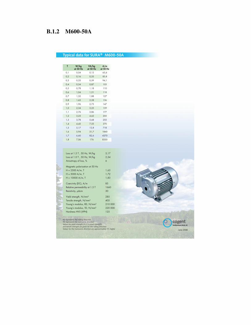
RD represents the rolling directionTD represents the transverse directionValues for yield strength (0.2 % proof strength)and tensile strength are given for the rolling directionValues for the transverse direction are approximately 5% higher June 2008
Typical data for SURA® M600-50A
B.1.2 M600-50A

RD represents the rolling directionTD represents the transverse directionValues for yield strength (0.2 % proof strength)and tensile strength are given for the rolling directionValues for the transverse direction are approximately 5% higher June 2008
Typical data for SURA® M800-50A
B.1.3 M800-50A

B.2. Magnets
B.2 Magnets
In this section, all the data-sheets for the magnets are presented. The ferrite data-sheet isretrieved via contact with the supplier [37]. The NdFeB data-sheet is retrieved from [38].
81
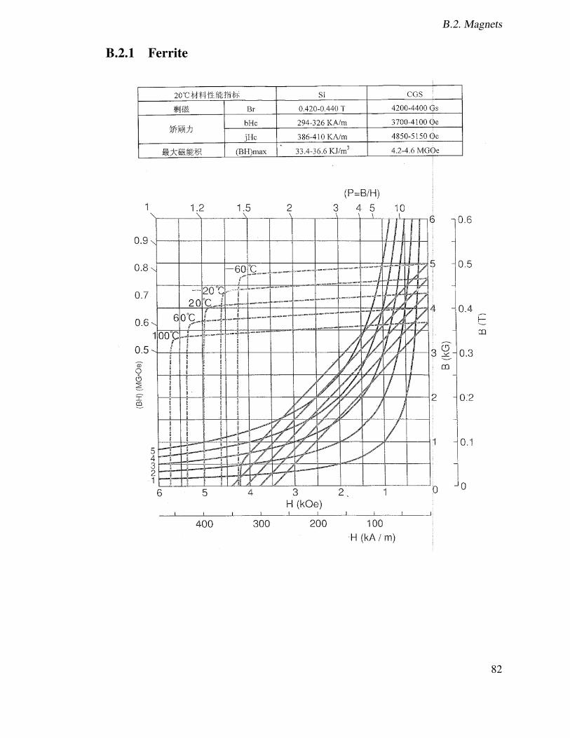
B.2. Magnets
B.2.1 Ferrite
82

Sintered Neodymium-Iron-Boron Magnets
Characteristic Units C // C�A
Reversible Temperature Coefficients (1)
of Induction, α(Br) %/ºC
of Coercivity, α(Hcj) %/ºC
Characteristic Units min. nominal max. Coefficient of Thermal Expansion (2) ∆L/L per ºCx10-6 7.5 -0.1
Gauss 11,300 11,650 12,000 Thermal Conductivity W / (m • K)
mT 1130 1165 1200 Specific Heat (3) J / (kg • K)
Oersteds 10,300 10,900 11,500 Curie Temperature, Tc ºC
kA/m 820 867 915 psi
Oersteds 30,000 MPa
kA/m 2,388 Density g/cm3
MGOe 31 34 36 Hardness, Vickers Hv
kJ/m3 247 267 287 Electrical Resistivity, U P: • cm
Notes: (1) Coefficients measured between 20 and 200 ºC
(2) Between 20 and 200 ºC (3) Between 20 and 140 ºC
Notes The material data and demagnetization curves shown above represent typical properties that may vary due to product shape and size.Magnets can be supplied thermally stabilized or magnetically calibrated to customer specifications.Additional grades are available. Please contact the factory for information.
N33EH
41,300
-0.120
Oth
erPr
oper
ties
7.5
180
Ther
mal
Pro
pert
ies
285
460
310
7.6
HcB, Coercivity
Flexural Strength
These are also referred to as "Neo" or NdFeB magnets. They offer a combination of high magnetic output at moderate cost. Please contact Arnold for additional grade information and recommendations for protective coating. Assemblies using these magnets can also be provided.
BHmax, Maximum Energy Product620
-0.420
Mag
netic
Pro
pert
ies
HcJ, Intrinsic Coercivity
Br, Residual Induction
-40°C
20°C
60°C
80°C
100°C
120°C
150°C
180°C 200°C 220°C
0
1
2
3
4
5
6
7
8
9
10
11
12
13
14
15
024681012141618202224262830
Pola
rizat
ion,
J
F
lux
Den
sity
, B
Demagnetizing Field, H
Material: N33EH
0.1
0.3
0.5 10.75 21.5 3 5
0
0.2
0.4
0.6
0.8
1.0
1.2
kG Tesla
1.4
kOe
kA/m 1750 1275 160 01430 1115 955 795 640 475 3202070 1910 15902230
Pc = B H
1 kA/m = 12.566 Oe 1 kOe = 79.577 kA/m
Rev. 151021a
© Arnold Magnetic Technologies Corp.770 Linden Avenue, Rochester, NY 14625
Ph: (+1) 585-385-9010E-mail: [email protected]
www.arnoldmagnetics.com
B.2.2 NdFeB - N33EH

Appendix C
Results
C.1 Demagnetization
84
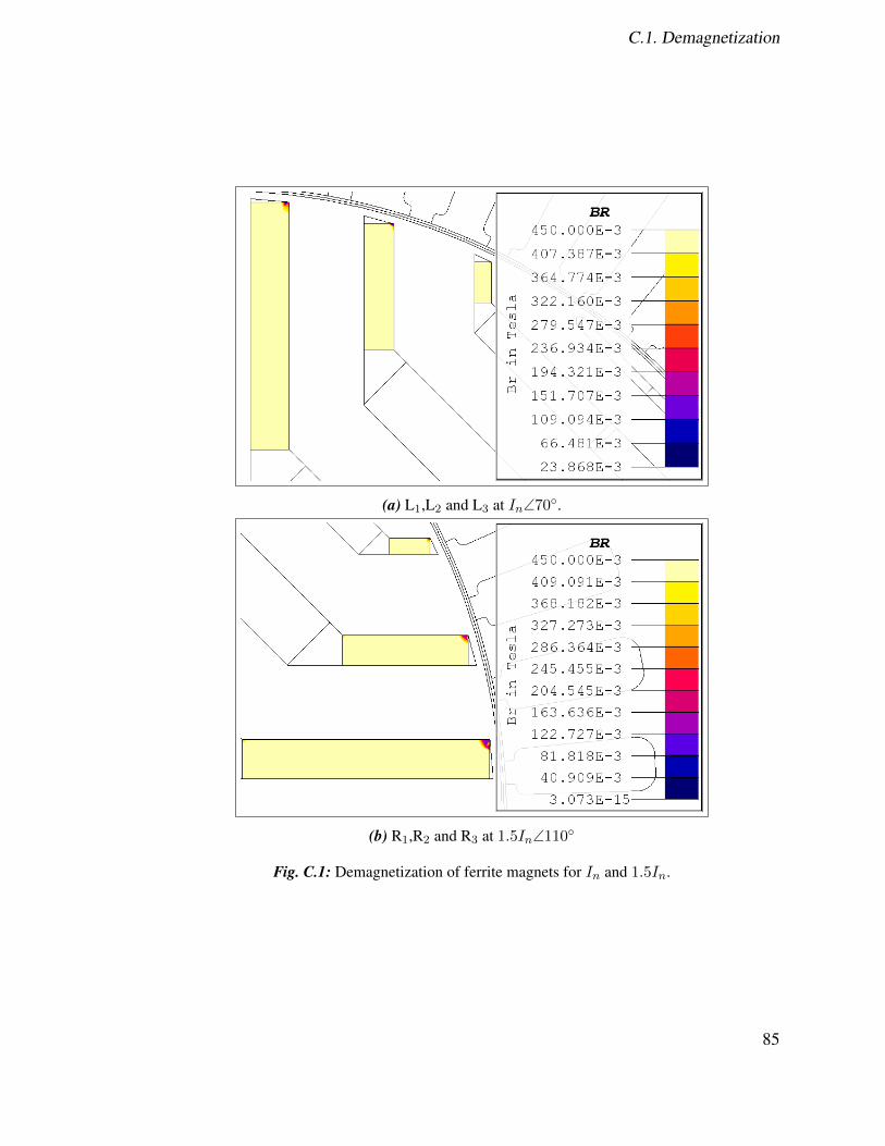
C.1. Demagnetization
(a) L1,L2 and L3 at In
\70�.
(b) R1,R2 and R3 at 1.5In
\110�
Fig. C.1: Demagnetization of ferrite magnets for In
and 1.5In
.
85
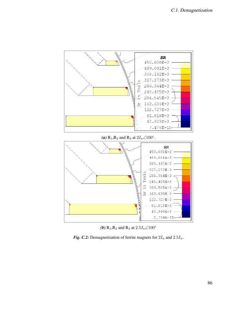
C.1. Demagnetization
(a) R1,R2 and R3 at 2In
\100�.
(b) R1,R2 and R3 at 2.5In
\100�
Fig. C.2: Demagnetization of ferrite magnets for 2In
and 2.5In
.
86

References
[1] R. Saidur, “A review on electrical motors energy use and energy savings,” Renewableand Sustainable Energy Reviews, vol. 14, no. 3, pp. 877 – 898, 2010. [Online].Available: http://www.sciencedirect.com/science/article/pii/S1364032109002494
[2] P. Waide and C. U. Brunner, “Energy-efficiency policy opportunities for electricmotor-driven systems,” may 2011. [Online]. Available: https://doi.org/10.1787/5kgg52gb9gjd-en
[3] Energimyndigheten, June 2015, [Accessed 2018-03-13]. [Online]. Avail-able: http://www.energimyndigheten.se/energieffektivisering/produkter-med-krav/produktgrupper/mapp-for-produkter/elmotorer/
[4] K. O. Armstrong, S. Das, and J. Cresko, “Wide bandgap semiconductoropportunities in power electronics,” in 2016 IEEE 4th Workshop on Wide BandgapPower Devices and Applications (WiPDA). IEEE, nov 2016. [Online]. Available:https://doi.org/10.1109/wipda.2016.7799949
[5] J.-R. Riba, C. Lopez-Torres, L. Romeral, and A. Garcia, “Rare-earth-freepropulsion motors for electric vehicles: A technology review,” Renewable andSustainable Energy Reviews, vol. 57, pp. 367–379, May 2016. [Online]. Available:https://doi.org/10.1016/j.rser.2015.12.121
[6] J. Rowlatt, “Rare earths: Neither rare, nor earths,” BBC News, Mar 2014, [Accessed2018-03-13]. [Online]. Available: http://www.bbc.com/news/magazine-26687605
[7] C. Bontron, “Rare-earth mining in china comes at a heavy cost for local villages,”The Guardian, Aug 2012, [Accessed 2018-03-13]. [Online]. Available: https://www.theguardian.com/environment/2012/aug/07/china-rare-earth-village-pollution
[8] A. T. de Almeida, F. J. T. E. Ferreira, and G. Baoming, “Beyond inductionmotors—technology trends to move up efficiency,” IEEE Transactions on IndustryApplications, vol. 50, no. 3, pp. 2103–2114, may 2014. [Online]. Available:https://doi.org/10.1109/tia.2013.2288425
87

References
[9] G. Pellegrino, T. M. Jahns, N. Bianchi, W. Soong, and F. Cupertino,The Rediscovery of Synchronous Reluctance and Ferrite Permanent MagnetMotors. Springer International Publishing, 2016. [Online]. Available: https://doi.org/10.1007/978-3-319-32202-5
[10] A. O. Dulanto”, “”design of a synchronous reluctance motor assisted with perma-nent magnets for pump applications”,” ”Master thesis”, ”KTH Royal Institute ofTechnology”, ”Stockholm”, ”2015”.
[11] R. Moghaddam, “Synchronous reluctance machine (synrm) in variable speed drives(vsd) applications,” Ph.D. dissertation, KTH Royal Institute of Technology, Stock-holm, 2011, doctoral thesis.
[12] N. Bianchi, E. Fornasiero, and W. Soong, “Optimal selection of PM fluxlinkage in a PM assisted synchronous reluctance machine,” in 2014 InternationalConference on Electrical Machines (ICEM). IEEE, sep 2014. [Online]. Available:https://doi.org/10.1109/icelmach.2014.6960356
[13] J. K. Kostko, “Polyphase reaction synchronous motors,” Journal of the AmericanInstitute of Electrical Engineers, vol. 42, no. 11, pp. 1162–1168, nov 1923.[Online]. Available: https://doi.org/10.1109/joaiee.1923.6591529
[14] T. Fukami, M. Momiyama, K. Shima, R. Hanaoka, and S. Takata, “Steady-stateanalysis of a dual-winding reluctance generator with a multiple-barrier rotor,”IEEE Transactions on Energy Conversion, vol. 23, no. 2, pp. 492–498, jun 2008.[Online]. Available: https://doi.org/10.1109/tec.2008.918656
[15] R. Rajabi Moghaddam, “Synchronous reluctance machine (synrm) design,” KTH,Skolan for elektro- och systemteknik (EES), Elektrisk energiomvandling, 2007.
[16] R. Moghaddam, F. Magnussen, C. Sadarangani, and H. Lendenmann, “New theoret-ical approach to the synchronous reluctance machine behavior and performance,” inElectrical Machines, 2008. ICEM 2008. 18th International Conference on. IEEE,September 2008, pp. 1–6.
[17] M. Kamper, “Effect of rotor dimensions and cross magnetisation on ld and lqinductances of reluctance synchronous machine with cageless flux barrier rotor,”IEE Proceedings - Electric Power Applications, vol. 141, no. 4, p. 213, 1994.[Online]. Available: https://doi.org/10.1049/ip-epa:19941261
[18] N. Bianchi, E. Fornasiero, and W. Soong, “Selection of pm flux linkage for max-imum low-speed torque rating in a pm-assisted synchronous reluctance machine,”IEEE Transactions on Industry Applications, vol. 51, no. 5, pp. 3600–3608, Sept2015.
88

References
[19] M. N. F. Ibrahim, “Design aspects of high performance synchronous reluctance ma-chines with and without permanent magnets,” Ph.D. dissertation, Ghent University,2017.
[20] T. Matsuo and T. Lipo, “Rotor design optimization of synchronous reluctancemachine,” IEEE Transactions on Energy Conversion, vol. 9, no. 2, pp. 359–365, jun1994. [Online]. Available: https://doi.org/10.1109/60.300136
[21] R.-R. Moghaddam and F. Gyllensten, “Novel high-performance SynRM designmethod: An easy approach for a complicated rotor topology,” IEEE Transactions onIndustrial Electronics, vol. 61, no. 9, pp. 5058–5065, sep 2014. [Online]. Available:https://doi.org/10.1109/tie.2013.2271601
[22] M. Palmieri, M. Perta, F. Cupertino, and G. Pellegrino, “Effect of thenumbers of slots and barriers on the optimal design of synchronous reluctancemachines,” in 2014 International Conference on Optimization of Electricaland Electronic Equipment (OPTIM). IEEE, may 2014. [Online]. Available:https://doi.org/10.1109/optim.2014.6850947
[23] A. Vagati, M. Pastorelli, G. Francheschini, and S. Petrache, “Design of low-torque-ripple synchronous reluctance motors,” IEEE Transactions on IndustryApplications, vol. 34, no. 4, pp. 758–765, 1998. [Online]. Available: https://doi.org/10.1109/28.703969
[24] M. Sanada, K. Hiramoto, S. Morimoto, and Y. Takeda, “Torque ripple improvementfor synchronous reluctance motor using an asymmetric flux barrier arrangement,”IEEE Transactions on Industry Applications, vol. 40, no. 4, pp. 1076–1082, jul2004. [Online]. Available: https://doi.org/10.1109/tia.2004.830745
[25] M. Xu, G. Liu, W. Zhao, and N. Aamir, “Minimization of torque ripplein ferrite-assisted synchronous reluctance motors by using asymmetric stator,”AIP Advances, vol. 8, no. 5, p. 056606, may 2018. [Online]. Available:https://doi.org/10.1063/1.5006114
[26] C. Babetto, G. Bacco, and N. Bianchi, “Analytical approach to determine the powerlimit of high-speed synchronous reluctance machines,” in 2017 IEEE InternationalElectric Machines and Drives Conference (IEMDC). IEEE, may 2017. [Online].Available: https://doi.org/10.1109/iemdc.2017.8002316
[27] A. Vagati, G. Franceschini, I. Marongiu, and G. Troglia, “Design criteria ofhigh performance synchronous reluctance motors,” in Conference Record of the1992 IEEE Industry Applications Society Annual Meeting. IEEE, 1992. [Online].Available: https://doi.org/10.1109/ias.1992.244463
89

References
[28] K. Khan, O. Wallmark, and M. Leksell, “Design aspects on magnet placementin permanent-magnet assisted synchronous reluctance machines,” in 5th IETInternational Conference on Power Electronics, Machines and Drives (PEMD2010). Institution of Engineering and Technology, 2010. [Online]. Available:https://doi.org/10.1049/cp.2010.0203
[29] K. S. Khan, “Design of a permanent-magnet assisted synchronous reluctance ma-chine for a plug-in hybrid electric vehicle,” KTH, Skolan for elektro- och sys-temteknik (EES), Elektrisk energiomvandling, Stockholm, 2011.
[30] O. Wallmark, AC Machine Analysis. KTH Royal Institute of Technology, Depart-ment of Electric Power and Energy Systems, 2017.
[31] S. Sjokvist, “Demagnetization studies on permanent magnets: Comparing fem sim-ulations with experiments,” Uppsala universitet, Teknisk-naturvetenskapliga veten-skapsomradet, Tekniska sektionen, Institutionen for teknikvetenskaper, Elektricitet-slara, Uppsala, 2014.
[32] D. K. Cheng, Field and Wave Electromagnetics (Addison-Wesley series in electricalengineering). Addison-Wesley Educational Publishers Inc, 1983.
[33] P. Zhou, D. Lin, Y. Xiao, N. Lambert, and M. A. Rahman, “Temperature-dependentdemagnetization model of permanent magnets for finite element analysis,” IEEETransactions on Magnetics, vol. 48, no. 2, pp. 1031–1034, feb 2012. [Online].Available: https://doi.org/10.1109/tmag.2011.2172395
[34] A. Krings and J. Soulard, “Overview and comparison of iron loss models for electri-cal machines,” Journal of Electrical Engineering, vol. 10, no. 3, pp. 162–169, 2010.
[35] T. Chevalier, A. Kedous-Lebouc, B. Cornut, and C. Cester, “A new dynamichysteresis model for electrical steel sheet,” Physica B: Condensed Matter, vol.275, no. 1-3, pp. 197–201, jan 2000. [Online]. Available: https://doi.org/10.1016/s0921-4526(99)00768-1
[36] “Download catalogues, datasheets and iso certificates,” Accessed 2018-06-19.[Online]. Available: https://cogent-power.com/downloads
[37] “NORDMAG.” [Online]. Available: http://www.nordmag.fi/#contact
[38] “Neodymium magnets (NdFeB),” Accessed 2018-06-19. [Online]. Available:http://www.arnoldmagnetics.com/products/neodymium-iron-boron-magnets/
90