design and modelling of a large-scale pv plant · design and modelling of a large-scale pv plant 1...
TRANSCRIPT

Master Thesis
Master’s degree in Energy Engineering
Design and Modelling of a Large-Scale PV Plant
REPORT
Author: Roca Rubí, Álvaro
Director: Gomis Bellmunt, Oriol
Date: June 2018
Escola Tècnica Superior
d’Enginyeria Industrial de Barcelona
Design and modelling of a large-scale PV plant 1
ABSTRACT
The current project is focused on the design a large-scale PV solar power plant, specifically a 50 MW
PV plant. To make the design it is carried out a methodology for the calculation of the different
parameters required for the realization of a project of this nature. Subsequently, the different parameters
obtained are compared with parameters obtained in literature and with the parameters obtained by means
of specialized PV software (PVsyst and SAM).
Before implementing the design calculation methodology, the main components in a large-scale PV
plant are described: PV modules, mounting structures, solar inverters, transformers, switchgears and DC
and AC cables. Furthermore, the following aspects are analysed in the current project: legislative and
administrative procedures, renewable energy support schemes and environmental aspects associated
with large-scale PV plants.
The calculations regarding the PV plant design are made for a specific location previously selected. The
site selected for the installation is in the location of l’Albagés (Lledia) which meets all the requirements
for the installation of a PV plant.
The results obtained for four different PV plant scenarios are compared between them in order to obtain
the best possible configuration, the different scenarios combine two different modules and two different
solar inverters. The calculation methodology is divided in: design calculations, energy calculations,
economic calculations and evaluation parameters calculation. The design parameters calculated are the
number of PV modules in the system, the number of PV modules in series and parallel and the total
installed capacity. The main purpose of the energy calculations is to obtain the Annual Energy
Production (AEP) of the system. The cost associated to the PV project and the Levelized Cost of Energy
(LCOE) are obtained by means of the economic calculations. Finally, evaluation parameters such as
Performance Ratio (PR) or Capacity Factor (CF) are calculated.
The four different scenarios are modelled by means of PVsyst and SAM and the results obtained are
compared with the results obtained in the calculations. The conclusion obtained is that the results
obtained with PV software are in accordance with the results obtained by means of the calculation
methodology implemented. The scenario analysed with the best results is the scenario which uses CdTe
thin-film module technology and the inverters with the highest nominal power. The main results
obtained for this scenario are: 484,960 PV modules and 14 inverters; Installed capacity of 53.35 MWp;
AEP of 83,001 MWh/year with an LCOE of 3.1154 c€/kWh; and evaluation parameters are 79,73% of
PR and 17.76% of CF.


Design and modelling of a large-scale PV plant 3
Contents
1. INTRODUCTION ........................................................................................................................... 5
1.1. GOALS AND PROJECT SCOPE ............................................................................................ 5
2. PV LARGE-SCALE COMPONENTS ........................................................................................... 6
2.1. SOLAR PV MODULES ........................................................................................................... 6
2.1.1. Silicon Crystalline Structure ........................................................................................... 7
2.1.2. Thin Film Technology ..................................................................................................... 8
2.2. MOUNTING STRUCTURES ................................................................................................. 10
2.3. SOLAR INVERTERS ............................................................................................................. 12
2.4. TRANSFORMERS ................................................................................................................. 14
2.5. SWITCHGEAR ...................................................................................................................... 16
2.6. DC AND AC CABLES ........................................................................................................... 16
3. LEGISLATIVE AND ADMINISTRTIVE PROCDEDURES ..................................................... 18
4. RENEWABLE ENERGY SUPPORT SCHEMES ....................................................................... 21
4.1. SUPPORT SCHEMES IN SPAIN .......................................................................................... 22
5. ENVIRONMETAL IMPACTS ASSOCIATED WITH LARGE-SCALE PV PLANTS ............. 24
6. LARGE-SCALE PV PLANT DESIGN ........................................................................................ 25
6.1. SITE IDENTIFICATION ....................................................................................................... 25
6.2. METHODOLOGY OF CALCULATION ............................................................................... 33
6.2.1. Design and Energy Calculations ................................................................................... 33
6.2.2. Economic Calculations ................................................................................................. 43
6.2.3. Evaluation Parameters Calculation .............................................................................. 45
6.3. RESULTS OBTAINED .......................................................................................................... 47
6.3.1. Economic Results .......................................................................................................... 55
6.3.2. Other Results ................................................................................................................. 59
7. RESULTS COMPARISON USING PV MODELLING SOFTWARE ........................................ 61
7.1. PVsyst MODELLING ............................................................................................................ 61
7.1.1. Pre-Design Phase .......................................................................................................... 61
7.1.2. Design Phase ................................................................................................................. 63
7.1.3. Results Obtained with PVsyst ........................................................................................ 65
7.2. SAM MODELLING ............................................................................................................... 78
7.2.1. Results Obtained with SAM ........................................................................................... 80
8. CONCLUSIONS ........................................................................................................................... 84
8.1. Future Work .......................................................................................................................... 86
References ............................................................................................................................................. 88
ANNEX A ............................................................................................................................................. 92
A. PV PLANT DESIGN METHODOLOGY. MATLAB CODE...................................................... 92

A. 1. DESIGN AND ENERGY CALCULATIONS .......................................................................... 92
A. 2. ECONOMIC CALCULATIONS ............................................................................................ 94
A. 3. EVALUATION PARAMETERS CALCULATIONS ................................................................ 95
Design and modelling of a large-scale PV plant 5
1. INTRODUCTION
During 2015, in Paris was held the United Nations Climate Change Conference, also known as COP21.
In that conference the so-called Paris Agreement was reached and signed by most of the major CO2
emitting countries. The aim of the Paris Agreement is the reduction of greenhouse gases emissions by
setting a limit of global warming below 2ºC compared to pre-industrial levels. To comply with the
agreements reached in Paris, the countries involved have to consider the decarbonisation of their energy
supply since 65% of the global CO2 emissions come from burning fossil fuels and 81% of the total
primary energy supply is based on fossil fuels [1]. One of the ways to decarbonize the energy supply of
a country, and probably the only way completely effective, is to make a change towards an energy
system with a higher penetration of renewable energy. Photovoltaic solar power plants are nowadays
the technology most extended regarding renewable energy generation and since 2016 PV solar energy
is the technology with higher growth [2]. The main factor driving the rapid growth of the PV solar
capacity is mainly economic, PV solar power plants have reduced their associated cost by 70% [2]. The
total cost reduction in PV solar power plants is caused by cost reduction due to technological
improvements, economies of scale in manufacturing and innovations in financing [3]. Furthermore, the
growing of PV capacity due to cost reduction is not expected to stop in the next years, but it is excepted
to increase the growth of PV in the future. In 2014, according to IFC [3] total PV installed capacity
worldwide was 137 GW with annual additions of approximately 40 GW. Traditionally, the area with
practically the totality of the total share of installed PV capacity was Europe, but since 2013 the installed
PV capacity in other areas, especially in Asia-Pacific, has grown very rapidly. In 2016 Asia-Pacific
became the zone with the highest share of installed PV capacity surpassing Europe. In this context
regarding the energy situation in the world and the role of the PV solar power plants is found the project
carried out.
1.1. GOALS AND PROJECT SCOPE
The main objective of the project is the design and modelling of a 50 MW PV solar power plant by
implementing a calculation methodology. By means of the calculation methodology the following
parameters of the PV plant are pursued to obtain through the course of the project: configuration of the
PV plant (number of PV modules, number of inverters and how they are connected between them);
energy produced by the PV plant; and performance parameters of the plant which can be used to compare
the results obtained. Purely electric aspects are not assessed in detail in this project. Another important
goal of this project is to make the design of the PV plant economically viable, thus an economic analysis
of the PV plant is included in the project, without going into detail in financing models. The last
objective of the project is to validate the results obtained by means of specialized software.

2. PV LARGE-SCALE COMPONENTS
In this chapter of the project a description of the main components forming a large-scale PV solar power
plant is done. The elements described below are going to be considered during the calculations used for
the system design. The components described are: PV modules, inverters, transformers, switchgears and
AC and DC cables.
2.1. SOLAR PV MODULES
PV modules convert the solar radiation directly into electric energy by means of the photovoltaic effect,
doing this process in a silent and clean manner. There are many different PV modules technologies and
nowadays research institutions are making efforts to discover new materials and designs with which the
performance of the solar cells can be improved. There are different types of solar cells and their
classification can be seen in Figure 2.1. In this project, the two major families of solar cells dominating
the market are going to be explained in more detail in this section: silicon crystalline structure and thin-
film technology.
Figure 2.1. Solar PV technologies classification.
In Figure 2.2 the production share of silicon crystalline structure (multicrystalline-Si and
monocrystalline-Si) and thin-film technology can be seen. In the early years of photovoltaics, mono-Si
practically monopolized the production, and as the years went the production of multi-Si has become
more important. The production of thin-film technology remains more or less constant over the years.

Design and modelling of a large-scale PV plant 7
Figure 2.2. Production share of different technologies over the years. Source: Statista [4]
2.1.1. Silicon Crystalline Structure
The first generation of PV modules exiting were silicon crystalline structure modules, despite silicon
crystalline technology was the first PV module technology developed, it is not nowadays obsolete and
some improvements have been made in recent years regarding this technology, in fact it is still the most
used PV module technology [5].
Usually the installation of PV modules requires a larger investment cost than the cost associated with
operation and maintenance. Although some governments give very attractive incentives for the
installation of PV systems, normally the payback time of these projects is long. Because of that it is
crucial to decrease the cost of production by increasing the efficiency of the modules.
In the family of silicon crystalline structure can be found monocrystalline photovoltaic cells, poly-
crystalline photovoltaic cells and back-contact photovoltaic cells.
Monocrystalline photovoltaic cell
This technology was in the early years of photovoltaics the module technology most commonly used,
both in utility-scale scale and stand-alone applications. But, as years went mono-Si modules have been
losing market share.
The manufacturing process of mono-Si modules is called Czochralski process which is a method of
crystal growth used to obtain single crystals. The processes consist on melting a high-purity,
semiconductor-grade silicon. Boron or phosphorous can be added as dopant impurity atoms, thus
changing the silicon into p-type or n-type, with different electronic properties. By controlling the
temperature gradient and the mechanical strengths of the process it is possible to extract a large single
crystal from the melt [6].

According to Green et al. [7] the maximum efficiency achieved under STC for monocrystalline solar
cell is 26.7%. Despite of the maximum efficiency record achieved, the module efficiencies normally
tends to be lower than cell efficiency due to internal electrical losses. Anyway, the record of efficiency
registered by NREL for a PV module is 20.4 % for a SunPower PV module [5].
Multicrystalline photovoltaic cell
Multicrystalline solar cells or also called poly-crystalline (or poly-Si) solar cells are the result of trying
to reduce the costs of production of mono-Si cells by means of new crystallization techniques. This
manufacturing technique consists on producing multicrystalline silicon by melting silicon and
solidifying it to orient crystals in a fixed direction, the ingot of multicrystalline silicon produced is sliced
into blocks and then into a thin wafer [8]. Multicrystalline cells can be easily recognizable because of
the aspect of metal flake effect caused by the multiple small silicon crystals that forming it.
The efficiency of this type of solar cells is significantly lower than monocrystalline solar cells, the
efficiency record achieved by a multicrystalline according to Green et al. [7] under STC condition is
21.9%. But, once again when looking at commercial available technology the efficiency is lower
compared to laboratory test, the efficiency for multicrystalline modules available in the market is in the
range from 14% to 19% [9]. Despite of the lower efficiency of this technology, the main advantage of
multi-crystalline solar cells respect other solar cell technologies is the reduction of cost achieved by
simplifying the manufacturing process.
Back-contact solar cell
Also called rear-contact solar cells have increased the efficiency respect other technologies achieved
through a better cell design rather than material improvements [5]. This can be achieved by moving all
or part of the front contact grids to the rear of the device [10]. The main advantage of this silicon modules
is that shading losses are zero and the contact resistance is low [11]. There are four different back-
contact cells technologies: metallization wrap through, emitter wrap through, interdigitated back-contact
and advanced back-junction solar cells. All these different technologies of back-contact solar cells are
already being used for different industrial processes.
2.1.2. Thin Film Technology
Related to the effort to make PV technology less costly, and hence to make more economically viable
projects, appears a new technology called thin-film solar cells [5]. Wolf and Lofersky discovered that
by decreasing the cell thickness, open circuit voltage increases due to reduced saturation current and
decreasing the geometry factor [12]. Thin-film technology consist on thin layers of a semiconductor
material applied to a solid backing material [9]. Using this technology, the amount of required material

Design and modelling of a large-scale PV plant 9
is reduced without compromising the lifespan of the photovoltaic cell or being hazardous for the
environment. Additionally, the cost of production is also reduced due to the photovoltaic materials used
are cheaper than those used for crystalline structures [5]. The market share of thin-films is 15-20%, and
the market growth in the recent years of this technology have been enormous [5].
The main advantage of thin-film technology is the reduced thickness of the layers, few microns
compared with the thickness of crystalline modules (several hundreds of microns) [5]. Furthermore, the
very low thickness of the layers provides flexible properties. On the other hand, the fact that thin-film
technology involves less photovoltaic material per cell has repercussions on lowering the capacity. But,
the capability of this technology to deposit many different materials and alloys leads to improvements
in efficiency. Degradation of this technology is also an important aspect to consider, the majority of
thin-film cells need an extra barrier to protect them from heat or moist which can accelerate their process
of degradation [5].
Amorphous silicon cell
Also called silicon thin-film solar cell is one of the first thin-film technologies developed and also the
most commonly used [5] [9]. The main difference between amorphous silicon and crystalline silicon
structure is the fact that in this technology the atoms of silicon are distributed randomly and not forming
a crystalline matrix. An important disadvantage of this type of photovoltaic cells is the fact that their
efficiency is lower than monocrystalline and multicrystalline solar cells, the maximum efficiency
achieved in laboratory test is around 10.2% [7]. But, the efficiency for commercially available cells is
in the range from 5% to 7% [9]. Despite of the lower efficiency compared with other technologies,
amorphous silicon cells are also an attractive alternative because they are less costly due to their specific
manufacturing process. Silicon is an abundant non-toxic material which requires low process
temperature, enabling module production on flexible and low-cost substrates [13].
In order to upgrade the efficiency of this type of solar cells, there are many variations of thin-film silicon
solar cells, the most popular variations are: amorphous silicon carbide (a-SiC), amorphous silicon
germanium (a-SiGe), microcrystalline silicon (µc-Si), amorphous silicon-nitride (a-SiN) and
hydrogenated amorphous silicon (a-Si:H) [9].
Tandem solar cell
Tandem solar cells were designed in order to increase the efficiency of a-Si solar cells in a cost-effective
manner. This technology consists on depositing two or more PV junctions on top of the other where the
layer of a-Si is located at the top [5]. This configuration of the solar cell provides an improved range of
efficiency 8-9% [5].
Cadmium telluride cell
Cadmium telluride (CdTe) cells are one of the most promising PV materials, since this material has the
ideal band gap (1.5 eV) with a high direct absorption coefficient, thanks to these two parameters with a
few of micrometres of this material is enough to absorb around 90% of the incident photons [13].
The efficiency achieved in laboratory of cadmium telluride cells is up to 21% [7] and the maximum
efficiency achieved for commercially available modules is 9% [5]. This technology is more appropriate
for large scale applications because it is easier to accumulate than other thin-film technologies.
The main drawback of this technology is the fact that cadmium is a toxic material, and some measures
have to be adopted in order to not to harm the environment [13]. Another important point is the scarcity
of telluride which can have repercussion on the future price of these cells [5].
Copper indium diselenide cell
Copper indium diselenide (CuInSe2) and copper indium selenide (CIS) cells are a photovoltaic
technology which uses semiconductor elements which are beneficial due to their high optical absorption
coefficients and good electrical characteristics [5]. By means of adding gallium (CIGS) the band gap of
the photovoltaic device is increased, this type of technology is known as multi-layered thin-film
composites [5].
The maximum efficiency achieved for a CIGS thin-film is 19.2% [7] and the efficiency for commercially
available modules is 13% [5]. As happened with telluride in CdTe cells, scarcity is also an issue with
indium which in addition is a very common material in electronic applications. Because of this fact,
recycling is going to be a crucial aspect for the future growth of these technologies.
2.2. MOUNTING STRUCTURES
Mounting structures are used to fix the PV modules to the ground and they determine the tilt angle and
the orientation of the modules. A classification of the mounting structures can be done depending on
their assembly to the ground [14]:
- Pole mounts. Mounting structures are directly installed into the ground or embedded in concrete.
- Foundation mounts. Structures are fixed into the ground by means of concrete slabs or poured
footings.
- Ballasted footing mounts. Mounting structures do not penetrate into the ground and are fixed to
it by means of the weight of concrete or steel bases.

Design and modelling of a large-scale PV plant 11
The selection criteria of the mounting structures involve many factors such as: cost of manufacturing,
cost of installation and difficulty of installation, lifespan of the structures, resistance to corrosion or
protection against adverse climatic conditions.
Besides, mounting structures are the responsible to endow to the PV modules the required tilt angle and
orientation. Regarding this aspect there are two main categories of mounting structures: fixed structures
and tracking axis systems. Fixed structures are not capable to modify neither the orientation nor the tilt
angle. This option is the less costly system, but the energy production will be not optimum. Tracking
axis systems can be divided in 1-axis tracking systems and 2-axis tracking systems, the difference
between both systems is the number of degrees of freedom (see Figure 2.3). Again, there is a
compromise between the cost of the system and the energy production of the PV plant, 2-axis tracking
system is better than 1-axis tracking systems in terms of energy capture, but it is more expensive to
manufacture, to install and also the maintenance is more complex.
Figure 2.3. Left 1-axis tracking system. Right 2-axis tracking system. Source: [15]
Another aspect to treat when looking at the mounting structures are the shading losses. Tracking systems
usually generate more shading losses than fixed systems due to the movement of the PV panels, note
that for higher tilt angle of the modules, inter-row spacing has to be higher or the shading losses will be
larger. The space required for a typical fixed system is in the range of 1.6 to 2.4 ha per MW, while the
space occupation for a typical 1-axis tracking system can be in the range of 1.8 to 3 ha per MW [16].
Because of that reason the sizing of the system and the inter-row spacing of the PV modules should be
studied in detail in order to not have unacceptable shading losses. For a good plant design, the
comparison between a PV plant using tracking system and without tracking system can be seen in Figure
2.4.

Figure 2.4. Comparison between output power obtained without tracking system (blue) and with tracking system (yellow).
Source: [3]
Tracking systems integrated in the mounting structures can be controlled by sensors or by control
algorithms which allows to control the system automatically. There is also one specific type of 1-axis
tracking system where the change of the tilt angle is done manually and with the change of season
(seasonal tilt angle). By changing tilt angle once in winter and once in summer it is achieved an
improvement over fixed system regarding the energy capture.
Sensor based control systems use sensors to determine the relative position between the sun and the PV
modules. Once the system detects the tilt angle (or orientation) of the PV module is not the optimum the
modules are tilted to achieve the optimum angle by means of actuators or motors [16]. Different
technologies are used in these systems including light dependant resistors, photo transistors, mini solar
cells or complementary metal-oxide-semiconductors (CMOS) [16].
Algorithm based control system uses GPS to determine the position and altitude of the sun. This
technology helps to develop predictions models of sun’s position which allows to the tracking system
to rotate the PV modules in a continuous and smooth manner [16]. One of the advantages of this tracking
system respect to sensor-based control system is that algorithm-based control system cannot be disturbed
by clouds or other perturbations [16].
2.3. SOLAR INVERTERS
Since PV modules generates power at DC current, at some point this generated electricity is needed to
be converted into AC current to accomplish with grid requirements. Distribution inside the PV plant can
be done in DC current, and also the power delivered to the grid can also be in DC, but nowadays, AC
technology seems to be the most realistic and affordable technology to operate. To invert the polarity of
the source to AC and to synchronize the power generated with the grid an inverter is required. The
Design and modelling of a large-scale PV plant 13
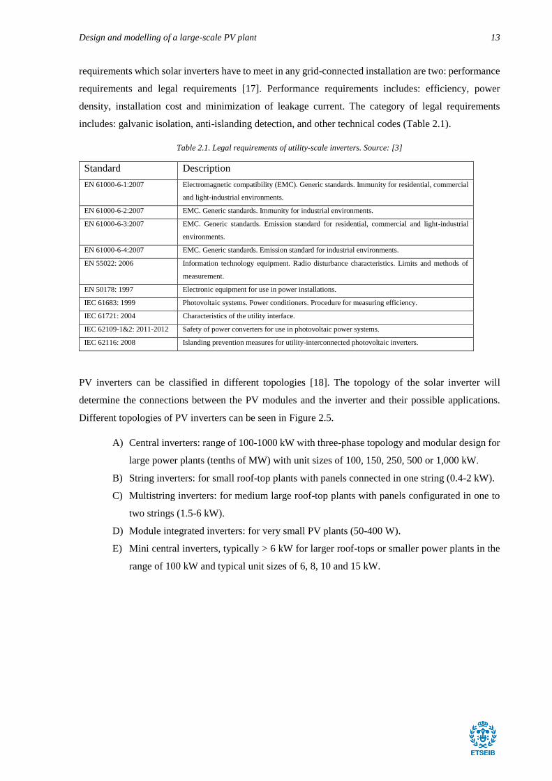
requirements which solar inverters have to meet in any grid-connected installation are two: performance
requirements and legal requirements [17]. Performance requirements includes: efficiency, power
density, installation cost and minimization of leakage current. The category of legal requirements
includes: galvanic isolation, anti-islanding detection, and other technical codes (Table 2.1).
Table 2.1. Legal requirements of utility-scale inverters. Source: [3]
Standard Description
EN 61000-6-1:2007 Electromagnetic compatibility (EMC). Generic standards. Immunity for residential, commercial
and light-industrial environments.
EN 61000-6-2:2007 EMC. Generic standards. Immunity for industrial environments.
EN 61000-6-3:2007 EMC. Generic standards. Emission standard for residential, commercial and light-industrial
environments.
EN 61000-6-4:2007 EMC. Generic standards. Emission standard for industrial environments.
EN 55022: 2006 Information technology equipment. Radio disturbance characteristics. Limits and methods of
measurement.
EN 50178: 1997 Electronic equipment for use in power installations.
IEC 61683: 1999 Photovoltaic systems. Power conditioners. Procedure for measuring efficiency.
IEC 61721: 2004 Characteristics of the utility interface.
IEC 62109-1&2: 2011-2012 Safety of power converters for use in photovoltaic power systems.
IEC 62116: 2008 Islanding prevention measures for utility-interconnected photovoltaic inverters.
PV inverters can be classified in different topologies [18]. The topology of the solar inverter will
determine the connections between the PV modules and the inverter and their possible applications.
Different topologies of PV inverters can be seen in Figure 2.5.
A) Central inverters: range of 100-1000 kW with three-phase topology and modular design for
large power plants (tenths of MW) with unit sizes of 100, 150, 250, 500 or 1,000 kW.
B) String inverters: for small roof-top plants with panels connected in one string (0.4-2 kW).
C) Multistring inverters: for medium large roof-top plants with panels configurated in one to
two strings (1.5-6 kW).
D) Module integrated inverters: for very small PV plants (50-400 W).
E) Mini central inverters, typically > 6 kW for larger roof-tops or smaller power plants in the
range of 100 kW and typical unit sizes of 6, 8, 10 and 15 kW.

Figure 2.5. PV inverter topologies: (a) Central inverter, (b) String inverter, (c) Multistring inverter and (d) Module
integrated inverter. Source: [19]
Because of the purpose of this project is the design and modelling of a large-scale PV solar power plant,
in this section the attention will be focused on central inverters. The most used central inverters
configuration is two-level voltage source inverter (2L-VSI) which is composed of three half-bridge
phase legs connected to a single dc-link [17]. Another configuration, but in this case less mature
technology are three-phase 3L-NPC and three phase 3L-T converters [17]. The main advantages of
central inverters are the reliability and robustness compared with other inverter’s topologies, but the
main drawbacks of this technology are the increased mismatch losses and the absence of MPPT for each
string of the array connected [3].
Normally, the inverters installed in large-scale PV solar power plants are containerised type. This type
of commercially available inverters also contains the transformer and the switchgear in the same
structure. With this solution, inverter, transformer and switchgear can be manufactured offside the PV
plant reducing the cost of installation [3]. The most common inverter’s manufacturers for utility-scale
applications are SMA, ABB and Kaco.
2.4. TRANSFORMERS
A transformer is an electric device which transfer electric power applied in a primary winding to a
secondary winding by electromagnetic induction. The transfer of power is done at the same frequency,
but with different voltage and current. The ratio between the number of turns in the primary winding
and the turns in the secondary winding determine if it is a step-up voltage transformer or step-down.
Figure 2.6 shows the main components of a transformer and its electrical scheme. Transformers are used
in PV solar power plants to step-up the voltage of the power produced in the modules and by means of

Design and modelling of a large-scale PV plant 15
increasing the voltage the losses of distribution are decreased. There can be two types of transformers
inside a PV plant [3]: distribution transformers and grid transformers. Distribution transformers are used
to step-up the voltage for the plant collection system. Grid transformers increase the voltage to meet the
grid requirements.
The most commonly used distribution transformers in PV power plants are pad-mounted type, in this
type of transformers the AC circuits associated are normally installed underground [20]. The maximum
voltage ratings for pad-mounted transformers are 35-36 kV. If the interconnection to the grid is above
35 kV a grid transformer is required. The power ratings for grid transformers are in the range from 2,500
kVA to 100 MVA [20]. Another benefit of the utilization of transformers in PV applications is the
galvanic isolation of the system provided by the air gap between the transformer windings [20].
Figure 2.6. Transformer scheme. Source: [20]
Selection criteria for transformers include technical and economic factors [3]: efficiency, guarantee,
vector group, system voltage, power rating, site conditions, sound power, voltage control capability and
duty cycle among other factors. Furthermore, the selected transformer for any utility-scale PV project
should be accredited by ISO 9001 [3].
The main difference between the transformers used for residential applications and utility-scale
applications is the admissible voltage level. For residential applications the interconnection between the
transformer and the grid is done at 249 Vac single-phase, for utility-scale applications the
interconnection is done at voltages in the range of 12-115 kV three-phase [20]. Because of this enormous
difference of voltage between applications, the price and volume of transformers in utility applications
is not comparable with other applications, even it is usual for transformers in utility applications to be
custom made due to variety of different requirements.
2.5. SWITCHGEAR
The switchgear is the set of switches, fuses or circuit breakers used to control, protect and isolate the
electrical equipment included in the system. The type of switchgear selected will depend on the
interconnection voltage level. Typical switchgear for applications up to 33 kV is an internal metal-clad,
cubicle type with gas/air insulated busbars and vacuum of SF6 breakers [3]. Switchgears installed in a
PV power plant should meet the following requirements [3]: accomplish IEC standards and national
electrical codes; show the on and off position clearly; option to be secured by locks in off/earth positions;
be rated for operational and short-circuit currents; rated for the correct operational voltage; and be
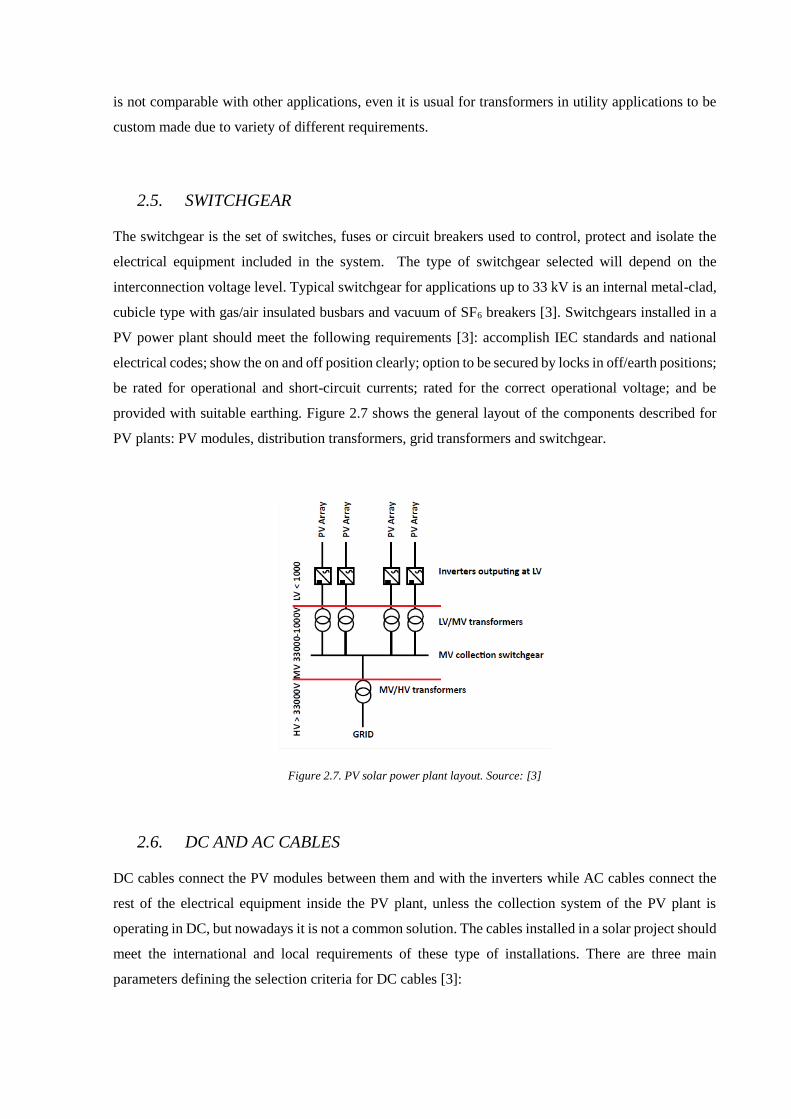
provided with suitable earthing. Figure 2.7 shows the general layout of the components described for
PV plants: PV modules, distribution transformers, grid transformers and switchgear.
Figure 2.7. PV solar power plant layout. Source: [3]
2.6. DC AND AC CABLES
DC cables connect the PV modules between them and with the inverters while AC cables connect the
rest of the electrical equipment inside the PV plant, unless the collection system of the PV plant is
operating in DC, but nowadays it is not a common solution. The cables installed in a solar project should
meet the international and local requirements of these type of installations. There are three main
parameters defining the selection criteria for DC cables [3]:
Design and modelling of a large-scale PV plant 17
- Cable voltage rating. The cable selected must withstand the voltage of the PV modules
connected. For this calculation open circuit voltage of the PV modules is used.
- Current carrying capacity of the cable. The cable must be sized in order to withstand the current
for the worst case possible.
- Minimization of voltage drop. Reduce the energy losses is a key aspect which can determine
the viability of a PV plant project, therefore it is important to reduce the voltage drop in the
cables. An acceptable voltage drop value would be 3%, but 1% or less of cable losses can be
achieved.
The cables installed in a specific PV solar plant should be adequately protected for the site conditions
(sun, moist, heat…). Some of the properties of commercial cables complying with standards are [21]:
ozone resistant, weather and UV resistant, halogen-free, resistant to acid and bases, flame-resistant,
abrasion resistant, resistant to short-circuits up to 200ºC, 25 years lifespan and hydrolysis and ammoniac
resistant.

3. LEGISLATIVE AND ADMINISTRTIVE PROCDEDURES
To perform any PV project, and specially a large-scale PV project, some legislative and administrative
procedures must be considered and accomplished. In Spain, photovoltaic installations must meet
legislations in different levels: European, national, local, Red Eléctrica Española regulation, and the
specific regulation of the distribution companies.
The administrative and legislative steps which should be followed during the design, installation and
operation of PV project located in Spain are described below in order of realization [22]:
1. Land obtention: A contractual agreement is needed between the owner of the land and the
project developer, unless the owner of the land is the same as the PV project developer. The
normal procedure in those cases is to rent the land for the time which the PV plant is estimated
to operate (usually 25 years of operation).
2. Bank guarantee: According to Royal Decree 1578/2008 the obtention of the bank guarantee or
the deposit of the required amount is mandatory and it has to be done in the Caja General de
Depósitos (CGD).
3. Access point and point of connection. The point of the electrical grid where the energy produced
is going to be injected. The point of connection belonging to the closest distribution company
has to accomplish technical and economical requirements.
4. Special Regime condition: According Royal Decree 661/2007 the condition of Special Regime
for any energy producer must be granted by the competent authority. Request of Special Regime
has to include financial and technical reports as well as the authorization of the site selected for
the installation. The denomination of Special Regime installations will be discussed in further
sections of the project (see section 4.1. SUPPORT SCHEMES IN SPAIN).
5. Environmental information request: Evaluation of the possible environmental burdens of the
location selected. Often, the selected land has to be reclassified by the corresponding city
council.
6. Project report realization: the realization of a project report for large-scale installations is
mandatory at this point of the project.
7. List of possible affected: The installation of a PV plant can represent a big impact on the zone
where it is going to be installed. Before tanking final decisions, it is recommended to consider
all the possible affected and apply the corresponding measures.
8. Administrative authorization and project approval. Administrative authorization is mandatory
for photovoltaic installation bigger than 100 kW. To obtain the authorization the project report
and all the previous authorizations and approvals have to be delivered.
9. Environmental, urban and cultural licenses: Depending on the autonomous community where
the PV project is going to be installed it is required to obtain: The Community Interest

Design and modelling of a large-scale PV plant 19
Declaration, Environmental Impact Assessment or the execution of a study of landscaping
integration.
10. IAE (Impuesto sobre Actividades Económicas) registration: According to Ministerial Order
EHA/1274/2007 any legal person which is going to start the activity of energy production has
to register on census of businessmen, professionals and withholding agents. The tariffs are
stipulated in Royal Decree 1175/1990.
11. Urban classification: By means of urban classification, a land conceived for other activity can
be used for a PV plant project. The competent authority of the autonomous community is the
responsible to grant the permissions regarding urban classification.
12. Construction permit: this permission authorizes the PV project and it has to be granted by city
council.
13. Activity license: This license is required and it has to be granted by the city council. The project
report of the PV installation has to be delivered in order to obtain this license.
14. Application for inclusion in special regime. Before starting the construction of the PV plant, the
project developer or the investor has to submit the request of Special Regime to Territorial
Service of Energy.
15. Contract with distribution company. The distribution company which the PV plant is going to
be connected has the legal obligation to collaborate with: admit the energy injection into the
grid through an accessible connection point, and technical verification of the energy supply and
meter mechanisms.
16. Inscription on the register of pre-assignation of retribution (RPR): According to Royal Decree
1578/2008 all new PV installations have to be registered. In the case of a utility-scale PV
installation, this will be catalogued as Type II installation.
17. Construction execution: Once all administrative and legislative requirements have been met, the
construction of the PV installation can start.
18. Provisional commissioning record for installation tests: To obtain the definitive commissioning
authorization, both provisional commissioning record and end of construction certificate have
to be delivered by the competent responsible in charge.
19. Paperwork with distribution company: At this point and once the distribution company is
involved in the project and the access point is obtained it is required to sign the technical contract
with distribution company.
20. Previous inscription on installations register of special regime: The inscription has to be
presented to the Register of Installations of Electric Energy Production in Special Regime in the
corresponding autonomous community.
21. Certificate issued by the person in charge of measurement reading: This certificate is issued by
the distribution company and the PV project has to accomplish the requirements specified in
Royal Decree 2018/1997.

22. Electric gird connection: Once the construction of the PV solar power plant is finished and the
test are approved by the corresponding authorities, the company owner of the point of
connection will authorize the final grid connection.
23. Commissioning record: End of construction certificate has to be delivered in order to apply for
the request for commissioning record. Installation with higher power than 10 MW must be
affiliated to a control centre of generation.
24. Application to the Activity Code and establishment of C.A.E. (special tax on electricity): The
application has to be presented by the owner of the installation to the corresponding
administrative office. The application has to be complemented with a description of the
installation and the purpose of it. Electricity tax has to be presented by telematics means and
filling Model 560.
25. Change of ownership: In case of needing a change in the ownership of the PV installation, the
paperwork has to be done in the General Directorate of Industry of the corresponding
autonomous community.
26. Definitive inscription on installations register of special regime: For the definitive inscription it
is mandatory to deliver: document of selling option for the energy produced, distribution
company certification, Authorized Control Body certificate, end of construction certificate,
measurements reading certificate, validation report issued by the system operator, accreditation
of accomplishment of the electricity market requirements.
27. Market agent selection: The electricity produced in a PV plant has to be sold to the electricity
market, the electricity is sold by means a market agent (according Royal Decree 661/2007).
Some companies that are dedicated to energy sales are: Abener, Acciona Energía, AME,
NEXUS, etc.
28. Billing at PV tariff: The billing of the energy injected into the grid can be done since the first
day of the next month from the commissioning record date, but the definitive inscription has to
be obtained before.
29. Bank guarantee refund: To obtain the deposited bank guarantee the following documentation
has to be presented: bank guarantee refund request for Special Regime installations;
commissioning record; and definitive inscription of the installation.

Design and modelling of a large-scale PV plant 21
4. RENEWABLE ENERGY SUPPORT SCHEMES
One of the biggest concerns of the energy sector is the decarbonation of the electricity mix. In order to
achieve an energy production less dependent of conventional energy generators, some countries have
developed support schemes to promote the installation of new renewable energy plants. Support
schemes are financial incentives to make renewable energy generators more competitive compared to
traditional energy generators. Support schemes can be classified in different categories depending on
their nature:
- Support schemes implemented on the energy price or the remuneration received, or if the
support schemes are implemented depending on the installed capacity or energy generated.
- Depending on when the support schemes are implemented. They can be implemented during
the initial phase of investment or during the final phase of energy generation.
The most popular renewables energy support schemes for photovoltaic solar applications which have
been implemented in different countries are: Feed-in tariffs (FITs), Feed-in premiums (FIPs), quota
obligations based on Tradable Green Certificates (TGCs), Tenders, investment or financial incentives
and tax exemptions.
Feed-in tariffs (FITs) and Feed-in premiums (FIPs)
FITs are generation-based, price regulation support schemes. The unit of energy produced by an energy
generator is paid at a fixed price by the utility, supplier or grid operator and also, FITs provides total
preferential to this type of energy generation. The fixed tariff which will be paid during the years of
operation of the plant is regulated by the government and determined by the system [23]. FIPs are also
price regulation support schemes which guarantee to pay the unit of energy on top of electricity
wholesale-market. FITs and/or FIPs have been used or are still being used in counties such as Austria,
Belgium, Germany, Denmark, France, Italy, The Nederland, Sweden or UK [24].
Quota obligations based on Tradable Green Certificates (TGCs)
TGCs are generation based renewable energy support schemes which impose to consumers, suppliers
or energy generators that a quota of the energy consumed or produced has to come from renewable
energy. At the end of the period estimated, the actors involved in quota obligations have to demonstrate
their compliance by delivering to National Regulatory Authority the quantity of Green Certificates
previously assigned [25]. Renewable energy generators can obtain economic benefits from selling Green
Certificates, besides of the normal revenues from injecting electricity into the grid. TGCs price covers
the gap between the marginal cost of renewable energy and the price of electricity at the wholesale-
market [24]. TGCs are used or have been used in countries such as Belgium, Italy, Poland, Sweden or
UK [24].

Tenders
Renewable energy producers, or the intermediaries, offer a determined quantity of power for a fixed
price in a given period. The companies offering the most competitive energy price win long period
contracts, usually the contracts can last up to 20 years. Implementing this support scheme, the variability
of the energy in the wholesales-market is eliminated, thus helping renewable energy developers to make
their projects more stable, and therefore more attractive to investors. The main drawback of tenders is
the fact that the most efficient technologies are a step ahead and this could limit the improvement of
other less mature renewable energy technologies. Tenders are used or have been used in countries such
as France, Italy, Lithuania or Portugal [24].
Investment and Financial incentives
Some countries grant investment incentives to new renewable energy plants. In this type of support
scheme, the competent government covers a part of the capital cost of the new installation. Financial
incentives are also granted by some countries in order to promote renewable energy. Reduced VAT or
tax exemption are some examples of financial incentives. Examples of counties using those type of
support schemes are: Germany, France, The Netherlands or Sweden [24].
4.1. SUPPORT SCHEMES IN SPAIN
The situation in Spain regarding renewable energy support schemes has been very changing along the
years. In 2004, Royal Decree 436/2004 stablished the legal and economic framework for installations
in Special Regime. According to this decree the owner of renewable energy installation has two
possibilities of remuneration:
- Remuneration based on a feed-in tariff system, where the price will be set according the power
installed and the years of operation of the installation.
- The price of the energy sold will the one corresponding to the electricity wholesale-market or
the one corresponding to a bilateral contract, but also renewable energy installations will take
benefit of an economic incentive to participate in the market and a bonus.
In 2007, after several modifications of the law concerning renewable energy installations, Royal Decree
661/2007 was approved in order to make the status of this type of installations more stable. In this new
decree the owner of a renewable energy installation still had the possibility to choose between feed-in
tariff or participate in the energy market. But, in the case of participating in the electricity market the
incentives to participate in it were eliminated. The remuneration of the electricity sold had upper and
lower limits depending on time.

Design and modelling of a large-scale PV plant 23
In 2012, favoured by the economic crisis, all renewable energy support schemes were revised and Royal
Decree 1/2012 was approved. In this law decree all economic incentives for new renewable energy
installations were eliminated. In the same year, the Royal Decree 661/2007 was modified and the
existent bonus for energy generation was also eliminated, besides since its approval it is not allowed to
change to feed-in tariff remuneration if before the installation has been in the free electricity market.
In 2013, Royal Decree 9/2013 was approved. In this royal decree there were approved urgent measures
to ensure the economic stability of the electric system creating a new legal and economic framework.
The category of Special Regime disappeared, thus being all generation installation equal in the
regulation and obligations. Despite this, renewable energy installations had the right to receive an
additional remuneration if the investment cost cannot be covered by the energy sold.
Finally, one of the last legal norms prevailing nowadays regarding renewable energy generation is the
Royal Decree 413/2014. According this royal decree the category of Special Regime remains cancelled,
and renewable energy installations only are able to receive investment incentives or operation incentives.
Investment incentives will be granted if the revenues from participating in the energy market do not
cover the investment cost of the installation. Operation incentives are an economical remuneration which
cover difference between the operating costs and the revenues from participating the electricity market.
It is important to consider that those incentives only will be granted during regulatory useful life of the
installation. The calculation of the corresponding incentives will be made by the Ministry of Industry,
Energy and Tourism which will establish the corresponding parameters for the evaluation under the
concept of “efficient and well-managed company”. The remuneration of the renewable energy
installations will be established between an upper and a lower limit. If the annual average price is outside
of the established limits, the installation will be rewarded during its operational lifetime.
5. ENVIRONMETAL IMPACTS ASSOCIATED WITH
LARGE-SCALE PV PLANTS
The benefits of the large-scale PV solar power plants compared to traditional generating technologies
are well-known, but the construction, operation and decommission of large-scale PV plants have
associated some negative environmental impacts. Most of the environmental impacts regarding this
technology are positive for us but there are also negative effects attached which have to be assessed in
detail. The main environmental aspects that should be analysed in a PV plant project are the ones related
to: land use, human health and air quality, plant and animal life, geohydrological resources and impacts
on climate.
The impact of the land use intensity is one of the important aspects to consider in the design of a PV
plant. Large-scale installations need large areas of land for their installation and operation. Depending
on the site selected the impact due to land use will be higher, e.g., if the land selected is a forested area
that area should be transformed to accommodate the PV plant. The installation of a PV plant has direct
impact on the soil and ecosystem of the area. Total time to recover the soil and ecosystem of the area
after the operation of a PV plant is assumed to be about 50 years [26]. Regarding the impacts affecting
the human health and air quality are generally positive impacts. CO2 emissions are reduced drastically
in comparison with traditional electricity generators, furthermore the emission of other pollutants such
as Hg, NOx and SO2 are reduced [26]. The negative impacts are the increase of particulate matter
(including PM2.5) in the area and the risk for the employees and public in general to be exposed to soil-
borne pathogens [27]. The impact associated to plant and animal life is in correlation with the
biodiversity of the land occupied by the PV plant. The main impact on wildlife is caused due to land
occupation itself. Usually PV plants are placed in delimited areas, thus the free movement of animals is
disturbed. Other aspect to consider is the vegetation, since the vegetation found in the area occupied by
the PV modules has to be mowed or removed in the worst cases. Furthermore, the installation of a large-
scale PV plant could be the cause of the death of birds and insects [26]. The impacts on geohydrological
resources caused by a large-scale PV plant can be the erosion of the topsoil, increase of sediment load,
reduction in the filtration of pollutants from air or rainwater, the reduction of groundwater recharge, or
the increase of risk of flooding [26]. Replacing traditional electricity generation by PV plants could have
a direct environmental impact by reducing the CO2 emissions from electricity generation producing a
potential climate mitigation. The primary energy consumption during the life-cycle of a PV project is in
the range from 7000 to 12000 kWh/kWp [28] and the emission factor is in the range from 16 to 40
gCO2/kWh [26]. A lower value if it is compared with the emission factor from gas-based generation
which is 488 gCO2/kWh [29].
Design and modelling of a large-scale PV plant 25
6. LARGE-SCALE PV PLANT DESIGN
The phases of a large-scale PV solar power plant project according to IFC [3] are:
1. Site identification or PV project opportunity
2. Pre-feasibility study
3. Feasibility study
4. Permitting, financing and contracts
5. Detailed design
6. Construction
7. Commissioning
This project is focused on pre-feasibility and feasibility phases, but for practical reasons some other
stages need to be done executed e.g. site identification. The calculations and estimations of the following
sections try to: identify a favourable site for a PV power plant; make an assessment of different
technologies (comparison of different PV modules and inverters); and technical and financial evaluation
of the PV project.
6.1. SITE IDENTIFICATION
Before doing the required calculations for the design of the PV power plant it is necessary to select the
site where the PV plant is going to be installed. The selection of the site it is a very important issue due
to the meteorological conditions of the site selected will largely determine the energy production of the
PV plant.
First of all, an estimate of the space required for the installation of a 50 MW PV solar power plant is
made. To make that estimate, a review of existing large-scale PV solar plants is made in order to make
a projection of the space that will be required (Figure 6.1). The projection is done by choosing different
PV solar plants of about 50 MW from different countries. The technology used in the different PV solar
plants analysed is not considered in this section, because the technology that is going to be used in the
current project is going to be defined afterwards.

Figure 6.1. PV power plants overview. Spain: Puertollano, Olmedilla, Magascona; Italy: Montalto di Castro, Rovigo,
Serenissima, Cellino San Marco; Germany: Alt Daber, Strasskirchen, Waldpolenz, Köthen; France: Crucey, Massangis,
Gabardan, Curbans; UK: Swindon, Crundale, Raf Colrishall; India: Bitta; Japan: Tahara, Tottori-Yoango, Kagoshima;
USA: Stanford University, Copper Mountain, Hopper, Silver State; China: Datong.
The information extracted from different PV plants do not show a clear relation between the capacity of
the plant and the space for installation required. This can be caused due to the following reasons: the
technology of photovoltaic modules used among the different PV plants is different, the manufacturer
is also different or also the year of construction could influence in this parameter. Another aspect that
can be critical in order to establish a relation between capacity and area required is that the space used
for other facilities is not clearly specified in the information available from the different PV power
plants. Between the examples analysed the maximum space required for a PV plant of 50 MW is 2.5
km2, corresponding to Silver State North Solar Project in USA, and the minimum space required for a
plant of 50 MW is 0.8 km2, corresponding to Tahara Solar-Wind Joint Project in Japan. It is known that
depending on the latitude where the PV plant is placed, the space between the PV modules rows (and
the tilt angle) should be greater or smaller, nevertheless no conclusion regarding this aspect can be
obtained.
For the present PV project an area of 2 km2 is set as a first conservative approximation. This is just an
estimated value required to make the first project calculations, during the course of the project this value
will be revised and recalculated.
Once the first approximate sizing of the PV power plant is done, some other criteria should be analysed
in order to choose the final location. The main aspects taking into account for the site selection are:
available area, solar resource, local climate, topography, land use, local regulations, environmental and
social considerations, geotechnical conditions, geopolitical risk, accessibility, grid connection, module
soiling, water availability and financial incentives [3].
0
0,25
0,5
0,75
1
1,25
1,5
1,75
2
2,25
2,5
2,75
0 10 20 30 40 50 60 70 80 90
Dim
ensi
on
s (k
m^2
)
Capacity (MW)
Spain
Italy
Germany
France
UK
Japan
USA
China
Design and modelling of a large-scale PV plant 27
Available area
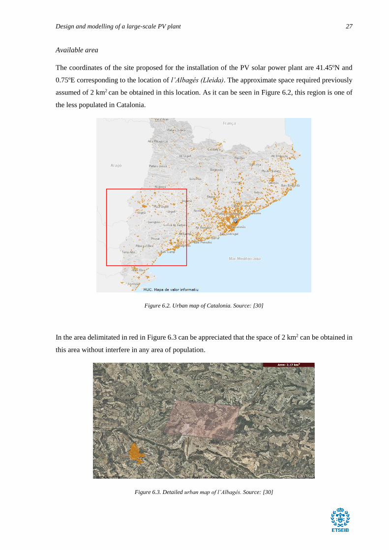
The coordinates of the site proposed for the installation of the PV solar power plant are 41.45ºN and
0.75ºE corresponding to the location of l’Albagés (Lleida). The approximate space required previously
assumed of 2 km2 can be obtained in this location. As it can be seen in Figure 6.2, this region is one of
the less populated in Catalonia.
Figure 6.2. Urban map of Catalonia. Source: [30]
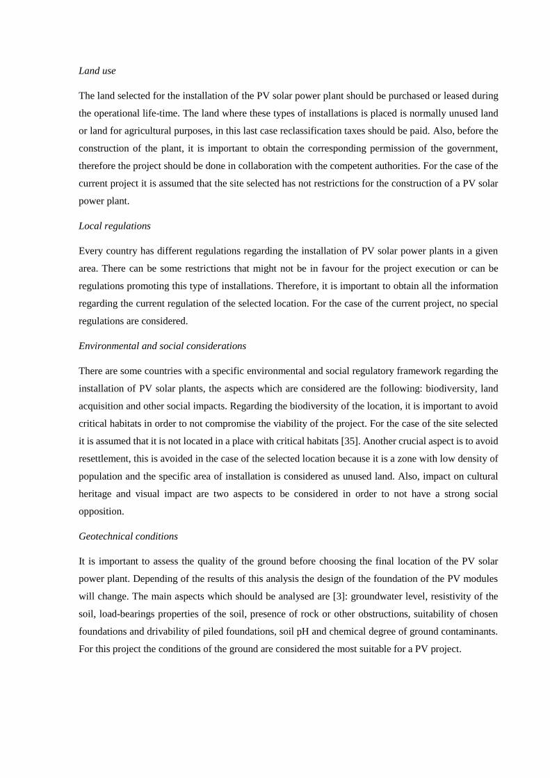
In the area delimitated in red in Figure 6.3 can be appreciated that the space of 2 km2 can be obtained in
this area without interfere in any area of population.
Figure 6.3. Detailed urban map of l’Albagés. Source: [30]

Solar resource
Spain in general and Catalonia in particular are some of the regions in Europe with more solar radiation,
in Figure 6.4 it can be observed that the mean solar radiation of the site selected is one of the highest in
Catalonia.
Figure 6.4. Daily global radiation in Catalonia [MJ/m2]. Source: [31]
Irradiance and other meteorological data for the specific location selected is obtained from PVWatts
calculation tool developed by NREL [32]. Due to the lack of reliable data the irradiance obtained is not
from the exact site of where the PV plant is going to be placed. The irradiance obtained corresponds to
Lleida (less than 30 km from the site selected). The meteorological data from two places not too distant
should not vary in excess. Figure 6.5 shows the profile of the irradiance during one year obtained.

Design and modelling of a large-scale PV plant 29
Figure 6.5. Hourly solar irradiance during one year in Lleida. Source: [32]
Local climate
Apart from obtaining the irradiance of the site selected, there are other aspects related with the climate
important for the development of a PV solar power plant project: temperature, wind speed, snow risk,
air pollutants and risk of flooding. The temperature of the location will determine the efficiency of the
solar cells and extreme temperatures can be critical for the correct operation of the PV plant. According
to Iberian Climate Atlas [33] the location selected does not have extreme temperatures. Also, extreme
wind speeds can damage the PV system specially, when solar tracking systems are installed. The
location of l’Albagés has not significant risk of extreme wind speeds [34]. The snow can reduce the
energy production of the plant during winter period and also add additional cost related with mounting
structures modifications and mitigating measures. Air pollutants are also an important aspect regarding
the energy capture, but for the site selected they are assumed to be in reasonable values which do not
affect the correct operation of the plant.
Topography
It is important to study in detail the topography of the site selected because it is directly correlated with
the cost of installation and the future energy production. The ideal situation would be a flat terrain or
with a slight south-facing slope, other configurations of the terrain could have a negative impact on the
cost of the project due to more complex mounting structures. Besides, the presence of mountains near
can produce undesirable shades. For this project the terrain where the PV modules are going to be
installed is considered flat and also the presence of near mountains is neglected.
Land use
The land selected for the installation of the PV solar power plant should be purchased or leased during
the operational life-time. The land where these types of installations is placed is normally unused land
or land for agricultural purposes, in this last case reclassification taxes should be paid. Also, before the
construction of the plant, it is important to obtain the corresponding permission of the government,
therefore the project should be done in collaboration with the competent authorities. For the case of the
current project it is assumed that the site selected has not restrictions for the construction of a PV solar
power plant.
Local regulations
Every country has different regulations regarding the installation of PV solar power plants in a given
area. There can be some restrictions that might not be in favour for the project execution or can be
regulations promoting this type of installations. Therefore, it is important to obtain all the information
regarding the current regulation of the selected location. For the case of the current project, no special
regulations are considered.
Environmental and social considerations
There are some countries with a specific environmental and social regulatory framework regarding the
installation of PV solar plants, the aspects which are considered are the following: biodiversity, land
acquisition and other social impacts. Regarding the biodiversity of the location, it is important to avoid
critical habitats in order to not compromise the viability of the project. For the case of the site selected
it is assumed that it is not located in a place with critical habitats [35]. Another crucial aspect is to avoid
resettlement, this is avoided in the case of the selected location because it is a zone with low density of
population and the specific area of installation is considered as unused land. Also, impact on cultural
heritage and visual impact are two aspects to be considered in order to not have a strong social
opposition.
Geotechnical conditions
It is important to assess the quality of the ground before choosing the final location of the PV solar
power plant. Depending of the results of this analysis the design of the foundation of the PV modules
will change. The main aspects which should be analysed are [3]: groundwater level, resistivity of the
soil, load-bearings properties of the soil, presence of rock or other obstructions, suitability of chosen
foundations and drivability of piled foundations, soil pH and chemical degree of ground contaminants.
For this project the conditions of the ground are considered the most suitable for a PV project.

Design and modelling of a large-scale PV plant 31
Geopolitical risk
A PV solar power plant is a long-term project and political stability is recommended for avoiding a
change of the initial terms during the operational life-time of the plant. Regarding the supports schemes
according to EPIA [36], Spain has the following political support environment: “Support to PV frozen
since 2012 and any new development blocked for several reasons (overcapacity, tariff deficit, etc.).
Heavy and slow administrative processes. Many attempts to revitalise the utility-scale segment without
incentives, but no significant development so far. Risk of grid tariff imposition”. According to EPIA,
Spain may not seem the best country to develop a PV project.
Accessibility
The accessibility of the site selected for the installation of the PV solar power plant is also an important
aspect. The materials needed during the construction and installation of the plant should be transported
by cargo trucks, thus the availability of suitable roads is crucial. In case that there were no roads already
constructed, the PV solar power plant developer should construct and pay them. For the case of the
current project, large expenses in construction of roads are not expected since the area is well-connected
by road.
Grid connection
There are three parameters which should be analysed regarding the grid connection [3]: Proximity, the
distance between the grid and the PV solar power plant have a direct impact on the initial economic
investment; Availability, the percentage of time that the network is able to accept power from the PV
solar power plant, the network operator is the responsible to provide this information; Capacity, the
power which the network is able to absorb. In case the capacity of the network is not enough to withstand
the power generated the network should be upgraded. For this project, the grid connection is considered
optimal.
Module soiling
The energy production of the plant can be reduced if the PV modules are covered by dust or other type
of particles, this situation can be a major problem if the PV plant is located in a very dusty area, e.g. a
desert area. For this project the incidence of dust or other particles in the PV module will be evaluated
during calculations, but the selected location is not considered critical area.
Water availability
For large-scale PV power plants, the availability of water is an important factor. Large amounts of water
are necessary for maintenance purposes (cleaning). Therefore, the system should be installed preferably
near a water source. The availability of water is not a problem for the site selected because it is

surrounded by different rivers. Also, it is important to assess the impact on the water availability for
local population after the construction of a PV solar power plant.
Financial incentives
No financial incentives or other type of renewable energy generation support schemes are considered
during the execution of the PV project. For more information regarding to financial incentives in Spain
see section 4.1. Support Schemes in Spain.

Design and modelling of a large-scale PV plant 33
6.2. METHODOLOGY OF CALCULATION
In this section of the chapter it is showed the calculation methodology followed for the obtention of the
design parameters, energy results, associated cost of the plant and other important parameters required
for the plant performance assessment. The formulas used in this project for the PV solar power plant
design are based on the paper published by Kerekes et al. [37], where they propose a methodology for
the design and optimization of large-scale PV plants.
6.2.1. Design and Energy Calculations
The steps followed for the calculations regarding the design parameters and energy calculations are
shown below:
1. PV modules and inverters selection
Before starting to implement the calculations of the PV plant design it is necessary to select the PV
modules and inverters which are going to be used during the process of calculation. Furthermore, it is
important to obtain the technical specifications of these components since they are going to be used
during calculations. The modules and inverters selected for the PV plant design are listed below:
Trinasolar TALLMAX TSM-PE14A
Trinasolar is a Chinese PV module’s manufacturer which operates also in United States and Europe. In
2014 this company became the first PV modules provider with a total of 3.66 GW of installed capacity.
The PV module selected belongs to TALLMAX series which are PV modules created for utility-scale
and commercial installations. The main characteristics of these PV modules are:
Type of technology: multicrystalline solar cells
Dimensions: 1960 x 992 x 40 mm
Weight: 22.5 kg
Maximum open circuit voltage: 45.5 V
Maximum short circuit current: 9.15 A
Peak power: 320 Wp
Module efficiency: 16.5%
See technical datasheet for more information [38].

First Solar Series 4 FS-4110-3
First Solar is a PV module’s manufacturer with headquarters in USA and production plants in Germany
and Malaysia. This company is specialized in thin-film technology. Series 4 PV modules are specially
designed for utility-scale power plants and to withstand adverse climatic conditions. The main
characteristics of this PV modules are:
Type of technology: Thin-film CdTe
Dimensions: 1200 x 600 x 6.8 mm
Weight: 12 kg
Maximum open circuit voltage: 86.4 V
Maximum short circuit current: 1.82 A
Peak power: 110 Wp
Module efficiency: 17%
See technical datasheet for more information [39].
Sungrow SG3000HV
Sungrow is one of the largest inverter’s manufacturer in China with over 40% of the market share. The
inverter selected is designed for large-scale applications and it has integrated fully grid support. The
main characteristics of the inverter are:
Type of inverter: Central inverter
Maximum input voltage: 1500 V
Maximum PV input current: 3508 A
Nominal output power: 2500 kW (at 50 ºC)
Nominal AC voltage: 550 V
Maximum inverter output current: 2886 A
Maximum efficiency: 99%
CEC efficiency: 98.7%
Dimensions: 2991 x 2591 x 2438mm
Weight: 5.9 T
Design and modelling of a large-scale PV plant 35
See technical datasheet for more information [40].
KACO new energy blueplanet 2200 TL3
KACO new energy is an inverter’s manufacturer with headquarters in Germany which also operates in
Asia and EEUU. The inverter selected has been designed with the economic development of utility-
scale PV installations in mind. The main characteristics of this model of inverter are:
Type of inverter: Central inverter
Maximum input voltage: 1000 V
Maximum PV input current: 3818 A
Nominal output power: 2200 kW (at 50 ºC)
Nominal AC voltage: 370 V
Maximum inverter output current: 3468 A
Maximum efficiency: 98.3%
CEC efficiency: 98%
Dimensions: 2150 x 3400 x 1400 mm
Weight: 5 T
See technical datasheet for more information [41].
2. Irradiance and meteorological data of the site selected:
Due to the lack of reliable data the information obtained is not from the exact site where the PV plant is
going to be placed. The meteorological information corresponds to Lleida (around 30 km from the
selected site).
The meteorological data is obtained from PVWatts calculation tool developed by NREL [32] (for more
information see section 6.1. SITE IDENTIFICATION). To obtain the meteorological data required the
following system parameters have to be introduced:
- DC system size of the system, for the current project 50 MW.
- Optimum tilt angle. The system is defined as one-axis tracking with seasonal variation.
Therefore, there are two optimum angles, one during summer season (14.2º) and other during
winter season (53.7º). Optimum tilt angle data is obtained from the NASA website [42].
- The optimum azimuth angle for installations in the northern hemisphere is 180º (facing south).

Data obtained that will be used in further calculations:
- Plane of array irradiance [W/m2]. Useful irradiance in the PV system, this irradiance is the result
of the sum of beam radiation, ground-reflected radiation and sky-diffuse radiation.
- Ambient temperature [ºC].
3. Number of PV modules calculation (𝑵𝑷𝑽)
Depending on the module technology selected for the PV plant the total number of PV panels required
in the system will vary as well as the area needed for the implementation of the PV plant will also differ
depending on that parameter.
For calculating the required number of PV panels, 𝑁𝑃𝑉, the following equation is used:
𝑁𝑃𝑉 = 𝑃𝑑𝑒𝑠𝑖𝑔𝑛 · 106
𝑃𝑀,𝑆𝑇𝐶 ( 6.1)
Where, 𝑃𝑑𝑒𝑠𝑖𝑔𝑛 [MW] is the power plant design capacity and 𝑃𝑀,𝑆𝑇𝐶 [W] is the PV module power rating.
The calculation of the number of PV modules is only an indicative calculation based on power plant
design capacity, the final number of PV modules in the system will be recalculated afterwards.
4. Area occupied by the PV modules (𝑺𝒂𝒓𝒓𝒂𝒚)
Calculation of the surface area of each PV module:
𝑆𝑃𝑉 = 𝑙𝑒𝑛𝑔𝑡ℎ · 𝑤𝑖𝑑𝑡ℎ ( 6.2)
Where, 𝑆𝑃𝑉 [m2] is the product of multiplying the length [m] by the width [m] of the PV module selected.
For calculating the total area occupied by the PV array, 𝑆𝑎𝑟𝑟𝑎𝑦 [km2], the following formula is used:
𝑆𝑎𝑟𝑟𝑎𝑦 = 𝑆𝑃𝑉 · 𝑁𝑃𝑉 · 10−6 ( 6.3)
Again, this calculation is not considering the final value of the number of PV modules, therefore this
parameter will also be recalculated afterwards.

Design and modelling of a large-scale PV plant 37
5. Calculation of the maximum number of PV modules in series and parallel
(𝑵𝒔,𝒎𝒂𝒙 , 𝑵𝒑,𝒎𝒂𝒙)
The calculation of the number of PV modules in series and parallel depends on the specifications of the
inverter selected. The algorithm used for the calculation of the maximum number of PV modules in
series per inverter is shown in Figure 6.6 :
Figure 6.6. Maximum number of PV modules in series algorithm.
Where, the specifications of the inverter are: 𝑉𝑖,𝑚𝑎𝑥 [V] is the DC input maximum MPP voltage, 𝑉𝑖,𝑚𝑖𝑛
[V] is the DC input minimum MPP voltage and 𝑉𝐷𝐶,𝑚𝑎𝑥 [V] is the maximum permissible DC input
voltage; and the specifications of the PV module are: 𝑉𝑀,𝑚𝑎𝑥 [V] maximum MPP voltage and 𝑉𝑜𝑐,𝑚𝑎𝑥
[V] maximum open-circuit voltage.
The optimum number of modules connected in series is a number smaller than 𝑁𝑠,𝑚𝑎𝑥, but to simplify
the calculations the number of PV modules in series used for further calculations is 𝑁𝑠,𝑚𝑎𝑥. By choosing
the maximum number of PV modules in series the number of necessary inverters is reduced, but in terms
of energy capture this procedure is not always the best option, since the inverter is more efficient when
is working closer to its rated power.
𝑁𝑠,𝑚𝑎𝑥 = 𝑁𝑠,𝑚𝑎𝑥 − 1
𝑁𝑠,𝑚𝑎𝑥 · 𝑉𝑜𝑐,𝑚𝑎𝑥
> 𝑉𝐷𝐶,𝑚𝑎𝑥
𝑉𝑚𝑖𝑑 = 𝑉𝑖,𝑚𝑎𝑥 + 𝑉𝑖,𝑚𝑖𝑛
2
𝑁𝑠,𝑚𝑎𝑥 = 𝑓𝑙𝑜𝑜𝑟 ቆ𝑉𝑚𝑖𝑑
𝑉𝑀,𝑚𝑎𝑥ቇ
YES
The number of PV modules connected in parallel is calculated using the values of current of the module
and the current of the inverter:
𝑁𝑝,𝑚𝑎𝑥 = 𝑓𝑙𝑜𝑜𝑟 ቆ𝐼𝐷𝐶,𝑚𝑎𝑥
𝐼𝑀,𝑚𝑎𝑥ቇ ( 6.4)
Where, the specification used of the inverter are: 𝐼𝐷𝐶,𝑚𝑎𝑥 [A] is maximum continuous current; and the
specification of the PV module used in this calculation: 𝐼𝑀,𝑚𝑎𝑥 [A] is maximum MPP current.
As it happens in the previous point when calculating the number of modules in series, the optimum
number of modules in parallel is a number smaller than 𝑁𝑝,𝑚𝑎𝑥. Again, to facilitate the calculations
𝑁𝑝,𝑚𝑎𝑥 is chosen as the final number of modules in parallel.
6. Number of inverters (𝑵𝒊)
After the calculation of the total number of PV modules in the PV plant, the number of modules in series
and the number of modules in parallel it is possible to obtain the number of necessary inverters in the
system. The formula used for this calculation is the following:
𝑁𝑖 = 𝑐𝑒𝑖𝑙 [𝑁𝑃𝑉
𝑁𝑠 · 𝑁𝑃] ( 6.5)
Where, it is considered 𝑁𝑠 = 𝑁𝑠,𝑚𝑎𝑥 and 𝑁𝑝 = 𝑁𝑝,𝑚𝑎𝑥 . The final value is obtained by rounding the
result to the greater nearest integer the value obtained in the calculation.
7. Final number of PV modules (𝑵𝒑𝒗,𝒇𝒊𝒏𝒂𝒍), installed capacity (𝑷𝒊𝒏𝒔𝒕𝒂𝒍𝒍𝒆𝒅) and final area
occupied by the PV modules (𝑺𝒂𝒓𝒓𝒂𝒚,𝒇𝒊𝒏𝒂𝒍)
Due to the final number of inverters needed is a rounded number, total number of PV modules previously
calculated must be recalculated. Another option, instead of recalculating the number of PV modules,
could be that one inverter (or more than one) was not connected to the maximum number of modules in
series and parallel. The final solution is to slightly oversize the system in order to make all the PV sets
in the system of the same size (number of modules per inverter). The formula used to calculate the final
number of PV modules in the PV plant is shown below:
𝑁𝑝𝑣,𝑓𝑖𝑛𝑎𝑙 = 𝑁𝑠 · 𝑁𝑝 · 𝑁𝑖 ( 6.6)
As the number of PV modules is changed respect to the initial design conditions, total installed capacity
in the PV power plant is also modified:
Design and modelling of a large-scale PV plant 39
𝑃𝑖𝑛𝑠𝑡𝑎𝑙𝑙𝑒𝑑 = 𝑁𝑝𝑣,𝑓𝑖𝑛𝑎𝑙 · 𝑃𝑀,𝑆𝑇𝐶 ( 6.7)
Also, the area occupied by the PV modules must be recalculated. The formula is the same as the one
previously explained in Equation ( 6.3), but in this case the number of PV modules is definitive:
𝑆𝑎𝑟𝑟𝑎𝑦,𝑓𝑖𝑛𝑎𝑙 = 𝑆𝑃𝑉 · 𝑁𝑃𝑉,𝑓𝑖𝑛𝑎𝑙 · 10−6 ( 6.8)
8. Solar panel temperature calculation (𝑻𝑴)
It is important to calculate the temperature of the PV module because this parameter is directly related
with the performance of the module. The formula based on [43] used for calculating the temperature of
the PV module is the following:
𝑇𝑀 = 𝑇𝑎𝑚𝑏 + 𝐺𝑡
800· (𝑁𝑂𝐶𝑇 − 20) ( 6.9)
Where, 𝑇𝑎𝑚𝑏 [ºC] is the ambient temperature, 𝐺𝑡 [W/m2] incident solar radiation and 𝑁𝑂𝐶𝑇 [ºC] nominal
operating cell temperature.
9. MPP power of each PV module (𝑷𝑴)
The power output of each PV module is calculated considering meteorological conditions such as
temperature of the PV panel and irradiance (both previously obtained). The formula describing the
power output of the PV modules is the following:
𝑃𝑀 = 𝑃𝑀,𝑆𝑇𝐶 ·𝐺𝑡
1000· [1 − 𝛾 · (𝑇𝑀 − 25)] ( 6.10)
Where, 𝛾 [%/ºC] is the temperature parameter of the PV module at MPP and it is specified in the
technical specifications of the PV modules selected.
10. Actual power output of each PV module (𝑷𝑷𝑽)
Once the MPP power of each module is obtained the actual power output of each module can be
calculated considering the losses of operation. The formula describing the actual power output is the
following:
𝑃𝑃𝑉 = (1 −𝑑𝑓
100) · (1 −
𝑆𝑝
100) · 𝑃𝑀 ( 6.11)

Where, 𝑑𝑓 (%) is the PV module output power derating factor due to the dirt that is deposited on its
surface. 𝑑𝑓 is set at 6.9% [37] for this project. 𝑆𝑝 [%] are the losses due to shading effect, these losses
are set at 3% [32]. The shading losses considered in this calculation step are only an assumption based
on results obtained from the literature, but for a more accurate calculation of shading losses a 3D model
of the PV power plant should be modelled or the real shading losses affecting the PV plant operation
can be obtained by on field measurements. Once the MPP power of each module (𝑃𝑀) and actual power
output power of each module (𝑃𝑃𝑉) are calculated, the power losses can be easily obtained:
𝑃𝑃𝑉,𝑙𝑜𝑠𝑠𝑒𝑠 = 𝑃𝑀 − 𝑃𝑃𝑉 ( 6.12)
11. Output power of each PV set (𝑷𝒊𝒏)
The number of PV modules forming a PV set is formed by the number of modules in series multiplied
by the number of modules in parallel (see Figure 6.7). The number of PV sets in the PV power plant is
equal to the number of inverters required.
Figure 6.7. PV set configuration on PV plant [37].
The calculation of the output power of each PV set depends on the actual power output of each module,
MPP efficiency of the inverter, voltage drop of the dc cable and mismatch losses:
𝑃𝑖𝑛 = 𝑁𝑠 · 𝑁𝑝 ·𝜂𝑚𝑝𝑝𝑡
100· (1 −
𝜂𝑑𝑐
100) · (1 −
𝜂𝑚𝑖𝑠𝑚𝑎𝑡𝑐ℎ
100) · 𝑃𝑃𝑉 ( 6.13)
Where, 𝜂𝑚𝑝𝑝𝑡 (%) is the MPP efficiency of the dc/ac inverter. The 𝜂𝑚𝑝𝑝𝑡 is set at 99% according to
Valentini et al. [44]. 𝜂𝑑𝑐(%) is the voltage drop of the dc cable, 1.5% of DC cable voltage drop is
assumed according to IFC [3]. Another important factor affecting PV set power output are mismatch

Design and modelling of a large-scale PV plant 41
losses, 𝜂𝑚𝑖𝑠𝑚𝑎𝑡𝑐ℎ. These losses appear due to slight difference in the manufacturing of PV modules
interconnected, or also they can be caused due to PV modules experiencing different conditions in the
same array. Mismatch losses for this project are estimated at 2% [32]. Once again, Equation ( 6.13) can
be improved by calculating cable losses in a more accurate manner. Furthermore, shading losses can be
added to this equation, but a more detailed study of the system is needed in order to obtain realistic
values.
12. Total output power of each DC/AC inverter (𝑷𝒐)
Each PV set is connected to an inverter and depending on the specifications of this inverter, the final
energy obtained will vary. The output power of each DC/AC inverter is calculated using the following
equations:
1) If 𝑃𝑖𝑛 ≤ 𝑃𝑖,𝑛𝑎 , then 𝑃𝑜 = 𝜂𝑖𝑛𝑣
100∗ 𝑃𝑖𝑛 , else 𝑃𝑜 =
𝜂𝑖𝑛𝑣
100∗ 𝑃𝑖,𝑛𝑎
( 6.14)
2) If 𝑃𝑖𝑛 ≤ 𝑃𝑖,𝑠𝑐 , then 𝑃𝑜 = 0
Where, 𝑃𝑖,𝑛𝑎 [W] is the inverter maximum permissible power level, 𝜂𝑖𝑛𝑣 [%] is the inverter power
conversion efficiency and 𝑃𝑖,𝑠𝑐 [W] is the self-power consumption of the inverter.
The efficiency of the inverter is considered constant and equal in all the PV sets to simplify the
calculations. Furthermore, the voltage of the PV set is considered always higher than the minimum
permissible MPP voltage level of the inverter, in case of this condition were not met the power output
of the inverter will be zero.
13. Land occupied by the PV solar power plant (𝑳𝒂𝒏𝒅)
For further calculations it is important to know the area which the PV power plant is going to occupy.
To make this calculation some assumptions have been made: The total dimensions of the land occupied
is assumed from literature [45] and it is set at 0.036 km2/MWac (𝑙𝑎𝑛𝑑𝑟𝑒𝑎𝑙𝑎𝑡𝑖𝑜𝑛).
𝐿𝑎𝑛𝑑 = max(𝑃𝑜) · 10−6 · 𝑁𝑖 · 𝑙𝑎𝑛𝑑𝑟𝑒𝑎𝑙𝑎𝑡𝑖𝑜𝑛 ( 6.15)
14. Power that PV plant can inject into the grid (𝑷𝑷𝑳𝑨𝑵𝑻)
Power that can be injected into the grid is calculated considering losses in the step-up transformer and
in the AC side cable. The formula used for this calculation is the following:
𝑃𝑃𝐿𝐴𝑁𝑇 = 𝜂𝑇
100·
𝜂𝑐𝑎𝑏𝑙𝑒
100· 𝑃𝑜 · 10−6 · 𝑁𝑖 ( 6.16)
Where, 𝜂𝑇 [%] is the efficiency of the interconnection transformer and it is set at 99% [37], 𝜂𝑐𝑎𝑏𝑙𝑒 [%]
is the efficiency of the AC cable connections, this value is set at 99.5% according to literature [46].
For a more accurate result of the total power that PV plant can inject into the grid a more complex study
of the system is required. E.g., to obtain the real value of the AC side cable losses, the length of the
cables in combination with power loss coefficient should analysed.
For practical reasons this 𝑃𝑃𝐿𝐴𝑁𝑇 is considered as the power that is injected into the grid, without power
and voltage grid limitations. For all time steps analysed in the calculation of the power output of the PV
plant this condition is assumed to be valid: 𝑃𝑃𝐿𝐴𝑁𝑇 ≤ 𝑃𝑔𝑟𝑖𝑑,𝑚𝑎𝑥.
Where, 𝑃𝑔𝑟𝑖𝑑,𝑚𝑎𝑥 [MW] is the maximum power that can be injected into the grid. For more accurate
calculation the characteristics of the grid should be analysed in order to evaluate if the condition is
accomplished for the period of operation assessed.
15. Total energy injected into the grid from the PV power plant (𝑬𝑷𝑳𝑨𝑵𝑻,𝑻𝑶𝑻)
The energy injected into the grid is calculated considering the time steps used along the previous
calculations and adding an availability factor of the PV power plant due to maintenance reasons. The
formula used in this step to calculate the energy injected for each time step is the following:
𝐸𝑃𝐿𝐴𝑁𝑇 =𝐸𝐴𝐹
100· 𝑃𝑃𝐿𝐴𝑁𝑇 · ∆𝑡 ( 6.17)
Where, EAF [%] is the energy availability factor of the PV plant due to maintenance of the PV power
plant components, this parameter is set at 99.5% [47]. ∆𝑡 [h] is the time step. Total energy injected into
the grid, or annual energy production (AEP) is calculated using the following formula:
𝐸𝑃𝐿𝐴𝑁𝑇,𝑇𝑂𝑇 =𝐸𝐴𝐹
100· ∑ 𝑃𝑃𝐿𝐴𝑁𝑇 · ∆𝑡
𝑛
𝑡=1
( 6.18)
Where, t is the number of time steps considered during the calculations of the PV power plant. For one-
year t is equal to 8760.

Design and modelling of a large-scale PV plant 43
The calculation methodology and the steps explained previously are summarised in Figure 6.8:
Figure 6.8. Calculation methodology scheme.
6.2.2. Economic Calculations
The methodology and formulas used regarding the economic calculations are also based on the paper
published by Kerkes et al. [37]. The steps followed are shown below:
1. Calculation of Total cost of the PV power plant (𝑪𝒄)
Capital cost is referred to one-time expenses associated with the PV power plant installation. With the
purpose of estimate the viability of any energy project it is important to calculate all the expenditures
associated with the project. The first step in the economic analysis is the calculation of the total capital
cost. The capital cost calculated for this project includes: the cost of the PV array, cost of the inverters,
cost of the step-up transformers, BOS cost (electrical wiring, meter, protections, junction boxes,
cabinets, switchgear, combiners, fuses, breaker and other non-electrical components), cost of civil work
and cost of the land. The formula used to calculate the capital cost is the following:
𝐶𝑐 = (𝑁𝑖 · 𝑁𝑠 · 𝑁𝑝 ·𝑃𝑀,𝑆𝑇𝐶
1000· 𝐶𝑃𝑉) + (𝑁𝑖 ·
𝑃𝑟𝑎𝑡𝑒𝑑
1000· 𝐶𝑖𝑛𝑣) + (𝐶𝑡𝑟𝑎𝑛𝑠𝑓𝑜𝑟𝑚𝑒𝑟 · 𝑃𝑝𝑙𝑎𝑛𝑡,𝑛𝑜𝑚
· 1000) + (𝐵𝑂𝑆 · 𝑃𝑝𝑙𝑎𝑛𝑡,𝑛𝑜𝑚 · 1000) + (𝐶𝐶&𝑖 · 𝑃𝑝𝑙𝑎𝑛𝑡,𝑛𝑜𝑚 · 1000)
+ (𝐶𝑙𝑎𝑛𝑑 · 𝑛 · 𝑙𝑎𝑛𝑑)
( 6.19)
Where, 𝐶𝑃𝑉 [€/kWp] is the cost of the PV modules, 𝑃𝑟𝑎𝑡𝑒𝑑[W] is the power rated of the solar inverters
and 𝐶𝑖𝑛𝑣 [€/kWp] is the cost of the solar inverters. 𝐶𝑡𝑟𝑎𝑛𝑠𝑓𝑜𝑟𝑚𝑒𝑟[€/kWp] is the cost of the step-up
transformers. 𝐶𝐶&𝑖[€/kWp] is the cost associated to construction and installation of the PV plant
components. 𝐵𝑂𝑆 [€/kWp] is the cost of the balance of system components. 𝐶𝑙𝑎𝑛𝑑 [€/km2-year] and
𝑙𝑎𝑛𝑑 [km2] are the cost of the land and the surface area required for the installation of the PV power
plant respectively. 𝑛 [years] is the operational lifetime of the PV plant.
2. Calculation of the Maintenance cost of the PV power plant during its operational lifetime
(𝑪𝒎)
Besides of knowing the total capital cost the PV power plant, the calculation of the maintenance cost
during its operational lifetime it is important to know the economic framework of the project. The
formula used to calculate this parameter is shown below:
𝐶𝑚 = 𝑃𝑝𝑙𝑎𝑛𝑡,𝑛𝑜𝑚 · 1000 · 𝑀𝑝𝑙𝑎𝑛𝑡 · 𝑛 ( 6.20)
Where, 𝑀𝑝𝑙𝑎𝑛𝑡 [€/kWp] is the maintenance cost of the PV power plant. The annual inflation rate and
nominal discount are not considered in this calculation due to the lack of realistic data, but for a more
accurate value of 𝐶𝑚 these values should be examined carefully.
3. Calculation of Replacement cost (𝑪𝒓𝒆𝒑)
Some of the components installed in the PV power plant will need to be replaced during the years of
operation. The time of operation of the PV plant being designed is 25 years. The decision of which
components should be replaced will be taken according the specifications of each component.
Design and modelling of a large-scale PV plant 45
4. Levelized Cost of Energy calculation (𝑳𝑪𝑶𝑬)
LCOE is an economic parameter which it is used to quantify the price of the energy that is being
produced for the specific conditions previously described. It is also one of the main parameters to
compare different generating technologies. The formula used in this project is the following:
𝐿𝐶𝑂𝐸 = 𝐶𝑐 + 𝐶𝑚 + 𝐶𝑟𝑒𝑝
𝐸𝑃𝐿𝐴𝑁𝑇,𝑛 · 1000 ( 6.21)
Where, 𝐸𝑃𝐿𝐴𝑁𝑇,𝑛 [MWh] is the total energy produced by the PV plant over its operational lifetime.
5. Gross Revenues (𝑹𝒈𝒓𝒐𝒔𝒔)
Gross revenues are the sum of all earnings generated by the PV plant during the project lifetime. The
calculation is made considering the price of the electricity over the operational lifetime of the PV plant.
This price can vary depending on the electricity market of the selected location and also it is important
to consider the support schemes available. The formula used for Gross Revenues is:
𝑅𝑔𝑟𝑜𝑠𝑠 = 𝑃𝑒𝑙𝑒𝑐𝑡𝑟𝑖𝑐𝑖𝑡𝑦 · 𝐸𝑃𝐿𝐴𝑁𝑇,𝑇𝑂𝑇 · 𝑛 ( 6.22)
Where, 𝑃𝑒𝑙𝑒𝑐𝑡𝑟𝑖𝑐𝑖𝑡𝑦 [€/MWh] is the price of the electricity for the operational life-time of the PV plant.
6.2.3. Evaluation Parameters Calculation
The parameters that are going to be described below can be seen as quality indicators of the PV solar
power plant designed, also these parameters can be used to make final decisions regarding the
technology used and to make comparisons between other types of energy generation technologies. The
parameters described in this section are: ground coverage ratio, performance ratio, capacity factor and
specific yield.
Ground coverage ratio (𝑮𝑪𝑹)
This parameter is an indicator of how the surface of installation is covered by PV modules and which
percentage is used for other components. The formula to calculate this parameter based on [48] is shown
below:
𝐺𝐶𝑅(%) = 𝑆𝑎𝑟𝑟𝑎𝑦,𝑓𝑖𝑛𝑎𝑙
𝑙𝑎𝑛𝑑· 100 ( 6.23)

The results obtained of GCR will be merely indicative, since the calculation of 𝑙𝑎𝑛𝑑 [km2] are based on
assumptions.
Performance ratio (𝑷𝑹)
Performance ratio expresses the relation between the real performance of the PV solar power plant and
its rated power capacity. This parameter can be seen as a quality indicator because usually it is used to
compare different photovoltaic systems independently of their installed capacity. The period analysed
is one year and the parameter is calculated by the following formula based on [3].
𝑃𝑅(%) = 𝐸𝑃𝐿𝐴𝑁𝑇,𝑇𝑂𝑇
𝑃𝑝𝑙𝑎𝑛𝑡,𝑛𝑜𝑚 · 𝐺𝑡 · 10−6· 100 ( 6.24)
Where, 𝐸𝑃𝐿𝐴𝑁𝑇,𝑇𝑂𝑇 [MWh] is the total energy generated for the PV power plant during one year.
Capacity factor (𝑪𝑭)
This parameter is the ratio of the PV power plant actual energy output for a year and its output at nominal
power during a year. It is typically expressed as percentage and the formula based on [3] describing this
parameter it is shown below:
𝐶𝐹(%) = 𝐸𝑃𝐿𝐴𝑁𝑇,𝑇𝑂𝑇
𝑃𝑝𝑙𝑎𝑛𝑡,𝑛𝑜𝑚 · 8760· 100 ( 6.25)
Specific yield (𝒀𝒊𝒆𝒍𝒅𝒔𝒑)
Specific yield of a PV solar power plant is the total energy output divided by the installed capacity [3].
This parameter expresses the number of hours that the PV array would need to operate at its rated power
to generate the same energy. The formula used is shown below, the results can be expressed in kWh/kWp
or hours:
𝑌𝑖𝑒𝑙𝑑𝑠𝑝 =𝐸𝑇𝑂𝑇𝐴𝐿
𝑃𝑝𝑙𝑎𝑛𝑡,𝑛𝑜𝑚 ( 6.26)

Design and modelling of a large-scale PV plant 47
6.3. RESULTS OBTAINED
The results are obtained by implementing the calculation methodology previously described in MATLAB
(See Annex A). To make the calculations four different scenarios, with two different PV modules and
two different inverters, have been selected (see Table 6.1). Later, the results of the different scenarios
are going to be compared in order to obtain the most favourable configuration considering different
modules and solar inverters technologies.
The main purpose of comparing four different scenarios is to obtain which is the module-inverter
combination with the best design results. To do that, two different modules with different technologies
are analysed, one module with poly-Si technology and the other with CdTe thin-film technology.
Additionally, the rated powers of the modules are markedly different, 320 Wp for poly-Si modules and
110 Wp for thin-film. These two modules technologies are selected for being analysed because poly-Si
and CdTe thin-film modules are nowadays one of the most common technologies used in large-scale
PV plants. Furthermore, two different inverters are compared in the different scenarios calculated. Both
inverters are central-inverters, but the rated power is considerably different, 3,000 Wp for Sungrow
inverter and 2,000 Wp for KACO new energy inverter.
Table 6.1. PV module and inverter selection for each of the different scenarios.
PV module Inverter
Scenario 1 TrinaSolar TALLMAX-PE14A Sungrow SG3000HV
Scenario 2 First Solar FS-4110-3 Sungrow SG3000HV
Scenario 3 TrinaSolar TALLMAX-PE14A Kaco new energy blueplanet 2200TL3
Scenario 4 First Solar FS-4110-3 Kaco new energy blueplanet 2200TL3
Results obtained regarding the number of elements in the system and the installed capacity for each of
the scenarios analysed are shown in Table 6.2:
Table 6.2. Results of different design parameters.
Scenario 1 Scenario 2 Scenario 3 Scenario 4
No. PV modules series
per PV set 29 16 18 10
No. PV modules parallel
per PV set 406 2,165 442 2,356
No. Inverters 14 14 20 20
No. of PV modules 164,836 484,960 159,120 471,200
Installed capacity (MWp) 52.75 53.35 50.92 51.83

The calculation of the number of PV modules in series is directly linked with the relation between the
voltage of the inverter and the voltage values of the PV modules. The number of modules in series in
Scenario 1 is larger than the number in Scenario 2, despite these two scenarios are sharing the same
inverter technology. This difference is caused due to the MPP voltage and the maximum open-circuit
voltage of the modules in Scenario 2 are higher than in Scenario 1. For higher voltage values of the
modules, less modules in series can be connected per inverter. The same applies with Scenario 3 and
Scenario 4, where, in this case the PV modules selected for Scenario 4 have higher MPP voltage and
maximum open-circuit voltage. Comparing Scenario 1 and Scenario 4, using the same PV modules but
different inverters, the number of PV modules in series in Scenario 1 are larger because voltage values
of the inverter selected for this scenario are higher.
Regarding the number of PV modules in parallel obtained for each scenario, the explanation of the
values obtained is similar than the explanation for the number of PV modules in series, but in this case
the values are linked with the current values. The scenarios with PV modules with higher current values
(Scenario 1 and Scenario 3) allow to connect less PV modules in parallel per inverter. The scenarios
using an inverter with higher current input parameters (Scenario 3 and Scenario 4) allow to connect
more PV modules in parallel than Scenarios 1 and 2.
The number of inverters in the PV solar power plant is directly correlated with the maximum admissible
input power of the inverters, for scenarios using a type of inverter with higher input admissible power
(Scenario 1 and Scenario 2) the number of inverters needed is smaller. The opposite happens with
Scenario 3 and Scenario 4 where the lower input admissible power of the inverter in those scenarios
leads to a larger number of inverters in the system.
Total number of PV modules installed in the PV plant is the result of the combination of the number
modules in series, modules in parallel and inverters in the system. The value of the number of PV
modules depends on both PV module technology (in greater extent) and inverter selected.
Initial design capacity of the PV plant was 50 MW for all the scenarios, but due to the number of modules
in series, modules in parallel and inverters has to be an integer number and also it is decided to make all
the PV set of the same size, the design capacity is modified in different manner for all the scenarios, all
the scenarios are slightly oversized. The scenario closer to the design capacity is Scenario 3, where
installed capacity calculated is 2% higher than the initial design capacity of 50MW. The scenario with
the higher difference is Scenario 2 with an installed capacity 6.7% higher than the initial value.
Actual power output for each PV module during one year for time steps of one hour is represented in
Figure 6.9. The power profile that is showed in Figure 6.9 shows the power output for each PV module
after applying losses due to dirt deposited on it and due to shading effect. This figure is related with the

Design and modelling of a large-scale PV plant 49
total number of PV modules which are required in the PV plant (Table 6.2). Obviously, the amount of
PV modules required will depend on their power output, in Figure 6.9 it can be seen that PV modules
used in Scenarios 1 and 3 have more than double of the power output of the PV modules used in
Scenarios 2 and 4, therefore it is coherent that the total number of PV modules is also more than double
in those scenarios.
Figure 6.9. PV module actual power output. PV module 1 (blue) is the technology used in Scenarios 1 and 3. PV module 2
(red) is the technology used in Scenarios 2 and 4.
Annual energy output for each module before and after applying losses is shown in Table 6.3. Note that
Scenarios 1 and 3 are using PV module no. 1; and Scenarios 2 and 4 are using PV module no. 2 (see
Table 6.1). Losses considered in this calculation are: losses due to dirt deposited on PV module surface
(soiling losses) and losses due shading effect. The annual reduction factor is not considered due to the
calculations are made for the first year of operation.
Table 6.3. Values obtained for PV module MPP output power and actual output power.
Scenario 1
Scenario 3
Scenario 2
Scenario 4
Annual energy output at MPP power
of each PV module [kWh/year] 585.6 205.03
Annual energy at actual output power
of each PV module [kWh/year] 528.84 185.16
Annual energy losses in each PV
module [kWh/year] 56.76 19.87

The losses applied are the same for the four scenarios, thus the amount of annual energy losses of each
PV module will depend on their rated power. The losses due to the dirt and the shading losses combined
add up to a total of approximate 10% for all scenarios.
Energy output of each PV set and energy output of each inverter for the different scenarios are shown
in Table 6.4. Note that the number of PV sets is equal to the number of inverters for each different
scenario.
Table 6.4. Values for energy output of each PV set and energy output for each inverter.
Scenario 1 Scenario 2 Scenario 3 Scenario 4
Annual energy output of
each PV set [MWh/year] 5,950.4 6,129.4 4,020.8 4,168.9
Annual energy output of each
DC/AC inverter [MWh/year] 5,872.1 6,048.8 3,962.7 4,108.7
Annual energy losses in each
PV set [MWh/year] 78.28 80.60 58.14 60.18
Losses in each PV set [%] 1.33 1.33 1.47 1.46
The energy losses between the energy output of the PV sets and the energy output of the DC/AC
inverters are caused by the efficiency of the inverter and also, they correspond to a calculation algorithm
where: 1) if the power output from the PV set is lower than self-power consumption of the inverter,
power output from the inverter will be zero; 2) if the power output from the PV set is lower than
maximum admissible input power of the inverter, the power output will only depend on the inverter’s
efficiency and the output power from the PV set. If the power output from the PV set is higher than
maximum admissible input power of the inverter, the power output will be maximum admissible input
power of the inverter multiplied by the inverter efficiency (see Equation ( 6.14)). The percentage of
losses in PV set are similar between the four scenarios. For Scenarios 1 and 2 the losses due to the
efficiency of the inverter are 1.3% the rest of the losses are caused due to calculation algorithm
previously described (approximately 0.03%). The losses due to the inverter’s efficiency in Scenario 3
and 4 are 1.4%. The losses from the calculation algorithm in Scenario 3 are 0.07% (the highest losses),
and the losses due to calculation algorithm is Scenario 4 are 0.06%.
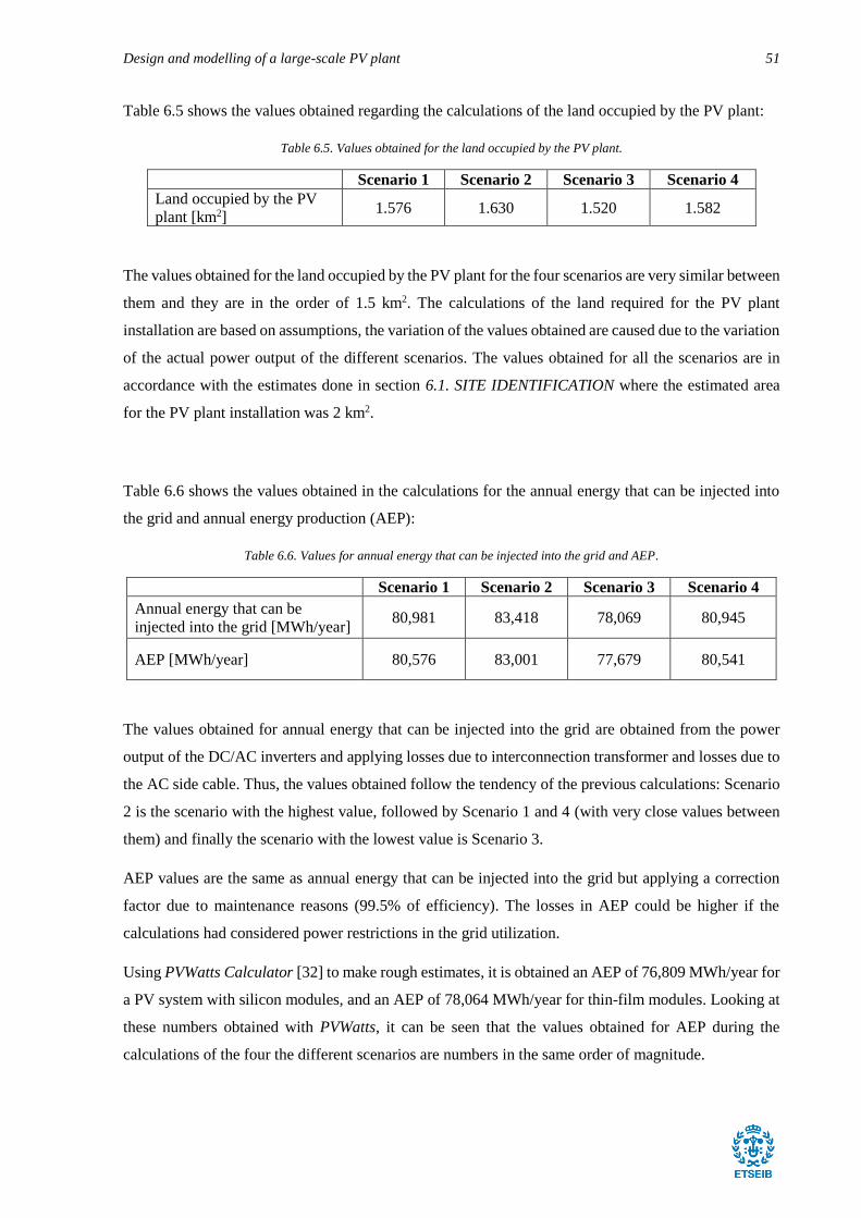
Design and modelling of a large-scale PV plant 51
Table 6.5 shows the values obtained regarding the calculations of the land occupied by the PV plant:
Table 6.5. Values obtained for the land occupied by the PV plant.
Scenario 1 Scenario 2 Scenario 3 Scenario 4
Land occupied by the PV
plant [km2] 1.576 1.630 1.520 1.582
The values obtained for the land occupied by the PV plant for the four scenarios are very similar between
them and they are in the order of 1.5 km2. The calculations of the land required for the PV plant
installation are based on assumptions, the variation of the values obtained are caused due to the variation
of the actual power output of the different scenarios. The values obtained for all the scenarios are in
accordance with the estimates done in section 6.1. SITE IDENTIFICATION where the estimated area
for the PV plant installation was 2 km2.
Table 6.6 shows the values obtained in the calculations for the annual energy that can be injected into
the grid and annual energy production (AEP):
Table 6.6. Values for annual energy that can be injected into the grid and AEP.
Scenario 1 Scenario 2 Scenario 3 Scenario 4
Annual energy that can be
injected into the grid [MWh/year] 80,981 83,418 78,069 80,945
AEP [MWh/year] 80,576 83,001 77,679 80,541
The values obtained for annual energy that can be injected into the grid are obtained from the power
output of the DC/AC inverters and applying losses due to interconnection transformer and losses due to
the AC side cable. Thus, the values obtained follow the tendency of the previous calculations: Scenario
2 is the scenario with the highest value, followed by Scenario 1 and 4 (with very close values between
them) and finally the scenario with the lowest value is Scenario 3.
AEP values are the same as annual energy that can be injected into the grid but applying a correction
factor due to maintenance reasons (99.5% of efficiency). The losses in AEP could be higher if the
calculations had considered power restrictions in the grid utilization.
Using PVWatts Calculator [32] to make rough estimates, it is obtained an AEP of 76,809 MWh/year for
a PV system with silicon modules, and an AEP of 78,064 MWh/year for thin-film modules. Looking at
these numbers obtained with PVWatts, it can be seen that the values obtained for AEP during the
calculations of the four the different scenarios are numbers in the same order of magnitude.
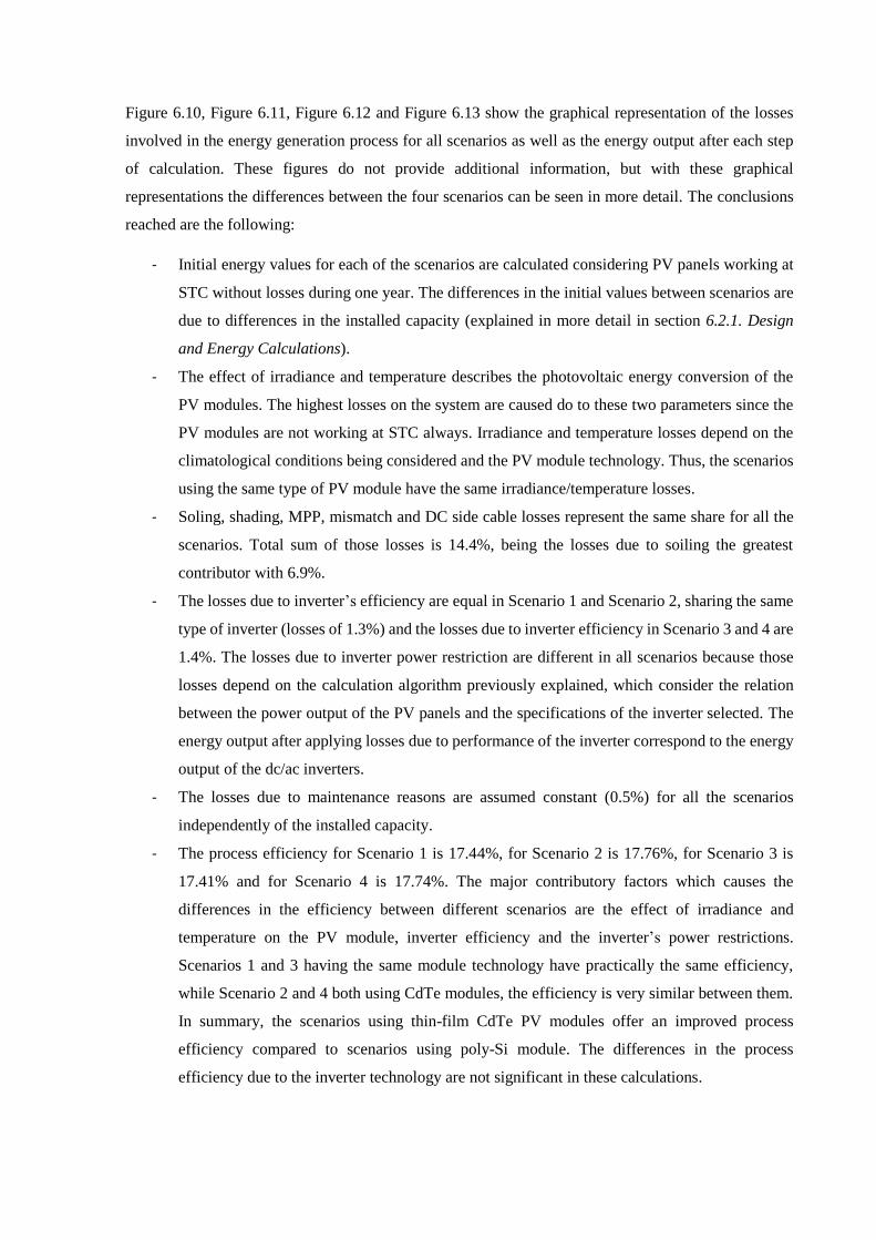
Figure 6.10, Figure 6.11, Figure 6.12 and Figure 6.13 show the graphical representation of the losses
involved in the energy generation process for all scenarios as well as the energy output after each step
of calculation. These figures do not provide additional information, but with these graphical
representations the differences between the four scenarios can be seen in more detail. The conclusions
reached are the following:
- Initial energy values for each of the scenarios are calculated considering PV panels working at
STC without losses during one year. The differences in the initial values between scenarios are
due to differences in the installed capacity (explained in more detail in section 6.2.1. Design
and Energy Calculations).
- The effect of irradiance and temperature describes the photovoltaic energy conversion of the
PV modules. The highest losses on the system are caused do to these two parameters since the
PV modules are not working at STC always. Irradiance and temperature losses depend on the
climatological conditions being considered and the PV module technology. Thus, the scenarios
using the same type of PV module have the same irradiance/temperature losses.
- Soling, shading, MPP, mismatch and DC side cable losses represent the same share for all the
scenarios. Total sum of those losses is 14.4%, being the losses due to soiling the greatest
contributor with 6.9%.
- The losses due to inverter’s efficiency are equal in Scenario 1 and Scenario 2, sharing the same
type of inverter (losses of 1.3%) and the losses due to inverter efficiency in Scenario 3 and 4 are
1.4%. The losses due to inverter power restriction are different in all scenarios because those
losses depend on the calculation algorithm previously explained, which consider the relation
between the power output of the PV panels and the specifications of the inverter selected. The
energy output after applying losses due to performance of the inverter correspond to the energy
output of the dc/ac inverters.
- The losses due to maintenance reasons are assumed constant (0.5%) for all the scenarios
independently of the installed capacity.
- The process efficiency for Scenario 1 is 17.44%, for Scenario 2 is 17.76%, for Scenario 3 is
17.41% and for Scenario 4 is 17.74%. The major contributory factors which causes the
differences in the efficiency between different scenarios are the effect of irradiance and
temperature on the PV module, inverter efficiency and the inverter’s power restrictions.
Scenarios 1 and 3 having the same module technology have practically the same efficiency,
while Scenario 2 and 4 both using CdTe modules, the efficiency is very similar between them.
In summary, the scenarios using thin-film CdTe PV modules offer an improved process
efficiency compared to scenarios using poly-Si module. The differences in the process
efficiency due to the inverter technology are not significant in these calculations.

Design and modelling of a large-scale PV plant 53
Figure 6.10. Energy flow chart Scenario 1.
Figure 6.11. Energy flow chart Scenario 2.
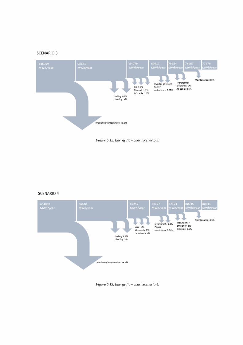
Figure 6.12. Energy flow chart Scenario 3.
Figure 6.13. Energy flow chart Scenario 4.

Design and modelling of a large-scale PV plant 55
6.3.1. Economic Results
To elaborate the economic calculations some assumptions regarding the cost of the components and
services involved have been made. Table 6.7 shows the assumptions made during the calculations:
Table 6.7. Cost assumed per component or service considered in the design of the PV plant.
Value Reference
PV module [USD/kWp] 600 for poly-Si
500 for thin-film [49]
Inverter [USD/kWp] 50 [50]
BOS [€/kWp] 74 [51]
Civil work [€/kWp] 165 [51]
Land [€/km2-year] 130,000 [52]
Transformer [€/kWp] 20 [53]
O&M [USD/kWp-year] 18 for poly-Si
19 for thin-film [49]
Total capital cost results obtained and cost breakdown of the PV power plant is shown in Table 6.8:
Table 6.8. Cost per component and service and the percentage they represent for each scenario.
Scenario 1 Scenario 2 Scenario 3 Scenario 4
Cost of the PV
modules [€] 25,635,000
(55.58%)
21,604,968 (50.93%)
24,746,000 (55.62%)
20,991,960 (50.98%)
Cost of the
inverters [€] 1,701,000
(3.69%)
1,701,000 (4.01%)
1,620,000 (3.64%)
1,620,000 (3.93%)
Cost of the
transformers [€] 1,055,000
(2.29%)
1,066,912 (2.52%)
1,018,368 (2.29%)
1,036,640 (2.52%)
BOS cost [€] 3,903,300 (8.46%)
3,947,600 (9.31%)
3,768,000 (8.47%)
3,835,568 (9.31%)
Civil work and
install. cost [€] 8,703,300
(18.87%)
8,802,024 (20.75%)
8,401,536 (18.88%)
8,552,280 (20.77%)
Cost of the land
[€] 5,122,500
(11.11%)
5,297,700 (12.49%)
4,939,800 (11.10%)
5,142,100 (12.49%)
TOTAL capital
cost [€] 46,120,000
(100%)
42,420,000 (100%)
44,494,000 (100%)
41,179,000 (100%)
PV modules are the components which contribute the most to the total capital cost, for all the scenarios
the cost of the PV modules represents above 50% of the total capital cost. The disparity in the cost of
PV modules for the different scenarios are caused due to differences in PV technology and differences
in the number of PV modules installed. The cost of the inverters represents about 4% of the total capital
cost, the variations in the cost of the inverters between the different scenarios are caused due to the
inverter technology employed and the number of inverters in the systems. BOS cost share varies between
8.5% for Scenarios 1 and 3, and 9.3% for Scenarios 2 and 4. Even though, the percentages of those
scenarios are equal the cost in € does not match for any of the scenarios. The reason of the disparity of
BOS cost is because it depends on the total installed capacity which is different for each scenario
analysed. Civil work is the second highest cost considered in the design of the PV plant, civil work cost

is in the range of 18.87%, in the lowest cost scenario and 20.77% for the scenario with the highest share
of civil work. The variations in the civil work cost between scenarios are caused (as happens with BOS
cost) by the total installed capacity of each scenario. The cost of the land is calculated assuming a
determined annual fixed cost per surface unit and using the value of land occupied by the PV plant
previously calculated. The percentage of the different costs of the land are in the range from 11.10% to
12.49%. Total capital cost is the result of the summation of the cost of all components and services
considered in the analysis. Regarding the total capital cost, total installed capacity is not a determining
factor. The scenario with the highest total capital cost is Scenario 1, but this scenario it is not the scenario
with the highest installed capacity (which it is Scenario 2). Scenario 4 which is the scenario with the
lowest total capital cost it is not the scenario with the lowest installed capacity (Scenario 3).
Total capital cost found in literature is very changing, according to NREL [50] the estimated total capital
cost for a 50 MW PV project is 60,500,000 USD, according to IRENA [49] the estimated total capital
cost is 75,000,000 USD, according to Solar Bankability [54] the estimated cost is 45,000,000 € for low
scenario and 60,000,000 € for high scenario, and according to KIC InnoEnergy [51] the total cost is
around 45,000,000 €. Looking at these values from literature, the values obtained in the calculations are
in the same order of magnitude, but they seem a slightly low when comparing with capital cost values
obtained in literature.
Operational and maintenance costs (O&M) associated for each of the four scenarios analysed are shown
in Table 6.9, the values of O&M costs are calculated for an operational lifetime of the PV plant of 25
years (see in more detail in section 6.2.2. Economic Calculations).
Table 6.9. O&M costs obtained for each scenario.
Scenario 1 Scenario 2 Scenario 3 Scenario 4
O&M cost [€/year] 769,060 820,990 742,390 797,690
O&M cost [€] for
25 years operation 19,226,000 20,525,000 18,560,000 19,942,362
The results obtained for O&M are linked with the total installed capacity in each Scenario and also with
modules technology being used for each scenario. The O&M costs [€/kWp] are assumed to be higher
for the scenarios using CdTe thin-film PV modules than for the scenarios using poly-Si modules. One
of the scenarios using CdTe modules is Scenario 2 which is the scenario with the highest O&M cost and
also the scenario with the highest installed capacity. In the same way, the scenario with the lowest O&M
cost is Scenario 3 which uses poly-Si technology and it is the scenario with the lowest capacity installed.
O&M costs calculated are consistent the with values found in literature. According NREL [50] estimated
O&M cost for a utility-scale PV plant with one-axis tracker is 925,000 USD-year (calculation for a 50
MW power plant), according to EIA [55] the estimated cost is 1,100,000 USD-year, and according to
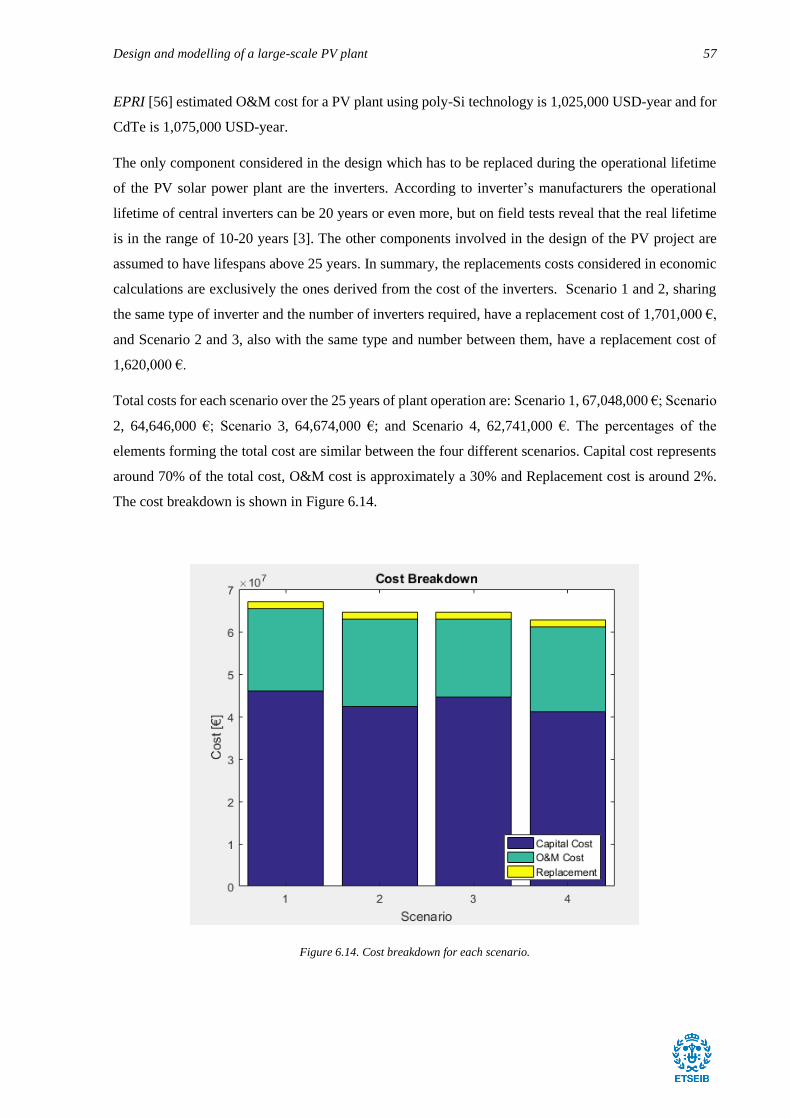
Design and modelling of a large-scale PV plant 57
EPRI [56] estimated O&M cost for a PV plant using poly-Si technology is 1,025,000 USD-year and for
CdTe is 1,075,000 USD-year.
The only component considered in the design which has to be replaced during the operational lifetime
of the PV solar power plant are the inverters. According to inverter’s manufacturers the operational
lifetime of central inverters can be 20 years or even more, but on field tests reveal that the real lifetime
is in the range of 10-20 years [3]. The other components involved in the design of the PV project are
assumed to have lifespans above 25 years. In summary, the replacements costs considered in economic
calculations are exclusively the ones derived from the cost of the inverters. Scenario 1 and 2, sharing
the same type of inverter and the number of inverters required, have a replacement cost of 1,701,000 €,
and Scenario 2 and 3, also with the same type and number between them, have a replacement cost of
1,620,000 €.
Total costs for each scenario over the 25 years of plant operation are: Scenario 1, 67,048,000 €; Scenario
2, 64,646,000 €; Scenario 3, 64,674,000 €; and Scenario 4, 62,741,000 €. The percentages of the
elements forming the total cost are similar between the four different scenarios. Capital cost represents
around 70% of the total cost, O&M cost is approximately a 30% and Replacement cost is around 2%.
The cost breakdown is shown in Figure 6.14.
Figure 6.14. Cost breakdown for each scenario.

The levelized Cost of Energy (LCOE) obtained for each of the scenarios are shown in Table 6.10:
Table 6.10. LCOE values obtained for each scenario.
Scenario 1 Scenario 2 Scenario 3 Scenario 4
LCOE [c€/kWh] 3.3284 3.1154 3.3303 3.1160
The LCOE obtained in Scenario 1 and 3 is very similar between both scenarios, these two scenarios are
sharing the same PV module technology, but the inverter used is different. The similarity between both
LCOE is caused due to the total cost and AEP is higher in Scenario 1, in the same manner these two
factors are smaller in Scenario 3 following the same tendency. Total cost in Scenario 1 is 4% higher
than in Scenario 3, as well as AEP in Scenario 1 is 4% higher than in Scenario 3. The same occurs
between Scenario 2 and 4 where the LCOE are very similar between them.
Looking at literature different values of LCOE can be found. The diversity between different values can
be caused due to the year of publication, country or technology being considered in the project.
According to Solar Bankability [54] in 2016 the estimated LCOE for utility-scale power plants is in the
range from 5.2 c€/kWh to 7.8 c€/kWh, these values are significantly different from the values obtained
in calculations. This difference can be caused due to a reduction of the cost associated with PV systems
in the recent years and with an improvement of the modules efficiency. NREL [50] in 2017 makes a
differentiation of LCOE values depending on the zone of installation. E.g. for a utility-scale one-axis
tracking PV plant in Phoenix the LCOE is estimated in 3.0 c€/kWh. According to PV Magazine [57],
citing Fraunhofer ISE, LCOE in 2018 ranges from 3.71 c€/kWh to 11.54 c€/kWh in Germany. In
summary, the values calculated for the different scenarios are consistent with the values found in
literature, but they will be in the lower range of the values observed.
The economic viability of the PV project is evaluated by means of calculating Net Present Value (NPV)
and Internal Rate of Return (IRR). The revenues of the PV plant are calculated by multiplying AEP by
the selling price of electricity. Since FITs and other financial support schemes have been eliminated in
Spain (see section 4.1. SUPPORT SCHEMES IN SPAIN for more details), PV solar power plants have
to sell their energy in the electricity wholesales market. The price of the electricity in the Spanish market
presents a high volatility, making challenging to make a prediction of the electricity price for a 25 years
project. For practical reasons a constant electricity price of 0.12 €/kWh is assumed during calculations.
This price is based on the former Spanish FIT for ground-mounted installations before its cancellation
[58]. Discount rate estimated for the calculations is 8%. Table 6.11 shows NPV and IRR obtained for
each of the scenarios analysed:

Design and modelling of a large-scale PV plant 59
Table 6.11. NPV and IRR values obtained for each scenario.
Scenario 1 Scenario 2 Scenario 3 Scenario 4
NPV [k€] 44,686 50,475 43,046 48,964
IRR [%] 19 21 19 21
For a positive value of NPV the project can be accepted because the investment will generate benefits
above the required rentability. The NPV of all different scenarios is calculated considering a discount
rate of 8%. The scenario with the highest NPV, thus the scenario with the highest potential benefits it is
Scenario 2 with an NPV of 50,475 k€. However, all the scenarios analysed have the potential to be
accepted due to a positive NPV.
IRR can also be used as a rentability indicator for a project. For a positive value of IRR, the project can
be economically accepted. For the case of the scenarios analysed all of them have a positive IRR. The
scenarios with the highest IRR are Scenario 2 and Scenario 4 with an IRR of 14% both.
Based on the results obtained of these two economic indicators, it can be asserted that the scenarios with
the highest economic viability are the scenarios using CdTe thin-film technology (Scenario 2 and 4).
Both scenarios present higher NPV and IRR than the scenarios using poly-Si technology. By looking at
NPV, the inverters used in Scenarios 1 and 2 seems to have a better economic impact on the project.
6.3.2. Other Results
Table 6.12 shows the results of other parameters calculated for all the scenarios analysed. These results
obtained help to understand the behaviour of the PV plant and permit to make comparisons between
different scenarios in order to observe which is the best configuration.
Table 6.12. Obtained values for: Ground Coverage Ratio (GCR), Performance ratio (PR), Capacity Factor (CF) and Specific
Yield (YieldSP).
Scenario 1 Scenario 2 Scenario 3 Scenario 4 GCR [%] 20.33 21.42 20.35 21.44
PR [%] 78.28 79.73 78.17 79.62
CF [%] 17.44 17.76 17.42 17.74
Yieldsp [kWh/kWp] 1,527.6 1,555.9 1,525.6 1,553.9
GCR calculated for all the scenarios is around 20%. The scenarios using thin-films have a higher GCR
than scenarios using poly-Si modules. These values obtained are just indicative values to see how the
surface of the PV plant is distributed. GCR calculated does not consider the optimum inter-row spacing
between modules in order to decrease the shading effect caused by the tilt angle. PR is a quality indicator,
which helps to compare different systems with different installed power. The scenario with the highest

PR is Scenario 2 with 79.73%, however all the scenarios have PR close to 80%. According to IFC [3] a
typical performance ratio for well-designed PV plant should be in the range between 77% and 86%. CF
expresses the ratio of the actual energy output of the PV plant over a year and its output if it had operated
at nominal power during a year. The scenario with the highest CF is also Scenario 2 with 17.76%, but
all the scenarios present a similar CF. According to IFC [3] a capacity factor of 16% would be typical
value for a PV plant located in southern Spain. YieldSP is the total annual energy generated over the total
capacity installed, it can be seen also as the number of hours which the PV plant is operating at its
nominal power. The scenario with the highest YieldSP is Scenario 2, with the values of the other scenarios
being similar.

Design and modelling of a large-scale PV plant 61
7. RESULTS COMPARISON USING PV MODELLING
SOFTWARE
In order to compare the results obtained in the calculations, the design of a 50 MW PV power plant is
implemented in different modelling software. In this chapter is shown the methodology of designing
and the results obtained with PVSYST and System Advisor Model (SAM).
7.1. PVsyst MODELLING
7.1.1. Pre-Design Phase
Before designing the entire system in PVsyst a pre-design phase is done in order to obtain the magnitude
of the design values. The steps followed during the pre-design phase are the following:
- Site and meteorology: Due to this first pre-design is not a meticulous phase, Barcelona is chosen
as the location of PV power plant installation (the nearest available meteorological database).
The real location of the PV plant was not able in the initial database, but for further modelling
steps it will be added.
- System definition: The nominal power of the system is set at 50 MW, active area and annual
yield are automatically calculated. Regarding the optimum tilt angle and azimuth, PVsyst find
the optimum values (Figure 7.1) depending on the location previously selected. For an
optimization on annual yield, optimum tilt angle is defined in 30º and azimuth angle in 0º (south
oriented).
Figure 7.1. Collector plane orientation PVsyst’s screen capture.
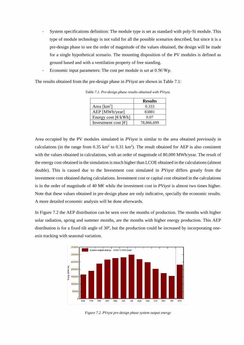
- System specifications definition: The module type is set as standard with poly-Si module. This
type of module technology is not valid for all the possible scenarios described, but since it is a
pre-design phase to see the order of magnitude of the values obtained, the design will be made
for a single hypothetical scenario. The mounting disposition of the PV modules is defined as
ground based and with a ventilation property of free standing.
- Economic input parameters: The cost per module is set at 0.5€/Wp.
The results obtained from the pre-design phase in PVsyst are shown in Table 7.1:
Table 7.1. Pre-design phase results obtained with PVsyst.
Results
Area [km2] 0.333
AEP [MWh/year] 83881
Energy cost [€/kWh] 0.07
Investment cost [€] 78,866,699
Area occupied by the PV modules simulated in PVsyst is similar to the area obtained previously in
calculations (in the range from 0.35 km2 to 0.31 km2). The result obtained for AEP is also consistent
with the values obtained in calculations, with an order of magnitude of 80,000 MWh/year. The result of
the energy cost obtained in the simulation is much higher than LCOE obtained in the calculations (almost
double). This is caused due to the Investment cost simulated in PVsyst differs greatly from the
investment cost obtained during calculations. Investment cost or capital cost obtained in the calculations
is in the order of magnitude of 40 M€ while the investment cost in PVsyst is almost two times higher.
Note that these values obtained in pre-design phase are only indicative, specially the economic results.
A more detailed economic analysis will be done afterwards.
In Figure 7.2 the AEP distribution can be seen over the months of production. The months with higher
solar radiation, spring and summer months, are the months with higher energy production. This AEP
distribution is for a fixed tilt angle of 30º, but the production could be increased by incorporating one-
axis tracking with seasonal variation.
Figure 7.2. PVsyst pre-design phase system output energy

Design and modelling of a large-scale PV plant 63
The investment cost (Table 7.1) can be divided in the cost of the different components or services
involved in the PV plant design. Again, the values obtained during the simulation done in PVsyst are
distant from the values obtained in the economic calculations based on estimations. Breakdown of the
capital cost calculated during pre-design phase is shown in Table 7.2:
Table 7.2. PVsyst pre-design phase breakdown capital cost.
Cost [€]
Module 25,000,000
Supports 32,000,000
Inverter(s) and wiring 10,000,000
Transport/Mounting 11,886,699
TOTAL 78,886,699
7.1.2. Design Phase
Once the pre-design phase is done with the corresponding results obtained and they are analysed, the
final design of the PV power plant project is made. In the final design phase with PVsyst the four
different scenarios, with their characteristics, are going to be analysed separately. The steps to calculate
the PV solar power plant final design are shown below:
- Location and climate data: In this case, to make the calculation more accurate a location closer
to the real location of the PV project is added to the meteorological database. The closer possible
location selected is Lleida (around 30 km to l’Albagés) and the data obtained for further
simulations is shown in Figure 7.3.
Figure 7.3. Global and diffuse irradiance, temperature and wind velocity in Lleida.
- PV modules orientation definition: For this simulation, the PV modules are determined as one-
axis tracking with seasonal variation. The tilt angle of the PV modules installed is going to be

different for winter and summer. In Figure 7.4 the optimum tilt angle for both seasons and the
azimuth angle can be seen.
Figure 7.4. PV modules orientation in PVsyst design phase
- System definition: This step is made for each of the different scenarios being studied. The
selection of module is set depending on the scenario as well as the inverter selected. The number
of PV modules in series, in parallel and the number of inverters needed for each of the scenarios
is calculated by PVsyst calculation tool by entering the parameter of design capacity.
- Detailed losses definition: Thermal losses are not modified respect to their default value for
outdoors systems with free ventilation. Ohmic losses are neither modified respect to their default
value. Mismatch losses are set at 2%, same value as considered in the calculations. Losses to
the dirt and dust deposited on the module surface are set at 6.9%. Losses named Incidence Angle
Modifier (IAM) are not changed respect to the default values, these losses are not considerate
during calculations. Auxiliaries energy losses are not considered in the simulation. Ageing of
the PV modules is not considered in the simulation. And the availability factor of the system is
set in 99.5% (same value as the calculations).
- Other input parameters: Far shadings are not modified respect to default values and near
shadings are not considered in the simulation. The system is not restricted with grid power
limitations.
- Economic evaluation: Cost of the components and services involved in the PV plant project will
be added depending on the scenario analysed. Except for the cost of BOS structures, BOS
electrical, civil work, cost of the land and cost of transformers. Table 7.3 shows the cost of the
components considered in the initial investment:
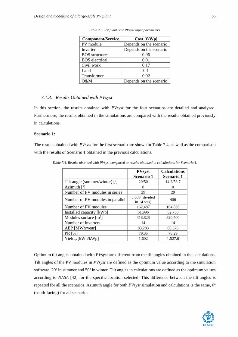
Design and modelling of a large-scale PV plant 65
Table 7.3. PV plant cost PVsyst input parameters.
Component/Service Cost [€/Wp]
PV module Depends on the scenario
Inverter Depends on the scenario
BOS structures 0.06
BOS electrical 0.01
Civil work 0.17
Land 0.1
Transformer 0.02
O&M Depends on the scenario
7.1.3. Results Obtained with PVsyst
In this section, the results obtained with PVsyst for the four scenarios are detailed and analysed.
Furthermore, the results obtained in the simulations are compared with the results obtained previously
in calculations.
Scenario 1:
The results obtained with PVsyst for the first scenario are shown in Table 7.4, as well as the comparison
with the results of Scenario 1 obtained in the previous calculations.
Table 7.4. Results obtained with PVsyst compared to results obtained in calculations for Scenario 1.
PVsyst
Scenario 1
Calculations
Scenario 1
Tilt angle (summer/winter) [º] 20/50 14.2/53.7
Azimuth [º] 0 0
Number of PV modules in series 29 29
Number of PV modules in parallel 5,603 (divided
in 14 sets) 406
Number of PV modules 162,487 164,836
Installed capacity [kWp] 51,996 52,750
Modules surface [m2] 318,828 320,500
Number of inverters 14 14
AEP [MWh/year] 83,283 80,576
PR [%] 79.35 78.29
Yieldsp [kWh/kWp] 1,602 1,527.6
Optimum tilt angles obtained with PVsyst are different from the tilt angles obtained in the calculations.
Tilt angles of the PV modules in PVsyst are defined as the optimum value according to the simulation
software, 20º in summer and 50º in winter. Tilt angles in calculations are defined as the optimum values
according to NASA [42] for the specific location selected. This difference between the tilt angles is
repeated for all the scenarios. Azimuth angle for both PVsyst simulation and calculations is the same, 0º
(south-facing) for all scenarios.

The number of PV modules connected in series obtained in the simulation are the same as the number
of PV modules in series obtained in the calculations (29 PV modules in series). The number of parallel
branches obtained in the simulation is 5,603 but dividing the number of parallel branches by the number
of inverters, the result obtained is the number of PV modules connected in parallel per PV set which is
400. There is a significant difference between this number and the number obtained during calculations
(406 PV modules in parallel per PV set). This difference is caused due to significant difference in the
final number of PV modules in the system, 162,487 PV modules in the simulation compared to 164,836
PV modules in the calculation. The number of inverters required both in calculations and simulation is
the same, 14 inverters.
The difference in the installed capacity are caused due to differences in the total number of PV modules
installed. In the simulation, total number of PV modules is around 1.5% lower than the total number of
PV modules obtained in the calculations. The lower number of PV modules installed in the simulation
has impact on a lower capacity installed in the system, 1.5% lower compared to the capacity installed in
calculations. The lower number of PV modules and the lower installed capacity obtained in PVsyst is in
accordance with a lower modules surface compared to the results obtained in the calculations.
AEP for Scenario 1 obtained in PVsyst simulation is 83,283 MWh/year, a higher value if it is compared
with the result obtained in the calculation which is 80,576 MWh/year. The difference in energy produced
over a year is around 3.4% higher in the simulation compared to the result obtained in the calculation.
This difference can be caused by the following reasons: 1) Differences in the methodology and formulas
used. 2) The performance of the PV modules and inverters in PVsyst is based on a combination of the
data from the manufacturer and experimental data, while the technical data considered in the calculation
is entirely based on manufacturer’s information. 3) Meteorological data used is from different sources
and could have repercussions on the results.
PR and Specific Yield (YieldSP) obtained are similar for both methodologies of calculation, with both
parameters higher for the results obtained with PVsyst. The differences in these two values can be also
caused by the factors listed above.

Design and modelling of a large-scale PV plant 67
Scenario 2:
The results obtained with PVsyst for the second scenario are shown in Table 7.5, as well as the
comparison with the results of Scenario 2 obtained in the previous calculations.
Table 7.5. Results obtained with PVsyst compared to results obtained in calculations for Scenario 2.
PVsyst
Scenario 2
Calculations
Scenario 2
Tilt angle (summer/winter) [º] 20/50 14.2/53.7
Azimuth [º] 0 0
Number of PV modules in series 15 16
Number of PV modules in parallel 32,121 (divided
into 14 sets) 2,165
Number of PV modules 481,815 484,960
Installed capacity [kWp] 53,000 53,350
Modules surface [m2] 346,907 349,200
Number of inverters 14 14
AEP [MWh/year] 90,176 83,001
PR [%] 84.29 79.76
Yieldsp [kWh/kWp] 1,701 1,555.9
The similarities and the differences between PVsyst simulation and calculations regarding optimum tilt
angle and azimuth are the same as the ones explained for Scenario 1.
In this scenario the number of PV modules in series does not match between the results obtained in
simulation (15 PV modules in series) and results obtained in calculations (16 PV modules in series).
This difference between values is caused due to differences in criteria for sizing the PV set and
differences in assess the maximum admissible voltage of the inverter. For the case of the results obtained
in the calculations, the inverter is considered to withstand more input voltage than for PVsyst results.
The number of PV modules in parallel is also different comparing the two different methodologies of
calculation. Total number of parallel branches obtained in the simulation is 32,121 with approximately
2,294 PV modules in parallel per PV set. The difference can be caused do to the same reasons of the
difference between the number of modules in series. The number of inverters obtained is the same for
simulation and calculations. Due to differences in the number of modules in series and the modules in
parallel between the two methodologies of calculation, the total number of PV modules obtained in the
system is also different. For this scenario, the number of PV modules is higher for the calculation,
484,960 modules compared to 481,815 in the simulation. The difference between the number of PV
modules between both calculation methodologies is around 0.7%. The difference in the number of
modules is also directly linked with the difference in the installed capacity obtained for each calculation
methodology. Installed capacity in calculations is 0.7% higher than the obtained value for the simulation
in PVsyst.

Surface area occupied by the PV modules is higher in the calculations because the number of PV
modules required is also higher.
AEP obtained for Scenario 2 is higher for the results obtained in the simulation. AEP in simulation is
90,176 MWh/year while the AEP obtained in calculations is 83,001 MWh/year, around 8.6% lower
compared with the simulation. AEP in simulation is higher despite total installed capacity in calculations
is higher compared to the result obtained in simulation, the following factors can be the responsible of
this situation: 1) Losses considered in calculations are higher compared to the losses considered in the
simulation. 2) Differences in the methodology and formulas used. 3) The performance of the
components can be considered different in the calculations and PVsyst simulation. 4) Meteorological
data used is from different sources. As PR and Specific Yield are PV plant performance indicators they
are also higher for the results obtained with PVsyst which has higher AEP with lower installed capacity.
The simulation done for Scenario 2 in PVsyst shows the following warning message: “The power of the
inverter is slightly undersized”. This circumstance leads to high overload losses, in the limit of the
acceptable values (3% or higher overload losses will be outside of the admissible limit). Overload losses
obtained in this scenario are 2.5%. These losses are caused do to the inverters cannot withstand all the
power output from the PV sets and the power output from these is curtailed in order to not to exceed the
power input limit of the inverter.
Scenario 3:
The results obtained with PVsyst for the third scenario are shown in Table 7.6, as well as the comparison
with the results of Scenario 3 obtained in the previous calculations.
Table 7.6. Results obtained with PVsyst compared to results obtained in calculations for Scenario 3.
PVsyst
Scenario 3
Calculations
Scenario 3
Tilt angle (summer/winter) [º] 20/50 14.2/53.7
Azimuth [º] 0 0
Number of PV modules in series 18 18
Number of PV modules in parallel 8,767 (divided
into 22 sets) 442
Number of PV modules 157,806 159,120
Installed capacity [kWp] 50,498 50,920
Modules surface [m2] 309,643 309,400
Number of inverters 22 20
AEP [MWh/year] 82,829 77,679
PR [%] 81.26 78.17
Yieldsp [kWh/kWp] 1,640 1,525.6

Design and modelling of a large-scale PV plant 69
The number of PV modules in series is the same for the simulation and the calculations. The total number
of parallel branches obtained in PVsyst simulation is 8,767 which divided by the number of inverters the
result is approximately 399 PV modules in parallel per PV set. There is a significant difference between
the number of PV modules in parallel obtained in simulation compared with the number obtained in
calculations. This difference can be due to differences in the methodology of calculation. Due to the
difference in the number of PV modules in parallel per PV set, the total number of PV modules is also
different. For this scenario the total number of PV panels is higher in the calculations, 159,120 compared
to 157,806 in the simulation. The higher number of modules in the calculations has impact on a higher
installed capacity compared with the installed capacity obtained in the simulation. The number of
modules obtained in calculations is around 0.8% higher than the number of modules in simulation, as
well as the installed capacity in calculation is 0.8% higher than the installed capacity in simulation.
In this scenario, the number of inverters in calculations and simulation is not the same. The number of
required inverters in simulation is 22, while the number of inverters obtained in calculations is 20. This
disparity occurs due to differences in the methodology of calculation. According to results obtained in
calculations, a lower number of inverters can withstand a higher number of PV modules compared to
the results obtained in the simulation.
The results obtained regarding the surface occupied for the PV modules are not consistent. Higher
surface is obtained in simulation where the number of PV modules is lower compared to result obtained
in calculations. The inconsistency is caused to the surface area per PV module considered in the
calculations is different compared to the one considered in PVsyst.
As it happens in Scenario 2, AEP is higher for the simulation in PVsyst, despite the total installed
capacity is higher in results obtained in calculations. AEP calculated in simulation is around 6.6% higher
compared to AEP in calculations. The factors which can make the AEP higher in simulation are the
same factors which are explained for Scenario 2. Performance ratio and Specific Yield are also higher
for the results obtained in the simulation.
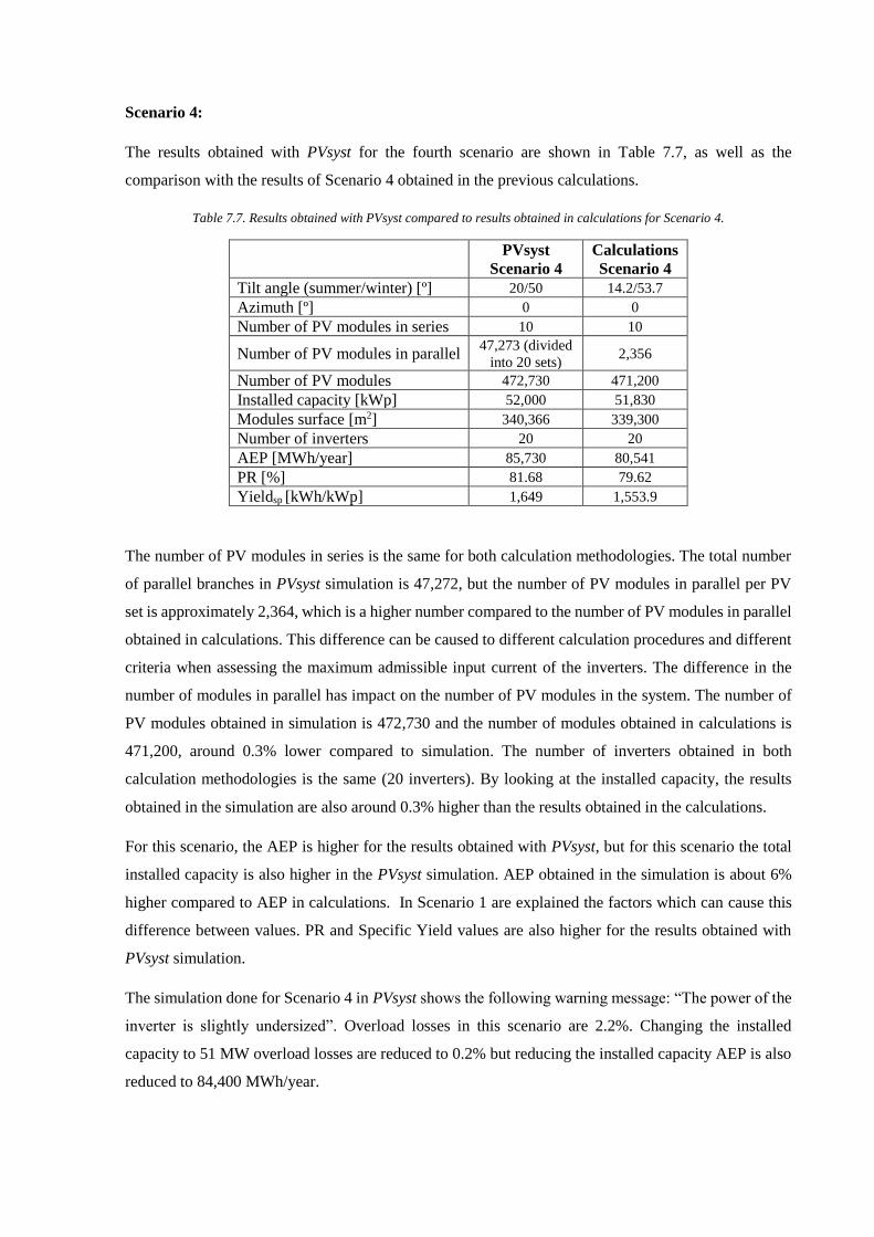
Scenario 4:
The results obtained with PVsyst for the fourth scenario are shown in Table 7.7, as well as the
comparison with the results of Scenario 4 obtained in the previous calculations.
Table 7.7. Results obtained with PVsyst compared to results obtained in calculations for Scenario 4.
PVsyst
Scenario 4
Calculations
Scenario 4
Tilt angle (summer/winter) [º] 20/50 14.2/53.7
Azimuth [º] 0 0
Number of PV modules in series 10 10
Number of PV modules in parallel 47,273 (divided
into 20 sets) 2,356
Number of PV modules 472,730 471,200
Installed capacity [kWp] 52,000 51,830
Modules surface [m2] 340,366 339,300
Number of inverters 20 20
AEP [MWh/year] 85,730 80,541
PR [%] 81.68 79.62
Yieldsp [kWh/kWp] 1,649 1,553.9
The number of PV modules in series is the same for both calculation methodologies. The total number
of parallel branches in PVsyst simulation is 47,272, but the number of PV modules in parallel per PV
set is approximately 2,364, which is a higher number compared to the number of PV modules in parallel
obtained in calculations. This difference can be caused to different calculation procedures and different
criteria when assessing the maximum admissible input current of the inverters. The difference in the
number of modules in parallel has impact on the number of PV modules in the system. The number of
PV modules obtained in simulation is 472,730 and the number of modules obtained in calculations is
471,200, around 0.3% lower compared to simulation. The number of inverters obtained in both
calculation methodologies is the same (20 inverters). By looking at the installed capacity, the results
obtained in the simulation are also around 0.3% higher than the results obtained in the calculations.
For this scenario, the AEP is higher for the results obtained with PVsyst, but for this scenario the total
installed capacity is also higher in the PVsyst simulation. AEP obtained in the simulation is about 6%
higher compared to AEP in calculations. In Scenario 1 are explained the factors which can cause this
difference between values. PR and Specific Yield values are also higher for the results obtained with
PVsyst simulation.
The simulation done for Scenario 4 in PVsyst shows the following warning message: “The power of the
inverter is slightly undersized”. Overload losses in this scenario are 2.2%. Changing the installed
capacity to 51 MW overload losses are reduced to 0.2% but reducing the installed capacity AEP is also
reduced to 84,400 MWh/year.
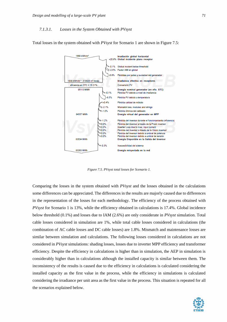
Design and modelling of a large-scale PV plant 71
7.1.3.1. Losses in the System Obtained with PVsyst
Total losses in the system obtained with PVsyst for Scenario 1 are shown in Figure 7.5:
Figure 7.5. PVsyst total losses for Scenario 1.
Comparing the losses in the system obtained with PVsyst and the losses obtained in the calculations
some differences can be appreciated. The differences in the results are majorly caused due to differences
in the representation of the losses for each methodology. The efficiency of the process obtained with
PVsyst for Scenario 1 is 13%, while the efficiency obtained in calculations is 17.4%. Global incidence
below threshold (0.1%) and losses due to IAM (2.6%) are only considerate in PVsyst simulation. Total
cable losses considered in simulation are 1%, while total cable losses considered in calculations (the
combination of AC cable losses and DC cable losses) are 1.8%. Mismatch and maintenance losses are
similar between simulation and calculations. The following losses considered in calculations are not
considered in PVsyst simulations: shading losses, losses due to inverter MPP efficiency and transformer
efficiency. Despite the efficiency in calculations is higher than in simulation, the AEP in simulation is
considerably higher than in calculations although the installed capacity is similar between them. The
inconsistency of the results is caused due to the efficiency in calculations is calculated considering the
installed capacity as the first value in the process, while the efficiency in simulations is calculated
considering the irradiance per unit area as the first value in the process. This situation is repeated for all
the scenarios explained below.

Total losses in the system obtained with PVsyst for Scenario 2 are shown in Figure 7.6:
Figure 7.6. PVsyst total losses for Scenario 2.
The similarities and differences between the losses obtained in PVsyst simulation and the losses obtained
in calculations for Scenario 2 are similar to those explained for Scenario 1. The main differences
between the results obtained in both scenarios are the temperature losses, in this scenario temperature
losses are 3.9%. Much lower value than temperature losses in Scenario 1 which are 8.5%. This great
difference is caused due to different module technology employed. The difference in the efficiency of
the process is not compared between simulation and calculations due to the inconsistency of the results
(explained previously in Scenario 1).

Design and modelling of a large-scale PV plant 73
Total losses in the system obtained with PVsyst for Scenario 3 are shown in Figure 7.7:
Figure 7.7. PVsyst total losses for Scenario 3.
The similarities and differences between the losses obtained in PVsyst simulation and the losses obtained
in calculations for Scenario 3 are similar to those explained in the previous scenarios. The main
difference is that for this scenario temperature losses are 5.4%. Once again, the efficiency of the process
cannot be compared with the efficiency obtained in calculations for this scenario due to differences in
the interpretation between both methodologies.

Total losses in the system obtained with PVsyst for Scenario 4 are shown in Figure 7.8:
Figure 7.8. PVsyst total losses for Scenario 4.
The similarities and differences between the losses obtained in PVsyst simulation and the losses obtained
in calculations for Scenario 4 are similar to those explained for the previous scenarios. With the only
exception of the temperature losses which are 6.2% in this scenario. The efficiency obtained in
calculations cannot be compared to the efficiency of the process in simulation due to calculation
differences.
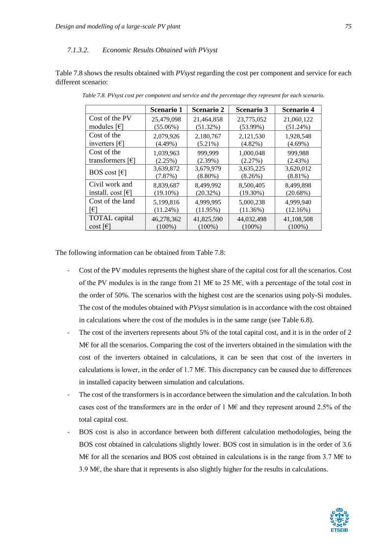
Design and modelling of a large-scale PV plant 75
7.1.3.2. Economic Results Obtained with PVsyst
Table 7.8 shows the results obtained with PVsyst regarding the cost per component and service for each
different scenario:
Table 7.8. PVsyst cost per component and service and the percentage they represent for each scenario.
Scenario 1 Scenario 2 Scenario 3 Scenario 4
Cost of the PV
modules [€] 25,479,098
(55.06%)
21,464,858
(51.32%)
23,775,052
(53.99%)
21,060,122
(51.24%)
Cost of the
inverters [€] 2,079,926
(4.49%)
2,180,767
(5.21%)
2,121,530
(4.82%)
1,928,548
(4.69%)
Cost of the
transformers [€] 1,039,963
(2.25%)
999,999
(2.39%)
1,000,048
(2.27%)
999,988
(2.43%)
BOS cost [€] 3,639,872
(7.87%)
3,679,979
(8.80%)
3,635,225
(8.26%)
3,620,012
(8.81%)
Civil work and
install. cost [€] 8,839,687
(19.10%)
8,499,992
(20.32%)
8,500,405
(19.30%)
8,499,898
(20.68%)
Cost of the land
[€] 5,199,816
(11.24%)
4,999,995
(11.95%)
5,000,238
(11.36%)
4,999,940
(12.16%)
TOTAL capital
cost [€] 46,278,362
(100%)
41,825,590
(100%)
44,032,498
(100%)
41,108,508
(100%)
The following information can be obtained from Table 7.8:
- Cost of the PV modules represents the highest share of the capital cost for all the scenarios. Cost
of the PV modules is in the range from 21 M€ to 25 M€, with a percentage of the total cost in
the order of 50%. The scenarios with the highest cost are the scenarios using poly-Si modules.
The cost of the modules obtained with PVsyst simulation is in accordance with the cost obtained
in calculations where the cost of the modules is in the same range (see Table 6.8).
- The cost of the inverters represents about 5% of the total capital cost, and it is in the order of 2
M€ for all the scenarios. Comparing the cost of the inverters obtained in the simulation with the
cost of the inverters obtained in calculations, it can be seen that cost of the inverters in
calculations is lower, in the order of 1.7 M€. This discrepancy can be caused due to differences
in installed capacity between simulation and calculations.
- The cost of the transformers is in accordance between the simulation and the calculation. In both
cases cost of the transformers are in the order of 1 M€ and they represent around 2.5% of the
total capital cost.
- BOS cost is also in accordance between both different calculation methodologies, being the
BOS cost obtained in calculations slightly lower. BOS cost in simulation is in the order of 3.6
M€ for all the scenarios and BOS cost obtained in calculations is in the range from 3.7 M€ to
3.9 M€, the share that it represents is also slightly higher for the results in calculations.
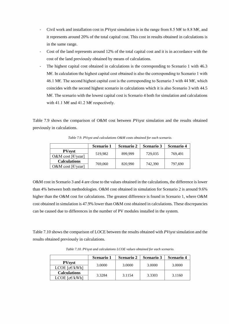
- Civil work and installation cost in PVsyst simulation is in the range from 8.5 M€ to 8.8 M€, and
it represents around 20% of the total capital cost. This cost in results obtained in calculations is
in the same range.
- Cost of the land represents around 12% of the total capital cost and it is in accordance with the
cost of the land previously obtained by means of calculations.
- The highest capital cost obtained in calculations is the corresponding to Scenario 1 with 46.3
M€. In calculation the highest capital cost obtained is also the corresponding to Scenario 1 with
46.1 M€. The second highest capital cost is the corresponding to Scenario 3 with 44 M€, which
coincides with the second highest scenario in calculations which it is also Scenario 3 with 44.5
M€. The scenario with the lowest capital cost is Scenario 4 both for simulation and calculations
with 41.1 M€ and 41.2 M€ respectively.
Table 7.9 shows the comparison of O&M cost between PVsyst simulation and the results obtained
previously in calculations.
Table 7.9. PVsyst and calculations O&M costs obtained for each scenario.
Scenario 1 Scenario 2 Scenario 3 Scenario 4
PVsyst 519,982 899,999 729,035 769,491
O&M cost [€/year]
Calculations 769,060 820,990 742,390 797,690
O&M cost [€/year]
O&M cost in Scenario 3 and 4 are close to the values obtained in the calculations, the difference is lower
than 4% between both methodologies. O&M cost obtained in simulation for Scenario 2 is around 9.6%
higher than the O&M cost for calculations. The greatest difference is found in Scenario 1, where O&M
cost obtained in simulation is 47.9% lower than O&M cost obtained in calculations. These discrepancies
can be caused due to differences in the number of PV modules installed in the system.
Table 7.10 shows the comparison of LOCE between the results obtained with PVsyst simulation and the
results obtained previously in calculations.
Table 7.10. PVsyst and calculations LCOE values obtained for each scenario.
Scenario 1 Scenario 2 Scenario 3 Scenario 4
PVsyst 3.0000 3.0000 3.0000 3.0000
LCOE [c€/kWh]
Calculations 3.3284 3.1154 3.3303 3.1160
LCOE [c€/kWh]

Design and modelling of a large-scale PV plant 77
LCOE calculated by means of PVsyst is the same for all the scenarios (3 c€/kWh). The scenario with
highest similarity of values between simulated and calculated is Scenario 2, where LCOE obtained in
simulation is 3.8% lower than LCOE obtained in calculations. The scenario with the highest difference
between LCOE values is Scenario 3, where LCOE obtained in simulation is 11% lower than LCOE
obtained in calculations. In summary, the results obtained in calculations regarding the LCOE do not
differ in excess from the values obtained in the simulation. The lower LCOE values obtained in
simulations comparing with the LCOE values obtained in the calculations are caused due to a higher
AEP with a similar total cost.
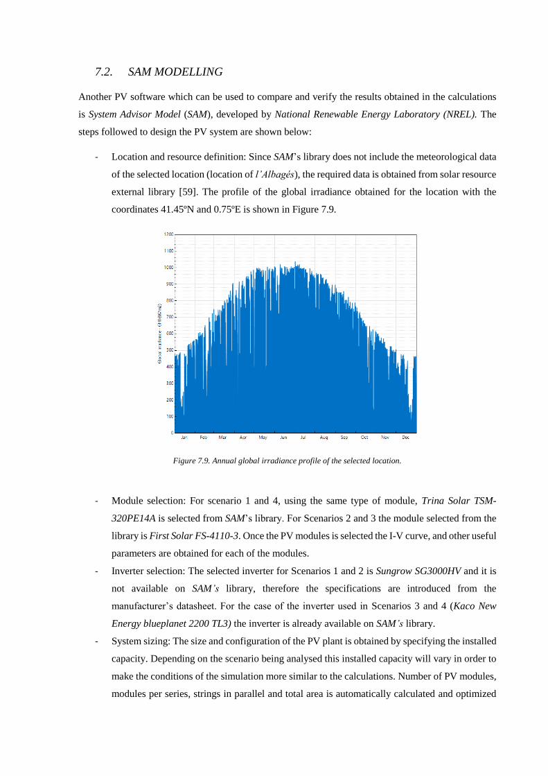
7.2. SAM MODELLING
Another PV software which can be used to compare and verify the results obtained in the calculations
is System Advisor Model (SAM), developed by National Renewable Energy Laboratory (NREL). The
steps followed to design the PV system are shown below:
- Location and resource definition: Since SAM’s library does not include the meteorological data
of the selected location (location of l’Albagés), the required data is obtained from solar resource
external library [59]. The profile of the global irradiance obtained for the location with the
coordinates 41.45ºN and 0.75ºE is shown in Figure 7.9.
Figure 7.9. Annual global irradiance profile of the selected location.
- Module selection: For scenario 1 and 4, using the same type of module, Trina Solar TSM-
320PE14A is selected from SAM’s library. For Scenarios 2 and 3 the module selected from the
library is First Solar FS-4110-3. Once the PV modules is selected the I-V curve, and other useful
parameters are obtained for each of the modules.
- Inverter selection: The selected inverter for Scenarios 1 and 2 is Sungrow SG3000HV and it is
not available on SAM’s library, therefore the specifications are introduced from the
manufacturer’s datasheet. For the case of the inverter used in Scenarios 3 and 4 (Kaco New
Energy blueplanet 2200 TL3) the inverter is already available on SAM’s library.
- System sizing: The size and configuration of the PV plant is obtained by specifying the installed
capacity. Depending on the scenario being analysed this installed capacity will vary in order to
make the conditions of the simulation more similar to the calculations. Number of PV modules,
modules per series, strings in parallel and total area is automatically calculated and optimized
Design and modelling of a large-scale PV plant 79
taking into account weather conditions, modules selected, inverters selected and the desired
array size.
- Tracking and orientation: The tracking system of the PV power plant is defined as seasonal tilt;
where the tilt angle during winter months is set at 53.7º and the tilt angle during summer season
is set at 14.2º (same values as used in calculations). Azimuth angle is defined fixed south-facing
180º (depending on the reference is 0º). By introducing these values and the install capacity of
the plant, the total area occupied by the PV modules is automatically calculated.
- String configuration: this parameter is not defined because the configuration of the modules in
the PV plant has not been analysed in calculations.
- Shading and snow losses: shading losses have been kept with default values from SAM, due to
there is not available a 3D model of the PV plant to study in detail that type of losses. Snow
losses are not considered since the location selected has not a high risk of snowing.
- Losses: Soiling losses, losses due to the dirt deposited on the PV module surface, are set at 6.9%
for every month of operation as literature [37] suggest (same as soiling losses in calculations).
DC wiring losses are kept with default values applied for central inverters. AC wiring losses are
assumed in 1% and the transformer losses are not considered. Curtailment and availability is
defined as constant losses of 0.5% (same as maintenance losses considered in calculations).
- Financial parameters: Capital cost is introduced in SAM interface depending on the scenario
analysed. The cost in $/kW is calculated by dividing the capital cost obtained in calculations by
total installed capacity. The same procedure is followed to calculate O&M cost. Fixed charge
rate is not modified from the default value provided by SAM.

7.2.1. Results Obtained with SAM
Once the system is modelled as explained above, the results obtained with SAM can be compared with
the results obtained in the calculations. Table 7.11 shows the results obtained with SAM for each
scenario.
Table 7.11. Results obtained with SAM.
Scenario 1 Scenario 2 Scenario 3 Scenario 4
Tilt angle
(summer/winter) [º] 14.2/53.7 14.2/53.7 14.2/53.7 14.2/53.7
Azimuth [º] 180 180 180 180
No. of PV modules 164,749 485,712 159,024 471,609
No. of PV modules
in series 29 16 16 9
No. strings in
parallel 5,681 (divided
into 18 sets)
30,357
(divided into
18 sets)
9,939 (divided
into 25 sets
52,401
(divided into
26 sets)
Total module area
[m2] 319,613 327,755 308,506 339,558
Number of inverters 18 18 25 26
Capacity installed
[kWp] 52,748 53,349 50,915 51,780
AEP [MWh/year] 91,433 94,891 85,202 91,007
PR [%] 81 83 78 82
CF [%] 19.8 20.3 19.1 20.1
Ysp [kWh/kWp] 1,733 1,779 1,673 1,757
LCOE [c$/kWh] 7.14 6.52 7.39 6.55
The following information can be obtained from the comparison between the results obtained with SAM
and the results obtained in calculations:
- Tilt angle obtained in SAM simulation is 14.2º in summer and 53.7º in winter for all the scenarios
analysed. These values are not a result of an optimization process by means of a simulation, but
they are manually introduced by looking at the values obtained in the calculations. The same
happens with azimuth angle, which is 180º (south facing) for all the scenarios.
- For all the scenarios analysed the number of PV modules obtained in simulation is in
accordance, with slight variation, with the number of PV modules obtained in the calculations:
For Scenario 1 the number of PV modules obtained in the simulation is only a 0.05% lower than
the number obtained in the calculations; For Scenario 2, the number of modules obtained in

Design and modelling of a large-scale PV plant 81
simulation is 0.16% higher; For Scenario 3, number of modules obtained in simulation is 0.06%
lower. Finally, for Scenario 4, the number of modules in simulation is 0.08% higher.
- The number of modules in series is the same for the simulation and the calculations for Scenarios
1 and 2, these two scenarios are considered using the same type of inverter. But, there is a
difference of 1 module between simulation and calculations in Scenario 2 and 4, using the same
inverter between them.
- The comparison of the number of PV panels in parallel is done considering the number of
parallel branches per PV set. For Scenarios 1 and 2, using inverters Sungrow SG3000HV, the
difference between the number of PV modules in parallel per PV set obtained in calculations
and simulation is 29% for Scenario 1 and 28% for Scenario 2, being the results of calculations
higher. For Scenarios 3 and 4, using inverters Kaco new energy blueplanet 2200TL3, the
difference is not that great. The number of modules in parallel in Scenario 3 in simulation is
11% lower, and the number of modules in parallel in Scenario 4 is 17% lower.
- The number of inverters obtained in simulation is the same for Scenario 1 and 2 (18 inverters)
but comparing these number with the results obtained in calculations there is a difference of 4
inverters more for both scenarios. For Scenario 3 the result obtained in simulation is 5 inverters
more than in calculations, and for Scenario 4 the result obtained in simulation is 6 inverters
more than in the calculations.
- The capacity installed obtained in simulation is in accordance with the capacity installed in
calculations. Installed capacity obtained in simulation in all the scenarios is less than 0.1% lower
than the results obtained in calculations. The difference of the capacity installed between
simulation and calculations is caused due to the nominal power of the PV modules considered.
In the calculations the nominal power of the modules is obtained from manufacturer and the
nominal power of the PV modules in SAM is obtained with a combination of data from the
manufacturer and experimental data. The difference of the number of PV modules can be also
explained because of this circumstance.
- AEP obtained in the simulations present higher values than AEP obtained in calculations:
Scenario 1 in simulation is 13.5% higher than AEP in calculations; Scenario 2 has an AEP
obtained in simulation 14.3% higher; Scenario 3 is 9.7% higher; and Scenario 4 is 13% higher.
This can be caused due to lower losses considered in SAM’s simulation or discrepancies in the
calculations between both methodologies.
- PR obtained in the simulations are around 80% for all scenarios, being the PR obtained for
Scenario 2 the highest with 83%. The PR obtained in the calculations are slightly lower (around
79%), but the scenario with the highest PR is also Scenario 2 with 79.73%.
- CF obtained in the simulations are around 20%, and the highest CF is the corresponding to
Scenario 2 with 20.3%. CF obtained in the calculations are lower, these parameters are in the
order of 17.5% for all scenarios. The highest CF in calculations is also the corresponding to
Scenario 2 with 17.76%.
- Specific Yields obtained in simulations are higher than the ones obtained in calculations. The
scenario with the highest Yieldsp is Scenario 2 with 1,779 kWh/kWp. The scenario in
calculations with the highest Yieldsp is also Scenario 2 with 1,555.9 kWh/kWp.
- The scenario with the highest LCOE obtained in simulations is the corresponding to Scenario 3
with 7.39 c$/kWh, approximately 6 c€/kWh. The highest LCOE obtained in calculations is also
the corresponding to Scenario 3 with 3.3303 c€/kWh, but the difference between values
obtained in both methodologies is more than significant. The lowest LCOE obtained in
simulations is the corresponding to Scenario 2 with 6.52 c$/kWh, approximately 5.5 c€/kWh.
The scenario with the lowest LCOE in simulation is in accordance with the scenario with the
lowest LCOE in calculations, which it is also Scenario 2 with 3.1154 c€/kWh. In summary, the
difference between the LCOE results obtained in SAM and the results obtained in calculations
is remarkable, for all the scenarios analysed the LCOE obtained in simulations are more than
70% higher than the values obtained in calculations. This considerable difference regarding the
LCOE can be caused due to SAM obtain the value by means of using financial parameters which
are not used in the calculations.
- The losses obtained with SAM are similar for all the scenarios analysed (in Figure 7.10 it can be
seen the losses diagram for Scenario 2 as example). The most important losses obtained in the
simulations are: soiling, about 6.9% for all the scenarios; modules losses, 6.8% for poly-Si
modules and 4.3% for CdTe modules; mismatch losses, around 2% for all the scenarios; DC
wiring losses, around 2%; availability and curtailment (maintenance), 0.5%; losses due to
inverter efficiency, 1.3 % for Scenarios 1 and 2, 1.6% for Scenarios 3 and 4; AC wiring losses,
around 1% for all the scenarios. The process efficiency for Scenario 1 is 13.3%, for Scenario 2
is 12.6%, for Scenario 3 is 12.85% and for Scenario 4 is 12.5%. The efficiencies obtained in the
simulation are lower than those obtained in the calculations.

Design and modelling of a large-scale PV plant 83
Figure 7.10. Losses diagram obtained wit SAM for Scenario 2.

8. CONCLUSIONS
During the calculations, four different PV solar power plant scenarios are compared, the scenarios
analysed combine two different modules and two different inverters. The main objective of this project
is to design a PV solar power plant of 50 MW and to do that a calculation methodology is implemented
and the different scenarios are compared between them to obtain the best possible configuration. Once
the results are obtained through the calculations, these results are compared and verified by means of
specialized software (PVsyst and SAM). The conclusions obtained from the project realisation are shown
below:
• The capacity installed is different in each scenario calculated and also the capacity installed in
all the scenarios is higher than the design capacity of 50 MW. This is caused due to: 1) the
number of inverters in the system has to be an integer number, thus the formula used to obtain
the number of inverters uses a function which round the result to the nearest integer greater
than the result. 2) It is considered that all the PV sets forming the PV plant have the same
number of PV modules.
• The number of modules, their configuration (number of modules in series and in parallel) and
the number of inverters is different for all the scenarios calculated. The disparity of these design
parameters is exclusively caused due to the module and inverter technology used for each
scenario.
• The order of magnitude of AEP calculated is around 80,000 MWh/year for all the scenarios
analysed. The results obtained in the calculations regarding the AEP are in accordance with the
capacity installed. The scenario with the highest installed capacity is also the scenario with
highest AEP, and this relation between installed capacity and AEP is maintained for all the
scenarios.
• The losses in the system considered in all scenarios are: losses due to the effect of irradiance
and temperature in the PV modules, soiling losses, shading losses, losses due to MPP efficiency
of the inverter, PV modules mismatch losses, DC side cable losses, losses due to inverter
efficiency, power losses due to power restrictions in the inverter, losses due to transformer
efficiency, AC side cable losses and losses and losses due to maintenance of the system (energy
availability factor). The energy obtained for all the scenarios is approximately about 17.5% of
the installed energy, and the scenarios which presents the best process efficiency are the
scenarios using CdTe thin-film modules.
• The capital costs calculated for the different scenarios are in the range from 41 M€ to 46 M€.
The components of the PV plant which contributes more to the capital cost are the PV modules
with approximately about 50% of the capital cost. Other components and services with
important share of the capital cost are the civil work and installation cost and cost of the land,

Design and modelling of a large-scale PV plant 85
with about 20% and 12% receptively. The differences in the capital cost obtained for the
different scenarios are minimal and they are result of the differences in the installed capacity
and the module and inverter technology employed. Capital cost represents about 70% of the
total cost associated with the PV plant project.
• The O&M costs calculated are in the range from 740,000 €/year to 820,000 €/year depending
on the scenario analysed. The magnitudes of the O&M costs calculated depend exclusively on
the installed capacity of the PV plant scenario. The scenario with the highest O&M cost is the
scenario with the highest installed capacity, and this relation in maintained for all the scenarios.
O&M costs represent about 30% of the PV plant total costs.
• The LCOE calculated for the four different scenarios is similar between them, although with
slight differences. The scenarios which have a lower LCOE are the scenarios using CdTe
modules. Scenario 2 using FirstSolar FS-4110-3 modules and Sungrow SG3000HV inverters
is the scenario with the lowest LCOE with 3.1154 c€/kWh.
• For all the scenarios the economic viability of the project is guaranteed. The four scenarios
present positive NPV and IRR. The scenario with the best results regarding NPV and IRR is
Scenario 2.
• For all the scenarios the performance ratio (PR) calculated is almost 80%, and the scenario with
the highest PR is Scenario 2 with 79.73%. The capacity factor (CF) calculated presents values
close to 18%, being the CF of Scenario 2 the highest with 17.76%. The same happens with the
specific yield (YieldSP) calculated where the values of the different scenarios are similar
between them, and the highest value of YieldSP corresponds to Scenario 2 with 1,555.9
kWh/kWp.
• The results obtained with PVsyst are in accordance with the results obtained in the calculations.
Depending on the scenario some of the design parameters obtained in PVsyst and the
parameters obtained in calculations are equal, in most of the scenarios the number of modules
in series and the number of inverters in the system are the same for both calculation
methodologies. Some other parameters slightly differ between the simulation and the
calculation, e. g. the number of PV modules in parallel and the total number of PV modules in
the PV plant. The AEP obtained PVsyst is higher than the AEP obtained in calculations for all
the scenarios, the difference is in the range from 2.2% for the scenario with the greatest
similarity, to 8.5% for the scenario presenting the highest difference. Capital and O&M costs
obtained in PVsyst are in the same order of magnitude as the values obtained in the calculations.
• Regarding the LCOE values obtained with PVsyst, they are also in accordance with LCOE
obtained in calculations. The LCOE obtained in PVsyst is 3c€/kWh and it is the same for all
the scenarios. The differences between LCOE obtained in PVsyst and obtained in calculations

are in the range from 3.8% for the scenario with the greatest similarity, to 11% for the scenario
with the highest difference.
• The results obtained with SAM are comparable with the results obtained in the calculation with
slight differences. The difference in the number of modules in the system between the results
obtained with SAM and the results obtained in calculations is less than 1% for all the scenarios,
as well as the difference in installed energy. The number of PV modules obtained with SAM is
the same as the number obtained in calculations for two scenarios, and for the rest of scenarios
the difference is minimal. The number of modules in parallel per PV set presents higher
differences between the simulation and calculations, the difference is 29% for the scenario with
the highest difference and 11% for the scenario with the greatest similarity. Regarding the AEP
obtained with SAM it presents higher values than the AEP obtained in calculations. The
difference of the scenario with the greatest difference is 14.3% and the difference of the
scenario with the lowest difference is 9.7%. The scenario with the highest AEP both for SAM
and calculations is Scenario 2. PR, CF and YieldSP obtained in SAM are in accordance with
values obtained in calculations, being the values corresponding to Scenario 2 the highest among
all the scenarios.
• The LCOE values obtained with SAM are in discrepancy with the values obtained in the
calculations. This is due two different calculation methodologies have been used to obtain this
parameter. The LCOE obtained with SAM is calculated by means of Fixed Charge Rate (FCR)
methodology where some financial parameters such as recovery factor, project financing factor
and construction financing factor are used during calculations. The factors used in FCR
methodology are not used in calculations.
In summary, the calculation methodology for a large-scale PV plant design implemented works
correctly, since the results obtained in the calculations are similar to the results obtained in literature and
similar to results obtained by means of PVsyst and SAM simulations. The scenario presenting the best
results is Scenario 2 which it has the highest AEP, the highest PR, CF and YieldSP and also has the
lowest LCOE.
8.1. Future Work
Even though the results obtained in the calculations can be considerate valid, some improvements can
be made in the calculation methodology in order to have more accurate results. The following aspects
of the PV plant design can be carried out in the future in order to improve the current project.
• Obtain more accurate meteorological data. One of the causes of the differences between the
values obtained in simulations and the values obtained in the calculations is because of the
disparity of the meteorological data employed in the different methodologies.
Design and modelling of a large-scale PV plant 87
• Design the configuration of the components inside the PV plant. By knowing the configuration
of the components, and in particular the configuration of the PV modules (optimum inter-row
spacing and space for corridors) the magnitude of the shading losses affecting the PV modules
can be obtained in a more accurate manner. A 3D model of the PV plant can be designed in
order to obtain the shading losses. Furthermore, by knowing the configuration of the
components inside the PV plant, AC and DC cables can be properly sized and their voltage drop
calculated.
• Another important aspect that can be improved in future work is the methodology calculation
of the number of PV modules in series and parallel. In the current project the number of modules
in series and in parallel per inverter is equal to the maximum number of modules in series and
in parallel admissible per inverter. An improvement regarding these design parameters would
be to implement an optimization process to obtain the best modules-inverter configuration.
• Study in more detail which are the grid requirements and calculate if the PV plant designed meet
those requirements, if not recalculate the design parameters. Furthermore, obtain the cost
associated with grid connections.
• Carry out a study more in-depth regarding the cost associated to the PV plant analysed. Try to
obtain the cost of the components/services for a PV project located in Europe, since almost all
the cost assumptions made in the project are based on reports developed for North America.
• Include an environmental analysis of the PV project. Obtain the primary energy consumption
to implement a large-scale PV plant and calculated the CO2 savings compared to other
traditional electricity generating technology.
• Try to execute the calculation methodology developed with other PV panels, inverters, with
different tracking system or located in another site, and examine if the results are in accordance
with the results previously obtained.
References
[1] R. Lacal and A. Jäger-Waldau, “Photovoltaics and wind status in the European Union ater the
Paris Agreement,” Renewable and Sustainbale Energy Reviews, vol. 81, pp. 2460-2471, 2018.
[2] International Energy Agency (IEA), “World energy outlook 2017,” 2017.
[3] IFC. International Finance Corporation, “Utility-Scale Solar Photovoltaic Power Plants,”
Washignton, D.C., 2015.
[4] Statista, “Distribution of solar photovoltaic production globally from 1980 to 2015, by
technology,” 2015. [Online]. Available: https://www.statista.com/statistics/676314/solar-pv-cel-
production-share-by-technology-globally/. [Accessed 2 April 2018].
[5] L. El Chaar, L. Lamont and N. El Zein, “Review of photovoltaics technologies,” Renewable and
Sustainable Energy Reviews, vol. 15, pp. 2165-2175, 2011.
[6] Wikipedia, “Czochralski process,” [Online]. Available:
https://en.wikipedia.org/wiki/Czochralski_process. [Accessed 4 May 2018].
[7] M. A. Green, Y. Hishikawa, W. Warta, E. D. Dunlop, D. H. Levi, J. Hohl-Ebinger and A. W. Y.
Ho-Baillie, “Solar cell efficiency tables (version 50),” Progress in photovoltaics, vol. 25, pp.
668-676, 217.
[8] V. V. Tyagi, N. A. A. Rahim, N. A. Rahim and J. Selvaraj, “Progress in solar PV technology:
Research and ahievement,” Renewable and sustainable energy reviews, vol. 20, pp. 443-461,
2013.
[9] B. Parida, S. Iniyan and R. Goic, “A review of solar photovoltaic technologies,” Renewable and
Sustainable Energy Reviews, vol. 15, pp. 1625-1636, 2011.
[10] PV Education, “Rear Contact Solar Cells,” [Online]. Available:
http://www.pveducation.org/pvcdrom/manufacturing/rear-contact. [Accessed 4 May 2018].
[11] M. Desa, S. Sepeai, A. W. Azhari, K. Sopian, M. Sulaiman, N. Amin and Z. S. H., “Silicon back
conatct solar cell configuration: a pathway towards higher efficiency,” Renewable and
sustainable energy reviews, vol. 60, pp. 1516-1532, 2016.
[12] A. Goetzberger, C. Hebling and H.-W. Schock, “Photovoltaic materials, history, status and
outlook,” Reports: a review journal, vol. 40, pp. 1-46, 2003.
[13] K. Chopra, P. Paulson and V. Dutta, “Thin-film solar cells: an overview,” Progress in
photovoltaics: research and applications, vol. 12, pp. 69-62, 2004.
[14] Wikipedia, “Photovoltaic mounting systems,” [Online]. Available:
https://en.wikipedia.org/wiki/Photovoltaic_mounting_system#cite_note-6. [Accessed 5 May
2018].
[15] LINAK, “solar-tracking,” [Online]. Available: http://www.solar-tracking.com/. [Accessed 8
May 2018].
Design and modelling of a large-scale PV plant 89
[16] M. Rycroft, “Solar PV tracking systems can increase output,” ee publishers, 14 April 2016.
[Online]. Available: http://www.ee.co.za/article/solar-pv-tracking-systems-can-increase-
output.html. [Accessed 9 May 2018].
[17] S. Kouro, L. Garcia and J. Leon, “Grid-connected photovoltaic systems: an overview of recent
research and emerging PV converter technology,” IEE industrial electronic magazine, pp. 1-36,
2015.
[18] R. Teodorescu, M. Liserre and P. Rodríguez, Grid converters for photovoltaic and wind power
system, Wiley, 2011.
[19] A. Cabrera, E. Bullich, M. Aragüés and O. Gomis, “Review of advanced grid requirements for
the integration of large scale photovoltaic power plants in the transmission system,” Renewable
and Sustainable Energy Reviews, vol. 62, pp. 971-987, 2016.
[20] A. Kondrashov and T. Booth, “Distribution and substation transformers,” Solarpro, March 2015.
[Online]. Available: http://solarprofessional.com/articles/design-installation/distribution-and-
substation-transformers?v=disable_pagination&nopaging=1#.WvGtZYiWTIX. [Accessed 8
May 2018].
[21] Helukabel, Cables and cable systems for photovoltaic installations.
[22] Censolar. Solar energy training center, “Trámites administrativos requerido para instalaciones
fotovoltaicas conectadas a la red,” Progensa, Sevilla, 2010.
[23] G. Resch, M. Ragwitz, A. Held, T. Faber and R. Haas, “Feed-in tariffs and quotas for renewable
energy in europe,” CESifo Report, Munich, 2007.
[24] E. Trujillo-Baute, P. del Río and P. Mir-Artigues, “Analysing the impact of renewable energy
regulation on retail electricity prices,” Energy Policy, vol. 114, pp. 153-164, 2018.
[25] Energía y Sociedad, “Mecanismos de apoyo a las energías renovables,” 2013. [Online].
Available: http://www.energiaysociedad.es/manenergia/3-4-mecanismos-de-apoyo-a-las-
energias-renovables/. [Accessed 14 May 2018].
[26] D. Turney and V. Fthenakis, “Environmental impacts from the installation and operation of larg-
scale solar power plants,” Renewable and Sustainable Energy Reviews, vol. 15, pp. 3261-3270,
2011.
[27] R. Hernandez, S. Easter, M. Murphy-Mariscal, F. Maestre, M. Tavassoli, E. Allen, C. Barrows,
J. Belnap, R. Ochoa-Hueso, S. Ravi and M. Allen, “Environmental impacts of utility-scale solar
energy,” Renewable and Sustainable Energy Reviews, vol. 29, pp. 766-779, 2014.
[28] Varun, I. Bhat and R. Prakash, “LCA of renewable energy for electricity generation systems - A
review,” Renewable and Sustainable Energy Reviews, vol. 13, pp. 1067-1073, 2009.
[29] Houses of Parliament, “Carbon Footprint of Electricity Generation,” 2011.
[30] Generlitat de Catalunya, “Mapa urbanístic de Catalunya,” [Online]. Available:
http://dtes.gencat.cat/muc-visor/AppJava/home.do. [Accessed 20 April 2018].
[31] Institu Català d'Energia (ICAEN) and UPC, “Atlas de radiació solar a Catalunya,” 2001.

[32] NREL, “PVWatts Calculator,” [Online]. Available: https://pvwatts.nrel.gov/pvwatts.php.
[Accessed 2 February 2018].
[33] Agencia estatal de meteorología, “Iberian climate atlas,” 2000.
[34] Instituto para la diversificación y ahorro de la energía, “Atlas eólico,” [Online]. Available:
http://atlaseolico.idae.es/meteosim/. [Accessed 14 March 2018].
[35] Ministerio de agricultura y pesca, alimentación y medio ambiente, “Sistema de información del
banco de datos de la naturaleza (BDN),” [Online]. Available: http://sig.mapama.es/bdn/.
[Accessed 15 March 2018].
[36] European Photovoltaic Industry Association (EPIA), “Global market outlook for photovoltaics
2014-2018,” 2014.
[37] T. Kerekes, E. Koutroulis, D. Séra, R. Teodorescu and M. Katsanevakis, “An Optimization
Method for Designing Large PV Plants,” IEEE Journal of Photovoltaics, vol. 3, no. 2, pp. 814-
822, 2013.
[38] TALLMAX, “The TALLMAX framed 72-cell module (1500V),” [Online]. Available:
http://static.trinasolar.com/sites/default/files/PS-M-
0353%20E%20Datasheet_Tallmax_1500V_2018_A.pdf. [Accessed 2018].
[39] First Solar, “First Solar Series 4 PV Module,” [Online]. Available: http://www.firstsolar.com/en-
EMEA/-/media/First-Solar/Technical-Documents/Series-4-Datasheets/Series-4V3-Module-
Datasheet.ashx. [Accessed 2018].
[40] Sungrow, “SG2500HV/SG3000HV,” [Online]. Available:
http://en.sungrowpower.com/product/view/9/45. [Accessed 2018].
[41] KACO new energy, “Blueplante 2200 TL3 outdoor datasheet,” [Online]. Available: http://kaco-
newenergy.com/fileadmin/data/downloads/products/blueplanet_2200_TL3_od/data_sheets/DT
S_bp_2200_TL3_OD_en_170622.pdf. [Accessed 2018].
[42] NASA, “NASA surface meteorology and solar energy,” [Online]. Available:
https://eosweb.larc.nasa.gov. [Accessed 20 March 2018].
[43] H.-T. Yang, H. Chao-Ming, Y.-C. Huang and Y.-S. Pai, “A weather-based method for 1-day
ahead hourly forecasting of PV power output,” Transactions os sustainable energy, vol. 5, no.
3, pp. 917-927, 2014.
[44] M. Valentini, A. Raducu, D. Sera and R. Teodorescu, “PV inverter test setup for european
efficiency, static and dynamic MPPT efficiency evaluation,” in Optimization of electrical and
electronic equipment, Aalborg, 2008.
[45] S. Ong, C. Campbell, P. Denholm, R. Margolis and G. Health, “Land-Use requirements for solar
power plants in the United States,” 2013.
[46] A. Verna and S. Singhal, “Solar PV performance parameter and recommendation for
optimization of performance in large scale grid connected solar PV plant,” Jornal of energy and
power resources, vol. 2, no. 1, pp. 40-53, 2015.
Design and modelling of a large-scale PV plant 91
[47] M. García, J. A. Vera, L. Marroyo, E. Lorenzo and M. Pérez, “Solar-tracking PV plants in
Navarra: A 10 MW assessment,” Progress in photovoltaics: research and applications, vol. 17,
no. 1, pp. 337-246, 2009.
[48] SunPower, “Impact of tilt angle on system economics for area constrained rooftops,” 2007.
[49] IRENA, “Renewable power generation costs in 2017,” 2018.
[50] R. Fu, D. Feldman, R. Margolis, M. Woodhouse and K. Ardani, “U.S. Solar photovoltaic system
cost benchmark: Q1 2017,” 2017.
[51] KICInnoEnergy, “Future renewable energy costs: solar photovoltaics,” 2015.
[52] J. Leal, “La energía solar "calienta" los precios de los terrenos agrícolas,” HOY.es, 28 10 2007.
[Online]. Available: http://www.hoy.es/20071015/mas-actualidad/campo/energia-solar-
calienta-precios-200710151158.html. [Accessed 22 05 2018].
[53] EU PV platform, “PV LCOE Europe2014-30,” 2015.
[54] Solar Bankability, “Best practice guidelines for PV cost calculation,” 2016.
[55] U. D. o. Energy, “Capital cost estimates for utility scale electricity generating plants,” 2016.
[56] E. P. R. I. (EPRI), “Budgeting for solar PV plant operations & maintenance: practices and
pricing,” 2015.
[57] D. Seeges, “PV has the lowest LCOE in Germany, finds Freaunhofer ISE,” PV Magazine, 20
March 2018. [Online]. Available: https://www.pv-magazine.com/2018/03/20/pv-has-the-
lowest-lcoe-in-germany-finds-fraunhofer-ise/. [Accessed 23 May 2018].
[58] PV magazine, “Feed-in tariffs (FITs) in Europe,” [Online]. Available: https://www.pv-
magazine.com/features/archive/solar-incentives-and-fits/feed-in-tariffs-in-europe/#spain.
[Accessed 21 May 2018].
[59] European Comission, “Photovoltaic geographical information,” [Online]. Available:
http://re.jrc.ec.europa.eu/pvg_tools/en/tools.html#TMY. [Accessed 29 April 2018].
[60] Ministerio de agricultura y pesca, alimentación y medio ambiente. Gobierno de España,
“Encuesta precios de la tierra 2016,” 2017.
[61] Statista, “Spain: inflatio rate from 2012 to 2022,” [Online]. Available:
https://www.statista.com/statistics/271077/inflation-rate-in-spain/. [Accessed 2 April 2018].
[62] IDAE. Intituto para la diversificación y ahorro de la energía, “Plan de energías reovables en
españa,” 2005.
[63] Z. Drobrotkova, K. Surana and P. Audinet, “The price of solar energy: Comparing competitive
auctions for utility-scale solar PV in developing countries,” Energy Policy, vol. 118, pp. 133-
148, 2018.
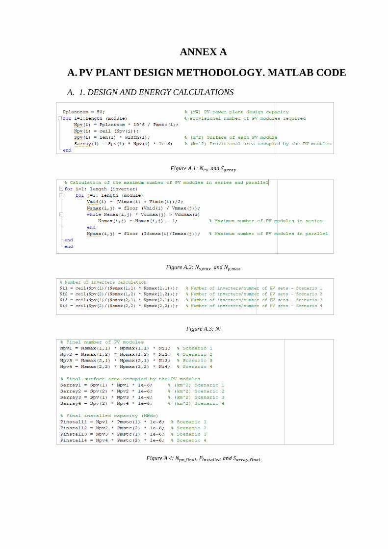
ANNEX A
A. PV PLANT DESIGN METHODOLOGY. MATLAB CODE
A. 1. DESIGN AND ENERGY CALCULATIONS
Figure A.1: 𝑁𝑃𝑉 and 𝑆𝑎𝑟𝑟𝑎𝑦
Figure A.2: 𝑁𝑠,𝑚𝑎𝑥 and 𝑁𝑝,𝑚𝑎𝑥
Figure A.3: Ni
Figure A.4: 𝑁𝑝𝑣,𝑓𝑖𝑛𝑎𝑙 , 𝑃𝑖𝑛𝑠𝑡𝑎𝑙𝑙𝑒𝑑 and 𝑆𝑎𝑟𝑟𝑎𝑦,𝑓𝑖𝑛𝑎𝑙

Design and modelling of a large-scale PV plant 93
Figure A.5: 𝑇𝑀, 𝑃𝑀, 𝑃𝑃𝑉 𝑎𝑛𝑑 𝑃𝑃𝑉,𝑙𝑜𝑠𝑠𝑒𝑠
Figure A.6: 𝑃𝑖𝑛
Figure A.7: 𝑃𝑜
Figure A.8: Land
Figure A.9: 𝑃𝑃𝐿𝐴𝑁𝑇

Figure A.10: 𝐸𝑃𝐿𝐴𝑁𝑇,𝑇𝑂𝑇
A. 2. ECONOMIC CALCULATIONS
Figure A.11:𝐶𝑐
Figure A.12: 𝐶𝑚
Figure A.13: 𝐶𝑟𝑒𝑝
Figure A.14: 𝐿𝐶𝑂𝐸
Figure A.15: 𝑅𝑔𝑟𝑜𝑠𝑠

Design and modelling of a large-scale PV plant 95
A. 3. EVALUATION PARAMETERS CALCULATIONS
Figure A.16: 𝐺𝐶𝑅
Figure A.17: 𝑃𝑅
Figure A.18: 𝐶𝐹
Figure A.19: 𝑌𝑖𝑒𝑙𝑑𝑠𝑝