design and operation optimisation of a mea-based co ... · design and operation optimisation of a...
TRANSCRIPT

Design and Operation Optimisation
of a MEA-Based CO2 Capture Unit
Artur José Rolo de Andrade
Thesis to obtain the Master of Science Degree in
Chemical Engineering
Supervisors:
Prof. Dr. Carla Isabel Costa Pinheiro
Dr. Javier Rodriguez Perez
Examination Committee
Chairperson: Prof. Dr. Sebastião Manuel Tavares da Silva Alves
Supervisor: Prof. Dr. Carla Isabel Costa Pinheiro
Member of the Committee: Prof. Dr. Rui Manuel Gouveia Filipe
November 2014


i
Education is experience and experience is self-reliance.
T. H. White

ii
This page was intentionally left blank.

iii
Acknowledgements
First of all, I would like to show my appreciation to Prof. Dr. Carla Pinheiro, Prof. Dr. Henrique
Matos, and especially to Prof. Dr. Costas Pantelides for presenting the possibility of taking an internship
in Process Systems Enterprise Limited, which was the basis of this thesis.
Also to Prof. Dr. Carla Pinheiro and to Dr. Javier Rodriguez, I would like to express my gratitude
for all the support, guidance and availability every time I needed help.
I would like to thank everyone in the Power & CCS team, with whom was a pleasure working
during these seven months. From this great team, I would like to particularly express my thanks to Mário
Calado for all his “great ideas at the right moment”.
I would also like to thank Dr. Maarten Nauta and Dr. Charles Brand for the initial gPROMS
training. To the remaining members of PSE, particularly the Portuguese and Italian “communities”, I
would like to show my gratitude for creating such an amazing working environment.
To my colleagues and friends from the “North”, Catarina Marques and Rubina Franco, I would
like to show my gratitude for all the great times we shared during this internship.
To my colleagues, friends and housemates during this few months, Mariana Marques and
Renato Wong, my deepest appreciation and gratitude for sharing this experience with me. Without them
it would not have been the same!
To my friends António Carvalho and Hugo Nogueira, which welcomed me in their home during
my first days in London, my deepest appreciation for all the great moments. To my friend Sara Oliveira,
the first person who said to me “Why not Chemical Engineering?”, my thanks for the great suggestion
and everything else.
To Sónia Ferreira, Carolina Silva, Tiago Fonseca, Carolina Oliveira and Francisco Patrocínio,
the people with whom I shared most of my time in the last five years, my thanks for all the friendship,
support and patience in this long road.
Last, but not least, I would like to show my deepest gratitude to my family and friends,
particularly to my parents and my brother for all the care, support and trust in every moment of my life.

iv
This page was intentionally left blank.
v
Abstract
The present thesis has the objective of analysing the cost reduction obtained through a rigorous
model-based optimisation of a post-combustion CO2 capture plant for carbon capture and storage
applications. Today’s capture technology is mainly based on chemical absorption with alkanolamines.
Even though this is a well-known technology, its application in power plants presents high costs, thus
limiting its implementation.
This way, a full scale capture plant model was developed considering MEA as the solvent. This
model is based on a conventional flowsheet and was implemented in gPROMS®, using the gCCS®
libraries. It comprises an absorption section, in which CO2 is dissolved by reacting with the amine, and
a regeneration section where it is stripped from the solvent. After its validation, the model was optimised
by modifying the design and operation parameters.
A cost estimation model was applied to the plant model, in order to determine capital and
operational expenditures. From the total cost obtained, 69% is due to the steam required in the
regeneration section. As for the equipment cost, the absorber packing is the most relevant fraction.
Considering typical values for the capture rate, CO2 purity and MEA concentration in the solvent
as constraints, the plant’s model optimisation led to a reduction of 15% in the specific total cost. Without
imposing these typical values, the total cost was further reduced. These results clearly show the
potential of model-based optimisation in the reduction of the cost associated with CO2 capture, thus
contributing to its effective implementation in power plants.
Keywords:
Carbon capture and storage, post-combustion capture, chemical absorption, MEA, cost
optimisation, gPROMS

vi
This page was intentionally left blank.

vii
Resumo
A presente tese tem como objetivo a análise da redução de custos obtida por otimização do
modelo de uma unidade de captura de CO2 por pós-combustão para captura e armazenamento de
carbono. As atuais tecnologias de captura são maioritariamente baseadas em absorção química por
alcanolaminas. Apesar de esta ser uma tecnologia conhecida, a sua aplicação em centrais elétricas
apresenta elevados custos, limitando a sua implementação.
Desta forma, foi desenvolvido o modelo de uma unidade de captura à escala industrial,
utilizando MEA como solvente. Este modelo é baseado num flowsheet convencional e foi implementado
em gPROMS®, recorrendo à biblioteca gCCS®. Neste considerou-se uma zona de absorção, onde o
CO2 é dissolvido por reação com a amina, e uma zona de regeneração, onde este o solvente é
regenerado. Após validação, o modelo foi otimizado por modificação dos parâmetros de design e
operação.
Um modelo de estimativa de custos foi aplicado ao modelo desenvolvido, de forma a
determinar despesas de investimento e operacionais. Do custo total obtido, 69% deve-se ao vapor
requerido pela regeneração. Do custo dos equipamentos, a fração mais relevante é o enchimento do
absorvedor.
Considerando valores típicos de taxa de captura, pureza da corrente de CO2 e concentração
do solvente, a otimização da unidade levou à redução do custo total específico em 15%. Não impondo
estes valores típicos, o custo total foi ainda mais reduzido. Estes resultados mostram o potencial da
otimização com recurso a modelos na redução dos custos de captura de CO2, contribuindo para a sua
implementação efetiva.
Palavras-chave:
Captura e armazenamento de carbono, captura pós-combustão, absorção química, MEA,
otimização de custos, gPROMS

viii
This page was intentionally left blank.

ix
Contents
1. Introduction ...................................................................................................................................... 1
1.1. Motivation ................................................................................................................................ 1
1.2. State of the Art ......................................................................................................................... 2
1.3. Original Contributions .............................................................................................................. 2
1.4. Dissertation Outline ................................................................................................................. 2
2. Background ..................................................................................................................................... 5
2.1. Carbon Capture and Storage .................................................................................................. 5
2.2. Carbon Capture Technologies ................................................................................................. 5
2.2.1. Post-Combustion Capture ............................................................................................. 6
2.2.2. Pre-Combustion Capture ............................................................................................... 7
2.2.3. Oxy Combustion ............................................................................................................ 8
2.3. Processes Based on Chemical Absorption ............................................................................. 9
2.3.1. Primary and secondary amine based processes ........................................................ 10
2.3.2. Tertiary amine based processes ................................................................................. 12
2.3.3. Ammonia based processes ......................................................................................... 15
2.3.4. Amino acid salts based processes .............................................................................. 16
2.3.5. Hot potassium carbonate based processes ................................................................ 17
2.4. Processes Based on Physical Solvents ................................................................................ 18
2.4.1. Available technology.................................................................................................... 19
3. Materials and Methods .................................................................................................................. 21
3.1. gPROMS® ModelBuilder ........................................................................................................ 21
3.2. gCCS® Capture Library .......................................................................................................... 21
3.2.1. Chemical Absorber (A) ................................................................................................ 21
3.2.2. Chemical Stripper (ST) ................................................................................................ 22
3.2.3. Condenser (C) ............................................................................................................. 22
3.2.4. Flow Multiplier (FM) ..................................................................................................... 23
3.2.5. Heat Exchanger (HX) .................................................................................................. 23
3.2.6. Heat Exchanger Process/Utility (HXU) ........................................................................ 23
3.2.7. Junction (M) ................................................................................................................. 23
3.2.8. Process Sink (S) .......................................................................................................... 24

x
3.2.9. Process Source (SR) ................................................................................................... 24
3.2.10. Pump Simple (P) ......................................................................................................... 24
3.2.11. Stream Converter Absorber/Stripper (SC) .................................................................. 24
3.2.12. Reboiler (R) ................................................................................................................. 25
3.2.13. Recycle Breaker (RB) .................................................................................................. 25
3.2.14. Utility Sink (SU) ........................................................................................................... 25
3.2.15. Utility Source (SRU) .................................................................................................... 25
3.3. Physical Properties Package – gSAFT .................................................................................. 26
4. Models Validation .......................................................................................................................... 27
4.1. Flowsheet A – Absorber Model Validation............................................................................. 27
4.2. Flowsheet B – MEA Capture Plant Model Validation ............................................................ 32
5. MEA Full Scale Capture Plant Model ............................................................................................ 37
5.1. Base Case ............................................................................................................................. 37
5.2. Cost Estimation Model ........................................................................................................... 39
5.2.1. CAPEX Estimation....................................................................................................... 39
5.2.2. OPEX Estimation ......................................................................................................... 41
5.3. Cost Estimation Results for the Base Case........................................................................... 42
6. Optimisation Problem Formulation ................................................................................................ 45
6.1. Objective Function ................................................................................................................. 45
6.2. Decision Variables ................................................................................................................. 45
6.3. Constraints ............................................................................................................................. 46
7. Optimisation Results ..................................................................................................................... 49
7.1. Base Case Optimisation with Standard Constraints .............................................................. 49
7.1.1. Specific Total Cost Minimisation ................................................................................. 49
7.1.2. Effect of the Initial Guesses in the Optimisation Results ............................................. 55
7.1.3. Effect of the Number of Absorption Trains .................................................................. 58
7.1.4. Specific Heat Requirement Minimisation..................................................................... 59
7.2. Effect of the Process Constraints .......................................................................................... 61
7.2.1. Effect of the Capture Rate ........................................................................................... 62
7.2.2. Effect of the CO2 Purity ............................................................................................... 66
7.2.3. Effect of the MEA Concentration ................................................................................. 68
xi
7.2.4. Specific Total Cost Minimisation with Inequality Constraints ...................................... 70
8. Conclusions and Future Work ....................................................................................................... 73
8.1. Conclusions ........................................................................................................................... 73
8.2. Future Work ........................................................................................................................... 75
9. Bibliography ................................................................................................................................... 77
Appendices ......................................................................................................................................... 83
A1. Cost Estimation Model Description ........................................................................................ 83
A1.1. Shell mass estimation ........................................................................................................ 83
A1.2. Heat exchanger area estimation ........................................................................................ 83
A1.3. Reboiler area estimation .................................................................................................... 84
A1.4. Condenser area estimation ................................................................................................ 84
A1.5. Pump volumetric flow rate and power estimation .............................................................. 84
A2. Base Case and Optimisations Detailed Results .................................................................... 87
xii
List of Figures
Figure 2.1 – Existing technologies for CO2 separation and capture [16]. -------------------------------------- 6
Figure 2.2 – Schematic of a coal-fired power plant with carbon capture [17]. -------------------------------- 6
Figure 2.3 – Schematic of an IGCC power plant with carbon capture [17]. ----------------------------------- 8
Figure 2.4 – Conventional flowsheet for a PCC plant [18]. -------------------------------------------------------- 9
Figure 2.5 – Split-flow configuration of the Fluor’s Econamine FG PlusSM process [30]. ----------------- 12
Figure 2.6 – Praxair’s Amine process flowsheet [35]. ------------------------------------------------------------- 14
Figure 2.7 – Shell’s Cansolv CO2 Capture System flowsheet [38]. -------------------------------------------- 14
Figure 2.8 – Alstom’s Chilled Ammonia process flowsheet [40]. ------------------------------------------------ 16
Figure 2.9 - CO2 bulk removal capacity for different solvents [49]. --------------------------------------------- 18
Figure 2.10 – UOP SelexolTM process flowsheet for CO2 and H2S co-capture [50]. ----------------------- 18
Figure 2.11 – Lurgi Rectisol® process flowsheet for CO2 and H2S selective capture [49]. --------------- 19
Figure 3.1 – Chemical absorber/stripper icon used in the gCCS® capture library. ------------------------- 21
Figure 3.2 – Parameters required for Onda correlation (on the left) and for Billet & Schultes correlation
(on the right). ---------------------------------------------------------------------------------------------------- 22
Figure 3.3 – Condenser icon used in the gCCS® capture library. ---------------------------------------------- 22
Figure 3.4 – Flow multiplier icon used in the gCCS® capture library. ------------------------------------------ 23
Figure 3.5 – Heat exchanger icon used in the gCCS® capture library. ---------------------------------------- 23
Figure 3.6 – Junction icon used in the gCCS® capture library. -------------------------------------------------- 23
Figure 3.7 – Process sink icon used in the gCCS® capture library. -------------------------------------------- 24
Figure 3.8 – Process source icon used in the gCCS® capture library. ---------------------------------------- 24
Figure 3.9 – Pump simple icon used in the gCCS® capture library. -------------------------------------------- 24
Figure 3.10 – Stream converter absorber/stripper icon used in the gCCS® capture library. ------------- 24
Figure 3.11 – Reboiler icon used in the gCCS® capture library. ------------------------------------------------ 25
Figure 3.12 – Recycle breaker icon used in the gCCS® capture library. -------------------------------------- 25
Figure 3.13 – Utility sink icon used in the gCCS® capture library. ---------------------------------------------- 25
Figure 3.14 – Utility source icon used in the gCCS® capture library. ------------------------------------------ 25
Figure 4.1 – Flowsheet A used for validation (a models use Billet & Schultes correlation and b models
use Onda correlation). ---------------------------------------------------------------------------------------- 28
Figure 4.2 – Parity diagram of the absorbed amount of CO2 (using Billet & Schultes correlation). ---- 30
Figure 4.3 – Deviation between experimental and simulated absorbed CO2 with the considered lean
solvent loading. ------------------------------------------------------------------------------------------------- 31
Figure 4.4 – Simulated and experimental temperature profiles for run 10 (lean loading of 0.284
molCO2/molMEA). ------------------------------------------------------------------------------------------------- 32
Figure 4.5 – Simulated and experimental temperature profiles for run 12 (lean loading of 0.307
molCO2/molMEA). ------------------------------------------------------------------------------------------------- 32
Figure 4.6 – Simulated and experimental temperature profiles for run 15 (lean loading of 0.357
molCO2/molMEA). ------------------------------------------------------------------------------------------------- 32
Figure 4.7 – Flowsheet B used for validation. ----------------------------------------------------------------------- 34
xiii
Figure 5.1 – MEA capture plant flowsheet as seen in gPROMS® ModelBuilder. --------------------------- 38
Figure 5.2 – Total cost distribution in the base case (Total = 43.15 €/tCO2). ---------------------------------- 42
Figure 5.3 – Distribution of main equipment costs for the base case. ----------------------------------------- 43
Figure 5.4 – OPEX distribution in the base case (Total = 64.56 M€/year). ----------------------------------- 43
Figure 5.5 – Distribution of variable production costs for the base case (Total = 61.4 M€/year). ------- 43
Figure 5.6 – Distribution of the amine losses in base case (Total = 12.5 kt/year). ------------------------- 44
Figure 5.7 – Distribution of the utilities costs for the base case (Total = 56.4 M€/year). ------------------ 44
Figure 6.1 – Ratio between vapour velocity and vapour flooding velocity across the absorber (on the
left) and the stripper (on the right), for the base case. ------------------------------------------------ 47
Figure 7.1 – Total cost distribution for the specific total cost minimisation with standard constraints (Total
= 36.69 €/tCO2). ------------------------------------------------------------------------------------------------- 51
Figure 7.2 – Distribution of main equipment costs for the specific total cost minimisation with standard
constraints. ------------------------------------------------------------------------------------------------------ 51
Figure 7.3 – CO2 molar flux to the liquid phase across the absorber (top of the absorber equivalent to
0), before and after the specific total cost minimisation with standard constraints. ------------ 52
Figure 7.4 – Representative temperature profiles of the lean-rich heat exchanger in the base case (on
the left) and after the total cost minimisation (on the right). ----------------------------------------- 52
Figure 7.5 – Representative temperature profiles of the lean solvent cooler in the base case (on the left)
and after the total cost minimisation (on the right). ---------------------------------------------------- 53
Figure 7.6 – Axial temperature profiles in the stripping columns for the gas phase (on the left) and the
liquid phase (on the right), before and after the specific total cost minimisation with standard
constraints. ------------------------------------------------------------------------------------------------------ 53
Figure 7.7 – CO2 and H2O molar fluxes from the gas phase to the liquid phase across the stripper (top
of the stripper equivalent to volume 0), before and after the specific total cost minimisation
with standard constraints. ------------------------------------------------------------------------------------ 54
Figure 7.8 – Axial temperature profile of the vapour (on the left) and liquid (on the right) phases in the
absorber for the optimised cases with initial lean loadings of 0.1, 0.2 and 0.3 molCO2/molMEA.
--------------------------------------------------------------------------------------------------------------------- 57
Figure 7.9 – Variation of the optimal absorber diameter with the number absorption trains. ------------ 58
Figure 7.10 – Variation of the optimal specific total cost (on the right) and specific CAPEX (on the right)
with the number of absorption trains. --------------------------------------------------------------------- 59
Figure 7.11 – Total cost distribution in the specific heat consumption minimisation (Total = 88.98 €/tCO2).
--------------------------------------------------------------------------------------------------------------------- 60
Figure 7.12 – Distribution of main equipment costs for the specific heat consumption minimisation. - 61
Figure 7.13 – OPEX distribution in the specific heat consumption minimisation (Total = 69.34 M€/year).
--------------------------------------------------------------------------------------------------------------------- 61
Figure 7.14 – Variation of the optimal specific total cost with the imposed capture rate. ----------------- 62
Figure 7.15 – Variation of the optimal lean solvent flow rate (on the right) and loading (on the left) with
the imposed capture rate. ------------------------------------------------------------------------------------ 63
xiv
Figure 7.16 – Axial temperature profile of the vapour phase (on the left) and liquid phase (on the right)
in the absorber for the optimised cases with capture rates (CR) of 70, 80, 90 and 99%. ---- 64
Figure 7.17 – Axial temperature profile of the vapour phase (on the left) and liquid phase (on the right)
in the stripper for the optimised cases with capture rates (CR) of 70, 80, 90 and 99%. ------ 64
Figure 7.18 – CO2 molar flux from the gas to the liquid phase across the stripper, for the optimised
cases with capture rates (CR) of 70, 80, 90 and 99%. ----------------------------------------------- 65
Figure 7.19 – sCAPEX percentage variation with the imposed capture rate (90% capture rate
considered 100%). --------------------------------------------------------------------------------------------- 66
Figure 7.20 – Variation of the optimal specific total cost with the imposed CO2 purity. ------------------- 66
Figure 7.21 – Variation of the optimal condenser temperature with the imposed CO2 stream purity. - 67
Figure 7.22 – H2O molar flux from the gas to the liquid phase across the stripper, for the optimised
cases with CO2 purities (CP) of 75, 85, 95 and 99%. ------------------------------------------------- 67
Figure 7.23 – Variation of the optimal specific total cost with the imposed MEA mass fraction in the CO2
free lean solvent. ----------------------------------------------------------------------------------------------- 69
Figure 7.24 – Variation of the optimal lean solvent flow rate with the imposed MEA mass fraction in the
CO2 free lean solvent. ---------------------------------------------------------------------------------------- 69
Figure 7.25 – Optimal specific total cost obtained through its minimisation with and without standard
constraints, and value in the base case. ----------------------------------------------------------------- 71
xv
List of Tables
Table 2.1 – Typical composition (volumetric fraction) of flue gas from coal and natural gas fired power
plants [18]. -------------------------------------------------------------------------------------------------------- 7
Table 2.2 – Commercially available processes using primary or secondary amine-based solvents [3,
28, 29]. ----------------------------------------------------------------------------------------------------------- 11
Table 2.3 – Available processes using tertiary amine-based solvents [35, 36]. ----------------------------- 13
Table 2.4 – Processes in development using ammonia-based solvents [40]. ------------------------------- 15
Table 2.5 – Available processes using hot potassium carbonate-based solvents [47, 48, 46]. --------- 17
Table 2.6 – Commercially available processes using physical solvents [50, 51, 49]. ---------------------- 19
Table 4.1 – Characteristics of the flue gas and lean solvent used by Tobiesen et al. [10]. -------------- 27
Table 4.2 - Characteristic data and constants for Sulzer Mellapak 250YTM [54, 57]. --------------------- 28
Table 4.3 – Experimental rich loading and simulation results using both Billet & Schultes correlation and
Onda correlation. ----------------------------------------------------------------------------------------------- 29
Table 4.4 – Experimental absorbed amount of CO2 and simulation results using both Billet & Schultes
correlation and Onda correlation. -------------------------------------------------------------------------- 30
Table 4.5 – Pilot plant design parameters [11]. --------------------------------------------------------------------- 33
Table 4.6 – Process specifications for examples 1 and 2 [11]. -------------------------------------------------- 33
Table 4.7 – Flue gas composition in each example. --------------------------------------------------------------- 33
Table 4.8 – Experimental and Simulation results for the process key parameters and respective
variation. --------------------------------------------------------------------------------------------------------- 35
Table 5.1 – Flue gas conditions considered in the MEA capture plant model. ------------------------------ 37
Table 5.2 – Design parameters and operating conditions considered in the original capture plant model.
--------------------------------------------------------------------------------------------------------------------- 37
Table 5.3 – Results obtained from the simulation of the original and base cases. ------------------------- 39
Table 5.4 – Type, construction/reference material, sizing variable and cost correlation parameters for
the main capture plant equipment [58]. Cost correlation parameters in a USD basis referred
to January 2010 (CEPCI2010=532.9).-------------------------------------------------------------------- 40
Table 5.5 – Typical installation factors for the estimation of project installed capital cost [58]. --------- 41
Table 5.6 – Other expenses required for the estimation of the total investment required [58]. ---------- 41
Table 5.7 – Utilities and solvents costs (CEPCI1998=389.5, CEPCI2004=444.2 [61]) [62]. ------------- 42
Table 6.1 – Decision variables, with respective initial value, lower bound and upper bound. ----------- 46
Table 6.2 – Equality constrained variables, with respective constrained value. ---------------------------- 46
Table 6.3 – Inequality constrained variables, with respective upper and lower bounds. ------------------ 46
Table 6.4 – Additional inequality constrained variables, with respective upper and lower bounds, used
for the minimisation of the specific heat consumption. ----------------------------------------------- 47
Table 7.1 – Detailed results from the specific total cost minimisation with standard constraints, and
comparison with the base case (Table A2.1).----------------------------------------------------------- 50
Table 7.2 – Modified initial guesses, used for comparison with the initial optimisation. ------------------- 55
xvi
Table 7.3 – Decision variables and key parameter resulting from the specific total cost minimisation,
starting from a lean loading of 0.1 molCO2/molMEA and comparison with the optimal results
previously obtained. ------------------------------------------------------------------------------------------- 56
Table 7.4 – Decision variables and key parameter resulting from the specific total cost minimisation,
starting from a lean loading of 0.3 molCO2/molMEA and comparison with the optimal results
previously obtained. ------------------------------------------------------------------------------------------- 56
Table 7.5 – Lagrange multipliers obtained for the equality constraints in the minimisation of the specific
total cost with standard constraints. ----------------------------------------------------------------------- 62
Table 7.6 – Additional inequality constrained variables, with respective upper and lower bounds, used
in the specific total cost minimisation without equality constraints. -------------------------------- 70
Table A1.1 – Minimum practical wall thickness [58]. --------------------------------------------------------------- 83
Table A1.2 – Typical maximum allowable stresses for stainless steel 304 [58]. ---------------------------- 83
Table A1.3 – Typical shaft efficiencies for centrifugal pumps [59]. --------------------------------------------- 85
Table A1.4 – Typical driver efficiencies for electrical motors [54]. ---------------------------------------------- 85
Table A2.1 – Detailed results from the application of the cost estimation model in the base case. ---- 87
Table A2.2 – Detailed results from the specific total cost minimisation with 1 absorber and standard
constraints, and comparison with the initial specific total cost minimisation results (Table 7.1).
--------------------------------------------------------------------------------------------------------------------- 88
Table A2.3 – Detailed results from the specific total cost minimisation with 3 absorber and standard
constraints, and comparison with the initial specific total cost minimisation results (Table 7.1).
--------------------------------------------------------------------------------------------------------------------- 89
Table A2.4 – Detailed results from the specific total cost minimisation with 4 absorber and standard
constraints, and comparison with the initial specific total cost minimisation results (Table 7.1).
--------------------------------------------------------------------------------------------------------------------- 90
Table A2.5 – Detailed results from the specific heat requirement minimisation with standard constraints,
and comparison with the base case. ---------------------------------------------------------------------- 91
Table A2.6 – Detailed results from the specific total cost minimisation with an imposed capture rate of
70%, and comparison with the initial specific total cost minimisation results (Table 7.1). --- 92
Table A2.7 – Detailed results from the specific total cost minimisation with an imposed capture rate of
80%, and comparison with the initial specific total cost minimisation results (Table 7.1). --- 93
Table A2.8 – Detailed results from the specific total cost minimisation with an imposed capture rate of
99%, and comparison with the initial specific total cost minimisation results (Table 7.1). --- 94
Table A2.9 – Detailed results from the specific total cost minimisation with an imposed CO2 purity of
75%, and comparison with the initial specific total cost minimisation results (Table 7.1). --- 95
Table A2.10 – Detailed results from the specific total cost minimisation with an imposed CO2 purity of
85%, and comparison with the initial specific total cost minimisation results (Table 7.1). --- 96
Table A2.11 – Detailed results from the specific total cost minimisation with an imposed CO2 purity of
99%, and comparison with the initial specific total cost minimisation results (Table 7.1). --- 97

xvii
Table A2.12 – Detailed results from the specific total cost minimisation with an imposed MEA mass
fraction the CO2 free lean solvent of 20%, and comparison with the initial specific total cost
minimisation results (Table 7.1). --------------------------------------------------------------------------- 98
Table A2.13 – Detailed results from the specific total cost minimisation with an imposed MEA mass
fraction the CO2 free lean solvent of 40%, and comparison with the initial specific total cost
minimisation results (Table 7.1). --------------------------------------------------------------------------- 99
Table A2.14 – Detailed results from the specific total cost minimisation with inequality constraints, and
comparison with the initial specific total cost minimisation results (Table 7.1). --------------- 100

xviii
List of Abbreviations
A – Chemical absorber
C – Condenser
CCS – Carbon capture and storage
CS – Carbon steel
CSIRO – Commonwealth Scientific and Industrial Research Organisation
EOR – Enhanced oil recovery
FG – Flue gas
FM – Flow multiplier
HSS – Heat stable salts
HX – Integrated heat exchanger
HXU – Heat exchanger using a utility
IGCC – Integrated gasification combined cycle
ISBL – Inside battery limits
LS – Lean solvent after make-up
M – Junction
MDEA – Methyldiethanolamine
MEA – Monoethanolamine
MSEP – Mean squared error of prediction
NLP – Nonlinear programing
OSBL – Offsite battery limits
P – Pump simple
PCC – Post-combustion capture
PSE – Process systems enterprise limited
R – Reboiler
RB – Recycle breaker
RR’NH – Generic primary/secondary amine
RR’R’’N – Generic tertiary amine
RS – Rich solvent
S – Process sink
SAFT – Statistical Associating Fluid Theory
SC – Stream converter absorber/stripper
SR – Process source
SRU – Utility source
SS-304 – Stainless steel 304
ST – Chemical stripper
SU – Utility sink
TG – Treated gas
USD – United states dollar
VR – Variable Range

xix
List of Symbols
Symbols
Variable Description Unit
a Cost parameter a -
A Area m2
b Cost parameter b -
C Installed capital cost/ISBL investment €
Ce Equipment cost USD/€
Cmaintenance Maintenance cost €
Ctaxes/insurance Taxes and insurance cost €
Cutilities Utilities total cost €
Csolvent Solvent total cost €
Cs/CFl/Ch/CP,0 Packing characteristic constants -
CAPEX Capital expenditures M€/year
CEPCI Chemical Engineering's Plant Cost Index -
CP CO2 purity %
CR CO2 capture rate %
D Diameter m
E Welded joint efficiency -
f Installation factor -
fm Material factor -
F Mass flow rate kg/s
FV Volumetric flow rate m3/s
L Height m
Mshell Shell’s mass kg
n Cost parameter n -
N Number of equipment units -
NRuns Number of experimental runs -
OF Objective function €/tCO2
OF2 Secondary objective function GJ/tCO2
OPEX Operational expenditure M€/year
P Pressure bar
PP Power required by each train of pumps kW
PS Power required by each pump W
Q Heat duty W
S Maximum allowable stress bar
Sv Sizing variable -
sCAPEX Specific CAPEX €/tCO2
sOPEX Specific OPEX €/tCO2
t Thickness mm
T Temperature K
U Overall heat transfer coefficient W/(m2.K)
v Value -
w Mass fraction g/g
WP Specific work J/kg
x Molar fraction Mol/mol
Δ Difference -
ΔP Pressure drop bar
η Efficiency -
ρ Mass density kg/m3

xx
Subscripts
Variable Description
0 Source column
1 Destination column
1998/2004/2010/2013 Reference year
bottom Extra bottom section of the column
c Civil
Cond Condenser
driver Pump driver
er Equipment erection
el Electrical
f Line
HX Heat exchanger
i Component
ic Instrumentation and control
l Lagging and paint
lm Logarithmic mean
liq Liquid phase
min Minimum value
Packing Packing section of the column
Pump Pump
Reb Reboiler
s Structures and buildings
shaft Pump shaft
steam Steam stream
top Extra top section of the column
utility Utility stream
vap Vapour phase
Superscripts
Variable Description
dry Dry basis fraction
exp Experimental value
in Inlet stream
m/construction Construction material
out Outlet stream
P Units in parallel
reference Reference material
S Stream
sim Simulated value
Unit Unitary variable

1
1. Introduction
CO2 is a naturally-occurring gas with a major influence in the reflection of solar radiation back
to Earth, keeping the planet’s surface temperature in levels suitable for the existence of life. However
due to human invention and industrialisation, its concentration in the atmosphere has greatly increased,
leading to a rapid rise in the planet’s temperature. According to the 2013 IEA report [1], between the
years of 2001 and 2011, the worldwide CO2 emissions from fossil fuel combustion increased by 31%,
reaching a value of 31 billion tonnes per year. From this value, approximately 42% are due to the
electricity and heat production sector.
The use of renewable energy sources is an option to mitigate CO2 emissions. However,
considering the 2013 IEA report on energy statistics [2], fossil fuels (coal, oil and natural gas) still
represent around 81% of the world’s primary energy supply.
According to the Global CCS Institute, carbon capture and storage has the potential to
significantly reduce the CO2 emissions to the atmosphere from power plants and chemical industries,
such as ammonia, hydrogen, steel and cement production, as well as in fuels preparation and natural
gas processing.
The 2005 IPCC Special report on CSS [3], states that, for a power plant, the capture cost is the
main component of the overall CCS costs, mainly due to the process energy requirements. For a power
plant, this implies an extra consumption of steam and electricity, leading to a reduction in net efficiency
and consequently an increase in the electricity costs.
Also according to this report, the improvement of commercially available capture technologies
should allow a reduction of its costs by 20 to 30%, being the option with more potential for the reduction
of CO2 emissions in the near future.
1.1. Motivation
Process Systems Enterprise Limited (PSE) is the world’s leading provider of advanced process
modelling to the process industries. In July 2014, the company has launched the gCCS® modelling
environment, being the first modelling software specifically designed for the modelling of full carbon
capture and storage (CCS) chains, from power generation through capture, compression and transport
to injection [4].
gCCS® is constructed on PSE’s platform for advanced modelling, gPROMS®, allowing the use
of high-fidelity predictive models. Using the gCCS® model libraries, it is possible to simulate each stage
of the CCS chain individually and to analyse the interoperability across different chain components.
Shell’s Peterhead CCS project will be the first commercial application of gCCS® in the United Kingdom,
where it will be used to provide insight into the transient behaviour of the amine-based capture unit, and
its effect on operations when integrated in the full CCS chain [5].
The gCCS® capture library contains models for the simulation of both chemical and physical
solvent-based pre- and post-combustion capture units. For rigorous physical properties estimation,
these models use gSAFT, a thermodynamic property package created by PSE, which is based on the
Statistical Associating Fluid Theory (SAFT) developed at Imperial College London [4].

2
With this in mind, the present thesis has the objective of applying gPROMS® optimisation
features to a conventional CO2 capture plant model, built using the gCCS® capture library, in order to
minimise the costs associated with the unit’s design and operation.
1.2. State of the Art
The current status off the CCS technology is well described in the 2005 IPCC Special report on
CSS [3], where not only CO2 capture processes based on absorption are addressed, but also more
recent technologies.
For well-known solvents, such as monoethanolamine (MEA), recent developments focus on the
processes improvement, in order to reduce the capture economic penalty. Abu-Zahra et al. [6], evaluate
the effect of specific parameters in the energy consumption. Ahn et al. [7] test different flowsheet
configurations in order to reduce the process heat requirement. In [8], Damartzis et al. optimise several
flowsheet configurations, based on the minimisation of not only the heat requirement, but of a set of the
key process parameters. Even though most of today’s studies are based on MEA, there are some
articles, such as [9] by Urech et al., in which the performance of different solvents is evaluated.
All of the examples mentioned above resort to process modelling to test new process
configurations or proceed to their optimisation. For the validation of these models, experimental data
are required. In the case of MEA-based capture plants, these data can be found in Tobiensen et al.
[10], and Notz et al. [11].
1.3. Original Contributions
As mentioned in the motivation section, the present thesis intends to further contribute to the
CO2 capture cost reduction. To that end, PSE’s gCC® libraries were used to assemble a capture plant
model based on the MEA solvent. These models were validated by comparison with experimental data
from Tobiensen et al. [10], and Notz et al. [11] articles.
Starting from a case study developed by PSE, the design and operating conditions of a MEA-
based capture were optimised using gPROMS®. For that, a model for the estimation of the CAPEX and
the OPEX associated with the capture plant was developed. The optimisation studies focused on the
minimisation of the total cost (CAPEX + OPEX) per tonne of captured CO2, initially imposing a capture
rate, CO2 purity and solvent concentration, and ultimately evaluating the effect of varying these
constraints.
1.4. Dissertation Outline
The present thesis is organised in the following way: Chapter 2 presents a literature review on
the technologies employed in CO2 capture, namely the solvents currently applied or being developed,
and processes examples. Chapter 3 features a brief description of gPROMS® ModelBuilder, the
required models from gCCS® capture library and the used physical properties package (gSAFT).
Chapter 4 describes the validation of flowsheets built using these models against experimental data
found in the literature. In Chapter 5, the capture plant model used as full scale base case is described,
as well as the model used for costs estimation and its application to the base case. Chapter 6 presents
the description of the considered optimisation problem, in terms of objective function, decision variables

3
and process constraints. In Chapter 7, the results from the base case optimisation are presented and
analysed, containing a study on the effect of the initial guesses, the number of absorption trains and a
comparison between the specific total cost minimisation and the specific heat requirement minimisation.
Chapter 7 also features an analysis on the effect on the optimal total cost of varying the initially imposed
process constraints. Finally, Chapter 8 contains the conclusions drawn from this thesis and future work
suggestions.

4
This page was intentionally left blank.
5
2. Background
A literature review was conducted in order to understand the basic concepts associated with
the CCS chain, and more specifically the existing technologies to capture CO2 from fossil fuelled power
plants. Amongst these technologies, solvent-based processes were further analysed.
2.1. Carbon Capture and Storage
The CCS chain comprises several technologies involved in removal of carbon dioxide from a
gaseous stream, its transportation and final sequestration in site away from the atmosphere, where it
will be stored for a long period. This can be applied to the CO2 obtained in the fossil fuel burning in a
power plant, in the preparation of natural gas, or in other chemical industries [3].
The capture stage features the processes required for CO2 separation from a stream
comprising a mixture of gases. After this, the CO2 stream is compressed in order to reduce its volume
fraction up to 0.2%. The transportation is mainly carried through pipelines, or alternatively through
shipping or road tanking. Considering the elevated amount of CO2 annually emitted (mentioned in
section 1.1), the available storage locations are geological formations or the deep ocean. The required
injection technology is similar to the one employed in the oil and gas industries, and can be associated
with enhanced oil recovery (EOR), thus constituting a possible revenue source. Besides storage, in the
past years the captured CO2 has been considered for the production of other chemical, mineral fixation
and the production of bio fuels through the use of micro-algae [3, 12].
Even though these technologies have been applied in several other industries, due to the
considerable costs associated with the application of the capture process to such high flow rates, its
application to the flue gas obtained in a large-scale power plant fuelled by coal or natural gas is currently
on a demonstration phase, [13]. Nevertheless, in April 2014, the Boundary Dam Power Station
(Canada) started a CCS project for the capture of 1 MtCO2/year, using amine-based post-combustion
technology, with the captured CO2 being used for EOR. The Kemper County IGCC power plant (United
States) will start operating in 2015. It will capture 3.5 MtCO2/year (65% capture rate), also destined to
EOR applications [14]. Besides these two examples, until 2018, there are planned the start-up of 4
more capture units in the United States, with capacities reaching the 3.5 MtCO2/year and are destined
to EOR. In Europe, there are 2 capture units, from which the Don Valley (United Kingdom) intends the
capture of 4.5 MtCO2/year for geological storage [15]. All the mentioned capture projects are set to be
applied in coal-fuelled power plants. As for gas-fuelled capture units, the first capture unit is set to be
operational in 2017 in Peterhead (United Kingdom), using post-combustion technologies to capture 1
MtCO2/year [14].
2.2. Carbon Capture Technologies
Most capture processes are based on gas scrubbing processes developed over 60 years ago
for the production of town gas. Since then, this technology has been improved in order to be applied in
other industries, and more recently to carbon capture [3]. Besides the gas scrubbing process, based on
the CO2 absorption in a suitable solvent, there are several other technologies being developed in order
6
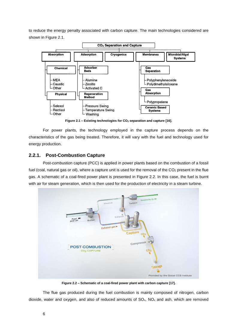
to reduce the energy penalty associated with carbon capture. The main technologies considered are
shown in Figure 2.1.
Figure 2.1 – Existing technologies for CO2 separation and capture [16].
For power plants, the technology employed in the capture process depends on the
characteristics of the gas being treated. Therefore, it will vary with the fuel and technology used for
energy production.
2.2.1. Post-Combustion Capture
Post-combustion capture (PCC) is applied in power plants based on the combustion of a fossil
fuel (coal, natural gas or oil), where a capture unit is used for the removal of the CO2 present in the flue
gas. A schematic of a coal-fired power plant is presented in Figure 2.2. In this case, the fuel is burnt
with air for steam generation, which is then used for the production of electricity in a steam turbine.
Figure 2.2 – Schematic of a coal-fired power plant with carbon capture [17].
The flue gas produced during the fuel combustion is mainly composed of nitrogen, carbon
dioxide, water and oxygen, and also of reduced amounts of SOx, NOx and ash, which are removed

7
through electrostatic precipitation and desulphurization before the capture process. The concentration
of each species will depend on the burnt fuel and its characteristics. Table 2.1 presents the typical
composition of flue gases obtained in coal and natural gas fuelled power plants [18].
Table 2.1 – Typical composition (volumetric fraction) of flue gas from coal and natural gas fired power plants [18].
Gas Constituent Composition (vol%)
Coal Natural Gas
N2 70-75 73-76
CO2 10-15 4-5
H2O 8-15 8-10
O2 3-4 12-15
Trace Gases <1 <1
As shown in Figure 2.1, CO2 capture can be achieved through several technologies.
Nevertheless, according to the Global CCS Institute report on post-combustion capture from 2012, [18],
the technologies currently tested on slip streams of pilot plants are universally based on absorption with
aqueous solvents.
Absorption processes allow CO2 capture rates between 80 and 90%, and purity as high as
99.9% (in volume) for the recovered CO2 [3]. Since the flue gas being treated has a considerably low
CO2 content and is at atmospheric pressure, the CO2 partial pressure is reduced. Therefore, the chosen
solvent has to be able to ensure acceptable loadings and kinetics in the referred conditions. Due to this,
chemical absorption poses a better option in PCC processes, when compared with physical solvents.
The solvent choice also requires the consideration of other parameters such as its volatility and
propensity to degrade [3].
The inclusion of a PCC unit in a coal fuelled power plant leads to an increase of 29% in the
energy input to achieve the same output, while for a natural gas fuelled power plant this increase is of
16% [13].
2.2.2. Pre-Combustion Capture
Pre-combustion capture technology is usually applied to power plants based on the gasification
of a fossil fuel, more specifically integrated gasification combined cycle (IGCC) plants. The gasification
process is achieved through partial oxidation in the presence of oxygen and produces synthesis gas
(syngas). This mixture, mainly composed of hydrogen and carbon monoxide, enters a water gas shift
reactor, where CO is converted to CO2. The obtained gas is typically at a total pressure that ranges
from 20 to 70 bar and has a CO2 content between 15% and 60%. After being purified, the hydrogen rich
gas is burnt in a gas turbine, producing electricity [3], as shown in Figure 2.3.
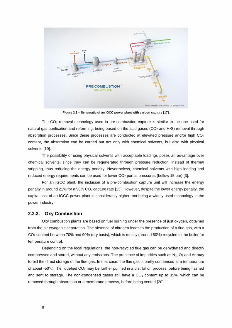
8
Figure 2.3 – Schematic of an IGCC power plant with carbon capture [17].
The CO2 removal technology used in pre-combustion capture is similar to the one used for
natural gas purification and reforming, being based on the acid gases (CO2 and H2S) removal through
absorption processes. Since these processes are conducted at elevated pressure and/or high CO2
content, the absorption can be carried out not only with chemical solvents, but also with physical
solvents [19].
The possibility of using physical solvents with acceptable loadings poses an advantage over
chemical solvents, since they can be regenerated through pressure reduction, instead of thermal
stripping, thus reducing the energy penalty. Nevertheless, chemical solvents with high loading and
reduced energy requirements can be used for lower CO2 partial pressures (bellow 15 bar) [3].
For an IGCC plant, the inclusion of a pre-combustion capture unit will increase the energy
penalty in around 21% for a 90% CO2 capture rate [13]. However, despite the lower energy penalty, the
capital cost of an IGCC power plant is considerably higher, not being a widely used technology in the
power industry.
2.2.3. Oxy Combustion
Oxy combustion plants are based on fuel burning under the presence of just oxygen, obtained
from the air cryogenic separation. The absence of nitrogen leads to the production of a flue gas, with a
CO2 content between 70% and 90% (dry basis), which is mostly (around 80%) recycled to the boiler for
temperature control.
Depending on the local regulations, the non-recycled flue gas can be dehydrated and directly
compressed and stored, without any emissions. The presence of impurities such as N2, O2 and Ar may
forbid the direct storage of the flue gas. In that case, the flue gas is partly condensed at a temperature
of about -50℃. The liquefied CO2 may be further purified in a distillation process, before being flashed
and sent to storage. The non-condensed gases still have a CO2 content up to 35%, which can be
removed through absorption or a membrane process, before being vented [20].
9
2.3. Processes Based on Chemical Absorption
As mentioned in the previous sections, the chemical absorption technology for CO2 separation
is widely used in the chemical industry. Post-combustion capture is mainly based on this technology,
as well as pre-combustion capture at lower CO2 partial pressures.
These processes are based on the CO2 chemical dissolution in an alkaline solvent, through its
selective reaction with one or several of the solvent components, usually amines. This dissolution is
conducted in a packed column (absorber) at a temperature usually between 40 and 60 °C. The solvent
loaded with CO2 (usually called rich solvent) is pumped to the regeneration section. Before entering the
regenerator, the rich solvent is heated through an integrated heat exchange with the regenerated
solvent (also called lean solvent). The regeneration process typically occurs through stripping at a
temperature between 100 and 140 °C and above atmospheric pressure. The heat demanded by this
process is provided by a reboiler, which constitutes the main energy requirement of the capture unit.
The lean solvent is pumped back to the absorber after being regenerated. Since the solvent is subject
to losses during the process, a make-up is required before re-entering the absorber. Some of these
losses are due to the solvent’s reaction with oxygen or other impurities, which produce compounds,
typically called heat stable salts (HSS) that are not regenerable in the stripper. These compounds are
removed through a reclaiming process, applied to a split stream of the lean solvent, which consists in
the application of a strong base, such as potassium hydroxide, at elevated temperatures. Besides this
treatment, an activated carbon filter is usually used before the solvent’s make-up [3].
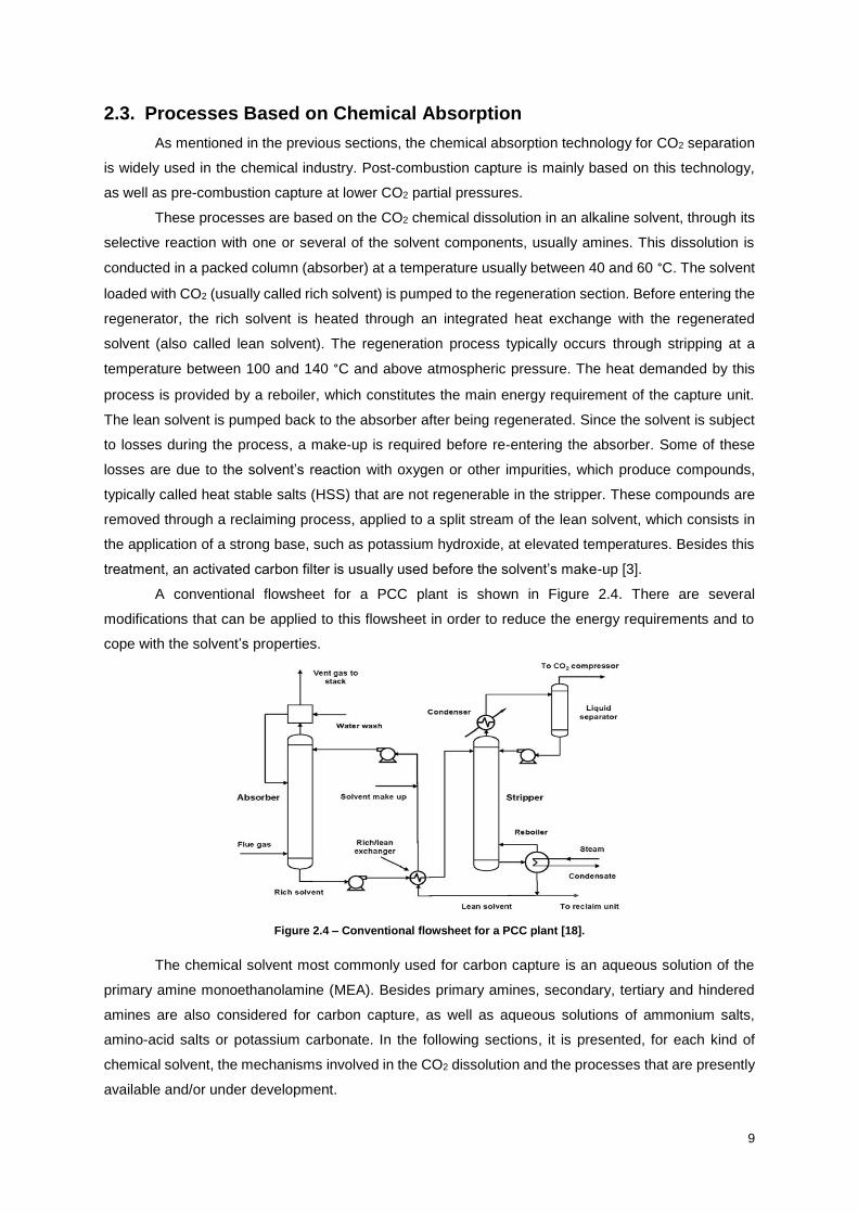
A conventional flowsheet for a PCC plant is shown in Figure 2.4. There are several
modifications that can be applied to this flowsheet in order to reduce the energy requirements and to
cope with the solvent’s properties.
Figure 2.4 – Conventional flowsheet for a PCC plant [18].
The chemical solvent most commonly used for carbon capture is an aqueous solution of the
primary amine monoethanolamine (MEA). Besides primary amines, secondary, tertiary and hindered
amines are also considered for carbon capture, as well as aqueous solutions of ammonium salts,
amino-acid salts or potassium carbonate. In the following sections, it is presented, for each kind of
chemical solvent, the mechanisms involved in the CO2 dissolution and the processes that are presently
available and/or under development.

10
2.3.1. Primary and secondary amine based processes
Alkanolamines are organic compounds that include an amine and a hydroxyl groups. When
compared with other amine compounds, the alkanolamines are typically preferred for CO2 dissolution,
since the hydroxyl group confers a reduced vapour pressure, an adequate basicity for the contact with
acid gases and an elevated solubility in water, as well as an elevated dielectric constant, which prevents
a liquid phase separation or salts precipitation [21].
Primary and secondary alkanolamines (simply named amines), differ from tertiary ones due to
the presence of at least one hydrogen atom in the amine group, which increases the molecule reactivity.
This way, primary and secondary amines react strongly with CO2 and at elevated reaction rates.
To cope with the elevated reactivity of primary or secondary amines, they can be modified so
that the carbon atom bounded to the amine group is secondary or tertiary, thus sterically hindering the
amine and reducing its reactivity. Examples of these amines are 2-amino-2-methyl-1-propanol and 2-
piperidineethanol [22].
2.3.1.1. Reaction with CO2
Primary or secondary amines (generally represented by 𝑅𝑅′𝑁𝐻) react with CO2 producing a
compound called carbamate (𝑅𝑅′𝑁𝐶𝑂𝑂−). This occurs through the formation of an intermediary
zwitterion (𝑅𝑅′𝑁𝐻+𝐶𝑂𝑂−), which corresponds to the mechanism’s slow step [23]. This mechanism can
be represented by equations (2.1) and (2.2).
𝐶𝑂2 + 𝑅𝑅′𝑁𝐻 ⇆ 𝑅𝑅′𝑁𝐻+𝐶𝑂𝑂− (2.1)
𝑅𝑅′𝑁𝐻+𝐶𝑂𝑂− + 𝑅𝑅′𝑁𝐻 ⇆ 𝑅𝑅′𝑁𝐶𝑂𝑂− + 𝑅𝑅′𝑁𝐻2+ (2.2)
Besides these reactions, CO2 is also converted into bicarbonate through the reaction described
in equation (2.3). Nevertheless, for loadings below 0.5 molCO2/molamine, the bicarbonate formation can
be considered insignificant when compared with the carbamate formation [24].
𝐶𝑂2 + 𝑅𝑅′𝑁𝐻 + 𝐻2𝑂 ⇆ 𝐻𝐶𝑂3− + 𝑅𝑅′𝑁𝐻2
+ (2.3)
In the case of hindered amines, these molecules form a carbamate of low stability due to the
large group connected to the amine group. This unstable carbamate is hydrolysed (equation (2.4)),
originating a bicarbonate ion, [22].
𝑅𝑅′𝑁𝐶𝑂𝑂− + 𝐻2𝑂 ⇆ 𝐻𝐶𝑂3− + 𝑅𝑅′𝑁𝐻 (2.4)
Combining the equations (2.1), (2.2) and (2.4), it can be observed that for hindered amines the
global reaction is equivalent to the reaction described by equation (2.3), being the reaction stoichiometry
of 1:1 between CO2 and the amine. In the case of un-hindered amines, the global stoichiometry is 1:2
between CO2 and the amine. This difference in the global stoichiometry leads to a maximum loading of
0.5 molCO2/molamine for unhindered amines, while hindered amines present a maximum loading of 1
molCO2/molamine [22].
2.3.1.2. Available processes
From the amines used as solvents for carbon capture, monoethanolamine (MEA) is the most
reactive, and therefore, the one used in most of the commercially available processes. The elevated
reactivity allows acceptable reaction rates at low CO2 partial pressures, which makes MEA the most
common choice in post-combustion capture [13].

11
Since higher amine concentrations lead to a reduction of the equipment size and the process
thermal and pumping requirements (the solvent flow rate is reduced), it is important to keep it as
elevated as possible. Nevertheless, due to its reactivity, MEA requires a considerably elevated heat of
regeneration and is highly prone to oxidative and thermal degradation, which limits the solvent
concentration. The application of oxidation inhibitors allows the increase of MEA concentration to the
typical value of 30% in weight [25]. Besides this, the solvent concentration is also limited by its tendency
to slip along the treated gas [13].
Amine-based processes are also conditioned by temperature, due to possibility of the
carbamate polymerization. In the case of MEA, this thermal degradation is negligible if the regeneration
temperature is kept below 110 to 120 °C [26].
For a coal-fuelled power plant, with a CO2 capture rate of 90% and a MEA concentration of 30
wt%, the energy required in the regeneration process is about 3.7 GJ/tCO2 [27].
Table 2.2 presents some of the commercially available processes for carbon capture, which
employ MEA or proprietary solvents containing a blend of sterically hindered amines. Most of them are
already used in other industries and pilot plants that received a side stream from a power plant flue gas.
Therefore, they just require an adequate scale-up to be applied in a full scale power plant.
Table 2.2 – Commercially available processes using primary or secondary amine-based solvents [3, 28, 29].
Process Solvent characteristics Process characteristics Other applications
ABB Lummus Cress
15 to 20 wt% of MEA. Conventional process. Soda ash production
Fluor’s Econamine FG
PlusSM
30 wt% of MEA;
Proprietary oxidation inhibitor.
Split flow configuration;
Absorber’s intercooling;
Lean vapour compression.
Beverages and urea production
MHI’s KM-CDR
KS1TM (blend of sterically hindered amines).
Lean vapour compression;
Reboiler’s condensate used for stripping.
Urea production
As can be seen in Table 2.2, the Fluor’s Econamine FG Plus process uses a solvent with a
MEA concentration of 30 wt% through the use of a proprietary inhibitor. According to [18], it is claimed
that Fluor’s Econamine FG PlusSM is able to reduce the steam consumption in 30%, when compared to
a conventional process using MEA. This technology is used in 25 capture units worldwide, working on
a portion of flue gas obtained from natural gas burning.
In order to improve the capture efficiency, the Fluor’s Econamine FG PlusSM process uses
several modifications to the conventional flowsheet. The absorber’s intercooling is based on the removal
of a fraction of the liquid circulating in the absorber, which is cooled to a selected temperature. This
temperature reduction improves the physical absorption of CO2 and leads the chemical absorption
equilibrium to the formation of products, increasing the capture rate and decreasing the solvent’s
circulation rate. According to Ahn et al. [7], this allows a reboiler heat duty reduction of about 3%,
comparing to an amine-based conventional process.
A lean vapour compression configuration is based on the lean solvent flashing at low pressure
and temperature. The obtained vapour is compressed and returns to the stripping column acting as a
stripping agent, thus reducing the steam consumption in the reboiler. The temperature reduction in the
lean solvent also leads to reduction in the cooling. According to [7], this leads to a reduction of 22% in

12
the reboiler heat duty. On the other hand, according to [28], this would also lead to an increase in the
cost of the equipment and in the electricity consumption.
The split flow-configuration is based on the splitting of the rich solvent into two streams to which
are applied different regeneration processes. This can occur through the rich solvent feeding at different
points of the stripping column (called double section column in [8] and [7]) or using separate
regeneration equipment, which can be two stripping columns (called multi-feed stripper in [8]) or a
stripping column and a flash drum (shown in [30]). In all of these configurations, one of the rich solvent
streams undergoes a less intensive stripping process, at lower temperature or pressure, thus reducing
the reboiler heat requirement, and originating a semi-lean solvent. In the case of only one regeneration
column is used, the semi-lean solvent is a liquid stream removed from a mid-point of the stripper. The
obtained semi-lean solvent is then fed to a mid-point of the absorption column, enhancing the average
driving force in the column and reducing the temperature (called multi-feed absorber in [8]). An example
of the combination of a flash drum and a stripping column in the Fluor’s Econamine FG PlusSM process
is presented in the patent US 7,337,967 B2 [30], and its flowsheet is presented in Figure 2.5.
Figure 2.5 – Split-flow configuration of the Fluor’s Econamine FG PlusSM process [30].
MHI’s KM-CDR process applies a proprietary solvent composed by sterically hindered amines
in order to reduce the heat requirements and the solvent degradation. According to [18], it is claimed
that this process is able to reduce the steam consumption in 32%, compared to a conventional MEA-
based process. This process is commercially available for post-combustion in natural gas fuelled power
plants, while is in a demonstration phase for coal-fired plants [29].
2.3.2. Tertiary amine based processes
Unlike primary or secondary amines, tertiary amines do not possess hydrogen atoms bounded
to the amine group. Therefore, the carbamate formation mechanism is not possible, which leads to
considerably slower capture kinetics. On the other hand, these solvents allow higher CO2 loadings in
the solvent and require less heat in the regeneration process [3].
13
The reduced capture rates are usually compensated with the addition of a more reactive amine,
such as triethylenetetramine [31] or piperazine [32]. Likewise, tertiary amines are also used as inhibitors
in order to reduce the high reactivity of primary and secondary amines [33, 34].
2.3.2.1. Reaction with CO2
As mentioned, tertiary amines (𝑅𝑅′𝑅′′𝑁) are not able to react directly with CO2 in order to form
a zwitterion. As opposed to primary and secondary amines, the amine base-catalytic effect on the CO2
conversion into HCO3- is the relevant one, being described by equations (2.5) and (2.6), which are
equivalent to the reaction in equation (2.3) [22].
𝐶𝑂2 + 𝑂𝐻− ⇆ 𝐻𝐶𝑂3− (2.5)
𝑅𝑅′𝑅′′𝑁 + 𝐻2𝑂 ⇆ 𝑅𝑅′𝑅′′𝑁𝐻+ + 𝑂𝐻− (2.6)
Considering this mechanism, the limiting step is the CO2 hydrolysis. Hence, tertiary amines
present a considerable reduced reaction rate when compared with primary or secondary amines. Since
the global stoichiometry is 1:1 between CO2 and the amine, the maximum loading is1 molCO2/molamine.
2.3.2.2. Processes in development
The possibility of achieving higher loadings and the lower heat of reaction make tertiary amines
a suitable choice not only for PCC, but also for pre-combustion capture. Most of these processes are
based methyldiethanolamine (MDEA), [3]. Two examples of processes using tertiary amine-based
solvents are shown in Table 2.3.
Table 2.3 – Available processes using tertiary amine-based solvents [35, 36].
Process Solvent characteristics Process characteristics
Praxair’s Amine 20 to 40 wt% of MDEA;
10 to 20 wt% of MEA. Oxygen tolerant process.
Shell’s Cansolv CO2 Capture
System
Customizable: o DC-103: low energy consumption; o DC-103B: improved kinetics.
Integrated separation of SO2 and CO2;
Absorber intercooling;
Lean vapour compression.
According to [35], pilot tests were being conducted in order to improve Praxair’s technology.
This process uses a maximum amine concentration of 50 wt%, blending a tertiary amine with a primary
amine. To cope with the oxidation problems associated with such an elevated concentration, the
process flowsheet is modified in order to include a vacuum flash separation in the rich solvent stream,
releasing the dissolved oxygen (Figure 2.6).
14
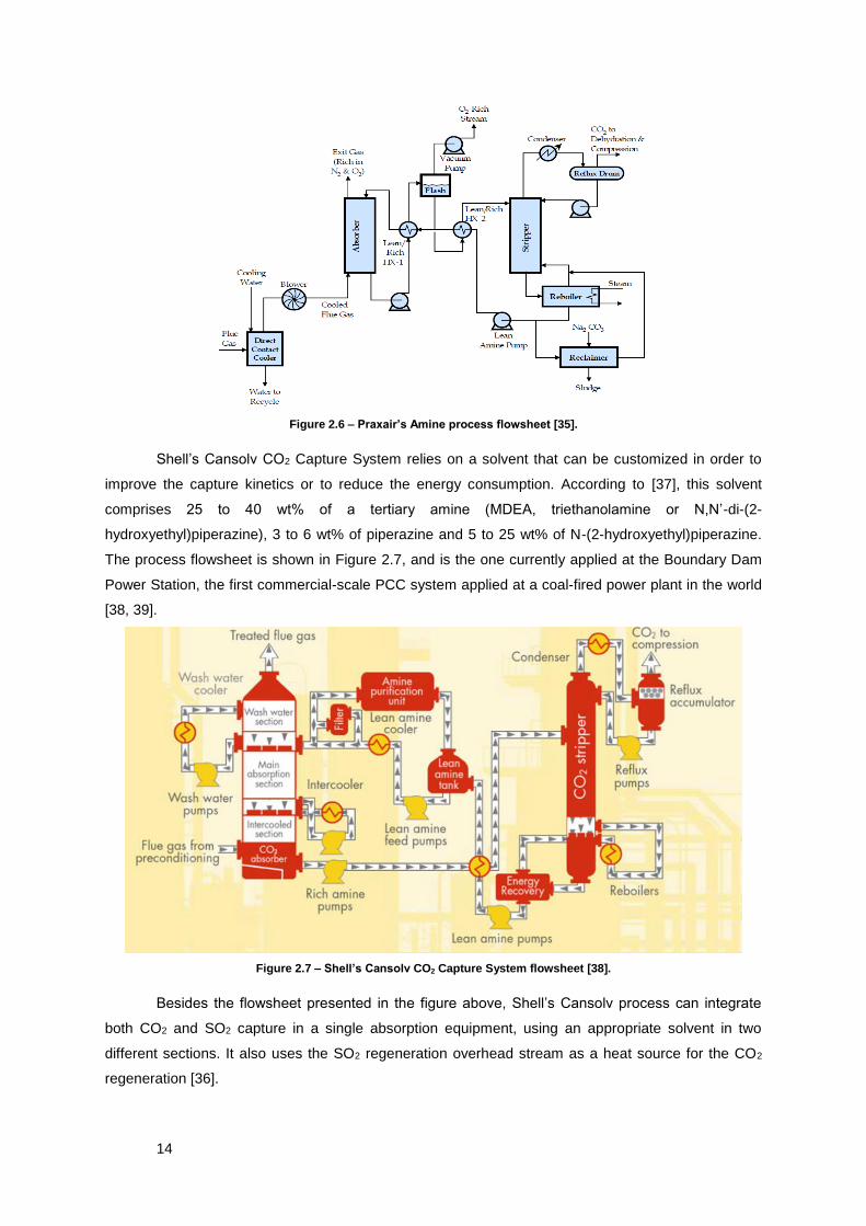
Figure 2.6 – Praxair’s Amine process flowsheet [35].
Shell’s Cansolv CO2 Capture System relies on a solvent that can be customized in order to
improve the capture kinetics or to reduce the energy consumption. According to [37], this solvent
comprises 25 to 40 wt% of a tertiary amine (MDEA, triethanolamine or N,N’-di-(2-
hydroxyethyl)piperazine), 3 to 6 wt% of piperazine and 5 to 25 wt% of N-(2-hydroxyethyl)piperazine.
The process flowsheet is shown in Figure 2.7, and is the one currently applied at the Boundary Dam
Power Station, the first commercial-scale PCC system applied at a coal-fired power plant in the world
[38, 39].
Figure 2.7 – Shell’s Cansolv CO2 Capture System flowsheet [38].
Besides the flowsheet presented in the figure above, Shell’s Cansolv process can integrate
both CO2 and SO2 capture in a single absorption equipment, using an appropriate solvent in two
different sections. It also uses the SO2 regeneration overhead stream as a heat source for the CO2
regeneration [36].

15
2.3.3. Ammonia based processes
Absorption with aqueous ammonia is widely used in the gas industry for gases sweetening, and
poses several advantages for carbon capture. When compared with conventional amine solvents,
ammonia is readily available and has a reduced cost. It is also more resistant to degradation, requires
a lower heat of regeneration and allows higher solvent loadings [40]. On the other hand, ammonia
solvents present slower kinetics than MEA and considerably higher volatility, which leads to a higher
solvent loss. To cope with this loss, the absorption is usually conducted at lower temperature (from 0
to 10 °C) and the regeneration is carried at higher pressure (from 2 to 136 bar) [13].
2.3.3.1. Reaction with CO2
Carbon dioxide absorption in aqueous ammonia solution is based on the equilibrium between
ammonium carbonate ((𝑁𝐻4)2𝐶𝑂3) and ammonium bicarbonate (𝑁𝐻4𝐻𝐶𝑂3), which is described by
equations (2.7) to (2.11), [40].
𝑁𝐻3 + 𝐻2𝑂 ⇆ 𝑁𝐻4+ + 𝑂𝐻− (2.7)
𝐶𝑂2 + 2𝐻2𝑂 ⇆ 𝐻𝐶𝑂3− + 𝐻3𝑂+ (2.8)
𝐻𝐶𝑂3− + 𝐻2𝑂 ⇆ 𝐶𝑂3
2− + 𝐻3𝑂+ (2.9)
𝑁𝐻4+ + 𝐻𝐶𝑂3
− ⇆ 𝑁𝐻4𝐻𝐶𝑂3 (2.10)
2𝑁𝐻4+ + 𝐶𝑂3
2− ⇆ (𝑁𝐻4)2𝐶𝑂3 (2.11)
Considering the CO2 loading, the rich solvent will be mainly composed of ammonium
bicarbonate, while the lean solvent will be mainly composed of ammonium carbonate. Due to the
absorption low temperature, these species tend to precipitate, and the solvent can be obtained as a
slurry [40].
2.3.3.2. Processes in development
One of the major concerns about the ammonia-based processes is the solvent slip due to its
vaporization. This loss can be reduced with an appropriate water washing system or by reducing either
the ammonia concentration in the solvent or the absorption temperature. Nevertheless, the reduction
of concentration, leads to a decrease of the solvent’s capacity, while the temperature reduction causes
a decrease in the reaction rate [40].
Table 2.4 presents processes based on ammonia solvents, which are already operating in pilot
plants and ready to proceed towards commercialization [40].
Table 2.4 – Processes in development using ammonia-based solvents [40].
Process Solvent characteristics Process characteristics
Alstom’s Chilled Ammonia
28 wt% of NH3.
Flue gas cooled to approximately 0 °C;
Stripping at a pressure from 20 to 40 bar;
Washing water regenerated in a stripper.
CSIRO Process 6 wt% of NH3. Flue gas cooled to approximately 10 °C;
Stripping at a pressure from 3 to 8.5 bar.
KIER Process 13 wt% of NH3. Flue gas cooled to approximately 25 °C;
Stripping at 6.5 bar.
RIST Process Less than 10 wt% of NH3.
Flue gas cooled to approximately 40 °C;
Stripping at 1 bar and 80 °C;
Washing water regenerated in a stripper.
16
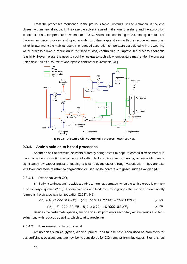
From the processes mentioned in the previous table, Alstom’s Chilled Ammonia is the one
closest to commercialization. In this case the solvent is used in the form of a slurry and the absorption
is conducted at a temperature between 0 and 10 °C. As can be seen in Figure 2.8, the liquid effluent of
the washing water process is stripped in order to obtain a gas stream with the recovered ammonia,
which is later fed to the main stripper. The reduced absorption temperature associated with the washing
water process allows a reduction in the solvent loss, contributing to improve the process economic
feasibility. Nevertheless, the need to cool the flue gas to such a low temperature may render the process
unfeasible unless a source of appropriate cold water is available [40].
Figure 2.8 – Alstom’s Chilled Ammonia process flowsheet [40].
2.3.4. Amino acid salts based processes
Another class of chemical solvents currently being tested to capture carbon dioxide from flue
gases is aqueous solutions of amino acid salts. Unlike amines and ammonia, amino acids have a
significantly low vapour pressure, leading to lower solvent losses through vaporization. They are also
less toxic and more resistant to degradation caused by the contact with gases such as oxygen [41].
2.3.4.1. Reaction with CO2
Similarly to amines, amino acids are able to form carbamates, when the amine group is primary
or secondary (equation (2.12)). For amino acids with hindered amine groups, the species predominantly
formed is the bicarbonate ion (equation (2.13)), [42].
𝐶𝑂2 + 2( 𝐾+ 𝐶𝑂𝑂−𝑅𝑅′𝑁𝐻) ⇄ (𝐾+)2 𝐶𝑂𝑂−𝑅𝑅′𝑁𝐶𝑂𝑂− + 𝐶𝑂𝑂−𝑅𝑅′𝑁𝐻2+ (2.12)
𝐶𝑂2 + 𝐾+ 𝐶𝑂𝑂−𝑅𝑅′𝑁𝐻 + 𝐻2𝑂 ⇄ 𝐻𝐶𝑂3− + 𝐾+𝐶𝑂𝑂−𝑅𝑅′𝑁𝐻2
+ (2.13)
Besides the carbamate species, amino acids with primary or secondary amine groups also form
zwitterions with reduced solubility, which tend to precipitate.
2.3.4.2. Processes in development
Amino acids such as glycine, alanine, proline, and taurine have been used as promoters for
gas purifying processes, and are now being considered for CO2 removal from flue gases. Siemens has

17
developed the Postcap process based on the bicarbonate formation, using a proprietary solvent in a
conventional flowsheet. According to [43], this process is suited for capture in IGCC plants and has
been tested in pilot plants, being ready for a full plant scale up.
2.3.5. Hot potassium carbonate based processes
Hot aqueous solutions of potassium carbonate have been used for the removal of carbon
dioxide from gaseous streams since 1954. Compared to conventional amine solvents, this solvent
allows the absorption to occur at higher temperature, thus reducing the heat requirement in the
regeneration process. Besides this, potassium carbonate is less expensive, shows reduced toxicity and
less propensity to degradation. Nevertheless, hot potassium carbonate solvents present a considerably
reduced reaction rate, which renders its unpromoted use unfeasible for PCC [44]. In the same way as
tertiary amine-based processes, promoters, such as piperazine, diethanolamine, arsenic trioxide and
boric acid, are blended with potassium carbonate in order to improve the process kinetics [45]. On the
other hand, since this is a process suited for absorption at high CO2 partial pressure, it presents an
option to IGCC, showing a lower capital cost, when compared with processes based on physical
solvents [45].
2.3.5.1. Reaction with CO2
As in tertiary amines processes, potassium carbonate does not react directly with CO2. Instead,
the carbonate ions increase the solvents alkalinity, thus improving the CO2 conversion to bicarbonate
ions, as can be seen through equations (2.15) and (2.16) [45].
𝐾2𝐶𝑂3 ⇄ 2𝐾+ + 𝐶𝑂32− (2.14)
𝐶𝑂2 + 𝑂𝐻− ⇄ 𝐻𝐶𝑂3− (2.15)
𝐶𝑂32− + 𝐻2𝑂 ⇄ 𝐻𝐶𝑂3
− + 𝑂𝐻− (2.16)
2.3.5.2. Processes in development
The application of hot potassium carbonate solvents to flue gases is an under development
technology, only tested in a pilot scale. Nevertheless, there are several commercial processes applied
to other industries, such as the ammonia production [46]. Two of these processes are presented in
Table 2.5.
Table 2.5 – Available processes using hot potassium carbonate-based solvents [47, 48, 46].
Process Solvent characteristics Process characteristics
UOP’s Benfield
Hot K2CO3;
Corrosion inhibitor;
ACT-1™ activator.
Different flowsheets available.
Giammarco-Vetrocoke’s Low
Energy
Hot K2CO3;
Glycine;
Secondary Amine.
Split-stream configuration;
High and low pressure strippers;
Semi-lean and lean streams obtained in the high pressure stripper used as stripping agents at the low pressure stripper;
Semi-lean and lean solvent obtained at the low pressure stripper fed at different points of the absorber.
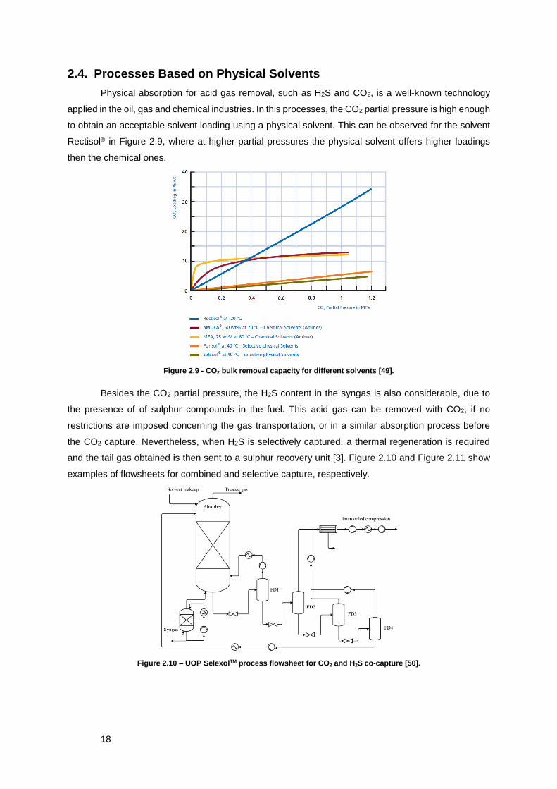
18
2.4. Processes Based on Physical Solvents
Physical absorption for acid gas removal, such as H2S and CO2, is a well-known technology
applied in the oil, gas and chemical industries. In this processes, the CO2 partial pressure is high enough
to obtain an acceptable solvent loading using a physical solvent. This can be observed for the solvent
Rectisol® in Figure 2.9, where at higher partial pressures the physical solvent offers higher loadings
then the chemical ones.
Figure 2.9 - CO2 bulk removal capacity for different solvents [49].
Besides the CO2 partial pressure, the H2S content in the syngas is also considerable, due to
the presence of of sulphur compounds in the fuel. This acid gas can be removed with CO2, if no
restrictions are imposed concerning the gas transportation, or in a similar absorption process before
the CO2 capture. Nevertheless, when H2S is selectively captured, a thermal regeneration is required
and the tail gas obtained is then sent to a sulphur recovery unit [3]. Figure 2.10 and Figure 2.11 show
examples of flowsheets for combined and selective capture, respectively.
Figure 2.10 – UOP SelexolTM process flowsheet for CO2 and H2S co-capture [50].
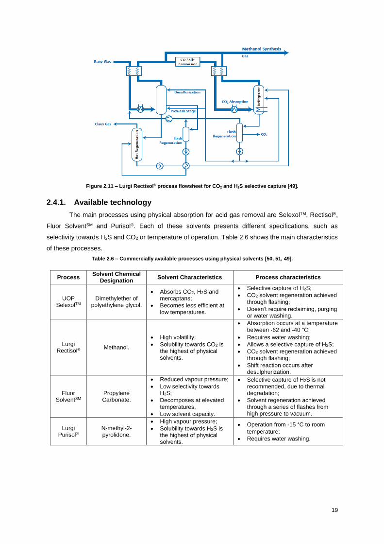
19
Figure 2.11 – Lurgi Rectisol® process flowsheet for CO2 and H2S selective capture [49].
2.4.1. Available technology
The main processes using physical absorption for acid gas removal are SelexolTM, Rectisol®,
Fluor SolventSM and Purisol®. Each of these solvents presents different specifications, such as
selectivity towards H2S and CO2 or temperature of operation. Table 2.6 shows the main characteristics
of these processes.
Table 2.6 – Commercially available processes using physical solvents [50, 51, 49].
Process Solvent Chemical
Designation Solvent Characteristics Process characteristics
UOP SelexolTM
Dimethylether of polyethylene glycol.
Absorbs CO2, H2S and mercaptans;
Becomes less efficient at low temperatures.
Selective capture of H2S;
CO2 solvent regeneration achieved through flashing;
Doesn’t require reclaiming, purging or water washing.
Lurgi Rectisol®
Methanol.
High volatility;
Solubility towards CO2 is the highest of physical solvents.
Absorption occurs at a temperature between -62 and -40 °C;
Requires water washing;
Allows a selective capture of H2S;
CO2 solvent regeneration achieved through flashing;
Shift reaction occurs after desulphurization.
Fluor SolventSM
Propylene Carbonate.
Reduced vapour pressure;
Low selectivity towards H2S;
Decomposes at elevated temperatures,
Low solvent capacity.
Selective capture of H2S is not recommended, due to thermal degradation;
Solvent regeneration achieved through a series of flashes from high pressure to vacuum.
Lurgi Purisol®
N-methyl-2-pyrolidone.
High vapour pressure;
Solubility towards H2S is the highest of physical solvents.
Operation from -15 °C to room
temperature;
Requires water washing.

20
This page was intentionally left blank.
21
3. Materials and Methods
3.1. gPROMS® ModelBuilder
Throughout the present thesis, gPROMS® ModelBuilder 3.7.1 is the simulation platform used
for flowsheet model simulation and optimisation. This advanced modelling tool can be used for the
development, validation, execution and deployment of models, using fast and robust numerical solvers.
Starting from an existing model library, such as the gCCS® library, it is possible to assemble a
flowsheet, through a drag and drop system, in the topology tab of a model entity. This way, a model is
built, being composed by the models retrieved from the library and the respective connections.
Nevertheless, in the gPROMS language tab of the same model, it is possible to include any other
auxiliary equations and custom sub models. Through the inclusion of the created model on a process
entity, it is possible its simulation.
Another feature of gPROMS® ModelBuilder is the optimisation tool, which can be used to
optimise the steady state and/or dynamic behaviour of a continuous flowsheet, considering both design
and operation properties. The optimisation procedure acts on a specified process, and requires the
indication of the unassigned variables acting as objective function or process constraints and the
assigned variables, which work as decision/control variables.
Since the models considered in this thesis are non-linear, the optimisation problem constitutes
a nonlinear programming problem (NLP). gPROMS® ModelBuilder 3.7.1 uses the SRQPD solver in the
solution of NLP problems, with an “Improved Estimation Based” convergence criterion [52].
3.2. gCCS® Capture Library
The gCCS® libraries contain steady-state and dynamic models for all the major operations along
the CCS chain. These high-fidelity models are based on rigorous physical properties and can be
implemented in the gPROMS® ModelBuilder environment. The capture library includes the different
models required for the simulation of a chemical-based post-combustion capture unit. In the following
sections these models are briefly described.
3.2.1. Chemical Absorber (A)
Figure 3.1 – Chemical absorber/stripper icon used in the gCCS® capture library.
One dimensional column model based on the gPROMS Advanced Model Library for Gas–Liquid
Contactors (AML:GLC). This rate-based model is based on the two-film theory, according to which the
liquid and gas bulk phases transfer heat and mass across liquid and gas films, separated by an
infinitesimally thin interface. It is considered chemical equilibrium in both bulk and films phases, as well
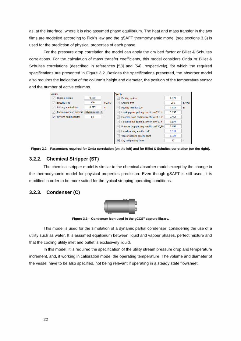
22
as, at the interface, where it is also assumed phase equilibrium. The heat and mass transfer in the two
films are modelled according to Fick’s law and the gSAFT thermodynamic model (see sections 3.3) is
used for the prediction of physical properties of each phase.
For the pressure drop correlation the model can apply the dry bed factor or Billet & Schultes
correlations. For the calculation of mass transfer coefficients, this model considers Onda or Billet &
Schultes correlations (described in references [53] and [54], respectively), for which the required
specifications are presented in Figure 3.2. Besides the specifications presented, the absorber model
also requires the indication of the column’s height and diameter, the position of the temperature sensor
and the number of active columns.
Figure 3.2 – Parameters required for Onda correlation (on the left) and for Billet & Schultes correlation (on the right).
3.2.2. Chemical Stripper (ST)
The chemical stripper model is similar to the chemical absorber model except by the change in
the thermodynamic model for physical properties prediction. Even though gSAFT is still used, it is
modified in order to be more suited for the typical stripping operating conditions.
3.2.3. Condenser (C)
Figure 3.3 – Condenser icon used in the gCCS® capture library.
This model is used for the simulation of a dynamic partial condenser, considering the use of a
utility such as water. It is assumed equilibrium between liquid and vapour phases, perfect mixture and
that the cooling utility inlet and outlet is exclusively liquid.
In this model, it is required the specification of the utility stream pressure drop and temperature
increment, and, if working in calibration mode, the operating temperature. The volume and diameter of
the vessel have to be also specified, not being relevant if operating in a steady state flowsheet.

23
3.2.4. Flow Multiplier (FM)
Figure 3.4 – Flow multiplier icon used in the gCCS® capture library.
Model applied for the multiplication of a process stream’s flow rate. It requires the specification
of the value by which the flow rate will be multiplied.
3.2.5. Heat Exchanger (HX)
Figure 3.5 – Heat exchanger icon used in the gCCS® capture library.
Steady state model that simulates the heat exchange between two process streams, which may
present a co-current or counter-current configuration. It is assumed a fixed heat transfer coefficient and
pressure drop, which must be specified. No heat losses to the exterior or fouling are also assumed.
In calibration mode, the outlet temperature of either the cold or the hot stream must be specified,
or alternatively the temperature approach in one of the heat exchanger sides. For operational mode,
the heat exchange area has to be specified.
3.2.6. Heat Exchanger Process/Utility (HXU)
This model is similar to the heat exchanger model, being one of the contacting streams a utility.
It requires the specification of the heat exchange applied to the process stream, if it is being cooled of
heated.
In operational mode, besides the outlet temperature for the process stream, the temperature
difference for the utility stream must also be specified, if its flow rate is set as calculated.
3.2.7. Junction (M)
Figure 3.6 – Junction icon used in the gCCS® capture library.
Steady state model applied to the mixing and/or splitting of a variable number of streams. In
this model, it is assumed no heat losses or pressure drop, ideal mixing and equal temperature, pressure
and composition for the outlet streams.
The outlet pressures may be equalised or set to be equal to the minimum inlet pressure. The
outlet flow rates may be set to be calculated by the downstream units, or calculated by specifying all
but one split fraction/percentage. The system phase also has to be specified for initialisation purposes.
24
3.2.8. Process Sink (S)
Figure 3.7 – Process sink icon used in the gCCS® capture library.
Model applied for the definition of a process stream leaving the flowsheet. It may be used for
the calculation of a cumulative flow rate, in dynamic operation. Both the pressure and the flow rate may
be calculated by upstream units or specified.
3.2.9. Process Source (SR)
Figure 3.8 – Process source icon used in the gCCS® capture library.
This model provides the introduction of a material flow into the flowsheet. It is assumed to have
infinite capacity, being able to calculate the cumulative solvent consumption in dynamic operation. The
property estimation method is defined by the solvent choice and the section of operation, that is,
absorption or stripping.
As inputs, this model requires the specification of the temperature, composition and phase. The
flow rate and the pressure can be chosen as specified or calculated by a downstream unit.
3.2.10. Pump Simple (P)
Figure 3.9 – Pump simple icon used in the gCCS® capture library.
Isothermal and isenthalpic steady state model, used for the specification of a stream flow rate
(manual mode) or its inlet/outlet pressures (advanced mode). The flow rate specification can be either
done manually (through a value input) or set through the models control signal port, using a controller
model. Due to the model’s simplicity, it can be used for the simulation of the pressure increase or
decrease of both liquid and gas streams.
3.2.11. Stream Converter Absorber/Stripper (SC)
Figure 3.10 – Stream converter absorber/stripper icon used in the gCCS® capture library.
This model is required for the transition between physical properties package used in the
absorber and the stripper models, due to the different operating conditions. It requires the specification
of the conversion direction and the outlet stream phase (liquid or gas).

25
3.2.12. Reboiler (R)
Figure 3.11 – Reboiler icon used in the gCCS® capture library.
Dynamic model with energy and mass holdup for simulation of a boiling MEA solution. In this
model, it is assumed equilibrium between liquid and vapour phase, perfect mixing and the total
condensation of the steam used as utility.
This model requires the specification of the steam pressure drop, initial phase, volume and
diameter. In calibration mode the operating temperature must also be specified. For operational mode,
it is only required a temperature initial guess.
If the dynamic mode is activated, the reboiler pressure must be specified, as well the initial
conditions. If heat losses are activated, the overall heat transfer coefficients must be specified for both
liquid and vapour phases, as well as the ambient temperature.
3.2.13. Recycle Breaker (RB)
Figure 3.12 – Recycle breaker icon used in the gCCS® capture library.
This is a model without physical meaning, being used for the initialisation of a recycle loop.
Considering the initial state as open, the inlet or outlet pressure and/or flow rate must be specified, as
well as the temperature, composition and phase. The final state can be specified as open, acting as a
source/sink, closed, and thus connecting the inlet and outlet streams, or make-up.
For the make-up final state, it is possible to calculate the amount of a specified solvent required
to fulfil the respective mass fraction and total flow rate. For that, it is required to indicate the component
not-closed and the solvents with make-up. In the present thesis, these are H2O and MEA respectively.
3.2.14. Utility Sink (SU)
Figure 3.13 – Utility sink icon used in the gCCS® capture library.
Similar to the process sink, this model is used to define a utility stream leaving the flowsheet.
3.2.15. Utility Source (SRU)
Figure 3.14 – Utility source icon used in the gCCS® capture library.
Model applied to the introduction of a water-based utility flow in the flowsheet. As in the source
capture model, the temperature and phase must be specified, while the flow rate and pressure can be
indicated or calculated by a downstream unit.

26
3.3. Physical Properties Package – gSAFT
gSAFT is a physical properties package commercialised by PSE, using the SAFT technology
developed at the Imperial College London. This technology uses the Statistical Associating Fluid Theory
(SAFT) equation of state, an advanced molecular thermodynamic method, based in physically-realistic
models of molecules and their interactions with other molecules. In these models it is taken into account
the shape, size and specific interactions between the existing molecules in a mixture, which are
considered as chains of spherical segments. This is particularly relevant when considering non-
spherical molecules with strong directional interactions, such as the hydrogen bounds in a MEA-based
solvent.
The current implementation of gSAFT is based on the equation of state SAFT-VR, according to
which the attraction/repulsion between segments or molecules is modelled using the “square-well”
potential energy function. This function is characterised by the diameter of the segment, the range of
dispersion interactions and its strength. The physical basis of these parameters allows its systematic
use to describe similar molecules or predict physical properties in a wide range of conditions [55].
For carbon capture, gSAFT presents a modelling alternative to phase and chemical equilibrium
in the CO2-MEA-H2O system. Using the SAFT equation of state the chemical bound between CO2 and
MEA can be incorporated as a short-range association, being included in the molecular model. This
way, the involved reactions are treated implicitly, thus greatly reducing the complexity of the model,
thus increasing its robustness. A more detailed description of the SAFT equation of state and its
application to the CO2-MEA-H2O system can be found in [56].
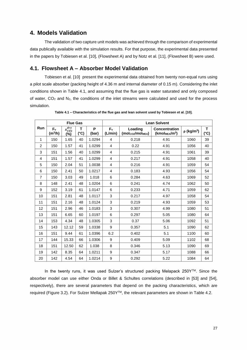
27
4. Models Validation
The validation of two capture unit models was achieved through the comparison of experimental
data publically available with the simulation results. For that purpose, the experimental data presented
in the papers by Tobiesen et al. [10], (Flowsheet A) and by Notz et al. [11], (Flowsheet B) were used.
4.1. Flowsheet A – Absorber Model Validation
Tobiesen et al. [10] present the experimental data obtained from twenty non-equal runs using
a pilot scale absorber (packing height of 4.36 m and internal diameter of 0.15 m). Considering the inlet
conditions shown in Table 4.1, and assuming that the flue gas is water saturated and only composed
of water, CO2 and N2, the conditions of the inlet streams were calculated and used for the process
simulation.
Table 4.1 – Characteristics of the flue gas and lean solvent used by Tobiesen et al. [10].
Run
Flue Gas Lean Solvent
Fv (m3/h)
𝒙𝑪𝑶𝟐𝒅𝒓𝒚
(%)
T
(°C) P
(bar) Fv
(L/min) Loading
(molCO2/molMEA) Concentration (kmolMEA/m3)
ρ (kg/m3) T
(°C)
1 150 1.65 40 1.0294 4 0.218 4.91 1060 39
2 150 1.57 41 1.0299 4 0.22 4.91 1056 40
3 151 1.56 40 1.0299 4 0.215 4.91 1061 39
4 151 1.57 41 1.0299 4 0.217 4.91 1058 40
5 150 2.04 51 1.0038 4 0.216 4.91 1059 54
6 150 2.41 50 1.0217 4 0.183 4.93 1056 54
7 150 3.03 49 1.018 6 0.284 4.63 1069 52
8 148 2.41 48 1.0204 6 0.241 4.74 1062 50
9 152 3.19 61 1.0147 6 0.233 4.71 1059 62
10 151 2.81 48 1.0117 3 0.217 4.97 1058 54
11 151 2.16 48 1.0124 3 0.219 4.93 1059 53
12 151 2.96 46 1.0183 3 0.307 4.99 1080 51
13 151 6.65 60 1.0197 6 0.297 5.05 1080 64
14 153 4.34 48 1.0305 3 0.37 5.06 1092 51
15 143 12.12 59 1.0338 9 0.357 5.1 1090 62
16 151 9.44 61 1.0396 6.2 0.402 5.1 1100 60
17 144 15.33 66 1.0306 9 0.409 5.09 1102 68
18 151 12.50 62 1.038 8 0.346 5.13 1090 69
19 142 8.35 64 1.0211 9 0.347 5.17 1088 66
20 142 4.54 64 1.0214 9 0.292 5.22 1084 64
In the twenty runs, it was used Sulzer’s structured packing Melapack 250YTM. Since the
absorber model can use either Onda or Billet & Schultes correlations (described in [53] and [54],
respectively), there are several parameters that depend on the packing characteristics, which are
required (Figure 3.2). For Sulzer Mellapak 250YTM, the relevant parameters are shown in Table 4.2.
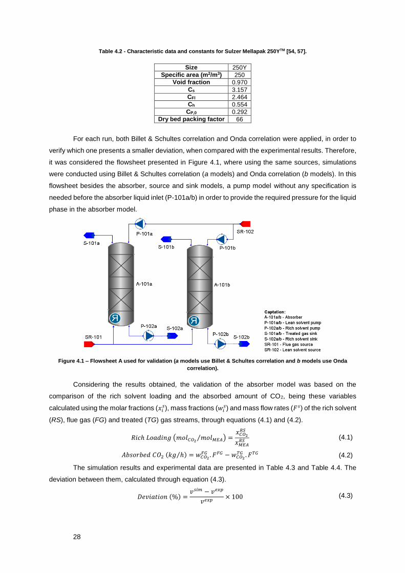
28
Table 4.2 - Characteristic data and constants for Sulzer Mellapak 250YTM [54, 57].
Size 250Y
Specific area (m2/m3) 250
Void fraction 0.970
Cs 3.157
CFl 2.464
Ch 0.554
CP,0 0.292
Dry bed packing factor 66
For each run, both Billet & Schultes correlation and Onda correlation were applied, in order to
verify which one presents a smaller deviation, when compared with the experimental results. Therefore,
it was considered the flowsheet presented in Figure 4.1, where using the same sources, simulations
were conducted using Billet & Schultes correlation (a models) and Onda correlation (b models). In this
flowsheet besides the absorber, source and sink models, a pump model without any specification is
needed before the absorber liquid inlet (P-101a/b) in order to provide the required pressure for the liquid
phase in the absorber model.
Figure 4.1 – Flowsheet A used for validation (a models use Billet & Schultes correlation and b models use Onda
correlation).
Considering the results obtained, the validation of the absorber model was based on the
comparison of the rich solvent loading and the absorbed amount of CO2, being these variables
calculated using the molar fractions (𝑥𝑖𝑠), mass fractions (𝑤𝑖
𝑠) and mass flow rates (𝐹𝑠) of the rich solvent
(RS), flue gas (FG) and treated (TG) gas streams, through equations (4.1) and (4.2).
𝑅𝑖𝑐ℎ 𝐿𝑜𝑎𝑑𝑖𝑛𝑔 (𝑚𝑜𝑙𝐶𝑂2𝑚𝑜𝑙𝑀𝐸𝐴⁄ ) =
𝑥𝐶𝑂2𝑅𝑆
𝑥𝑀𝐸𝐴𝑅𝑆 (4.1)
𝐴𝑏𝑠𝑜𝑟𝑏𝑒𝑑 𝐶𝑂2 (𝑘𝑔 ℎ⁄ ) = 𝑤𝐶𝑂2𝐹𝐺 . 𝐹𝐹𝐺 − 𝑤𝐶𝑂2
𝑇𝐺 . 𝐹𝑇𝐺 (4.2)
The simulation results and experimental data are presented in Table 4.3 and Table 4.4. The
deviation between them, calculated through equation (4.3).
𝐷𝑒𝑣𝑖𝑎𝑡𝑖𝑜𝑛 (%) =𝑣𝑠𝑖𝑚 − 𝑣𝑒𝑥𝑝
𝑣𝑒𝑥𝑝× 100 (4.3)

29
Table 4.3 – Experimental rich loading and simulation results using both Billet & Schultes correlation and Onda
correlation.
Run
Rich Loading (molCO2/molMEA)
Experimental Simulated
(Billet & Schultes Correlation) Deviation
(%) Simulated
(Onda Correlation) Deviation
(%)
1 0.284 0.295 4 0.255 -10
2 0.275 0.292 6 0.255 -7
3 0.272 0.288 6 0.250 -8
4 0.276 0.290 5 0.252 -9
5 0.274 0.294 7 0.255 -7
6 0.267 0.280 5 0.232 -13
7 0.345 0.364 6 0.328 -5
8 0.296 0.309 4 0.277 -6
9 0.299 0.309 3 0.274 -9
10 0.333 0.359 8 0.286 -14
11 0.309 0.331 7 0.272 -12
12 0.401 0.415 4 0.371 -8
13 0.39 0.401 3 0.366 -6
14 0.443 0.445 1 0.430 -3
15 0.435 0.438 1 0.428 -2
16 0.447 0.451 1 0.444 -1
17 0.451 0.449 -0.4 0.447 -1
18 0.429 0.425 -1 0.414 -3
19 0.4 0.408 2 0.393 -2
20 0.339 0.345 2 0.323 -5
As can be observed from the table above, the deviations verified for the rich solvent loading are
considerably lower than the ones verified for the absorbed amount of CO2. Therefore, it is possible to
conclude that the rich solvent loading is less sensible to errors, being the absorbed amount of CO2 a
better measure of the models accuracy. Comparing the values obtained using the different correlations,
simulation results show that, when the Onda correlation is used, the absorbed CO2 tends to be under-
calculated, while Billet & Schultes correlation usually predicts values above the experimental ones. It
can also be observed that Onda correlation leads to deviations between -44% and -10%, while Billet &
Schultes correlation leads to lower deviations, between -13% and 26%. Furthermore, calculating the
mean squared error of prediction (MSEP in equation (4.4)), for the absorbed amount of CO2, it has the
value of 0.45, when Billet & Schultes correlation is applied, and 2.44, when Onda correlation is applied.
𝑀𝑆𝐸𝑃 =∑ (𝑣𝑖
𝑠𝑖𝑚 − 𝑣𝑖𝑒𝑥𝑝
)2𝑁𝑟𝑢𝑛𝑠
𝑖=1
𝑁𝑟𝑢𝑛𝑠
(4.4)
Similar conclusions are retrieved from the rich loading analysis, where the MSEP is 0.0002 and
0.11, using Billet & Schultes and Onda correlations, respectively. Therefore, Billet & Schultes correlation
poses as a more reliable method for the calculation of the mass transfer coefficients in the absorber
model. Nevertheless, a maximum variation of 26% is deemed acceptable, considering that this is
predictive model, i.e. obtained without any fitting to the experimental data.

30
Table 4.4 – Experimental absorbed amount of CO2 and simulation results using both Billet & Schultes correlation and
Onda correlation.
Run
Absorbed CO2 (kg/h)
Experimental Simulated
(Billet & Schultes Correlation) Deviation
(%) Simulated
(Onda Correlation) Deviation
(%)
1 3.27 3.94 21 1.91 -42
2 2.93 3.69 26 1.78 -39
3 2.98 3.73 25 1.80 -40
4 3.04 3.71 22 1.80 -41
5 3.24 3.95 22 1.97 -39
6 4.43 4.96 12 2.48 -44
7 4.66 5.76 24 3.13 -33
8 4.22 4.99 18 2.65 -37
9 5.01 5.46 9 2.94 -41
10 4.66 5.46 17 2.64 -43
11 3.64 4.28 18 2.04 -44
12 3.79 4.19 11 2.47 -35
13 7.43 8.06 8 5.33 -28
14 3.02 2.96 -2 2.34 -23
15 9.25 9.50 3 8.35 -10
16 3.88 3.92 1 3.37 -13
17 4.94 4.62 -6 4.39 -11
18 10.7 9.30 -13 8.06 -25
19 7.05 7.26 3 5.44 -23
20 5.75 6.30 10 3.74 -35
The relation between the values of absorbed CO2 obtained through simulation and the
experimental ones is shown in Figure 4.2.
Figure 4.2 – Parity diagram of the absorbed amount of CO2 (using Billet & Schultes correlation).
Through Figure 4.3, it is observable that for higher lean loadings there is a reduction in the
deviation obtained. This trend is explained by the fact that at lower lean loadings there is a higher driving
force for the CO2 in the liquid film. This higher driving force lead to a maximisation of the errors
associated with the correlation used for calculating mass transfer coefficients, thus increasing the error
in the predicted value for the CO2 flux across the liquid film and, consequently, in the calculated
absorbed amount of CO2. On the other hand, for higher loading the system is closer to equilibrium,
0
2
4
6
8
10
0 2 4 6 8 10
Sim
ula
ted
Ab
sorb
ed
CO
2
(kg/
h)
Experimental Absorbed CO2 (kg/h)

31
hence the driving force is lower, which leads to a reduced deviation in the predicted flow of absorbed
CO2.
Figure 4.3 – Deviation between experimental and simulated absorbed CO2 with the considered lean solvent loading.
Besides the deviations due to the mass transfer coefficients calculation method, it should also
be considered the uncertainty associated with the experimental measures, which Tobiensen et al. refer
to be of ±2%. It should also be taken into account that the calculation of the water content in the flue
gas was conducted assuming that the flue gas was saturated in water. According to Tobiensen et al.,
this can lead to an error of 2% in the calculation of the CO2 molar fraction in the flue gas.
Besides the rich solvent loading and the absorbed amount of CO2, Tobiensen et al. provide
temperature profiles for the absorber in four of the runs. The comparison between experimental and
simulated temperature profiles is shown in Figure 4.4 to Figure 4.6, for runs 10, 12 and 15 (Table 4.3
and Table 4.4), thus representing the different ranges of lean loadings considered. It should be noted
that the temperature probes inside the column don’t allow to determine which phase, liquid or gas, is
being measured.
From the temperature profiles it is possible to observe in the three runs a maximum close to
the column’s top (approximately at 3 m). This show that most of the absorption occurs at the top of
column where the driving force is more elevated (solvent has a lower CO2 content). Since it is
considered resistance to heat and mass transfer, this maximum is located not at the precise column’s
top, but slightly below. This increase is in good agreement with the experimental data, for all the three
cases.
Comparing the temperature values, once again for a higher lean loading (run 15) it was possible
to obtain a more accurate simulation. From the analysed runs, the maximum deviation is observed in
run 12, with a variation of approximately 3.5 °C (6%), which is deemed acceptable. According to
Tobiensen et al., these profiles are affected by the water content in the gas feed, which may have
caused the verified deviation.
-14
-4
6
16
26
0.15 0.2 0.25 0.3 0.35 0.4 0.45
De
viat
ion
in A
bso
rbe
d
CO
2(%
)
Lean Loading (molCO2/molMEA)

32
Figure 4.4 – Simulated and experimental temperature profiles for run 10 (lean loading of 0.284 molCO2/molMEA).
Figure 4.5 – Simulated and experimental temperature profiles for run 12 (lean loading of 0.307 molCO2/molMEA).
Figure 4.6 – Simulated and experimental temperature profiles for run 15 (lean loading of 0.357 molCO2/molMEA).
4.2. Flowsheet B – MEA Capture Plant Model Validation
Notz et al. article [11] presents the mass balances obtained from a capture pilot plant for 2
examples of CO2 concentrations in the flue gas. In these experiments, it is used a MEA-based solvent
with a mass fraction of approximately 30%. The pilot plant’s configuration is based on a conventional
flowsheet, except for the use of water washing columns on the top of both the absorber and the stripper.
The pilot plant design parameters and process specifications for both examples are presented
in Table 4.5 and Table 4.6, respectively.
0
1
2
3
4
45 47 49 51 53 55 57 59 61 63
He
igh
t (m
)
T (°C)
Tvap, sim
Tliq, sim
Tvap,exp
Tliq, exp
0
1
2
3
4
45 47 49 51 53 55 57 59 61 63
He
igh
t (m
)
T (°C)
Tvap, sim
Tliq, sim
Tvap,exp
Tliq, exp
0
1
2
3
4
55 57 59 61 63 65 67 69 71 73 75
He
igh
t (m
)
T (°C)
Tvap, sim
Tliq, sim
Tvap,exp
Tliq, exp

33
Table 4.5 – Pilot plant design parameters [11].
Equipment Packing Packing Height (m) Diameter (m)
Absorber Structured packing: Sulzer Mellapak
250.YTM
4.20
0.12 Desorber 2.52
Washing sections 0.42
Table 4.6 – Process specifications for examples 1 and 2 [11].
Process variables Example 1 Example 2
Flue gas mass flow rate (kg/h) 72 72.4
Flue gas temperature (°C) 48.0 48.2
Flue gas pressure (bar) 1004.5 1009.7
Flue gas CO2 partial pressure (mbar) 54.6 109.4
Solvent mass flow rate (kg/h) 200.1 200.0
Solvent inlet temperature (°C) 40.0 40.2
MEA mass fraction in the CO2 free solvent (g/g) 0.288 0.303
Desorber pressure (bar) 1.9991 1.9995
Desorber inlet temperature (°C) 112.85 108.56
Evaporator heat requirement (kW) 6.48 6.76
Absorber washing water mass flow rate (kg/h) 30.9 55.1
Absorber washing water make-up (kg/h) 1.9 1.2
Absorber washing water temperature (°C) 43.9 37.4
Stripper washing water mass flow rate (kg/h) 1.62 1.14
The flue gas composition presented by Notz et al. was calculated considering the CO2 partial
pressure in the flue gas, the air average composition, assuming saturation in water. Since the available
models in the gCCS® libraries using MEA as a solvent don’t consider the presence of oxygen in the
system, its mass fraction in the flue gas was added to the nitrogen mass fraction. Therefore, the flue
gas and lean solvent starting composition considered in both examples is presented in Table 4.7.
Table 4.7 – Flue gas composition in each example.
Stream Component Mass fraction
Example 1 Example 2
Flue Gas
CO2 0.085 0.165
H2O 0.071 0.069
N2 (N2+O2) 0.844 0.766
Lean Solvent
CO2 0.052 0.063
H2O 0.673 0.653
MEA 0.275 0.284
Considering the plant configuration used by Notz et al. and the data presented in Table 4.5 to
Table 4.7, the examples 1 and 2 were simulated, using the flowsheet shown in Figure 4.7. In this
flowsheet, the washing water processes (A-202 and A-203) were simulated using absorber models.
Recycle-breaker models (RB-201 to RB-204) were required in order to initialise the cyclic operations,
particularly RB-204, which is also used to simulate the solvent’s make-up. The stream converters
models (SC-201 to SC-204) were also necessary in order to change the thermodynamic properties
prediction model from the one suited for the absorber process, to one more proper to the stripper
operating conditions. As in the flowsheet used for Validation A, the pump models P-201, P-202, P203
and P-205 were used to change the liquid stream pressure to the one required by the column’s gas
inlet. On the other hand, the pump model P-204 is used to set the pressure in the stripping column.
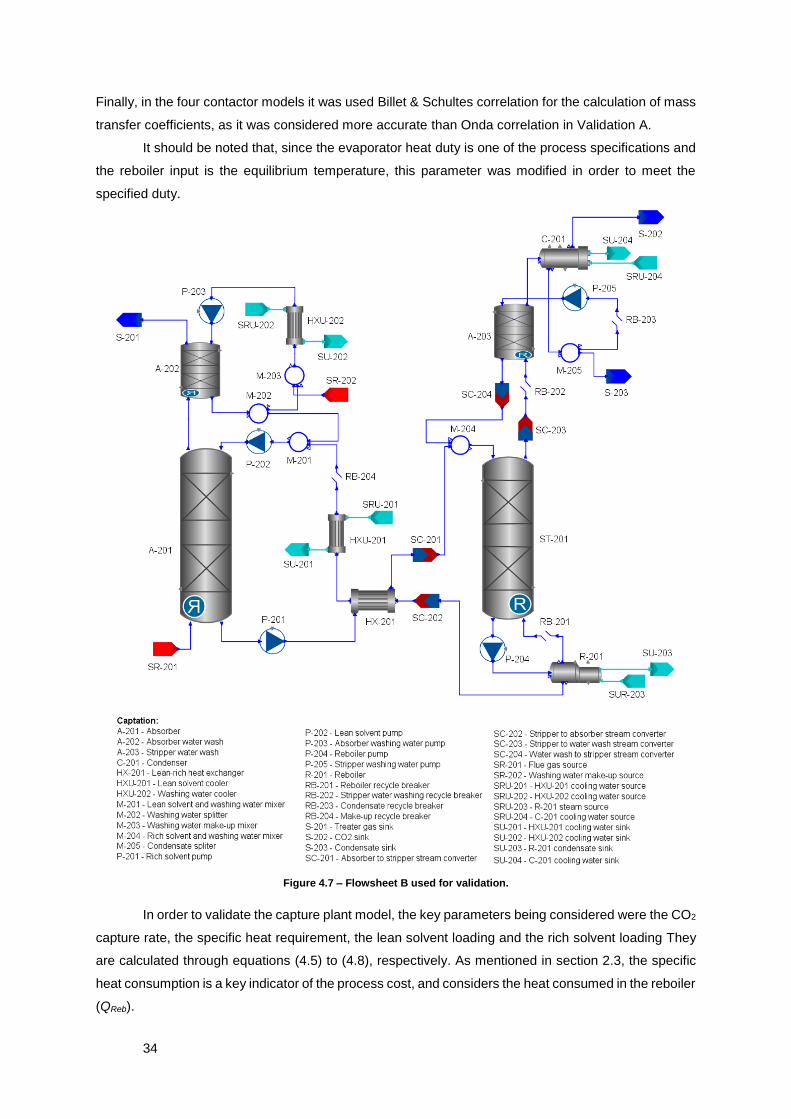
34
Finally, in the four contactor models it was used Billet & Schultes correlation for the calculation of mass
transfer coefficients, as it was considered more accurate than Onda correlation in Validation A.
It should be noted that, since the evaporator heat duty is one of the process specifications and
the reboiler input is the equilibrium temperature, this parameter was modified in order to meet the
specified duty.
Figure 4.7 – Flowsheet B used for validation.
In order to validate the capture plant model, the key parameters being considered were the CO2
capture rate, the specific heat requirement, the lean solvent loading and the rich solvent loading They
are calculated through equations (4.5) to (4.8), respectively. As mentioned in section 2.3, the specific
heat consumption is a key indicator of the process cost, and considers the heat consumed in the reboiler
(QReb).
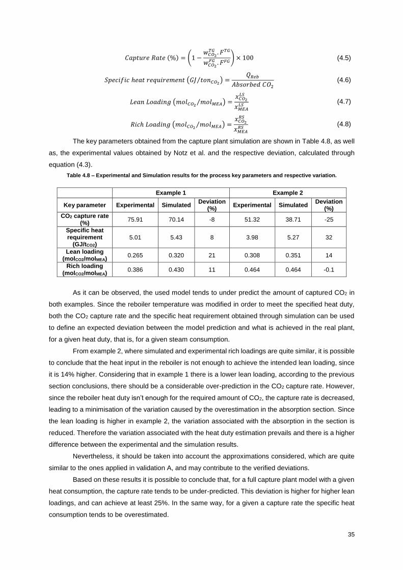
35
𝐶𝑎𝑝𝑡𝑢𝑟𝑒 𝑅𝑎𝑡𝑒 (%) = (1 −𝑤𝐶𝑂2
𝑇𝐺 . 𝐹𝑇𝐺
𝑤𝐶𝑂2
𝐹𝐺 . 𝐹𝐹𝐺) × 100 (4.5)
𝑆𝑝𝑒𝑐𝑖𝑓𝑖𝑐 ℎ𝑒𝑎𝑡 𝑟𝑒𝑞𝑢𝑖𝑟𝑒𝑚𝑒𝑛𝑡 (𝐺𝐽 𝑡𝑜𝑛𝐶𝑂2⁄ ) =
𝑄𝑅𝑒𝑏
𝐴𝑏𝑠𝑜𝑟𝑏𝑒𝑑 𝐶𝑂2
(4.6)
𝐿𝑒𝑎𝑛 𝐿𝑜𝑎𝑑𝑖𝑛𝑔 (𝑚𝑜𝑙𝐶𝑂2𝑚𝑜𝑙𝑀𝐸𝐴⁄ ) =
𝑥𝐶𝑂2𝐿𝑆
𝑥𝑀𝐸𝐴𝐿𝑆 (4.7)
𝑅𝑖𝑐ℎ 𝐿𝑜𝑎𝑑𝑖𝑛𝑔 (𝑚𝑜𝑙𝐶𝑂2𝑚𝑜𝑙𝑀𝐸𝐴⁄ ) =
𝑥𝐶𝑂2𝑅𝑆
𝑥𝑀𝐸𝐴𝑅𝑆 (4.8)
The key parameters obtained from the capture plant simulation are shown in Table 4.8, as well
as, the experimental values obtained by Notz et al. and the respective deviation, calculated through
equation (4.3).
Table 4.8 – Experimental and Simulation results for the process key parameters and respective variation.
Example 1 Example 2
Key parameter Experimental Simulated Deviation
(%) Experimental Simulated
Deviation (%)
CO2 capture rate (%)
75.91 70.14 -8 51.32 38.71 -25
Specific heat requirement
(GJ/tCO2) 5.01 5.43 8 3.98 5.27 32
Lean loading (molCO2/molMEA)
0.265 0.320 21 0.308 0.351 14
Rich loading (molCO2/molMEA)
0.386 0.430 11 0.464 0.464 -0.1
As it can be observed, the used model tends to under predict the amount of captured CO2 in
both examples. Since the reboiler temperature was modified in order to meet the specified heat duty,
both the CO2 capture rate and the specific heat requirement obtained through simulation can be used
to define an expected deviation between the model prediction and what is achieved in the real plant,
for a given heat duty, that is, for a given steam consumption.
From example 2, where simulated and experimental rich loadings are quite similar, it is possible
to conclude that the heat input in the reboiler is not enough to achieve the intended lean loading, since
it is 14% higher. Considering that in example 1 there is a lower lean loading, according to the previous
section conclusions, there should be a considerable over-prediction in the CO2 capture rate. However,
since the reboiler heat duty isn’t enough for the required amount of CO2, the capture rate is decreased,
leading to a minimisation of the variation caused by the overestimation in the absorption section. Since
the lean loading is higher in example 2, the variation associated with the absorption in the section is
reduced. Therefore the variation associated with the heat duty estimation prevails and there is a higher
difference between the experimental and the simulation results.
Nevertheless, it should be taken into account the approximations considered, which are quite
similar to the ones applied in validation A, and may contribute to the verified deviations.
Based on these results it is possible to conclude that, for a full capture plant model with a given
heat consumption, the capture rate tends to be under-predicted. This deviation is higher for higher lean
loadings, and can achieve at least 25%. In the same way, for a given a capture rate the specific heat
consumption tends to be overestimated.

36
This page was intentionally left blank.

37
5. MEA Full Scale Capture Plant Model
Under the assumption that the validation results presented in the previous section are still valid
for a full scale plant, a full size capture plant model was built. An approximate cost estimation model
was also developed, in order to estimate both the investment required and operational costs, which
were later optimised.
5.1. Base Case
The original flowsheet used for the simulation of a MEA based full scale capture plant was
based on a case study developed by PSE. The flue gas considered is characteristic of a natural gas
fuelled power plant emitting approximately 2 million tonnes of CO2 per year, and its conditions are
shown in Table 5.1.
Table 5.1 – Flue gas conditions considered in the MEA capture plant model.
Mass flow rate (kg/s) 1214.81
Mass fractions (g/g)
CO2 0.058
H2O 0.065
N2 0.877
Temperature (°C) 140.75
Pressure (bar) 1.013
Starting from these conditions, and before the capture process itself, the flue gas is saturated
in water at 40.95 °C, being used for that purpose process water at 25 °C. Then it enters the capture
process, whose flowsheet is defined by the design parameters and operating conditions shown in the
table below.
Table 5.2 – Design parameters and operating conditions considered in the original capture plant model.
Parameter Value
Absorber
Diameter (m) 20
Height (m) 11.89
Packing Sulzer Mellapak 250YTM
Stripper
Diameter (m) 8.5
Height (m) 10
Packing Sulzer Mellapak 250YTM
Lean-rich heat exchanger Cold stream outlet temperature (°C) 89.65
Lean solvent cooler Process stream outlet temperature (°C) 70.75
Reboiler Temperature (°C) 117.84
Reboiler pump Pressure (bar) 1.79
Condenser Temperature (°C) 40
Lean solvent Flow rate (kg/s) 736.02
MEA mass fraction (g/g) 0.300
The referred conditions were applied in a conventional PCC flowsheet, which topology is shown
in Figure 5.1. Besides the models already considered in section 4.2, this flowsheet includes a flash
model (F-301) used for the simulation of saturation process, in which the temperature is imposed by
the PID controller model (PID-301) that calculates the required flow rate of quenching water (P-301).
In order to keep the absorber pressure above atmospheric, the pump model P-302 acts as a gas blower,
in order to increase the flue gas pressure to 1.1 bar. In the columns’ models the Billet & Schultes
correlation was used for the calculation of the mass transfer coefficients and pressure drop. Since the

38
considered packing is the one used in the previous sections, its characteristic parameters are the ones
shown in Table 4.2.
Figure 5.1 – MEA capture plant flowsheet as seen in gPROMS® ModelBuilder.
In this model were also added several flow multiplier models (FM-301 to FM-310) at the inlets
and outlets of the absorber, regeneration section and reboiler to simulate the existence of equipment
working in parallel. For the estimation of the required number of absorption and stripping trains technical
restrictions found through PSE internal reports were considered. Due to construction limitations, the
absorber diameter should have a maximum value of 15 m or 20 m if in-site construction is possible.
Regarding the stripping section, it is considered a limit total reboiler duty of 200 MW per stripping train,
with a maximum of 4 reboilers per column (each with a duty inferior to 50 MW). Besides this, it must
also be considered that the vapour velocity in both columns should be between 70 and 80% of the
vapour flooding velocity, [54], being this velocities ratio an output of the columns model.
In order to obtain a case with a standard capture rate of 90% and a MEA mass fraction of 30%
in the CO2 free lean solvent, the lean-solvent flow rate and the respective MEA mass fraction were
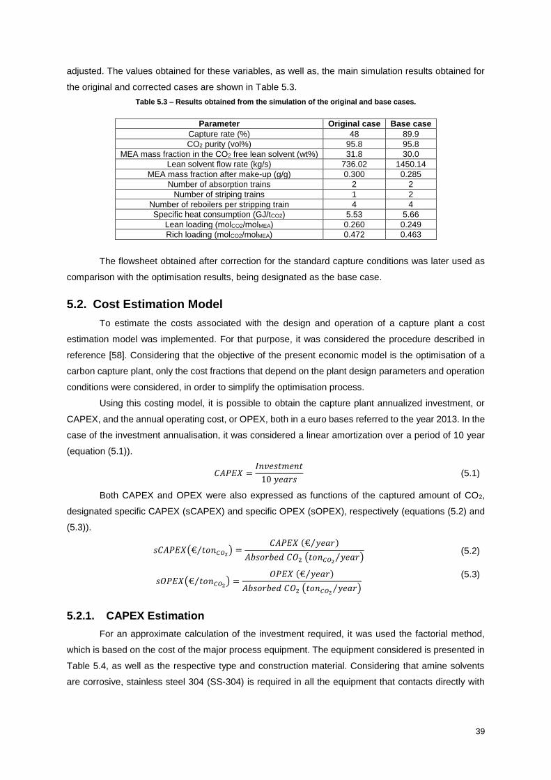
39
adjusted. The values obtained for these variables, as well as, the main simulation results obtained for
the original and corrected cases are shown in Table 5.3.
Table 5.3 – Results obtained from the simulation of the original and base cases.
Parameter Original case Base case
Capture rate (%) 48 89.9
CO2 purity (vol%) 95.8 95.8
MEA mass fraction in the CO2 free lean solvent (wt%) 31.8 30.0
Lean solvent flow rate (kg/s) 736.02 1450.14
MEA mass fraction after make-up (g/g) 0.300 0.285
Number of absorption trains 2 2
Number of striping trains 1 2
Number of reboilers per stripping train 4 4
Specific heat consumption (GJ/tCO2) 5.53 5.66
Lean loading (molCO2/molMEA) 0.260 0.249
Rich loading (molCO2/molMEA) 0.472 0.463
The flowsheet obtained after correction for the standard capture conditions was later used as
comparison with the optimisation results, being designated as the base case.
5.2. Cost Estimation Model
To estimate the costs associated with the design and operation of a capture plant a cost
estimation model was implemented. For that purpose, it was considered the procedure described in
reference [58]. Considering that the objective of the present economic model is the optimisation of a
carbon capture plant, only the cost fractions that depend on the plant design parameters and operation
conditions were considered, in order to simplify the optimisation process.
Using this costing model, it is possible to obtain the capture plant annualized investment, or
CAPEX, and the annual operating cost, or OPEX, both in a euro bases referred to the year 2013. In the
case of the investment annualisation, it was considered a linear amortization over a period of 10 year
(equation (5.1)).
𝐶𝐴𝑃𝐸𝑋 =𝐼𝑛𝑣𝑒𝑠𝑡𝑚𝑒𝑛𝑡
10 𝑦𝑒𝑎𝑟𝑠 (5.1)
Both CAPEX and OPEX were also expressed as functions of the captured amount of CO2,
designated specific CAPEX (sCAPEX) and specific OPEX (sOPEX), respectively (equations (5.2) and
(5.3)).
𝑠𝐶𝐴𝑃𝐸𝑋(€ 𝑡𝑜𝑛𝐶𝑂2⁄ ) =
𝐶𝐴𝑃𝐸𝑋 (€ 𝑦𝑒𝑎𝑟⁄ )
𝐴𝑏𝑠𝑜𝑟𝑏𝑒𝑑 𝐶𝑂2 (𝑡𝑜𝑛𝐶𝑂2𝑦𝑒𝑎𝑟⁄ )
(5.2)
𝑠𝑂𝑃𝐸𝑋(€ 𝑡𝑜𝑛𝐶𝑂2⁄ ) =
𝑂𝑃𝐸𝑋 (€ 𝑦𝑒𝑎𝑟⁄ )
𝐴𝑏𝑠𝑜𝑟𝑏𝑒𝑑 𝐶𝑂2 (𝑡𝑜𝑛𝐶𝑂2𝑦𝑒𝑎𝑟⁄ )
(5.3)
5.2.1. CAPEX Estimation
For an approximate calculation of the investment required, it was used the factorial method,
which is based on the cost of the major process equipment. The equipment considered is presented in
Table 5.4, as well as the respective type and construction material. Considering that amine solvents
are corrosive, stainless steel 304 (SS-304) is required in all the equipment that contacts directly with
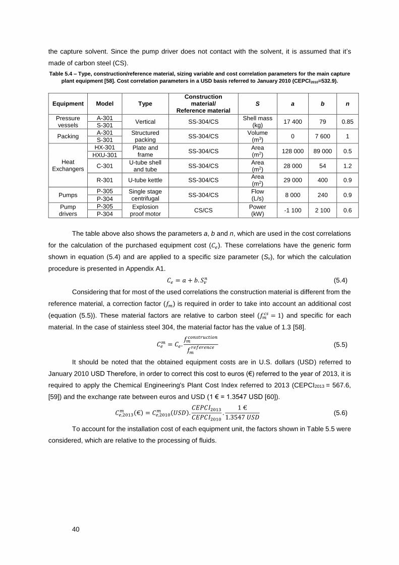
40
the capture solvent. Since the pump driver does not contact with the solvent, it is assumed that it’s
made of carbon steel (CS).
Table 5.4 – Type, construction/reference material, sizing variable and cost correlation parameters for the main capture
plant equipment [58]. Cost correlation parameters in a USD basis referred to January 2010 (CEPCI2010=532.9).
Equipment Model Type Construction
material/ Reference material
S a b n
Pressure vessels
A-301 Vertical SS-304/CS
Shell mass (kg)
17 400 79 0.85 S-301
Packing A-301 Structured
packing SS-304/CS
Volume (m3)
0 7 600 1 S-301
Heat Exchangers
HX-301 Plate and frame
SS-304/CS Area (m2)
128 000 89 000 0.5 HXU-301
C-301 U-tube shell
and tube SS-304/CS
Area (m2)
28 000 54 1.2
R-301 U-tube kettle SS-304/CS Area (m2)
29 000 400 0.9
Pumps P-305 Single stage
centrifugal SS-304/CS
Flow (L/s)
8 000 240 0.9 P-304
Pump drivers
P-305 Explosion proof motor
CS/CS Power (kW)
-1 100 2 100 0.6 P-304
The table above also shows the parameters a, b and n, which are used in the cost correlations
for the calculation of the purchased equipment cost (𝐶𝑒). These correlations have the generic form
shown in equation (5.4) and are applied to a specific size parameter (Sv), for which the calculation
procedure is presented in Appendix A1.
𝐶𝑒 = 𝑎 + 𝑏. 𝑆𝑣𝑛 (5.4)
Considering that for most of the used correlations the construction material is different from the
reference material, a correction factor (𝑓𝑚) is required in order to take into account an additional cost
(equation (5.5)). These material factors are relative to carbon steel (𝑓𝑚𝑐𝑠 = 1) and specific for each
material. In the case of stainless steel 304, the material factor has the value of 1.3 [58].
𝐶𝑒𝑚 = 𝐶𝑒 .
𝑓𝑚𝑐𝑜𝑛𝑠𝑡𝑟𝑢𝑐𝑡𝑖𝑜𝑛
𝑓𝑚𝑟𝑒𝑓𝑒𝑟𝑒𝑛𝑐𝑒
(5.5)
It should be noted that the obtained equipment costs are in U.S. dollars (USD) referred to
January 2010 USD Therefore, in order to correct this cost to euros (€) referred to the year of 2013, it is
required to apply the Chemical Engineering's Plant Cost Index referred to 2013 (CEPCI2013 = 567.6,
[59]) and the exchange rate between euros and USD (1 € = 1.3547 USD [60]).
𝐶𝑒,2013𝑚 (€) = 𝐶𝑒,2010
𝑚 (𝑈𝑆𝐷).𝐶𝐸𝑃𝐶𝐼2013
𝐶𝐸𝑃𝐶𝐼2010
.1 €
1.3547 𝑈𝑆𝐷 (5.6)
To account for the installation cost of each equipment unit, the factors shown in Table 5.5 were
considered, which are relative to the processing of fluids.
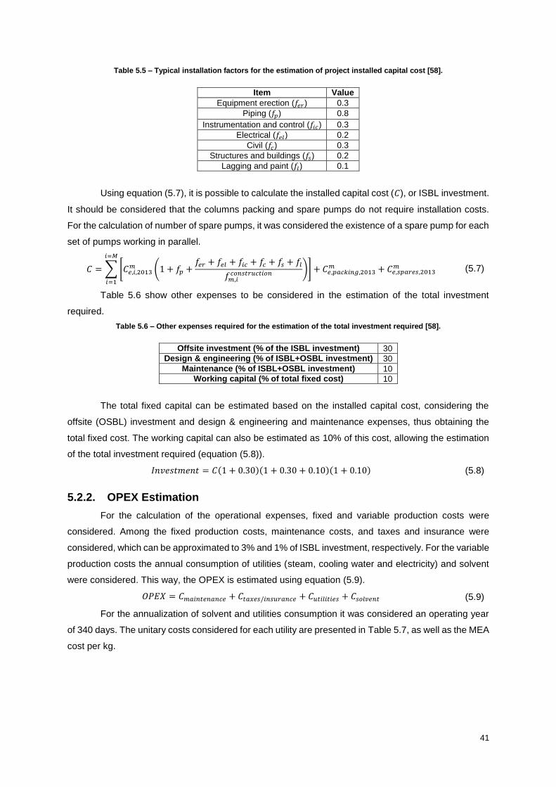
41
Table 5.5 – Typical installation factors for the estimation of project installed capital cost [58].
Item Value
Equipment erection (𝑓𝑒𝑟) 0.3
Piping (𝑓𝑝) 0.8
Instrumentation and control (𝑓𝑖𝑐) 0.3
Electrical (𝑓𝑒𝑙) 0.2
Civil (𝑓𝑐) 0.3
Structures and buildings (𝑓𝑠) 0.2
Lagging and paint (𝑓𝑙) 0.1
Using equation (5.7), it is possible to calculate the installed capital cost (𝐶), or ISBL investment.
It should be considered that the columns packing and spare pumps do not require installation costs.
For the calculation of number of spare pumps, it was considered the existence of a spare pump for each
set of pumps working in parallel.
𝐶 = ∑ [𝐶𝑒,𝑖,2013𝑚 (1 + 𝑓𝑝 +
𝑓𝑒𝑟 + 𝑓𝑒𝑙 + 𝑓𝑖𝑐 + 𝑓𝑐 + 𝑓𝑠 + 𝑓𝑙
𝑓𝑚,𝑖𝑐𝑜𝑛𝑠𝑡𝑟𝑢𝑐𝑡𝑖𝑜𝑛
)]
𝑖=𝑀
𝑖=1
+ 𝐶𝑒,𝑝𝑎𝑐𝑘𝑖𝑛𝑔,2013𝑚 + 𝐶𝑒,𝑠𝑝𝑎𝑟𝑒𝑠,2013
𝑚 (5.7)
Table 5.6 show other expenses to be considered in the estimation of the total investment
required.
Table 5.6 – Other expenses required for the estimation of the total investment required [58].
Offsite investment (% of the ISBL investment) 30
Design & engineering (% of ISBL+OSBL investment) 30
Maintenance (% of ISBL+OSBL investment) 10
Working capital (% of total fixed cost) 10
The total fixed capital can be estimated based on the installed capital cost, considering the
offsite (OSBL) investment and design & engineering and maintenance expenses, thus obtaining the
total fixed cost. The working capital can also be estimated as 10% of this cost, allowing the estimation
of the total investment required (equation (5.8)).
𝐼𝑛𝑣𝑒𝑠𝑡𝑚𝑒𝑛𝑡 = 𝐶(1 + 0.30)(1 + 0.30 + 0.10)(1 + 0.10) (5.8)
5.2.2. OPEX Estimation
For the calculation of the operational expenses, fixed and variable production costs were
considered. Among the fixed production costs, maintenance costs, and taxes and insurance were
considered, which can be approximated to 3% and 1% of ISBL investment, respectively. For the variable
production costs the annual consumption of utilities (steam, cooling water and electricity) and solvent
were considered. This way, the OPEX is estimated using equation (5.9).
𝑂𝑃𝐸𝑋 = 𝐶𝑚𝑎𝑖𝑛𝑡𝑒𝑛𝑎𝑛𝑐𝑒 + 𝐶𝑡𝑎𝑥𝑒𝑠/𝑖𝑛𝑠𝑢𝑟𝑎𝑛𝑐𝑒 + 𝐶𝑢𝑡𝑖𝑙𝑖𝑡𝑖𝑒𝑠 + 𝐶𝑠𝑜𝑙𝑣𝑒𝑛𝑡 (5.9)
For the annualization of solvent and utilities consumption it was considered an operating year
of 340 days. The unitary costs considered for each utility are presented in Table 5.7, as well as the MEA
cost per kg.
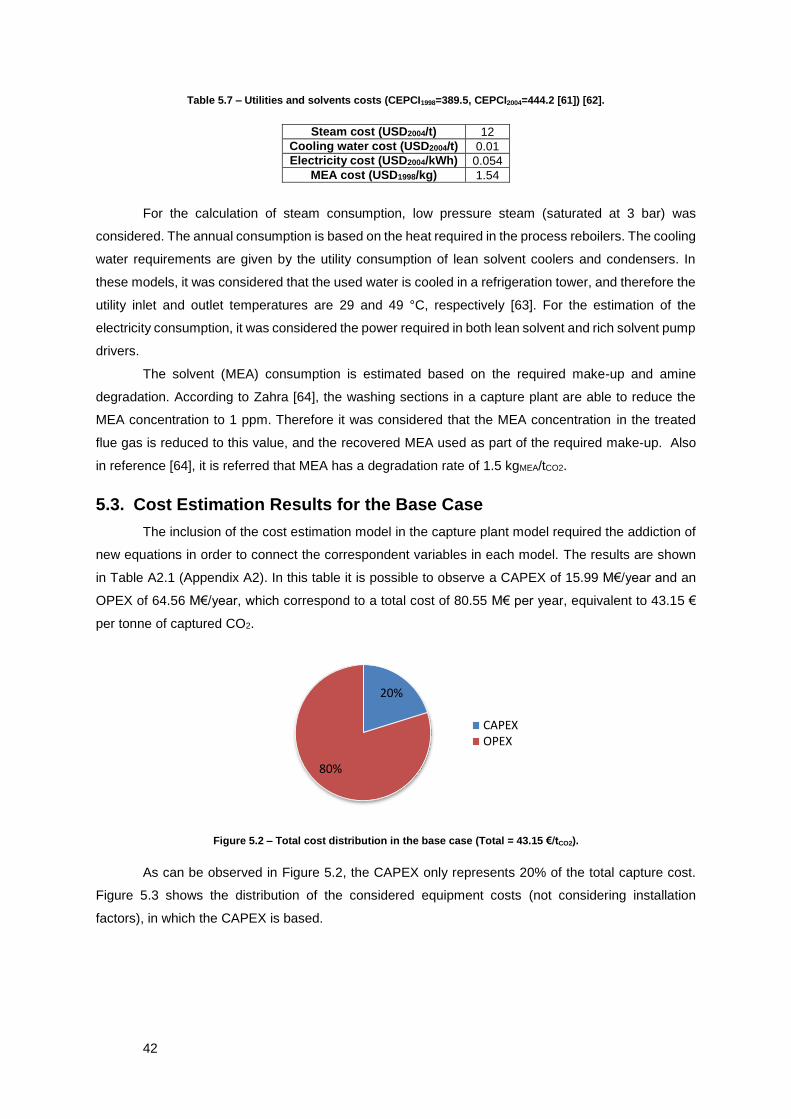
42
Table 5.7 – Utilities and solvents costs (CEPCI1998=389.5, CEPCI2004=444.2 [61]) [62].
Steam cost (USD2004/t) 12
Cooling water cost (USD2004/t) 0.01
Electricity cost (USD2004/kWh) 0.054
MEA cost (USD1998/kg) 1.54
For the calculation of steam consumption, low pressure steam (saturated at 3 bar) was
considered. The annual consumption is based on the heat required in the process reboilers. The cooling
water requirements are given by the utility consumption of lean solvent coolers and condensers. In
these models, it was considered that the used water is cooled in a refrigeration tower, and therefore the
utility inlet and outlet temperatures are 29 and 49 °C, respectively [63]. For the estimation of the
electricity consumption, it was considered the power required in both lean solvent and rich solvent pump
drivers.
The solvent (MEA) consumption is estimated based on the required make-up and amine
degradation. According to Zahra [64], the washing sections in a capture plant are able to reduce the
MEA concentration to 1 ppm. Therefore it was considered that the MEA concentration in the treated
flue gas is reduced to this value, and the recovered MEA used as part of the required make-up. Also
in reference [64], it is referred that MEA has a degradation rate of 1.5 kgMEA/tCO2.
5.3. Cost Estimation Results for the Base Case
The inclusion of the cost estimation model in the capture plant model required the addiction of
new equations in order to connect the correspondent variables in each model. The results are shown
in Table A2.1 (Appendix A2). In this table it is possible to observe a CAPEX of 15.99 M€/year and an
OPEX of 64.56 M€/year, which correspond to a total cost of 80.55 M€ per year, equivalent to 43.15 €
per tonne of captured CO2.
Figure 5.2 – Total cost distribution in the base case (Total = 43.15 €/tCO2).
As can be observed in Figure 5.2, the CAPEX only represents 20% of the total capture cost.
Figure 5.3 shows the distribution of the considered equipment costs (not considering installation
factors), in which the CAPEX is based.
20%
80%
CAPEXOPEX
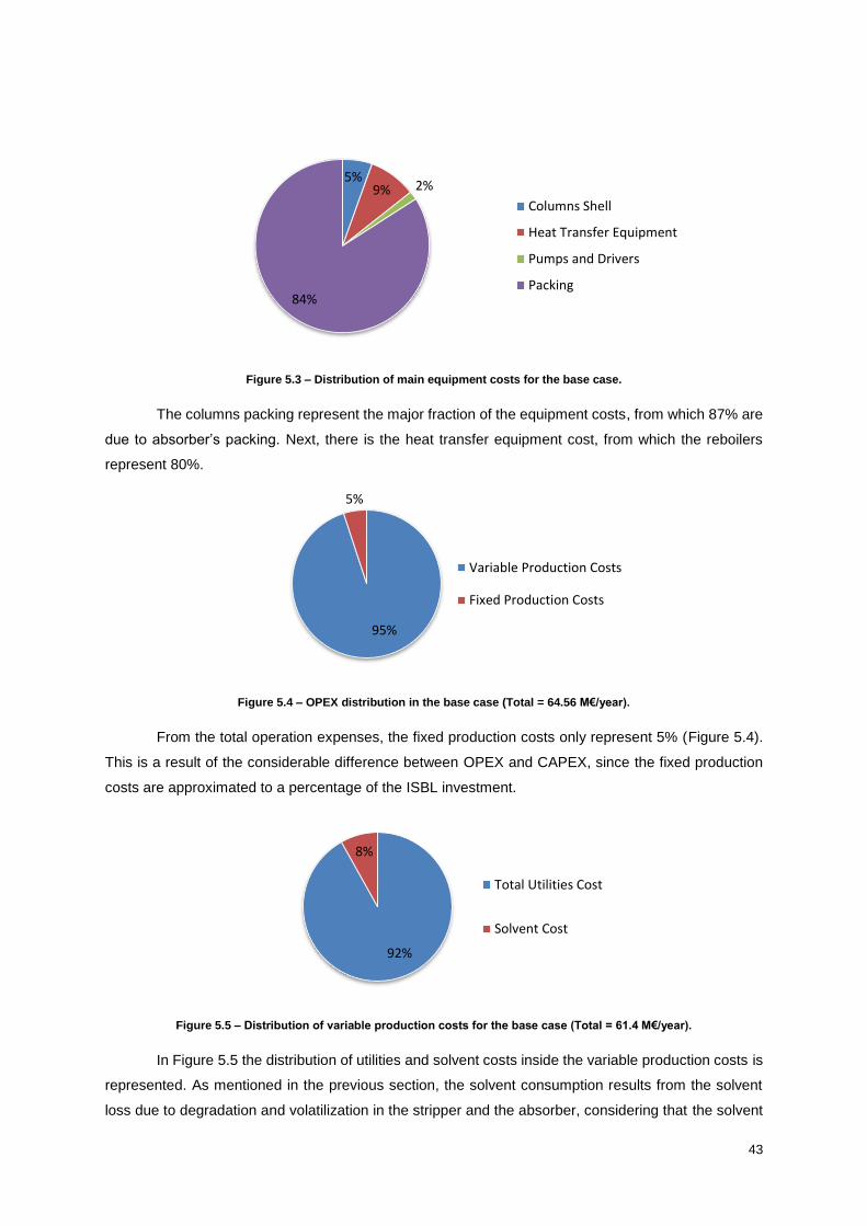
43
Figure 5.3 – Distribution of main equipment costs for the base case.
The columns packing represent the major fraction of the equipment costs, from which 87% are
due to absorber’s packing. Next, there is the heat transfer equipment cost, from which the reboilers
represent 80%.
Figure 5.4 – OPEX distribution in the base case (Total = 64.56 M€/year).
From the total operation expenses, the fixed production costs only represent 5% (Figure 5.4).
This is a result of the considerable difference between OPEX and CAPEX, since the fixed production
costs are approximated to a percentage of the ISBL investment.
Figure 5.5 – Distribution of variable production costs for the base case (Total = 61.4 M€/year).
In Figure 5.5 the distribution of utilities and solvent costs inside the variable production costs is
represented. As mentioned in the previous section, the solvent consumption results from the solvent
loss due to degradation and volatilization in the stripper and the absorber, considering that the solvent
5%9% 2%
84%
Columns Shell
Heat Transfer Equipment
Pumps and Drivers
Packing
95%
5%
Variable Production Costs
Fixed Production Costs
92%
8%
Total Utilities Cost
Solvent Cost

44
in the treated gas is partly recovered. Figure 5.6 features the distribution of MEA losses in the process,
without considering a washing section after the absorber.
Figure 5.6 – Distribution of the amine losses in base case (Total = 12.5 kt/year).
In the absence of water washing, the amine loss in the absorber represents 77% of a total loss
of 12.5 kt/year. Taking into account this loss, it is clear that a washing section is required after the
absorber, allowing the reduction of the MEA loss to 3.03 kt/year. This means a significant reduction in
the solvent expenses from 31.8 M€/year to 5 M€/year.
Nevertheless, Figure 5.5 shows that the major contribution to variable operating costs is due to
utilities consumption. The distribution of these expenses is shown in Figure 5.7.
Figure 5.7 – Distribution of the utilities costs for the base case (Total = 56.4 M€/year).
The steam consumption in the process reboilers strongly surpasses the electricity and water
consumption. In fact, the steam cost corresponds to 69% of the capture plant total cost
(CAPEX+OPEX), being the major process expense, as it is stated in literature (see section 2.3.1.2).
Considering the presented results, it is possible to conclude that CAPEX is mainly dependent
on the size of each absorber (height and diameter). It is also possible to see that the OPEX (and the
total cost, considering the relevance of the OPEX over the CAPEX) is mainly affected by the steam
consumed in the regeneration reboilers, which is directly related to the heat required. Therefore, it is
expected that the optimisation of the capture plant flowsheet will mainly rely on changing the absorbers’
size and the steam spent in the reboiler.
0%
77%
23%
Stripper
Absorber
Degradation
1%
98%
1%
Electricity
Steam
Cooled Water
45
6. Optimisation Problem Formulation
The optimisation of the capture process flowsheet was performed using the optimisation
functionalities of gPROMS® ModelBuilder 3.7.1. This functionality allows the minimisation of the
objective function, by modifying decision (or control) variables, considering the defined constraints.
In order to simplify the optimisation problem, several considerations were taken. The number
of absorption and stripping trains were not included in the optimisation problem, being changed
manually in the model for each case.
Since the pressure in the stripping section is set in the pump model (P-305) in Pascal, the
variation of this variable would be conditioned by the reduced effect on the objective function, being
considered a scale problem. Therefore, this pressure is instead explicitly defined in the flowsheet in bar
units, to improve its effect on the objective function during optimization.
According to Zahra [64], for a given lean solvent flow rate, capture rate and lean loading, the
optimal steam consumption is obtained for the combination of the highest possible stripping pressure
and reboiler temperature. Therefore, before proceeding to the process optimisation, the base flowsheet
was modified in order to start from the highest allowable temperature, which is 120 °C, as mentioned in
section 2.3.1. This way, this variable was not included in the optimisation problem. This assumption is
confirmed in the last optimisation (section 7.2.4), where the reboiler temperature was used as a decision
variable, which in fact converged to the imposed maximum value.
6.1. Objective Function
The objective function is defined by the process variable being minimised or maximised. For
the optimisation of the capture plant with the cost estimation model included, the objective function
should lead to the minimisation of both the specific CAPEX and specific OPEX. Therefore the objective
function (OF) is defined as the sum of these two costs (equation (6.1)).
𝑂𝐹 = 𝑠𝐶𝐴𝑃𝐸𝑋 + 𝑠𝑂𝑃𝐸𝑋 (6.1)
Considering that the steam spent in the reboilers is the major cost of the process, an alternative
objective function (OF2) can be defined as the specific heat requirement (defined in equation (4.6)),
since it is directly related with the specific steam cost. Nevertheless, this objective function was only
used as comparison in section 7.1.4.
𝑂𝐹2 = 𝑆𝑝𝑒𝑐𝑖𝑓𝑖𝑐 ℎ𝑒𝑎𝑡 𝑟𝑒𝑞𝑢𝑖𝑟𝑒𝑚𝑒𝑛𝑡 (6.2)
6.2. Decision Variables
The decision variables define which of the capture flowsheet variables are used to minimise the
objective function. In this case, the variables that define the equipment design and the process
operating conditions were chosen. It is also necessary to specify the initial value of the variable and a
lower and upper bound. Nevertheless, the range considered shouldn’t be excessive in order to facilitate
the optimization convergence. The decision variables, initial values and bounds, are show in Table 6.1.
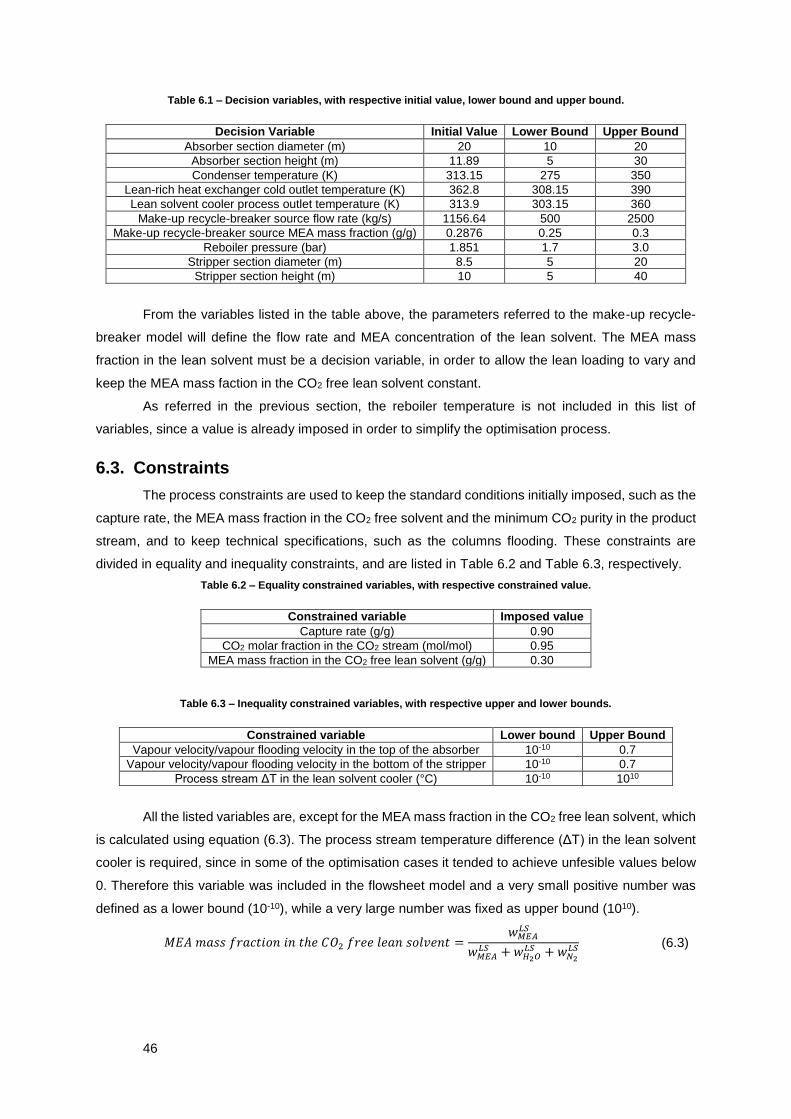
46
Table 6.1 – Decision variables, with respective initial value, lower bound and upper bound.
Decision Variable Initial Value Lower Bound Upper Bound
Absorber section diameter (m) 20 10 20
Absorber section height (m) 11.89 5 30
Condenser temperature (K) 313.15 275 350
Lean-rich heat exchanger cold outlet temperature (K) 362.8 308.15 390
Lean solvent cooler process outlet temperature (K) 313.9 303.15 360
Make-up recycle-breaker source flow rate (kg/s) 1156.64 500 2500
Make-up recycle-breaker source MEA mass fraction (g/g) 0.2876 0.25 0.3
Reboiler pressure (bar) 1.851 1.7 3.0
Stripper section diameter (m) 8.5 5 20
Stripper section height (m) 10 5 40
From the variables listed in the table above, the parameters referred to the make-up recycle-
breaker model will define the flow rate and MEA concentration of the lean solvent. The MEA mass
fraction in the lean solvent must be a decision variable, in order to allow the lean loading to vary and
keep the MEA mass faction in the CO2 free lean solvent constant.
As referred in the previous section, the reboiler temperature is not included in this list of
variables, since a value is already imposed in order to simplify the optimisation process.
6.3. Constraints
The process constraints are used to keep the standard conditions initially imposed, such as the
capture rate, the MEA mass fraction in the CO2 free solvent and the minimum CO2 purity in the product
stream, and to keep technical specifications, such as the columns flooding. These constraints are
divided in equality and inequality constraints, and are listed in Table 6.2 and Table 6.3, respectively.
Table 6.2 – Equality constrained variables, with respective constrained value.
Constrained variable Imposed value
Capture rate (g/g) 0.90
CO2 molar fraction in the CO2 stream (mol/mol) 0.95
MEA mass fraction in the CO2 free lean solvent (g/g) 0.30
Table 6.3 – Inequality constrained variables, with respective upper and lower bounds.
Constrained variable Lower bound Upper Bound
Vapour velocity/vapour flooding velocity in the top of the absorber 10-10 0.7
Vapour velocity/vapour flooding velocity in the bottom of the stripper 10-10 0.7
Process stream ΔT in the lean solvent cooler (°C) 10-10 1010
All the listed variables are, except for the MEA mass fraction in the CO2 free lean solvent, which
is calculated using equation (6.3). The process stream temperature difference (ΔT) in the lean solvent
cooler is required, since in some of the optimisation cases it tended to achieve unfesible values below
0. Therefore this variable was included in the flowsheet model and a very small positive number was
defined as a lower bound (10-10), while a very large number was fixed as upper bound (1010).
𝑀𝐸𝐴 𝑚𝑎𝑠𝑠 𝑓𝑟𝑎𝑐𝑡𝑖𝑜𝑛 𝑖𝑛 𝑡ℎ𝑒 𝐶𝑂2 𝑓𝑟𝑒𝑒 𝑙𝑒𝑎𝑛 𝑠𝑜𝑙𝑣𝑒𝑛𝑡 =𝑤𝑀𝐸𝐴
𝐿𝑆
𝑤𝑀𝐸𝐴𝐿𝑆 + 𝑤𝐻2𝑂
𝐿𝑆 + 𝑤𝑁2
𝐿𝑆 (6.3)
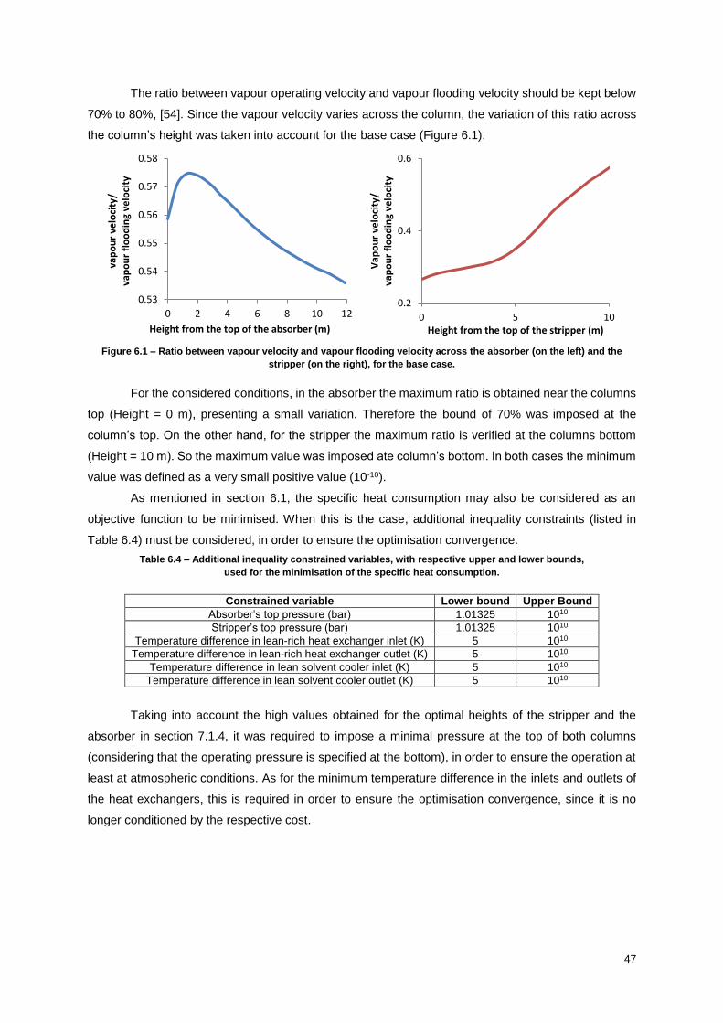
47
The ratio between vapour operating velocity and vapour flooding velocity should be kept below
70% to 80%, [54]. Since the vapour velocity varies across the column, the variation of this ratio across
the column’s height was taken into account for the base case (Figure 6.1).
Figure 6.1 – Ratio between vapour velocity and vapour flooding velocity across the absorber (on the left) and the
stripper (on the right), for the base case.
For the considered conditions, in the absorber the maximum ratio is obtained near the columns
top (Height = 0 m), presenting a small variation. Therefore the bound of 70% was imposed at the
column’s top. On the other hand, for the stripper the maximum ratio is verified at the columns bottom
(Height = 10 m). So the maximum value was imposed ate column’s bottom. In both cases the minimum
value was defined as a very small positive value (10-10).
As mentioned in section 6.1, the specific heat consumption may also be considered as an
objective function to be minimised. When this is the case, additional inequality constraints (listed in
Table 6.4) must be considered, in order to ensure the optimisation convergence.
Table 6.4 – Additional inequality constrained variables, with respective upper and lower bounds,
used for the minimisation of the specific heat consumption.
Constrained variable Lower bound Upper Bound
Absorber’s top pressure (bar) 1.01325 1010
Stripper’s top pressure (bar) 1.01325 1010
Temperature difference in lean-rich heat exchanger inlet (K) 5 1010
Temperature difference in lean-rich heat exchanger outlet (K) 5 1010
Temperature difference in lean solvent cooler inlet (K) 5 1010
Temperature difference in lean solvent cooler outlet (K) 5 1010
Taking into account the high values obtained for the optimal heights of the stripper and the
absorber in section 7.1.4, it was required to impose a minimal pressure at the top of both columns
(considering that the operating pressure is specified at the bottom), in order to ensure the operation at
least at atmospheric conditions. As for the minimum temperature difference in the inlets and outlets of
the heat exchangers, this is required in order to ensure the optimisation convergence, since it is no
longer conditioned by the respective cost.
0.53
0.54
0.55
0.56
0.57
0.58
0 2 4 6 8 10 12
vap
ou
r ve
loci
ty/
vap
ou
r fl
oo
din
g ve
loci
ty
Height from the top of the absorber (m)
0.2
0.4
0.6
0 5 10
Vap
ou
r ve
loci
ty/
vap
ou
r fl
oo
din
g ve
loci
ty
Height from the top of the stripper (m)

48
This page was intentionally left blank.
49
7. Optimisation Results
After solving the optimisation problem applied to the base case, a minimisation of the total cost
per tonne of captured CO2 was achieved. As mentioned before, for the base case optimisation a capture
rate of 90%, a MEA mass fraction in the CO2 free lean solvent of 30% and a minimum CO2 purity of 95
vol% were imposed. To evaluate the effect of each of these constraints in the total cost of the CO2
capture, they were changed, and the new optimal costs were compared with the standard ones (Section
7.2).
The main results of these optimisations are shown in Appendix A2, and commented in the
following sections.
7.1. Base Case Optimisation with Standard Constraints
The base case was optimised considering the decision variables and constraints mentioned
before, in order to minimise the total cost per tonne of captured CO2. Based on this procedure, the effect
of modifying the optimisation initial values was studied, namely the initial lean loading, and the effect of
having a different number of absorption trains.
Besides the minimisation of the total cost, another case was conducted with the minimisation
of the specific heat requirement with the objective of verifying if the minimum total cost leads to a
minimum heat consumption.
7.1.1. Specific Total Cost Minimisation
The results obtained from this optimisation process are presented in Table 7.1, where it also
can be observed its comparison with the base case. As it is shown, the main variations occur in the
absorber size (height and diameter are reduced by 29% and 12%, respectively), in the stripper size
(diameter is reduced by 15% and height is increased 69%) and in the lean solvent flow rate (reduced
by 18%).
It can be observed a reduction in the CAPEX of 21% and in the OPEX of 13%, which lead to a
specific total cost of 36.69 € per tonne of captured CO2 (Figure 7.1), which means a reduction of 15%.
As expected, there is a considerable variation in the specific heat requirement, which shows an optimal
value of 4.87 GJ/tCO2, with the steam consumption still representing 98% of the utilities requirements
and 69% of the total annual cost. Besides the reduction in the steam consumption, for the OPEX
reduction also contributes the decrease in the cooling water, electricity and solvent consumption, as
well as the other costs which are estimated based on the ISBL investment.

50
Table 7.1 – Detailed results from the specific total cost minimisation with standard constraints, and comparison with
the base case (Table A2.1).
Decision Variables Variation
Absorber (A-301) Diameter (m) 17.61 -12%
Height (m) 8.49 -29%
Stripper (ST-301) Diameter (m) 7.26 -15%
Height (m) 16.90 69%
Lean-Rich Heat Exchanger (HX-301) Outlet temperature of the rich solvent (K) 381.07 5%
Lean Solvent Cooler (HXU-301) Outlet temperature of the lean solvent (K) 313.87 -0.01%
Reboiler (R-301) Temperature (K) 393.15 1%
Pressure (bar) 1.85 3%
Condenser (C-301) Temperature (K) 317.01 1%
Lean Solvent (RB-303) Flow Rate (kg/s) 1 194.94 -18%
MEA mas fraction (g/g) 0.288 1%
Investment (k€) Variation
Equipment Cost
Absorber Shell (2 units) 1 796 -25%
Absorber Packing (2 units) 24 708 -45%
Stripper Shell (2 units) 1 257 18%
Stripper Packing (2 units) 8 354 23%
Lean-Rich Heat Exchanger (10 units) 765 203%
Lean Solvent Cooler (6 units) 436 25%
Reboiler (2x4 units) 4 310 1%
Condenser (2x2 units) 869 78%
Rich Solvent Pump (10 units) 262 -17%
Rich Solvent Pump Driver (10 units) 191 -5%
Lean Solvent Pump (10 units) 265 -18%
Lean Solvent Pump Driver (10 units) 129 -26%
ISBL Investment 62 823 -21%
Total Fixed Investment 125 772 -21%
Production Cost (k€/Year) Variation
Variable Production Costs
Electricity 358 -12%
Steam 47 533 -14%
Cooled Water 587 -23%
Solvent (MEA) 4 983 -0.6%
Total 53 462 -13%
Fixed Production Costs 2 513 -21%
Total Production Cost 55 975 -13%
Total Cost (M€/year) Variation
CAPEX 12.58 -21%
OPEX 55.97 -13%
Total 68.55 -15%
Key Parameters Variation
CO2 Capture Rate (%) 90 0.1%
CO2 Purity (vol%) 95 -0.8%
MEA mass fraction in the CO2 free lean solvent (wt%) 30 -0.01%
Vapour velocity/vapour flooding velocity in the top of the absorber 0.70 25%
Vapour velocity/vapour flooding velocity in the bottom of the stripper 0.70 22%
Process stream ΔT in the lean solvent cooler (K) 13.94 -57%
Lean Loading (molCO2/molMEA) 0.200 -20%
Rich Loading (molCO2/molMEA) 0.458 -1%
CO2 recovery rate in the regeneration section (%) 56 22%
Specific Energy Requirement (GJ/tCO2) 4.87 -14%
sCAPEX (€/tCO2) 6.73 -21%
sOPEX (€/tCO2) 29.95 -13%
Specific Total Cost (€/tCO2) 36.69 -15%
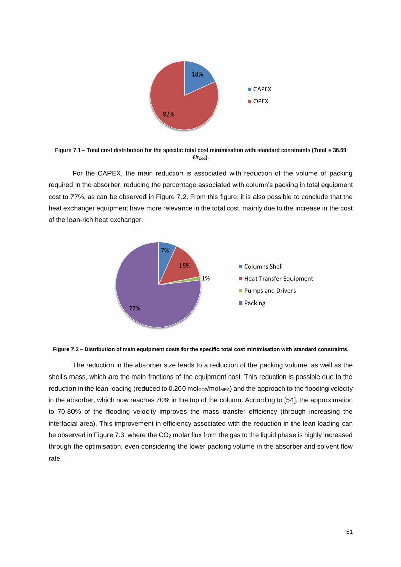
51
Figure 7.1 – Total cost distribution for the specific total cost minimisation with standard constraints (Total = 36.69
€/tCO2).
For the CAPEX, the main reduction is associated with reduction of the volume of packing
required in the absorber, reducing the percentage associated with column’s packing in total equipment
cost to 77%, as can be observed in Figure 7.2. From this figure, it is also possible to conclude that the
heat exchanger equipment have more relevance in the total cost, mainly due to the increase in the cost
of the lean-rich heat exchanger.
Figure 7.2 – Distribution of main equipment costs for the specific total cost minimisation with standard constraints.
The reduction in the absorber size leads to a reduction of the packing volume, as well as the
shell’s mass, which are the main fractions of the equipment cost. This reduction is possible due to the
reduction in the lean loading (reduced to 0.200 molCO2/molMEA) and the approach to the flooding velocity
in the absorber, which now reaches 70% in the top of the column. According to [54], the approximation
to 70-80% of the flooding velocity improves the mass transfer efficiency (through increasing the
interfacial area). This improvement in efficiency associated with the reduction in the lean loading can
be observed in Figure 7.3, where the CO2 molar flux from the gas to the liquid phase is highly increased
through the optimisation, even considering the lower packing volume in the absorber and solvent flow
rate.
18%
82%
CAPEX
OPEX
7%
15%
1%
77%
Columns Shell
Heat Transfer Equipment
Pumps and Drivers
Packing

52
Figure 7.3 – CO2 molar flux to the liquid phase across the absorber (top of the absorber equivalent to 0), before and
after the specific total cost minimisation with standard constraints.
The reduction in the lean solvent flow rate also reduces the size (and therefore the cost) of
pumps and respective drivers, and reduces the respective electricity consumption in 12%.
The increase of 5% in the rich solvent temperature at the lean-rich heat exchanger outlet
reduces the temperature difference across the stripper. Figure 7.4 shows the representative
temperature profile in the heat exchanger before and after optimisation, in which is possible to see a
reduction in the driving force for the heat transfer (ΔTlm). Both, the increase in the heat transferred and
the reduction in ΔTlm lead to an increase of the required area, which will require six additional heat
exchangers, increasing the cost in 203%.
Figure 7.4 – Representative temperature profiles of the lean-rich heat exchanger in the base case (on the left) and after
the total cost minimisation (on the right).
According to Zahra [64], the reduction in the absorber’s temperature should reduce the energy
required in regeneration, considering that the absorption process tends to be favoured at lower
temperatures, due to its exothermic nature. Nevertheless, the optimisation process does not change
considerably the outlet temperature of the lean solvent cooler (variation of -0.01%). Figure 7.5 features
the cooler temperature profile before and after optimisation.
0
0.003
0.006
0.009
0 1000 2000 3000 4000
CO
2m
ola
r fl
ux
(km
ol.
m-2
.s-1
)
Volume of packing from the absorber top (m3)
Base
Optimal
280
300
320
340
360
380
400
420
0 0.5 1
Tem
pe
ratu
re (
K)
Relative position to the cold stream inlet
Cold Stream Hot Stream
280
300
320
340
360
380
400
420
0 0.5 1
Tem
pe
ratu
re (
K)
Relative position to the cold stream inlet
Cold Stream Hot Stream
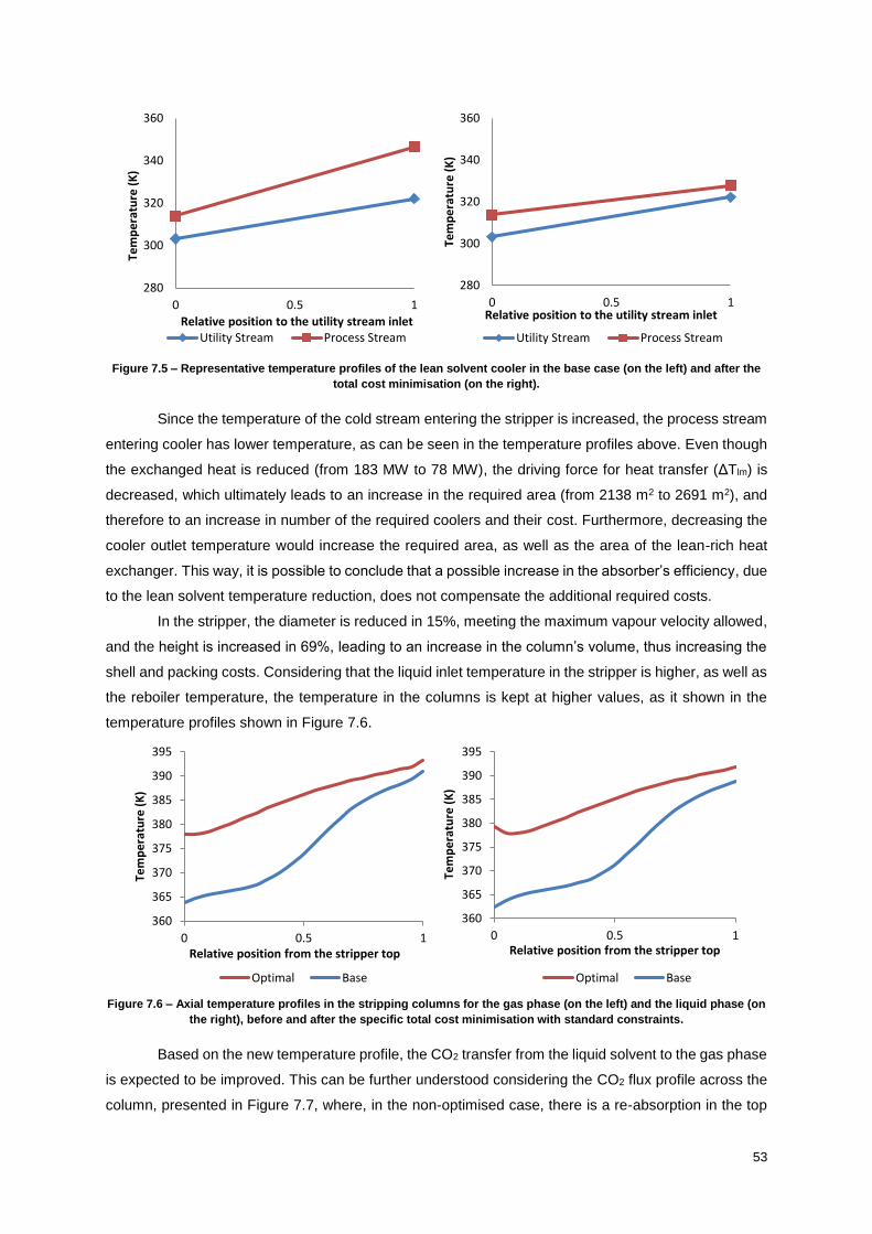
53
Figure 7.5 – Representative temperature profiles of the lean solvent cooler in the base case (on the left) and after the
total cost minimisation (on the right).
Since the temperature of the cold stream entering the stripper is increased, the process stream
entering cooler has lower temperature, as can be seen in the temperature profiles above. Even though
the exchanged heat is reduced (from 183 MW to 78 MW), the driving force for heat transfer (ΔTlm) is
decreased, which ultimately leads to an increase in the required area (from 2138 m2 to 2691 m2), and
therefore to an increase in number of the required coolers and their cost. Furthermore, decreasing the
cooler outlet temperature would increase the required area, as well as the area of the lean-rich heat
exchanger. This way, it is possible to conclude that a possible increase in the absorber’s efficiency, due
to the lean solvent temperature reduction, does not compensate the additional required costs.
In the stripper, the diameter is reduced in 15%, meeting the maximum vapour velocity allowed,
and the height is increased in 69%, leading to an increase in the column’s volume, thus increasing the
shell and packing costs. Considering that the liquid inlet temperature in the stripper is higher, as well as
the reboiler temperature, the temperature in the columns is kept at higher values, as it shown in the
temperature profiles shown in Figure 7.6.
Figure 7.6 – Axial temperature profiles in the stripping columns for the gas phase (on the left) and the liquid phase (on
the right), before and after the specific total cost minimisation with standard constraints.
Based on the new temperature profile, the CO2 transfer from the liquid solvent to the gas phase
is expected to be improved. This can be further understood considering the CO2 flux profile across the
column, presented in Figure 7.7, where, in the non-optimised case, there is a re-absorption in the top
280
300
320
340
360
0 0.5 1
Tem
pe
ratu
re (
K)
Relative position to the utility stream inletUtility Stream Process Stream
280
300
320
340
360
0 0.5 1
Tem
pe
ratu
re (
K)
Relative position to the utility stream inlet
Utility Stream Process Stream
360
365
370
375
380
385
390
395
0 0.5 1
Tem
pe
ratu
re (
K)
Relative position from the stripper top
Optimal Base
360
365
370
375
380
385
390
395
0 0.5 1
Tem
pe
ratu
re (
K)
Relative position from the stripper top
Optimal Base

54
of the stripping column, due to the solvent’s lower temperature when entering the column. On the other
hand, after optimisation the solvent temperature entering the stripping column is higher than the vapour
stream exiting in the same point. This leads to an increase in the CO2 flux to the vapour phase in the
strippers’ top, thus increasing the columns’ efficiency. The efficiency is also enhanced by the diameter
reduction and height increase, leading to an increase in the CO2 recovery rate from 46% to 56%, without
leading to an increase in the heat consumption.
Figure 7.7 – CO2 and H2O molar fluxes from the gas phase to the liquid phase across the stripper (top of the stripper
equivalent to volume 0), before and after the specific total cost minimisation with standard constraints.
Figure 7.7 also shows the water flux to the liquid phase. It can be observed that, in the optimised
case, the water flux to the liquid phase tends to be lower. In fact, less water is transferred from the
stripping gas to the liquid phase, and therefore the vapour exiting the column is richer in water (36%
compared to 19% in the base case).
The condenser’s temperature increase of 1% (Table 7.1) can be related to the allowed reduction
in the CO2 purity in the product stream, which changes from 95.8% to the bound of 95%, and to the
increase of 4% in reboiler pressure. This change in condenser’s temperature associated with the higher
temperature in stripper vapour outlet, increases the temperature difference of process stream in the
condenser from 51 K to 61 K. Considering that the vapour outlet of the stripping column is richer in
water, the flow rate of the condenser feed is increased. Both this factors contribute to the increase of
the heat exchanged in each stripping train condensers from 19 MW to 45 MW, which lead to an increase
in the condenser area, and consequently of the equipment cost of 78%. Furthermore, the cooling water
consumption in this equipment is also increased from 468 to 1134 kg/s. Nevertheless, the total water
consumption is reduced by 23%, due to the reduction verified in the lean solvent cooler.
According to Zahra [64], the heat required in the regeneration process can be divided into: heat
required to increase the reboiler inlet temperature (sensible heat); heat required to partly vaporize this
inlet (latent heat) and energy required to desorb the CO2 from the amine solution (heat of absorption).
With the decrease of the lean loading, it can be observed a decrease in the solvent flow rate, which
contributes to the reduction of the flow rate of the reboiler feed, thus reducing the sensible heat
requirement (despite the increase of 1% in the reboiler temperature). Due to the increased efficiency of
the stripping column, the CO2 flow rate in the vapour exiting each reboiler in each stripping train is
-0.015
-0.01
-0.005
0
0.005
0.01
0 200 400 600
CO
2m
ola
r fl
ux
(km
ol.
m-2
.s-1
)
Volume of packing from the stripper top (m3)
Base Optimal
-0.02
0
0.02
0.04
0.06
0 200 400 600H
2O m
ola
r fl
ux
(km
ol.
m-2
.s-1
)
Volume of packing from the stripper top (m3)
Base Optimal
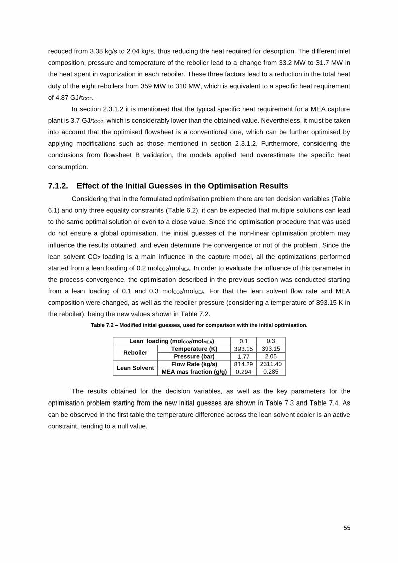
55
reduced from 3.38 kg/s to 2.04 kg/s, thus reducing the heat required for desorption. The different inlet
composition, pressure and temperature of the reboiler lead to a change from 33.2 MW to 31.7 MW in
the heat spent in vaporization in each reboiler. These three factors lead to a reduction in the total heat
duty of the eight reboilers from 359 MW to 310 MW, which is equivalent to a specific heat requirement
of 4.87 GJ/tCO2.
In section 2.3.1.2 it is mentioned that the typical specific heat requirement for a MEA capture
plant is 3.7 GJ/tCO2, which is considerably lower than the obtained value. Nevertheless, it must be taken
into account that the optimised flowsheet is a conventional one, which can be further optimised by
applying modifications such as those mentioned in section 2.3.1.2. Furthermore, considering the
conclusions from flowsheet B validation, the models applied tend overestimate the specific heat
consumption.
7.1.2. Effect of the Initial Guesses in the Optimisation Results
Considering that in the formulated optimisation problem there are ten decision variables (Table
6.1) and only three equality constraints (Table 6.2), it can be expected that multiple solutions can lead
to the same optimal solution or even to a close value. Since the optimisation procedure that was used
do not ensure a global optimisation, the initial guesses of the non-linear optimisation problem may
influence the results obtained, and even determine the convergence or not of the problem. Since the
lean solvent CO2 loading is a main influence in the capture model, all the optimizations performed
started from a lean loading of 0.2 molCO2/molMEA. In order to evaluate the influence of this parameter in
the process convergence, the optimisation described in the previous section was conducted starting
from a lean loading of 0.1 and 0.3 molCO2/molMEA. For that the lean solvent flow rate and MEA
composition were changed, as well as the reboiler pressure (considering a temperature of 393.15 K in
the reboiler), being the new values shown in Table 7.2.
Table 7.2 – Modified initial guesses, used for comparison with the initial optimisation.
Lean loading (molCO2/molMEA) 0.1 0.3
Reboiler Temperature (K) 393.15 393.15
Pressure (bar) 1.77 2.05
Lean Solvent Flow Rate (kg/s) 814.29 2311.40
MEA mas fraction (g/g) 0.294 0.285
The results obtained for the decision variables, as well as the key parameters for the
optimisation problem starting from the new initial guesses are shown in Table 7.3 and Table 7.4. As
can be observed in the first table the temperature difference across the lean solvent cooler is an active
constraint, tending to a null value.
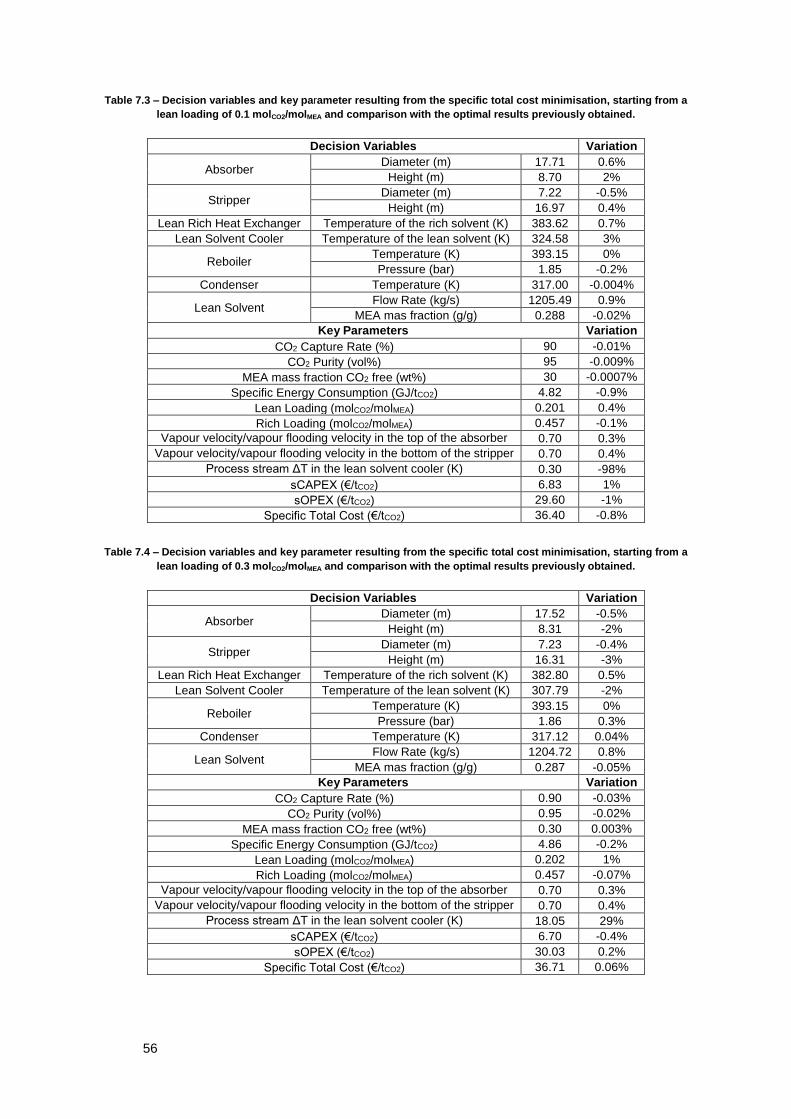
56
Table 7.3 – Decision variables and key parameter resulting from the specific total cost minimisation, starting from a
lean loading of 0.1 molCO2/molMEA and comparison with the optimal results previously obtained.
Decision Variables Variation
Absorber Diameter (m) 17.71 0.6%
Height (m) 8.70 2%
Stripper Diameter (m) 7.22 -0.5%
Height (m) 16.97 0.4%
Lean Rich Heat Exchanger Temperature of the rich solvent (K) 383.62 0.7%
Lean Solvent Cooler Temperature of the lean solvent (K) 324.58 3%
Reboiler Temperature (K) 393.15 0%
Pressure (bar) 1.85 -0.2%
Condenser Temperature (K) 317.00 -0.004%
Lean Solvent Flow Rate (kg/s) 1205.49 0.9%
MEA mas fraction (g/g) 0.288 -0.02%
Key Parameters Variation
CO2 Capture Rate (%) 90 -0.01%
CO2 Purity (vol%) 95 -0.009%
MEA mass fraction CO2 free (wt%) 30 -0.0007%
Specific Energy Consumption (GJ/tCO2) 4.82 -0.9%
Lean Loading (molCO2/molMEA) 0.201 0.4%
Rich Loading (molCO2/molMEA) 0.457 -0.1%
Vapour velocity/vapour flooding velocity in the top of the absorber 0.70 0.3%
Vapour velocity/vapour flooding velocity in the bottom of the stripper 0.70 0.4%
Process stream ΔT in the lean solvent cooler (K) 0.30 -98%
sCAPEX (€/tCO2) 6.83 1%
sOPEX (€/tCO2) 29.60 -1%
Specific Total Cost (€/tCO2) 36.40 -0.8%
Table 7.4 – Decision variables and key parameter resulting from the specific total cost minimisation, starting from a
lean loading of 0.3 molCO2/molMEA and comparison with the optimal results previously obtained.
Decision Variables Variation
Absorber Diameter (m) 17.52 -0.5%
Height (m) 8.31 -2%
Stripper Diameter (m) 7.23 -0.4%
Height (m) 16.31 -3%
Lean Rich Heat Exchanger Temperature of the rich solvent (K) 382.80 0.5%
Lean Solvent Cooler Temperature of the lean solvent (K) 307.79 -2%
Reboiler Temperature (K) 393.15 0%
Pressure (bar) 1.86 0.3%
Condenser Temperature (K) 317.12 0.04%
Lean Solvent Flow Rate (kg/s) 1204.72 0.8%
MEA mas fraction (g/g) 0.287 -0.05%
Key Parameters Variation
CO2 Capture Rate (%) 0.90 -0.03%
CO2 Purity (vol%) 0.95 -0.02%
MEA mass fraction CO2 free (wt%) 0.30 0.003%
Specific Energy Consumption (GJ/tCO2) 4.86 -0.2%
Lean Loading (molCO2/molMEA) 0.202 1%
Rich Loading (molCO2/molMEA) 0.457 -0.07%
Vapour velocity/vapour flooding velocity in the top of the absorber 0.70 0.3%
Vapour velocity/vapour flooding velocity in the bottom of the stripper 0.70 0.4%
Process stream ΔT in the lean solvent cooler (K) 18.05 29%
sCAPEX (€/tCO2) 6.70 -0.4%
sOPEX (€/tCO2) 30.03 0.2%
Specific Total Cost (€/tCO2) 36.71 0.06%

57
Comparing the results obtained for the two optimisations with the initial optimisation, it is
possible to observe minor variations in most of the decision variables (the reboiler temperature is
imposed in 393.15 K, thus the variation is null). This results in the variation of the value achieved for
the objective function between 36.43 and 36.73 €/tCO2, not changing more than 1% when compared
with initial optimisation result.
There are considerable variations in the absorber height, which are compensated by a slight
increase in the lean loading, in the first case, or in the lean solvent flow rate, in the second case. In the
same way, for the starting initial loading of 0.3 the stripper height is 3% lower, which can be related to
the increase of 1% in the lean loading.
One of the main differences observed is in the temperature of the lean solvent after the lean
solvent cooler, which changes between 307.79 and 324.58 K. Figure 7.8 shows the temperature profiles
across the absorber for both liquid and vapour phases, obtained from the three cases with three initial
lean loadings.
Figure 7.8 – Axial temperature profile of the vapour (on the left) and liquid (on the right) phases in the absorber for the
optimised cases with initial lean loadings of 0.1, 0.2 and 0.3 molCO2/molMEA.
From the profiles presented above, it is possible to conclude that, despite the different
temperature of the lean solvent, the temperature profile of both liquid and vapour phases across the
absorber tend to be similar in the three scenarios. Considering that the flue gas temperature isn’t
changed, since it was not included in the optimisation problem, and that the captured amount of CO2 is
approximately the same, the temperature profiles tend to be similar, thus showing the reduced
relevance of the lean solvent temperature for the considered conditions.
Considering this results, the need for a lean solvent cooler before the absorption section seems
to be questionable, suggesting that the advantage of increasing the absorber efficiency is surpassed
by the cooling related costs. The removal of these costs in both equipment and utilities costs lead to a
decrease of simply 0.01% in the specific total cost.
Since the cooler related costs show a small influence in the capture cost, and at least one of
the optimisation scenarios in section 7.2 requires the lean solvent cooling, it was decided not to remove
314
319
324
329
334
0 0.5 1
Tem
ep
ratu
re (
K)
Relative position to the absorber top
Initial Lean Loading = 0.1Initial Lean Loading = 0.2Initial Lean Loading = 0.3
308
318
328
338
0 0.5 1
Tem
pe
ratu
re (
K)
Relative position to the absorber top
Initial Lean Loading = 0.1Initial Lean Loading = 0.2Initial Lean Loading = 0.3

58
the lean solvent cooler from the flowsheet, nor from the cost estimation models, considering that this is
an equipment present in any conventional capture plant, that can increase the capture plant flexibility.
7.1.3. Effect of the Number of Absorption Trains
As mentioned in Section 5.1, the number of absorption trains was chosen considering the
construction limitation regarding the column’s diameter and the vapour flooding velocity. This process
variable was not considered in the optimisation problem, in order to simplify it, but it can be changed in
the base case model, and therefore optimised for each value.
Since the absorber diameter is a control variable of the optimisation problem, it was evaluated
the possibility of having only one absorption train and the consequences of having more than two (up
to four). It should be noted that in order to converge, the optimisation of the capture plant with only one
absorption train required the increase of the diameter upper bound to 30 m, thus suggesting that the
optimal value is above 20 m.
The results of these optimisations are shown in Table A2.1, Table A2.2 and Table A2.3 (in
Appendix A2), and allow to verify that the control variable with largest variation occurs in the absorber
diameter (Figure 7.9). As expected the optimal diameter for one absorption train is still above 20 m,
making this option unfeasible.
Figure 7.9 – Variation of the optimal absorber diameter with the number absorption trains.
Since one of the active constraints of the optimisation results is the approximation of the
absorber’s vapour velocity to the flooding velocity, it is expected that, by reducing the vapour flow rate
in one column, the optimal diameter is decreased. This is further justified by the fact that the vapour
flood velocity is approximately the same in the four cases, due to the ratio between the liquid and vapour
flow rates being approximately the same [54]. In Figure 7.9, it can also be observed that the optimal
absorber diameter tends to present a smaller variation for higher numbers of absorption trains.
Comparing the obtained cost results, it can be observed that the total cost and the CAPEX
show a similar trend, as can be observed in Figure 7.10. Therefore, it is possible to conclude that the
variation in the total cost is mainly due to the variation in the CAPEX, that is, in the equipment cost.
From the CAPEX, it is observed that the major variation occurs in the cost of the absorption shells
(Table A2.2 to Table A2.4), which is directly related to the absorber diameter.
0.0
10.0
20.0
30.0
1 2 3 4
Ab
sorb
er
dia
me
ter
(m)
Number of absorption trains

59
Figure 7.10 – Variation of the optimal specific total cost (on the right) and specific CAPEX (on the right) with the
number of absorption trains.
It should also be noted that the packing cost in the absorbers does not change considerably in
each optimisation, since it is proportional to the volume of packing in each absorber, and therefore to
the total volume of absorption packing. Even though the total volume doesn’t change considerably, from
one to four absorption trains it can be observed a reduction in it from 4 144 m3 to 4 065 m3, thus
suggesting an increase in the absorber’s efficiency with the reduction of its size.
Considering that for a single absorption train the absorber diameter is technically unfeasible,
the total cost varies approximately 0.8% between two and four absorption trains, thus showing the
reduced effect of the absorber’s shell cost, and consequently of the number of absorption trains, in the
total cost. Considering that for two absorption trains the absorber diameter is still 15 m, the use of three
absorption trains may be a better option, since the total cost difference is simply of 0.4%. Therefore,
the choice between two and three absorption trains would be a trade-off between the possibility of
constructing the columns in-site, and the cost of increasing the space required for the absorption
section. This would require a more accurate cost estimation, and therefore it was considered that 2
absorption trains would be a feasible solution, still being considered in the following optimisation studies.
7.1.4. Specific Heat Requirement Minimisation
The steam consumption is directly proportional to the heat required in the regeneration
reboilers, and represents 69% of the capture plant annual cost. The minimisation of the specific total
cost allowed a 14% reduction in specific heat requirement, from 5.66 GJ/tCO2 to 4.87 GJ/tCO2. However,
this value is still considerably higher than the one used as benchmark (3.7 GJ/tCO2).
In order to evaluate if a greater reduction in this parameter is possible, and its effect in the
capture total cost, the described optimisation procedure was conducted with a different objective
function (OF2 in equation (6.2)). It was also necessary to use the additional constraints shown in Table
6.4, as well as an increase in the absorber and stripper upper bounds to 60 and 70 m, respectively.
The results of this optimisation are presented in Table A2.5, showing that, when compared with
the results obtained for the total cost minimisation, a further reduction of 8% in the specific heat
requirement (to 4.46 GJ/tCO2) is possible. Nevertheless, this reduction is achieved through a drastic
increase in the absorber and stripper sizes, which increases the sCAPEX by 674%, hence increasing
the specific total cost in 142%, to the value of 88.98 € per tonne of captured CO2. This leads to an
increase in the CAPEX relevance in the total cost to 59%, as can be observed in Figure 7.11.
36.2
36.4
36.6
36.8
37.0
37.2
1 2 3 4
Spe
cifi
c to
tal c
ost
(€
/tC
O2)
Number of absorption trains
6.2
6.4
6.6
6.8
7.0
7.2
1 2 3 4
sCA
PEX
(€
/tC
O2)
Number of absorption trains

60
Figure 7.11 – Total cost distribution in the specific heat consumption minimisation (Total = 88.98 €/tCO2).
In the analysis of the reboiler related costs, it must be taken into account that the total heat
consumed is reduced from 310 MW to 285 MW, does reducing the number of required reboilers per
stripping train to 3 (maximum heat duty per reboiler of 50 MW, section 5.1), which contributes to a total
reboilers cost that is 11% lower.
The reduction in the specific heat requirement follows the same trend as in the total cost
minimisation, being the total reboiler inlet flow, the amount of CO2 regenerated and the total flow rate
of the vapour stream further reduced. These reductions are possible due to the increase in the stripping
columns height in 337%, and the reduction of the lean solvent flow rate in 13%. Once again the column’s
size is increased in order to maximize the stripping action inside the column. The stripping columns
optimal height results from a trade-off between reducing the amount of CO2 entering the reboilers and
the packing and shell costs increase. Since these costs are no longer being considered in the present
optimisation, the strippers’ height and diameter increase until the effect on the reboilers’ heat duty is no
longer significant.
Considering that the solvent flow rate and the lean loading are both reduced the absorber’s
height has to be increased in order to meet the desired capture rate, leading to an increase of 274%.
Both the increase in absorber and stripper sizes contribute to the increase of the respective shell and
packing costs, leading to an increase of the packing’s relevance (from 78% to 95%) in the cost of the
main equipment, as shown in Figure 7.12. Nevertheless, it should be noted that the obtained columns’
height (Table A2.5) may be technically unfeasible, thus requiring a more specific analysis of the
construction constraints.
59%
41% CAPEX
OPEX

61
Figure 7.12 – Distribution of main equipment costs for the specific heat consumption minimisation.
The reduction in the flow rate contributes to the reduction in the pumps cost and in the
respective electricity consumption. However, due to the increase in the absorber and stripper’s height,
the head required in each pump is increased, which ultimately leads to an increase of 130% in the
electricity, surpassing the reduction caused by the flow rate reduction. Nevertheless, the reduction in
the steam consumption, still lead to a reduction of 7% in variable production costs.
Despite these reductions, the OPEX increases in 24%, since the fixed production costs are
estimated based on the ISBL investment. This way, the variable production costs represent 72% of the
OPEX, as shown in Figure 7.13.
Figure 7.13 – OPEX distribution in the specific heat consumption minimisation (Total = 69.34 M€/year).
Based on this analysis, it is possible to conclude that the minimal specific heat requirement
(4.46 GJ/tCO2) doesn’t correspond to a minimal capture cost. This is achieved at the cost of increasing
the absorbers and strippers’ sizes, in a way that their cost surpasses the cost reduction achieved by
lowering the consumed steam.
7.2. Effect of the Process Constraints
The capture rate of 90%, the CO2 purity in the product stream of 95 vol% and the MEA mass
fraction in the CO2 free lean solvent of 30% are standard requirements usually imposed for a capture
plant. Therefore, in the formulation of the optimisation problem they were defined as equality constraints
(Table 6.2).
The optimisation feature of gPROMS® Model Builder 3.7.1 provides an output which includes
the Lagrange multiplier of active constraints. This parameter is defined as the derivative of the objective
4% 1%0%
95%
Columns Shell
Heat Transfer Equipment
Pumps and Drivers
Packing
72%
28% Variable ProductionCosts
Fixed ProductionCosts
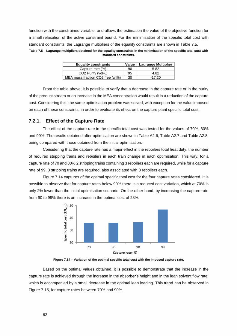
62
function with the constrained variable, and allows the estimation the value of the objective function for
a small relaxation of the active constraint bound. For the minimisation of the specific total cost with
standard constraints, the Lagrange multipliers of the equality constraints are shown in Table 7.5.
Table 7.5 – Lagrange multipliers obtained for the equality constraints in the minimisation of the specific total cost with
standard constraints.
Equality constraints Value Lagrange Multiplier
Capture rate (%) 90 5.82
CO2 Purity (vol%) 95 4.82
MEA mass fraction CO2 free (wt%) 30 -17.20
From the table above, it is possible to verify that a decrease in the capture rate or in the purity
of the product stream or an increase in the MEA concentration would result in a reduction of the capture
cost. Considering this, the same optimisation problem was solved, with exception for the value imposed
on each of these constraints, in order to evaluate its effect on the capture plant specific total cost.
7.2.1. Effect of the Capture Rate
The effect of the capture rate in the specific total cost was tested for the values of 70%, 80%
and 99%. The results obtained after optimisation are shown in Table A2.6, Table A2.7 and Table A2.8,
being compared with those obtained from the initial optimisation.
Considering that the capture rate has a major effect in the reboilers total heat duty, the number
of required stripping trains and reboilers in each train change in each optimisation. This way, for a
capture rate of 70 and 80% 2 stripping trains containing 3 reboilers each are required, while for a capture
rate of 99, 3 stripping trains are required, also associated with 3 reboilers each.
Figure 7.14 captures of the optimal specific total cost for the four capture rates considered. It is
possible to observe that for capture rates below 90% there is a reduced cost variation, which at 70% is
only 2% lower than the initial optimisation scenario. On the other hand, by increasing the capture rate
from 90 to 99% there is an increase in the optimal cost of 28%.
Figure 7.14 – Variation of the optimal specific total cost with the imposed capture rate.
Based on the optimal values obtained, it is possible to demonstrate that the increase in the
capture rate is achieved through the increase in the absorber’s height and in the lean solvent flow rate,
which is accompanied by a small decrease in the optimal lean loading. This trend can be observed in
Figure 7.15, for capture rates between 70% and 90%.
20
30
40
50
70 80 90 99
Spe
cifi
c to
tal c
ost
(€
/tC
O2)
Capture rate (%)

63
Figure 7.15 – Variation of the optimal lean solvent flow rate (on the right) and loading (on the left) with the imposed
capture rate.
On the other hand, the increase of the capture rate to 99% leads to the lean solvent flow rate
reduction, when compared with the 90% case, through the reduction of the optimal lean loading from
0.200 to 0.111 molCO2/molMEA. With the approximation to the physical limit, the costs of increasing the
solvent flow rate would surpass the costs of keeping a low CO2 recovery rate, that is, a higher lean
loading.
Looking into the lean solvent temperature at the cooler’s outlet (Table A2.6 to Table A2.8), it is
possible to see that with the increasing capture rate this temperature is decreased. In the cases of a
capture rate of 70 and 80% the temperature difference across the coolers tends to the imposed limit of
0, once again showing that this equipment might not be required.
Considering that the higher the capture rate the more heat is released in the absorber, for lower
capture rates the temperature in the absorber tends to be lower and solvent cooling loses relevance,
since the flue gas temperature is constant. On the other hand, for higher capture rates, such as 99%,
the temperature in the absorber tends to increase. Taking into account that the optimal flow rate in this
case is 20% lower than in the 90% capture rate case, this heating effect is enhanced, as can be verified
by looking to the absorber temperature profiles shown in Figure 7.16. Since the absorption efficiency
tends to decrease at high temperatures, for high capture rates the lean solvent cooling gains relevance.
Therefore, the lean solvent coolers’ outlet temperature shows a decrease with the increase of the
capture rate.
600
800
1000
1200
70 80 90 99
Lean
so
lve
nt
flo
w r
ate
(kg
/s)
Capture rate (%)
0
0.05
0.1
0.15
0.2
0.25
70 80 90 99
Lean
load
ing
(mo
l MEA
/mo
l CO
2)
Capture rate (%)

64
Figure 7.16 – Axial temperature profile of the vapour phase (on the left) and liquid phase (on the right) in the absorber
for the optimised cases with capture rates (CR) of 70, 80, 90 and 99%.
A reduction in the optimal rich solvent temperature at the lean-rich heat exchanger outlet is also
observed. The reduction is associated with a major change in the strippers’ operating conditions. This
can be observed in Figure 7.17, that shows the optimal temperature profiles in both liquid and vapour
phases for each optimisation.
Figure 7.17 – Axial temperature profile of the vapour phase (on the left) and liquid phase (on the right) in the stripper
for the optimised cases with capture rates (CR) of 70, 80, 90 and 99%.
Despite the lower inlet temperature of the rich solvent, the bulk temperature in both phases is
kept at a higher value across the column. This can be explained by the reduction of 20% in the solvent
flow rate, associated with an increase of 45% in the vapour flow rate exiting the reboiler (at the same
temperature), which reduces the temperature variation in the vapour phase.
Figure 7.17 also shows that for the 99% capture rate case, the temperature difference between
the strippers’ liquid inlet and vapour outlet changes. While for lower capture rates the liquid inlet optimal
temperature is higher than the vapour outlet temperature, in the 99% capture rate case, the liquid
310
315
320
325
330
335
0 0.5 1
Tem
ep
ratu
re (
K)
Relative position to the absorber top
CR = 70% CR = 80%CR = 90% CR = 99%
300
305
310
315
320
325
330
335
0 0.5 1
Tem
ep
ratu
re (
K)
Relative position to the absorber top
CR = 70% CR = 80%CR = 90% CR = 99%
370
375
380
385
390
395
0 0.5 1
Tem
ep
ratu
re (
K)
Relative position to the stripper top
CR = 70% CR = 80%CR = 90% CR = 99%
330
345
360
375
390
405
0 0.5 1
Tem
ep
ratu
re (
K)
Relative position to the stripper top
CR = 70% CR = 80%CR = 90% CR = 99%
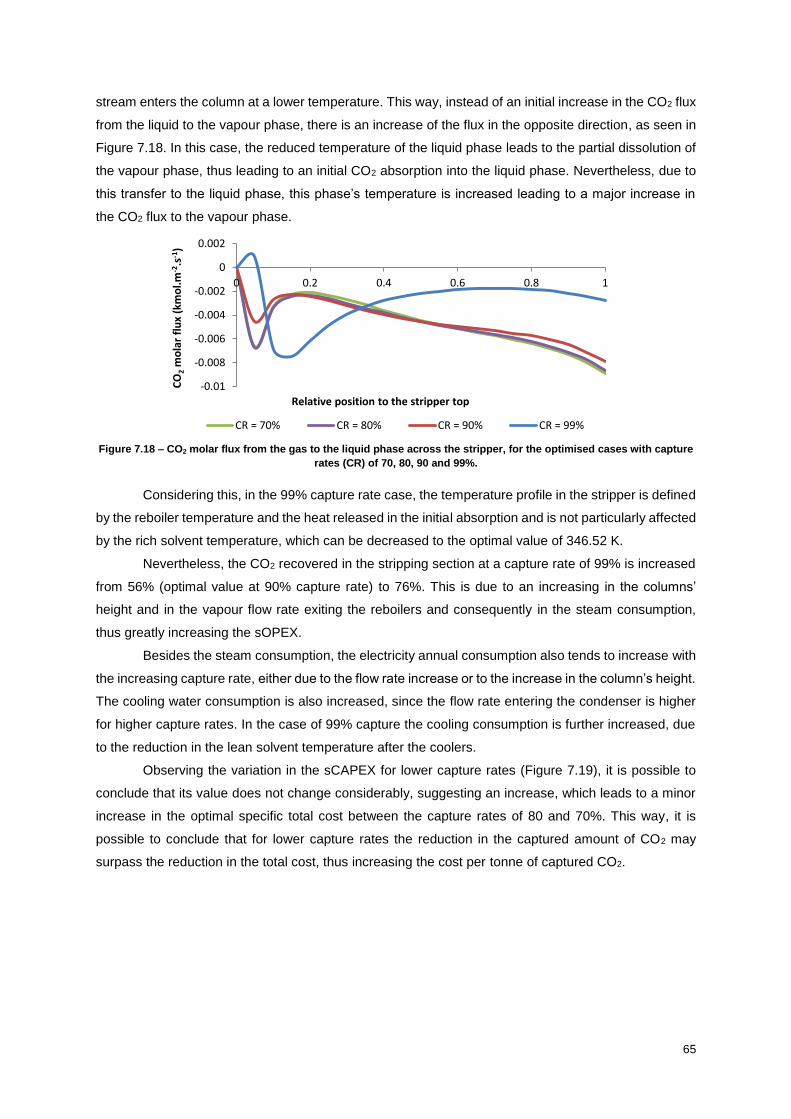
65
stream enters the column at a lower temperature. This way, instead of an initial increase in the CO2 flux
from the liquid to the vapour phase, there is an increase of the flux in the opposite direction, as seen in
Figure 7.18. In this case, the reduced temperature of the liquid phase leads to the partial dissolution of
the vapour phase, thus leading to an initial CO2 absorption into the liquid phase. Nevertheless, due to
this transfer to the liquid phase, this phase’s temperature is increased leading to a major increase in
the CO2 flux to the vapour phase.
Figure 7.18 – CO2 molar flux from the gas to the liquid phase across the stripper, for the optimised cases with capture
rates (CR) of 70, 80, 90 and 99%.
Considering this, in the 99% capture rate case, the temperature profile in the stripper is defined
by the reboiler temperature and the heat released in the initial absorption and is not particularly affected
by the rich solvent temperature, which can be decreased to the optimal value of 346.52 K.
Nevertheless, the CO2 recovered in the stripping section at a capture rate of 99% is increased
from 56% (optimal value at 90% capture rate) to 76%. This is due to an increasing in the columns’
height and in the vapour flow rate exiting the reboilers and consequently in the steam consumption,
thus greatly increasing the sOPEX.
Besides the steam consumption, the electricity annual consumption also tends to increase with
the increasing capture rate, either due to the flow rate increase or to the increase in the column’s height.
The cooling water consumption is also increased, since the flow rate entering the condenser is higher
for higher capture rates. In the case of 99% capture the cooling consumption is further increased, due
to the reduction in the lean solvent temperature after the coolers.
Observing the variation in the sCAPEX for lower capture rates (Figure 7.19), it is possible to
conclude that its value does not change considerably, suggesting an increase, which leads to a minor
increase in the optimal specific total cost between the capture rates of 80 and 70%. This way, it is
possible to conclude that for lower capture rates the reduction in the captured amount of CO2 may
surpass the reduction in the total cost, thus increasing the cost per tonne of captured CO2.
-0.01
-0.008
-0.006
-0.004
-0.002
0
0.002
0 0.2 0.4 0.6 0.8 1
CO
2m
ola
r fl
ux
(km
ol.
m-2
.s-1
)
Relative position to the stripper top
CR = 70% CR = 80% CR = 90% CR = 99%
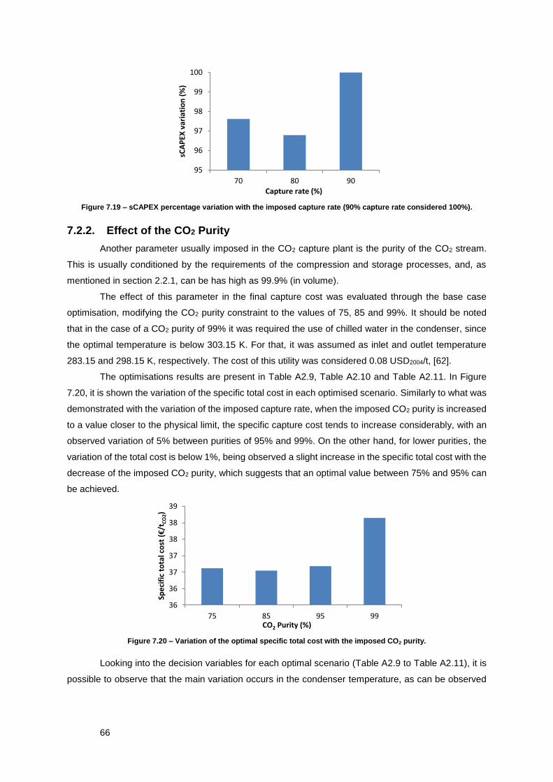
66
Figure 7.19 – sCAPEX percentage variation with the imposed capture rate (90% capture rate considered 100%).
7.2.2. Effect of the CO2 Purity
Another parameter usually imposed in the CO2 capture plant is the purity of the CO2 stream.
This is usually conditioned by the requirements of the compression and storage processes, and, as
mentioned in section 2.2.1, can be has high as 99.9% (in volume).
The effect of this parameter in the final capture cost was evaluated through the base case
optimisation, modifying the CO2 purity constraint to the values of 75, 85 and 99%. It should be noted
that in the case of a CO2 purity of 99% it was required the use of chilled water in the condenser, since
the optimal temperature is below 303.15 K. For that, it was assumed as inlet and outlet temperature
283.15 and 298.15 K, respectively. The cost of this utility was considered 0.08 USD2004/t, [62].
The optimisations results are present in Table A2.9, Table A2.10 and Table A2.11. In Figure
7.20, it is shown the variation of the specific total cost in each optimised scenario. Similarly to what was
demonstrated with the variation of the imposed capture rate, when the imposed CO2 purity is increased
to a value closer to the physical limit, the specific capture cost tends to increase considerably, with an
observed variation of 5% between purities of 95% and 99%. On the other hand, for lower purities, the
variation of the total cost is below 1%, being observed a slight increase in the specific total cost with the
decrease of the imposed CO2 purity, which suggests that an optimal value between 75% and 95% can
be achieved.
Figure 7.20 – Variation of the optimal specific total cost with the imposed CO2 purity.
Looking into the decision variables for each optimal scenario (Table A2.9 to Table A2.11), it is
possible to observe that the main variation occurs in the condenser temperature, as can be observed
95
96
97
98
99
100
70 80 90sC
AP
EX v
aria
tio
n (
%)
Capture rate (%)
36
36
37
37
38
38
39
75 85 95 99
Spe
cifi
c to
tal c
ost
(€
/tC
O2)
CO2 Purity (%)
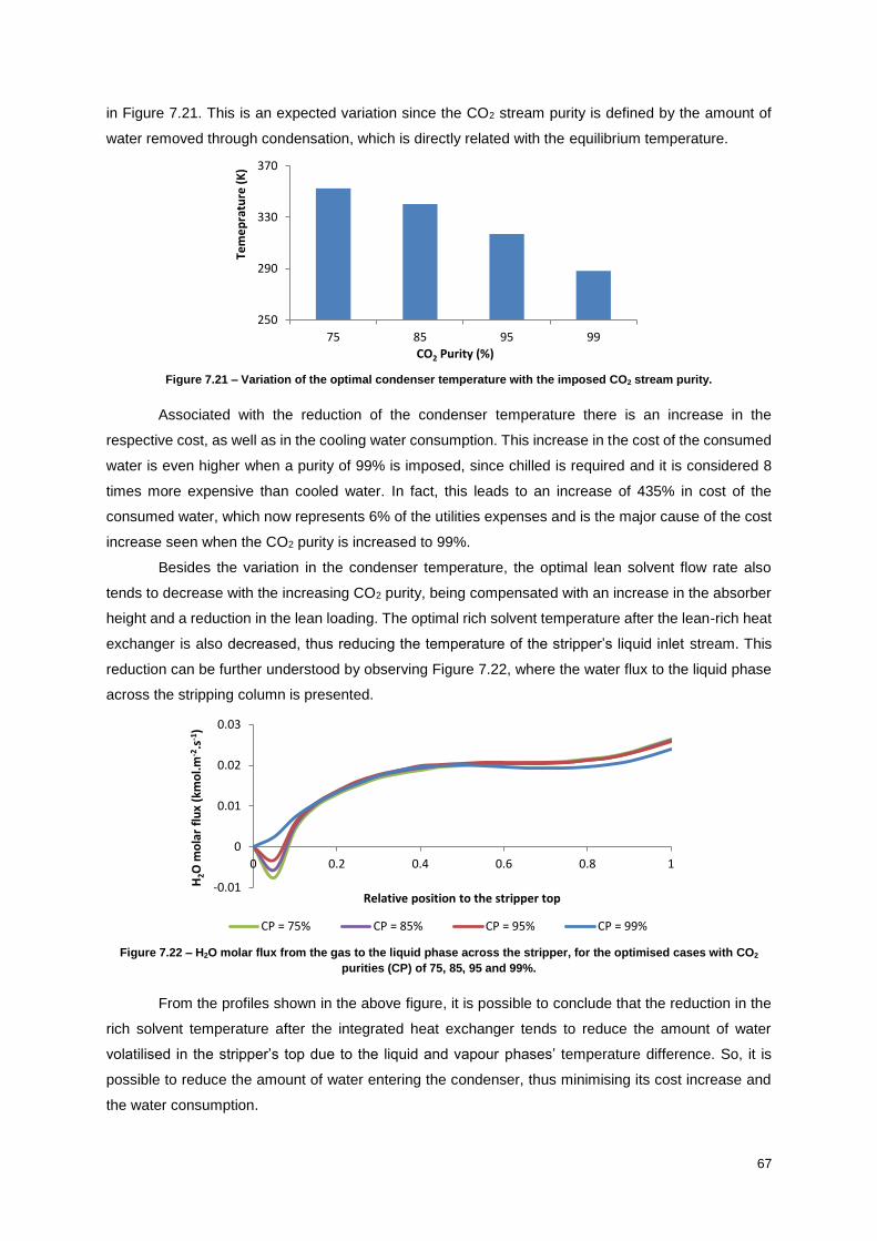
67
in Figure 7.21. This is an expected variation since the CO2 stream purity is defined by the amount of
water removed through condensation, which is directly related with the equilibrium temperature.
Figure 7.21 – Variation of the optimal condenser temperature with the imposed CO2 stream purity.
Associated with the reduction of the condenser temperature there is an increase in the
respective cost, as well as in the cooling water consumption. This increase in the cost of the consumed
water is even higher when a purity of 99% is imposed, since chilled is required and it is considered 8
times more expensive than cooled water. In fact, this leads to an increase of 435% in cost of the
consumed water, which now represents 6% of the utilities expenses and is the major cause of the cost
increase seen when the CO2 purity is increased to 99%.
Besides the variation in the condenser temperature, the optimal lean solvent flow rate also
tends to decrease with the increasing CO2 purity, being compensated with an increase in the absorber
height and a reduction in the lean loading. The optimal rich solvent temperature after the lean-rich heat
exchanger is also decreased, thus reducing the temperature of the stripper’s liquid inlet stream. This
reduction can be further understood by observing Figure 7.22, where the water flux to the liquid phase
across the stripping column is presented.
Figure 7.22 – H2O molar flux from the gas to the liquid phase across the stripper, for the optimised cases with CO2
purities (CP) of 75, 85, 95 and 99%.
From the profiles shown in the above figure, it is possible to conclude that the reduction in the
rich solvent temperature after the integrated heat exchanger tends to reduce the amount of water
volatilised in the stripper’s top due to the liquid and vapour phases’ temperature difference. So, it is
possible to reduce the amount of water entering the condenser, thus minimising its cost increase and
the water consumption.
250
290
330
370
75 85 95 99
Tem
ep
ratu
re (
K)
CO2 Purity (%)
-0.01
0
0.01
0.02
0.03
0 0.2 0.4 0.6 0.8 1
H2O
mo
lar
flu
x (k
mo
l.m
-2.s
-1)
Relative position to the stripper top
CP = 75% CP = 85% CP = 95% CP = 99%
68
The increase in the amount of water in the liquid phase of the stripper would cause an increase
in the steam consumption. Nevertheless the reduction on the optimal lean solvent flow rate tends to
minimise this effect, being the variation in the steam consumption quite reduced.
Nevertheless, the variation in rich solvent temperature leads to an increase in the lean-rich heat
exchanger and the lean solvent coolers cost with the increase of the CO2 purity. This way, the increase
in the heat exchanger’s and in the condenser’s costs is the major cause to the CAPEX increase.
The OPEX variation between the CO2 purities of 95% and 99% is mainly due to the use of
refrigerated water. Nonetheless, for lower purities, it can be seen that optimal OPEX tends to increase.
A lower purity in the CO2 stream means an increase in the MEA losses in the regeneration section,
which were not considered to be recovered. This way, the solvent cost gains relevance in the capture
cost for lower purities, in opposition to the effect of reducing the water consumption. This results in a
minor increase in the OPEX (0.5%), and consequently in the total cost (0.2%), between the optimal
cases with CO2 purities of 85% and 75%.
7.2.3. Effect of the MEA Concentration
As referred in section 2.3.1, the MEA concentration in the capture solvent is limited by its
corrosive potential and by its proclivity to slip in the absorption process. The corrosion inhibitors applied
nowadays allow the use of MEA concentrations as high as 30 wt%, and therefore this was the value
initially imposed in the optimisation problem. Understanding the economic benefits of increasing this
concentration may contribute to understanding if the development of new and more effective
degradation inhibitors is worth the associated costs.
This way, the equality constraint concerning the MEA mass fraction in the CO2 free lean solvent
was changed to the value of 40 wt%. In the same way, to evaluate the effects of reducing the MEA
concentration this variable was changed to the value of 20 wt%. The optimal results obtained for each
of these simulations are featured in Table A2.12 and Table A2.13. Once again, it should be noted that,
due to total heat consumption reduction, in the case of a MEA concentration of 40 wt% the number of
reboilers per stripping train is 3, instead of 4.
In Figure 7.23, it is possible to observe the reduction of the specific total cost with increasing
concentration of MEA in the solvent. In fact, the increase of the MEA mass fraction in the CO2 free lean
solvent to 40% allows the reduction of capture cost in 4%. On the other hand, the reduction of this
variable to 20% causes an increase of 6% in the total cost.

69
Figure 7.23 – Variation of the optimal specific total cost with the imposed MEA mass fraction in the CO2 free lean
solvent.
Comparing the decision variables optimal values, it is possible to conclude that the lean solvent
flow rate is the one with the main variation, besides the MEA mass fraction itself. Figure 7.24 shows
this reduction of flow rate with the increasing solvent concentration.
Figure 7.24 – Variation of the optimal lean solvent flow rate with the imposed MEA mass fraction in the CO2 free lean
solvent.
Associated with the solvent flow rate reduction, it is also verified a reduction in the diameter of
both the absorber and the stripper, in order to meet 70% of the vapour flooding velocity, and a reduction
in both the pump related costs and in the electricity consumption. On the other hand, for a higher MEA
concentration, the columns’ optimal height is increased, thus increasing their related costs in both the
20% and 40% optimal cases.
The reduction in the flow rate reduces the heat transferred in the lean-rich-heat exchangers.
When comparing the optimal cases with MEA mass fractions of 20% and 30%, the rich solvent
temperature after these heat exchangers is approximately the same, which leads to the decrease of
104% in this equipment cost (being required less 10 units), with the increasing amine concentration.
However, due to the same decrease in the flow rate, the heat released in the absorber leads to an
increase in the rich solvent temperature, which affects the heat exchange driving force in the lean-rich
heat exchanger and may lead to an increase of the heat exchange area. This is verified when comparing
the optimal cases with MEA mass fractions of 30% and 40%, in which the exchanged heat is in fact
reduced, but the area is increased, leading to an increase this equipment cost.
The mentioned factors lead to an increase of 8% in the optimal specific CAPEX when the MEA
mass fraction in the CO2 free lean solvent is reduced from 30% to 20%. This trend is not seen when
34
36
38
40
20 30 40
Spe
cifi
c to
tal c
ost
(€
/tC
O2)
MEA mass fraction in the CO2 free lean solvent (%)
500
800
1100
1400
1700
20 30 40
Lean
so
lve
nt
flo
w r
ate
(kg
/s)
MEA mass fraction in the CO2 free lean solvent (%)
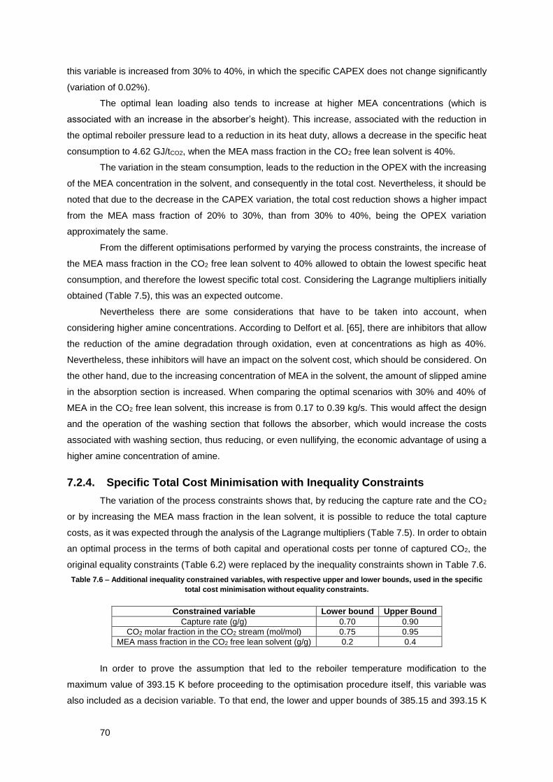
70
this variable is increased from 30% to 40%, in which the specific CAPEX does not change significantly
(variation of 0.02%).
The optimal lean loading also tends to increase at higher MEA concentrations (which is
associated with an increase in the absorber’s height). This increase, associated with the reduction in
the optimal reboiler pressure lead to a reduction in its heat duty, allows a decrease in the specific heat
consumption to 4.62 GJ/tCO2, when the MEA mass fraction in the CO2 free lean solvent is 40%.
The variation in the steam consumption, leads to the reduction in the OPEX with the increasing
of the MEA concentration in the solvent, and consequently in the total cost. Nevertheless, it should be
noted that due to the decrease in the CAPEX variation, the total cost reduction shows a higher impact
from the MEA mass fraction of 20% to 30%, than from 30% to 40%, being the OPEX variation
approximately the same.
From the different optimisations performed by varying the process constraints, the increase of
the MEA mass fraction in the CO2 free lean solvent to 40% allowed to obtain the lowest specific heat
consumption, and therefore the lowest specific total cost. Considering the Lagrange multipliers initially
obtained (Table 7.5), this was an expected outcome.
Nevertheless there are some considerations that have to be taken into account, when
considering higher amine concentrations. According to Delfort et al. [65], there are inhibitors that allow
the reduction of the amine degradation through oxidation, even at concentrations as high as 40%.
Nevertheless, these inhibitors will have an impact on the solvent cost, which should be considered. On
the other hand, due to the increasing concentration of MEA in the solvent, the amount of slipped amine
in the absorption section is increased. When comparing the optimal scenarios with 30% and 40% of
MEA in the CO2 free lean solvent, this increase is from 0.17 to 0.39 kg/s. This would affect the design
and the operation of the washing section that follows the absorber, which would increase the costs
associated with washing section, thus reducing, or even nullifying, the economic advantage of using a
higher amine concentration of amine.
7.2.4. Specific Total Cost Minimisation with Inequality Constraints
The variation of the process constraints shows that, by reducing the capture rate and the CO2
or by increasing the MEA mass fraction in the lean solvent, it is possible to reduce the total capture
costs, as it was expected through the analysis of the Lagrange multipliers (Table 7.5). In order to obtain
an optimal process in the terms of both capital and operational costs per tonne of captured CO2, the
original equality constraints (Table 6.2) were replaced by the inequality constraints shown in Table 7.6.
Table 7.6 – Additional inequality constrained variables, with respective upper and lower bounds, used in the specific
total cost minimisation without equality constraints.
Constrained variable Lower bound Upper Bound
Capture rate (g/g) 0.70 0.90
CO2 molar fraction in the CO2 stream (mol/mol) 0.75 0.95
MEA mass fraction in the CO2 free lean solvent (g/g) 0.2 0.4
In order to prove the assumption that led to the reboiler temperature modification to the
maximum value of 393.15 K before proceeding to the optimisation procedure itself, this variable was
also included as a decision variable. To that end, the lower and upper bounds of 385.15 and 393.15 K

71
were set. The obtained optimisation results are shown in Table A2.14, and prove that the reboiler
temperature indeed reached the upper bound, demonstrating that the highest temperature leads to the
reduction of the plant cost.
From the optimal results it is possible to conclude that, as expected, the minimum cost per
tonne of captured CO2 is achieved with the highest MEA concentration, with the respective variable
hitting the upper bound. On the other hand, it can be observed that both the capture rate and the CO2
purity do not reach the lower bound, showing optimal values of 75% and 88%, respectively. In these
conditions, the achieved specific heat requirement reaches the value of 4.60 GJ/tCO2, mainly due to a
reduction in the lean solvent flow rate and an increase in the lean loading.
Comparing these optimal results with those obtained from the constrained optimisation, there
is a general reduction in the equipment cost, mainly due the columns’ size and solvent flow rate
reduction, leading to a specific CAPEX 6% lower. Related to these reductions there is also a decrease
in the utilities consumption, as well as in the solvent degradation, leading to a reduction of 5% in the
specific OPEX. Figure 7.25 features the specific total cost in the base case and in the optimal cases
obtained with and without standard conditions, thus showing that without imposing the standard
constraints it is possible to reduce the specific total cost in 20% when comparing with the base case.
Figure 7.25 – Optimal specific total cost obtained through its minimisation with and without standard constraints, and
value in the base case.
As referred in the previous section, the use of a higher amine concentration requires a broader
study concerning the oxidation inhibitors requirements and respective cost and the effect of having a
larger washing section, due to the increase in the solvent slip.
30
35
40
45
Base Optimal withstandard constraints
Optimal withoutstandard constraints
Spe
cifi
c to
tal c
ost
(€
/tC
O2)

72
This page was intentionally left blank.
73
8. Conclusions and Future Work
8.1. Conclusions
One of the main focuses of the CCS-related investigation in the literature is the development
and improvement of the CO2 capture technology, in order to reduce the process cost. For a post-
combustion capture plant, the most common used capture technology is CO2 absorption by an amine-
based solvent, typically MEA, due to the low CO2 partial pressures in the flue gas. This technology is
currently applied in other industrial areas, and one of the main sources of expense is the energy
consumption in the solvent regeneration process. However, due to the high amount of CO2 emitted by
a power plant (in the order of millions of tonnes of CO2) the process scale-up leads to a considerable
increase in the electricity cost, thus limiting its application to a full scale plant.
The gCCS® capture library allowed the development of a capture plant model in the gPROMS®
ModelBuilder environment. In order to validate these models, the simulation results were compared
with experimental data found in the literature. From Tobiensen et al. [10], it was possible to conclude
that between Onda and Billet & Schultes correlations, the first one is more accurate in the prediction of
mass transfer coefficients in the absorption process. Using this correlation, deviations in the range of -
13% to 26% were obtained when comparing the simulated and experimental flow of captured CO2,
which are deemed acceptable when considering that the used models do not consider any fitting to the
experimental data. It was also verified that this deviation tends to increase with the decrease of the
solvent lean loading. From the experimental data found in Notz et al., it was observed that for a complete
pilot plant capture plant model with a specified heat input, the CO2 capture rate tends to be under
estimated, with deviations that can reach -25%, leading to an over prediction of the specific heat
requirement up to 32%.
For a full scale capture plant optimisation, it was considered as base case a PSE’s case study,
which lean solvent flowrate and MEA mass fraction were modified in order to meet a 90% capture rate
and a MEA fraction in the CO2 free lean solvent of 30%. It was also developed an approximate cost
estimation model, for the calculation of the capture plant CAPEX and OPEX. The application of this
model to the base case, allowed the estimation of a specific total cost of 43.15 €/tCO2, from which the
OPEX represents 80% and is associated to a specific heat requirement of 5.66 GJ/tCO2. The cost
estimation allowed to conclude that the most expensive equipment, and therefore, the fraction with
more influence in the CAPEX is the absorber’s packing (73% of the equipment total cost). For the
OPEX, the main expense is related with the reboilers’ steam consumption, which in fact represents 69%
of the annual total cost.
From the base case specific total cost minimisation, considering a capture rate of 90%, a CO2
purity of 95 vol% and a MEA fraction in the CO2 free lean solvent of 30%, it was possible to reduce the
total cost by 15%. Based on these results it is possible to conclude that a reduction in the absorber
diameter (in order to meet the flooding limit) and in the lean loading increase the absorber efficiency,
allowing the same capture rate in a smaller absorber and with a lower solvent flow rate. The stripper
efficiency is also increased by its diameter reduction and increase in the column’s height and the rich

74
solvent inlet temperature, thus allowing a lower lean loading with lower steam consumption (4.87
GJ/tCO2).
The effect of changing the lean loading before the optimisation procedure (by varying the lean
solvent flow rate and reboiler pressure) in the optimal specific total cost was tested, being observed a
variation of less than 1%. From these tests it was also possible to conclude that the lean solvent
temperature after the cooler is not a relevant parameter in the considered conditions. Furthermore, it
was concluded that in these cases the lean solvent cooler would not be required. Nevertheless, since
the condenser’s associated costs only represent 0.01% of the total cost, it was not removed from the
flowsheet model.
Starting from the same initial guesses the effect of increasing the number of absorption trains
was evaluated. This way, it was possible to conclude that the decision variable mainly affected is the
absorber diameter. Considering only one absorber would be technically unfeasible due to the high
optimal absorber diameter, being the use of two absorption trains conditioned by the possibility of using
absorber with a diameter above 15 m. Nevertheless, increasing the number from 1 to 4 only increased
the specific total cost in 0.4%, since the total volume of packing tends to be the same.
In order to conclude if the minimum total cost corresponds to the minimum steam consumption,
the optimisation procedure was conducted for the minimisation of the specific heat consumption. This
led to a further reduction of the specific heat requirement to 4.46 GJ/tCO2, but at the cost of greatly
increasing the columns’ height, thus leading to an increase in the total cost (143%).
For the evaluation of the effect of the imposed capture rate, CO2 purity and MEA concentration
on the specific total cost, the optimisation procedure was conducted by changing these constraints.
Regarding the capture rate it was observed that between 70% and 90%, the variation is achieved
through an increase in the lean solvent flow rate and in the absorber and stripper height, associated
with a slight decrease in the lean loading. This leads to an increase of 2% in the optimal total cost in
this capture rate range. On the other hand, between the capture rates of 90% and 99%, there is 28%
increase of the specific total cost, due to a major decrease in the optimal lean solvent flow rate and lean
loading, accompanied by a further increase in the columns’ height. In the case of a 99% capture it was
also concluded that due to the heat released in the absorption process and the reduced solvent flow
rate, the lean solvent cooler gains relevance. In the same case, the rich solvent temperature entering
the stripper is decreased, since the vapour flow rate is increased and the solvent flow rate is decreased,
being the temperature across the columns kept at higher values.
The tested variation of the imposed CO2 purity showed similar results to the capture rate
variation, but at a lower scale. Between the purities of 75% and 95%, there is an increase of only 0.2%
in the specific total cost. The condenser temperature is related to this variation, since it defines the
amount of water condensed, and therefore the purity of the final stream. This way, with the increasing
purity the cooling water consumption and the condenser costs tend to increase. On the other hand, for
a lower CO2 purity the amount of lost solvent in the regeneration process tends to increase, thus leading
to a minimum in the sOPEX. When the purity is increased to 99%, the specific cost increases by 4%,
associated with a major variation in the OPEX. This was due to the further reduction in the condenser
temperature that required the use of chilled water, which was considered eight times more expensive,
75
leading to an increase of 435% in the cooling/refrigerating water annual costs. Nevertheless, it was
verified that this parameter did not have a considerable influence in the specific heat consumption, thus
the reduced effect on the total cost.
The MEA concentration was varied by the modification of the imposed MEA mass fraction in
the CO2 free lean solvent to 20% and 40%. The variation in the specific total cost was more significant
than in the previous cases (except when approaching the physical limits), showing a reduction by 5%,
when changing this constraint from 20% to 30%, and by 4%, when changing it from 30% to 40%. These
variations are mainly due to the possibility of reducing the solvent flow rate, with the increasing
concentration, associated whit an increase in the optimal lean loading. Both factors contribute to the
reduction of the specific heat requirement, allowing the total cost reduction. Nevertheless, it should be
considered that there are implications of using a more concentrate solvent, which were not considered,
such as, the size of the water washing sections or the costs associated with the required oxidation
inhibitors cost.
At last, the same optimisation procedure was conducted, with only inequality constraints. This
led to the optimal capture rate of 75%, CO2 purity of 88% and MEA mass fraction in the CO2 free lean
solvent of 40%, which is the variable upper bound. This allowed a specific total cost reduction to 34.70
€/tCO2 (5% less when compared with the initial optimal results), associated with the specific heat
requirement of 4.60 GJ/tCO2.
The analysis presented shows that the total cost is greatly affected by the trade-off between
the solvent’s flow rate, the absorber height and the lean solvent’s loading. Increasing the MEA
concentration in the solvent has a positive effect in all this variables. This is also verified for the capture
rate in a limited range of values. It was also observed that at moderate capture rates, increasing both
the stripper’s height and the rich solvent temperature at its inlet also tend to reduce the steam
consumption, and therefore the total cost. The interconnection between these variables shows the
relevance of a model-based full plant optimisation for the reduction of the capture cost, which is an
important step for the effective CCS implementation in real power plants.
8.2. Future Work
The optimisation of a conventional flowsheet configuration using a typical solvent is simply the
first step in the reduction of a capture plant costs. As mentioned in section 2.3, today’s technology
already considers several modifications on the capture flowsheet which are considered more economic.
In the same section, are also mentioned other solvents, with considerable advantages, that are now
being tested for implementation in the CCS process. The construction of flowsheet models based on
these more economic configurations and solvents, and their optimisation will help to further reducing
the capture costs.
Nevertheless, for a conventional flowsheet as the one considered in the present thesis, further
work can also be applied. It should be considered that the flue gas preparation (including its saturation),
the washing sections and the CO2 compression were not optimised. The inclusion of these sections in
the flowsheet to be optimised, may lead to more accurate results.

76
One of the conclusions of the present thesis is that the use of a more concentrated solvent
would reduce the capture costs. As mentioned before, this would require larger washing sections and
more efficient corrosion inhibitors. It should also be considered that in the cost estimation model it was
considered a generic degradation rate for MEA, which may no longer be applicable. Taking this into
account, a further understanding of the use of more concentrated solvents should be considered.
Finally, the presented cost estimation model follows the factorial method, and is based on the
approximate calculation of the required sizing variables. This way, the use of a more precise model for
the process costing would provide more accurate results.
77
9. Bibliography
[1] International Energy Agency, “CO2 Emissions from Fuel Combustion,” Paris, 2013.
[2] International Energy Agency, “Key World Energy Statistics,” 2013.
[3] Working Group III of the Intergovernmental Panel on Climate Change, “IPCC Special Report on
Carbon Dioxide Capture and Storage,” Cambridge University Press, New York, 2005.
[4] Process Systems Enterprise Limited, “PSE: Press releases – gCCS v1.0 release – the world's
first whole-chain CCS modeling environment,” [Online]. Available:
http://www.psenterprise.com/news/press_releases/140710_gccs/index.html. [Accessed 29
September 2014].
[5] Process Systems Enterprise Limited, “gPROMS ModelBuilder process simulation, modeling &
optimization,” [Online]. Available: http://www.psenterprise.com/modelbuilder.html. [Accessed 29
September 2014].
[6] M. R. Abu-Zahra, L. H. Schneiders, J. P. Niederer, P. H. Feron and G. F. Versteeg, “CO2 capture
from power plants: Part I. A parametric study of the technical performance based on
monoethanolamine,” International Journal of Greenhouse Gas Control, vol. 1, no. 1, pp. 37-46,
2007.
[7] H. Ahn, M. Luberti, Z. Liu and S. Brandani, “Process configuration studies of the amine capture
process for coal-fired power plants,” International Journal of Greenhouse Gas Control, vol. 16,
pp. 29-40, 2013.
[8] T. Damartzis, A. I. Papadopoulos and P. Seferlis, “Optimum synthesis of solvent-based post-
combustion CO2 capture flowsheets through a generalized modeling framework,” Clean
Technologies and Environmental Policy, pp. 1-18, 2014.
[9] J. Urech, L. Tock, T. Harkin, A. Hoadley and F. Maréchal, “An assessment of different solvent-
based capture technologies within an IGCC–CCS power plant,” Energy, vol. 64, pp. 268-276,
2014.
[10] F. A. Tobiesen, H. F. Svendsen and O. Juliussen, “Experimental validation of a rigorous
absorber model for CO2 postcombustion capture,” AIChE Journal, vol. 53, no. 4, pp. 846-865,
2007.
[11] R. Notz, H. P. Mangalapally and H. Hasse, “Post combustion CO2 capture by reactive
absorption: Pilot plant description and results of systematic studies with MEA,” International
Journal of Greenhouse Gas Control, vol. 6, pp. 84-112, 2012.
[12] Global Carbon Capture and Storage Institute, “Home | Global Carbon Capture and Storage
Institute,” [Online]. Available: http://www.globalccsinstitute.com/. [Accessed 11 June 2014].
[13] E. S. Rubin, H. Mantripragada, A. Marks, P. Versteeg and J. Kitchin, “The outlook for improved
carbon capture technology,” Progress in Energy and Combustion Science, vol. 38, pp. 630-671,
2012.

78
[14] Carbon Capture and Sequestration Technologies @ MIT, “Carbon Capture and Sequestration
Project Database,” [Online]. Available: https://sequestration.mit.edu/tools/projects/. [Accessed
30 September 2014].
[15] International Energy Agency, “CO2 Capture Facilities and Capacities,” [Online]. Available:
http://www.iea.org/etp/tracking/ccs/index.html. [Accessed 30 Septemeber 2014].
[16] A. B. Rao and E. S. Rubin, “A Technical, Economic, and Environmental Assessment of Amine-
Based CO2 Capture Technology for Power Plant Greenhouse Gas Control,” Environmental
Science & Technology, vol. 36, no. 20, pp. 4467-4475, 2002.
[17] Global CCS Institute, “Understanding CCS Information Resources,” [Online]. Available:
http://cdn.globalccsinstitute.com/understanding-ccs/information-resources. [Accessed 14 May
2014].
[18] Global CCS Institute, “CO2 CAPTURE TECHNOLOGIES - POST COMBUSTION CAPTURE
(PCC),” EPRI, 2012.
[19] Global CCS Institute, “CO2 CAPTURE TECHNOLOGIES - PRE COMBUSTION CAPTURE,”
EPRI, 2012.
[20] Global CCS Institute, “CO2 CAPTURE TECHNOLOGIES - OXY COMBUSTION WITH CO2
CAPTURE,” EPRI, 2012.
[21] L. Raynal, P. Alix, P.-A. Bouillon, A. Gomez, M. l. F. d. Nailly, M. Jacquin, J. Kittel, A. d. Lella,
P. Mougin and J. Trapy, “The DMX™ process: An original solution for lowering the cost of post-
combustion carbon capture,” Energy Procedia, vol. 4, pp. 779-786, 2011.
[22] P. D. Vaidya and E. Y. Kenig, “CO2-Alkanolamine Reaction Kinetics: A Review of Recent
Studies,” Chemical Engineering & Technology, vol. 30, no. 11, pp. 1467-1474, 2007.
[23] H. Thee, Y. A. Suryaputradinata, K. A. Mumford, K. H. Smith, G. d. Silva, S. E. Kentish and G.
W. Stevens, “A kinetic and process modeling study of CO2 capture with MEA-promoted
potassium carbonate solutions,” Chemical Engineering Journal, vol. 210, pp. 271-279, 2012.
[24] F. M. Khan, V. Krishnamoorthi and T. Mahmud, “Modelling reactive absorption of CO2 in packed
columns for post-combustion carbon capture applications,” Chemical Engineering Research and
Design, vol. 89, no. 9, pp. 1600-1608, 2011.
[25] M. Wang, W. Lawal, P. Stephenson, J. Sidders and C. Ramshaw, “Post-combustion CO2
capture with chemical absorption: A state-of-the-art review,” Chemical Engineering Research
and Design, vol. 89, no. 9, pp. 1609-1624, 2011.
[26] J. Davis and G. Rochelle, “Thermal degradation of monoethanolamine at stripper conditions,”
Energy Procedia, vol. 1, no. 1, pp. 327-333, 2009.
[27] J. Pires, F. Martins, M. Alvim-Ferraz and M. Simões, “Recent developments on carbon capture
and storage: An overview,” Chemical Engineering Research and Design, vol. 89, no. 9, pp.
1446-1460, 2011.
79
[28] S. Reddy, D. Johnson and J. Gilmartin, “Fluor’s Econamine FG PlusSM Technology For CO2
Capture at Coal-fired Power Plants,” in Power Plant Air Pollutant Control “Mega” Symposium,
Baltimore, 2008.
[29] Mitsubishi Heavy Industries, America Inc., “KM-CDR Post-Combustion CO2 Capture with KS-
1™ Advanced Solvent,” in Eighth Annual Conference on Carbon Capture & Sequestration,
Pittsburgh, 2009.
[30] S. Reddy, J. Scherffius, J. Gilmartin and S. Freguia, “Split Flow Process and Apparatus”. United
States of America Patent 7,337,967 B2, 27 May 2008.
[31] J.-M. G. Amann and C. Bouallou, “CO2 capture from power stations running with natural gas
(NGCC) and pulverized coal (PC): Assessment of a new chemical solvent based on aqueous
solutions of N-methyldiethanolamine + triethylene tetramine,” Energy Procedia, vol. 1, no. 1, pp.
909-916, 2009.
[32] R. S. Alvis, N. A. Hatcher and R. H. Weil, “CO2 Removal from Syngas Using Piperazine‐
Activated MDEA and Potassium Dimethyl Glycinate,” in Nitrogen + Syngas 2012, Athens, 2012.
[33] R. Idem, M. Wilson, P. Tontiwachwuthikul, A. Chakma, A. Veawab, A. Aroonwilas and D.
Gelowitz, “Pilot Plant Studies of the CO2 Capture Performance of Aqueous MEA and Mixed
MEA/MDEA Solvents at the University of Regina CO2 Capture Technology Development Plant
and the Boundary Dam CO2 Capture Demonstration Plant,” Industrial & Engineering Chemistry
Research, vol. 45, no. 8, pp. 2414-2420, 2006.
[34] N. Rodríguez, S. Mussati and N. Scenna, “Optimization of post-combustion CO2 process using
DEA–MDEA mixtures,” Chemical Engineering Research and Design, vol. 9, no. 1763-1773, p.
89, 2011.
[35] S. Chakravarti, A. Gupta and B. Hunek, “Advanced Technology for the Capture of Carbon
Dioxide from Flue Gases,” in First National Conference on Carbon Sequestration, Washington,
DC, 2001.
[36] D. Shaw, “Cansolv CO2 Capture: The Value of Integration,” Energy Procedia, vol. 1, no. 1, pp.
237-246, 2009.
[37] L. E. Hakka and M. A. Ouimet, “Method for recovery of CO2 and SO2 from gas streams”. Europe
Patent 1 806 171 B1, 22 May 2013.
[38] Shell Global Solutions, “The CANSOLV CO2 Capture System,” 2014. [Online]. Available:
http://www.shell.com/global/products-services/solutions-for-businesses/globalsolutions/shell-
cansolv/shell-cansolv-solutions/co2-capture.html. [Accessed 28 May 2014].
[39] Shell Global Solutions, “Shell Cansolv Technology Used At The First Commercial-Scale Post-
Combustion Carbon Capture And Storage Plant - Shell Global,” [Online]. Available:
http://www.shell.com/global/products-services/solutions-for-businesses/globalsolutions/shell-
cansolv/shell-cansolv-news-library/shell-cansolv-media-releases/shell-cansolv-technology-
20141002.html. [Accessed 17 October 2014].
80
[40] K. Han, C. K. Ahn, M. S. Lee, C. H. Rhee, J. Y. Kim and H. D. Chun, “Current status and
challenges of the ammonia-based CO2 capture technologies toward commercialization,”
International Journal of Greenhouse Gas Control, vol. 14, pp. 270-281, 2013.
[41] D. Guo, H. Thee, C. Y. Tan, J. Chen, W. Fei, S. Kentish, G. W. Stevens and G. d. Silva, “Amino
Acids as Carbon Capture Solvents: Chemical Kinetics and Mechanism of the Glycine + CO2
Reaction,” Energy & Fuels, vol. 27, no. 7, pp. 3898-3904 , 2013.
[42] E. Sanchez-Fernandez, F. d. M. Mercader, K. Misiak, L. v. d. Ham, M. Linders and E. Goetheer,
“New Process Concepts for CO2 Capture based on Precipitating Amino Acids,” Energy Procedia,
vol. 37, pp. 1160-1171, 2013.
[43] Siemens Energy, Inc., “Slipstream Development & Testing of Post-Combustion CO2 Capture
and Separation Technology for Existing Coal-Fired Plants,” in 2011 NETL CO2 Capture
Technology Meeting, Pittsburgh, 2011.
[44] M. Bryngelsson and M. Westermark, “CO2 capture pilot test at a pressurized coal fired CHP
plant,” Energy Procedia, vol. 1, no. 1, pp. 1403-1410, 2009.
[45] K. A. Mumford, K. H. Smith, C. J. Anderson, S. Shen, W. Tao, Y. A. Suryaputradinata, D. M.
Quyn, A. Qader, B. Hooper, R. A. Innocenzi, S. E. Kentish and G. W. Stevens, “Post-combustion
Capture of CO2: Results from the Solvent Absorption Capture Plant at Hazelwood Power Station
Using Potassium Carbonate Solvent,” Energy & Fuels, vol. 26, no. 10, pp. 6449-6449, 2012.
[46] L. Tomasi, “Revamping out-of-date “hot pot” units: Better efficiency, less energy,” in
Nitrogen+Syngas 2010, International Conference & Exhibition, Bahrain, 2010.
[47] W. Echt, “Technologies for Efficient Purification of Natural and Synthesis Gases,” 2012. [Online].
Available: http://www.uop.com/technologies-for-efficient-purification-of-natural-and-synthesis-
gases/. [Accessed 30 May 2014].
[48] Giammarco - Vetrocoke, “Giammarco - Vetrocoke: About us - history,” [Online]. Available:
http://www.giammarco-vetrocoke.com/aboutus_history.htm. [Accessed 31 May 2014].
[49] Lurgi GmbH, The Rectisol(R) Process, Frankfurt am Main, 2007.
[50] R. Strube and G. Manfrida, “CO2 capture in coal-fired power plants—Impact on plant
performance,” International Journal of Greenhouse Gas Control, vol. 5, no. 4, pp. 710-726, 2011.
[51] B. Burr and L. Lyddon, “A Comparison of Physical Solvents for Acid Gas Removal,” in GPA,
Texas, 2008.
[52] Process Systems Enterprise Limited, gPROMS Documentation, Release 3.7, London, 2013.
[53] K. Onda, H. Takeuchi and Y. Okumoto, “Mass Transfer Coefficients Between Gas and Liquid
Phases in Packed Columns,” Journal of Chemical Engineering of Japan, vol. 1, pp. 56-62, 1968.
[54] R. Billet and M. Schultes, “Prediction of Mass Transfer Columns with Dumped and Arranged
Packings: Updated Summary of the Calculation Method of Billet and Schultes,” Chemical
Engineering Research and Design, vol. 77, no. 6, pp. 498-504, 1999.
81
[55] Process Systems Enterprise Limited, “PSE: The SAFT equation of state technology overview,”
[Online]. Available:
http://www.psenterprise.com/gproms/options/physprops/saft/technology.html. [Accessed 29
September 2014].
[56] C. V. Brand, “CO2 capture using monoethanolamine solutions: Development and validation of a
process model based on the SAFT-VR equation of state,” Centre for Process Systems
Engineering, Department of Chemical Engineering, Imperial College London, London, 2013.
[57] R. H. Perry, D. W. Green and J. O. Maloney, Perry's Chemical Engineers' Handbook, Seventh
Edition, New York, Chicago, San Francisco, Lisbon, London, Madrid, Mexico City, Milan, New
Delhi, San Juan, Seoul, Singapore, Sydney, Toronto: McGraw-Hill, 1998.
[58] G. Towler and R. Sinnot, Chemical Engineering Design : Principles, Practice and Economics of
Plant and Process Design 2nd ed., Oxford: Butterworth-Heinemann, 2013.
[59] “Economic Indicators,” Chemical Engineering, vol. 121, no. 3, p. 72, 2014.
[60] “Banco de Portugal : Daily reference exchange rates,” [Online]. Available:
http://www.bportugal.pt/en-
US/Estatisticas/Dominios%20Estatisticos/EstatisticasCambiais/Pages/Taxasdereferenciadiaria
s.aspx. [Accessed 11 June 2014].
[61] “Faculty of Natural Sciences and Technology - NTNU,” [Online]. Available:
http://www.nt.ntnu.no/users//magnehi/cepci_2011_py.pdf. [Accessed 11 June 2014].
[62] R. K. Sinnot, Coulson & Richardson's CHemical Engineering Series, Volume 6, Fourth Edition,
Chemical Engineering Design, Oxford: Butterworth-Heinemann, 2005.
[63] A. K. Coker, Ludwig’s Applied Process Design for Chemical and Petrochemical Plants,
Burlington: Gulf Professional Publishing, 2007.
[64] M. R. M. A. Zahra, “Carbon Dioxide Capture from Flue Gas: Development and Evaluation of
Existing,” 2009.
[65] B. Delfort, P.-L. Carrette and L. Bonnard, “MEA 40% with improved oxidative stability for CO2
capture in post-combustion,” Energy Procedia, vol. 4, pp. 9-14, 2011.

82
This page was intentionally left blank.
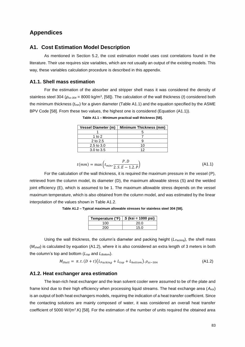
83
Appendices
A1. Cost Estimation Model Description
As mentioned in Section 5.2, the cost estimation model uses cost correlations found in the
literature. Their use requires size variables, which are not usually an output of the existing models. This
way, these variables calculation procedure is described in this appendix.
A1.1. Shell mass estimation
For the estimation of the absorber and stripper shell mass it was considered the density of
stainless steel 304 (ρss-304 = 8000 kg/m3, [58]). The calculation of the wall thickness (t) considered both
the minimum thickness (tmin) for a given diameter (Table A1.1) and the equation specified by the ASME
BPV Code [58]. From these two values, the highest one is considered (Equation (A1.1)).
Table A1.1 – Minimum practical wall thickness [58].
Vessel Diameter (m) Minimum Thickness (mm)
1 5
1 to 2 7
2 to 2.5 9
2.5 to 3.0 10
3.0 to 3.5 12
𝑡(𝑚𝑚) = max (𝑡𝑚𝑖𝑛 ,𝑃. 𝐷
2. 𝑆. 𝐸 − 1.2. 𝑃) (A1.1)
For the calculation of the wall thickness, it is required the maximum pressure in the vessel (P),
retrieved from the column model, its diameter (D), the maximum allowable stress (S) and the welded
joint efficiency (E), which is assumed to be 1. The maximum allowable stress depends on the vessel
maximum temperature, which is also obtained from the column model, and was estimated by the linear
interpolation of the values shown in Table A1.2.
Table A1.2 – Typical maximum allowable stresses for stainless steel 304 [58].
Temperature (°F) S (ksi = 1000 psi)
100 20.0
200 15.0
Using the wall thickness, the column’s diameter and packing height (LPacking), the shell mass
(Mshell) is calculated by equation (A1.2), where it is also considered an extra length of 3 meters in both
the column’s top and bottom (Ltop and LBottom).
𝑀𝑆ℎ𝑒𝑙𝑙 = 𝜋. 𝑡. (𝐷 + 𝑡)(𝐿𝑃𝑎𝑐𝑘𝑖𝑛𝑔 + 𝐿𝑡𝑜𝑝 + 𝐿𝑏𝑜𝑡𝑡𝑜𝑚). 𝜌𝑠𝑠−304 (A1.2)
A1.2. Heat exchanger area estimation
The lean-rich heat exchanger and the lean solvent cooler were assumed to be of the plate and
frame kind due to their high efficiency when processing liquid streams. The heat exchange area (AHX)
is an output of both heat exchangers models, requiring the indication of a heat transfer coefficient. Since
the contacting solutions are mainly composed of water, it was considered an overall heat transfer
coefficient of 5000 W/(m2.K) [58]. For the estimation of the number of units required the obtained area

84
was divided by cost correlation upper bound of applicability (500 m2), as seen in equation (A1.3). The
area for each heat exchanger used for the cost calculation (𝐴𝐻𝑋𝑈𝑛𝑖𝑡) is then calculated based on the
number of units, using equation (A1.4).
𝑁𝐻𝑋 = int (𝐴𝐻𝑋 (𝑚2)
500) + 1 (A1.3)
𝐴𝐻𝑋𝑈𝑛𝑖𝑡 =
𝐴𝐻𝑋
𝑁𝐻𝑋
(A1.4)
A1.3. Reboiler area estimation
The reboiler area is not an output of the respective model and therefore was estimated using
equation (A1.5). For that, it was assumed a typical overall heat transfer coefficient (UReb) of 1140
W/(m2.K), [63], as well as the heat exchanged in the reboiler (QReb), the steam temperature (TSteam) and
the reboiler temperature (TReb), which are model’s outputs.
𝐴𝑅𝑒𝑏 =𝑄𝑅𝑒𝑏
𝑈𝑅𝑒𝑏 . (𝑇𝑆𝑡𝑒𝑎𝑚 − 𝑇𝑅𝑒𝑏) (A1.5)
A1.4. Condenser area estimation
The condenser was assumed as being of the tube and shell type. Its area (ACond) is calculated
using equation (A1.6). In here, it is assumed the typical overall heat transfer coefficient (UCond) of 850
W/(m2.K), [63]. Besides this, it is also required the heat exchanged in the condenser (QCond), the cooling
water inlet and outlet temperature (𝑇𝑈𝑡𝑖𝑙𝑖𝑡𝑦𝐼𝑛 and 𝑇𝑈𝑡𝑖𝑙𝑖𝑡𝑦
𝑂𝑢𝑡 ) and the condenser inlet and outlet temperature
(𝑇𝐶𝑜𝑛𝑑𝐼𝑛 and 𝑇𝐶𝑜𝑛𝑑
𝑂𝑢𝑡 ), which are model’s outputs.
𝐴𝐶𝑜𝑛𝑑 =𝑄𝐶𝑜𝑛𝑑
𝑈𝐶𝑜𝑛𝑑 .((𝑇𝐶𝑜𝑛𝑑
𝑂𝑢𝑡 − 𝑇𝑈𝑡𝑖𝑙𝑖𝑡𝑦𝐼𝑛 ) − (𝑇𝐶𝑜𝑛𝑑
𝐼𝑛 − 𝑇𝑈𝑡𝑖𝑙𝑖𝑡𝑦𝑂𝑢𝑡 ))
ln ((𝑇𝐶𝑜𝑛𝑑
𝑂𝑢𝑡 − 𝑇𝑈𝑡𝑖𝑙𝑖𝑡𝑦𝐼𝑛 )
(𝑇𝐶𝑜𝑛𝑑𝐼𝑛 − 𝑇𝑈𝑡𝑖𝑙𝑖𝑡𝑦
𝑂𝑢𝑡 ))
(A1.6)
As in the heat exchangers unit area estimation, for the condenser it was used the cost
correlation upper bound (1000 m2), according to equations (A1.7) and (A1.8).
𝑁𝐶𝑜𝑛𝑑 = int (𝐴𝐶𝑜𝑛𝑑 (𝑚2)
1000) + 1 (A1.7)
𝐴𝐶𝑜𝑛𝑑𝑈𝑛𝑖𝑡 =
𝐴𝐶𝑜𝑛𝑑
𝑁𝐶𝑜𝑛𝑑
(A1.8)
A1.5. Pump volumetric flow rate and power estimation
The utilised pump models were modified in order to retrieve the density of the passing fluid (ρfl),
through which the volumetric flow rate (Fv) was calculated. The number of pumps working in parallel
(𝑁𝑃𝑢𝑚𝑝𝑃 ) is based on this value and considers the cost correlation upper bound (0.126 m3/s), according
to equation (A1.9). The unit volumetric flow rate (𝐹𝑉𝑈𝑛𝑖𝑡) is then calculated based on this value (equation
(A1.10)).
𝑁𝑃𝑢𝑚𝑝𝑃 = int (
𝐹𝑉 (𝑚3 𝑠⁄ )
0.126) + 1 (A1.9)
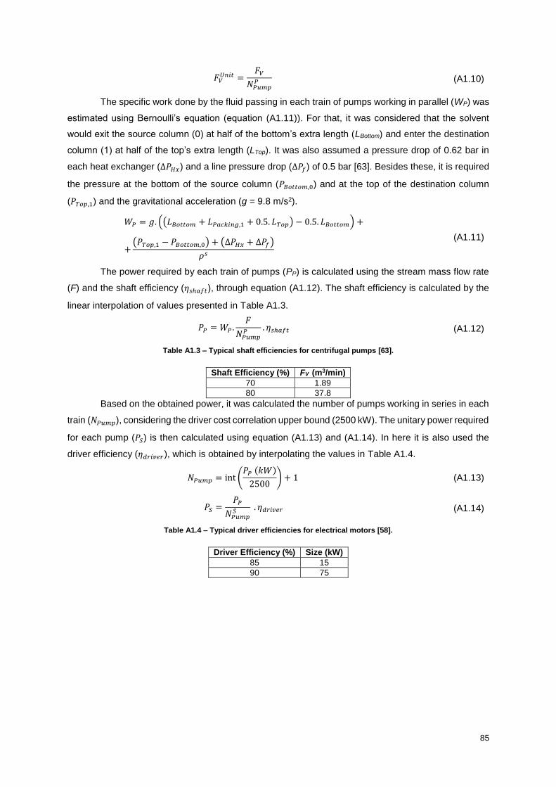
85
𝐹𝑉𝑈𝑛𝑖𝑡 =
𝐹𝑉
𝑁𝑃𝑢𝑚𝑝𝑃 (A1.10)
The specific work done by the fluid passing in each train of pumps working in parallel (WP) was
estimated using Bernoulli’s equation (equation (A1.11)). For that, it was considered that the solvent
would exit the source column (0) at half of the bottom’s extra length (LBottom) and enter the destination
column (1) at half of the top’s extra length (LTop). It was also assumed a pressure drop of 0.62 bar in
each heat exchanger (∆𝑃𝐻𝑥) and a line pressure drop (∆𝑃𝑓) of 0.5 bar [63]. Besides these, it is required
the pressure at the bottom of the source column (𝑃𝐵𝑜𝑡𝑡𝑜𝑚,0) and at the top of the destination column
(𝑃𝑇𝑜𝑝,1) and the gravitational acceleration (g = 9.8 m/s2).
𝑊𝑃 = 𝑔. ((𝐿𝐵𝑜𝑡𝑡𝑜𝑚 + 𝐿𝑃𝑎𝑐𝑘𝑖𝑛𝑔,1 + 0.5. 𝐿𝑇𝑜𝑝) − 0.5. 𝐿𝐵𝑜𝑡𝑡𝑜𝑚) +
+(𝑃𝑇𝑜𝑝,1 − 𝑃𝐵𝑜𝑡𝑡𝑜𝑚,0) + (∆𝑃𝐻𝑥 + ∆𝑃𝑓)
𝜌𝑠
(A1.11)
The power required by each train of pumps (PP) is calculated using the stream mass flow rate
(F) and the shaft efficiency (𝜂𝑠ℎ𝑎𝑓𝑡), through equation (A1.12). The shaft efficiency is calculated by the
linear interpolation of values presented in Table A1.3.
𝑃𝑃 = 𝑊𝑃 .𝐹
𝑁𝑃𝑢𝑚𝑝𝑃 . 𝜂𝑠ℎ𝑎𝑓𝑡 (A1.12)
Table A1.3 – Typical shaft efficiencies for centrifugal pumps [63].
Shaft Efficiency (%) FV (m3/min)
70 1.89
80 37.8
Based on the obtained power, it was calculated the number of pumps working in series in each
train (𝑁𝑃𝑢𝑚𝑝), considering the driver cost correlation upper bound (2500 kW). The unitary power required
for each pump (𝑃𝑆) is then calculated using equation (A1.13) and (A1.14). In here it is also used the
driver efficiency (𝜂𝑑𝑟𝑖𝑣𝑒𝑟), which is obtained by interpolating the values in Table A1.4.
𝑁𝑃𝑢𝑚𝑝 = int (𝑃𝑃 (𝑘𝑊)
2500) + 1 (A1.13)
𝑃𝑆 =𝑃𝑃
𝑁𝑃𝑢𝑚𝑝𝑆 . 𝜂𝑑𝑟𝑖𝑣𝑒𝑟 (A1.14)
Table A1.4 – Typical driver efficiencies for electrical motors [58].
Driver Efficiency (%) Size (kW)
85 15
90 75

86
This page was intentionally left blank.

87
A2. Base Case and Optimisations Detailed Results
Table A2.1 – Detailed results from the application of the cost estimation model in the base case.
Decision Variables
Absorber (A-301) Diameter (m) 20
Height (m) 11.89
Stripper (ST-301) Diameter (m) 8.5
Height (m) 10
Lean-Rich Heat Exchanger (HX-301) Outlet temperature of the rich solvent (K) 362.80
Lean Solvent Cooler (HXU-301) Outlet temperature of the lean solvent (K) 313.90
Reboiler (R-301) Temperature (K) 390.99
Pressure (bar) 1.79
Condenser (C-301) Temperature (K) 313.15
Lean Solvent (RB-303) Flow Rate (kg/s) 1 450.14
MEA mas fraction (g/g) 0.285
Investment (k€)
Equipment Cost
Absorber Shell (2 units) 2 385
Absorber Packing (2 units) 44 640
Stripper Shell (2 units) 1 064
Stripper Packing (2 units) 6 781
Lean-Rich Heat Exchanger (4 units) 252
Lean Solvent Cooler (5 units) 347
Reboiler (2x4 units) 4 266
Condenser (2x1 units) 488
Rich Solvent Pump (12 units) 317
Rich Solvent Pump Driver (12 units) 202
Lean Solvent Pump (12 units) 322
Lean Solvent Pump Driver (12 units) 175
ISBL Investment 79 873
Total Fixed Investment 159 905
Production Cost (k€/Year)
Variable Production Costs
Electricity 408
Steam 55 177
Cooled Water 767
Solvent (MEA) 5 013
Total 61 365
Fixed Production Costs 3 195
Total Production Cost 64 560
Total Cost (M€/year)
CAPEX 15.99
OPEX 64.56
Total 80.55
Key Parameters
CO2 Capture Rate (%) 90
CO2 Purity (vol%) 96
MEA mass fraction in the CO2 free lean solvent (wt%) 30
Vapour velocity/vapour flooding velocity in the top of the absorber 0.56
Vapour velocity/vapour flooding velocity in the bottom of the stripper 0.57
Process stream ΔT in the lean solvent cooler (K) 32.56
Lean Loading (molCO2/molMEA) 0.249
Rich Loading (molCO2/molMEA) 0.463
CO2 recovery rate in the regeneration section (%) 46
Specific Energy Requirement (GJ/tCO2) 5.66
sCAPEX (€/tCO2) 8.57
sOPEX (€/tCO2) 34.59
Specific Total Cost (€/tCO2) 43.15

88
Table A2.2 – Detailed results from the specific total cost minimisation with 1 absorber and standard constraints, and
comparison with the initial specific total cost minimisation results (Table 7.1).
Decision Variables Variation
Absorber (A-301) Diameter (m) 24.84 41%
Height (m) 8.55 0.7%
Stripper (ST-301) Diameter (m) 7.24 -0.2%
Height (m) 16.20 -4%
Lean-Rich Heat Exchanger (HX-301) Outlet temperature of the rich solvent (K) 381.24 0.04%
Lean Solvent Cooler (HXU-301) Outlet temperature of the lean solvent (K) 313.42 -0.1%
Reboiler (R-301) Temperature (K) 393.15 0%
Pressure (bar) 1.85 0.07%
Condenser (C-301) Temperature (K) 317.10 0.03%
Lean Solvent (RB-303) Flow Rate (kg/s) 1 198.15 0.3%
MEA mas fraction (g/g) 0.288 -0.02%
Investment (k€) Variation
Equipment Cost
Absorber Shell (1 unit) 1 220 -32%
Absorber Packing (1 unit) 24 763 0.2%
Stripper Shell (2 units) 1 223 -3%
Stripper Packing (2 units) 7 980 -4%
Lean-Rich Heat Exchanger (10 units) 781 2%
Lean Solvent Cooler (6 units) 445 2%
Reboiler (2x4 units) 4 312 0.04%
Condenser (2x2 units) 873 0.4%
Rich Solvent Pump (10 units) 263 0.2%
Rich Solvent Pump Driver (10 units) 189 -0.9%
Lean Solvent Pump (10 units) 266 0.2%
Lean Solvent Pump Driver (10 units) 129 0.3%
ISBL Investment 60 841 -3%
Total Fixed Investment 121 803 -3%
Production Cost (k€/Year) Variation
Variable Production Costs
Electricity 355 -0.8%
Steam 47 557 0.05%
Cooled Water 593 0.9%
Solvent (MEA) 4 992 0.2%
Total 53 497 0.1%
Fixed Production Costs 2 434 -3%
Total Production Cost 55 930 -0.08%
Total Cost (M€/year) Variation
CAPEX 12.18 -3%
OPEX 55.93 -0.08%
Total 68.11 -0.6%
Key Parameters Variation
CO2 Capture Rate (%) 90 -0.01%
CO2 Purity (vol%) 95 -0.02%
MEA mass fraction in the CO2 free lean solvent (wt%) 30 0.00%
Vapour velocity/vapour flooding velocity in the top of the absorber 0.70 0.5%
Vapour velocity/vapour flooding velocity in the bottom of the stripper 0.70 0.3%
Process stream ΔT in the lean solvent cooler (K) 14.19 2%
Lean Loading (molCO2/molMEA) 0.201 0.5%
Rich Loading (molCO2/molMEA) 0.458 0.05%
CO2 recovery rate in the regeneration section (%) 56 -0.3%
Specific Energy Requirement (GJ/tCO2) 4.87 0.08%
sCAPEX (€/tCO2) 6.52 -3%
sOPEX (€/tCO2) 29.94 -0.05%
Specific Total Cost (€/tCO2) 36.46 -0.6%

89
Table A2.3 – Detailed results from the specific total cost minimisation with 3 absorber and standard constraints, and
comparison with the initial specific total cost minimisation results (Table 7.1).
Decision Variables Variation
Absorber (A-301) Diameter (m) 14.38 -18%
Height (m) 8.41 -0.9%
Stripper (ST-301) Diameter (m) 7.25 -0.06%
Height (m) 17.25 2%
Lean-Rich Heat Exchanger (HX-301) Outlet temperature of the rich solvent (K) 381.09 0.005%
Lean Solvent Cooler (HXU-301) Outlet temperature of the lean solvent (K) 313.86 -0.002%
Reboiler (R-301) Temperature (K) 393.15 0%
Pressure (bar) 1.85 0.07%
Condenser (C-301) Temperature (K) 317.03 0.006%
Lean Solvent (RB-303) Flow Rate (kg/s) 1 192.99 -0.2%
MEA mas fraction (g/g) 0.288 0.01%
Investment (k€) Variation
Equipment Cost
Absorber Shell (3 units) 2 265 26%
Absorber Packing (3 units) 24 496 -0.9%
Stripper Shell (2 units) 1 273 1%
Stripper Packing (2 units) 8 518 2%
Lean-Rich Heat Exchanger (10 units) 764 -0.09%
Lean Solvent Cooler (6 units) 437 0.5%
Reboiler (2x4 units) 4 281 -0.7%
Condenser (2x2 units) 856 -1%
Rich Solvent Pump (10 units) 262 -0.1%
Rich Solvent Pump Driver (10 units) 192 0.5%
Lean Solvent Pump (10 units) 265 -0.09%
Lean Solvent Pump Driver (10 units) 128 -0.3%
ISBL Investment 64 053 2%
Total Fixed Investment 128 233 2%
Production Cost (k€/Year) Variation
Variable Production Costs
Electricity 360 0.4%
Steam 47 162 -0.8%
Cooled Water 582 -0.9%
Solvent (MEA) 4 949 -0.7%
Total 53 053 -0.8%
Fixed Production Costs 2 562 2%
Total Production Cost 55 615 -0.6%
Total Cost (M€/year) Variation
CAPEX 12.82 2%
OPEX 55.61 -0.6%
Total 68.44 -0.2%
Key Parameters Variation
CO2 Capture Rate (%) 89 -0.6%
CO2 Purity (vol%) 95 -0.002%
MEA mass fraction in the CO2 free lean solvent (wt%) 30 0.04%
Vapour velocity/vapour flooding velocity in the top of the absorber 0.70 -0.1%
Vapour velocity/vapour flooding velocity in the bottom of the stripper 0.69 -0.7%
Process stream ΔT in the lean solvent cooler (K) 13.93 -0.09%
Lean Loading (molCO2/molMEA) 0.201 0.6%
Rich Loading (molCO2/molMEA) 0.458 0.01%
CO2 recovery rate in the regeneration section (%) 56 0%
Specific Energy Requirement (GJ/tCO2) 4.86 -0.19%
sCAPEX (€/tCO2) 6.90 3%
sOPEX (€/tCO2) 29.94 -0.05%
Specific Total Cost (€/tCO2) 36.84 0.43%

90
Table A2.4 – Detailed results from the specific total cost minimisation with 4 absorber and standard constraints, and
comparison with the initial specific total cost minimisation results (Table 7.1).
Decision Variables Variation
Absorber (A-301) Diameter (m) 12.45 -29%
Height (m) 8.35 -2%
Stripper (ST-301) Diameter (m) 7.25 -0.04%
Height (m) 17.29 2%
Lean-Rich Heat Exchanger (HX-301) Outlet temperature of the rich solvent (K) 381.15 0.02%
Lean Solvent Cooler (HXU-301) Outlet temperature of the lean solvent (K) 313.71 -0.05%
Reboiler (R-301) Temperature (K) 393.15 0%
Pressure (bar) 1.85 -0.06%
Condenser (C-301) Temperature (K) 317.04 0.009%
Lean Solvent (RB-303) Flow Rate (kg/s) 1 192.70 -0.2%
MEA mas fraction (g/g) 0.288 0.02%
Investment (k€) Variation
Equipment Cost
Absorber Shell (4 units) 2 669 49%
Absorber Packing (4 units) 24 292 -2%
Stripper Shell (2 units) 1 274 1%
Stripper Packing (2 units) 8 539 2%
Lean-Rich Heat Exchanger (10 units) 770 0.7%
Lean Solvent Cooler (6 units) 437 0.4%
Reboiler (2x4 units) 4 312 0.06%
Condenser (2x2 units) 875 0.6%
Rich Solvent Pump (10 units) 262 -0.1%
Rich Solvent Pump Driver (10 units) 192 0.5%
Lean Solvent Pump (10 units) 265 -0.1%
Lean Solvent Pump Driver (10 units) 128 -0.5%
ISBL Investment 65 196 4%
Total Fixed Investment 130 523 4%
Production Cost (k€/Year) Variation
Variable Production Costs
Electricity 359 0.3%
Steam 47 567 0.07%
Cooled Water 590 0.5%
Solvent (MEA) 4 985 0.05%
Total 53 502 0.07%
Fixed Production Costs 2 608 4%
Total Production Cost 56 109 0.2%
Total Cost (M€/year) Variation
CAPEX 13.05 4%
OPEX 56.11 0.2%
Total 69.16 0.9%
Key Parameters Variation
CO2 Capture Rate (%) 90 0.001%
CO2 Purity (vol%) 95 -0.01%
MEA mass fraction in the CO2 free lean solvent (wt%) 30 -0.00008%
Vapour velocity/vapour flooding velocity in the top of the absorber 0.70 -0.09%
Vapour velocity/vapour flooding velocity in the bottom of the stripper 0.70 0.2%
Process stream ΔT in the lean solvent cooler (K) 14.03 0.6%
Lean Loading (molCO2/molMEA) 0.199 -0.5%
Rich Loading (molCO2/molMEA) 0.457 -0.1%
CO2 recovery rate in the regeneration section (%) 56 0.3%
Specific Energy Requirement (GJ/tCO2) 4.87 0.07%
sCAPEX (€/tCO2) 6.99 4%
sOPEX (€/tCO2) 30.03 0.2%
Specific Total Cost (€/tCO2) 37.01 0.9%
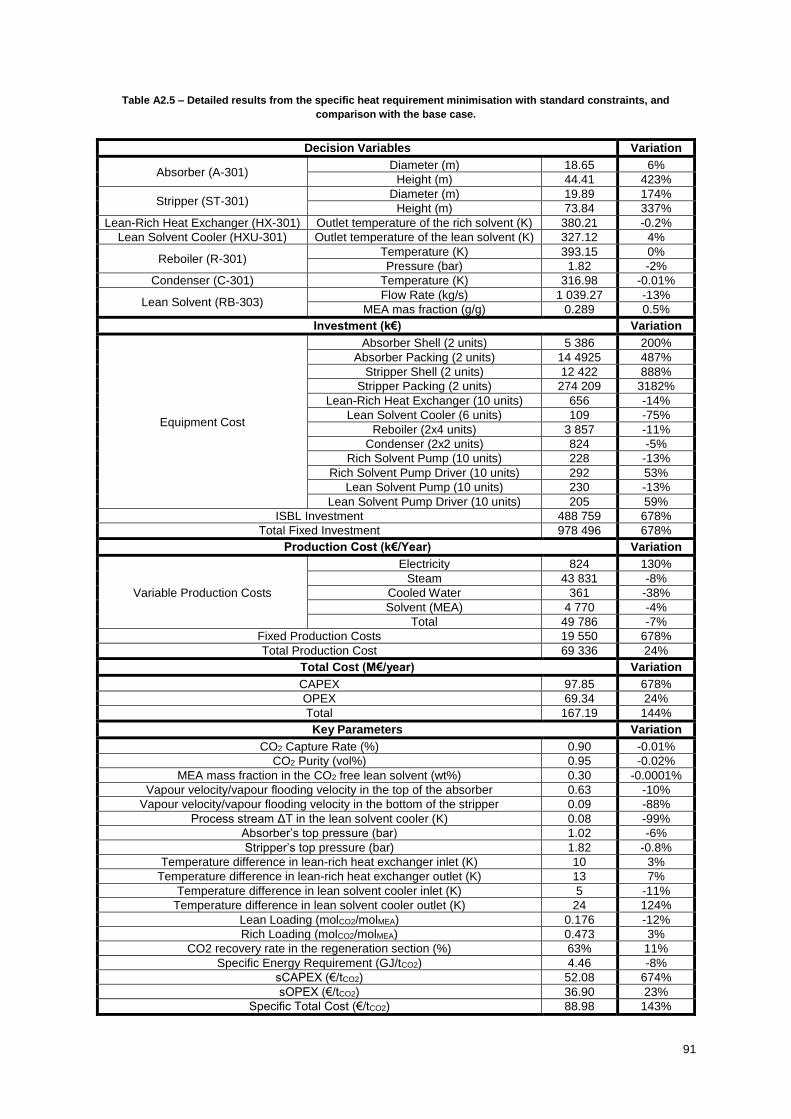
91
Table A2.5 – Detailed results from the specific heat requirement minimisation with standard constraints, and
comparison with the base case.
Decision Variables Variation
Absorber (A-301) Diameter (m) 18.65 6%
Height (m) 44.41 423%
Stripper (ST-301) Diameter (m) 19.89 174%
Height (m) 73.84 337%
Lean-Rich Heat Exchanger (HX-301) Outlet temperature of the rich solvent (K) 380.21 -0.2%
Lean Solvent Cooler (HXU-301) Outlet temperature of the lean solvent (K) 327.12 4%
Reboiler (R-301) Temperature (K) 393.15 0%
Pressure (bar) 1.82 -2%
Condenser (C-301) Temperature (K) 316.98 -0.01%
Lean Solvent (RB-303) Flow Rate (kg/s) 1 039.27 -13%
MEA mas fraction (g/g) 0.289 0.5%
Investment (k€) Variation
Equipment Cost
Absorber Shell (2 units) 5 386 200%
Absorber Packing (2 units) 14 4925 487%
Stripper Shell (2 units) 12 422 888%
Stripper Packing (2 units) 274 209 3182%
Lean-Rich Heat Exchanger (10 units) 656 -14%
Lean Solvent Cooler (6 units) 109 -75%
Reboiler (2x4 units) 3 857 -11%
Condenser (2x2 units) 824 -5%
Rich Solvent Pump (10 units) 228 -13%
Rich Solvent Pump Driver (10 units) 292 53%
Lean Solvent Pump (10 units) 230 -13%
Lean Solvent Pump Driver (10 units) 205 59%
ISBL Investment 488 759 678%
Total Fixed Investment 978 496 678%
Production Cost (k€/Year) Variation
Variable Production Costs
Electricity 824 130%
Steam 43 831 -8%
Cooled Water 361 -38%
Solvent (MEA) 4 770 -4%
Total 49 786 -7%
Fixed Production Costs 19 550 678%
Total Production Cost 69 336 24%
Total Cost (M€/year) Variation
CAPEX 97.85 678%
OPEX 69.34 24%
Total 167.19 144%
Key Parameters Variation
CO2 Capture Rate (%) 0.90 -0.01%
CO2 Purity (vol%) 0.95 -0.02%
MEA mass fraction in the CO2 free lean solvent (wt%) 0.30 -0.0001%
Vapour velocity/vapour flooding velocity in the top of the absorber 0.63 -10%
Vapour velocity/vapour flooding velocity in the bottom of the stripper 0.09 -88%
Process stream ΔT in the lean solvent cooler (K) 0.08 -99%
Absorber’s top pressure (bar) 1.02 -6%
Stripper’s top pressure (bar) 1.82 -0.8%
Temperature difference in lean-rich heat exchanger inlet (K) 10 3%
Temperature difference in lean-rich heat exchanger outlet (K) 13 7%
Temperature difference in lean solvent cooler inlet (K) 5 -11%
Temperature difference in lean solvent cooler outlet (K) 24 124%
Lean Loading (molCO2/molMEA) 0.176 -12%
Rich Loading (molCO2/molMEA) 0.473 3%
CO2 recovery rate in the regeneration section (%) 63% 11%
Specific Energy Requirement (GJ/tCO2) 4.46 -8%
sCAPEX (€/tCO2) 52.08 674%
sOPEX (€/tCO2) 36.90 23%
Specific Total Cost (€/tCO2) 88.98 143%

92
Table A2.6 – Detailed results from the specific total cost minimisation with an imposed capture rate of 70%, and
comparison with the initial specific total cost minimisation results (Table 7.1).
Decision Variables Variation
Absorber (A-301) Diameter (m) 17.24 -2%
Height (m) 6.37 -25%
Stripper (ST-301) Diameter (m) 6.35 -13%
Height (m) 15.52 -8%
Lean-Rich Heat Exchanger (HX-301) Outlet temperature of the rich solvent (K) 384.04 0.8%
Lean Solvent Cooler (HXU-301) Outlet temperature of the lean solvent (K) 323.60 3%
Reboiler (R-301) Temperature (K) 393.15 0%
Pressure (bar) 1.86 0.5%
Condenser (C-301) Temperature (K) 317.19 0.06%
Lean Solvent (RB-303) Flow Rate (kg/s) 972.93 -19%
MEA mas fraction (g/g) 0.287 -0.2%
Investment (k€) Variation
Equipment Cost
Absorber Shell (2 units) 1 546 -14%
Absorber Packing (2 units) 17 767 -28%
Stripper Shell (2 units) 1 068 -15%
Stripper Packing (2 units) 5 867 -30%
Lean-Rich Heat Exchanger (12 units) 902 18%
Lean Solvent Cooler (2 units) 126 -71%
Reboiler (2x3 units) 3 306 -23%
Condenser (2x2 units) 719 -17%
Rich Solvent Pump (8 units) 210 -20%
Rich Solvent Pump Driver (8 units) 150 -21%
Lean Solvent Pump (8 units) 213 -20%
Lean Solvent Pump Driver (8 units) 97 -25%
ISBL Investment 47 785 -24%
Total Fixed Investment 95 666 -24%
Production Cost (k€/Year) Variation
Variable Production Costs
Electricity 272 -24%
Steam 36 613 -23%
Cooled Water 349 -41%
Solvent (MEA) 3 739 -25%
Total 40 972 -23%
Fixed Production Costs 1 911 -24%
Total Production Cost 42 883 -23%
Total Cost (M€/year) Variation
CAPEX 9.58 -24%
OPEX 42.88 -23%
Total 52.45 -23%
Key Parameters Variation
CO2 Capture Rate (%) 70 -22%
CO2 Purity (vol%) 95 -0.02%
MEA mass fraction in the CO2 free lean solvent (wt%) 30 -0.0001%
Vapour velocity/vapour flooding velocity in the top of the absorber 0.70 0.4%
Vapour velocity/vapour flooding velocity in the bottom of the stripper 0.70 0.4%
Process stream ΔT in the lean solvent cooler (K) 0.55 -96%
Lean Loading (molCO2/molMEA) 0.211 5%
Rich Loading (molCO2/molMEA) 0.458 0.02%
CO2 recovery rate in the regeneration section (%) 54 -4%
Specific Energy Requirement (GJ/tCO2) 4.81 -1%
sCAPEX (€/tCO2) 6.57 -2%
sOPEX (€/tCO2) 29.45 -2%
Specific Total Cost (€/tCO2) 36.02 -2%

93
Table A2.7 – Detailed results from the specific total cost minimisation with an imposed capture rate of 80%, and
comparison with the initial specific total cost minimisation results (Table 7.1).
Decision Variables Variation
Absorber (A-301) Diameter (m) 17.48 -0.7%
Height (m) 7.17 -16%
Stripper (ST-301) Diameter (m) 6.80 -6%
Height (m) 15.61 -8%
Lean-Rich Heat Exchanger (HX-301) Outlet temperature of the rich solvent (K) 384.06 0.8%
Lean Solvent Cooler (HXU-301) Outlet temperature of the lean solvent (K) 323.51 3%
Reboiler (R-301) Temperature (K) 393.15 0%
Pressure (bar) 1.86 0.2%
Condenser (C-301) Temperature (K) 317.14 0.04%
Lean Solvent (RB-303) Flow Rate (kg/s) 1 098.27 -8%
MEA mas fraction (g/g) 0.287 -0.1%
Investment (k€) Variation
Equipment Cost
Absorber Shell (2 units) 1 649 -8%
Absorber Packing (2 units) 20 576 -17%
Stripper Shell (2 units) 1 134 -10%
Stripper Packing (2 units) 6 765 -19%
Lean-Rich Heat Exchanger (13 units) 1 023 34%
Lean Solvent Cooler (2 units) 145 -67%
Reboiler (2x3 units) 3 713 -14%
Condenser (2x2 units) 837 -4%
Rich Solvent Pump (9 units) 237 -10%
Rich Solvent Pump Driver (9 units) 169 -11%
Lean Solvent Pump (9 units) 240 -9%
Lean Solvent Pump Driver (9 units) 112 -13%
ISBL Investment 54 154 -14%
Total Fixed Investment 108 415 -14%
Production Cost (k€/Year) Variation
Variable Production Costs
Electricity 311 -13%
Steam 41 935 -12%
Cooled Water 406 -31%
Solvent (MEA) 4 281 -14%
Total 46 933 -12%
Fixed Production Costs 2 166 -14%
Total Production Cost 49 099 -12%
Total Cost (M€/year) Variation
CAPEX 10.84 -14%
OPEX 49.10 -12%
Total 59.94 -13%
Key Parameters Variation
CO2 Capture Rate (%) 80 -11%
CO2 Purity (vol%) 95 -0.02%
MEA mass fraction in the CO2 free lean solvent (wt%) 30 -0.0001%
Vapour velocity/vapour flooding velocity in the top of the absorber 0.70 0.4%
Vapour velocity/vapour flooding velocity in the bottom of the stripper 0.70 0.4%
Process stream ΔT in the lean solvent cooler (K) 0.75 -95%
Lean Loading (molCO2/molMEA) 0.207 4%
Rich Loading (molCO2/molMEA) 0.457 -0.08%
CO2 recovery rate in the regeneration section (%) 55 -3%
Specific Energy Requirement (GJ/tCO2) 4.82 -0.9
sCAPEX (€/tCO2) 6.51 -3%
sOPEX (€/tCO2) 29.50 -2%
Specific Total Cost (€/tCO2) 36.02 -2%

94
Table A2.8 – Detailed results from the specific total cost minimisation with an imposed capture rate of 99%, and
comparison with the initial specific total cost minimisation results (Table 7.1).
Decision Variables Variation
Absorber (A-301) Diameter (m) 17.23 -2%
Height (m) 14.39 69%
Stripper (ST-301) Diameter (m) 6.89 -5%
Height (m) 30.27 79%
Lean-Rich Heat Exchanger (HX-301) Outlet temperature of the rich solvent (K) 346.52 -9%
Lean Solvent Cooler (HXU-301) Outlet temperature of the lean solvent (K) 303.38 -3%
Reboiler (R-301) Temperature (K) 393.15 0%
Pressure (bar) 1.78 -4%
Condenser (C-301) Temperature (K) 316.15 -0.3%
Lean Solvent (RB-303) Flow Rate (kg/s) 960.64 -20%
MEA mas fraction (g/g) 0.293 2%
Investment (k€) Variation
Equipment Cost
Absorber Shell (2 units) 2 349 31%
Absorber Packing (2 units) 40 098 62%
Stripper Shell (3 units) 2 652 111%
Stripper Packing (3 units) 20 252 142%
Lean-Rich Heat Exchanger (1 units) 66 -91%
Lean Solvent Cooler (11 units) 864 98%
Reboiler (3x3 units) 5 793 34%
Condenser (3x2 units) 885 2%
Rich Solvent Pump (8 units) 212 -19%
Rich Solvent Pump Driver (8 units) 184 -4%
Lean Solvent Pump (8 units) 212 -20%
Lean Solvent Pump Driver (8 units) 121 -6%
ISBL Investment 98 912 57%
Total Fixed Investment 198 022 57%
Production Cost (k€/Year) Variation
Variable Production Costs
Electricity 387 8%
Steam 65 857 39%
Cooled Water 1 080 84%
Solvent (MEA) 5 724 15%
Total 73 047 37%
Fixed Production Costs 3 956 57%
Total Production Cost 77 004 38%
Total Cost (M€/year) Variation
CAPEX 19.80 57%
OPEX 77.00 38%
Total 96.81 41%
Key Parameters Variation
CO2 Capture Rate (%) 99 10%
CO2 Purity (vol%) 95 -0.02%
MEA mass fraction in the CO2 free lean solvent (wt%) 30 -0.0001%
Vapour velocity/vapour flooding velocity in the top of the absorber 0.70 0.4%
Vapour velocity/vapour flooding velocity in the bottom of the stripper 0.70 0.4%
Process stream ΔT in the lean solvent cooler (K) 61.81 343%
Lean Loading (molCO2/molMEA) 0.111 -45%
Rich Loading (molCO2/molMEA) 0.459 0.3%
CO2 recovery rate in the regeneration section (%) 76 35%
Specific Energy Requirement (GJ/tCO2) 6.09 25%
sCAPEX (€/tCO2) 9.58 42%
sOPEX (€/tCO2) 37.23 24%
Specific Total Cost (€/tCO2) 46.81 28%

95
Table A2.9 – Detailed results from the specific total cost minimisation with an imposed CO2 purity of 75%, and
comparison with the initial specific total cost minimisation results (Table 7.1).
Decision Variables Variation
Absorber (A-301) Diameter (m) 17.58 -0.2%
Height (m) 8.27 -3%
Stripper (ST-301) Diameter (m) 7.23 -0.4%
Height (m) 16.66 -1%
Lean-Rich Heat Exchanger (HX-301) Outlet temperature of the rich solvent (K) 381.61 0.1%
Lean Solvent Cooler (HXU-301) Outlet temperature of the lean solvent (K) 312.30 -0.5%
Reboiler (R-301) Temperature (K) 393.15 0%
Pressure (bar) 1.85 0.06%
Condenser (C-301) Temperature (K) 352.51 11%
Lean Solvent (RB-303) Flow Rate (kg/s) 1 210.01 1%
MEA mas fraction (g/g) 0.287 -0.04%
Investment (k€) Variation
Equipment Cost
Absorber Shell (2 units) 1 771 -1%
Absorber Packing (2 units) 23 973 -3%
Stripper Shell (2 units) 1 243 -1%
Stripper Packing (2 units) 8 178 -2%
Lean-Rich Heat Exchanger (11 units) 874 14%
Lean Solvent Cooler (6 units) 482 11%
Reboiler (2x4 units) 4 294 -0.4%
Condenser (2x1 units) 397 -54%
Rich Solvent Pump (10 units) 264 0.9%
Rich Solvent Pump Driver (10 units) 192 0.5%
Lean Solvent Pump (10 units) 267 0.6%
Lean Solvent Pump Driver (10 units) 129 -0.1%
ISBL Investment 60 857 -3%
Total Fixed Investment 121 836 -3%
Production Cost (k€/Year) Variation
Variable Production Costs
Electricity 360 0.5%
Steam 47 330 -0.4%
Cooled Water 544 -7%
Solvent (MEA) 5 538 11%
Total 53 772 0.6%
Fixed Production Costs 2 434 -3%
Total Production Cost 56 206 0.4%
Total Cost (M€/year) Variation
CAPEX 12.18 -3%
OPEX 56.21 0.4%
Total 68.39 -0.2%
Key Parameters Variation
CO2 Capture Rate (%) 90 -0.009%
CO2 Purity (vol%) 75 -21%
MEA mass fraction in the CO2 free lean solvent (wt%) 30 -0.0002%
Vapour velocity/vapour flooding velocity in the top of the absorber 0.70 0.3%
Vapour velocity/vapour flooding velocity in the bottom of the stripper 0.70 0.3%
Process stream ΔT in the lean solvent cooler (K) 14.54 4%
Lean Loading (molCO2/molMEA) 0.202 1% Rich Loading (molCO2/molMEA) 0.456 -0.2%
CO2 recovery rate in the regeneration section (%) 56 -1% Specific Energy Requirement (GJ/tCO2) 4.85 -0.4%
sCAPEX (€/tCO2) 6.52 -3% sOPEX (€/tCO2) 30.10 0.5%
Specific Total Cost (€/tCO2) 36.62 -0.2%

96
Table A2.10 – Detailed results from the specific total cost minimisation with an imposed CO2 purity of 85%, and
comparison with the initial specific total cost minimisation results (Table 7.1).
Decision Variables Variation
Absorber (A-301) Diameter (m) 17.58 -0.2%
Height (m) 8.43 -1%
Stripper (ST-301) Diameter (m) 7.24 -0.3%
Height (m) 16.78 -1%
Lean-Rich Heat Exchanger (HX-301) Outlet temperature of the rich solvent (K) 381.35 0.07%
Lean Solvent Cooler (HXU-301) Outlet temperature of the lean solvent (K) 313.05 -0.3%
Reboiler (R-301) Temperature (K) 393.15 0%
Pressure (bar) 1.85 0.02%
Condenser (C-301) Temperature (K) 340.31 7%
Lean Solvent (RB-303) Flow Rate (kg/s) 1 199.37 0.4%
MEA mas fraction (g/g) 0.288 -0.02%
Investment (k€) Variation
Equipment Cost
Absorber Shell (2 units) 1 787 -0.5%
Absorber Packing (2 units) 24 442 -1%
Stripper Shell (2 units) 1 249 -0.7%
Stripper Packing (2 units) 8 247 -1%
Lean-Rich Heat Exchanger (11 units) 817 7%
Lean Solvent Cooler (6 units) 457 5%
Reboiler (2x4 units) 4 298 -0.3%
Condenser (2x2 units) 519 -40%
Rich Solvent Pump (10 units) 263 0.3%
Rich Solvent Pump Driver (10 units) 191 0.09%
Lean Solvent Pump (10 units) 266 0.1%
Lean Solvent Pump Driver (10 units) 129 -0.06%
ISBL Investment 61 571 -2%
Total Fixed Investment 123 266 -2%
Production Cost (k€/Year) Variation
Variable Production Costs
Electricity 359 0.07%
Steam 47 376 -0.3%
Cooled Water 567 -4%
Solvent (MEA) 5 186 4%
Total 53 487 0.05%
Fixed Production Costs 2 463 -2%
Total Production Cost 55 950 -0.04%
Total Cost (M€/year) Variation
CAPEX 12.33 -2%
OPEX 55.95 -0.04%
Total 68.28 -0.4%
Key Parameters Variation
CO2 Capture Rate (%) 90 -0.008%
CO2 Purity (vol%) 85 -10%
MEA mass fraction in the CO2 free lean solvent (wt%) 30 -0.00004%
Vapour velocity/vapour flooding velocity in the top of the absorber 0.70 0.3%
Vapour velocity/vapour flooding velocity in the bottom of the stripper 0.70 0.2%
Process stream ΔT in the lean solvent cooler (K) 14.26 2%
Lean Loading (molCO2/molMEA) 0.201 0.4%
Rich Loading (molCO2/molMEA) 0.457 -0.06%
CO2 recovery rate in the regeneration section (%) 56 -0.3%
Specific Energy Requirement (GJ/tCO2) 4.85 -0.3%
sCAPEX (€/tCO2) 6.60 -2%
sOPEX (€/tCO2) 29.95 -0.01%
Specific Total Cost (€/tCO2) 36.55 -0.4%
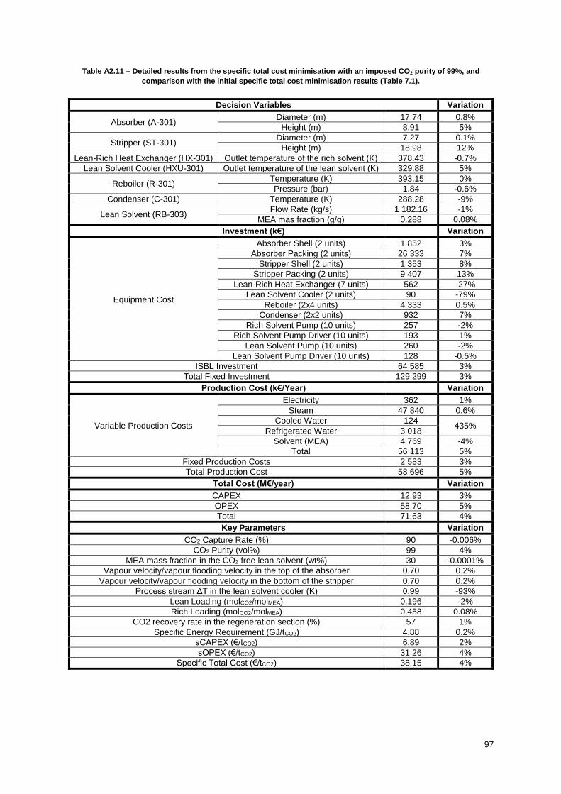
97
Table A2.11 – Detailed results from the specific total cost minimisation with an imposed CO2 purity of 99%, and
comparison with the initial specific total cost minimisation results (Table 7.1).
Decision Variables Variation
Absorber (A-301) Diameter (m) 17.74 0.8%
Height (m) 8.91 5%
Stripper (ST-301) Diameter (m) 7.27 0.1%
Height (m) 18.98 12%
Lean-Rich Heat Exchanger (HX-301) Outlet temperature of the rich solvent (K) 378.43 -0.7%
Lean Solvent Cooler (HXU-301) Outlet temperature of the lean solvent (K) 329.88 5%
Reboiler (R-301) Temperature (K) 393.15 0%
Pressure (bar) 1.84 -0.6%
Condenser (C-301) Temperature (K) 288.28 -9%
Lean Solvent (RB-303) Flow Rate (kg/s) 1 182.16 -1%
MEA mas fraction (g/g) 0.288 0.08%
Investment (k€) Variation
Equipment Cost
Absorber Shell (2 units) 1 852 3%
Absorber Packing (2 units) 26 333 7%
Stripper Shell (2 units) 1 353 8%
Stripper Packing (2 units) 9 407 13%
Lean-Rich Heat Exchanger (7 units) 562 -27%
Lean Solvent Cooler (2 units) 90 -79%
Reboiler (2x4 units) 4 333 0.5%
Condenser (2x2 units) 932 7%
Rich Solvent Pump (10 units) 257 -2%
Rich Solvent Pump Driver (10 units) 193 1%
Lean Solvent Pump (10 units) 260 -2%
Lean Solvent Pump Driver (10 units) 128 -0.5%
ISBL Investment 64 585 3%
Total Fixed Investment 129 299 3%
Production Cost (k€/Year) Variation
Variable Production Costs
Electricity 362 1%
Steam 47 840 0.6%
Cooled Water 124 435%
Refrigerated Water 3 018
Solvent (MEA) 4 769 -4%
Total 56 113 5%
Fixed Production Costs 2 583 3%
Total Production Cost 58 696 5%
Total Cost (M€/year) Variation
CAPEX 12.93 3%
OPEX 58.70 5%
Total 71.63 4%
Key Parameters Variation
CO2 Capture Rate (%) 90 -0.006%
CO2 Purity (vol%) 99 4%
MEA mass fraction in the CO2 free lean solvent (wt%) 30 -0.0001%
Vapour velocity/vapour flooding velocity in the top of the absorber 0.70 0.2%
Vapour velocity/vapour flooding velocity in the bottom of the stripper 0.70 0.2%
Process stream ΔT in the lean solvent cooler (K) 0.99 -93%
Lean Loading (molCO2/molMEA) 0.196 -2%
Rich Loading (molCO2/molMEA) 0.458 0.08%
CO2 recovery rate in the regeneration section (%) 57 1%
Specific Energy Requirement (GJ/tCO2) 4.88 0.2%
sCAPEX (€/tCO2) 6.89 2%
sOPEX (€/tCO2) 31.26 4%
Specific Total Cost (€/tCO2) 38.15 4%
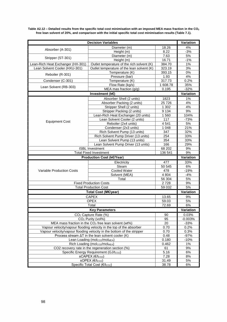
98
Table A2.12 – Detailed results from the specific total cost minimisation with an imposed MEA mass fraction in the CO2
free lean solvent of 20%, and comparison with the initial specific total cost minimisation results (Table 7.1).
Decision Variables Variation
Absorber (A-301) Diameter (m) 18.26 4%
Height (m) 8.22 -3%
Stripper (ST-301) Diameter (m) 7.63 5%
Height (m) 16.71 -1%
Lean-Rich Heat Exchanger (HX-301) Outlet temperature of the rich solvent (K) 384.70 1%
Lean Solvent Cooler (HXU-301) Outlet temperature of the lean solvent (K) 323.19 3%
Reboiler (R-301) Temperature (K) 393.15 0%
Pressure (bar) 1.93 4%
Condenser (C-301) Temperature (K) 317.73 0.2%
Lean Solvent (RB-303) Flow Rate (kg/s) 1 608.78 35%
MEA mas fraction (g/g) 0.195 -32%
Investment (k€) Variation
Equipment Cost
Absorber Shell (2 units) 1823 1%
Absorber Packing (2 units) 25 726 4%
Stripper Shell (2 units) 1 302 4%
Stripper Packing (2 units) 9 134 9%
Lean-Rich Heat Exchanger (20 units) 1 560 104%
Lean Solvent Cooler (2 units) 117 -73%
Reboiler (2x4 units) 4 541 5%
Condenser (2x3 units) 1 048 21%
Rich Solvent Pump (13 units) 347 32%
Rich Solvent Pump Driver (13 units) 254 33%
Lean Solvent Pump (13 units) 354 33%
Lean Solvent Pump Driver (13 units) 166 29%
ISBL Investment 68 202 9%
Total Fixed Investment 136 541 9%
Production Cost (k€/Year) Variation
Variable Production Costs
Electricity 477 33%
Steam 50 545 6%
Cooled Water 478 -19%
Solvent (MEA) 4 804 -4%
Total 56 304 5%
Fixed Production Costs 2 728 9%
Total Production Cost 59 032 5%
Total Cost (M€/year) Variation
CAPEX 13.65 9%
OPEX 59.03 5%
Total 72.69 6%
Key Parameters Variation
CO2 Capture Rate (%) 90 0.03%
CO2 Purity (vol%) 95 -0.003%
MEA mass fraction in the CO2 free lean solvent (wt%) 20 -33%
Vapour velocity/vapour flooding velocity in the top of the absorber 0.70 0.2%
Vapour velocity/vapour flooding velocity in the bottom of the stripper 0.70 0.3%
Process stream ΔT in the lean solvent cooler (K) 0.48 -97%
Lean Loading (molCO2/molMEA) 0.180 -10%
Rich Loading (molCO2/molMEA) 0.462 1%
CO2 recovery rate in the regeneration section (%) 61 9%
Specific Energy Requirement (GJ/tCO2) 5.16 6%
sCAPEX (€/tCO2) 7.28 8%
sOPEX (€/tCO2) 31.49 5%
Specific Total Cost (€/tCO2) 38.78 6%

99
Table A2.13 – Detailed results from the specific total cost minimisation with an imposed MEA mass fraction in the CO2
free lean solvent of 40%, and comparison with the initial specific total cost minimisation results (Table 7.1).
Decision Variables Variation
Absorber (A-301) Diameter (m) 17.35 -1%
Height (m) 9.39 11%
Stripper (ST-301) Diameter (m) 7.00 -4%
Height (m) 18.27 8%
Lean-Rich Heat Exchanger (HX-301) Outlet temperature of the rich solvent (K) 383.24 0.6%
Lean Solvent Cooler (HXU-301) Outlet temperature of the lean solvent (K) 325.87 4%
Reboiler (R-301) Temperature (K) 393.15 0%
Pressure (bar) 1.73 -7%
Condenser (C-301) Temperature (K) 315.77 -0.4%
Lean Solvent (RB-303) Flow Rate (kg/s) 994.07 -17%
MEA mas fraction (g/g) 0.377 31%
Investment (k€) Variation
Equipment Cost
Absorber Shell (2 units) 1 866 4%
Absorber Packing (2 units) 26 536 7%
Stripper Shell (2 units) 1 280 2%
Stripper Packing (2 units) 8 399 0.5%
Lean-Rich Heat Exchanger (11 units) 842 10%
Lean Solvent Cooler (3 units) 172 -60%
Reboiler (2x3 units) 3 966 -8%
Condenser (2x2 units) 909 5%
Rich Solvent Pump (8 units) 213 -19%
Rich Solvent Pump Driver (8 units) 155 -19%
Lean Solvent Pump (8 units) 213 -20%
Lean Solvent Pump Driver (8 units) 111 -14%
ISBL Investment 63 093 0.4%
Total Fixed Investment 126 312 0.4%
Production Cost (k€/Year) Variation
Variable Production Costs
Electricity 304 -15%
Steam 45 288 -5%
Cooled Water 453 -23%
Solvent (MEA) 4 905 -2%
Total 50 950 -5%
Fixed Production Costs 2 524 0.4%
Total Production Cost 53 474 -4%
Total Cost (M€/year) Variation
CAPEX 12.63 0.4%
OPEX 53.47 -4%
Total 66.10 -4%
Key Parameters Variation
CO2 Capture Rate (%) 90 0.002%
CO2 Purity (vol%) 95 -0.02%
MEA mass fraction in the CO2 free lean solvent (wt%) 40 33%
Vapour velocity/vapour flooding velocity in the top of the absorber 0.70 0.2%
Vapour velocity/vapour flooding velocity in the bottom of the stripper 0.70 0.2%
Process stream ΔT in the lean solvent cooler (K) 0.62 -96%
Lean Loading (molCO2/molMEA) 0.212 6%
Rich Loading (molCO2/molMEA) 0.450 -2%
CO2 recovery rate in the regeneration section (%) 53 -6%
Specific Energy Requirement (GJ/tCO2) 4.62 -5%
sCAPEX (€/tCO2) 6.73 0.02%
sOPEX (€/tCO2) 28.50 -5%
Specific Total Cost (€/tCO2) 35.23 -4%

100
Table A2.14 – Detailed results from the specific total cost minimisation with inequality constraints, and comparison
with the initial specific total cost minimisation results (Table 7.1).
Decision Variables Variation
Absorber (A-301) Diameter (m) 17.03 -3%
Height (m) 7.22 -15%
Stripper (ST-301) Diameter (m) 6.36 -12%
Height (m) 16.51 -2%
Lean-Rich Heat Exchanger (HX-301) Outlet temperature of the rich solvent (K) 383.56 0.7%
Lean Solvent Cooler (HXU-301) Outlet temperature of the lean solvent (K) 325.27 4%
Reboiler (R-301) Temperature (K) 393.15 -0.00004%
Pressure (bar) 1.74 -6%
Condenser (C-301) Temperature (K) 333.90 5%
Lean Solvent (RB-303) Flow Rate (kg/s) 858.77 -28%
MEA mas fraction (g/g) 0.376 31%
Investment (k€) Variation
Equipment Cost
Absorber Shell (2 units) 1 618 -10%
Absorber Packing (2 units) 19 647 -20%
Stripper Shell (2 units) 1 111 -12%
Stripper Packing (2 units) 6 268 -25%
Lean-Rich Heat Exchanger (10 units) 774 1%
Lean Solvent Cooler (2 units) 155 -64%
Reboiler (2x3 units) 3 380 -22%
Condenser (2x1 units) 479 -45%
Rich Solvent Pump (7 units) 185 -30%
Rich Solvent Pump Driver (7 units) 131 -31%
Lean Solvent Pump (7 units) 185 -30%
Lean Solvent Pump Driver (7 units) 90 -30%
ISBL Investment 49 397 -21%
Total Fixed Investment 98 892 -21%
Production Cost (k€/Year) Variation
Variable Production Costs
Electricity 246 -31%
Steam 37 568 -21%
Cooled Water 356 -39%
Solvent (MEA) 4 188 -16%
Total 42 357 -21%
Fixed Production Costs 1 976 -21%
Total Production Cost 44 333 -21%
Total Cost (M€/year) Variation
CAPEX 9.89 -21%
OPEX 44.33 -21%
Total 54.22 -21%
Key Parameters Variation
CO2 Capture Rate (%) 75 -17%
CO2 Purity (vol%) 88 -7%
MEA mass fraction in the CO2 free lean solvent (wt%) 40 33%
Vapour velocity/vapour flooding velocity in the top of the absorber 0.70 0%
Vapour velocity/vapour flooding velocity in the bottom of the stripper 0.70 0%
Process stream ΔT in the lean solvent cooler (K) 0.48 -97%
Lean Loading (molCO2/molMEA) 0.221 10%
Rich Loading (molCO2/molMEA) 0.451 -1%
CO2 recovery rate in the regeneration section (%) 51 -9%
Specific Energy Requirement (GJ/tCO2) 4.60 -1%
sCAPEX (€/tCO2) 6.33 -6%
sOPEX (€/tCO2) 28.37 -5%
Specific Total Cost (€/tCO2) 34.70 -5%