design and techno-economical analysis of a grid connected
TRANSCRIPT

An-Najah National University Faculty of Graduate Studies
Design and Techno-Economical Analysis of a Grid
Connected with PV/ Wind Hybrid System in
Palestine (Atouf Village-Case study)
By Mohammad Husain Mohammad Dradi
Supervisor Dr. Imad Ibrik
This Thesis is Submitted in Partial Fulfillment of the Requirements
for the Degree of Master of Program in Clean Energy and
Conservation Strategy Engineering, Faculty of Graduate Studies,
An-Najah National University, Nablus-Palestine 2012


iii
DEDICATION
To my father ….
To my mother, brothers and sisters…….
To my wife, daughters, and son……
To my uncle……
To the soul of my aunt ………..
To all friends and colleagues………
To every one working in this field……
To all of them,
I dedicate this work

iv
ACKNOWLEDGMENTS
It is an honor for me to have the opportunity to say a word to thank
all people who helped me to complete this study, although it is impossible
to include all of them here.
All appreciations go to my supervisor, Dr. Imad Ibrik for his
exceptional guidance and insightful comments and observations throughout
the duration of this project.
My thanks and appreciations go to the staff of Clean Energy and
Conservation Strategy Engineering Master Program in An-Najah National
University, especially Prof. Marwan Mahmoud for his valuable suggestions
and assistance.
This project would not have been possible without the endless
support and contributions from my family, especially my mother for her
kindness, my wife for here encouragement and patience, my brothers and
sisters for their support, also for my friends and colleagues for their useful
help, and to everyone who contributed to complete this effort.

v
الإقرار
عنوان تحمل التي الرسالة مقدم أدناه الموقع إنا
Design and Techno-Economical Analysis of a Grid
Connected with PV/ Wind Hybrid System in
Palestine (Atouf Village-Case study)
الهجينة شبكات الكهرباء مع الأنظمةالتحليل التقني والاقتصادي لربط التقييم و
دراسة حالة: قرية عطوف /رياح في فلسطينخلايا شمسية
تمـت مـا باستثناء ، الخاص جهدي نتاج هو إنما الرسالة هذه عليه اشتملت ما بان اقر
درجة أية لنيل قبل من يقدم لم منها جزء أو من ككل الرسالة هذه وان ورد، حيثما إليه الإشارة
.أخرى بحثية أو تعليمية مؤسسة أية لدى بحثي أو علمي بحث أو
Declaration
The work provided in this thesis, unless otherwise referenced, is the
researcher's own work, and has not been submitted elsewhere for any other
degree or qualification.
:Student's name :اسم الطالب
:Signature :التوقيع
:Date :التاريخ

vi
List of Abbreviations
AC Alternative current
GTI Grid tie inverter
GS Gaza Strip
GW Giga watt
GWh Giga watt hour
IEC Israel electric corporation
kVA Kilo volt ampere
kWh Kilo watt hour
NIS New Israeli shekel
PSH Peak sun hour
PT Palestinian Territories
FIT Feed in Tariff
STC Standard Test Condition
LCC Life Cycle Cost
PCC Point of common coupling
ERC Energy Research Center
CV Constant voltage method
IC Incremental Conductance method
CCM Continues Conduction Mode
rpm Revolution per minute

vii
Table of Contents
No. Content Page
Dedication iii Acknowledgments iv Declaration v List of Abbreviations vi Table of Contents vii List of Tables x List of Figures xi List of Map xvi List of Equations xix List of Appendices xx Abstract xxi Introduction 1 Objectives of Work 3 Organization of Thesis 3 Chapter One: Potential of Solar Energy in Palestine 5
1.1 Solar Radiation in Palestine 7 1.2 Ambient Temperature in Palestine 8 1.3 Solar Energy in Palestine 9 1.4 Photovoltaic PV Implemented Project in Palestine 10 Chapter Two: Potential of Wind Energy in Palestine 13
2.1 The Wind Resource 14 2.2 Wind Speed Distribution 15
2.3 Evaluation of Wind Data in Different Cities in West Bank (Ramallah and Nablus Cities)
18
Chapter Three: Components of Grid Tie PV/ Wind
Hybrid system 24
3.1 Grid Tie System configurations 25 3.2 Photovoltaic PV Technology 28 3.2.1 Mono Crystalline Silicon PV Cells 29 3.2.2 Multi-Crystalline Silicon PV Cells 30 3.2.3 Thin Film PV Technologies 31 3.3. Maximum Power Point Tracking 32 3.3.1 Maximum Power Point Tracking (MPPT) Techniques 33 3.4 Switched Mode DC-DC Converters 37 3.4.1 Buck Converter 37 3.4.2 Boost Converter 38 3.4.3 Buck-Boost Converter 39 3.5 Wind Turbine Technology 40 3.5.1 Types of Wind Turbine Grid Tie Connection 42

viii
No. Content Page
3.5.2 Control Types of Wind Turbine 46 3.6 Diesel Generator 47 3.6.1 Diesel Generator Set 48 3.6.2 Operating Characteristics of Diesel Generator 48 3.7 Grid Tie Inverter 51
Chapter Four: Mathematical Modeling and Simulink
of Grid Tie PV/Wind Hybrid System 53
4.1 Configuration of Grid Tie PV / Wind Hybrid System 54 4.2 Modeling of Grid Tie PV System 56 4.2.1 Modeling of Photovoltaic Array 56 4.2.2 Modeling of Boost Converter 70 4.2.3 Modeling of MPPT Controller 73 4.2.4 Modeling of Three Phase Voltage Source Inverter 74 4.3 Modeling of Wind Turbine 85 4.3.1 Modeling of Wind Turbine Aerodynamic 86 4.3.2 Modeling of Drive Train 90 4.3.3 Modeling of Grid Tie Wind Turbine Control 91 4.4 Modeling of Diesel Generator 97 4.4.1 Diesel Engine Model 97 4.4.2 Excitation System of Alternator Model 101
Chapter Five: Simulation of Grid Tie PV/Wind
hybrid system 107
5.1 Grid Tie PV/Wind Hybrid System Constructions 108 5.2 Simulation of Grid Tie PV/ Wind System 109 5.2.1 Simulation of the System for Different Radiations 109 5.2.2 Simulation of the System for Different Temperatures 113 5.2.3 Simulation of the System for Different Wind Speeds 116 5.2.4 Simulation of the System for Different Loads 118
5.3 Simulation of the System for On and Off Grid Connection
120
Chapter Six: Design and Simulation of Atouf Grid
Tie PV System 125
6.1 Introduction about Atouf Village 126 6.2 Potential of Solar Energy of Atouf Village 127 6.3 Energy Demand and Electrical Grid of Atouf Village 128 6.4 Current Situation of Consumers Connections 129 6.5 Design of Grid Tie PV System for Atouf Village 131 6.5.1 Electricity Consumption for Atouf Village 131 6.5.2 Design of Grid Tie PV System at 100% penetration 132 6.5.3 Design of Grid Tie PV System at 56% penetration 135

ix
No. Content Page
6.5.4 Energy Analysis of Grid Tie PV System at 100% penetration for Atouf Village
137
6.5.5 Energy Analysis of Grid Tie PV System at 56% penetration for Atouf Village
138
6.6 Simulink Configuration of Atouf village 139
Chapter Seven: Economical and Environmental
Impact of the Grid Tie PV/Wind Hybrid System 140
7.1 Determining the Cost of Producing One kWh from Grid Tie PV/Wind Hybrid System
141
7.1.1 Life cycle cost (LCC) 141 7.1.2 Economic Factors 143
7.1.3 Cost of producing one kWh from Grid Tie PV/wind hybrid System for Atouf village
145
7.2 Grid Tie System Tariffs 147 7.2.1 Net Metering Tariff 147 7.2.2 Feed in Tariff 148
7.3 Evaluation the Economic Impact of Atouf Grid Tie PV System
149
7.4 Environment Impact of Grid Tie PV/ Wind system 150
Chapter Eight: Conclusions and Future Scope of
Work 152
8.1 Conclusion 153 8.2 Scope of Future work 154 References 155 Appendices 160
ب الملخص

x
List of Tables
No. Table Page
Table (1.1) Monthly solar energy on horizontal surface for Nablus District –2011
7
Table (1.2) Hourly average solar radiation of typical summer day (11/6/2011)
9
Table (1.3) Ambient temperature in Tubas-2011 10 Table (2.1) Yearly wind calculations/Ramallah-2006 19 Table (2.2) Yearly wind calculations/Nablus- 2006 22 Table (4.1) KD135SX PV characteristics parameters 67 Table (4.2) Specifications of Boost Controller 71 Table (6.1) Monthly energy consumption of Atouf village 132 Table (6.2) Monthly energy production versus consumption 137
Table (6.3) Monthly energy production versus energy consumption
138
Table (7.1) Cost of elements and installation of grid tie PV system
145

xi
List of Figures
No. Figure Page
Fig. (1.1) Monthly solar energy for Tubas district-2011 on horizontal surface
8
Fig. (1.2) The global irradiation (W/m²) versus time (hours)-2011
9
Fig. (1.3) The daily ambient temperature curve-2011 10 Fig. (1.4) Imnazel photovoltaic (PV) project 11 Fig. (2.1) Weibull probability density distribution 16
Fig. (2.2) Number of hours per year for each wind speed range/Ramallah-2006
20
Fig. (2.3) Yearly energy and Weibull distributions/Ramallah site-2006
20
Fig. (2.4) Wind duration curve for Ramallah site-2006 21
Fig. (2.5) Yearly energy and Weibull distributions for Nablus site
22
Fig. (2.6) Wind duration curve for Nablus site 23 Fig. (3.1) Centralized AC-bus architecture 25 Fig. (3.2) Centralized DC-bus architecture 26 Fig. (3.3) Distributed AC-bus architecture 27 Fig. (3.4) The modified distributed Ac bus architecture 28 Fig. (3.5) Transition of cell, module and arrays 29 Fig. (3.6) The main industrialized PV technologies 29
Fig. (3.7) PV module is directly connected to a (variable) resistive load
33
Fig. (3.8)
I-V curves of BP SX 150S PV module and various resistive loads Simulated with the MATLAB model (1kW/m2, 25oC)
33
Fig. (3.9) CV algorithm and the code of Matlab embedded function
34
Fig. (3.10) Two-Method MPPT Control algorithm and the code of Matlab function
36
Fig. (3.11) P&Oa algorithm and the code of Matlab embedded function
37
Fig. (3.12) Buck converter 38 Fig. (3.13) Boost converter 39 Fig. (3.14) Buck Boost converter 39 Fig.(3.15) Lift and drag force components 40 Fig. (3.16) Horizontal wind turbine 41 Fig. (3.17) Typical wind turbine power curve 42 Fig. (3.18) Soft starter 43
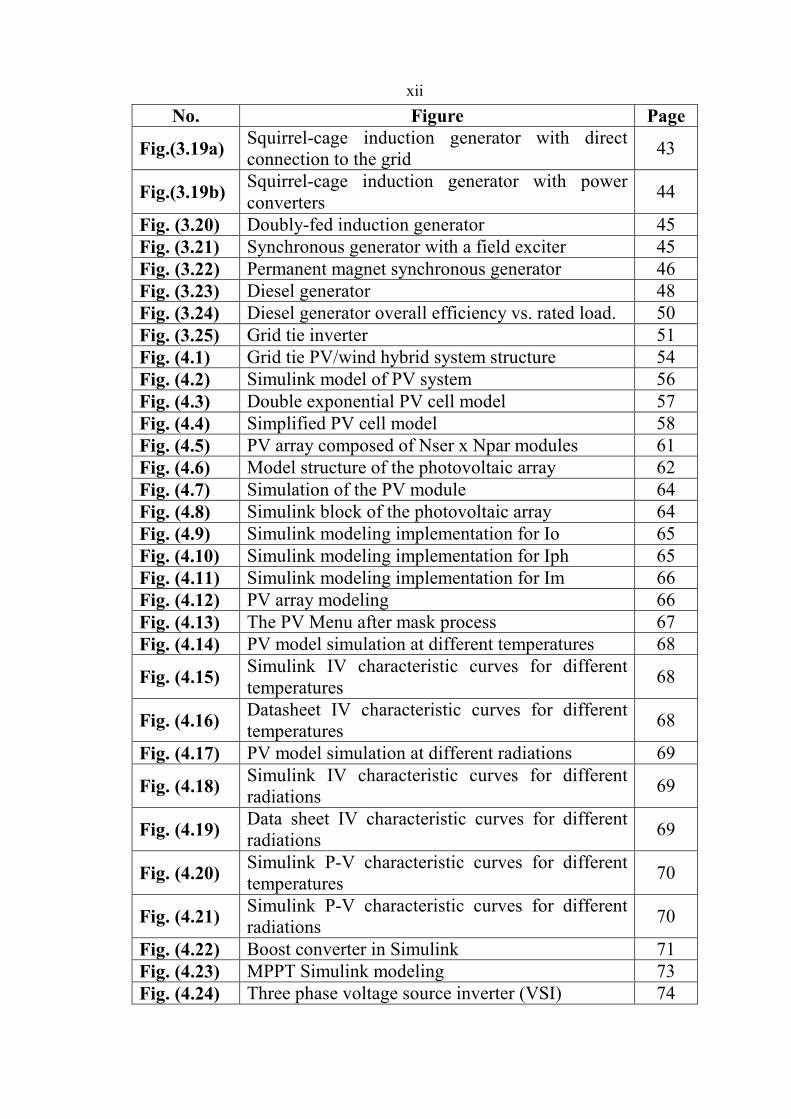
xii
No. Figure Page
Fig.(3.19a) Squirrel-cage induction generator with direct connection to the grid
43
Fig.(3.19b) Squirrel-cage induction generator with power converters
44
Fig. (3.20) Doubly-fed induction generator 45 Fig. (3.21) Synchronous generator with a field exciter 45 Fig. (3.22) Permanent magnet synchronous generator 46 Fig. (3.23) Diesel generator 48 Fig. (3.24) Diesel generator overall efficiency vs. rated load. 50 Fig. (3.25) Grid tie inverter 51 Fig. (4.1) Grid tie PV/wind hybrid system structure 54 Fig. (4.2) Simulink model of PV system 56 Fig. (4.3) Double exponential PV cell model 57 Fig. (4.4) Simplified PV cell model 58 Fig. (4.5) PV array composed of Nser x Npar modules 61 Fig. (4.6) Model structure of the photovoltaic array 62 Fig. (4.7) Simulation of the PV module 64 Fig. (4.8) Simulink block of the photovoltaic array 64 Fig. (4.9) Simulink modeling implementation for Io 65 Fig. (4.10) Simulink modeling implementation for Iph 65 Fig. (4.11) Simulink modeling implementation for Im 66 Fig. (4.12) PV array modeling 66 Fig. (4.13) The PV Menu after mask process 67 Fig. (4.14) PV model simulation at different temperatures 68
Fig. (4.15) Simulink IV characteristic curves for different temperatures
68
Fig. (4.16) Datasheet IV characteristic curves for different temperatures
68
Fig. (4.17) PV model simulation at different radiations 69
Fig. (4.18) Simulink IV characteristic curves for different radiations
69
Fig. (4.19) Data sheet IV characteristic curves for different radiations
69
Fig. (4.20) Simulink P-V characteristic curves for different temperatures
70
Fig. (4.21) Simulink P-V characteristic curves for different radiations
70
Fig. (4.22) Boost converter in Simulink 71 Fig. (4.23) MPPT Simulink modeling 73 Fig. (4.24) Three phase voltage source inverter (VSI) 74

xiii
No. Figure Page
Fig. (4.25) Relationship between the abc and dq reference frames
75
Fig. (4.26) Grid tie PV inverter control model 77
Fig. (4.27) Circuit diagram of a three phase grid connected inverter
78
Fig. (4.28) Schematic diagram of the DC link controller 81 Fig. (4.29) Schematic diagram of the phase locked loop (PLL) 82 Fig. (4.30) SPWM modulation signals for the VSI 85 Fig. (4.31) Simulink model for grid tie wind turbine 86 Fig. (4.32) Simulink block of wind turbine torque 87
Fig. (4.33) Simulink block of performance coefficient Cp (λ,β)
88
Fig. (4.34) Cp- λ Characteristics of wind turbine 89 Fig. (4.35) Simulink block of tip speed ratio λi model 89 Fig. (4.36) Model of drive train (2-mass system) 90 Fig. (4.37) Equivalent diagram of the drive train model 91
Fig. (4.38) Equivalent diagram for grid tie wind turbine control model
92
Fig. (4.39) Equivalent diagram of generator excitation control model
93
Fig. (4.40) Stabilization of power and speed through a single operating point
93
Fig. (4.41) Equivalent flow diagram for speed regulator 95
Fig. (4.42) Available power for different wind speeds; blade pitch angle of zero
95
Fig. (4.43) Available power for different wind speeds; pitch angle of 5 degrees
96
Fig. (4.44) Available power for different blade pitch angles; wind speed 15 m/s
96
Fig. (4.45) Equivalent flow diagram for pitch control 97 Fig. (4.46) Simulink model of diesel generator 98 Fig. (4.47) Speed Control of Diesel Engine 99 Fig. (4.48) Field-Controlled DC Commutator Exciters 102 Fig. (4.49) Simulink model of Excitation System 104
Fig. (4.50) Simulink model for Grid tie PV/Wind hybrid system
106
Fig. (5.1) Complete grid tie PV/Wind Simulink system 109 Fig. (5.2) Two different input radiations for PV array 110
Fig. (5.3) PV Inverter power output for two different radiations
110

xiv
No. Figure Page
Fig. (5.4) Three phase PV inverter current for two different radiations
111
Fig. (5.5) PV inverter dc bus voltage for two different radiations
111
Fig. (5.6) Wind turbine output power for the variation of input radiation of PV
112
Fig. (5.7) Grid power output for two different radiations 112 Fig. (5.8) Two different input temperatures for PV array 113
Fig. (5.9) PV Inverter power output for two different temperatures
114
Fig. (5.10) Three phase PV inverter current for two different temperatures
114
Fig. (5.11) Wind turbine power for the variation of input temperature on PV
115
Fig. (5.12) Performance of Grid power for two different temperatures
115
Fig. (5.13) Two different input wind speeds for wind turbine 116
Fig. (5.14) PV Inverter power under the variation of wind speed on wind turbine
117
Fig. (5.15) Wind turbine power for two different wind speeds 117
Fig. (5.16) Performance of Grid power for two different wind speeds
118
Fig. (5.17) PV Inverter power output for two different loads 119 Fig. (5.18) Wind turbine power for two different loads 119 Fig. (5.19) Performance of Grid power for two different loads 120 Fig. (5.20) PV Inverter power output for on and off grid 121 Fig. (5.21) PV inverter dc bus voltage for on and off grid 121
Fig. (5.22) Three phase PV inverter current for on and off grid
122
Fig. (5.23) Three phase grid voltage for on and off grid 122 Fig.(5.24) Wind turbine output power for on and off grid 123 Fig. (5.25) Performance of Grid power for on and off grid 123
Fig. (5.26) pu diesel generator mechanical power for on and off grid
124
Fig. (6.1) Picture for Atouf village 126
Fig. (6.2) The monthly average value of solar energy in Atouf village
128
Fig. (6.3) Atouf main distribution board. 129 Fig. (6.4) Diesel generator used in Atouf village. 130 Fig. (6.5) Atouf PV array (90 modules 135Wp). 130

xv
No. Figure Page
Fig. (6.6) Monthly electricity consumption in Atouf village. 132
Fig. (6.7) The configuration of PV generator for Atouf village at 100% penetration
134
Fig. (6.8) The configuration of PV generator for Atouf village at 56% penetration
136
Fig. (6.9) Monthly energy production versus consumption. 137
Fig. (6.10) Monthly energy production versus energy consumption.
138
Fig. (6.11) Simulink model of Atouf village 139
Fig. (7.1) Cash flow represents initial, operational cost and salvage revenue.
143
Fig. (7.2) Cash flow of grid tie PV system for Atouf village 146 Fig. (7.3) Grid tie net metering tariff 148 Fig. (7.4) Grid tie feed in tariff 149 Fig. (7.5) Atouf grid tie PV system electrical construction 150
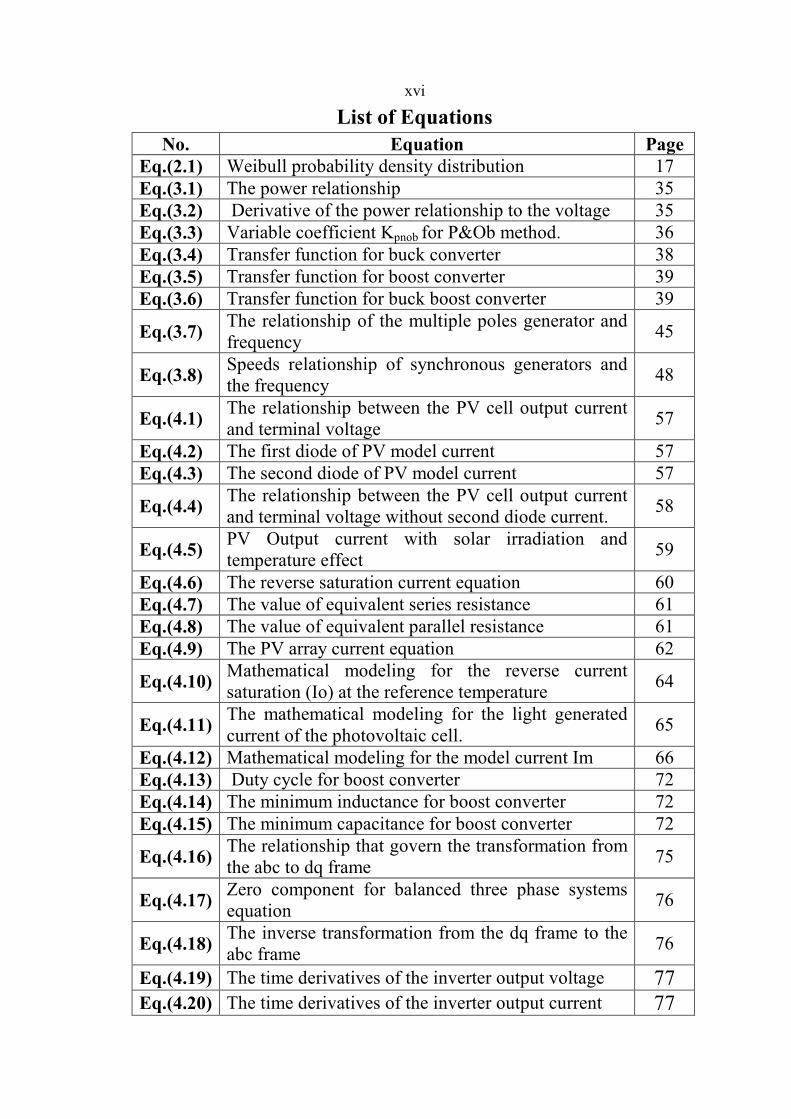
xvi
List of Equations
No. Equation Page
Eq.(2.1) Weibull probability density distribution 17 Eq.(3.1) The power relationship 35 Eq.(3.2) Derivative of the power relationship to the voltage 35 Eq.(3.3) Variable coefficient Kpnob for P&Ob method. 36 Eq.(3.4) Transfer function for buck converter 38 Eq.(3.5) Transfer function for boost converter 39 Eq.(3.6) Transfer function for buck boost converter 39
Eq.(3.7) The relationship of the multiple poles generator and frequency
45
Eq.(3.8) Speeds relationship of synchronous generators and the frequency
48
Eq.(4.1) The relationship between the PV cell output current and terminal voltage
57
Eq.(4.2) The first diode of PV model current 57 Eq.(4.3) The second diode of PV model current 57
Eq.(4.4) The relationship between the PV cell output current and terminal voltage without second diode current.
58
Eq.(4.5) PV Output current with solar irradiation and temperature effect
59
Eq.(4.6) The reverse saturation current equation 60 Eq.(4.7) The value of equivalent series resistance 61 Eq.(4.8) The value of equivalent parallel resistance 61 Eq.(4.9) The PV array current equation 62
Eq.(4.10) Mathematical modeling for the reverse current saturation (Io) at the reference temperature
64
Eq.(4.11) The mathematical modeling for the light generated current of the photovoltaic cell.
65
Eq.(4.12) Mathematical modeling for the model current Im 66 Eq.(4.13) Duty cycle for boost converter 72 Eq.(4.14) The minimum inductance for boost converter 72 Eq.(4.15) The minimum capacitance for boost converter 72
Eq.(4.16) The relationship that govern the transformation from the abc to dq frame
75
Eq.(4.17) Zero component for balanced three phase systems equation
76
Eq.(4.18) The inverse transformation from the dq frame to the abc frame
76
Eq.(4.19) The time derivatives of the inverter output voltage 77 Eq.(4.20) The time derivatives of the inverter output current 77

xvii
No. Equation Page
Eq.(4.21) Output currents and voltages of the voltage source inverter in matrix format
77
Eq.(4.22) Voltage source inverter model in the dq frame 78
Eq.(4.23) Voltage source inverter model in the dq frame inverse transformation
78
Eq.(4.24) Voltage source inverter model in the dq frame im matrix form.
79
Eq.(4.25) Voltage source inverter model in the dq frame when 0-component omitted.
79
Eq.(4.26) State equation for the capacitor voltage 79
Eq.(4.27) Control laws generate the required command voltages at the inverter output
79
Eq.(4.28) The bus capacitor voltage equation 80 Eq.(4.29) Control the real output power by controlling Id* 80
Eq.(4.30) Active and reactive powers injected from the PV system
81
Eq.(4.31)
Active and reactive powers injected from the PV system when the quadrature component forced to zero
81
Eq.(4.32) Rotation frequency ω in rad/s 83 Eq.(4.33) The amplitude modulation index, ma 83 Eq.(4.34) Frequency modulation index, mf 83
Eq.(4.35) The magnitude of the output phase voltage (rms) from inverter
85
Eq.(4.36) The mechanical power produced by the wind turbine equation
87
Eq.(4.37) Performance coefficient, CP (λ, β) equation 88 Eq.(4.38) Tip speed ratio λi equation 89
Eq.(4.39) The dynamics of the drive train on the generator side equation
90
Eq.(4.40) The dynamics of the drive train on the generator side simplified equation
90
Eq.(4.41) Electromagnetic torque equation 94 Eq.(4.42) Laplace transform for PID controller 98 Eq.(4.43) Transfer function for the speed PID controller 100 Eq.(4.44) The transfer function of the actuator 100 Eq.(4.45) The time delay block equation 100 Eq.(4.46) Mechanical power of Diesel generator. 101 Eq.(4.47) The Compensation voltage from block diagram 102 Eq.(4.48) The Compensation voltage from Simulink model 104

xviii
No. Equation Page
Eq.(4.49) The field voltage equation 105 Eq.(4.50) The terminal field voltage 105 Eq.(4.51) Voltage of Transducer output 105 Eq.(6.1) The peak power (Wp) of the PV generator 133 Eq.(6.2) The number of necessary PV modules 133 Eq.(7.1) Initial cost of grid tie PV/wind hybrid system 141
Eq.(7.2) Present worth P of an equivalent uniform annual series A
144
Eq.(7.3) Present worth P of a given future amount F 144 Eq.(7.4) The energy unit price 144

xix
List of Maps
No. Map Page Map (7.1) Location of Atouf village. 127 Map (7.2) Electrical network in Atouf village 131

xx
List of Appendices
No. Appendix Page
Appendix (A) Simulink blocks for each part of Grid Tied PV/Wind Hybrid system
161
Appendix (B) Specifications of the Grid Tie PV/Wind System elements
169
Appendix (C) Graphs to calculate K and C 177 Appendix (D) Table of interest at i = 10% 179 Appendix (E) Perturb and Observe Algorithm 180 Appendix (F) Simulation Results of Atouf Village 181

xxi
Design and Techno-Economical Analysis of a Grid Connected with PV/
Wind Hybrid System in Palestine (Atouf Village-Case study)
By Mohammad Husain Mohammad Dradi
Supervisor Dr. Imad Ibrik
Abstract
As renewable energy becomes more prevalent, more information on
how different technologies will behave needs to be available. This research
based on modeling the Grid tie PV/Wind hybrid system using Matlab
Simulink software program in order to study the techno-economic
performance analysis of building these systems according to our
environmental conditions and collecting data such as temperature, solar
radiation and wind speed.
By creating a Simulink program which predicts the power output as
a function of solar radiation, temperature and wind speed, a side-by-side
comparison of different sizes and configurations can be made. Current
predictive models are very useful for a grid tie system, which is limited to
operate at the maximum power point, thus adaptations to previous models
have been made. This model accurately predicts the power output of
different PV hybrid system based on side data specification.
The program is dynamic, and fit with the changes of parameters,
which are related to the reduced power output caused by increased
temperature, as well as the effect of non-linear absorption of solar radiation
on power output. Data was collected and analyzed as a case study for Atouf
village.

xxii
This research is important because it exposes weaknesses of different
environmental conditions of the locations, and allows for a direct
comparison of modeling different configurations of hybrid systems. This
research shows that tacking random value for determining the size of PV
system is not the best performance indicators of grid tie system.
Specifically, this research shows that the penetration factor of PV hybrid
system has a different effect on the power output of each PV array. The
size of this affect can be evaluated technically and economically by using
this software program.

1
INTRODUCTION

2
Introduction
Clean, economic and secure energy production gains importance
with the increasing of the world’s power demand. So, a new type of energy
sources has gained popularity. The sun and the wind energy are more
common alternative energy sources. Previously, they were used to supply
local loads in remote areas outside the national grid. Later, they have
become some of main sources [1], [2].
Alternative energy sources are operates in stand alone mode or grid
tie mode. It is difficult to obtain an efficient operation in stand-alone mode
and usually high capacity battery groups are required. Since the energy
produced from the wind and the solar are transferred to grid line, the way
of the transforming direct current (DC) energy to alternating current (AC)
is very important. This process has generally been achieved by a grid tie
inverter; inverter supplies the local loads and if the generated energy higher
than the demand the excess energy is export to the grid, so battery groups
are unneeded. On the other hand, control of the grid tied inverter is more
complex than the stand alone one [2].
The electric power generation system, which consists of renewable
energy sources connected to grid, has the ability to provide 24-hour
electricity to the load. This system offers a better reliability, efficiency,
flexibility of planning and environmental benefits compared to the stand-
alone system.

3
Each kilowatt-hour (kWh) generated from renewable resources saves
the environment from the burning of fossil fuels. The coal fired and the
natural gas fired power plants produce 1.05 Kg and 0.75 Kg carbon
dioxide, respectively, to generate 1kWh electricity [3].
Objectives of Work
The main objective of the present work is to design a grid tie
PV/Wind hybrid system by using Matlab Simulink program and apply this
system on Atouf village as a case study. To achieve this objective I study
the mathematical models which characterize each part of grid tie hybrid
system such as PV module, wind turbine, MPPT controller and diesel
generator, and then I convert the mathematical models to Simulink models.
After that I Investigate the design connection topologies for all components
of grid tie PV/wind hybrid system in order to study the operation of system
for different environmental conditions.
Organization of Thesis
The work carried out in this thesis has been summarized in eight
chapters
Chapter 1 studies the potential of solar energy, solar radiation and
temperature in Palestine, also describes Photovoltaic (PV) Implemented
Projects in Palestine.

4
Chapter 2 describes the potential of wind energy, wind resource, wind
distribution, wind data calculation for Ramallah and Nablus cities in
Palestine.
Chapter 3 consists of the main building constructions of grid tie PV/wind
system and basic information about PV systems, wind turbine system,
maximum power point tracker (MPPT), three-phase DC-AC inverter, DC-
DC converter, and also diesel generator.
Chapter 4 describes the mathematical modeling and Simulink for each part
of the grid tie PV/Wind hybrid system such as PV system, wind turbine and
diesel generator.
Chapter 5 describes the overall system and the simulation of it, with
different environmental conditions, and then observes operation results.
Chapter 6 introduces some information about Atouf village, potential of
solar energy, also, sizing the elements of the grid tie system for this village
and simulation results in different conditions such as solar radiation,
temperature and load.
Chapter 7 studies the economic and environmental impacts of grid tie PV
system, describes the grid tie tariffs such as net metering or feed in tariff,
evaluation the economic and environmental impacts of Atouf Grid tie PV
system.
Chapter 8 describes the main conclusions about grid tie hybrid system and
future scope of work.

5
CHAPTER ONE
POTINTIAL OF SOLAR
ENERGY IN PALESTINE

6
Chapter One
Potential of Solar Energy in Palestine
Introduction
Palestine is located between 34º:20´ - 35:30´ E and 31º: 10´ - 32º:30´
N, it consists of two separated areas from one another. The Gaza Strip is
located on the western side of Palestine adjacent to the Mediterranean Sea
and the West-Bank which extends from the Jordan River to the center of
Palestine [4].
Palestine's elevation ranges from 350m below sea level in Jordan
Valley, to sea level along the Gaza Strip sea shore and exceeding 1000m
above sea level in some mountains areas in the West Bank [4].
Climate conditions in Palestine vary widely. The coastal climate in
the Gaza Strip is humid and hot during summer and mild during winter.
These areas have low heating loads, while cooling is required during
summer. The daily average temperature and relative humidity range
between: (13.3 – 35.4) C° and (67 – 75) % respectively [13].
In the hilly areas of the West-Bank, cold winter conditions and mild
summer weather are prevalent. Daily average temperature and relative
humidity vary in ranges: (8 – 23) Cº and (51 – 83) % respectively [13]. In
some areas, the temperature decline below 0 ºC. Hence, high heating loads
are required, while little cooling is needed during summer.
Solar radiation and temperature affect on electric solar energy
production, so we should have to study these elements for Palestine.

7
1.1 Solar Radiation in Palestine
Since the area of Palestine is relatively small and the solar radiation
(W/m²) doesn't change significantly within such short distance (31° 10´ -
32° 30´ N), the measuring data for all regions (West-Bank & Gaza Strip)
may considered to be the same. Table (1.1) shows the measurement of the
global radiation on a horizontal surface in the Tubas District [13].
Table (1.1): Hourly average solar radiation of typical summer day
(11/6/2011) [13]
Hours Solar Radiation
(w/m²) Hours
Solar Radiation
(w/m²) 1:00 0 13:00 990 2:00 0 14:00 917 3:00 0 15:00 780 4:00 0 16:00 585 5:00 30 17:00 375 6:00 140 18:00 154 7:00 343 19:00 20 8:00 532 20:00 0 9:00 747 21:00 0
10:00 910 22:00 0 11:00 1019 23:00 0 12:00 1062 24:00 0
These measurements are obtained from the Energy Research Center
(ERC).
They have been done by horizontally oriented measuring devices,
and done on a 5-minute interval basis.
Figure (1.1) shows the daily irradiation-curve plotted from data of
table (1.1).

8
Figure (1.1): The global irradiation (W/m²) versus time (hours)-2011.
From table(1.1) & figure(1.1), it is obvious that the solar radiation is
more than 900 W/m² during the hours : 10, 11, 12, 13, and 14 pm and it is
also more than 135 W/m² in the morning hours 6, 7, 8, and 9 am, and in the
evening hours 15, 16, 17, and 18 pm. This means that we have enough
potential for solar radiation and we can obtain electric energy even in the
morning or evening.
1.2 Ambient Temperature in Palestine
As we mentioned before, temperature affects the PV generators
efficiency. The relation between temperature and efficiency is inversed.
The ambient temperature is the main factor that affects the PV generator's
temperature. Table (1.2) shows, for an example, the ambient temperature of
the target area.
The shown data is the average of two days measurement in June
2011. The original measurements are done on a 5-minute interval basis
[13].
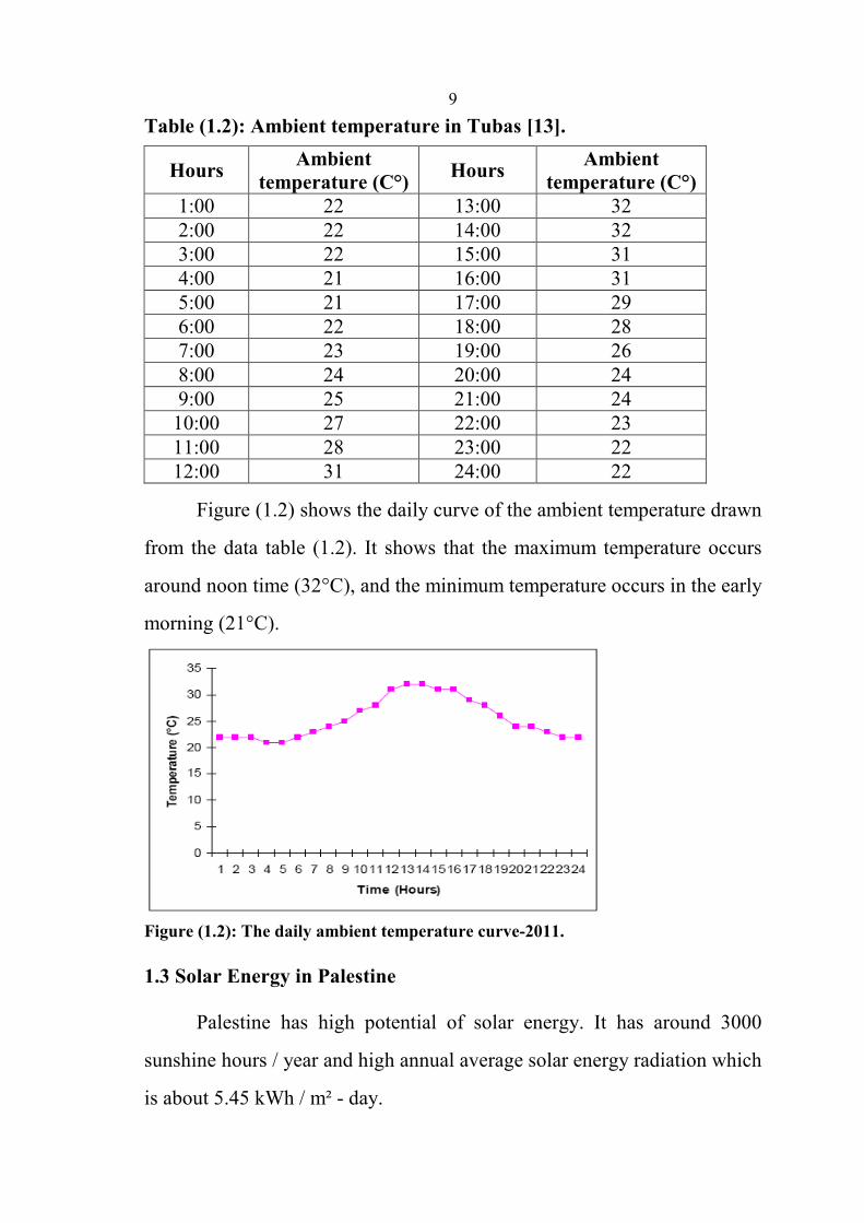
9
Table (1.2): Ambient temperature in Tubas [13].
Hours Ambient
temperature (C°) Hours
Ambient
temperature (C°)
1:00 22 13:00 32 2:00 22 14:00 32 3:00 22 15:00 31 4:00 21 16:00 31 5:00 21 17:00 29 6:00 22 18:00 28 7:00 23 19:00 26 8:00 24 20:00 24 9:00 25 21:00 24
10:00 27 22:00 23 11:00 28 23:00 22 12:00 31 24:00 22
Figure (1.2) shows the daily curve of the ambient temperature drawn
from the data table (1.2). It shows that the maximum temperature occurs
around noon time (32°C), and the minimum temperature occurs in the early
morning (21°C).
Figure (1.2): The daily ambient temperature curve-2011.
1.3 Solar Energy in Palestine
Palestine has high potential of solar energy. It has around 3000
sunshine hours / year and high annual average solar energy radiation which
is about 5.45 kWh / m² - day.
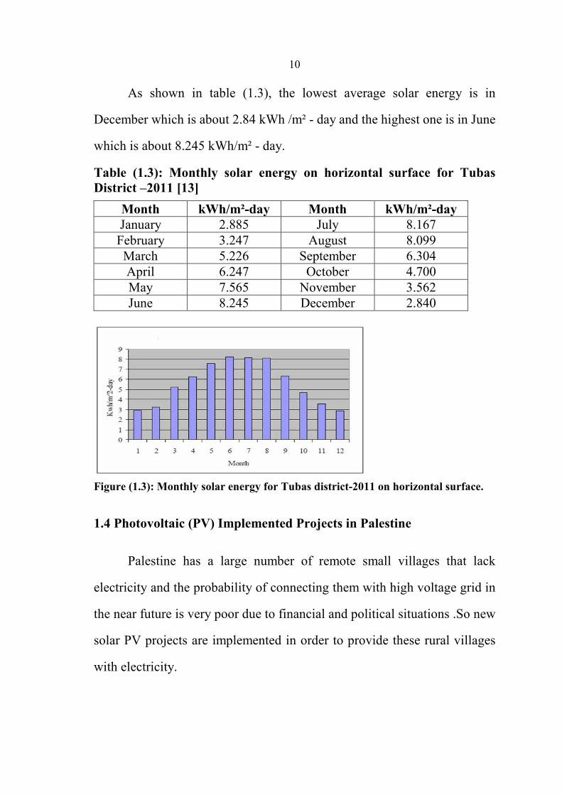
10
As shown in table (1.3), the lowest average solar energy is in
December which is about 2.84 kWh /m² - day and the highest one is in June
which is about 8.245 kWh/m² - day.
Table (1.3): Monthly solar energy on horizontal surface for Tubas
District –2011 [13]
Month kWh/m²-day Month kWh/m²-day January 2.885 July 8.167 February 3.247 August 8.099 March 5.226 September 6.304 April 6.247 October 4.700 May 7.565 November 3.562 June 8.245 December 2.840
Figure (1.3): Monthly solar energy for Tubas district-2011 on horizontal surface.
1.4 Photovoltaic (PV) Implemented Projects in Palestine
Palestine has a large number of remote small villages that lack
electricity and the probability of connecting them with high voltage grid in
the near future is very poor due to financial and political situations .So new
solar PV projects are implemented in order to provide these rural villages
with electricity.

11
A) Imnazel Photovoltaic (PV) Project:
Imnazel village is located south of Yatta in the Hebron District near
the Separation Wall, where a population is about 400 people, and there are
about 40 houses, a school and a mosque. The village was connected to
electricity, for the first time, through 13kW central system of solar cells as
shown in figure (1.4), and has been linked with a generator to help recharge
the batteries in case there is lack of energy [13].
Figure (1.4): Imnazel photovoltaic (PV) project [13].
B) Atouf Photovoltaic (PV) Project
Atouf village is located in north of West Bank, where the population
is about 200 people, and there are about 21 houses, a school and a mosque.
The village was connected to electricity, for the first time, through 12kW
central system of solar cells, and has been linked with a generator to help
recharge the batteries in case there is lack of energy. I will speak in details
about this village in chapter six.

12
Also there are new under construction projects using photovoltaic
PV system to feed other small villages and communities far from the
electricity grid such as Mkehel village and khirbit Alsaaed near Yabbad in
Jenin District [13].
In this chapter, I studied the potential of solar energy in Palestine and
the two main elements, solar radiation and temperature, which affecting
this energy.

13
CHAPTER TWO
POTINTIAL OF WIND
ENERGY IN PALESTINE

14
Chapter Two
Potential of Wind Energy in Palestine
Introduction
Wind energy has been used for thousands of years for milling grains,
pumping water and other mechanical power applications. But the use of
wind energy as an electrical supply with free pollution what makes it
attractive and takes more interest and used on a significant scale.
Attempts to generate electricity from wind energy have been made
since the end of nineteenth century. Small wind machines for charging
batteries have been manufactured since the 1930s. Wind now is one of the
most cost effective methods of electricity generation available in spite of
the relatively low current cost of fossil fuels.
The wind technology is continuously being improved both cheaper
and more reliable, so it can be expected that wind energy will become even
more economically competitive over the coming decades [12].
2.1 The Wind Resource
The main consideration for implementing a wind project in a certain
site is the wind resource. Other considerations include site accessibility,
terrain, land use and proximity to transmission grid for grid-connected
wind farms.
The main sources of the global wind movements are the earth
rotation, regional and seasonal variations of sun irradiance and heating.

15
Local effects on wind include differential heating of the land and the sea
(land heats up faster), topographical nature such as mountains and valleys,
existence of trees and artificial obstacle such as buildings.
At any location, wind is described by its speed and direction. The
speed of the wind is measured by anemometer in which the angular speed
of rotation is translated into a corresponding linear wind speed (in meters
per second or miles per hour). A Standard anemometer averages wind
speed every 10 minutes. Wind direction is determined by weather vane [6].
Average (mean) wind speed is the key in determining the wind
energy potential in a particular site. Although long-term (over 10 years)
speed averages are the most reliable data for wind recourse assessment, this
type of data is not available for all locations. Therefore, another technique
based on measurement, correlation and perdition is used. Wind speed
measurements are recorded for a 1-year period and then compared to a
nearby site with available long-term data to forecast wind speed for the
location under study [6].
2.2 Wind Speed Distribution
Average value for wind speed for a given location does not alone
indicate the amount of energy which wind turbine could produce there. To
assess the climatology of wind speeds at a particular location, a probability
distribution function is often fit to the observed data. Different locations
will have different wind speed distributions. The distribution model which

16
most frequently used to model wind speed climatology is a two-parameter
Weibull distribution because it is able to confirm a wide variety of
distribution shapes, from Gaussian to exponential.
Weibull Distribution
The measured wind speed variation for a typical site throughout a
year indicates that the strong gale force winds are rare, while moderate and
fresh winds are quite common, and this is applicable for most areas. Figure
(2.1) shows the Weibull distribution describing the wind variation for a
typical site.
Figure (2.1): Weibull probability density distribution [12].
The area under the curve is always exactly 1, since the probability
that the wind will be blowing at some wind speeds including zero must be
100 percent. The distribution of wind speeds is skewed; it is not
symmetrical.
Sometimes there are very high wind speeds, but they are very rare.
The statistical distribution of wind speeds varies from place to another
around the globe depending upon local climate conditions, the landscape,

17
and its surface. The Weibull distribution may thus vary, both in its shape,
and in its mean value. The Weibull probability density distribution function
is given by:
Where
K: is the Weibull shape factor; it gives an indication about the variation of
hourly average wind speed about the annual average,
C: is the Weibull scale factor [12].
Each site has its own K and C. Both can be found if the average wind
speed V and the available power in wind (flux) are calculated using the
measured wind speed values. Graph shown in figure C.1 in appendix C
gives a relation between the Weibull scale parameter C and average wind
speed V as a function of shape parameter K, and Graph shown in figure C.2
in appendix C gives a relation between Weibull scale parameter C and the
available power in wind (flux) as a function of shape parameter K.
Using these two graphs, beginning from K=2, and manipulating the
number of iterations until certain tolerance is achieved, the values of both
K and C can be found [12].
The second wind speed distribution is the Rayleigh distribution,
which is a specific form of the Weibull function in which the shape

18
parameter equals 2 and very closely mirrors the actual distribution of
hourly wind speeds at many locations.
2.3 Evaluation of Wind Data in Different Cities in the West Bank
(Ramallah and Nablus Cities).
Different wind measurements were carried out for each month
through the year 2006. The wind data obtained includes hourly average
wind speeds for each hour in the month. Calculations were performed
on these data for each month to obtain the duration in hours for each 1 m/s
speed range selected. The total wind speed range was divided into 1 m/s
speed ranges taking the ranges: 0-1, 1-2, 2-3, 3-4, and so on [12].
Table (2.1) shows in detail average wind speed, values for
percentage of occurrence for each wind speed range , power available in
the wind for each range per unit area using equation (4.14) , power density
by multiplying percentage of occurrence with power available in wind for
each range, Weibull values using equation (2.1), energy available in wind
by multiplying power density for each range with Weibull value, and
finally energy available in wind by multiplying power density for each
range with occurrence percentage for this range [12].

19
Table (2.1): Yearly wind calculations/Ramallah-2006 [12]
Speed
range
(m/s)
Mid
range
(m/s)
Duration
(hours) Occurrence
percentage
(%)
Power
(W/m²) Power
density
(W/m²)
Weibull
values Energy (kWh/m
using
Weibull
Energy (kWh/ m²)
using data
0-1 0.5 82 0.936 0.08 0.001 0.03601 0.02 0.01 1-2 1.5 589 6.724 2.04 0.137 0.08230 1.47 1.20 2-3 2.5 1058 12.078 9.45 1.142 0.11133 9.22 10.00 3-4 3.5 1209 13.801 25.94 3.580 0.12520 28.45 31.36 4-5 4.5 1242 14.178 55.13 7.816 0.12616 60.93 68.47 5-6 5.5 1240 14.155 100.66 14.248 0.11736 103.48 124.81 6-7 6.5 961 10.970 166.15 18.227 0.10235 148.96 159.67 7-8 7.5 728 8.311 255.23 21.211 0.08443 188.76 185.81 8-9 8.5 563 6.427 371.55 23.879 0.06626 215.66 209.18 9-10 9.5 390 4.452 518.71 23.093 0.04968 225.75 202.30
10-11 10.5 218 2.489 700.36 17.429 0.03569 218.98 152.68 11-12 11.5 159 1.815 920.13 16.701 0.02463 198.50 146.30 12-13 12.5 103 1.176 1181.64 13.894 0.01635 169.22 121.71 13-14 13.5 60 0.685 1488.53 10.195 0.01046 136.34 89.31 14-15 14.5 56 0.639 1844.42 11.791 0.00645 104.24 103.29 15-16 15.5 28 0.320 2252.94 7.201 0.00384 75.86 63.08 16-17 16.5 15 0.171 2717.74 4.654 0.00221 52.70 40.77 17-18 17.5 14 0.160 3242.42 5.182 0.00123 35.02 45.39 18-19 18.5 10 0.114 3830.63 4.373 0.00066 22.30 38.31 19-20 19.5 9 0.103 4486.00 4.609 0.00035 13.64 40.37 20-21 20.5 4 0.046 5212.15 2.380 0.00018 8.02 20.85 21-22 21.5 7 0.080 6012.72 4.805 0.00009 4.54 42.09 22-23 22.5 7 0.080 6891.33 5.507 0.00004 2.47 48.24 23-24 23.5 8 0.091 7851.61 7.170 0.00002 1.30 62.81
Sum 8760 100% 229.225 1.00328 2025.85 2008.01
Yearly average wind speed V= 5.521 m/s
Weibull shape factor K = 1.81 (calculated using special graphs in appendix C )
Weibull scale factor C = 6.35 m/s (calculated using special graphs in appendix C)
Density of air ρ = 1.21 kg/m³
Figure (2.2) shows a graphical representation of the distribution of
hourly duration for different ranges of wind speed.

20
Figure (2.2): Number of hours per year for each wind speed range/Ramallah-2006
Figure ( 2.3) shows the distribution of energy and Weibull
distribution for the wind measurements.
Figure (2.3): Yearly energy and Weibull distributions/Ramallah site-2006
Figure (2.4) shows the wind duration curve for Al-Mazra'a
Al-Sharqiyyah site. It is a cumulative frequency diagram. Its horizontal

21
axis represents the cumulative time duration in hours as wind speed group
decreases starting at the highest wind speed group. It can be used to
calculate graphically t h e energy produced by a certain wind turbine if its
power curve is known [12].
Figure (2.4): Wind duration curve for Ramallah site-2006
Table (2.2) shows percentage of occurrence for each wind speed
range, power available in wind for each range per unit area, power density,
Weibull values, energy available in wind using Weibull values, and finally
energy available in wind using wind data available.

22
Table (2.2): Yearly wind calculations/Nablus-2006 [12].
Speed
range
(m/s)
Mid
range
(m/s)
Duration
(hours)
Occurrence
percentage
(%)
Power
(W/m²)
Power
density
(W/m²)
Weibull
values
Energy
(kWh/
m²)
(using
Weibul)
Energy
(kWh/ m²)
(using
data)
0-1 0.5 733.68 8.375 0.08 0.006 0.05334 0.03 0.06 1-2 1.5 376.64 4.300 2.04 0.088 0.12065 2.08 0.77 2-3 2.5 1105.78 12.623 9.45 1.193 0.15541 12.90 10.45 3-4 3.5 1786.15 20.390 25.94 5.289 0.16174 37.70 46.33 4-5 4.5 1802.06 20.572 55.13 11.341 0.14702 73.62 99.35 5-6 5.5 1285.92 14.679 100.66 14.776 0.12044 110.12 129.44 6-7 6.5 788.24 8.998 166.15 14.950 0.09039 135.01 130.97 7-8 7.5 440.14 5.024 255.23 12.824 0.06274 141.05 112.34 8-9 8.5 205.65 2.348 371.55 8.723 0.04054 128.66 76.41
9-10 9.5 101.65 1.160 518.71 6.019 0.02450 104.17 52.73 10-11 10.5 55.81 0.637 700.36 4.462 0.01389 75.74 39.09 11-12 11.5 25.93 0.296 920.13 2.724 0.00741 49.87 23.86 12-13 12.5 9.67 0.110 1181.64 1.304 0.00372 29.94 11.42 13-14 13.5 5.17 0.059 1488.53 0.878 0.00177 16.47 7.69 14-15 14.5 2.83 0.032 1844.42 0.597 0.00079 8.33 5.23 15-16 15.5 8.17 0.093 2252.94 2.100 0.00034 3.89 18.40 16-17 16.5 3.83 0.044 2717.74 1.189 0.00014 1.68 10.42 17-18 17.5 0.83 0.010 3242.42 0.308 0.00005 0.67 2.70 18-19 18.5 0.67 0.008 3830.63 0.292 0.00002 0.25 2.55 19-20 19.5 0.50 0.006 4486.00 0.256 0.00001 0.09 2.24 20-21 20.5 1.00 0.011 5212.15 0.595 0.00000 0.03 5.21 21-22 21.5 7.83 0.089 6012.72 5.377 0.00000 0.01 47.10 22-23 22.5 0.67 0.008 6891.33 0.524 0.00000 0.00 4.59 23-24 23.5 11.17 0.127 7851.61 10.009 0.00000 0.00 87.68
Sum 8760 100.00 105.824 1.00490 932.33 927.02
Yearly average wind speed V= 4.346 m/s Weibull shape factor K = 1.9(calculated using special graphs in appendix C )
Weibull scale factor C = 6 m/s(calculated using special graphs in appendix C)
Density of air ρ= 1.21 kg/m³
Figures (2.5), (2.6) show yearly energy, Weibull values and yearly
wind duration curve for Nablus site respectively.
Figure (2.5): Yearly energy and Weibull distributions for Nablus site.

23
Figure (2.6): Wind duration curve for Nablus site.
In this chapter, I studied the potential of wind energy in Palestine. In
the next chapter I will study and analyze the components of grid tie
PV/Wind hybrid system.

24
CHAPTER THREE
COMPONENTS OF GRID TIE
PV/WIND HYBRID SYSTEM
25
Chapter Three
Components of Grid Tie PV/ Wind Hybrid System
3.1 Grid Tie System configurations
The aim of this chapter is to present an overview of the main
building blocks in a grid tied PV/wind system. These systems can be
classified in terms of their connection to the power system grid into the
following:
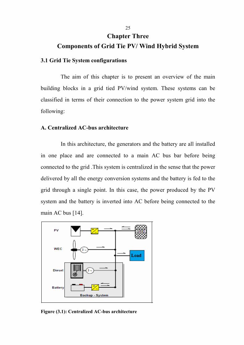
A. Centralized AC-bus architecture
In this architecture, the generators and the battery are all installed
in one place and are connected to a main AC bus bar before being
connected to the grid .This system is centralized in the sense that the power
delivered by all the energy conversion systems and the battery is fed to the
grid through a single point. In this case, the power produced by the PV
system and the battery is inverted into AC before being connected to the
main AC bus [14].
Figure (3.1): Centralized AC-bus architecture

26
B. Centralized DC-bus architecture
The second architecture utilizes a main centralized DC bus bar as
in figure (3.2). The wind turbine and the diesel generator, firstly deliver
their power to rectifiers to be converted into DC before it is being delivered
to the main DC bus bar. A main inverter takes the responsibility of feeding
the AC grid from this main DC bus [14].
Figure (3.2): Centralized DC-bus architecture
C. Distributed AC-bus architecture
The power sources in this architecture do not need to be installed
close to each other as in figure (3.3), and they do not need to be connected
to one main bus bar. Otherwise, the sources are distributed in different
geographical locations as appropriate and each source is connected to the
grid separately. The power produced by each source is conditioned
separately to be identical with the form required by the grid. The main
disadvantage of this architecture is the difficulty of controlling the system
[14].

27
Figure (3.3): Distributed AC-bus architecture
D. Modified Distributed Ac Bus Architecture
The following architecture is the one upon which the submitted
thesis is based. It is an improved version of the distributed AC-bus
architecture shown in figure (3.3).The improvement exists mainly in the
addition of a DC/DC converter for each energy conversion system and the
remove of storage battery. By this addition of the DC/DC converters, the
state values of the energy conversion sources become completely
decoupled from each other and from the state values of the grid the power
production of the different sources becomes now freely controllable
without affecting the state values of the grid.
Decoupling the state values means that the variations of the
renewable resources like the velocity of the wind and the intensity of the
solar radiation will not influence the state values of the electrical grid.

28
The main disadvantage of this architecture is the difficulty of
controlling the system, but this problem is not effective since the
improvement of wireless communications.
Figure (3.4): The modified distributed Ac bus architecture.
3.2 Photovoltaic PV Technology
The physics of the PV cell is very similar to that of the classical
diode with a pn junction. When the junction absorbs light, the energy of
absorbed photons is transferred to the electron–proton system of the
material, creating charge carriers that are separated at the junction. The
charge carriers in the junction region create a potential gradient, get
accelerated under the electric field, and circulate as current through an
external circuit [15].

29
The PV cell is the elementary unit, the interconnection of the number
of PV cell forms the module and similarly PV array is formed from number
of module as shown in Figure (3.5).
Figure (3.5): Transition of cell, module and arrays.
The main industrialized PV technologies are shown in figure (3.6).
Figure (3.6): The main industrialized PV technologies
a) Mono-crystalline PV b) Poly-crystalline PV c) Amorphous PV
3.2.1 Mono Crystalline Silicon PV cells
Comprising 20% of the earth’s crust composition, Silicon is
considered the second most abundant element on earth. it exists in nature in
the form of silicon dioxide minerals like quartz and silicate based minerals.

30
It has first to reach a high degree of purity before it can be used for
manufacturing single crystal PV cells.
High grade quartz or silicates are first treated chemically to form an
intermediate silicon compound (Liquid trichlorosilane SiHCl3), which is
then reduced in a reaction with hydrogen to produce chunks of highly pure
Silicon, about 99.9999% in purity. After that, these chunks of silicon are
melted and formed into a single large crystal of Silicon through a process
called the Czochralski process. The large Silicon crystal is then cut into
thin wafers using special cutting equipment. These wafers are then polished
and doped with impurities to form the required p-n junction of the PV cell.
Antireflective coating materials are added on top of the cell to reduce
light reflections and allow the cell to better absorb sunlight. A grid of
contacts made of silver or aluminum is added to the cell to extract the
electric current generated when it is exposed to light. PV modules’
efficiency is in the range of 12%-15% .The process of producing PV cells
using this technology is quite expensive, so this led to development of new
technologies that do not suffer from this drawback [16].
3.2.2 Multi-crystalline Silicon PV cells
In order to avoid the high cost of producing single crystal solar
cells, cheaper multi-crystalline cells were developed. As the name implies,
multi-crystalline Silicon solar cells do not have a single crystal structure.
They are rather derived from several smaller crystals that together form the

31
cell. The grain boundaries between each crystal reduce the net electric
current that can be generated because of electron recombination with
defective atomic bonds. However, the cost of manufacturing cells using
this technology is less than what would be in the case of a single crystalline
cell. The efficiency of modules produced using this technology ranges from
11%-14% [16].
3.2.3 Thin Film PV technologies
Thin film PV cells are manufactured through the deposition of
several thin layers of atoms or molecules of certain materials on a holding
surface. They have the advantage over their crystalline Silicon counter
parts in their thickness and weight. They can be 1 to 10 micrometers thin as
compared to 300 micrometers for Silicon cells. Another advantage is that
they can be manufactured using an automated large area process that
further reduces their cost. Thin film PV cells do not employ the metal grid
required for carrying current outside the cell. However, they make use of a
thin layer of conducting oxides to carry the output current to the external
circuit.
The electric field in the p-n junction of the cell is created between the
surface contacts of two different materials, creating what is called a hetero
junction PV cell. Thin film PV can be integrated on windows and facades
of buildings because they generate electricity while allowing some light to
pass through. Two common thin film materials are Copper indium
diselenide (CIS for short) and Cadmium Telluride (CdTe). CIS thin films

32
are characterized by their very high absorption. PV cells that are built from
this material are of the hetero junction type. The top layer can be cadmium
sulfide, while the bottom layer can be gallium to improve the efficiency of
the device. Efficiency for these technologies is about 10-13% [16].
3.3 Maximum Power Point Tracking
When a PV module is directly coupled to a load, the PV module’s
operating point will be at the intersection of its I–V curve and the load line
which is the I-V relationship of load. For example in figure (3.7), a
resistive load has a straight line with a slope of 1/RL as shown in figure
(4.8). In other words, the impedance of load dictates the operating
condition of the PV module. In general, this operating point is seldom at
the PV module’s MPP. Thus it is not producing the maximum power.
A study shows that a direct-coupled system utilizes a more 31% of
the PV capacity. A PV array is usually oversized to compensate for a low
power yield during winter months.
This mismatching between a PV module and a load requires further
over-sizing of the PV array and thus increases the overall system cost. To
mitigate this problem, a maximum power point tracker (MPPT) can be used
to maintain the PV module’s operating point at the MPP. MPPTs can
extract more than 97% of the PV power when properly optimized [17].

33
Figure (3.7): PV module is directly connected to a (variable) resistive load.
Figure (3.8): I-V curves of BP SX 150S PV module and various resistive loads
Simulated with the MATLAB model (1kW/m2, 25oC)
3.3.1 Maximum Power Point Tracking (MPPT) Techniques
MPPT techniques are used to control DC converters in order to
extract maximum output power from a PV array under a given weather
condition. The DC converter is continuously controlled to operate the array
at its maximum power point despite possible changes in the load
impedance. Several techniques have been proposed to perform this task
[18].
- Constant Voltage (CV) Method

34
- Open Voltage (OV) Method
- Incremental Conductance (IC) Methods
- Perturb and Observe (P&Oa and P&Ob) Methods
- Three Point Weight Comparison
- Fuzzy Logic Method
- Sliding Mode Method
- Artificial neural network Method
Constant Voltage (CV) Method
The principle of the Constant Voltage (CV) Method is simple: the
PV is supplied using a constant voltage, Temperature and Solar Irradiance
impacts are neglected, The reference voltage is obtained from the MPP of
the P(i) characteristic directly. Figure (3.9) shows the CV algorithm and the
code of the Matlab embedded function [18].
Figure (3.9): CV algorithm and the code of Matlab embedded function [18].

35
This Constant Voltage Method cannot be very effective, regarding
Solar Irradiance impact and certainly not regarding the temperature’s
influence.
The Open Voltage (OV) Method is based on the CV method, but it
makes the assumption that the MPP voltage is always around 75% of the
open-circuit voltage VOC. So mainly, this technique takes into account the
temperature. But it requests a special procedure to regularly disconnect the
PV and to measure the open-circuit voltage [18].
B) Incremental Conductance (IC) Methods
The principle of the Incremental Conductance (IC) Method is based
on the property of the MPP: the derivative of the power is null as in
equation (3.1). So, the IC method uses an iterative algorithm based on the
evolution of the derivative of conductance G, as in equation (3.2). Where
the conductance is the I / V ratio.
This method (ICa) has been improved, because when the voltage is
constant, dG is not defined. So, a solution is to mix the CV method with the
IC method. It is known as the Two- Method MPPT Control (or ICb). Figure
(3.10) shows the Two-Method MPPT Control algorithm and the code of the
Matlab embedded function [18]:

36
Figure (3.10): Two-Method MPPT algorithm and the code of Matlab function [18].
C) Perturb and Observe (P&O) Methods
The principle is based on perturbing the voltage and the current of
the PV regularly and then, in comparing the new power measure with the
previous to decide the next variation. Two Perturb and Observe (P&O)
Methods are well known [18]:
1- P&Oa with a fixed perturbing value.
2- P&Ob with a variable perturbing value.
The P&Ob method is similar to the P&Oa except for the constant
coefficient Kpnoa which is replaced by a variable coefficient Kpnob:
Figure (3.11) shows the P&Oa algorithm and the code of the Matlab
embedded function.

37
Figure (3.11): P&Oa algorithm and the code of Matlab embedded function [18].
3.4 Switched Mode DC-DC Converters
DC/DC converters are used in a wide variety of applications
including power supplies, where the output voltage should be regulated at a
constant value from a fluctuating power source or achieve multiple voltage
levels from the same input voltage. Several topologies exist to either
increase or decrease the input voltage or perform both functions together
using a single circuit [16].
3.4.1 Buck Converter
The schematic diagram of a buck DC converter is shown in figure
(3.12). It is composed with DC chopper and an output LC filter to reduce
the ripples in the resulting output. The output voltage of the converter is
less than the input as determined by the duration the semiconductor switch

38
Q is closed. Under continuous conduction mode (CCM), the current IL
passing through the inductor does not reach zero. The time integral of the
inductor voltage over one period in steady state equals zero. From that, the
relation between the input and output voltages can be obtained [16].
Figure (3.12): Buck converter
3.4.2 Boost Converter
The boost DC converter is used to step up the input voltage by
storing energy in an inductor for a certain time period, and then uses this
energy to boost the input voltage to a higher value.
The circuit diagram for a boost converter is shown in figure (3.13).
When switch Q is closed, the input source charges up the inductor while
diode D is reverse biased to provide isolation between the input and the
output of the converter. When the switch is opened, energy stored in the
inductor and the power supply is transferred to the load. The relationship
between the input and output voltages is given by [16]:

39
Figure (3.13): Boost converter
3.4.3 Buck-Boost Converter
This converter topology can be used to perform both functions of
stepping the input voltage up or down, but the polarity of the output voltage
is opposite to that of the input as in figure (3.14).
The input and output voltages of this configuration are related
through [16].
Figure (3.14): Buck Boost converter

40
3.5 Wind Turbine Technology
Wind turbines operate in an unconstrained air fluid. The force is
transferred from air fluid to the blades of the wind turbine. It can be
considered to be equivalent to two component forces acting in two
perpendicular directions, known as the drag force and the lift force. The
magnitude of these drag and lift forces depends on the shape of the blade,
its orientation to the direction of air, and the velocity of air [12].
The drag force is the component that is in line with the direction of
air. The lift force is the component that is at right angles to the direction of
the air. These forces are shown in figure (3.15).
Figure (3.15): Lift and drag force components [12].
A low pressure region is created on the downstream side of the
blade as a result of an increase in the air velocity on that side. In this
situation, there is a direct relationship between air speed and pressure: the
faster the airflow, the lower the pressure. The lift force acts as a pulling
force on the blade, in a direction at right angles to the airflow.

41
Wind turbines can be categorized according to the axis of rotation:
vertical and horizontal axis. The vertical wind turbines are suitable for low
power applications. The power efficiency is limited to 25%. The advantage
of the vertical wind turbines is that the generator and transformer can be
placed on the ground near the rotor blades. This results in low installation
and maintenance cost [9].
A more popular type of wind turbines shown in figure (3.16) is the
horizontal wind turbines. It can be built with two or three blades [9].
Figure (3.16): Horizontal wind turbine.
Each wind turbine has its own characteristic known as wind speed
power curve. The shape of this curve is influenced by the blades area,
the choice of airfoil, the number of blades, the blade shape, the optimum
tip speed ratio, the speed of rotation, the cut-in wind speed, the
shutdown speed, the rated speed, and gearing and generator efficiencies.
The power output of a wind turbine varies with wind speed and wind

42
turbine power curve. An example of such curve is shown in figure (3.17)
[12].
Figure (3.17): Typical wind turbine power curve [12].
3.5.1 Types of Wind Turbine Grid Tie Connections
In the context of the grid interconnection, it is inevitable to learn
about the wind generators. Each type of the generators requires different
power electronic grid interconnection.
Induction generator is widely used in the wind industry. There are
two types of the induction generators. The squirrel-cage induction
generator can be directly connected to the utility grid or connected with a
full-rated power electronic interface at a variable speed [9].
The system with a fixed speed is inexpensive due to its simplicity
and low maintenance requirements. Nonetheless, the direct connection of
the wind turbines and the utility grid causes mechanical stress problems
and high inrush current during start up. This problem can be solved by a
soft-starter mechanism.

43
A soft starter is comprised of thyristors, a power electronic
semiconductor device, limiting the maximum inrush current. After start up,
the thyristors are bypassed to avoid thermal breakdown, as shown in figure
(3.18) [9].
Figure (3.18): Soft starter
Additionally, the induction generator requires reactive power from
the utility grid that causes unacceptable conditions such as the voltage drop
or low power factor. The compensated reactive power can be supplied from
a switched capacitor bank or a power converter. For the fixed speed or
direct connection induction generators, the switched capacitor banks can
supply the reactive power as shown in figure 3.19.a).
For the variable speed squirrel-cage induction generator, the power
converter, therefore, must be able to provide reactive power to the
generators.
Figure (3.19 a): Squirrel-cage induction generator with direct connection to the
grid
44
For the direct connection, the induction generator has to operate at
the synchronous frequency of the grid. Thus, there must be a gearbox to
increase the low speed shaft of the rotor blades to the speed of the grid.
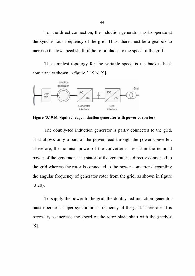
The simplest topology for the variable speed is the back-to-back
converter as shown in figure 3.19 b) [9].
Figure (3.19 b): Squirrel-cage induction generator with power converters
The doubly-fed induction generator is partly connected to the grid.
That allows only a part of the power feed through the power converter.
Therefore, the nominal power of the converter is less than the nominal
power of the generator. The stator of the generator is directly connected to
the grid whereas the rotor is connected to the power converter decoupling
the angular frequency of generator rotor from the grid, as shown in figure
(3.20).
To supply the power to the grid, the doubly-fed induction generator
must operate at super-synchronous frequency of the grid. Therefore, it is
necessary to increase the speed of the rotor blade shaft with the gearbox
[9].

45
Figure (3.20): Doubly-fed induction generator
Another type of the generators utilized in a wind farm is a
synchronous generator. The rotor winding of the synchronous generator
can be excited by an external field exciter, which requires the field current
supplied from the grid with an AC-DC converter as shown in figure (3.21).
The stator winding is connected to the full-rated power converters
supporting the variable speed concept. A multi-pole synchronous generator
can eliminate the gear box as mentioned previously. This results in a
simpler system and reduction in maintenance cost. The relationship of the
multiple poles and frequency can be expressed as
Where
P: is number of poles
Figure (3.21): Synchronous generator with a field exciter

46
The synchronous generator can be also excited by an internal
permanent magnet, as shown in figure (3.22). The gearless multi-pole
permanent magnet synchronous generator is attractive because it is light
and requires low maintenance cost. It also reduces the cost of transportation
and installation. Furthermore, it is considerably efficient compared to the
other types of generators [9].
Figure (3.22): Permanent magnet synchronous generator.
3.5.2 Control Types of Wind Turbine
A wind turbine has control system that regulates the speed of rotor
blades. The anemometer measures the wind speed and transmits the data to
the controller. The pitch angle of the rotor blades is controlled by the
controller to attain the maximum wind power and to limit the mechanical
power in case of the strong wind. The rotor blades are pitched to decrease
the angle of attack from the wind when the rated power is reached. The
yaw drive can turn the wind turbine compartment or so called nacelle
according to the direction of the wind measured by the wind vane [9].
In addition to the pitch control, the maximum power from the wind
can be limited by passive stall control for small and medium-size wind

47
turbines. The stall control avoids the rotation of the blades. Contrary to the
pitch-angle control, passive stall control has fixed pitch-angle rotor blades.
The passive stall control relates to the design of the rotor blades that
leads to turbulence or so called stall on the back of the blades to reduce the
power extracted from the wind.
As the capacity of wind turbines is increasing, active stall control is
used for large wind turbines, more than 1MW. The active stall control is
similar to the pitch-angle control. The rotor blades are rotated to obtain the
maximum power extract. When the extracted power reaches the rated
power, opposite to the pitch-angle control, the active stall control turns the
rotor blades to increase the angle of attack from the wind to provoke the
turbulence [9].
3.6 Diesel generator
A diesel generator is the combination of a diesel engine with an
electrical generator (often called an alternator) to generate electrical energy
and used in places without connection to the power grid, as emergency
power-supply if the grid fails [19].

48
Figure (3.23): Diesel generator
3.6.1 Diesel generator set
The packaged combination of a diesel engine, a generator and
various ancillary devices (such as base, canopy, sound attenuation, control
systems, circuit breakers, jacket water heaters and starting system) is
referred to as a "generating set" or a "genset" for short [19].
3.6.2 Operating Characteristics of Diesel generator
A) Rotation speed
The Corresponding speeds of 50 Hz generators are 3000 rpm and
1500 rpm synchronous generators obtained from the equation (3.8).
Where
n: speed (rpm)

49
f: frequency
P: number of poles
The 3000 rpm units are 2-pole machines and are of simpler
construction, resulting in lower acquisition cost. The 1500-rpm machines
are 4-pole machines and are somewhat more expensive, but more common
in the larger sizes or heavy duty units [19].
In general, higher rpm will apply more wear and tear on the bearings.
This means more frequent maintenance requirements. Two-pole generators
are most convenient for use in relatively light duty applications that require
less than 400 hours per year of operation. Four-pole generators are
recommended when there is more than 400 hours of operation.
B) Fuel types
Diesel engines differ from gasoline engines in that they do not have
spark plugs to ignite the fuel mixture, and work at much higher pressures.
Diesel engines need less maintenance than gasoline engines, and they are
more efficient [19].
C) Efficiency and fuel consumption
Electrical and mechanical losses are present in all generators.
However, the greatest losses in a generator system are attributable to the
prime mover engine. The efficiency of a diesel generator is proportional to
the size of the operated load by the diesel generator .Manufactures

50
endeavor to produce maximum efficiency at somewhere between 80-90%
of rated full load. Figure (3.24) shows approximate plots of efficiency vs.
percentage of rated electrical load [19].
Figure (3.24): Diesel generator overall efficiency vs. rated load [19].
D) Life cycle of diesel and regular maintenance requirements
A diesel generator can operate for between 5000–50000 hours
(average 20000 hours), depending on the quality of the engine, whether it
has been installed correctly, and whether O&M has been properly carried
out. Regular maintenance and low load operation are the main factors that
affect the diesel generators life [19].
E) Low load operation.
Another factor that affects the diesel generators life is the low load
operation which defined as when the engine operates for a prolonged
period of time below 40 – 50 % of rated output power [19]. During periods
of low loads, the diesel generator will be poorly loaded with the
consequences of poor fuel efficiency and low combustion temperatures.
The low temperatures cause incomplete combustion and carbon deposits

51
(glazing) on the cylinder walls, causing premature engine wear. Therefore,
to avoid glazing, we operate the diesel generator near its full rated power.
F) Pollutant emissions
The number of kg of CO2 produced per liter of fuel consumed by the
diesel generator depends upon the characteristics of the diesel generator
and of the characteristics of the fuel and it usually fall in the 2.4–2.8 kg/L
range [19].
3.8 Grid Tie Inverter
A grid-tie inverter (GTI) is a special type of inverter that converts
direct current (DC) electricity into alternating current (AC) electricity and
feeds it into an existing electrical grid. GTIs are often used to convert direct
current produced by many renewable energy sources, such as solar panels
or wind turbines, into the alternating current used to power homes and
businesses. The technical name for a grid-tie inverter is "grid-interactive
inverter". They may also be called synchronous inverters. Grid-interactive
inverters typically cannot be used in standalone applications where utility
power is not available [31].
Figure (3.25): Grid tie inverter [31].

52
Inverters take DC power and invert it to AC power so it can be fed
into the electric utility company grid. The grid tie inverter must
synchronize its frequency with that of the grid (e.g. 50 or 60 Hz) using a
local oscillator and limit the voltage to no higher than the grid voltage.
A high-quality modern GTI has a fixed unity power factor, which
means its output voltage and current are perfectly lined up, and its phase
angle is within 1 degree of the AC power grid. The inverter has an on-
board computer which will sense the current AC grid waveform, and output
a voltage to correspond with the grid [31].
Grid-tie inverters are also designed to quickly disconnect from the
grid if the utility grid goes down to prevent the energy produced from
harming any line workers who are sent to fix the power grid [31].
Properly configured, a grid tie inverter enables a home owner to use
an alternative power generation system like solar or wind power without
extensive rewiring and without batteries. If the alternative power being
produced is insufficient, the deficit will be sourced from the electricity grid
[31].

53
CHAPTER FOUR
MATHMATICAL MODELING
AND SIMULINK OF GRID TIE
PV/WIND HYBRID SYSTEM

54
Chapter Four
Mathematical Modeling and Simulink of Grid Tie PV/Wind
Hybrid System
4.1 Configuration of Grid Tie PV / Wind Hybrid System
The configuration of grid tie PV/wind hybrid system under study is
shown in figure (4.1). It consists of grid tie PV system, grid tie wind
turbine system, standby diesel generator and the load.
Figure (4.1): Grid tie PV/wind hybrid system structure
For grid tie PV system the output of the PV array is connected to
DC-DC boost converter that is used to perform MPPT functions and
increase the array terminal voltage to a higher value so it can be interfaced
to the distribution system grid.

55
A DC link capacitor is used after the DC converter and acts as a
temporary power storage device to provide the voltage source inverter with
a steady flow of power. The capacitor’s voltage is regulated using a DC
link controller that balances input and output powers of the capacitor.
The voltage source inverter is controlled in the rotating dq frame to
inject a controllable three phase AC current into the grid. To achieve unity
power factor operation, current is injected in phase with the grid voltage. A
phase locked loop (PLL) is used to lock on the grid frequency and provide
a stable reference synchronization signal for the inverter control system,
which works to minimize the error between the actual injected current and
the reference current obtained from the DC link controller[18].
RL load are connected to the grid to simulate some of the loads that
are connected to a distribution system network.
An LC low pass filter is connected at the output of the inverter to
attenuate high frequency harmonics and prevent them from propagating
into the power system grid.
For grid tie wind turbine the AC voltage out from three phase salient
pole synchronous generator is rectified to DC voltage then connected to
DC-DC boost converter that is used to regulate the speed and control the
output power.
The main difference between control system for wind turbine and PV
Array is the reactive power controller, which is used to regulate the reactive
power of wind turbine under grid voltage variations.
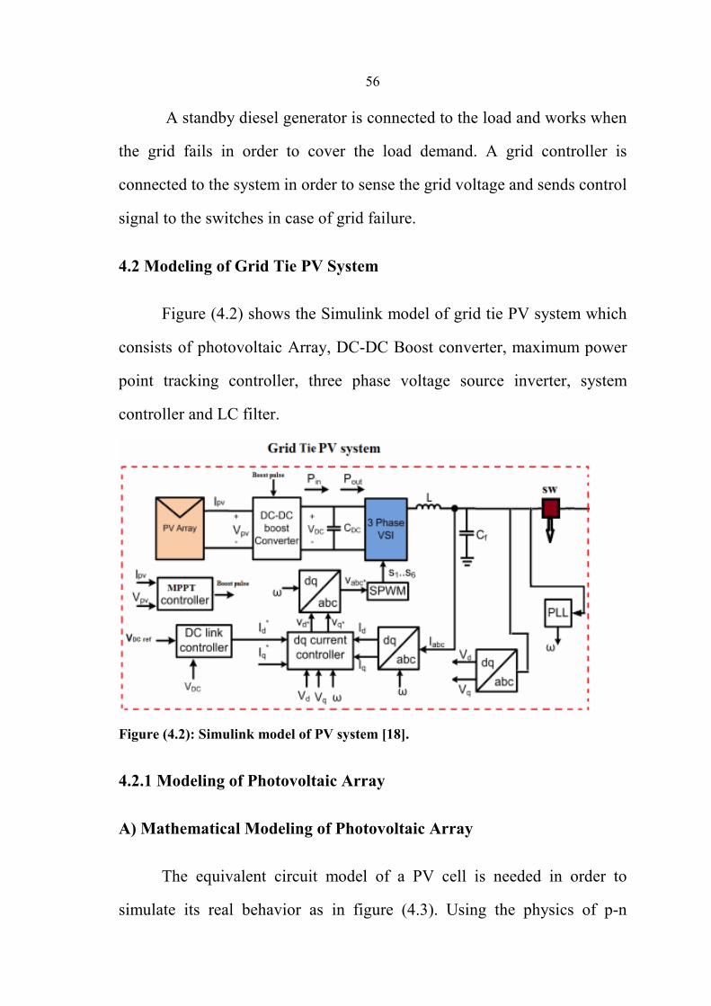
56
A standby diesel generator is connected to the load and works when
the grid fails in order to cover the load demand. A grid controller is
connected to the system in order to sense the grid voltage and sends control
signal to the switches in case of grid failure.
4.2 Modeling of Grid Tie PV System
Figure (4.2) shows the Simulink model of grid tie PV system which
consists of photovoltaic Array, DC-DC Boost converter, maximum power
point tracking controller, three phase voltage source inverter, system
controller and LC filter.
Figure (4.2): Simulink model of PV system [18].
4.2.1 Modeling of Photovoltaic Array
A) Mathematical Modeling of Photovoltaic Array
The equivalent circuit model of a PV cell is needed in order to
simulate its real behavior as in figure (4.3). Using the physics of p-n

57
junctions, a cell can be modeled as a DC current source in parallel with two
diodes that represent currents escaping due to diffusion and charge
recombination mechanisms. Two resistances, Rs and Rp, are included to
model the contact resistances and the internal PV cell resistance
respectively. The values of these two resistances can be obtained from
measurements or by using curve fitting methods based on the I-V
characteristic of the cell [16].
Figure (4.3): Double exponential PV cell model.
The relationship between the PV cell output current and terminal
voltage is governed by:
Where
Iph : is the PV cell internal generated photocurrent.
ID1 and ID2 : are the currents passing through diodes D1 and D2.

58
a : is the diode ideality factor.
k : is the Boltzmann constant (1.3806503 × 10⁻²³ J/K).
T: is the cell temperature in degrees Kelvin.
q : is the electron charge (1.6021× 10⁻¹⁹ C).
I01 and I02 : are the reverse saturation currents of each diode respectively.
Assuming that the current passing in diode D2 due to charge
recombination is small enough to be neglected, a simplified PV cell model
can be reached as shown in figure (4.4).
Figure (4.4): Simplified PV cell model.
This model provides a good compromise between accuracy and
model complexity and has been used in several previous works. In this
case, current ID2 can be omitted from equation (4.1) and the relation
simplifies to [16]:
It is clear that the relationship between the PV cell terminal voltage
and output current is nonlinear because of the presence of the exponential
term in equation (4.1) and (4.4).

59
The presence of the p-n semiconductor junction is the reason behind
this nonlinearity. The result is a unique I-V characteristic for the cell where
the current output is constant over a wide range of voltages until it reaches
a certain point where it starts dropping exponentially.
Another important relationship in PV cells is the power-voltage
characteristic. The product of current and voltage is evaluated at each point
in the curve to find out how much power can be obtained as voltage
changes. Power starts increasing as voltage increases. A certain point in the
curve is reached where maximum power output can be obtained; this point
is therefore referred to as the Maximum Power Point (MPP). After this
point, power starts dropping as the terminal voltage increases until it
eventually reaches zero at open circuit voltage.
The PV cell characteristics also depend on external factors including
temperature and solar irradiation level. To incorporate these effects into the
model, two additional relations are used.
Output current varies with solar irradiation and temperature through
[16]:
Where
In : is the nominal PV cell output current (at 25 °C and 1000 W/m2).
KI : is the current/temperature variation coefficient (A/°C).

60
∆T : is the variation from the nominal temperature (25°C).
Gn : is the nominal solar irradiation (1000 W/m2).
The value of KI is relatively small and this makes the cell output
current linearly dependent on solar radiation level more than temperature.
Temperature, however, has a strong effect on the reverse saturation current,
I0 in equation (4.6) [16].
Where
Isc,n : is the nominal short circuit current of the PV cell.
Voc,n : is the nominal open circuit voltage.
KI and KV : are the current and voltage temperature variation coefficients,
in A/ °C and V/ °C, respectively.
A PV module is the result of connecting several PV cells in series to
order to increase the output voltage. The characteristic has the same shape
except for changes in the magnitude of the open circuit voltage [16].
The PV array is composed of several interconnected photovoltaic
modules. The modeling process is the same as the PV module from the PV
cells. The same parameters from the datasheet are used. To obtain the
required power, voltage and current, the PV modules are associated in
series and parallel the number of modules connected in series and

61
connected in parallel must be calculated. Figure (4.5) shows a photovoltaic
array, which consists of multiple modules, linked in parallel and series. Nss
is the total quantity of modules within the series and Npp is the amount of
modules in parallel. The number of modules modifies the value of
resistance in parallel and resistance in series. The value of equivalent
resistance series and resistance parallel of the PV array are [20]:
Figure (4.5): PV array composed of Nss x Npp modules [16]
After extending the relation current voltage of the PV modules to a
PV array, the new relation of current voltage of the PV array is calculated
in by [20].
Where I0, Iph, Vt are the same parameters used for a PV modules.
This equation is valid for any given array formed with identical
modules.

62
The photovoltaic array will be simulated with this equation. The
simulation circuit must include the number modules series and parallel.
Figure (4.6) shows the circuit model of the PV array.
Figure (4.6): Model structure of the photovoltaic array [20].
B) Simulink Modeling of the Photovoltaic Array
The simulation of the photovoltaic array is realized with Simulink
block. Certain variables are modified for the application with maximum
power point tracking. The input parameters required for the model are:
Ns: number of cells in series
Npp: number modules in parallel
Nss: number of modules in series
A: 1.3977, diode constant
k: 1.38e-23, boltzmann constant
63
Isc,n: nominal short-circuit voltage
Kp: voltage temperature constant
Ki: current temperature coefficient
Vmp: voltage maximum power at STC
Imp: current at maximum power at STC
The PV characteristics from data sheet are used to generate the file
necessary for Rs, Rp and other parameters for the maximum power point.
The initial setup is used to obtain the I-V curve characteristics of the PV
array and show the maximum power point of the PV. The model of the PV
is used with the boost converter to determine the performance of the
maximum power point tracker [21].
The model of the photovoltaic array has been implemented in
Simulink as shown in figure (4.7). The temperature and the irradiance are
specified. The simulation allows having the curve I-V and P-V
characteristics.
The Simulink model uses a current source and the value of the
resistance in series and parallel of the PV [21].

64
Figure (4.7): Simulation of the PV module
The number of modules in series and parallel are set with Nss and
Npp. The Im result is used for the Simulink block as a current source to
obtain the voltage and current delivered from the PV.
Figure (4.8): Simulink block of the photovoltaic array
Figure (4.9) shows the Simulink model for the reverse current
saturation (Io) at the reference temperature which is given by the equation
(4.10) [21]:

65
Figure (4.9): Simulink modeling implementation for Io [21].
Figure (4.10) shows the Simulink model for the light generated
current of the photovoltaic cell which depends linearly on the influence of
temperature and solar radiation as given by the equation (4.11) [21]:
Figure (4.10): Simulink modeling implementation for Iph [21].
Figure (4.11) shows the Simulink model for the model current Im
which given by the equation (4.12) [21]:
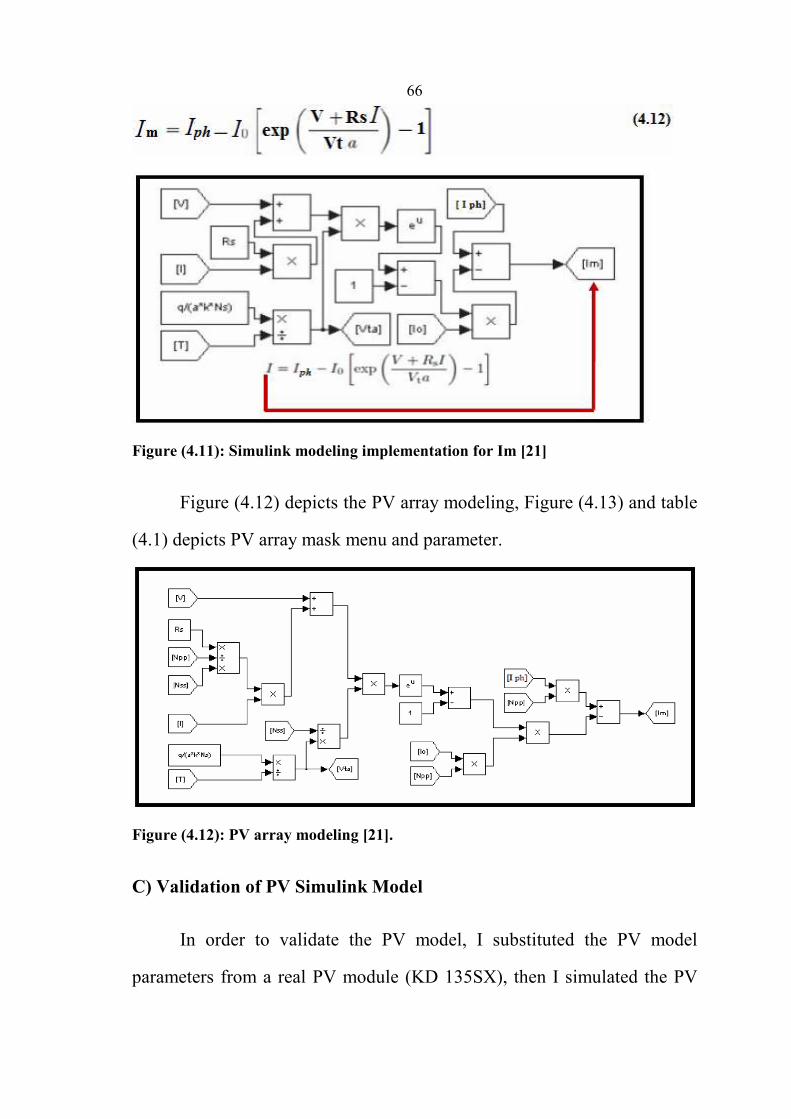
66
Figure (4.11): Simulink modeling implementation for Im [21]
Figure (4.12) depicts the PV array modeling, Figure (4.13) and table
(4.1) depicts PV array mask menu and parameter.
Figure (4.12): PV array modeling [21].
C) Validation of PV Simulink Model
In order to validate the PV model, I substituted the PV model
parameters from a real PV module (KD 135SX), then I simulated the PV

67
model under different temperatures and radiations. As a result, I achieved
the same curves from the simulation model and from data sheet PV model
as shown in figure (4.15) to (4.22).
Table (4.1): KD135SX PV characteristics parameters (Appendix B)
[22].
Figure (4.13): The PV Menu after mask process.

68
Validation of PV Module Model for Different Temperatures
Figure (4.14): PV model simulation at different temperatures.
Figure (4.15) shows the main effect of temperature on the PV
module voltage, which decreases when the temperature increases.
Figure (4.15): Simulink IV characteristic curves for different temperatures.
Figure (4.16): Datasheet IV characteristic curves for different temperatures [22].

69
Validation of the PV Module Model for Different Radiations
Figure (4.17): PV model simulation at different radiations.
Figure (4.18) shows the main effect of radiation on the PV module
current, which decreases when the radiation decreases.
Figure (4.18): Simulink IV characteristic curves for different radiations.
Figure (4.19): Data sheet IV characteristic curves for different radiations [22].

70
Figure (4.20) shows the effect of temperature on the PV module
power, which decreases when the temperature increases.
Figure (4.20): Simulink P-V characteristic curves for different temperatures.
Figure (4.21) shows the effect of radiation on the PV module power,
which decreases when the radiation decreases.
Figure (4.21): Simulink P-V characteristic curves for different radiations.
4.2.2 Modeling of Boost Converter
Figure (4.22) shows the Simulation of the boost converter. The input
of the boost converter is the photovoltaic output voltage. The inductance

71
and the capacitor need to be specified. The switching command of the
IGBT is obtained from the MPPT controller.
Figure (4.22): Boost converter in Simulink [14].
The design specifications of boost controller are shown in table (4.2).
The specifications are for a variable value of input voltage of the boost
controller where the input voltage comes from the renewable source of the
hybrid system and the output voltage of the boost controller is fixed 800V
DC.
Table (4.2): Specification of Boost Controller.
Based on the specification for input voltage and output voltage as
shown in table (4.2), the required duty cycle can be determined by using
Equation (4.13).
In this boost controller circuit, the duty cycle of the boost controller
changes with the value of its input voltage. Therefore, in order to determine

72
the value of minimum inductor Lmin and minimum capacitor Cmin of the
boost controller, the minimum of the duty cycle D of the boost controller is
used in which this duty cycle can be achieved when the input voltage of the
boost controller is at maximum value and the output voltage is fixed at
800V.
The minimum inductance can be determined by using Equation
(4.12).
The capacitance is calculated using Equation (4.15). Let the peak-to-
peak ripple voltage equal to 0.05.

73
4.2.3 Modeling of MPPT Controller
The maximum power point controller block is shown in figure
(4.23). The voltage and the current of the photovoltaic array are the input,
and the duty cycle is the output. The duty cycle is compared to a triangle
wave signal to generate the PWM. The frequency of the triangle wave is
the pulsation frequency of the boost converter [18].
Figure (4.23): MPPT Simulink modeling [18].
The perturb and observe algorithm is implemented and shown in
(Appendix E). The duty cycle is increased or decreased until the maximum
power point of the photovoltaic is reached. The step of the duty cycle is
variable, and it determines the efficiency and accuracy of the MPPT
controller [18].

74
4.2.4 Modeling of Three Phase Voltage Source Inverter
A) Three Phase Inverter Construction
Voltage source inverters (VSI) are mainly used to convert a constant
DC voltage into 3-phase AC voltages with variable magnitude and
frequency. Figure (4.24) shows a schematic diagram of a 3 phase VSI. The
inverter is composed of six switches S1 through S6 with each phase output
connected to the middle of each "inverter leg". Two switches in each phase
are used to construct one leg. The AC output voltage from the inverter is
obtained by controlling the semiconductor switches ON and OFF to
generate the desired output.
Figure (4.24): Three phase voltage source inverter (VSI)
Insulated Gate Bipolar Transistors (IGBTs) and power MOSFET
devices can be used to implement the switches. Each device varies in its
power ratings and switching speed. IGBTs are well suited for applications
that require medium power and switching frequency [11].
In order to discuss the modeling of inverter control, an overview
about abc/dq conversion will introduce in the following section.

75
B) The abc/dq Transformation
The dq transformation is used to transform three phase system
quantities like voltages and currents from the synchronous reference frame
(abc) to a synchronously rotating reference frame with three constant
components when the system is balanced [16].The relationship that govern
the transformation from the abc to dq frame is
Where x can be either a set of three phase voltages or currents to be
transformed, T is the transformation matrix or ω is the angular rotation
frequency of the frame. The angle between the direct axis (d-axis) and
phase a-axis is defined as θ as shown in figure (4.25).
Figure (4.25): Relationship between the abc and dq reference frames.

76
The result of this transformation is three constant rotating
components: the direct (d), quadrature (q) and zero (0) components. In
balanced three phase systems, the zero component can be ignored since
The inverse transformation from the dq frame to the abc frame can
be obtained by applying
This transformation is useful in developing the control system for the
voltage source inverter under current control to regulate the output of the
PV system.
C) Simulink Modeling of Three Phase VSI Control
The structure of control system blocks is introduced at figure
(4.26).The function of each block is examined in detail [16].

77
Figure (4.26): Grid tie PV inverter control model.
The state equations describing the dynamics of the output currents
and voltages of the voltage source inverter are derived in this section. The
time derivatives of the inverter output current and voltage are:
Where Lf and Cf are the filter’s inductance and capacitance
respectively, Vc is the capacitor voltage and IG is the current injected into
the grid as shown in figure (4.27).
Equations (4.21) and (4.22) are in matrix format [16] where

78
Figure (4.27): Circuit diagram of a three phase grid connected inverter.
Multiplying both sides of equation (4.21) by the transformation
matrix T in (4.18), the VSI model in the dq frame can be obtained [27]. The
following procedure is adopted to find the result of the transformation
Where (^) is used to denote dq quantities.
The previous steps use the relationship governing the inverse
transformation, which is:
As a result, equation (4.21) becomes:

79
Since the 0-component is not contributing to both sides of the
equation, it can be omitted and equation (4.24) can be written as:
This represents the state equation of the inverter output current in the
dq frame. Applying the same procedure on equation (4.22), the state
equation for the capacitor voltage is:
The output current from the VSI is regulated using proportional-
integral controllers to force the error signal in each dq-component to zero.
The error signal is defined as the difference between the measured output
current and the reference current.
Control laws shown in equation (4.27) generate the required
command voltages at the inverter output such that the error in the output
current is minimized [28]
Where Id* and Iq* are the dq reference currents, VGd and VGq are the
dq voltages at the point of common coupling. The command voltages, vd *
nd vq*, are transformed back to the natural frame to be sent to the
sinusoidal PWM block to generate the switching signals for the inverter.

80
Under unity power factor operation, the PV system injects real
power only into the grid. In that case, reactive power injection is forced to
zero by setting the reference current Iq* to zero. The real power injection is
controlled by Id* which is extracted from the power mismatch of the DC
link capacitor. The capacitor voltage changes according to equation (4.28):
Where Pin is the input power to the capacitor coming from the DC
converter, Pout is the output power going to the inverter and then to the grid
ignoring power losses, and C is the capacitance of the DC link. To keep the
voltage constant, it is necessary to balance Pin and Pout.
Since the input power is controlled by the DC converter to be the
maximum output power from the PV array, the control system of the
inverter performs the task of controlling the real output power by
controlling Id*. This is achieved by using a separate DC link voltage PI
controller using
A schematic diagram of the controller is shown in figure (4.28) . It
accepts the power mismatch of the DC link capacitor as an input, and uses
a proportional integral controller to generate a power control signal
necessary to drive the mismatch to zero. The power control signal is then
divided by the direct component of the grid voltage to obtain the reference

81
current Id*. This reference is sent to the current controllers to regulate the
output current of the inverter [16].
The PI controller had a low bandwidth due to slow variations in the
DC link power and to ensure that the reference current signal does not
suffer any abrupt changes.
Figure (4.28): Schematic diagram of the DC link controller.
Active and reactive powers injected from the PV system can be
calculated using equation (4.30) [16]:
Where Vd , Vq are the dq voltages at PCC at the grid side of the
transformer, Id,injected and Iq,injected are the dq components of the injected
current at the grid side. It is evident that in the computation of reactive
power Q, there is cross coupling between the direct and quadrature current
and voltage components. This can be eliminated through the use of a phase
locked loop (PLL) that locks on the grid frequency in such a way that the
quadrature component of the voltage at the point of PV system connection
is forced to zero. In this case, equation (4.30) simplifies to:

82
This means that the direct and quadrature components of the inverter
output current can be used to control the active and reactive output powers
from the PV array system, as they are related to the injected currents by the
transformer turns ratio. This is based on the assumption that the voltage at
the point of common coupling (PCC) is relatively constant. In current
practice, distribution systems have regulation mechanisms to keep voltage
within specified limits.
D) Phase Locked Loop (PLL)
The role of the phase locked loop is to provide the rotation
frequency, direct and quadrature voltage components at the point of
common coupling (PCC) by resolving the grid voltage abc components.
Multiple control blocks of the PV system rely on this information to
regulate their output command signals. As stated earlier, the PLL computes
the rotation frequency of the grid voltage vector by first transforming it to
the dq frame, and then force the quadrature component of the voltage to
zero to eliminate cross coupling in the active and reactive power terms
[26]. A proportional-integral controller is used to perform this task as
shown in figure (4.29).
Figure (4.29): Schematic diagram of the phase locked loop (PLL).

83
The output from the PI controller is the rotation frequency ω in rad/s.
Integrating this term results in the rotation angle θ in radians. The operation
of the PLL is governed by:
E) Sinusoidal Pulse Width Modulation (SPWM)
The sinusoidal pulse width modulation technique is used to control
the voltage source inverter by producing the gating signals for the
semiconductor switches. This technique is used to obtain three phase output
voltages that can be controlled in magnitude and frequency. A reference or
modulating signal is compared to a high frequency carrier signal; the result
of this comparison in each phase is used to activate the switches
accordingly. A separate modulating signal is used for each phase with a
phase shift of 120° between them as shown in figure (4.30). Two important
quantities in SPWM are the amplitude and frequency modulation indices,
ma and mf respectively. The amplitude modulation index, ma, is defined as
the ratio between the amplitude of the modulating signal to the carrier
signal, while the frequency modulation index, mf, is the ratio between the
frequency of the carrier signal to that of the modulating signal as in
equation (4.33) and (4.34) [16].

84
When the amplitude of the modulating signal is greater than that of
the carrier signal, the upper switch in the corresponding phase leg in figure
(4.24) is activated.
This leads to the output voltage to have the same magnitude of the
DC link voltage. The switches in each phase leg operate in a
complementary fashion in order to avoid shorting the DC kink capacitor.
Figure (4.30) shows the modulating signals for a three-phase inverter and
phases A and B output voltages. The line voltage between these two phases
is obtained by subtracting Vb from Va. It is clear that the output voltages
need to be filtered to obtain clean sinusoidal voltages. The harmonic
content in the output voltages of the inverter depends on the choice of the
frequency of the carrier signal. Any even harmonics in the output line
voltages in addition to harmonic orders below mf – 2 will be eliminated if
the following conditions hold [16].
In addition to that, harmonics will be centered at mf and its multiples
2 mf, 3 mf …etc., which helps ease the filtering requirements determined
by the cutoff frequency. A possible choice is to have mf = 99 which means
that

85
The magnitude of the output phase voltage (rms) can be determined using
Figure (4.30): SPWM modulation signals for the VSI shown in fig (4.32)
4.3 Modeling of Wind Turbine
In this section, the electrical and mechanical components of the wind
generator system are modeled depend on the wind turbine model from
Matlab Simulink library as shown in figure (4.31).

86
Figure (4.31): Simulink model for grid tie wind turbine [23].
The grid tie wind turbine system consists of aerodynamic model,
drive train, synchronous generator, three phase diode rectifier, DC-DC
boost converter three phase voltage source inverter, LC filter and different
control systems.
4.3.1 Modeling of Wind Turbine Aerodynamic
The wind turbine continuously extracts kinetic energy from the wind
by decelerating the air mass, and feeds it to the generator as mechanical
power. The aerodynamic model of the wind turbine is necessary because it
gives a coupling between the wind speed and the mechanical torque
produced by the wind turbine. The mechanical power, PM, produced by the
wind turbine rotor can be defined as [25]:
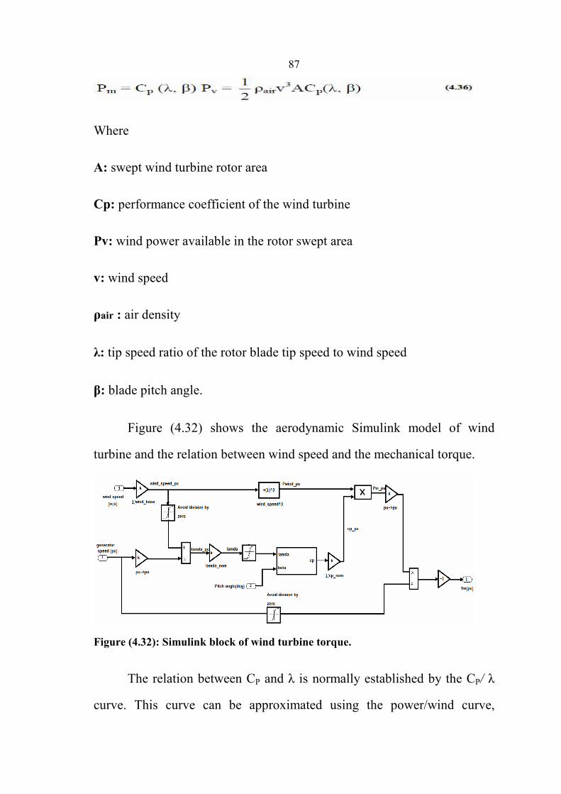
87
Where
A: swept wind turbine rotor area
Cp: performance coefficient of the wind turbine
Pv: wind power available in the rotor swept area
v: wind speed
ρair : air density
λ: tip speed ratio of the rotor blade tip speed to wind speed
β: blade pitch angle.
Figure (4.32) shows the aerodynamic Simulink model of wind
turbine and the relation between wind speed and the mechanical torque.
Figure (4.32): Simulink block of wind turbine torque.
The relation between CP and λ is normally established by the CP/ λ
curve. This curve can be approximated using the power/wind curve,

88
provided by wind turbine manufacturers. To perform this calculation, it is
supposed that the rotor speed does not depend on wind speed in steady-
state operation. Here, a generic equation is used to model the performance
coefficient, CP(λ,β). This equation based on the turbine model
characteristics [25]:
Where C1 = 0.5176, C2 = 116, C3= 0.4, C4 = 5, C5= 21, C6 =
0.0068. The Cp- λ characteristics, for different values of the pitch angle β,
are illustrated in figure (2.9). The maximum value of Cp (Cp max= 0.48) is
achieved for β = 0 degree and for λ1=18.1. This particular value of λ is
defined as the nominal value (λ_nom) [23].
Figure (4.33) shows the Simulink model for equation (4.37).
Figure (4.33): Simulink block of performance coefficient Cp (λ,β) [20],[21].

89
The Cp- λ characteristic of Figure (4.34) shows that the values of
performance coefficient Cp were increased when reducing the value of
blade pitch angle (degree) β. The maximum value of performance
coefficient Cp was obtained when the value of blade pitch angle (degree) β
was set to β = 0o [22].
Figure (4.34): Cp- λ Characteristics of wind turbine [22].
Also,
Figure (4.35) shows the Simulink model for equation (4.38).
Figure (4.35): Simulink block of tip speed ratio λi model [20],[21].

90
4.3.2 Modeling of Drive Train
The drive train model simulates the elastic connection between the
low-speed wind turbine shaft and the high-speed generator shaft. It consists
of the inertia of both the turbine and generator (2-mass system). The elastic
coupling between the two masses is modeled by spring, k, and damper, B.
The equivalent model for the drive train of the wind turbine referred to the
generator side is shown in figure (4.36).
Figure (4.36): Model of drive train (2-mass system).
The dynamics of the drive train on the generator side can be written
in equation (4.39) and (4.40) [9]:
Where

91
Figure (4.37) shows wind turbine drive train based on 2-mass model
Figure (4.37): Equivalent diagram of the drive train model.
4.3.3 Modeling of Grid Tie Wind Turbine Control
The control system for wind turbine consisting of four main parts,
inverter control, excitation control, speed regulator and pitch control.
Simulink Modeling of Grid Tie Wind Turbine Inverter Control
Figure (4.38 ) shows the control strategy for grid tie wind turbine
inverter which is the same control strategy used in grid tie PV inverter, but

92
with the addition of reactive power controller. During the voltage sag the
control systems try to regulate reactive power at their set points (0 kvar).
Figure (4.38): Equivalent diagram for grid tie wind turbine control model[23].
The second part of grid tie wind turbine control is the excitation
control:
A) Simulink Modeling of Excitation Control
The objective of this controller is to regulate the field winding
voltage of the synchronous generator. Higher excitation voltages increase
the maximum torque capability of the generator but result also in increased
iron losses. Hence, for operation at low wind speeds, and therefore at low
rotor speeds, the field voltage may be decreased since the generator torque

93
requirements are reduced. At high winds, on the other hand, a higher
excitation is needed for the generator to develop its full torque.
Figure (4.39): Equivalent diagram of generator excitation control model [23].
The third part of grid tie wind turbine control is the speed controller:
B) Simulink Modeling of Speed Controller
The goal of speed control is to maximize energy capture for wind
speeds below rated as shown in figure (4.40).
Figure (4.40): Stabilization of power and speed through a single operating point.

94
The available power (solid red line) characterizes the turbine’s
response to a given wind speed (12 m/s), as a function of rotation speed.
The tracking curve (dotted blue line) characterizes the operation strategy,
which consists in establishing speed set-points as a function of the power
generated. The intersection of the two curves defines the operating point.
This unique point is the key to maintaining the rotational speed [33].
If this unique point did not exist, it would not be possible to maintain
rotor speeds near those required for maximum available power. To
maintain the system at this point, the velocity error signal, provided by
comparing the required set-point speed and the actual speed, is converted to
an electromagnetic torque command signal using a P.I. controller. The
regulator obtains the required torque (T) by taking advantage of the
equation (4.41) [33]:
The speed controller shown in figure (4.41) regulates the speed of
the rotor by controlling the generator electrical power (and therefore
torque) according to the optimal speed vs. power control characteristic
discussed in the following. The measured turbine power determines the
reference rotor speed, and then the error of the rotor speed determines the
DC current set-point via a PI-controller. The DC current is then regulated at
the reference value by the PI controller of the boost converter.

95
Figure (4.41): Equivalent flow diagram for speed regulator.
C) Simulink Modeling of Pitch Control
Blade pitch angle can be modified to reduce the power transmitted to
the rotor. The pitch angle is adjusted by a mechanical controller attached to
the blades at the rotor hub[33].
Figures (4.42), (4.43) and (4.44) show various curves characterizing
available power as a function of wind speed and blade pitch angle.
Figure (4.42): Available power for different wind speeds; blade pitch angle of zero.

96
Figure (4.43): Available power for different wind speeds; pitch angle of 5 degrees.
Figure (4.44) shows that, when wind speed is 15 m/s, but design
speed is 12 m/s, the blade pitch angle (Beta) must be greater than 5 degrees
to satisfy the maximum power constraint of 1 p.u [33].
Figure (4.44): Available power for different blade pitch angles; wind speed 15 m/s.
The Simulink model of pitch angle controller shown in figure (4.45),
the generator power is regulated at its rated value to avoid overloading the

97
generator and converters, while the blade pitch angle is increased in order
to reduce Cp and the resulting mechanical torque. The objective is to
prevent the rotor speed from increasing beyond its maximum value. For
operation below rated wind speed, the pitch angle is approximately zero,
for maximum aerodynamic efficiency.
Figure (4.45): Equivalent flow diagram for pitch control.
4.4 Modeling of Diesel Generator
A diesel electricity generator is simulated by using an alternator
having its mechanical energy from diesel engine. Also, alternator gets its
field voltage from an excitation system, this system depend on the diesel
generator model from Matlab Simulink library as shown in figure (4.46).
4.4.1 Modeling of Diesel Engine
To simulate the complete dynamics of a diesel engine system, a very
large order model will be required. However for most studies on speed
dynamics of internal combustion engines, it is sufficient to use a lower
order model. Similar approaches have been adopted in diesel engine
simulation studies.
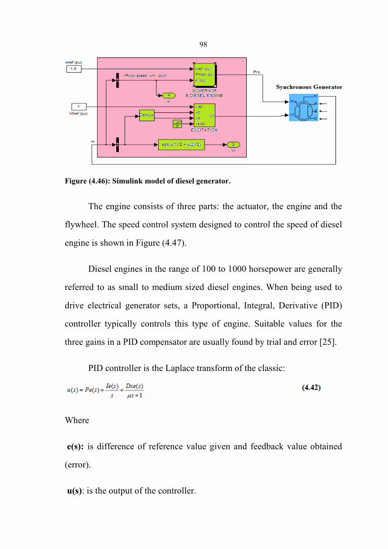
98
Figure (4.46): Simulink model of diesel generator.
The engine consists of three parts: the actuator, the engine and the
flywheel. The speed control system designed to control the speed of diesel
engine is shown in Figure (4.47).
Diesel engines in the range of 100 to 1000 horsepower are generally
referred to as small to medium sized diesel engines. When being used to
drive electrical generator sets, a Proportional, Integral, Derivative (PID)
controller typically controls this type of engine. Suitable values for the
three gains in a PID compensator are usually found by trial and error [25].
PID controller is the Laplace transform of the classic:
Where
e(s): is difference of reference value given and feedback value obtained
(error).
u(s): is the output of the controller.

99
A lag has been added to the denominator of the derivative term,
because high frequency noise tends to dominate a pure derivative function.
The time constant of this lag, µ, is typically made much smaller than the
time constants of any modeled system dynamics.
Figure (4.47): Speed Control of Diesel Engine [25].
A dead time TD in figure (5.47) represents un-modeled high
frequency dynamics, as well as the almost pure dead time associated with
an engine.
This dead time is the result of having several cylinders. Not all
cylinders will be in a position to accept more fuel at a given instant. The
dead time TD is largely made up of the time required for all cylinders to
come into position to be filled with more or less fuel [25].
In the simulated system, speed control for diesel engine and
supplying the torque obtained from it to a synchronous generator. The
diesel engine is assumed to be simulated and the speed obtained from it is
basically controlled by designing a speed control system for it.

100
The blocks basically take speed of engine as input and gives
mechanical power as its output. The speed of the diesel engine is the same
as that of the synchronous generator. To the summing block of the control
system, the reference angular speed ω provided is 1 pu. The actual speed
of the diesel engine is provided from the measurement port of the
synchronous machine which happens to be the same for both the engine
and generator.
The speed error is provided to the PID controller with Transfer
function:
The control system passes the output signal to the actuator, which
converts it to a torque signal.
The transfer function of the actuator is given by the two transfer
function blocks in cascade and the resultant transfer function is given by:
The control signal after passing through the integrator is made to
have a delay of 0.024 units. The integrator takes care that torque remains
between the limits from 0 to 1.2.
The time delay block, which is referred to as the input dead time of

101
the system, comprises of three parts:
(i) Time from a load disturbance to time when the cylinders respond.
(ii) Time between the fuel rack change and when a certain amount of fuel
has been injected into the chamber.
(iii) Time for fuel to burn and the generation of torque required.
Usually, the first one is called a "power-stroke delay" and the latter
two are regarded as an "ignition delay". The engine dead time is a function
of the engine speed and can be considered as a nonlinear part of the system.
The torque signal obtained is then fed to a product box along with
the velocity; the result of which gives the mechanical power, which is then
fed to the synchronous machine [25].
4.4.2 Excitation System of Alternator Model
This model, described by the block diagram of figure (4.48), is used
to represent field-control dc commutator exciters with continuously acting
voltage regulators. Because this model has been widely implemented by the
industry, it is sometimes used to represent other types of systems when
detailed data for them are not available or when a simplified model is
required [25].

102
Figure (4.48): Field-Controlled DC Commutator Exciters.
The principal input to this model is the output from the terminal
voltage transducer, VC. At the summing junction, terminal voltage
transducer output, VC, is subtracted from the set point reference, VREF. The
stabilizing feedback, VF, is subtracted and the power system stabilizing
signal, VS, is added to produce an error voltage. In the steady state, these
last two signals are zero, leaving only the terminal voltage error signal. The
resulting signal is amplified in the regulator. The major time constant, TA,
and gain, KA, associated with the voltage regulator are showing limits
typical of saturation or amplifier power supply limitations.
These voltage regulators utilize power sources that are essentially
unaffected by brief transients on the synchronous machine or auxiliary
buses [25].From the block diagram shown in Figure (4.48), the equation
(4.47) is obtained:
Where Vc: Voltage of Transducer output, Vref: reference Voltage,
Vf: stabilizing feedback, Vs: stabilizing signal, Vuel: terminal field voltage

103
The voltage regulator output, VR, is used to control the exciter,
which may be either separately excited or self-excited. When a self-excited
shunt field is used, the value of KE reflects the setting of the shunt field
rheostat. In some instances, the resulting value of KE can be negative and
allowance should be made for this. Most of these exciters utilize self-
excited shunt fields with the voltage regulator operating in a mode
commonly termed buck-boost [25].
The majority of station operators manually track the voltage
regulator by periodically trimming the rheostat set point so as to zero the
voltage regulator output. This may be simulated by selecting the value of
KE so that initial conditions are satisfied with VR = 0. In some programs, if
KE is entered as zero, it is automatically calculated by the program for self-
excitation.
If a nonzero value for KE is provided, the program should not
recalculate KE, as a fixed rheostat setting is implied. For such systems, the
rheostat is frequently fixed at a value that would produce self- excitation
near rated conditions. Systems with fixed field rheostat settings are in
widespread use on units that are remotely controlled. A value for KE = 1 is
used to represent a separately excited exciter.
The term SE[EFD] is a nonlinear function with values defined at two
or more chosen values of EFD. The output of this saturation block, VX, is the
product of the input, EFD, and the value of the nonlinear function SE[EFD]
at this exciter voltage.

104
A signal derived from field voltage is normally used to provide
excitation system stabilization, VF, via the rate feedback with gain, KF, and
time constant, TF. Figure (4.49) shows the model simulated in Matlab
Simulink environment [25].
Figure (4.49): Simulink model of Excitation System [25].
Here also, the input given to the Lead Lag Compensator can be
written as:
Where
Vcomp: is the input voltage given to compensator.
Vref: is the reference voltage if exciter.
Vfo: is initial value of field voltage.
Ka: is regulator gain.

105
Vf : is field voltage.
kf : is damping function gain.
tf: is filter time constant.
Comparing equations (4.48) and (4.47), it is inferred that:
Vs = Vstab = stabilizing voltage signal and
The terminal field voltage is calculated as:
Where
Vd and Vq : are direct and quadrature axis voltages,
Trs : is Low Pass filter time constant.
Also, Vc Voltage of Transducer output is given by:
Figure (4.50) shows complete grid tie PV/Wind hybrid Simulink
model.

106
Figure (4.50): Simulink model for Grid tie PV/Wind hybrid system.
In this chapter I discussed the mathematical modeling and simulink
of grid tie PV/Wind hybrid system; in the next chapter I will study the
simulation of grid tie PV/Wind system.

107
CHAPTER FIVE
SIMULATION OF GRID TIE
PV/WIND HYBRID SYSTEM

108
Chapter Five
Simulation of Grid Tie PV/Wind Hybrid System
5.1 Grid Tie PV/Wind Hybrid System Constructions
There are two designs for grid tie system:
A-Grid Tie System without Battery:
When the grid is disconnected or in off mode the system will stop
working and the inverter disconnect the renewable generators, so in order
to cover the load demand we need a diesel generator.
B-Grid Tie System with Battery:
In this system, when the grid is disconnected or on off mode, the
system will work isolated from the grid and takes its stability from the
battery via converter.
In my thesis, I will study and analyze the first system as shown in
figure (5.1) for safety issues in electrical network. This system contain PV
array with its controller and inverter, wind turbine system with its
controller and inverter, diesel generator, two loads one of them is the main
load and the other is the emergency load, and the controller with breakers
to check if the grid in off mode or not.

109
Figure (5.1): Complete grid tie PV/Wind Simulink system
I simulate the grid tie PV/Wind hybrid system for two different
conditions:
1- Grid tie hybrid system for different radiations, temperatures, wind
speeds and loads (Normal condition).
2- Grid tie hybrid system during on and off grid process.
5.2 Simulation of Grid Tie PV/ Wind Hybrid System
5.2.1 Simulation of the System for Different Radiations.
The system consists of 45kW PV array, 110kW wind turbine and
150kw load. These conditions are applied on the Simulink system to find
the performance of it.

110
1-The input temperature for the PV array is equal 25Cº.
2-The input radiation for PV array is equal 1000 W/m2 until 8s then change
to 500 W/m2.
3-The input wind speed for wind turbine is equal 15 m/s,
Figure (5.2): Two different input radiations for PV array.
Figure (5.3) shows that the output power from PV array decreases
when the input radiation decreases from 1000W/m2 to 500W/m2 .
Figure (5.3): PV Inverter power output for two different radiations.

111
Figure (5.4) shows that the output current from PV array inverter
decreases to half when the input radiation decreases from 1000W/m2 to
500W/m2 .
Figure (5.4): Three phase PV inverter current for two different radiations.
Figure (5.5) shows that the voltage is still constant on the input
capacitor of the PV inverter when the input radiation decreases from
1000W/m2 to 500W/m2 . This happens because of the active power
controller of the inverter.
Figure (5.5): PV inverter dc bus voltage for two different radiations.

112
Figure (5.6) shows that the output power from wind turbine is still
constant at 110 kW because the wind speed is constant and equals 15m/s.
Figure (5.6): Wind turbine output power for the variation of input radiation of pv.
Figure (5.7) shows that the output power from grid is in minus which
means that the power from PV and wind turbine is more than the load. This
condition lasts 8s, and then the grid power is positive and this means that
the grid source the load with power, this happens because of the reduction
in solar radiation.
Figure (5.7): Grid power output for two different radiations.

113
5.2.2 Simulation of the System for Different Temperatures.
The system consists of 45kW PV array, 110kW wind turbine and
150kw load. These conditions are applied to the system to find the system
performance.
1-The input temperature of the PV array equals 25ºC until 8s then changes
to 50 ºC.
2-The input radiation of PV array equals 1000 W/m2.
3-The input wind speed for wind turbine equals 15 m/s.
Figure (5.8): Two different input temperatures for PV array.
Figure (5.9) shows that the output power from PV array slightly
decreases because the temperature increases from 25 ºC to 50 ºC.

114
Figure (5.9): PV Inverter power output for two different temperatures.
Figure (5.10) shows that the output current from PV array inverter
slightly decreases because the temperature increases from 25 ºC to 50 ºC .
Figure (5.10): Three phase PV inverter current for two different temperatures.
The output power from wind turbine is still constant at 110 kW
because the wind speed is constant on15m/s as shown in figure (5.11).

115
Figure (5.11): Wind turbine power for the variation of input temperature on PV.
Figure (5.12) shows that the grid power sinks about 5kW because the
power from PV and wind is more than load, but after 8s the grid power
equal zero due to the reduction in PV array power.
Figure (5.12): Performance of Grid power for two different temperatures.

116
5.2.3 Simulation of the System for Different Wind Speed
The system consists of 45kW PV array, 110kW wind turbine and
190kw load. These conditions are applied to the system to find the system
performance.
1-The input temperature of the PV array equals 25 ºC.
2-The input radiation of the PV array equals 1000 W/m2.
3-The input wind speed for wind turbine equals 12 m/s until 7s then
changes to 7m/s.
Figure (5.13): Two different input wind speeds for wind turbine.
Figure (5.14) shows that the output power from PV array is still constant at
45 kW because the solar radiation is constant at 1000W/m2 .
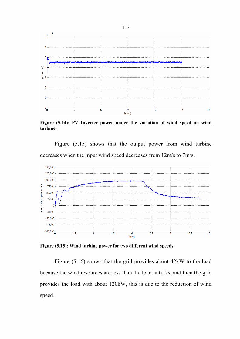
117
Figure (5.14): PV Inverter power under the variation of wind speed on wind
turbine.
Figure (5.15) shows that the output power from wind turbine
decreases when the input wind speed decreases from 12m/s to 7m/s .
Figure (5.15): Wind turbine power for two different wind speeds.
Figure (5.16) shows that the grid provides about 42kW to the load
because the wind resources are less than the load until 7s, and then the grid
provides the load with about 120kW, this is due to the reduction of wind
speed.

118
Figure (5.16): Performance of Grid power for two different wind speeds.
5.2.4 Simulation of the System for Different loads
The system consists of 45 kW PV array, 110 kW wind turbine. These
conditions are applied to the system to find the system performance.
1-The input temperature of the PV array equals 25 ºC.
2-The input radiation of the PV array equals 1000 W/m2.
3-The input wind speed for wind turbine equals 15 m/s.
4-The load equals 100 kW for 7s, and then changes to 200 kW.
Figure (5.17) shows that the output power from PV array is still
constant because it is not affected by the variation of load.
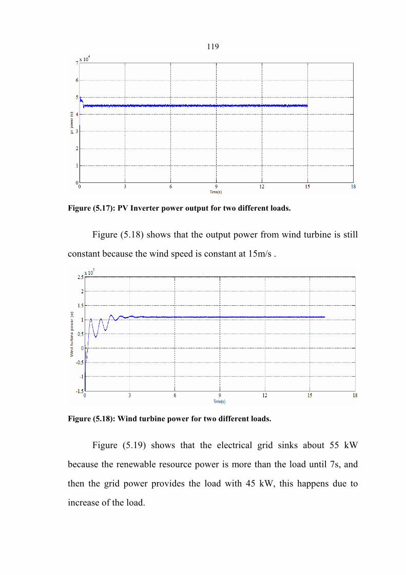
119
Figure (5.17): PV Inverter power output for two different loads.
Figure (5.18) shows that the output power from wind turbine is still
constant because the wind speed is constant at 15m/s .
Figure (5.18): Wind turbine power for two different loads.
Figure (5.19) shows that the electrical grid sinks about 55 kW
because the renewable resource power is more than the load until 7s, and
then the grid power provides the load with 45 kW, this happens due to
increase of the load.

120
Figure (5.19): Performance of Grid power for two different loads.
5.3 Simulation of the System for On and Off Grid Connection
The system consists of 45kW PV array, 110kW wind turbine,
200kW load, 40kW emergency load and 100kW diesel generator. These
conditions are applied to the system to find the system performance.
1-The input temperature of the PV array equals 25 ºC.
2-The input radiation of the PV array equals 1000 W/m2.
3-The input wind speed for wind turbine equals 12 m/s.
Figure (5.20) shows that the output power from PV array is still 45
kW for 7s, and then from 7s to 13s the PV power equals zero because the
grid is at off mode, so the controller disconnects the PV array. After 13s the
grid is at on mode so the controller reconnects the PV array.
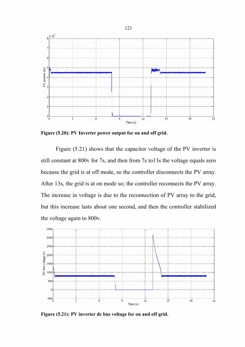
121
Figure (5.20): PV Inverter power output for on and off grid.
Figure (5.21) shows that the capacitor voltage of the PV inverter is
still constant at 800v for 7s, and then from 7s to13s the voltage equals zero
because the grid is at off mode, so the controller disconnects the PV array.
After 13s, the grid is at on mode so; the controller reconnects the PV array.
The increase in voltage is due to the reconnection of PV array to the grid,
but this increase lasts about one second, and then the controller stabilized
the voltage again to 800v.
Figure (5.21): PV inverter dc bus voltage for on and off grid.

122
Figure (5.22) shows the value of PV inverter current at on and off
grid
Figure (5.22): Three phase PV inverter current for on and off grid.
Figure (5.23) shows the value of grid voltage for on and off grid
Figure (5.23): Three phase grid voltage for on and off grid.
Figure (5.24) shows the value of power at on and off grid.

123
Figure (5.24): Wind turbine output power for on and off grid
Figure (5.25) shows the performance of grid power source for on and
of grid, the grid sources the load with about 50kW at on grid and zero at off
grid.
Figure (5.25): Performance of Grid power for on and off grid.
Figure (5.26) shows the pu diesel generator mechanical power at on
and off grid. When the grid is at on mode, the mechanical power of diesel
generator equals zero, but if the grid is at off mode, the pu of diesel

124
generator mechanical power will equal 0.4 because the controller connects
40kW emergency load to 100kW diesel generator.
Figure (5.26): pu diesel generator mechanical power for on and off grid.

125
CHAPTER SIX
DESIGN AND SIMULATION
OF ATOUF GRID TIE PV
SYSTEM

126
Chapter Six
Design and Simulation of Atouf Grid Tie PV System
6.1 Introduction about Atouf Village
Depending on a comprehensive assessment for electrified Villages
which have PV array, Atouf was found to be one of the most appropriate
villages to be subjected to a techno-economic analyses study on a grid tie
PV system [5].
Figure (6.1): Picture for Atouf village
Atouf is located in the Jordan valley (West of Jordan valley) at the
coordinates 32°15/N and 35°30/E and near Tamun town Map (6.1). Its
inhabitants work mainly in farming and cattle breeding. The population
amounts to about 200 living in 21 houses. A mosque, clinic and school are
available in Atouf. Drinking water is obtained from artesian wells in the
village area [5].

127
Map (6.1): Location of Atouf village.
The daily energy needs in such villages are very low. The
households use mainly wood and biomass for cooking and baking bread.
The village is connected to the nearest high voltage grid (33kV) in
Tamun town which is 10 km far from the village. Most houses of the
village have solar water heaters, which is enough to cover the total daily
hot water needs [30].
6.2 Potential of Solar Energy of Atouf Village
The solar radiation data has a great effect on the performance of
photovoltaic (PV) systems. Figure (6.2) shows the monthly values of solar
energy.

128
Figure (6.2): The monthly average value of solar energy in Atouf village [13].
It is clear from the figure that solar energy in this region is very high
during summer months, when it exceeds 8kWh/m2/day, while the lowest
average intensity is during January with a value of 3.2kWh/m2/day.
The village has around 3000 sun shine hours per year. The annual
average temperature amounts to 22 oC while it exceeds 37 oC during
summer months [9].
6.3 Energy Demand and Electrical Grid of Atouf Village
The electrical load in the village is mainly concentrated at night since
the people work during the day in the fields and cattle pasture. The main
electrical loads in the village are: house hold appliances (lighting, TV,
refrigerator, radio, washing machine and fan), street lighting (sodium
lamps), school appliances (lighting, educational TV and lab equipment).

129
6.4 Current Situation of Consumers Connections
Atouf village is connected with municipality grid with 100KVA
transformer 33KV/0.4KV as shown in figure (6.3).
Figure (6.3): Atouf main distribution board [13].
The village has unconnected 90 PV modules (135Wp for each) and
20KVA diesel generator as shown in figure (6.4) and (6.5).

130
Figure (6.4): Diesel generator used in Atouf village.
Figure (6.5): Atouf PV array (90 modules 135Wp).
Map (6.2) shows the electrical network of Atouf village.

131
Map (6.2): Electrical network in Atouf village [5].
6.5 Design of Grid Tie PV System for Atouf Village
6.5.1 Electricity Consumption for Atouf Village
The electrical load in the village is mainly concentrated at night, so
electricity consumption in Atouf village is not high compare to other
villages as shown in table (6.1) and figure (6.6).

132
Table (6.1): Monthly Energy consumption of Atouf village [13].
Month Energy consumption (kWh)
January 2316 February 2124 March 2576 April 2891 May 3020 June 3637 July 4624
August 6346 September 4982
October 3210 November 2894 December 2267
Total 40887
Figure (6.6): Monthly electricity consumption in Atouf village.
6.5.2 Design Grid Tie PV System at 100% penetration
A) PV Array Sizing
The peak power (Wp) of the PV generator is obtained from the
equation (6.1):

133
Where
EL : Energy consumption per day =40887/365 = 112 kWh
ηv : Inverter efficiency (grid tie inverter efficiency = 0.95)
ηR : Charge controller efficiency (because of grid tied inverter so this
efficiency omit from the equation).
PSH : (the peak sun hours) = 5.587
SF :( the safety factor =1 because of grid tied and it not necessary to put
safety factor).
To obtain this peak value, we select a multicrystalline-36 cells
module (KD135SX) of a 1m² area, rated at 12 VDC, and Pmpp=135 WP as
shown in (appendix B). The number of necessary PV modules is obtained
as:
We select the voltage of the PV generator to be =280V, so number of
modules in series is obtained as:

134
The configuration will be as shown in Figure (6.1). The area of the
array is (0.668*1.5) (16*10) = 160.3 m²
Figure (6.7): The configuration of PV generator for Atouf village at 100%
penetration
B) Inverter Sizing
In order to size the grid tied inverter suitable to PV system the main
parameters should be determined from (appendix B):
� Vinput should be located in the inverter MPPT voltage range
(DC100~500V) and V rated = 280v.

135
� Voutput should fulfill the specification of the electric grid of the village
specified as: Vrated=380V ± 5% AC, three phase 50 Hz, sinusoidal
wave voltage.
� Power of inverter’s size depends on PV array because of grid tied
Pnominal > 25kW.
� The efficiency = 95% - 97%
6.5.3 Design Grid Tie PV System at 56% penetration
A) PV Array Sizing
As I said previously, Atouf village has 90 module (135Wp), so the
power =12.15kW, so I will size the system about this value which is 56%
penetration
The configuration will be as shown in Figure (6.1). The area of the
array is (0.668*1.5) (16*6) = 96.12 m²
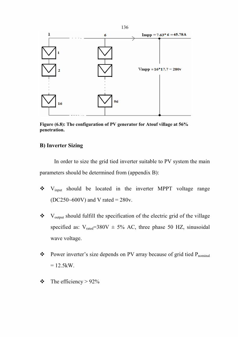
136
Figure (6.8): The configuration of PV generator for Atouf village at 56%
penetration.
B) Inverter Sizing
In order to size the grid tied inverter suitable to PV system the main
parameters should be determined from (appendix B):
� Vinput should be located in the inverter MPPT voltage range
(DC250~600V) and V rated = 280v.
� Voutput should fulfill the specification of the electric grid of the village
specified as: Vrated=380V ± 5% AC, three phase 50 HZ, sinusoidal
wave voltage.
� Power inverter’s size depends on PV array because of grid tied Pnominal
= 12.5kW.
� The efficiency > 92%

137
6.5.4 Energy Analysis of Grid Tie PV System at 100% penetration for
Atouf Village
Analysis of grid tied PV system for different months at 100%
penetration shown in Table (6.2), this table contains the output energy
produced from 21kWp PV array, energy consumption of the village and the
difference between the two energies.
Table (6.2): Monthly energy production versus consumption [13].
Month PV(kWh) Consumption(kWh) differences(kWh)
January 1729.35 2316 -586.6496434 February 2320.382 2124 196.3816112
March 3435.918 2576 859.9183797 April 4019.134 2891 1128.133703 May 5145.677 3020 2125.677294 June 5371.093 3637 1734.093174 July 5008.18 4624 384.1795795
August 4451.597 6346 -1894.40259 September 3796.264 4982 -1185.736469
October 2476.625 3210 -733.3753433 November 1974.014 2894 -919.985804 December 1575.08 2267 -691.9196578
Total 41303.31 40887 416.3142337
Figure (6.9) represent the graphical view of table (6.2).
Figure (6.9): Monthly energy production versus consumption.

138
6.5.5 Energy Analysis of Grid Tie PV System at 56% penetration for
Atouf Village
Analysis of grid tied PV system for different months at 56%
penetration shown in Table (3.2), this table contains the output energy
produced from 21kWp PV array, energy consumption of the village and the
difference between the two energies.
Table (6.3): Monthly energy production versus energy consumption
[13].
Month PV(kWh) Consumption(kWh) differences(kWh)
January 988.2002 2316 -1327.799796 February 1325.932 2124 -798.0676507
March 1963.382 2576 -612.6180687 April 2296.648 2891 -594.3521696 May 2940.387 3020 -79.61297504 June 3069.196 3637 -567.8039008 July 2861.817 4624 -1762.183097
August 2543.77 6346 -3802.230051 September 2169.293 4982 -2812.706554
October 1415.214 3210 -1794.78591 November 1128.008 2894 -1765.991888 December 900.0459 2267 -1366.95409
Total 23601.89 40887 -17285.10615
Figure (6.10) represent the graphical view of table (6.3).
Figure (6.10): Monthly energy production versus energy consumption.

139
6.6 Simulink Configuration of Atouf village
After designing and sizing all parts of Atouf village, figure (7.11)
shows the whole Simulink model, the simulation results for this system for
different conditions are in (Appendix F).
Figure (6.11): Simulink model of Atouf village.
In this chapter, I studied the simulation model of Atouf village, solar
energy potential for the village and system sizing; in the next chapter, I will
study the economic and environmental impact of grid tie system.

140
CHAPTER SEVEN
ECONOMIC AND
ENVIRONMENTAL IMPACT
OF GRID TIE PV/WIND
HYBRID SYSTEM

141
Chapter Seven
Economic and Environmental Impact of the Grid Tie
PV/Wind Hybrid System
7.1 Determining the Cost of Producing One kWh from Grid Tie
PV/Wind Hybrid System
The economic analysis used in this work is based on the use of life
cycle cost, cost annuity (NIS/kWh) and economic impact of grid tie
PV/Wind hybrid system.
7.1.1 Life cycle cost (LCC)
The life cycle cost (LCC) is defined as the sum of the PWs of all the
components. The life cycle cost may contain elements pertaining to original
purchase price, maintenance costs, operation costs, and salvage costs or
salvage revenues.
A) Initial Cost of Grid Tie PV/Wind Hybrid System
Initial cost includes purchasing equipment (PV-panels, grid tie
inverter, wires and other components used in installation). Also includes
labors and technicians costs for installation. These costs depend on the size
and type of a component. All these costs are summed to give the overall
initial cost.

142
Initial Cost of Photovoltaic Modules
PV-modules are available in different sizes and types, the size of PV
is characterized by their peak watt at STC (rated power).The price of peak
watt is the same for mono or poly crystalline, but the installation or
Structure cost will differ depending on the installed PV area. The (NIS/Wp)
will decrease as the size of module increases [32].
Initial Cost of Grid Tie PV Inverter
The grid tie inverter available in different sizes and types .The price
of the grid tied inverter depend on its capacity, efficiency, contain MPPT
controller or not, protection and other parameters[32].
Other Initial Costs
Shipping costs and accessories needed for installation and system
protection, wiring, rooms, should be also considered. These costs depend
on the system size and vary with the kind of the project; if it for public use
(may be land available free), or for private use.
B) Operation and Maintenance Cost of Grid Tie PV/Wind Hybrid
system
The operation costs considered are incurred after installation in order
to run the system for a certain number of years (system life time).

143
C) Salvage value
The salvage value is considered as the value of the project elements
after the system life time finishes.
Figure (7.1) shows the cash flow which represents the initial,
maintenance cost and salvages revenue.
Figure (7.1): The cash flow which represent initial, operational cost and salvage
revenue.
7.1.2 Economic Factors
In order to calculate the equivalent uniform annual series (Aw) of
cash flow in figure (7.1), the most important fact to remember is to first
convert everything to a present worth.
The life cycle cost of grid tie system= initial cost of PV system
+ present worth of maintenance and operation – present worth of salvage
value.
The life cycle cost of grid tie system= initial cost of the system
+ Operation and maintenance X (P / A, i,n) – salvage value X (P / F, i ,n).
The term A (P/A, i ,n) is called the uniform-series present worth
factor.

144
This expression determines the present worth P of an equivalent
uniform annual series A which begins at the end of year 1 and extends
for n years at an interest rate i, a n d ( P/A ) can be found by equation
(7.2):
The term F (P/ Fi, n ) is known as the single-payment present-
worth factor, or the P/F factor. This expression determines the present
worth P of a given future amount F after n years at interest rate i, and (P/F)
can be found by equation (7.3):
In order to simplify the routine engineering economy calculations
involving the factors, tables of factors values have been prepared for
interest rates from 0.25 to 50% and time period from 1 to large n
values, depending on the interest value 10% and interest table in appendix
(D).
The equivalent annual worth AW is obtained with appropriate A/P,
as follow: AW = PW (A / P i , n)
Then the energy unit price calculated from equation (7.4)

145
7.1.3 Cost of producing one kWh from Grid Tie PV/wind hybrid
System for Atouf village
The price of the PV system and its installation are important factors
in the economics of grid tied PV systems. These include the prices of PV
modules, inverter, and all other auxiliaries as shown in table (7.1). The cost
of installation must be taken into consideration.
Table (7.1): Cost of elements and installation of grid tie PV system
[13].
For the present PV system, the life cycle cost will be estimated as
follows:
1- The lifecycle of the system components will be considered as 25 years.
2- The interest rate is about 10%.
The initial cost of the PV system = PV array cost + inverter cost +
installation cost.
The initial cost of the PV system = 176000+20000+50000 =
246000 NIS.
The annual maintenance and operation costs are about 2% of
initial cost which is equal to 196.8 NIS/year, salvage value after 25
years is taken 15% from initial cost and it is equal to 36900 NIS.

146
The life cycle cost of PV system is obtained by drawing cash
flow as in figure (7.2):
Figure (7.2): Cash flow of grid tie PV system for Atouf village.
The life cycle cost of PV system = 2 46000 + 196.8(P / A, i,n) –
36900 (P / F, i ,n).
PW = 246000 + 196.8 (P / A 10%, 25) – 36900 (P / F 10%, 25).
The factors in the above equation are taken from appendix (D):
PW = 246000 + 196.8 x 9.0770 – 36900 x 0.0923
= 244380.44 NIS.
AW = PW (A / P i , n) = 244380.44 (A / P 10% , 25).
From appendix (D), the term (A / P 10%, 25) is equal to 0.11017,
then:
AW = 244380.44 (A / P 10%, 25)
AW =244380.44 x 0.11017 =26923.4NIS.
147
The cost of 1 kWh from the PV generator = 26923.4NIS / 23601.3 kWh
= 1.14 NIS/kWh.
7.2 Grid Tie System Tariffs
Electricity delivered to the grid can be compensated in several ways
such as net metering or feed-in tariff.
7.2.1 Net Metering Tariff
A solar PV system generates electricity by converting sunlight into
electricity that can be used in your home or business. This reduces the
amount of electricity you need to purchase from your utility. If your system
produces more electricity than you need at any given time, it will actually
spin your meter backwards to supply the grid. Your utility keeps track of
how much electricity you supply to the grid as well as how much you
purchase, and bills you only for your net electricity consumption (via net
metering). At the end of any billing period, if overall electricity production
exceeds consumption (indicated by a negative meter read), a billing credit
is applied to your next bill [31].

148
Figure (7.3): Grid tie net metering tariff.
7.2.2 Feed in Tariff
A feed-in tariff (FIT) encourages a new renewable energy
development by creating a long-term financial incentive to customers who
generate renewable electricity, offering a standardized and streamlined
process to do so, and easing the entry for new systems. Under a feed-in
tariff, a utility is contractually obligated to connect the renewable energy
generator to the grid and pay that generator for electricity at a fixed rate for
the life of the FIT contract, typically 10-20 years. The goal of a FIT is to
create a robust market for renewable energy to lower technology costs and
increase development of such resources for the duration of the program,
and potentially pave the way for future growth. The design of FITs can
vary considerably in how rates are calculated, eligibility of different
technologies and resource sizes, and the contract terms [31].

149
Figure (7.4): Grid tie feed in tariff
7.3 Evaluation the Economic Impact of Atouf Grid Tie PV system
As shown from figure (7.5) the bi-directional energy meter measures
the net value between the energy consumption by the load and the energy
transmitted to grid.
The following equation determines the cost of annual total energy
measure by the bi-directional energy meter.
Annual cost for energy measured by the meter = (Energy
consumption before PV installation – PV energy) X cost of 1kWh
= (40887 kWh - 23601.89 kWh) X 0.55 NIS = 9506.8105NIS

150
Figure (7.5): Atouf grid tie PV system electrical construction
In order to find the annual saving money for Atouf village:
Annual saving money for Atouf = cost of annual total bill before
PV installation - cost of annual total bill after PV installation
= (40887 kWh X 0.55NIS) - 9506.8105NIS.
Saving = 22487.85 NIS - 9506.8105NIS = 12981.04 NIS.
7.4 Environment Impact of Grid Tie PV/ Wind system
In the long term, environmental benefits may be the most important
reason for the implementation of grid-tied PV. The environmental impact

151
of PV is small when compared with all nonrenewable energy sources. Coal
plants produce huge quantities of CO2 as well as particulates and oxides of
sulfur and nitrogen. Of course, CO2 is inherent in the combustion process
and cannot be avoided. Scrubbers can reduce, but not eliminate sulfur and
particulate emissions. Gas fired plants are cleaner than coal plants, but still
produce greenhouse gases. Atmospheric emissions from nuclear plants are
negligible, but radioactive waste is an incessant problem with no clear cut
solution.
The amount of CO2 produced from conventional source using fossil
fuel is 1kg for 1kWh[13], so if I take Atouf village as a case study the
reduction of CO2 from energy saving 23601.89kWh is 23601.89kg
annually.

152
CHAPTER EIGHT
CONCLUSIONS AND FUTURE
SCOPE OF WORK

153
Chapter Eight
Conclusions and Future Scope of Work
8.1 Conclusions
From this research it was shown that it is possible to accurately
predict the power output from grid connected photovoltaic arrays by
including the effect of temperature and solar radiation. Furthermore, it was
shown that it is possible to adapt the size of models and the different PV
hybrid system configurations which are applicable to a grid connected and
modify it in such a way that important information about techno-economic
performance of these systems can be obtained.
Upon achieving this, a side-by-side comparison of different grid
connected PV sizes was performed. The form of this model was justified by
looking at different measured values over the collection period; such as;
power output vs. radiation, voltage vs. radiation and output power vs.
temperature. These plots gave an appropriate justification for the sizes and
percentage of penetration factor for all parameters connecting with grid.
General information was presented about the solar resource for Atouf
data collection, a temperature coefficient and non-linear radiation
coefficient was determined, the power output from each configuration can
be accurately predicted for general operating conditions.
Using this software Simulink program, and the determined the effect
of temperature coefficient and non-linear radiation term, the maximum
power output from each PV hybrid system sizes and configurations can

154
now be predicted with accuracy. This can be done, not only for a single
unrealistic value of solar radiation, but under general operating conditions.
Being able to accurately predict the power output is very important for
increased growth in the deployment of photovoltaic hybrid systems.
8.2 SCOPE FOR FUTURE WORK
After the completion of the simulation work, the scope is been
identified as:
� Study effects of switching & fault conditions for grid tied systems.
� Technical and economic analysis comparison between grid tied system
without storage battery and grid tied system with storage battery.
� Build Simulink dynamic smart system with all parts and controller.

155
References
[1] S.B. KJAER, J.K. PEDERSON, F. BLAABJERG "A review of single-
phase grid connected inverters for photovoltaic modules" IEEE
Transactions on Industry Applications, September/October, Vol. 41,
No.5, 2005, pp. 1292-1306.
[2] Đ. SEFA, N. ALTIN "Simulation of current controlled grid
interactive inverter" TPE-2006 3rd Conference on Technical and
Physical Problems in Power Engineering, Ankara(Turkey), May 2006,
pp. 964-968.
[3] U.S. Emission Data, Environment Energy-Related Emission Data &
Environmental Analysis, Energy Information Administration,
http://www.eia.doe.gov/environment.html [access date 10 April 2011]
[4] Bassam A. Abdel-Ghani "Techno-Economic Evaluation of
Electrification of Small Villages in Palestine by Centralized and
Decentralized PV System" A thesis presented to the University of
An-Najah National University, Nablus, Palestine, 2008.
[5] Asma M. Yasin "Optimal Operation Strategy and Economic
Analysis of Rural Electrification of Atouf Village by Electric
Network, Diesel Generator and Photovoltaic System" A thesis
presented to the University of An-Najah National University, Nablus,
Palestine,2008.

156
[6] Muthanna S. Abu-hamdeh "Modeling of Bi-directional Converter for
Wind Power Generation" Master thesis presented to the Ohio State
University, 2009.
[7] V. Quaschning, "Understanding Renewable Energy Systems,"
Earthscan, London, 2005.
[8] M.K. Patel "Wind and Solar Power Systems: Design, Analysis, and
Operation" CRC Press, FL, 2006.
[9] Siriya Skolthanarat "The Modeling and Control of a Wind Farm and
Grid Interconnection in a Multi-machine System" Doctor of
Philosophy thesis presented to Virginia Polytechnic Institute and State
University, August 26th, 2009
[10] David A. Spera "Wind turbine technology: fundamental concepts
of wind turbine engineering" page 66, New York, 1994.ASME
Press.
[11] Rudion K. "Aggregated modeling of wind farm" Dissertation in
electrical engineering at University of Magdeburg, Chapter 4.
[12] Mahmoud S. Abdel-Qader "Simulation of a Hybrid Power System
Consisting of Wind Turbine, PV, Storage Battery and Diesel
Generator with Compensation Network: Design, Optimization
and Economical Evaluation" A thesis presented to the University of
An-Najah National University, Nablus, Palestine, 2008.

157
[13] Energy Research Center (ERC) Meteorological measurements in West
Bank Nablus: An-Najah National University; 2011
[14] E. Ortjohann , O. Omari " A Simulation Model For Expandable
Hybrid Power Systems" University of Applied Sciences
Südwestfalen www.otti.de/ipv/ipvabstracts/6.4ortjohann.pdf
[Access Date 3-2- 2012]
[15] "Introduction of photovoltaic system" SECO, FACT SHEET NO.11,
pp. 1-4. www.infinitepower.org [Access Date 7-9- 2011]
[16] Ahmed S. Khalifa "Control and Interfacing of Three Phase Grid
Connected Photovoltaic Systems" A thesis presented to the
University of Waterloo, Ontario, Canada, 2010
[17] AKIHIRO OIE "Design and Simulation of Photovoltaic Water
Pumping System" A Thesis Presented to the Faculty of California
Polytechnic State University, San Luis Obispo, Requirements for the
Degree of Master of Science in Electrical Engineering,2005
[18] Ghislain Remy, Olivier Bethoux,"Review of MPPT Techniques for
Photovoltaic Systems" Laboratoire de Génie Electrique deParis
(LGEP)/ SPEE-Labs,Université Paris-Sud 11,france.
[19] Mo'ien A. Omar "COMPUTER – AIDED DESIGN AND
PERFORMANCE EVALUATION OF PV-DIESEL HYBRID
SYSTEM" A thesis presented to the University of An-Najah National
University, Nablus, Palestine, 2007.

158
[20] Falinirina F. Rakotomananandro "Study of Photovoltaic System"
Master thesis presented to the Ohio State University, 2011.
[21] SURESH A/L THANAKODI "Modeling and Simulation of Grid
Connected Photovoltaic System Using Matlab / Simulink" Master
thesis presented to University Technology Malaysia November 2009.
[22] PV module from kyocera data sheet
http://www.kyocerasolar.eu/index/products/download/English.-cps-
7724-files-20802-File.cpsdownload.tmp/KD135SX-1PU_Eng_March
%202011 .pdf [Access Date 2-1- 2012]
[23] MATLAB/Simulink simulation software 2009a.
[24] Slootweg, J.G.; Polinder, H. "Initialization of Wind Turbine Models
in Power System Dynamics Simulations", this paper appears in:
Power Tech Proceedings, 2001 IEEE Porto Issue Date: 2001 On
page(s): 6 pp. vol.4 September 2001.
[25] Ashima Taneja" Sustainable Energy Systems with HVDC
Transmition" Thesis submitted in the partial fulfillment for the award
of the degree of Master of Engineering in Power Systems & Electric
Drives, Thapar university Patiala,2011.
[26] Kroutikova, N.; Hernandez-Aramburo, C.A.; Green, T.C "State-space
model of grid-connected inverters under current control mode"
Electric Power Applications, IET , vol.1, no.3, pp.329-338,May 2007.

159
[27] Kawabata, T.; Miyashita, T.; Yamamoto, Y. "Dead beat control of
three phase PWM inverter" IEEE Transactions on Power
Electronics, vol.5, no.1, pp.21-28, Jan 1990
[28] Y. Mohamed and E. F. El-Saadany, "Adaptive Decentralized Droop
Controller to Preserve Power Sharing Stability of Paralleled
Inverters in Distributed Generation Microgrids" IEEE
Transactions on Power Electronics, vol. 23, pp. 2806-2816, 2008.
[29] Leland Blank, P.E. & Anthony Tarquin, P.E. "Engineering
Economy" Singapore, McGraw-Hill; 1998
[30] Marwan M.Mahmoud, Imad H.Ibrik "Techno-economic feasibility of
energy supply of remote villages in Palestine by PV systems, diesel
generators and electric grid" Renewable and sustainable Energy
Reviews 10(2006) 128 – 138.
[31] http://en.wikipedia.org/wiki/Grid-tie_inverter [Access Date 3-2-
2012].
[32] www.affordable-solar.com [Access Date 3-2- 2012].
[33] Marc Langevin, Consulting Engineer ,"Maximum Generating
Capacity of A Wind Farm Connected to 25 KV Distribution
Feeder" Report Presented to David Beauvais, Project Leader Canmet
ENERGY – Varennes Research Centre

160
APPENDICES
Appendix A: Simulink blocks for each part of grid tied
PV/wind system
Appendix B: Specifications of the grid tie PV/Wind system
elements
Appendix C: Graphs to calculate K and C
Appendix D: Table of interest at i = 10%
Appendix E: Perturb and Observe Algorithm
Appendix F: Simulation Results of Atouf Village

161
APPENDIX (A)
Simulink blocks for each part of grid tie PV/wind system
Figure (A.1): Simulink model of Grid tie PV/Wind hybrid system

162
Figure (A.2): PV system with MPPT and boost converter.
Figure (A.3): Boost dc-dc converter.

163
Figure (A.2): Unmask block of grid tie PV inverter measurement

164
Figure (A.3): Unmask control block for grid tie PV inverter

165
Figure (A.4): Unmasked Wind turbine model
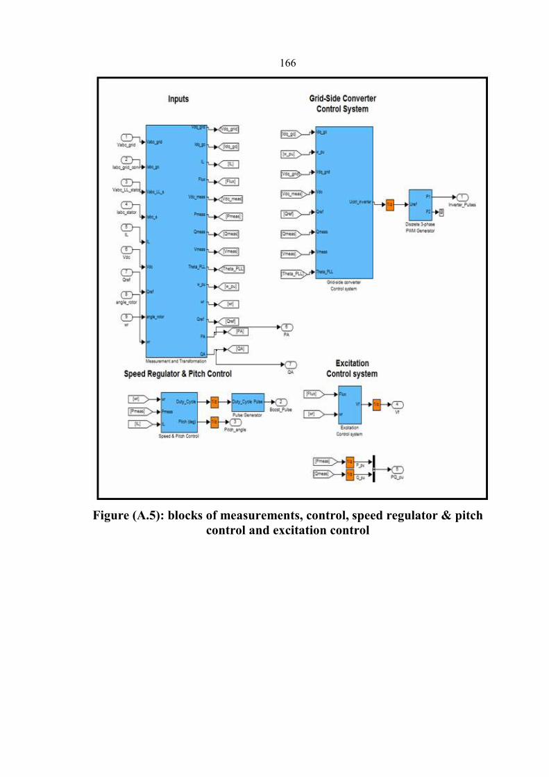
166
Figure (A.5): blocks of measurements, control, speed regulator & pitch
control and excitation control

167
Figure (A.6): Unmask measurements block for wind turbine

168
Figure (A.7): Unmask control block for wind turbine
Figure (A.8): Unmask speed regulator and pitch control block

169
APPENDIX (B)
Specifications of the grid tie PV/Wind hybrid system elements
(B.1): Solar PV module technical specifications

170

171
(B.2) : Grid tied inverter technical specifications (12kW)

172

173
(B.3): Grid tied inverter technical specifications (22kW)
Product Description: Solar inverter has CE, VDE0126-1, G83/1,
AS4777, and AS3100 Certificate.
• Conversion efficiency is 98%.
• islanding protection & MPPT.
• High efficiency and Wide range of MPPT.
• Wide input voltage range.
• High reliability due to complete protection function.
• Powerful communication interfaces.
• Easy operation and installation.
• Easy-to-set multilingual LCD display.
• Adjustable protection / operation parameters.
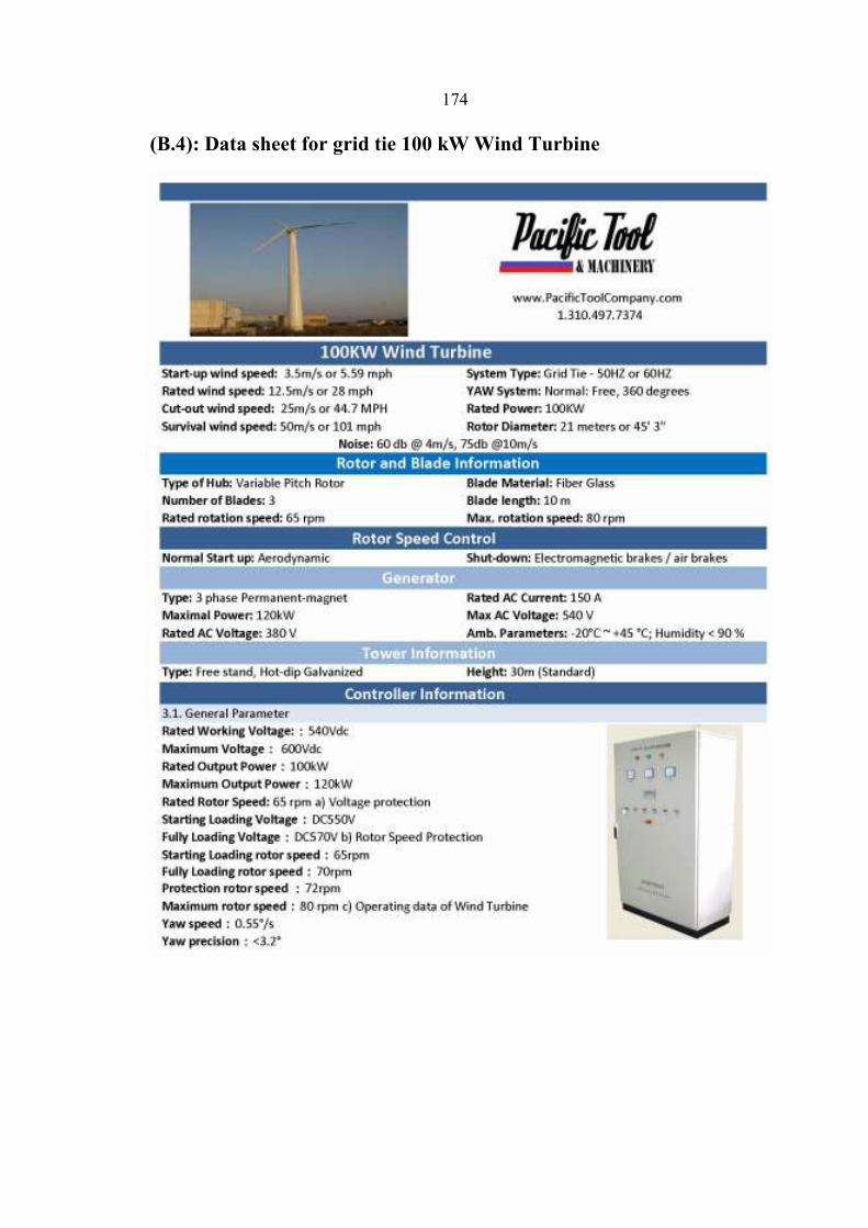
174
(B.4): Data sheet for grid tie 100 kW Wind Turbine

175

176

177
APPENDIX (C)
Graphs to calculate K and C
Figure (C.1): Relationship between coefficient V/C and shape
parameter K

178
Figure (C.2): Relationship between coefficient R and shape
parameter K

179
Appendix (D)
Table of interest at i = 10%

180
Appendix (E)
Perturb and Observe Algorithm
function y=pnob(u)
global A B Ka alpha_mli
Ka=.02*abs(u(1)-A); Ka=0.02*|DeltaP|
if (u(1)-A)==0
C=alpha_mli;
else
if(u(1)-A)>0
if(u(2)-B)>0
else
C=alpha_mli+Ka;
end
else
if(u(2)-B)>0
C=alpha_mli+Ka;
else
C=alpha_mli-Ka;
end
end
end
if(C<0) %saturation due negative
C=0;
end
if(C>1) %saturation due over one
C=1;
end
A=u(1); measure power
B=u(2); measure voltage
alpha_mli=C;
y=alpha_mli;

181
Appendix (F)
Simulation Results of Atouf Village
Simulation of the System for Different Radiations
These conditions applied on the system, 1000 W/m2 until 5s then change to
500 W/m2, 25 ºC, 7kW load.
Figure (F.1): Different input radiations for PV array.
0 1.5 3 4.5 6 7.5 9 10.5-1.5
-1
-0.5
0
0.5
1
1.5
2
2.5
3x 10
4
Time(s)
PV p
ower(w)
Figure (F.2): PV power for two different radiations.

182
Figure (F.3): Grid power for two different radiations.
0 1.5 3 4.5 6 7.5 9 10.520
25
30
35
40
45
50
55
60
Time(s)
PV
current
Figure (F.4): MPP current regulation for two different radiations.

183
0 1.5 3 4.5 6 7.5 9 10.50
100
200
300
400
500
600
Time(s)
MP
P v
oltage r
egula
tions (
v)
Figure (F.5): MPP voltage regulations for two different radiations.
0 1.5 3 4.5 6 7.5 9 10.50
100
200
300
400
500
600
700
800
900
Time(s)
DC
bus v
oltage (v)
Figure (F.6): Bus dc voltage for two different radiations.

184
0 1.5 3 4.5 6 7.5 9 10.5-150
-100
-50
0
50
100
150
Time(s)
Thre
e p
hase c
urrent (A
)
Figure (F.7): Three phase inverter current for two different radiations.
0 1.5 3 4.5 6 7.5 9 10.5
-600
-400
-200
0
200
400
600
Time(s)
Thre
e p
hase inverter voltage (v)
Figure (F.8): Grid voltage for two different radiations.

185
0 1.5 3 4.5 6 7.5 9 10.5-150
-100
-50
0
50
100
150
Time(s)
Three phase current (A
)
Figure (F.9): Three phase grid current for two different radiations.
Figure (F.10): P-V Curve for two different radiations for MPP control.
Figure (F.11): Three phase grid voltage.

186
Simulation of the System for Different Temperatures
These conditions applied on the system, 25 ºC until 5s then change to 50
ºC, 1000 W/m2, 7kW load
Figure (F.12): different input temperature for PV array.
0 1.5 3 4.5 6 7.5 9 10.50
0.5
1
1.5
2
2.5
3x 10
4
Time(s)
PV p
ower(w)
Figure (F.13): PV power for two different temperatures.

187
0 1.5 3 4.5 6 7.5 9 10.50
10
20
30
40
50
60
70
Time (s)
MP
P c
urrent re
gula
tion (A
)
Figure (F.14): MPP current regulation for two different temperatures.
0 1.5 3 4.5 6 7.5 9 10.5-100
-80
-60
-40
-20
0
20
40
60
80
100
Time(s)
Thre
e p
hase I
nvert
er
curr
ent
Figure (F.15): Three phase inverter current for two different
temperatures.

188
Figure (F.16): MPP voltage regulation for two different temperatures.
Figure (F.17): Grid power for two different temperatures.
0 1.5 3 4.5 6 7.5 9 10.50
100
200
300
400
500
600
700
800
900
Time (s)
DC b
us voltage (v)
Figure (F.18): Dc bus voltage for two different temperatures.

189
Figure (F.19): P-V Curve for two different temperature under MPP
controller.
Simulation of the System for Different Loads
These conditions applied on the system, 25 ºC, 1000 W/m2, 5kW
load until 5s then 10kW.
0 1.5 3 4.5 6 7.5 90
0.5
1
1.5
2
2.5
3x 10
4
Time (s)
PV p
ower (w
)
Figure (F.20): PV power for two different loads.
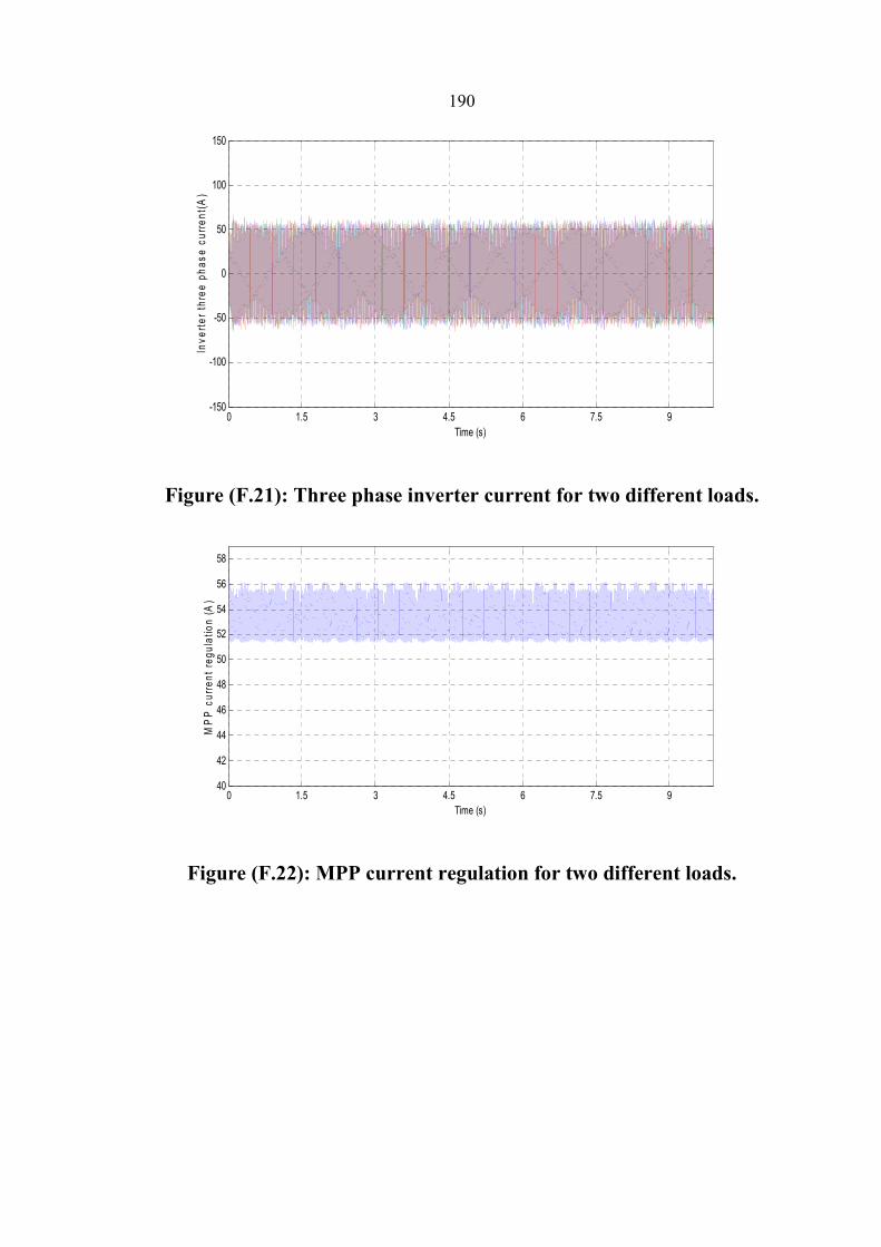
190
0 1.5 3 4.5 6 7.5 9-150
-100
-50
0
50
100
150
Time (s)
Inverter th
ree p
hase c
urrent(A)
Figure (F.21): Three phase inverter current for two different loads.
0 1.5 3 4.5 6 7.5 940
42
44
46
48
50
52
54
56
58
Time (s)
MPP c
urrent re
gula
tion (A)
Figure (F.22): MPP current regulation for two different loads.

191
0 1.5 3 4.5 6 7.5 90
100
200
300
400
500
600
Time (s)
MP
P v
oltage regula
tion (v)
Figure (F.23): MPP voltage regulation for two different loads.
0 1.5 3 4.5 6 7.5 9-3
-2.5
-2
-1.5
-1
-0.5
0x 10
4
Time(s)
Grid p
ower (w
)
Figure (F.24): Grid power for two different loads.

192
0 1.5 3 4.5 6 7.5 9-100
-80
-60
-40
-20
0
20
40
60
80
100
Time(s)
Grid thre
e p
hase c
urrent (A
)
Figure (F.25): Three phase grid current for two different loads.
0 1.5 3 4.5 6 7.5 90
200
400
600
800
1000
Time(s)
DC bus voltage(v)
Figure (F.26): DC bus voltage for two different loads.
Simulation of the System for On and Off Grid Connection
At this condition when the grid at off mode the controller
disconnects the grid, PV array and connect the standby diesel generator to
the load.

193
0 1.5 3 4.5 6 7.5 9 10.50
0.5
1
1.5
2
2.5
3
3.5
4x 10
4
Time (s)
PV p
ower (w
)
Figure (F.27): PV power for on and off grid.
0 1.5 3 4.5 6 7.5 9 10.50
10
20
30
40
50
60
Time (s)
MPP c
urrent re
gulations (A)
Figure (F.28): MPP current regulation for on and off grid.

194
0 1.5 3 4.5 6 7.5 9 10.50
100
200
300
400
500
600
700
Time(s)
MPP v
oltage regula
tion (v)
Figure (F.29): MPP voltage regulation for on and off grid.
0 1.5 3 4.5 6 7.5 9 10.5-1000
-800
-600
-400
-200
0
200
400
600
800
1000
Time (s)
Thre
e p
hase Inverter voltage (v)
Figure (F.30): Three phase inverter voltage for on and off grid.

195
0 1.5 3 4.5 6 7.5 9 10.5-150
-100
-50
0
50
100
150
Time (s)
Thre
e p
hase inverter current (A
)
Figure (F.31): Three phase inverter current for on and off grid.
0 1.5 3 4.5 6 7.5 9 10.5-4
-3
-2
-1
0
1
2
3
4x 10
4
Time (s)
Grid p
ower (w
)
Figure (F.32): Grid power for on and off grid.

196
0 1.5 3 4.5 6 7.5 9 10.5-100
-50
0
50
100
Time (s)
Thre
e p
hase G
rid c
urrent (A
)
Figure (F.33): Three phase grid current for on and off grid.
0 1.5 3 4.5 6 7.5 9 10.5-500
0
500
1000
1500
2000
2500
3000
3500
Time (s)
DC b
us v
oltage (v)
Figure (F.34): DC bus voltage for on and off grid.

197
0 1.6 3.2 4.8 6.4 8 9.6 11.20
0.2
0.4
0.6
0.8
1
Time (s)
PU d
iesel m
echanic
al power
Figure (F.35): pu diesel generator mechanical power for on and off
grid.

النجاح الوطنية جامعة
الدراسات العليا كلية
شبكات الكهرباء مع التحليل التقني والاقتصادي لربط التقييم و
: قرية عطوف /ن الهجينة خلايا شمسية رياح في فلسطيالأنظمة
دراسة حالة
إعداد
حسين محمد دريديمحمد
إشراف
عماد بريك. د
درجة الماجستير في هندسـة الطاقـة الحصول على متطلبات استكمالا ل الأطروحة ذه ه قدمت
. الترشيد بكلية الدراسات العليا في جامعة النجاح الوطنية نابلس فلسطينوإستراتيجيةالنظيفة
2012

ب
الهجينة خلايا شمسية الأنظمةشبكات الكهرباء مع التحليل التقني والاقتصادي لربط التقييم و
دراسة حالة:قرية عطوف /نرياح في فلسطي
إعداد
حسين محمد دريديمحمد
إشراف
عماد بريك. د
الملخص
زادت الحاجـة لمعرفـة المزيـد مـن , انتشارا أكثر أصبحت الطاقة المتجددة أنحيث
هذا البحث قائم علـى بنـاء . المختلفة من هذه التكنولوجيا الأنواعالمعلومات حول كيفية عمل
موصولة شمسية وتوربين رياح ألواحجين مكون من نموذج رياضي محوسب لنظام كهربائي ه
الأداءوذلك باستخدام برنامج الماتلاب سيميولينك من اجل دراسة وتحليـل , مع شبكة الكهرباء
بالاعتماد على تغير الظروف البيئية والبيانـات المناخيـة الأنظمة هذهالفني والاقتصادي لبناء
. سرعة الرياح,الشمسي الإشعاعكمية ,المتوفرة مثل درجة الحرارة
يتم معرفة تصميم القدرة اللازمة بالاعتماد إنشائهبرنامج السيميولينك الذي تم من خلال
إلـى مقارنة جنبا إجراءسرعة الرياح و يمكن , الشمسي الإشعاعكمية ,درجة الحرارة على تغير
الحالية مفيدة جـدا نماذج التنبؤ أنحيث ,والتوصيلات المختلفة للنظام الهجين الأحجامجنب بين
وبالتالي تـم .القدرة القصوى المتصلة بالشبكة الكهربائية والتي تعمل عند نقطة الأنظمةفي حالة
محاكـاة هذا النموذج المصمم يتم من خلاله عمل أنعمل تعديلات على النماذج السابقة بحيث
إنتـاج بدقة عن كميـة أيضا يتنبألمعرفة نتائج تشغيل عناصر النظام لكل فترة زمنية محددة و
.المقاسه وبالاعتماد على البيانات الطاقة خلال هذه الفترات
مـن الطاقة إنتاج كمية معرفة تصميمه تم الذي المحوسب البرنامج خلال من يتم كذلك
تم وقد ,الشمسي الإشعاع كمية أو الحرارة درجة زيادة, التشغيل ظروف بتغيير الهجينة الأنظمة
.حالة كدراسة عطوف كهرباء شبكة من هلمقاسا البيانات تحليل

ج
تغيـر تحـت النظـام أداء ضعف نواحي يبين لأنه العلمية الناحية من مهم البحث هذا
النظـام لمكونـات مختلفـة أشكال مقارنة خلاله من ويمكن ,المحددة للمواقع المناخية الظروف
مـن واحـدة نقطـة علـى دالاعتما خلال من الهجينة الأنظمة تصميم أن يبين كذلك. المقترح
عنـد وأداء تشغيل معايير أفضل يعطي أن بالضروري ليس) متوسطة قيمة (المناخية الظروف
النظام واقتصاديات الطاقة إنتاج كمية يبين البحث هذا أن وبالتحديد .الكهربائية الشبكة مع وصلة
عناصـر قـدرة تحديد عند وذلك,)الرياح وتوربينات (الشمسية الخلايا أنظمة تشغيل عن الناتج
.الكهربائية الأحمال تغذية في المشاركة ونسبة النظام