design considerations, modeling, and analysis of micro ...haich/thesis2.pdf · anton \tom"...

$: Design Considerations, Modeling, and Analysis of Micro ...haich/thesis2.pdf · Anton \Tom" Braun generously permitted me to examine his free-piston machinery and his proprietary data$
UNIVERSITY OF MINNESOTA

This is to certify that I have examined this bound copy of a doctoral thesis by

Hans Thomas Aichlmayr

and have found that it is complete and satisfactory in all respects,

and that any and all revisions required by the final

examining committee have been made.

David B. Kittelson and Michael R. Zachariah

Name of Faculty Advisers

Signature of Faculty Advisers

Date

GRADUATE SCHOOL

Design Considerations, Modeling, and Analysis of Micro-Homogeneous

Charge Compression Ignition Combustion Free-Piston Engines

A THESIS

SUBMITTED TO THE FACULTY OF THE GRADUATE SCHOOL

OF THE UNIVERSITY OF MINNESOTA

BY

Hans Thomas Aichlmayr

IN PARTIAL FULFILLMENT OF THE REQUIREMENTS

FOR THE DEGREE OF

DOCTOR OF PHILOSOPHY

David B. Kittelson and Michael R. Zachariah, Advisers

December 2002

c© Hans Thomas Aichlmayr December 2002

Dedication

I dedicate this thesis to my parents because their patience, encouragement, guidance, and support

were instrumental to my success.

i

Acknowledgments

This work could not have been completed without the support and assistance of the following

organizations and individuals:

Organizations:

• Defense Advanced Research Projects Agency supported this work under contract F30602-

99-C-0200.

• Honeywell International oversaw the project and permitted me to freely use their facilities

and equipment to conduct experiments.

• The Minnesota Supercomputing Institute provided computer time and travel funds to

present this work at two technical conferences.

Honeywell Personnel:

• Wei Yang managed the project, provided technical advice, and made the necessary ar-

rangements for me to access Honeywell facilities and take photographs on the premises.

• Ulrich Bonne generously provided technical advice and reviewed two technical manuscripts.

• Tom Rezacheck designed the single-shot experiment and facilitated my experimental work.

• Ivan Stegic oriented me to the use and maintenance of the single-shot experiment appa-

ratus.

• Rebecca Kemp played an instrumental role in the financial management of this project.

University of Minnesota Personnel:

• Professor Kittelson permitted me to work independently and he gave me valuable tech-

nical advice and critiques. I also appreciate his trust in me to participate in the financial

management of the project.

• Professor Zachariah also permitted me to work independently and he gave me valuable

technical advice. He also provided sage career advice and facilitated my accession to the

technical community.

• Professor Kulacki generously permitted me to use his facilities and equipment during the

first year of the project.

• Jim Garrison played an instrumental role in the financial management of this project.

Special Thanks:

• Anton “Tom” Braun generously permitted me to examine his free-piston machinery and

his proprietary data and parts.

• Bill Vork demonstrated and explained the operation of Mr. Braun’s engines.

• Bob Hain and the MEnet Support Staff developed and maintained the superb computing

environment that facilitated the rapid progress of this project. Bob Hain also provided

laptop computers to present this work at technical conferences.

• Jody Peterson generously edited the thesis.

ii

Abstract

This thesis is a feasibility study of micro- and meso-homogeneous charge compression ignition (HCCI)

free-piston engines. Although numerous fundamental issues arise in micro-engine design, HCCI

combustion in small scales is the focus of this work. To this end, single-shot experiments and

numerical modeling are employed to characterize micro-HCCI combustion. Experimental studies

with n-heptane reveal that HCCI combustion in small scales is feasible and that a wide range of

fuel-air equivalence ratios (0.2–2.9) may be used. The HCCI numerical models employ detailed ho-

mogeneous gas-phase chemical kinetics and they approximate the combustion chamber with fixed-

and variable-volume batch reactors. The fixed-volume reactor model is primarily used to charac-

terize potential fuels and the variable-volume reactor models are used to capture gas compression

and expansion processes. The variable-volume reactor models consider two types of piston mo-

tion: slider-crank and free-piston. The slider-crank model is used to explore fundamental aspects

of HCCI combustion and to obtain potential operating maps for miniature two-stroke HCCI en-

gines. The free-piston model couples the piston motion to gas-phase thermodynamics and chemical

kinetics. The free-piston model approximates the single-shot process; excellent correspondence be-

tween model predictions and experimental data is found. Parametric studies conducted with the

free-piston model are employed to: (1) Gain physical insight into the single-shot process., (2) In-

vestigate micro-HCCI free-piston engine design considerations., and (3) Explore kinetic constraints

for HCCI engine operation. Non-dimensional parameters are identified and subsequently used to

explore free-piston engine design and kinetic operating limits. Additionally, existing small engines

and fundamental aspects of free-piston engine operation and design are presented. The existing

body of HCCI literature is also thoroughly reviewed.

iii

Contents

Dedication . . . . . . . . . . . . . . . . . . . . . . . . . . . . . . . . . . . . . . . . . . . . . i

Acknowledgement . . . . . . . . . . . . . . . . . . . . . . . . . . . . . . . . . . . . . . . . ii

Abstract . . . . . . . . . . . . . . . . . . . . . . . . . . . . . . . . . . . . . . . . . . . . . . iii

List of Figures . . . . . . . . . . . . . . . . . . . . . . . . . . . . . . . . . . . . . . . . . . xii

List of Tables . . . . . . . . . . . . . . . . . . . . . . . . . . . . . . . . . . . . . . . . . . . xviii

Nomenclature . . . . . . . . . . . . . . . . . . . . . . . . . . . . . . . . . . . . . . . . . . . xx

Chapter 1 Introduction 1

1.1 Microtechnology-Based Energy and Chemical Systems . . . . . . . . . . . . . . . . . 1

1.1.1 Micro-Reactors and Heat Engines . . . . . . . . . . . . . . . . . . . . . . . . . 1

1.1.2 Heat Transfer in MECS . . . . . . . . . . . . . . . . . . . . . . . . . . . . . . 2

1.2 Micro-Engine Programs . . . . . . . . . . . . . . . . . . . . . . . . . . . . . . . . . . 3

1.2.1 Micro-Gas Turbine Engine . . . . . . . . . . . . . . . . . . . . . . . . . . . . . 3

1.2.2 MEMS Rotary Engine . . . . . . . . . . . . . . . . . . . . . . . . . . . . . . . 5

1.2.3 MEMS Free-Piston Engine-Generator . . . . . . . . . . . . . . . . . . . . . . 5

1.2.4 MEMS Free-Piston Knock Engine . . . . . . . . . . . . . . . . . . . . . . . . 7

1.2.4.1 HCCI in Micro-Engines . . . . . . . . . . . . . . . . . . . . . . . . . 7

1.2.4.2 Model Airplane Engines . . . . . . . . . . . . . . . . . . . . . . . . . 8

1.2.4.3 Free-Piston Engine Configuration . . . . . . . . . . . . . . . . . . . 12

1.3 Project Overview and Objectives . . . . . . . . . . . . . . . . . . . . . . . . . . . . . 14

iv

1.3.1 Honeywell Activities . . . . . . . . . . . . . . . . . . . . . . . . . . . . . . . . 14

1.3.1.1 Fabrication . . . . . . . . . . . . . . . . . . . . . . . . . . . . . . . . 14

1.3.1.2 Combustion Experiments . . . . . . . . . . . . . . . . . . . . . . . . 15

1.3.1.3 Scavenging . . . . . . . . . . . . . . . . . . . . . . . . . . . . . . . . 15

1.3.2 Work at The University of Minnesota . . . . . . . . . . . . . . . . . . . . . . 16

1.3.2.1 Scope of Work . . . . . . . . . . . . . . . . . . . . . . . . . . . . . . 17

1.3.2.2 Thesis Organization and Overview . . . . . . . . . . . . . . . . . . . 17

Chapter 2 Free-Piston Engines 19

2.1 Introduction . . . . . . . . . . . . . . . . . . . . . . . . . . . . . . . . . . . . . . . . . 19

2.2 Free-Piston Engine Fundamentals . . . . . . . . . . . . . . . . . . . . . . . . . . . . . 22

2.2.1 Dynamic Load-Piston Coupling . . . . . . . . . . . . . . . . . . . . . . . . . . 22

2.2.1.1 Kinematic and Dynamic Constraints . . . . . . . . . . . . . . . . . . 23

2.2.1.2 Free-Piston Loads . . . . . . . . . . . . . . . . . . . . . . . . . . . . 23

2.2.2 Free-Piston Engine Operation and Unique Features . . . . . . . . . . . . . . . 24

2.2.2.1 Bounce Chamber . . . . . . . . . . . . . . . . . . . . . . . . . . . . . 25

2.2.2.2 Frequency . . . . . . . . . . . . . . . . . . . . . . . . . . . . . . . . 26

2.2.2.3 Gas Exchange . . . . . . . . . . . . . . . . . . . . . . . . . . . . . . 26

2.2.2.4 Starting . . . . . . . . . . . . . . . . . . . . . . . . . . . . . . . . . . 27

2.2.2.5 Ignition Control . . . . . . . . . . . . . . . . . . . . . . . . . . . . . 27

2.2.2.6 Dynamic Balance . . . . . . . . . . . . . . . . . . . . . . . . . . . . 27

2.2.3 Free-Piston Engine Configurations . . . . . . . . . . . . . . . . . . . . . . . . 27

2.2.4 Free-Piston versus Slider-Crank Dynamics . . . . . . . . . . . . . . . . . . . . 29

2.3 Known Free-Piston Engines and Applications . . . . . . . . . . . . . . . . . . . . . . 30

2.3.1 Air Compressors . . . . . . . . . . . . . . . . . . . . . . . . . . . . . . . . . . 30

2.3.1.1 Pescara . . . . . . . . . . . . . . . . . . . . . . . . . . . . . . . . . . 33

v

2.3.1.2 Junkers . . . . . . . . . . . . . . . . . . . . . . . . . . . . . . . . . . 36

2.3.1.3 Braun . . . . . . . . . . . . . . . . . . . . . . . . . . . . . . . . . . . 38

2.3.2 Hydraulic Pumps . . . . . . . . . . . . . . . . . . . . . . . . . . . . . . . . . . 39

2.3.3 Gas-Generators . . . . . . . . . . . . . . . . . . . . . . . . . . . . . . . . . . . 41

2.3.3.1 SIGMA . . . . . . . . . . . . . . . . . . . . . . . . . . . . . . . . . . 45

2.3.3.2 General Motors . . . . . . . . . . . . . . . . . . . . . . . . . . . . . 46

2.3.3.3 Ford . . . . . . . . . . . . . . . . . . . . . . . . . . . . . . . . . . . . 47

2.3.3.4 Baldwin-Lima-Hamilton . . . . . . . . . . . . . . . . . . . . . . . . . 47

2.3.3.5 Cooper-Bessemer . . . . . . . . . . . . . . . . . . . . . . . . . . . . . 48

2.3.4 Linear Generators . . . . . . . . . . . . . . . . . . . . . . . . . . . . . . . . . 48

2.3.5 Summary . . . . . . . . . . . . . . . . . . . . . . . . . . . . . . . . . . . . . . 49

2.4 Free-Piston Engine Analysis and Modeling . . . . . . . . . . . . . . . . . . . . . . . . 49

2.4.1 Early Work . . . . . . . . . . . . . . . . . . . . . . . . . . . . . . . . . . . . . 49

2.4.2 Modern Work . . . . . . . . . . . . . . . . . . . . . . . . . . . . . . . . . . . . 50

2.4.3 Coupling Piston Motion and Combustion . . . . . . . . . . . . . . . . . . . . 51

2.5 Concluding Remarks . . . . . . . . . . . . . . . . . . . . . . . . . . . . . . . . . . . . 52

Chapter 3 Homogeneous Charge Compression Ignition Combustion 53

3.1 Introduction and Overview . . . . . . . . . . . . . . . . . . . . . . . . . . . . . . . . 53

3.1.1 Homogeneous Combustion . . . . . . . . . . . . . . . . . . . . . . . . . . . . . 53

3.1.2 Homogeneous Charge Compression Ignition Combustion . . . . . . . . . . . . 54

3.1.3 Chapter Objectives . . . . . . . . . . . . . . . . . . . . . . . . . . . . . . . . . 54

3.2 Experimental Characterization . . . . . . . . . . . . . . . . . . . . . . . . . . . . . . 55

3.2.1 Engine Operation and Performance . . . . . . . . . . . . . . . . . . . . . . . . 55

3.2.2 Combustion Visualization and Interrogation . . . . . . . . . . . . . . . . . . . 59

3.3 Modeling Techniques and Results . . . . . . . . . . . . . . . . . . . . . . . . . . . . . 62

vi

3.3.1 Hydrogen Peroxide Decomposition . . . . . . . . . . . . . . . . . . . . . . . . 63

3.3.2 Temperature History . . . . . . . . . . . . . . . . . . . . . . . . . . . . . . . . 63

3.3.3 Model Types . . . . . . . . . . . . . . . . . . . . . . . . . . . . . . . . . . . . 64

3.3.3.1 Homogeneous Models . . . . . . . . . . . . . . . . . . . . . . . . . . 65

3.3.3.2 Heterogeneous Models . . . . . . . . . . . . . . . . . . . . . . . . . . 69

3.3.4 Cycle Models . . . . . . . . . . . . . . . . . . . . . . . . . . . . . . . . . . . . 73

3.3.5 Modeling Summary . . . . . . . . . . . . . . . . . . . . . . . . . . . . . . . . 74

3.4 The HCCI Combustion Process . . . . . . . . . . . . . . . . . . . . . . . . . . . . . . 75

3.5 Conclusion . . . . . . . . . . . . . . . . . . . . . . . . . . . . . . . . . . . . . . . . . 75

Chapter 4 Performance Estimation and Design Considerations Unique to Small Dimensions 77

4.1 Abstract . . . . . . . . . . . . . . . . . . . . . . . . . . . . . . . . . . . . . . . . . . . 77

4.2 Introduction . . . . . . . . . . . . . . . . . . . . . . . . . . . . . . . . . . . . . . . . . 77

4.2.1 Micro Power Generation . . . . . . . . . . . . . . . . . . . . . . . . . . . . . . 78

4.2.2 Micro-Combustion . . . . . . . . . . . . . . . . . . . . . . . . . . . . . . . . . 78

4.2.3 Micro-Internal Combustion Engines . . . . . . . . . . . . . . . . . . . . . . . 79


4.2.5 Why HCCI in a Miniature Engine? . . . . . . . . . . . . . . . . . . . . . . . . 80

4.3 A Miniature Free-Piston HCCI Engine-Compressor . . . . . . . . . . . . . . . . . . . 81

4.4 Two-Stroke Engine Performance Estimation . . . . . . . . . . . . . . . . . . . . . . . 82

4.4.1 Performance Estimation . . . . . . . . . . . . . . . . . . . . . . . . . . . . . . 82

4.4.2 Performance Estimation Assumptions . . . . . . . . . . . . . . . . . . . . . . 84

4.5 Miniature Engine Design . . . . . . . . . . . . . . . . . . . . . . . . . . . . . . . . . . 85

4.5.1 Engine Characteristic Dimension and Compression Ratio . . . . . . . . . . . 85

4.5.2 Intake Conditions and Power Density . . . . . . . . . . . . . . . . . . . . . . 86

4.5.3 Estimating the Engine Speed . . . . . . . . . . . . . . . . . . . . . . . . . . . 88

vii

4.5.4 Engine Designs for Fixed Operating Conditions . . . . . . . . . . . . . . . . . 89

4.5.5 Small-Scale Considerations . . . . . . . . . . . . . . . . . . . . . . . . . . . . 91

4.6 Conclusion . . . . . . . . . . . . . . . . . . . . . . . . . . . . . . . . . . . . . . . . . 93

Chapter 5 Modeling HCCI Combustion in Small-Scales with Detailed Homogeneous Gas Phase Chemical Kinetics 94

5.1 Abstract . . . . . . . . . . . . . . . . . . . . . . . . . . . . . . . . . . . . . . . . . . . 94

5.2 Introduction . . . . . . . . . . . . . . . . . . . . . . . . . . . . . . . . . . . . . . . . . 94

5.3 Modeling HCCI Combustion . . . . . . . . . . . . . . . . . . . . . . . . . . . . . . . 95

5.3.1 Homogeneous Models . . . . . . . . . . . . . . . . . . . . . . . . . . . . . . . 95

5.3.2 Multi-Zone Models . . . . . . . . . . . . . . . . . . . . . . . . . . . . . . . . . 95

5.3.3 Engine Cycle Models . . . . . . . . . . . . . . . . . . . . . . . . . . . . . . . . 96

5.4 The Miniature HCCI Engine Model . . . . . . . . . . . . . . . . . . . . . . . . . . . 96

5.4.1 Model Formulation . . . . . . . . . . . . . . . . . . . . . . . . . . . . . . . . . 97

5.4.2 Heat Transfer Model . . . . . . . . . . . . . . . . . . . . . . . . . . . . . . . . 97

5.4.3 Radical Loss Model . . . . . . . . . . . . . . . . . . . . . . . . . . . . . . . . 99

5.5 Factors Which Affect HCCI In a Miniature Engine . . . . . . . . . . . . . . . . . . . 101

5.5.1 Ignition Delay Time, Equivalence Ratio, and Compressive Heating . . . . . . 101

5.5.2 Initial Temperature . . . . . . . . . . . . . . . . . . . . . . . . . . . . . . . . 105

5.5.3 Initial Pressure . . . . . . . . . . . . . . . . . . . . . . . . . . . . . . . . . . . 106

5.5.4 Compression Ratio . . . . . . . . . . . . . . . . . . . . . . . . . . . . . . . . . 108

5.6 Operational Maps for Miniature HCCI Engines . . . . . . . . . . . . . . . . . . . . . 110

5.6.1 Radical Losses . . . . . . . . . . . . . . . . . . . . . . . . . . . . . . . . . . . 110

5.6.2 Operational Maps . . . . . . . . . . . . . . . . . . . . . . . . . . . . . . . . . 110

5.6.2.1 Adiabatic 10W HCCI Engines—Cycle and Ignition Delay Times . 110

5.6.2.2 Heat Transfer . . . . . . . . . . . . . . . . . . . . . . . . . . . . . . 111

5.6.3 Intake Conditions and Operational Maps . . . . . . . . . . . . . . . . . . . . 112

viii

5.6.4 How Small Can an Engine Be? . . . . . . . . . . . . . . . . . . . . . . . . . . 115

5.7 Miniature HCCI Engine Performance . . . . . . . . . . . . . . . . . . . . . . . . . . . 118

5.8 Conclusion . . . . . . . . . . . . . . . . . . . . . . . . . . . . . . . . . . . . . . . . . 122

Chapter 6 Micro-HCCI Combustion: Experimental Characterization and Development of a Detailed Chemical Kinetic Model with Coupled Piston Motion124

6.1 Abstract . . . . . . . . . . . . . . . . . . . . . . . . . . . . . . . . . . . . . . . . . . . 124

6.2 Introduction . . . . . . . . . . . . . . . . . . . . . . . . . . . . . . . . . . . . . . . . . 125


6.2.2 Free-Piston Engines . . . . . . . . . . . . . . . . . . . . . . . . . . . . . . . . 126

6.3 Micro-HCCI Experiments . . . . . . . . . . . . . . . . . . . . . . . . . . . . . . . . . 126

6.3.1 Setup . . . . . . . . . . . . . . . . . . . . . . . . . . . . . . . . . . . . . . . . 127

6.3.2 Qualitative Results . . . . . . . . . . . . . . . . . . . . . . . . . . . . . . . . . 131

6.3.3 Shortcomings . . . . . . . . . . . . . . . . . . . . . . . . . . . . . . . . . . . . 131

6.4 Development of a Numerical Model of the Single-Shot Experiments . . . . . . . . . . 135

6.4.1 Development . . . . . . . . . . . . . . . . . . . . . . . . . . . . . . . . . . . . 135

6.4.2 Implementation . . . . . . . . . . . . . . . . . . . . . . . . . . . . . . . . . . . 137

6.4.3 Model Validation and Physical Insights . . . . . . . . . . . . . . . . . . . . . 137

6.4.3.1 Validation . . . . . . . . . . . . . . . . . . . . . . . . . . . . . . . . 137

6.4.3.2 Gap Fluid Motion . . . . . . . . . . . . . . . . . . . . . . . . . . . . 143

6.4.3.3 Physical Insights . . . . . . . . . . . . . . . . . . . . . . . . . . . . . 143

6.5 Single-Shot Parametric Model Study . . . . . . . . . . . . . . . . . . . . . . . . . . . 147

6.6 Non-Dimensional Analysis . . . . . . . . . . . . . . . . . . . . . . . . . . . . . . . . . 152

6.6.1 Compression Ratio . . . . . . . . . . . . . . . . . . . . . . . . . . . . . . . . . 153

6.6.2 Percent Mass Lost . . . . . . . . . . . . . . . . . . . . . . . . . . . . . . . . . 156

6.7 Conclusion . . . . . . . . . . . . . . . . . . . . . . . . . . . . . . . . . . . . . . . . . 159

ix

Chapter 7 How Small Can a Free-Piston HCCI Engine Be? 162

7.1 Introduction . . . . . . . . . . . . . . . . . . . . . . . . . . . . . . . . . . . . . . . . . 162

7.2 Generalizing the Single-Shot Process . . . . . . . . . . . . . . . . . . . . . . . . . . . 163

7.2.1 Parametric Study Formulation . . . . . . . . . . . . . . . . . . . . . . . . . . 163

7.2.2 Extending the Single-Shot Parametric Model Study . . . . . . . . . . . . . . 163

7.2.3 Extension to Small Characteristic Times and Dynamic Parameters . . . . . . 171

7.3 Kinetic Considerations for HCCI Combustion with a Free-Piston . . . . . . . . . . . 175

7.3.1 Non-Dimensional Ignition Timing . . . . . . . . . . . . . . . . . . . . . . . . . 175

7.3.1.1 Kinetic Time Scale . . . . . . . . . . . . . . . . . . . . . . . . . . . . 175

7.3.1.2 Ignition Time Representation and Optimal Timing . . . . . . . . . . 177

7.3.1.3 General Trends . . . . . . . . . . . . . . . . . . . . . . . . . . . . . . 179

7.3.2 Fundamental Limitations for HCCI Operation with a Free-Piston . . . . . . . 196

7.4 Conclusion . . . . . . . . . . . . . . . . . . . . . . . . . . . . . . . . . . . . . . . . . 198

Appendix A Single-Shot Experiment and Model Supplement 199

A.1 Single-Shot Experiment Uncertainty Analysis . . . . . . . . . . . . . . . . . . . . . . 199

A.2 Derivation of the Model Equations . . . . . . . . . . . . . . . . . . . . . . . . . . . . 201

A.2.1 Mass Balance . . . . . . . . . . . . . . . . . . . . . . . . . . . . . . . . . . . . 201

A.2.2 Energy Balance . . . . . . . . . . . . . . . . . . . . . . . . . . . . . . . . . . . 202

A.2.3 Force Balance . . . . . . . . . . . . . . . . . . . . . . . . . . . . . . . . . . . . 204

A.2.4 Geometric Relations . . . . . . . . . . . . . . . . . . . . . . . . . . . . . . . . 205

A.2.5 Perfect Gas Model . . . . . . . . . . . . . . . . . . . . . . . . . . . . . . . . . 205

A.2.6 Gap Reynolds Number . . . . . . . . . . . . . . . . . . . . . . . . . . . . . . . 206

A.3 Development of the Perfect Gas Dynamic Parameter . . . . . . . . . . . . . . . . . . 206

A.4 Dynamic Parameter Identities . . . . . . . . . . . . . . . . . . . . . . . . . . . . . . . 207

x

Appendix B Supplemental Material 208

B.1 The Gas Exchange Process in Two-Stroke Engines . . . . . . . . . . . . . . . . . . . 208

B.2 Compact Notation for use with Large Chemical Kinetic Mechanisms . . . . . . . . . 210

B.3 Variable Reactor Volume Function . . . . . . . . . . . . . . . . . . . . . . . . . . . . 211

Bibliography 213

xi

List of Figures

1.1 MECS Engine-Generator Package . . . . . . . . . . . . . . . . . . . . . . . . . . . . . 2

1.2 MIT Micro-Gas Turbine Engine . . . . . . . . . . . . . . . . . . . . . . . . . . . . . . 4

1.3 MEMS Rotary Engine . . . . . . . . . . . . . . . . . . . . . . . . . . . . . . . . . . . 5

1.4 Georgia Tech Micro-Engine . . . . . . . . . . . . . . . . . . . . . . . . . . . . . . . . 6

1.5 Honeywell Micro-Engine . . . . . . . . . . . . . . . . . . . . . . . . . . . . . . . . . . 7

1.6 Tee Dee 0.010 Glow Engine . . . . . . . . . . . . . . . . . . . . . . . . . . . . . . . . 9

1.7 PAW 0.49 “Diesel” Engine . . . . . . . . . . . . . . . . . . . . . . . . . . . . . . . . . 10

1.8 Davis and Glow Heads . . . . . . . . . . . . . . . . . . . . . . . . . . . . . . . . . . . 11

1.9 Cox 0.049 Engine Modification . . . . . . . . . . . . . . . . . . . . . . . . . . . . . . 11

1.10 HCCI Free-Piston Air Compressor . . . . . . . . . . . . . . . . . . . . . . . . . . . . 13

1.11 Steel Prototype . . . . . . . . . . . . . . . . . . . . . . . . . . . . . . . . . . . . . . . 15

1.12 Miniature HCCI Free-Piston Air Compressor . . . . . . . . . . . . . . . . . . . . . . 16

1.13 Honeywell Micro-Engine Scavenging Process . . . . . . . . . . . . . . . . . . . . . . . 18

2.1 Essential Features of a Free-Piston Engine . . . . . . . . . . . . . . . . . . . . . . . . 22

2.2 Generalized Loads on a Piston . . . . . . . . . . . . . . . . . . . . . . . . . . . . . . 22

2.3 Loads Compatible with Free-Piston Engines . . . . . . . . . . . . . . . . . . . . . . . 24

2.4 Free-Piston Operating Sequence . . . . . . . . . . . . . . . . . . . . . . . . . . . . . . 25

2.5 Comparison of Free-Piston and Slider-Crank Piston Motion . . . . . . . . . . . . . . 29

2.6 Basic Free-Piston Air Compressor . . . . . . . . . . . . . . . . . . . . . . . . . . . . . 31

xii

2.7 Bounce Chamber and Air Compressor Pressure-Position Diagrams . . . . . . . . . . 32

2.8 Rebound Potential of the Bounce Chamber and Air Compressor . . . . . . . . . . . 33

2.9 Single-Stage Pescara Asymmetric Free-Piston Air Compressor Schematic . . . . . . . 34

2.10 Three-Stage Pescara Asymmetric Free-Piston Air Compressor Schematic . . . . . . . 36

2.11 Junkers Free-Piston Air Compressor Schematic . . . . . . . . . . . . . . . . . . . . . 36

2.12 Braun Linear Engine Air Compressor Schematic . . . . . . . . . . . . . . . . . . . . 39

2.13 Free-Piston Hydraulic Pump Proposed by Li and Beachley (1988) . . . . . . . . . . . 40

2.14 Inward and Outward Compressing Gasifiers . . . . . . . . . . . . . . . . . . . . . . . 41

2.15 Inward Compressing Free-Piston Gasifier Operation . . . . . . . . . . . . . . . . . . 42

2.16 Free-Piston Gasifier and Turbine Flow Characteristics . . . . . . . . . . . . . . . . . 43

2.17 Twin Free-Piston Gasifier . . . . . . . . . . . . . . . . . . . . . . . . . . . . . . . . . 44

2.18 SIGMA Free-Piston Gasifier Schematic . . . . . . . . . . . . . . . . . . . . . . . . . . 45

2.19 Sandia Free-Piston HCCI Engine-Linear Alternator . . . . . . . . . . . . . . . . . . 48

3.1 Characteristic Decomposition Time of H2O2 . . . . . . . . . . . . . . . . . . . . . . . 64

3.2 HCCI Propagation Process . . . . . . . . . . . . . . . . . . . . . . . . . . . . . . . . 70

3.3 HCCI Modeling Strategies . . . . . . . . . . . . . . . . . . . . . . . . . . . . . . . . . 74

3.4 HCCI Combustion Process . . . . . . . . . . . . . . . . . . . . . . . . . . . . . . . . 76

4.1 Miniature Free-Piston Air Compressor . . . . . . . . . . . . . . . . . . . . . . . . . . 81

4.2 Definition of Cylinder Geometric Parameters . . . . . . . . . . . . . . . . . . . . . . 83

4.3 Compression Ratio Dependence of the Charging and Fuel Conversion Efficiencies . . 87

4.4 Cylinder Bore Dependence on Compression Ratio and Intake Parameter . . . . . . . 88

4.5 Engine Speed Dependence on Aspect Ratio and Intake Parameter . . . . . . . . . . . 89

4.6 Cylinder Volume Map for 10W Engines . . . . . . . . . . . . . . . . . . . . . . . . . 90

4.7 Speed Map for 10W Engines . . . . . . . . . . . . . . . . . . . . . . . . . . . . . . . 91

4.8 Non-Dimensional Surface-Area-to-Volume Ratio Function . . . . . . . . . . . . . . . 92

xiii

5.1 Axisymmetric Domain for Heat Transfer Model . . . . . . . . . . . . . . . . . . . . . 98

5.2 Non-Dimensional Heat Transfer Rate and Surface Area to Volume Ratio . . . . . . . 100

5.3 Ignition Delay Time Map for Stoichiometric Propane-Air . . . . . . . . . . . . . . . 102

5.4 Ignition Delay Time Map for Lean Propane-Air . . . . . . . . . . . . . . . . . . . . . 103

5.5 Temperature Histories—Equivalence Ratio Effect . . . . . . . . . . . . . . . . . . . . 103

5.6 Isentropic Compression Temperatures—Equivalence Ratio Effect . . . . . . . . . . . 104

5.7 Temperature Histories—Temperature Effect . . . . . . . . . . . . . . . . . . . . . . . 105

5.8 Effect of Initial Temperature on Temperature-Pressure Trajectories . . . . . . . . . . 106

5.9 Effect of Initial Pressure on Temperature-Pressure Trajectories . . . . . . . . . . . . 107

5.10 Temperature Histories—Compression Ratio Effect . . . . . . . . . . . . . . . . . . . 108

5.11 Effect of Compression Ratio on Temperature-Pressure Trajectories . . . . . . . . . . 109

5.12 Adiabatic Operational Map for 10W Engines . . . . . . . . . . . . . . . . . . . . . . 111

5.13 Compression Temperature of a Propane-Air Mixture—Initial Temperature . . . . . . 112

5.14 Compression Temperature of Propane-Air Mixtures—Equivalence Ratio . . . . . . . 113

5.15 Operational Map for 10W Engines . . . . . . . . . . . . . . . . . . . . . . . . . . . . 113

5.16 Dependence of Operational Maps on Intake Temperature . . . . . . . . . . . . . . . 114

5.17 Dependence of Operational Maps on Equivalence Ratio . . . . . . . . . . . . . . . . 114

5.18 Operational Map for 1W Engines . . . . . . . . . . . . . . . . . . . . . . . . . . . . . 115

5.19 Adiabatic Operational Map for 1W Engines . . . . . . . . . . . . . . . . . . . . . . . 116

5.20 Operational Map for 0.5W Engines . . . . . . . . . . . . . . . . . . . . . . . . . . . . 117

5.21 Adiabatic Operational Map for 0.5W Engines . . . . . . . . . . . . . . . . . . . . . . 117

5.22 Power Density Map . . . . . . . . . . . . . . . . . . . . . . . . . . . . . . . . . . . . . 118

5.23 Indicated Fuel Conversion Efficiencies—Φ=0.5 . . . . . . . . . . . . . . . . . . . . . 119



xiv

6.1 Basic Free-Piston Engine Configuration . . . . . . . . . . . . . . . . . . . . . . . . . 126

6.2 Single-Shot Experiment Schematic . . . . . . . . . . . . . . . . . . . . . . . . . . . . 126

6.3 Photograph of Single-Shot Piston and Cylinder . . . . . . . . . . . . . . . . . . . . . 127

6.4 Piston and End Plug Close-Up . . . . . . . . . . . . . . . . . . . . . . . . . . . . . . 128

6.5 Single-Shot Setup Close-Up . . . . . . . . . . . . . . . . . . . . . . . . . . . . . . . . 129

6.6 Experiment Layout . . . . . . . . . . . . . . . . . . . . . . . . . . . . . . . . . . . . . 130

6.7 Photograph of Experiment Setup . . . . . . . . . . . . . . . . . . . . . . . . . . . . . 130

6.8 Single-Shot Image Sequence Φ=0.69 . . . . . . . . . . . . . . . . . . . . . . . . . . . 132

6.9 Single-Shot Image Sequence Φ=0.25 . . . . . . . . . . . . . . . . . . . . . . . . . . . 133

6.10 Single-Shot Experiment that Destroys the Cylinder . . . . . . . . . . . . . . . . . . . 134

6.11 Single-Shot Model Schematic . . . . . . . . . . . . . . . . . . . . . . . . . . . . . . . 135

6.12 Model Sensitivity to Cylinder Bore Uncertainty . . . . . . . . . . . . . . . . . . . . . 139

6.13 Model Sensitivity to Initial Velocity Uncertainty . . . . . . . . . . . . . . . . . . . . 139

6.14 Measured and Predicted Piston Positions . . . . . . . . . . . . . . . . . . . . . . . . 140

6.15 Measured and Predicted Piston Positions Detail . . . . . . . . . . . . . . . . . . . . . 141

6.16 Measured and Predicted Piston Velocities . . . . . . . . . . . . . . . . . . . . . . . . 142

6.17 Gap Reynolds Number and Pressure Ratio Predictions . . . . . . . . . . . . . . . . . 143

6.18 Percent Mass Lost Prediction . . . . . . . . . . . . . . . . . . . . . . . . . . . . . . . 144

6.19 Pressure and Percent Mass Lost Predictions . . . . . . . . . . . . . . . . . . . . . . . 145

6.20 Predicted Temperature Trace . . . . . . . . . . . . . . . . . . . . . . . . . . . . . . . 146

6.21 Predicted P-V Diagram . . . . . . . . . . . . . . . . . . . . . . . . . . . . . . . . . . 146

6.22 Parametric Study Percent Mass Lost Predictions . . . . . . . . . . . . . . . . . . . . 148

6.23 Parametric Study Percent Efficiency Predictions . . . . . . . . . . . . . . . . . . . . 148

6.24 Parametric Study Efficiency Predictions—Φ=0.95, Leakage . . . . . . . . . . . . . . 149

6.25 Parametric Study Efficiency Predictions—Φ=0.95, No Leakage . . . . . . . . . . . . 149


xv




6.30 Geometric Interpretation of the Dynamic Parameter . . . . . . . . . . . . . . . . . . 153

6.31 Compression Ratio Versus Dynamic Parameter . . . . . . . . . . . . . . . . . . . . . 154

6.32 Compression Ratio Versus Dynamic Parameter—Perfect Gas . . . . . . . . . . . . . 155

6.33 Leakage Integral Versus Dynamic Parameter . . . . . . . . . . . . . . . . . . . . . . . 158

6.34 Approximate Percent Mass Lost Function . . . . . . . . . . . . . . . . . . . . . . . . 159

6.35 Predicted Maximum Initial Velocity . . . . . . . . . . . . . . . . . . . . . . . . . . . 160

7.1 First Single-Shot Extension Parametric Study—Piston Mass . . . . . . . . . . . . . . 165

7.2 First Single-Shot Extension Parametric Study—Compression Ratio (Mass Loss) . . . 166

7.3 First Single-Shot Extension Parametric Study—Compression Ratio (Idealized) . . . 167

7.4 First Single-Shot Extension Parametric Study—Percent Mass Lost . . . . . . . . . . 168

7.5 First Single-Shot Extension Parametric Study—Efficiency (Mass Loss) . . . . . . . . 169

7.6 First Single-Shot Extension Parametric Study—Efficiency (Idealized) . . . . . . . . . 170

7.7 Second Single-Shot Extension Parametric Study—Percent Mass Lost . . . . . . . . . 172

7.8 Second Single-Shot Extension Parametric Study—Efficiency (Mass Loss) . . . . . . . 172

7.9 Second Single-Shot Extension Parametric Study—Efficiency (Idealized) . . . . . . . 173

7.10 Second Single-Shot Extension Parametric Study—Piston Mass . . . . . . . . . . . . 173

7.11 Second Single-Shot Extension Parametric Study—Compression Ratio (Mass Loss) . 174

7.12 Second Single-Shot Extension Parametric Study—Compression Ratio (Idealized) . . 174

7.13 Temperature and Chemical Time Plot—Γ=0.03 . . . . . . . . . . . . . . . . . . . . . 176

7.14 Temperature and Chemical Time Plot—Γ=0.08 . . . . . . . . . . . . . . . . . . . . . 176

7.15 Dimensionless Ignition Timing Diagram—τH=2.2 ms . . . . . . . . . . . . . . . . . . 177

7.16 Illustration of the Single-Shot Process Times . . . . . . . . . . . . . . . . . . . . . . 178

xvi













7.29 Dimensionless Ignition Timing Diagram—τH=0.005 ms . . . . . . . . . . . . . . . . . 191

7.30 Dimensionless Ignition Timing Diagram—τH=0.002 ms . . . . . . . . . . . . . . . . . 192

7.31 Relationship Between Dynamic Parameter and Ignition Time . . . . . . . . . . . . . 193

7.32 Ignition Timing and Relative Efficiency . . . . . . . . . . . . . . . . . . . . . . . . . 194

7.33 Relationship Between Operating Range and Half-Cycle Time . . . . . . . . . . . . . 195

7.34 Relationship Between Dynamic Parameter and Efficiency . . . . . . . . . . . . . . . 195

7.35 Critical Compression Ratio for Ignition . . . . . . . . . . . . . . . . . . . . . . . . . 197

7.36 Critical Dynamic Parameter for Ignition . . . . . . . . . . . . . . . . . . . . . . . . . 197

A.1 Sliding Friction Experiment Results . . . . . . . . . . . . . . . . . . . . . . . . . . . 204

B.1 Four-Stroke Engine Cycle Gas Exchange Process . . . . . . . . . . . . . . . . . . . . 209

B.2 Two-Stroke Engine Cycle Gas Exchange Process . . . . . . . . . . . . . . . . . . . . 209

B.3 Slider-Crank Piston Motion . . . . . . . . . . . . . . . . . . . . . . . . . . . . . . . . 211

xvii

List of Tables

2.1 Free-Piston Air Compressor and Gasifier Development Time Line . . . . . . . . . . . 21

2.2 Free-Piston Engine Configurations . . . . . . . . . . . . . . . . . . . . . . . . . . . . 28

2.3 Junkers Free-Piston Air Compressor Performance Data . . . . . . . . . . . . . . . . . 37

2.4 Junkers Free-Piston Air Compressor Data . . . . . . . . . . . . . . . . . . . . . . . . 38

2.5 Free-piston Engine Application Summary . . . . . . . . . . . . . . . . . . . . . . . . 49

4.1 Representative Cylinder Bores . . . . . . . . . . . . . . . . . . . . . . . . . . . . . . . 86

4.2 Sample Engine Designs . . . . . . . . . . . . . . . . . . . . . . . . . . . . . . . . . . . 90

6.1 Parameters Assumed to Validate the Model . . . . . . . . . . . . . . . . . . . . . . . 138

6.2 Parametric Study Model Inputs . . . . . . . . . . . . . . . . . . . . . . . . . . . . . . 147

7.1 First Single-Shot Extension Parametric Study Inputs . . . . . . . . . . . . . . . . . . 164

7.2 Second Single-Shot Extension Parametric Study Inputs . . . . . . . . . . . . . . . . 171

7.3 Dimensionless Timing Data—τH=2.2 ms . . . . . . . . . . . . . . . . . . . . . . . . . 179







xviii


7.11 Dimensionless Timing Data—τH=0.08 ms . . . . . . . . . . . . . . . . . . . . . . . . 187




7.15 Summary of Minimum Conditions for Ignition . . . . . . . . . . . . . . . . . . . . . . 196

A.1 Typical Single-Shot Measurements . . . . . . . . . . . . . . . . . . . . . . . . . . . . 201

xix

Nomenclature

Roman Symbols

A Area(

m2)

, Eq. (1.1), p. (2).

AB Bounce chamber area(

m2)

, Eq. (1.2), p. (13).

AC Combustion chamber area(

m2)

, Eq. (1.2), p. (13).

Ac Cylinder cross-sectional area(

m2)

, Eq. (6.10), p. (136).

Acp Compressor area(

m2)

, Eq. (1.2), p. (13).

Ap Piston face area(

m2)

, Eq. (6.10), p. (136).

As Surface area(

m2)

, Eq. (1.1), p. (2).

As

VSurface area to volume ratio

(

1m

)

, Eq. (1.1), p. (2).

Asc Scavenge pump area(

m2)

, Eq. (1.2), p. (13).

At Gap area, At=π4

(

B2 −D2p

) (

m2)

, p. (135).

a Crank radius (cm), Eq. (2.8), p. (29).

B Cylinder bore (mm), p. (82).

Cd Discharge coefficient (unitless), Eq. (6.5), p. (136).

Ck Overall rate of creation of species k, Eq. (B.4), p. (212).

c Effective clearance distance, c= Vc

Ap(mm), p. (82).

cv Constant-volume mixture specific heat(

kJkgK

)

, Eq. (5.4), p. (97).

cvk Specific heat of species k(

kJkgK

)

, Eq. (A.18), p. (203).

DH-Air Binary diffusion coefficient(

cm2

s

)

, Eq. (5.11), p. (100).

Dp Piston diameter (mm), p. (135).

xx

DH2O2Overall rate of hydrogen peroxide destruction, Eq. (7.5), p. (175).

Dk Overall rate of destruction of species k, Eq. (B.4), p. (212).

Ds Scavenge pump displacement volume(

m3)

, Eq. (4.13), p. (85).

d Minimum distance between piston and end plug (mm), Eq. (A.7), p. (200).

ec Lower heating value of fuel(

kJkg

)

, Eq. (4.1), p. (82).

F Fuel-air ratio (mass basis), (unitless), p. (53).

FL Load force (N), Eq. (2.1), p. (23).

FN Piston normal force (N), p. (29).

Fx Force acting in the x-direction (N), Eq. (1.2), p. (13).

Fl Axial force applied to the connecting rod (N), Eq. (2.9), p. (29).

Fs Stoichiometric fuel-air ratio (mass basis), (unitless), p. (53).

h Specific enthalpy(

kJkg

)

, Eq. (A.14), p. (202).

I The total number of reactions in a mechanism (unitless), Eq. (B.2), p. (212).

IL Leakage integral (unitless), Eq. (6.40), p. (157).

i Reaction index (unitless), Eq. (B.1), p. (211).

J0 Zero-order Bessel function of the first kind, Eq. (5.6), p. (98).

J1 First-order Bessel function of the first kind, Eq. (5.6), p. (98).

k Species index, (unitless), Eq. (3.3), p. (69).

kT Thermal conductivity(

WmK

)

, Eq. (5.7), p. (99).

kif Forward rate coefficient of reaction i (units determined by Rxn order), Eq. (B.1), p. (211).

kir Reverse rate coefficient of reaction i (units determined by Rxn order), Eq. (B.1), p. (211).

L Initial distance between piston and end plug in the single-shot process (mm), p. (126).

L Slider-crank combustion chamber length (mm), p. (82).

l Connecting rod length (cm), Eq. (2.8), p. (29).

M Compressible flow function, M=M (P, P∞, γ) (unitless), Eq. (6.5), p. (136).

ML Percent mass lost (unitless), p. (143).

m Mass of material (kg), Eq. (1.1), p. (2).

m Summation index (unitless), Eq. (5.6), p. (98).

xxi

m0 Initial mass of cylinder contents, m0=V0

v0(g), Eq. (6.33), p. (156).

mf Final mass of cylinder contents, (g), Eq. (6.33), p. (156).

mcv Mass of the control volume (kg), Eq. (A.10), p. (201).

mk Mass of species k (kg), Eq. (A.12), p. (202).

mp Piston mass (kg), Eq. (1.2), p. (13).

m Mass flow rate of escaping gas(

kgs

)

, Eq. (6.2), p. (135).

ma Mass flow rate of air(

kgs

)

, Eq. (4.2), p. (83).

mf Mass flow rate of fuel(

kgs

)

, Eq. (4.1), p. (82).

mk Mass flow rate of species k(

kgs

)

, p. (136).

mk′′′ Mass volumetric rate of creation of species k

(

kgm3

)

, Eq. (A.12), p. (202).

N Engine speed (Hz), Eq. (4.3), p. (83).

Ns Scavenge pump speed (Hz), Eq. (4.13), p. (85).

Ns Total number of species (unitless), Eq. (5.3), p. (97).

n Summation index (unitless), Eq. (5.6), p. (98).

P Pressure (atm), Eq. (5.4), p. (97).

PB Bounce chamber pressure (atm), Eq. (1.2), p. (13).

PBR Delivered or brake power (W), Eq. (4.1), p. (82).

PC Combustion chamber pressure (atm), Eq. (1.2), p. (13).

Pcp Compressor pressure (atm), Eq. (1.2), p. (13).

Pd Power density(

Wcm3

)

, Eq. (4.17), p. (88).

Pe Exhaust port pressure (atm), Eq. (4.13), p. (85).

Psc Scavenge pump pressure (atm), Eq. (1.2), p. (13).

Pi Intake pressure (atm), Eq. (4.13), p. (85).

P0 Initial pressure (atm), Eq. (6.16), p. (152).

P1 Transfer port pressure (atm), Eq. (4.13), p. (85).

P Reference pressure (1 atm), Eq. (4.16), p. (87).

P∞ Ambient pressure (atm), p. (135).

xxii

Q Heat transfer rate (W), Eq. (1.1), p. (2).

q Specific heat transfer(

kJkg

)

, Eq. (5.2), p. (97).

qi Rate of progress variable for reaction i(

molcm3s

)

, Eq. (B.1), p. (211).

q Heat transfer rate per unit mass(

Wkg

)

, Eq. (1.1), p. (2).

q′′ Heat flux(

Wm2

)

, Eq. (1.1), p. (2).

¯′′q Average heat flux(

Wm2

)

, Eq. (1.1), p. (2).

R Stroke to bore aspect ratio, R= SB

(unitless), Eq. (4.5), p. (84).

Rm Mixture gas constant(

kJkgK

)

, Eq. (6.5), p. (136).

Rmax Ratio defined by Rmax=rcyl

rcyl−1 (unitless), Eq. (6.23), p. (153).

r Compression ratio, r= Vt

Vc(unitless), Eq. (4.7), p. (84).

r Radial coordinate, p. (98).

rcyl Maximum geometric compression ratio, rcyl=V0

Vc(unitless), Eq. (6.23), p. (153).

r′′R2 Heterogeneous reaction rate(

molcm2s

)

, Eq. (5.11), p. (100).

rR2 Pseudo-homogeneous reaction rate(

molcm3s

)

, Eq. (5.12), p. (100).

S Piston stroke (m), p. (82).

T Temperature (K), Eq. (3.1), p. (63).

Ti Intake temperature (K), Eq. (4.13), p. (85).

Tf Post-compression temperature (K), p. (111).

TRef Reference temperature used to estimate dynamic viscosity (100 C), p. (143).

Tw Uniform wall temperature (K), Eq. (5.5), p. (98).

T0 Initial temperature (K), Eq. (5.5), p. (98).

T0 Initial temperature (K), Eq. (6.16), p. (152).

T1 Transfer port temperature (K), Eq. (4.13), p. (85).

T Reference temperature (300K), Eq. (4.16), p. (87).

T∞ Ambient temperature (K), p. (135).

t Time (s), Eq. (1.2), p. (13).

∆t Time increment (s), Eq. (A.2), p. (199).

δt Camera temporal resolution (s), Eq. (A.2), p. (199).

xxiii

t0 Reference time (s), p. (131).

tDP Dead point time (s), p. (177).

tG Piston-cylinder gap, tG=B−Dp

2 (mm), Eq. (6.3), p. (135).

tIg Ignition time (s), Eq. (3.2), p. (63).

t∗c Non-dimensional cycle time, t∗c=τC

τH(unitless), Eq. (6.35), p. (156).

t∗DP Normalized dead point time (unitless), p. (179).

t∗Ig Normalized ignition time (unitless), p. (179).

Ucv Internal energy of the control volume (kJ), Eq. (A.14), p. (202).

Ud Minimum piston-end plug distance uncertainty (mm), Eq. (A.8), p. (200).

UL Initial chamber distance uncertainty (mm), Eq. (A.8), p. (200).

Up Mean piston speed(

ms

)

, Eq. (4.4), p. (83).

Ur Compression ratio uncertainty (unitless), Eq. (A.8), p. (200).

UV Velocity uncertainty(

ms

)

, Eq. (A.4), p. (200).

u Specific internal energy(

kJkg

)

, Eq. (5.2), p. (97).

uk Internal energy of species k(

kJkg

)

, Eq. (5.3), p. (97).

V Volume(

m3)

, Eq. (1.1), p. (2).

V (t) Time-dependent combustion chamber volume(

m3)

, p. (97).

Vc Cylinder clearance volume, Vc=πB2c

4

(

mm3)

, Eq. (4.7)

Vd Displacement volume, Vd=πB2S

4

(

mm3)

, Eq. (4.3), p. (83).

Vt Total cylinder volume, Vt=πB2L

4

(

mm3)

, Eq. (4.8), p. (84).

V0 Initial volume(

m3)

, Eq. (6.16), p. (152).

V1 Variable defined to obtain first-order ODEs(

m3

s

)

, Eq. (6.13), p. (137).

V Velocity(

ms

)

, Eq. (2.3), p. (23).

V1 Initial velocity(

ms

)

, Eq. (2.4), p. (23).

V2 Final velocity(

ms

)

, Eq. (2.4), p. (23).

v Specific volume(

m3

kg

)

, Eq. (5.1), p. (97).

v0 Initial specific volume(

kgm3

)

, Eq. (6.16), p. (152).

xxiv

W Rate of work done on the control volume (W), Eq. (A.14), p. (202).

Wk Molecular weight of species k(

gmol

)

, Eq. (5.1), p. (97).

WComp

Perfect gas work of compression (J), Eq. (A.38), p. (207).

W1→2

Work done from state 1 to 2 (J), Eq. (2.4), p. (23).

w Specific work(

kJkg

)

, Eq. (5.2), p. (97).

Xk Symbolic representation of species k (unitless), Eq. (B.1), p. (211).

[Xk] Molar concentration of species Xk

(

molcm3

)

, Eq. (B.1), p. (211).

x Cartesian coordinate or position (m), Eq. (1.2), p. (13).

x1 Initial position (m), Eq. (2.2), p. (23).

x2 Final position (m), Eq. (2.2), p. (23).

∆x Displacement (mm), Eq. (A.1), p. (199).

δx Camera spatial resolution (mm), Eq. (A.1), p. (199).

x Shorthand notation for dxdt

(

ms

)

, p. (138).

x0 Initial piston velocity, x0=x(0)(

ms

)

, Eq. (6.24), p. (153).

Yk Mass fraction of species k, (unitless), Eq. (3.3), p. (69).

Y ∗

k Equilibrium mass fraction of species k (see Kong et al., 1992), (unitless), Eq. (3.3), p. (69).

y Cartesian coordinate, p. (29).

z Axial coordinate, p. (98).

Greek Symbols

α Air-standard Otto cycle adjustment factor, α=0.6, Eq. (4.11), p. (85).

α Thermal diffusivity(

m2

s

)

, Eq. (5.5), p. (98).

β Piston connecting rod angle (degrees), Eq. (2.9), p. (29).

βn Eigenvalue defined by J0

(

βnB2

)

=0, Eq. (5.6), p. (98).

γ Specific heat ratio (unitless), Eq. (4.11), p. (85).

ηch Charging efficiency, ηch=Mass of Fresh Charge Retained

Reference Mass (unitless), p. (82).

ηfc Fuel conversion efficiency (unitless), Eq. (4.1), p. (82).

ηfc,i Indicated fuel conversion efficiency (unitless), p. (82).

xxv

ηm Mechanical efficiency (unitless), p. (82).

ηm Eigenvalue given by ηm= (2m+1)πL

, Eq. (5.6)

ηOtto Otto cycle efficiency (unitless), p. (179).

ηtr Trapping efficiency, ηtr=Mass of Fresh Charge TrappedMass of Fresh Charge Delivered (unitless), p. (85).

ηv Engine volumetric efficiency, ηv=ma

ρiVd(unitless), Eq. (4.3), p. (83).

ηv,s Scavenge pump volumetric efficiency (unitless), Eq. (4.13), p. (85).

θ Crank angle (degrees), Eq. (2.8), p. (29).

Λ Delivery ratio, Λ=Mass of Fresh Charge DeliveredReference Mass (unitless), p. (85).

µ Dynamic viscosity (Pa · s), p. (143).

µRef Reference dynamic viscosity (2.17 Pa · s), p. (143).

ν′

ki The forward stoichiometric coefficient of species k in reaction i (unitless), Eq. (B.1), p.

(211).

ν′′

ki The reverse stoichiometric coefficient of species k in reaction i (unitless), Eq. (B.1), p. (211).

ρ Density(

kgm3

)

, Eq. (1.1), p. (2).

ρ Reference density (air at 300K and 1 atm)(

kgm3

)

, Eq. (4.16), p. (87).

ρi Intake air density(

kgm3

)

, Eq. (4.3), p. (83).

ρ Mean density(

kgm3

)

, Eq. (1.1), p. (2).

τ Characteristic time (s), Eq. (6.16), p. (152).

τC Cycle time (s), p. (103).

τCh Characteristic conversion time appearing in the model of Kong et al. (1992), (s), Eq. (3.3),

p. (69).

τD Ignition delay time (s), Eq. (3.2), p. (63).

τH Half-cycle time, τH=LRmax

x0(s), Eq. (6.24), p. (153).

τH2O2Characteristic decomposition time of hydrogen peroxide (s), Eq. (3.1), p. (63).

Φ Fuel-air equivalence ratio, Φ= FFs

; Φ<1, fuel-lean; Φ>1, fuel-rich; (unitless), p. (53).

φ Angular coordinate, Eq. (5.5), p. (98).

ωk Molar production rate of species k(

molcm3s

)

, Eq. (5.1), p. (97).

xxvi

Dimensionless Parameters and Variables

P ∗ Non-dimensional pressure, P ∗= PP0

, Eq. (6.16), p. (152).

ReG Gap Reynolds number, ReG= mtG

Atµ, p. (143).

T ∗ Non-dimensional temperature, T ∗= TT0

, Eq. (6.16), p. (152).

t∗ Non-dimensional cycle time, t∗= tτC

, p. (103).

t∗ Non-dimensional process time, t∗= tτH

, Eq. (6.16), p. (152).

V ∗ Non-dimensional cylinder volume, V ∗= VV0

, Eq. (6.16), p. (152).

v∗ Non-dimensional specific volume, v∗= vv0

, Eq. (6.16), p. (152).

Γ Free-piston dynamic parameter, Γ=LRmaxApP∞

mpx20

, Eq. (6.27), p. (154).

ΓP Perfect gas dynamic parameter, ΓP= P0V0

(1−γ)mpx20, Eq. (6.31), p. (154).

ζ Intake parameter, ζ= ρi

ρ

Φ, Eq. (4.16), p. (87).

Ξ Non-dimensional specific heat transfer rate, Ξ(r, R)= B2

vkT(T0−Tw)δqdt

, Eq. (5.10), p. (99).

Ψ Non-dimensional surface-area-to-volume ratio, Ψ(r, R)=B As

V, Eq. (4.25), p. (92).

Ω Non-dimensional engine speed, Ω (R)=Up

NB=2R, Eq. (5.14), p. (110).

xxvii

Chapter 1

Introduction

1.1 Microtechnology-Based Energy and Chemical Systems

Electronic devices are ubiquitous today because miniaturization has steadily reduced both the size

and cost of integrated circuits. Microelectromechancial Systems (MEMS) are the result of this tech-

nology applied to sensors and actuators. That is, MEMS integrate electrical and mechanical features

into a single micro-fabricated device e.g., accelerometers for automotive air bags (Peterson, 2001).

Similarly, Microtechnology-based Energy and Chemical Systems (MECS) result when this technol-

ogy is applied to chemical reactors and energy conversion devices (Peterson, 2001; Ameel et al.,

1997).

1.1.1 Micro-Reactors and Heat Engines

Micro-reactors are sought because the point-of-use production of small quantities of specialty chem-

icals or hazardous chemical intermediates is possible. Moreover, these devices are well-suited to

applications where small volumes and compactness are essential (Jensen, 1999). For example,

Tonkovich et al. (1998) are developing micro-fuel reformers for automotive fuel cells.

Miniature heat engines are perhaps the most interesting MECS application because when combined

with a fuel tank and control unit (Figure 1.1), they promise power “cells” with specific energies

greater than batteries, and endurances limited only by fuel supply (Peterson, 2001). The primary

application of these units is to replace batteries in laptop computers and other portable electronic

devices. This is possible because the specific energies of hydrocarbons and batteries are disparate.

For example, the lower heating value of propane is approximately 46 MJkg , whereas the specific energies

of lithium batteries are approximately 1 MJkg (Yang et al., 1999). Consequently engine-generators with

fuel conversion efficiencies of only 2.5% would out-perform any battery. Of note, the fuel conversion

efficiency of the smallest mass-produced model airplane engine (Figure 1.6) is approximately 4%

(Yang, 2000). Hence this proposition is realistic.

1

Figure 1.1. MECS engine-generator and fuel tank package for battery replacement (Yang et al.,1999).

1.1.2 Heat Transfer in MECS

Mesoscopic dimensions1 give MECS unique features. Of these, large surface-area-to-volume ratios

are the most important because comparatively large heat and mass transfer rates are attainable. To

illustrate, assume that a stagnant gas occupies a chamber having a volume V , and a surface area

As. By geometry, the surface-area-to-volume ratio As/V , is inversely proportional to characteristic

length. Consequently the specific heat transfer rate q, is given by

q =Q

m=

∫

Asq′′dA

∫

VρdV

=¯′′q

ρ

(

As

V

)

, (1.1)

and it also varies inversely with characteristic length; similar arguments apply to mass transfer.

In general, large heat transfer rates give micro-reactors a tremendous advantage over their full-

size counterparts because unwanted thermal energy is easily dissipated. Consequently danger-

ous processes like catalytic partial-oxidation reactions (Srinivasan et al., 1997; Hsing et al., 2000;

Quiram et al., 2000, 1998) and oxidizing hydrogen to produce molecular water (Hagendorf et al.,

1998), are safe in micro-reactors (Franz et al., 1998).

In contrast, large heat transfer rates cause thermal energy losses to increase in micro-heat engines and

combustors. Consequently efficiencies are reduced or combustion is altogether impossible. Therefore

thermal management is the cornerstone of any small-scale combustion system. Drost et al. (1997) for

example, conduct several experiments with propane-oxygen flames to establish quenching distances

and to explore possible combustor configurations. Flame quenching is found to limit their combustor

to 5 cm long, 0.63 cm tall, and 1.5 cm wide.

1Peterson (2001) defines mesoscopic dimensions to be length scales from 25 µm to several millimeters.

2

1.2 Micro-Engine Programs

Currently, four micro-engine battery-replacement programs are underway. These include the Micro-

Gas Turbine Engine at the Massachusetts Institute of Technology (Epstein et al., 1997), the MEMS

Rotary Engine at The University of California Berkeley (Fernandez-Pello et al., 2001), the MEMS

Free-Piston Knock Engine at Honeywell International (Yang et al., 1999, 2001), and the MEMS Free-

Piston Engine-Generator at the Georgia Institute of Technology (Allen et al., 2001). The common

objective of these programs is to develop an engine-generator that delivers 10 to 20W of electricity

from a packaged volume of approximately 1 cm3.

Although the micro-engine premise is simple, “scaling down” full-size engine designs is not possible

because phenomena differ in small scales (Epstein et al., 1997; Kapat and Chow, 2001). Conse-

quently revisiting heat engines at a fundamental level is a prerequisite. For instance, heat engines

must communicate with hot and cold thermal reservoirs. If these reservoirs are not well-isolated, then

thermal energy can bypass the engine and the net work will be reduced. Kapat and Chow (2001)

call this loss “parasitic heat transfer” and they note that thermal isolation becomes increasingly

difficult when physical dimensions decrease. In fact, parasitic heat transfer can make micro-engines

infeasible (Kapat and Chow, 2001). Additionally, micro-fabrication techniques are limited to sim-

ple e.g., planar, geometries. Consequently micro-engines generally bear little resemblance to their

full-size counterparts.

Furthermore, combustion and gas exchange require special consideration because these processes

must be conducted in regimes markedly different from the full-size case (Epstein et al., 1997; Peterson,

2001). Flame quenching for instance, becomes a crucial limitation and it precludes the direct use of

traditional engine combustion modes e.g., spark ignition (SI) and Diesel.2 Therefore flame quenching

and thermal management are problems central to all micro-engine proposals. Hence each proposal

may be characterized by their solution.

1.2.1 Micro-Gas Turbine Engine

Epstein et al. (1997) are developing a micro-engine based upon the Brayton cycle because it offers

the greatest power density. Their proposal is depicted in Figure 1.2 and it consists of a single-shaft

and a 4 mm diameter radial-flow compressor and turbine surrounded by an annular combustion

chamber. A generator located above the compressor starts the engine and generates electricity.

Also, compressed air is circulated under the rotor to support and thermally isolate it from the

engine housing. The compressor is intended to feature a tip speed of 500 ms and a pressure ratio

of 4:1, but the design is challenging because the flows are laminar and supersonic (Epstein et al.,

1997). Also, the compressor vane geometry is relatively simple to facilitate micro-fabrication.

Using numerical simulations, Epstein et al. (1997) estimate the isentropic compressor efficiency to

2In this thesis “Diesel combustion” refers to the combustion process that involves injecting liquid fuel into a chamberoccupied by a gas at elevated temperatures and pressures i.e., the process that occurs in a typical Diesel engine. Thisprocess is typically called “Compression Ignition (CI)” combustion, but to avoid confusion with Homogeneous ChargeCompression Ignition (HCCI) combustion, this term is not used.

3

TurbineExhaust

3 mm

Diffuser Vanes

Starter and GeneratorFlame Holder

Combustion Chamber

InletCompressor

Turbine Nozzle Vanes

1 cm

Figure 1.2. Schematic of the Micro-Gas Turbine Engine under development at the MassachusettsInstitute of Technology (Waitz et al., 1998).

be greater than 70%. This claim however, is questionable because compressor efficiencies are known

to be sensitive to relative tolerances (Kapat and Chow, 2001). For example, Kapat and Chow note

that isentropic compressor efficiencies drop from 90% in 200MW engines to 60% in 50 kW engines

because the ratio of tip-gap- to tip-radius-dimension increases. In fact, Kapat and Chow argue

that rotor diameters smaller than 2mm are impractical even when state-of-the-art micro-fabrication

processes are used. If this is true, then the compressor efficiency reported by Epstein et al. appears

to be exaggerated.

Waitz et al. (1998) note that three problems arise when designing the combustor for the micro-gas

turbine engine. First, the residence time would be too short if conventional combustor proportions

are used. Therefore the combustion chamber is enlarged. Second, small dimensions increase surface

heat losses. This in turn, lowers combustion efficiencies and contracts flammability limits; both

effects have been explored computationally and experimentally (Waitz et al., 1998). Third, even

though the combustor is enlarged, the residence time is too short to permit both fuel-air mixing and

two-zone combustion processes. Consequently fuel is introduced prior to the compressor and lean

combustion is necessary. To satisfy these conditions, the fuel must feature: (1) Short reaction times.,

(2) Large diffusion velocities., and (3) Wide flammability limits. Thus fuel properties underpin the

combustor design.

Waitz et al. consider hydrogen to be an ideal fuel for this micro-engine because it precisely satisfies

the combustor requirements. To be practical however, this engine must burn hydrocarbons. Con-

sequently Waitz et al. propose a “radial labyrinth” combustor that is both a heat exchanger and

catalytic-wall reactor to burn hydrocarbons. Waitz et al. however, do not estimate the pressure drop

of this combustor—something which they previously identify to be a key consideration.

4

(a) Meso-scale prototype. (b) Micro-engine prototype.

Figure 1.3. MEMS Rotary engine prototypes under development at The University of California,Berkeley (Unknown, 2002).

1.2.2 MEMS Rotary Engine

A MEMS Rotary Engine (Fernandez-Pello et al., 2001) is under development at The University of

California, Berkeley. Two prototypes are depicted in Figure 1.3. Fernandez-Pello et al. choose a

rotary (Wankel) configuration because the part geometries are essentially planar and valves are not

required. Flame quenching and poor rotor-housing sealing however, are well-known problems of

conventional rotary engines and one can expect them to be exacerbated by small scales.

The MEMS Rotary Engine employs thermal management to circumvent flame quenching. That

is, the engine body is heated and low thermal conductivity materials e.g., silicon carbide, are used

(Knobloch et al., 2000). Knobloch et al. validate this concept by demonstrating that stable premixed

deflagrations in externally-heated 3mm ID tubes and tube arrays are feasible. Prototype engines of

this type have successfully run with spark- and glow-ignition (Fernandez-Pello, 2001) and they have

delivered 2.7W at 9,300RPM. Poor rotor-housing sealing however, continues to be a problem.

1.2.3 MEMS Free-Piston Engine-Generator

Allen et al. (2001) are developing a free-piston spark ignition (SI) engine-generator. This proposal

is depicted in Figure 1.4 and it employs a ferromagnetic piston and a permanent magnet array

to generate electricity. The target output is 20W and the piston oscillation frequency is esti-

mated to be between 25 and 50Hz. This engine has also successfully run and it has delivered 12W

(Fernandez-Pello, 2001).

To build this engine with micro-fabrication technologies, the combustion chamber height is limited

to 10mm (Disseau et al., 2000). Unfortunately, this requirement yields a geometry that maximizes

5

Piston

Combustion Chambers

Top View

Permanent Magnet Linear GeneratorSide View

Figure 1.4. Schematic of the Micro-Engine under development at the Georgia Institute of Technology.

flame-wall interaction (Disseau et al., 2000). Consequently deflagrations tend to quench before the

charge can be consumed. This in turn, reduces peak pressures and greatly curtails performance.

To characterize this phenomena, Disseau et al. (2000) conduct spark-ignition combustion experi-

ments in a transparent fixed-volume chamber 50mm long and 13mm wide. The chamber height

is adjustable from 3.175mm to 12.7mm. The chamber pressure is measured with a piezoresistive

pressure transducer and combustion images are obtained with a high-speed intensified CCD camera.

The charge is ignited with spark plugs electroplated on the combustion chamber walls and the spark

gaps are approximately 2mm.

Disseau et al. first investigate surface-area-to-volume ratio effects by considering chamber heights

of 3.175, 6.35, and 12.7mm. They use stoichiometric mixtures of propane and air and a single

igniter. They subsequently find that peak pressures are inversely proportional to the surface-area-

to-volume ratio. Disseau et al. next use three equally-spaced ignitors to explore the effect of ignitor

arrangement and ignition energy. Not surprisingly, they find similar pressure traces when using single

ignitors and they find that the pressure is maximized when all three are used. They also note that the

pressure rise is less sensitive to igniter configuration when the surface-area-to-volume ratio decreases.

Ignition energy however, is not found to affect the pressure rise. Next, Disseau et al. vary the thermal

conductivity of the chamber walls from 1 to 200 WmK , but no effect is found. Finally, Disseau et al.

vary the equivalence ratio and the chamber height. Interestingly, they find that the lean limit is 0.8,

irrespective of the surface-area-to-volume ratio. On the other hand, the rich limit varies inversely

with the surface-area-to-volume ratio. Neither limit however, agrees with flammability limits given

6


Permanent MagnetsPistons

Air Springs

Combustion Chamber

Exhaust Port Intake Port

Figure 1.5. Schematic of the Honeywell MEMS Free-Piston Knock Engine.

by Turns (2000) (Disseau et al., 2000) . Ultimately, Disseau et al. conclude that multiple, spatially-

distributed ignition points maximize charge consumption and the peak pressure. This in turn,

implies that flame-wall interaction is minimized.

1.2.4 MEMS Free-Piston Knock Engine

Yang et al. (1999) propose the free-piston engine generator depicted in Figure 1.5. This engine

features planar geometry to facilitate fabrication with techniques such as deep Reactive Ion Etch-

ing (RIE). This proposal employs opposed-pistons and permanent magnets to generate electricity.

Although somewhat similar to the MEMS Free-Piston Engine Generator, this proposal is unique be-

cause Yang et al. use Homogeneous Charge Compression Ignition (HCCI) combustion3 to minimize

quenching effects.

1.2.4.1 HCCI in Micro-Engines

HCCI is a novel engine combustion mode in which a premixed charge is compressed until it spon-

taneously ignites. Consequently ignition depends upon the oxidation kinetics of the fuel and the

compression process. HCCI is a form of “knock combustion,” but it does not damage engine compo-

nents because the charge is dilute. Additionally, variations in charge composition and temperature

cause ignition and combustion to be localized in “reaction centers.” Hence HCCI does not feature

flame propagation in the traditional sense. Further details of HCCI combustion are presented in

Chapter 3.

HCCI closely resembles the processes investigated by Disseau et al. (2000). That is, reaction centers

3HCCI is a form of “knock combustion.” One should refer to Chapter 3 for further details.

7

distributed throughout the combustion chamber take the place of electrodes. Consequently the

charge burns nearly uniformly. This also maximizes the pressure rise because the charge is consumed

before flame-wall interaction can quench combustion.

There is however, an important distinction between HCCI and the process of Disseau et al.: HCCI

does not employ an external ignition system. This has numerous advantages for micro-engines. First,

the benefits of multiple ignition locations can be realized without the complexities of micro-fabricated

spark plugs and an ignition control system. Second, relative to the proposal of Allen et al. (2001),

the overall efficiency will be greater because a power-consuming ignition system is not necessary.

Third, the maximum engine speed is determined by chemical kinetics. Consequently the operating

speeds of HCCI engines can surpass those of SI engines. This is a crucial result because engine

speeds must increase when characteristic dimensions decrease. Finally, fixed spark plugs and ignition

system capabilities limit combustion chamber dimensions e.g., when spark gaps approach quenching

distances. In contrast, HCCI does not have intrinsic dimensional constraints. Phenomena like heat

transfer however, indirectly impose limitations.

HCCI is presently a prominent topic in engine research and development because it promises to

reduce NOx emissions and improve fuel economy. Combustion timing however, is a problem because

conventional ignition control schemes e.g., spark plugs, are not applicable. In addition, excessive

hydrocarbon (HC) and CO emissions and low power densities are unresolved problems (Chapter 3).

Thus HCCI is experimental and the question arises, “Is HCCI feasible in small engines?” Model

airplane engines provide the answer.

1.2.4.2 Model Airplane Engines

Model airplane engines are the smallest commercially available engines. These engines typically

employ two-stroke cycles, but the four-stroke cycle is gaining popularity. These engines may employ

one of the following combustion modes: spark ignition (SI), glow ignition, or compression ignition

(Gierke, 1994). The first model airplane engines (pre-1950) were of the SI variety and like most

conventional two-stroke engines, they burned mixtures of gasoline and oil. Unfortunately, these

engines suffered from unreliable ignition systems (Gierke, 1994).

The invention of the glow ignition engine in the late 1940s revolutionized small engines because

it eliminated the troublesome ignition system (Gierke, 1994). Hence these engines are remarkably

simple and “novelty” engines such as the Tee Dee 0.010 shown in Figure 1.6, are commercially viable.

With a bore of 0.237 in (6.02mm) and a stroke of 0.226 in (5.74mm), the Tee Dee is the smallest

model airplane engine. It develops 0.028hp (20.88W) at 32,000rpm (533Hz) (Taylor, 1985b, p.

410).

In a glow engine, ignition occurs on a hot platinum wire i.e., the glow plug, located in the cylinder

head. Consequently the combustion is catalytic and glow engines are limited to fuels comprised of

methanol, nitomethane, and castor oil. During cold startup, current is applied to the glow plug until

the wire reaches a mean working temperature. One should note that warm glow engines can start

8

Figure 1.6. The Tee Dee 0.010 model airplane engine (glow ignition).

unexpectedly (Gierke, 1994). Glow ignition timing is optimized by judiciously varying features that

affect the thermal time constant of the glow plug e.g., wire diameter. The disadvantages of glow

ignition include fuel and speed inflexibility, and poor fuel economy. To the hobbyist however, easy

and reliable operation greatly outweigh these detriments.

Compression ignition is the third type of model airplane engine. Hobbyists call these engines

“Diesels,” but one should note that they are actually HCCI engines because they operate by auto-

igniting a premixed charge. Ignition timing is optimized by adjusting the compression ratio (typically

between 16 and 28, Clutton, 2000a). This is accomplished with a contra-piston located in the cylin-

der head. Model “Diesels” typically burn equal-part mixtures of kerosene, ether, and castor oil;

ether is essentially an initiator.

Progress Aero Works (PAW) is the largest and probably the only manufacturer of “Diesel” model

airplane engines. A PAW 0.49 is presented in Figure 1.7. Clutton (2000b) markets these engines and

provides starting procedures and operating tips. He recommends ether concentrations of 30% for

large engines and up to 50% for small engines—to facilitate starting. Clutton also suggests adding

two or four percent amyl nitrate, amyl nitrite, isopropyl nitrate, or methyl ethyl ketone peroxide to

the fuel. These compounds are said to permit smaller compression ratios to be used and to promote

smooth operation.

To start a model “Diesel,” Clutton suggests first reducing the compression ratio until the engine

turns freely. Next, the engine is primed with fuel. The compression ratio is then increased slightly

and the propeller is “flipped” by hand. One then repeats this step until the charge ignites. Optimal

operation is achieved by reducing the compression ratio until it is slightly greater than the misfire

limit. Clutton also notes that needle valve and compression ratio settings are usually inversely

related. That is, leaner mixtures require greater compression ratios and vice versa.

9

Figure 1.7. The Progress Aero Works 0.49 “Diesel” model airplane engine. The screw on the cylinderhead adjusts the compression ratio.

Davis Model Products manufactures kits to convert glow engines to “Diesel” operation (Richmond,

1996, 1999; Davis, 2001). The kits consist of a cylinder head that replaces the glow plug with a contra-

piston (Figure 1.8). The power increase following conversion to “Diesel” operation is substantial.

Richmond (1996) reports that an O.S. 0.40 glow engine develops 0.55hp (410W) before and 0.80 hp

(597W) after modification. Also, Richmond (1999) finds that modified engines can run 25% longer

and comparatively large propellers can be “spun.” The smallest kits available from Davis are for

0.049 engines (Figure 1.9). Market demand for 0.010 kits is probably too small to justify their

production because 0.009 model “Diesels” were commercially produced at one time (Clutton, 2000b).

The “Diesel” model airplane engine pre-dates the glow engine, but these engines have never been

popular with hobbyists. The chief objections include difficult cold starting and objectionable exhaust

odor (Gierke, 1994). Although, the smell can be improved with vanilla (Lee, 1993). Nonetheless,

the commercial success of PAW and Davis demonstrates that HCCI is feasible in small engines.

10

(a) Side View (b) Underside View

Figure 1.8. Cylinder heads for an 0.049 model airplane engine. The Davis converter head is on theleft and the the stock glow head is on the right. The contra-piston and the glow plugare visible in the underside view.

(a) Before Modification (b) After Modification

Figure 1.9. A Cox 0.049 model airplane engine shown before and after “Diesel Conversion.”

11

1.2.4.3 Free-Piston Engine Configuration

HCCI control is inherently difficult because ignition occurs when the charge reaches a state favorable

to auto-ignition. This state meanwhile, depends upon the compression process and the fuel oxidation

kinetics. Therefore from a control perspective, adjusting the fuel chemistry or the temperature-

pressure history of the charge are the only options. The latter technique is employed by “Diesel”

model airplane engines. Hence variable compression ratio is a “proven” control scheme.

The MEMS Free-Piston Knock engine employs a free-piston to achieve variable compression ratio

control. A contra-piston is not used because model “Diesels” are intended to operate at constant

speed. Consequently the compression ratio is typically set once rather than adjusted in response

to changing engine loads. The free-piston overcomes this limitation and when HCCI is used, the

combustion process and piston motion are dynamically coupled (Chapter 2). Consequently the free-

piston and HCCI are apparently an excellent match (Van Blarigan et al., 1998). Interestingly, Ensign

Fendall Marbury, Jr. reached essentially the same conclusion long ago (London and Oppenheim,

1952):

Free-piston engines have been built in various forms and designed, or at least con-

ceived, in yet other forms. However, one particular application of the free-piston system,

the burning of light fuels ignited by compression, appears to have been missed. In fact,

all the free-piston engines built to date have been Diesel types in which combustion oc-

curs when fuel is injected into the engine cylinder when the pistons are at inner dead

center.

A two-stroke free-piston air compressor, scavenged by a carbureted gasoline-air mix-

ture, for instance, has great advantages in both first cost and reliability over conventional

gasoline-engine-driven air compressors. A free-piston engine scavenged by a fuel-air mix-

ture will fire by compression and requires neither an electrical ignition system nor an

expensive high-pressure fuel injection injector. The carburetor would remain as a nec-

essary evil; but the coil, the distributor, and the spark plugs, the most troublesome

components of conventional gasoline engines, are not needed in this type of engine.

Of course a conventional gasoline engine can be made to fire by compression. Some

of the older automobile engines, for instance, occasionally would become overheated and

run quite well after the ignition was turned off, although they would not start cold as

compression-ignition engines.

To make a conventional gasoline engine start as a compression-ignition engine, it is

necessary to give only the engine a sufficiently high compression ratio to fire the fuel-air

mixture in spite of the low temperature in the cylinder before compression. Of course

such an engine would develop severe knocks quite soon after being started and would

run very badly.

In a free-piston gasoline engine, however, compression ignition is perfectly feasible,

because the compression ratio of the engine is variable. Referring to Fig. 8 of the paper, it

is seen that the compression ratio of a free-piston air compressor is variable and depends

primarily on the discharge-air pressure of the compressor.

12

Bounce ChamberExhaust PortFree−Piston Compressor

Scavenge Pump

Transfer DuctCombustion Chamber

(a) End of the expansion stroke.

HCCI Combustion

(b) End of the compression stroke.

mp

AC

Acp

AB

Asc

x

Psc

PB

PC

Pcp

(c) Piston free-body diagram.

Figure 1.10. HCCI free-piston air compressor (intake, compressed air outlet, and counter balancemechanism omitted).

This characteristic makes it possible to obtain enough compression to start the engine

cold by increasing the discharge-air pressure temporarily until the engine warms up

enough to run at its normal discharge pressure.

The salient feature of a free-piston engine is a mechanically unconstrained piston. Therefore in

contrast to a crankshaft-equipped engine, reciprocating motion is the result of gas pressure acting

on the piston. Hence the piston position is determined by a force balance and neither the stroke nor

the operating speed are constant. This dynamic also necessitates that a free-piston engine execute

a two-stroke cycle.

To illustrate free-piston engine dynamics, consider the air compressor depicted in Figure 1.10. A

force balance on the piston gives

∑

Fx = mp

d2x

dt2= PCAC − PscAsc − PcpAcp − PBAB, (1.2)

where mp, Pcp, PC, PB, and Psc are the piston mass and the compressor, combustion chamber, bounce

13

chamber, and scavenge pump pressures, respectively. One should note that Eq. (1.2) implicitly

couples the piston position to the states of the gases occupying the various chambers. In addition,

one should note that the gas pressures are related to piston position. Consequently Eq. (1.2) is

similar to a differential equation for a spring-mass system. Hence the piston oscillation frequency

depends upon the piston mass and mean gas pressures. Oppenheim and London (1950) coin the

phrase “thermodynamic-dynamic balance” to describe this feature. Chapter 2 greatly expands upon

this discussion.

1.3 Project Overview and Objectives

Micro-engine research at the University of Minnesota was conducted in support of the MEMS Free-

Piston Knock Engine Program. This project was funded by the Defense Advanced Research Projects

Agency (DARPA) and the primary contract was held by Honeywell International. Work at the

University of Minnesota was conducted under a subcontract from Honeywell.

1.3.1 Honeywell Activities

Work at Honeywell focused upon practical development aspects. That is, Honeywell personnel

assumed responsibility for the detailed design and fabrication of the engine. For example, they

evaluated fabrication techniques and they designed the scavenging scheme. They also conducted

experiments to demonstrate HCCI combustion in small scales.

Honeywell personnel expended considerable effort evaluating fabrication techniques and related is-

sues. These tests resulted in a rapid evolution of the engine design. First, synchronization of

opposing pistons was found infeasible. Hence a single piston configuration was adopted. Second,

suitable permanent magnet materials could not be found. The concept was subsequently modified

to deliver compressed air rather than electricity. Although the latter modification appears to be a

significant departure, compressed air output offers many advantages. For example, it may be used

to drive actuators or turbines and it can be readily stored. Thus miniature air compressors have

applications beyond battery replacement.

1.3.1.1 Fabrication

In addition, the state-of-the-art processes of deep RIE and LIGA initially held promise, but both

failed tolerance tests. Consequently the engine design gravitated toward the meso-scale, and more

conventional fabrication techniques like Electro-Discharge Machining (EDM) were evaluated. This

work yielded tool steel prototypes such as Figure 1.11. EDM yielded acceptable tolerances, but burrs

and friction made these prototypes unusable. Also, rectangular pistons were found to exacerbate

sealing problems and to maximize sliding friction. Consequently cylindrical geometry was adopted.

This is reflected in the latest design, which is depicted in Figure 1.12.

14

Figure 1.11. Tool steel engine prototype.

1.3.1.2 Combustion Experiments

Honeywell personnel also conducted single-shot and multiple-cycle combustion experiments. These

experiments used glass tubes for cylinders and gauge pins for pistons. The primary objective of the

single-shot experiments was to demonstrate that HCCI is feasible in small dimensions. Consequently

high-speed digital cameras were used to capture the piston motion and optical emissions. They

successfully demonstrated that HCCI combustion is possible in small scales with methanol, butane,

and heptane. Unfortunately, the multiple-cycle experiments failed due to poor scavenging4.

1.3.1.3 Scavenging

Honeywell personnel assumed responsibility for the scavenging system design. The performance

of two-stroke engines is known to depend strongly upon the scavenging efficiency (Section B.1).

Consequently the scavenging system ultimately determines the success or failure of an engine.

Honeywell personnel concentrated their efforts on a uniflow design. That is, the fresh charge and

exhaust enter and leave at opposite ends of the combustion chamber. Uniflow is desirable because

relative to the cross, loop, and Schnuerle arrangements, it tends to minimize short-circuiting and

other undesirable characteristics. An opposed-piston configuration (Figure 1.5) is the typical strat-

egy to achieve uniflow gas exchange. When this configuration is not feasible, uniflow can be achieved

with valves and ports. This is the approach taken at Honeywell; it is illustrated in Figure 1.13.

Referring to Figure 1.13, the scavenging process begins when the piston uncovers the exhaust port

(Figure 1.13(b)). Hence combustion products escape because they are at temperatures and pressures

greater than ambient. Next, the intake valve opens when the cylinder pressure drops (Figure 1.13(c)).

4Scavenging is the process by which exhaust is replaced with fresh charge (Section B.1). One should note thatin two-stroke engine, intake and exhaust occur simultaneously (Figure B.2). This has profound implications for theperformance of two-stroke engines (Heywood and Sher, 1999).

15

Figure 1.12. Miniature HCCI free-piston air compressor concept.

Fresh charge subsequently enters the combustion chamber and partially displaces the remaining

exhaust. The piston next seals the exhaust port shortly after it reverses direction (Figure 1.13(d)).

The cylinder pressure subsequently increases and the intake valve closes.

Therefore for scavenging to be successful, two conditions must be met: (1) The exhaust port must

be large enough to permit the exhaust to escape in the time available., and (2) The intake valve

opening and closing must be precisely timed. Satisfying the former criteria is straight-forward once

the operating speed is known. The latter case requires that the piston- and valve-positions be

synchronized. This is typically done with cams, but in a free-piston engine this is not possible.

Instead, the valve is actuated by differential pressure. Hence valve timing is determined by the

pressure phasing of gases and valve inertia. Clearly, this is a complicated problem in any length

scale. In fact, Honeywell expended more than a year on this problem and failed to develop a suitable

valve. Consequently none of the Honeywell prototypes achieved continuous operation.

1.3.2 Work at The University of Minnesota

The University of Minnesota was contracted to conduct emissions tests and to provide technical

assistance. Shortly after the project began however, it became clear to all project participants that

several fundamental questions existed. For instance, HCCI combustion was poorly understood and

effects of fuel properties and charge stoichiometry were unknown. In fact, enumeration of desirable

fuel properties was not possible. Consequently work at the University of Minnesota focused upon

these and other questions of a fundamental nature. These were primarily addressed through combus-

tion modeling, but pivotal physical insights were gained from single-shot combustion experiments.

16

1.3.2.1 Scope of Work

Combustion modeling was used to refine the micro-engine design and to characterize HCCI combus-

tion. Some specific questions addressed through modeling include: (1) What are plausible engine

dimensions and operating conditions?, (2) Is a micro-HCCI engine feasible?, (3) What are fuel

requirements and options?, (4) How small can an engine be and what are the physical limits of com-

bustion?, (5) How does a free-piston affect HCCI combustion and vice versa?, (6) How are free-piston

dynamics characterized?, and (7) What are the key considerations when a free-piston is used?

In addition, single-shot experiments were conducted to characterize the interaction of a free-piston

and HCCI combustion. Specifically, the influence of piston-cylinder blow-by is established through

validation of a numerical model. A parametric analysis conducted with the numerical model is used

to characterize mass loss in in terms of non-dimensional parameters.

1.3.2.2 Thesis Organization and Overview

This thesis is organized as follows: First, thorough reviews of free-piston engines concepts and

HCCI combustion are presented in Chapter 2 and Chapter 3. Next, performance estimation is used

in Chapter 45 to determine operating conditions and requisite dimensions for micro-engines. The

ultimate result of this effort is the development of families of micro-engine designs. A numerical

model incorporating detailed chemical kinetics and heat loss is subsequently developed in Chapter 56

and used to classify these designs according to feasibility. One should note that both efforts assume

slider-crank piston motion i.e., fixed compression ratio, to simplify the analyses. This simplification

is discarded in Chapter 67. Chapter 6 presents a concurrent modeling and experimental effort to

characterize free-piston dynamics and HCCI combustion in small scales with a single-shot process.

Additionally, a parametric modeling study is conducted and a non-dimensional analysis is performed.

The non-dimensional analysis identifies the characteristic time of the single-shot process and a non-

dimensional parameter that characterizes the compression process. Also, mass loss i.e., blow-by,

is addressed in Chapter 6 and analyzed using non-dimensional parameters. The results of further

parametric studies are presented in Chapter 7. These parametric studies generalize the single-shot

process by drawing upon the non-dimensional analysis presented in Chapter 6. Also, single-shot

time scales are related to hydrocarbon oxidation kinetics to determine fundamental conditions for

HCCI combustion with a free-piston. These conditions essentially yield kinetic limitations for engine

size. Lastly, Chapter 7 concludes with a general discussion of engine size limitations.

5Chapter 4 is derived from Aichlmayr et al. (2002b).6Chapter 5 is derived from Aichlmayr et al. (2002c).7Chapter 6 expands upon Aichlmayr et al. (2002a).

17

Exhaust Port

Piston

Intake Valve

(a)Expansion stroke: Combus-tion has just occurred.

(b)Blowdown: The exhaust portopens and products escape.

(c)Intake: The intake valveopens and fresh charge dis-places exhaust.

(d)Compression stroke: The ex-haust port is covered and theintake valve closes.

Figure 1.13. The Honeywell micro-engine scavenging process (uniflow).

18

Chapter 2

Free-Piston Engines

2.1 Introduction

Although considered a novelty today, free-piston engines were a topic of great interest for ap-

proximately forty years (Table 2.1). Pescara (1928) is generally credited with inventing the free-

piston engine, but one should note that contemporaries e.g., Junkers, were also developing free-

piston machinery (Neumann, 1935; Farmer, 1947). The first free-piston engines were compact air

compressors that featured perfect dynamic balance (Coutant, 1932; Swain, 1936). During World

War II, these machines supplied the compressed air to launch torpedoes from German submarines

(London and Oppenheim, 1952). Following the commercial success of the free-piston air compressor,

Pescara started work on the free-piston gas-generator-and-turbine prime-mover (Eichelberg, 1948).

This topic grew to preoccupy free-piston engine research and development throughout the 1950s.

The free-piston gasifier1 prime-mover was a center of attention because it approximated a gas turbine

engine (see Soo and Morain, 1955; London, 1955; Amann, 1999, for cycle analyses). To place this idea

in an appropriate context, one must recognize that gas turbine engines were in their infancy in the

1940s. Consequently relative to modern units, compressor efficiencies were poor and turbines were

restricted to low temperature operation. The gas-generator-and-turbine concept circumvented both

deficiencies because the compression, combustion, and initial expansion processes took place in the

free-piston engine and only the final expansion process occurred in the turbine. Additionally, copious

scavenge air further decreased turbine inlet temperatures. In principle, this arrangement combined

the best features of each machine (Eichelberg, 1948) and these devices were seriously considered for

use in applications that ranged from electrical generation to locomotive, marine, automobile, tractor,

and armored vehicle propulsion (Barthalon and Horgen, 1957; Underwood, 1957; Noren and Erwin,

1958; Hooker, 1957). Unfortunately, combining a pulsating-flow, positive displacement compressor

with a continuous-flow, dynamic expansion device proved to be a fatal flaw (Specht, 1962; Amann,

1999). Moreover, these machines were bulky and their fuel economy was no better than conventional

1The terms “gasifier” and “gas-generator” are interchangeable.

19

supercharged Diesel engines (London, 1955). Meanwhile, gas turbine engines matured and the

impetus for gas-generator development vanished. Consequently the free-piston engine was largely

abandoned in the early 1960s.

Following the failure of the gas-generator prime-mover concept, the focus of free-piston engine work

has returned to niche applications such as air compressors, hydraulic pumps, and linear generators.

Unfortunately, development efforts are mostly led by inventor-entrepreneurs (e.g., Braun and Schweitzer,

1973; Heinz, 1985; Achten, 1994; Achten et al., 2000). Consequently ingenious concepts are plenti-

ful, but technical details and physical principles underpinning their design are secret. Furthermore,

when one considers that much of the free-piston literature is scattered (Scanlan and Jennings, 1957)

or obsolete, fundamentals of free-piston engine design and operation have effectively been lost. The

objective of this chapter is to remedy this deficiency in the technical literature and provide a solid

foundation for future free-piston engine work. This is accomplished by: (1) Introducing free-piston

engine fundamentals gleaned from the existing literature., (2) Reviewing known free-piston engines to

demonstrate the application of these principles in practical machines., and (3) Reviewing free-piston

engine analysis and modeling work.

20

Table 2.1. Free-piston air compressor and gasifier development time line.Year Events1912 Junkers interest in free-piston machinery (Neumann, 1935).1921 General interest in free-piston concept (Farmer, 1947).1922 Pescara begins work (Farmer, 1947).1925 First Pescara compressor—SI combustion (Pescara, 1928; Farmer, 1947).1928 Second Pescara compressor—CI combustion (Farmer, 1947).1932 Pescara developments publicized in the United States (Coutant, 1932).1935 Junkers air compressors publicized in Mechanical Engineering (Neumann, 1935).1936 Junkers free-piston air compressors exhibited at the Liepzig fair (Swain, 1936).1937 The Swiss firm Societe d’Etudes et de Participations (SEP) acquires Pescara’s patents

(Unknown, 1957).1938 Gasifier prototype built by Societe Industrielle Generale de Mecanique Appliquee

(SIGMA)—French manufacturer associated with SEP (Unknown, 1957).1939 World War II; Junkers free-piston compressors in German submarines and destroyers

supply compressed air for torpedo launching (Oppenheim and London, 1950; Toutant,1952; London and Oppenheim, 1952).

1943 Free-piston development at Baldwin-Lima-Hamilton commences (Lasley and Lewis,1953).

1944 SIGMA develops GS-34 gasifier (Unknown, 1957).1945 World War II ends; Junkers-style compressors captured in the Pacific Theater

(Unknown, 1945).1946 Captured Junkers free-piston compressors distributed to various U. S. firms, Univer-

sities, and laboratories for evaluation and testing (Unknown, 1957).1947 Farmer (1947) provides first detailed description of free-piston air compressor oper-

ating and design principles.1948 Eichelberg (1948) presents the theory of operation for the GS-34 gasifier.1950 Oppenheim and London (1950) develop relations to predict free-piston gasifier per-

formance. Cooper-Bessemer begins free-piston gassifer development (London, 1954,Comment by W. A. Morain).

1952 Cooper-Bessemer testing program commences (McMullen and Ramsey, 1954).1953 General Motors and SIGMA enter testing and evaluation agreement (Unknown,

1957).1954 Ford free-piston engine development commences (Noren and Erwin, 1958). General

Motors is awarded a contract to refit the GTS William Patterson (Unknown, 1957).1955 Testing and development work that ultimately results in the GM-14 engine begins

(Unknown, 1957).1957 Barthalon and Horgen (1957) report that 95 GS-34 gasifiers are in service; appli-

cations range from electrical generation to ship and locomotive propulsion. GTSWilliam Patterson sea trials commence (Specht, 1962). Flynn (1957) documentswide fuel tolerance following extensive testing of the GS-34 and GM-14 gasifiers.Underwood (1957) presents the GMR 4-4 siamesed gasifier and the XP-500 experi-mental car.

1958 Ford 519 gasifier installed in a farm tractor (Noren and Erwin, 1958). Olson (1958)simulates a free-piston gasifier on a computer.

1961 GTS William Patterson withdrawn from service (Specht, 1962).1962 Fleming and Bayer (1962) study combustion in free-piston gasifiers.1968 630 GS-34 units in use (Samolewicz, 1971b).1971 Samolewicz (1971a,b) presents the last known technical evaluation of the free-piston

gasifier powerplant.

21

Combustion Chamber

Load

Rebound Device‘‘Free’’ Piston

Figure 2.1. Essential features of a free-piston engine.

Load

FLPC

AC

mp

x

Figure 2.2. Generalized loads acting on a piston.

2.2 Free-Piston Engine Fundamentals

A free-piston engine is a machine that employs pistons which are dynamically coupled to energy

storing- and absorbing-devices to convert thermal energy into a useful form. Although many con-

figurations are possible, all free-piston engines feature the following components (Figure 2.1): (1)

Combustion chamber., (2) Rebound device (energy storage device)., and (3) Load (energy absorbing

device). The salient feature of a free-piston engine is that these components interact i.e., they are

coupled, through a“free” piston. The piston is said to be “free” because kinematic constraints2 are

absent. Instead, the piston motion is exclusively the result of an imbalance of forces acting on the

piston. Consequently component-piston coupling is dynamic and the stroke is variable. In contrast,

the component-piston coupling in the familiar reciprocating internal combustion engine i.e., crank

engine, is kinematic.

2.2.1 Dynamic Load-Piston Coupling

Recognizing the manner in which pistons and loads3 are coupled in a free-piston engine is the key

to understanding the design and operation of these machines. To elaborate, consider the piston

depicted in Figure 2.2. It has mass mp, and it is subjected to a pressure force due to combustion,

PCAC, and a force applied by a load, FL. Consequently performing a force balance on the piston

2Mechanical linkages are frequently attached to “free” pistons to drive accessories, synchronize the motion of anopposing piston, and prevent collisions with the engine housing. One should recognize however, that these loads aresmall and that in normal operation these devices do not constrain the stroke. Consequently the piston is “free.”

3One can combine load and rebound device in one component; an example is presented in Section 2.3.1.2. Thereforerebound devices are a subtype of free-piston engine load.

22

yields∑

Fx = mp

d2x

dt2= PCAC − FL. (2.1)

Suppose the piston is initially at position x1. Then the work required to move the piston to position

x2, is

W1→2

= mp

∫ x2

x1

d2x

dt2dx = AC

∫ x2

x1

PC dx−

∫ x2

x1

FL dx. (2.2)

The piston velocity (V ) is defined to be

V =dx

dt. (2.3)

Hence this expression may be differentiated and substituted into Eq. (2.2). Also, V dt may be

substituted for dx in Eq. (2.2); the result is

W1→2

= mp

∫ V2

V1

V dV = AC

∫ x2

x1

PC dx−

∫ x2

x1

FL dx, (2.4)

which gives

W1→2

= mp

(

V 22 − V 2

1

2

)

= AC

∫ x2

x1

PC dx−

∫ x2

x1

FL dx, (2.5)

after performing the integration. Next, assume that the piston is at rest when located at positions

x1 and x2, i.e., they are dead points in the piston motion. Consequently the velocities V1 and V2

are zero and Eq. (2.5) reduces to

AC

∫ x2

x1

PC dx =

∫ x2

x1

FL dx. (2.6)

If one further assumes that the combustion pressure is a known function of the piston position e.g.,

PC=PC(x) when approximated by a polytropic process, and that x1 is known, then an additional

constraint is necessary for Eq. (2.6) to have a solution. The only possibilities are: location x2 is

known, or force FL is a prescribed function of piston position.

2.2.1.1 Kinematic and Dynamic Constraints

The former constraint fixes the piston position; therefore it is a kinematic condition. In contrast,

the latter constraint specifies a force applied to the piston; therefore it is a dynamic condition. Con-

sequently depending upon the type of constraint imposed, Eq. (2.6) may respectively be interpreted

to be an equation for the force transmitted to the load or the location of the dead point. The former

case characterizes crank engines because the piston is rigidly connected to a flywheel, whereas the

latter case characterizes free-piston engines because the stroke varies.

2.2.1.2 Free-Piston Loads

Kinematic and dynamic constraints cannot be simultaneously applied to Eq. (2.6). Therefore only

loads of a certain type are compatible with a free-piston. In particular, they must be able to

23

Linear Alternator

Air Compressor

Hydraulic Pump

Combustion Products

x1 x2

x

Load

Forc

e,F

LForc

e,P

CA

C

Figure 2.3. Loads compatible with free-piston engines. Please note that the diagrams are not drawnto scale and that the shaded regions represent equal areas.

interact with a piston dynamically i.e., through a force balance, and they cannot constrain the piston

kinematics. Also, well-understood force-position characteristics are essential to facilitate free-engine

design. Some loads that satisfy these requirements include: hydraulic pumps, air compressors, and

linear alternators.

The approximate relationships between resisting force and position for these devices are depicted

in Figure 2.3. For comparison, the approximate force provided by the combustion products is also

shown. One should note that the shaded regions in Figure 2.3 must have equal areas to satisfy

Eq. (2.6). This is obscured however, because Figure 2.3 is not drawn to scale. The hydraulic pump

has the simplest force-position characteristic because the working fluid is incompressible (Heinz,

1985). The air compressor force-position curve is discontinuous because it is essentially a polytropic

compression process followed by a constant pressure discharge process (Farmer, 1947). The linear

alternator force-position characteristic is slightly more complicated because the resisting force is

assumed to be proportional to the piston velocity (Goldsborough and Van Blarigan, 1999).

2.2.2 Free-Piston Engine Operation and Unique Features

The operation of the free-piston engine is best understood by following energy transfers. Therefore

referring to Figure 2.4, assume that the piston is initially moving to the left. Consequently energy

is transfered from the piston to the fresh charge during the compression process (Figure 2.4(a)).

This transfer is complete because the piston is brought to rest (Figure 2.4(b)). At about the same

24

(a)The fresh charge is com-pressed.

Load

(b) The piston is brought to rest. Load

(c) Combustion occurs. Load

(d) The piston reverses direction. Load

(e)The load and rebound deviceabsorb energy.

Load

(f) The piston is brought to rest. Load

Figure 2.4. Free-piston engine operating sequence.

time, energy is added to the system in a combustion process (Figure 2.4(c)). The thermal energy

of the combustion products is subsequently converted to kinetic energy when they do work on the

piston. Hence the piston moves to the right (Figure 2.4(d)). During the expansion process, some

energy is absorbed by the load, and neglecting frictional dissipation, the remainder is absorbed by

the rebound device (Figure 2.4(e)). Again, this transfer is complete because the piston is brought

to rest (Figure 2.4(f)). Shortly afterward, the energy stored in the rebound device is returned to

the piston i.e., the piston is accelerated to the left, and the cycle repeats.

2.2.2.1 Bounce Chamber

The rebound device is the key to the cyclic operation of the free-piston engine. The cyclic operation of

a crank engine also depends upon the action of an energy storage device i.e., the flywheel. Flywheels

however, are unsuitable for free-piston engines4 because they employ a rigid connection to the piston.

Consequently an energy storage device for free-piston applications must satisfy the free-piston load

criteria presented in Section 2.2.1.2; a pneumatic bounce chamber is such a device.

With the exception that the working fluid is retained, a pneumatic bounce chamber is similar to

an air compressor. That is, both devices employ a compressible working fluid and therefore have

similar position-force characteristics (Figure 2.3). The bounce chamber absorbs energy when the

contents of the bounce chamber are compressed. Unlike the air compressor however, this energy is

4One could “drive” a flywheel with a free-piston engine if a one-way transmission is employed. For example, a rackand pinion mechanism could be used if torque is transmitted from pinion to flywheel, but not vice versa. This wouldbe possible if the pinion acted through a ratchet or similar contrivance e.g., a bicycle drive train.

25

stored because the working fluid is retained. The stored potential is used to accelerate the piston in

the opposite direction and therefore it is returned to the piston. Also, one should note that if the

bounce chamber does not leak and that compression and expansion processes are reversible, then

the bounce chamber acts like a non-linear elastic spring.

2.2.2.2 Frequency

The motion of a free-piston is determined by a differential equation such as Eq. (2.1). Consequently,

the oscillation frequency depends upon the mass of the piston, the combustion process, and the load.

Furthermore, if one assumes that the piston mass is fixed, then the piston velocity and the locations

of the dead points depend exclusively upon the combustion process and the load.

Oppenheim and London (1950) note that Eq. (2.1) resembles a differential equation for a spring-mass

system. Consequently a mechanical spring-mass system analog may be used to interpret the behavior

of free-piston engines. For example, a free-piston oscillates at a “natural frequency” that is related

to the “stiffness” of the springs. Therefore when the load and the intensity of the combustion process

increase, these springs become “stiffer” and the operating speed tends to increase. Conversely, the

oscillation frequency diminishes at light load. Consequently one must vary either the piston mass

or the restoring force to change the operating speed. In the context of controlling an engine, only

the latter approach is practical and this is typically accomplished by adjusting the bounce chamber

pressure5 (e.g., Eichelberg, 1948; Frey et al., 1957; Huber, 1958; Noren and Erwin, 1958).

2.2.2.3 Gas Exchange

One should note that because energy transfers to and from the piston are complete, cycle-to-cycle

energy storage is not possible. Consequently energy to conduct induction and exhaust strokes is not

available and free-piston engines must execute a two-stroke engine cycle. Hence scavenge pumps

are generally essential components. Like most two-stroke engines, these pumps are designed so that

induction and discharge events occur opposite the combustion chamber compression and expansion

processes.

Also, because a two-stroke cycle is used, intake and exhaust processes are typically conducted through

ports. Consequently port size and location determine the duration and timing of these events. Unlike

a crank engine however, these parameters vary with operating conditions. This is a result of the

port dimensions and locations being fixed while the stroke is not (Farmer, 1947). Moreover, the

engine will stall if the piston fails to uncover the intake port. Therefore to ensure that this does not

occur, the stroke is constrained. This in turn, limits piston oscillation frequencies to narrow ranges.

One should note that the stroke must be controlled indirectly to avoid kinematic constraints on the

piston.

5Li and Beachley (1988) use a solenoid valve to delay the action of the rebound device and therefore decrease thepiston oscillation frequency. Consult Section 2.3.2 for a complete description.

26

2.2.2.4 Starting

Another consequence of complete energy transfers to and from the piston is that “motoring” a free-

piston engine is impossible (Noren and Erwin, 1958). Consequently a free-piston engine must start

on the first stroke (Braun and Schweitzer, 1973) and special techniques must be employed to do

this. Basically, one starts a free-piston engine by placing the piston at an extremity of its travel

and impulsing it. Some methods for accomplishing this include: (1) Igniting a fuel-air mixture in

the combustion chamber (Farmer, 1947; Noren and Erwin, 1958)., (2) Releasing a wound spring

(Farmer, 1947)., and (3) Pre-charging the rebound device. The third technique is the only practical

method for large engines (Farmer, 1947). Consequently it is the most frequently used (e.g., see

London and Oppenheim, 1952).

2.2.2.5 Ignition Control

Additionally, ignition or fuel injection timing in a free-piston engine is a challenge because the

stroke varies. Moreover, rotating parts that trigger these events in conventional engines are absent

(Noren and Erwin, 1958). Fortunately, this problem is diminished by narrow operating ranges.

2.2.2.6 Dynamic Balance

The piston motion in a free-piston engine is predominately linear (Braun and Schweitzer, 1973).

Consequently transverse piston loads are nearly absent and piston-cylinder friction is reduced. Fur-

thermore, frictional dissipation in crankshaft bearings is eliminated. In spite of these advantages, a

free-piston engine such as Figure 2.1 is unbalanced and therefore it will transmit significant vibra-

tions the support frame. For most applications, this is unacceptable because a vibration isolation

system is necessary. The common solution to this problem is to balance the engine by moving an

equal-mass piston or object in the opposite direction. The opposed-piston approach is used most

often (e.g., Pescara, 1928), but counterweights achieve the same result (Braun and Schweitzer, 1973).

2.2.3 Free-Piston Engine Configurations

Several variations on the free-piston engine concept are possible. The most recognized forms are

illustrated in Table 2.2. They include: the opposed piston, the single piston with dual combustion

chambers, and the single piston with single combustion chamber. The opposed-piston configuration

is the basis for several free-piston engine compressor, gasifier, and hydraulic pump designs (e.g.,

Farmer, 1947; Eichelberg, 1948; Frey et al., 1957; Huber, 1958; Beachley and Fronczak, 1992). These

engines employ a common combustion chamber and position the loads at the outer ends of the

pistons; these loads may be located on either face. In contrast, the single-piston, dual combustion

chamber configuration does not utilize bounce chambers. Instead, the expansion of products in

the opposite combustion chamber provide the rebound force. Hence the load is located at the

midsection of the engine. This configuration is the basis for linear alternators and hydraulic pumps

(Heinz, 1985; Van Blarigan et al., 1998; Atkinson et al., 1999; Tikkanen et al., 2000; Larmi et al.,

27

Table 2.2. Typical free-piston engine configurations.

Type Representation Comments

Opposed Piston

Synchronizing Linkage

Load and Rebound Devices

Combustion Chamber Intrinsically balancedand vibration-freewhen the pistons haveequal masses; pistonsynchronization isrequired.

Single Piston, Dual

Combustion Cham-

ber

LoadCombustion Chambers

Every oscillation isa power stroke—potentially greaterefficiency. Unbalancedand possibly difficultto control.

Single Piston and

Combustion Cham-

ber

Load and Rebound Device

Combustion Chamber

Simple and easy tocontrol, but it is unbal-anced. Counterweightsmay be used.

2001). The single piston configuration is essentially a simplification of the opposed-piston type. That

is, it shares many features with the opposed-piston variety, but it is much more compact because

the opposing piston—and mechanical gear associated with it—are eliminated. This configuration

is employed in free-piston air compressors and hydraulic pumps (Braun and Schweitzer, 1973; Hibi,

1984; Hibi and Kumagai, 1984; Li and Beachley, 1988; Baruah, 1988; Achten, 1994; Achten et al.,

2000).

Each of the aforementioned configurations has unique advantages and disadvantages (Achten, 1994).

For example, the opposed-piston type is inherently balanced when identical-mass pistons are em-

ployed. Unfortunately, the piston movements must be synchronized by a linkage or similar contrap-

tion6 to ensure that scavenge ports are uncovered at proper times and in the proper sequence. Also,

the combustion chamber is located deep within the engine unit. Consequently the thermal loading

is comparatively large and liquid cooling is essential. Alternatively, single piston configurations are

not intrinsically balanced, but the combustion chambers are far easier to cool. The single-piston

6Non-mechanical methods are also possible. For example, Beachley and Fronczak (1992) employ solenoid valvesto synchronize opposing pistons in their free-piston hydraulic pump.

28

Load

Bounce Chamber

Combustion Chamber

(a) Free-piston engine configuration.

AC

PC

mp

x

AB

PB

FL

(b) Piston free body diagram (friction ne-

glected).

a

l

x

β

θ

(c) Crank en-gine configura-tion.

x

PC

Ap

mp

Fl

β

yFN

(d) Piston free body

diagram (friction ne-glected).

Figure 2.5. A comparison of piston motion and energy storage device coupling methods.

dual combustion chamber engines can possibly achieve greater specific power than the other types

because the load extracts energy with every piston stroke. They may pose the greatest control chal-

lenges however, because combustion provides the rebound force (Achten, 1994; Achten et al., 2000).

Moreover, their performance is extremely sensitive to nuances of the load (Tikkanen et al., 2000).

2.2.4 Free-Piston versus Slider-Crank Dynamics

The free-piston and slider-crank engine configurations are frequently compared and contrasted. The

manner in which load and piston are coupled is by far the most significant difference between them.

This is demonstrated in the following analysis.

Consider the simplistic engine diagrams presented in Figure 2.5. First, in a free-piston machine the

piston motion is determined by a force balance (Figure 2.5(b)). Consequently applying Newton’s

29

Second Law to the piston yields

∑

Fx = mp

d2x

dt2= PCAC − PBAB − FL, (2.7)

where the combustion chamber pressure, PC and the bounce chamber pressure, PB are implicitly

time-dependent. In contrast, trigonometry (Figure 2.5(c)) determines the piston position in a crank

engine i.e.,

x = a

cos θ +

(

l

a

)2

− sin2 θ

12

. (2.8)

One should note that the symbols l, a, and θ represent the connecting rod length, crank radius,

and the time-dependent crank angle, respectively. Moreover, applying a force balance to the crank

engine piston (Figure 2.5(d)) in the x direction gives

∑

Fx = mp

d2x

dt2= PCAC − Fl cosβ, (2.9)

where Fl is the instantaneous connecting rod force.7 According to the Law of Cosines,

cosβ =x2 + l2 − a2

2lx. (2.10)

Consequently this force is actually given by

Fl =

(

mpd2xdt2− PCAC

)

2lx

x2 + l2 − a2, (2.11)

which is explicitly time-dependent when Eq. (2.8) is differentiated twice and substituted into Eq. (2.11).

Hence forces determine the piston motion in a free-piston engine whereas the opposite is true in a

crank engine; this is the fundamental difference between the two engine types.

2.3 Known Free-Piston Engines and Applications

A significant weakness in the existing free-piston technical literature is that contributions typically

describe a particular design and provide only a cursory introduction to free-piston engine principles.

This has the unfortunate consequence that commonalities among engine types and fundamentals

are obfuscated. Therefore, the objective of this section is to identify the common threads in known

free-piston engines and highlight the application of principles described in Section 2.2.

2.3.1 Air Compressors

Referring to Table 2.1, the air compressor is the initial application of the free-piston engine. This is

perhaps the most elementary use because the “stiffness” of the springs i.e., the combustion chamber

7One should note that a complete analysis of the piston, connecting rod, crankshaft, and flywheel dynamics isconsiderably more complicated than indicated here; one should consult Shigley and Uicker (1980, Chap. 14) or Taylor(1985b, Chap. 8) for this analysis.

30

Compressor

Combustion Chamber

Bounce Chamber

Piston

Intake Valves

Discharge Valves

Figure 2.6. A basic free-piston air compressor. One should note that ancillary components e.g., thescavenge pump, are omitted for clarity.

and load, are nearly constant. Hence the engine operates at a “natural frequency” that is nominally

fixed and the system is essentially self-regulating. Therefore minimal control is required. Moreover,

the bounce chamber and compressor possess similar force-position characteristics (Figure 2.3) and

employ a common working fluid. Hence the design of free-piston air compressors is relatively simple.

A basic free-piston air compressor is depicted in Figure 2.6. One should note that the opposed-piston

configuration (Table 2.2) is symmetric about the combustion chamber (Farmer, 1947). Consequently

Figure 2.6 represents both single piston, single combustion chamber and opposed piston configura-

tions. For generality, the Inner Dead Point (IDP) is defined to be the leftmost extent of the piston

motion i.e., the location where the piston velocity vanishes, and the Outer Dead Point (ODP) is

defined to be the rightmost extent of the piston travel.

To demonstrate the operation of a free-piston air compressor, assume that the piston is initially

located at IDP and that combustion has just occurred (state 1 in Figure 2.7). Consequently the

piston is accelerated to the right (Figure 2.6). Shortly afterward, air is compressed in the bounce

chamber and the compressor (Figure 2.7). Thus kinetic energy is transfered from the piston to the

working fluid. In the air compressor, compression proceeds until delivery pressure is achieved at

state 2 . Air is subsequently expelled at constant pressure until the piston stops at ODP. In the

bounce chamber however, compression continues until the piston reaches ODP.

The delivery8 of free-piston air compressors may be fixed or variable. This is possible because the

stroke is adjustable. One should note that because the piston oscillation frequency is nominally

fixed, this is the only “free” parameter. In practice, this accomplished by varying the intensity of

the combustion process e.g., varying amount of fuel injected (Farmer, 1947). In contrast, the delivery

of slider-crank air compressors is constant because the speed and stroke are fixed.

8The “delivery” is defined to be the mass flow rate of gas exiting the compressor.

31

IDP ODP2 ODP3ODP1

Mechanical Limit

Air

Com

pres

sor

Bou

nce

Cha

mbe

rPres

sure

Position

II

III

IV

2 3 4

1

I

5

Figure 2.7. Bounce chamber and air compressor Pressure-Position diagrams. Key: IDP—Inner DeadPoint; ODP1—Outer Dead Point corresponding to light load; ODP2—Outer Dead Pointcorresponding to an intermediate load; ODP3—Outer Dead Point corresponding to max-imum load.

Consider the variable-output case. The volume of air delivered is proportional to the stroke. There-

fore when lightly loaded, the piston stops at ODP1 and the air compressor executes the cycle

1 – 2 – 5 – 1 (Figure 2.7). Similarly, the piston reaches ODP2 and ODP3 at intermediate and

maximum loads. Hence the cycles 1 – 2 – 3 – 5 – 1 and 1 – 2 – 3 – 4 – 5 – 1 are executed.

Assuming that irreversibilities may be neglected, the compression and expansion processes in the

bounce chamber are identical. That is, cycles I – II – I , I – II – III – II – I , and I – II –

III – IV – III – II – I are executed at light, intermediate, and maximum output, respectively.

A feature unique to free-piston air compressors is that both bounce chamber and compressor are

“rebound devices.” That is, energy is stored in the clearance volumes of the compressor because the

working fluid is compressible. This is illustrated in Figure 2.8 where one should recognize that the

stored energy is proportional to the area of the shaded regions. The total rebound energy is therefore

related to the sum of the areas under the compressor and bounce chamber expansion curves e.g.,

areas III and IV in Figure 2.8.

From Figure 2.8, one should note that the contributions of the compressor and the bounce chamber

to the total rebound energy vary with ODP—and delivery. Therefore because energy transfers to

and from the piston are complete (Section 2.2.2), one would expect the compression ratio achieved

32

!!!!!!!!!!!!!!!!!!!!!!!!!!!!!!!!!!!!!!!!!!!!!!!!!!!!!!!!!!!!!!!!!!!!!!!!!!!!!!!!!!!!!!!!!!!!!!!!!!!!!!!!!!!!!!!!!!!!!!!!!!!!!!!!!!!!!!!!!!!!!!!!!!!!!!!!!!!!!!!!!!!!!!!!!!!!!!!!

""""""""""""""""""""""""""""""""""""""""""""""""""""""""""""""""""""""""""""""""""""""""""""""""""""""""""""""""""""""""""""""""""""""""""""""""""""""""""""""""

I

II

III

IV

IDP ODP2 ODP3ODP1

Mechanical Limit

Air

Com

pres

sor

Bou

nce

Cha

mbe

rPres

sure

Position

Figure 2.8. Rebound Potential of the bounce chamber and air compressor. Key: IDP—Inner DeadPoint; ODP1—Outer Dead Point corresponding to light load; ODP2—Outer Dead Pointcorresponding to an intermediate load; ODP3—Outer Dead Point corresponding to max-imum load.

in the combustion chamber to also vary with ODP. This in turn, would adversely affect the com-

bustion process and the piston dynamics. Therefore to prevent this from occurring, i.e., to keep

the compression ratio constant, bounce chambers are designed to maintain a constant total rebound

energy e.g., the sum of areas I and II equal the sum of areas III and IV, (Farmer, 1947). This is

accomplished by judiciously selecting the bounce chamber dimensions and the nominal operating

pressure. This has the added consequence that relating the combustion process to the delivery is

the only control9 requirement. Alternatively, in fixed-delivery free-piston air compressors, the stroke

is nearly constant. Consequently the energy stored in the clearance spaces is also constant and a

bounce chamber is not necessary (Farmer, 1947).

2.3.1.1 Pescara

Farmer (1947) credits Pescara with the invention and subsequent commercialization of the free-

piston engine. Pescara’s first air compressor prototype was completed in 1925 and employed spark

ignition. His second prototype was completed in 1928 and employed Diesel combustion. Refinement

9One should note that ancillary control equipment is required for engine start-up and to prevent the engine fromstalling (Farmer, 1947).

33

###############$$$$$$$$$$$$

%%%%%%%%%%&&&&&&&&&&''(()))))*****

++++++++

,,,,,,,,

-----------------------------------...................................

//////000000 111111111111111111

2222222222222222223344

555555555555555555555555555555555555666666666666666666666666666666666666

7777788888

999999999999999999::::::::::::::::::;;;;;<<<<<

=========================>>>>>>>>>>>>>>>>>>>>????????????????????@@@@@@@@@@@@@@@@@@@@

AAAAAAAAAAAABBBBBBBBBBBBCCCCCCCCCCCCCCCCDDDDDDDDDDDD EEEEEEFFFFFF

GGGGGGGGGGGGGGGGGGGGGGGGGGGGGGGGGGGGHHHHHHHHHHHHHHHHHHHHHHHHHHHHHHHHHHHH

IIIIIIIIIIIIJJJJJJJJJJJJ

KKKKKKKKKKKKKKKKKKKKK

LLLLLLLLLLLLLLLLLLLLL

MMMMNNNNOOOOOOOOOOOOOOOOOOOOOPPPPPPPPPPPPPPPPPPPPP

QQQQQQQQQQRRRRRRRRRRSSSSSSSSSSSSSSSSSSSSSSSSSSSSSSTTTTTTTTTTTTTTTTTTTTTTTTTTTUUVWWXYYYYZZ[[[[\\]]^__`aaaaaaaaaaaabbbbbbbbb ccccccccccccccccccccccccccccccccccccccccccccccccc

ddddddddddddddddddddddddddddddddddddddddddddddddd

eeeeeeffffff

gggggggggggggggg

hhhhhhhh

iiiiiiiiiiiiiiiiiiiiiiiiiiiiiiiiiiiiiii

jjjjjjjjjjjjjjjjjjjjjjjjjjjjjjjjjjjjjjj

kkkkkkkkkkkkllllllllllll

mmmmmmmmmmmmnnnnnnnnnnnn

ooooooooooooooppppppppppppppqqqqqqqqqqqqqqqqqqrrrrrrrrrrrrrrrssssssssttttttttuuuuvvvv

Compressed Air OutletCompressor

Scavenge PumpIntake ValvesPiston

Fuel InjectorCombustion Chamber

Exhaust Ports

Exhaust Duct

Bounce Chamber

Pressure−Limting ValveAir Box

Coolant Passages

Intake Ports

Piston

Figure 2.9. Single-Stage Pescara asymmetric free-piston air compressor (Farmer, 1947). Please notethat the piston synchronizing mechanism is not shown.

of this machine ultimately led to the production free-piston air compressor10 depicted in Figure 2.9

(Farmer, 1947).

Referring to Figure 2.9, the asymmetric free-piston air compressor has essentially four components:

(1) A bounce chamber., (2) A combination air compressor and scavenge pump., (3) A combustion

chamber located inside a plenum, and (4) An external linkage to synchronize the pistons. Simplisti-

cally, the right piston drives the air compressor and the scavenge pump while the left compresses the

bounce chamber. The scavenge pump discharges into an “air box” that surrounds the combustion

chamber. A conventional two-stroke Diesel cycle is conducted within the combustion chamber. Fresh

charge is admitted tangentially when the inlet ports are uncovered by the right piston. The exhaust

ports are located on the opposite end of the combustion chamber and uncovered by the opposing

piston; hence uniflow scavenging is employed. The synchronizing mechanism ensures that the ports

are opened and closed at appropriate times in the engine cycle and it prevents the pistons from

colliding with the engine housing. A shaft connected to the synchronizing linkage drives pumps that

circulate lube oil and provide hydraulic fluid for accessories. A second power take-off is connected

to a spring-loaded starting mechanism and a cam which actuates the fuel injection pump.

10The Pescara-Muntz P-42 free-piston air compressor is based upon this design and one is on display in the OldMechanical Engineering building on the University of Minnesota campus.

34

The asymmetric free-piston air compressor is a variable-output machine. The air delivery varies from

30 to 100 cfm11(

1.04− 3.46 kgmin

)

and the nominal delivery pressure is 100psi (690 kPa). Farmer

reports that at maximum delivery, this machine develops an indicated power of 37.2Hp (28 kW)

and operates at 940 cyclesmin . Conversely, it develops 14.8Hp (11 kW) and operates at 1000 cycles

min when

lightly loaded. Farmer attributes the decrease in operating speed with increasing load to greater

stroke lengths. That is, the mean cycle time does not change in proportion to the mean piston speed.

One should note however, that with a variation of 1 Hz, the operating speed is essentially constant.

The air compressor section appearing in Figure 2.9 differs from conventional air compressors in two

important ways: First, the clearance spaces are larger to accommodate a variable stroke. Con-

sequently this compressor has poor volumetric efficiency and greater intake areas are necessary.

Farmer notes however, that this is not detrimental to the overall efficiency of the engine-compressor

unit because compression work is independent of volumetric efficiency. Second, additional intake

flow area is required to compensate for greater mean piston speeds. The chief consequence of these

differences is that the cylinder head cannot accommodate both intake and discharge valves, hence

circumferential valves are used instead.

The asymmetric free-piston air compressor features a governor that performs two essential tasks:

(1) It relates the amount of fuel injected to the load., and (2) It prevents the engine from stalling.

The first task is accomplished by a spring-loaded piston that moves in response to a change in air

receiver pressure. Basically, the piston is connected to the fuel pump rack. Consequently the amount

of fuel injected is proportional to the delivery pressure. In regards to the second task, the engine

will stall if the receiver pressure drops below 75psi (517 kPa) (Farmer, 1947). This occurs because

the air trapped in the clearance volumes is not sufficient to rebound—or worse, to stop—the piston.

Consequently the governor blocks the receiver outlet when the compressor capacity is exceeded.

One should note that this condition also occurs during start-up because the receiver is initially at

atmospheric pressure. In this case, valves that respond to differential-pressure restrict the air flowing

into the receiver until it reaches working pressure.

Multiple stages are required when the working pressure exceeds 100psi (690 kPa) (Farmer, 1947).

In this case, principles used to design the asymmetric compressor are also applicable. For example,

Pescara proposed the three-stage intercooled free-piston air compressors depicted in Figure 2.10.

Apart from combining bounce chamber and scavenge pump, and employing three compressor stages,

it differs little from Figure 2.9.

11Unless noted otherwise, the unit “cubic feet per minute” (cfm) of air is interpreted to mean “standard cubic feetper minute” (scfm) i.e., the reference density is air at 60 F and 1 atm.

35

Air Box

Scavenge Pump

Intercooler

Outlet

Inlet IntakeExhaustSynchronizing Linkage

Combustion Chamber

Bounce ChamberIntercoolerFirst Compressor Stage

Figure 2.10. Three-Stage “Motor Compressor of the Free Piston Type” (Pescara, 1941). Arrowswith dotted tails represent gas flow paths through the machine.

wxwxwxwxwxwwxwxwxwxwxwwxwxwxwxwxwwxwxwxwxwxwwxwxwxwxwxwwxwxwxwxwxwwxwxwxwxwxw

yxyxyxyxyxyyxyxyxyxyxyyxyxyxyxyxyyxyxyxyxyxyyxyxyxyxyxyyxyxyxyxyxyyxyxyxyxyxy

zxzxzxzxzxzxxxxx|x|x|x|x||x|x|x|x||x|x|x|x|xxxxxxxxxxxx~x~x

xxxxxxxxxxxxxxxxxxxxxxxxxxxxxxxxxxxxxxxx

xxxxxxxxxxxxxxxxxxxxxxxxxxxxxxxxxxxxxxxxxxxxxxxxxxxxxxxxxxxxxxxxx

xxxxxxxxxxxxxxxxxxxxxxxxxxxxxxxxxxxxxxxxxxxxxxxx

xxxxxxxxxxxxxxxxxxxxxxxxxxxxxxxxxxxxxxxxxxxxxxxxxxxxxxxxxxxxxxxxxxxxxxxx

xxxxxxxxxxxxxxxxxxxxxxxxxxxxxxxxxxxxxxxxxxxxxxxxxxxxxxxxxxxxxxxxxxxx

xxxxxxxxxxxxxxxxxxxx

xxxxxxxxxxxxxxxxxxxxxxxx

x x x x x x x x x x x x x x x x x x x x ¡x¡x¡x¡x¡x¡¡x¡x¡x¡x¡x¡¡x¡x¡x¡x¡x¡¡x¡x¡x¡x¡x¡¢¢¢£££¤x¤x¤x¤x¤x¤x¤¥x¥x¥x¥x¥x¥

¦x¦¦x¦¦x¦¦x¦§§§§ ¨x¨x¨x¨x¨¨x¨x¨x¨x¨©x©x©x©x©©x©x©x©x©

ªxªxªxªxªªxªxªxªxªªxªxªxªxªªxªxªxªxªªxªxªxªxª«x«x«x«x««x«x«x«x««x«x«x«x««x«x«x«x««x«x«x«x«

¬x¬¬x¬¬x¬¬x¬¬x¬®x®x®x®x®®x®x®x®x®¯x¯x¯x¯x¯¯x¯x¯x¯x¯

°x°x°x°x°x°°x°x°x°x°x°°x°x°x°x°x°°x°x°x°x°x°°x°x°x°x°x°°x°x°x°x°x°°x°x°x°x°x°°x°x°x°x°x°

±x±x±x±x±x±±x±x±x±x±x±±x±x±x±x±x±±x±x±x±x±x±±x±x±x±x±x±±x±x±x±x±x±±x±x±x±x±x±±x±x±x±x±x±

²x²x²x²x²x²²x²x²x²x²x²²x²x²x²x²x²²x²x²x²x²x²²x²x²x²x²x²²x²x²x²x²x²²x²x²x²x²x²²x²x²x²x²x²

³x³x³x³x³x³³x³x³x³x³x³³x³x³x³x³x³³x³x³x³x³x³³x³x³x³x³x³³x³x³x³x³x³³x³x³x³x³x³³x³x³x³x³x³

´´´´´´´´´´

µµµµµµµµµµ

Third Stage

Shaft for Synchronizing Pinion

Fuel InjectorExhaust Duct

Piston

Exhaust Ports and PassagesIntake Ports and Passages

First StageScavenge Pump

Fourth Stage

Second Stage

Air Box

Yoke and Rack

Piston

Figure 2.11. Junkers four-stage free-piston air compressor (London and Oppenheim, 1952). Oneshould note that the fourth and third stage pistons are connected to the first and secondstage pistons with articulated links. Also, intake and discharge valves and inter-stagegas passages have been omitted for clarity.

2.3.1.2 Junkers

The four-stage Junkers free-piston air compressor is depicted in Figure 2.11 and it is one of the

most widely recognized examples of free-piston machinery. Development of these engines began

in 1912 (Neumann, 1935) and they were first exhibited in 1936 at the Leipzig Fair12 (Swain,

1936). These machines were designed to fill shot tanks with compressed air for torpedo-launching

(London and Oppenheim, 1952). Their nominal delivery is 70.5 cfm(

2.44 kgmin

)

and the working

pressure is 2950psi (20 MPa). Consequently these are nominally fixed-output machines and bounce

chambers are not required. Instead, the compressor stage discharge valves retain a significant amount

of air in the clearance spaces to provide the rebound force. Like the asymmetric air compressor

(Figure 2.9), the Junkers free-piston air compressor employs a conventional two-stroke Diesel cycle

12To demonstrate the superb dynamic balance achieved by the Junkers Engineers, these machines were displayedby suspending them from the exhibition hall ceiling with a single steel cable while running. They subsequentlybalanced pencils (on end) on the housing of the suspended, running compressor. Swain (1936) captured this feat ina photograph.

36

Table 2.3. The Junkers Machine Compared to Contemporary Air Compressors (from Unknown(1951) tests conducted at the United States Naval Experiment Station).

Feature Junkers Mfg. A Mfg. B Mfg. C Mfg. DStrokes per minute 877 550 545 300 300Total Weight (lb) 1210 4120 5176 6447 8547Working Pressure (psi) 2700 3000 3000 2500 3000Output (cfm @ 80 F, 14.7psia) 55.93 69.04 68.03 81.84 75.77Weight

(

lbcfmair

)

21.6 59.7 76.1 79.1 112.8Fuel Consumption

(

lbhrs

)

17.36 22.49 22.69 20.54 22.01cu−ftairlbfuel 193.3 184.2 179.9 238.0 206.8

and an air box. Also, uniflow scavenging and equal-mass opposed pistons are used.

Referring to Figure 2.11, this compressor features four stages. One should note that the fourth and

third stages are nested within the first and second stage pistons (London and Oppenheim, 1952).

This design yields an engine-compressor that is remarkably compact. In fact, at 2.1m long and

35.6 cm in diameter, this machine is approximately 50% smaller than comparable electric motor

and compressor units13 (Toutant, 1952). Table 2.3 also demonstrates that relative to comparable

engine-compressors, the performance of the Junkers compressor is impressive. Finally, the air stream

passes through external coolers not shown in Figure 2.11 between compressor stages.

In contrast to Pescara’s machines, the Junkers free-piston air compressor employs a rack and pinion

synchronization mechanism (London and Oppenheim, 1952). Four racks are attached to the piston

assemblies with yokes. These racks engage two pinions and subsequently drive two diametrically-

opposite shafts. One of these shafts is a power take-off for the lubricating oil and fuel pumps while

the second extends beyond the engine housing and may be turned with a wrench. To start this

free-piston engine, the second shaft is first turned until the pistons are automatically locked in their

outermost positions. Next, the first and second compressor stages are filled with compressed air

from a small air tank. When the pressures in these stages reach 414kPa and 1.21MPa, respectively,

the lock mechanism automatically disengages and the pistons rapidly move toward each other.

London and Oppenheim note that combustion is virtually assured because a compression ratio of

40:1 is achieved prior to fuel injection. Also like the asymmetric compressor, air is not delivered

until the fourth stage pressure reaches 5.2MPa.

Design and performance specifications of the Junkers engine-compressor are summarized in Table 2.4.

London and Oppenheim (1952) note that relative to conventional engine-compressor units, the

Junkers compressor has several unusual characteristics. For example, the engine speed is relatively

insensitive to the load (a variation of 0.4Hz). Alternatively, the speed increases slightly when the

delivery pressure increases. London and Oppenheim attribute this behavior to the “spring-mass”

nature of the machine. That is, greater delivery delivery pressures cause the bounce springs to

become “stiffer” and therefore cause the natural frequency of the system to increase. Addition-

13Toutant (1952)—a former submariner—complains that most of the technical literature pertaining to free-pistonmachinery is devoted to gas-generators whereas free-piston air compressors, which are essentially “proven” designsand unmatched in their compactness, are ignored.

37

Table 2.4. Design and performance data from the Junkers free-piston air compressor(London and Oppenheim, 1952).

Performance

Rated Compressed Air Delivery 2.44 kgmin @ 20.3MPa

Maximum Compressed Air Delivery 2.77 kgmin @ 12.4MPa

Minimum Compressed Air Delivery 1.41 kgmin @ 20.3MPa

Equivalent Shaft Power 34 kWFull Load Indicated Mean Effective Pressure (IMEP) 730kPaFuel Conversion Efficiency (Entire Load Range) 18–20 %

Speed

Rated (Full Load) Operating Frequency 880 cyclesmin

Minimum Load Operating Frequency 905 cyclesmin

Combustion Chamber and PistonsPiston Mass (Each Piston Assembly) 29.7kgPiston Diameter 115mmFull Load Piston Stroke 217mmLight Load Piston Stroke 198mmFull Load Compression Ratio 22:1Light Load Compression Ratio 40:1

Compressor Stage DiametersFirst 210mmSecond 105mmThird 45mmFourth 25mm

ally, the stroke increases with fuel rate because more energy must be absorbed by the air in the

stage clearance volumes. The greater stroke lengths subsequently cause the air delivery to increase

slightly. Moreover, London and Oppenheim note that decreasing the delivery pressure also causes

the delivery rate to increase—despite the fact that the operating frequency decreases.

2.3.1.3 Braun

Braun and Schweitzer (1973) developed the single-piston free-piston air compressor depicted in

Figure 2.12. This machine delivers 85 cfm(

2.94 kgmin

)

of air at 100psi (690 kPa). Hence this is

a fixed-output machine and air retained in the compressor clearance volume provides the rebound

force. At full load, it operates at 1350 cyclesmin and it develops an indicated power of 22Hp (16 kW).

When compared to other free-piston air compressors, the Braun machine has several unique features.

For example, it employs spark ignition combustion, loop scavenging, a single piston, and air cooling.

Consequently it is approximately 80% lighter than the asymmetric compressor (Braun and Schweitzer,

1973). A centrally-located spark plug ignites the premixed charge and electronic controls enable it to

be triggered by piston velocity rather than position. Also, a counterweight not shown in Figure 2.12

is used to balance this machine. A rack and pinion mechanism couples the counterweight to the

piston and causes these components to move in opposite directions. In addition, the pinions drive

lubricating oil and fuel pumps. Lastly, this free-piston air compressor is capable of starting and

38

¶ ¶ ¶ ¶ ¶ ¶ ¶¶ ¶ ¶ ¶ ¶ ¶ ¶¶ ¶ ¶ ¶ ¶ ¶ ¶¶ ¶ ¶ ¶ ¶ ¶ ¶¶ ¶ ¶ ¶ ¶ ¶ ¶¶ ¶ ¶ ¶ ¶ ¶ ¶¶ ¶ ¶ ¶ ¶ ¶ ¶

· · · · · · ·· · · · · · ·· · · · · · ·· · · · · · ·· · · · · · ·· · · · · · ·· · · · · · ·¸ ¸¸ ¸¹ ¹¹ ¹

º º ºº º ºº º º» »» »» »¼ ¼ ¼ ¼¼ ¼ ¼ ¼¼ ¼ ¼ ¼¼ ¼ ¼ ¼¼ ¼ ¼ ¼¼ ¼ ¼ ¼

½ ½ ½ ½½ ½ ½ ½½ ½ ½ ½½ ½ ½ ½½ ½ ½ ½½ ½ ½ ½¾ ¾¾ ¾¾ ¾¾ ¾¾ ¾¾ ¾

¿ ¿¿ ¿¿ ¿¿ ¿¿ ¿¿ ¿

À ÀÀ ÀÁ ÁÁ Á

Â Â Â ÂÂ Â Â ÂÂ Â Â ÂÃ Ã Ã ÃÃ Ã Ã ÃÃ Ã Ã Ã

Ä Ä Ä Ä Ä Ä ÄÄ Ä Ä Ä Ä Ä ÄÄ Ä Ä Ä Ä Ä ÄÄ Ä Ä Ä Ä Ä ÄÄ Ä Ä Ä Ä Ä Ä

Å Å Å Å Å Å ÅÅ Å Å Å Å Å ÅÅ Å Å Å Å Å ÅÅ Å Å Å Å Å ÅÅ Å Å Å Å Å ÅÆ Æ Æ Æ ÆÇ Ç Ç ÇÈ È È È ÈÉ É É ÉÊ Ê Ê Ê Ê Ê Ê ÊË Ë Ë Ë Ë Ë Ë

Ì Ì Ì Ì Ì Ì ÌÍ Í Í Í Í Í Í

Î Î Î Î Î Î Î ÎÎ Î Î Î Î Î Î ÎÏ Ï Ï Ï Ï Ï ÏÏ Ï Ï Ï Ï Ï ÏÐ Ð Ð Ð Ð Ð ÐÑ Ñ Ñ Ñ Ñ Ñ Ñ

Ò Ò ÒÒ Ò ÒÒ Ò ÒÒ Ò ÒÒ Ò ÒÒ Ò ÒÒ Ò ÒÒ Ò ÒÒ Ò Ò

Ó ÓÓ ÓÓ ÓÓ ÓÓ ÓÓ ÓÓ ÓÓ ÓÓ ÓÔ Ô Ô Ô Ô Ô Ô ÔÔ Ô Ô Ô Ô Ô Ô ÔÕ Õ Õ Õ Õ Õ ÕÕ Õ Õ Õ Õ Õ Õ

Ö Ö Ö Ö ÖÖ Ö Ö Ö ÖÖ Ö Ö Ö ÖÖ Ö Ö Ö ÖÖ Ö Ö Ö ÖÖ Ö Ö Ö Ö

× × × ×× × × ×× × × ×× × × ×× × × ×× × × ×

Ø Ø Ø Ø ØØ Ø Ø Ø ØÙ Ù Ù ÙÙ Ù Ù Ù

Ú ÚÚ ÚÚ ÚÛÛÛÜ Ü Ü Ü Ü Ü ÜÜ Ü Ü Ü Ü Ü ÜÝ Ý Ý Ý Ý Ý ÝÝ Ý Ý Ý Ý Ý ÝÞ ÞÞ Þßß

Balancer Rack Piston

OilerCharge IntakeSpark Plug

ExhaustScavenge Pump Charge Booster

Transfer Ports

Starting Valve

Auxiliary Chamber

Compressor

Figure 2.12. The Braun Linear Engine Air Compressor (Braun and Schweitzer, 1973). Please notethat pressure-limiting and intake valves and the counterbalance mechanism are omitted.

stopping automatically. That is, it operates somewhat like a stationary electric air compressor.

Unfortunately Braun and Schweitzer do not reveal any further details.

2.3.2 Hydraulic Pumps

Free-piston hydraulic pumps differ from free-piston air compressors in one crucial respect: The

working fluid is incompressible. This feature is both an advantage and a disadvantage. For example,

hydraulic pumps are significantly smaller than air compressors, but they are not intrinsically stable

(Heinz, 1985). Consequently small deviations from nominal operating conditions tend to grow and

active control is necessary. Moreover, energy cannot be stored in the working fluid. Therefore

the pump cannot contribute to the piston rebound and bounce chambers are essential. The use of

hydraulics however, introduces a great deal of flexibility in addressing this need. Hibi and Kumagai

(1984) for instance, use a system of accumulators and valves connected to the hydraulic load circuit

to store energy. This system enables them to use the low-pressure hydraulic line to rebound the

piston. On the other hand, elaborate systems are not necessary because Baruah (1988) employs a

traditional bounce chamber.

Li and Beachley (1988) note that Hibi and Kumagai maintain the “low pressure” hydraulic line at

approximately 1,000psi (7 MPa) and they subsequently conclude that this scheme is impractical.

Consequently Li and Beachley separate pump and rebound device in a manner similar to a free-

piston air-compressor in their design. This is accomplished with the rebound chamber and the

hydro-pneumatic rebound circuit depicted in Figure 2.13. One should note that the rebound accu-

mulator is the “bounce chamber” of this free-piston engine. Hence the incompressible fluid is an

intermediary and it permits the bounce chamber to be located externally. This design has three

significant advantages: First, the rebound accumulator can be fairly large. Consequently small com-

39

Hydraulic Load

Rebound Accumulator

High Pressure Accumulator

Low Pressure Accumulator

Bypass Circuit

Pump ChamberRebound Chamber

Combustion Chamber

Piston

Exhaust Port

Check Valves

Fuel Injector

Solenoid Valve

Hydro−Pneumatic Rebound Circuit

Intake Port

Figure 2.13. The single-piston free-piston hydraulic pump proposed by Li and Beachley (1988).

pression ratios can be used which in turn, minimize irreversibilities. Second, the rebound action can

be delayed by inserting solenoid and check valves into the hydro-pneumatic circuit. Third, the com-

pression ratio may be adjusted by varying the accumulator pressure (Achten, 1994; Achten et al.,

2000).

The ability to delay the rebound action is important because it may be used to control the piston

oscillation frequency. This is necessary because hydraulic power is the product of the pump dis-

placement, delivery pressure, and frequency. Typically, delivery pressure and displacement are fixed.

Consequently one must vary the frequency to vary the power output. To illustrate this process, as-

sume that the piston is initially moving to the right. Consequently hydraulic fluid is forced out of the

rebound chamber, through a check valve, and into the rebound accumulator where it subsequently

compresses a gas. In normal operation, the gas forces the fluid back into the rebound chamber and

accelerates the piston to the left. When the solenoid valve is closed however, the fluid cannot leave

the accumulator and the piston does not move. The piston moves immediately however, when the

valve is opened. Consequently the mean cycle time is increased by duration of the valve closing.

This control scheme is a key advancement because the pump output can be varied over a wide range,

but the engine continues to operate at peak efficiency (Hibi, 1984). Electronic controls enable this

to be done with great accuracy (Achten, 1994; Achten et al., 2000). Beachley and Fronczak (1992)

also adapt this control technique to synchronize the motion of opposing pistons. Li and Beachley

(1988) also devise an analogous method to vary the effective piston stroke, which in turn, varies the

delivery pressure. This method involves actuating a solenoid valve on the bypass line.

Heinz (1985) and Tikkanen et al. (2000) employ single piston, dual combustion chamber free-piston

engine configurations and Diesel combustion. Consequently the output of their pumps is determined

by the amount of fuel injected. When testing a prototype however, Tikkanen et al. found the piston

40

Combustion Chamber

Bounce Chambers

PistonsCompressors

Receiver

Turbine

Air Box

Shaft

(a) Inward Compressing

Scavenge HeaderCompressors

PistonsBounce Chambers

Combustion Chamber

Receiver

Turbine

Shaft

(b) Outward Compressing

Figure 2.14. Basic inward and outward compressing free-piston gas-generators.

motion to be asymmetrical. They attribute this to faulty fuel injectors, variations in friction, and

the pump design. Although the performance is only mildly affected, it demonstrates the difficulty

encountered when attempting to operate a free-piston engine of this type.

2.3.3 Gas-Generators

Pescara is credited with inventing the free-piston gas-generator and turbine prime-mover (Eichelberg,

1948). Two varieties of these units are depicted in Figure 2.14 and the operation of the inward-

compressing type is illustrated in Figure 2.15. Basically, the gas-generator is a free-piston air com-

pressor that has been modified to deliver high-pressure exhaust rather than compressed air. This

is accomplished by directing the output of the compressors to the air box or combustion chamber;

consequently the gasifier is a supercharged engine. Following combustion and the opening of the

exhaust ports, the gas enters a receiver and it is subsequently expanded to atmospheric pressure in

a turbine. Thus shaft work is the ultimate output.

In general, there are two classes of free-piston gasifiers: inward- and outward-compressing. These

types are illustrated in Figure 2.14(a) and Figure 2.14(b), respectively. The inward compressing

machines are relatively compact (Eichelberg, 1948), but the bounce chambers must be fairly large

to provide a rebound force sufficient to compress both the scavenge air and the charge (Samolewicz,

1971a). Alternatively, smaller bounce chambers are possible with the outward compressing type

41

(a) Expansion Stroke (b) Compression Stroke

Figure 2.15. Operation of the inward compressing free-piston gas-generator. One should note thatthe dashed lines indicate gas flow paths.

because they only compress the fresh charge. Soo and Morain (1955) and Morain and Soo (1955)

discuss this topic in greater detail and Lasley and Lewis (1953) present alternative configurations.

In addition, the pumping losses of the outward compressing gasifier are slightly smaller because the

scavenge air is fed to the combustion chamber rather than an air box (Underwood, 1957).

Eichelberg (1948) notes that the gasifier-turbine plant executes a novel thermodynamic cycle. He also

claims that it incorporates the best characteristics of each device i.e., gas turbine performance and re-

ciprocating engine efficiency. Soo and Morain (1955) and London (1955) analyze the gasifier-turbine

cycle in greater detail and they explore modifications to the basic cycle such as wet compression,

supercharging, intercooling, and reheat, to enhance specific power and thermal efficiency. Of note,

London concludes that supercharging and intercooling offers more disadvantages than advantages

and that turbine design strongly influences part-load efficiency. Consequently London recommends

variable-area nozzles; Fleming and Bayer (1962) reach the same conclusion.

Diagrams such as Figure 2.15 and most descriptions appearing in the literature belie the complexity

of the free-piston gasifier-turbine unit. Specifically, the free-piston gasifier is a pulsating-flow, positive

displacement pump and the turbine is a continuous-flow, dynamic expansion device. Consequently

the gasifier-turbine plant joins devices that are for the most part, incompatible. Therefore coupling

them is not a trivial task. This fact is not explicitly addressed in the literature, but one can easily

show that it underpins the design and ultimately constrains the performance of the free-piston

gasifier-turbine prime-mover.

First of all, the gasifier and turbine have disparate flow characteristics (Eichelberg, 1948; Huber,

1958). Consequently these devices are compatible over a limited range of pressures and flow rates

42

PressureM

ass

Flow

Rat

e

Gasifier Maxium

Gasifier Minimum

Turbine

Figure 2.16. Free-piston gasifier and turbine flow characteristics (adapted from Eichelberg (1948)).

(Figure 2.16). Moreover, the properties of the turbine strongly influence the design of the gasifier

e.g., piston diameters and nominal stroke. Worse, the gasifier output exceeds the turbine capacity

at light loads (low pressure). Therefore assuming that the turbine inlet geometry is fixed, the excess

flow must be exhausted through a waste gate. Obviously, this adversely affects fuel economy. Free-

piston gasifier-plants are therefore best suited to constant load applications e.g., electrical generation

(Samolewicz, 1971a). Recirculating the excess through the compressors however, is an effective

strategy to improve part-load fuel economy (Underwood, 1957). On the other hand, Morain and Soo

(1955) report that the delivery of outward-compressing gasifiers can be reduced virtually to zero,

thus circumventing the problem.

Second, the delivery and the working pressure of the gasifier must vary continuously to match the

turbine load. In free-piston machinery, the delivery depends upon the piston stroke (Section 2.3.1)

and the stroke is determined by the combustion process e.g., the amount of fuel injected in a Diesel

cycle (Huber, 1958; Morain and Soo, 1955). Consequently variable delivery is not a problem, but

variable pressure is a problem because the combustion chamber experiences a variable supercharge.

Hence the density of the fresh charge and the work required to compress it change with load. The

energy stored in the bounce chamber must vary with load to compensate for this effect. Consequently

the nominal working pressures of the bounce chambers must be adjusted automatically. Therefore

control of the average bounce chamber pressure is essential (Morain and Soo, 1955) and a device

frequently called a “stabilizer” performs this task. Stabilizers usually consist of a valve that admits

and removes air to the bounce chambers in proportion to the delivery pressure. One should note that

the filling time usually depends upon the piston speed, consequently the bounce chamber pressure

indirectly varies with the piston stroke (Eichelberg, 1948; Huber, 1958). Several variations on this

principle may be found in the literature. One should also recognize that because the “stiffness” of

the bounce- and combustion-chambers vary, the piston oscillation frequency and the gasifier delivery

are influenced by stabilizer design.

Third, this unnatural pairing leads to large pulsations in the intake and exhaust ducts; these are a

43

Figure 2.17. The “twinned” or “siamesed” free-piston gasifier and turbine (Eichelberg, 1948).

serious problem. In marine applications for example, the pressure oscillations that develop within

the intake ducts transmit vibrations to the hull. Moreover, if the intake air is drawn from a confined

space, the pulsations can cause “severe personnel discomfort” (Specht, 1962). Also, when two

gasifiers draw air from a common header14, pressure oscillations from one unit can disrupt the

operation of the other (Specht, 1962). Finally, exhaust pulsations must be dampened in receivers

before being fed to the turbine.

Eichelberg (1948) notes that pulsations can be significantly reduced and gasifier output increased

when a “twinned” configuration like that depicted in Figure 2.17 is used. Basically, two gasifiers

share an air box and operate 180 out of phase. Pulsations are reduced because the scavenging

processes occur at opposite times. Additional control equipment is required however, to ensure that

the gasifiers operate exactly 180 out of phase.

Lastly, a specific motivation for developing the gasifier-turbine plant is to achieve thermal efficiencies

comparable to, or greater than, Diesel engines. This goal is derived from the fact that free-piston

engines can achieve compression ratios that are much greater than conventional engines. In practice,

the gasifier-turbine plant at best, matches the specific fuel consumption of comparable Diesel engines

(Specht, 1962). One explanation for their disappointing performance is that free-piston gasifiers

consume four times more air per unit power output than conventional Diesel engines. Consequently

energy losses in ducts and valves offset any efficiency improvements provided by large compression

ratios (Samolewicz, 1971a).

14The output of several free-piston gasifiers may be combined in a common header and fed to a turbine. Thisstrategy increases the total output of a gasifier-plant and it is typically used in marine applications and electricalgeneration.

44

àààààààààààà

áááááááááááá

ââââââââââããããã

ääääääääääååååå

ææææææææææççççç

èèèèèèèèèèééééé

PistonIntake Valves

Compressor Exhaust PortsEqualizing Pipe

StabilizerStarter

Bounce Chambers

Combustion Chamber

Synchronizer

Scavenge Chamber (Air Box)

Exhaust DuctPiston Cooling Apparatus

Compressor Piston

Intake Ports

Figure 2.18. Partial cut-away diagram of the Societe Industrielle Generale de Mecanique Appliquee(SIGMA) Type GS-34 Free-Piston Gasifier (Eichelberg, 1948).

2.3.3.1 Societe Industrielle Generale de Mecanique Appliquee (SIGMA)

Pescara invented the free-piston gasifier and sold his patents to the Swiss organization Societe

d’Etudes et de Participations (SEP) in 1937 (Unknown, 1957). French affiliates Societe d’Etudes

Mechaniques et Energetiques (SEME) and Societe Industrielle Generale de Mecanique Appliquee

(SIGMA) refined Pescara’s designs and subsequently manufactured free-piston air compressors and

gasifiers (Unknown, 1957). SEME provided engineering expertise and SIGMA manufactured the

engines. Eichelberg (1948) credits Huber, the former leader of Pescara’s technical staff and later

Technical Director of SEME with bringing the free-piston gasifier concept to fruition. The SIGMA

GS-34 free-piston gasifier depicted in Figure 2.18 is the result of these efforts.

The GS-34 is by far the most developed and successful of the free-piston gasifiers. It is a com-

paratively large unit because it was designed for industrial and marine applications. The GS-34 is

an inward-compressing gasifier that employs opposed pistons and Diesel combustion. At full load,

the GS-34 delivers 3.65 kgs of gas at 343 kPa and 780K. Consequently if the gas were expanded to

atmospheric pressure isentropically, 997 kW would be developed and the thermal efficiency would

be 41% (Eichelberg, 1948). Also, the operating speed is 613 cyclesmin and the mean stroke is 443mm.

London and Oppenheim (1952) and Eichelberg (1948) provide detailed specifications of this machine

and Huber (1958) provides a succinct description of its design and operation.

45

2.3.3.2 General Motors

General Motors’ interest in free-piston engines began in 1953 following an agreement with SIGMA

to test and evaluate GS-34 gasifiers. The testing program was initiated in 1955 and ultimately led

to the development of the GM-14 gasifier (Unknown, 1957; Flynn, 1957). The GM-14 resembles the

GS-34 in many respects and even incorporates SIGMA components (Unknown, 1957).

Flynn (1957) summarizes the results of the General Motors free-piston engine testing program.

General Motors evaluated two free-piston air compressors and three gas-generators. The GS-34 was

found to be an essentially efficient, vibration-free machine, but several design flaws were identified.

Most flaws however, were easily corrected. Flynn also discovered that the GS-34 has exceptional

fuel tolerance. That is, operation was possible with fuels that range from gasolines having octane

ratings of 100 and lower, to kerosene, Diesel fuel, bunker “C”, crude oil, whale oil, cottonseed oil,

and peanut oil. Flynn concludes that “these engines do not care whether they get fuel with octane

or cetane numbers.” This testing program also revealed that recirculation can significantly improve

part-load fuel economy. In particular, it reduced the idle-to-full-load fraction of fuel consumed from

25% to 8% (Amann, 1999).

The United States Navy was interested in the GM-14 for marine propulsion. Consequently General

Motors received a contract in 1954 to refit the GTS William Patterson. The gasifier-turbine plant

comprised six GM-14 gasifiers and a single turbine (Unknown, 1957). Sea trials of the William

Patterson began in 1957 and ended in 1961 with disappointing results (Specht, 1962).

The General Motors Research (GMR) 4-4 “Hyprex” engine was a 250Hp (186kW) (gas-equivalent15)

inward-compressing, twin gasifier designed to power an automobile (Underwood, 1957). To justify

development of the Hyprex, Underwood cites the following advantages that a gasifier-turbine power

plant would have relative to a conventional engine: (1) Fuel insensitivity., (2) High efficiency., (3)

Smooth operation., (4) High torque at low speed., (5) High specific power., (6) Rapid throttle

response., (6) The possibility to employ an afterburner., and (7) Wide application versatility. Twin

gasifiers were employed to improve efficiency and specific power output. Preliminary results were

encouraging and the Hyprex was installed in the XP-500 experimental car. Unfortunately, the

Hyprex could not compete with traditional engines and it was abandoned (Amann, 1999).

Fleming and Bayer (1962) present the results of a detailed study of Diesel combustion in the GM-14

and Hyprex gasifiers. The GM-14 investigations employed pressure-time traces to determine the

influence of operating parameters such as stabilizer setting, injection timing, injection pressure, and

intake throttling, on Diesel ignition delay, combustion pressure, rate of pressure rise, and specific

fuel consumption. Their tests led to the conclusion that varying the delivery at constant exhaust

pressure e.g., like one could do with a variable-area turbine inlet nozzle, is the most efficient method

of loading a gasifier. This work ultimately led to the successful development of a computer program

to simulate GM-14 performance.

Fleming and Bayer also attempted to simulate the performance of the Hyprex gasifier. They found

15The power developed if the gas is expanded to atmospheric pressure isentropically.

46

however, that relationships between operating and combustion parameters differed greatly from those

of the GM-14. Additionally, severe mechanical failures such as cylinder erosion, piston burning, and

short ring life, plagued the Hyprex. Fleming and Bayer concluded that abnormal combustion was

the cause and they sought to correct it. Pressure-time traces and initial investigations confirmed

the presence of abnormal combustion and revealed that significant modifications to the engine were

necessary. The modifications included: (1) Redesigning the fuel injection system., (2) Replacing

the existing combustion chamber with a slightly longer version., and (3) Moving the ports farther

apart. These modifications decreased the piston oscillation frequency, increased charge trapping,

and delayed the injection timing. These changes essentially solved the problem.

In a parallel effort to understand the combustion process in the Hyprex, Fleming and Bayer pho-

tographed combustion in a modified single-cylinder Hyprex engine. These images allowed them to

determine the swirl rate and fuel spray penetration. Although the scope of the study was lim-

ited, they concluded that the opposed-piston free-piston gasifier is an excellent tool for combustion

photography.

2.3.3.3 Ford

Beginning in 1954, Ford explored the possibility of using small free-piston gas-generators in a variety

of applications (Noren and Erwin, 1958). Ford’s first prototype was an inward-compressing gasifier

that operated at 3600 cyclesmin and achieved a gas-equivalent output of 16Hp (12 kW). This engine

successfully ran on a wide variety of fuels and it was tested while using both spark ignition and Diesel

combustion (Noren and Erwin, 1958). These tests and the favorable torque-speed characteristic of

the gas turbine led Ford engineers to conclude that the gasifier-turbine plant was ideally suited

for installation in the Ford Typhoon tractor. Work on the model 519 gasifier began in 1955 with

the development of analytical models (Frey et al., 1957) and computer programs to facilitate and

optimize the gasifier design. Noren and Erwin (1958) describe the design of the 519 in detail and

present novel solutions to common gasifier design problems.

2.3.3.4 Baldwin-Lima-Hamilton

In 1943, Baldwin-Lima-Hamilton began developing free-piston gasifiers for marine propulsion under

the auspices of the United States Navy (Lasley and Lewis, 1953). Models A and B were outward-

compressing gasifiers designed specifically for marine propulsion and the Model D was designed

for locomotives (McMullen and Payne, 1954). Lasley and Lewis (1953) discuss the features and

underpinning design rationale for these engines in detail e.g., starting and bounce chamber configu-

rations. McMullen and Payne (1954) present performance data for the Model B and contrast it to

the SIGMA GS-34. McMullen and Payne note that the specific output of the Model B is superior

to the Cooper-Bessemer Model R and the SIGMA GS-34.

47

êêêêëëëë

ììììííííîïîïîïîïîïîïîïîîïîïîïîïîïîïîïîîïîïîïîïîïîïîïîðïðïðïðïðïðïðïððïðïðïðïðïðïðïððïðïðïðïðïðïðïð ñïñïññïñïññïñïñ

òïòïòòïòïòòïòïò

óïóïóïóïóïóïóïóïóïóïóóïóïóïóïóïóïóïóïóïóïóóïóïóïóïóïóïóïóïóïóïóôïôïôïôïôïôïôïôïôïôïôôïôïôïôïôïôïôïôïôïôïôôïôïôïôïôïôïôïôïôïôïô

õïõïõïõïõïõïõïõïõïõïõïõïõïõõïõïõïõïõïõïõïõïõïõïõïõïõïõõïõïõïõïõïõïõïõïõïõïõïõïõïõöïöïöïöïöïöïöïöïöïöïöïöïöïööïöïöïöïöïöïöïöïöïöïöïöïöïööïöïöïöïöïöïöïöïöïöïöïöïöïö

÷ï÷ï÷ï÷ï÷ï÷ï÷ï÷ï÷ï÷ï÷ï÷ï÷ï÷÷ï÷ï÷ï÷ï÷ï÷ï÷ï÷ï÷ï÷ï÷ï÷ï÷ï÷÷ï÷ï÷ï÷ï÷ï÷ï÷ï÷ï÷ï÷ï÷ï÷ï÷ï÷÷ï÷ï÷ï÷ï÷ï÷ï÷ï÷ï÷ï÷ï÷ï÷ï÷ï÷øïøïøïøïøïøïøïøïøïøïøïøïøïøøïøïøïøïøïøïøïøïøïøïøïøïøïøøïøïøïøïøïøïøïøïøïøïøïøïøïøøïøïøïøïøïøïøïøïøïøïøïøïøïø

ùïùïùùïùïùùïùïùùïùïùùïùïùúïúïúúïúïúúïúïúúïúïúúïúïú

ûïûïûïûïûïûïûïûïûïûûïûïûïûïûïûïûïûïûïûûïûïûïûïûïûïûïûïûïûûïûïûïûïûïûïûïûïûïûûïûïûïûïûïûïûïûïûïûüïüïüïüïüïüïüïüïüïüüïüïüïüïüïüïüïüïüïüüïüïüïüïüïüïüïüïüïüüïüïüïüïüïüïüïüïüïüüïüïüïüïüïüïüïüïüïü

ýïýïýïýïýïýïýýïýïýïýïýïýïýýïýïýïýïýïýïýþïþïþïþïþïþïþþïþïþïþïþïþïþþïþïþïþïþïþïþ

ÿïÿÿïÿÿïÿÿïÿ

Intake Ports

Intake

Scavenge Pump

Linear Alternator Piston

Transfer PortsCombustion Chambers

Exhaust Valves

Figure 2.19. The Sandia Free-Piston HCCI Engine—Linear Alternator (Van Blarigan et al., 1998).

2.3.3.5 Cooper-Bessemer

Cooper-Bessemer initiated experiments with free-piston gas-generator machinery in 1952 (McMullen and Ramsey,

1954). Like the SIGMA GS-34, the Cooper-Bessemer Model R was a large machine intended for ap-

plications such as electrical generation, pipeline pumping, and marine propulsion (McMullen and Ramsey,

1954). Although most details of the Model R are proprietary, Soo and Morain (1955) provide per-

formance estimates and Morain and Soo (1955) enumerate general design features.

2.3.4 Linear Generators

The free-piston engine linear generator is the most recent application of the free-piston concept.

Hybrid vehicles are presumed to be the ultimate use for these engines (Van Blarigan et al., 1998). For

example, Van Blarigan et al. (1998) propose the free-piston linear alternator depicted in Figure 2.19

to generate approximately 30 kW and use Homogeneous Charge Compression Ignition Combustion

(HCCI). Efficiency is the over-arching reason for Van Blarigan et al. to choose this combination of

engine configuration and combustion mode. Specifically, they expect to attain essentially ideal Otto

cycle efficiency and to generate negligible quantities of regulated emissions such as NOx.

One should note however, that a prototype based upon Figure 2.19 has not emerged. This is not

unusual, and with the exception of a few such as the spark ignition linear alternator engine of

Atkinson et al. (1999), these engines are primarily concepts. Consequently data such as force-load

characteristics of linear alternators, are not known. Goldsborough and Van Blarigan (1999) for

instance, simulate the engine depicted in Figure 2.19 and assume that the linear alternator force is

proportional to the piston velocity. Atkinson et al. (1999) on the other hand, substitute a friction

brake for a linear alternator to test their prototype and develop a numerical model. Consequently

particulars and design requirements such as starting, stroke control, and load response of free-piston

linear-generators are not known. Although, the work of Goldsborough and Van Blarigan (1999)

suggests that the design and control of a free-piston linear-alternator employing HCCI combustion

is a challenge (Section 2.4.3).

48

Table 2.5. Free-piston engine application summary.Application Delivery Bounce Chamber Control Speed

Air Compressor Fixed or Variable Optional Fuel Only FixedHydraulic Pump Fixed or Variable Required Fuel and Stroke Variable

Gasifier Variable Required Bounce and Fuel VariableLinear Alternator Unknown Unknown Unknown Unknown

2.3.5 Summary

To summarize, four applications of the free-piston concept were presented. The air compressor is

perhaps the most elementary because the control requirements are minimal and the design is fairly

intuitive. Moreover, depending upon whether the compressor is to have fixed- or variable-delivery,

the bounce chamber is optional. Also, the engine is essentially a conventional, naturally aspirated

two-stroke engine. The hydraulic pump is more complicated because the pump cannot contribute

to the piston rebound. Therefore a bounce chamber is required and a special apparatus is usually

necessary to employ one. Moreover, the hydraulic pump must feature active control of the stroke

and speed to vary the flow rate and the delivery pressure. The gasifier has many features in common

with the air compressor e.g., variable delivery, but its design is considerably more complicated. The

difficulty is essentially a consequence of matching a positive-displacement pump with a dynamic

expansion device. The requirement to operate at a variable supercharge is particularly troublesome

and necessitates the control of the bounce chamber pressures. The free-piston linear generator is

a new application and little is actually known about it. A matrix of free-piston engine application

requirements is presented in Table 2.3.5.

2.4 Free-Piston Engine Analysis and Modeling

Although free-piston engines are complicated machines, modeling them is straight-forward. Basi-

cally, “free-piston design calls for that practical and complete knowledge of thermodynamics which

has only become available through the large amount of research carried out on internal combustion

engines” (Farmer, 1947). This knowledge is combined when a force balance such as Eq. (2.1), is

applied to the piston. The force balance may subsequently be integrated to determine the piston

motion-time history. Free-piston engines also share complexities such as scavenging and combustion,

with their slider-crank counterparts; but the same modeling techniques may be used.

2.4.1 Early Work

Unfortunately, force balances applied to the piston invariably result in a differential equation. Con-

sequently before computers were available, modeling and analysis techniques relied upon charts and

tables (Farmer, 1947). Although crude, engines were successfully designed with them. Eichelberg

(1948) for example, writes P-V diagrams for various load conditions to determine the forces acting

on the piston. The force balance is subsequently integrated to yield operating parameters e.g., the

frequency. After this process is repeated for all load conditions, the stabilizer and other gasifier

49

components can be designed.

Oppenheim and London (1950) develop a “thermodynamic-dynamic” model of free-piston engines

and they employ the spring-mass analog. The “thermodynamic” portion of their model consists of

a work balance with contributions from each component. On the other hand, the “dynamic part”

is obtained by integrating Newton’s Second Law. Like Eichelberg (1948), Oppenheim and London

begin by estimating the forces on the piston and they employ an iterative approach. Additionally,

their design procedure calls for performing the calculations on a unit mass basis and extrapolating

the result to the appropriate engine dimensions via affinity relations. Samolewicz (1971a) reports

that this technique is accurate.

Frey et al. (1957) derive analytical expressions for the inboard and outboard strokes of a free-piston

gasifier using energy conservation. They subsequently use idealized processes to approximate the

actual compression and expansion events. The result is a system of non-linear algebraic equations for

the piston position. The equations were subsequently solved with a computer. They also investigated

dynamic stability.

2.4.2 Modern Work

Olson (1958) presents the first free-piston engine model in which the force balance is integrated

directly. Olson notes that “all of the desired performance results may be computed directly from

the piston motion-time history.” Consequently, he uses idealized P-V diagrams and polytropic

process approximations to obtain a detailed force balance for the piston. The combustion process is

approximated by a continuous energy addition to the gas occupying the combustion chamber. The

differential equations are subsequently solved with a Runge-Kutta method on a computer. Olson

subsequently compared model and experiment results. A small parametric study is also conducted

to explore the influence of port location.

Although integrating a force balance is the most direct approach to modeling a free-piston engine,

one must recognize that the problem is non-linear and that there are pitfalls. For instance, Olson

(1958) assumes an initial piston position and solves an initial value problem. Physically, the initial

and final positions should be the same. Unfortunately, this position cannot be determined a priori

and the solution must be iterated i.e., repeat the simulation with a new initial guess.

Li and Beachley (1988) develop an analytical model for a free-piston hydraulic pump. Their model

incorporates a force balance and employs a “Modified Ideal Cycle” to describe the combustion

process. They consider many design parameters and explore several valve designs. Baruah (1988)

also develops a model for a free-piston hydraulic pump based upon a force balance. This model

however, incorporates a much more sophisticated combustion model. Consequently Baruah is able

to explore parameters such as ignition advance and to predict regulated emissions.

Atkinson et al. (1999) employ a force balance applied to the piston to model a single-piston, dual-

combustion chamber, free-piston linear alternator. They substitute a constant force for the linear

alternator and assume constant friction forces. They also approximate gas compression and expan-

50

sion with polytropic processes. Lastly, they employ mass-fraction-burned and energy-release rate

expressions to model spark-ignition combustion.

Larmi et al. (2001) apply force and zero-dimensional energy balances to the piston, engine housing,

scavenge pump, and combustion chambers to model a single-piston, dual combustion chamber free-

piston hydraulic pump. They use the commercial code GT-Power to simulate combustion, but the

piston motion is determined by a custom code. Hence their model is a custom-commercial hybrid.

2.4.3 Coupling Piston Motion and Combustion

Goldsborough and Van Blarigan (1999) model the free-piston linear-alternator depicted in Figure 2.19

with a force balance, sub-models for friction, heat transfer, and scavenging. Also, they assume that

the alternator load is proportional to the piston velocity and they employ detailed chemical kinet-

ics to model HCCI combustion. Modeling HCCI combustion necessitates the integration of time-

dependent differential equations to determine temperature and composition. Consequently they use

the HCT (Lund, 1978) code to integrate these equations.

Goldsborough and Van Blarigan note that the extreme non-linearity of the system necessitates the

use of an initialization scheme to start the simulation. Specifically, the piston motion is first simulated

without combustion so that physical parameters e.g., port size, can be adjusted until consistent

piston motion is achieved. HCT is subsequently used to compute the temperature and concentration

histories of the charges. Goldsborough and Van Blarigan again adjust engine dimensions and initial

conditions to achieve desired test conditions, such as maximum compression ratio. Following this

step, the simulation has essentially converged and the current operating conditions represent the

steady-state solution.

Goldsborough and Van Blarigan investigate the effects of intake equivalence ratio and scavenging

efficiency and explore the possibility of controlling the scavenge temperature16 and the compression

ratio. The salient finding of their investigations is that the scavenge temperature strongly influences

the indicated fuel conversion efficiency. Basically, an increase in the scavenge temperature reduces

the compressive heating requirement for the auto-ignition of the charge i.e., a smaller compression

ratio is necessary. Unfortunately, the smaller compression ratio decreases the indicated fuel con-

version efficiency. Therefore to improve efficiency, greater scavenging efficiencies are desirable. The

penalty for greater scavenging efficiency however, is increased short-circuiting. Hence the overall fuel

conversion efficiency ultimately decreases. Therefore the fuel conversion efficiency strongly depends

upon the scavenging process. This in turn, depends upon the operating conditions, piston motion,

and the physical engine design. Consequently thermodynamics, piston dynamics, and engine design

are tightly intertwined in an HCCI free-piston engine and this must be reflected in any control

strategy.

16Goldsborough and Van Blarigan (1999) consider the “scavenge temperature” to be the pre-compression temper-ature of the trapped charge.

51

2.5 Concluding Remarks

The free-piston engine is a unique piece of machinery. In contrast to the familiar crank engine,

the piston is dynamically coupled to components. Consequently the piston oscillation frequency

and stroke depend upon engine operating conditions and physical properties of the engine. These

features however, impose limitations on the type of load that may be coupled to them. Specifically,

the load cannot be rigidly connected to the piston. Some examples of loads that satisfy this re-

quirement include: air compressors, hydraulic pumps, and linear alternators. Unfortunately, this

requirement limits the possible applications of free-piston engines. In contrast, a crank engine load

is kinematically coupled to the piston and practically all conceivable applications are amenable to

this arrangement. Hence the crank engine is clearly more versatile. Moreover, when combined with

the fact that the infrastructure to design, fabricate, and repair the crank engine is well-established,

free-piston engines can only compete in niche markets.

The air compressor is the first, and perhaps the simplest, application of the free-piston engine. With-

out question, machines such as the Junkers free-piston air compressor fulfilled a niche for extreme

compactness and performance. The Pescara-style free-piston air compressors were also successful.

In fact, the sale of these machines financed the development of the the free-piston gas-generator.

When reduced to elementary form, the gas-generator is an air compressor that supercharges the

combustion chamber rather than deliver air. Consequently the high-pressure exhaust may be used

to drive a gas turbine. Unfortunately, this entails matching two basically incompatible flow devices

and this introduces numerous problems. Furthermore, the gasifier-turbine plant offers only minimal

advantages over conventional power plants. Consequently the gasifier-turbine could not compete

with conventional power plants and the concept failed. Hydraulic pumps and linear alternators are

the current applications of the free-piston engine concept. These units are intended to fill niches for

compact prime-movers in construction equipment and hybrid vehicles.

Although free-piston engines are complicated machines, they are readily amenable to analysis by

applying energy and force balances. The difficulty in modeling and designing free-piston machin-

ery arises from the non-linear coupling of thermodynamics and dynamics. That is, engine hardware

cannot be separated from engine thermodynamics. Moreover, the use of combustion processes such as

HCCI, exacerbates this problem. Consequently modeling efforts like Goldsborough and Van Blarigan

(1999) are equivalent to developing a detailed engine design—unless of course, the engine already

exists. Therefore the free-piston engine designer faces the dilemma of having to specify fine- and

coarse-design details simultaneously.

52

Chapter 3

Homogeneous Charge Compression

Ignition Combustion

3.1 Introduction and Overview

Dale and Oppenheim (1982) note that decades of evolutionary change have essentially perfected the

reciprocating internal combustion engine. Consequently reducing undesirable emissions and improv-

ing fuel economy have become top priorities in engine research and development. Dale and Oppenheim

argue that although much progress has been made, little more can be expected because the Otto and

Diesel cycles are fundamentally flawed. For example, the former is limited to low compression ratios

to avoid knock1 and operation with lean2 mixtures is not possible. On the other hand, the latter

employs a combustion process that actually maximizes the production of NOx and soot. Therefore

to achieve these objectives, Dale and Oppenheim conclude that revolutionary change is necessary.

3.1.1 Homogeneous Combustion

The revolution advocated by Dale and Oppenheim (1982) is “homogeneous combustion.” This is an

engine combustion process that is essentially a “cross-breed” of the spark ignition (SI) and Diesel

processes because it: (1) Employs lean premixed charges., (2) Employs large compression ratios.,

and (3) Distributes ignition and combustion throughout the combustion chamber. According to

Dale and Oppenheim, lean charges and large compression ratios maximize fuel economy. Addition-

1Engine knock occurs in spark ignition engines when a pocket of unreacted charge i.e., the end gas, auto-ignitesbefore being consumed by an advancing flame front. When this happens, the end gas burns rapidly and the localpressure rises violently. This in turn, generates pressure waves that transit the combustion chamber and initiate variousphenomena that ultimately damage engine components. Therefore avoiding knock is a key design constraint for theseengines. Although considerable work has been directed toward understanding and mitigating knock (Oppenheim,1984), this requirement is usually satisfied by modest compression ratios e.g., 9:1. Unfortunately, this limits fuelconversion efficiencies.

2A lean fuel-air mixture has a fuel air ratio less than stoichiometric. The equivalence ratio is defined by Φ= F

Fs,

where F and Fs are the mass-based mixture and stoichiometric fuel-air ratios. Hence Φ<1 and Φ>1 denote fuel-leanand fuel-rich mixtures, respectively.

53

ally, lean mixtures minimize or preclude the production of NOx.3 On the other hand, distributing

combustion minimizes both soot production and the possibility of knock. Dale and Oppenheim

(1981) present and compare methods by which one could do this, but Homogeneous Charge Com-

pression Ignition (HCCI) is the only realization of this process (Dale and Oppenheim, 1982).

3.1.2 Homogeneous Charge Compression Ignition Combustion

Basically, HCCI entails compressing a fuel-air mixture until it explodes. Thus HCCI is a form of

“knock” combustion, but it is not destructive because the charge is dilute and the explosion is dis-

tributed. That is, tiny reaction centers appear throughout the combustion chamber and consume

the charge gradually. This feature also yields a nearly uniform energy release rate (Oppenheim,

1984). HCCI has many desirable features e.g., “Diesel-like” fuel economy without appreciable

NOx or soot (Thring, 1989), but it also has several problems. For instance, the emissions bene-

fit rapidly disappears and severe knock occurs when the mixture strength increases (Aoyama et al.,

1996; Christensen et al., 1997). This is a significant drawback because it limits HCCI engines to

low power densities. In fact, stationary natural-gas fueled HCCI engines offer little benefit over

their SI counterparts for this reason (Hiltner et al., 2002). Moreover, low combustion tempera-

tures yield comparatively large concentrations of unburned hydrocarbons and carbon monoxide

(Christensen et al., 1997).

Combustion phasing and moderation is another problem intrinsic to HCCI because conventional

control4 techniques are not applicable. Hence indirect methods i.e., those which alter the com-

pression process or the fuel oxidation kinetics, are necessary. Consequently much work has been

directed toward elucidating relationships between operating parameters and HCCI combustion (e.g.,

Najt and Foster, 1983; Thring, 1989; Ryan and Callahan, 1996; Christensen et al., 1997; Gray and Ryan,

1997; Flowers et al., 2000; Chen et al., 2000). Considerable modeling efforts have also been directed

to this end (e.g., Najt and Foster, 1983; Aceves et al., 1999, 2000). Variable compression ratio is

another possible solution. Hence alternative engine configurations such as the free-piston, are under

consideration (Van Blarigan et al., 1998; Galileo Reseach Inc., 2001).

Interestingly, the characteristically poor scavenging efficiency of two-stroke engines actually facili-

tates HCCI control (Gentili et al., 1997). Consequently two-stroke engine work has culminated in

the development of an HCCI-SI motorcycle engine (Ishibashi and Asai, 1996, 1998); spark ignition is

used at full load and HCCI is used at idle. Conversely, efficient gas exchange makes HCCI relatively

difficult to control in four-stroke engines.

3.1.3 Chapter Objectives

Presently, HCCI is a topic of great interest to the engine community because the limits of conven-

tional emission control technologies have been reached—a result foreseen by Dale and Oppenheim

3Lean mixtures reduce or eliminate NOx because the combustion temperatures are low (about 1800 K). Conse-quently the initiation step of the Zeldovich mechanism is not activated.

4For example, ignition control in spark ignition and Diesel engines is achieved by firing a spark plug and injectingfuel, respectively; neither technique applies to HCCI.

54

(1982). In general, HCCI is a promising but immature technology. Consequently work directed to-

ward understanding and characterizing HCCI is ongoing. The objective of this chapter is to provide

an overview of HCCI experimental and modeling work.

3.2 Experimental Characterization

Although one could argue that Diesel fumigation (Alperstein et al., 1958) and other novel combustion

strategies (see Pucher et al., 1996), are forms of HCCI combustion, Onishi et al. (1979) are credited

with recognizing that HCCI is a distinct engine combustion mode. They also performed some of the

earliest experimental work. Their work and the efforts of many others have identified the general

properties of HCCI and established general relationships between operating- and cycle-parameters

e.g., ignition timing. The HCCI combustion process has also been extensively studied, but it is not

fully understood.

3.2.1 Engine Operation and Performance

Onishi et al. (1979) investigate HCCI in a loop-scavenged, two-stroke SI engine. They find that

when operating in HCCI mode, hydrocarbon emissions are significantly reduced and that light-load

stability is improved. They also find that HCCI is most sensitive to the mixture composition and

the mean charge temperature.

Noguchi et al. (1979) evaluate the performance of a two-stroke, opposed-piston SI engine. They find

that when operating in HCCI mode, HC emissions and fuel consumption are reduced by 33% and

40%, respectively. They hypothesize that the fuel consumption is reduced because the maximum

rate of heat release occurs immediately after top dead center (TDC); whereas it occurs much later

in SI mode.

Najt and Foster (1983) use a four-stroke Consolidated Fuels Research (CFR) engine to conduct the

first systematic investigation to determine relationships between operating parameters and HCCI

properties. They explore the effects of compression ratio, equivalence ratio, engine speed, intake

temperature, and exhaust gas recirculation (EGR) on ignition timing and energy release rate. First,

they find that increasing the compression ratio from 7.5:1 to 10:1 permits cooler or leaner charges to

be ignited. On the other hand, it also causes the energy release rate to increase. Next, they find that

increasing the equivalence ratio from 0.8 to 0.9 advances the ignition timing and that it causes the

energy release rate to increase. They also note that engine speed only affects the residence time for

auto-ignition e.g., ignition is retarded when the speed increases. To compensate for this effect, they

increase the charge temperature. This is done with a combination of EGR and external heating.

Hence they conclude that EGR primarily increases the charge temperature. They also find that the

energy release rate is not affected by EGR.

Thring (1989) investigates HCCI combustion in a four-stroke Cooperative Lubricants Research

(CLR) engine. Thring notes that HCCI offers the greatest benefits at light load and that it is

impractical at high loads. Consequently he proposes that engines should use HCCI at idle and

55

switch to SI at high load. Thring explores a parameter space where equivalence ratios range from

0.3 to 1.2 and EGR rates range from 17% to 31%. The regions of operation are found to be bounded

by severe knock and insufficient power output. Additionally, Thring finds that increasing charge

temperatures from 370 to 400 C extends regions of acceptable operation.

Iida (1994) studies HCCI combustion in a two-stroke SI engine with methanol and gasoline. In-

terestingly, methanol is found to expand the region of acceptable HCCI operation. This extension

is primarily toward low speeds and small mean effective pressures. Iida also finds that relative to

gasoline, methanol ignites sooner.

Ryan and Callahan (1996) employ a modified single-cylinder Diesel engine to explore the effects of

compression ratio, air-fuel ratio, EGR rate, and intake temperature on HCCI ranges of operation.

They find that HCCI is most sensitive to the EGR rate, followed by the compression ratio and

the equivalence ratio. Ryan and Callahan also assume that EGR primarily increases the charge

temperature. Ryan and Callahan report that the Bosch smoke number is zero when the engine

operates in HCCI mode and that the optimal operating conditions are a compression ratio of 8:1

and an EGR rate of 45%.

Aoyama et al. (1996) experimentally compare the performance and emissions of single-cylinder SI,

Diesel, and HCCI engines. Initially, they find the operating range of the HCCI engine to be greatly

limited and that it generates the greatest amount of HC emissions. On the other hand, it has

by far the smallest NOx emissions and indicated specific fuel consumption. Aoyama et al. also

explore the possibility of using intake heating and supercharging to extend the region of operation.

They find that intake heating extends both the lean and rich limits. The NOx emissions however,

increase substantially near the rich limit. Supercharging is found to advance ignition, but they note

that ignition is far less sensitive to pressure than temperature. Additionally, the indicated mean

effective pressure is found to increase while both the NOx emissions and the indicated specific fuel

consumption are constant. Hence they conclude that supercharging is a promising means to extend

the operating ranges of HCCI engines.

Christensen et al. (1997) note that HCCI experiments in two- and four-stroke engines yield contra-

dictory trends for HC emissions. That is, HCCI reduces HC emissions in the former and increases

them in the latter. To address this controversy, they investigate HCCI in a four-stroke engine. A

secondary objective is to explore fuel effects on HCCI. Hence they consider iso-octane, ethanol, and

natural gas. They find that the intake temperature that yields optimal ignition timing scales with

octane number. Also, they note that gross indicated efficiencies are maximized when the intake

temperature is small and the mixture is comparatively rich. Christensen et al. also compare NOx

emissions from SI and HCCI operation. They find that under HCCI operation, NOx emissions are

reduced by approximately two orders of magnitude—irrespective of the fuel. They find that HC and

CO emissions are greatest when the load is light and the intake temperature is low. This is attributed

to incomplete combustion because Christensen et al. observe cases where CO concentrations exceed

CO2.

56

Gray and Ryan (1997) use a variable compression ratio CLR engine to explore HCCI operating

ranges. They evaluate Diesel fuel, heptane, and a mixture of heptane and hexadecane. They find

however, that operation with heptane is nearly impossible. Moreover, Diesel fuel and the blend

are found to have markedly different properties. Thus most work is conducted with Diesel fuel.

Gray and Ryan find that in terms of the air-fuel ratio, the range of acceptable operation increases

with compression ratio and decreases with EGR rate. They also find that the ignition point is very

sensitive to the compression ratio. Gray and Ryan also evaluate the engine when ceramic-coated

parts are substituted for stock parts. These tests reveal that a low-heat-rejection scheme extends

the range of operation, but Gray and Ryan do not find evidence that the indicated specific fuel

consumption decreases.

Christensen et al. (1998) note that because dilute charges are intrinsic to HCCI, the indicated

mean effective pressures (IMEP) are smaller relative to SI and Diesel engines. To increase IMEP,

Christensen et al. investigate supercharged HCCI engines. They consider boost pressures of 1 bar

and 2bar and they operate with iso-octane, ethanol, and natural gas. In general, they find that

HCCI responds well to supercharging. That is, NOx emissions remain low and CO and HC emissions

decrease when either the boost pressure or equivalence ratio increases. In addition, they conclude

that high-octane fuels are most suitable for HCCI. These are considered advantageous because their

comparatively long ignition delay times permit richer mixtures and large boost pressures to be used;

both increase IMEP.

Christensen and Johansson (1998) investigate the influence of EGR rate on HCCI combustion when

operating with iso-octane, ethanol, and natural gas. They first map combinations of equivalence

ratio and EGR rate that give acceptable operation. Generally, they find that greater EGR rates

permit richer mixtures to be used. The IMEP however, is found to be nearly independent of EGR

rate for all fuels considered. They also find that when EGR rate increases, the rate of heat release

decreases and the combustion duration increases. Christensen and Johansson note that for virtually

all cases considered, the NOx emissions are essentially independent of EGR rate while HC emissions

decrease with EGR rate. The CO emissions on the other hand, are found to be exclusively sensitive

to preheat and load.

Christensen and Johansson (1999) explore the possibility of using water injection to control HCCI

timing and the rate of heat release. While they find that water injection can control HCCI within a

narrow range, it also increases CO and HC emissions. Thus water injection exacerbates the emissions

problem. They argue however, that water injection could be useful to reduce NOx at high load.

Christensen et al. (1999) determine combinations of compression ratio, fuel octane number, and

intake air temperature to achieve ignition at TDC in an HCCI engine. They also search for an

optimal fuel octane number i.e., one which maximizes efficiency and minimizes emissions. They

vary octane number by mixing iso-octane and n-heptane. They also consider mixtures of gasoline

and Diesel fuel. They successfully operate the engine on all fuel mixtures. Hence they conclude

that an HCCI engine can operate on virtually any fuel when the compression ratio is variable.

Throughout their experiments, Christensen et al. find that NOx emissions vary little. On the other

57

hand, CO and HC emissions depend upon both fuel and compression ratio. They cannot determine

however, whether this indicates a fuel dependence or if it is an artifact of the experiment.

Flowers et al. (2000) conduct experiments with a single-cylinder CFR engine to discern relation-

ships between the equivalence ratio and the intake temperature on peak heat release timing, IMEP,

indicated efficiency, and regulated emissions. Fuels of interest include propane and mixtures of

dimethyl ether (DME) and methane. Firstly, they find that for all intake temperatures considered,

the relation between equivalence ratio and peak heat release is essentially monotonic i.e., greater

equivalence ratios advance ignition. Also, they find that the propane timing is more sensitive to

equivalence ratio than the DME-methane mixture. Interestingly, Flowers et al. find that the IMEP

decreases when the ignition is delayed, but the opposite trend applies to efficiency. Therefore an

optimal ignition timing exists. Moreover, HC emissions tend to increase with later ignition timing,

but NOx emissions decrease significantly.

Chen et al. (2000) modify a small commercial Diesel engine to operate in HCCI mode and burn

mixtures of DME and natural gas. They explore the effect of DME proportion on the range of

operation, rate of heat release, efficiency, and emissions. Chen et al. find that the range of operation

depends chiefly upon the DME concentration because it affects ignition. In contrast, the Brake

Mean Effective Pressure (BMEP) largely depends upon natural gas content. They also find that the

efficiency under HCCI operation exceeds Diesel operation under all test conditions.

Flowers et al. (2001) investigate the HCCI operation of a four-cylinder Volkswagen TDI engine

operating on propane. Their primary objective is to investigate cylinder-to-cylinder effects and to

explore possible control strategies. They find that the combustion timing of individual cylinders

can vary widely even though each has identical intake conditions. Thus Flowers et al. conclude that

multi-cylinder engines require individual cylinder control.

Kaahaaina et al. (2001) conduct experiments with a single-cylinder engine to explore the possibility

of controlling HCCI by recirculating combustion products from the the previous cycle into the

combustion chamber. This is accomplished by electrically controlled and actuated exhaust valves;

they find this scheme feasible.

Girard et al. (2002) explore the effect of charge homogeneity on the performance of an HCCI engine.

They develop an instrument to determine fuel concentration in real-time. They find that the dis-

tance from the intake manifold to the fuel addition point significantly affects mixture homogeneity.

Interestingly, Girard et al. find that better charge mixing reduces regulated emissions and cycle-

to-cycle variations, but IMEP, ignition timing, and combustion duration are found to be relatively

insensitive to homogeneity.

In summary, engine experiments have uncovered the following properties of HCCI: (1) Intake tem-

perature strongly affects ignition timing., (2) Cycle-to-cycle variations are small., (3) HCCI responds

well to supercharging., (4) HCCI is feasible with a wide variety of fuels, but high-octane number

fuels are preferable., (5) NOx emissions can be significantly reduced at light load., (6) CO and HC

emissions are comparatively large, but they decrease when the load is increased., (7) EGR decreases

58

the energy release rate and advances ignition., and (8) Fuel-air mixing affects emissions, but it does

not affect macroscopic quantities such as IMEP.

3.2.2 Combustion Visualization and Interrogation

Onishi et al. (1979) use Schlieren photography to visualize the HCCI combustion process. When

comparing SI and HCCI combustion, they find the two processes to be very different. That is,

in contrast to SI combustion, HCCI apparently does not employ flame fronts. Instead, the com-

bustion chamber is filled with small-scale density variations that are presumed to be reaction cen-

ters. Onishi et al. surmise that the charge is consumed uniformly and they attribute the remark-

ably smooth engine operation to this feature. Further investigation reveals that HCCI depends

strongly upon the pre-compression temperature of the charge and the fraction of exhaust residual.

Onishi et al. attribute the latter feature to the presence of radical species in the residual.

Noguchi et al. (1979) also use Schlieren photography to investigate HCCI flame structure in an

opposed-piston, two-stroke, spark ignition engine. They find that HCCI is initiated at several

locations near the center of the combustion chamber and they confirm that HCCI proceeds through

distributed reaction centers. Noguchi et al. also detect radicals with spectroscopy. Their technique

employs optical filters to isolate species and photomultipliers to detect their emissions. Significantly,

they find that the orders in which radicals appear in HCCI and SI combustion operation are different.

Also, OH is found to appear last and its appearance immediately precedes ignition.

Iida (1994) argues that Schlieren photography is a poor diagnostic tool for HCCI because density

variations resulting from the mixing of hot residual and fresh charge obscure the combustion process.

Moreover, the technique used by Noguchi et al. (1979) has shortcomings. Consequently Iida develops

a technique to continuously acquire chemiluminescence spectra. This technique basically entails

collecting visible and ultraviolet emissions and transmitting them to a spectrometer. Spectra are

subsequently recorded by an intensified Charge Coupled Device (CCD) camera. Also, the camera is

gated so that spectra can be correlated to piston position.

Iida conducts experiments with gasoline and methanol. He discovers the following: (1) In contrast to

spark ignition, radicals are present throughout the combustion chamber., (2) Relative to SI operation,

HCCI yields a narrow luminescence intensity distribution., (3) The maximum concentration of OH

immediately precedes the main heat release. Hence Iida concludes that OH plays a key role in HCCI

initiation.

Lavy et al. (1996) photograph HCCI in a two-stroke engine with a 35mm camera and record movies

with a gated CCD video camera. The photographs reveal that SI generates a uniform blue light

while HCCI generates red-yellow spots in a blue background. Although, they cannot confirm that

the observed spots are auto-ignition sites and they acknowledge that the spots could indicate soot

oxidation in fuel-rich regions. Lavy et al. also find that the luminous regions are non-uniformly

distributed. Gentili et al. (1997) continue this work and they visualize the flow field with Mie

scattering. From the scattering images, they conclude that large flow fields are not present. They

59

emphasize however, that their images are obtained when the least in-cylinder motion is expected.

Aoyama et al. (1996) visualize HCCI combustion in a four-stroke engine with conventional- and

image-intensified- cameras. They find the natural luminosity to be insufficient; hence they pho-

tograph flame shadows. This work confirms that ignition commences at multiple locations in the

combustion chamber.

Richter et al. (1999) conduct a preliminary study to ascertain the suitability of absorption and emis-

sion measurements, Planar Laser Induced Fluorescence (PLIF), and Raman scattering, to interrogate

HCCI combustion. Their experiments are conducted in a modified Volvo TD 102, four-stroke engine

and they use alcohols, iso-octane, and mixtures of iso-octane and n-heptane. They first employ

deuterium, mercury, and xenon lamps and a spectrometer-CCD camera apparatus to compare time-

resolved absorption spectra for the various fuels. In general, they find that with the exception of

heptane, the fuels have similar absorption characteristics. They attribute the heptane anomaly to

cool flame reactions. Richter et al. subsequently use PLIF to investigate the fuel distribution within

the combustion chamber and to record the progress of combustion. They find that the charge is

largely homogeneous and they obtain convincing evidence that ignition begins simultaneously at

multiple locations in the combustion chamber. Raman scattering is used to estimate the cycle-

to-cycle variations in the fuel-air ratio. Variations are detected, but Richter et al. note that they

are comparable to the PLIF results. Therefore these variations may be a consequence of charge

inhomogeneity rather than macroscopic fuel-air ratio variability.

Hultqvist et al. (1999) use spectroscopy and chemiluminescence imaging to investigate the transient

development of HCCI. They employ a spectrometer and intensified CCD cameras. The cameras

are gated; hence images are correlated to cylinder pressure and piston position. They also employ

a “streak camera” that consists of a bank of eight intensified CCD detectors to capture transient

structures. Also, they employ band-pass filters to isolate species such as OH and CH. Hultqvist et al.

first investigate the cool-flame reactions that precede the main heat release. Notably, they find that

the spectra lack features associated with soot. Also, unfiltered chemiluminescence images indicate

that on the micro-scale, cool-flame reactions exhibit a great deal of heterogeneity. Variations in

macro-scale parameters however, are not found.

Hultqvist et al. next study the main heat release. In the filtered emissions, they observe CH before

OH and they note that the OH emission images appear more diffuse relative to the others. Interest-

ingly, they find that although emission patterns vary markedly on a cycle-to-cycle basis, macroscopic

properties such as the pressure, are essentially constant. Next, they ensemble-average filtered and

unfiltered chemiluminescence images to discern HCCI “flame” structure. They note that cool-flame

reactions exhibit fine small-scale structures while macro-structures are generally absent. Alterna-

tively, the main heat release begins when a central “fast-burning core” reacts. This is followed by

“re-burning” in the boundary layers. Hultqvist et al. offer two explanations for this phenomena: (1)

Initially, the boundary layers are too cool to react, hence they must be heated by the core to react.,

and (2) Liquid fuel is deposited on the combustion chamber walls and the boundary layer burns

like a diffusion flame. For most cases studied however, Hultqvist et al. presume that the former

60

explanation applies. The filtered and ensemble-averaged CH and OH images also suggest that these

species are distributed uniformly. The images also indicate that the OH field has comparatively

thick boundary layers.

Richter et al. (2000) use PLIF to investigate the influence of charge inhomogeneity on HCCI. Acetone

is their fuel-tracer and they also acquire OH emission images. They employ two mixture preparation

techniques to vary charge homogeneity. They quantify the “mixedness” of the charge with an image

processing procedure. Interestingly, they expect mixture variations to affect initiation, yet they find

no evidence to support this hypothesis. Instead the initiation processes of both the well- and poorly-

mixed cases are observed to have large spatial variations and initiation is evidently independent of

mixing. Also, they are perplexed by the appearance of large spatial variations in the ignition process

in the well-mixed cases. Temperature variations are assumed to account for this phenomena, but

this assumption is contradicted by observations that reaction centers do not preferentially form in

regions that are expected to be hotter. Richter et al. admit however, that this could be an artifact

of the experimental technique.

Hultqvist et al. (2001) use PLIF, Laser Doppler Velocimetry (LDV), and computational fluid dy-

namics (CFD) to characterize HCCI combustion in the vicinity of the cylinder wall. Specifically, their

objective is to evaluate the hypothesis that wall-quenching is the primary source of HC emissions.

LDA and pressure measurements are used to determine boundary conditions for the CFD code.

The CFD code is subsequently used to estimate fuel-concentration- and temperature-distribution

in the boundary layer. They note that the CFD solution suggests that the temperature increase

in the boundary layer is mostly due to rising bulk pressure, rather than turbulent transport. The

simulation also suggests that combustion is delayed rather than quenched in the boundary layer.

Hultqvist et al. next ensemble-average and normalize PLIF images to the piston top. The images

indicate that combustion is in fact, delayed in the boundary layers and that all of the fuel is eventu-

ally consumed. Hultqvist et al. therefore conclude that wall-quenching is an unlikely source of HC

emissions—with the caveat that the evidence is not conclusive.

Hultqvist et al. (2002) employ high-speed PLIF and simultaneous chemiluminescence imaging to

investigate the HCCI propagation process. That is, they wish to determine whether the charge is

consumed gradually by distributed reaction centers or by a turbulent flame front. They first consider

cycle-resolved fuel-tracer PLIF images. These images reveal that reaction centers appear in regions

where conditions are favorable to auto-ignition. Hultqvist et al. find that these reaction centers grow

to form “flame islands” and new reaction centers appear later; thus fuel consumption is gradual.

On the other hand, SI combustion clearly exhibits a sharp boundary between burned and unburned

regions. Sharp borders between burned and unburned regions however, also appear in the latter

stages of HCCI. Consequently turbulent flame propagation may play a role.

To investigate the possibility that turbulent flame propagation occurs in HCCI, Hultqvist et al.

search fuel concentration histograms for features consistent with this phenomena. Although some

similarities are found, the analysis is inconclusive because compression by hot combustion products

yield essentially the same result. Finally, they attempt to determine the burning rate i.e., the effec-

61

tive flame speed, of the growing reaction centers. Hultqvist et al. estimate the bulk HCCI spreading

velocity to be 82 ms —a dubious result. Consequently they dismiss the possibility that global prop-

agation is actually turbulent flame propagation. Instead, they presume that HCCI propagates by

local pressure-driven temperature increases.

Hultqvist et al. next turn their attention to reaction centers and “flame islands.” Repeating the

analysis, they estimate that the average propagation rate of these structures is 15 ms . They consider

this to be a reasonable result. Consequently turbulent flame propagation may occur in the micro-

scale. Hultqvist et al. also find that pockets of unburned fuel are compressed in successive images

and that they suddenly disappear. Therefore Hultqvist et al. conclude that a type of “thermal

feedback” occurs whereby local combustion yields temperature variations that accelerate chemistry

in unreacted regions. Hultqvist et al. conclude that HCCI occurs in three stages: (1) Combustion

onset by evenly distributed reaction centers., (2) Increased chemical activity and the formation of

new reaction centers due to thermal feedback from preexisting reaction centers., and (3) Coalescence

of reaction centers to form large structures that may grow by turbulent flame propagation.

Christensen et al. (2002) investigate the effect of turbulence on the HCCI rate of heat release. Their

primary motivation is to address a controversy in the HCCI modeling literature i.e., Aceves et al.

(2001a) claim that turbulence is not important and Kong et al. (2002) claim the opposite. Christensen et al.

vary the piston shape i.e., flat and square-bowl, to obtain two mean in-cylinder turbulence intensities.

The former shape maximizes turbulence intensity while the latter minimizes it. This is confirmed

with LDV. Christensen et al. find that in general, combustion duration and CO and hydrocarbon

emissions increase when the square bowl is used. Alternatively, the rate of heat release and com-

bustion efficiency decrease when the square bowl is used. The NOx emissions however, are nearly

identical in both cases. Christensen et al. attribute some of these characteristics to increased heat

transfer to the walls. Although, identical NOx emissions suggest that peak combustion temperatures

are also identical. Therefore Christensen et al. conclude that combustion chamber geometry affects

HCCI, but the physical mechanism is not known.

From these experiments, the salient properties of HCCI combustion are: (1) For virtually all fuels

of interest, OH plays a key role in ignition chemistry. (2) Combustion proceeds through reaction

centers distributed throughout the combustion chamber., (3) In-cylinder fluid motion contributes to

charge inhomogeneity and it causes the reaction centers to be non-uniformly distributed., (4) HCCI

does not generate macroscopic flame fronts, but it may propagate by microscopic flame fronts. On

the other hand, no evidence has emerged to suggest that radical species in the exhaust affect HCCI.

Similarly, effects of in-cylinder turbulence are not clear.

3.3 Modeling Techniques and Results

Modeling is widely used to gain physical insights into the HCCI combustion process and to clarify

relationships between operating parameters and performance metrics. This is partly due to the fact

that modeling HCCI is relatively easy when requisite thermodynamic and kinetic data are available.

That is, in contrast to transport-dominated processes such as spark ignition and Diesel combustion,

62

HCCI is dominated by gas thermodynamics and chemical kinetics i.e., the compression process and

fuel oxidation chemistry. Consequently reasonably accurate results are possible even with greatly

simplified treatments; accuracy however, clearly depends upon detail.

3.3.1 Hydrogen Peroxide Decomposition

Ignition is perhaps the most elementary feature of HCCI that one may wish to predict. Westbrook

(2000) argues that for virtually any hydrocarbon fuel, ignition commences when H2O2 decomposes

viz.,

H2O2 + M→ OH + OH + M. (R1)

This claim is supported by numerous observations that OH appears in large concentrations immedi-

ately before ignition (Section 3.2.2) and the modeling work of Aceves et al. (2000). The characteristic

decomposition time of H2O2 is given by

τH2O2= 8.3× 10−18 mol · s

cm3· exp

(

22750 K

T

)

·1

[M], (3.1)

where [M] is the total gas concentration (Westbrook, 2000). Therefore ignition occurs when the

decomposition time is “short” relative to the residence time. Hence finding combinations of engine

operating parameters that yield ignition at a particular time is essentially a reaction engineering

problem.

Westbrook notes that Rxn. (R1) accelerates at temperatures of 950–1000K (Figure 3.1). This im-

plies that there is a “trigger” temperature for ignition. Consequently modeling HCCI is relatively

easy if the temperature history is accurately represented (Westbrook, 2000). Additionally, this result

provides an explanation for the success of researchers such as Ryan and Callahan (1996), who report

accurate results using Livengood and Wu (1955) theory5 and correlations for ignition delay times.6

3.3.2 Temperature History

Although predicting ignition is easy, accurately predicting the temperature history of the charge

is not. First of all, an accurate heat transfer model is essential. Fiveland and Assanis (2000) for

example, demonstrate that the choice of heat transfer model can significantly affect ignition timing.

Second, hydrocarbons such as n-heptane, exhibit significant low temperature reactivity i.e., cool-

flame chemistry. Consequently exothermic reactions increase the charge temperature slightly above

the isentropic compression temperature. Although this change is small, it can significantly influence

5To correlate ignition delay times obtained in rapid compression machine experiments to SI engine conditions,Livengood and Wu (1955) develop

t=tIg

t=0

1

τD

dt = 1.0, (3.2)

where τD is a function of temperature and pressure and tIg is the auto-ignition time.6One should note that correlations represent global kinetics and therefore include Eq. (3.1) to some extent.

63

0 500 1000 1500 2000 2500 300010

−10

10−5

100

105

1010

1015

1020

1025

PSfrag replacements

Temperature (K)

Chara

cter

istic

tim

e,τ H

2O

2(m

s)

Figure 3.1. The characteristic decomposition time of H2O2 ([M] = 1×10−4 molcm3 assumed in Eq. (3.1))

(Westbrook, 2000).

ignition timing (Westbrook, 2000). Cool-flame chemistry is complicated because it involves numerous

abstraction, isomerization, and decomposition reactions (Westbrook, 2000). Consequently detailed

chemical kinetics is required to capture this phenomena. Finally, experimental work suggests that

transport processes play a role in HCCI. For example, fluid motion creates heterogenous species

distributions and energy transport creates a non-uniform temperature field. This in turn, affects

energy release rates and the production of regulated emissions such as CO. Therefore an HCCI model

must ideally incorporate both detailed chemical kinetics and turbulent species- and energy-transport.

In practice, this is impractical and a compromise is necessary.

3.3.3 Model Types

Generally, there are two approaches to modeling HCCI combustion: Homogeneous and Heteroge-

neous. The fundamental distinction between these strategies is whether or not gradients are assumed

to exist in the combustion chamber; the latter does and the former does not. Typically, both types

incorporate chemical kinetics and sub-models for heat transfer. These models are also usually lim-

ited to one compression-expansion event. Cycle models on the other hand, capture the effect of

ancillary processes such as gas exchange, and they may employ combustion models of either type.

Homogeneous models are typically developed by considering the combustion chamber to be a variable-

volume batch reactor and selecting an appropriate kinetic mechanism. Consequently these models

integrate the time-dependent energy- and species-conservation equations to yield temperature, pres-

sure, and concentration histories for the entire charge. Homogeneous models have the advantages

that they predict ignition well and they are convenient tools for investigating the chemistry of HCCI

64

combustion (Lu et al., 1994; Aceves et al., 1999; Flowers et al., 1999, 2000; Kelly-Zion and Dec,

2000; Martinez-Frias et al., 2000; Yamasaki and Iida, 2000; Dec, 2002).

Conversely, homogeneous models fail to accurately predict burn duration, peak cylinder pressure, in-

dicated fuel conversion efficiency, and carbon monoxide- and hydrocarbon-emissions (Christensen et al.,

1998; Aceves et al., 1999). Experiments provide convincing evidence that this a consequence of

charge inhomogeneity. Models that incorporate both fluid mechanics and detailed chemical kinetics

however, are impractical because computational requirements vastly exceed capacity (Aceves et al.,

2001a). Therefore heterogeneous models employ various approximate techniques to capture charge

inhomogeneity. Some of these techniques include: (1) Partitioning the combustion chamber into

multiple, weakly-coupled cells (Aceves et al., 2000; Amano et al., 2001)., (2) Segregating the com-

bustion chamber into “core” and “boundary layer” regions (Fiveland and Assanis, 2001, 2002)., and

(3) Solving a simplified reacting flow problem in the combustion chamber (Kong et al., 1992, 2001,

2002).

3.3.3.1 Homogeneous Models

Najt and Foster (1983) establish the homogeneous model paradigm and they demonstrate that HCCI

can be interpreted with hydrocarbon kinetics. Their objective is to relate ignition timing and energy

release rate to the various operating parameters. To do this, they concurrently develop mathematical

models and perform experiments with a four-stroke engine. To model ignition, they employ a global

fuel oxidation mechanism that had previously been used in conjunction with engine knock. The

energy release rate on the other hand, is modeled with a semi-empirical global kinetic mechanism.

The success of this model suggests that HCCI can be interpreted in terms of hydrocarbon kinetics.

In addition, Najt and Foster relate changes in the ignition event and the energy release rate to

the compression ratio, equivalence ratio, speed, and EGR fraction. Najt and Foster find that EGR

primarily increases the charge temperature. Consequently they reject the hypothesis that radical

species in the exhaust affect ignition.

The connection between chemical kinetics and HCCI is augmented by Lu et al. (1994). Their objec-

tive is to determine the effects of initial radical and intermediate species concentrations on ignition

timing. They employ Chemkin-II and a detailed hydrogen-air mechanism. They first consider a

fixed volume, homogeneous, adiabatic batch reactor model to determine ignition delay times for

various initial conditions. They find that these times can be significantly reduced by the addition of

intermediate species such as OH, HO2, and H2O2.

Lu et al. next explore the effects of initial concentrations of intermediate species on the requisite

intake temperature for optimal ignition timing. They consider a compression ratio of 8.5:1, an

initial pressure of 1 atm, and engine speeds of 600 and 1500RPM. They find that adding 2% H2O2

decreases this temperature. On the other hand, increasing the fraction to 5% yields has no effect

and increasing it beyond 5% actually increases this temperature requirement. Lu et al. attribute

this phenomena to the decreasing effectiveness of compressive heating. That is, the mixture specific

heat increases when H2O2 is added. Lu et al. also find that intake temperature must increase with

65

engine speed to compensate for the residence time decrease.

Smith et al. (1997) use HCT (Lund, 1978) to model methane HCCI combustion with detailed chemi-

cal kinetics in an homogeneous, variable-volume, batch reactor. Also, they incorporate heat transfer

with the Woschni (1967) correlation. They map ignition timing, burn duration, indicated efficiency,

and NO production at operating speeds of 1200 and 2400RPM in terms of equivalence ratio and

residual gas trapped (RGT) fraction. One should note that RGT is “immediate” EGR i.e., residual

from the previous cycle. Consequently it is typically hotter than EGR. Smith et al. presume that

RGT control can be achieved with variable exhaust valve timing.

Smith et al. define acceptable operation in terms of burn duration and ignition timing. In general,

best operation corresponds to large equivalence ratios and small RGT fraction. Burn durations

are found to be unrealistic, but Smith et al. argue that this is a consequence of the homogeneous

formulation. Smith et al. also find that best-operation burn durations are more sensitive to equiv-

alence ratio than RGT fraction. Additionally, Smith et al. find that concentrations of NO increase

substantially when the equivalence ratio is greater than 0.5. Production of NO however, is found to

be less sensitive to RGT fraction than equivalence ratio. Smith et al. also find that increasing the

engine speed causes the region of best operation to migrate toward larger RGT fractions. Although,

burn durations remain essentially constant. Lastly, NO and indicated efficiency are plotted versus

indicated power. Smith et al. find that NO peaks at equivalence ratios of 0.9 and that the indicated

efficiency is essentially constant over a wide load range. Hence Smith et al. conclude that methane

is a promising HCCI fuel.

Christensen et al. (1998) develop a numerical model for HCCI combustion that employs methane

oxidation kinetics and an homogeneous, adiabatic, variable-volume batch reactor formulation. They

use the model to predict natural gas ignition. When comparing model results to data from concur-

rent experiments, Christensen et al. find that ignition occurs sooner in the engine. The model is

also found to exaggerate peak temperatures and pressures. Christensen et al. attribute the timing

discrepancy to higher hydrocarbons e.g., ethane, propane, and butane, that are present in the nat-

ural gas, but not in the kinetic mechanism. This hypothesis is confirmed in subsequent modeling

work.

Aceves et al. (1999) augment the work of Smith et al. (1997) by mapping the performance of a

supercharged methane-fueled HCCI engine. The independent parameters are equivalence ratio and

residual gas trapping (RGT) fraction. Aceves et al. consider compression ratios of 14:1, 16:1, and

18:1 and the engine speed and intake pressure are held at 1200RPM and 3 atm, respectively. Like

Smith et al. (1997), Aceves et al. find that decreasing the compression ratio contracts regions of

acceptable operation while increasing it extends these regions to progressively lower equivalence

ratios. Aceves et al. also note that maximum pressure (and IMEP) occurs when the equivalence

ratio is maximized and RGT fraction is minimized. They also note that the optimal compression

ratio is approximately 16:1 when the the cylinder pressure is restricted to industry-standard limits

(Christensen et al., 1998) and IMEP is maximized.

Aceves et al. also simulate the experiments of Christensen et al. (1998). Aceves et al. estimate nat-

66

ural gas composition and adjust the intake temperature to match ignition timing. They estimate

indicated efficiency, burn duration, peak pressure, and indicated mean effective pressure. When

these predictions are compared to data, Aceves et al. find that indicated efficiencies, peak pressures,

and indicated mean effective pressures are exaggerated, but burn duration is under-predicted. They

also note that the 19:1 case gives a closer correspondence to experimental data than the 17:1 case.

Aceves et al. attribute these discrepancies to temperature gradients in the combustion chamber, i.e.,

phenomena that an homogeneous model cannot capture. They note however, that the homogeneous

model reliably predicts ignition because this is determined primarily by chemical kinetics and the

temperature history of the hottest region of the charge.

Flowers et al. (1999) continue the work of Smith et al. (1997) and explore the effects of natural gas

composition on HCCI. In contrast to previous investigators, their objective is to find conditions

that maximize the thermal efficiency within an operational range. They argue that this requirement

is equivalent to attaining peak energy release at TDC. They consider the effect of natural gas

composition on the energy release timing relative to pure methane. They also derive a figure of merit

that correlates crank angle for maximum heat release to natural gas composition. Composition is

found to significantly affect HCCI. Therefore composition compensation is deemed essential for a

natural gas-fueled HCCI engine. This in turn, adds complexity to an intrinsically difficult control

problem.

Flowers et al. also propose and evaluate three HCCI control strategies. These techniques include:

(1) Adding dimethyl ether to the fresh charge., (2) Heating the charge., and (3) Adding exhaust

gas recirculation (EGR) to the charge. Compression ratios of 12:1 and 18:1, and intake pressures of

1 atm and 2 atm are considered. In all cases, the engine speed is held at 1200RPM and the effects

of residual gases trapped in the cylinder are not considered. Each control strategy is evaluated by

adjusting a particular variable until the maximum energy release occurs at TDC. Although each

control strategy is deemed feasible, Flowers et al. find intake heating to be the most the practical.

Additionally, they conclude that supercharging is necessary to achieve reasonable power densities.

Kelly-Zion and Dec (2000) explore the effect of fuel type on ignition timing in an HCCI engine with

detailed chemical kinetics. Their objective is limited to estimating the ignition time. Consequently,

a variable-volume, homogeneous, adiabatic, batch reactor model with detailed chemical kinetics i.e.,

Senkin (Lutz et al., 1988), is adequate. They select iso-octane and n-heptane to represent high

and low octane fuels. They vary the compression ratio, equivalence ratio, engine speed, and EGR

fraction. Kelly-Zion and Dec note that the two fuels have markedly different ignition characteristics.

That is, iso-octane exhibits “single stage” ignition while n-heptane exhibits “two-stage” ignition.

One should note that these characteristics are a consequence of the fuels having different cool-flame

fuel chemistries.

Kelly-Zion and Dec conclude that the disparate ignition characteristics of iso-octane and n-heptane

have significant ramifications for HCCI engines. For instance, iso-octane requires greater compres-

sion ratios to auto-ignite. Consequently high octane fuels permit large compression ratios to be

used. This in turn, enhances cycle efficiencies. On the other hand, fuels with prominent “two-stage”

67

ignition e.g., n-heptane, exacerbate the ignition control problem. Therefore Kelly-Zion and Dec

conclude that high-octane fuels are generally better-suited to HCCI.

Martinez-Frias et al. (2000) propose an elaborate ignition timing control system that involves varying

the intake temperature of an HCCI engine. Their control system consists of an exhaust-fresh charge

heat exchanger, a supercharger, an EGR addition valve, and an intercooler. Including equivalence

ratio yields a control system that has five independent parameters. To ascertain the feasibility of

this scheme, Martinez-Frias et al. use the HCT code in single-zone mode and ancillary equations

for the heat exchangers and supercharger. They subsequently use Supercode (Haney et al., 1978)

to find optimal combinations of the five parameters. The constraints are: (1) NOx emissions are

less than 100ppm., (2) The peak cylinder pressure is limited., (3) Minimum fuel consumption at

idle., (4) Maximum thermal efficiency at any arbitrary load., and (5) Maximum torque regardless of

the cycle efficiency. They conclude that the engine can operate over the entire load range with this

scheme.

Flowers et al. (2000) investigate the effects of intake heating and equivalence ratio on the timing of

the maximum energy release in an HCCI engine. They evaluate data obtained from a single-cylinder

Cooperative Fuels Research (CFR) engine operating on propane and mixtures of dimethyl ether and

methane. They subsequently compare the data to results from an homogeneous, variable-volume,

detailed kinetic model. Their model includes EGR and heat transfer through the Woschni (1967)

correlation.

Flowers et al. acknowledge the limitations of the single-zone model, but they argue that it is useful

to predict ignition timing and elucidate general trends. To that end, they compare predictions of

the single-zone model to data. They find that mixtures of dimethyl ether and methane exhibit

a “bi-modal” energy release due to differences in the oxidation chemistries of the constituents.

Flowers et al. also find that model and experiment essentially agree on indicated efficiency and intake

temperature, but they differ on mean effective pressure. Flowers et al. attribute this discrepancy is

to their crude heat transfer model.

Dec (2002) uses Chemkin to explore the bulk generation of CO and HC at low loads and to identify

the physical mechanisms by which EGR influences the energy release rate. Dec notes that although

the overall effects of EGR are well-documented, the physical processes responsible for these effects

are not understood. This study is conducted with an homogeneous model and a detailed iso-octane

mechanism. Dec notes that these models have two key advantages relative to their heterogeneous

counterparts: (1) They adequately predict ignition and therefore capture the fundamental processes

affected by EGR., and (2) They effectively isolate chemical and thermodynamic phenomena from

the various in-cylinder processes.

Dec first investigates HCCI at extremely low loads e.g., equivalence ratios from 0.05 to 0.3. At

these low fueling rates, clear evidence is found that the bulk quenching of fuel-consuming reactions

and the suppression of CO to CO2 conversion contributes appreciably to CO and HC emissions.

Following examination of combustion efficiencies, Dec concludes that this effect is most prominent

at equivalence ratios less than 0.2; hence this constitutes a lower limit for HCCI operation. After

68

a thorough analysis, Dec concludes that EGR principally reduces energy release rates by increasing

heat capacities. EGR also indirectly reduces energy release rates by retarding ignition. EGR is also

found to suppress kinetics by reducing reactant concentrations and supplying efficient third bodies.

Dec notes that EGR is most beneficial when maximum EGR is used to slow kinetics and ignition is

retarded to the misfire limit.

3.3.3.2 Heterogeneous Models

Kong et al. (1992) develop a reacting-flow type model for HCCI combustion. They use KIVA-II and

a k−ε turbulence model to compute the flow, temperature, and species fields. They also employ

sub-models for combustion, wall heat flux, and crevice flow. Their combustion model is formulated

by approximating the local production and destruction rates with

dYk

dt= −

(Yk − Y ∗

k )

τCh

. (3.3)

where k is C2H4, O2, N2, CO2, CO, H2, or H2O, Y ∗

k is the local equilibrium mass fraction of species

k, and τCh is a characteristic conversion time. The characteristic time is the sum of three terms: (1)

Characteristic time for a laminar ethylene flame., (2) Characteristic ethylene ignition time., and (3)

Turbulent mixing time.

Kong et al. compare model predictions to experimental data. They first explore consequences of

excluding characteristic times. They find that the shapes of the measured and experimental pressure

profiles are closely matched only when the turbulent time scale is included. They also note that

including only the ignition time yields an unrealistic pressure profile. When all time scales are

included, fair correspondence is found. Kong et al. conclude that turbulence strongly influences

the post-combustion rate of pressure rise. Although, the ignition time correspondence is marginal.

Kong et al. attribute this discrepancy to heat transfer, but it is most likely a consequence of their

vastly simplified treatment of fuel oxidation kinetics.

Aceves et al. (2000) are the progenitors of the multi-zone HCCI model. The salient features of

this model include the partitioning of the combustion chamber into several homogeneous, variable-

volume, batch reactors and the sequential use of KIVA (Amsden, 1993) and HCT. Initially, the

distribution of mass among the zones and the initial temperature field are determined by KIVA. A

temperature-mass distribution is subsequently used to assign initial temperatures to the cells before

passing the solution to HCT. HCT then computes temperature and species concentration histories

for each zone with detailed kinetics. That is, each zone is essentially an homogeneous, variable-

volume batch reactor with a unique temperature history. One should note that a variable-volume

formulation is necessary to maintain a uniform pressure in the combustion chamber. Also heat and

mass transfer among the zones is neglected, but each zone features a bulk heat sink derived from

the Woschni correlation. Thus zones are coupled only through cylinder pressure; this minimizes

computational cost.

Aceves et al. use the model to infer the sequence by which HCCI combustion proceeds: (1) Chemical

69

Last Region to ReactFirst Region to React

Next Region to React

Figure 3.2. Propagation process for HCCI described by Aceves et al. (2000).

reactions are initiated in the center of the of the combustion chamber because it is the hottest.; (2)

The central zone expands to compress adjacent zones.; (3) Adjacent zones are heated by compression

and chemical reactions are initiated shortly afterward.; (4) Once reactions commence, these zones

also expand and compress their neighbors.; (5) The process repeats until the fuel in adjacent zones

fails to react. This process is illustrated in Figure 3.2 and one should note that this “ignition

cascade” continues well into the expansion stroke. Moreover, it terminates when the zones closest to

the walls are too cold to react or the bulk reactions are quenched by cooling gases. This description

provides an explanation for the relatively large HC emissions and delayed energy release intrinsic to

HCCI.

Aceves et al. also provide insight into the chemistry of the ignition process. They find that ignition

generally occurs when the charge reaches a temperature between 1000 and 1100K. Upon further

examination of the rates of formation and destruction of OH, H, HO2, and H2O2, they conclude

that ignition is “triggered” by the decomposition of H2O2.

To validate the multi-zone model, Aceves et al. compare model predictions to data obtained by

Christensen et al. (1998). They find excellent correspondence between peak pressure, burn duration,

indicated efficiency, and combustion efficiency. The correspondence between CO and hydrocarbon

emissions however, is fair. They attribute this discrepancy to inadequately modeling crevice areas

and general difficulties stemming from the fact that CO is an intermediate. Nonetheless, the multi-

zone model resolves many discrepancies between predictions and experiments. Hence Aceves et al.

conclude that despite many approximations and simplifications applied, the multi-zone formulation

70

adequately captures the HCCI combustion process.

Aceves et al. (2001a) conduct experiments with a Cummins C engine modified for HCCI opera-

tion on propane to further validate the multi-zone model (Aceves et al., 2000). Their secondary

objectives are to investigate the influence of heat transfer model on the solution, and to explore

strategies that may reduce HC and CO emissions. Aceves et al. compare experiment and predicted

pressure- and apparent-heat-release traces. They find excellent correspondence. They also find ex-

cellent correspondence between peak pressure, burn duration, indicated efficiency, and combustion

efficiency for the conditions considered. The accuracy of HC and CO emissions however, is erratic.

Aceves et al. next assess the sensitivity of the model to the Woschni (1967) heat transfer correlation.

To do this, they omit the bulk heat sink i.e., the cells are adiabatic. KIVA however, continues to

compute the pre-ignition portion of the simulation. Consequently heat transfer occurs during the

compression stroke. Interestingly, these results are virtually indistinguishable from the base cases.

Aceves et al. therefore conclude that reasonably accurate predictions of post-ignition features are

obtained even when a poor heat transfer model is used. Aceves et al. attribute this insensitivity to

fast combustion. To reduce HC and CO emissions, Aceves et al. explore three possible techniques:

(1) Low swirl., (2) Heated walls., and (3) Reduction of crevice areas. They find low swirl to be the

least effective, followed by heated walls and crevices. When all techniques are employed however,

CO and HC emissions are nearly zero.

Aceves et al. (2001b) report that when using comparatively large molecule fuels such as iso-octane,

the computational time required by the multi-zone model described by Aceves et al. (2000) is pro-

hibitive. Therefore to reduce the computational effort, Aceves et al. (2001b) develop a multi-zone

model with a sequential solver. They argue that this approach is acceptable because the coupling

between fluid mechanics and chemistry is weak. They validate the model by comparing predictions

to experimental data and they find that this technique reduces computational times by an order of

magnitude.

Noda and Foster (2001) develop a multi-zone HCCI model and use it to investigate the effects of

temperature and fuel concentration variations on HCCI. Their model is essentially zero-dimensional

because the combustion chamber is divided into zones and they are coupled exclusively through a

common cylinder pressure. Consequently spatial information is irrelevant. Moreover, they impose

arbitrary temperature distribution functions. Their model evidently consists of several batch reactor

problems, and the Chemkin libraries are used to integrate the energy and species equations. Also,

Noda and Foster use a detailed hydrogen mechanism.

Noda and Foster first compare the effects of equivalence ratio and temperature variations on ignition

timing; temperature is found to dominate. Moreover, they find that temperature variations decrease

the rate of heat release. Next, they consider a series of mean temperatures and variations up to

180K. This study reveals an interesting result: There appears to be an optimal variation for a given

mean temperature. For example, Noda and Foster find that if the entire combustion chamber is at

360K, it will not ignite. When a variation of approximately 60K is introduced however, it does.

On the other hand, introducing greater temperature variations can actually prevent the charge from

71

igniting. Finally, they consider different temperature distribution functions and obtain results that

are more or less expected. Hence Noda and Foster conclude that a temperature-stratified charge

is advantageous and that this phenomena may be employed for ignition control. One should note

that this conclusion is based upon observations that variations tend to increase regions of operation

and the fact that the charge can ignite at lower bulk temperatures; and thus improve power density.

Noda and Foster however, do not propose a method for doing this and they admit that their results

are sensitive to distribution function.

Amano et al. (2001) also investigate the effect of charge temperature distribution HCCI. Like Aceves et al.

(2000), they employ a multi-zone approach where the temperature distribution is determined by a

CFD model. They find that the zone with the greatest peak temperature or fuel concentration and

the time-lag between cell ignition are critical factors.

Kong et al. (2001) couple detailed chemical kinetics and the KIVA (Amsden, 1993) CFD code.

Basically, KIVA computes the flow field and relays species and thermodynamic property data for each

cell to Chemkin. Chemkin subsequently performs chemistry computations and returns species and

energy release data to KIVA. They employ turbulent-mixing- and kinetic-time scales to approximate

the production and destruction rates of species. Also, Kong et al. assume that the kinetic time scale

is dominant to simplify the model. Kong et al. compare the results of the model to experiments;

good correspondence is found. Kong et al. conclude that although ignition occurs in large regions

within the combustion chamber, accounting for flow turbulence is essential to accurately predict

combustion phasing and to capture the effects of EGR. Additionally, Kong et al. find that radical

species in the residual could enhance reactivity and therefore promote ignition.

Fiveland and Assanis (2001) develop a two-zone model from first principles. They assume that

the combustion chamber consists of an adiabatic core and a boundary layer region. This model

permits heat transfer coefficients, boundary layer thicknesses, and the amount of mass trapped in

the boundary layers to be predicted. The adiabatic core is approximated by a well-stirred reactor

and a turbulent flow model is used to define the boundary layer. Fiveland and Assanis note that

heat transfer is typically given far less attention than chemical kinetics and they argue that this is

a mistake. Although when compared to experimental data, this model evidently does not predict

peak cylinder pressures or combustion duration any better than an homogeneous model.

Ogink and Golovitchev (2002) develop a nine-zone heterogeneous model for HCCI. This model is

developed by modifying Senkin. The zones are grouped into crevice, quench layer, and core regions.

Also, zones at the boundary between the “core” and “quench layer” are permitted to exchange mass.

Ogink and Golovitchev assume a Gaussian temperature-mass distribution rather than use CFD. The

shape of this distribution is derived from experimental heat release data. Ogink and Golovitchev

conclude that this model predicts pressure and heat release traces reasonably well and they find

close correspondence between model and experiment ignition timing.

Kong et al. (2002) use the model developed by Kong et al. (2001) and a detailed iso-octane kinetic

mechanism to simulate the operation of a gasoline-fueled HCCI engine. When compared to exper-

imental data, Kong et al. find that ignition is accurately captured. They also find that when the

72

charge is stratified due to late injection, HC emissions can be reduced. This comes however, at

the expense of increased NOx emissions. Thus a trade-off between HC and NOx emissions exists.

Finally, Kong et al. argue that charge stratification may be used to optimize ignition timing.

Fiveland and Assanis (2002) attempt to develop a model that combines the best features of the

homogeneous and heterogeneous types. To do this, they improve the model of Fiveland and Assanis

(2001) by incorporating three regions: (1) Adiabatic core., (2) Thermal boundary layer., and (3)

Ring crevice. Fiveland and Assanis assume that reactions cannot proceed in the crevice area.

Also, one should note that in contrast to most multi-zone models, these zones exchange mass.

Fiveland and Assanis compare model predictions to experiment and they find that performance

and emissions are generally well predicted. Like others (e.g., Aceves et al., 2001a) they are un-

able to predict HC and CO emissions reliably. Interestingly, HC emissions are over-predicted and

Fiveland and Assanis attribute this discrepancy to assuming that the crevice areas do not react.

3.3.4 Cycle Models

Goldsborough and Van Blarigan (1999) develop a model for a hydrogen-fueled free-piston linear-

alternator HCCI engine. The salient feature of this model is the direct coupling between the piston

motion and the combustion process (Section 2.4.3). Consequently a cycle model is essential. HCCI

combustion is modeled with detailed chemical kinetics in a homogeneous, variable-volume, batch re-

actor and HCT. Hydrogen is assumed to be the fuel. Additionally, bulk heat transfer is incorporated

with the Woschni (1967) correlation.

Fiveland and Assanis (2000) develop a cycle model for a four-stroke HCCI engine. They note that

although homogeneous models are valuable for exploring the chemical nature of HCCI combustion,

ancillary physical processes intrinsic to the engine cycle are neglected or inappropriately modeled.

For instance, Fiveland and Assanis note that the Woschni (1967) correlation is widely used, but

they argue that this model has dubious validity for an HCCI engine because it is derived from Diesel

engine data. Moreover, gas exchange processes are seldom considered.

The cycle model of Fiveland and Assanis is comprised of three parts: (1) Conservation laws and

chemical kinetics., (2) One-dimensional quasi-steady gas exchange process., and (3) Turbulent heat

transfer. The implementation of the conservation laws is similar to those of previous investigators

i.e., this is an homogeneous model. Moreover, detailed chemical kinetics are incorporated with the

Chemkin (Kee et al., 1996) libraries. On the other hand, the gas exchange processes are modeled by

compressible flow through valves. The heat transfer model includes the effects in-cylinder turbulence

with a k-ε model.

Following an initial validation of the model, Fiveland and Assanis simulate HCCI combustion in a

single cylinder, four-stroke hydrogen-fueled engine operating at an equivalence ratio of 0.3, speed

of 1500RPM, intake pressure of 1.5 atm, and an intake temperature of 425K. They note that gas

exchange strongly affects the heat transfer coefficient and that it varies widely over the engine cycle.

Further, they find that the Woschni (1967) correlation retards ignition timing. Fiveland and Assanis

73

Kinetics →

←Tra

nsp

ort

Ignition Delay Time Correlations Homogeneous Model with Detailed Ki-netics; Multi-Zone Model with DetailedKinetics

Multi-Zone Model with CFD; CFD withSimplified Kinetics.

CFD & Detailed Kinetics

Figure 3.3. HCCI modeling strategies and limitations.

also investigate the effects of valve timing. Closing the exhaust valve early is found to increase RGT.

This in turn, advances ignition, but it also reduces thermal and volumetric efficiencies.

Fiveland and Assanis also investigate the effects of intake temperature, equivalence ratio, and com-

pression ratio in a parametric study. First, the intake temperature is varied from 400 to 800K. They

find that while increasing the intake temperature advances ignition, it also decreases the volumetric

efficiency, thermal efficiency, and the amount of trapped mass. Therefore ignition timing can be ad-

justed with the intake temperature, but at the expense of engine power. Next, Fiveland and Assanis

vary the equivalence ratio from 0.15 to 0.4; this also advances ignition and increases cylinder pres-

sure. Finally, they vary the compression ratio. They conclude that the combination of lean mixtures

and high intake temperatures account for the poor power density of HCCI engines. To offset these

effects, Fiveland and Assanis seek combinations of supercharge pressure and compression ratio that

yield acceptable power and ignition timing. They find that a compression ratio of 17:1 and a su-

percharge pressure of 3 atm are optimal for natural gas operation. Fiveland and Assanis however,

investigate neither burn duration nor emissions.

3.3.5 Modeling Summary

Modeling HCCI ignition and obtaining reasonably accurate results is relatively easy because the

process is dominated by gas thermodynamics and chemical kinetics. That is, ignition begins when

the hottest region of the charge begins to react. Homogeneous models adequately capture the heating

and the auto-ignition chemistry that occurs in this region.

Homogeneous models fail to predict HCCI burn duration and peak pressure because the charge

is neither homogeneous nor is it consumed simultaneously. Instead, ignition and combustion are

localized because temperature and species distributions are not uniform. These distributions are

largely a result of in-cylinder fluid motion. To capture both phenomena in detail, a model comprised

of detailed chemical kinetics and fluid dynamics is necessary. Such a model however, is impractical.

Consequently, compromises in the level of detail must be made. Alternatively, one may consider

fluid dynamics in detail and employ simplified kinetics or vice versa. These modeling options are

summarized in Figure 3.3.

74

Before one chooses a modeling strategy, the objectives of the modeling effort must be clear. For

example, the most elementary models treat ignition in a cursory fashion, but they are reasonably

accurate and they are the simplest. Detailed kinetics offer the next level of accuracy and they

are essential when cool-flame chemistry is appreciable. Alternatively, CFD is clearly the best ap-

proach when the fuel is introduced in a spray or the combustion chamber geometry is complicated.

Unfortunately, chemistry must be simplified.

The multi-zone modeling strategy balances detailed kinetics and detailed transport and it captures

the essence of distributed reactions. This approach has gained widespread acceptance, but the

qualities of models appearing in the literature vary widely. For instance, Aceves et al. (2001a) derive

the zone properties from KIVA whereas Noda and Foster (2001) arbitrarily define them. Results

from the latter model are known to be sensitive to distribution function. Consequently the key

to a successful multi-zone model is evidently judicious assignment of zone properties. Accurate

predictions of CO and HC emissions however, have eluded all modelers.

3.4 The HCCI Combustion Process

Using clues from the various experimental and modeling studies, a picture of the the HCCI combus-

tion process may be drawn. First, the charge enters the combustion chamber and it may be partially

or completely premixed. Second, the charge is compressed and in-cylinder motion distributes both

reactants and thermal energy about the combustion chamber. Third, gas temperatures and pres-

sures increase. Depending upon the fuel, cool-flame reactions may commence. The speeds of these

reactions depend upon the local composition and thermodynamic state. Fourth, the temperature

continues to rise and H2O2 accumulates. When the temperature reaches approximately 1000K how-

ever, H2O2 decomposes to generate the OH radical pool and initiate the main heat release. These

reactions first occur in regions where conditions are most favorable to auto-ignition (Figure 3.4(a)).

Fifth, exothermic reactions cause the temperatures in these reaction centers to rise substantially.

They in turn, grow and compress surrounding pockets of unreacted charge. Also, reaction centers

may grow and coalesce or turbulent flame propagation may occur on the micro-scale (Figure 3.4(b)).

Sixth, temperatures in the unreacted regions rise due to compression and new reaction centers ap-

pear shortly afterward. This process continues until the entire charge is consumed or chemistry is

quenched by gas expansion or cool boundaries. Finally, even though the homogeneity of the charge

may vary from cycle-to-cycle, properties integrated over the entire combustion chamber e.g., pressure

are basically invariant.

3.5 Conclusion

HCCI represents a revolutionary change to the reciprocating internal combustion engine. It promises

to minimize undesirable emissions and maximize fuel economy by “correcting” the fundamental

flaws of the Otto and Diesel combustion processes. In particular, NOx emissions are reduced to

insignificant levels in the most elegant way i.e., they are not generated in the first place. HCCI

however, has problems that must be resolved before it can be widely used. These include: (1)

75

Reaction Centers

(a) Primary Reaction Centers.

Reaction Centers

(b) Secondary Reaction Centers

Figure 3.4. The HCCI combustion process.

Control., (2) Excessive CO and HC emissions., and (3) Low power density. These problems however,

are not insurmountable. Therefore assuming that regulatory emissions and fuel economy pressures

persist, HCCI could very well dictate future engine design.

In the context of a micro-engine, the greatest benefits offered by HCCI include: (1) Ignition without

external apparatus., (2) Rapid combustion., and (3) Weak dependence upon transport processes.

Moreover, fuel-flexibility is an important asset.

76

Chapter 4

Performance Estimation and

Design Considerations Unique to

Small Dimensions

4.1 Abstract

Research and development activities pertaining to the development of a 10Watt, homogeneous

charge compression ignition free-piston engine-compressor are presented. Emphasis is placed upon

the miniature engine concept and design rationale. Also, a crankcase-scavenged, two-stroke engine

performance estimation method (slider-crank piston motion) is developed and used to explore the

influence of engine operating conditions and geometric parameters on power density and establish

plausible design conditions. The minimization of small-scale effects such as enhanced heat transfer,

is also explored.

4.2 Introduction

This paper (Aichlmayr et al., 2002b) is the first in a two-part series that presents results of re-

cent small-scale engine research and development efforts conducted at the University of Minnesota.

Specifically, it introduces the miniature free-piston Homogeneous Charge Compression Ignition

(HCCI) engine-compressor concept, explores possible operating conditions and constraints, estab-

lishes potential engine configurations, and identifies design considerations peculiar to miniature

engines. It does not however, address details of the HCCI combustion process; this is left to the

second paper (Aichlmayr et al., 2002c, or Chapter 5).

77

4.2.1 Micro Power Generation

Considerable efforts have been directed toward enhancing portable electronic devices, yet their pri-

mary power source i.e., batteries, remain essentially unchanged. Batteries enable one to take these

devices virtually anywhere, but their intrinsically low energy densities and short lifetimes impose a

fundamental limitation. To mitigate it, only two options exist: Enhance batteries or develop minia-

ture energy conversion devices. Only modest gains may be expected from the former, consequently

the latter is being vigorously pursued (Peterson, 2001). In particular, miniature engine-generators

(Epstein et al., 1997; Yang et al., 1999; Allen et al., 2001; Fernandez-Pello et al., 2001) are consid-

ered especially promising.

At first glance, replacing batteries with miniature engine-generators appears to be an absurd proposi-

tion. Consider however, the enormous energy densities of hydrocarbon fuels e.g., 46 MJkg . In contrast,

the energy density of premium lithium batteries is approximately 1 MJkg (Yang et al., 1999). There-

fore, an engine-generator having a fuel conversion efficiency of only 2.5% would out-perform any

battery. Of note, the fuel conversion efficiency of the smallest commercially available model airplane

engine (Cox .010) is approximately 4% (Yang, 2000). Hence this proposition is sensible.

4.2.2 Micro-Combustion

Despite the clear advantage that a miniature engine-generator has relative to a battery, significant

technical obstacles exist, some of which include: (1) Micro-combustion., (2) Thermal management.,

(3) Gas exchange., (4) Friction., (5) Sealing., and (6) Materials and fabrication limitations. Thus

far, work at the University of Minnesota has focused upon micro-combustion.

Micro-combustion could be influenced by substantial heat and mass transfer to the boundaries. To

illustrate, consider the specific heat transfer rate from a stagnant gas occupying a chamber having

a volume V and surface area As. If one further considers an average heat flux and density, then the

specific heat transfer rate defined by

q =Q

m=

∫

Asq′′dA

∫

VρdV

=¯′′q

ρ

(

As

V

)

, (1.1)

increases with the surface-area-to-volume ratio, As/V . The surface-area-to-volume ratio meanwhile,

is inversely proportional to the characteristic dimension of the chamber. Thus the specific heat

transfer rate increases when the characteristic dimension decreases.

The phenomena demonstrated by Eq. (1.1) is advantageous in micro-chemical systems (Jensen, 1999)

because highly exothermic processes such as catalytic partial-oxidation reactions (Srinivasan et al.,

1997; Hsing et al., 2000; Quiram et al., 2000, 1998) and the catalytic oxidation of H2 (Hagendorf et al.,

1998) can be controlled. Conversely, this is a disadvantage if one wishes to minimize heat loss e.g.,

from a flame, in a micro-sized chamber.

78

4.2.3 Micro-Internal Combustion Engines

Several miniature engine programs are underway. Epstein et al. (1997), for instance, are devel-

oping a Micro-Gas Turbine Engine at the Massachusetts Institute of Technology. Honeywell In-

ternational (Yang et al., 1999) is pursuing a 10W, Free-Piston Homogeneous Charge Compression

Ignition (HCCI) engine-compressor. Similarly, Allen et al. (2001) are developing a free-piston spark

ignition (SI) engine-generator at the Georgia Institute of Technology. Alternatively, a MEMS rotary

engine (Fernandez-Pello et al., 2001) is under development at The University of California, Berkeley.

Although each of the aforementioned micro-engine programs has unique advantages and disadvan-

tages, they all share a common problem: Flame quenching. Each engine proposal may then be

characterized according to their solution: Waitz et al. (1998) exploit the unique burning properties

of hydrogen and plan to burn hydrocarbons with the assistance of a catalyst; Disseau et al. (2000)

employ several miniature spark plugs to maximize the amount of charge consumed before quench-

ing occurs; and Knobloch et al. (2000) reduce quenching effects by heating the walls. Yang et al.

propose a novel solution: HCCI combustion.


Homogeneous Charge Compression Ignition combustion is an alternative engine combustion mode

first identified by Onishi et al. (1979). Briefly, HCCI entails compressing a fuel-air mixture until

an explosion occurs. It differs from Diesel combustion because the fresh charge is premixed and it

differs from SI combustion because the charge auto-ignites. Consequently HCCI has the following

experimentally verified (Iida, 1994; Lavy et al., 1996; Gentili et al., 1997) characteristics: (1) Ignition

occurs simultaneously at numerous locations within the combustion chamber., (2) An absence of

traditional flame propagation., (3) The charge is consumed rapidly., and (4) Ignition is not initiated

by an external event.

Although HCCI is a relatively recent research topic, the rudiments of HCCI are well-known. That

is, HCCI is a form of “knock” combustion and therefore its occurrence depends upon chemical kinet-

ics and the compression process (Najt and Foster, 1983). Knock combustion is typically associated

with SI engines and it occurs when a pocket of unreacted charge i.e., the end gas, auto-ignites before

being consumed by an advancing flame front. When this happens, the end gas burns rapidly and

causes the local pressure to rise violently. This in turn, generates pressure waves that transit the

combustion chamber and initiate phenomena that ultimately damage engine components. Conse-

quently avoiding knock is a basic design constraint for SI engines and despite considerable research

efforts (Oppenheim, 1984), it is generally satisfied by restricting compression ratios to modest values

e.g., 9:1. Unfortunately, constraining the compression ratio also limits the fuel conversion efficiency.

While knock combustion is generally avoided, it has advantages over more traditional engine com-

bustion modes, some of which include: (1) The capability to burn extremely lean mixtures., (2) No

compression ratio limitation., (3) No external ignition system., (4) Unrestricted air intake, and (5)

A wide variety of fuels may be used. Burning extremely lean mixtures (Φ<0.5) is presently the most

79

appealing feature because the resulting low combustion temperatures yield small NOx emissions.

This benefit however, disappears when the mixture strength is increased (Stanglmaier and Roberts,

1999). Additionally, low combustion temperatures yield relatively large emissions of unburned hy-

drocarbons and carbon monoxide. Nonetheless, HCCI remains attractive because the combination

of lean mixtures, unthrottled air intake, and large compression ratios can result in engines that have

“Diesel-like” fuel economy (Thring, 1989) and small NOx emissions.

Although promising, HCCI is presently impractical. The chief impediment is ignition control—a re-

quirement shared by any engine that employs a reciprocating piston. One should note that in spark

ignition and Diesel engines, ignition control is achieved by firing a spark plug and injecting fuel,

respectively. Neither technique however, is applicable to HCCI. Hence one must resort to indirect

methods i.e., those which alter the compression process or the fuel oxidation kinetics. Consequently

much work has been directed toward devising and evaluating control schemes (Najt and Foster, 1983;

Thring, 1989; Ryan and Callahan, 1996; Aoyama et al., 1996; Christensen et al., 1997; Gray and Ryan,

1997; Christensen and Johansson, 1998; Christensen et al., 1998; Iwabuchi et al., 1999; Christensen and Johansson,

1999; Hultqvist et al., 1999; Richter et al., 1999; Christensen et al., 1999; Flowers et al., 2000; Chen et al.,

2000). Of note, ignition control is somewhat less of a problem for two-stroke engines due to incom-

plete gas exchange (Gentili et al., 1997).

In addition, crankshaft-equipped engines have a feature which exacerbates the ignition control prob-

lem: A fixed compression ratio. Hence ignition timing is usually adjusted with pre-conditioning

techniques such as varying the charge composition or temperature. These techniques however, have

the disadvantages that HCCI is very sensitive to them and that they can be difficult to implement.

In light of these difficulties, alternative engine configurations such as the free-piston, are being

explored (Van Blarigan et al., 1998; Goldsborough and Van Blarigan, 1999; Galileo Reseach Inc.,

2001). These engines feature a mechanically unconstrained piston and hence a variable compression

ratio. Advantages offered by an HCCI-variable compression ratio engine configuration are presented

in the next chapter.

4.2.5 Why HCCI in a Miniature Engine?

In the context of conventional engines, HCCI is pursued because NOx emissions can be dramati-

cally reduced. Therefore assuming that other regulated emissions requirements—hydrocarbons in

particular—can be met and that control problems can be resolved, HCCI is an appealing means to

comply with stringent future emissions regulations. In the context of miniature engines however,

the most important attributes of HCCI are that the charge is burned essentially without flame prop-

agation and that an external ignition system is not required. Furthermore, auto-ignition implies

that the charge is consumed both rapidly and uniformly—much like the SI scheme employed by

Disseau et al. (2000). Consequently quenching effects are minimized without resorting to compli-

cated ignition schemes.

HCCI offers another benefit to miniature engines: A combustion rate that is essentially limited by

kinetics rather than transport. Therefore HCCI engine operational speeds may far exceed those of

80

Bounce ChamberExhaust PortFree−Piston Compressor

Scavenge Pump

Transfer DuctCombustion Chamber

(a) End of the expansion stroke.

HCCI Combustion

(b) End of the compression stroke.

mp

AC

Acp

AB

Asc

x

Psc

PB

PC

Pcp

(c) Piston free-body diagram.

Figure 4.1. Miniature free-piston engine concept (intake, compressed air outlet, and counter balancemechanism omitted).

conventional engines. This is a crucial result because operating speeds scale inversely with size when

other variables are fixed. Hence HCCI promises very small engine sizes; this topic is explored further

in the second paper.

4.3 A Miniature Free-Piston HCCI Engine-Compressor

Originally based upon the MEMS Free-Piston Knock Engine (Yang et al., 1999, 2001), the miniature

free-piston HCCI engine-compressor concept that is the subject of this work is depicted in Figure 4.1.

The salient feature of this engine is a mechanically unconstrained piston. Therefore in contrast to a

crankshaft-equipped engine, reciprocating motion is the result of gas pressure acting on the piston.

To illustrate, a force balance (Figure 4.1(c)) on the piston gives

∑

Fx = mp

d2x

dt2= ACPC −AscPsc −AcpPcp −ABPB, (1.2)

which couples the piston motion to the states of the gases occupying the combustion and bounce

81

chambers, the scavenge pump, and the compressor. Thus free-piston motion is the result of a

“thermodynamic-dynamic balance” (Oppenheim and London, 1950). Also note that because the gas

pressures in Eq. (1.2) depend upon the piston position, Eq. (1.2) is akin to a differential equation

describing a spring-mass system. Consequently free-piston engines are nominally constant-speed

machines whose oscillation frequency is determined by the piston mass and mean gas pressures.

Another prominent feature of free-piston engines is that they execute a two-stroke cycle i.e., each

expansion stroke is a power stroke. This is a necessary requirement because the combustion chamber

pressure PC, must increase during the compression stroke (Figure 4.1(b)) and the bounce chamber

pressure PB, must increase during the expansion stroke (Figure 4.1(a)) to maintain reciprocating

motion. A consequence of employing a two-stroke cycle is that a scavenge pump (Figure 4.1(a)) is

required to force the fresh charge into the combustion chamber. Lastly, the air compressor is used

to extract energy from the piston.

4.4 Two-Stroke Engine Performance Estimation

Thus far, features of the miniature free-piston HCCI engine-compressor have been presented, but

specific engine dimensions and operating speeds required to deliver 10W have not. To provide these

details and to explore the influence of various geometric parameters, a two-stroke engine performance

estimation method is developed.

One should note that although a free-piston engine configuration is the ultimate objective, the fol-

lowing analysis assumes a slider-crank engine configuration. This simplification is imposed because

an expression like Eq. (1.2) is necessary to determine basic operating parameters such as the engine

speed in a free-piston engine. Unfortunately, to use an expression like Eq. (1.2), many ancillary

details e.g., the piston geometry and mass, bounce chamber pressure, and air compressor and scav-

enge pump performance are required. Such a model would therefore be complicated and generally

inappropriate for preliminary work.

4.4.1 Performance Estimation

Consider a single-cylinder, two-stroke, crankcase-scavenged engine having the geometry depicted in

Figure 4.2. The power delivered PBR, is given by

PBR = mfecηfc, (4.1)

where mf is the mass flow rate of fuel, ec is its lower heating value, and ηfc is the fuel conversion

efficiency.

The fuel conversion efficiency is defined by Eq. (4.1) and it accounts for various thermodynamic

limitations and dissipative effects. Consequently it is an aggregate quantity and it is usually con-

sidered to be the product of: (1) The indicated fuel conversion efficiency, ηfc,i., (2) The mechanical

efficiency, ηm., and (3) The charging efficiency, ηch. The indicated fuel conversion efficiency is the

82

PSfrag replacements

c

S

B

L

Figure 4.2. Single cylinder engine geometry assumed in the performance analysis.

thermal efficiency of the engine cycle, or historically, that which one would obtain from an ex-

perimental P-V diagram. Hence the indicated fuel conversion efficiency is a measure of how well

chemical energy is converted to work. Similarly, the mechanical efficiency accounts for dissipation

in mechanical components. The charging efficiency is a scavenging metric. That is, it indicates

how well the combustion chamber is replenished with fresh charge i.e., the fuel-air mixture. Hence

the scavenging efficiency depends upon the fluid dynamics of the gas exchange process and engine

design. Consequently the scavenging efficiency is strongly related to operating conditions, scavenge

port design, and scavenge pump efficiency.

Next, the mass flow rate of fuel is replaced with the product of the mass flow rate of air and the mass-

based fuel-air ratio. The fuel-air ratio is subsequently replaced by the product of the equivalence

ratio Φ, and the stoichiometric fuel-air ratio Fs. The result is

mf = maFsΦ. (4.2)

Similarly, the mass flow rate of air is related to the gas exchange process through

ma = NρiVdηch. (4.3)

Where N is the engine speed, ρi is the intake air density, and Vd is the swept volume of the cylinder.

Here the charging efficiency is defined to be the ratio of the actual mass of air inducted to the mass

of air that the cylinder could contain at ambient conditions. Of note, this assumption results in the

charging and volumetric efficiencies being identical (Heywood and Sher, 1999).

The engine speed however, is not a free variable. Instead, the engine speed and the stroke S, are

related through the mean piston speed (Heywood, 1988)

Up = 2SN. (4.4)

According to Heywood, the mean piston speed is an indicator of how well an engine handles loads

such as friction, inertia, and gas flow resistance. Data from a wide variety of engines operating at

rated conditions reveals that the mean piston speed is nearly invariant. Consequently the mean

83

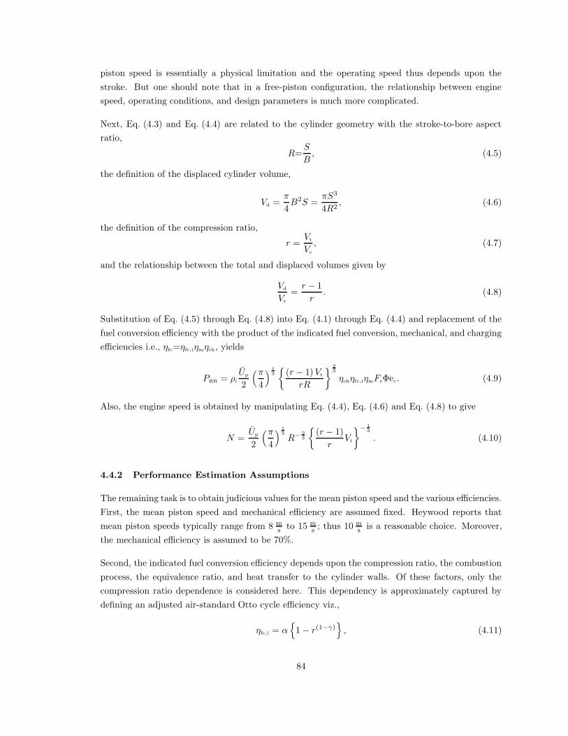
piston speed is essentially a physical limitation and the operating speed thus depends upon the

stroke. But one should note that in a free-piston configuration, the relationship between engine

speed, operating conditions, and design parameters is much more complicated.

Next, Eq. (4.3) and Eq. (4.4) are related to the cylinder geometry with the stroke-to-bore aspect

ratio,

R=S

B, (4.5)

the definition of the displaced cylinder volume,

Vd =π

4B2S =

πS3

4R2, (4.6)

the definition of the compression ratio,

r =Vt

Vc

, (4.7)

and the relationship between the total and displaced volumes given by

Vd

Vt

=r − 1

r. (4.8)

Substitution of Eq. (4.5) through Eq. (4.8) into Eq. (4.1) through Eq. (4.4) and replacement of the

fuel conversion efficiency with the product of the indicated fuel conversion, mechanical, and charging

efficiencies i.e., ηfc=ηfc,iηmηch, yields

PBR = ρi

Up

2

(π

4

)13

(r − 1) Vt

rR

23

ηchηfc,iηmFsΦec. (4.9)

Also, the engine speed is obtained by manipulating Eq. (4.4), Eq. (4.6) and Eq. (4.8) to give

N =Up

2

(π

4

)13

R−23

(r − 1)

rVt

−13

. (4.10)

4.4.2 Performance Estimation Assumptions

The remaining task is to obtain judicious values for the mean piston speed and the various efficiencies.

First, the mean piston speed and mechanical efficiency are assumed fixed. Heywood reports that

mean piston speeds typically range from 8 ms to 15 m

s ; thus 10 ms is a reasonable choice. Moreover,

the mechanical efficiency is assumed to be 70%.

Second, the indicated fuel conversion efficiency depends upon the compression ratio, the combustion

process, the equivalence ratio, and heat transfer to the cylinder walls. Of these factors, only the

compression ratio dependence is considered here. This dependency is approximately captured by

defining an adjusted air-standard Otto cycle efficiency viz.,

ηfc,i = α

1− r(1−γ)

, (4.11)

84

where γ is a mean specific heat ratio and α is an adjustment factor. A reasonable value for α is

0.6 (Taylor, 1985a) and γ=1.3 is assumed. Other factors that affect the indicated fuel conversion

efficiency could be appreciable and they are explored in the second paper.

Next, consider the charging efficiency. This parameter depends upon the mass of fresh charge

delivered to the combustion chamber by the scavenge pump and the fraction of the delivered charge

that is retained in the combustion chamber. These dependencies are captured by the delivery ratio

Λ, and the trapping efficiency ηtr; hence ηch=Ληtr. Unfortunately, both parameters depend strongly

upon the engine design and they are impossible to determine a priori.

Fortunately, physical bounds exist for the charging efficiency (Heywood and Sher, 1999). For in-

stance, if the fresh charge were to completely displace the exhaust, then the charging efficiency and

the delivery ratio would be identical i.e., ηch=Λ. On the other hand, if the fresh charge were to

completely mix with the exhaust, then the charging efficiency is given by

ηch = 1− e−Λ. (4.12)

These extremes represent maximum and minimum bounds for the charging efficiency and the arith-

metic mean of these extremes is a reasonable approximation.

Lastly, the charging efficiency depends upon the delivery ratio. Taylor (1985a) gives

Λ =

(

Ns

N

)(

Ds

Vt

)(

P1

Pe

)(

Ti

T1

)

ηv,s, (4.13)

where Ns, Ds, P1, Pe, Ti, T1, and ηv,s are the scavenging pump speed, scavenging pump displacement

volume, transfer port pressure, exhaust port pressure, intake temperature, transfer port temperature,

and the volumetric efficiency of the scavenging pump, respectively.

Typically, the delivery ratio is found experimentally for a particular engine design and operating

condition. Consequently scavenge pump performance data is scarce. But for a non-supercharged,

crankcase-scavenged two-stroke engine, Taylor recommends Ns

N=1, P1

Pe≈1, and ηv,s=0.5. Also, the

quantity Ds

Vtis approximated by Eq. (4.8) and Ti

T1≈1. Under these assumptions, Eq. (4.13) reduces

to

Λ =

(

r − 1

r

)

ηv,s, (4.14)

and this completes the set of equations and assumptions required for performance estimation.

4.5 Miniature Engine Design

4.5.1 Engine Characteristic Dimension and Compression Ratio

The method developed in the previous section may now be used to obtain specific estimates for

the size and operating speed of a 10W engine. Before proceeding however, consider Eq. (4.9).

This equation implies that PBR depends upon Ti, Pi, Φ, Vt, r, R, Up, ηch, ηfc,i, ηm, ec, and Fs

85

Table 4.1. Sample cylinder bores for Pi=1 atm, Ti=300 K and Φ=0.5 (propane is the fuel).Compression Ratio, r Cylinder Bore, B (mm) Power Output (W)

5 4.97 1010 4.13 1020 3.70 1030 3.53 105 1.57 110 1.31 120 1.17 130 1.12 1

when ρi=ρi(Ti, Pi) is assumed. Characterizing this function in terms of all eleven parameters is an

intractable problem. Consequently the independent variables are grouped into: “Intake Conditions”

(Ti, Pi, Φ), “Fuel” (ec, Fs), and “Engine Design”(

Up, Vt, r, R, ηch, ηfc,i, ηm

)

. The parameter space

may be further reduced by fixing the power output, operating conditions, mechanical efficiency, and

mean piston speed. Finally, propane is assumed to be the fuel throughout this paper. Under these

constraints, Eq. (4.9) reduces to

B2ηchηfc,i =8PBR

πηmFsecρiΦUp

= Const., (4.15)

where Eq. (4.5), Eq. (4.6), and Eq. (4.8) were used to eliminate the aspect ratio R, and displacement

Vt.

Next, recall that ηch and ηfc,i are assumed in Section 4.4.2 to only depend upon the compression ratio.

Consequently B=B (r) which implies that the cylinder bore is a characteristic dimension under these

conditions. To illustrate this dependence, Table 4.1 presents the results of several computations with

an initial temperature and pressure of 300K and 1 atm while the engine is assumed to operate at an

equivalence ratio of 0.5.

In Table 4.1, the cylinder bore decreases with compression ratio. This result is a consequence of the

charging and fuel conversion efficiencies increasing with the compression ratio (Figure 4.3). That

is, increasing the compression ratio causes the fuel conversion efficiency to increase and therefore

permits a smaller engine to deliver the same power—an intuitive result.

Additionally, Figure 4.3 indicates that despite the many crude approximations employed, the overall

fuel conversion efficiency prediction is reasonably accurate for the smallest commercially-available

engine. One should also note that the generally low fuel conversion efficiency is attributable to poor

charging efficiency—a well-known characteristic of two-stroke engines.

4.5.2 Intake Conditions and Power Density

The influence of the intake conditions on the cylinder bore are explored next. Rather than con-

sider each parameter i.e., Ti, Pi, and Φ, separately, their combined effect on engine performance is

86

0 10 20 30 400

10

20

30

40

50

ηfci

η

ch

ηfc

η

fc, Cox 0.010

PSfrag replacements

Compression Ratio, r

Per

cent

Figure 4.3. The dependence of the charging and fuel conversion and efficiencies upon the compressionratio and comparison to the Cox .010 Glow-Ignition Model Airplane engine (Yang, 2000).Note that ηfc=ηfc,iηchηm and that ηm=0.70.

investigated by defining an “intake parameter” viz.,

ζ =ρi

ρΦ =

(

Pi

P

)(

T

Ti

)

Φ, (4.16)

where ρ is the density of air at 300K and 1 atm. Hence this parameter represents the properties of

the fresh charge relative to a stoichiometric mixture at ambient conditions; a convenience because

ζ=1.0 is a maximum value for non-supercharged HCCI engines. Whereas ζ=0.5 is typical for HCCI

engines because the fresh charge is usually preheated and very lean mixtures are employed. One

should note however, that ζ has little if any, physical significance outside the context of performance

estimation.

Next, the cylinder bore is plotted in Figure 4.4 versus ζ and the compression ratio r. Immediately,

one notices that the cylinder bore is minimized when both the compression ratio and ζ are maximized.

The relationship between compression ratio and cylinder bore was already discussed in Section 4.5.1.

On the other hand, ζ captures the effect of charge density. That is, the mass of fuel burned and

hence the work obtained from each cycle increases with ζ. Therefore increasing ζ allows one to

increase the power output of a given engine or substitute a smaller engine in its place.

The relationships between r, ζ, and the cylinder bore are important results because to be consistent

87

0

20

40

00.5

1

0

5

10

15

PSfrag replacements

Compression Ratio,

rIntake Parameter, ζ

Cylinder

Bore

,B

(mm

)

Figure 4.4. The cylinder bore dependence upon the compression ratio and intake conditions for anon-supercharged 10W engine. ζ=1.0 corresponds to Pi=1 atm, Ti=300 K, and Φ=1.0.

with the overall objective of battery replacement, maximizing the power density

Pd=PBR

Vt

=4PBR

πSB2, (4.17)

is a goal. Consequently for fixed power output and stroke, maximizing the power density is equivalent

to minimizing the cylinder bore. This in turn, implies that both r and ζ should be maximized.

According to Figure 4.4, the power density can be increased without bound; obviously, there are

limits. For instance, preheating the fresh charge i.e., Ti>300 K, and using lean mixtures are frequent

requirements for HCCI engines; both decrease ζ. Although, these requirements may be offset to some

extent by supercharging i.e., Pi>1 atm. The degree to which this can be done however, is constrained

by peak cylinder pressures. Moreover, sealing becomes increasingly difficult when the compression

ratio is increased and Figure 4.3 may differ from an HCCI process; the latter possibility is explored

in the second paper.

4.5.3 Estimating the Engine Speed

Thus far, the compression ratio and intake parameter have been shown to be important parameters;

the engine speed is considered here. According to Eq. (4.10), it depends upon the compression ratio,

88

05

10 0

0.5

10

2000

4000

6000

8000

10000

12000

PSfrag replacements

Aspect Ratio, RInt

akePara

meter, ζ

Engin

eSpee

d,N

(Hz)

Figure 4.5. The engine speed dependence upon the aspect ratio and intake conditions for a 10Wengine, r=25. ζ=1.0 corresponds to Pi=1 atm, Ti=300 K, and Φ=1.0.

mean piston speed, total volume, and stroke-to-bore aspect ratio; but simplification yields

NB =Up

2R. (4.18)

Again, the cylinder bore is prominent. Alternatively, substituting Eq. (4.15) into Eq. (4.18) and

rearranging gives

N =U

32p

2R

[

πηmFsecρζ

8PBR

·1

ηchηfc,i

]12

. (4.19)

One may infer from Figure 4.3 however, that the product ηchηfc,i varies from approximately 0.12 to

0.2. Consequently the compression ratio dependence is weak and N≈N (R, ζ) when power output

is fixed. Hence the engine speed is plotted in Figure 4.5 with r=25 assumed. The engine speed

depends strongly upon the aspect ratio, R. Hence one may conclude that the speed is essentially

determined by the aspect ratio in this analysis.

4.5.4 Engine Designs for Fixed Operating Conditions

After exploring the influence of compression ratio, intake parameter, and aspect ratio separately,

combinations of these parameters are now considered. To do this, the intake parameter is fixed and

families of engine designs that deliver 10W are obtained.

For example, consider propane-fueled engines with Φ=0.5, Ti=500 K, and Pi=1 atm (ζ=0.3). As-

89

5 10 15 20 25 30 35 40

1

2

3

4

5

6

7

8

9

10

1595

1293

1041

890

790

689

589

488

387

287

186

136

86PSfrag replacements


Asp

ect

Ratio,R

Figure 4.6. Total cylinder volume, Vt

(

mm3)

required to deliver 10W when operating with a mixtureof propane and air, Φ=0.5, Ti=500 K and Pi=1 atm (ζ=0.3).

Table 4.2. Representative engine designs depicted in Figure 4.6 and Figure 4.7.Compression Ratio, r Aspect Ratio, R Vt

(

mm3)

N (Hz) B (mm)10 5 662 188 5.3310 10 1324 94 5.3335 1 73 1113 4.4935 8 587 139 4.49

suming that the compression ratio and the aspect ratio are free variables, Eq. (4.9) and Eq. (4.10)

are used to generate the displacement and speed “maps” depicted in Figure 4.6 and Figure 4.7.

Specific engine designs are then obtained by choosing a compression ratio and an aspect ratio.

To illustrate, several engine designs are presented in Table 4.2. Note that even though the bore is

independent of aspect ratio, two types of engines are apparent: “small and fast” (large r, small R)

and “big and slow” (small r, large R). To maximize power density, the former variety are preferred.

Performance estimation gives valuable guidance regarding the selection of key design parameters,

but a fundamental question has been neglected: Can an HCCI engine operate within an entire design

map such as Figure 4.6? Intuitively, one would expect not. Consequently the objective of the second

paper is to identify regions in the compression ratio-aspect ratio space where operating conditions

and HCCI are compatible.

90

5 10 15 20 25 30 35 40

1

2

3

4

5

6

7

8

9

10

120

163

206

248

291334

419

547717



Asp

ect

Ratio,R

Figure 4.7. Engine speed, N (Hz) required to deliver 10W when operating with a mixture of propaneand air, Φ=0.5, Ti=500 K and Pi=1 atm (ζ=0.3).

4.5.5 Small-Scale Considerations

In addition to neglecting design-HCCI compatibility, consequences of small engine dimensions have

been overlooked. In the context of micro-combustion, these effects are primarily enhanced heat and

mass transfer rates. Greater heat transfer rates are hypothesized to have two adverse effects on an

HCCI engine: (1) Decrease the effectiveness of compressive heating., and (2) Decrease the indicated

fuel conversion efficiency. The effect of enhanced mass transfer rates however, is unclear. That is,

radicals could be destroyed or produced on the walls and these phenomena yield totally opposite

effects. Further investigation of heat and mass transfer rates is left to the second paper.

Although heat and mass transfer effects are strictly beyond the scope of the present analysis, one can

infer favorable design conditions using geometry. According to Eq. (1.1), the surface-area-to-volume

ratio is the relevant parameter. Referring to Figure 4.2,

r =L

c, (4.20)

and the surface-area-to-volume ratio is given by

As

V=

2

L+

4

B. (4.21)

The clearance distance c, and the stroke however are related by

c =S

r − 1. (4.22)

91

020

40

0

5

10

4

5

6

7

8

PSfrag replacements

Compression Ratio,

rAspect Ratio, R

Dim

ensi

onle

sssu

rface

-are

a-t

o-v

olu

me

ratio,Ψ

Figure 4.8. Non-dimensional surface-area-to-volume ratio function, Eq. (4.25).

Next, using Eq. (4.20), Eq. (4.22), and Eq. (4.5), the total combustion chamber volume becomes

Vt =πrS3

4R2 (r − 1), (4.23)

and substitution of Eq. (4.20), Eq. (4.22), Eq. (4.5) and Eq. (4.23) into Eq. (4.21) and simplification

yields

As

V=

(

π

Vt

)13

2 (r − 1) + 4 (rR)

413 (rR)

23 (r − 1)

13

. (4.24)

Finally, Eq. (4.5), Eq. (4.6), and Eq. (4.8) are used to further simplify Eq. (4.24). Rearrangement

yields

Ψ(r, R) = BAs

V=

2 (r − 1)

rR+ 4

, (4.25)

which is essentially a non-dimensional surface-area-to-volume ratio function.

According to Eq. (1.1), the specific heat transfer rate is smallest when Ψ is minimized. Inspection

of Figure 4.8 reveals that this occurs when large aspect ratios are employed. Also, Figure 4.8 sug-

gests that the compression ratio dependence is weak. In contrast, small aspect ratios maximize

power density (Section 4.5.2). Therefore minimizing heat transfer and maximizing power density

are opposing objectives.

Lastly, the degree to which heat transfer can be decreased by large aspect ratios is limited. That is,

92

Eq. (4.25) has a minimum value of 4, and Ψ is within 5% of this limit when the aspect ratio is 10.

Thus aspect ratios greater than 10 offer almost no benefit.

4.6 Conclusion

This paper has presented a concept for a 10W miniature free-piston engine-compressor and various

considerations for its design. Specific results are summarized as follows:

• Combustion Mode.

In small scales, traditional engine combustion schemes are generally infeasible due to quenching

effects; HCCI is a promising alternative.

• Compression Ratio.

The nominal compression ratio for this engine is a crucial parameter because it determines

the compression history of the charge, affects the fuel conversion efficiency, and establishes

the engine size. On the other hand, it affects neither the engine speed nor the specific heat

transfer rate. Also, HCCI does not have a fundamental compression ratio limitation like SI.

Consequently the compression ratio may be increased virtually without bound. Practically

however, sealing and material properties will impose limits.

• Aspect Ratio.

The performance analysis revealed that for a crankshaft-equipped engine, the stroke-to-bore

aspect ratio establishes the engine speed and it determines the surface-area-to-volume ratio.

More significantly however, small aspect ratios were found to maximize power density while

large aspect ratios were found to minimize heat transfer. Consequently a compromise must be

sought between maximizing power density and minimizing heat transfer rates. Also, essentially

no further reduction in heat transfer may be achieved with aspect ratios greater than 10.

Finally, HCCI depends strongly upon engine operation and design. Small scales are expected to

impose additional constraints. Consequently the next step is to investigate these aspects in detail.

93

Chapter 5

Modeling HCCI Combustion in

Small-Scales with Detailed

Homogeneous Gas Phase Chemical

Kinetics

5.1 Abstract

Operational maps for crankshaft-equipped miniature homogeneous charge compression ignition en-

gines are established using performance estimation, detailed chemical kinetics, and diffusion models

for heat transfer and radical loss. In this study, radical loss was found to be insignificant. In

contrast, heat transfer was found to be increasingly significant for 10W, 1W, and 0.1W engines, re-

spectively. Also, temperature-pressure trajectories and ignition delay time maps are used to explore

relationships between engine operational parameters and HCCI. Lastly, effects of engine operating

conditions and design on the indicated fuel conversion efficiency are investigated.

5.2 Introduction

This paper (Aichlmayr et al., 2002c) is the second in a two-part series that presents results of recent

small-scale engine research and development activities conducted at the University of Minnesota.

The first paper (Aichlmayr et al., 2002b, or Chapter 4) presented a 10W Homogeneous Charge

Compression Ignition (HCCI) engine-compressor concept and used performance estimation to ex-

plore various aspects of miniature engine design. The analysis however, did not couple HCCI and

operating parameters or account for phenomena such as enhanced heat transfer rates. Consequently

the objective of this paper is to mitigate these shortcomings by combining performance estimation

with a model for small-scale HCCI combustion, resulting in plausible operational maps for miniature

94

engines.

This paper is organized as follows: First, the HCCI model employed in this study is described.

Second, models for heat transfer and radical loss in small volumes are developed. Third, relationships

between engine operating parameters and HCCI combustion are explored. Fourth, operational

maps for miniature HCCI engines are established. Finally, miniature HCCI engine performance is

discussed.

5.3 Modeling HCCI Combustion

In contrast to transport-limited engine combustion modes such as spark ignition and Diesel, HCCI

depends primarily upon the compression process and fuel oxidation kinetics. Therefore matching

engine operating conditions and HCCI combustion is essentially a reaction engineering problem.

Generally, there are two HCCI modeling strategies: Homogeneous and Multi-Zone. The distinction

between them is whether gradients are assumed to exist in the combustion chamber i.e., the multi-

zone does while the homogeneous does not.

5.3.1 Homogeneous Models

Typically, homogeneous models are developed by considering the combustion chamber to be a

variable-volume batch reactor and selecting an appropriate kinetic mechanism. Hence these mod-

els integrate the time-dependent energy and species conservation equations to yield temperature,

pressure, and concentration histories for the charge. Najt and Foster (1983) are credited with estab-

lishing this paradigm and demonstrating that HCCI could be explained using hydrocarbon kinetics.

Their efforts were followed by Lu et al. (1994) who employed Chemkin-II and a detailed hydrogen-

air mechanism to investigate the role of hydrogen peroxide and radical species in HCCI. Lu et al. in

turn, were followed by several investigations that used HCT (Lund, 1978), detailed chemical kinet-

ics, and bulk heat loss via the Woschni (1967) correlation (Smith et al., 1997; Aceves et al., 1999;

Flowers et al., 1999, 2000; Martinez-Frias et al., 2000). Additionally, Kelly-Zion and Dec (2000)

used Chemkin-III (Kee et al., 1996), Senkin (Lutz et al., 1988) and detailed kinetic mechanisms for

iso-octane and n-heptane oxidation to determine the suitability of single-stage and two-stage ignition

fuels for HCCI.

5.3.2 Multi-Zone Models

The strengths of homogeneous models include the ability to predict changes in ignition timing and

the capability to investigate the chemistry of HCCI combustion (Lu et al., 1994; Aceves et al., 1999;

Flowers et al., 1999, 2000; Kelly-Zion and Dec, 2000; Martinez-Frias et al., 2000). Unfortunately,

homogeneous models fail to accurately predict burn duration, peak cylinder pressure, indicated fuel

conversion efficiency, and CO and hydrocarbon emissions (Christensen et al., 1998; Aceves et al.,

1999). Aceves et al. (1999) attribute these limitations to neglecting gradients i.e., inhomogeneity, in

the combustion chamber.

95

Therefore to capture effects of charge inhomogeneity, Aceves et al. (2000) develope a multi-zone

HCCI model. The salient features of this model include the partitioning of the combustion chamber

into several homogeneous, variable-volume, batch reactors and the sequential use of KIVA (Amsden,

1993) and HCT. Initially, the distribution of mass among the zones and the initial temperature

field are determined by KIVA. HCT subsequently computes temperature and species concentration

histories for individual zones. Also, heat and mass transfer between zones is neglected to minimize

computational requirements, but each zone features a bulk heat sink based upon the Woschni corre-

lation. Aceves et al. find excellent correspondence between model predictions and the experimental

results of Christensen et al. (1998).

Aceves et al. provide many significant contributions to the understanding of HCCI. First, they give

the following sequence by which HCCI combustion proceeds: (1) Chemical reactions are initiated

in the center of the combustion chamber because it is the hottest.; (2) The central zone expands to

compress adjacent zones.; (3) Adjacent zones are heated by compression and chemical reactions are

initiated shortly afterward.; (4) Once reactions commence, these zones also expand and compress

their neighbors.; (5) The process repeats until the fuel in adjacent zones fails to react—which results

in relatively large hydrocarbon emissions. Second, Aceves et al. link the ignition event to the de-

composition of hydrogen peroxide and thus explain observed similarities in the behavior of various

hydrocarbon fuels. Finally, Aceves et al. find that with the exception of CO and hydrocarbon emis-

sions, the multi-zone model resolves many discrepancies between predictions and experiments. Con-

sequently this modeling approach has been widely adopted (Noda and Foster, 2001; Amano et al.,

2001; Kong et al., 2001; Aceves et al., 2001a; Easley et al., 2001; Fiveland and Assanis, 2001).

5.3.3 Engine Cycle Models

Despite their individual merits, homogeneous and multi-zone models consider only one compression-

expansion cycle. Consequently ancillary but significant processes intrinsic to the engine cycle are ne-

glected or inappropriately modeled (Fiveland and Assanis, 2000). In contrast, an engine cycle model

attempts to capture all events that occur during the cycle and may employ either the homogeneous or

multi-zone approach. Examples include the free-piston engine model of Goldsborough and Van Blarigan

(1999) and the four-stroke engine model of Fiveland and Assanis.

5.4 The Miniature HCCI Engine Model

Although much progress has been made in understanding HCCI, the current knowledge base gener-

ally does not apply to miniature engines. For example, miniature engines are anticipated to operate

between 300Hz (18,000RPM) and 2000Hz (120,000RPM). Whereas most full-size HCCI engines

operate at approximately 1000RPM. Consequently relationships between chemical times and the

engine cycle will be different. Additionally, compression ratios of 30:1 or higher, are desirable in

miniature engines while compression ratios of conventional engines seldom exceed 25:1. Finally,

miniature engines feature large surface-area-to-volume ratios. Hence accurate modeling of heat and

mass transfer rates in these circumstances is vital and widely-used models like the Woschni (1967)

96

correlation are inapplicable.

The objective of this work is to find combinations of operating and design conditions that are

compatible with HCCI. Therefore the present work focuses upon the auto-ignition of the charge and

investigations of charge inhomogeneity and regulated emissions such as NOx, are deferred to future

work. Consequently the homogeneous modeling approach is adopted and the collection of batch

reactor codes that comprise Senkin (Lutz et al., 1988) and detailed gas-phase kinetics are employed.

5.4.1 Model Formulation

To include effects such as heat transfer and radical loss, Senkin is modified as follows: First, the

governing equations for a non-isothermal, non-adiabatic batch reactor (closed system) are mass

conservation,dYk

dt− vωkWk = 0, (5.1)

and the First Law of Thermodynamics for a simple compressible system viz.,

du

dt=

δq

dt−

δw

dt. (5.2)

Where Yk and ωk are the mass fractions and net production rates of species k, respectively. Next,

the term on the left hand side of Eq. (5.2) is given by

du

dt=

Ns∑

k=1

uk

dYk

dt+

Ns∑

k=1

Yk

duk

dt. (5.3)

Substitution of Eq. (5.3) and Eq. (5.1) into Eq. (5.2) yields

dT

dt+

v

cv

Ns∑

k=1

ukωkWk +P

cv

dv

dt−

1

cv

δq

dt= 0, (5.4)

after simplification. Consequently when a mechanism of Ns species is used, Eq. (5.4) and Eq. (5.1)

comprise a set of Ns+1 non-linear ordinary differential equations; integration yields T (t) and Yk(t).

Note that several batch reactor models may be derived from Eq. (5.4). For example, discarding

both work and heat transfer terms results in a fixed-volume adiabatic batch reactor model. On the

other hand, if slider-crank kinematics (Heywood, 1988, or Section B.3) are used to define V (t), then

a model for a crankshaft-equipped HCCI engine results1.

5.4.2 Heat Transfer Model

To model heat transfer in a miniature engine, several approaches with varying levels of complexity

may be taken. To be consistent with the objectives of this study however, the heat transfer model

1One should note that in this chapter, v(t) is directly proportional to V (t) because the mass of the control volumeis constant.

97

PSfrag replacements

r

z

T (r, z, t) B2

L2

Figure 5.1. Axisymmetric region used to develop the conduction model.

should be relatively simple, yet capture the surface-area-to-volume ratio dependence. To this end,

conduction is assumed to be the dominant heat transfer mode. This assumption is tenable because

conduction from the charge to an isothermal wall represents a “worst case” scenario in terms of heat

loss.

The conduction model is developed thusly. Consider a combustion chamber of length L and bore B

divided into axisymmetric regions like Figure 5.1. Next, the partial differential equation

1

α

∂T

∂t= ∇2T, (5.5)

is solved within the domain using well-known analytical techniques and the boundary conditions

T (r, z, 0) = T0, T (0, z, t) Finite,

∂T

∂z

∣

∣

∣

∣

z=0

= 0,∂T

∂φ= 0,

T (B/2, z, t) = Tw, T (r, L/2, t) = Tw,

that result from assuming a uniform initial temperature, symmetry, and isothermal walls. The

solution is

T (r, z, t) = Tw +16 (T0 − Tw)

B

∞∑

m=0

∞∑

n=1

(−1)m J0 (βnr) cos (ηmz) exp(

−α(

β2n + η2

m

)

t)

(2m + 1) πβnJ1

(

βnB2

) . (5.6)

Next, an average wall heat flux is derived by: (1) Considering only the initial rate (t=0)., (2)

Retaining only the first term of the double-infinite series i.e., m=0 and n=1., (3) Computing the

total wall heat flux., and (4) Dividing the total wall heat flux by the surface area of the combustion

98

chamber. This yields

¯′′q =2kT (T0 − Tw)

L

[

0.440332π2 + 5.09296 (L/B)2

π + 2π (L/B)

]

. (5.7)

One should note that although Eq. (5.7) is based upon the premise that t=0, the expression is quasi

time-dependent because L and kT vary with time. Also, T0 is equivalent to the bulk temperature by

assumption.

Lastly, the specific heat transfer rate appearing in Eq. (5.4) is related to Eq. (5.7) by

δq

dt=

(

Surface Area

System Mass

)

¯′′q, (5.8)

where the surface area is given by

As =πB2

2+ πBL. (5.9)

The relationship between heat transfer and the combustion chamber geometry may be further ex-

plored by substituting Eq. (5.9), Eq. (5.7), and the identity L/B= (r/r−1) R into Eq. (5.8) and rear-

ranging. The result is a non-dimensional heat transfer rate defined by

Ξ (r, R) =B2

vkT (T0 − Tw)

δq

dt= Ψ (r, R)

[

2 (r − 1)

rR

]

0.440332π2 + 5.0926 (rR/r−1)2

π + 2π (rR/r−1)

. (5.10)

Hence the non-dimensional heat transfer rate is proportional to the non-dimensional surface-area-

to-volume ratio (Ψ) and it depends exclusively upon the compression ratio and the aspect ratio. For

comparison, both Ξ and Ψ are plotted in Figure 5.2. Evidently, large aspect ratios tend to minimize

heat transfer because Ξ decreases with R. Moreover, this effect is greatest for R<2 and disappears

when R>3. Thus 2≤R≤3 appears to be optimal. Additionally, Figure 5.2 indicates that this result

is essentially independent of the compression ratio.

5.4.3 Radical Loss Model

Diffusion fluxes also increase with surface-area-to-volume ratio. Therefore assuming that radical

recombination reactions on the combustion chamber walls are mass transfer-limited, the frequency

of these events are hypothesized to increase with the surface-area-to-volume ratio. This effect is

modeled by assuming the walls to be perfect radical sinks and that diffusion dominates.

99

0 1 2 3 4 50

5

10

15

20

25

30Ξ(5,R) Ψ(5,R) Ξ(10,R) Ψ(10,R)Ξ(50,R) Ψ(50,R)

PSfrag replacements

Ψor

Ξ(d

imen

sionle

ss)

Aspect Ratio, R

Figure 5.2. Non-dimensional specific heat transfer rate (Ξ) and surface area to volume ratio function(Ψ).

Hence diffusion-limited pseudo-reactions such as

H →WALLH, (R2)

involving fictitious species (WALLH) are inserted into the kinetic mechanism. Next, the heat and

mass transfer analogy is used to obtain pseudo-heterogeneous reaction rates from Eq. (5.7) e.g.,

r′′R2 =2DH-Air

L

[

0.440332π2 + 5.09296 (L/B)2

π + 2π (L/B)

]

[H] . (5.11)

These rates are incorporated into the kinetic mechanism via pseudo-homogeneous reaction rates

(Schmidt, 1998) such as

rR2 =

(

As

V (t)

)

r′′R2

, (5.12)

where the surface-area-to-volume-ratio is given by

As

V (t)=

2

L+

4

B. (5.13)

Lastly, the following is done to implement radical losses in Senkin: (1) “Wall” species are assumed

100

to have thermodynamic properties identical to their authentic counterparts., (2) Temperature de-

pendent terms of the pseudo-reaction rates are included in the kinetic mechanism while pressure

and geometry-dependent parts are incorporated in the source code., (3) Transport properties of

the charge are assumed identical to air and the Fuller et al. (1966) correlation is used to estimate

diffusion coefficients.

5.5 Factors Which Affect HCCI In a Miniature Engine

To achieve HCCI, the charge must be brought by compression to a thermodynamic state such

that the ignition delay time is short relative to the residence time. Therefore in contrast to typical

reaction engineering problems, the bulk temperature, chemical time, and residence time are variables.

Additionally, HCCI depends strongly upon the initial conditions and the compression ratio. Hence

relationships between the various parameters and HCCI are seldom obvious; an attempt to clarify

them is made in this section.

Throughout this paper and the previous one, the fuel is assumed to be propane. Consequently a

mechanism developed by Westbrook (1999) is used and nitrogen chemistry is added (Turns, 2000).

The resulting mechanism is comprised of 394 species and 1909 reactions. Propane is chosen because

it has a comparatively low molecular weight and thus favorable compressive heating characteris-

tics. Propane also exhibits essentially single-stage ignition due to mild low-temperature reactivity.

Hence it offers many advantages e.g., large compression ratios may be used, for HCCI applications

(Kelly-Zion and Dec, 2000).

5.5.1 Ignition Delay Time, Equivalence Ratio, and Compressive Heating

First, consider the chemical time—or in the context of HCCI—the kinetic ignition delay time. HCCI

is not characterized by a fixed ignition delay time because the temperature and pressure of the charge

vary during compression. Temperature- and pressure-dependent ignition delay times however, may

be readily estimated using an homogeneous, fixed-volume batch reactor model. The results of several

simulations with Φ=1.0 and Φ=0.2 are presented in Figure 5.3 and Figure 5.4, respectively.

According to Figure 5.3 and Figure 5.4, ignition delay times for a given temperature and pressure

increase when the equivalence ratio decreases. Therefore if the time available for reaction and all

other variables were fixed, one would expect a stoichiometric charge to ignite sooner than a lean

charge. To test this hypothesis, an adiabatic, variable-volume batch reactor model is used to simulate

engine operation with charges having equivalence ratios of 0.2, 0.4, 0.6, 0.8, and 1.0. The results are

presented in Figure 5.5.

Although ignition may be defined in several ways, here it is assumed to coincide with the appearance

of a sudden temperature rise i.e. a “spike.” Consequently one may deduce from Figure 5.5 that

mixtures with equivalence ratios of 0.2 and 0.4 ignite while the others do not—an unexpected result.

Of the mixtures considered in Figure 5.5, one would assume from Figure 5.3 and Figure 5.4 that

101

700 800 900 1000 1100

20

40

60

80

100

120

140 25

7

10

17

2941

PSfrag replacements

Temperature (K)

Pre

ssure

(atm

)

Figure 5.3. Ignition delay time map for a stoichiometric mixture of propane and air. Ignition delaytimes are reported in milliseconds.

the stoichiometric mixture has the shortest ignition delay time and therefore it should ignite—yet

it does not. The explanation for this counterintuitive result is that the charges do not reach the

same temperature following compression. To illustrate, mixture specific heats increase with equiv-

alence ratio. Consequently for equal compression ratios, a mixture with Φ=0.4 will have a greater

temperature following compression and therefore a shorter ignition delay time, than a stoichiometric

mixture (Figure 5.6). Incidentally, compressive heating also causes a mixture with Φ=0.2 to ignite

before Φ=0.4. One should note however, that combustion is very weak because there is little fuel to

consume.

102

700 800 900 1000 1100 1200

20

40

60

80

100

120

140

38

1315

1823

25

20

PSfrag replacements

Temperature (K)

Pre

ssure

(atm

)

Figure 5.4. Ignition delay time map for a mixture of propane and air with Φ=0.2. Ignition delaytimes are reported in milliseconds.

0 0.2 0.4 0.6 0.8 1

500

1000

1500

2000

Φ=0.2Φ=0.4Φ=0.6Φ=0.8Φ=1.0

PSfrag replacements

Tem

per

atu

re(K

)

Non-Dimensional Cycle Time, t∗=t/τC

Figure 5.5. Temperature profiles for an adiabatic, variable volume batch reactor model. Variousequivalence ratios are considered for combustion of propane and air, Ti=400 K, Pi=1 atm,N=500 Hz, and r=30 is assumed. The non-dimensional cycle time is defined t∗=t/τC; 0.5corresponds to the top dead center (TDC) position in slider-crank piston motion.

103

0 10 20 30 40 50400

600

800

1000

1200

1400

1600Φ=1.0Φ=0.8Φ=0.5Φ=0.2

PSfrag replacements

Tem

per

atu

re(K

)

Compression ratio, r

Figure 5.6. Isentropic compression temperatures of propane-air mixtures obtained with Equil(Lutz et al., 1998); Ti=400 K and Pi=1 atm assumed.

104

0 0.2 0.4 0.6 0.8 1

500

1000

1500

2000

2500

3000T

i=300 K

Ti=400 K

Ti=450 K

Ti=500 K

Ti=600 K

PSfrag replacements

Tem

per

atu

re(K

)


Figure 5.7. Temperature profiles for an adiabatic, variable volume batch model. Various initialtemperatures are considered. A stoichiometric mixture of propane and air with an initialpressure of 1 atm, compression ratio of 30:1, and engine speed of 500Hz is assumed. Thenon-dimensional cycle time is defined t∗=t/τC; 0.5 corresponds to the top dead center(TDC) position of the piston.

5.5.2 Initial Temperature

Next, the influence of the initial temperature is investigated using the adiabatic variable volume

batch reactor model. Temperature-cycle time profiles for stoichiometric mixtures of propane and

air are plotted in Figure 5.7. For these conditions, Ti=450 K is evidently the minimum initial

temperature for ignition. Also note that if the temperature is increased beyond this value, ignition

occurs sooner in the cycle, or it is said to be “advanced.” This property is the basis for variable

intake temperature control strategies.

Although the connection between operating parameters and fuel oxidation kinetics in HCCI is widely

recognized, the nature of the relationship is difficult to discern. One approach to visualize this

interaction is to consider temperature-pressure traces—or trajectories—superimposed onto ignition

delay time maps e.g., Figure 5.8. Note that in this representation, ignition is indicated by a trajectory

which does not terminate.

An examination of the trajectories in Figure 5.8 reveals that the initial temperature affects both the

curvature and the termini of the trajectories. Consequently if the initial temperature were increased,

the terminus of a trajectory would be translated to the right i.e., toward increasingly shorter ignition

delay time contours. Therefore the extreme initial temperature sensitivity of HCCI may be broadly

attributed to the steepness of the ignition delay time surface.

105

400 600 800 1000 1200 1400 1600 1800

20

40

60

80

100

120

140

160

0.10

0.220.49

1.10

2.45

5.4512.1226.97

60.00

Ti=300 K

Ti=400 K

Ti=450 K

Ti=500 K

Ti=600 K

PSfrag replacements

Temperature (K)

Pre

ssure

(atm

)

Figure 5.8. Temperature-pressure trajectories superimposed on the ignition delay time map for astoichiometric mixture of propane and air; initial temperature variations considered.Ignition delay times are reported in milliseconds.

5.5.3 Initial Pressure

The influence of the initial pressure is investigated in a similar manner. Initial pressures of 1 atm,

2 atm, 4 atm, 5 atm, and 8 atm are simulated and the resulting temperature-pressure trajectories are

plotted in Figure 5.9. Like the initial temperature, the initial pressure affects both the curvature and

termini of the trajectories. In this case however, the termini are translated to the left and virtually

parallel to ignition delay time contours. Consequently ignition delay times do not appreciably

decrease when the initial pressure is increased. Therefore HCCI is relatively insensitive to the initial

pressure. This result bodes well for supercharging because the power density can be substantially

increased without affecting the ignition timing.

106

400 600 800 1000 1200 1400 1600 1800

20

40

60

80

100

120

140

1600.10

0.220.49

1.10

2.45

5.4512.1226.97

60.00

Pi=1 atm

Pi=2 atm

Pi=4 atm

Pi=5 atm

Pi=8 atm

PSfrag replacements

Temperature (K)

Pre

ssure

(atm

)

Figure 5.9. Temperature-pressure paths superimposed on the ignition delay time map for a stoichio-metric mixture of propane and air; initial pressure variations considered. Ignition delaytimes are reported in milliseconds.

107

0 0.2 0.4 0.6 0.8 1

500

1000

1500

2000

2500

3000 r=10r=20r=30r=40r=50

PSfrag replacements

Tem

per

atu

re(K

)


Figure 5.10. Temperature profiles for an adiabatic, variable volume batch model. Various compres-sion ratios are considered. A stoichiometric mixture of propane and air with an initialtemperature and pressure of 350K and 1 atm, respectively. The engine speed is held at500Hz. The non-dimensional cycle time is defined t∗=t/τC; 0.5 corresponds to the topdead center (TDC) position of the piston.

5.5.4 Compression Ratio

Although fixed in a conventional engine, the compression ratio is considered here to be an operating

parameter. Its influence on HCCI is also investigated using the adiabatic variable volume batch

reactor model. Results of simulations with compression ratios ranging from 10 to 50 are presented

in Figure 5.10.

Initially, one may conclude that varying the compression ratio is equivalent to varying the initial

temperature because Figure 5.10 resembles Figure 5.7. This supposition however, is invalidated

upon inspection of Figure 5.11. That is, in contrast to varying the initial temperature, varying

the compression ratio preserves the shapes of trajectories and instead defines where they termi-

nate. Consequently any properly-directed trajectory can be made to terminate in a region with a

sufficiently short ignition delay time by increasing the compression ratio.

The preceding result is significant because it implies that ignition can be moderated in a virtually

arbitrary manner if the compression ratio is a variable. To exploit this feature however, an engine

must have an infinitely variable compression ratio. Free-piston engines satisfy this requirement and

therefore offer great potential to be practical HCCI engines.

Lastly, variations in the engine speed are considered. Although ignition is not observed when a

certain engine speed is exceeded, engine speed affects neither the shape nor the termini of trajectories.

108

400 600 800 1000 1200 1400 1600 1800

20

40

60

80

100

120

140

160

0.100.22

0.491.102.45

5.45

12.1226.97

60.00

r=10r=20r=30r=40r=50

PSfrag replacements

Temperature (K)

Pre

ssure

(atm

)

Figure 5.11. Temperature-pressure paths superimposed on the ignition delay time map for a stoichio-metric mixture of propane and air. Ignition delay times are reported in milliseconds.

This result is expected because the engine speed is akin to a residence time. Therefore it determines

the ignition delay time required for ignition, but otherwise does not affect HCCI.

109

5.6 Operational Maps for Miniature HCCI Engines

The first paper established design maps consisting of combinations of compression ratio and aspect

ratio for 10W engines. All combinations of these parameters however, are not expected to be

serviceable. Consequently engine designs are classified according to feasibility in this section.

5.6.1 Radical Losses

Despite the enhancement of mass transfer rates by large surface-area-to-volume ratios, radical losses

are found to be negligible for a 10W engine. In short, radical removal is much slower than radical

production and ignition proceeds normally. In light of this result and the enormous computational

effort required to obtain it, radical losses are henceforth neglected.

5.6.2 Operational Maps

To systematically evaluate engine designs for compatibility with HCCI, simulations are conducted

in the following way: First, a set of intake conditions i.e., an initial temperature, pressure, and

equivalence ratio, are assumed. Second, pairs of aspect ratio and compression ratio (designs) are

selected for evaluation. Third, engine dimensions and operating speeds are computed for the selected

designs using performance estimation. Fourth, a simulation is conducted. Fifth, the engine design

is designated “Ignition” or “No-Ignition,” depending upon the result of the simulation. Lastly,

indicated fuel conversion efficiencies are computed. Also, both adiabatic and diathermal cases are

considered.

5.6.2.1 Adiabatic 10W HCCI Engines—Cycle and Ignition Delay Times

An operational map for 10W engines with Φ=0.5, Ti=500 K, and Pi=1 atm is presented in Figure 5.12.

Note that this map corresponds to the design map presented in the first paper and that values for

the intake parameter (ζ=ρi/ρΦ), are given for comparison.

Consistent with expectations, not all engine designs in Figure 5.12 are serviceable. In this case, the

incompatibility of HCCI and engine designs may be attributed entirely to time effects i.e., cycle and

ignition delay times, because heat transfer is excluded. First, consider the non-dimensional cycle

time given by

Ω (R) =Up

NB= 2R. (5.14)

This parameter depends exclusively upon the aspect ratio and demonstrates that the cycle time

(1/N), is directly proportional to R when Up, ζ, and r are fixed (B=B (r, ζ)). Hence along the line

r=15, R=5 corresponds to the minimum cycle time (maximum engine speed) that is compatible

with HCCI under these conditions; specifically, it is 5 ms (N=202 Hz). Similarly, R=1 and R=0.5

yield minimum cycle times of 0.95ms (N=1050 Hz) and 0.46ms (N=2200 Hz) when r=20 and r=30,

respectively.

110

5 10 15 20 25 30 35 40

1

2

3

4

5

6

7

8

9

10

1595

1293

1041

890

790

689

589

488

387

287

186

136

86

Ignition No Ignition

PSfrag replacements


Asp

ect

Ratio,R

Figure 5.12. Operational map for an adiabatic 10W miniature HCCI engine operating with propaneand air; Φ=0.5, Ti=500 K, and Pi=1 atm (ζ=0.3) is assumed. Contours indicate Vt inmm3.

Next, ignition delay times decrease with compression ratio because compressive heating increases.

Consequently minimum cycle times also decrease with compression ratio. To illustrate, Figure 5.13

and Figure 5.14 show that compressive heating depends upon the equivalence ratio, initial conditions,

and compression ratio, but not the aspect ratio. Hence vertical lines in Figure 5.12 correspond to

fixed post-compression temperatures and thus represent constant ignition delay times.

To conclude, the compatibility of an engine design with HCCI implies that the cycle time exceeds the

ignition delay time. Cycle times increase with R along lines of constant compression ratio. Ignition

delay times decrease with compression ratio, but are constant along lines of constant r. Designs such

as r=15 and R=5, indicate that the cycle time slightly exceeds the ignition delay time. Therefore,

any design having r>15 and R>5 will be compatible with HCCI; similar arguments apply to the

designs r=20, R=1, and r=30, R=0.5.

5.6.2.2 Heat Transfer

Heat transfer further constrains operational maps because it offsets compressive heating. This effect

is illustrated in Figure 5.15 where a wall temperature of 300K is assumed. One should note that

Figures 5.12 5.15 have a similar appearance, but the designs (r=20, R=1) and (r=30, R=0.5) are

excluded from the regions of operation. Thus post-compression temperatures are sufficiently reduced

that ignition does not occur. Alternatively, the design (r=15, R=5) is included in the regions of

operation in both Figures 5.12 and 5.15; hence this limit is a consequence of time effects.

111

0

20

40

200

400

600

8000

500

1000

1500

2000

PSfrag replacements

Compression Ratio,

r

Intake Temperature, Ti (K)

Fin

alTem

per

atu

re,T

f(K

)

Figure 5.13. The compressive heating of a stoichiometric propane-air mixture—effect of initial tem-perature (Pi=1 atm).

5.6.3 Intake Conditions and Operational Maps

Initial conditions also affect engine operational maps. To illustrate, operational maps corresponding

to initial temperatures of 400K, 450K, and 500K are presented in Figure 5.16. Also, equivalence

ratios are held at 0.5 to facilitate comparison to Figure 5.12, but one should recognize that each

plane appearing in Figure 5.16 represents an engine design map because cylinder volumes and op-

erating speeds vary with the initial conditions. According to Figure 5.16, decreasing the initial

temperature contracts the boundaries of operational maps. This result is expected because the ter-

mini of temperature-pressure trajectories are translated into regions with longer ignition delay times

(Figure 5.8).

Next, initial temperatures are held at 500K but equivalence ratios of 0.2, 0.5, 0.8, and 1.0 are

considered. The resulting maps are plotted in Figure 5.17 and the equivalence ratio is again observed

to have a counter-intuitive effect. That is, regions of operation are extended when the equivalence

ratio is decreased. This effect is attributable to compressive heating, but one should again recognize

that combustion becomes very weak when the equivalence ratio is reduced.

112

0

20

40

0

0.5

10

500

1000

1500

PSfrag replacements

Compression Ratio,

rEquivalence Ratio, Φ

Fin

alTem

per

atu

re,T

f(K

)

Figure 5.14. The compressive heating of propane-air mixtures—effect of equivalence ratio (Ti=300 Kand Pi=1 atm).

5 10 15 20 25 30 35 40

1

2

3

4

5

6

7

8

9

10

1595

1293

1041

890

790

689

589

488

387

287

186

136

86


PSfrag replacements


Asp

ect

Ratio,R

Figure 5.15. Operational map for a 10W miniature HCCI engine operating with propane and air;Φ=0.5, Ti=500 K, Pi=1 atm (ζ=0.3), and Tw=300 K is assumed. Contours indicate Vt

in mm3.

113

20

30

40

0

5

10400

420

440

460

480

500

PSfrag replacements

Compression Ratio,

rAspect Ratio, R

Initia

lTem

per

atu

re,T

i(K

)

Figure 5.16. Operational maps for a 10W miniature HCCI engine operating with propane and air,Φ=0.5, Pi=1 atm, and Tw=300 K are assumed. The shaded areas indicate regions ofoperation. Also note that although cylinder volumes are not shown, they vary with theinitial temperature.

2030

40

05

100.2

0.4

0.6

0.8

1

PSfrag replacements

Compression Ratio,

rAspect Ratio, R

Equiv

ale

nce

Ratio,Φ

Figure 5.17. Operational maps for a 10W miniature HCCI engine operating with propane and air,Ti=500 K, Pi=1 atm, and Tw=300 K are assumed. The shaded areas indicate regions ofoperation. Also note that although cylinder volumes are not shown, they vary with theequivalence ratio.

114

5 10 15 20 25 30 35 40

1

2

3

4

5

6

7

8

9

10

5244

38 3330

27

23

20

17

14

11

76

4

3

9


PSfrag replacements


Asp

ect

Ratio,R

Figure 5.18. Operational map for a 1W miniature HCCI engine operating with propane and air,Φ=0.5; Vt in mm3, intake conditions of Ti=500 K, Pi=1 atm (ζ=0.3), and Tw=300 Kassumed. Contours indicate Vt in mm3.

5.6.4 How Small Can an Engine Be?

Thus far, effects of heat transfer have been relatively small. According to Eq. (5.10) however, the

specific heat transfer rate greatly increases when the engine size or aspect ratio is reduced. Therefore

one may hypothesize that heat transfer will ultimately limit the engine size.

To substantiate this hypothesis, simulations are conducted with fixed initial conditions and the

power output constrained to be 1W or 0.1W. When this is done, performance estimation demands

that characteristic dimensions decrease and operating speeds increase. For example, a 10W engine

with R=5 and r=20 has a bore of 4.8mm and it operates at 209Hz. A 1 W version however, has

B=1.5 mm and N=662 Hz while a 0.1W version has B=0.5 mm and N=2095 Hz. Consequently

reducing the engine size immediately implies that ignition delay times must decrease and one would

expect that greater compression ratios will be necessary.

An operational map for a 1W engine is presented in Figure 5.18. In comparison to Figure 5.15,

the region of operation is significantly reduced. To determine the contribution from heat transfer,

corresponding adiabatic cases are plotted in Figure 5.19. Immediately, one notices that heat transfer

increases the minimum aspect ratio that is compatible with HCCI. For example, when r=20 this

threshold increases from R≥5 in Figure 5.19 to R≥10 in Figure 5.18. Additionally, heat transfer

excludes designs with R<2 irrespective of the compression ratio.

Similarly, an operational map for a 0.1W engine is presented in Figure 5.20. Again, the region of

115

5 10 15 20 25 30 35 40

1

2

3

4

5

6

7

8

9

10

5244

38 3330

27

23

20

17

14

11

76

43

9


PSfrag replacements


Asp

ect

Ratio,R

Figure 5.19. Operational map for an adiabatic 1W miniature HCCI engine operating with propaneand air, Φ=0.5; Vt in mm3, intake conditions of Ti=500 K and Pi=1 atm (ζ=0.3).Contours indicate Vt in mm3.

operation is substantially reduced compared to Figure 5.18 and Figure 5.15. In fact, compression

ratios less than 50 are infeasible. Examining the adiabatic cases in Figure 5.21 reveals that the

reduced region of operation is largely attributable to heat transfer. Hence the minimum engine size

is essentially limited by heat transfer and the essence of the hypothesis is confirmed. One should

note however, that an absolute minimum engine size has not been established because the effects of

many parameters have not been considered.

116

10 20 30 40 50

1

2

3

4

5

6

7

8

9

10

1.49

1.24

1.04

0.89

0.79

0.64

0.54

0.44

0.34

0.23

0.130.08


PSfrag replacements


Asp

ect

Ratio,R

Figure 5.20. Operational map for a 0.1W miniature HCCI engine operating with propane and air,Φ=0.5; Vt in mm3, intake conditions of Ti=500 K, Pi=1 atm (ζ=0.3), and Tw=300 Kassumed. Contours indicate Vt in mm3.

10 20 30 40 50

1

2

3

4

5

6

7

8

9

10

1.49

1.24

1.04

0.89

0.79

0.64

0.54

0.44

0.34

0.23

0.130.08


PSfrag replacements


Asp

ect

Ratio,R

Figure 5.21. Operational map for an adiabatic 0.1W miniature HCCI engine operating with propaneand air, Φ=0.5; Vt in mm3, intake conditions of Ti=500 K and Pi=1 atm (ζ=0.3).Contours indicate Vt in mm3.

117

5 10 15 20 25 30 35 40

1

2

3

4

5

6

7

8

9

10

9

15

20

26

3137

42

5370

97135

PSfrag replacements


Asp

ect

Ratio,R

Figure 5.22. Power density, Pd

(

Wcm3

)

for a 10W engine operating with a mixture of propane andair, Φ=0.5, Ti=500 K and Pi=1 atm (ζ=0.3).

5.7 Miniature HCCI Engine Performance

Although operational maps establish where in the engine design space one may operate a miniature

HCCI engine, they do not provide any guidance with regard to selecting a design. To that end,

power density maximization is considered here.

Recall that power density Pd=PBR/Vt, depends upon the compression ratio, aspect ratio, and ini-

tial conditions. This dependence is illustrated in Figure 5.22 for Φ=0.5, Ti=500 K, and Pi=1 atm

(ζ=0.3). Evidently, the power density is greatest for large compression ratios and small aspect

ratios—a conclusion reached in the first paper. Moreover, the aspect ratio dependence is strongest.

In the first paper, power density was found to be maximized when the initial temperature is min-

imized and the initial pressure, equivalence ratio, and fuel conversion efficiency are maximized.

According to Figure 5.16 and Figure 5.17 however, regions of operation are largest when the initial

temperature is maximized and the equivalence ratio is minimized. Unfortunately, both situations de-

crease ζ and therefore decrease power density. Consequently the engine operational space is extended

at the expense of power density. Of note, this may be mitigated to some extent by supercharging,

but this possibility is not explored here.

Next, fuel conversion efficiencies are considered. Efficiencies corresponding to Figure 5.12 and

Figure 5.15 are plotted in Figure 5.23. One should note that the efficiencies are bracketed by

the Otto cycle efficiency (γ=1.3) and the fuel conversion efficiency assumed during performance

estimation (“Estimated”).

118

10 15 20 25 30 35 400

10

20

30

40

50

60

70

Otto Cycle Estimated R=1.0 R=5.0 R=10.0 R=1.0, Adiabatic R=5.0, Adiabatic R=10.0, AdiabaticPSfrag replacements


η fc,i

(Per

cent)

Figure 5.23. The indicated fuel conversion efficiency 10W miniature HCCI engines operating withpropane and air; Φ=0.5, Ti=500 K, Pi=1 atm (ζ=0.3), and Tw=300 K is assumed. Notethat “Estimated” refers to the performance estimation result.

Several trends may be observed in Figure 5.23. First, with the exception of cases in which the charge

does not ignite (ηfc,i=0), indicated fuel conversion efficiencies exceed the estimated efficiency. Con-

sequently one may surmise that indicated fuel conversion efficiencies are generally under-predicted

by the performance estimation procedure and that engine designs are somewhat over-sized. Second,

the Otto cycle predicts that the indicated fuel conversion efficiency increases monotonically with

compression ratio. Instead, efficiencies are maximized at approximately r=20—a result shared by

full-size engines. Third, heat transfer decreases efficiencies and this effect is greatest for small aspect

ratios—both expected results. For example, heat transfer causes the case r=40 and R=1.0 to have

the smallest observed efficiency. In contrast, the greatest efficiencies are observed when R=1.0 and

the engine is adiabatic. Therefore, from the perspective of maximizing the indicated fuel conver-

sion efficiency—and thus the power density—an “optimal” engine design for this set of operating

parameters would be r=20 and R=5.

When the equivalence ratio is reduced to 0.2 (Figure 5.24), many of the same trends may be ob-

served. In fact, even greater efficiencies are achieved. The Otto cycle efficiency however, is slightly

exceeded—an improbable result. Subsequent comparisons between the air-standard Otto cycle and

simulated P-V diagrams revealed that γ=1.35 is a better choice when Φ=0.2. Whereas γ=1.3 is

assumed throughout this chapter and Chapter 4.

Although the leanest cases (Φ=0.2) yield the greatest fuel conversion efficiencies, they also feature

the smallest power density. Unfortunately, increased efficiencies are not able to offset this result and

supercharging is likely to be a necessity when very lean mixtures be used. In contrast, if Φ=1.0 is

119

10 15 20 25 30 35 400

10

20

30

40

50

60

70



η fc,i

(Per

cent)

Figure 5.24. The indicated fuel conversion efficiency 10W miniature HCCI engines operating withpropane and air; Φ=0.2, Ti=500 K, Pi=1 atm (ζ=0.12), and Tw=300 K is assumed.Note that “Estimated” refers to the performance estimation result.

employed to maximize power density, then efficiencies are noticeably smaller than Φ=0.5 or Φ=0.2

(Figure 5.25). Consequently a tradeoff exists between indicated fuel conversion efficiency and power

density.

120

15 20 25 30 35 400

10

20

30

40

50

60

70



η fc,i

(Per

cent)

Figure 5.25. The indicated fuel conversion efficiency 10W miniature HCCI engines operating withpropane and air; Φ=1.0, Ti=500 K, Pi=1 atm (ζ=0.6), and Tw=300 K is assumed. Notethat “Estimated” refers to the performance estimation result.

121

5.8 Conclusion

This paper has established operational maps for 10W HCCI engines using performance estimation

and models for HCCI combustion in small-scales. HCCI combustion was modeled using detailed

chemical kinetics in a variable-volume batch reactor while small-scale effects were incorporated

via diffusion-based sub-models for heat- and mass-transfer. Operational maps were found to feature

distinct boundaries between feasible and infeasible designs; a lengthy analysis followed. Additionally,

size limitations for miniature HCCI engines were explored by considering power outputs of 1W and

0.1W. Finally, the performance of miniature HCCI engines in regard to power density and indicated

fuel conversion efficiency was investigated.

Significant results arising from the establishment of operational maps and the performance analysis

include:

• Radical loss is negligible for a 10W engine.

• For a 10W engine, the boundaries of the operational zones are largely determined by the

interaction of cycle time and compressive heating. Also ignition is most likely when the aspect

ratio, R and the compression ratio, r are large.

• Heat transfer is greatest for small aspect ratios e.g., R<4.

• A minimum HCCI engine size exists; it is determined by heat transfer.

• Increasing the initial temperature extends the boundaries of engine operation, but decreases

power density.

• Decreasing the equivalence ratio also extends regions of operation and decreases the power

density.

• The performance estimation method employed in the previous paper generally under-predicts

the indicated fuel conversion efficiency—iteration is required.

• Heat transfer reduces indicated fuel conversion efficiencies.

• Like full-size engines, indicated fuel conversion efficiencies do not increase monotonically with

compression ratio.

• The indicated fuel conversion efficiency depends upon the aspect ratio. Small aspect ratios

yield the greatest efficiencies for adiabatic engines; heat transfer reverses this trend.

• Indicated fuel conversion efficiencies are greatest for lean mixtures. This effect however, cannot

offset the corresponding reduction in power density.

• In general, the extent of the engine operational space may be increased at the expense of power

density.

122

Additionally, aspects of HCCI combustion were investigated using detailed chemical kinetics and adi-

abatic batch reactor models. Specifically, the significance of compressive heating was demonstrated

and the interaction between engine operating parameters and chemical kinetics was explored. The

salient findings of the investigation include:

• Compressive heating is a crucial component of HCCI and it accounts the counterintuitive result

that a lean mixture can ignite before a stoichiometric mixture.

• The initial temperature affects the curvature of temperature-pressure trajectories and trans-

lates their termini toward shorter ignition delay times. The initial pressure has a similar effect

but with one key difference: The termini are translated virtually parallel to the ignition delay

time contours. Due to the topography of the delay time surface, HCCI is relatively insensitive

to the initial pressure and very sensitive to the initial temperature.

• The compression ratio defines the termini of temperature-pressure trajectories and it does not

affect their curvature. Consequently ignition may be achieved with an otherwise incompatible

combination of cycle time and intake temperature by increasing the compression ratio. Little

else however, is affected.

• Free-piston engines are a promising HCCI engine concept because they feature variable com-

pression ratios and can thus exploit the unique relationship between HCCI and compression

ratio identified in this paper.

Lastly, the preceding analysis applied to crankshaft-equipped engines. Future work will abandon

this assumption and couple HCCI and free-piston motion. Additionally, Aceves et al. (2000) demon-

strated that charge inhomogeneity has a significant effect upon rates of pressure rise and therefore

engine performance. Assuming that these effects increase with surface-area-to-volume ratios, they

may ultimately constrain the combustion chamber dimensions. Consequently a multi-zonal formu-

lation must be considered in the future.

123

Chapter 6

Micro-HCCI Combustion:

Experimental Characterization and

Development of a Detailed

Chemical Kinetic Model with

Coupled Piston Motion

6.1 Abstract

Results of experimental and modeling efforts to characterize Homogeneous Charge Compression

Ignition (HCCI) combustion in sub-millimeter scales are presented. The numerical model is zero-

dimensional and it incorporates detailed chemical kinetics, heat transfer, and blow-by1. Additionally,

the piston motion and gas thermodynamics are coupled through a force balance. The model consists

of a new “Reactor Problem” within Senkin2. Hence the Dassac solver and Chemkin libraries are

utilized and the standard input and output subroutines are modified accordingly. The model is

validated and it is used to interpret the experimental results. Consequences of coupling HCCI

combustion to a free-piston are explored in a parametric study. Pertinent parameters are identified

by non-dimensionalizing the model equations. These parameters are found to correlate overall results

of the parametric study e.g., mass of charge lost to blow-by, to initial conditions.

1The terms “Leakage,” “blow-by,” and “mass loss” are synonymous.2The name “Senkin” is derived from Sensitivity and Kinetics. Senkin is an application program for Chemkin

and it is basically a collection of Fortran subroutines that solve equations that describe idealized reaction engineeringproblems e.g., a batch reactor. Senkin is widely used for purposes that range from modeling engine knock to validatingdetailed kinetic mechanisms.

124

6.2 Introduction

Micro-engine-based power supplies can potentially deliver 10W from 1 cm3 packaged volumes (Yang et al.,

1999) and replace batteries in various applications. Presently, four micro-engine programs are under-

way: The Micro-Gas Turbine Engine at the Massachusetts Institute of Technology (Epstein et al.,

1997); The MEMS Rotary Engine at The University of California Berkeley (Fernandez-Pello et al.,

2001); The MEMS Free-Piston Knock Engine at Honeywell International (Yang et al., 1999, 2001);

and the MEMS Free-Piston Engine-Generator at the Georgia Institute of Technology (Allen et al.,

2001).

Small-scales present several challenges to the micro-engine designer. Quenching is perhaps the

greatest concern because the specific heat transfer rate i.e.,

q =Q

m=

∫

Asq′′ dA

∫

Vρ dV

=¯′′q

ρ

(

As

V

)

, (1.1)

varies inversely with the characteristic dimension (Aichlmayr et al., 2002b). All micro-engine pro-

grams share this problem and their solutions include: (1) Using fuels with wide flammability limits

(Waitz et al., 1998)., (2) Adiabatic boundaries (Fernandez-Pello et al., 2001)., (3) Multiple ignition

points (Allen et al., 2001)., and (4) Homogeneous Charge Compression Ignition (HCCI) combustion

(Yang et al., 1999, 2001).


HCCI is a novel engine combustion mode that entails compressing a fuel-air mixture until it explodes

(Onishi et al., 1979). HCCI has the following experimentally verified (Iida, 1994; Lavy et al., 1996;

Gentili et al., 1997) features: (1) Ignition occurs at several locations in the combustion chamber.,

(2) Traditional flame propagation is absent., (3) The charge is consumed rapidly., (4) Extremely

lean mixtures can be ignited., and (5) Fuel flexibility. Ignition results from the interaction of

the compression process and the fuel oxidation kinetics (Najt and Foster, 1983). Consequently

ignition control is difficult. Additionally, HCCI suffers from poor power density and comparatively

large CO and hydrocarbon emissions. Nonetheless, many efforts to adapt conventional engines to

HCCI operation are underway because the possibility of simultaneously reducing NOx emissions

and increasing fuel economy exists (Thring, 1989). In the context of micro-engines however, HCCI

is pursued because the charge can be ignited without a spark and consumed rapidly.

125

Bounce Chamber

Combustion Chamber

(a) Basic free-piston engine.

AC

PC

mp

PB

x

AB

(b) Free-body diagram.

Figure 6.1. The free-piston configuration. Note that a counterbalancing mechanism, work extractionscheme, and scavenging pump are omitted.

3 mm

8.405 mmInjector PinHammer

Compressed Air Piston Pyrex Tube End Plug

L

Figure 6.2. Single-shot experiment schematic.

6.2.2 Free-Piston Engines

One solution to the HCCI control problem is a variable compression ratio (Aichlmayr et al., 2002c).

This in turn, necessitates a free-piston configuration (Van Blarigan et al., 1998; Goldsborough and Van Blarigan,

1999; Van Blarigan, 2001; Aichlmayr et al., 2002b). A free-piston engine is depicted in Figure 6.1(a).

The salient feature of this configuration is a mechanically unconstrained piston. Consequently the

piston oscillation is entirely the result of gas pressure forces acting on the piston (Figure 6.1(b)). To

illustrate, a force balance on the piston gives

∑

Fx = mp

d2x

dt2= PCAC − PBAB, (6.1)

where mp, PC, and PB are the piston mass and the combustion- and bounce-chamber pressures,

respectively.

6.3 Micro-HCCI Experiments

To characterize HCCI combustion and free-piston dynamics in small scales, single-shot experiments

are conducted at Honeywell Laboratories. The experiment is illustrated schematically in Figure 6.2

and the principle is equally simple: A piston is driven into a cylinder filled with a combustible

mixture and digital movies of the process are obtained. The movies capture visible emissions and

126

Figure 6.3. Piston-cylinder assembly. The piston is on the left and the end plug is on the right.

they yield temporal measurements of piston position and velocity.

6.3.1 Setup

Basically, compressed air is used to accelerate a 5.238g “hammer” in a stainless steel guide tube. The

hammer collides with the injector pin and this in turn, impulses the piston. The cylinder is initially

filled with a fuel-air mixture, consequently the piston compresses the charge until it explodes. Also,

one should note that the travel of the injector pin is limited to 2.54mm to prevent it from interfering

with the piston motion.

A photograph of the piston and cylinder assembly is presented in Figure 6.3. The piston is a

machined steel gauge pin and it has a mass of 0.435g. The diameter and the length of the piston

are 2.997 ± 0.003 mm and 8.405 ± 0.003 mm. The cylinders are Pyrex tubes that nominally have

inside diameters of 3mm. This dimension however, varies considerably. Consequently fit-tests

are employed to select cylinders. The best fit is achieved when the piston-cylinder clearance is

approximately 5 µm. Also, one should note that the piston is neither lubricated nor sealed e.g., with

piston rings. Instead, a gas layer separates the piston and cylinder. This arrangement has mixed

benefits: The piston motion is essentially frictionless (Figure A.1), but at the expense of losing a

significant amount of the fresh charge. The cylinder length (dimension L in Figure 6.2) is typically

between 25 and 57mm. The cylinder is sealed with a brass plug that has been machined to accept

three O-rings. A photograph of the piston and end plug is presented in Figure 6.4.

127

Figure 6.4. Close-up photograph of the piston and end plug.

128

Figure 6.5. Single-shot experiment setup detail. The hammer slides in the guide tube originatingfrom the left. The large black object appearing on the right is an aluminum stop block.The hammer and injector pin collide between two small aluminum blocks on the left.

In Figure 6.5, the piston-cylinder assembly is shown immediately before an experiment. The assem-

bly rests on a plastic cradle and it is sandwiched between an adjustable stop and the injector pin.

These components are mounted to an aluminum frame which in turn, is secured to an optical table.

Also, microscope lights with fiber-optic extensions illuminate the test section.

The bubbler and syringe are visible in Figure 6.6. These devices and the following procedure are

used to prepare the charge. First, a reference volume of n-heptane and air mixture is drawn from

the bubbler into the syringe. Next, the mixture is diluted with ambient air to reduce the equivalence

ratio. This method is capable of delivering charge equivalence ratios that range from 0.25 to 2.9.

Finally, the mixture is injected into the cylinder and the end plug is inserted.

Movies are obtained with a Vision Research Phantom v4.0 digital camera. The camera is mounted

on the tripod in Figure 6.7. The maximum sampling rate and temporal resolution of the camera are

62, 500 Pixelss and 16 µs. The spatial resolution depends upon the camera position and it typically

varies from 0.1mm to 0.4mm per pixel. Also, the camera is triggered when the compressed air

solenoid valve is actuated.

129

Figure 6.6. Single-shot experiment layout. The primary experimental apparatus is in the foreground.The objects appearing in the background are (starting on the left hand side and movingclockwise): (1) Solenoid valves to admit compressed air or pull vacuum on the hammerguide tube., (2) Compressed air supply absolute pressure transducer indicator., (3) Com-pressed air shot tank and absolute pressure transducer., (4) Bubbler partially filled withn-heptane., and (5) Microscope lights with fiber-optic extensions.

Figure 6.7. Photograph of the overall experiment setup. The Vision Research Phantom v4.0 digitalcamera is mounted on the tripod.

130

6.3.2 Qualitative Results

Representative single-shot image sequences are presented in Figure 6.8 and Figure 6.9. These images

have interesting features. First, Figure 6.8 conclusively demonstrates that combustion of a large

alkane in a space approximately 3mm in diameter and 0.3mm long is possible. This is noteworthy

because the charge is initially at ambient conditions and the cylinder is neither insulated nor heated.

Second, the piston is essentially stationary during combustion. Therefore combustion is essentially

a constant-volume process and one would expect the fuel conversion efficiency to approach the

Otto cycle limit. Third, a distinguishing feature of HCCI is the capability to ignite mixtures that

traditionally cannot be burned. The images presented Figure 6.9 demonstrate that this property

also holds for micro-HCCI i.e., the equivalence ratio is 0.25. Finally, Figure 6.9 suggests that ignition

commences at the center of the combustion chamber and that the charge is consumed through local

reaction centers.

6.3.3 Shortcomings

Although interesting, the single-shot experiments have several shortcomings. First of all, they are of

limited quantitative value because the velocity relative uncertainty is large e.g., between 20 and 50%

(Section A.1). Moreover, the camera resolution precludes accurate measurements of the geometric

compression ratio. Second, the method used to impulse the piston is unreliable. For example, the

hammer can momentarily jam in the guide tube or the compressed air fittings can leak. Both events

ultimately diminish the impulse applied to the piston. This in turn, causes the compression ratio to

be much smaller than anticipated. Combustion however, is entirely predictable when specified initial

velocities are achieved. Finally, the end plug design results in a substantial clearance volume. Hence

the maximum achievable compression ratio is between 200 and 2500—depending upon how well the

small O-rings perform. This limitation has the consequence that the piston can contact the end

plug and force the reacting mixture into the annular clearance volume. The mixture subsequently

explodes in this space and the Pyrex tube is invariably destroyed; Figure 6.10 captures one of these

events.

131

Image Description

Compression stroke, t = t0. Distance be-tween piston and end plug: 1.1mm.

Compression stroke, t = t0 + 16µs. Distancebetween piston and end plug: 0.5mm.

Ignition, t = t0 + 32µs. Distance betweenpiston and end plug: 0.3mm.

Combustion and beginning of the expansionstroke, t = t0 + 64µs. Distance between pis-ton and end plug: 0.5mm.

Expansion stroke, t = t0 + 96µs. Distancebetween piston and end plug: 0.8mm.






Expansion stroke and end of combustion, t =t0 +288µs. Distance between piston and endplug: 3.9mm.

Figure 6.8. A typical sequence of images from a single-shot experiment. The fuel is n-heptane andthe equivalence ratio is 0.69. Also, the charge was initially at room temperature andpressure. The dimension L is 57mm. Refer to Figure 6.2 for additional dimensions.

132

Image Description

Compression stroke, t = t0. Distance be-tween piston and end plug: 1.7mm.





Combustion and beginning of the expansionstroke, t = t0 + 128µs. Distance betweenpiston and end plug: 0.7mm.





Expansion stroke and end of combustion, t =t0 +288µs. Distance between piston and endplug: 2.9mm.

Figure 6.9. A typical sequence of images from a single-shot experiment. The fuel is n-heptane andthe equivalence ratio is 0.25. Also, the charge was initially at room temperature andpressure. The dimension L is 57mm. Refer to Figure 6.2 for additional dimensions.

133

Image Description

The compression stroke is in progress.

The piston decelerates.

The piston contacts the end plug and forcesthe reacting mixture into the clearance vol-ume.

The charge explodes in the clearance volume.

The Pyrex tube shatters circumferentially.

The Pyrex tube shatters longitudinally.

Figure 6.10. A sequence of images from a single-shot experiment where the charge is forced into theclearance volume. The mixture explodes and destroys the tube. The inner diameter ofthe clearance volume is 2.969mm and the distance from the end of the plug to the firstO-ring is 0.508mm.

134

mp

T∞

P∞

T (t)

P (t)

Dp

BLx

V (t)

v(t)

Yk(t)

Figure 6.11. Single-shot model diagram (dashed-line indicates the control surface).

6.4 Development of a Numerical Model of the Single-Shot Experiments

In addition to the shortcomings described in Section 6.3.3, the single-shot experiment setup is too

small for standard instruments e.g., pressure transducers, to be installed. Therefore a mathematical

model must be relied upon to interpret the experimental results and to gain physical insight; this

model is described here.

6.4.1 Development

The physical system under consideration is depicted in Figure 6.11 and the following assumptions

are made: (1) Temperature, pressure, and species concentrations are uniform., (2) The gas escaping

through the piston-cylinder gap (leakage or blow-by) may be described by one-dimensional quasi-

steady compressible flow3., (3) The compression process is quasi-static., (4) Compressibility effects

within the combustion chamber are negligible., and (5) Conduction is the dominant heat transfer

mode.

The model is developed by applying mass and energy balances to the gas and applying a force

balance to the piston. The complete derivation is presented in Section A.2 and it is summarized

here. First, a mass balance is applied to the control volume. The result is

1

v

dV

dt−

V

v2

dv

dt+ m = 0, (6.2)

which relates the geometric volume V , to the specific volume, v. Additionally, m is the mass flow

rate of gas escaping through the piston-cylinder gap i.e., “blow-by.” One should note that the gap

dimension is defined by

tG =B −Dp

2, (6.3)

and that Eq. (A.11) defines the gap area, At. By assumption, the mass flow rate of escaping gas is

given by

m =CdAtP

(RmT )12

M (P, P∞, γ) , (6.4)

3Treating the gap flow like a Fanno flow problem is an alternate approach; this strategy is a necessity if the pressuredrop in the piston-cylinder gap is appreciable.

135

where

M (P, P∞, γ) =

(

P∞

P

)

1γ

2γγ−1

[

1−(

P∞

P

)

γ−1γ

]12

P∞

P>(

2γ+1

)

γγ−1

γ12

(

2γ+1

)

γ+12(γ−1) P∞

P≤(

2γ+1

)

γγ−1

. (6.5)

Next, species and energy balances are applied to the control volume. Additionally, the key assump-

tion: mk=mYk is made. Consequently the species balances reduce to

dYk

dt= vωkWk, (6.6)

and the energy balance becomes

cv

dT

dt+ v

Ns∑

k=1

ukωkWk − q + Pdv

dt= 0. (6.7)

The heat loss per unit mass q, is defined by

q =v

V

[

πB2

2+ πB (L− x)

]

¯′′q, (6.8)

and conduction is assumed to be the dominant heat transfer mode. Consequently the heat flux ¯′′q,

is given by

¯′′q =2kT (T0 − Tw)

(L− x)

[

0.440332π2 + 5.09296(

L−xB

)2

π + 2π(

L−xB

)

]

, (6.9)

where T0 and Tw are the bulk and wall temperatures, respectively.

Finally, a force balance is applied to the piston. The result is

d2V

dt2= −

AcAp (P∞ − P )

mp

, (6.10)

where mp and P∞ are the piston mass and the ambient pressure. Also, Ac and Ap are the cross-

sectional areas of the cylinder and the piston. These quantities are defined by Eq. (A.29) and

Eq. (A.30), respectively.

136

6.4.2 Implementation

To implement the single-shot model, Senkin (Lutz et al., 1988) is modified to incorporate a new

“reactor problem.” The problem consists of the differential equations

dT

dt=

q

cv

−P

cv

dv

dt−

v

cv

Ns∑

k=1

ukωkWk, (6.11)

dYk

dt= vωkWk, (6.12)

dV1

dt= −

AcAp (P∞ − P )

mp

, (6.13)

dV

dt= V1, (6.14)

and

dv

dt=

v2

Vm +

v

VV1; (6.15)

the leakage and heat transfer models given by Eq. (6.4) and Eq. (6.8); and Chemkin (Kee et al.,

1996) subroutines that return the pressure and specific heat of a multi-component ideal gas mixture.

Also, the keyword input facilities and the post-processor are modified to accommodate the new

problem. Hence the user specifies T (0), P (0), and Yk(0) using the standard input procedure. The

same applies to v(0), V (0), and V1(0), except that they are derived from ancillary keyword inputs.

One should note that V1 is introduced to make the system first order and that it is defined by

Eq. (6.14). Lastly, a perfect gas (no combustion) model is obtained by deriving a system of equations

comparable to Eq. (6.11) through Eq. (6.15) for a perfect gas and integrating them with Matlab (See

Section A.2.5).

6.4.3 Model Validation and Physical Insights

The single-shot model is validated by simulating the experiment that yielded the image sequence

presented in Figure 6.8. The model parameters employed are listed in Table 6.1. These quantities are

mostly measurements, but one can argue that experimental uncertainties exaggerate discrepancies

between model and experiment. Consequently adjusting model parameters within experimental

uncertainty to improve model-experiment correspondence is permissible.

6.4.3.1 Validation

The cylinder bore is adjusted to maximize the correspondence between model and experiment during

the expansion stroke. The cylinder bore is adjusted because it affects only the expansion trace. This

is illustrated in Figure 6.12 where results of a perfect gas single-shot model are presented. Therefore

discrepancies in the expansion path are probably a consequence of an inaccurate cylinder bore

estimate. This is plausible because the cylinder bore is inferred rather than measured. That is,

to “measure” the cylinder bore, one inserts successively larger gauge pins into the cylinder until a

137

Table 6.1. Parameters assumed when validating the single-shot model. Uncertainties are includedwhen available; see Section A.1 for further details.

Parameter Value(s) UnitInitial Velocity (x0) 41± 8 m

sChamber Length (L) 57.00± 0.03 mmEquivalence ratio (Φ) 0.69 NAFuel (Kinetic Mechanism) Heptane (Curran et al., 1998) NADischarge Coefficienta (Cd) 0 and 1 NAInitial Temperature (T0) 300 KInitial Pressure (P0) 1 atmPiston Mass (mp) 0.431± 0.001 gClearance Volume (Vc) 0.71591E-03 cm3

Piston Diameter (Dp) 2.997± 0.003 mmCylinder Boreb (B) 3.007± 0.003 mmWall Temperature (Tw) 300 K

aThis parameter is varied to obtain “Leakage” and “No Leakage” solutions.bEstimate based upon the gauge pin fit; considered an adjustable parameter.

“press fit” is achieved. The cylinder bore and gauge pin diameter are then assumed equal. Hence

this measurement is somewhat subjective.

Although this is not done, one could also justify adjusting the piston initial velocity. These measure-

ments are relatively inaccurate (Section A.1) and the model is unfortunately very sensitive to them.

This is demonstrated in Figure 6.13 with the perfect gas model. Hence a slightly inaccurate initial

velocity can markedly skew the model prediction. Consequently the model-experiment correspon-

dence could be significantly improved while maintaining the assumed velocity within the bounds of

experimental uncertainty.

Predicted and experimental results are compared in Figure 6.14, Figure 6.15, and Figure 6.16. The

correspondence between model and experiment is excellent. One should note that increasing the

cylinder diameter by 0.003mm is the only adjustment made. Moreover, position and velocity pre-

dictions are well within the bounds of experimental uncertainty (Section A.1). Hence the model is

validated.

138

0 0.5 1 1.5 2 2.5 3 3.5 40

1

2

3

4

5

6B=3.010 mmB=3.007 mmB=3.004 mm

PSfrag replacements

Posi

tion

(cm

)

Time (ms)

Figure 6.12. The effect of cylinder bore uncertainty on the predicted piston position (perfect gasmodel with γ=1.3175). The model parameters are listed in Table 6.1.

0 1 2 3 4 50

1

2

3

4

5

6Vel(0)=33 m/sVel(0)=41 m/sVel(0)=49 m/s

PSfrag replacements

Posi

tion

(cm

)

Time (ms)

Figure 6.13. The effect of initial velocity uncertainty on the piston position prediction (perfect gasmodel with γ=1.3175). The model parameters are listed in Table 6.1.

139

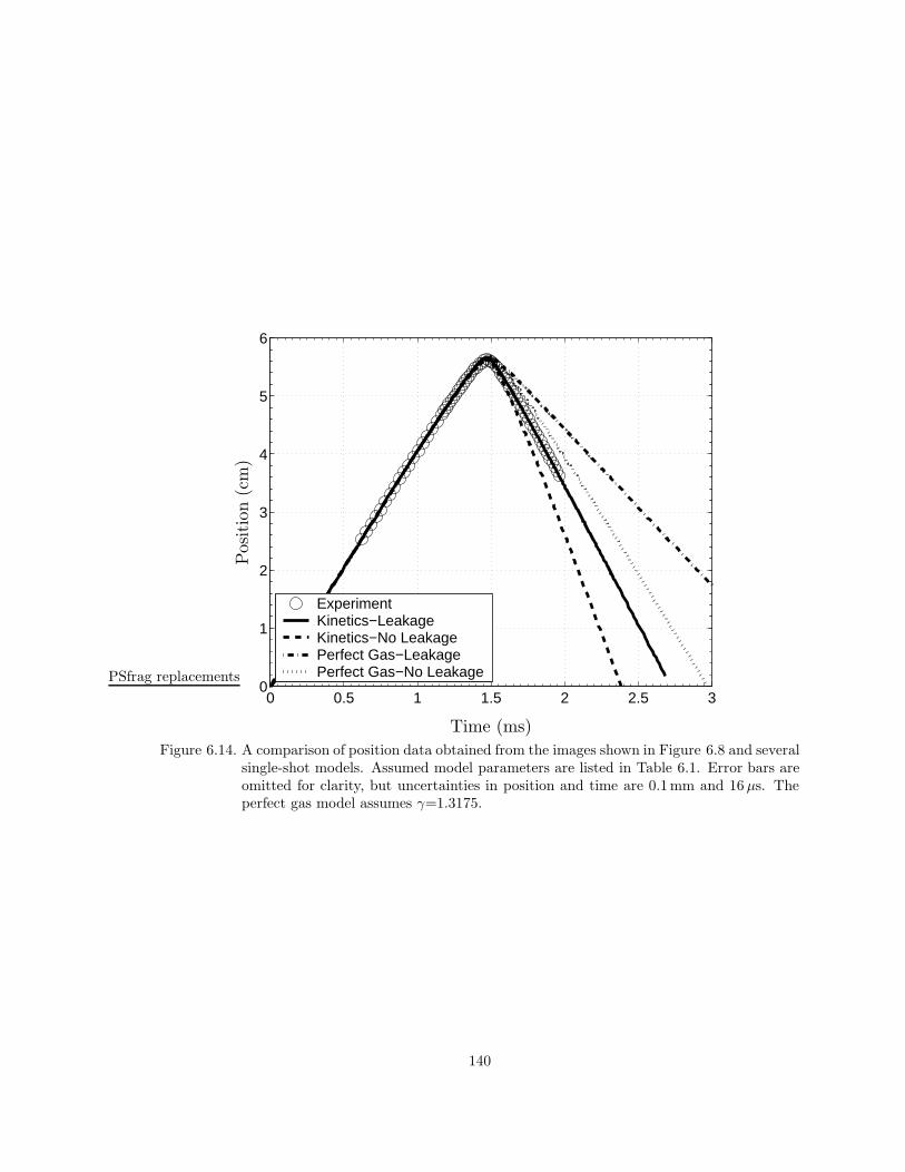
0 0.5 1 1.5 2 2.5 30

1

2

3

4

5

6

ExperimentKinetics−LeakageKinetics−No LeakagePerfect Gas−LeakagePerfect Gas−No LeakagePSfrag replacements

Posi

tion

(cm

)

Time (ms)

Figure 6.14. A comparison of position data obtained from the images shown in Figure 6.8 and severalsingle-shot models. Assumed model parameters are listed in Table 6.1. Error bars areomitted for clarity, but uncertainties in position and time are 0.1mm and 16 µs. Theperfect gas model assumes γ=1.3175.

140

1.3 1.4 1.5 1.6 1.7 1.84.8

4.9

5

5.1

5.2

5.3

5.4

5.5

5.6

5.7

5.8

Experiment Kinetics−Leakage Kinetics−No Leakage Perfect Gas−Leakage Perfect Gas−No LeakagePSfrag replacements

Posi

tion

(cm

)

Time (ms)

Figure 6.15. A comparison of position data obtained from the images shown in Figure 6.8 and severalsingle-shot models in detail. Assumed model parameters are listed in Table 6.1. Errorbars are omitted for clarity, but uncertainties in position and time are 0.1mm and 16 µs.The perfect gas model assumes γ=1.3175.

141

1 1.2 1.4 1.6 1.8 2

−60

−50

−40

−30

−20

−10

0

10

20

30

40

Kinetics−Leakage Kinetics−No Leakage Perfect Gas−Leakage Perfect Gas−No LeakageExperiment

PSfrag replacements

Vel

oci

ty(m s

)

Time (ms)

Figure 6.16. A comparison of velocity data obtained from the images shown in Figure 6.8 and varioussingle-shot models. Assumed model parameters are listed in Table 6.1. Error barsare omitted for clarity, but uncertainties in time and velocity are 16 µs and 20–50%,respectively. The largest uncertainties are obtained when the piston reverses direction(1.4–1.6ms). The perfect gas model assumes γ=1.3175.

142

0 50 100 1500

2000

4000

6000

8000

10000

0 50 100 1500

100

200

300

400

500

PSfrag replacements


Gap

Rey

nold

sN

um

ber

,R

e G

Pre

ssure

Ratio

Figure 6.17. Predictions of the gap Reynolds number and the pressure ratio using the perfect gasmodel and assuming γ=1.3175. Also, the Reynolds number computation assumes that

the charge viscosity is equal to air. The relation µ(T )=µRef (T/TRef)12 is used to approx-

imate the temperature dependence of viscosity (µRef=2.17 Pa · s @ 100 C).

6.4.3.2 Gap Fluid Motion

The sensitivity of piston position to the cylinder diameter (Figure 6.12) indicates that blow-by is

a significant effect. The flow in the piston-cylinder gap is assumed to be one-dimensional, quasi-

steady, and compressible. To assess the validity of these assumptions, the gap Reynolds number,

ReG (Section A.2.6) and the pressure ratio are estimated with the perfect gas single-shot model. The

results are presented in Figure 6.17. Upon inspection, one immediately notices that the pressure ratio

is well above critical for virtually the entire process. This in turn, implies that the flow is choked.

Additionally, the large Reynolds numbers (Figure 6.17) suggest that the flow in the piston-cylinder

gap is turbulent.

6.4.3.3 Physical Insights

The numerical model provides many valuable physical insights into the single-shot experiments. To

demonstrate, the following cases are considered: (1) Detailed kinetics with leakage., (2) Detailed

kinetics without leakage., (3) Perfect gas with leakage., and (4) Perfect gas without leakage. These

cases are plotted in Figure 6.14, Figure 6.15, and Figure 6.16 with the experimental results.

First, all cases in Figure 6.14 and Figure 6.15 give similar predictions for the compression path, but

the expansion paths vary greatly. This occurs because most of the mass loss occurs when the piston

reverses direction. To demonstrate, percent mass lost predictions of the kinetics and perfect gas

models are plotted in Figure 6.18. These curves indicate that approximately 40% of the charge is

143

0 0.5 1 1.5 2 2.50

10

20

30

40

50

60 Kinetics Perfect Gas

PSfrag replacements

Time (ms)

Per

cent

Mass

Lost

,M

L

Figure 6.18. Percent mass lost prediction corresponding to the images presented in Figure 6.8. Modelparameters are listed in Table 6.1.

lost when the piston reverses direction (circa 1.5ms). Thus a step change in charge mass occurs at

maximum compression ratio. Consequently the position traces are identical during the compression

stroke and they have different slopes during the expansion stroke.

Figure 6.18 reveals another interesting result: The perfect gas model yields the greatest percent mass

loss. That is, combustion apparently decreases the percent mass loss. Intuitively, one would expect

the opposite to be true because combustion increases the temperature and pressure. Therefore the

pressure gradient and the blow-by mass flow rate should increase. This quandary however, is resolved

by plotting the percent mass lost and pressure versus compression ratio in Figure 6.19.

The key to understanding this counterintuitive result is to recognize that the compression ratio

varies. To illustrate, the kinetics and perfect gas pressure curves in Figure 6.19 coincide until the

compression ratio is approximately 90:1; the behavior of the percent mass lost curve is identical.

When a volumetric compression ratio of 90:1 is reached, the kinetics model predicts that the charge

explodes and that the pressure rises above the perfect gas case—like one would expect. With a

free-piston however, this additional pressure rise decelerates the piston faster than the perfect gas

case. Hence the piston is brought to rest at a compression ratio of approximately 100:1. This

faster deceleration also implies that the piston spends less time at maximum compression ratio (see

Figure 6.15). On the other hand, the piston is not brought to rest until a compression ratio of 115:1

is reached in the perfect gas case and the residence time is greater. Therefore when combustion

occurs, the piston spends less time at large compression ratios and pressures. This in turn, yields a

144

100

101

102

103

0

20

40

60

KineticsPerfect Gas

100

101

102

1031

10

100

1e+03

Expansion

Expansion

Compression

PSfrag replacements


Per

cent

Mass

Lost

,M

L

Pre

ssure

(atm

)

Figure 6.19. Pressure and percent mass lost predictions corresponding to the images presented inFigure 6.8. Model parameters are listed in Table 6.1.

smaller percent mass lost than the perfect gas case. Alternatively, if the compression ratio were fixed

e.g., in a crank engine, then the residence times would be identical and combustion would maximize

the percent mass loss.

Next, if a “Leakage” and “No-Leakage” pair of curves in Figure 6.15 are compared, one should find

that the volumetric compression ratio increases when mass is lost. This occurs because blow-by

alters the relationship between density and volume (Eq. (6.2)). Therefore the charge occupies a

smaller volume when compressed to an equivalent density.

Finally, the predicted temperature history and pressure-volume (P-V) diagrams are plotted in

Figure 6.20 and Figure 6.21. Ignition is indicated by the sudden temperature rise in Figure 6.20.

One should note that the timing is mildly affected by leakage. This result is expected because most

of the mass loss occurs shortly after ignition (Figure 6.18). Alternatively, the loss of mass causes

the product temperatures to fall faster during the expansion stroke. Mass loss also decreases the

cycle work (Figure 6.21). Consequently the fuel conversion efficiency is reduced because the cases

in Figure 6.21 have identical initial conditions.

145

1.4 1.5 1.6 1.7 1.8 1.9

500

1000

1500

2000

2500

3000Kinetics−Leakage Kinetics−No Leakage Perfect Gas−Leakage Perfect Gas−No Leakage

PSfrag replacements

Time (ms)

Tem

per

atu

re(K

)

Figure 6.20. Predicted charge temperatures for conditions corresponding to Figure 6.8. Model pa-rameters are listed in Table 6.1.

10−3

10−2

10−1

100

100

101

102

103

Leakage No Leakage

PSfrag replacements

Volume(

cm3)

Pre

ssure

(atm

)

Figure 6.21. Predicted P-V diagram for conditions corresponding to Figure 6.8. Model parametersare listed in Table 6.1.

146

Table 6.2. Parametric study model inputs.Parameter Value(s) UnitInitial Velocity (x0) 5, 10, 15, 20, 25, 30, 35, 40, 45, 50 m

sChamber Length (L) 0.6, 1.5, 3.0, 4.5, 7.5, 9.0 cmEquivalence ratio (Φ) 0.25, 0.47, 0.69, 0.95, 1.5, 2.9 NAFuel (Kinetic Mechanism) Heptane (Curran et al., 1998) and

Propane (Westbrook, 1999)NA

Discharge Coefficient (Cd) 0 and 1 NAInitial Temperature (T0) 300 KInitial Pressure (P0) 1 atmPiston Mass (mp) 0.431 gClearance Volume (Vc) 0.71591E-03 cm3

Piston Diameter (Dp) 0.29972 cmCylinder Bore (B) 0.300228 cmWall Temperature (Tw) 300 K

6.5 Single-Shot Parametric Model Study

A parametric study is conducted to identify relationships between initial conditions and overall

results. The details of the parametric study are summarized in Table 6.2. Also, propane and

heptane are considered representative of single-stage- and two-stage-ignition fuels, respectively. The

indicated fuel conversion efficiency and the percent mass lost are of particular interest. Consequently

predictions of these quantities are plotted in Figure 6.22 and Figure 6.23, respectively.

Two key findings of the parametric study are that efficiencies and mass loss are related and that they

have complimentary features. These are not unexpected results because mass loss is known to sig-

nificantly decrease cycle work (Figure 6.21). To demonstrate, Figure 6.22 indicates that the percent

mass lost decreases with chamber length (L). Meanwhile, the maximum efficiencies in Figure 6.23

are obtained with a chamber length of 9.0 cm. Consequently maximum efficiency corresponds to

minimum mass lost. Also, efficiencies are maximized when the compression ratio is smaller than 200

(Figure 6.23), but one expects efficiencies to increase with compression ratio. This counterintuitive

result is also a consequence of mass loss i.e., Figure 6.19 demonstrates that mass loss increases with

compression ratio. Therefore the influence of mass loss on efficiency is apparently greater than the

compression ratio. Finally, Figure 6.22 and Figure 6.23 indicate that both the percent mass lost and

the indicated fuel conversion efficiency are relatively insensitive to the fuel.

On the other hand, the percent mass lost is insensitive to the equivalence ratio while the indicated

fuel conversion efficiency is not. This is an expected result because mass loss affects the relationship

between efficiency and equivalence ratio. To illustrate, indicated efficiencies obtained in cases with

and without mass loss are plotted in Figure 6.24 and Figure 6.25 when Φ=0.95. Similarly, Φ=0.47

and Φ=0.25 cases are plotted in Figures 6.26 and 6.27, and Figures 6.28 and 6.29, respectively.

147

0

5

10 20

30

40

500

10

20

30

40

50

60

Φ=0.95Φ=0.47Φ=2.90Φ=0.25Φ=1.50Φ=0.69

PSfrag replacements

Per

cent

Mass

Lost

,M

L

Initia

l Velocit

y,x0

( ms

)

Chamber Length, L (cm)

Figure 6.22. Percent mass lost versus chamber length and initial velocity for cases in which the chargeignites; open symbols indicate heptane-air and dark symbols indicate propane-air.

01

23

0

200

400

0

10

20

30

40

50

L=9.0 cmL=7.5 cmL=4.5 cmL=3.0 cmL=1.5 cm

PSfrag replacements

η fc,i

(Per

cent)

Com

pressionRatio, r Equivalen

ce Ratio,Φ

Figure 6.23. Indicated fuel conversion efficiency versus compression ratio and equivalence ratio whenthe model includes blow-by. Open symbols indicate heptane-air and dark symbolsindicate propane-air mixtures.

148

0 50 100 150 200 250 3000

10

20

30

40

50

60

70

80

90OttoFuel−AirL=9.0 cmL=7.5 cmL=4.5 cmL=3.0 cmL=1.5 cm

PSfrag replacements

η fc,i

(Per

cent)


Figure 6.24. Indicated fuel conversion efficiency versus compression ratio with mass loss and Φ=0.95.Open symbols indicate heptane-air and dark symbols indicate propane-air. The Ottocycle efficiency is computed by assuming γ=1.3. Heptane is used in the fuel-air cyclecomputations.

0 50 100 150 200 250 3000

10

20

30

40

50

60

70

80

90

OttoFuel−AirL=9.0 cmL=7.5 cmL=4.5 cmL=3.0 cmL=1.5 cm

PSfrag replacements

η fc,i

(Per

cent)


Figure 6.25. Indicated fuel conversion efficiency versus compression ratio without mass loss andΦ=0.95. Open symbols indicate heptane-air and dark symbols indicate propane-air.The Otto cycle efficiency is computed by assuming γ=1.3. Heptane is used in thefuel-air cycle computations.

149

0 50 100 150 200 250 3000

10

20

30

40

50

60

70

80

90

OttoFuel−AirL=9.0 cmL=7.5 cmL=4.5 cmL=3.0 cm

PSfrag replacements

η fc,i

(Per

cent)



0 50 100 150 200 250 3000

10

20

30

40

50

60

70

80

90

OttoFuel−AirL=9.0 cmL=7.5 cmL=4.5 cmL=3.0 cmL=1.5 cm

PSfrag replacements

η fc,i

(Per

cent)



150

0 50 100 150 200 250 3000

10

20

30

40

50

60

70

80

90

OttoFuel−AirL=9.0 cmL=7.5 cmL=4.5 cmL=3.0 cm

PSfrag replacements

η fc,i

(Per

cent)



0 50 100 150 200 250 3000

10

20

30

40

50

60

70

80

90

OttoFuel−AirL=9.0 cmL=7.5 cmL=4.5 cmL=3.0 cmL=1.5 cmL=0.6 cm

PSfrag replacements

η fc,i

(Per

cent)



151

One expects efficiency and equivalence ratio to be inversely related. This is indeed true for cases

without mass loss (Figures 6.25, 6.27, and 6.29) and the fuel-air cycle. The opposite is true however,

when mass loss occurs (Figures 6.24, 6.26, and 6.28).

A comparison of cases with and without mass loss e.g., Figure 6.24 and Figure 6.25, reveals the

degree to which mass loss decreases the fuel conversion efficiency. Also, cases without mass loss

(Figures 6.25, 6.27, and 6.29) confirm that the combination of HCCI combustion and a free-piston

approximates an ideal Otto cycle for compression ratios less than 100:1—which incidentally, is

consistent with conventional engine trends. Moreover, mass loss causes the maximum efficiency

to occur when 50≤r≤100. Finally, a few cases in Figure 6.27 and Figure 6.29 exceed the Otto

cycle efficiency. The fuel-air cycle efficiency however, is never exceeded. Therefore these seemingly

implausible results are actually a consequence of using an inappropriate specific heat ratio to compute

the Otto cycle efficiency.

6.6 Non-Dimensional Analysis

The model equations are non-dimensionalized to characterize the single-shot process. First, the

non-dimensional variables are defined. Let

V ∗ =V

V0, t∗ =

t

τ, v∗ =

v

v0, T ∗ =

T

T0, and P ∗ =

P

P0, (6.16)

where V0, v0, T0, and P0 represent initial values4 and τ is a characteristic time. Next, if one

assumes that P0=P∞ and T0=T∞, then the non-dimensional forms of Eq. (6.6), Eq. (6.7), Eq. (6.2),

Eq. (A.31), and Eq. (A.32) are given by

dYk

dt∗= v∗v0τωkWk, (6.18)

dT ∗

dt∗+

v0τ

cvT0v∗

Ns∑

k=1

ukωkWk −qτ

cvT0+

P0v0

cvT0P ∗

dv∗

dt∗= 0, (6.19)

dv∗

dt∗=

τv0m

V0

v∗2

V ∗+

v∗

V ∗

dV ∗

dt∗, (6.20)

dV ∗

dt∗= −

xτ

LRmax

, (6.21)

and

d2V ∗

dt∗2 =τ2P∞

LRmax (mp/Ap)(P ∗ − 1) , (6.22)

4The initial volume is given byV0=ApL+Vc. (6.17)

Hence the volume of the piston-cylinder gap is neglected.

152

L cLR

max

Ap

P∞

Figure 6.30. The relation between the piston initial position, clearance distance c, Rmax, and L. Notethat the piston travel physically cannot exceed L.

respectively. One should note that Rmax is defined by

Rmax =rcyl

rcyl − 1, (6.23)

where rcyl=V0/Vc and Vc is the clearance volume. Thus rcyl is the maximum compression ratio that

can be achieved with a given piston and cylinder5. The relationship between L, c, and Rmax is

illustrated in Figure 6.30.

6.6.1 Compression Ratio

Although Eq. (6.18) through Eq. (6.22) are non-linearly coupled, examining Eq. (6.21) and Eq. (6.22)

yields key parameters that govern the piston motion. The first task is to identify the characteris-

tic time. The cycle time is an obvious candidate, but it is not known a priori. Moreover, with

the exception of a perfect gas with no losses, the piston paths appearing in Figure 6.15 are clearly

not symmetric about the dead point (x=0). On the other hand, the compression paths are virtu-

ally identical. Consequently the piston motion is characterized by the “half-cycle” rather than the

“full-cycle” time. To define the half-cycle time, τH, let

dV ∗

dt∗

∣

∣

∣

∣

t∗=0

= −x0τH

LRmax

= −1, (6.24)

where x0=x(0) i.e., it is the initial velocity of the piston. Consequently the half-cycle time is defined

by

τH=LRmax

x0, (6.25)

and physically, it approximates the time required to decelerate the piston from x0 to zero (Figure 6.30).

Next, the half-cycle time is substituted into Eq. (6.22). The result is

d2V ∗

dt∗2 =LRmaxP∞

x20 (mp/Ap)

(P ∗ − 1) . (6.26)

5One should note that Rmax→1 when rcyl→∞; which is equivalent to c→0 in Figure 6.30.

153

10−2

10−1

100

101

100

101

102

103

Optimal

Φ=0.95Φ=0.69Φ=0.47Φ=0.25Φ=1.5Φ=2.9

PSfrag replacements

Com

pre

ssio

nra

tio,r

Dynamic Parameter, Γ

Figure 6.31. Compression ratio versus dynamic parameter, Γ for all parametric cases. Open symbolsindicate heptane-air and dark symbols denote propane-air cases. Also, smaller symbolsrepresent cases where leakage is neglected.

Consequently a dimensionless “dynamic” parameter may be defined by

Γ =LRmaxApP∞

mpx20

, (6.27)

and Eq. (6.26) becomesd2V ∗

dt∗2 = Γ (P ∗ − 1) . (6.28)

One should note that by definition, V ∗=1/r (Eq. (6.16)). Consequently substituting this identity

into Eq. (6.28) yields

2

r3

(

dr

dt∗

)2

−1

r2

d2r

dt∗2 = Γ (P ∗ − 1) , (6.29)

which relates the compression ratio to the dynamic parameter, Γ. To investigate this relationship, the

maximum compression ratios achieved in the parametric cases are plotted in Figure 6.31. Evidently,

the maximum compression ratio correlates to the dynamic parameter very well. In fact, the equiv-

alence ratio and mass loss appear to be minor influences. This is noteworthy because blow-by is

known to increase the compression ratio (Section 6.4.3.3). Hence the maximum compression ratio

is essentially determined by the dynamic parameter. Moreover, if one assumes from Figure 6.24

that 50≤r≤100 is necessary to maximize the fuel conversion efficiency, then Figure 6.31 implies that

154

10−2

10−1

100

101

100

101

102

103

104

105

γ=1.250γ=1.300γ=1.350γ=1.400

PSfrag replacements

Com

pre

ssio

nR

atio,r

Dynamic Parameter, ΓP

Figure 6.32. Compression ratio versus perfect gas dynamic parameter, ΓP (Eq. (6.32))

0.045≤Γ≤0.1 is optimal.

Physical insight into dynamic parameter is gained by recognizing that the product LApRmax is the

initial volume of the charge (Figure 6.30). Therefore LRmaxApP∞ is the work required to displace

this volume to the ambient. Meanwhile, mpx20 is twice the initial kinetic energy of the piston. This

quantity however, is equal to double the magnitude of the compression work because the final piston

velocity is zero. Consequently the dynamic parameter has the physical interpretation

Γ =Work required to displace the cylinder contents

2×Work of compression. (6.30)

Using this physical interpretation, a dynamic parameter for the isentropic compression of a perfect

gas by a free-piston (Section A.3) may be developed i.e.,

ΓP =P0V0

(1− γ) mpx20

. (6.31)

In this case however, the compression ratio is an explicit function of the dynamic parameter. This

function is given by

r =

[

1

2ΓP

+ 1

]1

γ−1

, (6.32)

and it is plotted in Figure 6.32 for specific heat ratios of 1.25, 1.3, 1.35, and 1.4. These plots

155

suggest that variations in the specific heat ratio account for some of the “scatter” in Figure 6.31.

That is, for a given dynamic parameter, a smaller specific heat ratio will yield a larger compression

ratio. Inspection of Figure 6.31 reveals that this is indeed the case because for a given dynamic

parameter, the largest compression ratios correspond to Φ=2.9 (smallest γ). Hence decreasing the

specific heat ratio of a mixture results in a “softer spring.” Finally, a comparison of Figure 6.31

and Figure 6.32 reveals that the perfect gas model greatly exaggerates compression ratios when the

dynamic parameter is small i.e., Γ<0.1. Hence variable specific heats and other non-linear effects

become increasingly significant when the dynamic parameter decreases.

6.6.2 Percent Mass Lost

Mass loss is a problem intrinsic to the single-shot process. Presumably, any micro-engine design

that features an unsealed piston will have the same problem. Therefore understanding the relation

between percent mass lost and the initial conditions is essential.

First, the percent mass lost is defined by

ML =m0 −mf

m0× 100%, (6.33)

where the initial mass m0, is given by m0=V0/v0. The fundamental theorem of calculus is used to

relate Eq. (6.33) to Eq. (A.10). The result is

ML = 100%

∫ τC

0

v0m

V0dt. (6.34)

One should note that the “full cycle” time τC, is used here because mass is lost throughout the

process. Next, non-dimensionalization of the integral yields

ML = 100%

∫ t∗c

0

τHv0m

V0dt∗, (6.35)

where the non-dimensional cycle time t∗c , is defined by t∗c=τC/τH. Next, Eq. (6.4) is substituted for

m in Eq. (6.35). This gives

τHv0m

V0=

(

At

Ac

)

τHv0P∞CdM (P∞P ∗, P∞, γ)

LRmax (RmT0)12

(

P ∗

T ∗12

)

, (6.36)

for the integrand. From geometry (Figure 6.11),

At

Ac

=

(

tGDp

)

4 (tG/Dp) + 4

4 (tG/Dp)2

+ 4 (tG/Dp) + 1, (6.37)

and this ratio is approximately given by

At

Ac

≈ 4

(

tGDp

)

, (6.38)

156

when the ratio of gap to piston diameter tG/Dp, is small. Consequently the percent mass lost is given

by

ML ≈ 100%× 4

(

tGDp

)

[

τHv0P∞Cd

LRmax (RmT0)12

]

IL, (6.39)

where IL is the “leakage integral.” This integral is defined by

IL =

∫ t∗c

0

M (P∞P ∗, P∞, γ) P ∗

T ∗12

dt∗, (6.40)

and it depends upon the non-dimensional temperature-pressure history of the charge.

Immediately, Eq. (6.39) implies that the percent mass lost is inversely proportional to the chamber

length. This result is encouraging because it is consistent with Figure 6.22. When the half-cycle

time is substituted into Eq. (6.39) however, the result is

ML ≈ 100%× 4

(

tGDp

)

[

v0P∞Cd

x0 (RmT0)12

]

IL, (6.41)

and the length dependence disappears. Consequently the leakage integral must account for the

chamber length dependence. To investigate this hypothesis, the leakage integral is computed and

plotted in Figure 6.33 for the various parametric cases.

Clearly, the leakage integral, IL is a function of the dynamic parameter, Γ. This integral however,

cannot be expressed in closed form. Therefore it is approximated with a second-order curve fit viz.,

IL = exp[

−0.0195 (log Γ)2− 0.7461 logΓ + 0.6920

]

. (6.42)

Next, this expression is substituted into Eq. (6.41) to obtain an analytical expression for the percent

mass lost in terms of initial conditions. This expression is plotted in Figure 6.34 versus L and x0.

Qualitatively, Figure 6.34 is similar to Figure 6.22 because it captures three essential features: (1)

The percent mass lost is most sensitive to the chamber length., (2) The percent mass lost is inversely

proportional to the chamber length., and (3) The percent mass lost depends weakly upon the initial

velocity. A direct comparison of Figures 6.34 and 6.22 however, reveals that this surface exaggerates

the percent mass lost.

Additionally, the predicted 100% mass lost curve is identified and projected onto the chamber length-

initial velocity plane. This curve is also plotted in Figure 6.35 and it yields an interesting result:

Certain combinations of initial velocity and chamber length are incompatible. This in turn, places

restrictions on the combustion chamber dimensions and the initial conditions. Therefore reducing

blow-by is a key objective.

To facilitate future design work, a scaling relation for ML is developed. First, a simpler correlation

IL = exp [−0.7015 logΓ + 0.6743] , (6.43)

157

10−2

10−1

100

101

10−1

100

101

102

Φ=0.95 Φ=0.69 Φ=0.47 Φ=0.25 Φ=1.5 Φ=2.9 Fitted Line

PSfrag replacements

Lea

kage

Inte

gra

l,I L


Figure 6.33. Leakage integral versus dynamic parameter, Γ for all parametric cases. Opensymbols indicate heptane-air and dark symbols denote propane-air cases. Notethat γ=1.3 is assumed to compute M(P ∗, γ). The equation of the fitted line is

IL= exp[

−0.0195 (log Γ)2− 0.7461 logΓ + 0.6920

]

.

is obtained. Next, Eq. (6.43) is substituted into Eq. (6.41) and the result is simplified. This gives

ML ≈ 100%× 9.300tGCdv0P

0.2985∞

x0.4030

D2.403p

(RmT∞)12

(

mp

LRmax

)0.7015

. (6.44)

Although approximate, this expression sheds considerable light on the mass loss problem. First of

all, Eq. (6.39) implies that the percent mass lost is proportional to the gap and inversely proportional

to the piston diameter. Eq. (6.44) however, reveals that the piston diameter dependence is actually

much stronger. Therefore increasing or decreasing the piston diameter will have a considerable effect

on the percent mass lost. Second, Eq. (6.44) predicts that the percent mass lost will increase—

albeit slowly—with the piston initial velocity. This result is corroborated by Figure 6.22. Third,

like Eq. (6.39), Eq. (6.44) indicates the percent mass lost is inversely proportional to the chamber

length. Although the length dependence predicted by Eq. (6.44) is somewhat weaker. Finally,

Eq. (6.44) reveals that the percent mass lost is proportional to the piston mass. Therefore one may:

(1) Increase the cylinder length., (2) Increase the piston diameter., (3) Decrease the gap width., or

(4) Increase the piston mass., to reduce the percent mass lost.

158

0

20

40

60

0 2 4 6 8 10

0

20

40

60

80

100

PSfrag replacements

Per

cent

Mass

Lost

,M

L

Initial

Velocity, x

0

(

ms

)


Figure 6.34. Predicted percent mass lost versus chamber length and initial velocity. The surface isobtained by substituting Eq. (6.42) into Eq. (6.41) and assuming that the fresh chargeis air. The curve projected onto the x0-L plane denotes 100% mass lost.

6.7 Conclusion

This chapter presents results from single-shot micro-HCCI experiments and a detailed chemical

kinetic model. The relationship between the initial conditions, leakage, and the indicated fuel

conversion efficiency are explored via parametric model study. Also, the governing equations are non-

dimensionalized to reveal: (1) An appropriate characteristic time., (2) A non-dimensional parameter

that essentially determines the compression ratio., and (3) An approximate functional relationship

between the initial conditions and the percent mass lost.

159

0.6 0.7 0.8 0.9 1 1.1 1.2 1.3 1.45

10

15

20

25

30

35

40

45

Forbidden

PSfrag replacements

Initia

lVel

oci

ty,x

0

(

m s

)


Figure 6.35. Predicted maximum initial velocity. This is the 100% mass lost curve projected ontothe x0-L plane in Figure 6.34.

The salient findings of this chapter include:

• HCCI is possible in spaces 3mm diameter and 0.3mm long.

• HCCI combustion with equivalence ratios of Φ=0.69 and Φ=0.25 is demonstrated.

• A model which couples free-piston motion and detailed chemical kinetics is developed and used

to model the single-shot micro-HCCI experiments.

• The single-shot numerical model employing detailed chemical kinetics is shown to reproduce

piston position and velocity measurements very well.

• Leakage (blow-by) accounts for:

– A distortion of the piston-time path during the expansion stroke.

– An increase in the compression ratio relative to an ideal case.

– A decrease in the fuel conversion efficiency.

• Leakage may be reduced by:

– Increasing the chamber length.

– Increasing the piston diameter.

– Decreasing the piston-cylinder gap.

– Decreasing the piston mass.

160

• The dynamic parameter Γ, is defined by Eq. (6.27) and it:

– Characterizes the compression process i.e., it captures the relationship between initial

conditions and the compression ratio.

– May be interpreted to be the ratio of “The work required to displace the volume swept

by the piston to double the compression work.”

– If one assumes that a compression ratio between 50 and 100 is optimal, then the piston

mass, initial velocity, and cylinder length must satisfy the constraint 0.045≤Γ≤0.1.

161

Chapter 7

How Small Can a Free-Piston

HCCI Engine Be?

7.1 Introduction

Fundamental constraints on HCCI combustion and engine size are first explored in Section 5.6.4.

The section presents an argument that heat transfer limits engine size because thermal energy losses

prevent the charge from reaching ignition conditions during compression. These losses increase in

small scales (Section 1.1.2), consequently operating an engine smaller than a certain size is impos-

sible. An absolute minimum engine size however, is not determined.

One should note that the size constraint imposed by heat transfer is obtained by comparing opera-

tional maps of adiabatic and diathermal engines. Heat transfer obviously limits the operation of the

latter, but the limiting factor of the former is not clear. For instance, ignition could be impossible

due to insufficient residence time, inadequate compressive heating, or kinetics. In general, limitations

due to residence time or compressive heating can be overcome by changing operating conditions or

engine redesign. In contrast, little can be done to mitigate a kinetic constraint. Therefore kinetics

will ultimately constrain HCCI engine operation.

The minimum size of an HCCI engine however, may be unrelated to kinetics. For example, the

kinetic limit could be practically unattainable. The objectives of this chapter are to explore size and

operational limitations of HCCI engines and to provide a basis for future micro-engine work. This is

accomplished primarily through parametric studies that employ the single-shot model (Section 6.4).

Additionally, other factors that constrain the size of free-piston HCCI engines are discussed.

162

7.2 Generalizing the Single-Shot Process

The parametric study presented in Section 6.5 was instrumental to the discovery that the single-

shot process is characterized by the half-cycle time and the dynamic parameter. Unfortunately, the

time scales and physical dimensions are limited to those attainable in the single-shot experiments.

Consequently the single-shot process is partially explored. Therefore to characterize this process in

general, a parametric study is conducted to extend the single-shot process to a wide range of time

scales and dynamic parameters.

7.2.1 Parametric Study Formulation

The strategy employed in the following parametric studies is to vary the half-cycle time and the

dynamic parameter independently. Physical dimensions however, are constant (Table 7.1). This

assumption simplifies the analysis, but it can result in conditions that are physically unrealistic.

One should note that this is not a severe limitation because realistic dimensions can be obtained

through similitude.

When the half-cycle time is prescribed and L and Rmax are fixed, the initial velocity of the piston is

given by

x0 =LRmax

τH

. (7.1)

One should note that the dynamic parameter and the half-cycle time are not independent e.g.,

Γ =τHApP∞

mpx0, (7.2)

which is an alternate form of the dynamic parameter. Consequently the piston mass must vary if

the dynamic parameter and the half-cycle time are to be independent. Hence the piston mass is

computed from

mp =τHApP∞

x0Γ. (7.3)

7.2.2 Extending the Single-Shot Parametric Model Study

In the previous parametric study (Section 6.5), the initial velocity and chamber length are inde-

pendent parameters while the piston mass is fixed (mp=0.431 g). This strategy has the unintended

consequence that chamber length is the primary dependence captured. To illustrate, substituting

Eq. (7.1) into Eq. (7.2) and rearranging yields

Γ

τ2H

=ApP∞

LRmaxmp

. (7.4)

Hence the behavior of efficiency and percent mass lost over the entire “Γ-τH” plane is not captured.

In contrast, this parametric study assumes a fixed chamber length. Further details of the parametric

study are presented in Table 7.1. Also, one should note that two sets of results are obtained; one set

considers mass loss and heat transfer while the other is “idealized” and therefore considers neither.

163

Table 7.1. First single-shot extension parametric study inputs.Parameter Value(s) UnitDynamic Parameter (Γ) 0.03, 0.04, 0.05, 0.06, 0.07, 0.08, 0.09, 0.1 NAHalf-Cycle Time (τH) 0.8, 1.2, 1.5, 1.8, 2.2 msChamber Length (L) 6.0 cmInitial Velocity (x0) Determined by Eq. (7.1) m

sPiston Mass (mp) Determined by Eq. (7.3) gEquivalence ratio (Φ) 1.0 NAFuel (Kinetic Mechanism) Heptane (Curran et al., 1998) NADischarge Coefficient (Cd) 0 and 1 NAInitial Temperature (T0) 300 KInitial Pressure (P0) 1 atmClearance Volume (Vc) 0.71591E-03 cm3


First, constant piston mass contours are computed with Eq. (7.3) and plotted in Figure 7.1. The

dashed contour denotes mp=0.431 g. Consequently this line represents the Γ-τH domain considered

in the previous parametric study (Section 6.5).

Next, maximum compression ratio contours are plotted in Figure 7.2 and Figure 7.3 for non-ideal

and idealized conditions, respectively. These plots have several interesting features. First, the

compression ratio contours are nearly vertical in both figures. This supports the hypothesis that

compression ratio is primarily a function of the dynamic parameter. Interestingly, this is especially

true when mass is lost. Second, a comparison of Figure 7.2 and Figure 7.3 at a given dynamic

parameter further demonstrates that mass loss exaggerates the compression ratio. Third, the dashed

contours indicate the results of the previous parametric study and this line is essentially a “top

edge view” of Figure 6.31. Alternatively, one may consider Figure 6.31 to be a “slice” through the

compression ratio surfaces plotted in Figures 7.2 and 7.3. Lastly, inspection of Figure 7.2 suggests

that mass loss causes the compression ratio to be more sensitive to the dynamic parameter, whereas

the dashed line is nearly normal to the compression ratio contours in Figure 7.3.

Percent mass lost contours are plotted in Figure 7.4. One should note that the dashed line indicates

the results of the previous study and that it essentially coincides with the 31% mass lost contour.

Although unexpected, this result is easily attributed to previously discovered phenomena. For

instance, according to Eq. (6.44), the percent mass lost scales with mp/L. Consequently the percent

mass lost is constant along the contour because this quotient is invariant. This result follows from

the dashed line being a constant piston mass contour (Figure 7.1) and L being constant everywhere.

Finally, 31% mass lost is consistent with a chamber length of 6.0 cm (Figure 6.22).

Indicated fuel conversion efficiencies are plotted in Figure 7.5 and Figure 7.6 for non-ideal and ide-

alized cases, respectively. These figures provide several interesting insights. First, a comparison

of Figure 7.5 and Figure 7.6 confirms that mass loss generally decreases indicated fuel conversion

efficiencies. Second, Figure 7.5 provides an explanation for the essentially constant efficiencies in

164

0.03 0.04 0.05 0.06 0.07 0.08 0.09 0.1

1

1.2

1.4

1.6

1.8

2

2.2

0.1000.200

0.200

0.200

0.300

0.300

0.300

0.300

0.431

0.431

0.431

0.431

0.500

0.500

0.500

0.500

0.600

0.600

0.600

0.600

0.700

0.700

0.700

0.900

0.900

1.000

1.000

1.2001.

500

PSfrag replacements

Half-C

ycl

eT

ime,

τ H(m

s)


Figure 7.1. Piston mass (g) contours from the first single-shot extension parametric study. Thedashed contour represents the domain considered in an earlier parametric study(Section 6.5). Model input parameters are listed in Table 7.1.

Figure 6.24 (50≤r≤100). That is, for 0.04≤Γ≤0.08 in Figure 7.5, the dashed curve transits a region

having essentially constant efficiency. Consequently Figure 6.24 is a “slice” through the efficiency

surface in Figure 7.5. Likewise, Figure 6.25 is a slice through the efficiency surface in Figure 7.6.

Also, the efficiency surfaces plotted in Figure 7.5 and Figure 7.6 have vastly different topographies.

In particular, the former has a maximum when 0.045≤Γ≤0.065, while the latter surface generally

increases when τH and Γ decrease. Also, mass loss causes an “optimal” range for the dynamic

parameter to emerge. In fact, the line segment defined by the intersections of the dashed line and the

40% contour in Figure 7.5 (0.04≤Γ≤0.08) virtually coincides with the boxed region in Figure 6.31.

This optimal range however, appears to narrow when the characteristic time decreases.

165

0.03 0.04 0.05 0.06 0.07 0.08 0.09 0.1

1

1.2

1.4

1.6

1.8

2

2.2

4848

67

67

8585

104104

122122

141141

159

159

178

178196

196

PSfrag replacements

Half-C

ycl

eT

ime,

τ H(m

s)


Figure 7.2. Predicted compression ratio contours from the first single-shot extension parametricstudy. The dashed line indicates the region explored in an earlier parametric study(Section 6.5). Mass loss and heat transfer are considered. Model input parameters arelisted in Table 7.1.

166

0.03 0.04 0.05 0.06 0.07 0.08 0.09 0.1

1

1.2

1.4

1.6

1.8

2

2.242

42

58

58

73

73

73

88

88

88

103103

119119

134

134149

164

PSfrag replacements

Half-C

ycl

eT

ime,

τ H(m

s)


Figure 7.3. Predicted compression ratio contours from the first single-shot extension parametricstudy. The dashed line indicates the region explored in an earlier parametric study(Section 6.5). Mass loss and heat transfer are not considered. Model input parametersare listed in Table 7.1.

167

0.03 0.04 0.05 0.06 0.07 0.08 0.09 0.1

1

1.2

1.4

1.6

1.8

2

2.2

18.02

18.02

22.32

22.32

22.32

26.63

26.63

26.63

30.93

30.93

30.93

30.93

35.24

35.24

35.24

35.2439.54

39.54

39.54

43.84

43.8

4

48.1

5

52.4

5

PSfrag replacements

Half-C

ycl

eT

ime,

τ H(m

s)


Figure 7.4. Percent mass lost contours from the first single-shot extension parametric study. Thedashed line indicates the region explored in an earlier parametric study (Section 6.5).Model input parameters are listed in Table 7.1.

168

0.03 0.04 0.05 0.06 0.07 0.08 0.09 0.1

1

1.2

1.4

1.6

1.8

2

2.2

5

5

5

10

10

10

10

20

20

20

2030

30

30

30

30

3535

35

35

35

35

40

40

40

40

40

4545

45

45 50 50


Half-C

ycl

eT

ime,

τ H(m

s)


Figure 7.5. Predicted fuel conversion efficiency (percent) contours from the first single-shot extensionparametric study. The dashed line indicates the region explored in an earlier parametricstudy (Section 6.5). Mass loss and heat transfer are considered. Model input parametersare listed in Table 7.1.

169

0.03 0.04 0.05 0.06 0.07 0.08 0.09 0.1

1

1.2

1.4

1.6

1.8

2

2.2

5 5

10

10

20

20

20

40

40

40

50

50

50

60

60

60

63

63

63

65

65

65

66

66

66

68

68

68

70

70


Half-C

ycl

eT

ime,

τ H(m

s)


Figure 7.6. Predicted fuel conversion efficiency (percent) contours from the first single-shot extensionparametric study. The dashed line indicates the region explored in an earlier paramet-ric study (Section 6.5). Mass loss and heat transfer are not considered. Model inputparameters are listed in Table 7.1.

170

Table 7.2. Second single-shot extension parametric study inputs.Parameter Value(s) UnitDynamic Parameter (Γ) 0.01, 0.02, 0.03, 0.04, 0.05, 0.06, 0.07 NAHalf-Cycle Time (τH) 0.6, 0.4, 0.2, 0.08, 0.05 msChamber Length (L) 6.0 cmInitial Velocity (x0) Determined by Eq. (7.1) m

sPiston Mass (mp) Determined by Eq. (7.3) gEquivalence ratio (Φ) 1.0 NAFuel (Kinetic Mechanism) Heptane (Curran et al., 1998) NADischarge Coefficient (Cd) 0 and 1 NAInitial Temperature (T0) 300 KInitial Pressure (P0) 1 atmClearance Volume (Vc) 0.71591E-03 cm3


7.2.3 Extension to Small Characteristic Times and Dynamic Parameters

One may draw an interesting conclusion from the percent mass lost contours in Figure 7.4 and the

efficiency contours in Figure 7.5: Small half-cycle times and dynamic parameters apparently mini-

mize mass loss and maximize efficiency. Consequently from a design perspective, these conditions are

desirable. To explore this possibility, another parametric study is conducted; details are presented

in Table 7.2.

Percent mass lost and indicated fuel conversion efficiency contours are plotted in Figure 7.7 and

Figure 7.8, respectively. These figures suggest that the percent mass lost can be reduced to approxi-

mately 5% and that efficiencies of 70% are attainable. Also, idealized efficiency contours are plotted

in Figure 7.9. Interestingly, an efficiency “plateau” is found when Γ≤0.04 and τH≤0.6 ms. Hence

dynamic parameters smaller than 0.04 are expected to offer few advantages.

Although appealing, employing small half-cycle times and dynamic parameters is generally impossi-

ble. To demonstrate, piston mass contours are plotted in Figure 7.10 and one should note that they

approach ridiculous values e.g., 1mg. Additionally, if one recalls that percent mass lost scales with

mp/L, then to achieve an equivalent mass loss with a 0.5 g piston, the chamber length must be 30m

long—which is obviously unrealistic. Furthermore, compression ratios are plotted in Figure 7.11 and

Figure 7.12. They indicate that compression ratios greater than 200:1 would be necessary. Typically,

one would argue that blow-by renders these compression ratios unrealistic; clearly this argument is

nullified by Figure 7.7. Instead, the maximum compression ratio is limited by fabrication technique.

171

0.01 0.02 0.03 0.04 0.05 0.06 0.07

0.1

0.2

0.3

0.4

0.5

0.6

4.354.35

4.357.62

7.62

7.62

10.89

10.89

10.89

10.89

14.16

14.16

14.16

17.44

17.4

4

20.7

1

20.7

123

.98

27.2

5

30.5

2

PSfrag replacements

Half-C

ycl

eT

ime,

τ H(m

s)


Figure 7.7. Percent mass lost contours from the second single-shot extension parametric study.Model input parameters are listed in Table 7.2.

0.01 0.02 0.03 0.04 0.05 0.06 0.07

0.1

0.2

0.3

0.4

0.5

0.6

5

5

5

5

10

10

10

10

20

20

20

2040

40

40

40

40

50

50

50

50

50

60

60

60

60

60

60

63

63

63

63

63

65

65

65

65

68

68

68

70

70

70

72

72

7275 75PSfrag replacements

Half-C

ycl

eT

ime,

τ H(m

s)


Figure 7.8. Predicted fuel conversion efficiency (percent) contours from the second single-shot ex-tension parametric study. Mass loss and heat transfer are considered. Model inputparameters are listed in Table 7.2.

172

0.01 0.02 0.03 0.04 0.05 0.06 0.07

0.1

0.2

0.3

0.4

0.5

0.6

10

10

10

40

40

40

50

50

50

70

70

70

72

72

72

75

75

75


Half-C

ycl

eT

ime,

τ H(m

s)


Figure 7.9. Predicted fuel conversion efficiency (percent) contours from the second single-shot ex-tension parametric study. Mass loss and heat transfer are not considered. Model inputparameters are listed in Table 7.2.

0.01 0.02 0.03 0.04 0.05 0.06 0.07

0.1

0.2

0.3

0.4

0.5

0.6

0.001 0.0010.005

0.0050.005

0.010

0.010

0.010

0.020

0.020

0.020

0.030

0.030

0.030

0.030

0.040

0.040

0.040

0.040

0.050

0.050

0.050

0.0500.080

0.080

0.080

0.100

0.100

0.10

00.

200

PSfrag replacements

Half-C

ycl

eT

ime,

τ H(m

s)


Figure 7.10. Piston mass (g) contours from the second single-shot extension parametric study. Modelinput parameters are listed in Table 7.2.

173

0.01 0.02 0.03 0.04 0.05 0.06 0.07

0.1

0.2

0.3

0.4

0.5

0.6

6060

60

8080

80

100

100

100

120

120

120

140

140140

180

180180

200200

200300300

300

400400

400

500500

500

600600

600

1000

10001000

PSfrag replacements

Half-C

ycl

eT

ime,

τ H(m

s)


Figure 7.11. Compression ratio contours from the second single-shot extension parametric study.Mass loss and heat transfer are considered. Model input parameters are listed inTable 7.2.

0.01 0.02 0.03 0.04 0.05 0.06 0.07

0.1

0.2

0.3

0.4

0.5

0.610

0

100100

150150

150

200

200

200

300300

300

400

400400

500500

500

800800

800

PSfrag replacements

Half-C

ycl

eT

ime,

τ H(m

s)


Figure 7.12. Compression ratio contours from the second single-shot extension parametric study.Mass loss and heat transfer are not considered. Model input parameters are listed inTable 7.2.

174

7.3 Kinetic Considerations for HCCI Combustion with a Free-Piston

Chemical kinetics impose a fundamental limitation for HCCI engine operation. This limit is elusive

because ignition depends non-linearly upon the compression process, residence time, and kinetics.

Moreover, these dependencies are intrinsically coupled when a free-piston is employed. Fortunately,

the dynamics of the single-shot process are characterized by the half-cycle time and the dynamic

parameter and these dependencies may be readily investigated in concert.

Basically, the task at hand is to relate chemical kinetics to the single-shot dynamics; time scales

provide this link. The results of the parametric studies described in Section 7.2 are used to explore

the relationships between single-shot dynamics and chemical kinetics. Also, only the idealized cases

are considered i.e., heat transfer and mass loss are neglected.

7.3.1 Non-Dimensional Ignition Timing

To relate the time scales of the single-shot process to chemical kinetics, the characteristic decom-

position time of hydrogen peroxide is employed. Experimental and modeling work has provided

ample evidence that hydrogen peroxide decomposition plays a central role in HCCI. In particular,

decomposition is known to immediately precede ignition (Chapter 3).

7.3.1.1 Kinetic Time Scale

The characteristic destruction time of hydrogen peroxide τH2O2, is given by

τH2O2=

[H2O2]

DH2O2

, (7.5)

where DH2O2is the net rate of H2O2 destruction (Section B.2). The net destruction rate and the

characteristic destruction time are computed by Chemkin subroutines1 (Kee et al., 1996). Con-

sequently the Senkin post-processor is modified to compute characteristic destruction times from

Senkin problem solutions.

To demonstrate the relationship between hydrogen peroxide destruction time and temperature,

these quantities are plotted in Figure 7.13 for Γ=0.03 and τH=0.8 ms. This plot suggests that a

rapid decrease in the hydrogen peroxide destruction time is a reliable indicator for ignition. For

comparison, the result of a partial reaction is presented Figure 7.14.

1Chemkin actually adds a small number (10−16) to the net destruction rate to prevent division by zero (Kee et al.,1996).

175

0 0.5 1 1.510

−10

10−5

100

105

1010

1015

1020

0 0.5 1 1.50

500

1000

2000

3000

4000

PSfrag replacements Dim

ensi

onle

ssC

hem

icalT

ime,

τH

2O

2/τ

H

Tem

per

atu

re,(K

)

Dimensionless Process Time, t∗=t/τH

Figure 7.13. Normalized hydrogen peroxide characteristic time and bulk temperature. Mass loss andheat transfer are considered τH=0.8 ms, L=6.0 cm, Γ=0.03.

0 0.5 1 1.510

−5

100

105

1010

1015

1020

0 0.5 1 1.50

500

1000

1500

PSfrag replacements Dim

ensi

onle

ssC

hem

icalT

ime,

τH

2O

2/τ

H

Tem

per

atu

re,(K

)


Figure 7.14. Normalized hydrogen peroxide characteristic time and bulk temperature. Mass loss andheat transfer are considered τH=0.8 ms, L=6.0 cm, Γ=0.08.

176

0.95 1 1.05 1.1 1.15 1.2

10−8

10−6

10−4

10−2

100

Γ=0.03Γ=0.04Γ=0.05Γ=0.06Γ=0.07Γ=0.08Γ=0.09Γ=0.10

PSfrag replacements

Dim

ensi

onle

ssC

hem

icalT

ime,

τH

2O

2/τ

H


Figure 7.15. Dimensionless ignition timing diagram for τH=2.2 ms. Mass loss and heat transfer arenot considered. Model input parameters and timing data are listed in Tables 7.1 and7.3.

7.3.1.2 Ignition Time Representation and Optimal Timing

To explore the interaction of free-piston dynamics and chemical kinetics, a non-dimensional rep-

resentation of HCCI ignition with a free-piston is developed. These diagrams are obtained by

plotting the characteristic decomposition of hydrogen peroxide versus integration time. Both times

are normalized by the half-cycle time (τH) to obtain a non-dimensional representation. An example

non-dimensional ignition diagram is presented in Figure 7.15.

To facilitate the interpretation of Figure 7.15 and subsequent ignition timing plots, one should

become familiar with several times intrinsic to the single-shot process; these are illustrated in

Figure 7.16. The half-cycle time represents the intersection of the initial piston trajectory and

the fictitious position LRmax. Hence the slope of this trajectory is equal to the initial velocity of

the piston i.e., x0. One should note however, that the piston begins to decelerate immediately.

Consequently the half-cycle time significantly under-estimates the time required for the piston to

decelerate from its initial velocity to zero. The actual time required to bring the piston to rest is

called the dead point time, tDP. Similarly, the ignition time is denoted by tIg and it is assumed to

correspond to a vertical drop in the hydrogen peroxide characteristic decomposition time. The dead

point (DP) is analogous to top dead center (TDC) in a slider-crank configuration (Chapter 2). Con-

sequently ignition may be considered “advanced” when it precedes the dead point and “retarded”

when it follows. The ignition and dead point times corresponding to Figure 7.15 are tabulated in

Table 7.3.

177

Piston PathL

LRmax

t

τH

tIg+

x

tIg−

tDP

τC

x0

Figure 7.16. Critical times in the single-shot process and their relation to the piston position arepresented. The half-cycle time, τH is defined by the intersection of a line having slopex0 and LRmax. One should note that physically, the piston position cannot exceed L.The dead point time (x=0) is denoted by tDP and it is analogous to top dead center(TDC) in a slider-crank configuration. The charge ignites at tIg. The charge may ignitebefore (tIg+) or after (tIg−) the dead point. Consequently ignition may be “advanced”or “retarded.” The cycle time is denoted by τC and in general, τC 6=2tDP.

Using Figure 7.15 and Table 7.15, optimal ignition timing with a free-piston may be explored. First,

consider the case Γ=0.10. Here t∗Ig=1.1525 and t∗DP=1.1023. Consequently ignition occurs after

DP. On the other hand, when Γ=0.03, t∗Ig=1.0125 and t∗

DP=1.0305. Hence ignition occurs before

DP. These cases give efficiencies that are within 6.89% and 9.19% of the Otto cycle. Therefore

if maximizing the relative efficiency is considered optimal, then Table 7.3 suggests that the case

Γ=0.08 is best. In this case, the charge ignites essentially at DP and one may conclude that this is

the optimal situation for a free-piston. Unfortunately, the dead point time cannot be determined a

priori and the ignition time, t∗Ig is the relevant parameter for design.

178

Table 7.3. Ignition and dead point timing data and efficiency corresponding to Figure 7.15(τH=2.2 ms).Γ r t∗

Igt∗DP

t∗Ig−t∗

DPηfc,i (%) ηOtto (%) ηOtto−ηfc,i (%)

0.03 125.5 1.0125 1.0305 -0.018 67.35 76.54 9.190.04 86.98 1.0225 1.0373 -0.015 66.67 73.81 7.140.05 67.52 1.0325 1.0455 -0.013 66.04 71.74 5.700.06 55.35 1.0450 1.0545 -0.010 65.07 70.00 4.930.07 46.51 1.0600 1.0664 0.006 63.96 68.40 4.440.08 39.18 1.0775 1.0805 -0.003 65.66 66.73 1.070.09 32.18 1.1025 1.0936 0.009 60.58 64.79 4.210.10 27.10 1.1525 1.1023 0.050 55.95 62.84 6.89


Igt∗DP

t∗Ig−t∗


0.03 135.9 1.0150 1.0311 -0.016 68.33 77.09 8.760.04 93.81 1.0250 1.0389 -0.014 67.74 74.39 6.650.05 72.31 1.0350 1.0467 -0.012 66.74 72.32 5.580.06 58.75 1.0500 1.0578 -0.008 65.82 70.54 4.720.07 48.69 1.0650 1.0694 -0.004 64.56 68.83 4.270.08 39.99 1.0875 1.0856 0.002 62.86 66.93 4.070.09 32.61 1.1200 1.0950 0.025 59.68 64.84 5.16

7.3.1.3 General Trends

To explore general ignition timing trends, additional non-dimensional ignition timing diagrams are

presented in Figures 7.17 through 7.30. Also, timing data associated with these figures are presented

in Tables 7.4 through 7.14. One should note that the time scales represented in these figures range

from 1.8 to 0.02ms, respectively. Ignition timing data are not available for time scales smaller than

0.01ms. Also, a specific heat ratio of 1.3 is used to compute Otto cycle efficiencies.

179

0.95 1 1.05 1.1 1.15 1.2

10−8

10−6

10−4

10−2

100

Γ=0.03Γ=0.04Γ=0.05Γ=0.06Γ=0.07Γ=0.08Γ=0.09Γ=0.10

PSfrag replacements

Dim

ensi

onle

ssC

hem

icalT

ime,

τH

2O

2/τ

H



180

0.95 1 1.05 1.1 1.15 1.2

10−8

10−6

10−4

10−2

100

Γ=0.03Γ=0.04Γ=0.05Γ=0.06Γ=0.07Γ=0.08Γ=0.09Γ=0.10

PSfrag replacements

Dim

ensi

onle

ssC

hem

icalT

ime,

τH

2O

2/τ

H



Table 7.5. Ignition and dead point timing data and efficiency corresponding to Figure 7.18(τH=1.5 ms).Γ r t∗Ig t∗DP t∗Ig−t∗DP ηfc,i (%) ηOtto (%) ηOtto−ηfc,i (%)

0.03 146.7 1.0150 1.0307 -0.016 69.33 77.61 8.280.04 100.7 1.0250 1.0393 -0.014 68.62 74.93 6.310.05 77.13 1.0400 1.0487 -0.009 67.56 72.85 5.280.06 62.01 1.0525 1.0600 -0.008 66.53 71.01 4.480.07 50.50 1.0700 1.0733 -0.003 64.98 69.17 4.190.08 40.37 1.0950 1.0873 0.008 62.74 67.03 4.290.09 32.73 1.1625 1.0960 0.067 55.39 64.88 9.49

181

0.95 1 1.05 1.1 1.15 1.2

10−8

10−6

10−4

10−2

100

Γ=0.03Γ=0.04Γ=0.05Γ=0.06Γ=0.07Γ=0.08Γ=0.09Γ=0.10

PSfrag replacements

Dim

ensi

onle

ssC

hem

icalT

ime,

τH

2O

2/τ

H




Igt∗DP

t∗Ig−t∗


0.03 161.8 1.0200 1.0317 -0.012 70.56 78.26 7.700.04 110.3 1.0300 1.0400 -0.010 69.76 75.61 5.850.05 83.26 1.0425 1.0500 -0.008 68.59 73.49 4.900.06 66.07 1.0575 1.0625 -0.005 67.33 71.56 4.230.07 53.29 1.0750 1.0767 -0.002 65.68 69.66 3.980.08 40.68 1.1125 1.0883 0.0242 61.59 67.10 5.51

182

0.95 1 1.05 1.1 1.15 1.2

10−8

10−6

10−4

10−2

100

Γ=0.03Γ=0.04Γ=0.05Γ=0.06Γ=0.07Γ=0.08Γ=0.09Γ=0.10

PSfrag replacements

Dim

ensi

onle

ssC

hem

icalT

ime,

τH

2O

2/τ

H




Igt∗DP

t∗Ig−t∗


0.03 194.7 1.0225 1.0320 -0.010 72.85 79.43 6.580.04 130.8 1.0350 1.0415 -0.007 72.10 76.83 4.820.05 96.64 1.0500 1.0540 -0.004 70.64 74.62 3.980.06 72.57 1.0700 1.0696 0.000 68.54 72.35 3.810.07 53.31 1.1050 1.0817 0.0232 64.14 69.66 5.52

183

0.95 1 1.05 1.1 1.15 1.210

−10

10−8

10−6

10−4

10−2

100

Γ=0.01Γ=0.02Γ=0.03Γ=0.04Γ=0.05Γ=0.06Γ=0.07

PSfrag replacements

Dim

ensi

onle

ssC

hem

icalT

ime,

τH

2O

2/τ

H




Igt∗DP

t∗Ig−t∗


0.01 1817 1.0025 1.0117 -0.0092 75.60 89.48 13.90.02 417.6 1.0125 1.0223 -0.0098 75.02 83.64 8.620.03 219.2 1.0250 1.0322 -0.0072 74.43 80.15 5.720.04 146.8 1.0375 1.0435 -0.0060 73.40 77.61 4.210.05 105.7 1.0550 1.0573 -0.0023 71.81 75.30 3.490.06 74.35 1.0800 1.0728 0.0072 68.65 72.55 3.90

184

0.95 1 1.05 1.1 1.15 1.210

−10

10−8

10−6

10−4

10−2

100

Γ=0.01Γ=0.02Γ=0.03Γ=0.04Γ=0.05Γ=0.06Γ=0.07

PSfrag replacements

Dim

ensi

onle

ssC

hem

icalT

ime,

τH

2O

2/τ

H




Igt∗DP

t∗Ig−t∗


0.01 2032 1.0050 1.0115 -0.0065 76.82 89.82 13.00.02 471.2 1.0150 1.0223 -0.0073 76.46 84.22 7.760.03 248.2 1.0275 1.0328 -0.0052 75.87 80.88 5.010.04 166.0 1.040 1.0450 -0.0050 74.70 78.42 3.270.05 113.9 1.0625 1.0622 0.0003 72.64 75.84 3.20

185

0.95 1 1.05 1.1 1.15 1.210

−10

10−8

10−6

10−4

10−2

100

Γ=0.01Γ=0.02Γ=0.03Γ=0.04Γ=0.05Γ=0.06Γ=0.07

PSfrag replacements

Dim

ensi

onle

ssC

hem

icalT

ime,

τH

2O

2/τ

H




0.01 2348 1.0050 1.0115 -0.0040 78.31 90.26 11.950.02 545.9 1.0175 1.0220 -0.0020 77.77 84.90 7.130.03 288.7 1.0300 1.0335 -0.0010 77.15 81.72 4.570.04 187.7 1.0450 1.0475 0.0050 75.94 79.20 3.26

186

0.95 1 1.05 1.1 1.15 1.210

−10

10−8

10−6

10−4

10−2

100

Γ=0.01Γ=0.02Γ=0.03Γ=0.04Γ=0.05Γ=0.06Γ=0.07

PSfrag replacements

Dim

ensi

onle

ssC

hem

icalT

ime,

τH

2O

2/τ

H




0.01 2745 1.0075 1.0112 -0.0037 82.29 90.70 8.410.02 640.8 1.0200 1.0212 -0.0012 79.66 85.61 5.950.03 328.3 1.0325 1.0350 -0.0025 78.51 82.42 3.910.04 199.3 1.0525 1.0509 0.0016 76.34 79.58 3.24

187

0.95 1 1.05 1.1 1.15 1.210

−10

10−8

10−6

10−4

10−2

100

Γ=0.01Γ=0.02Γ=0.03Γ=0.04Γ=0.05Γ=0.06Γ=0.07

PSfrag replacements

Dim

ensi

onle

ssC

hem

icalT

ime,

τH

2O

2/τ

H




Igt∗DP

t∗Ig−t∗


0.01 1705 1.0075 1.0100 -0.0025 82.89 89.27 6.380.02 713.8 1.0175 1.0220 -0.0045 81.75 86.07 4.320.03 363.7 1.0325 1.0340 -0.0015 79.83 82.95 3.12

188

0.95 1 1.05 1.1 1.15 1.210

−10

10−8

10−6

10−4

10−2

100

Γ=0.01Γ=0.02Γ=0.03Γ=0.04Γ=0.05

PSfrag replacements

Dim

ensi

onle

ssC

hem

icalT

ime,

τH

2O

2/τ

H




Igt∗DP

t∗Ig−t∗


0.01 1617 1.0075 1.0100 -0.0025 77.14 89.10 11.960.02 731.0 1.0200 1.0225 -0.0025 83.78 86.17 2.390.03 373.2 1.0375 1.0350 0.0025 80.51 83.08 2.57

189

0.95 1 1.05 1.1 1.15 1.210

−10

10−8

10−6

10−4

10−2

100

Γ=0.01Γ=0.02Γ=0.03Γ=0.04Γ=0.05

PSfrag replacements

Dim

ensi

onle

ssC

hem

icalT

ime,

τH

2O

2/τ

H




Igt∗DP

t∗Ig−t∗


0.01 1821 1.0075 1.0100 -0.0025 56.63 89.48 32.850.02 528.8 1.0200 1.0200 0.0000 84.03 84.76 0.730.03 397.7 1.0350 1.0350 0.0000 77.82 83.4 5.58

190

0.95 1 1.05 1.1 1.15 1.210

−10

10−8

10−6

10−4

10−2

100

Γ=0.02Γ=0.03Γ=0.04Γ=0.05

PSfrag replacements

Dim

ensi

onle

ssC

hem

icalT

ime,

τH

2O

2/τ

H


Figure 7.28. Dimensionless ignition timing diagram for τH=0.01 ms. Mass loss and heat transfer arenot considered. Model input parameters are listed in Table 7.2.

0.95 1 1.05 1.1 1.15 1.210

−10

10−8

10−6

10−4

10−2

100

Γ=0.02Γ=0.03Γ=0.04Γ=0.05

PSfrag replacements

Dim

ensi

onle

ssC

hem

icalT

ime,

τH

2O

2/τ

H


Figure 7.29. Dimensionless ignition timing diagram for τH=0.005 ms. Mass loss and heat transferare not considered. Model input parameters are listed in Table 7.2.

191

0.95 1 1.05 1.1 1.15 1.210

−10

10−8

10−6

10−4

10−2

100

Γ=0.02Γ=0.03Γ=0.04Γ=0.05

PSfrag replacements

Dim

ensi

onle

ssC

hem

icalT

ime,

τH

2O

2/τ

H


Figure 7.30. Dimensionless ignition timing diagram for τH=0.002 ms. Mass loss and heat transferare not considered. Model input parameters are listed in Table 7.2.

192

0 0.02 0.04 0.06 0.08 0.1 0.121

1.025

1.05

1.075

1.1

1.125

1.15

1.175

1.2τ H=2.20 msτ H=1.80 msτ H=1.50 msτ H=1.20 msτ H=0.80 msτ H=0.60 msτ H=0.40 msτ H=0.20 msτ H=0.08 msτ H=0.05 msτ H=0.04 msτ H=0.02 ms

PSfrag replacements


Dim

ensi

onle

ssIg

nitio

nT

ime,

t∗ Ig=

t Ig/τ

H

Figure 7.31. Relationship between dynamic parameter and dimensionless ignition time forFigures 7.15–7.27.

Several properties of the single-shot process are revealed in Figures 7.17 through 7.30. For instance,

the relationship between dynamic parameter and dimensionless time depends upon the half-cycle

time (τH). Consider for example, Γ=0.08. This case yields dimensionless ignition times of 1.0775,

1.0875, 1.0950, and 1.1125 in Figures 7.15, 7.17, 7.18, and 7.19, respectively. These ignition times

correspond to half-cycle times of 2.2, 1.8, 1.5, and 1.2ms. Relationships for other dynamic parame-

ters considered are presented in Figure 7.31.

Referring to Figure 7.31, if the dynamic parameter is constant, then decreasing the characteristic

time causes ignition to occur sooner. Additionally, decreasing the dynamic parameter and fixing

the half-cycle time yields the same effect. Incidentally, Figure 7.31 suggests that the dimensionless

ignition time approaches t∗=1 when the dynamic parameter approaches zero. Also, the optimal

ignition time decreases with characteristic time (Figure 7.32).

Non-dimensional ignition time diagrams capture the “envelope” of possible operation for a given half-

cycle time. For example, when τH≤0.8 ms, ignition with Γ=0.08 is not possible. Whereas, Γ=0.03

results in ignition with any characteristic time from 2.2 to 0.02ms (Figures 7.15–7.27). Moreover,

operation is essentially impossible when τH<0.02 ms (Figures 7.28–7.30).

Intuitively, one expects the range of possible operation to decrease with characteristic time because

less time is available for chemical reactions to proceed. Inspection of Figures 7.17 through 7.27 con-

firms this hypothesis. This decrease in operational range with half-cycle time is presented succinctly

in Figure 7.33. For example, the range of operation is 0.03≤Γ≤0.10 when τH=2.2 ms and it decreases

193

1 1.025 1.05 1.075 1.1 1.125 1.15 1.175 1.20

5

10

15

20

25

30

35τ H=2.20 msτ H=1.80 msτ H=1.50 msτ H=1.20 msτ H=0.80 msτ H=0.60 msτ H=0.40 msτ H=0.20 msτ H=0.08 msτ H=0.05 msτ H=0.04 msτ H=0.02 ms

PSfrag replacements

Effi

cien

cyD

iffer

ence

,η

Otto−

η fc,i

(Per

cent)

Dimensionless Ignition Time, t∗Ig=tIg/τH

Figure 7.32. Ignition timing and relative efficiency for Figures 7.15–7.27.

to 0.01≤Γ≤0.03 when τH=0.05 ms.

In general, efficiency scales inversely with dynamic parameter. This is illustrated in Figure 7.34.

This result is expected because the dynamic parameter and compression ratio are inversely related

(Figure 6.31). Also, Figure 7.34 indicates that for a given dynamic parameter, smaller characteristic

times yield greater efficiencies. One should note however, that this efficiency increase is probably a

consequence of slightly greater compression ratios. This conclusion is readily achieved by comparing

Tables 7.3 through 7.14.

194

10−2

10−1

100

101

0

0.02

0.04

0.06

0.08

0.1

0.12

PSfrag replacements

Dynam

icPara

met

er,Γ

Half-Cycle Time, τH (ms)

Figure 7.33. Relationship between operating range and half-cycle time for Figures 7.15–7.30.

0 0.02 0.04 0.06 0.08 0.1 0.1255

60

65

70

75

80

85τ H=2.20 msτ H=1.80 msτ H=1.50 msτ H=1.20 msτ H=0.80 msτ H=0.60 msτ H=0.40 msτ H=0.20 msτ H=0.08 msτ H=0.05 msτ H=0.04 msτ H=0.02 ms

PSfrag replacements


Indic

ate

dE

ffici

ency

,η

fc,i

(Per

cent)

Figure 7.34. Relationship between dynamic parameter and indicated efficiency for Figures 7.15–7.27.

195

Table 7.15. Summary of marginal conditions for ignition. Minimum ignition temperatures are ob-tained from maximum chemical time and Eq. (3.1). One should note that [M] =1× 10−4 mol

cm3 is assumed.

Figure τH τH2O2T (K) Γ t∗Ig r ηfc,i

7.15 2.2ms 22µs 1173 0.10 1.1525 27.1 55.957.17 1.8ms 18µs 1185 0.09 1.1200 32.6 59.687.18 1.5ms 15µs 1197 0.09 1.1625 32.7 55.397.19 1.2ms 12µs 1211 0.08 1.1125 40.7 61.597.20 0.8ms 8µs 1238 0.07 1.1050 53.3 64.147.21 0.6ms 6µs 1257 0.06 1.0800 74.4 68.657.22 0.4ms 4µs 1286 0.05 1.0625 113.9 72.647.23 0.2ms 2µs 1338 0.04 1.0450 187.7 75.497.24 0.08ms 800ns 1415 0.04 1.0525 199.3 76.347.25 0.05ms 500ns 1457 0.03 1.0325 363.7 79.837.26 0.04ms 400ns 1478 0.03 1.0375 373.2 80.517.27 0.02ms 200ns 1548 0.02 1.0350 397.7 77.82

7.3.2 Fundamental Limitations for HCCI Operation with a Free-Piston

Although the relationship between dimensionless chemical- and process-times in Figures 7.15 through

7.30 depend upon the half-cycle time, they have one significant commonality: The dimensionless

chemical time must fall well below 10−2 for the charge to ignite. Consequently the kinetic constraint

for HCCI free-piston engine operation is simply that τH>100τH2O2.

Referring to Figure 3.1 the characteristic decomposition time of hydrogen peroxide is temperature-

dependent. Consequently this constraint essentially defines a critical ignition temperature for a

given half-cycle time. For example, when τH=2.2 ms, the requisite chemical time is τH2O2=22 µs.

Therefore according to Eq. (3.1), this critical temperature is approximately 1173K. This temperature

is attained by compressive heating. Hence this requirement also implies that a critical compression

ratio for ignition exists. In a free-piston, a critical compression ratio implies that a critical dynamic

parameter exists. For example, when τH=2.2 ms, these quantities are 27.1 and 0.10, respectively.

Critical ignition conditions corresponding to Figures 7.15 through 7.30 are presented in Table 7.15.

Additionally, critical compression ratios and dynamic parameters are plotted in Figures 7.35 and

7.36. Additionally, critical ignition conditions obtained from a parametric study which assumes the

initial temperature is 400K are plotted in Figures 7.35 and 7.36.

Figures 7.35 and 7.36 are provocative because they demonstrate that a fundamental limit to HCCI

engine operation exists. This is a crucial result because it bounds the work presented in Chapter 5.

That is, engine operational maps cannot be extended indefinitely by increasing the compression

ratio. Alternatively, one may increase the range of operation by increasing the initial temperature

of the charge (Section 5.6.3). This result is reflected in Figures 7.35 and 7.36 where the results from

an identical parametric study with an initial temperature of 400K are plotted. Thus engine size

can be somewhat reduced when the intake temperature is increased, but power density will decrease

(Section 5.7).

196

10−3

10−2

10−1

100

101

0

50

100

150

200

250

300

350

400Ti=300 KTi=400 K

PSfrag replacements

Com

pre

ssio

nR

atio,r


Figure 7.35. Critical compression ratio for ignition.

10−3

10−2

10−1

100

101

0.02

0.03

0.04

0.05

0.06

0.07

0.08

0.09

0.1

0.11Ti=300 KTi=400 K

PSfrag replacements


Dynam

icPara

met

er,Γ

Figure 7.36. Critical dynamic parameter for ignition.

197

7.4 Conclusion

The results of the parametric modeling studies presented in this chapter demonstrate that the

size of micro-HCCI engines cannot be reduced without bound. Chemical kinetics for instance, di-

rectly impose a time-scale limitation i.e., τH>100τH2O2, and they indirectly impose a length-scale

limitation through the critical dynamic parameter. These limitations however, probably cannot

be realized (Section 7.2.3). Moreover, mass loss and efficiency are expected depend strongly upon

fabrication tolerances (Section 6.6.2). Fabrication limitations also underpin the scavenging scheme

(Section 1.3.1.3). Consequently the minimum engine size will ultimately be determined by fabri-

cation techniques and the realization of micro-engines will hinge upon improvements in fabrication

methods. On the other hand, novel engine configurations that circumvent fabrication limitations

e.g., a liquid piston (Yang, 2001), may be necessary.

198

Appendix A

Single-Shot Experiment and Model

Supplement

A.1 Single-Shot Experiment Uncertainty Analysis

In the single-shot experiments, movies acquired with the Vision Research Phantom v4.0 digital

camera serve three purposes: (1) They indicate that combustion occurs and they provide other

qualitative information., (2) They provide position-time data., and (3) They provide velocity-time

data.

The measurements rely upon length and time calibrations. A distance calibration is required for

each experiment. Basically, one uses the manufacturer’s software to relate a known distance to a

certain number of pixels. The software then determines the resolution (δx) and computes distances

by counting pixels between user-specified locations. Therefore the physical distance, ∆x is given by

∆x = (#Pixels) δx. (A.1)

Velocity is determined in a similar manner, except that frames are incremented rather than pixels.

This is again accomplished with the software. In this case, the user: (1) Marks the initial position

of an object., (2) Advances the movie one or more frames., and (3) Marks the final position of the

object. One should note that the same physical location must be marked each time for this method

to be accurate. Hence the time increment (∆t) is computed by

∆t = (#Frames) δt, (A.2)

where δt is the time resolution. Physically, the time resolution is the greater of the shutter speed

and the frame refresh rate. In all single-shot experiments, the larger quantity is the refresh rate and

199

it is set to 16µs. For the purposes of this analysis, this quantity is assumed exact.

The velocity (V ) is computed with

V =∆x

∆t. (A.3)

The velocity relative uncertainty is therefore given by

(

UV

V

)2

=

(

δx

∆x

)2

+

(

δt

∆t

)2

, (A.4)

when resolutions and uncertainties are assumed to be identical. If Eq. (A.1) and Eq. (A.2) are

substituted into Eq. (A.4) however, the result is

(

UV

V

)2

=

(

1

#Pixels

)2

+

(

1

#Frames

)2

. (A.5)

Hence the velocity relative uncertainty depends upon the number of pixels traveled and the number

of frames elapsed. The camera field of view is 32 pixels high and 256 pixels long. In contrast, the

entire compression process i.e., from initial velocity to zero, occurs in tens of frames. Consequently

the number of pixels traveled is always much greater than the number of frames elapsed. Therefore

the velocity relative uncertainty isUV

V∼

1

#Frames. (A.6)

Velocity measurements are usually taken over two or five frames because the piston velocity changes

quickly. Thus velocity relative uncertainties are unavoidably between 20% and 50%. Hence piston

velocity measurements are considered approximate.

Experiments have yielded the observation that ignition depends chiefly upon the geometric com-

pression ratio. The geometric compression ratio is computed with

r =L

d, (A.7)

where L is the initial distance between the piston and end plug (see Figure 6.2) and d is the minimum

distance. The compression ratio relative uncertainty is therefore given by

(

Ur

r

)2

=

(

UL

L

)2

+

(

Ud

d

)2

. (A.8)

Typical experimental values are given in Table A.1. When these values are substituted into Eq. (A.7)

and Eq. (A.8), one obtains r=120±40. Hence measurements of the geometric compression ratio are

also approximate at best. This result is also unavoidable because the right hand term dominates

Eq. (A.8). That is,Ur

r∼

δx

d, (A.9)

hence this measurement is limited by the camera resolution.

200

Table A.1. Typical measurements from a single-shot experiment. These measurements are obtainedwith a micrometer and dial calipers.

Quantity ValueL 34.87mmUL 0.03mmd 0.3mmUd 0.1mm

A.2 Derivation of the Model Equations

The detailed derivation of the single-shot model equations is presented in this section. One should

refer to Figure 6.11 for the definitions of the geometric parameters and Section 6.4.1 for the model

assumptions.

A.2.1 Mass Balance

A mass balance applied to the control volume gives:

dmcv

dt+ m = 0. (A.10)

where m is the mass flow rate of escaping gas. Alternatively, Eq. (A.10) may be expressed in terms

of the cylinder volume V , and specific volume v, by making the substitution mcv=V/v. The result is

1

v

dV

dt−

V

v2

dv

dt+ m = 0. (6.2)

Also, the blow-by mass flow rate is assumed to be given by

m =CdAtP

(RmT )12

M (P, P∞, γ) , (6.4)

where

M (P, P∞, γ) =

(

P∞

P

)1γ

2γγ−1

[

1−(

P∞

P

)

γ−1γ

]12

P∞

P>(

2γ+1

)

γγ−1

γ12

(

2γ+1

)

γ+12(γ−1) P∞

P≤(

2γ+1

)

γγ−1

, (6.5)

and At is the area of the piston-cylinder gap. This area is defined by

At =π

4

(

B2 −D2p

)

. (A.11)

A mass balance on species k yields

dmk

dt= mk

′′′V − mk, (A.12)

where mk′′′ is the volumetric rate of creation of species k. Next, if one assumes that mk=mYk and

201

substitutes mk=Ykmcv and mk′′′=ωkWk into Eq. (A.12), then

mcv

dYk

dt= ωkMkV − Yk

[

m +dmcv

dt

]

. (A.13)

The quantity in square brackets however, is Eq. (A.10). Thus Eq. (A.13) reduces to

dYk

dt= vωkWk, (6.6)

which interestingly, is exactly the same expression that one would obtain if mass loss had been

neglected i.e., Eq. (5.1).

A.2.2 Energy Balance

An energy balance applied to the control volume gives:

dUcv

dt= Q− W − mh. (A.14)

Next, Ucv=mcvu and

u =

Ns∑

k=1

ukYk, (A.15)

are differentiated to yielddUcv

dt= mcv

du

dt+ u

dmcv

dt, (A.16)

and

du

dt=

Ns∑

k=1

uk

dYk

dt+

Ns∑

k=1

Yk

duk

dt, (A.17)

respectively. Then

uk = cvkT, (A.18)

is differentiated and substituted into Eq. (A.17) along with

cv =

Ns∑

k=1

cvkYk, (A.19)

and Eq. (6.6). The result is

du

dt= v

Ns∑

k=1

ukωkWk + cv

dT

dt. (A.20)

Eq. (A.14) and Eq. (A.16) are used to eliminate dUcv

dt, i.e.,

mcv

du

dt= Q− W − mh− u

dmcv

dt. (A.21)

202

But when Eq. (A.10) is substituted for m, we have

mcv

du

dt= Q− W + (h− u)

dmcv

dt, (A.22)

which in turn, reduces to

mcv

du

dt= Q− W + Pv

dmcv

dt. (A.23)

Next, the work and heat transfer terms are assumed to be

W = PdV

dt, (A.24)

and

Q = mcvq, (A.25)

respectively. The rate of heat loss per unit mass q, depends upon the cylinder geometry and it is

given by

q =v

V

[

πB2

2+ πB (L− x)

]

¯′′q, (6.8)

where ¯′′q is the average heat flux. We assume that conduction is the dominant heat transfer mode.

Consequently the average heat flux may be determined analytically (Aichlmayr et al., 2002c) and it

is given by

¯′′q =2kT (T0 − Tw)

(L− x)

[

0.440332π2 + 5.09296(

L−xB

)2

π + 2π(

L−xB

)

]

. (6.9)

Substituting Eq. (A.24) and Eq. (A.25) into Eq. (A.23) gives

mcv

du

dt= mcvq − P

dV

dt+ Pv

[

1

v

dV

dt−

V

v2

dv

dt

]

, (A.26)

which reduces todu

dt= q − P

dv

dt, (A.27)

after canceling terms. Lastly, Eq. (A.20) is substituted into Eq. (A.27) and rearranged to yield

cv

dT

dt+ v

Ns∑

k=1

ukωkWk − q + Pdv

dt= 0. (6.7)

Like Eq. (6.6), Eq. (6.7) is exactly the same expression that one would obtain if blow-by were

neglected. Consequently Eq. (6.2) which relates density to cylinder volume, is the only expression

that is explicitly affected by mass loss.

203

0 0.5 1 1.5

0.5

1

1.5

2

2.5

3

3.5

4Data Linear Fit

PSfrag replacements

Posi

tion

(cm

)

Time (ms)

Figure A.1. Position data from a single-shot experiment with the end plug removed. The slope ofthe fitted line is −29.5 m

s .

A.2.3 Force Balance

Next, a force balance is applied to the piston. In the following analysis, only gas pressure forces are

considered, i.e., the piston is frictionless. To determine the validity of this assumption, a single-shot

experiment was conducted with the end plug removed. The position data is plotted in Figure A.1

and it reveals that the velocity is constant; which validates the frictionless piston assumption.

To proceed with the force balance, the volume of the combustion chamber is

V (x) = Ac (L− x) + Vc, (A.28)

where Vc is the clearance volume and Ac is the cylinder cross-sectional area. This area is defined by

Ac =πB2

4. (A.29)

Similarly, the piston cross-sectional area is

Ap =πD2

p

4. (A.30)

Next, Eq. (A.28) is differentiated twice to yield

dV

dt= −Ac

dx

dt(A.31)

204

and

d2V

dt2= −Ac

d2x

dt2. (A.32)

Consequently a force balance on the piston, viz.

mp

d2x

dt2= Ap (P∞ − P ) , (A.33)

may be expressed in terms of the cylinder volume by substituting Eq. (A.33) into Eq. (A.32), i.e.,

d2V

dt2= −

AcAp (P∞ − P )

mp

. (6.10)

A.2.4 Geometric Relations

This model employs several geometric parameters and the relations between them. For instance,

At=Ac −Ap. Additionally, the piston-cylinder gap is defined by

tG =B −Dp

2. (6.3)

Consequently the gap area At, is also given by

At =πtG2

(B + Dp) . (A.34)

Additionally, dividing Eq. (A.11) by Eq. (A.29) and simplifying yields

At

Ac

=

(

tGDp

)

4 (tG/Dp) + 4

4 (tG/Dp)2 + 4 (tG/Dp) + 1

, (6.37)

and one can show that it becomesAt

Ac

≈ 4

(

tGDp

)

, (6.38)

when tG/Dp → 0.

A.2.5 Perfect Gas Model

A perfect-gas single-shot model is also developed. In this case, the charge is assumed to be a perfect

gas and chemistry is neglected. An identical derivation is performed, but with the obvious exception

that species conservation equations are not needed. Identical expressions for the mass and force

balances are obtained. The energy balance however, is given by

dT

dt=

(

γ − 1

γ

)

q

Rm+

(

γ − 1

γ

)

T

P

dP

dt. (A.35)

One should note that the dvdt

term is eliminated by differentiating the ideal gas equation of state.

205

A.2.6 Gap Reynolds Number

The gap Reynolds number is defined by

ReG =mtGAtµ

. (A.36)

This expression may be rewritten by substituting Eq. (A.34) into Eq. (A.36). The result is

ReG =2m

πµ (B + Dp). (A.37)

A.3 Development of the Perfect Gas Dynamic Parameter

A dynamic parameter similar to Eq. (6.27), may be developed for the isentropic compression of a

perfect gas by a free-piston. First, the work required to compress the gas from an initial volume V0,

to an arbitrary volume V , is

WComp

=

∫ V

V0

P dV. (A.38)

If the compression is isentropic, then PV γ=P0Vγ0 . Consequently Eq. (A.38) becomes

WComp

= P0Vγ0

∫ V

V0

V −γ dV, (A.39)

and integration yields

WComp

=P0V

γ0

1− γ

V 1−γ − V 1−γ0

. (A.40)

Next, the definition of the compression ratio, r=V0/V is substituted into Eq. (A.40) and the result

is simplified. This gives

WComp

=P0V0

1− γ

(

rγ−1 − 1)

, (A.41)

which may be solved for the compression ratio viz.,

r =

(1− γ) WComp

P0V0+ 1

1γ−1

. (A.42)

Next, the work of compression is known when a free-piston is employed. That is,

WComp

= 0−1

2mpx

20, (A.43)

because the piston is decelerated to rest. When substituted into Eq. (A.42), the result is

r =

[

(1− γ) mpx20

2P0V0+ 1

]1

γ−1

. (A.44)

206

Consequently the perfect gas dynamic parameter is defined

ΓP =P0V0

(1− γ) mpx20

, (6.31)

which is consistent with Eq. (6.30) i.e., the denominator is double the initial kinetic energy of the

piston. Therefore Eq. (A.44) becomes

r =

[

1

2ΓP

+ 1

]1

γ−1

, (6.32)

which explicitly relates the compression ratio to the dynamic parameter.

A.4 Dynamic Parameter Identities

The dynamic parameter,

Γ =LRmaxApP∞

mpx20

, (6.27)

has several forms. First, the definition of the half-cycle time,

τH=LRmax

x0, (6.25)

may be solved for the initial velocity, x0 and substituted into Eq. (6.27). This yields

Γ =τHApP∞

mpx0. (7.2)

The denominator is the initial momentum of the piston. Consequently the numerator is essentially

an “impulse” from the ambient.

Next, if Eq. (6.25) is substituted into Eq. (7.2), the result is

Γ =τ2HApP∞

LRmaxmp

, (A.45)

and the initial velocity is eliminated. Additionally, the definition V0=LRmaxAp may be substituted

into Eq. (A.45) to yield

Γ =τ2HA2

pP∞

V0mp

. (A.46)

207

Appendix B

Supplemental Material

B.1 The Gas Exchange Process in Two-Stroke Engines

With the exception of applications where specific power output is paramount, e.g., model aircraft

and chain saws, the four-stroke engine is dominant and it is a logical place to launch a discussion of

scavenging. The basic processes occurring in a four-stroke engine are depicted in Figure B.1. They

consist of the compression stroke (Figure B.1(a)), the expansion (power) stroke (Figure B.1(b)), the

exhaust stroke (Figure B.1(c)), and the induction stroke (Figure B.1(d)). Combustion occurs only

between the compression and the expansion stroke, hence a power stroke occurs every two crankshaft

revolutions.

The gas exchange processes consist of the exhaust and induction strokes. Their functions are to

expel the combustion products and to induct the fresh charge, respectively. Near the end of the

expansion stroke, the exhaust valve opens. After the initial “blow-down”, the exhaust valve remains

open and the piston is used to expel most of the combustion products. The induction stroke begins

when the intake valve opens. During which, the fresh charge is drawn in to the cylinder because

a partial vacuum exists in the combustion chamber. Separate induction and exhaust strokes yield

good scavenging, i.e. the replacement of exhaust with fresh charge. Only about 20% of the cylinder

contents is comprised of residual combustion products (Heywood, 1988).

The two-stroke engine differs from the four-stroke engine in one crucial respect: A power stroke

occurs every crankshaft revolution. Therefore the brake torque delivered by a two-stroke engine

should be twice that of a comparable four-stroke engine. This assertion however, is generally a

fallacy; comparisons of this type typically yield a factor of 1.4 (Heywood and Sher, 1999). The

discrepancy is attributable largely to the inherently poor scavenging performance of the two-stroke

engine.

Two-stroke engines are characterized by poor scavenging because the exhaust must be expelled and

replaced with fresh charge during one piston stroke. This is a necessity for the engine to have a

208

(a) Compres-sion Stroke.

(b) Expan-sion stroke.

(c) Exhauststroke; ex-haust valveopen.

(d) Inductionstroke; intakevalve open.

Figure B.1. The gas exchange process in a four-stroke engine cycle.

(a) Compres-sion Stroke.

(b) Theexhaust portopens.

(c) Intakeport opensand pistonreversesdirection.

(d) Intakeport closes.

Figure B.2. The gas exchange process in a two-stroke engine cycle.

power stroke every crankshaft revolution. The two-stroke cycle gas exchange process is depicted in

Figure B.2. Like their four-stroke counterparts, combustion in two-stroke engines occurs between

compression (Figure B.2(a)) and expansion strokes. The expansion stroke however, ends when the

exhaust port is uncovered (Figure B.2(b)). At which time, combustion products escape because the

cylinder pressure is significantly above ambient, i.e., the exhaust “blow-down”.

Next, the piston continues to move and uncovers the intake port to admit the fresh charge; this

is depicted in Figure B.2(c). By this time however, the cylinder pressure has dropped to ambient

levels. Thus the fresh charge must be pressurized for it to flow into the cylinder. Hence, the fresh

charge is not inducted; it is pumped-in. A scavenge pump is therefore an indispensable feature of

a two-stroke engine. Scavenge pumps may consist of the underside of the piston and the crankcase,

209

i.e., crankcase scavenging1, or they may be an external component, e.g., a roots blower.

Some of the mechanisms by which the scavenging process degrades the performance of two-stroke

engines are illustrated in Figure B.2(c) and Figure B.2(d). They include:

1. The fresh charge does not replace all of the combustion products (Figure B.2(c)). Hence a

significant portion of the combustion chamber is occupied by residual exhaust. This effect

yields part-load combustion instability in spark ignition engines and decreased power.

2. The intake and exhaust ports are open simultaneously (Figure B.2(c)). Thus a portion of

the fresh charge is permitted to transit the cylinder and exit through the exhaust port. This

phenomena is called short-circuiting and it is known to substantially diminish the performance

of homogeneous charge two-stroke engines and contribute to hydrocarbon emissions2.

3. The exhaust port remains open after the intake port is closed (Figure B.2(d)). Consequently,

additional fresh charge is permitted to escape. This effect further reduces engine power in

homogeneous charge engines.

In addition to the aforementioned processes, the performance of the scavenge pump and the design

of the transfer duct, intake and exhaust ports, and exhaust system also affect the performance of

two-stroke engines rather substantially. Hence the significance of the gas exchange process in two-

stroke engines is evident. Consequently, significant experimental and modeling efforts have been

directed toward improving them (Heywood and Sher, 1999).

B.2 Compact Notation for use with Large Chemical Kinetic Mechanisms

To facilitate the use of large mechanisms, i.e., hundreds of species and a thousand or more elementary

reactions, in computational codes, a compact notation is used. First, reactions involving Ns species

may be represented by

∑Ns

k=1 ν′

kiXk ∑Ns

k=1 ν′′

kiXk, (R3)

where ν′

ki and ν′′

ki are the stoichiometric coefficients for species k appearing in reaction i. Also, Xk

is the symbol for species k. Next, the rate of progress variable for reaction i is defined to be

qi = kifΠKk=1 [Xk]ν

′

ki − kirΠKk=1 [Xk]ν

′′

ki . (B.1)

Finally, the molar production rate of species k resulting from all reactions taking place is given by

ωk =

I∑

i=1

(ν′′

ki − ν′

ki) qi. (B.2)

1Typically crankcase scavenging is employed in small engines because it is the simplest. Wet-sump lubricationhowever, is generally not possible in this case. Instead, the engine is lubricated by oil mixed with the fuel.

2The performance of two-stroke Diesel engines is only slightly affected by this problem because the fresh chargeconsists entirely of air. That is, fuel does not escape.

210

PSfrag replacements θ

a

l

B

S

TDC

BDC

Figure B.3. The geometry of slider-crank piston motion.

Also, the molar production rate of species k may be expressed in terms of overall production and

destruction rates. That is,

ωk = Ck − Dk, (B.3)

where Ck and Dk are the overall rates of creation and destruction of species k. The creation and

destruction rates are given by

Ck =

I∑

i=1

ν′

kikir

Ns∏

j=1

[Xj ]ν′′

ji +

I∑

i=1

ν′′

kikif

Ns∏

j=1

[Xj ]ν′

ji , (B.4)

and

Dk =

I∑

i=1

ν′

kikif

Ns∏

j=1

[Xj ]ν′

ji +

I∑

i=1

ν′′

kikir

Ns∏

j=1

[Xj ]ν′′

ji , (B.5)

respectively.

B.3 Variable Reactor Volume Function

For the variable volume batch reactor model, the reactor volume varies with time according to

V (t)

Vc= 1 +

r − 1

2

l

a+ 1− cos θ −

(

(

l

a

)2

− sin2 θ

)12

, (B.6)

and

1

Vc

dV

dtt =

dθ

dtt

r − 1

2

sin θ

1 +cos θ

[

(

la

)2− sin2 θ

]12

. (B.7)

211

The variables appearing in Eq. (B.6) and Eq. (B.7) are defined in Figure B.3. Also in Figure B.3,

the Top Dead Center (TDC) and Bottom Dead Center (BDC) piston positions are indicated.

212

Bibliography

Aceves, S. M., Flowers, D. L., Martinez-Frias, J., Smith, J. R., Westbrook, Charles, K., Pitz, W. J.,

Dibble, R., Wright, J. F., Akinyemi, W. C., and Hessel, R. P., 2001a. “A Sequential Fluid-

Mechanic Chemical-Kinetic Model of Propane HCCI Combustion.” In J. R. Agama and J. D.

Hiltner, editors, Homogeneous Charge Compression Ignition (HCCI) Combustion, SP-1623, pp.

51–61. Society of Automotive Engineers, Warrendale, PA.

Aceves, S. M., Flowers, D. L., Westbrook, C. K., Smith, J. R., Pitz, W., Dibble, R., Christensen,

M., and Johansson, B., 2000. “A Multi-Zone Model for Prediction of HCCI Combustion and

Emissions.” SAE Technical Paper 2000-01-0327.

Aceves, S. M., Martinez-Frias, J., Flowers, D. L., Smith, J. R., Dibble, R., Wright, J. F., and Hessel,

R. P., 2001b. “A Decoupled Model of Detailed Fluid Mechanics Followed by Detailed Chemical

Kinetics for Prediction of Iso-Octane HCCI Combustion.” SAE Technical Paper 2001-01-3612.

Aceves, S. M., Smith, J. R., Westbrook, C. K., and Pitz, W. J., 1999. “Compression Ratio Effect on

Methane HCCI Combustion.” Jounal of Engineering for Gas Turbines and Power, vol. 121, no. 3,

pp. 569–574.

Achten, P. A. J., 1994. “A Review of Free Piston Engine Concepts.” SAE Technical Paper 941776.

Achten, P. A. J., Oever, J. P. J., Potma, J., and Vael, G. E. M., 2000. “Horespower with Brains:

The Design of the CHIRON Free Piston Engine.” SAE Technical Paper 2000-01-2545.

Aichlmayr, H. T., Kittelson, D. B., and Zachariah, M. R., 2002a. “Micro-HCCI Combustion: Ex-

perimental Characterization and Development of a Detailed Chemical Kinetic Model with Piston

Motion Coupling.” Manuscript in Preparation.

Aichlmayr, H. T., Kittelson, D. B., and Zachariah, M. R., 2002b. “Miniature Free-Piston Homoge-

neous Charge Compression Ignition Engine Concept—Part I: Performance Estimation and Design

Considerations Unique to Small Dimensions.” Chemical Engineering Science, vol. 57, no. 19,

pp. 4161–4171.

Aichlmayr, H. T., Kittelson, D. B., and Zachariah, M. R., 2002c. “Miniature Free-Piston Homo-

geneous Charge Compression Ignition Engine Concept—Part II: Modeling HCCI Combustion in

Small-Scales with Detailed Homogeneous Gas Phase Chemical Kinetics.” Chemical Engineering

Science, vol. 57, no. 19, pp. 4173–4186.

213

Allen, M. et al., 2001. “Research Topics–Miniature MEMS Free-Piston Engine Generator.” Georgia

Institute of Technology Internet Document (Last loaded July 2001).

URL http://comblab5.ae.gatech.edu/Minipiston/intro.htm

Alperstein, M., Swim, W. B., and Schweitzer, P. H., 1958. “Fumigation Kills Smoke—Improves

Diesel Performance.” SAE Transactions, vol. 66, pp. 574–595.

Amann, C. A., 1999. “Evaluating Alternative Internal Combustion Engines: 1950–1975.” Jounal of

Engineering for Gas Turbines and Power, vol. 121, no. 3, pp. 540–545.

Amano, T., Morimoto, S., and Kawabata, Y., 2001. “Modeling the Effect of Air/Fuel Ratio and

Temperature Distribution on HCCI Engines.” In J. R. Agama and J. D. Hiltner, editors, Ho-

mogeneous Charge Compression Ignition (HCCI) Combustion, SP-1623, pp. 23–29. Society of

Automotive Engineers, Warrendale, PA.

Ameel, T. A., Warrington, R. O., Wegeng, R. S., and Drost, M. K., 1997. “Miniaturization tech-

nologies applied to energy systems.” Energy Conversion and Management, vol. 38, no. 10-13,

pp. 969–982.

Amsden, A. A., 1993. “KIVA-3: A KIVA Program with Block-Strutured Mesh for Complex Geome-

tries.” Report. LA-12503-MS, Los Alamos National Laboratory, Los Alamos, NM.

Aoyama, T., Hattori, Y., and Mizuta, J., 1996. “An Experimental Study on Premixed-Charge

Compression Ignition Gasoline Engine.” SAE Technical Paper 960081.

Atkinson, C. M., Petreanu, S., Clark, N. N., Atkinson, R. J., I., M. T., Nandkumar, S., and Famouri,

P., 1999. “Numerical Simuation of a Two-Stroke Linear Engine-Alternator Combination.” SAE

Technical Paper 1999-01-0921.

Barthalon, M. E. and Horgen, H., 1957. “French Experience with Free-Piston Engines.” Mechanical

Engineering, vol. 79, no. 5, pp. 428–431.

Baruah, P. C., 1988. “A Free-Piston Engine Hydraulic Pump for an Automotive Propulsion System.”

SAE Technical Paper 880658.

Beachley, N. H. and Fronczak, F. J., 1992. “Design of a Free-Piston Engine-Pump.” SAE Technical

Paper 921740.

Braun, A. T. and Schweitzer, P. H., 1973. “The Braun Linear Engine.” SAE Technical Paper 730185.

Chen, Z., Konno, M., Oguma, M., and Yani, T., 2000. “Experimental Study of CI Natural-Gas/DME

Homogeneous Charge Engine.” SAE Technical Paper 2000-01-0329.

Christensen, M., Hultqvist, A., and Johansson, B., 1999. “Demonstrating the Multi Fuel Capability

of a Homogeneous Charge Comression Ignition Engine with Variable Compression Ratio.” SAE


Christensen, M. and Johansson, B., 1998. “Influence of Mixture Quality on Homogenous Charge

Compression Ignition.” SAE Technical Paper 982454.

214

http://comblab5.ae.gatech.edu/Minipiston/intro.htm

Christensen, M. and Johansson, B., 1999. “Homogenous Charge Compression Ignition with Water

Injection.” SAE Technical Paper 1999-01-0182.

Christensen, M., Johansson, B., Amneus, P., and Mauss, F., 1998. “Supercharged Homogenous

Charge Compression Ignition.” SAE Technical Paper 980787.

Christensen, M., Johansson, B., and Einwall, P., 1997. “Homogenous Charge Compression Ignition

(HCCI) Using Isooctane, Ethanol, and Natural Gas-A Comparison with Spark Ignition Opera-

tion.” SAE Technical Paper 972874.

Christensen, M., Johansson, B., and Hultqvist, A., 2002. “The Effect of Combustion Chamber

Geometry on HCCI Operation.” SAE Technical Paper 2002-01-0425.

Clutton, E., 2000a. Progress Aero Works Engine Literature and User Guide. 913 Cedar Lane,

Tullahoma, TN 37388 (931) 455-2256.

Clutton, E., 2000b. “Dr. Diesel’s Diary: All You Wanted To Know About Model Diesels.” Author

Prepared Pamphlet. 913 Cedar Lane, Tullahoma, TN 37388 (931) 455-2256.

Coutant, J. G., 1932. “Free-Piston Engine Compressor.” Power, vol. 76, no. November, pp. 237.

Curran, H. J., Gaffuri, P., Pitz, W. J., and Westbrook, C. K., 1998. “A Comprehensive Modeling

Study of n-Heptane Oxidation.” Combustion and Flame, vol. 114, pp. 149–177.

Dale, J. D. and Oppenheim, A. K., 1981. “Enhanced Ignition for I. C. Engines with Premixed

Gases.” SAE Technical Paper 810146.

Dale, J. D. and Oppenheim, A. K., 1982. “A Rationale for Advances in the Technology of I. C.

Engines.” SAE Technical Paper 820047.

Davis, B., 2001. Davis Model Products Catalog and User Guides. PO Box 141 Milford, CT 06460

(203) 877-1670.

Dec, J. E., 2002. “A Computational Study of the Effects of Low Fuel Loading and EGR on Heat

Release Rates and Combustion Limits in HCCI Engines.” SAE Technical Paper 2002-01-1309.

Disseau, M. L. D. S. et al., 2000. “Investigation of Combustion Processes in Small Aspect Ratio

Combustors.” Georgia Institute of Technology Internet Document (Last loaded August 2000).

URL http://comblab5.ae.gatech.edu/Minipiston/ConstVol.htm

Drost, M. K., Call, C., and Wegeng, R., 1997. “Microchannel Combustor/Evaporator Thermal

Processes.” Microscale Thermophysical Engineering, vol. 1, no. 4, pp. 321–332.

Easley, W. L., Apoorva, A., and Lavoie, G. A., 2001. “Modeling HCCI Combustion and Emissions

Using Detailed Chemistry.” In J. R. Agama and J. D. Hiltner, editors, Homogeneous Charge

Compression Ignition (HCCI) Combustion, SP-1623, pp. 79–95. Society of Automotive Engineers,

Warrendale, PA.

215

http://comblab5.ae.gatech.edu/Minipiston/ConstVol.htm

Eichelberg, G., 1948. “Free Piston Generators.” Schweizrische Bauzeitung, vol. November, Decem-

ber, pp. 673–679,661–667. English translation by A. K. Oppenheim and A. L. London.

Epstein, A. H., Senturia, S. D., Anathasuresh, G., Ayon, A., Breuer, K., Chen, K., Ehrich, F. E.,

Gauba, G., Ghodssi, R., Groshenry, C., Jacobson, S., Lang, J. H., Lin, C., Mehra, A., Miranda,

J. M., Nagle, S., Orr, D. J., Piekos, E., Schmidt, M. A., Shirley, G., Spearing, M. S., Tan, C. S.,

Tzeng, Y., and Waitz, I. A., 1997. “Power MEMS and Microengines.” In Transducers ’97 Chicago

: digest of technical papers, pp. 753–756. IEEE, Chicago, Ill.

Farmer, H. O., 1947. “Free-Piston Compressor-Engines.” Proceedings of the Institution of Mechan-

ical Engineers, vol. 156, pp. 253–271.

Fernandez-Pello, A. C., 2001. “Microscale Combustion: Issues and Opportunities.” Invited lecture,

2001 Technical Meeting of the Easter States Section of the Combustion Insitute, Hilton Head S.C.

5 December 2001.

Fernandez-Pello, C., Liepmann, D., Pisano, A., et al., 2001. “MEMS Rotary Combustion Labora-

tories.” University of California at Berkeley Internet Document (Last loaded July 2001).

URL http://www.me.berkeley.edu/mrcl/

Fiveland, S. B. and Assanis, D. N., 2000. “A Four-Stroke Homogeneous Charge Compression Ignition

Engine Simulation for Combustion and Performance Studies.” SAE Technical Paper 2000-01-0332.

Fiveland, S. B. and Assanis, D. N., 2001. “Development of a Two-Zone HCCI Combustion Model

Accounting for Boundary Layer Effects.” In J. R. Agama and J. D. Hiltner, editors, Homogeneous

Charge Compression Ignition (HCCI) Combustion, SP-1623, pp. 63–77. Society of Automotive

Engineers, Warrendale, PA.

Fiveland, S. B. and Assanis, D. N., 2002. “Development and Validation of a Quasi-Dimensional

Model for HCCI Engine Performance and Emissions Studies Under Turbocharged Conditions.”

SAE Technical Paper 2002-01-1757.

Fleming, J. D. and Bayer, R. J., 1962. “Diesel Combustion Phenomena as Studied in Free Piston

Gasifiers.” SAE Technical Paper 472A.

Flowers, D., Aceves, S., Smith, R., Torres, J., Girard, J., and Dibble, R., 2000. “HCCI in a CFR

Engine: Experiments and Detailed Kinetic Modeling.” SAE Technical Paper 2000-01-0328.

Flowers, D., Aceves, S., Westbrook, C. K., Smith, J. R., and Dibble, R., 1999. “Sensitivity of Natural

Gas HCCI Combustion to Fuel and Operating Parameters using Detailed Kinetic Modeling.” In

S. M. Aceves, S. Garimella, and R. Peterson, editors, Proceedings of the American Society of

Mechanical Engineers Advanced Energy Systems Division AES-Vol. 39, pp. 465–474. American

Society of Mechanical Engineers, New York, NY.

Flowers, D., Aceves, S. M., Martinez-Frias, J., Smith, J. R., Au, M., Girard, J., and Dibble, R., 2001.

“Operation of a Four-Cylinder 1.9L Propane Fueled Homogeneous Charge Compression Ignition

Engine: Basic Operating Characteristics and Cylinder-to-Cylinder Effects.” SAE Technical Paper

2001-01-1895.

216

http://www.me.berkeley.edu/mrcl/

Flynn, G. J., 1957. “Observations on 25,000 Hours of Free-Piston Engine Operation.” SAE Trans-

actions, vol. 65, pp. 508–515.

Franz, A. J., Quiram, D., Srinivasan, R., Hsing, I., Firebaugh, S. L., Jensen, K. F., and Schmidt,

M. A., 1998. “New Operating Regimes and Applications Feasible with Microreactors.” In Pro-

cess Miniturization: 2nd International Conference on Microreaction Technology, pp. 33–38. The

American Institute of Chemical Engineers, New Orleans, LA.

Frey, D. N., Klotsch, P., and Egli, A., 1957. “The Automotive Free-Piston-Turbine Engine.” SAE

Transactions, vol. 65, pp. 628–634.

Fuller, E. N., Schettler, P. D., and Giddings, J. C., 1966. “A New Method for Prediction of Binary

Gas-Phase Diffusion Coefficients.” Industrial and Engineering Chemistry, vol. 58, no. 5, pp. 19–27.

Galileo Reseach Inc., 2001. “Free-Piston Engine-Generator Technology.” Internet Document (Last

loaded September 2001).

URL http://www.galileoresearch.com/FPEG_Technology/fpeg_technology.htm

Gentili, R., Frigo, S., Tognotti, L., Patrice, H., and Lavy, J., 1997. “Experimental Study on ATAC

(Active Thermo-Atmosphere Combustion) in a Two-Stroke Gasoline Engine.” SAE Technical

Paper 970363.

Gierke, C. D., 1994. Two-Stroke Glow Engines for R/C Aircraft. Air Age Inc., 251 Danbury Rd.

Wilton, CT 06897.

Girard, J. W., Dibble, R. W., Flowers, D. L., and Aceves, S. M., 2002. “An Investigation of the

Effect of Fuel-Air Mixedness on the Emissions from an HCCI Engine.” SAE Technical Paper

2002-01-1758.

Goldsborough, S. S. and Van Blarigan, P., 1999. “A Numerical Study of a Free Piston IC Engine

Operating on Homogeneous Charge Compression Ignition Combustion.” SAE Technical Paper

990619.

Gray, III, A. and Ryan, III, T. W., 1997. “Homogeneous Charge Compression Ignition (HCCI) of

Diesel Fuel.” SAE Technical Paper 971676.

Hagendorf, U., Janicke, M., Schuth, F., Schubert, K., and Fichtner, M., 1998. “A Pt/Al2O3 Coated

Microstrucured Reactor/Heat Exchanger for the Controlled H2/O2-Reaction in the Explosion

Regime.” In Process Miniturization: 2nd International Conference on Microreaction Technology,

pp. 81–87. The American Institute of Chemical Engineers, New Orleans, LA.

Haney, S. W., Barr, W. L., Crotinger, J. A., Perkins, L. J., Solomon, C. J., Chaniotakis, E. A.,

Friedberg, J. P., Wei, J., Galambos, J. D., and Mandrekas, J., 1978. “A SUPERCODE for System

Analysis of Tokamak Experiments and Reactors.” Fusion Technology, vol. 21, pp. 1749.

Heinz, R. P., 1985. “Theory of Operation of a Free Piston Engine-Pump.” SAE Technical Paper

859316.

217

http://www.galileoresearch.com/FPEG_Technology/fpeg_technology.htm

Heywood, J. B., 1988. Internal Combustion Engine Fundamentals. McGraw-Hill, New York.

Heywood, J. B. and Sher, E., 1999. The Two-Stroke Cycle Engine: Its Development, Operation,

and Design. Society of Automotive Engineers, Warrendale, PA.

Hibi, A., 1984. “Hydraulic free piston internal combustion engine.” Power, vol. 30, no. 351, pp. 57–

59.

Hibi, A. and Kumagai, S., 1984. “Hydraulic free piston internal combustion engine—test result.”

Power, vol. 30, no. 357, pp. 244–249.

Hiltner, J., Fiveland, S., Agama, R., and Willi, M., 2002. “System Efficiency Issues for Natural Gas

Fueled HCCI Engines in Heavy-Duty Stationary Applications.” SAE Technical Paper 2002-01-

0417.

Hooker, R. J., 1957. “ORION A Gas-Generator Turbocombound Engine.” SAE Transactions,

vol. 65, pp. 293–330.

Hsing, I. M., Srinivasan, R., Harold, M. P., Jensen, K. F., and Schmidt, M. A., 2000. “Simulation

of micromachined chemical reactors for heterogeneous partial oxidation reactions.” Chemical

Engineering Science, vol. 55, no. 1, pp. 3–13.

Huber, R., 1958. “Present State and Future Outlook of the Free-Piston Engine.” Transactions of

the ASME, vol. 80, no. 8, pp. 1779–1790. Based upon ASME Technical Paper 58-GTP-9.

Hultqvist, A., Christensen, M., Johansson, B., Franke, A., Richter, M., and Alden, M., 1999. “A

Study of the Homogeneous Charge Compression Ignition Combustion Process by Chemilumines-

cent Imaging.” SAE Technical Paper 1999-01-3680.

Hultqvist, A., Christensen, M., Johansson, B., Richter, M., Nygren, J., Hult, J., and Adlen, M., 2002.

“The HCCI Combustion Process in a Single Cycle—Speed Fuel Tracer LIF and Chemiluminescence

Imaging.” SAE Technical Paper 2002-01-0424.

Hultqvist, A., Engdar, U., Johansson, B., and Klingmann, J., 2001. “Reacting Boundary Layers in a

Homogeneous Charge Compression Ignition HCCI Engine.” SAE Technical Paper 2001-01-1032.

Iida, N., 1994. “Combustion Analysis of Methanol-Fueled Active Thermo-Atmosphere Combustion

(ATAC) Engine using a Spectroscopic Observation.” SAE Technical Paper 940684.

Ishibashi, Y. and Asai, M., 1996. “Improving the Exhaust Emissions of Two-Stroke Engines by

Applying the Activated Radical Combustion.” SAE Technical Paper 960742.

Ishibashi, Y. and Asai, M., 1998. “A Low Pressure Direct Injection Two-Stroke Engine by Activated

Radical Combustion Concept.” SAE Technical Paper 980757.

Iwabuchi, Y., Kawai, K., Shoji, T., and Takeda, Y., 1999. “Trial of New Concept Diesel Combustion

System-Premixed Compression-Ignited Combustion-.” SAE Technical Paper 1999-01-0185.

218

Jensen, K. F., 1999. “Microchemical Systems: Status, Challenges and Opportunities.” AIChE

Journal, vol. 45, no. 10, pp. 2051–2054.

Kaahaaina, N. B., Simon, A. J., Caton, P. A., and Edwards, C. F., 2001. “Use of Dynamic Valving

to Achieve Residual-Affected Combustion.” SAE Technical Paper 2001-01-0549.

Kapat, J. and Chow, L., 2001. “Scaling Laws in Miniature Heat Engines.” ASME Advanced Energy

Systems Division Newsletter, Fall 2001.

Kee, R. J., Rupley, F. M., and Meeks, E., 1996. “CHEMKIN-III: A Fortran Chemical Kinetics

Package for the Analysis of Gas-Phase Chemical and Plasma Kinetics.” Sandia Rep. SAND96-

8216, Sandia National Laboratory.

Kelly-Zion, P. L. and Dec, J. E., 2000. “A Computational Study of the Effect of Fuel-Type on Ignition

Time in HCCI Engines.” In Proceedings of the Combustion Institute, vol. 28, pp. 1187–1194. The

Combustion Institute, Pittsburgh, PA. Formerly Symposium (International) on Combustion.

Knobloch, A. et al., 2000. “MEMS Rotary Combustion Laboratories.” University of California at

Berkeley Internet Document (Last loaded August 2000).

URL http://euler.me.berkeley.edu/mrcl/

Kong, S., Ayoub, N., and Reitz, R. D., 1992. “Modeling Combustion in Compression Ignition

Homoegeneous Charge Engines.” SAE Technical Paper 920512.

Kong, S.-C., Marriott, C. D., Reitz, R. D., and Christensen, M., 2001. “Modeling and Experiments

of HCCI Engine Combustion Using Detailed Chemical Kinetics and Multidimensional CFD.”

In J. R. Agama and J. D. Hiltner, editors, Homogeneous Charge Compression Ignition (HCCI)

Combustion, SP-1623, pp. 39–50. Society of Automotive Engineers, Warrendale, PA.

Kong, S.-C., Marriott, C. D., Rutland, C. J., and Reitz, R. D., 2002. “Experiments and CFD

Modeling of Direct Injection Gasoline HCCI Engine Combustion.” SAE Technical Paper 2002-01-

1925.

Larmi, M., Isaksson, S., Tikkanen, S., and Lammila, M., 2001. “Performance Simulation of a

Compression Ignition Free Piston Engine.” SAE Technical Paper 2001-01-0280.

Lasley, R. A. and Lewis, F. M., 1953. “The Development of High Output Free Piston Gas Genera-

tors.” ASME Technical Paper 53-S-34.

Lavy, J., Duret, P., Habert, P., Esterlingot, E., and Gentili, R., 1996. “Investigation on controlled

auto-ignition combustion (A.T.A.C.) in two-stroke gasoline engine.” In Selected Presentations

from the Second International Workshop and Thematic Network Meeting on Modernised 2/Stroke

Engines, The 2/Stroke Thematic Network Circular. Manchester, UK.

Lee, C., 1993. “Engine Clinic.” Radio Control Modeler, vol. 30, no. 5, pp. 20–22.

Li, L.-J. and Beachley, N. H., 1988. “Design Feasibility of a Free Piston Internal Combustion

Engine/Hydraulic Pump.” SAE Technical Paper 880657.

219

http://euler.me.berkeley.edu/mrcl/

Livengood, J. C. and Wu, P. C., 1955. “Correlation of Autoignition Phenomena in Internal Com-

bustion Engines and Rapid Compression Machines.” In Fifth Symposium (International) on

Combustion, pp. 347–356. The Combustion Institute, Pittsburgh, PA.

London, A. L., 1954. “Free-Piston and Turbine Compound Engine—Status of the Development.”

SAE Transactions, vol. 62, pp. 426–436.

London, A. L., 1955. “The Free-Piston-and-Turbine Compound Engine—A Cycle Analysis.” Trans-

actions of the ASME, vol. 77, no. 1, pp. 197–210. Based upon ASME Technical Paper 53-A-212.

London, A. L. and Oppenheim, A. K., 1952. “The Free-Piston Engine Development—Present Status

and Design Aspects.” Transactions of the ASME, vol. 74, no. 2, pp. 1349–1361. Based upon ASME

Technical Paper 52-S-17.

Lu, J., Gupta, A. K., Pouring, A. A., and Keating, E. L., 1994. “A Preliminary Study of Chemically

Enhanced Autoignition in an Internal Combustion Engine.” SAE Technical Paper 940758.

Lund, C. M., 1978. “HCT–A General Computer Program for Calculating Time-Dependent Phe-

nomena Involving One-Dimensional Hydrodynamics, Transport, and Detailed Chemical Kinetics.”

Report. UCRL-52504, Lawrence Livermore National Laboratory, Livermore, CA.

Lutz, A. E., Kee, R. J., and Miller, J. A., 1988. “SENKIN: A Fortran Program for Predicting

Homogeneous Gas Phase Chemical Kinetics with Sensitivity Analysis.” Sandia Rep. SAND87-

8248, Sandia National Laboratory.

Lutz, A. E., Rupley, F. M., Kee, R. J., Reynolds, W. C., and Meeks, E., 1998. EQUIL: A CHEMKIN

Implementation of STANJAN for Computing Chemical Equilibria. Reaction Design Inc., 6500

Dublin Boulevard, Dublin, CA 94568 USA. Manual authored by Ellen Meeks.

Martinez-Frias, J., Aceves, S. M., Flowers, D., Smith, J. R., and Dibble, R., 2000. “Exhaust Energy

Recovery for Control of a Homogeneous Charge Compression Ignition Engine.” In S. Garimella,

M. von Spakovsky, and S. Somasundaram, editors, Proceedings of the American Society of Me-

chanical Engineers Advanced Energy Systems Division AES-Vol. 40, pp. 349–356. American So-

ciety of Mechanical Engineers, New York, NY.

McMullen, J. J. and Payne, W. G., 1954. “Performance of Free-Piston Gas Generators.” Transactions

of the ASME, vol. 76, no. 1, pp. 1–13. Based upon ASME Technical Paper 53-S-18.

McMullen, J. J. and Ramsey, R. P., 1954. “The Free-Piston Type of Gas-Turbine Plant and Ap-

plications.” Transactions of the ASME, vol. 76, no. 1, pp. 15–29. Based upon ASME Technical

Paper 53-S-13.

Morain, W. A. and Soo, S. L., 1955. “Some Design Aspects of The FREE-PISTON GAS-

GENERATOR-TURBINE PLANT PART I CONTROLS AND ACCESSORIES.” ASME Tech-

nical Paper 55-A-155.

Najt, P. M. and Foster, D. E., 1983. “Compression-Ignited Homogeneous Charge Combustion.”

SAE Technical Paper 830264.

220

Neumann, K., 1935. “Junkers Free-Piston Compressor.” Mechanical Engineering, vol. 57, no. 3,

pp. 246–247. Found in ”Briefing the Record” section.

Noda, T. and Foster, D. E., 2001. “A Numerical Study to Control Combustion Duration of Hydrogen-

fueled HCCI by Using Multi-zone Chemical Kinetics Simulation.” In J. R. Agama and J. D.

Hiltner, editors, Homogeneous Charge Compression Ignition (HCCI) Combustion, SP-1623, pp.

9–14. Society of Automotive Engineers, Warrendale, PA.

Noguchi, M., Tanaka, Y., Tanaka, T., and Takeuchi, Y., 1979. “A Study on Gasoline Engine Com-

bustion by Observation of Intermediate Reactive Products during Combustion.” SAE Technical

Paper 790840.

Noren, O. B. and Erwin, R. L., 1958. “The Future of the FREE-PISTON ENGINE in Commercial

Vehicles.” SAE Transactions, vol. 66, pp. 305–314.

Ogink, R. and Golovitchev, V., 2002. “Gasoline HCCI Modeling: An Engine Cycle Simulation Code

with a Multi-Zone Combustion Model.” SAE Technical Paper 2002-01-1745.

Olson, D. R., 1958. “Simulation of a Free-Piston Engine with a Digital Computer.” SAE Transac-

tions, vol. 66, pp. 668–682.

Onishi, S., Jo, S. H., Shoda, K., Jo, P. D., and Kato, S., 1979. “Active Thermo-Atmosphere Com-

bustion (ATAC)–A New Combustion Process for Internal Combustion Engines.” SAE Technical

Paper 790501.

Oppenheim, A. K., 1984. “The Knock Syndrome-Its Cures and Its Victims.” SAE Technical Paper

841339.

Oppenheim, A. K. and London, A. L., 1950. “The Free-Piston Gas Generator: A Thermodynamic-

Dynamic Analysis.” Tech. rep., Stanford University. Report FP-1, Navy Contract N6-ONR-251

Task Order 6.

Pescara, R. P., 1928. “Motor Compressor Apparatus.” U. S. Patent 1,657,641.

Pescara, R. P., 1941. “Motor Compressor of the Free Piston Type.” U. S. Patent 2,241,957.

Peterson, R. B., 2001. “Small Packages.” Mechanical Engineering, vol. 123, no. 6, pp. 58–61.

Pucher, G. R., Gardiner, D. P., Bardon, M. F., and Battista, V., 1996. “Alternative Combustion

Systems for Piston Engines Involving Homogeneous Charge Compression Ignition Concepts–A

Review of Studies Using Methanol, Gasoline, and Diesel Fuel.” In Topics in Alternative Fuels and

their Emissions, SP-1208, pp. 215–225. Society of Automotive Engineers, Warrendale, PA.

Quiram, D. J., Hsing, I., Franz, A. J., Jensen, K. F., and Schmidt, M. A., 2000. “Design issues

for membrane-based, gas phase microchemical systems.” Chemical Engineering Science, vol. 55,

no. 16, pp. 3065–3075.

221

Quiram, D. J., Hsing, I., Franz, A. J., Srinivasan, R., Jensen, K. F., and Schmidt, M. A., 1998.

“Characterization of Microchemical Systems Using Simulations.” In Process Miniturization: 2nd

International Conference on Microreaction Technology, pp. 205–210. The American Institute of

Chemical Engineers, New Orleans, LA.

Richmond, S., 1996. “A Close Look at the Davis Diesel Converter Heads.” Radio Control Modeler,

vol. 33, no. 10, pp. 164–168.

Richmond, S., 1999. “Sunday Fun.” Radio Control Modeler, vol. 36, no. 8, pp. 38,40.

Richter, M., Engstrom, J., Franke, A., Alden, M., Hultqvist, A., and Johansson, B., 2000. “The

Influence of Charge Inhomogeneity on the HCCI Combustion Process.” SAE Technical Paper

2000-01-2868.

Richter, M., Franke, A., Alden, M., Hultqvist, A., and Johansson, B., 1999. “Optical Diagnos-

tics Applied to a Naturally Aspirated Homogenous Charge Compression Igntion Engine.” SAE


Ryan, III, T. W. and Callahan, T. J., 1996. “Homogeneous Charge Compression Ignition of Diesel

Fuel.” SAE Technical Paper 961160.

Samolewicz, J. J., 1971a. “Experimental and Analytical Study of a Small Free-Piston Gasifier.”

ASME Technical Paper 71-DGP-5.

Samolewicz, J. J., 1971b. “Free Piston Engine Historical Background and Recent Studies.” Quarterly

Bulletin of the Division of Mechanical Engineering and the National Aeronautical Establishment,

pp. 1–10.

Scanlan, J. A. and Jennings, B. H., 1957. “Free-Piston Engines and Compressors.” Mechanical

Engineering, vol. 79, no. 4, pp. 339–340,355. Bibliography.

Schmidt, L. D., 1998. The Engineering of Chemical Reactions. Oxford University Press, New York.

Shigley, J. E. and Uicker, J. J., 1980. Theory of Machines and Mechanisims. McGraw-Hill, New

York.

Smith, J. R., Aceves, S. M., Westbrook, C., and Pitz, W., 1997. “Modeling of Homogeneous

Charge Compresssion Ignition (HCCI) of Methane.” In T. Uzkan, editor, Predictive Engine

Design, Validation and Experiment ICE-Vol. 29-3, vol. 3 of Engine Combustion Performance

and Emissions, Proceedings of the 19th Annual Fall Technical Conference of the ASME Internal

Combustion Engine Division, Madison, WI 9/28-10/1, pp. 85–90. American Society of Mechanical

Engineers, New York, NY.

Soo, S. L. and Morain, W. A., 1955. “Some Design Aspects of The FREE-PISTON GAS-

GENERATOR-TURBINE PLANT PART I THERMODYNAMICS AND COMPONENT CHAR-

ACTERISTICS.” ASME Technical Paper 55-A-146.

Specht, D. H., 1962. “Evaluation of Free Piston-Gas Turbine Marine Propulsion Machinery in GTS

William Patterson.” SAE Technical Paper 604A.

222

Srinivasan, R., Hsing, I., Berger, P. E., Jensen, K. F., Firebaugh, S. L., Schmidt, M. A., et al.,

1997. “Micromachined reactors for catalytic partial oxidation reactions.” AIChE Journal, vol. 43,

no. 11, pp. 3059–3069.

Stanglmaier, R. H. and Roberts, C. E., 1999. “Homogeneous Charge Compression Ignition (HCCI):

Benefits, Compromises, and Future Engine Applications.” SAE Technical Paper 1999-01-3682.

Swain, P. W., 1936. “Acres of DIESELS at the Leipzig Fair.” Power, vol. 80, no. April, pp. 214–216.

Taylor, C. F., 1985a. The Internal Combustion Engine in Theory and Practice: Volume I: Thermo-

dynamics, Fluid Flow, Performance. The M.I.T. Press, Cambridge, MA.

Taylor, C. F., 1985b. The Internal Combustion Engine in Theory and Practice: Volume II: Com-

bustion, Fuels, Materials, Design. The M.I.T. Press, Cambridge, MA.

Thring, R. H., 1989. “Homogeneous-Charge Compression Ignition (HCCI) Engines.” SAE Technical

Paper 892068.

Tikkanen, S., Lammila, M., Herranen, M., and Vilenius, M., 2000. “First Cycles of the Dual

Hydraulic Free Piston Engine.” SAE Technical Paper 2000-01-2546.

Tonkovich, A. L., Jimenez, D. M., Zilka, J. L., LaMont, M. J., Wang, Y., and Wegeng, R. S.,

1998. “Microchannel Chemical Reactors for Fuel Processing.” In Process Miniturization: 2nd

International Conference on Microreaction Technology, pp. 186–195. The American Institute of

Chemical Engineers, New Orleans, LA.

Toutant, W. T., 1952. “The Worthington-Junkers Free Piston Air Compressor.” Journal of the

American Society of Naval Engineers, vol. 64, no. 3, pp. 583–594.

Turns, S. R., 2000. An Introduction to Combustion Concepts and Applications. Mc-Graw Hill,

Boston, 2nd edn.

Underwood, A. F., 1957. “The GMR 4-4 ”HYPREX” Engine A Concept of the Free-Piston Engine

for Automotive Use.” SAE Transactions, vol. 65, pp. 377–391.

Unknown, 1945. “Free-Piston Compressor.” Mechanical Engineering, vol. 67, no. 12, pp. 852–854.

Found in ”Briefing the Record” section.

Unknown, 1951. “Tests Prove Compressor Efficiency.” Machine Design, vol. 23, no. 1, pp. 121.

Unknown, 1957. “History and Description of the free-piston engine.” Diesel Times, vol. March-April,

pp. 3–17.

Unknown, 2002. “MEMS Rotary Engine High Resolution Art Gallery.” Internet Document (Last

loaded October 2002).

URL http://www.me.berkeley.edu/mrcl/media.html

Van Blarigan, P., 2001. “Free-Piston Engine.” U. S. Patent 6,199,519.

223

http://www.me.berkeley.edu/mrcl/media.html

Van Blarigan, P., Paradiso, N., and Goldsborough, S. S., 1998. “Homogeneous Charge Compression

Ignition with a Free Piston: A New Approach to Ideal Otto Cycle Performance.” SAE Technical

Paper 982484.

Waitz, I. A., Gauba, G., and Tzeng, Y., 1998. “Combustors for Micro-Gas Turbine Engines.” Journal

of Fluids Engineering, vol. 120, no. 1, pp. 109–117.

Westbrook, C. K., 1999. Personal communication.

Westbrook, C. K., 2000. “Chemical Kinetics of Hydrocarbon Ignition in Practical Combustion

Systems.” In Proceedings of the Combustion Institute, vol. 28, pp. 1563–1577. The Combustion

Institute, Pittsburgh, PA. Invited Topical Review.

Woschni, G., 1967. “A Universally Applicable Equation for the Instantaneous Heat Transfer Coef-

ficient in the Internal Combustion Engine.” SAE Technical Paper 670931.

Yamasaki, Y. and Iida, N., 2000. “Numerical Simulation of Auto-Ignition and Combustion of n-

Butane and Air Mixtures in a 4 Stroke HCCI Engine by Using Elementary Reactions.” SAE


Yang, W., 2000. Personal communication.

Yang, W., 2001. “Liquid Piston Microengine.” Technical Proposal, DARPA BAA01-09 Micro Power

Generation (MPG). Honeywell Technology Center, 12001 State Highway 55, Plymouth, MN

55441.

Yang, W., Bonne, U., et al., 1999. “MEMS Free-Piston Knock Engine.” Technical Proposal, DARPA

Contract F30602-99-C-0200. Honeywell Technology Center, 12001 State Highway 55, Plymouth,

MN 55441.

Yang, W., Bonne, U., and Johnson, B. R., 2001. “Microcombustion Engine/Generator.” U. S.

Patent 6,276,313.

224

design considerations, modeling, and analysis of micro ...haich/thesis2.pdf · anton \tom"...

Documents