design, development and control of a new … · generation high performance linear actuator for ......
TRANSCRIPT

DESIGN, DEVELOPMENT AND CONTROL OF A NEW
GENERATION HIGH PERFORMANCE LINEAR ACTUATOR FOR
PARALLEL ROBOTS AND OTHER APPLICATIONS
By
© Md Toufiqul Islam
A thesis submitted to the School of Graduate Studies
in partial fulfillment of the requirement for the degree of
Master of Engineering
Faculty of Engineering and Applied Science
Memorial University of Newfoundland
May, 2016
St. John’s, Newfoundland, Canada

ii
ABSTRACT
The main focus of this research is to design and develop a high performance linear
actuator based on a four bar mechanism. The present work includes the detailed analysis
(kinematics and dynamics), design, implementation and experimental validation of the
newly designed actuator. High performance is characterized by the acceleration of the
actuator end effector. The principle of the newly designed actuator is to network the four
bar rhombus configuration (where some bars are extended to form an X shape) to attain
high acceleration.
Firstly, a detailed kinematic analysis of the actuator is presented and kinematic
performance is evaluated through MATLAB simulations. A dynamic equation of the
actuator is achieved by using the Lagrangian dynamic formulation. A SIMULINK control
model of the actuator is developed using the dynamic equation. In addition, Bond Graph
methodology is presented for the dynamic simulation. The Bond Graph model comprises
individual component modeling of the actuator along with control. Required torque was
simulated using the Bond Graph model. Results indicate that, high acceleration (around
20g) can be achieved with modest (3 N-m or less) torque input.
A practical prototype of the actuator is designed using SOLIDWORKS and then
produced to verify the proof of concept.
iii
The design goal was to achieve the peak acceleration of more than 10g at the middle
point of the travel length, when the end effector travels the stroke length (around 1 m).
The actuator is primarily designed to operate in standalone condition and later to use it in
the 3RPR parallel robot.
A DC motor is used to operate the actuator. A quadrature encoder is attached with the DC
motor to control the end effector. The associated control scheme of the actuator is
analyzed and integrated with the physical prototype. From standalone experimentation of
the actuator, around 17g acceleration was achieved by the end effector (stroke length was
0.2m to 0.78m). Results indicate that the developed dynamic model results are in good
agreement.
Finally, a Design of Experiment (DOE) based statistical approach is also introduced to
identify the parametric combination that yields the greatest performance. Data are
collected by using the Bond Graph model. This approach is helpful in designing the
actuator without much complexity.

iv
ACKNOWLEDGEMENT
First and foremost, all praise to God, the most gracious and merciful who gave me the
opportunity and patience to carry out this research work.
I would like to express my sincerest gratitude to my academic supervisor, Dr. Luc
Rolland for his invaluable guidance, supervision and constant encouragement throughout
this research work. Working with him was a great learning experience and indeed without
his assistance and support, this thesis would not have been completed.
Sincere thanks to all the members of High Performance Robotics Research group,
Memorial University for their valuable suggestions and help during this work.
This investigation has been funded by Research and Development Corporation (RDC). I
am grateful to them for their financial support.
I would like to extend my gratitude to my parents, wife and brother for their inspiration
and motivation in my higher study.

v
TABLE OF CONTENTS
ABSTRACT……………………………………….……………………...........................ii
ACKNOWLEDGEMENTS……………………………………………………………....iv
TABLE OF CONTENTS………………………………………………………….............v
LIST OF TABLES…………………………………………………………………..........xi
LIST OF FIGURES……………………………………………………………………...xii
LIST OF SYMBOLS………………………………………..…………………………..xix
Chapter 1 Introduction………………………………………………………………….1
1.1 Motivation and Background……………….....……………………………...….2
1.2 Requirements for the New Actuator……………..………………………….......3
1.3 Objectives……………………………………………………………………….4
1.4 Thesis Outlines…………………………………………………………………..4
Chapter 2 Literature Review……………………………………………………………6
2.1 Introduction…………………………………………………………………...…6
2.2 Actuator Classifications……………....…………………………………………7
2.2.1 Hydraulic Actuator ………………………………...…..………………..7
2.2.2 Pneumatic Actuator……………………………………………………...9
2.2.3 Linear Motors…………………………………………………..………11
2.2.4 Electrostatic Linear Motors…………………………………………….12
2.2.5 Pneumatic Artificial Muscles (PAMs) Actuators……………………...14
vi
2.2.6 Mechanical Actuators………………………………………………….15
2.2.7 Micro and Nano Actuators…………………………………………….16
2.2.8 Actuator using piezo elements………………………………………....17
2.2.9 Actuator Based on Parallel Mechanisms………………………………18
2.2.10 Magnetically Levitated Planar Actuator……………………………….19
2.2.11 Voice Coil Actuator…………………………………………………....20
2.2.12 Unconventional Actuator………………………………………………20
2.3 Brief History of Straight Line Mechanisms …………………………………...21
2.4 Effective Solutions…….…………………………….…………………………22
2.5 Final Decision…………………………………………………………...……..24
Chapter 3 Scissor Lift as Linear Actuator……………………………………………25
3.1 Introduction………………………………………………………………….…25
3.2 Kinematic Analysis of the Mechanism…………………………….…..………27
3.3 Dynamic Analysis of the Mechanism………...………………………………...29
3.3.1 Bond Graph Model of Each Link………………………………………30
3.3.2 Parasitic Stiffness and Damping…………………………………..…...32
3.3.3 Motor Modeling………………...……………………………..…….…33
3.3.4 Control Mechanism……………...……………………………………..34
3.3.5 Simulation………………………………………….…………………..37
3.3.6 Result Interpretation…………………………………………………....40

vii
3.4 Parametric Design Optimization using DOE…………………………………...40
3.4.1 Experimental Factors and Responses……………………………..……41
3.4.2 Fractional Factorial Design of the Experiment…………………..….....42
3.4.3 Analysis of Experimental Data………………...…………….………...43
3.4.4 Pareto Chart and Half Normal Plot…………………………………….45
3.4.5 ANOVA analysis and Regression Model……………………………...46
3.4.6 Residual Analysis………………………………………………………46
3.4.7 Interactions……………………………………………………………..50
3.4.8 Model Optimization……………………………………………………54
3.5 Discussions…………………………………........................................................54
Chapter 4 Kinematic Analysis of the Actuator………………............…………….…55
4.1 Introduction………………………………………………………………….…55
4.2 Kinematic Formulation……………………………………………………...…56
4.3 Singularity Analysis …………………………………………….…………..…58
4.4 Range of Motion …………………..………………………………………..…57
4.5 Encumbrance…………………………………………….………………….…61
4.6 Networking of Rhombus Configuration…………………………………….....60
4.7 Motion Analysis…….……………………………………………………….....65
4.8 Discussions…………….……………………………………………………....66
Chapter 5 Lagrangian Dynamic Analysis of the Actuator…..…….......…………….67
5.1 Introduction………………………………………………………….……...…67

viii
5.2 Lagrangian Formulation for Single Network…………………………..…...…68
5.2.1 Lagrangian Function……………………………………………...……69
5.2.2 Lagrangian Analysis………...………………………………….……...70
5.3 Lagrangian Formulation for Double Network ……………….……………….78
5.4 Discussions…………………………………………………………………….94
Chapter 6 Bond Graph Dynamic Analysis of the Actuator…….………..………..…95
6.1 Introduction………………………………………………………….……...…95
6.2 Bond Graph Modeling…………………………………………………………96
6.2.1 Control Mechanism………………………………………………….…96
6.2.2 Torque Transmission System……………………………...…………...98
6.3 End Effector Loading ………………………………………………….………99
6.4 Simulation...………………………………………………………...…………100
6.4.1 Simulation Properties………..………………………………………..100
6.4.2 Simulation Parameters………………………………………………..101
6.5 Result Interpretation……………………………………………….………….123
6.6 Discussions…………………………………………………………………....123
Chapter 7 Practical Design and Calculations………….. ………………………...…124
7.1 Introduction………………………………………………………………...…124
7.2 Bar Length Calculation………………………………………………….……124
7.3 Workspace and Encumbrance Calculation……………………………..…….126
7.4 Required Speed Calculation…….…………………………………………….126
7.5 Deflection Calculation……………………………………………………..…128

ix
7.6 Solidworks Model…………………………………………………………….128
7.7 High Performance Actuator with 3RPR robot………………………………..135
7.8 Design Recommendations……………………………………………………135
Chapter 8 Control of the Actuator………….. …………………………….……...…137
8.1 Introduction……………………………………………………………..…...…137
8.2 General Control Schematic……………………………………………..………138
8.3 Control Scheme and Algorithm……………………………………………..….141
8.4 Simulation and Result Interpretation…………………………………………...145
8.5 Practical Controller Implementation…………………………………………....148
Chapter 9 DOE Data Analysis and Design Optimization……………..……………154
9.1 Introduction………………………………………………………..………...…154
9.2 Experimental Factors and Responses……………………………………….…..155
9.3 Optimal (custom) Design of the Experiment…………………………………...156
9.4 ANOVA Analysis and Regression Model……………………………………...157
9.5 Residual Analysis……………………………………………………………….158
9.6 Model Transformation………………………………………………………….160
9.7 Model Optimization…………………………………………………………….163
9.8 Discussions……………………………………………………………………..164
Chapter 10 Contributions and Future Work………………………………………165
10.1 Contributions………….…….……………………………………………...…165
10.2 Future Works….……………………………………………….………….…..167

x
Appendix A: Bond Graph and Motor Specifications ………………………….………169
Appendix B: Introduction to Design of Experiment (DOE) and Term Definitions …..173
Appendix C: Controller Specification and Sample MATLAB code ……………….…176
References ………………………………………………………………………..……183

xi
LIST OF TABLES
Table 3.1 Scissor Lift Simulation Results………………………………………….37
Table 6.1 Dynamic Simulation Properties for Actuator…………………………..101
Table 6.2 Dynamic Simulation Summary (Horizontal Simulation)….…..……….122
Table 6.3 Dynamic Simulation Summary (Vertical Simulation)………………....123
Table 8.1 Motor Specifications………………………………………………..….148
Table 8.2 Encoder Specifications……………………………..………………..…149
Table 8.3 Control Performance Summary………………………………………...153
Table 9.1 ANOVA Analysis……………………………………………………...157
Table 9.2 ANOVA Analysis after Transformation…………………………….…160
Table 9.3 Optimization Run………………………………………………………164

xii
LIST OF FIGURES
Figure 2.1 Schematic of a Typical Hydraulic Actuator…………………………….…8
Figure 2.2 3D view of the EHA………………………………………………………8
Figure 2.3 Double Pneumatic Cylinder Tool……………………………………….....9
Figure 2.4 Deburring Robot…………………………………………………………10
Figure 2.5 Schematic of a Linear Actuator…………………………………………..12
Figure 2.6 Electrostatic Motor Structure………………………………………...…..13
Figure 2.7 Driving Principle………………………………………………………....13
Figure 2.8 PAM bladder and PAM robot arm……………………………………....15
Figure 2.9 Rack and Pinion………………………………………………………….16
Figure 2.10 ECF Micro Motors……………………………………………………….17
Figure 3.1 Basic Construction of a 2 stage Scissor Lift Mechanism………………...26
Figure 3.2 Kinematic Analysis Figure…………………………………………….....27
Figure 3.3 Schematic of a Single Link…………………………………………...….30
Figure 3.4 Bond Graph of a Single Link………………………………………….…32
Figure 3.5 Parasitic Stiffness and Damping………………………………………....33
Figure 3.6 DC Motor Circuit Diagram………………………………………………33
Figure 3.7 DC motor schematic:
(a) Bond Graph of DC motor with motor shaft……………………..34
(b) DC motor gear ratio representation…………………………..…..34
Figure 3.8 Control Schematic:

xiii
(a) Controller Block………………………………………………….35
(b) Control Simulation of Scissor Lift…………………………….…35
Figure 3.9 Bond Graph Model of Scissor Lift Mechanism with 2 rhombus stages…36
Figure 3.10 Simulation for Upward Movement (Desired Height = 2.5 m, Initial Height
= 2.0 m)…………………………………………………………………..38
Figure 3.11 Simulation for Downward Movement (Desired Height = 1.5 m, Initial
Height = 2.0 m)…………………………………………………………..39
Figure 3.12 Alliased terms including run list and Data for Experiment…………..….44
Figure 3.13 Effect List………………………………………………………………..44
Figure 3.14 Pareto Chart……………………………………………………………...45
Figure 3.15 Half Normal Plot………………………………………………………....45
Figure 3.16 ANOVA Table with Summary…………………………………………...47
Figure 3.17 Regression Model…………………………...…………………………...48
Figure 3.18 Normal Plot……………………………………………………………....46
Figure 3.19 Residuals vs. Predicted Plot……………………………………….……..49
Figure 3.20 Residuals vs. Run Plot ……………………………….………………….49
Figure 3.21 Box-Cox plot for Power Transformation………….…………………..…50
Figure 3.22 Single Factor Interaction Graph………………………………………....52
Figure 3.23 Two Factors Interactions………………………………………………...53
Figure 3.24 Optimization Runs for Validation…………………………..………..…..53
Figure 4.1 Four bar Rhombus………………………………………………….…….56
Figure 4.2 Rhombus Extreme Positions…………………………………………......60

xiv
Figure 4.3 The Rhombus Encumbrance……………………………………………..62
Figure 4.4 Double Rhombus and Tripple Rhombus Configurations………………...63
Figure 4.5 Single Network Rhombus Kinematic Performance……………...……....65
Figure 4.6 Double Network Rhombus Kinematic Performance …………….……....66
Figure 5.1 Four bar Rhombus Configuration for Dynamic Analysis……………..…68
Figure 5.2 Four bar Double Network Rhombus Configuration for Dynamic
Analysis…………………………………………………………………..78
Figure 6.1 (a) Input angle of the actuator (Network # 3)……………………….97
(b) Control Schematic……………………………………….…….....97
Figure 6.2 Torque Transmission Schematic
(a) Bond Graph……………………………………………………...98
(b) Physical Model………………………………………………..…98
Figure 6.3 End Effector Load Simulation…………………………………………...99
Figure 6.4 Bond Graph Schematic of the System (Network # 1: Horizontal)……..102
Figure 6.5 Simulation Graph of the System(Network # 1: Horizontal)
(a) 3D Schematic…………………………………………………...103
(b) Dynamic Behavior……………………………………………...103
Figure 6.6 Bond Graph Schematic of the System (Network # 1: Vertical)……..…104
Figure 6.7 Simulation Graph of the System(Network # 1: Vertical)
(a) 3D Schematic…………………………………………………...105
(b) Dynamic Behavior……………………………………………...105
Figure 6.8 Bond Graph Schematic of the System (Network # 2: Horizontal)……..106

xv
Figure 6.9 Simulation Graph of the System(Network # 2: Horizontal)
(a) 3D Schematic…………………………………………………...107
(b) Dynamic Behavior……………………………………………...107
Figure 6.10 Bond Graph Schematic of the System (Network # 2: Vertical)……..…108
Figure 6.11 Simulation Graph of the System(Network # 2: Vertical)
(a) 3D Schematic…………………………………………………...109
(b) Dynamic Behavior……………………………………………...109
Figure 6.12 Bond Graph Schematic of the System (Network # 3: Horizontal)…..…110
Figure 6.13 Simulation Graph of the System(Network # 3: Horizontal)
(a) 3D Schematic…………………………………………………...111
(b) Dynamic Behavior……………………………………………...111
Figure 6.14 Bond Graph Schematic of the System (Network # 3: Vertical)………..112
Figure 6.15 Simulation Graph of the System(Network # 3: Vertical)
(a) 3D Schematic……………………………………………….…..113
(b) Dynamic Behavior…………………………………………..….113
Figure 6.16 Bond Graph Schematic of the System (Network # 4: Horizontal)……..114
Figure 6.17 Simulation Graph of the System(Network # 4: Horizontal)
(a) 3D Schematic…………………………………………………...115
(b) Dynamic Behavior……………………………………………...115
Figure 6.18 Bond Graph Schematic of the System (Network # 4: Vertical)………..116
Figure 6.19 a) Simulation Graph of the System(Network # 4: Vertical)
b) 3D Schematic…………………………………………………...117

xvi
c) Dynamic Behavior……………………………………………...117
Figure 6.20 Bond Graph Schematic of the System (Network # 5: Horizontal)……..118
Figure 6.21 a) Simulation Graph of the System(Network # 5: Horizontal)
b) 3D Schematic…………………………………………………...119
c) Dynamic Behavior……………………………………………...119
Figure 6.22 Bond Graph Schematic of the System (Network # 5: Vertical)………..120
Figure 6.23 Simulation Graph of the System(Network # 5: Vertical)
(a) 3D Schematic…………………………………………………...121
(b) Dynamic Behavior…………………………………………..….121
Figure 7.1 Long Bar with Dimensions …………………….…………………..…..125
Figure 7.2 Maximum Velocity and Acceleration Curve………………………...…127
Figure 7.3 Motor Stator Bar……………………………………………………..…129
Figure 7.4 Rotor Shaft Bar………………………………………………………....129
Figure 7.5 Upper Bar (Short and Long)…………………………………………....130
Figure 7.6 Lower Bar………………………………………………………..……..130
Figure 7.7 Bearings and Shoulder Screw Assembly…………………..…………...131
Figure 7.8 Actuator Assembly…………………………………………………..….131
Figure 7.9 Fixed Base…………………………………………………………..….132
Figure 7.10 Base Flange………………………………………………………….….132
Figure 7.11 Base Connector………………………………………………………....133
Figure 7.12 Base Assembly………………………………….…………………...….133
Figure 7.13 Actuator and Base Assembly…………………………………...………134

xvii
Figure 7.14 Actuator Prototype………………………………………………….…..134
Figure 7.15 Schematic of a 3RPR parallel robot…………………………………….135
Figure 8.1 Block Diagram of Actuator Control……………………………………138
Figure 8.2 Controller Block Diagram………………………………………………138
Figure 8.3 Schematic of a H bridge drive…. ………………………………………139
Figure 8.4 Microcontroller-Encoder flow Diagram………………………………..140
Figure 8.5 Electrical Model of the Actuator……………………………………….143
Figure 8.6 General Block Diagram of Actuator Control…………………………..143
Figure 8.7 Simulation Diagram of Direct PID Control…………………………….144
Figure 8.8 Desired Position and Actual Trajectory………………………………...145
Figure 8.9 Desired Angle and Actual Angle…………………………………….…146
Figure 8.10 End Effector Velocity…………………………………………………..146
Figure 8.11 End Effector Acceleration………………………………………………147
Figure 8.12 Trajectory Error………………………………………………………....147
Figure 8.13 Phidget Controller…………………………………………..…………..150
Figure 8.14 Linear Actuator with Controller………………………………………...151
Figure 8.15 Controller Connection Window……………………………………...…151
Figure 8.16 Controller Performance Window…………………………………….…152
Figure 9.1 Run Data…………………………………………………………….….156
Figure 9.2 Box-Cox Plot……..............................................................................….159
Figure 9.3 Mathematical Equation for Output………………………………….….161
Figure 9.4 Normal Plot of Residuals (with inverse square root transformation)..…161

xviii
Figure 9.5 Residuals vs. Actual Plot (with inverse square root transformation)…...162
Figure 9.6 Residuals vs. Run Plot (with inverse square root transformation)……...162
Figure 9.7 Box-Cox Plot (with inverse square root transformation).……...……….163

xix
LIST OF SYMBOLS
KS Sensor Stiffness
dS Sensor Damping
ma Actuator Piston Mass
me Environmental Mass
de Environmental Damping
Ke Environmental Stiffness
Gi Entering Mass Flow
Pi Chamber Pressure
Vi Volume of Chamber
Ai Area of Piston
Fek External Forces
Frk Frictional Forces
XK Position
ml Mass of Each Link
l Length of Each Link
qi Each Joint angle and displacement
θ Control Angle
θ’ Input Angle of Scissor Lift
h Height of First Moving Central Joint of Scissor Lift
S Input Link Length of Scissor Lift
H Total Height of Scissor Lift Platform

xx
v Linear Velocity of a Point
r Linear Distance Between Two Point
Ra Motor Resistance
La Motor Inductance
J Rotor Inertia
Vc Voltage of the Coil
ω Angular Velocity
x Linear Distance
α Angular Acceleration
a Linear Acceleration
W Width of Bar
I Inertia at the Centre of the mass of a link
K Kinetic energy
L Lagrangian Function
U Potential Energy
g Gravitational Acceleration
R Damping Element
C Compliance
TF Transformer
I Inertia Element
GY Gyrator
E Encumbrance

xxi
KB Back EMF Constant
Fa Actuator Force
M Mass Matrix
N Non Linear Matrix
G Gravity Matrix

22

1
Chapter 1
Introduction
The linear actuator develops force and provides motion through a straight line. There are
different designs and concepts for linear actuator technology to attain high performance
in terms of speed, acceleration, precision etc. Based on the working principles, these
designs and concepts are broadly categorized (i.e. mechanical, electrical, hydraulic,
pneumatic, magnetic etc.). However, very few of these can actually obtain rapid
acceleration with modest repeatability for industrial and practical applications.

2
This thesis presents the design, development and control of a new generation linear
actuator based on a four bar mechanism, namely the rhombus configuration. The main
concept is to network the rhombus configuration to obtain high performance (rapid
acceleration). Like any other parallel mechanism, the proposed architecture is also
providing a more rigid linkage compared to the serial mechanisms. The rigidity
advantage leads to larger actuator bandwidth, thereby allowing for increased
accelerations which result in larger force being applicable to the extremity while keeping
the overall mass very low [1].
1.1 Motivation and Background
Over the past few decades actuators have been widely used for motion control of various
machines and in industrial automation. An actuator is an energy conversion device that
employs one or more energy sources to achieve mechanical motion. Depending on the
specific applications, such mechanical motion can be linear, or rotary, or a combination
of both (translation and rotation). For many years conventional electric motors played the
most important role in the linear actuation technology along with hydraulic and
pneumatic systems. Despite important breakthroughs, linear motors are still limited to
low accelerations (around 5g) and limited torque [2]. Translation actuators are now
widely proposed in parallel robots, such as the Gough platform (often referred to as the
Stewart platform) [3]. The available actuators are limited to low acceleration (reaching
hardly 2g). There are also alignment problems that are difficult to overcome and create
non-linear friction in the translation motion [4].

3
The key challenge for these actuator technologies is to achieve both high acceleration and
precise control simultaneously. The performance of the actuator is mainly represented by
the output force, the motion stroke, the mover mass, the power density, etc.
1.2 Requirements for the New Actuator
The major requirements of the newly designed linear actuator are described as follows:
1. The proposed new actuator needs to be compact and mechanically rigid, so that it
can be installed on the robots or can work in standalone condition. The actuator
will provide enough force to the actuation with very high acceleration (10g or
more).
2. The main design will be based on the networking of a four bar rhombus
mechanism. The stroke length of the actuator is around 1m.
3. Extremity positions will be having a minimum offset.
4. Actuator acceleration is a more important factor than speed. The desired
acceleration is 10g, when the end effector travels the stroke length.
5. Actuator position has to be selected the closest to the base (i.e. non moving
joints).
6. An encoder will be connected to the DC motor shaft for position feedback. PID
controller will be used to control the actuator.

4
1.3 Objectives
The major objectives of this thesis include the design, development and control of the
newly designed linear actuator. They are described as follows:
1. To design a high performance linear actuator that is able to achieve high
acceleration (10g or more).
2. To perform design optimization for the newly designed actuator.
3. To implement the proper control system.
4. To test and characterize the performance of the actuator by experiments.
1.4 Thesis Outline
Chapter 2 summarizes the relevant concepts and advancements pertaining to the linear
actuator modeling and control. This chapter also introduces the design concept of the new
linear actuator to satisfy the design requirements and goals.
Chapter 3 determines the feasibility of the scissor lift mechanism as prismatic actuator. It
includes the dynamic analysis and parametric optimization of the mechanism.
Chapter 4 represents brief kinematic analysis of the four bar rhombus mechanism and
their networking formulation.
Chapter 5 provides detailed dynamic analysis of the actuator with different networking
performance. Lagrangian analysis has been used to construct the conventional dynamic
formulation.

5
Chapter 6 shows detailed dynamic simulation through bond graph modeling of the newly
designed actuator.
Chapter 7 introduces the practical design aspects and associated calculations for the
actuator body and the base.
Chapter 8 discusses the detailed control features of the newly designed actuator for
forward and backward movement.
Chapter 9 shows the data collection procedure and analysis method for parametric design
optimization through DOE (Design of Experiment) procedures.
Chapter 10 outlines the contribution of the research, and discusses more potential
applications and suggestions for future work to improve the design.

6
Chapter 2
Literature Review
2.1 Introduction
An actuator converts energy in a controllable way from one or more external energy
sources into mechanical motion. Different mechanisms can be involved in an individual
or hybrid actuating device. This chapter describes the most significant linear actuator
designs which are currently available.
7
2.2 Actuator Classifications
For linear actuator design, many concepts have been introduced and used practically
based on the requirements and resources available. Still, development of the high
performance actuator is recognized as one of the key technologies for the next generation.
Based on the available actuators, we can classify them on some broad categories: (1)
Power Actuators, (2) Mechanical Actuators, (3) Micro and Nano Actuators, (4) Actuators
Based on Parallel Mechanism (5) Actuators for Special Environment, and (6)
Unconventional Actuators.
2.2.1 Hydraulic Actuator
Hydraulic actuators are famous for their very high force to weight ratio and very fast
response time. These types of actuators are capable of maintaining their loading capacity
indefinitely, provided their hydraulic circuit is not leaking. For this property, excessive
heat is generated in the electrical components. This is a backdrop for this type of actuator
[5]. Figure 2.1 is showing a typical hydraulic actuator with environmental interaction
design [6]. The sensor with stiffness ks and damping ds connects the actuator piston,
represented by the mass ma, to the environment. The environment is represented by mass
me, damping de, and stiffness ke .In the hydraulic actuation system, control signals
activate the spool valve that controls the flow of the hydraulic fluid. The flow causes a
differential pressure build up and this is proportional to the actuator force [6]. Compared
to the electrical system, force control is a very difficult problem for the hydraulic
actuation system [7, 8].

8
Hydraulic systems are also highly nonlinear and subject to parameter uncertainty. To
resolve the control problem, a quantitative feedback theory (QFT) based control method
was proposed by Navid et al. (2001).To improve the performance and resolve the
drawbacks extensive research is going on the hydraulic actuation system. Electro
hydraulic actuators (EHA) are now much more popular instead of only hydraulic
actuation system (HAS).
Figure 2.1 Schematic of a Typical Hydraulic Actuator [6]
Figure 2.2 3D view of the EHA [9]

9
EHA’s have superior energy efficiency. The use of the compact EHA’s, permit to
combine the power to weight ratio of hydraulic actuators with the ease of control and
wiring advantage of electrical system. Altare et al. (2014) proposed a complete EHA
system for industrial production [9]. Schematic of the proposed compact EHA system is
shown in Figure 2.2.
2.2.2 Pneumatic Actuators
Pneumatic actuators are based on the pneumatic actuation system. This kind of actuator
offers several advantages: low cost, high power to weight ratio, ease of maintenance,
cleanliness, and having a readily available cheap power source [10]. Actuation system
design depends on the application areas. Pneumatic actuators are actually widely used in
industrial machines.
Figure 2.3 Double Pneumatic Cylinder Tool [11]

10
Figure 2.3 shows a double active pneumatic tools for robotic deburring [11]. In the
figure, i=1, 2, 3, 4. Gi is the entering mass flow, Pi is the chamber pressure, Vi is the
volume of the chamber, Ai is the area of the piston, Fek and Frk are the external and
friction forces, respectively, Xk is the position. Further differentiation of Xk gives the
velocity and acceleration of the piston, X0 is the initial position of the piston where, k = 1;
2. Pneumatic actuators can also be used in the robotic manipulator. Figure 2.4 shows a
robotic manipulator with the pneumatic actuation system [11].
Figure 2.4 Deburring Robot [11]
The pneumatic actuator is hardly used for continuous position control, since it requires
very complex secondary control units which are highly non-linear in nature and
compressible property of the air introduces flexibility in the system. The best control
method for these actuators can be achieved through the hybrid control method, when the
actuator is working individually.

11
However, with the robotic system this control method is not so much effective. Because,
hybrid control explicitly controls the position and the force. So, for effective control
design one should consider the task space rather than the joint space and actuator space.
Still, the control problem limits the use of this type of actuator on the robotic manipulator.
2.2.3 Linear Motors
Linear motor drives are mostly used actuation technology for different applications of
machining and automated systems. They can achieve high performance and good
resolution, but their configuration for multiple degrees of freedom is difficult to realize.
To use them into the parallel structures angular guides are required, which create friction
[12].The friction can be eliminated by the air bearings, leading to enhanced precision
[13]. Unfortunately, air bearings have the detrimental behavior that their stiffness varies
in relation to the applied load. As the air bearings are exposed to tensile and compression
stress, the natural frequencies of the entire system vary in a nonlinear manner. These
varying natural frequencies limit the attainable system dynamics, since control theory still
has problems in treating them without the loss of bandwidth. Further disadvantages of
these solutions are their complex designs (e.g. 3 planar air bearings) and mass resulting
from the angular guides, which is to be moved. Magnetization problem is also a great
concern for this type of actuator.
12
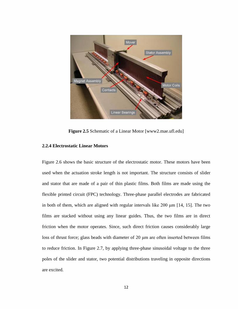
Figure 2.5 Schematic of a Linear Motor [www2.mae.ufl.edu]
2.2.4 Electrostatic Linear Motors
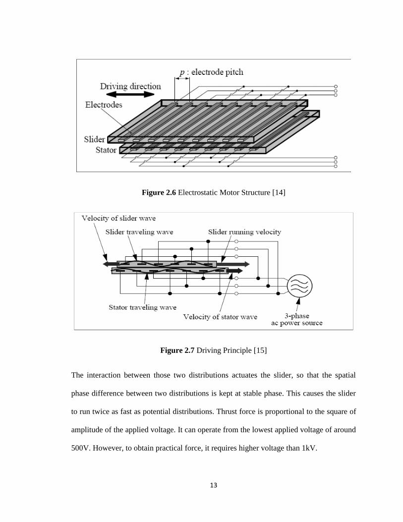
Figure 2.6 shows the basic structure of the electrostatic motor. These motors have been
used when the actuation stroke length is not important. The structure consists of slider
and stator that are made of a pair of thin plastic films. Both films are made using the
flexible printed circuit (FPC) technology. Three-phase parallel electrodes are fabricated
in both of them, which are aligned with regular intervals like 200 μm [14, 15]. The two
films are stacked without using any linear guides. Thus, the two films are in direct
friction when the motor operates. Since, such direct friction causes considerably large
loss of thrust force; glass beads with diameter of 20 μm are often inserted between films
to reduce friction. In Figure 2.7, by applying three-phase sinusoidal voltage to the three
poles of the slider and stator, two potential distributions traveling in opposite directions
are excited.
13
Figure 2.6 Electrostatic Motor Structure [14]
Figure 2.7 Driving Principle [15]
The interaction between those two distributions actuates the slider, so that the spatial
phase difference between two distributions is kept at stable phase. This causes the slider
to run twice as fast as potential distributions. Thrust force is proportional to the square of
amplitude of the applied voltage. It can operate from the lowest applied voltage of around
500V. However, to obtain practical force, it requires higher voltage than 1kV.
14
With such a high voltage of over 1kV, electric discharge may occur in the atmospheric
air, which disturbs the electrostatic field inside the motor and causes improper motor
behavior. To prevent such discharge, a dielectric liquid like Fluorinert is used for
insulation. Another disadvantage of this system is, the stroke length is not sufficient for
machine design where important ranges are required.
2.2.5 Pneumatic Artificial Muscles (PAMs) Actuators
PAMs are new generation actuators. This type of actuator contains electrostatic bladder
surface surrounded by a braided sleeve. Applying pressure inside the soft bladder (i.e.,
inflation) increases the diameter and decreases the length of the actuator through
reorientation of the stiff braid fibers, generating a contractile stroke and pulling force
similar to human muscle [16]. PAMs can achieve much higher power-to-weight ratios
than electrical and hydraulic actuators [17]. They are capable of producing high forces at
high speed [18]. No gears are necessary, thus there is no inertia or backlash added to the
system. Other benefits of these devices include durability, reliability, operation without
precise mechanical alignment, and high force capability at comparably low operational
pressures (0_150 psi) [19]. Figure 2.8 shows a typical PAM bladder with braided sleeves
and a PAM actuation based robotic arm. The bladder is made of low viscosity additional
cure silicone rubber and two end fittings are integrated at the end of the bladder.

15
Figure 2.8 PAM bladder and PAM robot arm [16].
Due to the lightweight structure compared to the hydraulic system, use of PAM actuator
can add some advantages. Reliability is a great concern for this type of actuator. The
actuation principle is mainly based on the pneumatic principle and this actuation is error
prone when dealing with large loads. Precise flow control is required for accurate
functioning and research is going on the controller design.
2.2.6 Mechanical Actuators
Mechanical linear actuators convert the rotary motion into linear motion (motion in a
straight line) of a control knob or handle into linear displacement using the screws and/or
gears to which the knob or handle is attached. This type of actuators have great use in the
lasers and optics field to manipulate the position of linear stages, rotary stages, mirror
mounts, goniometers and other positioning instruments [20]. For accurate and repeatable
positioning, index marks may be used on control knobs. Some linear actuator designs
include an encoder and digital position readout.

16
Mechanical actuators can be classified in three broad categories:
1. Machine Screws (lead screw, screw jack, ball screw and roller screw etc.)
2. Wheel and axle (Hoist, winch, rack and pinion, chain drive, belt drive, rigid chain
and rigid belt linear actuators etc.)
3. Cam type
Figure 2.9 Rack and pinion [en.wikipedia.org]
Mechanical actuators are very rigid only if they have low backlash. They have a very
high load handling capability. Their main disadvantages are their teeth being flexible
limiting their accelerations and also often requiring guiding for long strokes (hard to
implement without being fixed). Another problem is matching the gears perfectly to
avoid backlash and shocks. Cam and plunger often has problem of slip and wear. Plunger
also needs guiding that limit its use in robotics. Mechanical actuators are mainly used in
the human operated system to ease the workload.
2.2.7 Micro and Nano Actuators
With the advancement of MEMS (micro electro mechanical systems) technologies, many
kinds of micro and nano actuators have been developed.
17
As micro and nano actuators need to be very precise, research is going on to develop the
next generation micro and nano actuators. For higher precision, the micro actuator has an
advantage that it is allowed to employ various kinds of materials, since the cost of
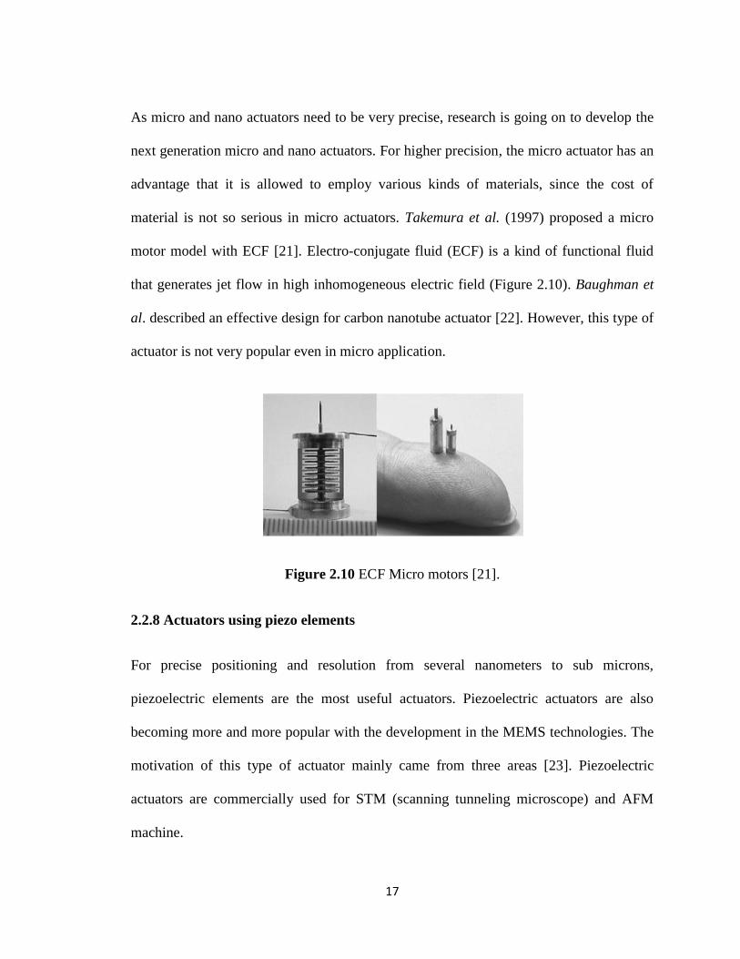
material is not so serious in micro actuators. Takemura et al. (1997) proposed a micro
motor model with ECF [21]. Electro-conjugate fluid (ECF) is a kind of functional fluid
that generates jet flow in high inhomogeneous electric field (Figure 2.10). Baughman et
al. described an effective design for carbon nanotube actuator [22]. However, this type of
actuator is not very popular even in micro application.
Figure 2.10 ECF Micro motors [21].
2.2.8 Actuators using piezo elements
For precise positioning and resolution from several nanometers to sub microns,
piezoelectric elements are the most useful actuators. Piezoelectric actuators are also
becoming more and more popular with the development in the MEMS technologies. The
motivation of this type of actuator mainly came from three areas [23]. Piezoelectric
actuators are commercially used for STM (scanning tunneling microscope) and AFM
machine.
18
The success of STM and AFM proves that this type of actuator can manipulate probes
and specimens at an atomic scale. The STM probe positioned with the resolution of nm,
even angstroms. Now only the piezoelectric elements can satisfy the nano positioning
requirements commercially. For the frequency response, a piezo element itself can
deform much faster than usual electric linear motors (i.e. a voice coil motor). So, the
piezoelectric element seems to be the most convenient actuator when we need to position
a rather small object with high accuracy. On the other hand, the maximum deformation of
a piezo element itself is limited to very small, like 10 micrometers for a 10 mm long
piezo element. Since the displacement of a piezo itself is limited, several methods have
been developed to realize longer or boundless movement by combining some mechanism
with piezo elements. The typical mechanisms are “inchworm,” “impact drive
mechanism,” [24] and ultrasonic motors [25]. Since PZT contains lead that should be
eliminated from all consumer goods. Development of lead-free piezo elements with good
property of actuation becomes a serious and urgent problem [26, 27, 28]. The miniature
size of this type of actuator provides opportunity to arrange them in several ways.
2.2.9 Actuator Based on Parallel Mechanisms
Fast parallel drives similar to the Delta-Robot [29], have the advantage that their motors
are fixed and don’t have to be moved. This reduces the moved mass and allows the
achievement of high acceleration. But these robots use ball bearings for the joints, which
have radial run-out of several μm. The inaccuracy accumulates with each joint of the
robot arranged in a chain-like structure.

19
Other problems are the low stiffness of these structures, the frictional forces in the joints
and the complex kinematics and dynamics. All these effects make it difficult to achieve
high precision combined with large acceleration. This may be improved when using
direct visual feedback, however, the limit cycles resulting from the frictional forces and
the speed of image processing will still be the limiting factors. Research is now going on
the high performance linear actuator based on the parallel mechanism.
2.2.10 Magnetically Levitated Planar Actuator (MLPA)
MLPAs are alternatives of the xy drive stacked linear motors. The translator of these
actuators is suspended above the stator with no support other than the magnetic fields.
The gravitational force is fully counteracted by the electromagnetic force. The translator
of these ironless planar actuators can move over relatively large distances in the xy plane
only, but it has to be controlled in six degrees of freedom (6-DOF) because of the active
magnetic bearing. The advantage of the magnetically levitated planar actuators is that
they can operate in vacuum (e.g. extreme-UV lithography equipment). Planar actuators
can be constructed in two ways. The actuator has either moving coils and stationary
magnets [30] or moving magnets and stationary coils [31]–[34]. The last type of planar
actuator does not require a cable to the moving part. The change of magnetization
between the active coils causes the movement of the translator. The problem of this type
of actuator is that the coil at the edge of the magnet can produce significant force and
torque. To overcome that problem, current amplifiers were used for the coil with weak
force and torque generation capacity [35].

20
The controller for this type of actuator calculates a force and torque reference or wrench
command every sample time. Then this wrench command is converted to the current set
points for the power amplifiers.
2.2.11 Voice Coil Actuator
Voice-coil actuators are the simplest form of electric motor. They consist of a non-
commutated single coil or winding moving through a fixed magnetic field produced by
the stationary permanent magnets. It is generally the end user’s responsibility to couple
the voice-coil actuator with a linear bearing system, position feedback device, switch-
mode or linear servo amplifier, and motion controller. The integration of multiple discrete
components adversely affects the system reliability and renders minimization and
packaging difficult, particularly when multiple actuators are required. Current voice coil
(i.e., linear electric) actuators are simple electromechanical devices that generate precise
forces in response to an electrical input signal. Fundamentally, they are the simplest form
of electric motor consisting of a non-commutated single coil or winding moving through
a fixed magnetic field produced by stationary permanent magnets[36] [37] [38].
2.2.12 Unconventional Actuator
According to the advancements of science and technology, the use of unconventional
environments such as super-clean, ultra high vacuum, high temperature and cryogenic
environment must be increasing. For the material handling and processing in the
unconventional environments, conventional electric motors do not always act well. As a
permanent magnet loses its magnetic potential at Curie temperature, conventional

21
electromagnetic actuators are difficult for use in high temperature. For shape memory
alloy actuators, new materials which can work in cryogenic condition [39] and in high
temperature [40] have been developed. Combination of direct drive motors and contact
free bearings (i.e. magnetic bearings) is a typical solution for super clean environment
actuator [41]. If a magnetic field is avoided, electrostatic motor combined with
electrostatic levitation seems to be promising [42].
2.3 Brief History of Straight Line Mechanisms
Inventing a straight line mechanism has been the concern for many researchers and
engineers even long before the industrial revolution. In seventeenth century, Christopher
Scheiner invented the pantograph that may be regarded as the first example of the four
bar linkage [43]. In that design, the actuator was located to one end and the device can
make a straight line provided that the input follows a straight line. At that time it was
extremely difficult to machine the straight and flat surface. Prismatic pair construction
without backlash had become difficult and much effort was then devoted towards the
straight line motion by linkage coupler contains only revolute joint. Later James Watt
proposed a four bar mechanism which was able to generate roughly a straight line. In
1864, Peaucellier introduced the first planar linkage capable of transforming rotary
motion into exact straight line motion. After that Grashof linkage also provided exact
straight line. A Grashof linkage is a “Crank-Rocker”. The input link rotates through 360
degree while the output rocks back and forth [44]. Then in Hart’s linkage and in A-frame
they used only five links to produce straight line motion [3]. The Kmoddl library from

22
Cornell University presents 39 linkages imagined to produce linear motion [45, 46]. But
most of them were relatively complex architecture and difficult to use in robot design.
There were several other proposals of linkage designs to produce the straight line motion.
Hoekens, Chebyshev, Evens, Roberts and Burmester are few of them. These designs
could produce straight lines over some limited range of their motion. The commonality of
these mechanisms is most of the designs are based on parallel topology [3].
2.4 Effective Solutions:
The simplest forms of parallel mechanisms are the ones producing one degree of
freedom. Among these mechanisms there are several classes which can produce straight
line motion. Out of these classes some four bar mechanism can produce approximate
straight line motion of a point on the coupler, not the coupler itself. So, specific four bar
linkage can be made to produce straight line path if they are made with appropriate
dimensions and their coupler curves are considered on the link extensions. For designing
fast linear actuator from different configuration of four bar mechanism some effective
solutions can be:
1. The parallelogram configuration

23
2. The rhombus configuration
3. The kite or diamond configuration
4. Scissor lift mechanism
[Figure Source: highaccessgroup.com.au]

24
2.5 Final Decision
All the proposed effective solutions are single DOF mechanism. Among these, four bar
rhombus configuration was chosen to design the new actuator. Kinematic analysis of the
four bar rhombus was performed on the following criteria:
1. Range of Motion
2. Singularity Avoidance
3. Linkage Encumbrance
4. Linearity in Motion Transmission
25
Chapter 3
Scissor Lift as Linear Actuator
3.1 Introduction
During the development of the newly designed actuator at the very beginning, the scissor
lift mechanism was also studied to verify its suitability as a fast linear actuator. Therefore,
a proper dynamic model is necessary to investigate the dynamic behavior of the system.
This chapter describes the implementation of general multibody system dynamics on the
scissor lift Mechanism within a bond graph (Appendix A) modeling framework. There are
several methods for deriving the dynamic equations of rigid bodies in classical mechanics
(i.e. Classic Newton-D’Alembert, Newton-Euler, Lagrange, Hamilton, Kanes to name a
few). But, these are labor-intensive for large and complicated systems and thereby error
prone. Here, the multibody dynamics model of the mechanism is developed in bond graph
formalism, because it offers flexibility for modeling of closed loop kinematic systems

26
without any causal conflicts, and control laws can be included. The proposed multibody
dynamics model of the mechanism offers a method to analyze the dynamics of the
mechanism knowing that there is no such work available for scissor lifts. Figure 3.1 shows
the complete system model of a scissor lift mechanism. There is a driving mechanism
connected with the lower end of the moving link which is located at the ground platform.
The driving mechanism can be electric, hydraulic or pneumatic based on the design
criteria. Here, we considered a DC motor as the driving mechanism. It is located at the
base and connected with the prismatic link. Design of Experiment (DOE) based statistical
approach has been used for optimizing the parametric design and performance (e.g.
height) of the scissor lift elevators.
Figure 3.1 Basic Construction of a 2 stage Scissor Lift Mechanism

27
Figure 3.2 Kinematic Analysis Figure
3.2 Kinematic Analysis of the Mechanism
Kinematic analysis can be done by looking at the loops. For the design in Figure 3.2, link
length (l) is equal for each of the link. Input distance is S and the midpoint height is h.
Total height for one stage is, H=H1 =2h.
The height h with respect to the input angle θ’ is:
(3.1)
The inverse kinematics problem is expressed as:
(3.2)

28
Height h can be expressed in terms of input link length (S):
√
(3.3)
From Eq. (3.3) we can write inverse kinematics in terms of input link length:
√ (3.4)
Derivative of Eq. (3.4) gives the velocity of the platform for one stage:
√
(3.5)
Further derivation of Eq. (3.5) gives the acceleration of the end effector (platform):
(
) (
(
)
) (
)
(
) (
√
)
(3.6)
For two stage scissor lift total height is, H = H2 = 4h.
(3.7)
Inverse kinematics in terms of the input angle θ’ is:
(3.8)
Inverse kinematics in terms of the input link length:
√
(3.9)
29
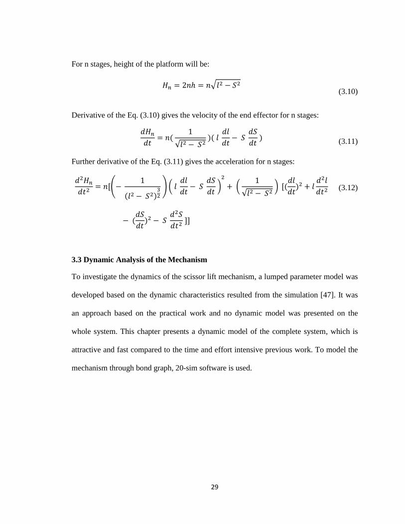
For n stages, height of the platform will be:
√
(3.10)
Derivative of the Eq. (3.10) gives the velocity of the end effector for n stages:
√
(3.11)
Further derivative of the Eq. (3.11) gives the acceleration for n stages:
(
) (
)
(
√ )
(3.12)
3.3 Dynamic Analysis of the Mechanism
To investigate the dynamics of the scissor lift mechanism, a lumped parameter model was
developed based on the dynamic characteristics resulted from the simulation [47]. It was
an approach based on the practical work and no dynamic model was presented on the
whole system. This chapter presents a dynamic model of the complete system, which is
attractive and fast compared to the time and effort intensive previous work. To model the
mechanism through bond graph, 20-sim software is used.

30
Figure 3.3 Schematic of a Single Link
3.3.1 Bond Graph Model of Each Link
For the bond graph modeling, a single beam is considered with mass and rotational inertia.
External forces are applied at port A and B. Formulation becomes much easier, when all
bodies in a multibody system contains three inertial coordinate (x,y,θ). Velocity of the
point B with respect to the point G can be formulated as:
(3.13)
Where, the point G is the center of the gravity of the link. If the distance from the point G
to the point B is r, then the equation will be:
(3.14)
31
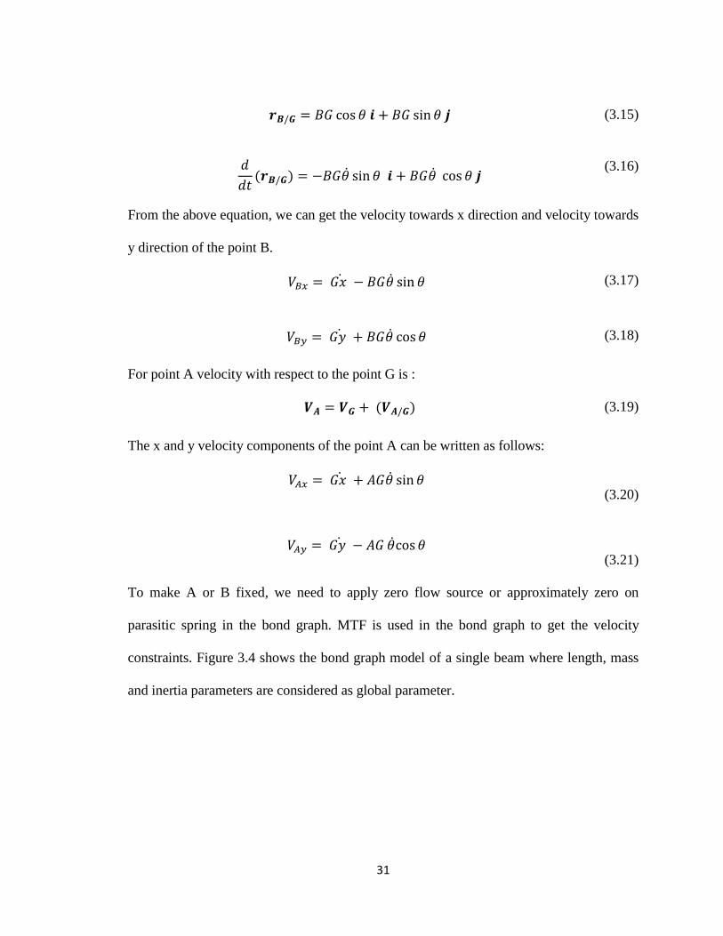
(3.15)
(3.16)
From the above equation, we can get the velocity towards x direction and velocity towards
y direction of the point B.
(3.17)
(3.18)
For point A velocity with respect to the point G is :
(3.19)
The x and y velocity components of the point A can be written as follows:
(3.20)
(3.21)
To make A or B fixed, we need to apply zero flow source or approximately zero on
parasitic spring in the bond graph. MTF is used in the bond graph to get the velocity
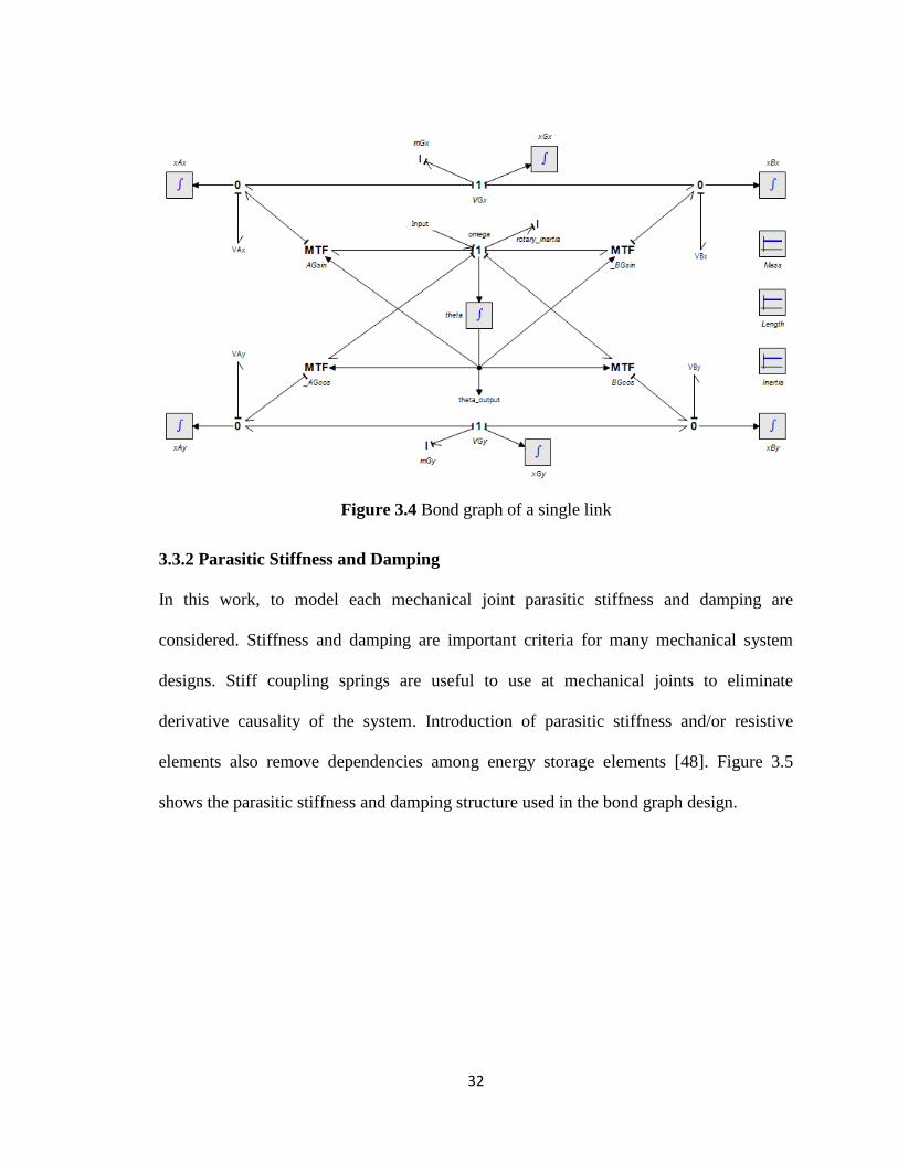
constraints. Figure 3.4 shows the bond graph model of a single beam where length, mass
and inertia parameters are considered as global parameter.
32
Figure 3.4 Bond graph of a single link
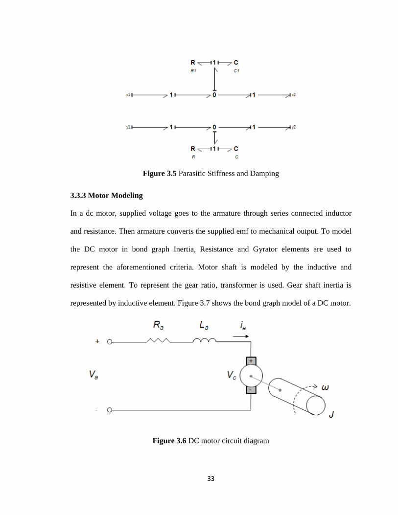
3.3.2 Parasitic Stiffness and Damping
In this work, to model each mechanical joint parasitic stiffness and damping are
considered. Stiffness and damping are important criteria for many mechanical system
designs. Stiff coupling springs are useful to use at mechanical joints to eliminate
derivative causality of the system. Introduction of parasitic stiffness and/or resistive
elements also remove dependencies among energy storage elements [48]. Figure 3.5
shows the parasitic stiffness and damping structure used in the bond graph design.
33
Figure 3.5 Parasitic Stiffness and Damping
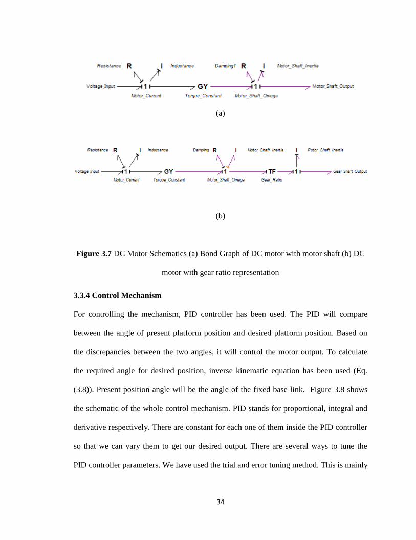
3.3.3 Motor Modeling
In a dc motor, supplied voltage goes to the armature through series connected inductor
and resistance. Then armature converts the supplied emf to mechanical output. To model
the DC motor in bond graph Inertia, Resistance and Gyrator elements are used to
represent the aforementioned criteria. Motor shaft is modeled by the inductive and
resistive element. To represent the gear ratio, transformer is used. Gear shaft inertia is
represented by inductive element. Figure 3.7 shows the bond graph model of a DC motor.
Figure 3.6 DC motor circuit diagram
34
(a)
(b)
Figure 3.7 DC Motor Schematics (a) Bond Graph of DC motor with motor shaft (b) DC
motor with gear ratio representation
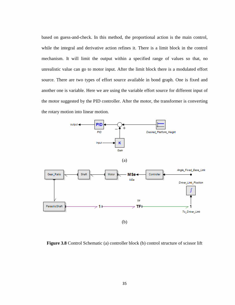
3.3.4 Control Mechanism
For controlling the mechanism, PID controller has been used. The PID will compare
between the angle of present platform position and desired platform position. Based on
the discrepancies between the two angles, it will control the motor output. To calculate
the required angle for desired position, inverse kinematic equation has been used (Eq.
(3.8)). Present position angle will be the angle of the fixed base link. Figure 3.8 shows
the schematic of the whole control mechanism. PID stands for proportional, integral and
derivative respectively. There are constant for each one of them inside the PID controller
so that we can vary them to get our desired output. There are several ways to tune the
PID controller parameters. We have used the trial and error tuning method. This is mainly
35
based on guess-and-check. In this method, the proportional action is the main control,
while the integral and derivative action refines it. There is a limit block in the control
mechanism. It will limit the output within a specified range of values so that, no
unrealistic value can go to motor input. After the limit block there is a modulated effort
source. There are two types of effort source available in bond graph. One is fixed and
another one is variable. Here we are using the variable effort source for different input of
the motor suggested by the PID controller. After the motor, the transformer is converting
the rotary motion into linear motion.
(a)
(b)
Figure 3.8 Control Schematic (a) controller block (b) control structure of scissor lift

36
Figure 3.9 Bond graph model of Scissor-lift mechanism with two rhombus stages

37
3.3.5 Simulation
For the simulation, considered length for each of the link is set to 2 m. Width is 0.05 m
and thickness is also 0.05m. To calculate mass properties, Carbon Fiber (Zoltek Panex
33) material has been used. Maxon motor (Model # 167131) is chosen as a DC motor
with maxon gearhead (model # 110408). Material properties and motor specifications are
mentioned in Appendix A.
Table 3.1 Simulation Result
Simulation Direction PID Controller Parameter
Simulation Data
Forward Simulation
Initial Height = 2 m
Desired Height = 2.5 m
Proportional gain
kp = -32.0 ;
Derivative time constant
tauD = 7.0 s;
Tameness constant
beta = 0.05 ;
Integral time constant
tauI = 40.0 s;
Driver Link position = 1.56 m
Max Velocity = 0.27 m/s
Max Acceleration = 0.7 m/s2
Peak Torque Duration = 0.4 s
Backward Simulation
Initial Height = 2 m
Desired Height = 1.5 m
Proportional gain
kp = -32.0 ;
Derivative time constant
tauD = 11.0 s;
Tameness constant
beta = 0.05 ;
Integral time constant
tauI = 40.0 s;
Driver Link position = 1.85 m
Max Velocity = 0.25 m/s
Max Acceleration = 0.7 m/s2
Peak Torque Duration = 0.7 s
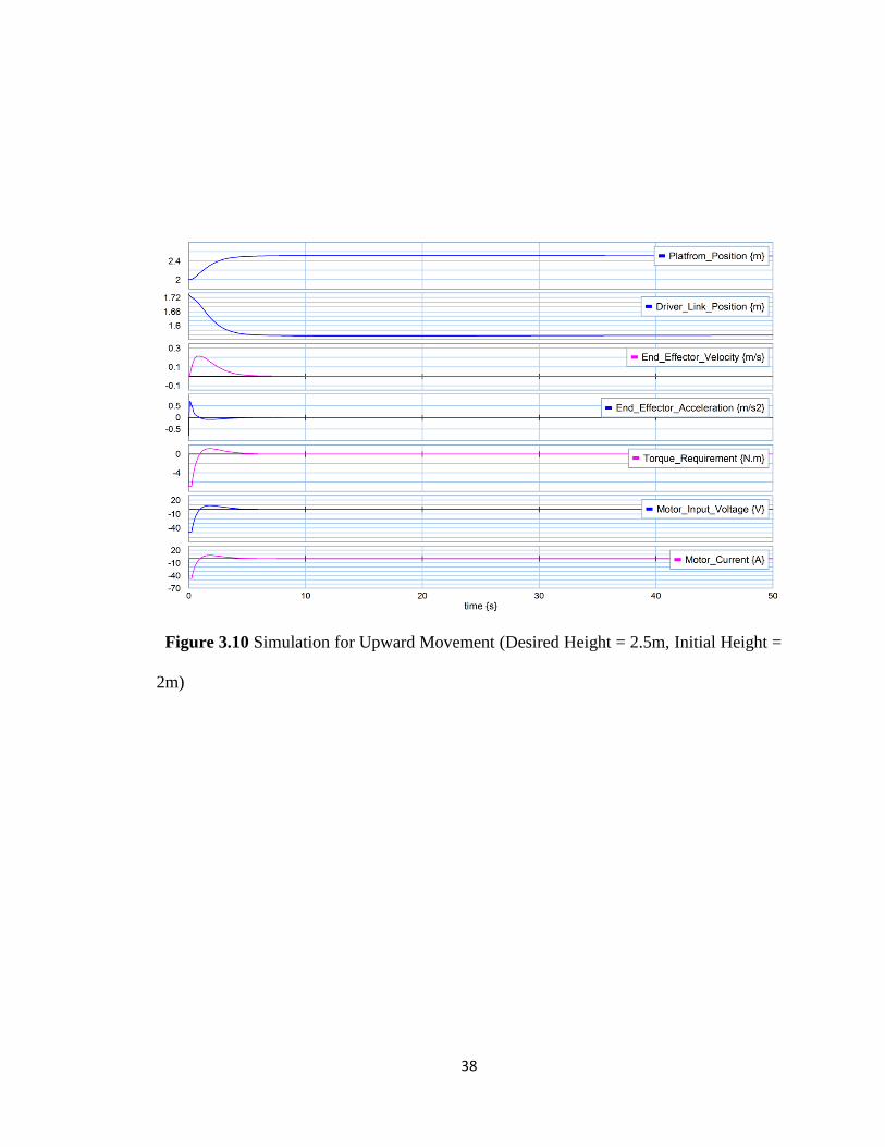
38
Figure 3.10 Simulation for Upward Movement (Desired Height = 2.5m, Initial Height =
2m)

39
Figure 3.11 Simulation for Downward Movement (Desired Height = 1.5m, Initial
Height = 2.0m)

40
3.3.6 Result Interpretation
In Figure 3.10, the platform moved towards a height of 2.5m higher than its initial height
of 2 m. Driver link on the base should move in the backward direction from its initial
position. From the inverse kinematics calculation, required position was 1.56 meter.
Simulation shows exactly the same position of the driver link. Figure 3.11 shows
simulation curves for the downward movement. Simulation results follow the calculation
closely, which signifies the effectiveness of the dynamic modeling. It is more like the
steady state of the dynamics under control is actually reaching the value calculated by the
inverse kinematics.
3.4 Parametric Design optimization using Design of Experiment (DOE)
The objective of the DOE optimization is to find out the ideal parametric combination of
a scissor lift mechanism for a certain height. Using dynamic and kinematic analysis of the
scissor lift elevator, performance of the mechanism is simulated for different parametric
combination to achieve certain height by the end effector or the platform. Liu et al. in
[49] proposed a simulative calculation based optimal design approach of scissor lift,
where the actuation principle is based on a hydraulic system. Usually, the performances
of the scissor lift elevators are tested in the laboratory associated with important cost and
time. That is why, effective statistical analysis is a great addition for this type of
mechanism. From the analysis, link length was screened out as the most important factor
for the height performance, compared to the stage repetition and motor torque. Brief
description of the DOE is presented in Appendix B.
41
3.4.1 Experimental Factors and Response
Various parameters influencing the performance of a scissor lift are identified based on
their kinetic and dynamic analysis. We considered five parameters as input factors and the
output response is the height of the platform.
Mass of Link (A): Each of the links has an effect on mechanism performance. For
experiment, link mass is allowed to have two different levels (Two different
material properties have been used). We considered, link mass – 1.36 Kg (low
level) and link mass– 2.27 Kg (high level) for analysis.
Link Length (B): If the length of the link increases, then it will increase the height
coverage of the scissor lift. But, on the other hand mass will also increase. The
DC motor needs to supply more torque. Considered two different link lengths are
0.4 m (low level) and 0.6 m (high level).
Platform Load (C): There is a platform on the top of the scissor lift elevator to
carry load. Platform load combines the mass of the platform as well as the
carrying load. Here in this design the chosen platform loads are 5 Kg (low level)
and 8 Kg (high level).
Motor Torque (D): Based on the supplied motor torque, the end effector will
move. When the mass of the system or load increases, then the motor needs to
supply more torque. The considered two levels are 2.26 Nm (low level) and 3.4
Nm (high level). Motor torque is constant at low and high level.
42
Repetition of Stages (E): Repetition of stages is done since, it reduces the
transverse width thereby mechanism space utilization. Two links connected in
their center of mass form a stage. Increase in the number of stages, will cause
increase in the height performance of the mechanism. But increase of stages will
also cause increase in weight and requires more torque to lift the same load up to
certain height. Here, we considered 2 stage repetition as low level and 3 stage
repetition as high level.
The response is the platform movement lifted by the scissor lift. For different level of the
considered five factors, response (height) was recorded from the simulation. For five
factors, a full factorial design needs a total of 25
= 32 runs. Instead, we have used a half
fractional factorial design with a total of 25-1
= 16 runs. One effect has to be confounded
(Appendix B) and we choose I = ABCDE as the confounding effect. As this is a
resolution V design, all the main effects and two factor interactions can be estimated
clearly. Three factor interactions are aliased with two factor interactions. But, they are
not significant and can be ignored. Response data collected from 20 sim simulation.
3.4.2 Fractional Factorial Design of the Experiment
A 25-1
fractional factorial (requiring 16 runs) design is used to determine the influence of
the five factors and interactions of factors. Design Expert software (version 8.0.6) by
Stat-Ease has been used to develop a design of Resolution V. An alias structure
automatically chosen by the software takes the advantage of the sparsity of effects - that
is, high order interactions are aliased with main and two factor interactions. Figure 3.12
shows the run order data. Figure 3.13 shows the effect list.

43
3.4.3 Analysis of Experimental Data
While analyzing data, most important factors and their significant interaction effects are
considered. Figure 3.14 and Figure 3.15 shows the effect of A, B, C, D, E and the
interaction BE are the main contributors as their percentage contributions are very high.
Remaining factors have no significant contributions to the height performance, as there
percentage contributions are less.

44
Figure 3.12 Aliased terms including run list and Data for Experiment
Figure 3.13 Effect List

45
3.4.4 Pareto Chart and Half Normal Plot
From the pareto chart and half normal plot (Appendix B), we can screen out the most
significant factors and their interaction effects.
Figure 3.14 Pareto Chart
Figure 3.15 Half Normal Plot
0.00
5.50
11.01
16.51
22.01
27.52
1 2 3 4 5 6 7 8 9 10 11 12 13 14 15
Pareto Chart
Rank
t-V
alu
e o
f |E
ffe
ct|
Bonf erroni Limit 3.95422
t-Value Limit 2.26216
B-Link Length
E-Repitition of Stages
BE
D-Motor Torque
A-Mass of LinkC-Platform Load
Design-Expert® Software
Platform Height
Shapiro-Wilk test
W-value = 0.930
p-value = 0.477
A: Mass of Link
B: Link Length
C: Platform Load
D: Motor Torque
E: Repitition of Stages
Positive Effects
Negative Effects
-0.05 0.09 0.22 0.35 0.49
1
5
10
20
30
50
70
80
90
95
99
Normal Plot
Standardized Effect
No
rma
l %
Pro
ba
bil
ity
A-Mass of Link
B-Link Length
C-Platform Load
D-Motor Torque
E-Repitition of StagesBE
46
Figure 3.14 shows that from our considered parameters, all the single factor effects are
significant. Interactions between BE is the most dominant interaction effect. Figure 3.15
shows the half normal plot and it justifies the same result for the effects. The most
significant factors will be away from the line in the half normal plot.
3.4.5 ANOVA Analysis and Regression Model
The ANOVA table summarizes the significance. From the F-value and probability value
comparison of the effects, the software computes the significance. In summary, the
standard shows the deviation of the error term. R2
presents the percentage of total
variability explained by the model. Addition of effect will increase the R value. That is
why we should look at the adjusted R value produced by the model. The difference
between the two R2 should be very small. Precision should be greater than 4 for an
adequate model. Figure 3.16 shows the ANOVA table and the ANOVA summary for the
proposed model. The R2 values are very close and precision is much greater than 4 which
signify the adequacy of the model. Figure 3.17 represents a mathematical model for the
output response of the scissor lift.
3.4.6 Residual Analysis
Residual analysis checks whether the assumptions of the ANOVA are correct or not. We
made following assumptions:
1. Random Samples from their respective population.
2. All samples are independent.
3. Departures from group mean are normally distributed for all data groups.
4. All data groups have equal variance.

47
Figure 3.16 ANOVA table with the summary

48
Figure 3.17 Regression Model
Figure 3.18 Normal Plot
From the normal probability plot (Figure 3.18), one can observe that maximum points
follow a straight line. So, the distributions of residuals are almost normal. The plot of
Residuals vs. Predicted (Figure 3.19) looks like well scattered, which indicates constant
variance. Figure 3.20 shows the Residuals vs Run plot. From the plot we can see, most of
the data are random (i.e. no trend and points are beyond the red line). Finally, from the
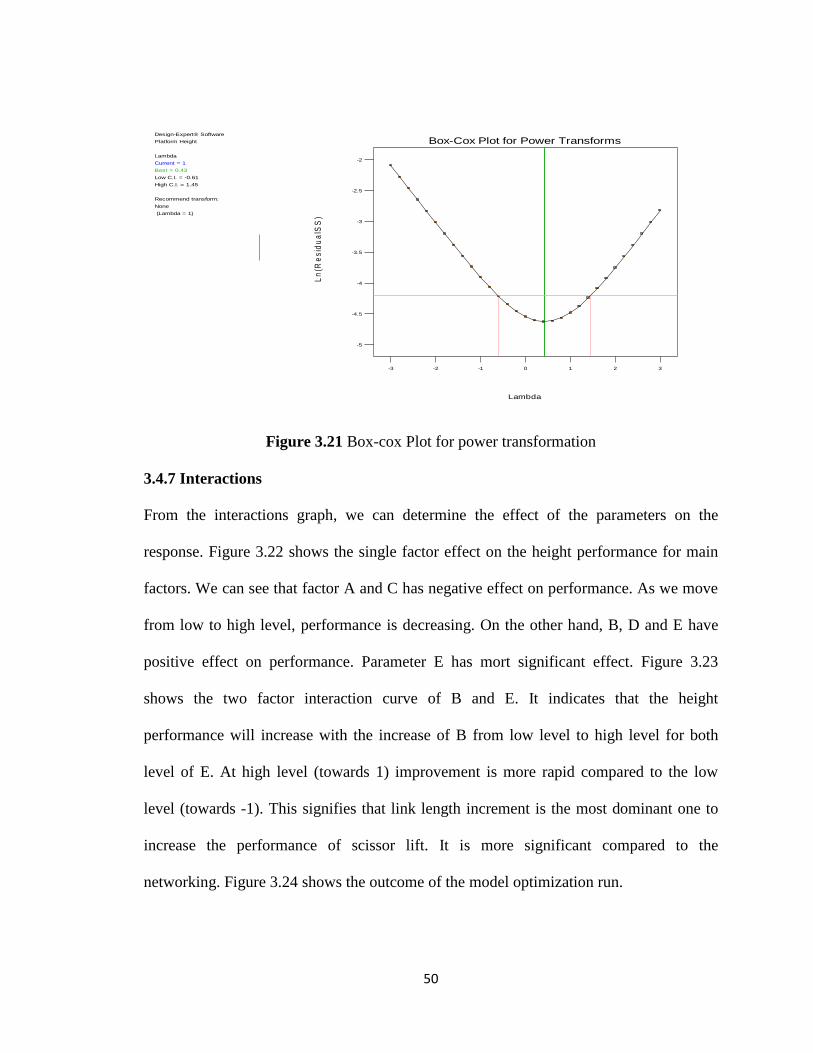
Box-Cox plot of Figure 3.21 we can see that the current line (blue line) is between the
Design-Expert® Software
Platform Height
Color points by value of
Platform Height:
1.74
0.65
Externally Studentized Residuals
No
rma
l %
Pro
ba
bil
ity
Normal Plot of Residuals
-3.00 -2.00 -1.00 0.00 1.00 2.00 3.00
1
5
10
20
30
50
70
80
90
95
99

49
ranges (between Low & High Confidence Interval). This result means no transformation.
So, we can conclude that the assumptions of ANOVA are satisfied.
Figure 3.19 Residuals vs. Predicted Plot
Figure 3.20 Residuals vs. Run Plot
Design-Expert® Software
Platform Height
Color points by value of
Platform Height:
1.74
0.65
Predicted
Ex
tern
all
y S
tud
en
tiz
ed
Re
sid
ua
ls
Residuals vs. Predicted
-4.00
-2.00
0.00
2.00
4.00
0.6 0.8 1 1.2 1.4 1.6 1.8
Design-Expert® Software
Platform Height
Color points by value of
Platform Height:
1.74
0.65
Run Number
Ex
tern
all
y S
tud
en
tiz
ed
Re
sid
ua
ls
Residuals vs. Run
-4.00
-2.00
0.00
2.00
4.00
1 4 7 10 13 16
50
Figure 3.21 Box-cox Plot for power transformation
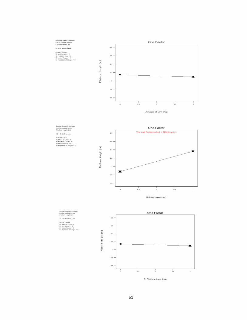
3.4.7 Interactions
From the interactions graph, we can determine the effect of the parameters on the
response. Figure 3.22 shows the single factor effect on the height performance for main
factors. We can see that factor A and C has negative effect on performance. As we move
from low to high level, performance is decreasing. On the other hand, B, D and E have
positive effect on performance. Parameter E has mort significant effect. Figure 3.23
shows the two factor interaction curve of B and E. It indicates that the height
performance will increase with the increase of B from low level to high level for both
level of E. At high level (towards 1) improvement is more rapid compared to the low
level (towards -1). This signifies that link length increment is the most dominant one to
increase the performance of scissor lift. It is more significant compared to the
networking. Figure 3.24 shows the outcome of the model optimization run.
Design-Expert® Software
Platform Height
Lambda
Current = 1
Best = 0.43
Low C.I. = -0.61
High C.I. = 1.45
Recommend transform:
None
(Lambda = 1)
Lambda
Ln
(Re
sid
ua
lSS
)
Box-Cox Plot for Power Transforms
-5
-4.5
-4
-3.5
-3
-2.5
-2
-3 -2 -1 0 1 2 3
51
Design-Expert® Software
Factor Coding: Actual
Platform Height (m)
X1 = A: Mass of Link
Actual Factors
B: Link Length = 0
C: Platform Load = 0
D: Motor Torque = 0
E: Repitition of Stages = 0
A: Mass of Link (Kg)
-1 -0.5 0 0.5 1
Pla
tfo
rm H
eig
ht
(m)
0.6
0.8
1
1.2
1.4
1.6
1.8
One Factor
Design-Expert® Software
Factor Coding: Actual
Platform Height (m)
X1 = B: Link Length
Actual Factors
A: Mass of Link = 0
C: Platform Load = 0
D: Motor Torque = 0
E: Repitition of Stages = 0
B: Link Length (m)
-1 -0.5 0 0.5 1
Pla
tfo
rm H
eig
ht
(m)
0.6
0.8
1
1.2
1.4
1.6
1.8Warning! Factor involved in BE interaction.
One Factor
Design-Expert® Software
Factor Coding: Actual
Platform Height (m)
X1 = C: Platform Load
Actual Factors
A: Mass of Link = 0
B: Link Length = 0
D: Motor Torque = 0
E: Repitition of Stages = 0
C: Platform Load (Kg)
-1 -0.5 0 0.5 1
Pla
tfo
rm H
eig
ht
(m)
0.6
0.8
1
1.2
1.4
1.6
1.8
One Factor

52
Figure 3.22 Single Factor Interaction Graph
Design-Expert® Software
Factor Coding: Actual
Platform Height (m)
X1 = D: Motor Torque
Actual Factors
A: Mass of Link = 0
B: Link Length = 0
C: Platform Load = 0
E: Repitition of Stages = 0
D: Motor Torque (Nm)
-1 -0.5 0 0.5 1
Pla
tfo
rm H
eig
ht
(m)
0.6
0.8
1
1.2
1.4
1.6
1.8
One Factor
Design-Expert® Software
Factor Coding: Actual
Platform Height (m)
X1 = E: Repitition of Stages
Actual Factors
A: Mass of Link = 0
B: Link Length = 0
C: Platform Load = 0
D: Motor Torque = 0
E: Repitition of Stages
-1 -0.5 0 0.5 1
Pla
tfo
rm H
eig
ht
(m)
0.6
0.8
1
1.2
1.4
1.6
1.8Warning! Factor involved in BE interaction.
One Factor

53
Figure 3.23 Two factors interaction
Figure 3.24 Optimization Runs for validation
Design-Expert® Software
Factor Coding: Actual
Platform Height (m)
X1 = B: Link Length
X2 = E: Repitition of Stages
Actual Factors
A: Mass of Link = 0
C: Platform Load = 0
D: Motor Torque = 0
E- -1
E+ 1
B: Link Length (m)
E: Repitition of Stages
-1 -0.5 0 0.5 1
Pla
tfo
rm H
eig
ht
(m)
0.6
0.8
1
1.2
1.4
1.6
1.8
Interaction

54
3.4.8 Model Optimization
The model was optimized and extra runs performed for validity check. Four factors were
kept in range and the platform height was fixed at 1.65m to get the optimum runs with
maximum platform load. First five combinations were verified in 20 sim. Figure 3.24
shows that for the certain height all factors are in their specified range and we can
determine the values for each of the factor. Output confirms the validity of the model to
find the parametric combination and their respected values for certain height coverage.
Factor values are given in their coded form.
3.5 Discussions
Dynamic behavior of the scissor lift mechanism is modeled and verified through the
application of desired output criteria. Design optimization of scissor lift type elevating
platform using the DOE methodology has also been presented. From the simulation, we
can conclude the DC motor based scissor elevator can also be used as linear actuator for
parallel manipulator. But this actuator has the following backdrops:
Presence of slider
Friction
Prismatic pair
Low acceleration
These problems limit their use as a high performance linear actuator. But, this chapter can
be used as a good reference for practical designing of scissor type actuator and it was a
good learning experience for designing the high performance linear actuator.

55
Chapter 4
Kinematic Analysis of the Actuator
4.1 Introduction
This chapter presents the detailed kinematic analysis of the newly designed actuator
along with the networking formulations. To build a linear actuator using a parallel
topology, we can put them into a cross, or X, or scissors. Then we need to close them and
there are two ways to achieve that: (1) by closing with a bar containing a slide (i.e the
scissor lift mechanism), or (2) by closing with two bars, separated by a revolute joint (X-
track with one DC motor at one revolute end). Figure 4.1 shows a single network
rhombus configuration (X-Track with the DC motor) of the newly designed actuator.
Hence, the newly designed actuator is different from the scissor lift platforms, since there
are no sliders that produce dynamic problems forbidding high acceleration.

56
The four bar rhombus configuration is a special case of the four bar linkage, where all the
link lengths are equal. All sides of a rhombus are congruent and they can have any angle.
The identical nature of the structure gives the opportunity of networking them very easily
to improve performance. Networking of these identical linkages helps to reduce the
encumbrance. Brief kinematic analysis of the four bar actuator is described in [3].
Figure 4.1 Four Bar Rhombus Configuration
4.2 Kinematic Formulation
From Figure 4.1, we can see OA = AB = BC = OC. For our analysis, we considered the
link length as r. The mechanism configuration even includes the square, when angles are
set to 90 degrees. The forward kinematics problem becomes:
(4.1)
Where,
x = Linear distance between the point O and B.
θ = Angle between the bar OA and OC

57
The Inverse kinematics problem is expressed as:
(4.2)
Derivation of Eq. (4.2) will give us the linear velocity. The forward differential
kinematics is expressed by the following equation:
(4.3)
where,
ω =
We take the following geometric property:
(4.4)
Applying Pythagoras theorem:
√
(4.5)
After putting the values from Eq. (4.5) the linear velocity of the end effector becomes:
√
(4.6)
From Eq. (4.6) we can calculate the angular velocity. Angular velocity can be rewritten
as:
(4.7)

58
After putting the value of sin (
) from the Eq. (4.5) the angular velocity will be:
√
(4.8)
Further differentiation of the Eq. (4.3) will give the acceleration of the extremity:
(
)
(
)
(4.9)
After substituting values from Eq. (4.4) and (4.5) we can write:
√ (
)
(4.10)
From Eq. (4.9) the angular acceleration α is:
(
)
(4.11)
After substituting values of (
) and
we will get the final equation for angular
acceleration:
√
√
(4.12)
4.3 Singularity Analysis
Singularity is a point at which a function takes an infinite value. It is either addition or
loss of DOF; meaning a point where the torque becomes infinite and mechanism locks
itself or a point where the mechanism is moving whatever the motor torque. In actuator
design this points are very important as we need to identify those points to avoid them

59
during the movement of the actuator. Geometrically links have no material existence (no
mass) and they can occupy the same position in space. In reality, the mass doesn’t allow
such cases. Here, we calculated singularity in terms of the input angle and the extremity
positions. First, we can calculate the singularity in terms of the input angle θ :
(
)
(4.13)
Hence, we find a singularity at θ = 0 and its counterpart, θ = 360 degrees. So, during
construction of the actuator we have to be careful so that the configuration can’t reach to
those points. To avoid those point’s, we have to introduce some physical constrain.
In terms of the extremity position (x):
√
(4.14)
By solving the above equation we can see the singular position exist at x = 2r
corresponds to the same in terms of the input angle as θ = 0.
4.4 Range of Motion
The second important performance criterion is usually the range of motion of the end
effector. For single DOF mechanism, range of motion reduces itself to a single DOF
curve segment. In our case, it becomes a line segment. We always wish to maximize the
range of motion as much as we can. Considering the Forward Kinematics equation, the
maximum value is obtained when cos (
) = 1 and the minimum value will be at cos (
) =
−1. Hence, from the Eq. (4.4) we can write, xmax = 2r and the related angle is then θ = 0.
Moreover, xmin = −2r and the related angle is then θ = −2π.
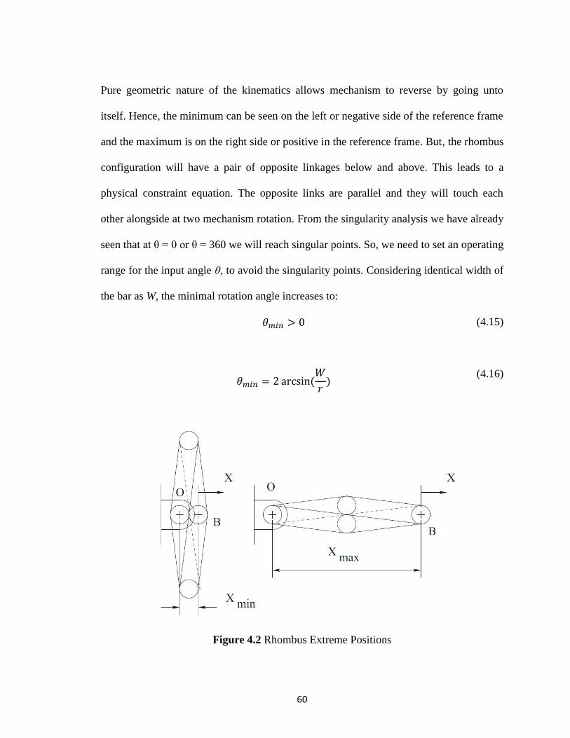
60
Pure geometric nature of the kinematics allows mechanism to reverse by going unto
itself. Hence, the minimum can be seen on the left or negative side of the reference frame
and the maximum is on the right side or positive in the reference frame. But, the rhombus
configuration will have a pair of opposite linkages below and above. This leads to a
physical constraint equation. The opposite links are parallel and they will touch each
other alongside at two mechanism rotation. From the singularity analysis we have already
seen that at θ = 0 or θ = 360 we will reach singular points. So, we need to set an operating
range for the input angle θ, to avoid the singularity points. Considering identical width of
the bar as W, the minimal rotation angle increases to:
(4.15)
(4.16)
Figure 4.2 Rhombus Extreme Positions

61
For the upper range of the theta values, we have to calculate the θmax :
(4.17)
(4.18)
Extreme positions can be calculated from these values. Minimum length would be:
(4.19)
Substituting we get:
(4.20)
Similarly, maximum length will occur at minimum angular displacement:
(4.21)
Substituting we get:
(4.22)
4.5 Encumbrance
Encumbrance is the distance from one side of the mechanism to the other side taking into
account the linkage width. Encumbrance is an important issue considering that the
mechanism spread sideways making them subjects to collisions, if other actuator would
be in the vicinity. To use them with parallel manipulator this has even much more
importance.

62
A rhombus would have minimum encumbrance of at angle Maximum
encumbrance occurring at the maximum input angle .
√ (4.23)
Figure 4.3 The Rhombus Encumbrance
4.6 Networking of Rhombus Configuration
The main advantage of the four bar rhombus configuration is that we can easily increase
its range of motion (stroke length) by doing networking. As in the rhombus configuration
all the four bars are identical, it becomes very easy to network the mechanism to achieve
certain end effector position based on the calculation. Figure 4.4 shows the networking
of double and triple rhombus.

63
Figure 4.4 Double rhombus and triple rhombus configuration
For the double rhombus configuration distance traveled by the first moving central joint:
(4.24)
This formula is similar to the forward kinematics of the four bar rhombus without any
networking. Then distance traveled by the second moving joint or the end effector for the
double rhombus:
(4.25)
Distance traveled by the third moving central joint of triple rhombus:
(4.26)
From the above calculation we can write a general formula for rhombus networking. For
n number of networking the extremity position will be:
(4.27)
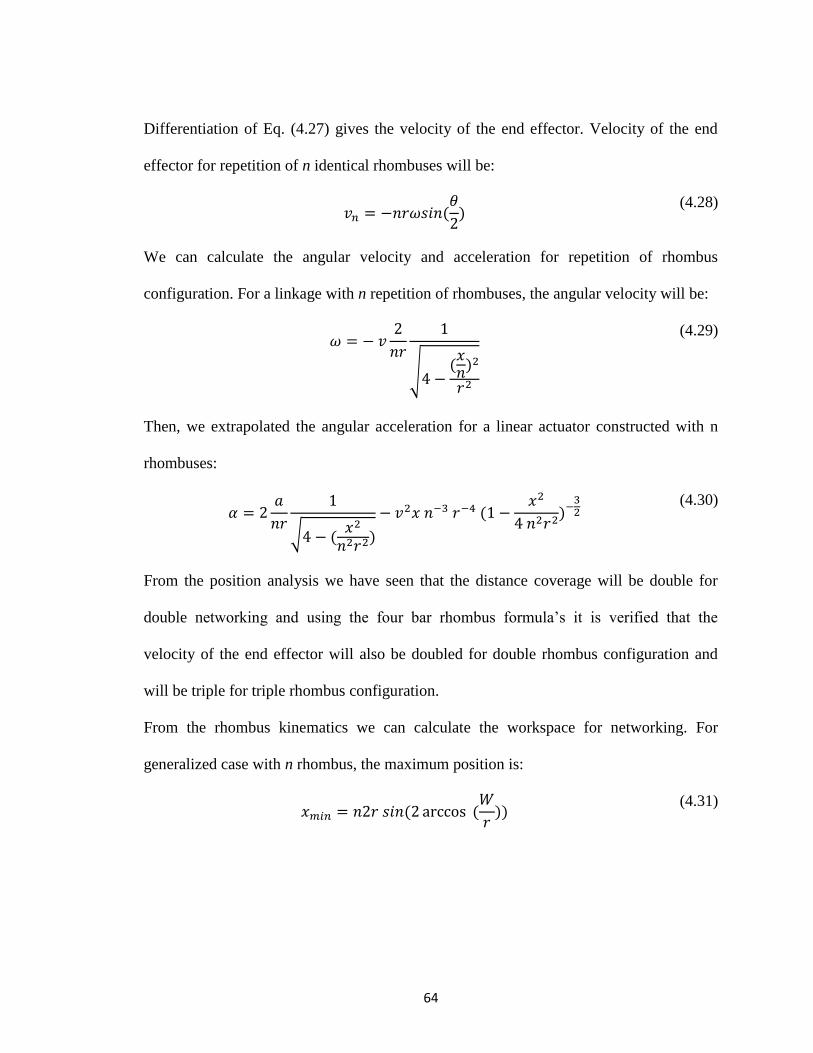
64
Differentiation of Eq. (4.27) gives the velocity of the end effector. Velocity of the end
effector for repetition of n identical rhombuses will be:
(4.28)
We can calculate the angular velocity and acceleration for repetition of rhombus
configuration. For a linkage with n repetition of rhombuses, the angular velocity will be:
√
(4.29)
Then, we extrapolated the angular acceleration for a linear actuator constructed with n
rhombuses:
√
(4.30)
From the position analysis we have seen that the distance coverage will be double for
double networking and using the four bar rhombus formula’s it is verified that the
velocity of the end effector will also be doubled for double rhombus configuration and
will be triple for triple rhombus configuration.
From the rhombus kinematics we can calculate the workspace for networking. For
generalized case with n rhombus, the maximum position is:
(4.31)

65
The maximum position is calculated using:
(4.32)
The networking of rhombuses is not affecting the encumbrance. Because, each of the bar
width is identical.
4.7 Motion Analysis
Figure 4.5 and Figure 4.6 shows the kinematic performance of the single rhombus and
triple rhombus network. From those figures we can see for both cases, end effector
maintains almost a linear trajectory with respect to the input angle. Linear velocity and
acceleration plot shows variation with time when our target acceleration is 10g. For
single network considered link length was 0.4 m and 0.1333 m for triple network.
Figure 4.5 Single Network Rhombus Kinematic Performance

66
Figure 4.6 Double Network Rhombus Kinematic Performance
4.8 Discussions
From the kinematic formulations and MATLAB simulation we can see that networking
of the rhombus configuration increases the velocity and acceleration drastically.
Compared to the velocity, there is a more rapid change in the acceleration due to
networking. For our newly designed actuator, acceleration is an important criterion. From
the kinematic simulation we get a fair idea of how networking improves the performance
of the actuator. Here, angular velocity and acceleration of the actuator is derived as a
function of the end effector motion. This formulation gives the opportunity to design a
controller, where we can command the rotational motion between the links at the revolute
end connected to the motor. Commanding such rotary motion can produce good
performance, because we can measure it with encoders.

67
Chapter 5
Lagrangian Dynamic Analysis of the Actuator
5.1 Introduction
This chapter describes the detailed steps in formulating the dynamic equations of the
newly designed linear actuator using Lagrangian formulation. Dynamic formulations of
the actuator provide the opportunity to use them into the Simulink control model. The
Lagrangian dynamic analysis approach is essentially an energy based approach, where we
need to know the kinetic and potential energy associated with each link. Here, we used
the single and double network rhombus configuration to derive the dynamic equations.
There are also discussions on associated complexities as the network number goes higher.

68
5.2 Lagrangian Formulation for Single Network
This section describes the dynamic analysis of a four bar rhombus configuration.
Dynamic analysis is performed by considering the following figure of the four bar
rhombus:
Figure 5.1 Four bar rhombus configuration for dynamic analysis
For detailed analysis of the mechanism, we will consider the following parameters:
l1 = OA = Length of the link 1
l2 = AB = Length of the link 2
l3 = BC = Length of the link 3
l4 = OC = Length of the link 4
m1 = mass of the link 1
m2 = mass of the link 2
m3 = mass of the link 3
m4 = mass of the link 4
I1 = Inertia of link 1 at its center of mass point
I2 = Inertia of link 2 at its center of mass point

69
I3 = Inertia of link 3 at its center of mass point
I4 = Inertia of link 4 at its center of mass point
Angles are considered with respect to a fixed axis at the base extremity. The associated
angle for each of the links is mentioned in Figure 4.1.
5.2.1 Lagrangian Function
In Lagrangian formulation, the Lagrangian of the entire system is defined by the total
kinetic energy minus the total potential energy of the system [50]. The Lagrangian
function of the entire system is given by:
(5.1)
Where,
K = Kinetic Energy
U = Potential Energy
Lagrangian Equation of motion is defined as:
(
)
(5.2)
Here,
= Generaized non conservative force or torque
i = 1, 2, 3………….n
The kinetic energy of a typical link can be expressed as:
(
) (
)
(5.3)
Where, is the velocity of the link i and is the angular velocity of the link,
represents the inertia of the link i at its center of mass point.

70
Potential energy stored in a link is defined as the amount of work required to displace the
center of mass of link from the base frame to a certain position. Hence, the potential
energy stored in a bar according to Lagrangian formulation is:
(5.4)
Where is the position vector of the center of mass from the base frame of the link.
5.2.2 Lagrangian Analysis
For the considered mechanism, the Lagrangian function can be written as:
(
)
(
)
(5.5)
Velocity of link 1 at G1 point can be expressed as:
(5.6)
Angular velocity matrix of link 1 is given by:
[
] (5.7)
Radial position of the center of mass point:
[
]
(5.8)
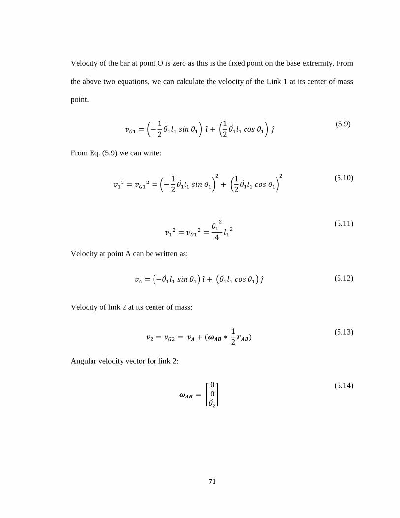
71
Velocity of the bar at point O is zero as this is the fixed point on the base extremity. From
the above two equations, we can calculate the velocity of the Link 1 at its center of mass
point.
(
) (
)
(5.9)
From Eq. (5.9) we can write:
(
)
(
)
(5.10)
(5.11)
Velocity at point A can be written as:
( ) ( ) (5.12)
Velocity of link 2 at its center of mass:
(5.13)
Angular velocity vector for link 2:
[
] (5.14)

72
Associated radial vector of the link 2 can be expressed as:
[
]
(5.15)
Substituting Eq. (5.14) and (5.15) in to Eq. (5.13) we get:
(
) (
)
(5.16)
From Eq. (5.16), we can write:
(5.17)
For forward movement of the end effector, both link 1 and link 2 will move in the
direction of gravity. Potential energy of the link 1:
(5.18)
Potential energy stored in the link 2:
(5.19)
For backward movement of the end effector, potential energy stored in the link will be
opposite of forward movement.
(5.20)

73
(5.21)
Kinematic Energy of each link has rotational and translational components. Rotational
kinetic energy of link 1:
(5.22)
Translational kinetic energy can be expressed as:
(5.23)
Total kinetic energy of link 1:
(5.24)
In the same way, we can calculate the total kinetic energy of the link 2. Rotational
energy:
(5.25)
Translational kinetic energy:
(5.26)
Total kinetic energy:
(5.27)

74
Lagrangian function for the forward movement:
(5.28)
Simplifying Eq. (5.28) we get:
(5.29)
From Eq. (5.29) we can write:
(5.30)
For the Lagrangian formulation, we need the derivative of the Eq. (5.30):
(
)
(5.31)
Partial derivatives of the Lagrangian function with respect to :
(5.32)

75
For forward directional movement, the total torque of link 1 can be expressed as follows:
(5.33)
Lagrangian Equations for link 2 :
(5.34)
(
)
(5.35)
(5.36)
Required torque for link 2 :
(5.37)

76
In the four bar rhombus configuration, link 1 and 2 form symmetry with link 3 and 4.
Kinematic energy equations are also the same, and there will be change in the potential
energy equations due to the change in the link movement direction. So, we can calculate
the torque equations by using Eq. (5.33) and Eq. (5.37). Torque of link 3:
(5.38)
Required torque equation for link 4:
(5.39)
In matrix form, Lagrangian equation of motion is:
(5.40)
Where,
M = Mass or Inertia Matrix
N = Nonlinear Matrix
G = Gravity matrix
Q = Torque Matrix

77
For the four bar rhombus configuration, the Lagrangian equation of motion is:
[
] [
]
[
]
[
]
[
]
(5.41)
Here,
78
For backward motion of the end effector, only the sign of the gravity matrix components
will change. The other matricies will remain same. Gravity matrix for backward
movement:
[
]
(5.42)
5.3 Lagrangian Formulation for Double Network
Figure 5.2 Four bar double network rhombus configuration for dynamic analysis
Figure 5.2 shows a double rhombus network. For detailed analysis of the mechanism, we
will consider following parameter:
l1 = OA = Length of the link 1
l2 = AF = Length of the link 2

79
l3 = CD = Length of the link 3
l4 = OC = Length of the link 4
l5 = DE = Length of the link 5
l6 = FE = Length of the link 6
m1 = mass of the link 1
m2 = mass of the link 2
m3 = mass of the link 3
m4 = mass of the link 4
m5 = mass of the link 5
m6 = mass of the link 6
I1 = Inertia of link 1 at its center of mass point
I2 = Inertia of link 2 at its center of mass point
I3 = Inertia of link 3 at its center of mass point
I4 = Inertia of link 4 at its center of mass point
I5 = Inertia of link 5 at its center of mass point
I6 = Inertia of link 6 at its center of mass point
From single network analysis, we can directly write the velocity equation for link1:
(5.43)
Velocity of link 2 at its center of mass point:
(5.44)

80
In the double network for horizontal movement, G2 point has no vertical displacement
along the Y axis. It will only travel along the X axis.
( ) ( ) [
] [
]
(5.45)
After vector multiplication, Eq. (5.45) becomes:
( ) ( ) (
)
(5.46)
( )
(5.47)
Square of the both side of Eq. (5.47) gives:
(5.48)
From previous analysis, velocity of the link 4 is:
(5.49)
From Eq. (5.48), we can derive the velocity square equation for link 3:
(5.50)
In double network rhombus configuration, link 1, 2 and 6 form one side. The other side
contains link 4, 3 and 5. For velocity of link 6, we need to calculate velocity at F point.

81
Velocity at F point:
(5.51)
Putting the values into the Eq. (5.51) we get:
( ) ( ) [
]
[
]
(5.52)
From Eq. (5.52), we can write:
(
)
(5.53)
Velocity of link 6 at its center of mass point:
(5.54)
We already know the velocity at the F point. By substituting the values of from Eq.
(5.53) and the vector matricies we get:
(
) ( )
[
]
[
]
(5.55)

82
Resultant velocity after vector multiplication:
(
)
(5.56)
From Eq. (5.56) we can write:
(
)
(5.57)
By solving Eq. (5.57) we get:
(5.58)
Potential energy of link 1due to forward movement:
(5.59)
In Figure 5.2, link 2 and link 3 are connected in their center of mass pint G2. At this
point, there is no vertical deflection and the bars are opposing each other’s gravity effect.
So, there will be no gravity effect for link 2 and link 3.

83
(5.60)
Potential energy stored at center of mass point of link 6:
(5.61)
For backward movement potential energy will remain same only their sign will be
opposite of forward moment.
Rotational kinematic energy of the each link 1:
(5.62)
Translational kinetic energy:
(5.63)
Total kinetic energy:
(5.63)
Rotational component of kinetic energy for link 2:
(5.64)
Translational component:
(5.65)

84
Energy equations for link 6:
(5.66)
(5.67)
Total kinetic energy for forward movement (link 1, 2 and 6):
(5.68)

85
For the rhombus network, we consider the mass and length of the short links identical,
which means m1= m4= m5= m6=m, and l1 = l4= l5 = l6= l. Long links mass and lengths
are twice that of short links. For long links m5= m6=2m and l2 = l3=2 l.
(5.69)
Lagrangian function for double network :
(5.70)
We need to calculate the necessary equations to formulate the Lagrangian dynamic
equation. As in the single network analysis, we can follow the same steps to construct the
equations.

86
(5.71)
Derivative of Eq. (5.71) gives:
(
)
(5.72)
(
)
(5.73)
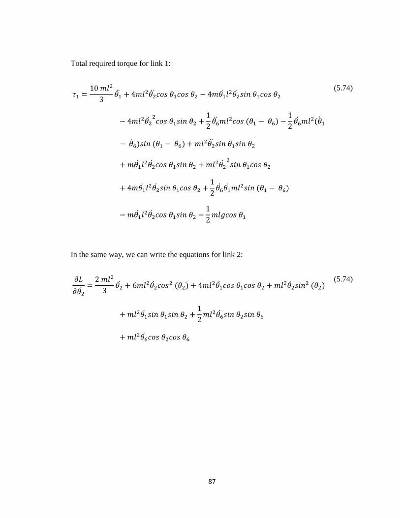
87
Total required torque for link 1:
(5.74)
In the same way, we can write the equations for link 2:
(5.74)

88
From Eq. (5.74) we can write:
(
)
(5.75)
Partial derivative of Lagrangian function with respect to gives:
(5.76)

89
Required torque for link 2:
(5.77)
For link 6:
(5.78)
From Eq. (5.78) we get:
(
)
(5.79)

90
(5.80)
Associated torque of link 6:
(5.81)
Torque equation of link 4 is similar to link 1. From Eq. (5.74)
(5.82)

91
Torque equation of link 3:
(5.83)
(5.84)

92
For the four bar rhombus configuration, the Lagrangian equation of motion is:
[ ]
[
]
[
]
[
]
[
]
(5.85)
Here, mass matrix components are:

93
Nonlinear matrix terms are:

94
For backward motion of the end effector, only the gravity matrix will change. The others
will remain the same. Gravity matrix for backward movement:
[
]
(5.86)
5.4 Discussions
Following the same step, we can formulate the Lagrangian dynamic equations for a large
number of networks. But, from the detailed analysis, we can see that as the rhombus
network increases, the conventional Lagrangian approach becomes much more difficult
and without computer simulation it is very hard to handle such computational
complexity. That is why bond graph has been used to create dynamic analysis for more
than two networks.

95
Chapter 6
Bond Graph Dynamic Analysis of the Actuator
6.1 Introduction
This chapter provides the detailed dynamic simulation of the newly designed actuator for
different network combinations, using the bond graph analysis. Bond graph provides
great flexibility for dynamic modeling with the inclusion of control. Simulation has been
done for horizontal and vertical movement of the end effector, to identify the effect of
gravity on the actuator performance. Simulation graphs gives a clear idea about dynamic
behaviour (position, velocity, acceleration etc.) and motor torque requirement of the
actuator for different networks.

96
6.2 Bond Graph Modeling
Bond graph provides a graphical representation of a physical dynamic system. For bond
graph modeling of a dynamic system, first we need to identify the components of the
model and then need to develop their individual model. Proper connection between the
components will give us the dynamic model of the system. There are several components
in the newly deigned linear actuator model:
1. Links
2. Joints
3. Motor model
4. Motor gear modeling
5. Control mechanism
6. Torque transmission system
7. End effector modeling
Among these, detailed modeling procedures for the links, joints, and motor with gear box
have already been described in the scissor lift chapter (Chapter 3).
6.2.1 Control Mechanism
One PID controller is used to control the mechanism motor but not the mechanism end
effector. Here, we are controlling the input angle of the mechanism (Figure 6.1 (a)). For a
desired position of the end effector, input angle can be calculated from the kinematic
relationship (inverse kinematic model). This angle is the desired angle for the actuator.
Angle between the motor rotor and stator link gives the present angle.

97
Difference between the two angles will give the error term and it will be fed into the PID
controller input. Then controller drives the mechanism to its required position based on
the command input. Limit block is there to protect the motor from overlimit voltage
command. Figure 6.1 (b) shows the bond grapg control schematic for the actuator.
(a)
(b)
Figure 6.1 (a) Input angle of the actuator (Network # 3) (b) Bond Graph Control
Schematic

98
6.2.2 Torque Transmission System
In the physical system, the motor stator is connected to a bar and the rotor shaft is
connected to the other bar on the base extremity. When the rotor shaft rotates the rotor
bar, due to reaction force the stator bar will move in the opposite direction from the
application of the third law of Newton (action-reaction). To model this phenomena, a
gear is used. In the model, motor torque directly goes to the rotor bar and the stator bar is
connected through a transformer with a gear ratio of 1.
(a)
(b)
Figure 6.2 Torque transmission system schematic: (a) Bond Graph (b) Physical Model

99
6.3 End Effector Loading
To model the end effector loading, an inertia (I) element is used. It is connected with the
system through parasitic stiffness and damping. Figure 6.3 shows the end effector load
simulation.
Figure 6.3 End Effector Load Simulation

100
6.4 Simulation
Simulation has been done for horizontal and vertical movement of the end effector. For
horizontal movement, end effector load (I parameter) was connected in the X axis
direction and for vertical movement it was in the Y axis direction.
6.4.1 Simulation Properties
Initial height was 0.17 m and the desired height was 0.77m. So, the desired end effector
movement is 0.6m. Mass properties of the links are calculated using Solidworks.
Aluminium alloy (Al 7075) has been used as the material. Maxon motor (Model #
167131) is chosen with maxon gearhead (model # 110408). Motor specifications are
already mentioned in the scissor lift chapter. End effector loading was 0.05 kg. Initial
position is calculated using the maximum input angle from kinematics. Similarly,
minimum input angle gives the maximum movement position of the end effector. To
calculate the maximum and minimum input angle, link dimensions (e.g. width, length
etc.) and network numbers are the most important. There is an inverse relationship
between the end effector position and input angle of the actuator. Increase in the input
angle results in a decrease of the end effector position. So, in the controller gain
parameter proportional gain is negative. PID controller tuning was performed through
trial and error method, since the goal of the work is to provide for a proof-of-concept
leaving the PID optimization to the users. Table 6.1 shows the PID controller gain for
simulation. Link length varies with the network number, but the cross sectional areas of
the links remain the same.

101
6.4.2 Simulation Parameters
Simulation was performed for five network combinations (n = 1,2,3,4,5). Each of the case
positon, velocity and acceleration of the end effector was simulated. To show the
simulation outcome for each of the case, the system schematic is presented first, followed
by the 3D schematic and dynamic behavior of the system.
Table 6.1 Simulation Properties
Position of the End
Effector
Vertical Movement
Horizontal Movement
Initial Position
= 0.17 m
Desired Position
= 0.77 m
End Effector Loading
= 0.05 Kg
Proportional gain
kp = -1.0 ;
Derivative time constant
tauD = 0.5 s;
Tameness constant
beta = 0.09 ;
Integral time constant
tauI = 1.0 s;
Proportional gain
kp = -1.3 ;
Derivative time constant
tauD = 0.5 s;
Tameness constant
beta = 0.09 ;
Integral time constant
tauI = 1.0 s;

102
Figure 6.4 Bond Graph Schematic of the system (Network # 1: Horizontal)

103
(a)
(b)
Figure 6.5 Simulation graphs of the system (Network # 1: Horizontal) (a) 3D Schematic
(b) Dynamic Behavior
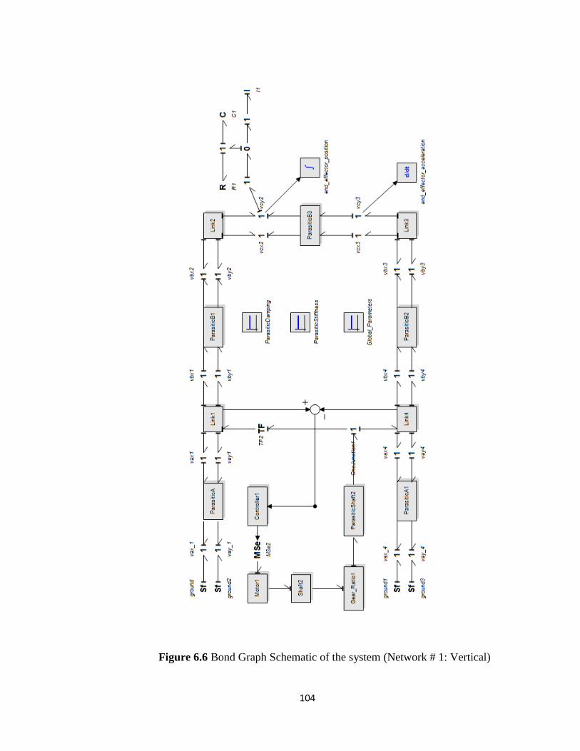
104
Figure 6.6 Bond Graph Schematic of the system (Network # 1: Vertical)

105
(a)
(b)
Figure 6.7 Simulation graphs of the system (Network # 1: Vertical) (a) 3D Schematic (b)
Dynamic Behavior

106
Figure 6.8 Bond Graph Schematic of the system (Network # 2: Horizontal)

107
(a)
(b)
Figure 6.9 Simulation graphs of the system (Network # 2: Horizontal) (a) 3D Schematic
(b) Dynamic Behavior

108
Figure 6.10 Bond Graph Schematic of the system (Network # 2: Vertical)

109
(a)
(b)
Figure 6.11 Simulation graphs of the system (Network # 2: Vertical) (a) 3D Schematic
(b) Dynamic Behavior
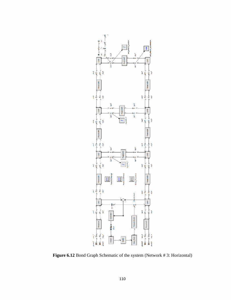
110
Figure 6.12 Bond Graph Schematic of the system (Network # 3: Horizontal)

111
(a)
(b)
Figure 6.13 Simulation graphs of the system (Network # 3: Horizontal) (a) 3D Schematic
(b) Dynamic Behavior

112
Figure 6.14 Bond Graph Schematic of the system (Network # 3: Vertical)
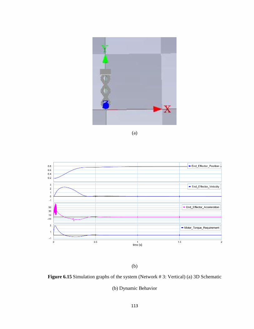
113
(a)
(b)
Figure 6.15 Simulation graphs of the system (Network # 3: Vertical) (a) 3D Schematic
(b) Dynamic Behavior
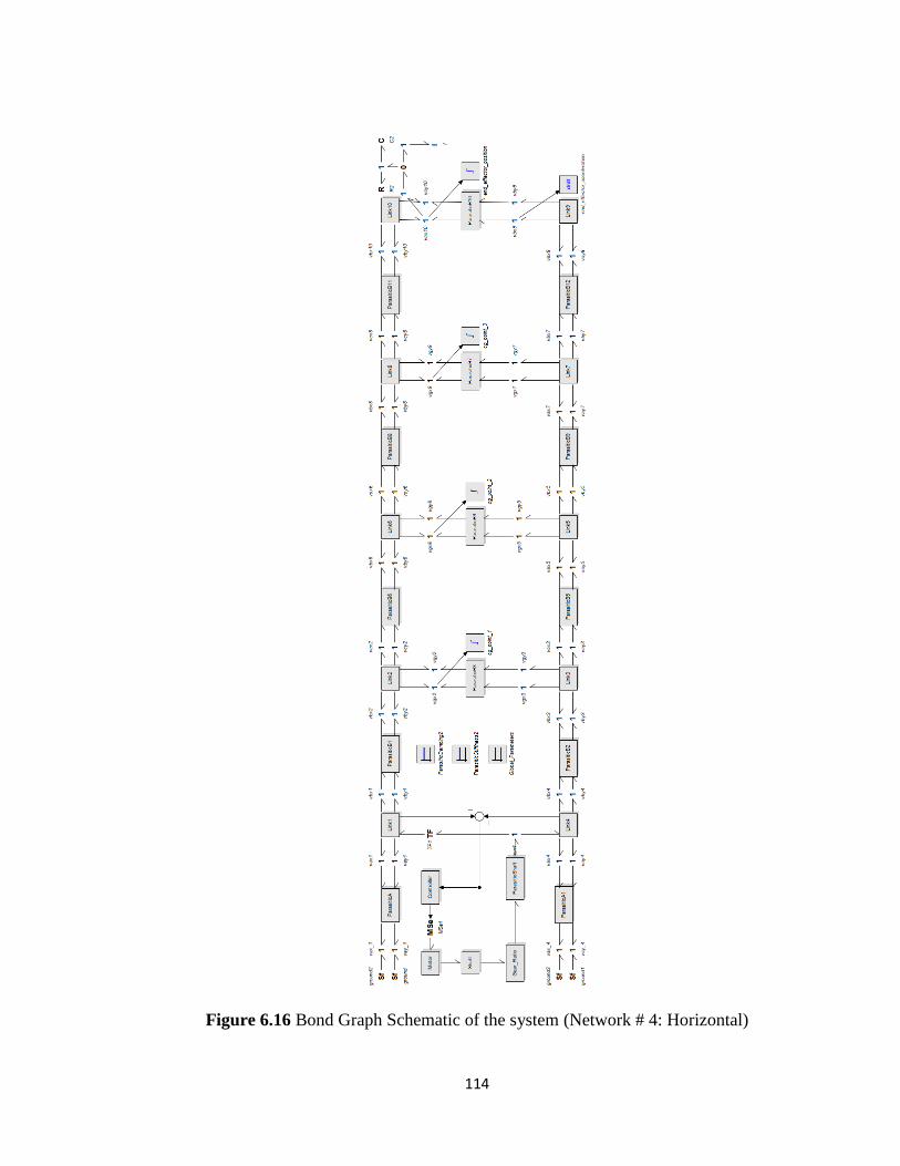
114
Figure 6.16 Bond Graph Schematic of the system (Network # 4: Horizontal)

115
(a)
(b)
Figure 6.17 Simulation graphs of the system (Network # 4: Horizontal) (a) 3D Schematic
(b) Dynamic Behavior

116
Figure 6.18 Bond Graph Schematic of the system (Network # 4: Vertical)

117
(a)
(b)
Figure 6.19 Simulation graphs of the system (Network # 4: Vertical) (a) 3D Schematic
(b) Dynamic Behavior

118
Figure 6.20 Bond Graph Schematic of the system (Network # 5: Horizontal)

119
(a)
(b)
Figure 6.21 Simulation graphs of the system (Network # 5: Horizontal) (a) 3D Schematic
(b) Dynamic Behavior

120
Figure 6.22 Bond Graph Schematic of the system (Network # 5: Vertical)

121
(a)
(b)
Figure 6.23 Simulation graphs of the system (Network # 5: Vertical) (a) 3D Schematic
(b) Dynamic Behavior

122
From the simulation data we can construct a table for the maximum values of the
simulation parameters.
Table 6.2 Simulation Summary (Horizontal Simulation)
Simulation Network 1 Network 2 Network 3 Network 4 Network 5
Short Link Length
(m)
0.4 0.2 0.1333 0.1 0.08
Long Link Length
(m)
- 0.4 0.2666 0.2 0.16
Maximum Velocity
(m/s)
2.32 0.85 2.4 1.95 2.4
Maximum
Acceleration
(m/s2)
40 8 70 240 65
Maximum Torque
Requirement
(Nm)
2.92 2.92 2.92 2.73 2.9
Torque Requirement
Duration
(S)
0.14 0.83 0.13 0.19 0.13

123
Table 6.3 Simulation Summary (Vertical Simulation)
Simulation Network 1 Network 2 Network 3 Network 4 Network 5
Short Link Length
(m)
0.4 0.2 0.1333 0.1 0.08
Long Link Length
(m)
- 0.4 0.2666 0.2 0.16
Maximum Velocity
(m/s)
2.32 2.34 2.4 2.4 1.87
Maximum
Acceleration
(m/s2)
40 45 65 60 200
Maximum Torque
Requirement
(Nm)
2.92 2.92 2.9 2.92 2.93
Torque Requirement
Duration
(S)
0.13 0.14 0.13 0.13 0.14

124
6.5 Result Interpretation
Position, velocity and acceleration of the end effector are recorded for different network
combinations. By keeping the maximum travel distance of the end effector equal,
different network simulation shows different acceleration value with the same motor.
From the simulation, we get a clear idea about the motor torque requirements. Torque
varies from 2.7 Nm to 3 Nm.
6.6 Discussions
Dynamic simulation gives a clear idea about the performance of the different network
combinations. During vertical simulation actuator needs to encounter the gravity force.
So, the torque requirement is higher compared to the horizontal simulation. Though
torque requirement doesn’t varies that much, but the duration of torque supply from
motor varies with different network. From the simulation, we can see that the network 4
configuration gives the maximum acceleration under horizontal operating condition for a
certain linear distance while comparing with the other possible combinations. For
practical design, we choose this operating condition for the actuator.

124
Chapter 7
Practical Design and Calculations
7.1 Introduction
A physical model of the newly designed actuator was built to validate the proof of
concept. This chapter describes the SOLIDWORKS designs and associated calculations
related to the production process. The actuator assembly consists of two major
components: actuator part and base assembly. In the actuator part, there are motor stator
bar, motor rotor bar, and bars with end effector connector. Between the motor and the end
effector, the body of the actuator consists of long bars connected as a X by the shaft
screws and bearings.

125
7.2 Bar Length Calculation
There are long and short bars in the actuator assembly. Length of the bar depends on the
networking number of the rhombus and desired stroke length. It is very important to
calculate the proper bar length for a particular number of network, to get adequate
functionality of the atuator. For all the bars, the cross sectional area will remain equal. If
the end effector stroke length is H and the number of network is n, then the short link
length would be:
(7.1)
For the rhombus configuration, length of a long bar is equal to the interjoint distance
between two consecutive central moving joints. So, length between the joint center is:
(7.2)
Figure 7.1 Long Bar with Dimensions (cm)

126
From the Bond Graph dynamic simulation, we have seen that network number four gives
the best performance in horizontal operating conditon. For the practical design, the 4
rhombus network model was chosen with a maximum end effector movement of 0.8m.
Using Eq. (7.1), calculated short link length is 0.1 m. and long bar length is 0.2 m. Figure
7.1 shows a long bar for our designed actuator, where all the dimensions are measured in
centimeter (cm).
7.3 Workspace and Encumbrance Calculation
From kinematic formulation (Chapter 4), we can calculate the workspace and
encumbrance for the network 4 rhombus confuguration based linear actuator. For a bar
width of 0.01 m, the minimum position of the end effector would be:
( (
))
(7.3)
Maximum position of the end effector:
( (
))
(7.4)
Maximum encumbrance of the actuator for the chosen configuration:
√ (7.5)
7.4 Required Speed Calculation
From the workspace calculation, stroke length of the actuator is around 0.6 m. Our design
goal is to achive a acceleration of 10g, where the actuator will accelrate constantly upto
the half way point, and then decelerate to reach the final point.

127
Figure 7.2 Maximum velocity and acceleration curve
For 10g acceleration, linear velocity of the actuator can be calculated from Newton’s
laws of motion equations and the value was 7.67 m/s. From kinematics, we can calculate
the required angular velocity for the motor. Angular velocity for 10 g acceleration with a
short link length of 0.1m is:
√
( )
(7.6)
From the dynamic simulation, we observed that the motor torque is around 3 Nm.
Minimum required speed of the motor is 198 rpm. Based on the torque and angular
velocity, Phidgets motor (Model # 3271_1) has been chosen for the practical prototype.
Motor Specifications are presented in Chapter 8 (Section 8.5).

128
7.5 Deflection calculation
One end of the actuator will be connected on the base and the end effector will move
freely. So, the actuator resembles a one end loaded cantiliver beam [51]. Vertical
deflection of the end effector is calculated using the following formula:
(7.7)
In the above equation, F is the force acting on the tip of the beam, L is the length of the
beam, E is modulus of elasticity and I stands for the area moment of inertia. Al 7079
alloy has been used as the material and from its properties the calculated deflection of the
end effetor is 0.0000714 cm.
7.6 Solidworks model
Based on the required design criteria and dimentions, a SolidWorks model was developed
for the machining of the actuator. Shaft screws are used to connect the bars along with
the bearings, to maintain a smooth rotation of the bar. Figure 7.3 shows the stator bar.
Motor will be screwed with this bar at the base extremity. There will be a bearing inside
the hole of the stator bar. Motor rotor shaft will go through that bearing and end up in the
rotor bar. Figure 7.4 shows the rotor shaft bar. There will be a key way in the rotor bar to
lock the rotor shaft with the bar. A set screw is used in the 90 degree direction to make
the rotor shaft tight enough so that it can not move out during rotation. Below the rotor
bar, there are holes for the screws to connect the actuator with robot or any other
applications where it will be useful.

129
Figure 7.3 Motor stator bar
Figure 7.4 Rotor shaft bar

130
In the Figure 7.5, the holes in the upper bars create a housing for the shaft screws and the
lower bars (Figure 7.6) consist of a bearing in each of the joint.
Figure 7.5 Upper bars (short and long)
Figure 7.6 Lower bar

131
Figure 7.7 shows the bearing and shoulder screw assembly inside the actuator. Figure 7.8
shows the complete actuator assembly. In the end effector plate, there are holes to
connect the screws for the load.
Figure 7.7 Bearing and Shoulder Screw Assembly
Figure 7.8 Actuator assembly

132
The base assembly consists of a fixed plate, flange and connector. The rotor shaft bar is
screwed to the connector to demonstrate the reactive force movement of the motor.
Figure 7.9 Fixed base
Between the flange and connector, a bearing is used to ensure smooth movement of the
actuator.
Figure 7.10 Base flange

133
Figure 7.11 Base connector
Figure 7.12 Base assembly

134
Figure 7.13 Actuator and base assembly
Figure 7.14 Actuator Prototype

135
7.7 High Performance Actuator with 3RPR robot
The newly designed actuator can be used in a standalone condition or in different robots.
In our lab, after the standalone experimentation we want to use the actuator for the 3RPR
parallel robot. Figure 7.15 shows a typical 3 RPR parallel robot. In a 3RPR robot, there
are three prismatic actuators. As prismatic actuators are very slow in acceleration, we
want to replace them by our high performance actuator. Another masters thesis is being
done on the integration of the high performance actuator with 3RPR parallel robot and
their performance evaluation with a parallel robot.
Figure 7.15 Schematic of a 3RPR Parallel Robot
7.9 Design Recommendations
The actuator prototype is to provide for a proof of concept. For precise movement of the
end effector position, we need a motor with minimal backlash to reduce position error.
From the actuator design, we can see that a small variation in the input angle will create a
significant error in the linear position. This will increase as the number of network also

136
increases. The mechanism provides motion amplification, which is very well suited for
high acceleration, but would require careful encoder choice in high precision
applications. We used aluminum as the material. Any high strength material with low
mass density (e.g. carbon fiber) will increase the performance of the actuator even more.
Based on the requirements bar length, width and thickness can be reduced. It will reduce
the overall mass and subsequently increase acceleration for the same amount of torque.

137
Chapter 8
Control of the Actuator
8.1 Introduction
This chapter provides the detailed control analysis of the newly designed actuator. For
simulation and hardware implementation of control, conventional PID controller has been
used. Controller provides control of the input angle of the actuator, but doesn’t directly
control the end effector (length of the linkage). As the designed actuator system is highly
dynamic and nonlinear in nature, the PID controller is heavily impacted by the
mathematical modeling of the system. For practical implementation Phidgets motor
controller has been used [52].
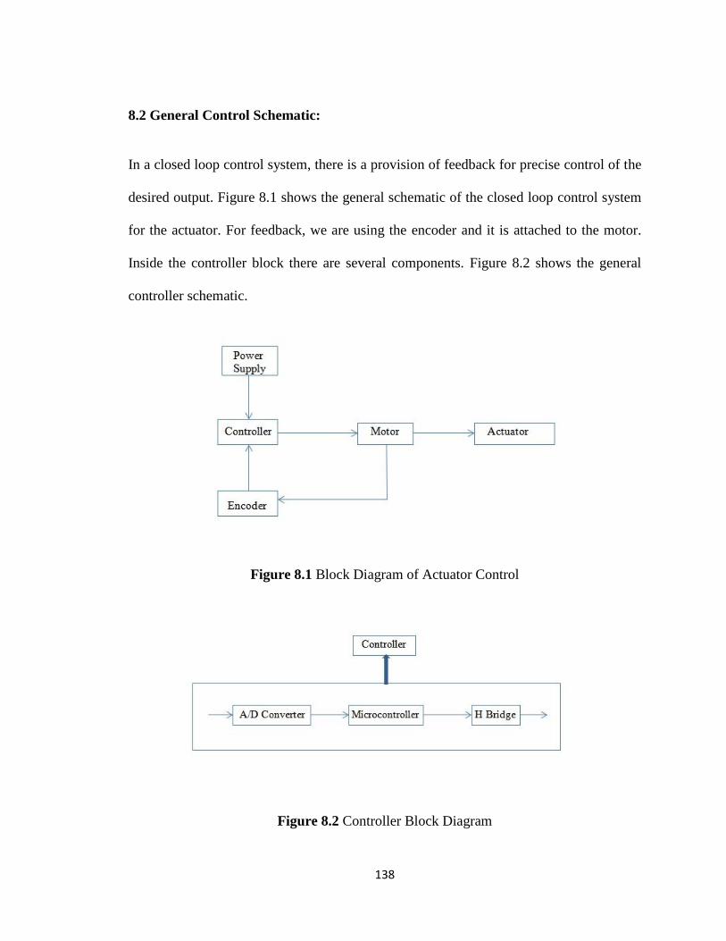
138
8.2 General Control Schematic:
In a closed loop control system, there is a provision of feedback for precise control of the
desired output. Figure 8.1 shows the general schematic of the closed loop control system
for the actuator. For feedback, we are using the encoder and it is attached to the motor.
Inside the controller block there are several components. Figure 8.2 shows the general
controller schematic.
Figure 8.1 Block Diagram of Actuator Control
Figure 8.2 Controller Block Diagram

139
Closed loop control system contains a sensor, a motor, a controller, and a driver.
Generally, the driver is an H bridge. Most common way is to let the controller turn the
driver ON and OFF at very high rates, changing the ratio between ON and OFF time to
control the speed of the motor. This technique is well known as PWM (pulse-width-
modulation). In general, the H bridge contains four switching elements with the load at
the center. Switching elements are usually BJT (Bipolar Junction Transistor), FET (Field
Effect Transistor) or IGBT’s (Insulated Gate Bipolar Junction Transistor). By controlling
the ON-OFF sequence of the FET or IGBT we can reverse the current direction and
hence can control the motor in clockwise and counterclockwise direction.
Figure 8.3 Schematic of H-Bridge Driver
While working with a DC motor, a shaft encoder is the most common and accurate way
of providing feedback to the controller. Shaft encoders are rotary encoders. A shaft
encoder provides the microcontroller internal counter with a sequence of pulses during a

140
period of time, which corresponds to the rotation of the motor. Microcontroller
recalculates the actual angle of the shaft or the revolution. Then it controls the speed of
the motor by comparing number of pulses with a fixed number, which is referred as the
“required pulses”. Required pulses are calculated based on the program saved in the
memory of the microcontroller chip. Figure 8.4 shows a general flow chart for encoder
signal to the microcontroller to control the speed of motor.
Figure 8.4 Microcontroller-Encoder Flow Diagram

141
8.3 Control Scheme and Algorithm
An electrical system model of a voice coil actuator for controlling a parallel orientation
manipulator is presented in [52]. In our newly designed actuator, a DC motor provides
the required input forces. In their causal structure, it needs to overcome the frictional
force to move the end effector. Figure 8.5 shows an electrical model of the actuator with
the friction model incorporated in it. Here, actuator velocity is the causal input and
actuator force is the causal output. Motor transfer function can be achieved through the
general control theory for simple DC motor circuit (armature with series connected
inductance and resistance).
Figure 8.5 Electrical Model of the Actuator
As the actuator system is highly nonlinear, we cannot derive the transfer function until
we build up a linearized model. This process is difficult for any parallel mechanism, since

142
there are computational complexities associated with it. That is why direct PID control is
an effective way to implement the actuator control system. For PID control, performance
of the system is determined by three parameters (Proportional, Integral and Derivative).
Essentially, a PID controller looks like this:
( ) ( ) ∫ ( )
( )
(8.1)
Where, Kp = Proportional gain, Ki = Integral gain, Kd = Derivative Gain, e = error and t=
time or instantaneous time. Figure 8.6 shows the general block diagram of the direct PID
control system. Here, input is the desired position of the end effector. We are controlling
the input angle (denoted as θ) between the stator and rotor bar at the base extremity.
Actuator body contains several four bar rhombus configuration. From kinematic
relationship we can calculate the link length based on the number of rhombus network.
For a known link length, IKM (Inverse Kinematics Model) will produce the desired
angle. From the present θ value between the stator and rotor bar, approximation of the
end effector position can be calculated using the FKM (Forward Kinematics Model).
From the initial position to the desired position actuator follows a trajectory. For a linear
actuator it should be one straight line. End effector of the actuator travels the path and its
actual trajectory can be calculated from the FKM. Here, controller only manages the
angular position of the motor and the actuator linear position is derived by kinematics
calculation. One PID controller is dedicated to one linear actuator. When this actuator is
implemented in one robot or any machine, the external loop is closed at the robot

143
controller level. That means all the actuator controller will be connected with another
main controller. The main controller will control the robot base as well as the actuator.
Figure 8.6 General Block Diagram of Actuator Control
Figure 8.7 shows the Simulink model of direct PID control. Actuator dynamics is used to
get the actual θ value. For actuator dynamics, we can use any conventional dynamic
formulation method. Here, Lagrangian formulation is used to get the actual θ of the
system while moving from the initial position to the desired position. From Lagrangian
formulation we know:
(8.2)
Solving Eq. (8.2) we can calculate the angular acceleration ( ) of the system.
( ) (8.3)
Integration of gives the angular velocity and subsequently the present angle.

144
Figure 8.7 Simulink Diagram of Direct PID Control
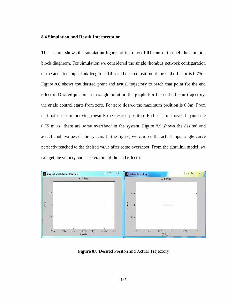
145
8.4 Simulation and Result Interpretation
This section shows the simulation figures of the direct PID control through the simulink
block diaghram. For simulation we considered the single rhombus network configuration
of the actuator. Input link length is 0.4m and desired psition of the end effector is 0.75m.
Figure 8.8 shows the desired point and actual trajectory to reach that point for the end
effector. Desired position is a single point on the graph. For the end effector trajectory,
the angle control starts from zero. For zero degree the maximum position is 0.8m. From
that point it starts moving towards the desired position. End effector moved beyond the
0.75 m as there are some overshoot in the system. Figure 8.9 shows the desired and
actual angle values of the system. In the figure, we can see the actual input angle curve
perfectly reached to the desired value after some overshoot. From the simulink model, we
can get the velocty and acceleration of the end effector.
Figure 8.8 Desired Positon and Actual Trajectory

146
Figure 8.9 Desired angle and Actual Angle
Figure 8.10 End effector velocity

147
Figure 8.11 End Effector Acceleration
Figure 8.12 Trajectory Error
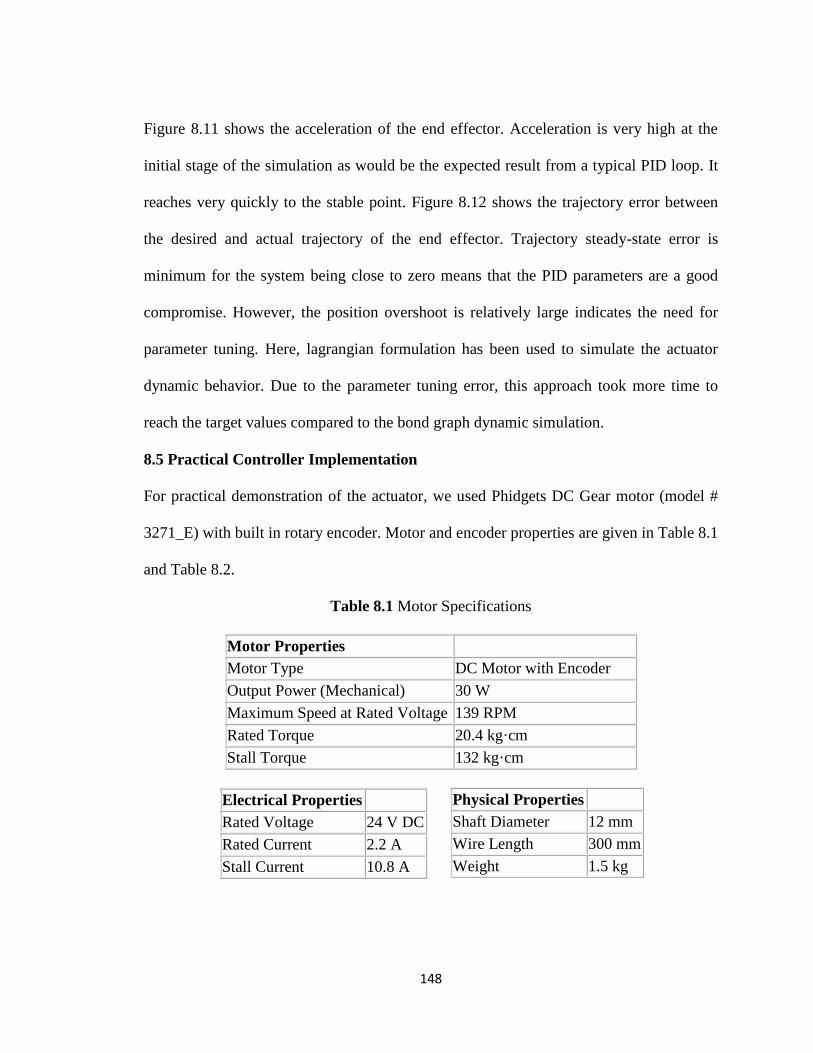
148
Figure 8.11 shows the acceleration of the end effector. Acceleration is very high at the
initial stage of the simulation as would be the expected result from a typical PID loop. It
reaches very quickly to the stable point. Figure 8.12 shows the trajectory error between
the desired and actual trajectory of the end effector. Trajectory steady-state error is
minimum for the system being close to zero means that the PID parameters are a good
compromise. However, the position overshoot is relatively large indicates the need for
parameter tuning. Here, lagrangian formulation has been used to simulate the actuator
dynamic behavior. Due to the parameter tuning error, this approach took more time to
reach the target values compared to the bond graph dynamic simulation.
8.5 Practical Controller Implementation
For practical demonstration of the actuator, we used Phidgets DC Gear motor (model #
3271_E) with built in rotary encoder. Motor and encoder properties are given in Table 8.1
and Table 8.2.
Table 8.1 Motor Specifications
Motor Properties
Motor Type DC Motor with Encoder
Output Power (Mechanical) 30 W
Maximum Speed at Rated Voltage 139 RPM
Rated Torque 20.4 kg·cm
Stall Torque 132 kg·cm
Electrical Properties
Rated Voltage 24 V DC
Rated Current 2.2 A
Stall Current 10.8 A
Physical Properties
Shaft Diameter 12 mm
Wire Length 300 mm
Weight 1.5 kg

149
Gearbox Properties
Gearbox Type Planetary
Gear Ratio 18 1⁄16 : 1
Number of Gear Trains 2
Maximum Strength of Gears 153 kg·cm
Shaft Maximum Axial Load 200 N
Shaft Maximum Radial Load 100 N
Backlash Error 3°
Table 8.2 Encoder Specifications
Encoder Resolution 360 CPR
Connector Type E4P
Current Consumption Min 27 mA
Supply Voltage Min 4.5 V DC
Supply Voltage Max 5.5 V DC
Phidget 1065 motor controller has been used. The 1065 controller control the direction,
velocity and acceleration of one DC Motor. The motor is powered by an external power
supply (9 to 28VDC). By applying a voltage, or pulsing a voltage rapidly, at the terminals
of the motor, current flows through the motor and it will begin rotating. Depending on the
direction of the current, the motor will rotate clockwise or counterclockwise. The 1065
changes the effective voltage by changing the percentage of time the full supply voltage
is applied to the motor. By switching the voltage very quickly (a technique called PWM),
the controller is made smaller, more efficient, and cheaper. Control of actual motor speed
can be achieved automatically in software by using the Back EMF property, or current
sensing [49]. Precise position control of DC motors is achieved by using encoders.

150
Control loops implemented through software by using the data provided by the on-board
digital inputs, analog inputs and encoder input. There is an event that triggers every 16
ms and returns the back-EMF value for the attached motor, which is used for PID control.
Figure 8.13 shows the schematic of the controller. Figure 8.14 shows the linear actuator
with controller connected in it. This controller also provides built in over voltage and
over current protection. Detailed controller properties are given in Appendix C.
Figure 8.13 Phidget Controller
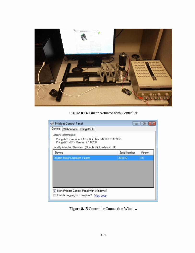
151
Figure 8.14 Linear Actuator with Controller
Figure 8.15 Controller Connection Window
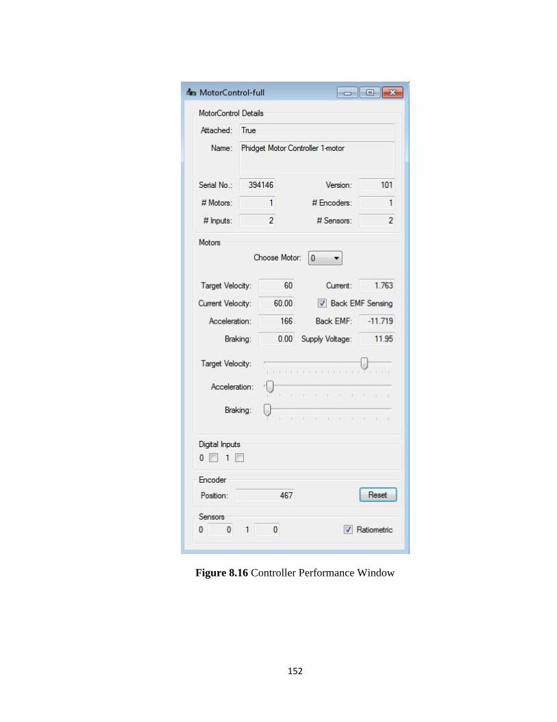
152
Figure 8.16 Controller Performance Window

153
Table 8.3 Control Performance Summary
Supply Voltage 11.95 V
Current 1.763 A
Maximum Velocity 60 m/s
Maximum Acceleration 166 m/s2
Figure 8.15 shows the Phidgets motor control connection window. When a device is
connected with the controller board, it shows the device ID. In our experimental set up,
the Phidget DC motor (serial # 394146) is connected as we are controlling the input angle
from encoder reading. Figure 8.16 shows the motor control panel. From the figure one
can observe the motor run data. Its showing that 1 motor and 1 encoder is connected.
With the slider one can vary the target velocity. For this typical case supply voltage was
12V and current was 1.763 Amps. Actuator target velocity was set to 60 m/s and
acceleration is around 17g. From the data, we can see that the current velocity and
acceleration resembles the target velocity and acceleration.

154
Chapter 9
DOE Data Analysis and Design Optimization
9.1 Introduction
Using the Bond Graph dynamic model and kinematic formulation of the newly designed
actuator, acceleration of the end effector is simulated for different parametric
combinations. For the practical design, to achieve the high performance (acceleration) is
the main concern. This chapter describes the detailed procedures to determine the ideal
parametric combinations for the actuator, so that it gives the best performance. Statistical
data analysis is a great addition for this type of parallel mechanism. Brief description of
DOE is presented in Appendix B.

155
9.2 Experimental Factors and Response
We considered five parameters as input factors and the output response is the acceleration
of the end effector for different loading condition.
Network (A): Network means how many identical rhombus structures are in the
actuator body. Networking of rhombus has significant effect on the acceleration of
end effector. Because, each network linearly increases the velocity of the end
effector and subsequently acceleration.
Link Length (B): Considered link length is the length of the short bar. Link length
varies with the number of network. As the network number goes higher, it goes
smaller. Motor stator and rotor shaft both are connected with one but distinct short
bar. So this factor is very important.
Torque Requirement Duration (C): From dynamic simulation, we have seen that
the peak torque requirement for different networks combination remains constant
but the torque requirement duration varies.
End Effector Loading (D): End effector loading has a negative impact on the
acceleration. So, this is a very crucial parameter for design calculation. Data
collected for three different loading conditions (0.5 Kg, 1Kg and 1.5Kg).
Movement Direction (E): The newly designed actuator can be used both in
horizontal and vertical direction. For vertical movement there will be extra torque
required to overcome the gravity force.
Response is the acceleration of the end effector. The main goal of this design is to
achieve high acceleration while using them in robots or in standalone condition.

156
9.3 Optimal (custom) Design of the Experiment
Response surface methodology (Appendix B) has been used to analyze the collected data.
Computer based optimal (custom) design is chosen to build up the model. For 5 factors (4
numeric and 1 categorical), it requires total 30 runs. Design Expert software (version 9)
by Stat-Ease has been used to develop the optimal design. For network and link length
there are 5 different levels. Torque requirement duration (motor run time) is different for
each of the simulation run. For directional movement, level 2 considered as vertical
direction and level 1 considered as horizontal direction.
Figure 9.1 Run Data

157
9.4 ANOVA Analysis and Regression Model
ANOVA table summarizes the statistical significance of the proposed DOE model. From
the F-value and probability value comparison of the effects, the software determines the
significance.
Table 9.1 ANOVA Analysis
Std. Dev. 8.68 R-Squared 0.8619
Mean 18.12 Adj R-Squared 0.7139
C.V. % 47.91 Pred R-Squared N/A
PRESS N/A Adeq Precision 8.256

158
In summary, the standard deviation shows the deviation of the error term. R2
presents the
percentage of total variability explained by the model. Addition of effect will increase the
R value. That is why we should look at the adjusted R value produced by the model. The
difference between the two R2 should be very small. Precision should be greater than 4 for
an adequate model. Table 9.1 shows the ANOVA table and the ANOVA summary for the
2FI backward elimination model. The backward method is considered the most robust
choice for algorithmic model reduction because all model terms will be given a chance to
be included in the model and categorical terms removed hierarchically. For our analysis,
the R2 values are not very close but precision is much greater than 4 which signify the
adequacy of the model. But there may be a possibility of model transformation.
9.5 Residual Analysis
Residual analysis checks whether the assumptions of the ANOVA are correct or not. We
made the following assumptions:
1. Random Samples from their respective population.
2. All samples are independent.
3. Departures from group mean are normally distributed for all data groups.
4. All data groups have equal variance.
We have seen from the ANOVA table that there are some differences in the R2 values.
Before further analysis, we will determine whether any transformation is required or not.
From the Box-Cox plot of Figure 9.2 we can see that the current line is outside of the
ranges (between Low & High Confidence Interval). That means transformation is

159
required and inverse square root transformation is recommended. So, we can conclude
that the assumptions of ANOVA are not satisfied.
Figure 9.2 Box-Cox plot
Design-Expert® Software
Maximum Acceleration
Lambda
Current = 1
Best = -0.4
Low C.I. = -1.07
High C.I. = 0.15
Recommend transform:
Inverse Sqrt
(Lambda = -0.5)
Lambda
Ln
(Re
sid
ua
lSS
)
Box-Cox Plot for Power Transforms
4
6
8
10
12
14
-3 -2 -1 0 1 2 3

160
9.6 Model Transformation
Table 9.2 shows the summary of the model after inverse square root transformations.
From the fit summary table, we can see that transformation improved the model
adequacy. But the suggested models remain similar (Linear or 2FI). 2FI backward
elimination model is chosen for residual analysis.
Table 9.2 ANOVA Analysis After Model Transformation
ANOVA for Response Surface Reduced 2FI model
Analysis of variance table [Partial sum of squares - Type III]
Sum of
Mean F p-value
Source Squares df Square Value Prob > F
Model 0.24 9 0.026 29.27 < 0.0001 significant
A-Network 6.738E-004 1 6.738E-004 0.75 0.3980
B-Link Length 0.029 1 0.029 31.68 < 0.0001
C-Torque Requirement Duration 0.059 1 0.059 65.12 < 0.0001
D-End Effector Loading 0.024 1 0.024 26.19 < 0.0001
AB 0.061 1 0.061 68.07 < 0.0001
AD 7.875E-003 1 7.875E-003 8.72 0.0079
BC 0.061 1 0.061 67.46 < 0.0001
BD 0.056 1 0.056 62.47 < 0.0001
CD 1.417E-003 1 1.417E-003 1.57 0.2248
Residual 0.018 20 9.031E-004
Cor Total 0.26 29
Std. Dev. 0.030 R-Squared 0.9294
Mean 0.29 Adj R-Squared 0.8977
C.V. % 10.49 Pred R-Squared N/A
PRESS N/A Adeq Precision 23.316

161
Figure 9.3 Mathematical Equation for Output
Figure 9.4 shows the normal plot. The actual results show that, all the data points are
randomly distributed. Residual plots provide information about the normal distribution
and constant variance of collected data. The results in the Box-cox plot (Figure 9.7)
suggested no transformation is required.
Figure 9.4 Normal plot of residuals (with inverse square root transformation)
Design-Expert® Software
1/Sqrt(Maximum Acceleration)
Color points by value of
1/Sqrt(Maximum Acceleration):
0.118
0.530
Externally Studentized Residuals
No
rma
l %
Pro
ba
bil
ity
Normal Plot of Residuals
-4.00 -3.00 -2.00 -1.00 0.00 1.00 2.00 3.00
1
5
10
20
30
50
70
80
90
95
99

162
Figure 9.5 Predicted vs. actual plot (with inverse square root transformation)
Figure 9.6 Residual vs. Run plot (with inverse square root transformation)
Design-Expert® Software
1/Sqrt(Maximum Acceleration)
Color points by value of
1/Sqrt(Maximum Acceleration):
0.118
0.530
Actual
Pre
dic
ted
Predicted vs. Actual
0.1
0.2
0.3
0.4
0.5
0.6
0.1 0.2 0.3 0.4 0.5 0.6
Design-Expert® Software
1/Sqrt(Maximum Acceleration)
Color points by value of
1/Sqrt(Maximum Acceleration):
0.118
0.530
Run Number
Ex
tern
all
y S
tud
en
tiz
ed
Re
sid
ua
ls Residuals vs. Run
-4.00
-2.00
0.00
2.00
4.00
1 5 9 13 17 21 25 29

163
Figure 9.7 Box-cox plot (with inverse square root transformation)
9.7 Model Optimization
The model was optimized and extra runs performed for validity check. All factors were
kept in range and acceleration was fixed at 50 m/s2 to get the optimum runs. For the first
ten combinations, obtained output is within our specified range to describe the model as a
valid one. Table 9.3 shows that for the certain target acceleration all factors are in their
specified range and we can determine the values for each of the factor. Output confirms
the validity of the model to find the parametric combination and their respected values for
certain height coverage. Here factor values are taken from their original run data sheet.
For the first run, the suggested network combination is the network 3 and movement
direction is vertical. Motor run time was 1.14 second. In the same way, from optimization
run we can determine the ideal parametric combination based on the provided options.
Design-Expert® Software
1/Sqrt(Maximum Acceleration)
Lambda
Current = -0.5
Best = -0.45
Low C.I. = -1.01
High C.I. = 0.03
Recommend transform:
Inverse Sqrt
(Lambda = -0.5)
Lambda
Ln
(Re
sid
ua
lSS
)
Box-Cox Plot for Power Transforms
4
6
8
10
12
14
-3 -2 -1 0 1 2 3

164
Table 9.3 Optimization Run
Constraints
Lower Upper Lower Upper
Name Goal Limit Limit Weight Weight Importance
A:Network is in range 1 5 1 1 3
B:Link Length is in range 0.08 0.4 1 1 3
C:Torque Requirement
Duration is in range 0.8 2.5 1 1 3
D:End Effector Loading is in range 0.5 1.5 1 1 3
Maximum Acceleration is target = 60 1.57 72 1 1 3
Network Link
Length
Torque Requirement
Duration
End Effector
Loading
Movement
Direction
3 0.1333 1.14 1 Level 2 of E
5 0.08 0.93 0.5 Level 2 of E
2 0.2 0.88 0.5 Level 2 of E
3 0.1333 0.92 0.5 Level 2 of E
4 0.1 0.99 1 Level 2 of E
1 0.4 0.93 0.5 Level 1 of E
3 0.1333 0.8 0.5 Level 1 of E
2 0.2 1.9 0.5 Level 1 of E
3 0.1333 1.15 1 Level 1 of E
5 0.08 1.24 1.5 Level 2 of E
9.8 Discussions
Design of Experiment (DOE) is a very effective approach for design optimization of the
newly designed actuator. One important advantage is that we can include some
parameters, which are not considered for equation formulation. The approach can generate
an empirical mathematical model after analyzing all the data.
165
Chapter 10
Contributions and Future Work
10.1 Contributions
In this thesis, the dynamic behavior, kinematic formulation and experimentation of the
newly designed actuator were discussed. The major contribution of this research includes
the detailed analysis (kinematics and dynamics), design (SOLIDWORKS model) and
control of the high performance linear actuator. Kinematic formulations are newly
derived for this research. The Lagrangian based dynamic analysis is also not available for
the rhombus networking. The Bond Graph model is unique and a chestnut contribution of
the thesis. A DOE based optimal design approach is a new addition for linear actuator
design.

166
Detailed control scheme of the actuator is provided in the thesis. We are controlling the
motor at the base extremity.
The SOLIDWORKS model was newly designed for machine shop production of the
actuator. Detailed component design of the actuator (Chapter 7), gives a clear idea about
the industrial production design.
A statistical approach is provided to achieve the optimal design for a desired acceleration
with a specified payload. Along with the conventional design approach, the statistical
approach can be an efficient way to screen out refined parametric combinations for high
performance.
The actuator performance was fully characterized by the computer simulations (Chapter 6
and Chapter 8) and validated by experimental set up (Chapter 8). The actuator possesses
a very high peak acceleration of around 17g, which exceeded the initial design goal
(10g).
The proposed actuator can be a good replacement of the current available prismatic
or/and linear actuators for parallel robots, machine tools or any other machines.
Detailed analysis of the scissor lift mechanism gives a clear idea about their feasibility as
a linear actuator. The dynamic model and the statistical analysis of the mechanism can be
used for design purposes. This mechanism can be a good replacement of the conventional
prismatic actuators.

167
10.2 Future Work
Performance of the newly designed actuator has been analyzed and its superior behavior
is also investigated. The next step is to carry out further improvement of the structural
design, material processing and control strategies. Overall mass of the actuator can be
reduced by more efficient material selection. Detailed controller tuning procedures can be
included to give the users a clear idea about precise operation with no overshoot. A better
data acquisition system is needed for future work. High initial torque motor can be used,
so that the actuator will not collapse under loaded condition.

168
APPENDIX

169
Appendix A: Bond Graph and Motor Specifications
Bond Graph:
Bond graphs are a domain-independent graphical description of dynamic behavior of
physical systems. This means that systems from different domains (e.g. electrical,
mechanical, hydraulic, acoustical, thermodynamic, material) are described in the same
way. The basis is that bond graphs are based on energy and energy exchange. Analogies
between domains are more than just equations being analogous: the used physical
concepts are analogous [54].
The language of bond graphs aspires to express general class physical systems through
power interactions. The factors of power i.e., Effort and Flow have different
interpretations in different physical domains. Yet, power can always be used as a
generalized co-ordinate to model coupled systems residing in several energy domains
[55].
effort
A B
flow

170
Effort and Flow Variables for Different Physical Domains:
Zoltek Panex 33 Material Properties:
Physical Properties Metric English Comments
Density 1.81 g/cc 0.0654 lb/in³
Mechanical Properties Metric English Comments
Tensile Strength, Ultimate 3800 MPa 551000 psi Tow Tensile Test
Modulus of Elasticity 228 GPa 33100 ksi In Tension; Tow Tensile
Test
Electrical Properties Metric English Comments
Electrical Resistivity 0.00172 ohm-
cm
0.00172 ohm-
cm
Component Elements
Properties Metric English Comments
Carbon, C 95 % 95 %

171
DC Motor Specifications (Maxon Model # 167131):
Values at nominal voltage
Nominal voltage 48 V
No load speed 3100 rpm
No load current 194 mA
Nominal speed 2670 rpm
Nominal torque (max. continuous torque) 859 mNm
Nominal current (max. continuous current) 5.94 A
Stall torque 6820 mNm
Stall current 46.4 A
Max. efficiency 88 %
Characteristics
Terminal resistance 1.03 Ω
Terminal inductance 0.82 mH
Torque constant 147 mNm/A
Speed constant 65 rpm/V
Speed / torque gradient 0.457 rpm/mNm
Mechanical time constant 3.98 ms
Rotor inertia 831 gcm²
Thermal data
Thermal resistance housing-ambient 1.3 K/W
Thermal resistance winding-housing 0.5 K/W
Thermal time constant winding 33.9 s
Thermal time constant motor 1200 s
Ambient temperature -20...+100 °C
Max. winding temperature +125 °C
Mechanical data
Bearing type ball bearings
Max. speed 7000 rpm
Axial play 0 - 0.14 mm
Max. axial load (dynamic) 24 N
Max. force for press fits (static) 390 N
(static, shaft supported) 6000 N

172
Gearhead Properties (Maxon Model # 110408):
General information
Gearhead type GP
Outer diameter 81 mm
Version A
Gearhead Data
Reduction 3.7 : 1
Absolute reduction 67/17
Max. motor shaft diameter 14 mm
Number of stages 1
Max. continuous torque 20 Nm
Max. intermittent torque 30 Nm
Direction of rotation, drive to output =
Max. efficiency 80 %
Average backlash no load 0.5 °
Mass inertia 165 gcm²
Gearhead length (L1) 92 mm
Max. transmittable power (continuous) 1700 W
Max. transmittable power (intermittent) 2500 W
Technical Data
Radial play max. 0.1 mm, 8 mm from flange
Axial play max. 1 mm
Max. radial load 400 N, 24 mm from flange
Max. axial load (dynamic) 80 N
Max. force for press fits 1500 N
Max. continuous input speed 3000 rpm
Max. intermittent input speed 3000 rpm
Recommended temperature range -30...+140 °C
Number of autoclave cycles 0
Product
Weight 2300 g

173
Appendix B: Introduction to Design of Experiment (DOE) and Term Definitions
Design of Experiment:
This branch of applied statistics deals with planning, conducting, analyzing and
interpreting controlled tests to evaluate the factors that control the value of a parameter or
group of parameters. For DOE analysis Design Expert software has been used. In their
online helpline there are lots of tutorials [56]. All the definitions are taken from website.
Aliased Terms:
Whenever there are fewer independent points in the design than there are terms in a
model, there are parameters that cannot be estimated independently. The message for
this aliased condition will be displayed prominently at several points in DESIGN-
EXPERT so the user is aware that the model is inappropriate. Listings of confounded
effects are known as Alias structure.
Confounded Effects:
Effects that cannot be estimated independently of each other: one is completely or
partially correlated with the other.
Fractional Factorial:
An experimental design which includes only a subset of all possible combinations of
factor levels, causing some of the effects to be confounded.
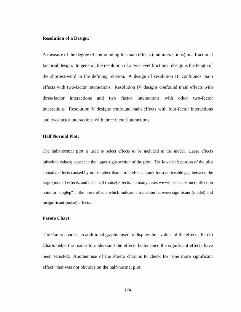
174
Resolution of a Design:
A measure of the degree of confounding for main effects (and interactions) in a fractional
factorial design. In general, the resolution of a two-level fractional design is the length of
the shortest-word in the defining relation. A design of resolution III confounds main
effects with two-factor interactions. Resolution IV designs confound main effects with
three-factor interactions and two factor interactions with other two-factor
interactions. Resolution V designs confound main effects with four-factor interactions
and two-factor interactions with three factor interactions.
Half Normal Plot:
The half-normal plot is used to select effects to be included in the model. Large effects
(absolute values) appear in the upper-right section of the plot. The lower-left portion of the plot
contains effects caused by noise rather than a true effect. Look for a noticeable gap between the
large (model) effects, and the small (noise) effects. In many cases we will see a distinct inflection
point or "dogleg" in the noise effects which indicate a transition between significant (model) and
insignificant (noise) effects.
Pareto Chart:
The Pareto chart is an additional graphic used to display the t-values of the effects. Pareto
Charts helps the reader to understand the effects better once the significant effects have
been selected. Another use of the Pareto chart is to check for "one more significant
effect" that was not obvious on the half-normal plot.
175
Box-Cox Plot:
The Box-Cox plot is a tool to help you determine the most appropriate power transformation to
apply to response data.
Response Surface Methodology:
Response surface methodology (RSM) explores the relationships between several
explanatory variables and one or more response variables. The method was introduced by
G. E. P. Box and K. B. Wilson in 1951. The main idea of RSM is to use a sequence of
designed experiments to obtain an optimal response. Box and Wilson suggest using a
second-degree polynomial model to do this. They acknowledge that this model is only an
approximation, but use it because such a model is easy to estimate and apply, even when
little is known about the process.

176
Appendix C: Controller Specification and Sample MATLAB code
Controller Properties:
API Object Name MotorControl
Motor Type DC Motor
Number of Motor Ports 1
Velocity Resolution 0.39 % Duty Cycle
Acceleration Resolution 24.5 % Duty Cycle/s
Acceleration Min 24.5 % Duty Cycle/s
Acceleration Max 6250 % Duty Cycle/s
Acceleration Time Min 31.3 ms
Acceleration Time Max 8.2 s
Encoder Interface:
Number of Encoder Inputs 1
Count Rate Max 500000 cycles/s
Encoder Interface Resolution x1
Update Rate 125 samples/s
Time Resolution 0.33 ms
Encoder Input Low Voltage Max 800 mV DC
Encoder Input High Voltage Min 2.1 V DC
Encoder Pull-up Resistance 2.4 kΩ
Electrical Properties:
Supply Voltage Min 9 V DC
Supply Voltage Max 28 V DC
Continuous Motor Current Max 5 A
Overcurrent Trigger 8 A
Current Consumption Min 20 mA
Current Consumption Max 100 mA
USB Speed Full Speed
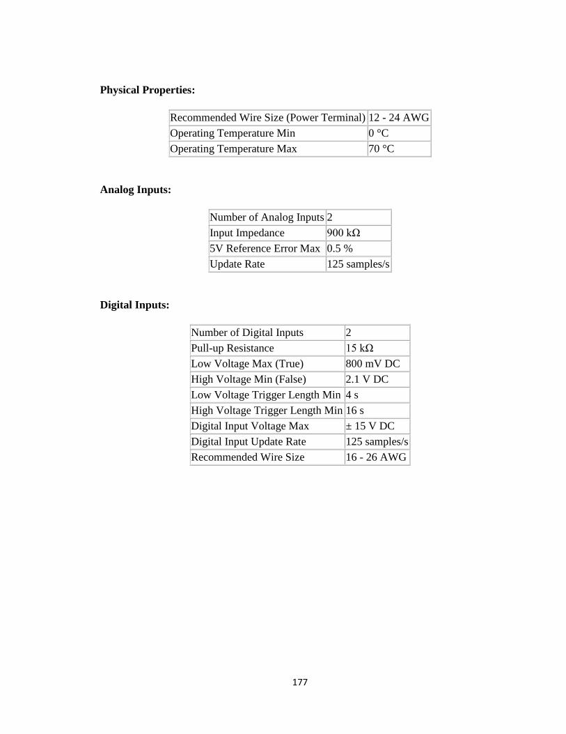
177
Physical Properties:
Recommended Wire Size (Power Terminal) 12 - 24 AWG
Operating Temperature Min 0 °C
Operating Temperature Max 70 °C
Analog Inputs:
Number of Analog Inputs 2
Input Impedance 900 kΩ
5V Reference Error Max 0.5 %
Update Rate 125 samples/s
Digital Inputs:
Number of Digital Inputs 2
Pull-up Resistance 15 kΩ
Low Voltage Max (True) 800 mV DC
High Voltage Min (False) 2.1 V DC
Low Voltage Trigger Length Min 4 s
High Voltage Trigger Length Min 16 s
Digital Input Voltage Max ± 15 V DC
Digital Input Update Rate 125 samples/s
Recommended Wire Size 16 - 26 AWG

178
Scissor Lift Height Formulation:
parameters
real global l;
real global H;
variables
real input;
equations
input=(H/(2*l));
output = arcsin(input);
Actuator Desired Length Calculation:
parameters
real global L;
real global H;
variables
real input;
equations
input=(H/(10*L));
output = 2*arccos(input);

179
Kinematic Simulation for Network # 3:
r=0.4; %angular velocity from calculation theta_dot=20.68; %angular acceleration from calculation alpha=-353.89; %time required for one revolution t_rev=2*pi/theta_dot; %time t=linspace(0,t_rev,200); %required angle theta=theta_dot*t; %position calculation x=6*r*cos(theta/2); %linear velocity calculation v=-3*r*theta_dot*sin(theta/2); %linear acceleration calculation a=(-3*r*alpha*sin(theta/2))-((3/2)*r*theta_dot^2*cos(theta/2)); % plot the figures subplot(2,2,1) plot(theta,x); xlabel('Theta (radian)') ylabel('Position (m)') title('Position vs Input Angle') subplot(2,2,2) plot(t,v) xlabel('Time (s)') ylabel('Velocity (m/s)') title('Linear Velocity vs Time') subplot(2,2,3) plot(t,a) xlabel('Time (s)') ylabel('Acceleration (m/s2)') title('Linear Acceleration vs Time')
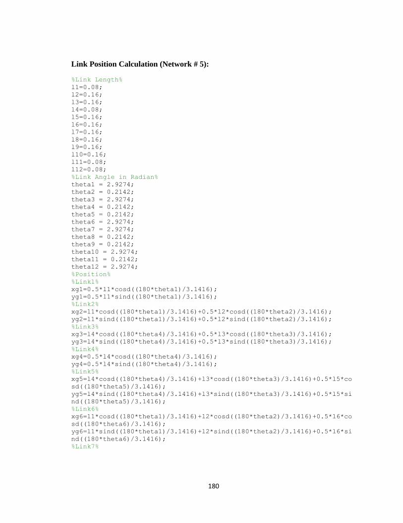
180
Link Position Calculation (Network # 5):
%Link Length% l1=0.08; l2=0.16; l3=0.16; l4=0.08; l5=0.16; l6=0.16; l7=0.16; l8=0.16; l9=0.16; l10=0.16; l11=0.08; l12=0.08; %Link Angle in Radian% theta1 = 2.9274; theta2 = 0.2142; theta3 = 2.9274; theta4 = 0.2142; theta5 = 0.2142; theta6 = 2.9274; theta7 = 2.9274; theta8 = 0.2142; theta9 = 0.2142; theta10 = 2.9274; theta11 = 0.2142; theta12 = 2.9274; %Position% %Link1% xg1=0.5*l1*cosd((180*theta1)/3.1416); yg1=0.5*l1*sind((180*theta1)/3.1416); %Link2% xg2=l1*cosd((180*theta1)/3.1416)+0.5*l2*cosd((180*theta2)/3.1416); yg2=l1*sind((180*theta1)/3.1416)+0.5*l2*sind((180*theta2)/3.1416); %Link3% xg3=l4*cosd((180*theta4)/3.1416)+0.5*l3*cosd((180*theta3)/3.1416); yg3=l4*sind((180*theta4)/3.1416)+0.5*l3*sind((180*theta3)/3.1416); %Link4% xg4=0.5*l4*cosd((180*theta4)/3.1416); yg4=0.5*l4*sind((180*theta4)/3.1416); %Link5% xg5=l4*cosd((180*theta4)/3.1416)+l3*cosd((180*theta3)/3.1416)+0.5*l5*co
sd((180*theta5)/3.1416); yg5=l4*sind((180*theta4)/3.1416)+l3*sind((180*theta3)/3.1416)+0.5*l5*si
nd((180*theta5)/3.1416); %Link6% xg6=l1*cosd((180*theta1)/3.1416)+l2*cosd((180*theta2)/3.1416)+0.5*l6*co
sd((180*theta6)/3.1416); yg6=l1*sind((180*theta1)/3.1416)+l2*sind((180*theta2)/3.1416)+0.5*l6*si
nd((180*theta6)/3.1416); %Link7%

181
xg7=l4*cosd((180*theta4)/3.1416)+l3*cosd((180*theta3)/3.1416)+l5*cosd((
180*theta5)/3.1416)+0.5*l7*cosd((180*theta7)/3.1416); yg7=l4*sind((180*theta4)/3.1416)+l3*sind((180*theta3)/3.1416)+l5*sind((
180*theta5)/3.1416)+0.5*l7*sind((180*theta7)/3.1416); %Link8% xg8=l1*cosd((180*theta1)/3.1416)+l2*cosd((180*theta2)/3.1416)+l6*cosd((
180*theta6)/3.1416)+0.5*l8*cosd((180*theta8)/3.1416); yg8=l1*sind((180*theta1)/3.1416)+l2*sind((180*theta2)/3.1416)+l6*sind((
180*theta6)/3.1416)+0.5*l8*sind((180*theta8)/3.1416); %Link9% xg9=l4*cosd((180*theta4)/3.1416)+l3*cosd((180*theta3)/3.1416)+l5*cosd((
180*theta5)/3.1416)+l7*cosd((180*theta7)/3.1416)+0.5*l9*cosd((180*theta
9)/3.1416); yg9=l4*sind((180*theta4)/3.1416)+l3*sind((180*theta3)/3.1416)+l5*sind((
180*theta5)/3.1416)+l7*sind((180*theta7)/3.1416)+0.5*l9*sind((180*theta
9)/3.1416); %Link10% xg10=l1*cosd((180*theta1)/3.1416)+l2*cosd((180*theta2)/3.1416)+l6*cosd(
(180*theta6)/3.1416)+l8*cosd((180*theta8)/3.1416)+0.5*l10*cosd((180*the
ta10)/3.1416); yg10=l1*sind((180*theta1)/3.1416)+l2*sind((180*theta2)/3.1416)+l6*sind(
(180*theta6)/3.1416)+l8*sind((180*theta8)/3.1416)+0.5*l10*sind((180*the
ta10)/3.1416); %Link11% xg11=l1*cosd((180*theta1)/3.1416)+l2*cosd((180*theta2)/3.1416)+l6*cosd(
(180*theta6)/3.1416)+l8*cosd((180*theta8)/3.1416)+l10*cosd((180*theta10
)/3.1416)+0.5*l11*cosd((180*theta11)/3.1416); yg11=l1*sind((180*theta1)/3.1416)+l2*sind((180*theta2)/3.1416)+l6*sind(
(180*theta6)/3.1416)+l8*sind((180*theta8)/3.1416)+l10*sind((180*theta10
)/3.1416)+0.5*l11*sind((180*theta11)/3.1416); %Link12% xg12=l4*cosd((180*theta4)/3.1416)+l3*cosd((180*theta3)/3.1416)+l5*cosd(
(180*theta5)/3.1416)+l7*cosd((180*theta7)/3.1416)+l9*cosd((180*theta9)/
3.1416)+0.5*l12*cosd((180*theta12)/3.1416); yg12=l4*sind((180*theta4)/3.1416)+l3*sind((180*theta3)/3.1416)+l5*sind(
(180*theta5)/3.1416)+l7*sind((180*theta7)/3.1416)+l9*sind((180*theta9)/
3.1416)+0.5*l12*sind((180*theta12)/3.1416);
%End Effector Position% xg_e=l1*cosd((180*theta1)/3.1416)+l2*cosd((180*theta2)/3.1416)+l6*cosd(
(180*theta6)/3.1416)+l8*cosd((180*theta8)/3.1416)+l10*cosd((180*theta10
)/3.1416)+l11*cosd((180*theta11)/3.1416); yg_e=l1*sind((180*theta1)/3.1416)+l2*sind((180*theta2)/3.1416)+l6*sind(
(180*theta6)/3.1416)+l8*sind((180*theta8)/3.1416)+l10*sind((180*theta10
)/3.1416)+l11*sind((180*theta11)/3.1416);
182
MATLAB Function for Control SIMULINK Model:
function y = fcnarmdynamics(u) m1=0.216; m2=0.216; m3=0.216; m4=0.216; l1=0.4; l2=0.4; l3=0.4; l4=0.4; %g=9.81;
torque=u(1); theta=u(2); %dtheta=u(3);
M=((m1+3*m2)/6)*(l1^2)+m2*((l2^2)/6)+((m2*l1*l2)/2)*cos(theta)+
m3*((l3)^2/6)+ m3*((l2*l4*cos(theta))/2)+((m4+3*m3)/6)*(l4^2); M_inverse=inv(M);
%N=[-m2*a1*a2*sin(theta1)*(dtheta1*dtheta2+((dtheta2)^2/2));
(m2/2)*a1*a2*((dtheta1)^2/2)*sin(theta2)]; %without friction %N=[-
m2*a1*a2*sin(theta1)*(dtheta1*dtheta2+((dtheta2)^2/2))+(0.1*dtheta1);
(m2/2)*a1*a2*((dtheta1)^2/2)*sin(theta2)+(0.1*dtheta1)]; %with friction
%G=[((m1+m2)/2)*g*a1*cos(theta1)+(m2/2)*g*a2*cos(theta1+theta2);
m2*g*(a2/2)*cos(theta1+theta2)]; y = M_inverse*(torque); %#ok<*MINV>
183
References
[1] J. P. Merlet (2006), Parallel Robots, Second Edition, Springer, INRIA, France.
[2] B. Yao, Y. Hong, C, Hu, and Q. Wang, “Precision motor control of linear motor
drive systems for micro/nano-positioning,” Micro Nano China 2007, January 2007,
Sanya, Haina, China.
[3] Gough, V. E. and Whitehall, S. G. (1962), “Universal tyre testing machine”,
Proceedings of the 9th
International Automobile Technical Congress, discussion,
Federation Internationale des Societes d Ingenieurs des Techniques de Automobile
(FISITA) (Ed. G. Eley), (IMechE 1, London, UK), pp. 117137.
[4] Rolland, L. 2010, “Kinematic Synthesis of a New Generation of Rapid Linear
Actuator for High Velocity Robotics”, Advanced Strategies for Robot Manipulators, S.
Ehsan Shafiei (Ed.), ISBN: 978-307-099-5.
[5] A. Alleyene,”Nonlinear force control of an electro hydraulic actuator,” In proc.
Japan/USA Symposium, Flexible Automation, Boston, MA, 1996, pp. 193-200.

184
[6] N. Niksefat, N Sepheri, “ Designing Robust Force Control of Hydraulic Actuator‟s
Despite systems and Environmental Uncertainties”, IEEE control system Magazine,
2001, pp. 66-77.
[7] Conrad and C.J.D. Jensen, “Design of hydraulic force control systems with state
estimate feedback,” In Proc. IFAC 10th Triennial Congress, Munich, Germany, 1987,
pp. 307-312.
[8] N. Niksefat and N. Sepehri, “Robust force controller design for an electro hydraulic
actuator based on nonlinear model,” In Proc. IEEE Conf. Robotics and Automation,
Detroit, MI, 1999, pp. 200-206.
[9] Altare, A. Vacca, C. Ritcher, “A Novel Design for an Efficient and Compact Electro-
hydraulic Actuator”, IEEE Aerospace Conference, May 2014, MT, USA.
[10] Wang, J., Pu, J. and Moore, P.R. (1997), “A practicable control strategy for servo
pneumatic actuator systems”, Control Eng. Pract., Vol. 7, pp. 1483-8.
[11] C. Kim, J. H. Chung, “Application of an active pneumatic actuator to robotic
deburring”, Industrial Robotics: An International Journal, vol. 34/6, pp. 487-494, 2007.

185
[12] Okamura M., Ohshige T. and Watanbe M., “High Speed and High Accuracy XY-
Stage for Electronic Assembly”, Fourth IEEE/CHMT European International Electronic
Manufacturing Technology Symposium, Proceedings, pp.104-107, 1988.
[13] Meisser C., Eggenschwiler H. and Nehls W., “Einrichtungzur Durchführung der
Zustellbewegung eines Arbeitsorganszu einer Arbeitsstation”, European Patent
Application No. 0317787B1, ESEC SA, 1988.
[14] T. Niino, S. Egawa and T. Higuchi, “High-Power and High efficiency Electrostatic
Actuator”, Proc. 1993 IEEE Workshop on Micro Electro Mechanical Systems, (1993)
236-241.
[15] T. Niino, T. Higuchi and S. Egawa, “Dual Excitation Multiphase Electrostatic
Drive”, Proc. 1995 IEEE IAS annual meeting (1995), pp. 1318-1325.
[16] R. M. Robinson, C. S. Kothera, B. K. S. Woods, R. D. Vockee and N. M. Wereley, “
High Specific Power Actuators for Robotic Manipulators”, Journal of Intelligent
Material Systems and Structure, vol. 22, 2011, pp. 1501-1511.
[17] Klute, G., Czerniecki, J. and Hannaford, B., „„Artificial Muscles: Actuators for Bio-
robotic Systems,‟‟ International Journal of Robotics Research (2002), 21:295_309.
186
[18] Lightner, S. and Lincoln, R., „„The Fluidic Muscle: A „New‟ Development,‟‟ The
International Journal of Modern Engineering, 2002, 2:8 pages.
[19] Woods, B.K.S., Gentry, M., Kothera, C.S., and Wereley, N.M., "Fatigue Life
Testing of Swaged Pneumatic Artificial Muscles for Aerospace Morphing Applications,"
51st AIAA/ASME/ASCE/AHS/ASC Structures, Structural Dynamics, and Materials
Conference, 12-15 April 2010, Orlando, FL, AIAA 2010_2662.
[20] www.wikipedia.org
[21] K. Takemura, H. Kozuki, K. Edamura and S. Yokota, “A micromotor using electro-
conjugate fluid - Improvement of motor performance by using saw-toothed electrode
series”, Sensors and Actuators A: Physical, 140 (2007) 131-137.
[22] Baughman, Ray H., Cui, Changxing, Zakhidov, Anvar A., Iqbal, Zafar, Barisci,
Joseph N., Spinks, Geoff M., Wallace, Gordon G., Mazzoldi, Alberto, de Rossi, Danillo,
Rinzler, Andrew G., Jaschinski, Oliver, Roth, Siegmar, Kertesz, Miklos, “Carbon
nanotube actuators”, Science, 284(5418), 1999.
[23] K. Uchino, “Piezoelectric Actuators 2006”, Journal of Electro ceramics, August
2008, Volume 20, Issue 3-4, pp 301-311.
[24] Y. Okamoto, R. Yoshida, H. Sueyoshi, Konica Minolta Tech. Report 1, 23 (2004).

187
[25] S. Kawashima, O. Ohnishi, H. Hakamata, S. Tagami, A. Fukuoka,T.Inoue, S.
Hirose, Proc. IEEE Int’l Ultrasonic Symp. , 1994, France (1994).
[26] K. Uchino, “Piezoelectric Actuators and Ultrasonic Motors”, (Kluwer, Norwell, MA
1996).
[27] K. Uchino, “Ferroelectric Devices” (CRC, Dekker, NY, 2000).
[28] K. Uchino, “Micromechatronics” (CRC, Dekker, NY 2003).
[29] Clavel R., “DELTA, a Fast Robot with Parallel Geometry”, Int. Symp. On Industrial
Robots (ISIR), pp. 91-100, 1988.
[30] J. C. Compter, “Electro-dynamic planar motor,” Precision Eng., vol. 28, no. 2, pp.
171–180, Apr. 2004.
[31] W. J. Kim, D. L. Trumper, and J. H. Lang, “Modeling and vector control of a planar
magnetic levitator,” IEEE Trans. Ind. Appl., vol. 34, no. 6,pp. 1254–1262, Nov./Dec.
1998.
[32] A. J. Hazelton, M. B. Binnard, and J. M. Gery, “Electric motors and positioning
devices having moving magnet arrays and six degrees of freedom,” U.S. Patent 6 208
045, Mar. 27, 2001.

188
[33] N. Korenaga, “Alignment apparatus and exposure apparatus using thesame,” U.S.
Patent 7 075 198, Jul. 11, 2006.
[34] J. C. Compter, P. C. M. Frissen, and J. van Eijk, “Displacement device,” Patent WO
2006/075 291 A2, Jul. 20, 2006.
[35] C. M. M. van Lierop, J. W. Jansen, A. A. H. Damen, and P. P. J. van den Bosch,
“Control of multi-degree-of-freedom planar actuators,” In Proc. IEEE Int. CCA, Munich,
Germany, Oct. 2006, pp. 2516–2521.
[36] F. Baronti, A. Lazzeri, F. Lenzi, R. Roncella, R. Saletti, and S. Saponara, “Voice
Coil Actuators: From Model and Simulation to Automotive Application,” 35th Annual
IEE Conference on Industrial Electronics (IECON’09), 2009, pp. 1805-1810.
[37] W. Robertson, B. Cazzolato, and A. Zander, “Parameters for Optimizing the Forces
Between Linear Multipole Magnetic Arrays,” IEEE Magnetic Letters, Vol. 1, 2010.
[38] X.M. Feng, Z.J. Duan, Y. Fu, and A.L. Sun, “The technology and Application of
Voice Coil Actuator,” 2nd International Conference on Mechanical Automation and
Control Engineering (MACE), 2011, pp. 892-895.

189
[39] K. Tsuchiya, Y. Todaka and M. Umemoto, “TEM Investigation of Intermediate
Phase Transformation and Micro modulationin Ni–Mn–Ga Ferromagnetic Shape memory
Alloys”, Mater. Sci. Tech., 24 (2008) 920-926.
[40] Y. Okimori, T. Inamura, H. Hosoda and K. Wakashima, “Diffusion Bonding of Co
to TiAu High Temperature Shape Memory Alloy”, Materials Transactions, 49 (2008)
1998-2005.
[41] T. Higuchi, A. Horikoshi and T. Komori, “Development of an actuator for super
clean rooms and ultra-high vacuum”, Proc. of 2nd International Symposium on Magnetic
Bearings, Tokyo, Japan, (1990) 115-122.
[42] Yasui, A. Yamamoto and T. Higuchi, “Non-Contact Levitation control System for
Electrostatic Motor”, Proc. Of 8th International Symposium on Magnetic Bearings, Mito,
Japan, (2002), pp. 175-180.
[43] Scheiner, C. (1631), “Pantographice, seu ars delineandi res quaslibet per
parallelogrammum lineare seu cavum, mechanicum, mobile. Romae: Ex typographia
Ludouici Grignani, sumptibus Hermanni Scheus, vol. 12, 108 pages.
[44] https://www.cs.cmu.edu/~rapidproto/mechanisms/chpt5.html
190
[45] Moon, F.C. (2007) The Machines of Leonardo Da Vinci and Franz Reuleaux.
Volume on Kinematics of Machines from the Renaissance to the 20th Century, Series on
History of Mechanism and Machine Science, Springer Netherlands, 417 pages.
[46] Reuleaux, F. (1876) Kinematics of Machinery: Outlines of a Theory of Machines.
Macmillan and Co., London.
[47] Ren G. Dong, Christopher S. Pan, Jared J. Hartsell, Daniel E. Welcome, Tim Lutz,
Anne Brumfield, James R. Harris, John Z. Wu, Bryan Wimer, Victor Mucino, Kenneth
Means, “An Investigation on the Dynamic Stability of Scissor Lift.”
[48] Geoff Rideout and Jeffrey L. Stein, “An Energy-Based Approach to Parameterizing
Parasitic Elements for Eliminating Derivative Causality”, International Conference on
Bond Graph Modeling (ICBGM’ 2003).
[49] Tao Liu1, Jian Sun, “Simulative Calculation and Optimal Design of Scissor Lifting
Mechanism,” 2009 Chinese Control and Decision Conference (CCDC 2009).
[50] Lung-Wen Tsai (1999), “Robot analysis: the mechanics of serial and parallel
manipulators”, Wiley, New York.
[51] http://web.mit.edu/emech/dontindex-build/full-text/emechbk_8.pdf

191
[52] www. phidgets.com
[53] T. Rahman, D. Hicks, M. R. Hossain, and Nicholas Krouglicof, “Digital Hardware
Implementation of an Active Disturbance Rejection Controller for a Highly Dynamic
Parallel Orientation Manipulator”, 2014 IEEE International Conference on Robotics &
Automation (ICRA), Hong Kong Convention and Exhibition Center, May 31 - June 7,
2014. Hong Kong, China
[54] Jan F. Broenink, “Introduction to Physical Systems Modelling with Bond Graphs”,
University of Twente, Dept EE, Control Laboratory.
[55] www.bondgraphs.com
[56] http://www.statease.com/dx9.html