design exercise ct5550-2008 - tu delft

Design exercise CT 5550 - 1 -

1. Design exercise CT5550

1.1. Introduction The goal of the exercise is to get some experience in the handling of a network calculation program, to set up a network model and to make a rough design of a drinking water system. A few practical problems will be solved using the model. The network we consider is a network for an expanding town in a mildly sloped area in a third world country. The exercise is based on an existing city (Safi Town in Yemen), but modified for educational purposes. The exercise is build up in close cooperation with the UNESCO-IHE in Delft. We will consider a design period of 20 years, in which the town will grow relatively quickly. The exercise is individualised by variable data on some points as demand development and locations of pumping stations. The individual data will be handed to the participant on subscribing to the exercise. The exercise is reported individually. Contact and discussion amongst the participants is encouraged though, because this will stimulate the design process and creativity. The network calculation program ALEID is used, which is developed for the Dutch drinking water companies. For the exercise a student version of the program is available with limited capabilities compared to the full version. An alternative for ALEID is the program EPANET, developed by the American Environmental Protection Agency. This program can be downloaded from http://www.epa.gov/ORD/NRMRL/wswrd/epanet.html and is freeware. The exercise will result in an individual report that may be accompanied by the relevant input files of the calculations. No output or other formats. In the exercise the essentials of the calculation must be reported using graphs and tables. The report of the exercise is individually graded and will be the base for an oral examination. The grade of the exercise is 50% of the final grade and the oral examination the other 50%.

1.2. Set up of the exercise Basically, the exercise is a complete design of a new network, but in a condensed form. The exercise has three parts: The first part is the design of the pipe diameters and pipe tracks together with the operational scheme of the pumping station. The second part is the reliability analysis, the regular operation of the network and the operation under extreme circumstances. The last part is the design of an actual distribution network, connected to the main network that is designed in the first part of the exercise. Roughly the following steps will be made. The specific questions will guide you through the process


First part: design of the network: � Start with appreciating the lay out of the city and the level differences and

topography. � Than locate the demands, the time dependency of the demands and the possible

supply points. � The capacity of the supply point must be tested quantitatively (make a water

balance). � The first rough design can be made when the pipe tracks are known (basically the

main streets or main projected streets) and the projected demand nodes determined. The first design is made with a fixed pressure point as input boundary and usually the maximum demand is the normative demand situation.

� In an educated trial-and-error process the design is optimised and tested in several demand situations, analysed on velocities and pressure drops and optimised again, resulting in a first representative version of the design.

� Now the pumping station can be designed after the construction of the network characteristic and designed pump characteristics.

� In a 24 hour analysis the operational scheme of the pumping station is constructed and the pressure graphs of representative demand nodes can be made. This concludes the primary design of the network.

Second part: enhancement of the network � A day-to-day operational scheme of the pumping station is made: when do which

pumps work? � Two specific cases of operation under extreme circumstances are analysed. � Following the two specific cases a general reliability analysis of the network gives

an insight in the weak points and is used to enhance the design to a fully operational network.

� All aspects are summarised and a final design is presented taking into account the different aspects of normal and extraordinary circumstances.

Third part � Design of a distribution network and allocation of valves.

1.3. Design of a network A drinking water network is a complicated system with a relatively simple goal: bring water from the treatment plant to the consumer. As there are several ways to get to Rome, there are as many ways to accomplish the goal of the network. There is no such thing as the best network. The boundary conditions a network should meet to fulfil the primary goal are both quantitative and qualitative. Next to the purely technical requirements there is obviously also an economical requirement that demand for the lowest costs. The complicating factor is that these three types of requirements (quantity, quality and costs) are conflicting. The goal of the design process is to come up with solutions that fulfil an optimal combination of the requirements. The quantitative requirements are relatively simple: supply the demanded volume flow under sufficient pressure. The knowledge about the influence of the hydraulics


on the water quality is recent and proposes a relatively new requirement to network design. Velocity should be within certain limits. Increasing age of the network and the vulnerability of components to failure leads to more attention towards the operation of the network under failure conditions. This is formalised into the reliability analysis (see chapter 6 in the lecture notes). The intuitive solution to reliability issues is to extend the network, but that could have a counter effect on the water quality and certainly on the costs. As the network will be designed for a certain period, the demand has to be forecasted for that period. This is a tricky part, because the expected lifetime of a network exceeds the period that can realistically be overseen. For the design exercise we consider linear growth scenarios over a 30-year period. Comments on this method can be issued at the end of the exercise. Next to the technical conflicting requirements the costs of the design is an extra complicating factor. All aspects of costs should be considered: investment ánd operational costs. A simple example illustrates the tension between them: a pipe with a smaller diameter is lower in investment costs but higher in operational costs (more energy needed to transport the same amount of water and maybe additional cleaning costs). For the purpose or the exercise there is no full economical analysis required, but some comments should be made when relevant. As a rule of thumb one may consider the investments required in pipes are roughly linearly dependant of the diameter of the pipe: the investment is €0.50 to €0.60 per mm diameter per meter: A 400 mm pipe costs €200.= to €240.= per meter. The operational costs are mostly the energy costs needed to pump the water. A good estimation of energy costs can be made through a simple energy balance. The general requirements are: � Actual pressure in the main network should be within the range of 25 to 60 mWc

(250 to 600 kPa with respect to ground level)). The need for a minimum requirement is obvious, a maximum is required for customer convenience reasons and to limit leakages, water hammer and pipe failures.

� Velocities in the network should be at the maximum demand situation at least 0,3 to 0,4 m/s. In that way sedimentation and accumulation of deposits can be minimised and also the residence time will be within acceptable limits or at least as minimal as possible. High velocities superseding 1,5 to 2,0 m/s should be avoided, although there is some flexibility towards the maximum velocity. As long as sufficient protection against water hammer is available it shouldn’t be a problem. High velocities however can cause noise problems in smaller networks and of course will cause large pressure drops.

� Reliability of the network should meet the requirements as illustrated in chapter 6 of the lecture notes. See also the additional remarks at the specific questions.

1.4. Topography of the town The topography of the system is shown in figure 1 using a contour map


2624

22

20

18

16

14

12

10 8 6 8 10 12 14

16

18

20

22

0

200

400

600

800

1000[m]

2624

22

20

18

16

14

12

10 8 6 8 10 12 14

16

18

20

22

0

200

400

600

800

1000[m]

0

200

400

600

800

1000[m]

E3

C1

D1B

D2D3E1

C2

E2

C4

C3 A

FE3

C1

D1B

D2D3E1

C2

E2

C4

C3 A

F

Figure 1 Map of Safi Town with contour lines The boundaries of the city are given with the heavily dotted line. The lighter dotted lines configure the main streets in the city, the most logical places to put in main underground infrastructure. (Drinking water, sewerage and drainage systems, electricity, gas and cables) This picture shows that the town is built in a slightly sloped area with a level difference of about 18 meters (between 24 and 6 msl) as indicated by the contour lines. The area surfaces in ha is given in table 1.

Table 1 Area of districts Distr. A[ha] Distr. A[ha] Distr. A[ha]

A B C1 C2

83.2 30.8 73.6 80.8

C3 C4 D1 D2

50.0 84.4 37.2 55.6

D3 E1 E2 E3 F

78.0 97.2 117.2 83.2 29.6

1.5. Population and demands Construction of a new area urges for estimation of demand rather than actual measuring. The demands are estimated based on the projected type of building and prognoses of number of people. The town is divided into six district areas (A-F) of


homogeneous yet different population density. Apart from the population a factory is planned on the outskirts of the city. The domestic consumption per capita is planned to be 150 l/d. In addition the projected water demand of the new factory is planned to be 1080 m3/d. The unaccounted for water (UFW, sometimes called leakage) is not expected to exceed 10% of the planned water consumption after commissioning. A further increase of the UFW can be expected with a further 5% towards the end of the design period, resulting in a total UFW of 15%. The diurnal pattern of the domestic consumption pattern is shown in figure 2. Apart from the daily pattern also a week and seasonal pattern is given. The week pattern varies between a factor 0,95 to 1.10, the seasonal pattern between 0,90 and 1,15. The factory will demand a constant supply during 12 hours, between 7 a.m. and 7 p.m. (double shift labour structure) This is constant over the weeks and seasons. For the growing of the city a linear growth is projected for the next 30 year with grow rates as put together in table 2.

Diurnal pattern house hold demand

0,3

36

0,21

2

0,2

15

0,1

69

0,0

98

0,1

33

0,41

8

1,0

08

1,4

85

1,5

76

1,51

7

1,4

01

1,4

93

1,3

48

1,1

08

0,9

51 1,07

7

1,3

75

1,7

31 1,8

5

1,6

72

1,4

11

1,1

25

0,2

91

0

0,2

0,4

0,6

0,8

1

1,2

1,4

1,6

1,8

2

0 1 2 3 4 5 6 7 8 9 10 11 12 13 14 15 16 17 18 19 20 21 22 23

hours

fact

or

Figure 2 Diurnal pattern of household demand


Table 2 Population density and growth

District Present [inh/ha]

Annual growth [%]

A B

C1,2,3,4 D1,2,3

E1,2,3 F

0.6 NR 0.7 NR 0.4 NR 0.5 NR 0.3 NR 0.2 NR

2.0 1.0 2.4 2.8 3.5 3.5

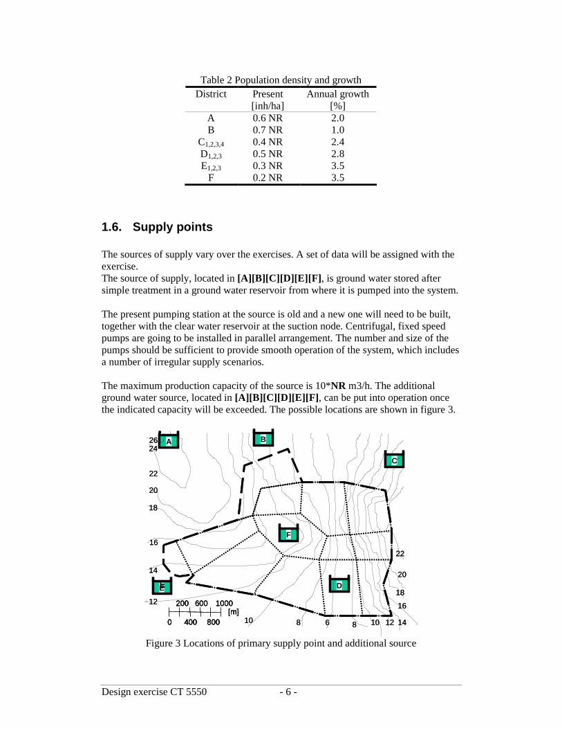
1.6. Supply points The sources of supply vary over the exercises. A set of data will be assigned with the exercise. The source of supply, located in [A][B][C][D][E][F], is ground water stored after simple treatment in a ground water reservoir from where it is pumped into the system. The present pumping station at the source is old and a new one will need to be built, together with the clear water reservoir at the suction node. Centrifugal, fixed speed pumps are going to be installed in parallel arrangement. The number and size of the pumps should be sufficient to provide smooth operation of the system, which includes a number of irregular supply scenarios. The maximum production capacity of the source is 10*NR m3/h. The additional ground water source, located in [A][B][C][D][E][F], can be put into operation once the indicated capacity will be exceeded. The possible locations are shown in figure 3.

AA BB

CC

DDEE

FF

2624

22

20

18

16

14

12

10 8 6 8 10 12 14

16

18

20

22

0

200

400

600

800

1000[m]

2624

22

20

18

16

14

12

10 8 6 8 10 12 14

16

18

20

22

0

200

400

600

800

1000[m]

0

200

400

600

800

1000[m]

Figure 3 Locations of primary supply point and additional source


1.7. Distribution Mains System The distribution main pipes will be laid along the main streets of SAFI. The main street structure and thus the possible pipe routes are shown in figure 4, with the lengths of the pipe routes. The intersections (nodes) are numbered. Connection of the factory (node 1) to the system is planned to be in node 6.

0

200

400

600

800

1000[m]

0

200

400

600

800

1000[m]

2

8

5

11 1920

22

21

1812

9

10

4

15

14

7

3

24

2317

136

16

1050

1500700

200

1250

1450

1000

300

500

800

800

750800

850

1050

850

600

450

500

600

700

350

500

800

600

6 00500

600

1050

600650

1100

800

7 = node number1050 = pipe length [m]

Figure 4 Nodes and street dimensions Regarding the local situation (soil conditions, local manufacturing), PVC is chosen as a pipe material for the network. A table of pipe data is given in figure XX. Due to such a choice, it is assumed that the roughness of the pipe will remain low throughout the design period. The accepted k-value of 0.5 mm includes impacts of local (minor) losses in the network.


Figure 5 Pipe data on PVC


2. Questions

Part 1 Hydraulic design Preliminary concept 1.1 Calculate the demand at the beginning of the design period and the end. 1.2 Regarding the supply points:

� determine if and when the second source will need to be put into operation and calculate if necessary its maximum required capacity,

� decide in which nodes the sources will be connected to the network, � determine the lengths of the connecting pipes.

1.3 Develop a preliminary supply strategy: suggest possible phases in

development of the system, function of the pumping stations, reservoirs, etc. Nodal Consumption 1.4 Calculate the average consumption for nodes 01-24 (see appendix):

� at the beginning of the design period, � at the end of the design period.

Network Layout 1.5 Size the pipe diameters in the system at the beginning and the end of the

design period. Use for the supply points a fixed pressure point, but be aware of the accumulated inflow over 24 hour when two supply points are used.

Pumping Stations 1.6 For the source pumping stations, determine:

� The required head, inflow and maximum pressure drop in the system for 24 hour, based on the calculations of 1.5. (Pipe characteristic)

� A provisional number and arrangement of the pumping units, both at the beginning and the end of the design period. Design your own pumping curves.

Storage 1.7 Determine the volume of the clear water reservoir at the suction side of the

source pumping stations at the beginning and the end of the design period (assume ground level tanks).

Summary Part 1 1.8 Draw conclusions based on the hydraulic performance of the system

throughout the entire design period. Explain phased development of the design, if applied.


PART 2 - System Operation Upgrade the computer models of the selected layout at the end of the design period. Model the pumping station operation by assuming parallel arrangement of the pump units. Regular Operation 2.1 Propose a plan of operation of the pumping station(s), during regular supply

conditions. Factory Supply Under Irregular Conditions 2.2 A reliable supply and fire protection have to be provided for the factory.

Analyse the design under the maximum consumption hour conditions, if: o pipe 06 - 02 or 06 - 05 bursts, o a fire requirement of Nr m3/h at pressure of 30 mwc is needed in node

01. If necessary, propose operation that can provide supply of the required quantities and pressures. Network Reliability Assessment The reliability assessment is performed according to chapter 6 of the lecture notes, however is an abbreviated form. For each pipe failure only the maximum hour has to be analysed. The criterion is changed to 60% of the maximum hourly demand as experience learns that if this is reached, than the 75% over the 24 hour analysis is not a problem, unless special circumstances are valid. For the reliability assessment of this design it is best to use a fixed pressure point as an input. 2.3 Assess the reliability of the distribution network only at maximum

circumstances. Determine the consequences of every possible single pipe failure event and propose measures when the supply of 60 % of the maximum consumption hourly demand is not reached. Comment on the pressure situation and the ability of the pumping station to deliver the required head and flow.

Choice of Final Layouts 2.4 Show the network layout, the number and size of the pump units and the

distribution of the storage volume at the beginning and at the end of the design period. Comment on adjustment necessary to meet the reliability requirement.

2.6 Describe the steps in (re)construction/extension of the system during the

design period.


PART 3: design of distribution network The design of a distribution network is based on chapter 8 of the lecture notes. In the area showed in figure 6 the plan for several houses is given. The heavily dotted line limits the area. In the area a total of around 380 houses will be build, of which the location of the majority is known. There is one house at every lot, except in eastern area where 4-storage living buildings are projected. In the south east area a special type of buildings is projected, the exact nature however is not known yet and will be filled in within the next 15 years. In the middle a shopping mall is projected with a few stores. The fire fighting demand is over the whole area restricted to 30 m3/h, except in the shopping area where the conventional 60 m3/h is demanded. Hydrants must be present maximal 50 meters distance from any object in the area. The connection points for connection to the main system with a guaranteed pressure of 30 mWc can be found at the transportation line. The houses must be connected to the main system under the requirement that once a day the velocity is at least 0,4 m/s. The one-family houses have an installation with 29 Tapping Units. The multi storage houses have an installation of 20 TU. Maximum number of connections in one section is 120.

Main pipe, 300 kPaguaranteed

Specialdestination

Shoppingarea4 storage

buildings

Figure 6 Neighbourhood plan for design of network 3.1 Determine sections of maximum 120 connections and locate special objects

with regard to the fire fighting 3.2 Construct the pipe routes (following the streets) and the connection points to

the main structure


3.3 Compose a table using maximal 4 diameters of PVC pipe and the transport capacity for a number of dwellings.

3.4 Size the sections 3.5 Locate fire hydrants and see if any adjustment in necessary. Give arguments

on how to solve inconsistencies 3.6 Pick one section and check the total pressure drop during normal operation

and during fire fighting. 3.7 Locate valves to limit the effect of any failure in this system. Be aware that the

functionality of the valve will deteriorate over time to 80% or less.


Appendix 1. Tutorial exercise Preliminary concept Designing a network is a circular process that starts with a first assessment of the boundaries of the system. In practise this preliminary concept will deviate from the final network lay out and won’t be reported. For this exercise the preliminary concept must be reported to help starting the design process. It will show the development of the design. Typically in this phase of the design no computer calculations are made. Major goal is to get a feeling of the quantities of water that have to supplied and to realise what the projected growth of the system will be. Also a consideration on phasing the development of the system is necessary. Every investment that can be postponed will save money. Moreover phasing will allow for adjustment in the course of time. A design period of 30 years is very difficult in terms of actual demand forecasting. An assessment of the sources is necessary to find out whether one source will be sufficient or when a second source or network storage shall be useful. Nodal consumption In this case the allocation of the demands is supposed to be equally spread over certain areas. The growth of the demands will be also evenly spread over the area. For modelling purposes on this transportation scale this is a viable assumption, because the connection of the secondary distribution area to the primary transportation network that we are designing is concentrated to certain points. The demands are supposed to be concentrated in the nodes that connect the pipes. The areas of demand that are located to the nodes can be determined by drawing perpendicular lines in the middle of the connecting lines. The intersections of these perpendicular lines limit the area that can be allocated to the nodes. See figure 7. Another possibility is to add up the length of the loop of pipes surrounding an area and to divide the consumption of this area over the nodes proportionally with the length of pipes connected to the nodes (Half of the length of the connected pipes).

Figure 7 Allocation of area based demands Network Layout This is the calculation intensive part of the exercise. Necessary is to have a running model that is geographically sound. This is provided in ALEID-layout and the file


contains the network layout and connectivity of the nodes. The file has to be filled in with the actual demands and demand patterns as well as the pipe diameters. Start the design by estimating the diameters and fill in a fixed pressure point at the source point. If the calculation runs without errors you can see how the pressure drops are over the system. Bare in mind that the pressure drops are the most important at this moment and they shouldn’t exceed the 35 mWc according to reference level. (The difference between the allowable pressure ranges from 60 to 25 meter. This part of the exercise will get you used to designing a network. Pumping station In the first design a fixed pressure point is used for the input source. At this point a network characteristic of the system can be made and the necessary pump curves can be determined. In this case you can size the curves yourself in such a way that the (in your opinion) ideal combination of pumps can be arranged. In practise some libraries of pump curves can be available from which to choose. However to get an idea of what you need is this way of designing appropriate to make up your mind when actually buying pumps. If booster station(s) is a part of the design, you can size them in the same way. A booster station can be helpful is case of long transportation distances. A booster instead of a large diameter pipe can compensate the pressure drop over the transport distance. Part 2 System Operation The design of the system is based on the normal situation. The refinement of the design is in the daily operation and irregular circumstances. Regular operation The number and characteristics of pumps is determined in the first phase. The operation of them to maintain a as constant as possible pressure in the network is reached by switching on and off pumps. Also the real behaviour of high-level reservoirs can be observed and optimised. Factory supply under irregular conditions Not all connections demand for the same reliability of supply. An interruption of the supply for a factory can have serious consequences if the production process is dependant of the water. The reliability rules as are valid for the overall consumption can be too light for the factory demand and in fact they are. To assess whether requirements can be met under all circumstances the calculations with a broken supply line are preformed as well as the special fire fighting requirements. When looking for solutions also look at what the factory itself can do and how for possible measurements must be paid and by whom. Network reliability assessment Applying the quantitative guideline for reliability for the complete system results in a very large calculation exercise. That’s why only the maximum hour is analysed and a threshold of 60% is maintained. In fact this is the first step in a complete reliability


assessment. When in the maximum hour with a dominantly house hold pattern 60% of the demand is satisfied, over the whole day the 75% will be realised.


Appendix 2. Pumps in ALEID Add a pump to an existing network The first design of the network is made with a fixed pressure point. This is the equivalent of a high level reservoir with a fixed level: a true snap shot model. A pump in a network is a special pipe: instead of pressure loss in the flow direction pressure will be added in the flow direction. For the model a pipe should be added with at the low-pressure side (the suction node) a reservoir with a level that is appropriate. This level is the level from which the pressure is added. The original fixed pressure point is changed to a normal node and this node is connected to the new suction node with a pipe that acts like a pump. Following this the pump curve must be identified in the pump data file and in the case of more pumps the controls have to be added. To replace this fixed pressure point with a more realistic pump curve the following steps have to be taken: 1. Open the project that contains the fixed pressure point as single feeding point. 2. In the dialog box ‘open project’ click on the arrow next to the button ‘Open’

and chose the option ‘Save then open’. This gives the opportunity to change the names of the files in the project. You have to fill in a name in the box ‘Pump data’ to make an empty pump data file (section 4.12 Manual)

3. Then add a node to the system as a reservoir node with fixed pressure. This will be the suction node for the pump.

4. Change the original fixed pressure node to a normal node (Right click on the node en choose ‘edit’ (section 5.5 in the manual)

5. Connect the suction node (the new fixed pressure point) with the network, preferably at the former reservoir and label this as ‘Pump’-type.

6. Identify the pump number. This identifies the pump curve that is in the PHF-file. At this point there is no pump curve defined, so you can do this by clicking on the box next to the ‘Pump no’. Refer to section 5.5.2.5 of the manual.

7. Adding controls as is demonstrated in section 5.5.2.4. in the manual. This is especially necessary if multiple pumps are available.

design exercise ct5550-2008 - tu delft

Documents