Louisiana State UniversityLSU Digital Commons

LSU Master's Theses Graduate School

2011

Design, Fabrication and Characterization of a NewWind Tunnel Facility – Linear Cascade with aWake SimulatorJean-Philippe Junca-LaplaceLouisiana State University and Agricultural and Mechanical College

Follow this and additional works at: https://digitalcommons.lsu.edu/gradschool_theses

Part of the Mechanical Engineering Commons

This Thesis is brought to you for free and open access by the Graduate School at LSU Digital Commons. It has been accepted for inclusion in LSUMaster's Theses by an authorized graduate school editor of LSU Digital Commons. For more information, please contact gradetd@lsu.edu.

Recommended CitationJunca-Laplace, Jean-Philippe, "Design, Fabrication and Characterization of a New Wind Tunnel Facility – Linear Cascade with a WakeSimulator" (2011). LSU Master's Theses. 2773.https://digitalcommons.lsu.edu/gradschool_theses/2773

DESIGN, FABRICATION, AND CHARACTERIZATION

OF A NEW WIND TUNNEL FACILITY - LINEAR CASCADE

WITH A WAKE SIMULATOR

A Thesis

Submitted to the Graduate Faculty of the

Louisiana State University and

Agricultural and Mechanical College

in partial fulfillment of the

requirements for the degree of

Master of Science in Mechanical Engineering

in

The Department of Mechanical Engineering

by

Jean-Philippe Junca-Laplace

Institut Supérieur de l‟Aéronautique et de l‟Espace, ENSICA, Toulouse, France

August 2011

ii

Acknowledgments

I am very grateful to my advisors, Dr. S. M. Guo and Dr. D. E. Nikitopoulos for giving

me the chance to work on this project. The support from the Air Force Research Laboratories is

greatly appreciated as well.

I would like to thank all the Mechanical Engineering machine shop technicians, Barry

Savoy, Don Colvin and Jim Layton who is unfortunately no longer with us. Without their great

work and help, this research project would not have been realized in such a manner. Thanks are

also due to Paul Rodriguez, Chemical Engineering shop manager for his precious advice and

good work quality.

I would also like to thank all the members of the Friday afternoon weekly meetings for

their support and guidance: Guillaume Bidan, Lem Wells and Jason W. Bitting. In addition, I

would like to thank Chris Foreman for sweating it out with me during the assembling of the wind

tunnel.

Thanks to all the friends I made here: Avishek, Guillaume and Joe for our afternoon

finger soccer games. Diane, Tony and Sara for sharing the Louisianan culture with me. I would

also like to thank Tim, Heather and Bidur for being outstanding roommates. And of course,

Farren for all the great times we shared together in Baton Rouge and New Orleans.

Finally, thanks to my parents and my sisters for their support and the delicious packages

they have sent from France during these two years.

iii

Table of Contents

Acknowledgments………………………………………………………………................ ii

List of Tables……………………………………………………………………................ v

List of Figures………………………………………………………………....................... vi

Nomenclature……………………………………………………………………………... ix

Abstract……………………………………………………………………………………. xi

Chapter 1: Introduction………………………………………………………………….. 1

1.1 Background………………………………………………………………………… 3

1.2 Film Cooling……………………………………………………………………...... 3

1.3 Motivation………………………………………………………………………...... 3

1.4 Literature Survey…………………………………………………………………... 4

1.5 Objectives………………………………………………………………………...... 10

1.6 Outline of Thesis…………………………………………………………………… 10

Chapter 2: Wind Tunnel Design………………………………………………………..... 12

2.1 General Description………………………………………………………………... 13

2.2 Components………………………………………………………………………... 15

2.2.1 Divergent Cone……………………………………………………………….... 15

2.2.2 Corner Vanes…………………………………………………………………... 15

2.2.3 Settling Chamber………………………………………………………………. 16

2.2.4 Contraction Cone………………………………………………………………. 22

2.2.5 Fan……………………………………………………………………………... 25

2.2.6 Fan Pitch Control Device………………………………………………………. 25

2.2.7 Windows and Safety Screens…………………………………………………... 27

2.2.8 Breather………………………………………………………………………… 27

2.2.9 Supporting Structure………………………………………………………….... 28

2.3 Pressure Loss Estimation in the Wind Tunnel……………………………………... 31

2.3.1 Straight, Constant Area Sections………………………………………………. 32

2.3.2 Corners…………………………………………………………………………. 34

2.3.3 Divergent Sections……………………………………………………………... 34

2.3.4 Contraction Cone………………………………………………………………. 35

2.3.5 Settling Chamber: Screens and Honeycomb……………………………………35

2.3.6 Summary of Pressure Losses…………………………………………………... 35

2.4 Wind Tunnel Energy Ratio and Design Analysis………………………………….. 36

Chapter 3: Cascade with Wake Simulator Design………………………………………37

3.1 Setup Characteristics……………………………………………………………….. 38

3.1.1 Linear Cascade Characteristics………………………………………………… 38

3.1.2 Wake Simulator Characteristics………………………………………………... 39

3.1.3 Cascade Inlet Plane Angle……………………………………………………... 39

3.2 Test Section Design………………………………………………………………... 40

3.3 Wake Simulator Design……………………………………………………………. 42

3.3.1 Frame…………………………………………………………………………... 43

3.3.2 Belt……………………………………………………………………………... 44

iv

3.3.3 Shafts…………………………………………………………………………... 46

3.3.4 Sprockets………………………………………………………………………. 46

3.3.5 Wearstrips……………………………………………………………………… 47

3.3.6 Gearmotor……………………………………………………………………… 47

3.3.7 Stand…………………………………………………………………………… 49

3.3.8 Shell……………………………………………………………………………. 50

3.3.9 Plate Assembly…………………………………………………………………. 51

3.3.10 Final Conveyor Assembly………………………………………………………53

3.3.11 Vibration Reduction……………………………………………………………. 54

3.3.12 Acoustic Resonance……………………………………………………………..55

Chapter 4: Characterization of the Wind Tunnel…………………………………….... 58

4.1 Characterization Parameters……………………………………………………….. 58

4.1.1 Turbulence Intensity…………………………………………………………… 59

4.1.2 Boundary Layer Profile………………………………………………………... 60

4.2 Measurements Techniques…………………………………………………………. 60

4.2.1 Constant Temperature Anemometry…………………………………………… 60

4.2.2 Pressure Measurements………………………………………………………… 64

4.2.3 Temperature Measurements……………………………………………………. 65

4.3 Experimental Procedures…………………………………………………………... 66

4.3.1 CTA Probe Calibration………………………………………………………… 66

4.3.2 CTA System Location…………………………………………………………. 67

4.3.3 Data Acquisition and Reduction……………………………………………...... 68

4.3.4 Uncertainty Analysis………………………………………………………….... 68

4.3.5 Data Analysis…………………………………………………………………... 69

4.4 Results and Discussion…………………………………………………………….. 69

4.4.1 Pressure Distribution along the Wind Tunnel…………………………………. 69

4.4.2 Fan Pitch Setting and Operating Conditions…………………………………… 71

4.4.3 Noise Measurements…………………………………………………………… 71

4.4.4 Temperature Variation through Time………………………………………….. 72

4.4.5 Velocity Distribution over the Test Section Inlet Cross-Section………………. 73

4.4.6 Streamwise Turbulence Intensity over the Test Section Inlet Cross-Section…. 76

4.4.7 Boundary Layer Profile…………………………………………………………77 4.4.8 Cascade Blade Wake……………………………………………………………78

Chapter 5: Conclusion……………………………………………………………………. 82

References…………………………………………………………………………………. 85

Appendix A: Wind Tunnel Parts - Detailed Drawings…………………………………. 88

Appendix B: Supporting Structure - Detailed Drawings and Specifications…………. 94

Appendix C: Test Section Parts - Detailed Drawings…………………………………... 104

Appendix D: Wake Simulator Mechanism - Detailed Drawings………………………. 111

Vita………………………………………………………………………………………… 122

v

List of Tables

Table 2.1. Screen combination in the settling chamber……………………………………. 18

Table 2.2. Turbulence reduction factors and pressure loss coefficients of screens………... 20

Table 2.3. Estimate of wind tunnel part weights…………………………………………... 28

Table 2.4. Pressure losses estimation………………………………………………………. 35

vi

List of Figures

Figure 1.1. Specific fuel consumption versus pressure ratio and turbine inlet temperature

(Gas Turbine Engineering Handbook, Third Edition)……………………………………... 1

Figure 1.2. Vane and blade cooling in a high pressure turbine stage (Reproduced from Rolls-

Royce plc)………………………………………………………………………………..... 2

Figure 1.3. CAD drawing and schematic of wake generating system used at Ohio State

University (Bloxham et al, 2009)…………………………………………………………... 5

Figure 1.4. Cascade with upstream symmetrical airfoil used by Olson et al. (2011) at the

University of Minnesota…………………………………………………………………… 6

Figure 1.5. Wake generating mechanism at Texas A&M University……………………… 9

Figure 1.6. Wake generating rig at the NASA Glenn Research Center…………………..... 9

Figure 2.1. Global view of the wind tunnel………………………………………………... 12

Figure 2.2. 2D drawing of the wind tunnel………………………………………………… 14

Figure 2.3. Wind-tunnel parts……………………………………………………………… 14

Figure 2.4. Corner vanes a) Type 1 b) Type 2……………………………………………... 16

Figure 2.5. Settling chamber configuration and screen spacing…………………………… 18

Figure 2.6. (a) Screen with aluminum frame (b) Opened settling chamber image………… 22

Figure 2.7. Matched cubic polynomials lateral curve of the contraction cone…………….. 23

Figure 2.8. Contraction Cone Image……………………………………………………….. 24

Figure 2.9. Pitch Control Supply Pressure System………………………………………… 26

Figure 2.10. Pitch Control System Images. a) Pressure Supply b) Piston Actuator……….. 27

Figure 2.11. Images of the fan installation with supporting structure……………………... 29

Figure 2.12. Test section support image. a) Overhead support b) Global view.…………... 30

Figure 2.13. Overhead support load model………………………………………………… 31

vii

Figure 2.14. Moody diagram (from http://www.engineeringtoolbox.com)......................... 33

Figure 3.1. 3-D view of the test section……………………………………………………. 37

Figure 3.2. Linear cascade with wake simulator 2-D sketch………………………………. 38

Figure 3.3. Cascade angles and velocity triangle…………………………………………... 40

Figure 3.4. Cascade image…………………………………………………………………. 41

Figure 3.5. Cascade endwall plate location………………………………………………... 41

Figure 3.6. CAD view and picture of the wake simulator…………………………………. 42

Figure 3.7. Conveyor frames………………………………………………………………. 43

Figure 3.8. Intralox Series 800 modular plastic conveyor belt (from Intralox® Conveyor

Belting Engineering Manual)………………………………………………………………. 44

Figure 3.9. Conveyor shaft with sprockets image…………………………………………..46

Figure 3.10. Image of the inside frame of the conveyor with wearstrips………………….. 47

Figure 3.11. Conveyor stand picture. (a) General view (b) Zoom on clevis rods…………. 50

Figure 3.12. Views of the wake simulator mechanism integrated to the test section……… 51

Figure 3.13. Plate assembly image (a) Stand alone (b) Fixed to belt……………………… 52

Figure 3.14. Moving plate assembling process…………………………………………….. 53

Figure 3.15. Conveyor assembling steps…………………………………………………... 53

Figure 4.1. Velocity signal through time…………………………………………………... 59

Figure 4.2. Schematic of a Constant Temperature Anemometer…………………………... 61

Figure 4.3. Measuring chain components of a CTA system (Jorgensen, 2002)…………… 62

Figure 4.4. TSI 1211- 20 standard CTA probe ……………………………………………. 63

Figure 4.5. CTA experimental setup……………………………………………………….. 64

viii

Figure 4.6. Image of Pitot tube with handheld manometer…………………………………65

Figure 4.7. Calibration fitting curve……………………………………………………….. 66

Figure 4.8. Slot locations for the traverse system………………………………………….. 67

Figure 4.9. Variation of static dynamic and total pressure along the wind tunnel………… 70

Figure 4.10. Fan operating conditions. a) Volume flow rate versus pitch setting. b) Total

pressure rise versus pitch setting……………………………………………………………71

Figure 4.11. Temperature variation through time in the wind tunnel……………………… 72

Figure 4.12. CTA measurement points location over the test section inlet plane „S0‟…….. 73

Figure 4.13. Velocity contours over the test section inlet „S0‟ plane (in m/s)…………….. 74

Figure 4.14. CTA measurement points location over the test section inlet plane „S0‟ bottom

right corner ………………………………………………………………………………… 75

Figure 4.15. Velocity contours over the plane „S0‟ bottom right corner (in m/s)……........ 75

Figure 4.16. Streamwise turbulence intensity contours over the cross-section „S0‟ in %.... 76

Figure 4.17. Streamwise turbulence intensity contours over the plane „S0‟ bottom right

corner (in %)......................................................................................................................... 77

Figure 4.18. Figure 4.17. Boundary layer profile at the center of the plane „S0‟ bottom

wall…………………………………………………………………………………………. 77

Figure 4.19. Inclined CTA traverse setup………………………………………………….. 79

Figure 4.20. Wake velocity profile on a L1A blade at Re=450,000……………………….. 79

Figure 4.21. Turbulence intensity profile on a L1A blade at Re=450,000………………… 80

ix

Nomenclature

c Axial chord length

C Contraction ratio, Absolute velocity

CX Axial chord length

D Local equivalent diameter

E Young modulus

ERt Wind tunnel energy ratio

fa Axial turbulence reduction factor

fl Lateral turbulence reduction factor

H Boundary layer shape factor

I Moment of inertia

k Absolute roughness

K Pressure loss coefficient

K0 Pressure loss coefficient referred to jet dynamic pressure q0

Kt Total pressure loss coefficient

L Section length

M Mesh size (number of wires per inch)

P Pressure

q Mean flow dynamic pressure

q0 Jet dynamic pressure

Rd Reynolds number based on wire diameter

Re Reynolds number

U Rotor blade velocity

W Relative velocity

Greek Symbols

α Divergence equivalent angle

β Open-area ratio (%)

x

δmax Maximum deflection length

δ* Boundary layer displacement thickness

Skin friction coefficient

θ* Boundary layer momentum thickness

Acronyms

2-D Two dimensional

3-D Three dimensional

AC Alternative Current

AFRL Air Force Research Laboratories

AISC American Institute of Steel Construction

CAD Computer-Aided Design

CFD Computational Fluid Dynamics

CFM Cubic Feet per Minute

CNC Computer Numerical Control

CTA Constant Temperature Anemometry

FPS Feet Per Second

HP Horse Power

LPT Low Pressure Turbine

NGV Nozzle Guide Vanes

RPM Rotation Per Minute

SFC Specific Fuel Consumption

TIT Turbine Inlet Temperature

UHMW Ultra High Molecular Weight

VFD Variable Frequency Drive

xi

Abstract

A new wind tunnel has been designed and constructed at the LSU Mechanical

Engineering Laboratories. The objective was to design a versatile test facility, suitable for a wide

range of experimental measurements on turbine blades. The future study will investigate the

impact of unsteady inflow conditions on film cooling performance. More specifically, it will

study how the unsteady flow due to the upstream passing wakes coming from the front row vane

affects the film cooling performances on the turbine blades.

The test section consists of a four passage linear cascade composed of three full blades

and two shaped wall blades. The 2D blade shape profile of the cascade was provided by the Air

Force Research Laboratories (AFRL). It is a High Lift Low Pressure Turbine (LPT) blade, „L1A‟

profile. A conveyor setup was designed and fabricated to simulate the passing wakes upstream of

the testing blades. Wakes are generated with thick plates in translation on this conveyor. These

moving plates simulate the wake passing of the front row vane. This facility has been designed to

enable easy interchanges of different experimental setups. The new test facility was chosen to be

a closed-circuit wind tunnel to ensure a controlled return flow and reach low levels of turbulence

and unsteadiness in the test section. Preliminary characterization of the experimental apparatus

was conducted using a Constant Temperature Anemometry technique coupled to pressure and

temperature measurements. The velocity variation over the cascade inlet cross section is found to

be less than 2% at a mean velocity of 50 m/s (164 fps) and the freestream turbulence intensity

reaches values as low as 0.12% at the cascade inlet cross section.

1

Chapter 1: Introduction

1.1 Background

Gas turbine manufacturers are continually developing cutting-edge technologies to

improve the performance of their engines in order to meet the demand of today‟s market. Newly

developed aircraft engines have to meet the needs for high efficiency, performance and longevity

in addition to the environmental constraints through reduced chemical and noise pollutions. A

parameter that is used to define the performance and the efficiency of a gas turbine is the

Specific Fuel Consumption (SFC). The SFC is the fuel consumption per unit net work output or

per unit thrust for aircraft engines. Figure 1.1 illustrates the variation of SFC with turbine inlet

temperature (TIT) and compressor pressure ratio, based on the thermodynamics of the gas

turbine cycle. It can be observed that increasing the TIT at a constant pressure ratio through a

change in fuel/air ratio causes a reduction in SFC and an increase in efficiency.

Figure 1.1. Specific fuel consumption versus pressure ratio and turbine inlet temperature.

(Gas Turbine Engineering Handbook, Third Edition)

2

In modern gas turbine, the turbine inlet temperature has been increased up to 3,000 °F,

well above the turbine blade and vane operating temperature of 1,700 °F. This advancement has

been partly due to improvements in materials used for turbine blades, but more significantly due

to extensive cooling on the blades to protect them from extreme temperatures. A variety of

cooling techniques have been investigated but we can specify two main categories usually used

in combination:

Internal convection cooling, in which cool air is circulated inside the blade in cast

channels and used as a heat sink before being ejected into the main flow, usually at the

trailing edge.

External cooling, such as film cooling for which numerous discrete holes across the blade

surface discharge coolant air to form a thin film which insulates the blade from the main

flow, as illustrated in Figure 1.2.

Figure 1.2. Vane and blade cooling in a high pressure turbine stage (Reproduced from

Rolls-Royce plc)

3

1.2 Film Cooling

Film cooling is widely used in modern high temperature and high pressure gas turbine

engines as an active cooling technique. The air used for cooling is drawn from the outlet of the

compressor, before the combustion chamber where the air is relatively cooler, resulting in losses

in overall engine efficiency due to loss of work producing capacity. In addition, thermodynamic

and aerodynamic losses are introduced when the cooling air is mixing with the hot mainstream

airflow and then affects the efficiency of the turbine stage. Nonetheless, the benefits from an

increase in permissible TIT to reduce the SFC are still substantial even when the additional

losses introduced by the cooling techniques are taken into account (Cohen, 1996).

The objective of film cooling is to provide a relatively uniform and constant material

temperature within the material operating temperature limit in order to minimize the thermal

stress and maximize the component life. Ongoing research on film-cooling is focusing on

minimizing the amount of coolant used while keeping a satisfactory cooling of the blades.

Several solutions are explored to improve the cooling efficiency such as optimizing the shape of

the cooling holes or using an actively controlled pulsed film-cooling to minimize the necessary

coolant mass flow rate and increase the global performance.

1.3 Motivation

Film cooling has been studied for more than four decades in order to increase the cooling

efficiency and minimize the induced losses, but very few studies have investigated the impact of

unsteady inflow conditions. In real gas turbines, the flow is highly unsteady. Two types of

unsteadiness can be specified: the unsteadiness due to high freestream turbulence in the flow and

the unsteadiness due to the interaction between vane and blade rows (Womack, 2008). Upstream

4

wakes coming from vanes cause a deficit of mean velocity coupled to an increased turbulence,

altering greatly film cooling performance. Passing wakes can cause a disruption of the film

cooling jet and may cause a decrease in film cooling efficiency in some areas and an increase in

others. Some studies (see Literature Survey Part 1.4) have shown that an increase in freestream

turbulence causes an increase in heat transfer coefficient and reduce the film cooling efficiency.

Wake induced turbulence may also reduce the overall performance of film cooling.

An actively controlled film cooling system that takes into consideration the effects of

periodic wakes coming from the front row vanes may enhance the overall performance of film

cooling on the following blade row. A closed loop active control of pulsed jets could be

investigated to mitigate the detrimental effects of passing wakes on film cooling and emphasize

positive effects if known. This control of coolant fluid may reduce the necessary coolant mass

flow rate for good cooling performance and therefore increase the overall engine efficiency.

1.4 Literature Survey

The impact of unsteady inflow conditions on turbine blades due to upstream passing-

wakes has been investigated with different approaches during the last decade. Several wake

generating mechanisms have been designed for this purpose and the idea of an active control

system to enhance the aerodynamic or heat transfer of the blades has been issued several times.

Bloxham et al. (2009) suggested a synchronization of the unsteady jet disturbance with

the unsteady passing wakes for a separation control system. Although this research study is not

directly linked with film cooling, it involves active control techniques of the jets on the blades to

reduce blade aerodynamic losses. Wakes are generated using a spoked-wheel and passing rods.

This wake generator is placed 0.53Cx upstream of the cascade inlet plane and made with carbon

5

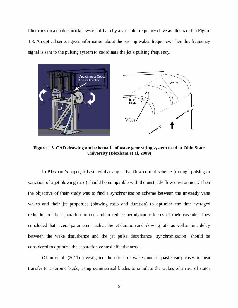
fiber rods on a chain sprocket system driven by a variable frequency drive as illustrated in Figure

1.3. An optical sensor gives information about the passing wakes frequency. Then this frequency

signal is sent to the pulsing system to coordinate the jet‟s pulsing frequency.

Figure 1.3. CAD drawing and schematic of wake generating system used at Ohio State

University (Bloxham et al, 2009)

In Bloxham‟s paper, it is stated that any active flow control scheme (through pulsing or

variation of a jet blowing ratio) should be compatible with the unsteady flow environment. Then

the objective of their study was to find a synchronization scheme between the unsteady vane

wakes and their jet properties (blowing ratio and duration) to optimize the time-averaged

reduction of the separation bubble and to reduce aerodynamic losses of their cascade. They

concluded that several parameters such as the jet duration and blowing ratio as well as time delay

between the wake disturbance and the jet pulse disturbance (synchronization) should be

considered to optimize the separation control effectiveness.

Olson et al. (2011) investigated the effect of wakes under quasi-steady cases to heat

transfer to a turbine blade, using symmetrical blades to simulate the wakes of a row of stator

6

blades (see Figure 1.4). They also studied in parallel the effect of the background turbulence

level using several turbulence-generating grids. A heat transfer study was conducted using a

naphthalene mass transfer technique to determine the local mass transfer coefficient, and then get

the heat transfer coefficient according to the heat/mass transfer analogy. Velocity and turbulent

intensity profiles were measured at 4 locations downstream the vanes.

Figure 1.4. Cascade with upstream symmetrical airfoil used by Olson et al. (2011) at the

University of Minnesota

Olson investigated the effect of wakes and turbulence in a two-dimensional cascade on

heat transfer to turbine blades (without film-cooling). They studied:

- the effect of the wake-blade (vane blade) position

- the effect of the wake-blade pitch

- the effect of the wake-blade gap (distance between the trailing edge of the vane row and

the leading edge of the turbine-blade row). Ratios “gap over axial chord” were changed

to various values: 20, 40 and 80%.

7

They noticed that wakes coming from the vanes caused an earlier start of transition to a

turbulent boundary layer on the suction side when the vanes are near the leading edge of the

turbine blades, which highly increases the heat transfer coefficient.

As for the effect of the wake-blade pitch, they noticed that when the vane was in the

center of the passage, changing the pitch had no or few effect. Though, when the vane trailing

edges are directly ahead of the turbine blade leading edge, they observed that a lower pitch

caused an earlier start of transition to a turbulent boundary layer on the suction surface and a

greater separation on the suction surface. In addition, they pointed out that a wake directly

upstream of the leading edge of the turbine blade reduced the separation on the suction surface.

Increasing the gap between the blade rows delays the transition to a turbulent boundary

layer on the suction side and reduces the effect of the wake on the separation phenomenon on the

pressure side. The further the blade is, the less the effects of the wakes can be observed.

At a higher Reynolds number, the heat transfer coefficient globally increases, and the

transition to a turbulent boundary layer on the suction surface moves upstream. On the pressure

surface, the separation phenomenon near to the leading edge is reduced. Higher background

turbulence can be viewed as dampening the effect of the wakes on heat transfer.

Womack, Volino and Schultz (2008) studied experimentally film cooling flows with

periodic wakes as well as the combined effects of wakes and pulsed film cooling. They generated

the wakes with a spoked-wheel similar to Bloxham et al (2009) in front of a flat plate. It is stated

that over a cycle of wake passing, film cooling jets provide a good coverage and a good film

cooling effectiveness during a part of the cycle, but when the wake passes over the film cooling

jets, the effectiveness drops and the heat transfer coefficient increases. Then an active control

over each cycle may increase the overall film cooling efficiency. It is suggested to control the jet

8

pulsing favorably with respect to the wake passing event. Activating the jet when the film

cooling efficiency is optimal may be an option. Nonetheless, decreasing the jet blowing ratio

when the wake passes may cause damages to the blades on the long term. When the wake

impinges on the blade, the film cooling efficiency drops, the heat transfer coefficient increases

and the blade surface may need to be protected by a better film cooling layer.

Womack et al studied transient flow behavior with phase averaged flow temperature

measurements. It was clearly observed that wakes are disturbing the film cooling jets resulting in

what they called an “unsteady effectiveness” during the wake passing, lower than the steady case

effectiveness. The jet recovery between wakes depended on the wake Strouhal number (the

Strouhal number is proportional the frequency and size of the wake generating body and

inversely proportional to the mainstream flow velocity). At low Strouhal number, the recovery of

the jets was good but at high Strouhal number, it was insufficient, reducing the cooling

effectiveness by 50%.

In a following paper (2008), Womack et al investigated the combined effect of wakes and

jet pulsing. After studying the effect of all combination of jet pulsing and wake timing, they

concluded there was no clear benefit to imposing pulsation on film cooling on their flat plate

with a cooling hole geometry. Though, they provided a better comprehension of how wakes are

affecting the film cooling behavior. For instance, at low blowing ratios (B=0.5), when the jet

stays well attached to the cooled surface, both jet pulsing and passing wakes are detrimental to

the film cooling effectiveness and the combination of both effects is even worse. However, for a

higher blowing ratio (B=1.0), when the cooling jet is lifting off, pulsing was still reducing the

film cooling effectiveness but wakes tended to increase the overall cooling effectiveness by

forcing the jet coolant fluid closer to the wall.

9

Other noteworthy wake simulator mechanisms can be pointed out. A facility was

designed at Texas A&M University to study unsteady boundary layer transition on the blade

surface (Shobeiri, 2007) and later on, the effect of upstream wakes with vortex on blade platform

film cooling behavior (Wright, 2009). This system also uses cylindrical rods and their size, their

distance upstream from the cascade; their pitch and velocity are chosen so that generated wakes

are matched to the wakes shed from vane blades.

Figure 1.5. Wake generating mechanism at Texas A&M University (Shobeiri, 2007)

Another wake generating mechanism was designed at the NASA Glenn Research Center.

It is a rotating rig with cylindrical rods in an annular cascade (Figure 1.6). Heidmann (2001) used

this facility to investigate the effect of wake-passing on turbine blade film cooling.

Figure 1.6. Wake generating rig at the NASA Glenn Research Center (Heidmann, 2001)

10

An average reduction of 0.094 due to the effect of wakes on film cooling effectiveness

was found. They also observed a better film cooling effectiveness at higher Strouhal numbers on

the blade pressure side because wakes force the jet towards the blade surface. An opposite effect

was found on the suction side. It is also recommended to have an advance instrumentation

capable of resolving high frequency data if transient measurements are to be done.

1.5 Objectives

The primary objective of this study will be to investigate the impact of Nozzle Guide

Vanes (NGV) wakes on turbine blades, and, their influence on pulsed film cooling performances.

Although several studies have investigated the effect of upstream passing wakes with rods and

spoked-wheel, never has a study investigated the transient flow behavior of film cooling with

more realistic vane profiles at a high Reynolds number.

The present work will focus on the design and fabrication of a new low turbulence wind

tunnel facility with a versatile experimental setup suitable to a wide range of heat transfer and

aerodynamic measurements on turbine blades. The new facility will include a linear cascade with

a wake simulator mechanism consisting of flat plates moving in translation upstream of the linear

cascade. It should enable easy interchanges to study the influence of different trailing and

leading edges on these flat plates. These plates should also be easily replaced by blade profiles in

the future. An approximate Reynolds number of 500,000 based on the blade axial chord and

similar to real engine conditions is targeted.

1.6 Outline of Thesis

The content of this thesis will cover in detail the design and fabrication of all the different

components of the new facility. The closed circuit wind tunnel design will be described in the

11

second chapter. The design of the experimental apparatus -the linear cascade with the wake

simulator- and its operating conditions will be covered in the third chapter. Most of the detailed

drawings of the designed parts can be found in the appendices. The fourth chapter will present a

first characterization of the wind tunnel performances, with the nominal operating conditions.

Constant temperature anemometry (CTA) measurement technique with an automated traverse

was utilized for this characterization. A summary and conclusion of this work will be presented

in the fifth and last chapter.

12

Chapter 2: Wind Tunnel Design

A new wind tunnel has been designed and constructed at the LSU Mechanical

Engineering Laboratories. The design of this wind tunnel facility with all relevant dimensions

and observations of interest are given in this chapter for future works.

The objective was to design a test facility adapted to a wide range of experimental

measurements on turbine blades. The test section consists of a 4 passage linear cascade. A

conveyor setup was designed and fabricated to simulate passing wakes upstream of the cascade

in order to study their impact on the turbine blade performances. This facility has been designed

to enable easy interchanges of different experimental setups. All the parts, as well as the

complete assembly, have been fully designed using a Computer Aided Design (CAD) software.

Figure 2.1 shows a general view of the 3D design.

Figure 2.1. Global view of the wind tunnel

13

The new test facility was chosen to be a closed-circuit wind tunnel to ensure a controlled

return flow and to reach low levels of turbulence and unsteadiness in the test section. In order to

achieve a first design of this facility, general design rules and suggestions from Bradshaw P. and

Mehta R. (1979) and Rae W. H. and Pope A. (1984) were first followed.

2.1 General Description

The whole wind tunnel is about 33 feet long and 11 feet high. The fan diameter is 38

inches. Velocity distribution in the wind tunnel is shown in Figure 2.2. After the test section, the

flow is expanding through a first diverging duct and reaches the first corner vanes (see Figure

2.3). Then 2 consecutive diffusers with equivalent cone angle of 5° expand the flow without

separation before passing through the fan. The fan is surrounded by 2 flexible ducts to prevent

excessive vibration propagation within the wind tunnel. After the fan, the flow passes through a

last diffuser and expands into a 38 inches side square section duct. Then the flow goes through 2

more corners with 13 corner vanes in each. A 19 feet long duct with constant section follows

before the flow goes into the settling chamber. The settling chamber consists of a 2 inch thick

honeycomb to straighten the flow and 5 screens to reduce turbulence levels. Wood spacers are

used to hold them in place inside the settling chamber box. The screen spacing depends on the

mesh length of each upstream screen in order to optimize the turbulence reduction of the air flow

(see Part 2.2.3). Then, the well-conditioned and uniformed flow enters the contraction cone and

is accelerated to the test section inlet. The contraction cone consists of 2 matched cubic

polynomial curves to guide the flow from a 38 inch square duct to a 19.5 inch x 12 inch rectangle

duct, equivalent to a contraction ratio of 6.16.

14

Figure 2.2. 2D drawing of the wind tunnel

Figure 2.3. Wind-tunnel parts

10 m/s(33 fps)

8 m/s(26 fps)

8 m/s(26 fps)

50 m/s(164 fps)

39 m/s (128 fps)19 m/s(62 fps)

Cascade setup with wake simulator

Divergent cones: 5° equivalent angle

Fan

Settling chamber 1 honeycomb & 5 screens

(condition the flow)

Contraction cone: matched cubic

polynomial curve

Divergent 2aPreFan

FanDivergent 3 Turn 1

Turn 2

Turn 3

Lateral duct

Main duct 2Main Duct 3

Settling chamber

Test sectionContraction cone

Divergent 2b

Main duct 1

w

w

w

W: Windows

15

2.2 Components

The wind tunnel is mainly made of 16 gage galvanized sheet metal except for the test

section parts that are mostly made out of acrylic to allow visualizations and non-intrusive

measurement techniques. Adapted stiffeners have been added to prevent excessive vibration in

some of the large tunnel ducts. Quarter inch thick rubber gaskets are placed between all flanges

to reduce vibration and for sealing concerns. Detailed dimensions are given in appendix A.

2.2.1 Divergent Cone

Two divergent cones, or diffusers, expand the flow from the test section to the fan with a

total section area ratio of 4.6. One more diffuser is located downstream of the fan to increase the

wind tunnel section area and to reach a good contraction ratio to get a better flow quality in the

test section (see Contraction Cone part). For best flow steadiness, the equivalent angle of the

diffusers, considering a circular cone with the same length and same area ratio, do not exceed 5°.

When this condition is satisfied, the boundary layer does not separate and unwanted pressure

fluctuations with time in the wind tunnel are prevented (Mehta and Bradshaw, 1979).

2.2.2 Corner Vanes

Corner vanes are generally used as guide vanes, which deflect the flow while avoiding

separation of the boundary layer in a bend. There are two different types of corner vanes in this

wind tunnel. Both are made out of sheet metal.

The first type of corner vane, used in the corners “Turn 1” and “Turn 2” is the most

conventional one (Mehta and Bradshaw, 1979). The design rule of those 90° circular arc vanes is

similar to a turbomachine cascade. This cascade consists of 17 vanes with a 10 inch chord and a

16

gap of 3 inches between each other. The gap-chord ratio of the vanes is less than 1:3, as

recommended according to experience. The wake effect from each vane disappears over a

shorter distance if many short chord vanes are used instead of fewer large-chord vanes.

For design concerns, the first corner “turn 1” downstream the test section, with a non 90°

angle has a different configuration. Larger-chord vanes are used while keeping a similar gap-

chord ratio. In addition, the turning vane is extending before and after the bend by 10% of its

chord to provide a better guide.

a) b)

Figure 2.4. Corner vanes a) Type 1 b)Type 2

2.2.3 Settling Chamber

In order to reduce the turbulence level in the test section and to get a good flow quality, 5

screens and a honeycomb are installed upstream of the contraction cone. The role of the

honeycomb is to remove some swirl and lateral velocity variations. Screens mostly reduce

streamwise velocity fluctuations.

17

2.2.3.1 Design and Specifications

The settling chamber consists of a 2 inch thick, 1/4 inch cell honeycomb to straighten the

flow and 5 stainless steel wire mesh screens. Different open-area ratio and mesh size screens are

combined to optimize the turbulence level reduction. Two of the screens are used before and

after the honeycomb to hold it in place. All screens have an open-area ratio greater than 57%.

For lower open-area ratios, flow instabilities due to jet coalescence may occur (Morgand, 1960).

Turbulence reduction by use of screens was investigated by Tan-Atichat et al (1982) and Groth

and Johansson (1988). They found that the turbulence damping ability was improved -for a given

open area ratio- when decreasing the mesh size. Groth and Johansson demonstrated that

subcritical screens - for Reynolds numbers based on the wire mesh diameter Red less than 40 -

resulted in a better turbulence reduction but with a large pressure drop. Tan-Atichat observed

that for supercritical screens, the length scale of the mesh should be chosen so that the turbulence

eddies generated by the screen are smaller than the incoming ones. Groth and Johansson found

that the maximum turbulence suppression for a given total pressure loss was obtained with a

cascade type combination of supercritical screens with decreasing mesh size in the streamwise

direction. In addition, they recommended the furthest screen downstream to have a low

supercritical Reynolds number (Red = 50-60) and the first screen upstream to have a relatively

coarse mesh while keeping its wire mesh Reynolds number less than 300. Over a Reynolds

number of 300, increasing the wire mesh diameter is not as beneficial in terms of pressure drop

reduction.

Our final screen configuration is showed in Table 2.1 below. The Reynolds number has

been calculated for a nominal air velocity of 50 m/s (164 fps) in the test-section, corresponding

to a velocity of 8.1 m/s (26.6 fps) in the settling chamber.

18

Table 2.1. Screen combination in the settling chamber

Screen Mesh Size (per in)

Open-area ratio Wire diameter (in)

Reynolds number Rd

1 12 M 61.5% 0.018 215

2 20 M 67.2 % 0.009 107

3 24 M 67.4% 0.0075 89

4 42 M 59.1% 0.0055 78.5

5 56 M 60% 0.004 57

Screen spacing is adapted to the upstream mesh diameter size. Groth and Johansson

found an initial turbulence decay region after a screen depending on the mesh size. Within the

first 15-25 mesh widths, the turbulence intensities decay rapidly for a single screen. Though, for

a combination of screens, they recommended to choose a larger spacing than this initial decay

region. Then, the configuration shown in Figure 2.5 was chosen.

Figure 2.5. Settling chamber configuration and screen spacing

cH

on

eycom

b

Air flow

Wood spacers

Contraction Cone

Screens: 1 2 3 4 5

Spacing (in upstream screen mesh widths): 145 132 147

19

2.2.3.2 Pressure Losses and Turbulence Reduction Estimate

Most of the turbulence theories are based on a pressure loss coefficient K. This

coefficient is defined as the ratio of pressure loss across the screen ∆P over the mean flow

dynamic pressure q. DeVahl (1964) found that this pressure loss coefficient was equal to:

With,

The turbulence reduction factor f is then calculated from the pressure loss coefficient K.

This factor f represents the rate of turbulence reduction. DeVahl found some consistent results to

determine the turbulence reduction factor based on the pressure loss. Though, he did not observe

any trend based on the velocity. His experiment was covering a range of screen Reynolds

number based on the diameter from 70 to 300, similar to our case. The average measured values

of fa for axial turbulence reduction and fl for lateral turbulence reduction were following the

equations below in function of the pressure loss coefficient:

20

The following table summarizes the different coefficients for each screen:

Table 2.2. Turbulence reduction factors and pressure loss coefficients of screens

Screen 1 2 3 4 5

β 0.615 0.672 0.674 0.591 0.6 Rd 215 107 89 78.5 57 K0 0.462 0.286 0.281 0.562 0.522 K 0.718 0.801 0.9 1.26 1.5

fa 0.582 0.55 0.53 0.44 0.4

fl 0.76 0.745 0.725 0.665 0.63

The total turbulence reduction factor is the product of each individual screen turbulence

reduction factor when multiple screens are used. The total pressure loss is the sum of each

individual screen pressure loss, when their spacing between each other is greater than their initial

turbulence decay region length. As shown by Groth and Johansson, this region length is less than

30 mesh widths and in our settling chamber, the spacing between 2 screens is always greater than

130 mesh widths. Therefore, we obtain the total axial and lateral turbulence reduction factors Fa

and Fl and the total pressure loss Kt due to screens only:

We can notice that the screens mostly reduce the axial turbulence, reducing it by more

than 97%. As for the lateral turbulence, the screens suppress only 83% of the turbulence. That is

why we add a honeycomb upstream of the screens to improve the lateral turbulence factor.

According to Loerhke and Nagib (1976), a ¼ inch cell honeycomb at similar velocities as

the operating one in our settling chamber has the same axial reduction factor fa-HC as a 20 mesh

21

screen but is equivalent to three 20 mesh screens in terms of lateral turbulence reduction, fl-HC .

As for its pressure loss coefficient KHC, it is similar to the pressure loss coefficient for a 20 mesh

screen. It yields the following coefficients for the honeycomb:

The total axial and lateral turbulence reduction factors Fa-SC and Fl-SC, as well as the total

pressure loss Kt-SC for the whole settling chamber can now be computed:

It can be concluded that the settling chamber will reduce the axial turbulence by 98.4%

and the lateral turbulence by 93%. The total pressure loss coefficient is 5.97, which means when

operating at a nominal velocity of 8.1 m/s (26.6 fps), with a dynamic pressure q of 0.16 inH2O,

the settling chamber will introduce a pressure loss of 0.95 inH2O.

2.2.3.3 Fabrication

The screens are tightened and mounted on aluminum frames. A uniform and good tension

is ensured by the means of a ¼ inch aluminum rod located in a channel between opposite panels

of the aluminum frame. The screen is tightened when the two panels are clamped together and

compress both the rod and the screen into the channel. This ensures a better fastening with a high

degree of tension (see Figure 2.6.a).

22

(a) (b)

Figure 2.6. (a) Screen with aluminum frame (b) Opened settling chamber image

The five screens and the honeycomb can easily be removed from the settling chamber for

cleaning purpose (see Figure 2.6.b). Indeed, screens have a tendency to accumulate dirt and dust

and should be cleaned at regular intervals to maintain their pressure drop at a reasonable level.

Once the screens and the honeycomb are cleaned, a 16 gage sheet metal plate is used to close the

settling chamber. Suitable 1/16 inch thick weather-stripping has been installed to prevent any

leaks through the cover.

2.2.4 Contraction Cone

The contraction cone accelerates the flow from the settling chamber to the test section. Its

role is to guide the flow smoothly, without degradation of the quality of the flow from a 38 inch

square duct to a 19.5 inch x 12 inch rectangle duct, which gives a contraction ratio of 6.16. The

axial length of the contraction is 3 feet. Mehta and Bradshaw (1979) pointed out two main

advantages of the contraction cone:

• It increases the mean velocity, increasing the Reynolds number in the test section while

keeping reasonable pressure losses in the settling chamber where the velocity through the

honeycomb and screens are much lower.

23

• It reduces both lateral and axial turbulence levels to a smaller fraction of the mean velocity.

Two different curves of 2 matched cubic polynomials have been used to generate the 3D

contraction profile, one for the lateral contraction and the other for the vertical. Those curves

have their first derivatives equal to zero at the entrance and exit of the contraction, giving a good

conditioning to the flow. Watmuff (1986) found with both experimental and numerical studies

that a matched cubic polynomial curve offered the smallest adverse pressure gradient at the entry

and exit of the contraction cone compared to other polynomial curves, and reduces the upstream

and downstream influence of the contraction cone. He found the flow at the exit of such a

contraction cone to be uniform within +/- 1%. The inflection point of our contraction curve is

located at 60% of the axial length. Therefore, the radius of curvature is slightly larger at the wide

inlet than at the outlet to avoid a danger of boundary layer separation. The lateral contraction

profile is shown Figure 2.8., with the first derivative of the matched cubic polynomial.

Figure 2.7. Matched cubic polynomials lateral curve of the contraction cone

24

Accelerating the flow through the contraction cone is also beneficial to reduce the

turbulence level in the test section. Mehta and Bradshaw stated that a simple analysis due to

Prandtl can show that the axial turbulence is reduced by a factor 1/C² while the lateral turbulence

level will be increased by √C, where C is the contraction ratio.

In our case, the axial turbulence reduction factor of the contraction cone is 0.026, while

the lateral turbulence level increases by a factor 2.48. This increase in lateral turbulence is linked

to the strong variations in intensity of elementary longitudinal vortex lines through the

contraction cone.

As for fabrication concerns, precise curves, point coordinates tables and 3D drawings

have been given to the manufacturer to get a good precision in fabrication (Figure 2.9.).

Figure 2.8. Contraction Cone Image

25

2.2.5 Fan

The facility is powered by a 60 HP axial fan with an output capacity of 408 lb/min (15

kg/s). This fan is a Joy Manufacturing Company (current owner is Howden Buffalo Inc.),

AXIVANE series 2000. It has a 38 inch diameter and an output rotational speed of 1770 rpm.

The wind tunnel has been dimensioned to be able to run experiments at a Reynolds number of

500,000, based on the axial chord, similar to engine conditions.

The 60 HP wind tunnel fan has been renovated, its 18 blades with the rotor mechanism

has been sandblasted and rebalanced for vibration concerns. The electric motor is a Reliance

Electric (the current company is Baldor), Duty Master AC, 3 phases, rotating at 1775 rpm. This

60 HP motor has been rewound from 200 V to 460 V so that it can be compatible to the new

power drop of 75 A/460 V installed in the LSU laboratory. A simple full-voltage starter is used

to start the motor. The flow rate of the fan is controlled by a pitch control device using a

pneumatic piston actuator linked to the fan blades (see part 2.2.6).

The fan is located at a constant section area to get straight flow nominal conditions

upstream and downstream. It is connected to the surrounded parts of the wind tunnel with

flexible cylinder couplings made out of rubber to reduce vibration. In addition, the fan and its

stand are mounted on anti-vibration pads. Any metal to metal connection has been suppressed to

reduce vibration propagation.

2.2.6 Fan Pitch Control Device

The pitch control device mechanical power is supplied by a Fisher® 480 Series yokeless

piston actuator (Fisher® owned by Emerson Company). This actuator requires a pressure loading

from a double-acting positioned (the 3570 Series). It can operate at a wide range of supply

26

pressure from 35 psi to 150 psi. The needed supply pressure to control the pitch of the fan blades

is 60 psi, which is equivalent to a thrust force of 1600 lbs according to the manufacturer

specification for our actuator size 40. The supply pressure connection is a 1/4 NPT pipe. The

input pressure signal range is from 3 psi to 20 psi. Its connection is a 1/8 NPT pressure pipe.

Two pressure regulators are used, the first one is to control the supply pressure and lower

it from 290 psi (maximum nominal working pressure coming from the main compressor) to

about 60-80 psi and keep a steady pressure supply. The second pressure regulator enables us to

control the input pressure signal from 0 to 20 psi.

Figure 2.9. Pitch Control Supply Pressure System

The principle of operation of the actuator is based on a pressure unbalance that moves the

piston. The translational motion is then transmitted to the pitch control mechanism that

transforms the translational motion into a rotational motion through independent crank-

connecting rod systems for each blade and change their pitches simultaneously.

27

a) b)

Figure 2.10. Pitch Control System Images. a) Pressure Supply b) Piston Actuator

2.2.7 Windows and Safety Screen

A safety screen is located upstream of the fan between the parts “div2a” and “div2b” (see

Figure 2.3) to protect the fan from potential objects blown out of the test section. Three

transparent ¼ inch thick acrylic windows are located upstream of the safety screen, between the

corners “Turn 1” and “Turn 2” and downstream of the last one. It allows the user to visualize

unexpected objects blocked in the turning vanes or safety screen and get an access to remove

them if necessary.

2.2.8 Breather

A “breather”, slot on the top and bottom wall of the duct, is located after the test section

at the beginning of the first diffuser, in order to increase the test section static pressure close to

atmospheric pressure and reduce leaks into the test section. This opening also prevents unwanted

pressure oscillations in the wind tunnel, as well as an internal pressure increase as the air heats

up during a run. A 24 mesh metal screen around the perimeter enables to dampen the noise and

28

secures the opening. The breather opening area is about 25% of the cross section area of the test

section outlet. This opening ratio can easily be reduced by adding some spacers over the

breather.

2.2.9 Supporting Structure

A steel supporting structure has been designed to support all different parts of the wind

tunnel. This one being a vertical closed-loop type, loads have been carefully estimated before

designing a proper supporting structure. Table 2.3 presents an estimate of the weights of the

different parts composing the wind tunnel:

Table 2.3. Estimate of wind tunnel part weights

The method of “Load and Resistance Factor Design” from the American Institute of Steel

Construction (AISC) manual, 2nd

edition (1994), has been used to select the appropriate beams

and bracings.

PARTS WEIGHTS (in lb)

Up

per

par

ts

Turn 1 66

Divergent 2a 242

Divergent 2b 264

Pre Fan 99

Fan 2200

Divergent 3 220

Turn N2 264

TOTAL UP 3355

Lateral duct 154

Bo

tto

m p

arts Turn N3 264

Main duct 1 308

Main duct 2 308

Main duct 3 264

Settling duct 220

Contraction cone 154

TOTAL ALL 5027

29

2.2.9.1 Top supporting structure

The top structure has been designed considering its flexural strength. Two main I-beams

are resting on cantilever beams which are welded to existing pillars in the room. Part legs are

bolted to the I-beams and anti-vibration pads have been placed to reduce vibration. Bending

moments have been computed to make sure it was not exceeding its critical value according to

the method of Load & Factor Resistance Design manual (LFRD) specification of the AISC (part

4, Beam and Girder Design). Maximum beam deflections have also been verified. Beams have

been chosen in function of their nominal flexural strength. Cantilever beams are W4x13 shape.

Cross beams and cantilever bracings are S3x5.7 shape (see appendix A for detailed structures).

2.2.9.2 Fan Support

The fan support is made out of two different structures to be able to lift it and put it in

place with a forklift as shown on the Figure 2.12 (see appendix B for detailed drawings). The

main columns, axially loaded, have been sized to withstand the weight of the fan (more 2,000

lbs) according to the LFRD manual of the AISC (part 3, Column Design, Column Load Tables, p

3-30).

Figure 2.11. Images of the fan installation with supporting structure

30

2.2.9.3 Bottom Supporting Structure

Each bottom part is supported with a different stands made out of 2 inch angle beams.

Those stands were also fabricated in the LSU Mechanical Engineering machine shop. Their

height is adaptable thanks to leveling feet. Rubber pads are used to reduce vibration and avoid

any metal to metal contact.

2.2.9.4 Test Section Support

A particular attention has been given to the test section support to leave as much free

space as possible for future measurement apparatuses. An overhead support has been designed

for that purpose as shown in Figure 2.13. The total weight of all test section parts is estimated to

be 400 lbs. The different supporting elements have been designed to withstand this load. A

detailed description of all test section supporting structures can be found in Appendix B.

(a) (b)

Figure2.12. Test section support image. a) Overhead support b) Global view

A simple calculation example is shown below to find the estimated deflection of the

overhead support. A cantilever beam model with a uniform load per unit length w is used.

31

Figure 2.13. Overhead support load model

The distributed load on each cantilever beam is estimated at w = 10 lbs/in over a length l

= 24 inches. Beams are 2 inch square tubes with a ¼ inch wall thickness. The Young‟s modulus

for hot-rolled steel is E = 30 x 106 psi. The moment of inertia of this square tube is I = 0.745 in

4.

Then, the estimated maximum deflection is δmax such that:

Numerically, we find a reasonable value of δmax= 0.017 inches.

2.3 Pressure Loss Estimation in the Wind Tunnel

In this closed-loop wind tunnel, the axial fan produces a rise in static pressure, which

compensate for the total pressure losses in the rest of the tunnel. To estimate pressure losses

through the different parts of the wind tunnel, the pressure loss coefficient K is used. This

coefficient is defined as the ratio of pressure drop in static pressure ∆p over the mean flow

dynamic pressure q.

Wattendorf (1938) developed a logical approach to calculate the different pressure losses

in a closed circuit wind tunnel. This approach was to divide the wind tunnel into four different

kinds of parts: (1) straight, constant area sections, (2) corners, (3) divergent sections, (4)

32

contracting sections. Then, he referred all local losses to the “jet” dynamic pressure q0, greatest

dynamic pressure in the wind tunnel. In our wind tunnel, this dynamic pressure q0 occurs at the

exit of the cascade. Then the coefficient of loss becomes:

Where: D0 = jet equivalent diameter, D = local tunnel equivalent diameter

Then, the wind tunnel energy ratio ERt can be defined as:

Below is an estimation of the loss coefficients for each wind tunnel components, as

suggested by Wattendorf:

2.3.1 Straight, Constant Area Sections

Where = skin friction coefficient, L = section length.

The local friction coefficient is determined in function of two parameters: the local

Reynolds number based on the equivalent diameter Re, and the relative roughness of the local

duct wall k/D (where k is the absolute roughness of the wall material and D is the equivalent

diameter). From this two parameters and solving the Colebrooke equation, valid in turbulent

flow condition, which is true in our case, we obtain the local friction coefficient.

33

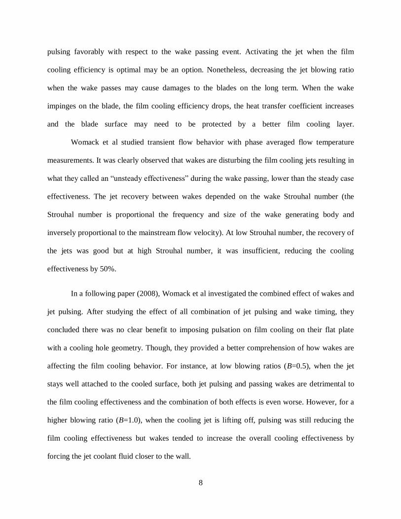
A graphical method can be used to solve the Colebrooke equation, called the Moody

diagram shown Figure 2.14.

Figure 2.14. Moody diagram (from http://www.engineeringtoolbox.com)

For example, the main part of constant section area duct is made of galvanized sheet

metal over a total length of 30 feet with an equivalent diameter of 38 inches. The nominal air

velocity is 8.1 m/s (26.6 fps) for a 50 m/s (164 fps) velocity at the cascade inlet, and yields to a

Reynolds number based on the equivalent diameter of 580,000. For galvanized sheet metal, the

roughness coefficient is ft, which gives a relative roughness coefficient

. Reporting this values on the Moody diagram, we obtain the friction

coefficient for this part of the duct = 0.017.

34

2.3.2 Corners

Raw and Pope (1984) related that for corners of the type presented Part 2.2.2., one third

of pressure losses are caused by friction in the guide vanes while rotation losses account for

about two-thirds. Then, they suggested a partly empirical relation to estimate pressure losses

through this type of corners:

Pressure losses through the cascade turbine blade are more delicate to estimate. In

Garmoe‟s thesis (2005), from the Air Force Institute of Technology, we can find some

experimental data on a cascade of pack-B turbine blades, similar to the high lift low pressure

turbine profiles we are studying. He reported an integrated total pressure loss coefficient through

the cascade of about 0.10 at a Reynolds number of 100,000. This loss only considers the

integrated pressure profile at mid-span of the 2D profile. It does not take fully into consideration

all the secondary losses such as endwall effects. Though, our operating Reynolds number is

500,000 - similar to engine conditions- and closer to the optimal operating condition of this blade

profile. Therefore, it should reduce the pressure loss coefficient of the cascade. Thus, we will

assume as a first guess a total pressure loss coefficient of the cascade K = 0.1.

2.3.3 Divergent Sections

In divergent section, expansion losses are added to the friction losses. Wattendorf found

the combined losses give the following relation where K0 is expressed as a function of the

divergence equivalent angle α:

35

Where D1 = smaller equivalent diameter and D2 = larger equivalent diameter.

From this relationship, it can be found that the most efficient divergent angle is about 5°.

2.3.4 Contraction Cone

In the contraction cone, losses are caused by friction only and:

Where LC = length of contraction cone

2.3.5 Settling Chamber: Screens and Honeycomb

Pressure losses in the settling chamber are studied Part 2.2.3.2. The total pressure drop K

was found as K = 5.97. This yields to a loss coefficient

2.3.6 Summary of Pressure Losses

Table 2.4. Pressure losses estimation

Part K₀ Total Losses (%)

Test section inlet 0.021 6.86 Cascade 0.0384 12.55 Test section outlet 0.0348 11.38 Divergent 1 0.0886 28.96 Corner 1 0.0377 12.32 Divergent 2 & 3 0.0187 6.11 Main duct 0.0017 0.56 Corner 2 0.0015 0.49 Corner 3 0.0015 0.49 Settling chamber 0.0615 20.10 Contraction cone 0.0005 0.16

TOTAL 0.3059 100.00

36

2.4 Wind Tunnel Energy Ratio and Design Analysis

The energy ratio can now be calculated:

For our nominal velocity conditions, 50 m/s (164 fps) velocity at the cascade inlet and 100 m/s

(328 fps) at the cascade outlet, equivalent to a 24 in H2O of jet dynamic pressure q0, the

estimated total pressure loss of the wind tunnel is 7.34 in H2O. An energy ratio of 3.27 is within

the range of most closed circuit wind tunnels (from 3 to 7 according to Raw and Pope). Some

changes that could have improved this factor as well as their downsides can be pointed out:

Extending the length of the part “Divergent 1” to reduce its divergence angle from 19° to

5° would have reduced the divergence losses of this part by 20% and the total losses by

5.7 %. Though, such an extension would have extended the height or the length of the

wind tunnel by 10 feet and would have, increasing the cost and complexity of fabrication.

Choose a smaller fan, closer to the test section size to lower the divergent sections length.

Though, we already owned this fan before designing the wind tunnel, and investing in a

new fan would have been an extra expense.

Increase the size of the cascade blades to have a larger size closer to the fan size and limit

the divergent section length. Yet, increasing the size of the cascade would have greatly

increased the fabrication cost of the test section. Blades are made with 3D printers and

their fabrication material and process are somewhat expensive, with a price proportional

to the volume of material used.

Thus, this design can be seen as a good balance between flow quality, cost, and

complexity of fabrication.

37

Chapter 3: Cascade with Wake Simulator Design

As stated before, the primary objective was to design a test section adapted to a wide

range of experimental measurements on turbine blades. The test section consists of a 4 passage

linear cascade composed of 3 full blades and 2 shaped wall blades (inner and outer blades). A

conveyor setup was designed and fabricated to simulate passing wakes upstream of the cascade.

Wakes are generated with thick plates in translation on the conveyor. These moving plates

simulate the wake passing of the front row vane in order to study their impact on the cascade test

blades and, later on, on pulsed film cooling performance. Aerodynamic and heat transfer

experimental tests will be conducted in a relative frame with fixed rotor turbine blades while the

nozzle guide vanes are rotating. This facility has been designed to enable easy interchanges of

different experimental setups.

Figure 3.1. 3-D view of the test section

38

3.1 Setup Characteristics

3.1.1 Linear Cascade Characteristics

The 2D blade shape profile of the cascade was provided by the Air Force Research

Laboratories (AFRL). It is a High Lift Low Pressure Turbine (LPT) blade „L1A‟ profile with a

1.34 incompressible Zweifel coefficient. A 6-inch axial chord and 1 foot span were chosen. The

span is chosen to be two times the axial chord to make sure we have a nominally 2D flow at the

mid span. The solidity of the cascade, ratio of the axial chord to the spacing, is 1. The blade inlet

air angle is 35 degrees from axial, and the exit angle is -60 degrees from axial, resulting in a 95

degrees total turning. The linear cascade inlet plane is 1 ft high and 2 ft wide. The nominal inlet

velocity is 50 m/s (164 fps) and was chosen as a reference, with the axial chord to determine the

Reynolds number. Two inlet bleeds and two tailboards are placed upstream and downstream of

the cascade to adjust the flow and obtain periodic cascade performances as specified by Eldrege

and Bons (2004).

Figure 3.2. Linear cascade with wake simulator 2-D sketch

39

3.1.2 Wake Simulator Characteristics

Wakes are generated with thick plates in translation on a conveyor setup while staying

parallel to the mainstream airflow. Those plates are 3/8 inch thick and are designed to be in size

similar to the cascade test blades. The conveyor with the 17 moving plates will be enclosed in an

airtight shell. The design speed is 1 m/s (3.28 fps) but can be adjusted to study its influence. The

length of the plates was chosen to be equal to the axial chord of the cascade blade, 6 inches.

Their pitch is the same as the pitch of the cascade blades, 6 inches. This configuration will

markedly simplify future CFD models. The distance between the trailing edges of the plate and

the cascade inlet plane is 2.4 inches, which is 40 % of their chord, and similar to engine stator-

rotor stage spacing. Trailing and leading edges of the plates are interchangeable to study

different configurations. In addition, plates are removable and can be substituted with more

realistic airfoil profiles if wanted in the future.

3.1.3 Cascade Inlet Plane Angle

The cascade inlet plane angle was adjusted from 35°, flow inlet angle of the cascade

blades to 36° to take into consideration the deviation of the mainstream airflow due to the wake

simulator. The tangential velocity component induced by the wake generator can be estimated at

1m/s (3.28 fps), which is the nominal operating velocity of the moving plates. Considering a 50

m/s (164 fps) nominal freestream velocity, a simple vector decomposition gives a velocity

triangle with about 1° angle of deviation of the mainstream flow as shown Figure 3.3. The

designation used is the same as turbomachinery theory, the absolute velocity is C, the relative

velocity is W = 50 m/s and U is the rotor blade speed 1 m/s. Then, the total turning angle of the

cascade with wake simulator is 96°, which is 1° more than the deviation angle of the test blades.

40

Figure 3.3. Cascade angles and velocity triangle

3.2 Test Section Design

The test section parts are mostly in acrylic to allow visualizations and use non-intrusive

measurement techniques such as Particle Image Velocimetry in the future. Aluminum angle bars

are used to hold acrylic walls together. They are attached to the acrylic panels flat screws in

countersunk holes to keep a flat surface on the inside walls. Two different cascade configurations

were designed: with or without the wake simulator. Both configurations can be easily

interchanged. Several mechanisms are used in this experimental setup to keep an adjustable

cascade such as inlet bleeds or tailboards as summarized on Figure 3.4.

41

Figure 3.4. Cascade image

All blades were fabricated out of plastic using a 3-D printer. Blades are fixed to the endwall with

bolts inserted into helocoils. Different blade setups for various experiments can be interchanged

quickly by removing and replacing the cascade endwall plate with the three inner blades fixed on

it as shown Figure 3.5. Some detailed drawings can be found in Appendix C.

Figure 3.5. Cascade endwall plate location

Stud with ball joint linkages to position tailboards

Friction hinge to position inlet bleeds

Piano hinge to change tailbord angle

Adjustable divergent section

Rubber weatherstripping to seal adjustable components

Cascade inner blades location

42

3.3 Wake Simulator Design

A conveyor mechanism has been specially designed and fabricated for this purpose. The

conveyor belt and standard conveyor components such that spockets, wearstrips or shafts have

been purchased from a company specialized in modular plastic conveyor belts, Intralox L.L.C.

Main design guidelines and belt selection instructions have been followed based on the Intralox®

Conveyor Belting Engineering manual. Besides, the frames, the stand, the cover or plate

assemblies have been designed using a CAD software. All drawings have been submitted to the

LSU Mechanical and Chemical Engineering machine shops where parts have been fabricated.

The conveyor shell has been made separately by an external contractor, specialized in sheet

metal work (BMR Metal Works LLC, Watson. LA).

The design of this rotating mechanism with all relevant dimensions and observations of

interest for future works is given below in this chapter.

Figure 3.6. CAD view and picture of the wake simulator

43

3.3.1 Frame

The frame is composed of three main elements. The inside frame which is carrying and

guiding the belt (green part on Figure 3.7) and two outer frames which are structural supports for

the bearings, shafts or motor (blue part on Figure 3.7) and allow us to mount the conveyor on the

stand and adapt its angle and height.

The inside frame is in aluminum to reduce the total weight of the mechanism while the

outer frames are mainly made of 1‟‟1/2 carbon steel angle (1/4 inch wall thickness) to increase

their strength. Welding has been avoided as much as possible not to have any deformation and to

keep a straight frame. Precise drawings of the conveyor frames can be found in Appendix D.

Two take-up bearings holding the idler shaft are used as tensioners for the belt. Their role

is to properly accommodate the increase (or decrease) in the length of the belt while operating.

Control of the belt length is crucial to make sure the belt engages properly on the sprockets.

Figure 3.7. Conveyor frames

Idle shaft location

Drive shaft location Motor side

Flange mounted bearing

44

3.3.2 Belt

3.3.2.1 Characteristics

The belt, sprockets, carryways and both shafts have been ordered at Intralox L.L.C,

corporation specialized in modular plastic conveyor belts. The belt is made out of polypropylene,

with a specific gravity of 0.90. The belt is a Series 800 Intralox® flat top type. It is 6 inches wide

and consists of 2 inch long plastic modules linked together with polypropylene rods as shown in

Figure 3.8. The belt strength is 1000 lb/ft.

Figure 3.8. Intralox Series 800 modular plastic conveyor belt (from Intralox® Conveyor

Belting Engineering Manual).

This belt has been chosen for its strength and its dimension. One of the criteria was to get

a module length compatible with the required moving plate pitch of 6 inches. With 2 inch belt

modules, a plate assembly can be attached every three modules to obtain a 6 inch pitch.

3.3.2.2 Estimation of Belt Elongation

Several factors can cause a variation of the belt length (Intralox Engineering Manual,

2010):

Temperature variation: The belt being made of plastic, any significant change in

temperature will result in a contraction or elongation of the belt due to thermal

elongation.

45

Elongation (strain) under load: Any material will elongate if tension is applied. This

strain should not exceed 2.5 % of the conveyor length for our conveyor belt.

Elongation due to break in and wear: New belts usually experience an elongation in the

first hours of operation as the belt modules and linking rods “seat” themselves while

older belts will experience elongation due to wear.

The first type of elongation is due to thermal expansion. The change in the dimension of

the conveyor belt ∆L can be written as:

Where: L1 = total belt length (ft.), T2 = Operating temperature, T1 = initial temperature,

e = Coefficient of thermal expansion (in/ft/°F).

For our case, with a polypropylene belt e = 0.001 in/ft/°F and L = 9 ft, an initial room

temperature T1 = 70 °F and an operating temperature (wind tunnel airflow when not cooled)

T2 = 115 °F, the thermal expansion will be ∆L = 0.4 in. The increase in shaft to shaft length

would then be about 0.2 inch.

The second type of elongation is due to strain under load and wear. This elongation

should not exceed 2.5 % of the conveyor length according to the belt manufacturer. For our belt,

the elongation due to strain and wear would then be about 2.5 inches, which gives an increase of

about 1.25 inch of the shaft to shaft length.

Therefore, the total maximum shaft to shaft elongation is estimated at 1.45 inch. The

tensioning mechanisms with take-up bearings, as well as the conveyor shell have been designed

to meet this requirement.

46

3.3.3 Shafts

1.5 Inch Square stainless steel 303 shafts are used to drive the belt. The motor end of the

drive shaft is 1.25 inch diameter bore with a 1/4 inch width keyway for motor transmission. All

other shaft ends are 1 inch diameter bore rotating into ball bearings. Precise dimension can be

found in Appendix D.

3.3.4 Sprockets

Sprockets are made out of acetal and are used to transmit the torque from the square shaft

to the belt. The largest available sprockets have been selected to minimize the centrifugal force

on the plate assembly when turning, with a 10.3 inch diameter. Three sprockets are used on each

shaft. They are laterally retained with two retainer rings, as shown on Figure 3.9. Some lateral

play is also left to allow the sprockets to move laterally and accommodate for possible lateral

thermal expansion of the belt.

Figure 3.9. Conveyor shaft with sprockets image

3 sprockets

Drive shaft, motor end

Square shaft

Retainer rings

47

3.3.5 Wearstrips

Wearstrips are plastic strips that are added to the conveyor frame to carry the belt and

reduce sliding friction forces. They are made of Ultra High Molecular Weight Polyethylene

(UHMW), plastic material with a very low friction coefficient, good abrasion resistance and self-

lubricating properties. Two different kinds of wearstrips are used: carryway wearstrips and side

wearstrips that are attached to the frame to guide the belt into a U-channel (see Figure 3.10.).

Figure 3.10. Image of the inside frame of the conveyor with wearstrips

3.3.6 Gearmotor

3.3.6.1 Specifications

The conveyor gearmotor is a combination of an AC electric motor, a gear unit to reduce

the rotational speed and a Variable Frequency Drive (VFD) to control the output speed of the

motor. This is a SEW-EURODRIVE gearmotor, model # KAF37DRE80M4 / MM11.

Side wearstrips

Carryway wearstrips

Aluminum frame

48

The AC electric motor is a DRE80M4 model, 3-phase with a 1.5 HP power. It is rated at

2.4 A, 460 V, 100 Hz for a 2900 RPM output speed. The gear unit is a KAF37 model: it is a

helical-bevel gear unit, flange-mounted with a hollow shaft. Its speed reduction ratio is 15.31.

Coupled to a MM11 VFD, the output speed range of this gearmotor can vary from 19 to 189

RPM, with a 486 in-lb nominal torque at 189 RPM. This RPM range corresponds to a belt

velocity range from 0.28 m/s (0.92 fps) to 2.76 m/s (9.05 fps).

The speed of the motor can be controlled either directly on the VFD box using the keypad

or with an external computer with the SEW MOVITOOLS -Motion Studio software under

manual operation. The output speed of the motor can also be recorded with this software. The

operating output speed range can be adjusted through potentiometers and switches of the VFD

controller (called MOVIMOT®). Two main parameters can be set with the available switches:

Minimum VFD frequency and acceleration of the drive (also called ramp time). The

potentiometer is used to set the maximum frequency. More information can be found in the

MOVIMOT® Operating Instructions Manual.

3.3.6.2 Required Power Estimation

The required 1.5 HP motor power has been calculated based on the Intralox Engineering

Manual design guidelines. This calculation is based on several parameters such as the belt

loading, the belt speed, width and weight, the length of the conveyor or its elevation change. This

calculation also determines if the chosen belt is suitable for our application. The main lines of

this calculation are:

Belt tension load estimated at 30 lb/ft

49

Adjust the belt tension load to specific service conditions. In our case, we have a

relatively high speed of the belt. This increases the number rotations per time unit and

decreases the belt life. Combined with the fact this is an elevating mechanism with

frequent starts under load, a Service Factor of 3 is taken and we adjust the estimated belt

tension load to about 100 lb/ft.

The next step is to calculate the belt strength. In our case, we have a very high ratio belt

speed over belt length due to the short length of the mechanism. As a result, the belt

strength drops by a factor 5 to reach 200 lb/ft. Though, the adjusted belt strength still

exceeds the adjusted belt tension load. Then, the belt is strong enough for our application.

The last step is to determine the required torque and power to drive the belt. These values

vary with the belt tension load. The torque depends on the sprocket diameter while the

power depends on the velocity of the belt.

The required torque was estimated to 300 in.lb and the required power to about 0.75 HP.

Therefore, a 1.5 HP motor, 486 in-lb drive has been chosen to be able to reach higher speeds if

needed.

3.3.7 Stand

The conveyor stand is a steel structure mainly made of 1‟‟1/2 - 1/4 inch wall thickness

square tubes. Some additional bracings are used to reinforce the motor side. The angle and height

of the conveyor can be adjusted to the cascade plane at 36° from horizontal with two pairs of

clevis rod ends that can be screwed or unscrewed inside the structure. The bottom link between

the conveyor and the stand clevis rods is a revolute pair while the upper link is a prismatic pair.

50

In addition, some vibration damping leveling mounts are used to reduce mechanical vibrations

and as a second way to adjust the height and angle of the mechanism.

(a) (b)

Figure 3.11. Conveyor stand picture. (a) General view (b) Zoom on clevis rods

3.3.8 Shell

A shell was designed and fabricated to keep the wind tunnel mainstream flow contained,

and to suppress any additional leakage when moving plates are entering or leaving the wind

tunnel test section. This airtight shell will keep the whole apparatus in an enclosed area with a

constant static pressure. In fact, the pressure difference between the inside of the test section and

the room atmospheric pressure can be quite important, and the mainstream flow may be

considerably altered when moving blades are entering the test section if not contained in an

enclosed space. Therefore, the incoming cross flow will be well conditioned inside the shell

before reaching the mainstream test section flow upstream of the cascade (see Figure 3.12).

51

This shell is made out of 16 gage sheet metal and some appropriate stiffeners have been

designed. Detailed drawings can be found in Appendix D. Some soft foam is covering the inside

walls of the shell in order to get a better flow quality but also to reduce small vibrations.

Figure 3.12. Views of the wake simulator mechanism integrated to the test section

3.3.9 Plate Assembly

The moving plate assembly was designed to allow easy part replacements or interchanges

for future works. Plates can be easily replaced by more realistic airfoil profiles as well as leading

and trailing edges that can be changed to study different configurations. Its weight was a critical

parameter not to overload the belt, especially when a plate is turning; the centrifugal force added

to the plate weight generates high tension load in the 3/8 inch thick nylon belt.

Each plate is fixed to the plastic belt using an intermediate aluminum plate, ensuring a

better material strength (see Figure 3.13). A set of three 6-32 screws and two 3/16 inch dowel

pins is used to tie the plate to the aluminum plates. Then, the aluminum plate is attached to the

52

plastic belt thanks to four 10-32 flat screws. Hexagonal press fit inserts are used in the plastic

belt to get extra strength and pull-out resistance. Detailed drawings are given in Appendix D.

(a) (b)

Figure 3.13. Plate assembly image (a) Stand alone (b) Fixed to belt

The plate is 3/8 inch thick and made out of black MDS-filled nylon 6/6, a plastic material

with good wear-resistance and easy-machining properties. To reduce the total weight of the

assembly, the plate has a hollow structure while keeping a structural skeleton to keep a good

strength. This structure was designed to be able to machine the 17 blades with a Computer

Numerical Control (CNC) machine. A 1/16 inch thick aluminum plate covers the hollow plate.

This aluminum cover is fixed to the plate with 4-40 flat head machine screws to keep a flat and

smooth surface.

The trailing and leading edges are made of acrylic and fixed to the plate with 6-32 nylon

screws still to optimize the weight of the assembly. The Figure 3.14 shows the principle steps of

the assembling. Detailed drawings can be found in Appendix D.

53

Figure 3.14. Moving plate assembling process

3.3.10 Final Conveyor Assembly

The figure below summarizes the different steps of the conveyor assembling procedure:

Figure 3.15. Conveyor assembling steps

3) Cover in aluminium over hollow plate

1) Four 10-32 inserts in Intralox belt module

2) Intermidiate aluminum plate

4) Flat plat on aluminum plate

5) Fix leading and trainling edges

5) Final plate assembly

1 2

7

4

65

3

8

54

Step 1: Fix first structural frame to the stand. Adjust height and angle and fix the motor and the

first take-up bearing to the frame.

Step 2: Place the main shell on the first frame.

Step 3: Attach the inside frame to the frame and tighten them together with the shell in between.

Step 4: Place shafts and sprockets. The key is to be inserted into the drive shaft key way.

Step 5: Attach the second structural frame to the inside frame without any bearings on it. A

special aluminum cover plate is to be placed between the two parts.

Step 6: Fix bearings on the second frame and insert the belt.

Step 7 & 8: Attach both of the top covers to close the shell.

Once the conveyor mechanism is assembled, the moving plates can be removed or added

without disassembling any other components. As explained before, four inserts are located every

three modules to attach these moving plate assemblies as shown on Figure 3.13.b. Nevertheless,

it can be noticed that to disassemble the belt modules, it is necessary to cut polypropylene rods

that link the modules together. Those rods need to be replaced afterwards. Then, it is preferable

to disconnect these modules three by three when necessary.

3.3.11 Vibration Reduction

Some optimizations have been done to reduce vibration levels of the mechanism. The belt

height was adjusted so that the belt stays in contact with both the carryways underneath and the

U channel on top of it and is tightly guided at all times. Side wearstrips and carryways were

chamfered to get a gentle insertion of the belt into the guides. Light foam placed on the inside

55

walls of the shell also reduce vibration by friction. In addition, the shaft to shaft length of the

mechanism needs to be adjusted with the take-up bearings so that the belt modules and the

sprockets are fitting together at each rotation.

3.3.12 Acoustic Resonance

The wake simulator mechanism may introduce some acoustic resonance noise and

vibration concerns due to the high velocity airflow in the test section. Between each intermediate

aluminum plate attached on the conveyor belt, there is a 1/4 inch deep - 1/8 of an inch wide gap.

This gap is linking the test section with a high flow rate to the wake simulator cavity inside the

belt loop where the airflow is at rest. Although the plastic belt is separating the test section from

this cavity, the belt is not completely airtight and these gaps could introduce some flow-induced

vibrations and noise due to a Helmholtz resonator type structure. The frequency of this resonance

can be determined by a simple, flow velocity independent equation:

Where S is the total surface of the gaps, L is its depth, V is the volume of the cavity and c is the

speed of sound. In our case: S = 4 x Sgap = 4 x 1/8 x 5 = 2.5 in²; V ≈ 2,300 in3 and L = 1/4 in.

Hence, the Helmholtz resonance frequency of the system is estimated to be: f ≈ 3.5 Hz.

The frequency of the moving plate passing event is 6.6 Hz, which is two times the Helmholtz

resonance frequency. Then, both frequencies may interact together, amplifying their noise and

vibration levels. This induced noise and vibration can become a concern if the amplitude

becomes too high. In this case, the addition of flexible rubber flaps covering gaps between each

aluminum plates is recommended. Making the aluminum plates wider to reduce the gaps (6

56

inches wide instead of 5.875 inches previously) can also be a solution. Another solution to

modify the Helmholtz resonance frequency is to fill the existing resonating cavity with some

material such as foam to change its volume and then, change the resonance frequency.

Another source of vibration may be the formation of a cavity when a moving plate is

leaving the test section and moves into the shell. The limit case of this configuration is the

presence of a 6 inch deep slanted cavity, with an opening area of 5 by 12 inches. A shear layer is

started at the upstream edge of the cavity opening and creates a resonator. This configuration was

investigated by U. Ingard (2008) as a side-branch resonator in a duct. In this case, if U is the

velocity of the mainstream airflow, a flow perturbation of the shear layer is carried by the shear

layer with a speed U’ = β.U and makes a “roundtrip” in the cavity. This “roundtrip” defines a

characteristic frequency for the shear layer: , where M = U/c is the

Mach number, the coefficient β is approximately 0.5 and D is the depth of the cavity. In addition,

the frequency of the nth mode of the cavity resonator is , where the acoustic

length of the resonator is estimated to be L’ = L + 0.43D from experimental results. In our case,

U = 50 m/s (164 fps), M = 0.147, D = 6 inches yields to fU = 155 Hz and f1 = 404 Hz, f2 = 1212

Hz, etc. The mth mode frequency of the flow m.fU may interact with the nth acoustic mode of the

resonator and generate instabilities when the condition m.fU = fn is satisfied. For example, in our

case, 8.fU = 1240 ≈ f2. Then, an acoustic mode around 1240 Hz may be amplified. However,

these frequencies are far away from the wake passing event frequency of the wake simulator

mechanism of 6.6 Hz. There are then little chances of vibration amplification due to interactions

with this cavity resonator. Furthermore, U. Ingrad (2008) stated that when the cavity is slanted

with the same flow direction configuration as in our case, “the flow is striking the blunt

downstream edge and no acoustic tone is produced”.

57

It can also be relevant to investigate the natural frequencies of the wind tunnel structure

to evaluate possible interactions between the wake simulator mechanism and the wind tunnel

acoustic vibrations. These frequencies depend on the duct geometry and are of the form f ≅

c/(2L) where c is the speed of sound and L is a characteristic length of the wind tunnel section. It

is known that a wave can propagate in a rectangular duct only if its frequency exceeds the cut-off

frequency of the duct which is:

Where: c is the speed of sound; m,n are positive integers; Ly and Lz are respectively the height

and the width of the duct.

In our case, the lowest mode of this cut-off frequency is f1,0 = f0,1 = (c/2L) (except for the

plane wave which is the fundamental mode for which m = n = 0). It corresponds to the wind

tunnel largest duct with a 38 inch side square section. Numerically, this frequency is f1,0 = f0,1 =

157 Hz, and is much higher than the frequency of the passing plates of the wake simulator

mechanism of 6.6 Hz. Then, acoustic waves originating from the wake simulator will be

evanescent and will not propagate in the wind tunnel duct. Conversely, there are few chances to

get any interaction between the wind tunnel acoustic frequencies and the wake simulator

mechanism.

58

Chapter 4: Characterization of the Wind Tunnel

Experimental studies in wind tunnels generally aim at measuring various parameters of

the airflow around aerodynamic bodies. In general, three main parameters are measured:

velocity, pressure and temperature. These data measured over an area and through time can yield

to more practical characteristics such as heat transfer or aerodynamic measurements, turbulence

level or boundary layer profiles.

In order to perform reliable measurements on different quantities in a wind tunnel,

several steps are necessary: 1- Selection of equipment, 2- Experiment planning, 3- System

configuration and installation, 4- Calibration, 5- Data acquisition, 6- Data reduction.

Finally, data can be analyzed and some corrections can be applied if necessary. All these steps

will be detailed in the following chapter.

4.1 Characterization Parameters

Several parameters are to be measured to characterize a wind tunnel:

The static and total pressure distribution along the closed-loop wind tunnel is to be

known, especially in order to know what is the working point of the fan, defined by a

specific rise in static pressure for a given flow rate.

The temperature variation through time in the test section: All the energy supplied to the

motor driving a wind tunnel is finally dissipated into heat and results in an increase of

temperature of the tunnel air until the heat losses finally reach an equilibrium point with

the input of energy.

The tunnel cross section flow can be described with the following parameters:

Mean velocity component: Distribution and variation through time

59

Stream wise turbulence intensity distribution

Total pressure measurements

Static pressure measurements

Temperature distribution and variation through time

4.1.1 Turbulence Intensity

This is one of the most important aspects of the flow quality in the test section. Much

work during the design phase of a wind tunnel is devoted to reduce the turbulence levels. As

developed in Part 2.2, screens and honeycomb in the settling chamber before the contraction

cone are carefully designed, but also diverging and contracting ducts must follow some precise

rules to avoid separations or recirculation areas in the flow and keep low turbulence levels.

Figure 4.1. Velocity signal through time

Below are useful formulas to estimate the Turbulence Intensity from a velocity signal:

Mean Velocity:

Standard deviation of velocity:

Turbulence intensity:

If the flow is well conditioned throughout the wind tunnel, turbulence intensity levels as

low as 0.1 % can be reached. When it is needed, proper mesh frames can be placed right in front

of the test section, to simulate the real turbulence level in a gas turbine.

60

4.1.2 Boundary Layer Profile

The boundary layer plays a major role in the quality of a test section. If the test section of

a wind tunnel is too long, the boundary layer will develop too much and lead to span wise

detrimental effect on the cascade blades. The boundary layer thickness δ99%, the displacement

thickness δ*, the momentum thickness θ* and the shape factor H can be computed as:

4.2 Measurement Techniques

Different instrumentations were utilized to characterize the wind tunnel airflow. Most

velocity measurements were done with a Constant Temperature Anemometry (CTA) system

(also called Hotwire Anemometry). Static and total pressures at various locations in the wind

tunnel were measured with Pitot tubes. Temperature probes were used to get temperature

variation measurements and a basic sound level meter was used to measure noise levels next to

the wind tunnel test section and fan.

4.2.1 Constant Temperature Anemometry (CTA)

4.2.1.1 Principle

Fundamentally, the CTA makes use of the principle of heat transfer from a heated wire

being dependent upon the flow conditions passing over it. An electrical current maintains the

wire at a constant temperature and the velocity is determined from the current needed to keep the

61

hot wire at a constant temperature. To do so, a feedback circuit coupled to a Wheastone bridge is

used as shown Figure 4.2.

Figure 4.2. Schematic of a Constant Temperature Anemometer

The probe used for our study consists of one thin platinum film sensor of 1mm length by

50 μm width. The heat transfer q due to a normal flow past the film is a function of the flow

velocity U, the film temperature and the fluid properties as illustrated by the following equation

(G. Bidan MSc thesis, 2008):

≅ ≅

The higher the flow velocity, the higher the current will be needed to maintain the film at

a constant elevated temperature. The voltage, proportional to the current through the Wheastone

bridge is then measured with a simple Ohm‟s law.

Constant Temperature Anemometry has various advantages:

Its ability to measure very rapid changes in velocity thanks to its high frequency response

due to the use of very fine sensing elements. Frequency responses can be as low as 10 μs.

Its high spatial resolution is a clear benefit: Directly related to the size of the sensor of

1mm, it allows us to make measurements very close to a wall for instance.

Its wide operation and measurement range. Probes used in our experiments are calibrated

for velocities from 0 to 50 m/s (164 fps) and for temperatures up to 150°C (302 °F).

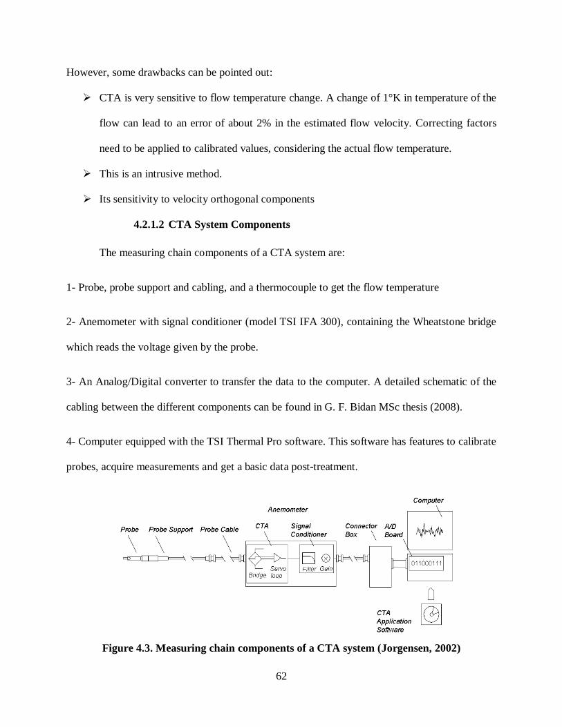
62

However, some drawbacks can be pointed out:

CTA is very sensitive to flow temperature change. A change of 1°K in temperature of the

flow can lead to an error of about 2% in the estimated flow velocity. Correcting factors

need to be applied to calibrated values, considering the actual flow temperature.

This is an intrusive method.

Its sensitivity to velocity orthogonal components

4.2.1.2 CTA System Components

The measuring chain components of a CTA system are:

1- Probe, probe support and cabling, and a thermocouple to get the flow temperature

2- Anemometer with signal conditioner (model TSI IFA 300), containing the Wheatstone bridge

which reads the voltage given by the probe.

3- An Analog/Digital converter to transfer the data to the computer. A detailed schematic of the

cabling between the different components can be found in G. F. Bidan MSc thesis (2008).

4- Computer equipped with the TSI Thermal Pro software. This software has features to calibrate

probes, acquire measurements and get a basic data post-treatment.

Figure 4.3. Measuring chain components of a CTA system (Jorgensen, 2002)

63

4.2.1.3 Probe Selection

Probes are selected on the basis of various parameters such as the medium, number of

velocity components measured, velocity range or the wanted resolution. In other words,

depending on the parameters measured and on the spatial distribution wanted, we can choose the

probe.

For our case, we used a single wire probe, which is a probe with only one sensor and

designed to measure only one component of a flow. With this probe we can measure stream wise

properties of the flow such as mean velocities and get stream wise turbulence intensities. There

are different kinds of single wire probes: straight, boundary layer, bent. A TSI probe type 1211-

20 was chosen. This sensor (see Figure 4.4) - platinum film type - is good for cross flow

measurements, probe interference being reduced by mounting it parallel to the probe body.

Figure 4.4. TSI 1211- 20 standard CTA probe

4.2.1.4 Traverse System

The traverse system used for our measurements is a 2 axis VELMEX traverse with a

NF90 controller which controls two stepping motors (one for each axis) with a 0.05 mm

positioning precision. It will be used to measure the cross section flow quality. The traverse is

controlled through the provided TSI Thermal Pro software.

A probe holder stiffener was fabricated to suppress any vibration during the measurement

process. Indeed, velocities as high as 50 m/s (164 fps) induce non-negligible forces on the probe

64

support. In order to characterize the test section inlet cross section flow and the cascade

outlet flow, various slots will be located at different positions in one of the test section walls so

that the CTA probe can remain in the flow while moving on the traverse system (see part 4.3.2).

Figure 4.5. CTA experimental setup

4.2.2 Pressure Measurements

In order to carry out pressure measurements, various instrumentations are available. First,

a classic Pitot-tube with a handheld digital manometer will be utilized (Figure 4.6). The Pitot

tube consists of a tube pointing directly into the airflow. Then, the moving fluid is brought to rest

at the tip of the probe, we reach a stagnation point and we obtain the total pressure. A pressure

transducer transforms the pressure value in an electrical signal and then to the handheld digital

manometer uses an A/D converter to display the pressure value. The handheld manometer is a

HHP4252 model from Omega® with a range from 0 to 55 inches H2O and an accuracy of +/-

0.3% FS, which is 0.165 inch H2O.

Traverse slot

TSI IFA 300 Bridge Chassis

Traverse system

Acquisition Computer

65

Figure 4.6. Image of Pitot tube with handheld manometer

Another common technique is the use of pressure taps over the body surface to

characterize a pressure field. This technique will be used in the future to characterize the linear

cascade pressure distribution. The center blade and the two surrounding blades will be

instrumented with pressure taps. The center blade will have pressure taps on both suction and

pressure side while the two surrounding ones will have only taps on one of their pressure/suction

side. On the center blade, pressure taps will be located at half span location as well as at other

span wise location (with a lesser concentration) to evaluate the span wise 2-D assumption.

4.2.3 Temperature Measurements

An ungrounded T-type thermocouple, with a stainless steel 1/8 inch diameter, 6 inch long

tube was selected. It is located in the settling chamber where flow velocities are relatively low

the signal received and is directly linked to the TSI CTA system. In addition a handheld J input

thermocouple thermometer, model HH802W from Omega® was used to measure the flow

temperature at different wind tunnel locations. Its accuracy is +/- 0.05% rdg +0.3 °C (0.54 °F),

which gives 0.32 °C (0.58 °F) at 40 °C (104 °F) and its temperature range is from - 50 °C (-58

°F) to 1370 °C (2498 °F).

Pitot tube

Handheld manometer

66

4.3 Experimental Procedures

4.3.1 CTA Probe Calibration

Calibration plays an important role in the accuracy and quality of the measurements.

CTA calibrations are performed in a dedicated calibrator TSI model 1129 with a low turbulence

free jet, whose velocity is calculated on basis of the pressure drop at its exit. The calibration

process consists in recording the voltage output corresponding to an effective velocity input. The

accuracy of this method is about 0.5%. The objective is quite simple: Find which velocity

corresponds to an output voltage value. To do so, in addition to the CTA setup, a pressure

transducer and a calibrator are necessary. A bridge voltage output value is acquired for each

different velocity for 17 points from 0 to 50 m/s (164 fps). Then, we compute the fitting 4th order

polynomial coefficients. The result of a calibration is the following parameters: the gain of the

probe, the offset, the temperature of the calibration and the polynomial regression coefficients.

The obtained points with the fitting curve are illustrated Figure 4.7.

Figure 4.7. Calibration fitting curve

67

4.3.2 CTA System Location

The test section is designed so that CTA measurements can be done easily. The probe

should be able to cover any plane we are interested in with the traverse system. Therefore, one of

the side walls of the test section is made out of wood and removable to enable easy machining

and interchange.

The traverse can be oriented at two different axis angles,

First axis orthogonal to the incoming airflow (θ=0°) upstream of the cascade to

characterize the inlet flow quality (see figure 4.8). The slot S0 is located 18 inches

downstream of the contraction cone outlet.

Second axis parallel to the cascade inlet plane (θ=36°). The slot S1 is located 50% of the

axial chord downstream of the cascade outlet plane to characterize the cascade blade

wake.

Figure 4.8. Slot locations for the traverse system

Contraction Cone

Airflow

Slot 0 (S0)Slot 1 (S1)

18 inches

End of contractionTest blades

Cascade Outlet plane

50% Cx

θ= 36°

68

4.3.3 Data Acquisition and Reduction

Data acquisition was automated and executed using the TSI Thermal Pro Software. The

sampling frequency and acquisition time for CTA measurements needs to be chosen to be

relevant. The integral time scale was computed using the autocorrelation method over a first

exploratory survey of velocity data with a large number of points. The necessary sampling

frequency to get uncorrelated data was found to be 20 Hz or less in the middle of the test section

inlet plane. Then, the acquisition time was picked to get a reasonable amount of points and

therefore, a reasonable uncertainty. Generally, an acquisition time of 2 seconds, which gives 40

data points, was taken.

Experiments generally generate a high quantity of raw data, from voltage files recorded

into text files to velocity files and post-processed data. This raw data need to be processed and

data reduction was mostly done with the Mathwork® software Matlab, and programs such as

Tecplot360 were also utilized to create and analyze plots.

4.3.4 Uncertainty Analysis

For each measurement -velocity, pressure, temperature or turbulence intensity- an

appropriate uncertainty estimation method is to be used. Generally, a 95% confidence interval, or

“two-sigma error” (1.96σ) was chosen in this study to estimate the uncertainty. The statistical

method depends on the analyzed parameter and on the number of data points. For raw data with a

number of points less than 30, the student‟s t-distribution law is applied. If the number of points

is greater than 30, a normal distribution is appropriate. For data based on the standard deviation

such as the turbulence intensity, a χ2 -distribution law is applied (Beckwith, 1993).

69

4.3.5 Data Analysis

In this part, some potential reasons for abnormal pressure, temperature variation or high

turbulence levels in a wind-tunnel will be discussed. The most important factors concern:

Mean flow variations in time and space over the test section cross section area:

A mean flow variation in time would indicate problems with the fan or with static

pressure changes. This kind of problems can be eliminated by changing fan blade angles

or by increasing the flow through the breathe slit downstream the test section.

The turbulence intensities fluctuation:

Mean flow non-uniformities can originate from separation on some of the corner guide-

vanes, diffuser separation or by flow blockage due to inefficient screens or honeycomb.

If these deficiencies are small the problems can be taken care of by the contraction but

larger deficiencies and problems generated in the contraction are difficult to eliminate.

High turbulence levels often originate from small separations or deficient screen and

honeycomb design.

Temperature variations in time and over the same cross section area:

Large temperature variations in time suggest an insufficient control system and large

variations in space that the heat exchanger is located too close to the test section or that

the water flow rate is not large enough (Lindgren, 2002).

4.4 Results and Discussion

4.4.1 Pressure Distribution along the Wind Tunnel

Static and dynamic pressures were measured with a Pitot tube linked to a handheld digital

manometer at different locations along the flow path in the closed circuit wind tunnel. Figure 4.9

70

represents the variation of static, dynamic and total pressure along the wind tunnel for a mean

velocity in the test section inlet of 53 m/s (174 fps). The graph starts at the test section inlet (x=0

foot) and ends at the contraction cone outlet (x= 70 feet) to close the loop. Uncertainty bars,

based on the student‟s t-distribution law (see Part 4.3.4) are represented for each measurement.

Figure 4.9. Variation of static dynamic and total pressure along the wind tunnel

As expected, a permanent total pressure decrease along the wind tunnel occurs due to

pressure losses. Static and dynamic pressures vary symmetrically, in function of the section

areas. As predicted Part 2.3, most pressure losses occur around the cascade, where the dynamic

pressure is the highest. Static pressure rises across the fan by 7 inches H2O at this particular wind

tunnel working point with a calculated flow rate of around 17,000 CFM.

71

4.4.2. Fan Pitch Setting and Operating Conditions

The Figure 4.10 shows the variation of volume flow rate through the fan versus the pitch

setting. As explained Part 2.2.6, the pitch of the fan blades can be changed through a pitch

control device. The input pressure signal from 0 to 15 psi can be changed using a pressure

regulator (see Figure 2.9). Then, we can control the operating conditions of the wind tunnel and

the velocity in the test section. A flow rate of 15,900 CFM and a velocity of 50 m/s in the test

section (164 fps) are reached for a pitch setting of 8.1. It can as well be observed the fan starts

stalling when the pitch is greater than 9.5.

Figure 4.10. Fan operating conditions. a) Volume flow rate versus pitch setting. b) Total

pressure rise versus pitch setting

4.4.3 Noise Measurements

Noise measurements were performed along the wind tunnel using a simple sound meter.

It was found that the sound level was the highest next to the cascade where velocities can reach

72

values as high as 80 m/s (262.4 fps). The noise level next to the test section at a nominal cascade

inlet velocity of 50 m/s (164 fps) is 94.5 db with a +/- 0.8 db uncertainty using a t-student law

distribution and taking a 95% confidence interval. For the same operating point, the noise level

measured from the ground next to the fan is 91 db. At the opposite end from the cascade, when

velocities are lower (8 m/s or 164 fps), the noise level was found to be 89.5 db. Therefore, when

working next to the test section during a long time, it is recommended to wear ear protectors.

4.4.4 Temperature Variation through Time

Temperature was measured in the settling chamber where flow velocities are relatively

low so that we obtain directly the static temperature. A K-type thermocouple was used (see Part

4.2.3 for details). All the energy supplied to the motor driving a wind tunnel is finally dissipated

into heat and results in an increase of temperature of the tunnel air until the heat losses finally

reach an equilibrium point with the input of energy. The temperature rise in the wind tunnel is

described by the curve Figure 4.11.

Figure 4.11. Temperature variation through time at the test section inlet

73

This measurement was taken for an operating velocity at the test section inlet of 50 m/s

(164 fps). We can see that the temperature reaches a first plateau at 44.1 °C (111.4 °F) from t =

65 min to t = 100 min. Then the temperature varies again to reach a second plateau at 45 °C (113

°F) after t=123 min. This variation from 44 to 45 °C is due to temperature change in the room.

Though, an AC ventilation system keeps the room within a temperature range of 2° C (3.6 °F),

and therefore, temperature variations stay within a reasonable range after the temperature reaches

a first plateau.

4.4.5 Velocity Distribution over the Test Section Inlet Cross-Section

To measure the velocity distribution over the test section inlet cross-section, a CTA

system with an automated traverse were employed as explained Part 4.3. Measurement point

locations are represented Figure 4.12. The plane is located at the slot (S0) as shown Figure 4.8.

Its width is L = 12 inches and its height is H = 19.5 inches. The axis values are adimensional.

Figure 4.12. CTA measurement points location over the test section inlet plane ‘S0’

74

After acquiring mean velocity values for each measurement points at a 20 Hz sampling

frequency over 2 seconds, the velocity contour distribution illustrated Figure 4.13 was obtained.

Figure 4.13. Velocity contours over the test section inlet ‘S0’ plane (in m/s)

Mean velocity contour values, outside the boundary layer, are varying from 50 m/s (164

fps) to 50.8 m/s (167 fps). The velocity variation over the section is less than 2%. The

uncertainty was computed using the Normal-distribution law and was found to be +/- 0.02 m/s

(+/- 0.06 fps) with a “95% confidence interval”.

A refined measurement was done over a corner of the same plane „S0‟ to get more

information about the flow near from the walls and in the corners. The measurement points were

distributed as shown Figure 4.14, with a finer mesh near the walls.

75

Figure 4.14. CTA measurement points location over the test section inlet plane ‘S0’ bottom

right corner

Results are shown Figure 4.15. The estimated uncertainty based on the Student‟s t-

distribution law is +/- 0.06 m/s (0.20 fps) in the outer boundary region flow, and +/- 1.5 m/s

(4.92 fps) in the corner flow for a 95% confidence interval. A first estimate of the boundary layer

thickness of about 0.05L was obtained.

Figure 4.15. Velocity contours over the plane ‘S0’ bottom right corner (in m/s)

76

4.4.6 Streamwise Turbulence Intensity over the Test Section Inlet Cross-Section

Turbulence intensity was computed with the data acquired for the mean velocity values in

the previous part. The measurement point locations are therefore the same. The result is also

represented with contours on Figure 4.16.

Figure 4.16. Streamwise turbulence intensity contours over the cross-section ‘S0’ in %

The turbulence intensity reaches levels as low as 0.12% in the center of the cross-section,

with an uncertainty for a 95% confidence interval of +/-0.03%, based on a χ2 -distribution law. In

the corners, the streamwise turbulence intensity reaches higher levels, up to 7 %, as illustrated

Figure 4.17. This result is based on the refined measuring mesh shown Figure 4.14.

77

Figure 4.17. Streamwise turbulence intensity contours over the plane ‘S0’ bottom right

corner (in %)

4.4.7 Boundary Layer Profile

The boundary layer profile was characterized using the CTA system and the automated

traverse. The mainstream flow velocity was 50 m/s (164 fps). Velocities were measured every

millimeter starting from as close to the wall as possible, which is 1/8 inch from the wall (see

Figure 4.18). The resulting profile curve was extrapolated to reach a zero velocity at the wall in

order to characterize the boundary layer profile and compute the different parameters defining it.

Figure 4.18. Boundary layer profile at the center of the plane ‘S0’ bottom wall

78

This profile yields to the following values:

Boundary layer thickness at 99%:

Displacement thickness:

Momentum thickness:

Shape factor:

The shape factor is close to the one found with the classic 1/7 Power Law used for

turbulent boundary layer profile over a flat plate (H=1.28). The velocity overlap is characteristic

of the flow distribution at the outlet of a finite length contraction. This concave velocity

distribution was observed by Morel (1975) in a paper about the design of axisymmetric wind

tunnel contractions. This velocity overlap of 1.2% may also be found for turbulent boundary

layers. This characteristic of turbulent boundary layer has been discussed over the last two

decades in order to redefine the classical boundary layer theory, and find a new analytical

description of the turbulent boundary layer. Osterlund (2000) claimed that this overlap region

becomes significant when the Reynolds number based on the momentum thickness is greater

than 6,000. In our case, the Reynolds number based on the momentum thickness is 4,334.

4.4.8 Cascade Blade Wake

A first characterization of the cascade wake profile was performed using the Constant

Temperature Anemometry system. The traverse was inclined at 36° to be aligned with the

cascade outlet plane as illustrated Figure 4.19. Then the probe is moving along the axis parallel

to the slot S1 as illustrated Figure 4.8.

79

Figure 4.19. Inclined CTA traverse setup

The mean velocity values were measured at mid-span, 50% of the axial chord

downstream of the cascade outlet plane at the slot S1 (refer Figure 4.8). The inlet mean velocity

was 50 m/s (164 fps), which gives a Reynolds number based on the blade axial chord of 450,000.

The wake profile of the center blade of the cascade is shown Figure 4.20. The pressure side is on

the right side of the graph and the suction side is on the left.

Figure 4.20. Wake velocity profile 50% of the axial chord downstream of the L1A cascade

center blade at mid-span at Re=450,000

Slot S1

Inclined traverse (36°)

Hot wire probe

Cascade

80

The turbulence intensity profile was then computed and is illustrated Figure 4.21.

Figure 4.21. Turbulence intensity profile 50% of the axial chord downstream of the L1A

cascade center blade at mid-span at Re=450,000

It can be noticed the minimum velocity is 85% of the freestream. It was found the

freestream velocity was about 77 m/s (253 fps) for a 50 m/s (164 fps) inlet velocity. In addition,

it can be observed this wake is not symmetrical: the wake velocity is lower on the pressure side

than on the suction side. This characteristic was also obtained in Garmoe‟s experimental study

on similar low pressure turbine blades in a cascade (2005) at a Reynolds number of 100,000. It

can also be observed that the turbulence intensity is higher on the pressure side than on the

suction side near from the center of the wake and reaches a local minimum at the center of the

wake. The turbulence intensity reaches levels as low as 0.15% in the outer region of the wake. It

can be observed that the velocity profile is not periodic in the cascade with the current

configuration. A 2.5% velocity difference between the pitchwise locations +0.5 and -0.5 can be

81

observed in Figure 4.20. The cascade flow can be adjusted and periodic flow conditions should

be obtained by adjusting movable elements such as the tailboards or the inlet bleeds as illustrated

Figure 3.2. In addition, a better attention should be given when installing the blades in the

cascade in future studies to make sure they are evenly spaced over the whole span.

82

Chapter 5: Conclusion

This new experimental facility was designed to investigate how the unsteady flow due to

the upstream passing wakes coming from the front row vane affects the film cooling

performances on turbine blades. The facility can reach velocities as high as 50 m/s (164 fps) as

expected, with turbulence intensity values as low as 0.12 %. The velocity variation over the

cascade inlet section is less than 2 % of the mean value.

The test section, made out of acrylic walls, will enable the users to carry out Particle

Image Velocimetry (PIV) measurements in the future. Blades with pressure taps on their surface

are currently being fabricated to obtain information about test blade surface pressure distribution

and later on, about the cascade flow periodicity. The airflow in the cascade can be adjusted for

periodicity by the use of the tailboards and inlet bleeds in order to “balance” the flow.

Although the experimental studies about film cooling are not part of this thesis, a wake

simulator mechanism to simulate passing-wakes upstream of a 4 passage linear cascade was

designed. A special attention in the design of the components has been given to make them

easily interchangeable. The cascade test blades can be easily replaced. Wake generating blades

can be quickly changed to study different wake properties. In addition, trailing and leading edge

of the designed flat plates can be replaced with new profiles. This experimental setup is the first

wake simulator mechanism upstream of a linear cascade which can use realistic vane profiles.

Future works will also investigate heat-transfer performance of film cooling. In parallel

with this work, a student team was preparing the experimental apparatus to study transient heat

transfer behavior of film cooling. Furthermore, a heat exchanger has been recently designed to be

able to control to wind tunnel flow temperature and facilitate future studies.

83

Eventually, a list of technical recommendations for complementary work with the new

facility in a close future is suggested below:

Heat exchanger installation: A heat exchanger is currently being installed in the wind

tunnel duct, introducing new pressure losses. A new survey of the wind tunnel

characteristics should be performed after installation, in order to know the new operating

velocity range and the influence of the heat exchanger coil on turbulence intensities

values. In addition, a special attention should be given to possible humidity and water

drops introduced by the heat exchanger coil in the wind tunnel duct.

Wind tunnel sheet metal parts: the wind tunnel 16 gage sheet metal walls are not stiff

enough for large surfaces and introduce extra vibration when the wind tunnel is

operating, due to substantial pressure forces on those walls. A quote has been processed

with a local contractor to add stiffeners on the larger sheet metal panels. This stiffening

work should be processed after installing the heat exchanger.

Cascade operation: the objective of the cascade is to obtain a periodic airflow. Then a

particular care should be given to the fabrication and installation of the 2-D blades so that

they are precisely located, straight (2-D assumption) and evenly spaced. The use of

blades with pressure taps should facilitate the characterization of the cascade. The

adjustment of the movable elements such as the “inlet bleeds” and the “tailboards” to

obtain a periodic airflow. The influence of such elements should be investigated.

Wake simulator mechanism operation: the wake simulator was designed to be compatible

with the test section and the cascade. Though, the addition of this new element to the test

section apparatus may introduce some additional leaks. A special care to keep the whole

mechanism airtight should be given. The use of caulk for permanent links is well adapted.

84

The use of aluminum tape can be a convenient means in some cases. As described in Part

3.3, the wake simulator height and angle can be adjusted in order to adjust the whole

mechanism to the cascade. A preliminary vibration analysis was performed in this thesis

but some tests need to be performed in situ to make sure that vibration due acoustic

resonance (Helmholtz resonator) or due to the rotating parts will not disturb future

cascade measurements. Excessive vibrations of the moving plates may also become a

concern. In this case, lowering the operating speed of the belt can be a good solution.

Increasing the width of the moving plate and make them stiffer could also allow the user

to operate the mechanism at a higher velocity without having vibration concerns if

needed. For additional recommendations about the assembly of the mechanism, the

reader can refer to the Part 3.3 of this thesis.

85

References

American Institute of Steel Construction (AISC) (1994), Load & Resistance Factor Design, 2nd

edition

Beckwth T.G., Marangoni R.D. and Lienard J.H. (1993), Mechanical Measurements, Fifth

edition, Wesley

Bidan G. F. (2008), Parametric Study of a Pulsed Jet in Cross Flow, Louisiana State University,

MSc thesis

Bloxham M., Reimann D., Crapo K., Pluim J., Bons J. P. (2009), Synchronizing Separation Flow

Control With Unsteady Wakes in a Low-Pressure Turbine Cascade, Journal of Turbomachinery,

Vol. 131, April

Bradshaw P. and Mehta R., “Wind Tunnel Design,”

URL: http://www-htgl.stanford.edu/bradshaw/tunnel/index.html [cited in March 2010]

Cohen H., Rogers G.F.C and Saravanmuttoo H.I.H. (1996), Gas Turbine Theory, Fourth edition,

Longman Group Ltd

Jorgensen F.E. (2002), How to Measure Turbulence with Hot Wire Anemometers - A Practical

Guide, Dantec Dynamics

DeVahl D.G. (1964), The Flow of Air Through Wire Screens, Hydraulics and Fluid Mechanics,

R. Sylvester (ed.), Pergamon, New York, pp.191-212

Eldredge, R. G., and Bons, J. P. (2004), Active Control of a Separating Boundary Layer with

Steady Vortex Generating Jets—Detailed Flow Measurements,” AIAA-2004-751

Garmoe T. L. (2005), Characterization of the Global Hawk low pressure turbine first rotor,

Aeronautics and Astronautics, Air Force Institute of Technology, MSc thesis, pp. 40; 67; 103

Groth J. and Johansson A. V. (1988), Turbulence Reduction by Screens, Journal of Fluid

Mechanics 197:139-155

Heidmann J.D., Lucci B.L. and Reshotko E. (2001), An Experimental Study of the Effect of Wake

Passing on Turbine Blade Film Cooling, Journal of Turbomachinery, Vol. 123, April

Ingard U. (2008), Notes on Acoustics, Infinity Science Press, 226-229

Intralox L.L.C (2010), Conveyor Belting Engineering Manual, Design Guidelines, 317-338

Lindgren B. and Johansson A. V. (2002), Design and evaluation of a low-speed wind-tunnel with

expanding corners, Dept. of Mechanics, KTH, SE-100 44 Stockholm, Sweden

86

Loehrke R. I. and Nagib H. M. (1976), Control of free stream turbulence by means of

honeycombs - A balance between suppression and generation, J. Fluids Engineering, 342-353,

September

Mathew J. et al (2005), Design, Fabrication and Characterization of an Anechoic Wind-Tunnel

11th AIAA/CEAS Aeroacoustic Conference, Monterey, California

Measurement, Instrumentation and Sensors Handbook (1999), Webster, (ISBN 084932145X)

Meherwan P. B. (2006), Gas Turbine Engineering Handbook, 3rd edition, Gulf Professional

Publishing, 429-453

Mehta R. D. and Bradshaw P. (1979), “Design Rules for Small Low Speed Wind Tunnels”,

Aeronautical Journal of the Royal Aeronautical Society, November

Morel T. (1975), Comprehensive Design of Axisymmetric Wind Tunnel Contractions, J. Fluids

Eng., Volume 97, Issue 2, 225

Morgand P. G. (1960), The Stability of Flow Through Porous Screens, JAS 64, 359

Olson S., Sanitjai S., Ghosh K. and Goldstein R. J. (2011), Effect of Wake-Disturbed Flow on

Heat (Mass) Transfer to a Turbine Blade, Journal of Turbomachinery, Vol. 133, January

Osterlund J. M. and Johansson A. V., Nagib H. M. and Hites M. H. (2000), A note on the overlap

region in turbulent boundary layers, Physics of Fluids, January, Vol. 12-1

Rae W. H. and Pope A. (1984), Low Speed Wind-Tunnel Testing, Wiley

Schobeiri M. T., Ozturk B. and Ashpis D.E. (2007), Effect of Reynolds Number and Periodic

Unsteady Wake Flow Condition on Boundary Layer Development, Separation, and

Intermittency Behavior Along the Suction Surface of a Low Pressure Turbine Blade, Journal of

Turbomachinery, Vol. 129, January

Tan-Atichat J, Nagib HM, Loehrke RI. (1982), Interaction of free-stream turbulence with

screens and grids: a balance between turbulence scales Journal of Fluid Mechanics 114:501-28

TSI Incorporated (2008), TSI Thermal Anemometry Catalog

Watmuff J. H. (1986), Wind Tunnel Contraction Design, 9th

Australian Fluid Mechanics

Conference, 8-12 December

Wattendorf F.L. (1938), Factors influencing the energy ratio of return flow wind tunnels, 5th

International Congress for Applied Mechanics, 538, Cambridge

Womack K. M., Volino R. J., Schultz M.P. (2008), Combined Effects of Wakes and Jet Pulsing

on Film Cooling, Journal of Turbomachinery, Vol. 130, October

87

Womack K. M., Volino R. J., Schultz M.P. (2008), Measurements in Film Cooling Flows With

Periodic Wakes, Journal of Turbomachinery, Vol. 130, October

Wright L.M., Blake S. A., Rhee D.H., Han J.C.(2009), Effect of Upstream Wake With Vortex on

Turbine Blade Platform Film Cooling With Simulated Stator-Rotor Purge Flow, Journal of

Turbomachinery, Vol. 131, April

88

Appendix A: Wind Tunnel Parts - Detailed Drawings

89

90

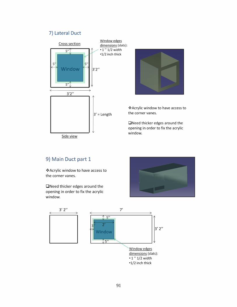
91

92

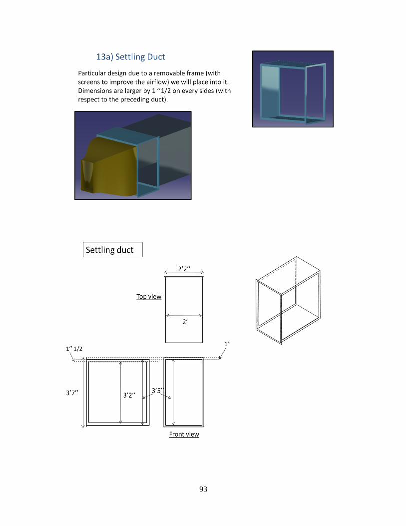
93

94

Appendix B: Supporting Structure - Detailed Drawings and Specifications

95

96

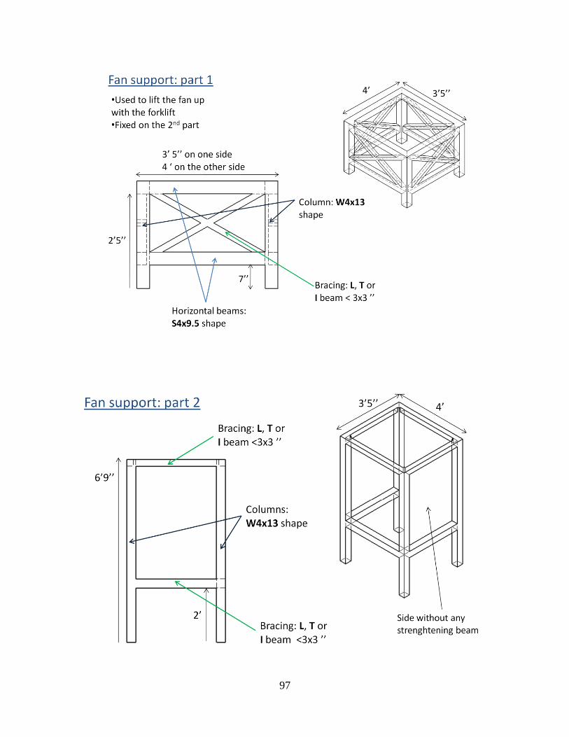
97

98

99

100

101

102

103

Top plate with threaded holes

104

Appendix C: Test Section Parts - Detailed Drawings

1) Overview

2) Cascade outlet - Permanent frame

Contraction outlet

Permanent frame

Test Section Inlet

Cascade Plate

Tailboard

Test Section

Outlet – Part 2

Test Section

Outlet – Part 1

Inside wall in ½ inch plywood

105

3) Test Section Inlet (case without conveyor)

Acrylic panels:

Flange 1 (blue):

106

4) Cascade Endwall Plate

Permanent plate (1/2 inch thick aluminum):

107

5) Tailboards (1/2 inch thick acrylic)

Outer tailboard:

Inner tailboard:

108

6) Test Section Outlet - Part 1

Acrylic panel:

109

7) Test Section Outlet - Part 2

½ inch plywood panels: Bottom aluminum frame:

110

Top aluminum frame:

8) Test Section Cover

Made out of ½ inch plywood. Can be made out of acrylic for visualizations.

111

Appendix D: Wake Simulator Mechanism - Detailed Drawings

1) Inside Frame

Front

view

Side view

Top view

112

113

2) Outside Frame, Drive Side

Side view Front view Top view

Isometric view

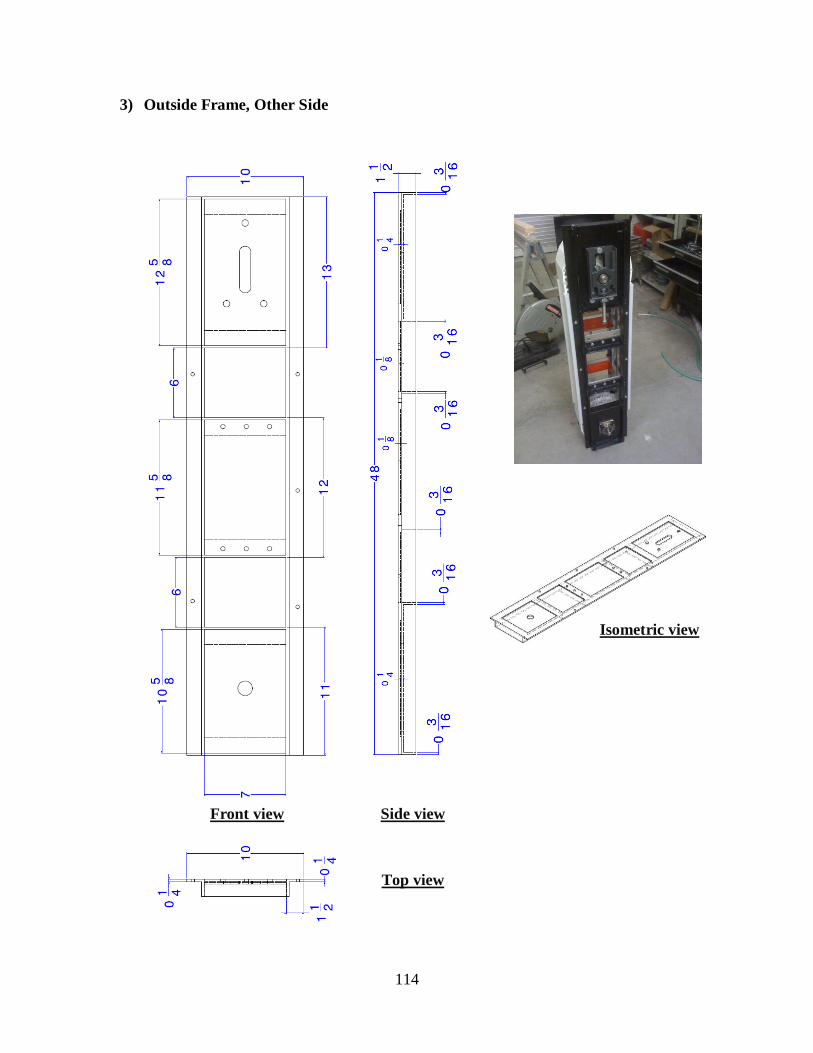
114

3) Outside Frame, Other Side

Isometric view

Front view

Top view

Side view

115

4) Conveyor Stand

Isometric view

Front view

Top view

Side view

116

5) Conveyor Shell

Shell Assembly

• 16 gage sheet metal

• About 6 ft x 3 ft x 8 in

• Main “shell” + 2 covers

5.1 . Main Shell drawing

Front view

Isometric view

117

5.2 . Top Cover Drawings

Front view Left view

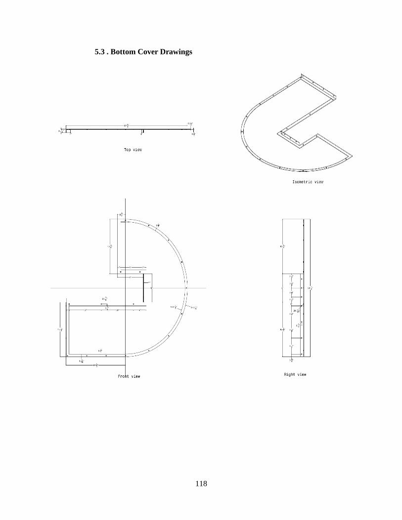
118

5.3 . Bottom Cover Drawings

119

6) Shaft Specifications

120

7) Moving Plate Assembly

i. Intralox Plastic Belt Module

ii. Intermediate Aluminum Plate

121

iii. Flat Plate iv. Cover Plate

v. Leading and Trailing Edges

122

Vita

Jean-Philippe Junca-Laplace, the son of Bernadette and Jean-Bernard Junca-Laplace,

brother of Camille and Lauriane Junca-Laplace, was born in November, 1986 in Tours, France.

He quickly left this city after six months to settle in Bordeaux. After obtaining his

Baccalauréat with honors in 2004, he joined the “Classes Préparatoires aux Grandes Ecoles” for

three years at Lycée Michel Montaigne in Bordeaux, with a physics and engineering sciences

specialization.

He entered the Institut Supérieur de l‟Aéronautique et de l‟Espace, ENSICA program in

2007 and started a master‟s program in aerospace engineering. He then joined the Department of

Mechanical Engineering at Louisiana State University in 2009 to complete a Master of Science

in Mechanical Engineering with a specialization in thermal sciences. He submitted his research

about the design, fabrication and characterization of a new wind tunnel facility under the

supervision of Dr. Shengmin Guo and Dr. Dimitris E. Nikitopoulos in June 2011. He is

expecting to receive both master‟s degrees in August 2011.

Jean-Philippe continues to play regularly the piano and the guitar. He is thinking about

composing music. Also, during his free time, he enjoys swimming, biking and running; one day

he hopes to compete in a triathlon or an adventure race.