design for manual assembly
TRANSCRIPT

3Product Design for Manual Assembly
3.1 INTRODUCTIONDesign for assembly (DFA) should be considered at all stages of the designprocess, but especially the early stages. As the design team conceptualizesalternative solutions, it should give serious consideration to the ease of assemblyof the product or subassembly. The team needs a DFA tool to effectively analyzethe ease of assembly of the products or subassemblies it designs. The design toolshould provide quick results and be simple and easy to use. It should ensureconsistency and completeness in its evaluation of product assemblability. Itshould also eliminate subjective judgment from design assessment, allow freeassociation of ideas, enable easy comparison of alternative designs, ensure thatsolutions are evaluated logically, identify assembly problem areas, and suggestalternative approaches for simplifying the product structure—thereby reducingmanufacturing and assembly costs.
By applying a DFA tool, communication between manufacturing and designengineering is improved, and ideas, reasoning, and decisions made during thedesign process become well documented for future reference.
The Product Design for Assembly handbook [1] originally developed as aresult of extensive university research, and, more recently, expanded versions insoftware form provide systematic procedures for evaluating and improvingproduct design for ease of assembly. This goal is achieved by providing assemblyinformation at the conceptualization stage of the design process in a logical andorganized fashion. This approach also offers a clearly defined procedure forevaluating a design with respect to its ease of assembly. In this manner a feedbackloop is provided to aid designers in measuring improvements resulting from
specific design changes. This procedure also functions as a tool for motivatingdesigners; through this approach they can evaluate their own designs and, ifpossible, improve them. In both cases, the design can be studied and improved atthe conceptual stage when it can be simply and inexpensively changed. The DFAmethod accomplishes these objectives by:
1. Providing a tool for the designer or design team which assures thatconsiderations of product complexity and assembly take place at the earliestdesign stage. This eliminates the danger of focusing exclusively during earlydesign on product function with inadequate regard for product cost andcompetitiveness.
2. Guiding the designer or design team to simplify the product so that savings inboth assembly costs and piece parts can be realized.
3. Gathering information normally possessed by the experienced design engi-neer and arranging it conveniently for use by less-experienced designers.
4. Establishing a database that consists of assembly times and cost factors forvarious design situations and production conditions.
The analysis of a product design for ease of assembly depends to a large extent onwhether the product is to be assembled manually, with special-purpose automa-tion, with general-purpose automation (robots), or a combination of these. Forexample, the criteria for ease of automatic feeding and orienting are much morestringent than those for manual handling of parts. In this chapter we shallintroduce design for manual assembly, since it is always necessary to use manualassembly costs as a basis for comparison. In addition, even when automation isbeing seriously considered, some operations may have to be carried out manually,and it is necessary to include the cost of these in the analysis.
3.2 GENERAL DESIGN GUIDELINES FOR MANUALASSEMBLY
As a result of experience in applying DFA it has been possible to develop generaldesign guidelines that attempt to consolidate manufacturing knowledge andpresent them to the designer in the form of simple rules to be followed whencreating a design. The process of manual assembly can be divided naturally intotwo separate areas, handling (acquiring, orienting and moving the parts) andinsertion and fastening (mating a part to another part or group of parts). Thefollowing design for manual assembly guidelines specifically address each ofthese areas.
3.2.1 Design Guidelines for Part HandlingIn general, for ease of part handling, a designer should attempt to:

(a) 0 I (I I
asymmetrical symmetrical
slightly asymmetrical pronounced asymmetrical
uwill jam cannot jam
will tangle cannot tangle
FIG. 3.1 Geometrical features affecting part handling.
1 . Design parts that have end-to-end symmetry and rotational symmetry aboutthe axis of insertion. If this cannot be achieved, try to design parts having themaximum possible symmetry (see Fig. 3. la).
2. Design parts that, in those instances where the part cannot be madesymmetric, are obviously asymmetric (see Fig. 3.1b).
3. Provide features that will prevent jamming of parts that tend to nest or stackwhen stored in bulk (see Fig. 3.1c).
4. Avoid features that will allow tangling of parts when stored in bulk (see Fig.3. Id).
5. Avoid parts that stick together or are slippery, delicate, flexible, very small, orvery large or that are hazardous to the handler (i.e., parts that are sharp,splinter easily, etc.) (see Fig. 3.2).
3.2.2 Design Guidelines for Insertion and FasteningFor ease of insertion a designer should attempt to:
1. Design so that there is little or no resistance to insertion and providechamfers to guide insertion of two mating parts. Generous clearance

very small slippery
sharp IJ flexible
FIG. 3.2 Some other features affecting part handling.
should be provided, but care must be taken to avoid clearances that will resultin a tendency for parts to jam or hang-up during insertion (see Figs. 3.3 to3.6).
2. Standardize by using common parts, processes, and methods across allmodels and even across product lines to permit the use of higher volumeprocesses that normally result in lower product cost (see Fig. 3.7).
3. Use pyramid assembly—provide for progressive assembly about one axis ofreference. In general, it is best to assemble from above (see Fig. 3.8).
4. Avoid, where possible, the necessity for holding parts down to maintain theirorientation during manipulation of the subassembly or during the placementof another part (see Fig. 3.9). If holding down is required, then try to designso that the part is secured as soon as possible after it has been inserted.
5. Design so that a part is located before it is released. A potential source ofproblems arises from a part being placed where, due to design constraints, it
part jams across corners part cannot jam
FIG. 3.3 Incorrect geometry can allow part to jam during insertion.
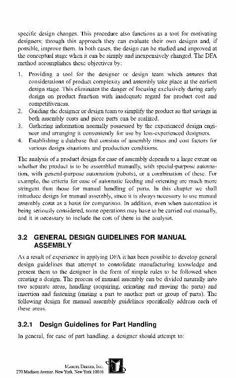
insertiondifficult ^°'e in work hole in P'n "at on pin
FIG. 3.4 Provision of air-relief passages to improve insertion into blind holes.
6.
must be released before it is positively located in the assembly. Under thesecircumstances, reliance is placed on the trajectory of the part beingsufficiently repeatable to locate it consistently (see Fig. 3.10).When common mechanical fasteners are used the following sequenceindicates the relative cost of different fastening processes, listed in order ofincreasing manual assembly cost (Fig. 3.11).
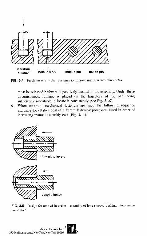
difficult to insert
easy to insert
FIG. 3.5 Design for ease of insertion—assembly of long stepped bushing into counter-bored hole.
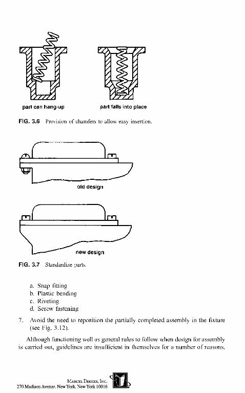
part can hang-up part falls into place
FIG. 3.6 Provision of chamfers to allow easy insertion.
old design
new design
FIG. 3.7 Standardize parts.
a. Snap fittingb. Plastic bendingc. Rivetingd. Screw fastening
7. Avoid the need to reposition the partially completed assembly in the fixture(see Fig. 3.12).
Although functioning well as general rules to follow when design for assemblyis carried out, guidelines are insufficient in themselves for a number of reasons.
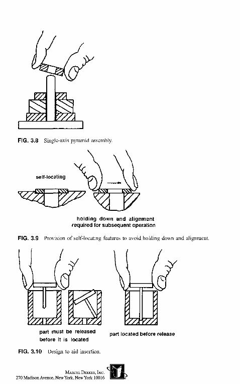
FIG. 3.8 Single-axis pyramid assembly.
holding down and alignmentrequired for subsequent operation
FIG. 3.9 Provision of self-locating features to avoid holding down and alignment.
part must be releasedbefore it is located
FIG. 3.10 Design to aid insertion.
part located before release

FIG. 3.11 Common fastening methods.
First, guidelines provide no means by which to evaluate a design quantitativelyfor its ease of assembly. Second, there is no relative ranking of all the guidelinesthat can be used by the designer to indicate which guidelines result in the greatestimprovements in handling, insertion, and fastening; there is no way to estimatethe improvement due to the elimination of a part, or due to the redesign of a partfor handling, etc. It is, then, impossible for the designer to know which guidelinesto emphasize during the design of a product.
Finally, these guidelines are simply a set of rules that, when viewed as a whole,provide the designer with suitable background information to be used to developa design that will be more easily assembled than a design developed without sucha background. An approach must be used that provides the designer with anorganized method that encourages the design of a product that is easy toassemble. The method must also provide an estimate of how much easier it isto assemble one design, with certain features, than to assemble another designwith different features. The following discussion describes the DFA methodology,which provides the means of quantifying assembly difficulty.
FIG. 3.12 Insertion from opposite direction requires repositioning of assembly.

3.3 DEVELOPMENT OF THE SYSTEMATIC DFAMETHODOLOGY
Starting in 1977, analytical methods were developed [2] for determining the mosteconomical assembly process for a product and for analyzing ease of manual,automatic, and robot assembly. Experimental studies were performed [3-5] tomeasure the effects of symmetry, size, weight, thickness, and flexibility onmanual handling time. Additional experiments were conducted [6] to quantifythe effect of part thickness on the grasping and manipulation of a part usingtweezers, the effect of spring geometry on the handling time of helical compres-sion springs, and the effect of weight on handling time for parts requiring twohands for grasping and manipulation.
Regarding the design of parts for ease of manual insertion and fastening,experimental and theoretical analyses were performed [7-11] on the effect ofchamfer design on manual insertion time, the design of parts to avoid jammingduring assembly, the effect of part geometry on insertion time, and the effects ofobstructed access and restricted vision on assembly operations.
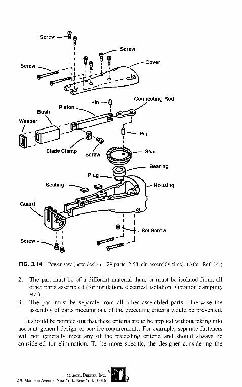
A classification and coding system for manual handling, insertion, andfastening processes, based on the results of these studies, was presented in theform of a time standard system for designers to use in estimating manualassembly times [12,13]. To evaluate the effectiveness of this DFA method theease of assembly of a two-speed reciprocating power saw and an impact wrenchwere analyzed and the products were then redesigned for easier assembly [14].The initial design of the power saw (Fig. 3.13) had 41 parts and an estimatedassembly time of 6.37min. The redesign (Fig. 3.14) had 29 parts for a 29%reduction in part count, and an estimated assembly time of 2.58min for a 59%reduction in assembly time. The outcome of further analyses [14] was a more than50% savings in assembly time, a significant reduction in parts count and ananticipated improvement in product performance.
3.4 ASSEMBLY EFFICIENCY
An essential ingredient of the DFA method is the use of a measure of the DFAindex or "assembly efficiency" of a proposed design. In general, the two mainfactors that influence the assembly cost of a product or subassembly are
The number of parts in a product.The ease of handling, insertion, and fastening of the parts.
The DFA index is a figure obtained by dividing the theoretical minimumassembly time by the actual assembly time. The equation for calculating the DFAindex Em3 is

Screw Screw
Cover
Bearing
Piston
Blade Clamp \Screw
Guard
,SealNeedle Bearing
Roll Pin Washer
Pin
Counterweight
"-Gear
Bearing
Housing
Washer
Set Screw
FIG. 3.13 Power saw (initial design—41 parts, 6.37min assembly time). (After Ref. 14.)
where N^ is the theoretical minimum number of parts, ta is the basic assemblytime for one part, and fma is the estimated time to complete the assembly of theproduct. The basic assembly time is the average time for a part that presents nohandling, insertion, or fastening difficulties (about 3 s).
The figure for the theoretical minimum number of parts represents an idealsituation where separate parts are combined into a single part unless, as each partis added to the assembly, one of the following criteria is met:
1. During the normal operating mode of the product, the part moves relative toall other parts already assembled. (Small motions do not qualify if they canbe obtained through the use of elastic hinges.)
Screw
Screw
Screw Cover
Connecting Rod
>— Housing
Set Screw
Screw
FIG. 3.14 Power saw (new design—29 parts, 2.58 min assembly time). (After Ref. 14.)
2. The part must be of a different material than, or must be isolated from, allother parts assembled (for insulation, electrical isolation, vibration damping,etc.).
3. The part must be separate from all other assembled parts; otherwise theassembly of parts meeting one of the preceding criteria would be prevented.
It should be pointed out that these criteria are to be applied without taking intoaccount general design or service requirements. For example, separate fastenerswill not generally meet any of the preceding criteria and should always beconsidered for elimination. To be more specific, the designer considering the

design of an automobile engine may feel that the bolts holding the cylinder headonto the engine block are necessary separate parts. However, they could beeliminated by combining the cylinder head with the block—an approach that hasproved practical in certain circumstances.
If applied properly, these criteria require the designer to consider meanswhereby the product can be simplified, and it is through this process thatenormous improvements in assemblability and manufacturing costs are oftenachieved. However, it is also necessary to be able to quantify the effects ofchanges in design schemes. For this purpose the DFA method incorporates asystem for estimating assembly cost which, together with estimates of parts cost,will give the designer the information needed to make appropriate trade-offdecisions.
3.5 CLASSIFICATION SYSTEMSThe classification system for assembly processes is a systematic arrangement ofpart features that affect acquisition, movement, orientation, insertion, and fasten-ing of the part together with some operations that are not associated with specificparts such as turning the assembly over.
Selected portions of the complete classification system, its associated defini-tions, and the corresponding time standards are presented in tables in Figs. 3.15 to3.17. It can be seen that the classification numbers consist of two digits; the firstdigit identifies the row and the second digit identifies the column in the table.
The portion of the classification system for manual insertion and fasteningprocesses is concerned with the interaction between mating parts as they areassembled. Manual insertion and fastening consists of a finite variety of basicassembly tasks (peg-in-hole, screw, weld, rivet, press-fit, etc.) that are common tomost manufactured products.
It can be seen that for each two-digit code number, an average time is given.Thus, we have a set of time standards that can be used to estimate manualassembly times. These time standards were obtained from numerous experiments,some of which will now be described.
3.6 EFFECT OF PART SYMMETRY ON HANDLING TIME
One of the principal geometrical design features that affects the times required tograsp and orient a part is its symmetry. Assembly operations always involve atleast two component parts: the part to be inserted and the part or assembly(receptacle) into which the part is inserted [15]. Orientation involves the properalignment of the part to be inserted relative to the corresponding receptacle andcan always be divided into two distinct operations: (1) alignment of the axis of the

for parts that can be grasped and manipulated with one hand without theaid of grasping tools
sym (deg) =(alpha* beta)
sym < 360
360 <= sym <540
540 <= sym<720
sym = 720
0
1
2
3
no handling difficultiesthickness > 2mm
size> 15mm
0
1.13
1.5
1.8
1.95
6mm <size
< 15mm1
1.43
1.8
2.1
2.25
< 2mm
size> 6mm
2
1.69
2.06
2.36
2.51
part nests or tanglesthickness > 2mm
size> 15mm
3
1.84
2.25
2.57
2.73
6mm <size
< 15mm4
2.17
2.57
2.9
3.06
<2mm
size> 6mm
5
2.45
3.0
3.18
3.34
for parts that can be lifted with one hand but require two hands becausethey severely nest or tangle, are flexible or require forming etc.
4
alpha <= 180
size> 15mm
0
4.1
6mm <size
<15mm1
4.5
alpha= 360
size> 6mm
2
5.6
FIG. 3.15 Selected manual handling time standards, seconds (parts are within easyreach, are no smaller than 6mm, do not stick together, and are not fragile or sharp).(Copyright 1999 Boothroyd Dewhurst, Inc.)
part that corresponds to the axis of insertion, and (2) rotation of the part aboutthis axis.
It is therefore convenient to define two kinds of symmetry for a part:
1. Alpha symmetry: depends on the angle through which a part must be rotatedabout an axis perpendicular to the axis of insertion to repeat its orientation.

part inserted but not secured immediately or secured by snap fit
no accessor vision
difficultiesobstructed access
orrestricted vision
obstructed accessand
restricted vision
0
1
2
secured by separate operation or partno holding down
requiredeasy toalign
0
1.5
3.7
5.9
not easyto align
1
3.0
5.2
7.4
holding downrequired
easy toalign
2
2.6
4.8
7.0
not easyto align
3
5.2
7.4
9.6
secured oninsertion by snap
fiteasy toalign
4
1.8
4.0
7.7
noteasy toalign
5
3,3
5.5
7.7
part inserted and secured immediately by screw fastening with power tool(times are for 5 revs or less and do not include a tool acquisition lime of 2.9s)
no accessor vision
difficultiesrestricted
visiononly
obstructed accessonly
3
4
5
easy toalign
0
3.6
6.3
9.0
not easyto align
1
5.3
S.O
10.7
FIG. 3.16 Selected manual insertion time standards, seconds (parts are small and there isno resistance to insertion). (Copyright 1999 Boothroyd Dewhurst, Inc.)
2. Beta symmetry: depends on the angle through which a part must be rotatedabout the axis of insertion to repeat its orientation.
For example, a plain square prism that is to be inserted into a square hole wouldfirst have to be rotated about an axis perpendicular to the insertion axis. Since,with such a rotation, the prism will repeat its orientation every 180°, it can be

6
screw tightenwith power
tool0
5.2
manipulation,reorientation or
adjustment1
4.5
additionof
non solids2
7
FIG. 3.17 Selected separate operation times, seconds (solid parts already in place).(Copyright 1999 Boothroyd Dewhurst, Inc.)
Definitions:
For Fig. 3.15Alpha is the rotational symmetry of a part about an axis perpendicular to its axis ofinsertion. For parts with one axis of insertion, end-to-end orientation is necessary whenalpha equals 360 degrees, otherwise alpha equals 180 degrees.
Beta is the rotational symmetry of a part about its axis of insertion. The magnitude ofrotational symmetry is the smallest angle through which the part can be rotated andrepeat its orientation. For a cylinder inserted into a circular hole, beta equals zero.
Thickness is the length of the shortest side of the smallest rectangular prism thatencloses the part. However, if the part is cylindrical, or has a regular polygonal cross-section with five or more sides, and the diameter is less than the length, then thicknessis defined as the radius of the smallest cylinder which can enclose the part.
Size is the length of the longest side of the smallest rectangular prism that can enclosethe part.
For Fig. 3.16Holding down required means that the part will require gripping, realignment, or holdingdown before it is finally secured.
Easy to align and position means that insertion is facilitated by well designed chamfersor similar features.
Obstructed access means that the space available for the assembly operation causes asignificant increase in the assembly time.
Restricted vision means that the operator has to rely mainiy on tactile sensing during theassembly process.
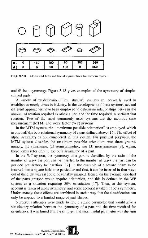
termed 180° alpha symmetry. The square prism would then have to be rotatedabout the axis of insertion, and since the orientation of the prism about this axiswould repeat every 90°, this implies a 90° beta symmetry. However, if the squareprism were to be inserted in a circular hole, it would have 180° alpha symmetry
d
a
& O <O» <€^ © <€?*00
180 180 90 90 1!
0 360 360JO 0 360
FIG. 3.18 Alpha and beta rotational symmetries for various parts.
and 0° beta symmetry. Figure 3.18 gives examples of the symmetry of simple-shaped parts.
A variety of predetermined time standard systems are presently used toestablish assembly times in industry. In the development of these systems, severaldifferent approaches have been employed to determine relationships between theamount of rotation required to orient a part and the time required to perform thatrotation. Two of the most commonly used systems are the methods timemeasurement (MTM) and work factor (WF) systems.
In the MTM system, the "maximum possible orientation" is employed, whichis one-half the beta rotational symmetry of a part defined above [16]. The effect ofalpha symmetry is not considered in this system. For practical purposes, theMTM system classifies the maximum possible orientation into three groups,namely, (1) symmetric, (2) semisymmetric, and (3) nonsymmetric [3], Again,these terms refer only to the beta symmetry of a part.
In the WF system, the symmetry of a part is classified by the ratio of thenumber of ways the part can be inserted to the number of ways the part can begrasped preparatory to insertion [17]. In the example of a square prism to beinserted into a square hole, one particular end first, it can be inserted in four waysout of the eight ways it could be suitably grasped. Hence, on the average, one-halfof the parts grasped would require orientation, and this is defined in the WFsystem as a situation requiring 50% orientation [17]. Thus, in this system,account is taken of alpha symmetry, and some account is taken of beta symmetry.Unfortunately, these effects are combined in such a way that the classification canonly be applied to a limited range of part shapes.
Numerous attempts were made to find a single parameter that would give asatisfactory relation between the symmetry of a part and the time required fororientation. It was found that the simplest and most useful parameter was the sum

Group I III IV
f D Square prisms]o Hexagonal prisms
3.2
3.0W. 2.8o>6 ?B™ ^.t>D)£ 2.4c 22^
2.0
1.8
1.6
1.4
0 180 360 540 720total angle of symmetry (<x + & ),deg
FIG. 3.19 Effect of symmetry on the time required for part handling. Times are averagefor two individuals and shaded areas represent nonexistent values of the total angle ofsymmetry.
of the alpha and beta symmetries [5]. This parameter, which will be termed thetotal angle of symmetry, is therefore given by
Total angle of symmetry = alpha + beta (3.2)
The effect of the total angle of symmetry on the time required to handle (grasp,move, orient, and place) a part is shown in Fig. 3.19. In addition, the shaded areasindicate the values of the total angle of symmetry that cannot exist. It is evidentfrom these results that the symmetry of a part can be conveniently classified intofive groups. However, the first group, which represents a sphere, is not generallyof practical interest; therefore, four groups are suggested that are employed in thecoding system for part handling (Fig. 3.15). Comparison of these experimentalresults with the MTM and WF orientation parameters showed that these param-eters do not account properly for the symmetry of a part [5].
3.7 EFFECT OF PART THICKNESS AND SIZE ONHANDLING TIME
Two other major factors that affect the time required for handling during manualassembly are the thickness and the size of the part. The thickness and size of apart are defined in a convenient way in the WF system, and these definitions have

«£ © x>4tnickness
thicknessthickness
1.2
1.0
0.8
0.6
0.4
0.2
0
thin
cylindrical
not thin
\, . curve tor long cylinders,V It 'thickness' = diameter
non-cylindrical
s^-
FIG. 3.20 Effect of part thickness on handling time.
2 3thickness mm
been adopted for the DFA method. The thickness of a "cylindrical" part isdefined as its radius, whereas for noncylindrical parts the thickness is defined asthe maximum height of the part with its smallest dimension extending from a flatsurface (Fig. 3.20). Cylindrical parts are defined as parts having cylindrical orother regular cross sections with five or more sides. When the diameter of such apart is greater than or equal to its length, the part is treated as noncylindrical. Thereason for this distinction between cylindrical and noncylindrical parts whendefining thickness is illustrated by the experimental curves shown in Fig. 3.20. Itcan be seen that parts with a "thickness" greater than 2mm present no graspingor handling problems. However, for long cylindrical parts this critical value wouldhave occurred at a value of 4mm if the diameter had been used for the"thickness". Intuitively, we see that grasping a long cylinder 4mm in diameteris equivalent to grasping a rectangular part 2 mm thick if each is placed on a flatsurface.
The size (also called the major dimension) of a part is defined as the largestnondiagonal dimension of the part's outline when projected on a flat surface. It isnormally the length of the part. The effects of part size on handling time areshown in Fig. 3.21. Parts can be divided into four size categories as illustrated.Large parts involve little or no variation in handling time with changes in theirsize; the handling time for medium and small parts displays progressively greatersensitivity with respect to part size. Since the time penalty involved in handlingvery small parts is large and very sensitive to decreasing part size, tweezers willusually be required to manipulate such parts. In general, tweezers can be assumedto be necessary when size is less than 2 mm.

£ 2
L<D
. cylindrical parts
noncylindrical parts
10 size, mm 2°
L>Dvery 'small1 medium ' largesmall
FIG. 3.21 Effect of part size on handling time.
3.8 EFFECT OF WEIGHT ON HANDLING TIMEWork has been carried out [18] on the effects of weight on the grasping,controlling, and moving of parts. The effect of increasing weight on graspingand controlling is found to be an additive time penalty and the effect on moving isfound to be a proportional increase of the basic time. For the effect of weight on apart handled using one hand, the total adjustment tpw to handling time can berepresented by the following equation [3]:
fpw = 0.0125 FF + O.OllWth (3.3)
where W (Ib) is the weight of the part and th (s) is the basic time for handling a"light" part when no orientation is needed and when it is to be moved a shortdistance. An average value for th is 1.13, and therefore the total time penalty dueto weight would be approximately 0.025 W.
If we assume that the maximum weight of a part to be handled using one handis around 10-20 Ib, the maximum penalty for weight is 0.25-0.5 s and is a fairlysmall correction. It should be noted, however, that Eq. (3.3) does not take intoaccount the fact that larger parts will usually be moved greater distances, resultingin more significant time penalties. These factors will be discussed later.

3.9 PARTS REQUIRING TWO HANDS FOR MANIPULATIONA part may require two hands for manipulation when:
The part is heavy.Very precise or careful handling is required.The part is large or flexible.The part does not possess holding features, thus making one-hand grasp difficult.
Under these circumstances, a penalty is applied because the second hand couldbe engaged in another operation—perhaps grasping another part. Experienceshows that a penalty factor of 1.5 should be applied in these cases.
3.10 EFFECTS OF COMBINATIONS OF FACTORSIn the previous sections, various factors that affect manual handling times havebeen considered. However, it is important to realize that the penalties associatedwith each individual factor are not necessarily additive. For example, if a partrequires additional time to move it from A to B, it can probably be oriented duringthe move. Therefore, it may be wrong to add the extra time for part size and anextra time for orientation to the basic handling time. The following gives someexamples of results obtained when multiple factors are present.
3.11 EFFECT OF SYMMETRY FOR PARTS THAT SEVERELYNEST OR TANGLE AND MAY REQUIRE TWEEZERS FORGRASPING AND MANIPULATION
A part may require tweezers when (Fig. 3.22):
Its thickness is so small that finger-grasp is difficult.Vision is obscured and prepositioning is difficult because of its small size.Touching it is undesirable, because of high temperature, for example.Fingers cannot access the desired location.
A part is considered to nest or tangle severely when an additional handling timeof 1.5 s or greater is required due to these factors. In general, two hands will berequired to separate severely nested or tangled parts. Helical springs with openends and widely spaced coils are examples of parts that severely nest or tangle.Figure 3.23 shows how the time required for orientation is affected by the alphaand beta angles of symmetry for parts that nest or tangle severely and may requiretweezers for handling.
In general, orientation using hands results in a smaller time penalty thanorientation using tweezers, therefore factors necessitating the use of tweezersshould be avoided if possible.

thickness so smallthat linger graspis difficult
I /
vision is obscured and pre-position-ing is difficult because of small size
fingers cannotaccess desiredlocation
undesirable to touch the part
FIG. 3.22 Examples of parts that may require tweezers for handling.
HOT
—— manipulation by tweezers• — •- manipulation by ham
100 200 300/8,deg
FIG. 3.23 Effect of symmetry on handling time when parts nest or tangle severely.(Disentangling time is not included.)
3.12 EFFECT OF CHAMFER DESIGN ON INSERTIONOPERATIONS
Two common assembly operations are the insertion of a peg (or shaft) into a holeand the placement of a part with a hole onto a peg. The geometries of traditionalconical chamfer designs are shown in Fig. 3.24. In Fig. 3.24a, which shows the

(a) Geometry of Peg
<fW2r
(b) Geometry of Hole
FIG. 3.24 Geometries of peg and hole.
design of a chamfered peg, d is the diameter of the peg, wl is the width of thechamfer, and 0j is the semiconical angle of the chamfer. In Fig. 3.24b, whichshows the design of a chamfered hole, D is the diameter of the hole, w2 is thewidth of the chamfer, and 62 is the semiconical angle of the chamfer. Thedimensionless diametral clearance c between the peg and the hole is defined by
(D - d)/D (3.4)
A typical set of results [9] showing the effects of various chamfer designs onthe time taken to insert a peg in a hole are presented in Fig. 3.25. From these andother results, the following conclusions have been drawn:
1. For a given clearance, the difference in the insertion time for two differentchamfer designs is always a constant.
2. A chamfer on the peg is more effective in reducing insertion time than thesame chamfer on the hole.
3. The maximum width of the chamfer that is effective in reducing the insertiontime for both the peg and the hole is approximately 0.1-D.
4. For conical chamfers, the most effective design provides chamfers on boththe peg and the hole, with wj = w2 = 0.1-D and 9l = 62 < 45.
5. The manual insertion time is not sensitive to variations in the angle of thechamfer for the range 10 < 6 < 50.

6. A radiused or curved chamfer can have advantages over a conical chamfer forsmall clearances.
It was learned from the peg insertion experiments [9] that the long manualinsertion time for the peg and hole with a small clearance is probably due to thetype of engagement occurring between the peg and the hole during the initialstages of insertion. Figure 3.26 shows two possible situations that will causedifficulties. In Fig. 3.26a, the two points of contact arising on the same circularcross section of the peg give rise to forces resisting the insertion. In Fig. 3.26b,the peg has become jammed at the entrance of the hole. An analysis was carriedout to find a geometry that would avoid these unwanted situations. It showed thata chamfer conforming to a body of constant width (Fig. 3.27) is one of thedesigns having the desired properties. It was found that for such a chamfer, theinsertion time is independent of the dimensionless clearance c in the rangec > 0.001. Therefore, the curved chamfer is the optimum design for peg-in-holeinsertion operations (Fig. 3.25). However, since the manufacturing costs forcurved chamfers would normally be greater than for conical chamfers, themodified chamfer would only be worthy of consideration for very small valuesof clearance when the significant reductions in insertion time might compensatefor the higher cost. An interesting example of a curved chamfer is the geometry ofa bullet. Its design not only has aerodynamic advantages but is also ideal for easeof insertion.
no chamferschamfer on hole
chamfer on pegchamfer on peg
and holecurved chamfer
o.ooi 0.01 0,1dimensionless clearance, c
FIG. 3.25 Effect of clearance on insertion time. (After Ref. 9.) (For clarity, experimentalresults are shown for only one case.)

(a)
point of contact may exist
points of contact causing highinsertion force
normal line at A
line parallel tocenter line of holeand tangentto peg at A
(b)
points of contact causing highinsertion force
FIG. 3.26 Points of contact on chamfer and hole.
3.13 ESTIMATION OF INSERTION TIME
Empirical equations have been derived [9] to estimate the manual insertion time t{for both conical chamfers and curved chamfers. For conical chamfers (Fig. 3.24),where the width of 45° chamfers is 0 . Id , the manual insertion time for a plaincylindrical peg £; is given by
t{ = -70 Inc +/(chamfers) + 3.7L + Q.lSd ms
or
t{ = 1.4L+ 15 ms
whichever is larger, and where
/(chamfers) = —100 (no chamfer)— 220 (chamfer on hole)— 250 (chamfer on peg)— 370 (chamfer on peg and hole)
(3.5)
(3.6)
(3.7)

d < r < D
FIG. 3.27 Chamfer of constant width.
For modified curved chamfers (Fig. 3.27) the insertion time is given by
ti=\AL+\5 (3.8)
Example: D = 20mm, d = 19.5mm, and L = 75mm. There are chamfers onboth peg and hole. From Eq. (3.4):
c = (20 -19.5)/20 = 0.025
From Eq. (3.5):
ti = -701n(0.025) - 370 + 3.7(75) + 0.75(19.5)= 181 ms
From Eq. (3.6):
tt = 120 ms
3.14 AVOIDING JAMS DURING ASSEMBLYParts with holes that must be assembled onto a peg can easily jam if they are notdimensioned carefully. This problem is typical of assembling a washer on a bolt.In analyzing a part assembled on a peg [7] the hole diameter can be taken to beone unit; all other length dimensions are then measured relative to this unit andare dimensionless (Fig. 3.28). The peg diameter is 1 — c, where c is thedimensionless diametral clearance between the two mating parts. The resultantforce applied to the part during the assembly operation is denoted by P. The lineof action of P intercepts the x axis at e, 0. If the following equation is satisfied, thepart will slide freely down the peg:
(3.9)
(3.10)
Pcos6
By resolving forces horizontally
-Nl =0

1-c
(a) Part Assembled on Peg (b) Part Wedged on Peg
FIG. 3.28 Geometry of part and peg.
and by taking moments about (0, 0)
{[1+L2 -(1 -c)2]1/2 + Xl -c)}N2-ePcos6 = Q
From Eqs. (3.9), (3.10), and (3.11):
(2fj£/q- 1) cos # + /,( sinS < 0
where
(3.11)
(3.12)
Thus, when e = 0 and cos 9 > 0, the condition
tan9 < \/[t (3.13)
ensures free sliding. If e = 0 and cos 6 is less than 0, then the condition becomes
t a n O > l / / j . (3.14)
In the case when 6 = 0 (the assembly force is applied vertically), Eq. (3.12) yield
2/ie<q (3.15)
or
e = m(l-c)/2 (3.16)
where m is a positive number. Substituting Eq. (3.16) into Eq. (3.15) gives
1+L2 > (1 - c)V(m - I)2 + 1] (3.17)

When m = 1, the force is applied along the axis of the peg. Because (1 +L2)must always be larger than (1 — c)2, the parts will never jam under thesecircumstances.
Even if the part jams, a change in the line of action of the force applied willfree the part. However, it is also necessary to consider whether the part can berotated and wedged on the peg. If the net moment of the reaction forces at thecontact points is in the direction that rotates the part from the wedged position,then the part will free itself. Thus, for the part to free itself when released:
1+L2 > (1 - c)2(/,i2 + 1) (3.18)
Comparing Eq. (3.17) with Eq. (3.18), shows that the condition for the part towedge without freeing itself occurs when m = 2 in Eq. (3.17).
3.15 REDUCING DISC-ASSEMBLY PROBLEMS
When an assembly operation calls for the insertion of a disc-shaped part into ahole, jamming or hang-up is a common problem. Special handling equipment canprevent jams but a simpler, less-costly solution is to analyze all part dimensionscarefully before production begins.
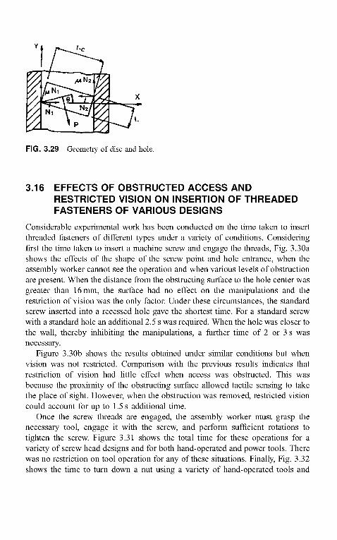
Again, the diameter of the hole is one unit; all other dimensions are measuredrelative to this unit and are dimensionless (Fig. 3.29). The disc diameter is 1 — c,where c is the dimensionless diametral clearance between the mating parts, P isthe resultant force in the assembly operation, and /j. is the coefficient of friction.When a disc with no chamfer is inserted into a hole, the condition for free slidingcan be determined by
L2>n2 + 2c-c2 (3.19)
If c is very small, then Eq. (3.19) can be expressed as
L>n + c/n (3.20)
If the disc is very thin, that is, if
( l - c ) 2 + L 2 < l (3.21)
the disc can be inserted into the hole by keeping its circular cross section parallelto the wall of the hole and reorienting it when it reaches the bottom of the hole.
/uN2
FIG. 3.29 Geometry of disc and hole.
3.16 EFFECTS OF OBSTRUCTED ACCESS ANDRESTRICTED VISION ON INSERTION OF THREADEDFASTENERS OF VARIOUS DESIGNS
Considerable experimental work has been conducted on the time taken to insertthreaded fasteners of different types under a variety of conditions. Consideringfirst the time taken to insert a machine screw and engage the threads, Fig. 3.30ashows the effects of the shape of the screw point and hole entrance, when theassembly worker cannot see the operation and when various levels of obstructionare present. When the distance from the obstructing surface to the hole center wasgreater than 16mm, the surface had no effect on the manipulations and therestriction of vision was the only factor. Under these circumstances, the standardscrew inserted into a recessed hole gave the shortest time. For a standard screwwith a standard hole an additional 2.5 s was required. When the hole was closer tothe wall, thereby inhibiting the manipulations, a further time of 2 or 3 s wasnecessary.
Figure 3.30b shows the results obtained under similar conditions but whenvision was not restricted. Comparison with the previous results indicates thatrestriction of vision had little effect when access was obstructed. This wasbecause the proximity of the obstructing surface allowed tactile sensing to takethe place of sight. However, when the obstruction was removed, restricted visioncould account for up to 1.5s additional time.
Once the screw threads are engaged, the assembly worker must grasp thenecessary tool, engage it with the screw, and perform sufficient rotations totighten the screw. Figure 3.31 shows the total time for these operations for avariety of screw head designs and for both hand-operated and power tools. Therewas no restriction on tool operation for any of these situations. Finally, Fig. 3.32shows the time to turn down a nut using a variety of hand-operated tools and

effect due to restricted vision only
clearance
pilot pointscrewstandardhole
2 4 6 8 10 12 14 16 18 20clearance, mm
(a) Restricted Access and Restricted Vision
8
2 4 6 8 10 12 14 16 18 20clearance, mm
(b) Restricted Access Only
FIG. 3.30 Effects of restricted access and restricted vision on initial engagement ofscrews.
where the operation of the tools was obstructed to various degrees. It can be seenthat the penalties for a box-end wrench are as high as 4 s per revolution whenobstructions are present. However, when considering the design of a new product,the designer will not normally consider the type of tool used and can reasonablyexpect that the best tool for the job will be selected. In the present case this wouldbe either the nut driver or the socket ratchet wrench.

16slot-head 14screws 12
« 10
Philips-head Iscrew g 6
I 4
(^ o- 2
Alien screw
£ = = gfot^erd (power tool)
2 4 6 8 10 12 14number of threads
FIG. 3.31 Effect of number of threads on time to pick up the tool, engage the screw,tighten the screw, and replace the tool.
clearance
u clearance
open-end wrenchI " It
box-end wrench
hex nut driver
socket ratchet wrench
810
k. $
3= 4
box-end wrench
10 20 30 40 50 100 200clearance, mm
FIG. 3.32 Effect of obstructed access on time to tighten a nut.

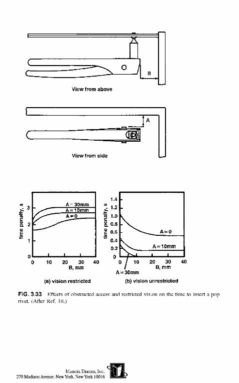
3.17 EFFECTS OF OBSTRUCTED ACCESS ANDRESTRICTED VISION ON POP-RIVETING OPERATIONS
Figure 3.33 summarizes the results of experiments [10] on the time taken toperform pop-riveting operations. In the experiments, the average time taken topick up the tool, change the rivet, move the tool to the correct location, insert therivet and return the tool to its original location was 7.3 s. In Fig. 3.33a thecombined effects of obstructed access and restricted vision are summarized, andFig. 3.33b shows the effects of obstructed access alone. In the latter case, timepenalties of up to I s can be incurred although, unless the clearances are quitesmall, the penalties are negligible. With restricted vision present, much higherpenalties, on the order of 2 to 3 s, were obtained.
3.18 EFFECTS OF HOLDING DOWNHolding down is required when parts are unstable after insertion or duringsubsequent operations. It is defined as a process that, if necessary, it maintains theposition and orientation of parts already in place prior to or during subsequentoperations. The time taken to insert a peg vertically through holes in two or morestacked parts can be expressed as the sum of a basic time tb and a time penalty tp.The basic time is the time to insert the peg when the parts are prealigned and self-locating, as shown in Fig. 3.34a and can be expressed [11] as:
tb = -0.071nc-0.1 + 3.7L + 0.75rfg (3.22)
wherec = (D — d)/D and is the dimensionless clearance (0.1 > c > 0.0001)L = the insertion depth in meters
rfg = the grip size in meters (0.1 m > rfg > 0.01 m).
Example: D = 20mm, d = 19.6mm, c = (D - d)/D = (20 - 19.6)/20 = 0.02,L = 100 mm = 0.10m, dg = 40 mm = 0.04m then
tb = -0.07 In c - 0.1 + 3.7L + Q.15dg
= -0.07In0.02-0.1+3.7 x 0.10+ 0.75 x 0.04= 0.27-0.1+0.37 + 0.03= 0.57 s
The graphs presented in Figs. 3.34 and 3.35 will allow the time penalty tp to bedetermined for three conditions:
When easy-to-align parts have been aligned and require holding down (Fig.3.34b)
View from above
View from side
(B
I 2<u
10
A = 30mmA = 10mmA = 0
20 30B, mm
40
1.4(0
| 1.08.0.8
| 0.6
~ 0.40.2
0(
-
V- ^-^^ A = 0ii v^ A=10mm
^"vj i i) / 10 20 30 4(
/ B, mm
(a) vision restrictedA = 30mm
(b) vision unrestricted
FIG. 3.33 Effects of obstructed access and restricted vision on the time to insert a poprivet. (After Ref. 10.)

(a)Parts self-locatingand pre-aligned
0.8
•0.6
Q. '01
0.2
0.8
0.6
g.0.4Q)
0.2
interfaces (b)easy-to-alignparts
0 0.2 0.4 0.6 0.8 1.0
noteasy-to-alignparts
0 0.2 0.4 0.6 0.8 1.0tb, S
FIG. 3.34 Effects of holding down on insertion time. (After Ref. 11.)
rac<uauE
interfaces
0.2 0.4 0.6 0.8tb,S
1.0
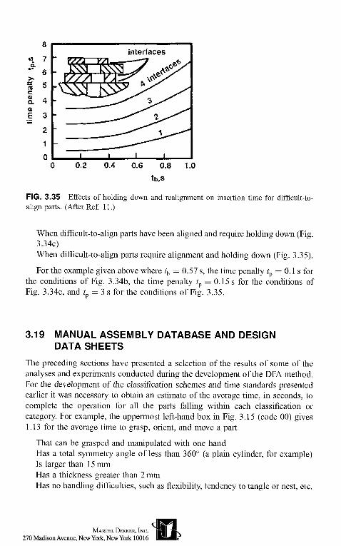
FIG. 3.35 Effects of holding down and realignment on insertion time for difficult-to-align parts. (After Ref. 11.)
When difficult-to-align parts have been aligned and require holding down (Fig.3.34c)When difficult-to-align parts require alignment and holding down (Fig. 3.35).
For the example given above where tb =0.57 s, the time penalty tp = 0.1 s forthe conditions of Fig. 3.34b, the time penalty tp = 0.15 s for the conditions ofFig. 3.34c, and tp = 3 s for the conditions of Fig. 3.35.
3.19 MANUAL ASSEMBLY DATABASE AND DESIGNDATA SHEETS
The preceding sections have presented a selection of the results of some of theanalyses and experiments conducted during the development of the DFA method.For the development of the classification schemes and time standards presentedearlier it was necessary to obtain an estimate of the average time, in seconds, tocomplete the operation for all the parts falling within each classification orcategory. For example, the uppermost left-hand box in Fig. 3.15 (code 00) gives1.13 for the average time to grasp, orient, and move a part
That can be grasped and manipulated with one handHas a total symmetry angle of less than 360° (a plain cylinder, for example)Is larger than 15mmHas a thickness greater than 2 mmHas no handling difficulties, such as flexibility, tendency to tangle or nest, etc.

Clearly, a wide range of parts will fall within this category and their handlingtimes will vary somewhat. The figure presented is only an average time for therange of parts.
To illustrate the type of problem that can arise through the use of the grouptechnology coding or classification scheme employed in the DFA method, we canconsider the assembly of a part having a thickness of 1.9 mm. We shall assumethat, except for its thickness of less than 2 mm, the part would be classified ascode 00 (Fig. 3.15). However, because of the part's thickness, the appropriatecode would be 02 and the estimated handling time would be 1.69 instead of1.13s, representing a time penalty of 0.56s. Turning now to the results ofexperiments for the effect of thickness (Fig. 3.20), it can be seen that for acylindrical part the actual time penalty is on the order of only 0.01 to 0.02 s. Wewould therefore expect an error in our results of about 50%. Under normalcircumstances, experience has shown that these errors tend to cancel—with someparts the error results in an overestimate of time and with some an underestimate.However, if an assembly contains a large number of identical parts, care must betaken to check whether the part characteristics fall close to the limits of theclassification; if they do, then the detailed results presented above should beconsulted.
3.20 APPLICATION OF THE DFA METHODOLOGY
To illustrate how DFA is applied in practice, we shall consider the controllerassembly shown in Fig. 3.36. The assembly of this product first involves securinga series of assemblies to the metal frame using screws, connecting theseassemblies together in various ways and then securing the resulting assemblyinto the plastic cover, again using screws. An undesirable feature of the design ofthe plastic cover is that the small subassemblies must be fastened to the metalframe before the metal frame can be secured to the plastic cover.
Figure 3.37 shows a completed worksheet analysis for the controller in theform of a tabulated list of operations and the corresponding assembly times andcosts. Each assembly operation is divided into handling and insertion, and thecorresponding times and two-digit code numbers for each process are given.Assembly starts by placing the pressure regulator (a purchased item) upside-down into a fixture. The metal frame is placed onto the projecting spindle of thepressure regulator and secured with the nut. The resulting assembly is then turnedover in the fixture to allow for the addition of other items to the metal frame.
Next the sensor and the strap are placed and held in position while two screwsare installed. Clearly, the holding of these two parts and the difficulty of the screwinsertions will impose time penalties on the assembly process.
After tape is applied to the thread on the sensor, the adaptor nut can bescrewed into place. Then one end of the tube assembly is screwed to the threaded

Earth Lead -150x8
Pressure Regulator- 114x58
Connector
Tube Assembly - 55x40x12
Adaptor Nut-25x18
IStrap - 50x20x16
I Screw-10x9
PCB Assembly - 100x40x20
Metal Frame-114x77x51
Plastic Cover - 155x51x51
Knob - 25x25
FIG. 3.36 Controller assembly.
Not to Scale
Dimensions In mm
extension on the pressure regulator and the other end to the adaptor nut. Clearly,both of these are difficult and time-consuming operations.
The printed circuit board (PCB) assembly is now positioned and held in placewhile two screws are installed, after which its connector is snapped into the sensorand the earth lead is snapped into place.
The whole assembly must be turned over once again to allow for thepositioning and holding of the knob assembly while the screw-fastening operationcan be carried out. Finally, the plastic cover is placed in position and the entire

1 . Pressure regulator2. Metal frame3. Nut4. Reorientation5, Sensor6. Strap7. Screw8, Apply tape9. Adapter nut10. Tube assembly11 Screw fastening12. PCB assembly13. Screw14. Connector15. Earth lead16. Reorientation17. Knob assembly18. Screw fastening19 Plastic cover20. Reorientation21. Screw
Mo.ofitemsRP
111111211111211111113
ToolaquiretimeTA
2.9
2.9
2.9-
2.9
2.9_
2.9
-2,9
Hand-lingcode
303000
302011
1042
42113042
_30
30-
11
Hand-lingtimeTH
1.951.951.13
-1.951.801.80
-1.505.60
5.601.801.9S5.60
1,95
1,95-
1,80
Insert-ioncode
000231610303316261106003310505610360036151
Insert-iontimeTl
1.52.65.34.55.25.25.37.010.73.75.25.25.33.33.34.55.25.25.24.510.7
TotaltimeTA+RP-(TH+Tt)
3.454.559.334.507.157,0017.107,0015.109,308,1010.8017.105.258.904.507.158.107.154.5040.4
206.43
Mini-mumpartcount
110
100
00
1000
1
0
05
Place in fixtureAddAdd and screw fastenReorient and adjustAddAdd and hold downAdd and screw fastenSpecial operationAdd and screw fastenAdd and screw fastenStandard operationAdd and hold downAdd and screw fastenAdd and snap fitAdd and snap fitReorient and adjustAdd and hold downStandard operationAdd and hold downReorient and adjustAdd and screw fastenTotals
FIG. 3.37 Completed worksheet analysis for the controller assembly.
assembly is turned over for the third time to allow the three screws to be inserted.It should be noted that access for the insertion of these screws is very restricted.
It is clear from this description of the assembly sequence that many aspects ofthe design could be improved. However, a step-by-step analysis of each operationis necessary before changes to simplify the product structure and reduce assemblydifficulties can be identified and quantified. First we shall look at how thehandling and insertion times are established. The addition of the strap will beconsidered by way of example. This operation is the sixth item on the worksheetand the line of information is completed as follows:
NUMBER OF ITEMS, RP
There is one strap.
HANDLING CODE
The insertion axis for the strap is horizontal in Fig. 3.36 and the strap can onlybe inserted one way along this axis, so the alpha angle of symmetry is 360°. If thestrap is rotated about the axis of insertion, it will repeat its orientation every 180°,which is, therefore, the beta angle of symmetry. Thus, the total angle of symmetryis 540°. Referring to the database for handling time (Fig. 3.15), since the strapcan be grasped and manipulated using one hand without the aid of tools and alphaplus beta is 540°, the first digit of the handling code is 2. The strap presents nohandling difficulties (can be grasped and separated from bulk easily), its thickness

is greater than 2mm, and its size is greater than 15mm; therefore, the seconddigit is 0 giving a handling code of 20.
HANDLING TIME PER ITEM, TH
A handling time of 1.8 s corresponds to a handling code of 20 (Fig. 3.15).
INSERTION CODE
The strap is not secured as part of the insertion process and since there is norestriction to access or vision, the first digit of the insertion code is 0 (Fig. 3.16).Holding down is necessary while subsequent operations are carried out, and thestrap is not easy to align because no features are provided to facilitate alignmentof the screw holes. Therefore, the second digit will be 3, giving an insertion codeof 03.
INSERTION TIME PER ITEM, TI
An insertion time of 5.2s corresponds to an insertion code of 03 (Fig. 3.16).
TOTAL OPERATION TIME
This is the sum of the handling and insertion times multiplied by the numberof items plus tool acquisition time if necessary i.e., TA + RP(TH + TI). For thestrap the total operation time is therefore 7.0 s.
FIGURES FOR MINIMUM PARTS
As explained earlier, the establishment of a theoretical minimum part count isa powerful way to identify possible simplifications in the product structure. Forthe strap the three criteria for separate parts are applied after the pressureregulator, the metal frame, the nut, and the sensor have been assembled.
1. The strap does not move relative to these parts and so it could theoretically becombined with any of them.
2. The strap does not have to be of a different material—in fact it could be ofthe same plastic material as the body of the sensor and therefore take theform of two lugs with holes projecting from the body. At this point in theanalysis the designer would probably determine that since the sensor is apurchased stock item, its design could not be changed. However, it isimportant to ignore these economic considerations at this stage and consideronly theoretical possibilities.
3. The strap clearly does not have to be separate from the sensor in order toallow assembly of the sensor, and therefore none of the three criteria are metand the strap becomes a candidate for elimination. For the strap a zero isplaced in the column for minimum parts.
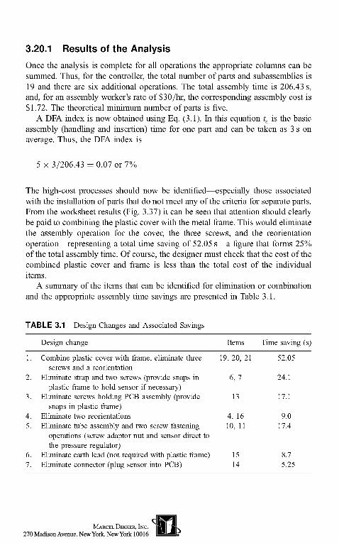
3.20.1 Results of the AnalysisOnce the analysis is complete for all operations the appropriate columns can besummed. Thus, for the controller, the total number of parts and subassemblies is19 and there are six additional operations. The total assembly time is 206.43 s,and, for an assembly worker's rate of $30/hr, the corresponding assembly cost is$1.72. The theoretical minimum number of parts is five.
A DFA index is now obtained using Eq. (3.1). In this equation fa is the basicassembly (handling and insertion) time for one part and can be taken as 3 s onaverage. Thus, the DFA index is
5 x 3/206.43 = 0.07 or 7%
The high-cost processes should now be identified—especially those associatedwith the installation of parts that do not meet any of the criteria for separate parts.From the worksheet results (Fig. 3.37) it can be seen that attention should clearlybe paid to combining the plastic cover with the metal frame. This would eliminatethe assembly operation for the cover, the three screws, and the reorientationoperation—representing a total time saving of 52.05 s—a figure that forms 25%of the total assembly time. Of course, the designer must check that the cost of thecombined plastic cover and frame is less than the total cost of the individualitems.
A summary of the items that can be identified for elimination or combinationand the appropriate assembly time savings are presented in Table 3.1.
TABLE 3.1 Design Changes and Associated Savings
1.
2.
3.
4.5.
6.7.
Design change
Combine plastic cover with frame, eliminate threescrews and a reorientation
Eliminate strap and two screws (provide snaps inplastic frame to hold sensor if necessary)
Eliminate screws holding PCS assembly (providesnaps in plastic frame)
Eliminate two reorientationsEliminate tube assembly and two screw fastening
operations (screw adaptor nut and sensor direct tothe pressure regulator)
Eliminate earth lead (not required with plastic frame)Eliminate connector (plug sensor into PCS)
Items
19, 20, 21
6, 7
13
4, 1610, 11
1514
Time saving (s)
52.05
24.1
17.1
9.017.4
8.75.25

We have now identified design changes that could result in savings of 133.8 sof assembly time, which forms 65% of the total. In addition, several items ofhardware would be eliminated, resulting in reduced part costs. Figure 3.38 showsa conceptual redesign of the controller in which all the proposed design changeshave been made, and Fig. 3.39 presents the corresponding revised worksheet. Thetotal assembly time is now 77.93 s and the assembly efficiency is increased to19%—a fairly respectable figure for this type of assembly. Of course, the designeror design team must now consider the technical and economic consequences ofthe proposed designs.
First there is the effect on the cost of the parts. However, experience shows,and this example would be no exception, that the savings from parts costreduction would be greater than the savings in assembly costs, which in thiscase is $1.07. It should be realized that the documented savings in materials,
Pressure Regulator114x58 \
Plastic Cover155x51x51
PCS Assembly80x50x20
Sensor48x32x32
Through Holesfor Core
Nut - 20x3
I ^*s r *S^rNot to Scale
Dimensions In mm
FIG. 3.38 Conceptual redesign of the controller assembly.
Knob• 25x25
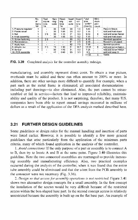
1. Pressure regulator2. Plastic cover3, Nut4 Knob assembly5. Screw fastening6, Reorientation7 Apply tapea Adapter nut9 Sensor10. PCB assembly
No.ofitemsRP
ToolaquiretimeTA
2,9
2.9__
2.9
_
Hand-lingcode
30300030-..
103042
Hand-lingtimeTH
1.951.951.131.95
-..
1.505.955.60
Insert-ioncode
00033103606162513105
Insert-iontimeTl
1.55.25.35.25.24.57.01075.33.3
TotaltimeTA+RP*(TH+TI)
3.457.159.337.158.104.507.0015.107.25e.s
77.93
Mini-mumpartcount
11a1.
n115
Place in fixtureAdd and hold downAdd and screw fastenAdd and hold downStandard operationReorient and adjustSpecial operationAdd and screw fastenAdd and screw fastenAdd and snap fitTotals
FIG. 3.39 Completed analysis for the controller assembly redesign.
manufacturing, and assembly represent direct costs. To obtain a true picture,overheads must be added and these can often amount to 200% or more. Inaddition, there are other savings more difficult to quantify. For example, when apart such as the metal frame is eliminated, all associated documentation—including part drawings—is also eliminated. Also, the part cannot be misas-sembled or fail in service—factors that lead to improved reliability, maintain-ability and quality of the product. It is not surprising, therefore, that many U.S.companies have been able to report annual savings measured in millions ofdollars as a result of the application of the DFA analysis method described here.
3.21 FURTHER DESIGN GUIDELINES
Some guidelines or design rules for the manual handling and insertion of partswere listed earlier. However, it is possible to identify a few more generalguidelines that arise particularly from the application of the minimum partscriteria, many of which found application in the analysis of the controller.
1. Avoid connections'. If the only purpose of a part or assembly is to connect Ato B, then try to locate A and B at the same point. Figure 3.40 illustrates thisguideline. Here the two connected assemblies are rearranged to provide increas-ing assembly and manufacturing efficiency. Also, two practical examplesoccurred during the analysis of the controller, when it was found that the entiretube assembly could be eliminated and that the wires from the PCB assembly tothe connector were not necessary (Fig. 3.36).
2. Design so that access for assembly operations is not restricted: Figure 3.41shows two alternative design concepts for a small assembly. In the first conceptthe installation of the screws would be very difficult because of the restrictedaccess within the box-shaped base part. In the second concept access is relativelyunrestricted because the assembly is built up on the flat base part. An example of

Increased Efficiency
FIG. 3.40 Rearrangement of connected items to improve assembly efficiency and reducecosts.
this type of problem occurred in the controller analysis when the screws securingthe metal frame to the plastic cover were installed (item 21—Fig. 3.37).
3. Avoid adjustments: Figure 3.42 shows two parts of different materialssecured by two screws in such a way that adjustment of the overall length of theassembly is necessary. If the assembly were replaced by one part manufactured
Restricted access for assembly of screws
FIG. 3.41 Design concept to provide easier access during assembly.

Stainless Steel Fingers
1
Low Carbon Steel Bracketadjustment required
Stainless Steel Bracketno adjustment
FIG. 3.42 Design to avoid adjustment during assembly.
from the more expensive material, difficult and costly operations would beavoided. These savings would probably more than offset the increase in materialcosts.
4. Use kinematic design principles'. There are many ways in which theapplication of kinematic design principles can reduce manufacturing and assem-bly cost. Invariably, when located parts are overconstrained, it is necessary eitherto provide a means of adjustment of the constraining items or to employ moreaccurate machining operations. Figure 3.43 shows an example where to locate thesquare block in the plane of the page, six point constraints are used, each onerequiring adjustment. According to kinematic design principles only three pointconstraints are needed together with closing forces. Clearly, the redesign shown inFig. 3.43 is simpler, requiring fewer parts, fewer assembly operations, and lessadjustment. In many circumstances designs where overconstraint is involvedresult in redundant parts. In the design involving overconstraint in Fig. 3.44 one
E
0 0
-TOverconstrained Design Sound Kinematic Design
FIG. 3.43 Showing how overconstraint leads to unnecessary complexity in productdesign.

Over-constrained Kinematically sound
FIG. 3.44 Showing how overconstraint leads to redundancy of parts.
of the pins is redundant. However, application of the minimum parts criteria to thedesign with a single pin would suggest combining the pin with one of the majorparts and combining the washer with the nut.
3.22 LARGE ASSEMBLIES
In the original DFA (design for assembly) method estimates of assembly timewere based on a group technology approach in which design features of parts andproducts were classified into broad categories and, for each category, averagehandling and insertion times were established. Clearly, for any particular opera-tion, these average times can be considerably higher or lower than the actualtimes. However, for assemblies containing a significant number of parts, thedifferences tend to cancel so that the total time will be reasonably accurate. Infact, application of the DFA method in practice has shown that assembly timeestimates are reasonably accurate for small assemblies in low-volume productionwhere all the parts are within easy arm reach of the assembly worker.
Clearly, with large assemblies, the acquisition of the individual parts from theirstorage locations in the assembly area will involve significant additional time.Also, in mass production transfer-line situations, the data for low-volumeproduction will overestimate these times. Obviously, one database of assemblytimes cannot be accurate for all situations.
Let us take one example. From the DFA databases in Figs. 3.15 to 3.17, thetime for acquiring and inserting a standard screw, which is not easy to align, is8.2s. This time includes acquisition of the screw, placing it in the assemblymanually with a couple of turns, acquiring the power tool, operating the tool, andthen replacing it. However, in high-volume production situations, the screws areoften automatically fed, and so the time is reduced to about 3.6 s per screw or, forwell-designed screws, the time per screw can be less than 2 s.
The DFA method was extended to allow for these possibilities, and moreaccurate estimates of assembly times are obtained. However, this can reduce theeffectiveness of the method. In the preceding example, an analysis using theshorter time for screw insertion would indicate that eliminating screws would notbe so advantageous in reducing the assembly time. However, it is known thatsimplifying the product by combining parts and eliminating separate fasteners hasthe greatest benefit through reductions in parts cost rather than through reductionsin assembly cost; yet the suggestions for these improvements arise from analysesof the assembly of the product. Hence, separate fasteners should, perhaps, beseverely penalized even if they take little time to install. In fact, it can be arguedthat in the preceding example, where screws could be inserted quickly, specialequipment was being used to solve problems arising from poor design. This is agood argument for suggesting that early DFA analyses should be carried outassuming that only standard equipment is available. Perhaps later, at the detailed-design stage, attempts can be made to improve the assembly time estimates.Clearly, accurate estimates cannot be made unless detailed descriptions ofmanufacturing and assembly procedures are available—a situation not presentduring the early stages of design when the possibilities for cost savings throughimproved product design are at their greatest. On the other hand, a database ofassembly times suitable for small assemblies measuring only a few inches cannotbe expected to give even approximate estimates for assemblies containing largeparts measuring several feet. It is desirable, therefore, to have databases appro-priate to those situations where the size of the product and the productionconditions differ significantly. Again, it should be realized that great detailregarding the assembly work area will not generally be available to the designerduring the conceptual stages of design.
With these points in mind, the following sections describe an approach to thedevelopment of databases that are used to estimate acquisition and insertion timesfor parts assembled into large products.
3.23 TYPES OF MANUAL ASSEMBLY METHODS
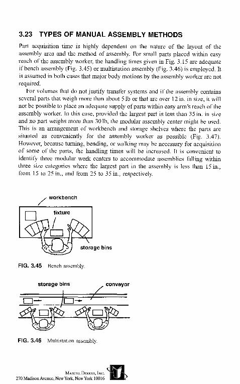
Part acquisition time is highly dependent on the nature of the layout of theassembly area and the method of assembly. For small parts placed within easyreach of the assembly worker, the handling times given in Fig. 3.15 are adequateif bench assembly (Fig. 3.45) or multistation assembly (Fig. 3.46) is employed. Itis assumed in both cases that major body motions by the assembly worker are notrequired.
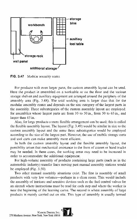
For volumes that do not justify transfer systems and if the assembly containsseveral parts that weigh more than about 5 Ib or that are over 12 in. in size, it willnot be possible to place an adequate supply of parts within easy arm's reach of theassembly worker. In this case, provided the largest part is less than 35 in. in sizeand no part weighs more than 30 Ib, the modular assembly center might be used.This is an arrangement of workbench and storage shelves where the parts aresituated as conveniently for the assembly worker as possible (Fig. 3.47).However, because turning, bending, or walking may be necessary for acquisitionof some of the parts, the handling times will be increased. It is convenient toidentify three modular work centers to accommodate assemblies falling withinthree size categories where the largest part in the assembly is less than 15 in.,from 15 to 25 in., and from 25 to 35 in., respectively.
workbench
\storage bins
FIG. 3.45 Bench assembly.
storage bins conveyor
FIG. 3.46 Multistation assembly.
\
wall
workbench
storage rackjanel
— storagebins
— auxiliarytool table
additional storage'
FIG. 3.47 Modular assembly center.
For products with even larger parts, the custom assembly layout can be used.Here the product is assembled on a worktable or on the floor and the variousstorage shelves and auxiliary equipment are arranged around the periphery of theassembly area (Fig. 3.48). The total working area is larger than that for themodular assembly center and depends on the size category of the largest parts inthe assembly. Three subcategories of the custom assembly layout are employed:for assemblies whose largest parts are from 35 to 50 in., from 50 to 65 in., andlarger than 65 in.
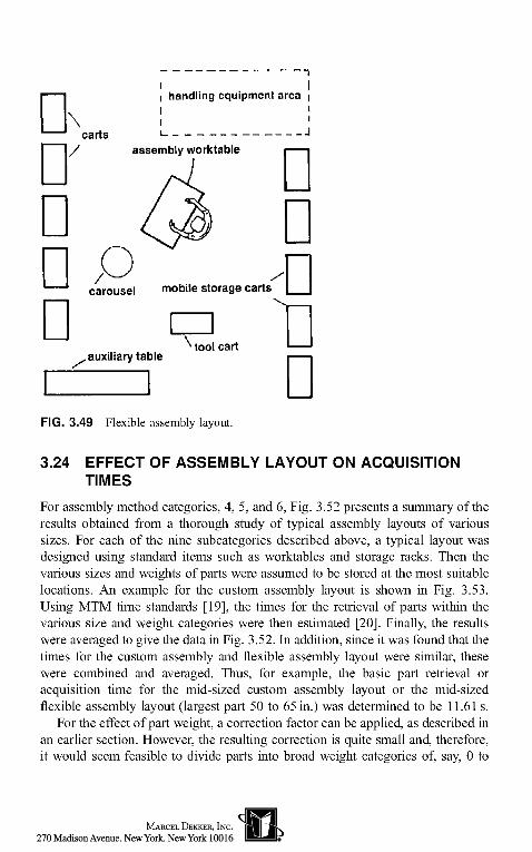
Also, for large products a more flexible arrangement can be used; this is calledthe flexible assembly layout. The layout (Fig. 3.49) would be similar in size to thecustom assembly layout and the same three subcategories would be employedaccording to the size of the largest part. However, the use of mobile storage cartsand tool carts can make assembly more efficient.
In both the custom assembly layout and the flexible assembly layout, thepossibility arises that mechanical assistance in the form of cranes or hand trucksmay be needed. In these cases, the working areas may need to be increased inorder to accommodate the additional equipment.
For high-volume assembly of products containing large parts (such as in theautomobile industry) transfer lines moving past manual assembly stations wouldbe employed (Fig. 3.50).
Two other manual assembly situations exist. The first is assembly of smallproducts with very low volumes—perhaps in a clean room. This would includethe assembly of intricate and sensitive devices such as the fuel control valves foran aircraft where instructions must be read for each step and where the worker isnear the beginning of the learning curve. The second is where assembly of largeproducts is mainly carried out on site. This type of assembly is usually termed

.hopper or utility truck
auxiliary table
storage area
carousel
\assemblywork table
lift table
accessory panel
pedestal jib crane
FIG. 3.48 Custom assembly layout
drumoinstallation, and an example would be the assembly and installation of apassenger elevator in a multistory building.
In any assembly situation, special equipment may be needed. For example, apositioning device is sometimes needed for positioning and aligning the part—especially prior to welding operations. In these cases, the device must be broughtfrom storage within the assembly area, and then returned after the part has beenpositioned and perhaps secured. Thus, the total handling time for the device willbe roughly twice the handling time for the part and must be taken into account ifthe volume to be produced is small.
Figure 3.51 summarizes the basic types of manual assembly methodsdescribed above. It can be seen that the first three methods assume only smallparts are being assembled. In these cases it can be assumed that the parts are allplaced close to hand and will be acquired one-at-a-time. Therefore if, say, sixscrews are to be inserted, there is no advantage in collecting the six screwssimultaneously. However, with the assembly of products containing large parts,where small items such as fasteners may not be located within easy reach orwhere the assembly worker must move to various locations for the small items,there may be considerable advantage in acquiring multiple parts when needed.
handling equipment areaI
\carts
I
assembly worktable
ocarousel mobile storage carts
, auxiliary table* tool cart
DFIG. 3.49 Flexible assembly layout.
3.24 EFFECT OF ASSEMBLY LAYOUT ON ACQUISITIONTIMES
For assembly method categories, 4, 5, and 6, Fig. 3.52 presents a summary of theresults obtained from a thorough study of typical assembly layouts of varioussizes. For each of the nine subcategories described above, a typical layout wasdesigned using standard items such as worktables and storage racks. Then thevarious sizes and weights of parts were assumed to be stored at the most suitablelocations. An example for the custom assembly layout is shown in Fig. 3.53.Using MTM time standards [19], the times for the retrieval of parts within thevarious size and weight categories were then estimated [20]. Finally, the resultswere averaged to give the data in Fig. 3.52. In addition, since it was found that thetimes for the custom assembly and flexible assembly layout were similar, thesewere combined and averaged. Thus, for example, the basic part retrieval oracquisition time for the mid-sized custom assembly layout or the mid-sizedflexible assembly layout (largest part 50 to 65 in.) was determined to be 11.61 s.
For the effect of part weight, a correction factor can be applied, as described inan earlier section. However, the resulting correction is quite small and, therefore,it would seem feasible to divide parts into broad weight categories of, say, 0 to

sub-assembly conveyor
conveyor
tool cart
FIG. 3.50 Multistation assembly of large products.
30 lb and over 30 Ib. The reason for the last category is that such parts wouldnormally require two persons or lifting equipment for handling. Corrected valuesof handling time for the first weight category (0-30 lb) were obtained byassuming an average weight of 15 lb.
For the second weight category, the part requires two persons to handle. Thefigures for this category were obtained by estimating the time for two persons toacquire a part weighing 45 lb, doubling this time, and multiplying the result by afactor of 1.5. This factor allows for the fact that two persons working together willtypically only manage to work in coordination for 67% of their time.
For the third weight category, where lifting equipment is needed, allowancemust be provided for the time taken for the worker to acquire the equipment, useit to acquire the part, move the part to the assembly, release the part, and finallyreturn the lifting equipment to its original location. Figure 3.52 gives theestimated times for these operations, assuming that no increase in the size ofthe assembly area was required in order to accommodate the lifting equipment.These estimates were obtained using the MOST time standard system [21] andincluded the times required to acquire the equipment, move it to the parts'

Manual Assembly[
7 \small parts all within easyarm reach - workers sitting
1. very low volume -clean room or workerat beginning oflearning curve
Z. bench assembly •repetitive work
——13. multi-station assembly |
FIG. 3.51 Manual assembly methods.
large parts - require majorbody motions for acquisition |
mechanical assistancemay be required
4. modular assembly center -largest pan shorter than 35 in,
5. custom assembly Iproducts assembled o
layout - Iid one-at-a*time I
6. flexible assembly layout -products may be assembledin batches
| 7. installation - assembly on site |
18. multi-station assembly |
location, hook the part, transport it to the assembly, unhook the part, and, finally,return the equipment to its original location.
For small parts, where several are required and can be grasped in one hand, itwill usually be advantageous to acquire all the needed parts in one trip to thestorage location. Figure 3.54 presents the results of an experiment where theeffect of the distance traveled by the assembly worker on the acquisition andhandling time per part was studied. It can be seen that when the parts are storedout of easy arm reach, it is preferable to acquire all the parts needed in the one tripto the storage location. From results such as these it is possible to estimateacquisition times for the multiple acquisition of parts stored away from theassembly fixture. Figure 3.52 presents these times for each of the product sizecategories.
In the work [20] leading to the development of Fig. 3.52, the size of the largestpart in the product was assumed to determine the size and nature of the assemblyarea layout. However, to provide an alternative method of identifying the layoutsize, for each layout an average distance from the assembly to the storage locationof the major parts was determined. These averages are listed in the secondcolumn in Fig. 3.52 and provide an alternative method for the determination ofthe appropriate layout.

l !o S"
=
ffi
l fe§-2
- n
I I
8v
So
.
0
35o
8sS
?§
5.stoT~A
Q•o'oPQIIoU•SHO.B•S'CMinCO(5
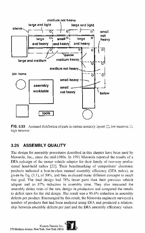
medium not heavylarge and light \ large and light
—" -sj- —— \--oj
large £
bin items
O
— /— n ——— 7 —— if!
large °J small ° i large °and heavy land heavy] and heavy
——$md medium
m
assemblyworktable
|_tools
o!_/—___• __ .j/ ^ below
medium heavy '
edium not heavy^
small heavy -
small — — —not heavy
a
/
\ °
O
— — »
— ---*
n
smallnotheavy
("Ipj
O
befow
FIG. 3.53 Assumed distribution of parts in custom assembly layout: Q, low turnover; O,high turnover.
3.25 ASSEMBLY QUALITY
The design for assembly procedures described in this chapter have been used byMotorola, Inc., since the mid-1980s. In 1991 Motorola reported the results of aDFA redesign of the motor vehicle adapter for their family of two-way profes-sional hand-held radios [22]. Their benchmarking of competitors' electronicproducts indicated a best-in-class manual assembly efficiency (DFA index), asgiven by Eq. (3.1), of 50%, and they evaluated many different concepts to reachthat goal. The final design had 78% fewer parts than their previous vehicleadapter and an 87% reduction in assembly time. They also measured theassembly defect rates of the new design in production and compared the resultsto defect rates for the old design. The result was a 95.6% reduction in assemblydefects per product. Encouraged by this result, the Motorola engineers surveyed anumber of products that had been analyzed using DFA and produced a relation-ship between assembly defects per part and the DFA assembly efficiency values.

O)5
CTO
parts collected and insertedone-at-a-time using one hand
a.o
c 3or0)CO
' I 2 /J^-^r-——\ra ^o——— 5 parts collected simultaneouslyand inserted one-at-a-time using two hands
20 40 60 80 100 in.
0 0.5 1.0 1,5 2.0 2.5mdistance to storage location
FIG. 3.54 Effects of distance to storage location on the acquisition and assembly timefor small parts.
This relationship was discussed in Chapter 1, and as illustrated in Fig. 1.10 showsa strong relationship between assembly quality and the assembly efficiency valueof a product.
These Motorola data were subsequently analyzed independently by otherresearchers [23] to produce an even more powerful relationship for use in earlydesign evaluation. These researchers postulated that since DFA assembly timevalues are related to the difficulty of assembly operations, then the probability ofan assembly error may also be a function of predicted assembly operation times.In the study it was reported that 50 combinations of defect rates versus assemblycharacteristics were tested for meaningful correlation. Of these, the variation ofaverage assembly defect rate per operation with average DFA time estimate peroperation showed the strongest linear correlation, with correlation coefficientr = 0.94. The actual data are shown in Fig. 3.55. The equation of the regressionline is given by
A = O.OOOK/i - 3.3) (3.23)
where £>; = average probability of assembly defect per operationti = average assembly time per operation
As discussed earlier, the average assembly time predicted by the DFA timestandard database, for parts which present no assembly difficulties, is approxi-

Product Design for Manual Assembly 139
-T 0.0014
•§. 0.0012
g- 0.0010
2 0.0008"5f 0.0006
H 0.0004
<: 0.0002
D, = 0.0001 (t-3.3)
5 10 15Average assembly time/operation, t , , s
20
FIG. 3.55 Relation between assembly defect rate and average DFA assembly time.(After Ref. 23.)
mately 3 s. Thus Eq. (3.23) can be interpreted as an estimated assembly defectrate of 0.0001, or 1 in 10,000, for every second of extra time associated withdifficulties of assembly. In fact, if the regression line in Fig. 3.55 is constrained topass through f; = 3, then the correlation coefficient is still 0.94 to two decimalplaces. For this reason we will use 3.0 instead of 3.3 in the expressions andcalculations below.
For a product requiring n assembly operations, the probability of a defectiveproduct, containing one or more assembly errors, is therefore approximately
£>a= 1-[1-0.0001ft-3.0)]" (3.24)Alternatively, the expected number of assembly errors in one of these products isgiven by
Nd = 0.0001ft - 3.0)n (3.25)
These relationships can be applied very easily in the early stages of design tocompare the likely assembly error rates of alternative design concepts for smallproducts assembled in large quantities. This can provide powerful directionalguidance for product quality improvements, since it is becoming widely acceptedthat faulty assembly steps, rather than defective components, are more often thereason for production quality problems [24].
For the controller assembly example discussed earlier, the existing designrequires 25 operations for final assembly and has a total estimated assembly time,

obtained from the DFA analysis, of 206.43 s; see Fig. 3.37. The average time peroperation is thus 206.43/25, equal to 8.26 s. Applying Eq. (3.24) then gives
Da = 1 - [1 - 0.0001(8.26 - 3.0)]25 = 0.0131 (3.26)
Thus, the estimated probability of a defective assembly is 0.0131, or 1.31%.For the redesigned controller assembly, the number of final assembly opera-
tions has been reduced to 10, and the estimated assembly time is 77.93 s; see Fig.3.39. The average time per operation is now 7.8s, and the likely number ofdefective assemblies is given by
Da = 1 - [1 - 0.0001(7.8 - 3.0)]10 = 0.0048 (3.27)
Thus the predicted assembly defect rate is about one-third of that for the originaldesign. This defect rate could be reduced further, by considering detail designimprovements to further decrease the average operation time of 7.8 s.
The expression (ti — 3.Q)n in Eq. (3.25) can be interpreted as the total timepenalty associated with the assembly of a product. For example, for the originaldesign of the controller assembly, the 25 assembly operations would take only75.0 s if there were no assembly difficulties. The total assembly time penalty is(8.25 - 3.0) 25, equal to 131.4 s. Equation (3.25) thus predicts that the assemblydefects per unit will be proportional to the total assembly time penalty. Thisinterpretation is supported by another set of industrial quality data illustrated inFig. 3.56. These data were obtained from a disk drive manufacturer [25], and it
100 200 300 400 500 600 700 800Total assembly time penalty, s
FIG. 3.56 Relation between total DFA assembly time penalty and assembly defect ratesper unit. (After Ref. 26.)

should be noted that one outlier with a defect rate of approximately 65% has beenomitted from the figure. It should also be noted that the slope of the regressionline in Fig. 3.56 is approximately 0.0004. This suggests that the assembly workersare making mistakes at four times the rate of those involved in building theMotorola products. This may be the result of the delicate nature of disk driveassemblies and the need to maintain very small clearances in these devices.
3.26 APPLYING LEARNING CURVES TO THE DFA TIMES
Learning-curve theory applied to industrial production has its roots in earlyaerospace manufacturing. A now-famous paper by T. P. Wright [26] resulted fromthe study of small aircraft construction in the 1920s and 1930s. Wright noted thatas repetitive tasks are performed, improvement occurs at a diminishing rate. Inparticular, he noted that twice as many repetitions are required to achieve eachsuccessive constant incremental improvement. This constant improvement withdoubling is embodied in a simple power law, referred to as the Wright model,which is expressed as
ru = T,xb (3.28)
whereTl x = average time of production for x units
Tl = time of production for the first unitx = number of identical unitsb = the reduction exponent
The reduction exponent can, in turn, take the general form
A = logr/log/ (3.29)
wherer = the average time for a factor increase in output divided by the time for the
first output expressed as a percentage/ = the factor increase in output
Normally a doubling of output is the basis for learning curve analyses, and theimprovement is given as r percent. For this case Eq. (3.29) becomes
b = Iog(r/100)/log2 (3.30)
For example, the often-quoted 90% learning curve represents the situation wherethe average time to produce 2x units will be 90% of the average time taken toproduce the first x of those units. From Eq. (3.30) this gives
A = log0.9/log2 = -0.152

Note that if b is known, then the learning curve percent value is given by theinverse of Eq. (3.30)
r = 2*100% (3.31)
Other forms of learning curve have been proposed and used since the work ofWright; see Refs. [27] and [28]. In particular, in cases where the times forproducing successive individual units are of primary interest a more appropriatemodel may be represented by
Tx = 7X (3.32)
whereT"x = time to produce the xth unitx = number of identical unitsc= "individual" reduction exponent
This alternative model is attributed to Crawford [29], whose work was carried outfor Lockheed Aircraft Corporation. For batch assembly work the Wright model ismore appropriate and will be used below to calculate learning-curve adjustmentsto predicted assembly times.
The reduction exponent represents the improvements that would be expectedas the worker "learns" to operate more efficiently through repetitive identicaltasks. However, Eq. (3.28) can be viewed in a much broader sense as a progressfunction that models progress accomplished through improved process tech-niques, tools, and training methods, as well as the learning associated withrepetitions of the same task [30]. For these situations a learning-curve percentagevalue of 85 is more appropriate than the 90% value typically used to modelworker performance improvement only [27].
The learning-curve equations described above can be used to adjust DFA timesfor situations in which only a few assemblies are to be produced. To carry out thisadjustment, the number of task repetitions, for which the DFA times apply, mustfirst be established. Since the handling and insertion experiments used to obtainthe DFA times were mainly based on 100 task repetitions, this number will beused as the basis for the example calculations below. In other words, it will beassumed that DFA times are equivalent to rljloo times on the appropriate learningcurve. We can thus make learning-curve transformations, using the Wrightmodel, as follows:
ruoo = r1ioo6 (3.33)or
(3.34)

Thus for the first assembly of a small batch B of products, the average time will begiven by the Wright model as
r13 = T,Bb (3.35)
Finally, substituting from Eq.(3.34) for Tl gives
V = Tuoo(B/WO)b (3.36)
whereb = reduction exponent
rljB = adjusted DFA time for batch size BB = total batch to be assembled
Tl 100 = assumed basic DFA time value
Example: A set of only five measuring instruments is to be produced. A DFAanalysis shows an estimated assembly time given by TA. Using a 90% learningcurve, provide an estimate for the average time to build the first two units. Usethis value to determine the average time to assemble the next three units. Assumethat the DFA time estimate would apply well for the average assembly time of 100units.
(a) Substituting TA for Tl 100 in Eq. (3.36) and using b = —0.152 for a 90%learning curve gives
ru = (2/ioo)~°-152rA = i.sirA (3.37)(b) The predicted assembly time for all five units is given by
5 x Jlj2 = 5(5/100r°'152:rA = 7.88rA (3.38)
Similarly the total time for the first two units is
2 x Jlj2 = 2(2/100r(U527A = 3.62rA (3.39)
Thus, the average time for units 3, 4, and 5 can be given byT3j5 = (7.88 - 3.62)74/3 = 1.42JA (3.40)
REFERENCES1. Boothroyd, G., Product Design for Assembly, Department of Mechanical Engineer-
ing, University of Massachusetts, Amherst, 1980.2. Boothroyd, G., Design for Economic Manufacture, Annals CIRP, Vol. 28, No. 1,
1979, p. 345.3. Yoosufani, Z., and Boothroyd, G., Design of Parts for Ease of Handling, Report No. 2,
Department of Mechanical Engineering, University of Massachusetts, September1978.

4. Boothroyd, G., Design for Manual Handling and Assembly, Report No. 4, Departmentof Mechanical Engineering, University of Massachusetts, Amherst, September 1979.
5. Yoosufani, Z., Ruddy, M., and Boothroyd, G., Effect of Part Symmetry on ManualAssembly Times, I Manuf. Syst, Vol. 2, No. 2, 1983, pp. 189-195.
6. Seth, B., and Boothroyd, G., Design for Manual Handling, Report No. 9, Departmentof Mechanical Engineering, University of Massachusetts, January 1979.
7. Ho, C., and Boothroyd, G., Avoiding Jams During Assembly, Machine Des., Tech.Brief, January 25, 1979.
8. Ho, C., and Boothroyd, G., Reducing Disc-Assembly Problems, Machine Des., Tech.Brief, March 8, 1979.
9. Ho, C., and Boothroyd, G., Design of Chamfers for Ease of Assembly, Proc. 7th NorthAmerican Metalworking Conference, May 1979, p. 345.
10. Fujita, T., and Boothroyd, G., Data Sheets and Case Study for Manual Assembly,Report No. 16, Department of Mechanical Engineering, University of Massachusetts,Amherst, April 1982.
11. Yang, S.C., and Boothroyd, G., Data Sheets and Case Study for Manual Assembly,Report No. 15, Department of Mechanical Engineering, University of Massachusetts,Amherst, December 1981.
12. Dvorak, W.A., and Boothroyd, G., Analysis of Product Designs for Ease of ManualAssembly: A Systematic Approach, Report No. 11, Department of MechanicalEngineering, University of Massachusetts, Amherst, May 1982.
13. De Lisser, W.A., and Boothroyd, G., Analysis of Product Designs for Ease of ManualAssembly: A Systematic Approach, Report No. 17, Department of MechanicalEngineering, University of Massachusetts, Amherst, May 1982.
14. Ellison, B., and Boothroyd, G., Applying Design for Assembly Handbook toReciprocating Power Saw and Impact Wrench, Report No. 10, Department ofMechanical Engineering, University of Massachusetts, Amherst, August 1980.
15. Karger, W., and Bayha, EH., Engineered Work Measurement, Industrial Press, Inc.,New York, 1966.
16. Raphael, David L., A Study of Positioning Movements, Research Report No. 109,MTM Association of Standards and Research, Ann Arbor, Michigan, 1957 and 1967.
17. Quick, Joseph H., Work Factor Time Standards, McGraw-Hill, New York, 1962.18. Raphael, D.L., A Study of Arm Movements Involving Weight, Research Report No.
108, MTM Association of Standards and Research, Ann Arbor, Michigan 1955 and1968.
19. Karge, D.W, and Hancock, W.M., Advanced Work Measurement, H.B. Maynard &Co., Pittsburgh, 1982.
20. Fairfield, M.C., and Boothroyd, G., Part Acquisition Time During Assembly of LargeProducts, Report No. 44, Department of Industrial and Manufacturing Engineering,University of Rhode Island, 1991.
21. Zandin, K.B., MOST Work Measurement Systems, 2nd ed., Marcel Dekker, NewYork, 1989.
22. Branan, W, DFA Cuts Assembly Defects by 80%, Appliance Manufacturer, Novem-ber 1991.
23. Barkan, P., and Hinckley, C.M., The Benefits and Limitations of Structured DesignMethodologies, Manufacturing Rev, Vol. 6, No. 3, September 1993.
24. Hinckley, C.M., The Quality Question, Assembly, November 1997.25. Hinckley, C.M., Global Conformance Quality Model, Sandia National Laboratory
Report SAND94-8451, 1994.
26. Wright, T.P., Factors Affecting the Cost of Aeroplanes, J. Aeronaut. Sci., Vol. 3, 49—73, 1936.
27. Teplitz, C.J., The Learning Curve Deskbook, Quorum Books, Westport, CT, 1991.28. Belkaoni, A., The Learning Curve: A Management Accounting Tool, Greenwood
Press, Westport, CT, 1986.29. Crawford, J.R., Learning Curve, Ship Curve, Ratios, Related Data, Lockheed Aircraft
Corporation, Burbank, CA.30. Kniep, J.G., The Maintenance Program Function, J. Ind. Eng., November-December,
1965.