design for testability - ttu.ee · pseudorandom test generation with lfsr ... linear feedback shift...
TRANSCRIPT

Technical University Tallinn, ESTONIA
Overview
1. Introduction2. Testability measuring3. Design for testability
4. Built in Self-Test
Technical University Tallinn, ESTONIA
Built-In Self-Test
Outline• Motivation for BIST• Testing SoC with BIST• Test per Scan and Test per Clock• HW and SW based BIST• Hybrid BIST• Pseudorandom test generation with LFSR• Exhaustive and pseudoexhaustive test generation• Response compaction methods• Signature analyzers

Technical University Tallinn, ESTONIA
Testing Challenges: SoC TestCores have to be tested on chip
Source: ElcoteqSource: Intel

Technical University Tallinn, ESTONIA
Built-In Self-Test
• Advances in microelectronics technologyhave introduced a new paradigm in ICdesign: System-on-Chip (SoC)
• Many systems are nowadays designed byembedding predesigned and preverifiedcomplex functional blocks (cores) intoone single die
• Such a design style allows designers toreuse previous designs and will lead toshorter time-to-market and reduced cost
System-on-Chip
E mD
I n C
C o pc o r
U D L
L e g ac o r e
Dc
Sc o
1 1 4 9 .
U D
SoC structure breakdown:• 10% UDL• 75% memory• 50% in-house cores• 60-70% soft cores

Technical University Tallinn, ESTONIA
Self-Test in Complex Digital Systems
SoC
SRAMPeripheral ComponentInterconnect
SRAM
CPU
WrapperCoreUnderTest
ROM
MPEG UDLDRAM
Test AccessMechanism
Test AccessMechanism
Sink
SoC
Source
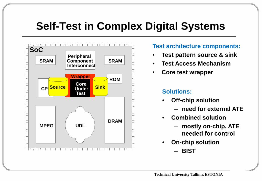
Test architecture components:• Test pattern source & sink• Test Access Mechanism• Core test wrapper
Solutions:• Off-chip solution
– need for external ATE• Combined solution
– mostly on-chip, ATE needed for control
• On-chip solution– BIST
Technical University Tallinn, ESTONIA
Self-Test in Complex Digital Systems
SoC
SRAMPeripheral ComponentInterconnect
SRAM
CPU
WrapperCoreUnderTest
ROM
MPEG UDLDRAM
Sink
SoC
Source
Test architecture components:• Test pattern source & sink• Test Access Mechanism• Core test wrapper
Solutions:• Off-chip solution
– need for external ATE• Combined solution
– mostly on-chip, ATE needed for control
• On-chip solution– BIST

Technical University Tallinn, ESTONIA
What is BIST
• On circuit– Test pattern generation– Response verification
• Random pattern generation, very long tests
• Response compression
BIST Control Unit
Circuitry Under Test
CUT
Test Pattern Generation (TPG)
Test Response Analysis (TRA)
IC

Technical University Tallinn, ESTONIA
SoC BIST
System on Chip
Core 2
Core 3 Core 4 Core 5
Embedded TesterCore 1
Test accessmechanismBIST BIST
BISTBISTBIST
Test Controller
TesterMemory
Optimization:- testing time ↓- memory cost ↓- power consumption ↓- hardware cost ↓- test quality ↑

Technical University Tallinn, ESTONIA
Built-In Self-Test
• Motivations for BIST:– Need for a cost-efficient testing (general motivation)– Doubts about the stuck-at fault model– Increasing difficulties with TPG (Test Pattern Generation)– Growing volume of test pattern data– Cost of ATE (Automatic Test Equipment)– Test application time– Gap between tester and UUT (Unit Under Test) speeds
• Drawbacks of BIST:– Additional pins and silicon area needed– Decreased reliability due to increased silicon area– Performance impact due to additional circuitry– Additional design time and cost

Technical University Tallinn, ESTONIA
Costly Test Problems Alleviated by BIST
• Increasing chip logic-to-pin ratio – harder observability• Increasingly dense devices and faster clocks• Increasing test generation and application times• Increasing size of test vectors stored in ATE• Expensive ATE needed for 1 GHz clocking chips • Hard testability insertion – designers unfamiliar with gate-
level logic, since they design at behavioral level• In-circuit testing no longer technically feasible• Shortage of test engineers• Circuit testing cannot be easily partitioned
Technical University Tallinn, ESTONIA
BIST in Maintenance and Repair
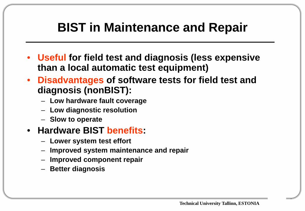
• Useful for field test and diagnosis (less expensive than a local automatic test equipment)
• Disadvantages of software tests for field test and diagnosis (nonBIST):– Low hardware fault coverage– Low diagnostic resolution– Slow to operate
• Hardware BIST benefits:– Lower system test effort– Improved system maintenance and repair– Improved component repair– Better diagnosis
Technical University Tallinn, ESTONIA
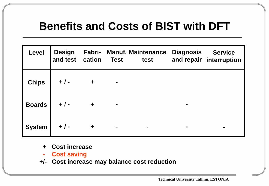
Designand test
+ / -
+ / -
+ / -
Fabri-cation
+
+
+
Manuf.Test
-
-
-
Level
Chips
Boards
System
Maintenancetest
-
Diagnosisand repair
-
-
Serviceinterruption
-
+ Cost increase- Cost saving
+/- Cost increase may balance cost reduction
Benefits and Costs of BIST with DFT
Technical University Tallinn, ESTONIA
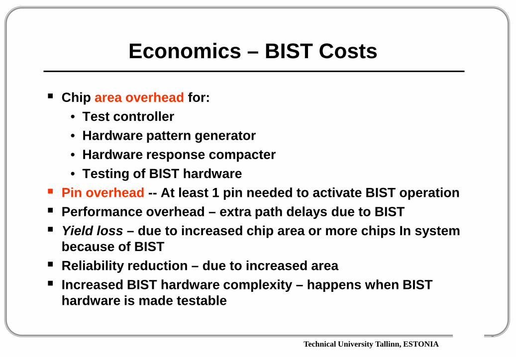
Economics – BIST Costs
Chip area overhead for:• Test controller• Hardware pattern generator• Hardware response compacter• Testing of BIST hardware
Pin overhead -- At least 1 pin needed to activate BIST operation Performance overhead – extra path delays due to BIST Yield loss – due to increased chip area or more chips In system
because of BIST Reliability reduction – due to increased area Increased BIST hardware complexity – happens when BIST
hardware is made testable
Technical University Tallinn, ESTONIA
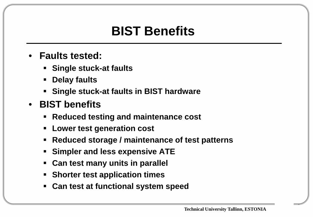
BIST Benefits
• Faults tested: Single stuck-at faults Delay faults Single stuck-at faults in BIST hardware
• BIST benefits Reduced testing and maintenance cost Lower test generation cost Reduced storage / maintenance of test patterns Simpler and less expensive ATE Can test many units in parallel Shorter test application times Can test at functional system speed
Technical University Tallinn, ESTONIA
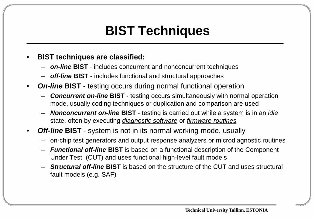
BIST Techniques
• BIST techniques are classified: – on-line BIST - includes concurrent and nonconcurrent techniques– off-line BIST - includes functional and structural approaches
• On-line BIST - testing occurs during normal functional operation– Concurrent on-line BIST - testing occurs simultaneously with normal operation
mode, usually coding techniques or duplication and comparison are used – Nonconcurrent on-line BIST - testing is carried out while a system is in an idle
state, often by executing diagnostic software or firmware routines• Off-line BIST - system is not in its normal working mode, usually
– on-chip test generators and output response analyzers or microdiagnostic routines – Functional off-line BIST is based on a functional description of the Component
Under Test (CUT) and uses functional high-level fault models – Structural off-line BIST is based on the structure of the CUT and uses structural
fault models (e.g. SAF)

Technical University Tallinn, ESTONIA
General Architecture of BIST
BIST Control Unit
Circuitry Under Test
CUT
Test Pattern Generation (TPG)
Test Response Analysis (TRA)
• BIST components:– Test pattern generator
(TPG)– Test response
analyzer (TRA)• TPG & TRA are usually
implemented as linear feedback shift registers (LFSR)
• Two widespread schemes:
– test-per-scan– test-per-clock

Technical University Tallinn, ESTONIA
Detailed BIST Architecture
Source: VLSI Test: Bushnell-Agrawal

Technical University Tallinn, ESTONIA
Built-In Self-Test
Scan Path
Scan Path
Scan Path
.
.
.
CUT
Test pattern generator
Test response analysator
BIST Control
• Assumes existing scan architecture
• Drawback:– Long test application time
Test per Scan:
Initial test set:
T1: 1100T2: 1010T3: 0101T4: 1001
Test application:
1100 T 1010 T 0101T 1001 TNumber of clocks = 4 x 4 + 4 = 20
Technical University Tallinn, ESTONIA
Scan-Path Design
Combinational circuit
IN OUT
R
Scan-IN
Scan-OUT
1&&
q
qScan-IN
T
TDC
Scan-OUT
q’
q’
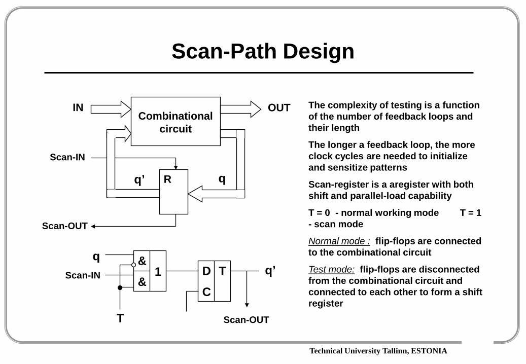
The complexity of testing is a function of the number of feedback loops and their length
The longer a feedback loop, the more clock cycles are needed to initialize and sensitize patterns
Scan-register is a aregister with both shift and parallel-load capability
T = 0 - normal working mode T = 1 - scan mode
Normal mode : flip-flops are connected to the combinational circuit
Test mode: flip-flops are disconnected from the combinational circuit and connected to each other to form a shift register

Technical University Tallinn, ESTONIA
Built-In Self-Test
Test per Clock:• Initial test set:
• T1: 1100• T2: 1010• T3: 0101• T4: 1001
• Test application:
• 1 10 0 1 0 1 0 01 01 1001 •
• T1 T4 T3 T2• Number of clocks = 10
Combinational Circuit
Under Test
Scan-Path Register

Technical University Tallinn, ESTONIA
BILBO BIST Architecture
Working modes:
B1 B20 0 Reset0 1 Flip-flop (normal)1 0 Scan mode1 1 Test mode
Testing modes:
CC1: LFSR 1 - TPGLFSR 2 - SA
CC2: LFSR 2 - TPGLFSR 1 - SA
LFSR 1
CC1
LFSR 2
CC2
B1B2
B1B2
Technical University Tallinn, ESTONIA
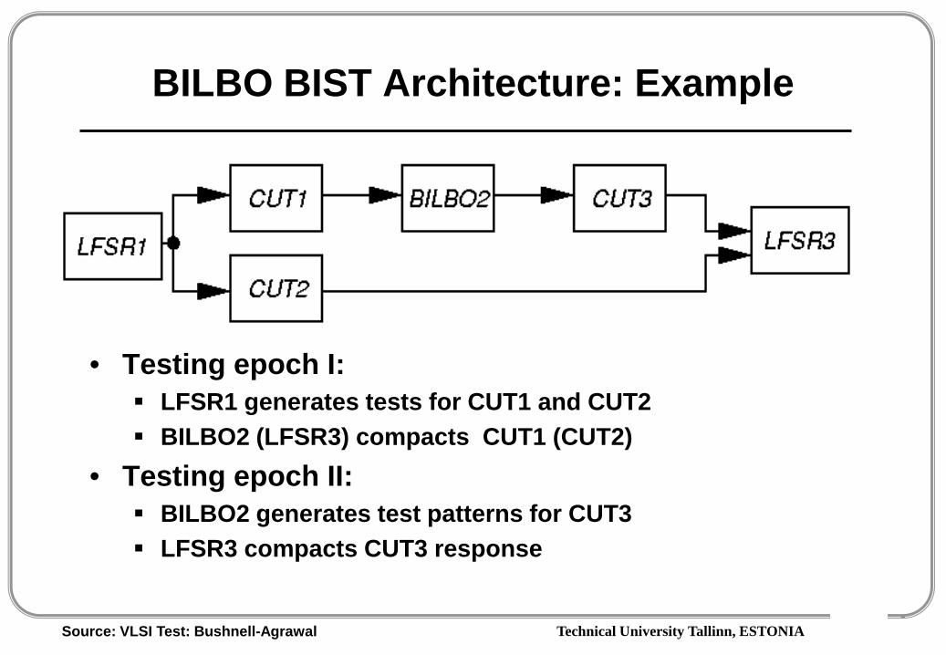
BILBO BIST Architecture: Example
• Testing epoch I: LFSR1 generates tests for CUT1 and CUT2 BILBO2 (LFSR3) compacts CUT1 (CUT2)
• Testing epoch II: BILBO2 generates test patterns for CUT3 LFSR3 compacts CUT3 response
Source: VLSI Test: Bushnell-Agrawal
Technical University Tallinn, ESTONIA
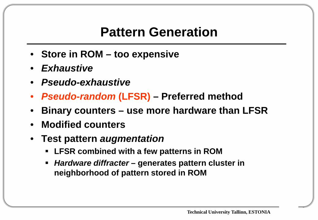
Pattern Generation• Store in ROM – too expensive• Exhaustive• Pseudo-exhaustive• Pseudo-random (LFSR) – Preferred method• Binary counters – use more hardware than LFSR• Modified counters• Test pattern augmentation
LFSR combined with a few patterns in ROM Hardware diffracter – generates pattern cluster in
neighborhood of pattern stored in ROM

Technical University Tallinn, ESTONIA
Pattern Generation
Pseudorandom Test generation by LFSR:
CUT
LFSR
LFSR
X1Xo Xn. . .
ho h1 hn
. . .
• Using special LFSR registers• Several proposals:
– BILBO– CSTP
• Main characteristics of LFSR:– polynomial– initial state– test length

Technical University Tallinn, ESTONIA
Some Definitions
• LFSR – Linear feedback shift register, hardware that generates pseudo-random pattern sequence
• BILBO – Built-in logic block observer, extra hardware added to flip-flops so they can be reconfigured as an LFSR pattern generator or response compacter, a scan chain, or as flip-flops
• Exhaustive testing – Apply all possible 2n patterns to a circuit with n inputs
• Pseudo-exhaustive testing – Break circuit into small, overlapping blocks and test each exhaustively
• Pseudo-random testing – Algorithmic pattern generator that produces a subset of all possible tests with most of the properties of randomly-generated patterns

Technical University Tallinn, ESTONIA
More Definitions
• Irreducible polynomial – Boolean polynomial that cannot be factored• Primitive polynomial – Boolean polynomial p(x) that can be used to
compute increasing powers n of xn modulo p(x) to obtain all possiblenon-zero polynomials of degree less than p(x)
• Signature – Any statistical circuit property distinguishing between bad and good circuits
• TPG – Hardware test pattern generator• PRPG – Hardware Pseudo-Random Pattern Generator• MISR – Multiple Input Response Analyzer

Technical University Tallinn, ESTONIA
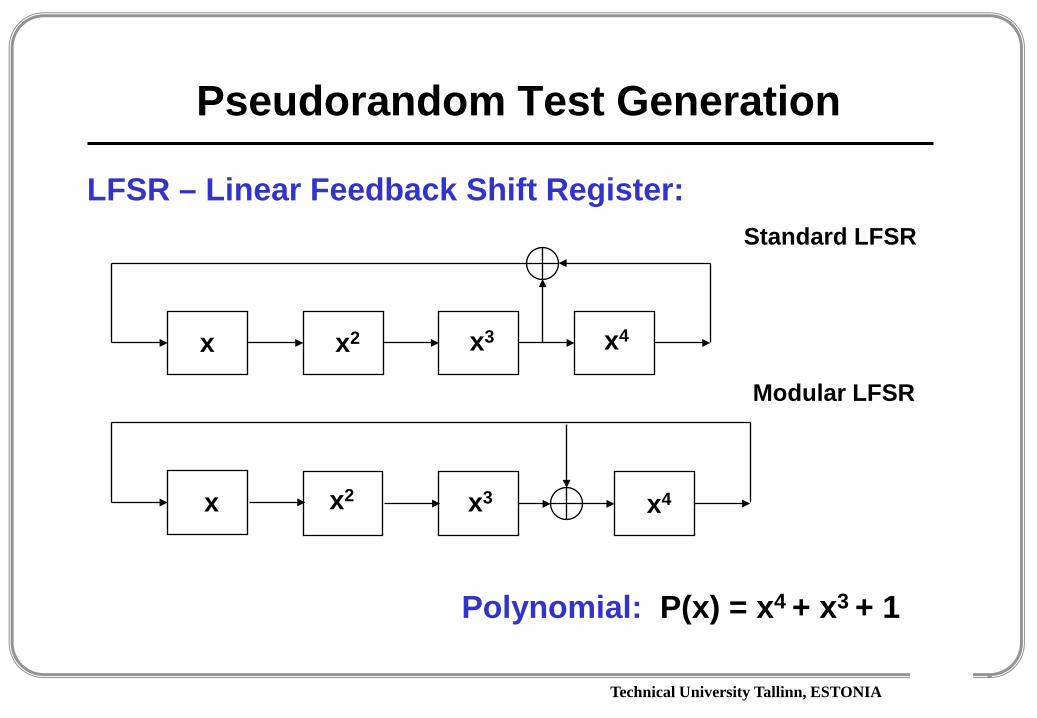
Pseudorandom Test Generation
LFSR – Linear Feedback Shift Register:
x x2 x3 x4
x3x2 x4x
Polynomial: P(x) = x4 + x3 + 1
Standard LFSR
Modular LFSR
Technical University Tallinn, ESTONIA
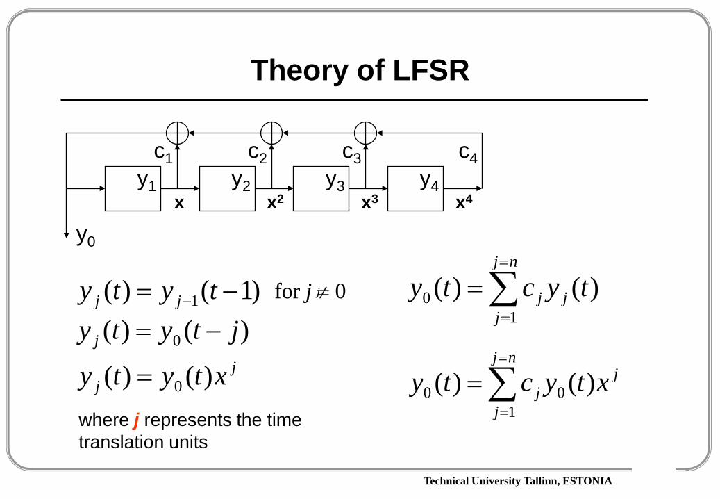
Theory of LFSR
y0
y1 y2 y3 y4
c4c3c2c1
)1()( 1 −= − tyty jj
jj xtyty )()( 0=
x x2 x3 x4
)()(1
0 tycty j
nj
jj∑
=
=
=
jnj
jj xtycty )()( 0
10 ∑
=
=
=
jfor j ≠ 0
)()( 0 jtyty j −=
where j represents the time translation units

Technical University Tallinn, ESTONIA
Theory of LFSR
y0
y1 y2 y3 y4
c4c3c2c1
x x2 x3 x4
jnj
jj xctyty ∑
=
=
=1
00 )()(
jnj
jj xtycty )()( 0
10 ∑
=
=
=0)1)((
10 =+∑
=
=
jnj
jj xcty
Polynomial:
0)()(0 =xPty n

Technical University Tallinn, ESTONIA
Theory of LFSR
y0
y1 y2 y3 y4
c4c3c2c1
x x2 x3 x4
0)()(0 =xPty nj
nj
jjn
n
xcxP
xPty
∑=
=
+=
=≠
1
0
1)( where
0)( 0)(For
Characteristic polynomial:

Technical University Tallinn, ESTONIA
Pseudorandom Test Generation
LFSR – Linear Feedback Shift Register:
x x2 x3 x4
Polynomial: P(x) = x4 + x3 + 1

Technical University Tallinn, ESTONIA
Matrix Equation for Standard LFSR
Xn (t + 1)Xn-1 (t + 1)...X3 (t + 1)X2 (t + 1)X1 (t + 1)
10...00
hn-1
01...00
hn-2
00...001
……
………
00...10h2
00...01h1
Xn (t)Xn-1 (t)...X3 (t)X2 (t)X1 (t)
=
X (t + 1) = Ts X (t) (Ts is companion matrix)
x x2 x3 x4

Technical University Tallinn, ESTONIA
Pseudorandom Test Generation
x x2 x3 x4
Polynomial: P(x) = x4 + x3 + 1
X4 (t + 1)X3 (t + 1)X2 (t + 1)X1 (t + 1)
100h3
010h2
0001
001h1
=
X4 (t)X3 (t)X2 (t)X1 (t)
t x x2 x3 x4 t x x2 x3 x4
1 0 0 0 1 9 0 1 0 12 1 0 0 0 10 1 0 1 03 0 1 0 0 11 1 1 0 14 0 0 1 0 12 1 1 1 05 1 0 0 1 13 1 1 1 16 1 1 0 0 14 0 1 1 17 0 1 1 0 15 0 0 1 18 1 0 1 1 16 0 0 0 1
1 0 0

Technical University Tallinn, ESTONIA
• Irreducible polynomial – cannot be factored, is divisible only by itself
• Irreducible polynomial of degree n is characterized by:– An odd number of terms including 1 term– Divisibility into 1 + xk, where k = 2n – 1
• Any polynomial with all even exponents can be factored and hence is reducible
• An irreducible polynomial is primitive if it divides the polynomial 1+xk for k = 2n – 1, but not for any smaller positive integer k
Theory of LFSR: Primitive Polynomials
Properties of Polynomials:
Technical University Tallinn, ESTONIA
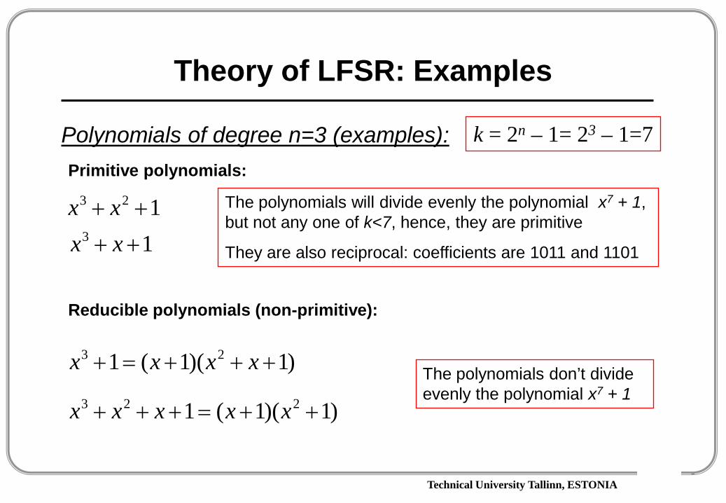
Theory of LFSR: Examples
Polynomials of degree n=3 (examples):
123 ++ xx
Primitive polynomials:
13 ++ xx
The polynomials will divide evenly the polynomial x7 + 1, but not any one of k<7, hence, they are primitive
They are also reciprocal: coefficients are 1011 and 1101
Reducible polynomials (non-primitive):
)1)(1(1
)1)(1(1
223
23
++=+++
+++=+
xxxxx
xxxx
k = 2n – 1= 23 – 1=7
The polynomials don’t divide evenly the polynomial x7 + 1

Technical University Tallinn, ESTONIA
Theory of LFSR: Examples
100110111011101010001100
100010101110111011001100
100010001100010001100010
100110011001100110011001
Comparison of test sequences generated:
123 ++ xxPrimitive polynomials
13 ++ xx 1 1 233 ++++ xxxxNon-primitive polynomials
Technical University Tallinn, ESTONIA
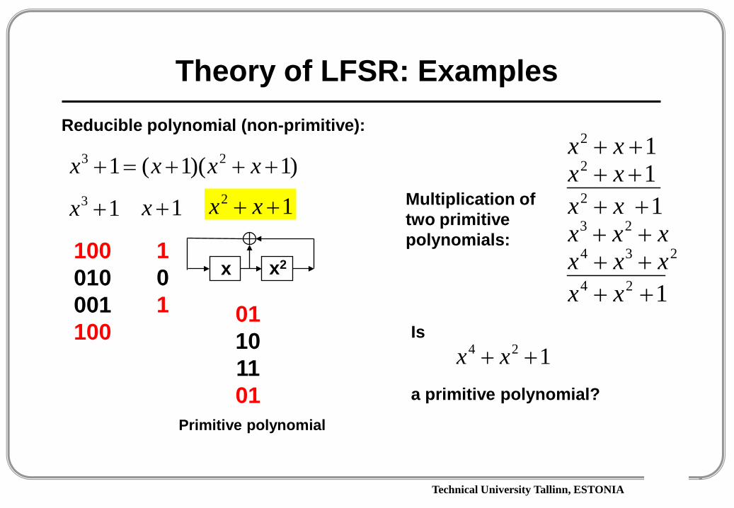
Theory of LFSR: ExamplesReducible polynomial (non-primitive):
)1)(1(1 23 +++=+ xxxx
100010001100
101 01
101101
x x2
13 +x 12 ++ xx1+x
Primitive polynomial
Multiplication of two primitive polynomials:
1
1 11
24
234
23
2
2
2
++++++++++++
xxxxxxxx
xxxxxx
Is124 ++ xx
a primitive polynomial?

Technical University Tallinn, ESTONIA
Theory of LFSR: Examples
Is a primitive polynimial?124 ++ xx
1
1
1
1
1
3
357
57
579
9
91113
1113
111315
15
+++++++
+++++++
+
xxxx
xxxxx
xxxx
xxxxx
x
35911 xxxx +++
124 ++ xxIrreducible polynomial of degree n is characterized by:
- An odd number of terms including 1 term?
Yes, it includes 3 terms
-Divisibility into 1 + xk, where k = 2n – 1
No, there is remainder
Divisibility check:
13 +x
is non-primitive?124 ++ xx
Technical University Tallinn, ESTONIA
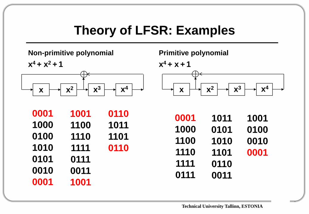
Non-primitive polynomialx4 + x2 + 1
Theory of LFSR: Examples
x x2 x3 x4
0001100001001010010100100001
1001110011101111011100111001
0110101111010110
Primitive polynomialx4 + x + 1
x x2 x3 x4
000110001100111011110111
101101011010110101100011
1001010000100001
Technical University Tallinn, ESTONIA
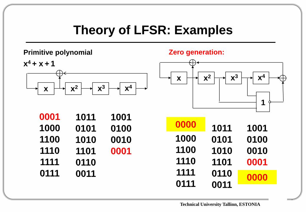
Theory of LFSR: ExamplesPrimitive polynomialx4 + x + 1
x x2 x3 x4
000110001100111011110111
101101011010110101100011
1001010000100001
Zero generation:
x x2 x3 x4
1
10001100111011110111
101101011010110101100011
10010100001000010000
0000

Technical University Tallinn, ESTONIA
Theory of LFSR: Reciprocal PolynomialsThe reciprocal polynomial of P(X) is defined by:
(X) =XN PN (1/X) = XN {1 + Cj X-J}
(X) = XN + Cj XN-J for 1 ≤ i ≤ N
Thus every coefficient Ci in P(X) is replaced by CN-I.
Example:The reciprocal of polynomial P3(X) = 1 + X + X3
is P’3 (X) = 1 + X2 + X3
The reciprocal of a primitive polynomial is also primitive

Technical University Tallinn, ESTONIA
Theory of LFSR: Primitive Polynomials
Number of primitive polynomials of degree N
N No1 12 14 28 16
16 204832 67108864
N Primitive Polynomials1,2,3,4,6,7,15,22 1 + X + Xn
5,11, 21, 29 1 + X2 + Xn
10,17,20,25,28,31 1 + X3 + Xn
9 1 + X4 + Xn
23 1 + X5 + Xn
18 1 + X7 + Xn
8 1 + X2 + X3 + X4 + Xn
12 1 + X + X3 + X4 + Xn
13 1 + X + X4 + X6 + Xn
14, 16 1 + X + X3 + X4 + Xn
Table of primitive polynomials up to degree 31
Technical University Tallinn, ESTONIA
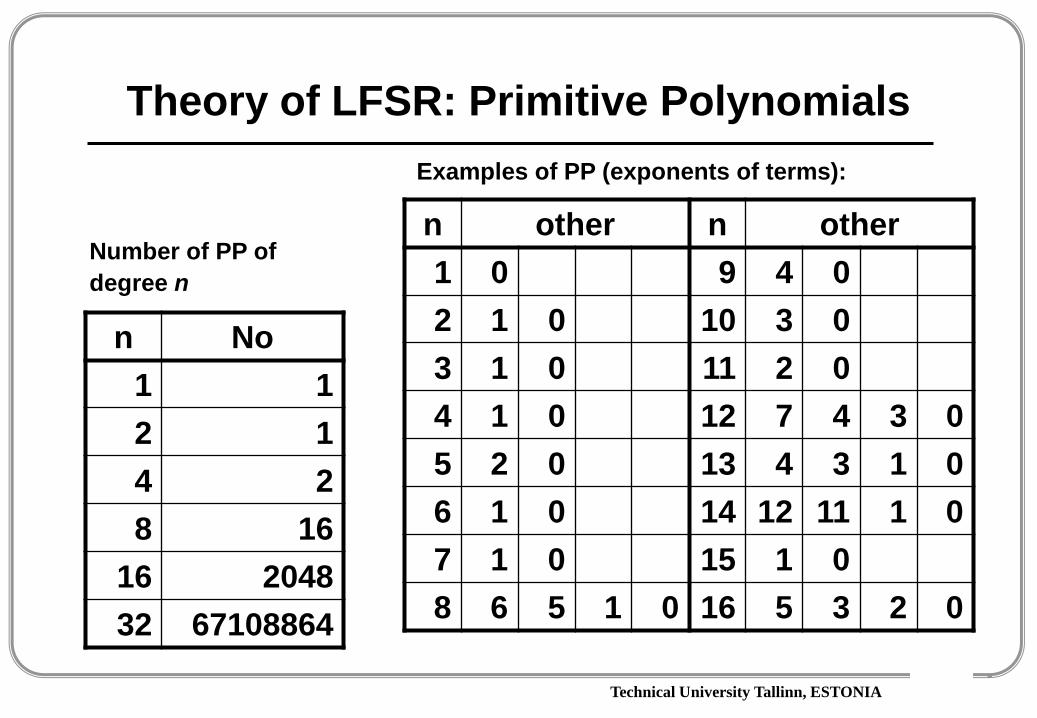
Theory of LFSR: Primitive Polynomials
Number of PP of degree n
n No1 12 14 28 16
16 204832 67108864
Examples of PP (exponents of terms):
n other n other1 0 9 4 02 1 0 10 3 03 1 0 11 2 04 1 0 12 7 4 3 05 2 0 13 4 3 1 06 1 0 14 12 11 1 07 1 0 15 1 08 6 5 1 0 16 5 3 2 0
Technical University Tallinn, ESTONIA
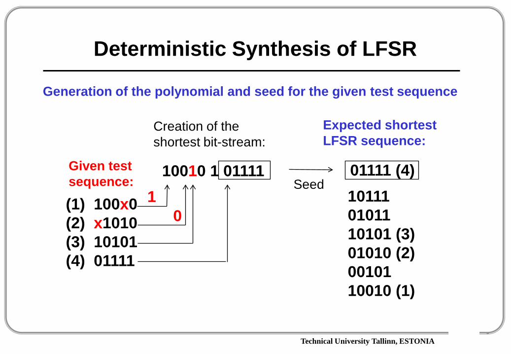
Deterministic Synthesis of LFSR
Generation of the polynomial and seed for the given test sequence
(1) 100x0(2) x1010(3) 10101(4) 01111
Given test sequence:
Creation of the shortest bit-stream:
Expected shortest LFSR sequence:
10010 1 011111
0
01111 (4)101110101110101 (3)01010 (2)0010110010 (1)
Seed
Technical University Tallinn, ESTONIA
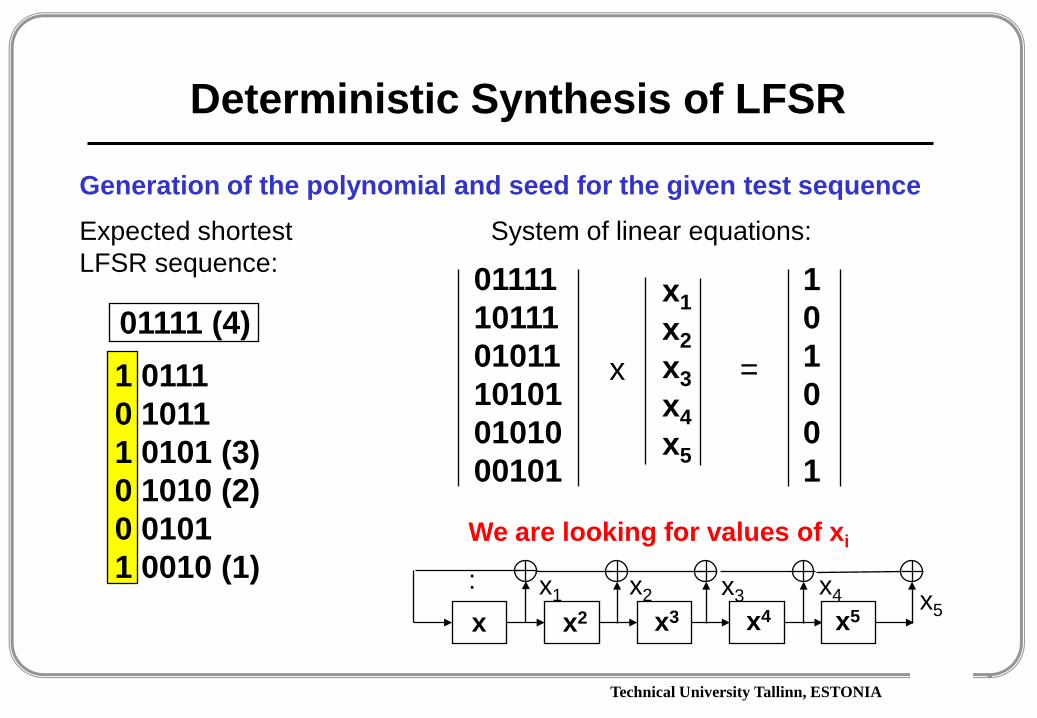
Deterministic Synthesis of LFSR
Expected shortest LFSR sequence:
01111 (4)1 01110 10111 0101 (3)0 1010 (2)0 01011 0010 (1)
011111011101011101010101000101
System of linear equations:
Generation of the polynomial and seed for the given test sequence
x
x1x2x3x4x5
101001
=
x x2 x3 x4 x5x1 x2 x3 x4 x5
We are looking for values of xi
:

Technical University Tallinn, ESTONIA
Deterministic Synthesis of LFSR
011111011101011101010101000101
System of linear equations:
Generation of the polynomial and seed for the given test sequence
x
x1x2x3x4x5
101001
=
x x2 x3 x4 x5x1 x5
010001000000100000100000100001
Solving the equation by Gaussian elimination:
x
x1x2x3x4x5
010011
=
123456
1,2,4,64,61,32,41,2,3,4,6
Polynomial: x5 + x + 1 Seed: 01111Solution: x1 x2 x3 x4 x5
1 0 0 0 1

Technical University Tallinn, ESTONIA
Deterministic Synthesis of LFSR
Embedding deterministic test patterns into LFSR sequence:
x x2 x3 x4 x5x1 x5
Polynomial: x5 + x + 1 Seed: 01111
(1) 100x0(2) x1010(3) 10101(4) 01111
Given deterministic test sequence:
LFSR sequence:
(1) 01111 (4)(2) 10111(3) 01011(4) 10101 (3)(5) 01010 (2)(6) 00101(7) 10010 (1)

Technical University Tallinn, ESTONIA
BIST: Test Generation
Problems:• Very long test
application time• Low fault coverage• Area overhead• Additional delay
Pseudorandom Test generation by LFSR:
Possible solutions • Weighted pattern PRPG• Combining pseudorandom
test with deterministic test– Multiple seed– Hybrid BIST
Time
Faul
t Cov
erag
e
Time
Faul
t Cov
erag
e
breakpoint
Technical University Tallinn, ESTONIA
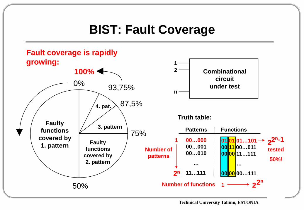
BIST: Fault CoverageFault coverage is rapidly growing: 1
2
n
Combinational circuit
under test
Truth table:
Patterns
00…00000…001 00…010
…
11…111
Functions
01 01 01…10100 11 00…011 00 00 11…111
…
00 00 00…111 2n
1
1 2n2
Number of patterns
Number of functions
2n-12tested
50%!
0%
Faulty functions
covered by 1. pattern Faulty
functions covered by 2. pattern
50%
75%3. pattern
4. pat. 87,5%
93,75%
100%

Technical University Tallinn, ESTONIA
BIST: Fault Coverage
Time
Faul
t Cov
erag
e
Pseudorandom Test generation by LFSR:
Reasons of the high initial efficiency:
A circuit may implement functions
A test vector partitions the functions into 2 equal sized equivalence classes (correct circuit in one of them)
The second vector partitions into 4 classes etc.
After m patterns the fraction of functions distinguished from the correct function is
n22
Motivation of using LFSR:
- low generation cost- high initial efeciency
,212
11
22 ∑
=
−
−
m
i
in
nnm 21 ≤≤

Technical University Tallinn, ESTONIA
BIST: Different Techniques
Pseudorandom testing of sequential circuits:The following rules suggested:• clock-signals should not be random• control signals such as reset, should be activated
with low probability• data signals may be chosen randomlyMicroprocessor testing• A test generator picks randomly an instruction
and generates random data patterns• By repeating this sequence a specified number of
times it will produce a test program which will test the microprocessor by randomly excercising its logic
Pseudorandom Test generation by LFSR:
Full identification is achieved only after 2n input combinations have been tried out (exhaustive test)
A better fault model (stuck-at-0/1)may limit the number of partitions necessary
,212
11
122 ∑
=
−
−
m
i
n
n
nm 21 ≤≤

Technical University Tallinn, ESTONIA
BIST: Structural Approach to Test
Testing of structural faults: 12
n
Combinational circuit
under test
Fault coverage
100%
Number of patterns
4
4. pat.Not tested
faults
Faults covered by 1. pattern
2. pattern
3. patttern

Technical University Tallinn, ESTONIA
BIST: Two Approaches to Test
Testing of functions:
100% will be reached onlyafter 2n test patterns
Testing of faults:
100% will be reached when all faults from the fault list are covered
0%
Faulty functions
covered by 1. pattern Faulty
functions covered by 2. pattern
50%
75%3. pattern
4. pat. 87,5%
93,75%
100%
100%
Testing of faults
Testing of functions
4. pat.Not tested
faults
Faults covered by 1. pattern
2. pattern
3. patttern

Technical University Tallinn, ESTONIA
BIST: Other test generation methodsUniversal test sets
1. Exhaustive test (trivial test)2. Pseudo-exhaustive test
Properties of exhaustive tests1. Advantages (concerning the stuck at fault model):
- test pattern generation is not needed- fault simulation is not needed- no need for a fault model- redundancy problem is eliminated- single and multiple stuck-at fault coverage is 100%- easily generated on-line by hardware
2. Shortcomings:- long test length (2n patterns are needed, n - is the number of inputs)- CMOS stuck-open fault problem

Technical University Tallinn, ESTONIA
BIST: Other test generation methods
Pseudo-exhaustive test sets:– Output function verification
• maximal parallel testability• partial parallel testability
– Segment function verification
Output function verification
4
4
4
4
216 = 65536 >> 4x16 = 64 > 16 Exhaustive
testPseudo-
exhaustivesequential
Segment function verification
F &1111
01010011
Pseudo-exhaustive
parallel
Primitive polynomials
Technical University Tallinn, ESTONIA
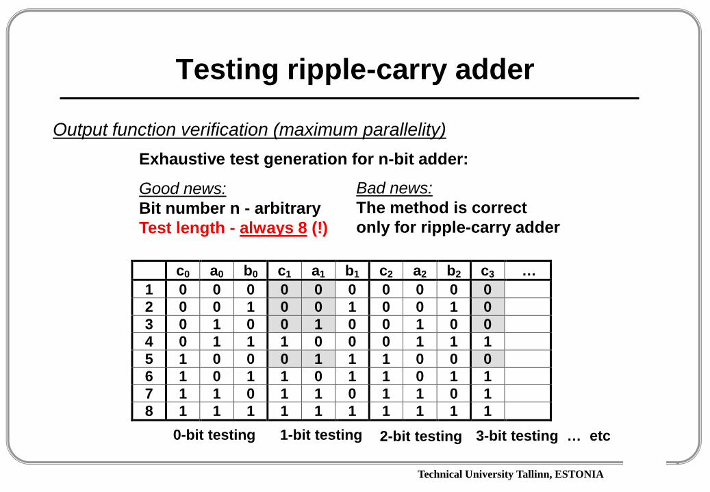
Testing ripple-carry adder
Output function verification (maximum parallelity)
c0 a0 b0 c1 a1 b1 c2 a2 b2 c3 …1 0 0 0 0 0 0 0 0 0 02 0 0 1 0 0 1 0 0 1 03 0 1 0 0 1 0 0 1 0 04 0 1 1 1 0 0 0 1 1 15 1 0 0 0 1 1 1 0 0 06 1 0 1 1 0 1 1 0 1 17 1 1 0 1 1 0 1 1 0 18 1 1 1 1 1 1 1 1 1 1
Exhaustive test generation for n-bit adder:
Good news:Bit number n - arbitraryTest length - always 8 (!)
0-bit testing 2-bit testing1-bit testing 3-bit testing … etc
Bad news:The method is correctonly for ripple-carry adder
Technical University Tallinn, ESTONIA
Testing carry-lookahead adder
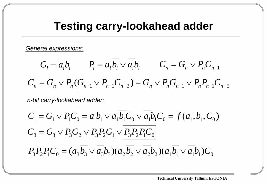
General expressions:
iii baG = iiiii babaP ∨= 1−∨= nnnn CPGC
211211 )( −−−−−− ∨∨=∨∨= nnnnnnnnnnnn CPPGPGCPGPGC
n-bit carry-lookahead adder:
01231232333 CPPPGPPGPGC ∨∨∨=
),,( 011011011110111 CbafCbaCbabaCPGC =∨∨=∨=
01111222233330123 ))()(( CbabababababaCPPP ∨∨∨=
Technical University Tallinn, ESTONIA
Testing carry-lookahead adder
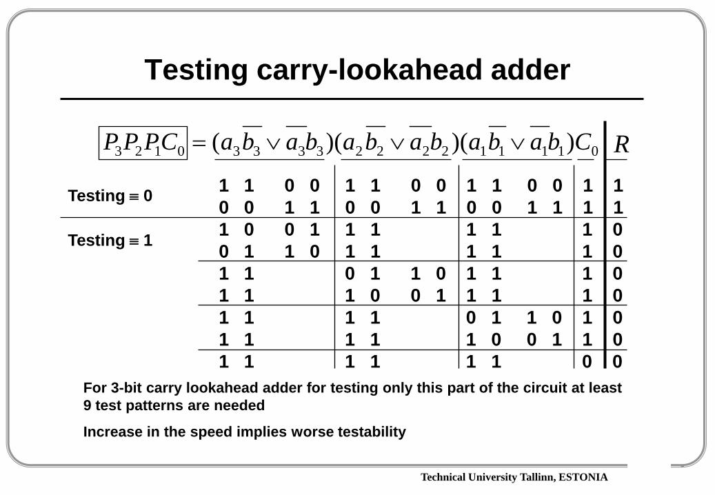
01111222233330123 ))()(( CbabababababaCPPP ∨∨∨=
1 1 0 0 1 1 0 0 1 1 0 0 1 1 0 0 1 1 0 0 1 1 0 0 1 1 1 11 0 0 1 1 1 1 1 1 00 1 1 0 1 1 1 1 1 01 1 0 1 1 0 1 1 1 0 1 1 1 0 0 1 1 1 1 01 1 1 1 0 1 1 0 1 01 1 1 1 1 0 0 1 1 01 1 1 1 1 1 0 0
For 3-bit carry lookahead adder for testing only this part of the circuit at least 9 test patterns are needed
Increase in the speed implies worse testability
Testing ≡ 0
Testing ≡ 1
R

Technical University Tallinn, ESTONIA
BIST: Other test generation methods
Output function verification (partial parallelity)
x1
x2
x3
x4
F1(x1, x2)F2(x1, x3)F3(x2, x3)F4(x2, x4)F5(x1, x4)F6(x3, x4)
0011- -
010101
010110
00-11-000111
0011- 0F1
F3
F2
F4F5
Exhaustive testing - 16Pseudo-exhaustive, full parallel - 4Pseudo-exhaustive, partially parallel - 6

Technical University Tallinn, ESTONIA
Problems with Pseudorandom Test
Time
Fau
lt C
ove
rag
e
Problem: low fault coverageThe main motivations of using random patterns are:
- low generation cost- high initial efeciency
Counter
Decoder
&
LFSR
Reset
If Reset = 1 signal has probability 0,5 then counter will not work and 1 for AND gate may never be produced
1
Technical University Tallinn, ESTONIA
Sequential BIST
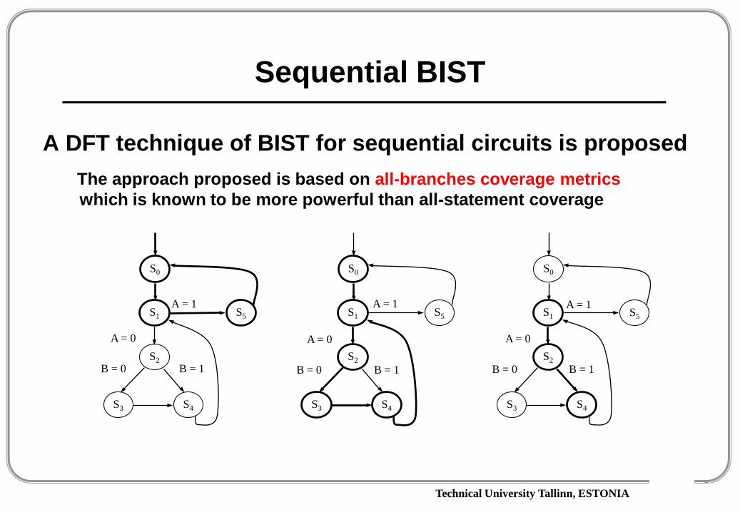
A DFT technique of BIST for sequential circuits is proposed The approach proposed is based on all-branches coverage metricswhich is known to be more powerful than all-statement coverage
S4
S0
S1 S5
S2
S3
A = 1
A = 0
B = 0 B = 1
S4
S0
S1 S5
S2
S3
A = 1
A = 0
B = 0 B = 1
S4
S0
S1 S5
S2
S3
A = 1
A = 0
B = 0 B = 1
Technical University Tallinn, ESTONIA
Sequential BIST
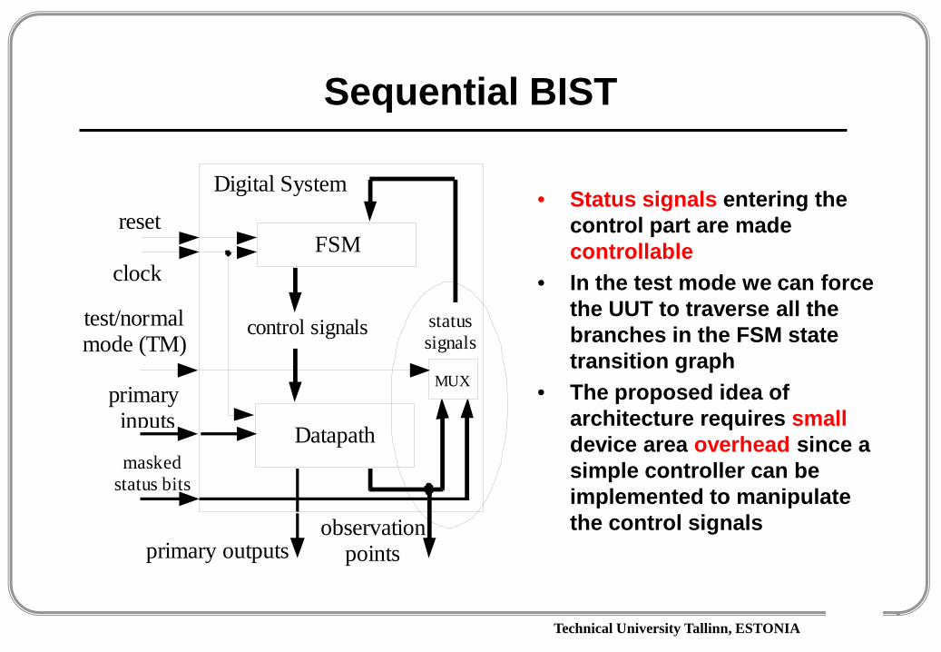
• Status signals entering thecontrol part are made controllable
• In the test mode we can force the UUT to traverse all the branches in the FSM state transition graph
• The proposed idea of architecture requires smalldevice area overhead since a simple controller can be implemented to manipulate the control signals
Digital System
FSM
Datapath
control signals status signals
reset
clock
primary inputs
primary outputs
maskedstatus bits
MUX
test/normal mode (TM)
observation points

Technical University Tallinn, ESTONIA
BIST: Weighted pseudorandom test
Hardware implementation of weight generator
LFSR
&&&
MUXWeight select
Desired weighted value Scan-IN
1/21/41/81/16
Technical University Tallinn, ESTONIA
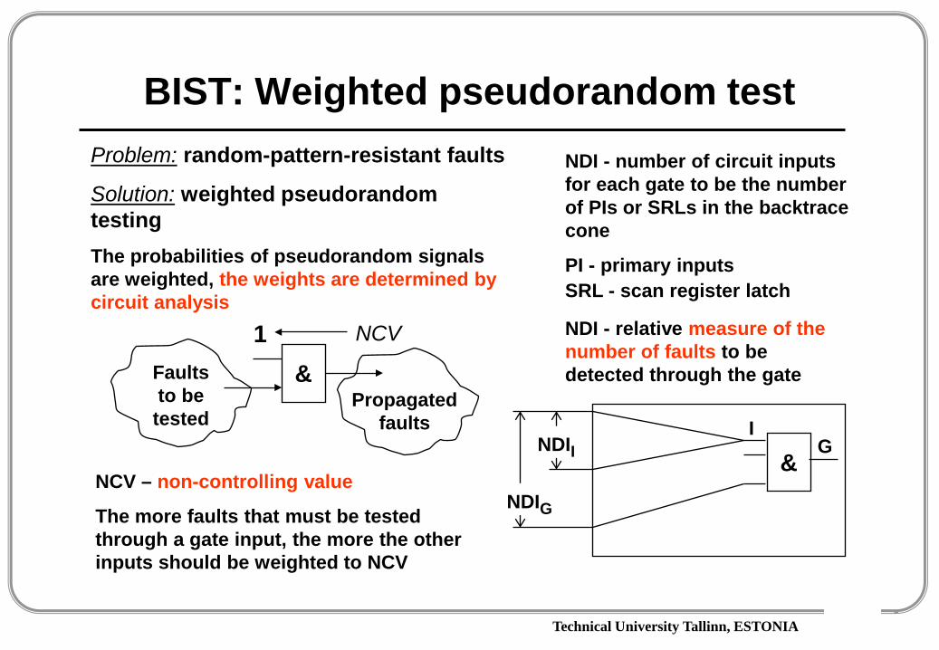
BIST: Weighted pseudorandom testProblem: random-pattern-resistant faults
Solution: weighted pseudorandom testingThe probabilities of pseudorandom signals are weighted, the weights are determined by circuit analysis
NCV – non-controlling value
The more faults that must be tested through a gate input, the more the other inputs should be weighted to NCV
&Faults to be
tested
1 NCV
Propagated faults
NDI - number of circuit inputs for each gate to be the number of PIs or SRLs in the backtrace cone
PI - primary inputs SRL - scan register latch
&NDIG
NDIII
G
NDI - relative measure of the number of faults to be detected through the gate
Technical University Tallinn, ESTONIA
BIST: Weighted pseudorandom test
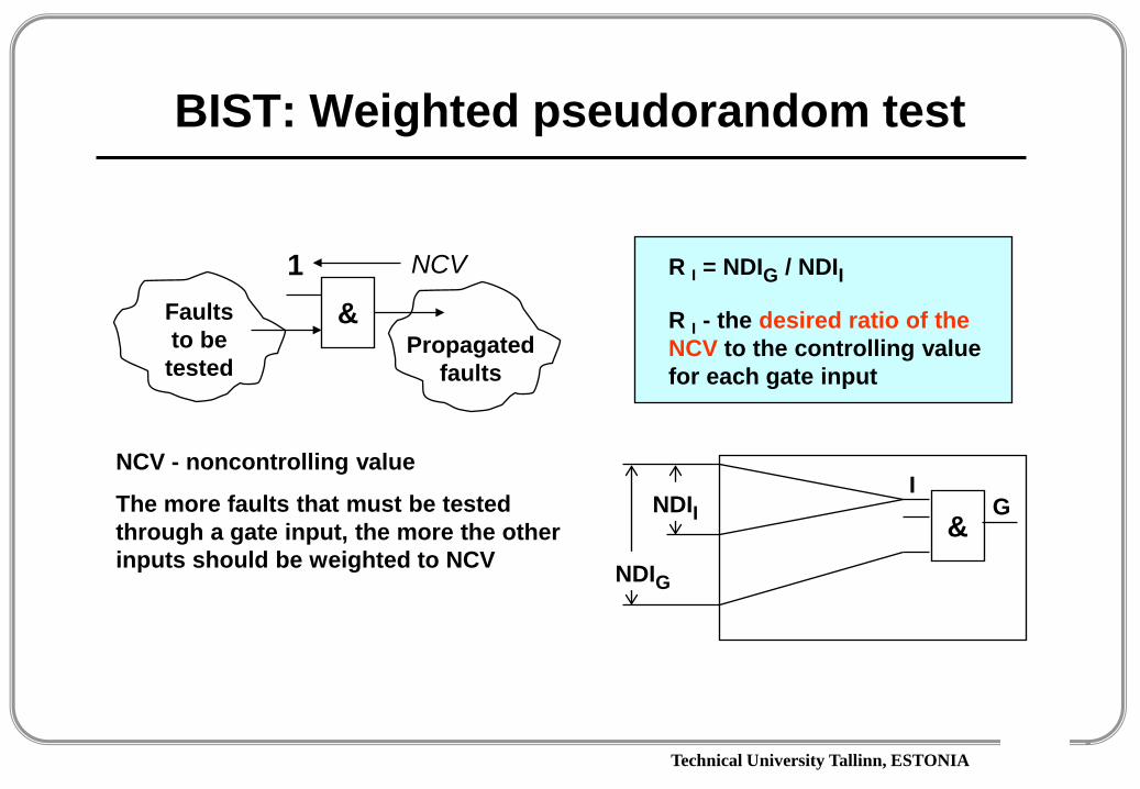
NCV - noncontrolling value
The more faults that must be tested through a gate input, the more the other inputs should be weighted to NCV
&Faults to be
tested
1 NCV
Propagated faults
&NDIG
NDIII
G
R I = NDIG / NDII
R I - the desired ratio of the NCV to the controlling value for each gate input
Technical University Tallinn, ESTONIA
BIST: Weighted pseudorandom test
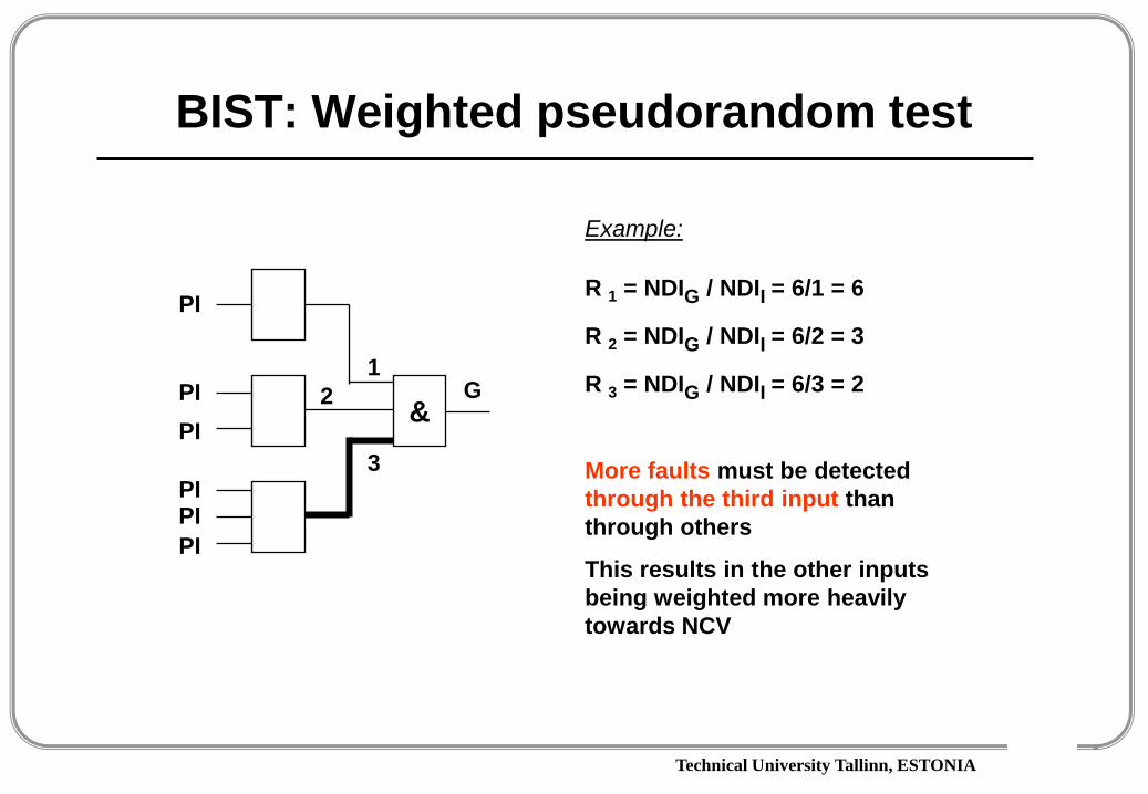
Example:
R 1 = NDIG / NDII = 6/1 = 6
R 2 = NDIG / NDII = 6/2 = 3
R 3 = NDIG / NDII = 6/3 = 2&
G1
2
3
PI
PI
PIPIPI
PIMore faults must be detected through the third input than through others
This results in the other inputs being weighted more heavily towards NCV
Technical University Tallinn, ESTONIA
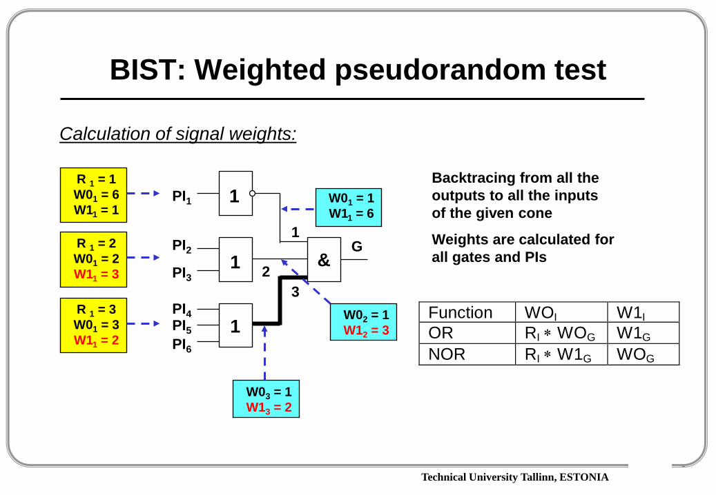
BIST: Weighted pseudorandom test
&G
1
23
PI
PI
PIPIPI
PI
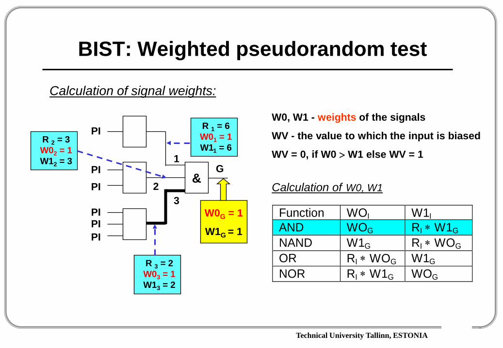
W0, W1 - weights of the signals
WV - the value to which the input is biased
WV = 0, if W0 > W1 else WV = 1
Calculation of signal weights:
Function WOI W1IAND WOG RI ∗ W1G
NAND W1G RI ∗ WOG
OR RI ∗ WOG W1G
NOR RI ∗ W1G WOG
W0G = 1
W1G = 1
Calculation of W0, W1
R 1 = 6W01 = 1W11 = 6
R 3 = 2W03 = 1W13 = 2
R 2 = 3W02 = 1W12 = 3
Technical University Tallinn, ESTONIA
BIST: Weighted pseudorandom test
&G
1
23
W01 = 1W11 = 6
W03 = 1W13 = 2
W02 = 1W12 = 3
1
1
1
PI1
PI2
PI6PI5PI4
PI3
R 1 = 1W01 = 6W11 = 1
R 1 = 2W01 = 2W11 = 3
R 1 = 3W01 = 3W11 = 2
Backtracing from all the outputs to all the inputs of the given cone
Weights are calculated for all gates and PIs
Function WOI W1IOR RI ∗ WOG W1G
NOR RI ∗ W1G WOG
Calculation of signal weights:

Technical University Tallinn, ESTONIA
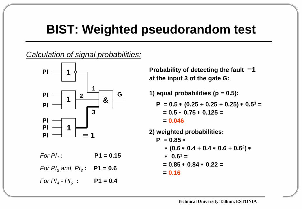
BIST: Weighted pseudorandom test
WF - weighting factor indicating the amount of biasing toward weighted value
WF = max {W0,W1} / min {W1,W0}
Probability:
P = WF / (WF + 1)
Calculation of signal probabilities:
For PI1 : W0 = 6 W1 = 1 P1 = 1/7 = 0.15
For PI2 and PI3 : W0 = 2 W1 = 3 P1 = 3/5 = 0.6
For PI4 - PI6 : W0 = 3 W1 = 2 P1 = 2/5 = 0.4
&G
1
23
1
1
1
PI1
PI2
PI6PI5PI4
PI3
R 1 = 1W01 = 6W11 = 1
R 1 = 2W01 = 2W11 = 3
R 1 = 3W01 = 3W11 = 2
Technical University Tallinn, ESTONIA
BIST: Weighted pseudorandom test
&G
12
3
PI
PI
PIPIPI
PI
Calculation of signal probabilities:
For PI1 : P1 = 0.15
For PI2 and PI3 : P1 = 0.6
For PI4 - PI6 : P1 = 0.4
1
1
1
Probability of detecting the fault ≡1at the input 3 of the gate G:
1) equal probabilities (p = 0.5):
P = 0.5 ∗ (0.25 + 0.25 + 0.25) ∗ 0.53 == 0.5 ∗ 0.75 ∗ 0.125 = = 0.046
2) weighted probabilities:P = 0.85 ∗
∗ (0.6 ∗ 0.4 + 0.4 ∗ 0.6 + 0.62) ∗∗ 0.63 =
= 0.85 ∗ 0.84 ∗ 0.22 = = 0.16
≡ 1
Technical University Tallinn, ESTONIA
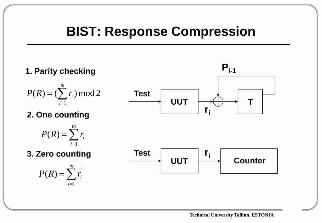
BIST: Response Compression
1. Parity checking
2mod)()(1∑=
=m
iirRP
UUTTest
Tri
Pi-1
2. One counting
∑=
=m
iirRP
1)(
UUTTest ri Counter
3. Zero counting
∑=
=m
iirRP
1)(

Technical University Tallinn, ESTONIA
BIST: Response Compression
4. Transition counting
UUTTest
T
ri
ri-1)()(2
1∑=
−=m
iii rrRP
)()(2
1∑=
−=m
iii rrRP
a) Transition 0→1
b) Transition 1→0
UUTTest
T
ri
ri-1
5. Signature analysis
&
&
Technical University Tallinn, ESTONIA
Pseudorandom Test Generation
LFSR – Linear Feedback Shift Register:
x x2 x3 x4
x3x2 x4x
Polynomial: P(x) = x4 + x3 + 1
Standard LFSR
Modular LFSR

Technical University Tallinn, ESTONIA
BIST: Signature Analysis
1 x x2
x3
x4
x2x1 x4
x3
Polynomial: P(x) = 1 + x3 + x4
Signature analyzer:Standard LFSR
Modular LFSR
UUT
Response string
Response in compacted by LFSR
The content of LFSR after test is called signature

Technical University Tallinn, ESTONIA
Theory of LFSR
The principles of CRC (Cyclic Redundancy Coding) are used in LFSR based test response compactionCoding theory treats binary strings as polynomials:
R = rm-1 rm-2 … r1 r0 - m-bit binary sequence
R(x) = rm-1 xm-1 + rm-2 xm-2 + … + r1 x + r0 - polynomial in x
Example:
11001 → R(x) = x4 + x3 + 1
Only the coefficients are of interest, not the actual value of x
However, for x = 2, R(x) is the decimal value of the bit string
Technical University Tallinn, ESTONIA
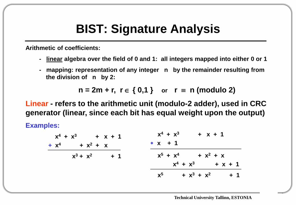
BIST: Signature AnalysisArithmetic of coefficients:
- linear algebra over the field of 0 and 1: all integers mapped into either 0 or 1
- mapping: representation of any integer n by the remainder resulting fromthe division of n by 2:
n = 2m + r, r ∈ { 0,1 } or r ≡ n (modulo 2)
Linear - refers to the arithmetic unit (modulo-2 adder), used in CRC generator (linear, since each bit has equal weight upon the output)Examples:
x4 + x3 + x + 1+ x4 + x2 + x
x3 + x2 + 1
x4 + x3 + x + 1∗ x + 1
x5 + x4 + x2 + x x4 + x3 + x + 1
x5 + x3 + x2 + 1
Technical University Tallinn, ESTONIA
Theory of LFSR
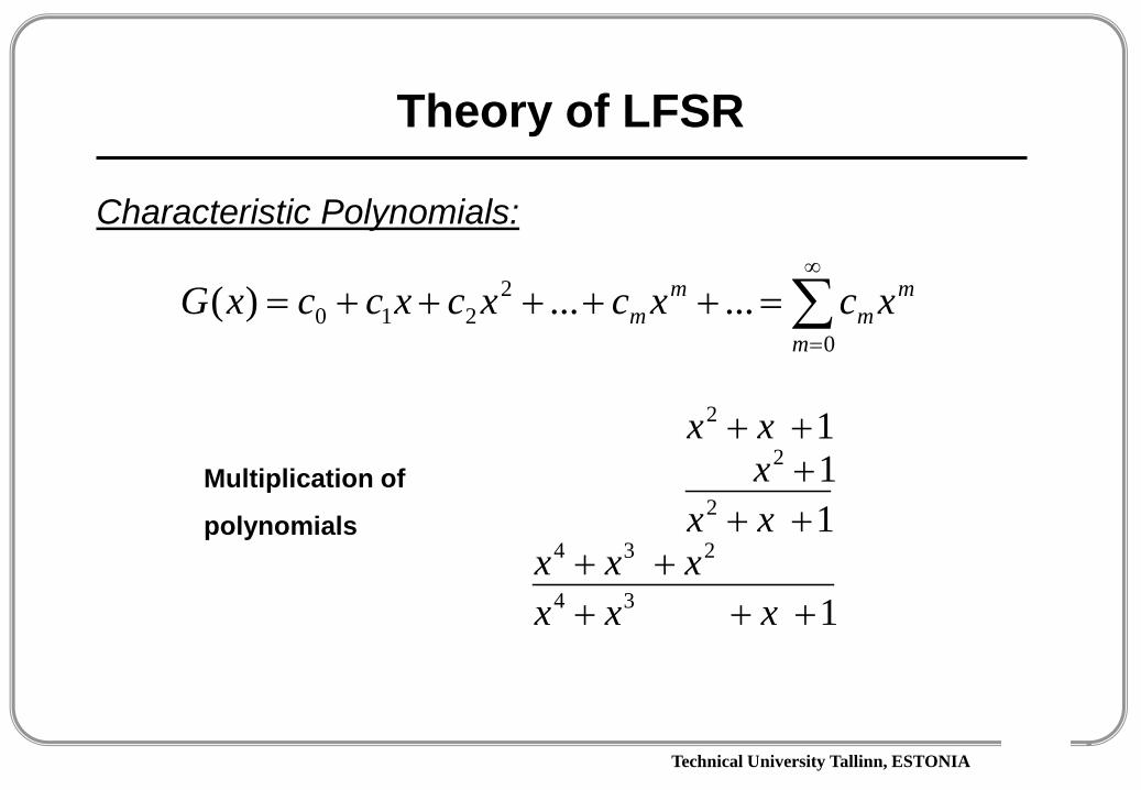
Characteristic Polynomials:
∑∞
=
=+++++=0
2210 ......)(
m
mm
mm xcxcxcxccxG
Multiplication of
polynomials
1
1 1 1
34
234
2
2
2
+++++
+++++
xxxxxx
xxxxx
Technical University Tallinn, ESTONIA
Theory of LFSR
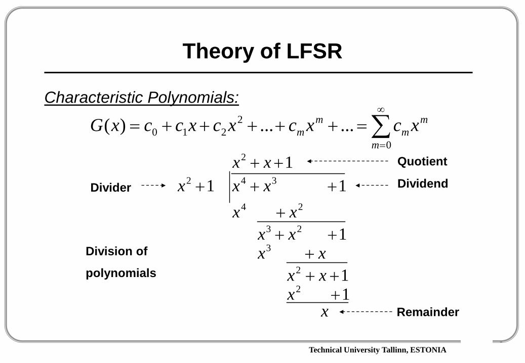
Characteristic Polynomials:
∑∞
=
=+++++=0
2210 ......)(
m
mm
mm xcxcxcxccxG
Division of
polynomials
xx
xxxx
xxxx
xxxxx
1 1
1
1 1
1
2
2
3
23
24
342
2
+++
+++
+
+++++ Quotient
Remainder
DividendDivider

Technical University Tallinn, ESTONIA
BIST: Signature Analysis
Division of one polynomial P(x) by another G(x) produces a quotient polynomial Q(x), and if the division is not exact, a remainder polynomial R(x)
)()()(
)()(
xGxRxQ
xGxP
+=
Example:
111
1)()(
35
223
35
37
++++
+++=+++
++=
xxxxxx
xxxxxx
xGxP
Remainder R(x) is used as a check word in data transmissionThe transmitted code consists of the unaltered message P(x) followed by the check word R(x)
Upon receipt, the reverse process occurs: the message P(x) is divided by known G(x), and a mismatch between R(x) and the remainder from the division indicates an error

Technical University Tallinn, ESTONIA
BIST: Signature AnalysisIn signature testing we mean the use of CRC encoding as the data compressor G(x) and the use of the remainder R(x) as the signatureof the test response string P(x) from the UUT
Signature is the CRC code word )()()(
)()(
xGxRxQ
xGxP
+=
Example:
1)()(
35
37
+++++
=xxx
xxxxGxP
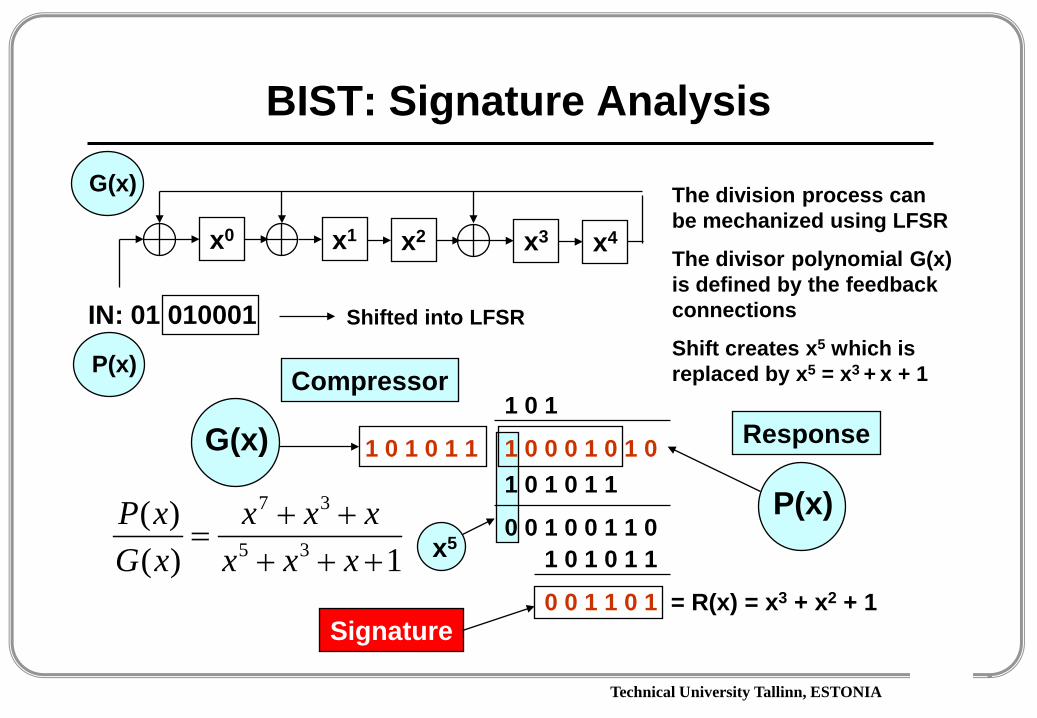
1 0 1 = Q(x) = x2 + 1
1 0 1 0 1 1 1 0 0 0 1 0 1 01 0 1 0 1 1
0 0 1 0 0 1 1 01 0 1 0 1 1
0 0 1 1 0 1 = R(x) = x3 + x2 + 1
P(x)
G(x)
Signature
Technical University Tallinn, ESTONIA
BIST: Signature Analysis
1)()(
35
37
+++++
=xxx
xxxxGxP
1 0 1
1 0 1 0 1 1 1 0 0 0 1 0 1 01 0 1 0 1 1
0 0 1 0 0 1 1 01 0 1 0 1 1
0 0 1 1 0 1 = R(x) = x3 + x2 + 1
P(x)
G(x)
Signature
The division process can be mechanized using LFSR
The divisor polynomial G(x) is defined by the feedback connections
Shift creates x5 which is replaced by x5 = x3 + x + 1
x0 x1 x2 x3 x4
IN: 01 010001 Shifted into LFSR
x5
G(x)
P(x) Compressor
Response
Technical University Tallinn, ESTONIA
BIST: Signature Analysis
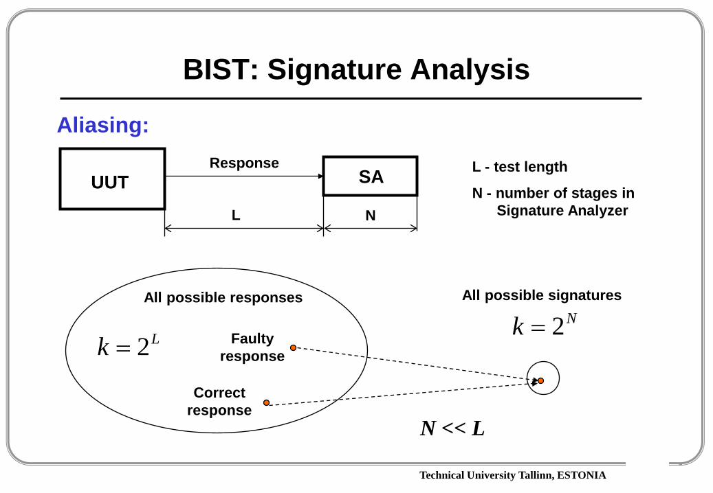
Aliasing:
UUTResponse
SA
L N
L - test length
N - number of stages inSignature Analyzer
Lk 2=
All possible responses All possible signaturesNk 2=Faulty
response
Correct response
N << L

Technical University Tallinn, ESTONIA
BIST: Signature AnalysisAliasing:
UUTResponse
SA
L N
L - test length
N - number of stages inSignature Analyzer
Lk 2= - number of different possible responses
No aliasing is possible for those strings with L - N leading zeros since they are represented by polynomials of degree N - 1 that are not divisible by characteristic polynomial of LFSR
12 −−NL
Probability of aliasing:1212
−−
=−
L
NL
P NP21
=1>>L
- aliasing is possible000000000000000 ... 00000 XXXXX
L N

Technical University Tallinn, ESTONIA
BIST: Signature Analysis
x2 x 1x4
x3
Parallel Signature Analyzer:
UUT
x2 x 1x4
x3
UUT Multiple Input Signature Analyser (MISR)
Single Input Signature Analyser
Technical University Tallinn, ESTONIA
BIST: Signature Analysis
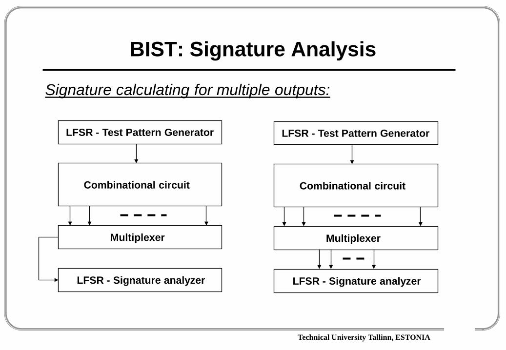
Signature calculating for multiple outputs:
LFSR - Test Pattern Generator
Combinational circuit
LFSR - Signature analyzer
Multiplexer
LFSR - Test Pattern Generator
Combinational circuit
LFSR - Signature analyzer
Multiplexer
Technical University Tallinn, ESTONIA
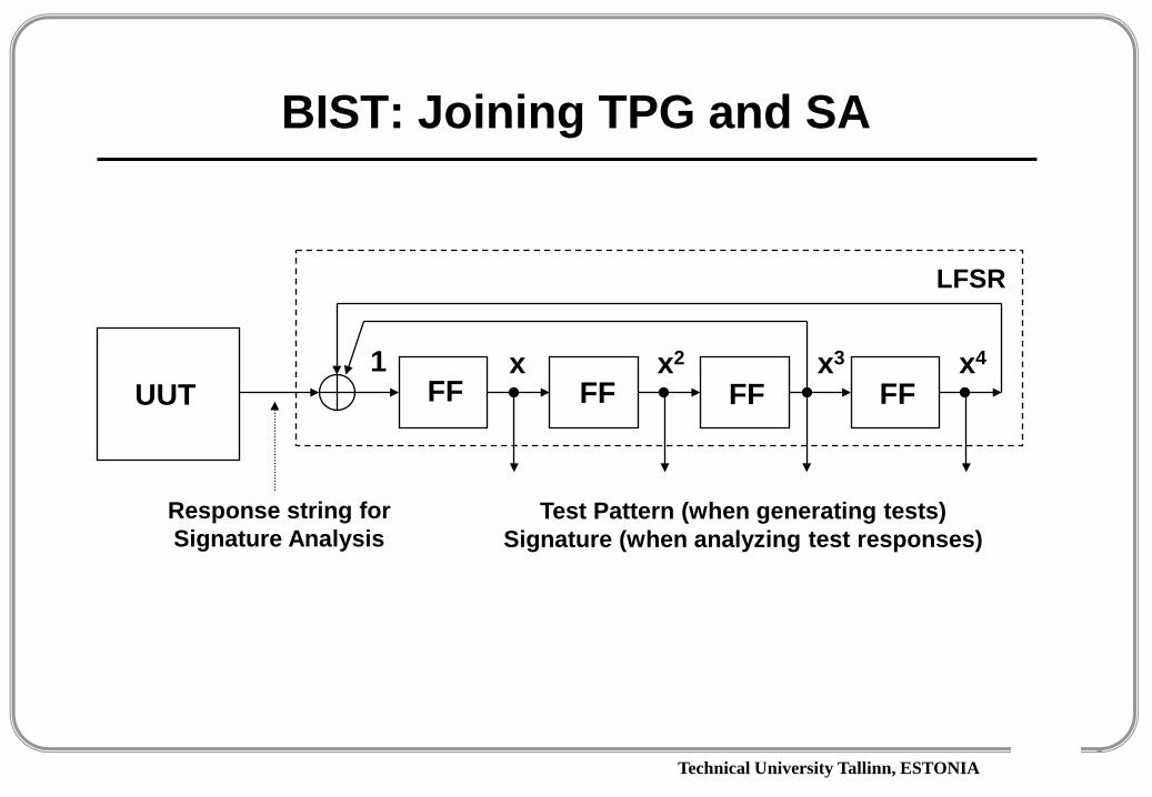
BIST: Joining TPG and SA
1 x x2 x3 x4
LFSR
UUT
Response string for Signature Analysis
Test Pattern (when generating tests)Signature (when analyzing test responses)
FF FF FF FF
Technical University Tallinn, ESTONIA
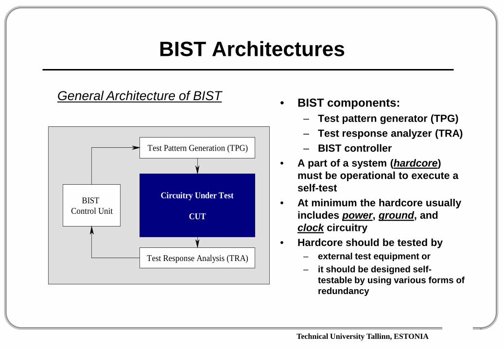
BIST Architectures
BIST Control Unit
Circuitry Under Test
CUT
Test Pattern Generation (TPG)
Test Response Analysis (TRA)
• BIST components:– Test pattern generator (TPG)– Test response analyzer (TRA)– BIST controller
• A part of a system (hardcore) must be operational to execute a self-test
• At minimum the hardcore usually includes power, ground, and clock circuitry
• Hardcore should be tested by – external test equipment or – it should be designed self-
testable by using various forms of redundancy
General Architecture of BIST

Technical University Tallinn, ESTONIA
BIST Architectures
Test per Clock:
Disjoint TPG and SA: BILBO
Joint TPG and SA:
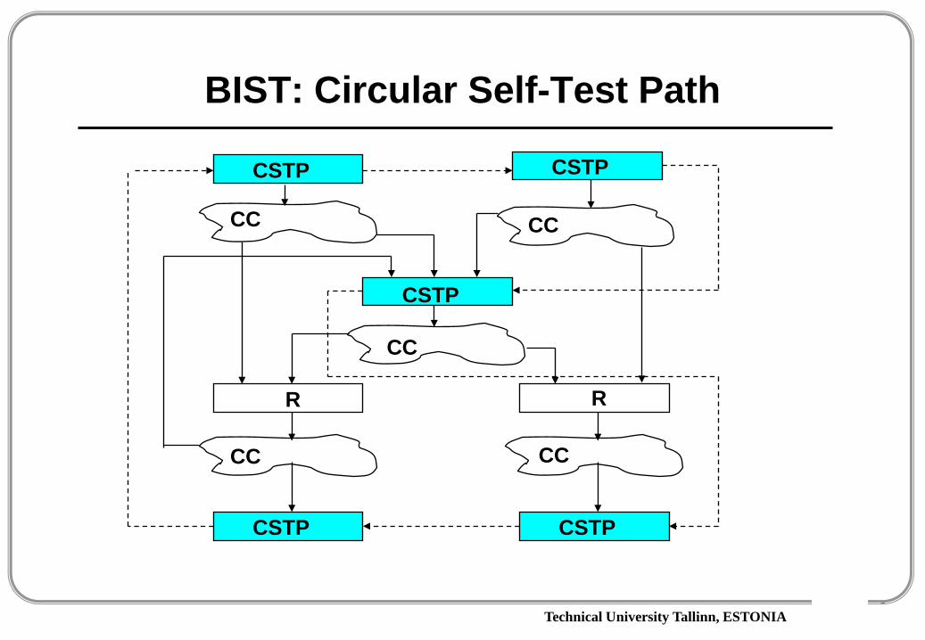
CSTP - Circular Self-Test Path:
LFSR - Test Pattern Generator
Combinational circuit
LFSR - Signature analyzer
LFSR - Test Pattern Generator
& Signature analyser
Combinational circuit

Technical University Tallinn, ESTONIA
BIST: Circular Self-Test Architecture
Circuit Under Test
FF FFFF
Technical University Tallinn, ESTONIA
BIST: Circular Self-Test Path
CSTP CSTP
CSTP
CSTP CSTP
CC CC
CC
CC
CC
R R

Technical University Tallinn, ESTONIA
BIST Embedding Example
M1 M2
M3M5
LFSR1
M4
MISR1
BILBO
M6
MUX
CSTP
LFSR2
MISR2
MUXLFSR, CSTP → M2 → MISR1M2 → M5 → MISR2 (Functional BIST)CSTP → M3 → CSTPLFSR2 → M4 → BILBO
Concurrent testing:

Technical University Tallinn, ESTONIA
BIST Architectures
Test Pattern Generator
MISR
Scan
cha
in
CUT...
STUMPS:Self-Testing Unit Using MISR and Parallel Shift Register Sequence Generator
LOCST: LSSD On-Chip Self-Test
CUT
Error
Test ControllerSI SO
TPG SA
CUT
BS BS
Scan Path
Scan
cha
in
IC
Technical University Tallinn, ESTONIA
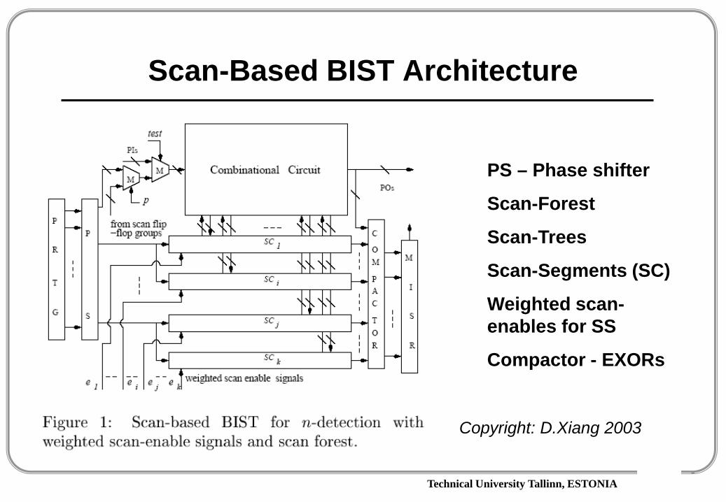
Scan-Based BIST Architecture
Copyright: D.Xiang 2003
PS – Phase shifter
Scan-Forest
Scan-Trees
Scan-Segments (SC)
Weighted scan-enables for SS
Compactor - EXORs

Technical University Tallinn, ESTONIA
Software BIST
To reduce the hardware overhead cost in the BIST applications the hardware LFSR can be replaced by software
Software BIST is especially attractive to test SoCs, because of the availability of computing resources directly in the system (a typical SoC usually contains at least one processor core)
SoC ROMCPU CoreLFSR1: 001010010101010011N1: 275
LFSR2: 110101011010110101N2: 900...
load (LFSRj); for (i=0; i<Nj; i++) ...end;
Core j Core j+1 Core j+...
Software based test generation:
The TPG software is the same for all cores and is stored as a single copy All characteristics of the LFSR are specific to each core and stored in the ROM They will be loaded upon request. For each additional core, only the BIST characteristics for this core have to be stored
Technical University Tallinn, ESTONIA
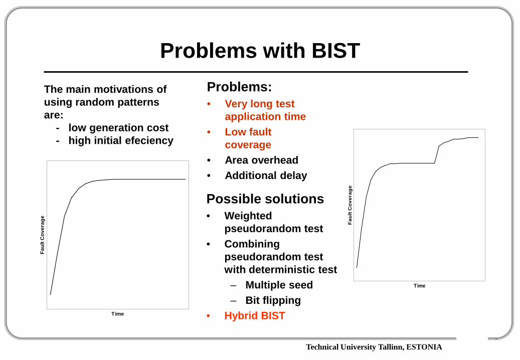
Problems with BIST
Time
Faul
t Cov
erag
e
Problems:• Very long test
application time• Low fault
coverage• Area overhead• Additional delay
Possible solutions • Weighted
pseudorandom test• Combining
pseudorandom test with deterministic test
– Multiple seed– Bit flipping
• Hybrid BIST
Time
Fau
lt C
ove
rag
e
The main motivations of using random patterns are:
- low generation cost- high initial efeciency
Technical University Tallinn, ESTONIA
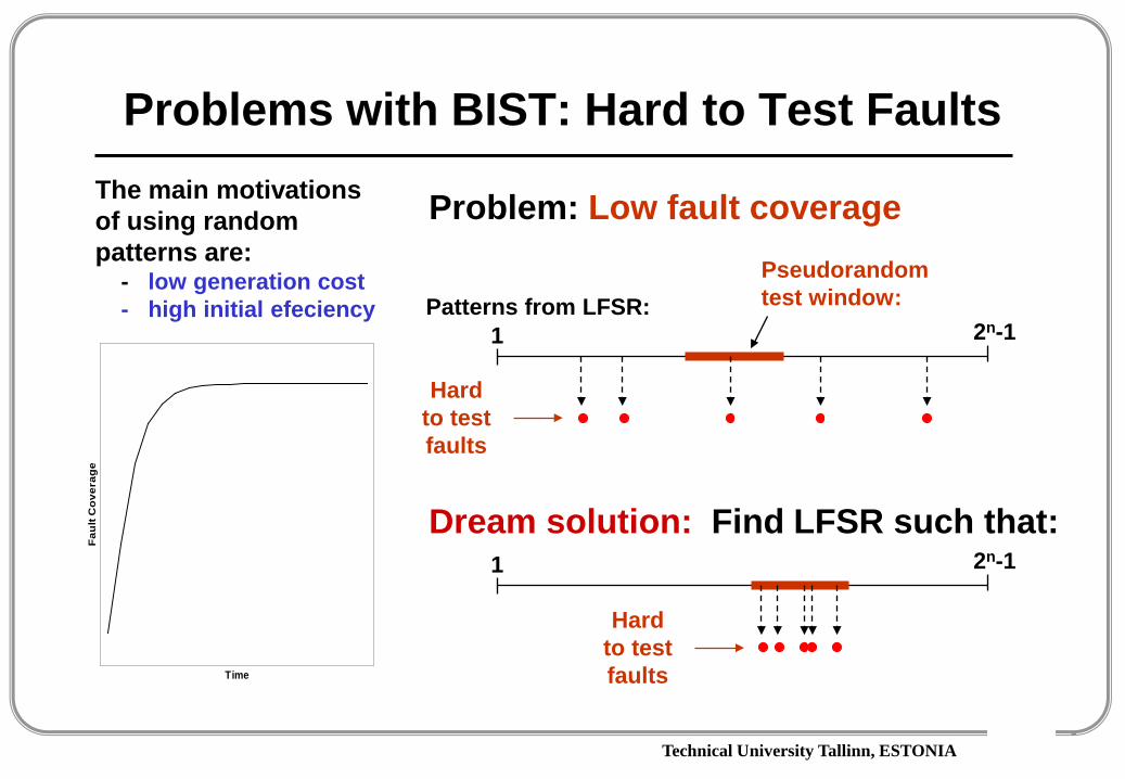
Problems with BIST: Hard to Test Faults
Time
Fau
lt C
ove
rag
e
Problem: Low fault coverageThe main motivations of using random patterns are:
- low generation cost- high initial efeciency
1 2n-1Patterns from LFSR:
Pseudorandom test window:
Hard to test faults
1 2n-1Dream solution: Find LFSR such that:
Hard to test faults

Technical University Tallinn, ESTONIA
Hybrid Built-In Self-Test
PRPG
CORE UNDERTEST
. . .. . .
. . .
ROM
. . . . . .
SoC
Core
MISR
BIS
T C
ontro
ller
Hybrid test set contains pseudorandom and deterministic vectors
Pseudorandom test is improved by a stored test set which is specially generated to target the random resistant faults
Optimization problem:
Pseudorandom Test Determ. Test
Where should be this breakpoint?
Deterministic patterns
Pseudorandom patterns

Technical University Tallinn, ESTONIA
Optimization of Hybrid BIST
Cost of BIST:
k rDET(k) rNOT(k) FC(k) t(k)1 155 839 15.6% 1042 76 763 23.2% 1043 65 698 29.8% 1004 90 608 38.8% 1015 44 564 43.3% 99
10 104 421 57.6% 9520 44 311 68.7% 8750 51 218 78.1% 74
100 16 145 85.4% 52200 18 114 88.5% 41411 31 70 93.0% 26954 18 28 97.2% 12
1560 8 16 98.4% 72153 11 5 99.5% 33449 2 3 99.7% 24519 2 1 99.9% 14520 1 0 100.0% 0
Total Cost CTOTAL
Figure 2: Cost calculation for hybrid BIST
Cost of pseudorandom test
patterns CGEN
Number of remaining faults after applying k
pseudorandom test patterns rNOT(k)
Cost of stored test CMEM
Number of pseudorandom test patterns applied, k
# faults
# faults not
detected
# tests needed
PR test length
PR test length k
# tests
FAST estimation
SLOW analysis
CTOTAL = α k + β t(k)
β t(k)
α k
min CTOTAL
Det. TestPseudorandom Test

Technical University Tallinn, ESTONIA
Deterministic Test Length Estimation
i
F
F D k ( i ) F P E k ( i )
i *
F*
| T D E k ( i ) |
100%
| T D F k | j i
Fault coverage
Pseudorandom test length
Deterministic test (DT)Pseudorandom test (PT)
Deterministic test length estimation
For each PT length i* we determine - PT fault coverage F*, and- the imaginable part of DT
FDk(i) to be used for the same fault coverage
Then the remaining part of DT TDE
k(i) will be the estimation of the DT length
Fast estimation for the length of deterministic test:

Technical University Tallinn, ESTONIA
Calculation of the Deterministic Test Cost
Two possibilities to find the length of deterministic data for each possible breakpoint in the pseudorandom test sequence:
ATPG based approachFor each breakpoint of P-sequence, ATPG is usedFault table based approach A deterministic test set with fault table is calculatedFor each breakpoint of P-sequence, the fault table is updated for not yet detected faults
FAST estimationOnly fault coverage is calculated
ATPG
Detected Faults
All PR patterns?
YesEnd
No
Next PR pattern
ATPG based:
ATPG
Fault table update
All PR patterns?
YesEnd
No
Next PR pattern
Fault table based:

Technical University Tallinn, ESTONIA
Calculation of the Deterministic Test Cost
ATPG based approachFor each breakpoint of P-sequence, ATPG is used
ATPG
Detected Faults
All PR patterns?
YesEnd
No
Next PR pattern
ATPG based:
T1T2....
Tn
Tn+1
Tp
R1 R2 Rk Rk+1 Rk+2 Rn
Faults detected
bypseudo-random patterns
Faults to be detected
by
deterministic patterns
New detected faults
Task for ATPG
Task for fault
simulator

Technical University Tallinn, ESTONIA
Calculation of the Deterministic Test Cost
ATPG
Fault table update
All PR patterns?
YesEnd
No
Next PR pattern
Fault table based:
T1T2....
Tn
Tn+1
Tp
R1 R2 Rk Rk+1 Rk+2 Rn
Faults detected
By
pseudo-random patterns
To be detected faults
Task for fault
simulator
Fault table based approach A deterministic test set with fault table is calculatedFor each breakpoint of P-sequence, the fault table is updated
Fault table for full
deterministic test
Updated fault tabel
Technical University Tallinn, ESTONIA
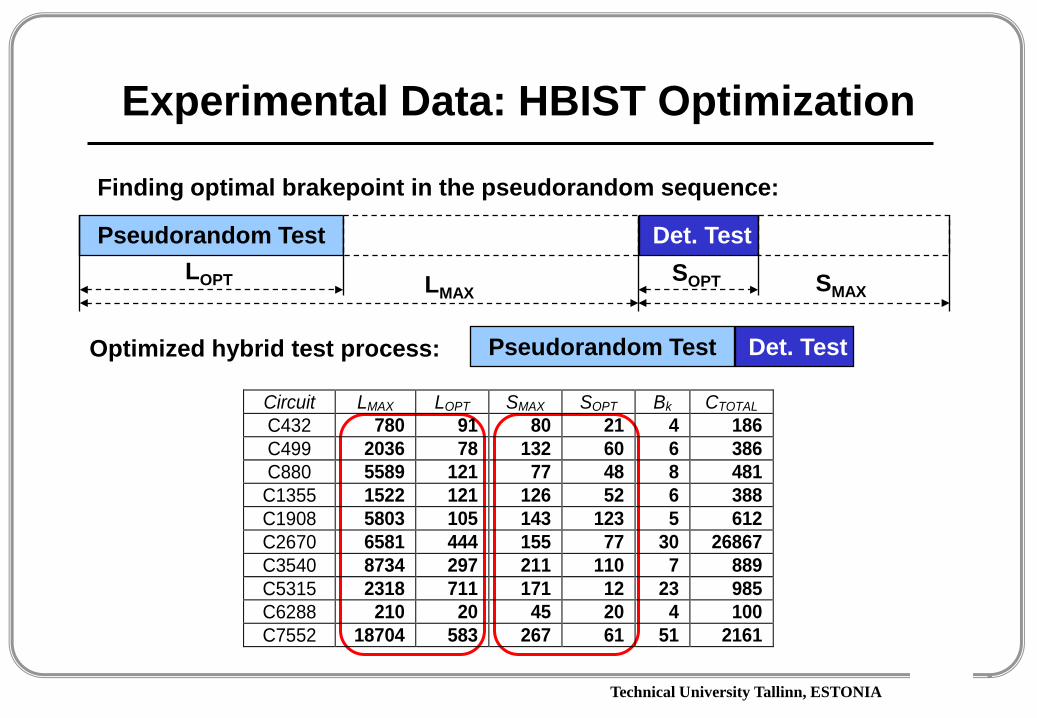
Experimental Data: HBIST Optimization
Pseudorandom Test Det. Test
Finding optimal brakepoint in the pseudorandom sequence:
Circuit LMAX LOPT SMAX SOPT Bk CTOTAL C432 780 91 80 21 4 186 C499 2036 78 132 60 6 386 C880 5589 121 77 48 8 481 C1355 1522 121 126 52 6 388 C1908 5803 105 143 123 5 612 C2670 6581 444 155 77 30 26867 C3540 8734 297 211 110 7 889 C5315 2318 711 171 12 23 985 C6288 210 20 45 20 4 100 C7552 18704 583 267 61 51 2161
LMAXLOPT SMAX
SOPT
Pseudorandom Test Det. TestOptimized hybrid test process:

Technical University Tallinn, ESTONIA
Hybrid BIST with Reseeding
Time
Fau
lt C
ove
rag
e
Problem: low fault coverage → long PR testThe motivation of using random patterns is:
- low generation cost- high initial efeciency
1 2n-1
Solution: many seeds:Pseudorandom test:
Hard to test faults
1 2n-1
Pseudorandom test:

Technical University Tallinn, ESTONIA
Store-and-Generate Test Architecture
• ROM contains test patterns for hard-to-test faults • Each pattern Pk in ROM serves as an initial state of the LFSR for test pattern
generation (TPG) - seeds• Counter 1 counts the number of pseudorandom patterns generated starting
from Pk - width of the windows• After finishing the cycle for Counter 2 is incremented for reading the next
pattern Pk+1 – beginning of the new window
ROM TPG UUT
ADR
Counter 2 Counter 1
RD
CL
Seeds
WindowPseudorandom test windows
Seeds
# seeds

Technical University Tallinn, ESTONIA
HBIST Optimization Problem
1 2n-1
Using many seeds:Pseudorandom test:
Deterministic test (seeds):
Pseudo-random
sequences:
Block size:
Seed 1
Seed 1
Seed 2
Seed 2
Seed nSeed n
Constraints
Problems:How to calculate the number and size of blocks?
Which deterministic patterns should be the seeds for the blocks?
Minimize L at given M and
L
M
100% FC
100% FC

Technical University Tallinn, ESTONIA
Hybrid BIST Optimization Algorithm 1
ATPG patterns
Pattern selectionPRi
Pseudorandomsequence
FC(PRi)
ModifiedATPG pattern
table
Detected faults subtraction,optimization of ATPG patterns
Deterministic test patterns with 100% quality are generated by ATPG
The best pattern is selected as a seed
A pseudorandom block is produced and the fault table of ATPG patterns is updated
The procedure ends when 100% fault coverage is achieved
Algorithm is based on D-patterns ranking
D-patterns are ranked

Technical University Tallinn, ESTONIA
Hybrid BIST Optimization Algorithm 2
Deterministic test patterns with 100% quality are generated by ATPG
All P-blocks are generated for all D-patterns and ranked
The best P-block is selected includeed into sequence and updated
The procedure ends when 100% fault coverage is achieved
…
…
PTmin
PT*
Deterministic test vector (seed) DTi Pseudorandom test sequence PRi Pseudorandom sequence removed with the block length optimization
Algorithm is based on P-blocks ranking
P-blocks are ranked
Technical University Tallinn, ESTONIA
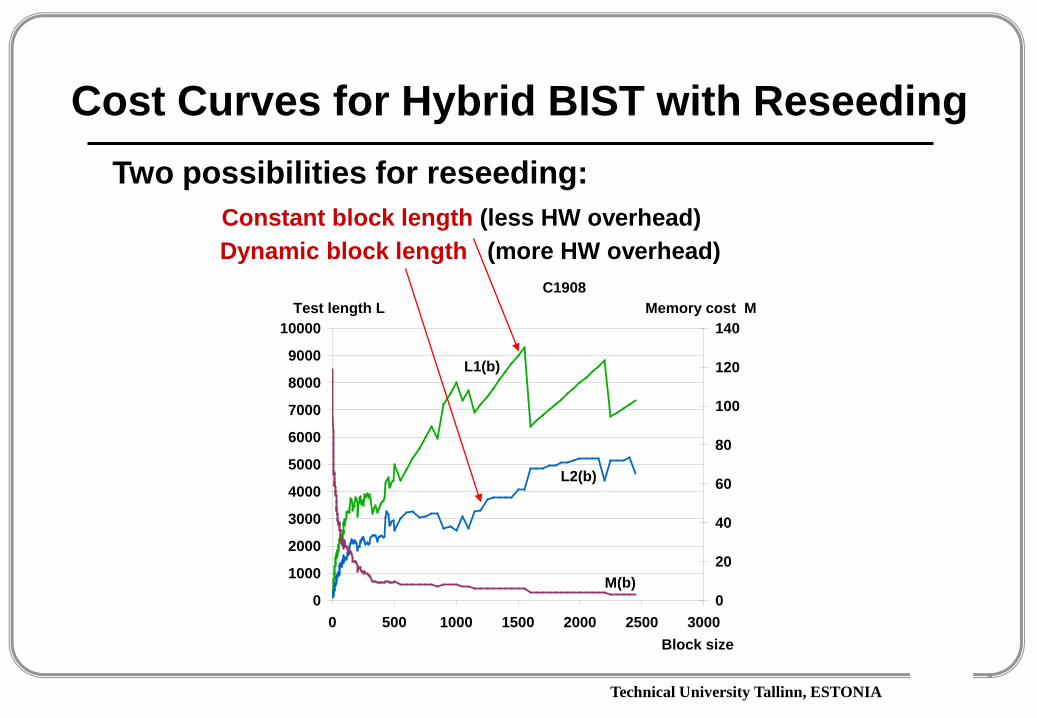
Cost Curves for Hybrid BIST with Reseeding
C1908
0
1000
2000
3000
4000
5000
6000
7000
8000
9000
10000
0 500 1000 1500 2000 2500 30000
20
40
60
80
100
120
140Test length L Memory cost M
M(b)
L1(b)
L2(b)
Block size
Two possibilities for reseeding: Constant block length (less HW overhead)Dynamic block length (more HW overhead)
Technical University Tallinn, ESTONIA
Functional Self-Test
• Traditional BIST solutions use special hardware for patterngeneration on chip, this may introduce area overhead andperformance degradation
• New methods have been proposed which exploit specific functionalunits like arithmetic blocks or processor cores for on-chip testgeneration
• It has been shown that adders can be used as test generators forpseudorandom and deterministic patterns
• Today, there is no general method how to use arbitrary functionalunits for built-in test generation
Technical University Tallinn, ESTONIA
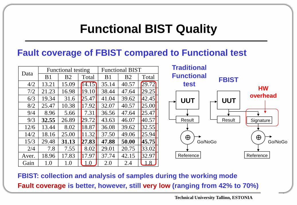
Functional BIST Quality
Fault coverage of FBIST compared to Functional test
Functional testing Functional BIST Data B1 B2 Total B1 B2 Total 4/2 13.21 15.09 14.15 35.14 40.57 29.72 7/2 21.23 16.98 19.10 38.44 47.64 29.25 6/3 19.34 31.6 25.47 41.04 39.62 42.45 8/2 25.47 10.38 17.92 32.07 40.57 25.00 9/4 8.96 5.66 7.31 36.56 47.64 25.47 9/3 32.55 26.89 29.72 43.63 46.07 40.57
12/6 13.44 8.02 18.87 36.08 39.62 32.55 14/2 18.16 25.00 11.32 37.50 49.06 25.94 15/3 29.48 31.13 27.83 47.88 50.00 45.75
2/4 7.8 7.55 8.02 29.01 20.75 33.02 Aver. 18.96 17.83 17.97 37.74 42.15 32.97 Gain 1.0 1.0 1.0 2.0 2.4 1.8
Reference
Result
⊕Go/NoGo
UUT
Reference
Result
⊕Go/NoGo
UUT
Signature
Traditional Functional
test FBIST
FBIST: collection and analysis of samples during the working modeFault coverage is better, however, still very low (ranging from 42% to 70%)
HW overhead

Technical University Tallinn, ESTONIA
Example: Functional BIST
Register block
ControlALU
Signature analyser
Functional test
Data
K
Samples from N=120 cycles
K*N Fault simulator
Fault coverage
Test patterns (samples) are produced on-line during the working mode
DB=64
SB=105
Data compression:
N*SB / DB = 197
Functional BIST quality analysis

Technical University Tallinn, ESTONIA
Hybrid Functional BIST
• To improve the quality of FBIST we introduce the method of Hybrid FBIST
• The idea of Hybrid FBIST consists in using for test purposes the mixture of– functional patterns produced by the microprogram (no
additional HW is needed), and – additional stored deterministic test patterns to improve the total
fault coverage (HW overhead: MUX-es, Memory)• Tradeoff should be found between
– the testing time and– the HW/SW overhead cost
Technical University Tallinn, ESTONIA
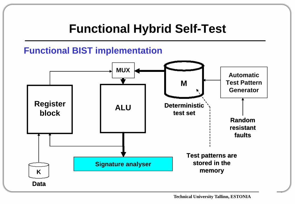
Functional Hybrid Self-Test
Register block
ALU
Signature analyser
Deterministictest set
Data
K
M Automatic
Test Pattern Generator
Randomresistant
faults
Test patterns are stored in the
memory
MUX
Register block
ALU
Signature analyser
Deterministictest set
Data
K
M Automatic
Test Pattern Generator
Randomresistant
faults
Test patterns are stored in the
memory
MUX
Functional BIST implementation

Technical University Tallinn, ESTONIA
Cost Functions for Hybrid Functional BIST
Total cost:CTotal = CFB_Total +CD_Total
The cost of functional test part: CFB_Total = CFB_Const + αCFB_T + βCFB_M
The cost of deterministic test part:CD_Total = CD_Const + αCD_T + βCD_M
CFB_Const, CD_Const - HW/SW overheadCFB_T, CD_T - testing time costα, β - weights of time and
memory expenses
αCFB_T + βCFB_M
CD_Const
Cost
CTotal = CFB_Total +CD_Total
CFB_ConstLength of FBIST
Opt. cost
Opt. length
αCD_T + βCD_M
Problem: minimize CTotal

Technical University Tallinn, ESTONIA
Functional Self-Test with DFT
Example: N-bit multiplier
Register block
ALU
Signature analyser
Data
K
N cycles
T
MUX
F
Improving controllability
EXORImproving
observability
Technical University Tallinn, ESTONIA
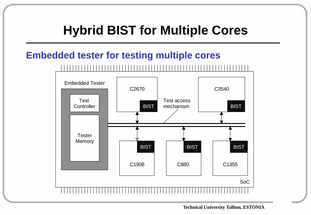
Hybrid BIST for Multiple Cores
SoC
C3540
C1908 C880 C1355
Embedded Tester C2670
Test accessmechanismBIST BIST
BISTBISTBIST
Test Controller
TesterMemory
Embedded tester for testing multiple cores

Technical University Tallinn, ESTONIA
Hybrid BIST for Multiple Cores
Deterministic test (DT)
Pseudorandom test (PT)
How to packknapsack?How to compress thetest sequence?

Technical University Tallinn, ESTONIA
Cost of BIST: Total Cost
CTOTAL
Figure 2: Cost calculation for hybrid BIST
Cost of pseudorandom test
patterns CGEN
Number of remaining faults after applying k
pseudorandom test patterns rNOT(k)
Cost of stored test CMEM
Number of pseudorandom test patterns applied, k
# faults
PR test length k
# tests
FAST estimation
SLOW analysis
CTOTAL = α k + β t(k)
β t(k)
α k
min CTOTAL
Det. TestPseudorandom Test
How to avoid the calculation of the very expensive full DT cost curve?
Two problems:1) Calculation of DT cost is
difficult2) We have to optimize n (!)
processes
Multi-Core Hybrid BIST Optimization

Technical University Tallinn, ESTONIA
Deterministic Test Length Estimation
i
F
F D k ( i ) F P E k ( i )
i *
F*
| T D E k ( i ) |
100%
| T D F k | j i
Fault coverage
Pseudorandom test length
Deterministic test (DT)Pseudorandom test (PT)
Deterministic test length estimation for a single core
For each PT length i* we determine - PT fault coverage F*, and- the imaginable part of DT
FDk(i) to be used for the same fault coverage
Then the remaining part of DT TDE
k(i) will be the estimation of the DT length
Solution of the first problem:
Technical University Tallinn, ESTONIA
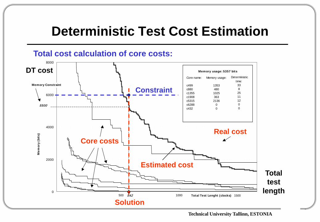
Deterministic Test Cost Estimation
0
2000
4000
6000
8000
Memory usage: 5357 bits
1000 1500500
5500
542
Mem
ory
(bit
s)
Memory usage:
135348010253632136
00
Core name:
c499 c880c1355c1908c5315c6288c432
Deterministic time: 33825111200
Total Test Lenght (clocks)
Estimated CostReal Cost
Cost Estimatesfor Individual Cores
Memory Constraint
Core costsReal cost
Estimated cost
DT cost
Total test
length
Total cost calculation of core costs:
Constraint
Solution

Technical University Tallinn, ESTONIA
Total Test Cost Estimation
COST P,k
COST T,k
COST
j COST D,k
j min
COST E* T
j* k
Solution
E
E
DT cost
Pseudorandom test (PT) length
Total cost
PT cost
Total cost solution
Using total cost solution we find the PT length:
Using PT length, we calculate the test processes for all cores:
PT length solution
136
86
40
19
48
50
46
21
13
25
6
4
4
2
73
123
169
205
203
190
0 50 100 150 200
c499
c1355
c5315
c1908
c880
c6288
c432DeterministicPseudorandom
Total Test
Technical University Tallinn, ESTONIA
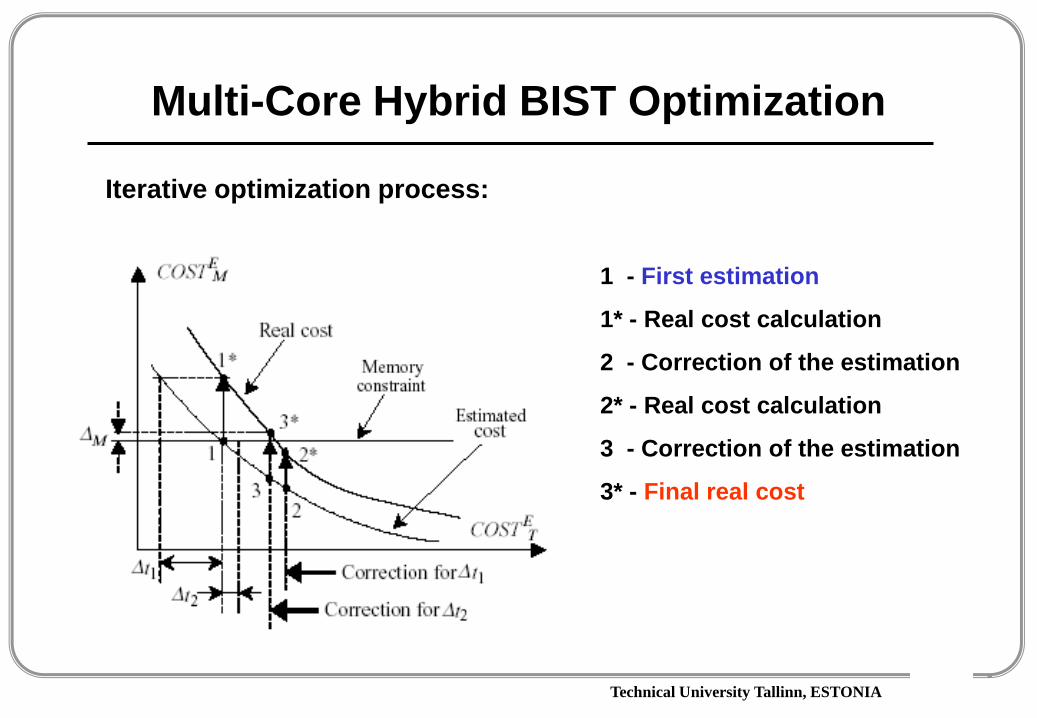
Multi-Core Hybrid BIST Optimization
Iterative optimization process:
1 - First estimation
1* - Real cost calculation
2 - Correction of the estimation
2* - Real cost calculation
3 - Correction of the estimation
3* - Final real cost

Technical University Tallinn, ESTONIA
Optimized Multi-Core Hybrid BIST
Pseudorandom test is carried out in parallel, deterministic test - sequentially

Technical University Tallinn, ESTONIA
Test-per-Scan Hybrid BIST
Embedded Tester
Test Controller
TesterMemory
Scan Path
Scan Path
Scan Path
Scan Path
LFS
R
LFSR
Scan Path
Scan Path
Scan Path
Scan Path
LFSR
LFS
R
Scan Path
Scan Path
Scan Path
Scan Path
Scan Path
Scan Path
Scan Path
Scan Path
LFS
R
LFS
R
LFSR
LFSR
s838s1423
s3271 s298
SoC
TAM
Deterministic tests can only be carried out for one core at a time
Only one test access bus at the system level is needed.
Every core’s BIST logic is capable to produce a set of independent pseudorandom test The pseudorandom test sets for all the cores can be carried out simultaneously
Technical University Tallinn, ESTONIA
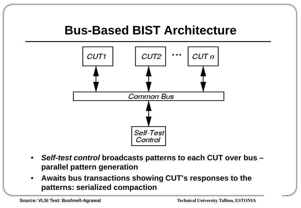
Bus-Based BIST Architecture
• Self-test control broadcasts patterns to each CUT over bus –parallel pattern generation
• Awaits bus transactions showing CUT’s responses to the patterns: serialized compaction
Source: VLSI Test: Bushnell-Agrawal
Technical University Tallinn, ESTONIA
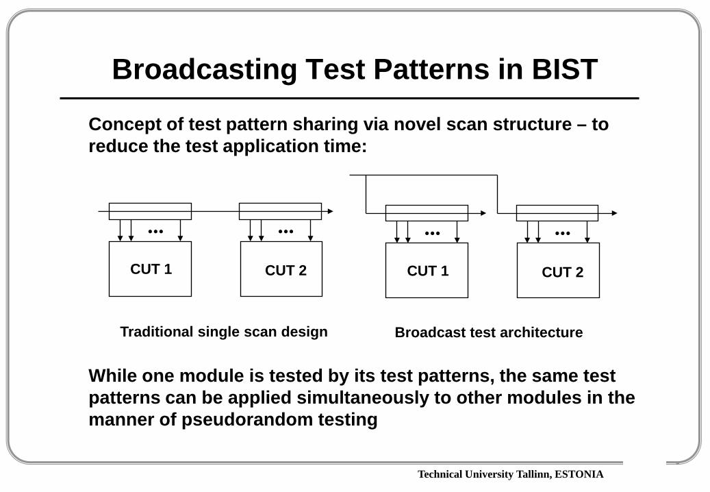
Broadcasting Test Patterns in BIST
Concept of test pattern sharing via novel scan structure – to reduce the test application time:
... ...
CUT 1 CUT 2
... ...
CUT 1 CUT 2
Traditional single scan design Broadcast test architecture
While one module is tested by its test patterns, the same test patterns can be applied simultaneously to other modules in the manner of pseudorandom testing
Technical University Tallinn, ESTONIA
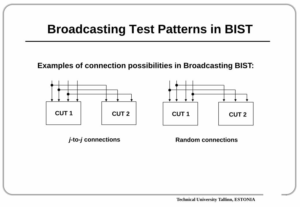
Broadcasting Test Patterns in BIST
Examples of connection possibilities in Broadcasting BIST:
CUT 1 CUT 2 CUT 1 CUT 2
j-to-j connections Random connections
Technical University Tallinn, ESTONIA
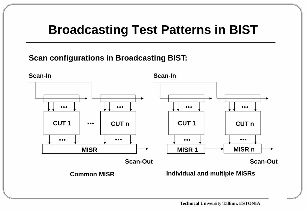
Broadcasting Test Patterns in BIST
... ...
CUT 1 CUT n
Scan configurations in Broadcasting BIST:
...
MISR
Scan-In
Scan-Out
... ...
... ...
CUT 1 CUT n
MISR 1
Scan-In
Scan-Out
... ...MISR n
Common MISR Individual and multiple MISRs

Fault-Model Free Fault DiagnosisCombined cause-effect and effect-cause diagnosis
Faulty system
Faulty area
Faulty area
Faulty block
Failing test
patternsTest
Fault1) Cause-Effect Fault DiagnosisSuspected faulty area is located
2) Effect-Cause Fault DiagnosisFaulty block is located in the suspected faulty area
3) Fault ReasoningFailing test patterns are mapped into the suspected defect or into a set of suspected defects in the faulty block
Effect
Cause
Effect
Cause

Technical University Tallinn, ESTONIA4/20
BISD scheme:
Test Pattern Generator(TPG)
Circuit Under Diagnosis(CUD)
. . . . . .
Output Response Analyser (ORA)
. . . . . .
BISDControl Unit
Pattern Signature Faults............ ............. ................... ............. ................... ............. ................... ............. ................... ............. ................... ......... .... ................... ............. ................... ............. .......
Test patterns
............ ............. .......
............ ............. .......
............ ............. .......
............ ............. .......
............ ............. .......
............ ............. .......
............ ............. .......
............ ............. .......
May 11-14, 2008 26th International Conference on Microelectronics, Niš, Serbia
Diagnostic Points (DPs) –patterns that detect new faultsFurther minimization of DPs –as a tradeoff with diagnostic resolution
Pseudorandom test sequence:
Embedded BIST Based Fault Diagnosis

Technical University Tallinn, ESTONIA
Built-In Fault Diagnosis
Test Pattern Generator (TPG)
Circuit Under Test (CUT)
. . . . . .
Output Response Analyser (ORA)
. . . . . .
BIST Control Unit
Test patterns Number Signature Faults ............ ............. ....... ............ ............. ....... ............ ............. ....... ............ ............. ....... ............ ............. ....... ............ ............. ....... ............ ............. ....... ............ ............. .......
Test patterns Number Signature Faults ............ ............. ....... ............ ............. ....... ............ ............. ....... ............ ............. ....... ............ ............. ....... ............ ............. ....... ............ ............. ....... ............ ............. .......
Faulty signature
1. test 2. test 3. test
3. test
Faulty signature
Correct signature
Diagnosis procedure:

Technical University Tallinn, ESTONIA
Built-In Fault Diagnosis
№ All faults New faults Coverage1 5 5 16.67%2 15 10 50.00%3 16 1 53.33%4 17 1 56.67%5 20 3 66.67%6 21 1 70.00%7 25 4 83.33%8 26 1 86.67%9 29 3 96.67%
10 30 1 100.00%
Pseudorandom test fault simulation
Binary search with bisectioning of test patterns
5
1
7
8
6 9
10101
15
1
3
1
2
3
413 4
Average number of test sessions: 3,3Average number of clocks: 8,67
Technical University Tallinn, ESTONIA
Built-In Fault Diagnosis
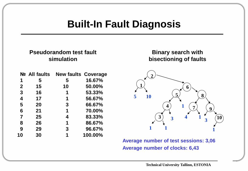
№ All faults New faults Coverage1 5 5 16.67%2 15 10 50.00%3 16 1 53.33%4 17 1 56.67%5 20 3 66.67%6 21 1 70.00%7 25 4 83.33%8 26 1 86.67%9 29 3 96.67%
10 30 1 100.00%
Pseudorandom test fault simulation
2
61
105 5
4
3
8
7 9
10
1
3 4
1
1
1 31
Binary search with bisectioning of faults
Average number of test sessions: 3,06Average number of clocks: 6,43
Technical University Tallinn, ESTONIA
Built-In Fault Diagnosis
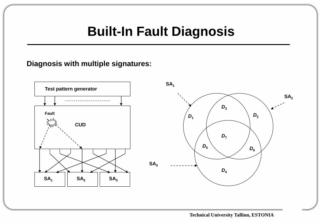
Test pattern generator
CUD
SA1 SA2 SA3
Fault
Diagnosis with multiple signatures:
SA1
SA2
SA3
D1 D2
D3
D4
D5 D6
D7
Technical University Tallinn, ESTONIA
Built-In Fault Diagnosis
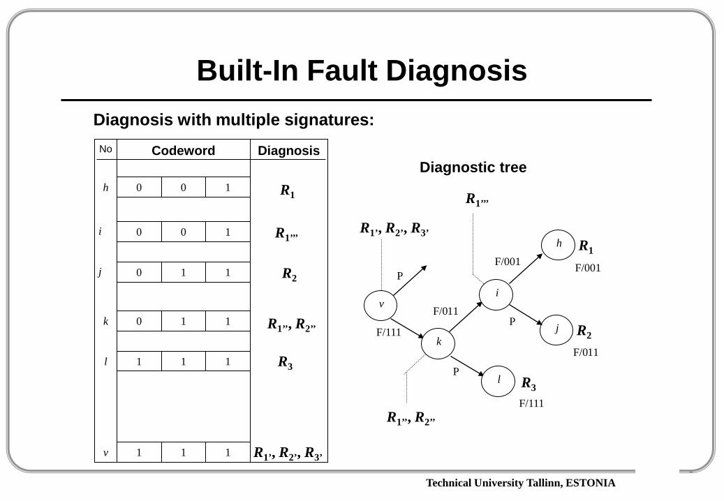
1 1 1
1 1 1
0 0 1
0 0 1
0 1 1
h
i
k
l
v
R1
R1’’’
R3
No Codeword Diagnosis
0 1 1j R2
R1’, R2’, R3’
R1’’, R2’’
v
P
F/111k
F/011
i
j
F/011
F/111
l R3
R2
h R1
R1’’’
R1’’, R2’’
F/001
R1’, R2’, R3’
Diagnostic tree
P
P
F/001
Diagnosis with multiple signatures:

Technical University Tallinn, ESTONIA
Test pattern generator
CUD
SA1 SA2 SA3
Fault
SA1
SA2
SA3
D1 D2
D3
D4
D5 D6
D7
Faulty signature
Faulty signature
Correct signature
Intersection using SA-s
Intersection using tests
Built-In Fault Diagnosis
BIST with multiple signature analyzers
Optimization of the interface between CUD and SA-s
Technical University Tallinn, ESTONIA
Built-In Fault Diagnosis
0.010.020.030.040.050.060.070.080.090.0
100.0110.0120.0130.0140.0150.0160.0170.0180.0190.0200.0210.0220.0230.0240.0
1 2 3 4 5 6 7 8 9 10 ALL
Failed patterns
Ave
rage
reso
lutio
n
5.0
10.0
15.0
20.0
25.0
30.0
35.0
40.0
45.0
50.0
55.0
60.0
65.0
Ave
rage
test
leng
th
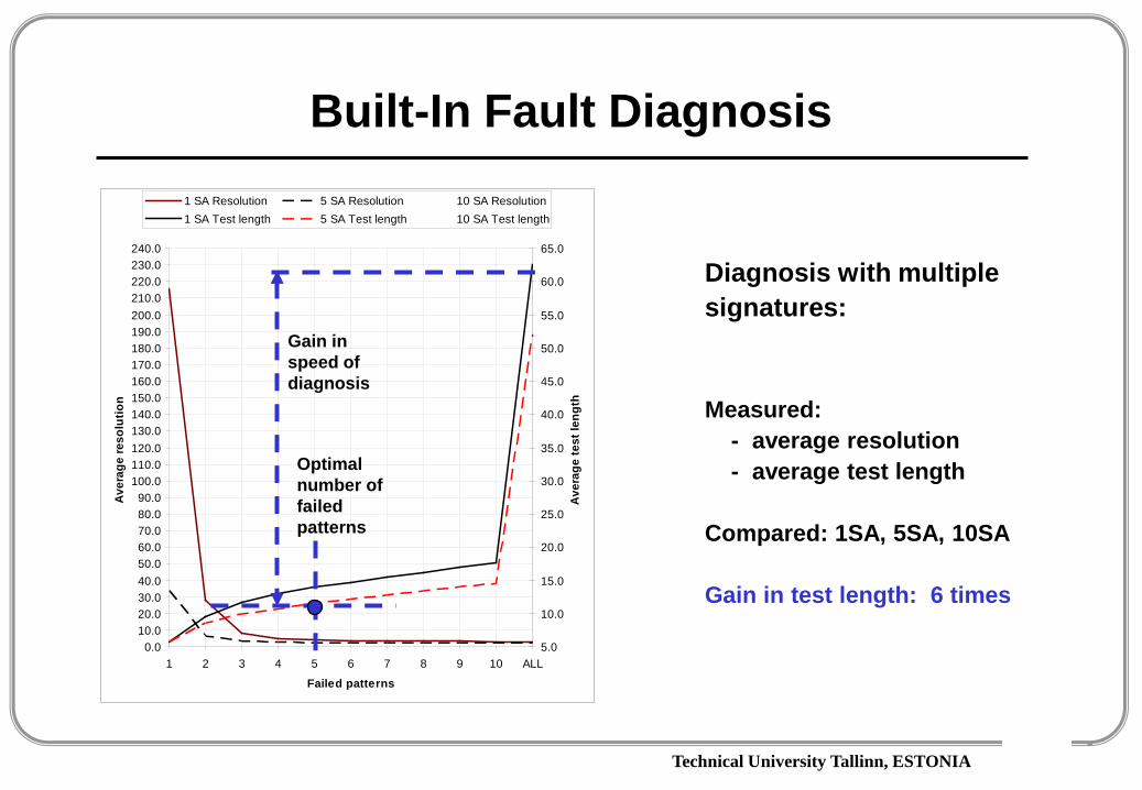
1 SA Resolution 5 SA Resolution 10 SA Resolution1 SA Test length 5 SA Test length 10 SA Test length
Optimal number of failed patterns
Gain in speed of diagnosis
Diagnosis with multiple signatures:
Measured:- average resolution- average test length
Compared: 1SA, 5SA, 10SA
Gain in test length: 6 times

Technical University Tallinn, ESTONIA
Extended Fault Models
Defect
Extensions of the parallel critical path tracing for two large general fault classes for modeling physical defects:
0101
Conditional faultPattern fault
Constrained SAFSingle faulty signal
X-faultByzantine fault
BridgesStuck-opens
Multiple faulty signal
Resistive bridge fault
SAF
Multiple fault

Technical University Tallinn, ESTONIA
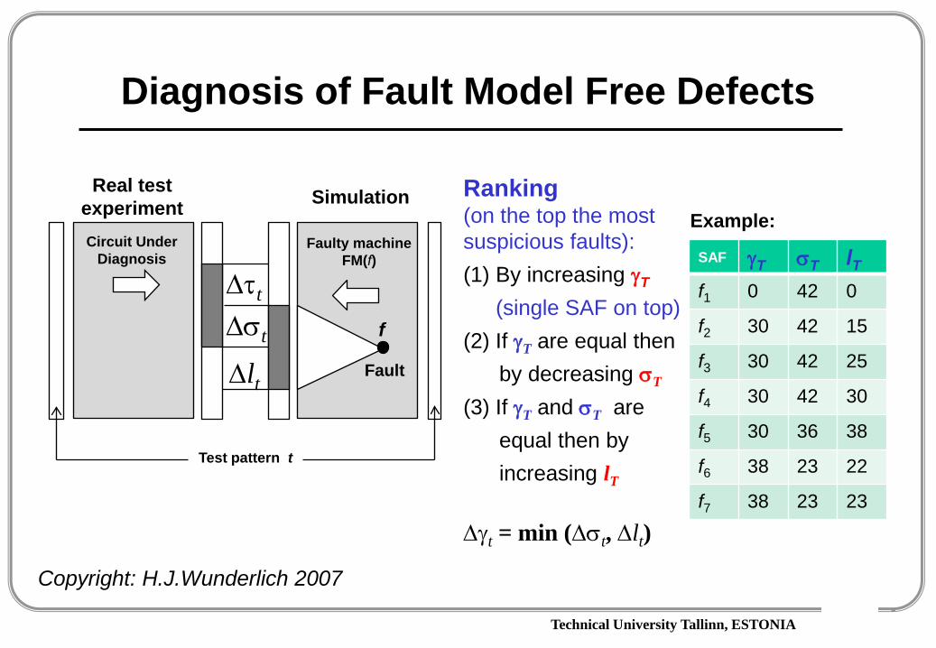
Diagnosis of Fault Model Free Defects
Real test experiment Simulation
Faulty machineFM(f)
Circuit Under Diagnosis
Test pattern t
Fault
f
Copyright: H.J.Wunderlich 2007
∆σt
∆τt
∆lt
Fault evidence:for test pattern te(f,t) = (∆τt , ∆σt, ∆lt, ∆γt)∆γt = min (∆σt, ∆lt)for full test T (sum)e(f,T) = (∆τ , ∆σ, ∆l, ∆γ)

Technical University Tallinn, ESTONIA
Diagnosis of Fault Model Free Defects
Copyright: H.J.Wunderlich 2007
Real test experiment Simulation
Faulty machineFM(f)
Circuit Under Diagnosis
Test pattern t
Fault
f∆σt
∆τt
∆lt
Classic model lt τt γt
Single SAF 0 0 0
Multiple SAF 0 >0 0
Single conditional SAF >0 0 0
Multiple cond. SAF >0 >0 0
Delay fault >0 0 >0
General case >0 >0 >0
Different classical fault cases
Technical University Tallinn, ESTONIA
Diagnosis of Fault Model Free Defects
Copyright: H.J.Wunderlich 2007
Real test experiment Simulation
Faulty machineFM(f)
Circuit Under Diagnosis
Test pattern t
Fault
f∆σt
∆τt
∆lt
Ranking (on the top the most suspicious faults): (1) By increasing γT
(single SAF on top)(2) If γT are equal then
by decreasing σT
(3) If γT and σT areequal then byincreasing lT
∆γt = min (∆σt, ∆lt)
SAF γT σT lTf1 0 42 0
f2 30 42 15
f3 30 42 25
f4 30 42 30
f5 30 36 38
f6 38 23 22
f7 38 23 23
Example:

Technical University Tallinn, ESTONIA
Fault Diagnosis Without Fault Models
Defective area
dy
Reverse defect
mappingx1
x2
x3
x4
x5
System level
Wd
Logic levelError
detection
Defect
Error (defective area) diagnosis
&
&
&
1
&
&
&R2M3
+M1
*M2
R1
IN
Logic levelTransistor level
RT Level

Technical University Tallinn, ESTONIA1 0 1 0
S1 S2
S10
S11
S5
S8
S3
S6
S9
S4
S7
1 2 3 41 12 13 14 15 1 1 06 17 18 1 1 09 110 1 111 1 1 1 0
Fault Model Free Fault Diagnosis
1 0 1 0Test response:
Diagnosis: s11
No match
Rectified code
Because of the unidirectional
“distortions” of test responses,
rectification is possible
Diagnostic tableSystem network graph
Technical University Tallinn, ESTONIA
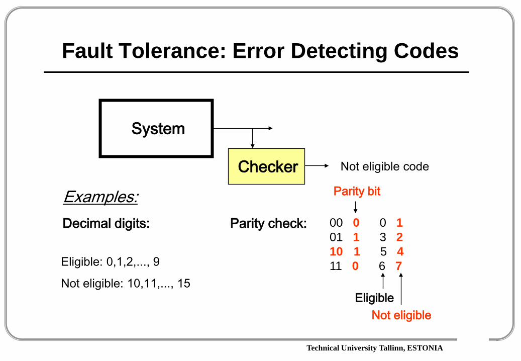
Fault Tolerance: Error Detecting Codes
System
Checker Not eligible code
Examples:Decimal digits:
Eligible: 0,1,2,..., 9
Not eligible: 10,11,..., 15
Parity check: 00 0 0 101 1 3 210 1 5 411 0 6 7
Parity bit
EligibleNot eligible

Technical University Tallinn, ESTONIA
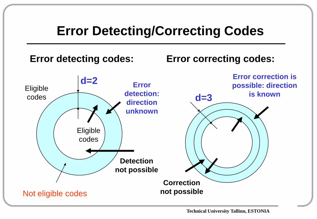
Error Detecting/Correcting Codes
d
Hamming distance between codes: Minimal number of bits how two codes differ from each other
Eligible codes
Eligible codes
Not eligible codes
Parity check: 00 0 0 101 1 3 210 1 5 411 0 6 7
Parity bit
EligibleNot eligible
101100111001
110
011
000d = 2
010
Technical University Tallinn, ESTONIA
Error Detecting/Correcting Codes
d=2Eligible codes
Eligible codes
Not eligible codes
Error detecting codes: Error correcting codes:
Error detection: direction unknown
Error correction is possible: direction
is knownd=3
Eligible codes
Detection not possible
Correction not possible
Technical University Tallinn, ESTONIA
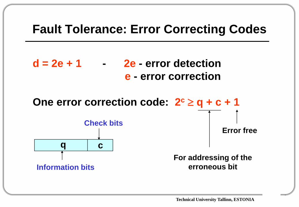
Fault Tolerance: Error Correcting Codes
d = 2e + 1 - 2e - error detection e - error correction
One error correction code: 2c ≥ q + c + 1
Error free
q cFor addressing of the
erroneous bit
Check bits
Information bits

Technical University Tallinn, ESTONIA
Fault Tolerance: One Error Correcting Code
One error correction code: 2c ≥ q + c + 1
Check bits
b2i, i = 0,1,,...,c-1
Calculation of check sums:
bc+q b2b1
1234567
cibkPk i
,...,1,0 ==∑∈
Pi – number of bits where bi = 1
P1 = b1 ⊕ b3 ⊕ b5 ⊕ b7 = 0P2 = b2 ⊕ b3 ⊕ b6 ⊕ b7 = 0P3 = b4 ⊕ b5 ⊕ b6 ⊕ b7 = 0

Technical University Tallinn, ESTONIA
Fault Tolerance: One Error Correcting Code
Location of erroneous bit:
Check bits
b2i, i = 1,...,c
1234567
P1 = b1 ⊕ b3 ⊕ b5 ⊕ b7 = 0P2 = b2 ⊕ b3 ⊕ b6 ⊕ b7 = 0P3 = b4 ⊕ b5 ⊕ b6 ⊕ b7 = 0
Analogy with fault diagnosis by using fault table:
7 6 5 4 3 2 1 01 1 11
1 1 111 111
P1P2
P3
Received code
Test
001
Diagnosis
0011101
0010101 Initial code
Check bits have to be independently assigned
Technical University Tallinn, ESTONIA
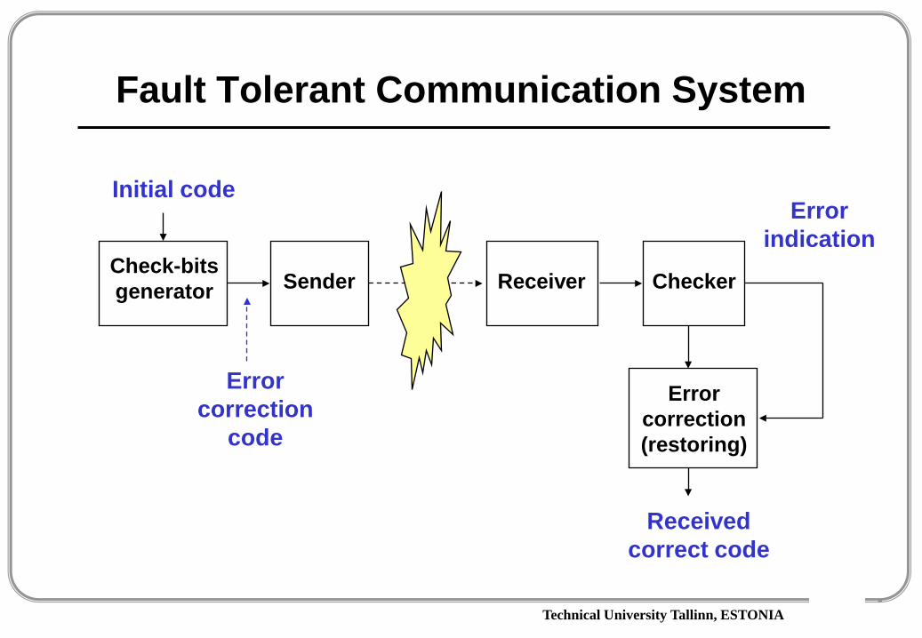
Fault Tolerant Communication System
Initial code
Check-bits generator Sender Receiver
Error correction
code
Checker
Error correction (restoring)
Error indication
Received correct code
Technical University Tallinn, ESTONIA
Error Detection in Arithmetic Operations
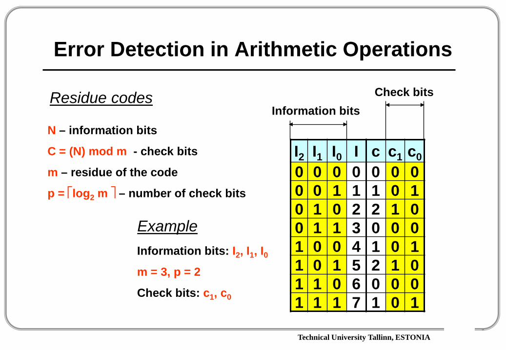
Residue codes
N – information bits
C = (N) mod m - check bits
m – residue of the code
p = log2 m – number of check bits
ExampleInformation bits: I2, I1, I0m = 3, p = 2
Check bits: c1, c0
I2 I1 I0 I c c1 c00 0 0 0 0 0 00 0 1 1 1 0 10 1 0 2 2 1 00 1 1 3 0 0 01 0 0 4 1 0 11 0 1 5 2 1 01 1 0 6 0 0 01 1 1 7 1 0 1
Information bitsCheck bits

Technical University Tallinn, ESTONIA
Error Detection in Arithmetic OperationsAddition:
Information bits Check bits0 0 1 0 1 0 2.20 1 0 0 0 1 4.1
0 1 1 0 1 1 6.3 (6)mod3 = 0 (3)mod3 = 0
Multiplication:
Information bits Check bits0 0 1 0 1 0 2.20 1 0 0 0 1 4.1
1 0 0 0 1 0 8.2 (8)mod3 = 2 (2)mod3 = 2
Information bits Check bits0 0 1 0 1 0 2.20 1 0 0 0 1 4.1
0 1 0 0 1 1 4.3 (4)mod3 = 1 (3)mod3 = 0
Error!
Information bits Check bits0 0 1 0 1 0 2.20 1 0 0 0 1 4.1
1 0 0 1 1 0 9.2 (9)mod3 = 0 (2)mod3 = 2
Error!
Technical University Tallinn, ESTONIA
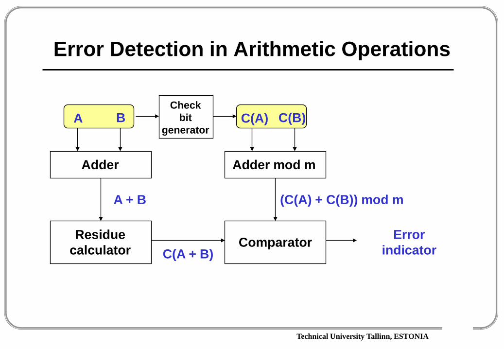
Error Detection in Arithmetic Operations
A B
Adder
Residue calculator
A + B
C(A) C(B)
Adder mod m
(C(A) + C(B)) mod m
ComparatorC(A + B)
Error indicator
Check bit
generator
Technical University Tallinn, ESTONIA
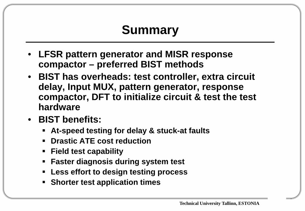
Summary
• LFSR pattern generator and MISR response compactor – preferred BIST methods
• BIST has overheads: test controller, extra circuit delay, Input MUX, pattern generator, response compactor, DFT to initialize circuit & test the test hardware
• BIST benefits: At-speed testing for delay & stuck-at faults Drastic ATE cost reduction Field test capability Faster diagnosis during system test Less effort to design testing process Shorter test application times

Technical University Tallinn, ESTONIA
Testing of Networks-on-Chip (NoC)
• Consider a mesh-like topology of NoC consisting of – switches (routers), – wire connections between them and – slots for SoC resources, also referred to as tiles.
• Other types of topological architectures, e.g. honeycomb and torus may be implemented and their choice depends on the constraints for low-power, area, speed, testability
• The resource can be a processor, memory, ASIC core etc. • The network switch contains buffers, or queues, for the incoming
data and the selection logic to determine the output direction,where the data is passed (upward, downward, leftward and rightward neighbours)

Technical University Tallinn, ESTONIA
Testing of Networks-on-Chip
• Useful knowledge for testing NoC network structures can be obtained from the interconnect testing of other regular topological structures
• The test of wires and switches is to some extent analogous to testing ofinterconnects of an FPGA
• a switch in a mesh-like communication structure can be tested by using only three different configurations
Technical University Tallinn, ESTONIA
Testing of Networks-on-Chip
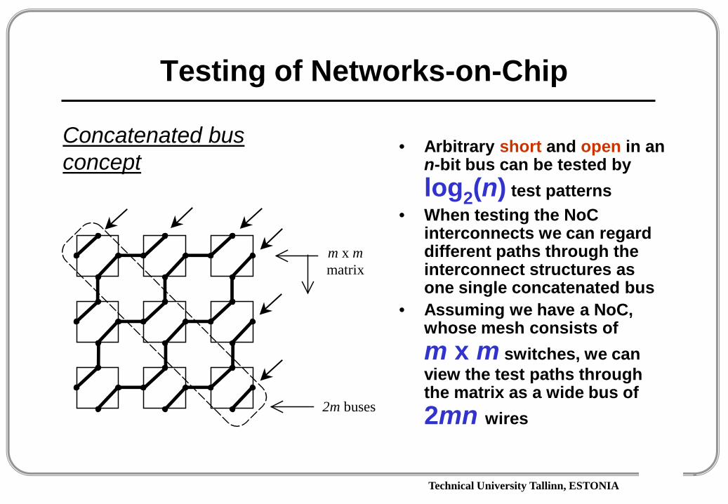
• Arbitrary short and open in an n-bit bus can be tested by log2(n) test patterns
• When testing the NoC interconnects we can regard different paths through the interconnect structures as one single concatenated bus
• Assuming we have a NoC, whose mesh consists of m x m switches, we can view the test paths through the matrix as a wide bus of 2mn wires
m x mmatrix
2m buses
Concatenated bus concept

Technical University Tallinn, ESTONIA
Testing of Networks-on-Chip
• The stuck-at-0 and stuck-at-1faults are modeled as shorts to Vdd and ground
• Thus we need two extra wires, which makes the total bitwidth of the bus 2mn + 2 wires.
• From the above facts we can find that 3[log2(2mn+2)]test patterns are needed in order to test the switches and the wiring in the NoC
m x mmatrix
2m buses
Concatenated bus concept
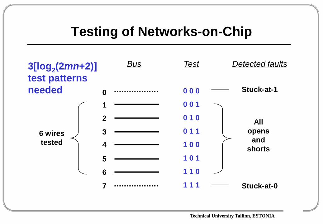
Technical University Tallinn, ESTONIA
Testing of Networks-on-Chip
01
2
34
5
6
7
Bus
0 0 0
0 0 1
0 1 0
0 1 1
1 0 0
1 0 1
1 1 0
1 1 1
Test Detected faults
Stuck-at-1
Stuck-at-0
All opens
and shorts
6 wires tested
3[log2(2mn+2)]test patterns needed

Technical University Tallinn, ESTONIA
IEEE P1500 standard for core test
• The following components are generally required to test embedded cores– Source for application of test stimuli and a sink for observing
the responces– Test Access Mechanisms (TAM) to move the test data from
the source to the core inputs and from the core outputs to the sink
– Wrapper around the embedded core
embeddedcore
wrapper
testpatternsource
TAMtest
responces’sink
TAM
Technical University Tallinn, ESTONIA
IEEE P1500 standard for core test
• The two most important components of the P1500 standard are– Core test language (CTL) and – Scalable core test architecture
• Core Test Language– The purpose of it is to standardize the core test knowledge
transfer – The CTL file of a core must be supplied by the core provider – This file contains information on how to
• instanciate a wrapper, • map core ports to wrapper ports, • and reuse core test data

Technical University Tallinn, ESTONIA
IEEE P1500 standard for core test
Core test architecture• It standardizes only the wrapper and the interface between the
wrapper and TAM, called Wrapper Interface Port or (WIP) • The P1500 TAM interface and wrapper can be viewed as an
extension to IEEE Std. 1149.1, since – the 1149.1 TAP controller is a P1500-compliant TAM interface, – and the boundary-scan register is a P1500-compliant wrapper
• Wrapper contains– an instruction register (WIR), – a wrapper boundary register consisting of wrapper cells, – a bypass register and some additional logic.
• Wrapper has to allow normal functional operation of the core plus it has to include a 1-bit serial TAM.
• In addition to the serial test access, parallel TAMs may be used.

Technical University Tallinn, ESTONIA
IEEE P1500 standard for core test
System chip
Source/Sink(Stimuli/Responses)
Off-chip or
On-chip
User-defined test access mechanism (TAM) On-chip
P1500 wrapper
Core 1
WIR
WPI WPOFunctional
inputs/outputs
P1500 wrapper
Core n
WIR
WPI WPOFunctional
inputs/outputs
P1500 Wrapper interface port (WIP)
WSIWSI WSO WSO
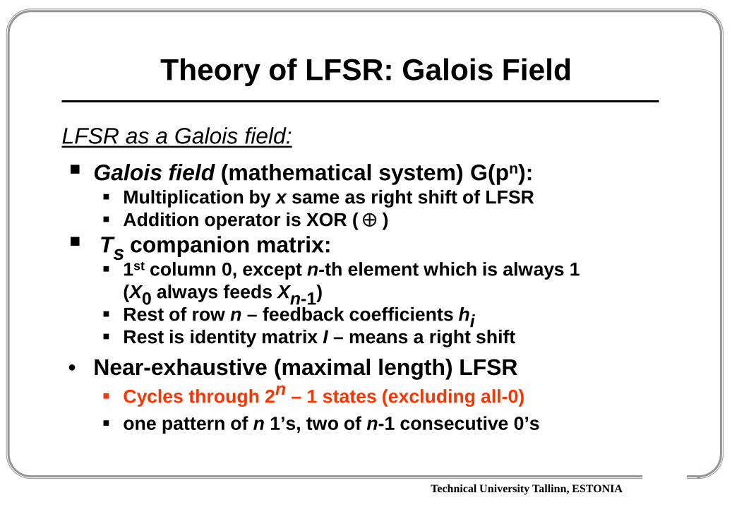
Technical University Tallinn, ESTONIA
Theory of LFSR: Galois Field
Galois field (mathematical system) G(pn): Multiplication by x same as right shift of LFSR Addition operator is XOR ( ⊕ )
Ts companion matrix: 1st column 0, except n-th element which is always 1
(X0 always feeds Xn-1) Rest of row n – feedback coefficients hi Rest is identity matrix I – means a right shift
• Near-exhaustive (maximal length) LFSR Cycles through 2n – 1 states (excluding all-0) one pattern of n 1’s, two of n-1 consecutive 0’s
LFSR as a Galois field: