design, implementation and evaluation of an...
TRANSCRIPT
PONTIFICIA UNIVERSIDAD CATOLICA DE CHILE
ESCUELA DE INGENIERIA
DESIGN, IMPLEMENTATION AND
EVALUATION OF AN AUXILIARY ENERGY
SYSTEM FOR ELECTRIC VEHICLES, BASED
ON ULTRACAPACITORS AND BUCK-BOOST
CONVERTER
MICAH E. ORTÚZAR
Thesis submitted to the Office of Research and Graduate Studies in partial
fulfillment of the requirements for the Degree of Doctor in Engineering
Sciences
Advisor:
JUAN W. DIXON
Santiago de Chile, July, 2005
PONTIFICIA UNIVERSIDAD CATOLICA DE CHILE
ESCUELA DE INGENIERIA
Departamento de Ingeniería Eléctrica
DESIGN, IMPLEMENTATION AND
EVALUATION OF AN AUXILIARY ENERGY
SYSTEM FOR ELECTRIC VEHICLES, BASED
ON ULTRACAPACITORS AND BUCK-BOOST
CONVERTER
MICAH E. ORTÚZAR
Members of the Committee:
JUAN W. DIXON
LUIS MORÁN
JOSÉ RODRIGUEZ
MARCELO GUARINI
BIMAL K. BOSE
RAFAEL RIDDELL
Thesis submitted to the Office of Research and Graduate Studies in partial
fulfillment of the requirements for the Degree of Doctor in Engineering
Sciences
Santiago de Chile, July, 2005

A mi Familia y mis amigos,
A todos los que me apoyaron.

AGRADECIMIENTOS
Después de más de cuatro años de trabajo y estudio son muchos los cambios, muchas las
experiencias vividas, profesional y personalmente. El apoyo de mi familia, desde distintos
lugares del mundo, ha sido fundamental, me ha ayudado en momentos críticos y hoy me
acompañan en este paso. A ellos, mi Papá, Mamá; a mis hermanos, a Margarita y Thomas,
a todos ellos muchas gracias.
Mis amigos han jugado un papel importante durante este período. Ellos han sido mi
segunda familia y un apoyo emocional imprescindible. Un cariñoso saludo a todos ellos.
También me siento profundamente agradecido de todos quienes me apoyaron al interior del
departamento de Ingeniería Eléctrica. Un agradecimiento especial a Eduardo Cea por su
ayuda y su amistad. Muchas gracias a Betty y Elena por su apoyo materno, gracias a
Virginia y Carlos por cuidar de nosotros. Gracias también a Nelson Saleh por su ayuda y
buena voluntad.
Una mención especial merece el profesor Juan Dixon y su familia por quienes me sentí
muy acogido. Juan se involucró a fondo en este proyecto y gracias a su empuje e iniciativa
hemos llegado a puerto. Todos los resultados y logros de este proyecto se deben, en gran
medida, a su iniciativa y su experiencia. También agradezco su amistad y comprensión a lo
largo de varios años en que hemos trabajado juntos. Un saludo especial para Juan.

CONTENTS
Pág.
TABLE INDEX............................................................................................................ 7
FIGURE INDEX.......................................................................................................... 8
RESUMEN................................................................................................................. 10
ABSTRACT............................................................................................................... 12
I INTRODUCTION ............................................................................................ 14 I.1 Electric and hybrid vehicles ..................................................................... 14 I.2 Integrating different energy systems ........................................................ 16 I.3 What are ultracapacitors and how do they work? .................................... 19 I.4 State-of-the-art traction systems using ultracapacitors ............................ 23 I.5 Objectives and hypothesis ........................................................................ 27 I.6 Methodology ............................................................................................ 29
II STATIC CONVERTER DESIGN AND IMPLEMENTATION ..................... 32 II.1 Introduction .............................................................................................. 32 II.2 Power design ............................................................................................ 35
II.2.1 Buck-boost topology...................................................................... 35 II.2.2 Static converter components design and selection ........................ 39
II.3 Safety features .......................................................................................... 45 II.4 Thermal design......................................................................................... 46 II.5 Mechanical design.................................................................................... 48
III MONITORING AND CONTROL SYSTEM .................................................. 51 III.1 Introduction .............................................................................................. 51 III.2 Control algorithms.................................................................................... 51 III.3 Communication layout ............................................................................. 56 III.4 Implementation via DSP .......................................................................... 57 III.5 Real-time monitoring software................................................................. 58 III.6 Failure detection....................................................................................... 59
IV URBAN CIRCUIT TESTS............................................................................... 60

IV.1 Introduction .............................................................................................. 60 IV.2 Test circuit................................................................................................ 60 IV.3 Tests results .............................................................................................. 61
V RESULTS ANALYSIS .................................................................................... 65 V.1 Economic approach on results.................................................................. 65 V.2 Related researches .................................................................................... 68 V.3 General discussion.................................................................................... 70
VI CONCLUSIONS .............................................................................................. 73
REFERENCES........................................................................................................... 75
A P P E N D I C E S................................................................................................... 82
Appendix A: Buck-Boost Converter Operation Analysis .......................................... 83
Appendix B: Disipated energy and heat generation in semiconductors..................... 86
Appendix C: Economic Evaluation Considerations................................................... 91
Appendix D: TMS320F241 DSP Controller, Texas Instruments .............................. 92
Appendix E: DSP code, Assembler Language........................................................... 94
7
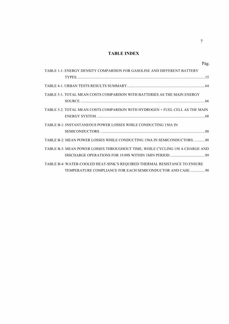
TABLE INDEX
Pág. TABLE 1-1: ENERGY DENSITY COMPARISON FOR GASOLINE AND DIFFERENT BATTERY
TYPES........................................................................................................................................15
TABLE 4-1. URBAN TESTS RESULTS SUMMARY. .................................................................................64
TABLE 5-1. TOTAL MEAN COSTS COMPARISON WITH BATTERIES AS THE MAIN ENERGY
SOURCE. ...................................................................................................................................66
TABLE 5-2. TOTAL MEAN COSTS COMPARISON WITH HYDROGEN + FUEL CELL AS THE MAIN
ENERGY SYSTEM. ..................................................................................................................68
TABLE B-1: INSTANTANEOUS POWER LOSSES WHILE CONDUCTING 150A IN
SEMICONDUCTORS. ..............................................................................................................88
TABLE B-2: MEAN POWER LOSSES WHILE CONDUCTING 150A IN SEMICONDUCTORS. ...........88
TABLE B-3: MEAN POWER LOSSES THROUGHOUT TIME, WHILE CYCLING 150 A CHARGE AND
DISCHARGE OPERATIONS FOR 19.09S WITHIN 1MIN PERIOD. ....................................89
TABLE B-4: WATER-COOLED HEAT-SINK’S REQUIRED THERMAL RESISTANCE TO ENSURE
TEMPERATURE COMPLIANCE FOR EACH SEMICONDUCTOR AND CASE................90
8
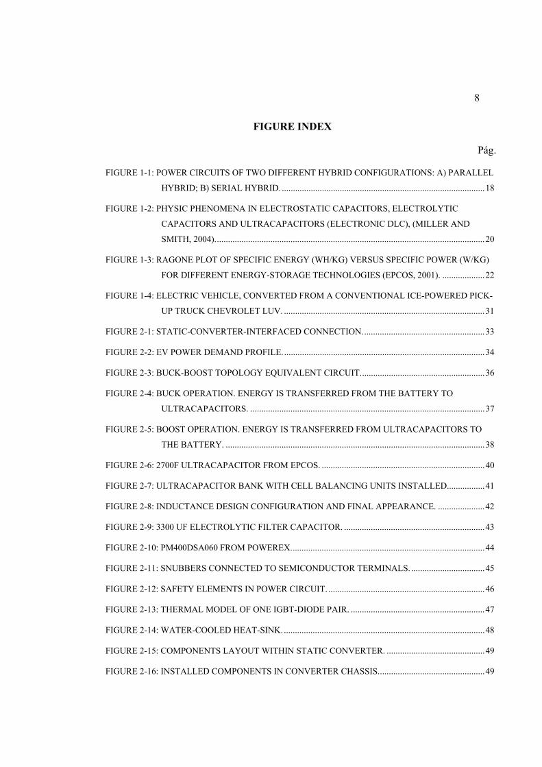
FIGURE INDEX
Pág.
FIGURE 1-1: POWER CIRCUITS OF TWO DIFFERENT HYBRID CONFIGURATIONS: A) PARALLEL
HYBRID; B) SERIAL HYBRID. ...........................................................................................18
FIGURE 1-2: PHYSIC PHENOMENA IN ELECTROSTATIC CAPACITORS, ELECTROLYTIC
CAPACITORS AND ULTRACAPACITORS (ELECTRONIC DLC), (MILLER AND
SMITH, 2004).........................................................................................................................20
FIGURE 1-3: RAGONE PLOT OF SPECIFIC ENERGY (WH/KG) VERSUS SPECIFIC POWER (W/KG)
FOR DIFFERENT ENERGY-STORAGE TECHNOLOGIES (EPCOS, 2001). ...................22
FIGURE 1-4: ELECTRIC VEHICLE, CONVERTED FROM A CONVENTIONAL ICE-POWERED PICK-
UP TRUCK CHEVROLET LUV. ..........................................................................................31
FIGURE 2-1: STATIC-CONVERTER-INTERFACED CONNECTION.......................................................33
FIGURE 2-2: EV POWER DEMAND PROFILE...........................................................................................34
FIGURE 2-3: BUCK-BOOST TOPOLOGY EQUIVALENT CIRCUIT........................................................36
FIGURE 2-4: BUCK OPERATION. ENERGY IS TRANSFERRED FROM THE BATTERY TO
ULTRACAPACITORS. .........................................................................................................37
FIGURE 2-5: BOOST OPERATION. ENERGY IS TRANSFERRED FROM ULTRACAPACITORS TO
THE BATTERY. ....................................................................................................................38
FIGURE 2-6: 2700F ULTRACAPACITOR FROM EPCOS. .........................................................................40
FIGURE 2-7: ULTRACAPACITOR BANK WITH CELL BALANCING UNITS INSTALLED.................41
FIGURE 2-8: INDUCTANCE DESIGN CONFIGURATION AND FINAL APPEARANCE. .....................42
FIGURE 2-9: 3300 UF ELECTROLYTIC FILTER CAPACITOR. ...............................................................43
FIGURE 2-10: PM400DSA060 FROM POWEREX.......................................................................................44
FIGURE 2-11: SNUBBERS CONNECTED TO SEMICONDUCTOR TERMINALS. .................................45
FIGURE 2-12: SAFETY ELEMENTS IN POWER CIRCUIT. ......................................................................46
FIGURE 2-13: THERMAL MODEL OF ONE IGBT-DIODE PAIR. ............................................................47
FIGURE 2-14: WATER-COOLED HEAT-SINK...........................................................................................48
FIGURE 2-15: COMPONENTS LAYOUT WITHIN STATIC CONVERTER. ............................................49
FIGURE 2-16: INSTALLED COMPONENTS IN CONVERTER CHASSIS................................................49
9
FIGURE 2-17: STATIC CONVERTER A) POWER CIRCUIT INSTALLATION, B) LOCATION IN
FRONT COMPARTMENT....................................................................................................50
FIGURE 3-1: HEURISTICS-SOC-CONTROL ALGORITHM AND SIGNALS MANIPULATION. ..........53
FIGURE 3-2: OPTIMAL CONTROL DATA GENERATION AND NEURAL NETWORK TRAINING
PROCESSES. .........................................................................................................................55
FIGURE 3-3: OPTIMAL-CONTROL ALGORITHM, IMPLEMENTED USING NEURAL NETWORKS.56
FIGURE 3-4: COMMUNICATION AND COMMAND FLOW DIAGRAM. ...............................................57
FIGURE 3-5: DSP CONTROL BOARD, SIGNALS AND DATA PORTS. ..................................................58
FIGURE 3-6: CONTROL AND DATA MONITORING/ACQUISITION SOFTWARE SCREENS. ...........58
FIGURE 4-1: URBAN CIRCUIT TEST COURSE.........................................................................................61
FIGURE 4-2: LOAD CURRENT AND BATTERY VOLTAGE WITHOUT AES’S POWER SUPPORT...62
FIGURE 4-3: CURRENTS AND BATTERY VOLTAGE FOR A POWER-SUPPORTED SYSTEM. ........63

10
PONTIFICIA UNIVERSIDAD CATOLICA DE CHILE ESCUELA DE INGENIERIA DEPARTAMENTO DE INGENIERÍA ELÉCTRICA
DISEÑO, IMPLEMENTACIÓN Y EVALUACIÓN DE UN SISTEMA AUXILIAR
DE ENERGÍA PARA VEHÍCULOS ELÉCTRICOS, BASADO EN
ULTRACAPACITORES Y CONVERTIDOR BUCK-BOOST
Tesis enviada a la Dirección de Investigación y Postgrado en cumplimiento parcial de
los requisitos para el grado de Doctor en Ciencias de la Ingeniería.
MICAH E. ORTÚZAR
RESUMEN
El trabajo expuesto en esta tesis explora los factores clave que impiden a los vehículos
eléctricos ser ampliamente aceptados en los mercados de transporte público y privado. En
particular, se analizan las limitaciones que presentan los sistemas de almacenaje de energía
para entregar altas potencias durante la aceleración o recibirlas durante el frenado. Para
resolver estos problemas de potencia se propone la combinación de elementos de alta
potencia específica con elementos de alta energía específica. En este contexto se ha
diseñado, implementado y evaluado un Sistema Auxiliar de Potencia (SAP), basado en
ultracapacitores y un convertidor Buck-Boost para ser usado en combinación con baterías
de plomo-ácido. Los procesos de diseño e implementación se describen en detalle; también
se presentan los resultados del proceso de evaluación. Finalmente se complementa la
discusión de los resultados con un análisis desde el punto de vista económico de la
implementación de este tipo de sistemas.
La falta de elementos de almacenaje de energía eléctrica que presenten, simultáneamente,
alta potencia específica y alta energía específica, y los altos costos de estos equipos, se
consideran los mayores obstáculos para introducir vehículos de cero emisiones en los
mercados de transporte público y privado. La combinación de elementos de alta energía
específica, como celdas de combustible o baterías avanzadas, con elementos de alta

11
potencia específica, como los ultracapacitores, se presenta como la solución más viable
para solucionar los problemas de baja autonomía y/o desempeño deficiente en el corto
plazo.
El SAP propuesto, basado en ultracapacitores y convertidor buck-boost, se ha diseñado e
implementado en un vehículo eléctrico a escala real en combinación con baterías de
plomo-ácido. Los procesos de diseño e implementación, así como el período de pruebas y
sus resultados, se describen en detalle.
Los resultados de la evaluación muestran que, con el SAE instalado y operando en el
vehículo, la potencia disponible ha aumentado de 40 kW a 85 kW. Se han evaluado dos
algoritmos de administración de energía, uno basado en heurística y el otro basado en
técnicas de control óptimo aplicado a redes neuronales; el rendimiento del vehículo
(km/kWh) aumentó en un 5.2% y un 8.9% con el primer y segundo algoritmo,
respectivamente. Del análisis económico se concluyó que, si se consideran los costos
solamente, con el sistema propuesto se requeriría que la vida útil de la batería se extendiese
en un 50% o más para compensar los costos del SAE.
Para mejorar la autonomía y para realizar, en el futuro, nuevos análisis al sistema
desarrollado, se ha instalado una batería de Na/Ni-Cl2 (conocida comercialmente como
batería ZEBRA) en reemplazo de las baterías de plomo-ácido.
Members of the Doctoral Thesis Committee:
JUAN W. DIXON
LUIS MORÁN
JOSÉ RODRÍGUEZ
MARCELO GUARINI
BIMAL K. BOSE
RAFAEL RIDDELL
Santiago, July, 2005
12
PONTIFICIA UNIVERSIDAD CATOLICA DE CHILE ESCUELA DE INGENIERIA DEPARTAMENTO DE INGENIERÍA ELÉCTRICA
DESIGN, IMPLEMENTATION AND EVALUATION OF AN AUXILIARY
ENERGY SYSTEM FOR ELECTRIC VEHICLES, BASED ON
ULTRACAPACITORS AND BUCK-BOOST CONVERTER
Thesis submitted to the Office of Research and Graduate Studies in partial
fulfillment of the requirements for the Degree of Doctor in Engineering Sciences by
MICAH E. ORTÚZAR
ABSTRACT
This thesis addresses key issues that prevent electric vehicles from being broadly adopted
by private and public transportation markets. In particular, the limitations of energy storage
devices to deliver energy at high power rates during acceleration and accept high power
regeneration during braking are analyzed. To solve available power problems, the
combination of a high specific-power storage device with a high specific-energy storage
device is proposed. Accordingly, an Auxiliary Energy System (AES), based on
ultracapacitors and a buck-boost converter, has been designed, implemented and evaluated
in an electric vehicle. The system’s design and implementation are described; also an
evaluation process and its outcomes are presented. Finally, an economic approach is
applied to the general discussion on obtained results.
The lack of a single energy storage element that presents, simultaneously, high specific
power and high specific energy for electric vehicles, and the high cost of these devices, are
identified as the main obstacles to successfully introduce zero-emission vehicles to public
and private transport markets. The combination of high specific-energy storage devices or
elements, such as advanced batteries or hydrogen (through Fuel Cells), with high specific
power storage devices, such as ultracapacitors, is presented as the most viable solution to
the problems of low autonomy and/or poor performance in the short term.
13
The proposed AES, based on ultracapacitors and a buck-boost static converter, has been
designed and implemented in an electric vehicle in combination with lead acid batteries
energy storage. The design and implementation processes of the proposed system are
described in detail.
Evaluation results demonstrated that, with the AES installed in the vehicle, available
power was increased from 40 kW to 85 kW. Two energy management algorithms were
evaluated, one based on heuristics and the other one based on optimal control techniques
applied to neural networks; the vehicle’s yield (km/kWh) was increased in 5.2% and 8.9%
with the first and second algorithms, respectively. Economic analysis concluded that, in
terms of costs only, with the proposed system a battery life extension of 50% would be
needed to compensate for the AES’s costs.
For better autonomy and to perform developments in the future on the integrated system, a
Na/Ni-Cl2 battery (commercially know as ZEBRA battery) has been installed in exchange
for the lead-acid battery.
Members of the Doctoral Thesis Committee:
JUAN W. DIXON
LUIS MORÁN
JOSÉ RODRÍGUEZ
MARCELO GUARINI
BIMAL K. BOSE
RAFAEL RIDDELL
Santiago, July, 2005
14
I INTRODUCTION
I.1 Electric and hybrid vehicles
In the early days of the automotive era, around the end of the 19th century and
beginning of the 20th century, electric-powered and internal-combustion-engine-
powered vehicles not only offered comparable performance characteristics, but also,
electric vehicles where more reliable and safe. Accordingly, the first known
automotive-hire service in the US (the Electric Carriage & Wagon Company,
established on 1897) was served by electric vehicles (Kirsch, 1996). However,
because of the low power and low autonomy (inability to run long distances without
recharging) presented by electric vehicles (EV), this early advantage ended quickly
when design improvements performed on internal combustion engines (ICE) made
them reliable enough to be competitive. While a series of unfortunate events and final
bankruptcy buried the EC&WC’s future, the scarce autonomy EVs presented plus
governing technical and economical conditions in the early 20th century resulted in
the general adoption of ICE-powered vehicles in the US and worldwide.
During the fourth quarter of the 20th century and due to several circumstances, such
as the oil crisis, environmental issues and technological breakthroughs, the effort to
develop viable EVs regained strength. Power electronics technology advances during
the ‘70s, and subsequent improvements in the ‘80s, gave birth to new efficient and
powerful inverters, which made viable the use of AC motors, which are simpler,
more efficient and with more specific power than the classic DC motor. In addition,
around the late ’80s the brushless DC motor, invented in 1962 by T.G Wilson and
P.H Trickey (Wilson and Trickey, 1962), was improved and made competitive. This
machine, a version of the synchronous motor in which permanent magnets in the
rotor establish the excitation field, behaves as a DC motor when adequate electronic
control is applied. Hence, it incorporates the DC motor’s advantage of high torque at
low speeds, but also incorporates the advantage of AC-motor’s simplicity and high
specific power, while achieving an excellent dynamic behavior.
15
These advances dissipated doubts about efficiency and specific power in EVs.
Nevertheless, EVs continued to be a poor competitor to ICE-powered vehicles,
mainly due to the reduced capacity of energy storage devices (compared to specific
energy in fossil fuels). This handicap, even though still present to date, has been
constantly reduced due to technological advances (new battery technologies, fuel
cells, etc.). Nowadays, electric propulsion systems efficiency rates are much higher,
surpassing 80% (Eaves and Eaves, 2004), against a typical of around 18% for
conventional gas engines (Fueleconomy, 2005) and 35-40% for modern Diesel
engines in urban drive conditions. Still, energy density (Wh/l) and specific energy
(Wh/kg) is considerably higher in fossil fuels than in most advanced batteries (API,
1988; Chan and Wong, 2004). This is shown in table 1-1.
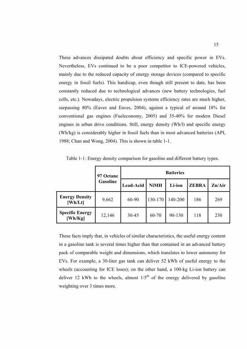
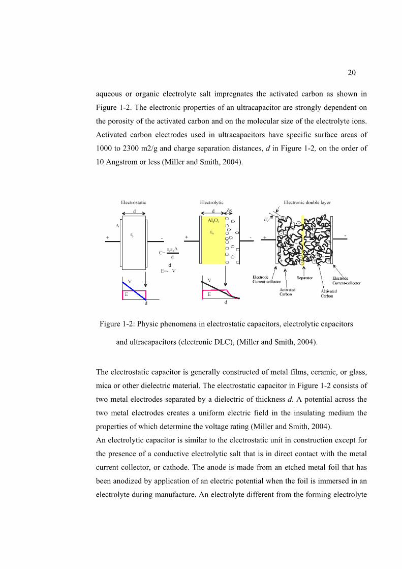
Table 1-1: Energy density comparison for gasoline and different battery types.
Batteries
97 Octane Gasoline
Lead-Acid NiMH Li-ion ZEBRA Zn/Air
Energy Density [Wh/Lt] 9,662 60-90 130-170 140-200 186 269
Specific Energy [Wh/Kg] 12,146 30-45 60-70 90-130 118 230
These facts imply that, in vehicles of similar characteristics, the useful energy content
in a gasoline tank is several times higher than that contained in an advanced battery
pack of comparable weight and dimensions, which translates to lower autonomy for
EVs. For example, a 30-liter gas tank can deliver 52 kWh of useful energy to the
wheels (accounting for ICE loses); on the other hand, a 100-kg Li-ion battery can
deliver 12 kWh to the wheels, almost 1/5th of the energy delivered by gasoline
weighting over 3 times more.

16
The aforementioned issue plus the problem of high initial cost and low specific
power of most batteries conform the main obstacles to successfully introduce
competitive EVs to the public and private transport industry.
A comprehensive solution would require the development of more advanced
batteries, achievable only through major research breakthroughs and investment in
new technologies, or the integration of fossil-fuel energy-storage and electric power
conversion and management (higher efficiency, lower noise, lower maintenance costs
and lower environmental impact).
The second scheme may achieve higher autonomy than pure EVs and higher
efficiency than regular ICE-powered vehicles but, in order to reach maximum
efficiency and minimum emissions, the main energy transformer (Diesel or gas
engine, gas turbine, fuel cell, etc.) must work at its optimum power output which will
contrast with the variable power requirements of the vehicle. Also, to reach its
potential, the system should be able to recover energy from braking, which fossil-
based energy-storage systems cannot do. Therefore, the integration of these
dissimilar energy conversion mechanisms require a temporary auxiliary-energy-
storage device; in such a way the vehicle is able to recover, and reuse, energy from
braking, and the main energy transformer (ICE, gas turbine, FC, etc.) is dimensioned
to satisfy mean (not peak) power demand, reducing the acquisition cost. These
auxiliary energy storage devices should have high power density, high specific power
and high efficiency. Vehicles that use such a combination of different energy storage
devices are commonly known as hybrid systems.
I.2 Integrating different energy systems
Recent commercial debut of hybrid vehicles is a proof of the improved efficiency and
performance of electric powered vehicles, regardless of the original source of energy
(electricity, gasoline, natural gas, hydrogen, etc.). Nevertheless, in terms of power-to-
weight ratio and cost, new hybrid models still do not strongly compete with
traditional gasoline or diesel-powered vehicles; moreover, although hybrids’ yield
(km/lt) is usually higher than most gas-powered vehicles, it is comparable to that of
some diesel models. Also, the use of combustion engines and complicated gearboxes

17
surely influences cost and weight. On the other hand, power is an issue that must be
resolved using appropriate auxiliary energy sources to support peak power
requirements. Therefore, all new topologies that could offer improvements in terms
of cost, weight and power should be explored and tested by researchers. In
accordance, the project presented here studies the technical and economical viability
of a seldom-explored hybrid configuration: the combination of batteries and
ultracapacitors.
At this stage, it is convenient to define different types of hybrids and the energy
sources they use or could use.
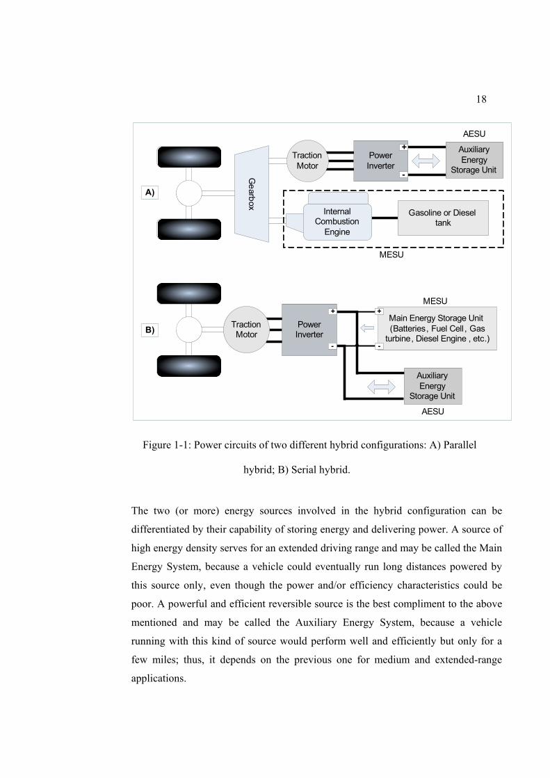
a) Parallel hybrid: is the combination in parallel of two different energy sources, both
with independent mechanical outputs that are combined in a special gearbox to
deliver or accept energy from the wheels (Fig. 1-A). This topology has been applied
in most commercial models; it usually combines an internal combustion engine and
an electric motor, which is connected to an electrochemical storage device, such as
batteries.
b) Serial hybrid: both energy sources deliver energy to the power train through the
same electro-mechanical converter (an electric motor), to which they are electrically
connected in parallel, as shown in Fig. 1-B. In this case, any two sources that deliver
electrical energy could be used, as long as they are compatible in terms of electrical
variables. This topology is also the only possible when the main energy source is a
battery or hydrogen (through Fuel Cell), because (unlike ICE) they do not produce
mechanical power.
18
A)
Gasoline or Diesel tank
Gearbox
Internal Combustion
Engine
Traction Motor
Power Inverter
Auxiliary Energy
Storage Unit
AESU
-
+
MESU
B) Traction Motor
Power Inverter
Main Energy Storage Unit (Batteries, Fuel Cell , Gas
turbine, Diesel Engine , etc.)
+
--
+
Auxiliary Energy
Storage Unit
AESU
MESU
Figure 1-1: Power circuits of two different hybrid configurations: A) Parallel
hybrid; B) Serial hybrid.
The two (or more) energy sources involved in the hybrid configuration can be
differentiated by their capability of storing energy and delivering power. A source of
high energy density serves for an extended driving range and may be called the Main
Energy System, because a vehicle could eventually run long distances powered by
this source only, even though the power and/or efficiency characteristics could be
poor. A powerful and efficient reversible source is the best compliment to the above
mentioned and may be called the Auxiliary Energy System, because a vehicle
running with this kind of source would perform well and efficiently but only for a
few miles; thus, it depends on the previous one for medium and extended-range
applications.
19
For the Main Energy System (MES), the most popular and proven choice has been
the internal combustion engine (ICE), followed by the gas turbine and, lately, the
Fuel Cell (FC). For the Auxiliary Energy System (AES), the most mentioned
candidates are high power batteries, ultracapacitors and flywheels, of which only the
first two are commercially available. All of these AES offer high efficiency, high
power-density and reversibility (Rutquist, 2002).
Because an ICE’s natural output is mechanical power (at manageable speeds for
gearboxes) and any unnecessary energy transformation is undesirable, it is usually
applied in parallel configuration. For the gas turbine, and most other candidates for
main energy sources, such as FCs, primary and secondary batteries, the series
configuration is more suitable. Recent developments in the areas of FCs and batteries
(Zinc-Air, ZEBRA, etc.) suggest a good chance of being a competitive alternative to
the ICE for Main Energy System in the near future (DOE, 2003), using series hybrid
configuration.
The two commercially available storage-device alternatives to implement the AES
are advanced batteries and ultracapacitors. Of these, the second present several
advantages over batteries for this particular application. The higher specific power
and higher efficiency are the most notable; but also, the longer cycle life and no
maintenance characteristics translate conveniently into no-replacement-cost and
lower-service-cost (Mazaika and Schulte, 2005).
These facts motivated the research described in this thesis, regarding the
development of an Auxiliary Energy System (AES) based on ultracapacitors and a
static converter. This AES has been conceived to be used in series hybrid
configurations (Jeong et al, 2002) in combination with different main energy systems.
I.3 What are ultracapacitors and how do they work?
Electronic double layer capacitors, DLC, or ultracapacitors, were first developed and
patented in 1961 by SOHIO. The construction of an ultracapacitor consists of a pair
of metal foil electrodes, each of which has an activated carbon (AC) fiber mat
deposited on metal foil. The activated carbon side of each electrode is separated by
an electronic barrier such as glass paper then sandwiched or rolled into a package. An
20
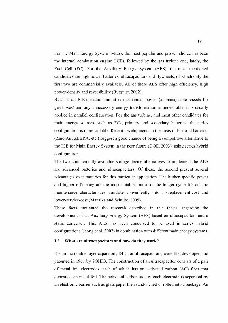
aqueous or organic electrolyte salt impregnates the activated carbon as shown in
Figure 1-2. The electronic properties of an ultracapacitor are strongly dependent on
the porosity of the activated carbon and on the molecular size of the electrolyte ions.
Activated carbon electrodes used in ultracapacitors have specific surface areas of
1000 to 2300 m2/g and charge separation distances, d in Figure 1-2, on the order of
10 Angstrom or less (Miller and Smith, 2004).
Figure 1-2: Physic phenomena in electrostatic capacitors, electrolytic capacitors
and ultracapacitors (electronic DLC), (Miller and Smith, 2004).
The electrostatic capacitor is generally constructed of metal films, ceramic, or glass,
mica or other dielectric material. The electrostatic capacitor in Figure 1-2 consists of
two metal electrodes separated by a dielectric of thickness d. A potential across the
two metal electrodes creates a uniform electric field in the insulating medium the
properties of which determine the voltage rating (Miller and Smith, 2004).
An electrolytic capacitor is similar to the electrostatic unit in construction except for
the presence of a conductive electrolytic salt that is in direct contact with the metal
current collector, or cathode. The anode is made from an etched metal foil that has
been anodized by application of an electric potential when the foil is immersed in an
electrolyte during manufacture. An electrolyte different from the forming electrolyte

21
is used as the ionic conductor. When the formed anode foil with its alumina dielectric
layer is rolled up along with the cathode foil, an insulating separator such as Kraft
paper is placed on the outside of the anode foil to insulate it. The negative foil is
typically the outside of the electrolytic can.
When an external potential is applied across the electrolyte terminals, a uniform
electric field is established across the anodized layer of alumina while a decaying
electric field exists some distance, δx, into the electrolyte according to Poisson’s
equation. Because of the presence of an electric field that extends into the electrolyte,
this capacitor will have a more limited breakdown voltage than an electrostatic
capacitor. Electrolytic capacitor manufacturers design for breakdown voltages
somewhat above the surge rating of the unit. Typically, higher surge rated electrolytic
capacitors also have higher resistance, hence a higher equivalent series resistance,
ESR, and therefore higher losses in power electronic circuits. Another consequence
of an electric field in the electrolyte is the fact that capacitor current is now a function
of both voltage change and capacitance change as a function of voltage (Miller and
Smith, 2004).
The voltage rating of ultracapacitors is constrained by the same phenomena of
electric field presence within the electrolyte as in conventional metal foil electrolytic
capacitors. Ultracapacitors with organic electrolytes have voltage ratings of <3.0 V
per cell whereas with aqueous electrolytes the voltage rating drops to <1.23 V per
cell, typically 0.9 V. In all ultracapacitors the terminal capacitance consists of the
series combination of an anode DLC and the cathode DLC, so the net rated voltage is
twice the value of the electrolyte decomposition voltage. Organic electrolyte
ultracapacitors have higher decomposition voltages and higher specific energy but
higher resistance than aqueous types. Low conductivity of organic-electrolyte-
ultracapacitors results in higher ESR. ESR can be reduced in general by the addition
of vapor grown carbon fiber to the AC.
Because capacitance is proportional to the electrodes surface-area and inversely
proportional to charge separation distance d, ultracapacitors advantage conventional
capacitors, such as electrolytic and electrostatic capacitors, by their porous-AC-
electrodes enormous effective areas and the extremely small charge separation
22
distance (Miller and Smith, 2004). The drawback, despite their two capacitive layers
instead of one, is the limited maximum voltage ultracapacitors withstand, usually
between 2.3V and 2.8V.
Ultracapacitors have greater specific power (more than 1.5kW/kg) than conventional
or advanced batteries; and higher specific energy (of about 3 to 5 Wh/kg) than
aluminum electrolytic capacitors (Dietrich, 2001; Burke and Miller, 2002). Their
advantage over batteries, in terms of power, is due to their reduced equivalent series
resistance (ESR) and that in these elements, unlike batteries, there are no chemical
reactions involved in the process of charge and discharge. Therefore, the speed
needed to deliver energy does not depend on the speed of such reactions or the ability
of chemical components to recombine, but on electrostatic phenomena, which does
not require molecular mutation to take place. Also, the longer cycle life and good
behavior at low temperatures (Schneuwly and Smith, 2005) are important
advantages.
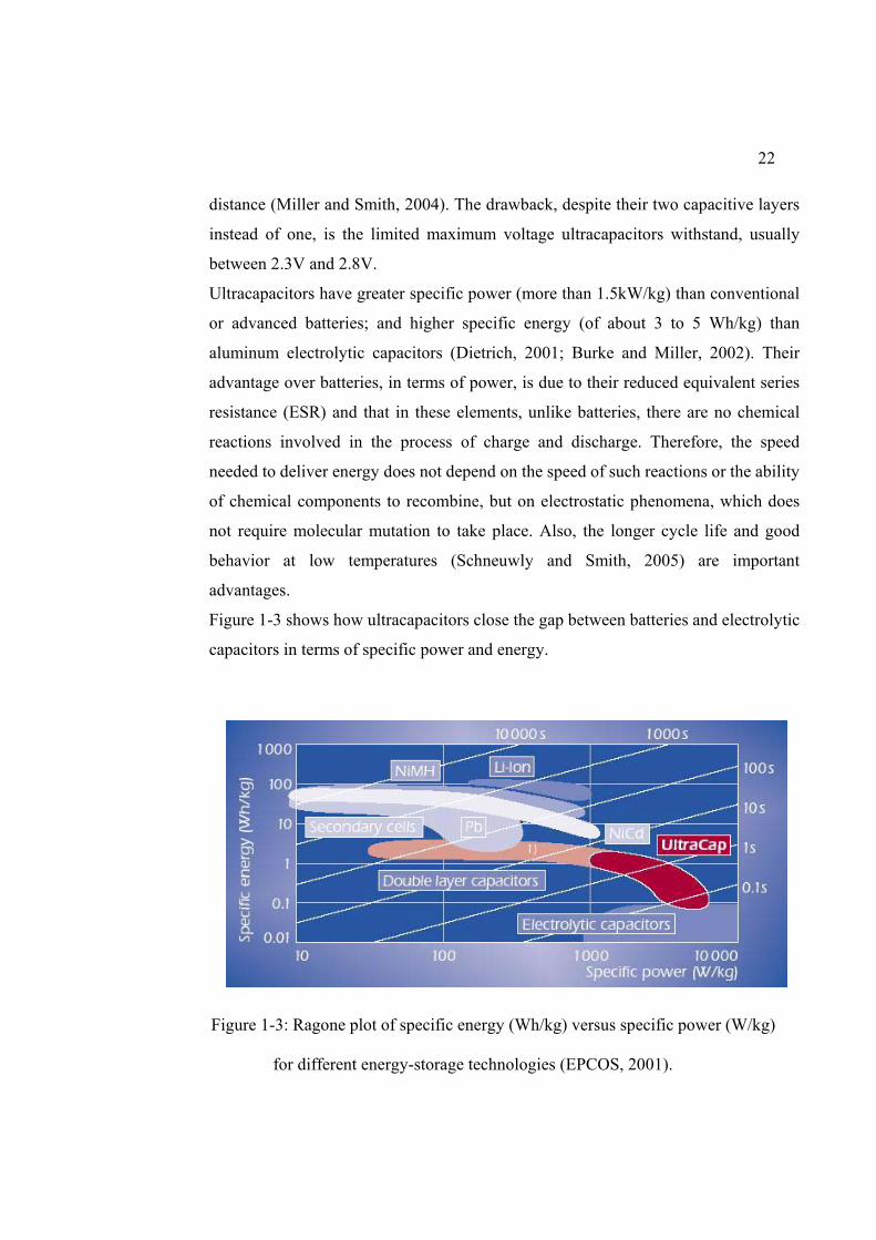
Figure 1-3 shows how ultracapacitors close the gap between batteries and electrolytic
capacitors in terms of specific power and energy.
Figure 1-3: Ragone plot of specific energy (Wh/kg) versus specific power (W/kg)
for different energy-storage technologies (EPCOS, 2001).

23
Because they present low losses and high cycle life at high power demands, these
elements of recent development cover a wide field of uses in power engineering
applications, especially in schemes with high peak power demand and medium-low
energy requirements (Cohen and Smith, 2002). Consequently, they present
advantages for complementary use in electric vehicles (EVs) and hybrid electric
vehicles (HEV), especially in their energy storage systems.
Accordingly, there are an increasing number of studies in which ultracapacitors are
used as a complement of the main energy system (ICE, FC, batteries, etc.) in hybrid
vehicles.
I.4 State-of-the-art traction systems using ultracapacitors
Contents of this section show the bibliography analysis made during the thesis-
project formulation period. Works reviewed in this process served as a knowledge
base of the up-to-date developments in Auxiliary Energy System using
ultracapacitors and their results. All publications discussed in this section are
contemporary or previous to the project formulation. Works published thereafter, as
well as publications presenting this project’s results, are discussed in chapter V.
Publications regarding ultracapacitors and auxiliary energy storage may be classified
in three groups: i) the ultracapacitor industry reports and surveys, which deal with
new material fabrication processes, specific characteristics measurements and testing
under different operating conditions; ii) the speculative kind, whose approach is
focused in forecasting long term industry trends and suggesting certain technology
adoption for the particular application (analysis and conclusions presented in these
essays are based on inference and experience acquired within the industry); iii)
finally, a third group presents technical reports on practical applications, which
expose useful data about behavior and performance obtained from experimental
prototypes (or rigorous simulations using real data sets). Publications within this last
group describe the state-of-the-art power topologies for EVs and HEVs, therefore an
updated analysis on viability of these schemes can be extracted from them.
The first group of publications presents studies that describe the state of the industry
and its projections (Cohen and Smith, 2002). Production-models characteristics and
24
behavior under stress (and abuse) are measured to evaluate adequacy for different
applications (Jehoulet et al, 2000; Varakin et al, 2001; Goesmann et al, 2002; Conte
and Pirker, 2005). Projected future materials improvements and costs are also
forecasted, based on research’s preliminary results and suggested technology
inversions (Burke and Miller, 2001). Most of these works are presented by
ultracapacitor manufacturers, a fact that could suggest questionable objectiveness, but
data contained in them should be reliable because they are subject to the industry
scrutiny and benchmarking. The most useful information contained in these
publications is related to behavior under abuse and safety considerations (Goesmann
et al, 2002; Conte and Pirker, 2005).
The second group of publications could be considered the vanguard analysis that may
inspire future developments. Even though they lack real-life experimental results,
these works are a sample of the engineering analysis process preliminary to any
serious innovative attempt (Furubayashi et al, 2000; Mitsui et al, 2002; Dixon et al,
2000).
The third classification group, consisting of practical applications reports, comprises
most publications on ultracapacitors to be found. There is a wide variety of explored
topologies and the analysis scope spread over an ample spectrum of profoundness.
Miscellaneous applications from peripheral-load power-support (Folchert et al, 2002)
to ultracapacitors-as-the-single-energy-source configurations (Barrade and Rufer,
2001) can be found. There are several reports on HEVs implementations using
ultracapacitors in combination with non-reversible energy sources such as ICEs, FCs
and primary batteries among others (Furubayashi et al, 2000; Burke and Miller 2001;
Di Napoli et al, 2001; Lott and Späth, 2001; Varakin et al, 2001; Jeong et al, 2002;
Okamura, 2002). A couple of publications describing idle stop systems were found
(Furubayashi et al, 2001; Mitsui et al, 2002); this application consists of using
ultracapacitors in urban buses to power the starter motor of ICEs, which are turned
off at every stop to avoid inefficient and contaminating idling conditions. In these
cases, ultracapacitors are used to avoid battery deterioration due to successive peak
power episodes and to decouple this strongly-perturbing load from other on-board
electronic loads. Finally, there is a constantly-growing number of reports that present
25
HEV implementations combining ultracapacitors as Auxiliary-Energy-Systems and
different types of batteries as Main-Energy-Systems (Arnet and Haines, 2000; Härri
and Egger, 2001; Heinemann et al, 2001; Wight et al, 2001; Wight et al, 2002). These
works conformed the most valuable and updated information source when this
project was elaborated, because they expose practical details and evaluation results of
the early experimental implementations on the topology being evaluated in this
research. A thorough review of the highlights of each publication found in this sub-
group is presented in the following pages.
Arnet (Arnet and Haines, 2000) presents the hardware and algorithm concepts used in
the implementation of an AES based on ultracapacitors to be implemented in an
electric vehicle using lead-acid batteries as MES. This design was part of Solectria
Corporation’s new energy storage devices development program. The static converter
used in his design has a Buck-Boost topology, such as the one used in the project
presented in this thesis. He also used algorithms that establish an inverse relation
between the vehicle’s kinetic energy and the ultracapacitor’s state of charge (SOC).
This work is contemporary with the first publication that emanated from this project
(Dixon et al, 2000), in which general hardware configuration and algorithm concepts
were presented; coincidently, Arnet’s general approach is very similar to that
exposed in (Dixon et al, 2000), therefore early conclusions on the feasibility of this
implementation could have been extracted from his findings, but his results were
preliminary and did not evaluate the general performance of the equipment in real-
life operation. Also, some differences appeared in hardware design and algorithm
implementation, hence Arnet’s work and this project results could complement each-
other.
Härri (Härri and Egger, 2001) introduces an energy scheme concept he calls SAM
(Super Accumulator Module), which consists on combining batteries and
ultracapacitors using a topology he refers to as Virtual Parallel (VP). But the actual
semiconductor configuration is not at all clear, nor is under what criterion the
different operation modes are selected and the capacitor SOC controlled. Test results
and performance data are not presented either. Therefore, this essay does not provide
useful orienting insights.
26
Heinemann’s work (Heinemann et al, 2001) is interesting because of exposed
temperature management data and ultracapacitor behavior under different operation
conditions. Also, his exploration of different energy management strategies presents
interesting alternatives. Nevertheless, his findings are mostly simulations or small
scale bench tests, and do not deliver conclusive data about the overall efficiency
increase and/or available power.
By 2002, Wight’s publications (Wight et al, 2001; Wight et al, 2002) had the most
illustrative results on ultracapacitors and lead-acid batteries combination for EVs.
Data presented in both works summarize test procedures on real-life-scale vehicles
using the static converter developed by Arnet and two different ultracapacitor brands,
one in each publication. The first study shows a complete set of tests comprising
urban, suburban, acceleration and dynamometer experiments on two identical
vehicles, both equipped with lead-acid batteries as MES, the first one using the
ultracapacitor-based AES and the second one (control subject), which did not have an
AES. General conclusions showed that, when using that particular ultracapacitor-
based AES, more available power was observed by the driver, acceleration was faster
and more energy could be extracted from the batteries before reaching the
“discharged” threshold minimum voltage (which allowed some increased autonomy).
Nevertheless, even though more energy was extracted from the batteries, in most
experiments the overall efficiency or yield (km/Wh) was lower on the vehicle
equipped with the AES. The second essay shows almost identical tests but using a
different ultracapacitor brand. Results resemble very much those obtained in the first
publication; the amount of energy extracted from batteries in the vehicle equipped
with the AES was greater in all tests than that extracted from batteries in the control
vehicle. This time the results on efficiency where non-conclusive.
From available literature, at the time of the research project-formulation, it could be
concluded that there was scarce experience of this kind of application and few real-
life-scale tests had been performed. Results obtained by Wight suggested that the use
of a high-specific-power AES, like the one proposed in this research, would lessen
main battery deterioration due to the reduction of peak power demanded and
therefore, would probably extend battery life. On the other hand, Wight’s results
27
were not conclusive regarding overall efficiency impact that the use of this AES
produced on EVs; there is a chance that efficiency results from his tests could have
been influenced by the algorithm structure or its parameters and/or by the efficiency
characteristics of his particular static converter.
This reasoning suggested that, by incorporating an ultracapacitor-based AES to EVs,
in addition to battery life extension and a better acceleration response, overall
increase in vehicle efficiency could be achieved if improvements where performed on
static-converter design and energy-management algorithm structure.
I.5 Objectives and hypothesis
The central objective of this research is to identify and improve some of the
deficiencies that prevent clean and efficient transport technologies, such as EVs, from
successfully competing against traditional pure-ICE-based vehicles. This objective
has been partially realized in previous analysis, identifying obstacles such as reduced
autonomy, high cost and limited power of EVs and HEVs as the predominant barriers
to achieve competitive clean vehicles.
Reduced autonomy is a characteristic of pure EVs, which are powered with reduced
energy-density electrochemical batteries. This problem has been partially overcome
with the development of HEVs, equipped with Main Energy System (MES) of higher
specific energy. Nevertheless, some of the energy converters used in these
configurations are not as clean or efficient as it would be desirable, as in the case of
Internal Combustion Engines (ICEs) and Fuel Cells (FCs) (Galliers, 2003).
The problem of high cost, common to all clean mobility solutions, is particularly
pronounced in the case of FCs, for which forecasts are not optimistic in the short and
medium terms (Galliers, 2003; Chan and Wong, 2004). In the case of ICEs, although
actual costs are not prohibitive, simple reasoning concludes that their complexity
makes them expensive to maintain. Furthermore, if battery technologies are
consistently improved and acceptable energy densities are achieved, it is not
unreasonable to speculate that manufacturing costs of an electrochemical storage unit
with fewer and simpler components could be lower than those of an intricate ICE. Of
course complex manufacturing of special alloys and compounds have to be perfected
28
and made cheaper, but that is not impossible given the rate at which manufacturing
processes are advancing. Hence, electrochemical batteries seem to be the alternative
clean-energy-source that could first break the barrier of unacceptable costs and
consistently bring them to competitive levels.
The power issue is also prevalent in all technologies previously reviewed. In the case
of HEVs efficiency considerations make it transcendental that their MES’s work at
constant or near-constant power levels, lower than the peak power demanded; also,
cost constraints force the MES’s power-rating reduction to levels near mean power
demand. This leaves the burden of power on the AES, whose duty is to quickly
deliver or accept bursts of energy as a response to the power-train’s demands. The
first elements used for AES implementations were high power batteries, but these
require sophisticated charge equalization management (Schneuwly and Smith, 2005)
and present a short cycle life, which had an impact in cost; that is why new energy-
storage elements such as ultracapacitors and flywheels are being tested and
implemented in HEVs to address high power issues. In the case of battery-powered
pure EVs, batteries present varied problems, such as low specific power, DOD-
dependant cycle life (Mazaika and Schulte, 2005), inefficiency at high power
demands, etc. This has motivated the experimentation of different technology
combinations to satisfy separate energy and power needs. This is particularly
important when primary batteries (such as Zn-air) or high-specific-energy but low-
specific-power batteries (such as Na/Ni-Cl2 or ZEBRA) are used; in the case of these
battery technologies, very promising in terms of specific energy, power support is
fundamental.
From this analysis it can be deduced that, in the medium term, the clean transport
technology that will most certainly reduce its costs is battery electrochemical storage.
Of which some chemistries have lately achieved important specific-energy
improvements. Therefore, an efficient, cost-effective and reliable power support unit
could close the circle and make battery-powered EVs a competitive choice in the near
future.
This reasoning has motivated the development of an ultracapacitor-based AES to be
implemented in a lead-acid battery-powered vehicle. The lead-acid technology would

29
be subsequently changed to Na/Ni-Cl2 (ZEBRA) of greater energy density and lower
power density.
The incorporation of this power support system would certainly increase available
power, but it also raises obvious concerns about costs. On the other hand, a question
regarding other EVs limitations arise: would this system have a negative effect on
efficiency and therefore on autonomy? In this author’s opinion, no, on the contrary:
the reduction of maximum power demanded to the battery would increase battery
operation efficiency and more energy would be recovered from regenerative braking
even when the battery is fully charged; this would more than compensate for the
expected losses produced in the static converter interfacing energy flow to and from
ultracapacitors. If this reasoning proves correct, then costs could also be
compensated, or even reduced, as a result of energy savings and battery life
extension.
This expectation, founded on intuitive reasoning, could be formulated as a hypothesis
to be demonstrated.
“The adequate use of ultracapacitor-based Auxiliary-Energy-System in electric
vehicles powered with lead-acid batteries, under congested city driving conditions,
increases total energetic efficiency and extends its autonomy. That is, in driving
conditions with a high number of stops and accelerations respective to the covered
distance, the total energy spent (per kilometer) will be measurably lower in a lead-
acid battery equipped vehicle that uses a ultracapacitor-based AES than that spent in
the same vehicle without the AES. The AES-equipped vehicle would also be able to
cover a longer distance with one charge.”
The demonstration or refutation of this hypothesis will be the central aim of this
thesis. A discussion on costs will also be included in the final analysis, but does not
fall within the preset scope of this study.
I.6 Methodology
To demonstrate, or refute, the proposed hypothesis, a real-life scale AES prototype
using ultracapacitors and a static converter was designed and constructed. The system
was implemented in an EV and tested in an urban drive circuit. Finally, results were
30
analyzed and compared to those obtained without the use of the AES, leading to final
conclusions, from which economical implications where drawn.
The AES design and implementation were key processes to ensure the success of this
project. The ease of power flow control, operational safety and overall system
efficiency, depended directly on the adequacy of the power topology, as well as the
thorough study and design of converter components and control system. A Buck-
Boost power topology was used, where the ultracapacitor bank was connected at the
low voltage side of the converter, allowing bi-directional power flow with variable
voltage at the ultracapacitor terminals. The specially designed and constructed
smoothing inductor (of 1.6 mH) and water-cooled heat-sink allowed high efficiency
and high power rating by ensuring low amplitude ripple current and stable thermal
management. A control and monitoring system was also designed and implemented
using a DSP from Texas Instruments. This system allowed the implementation of
different energy management strategies without hardware modification and provided
real time information through its monitoring and data-logging features.
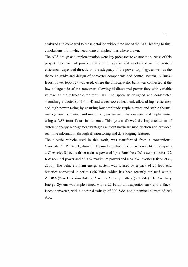
The electric vehicle used in this work, was transformed from a conventional
Chevrolet “LUV” truck, shown in Figure 1-4, which is similar in weight and shape to
a Chevrolet S-10; its drive train is powered by a Brushless DC traction motor (32
KW nominal power and 53 KW maximum power) and a 54 kW inverter (Dixon et al,
2000). The vehicle’s main energy system was formed by a pack of 26 lead-acid
batteries connected in series (356 Vdc), which has been recently replaced with a
ZEBRA (Zero Emission Battery Research Activity) battery (371 Vdc). The Auxiliary
Energy System was implemented with a 20-Farad ultracapacitor bank and a Buck-
Boost converter, with a nominal voltage of 300 Vdc, and a nominal current of 200
Adc.

31
Figure 1-4: Electric vehicle, converted from a conventional ICE-powered pick-up
truck Chevrolet LUV.
The test circuit was a slow and mid-speed driving urban route. Special care was taken
to perform tests under similar environmental and technical conditions, such as
ambient temperature, traffic conditions, tire pressure, etc.
Tests were performed without regeneration, with battery-only-regeneration and with
AES-assisted regeneration (two algorithms were tested). Available power (kW) and
yield (km/kWh) were the measured performance indicators.
32
II STATIC CONVERTER DESIGN AND IMPLEMENTATION
II.1 Introduction
The battery pack, composed of 26 series-connected lead-acid batteries, has a no-load
voltage that ranges from 358V, when recently charged, to 312V when discharged.
This voltage is also load-dependant, reaching under 250V when heavily loaded and in
low SOC condition. On the other hand, it can reach more than 400V when it has been
recently charged and regenerative braking is applied. These are extreme conditions
which not only deteriorate batteries and shorten their life, but may also damage
power inverter (traction equipment has minimum and maximum voltage limits of 250
and 400 V respectively). This situation cannot be avoided unless the vehicle’s drive
train power is restricted according to battery voltage. This strategy would avoid
inverter damage and could help preserve batteries longer, but would severely affect
vehicle performance and efficiency (by restricting power and regeneration); it would
limit available power when batteries are partially discharged and, over time, batteries
aging would also noticeably affect performance. In other words, batteries would go
through a long agony and this would be reflected in vehicle performance. This is
where the Auxiliary Energy System fills the gap.
As previously defined, the most adequate hybrid configuration to be implemented in
a battery-powered EV is a series-hybrid topology, shown in Figure 1-1B. Even
though it is called ‘serial’ hybrid (because of the serial mechanical output), the Main
and Auxiliary Energy Systems are connected in parallel. Therefore, if the Main
Energy System (batteries) remains the same, the AES must be designed in such a way
that it adapts to the pre-established power-circuit voltage-rating, and there is an
adequate supporting-power-flow during peak power demand.
Even though there have been some experiences connecting ultracapacitors directly to
the Main Energy System (Jeon et al, 2005; Massé and Freeman 2005), a static
converter should interface power connection between batteries and ultracapacitors for
several reasons, but three are fundamental. First, batteries work at relatively constant
voltage levels while capacitor’s voltage is directly related to their SOC, therefore to
33
use all or most energy storage capacity of ultracapacitors a voltage interface is
required. Second, the only way to implement different energy management strategies
is by controlling power flow and SOC of at least one of the energy source units, and
this can only be done by placing a static converter between the two sources. Third,
directly connected capacitors will only support power demand during transients,
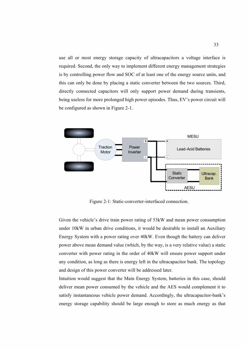
being useless for more prolonged high power episodes. Thus, EV’s power circuit will
be configured as shown in Figure 2-1.
AESU
Traction Motor
Power Inverter
Lead-Acid Batteries
+
--
+MESU
Static Converter
Ultracap . Bank
Figure 2-1: Static-converter-interfaced connection.
Given the vehicle’s drive train power rating of 53kW and mean power consumption
under 10kW in urban drive conditions, it would be desirable to install an Auxiliary
Energy System with a power rating over 40kW. Even though the battery can deliver
power above mean demand value (which, by the way, is a very relative value) a static
converter with power rating in the order of 40kW will ensure power support under
any condition, as long as there is energy left in the ultracapacitor bank. The topology
and design of this power converter will be addressed later.
Intuition would suggest that the Main Energy System, batteries in this case, should
deliver mean power consumed by the vehicle and the AES would complement it to
satisfy instantaneous vehicle power demand. Accordingly, the ultracapacitor-bank’s
energy storage capability should be large enough to store as much energy as that
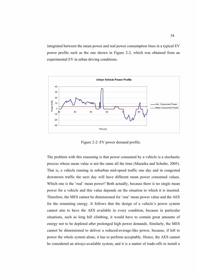
34
integrated between the mean power and real power consumption lines in a typical EV
power profile such as the one shown in Figure 2-2, which was obtained from an
experimental EV in urban driving conditions.
Urban Vehicle Power Profile
-30
-20
-10
0
10
20
30
40
30 40 50 60 70 80
Time [s]
Pow
er [k
W]
Inst. Consumed PowerMean Consumed Power
Figure 2-2: EV power demand profile.
The problem with this reasoning is that power consumed by a vehicle is a stochastic
process whose mean value is not the same all the time (Mazaika and Schulte, 2005).
That is, a vehicle running in suburban mid-speed traffic one day and in congested
downtown traffic the next day will have different mean power consumed values.
Which one is the ‘real’ mean power? Both actually, because there is no single mean
power for a vehicle and this value depends on the situation to which it is inserted.
Therefore, the MES cannot be dimensioned for ‘one’ mean power value and the AES
for the remaining energy. It follows that the design of a vehicle’s power system
cannot aim to have the AES available in every condition, because in particular
situations, such as long hill climbing, it would have to contain great amounts of
energy not to be depleted after prolonged high power demands. Similarly, the MES
cannot be dimensioned to deliver a reduced-average-like power, because, if left to
power the whole system alone, it has to perform acceptably. Hence, the AES cannot
be considered an always-available system, and it is a matter of trade-offs to install a
35
small, cheap, seldom-available system, or a big, expensive, always-available power
source. The idea is to have the system available ‘most’ of the time at a ‘reasonable’
cost. Both of which are relative concepts but that is the nature of consumer products.
These concepts were incorporated when dimensioning the system, but because of the
experimental nature of this system, costs were not the priority constraint.
To have an idea of the amount of energy the vehicle will use in a single power-
demanding operation, acceleration and hill climbing (the most demanding tasks in
terms of power) energy requirements are the best examples. The vehicle in question
plus its Auxiliary Energy System weighs around 2000 kg. Therefore its kinetic
energy at 60 kph is about 77 Wh. This amount of energy plus losses will be spent to
accelerate from 0 kph to 60 kph. If a constant speed over a hill climb of 30 m height
difference is desired, an approximate amount of 163 Wh (potential energy difference)
plus air drag and mechanical losses will be spent. Considering these figures, the AES
was designed to store enough energy to consecutively support power during both
tasks. Thus the ultracapacitor bank has a 255 Wh energy-storage-capacity, of which
only 90 % would be used because of efficiency concerns. This allows sustained
power support during most demanding regular tasks in city driving conditions.
II.2 Power design
Terminal voltage in a capacitor bank, by definition depends directly on its state of
charge (SOC). More precisely, the ultracapacitor-bank’s SOC is proportional to its
square voltage; hence, as energy is transferred to and from the bank its voltage will
change accordingly. For this reason, the static converter topology, shown in Figure 2-
1, must be able to transfer energy between a relatively constant voltage source
(battery) and a variable voltage source (ultracapacitor).
II.2.1 Buck-boost topology
The above mentioned characteristics of the static converter call for a power topology
that adapts to the variable nature of capacitor voltage and the relatively constant
battery voltage. For this reason a buck-boost topology was chosen. Figure 2-3 shows
an equivalent circuit of the power circuit in which the battery is represented by a

36
voltage source and an internal resistance. The ultracapacitor bank is also represented
by a voltage source (which, for short periods of time, it is) and its equivalent series
resistance (ESR). This topology is conceived to establish controlled bidirectional
power transfer between both sources as long as ultracapacitor voltage VU is smaller
than battery voltage VB. If this condition does not hold, a current will flow through
diode D2.
ultracapacitor bank
+ + +
VU
ESR
LS T2 D2 T1 D1
VB
Rint
C
iBAT
Buck Side Boost Side
Battery
VC
VS
iC
iU
Figure 2-3: Buck-boost topology equivalent circuit.
During ‘buck’ operation, energy goes from battery to ultracapacitor. This task is
performed by commutating semiconductor T2 at a frequency f (period T) and duty
cycle δ. This operation is shown in Figure 2-4, where it is clear how current iC
through semiconductor T2 has strong discontinuities. Capacitor C acts as a filter so
the battery sees a smoother continuous current.

37
Time
iU
iC
iBAT
iBAT iC
iU
VBVU
T2
D1δ
T= 1/f
Figure 2-4: Buck operation. Energy is transferred from the battery to
ultracapacitors.
In buck operation, mean currents through battery BATi and through ultracapacitors Ui
behave like in a DC transformer (where a=δ) and may be calculated accordingly, as
long as VBVU≥δ . This is applied in equations 2.1 and 2.2.
+
−
=int2 RESR
VUVBiBAT
δ
δ (2.1)
( )( )2int δ
δ⋅+
−⋅=
RESRVUVBiU (2.2)
During ‘boost’ operation, energy goes from ultracapacitor to battery pack. This
operation is very similar to the one previously described. Semiconductor T1 is
commutated at a frequency f and a duty cycle δ. Figure 2-5 shows this operation and
current waveforms. As before, strong discontinuities are present in current iC which,
again are filtered by capacitor C.

38
Time
iU
iC
iBAT
T1
iBAT iC
iUD2
VBVU
δ
T= 1/f
Figure 2-5: Boost operation. Energy is transferred from ultracapacitors to the
battery.
Once again, mean currents BATi and Ui can be analyzed like in a DC transformer,
where the turns ratio is 1/ ( )δ−1 , as long as ( ) VBVU≥− δ1 . This has been applied
in equations 2.3 and 2.4.
( )
( )
−+
−
−=
21int
1
δ
δ
ESRR
VBVU
iBAT (2.3)
( )( )( )( )ESRR
VBVUiU+−⋅−⋅−
= 21int1
δδ (2.4)
Ultracapacitor current ripple amplitude is an important design variable, because
mechanical vibrations, induced-current-losses and undesirable EMI could be
produced if special care is not taken. Expression 2.5 shows the maximum ripple
amplitude as a function of VC, f and LS (calculated in Appendix A).
LsfV
ripplei CU ⋅⋅
=4
max__ (2.5)

39
II.2.2 Static converter components design and selection
The converter was designed and tested to deliver up to 60 kW, but current was
limited to 150A on the ultracapacitors side to avoid high losses. Hence, the converter
can deliver a peak power of 45 kW, which decreases with ultracapacitor voltage,
reaching 30 kW at ultracapacitor voltage of 200 V (which is seldom lower).
According to this power rate and interconnected systems, buck-boost converter
components were selected or designed to work properly at currents up to 200A and
voltages up to 400V.
a) Ultracapacitor bank
Battery voltage can decrease to levels below 250V on heavy loads (when working in
battery-only mode), but usually stays over 300V when a regular load is applied. With
AES power-support this voltage decreases, at the most, to 300V on full load.
Therefore, to avoid voltage crossing, the ultracapacitor bank maximum voltage rating
was set to 295 V.
The AES was implemented with 132 series-connected ultracapacitors. These units
have 2700 Farads each, an ESR of 1 mOhm and a voltage rating of 2.3 V. The bank
totals 20.45 Farads, an equivalent series resistance of 132 mOhm, and a total
maximum voltage of 303.6 V (limited by software to 295 V). Figure 2-6 illustrates
one ultracapacitor and its physical characteristics.

40
Figure 2-6: 2700F ultracapacitor from Epcos.
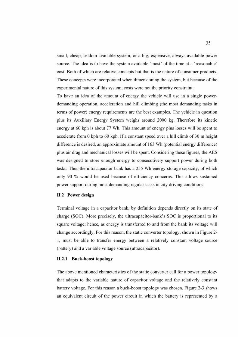
Due to slight differences in capacitance, ultracapacitors may charge unevenly and
some units may eventually overcharge. To avoid this, dissipative voltage limiters
were installed in each unit as shown in Figure 2-7.
41
Figure 2-7: Ultracapacitor bank with cell balancing units installed.
b) Smoothing inductance LS
For the smoothing inductance design, maximum current ripple amplitude of 5A was
the aim. Therefore, according to expression 2.5 and considering a 12 kHz
commutation frequency and a battery voltage of 360 V, the inductance LS should
have at least 1.5 mH. It also should be able to conduct currents up to 200A without
saturating and/or generating excessive resistive losses.
After pondering the electromagnetic relations between material saturation, core-
section area and core-length, number of turns and final achieved inductance, an air-
core design was implemented, because it would not saturate and the high reluctance
could be compensated with more turns, of lower volume and weight ‘cost’ than the
other core alternatives required (Ortúzar, 2002).
42
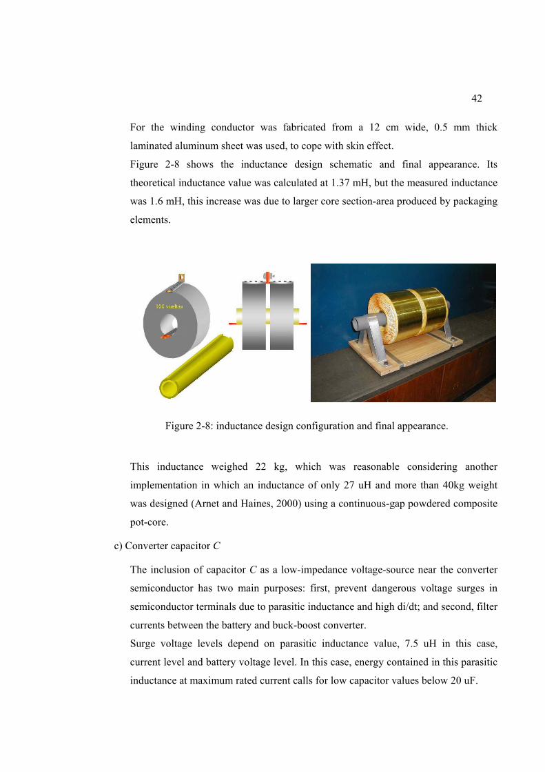
For the winding conductor was fabricated from a 12 cm wide, 0.5 mm thick
laminated aluminum sheet was used, to cope with skin effect.
Figure 2-8 shows the inductance design schematic and final appearance. Its
theoretical inductance value was calculated at 1.37 mH, but the measured inductance
was 1.6 mH, this increase was due to larger core section-area produced by packaging
elements.
Figure 2-8: inductance design configuration and final appearance.
This inductance weighed 22 kg, which was reasonable considering another
implementation in which an inductance of only 27 uH and more than 40kg weight
was designed (Arnet and Haines, 2000) using a continuous-gap powdered composite
pot-core.
c) Converter capacitor C
The inclusion of capacitor C as a low-impedance voltage-source near the converter
semiconductor has two main purposes: first, prevent dangerous voltage surges in
semiconductor terminals due to parasitic inductance and high di/dt; and second, filter
currents between the battery and buck-boost converter.
Surge voltage levels depend on parasitic inductance value, 7.5 uH in this case,
current level and battery voltage level. In this case, energy contained in this parasitic
inductance at maximum rated current calls for low capacitor values below 20 uF.
43
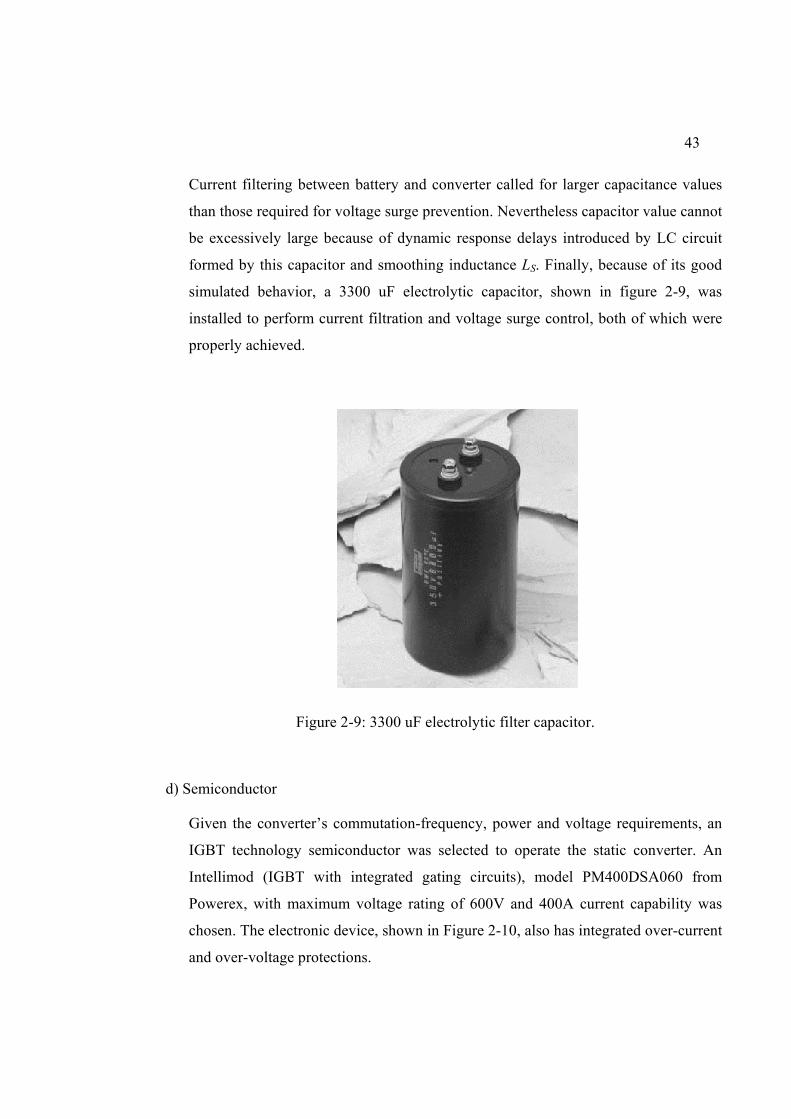
Current filtering between battery and converter called for larger capacitance values
than those required for voltage surge prevention. Nevertheless capacitor value cannot
be excessively large because of dynamic response delays introduced by LC circuit
formed by this capacitor and smoothing inductance LS. Finally, because of its good
simulated behavior, a 3300 uF electrolytic capacitor, shown in figure 2-9, was
installed to perform current filtration and voltage surge control, both of which were
properly achieved.
Figure 2-9: 3300 uF electrolytic filter capacitor.
d) Semiconductor
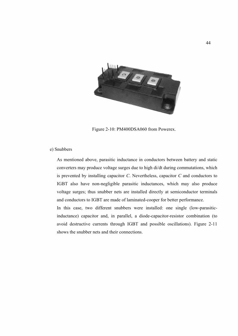
Given the converter’s commutation-frequency, power and voltage requirements, an
IGBT technology semiconductor was selected to operate the static converter. An
Intellimod (IGBT with integrated gating circuits), model PM400DSA060 from
Powerex, with maximum voltage rating of 600V and 400A current capability was
chosen. The electronic device, shown in Figure 2-10, also has integrated over-current
and over-voltage protections.
44
Figure 2-10: PM400DSA060 from Powerex.
e) Snubbers
As mentioned above, parasitic inductance in conductors between battery and static
converters may produce voltage surges due to high di/dt during commutations, which
is prevented by installing capacitor C. Nevertheless, capacitor C and conductors to
IGBT also have non-negligible parasitic inductances, which may also produce
voltage surges; thus snubber nets are installed directly at semiconductor terminals
and conductors to IGBT are made of laminated-cooper for better performance.
In this case, two different snubbers were installed: one single (low-parasitic-
inductance) capacitor and, in parallel, a diode-capacitor-resistor combination (to
avoid destructive currents through IGBT and possible oscillations). Figure 2-11
shows the snubber nets and their connections.

45
Capacitor snubber
Dumped capacitor-diode snubber
Figure 2-11: Snubbers connected to semiconductor terminals.
II.3 Safety features
A series of hardware and software safety measures were implemented to prevent
malfunction and/or dangerous situations. Software measures are mainly failure
detection capabilities, which are described further on.
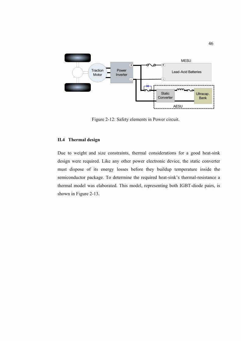
The equipment was hardware-protected by fuses on each side of the static converter
and a diode to allow boost discharge, preventing capacitor C overcharge if the fuse
on the battery side blows. Figure 2-12 shows these safety elements installed in the
power circuit.
46
AESU
Traction Motor
Power Inverter
Lead-Acid Batteries
+
--
+MESU
Static Converter
Ultracap . Bank
Figure 2-12: Safety elements in Power circuit.
II.4 Thermal design
Due to weight and size constraints, thermal considerations for a good heat-sink
design were required. Like any other power electronic device, the static converter
must dispose of its energy losses before they buildup temperature inside the
semiconductor package. To determine the required heat-sink’s thermal-resistance a
thermal model was elaborated. This model, representing both IGBT-diode pairs, is
shown in Figure 2-13.
47
Rth(c-f) Rth(f-amb) Tf
Tamb
Rth(j-c)F
Rth(j-c)QTjQ
PQ1
PF1
TjF
Tc
INTELLIMOD PM400DSA060
Rth(j-c)F
Rth(j-c)QTjQ
PQ2
PF2
TjF
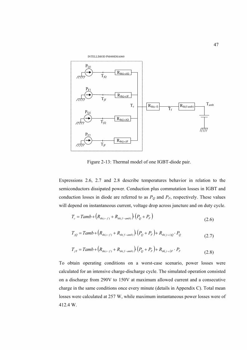
Figure 2-13: Thermal model of one IGBT-diode pair.
Expressions 2.6, 2.7 and 2.8 describe temperatures behavior in relation to the
semiconductors dissipated power. Conduction plus commutation losses in IGBT and
conduction losses in diode are referred to as PQ and PF, respectively. These values
will depend on instantaneous current, voltage drop across juncture and on duty cycle.
( ) ( )FQambfthfcthc PPRRTambT +⋅++= −− )()( (2.6)
( ) ( ) QQcjthFQambfthfcthjQ PRPPRRTambT ⋅++⋅++= −−− )()()( (2.7)
( ) ( ) ( ) FFcjthFQambfthfcthj PRPPRRTambT ⋅++⋅++= −−− )()(F (2.8)
To obtain operating conditions on a worst-case scenario, power losses were
calculated for an intensive charge-discharge cycle. The simulated operation consisted
on a discharge from 290V to 150V at maximum allowed current and a consecutive
charge in the same conditions once every minute (details in Appendix C). Total mean
losses were calculated at 257 W, while maximum instantaneous power losses were of
412.4 W.
48
Individual semiconductor mean power losses and thermal characteristics provided by
the manufacturer (Appendix D) were applied to the thermal model mentioned above.
The required heat-sink’s thermal resistance was calculated to maintain junctures and
case temperatures below maximum levels for the evaluated operation conditions. The
required thermal resistance for the heat-sink is of 0.107 ºC/W.
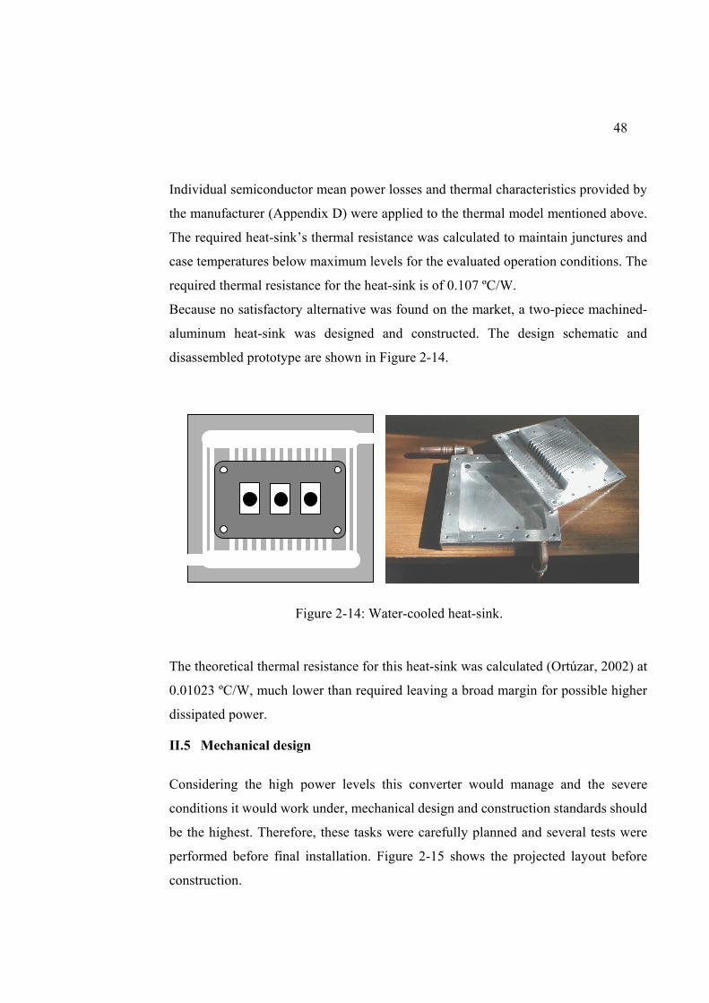
Because no satisfactory alternative was found on the market, a two-piece machined-
aluminum heat-sink was designed and constructed. The design schematic and
disassembled prototype are shown in Figure 2-14.
Figure 2-14: Water-cooled heat-sink.
The theoretical thermal resistance for this heat-sink was calculated (Ortúzar, 2002) at
0.01023 ºC/W, much lower than required leaving a broad margin for possible higher
dissipated power.
II.5 Mechanical design
Considering the high power levels this converter would manage and the severe
conditions it would work under, mechanical design and construction standards should
be the highest. Therefore, these tasks were carefully planned and several tests were
performed before final installation. Figure 2-15 shows the projected layout before
construction.

49
Snnubers INTELLIMOD Power connectors to
ultracapacitor bank
Current LEM
uProcessor and control circuit box.
Capacitor C
Water circuit pipes.
Heat-sink
Positive terminal to battery
Fuse F1
Negative Terminal to battery
Figure 2-15: Components layout within static converter.
Laminated conductors and placed components within the converter chassis are shown
in Figure 2-16. Also snubbers connected directly to the semiconductor terminals are
visible.
Laminated conductors
Snubbers Control circuits
Intellimod
Heat-sink
Figure 2-16: Installed components in converter chassis.
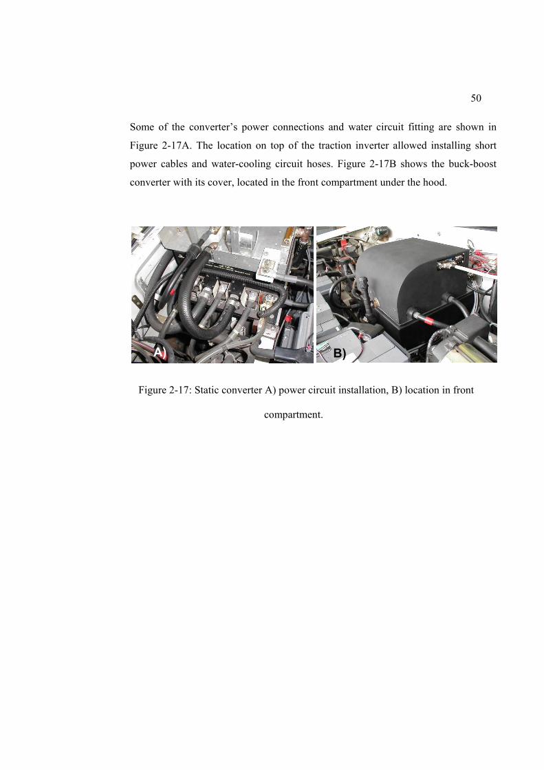
50
Some of the converter’s power connections and water circuit fitting are shown in
Figure 2-17A. The location on top of the traction inverter allowed installing short
power cables and water-cooling circuit hoses. Figure 2-17B shows the buck-boost
converter with its cover, located in the front compartment under the hood.
A) B)
Figure 2-17: Static converter A) power circuit installation, B) location in front
compartment.
51
III MONITORING AND CONTROL SYSTEM
III.1 Introduction
In addition to power-circuit design and assembly, several guidelines were established
regarding the monitoring and control system-requirements to ensure controllable
behavior, safety, ease of debugging and means to evaluate performance.
The implemented energy management algorithms would determine the AES behavior
under different situations and, consequently, the system adequacy to different driving
conditions. Such an algorithm for an AES like this one should ensure two basic
conditions: 1) to provide power support to the traction system on most probable
driving conditions (prioritary rule); and 2) the long term State of Charge (SOC)
convergence (i.e. to have stored energy for accelerations and space to store it after
braking). At the same time the implemented algorithm should provide both
conditions with the highest possible efficiency. These challenges were addressed by
implementing and testing two different energy management algorithms, the first one
based on heuristics and the second one based on the offline optimization of power
flows for known conditions and the training of Neural Networks (NN) to apply this
experience on a real-time basis.
To allow for easy implementation of these and other energy-management-algorithms,
a basic structure or shell was designed, over which algorithms would be programmed
to manipulate high-level variables. Within this shell, a series of low-level functions
are performed, such as ultracapacitor-current-control, voltage-driven current-limiting
(to prevent ultracapacitor overcharge), failure detection and diagnosis, and user-
control of low level variables for debugging, among others. This structure consists of
a combination of hardware and software elements, which will be detailed in this
section.
III.2 Control algorithms
The control algorithms to be implemented and evaluated were programmed in the
DSP using specially-defined high-level variables. These algorithms could use and

52
manipulate acquired variables such as motor speed and power, battery voltage and
SOC, and system temperature among others. The output these algorithms delivered
was the ultracapacitor current-reference, which would then be processed by the low-
level control loop and final PWM command signals would be delivered to the IGBT
power module.
Two different algorithms were implemented and evaluated. The aim was to compare
performance and energy efficiency of an intuitive heuristics-based algorithm to those
achieved by an optimal-control-based algorithm. Both energy management strategies
were programmed above the low-level control shell and data was acquired using the
monitoring program.
a) Heuristic-based energy management algorithm.
The first implemented algorithm was based on the notion that long term vehicle
energy behavior can be compared to an energy pendulum, where on one side there is
electrical energy ready to swing the pendulum to the kinetic energy side and return.
This pendulum obviously has losses but these can be supplied by the Main Energy
System (the battery) while fast energy swings can be managed by the Auxiliary
Energy System. This reasoning did not take into account energy variation due to a
change in the vehicle’s altitude position but resembles energy behavior for most
situations in city driving. The mentioned heuristic is designed to prepare
ultracapacitors (with energy to deliver or space to store it) for the next most probable
situation, i.e. deliver power when vehicle is stopped and receive it when vehicle is
driving at high speeds. Therefore, it is a reaction to the present situation and serves
for long-term convergence of ultracapacitor SOC. But for the immediate future a
short-term-oriented rule was included: a software-defined battery-current limit, which
operates delivering the required balance current to maintain battery current within
established values (as long as there is energy in the ultracapacitors to deliver, or
space to store it). These features complement each other. One reacts to speed changes
and establishes a new SOC reference for the ultracapacitors accordingly. The second
(with priority over the first one) reacts to instantaneous power level changes and
maintains battery working inside pre-defined boundaries.
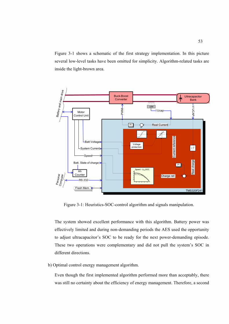
53
Figure 3-1 shows a schematic of the first strategy implementation. In this picture
several low-level tasks have been omitted for simplicity. Algorithm-related tasks are
inside the light-brown area.
V U
CAPP
WM
Motor Control Unit
Ah Counter
Batt. State of charge
Voltageprotection
PI+
-
( )2
PI
Rea
l cha
rge
Charge ref.
Real Current
Buck-BoostConverter
Batt Voltage
System Current
Speed
LEM
I Ucap
TMS320F241
+ -C
urre
nt re
fere
nce
RS 232
Flash Mem.
Batte
ry a
nd m
ain
driv
e
Per
sona
l C
ompu
ter
Ultracapacitor Bank
Speed - UcapSOC
Figure 3-1: Heuristics-SOC-control algorithm and signals manipulation.
The system showed excellent performance with this algorithm. Battery power was
effectively limited and during non-demanding periods the AES used the opportunity
to adjust ultracapacitor’s SOC to be ready for the next power-demanding episode.
These two operations were complementary and did not pull the system’s SOC in
different directions.
b) Optimal control energy management algorithm.
Even though the first implemented algorithm performed more than acceptably, there
was still no certainty about the efficiency of energy management. Therefore, a second

54
algorithm was designed and programmed by a master’s degree program student, as
part of the same research project (Moreno et al, 2004). This algorithm was based on
the application of optimal control techniques to determine the optimal power support
for a real-life power-demand-profile.
The optimal control process consisted on calculating (offline) the optimal power-
support for real power demand data series. To do this, thirty power-demand data
series were recorded while driving an EV on urban driving conditions. For each of
these data series a power support sequence that would minimize the energy extracted
from the battery was found; this is the power support that, if delivered by an AES,
would maximize the system efficiency for that driving sequence. An efficiency
model of the drive system and the AES was used to implement the cost function. A
constraint that forced the ultracapacitors’ state of charge at the end of the exercise to
be the same than that at the beginning of it ensured optimization consistency. The
power demand data series, together with the corresponding optimal power support
data series, were used as the knowledge base to train a Neural Network (NN) offline.
The NN would then apply the learned information to determine the power support on
real-life experiments, to do this the NN would imitate optimal control behavior on
situations similar to those optimized before. Figure 3-2 illustrates the optimal control
data generation process and how that information is used to train the NN.

55
Data
Power Speed Voltage ...10100 00110 1010011100 01000 11110 11110 00001 00110 10010 00101 0100011101 01010 0101011100 00001 1110100010 01010 10010
Optimal Control Process (eficiency
model)
Iterations
Optimal Power Support data
Power Speed Voltage Power - support10100 00110 10100 0011011100 01000 11110 0000111110 00001 00110 0010110010 00101 01000 01010 11101 01010 01010 00001 11100 00001 11101 1111000010 01010 10010 11101
Data Logging ProcessBatts. only
Application of learned informationBatts. + AES
Neural Network Training
Figure 3-2: Optimal Control data generation and Neural Network training
processes.
During offline optimal control path calculation, results obtained presented a mean
calculated efficiency increase of 5% compared to that obtained with the simulated
operation of the SOC-control-algorithm (illustrated in Figure 3-1). This predicted a
positive change in vehicle efficiency using the new optimal-control algorithm.
Thirty different power demand series, with calculated optimal power-support data,
were used on the NN training process. The Levenberg–Marquardt training algorithm
was used. Of the 30 data series, 10 were used for NN training and the remaining 20
for validation. The validation indicator used was the mean square error. To define
optimal net architecture, ‘prunning’ algorithms were used (the Optimal Brain
Surgeon algorithm in particular). Figure 3-3 illustrates interaction of trained NN with
the DSP variables to implement optimal control algorithm.

56
V U
CAPP
WM
Motor Control Unit
Ah counter
Batt SOC
Ultracapacitor Bank
VoltageProtection
PI+
- Actual Current
Buck-BoostConverter
Batt. Voltage
Load Current
Speed
LEM
I Ucap
TMS320F241
Cur
rent
Ref
eren
ce
Neural Network
RS 232
Flash Mem.
Ba t
t er y
and
mai
n dr
ive
Pers
onal
C
ompu
ter
Iload(k)Iload(k-1)Pload(k)
Pload(k-1)V(k)
V(k-1)E(k)
E(k-1)Bias(+1) Bias(+1)
Figure 3-3: Optimal-control algorithm, implemented using neural networks.
The trained NN presented excellent replication of optimal behavior learned during
the training process. This was verified after training by comparing the power-support
output from the NN to the optimal output of one validation data series.
III.3 Communication layout
The basic shell mentioned above consists of a hardware command-and-
communication layout, which is managed by a central microprocessor. A low-level
routine, programmed in this microprocessor, allows implementation of data-
acquisition functions, a communication protocol and the basic current control loop.
The command and communication layout is illustrated in Figure 3-4.

57
V U
CAPMotor Control Unit
Ah Counter
Batt. State of charge
Buck-BoostConverter
Batt Voltage
Motor Current
Speed Control Circuit Board
RS 232
Flash Mem.
Batte
ry a
nd m
ain
driv
e
Perso na l
Co m
pu ter
Ultracapacitor Bank
LEM
I Ucap
PW
M
Figure 3-4: Communication and command flow diagram.
III.4 Implementation via DSP
The command and communication layout was implemented in a power-electronics-
oriented DSP, the TMS320F240 from Texas instruments. This microprocessor was
installed in a specially designed circuit board that included signal conditioning for
data acquisition, an external flash memory to store user-manageable control-
parameters, communication ports and command signal ports.
The board with DSP and associated circuitry is illustrated in Figure 3-5.

58
Figure 3-5: DSP control board, signals and data ports.
III.5 Real-time monitoring software
Given the need, and special aim of this work, to acquire and analyze power system
behavior data, special monitoring and acquisition software was programmed in
Visual Basic. The definition of a DSP-PC communication protocol and the simplicity
of programming in this environment allowed implementing a satisfactory real-time
monitoring feature, while monitored data could be stored for further analysis. Figure
3-6 illustrates the main control screen and a data monitoring screen.
Figure 3-6: Control and data monitoring/acquisition software screens.
59
The screen on the left shows and allows modification of user-controllable parameters.
Data monitoring and low-level control can be commanded from this window too. The
screen on the right shows monitored data in a real-time sliding-chart.
III.6 Failure detection
This feature was designed with the double purpose of preventing dangerous
conditions and facilitating the debugging process. The failure detection operates as a
software routine that interrupts operation when an abnormal condition is detected.
Three abnormal condition types are sensed: battery-side fuse blown, failure signal
received from IGBT module and communication interrupted while operating in PC-
supervised mode. In all cases gating operations are disabled and failure information is
displayed in the monitoring software’s main control screen (if connected). Operations
will remain disabled until re-enabled by user with monitoring software. The last
failure cause is always stored and displayed on the main control screen.

60
IV URBAN CIRCUIT TESTS
IV.1 Introduction
Once all supporting parts of the system (power and control) were tested and ready,
the evaluation process was prepared. The goal was to determine and quantify the
improvements in vehicle performance due to the use of the AES. This assessment
would be used to determine the technical and economic contribution of this kind of
equipment to pure electric vehicles and the possible application to hybrid vehicles.
The performance indicators to be evaluated were: available power (kW) and yield
(km/kWh), with and without the aid of this particular AES. Therefore, a protocol to
measure these variables was established.
During tests, the monitoring system logged and stored variables such as vehicle
speed, battery and ultracapacitor voltage, power demanded by motor and power
delivered by AES among others. Of more than 40 tests, 23 where performed
measuring total energy used (as seen from the charger) in four different conditions:
without regeneration, with battery-only regeneration and with AES-assisted
regeneration using both described algorithms.
Every test was performed with identical tire pressure, at the same time of the day and
over a period of one month to ensure relatively identical conditions. The driver plus
one passenger rode on tests when the AES was out of action, but an extra passenger
was included when this power support system was used to emulate the AES’s extra
weight.
IV.2 Test circuit
Because this system is conceived to support power mainly during acceleration and
braking periods, its application is naturally directed to urban driving. Hence, a 14 km
urban-drive circuit was established as the standard measure. The circuit has a slow
driving portion (inside university campus) and a faster one but with stops every one
to two hundred meters. The stops where introduced to simulate congested urban
driving conditions. Most stops were dummy traffic jams, which were actually marks

61
on a map where identical stops had been programmed for every test. The
approximate mean speed was of 18 km/h, with maximum speeds of 60 km/h. Figure
4-1 illustrates the map of the test course.
100m0m 200m 300m
Figure 4-1: Urban circuit test course.
IV.3 Tests results
The general driving appreciation was that available power had noticeably increased,
allowing fast accelerations, even when batteries were deeply discharged. This can be
corroborated by analyzing data plots obtained with the monitoring system. Figure 4-2
illustrates normal load currents for a urban drive and corresponding battery voltage
when no power support is applied.
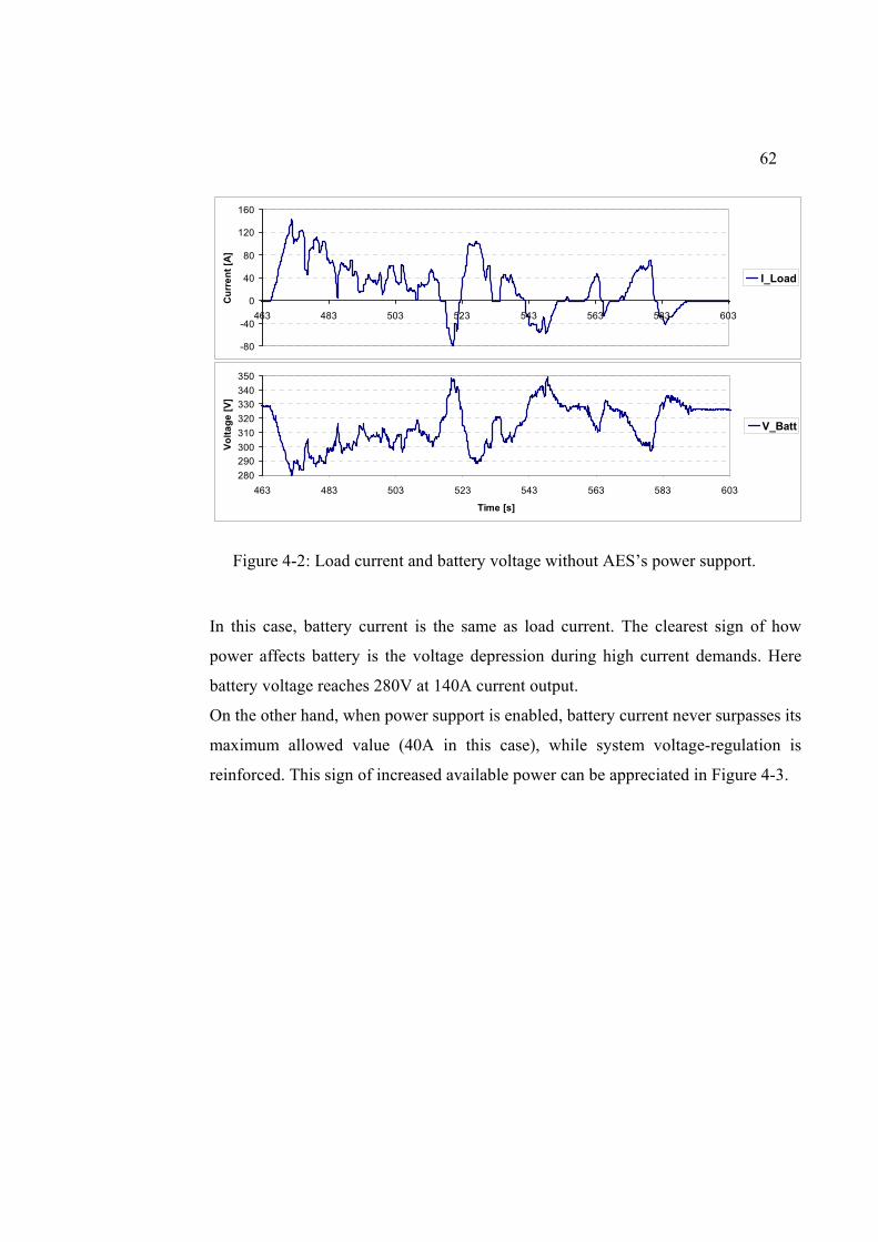
62
-80
-40
0
40
80
120
160
463 483 503 523 543 563 583 603
Cur
rent
[A]
I_Load
280290300310320330340350
463 483 503 523 543 563 583 603
Time [s]
Volta
ge [V
]
V_Batt
Figure 4-2: Load current and battery voltage without AES’s power support.
In this case, battery current is the same as load current. The clearest sign of how
power affects battery is the voltage depression during high current demands. Here
battery voltage reaches 280V at 140A current output.
On the other hand, when power support is enabled, battery current never surpasses its
maximum allowed value (40A in this case), while system voltage-regulation is
reinforced. This sign of increased available power can be appreciated in Figure 4-3.

63
-80
-40
0
40
80
120
160
162 182 202 222 242 262
Cur
rent
[A]
I_LoadI_AESUI_Batt
280290300310320330340350
162 182 202 222 242 262
Time [s]
Volta
ge [V
]
V_Batt
Figure 4-3: Currents and battery voltage for a power-supported system.
When the AES supplies power support, battery power output is limited to around 12
kW. This is done by supplying the balance demanded current. In this way battery
does not “see” peak demanded power but values near mean demanded power.
Negative power is also limited to a fixed value around -3 kW; this value is
automatically manipulated by software when it detects battery voltage rising to
prevent gassing, which is especially useful when batteries have been recently
charged. In this plot this feature can be observed when battery voltage approaches
340 V.
The motor-drive controller, a microprocessor provided by the drive manufacturer,
disables power when battery voltage decreases under 250 V. This generally occurred
to battery-alone configuration when demanded current surpassed 160 A, but never
occurred with AES-supported system. From this, battery available power may be
calculated at around 40 kW. The AES-supported system has nominal power of 45
kW+12 kW from battery, but up to 85 kW in total could be delivered if required, by
using all 40 kW form battery.
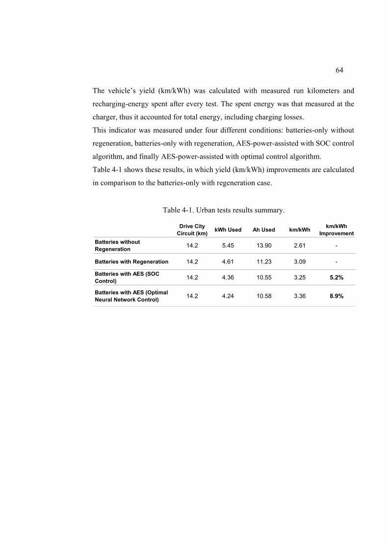
64
The vehicle’s yield (km/kWh) was calculated with measured run kilometers and
recharging-energy spent after every test. The spent energy was that measured at the
charger, thus it accounted for total energy, including charging losses.
This indicator was measured under four different conditions: batteries-only without
regeneration, batteries-only with regeneration, AES-power-assisted with SOC control
algorithm, and finally AES-power-assisted with optimal control algorithm.
Table 4-1 shows these results, in which yield (km/kWh) improvements are calculated
in comparison to the batteries-only with regeneration case.
Table 4-1. Urban tests results summary.
Drive City Circuit (km) kWh Used Ah Used km/kWh km/kWh
ImprovementBatteries without Regeneration 14.2 5.45 13.90 2.61 -
Batteries with Regeneration 14.2 4.61 11.23 3.09 -
Batteries with AES (SOC Control) 14.2 4.36 10.55 3.25 5.2%
Batteries with AES (Optimal Neural Network Control) 14.2 4.24 10.58 3.36 8.9%
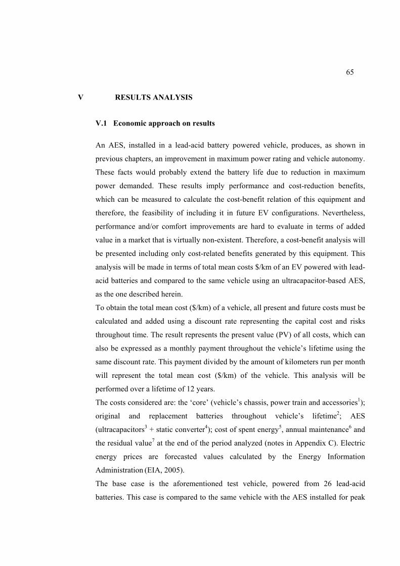
65
V RESULTS ANALYSIS
V.1 Economic approach on results
An AES, installed in a lead-acid battery powered vehicle, produces, as shown in
previous chapters, an improvement in maximum power rating and vehicle autonomy.
These facts would probably extend the battery life due to reduction in maximum
power demanded. These results imply performance and cost-reduction benefits,
which can be measured to calculate the cost-benefit relation of this equipment and
therefore, the feasibility of including it in future EV configurations. Nevertheless,
performance and/or comfort improvements are hard to evaluate in terms of added
value in a market that is virtually non-existent. Therefore, a cost-benefit analysis will
be presented including only cost-related benefits generated by this equipment. This
analysis will be made in terms of total mean costs $/km of an EV powered with lead-
acid batteries and compared to the same vehicle using an ultracapacitor-based AES,
as the one described herein.
To obtain the total mean cost ($/km) of a vehicle, all present and future costs must be
calculated and added using a discount rate representing the capital cost and risks
throughout time. The result represents the present value (PV) of all costs, which can
also be expressed as a monthly payment throughout the vehicle’s lifetime using the
same discount rate. This payment divided by the amount of kilometers run per month
will represent the total mean cost ($/km) of the vehicle. This analysis will be
performed over a lifetime of 12 years.
The costs considered are: the ‘core’ (vehicle’s chassis, power train and accessories1);
original and replacement batteries throughout vehicle’s lifetime2; AES
(ultracapacitors3 + static converter4); cost of spent energy5, annual maintenance6 and
the residual value7 at the end of the period analyzed (notes in Appendix C). Electric
energy prices are forecasted values calculated by the Energy Information
Administration (EIA, 2005).
The base case is the aforementioned test vehicle, powered from 26 lead-acid
batteries. This case is compared to the same vehicle with the AES installed for peak
66
power support. For the evaluated alternative two different assumptions were explored
for the increase in battery life, first a rather optimistic 50% extended life and second
a more realistic 20% extended life.
Table 5-1 illustrates all of these costs and the corresponding present value and total
average cost for each case analyzed.
Table 5-1. Total mean costs comparison with batteries as the main energy source.
Component Batteries Only Batteries (50%+) + Ucaps Batteries (20%+) + Ucaps
Vehicle(1) $ 8,000 $ 8,000 $ 8,000Bateries(2) $ 16,181 $ 11,595 $ 13,897Ucaps(3) + static converter(4) $ 0 $ 5,160 $ 5,160Total cost of energy(5) $ 3,288 $ 3,024 $ 3,024Maintenance(6) $ 2,856 $ 2,856 $ 2,856Residual value(7) -$ 450 -$ 724 -$ 578
PV of total costs(8) $ 29,874 $ 29,910 $ 32,358
Total average cost ($/km) $ 0.191 $ 0.192 $ 0.207
Cost change percentage - 0.1% 8.3%
Total average costs calculated for each case show that AES’s convenience is relative
to the battery life extension it produces. If batteries last 50% longer (an optimistic
hypothetic scenario) with the AES working, the total mean cost is almost the same as
the cost of the vehicle working on batteries only; therefore, in this case, battery life
savings are high enough to compensate for the AES’s cost. On the other hand, if
batteries last 20% more cycles (a more realistic scenario), then the total mean costs
are 8.3% higher for the vehicle equipped with the AES. Hence, in terms of costs only,
the system described in this paper would only justify its inclusion in a lead-acid
battery equipped vehicle if battery life extension is equal or higher than 50%. If
customer satisfaction is included in the analysis, then more accurate data about
battery life extension would be needed to evaluate the convenience of the system. In
the case when battery life is extended by 20%, customer satisfaction would have to
be high enough to justify an increase in total costs of approximately 8%.
Nevertheless, the added complexity of the whole system plus the higher component
count could increase failure probability and/or maintenance costs. These facts, as

67
well as the influence of costumer satisfaction are hard to measure in a market (EV’s
market) where there is scant experience regarding component failure and costumer
acceptance.
Continuing the research project’s line of investigation, oriented to evaluate feasible
vehicles for the short and medium terms, it is interesting to evaluate the integration of
other promising battery technologies for MES and the AES presented herein.
Therefore a new EV configuration, that combines a ZEBRA (Na/Ni-Cl2) battery
MES and the same ultracapacitor-based AES, has been implemented for evaluation.
That experience does not fall within the scope of this thesis; therefore its outcome
will be presented and analyzed in other instances within the near future. At the
moment of this thesis redaction, the newly configured vehicle was undergoing
preliminary tests and being prepared to perform efficiency and power evaluations on
it.
Regarding long term aimed EVs, a probable scenario to consider is that in which
fuel-cell powered vehicles are adopted by automakers and the industry. For this
analysis, three power configurations are evaluated: the vehicle powered by fuel cells
only, fuel cells plus Li-ion batteries and fuel cells plus ultracapacitors. The efficiency
for a fuel cell vehicle (running on gas hydrogen from electrolysis) from the power
grid to the wheels, can be derived from the composition of typical efficiencies of all
conversion processes involved: electrolysis (72 %), fuel cell (54 %) and electric drive
train (89 %), with a total integrated efficiency of 34 % (Eaves and Eaves, 2004). The
yield achieved by the wheel-to-road conversion was assumed at 8 km/kWh,
equivalent to running 300 miles with 60 kWh coming out of the wheels (Eaves and
Eaves, 2004); therefore an integrated yield (power-grid to wheels) for a fuel-cell
only vehicle was calculated at 2.72 km/kWh. An extra 18 % yield was considered for
the fuel cell plus batteries configuration (because of regeneration savings), and a 24
% of extra yield was attributed to the configuration running on fuel cells and
ultracapacitors. These numbers were obtained from experience acquired while testing
the AES with and without regeneration.
Costs in Table 5-2 clearly illustrate how fuel cells represent an important percentage
in the cost structure, and therefore a small fuel cell drastically reduces mean costs,

68
which can be seen in the case of combination with batteries or ultracapacitors. The
use of a much smaller fuel cell (20 kW in combination cases) is compensated by the
power support from batteries or ultracapacitors during peak power demand; however,
this cannot be sustained for a long time due to the limited amount of energy stored in
these devices. Hence, the use of combination configurations would limit the amount
of continuous time allowed to drive at maximum power, making it unsuitable for
sustained high speeds or hill climbing. Nevertheless, these configurations equipped
with an AES such as the one described in this thesis could still perform more than
well in urban conditions and even on highways at reasonable speeds (assuming good
aerodynamics), and the mean cost is drastically reduced in almost equal amounts of
33.7 % and 31.7 % for combinations with ultracapacitors and batteries, respectively.
Table 5-2. Total mean costs comparison with Hydrogen + Fuel Cell as the main energy system.
Component FuelCell Only FuelCell + Batteries FuelCell + Ucaps
Vehicle(1) $ 8,000 $ 8,000 $ 8,000Bateries(9) $ 0 $ 5,706 $ 0Fuel Cell(10) $ 20,000 $ 4,000 $ 4,000Ucaps(3) + static converter(4) $ 0 $ 0 $ 5,160Total cost of energy(5) $ 3,670 $ 3,110 $ 2,960Maintenance(6) $ 2,856 $ 2,856 $ 2,856Residual value(7) -$ 238 -$ 238 -$ 238
PV of total costs(8) $ 34,287 $ 23,433 $ 22,737
Total average cost ($/km) $ 0.220 $ 0.150 $ 0.146
Cost change percentage - -31.7% -33.7%
V.2 Related researches
During the last three years, a growing number of scientists have implemented and
tested systems of similar characteristics, which is a sign that this project was aimed in
the right direction. Moreover, by analyzing their results it is clear that some technical
issues have been well resolved in this design and innovative strategies, such as the
69
algorithms developed, have rewarded positive improvements. A brief review of
related publications of other authors during this period follows and relevant
conclusions will be compared to results from this project.
Presently general trends are inclined towards HEVs as a viable approach to zero (or
near zero) emission vehicles. The separation of energy-storage and power-support
tasks has proved a very efficient and effective strategy; more adequate elements have
been applied to each task, which has had a positive impact in power and efficiency,
and therefore in autonomy as well. Also, although HEV’s total costs are still not
competitive, its advantages compared to traditional ICE-vehicles are being
recognized by the industry, such as reduction in maintenance costs (King et al, 2005)
and improved comfort.
On the subject of available MESs for zero and near-zero-emission HEVs, most
projects are experimenting with FCs as being feasible in the long term, even though
primary and secondary batteries are the most viable in the short-medium term
because of costs and infrastructure concerns (Chan and Wong, 2004). Nevertheless,
there are two interesting researches showing hybrid systems using batteries as the
MES, both of them primary Zn/air batteries (Stanislowski et al, 2003; King et al,
2005), and ultracapacitor-based AESs.
In the case of power sources (AESs), batteries and ultracapacitors are currently the
only commercially available choices, where ultracapacitors have proved superior in
most cases. Longer and DOD-independent cycle life, good performance at low
temperatures(-40ºC), lower cost per kW and higher specific power are the most
outstanding advantages against batteries (Schneuwly and Smith, 2005; Jeon et al
2005). But also, performance evaluation in several researches have demonstrated
better overall system efficiency, and therefore lower operation costs and higher
autonomy in HEVs when evaluating ultracapacitors compared to power-batteries as
AES (Mazaika and Schulte, 2005).
Some studies have explored and confirmed the influence of energy management
strategies on vehicle performance and efficiency (Stanislowski et al, 2003; Mazaika
and Schulte, 2005), which has been an important subject in this thesis. This contrasts
with some other studies where ultracapacitors have been applied as AESs directly

70
connected to the power bus (Massé and Freeman, 2005; Jeon et al 2005), without a
static converter interface, an approach that limits or eliminates any possibility of
managing energy and power. Such an approach, even though it may save some losses
by eliminating a static converter, is inefficient in the use of ultracapacitor energy
storage space; its power support is uneven and only available during transients.
In the meanwhile, the use of ultracapacitor-based AESs grows in number and
application variety. An example is a sport HEV, integrating an ICE and ultracapacitor
power support (Martellucci and Santoro, 2005). This is a different approach than the
typical efficiency oriented HEV; nevertheless it confirms the power potential
ultracapacitors have.
Finally, some more specific technical papers seek to extend the knowledge regarding
ultracapacitor behavior. One interesting example evaluates performance under
thermal and mechanical stress (Conte and Pirker, 2005); another addresses key
issues, such as cell balancing, materials optimization and safety (Okamura and
Nakamura, 2003).
V.3 General discussion
Since the beginning of this project, relevant advances and results obtained from it
have been published in engineering journals and/or presented in specialized
symposiums. Among these publications, the most relevant published topics are:
system configuration proposal and simulated behavior analysis (Dixon et al, 2000);
partial results and system behavior description (Dixon and Ortúzar, 2001; Dixon et
al, 2003; Ortúzar et al, 2003); new energy management strategy proposal (Moreno et
al, 2004); fire incident description and analysis (Ortúzar et al, 2004); Final results and
system feasibility analysis (Ortúzar et al, 2005), and a new HEV configuration, using
a ZEBRA (Na/Ni/Cl2) battery and the AES described in this thesis (Dixon et al,
2005). The most relevant conclusions from those works have been mentioned in this
thesis; nevertheless, some have been omitted for practical reasons.
Regarding technical achievements in this project, it was demonstrated that power,
efficiency and yield were increased as a result of incorporating the ultracapacitor-
based AES to an EV using lead-acid batteries as a MES. Power increase was

71
noticeable for different drivers, but also was measured in the form of voltage
depression reduction. This experience confirms previous findings about available
power (Wight et al, 2001; Wight et al, 2002), but also demonstrates that efficiency,
and therefore autonomy, can be increased using this type of power support. However,
it was established that efficiency increase is directly linked to energy management
adequacy. This finding can be extended to the reasonable deduction that the energy
storage system usage can be maximized with an adequate power and energy control.
In this way the MES and AES for a particular vehicle can be optimized in size and
weight and therefore costs may be reduced.
Conclusions are relative regarding the convenience of this type of AES for lead-acid
batteries-based vehicles. In an optimistic scenario, where batteries life-cycle
increases in 50%, the ultracapacitor-based AES’s cost is compensated by savings in
battery replacement and energy, while adding the value of higher power and
autonomy. In the not-so-optimistic scenario, where battery life-cycle increases by
20%, the present value of costs increase by about 8% when using the studied AES,
while vehicle power rating is improved; therefore, in this scenario the system’s
convenience will depend on the value of consumer satisfaction due to the improved
vehicle performance.
The experience acquired in this project, while working with the designed and
constructed AES, suggests that a better complement could be achieved if the
designed system is combined with more energy-oriented batteries (higher specific
energy, lower specific power). Primary batteries, such as Zn/air or Al/air, have
already been successfully tested in combination with ultracapacitor-based AES
(Stanislowski et al, 2003; King et al, 2005). But because of the extremely low
specific power these batteries have, such configurations need (and have used) a
second battery to provide power for prolonged high power demand episodes, like
uphill or high speed driving. Hence, a battery of power and energy characteristics in
between Zn/air and lead-acid could perfectly match with an ultracapacitor-based
AES.
As a consequence of previous analysis, the project described in this thesis has been
extended to evaluate the proposed approach: the better match of a higher specific-

72
energy (and lower specific-power) battery, and the designed AES for efficient and
powerful performance. This configuration has already been implemented using a
ZEBRA (Na/Ni-Cl2) battery and is being tested to determine behavior and
performance under different situations and driving conditions.
73
VI CONCLUSIONS
In this thesis a power-energy system specially developed for state of the art Electric
Vehicles has been described, analyzed and evaluated. As for the project’s outcome, it is
valid to say that the general project objectives, as well as particular design objectives, have
been broadly fulfilled. During the whole process there has been constant screening and
interaction with other researchers working on similar projects, which has allowed for an up
to date critical evaluation and makes results presented here a real contribution to the
modern transport industry.
The search for innovative solutions to address contemporary transport and environmental
issues has motivated the development of a practical, powerful and clean transport
alternative. Starting from an EV configured with state-of-the-art equipment, key technical
problems have been addressed; namely: instantaneous available power, efficiency and
autonomy. An Auxiliary Energy System based on ultracapacitors and a buck-boost
converter has been designed, implemented and tested. Its performance has been technically
and economically evaluated, whose results have been extended to fuel-cell powered
vehicles.
In particular, the achieved power and energy management capabilities were more than
satisfactory, being able to deliver or accept more than 60 kW of power. The ease of power-
flow control and overall system efficiency may be attributed to the thorough design of key
components, such as the 1.6 mH smoothing inductor and the water-cooled heat-sink,
among others, as well as the adequate topology configuration and implementation. These
features allowed for a powerful and controllable device that could be integrated into an
electric vehicle and safely interact with other power components without conflict.
The control and monitoring structure was also an important component of the Auxiliary
Energy System and one of the keys to the project success. The control system composed of
digital hardware and software, not only allowed for a fine control of power flow and safe
operation, but also supported the evaluation process by allowing the implementation of
different energy management strategies and by providing data logging and real-time
monitoring features.

74
The implemented system achieved an increase in vehicle yield (km/kWh), and therefore in
vehicle efficiency, of up to 8.9% using an optimum control energy management algorithm.
The available power was increased from an unreliable 40 kW value to a nominal 57 kW
and maximum 85 kW, which was evident to the driver.
Economical evaluation showed mixed results. While a hypothetical increase of 50% in
battery life would compensate for the costs of an AES such as the one being evaluated,
lower increases in battery life would not and, therefore, the influence of consumer
satisfaction would be the measure by which the convenience of this particular
configuration should be judged.
The hypothetical combination of fuel-cells and ultracapacitors was also economically
evaluated in comparison to pure fuel-cell as well as fuel-cell combined with batteries. The
outcome was that the reduction of fuel-cell size in both combination cases (with batteries
and with ultracapacitors) allowed for an important reduction in total costs, both alternatives
being more than 30% cheaper than the pure FC configuration in terms of total life cycle
costs.
This project’s results were compared to and complemented by those obtained from other
researchers working on similar projects. Also, relevant results from every stage of
development were published and presented in pertinent journals and symposiums. Thus,
conclusions presented here meet the highest standards of the international scientific
community and transport industry.
Therefore, it is fair to say that every major and particular objective of this thesis has been
fulfilled, and that the proposed hypothesis has been demonstrated and adequately
discussed.
Improvements achieved are consistent and significant, but as mentioned above, better
energy storage devices combinations may be implemented by using more energy-oriented
batteries. In this particular project, that challenge has already been assumed, therefore a
new high specific-energy ZEBRA (Na/Ni-Cl2) battery, in combination with the
aforementioned AES, has been installed in the same EV. The vehicle is now undergoing
preliminary tests; a general evaluation, like the one presented in this thesis, will be
performed in the near future.

75
REFERENCES
AMERICAN PETROLEUM INSTITUTE, API (1988) Alcohols and Ethers,
Publication No. 4261, Table B-1. 2nd ed. Washington DC, USA.
ARNET, B.J. and HAINES, L.P. (2000) Combining Ultra-Capacitors with Lead-Acid
Batteries. 17th Electric Vehicle Symposium, Montreal, Canada.
BARRADE, P. and RUFER, A. (2001) High-Power Fast Energy Exchange between
Storage Systems :Supercapacitors as energy buffer in transportation systems. 18th
Electric Vehicle Symposium, Berlin, Germany.
BURKE, A. and MILLER, M. (2002) Comparisons of Ultracapacitors and Advanced
Batteries for Pulse Power in Vehicle Applications:Performance, Life, and Cost. 19th
Electric Vehicle Symposium, Busan, Korea.
BURKE, A. and MILLER, M. (2001) Update of Ultracapacitor Technology and Hybrid
Vehicle Applications: Passenger Cars and Transit Buses. 18th Electric Vehicle
Symposium, Berlin, Germany.
CHAN, C. and WONG, Y. (2004) Electric Vehicles Charge Forward. IEEE Power & Energy Magazine. November/December.
COHEN, M. and SMITH, R. (2002) Here and Now; Ultracapacitors are a Standard
Option. 19th Electric Vehicle Symposium, Busan, Korea.
CONTE, F. and PIRKER, F. (2005) Electrical Performances of High power Electric
Double layer Capacitor under Thermal and Mechanical Stress. 21st Electric Vehicle
Symposium, Monaco.
DIETRICH, T. (2001) UltraCaps - A new Energy Storage Device for Peak Power
Applications. 18th Electric Vehicle Symposium, Berlin, Germany.
DI NAPOLI, A., CRESCIMBINI, F., SOLERO, L., PEDE, G., LO BIANCO, G.,
PASQUALI, M. (2001) Ultracapacitor and Battery Storage System Supporting Fuel-
Cell Powered Vehicles. 18th Electric Vehicle Symposium, Berlin, Germany.
76
DIXON, J., ORTÚZAR, M., WIECHMANN E. (2000) Regenerative Braking for an
Electric Vehicle Using Ultracapacitors and a Buck-Boost Converter. 17th Electric
Vehicle Symposium, Montreal, Canada.
DIXON, J., ORTÚZAR, M., SCHMIDT, R., LAZO, G., LEAL, I., GARCÍA, F.,
RODRÍGUEZ, M., AMARO, A., WIECHMANN, E. (2000) Performance
Characteristics of the First, State-of-the-art Electric Vehicle Implemented in Chile. 17th
Electric Vehicle Symposium, Montreal, Canada.
DIXON, J. and ORTÚZAR, M. (2001) Tests Results with Regenerative Braking based
on Ultracapacitors and a Buck-Boost Converter. 18th Electric Vehicle Symposium,
Berlin, Germany.
DIXON, J., ORTÚZAR, M., MORENO, J. (2002) Monitoring System for Testing the
Performance of an Electric Vehicle Using Ultracapacitors. 19th Electric Vehicle
Symposium, Busan, Korea.
DIXON, J., ORTÚZAR, M., MORENO, J., (2003) DSP Based Ultracapacitor System
for Hybrid-Electric Vehicles. 20th Electric Vehicle Symposium, Long Beach,
California, USA.
DIXON, J., ORTÚZAR, M., ARCOS, E., NAKASHIMA, I. (2005) ZEBRA plus
ultracapacitors: A good match for energy efficient EVs. 21st Electric Vehicle
Symposium, Monaco.
EAVES, S. and EAVES, J. (2004) A Cost Comparison of Fuel-Cell and Battery
Electric Vehicles. Journal of Power Sources, 130(1-2), pp.208-212.
EIA (2005) Annual Energy Outlook 2005. Report #: DOE/EIA-0383(2005). US
Department Of Energy.
EPCOS (2001) UltraCapTM Double Layer Capacitors, A New Energy Storage Device
for Peak Power Applications. Product Profile 2001. EPCOS AG Marketing
Comunications.
77
FURUBAYASHI, M., TAKEDA, T., OKUMURA, E., KOBAYASHI, M. (2000)
Application of Ultra-Capacitors with Large Capacitance to HEV. 17th Electric Vehicle
Symposium, Montreal, Canada.
FOLCHERT, J., NAUNIN, D., TSERONIS, D. (2002) Ultra Capacitor Storages for
Automotive Applications. 19th Electric Vehicle Symposium, Busan, Korea.
FURUBAYASHI, M., USHIO, Y., OKUMURA, E., TAKEDA, T., ANDOU, D.,
SHIBUYA, H. (2001) Application of High Power Super Capacitors to an Idling Stop
System for City Buses. 18th Electric Vehicle Symposium, Berlin, Germany.
GOESMANN, H., MICHEL, H., WEBER, C. (2002) Safety and Environmental Risk
Management of UltraCaps. 19th Electric Vehicle Symposium, Busan, Korea.
GALLIERS S. (2003) Practical Application of Fuel Cells in Buildings.
CIBSE/ASHRAE conference, Edinburgh, Great Britain.
HÄRRI, V. and EGGER, S. (2001) Supercapacitor Circuitry Concept "SAM" for
Public Transport Vehicles and other Applications. 18th Electric Vehicle Symposium,
Berlin, Germany.
HEINEMANN, D., NAUNIN, D., PETSCH, G. (2001) Ultracaps in power-assist
applications in Battery Powered Electric Vehicles -Implications on Energy
Management Systems. 18th Electric Vehicle Symposium, Berlin, Germany.
HEINEMANN, D., NAUNIN, D., PETSCH, G. (2001) Ultracaps in power-assist
applications in Battery Powered Electric Vehicles -Implications on Energy
Management Systems. 18th Electric Vehicle Symposium, Berlin, Germany.
JEON, S., LEE, J., JEONG, S., LIM, T. (2005) Hyundai Supercapacitor Fuel Cell
Hybrid Electric Vehicle. 21st Electric Vehicle Symposium, Monaco.

78
JEONG, J., LEE, H., KIM, C., CHI, H., CHO, B. (2002) A Development of an Energy
Storage System for Hybrid Electric Vehicles Using Supercapacitor. 19th Electric
Vehicle Symposium, Busan, Korea.
JEHOULET, C., MOREAU, L., PICHON, B., ROCHARD, D., CESBRON, D.,
CHAILLET, A. (2000) Ultracapacitors: Power Buffer for Automotive Applications.
17th Electric Vehicle Symposium, Montreal, Canada.
JEONG, J., LEE, H., KIM, C., CHOI, H., CHO, B. (2002) A Development of an
Energy Storage System for Hybrid Electric Vehicles Using Supercapacitor. 19th
Electric Vehicle Symposium, Busan, Korea.
KING, R., NASADOSKI, J., BELANGER, M., GILON, Y. (2005) Ultracapacitor
(1kWh) Enhaced Zero Emissions Zinc-Air All Electric Transit Bus – Performance Test
Results. 21st Electric Vehicle Symposium, Monaco.
KIRSCH D. (1996) The Electric Car and the Burden of History: Studies in Automotive
Systems Rivalry in the United States, 1890 – 1996. Ph.D. diss., Stanford University,
UMI 97-14137.
LAMPÉRTH, M., SUAREZ, T., GUO, X. (2005) Simple Ultra Capacitor Circuit to
Improve the performance and Life of Lead Acid Batteries. 21st Electric Vehicle
Symposium, Monaco.
LOTT, J. and SPÄTH, H. (2001) Double Layer Capacitors as additional Power Source
in Electric Vehicles. 18th Electric Vehicle Symposium, Berlin, Germany.
MARTELLUCCI, L. and SANTORO, M. (2005) MAGICA II Project: Experimental
Results Analysis and Electronic management Optimization. 21st Electric Vehicle
Symposium, Monaco.
MASSÉ, S. and FREEMAN, N. (2005) Fuel Cells and Ultracapacitors in Light
Mobility Applications. 21st Electric Vehicle Symposium, Monaco.

79
MAZAIKA, D. and SCHULTE, J. (2005) Batteries vs Ultracapacitors in Hybrid
Electric Buses. 21st Electric Vehicle Symposium, Monaco.
MILLER, J., and SMITH, R. (2004) Ultracapacitor Assisted Electric Drives for
Transportation. Maxwell technologies, White Papers. www.maxwell.com.
MITSUI, K., NAKAMURA, H., OKAMURA, M. (2002) Capacitor-Electronic Systems
(ECS) for ISG/Idle Stop Applications. 19th Electric Vehicle Symposium, Busan, Korea.
MORENO, J., DIXON, J., ORTÚZAR, M., LA ROSA, P. (2004) Energy Management
System for a Hybrid Electric Vehicle, Using Ultracapacitors and Neural Networks.
IEEE Transactions on power electronics, accepted for publication.
OKAMURA, M. (2002) Buses, Trucks and FCVs using the Capacitor Hybrid System ~
ECS. 19th Electric Vehicle Symposium, Busan, Korea.
OKAMURA, M. and NAKAMURA, H. (2003) Important Issues of a Capacitor Storage
System Other Than Energy Density. 20th Electric Vehicle Symposium, Long Beach,
California, USA.
ORTÚZAR, M. (2002) Diseño y Construcción de Conversor DC-DC Para Control de
Ultracapacitores en Vehículo Eléctrico. Memoria de Título, Departamento de
Ingeniería Eléctrica, Pontificia Universidad Católica de Chile.
ORTÚZAR, M., DIXON, J., MORENO, J. (2003) Design, Construction and
Performance of a Buck-Boost Converter for an Ultracapacitor-Based Auxiliary Energy
System for Electric Vehicles. 29th Industrial Electronics Conference, Roanoke,
Virginia, USA.
ORTÚZAR, M., MORENO, J., DIXON, J. (2004) Report on Fire Event Originated by
Ultracapacitors in an Experimental Electric Vehicle. IEEE Vehicular Power and
Propulsion, Paris, France.
80
ORTÚZAR, M., MORENO, J., DIXON, J. (2005) Implementation and Evaluation of
an Ultracapacitor-Based Auxiliary Energy System for Electric Vehicles. IEEE
Transactions on Industrial Electronics, submitted for revision.
RUTQUIST, P. (2002) Optimal Control for the Energy Storage in a Hybrid Electric
Vehicle. 19th Electric Vehicle Symposium, Busan, Korea.
SCHNEUWLY, A. and SMITH, R. (2005) Ultracapacitor to Address Power and
Redundancy Needs of Vehicles. 21st Electric Vehicle Symposium, Monaco.
STANISLOWSKI, R., AMENT, C., BREDEMEIER, C., GOCH, G. (2003) Energy
Management System for Combined Electric Storage System for High Energy and High
Power. 20th Electric Vehicle Symposium, Long Beach, California, USA.
SUND, M. and TRICE, P. (2001). Maxwell Technologies to Supply PowerCache
Ultracapacitors to General Motors for Hybrid Electric Vehicles. Press release:
http://www.powercache.com/news/press_releases/2001/jan03-01.html
TAYLOR, D. (2003) Simplified Life Cycle Cost Analysis of Plug-in HEVs, Engine
Dominant HEVs and Conventional Vehicles in 2012. EPRI Hybrid Electric Vehicle
Working Group.
U.S. DEPARTMENT OF ENERGY, DOE (2003) Fact Sheets: Vehicles and Fuels,
Electric Vehicle Batteries. Energy Efficiency and Renewable Energy.
VARAKIN, I., KARPOV, V., KLEMENTOV, A, LITVINENKO, S., SAMITIN, V.,
SMELKOV, A., STARODUBTSEV, N. (2001) Module of Electrochemical Capacitors
for Applications in Hybrid Vehicles. 18th Electric Vehicle Symposium, Berlin,
Germany.
WILSON, T.G. and TRICKEY, P.H. (1962) DC Machine with Solid State
Commutation. AIEE paper # CP62-1372.
81
WIGHT, G., GARABEDIAN, H., ARNET, B., MORNEAU, J., (2001) Integration and
Testing of a DC/DC Controlled Supercapacitor into an Electric Vehicle. 18th Electric
Vehicle Symposium, Berlin, Germany.
WIGHT, G., JUNG, D., GARABEDIAN, H. (2002) On-Road and Dynamometer
Testing of a Capacitor-Equipped Electric Vehicle. 19th Electric Vehicle Symposium,
Busan, Korea.

82
A P P E N D I C E S

83
APPENDIX A: BUCK-BOOST CONVERTER OPERATION ANALYSIS
Figure A.1 illustrates a buck-boost topology for current ripple analysis and equation
deduction.
ultracapacitor bank
+ + +
VU
ESR
LS T2 D2 T1 D1
VB
Rint
C
iBAT
Buck Side Boost Side
Battery
VC
VS
iC
iU
Figure A.1: Buck-Boost topology.
Equation A.1 defines the duty cycle (δ) as the percentage of time a semiconductor (T1 or
T2) is switched on.
Tt0=δ (A.1)
Where T is the commutation period and t0 is the amount of time the IGBT in question is
conducting.
Equation A.2 describes the mean voltage SV when IGBT T2 commutates (buck operation).
VCVCTt
sV ⋅=⋅= δ0 (A.2)
Figure A.2 illustrates the current through Ls and its ripple. This plot will be used to deduce
equations that describe this current behavior.
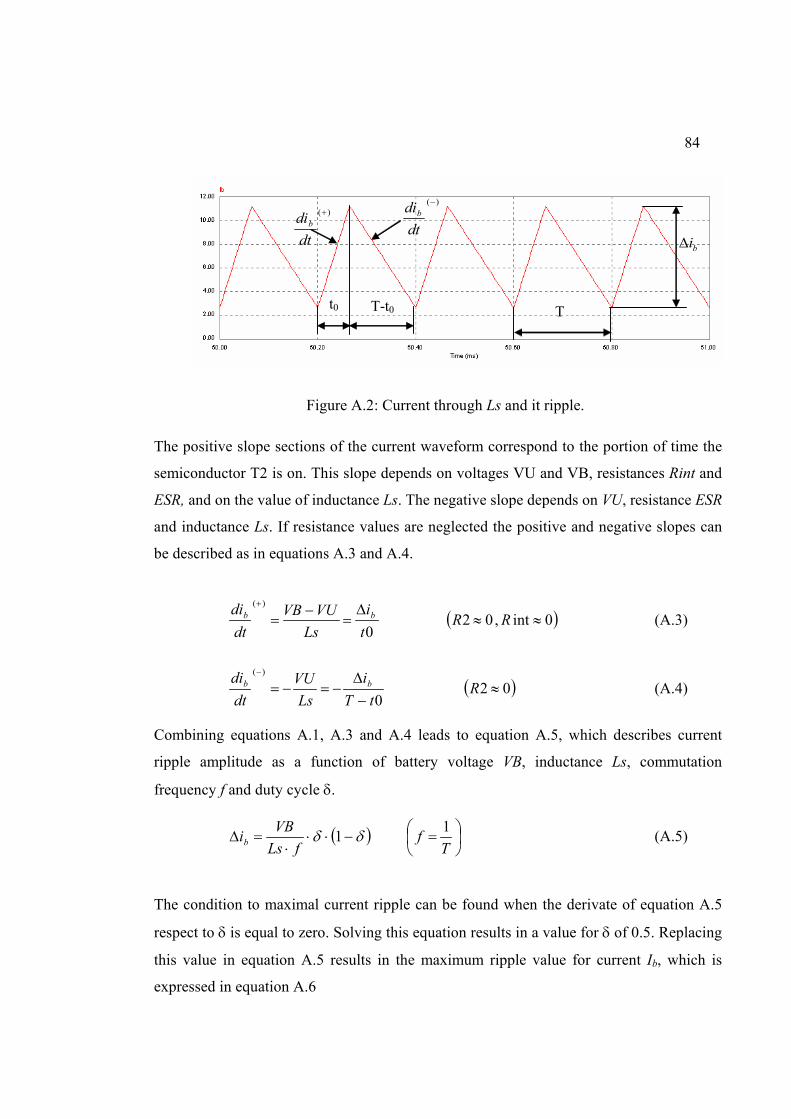
84
t0 T-t0 T
)(+
dtdib
)(−
dtdib
bi∆
Figure A.2: Current through Ls and it ripple.
The positive slope sections of the current waveform correspond to the portion of time the
semiconductor T2 is on. This slope depends on voltages VU and VB, resistances Rint and
ESR, and on the value of inductance Ls. The negative slope depends on VU, resistance ESR
and inductance Ls. If resistance values are neglected the positive and negative slopes can
be described as in equations A.3 and A.4.
( )0int,020
)(
≈≈∆
=−
=+
RRti
LsVUVB
dtdi bb (A.3)
( )020
)(
≈−
∆−=−=
−
RtT
iLs
VUdtdi bb (A.4)
Combining equations A.1, A.3 and A.4 leads to equation A.5, which describes current
ripple amplitude as a function of battery voltage VB, inductance Ls, commutation
frequency f and duty cycle δ.
( )
=−⋅⋅
⋅=∆
Tf
fLsVBib
11 δδ (A.5)
The condition to maximal current ripple can be found when the derivate of equation A.5
respect to δ is equal to zero. Solving this equation results in a value for δ of 0.5. Replacing
this value in equation A.5 results in the maximum ripple value for current Ib, which is
expressed in equation A.6

85
LsfVdcib ⋅⋅
=∆4
max (A.6)
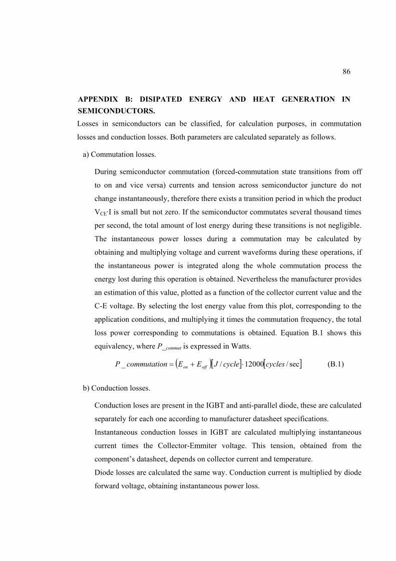
86
APPENDIX B: DISIPATED ENERGY AND HEAT GENERATION IN SEMICONDUCTORS. Losses in semiconductors can be classified, for calculation purposes, in commutation
losses and conduction losses. Both parameters are calculated separately as follows.
a) Commutation losses.
During semiconductor commutation (forced-commutation state transitions from off
to on and vice versa) currents and tension across semiconductor juncture do not
change instantaneously, therefore there exists a transition period in which the product
VCE·I is small but not zero. If the semiconductor commutates several thousand times
per second, the total amount of lost energy during these transitions is not negligible.
The instantaneous power losses during a commutation may be calculated by
obtaining and multiplying voltage and current waveforms during these operations, if
the instantaneous power is integrated along the whole commutation process the
energy lost during this operation is obtained. Nevertheless the manufacturer provides
an estimation of this value, plotted as a function of the collector current value and the
C-E voltage. By selecting the lost energy value from this plot, corresponding to the
application conditions, and multiplying it times the commutation frequency, the total
loss power corresponding to commutations is obtained. Equation B.1 shows this
equivalency, where P_conmut is expressed in Watts.
( )[ ] [ ]sec/12000/_ cyclescycleJEEncommutatioP offon ⋅+= (B.1)
b) Conduction losses.
Conduction loses are present in the IGBT and anti-parallel diode, these are calculated
separately for each one according to manufacturer datasheet specifications.
Instantaneous conduction losses in IGBT are calculated multiplying instantaneous
current times the Collector-Emmiter voltage. This tension, obtained from the
component’s datasheet, depends on collector current and temperature.
Diode losses are calculated the same way. Conduction current is multiplied by diode
forward voltage, obtaining instantaneous power loss.
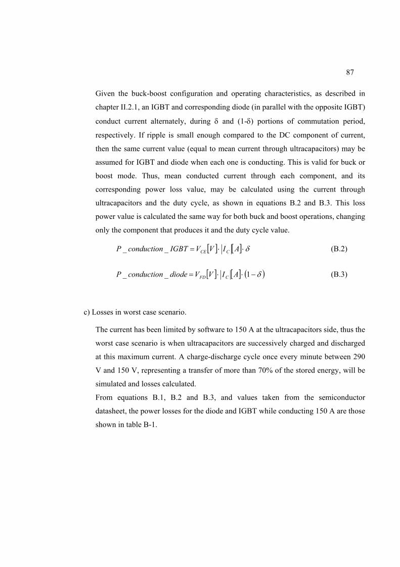
87
Given the buck-boost configuration and operating characteristics, as described in
chapter II.2.1, an IGBT and corresponding diode (in parallel with the opposite IGBT)
conduct current alternately, during δ and (1-δ) portions of commutation period,
respectively. If ripple is small enough compared to the DC component of current,
then the same current value (equal to mean current through ultracapacitors) may be
assumed for IGBT and diode when each one is conducting. This is valid for buck or
boost mode. Thus, mean conducted current through each component, and its
corresponding power loss value, may be calculated using the current through
ultracapacitors and the duty cycle, as shown in equations B.2 and B.3. This loss
power value is calculated the same way for both buck and boost operations, changing
only the component that produces it and the duty cycle value.
[ ] [ ] δ⋅⋅= AIVVIGBTconductionP CCE__ (B.2)
[ ] [ ] ( )δ−⋅⋅= 1__ AIVVdiodeconductionP CFD (B.3)
c) Losses in worst case scenario.
The current has been limited by software to 150 A at the ultracapacitors side, thus the
worst case scenario is when ultracapacitors are successively charged and discharged
at this maximum current. A charge-discharge cycle once every minute between 290
V and 150 V, representing a transfer of more than 70% of the stored energy, will be
simulated and losses calculated.
From equations B.1, B.2 and B.3, and values taken from the semiconductor
datasheet, the power losses for the diode and IGBT while conducting 150 A are those
shown in table B-1.
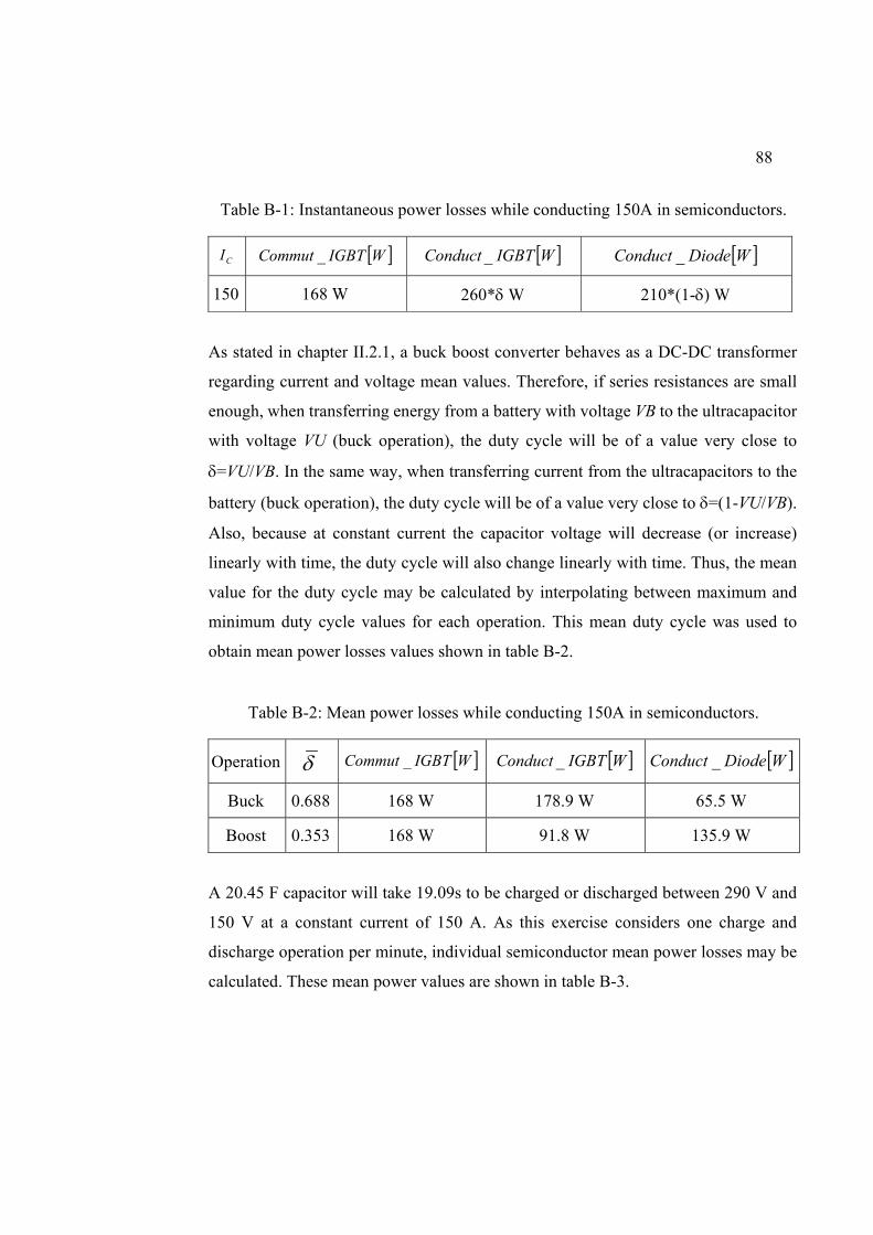
88
Table B-1: Instantaneous power losses while conducting 150A in semiconductors.
CI [ ]WIGBTCommut _ [ ]WIGBTConduct _ [ ]WDiodeConduct _
150 168 W 260*δ W 210*(1-δ) W
As stated in chapter II.2.1, a buck boost converter behaves as a DC-DC transformer
regarding current and voltage mean values. Therefore, if series resistances are small
enough, when transferring energy from a battery with voltage VB to the ultracapacitor
with voltage VU (buck operation), the duty cycle will be of a value very close to
δ=VU/VB. In the same way, when transferring current from the ultracapacitors to the
battery (buck operation), the duty cycle will be of a value very close to δ=(1-VU/VB).
Also, because at constant current the capacitor voltage will decrease (or increase)
linearly with time, the duty cycle will also change linearly with time. Thus, the mean
value for the duty cycle may be calculated by interpolating between maximum and
minimum duty cycle values for each operation. This mean duty cycle was used to
obtain mean power losses values shown in table B-2.
Table B-2: Mean power losses while conducting 150A in semiconductors.
Operation δ [ ]WIGBTCommut _ [ ]WIGBTConduct _ [ ]WDiodeConduct _
Buck 0.688 168 W 178.9 W 65.5 W
Boost 0.353 168 W 91.8 W 135.9 W
A 20.45 F capacitor will take 19.09s to be charged or discharged between 290 V and
150 V at a constant current of 150 A. As this exercise considers one charge and
discharge operation per minute, individual semiconductor mean power losses may be
calculated. These mean power values are shown in table B-3.
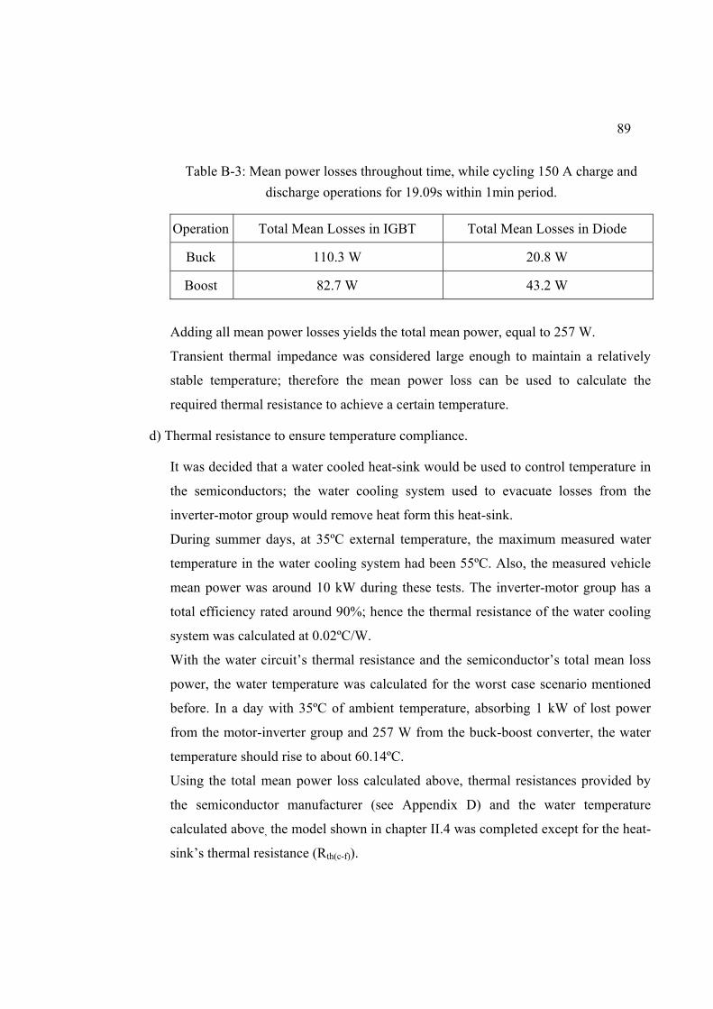
89
Table B-3: Mean power losses throughout time, while cycling 150 A charge and discharge operations for 19.09s within 1min period.
Operation Total Mean Losses in IGBT Total Mean Losses in Diode
Buck 110.3 W 20.8 W
Boost 82.7 W 43.2 W
Adding all mean power losses yields the total mean power, equal to 257 W.
Transient thermal impedance was considered large enough to maintain a relatively
stable temperature; therefore the mean power loss can be used to calculate the
required thermal resistance to achieve a certain temperature.
d) Thermal resistance to ensure temperature compliance.
It was decided that a water cooled heat-sink would be used to control temperature in
the semiconductors; the water cooling system used to evacuate losses from the
inverter-motor group would remove heat form this heat-sink.
During summer days, at 35ºC external temperature, the maximum measured water
temperature in the water cooling system had been 55ºC. Also, the measured vehicle
mean power was around 10 kW during these tests. The inverter-motor group has a
total efficiency rated around 90%; hence the thermal resistance of the water cooling
system was calculated at 0.02ºC/W.
With the water circuit’s thermal resistance and the semiconductor’s total mean loss
power, the water temperature was calculated for the worst case scenario mentioned
before. In a day with 35ºC of ambient temperature, absorbing 1 kW of lost power
from the motor-inverter group and 257 W from the buck-boost converter, the water
temperature should rise to about 60.14ºC.
Using the total mean power loss calculated above, thermal resistances provided by
the semiconductor manufacturer (see Appendix D) and the water temperature
calculated above, the model shown in chapter II.4 was completed except for the heat-
sink’s thermal resistance (Rth(c-f)).
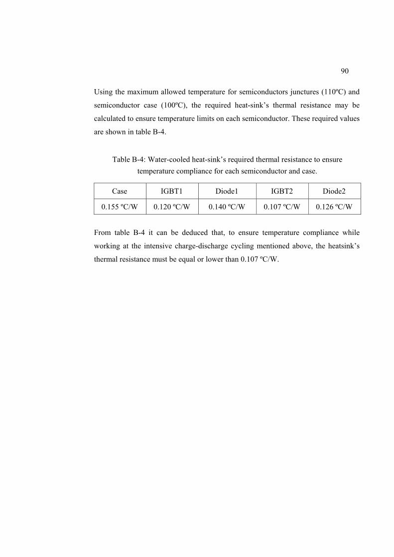
90
Using the maximum allowed temperature for semiconductors junctures (110ºC) and
semiconductor case (100ºC), the required heat-sink’s thermal resistance may be
calculated to ensure temperature limits on each semiconductor. These required values
are shown in table B-4.
Table B-4: Water-cooled heat-sink’s required thermal resistance to ensure temperature compliance for each semiconductor and case.
Case IGBT1 Diode1 IGBT2 Diode2
0.155 ºC/W 0.120 ºC/W 0.140 ºC/W 0.107 ºC/W 0.126 ºC/W
From table B-4 it can be deduced that, to ensure temperature compliance while
working at the intensive charge-discharge cycling mentioned above, the heatsink’s
thermal resistance must be equal or lower than 0.107 ºC/W.
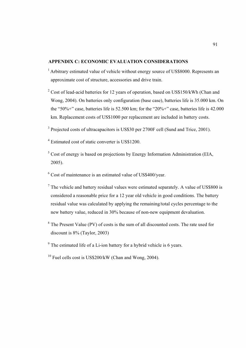
91
APPENDIX C: ECONOMIC EVALUATION CONSIDERATIONS 1 Arbitrary estimated value of vehicle without energy source of US$8000. Represents an
approximate cost of structure, accessories and drive train.
2 Cost of lead-acid batteries for 12 years of operation, based on US$150/kWh (Chan and
Wong, 2004). On batteries only configuration (base case), batteries life is 35.000 km. On
the “50%+” case, batteries life is 52.500 km; for the “20%+” case, batteries life is 42.000
km. Replacement costs of US$1000 per replacement are included in battery costs.
3 Projected costs of ultracapacitors is US$30 per 2700F cell (Sund and Trice, 2001).
4 Estimated cost of static converter is US$1200.
5 Cost of energy is based on projections by Energy Information Administration (EIA,
2005).
6 Cost of maintenance is an estimated value of US$400/year.
7 The vehicle and battery residual values were estimated separately. A value of US$800 is
considered a reasonable price for a 12 year old vehicle in good conditions. The battery
residual value was calculated by applying the remaining/total cycles percentage to the
new battery value, reduced in 30% because of non-new equipment devaluation.
8 The Present Value (PV) of costs is the sum of all discounted costs. The rate used for
discount is 8% (Taylor, 2003)
9 The estimated life of a Li-ion battery for a hybrid vehicle is 6 years.
10 Fuel cells cost is US$200/kW (Chan and Wong, 2004).

92
APPENDIX D: TMS320F241 DSP CONTROLLER, TEXAS INSTRUMENTS

93
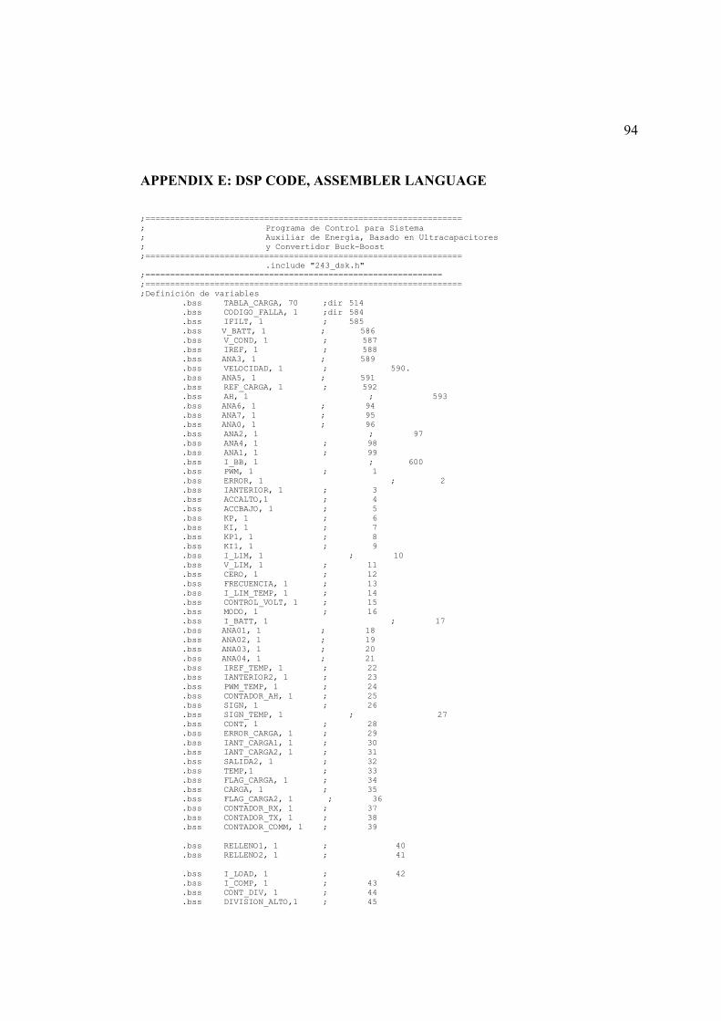
94
APPENDIX E: DSP CODE, ASSEMBLER LANGUAGE ;================================================================ ; Programa de Control para Sistema ; Auxiliar de Energía, Basado en Ultracapacitores ; y Convertidor Buck-Boost ;================================================================ .include "243_dsk.h" ;============================================================ ;================================================================ ;Definición de variables
.bss TABLA_CARGA, 70 ;dir 514 .bss CODIGO_FALLA, 1 ;dir 584 .bss IFILT, 1 ; 585 .bss V_BATT, 1 ; 586 .bss V_COND, 1 ; 587 .bss IREF, 1 ; 588 .bss ANA3, 1 ; 589 .bss VELOCIDAD, 1 ; 590. .bss ANA5, 1 ; 591 .bss REF_CARGA, 1 ; 592 .bss AH, 1 ; 593 .bss ANA6, 1 ; 94 .bss ANA7, 1 ; 95 .bss ANA0, 1 ; 96 .bss ANA2, 1 ; 97 .bss ANA4, 1 ; 98 .bss ANA1, 1 ; 99 .bss I_BB, 1 ; 600 .bss PWM, 1 ; 1 .bss ERROR, 1 ; 2 .bss IANTERIOR, 1 ; 3 .bss ACCALTO,1 ; 4 .bss ACCBAJO, 1 ; 5 .bss KP, 1 ; 6 .bss KI, 1 ; 7 .bss KP1, 1 ; 8 .bss KI1, 1 ; 9 .bss I_LIM, 1 ; 10 .bss V_LIM, 1 ; 11 .bss CERO, 1 ; 12 .bss FRECUENCIA, 1 ; 13 .bss I_LIM_TEMP, 1 ; 14 .bss CONTROL_VOLT, 1 ; 15 .bss MODO, 1 ; 16 .bss I_BATT, 1 ; 17 .bss ANA01, 1 ; 18 .bss ANA02, 1 ; 19 .bss ANA03, 1 ; 20 .bss ANA04, 1 ; 21 .bss IREF_TEMP, 1 ; 22 .bss IANTERIOR2, 1 ; 23 .bss PWM_TEMP, 1 ; 24 .bss CONTADOR_AH, 1 ; 25 .bss SIGN, 1 ; 26 .bss SIGN_TEMP, 1 ; 27 .bss CONT, 1 ; 28 .bss ERROR_CARGA, 1 ; 29 .bss IANT_CARGA1, 1 ; 30 .bss IANT_CARGA2, 1 ; 31 .bss SALIDA2, 1 ; 32 .bss TEMP,1 ; 33 .bss FLAG_CARGA, 1 ; 34 .bss CARGA, 1 ; 35 .bss FLAG_CARGA2, 1 ; 36 .bss CONTADOR_RX, 1 ; 37 .bss CONTADOR_TX, 1 ; 38 .bss CONTADOR_COMM, 1 ; 39 .bss RELLENO1, 1 ; 40 .bss RELLENO2, 1 ; 41 .bss I_LOAD, 1 ; 42 .bss I_COMP, 1 ; 43 .bss CONT_DIV, 1 ; 44 .bss DIVISION_ALTO,1 ; 45

95
.bss DIVISION_BAJO,1 ; 46 .bss V_COND_2,1 ; 47 .bss V_BATT_2, 1 ; 48 .bss MULTIPLO,1 ; 49 .bss EXPONENTE,1 ; 50 .bss RESTO, 1 ; 51 .bss MODO_FLASH, 1 ; 52 .bss READY, 1 ; 53 .bss READY2, 1 ; 54 .bss CONTADORSPI, 1 ; 55 .bss CONTADORSPI_TX, 1 ; 56 .bss CONTADORSPI_RX, 1 ; 57 .bss DIRSPI, 1 ; 58 .bss BUFFERSCI, 1 ; 59 .bss FLAG_HISTERESIS, 1 ; 60 .bss FLAG_FALLA, 1 ; 61 .bss FLAG_ESCALA, 1 ; 62 .bss DIRECCION_PEDIDA, 1 ; 63 .bss REGISTRO_PRUEBA, 1 ; 64 .bss DIVISOR, 1 ; 65 .bss I_LIM_NEG_T, 1 ; 66 .sect ".estados" ;----------------------------------------------------------------------- ;Definición de variables globales .global INICIO ;================================================================ ;================================================================ .sect "vectors" RSVECT B 1F00h INT1 B GISR1 ;Int externas, alta prioridad INT2 B GISR2 ;Int Timer 1 INT3 B PHANTOM ; PM 6 Int level 3 6 INT4 B INT4_ISR ; PM 8 Int level 4 7 INT5 B INT5_ISR ; PM A Int level 5 8 INT6 B PHANTOM ; PM C Int level 6 9 ;================================================================ ;Inicializaciones generales ;=================================================================== ; Constantes I_LIM_MIN .set 10 dV_1 .set 5 dV_2 .set 15 I_LIM_NEG1 .set 4 I_LIM_NEG2 .set 6 V_BATT_LIM1 .set 350 ;=================================================================== .text INICIO LDP #0h SETC INTM ;Interrupt mode, 0=todas las mascarables deshabilitadas. CLRC CNF ;DARAM config, 1=RAM para datos. CLRC SXM ;Sign extension, 0=supress extension. CLRC OVM ;Overflow mode, 0=resultado de overfl va al acc. SETC XF ;XF es un flag externo, 0=pin en low. SPLK #0000h, IMR ;Mascaras de interrupción (1-6). LDP #0E0h SPLK #068h, WDCR ;Desabilita el Watch Dog timer. ; Configuración PWM LDP #0E8h SPLK #00000h, T1CNT ;Inicializo contadores en 1. SPLK #00000h, T2CNT SPLK #00000h, T1CMPR ;Se inicia en PWM=0. SPLK #00000h, T2CMPR SPLK #00320h, T1PR ;Seteo Período timer a 833 ciclos(341) SPLK #01187h, T2CON ;Seteo de control del contador 2. SPLK #01146h, T1CON ;Seteo de control del contador 1. SPLK #00045h, GPTCON ;enciendo los pwm.

96
;Configuración de Comparadores del modulo Capture SPLK #00h, CAPFIFO SPLK #0010001001010000b, CAPCON ;===================================================================== ; Borrar datos en la RAM ;===================================================================== LAR AR0,#0200h ; AR2 -> B0 start address MAR *,AR0 ; Set ARP=AR2 ZAC ; Set ACC = 0 RPT #0255 ; Set repeat cntr for 255+1 loops SACL *+ ; Write zeros to B0 RAM ;===================================================================== ;Bloque de Configuración Puertos I/O LDP #000E1h ;Página 225 (7080h) SPLK #0301Fh, OCRA ;Registro de control de puertos de entrada y SPLK #0031Ch, OCRB ; salida. SPLK #0E000h, PADATDIR ;Configura los pines del Puerto A para lectura SPLK #0CF00h, PBDATDIR ;Configura los pines del Puerto B para lectura SPLK #06020h, PCDATDIR SPLK #00000h, PDDATDIR ;Bloque Conversores A/D LDP #00E0h SPLK #00000h, ADCTRL2 SPLK #3910h, ADCTRL1 ;Se inicia conversión de datos 0 y 1 ESPERA10 BIT ADCTRL1, 7 BCND ESPERA10, NTC LACL ADCFIFO1 ;Clear ADC FIFOs LACL ADCFIFO1 LACL ADCFIFO2 ;Clear ADC FIFOs LACL ADCFIFO2 ;Configuración SPI SPLK #00h, SPICCR SPLK #0Ah, SPIBRR SPLK #00000110b, SPICTL SPLK #040h, SPIPRI SPLK #10001111b, SPICCR ;===================================================================== ; Inicialización de rutina de comunicación ;===================================================================== SCI_INIT: LDP #00E0h SPLK #0027h, SCICCR ;1 stop bit,odd parity,8 char bits, ;async mode, idle-line protocol SPLK #0003h, SCICTL1 ;Disable RX ERR, SLEEP, TXWAKE SPLK #0003h, SCICTL2 ;Enable RX INT,enable TX INT SPLK #0000h, SCIHBAUD SPLK #0040h, SCILBAUD ;Baud Rate=38400 b/s (20 MHz SYSCLK) SPLK #0023h, SCICTL1 ;Relinquish SCI from Reset. SPLK #0060h, SCIPRI ;Prioridad baja para el SCI LAR AR1, #SCITXBUF ;Load AR0 with SCI_TX_BUF address LAR AR2, #SCIRXBUF ;Load AR1 with SCI_RX_BUF address ;================================================================ ;Bloque principal ;================================================================ ;Lectura de Ah y parametros en mem Flash CALL LEER_PARAM_FLASH CALL LEER_AH_FLASH CALL LEER_TABLA_FLASH LDP #04 LACL CERO SACL IANT_CARGA2

97
SPLK #0, MODO ;================================================================ ;Seteo de interrupciones ;================================================================ LDP #0h LACC IFR ;Load ACC with Interrupt flags SACL IFR ;Clear all pending interrupt flags CLRC INTM ;Enable interrupts SPLK #011011b, IMR ;Desenmascaro (INT1 e) INT2 LDP #0E0h SPLK #0101b, XINT1CR ;Configuración de las interrupciones SPLK #0101b, XINT2CR ; externas. LDP #0E8h SPLK #080h, EVIMRA ;habilita interrupción de periodo1. SPM #00h SPLK #03h, EVIMRC ;habilita interrupción de captura LDP #04h ;Se almacena el cero en el registro de LACL CERO ;integración del control de corriente de SACL IANT_CARGA2 ;referencia para que no parta en otro valor. ;================================================================ ;LOOP principal, dummy ;================================================================ LOOP LDP #04h LACL FRECUENCIA LDP #0E8h SACL T1PR LDP #0E1h ;Esta parte del Loop verifica que esté prendido BIT PCDATDIR, 8 ;el inversor principal de la camioneta para BCND NO_READY, NTC ;setear el bit Ready. LDP #05h SPLK #01h, READY SPLK #01h, READY2 B XXXX NO_READY LDP #05h SPLK #00h, READY BIT READY2, 15 ; CC ESCRIBIR_AH_FLASH, TC XXXX LDP #0E1h ;en el loop principal solo se verifica una BIT PDDATDIR,15 ;entrada digital para ver si el AH counter BCND RESETEA_AH, NTC ;tiene valores negativos, si es así se B LOOP ;resetea a cero la cuenta de AH en el DSP. RESETEA_AH LDP #04 LACL AH SPLK #00h, AH CC ESCRIBIR_AH_FLASH, NEQ ;la cuenta de AH en el DSP se guarda en el ;Registro de codigo de falla. B LOOP ;**************************************************************** ;Escritura de Ah ;================================================================ ; Interrupción por falla ;================================================================ GISR1 MAR *,AR0 ;Esta es la pequeña rutina que almacena lAR AR0,#0200h ;los valores de configuración al entrar a SST #1, *+ ;una Interrupción. se guarda ST0 y ST1, SST #0, * ;además de el acumulador alto y bajo. LDP #04h SACL ACCBAJO SACH ACCALTO LDP #0h LDP #0E0h LACL PIVR ;Se carga el Periferal Interrupt Vector, SUB #01h ;Para ver si la falla fue en el IGBT 1 o 2.
98
BCND FALLA1, EQ LACL PIVR SUB #011h BCND FALLA2, EQ B SALIDA FALLA1 LDP #0E0h LACL XINT1CR ;se borra el flag de interrupción SACL XINT1CR LDP #05h ;Falla en IGBT1 SPLK #01, FLAG_FALLA B SALIDA FALLA2 LDP #0E0h LACL XINT2CR ;se borra el flag de interrupción SACL XINT2CR LDP #05h SPLK #02, FLAG_FALLA B SALIDA SALIDA LDP #04h LACL ACCBAJO ;Se recupera el acumulador y los LACC ACCALTO, 16 ;registros de estado MAR *, AR0 LAR AR0,#0201h LST #0, *- ; load ST0 LST #1, * ; load ST1 CLRC INTM RET ;================================================================ ; Interrupción de conversión A/D y PI ;================================================================ GISR2 MAR *,AR0 ;Almacenaje de datos para la int. lAR AR0,#0200h SST #1, *+ ; save ST1 SST #0, * ; save ST0 SETC XF LDP #04h SACL ACCBAJO SACH ACCALTO RPT #120 NOP LDP #0E0h SPLK #00000h, ADCTRL2 SPLK #3910h, ADCTRL1 ;Se inicia conversión de datos 0 y 1 ESPERA1 BIT ADCTRL1, 7 BCND ESPERA1, NTC SPLK #3934h, ADCTRL1 ;Se inicia conversión de datos 2 y 3 ESPERA2 BIT ADCTRL1, 7 BCND ESPERA2, NTC LACC ADCFIFO1, 10 ;Se guardan datos 0 y 2 LDP #04h SACH ANA0 LDP #0E0h LACC ADCFIFO1, 10 LDP #04h SACH ANA2 LDP #0E0h LACC ADCFIFO2, 10 ;Se guardan datos 1 y 3 LDP #04h SACH ANA1 LDP #0E0h LACC ADCFIFO2, 10 LDP #04h SACH ANA3 LDP #0E0h SPLK #3958h, ADCTRL1 ;Se inicia conversión de datos 4 y 5 ESPERA3 BIT ADCTRL1, 7 BCND ESPERA3, NTC LACC ADCFIFO1, 10 ;Se guardan datos 4 y 6 LDP #04h SACH ANA4 LDP #0E0h LACC ADCFIFO2, 10 ;Se guardan datos 5 y 7

99
LDP #04h SACH ANA5 ;================================================================ ;FITRO DMOV ANA03 ;Se suman los ultimos cuatro valores DMOV ANA02 ;de corriente y se dividen por 4 DMOV ANA01 ; (promedio movil simple) LACL ANA0 SACL ANA01 ADD ANA02 ADD ANA03 ADD ANA04 SFR SFR SACL IFILT LACL CERO ADD CERO SUB IFILT SACL IFILT ;================================================================ ;Ajuste de Voltaje LACL ANA1 ;Se carga el valor de voltaje de SFR ;Batt y se divide por dos, para SACL V_BATT ;obtener el valor real, se guarda. ;================================================================ ;Control de carga ;================================================================ ;Valor de carga real Corregida LACL ANA2 SFR SACL V_COND LACL CERO SUB IFILT ;(IFILT - CERO)/16=~(IFILT - CERO)/(2*7.5). BCND C_NEG, C LACL IFILT SUB CERO RPT #03 SFR SACL I_BB LACL V_COND SUB I_BB SACL I_BB BCND NO_CERO,C ZAC B NO_CERO C_NEG RPT #03 SFR SACL I_BB ;Se guarda el valor de la operación ADD V_COND ;a esto se le resta I_BB, *** NO_CERO SACL I_BB ;con esto se calcula la tensión del condensador, SQRA I_BB ;corregida con la corriente, y elevada al cuadrado. PAC SFL ;se divide por 256, ya que 300^2=90.000 SACH CARGA, 7 ;y ese numero no cabe en 16 bits ;================================================================ ; Valor de ref. de carga LACC ANA4, 13 ;el ADC, 6825 RPM equivale a 130 KPH =~ 1023/8 SACH VELOCIDAD ;se almacena como velocidad la entrada analoga LACL VELOCIDAD ;dividida por 8 LAR AR5, #69 SUB #69 ;si la velocidad es mas de 70 se toma el valor BCND MAS_DE_70, C ;de la tabla correspondiente a 70 LAR AR5, VELOCIDAD ;si no, se toma la velocidad real MAS_DE_70 MAR *, AR5 ADRK #0FFh ;se le suma el offset de 512 a la velocidad ADRK #0FFh ;para utilizar el valor como puntero de tabla ADRK #04h LACL * ;entonces (1+100/128)=1/(0.56). ADD #2250 ;al final se suma la carga base.(2250=300^2/4*0.1) RPT #2
100
SFL SACH REF_CARGA, 7 ;... y se almacena como referencia ;================================================================ ;Verificación de comunicaión y Bit Ready. LDP #05h BIT READY, 15 BCND MODO_0, NTC LDP #04h ;cuando se esta funcionando conectado LACL MODO ;a un PC y se hacen pruebas de PWM SUB #03h ;fijo o ref de corriente fija, se debe BCND VALIDA_FALLA, EQ ;tener la precaución de comprobar que ;existe comunicación para continuar LACL CONTADOR_COMM ;ya que si no se puede sobrecargar el SUB #24000 ;ultracapacitor, esto evita que el BCND OK, NC ;equipo quede a la deriva con corriente. SPLK #0, MODO ;Si se ha perdido la comunicación se ;hace cero la corriente y se pasa a SPLK #01, CODIGO_FALLA ;modo CERO, o sea apagado. SPLK #00, CONTADOR_COMM ;OJO que si se deja el equipo en OK ADD #24001 ;MODO_3 y se pierde la conexión SACL CONTADOR_COMM ;el eqipo sigue funcionando. ;================================================================ ;Rutina para verificar que las fallas detectadas sean reales y no solo Ruido. VALIDA_FALLA LDP #05h BIT FLAG_FALLA, 15 BCND PRUEBA_FALLA2, NTC SPLK #10000b, FLAG_FALLA LDP #000E1h ;Página 225 (7080h) SPLK #0301Bh, OCRA BIT PADATDIR, 13 BCND NOHAY, NTC LDP #000E1h ;Página 225 (7080h) SPLK #0301Fh, OCRA LDP #04h ;Falla en IGBT1 SPLK #02, CODIGO_FALLA ;almaceno el codigo de falla corresp. B APAGA NOHAY LDP #000E1h ;Página 225 (7080h) SPLK #0301Fh, OCRA LDP #05h PRUEBA_FALLA2 BIT FLAG_FALLA, 14 BCND NOFALLA, NTC SPLK #100000b, FLAG_FALLA LDP #000E1h SPLK #0011Ch, OCRB BIT PDDATDIR, 14 BCND NOHAY2, NTC LDP #000E1h SPLK #0031Ch, OCRB LDP #04h SPLK #03, CODIGO_FALLA APAGA SPLK #00h, MODO ;pasamos a modo cero LDP #0E8h SPLK #00000h, T1CMPR ;se apagan los PWMs SPLK #00000h, T2CMPR LDP #0E1h SPLK #0CF40h, PBDATDIR ;Se prende la luz de falla NOHAY2 LDP #000E1h SPLK #0031Ch, OCRB NOFALLA LDP #04h BIT CODIGO_FALLA, 15 BCND CODIG_1, NTC LDP #0E1h SPLK #0CF40h, PBDATDIR LDP #04 CODIG_1 LACL CODIGO_FALLA BCND MODO_0, NEQ ;================================================================ ; SELECCIÓN DE MODO DE FUNCIONAMIENTO LACL MODO ;Verifica el modo de funcionamiento BCND MODO_0, EQ ;y salta al codigo correspondiente. SUB #01h

101
BCND MODO_1, EQ LACL MODO SUB #02h BCND MODO_21, EQ LACL MODO SUB #03h BCND MODO_3, EQ SPLK #0, MODO B MODO_0 ;================================================================ ;Calculo del error, saturación y control PI MODO_3 LDP #04h LACL V_COND ;Al encender el sistema primero hay que cargarlo con SUB #20 ;corrientes moderadas, para esto se hace una escala SPLK #525, IREF ;de corrientes hasta los 80 volts para cargar en forma BCND MODO_2, NC ;lenta. LACL V_COND SUB #50 SPLK #545, IREF BCND MODO_2, NC LACL V_COND SUB #80 SPLK #575, IREF BCND MODO_2, NC LACL REF_CARGA SUB CARGA ;calculo y almaceno el error de carga, SACL ERROR_CARGA ;REF_CARGA-CARGA es el valor del error BCND NEXT, NC SUB #4 BCND NEXT1, C BIT FLAG_CARGA2, 15 BCND ESC, TC BIT FLAG_CARGA, 15 BCND NEXT3, TC ESC SPLK #1, FLAG_CARGA2 LACL CERO SACL IANT_CARGA2 SACL SALIDA2 B NORMAL2 NEXT ADD #4 BCND NEXT2, NC BIT FLAG_CARGA2, 15 BCND ESC, TC BIT FLAG_CARGA, 15 BCND NEXT3, NTC B ESC NEXT1 SPLK #1, FLAG_CARGA SPLK #0, FLAG_CARGA2 B NEXT3 NEXT2 SPLK #0, FLAG_CARGA SPLK #0, FLAG_CARGA2 NEXT3 LT ERROR_CARGA ;si la carga es menor que la ref. se suma un MPY KI1 ;valor positivo a la integral con esto la PAC ADD IANT_CARGA1 ADD IANT_CARGA2, 16 SACH IANT_CARGA2 SACL IANT_CARGA1 ROL BCND SAT_CERO, C LACL IANT_CARGA2 SUB #1000 BCND NO_SAT2, NC SPLK #1000, IANT_CARGA2 B NO_SAT2 SAT_CERO SPLK #0, IANT_CARGA1 SPLK #0, IANT_CARGA2 NO_SAT2 MPY KP1 PAC ADD IANT_CARGA2, 3 RPT #5 SFL SACH SALIDA2, 7 BIT SALIDA2, 0 LACL SALIDA2

102
BCND NORMAL, NTC SPLK #0, SALIDA2 B NORMAL2 NORMAL SUB #1023 BCND NORMAL2, NC SPLK #1023, SALIDA2 NORMAL2 ;================================================================ ;Control de voltaje de batt. LACL V_BATT SUB V_LIM BCND NO1, NC LDP #5 SPLK #I_LIM_NEG1, I_LIM_NEG_T B NXT NO1 LACL V_BATT SUB #V_BATT_LIM1 BCND NO2, NC LACL V_LIM SUB V_BATT LDP #5 SACL I_LIM_NEG_T LT I_LIM_NEG_T LACL #I_LIM_NEG2 SUB #I_LIM_NEG1 SACL I_LIM_NEG_T MPY I_LIM_NEG_T PAC SACL DIVISION_BAJO SACH DIVISION_ALTO LDP #4 LACL V_LIM SUB #V_BATT_LIM1 LDP #5 SACL DIVISOR CALL RUTINA_DIV LACL CONT_DIV ADD #I_LIM_NEG1 SACL I_LIM_NEG_T B NXT NO2 LDP #5 SPLK #I_LIM_NEG2, I_LIM_NEG_T NXT ;================================================================ ;Control de cruces de tensión LDP #4 LACL V_BATT SUB V_COND BCND NO3, NC SUB #dV_2 BCND NO3, NC LACL I_LIM SACL I_LIM_TEMP B NXT2 NO3 LACL V_BATT SUB V_COND BCND NO4, NC SUB #dV_1 BCND NO4, NC SACL I_LIM_TEMP LT I_LIM_TEMP LACL I_LIM SUB #I_LIM_MIN SACL I_LIM_TEMP MPY I_LIM_TEMP PAC LDP #5 SACL DIVISION_BAJO SACH DIVISION_ALTO LACL #dV_2 SUB #dV_1 SACL DIVISOR CALL RUTINA_DIV LACL CONT_DIV ADD #I_LIM_MIN LDP #4 SACL I_LIM_TEMP B NXT2
103
NO4 SPLK #I_LIM_MIN, I_LIM_TEMP NXT2 ;================================================================ ;Control de corriente de batt LACL ANA3 ;se carga el valor de corriente SUB #512 ;de carga, se centra en cero ??????"SUB #512" BCND CORR_NEG, NC ;si I_load era neg se salta. LDP #05h SACL I_LOAD ;si no se guarda y se escala: LT I_LOAD ;para escalar se multiplica por MPY #600 ;300 y luego se divide por 512 PAC RPT #8 SFR SACL I_LOAD LDP #04 LACL CERO ;le sumo el cero artificial y lo LDP #05 SUB I_LOAD ;guardo, con la convención de corr BCND NO_NEG, C ZAC NO_NEG SACL I_LOAD ;positivas bajo el cero. B ADELANTE ;salto adelante. CORR_NEG LACL #512 ;si la corriente era negativa SUB ANA3 ;le saco el cero, LDP #05h SACL I_LOAD LT I_LOAD ;la multiplico por 200 y la divido MPY #400 ;por 512, segun la escala de la PAC ;fuente de datos. RPT #8 SFR LDP #04 ADD CERO ;le sumo el cero artificial y lo LDP #05 SACL I_LOAD ;guardo. ADELANTE LDP #04 ;Para comprobar que se respeten ADD I_LIM_TEMP,1 ;los limites de corriente se le SUB SALIDA2 ;suma I_LIM y se resta la salida, BCND ADELANTE2, C ;si esta Ok se sigue adelante, LDP #05 ;si no esta Ok se vuelve a cargar LACL I_LOAD ;I_LOAD y se le suma I_LIM LDP #04 ADD I_LIM_TEMP,1 SACL SALIDA2 ;esto queda como la salida. SACL IANT_CARGA2 ;y se limita a este valor la integral ADELANTE2 LDP #05 ;Ahora se comprueba que esté por LACL I_LOAD ;sobre I_LOAD-I_LIM_TEMP SUB I_LIM_NEG_T LDP #04 SUB SALIDA2 BCND ADELANTE3, NC ;si esta dentro del limite se sigue LDP #05 ;si no, se fija la salida como LACL I_LOAD SUB I_LIM_NEG_T LDP #04 SACL SALIDA2 ;se guarda y también se fija a este SACL IANT_CARGA2 ;valor la integral ADELANTE3 ;================================================================ ;Ajuste de ref de corriente para escala de voltaje de condensador MODO_21 LDP #04 LACL V_COND ;para evitar las divisiones por LDP #05h ;cero ó números chicos se toma como SACL V_COND_2 ;voltaje mínimo 70 V. SUB #70 BCND VOLT_OK, C SPLK #70, V_COND_2 VOLT_OK LDP #04h ;se prepara la salida para escalar, LACL SALIDA2 ;primero se le quita el cero y se SUB CERO ;ve si es negativo, si es así se BCND SALIDA_NEG, C ;salta adelante, si no sigue. LACL CERO ;si es positivo, se saca el cero SUB SALIDA2 ;para escalar. LDP #05h SACL I_COMP LT I_COMP

104
LDP #04h MPY V_BATT ;se multiplica por V_BATT. LDP #05h PAC ;el resultado de la mult. se pasa al SACH DIVISION_ALTO ;ACC y se guarda para ser dividido SACL DIVISION_BAJO SPLK #04000h, MULTIPLO ;comienza la división con 2^15. DIVIDIR3 LACC DIVISION_ALTO, 16 ;cargo el numero a dividir ADD DIVISION_BAJO LT MULTIPLO ;cargo el multiplo y multiplico por MPY V_COND_2 ;el numero divisor SPAC ;este se resta al numero a dividir BCND MENOR3,NC ;si la resta es negativa se salta, SACH DIVISION_ALTO ;si no es negativa se guarda el numero SACL DIVISION_BAJO ;a dividir restado y al resultado se LACL CONT_DIV ;le suma el multiplo ADD MULTIPLO SACL CONT_DIV MENOR3 BIT MULTIPLO, 15 ;pruebo si llegue al fin de la division BCND FIN_DIV3, TC ;si es asi, salto al final, LACL MULTIPLO ;si no es asi corro la coma del SFR ;multiplo una posición. SACL MULTIPLO B DIVIDIR3 ;vuelvo a iterar. FIN_DIV3 LACL CONT_DIV ;si terminó la división compruebo que SUB #300 ;el resultado no sea mas de 150 amps BCND LIMITADOR1, NC SPLK #300, CONT_DIV LIMITADOR1 LDP #04h LACL CERO ;se le introduce el cero al resultado. LDP #05h SUB CONT_DIV SACL I_COMP ;guardo el resultado final como I_COMP SPLK #0, CONT_DIV ;reseteo CONT_DIV para otra division. B ADELANTE4 SALIDA_NEG LDP #05h SACL I_COMP ;la división de numeros negativos es LT I_COMP ;analoga. LDP #04h MPY V_BATT LDP #05h PAC SACH DIVISION_ALTO SACL DIVISION_BAJO SPLK #04000h, MULTIPLO DIVIDIR4 LACC DIVISION_ALTO, 16 ADD DIVISION_BAJO LT MULTIPLO MPY V_COND_2 SPAC BCND MENOR4,NC SACH DIVISION_ALTO SACL DIVISION_BAJO LACL CONT_DIV ADD MULTIPLO SACL CONT_DIV MENOR4 BIT MULTIPLO, 15 BCND FIN_DIV4, TC LACL MULTIPLO SFR SACL MULTIPLO B DIVIDIR4 FIN_DIV4 LACL CONT_DIV SUB #300 BCND LIMITADOR2, NC SPLK #300, CONT_DIV LIMITADOR2 LDP #04h LACL CERO LDP #05h ADD CONT_DIV SACL I_COMP SPLK #0, CONT_DIV ADELANTE4 LDP #05h LACL I_COMP ;Manda el valor de I_comp calculado LDP #04h ;anteriormente como I_Ref ... y punto. SACl IREF ;================================================================

105
;Control de corrientes maximas para buck_boost y carga minima ;la corriente maxima se fija en 200 LACL IREF ;compruebo que este por debajo ADD #400 SUB CERO ;de este valor, si no, se fija al BCND MAX_NEG, C ;tope. LACL CERO SUB #400 SACL IREF MAX_NEG LACL CERO ;lo mismo para el maximo negativo ADD #400 SUB IREF ;que es -200. BCND MAX_POS, C LACL CERO ADD #400 SACL IREF MAX_POS LACL CARGA ;si la carga es mayor que 22500 SUB #351 ;(que es el maximo) se impiden las BCND V_MAX, NC ;corrientes negativas, es decir LACL IREF ;no se permite cargar mas los SUB CERO ;condensadores. BCND V_MAX, NC LACL CERO SACL IREF V_MAX LACL CARGA ;si la carga es menor que 2250 SUB #35 ;(que es el minimo 10%) se impiden BCND V_MIN, C ;las corrientes positivas, es decir LACL IREF ;no se permite descargar los SUB CERO ;condensadores. BCND V_MIN, C LACL CERO SACL IREF V_MIN B MODO_2 ;===================================================================== MODO_0 LDP #04h SPLK #00h, IANTERIOR SPLK #00, IANTERIOR2 SPLK #00h, PWM MODO_01 LDP #0E1h ;en modo cero solo se monitorean SPLK #0E000h, PADATDIR ;las variables, ambas PWM son 0. LACL PBDATDIR ;se modifican las salidas AND #0CF40h ;digitales correspondientes a los OR #00001h ;leds. SACL PBDATDIR LDP #0E8h SPLK #00000h, T1CMPR SPLK #00000h, T2CMPR LDP #05h SPLK #0, FLAG_ESCALA LDP #04h B FIN ;-------------------------------------------------- MODO_1 LACL SIGN_TEMP ;En el modo_1 se trabaja segun una SUB SIGN ;PWM determinada por el programa BCND DALE_NOMAS, EQ ;o recibida del PC monitor. LACL CONT BCND TIEMPO_MTO, NEQ ;se implementó un tiempo muerto que SPLK #05, CONT ;tiene el largo del Nº en esta línea B MODO_0 ;por la duración del período de PWM. TIEMPO_MTO SUB #01 SACL CONT BCND FIN_TM, EQ B MODO_0 FIN_TM LACL SIGN_TEMP SACL SIGN DALE_NOMAS BIT SIGN, 15 ;Según el signo que aparece en el BCND PWMEN1, TC ;mismo registro de la PWM se envía LACL PWM ;la señal al IGBT correspondiente LDP #0E1h ;y el otro ...callaito no mas. SPLK #0E080h, PADATDIR ;También se encienden las luces SPLK #0CF00h, PBDATDIR ;correspondientes. NOLUZ LDP #0E8h SPLK #00000h, T1CMPR SACL T2CMPR CTRL_CARGA:

106
LDP #04h LACL V_COND ;si la carga es mayor que 22500( CARGA) SUB #290 LDP #05h ;(que es el maximo) se impiden las (V_COND MAX = 290) BCND CTRL_CARGA2, NC ;corrientes negativas, es decir SPLK #01, FLAG_HISTERESIS LDP #04h B MODO_0 CTRL_CARGA2 BIT FLAG_HISTERESIS, 15 BCND FIN, NTC LDP #04h LACL V_COND SUB #285 ;Control de voltaje de condensador V de recuperación=288 BCND CTRL_CARGA3, NC LDP #04h B MODO_0 CTRL_CARGA3 LDP #05h SPLK #00, FLAG_HISTERESIS B FIN PWMEN1 LACL PWM LDP #0E1h SPLK #0E040h, PADATDIR SPLK #0CF00h, PBDATDIR ;correspondientes. NOLUZ2 LDP #0E8h SPLK #00000h, T2CMPR SACL T1CMPR LDP #04 LACL V_COND SUB #40 BCND CONTROL_DESC, C B MODO_0 CONTROL_DESC B FIN ;-------------------------------------------------- MODO_2 LDP #04 LACL CERO ;En MODO_2 se debe seguir una referencia SUB IREF ;de corriente obtenida del programa BCND MODO_0, EQ ;o recibida del PC monitor. BCND I_POS, C ;Aquí se decide si la corriente es positiva ;o negativa. I_NEG LACL IREF ;Si es negativa se saca el valor de error SUB IFILT ;y se setea el signo en cero (equivale a -) SACL ERROR SPLK #00, SIGN_TEMP B PI I_POS LACL IFILT ;Si es positiva, lo mismo pero al revés. SUB IREF SACL ERROR SPLK #01, SIGN_TEMP B PI FIN LDP #0E8h ;este pedacito de rutina es el que finaliza LACL EVIFRA ;la interrupción, borra los flags y ese SACL EVIFRA ;tipo de cosas. LDP #04h LACL ACCBAJO ;recupera el acumulador y los registros LACC ACCALTO, 16 ;de estado MAR *, AR0 LAR AR0,#0201h LST #0, *- LST #1, * CLRC INTM CLRC XF RET ;================================================================ PI ;Esta es la rutina de control PI, ;aqui se calcula el PI para obtener ;la PWM necesaria.
107
LDP #05h BIT FLAG_ESCALA, 15 CC ESCALA_CORRIENTE, NTC LDP #04h ;Cargo el error para multiplicarlo por LT ERROR ;Ki MPY KI PAC ;El resultado pasa al acumulador ADD IANTERIOR ;le sumo la integral anterior *1024 ADD IANTERIOR2, 16 SACL IANTERIOR ;guardo todo dividido por 1024 SACH IANTERIOR2 ROL ;saco el bit mas significativo, BCND SATURNEG, C ;si es 1 esta negativo, en ese caso... LACL IANTERIOR2 ;devuelvo el bit mas significativo SUB FRECUENCIA ;le resto el PWM mas grande posible SUB #01 ROL ;para ver si esta saturado, BCND NOSATURADO, C ;si no es así salto, LACL FRECUENCIA ADD #01 SACL IANTERIOR2 ;pero si esta saturado, guardo este Nº B NOSATURADO ; y salto igual SATURNEG SPLK #0, IANTERIOR ;... se pone un cero en la integral SPLK #0, IANTERIOR2 NOSATURADO MPY KP ;multiplico el error por Kp PAC ;lo paso al Acc. ADD IANTERIOR2,10 ;le sumo la integral *1024, ROL ;le saco el bit mas signif. para ver BCND TODOCERO, C ;si esta negativo, si es así salto... ROR ;, si no devuelvo el bit SACH PWM,6 ;y guardo la suma como PWM B MODO_1 ;Paso al Modo_1 donde aplico la PWM. TODOCERO SPLK #00h, PWM ;... y pongo un Cero. B MODO_0 ;luego salto a Modo_0 ;===================================================================== ESCALA_CORRIENTE LDP #04h LACL V_BATT LDP #05h SACL V_BATT_2 LDP #04h BIT SIGN_TEMP, 15 BCND ESCALA_BOOST, TC LT V_COND MPY FRECUENCIA LDP #05h PAC ;el resultado de la mult. se pasa al SACH DIVISION_ALTO ;ACC y se guarda para ser dividido SACL DIVISION_BAJO B ESCALAR ESCALA_BOOST LACL V_BATT SUB V_COND SACL TEMP LT TEMP MPY FRECUENCIA LDP #05h PAC SACH DIVISION_ALTO SACL DIVISION_BAJO ESCALAR SPLK #00, CONT_DIV SPLK #0400h, MULTIPLO ;comienza la división con 2^10. DIVIDIR31 LACC DIVISION_ALTO, 16 ;cargo el numero a dividir ADD DIVISION_BAJO LT MULTIPLO ;cargo el multiplo y multiplico por MPY V_BATT_2 ;el numero divisor SPAC ;este se resta al numero a dividir BCND MENOR31,NC ;si la resta es negativa se salta, SACH DIVISION_ALTO ;si no es negativa se guarda el numero SACL DIVISION_BAJO ;a dividir restado y al resultado se LACL CONT_DIV ;le suma el multiplo ADD MULTIPLO SACL CONT_DIV MENOR31 BIT MULTIPLO, 15 ;pruebo si llegue al fin de la division BCND FIN_DIV31, TC ;si es asi, salto al final, LACL MULTIPLO ;si no es asi corro la coma del SFR ;multiplo una posición.

108
SACL MULTIPLO B DIVIDIR31 ;vuelvo a iterar. FIN_DIV31 SPLK #01, FLAG_ESCALA LT CONT_DIV MPY #29 PAC RPT #4 SFR LDP #04h SACL IANTERIOR2 SPLK #0, ERROR RET ;===================================================================== RUTINA_DIV LDP #5 SPLK #0400h, MULTIPLO ;comienza la división con 2^10. SPLK #0, CONT_DIV XDIVIDIR31 LACC DIVISION_ALTO, 16 ;cargo el numero a dividir ADD DIVISION_BAJO LT MULTIPLO ;cargo el multiplo y multiplico por MPY DIVISOR ;el numero divisor SPAC ;este se resta al numero a dividir BCND XMENOR31,NC ;si la resta es negativa se salta, SACH DIVISION_ALTO ;si no es negativa se guarda el numero SACL DIVISION_BAJO ;a dividir restado y al resultado se LACL CONT_DIV ;le suma el multiplo ADD MULTIPLO SACL CONT_DIV XMENOR31 BIT MULTIPLO, 15 ;pruebo si llegue al fin de la division BCND XFIN_DIV31, TC ;si es asi, salto al final, LACL MULTIPLO ;si no es asi corro la coma del SFR ;multiplo una posición. SACL MULTIPLO B XDIVIDIR31 ;vuelvo a iterar. XFIN_DIV31 RET ;===================================================================== ;Captura de corriente ;Esta rutina captura los pulsos del Ah ;meter y los suma consistentemente para INT4_ISR MAR *,AR0 ;calcular el valor de Ah consumido. LAR AR0,#0200h SST #1, *+ SST #0, * ;Primero se hece la rutina de guardar LDP #04h ;datos para la interrupción. SACL ACCBAJO SACH ACCALTO LDP #0E8h ;Se carga el registro de flags de interr. LACL EVIFRC ;por captura para ver que unidad capturó SUB #01h ;un flanco de subida. BCND CAP1_INT, EQ LACL EVIFRC SUB #02h BCND CAP2_INT, EQ SPLK #03h, EVIFRC LDP #04 LACL IFILT LDP #05 SACL REGISTRO_PRUEBA B BAD_INT2 CAP1_INT SPLK #01h, EVIFRC ;Si fue la unidad 1 se borra ese flag, LACL CAP1FIFO ;se lee el registro cap1fifo para borrarlo LDP #04h ;y asi se puede producir otra int. LACL CONTADOR_AH ;Se suma 1 al contador de Ah. ADD #01 SACL CONTADOR_AH ;Se guarda el resultado, SUB #00B40h ;resto 2880 para ver si pasó 1/5 Ah, BCND SUMA_UNO, C ;si es así se suma uno al contador oficial. B FIN_INT_CAP ;si no se salta al final de la int. SUMA_UNO LACL AH ;este es el contador oficial, aqui se ADD #01 ;le suma 1 (corrido en 8 bits). SACL AH SPLK #0, CONTADOR_AH ;se resetea el contador Ah. B FIN_INT_CAP ;salto al fin de la int. CAP2_INT PLK #02h, EVIFRC ;Si fue la unidad 2 se borra ese flag, LACL CAP2FIFO ;se lee el registro cap2fifo para borrarlo LDP #04h
109
LACL CONTADOR_AH BCND RESTA_UNO, EQ ;...el resto es analogo al anterior... SUB #01 SACL CONTADOR_AH B FIN_INT_CAP RESTA_UNO LACL AH BCND FIN_INT_CAP, EQ SPLK #00B40h, CONTADOR_AH LACL AH SUB #01h SACL AH FIN_INT_CAP LACL ACCBAJO LACC ACCALTO, 16 MAR *, AR0 LAR AR0,#0201h LST #0, *- LST #1, * CLRC INTM RET ;===================================================================== INT5_ISR: ;Esta rutina es la que maneja las ;comunicaciones con el PC Monitor. MAR *,AR0 lAR AR0,#0200h ;Esta es la rutina de inicio de la int. SST #1, *+ SST #0, * LDP #04h SACL ACCBAJO SACH ACCALTO LDP #00E0h LACL PIVR ;cargo el registro de flags de interrupciones SUB #0006h ;salto a la rutina correspondiente a la BCND SCI_RX_ISR,EQ ;evento que inició la interr. LACL PIVR SUB #0007h BCND SCI_TX_ISR,EQ B BAD_INT ;si no es ninguna de las ant. salto a bad_int SCI_RX_ISR: DP #04h ;esta es la rutna de recepción de datos SPLK #0, CONTADOR_COMM ;Reseteo el contador de seguridad. LACL CONTADOR_RX ;Cargo el contador de recepción. MAR *,AR2 ;activo el registro auxiliar AR2. BCND NO_GUARDA, EQ ;Si el contador es 0 salto a NO_GUARDA. BIT CONTADOR_RX, 15 ;pruebo el bit menos signif para ver BCND IMPAR, TC ;si el contador esta impar. salta... LACC *,8,AR4 ;si es par carga el pedazo mas signif de dato SACL * ;y lo manda a su direccion destino en AR4. B ISR_END1 ;pasa al fin de la int. IMPAR LACC *,AR4 ;si es impar carga el pedazo menos signif de dato OR * ;se hace OR con el pedazo mas signif y luego SACL *+ ;se guarda en la dirección destino, esta se incrementa. B ISR_END1 ;paso al final de la interrupción. NO_GUARDA LACL * ;en el caso de no estar esperando datos, lo SUB #032h ;que llega se interpreta como un comando, para BCND GUARDAR_PAR, EQ ;lo que se identifica el valor del LACL * ;comando y se salta a su rutina SUB #033h ;correspondiente. BCND CONTINUAR_0, EQ LACL * SUB #037h BCND ENVIAR_PAR, EQ LACL * SUB #038h BCND BORRA_FALLA, EQ LACL * SUB #039h BCND NUEVO_CERO, EQ LACL * SUB #031h

110
BCND RECIBIR_TABLA, EQ LACL * SUB #034h BCND CONTINUAR_1, EQ LACL * SUB #035h BCND CONTINUAR_2, EQ LACL * SUB #036h BCND CONTINUAR_3, EQ LACL * SUB #045h BCND RECIBIR_DIRECCION, EQ LACL * SUB #046h BCND ENVIAR_DIRECCION, EQ LACL * SUB #047h BCND ESCRIBIR_DIRECCION, EQ LACL * SUB #041h CC GUARDAR_TABLA_FLASH, EQ LACL * SUB #042h CC LEER_TABLA_FLASH, EQ LACL * SUB #043h CC GUARDAR_PARAM_FLASH, EQ LACL * SUB #044h CC LEER_PARAM_FLASH, EQ B ISR_END GUARDAR_PAR: ;Esta rutina guardará los parametros de DMOV MODO ;funcinamiento como p Ej. Kp o Ki... SPLK #0, MODO ;estos datos son 7 por lo que se pone un SPLK #16, CONTADOR_RX ;16 en el contador de recepción. LAR AR4, #KP ;Se apunta el AR4 al Kp que es el primero B ISR_END ;de los datos a almacenar. RECIBIR_TABLA: ;Aqui se espera recibir la tabla de ref de DMOV MODO ;cargas la que tiene una longitud de 70, SPLK #0, MODO ;por lo que se pone un 140 en el contador SPLK #140, CONTADOR_RX ;de recepción. LAR AR4, #TABLA_CARGA ;Y apunto al comianzo de la tabla B ISR_END ;con el AR4. RECIBIR_DIRECCION: DMOV MODO SPLK #0, MODO SPLK #2, CONTADOR_RX LDP #05 LAR AR4, #DIRECCION_PEDIDA B ISR_END ESCRIBIR_DIRECCION DMOV MODO SPLK #0, MODO SPLK #2, CONTADOR_RX LDP #05 LAR AR4, DIRECCION_PEDIDA B ISR_END CONTINUAR_0: ;Continuar_0 significa que seguimos en SPLK #0, MODO ;modo apagado (0) y solo enviamos datos. ENVIAR_DATO SPLK #20, CONTADOR_TX ;los datos a enviar son 9 por lo que LAR AR3, #CODIGO_FALLA ;ponemos un 18 en el contador TX y LDP #0E0h ;apuntamos con AR3 al primer dato a enviar. B SCI_TX_ISR ENVIAR_DIRECCION SPLK #2, CONTADOR_TX LDP #5 LAR AR3, DIRECCION_PEDIDA LDP #0E0h B SCI_TX_ISR CONTINUAR_1: ;Esta rutina prepara la recepción del
111
SPLK #2, CONTADOR_RX ;valor de PWM desde el PC. SPLK #1, MODO LAR AR4, #PWM_TEMP B ENVIAR_DATO CONTINUAR_2: ;Esta recibirá un valor de referencia de SPLK #2, CONTADOR_RX ;corriente y lo pasará al control SPLK #2, MODO ; de corriente para que la produzca. LAR AR4, #IREF_TEMP B ENVIAR_DATO CONTINUAR_3: ;Aqui solo se setea el modo y se pasa al SPLK #3, MODO ;pedazo de rutina de Continuar_0 que envía B ENVIAR_DATO ;los datos. ENVIAR_PAR: SPLK #16, CONTADOR_TX ;Envía los parametros almacenados en LAR AR3, #KP ;el DSP. (LAR AR3, #KP) LDP #0E0h B SCI_TX_ISR BORRA_FALLA: ;Esta rutina es llamada desde el PC cuando SPLK #00, CODIGO_FALLA ;detecta una falla para borrarla del codigo ;También apaga la luz de falla. LDP #04h B ENVIAR_DATO NUEVO_CERO ; LACL IFILT ;Esta rutina invocada por el PC resetea el 0 SACL CERO ;al valor de corriente medido en el instante, B ENVIAR_DATO ;obviamente no se llama a esta rutina si ;se esta funcionando en un modo distinto ;de 0. SCI_TX_ISR: BIT SCICTL2, BIT7 ;Antes de enviar datos se prueba el bit BCND SCI_TX_ISR, NTC ;que indica que se está listo para LDP #04h ;mandar datos. LACL CONTADOR_TX ;se carga el contador de TX y si no es BCND CONTINUAR1, NEQ ;0 se envía lo que este esperando. B ISR_END ;si es 0 se pasa al fin de la int. CONTINUAR1: MAR *,AR3 ;Aqui se hace algo analogo a la recepción. BIT CONTADOR_TX, 15 BCND TX_IMPAR, TC LACC *+,8,AR1 SACH * LDP #05h SACL BUFFERSCI B FIN_TX0 TX_IMPAR: LDP #05h LACC BUFFERSCI,8 MAR *, AR1 SACH * B FIN_TX0 ISR_END1: LACL CONTADOR_RX ;Esta es la rutina que fianliza para la RX SUB #01 ;disminuye el contador de RX y si este SACL CONTADOR_RX ;no queda en 0 pasa afinalizar la int. BCND ISR_END, NEQ; CAMBIAMODO LACL MODO ;si era 0 el contador prueba en que modo ;se encuetra funcionando, por que si es 1 SUB #1 ;ó 2 carga la ref de PWM o de Corriente BCND PRUEB_MODO, NEQ ;respectivamente para ser utilizadas. LACL PWM_TEMP SACH SIGN_TEMP,1 ;en los modos 1 y 2 el PC manda la PWM o AND #07FFFh ;una ref de Corriente que el DSP utiliza SACL PWM ;para obtener las salidas. B ISR_END PRUEB_MODO LACL MODO SUB #2 BCND ISR_END, NEQ LACL IREF_TEMP SACL SALIDA2 B ISR_END
112
FIN_TX0: LDP #04h ;Esta rutina disminuye en 1 el contador TX. LACL CONTADOR_TX SUB #1 SACL CONTADOR_TX ISR_END: LDP #04h ;Aquí se finaliza la interrupción de comm. LACL ACCBAJO ;y para eso se recuperan todos los datos LACC ACCALTO, 16 ;relevantes. MAR *, AR0 LAR AR0,#0201h LST #0, *- LST #1, * CLRC INTM ;se habilitan nuevamente las interrupciones. RET GUARDAR_TABLA_FLASH: CALL APAGA2 LDP #05h LACL CONTADORSPI_RX ADD CONTADORSPI_TX RETC NEQ SPLK #140, CONTADORSPI_TX SPLK #00, CONTADORSPI_RX SPLK #00, DIRSPI LDP #04h SPLK #07, CODIGO_FALLA LAR AR7, #TABLA_CARGA GRABA1 LDP #05h SPLK #0, CONTADORSPI CALL STAT CALL WRITE_ENABLE CALL WRITE CALL DIRECCION B ENVIASPI LEER_TABLA_FLASH: CALL APAGA2 LDP #05h LACL CONTADORSPI_RX ADD CONTADORSPI_TX RETC NEQ SPLK #140, CONTADORSPI_RX SPLK #00, CONTADORSPI_TX SPLK #00, DIRSPI LDP #04h SPLK #09, CODIGO_FALLA LAR AR7, #TABLA_CARGA LEE1 CALL STAT CALL LEESPI CAll DIRECCION SPLK #00, SPITXBUF ESP6 BIT SPISTS, 9 BCND ESP6, NTC B RECIBESPI GUARDAR_PARAM_FLASH: CALL APAGA2 LDP #05h LACL CONTADORSPI_RX ADD CONTADORSPI_TX RETC NEQ SPLK #16, CONTADORSPI_TX SPLK #00, CONTADORSPI_RX SPLK #160, DIRSPI LDP #04h SPLK #07, CODIGO_FALLA LAR AR7, #KP B GRABA1 LEER_PARAM_FLASH: CALL APAGA2 LDP #05h LACL CONTADORSPI_RX ADD CONTADORSPI_TX RETC NEQ SPLK #16, CONTADORSPI_RX SPLK #00, CONTADORSPI_TX SPLK #160, DIRSPI LDP #04h SPLK #09, CODIGO_FALLA

113
LAR AR7, #KP B LEE1 LEER_AH_FLASH CALL APAGA2 LDP #05h LACL CONTADORSPI_RX ADD CONTADORSPI_TX RETC NEQ SPLK #2, CONTADORSPI_RX SPLK #00, CONTADORSPI_TX SPLK #180, DIRSPI LDP #04h SPLK #09, CODIGO_FALLA LAR AR7, #AH B LEE1 ESCRIBIR_AH_FLAS CALL APAGA2 DP #05h LACL CONTADORSPI_RX ADD CONTADORSPI_TX RETC NEQ SPLK #00h, READY2 SPLK #2, CONTADORSPI_TX SPLK #00, CONTADORSPI_RX SPLK #180, DIRSPI LDP #04h SPLK #08, CODIGO_FALLA LAR AR7, #AH B GRABA1 ENVIASPI: LDP #05h LACL CONTADORSPI SUB #32 BCND NUEVA_PAG, EQ ADD #34 SACL CONTADORSPI LACL CONTADORSPI_TX BCND SALTO1, NEQ LDP #0E1h SPLK #06020h, PCDATDIR RET SALTO1 SUB #02 SACL CONTADORSPI_TX MAR *, AR7 LACL *+ LDP #0E0h SACL SPITXBUF ESP7 BIT SPISTS, 9 BCND ESP7, NTC LACL SPIRXBUF B ENVIASPI NUEVA_PAG SPLK #00, CONTADORSPI LACL DIRSPI ADD #32 SACL DIRSPI LDP #0E1h SPLK #06020h, PCDATDIR B GRABA1 RECIBESPI LDP #0E0h LACL SPIRXBUF MAR *, AR7 SACL *+ LDP #05h LACL CONTADORSPI_RX SUB #2 SACL CONTADORSPI_RX BCND SALTO2, NEQ LDP #0E1h SPLK #06020h, PCDATDIR RET SALTO2 LDP #0E0h SPLK #00, SPITXBUF ESP8 BIT SPISTS, 9 BCND ESP8, NTC B RECIBESPI

114
BAD_INT: LDP #04h ;Cuando se produce una interrupción SPLK #04, CODIGO_FALLA ;y no se logra identificar el periferico LDP #0E1h ;que la produjo, se llama a esta rutina SPLK #0CF40h, PBDATDIR ;que avisa de la situación mediante el LDP #04h ;codigo de falla y vuelve al LACL ACCBAJO ;funcionamiento normal, recuperando antes LACC ACCALTO, 16 ;los datos de configuación. MAR *, AR0 LAR AR0,#0201h LST #0, *- LST #1, * CLRC INTM RET BAD_INT2: LDP #04h ;Cuando se produce una interrupción SPLK #10, CODIGO_FALLA ;y no se logra identificar el periferico LDP #0E1h ;que la produjo, se llama a esta rutina SPLK #0CF40h, PBDATDIR ;que avisa de la situación mediante el LDP #04 LACL IFILT LDP #05 SACL REGISTRO_PRUEBA LDP #04h ;codigo de falla y vuelve al LACL ACCBAJO ;funcionamiento normal, recuperando antes LACC ACCALTO, 16 ;los datos de configuación. MAR *, AR0 LAR AR0,#0201h LST #0, *- LST #1, * CLRC INTM RET ;**************************************************************************** STAT LDP #0E1h SPLK #06000h, PCDATDIR LDP #0E0h SPLK #10001111b, SPICCR SPLK #0500h, SPITXBUF ESP1 BIT SPISTS, 9 BCND ESP1, NTC LACL SPIRXBUF LDP #0E1h SPLK #06020h, PCDATDIR ROR BCND STAT, C RET WRITE_ENABLE: LDP #0E1h SPLK #06000h, PCDATDIR LDP #0E0h SPLK #10000111b, SPICCR SPLK #0600h, SPITXBUF ESP2 BIT SPISTS, 9 BCND ESP2, NTC LACL SPIRXBUF LDP #0E1h SPLK #06020h, PCDATDIR NOP NOP NOP RET WRITE SPLK #06000h, PCDATDIR LDP #0E0h SPLK #10000111b, SPICCR SPLK #0200h, SPITXBUF ESP3 BIT SPISTS, 9 BCND ESP3, NTC LACL SPIRXBUF NOP NOP RET DIRECCION LDP #0E0h SPLK #10001111b, SPICCR
115
LDP #05h LACL DIRSPI LDP #0E0h SACL SPITXBUF ESP4 BIT SPISTS, 9 BCND ESP4, NTC LACL SPIRXBUF RPT #10 NOP RET LEESPI LDP #0E1h SPLK #06000h, PCDATDIR LDP #0E0h SPLK #10000111b, SPICCR SPLK #0300h, SPITXBUF ESP5 BIT SPISTS, 9 BCND ESP5, NTC LACL SPIRXBUF NOP NOP RET APAGA2 LDP #0E8h SPLK #00000h, T1CMPR SPLK #00000h, T2CMPR LDP #0E1h SPLK #0CF40h, PBDATDIR RET ;===================================================================== ; I S R - PHANTOM ; ; Description: Dummy ISR, used to trap spurious interrupts. ;===================================================================== PHANTOM: MAR *,AR0 lAR AR0,#0200h ;Phantom es una rutina de interrupción SST #1, *+ ;solo por si se desencadena accidentalmente SST #0, * ;una de las interrupciones que estan LDP #04h ;enmascaradas. SACL ACCBAJO ;la situación se avisa mediante el codigo SACH ACCALTO ;de falla y luego se retorna al SPLK #05, CODIGO_FALLA ;funcionamiento normal. LDP #0E1h SPLK #0CF40h, PBDATDIR LDP #04 LACL IFILT LDP #05 SACL REGISTRO_PRUEBA LDP #04h LACL ACCBAJO LACC ACCALTO, 16 MAR *, AR0 LAR AR0,#0201h LST #0, *- LST #1, * CLRC INTM RET