design of a gsm v - university of texas at...
TRANSCRIPT

Design of a GSM Vocoder using SpecC Methodology
Technical Report ICS-99-11February 26, 1999
Andreas Gerstlauer, Shuqing Zhao, Daniel D. Gajski
Department of Information and Computer ScienceUniversity of California, IrvineIrvine, CA 92697-3425, USA
(949) 824-8059
fgerstl, szhao, [email protected]
Arkady M. Horak
Motorola Semiconductor Products SectorSystem on a Chip Design Technology
Austin, TX 78731, USA
Abstract
This report describes the design of a voice encoder/decoder (vocoder) based on the European GSM standardemploying the system-level design methodology developed at UC Irvine. The project is a result of a cooperationbetween UCI and Motorola to demonstrate the SpecC methodology. Starting from the abstract executablespeci�cation written in SpecC di�erent design alternatives concerning the system architecture (componentsand communication) are explored and the vocoder speci�cation is gradually re�ned and mapped to a �nalHW/SW implementation such that the constraints are satis�ed optimally. The �nal code for downloading ontothe processors and the RTL hardware descriptions for synthesis of the ASICs are generated for the softwareand hardware parts, respectively.
Contents
1 Introduction 11.1 GSM Enhanced Full Rate Vocoder . . . . . . . . . . . . . . . . . . . . . . . . . . . . . . . . . . . . 1
1.1.1 Human Vocal Tract . . . . . . . . . . . . . . . . . . . . . . . . . . . . . . . . . . . . . . . . 21.1.2 Speech Synthesis Model . . . . . . . . . . . . . . . . . . . . . . . . . . . . . . . . . . . . . . 21.1.3 Speech Encoding and Decoding . . . . . . . . . . . . . . . . . . . . . . . . . . . . . . . . . . 2
1.2 System-Level Design . . . . . . . . . . . . . . . . . . . . . . . . . . . . . . . . . . . . . . . . . . . . 31.2.1 SpecC Methodology . . . . . . . . . . . . . . . . . . . . . . . . . . . . . . . . . . . . . . . . 31.2.2 SpecC Language . . . . . . . . . . . . . . . . . . . . . . . . . . . . . . . . . . . . . . . . . . 4
1.3 Overview . . . . . . . . . . . . . . . . . . . . . . . . . . . . . . . . . . . . . . . . . . . . . . . . . . 4
2 Speci�cation 42.1 General . . . . . . . . . . . . . . . . . . . . . . . . . . . . . . . . . . . . . . . . . . . . . . . . . . . 4
2.1.1 Formal, Executable Speci�cation . . . . . . . . . . . . . . . . . . . . . . . . . . . . . . . . . 42.1.2 Modeling Guidelines . . . . . . . . . . . . . . . . . . . . . . . . . . . . . . . . . . . . . . . . 5
2.2 Vocoder Speci�cation . . . . . . . . . . . . . . . . . . . . . . . . . . . . . . . . . . . . . . . . . . . . 52.2.1 Overview . . . . . . . . . . . . . . . . . . . . . . . . . . . . . . . . . . . . . . . . . . . . . . 62.2.2 Coder Functionality . . . . . . . . . . . . . . . . . . . . . . . . . . . . . . . . . . . . . . . . 62.2.3 Decoder Functionality . . . . . . . . . . . . . . . . . . . . . . . . . . . . . . . . . . . . . . . 72.2.4 Constraints . . . . . . . . . . . . . . . . . . . . . . . . . . . . . . . . . . . . . . . . . . . . . 8
3 Architectural Exploration 93.1 Models . . . . . . . . . . . . . . . . . . . . . . . . . . . . . . . . . . . . . . . . . . . . . . . . . . . . 9
3.1.1 Speci�cation Model . . . . . . . . . . . . . . . . . . . . . . . . . . . . . . . . . . . . . . . . 93.1.2 Architecture Model . . . . . . . . . . . . . . . . . . . . . . . . . . . . . . . . . . . . . . . . . 10
3.2 Exploration Flow . . . . . . . . . . . . . . . . . . . . . . . . . . . . . . . . . . . . . . . . . . . . . . 113.3 Analysis and Estimation . . . . . . . . . . . . . . . . . . . . . . . . . . . . . . . . . . . . . . . . . . 11
3.3.1 General Discussion . . . . . . . . . . . . . . . . . . . . . . . . . . . . . . . . . . . . . . . . . 113.3.2 Initial Simulation and Pro�ling . . . . . . . . . . . . . . . . . . . . . . . . . . . . . . . . . . 123.3.3 Estimation . . . . . . . . . . . . . . . . . . . . . . . . . . . . . . . . . . . . . . . . . . . . . 123.3.4 Vocoder Analysis and Estimation . . . . . . . . . . . . . . . . . . . . . . . . . . . . . . . . . 13
3.4 Architecture Allocation . . . . . . . . . . . . . . . . . . . . . . . . . . . . . . . . . . . . . . . . . . 153.4.1 General Discussion . . . . . . . . . . . . . . . . . . . . . . . . . . . . . . . . . . . . . . . . . 153.4.2 Allocation Flow . . . . . . . . . . . . . . . . . . . . . . . . . . . . . . . . . . . . . . . . . . . 163.4.3 Vocoder Architecture . . . . . . . . . . . . . . . . . . . . . . . . . . . . . . . . . . . . . . . 17
3.5 Partitioning . . . . . . . . . . . . . . . . . . . . . . . . . . . . . . . . . . . . . . . . . . . . . . . . . 183.5.1 General Discussion . . . . . . . . . . . . . . . . . . . . . . . . . . . . . . . . . . . . . . . . . 183.5.2 Partitioning Flow . . . . . . . . . . . . . . . . . . . . . . . . . . . . . . . . . . . . . . . . . . 193.5.3 Partitioning for Vocoder . . . . . . . . . . . . . . . . . . . . . . . . . . . . . . . . . . . . . . 20
3.6 Scheduling . . . . . . . . . . . . . . . . . . . . . . . . . . . . . . . . . . . . . . . . . . . . . . . . . . 223.6.1 General . . . . . . . . . . . . . . . . . . . . . . . . . . . . . . . . . . . . . . . . . . . . . . . 223.6.2 Vocoder Scheduling . . . . . . . . . . . . . . . . . . . . . . . . . . . . . . . . . . . . . . . . 23
3.7 Results . . . . . . . . . . . . . . . . . . . . . . . . . . . . . . . . . . . . . . . . . . . . . . . . . . . . 23
4 Communication Synthesis 244.1 Protocol Selection . . . . . . . . . . . . . . . . . . . . . . . . . . . . . . . . . . . . . . . . . . . . . 244.2 Transducer Synthesis . . . . . . . . . . . . . . . . . . . . . . . . . . . . . . . . . . . . . . . . . . . . 254.3 Protocol Inlining . . . . . . . . . . . . . . . . . . . . . . . . . . . . . . . . . . . . . . . . . . . . . . 254.4 Vocoder Communication Synthesis . . . . . . . . . . . . . . . . . . . . . . . . . . . . . . . . . . . . 26
4.4.1 Protocol Selection . . . . . . . . . . . . . . . . . . . . . . . . . . . . . . . . . . . . . . . . . 264.4.2 Protocol Inlining . . . . . . . . . . . . . . . . . . . . . . . . . . . . . . . . . . . . . . . . . . 27
4.5 Results . . . . . . . . . . . . . . . . . . . . . . . . . . . . . . . . . . . . . . . . . . . . . . . . . . . . 28
i

5 Backend 295.1 Software Synthesis . . . . . . . . . . . . . . . . . . . . . . . . . . . . . . . . . . . . . . . . . . . . . 29
5.1.1 Code Generation . . . . . . . . . . . . . . . . . . . . . . . . . . . . . . . . . . . . . . . . . . 295.1.2 Compilation . . . . . . . . . . . . . . . . . . . . . . . . . . . . . . . . . . . . . . . . . . . . . 305.1.3 Simulation . . . . . . . . . . . . . . . . . . . . . . . . . . . . . . . . . . . . . . . . . . . . . 30
5.2 ASIC exploration . . . . . . . . . . . . . . . . . . . . . . . . . . . . . . . . . . . . . . . . . . . . . . 325.2.1 Behavioral Model . . . . . . . . . . . . . . . . . . . . . . . . . . . . . . . . . . . . . . . . . . 335.2.2 Architecture Exploration . . . . . . . . . . . . . . . . . . . . . . . . . . . . . . . . . . . . . 355.2.3 Performance analysis . . . . . . . . . . . . . . . . . . . . . . . . . . . . . . . . . . . . . . . . 40
6 Conclusions 42
References 44
A C Reference Implementation Block Diagrams 46A.1 Coder: coder . . . . . . . . . . . . . . . . . . . . . . . . . . . . . . . . . . . . . . . . . . . . . . . . 47
A.1.1 Encoding: coder 12k2 . . . . . . . . . . . . . . . . . . . . . . . . . . . . . . . . . . . . . . . 48A.2 Decoder: decoder . . . . . . . . . . . . . . . . . . . . . . . . . . . . . . . . . . . . . . . . . . . . . 53
A.2.1 Decoding: decoder 12k2 . . . . . . . . . . . . . . . . . . . . . . . . . . . . . . . . . . . . . 54A.2.2 Post-processing: Post Filter . . . . . . . . . . . . . . . . . . . . . . . . . . . . . . . . . . . 55
B Vocoder Speci�cation 56B.1 General (shared) behaviors . . . . . . . . . . . . . . . . . . . . . . . . . . . . . . . . . . . . . . . . 56B.2 Coder . . . . . . . . . . . . . . . . . . . . . . . . . . . . . . . . . . . . . . . . . . . . . . . . . . . . 57
B.2.1 Preprocessing: pre process . . . . . . . . . . . . . . . . . . . . . . . . . . . . . . . . . . . . 58B.2.2 Linear prediction analysis and quantization . . . . . . . . . . . . . . . . . . . . . . . . . . . 58B.2.3 Open-loop pitch analysis . . . . . . . . . . . . . . . . . . . . . . . . . . . . . . . . . . . . . . 59B.2.4 Closed loop pitch analysis . . . . . . . . . . . . . . . . . . . . . . . . . . . . . . . . . . . . . 60B.2.5 Algebraic (�xed) codebook analysis . . . . . . . . . . . . . . . . . . . . . . . . . . . . . . . . 62B.2.6 Filter memory updates . . . . . . . . . . . . . . . . . . . . . . . . . . . . . . . . . . . . . . . 65B.2.7 Serialization: Prm2bits 12k2 . . . . . . . . . . . . . . . . . . . . . . . . . . . . . . . . . . . 65
B.3 Decoder . . . . . . . . . . . . . . . . . . . . . . . . . . . . . . . . . . . . . . . . . . . . . . . . . . . 67B.3.1 Parameter extraction: Bits2prm 12k2 . . . . . . . . . . . . . . . . . . . . . . . . . . . . . . 67B.3.2 Decoding of LP �lter parameters . . . . . . . . . . . . . . . . . . . . . . . . . . . . . . . . . 67B.3.3 Decoding subframe and synthesizing speech . . . . . . . . . . . . . . . . . . . . . . . . . . . 68B.3.4 Post-�ltering: Post Filter . . . . . . . . . . . . . . . . . . . . . . . . . . . . . . . . . . . . 69B.3.5 Up-scaling . . . . . . . . . . . . . . . . . . . . . . . . . . . . . . . . . . . . . . . . . . . . . . 70
C Simulation Results 72C.1 Software . . . . . . . . . . . . . . . . . . . . . . . . . . . . . . . . . . . . . . . . . . . . . . . . . . . 72
D ASIC Datapath Schematic 77
E SpecC Source Listing for the code book search 78
F Behavioral VHDL Source Listing for the code book search 95
G RTL VHDL Source Listing for the code book search 123
ii

List of Figures
1 Speech synthesis model. . . . . . . . . . . . . . . . . . . . . . . . . . . . . . . . . . . . . . . . . . . 22 SpecC methodology. . . . . . . . . . . . . . . . . . . . . . . . . . . . . . . . . . . . . . . . . . . . . 33 Vocoder. . . . . . . . . . . . . . . . . . . . . . . . . . . . . . . . . . . . . . . . . . . . . . . . . . . . 54 Coder. . . . . . . . . . . . . . . . . . . . . . . . . . . . . . . . . . . . . . . . . . . . . . . . . . . . . 65 Encoding. . . . . . . . . . . . . . . . . . . . . . . . . . . . . . . . . . . . . . . . . . . . . . . . . . . 76 Decoder. . . . . . . . . . . . . . . . . . . . . . . . . . . . . . . . . . . . . . . . . . . . . . . . . . . . 77 Timing constraints. . . . . . . . . . . . . . . . . . . . . . . . . . . . . . . . . . . . . . . . . . . . . . 88 General speci�cation model. . . . . . . . . . . . . . . . . . . . . . . . . . . . . . . . . . . . . . . . . 99 General model for architectural exploration. . . . . . . . . . . . . . . . . . . . . . . . . . . . . . . . 1010 Architectural exploration ow. . . . . . . . . . . . . . . . . . . . . . . . . . . . . . . . . . . . . . . 1111 Sample operation pro�le. . . . . . . . . . . . . . . . . . . . . . . . . . . . . . . . . . . . . . . . . . 1212 Estimates for computational complexity of coder parts. . . . . . . . . . . . . . . . . . . . . . . . . 1413 Breakdown of initial coder delays. . . . . . . . . . . . . . . . . . . . . . . . . . . . . . . . . . . . . 1414 Initial coder delay. . . . . . . . . . . . . . . . . . . . . . . . . . . . . . . . . . . . . . . . . . . . . . 1415 Estimates for computational complexity of decoder parts. . . . . . . . . . . . . . . . . . . . . . . . 1416 Breakdown of initial decoder delays. . . . . . . . . . . . . . . . . . . . . . . . . . . . . . . . . . . . 1417 Initial decoder delay. . . . . . . . . . . . . . . . . . . . . . . . . . . . . . . . . . . . . . . . . . . . . 1418 Examples of mixed HW/SW architectures. . . . . . . . . . . . . . . . . . . . . . . . . . . . . . . . . 1619 Allocation search tree. . . . . . . . . . . . . . . . . . . . . . . . . . . . . . . . . . . . . . . . . . . . 1620 Component matching. . . . . . . . . . . . . . . . . . . . . . . . . . . . . . . . . . . . . . . . . . . . 1721 Computational requirements. . . . . . . . . . . . . . . . . . . . . . . . . . . . . . . . . . . . . . . . 1722 Example of an encoder partitioning. . . . . . . . . . . . . . . . . . . . . . . . . . . . . . . . . . . . 1923 Criticality of vocoder behaviors. . . . . . . . . . . . . . . . . . . . . . . . . . . . . . . . . . . . . . . 2024 Balancing resource utilization. . . . . . . . . . . . . . . . . . . . . . . . . . . . . . . . . . . . . . . . 2025 Final vocoder partitioning. . . . . . . . . . . . . . . . . . . . . . . . . . . . . . . . . . . . . . . . . 2126 Channel partitioning. . . . . . . . . . . . . . . . . . . . . . . . . . . . . . . . . . . . . . . . . . . . . 2227 Sample encoder partition after scheduling. . . . . . . . . . . . . . . . . . . . . . . . . . . . . . . . . 2228 Final dynamic scheduling of vocoder tasks. . . . . . . . . . . . . . . . . . . . . . . . . . . . . . . . 2329 Breakdown of coder delays after exploration. . . . . . . . . . . . . . . . . . . . . . . . . . . . . . . 2430 Breakdown of decoder delays after exploration. . . . . . . . . . . . . . . . . . . . . . . . . . . . . . 2431 Architecture model. . . . . . . . . . . . . . . . . . . . . . . . . . . . . . . . . . . . . . . . . . . . . 2432 General model after protocol selection. . . . . . . . . . . . . . . . . . . . . . . . . . . . . . . . . . . 2433 Sample model after transducer synthesis. . . . . . . . . . . . . . . . . . . . . . . . . . . . . . . . . . 2534 General communication model after inlining. . . . . . . . . . . . . . . . . . . . . . . . . . . . . . . 2535 Vocoder model with processor bus protocol selected. . . . . . . . . . . . . . . . . . . . . . . . . . . 2636 Vocoder communication model after inlining. . . . . . . . . . . . . . . . . . . . . . . . . . . . . . . 2637 Vocoder hardware/software interfacing model. . . . . . . . . . . . . . . . . . . . . . . . . . . . . . . 2738 Original C source code example. . . . . . . . . . . . . . . . . . . . . . . . . . . . . . . . . . . . . . 3139 Assembly output of Motorola compiler. . . . . . . . . . . . . . . . . . . . . . . . . . . . . . . . . . 3140 Assembly code after optimizations. . . . . . . . . . . . . . . . . . . . . . . . . . . . . . . . . . . . . 3141 HLS design ow. . . . . . . . . . . . . . . . . . . . . . . . . . . . . . . . . . . . . . . . . . . . . . . 3242 State-oriented models. . . . . . . . . . . . . . . . . . . . . . . . . . . . . . . . . . . . . . . . . . . 3343 The sample encoder partition. . . . . . . . . . . . . . . . . . . . . . . . . . . . . . . . . . . . . . . 3444 Scheduled encoder ASIC partition (Note: DataIn and DataOut FSMD for behaviors other than the
2nd Levinson-Durbin are omitted.) . . . . . . . . . . . . . . . . . . . . . . . . . . . . . . . . . . . . 3445 The scheduled codebook search CHSFSMD model. . . . . . . . . . . . . . . . . . . . . . . . . . . 3546 Data- ow view of codebook search behavioral model. . . . . . . . . . . . . . . . . . . . . . . . . . 3647 A generic control unit/datapath implementation. . . . . . . . . . . . . . . . . . . . . . . . . . . . 3748 Hardware exploration. . . . . . . . . . . . . . . . . . . . . . . . . . . . . . . . . . . . . . . . . . . 3849 Operation pro�le for one sub-frame. . . . . . . . . . . . . . . . . . . . . . . . . . . . . . . . . . . . 3850 Behavior prefilter FSMD. . . . . . . . . . . . . . . . . . . . . . . . . . . . . . . . . . . . . . . . 39
iii

51 Datapath diagram. . . . . . . . . . . . . . . . . . . . . . . . . . . . . . . . . . . . . . . . . . . . . 3952 A FSMD implementation with a decomposed-CU . . . . . . . . . . . . . . . . . . . . . . . . . . . 4053 Control unit decomposition . . . . . . . . . . . . . . . . . . . . . . . . . . . . . . . . . . . . . . . . 4054 sub-FSM in VHDL . . . . . . . . . . . . . . . . . . . . . . . . . . . . . . . . . . . . . . . . . . . . 4155 Execution time distribution. . . . . . . . . . . . . . . . . . . . . . . . . . . . . . . . . . . . . . . . 4256 Critical path candidates. . . . . . . . . . . . . . . . . . . . . . . . . . . . . . . . . . . . . . . . . . 4357 Vocoder project tasks schedule. . . . . . . . . . . . . . . . . . . . . . . . . . . . . . . . . . . . . . . 4558 Coder . . . . . . . . . . . . . . . . . . . . . . . . . . . . . . . . . . . . . . . . . . . . . . . . . . . . 5759 LP Analysis . . . . . . . . . . . . . . . . . . . . . . . . . . . . . . . . . . . . . . . . . . . . . . . . . 5860 Open-loop pitch analysis . . . . . . . . . . . . . . . . . . . . . . . . . . . . . . . . . . . . . . . . . . 5961 Closed loop pitch search. . . . . . . . . . . . . . . . . . . . . . . . . . . . . . . . . . . . . . . . . . . 6062 Algebraic (�xed) codebook search . . . . . . . . . . . . . . . . . . . . . . . . . . . . . . . . . . . . . 6263 Filter memory update . . . . . . . . . . . . . . . . . . . . . . . . . . . . . . . . . . . . . . . . . . . 6564 Coder block diagram. . . . . . . . . . . . . . . . . . . . . . . . . . . . . . . . . . . . . . . . . . . . 6665 Decoder . . . . . . . . . . . . . . . . . . . . . . . . . . . . . . . . . . . . . . . . . . . . . . . . . . . 6766 LSP decoding . . . . . . . . . . . . . . . . . . . . . . . . . . . . . . . . . . . . . . . . . . . . . . . . 6767 Subframe decoding . . . . . . . . . . . . . . . . . . . . . . . . . . . . . . . . . . . . . . . . . . . . . 6868 Post �ltering . . . . . . . . . . . . . . . . . . . . . . . . . . . . . . . . . . . . . . . . . . . . . . . . 7069 Decoder block diagram. . . . . . . . . . . . . . . . . . . . . . . . . . . . . . . . . . . . . . . . . . . 71
iv
Design of a GSM Vocoder using SpecC Methodology
A. Gerstlauer, S. Zhao, D. Gajski
Information and Computer Science
University of California, Irvine
Irvine, CA 92697-3425, USA
A. Horak
Motorola Semiconductor Products Sector
System on a Chip Design Technology
Austin, TX 78731, USA
Abstract
This report describes the design of a voice en-coder/decoder (vocoder) based on the European GSMstandard employing the system-level design methodol-ogy developed at UC Irvine. The project is a result ofa cooperation between UCI and Motorola to demon-strate the SpecC methodology. Starting from the ab-stract executable speci�cation written in SpecC di�er-ent design alternatives concerning the system archi-tecture (components and communication) are exploredand the vocoder speci�cation is gradually re�ned andmapped to a �nal HW/SW implementation such thatthe constraints are satis�ed optimally. The �nal codefor downloading onto the processors and the RTL hard-ware descriptions for synthesis of the ASICs are gen-erated for the software and hardware parts, respec-tively.
1 Introduction
For the near future, the recent predictions androadmaps on silicon semiconductor technology allagree that the number of transistors on a chipwill keep growing exponentially according to Moore'sLaw, pushing technology towards the System-On-Chip(SOC) era. However, we are increasingly experiencinga productivity gap where the chip complexity that canbe handled by current design teams falls short of thepossibilities o�ered by technology advances. Togetherwith growing time-to-market pressures this drives theneed for innovative measures to increase design pro-ductivity by orders of magnitude.
It is commonly agreed on that the solutions forachieving such a leap in design productivity lie in ashift of the focus of the design process to higher lev-els of abstraction on the one hand and in the mas-sive reuse of predesigned, complex system components(intellectual property, IP) on the other hand. In or-der to be successful, both concepts eventually require
the adoption of new methodologies for system designin the companies, backed-up by the availability of acorresponding set of system-level design automationtools.
At UC Irvine, evolving from a background in be-havioral or high-level synthesis, research has been con-ducted in this area for a number of years now. AnIP-centric system-level design methodology includinga new system speci�cation language called SpecC wasdeveloped. Currently, work in progress at UCI dealswith the creation of algorithms and tools for automa-tion of the steps in this design process.
UCI, in cooperation with Motorola, launched aproject in June 1998 with the goal of demonstrat-ing the SpecC methodology on a real design example.For this purpose, the design and implementation of avoice encoder/decoder (vocoder) for cellular applica-tions was chosen as an example. The actual designof the vocoder was done at UCI whereas Motorolais responsible for the �nal integration, implementa-tion, and eventually manufacturing of the chip. Inthis report we document the design of the vocoderchip employing the SpecC methodology as a result ofthe project part done at UC Irvine.
1.1 GSM Enhanced Full Rate Vocoder
The vocoder used in this project is based on the stan-dard for speech coding and compression in the Euro-pean cellular telephone network system GSM (GlobalSystem for Mobile Communications). The codecscheme was originally developed by Nokia and theUniversity of Sherbrooke [10]. The so called EnhancedFull Rate (EFR) speech transcoding is now standard-ized by the European Telecommunication StandardsInstitute (ETSI) as GSM 06.60 [9]. In addition, thesame codec has also been adopted as a standard for theAmerican PCS 1900 system by the Telecommunica-tions Industry Association (TIA) [11]. In general, thiscodec scheme and variations thereof are widely used
1
Short-termSynthesis Filter
Long-TermPitch Filter
ResidualPulses
+ Speech
Fixed codebook
10th-order LP filter
Delay / Adaptive codebook
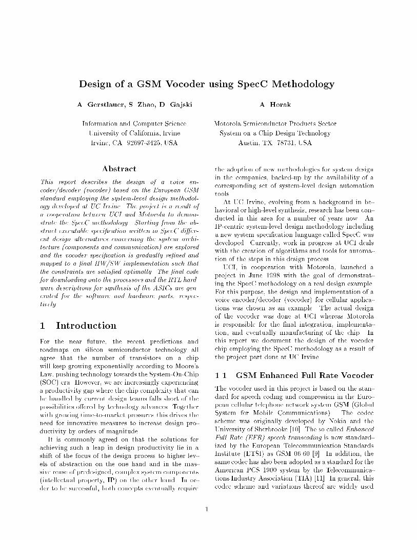
Figure 1: Speech synthesis model.
in voice compression and encoding for speech trans-mission (e.g. [12]).
1.1.1 Human Vocal Tract
Conceptually, the main idea of a speech synthesisvocoder is based on modeling the human vocal tractusing digital signal processing (DSP) techniques in or-der to synthesize or recreate speech at the receivingside.
Human speech is produced when air from the lungsis forced through an opening between the two vocalfolds called the glottis. Tension in the vocal chordscaused by muscle contractions and forces created bythe turbulence of the moving air force the glottis toopen and close at a periodic rate. Depending on thephysical construction of the vocal tract, these oscilla-tions occur between 50 to 500 times per second. Theoscillatory sound waves are then modi�ed when theytravel through the throat, over the tongue, throughthe mouth and over the teeth and lips.
1.1.2 Speech Synthesis Model
The model assumes that the speech signal is producedby a buzzer at the end of a tube. The glottis producesthe buzz which is characterized by intensity (loudness)and frequency (pitch). The vocal tract (throat andmouth) is modeled by a system of connected losslesstubes.
Figure 1 shows the GSM vocoder speech synthesismodel. A sequence of pulses is combined with the out-put of a long-term pitch �lter. Together, they modelthe buzz produced by the glottis and they build theexcitation for the �nal speech synthesis �lter whichin turn models the throat and mouth as a system oflossless tubes.
The initial sequence of so called residual pulsesis constructed by assembling prede�ned pulse wave-forms taken out of a given, �xed codebook. The code-book contains a selection of so called �xed code vectorswhich are basically �xed pulse sequences with varying
frequency. In addition, the pulse intensities are scaledby applying a variable gain factor.
The output of the long-term pitch �lter is simplya previous excitation sequence, modi�ed by scaling itwith a variable gain factor. The amount by which ex-citations are delayed in the pitch �lter is a parameterof the speech synthesis model and can vary over time.The long-term pitch �lter is also referred to as adap-tive codebook since the history of all past excitationsbasically forms a codebook with varying contents outof which one past excitation sequence, the so calledadaptive code vector, is chosen.
Finally, the excitation which is constructed byadding �xed and adaptive codebook vectors is passedthrough the short-term speech synthesis �lter whichsimulates a system of connected lossless tubes. Tech-nically, the short-term �lter is a tenth order linear pre-diction �lter meaning that its output is a linear com-bination (linear weighted sum) of ten previous inputs.The ten linear prediction coe�cients are intended tomodel the re ections and resonances of the human vo-cal tract.
1.1.3 Speech Encoding and Decoding
Instead of transmitting compressed speech samples di-rectly, the input speech samples are analyzed in or-der to extract the parameters of the speech synthesismodel which are then transmitted to the receiving sidewhere they are in turn used to synthesize the recon-structed speech.
On the encoding side, the input speech is analyzedto estimate the coe�cients of the linear prediction �l-ter, removing their e�ects and estimating the inten-sity and frequency. The process of removing the lin-ear prediction e�ects is performed by inverse �lteringof the incoming speech. The remaining signal calledthe residual is then used to estimate the pitch �lterparameters. Finally, the pitch �lter contribution is re-moved in order to �nd the closest matching residualpulse sequence in the �xed codebook.
At the receiver, the transmitted parameters are de-coded, combining the selected �xed and adaptive codevectors to build the short-term excitation. The linearprediction coe�cients are decoded and the speech issynthesized by passing the excitation through the pa-rameterized short-term �lter.
All together, this speech synthesis method has theadvantages of achieving a high compression ratio sinceit tries to transmit only the actual information inher-ent in the speech signal. All the redundant relation-ships which are due to the way the human vocal tractis organized are captured by the �lters of the speech
2

Compilation Interfacesynthesis
Backend
Simulation model
Simulation model
Manufacturing
Communication model
Simulation model
Simulation model
Implementation model
Validation ofalgorithm andfunctionality
Validation offunctionality andsynchronization
Validation offunctionality and
performance
Validation of
performancetiming and
High level synthesis
Protocol selection
Protocol inlining
Communication synthesis
Behavior partitioning
Synthesis flow Analysis and validation flow
IP
IP
Estimation
Estimation
Estimation
Estimation
Architecture exploration
Architecture model
Channel partitioning
Variable partitioning
Specificationmodel
Transducer synthesis
Figure 2: SpecC methodology.
synthesis model. The vocal tract model provides anaccurate simulation of the real world and is quite e�ec-tive in synthesizing high quality speech. In addition,encoding and decoding are relatively e�cient to com-pute.
1.2 System-Level Design
1.2.1 SpecC Methodology
The system-level design methodology which has beendeveloped at UC Irvine is shown in Figure 2 [3, 5]. Thesystem methodology starts with an executable speci�-cation. This speci�cation describes the functionalityas well as the performance, power, cost and other con-straints of the intended design. It does not make anypresumptions regarding the implementation details.
As shown in Figure 2, the synthesis ow of the code-sign process consists of a series of well-de�ned designsteps which will eventually map the executable speci�-cation to the target architecture. In this methodology,we distinguish two major system level tasks, namelyarchitecture exploration and communication synthe-sis.
Architecture exploration includes the design steps ofallocation and partitioning of behaviors, channels and
variables. Allocation determines the number and thetypes of the system components, such as processors,ASICs and busses, which will be used to implementthe system behavior. Allocation includes the reuse ofintellectual property (IP), when IP components areselected from the component library.
Behavior partitioning distributes the behaviors (orprocesses) that comprise the system functionalityamongst the allocated processing elements, whereasvariable partitioning assigns variables to memories andchannel partitioning assigns communication channelsto busses. Scheduling is used to determine the order ofexecution of the behaviors assigned to the processors.
Architecture exploration is an iterative processwhose �nal result is the de�nition of the system archi-tecture. In each iteration, estimators are used to eval-uate the satisfaction of the design constraints. As longas any constraints are not met, component and con-nectivity reallocation is performed and a new archi-tecture with di�erent components, connectivity, par-titions, schedules or protocols is evaluated.
After the architecture model is de�ned, commu-nication synthesis is performed in order to obtain adesign model with re�ned communication. The taskof communication synthesis includes the selection ofcommunication protocols, synthesis of interfaces andtransducers, and inlining of protocols into synthesiz-able components. Thus, communication synthesis re-�nes the abstract communications between behaviorsinto an implementation.
It should be noted that the design decisions in eachof the tasks can be made manually by the designer,e. g. by using an interactive graphical user interface,as well as by automatic synthesis tools.
The result of the synthesis ow is handed-o� to thebackend tools, shown in the lower part of Figure 2.Code for the software and hardware parts is gener-ated automtatically. The software part of the hand-o� model consists of C code and the hardware partconsists of behavioral VHDL or C code. The backendtools include compilers and a high-level synthesis tool.The compilers are used to compile the software C codefor the processor onto which the code is mapped. Thehigh-level synthesis tool is used to synthesize the func-tionality mapped to custom hardware and the inter-faces needed to connect di�erent processors, memoriesand IPs.
During each design step, the model is staticallyanalyzed to estimate certain quality metrics such asperformance, cost and power consumption. This de-sign model is also used in simulation to verify thecorrectness of the design at the corresponding step.
3

For example, at the speci�cation stage, the simulationmodel is used to verify the functional correctness ofthe intended design. After architecture exploration,the simulation model will verify the synchronizationbetween behaviors on di�erent processing elements(PEs). After communication synthesis, the simulationmodel is used to verify the performance of the systemincluding computation and communication.
1.2.2 SpecC Language
The methodology described in the previous section issupported by a new system-level description and spec-i�cation language called SpecC [1, 2, 4] which was de-veloped at UC Irvine in realization that existing lan-guages lack many of the features needed for system-level design [3]. At all stages of the SpecC method-ology, the current state of the design is representedby a model described in the SpecC language. In thishomogeneous approach transformations are made onthe SpecC description in contrast to a heterogeneousapproach where each step also transforms the designinto a new language, ending up with a mix of designrepresentations at di�erent stages of the process.
SpecC is being built as a superset of ANSI-C [6]which allows easy reuse of the existing algorithmic andbehavioral C descriptions that are common in todaysindustrial practice. SpecC contains all of the featuresrequired to support system-level design including IPintegration in general and the SpecC methodology inparticular:
� Structural and behavioral hierarchy.
� Concurrency.
� Communication with explicit separation of com-putation (behavior) from communication (chan-nel).
� Synchronization.
� Exception handling (traps and interrupts).
� Timing.
� Explicit state transitions (FSM modeling).
All these features are explicitly speci�ed in a clear andorthogonal manner which makes it easy to understandand analyze given SpecC descriptions both for humansand for automation tools. This is an essential require-ment to enable successful design automation and syn-thesis of high-quality results.
SpecC descriptions are translated into a C++model by the SpecC compiler. These C++ descrip-tions are then in turn compiled into a native exe-cutable for simulation and veri�cation. This resultsin very high simulation speeds due to the fact thatthe design is compiled instead of interpreted.
1.3 Overview
The rest of the report is organized as follows: Sec-tion 2 describes the speci�cation of the vocoder stan-dard in SpecC, including a more detailed descriptionof the functionality and other requirements. In Sec-tion 3 the di�erent steps performed during architec-tural exploration are shown. Starting with a gen-eral overview the �nal vocoder architecture is devel-oped. The process of mapping the abstract commu-nication onto real protocols, busses, etc. is describedin Section 4. Communication synthesis also shows therequirements for successful integration of intellectualproperty (IP). Again, a general discussion is followedby the vocoder speci�cs. Finally, Section 5 concen-trates on the synthesis of the system's software andhardware parts in the backend. Section 6 concludesthe report with a summary.
2 Speci�cation
2.1 General
The �rst step in any design process is the speci�ca-tion of the system requirements. This includes bothfunctionality as well as other requirements like timing,power consumption or area.
2.1.1 Formal, Executable Speci�cation
As outlined in the introduction, in the SpecC systemthe speci�cation is formally captured and written inthe SpecC language. As opposed to the informal spec-i�cations (e.g. in plain English) that have been com-monly used in the past, a formal speci�cation of thesystem has two main advantages:
1. It is executable for simulation and veri�cation ofthe desired functionality or for feasibility studiesat an early stage.
2. The formal, executable speci�cation directlyserves as an input to the following synthe-sis and exploration stages that eventually leadto the �nal implementation without the needfor time-consumingmodi�cations or translationsinto other languages and models.
4

2.1.2 Modeling Guidelines
The initial SpecC speci�cation should model the sys-tem at a very abstract level without already introduc-ing unnecessary implementation details. In addition,a good synthesis result using automated tools also re-quires the user to follow certain modeling guidelineswhen developing the initial speci�cation. Basically,the speci�cation should capture the required systemfunctionality in a natural way and in a clear and con-cise manner. Speci�cally, some of the main guidelinesfor developing the initial system speci�cation are:
� Separating communication and computation.Algorithmic functionality has to be detachedfrom communication functionality. In addition,inputs and outputs of a computation have to beexplicitly speci�ed to show data dependencies.
� Exposing parallelism inherent in the systemfunctionality instead of arti�cially serializing be-haviors in expectancy of a serial implementation.In essence, all parallelism should be made avail-able to the exploration tools in order to increaseroom for optimizations.
� Using hierarchy to group related functionalityand abstract away localized e�ects at higher lev-els. For example, local communication and localdata dependencies are grouped and hidden bythe hierarchical structure.
� Choosing the granularity of the basic partsfor exploration such that optimization possibil-ities and design complexity are balanced whensearching the design space. Basically, the leafbehaviors which build the smallest indivisibleunits for exploration should re ect the divisioninto basic algorithmic blocks.
� Using state transitions to explicitly model thesteps of the computation in terms of basic algo-rithms or abstracted, hierarchical blocks.
The SpecC language provides all the necessary sup-port to e�ciently describe the desired system featuresfollowing these guidelines. Each of the modeling con-cepts like parallelism or hierarchy is re ected in theSpecC description in an explicit and clear way.
2.2 Vocoder Speci�cation
The GSM 06.60 standard for the EFR vocoder con-tains a detailed description of the required vocoderfunctionality [9]. The standard description was trans-lated into a formal, executable SpecC speci�cation
������������
������������
coder
������������
������������
������������
������������
������������
������������
decoder
vocoderspeech bits
speechbits
Figure 3: Vocoder.
building the basis for the following synthesis and de-sign steps. In addition, the speci�cation was simulatedto verify the vocoder functionality.
The SpecC speci�cation was developed followingthe guidelines mentioned in the previous section. Inour case, part of the vocoder standard is a completeimplementation of the vocoder functionality in C (seeAppendix A). The C code is based on a 16-bit �xed-point implementation of the algorithms and it servesas a bit-exact reference for all implementations of thevocoder standard, i.e. the C code speci�es the vocoderfunctionality down to the bit level.
Therefore, for the vocoder, the C reference im-plementation builds the basis for the speci�cation inSpecC. However, a great amount of time had to bespent on analyzing and understanding the standardincluding the 13,000 lines of C code in order to extractthe high-level structure and the global interdependen-cies. Once this was done, a mapping into a SpecC rep-resentation was straightforward. Using the guidelinesof Section 2.1.2, the high-level picture of the vocoder'sabstracted functionality could be directly and natu-rally re ected in its SpecC speci�cation.
As will be seen in the following sections this greatlyeases understanding of the vocoder basics and there-fore supports quick exploration of di�erent design al-ternatives at the system level in the �rst place. Ateach level, the SpecC description hides unnecessarydetails but explicitly depicts the major aspects, focus-ing the view of the user and the tools onto the im-portant decisions at each step. For example, at thelowest level, detailed algorithmic code is hidden in theleaf behaviors whereas the relations between the be-haviors are made explicit through state transitions.
In terms of the actual algorithmic behavior, SpecCbeing build on top of ANSI-C made it possible to di-rectly plug the C code of each basic function in the Cdescription into the corresponding leaf behavior of theSpecC speci�cation.
5

Filter memory
update
Closed-loop
pitch search
pitch search
Open loop
Algebraic (fixed)
codebook search
Linear prediction
(LP) analysis
��������
��������
��������
��������
��������
��������
��������
��������
��
��
��
��
��
����
����
����
����
����
����
�� ��
����
��������
��������
����
����
prm[57]
speech[160]
bits
pre_process
code_12k2
prm2bits_12k2
mem
ory
2x per fram
e
A(z)
2 sub
frames
code_12k2
prm
speech[160]
sample coder
Figure 4: Coder.
2.2.1 Overview
Figure 3 shows the top level of the vocoder speci�ca-tion in SpecC consisting of independent coding anddecoding subbehaviors running in parallel. The coderreceives an input stream of 13 bit wide speech samplesat a sampling rate of 8 kHz, corresponding to an inputbit rate of 104 kbit/s. It produces an output bit streamof encoded parameters with a bit rate of 12:2 kbit/s.Decoding, on the other hand, is the reverse process ofsynthesizing a reconstructed stream of speech samplesfrom an input parameter bit stream. The followingsections will describe the encoding and decoding pro-cesses in more detail in so far as they are relevantfor the following discussions about the vocoder designprocess. See Appendix B for an in-depth descriptionof the vocoder functionality in SpecC.
2.2.2 Coder Functionality
Coding is based on a segmentation of the incomingspeech into frames of 160 samples corresponding to20ms of speech. Speech parameters are extracted ona frame-by-frame basis. For each speech frame thecoder produces a frame of 244 encoded bits resultingin the aforementioned output bit rate of 12:2 kbit/s.
Figure 4 shows the �rst two levels of the coder hi-erarchy. At the top level, the coder consists of threemain parts which execute in a pipelined fashion:
1. Pre-processing: Bu�ering of the incomingspeech stream into frames of 160 samples. Initialhigh-pass �ltering and downscaling of the speechsignal.
2. Encoding: The main encoding routine whichextracts a set of 57 speech synthesis parametersper speech frame. Encoding will be described inmore detail in the following paragraphs.
3. Serialization: Conversion and encoding of theparameter set into a block of 244 bits per frame.Transmission of the encoded bit stream.
Due to the pipelined nature, all three parts operatein parallel but each on a di�erent frame, i.e. while aframe is encoded the next frame is pre-processed andbu�ered, and the previous frame is serialized.
In general, encoding uses an analysis-by-synthesisapproach where the parameters are selected in such away as to minimize the error between the input speechand the speech that will be synthesized on the decod-ing side. Therefore, the encoder has to simulate thespeech synthesis process.
In order to increase reaction time of certain �lters,the main encoding routine (also shown in Figure 4)further subdivides each frame into subframes of 40samples (or 5ms) each. Depending on their criticality,parameters are computed either once per frame, onceevery two subframes or once per subframe.
Encoding Encoding itself basically follows the re-verse process of speech synthesis. Given the speechsamples, in a �rst step the parameters of the LP �lterare extracted. The contribution of the LP �lter is thensubtracted from the input speech to get the remain-ing LP �lter excitation. The LP �lter parameters areencoded in so called Line Spectral Pairs (LSPs) whichreduce the amount of redundant information. Twosets of LP parameters are extracted per frame, takinginto account the current speech frame plus one half ofthe previous frame. LP analysis produces a block of 5parameters containing the two LSP sets.
Next, using the past history of excitations, all thepossible delay values of the pitch �lter are searchedfor a closest match with the required excitation. Thesearch is divided into an open-loop and a closed-loopsearch. A simple open-loop calculation of delay esti-mates is done twice per frame. In each subframe aclosed-loop, analysis-by-synthesis search is then per-formed around the previously obtained estimates toobtain the exact �lter delay and gain values.
The long-term �lter contribution is subtraced fromthe excitation. The remaining residual is the inputto the following �xed codebook search. For each sub-frame an extensive search of the codebook for the clos-est code vector is performed. All possible code vectors
6

Searchcodebook
Prefilterresponse
Updatetarget
Prefiltercode vector
Calculatecodebook gain
Codebook
pitch delayFind
Computecode vector
pitch gainCalculate
Impulseresponse
Targetsignal
Closed_loop
Synthesizespeech
Update filtermemories
Quantizecodebook gain
Update
Find open looppitch delay
Open_loop
speechWeighted
2 su
bfr
ames
Interpolation &LSP -> A(z)
QuantizationLSP
Interpolation &LSP -> Aq(z)
Windowing &Autocorrelation
Windowing &Autocorrelation
Levinson-Durbin
Levinson-Durbin
LP_analysis
A(z) -> LSP
2x per frame
2 subframes
code_12k2
Figure 5: Encoding.
are searched such that the mean square error betweencode vector and residual is minimized.
For each subframe the coder produces a block of 13parameters for transmission. Finally, using the calcu-lated parameters the reconstructed speech is synthe-sized in order to update the memories of the speechsynthesis �lters, reproducing the conditions that willbe in e�ect at the decoding side.
Figure 5 exposes the next level of hierarchy in theencoding part, showing more details of the encodingprocess. Note that for simplicity only the behavioralhierarchy and no structural information is shown, i.e.the diagram doesn't include the information aboutconnectivity between behaviors. A complete block di-agram of the coder which provides an idea about thecomplexity by exposing all levels of hierarchy downto the leaf behaviors can be found in Appendix B onpage 66 (Figure 64).
As can be seen, at this level, the coder speci�cationexhibits some limited explicit parallelism. However, ingeneral, due to the inherent data dependencies boththe coder and decoder parts of the system are mostlysequential in their natures.
��
��
��
��
����
��
����
��
��
��
��������
��������
decode_12k2
Post_Filter
Bits2prm_12k2
Decode
LP parameters
4 sub
frames
bits
speech[160]
A(z)
synth[40]
synth[40]
prm[57]
prm[13]
decoder
Figure 6: Decoder.
2.2.3 Decoder Functionality
Decoding (Figure 6) basically follows the speech syn-thesis model in a straightforward way and is more orless the reverse process of encoding. The decoder re-ceives an encoded bit stream at a rate of 12; 2 kbits/sand reproduces a stream of synthesized speech samplesat a sampling rate of 8 kHz. For each incoming frameof 244 encoded bits a frame of 160 speech samples isgenerated.
Incoming bit frames are received and the corre-
7

sponding set of 5 + 4 � 13 = 57 speech parametersis reconstructed. The �rst 5 parameters containingthe Line Spectral Pairs are decoded to generate thetwo sets of LP �lter parameters. Then, once for eachsubframe the following blocks of 13 parameters eachare consumed, decoded and the speech subframe of 40samples is synthesized by adding the long-term pitch�lter output to the decoded �xed code vector and �l-tering the resulting excitation through the short-termLP �lter. Finally, the synthesized speech is passedthrough a post �lter in order to increase speech qual-ity.
A more detailed block diagram of the decoder show-ing all levels of hierarchy down to the leaf behaviorscan be found in Appendix B, Figure 69 on page 71.Compared to the encoding process, decoding is muchsimpler and computationally much cheaper.
2.2.4 Constraints
Transcoder Delay The GSM vocoder standardspeci�es a constraint for the total transcoder delaywhen operating coder and decoder in back-to-backmode. According to the standard, back-to-back modeis de�ned as passing the parameters produced by theencoder directly into the decoder as soon as they areproduced. Note that this de�nition doesn't includeencoding and decoding, parallel/serial conversions, ortransmission times of the encoded bit stream. Back-to-back mode is not considered as the connection ofthe coder output with the decoder input. Instead, the57 parameters produced by the encoder are assumed tobe passed directly into the decoder inside the vocodersystem.
The transcoder delay is then de�ned as the delaystarting from the time when a complete speech frameof 160 samples is received up to the point when the lastspeech sample of the reconstructed, synthesized frameleaves the decoder. The GSM EFR vocoder standardspeci�es a maximum timing constraint of 30ms forthis transcoder delay.
Analysis and Budgeting In addition to the explic-itly given transcoder delay constraint the requirementson the input and output data rates pose additionalconstraints on the vocoder timing. All requirementsof the standard were analyzed to derive timing bud-gets for di�erent parts of the vocoder, resulting in theactual constraints of the SpecC description.
Figure 7 depicts an analysis of the transcoder de-lay constraint. Note that the time di�erence betweenthe �rst and the last sample of synthesized speech
Pre_process
LP_analysis
Open_loop
Subframe
SubframeCode
Code
Open_loop
Subframe
SubframeCode
SubframeDecode
Code
Decode
SubframeDecode
D_lsp
Subframe
Subframe
Decode
Coder
prm
prm
prm
prm
prm
Start
speech
speech
speech
speech
Start
5 m
s5
ms
5 m
s5
ms
Ou
tpu
t sp
eech
fra
me
(20
ms)
Inp
ut
fram
e ra
te (
20 m
s)
Tra
nsc
od
er d
elay
<=
30 m
s
Decoder
Pre_process
LP_analysis
Open_loop
CodeSubframe
D_lsp
DecodeSubframe
Coder
Decoder
Del
ay <
= 10
ms
Figure 7: Timing constraints.
at the decoder output is 20ms (with the given sam-pling rate). Therefore, if encoding and decoding wouldhappen instantaneously in zero time the theoreticallyachievable minimum for the transcoder delay is 20ms,too. In other words, the �rst sample of reconstructedspeech has to leave the decoder not more than 10msafter the input speech frame is received.
Hence, encoding and decoding of the �rst subframeof 40 speech samples has to happen in less than 10ms.This includes all the information needed for the �rstsubframe, i.e. encoding and decoding of the 5 LP�lter parameters plus the set of 13 parameters forthe �rst subframe. Then, while the speech samplesare written to the decoder output at their sampling
8

rate, the following three subframes have to be encodedinto blocks of 13 parameters and decoded into recon-structed speech subframes such that the following sub-frames are available at intervals of at most 5ms.
However, while encoding and decoding of the cur-rent frame take place the next frame is already re-ceived and bu�ered, and processing of the next framewill have to start once its last sample is received.Therefore, an additional, implicit constraint is thatencoding and decoding of a complete frame of 160samples have to be done in less than the intra-frameperiod of 20ms. Hence, decoding of the last subframewill have to be done before that time or|in relationto the transcoder delay constraint|up to 10ms beforethe last sample of the synthesized speech frame at thedecoder output. Note that this requires a bu�ering ofthe decoded speech subframes at the decoder output.
To summarize the constraints for the vocoder, thereare two basic timing constraints derived from the giventime budgets:
� The encoding and decoding delay for the �rstsubframe (5 + 3 parameters) has to be less than10ms.
� The time to encode and decode a complete frame(all 57 parameters) has to be less than 20ms.
3 Architectural Exploration
The goal of architectural exploration is initially toquickly explore a large number of target architectures,comparing them to each other after an initial mappingof the design onto the architecture has been done and�nally pruning the design space down to a few can-didate architectures. These system architectures arethen evaluated further, trying to improve the map-ping of the design onto the architecture and possiblymodifying certain aspects of the system until a �nalarchitecture is selected.
Exploration is a part where the design processcan bene�t to a great deal from human experience.Therefore, interactivity is an important requirementof system-level design environments. However, withthe help of automated tools that quickly search largeparts of the design space, provide feedback about de-sign quality, perform tedious, time-consuming jobs au-tomatically, etc. the designer will be able to explorea large number of promising design alternatives in ashorter amount of time. In general, exploration is aniterative process where the di�erent steps describedin the next sections are repeated for di�erent archi-
Figure 8: General speci�cation model.
tectures. Design automation tools signi�cantly reducethe time needed for each iteration.
Since the corresponding tools are not yet availableat this time exploration for the vocoder project hadto be done mostly manually. However, manual explo-ration strictly followed the ow and the step-by-stepprocedures proposed for the implementation of the au-tomated tools. Nevertheless, due to the lack of toolswe had to restrict ourselves to a very small number ofcandidate architectures.
3.1 Models
3.1.1 Speci�cation Model
The initial speci�cation written by the designer isthe basis for architectural exploration. The speci�-cation model at the input to architectural explorationis shown in Figure 8. The speci�cation model is a su-perstate �nite state machine (SFSM) with hierarchyand concurrency.
At each level of hierarchy, the superstates (SpecCbehaviors) are decomposed further into either paral-lel or sequential substates. Superstates at the bottomof the hierarchy are called leaf states (or leaf behav-iors). They �nally contain actual program fragmentsdescribing the algorithmic behavior of the leaf states.
In a sequential composition of states at any level ofhierarchy the states are traversed in a stepwise fashion.After attening of the hierarchy, the model resemblesa standard state machine with the additional featureof parallelism. In contrast to a classical low-level FSMor FSMD, however, superstates can take an arbitrary
9
ASIC1
ASIC2
Bus
MPEG IP
DSP Bus
ASIC3
DSP core
CPU core
Figure 9: General model for architectural exploration.
amount of time to execute the statements or substatescontained within. Much like a data ow model, a statedoesn't start to execute until all of its predecessors are�nished. In addition, control ow is introduced by thepossibility to augment transitions with conditions.
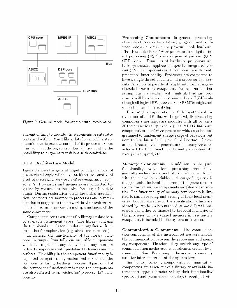
3.1.2 Architecture Model
Figure 9 shows the general target or output model ofarchitectural exploration. An architecture consists ofa set of processing, memory and communication com-ponents. Processors and memories are connected to-gether by communication links, forming a bipartitegraph. During exploration, given the initial speci�ca-tion, behaviors are mapped to processors and commu-nication is mapped to the network in the architecture.The architecture can contain multiple instances of thesame component.
Components are taken out of a library or databaseof available component types. The library containsthe functional models for simulation together with in-formation for exploration (e.g. about speed or cost).
In general, the functionality of the library com-ponents ranges from fully customizable componentswhich can implement any behavior and any interfaceto �xed components with prede�ned behaviors and in-terfaces. Flexibility in the component functionality isexploited by synthesizing customized versions of thecomponents during the design process. If part or all ofthe component functionality is �xed the componentsare also referred to as intellectual property (IP) com-ponents.
Processing Components In general, processingelements (PEs) can be arbitrary programmable soft-ware processor cores or non-programmable hardwarePEs. Examples for software processors are digital sig-nal processing (DSP) cores or general purpose (GP)CPU cores. Examples of hardware processors arefully synthesized application speci�c integrated cir-cuit (ASIC) components or IP components with �xed,prede�ned functionality. Processors are considered tohave a single thread of control. If a processor can exe-cute behaviors in parallel it is split into logical single-threaded processing components for exploration. Forexample, an architecture with multiple hardware pro-cessors will have several custom-hardware FSMDs al-though all logical HW processors or FSMDs might endup on the same physical chip.
Processing components are fully synthesized ortaken out of an IP library. In general, IP processingcomponents are hardware modules with all or partsof their functionality �xed, e.g. an MPEG hardwarecomponent or a software processor which can be pro-grammed to implement a large range of behaviors butnevertheless has a �xed, prede�ned interface, for ex-ample. Processing components in the library are char-acterized by their functionality and parameters likecost, power, speed, etc.
Memory Components In addition to the purefunctionality, system-level processing componentsgenerally include some sort of local memory. Alongwith the behaviors, variables and storage in general ismapped onto the local memories of the processors. Aspecial case of system components are (shared) memo-ries. The functionality of memory components is lim-ited to simple reading and writing of their local mem-ories. Global variables in the speci�cation which areshared by two behaviors mapped to two di�erent pro-cessors can either be mapped to the local memories ofthe processor or to a shared memory in case such acomponent is included in the system architecture.
Communication Components The communica-tion components of the interconnect network handlethe communication between the processing and mem-ory components. Therefore, they include any type ofcommunication media used to implement system-levelcommunication. For example, busses are commonlyused for interconnection at the system level.
Similar to processing components, communicationcomponents are taken out of a library of available in-terconnect types characterized by their functionality(protocol) and parameters like delay, throughput, etc.
10

Specification
Partitioning
Allocation
SimulationProfiling
Estimation
IP
Scheduling
Architecture
Estimation
Components
Implementation
Figure 10: Architectural exploration ow.
Protocols in the library are usually at least partly pre-de�ned, implementing industry standards like PCI orVME. On the other hand, protocols are customized orfull-custom protocols are synthesized during the de-sign process.
3.2 Exploration Flow
The general ow of steps performed during architec-tural exploration is shown in Figure 10. With thedesign speci�cation at the input, exploration createsan architecture for implementation of this design.
Initially, during simulation the speci�cation is pro-�led to extract estimates about the design com-plexity and the dynamic behavior. Using theseimplementation-independent estimates a set of com-ponents is selected out of a library during allocation.Allocation is based on matching components with thecomputational requirements and the available paral-lelism of the speci�cation.
Once a set of components has been selected, designmetrics like cost, delay, etc. of implementing the partsof the speci�cation on these components are estimatedtaking into account information obtained during ini-tial pro�ling. In the next step, partitioning is per-formed to map the design onto the components based
on these component-related estimates. During parti-tioning design trade-o�s related to implementation ofbehaviors on di�erent components and parallel versussequential execution of behaviors are explored.
After the design has been mapped onto the al-located components the design space is reduced toa single implementation of the design parts on thecomponents they are bound to. A more accurate re-estimation of this implementation is then performed.Finally, the design is scheduled with this informationto derive the actual system timing. Constraints areveri�ed and depending on the severity of the viola-tions a new iteration of the exploration loop is startedwith reallocation or repartitioning until an optimal ar-chitecture has been found.
3.3 Analysis and Estimation
3.3.1 General Discussion
The basis for any exploration of the design space|including system-level architectures|is the availabil-ity of good and useful design quality metrics. Onthe one hand, metrics are closely related to the de-sign constraints like performance, power or cost (area,code size, etc.). On the other hand, other metrics canprovide additional useful information. Basically, thesemetrics are the only means of deciding how good a cho-sen architecture is in comparison with other possiblearchitectures. Therefore, analysis of the speci�cationand estimation of the design metrics for di�erent im-plementations is an integral part of the design process.
Behavior Estimation During architectural explo-ration behaviors are mapped to the processing com-ponents of the architecture. For each type of targetprocessor the behaviors will exhibit di�erent metrics,i.e. di�erent cost, di�erent performance, etc. There-fore, by combining the properties of the speci�cationwith the abstracted properties of the target compo-nents estimates about the behavior metrics are ob-tained without actually implementing the behavior onthe component.
However, di�erent implementations of a behavioron the same processor resulting in di�erent metricshave to be considered during architectural exploration,too. For example, the behavior can be optimized forcost resulting in the least-cost solution. At the otherend of the spectrum, a behavior can be optimized forperformance to achieve the fastest execution possible.Based on the estimated values, the exploration toolswill assign budgets for cost or performance, for exam-ple, to behaviors or groups of behaviors. This infor-
11

mation is then passed to the backend where it is usedto guide the synthesis process.
Communication Estimation In general, the over-head of communicating data values between the be-haviors of the speci�cation can not be neglected whenevaluating possible target architectures. For behaviorsmapped to the same component, communication be-tween those behaviors is handled according the compo-nent's communicationmodel and is therefore includedin the behavior estimation. For example, on softwareprocessor the call overhead of pushing/popping valuesto/from the stack is part of the software implementa-tion of the caller and callee on the processor.
On the other hand, communication among behav-iors mapped to di�erent processing components re-quires transferring data over the channels in the sys-tem architecture. Estimates for the overhead of thiscommunication are taken into account during explo-ration. The main communication overhead is due tothe delay of transmitting values from one componentto the other.
Basic estimates about the time needed for commu-nication are obtained by evaluating the size of the datablock to be transmitted divided by the channel datarate. More elaborate estimates are obtained by con-sidering the protocol overhead of the channel includ-ing possibly the segmentation of the data block intosmaller packets for transmission.
3.3.2 Initial Simulation and Pro�ling
In the �rst step an analysis of the initial speci�cationindependent of any implementation is performed bypro�ling the speci�cation during initial simulations.Simulation of the initial speci�cation is necessary inany case to verify functional correctness. Therefore,these simulations can be augmented to obtain valuableinformation which will be used for implementation-dependent estimations and exploration in general.
Estimates about the relative computational com-plexity and the computational requirements of di�er-ent parts of the speci�cation are obtained by count-ing basic arithmetic operations (additions, multiplica-tions, etc.), logic operations (and, or, shift, etc.), andmemory access operations (moves) during simulation.For each behavior an operation histogram (Figure 11)is created in which the complexity of an execution ofthe behavior is broken down into the number of oc-currences of each basic operation.
Operation pro�les are summed according to thespeci�cation hierarchy such that total pro�les for each
����������������������������������������
����������������������������������������
����������������������������
����������������������������
��������
��������
������������������
������������������
����������������������������������
����������������������������������
������
������
������������������
������������������
Occ
ure
nce
co
un
t
MOVE R
egADD
MAC
ANDSHL
MUL
MOVE M
em Operations
Figure 11: Sample operation pro�le.
constrained execution path are obtained. The compu-tational requirements for each path can then be cal-culated by summing the operation counts counti anddividing the sum by the path's timing constraint Tpath:
MOPS =
PcountiTpath
;
giving the complexity in million operations per second(MOPS). Note that these initial estimates are archi-tecture independent and therefore don't have to berecalculated during exploration.
In addition, with dynamic pro�ling informationabout the dynamic dependencies both among the be-haviors and inside the behaviors can be derived. Forexample, for data dependent loop bounds informationabout the worst case execution is obtained by countingthe number of loop iterations. In general, a dynamicanalysis of the possible paths through the speci�ca-tion and through the behaviors from inputs to outputsalong with the frequency at which each path is takenis performed and the results are stored for future esti-mations.
3.3.3 Estimation
In contrast to the architecture independent initial sim-ulation and pro�ling the actual estimation during ar-chitectural exploration is concerned with deriving themetrics for an implementation of the speci�cation onan underlying architecture. Using the previously col-lected pro�ling data a retargetable estimator is usedto obtain metrics for a wide range of HW and SW im-plementations. Depending on the stage in the explo-ration ow the estimator can work at di�erent levelsof accuracy in return for estimation speed.
12

Coarse Estimation For the initial exploration, arelative comparison of a large number of architectureshas to be done in order to select the best candidates.Therefore, at this point absolute accuracy is not ofutmost importance. The estimates should rather beobtained very quickly and provide a good relative ac-curacy, the so called �delity. On the other hand, inorder to evaluate di�erent architectures estimation ofan implementation on the currently selected target ar-chitecture has to be performed.
With the help of retargetable pro�lers and estima-tors the behaviors are analyzed statically on the basicblock level. For each basic block the number of cy-cles required for execution of that block on each ofthe allocated processors are estimated. With the ad-ditional dynamic information about the relations ofbasic block executions and execution frequencies thatwere obtained during simulation and pro�ling of theinitial speci�cation �nal estimates about the executiontimes of the behaviors on the allocated components arecomputed.
Estimation is very fast this way since both unopti-mized synthesis and basic block pro�ling can be per-formed quickly. Extensive, time-consuming simulationof the complete speci�cation is not necessary. Due tothe unoptimized nature of the implementations, theabsolute accuracy of these results is low. However,under the assumption that optimization gains are in-dependent of the actual target these estimates exhibita high �delity.
In addition, in each iteration of the exploration loopestimates have to be derived for the newly allocatedcomponents only. For previously allocated compo-nents the information about behavior execution timesfrom quick or accurate estimates of previous iterationsare retained.
Fine Estimation Later, as the design progresses,the solutions have to be evaluated in relation to thedesign constraints thus requiring estimates with highabsolute accuracy. However, the closer the design getsto a �nal implementation the smaller is the numberof architectures under consideration. Major decisionshave already been made. For each behavior the com-ponent on which it will execute is known after par-titioning. Since estimation is �xed to one implemen-tation per behavior more time can be spent on itsanalysis. Therefore, estimation run times are tradedo� for absolute accuracy.
Basically, accurate estimation creates an actual, op-timized hardware or software implementation of thebehaviors. Using the backend process, software is
compiled and hardware is synthesized with all opti-mizations enabled in the same manner as for the �naldesign. Accurate estimated are obtained by combin-ing a static analysis of the �nal hardware and softwareexecution times with the dynamic information com-puted during initial simulation and pro�ling. Sincestatic analysis is done only once for each basic block|the dynamic nature of multiple executions is capturedthrough the initial analysis information|estimation isfaster than extensive simulation of the complete im-plementation.
Only when a �nal architecture has been selectedand pushed through the backend, an overall simulationof the �nal design will be done in order to verify both,the functionality of the �nal implementation and thesatisfaction of design constraints.
3.3.4 Vocoder Analysis and Estimation
For the vocoder example, the goal was basically tocome up with the least-cost solution that satis�es thegiven timing constraints. Therefore, the speci�cationwas analyzed to obtain estimates about the executiontimes and hence eventually the actual delays of thedi�erent vocoder parts.
Initial Analysis Initially, analysis of the vocoderspeci�cation was performed with the goal of obtainingestimates about the relative computational complexityof the behaviors in the speci�cation. Computationalcomplexity is directly related to execution times ondi�erent platforms. The higher the complexity thelonger it will take to compute the result on any plat-form.
In case of the vocoder example, the C referenceimplementation of the vocoder standard (see Ap-pendix A) already provided initial estimates throughdynamic pro�ling by counting basic arithmetic, logicand memory access operations. The operations arecounted on a frame-per-frame basis, weighted accord-ing to their estimated relative complexity and �-nally combined into the so called WMOPS estimate(weighted million operations per second) by divid-ing the sum through the time allowed for each frame(20ms).
Figure 12 and Figure 15 show the WMOPS es-timates for the coder and the decoder, respectively.The estimates are broken down into the major partsLP analysis, closed-loop search, open-loop search andcodebook search for the coder, and LSP decoding, sub-frame decoding and post �ltering for the decoder. Foreach part both the total per frame and the major con-tributing subbehaviors are shown. Each subbehavior
13

0.0
0.5
1.0
1.5
2.0
2.5
3.0
3.5
4.0
4.5
5.0
Total per frame Single execution
Residu
Levin
son
Az_lsp
Q_plsf
_5
Autoc
orr
Weig
ht_A
i
Syn_f
ilt
Residu
Pitch_
ol
Pred_
lt_6
Convo
lve
cor_
h_x
Syn_f
ilt
Pitch_
fr_6
Syn_f
ilt
cor_
h
sear
ch_1
0i40
Wei
gh
ted
MO
PS
(W
MO
PS
)
LP
_an
alys
is
Op
en_l
oo
p
Clo
sed
_lo
op
Co
deb
oo
k
Figure 12: Estimates for computational complexity ofcoder parts.
0
200000
400000
600000
800000
1000000
1200000
First subframe Remaining frame Single execution
Co
deb
oo
k
�������
�������
�������
�������
������
������
���
���
��������
Clo
sed
_lo
op
����
���� ���
���
����
����
����������
����������
�����
���
����������
����������
���
���
����������
��������
Autoc
orr
����������������������������������������������������������������
Q_plsf
_5��
Az_lsp
Weig
ht_A
i
Op
en_l
oo
p
Levin
son
��������
��������������������
��������������������
Cyc
les
Syn_f
ilt
sear
ch_1
0i40
cor_
h
cor_
h_x
Syn_f
ilt
Pitch_
fr_6
Residu
Pitch_
ol
Pred_
lt_6
Convo
lve
Residu
Syn_f
ilt���������������
���������������
LP
_an
alys
is
Figure 13: Breakdown of initial coder delays.
0 ms 10 ms 20 ms 30 ms 40 ms 50 ms
LP_analysis Open_loop Closed_loop Codebook��
���������������������������
���������������������������
Figure 14: Initial coder delay.
0.0
0.1
0.2
0.3
0.4
0.5
0.6
0.7
Total per frame Single execution
Int_
lpc
D_plsf
_5
d_ga
in_co
deag
c2
Syn_f
ilt
Pred_
lt_6
pree
mph
asis
Syn_f
ilt
Residuag
c
D_L
SP
Dec
od
e_12
k2
Po
st_f
ilter
Wei
gh
ted
MO
PS
(W
MO
PS
)
Figure 15: Estimates for computational complexity ofdecoder parts.
0
20000
40000
60000
80000
100000
120000
140000
160000
180000
First subframe Remaining frame Single execution
������������
��������
��������
��������������
��������������
������������
������������
��������������������������������������������������������������������������
��������
������������
������������
����������������
����������������
��������
������
������
������ ���� ������
Int_
lpc
d_ga
in_co
de
dec
od
e_12
k2
Po
st_f
ilter
D_l
sp
Syn_f
ilt
Cyc
les
D_plsf
_5ag
c2
Syn_f
ilt
Pred_
lt_6
pree
mph
asis
agc
Residu
Figure 16: Breakdown of initial decoder delays.
0 ms 1 ms 2 ms 3 ms 4 ms 5 ms 6 ms
D_lsp Decode_12k2 Post_filter����
����������
����������
Figure 17: Initial decoder delay.
14

of the di�erent vocoder parts can be executed sev-eral times per frame (e.g. in a loop or once for eachsubframe). Therefore, for the subbehaviors both thetotal complexity per frame and the complexity of asingle execution, i.e. the total complexity divided bythe number of executions are shown.
Accurate Estimation In order to obtain more ac-curate estimates about the real execution times on thetarget platform, a quick and straightforward compila-tion of the behaviors for the target processor underconsideration was done next.
Due to the unavailability of the retargetable estima-tors and pro�les, the target analysis of the vocoder wasdone by compiling the behavior code for the chosentarget processor (Motorola DSP56600 family, see Sec-tion 3.4) using the o�cial compiler Motorola providesfor their processors. The resulting machine code wasthen simulated on the Motorola Instruction Set Sim-ulator (ISS) to obtain cycle-accurate execution times.
Simulations were performed using typical inputdata. The results given here represent average execu-tion times per frame or per execution. An analysis ofthe code reveals that the execution times at this levelhave only minimal dynamic data dependencies in theorder of a few statements di�erence (at most 10% dif-ference between worst case and average case). Somesubbehaviors exhibit static execution time variationsthrough constant parameters passed into the routinesdepending on the calling environment but these vari-ations are averaged out at the higher levels of the hi-erarchy.
Figure 13 and Figure 16 show the execution timeresults (in number of cycles) for the coder and de-coder, again broken down into parts and their majorsubbehaviors. According to the timing budgets de-rived from the constraints in the initial speci�cation(see Section 2.2.4), the �gures show cycles for encod-ing or decoding of the �rst subframe plus the rest ofthe frame totaling in the cycles per complete frame.In addition, the cycles for a single execution of eachbehavior are included in order to show the complexityof each behavior in comparison with the initial esti-mates.
Finally, Figure 14 and Figure 17 show the sequencesof execution of the parts for one frame as time pro-gresses in the coder and decoder. The given times aregiven based on a processor clock frequency of 60MHz.As can be seen easily, for this initial implementationboth timing constraints are severely violated. For acomplete list of simulation results, see Appendix C,Section C.1.
As mentioned earlier, the results con�rm that thecoding part is the major contributor to the delays andthe computational complexity in general. Therefore,architectural exploration should focus on this part ofthe system.
Inside the coder, overall, the codebook search isthe most critical part since it contributes the most tothe violation of the two timing constraints. Also, thelargest indivisible leaf behavior in terms of executiontime is the actual search routine (search 10i40) in-side the codebook search.
Furthermore, comparing the actual execution timeswith the initial WMOPS estimates suggests that animplementation of the codebook search on the pro-cessor introduces a higher overhead of operations notdirectly related to the computation than the softwareimplementation of the other parts. Analysis of thespeci�cation shows that most of the time of the otherparts is spent inside very tight loops with loop bod-ies of a few statements only but a large loop countas they are typical in DSP-style applications. Theseloops promise very good opportunities for optimiza-tions even in software. An exception to this is thecodebook search since it is relatively irregular withlarge and hard to optimize code blocks.
3.4 Architecture Allocation
3.4.1 General Discussion
The �rst step in each iteration of the search throughthe architectural design space is the choice of an archi-tecture to be evaluated further. Architecture alloca-tion selects the types of components and the numberof components of each type in the system. Along withthe selection of processors, architecture allocation alsode�nes the general connectivity between the proces-sors by selecting the types and numbers of communi-cation components between processing components.
Typically, processing elements (PEs) are either pro-grammable processor cores running software or proces-sors implementing a �xed functionality in hardware.Under the aspect of design reuse the architecture caninclude prede�ned components taken out of an in-tellectual property (IP) library, either from in-housesources or provided by a third-party vendor. Usuallythe functionality of these IP components is �xed andlimited to a small range of possible behaviors. An ex-ception are the software processors. Although they aretaken out of the library of prede�ned IP componentsthey are fully programmable and able to implementbasically any behavior.
Possible system architectures range from pure soft-
15
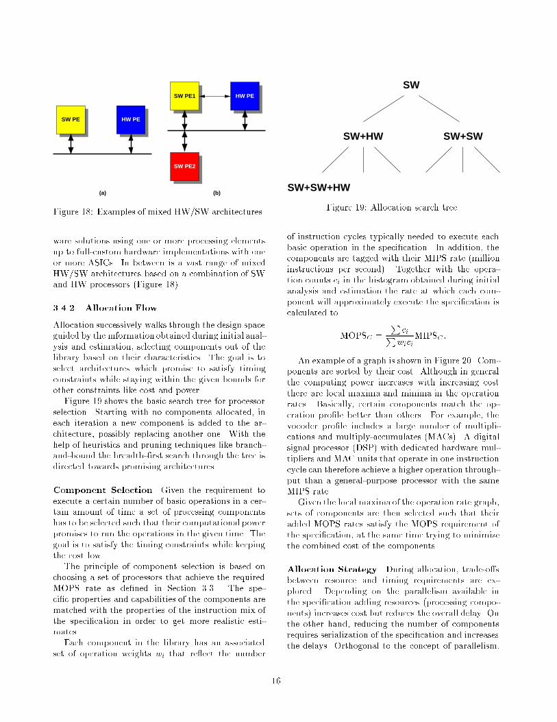
(b)(a)
SW PE HW PE
HW PESW PE1
SW PE2
Figure 18: Examples of mixed HW/SW architectures.
ware solutions using one or more processing elementsup to full-custom hardware implementations with oneor more ASICs. In between is a vast range of mixedHW/SW architectures based on a combination of SWand HW processors (Figure 18).
3.4.2 Allocation Flow
Allocation successively walks through the design spaceguided by the information obtained during initial anal-ysis and estimation, selecting components out of thelibrary based on their characteristics. The goal is toselect architectures which promise to satisfy timingconstraints while staying within the given bounds forother constraints like cost and power.
Figure 19 shows the basic search tree for processorselection. Starting with no components allocated, ineach iteration a new component is added to the ar-chitecture, possibly replacing another one. With thehelp of heuristics and pruning techniques like branch-and-bound the breadth-�rst search through the tree isdirected towards promising architectures.
Component Selection Given the requirement toexecute a certain number of basic operations in a cer-tain amount of time a set of processing componentshas to be selected such that their computational powerpromises to run the operations in the given time. Thegoal is to satisfy the timing constraints while keepingthe cost low.
The principle of component selection is based onchoosing a set of processors that achieve the requiredMOPS rate as de�ned in Section 3.3. The spe-ci�c properties and capabilities of the components arematched with the properties of the instruction mix ofthe speci�cation in order to get more realistic esti-mates.
Each component in the library has an associatedset of operation weights wi that re ect the number
SW
SW+HW SW+SW
SW+SW+HW
Figure 19: Allocation search tree.
of instruction cycles typically needed to execute eachbasic operation in the speci�cation. In addition, thecomponents are tagged with their MIPS rate (millioninstructions per second). Together with the opera-tion counts ci in the histogram obtained during initialanalysis and estimation the rate at which each com-ponent will approximately execute the speci�cation iscalculated to
MOPSC =
PciPwici
MIPSC :
An example of a graph is shown in Figure 20. Com-ponents are sorted by their cost. Although in generalthe computing power increases with increasing costthere are local maxima and minima in the operationrates. Basically, certain components match the op-eration pro�le better than others. For example, thevocoder pro�le includes a large number of multipli-cations and multiply-accumulates (MACs). A digitalsignal processor (DSP) with dedicated hardware mul-tipliers and MAC units that operate in one instructioncycle can therefore achieve a higher operation through-put than a general-purpose processor with the sameMIPS rate.
Given the local maxima of the operation rate graph,sets of components are then selected such that theiradded MOPS rates satisfy the MOPS requirement ofthe speci�cation, at the same time trying to minimizethe combined cost of the components.
Allocation Strategy During allocation, trade-o�sbetween resource and timing requirements are ex-plored. Depending on the parallelism available inthe speci�cation adding resources (processing compo-nents) increases cost but reduces the overall delay. Onthe other hand, reducing the number of componentsrequires serialization of the speci�cation and increasesthe delays. Orthogonal to the concept of parallelism,
16

�����������������
�����������������
�����
�����
�������
�������
�����
�����
�������
�������
������������
������������
���������
���������
��������
��������
���������������
���������������
�������������
�������������
�����������������
�����������������
���������������������
���������������������
Cost
Components
MO
PS
Spec
Figure 20: Component matching.
the speed of the components as described in the pre-vious paragraphs, determines how fast the operationsof the speci�cation will run.
To combine the parallelism available in the speci�-cation with the computational requirements, the spec-i�cation SFSM is divided into basic steps accordingto the boundaries between the leaf behaviors. In eachstep along a path from inputs to outputs the operationpro�les of the behaviors obtained during initial esti-mation are combined. In case a behavior covers multi-ple steps its operational requirements are distributedevenly among the range of steps.
Figure 21 shows an example of the graph obtainedfor the given SFSM assuming unit operation require-ments per behavior. The graph shows the combina-tion of computational requirements and available par-allelism in each step. Note that the duration of eachstep can and will vary depending on the processorson which the corresponding behaviors will be imple-mented.
Given the graph, parallelism in the speci�cation isexplored by dividing the operations along the graphinto chunks assigned to run on di�erent processors inparallel. The amount of operations to be executed oneach processing element together with the total tim-ing constraint determines the required MOPS ratesfor component selection. On the other hand, given aselection of well-matching components a �tting cut ofthe operation graph can be found.
In general, exploration of parallelism focuses on bal-ancing resource utilization and keeping the allocatedparallel components busy. In addition to the explo-ration of overall parallelism, single peaks in the oper-ation waveform that temporarily exceed the process-ing rate of the selected components can be cut and attened by allocating a small and fast coprocessor(ideally an IP component or a small custom ASIC)that will run the operations in a short time. Depend-
������������������������������������������������������������������������������������������������������������������������������������������������������������������������������������������������������������������������������������������������������������������������������������������������������������������������������������������������������������������������������������������������������������������������������������������������������������������������������������������������
������������������������������������������������������������������������������������������������������������������������������������������������������������������������������������������������������������������������������������������������������������������������������������������������������������������������������������������������������������������������������������������������������������������������������������������������������������������������������������������������
Step
s
Operations
PE1 PE2
Figure 21: Computational requirements.
ing on the available parallelism other processors areeither idle or can run other parallel behaviors whilethe coprocessor is executing.
3.4.3 Vocoder Architecture
As mentioned previously, for the vocoder project wewere restricted to evaluating one architecture. Thegoal is an implementationwhich is as cheap as possiblewhile satisfying the constraints.
Initially, a pure software solution based on a sin-gle, cheap programmable processor core is assumed tobe the cheapest possible solution. Due to the signal-processing nature of the vocoder the instruction pro-�les of digital signal processors (DSP) conform thebest with the application's operation histograms.
Since the vocoder is based on a 16-bit �xed-pointimplementation out of the class of DSP componentsa 16-bit architecture matches best. Increasing the bitwidth of the DSP to 24 bits, for example, just increasescost without reducing the number of instructions re-quired since the additional precision is not needed andtherefore not used.
For the vocoder we selected the DSP56600 family[13] out of the DSPs available from Motorola as theone satisfying the above mentioned criteria.
However, the execution time estimation describedin Section 3.3 showed that even under the assumptionof a poor accuracy of the results the given constraintscan't be satis�ed by a software solution on the DSP.In the analysis it was also noted that the parallelism
17

inherent in the vocoder is quite limited. Therefore,architectures with multiple parallel processing com-ponents will not prove to be bene�cial. Since there isnot much parallelism to be exploited no speedup canbe expected by adding parallel components. In con-trast, since the utilization of these components will below such architectures are cost-ine�ective.
Therefore, the option of adding additional process-ing elements is not considered further. This leaves twooptions for decreasing the vocoder delays, choosing afaster processor or adding an ASIC component andmoving parts of the vocoder functionality into hard-ware. In the former case, since the DSP architectureis already optimal for the given application faster soft-ware execution can only be achieved by increasing theprocessor clock frequency. However, with increasingprocessor frequency and speed in general both powerconsumption and cost increase dramatically.
Under these assumptions, moving to a faster pro-cessor is not the most cost-e�ective next step at thispoint. Instead, adding a small ASIC component forsequential implementations of vocoder parts in simplehardware promises a signi�cant speedup at a reason-able cost increase.
In conclusion and under consideration of all thesepoints at the end of the process an architecture asshown in Figure 18(a) with one DSP (DSP56600)and one ASIC connected through one communica-tion channel was selected for implementation of thevocoder.
3.5 Partitioning
3.5.1 General Discussion
After an architecture has been selected for evaluationthe next step is to map the speci�cation onto the archi-tecture. This includes partitioning the behaviors ontothe system processors and partitioning the behaviorcommunication according to the system connectivity.Note that partitioning is closely related to scheduling(Section 3.6) in the sense that partitioning has to befollowed immediately by scheduling in order to get thetotal delay and therefore feedback about the qualityof the partition.
Behavior Partitioning Behavior partitioning dis-tributes the functionality of the system onto the avail-able system processing components. The goal is toreach a near optimal partition under consideration ofdesign constraints like cost, timing, power, etc., e.g.by looking for a solution that satis�es the timing con-straints with minimal cost in the case of the vocoder.
During partitioning several options for trading o�di�erent design aspects exist. Mapping behaviors todi�erent types of components results in di�erent ex-ecution times where a speedup is usually associatedwith an increase in cost. For example, implementinga behavior in hardware instead of software will de-crease the delay. On the other hand, multiple process-ing components of the same or di�erent type allow theexploration of parallelismamong behaviors and amongcomponents during partitioning and scheduling.
Partitioning will also insert additional synchroniza-tion in places where it is necessary to coordinate theexecution of the components operating generally inparallel. For example, in case of data dependenciessuccessive behaviors mapped to di�erent componentshave to be synchronized in order to ensure correct-ness and equivalence with the semantics of the originalspeci�cation.
Figure 22 shows an example of a HW/SW parti-tioning for the encoding part of the vocoder based onthe selected target architecture with one DSP and oneASIC. Although the available parallelism in the en-coder is limited, the partition tries to exploit the par-allel execution on the DSP and the ASIC. Mostly, how-ever, the partition is based on moving computation-ally expensive parts into hardware, thereby reducingexecution times and satisfying constraints even whenDSP and ASIC operate in a serialized fashion.
Note that the example shown is only one partitionout of thousands of possible mappings. Again, thisjusti�es the need for automated partitioning and esti-mation tools in order to be able to quickly explore alarge number of di�erent architectures and partitions.
Channel and Variable Partitioning Similar tothe mapping of behaviors onto processing compo-nents, after behavior partitioning the communicationand synchronization of behaviors across componentboundaries has to be mapped onto the available sys-tem interconnectivity.
The abstract communication between behaviors intwo di�erent processors is grouped into abstract sys-tem channels corresponding to the mapping of eachcommunication onto the available connectivity be-tween the processing components in the system archi-tecture. In reference to behavior partitioning, channelpartitioning selects the type of system connection tobe used to implement a given abstract communication.After channel partitioning and successive schedulingof communication the grouping into abstract channelsre ects the mapping of communication onto systemconnections.
18

2 subframes
Closed_loop Codebook
Update
signalTarget
Synthesizespeech
Update filtermemories
Quantizecodebook gain
Computecode vector
pitch gainCalculate
Impulseresponse
SearchcodebookFind
pitch delay
2x per frame
Windowing &Autocorrelation
A(z) -> LSP
LP_analysis
Levinson-Durbin
Interpolation &LSP -> A(z)
Interpolation &LSP -> Aq(z)
LSPQuantization
Levinson-Durbin
Windowing &Autocorrelation
speech
Open_loop
2 su
bfra
mes
Weighted
Find open looppitch delay
Prefilterresponse
Updatetarget
Prefiltercode vector
Calculatecodebook gain
Hardware behaviors
Software behaviors
ASIC
DSP
Figure 22: Example of an encoder partitioning.
In case of communication through variables orbu�ers in general, the task of variable partition-ing maps these component-global variables into localmemories or into a shared memory if a global memoryhas been included into the system architecture.
3.5.2 Partitioning Flow
In each iteration of the exploration loop the parti-tioning step re�nes the current partition by movingselected behaviors between components. After eachchange, the partition is rescheduled. This process isrepeated until a partition is found that promises tosatisfy the timing constraints. If no partition can befound a reallocation will become necessary.
Similar to the situation during allocation partition-ing can either focus on the speed of the componentstrying to satisfy the timing constraints or it can try tobalance and maximize resource utilization. The selec-tion of a strategy or a combination of both strategies isdone in each iteration of the exploration loop depend-ing on the constraints the the component capabilities.Strategies are switched between iterations to exploredi�erent dimensions of the design space and to opti-mize for di�erent constraints.
Timing-Driven Partitioning The basis fortiming-driven partitioning is a strategy with the goal
of satisfying the timing constraints while keepingimplementation cost low. Behaviors on the criticalpaths are speeded up by moving them to fasterprocessing components. Under the assumption thatthe implementation costs of all behaviors are approx-imately the same, a least-cost solution is achieved bymaking moves that exhibit the highest gains in totalpath delay.
The general principle for timing-driven partitioningis based on a measure of so called criticality. Given acurrent partition, the criticality tries to measure thecontribution of a behavior mapped to a certain com-ponent to the violated overall timing constraints. Foreach critical path the delay a behavior on that pathcontributes to the overall path delay is given by thebehavior execution time d and the number of times nthe behavior is executed. The criticality of a behav-ior is then the sum of its relative contributions on allcritical paths:
Criticality =X
paths p
np � dpTp
with Tp being the total delay of path p, i.e. thesum of behavior execution times with behaviors be-ing mapped to di�erent components along the path.Note that by summing over all paths behaviors thatcontribute to multiple critical paths are favorized. As
19

0.00%
10.00%
20.00%
30.00%
40.00%
50.00%
60.00%
First subframe Total frame
Cri
tica
lity
Codeb
ook
LP_A
nalys
is
Closed
_loop
Open_
loop
Post_
filter
Decod
e_12
k2D_ls
p
Figure 23: Criticality of vocoder behaviors.
an example, Figure 23 shows the criticality for thetop-level behaviors of the vocoder.
Under consideration of increases in cost due to be-havior moves, timing-driven partitioning then tries tospeed up the most critical behaviors by moving themto faster components. Behaviors are selected depend-ing on the gain in criticality that is achieved by a move.Note that moving the most critical behavior doesn'tnecessarily result in the highest gain when other be-haviors experience higher speedups during a move.In addition, information about available parallelismamong critical behaviors can be included in decidingwhich behavior to select. Additional speedups can beobtained by moving critical behaviors such that theycan execute in parallel with other critical behaviors.
Resource-Driven Partitioning In contrast totiming-driven partitioning, resource-driven partition-ing tries to speed up the design as much as possibleby balancing resource usage and thereby utilizing theresource parallelism maximally. The peak computa-tional power of the system is reached when all thecomponents are fully utilized.
The basic idea is to assign parallel behaviors to thecomponents in such a way that the slack is minimized.The slack (see Figure 24) of a parallel decompositionof behaviors is the total amount of unutilized compu-tational power resulting from components being idleduring the execution of the graph. If the slack is zeroall components are fully utilized and peak performanceis reached.
Mapping the behaviors to di�erent components re-sults in di�erent execution times for the same be-havior. Theoretically, the shortest delay that can beachieved is given by the critical path after choosingthe fastest implementation of every behavior. How-
���������������������������������������������
���������������������������������������������
���������������������������
���������������������������
���������������������������
���������������������������
���������������������������
���������������������������
�����
�����
�����
�����
PE2
B2 B3
B4
B1
PE1
Time
Slack
B2
B3
B4
B1
Figure 24: Balancing resource utilization.
ever, parallel behaviors mapped to the same compo-nent have to be serialized and dependencies amongthe behaviors have to respected. In general, both iter-ative and constructive approaches for slack minimiza-tion and optimization of resource utilization are pos-sible.
3.5.3 Partitioning for Vocoder
In case of the vocoder, the target system architectureconsists of one DSP and one ASIC connected by onesystem channel.
Behavior Partitioning The objective is to moveparts of the vocoder functionality into the ASIC,achieving a speedup through implementation in hard-ware in order to satisfy the timing constraints. Tokeep the cost low the ASIC should be kept as small aspossible while the software has to �t into the selectedprocessor (i.e. program and data memory).
Starting from a pure software solution where allbehaviors are mapped to the DSP, the basic strategyfollowed for partitioning of the vocoder example ontothe selected architecture was to successively move themost critical behaviors in terms of violation of the tim-ing constraints from the DSP into the ASIC until theconstraints are satis�ed. At the same time, on theother end, starting with the least critical behaviors thesoftware implementation was improved by optimizingthe code. Assuming that the cost of implementingeach behavior in hardware is is in the same order ofmagnitude, moving behaviors �rst where the largest
20

��������
��������
������������
������������
������������
��������
��������
Bits2PrmSpeech_In
��������
������������
��������
������������
������������
Speech_outPrm2Bits
prm
prm
speech
speech
bits_out synth_out
Pre_process
LP_analysis
Open_loop
Closed_loop
Start
Wait
Update
D_lsp
Decode_12k2
Post_Filter
speech_in bits_in
Codebook
ASIC
DSP
Figure 25: Final vocoder partitioning.
gain in execution time is expected will eventually re-sult in the least-cost solution.
As the analysis in Section 3.3 has shown, the code-book search is the most critical part under consider-ation of both timing constraints. In addition, it hasbeen noted that the codebook search comes with ahigh software overhead and is not as amenable to opti-mizations compared to the other parts with their tightDSP-style loops.
Therefore, it was decided initially to move thecodebook search into hardware. To reduce the ex-pected communication overhead between the DSPand the ASIC not only the actual search routine(search 10i40) but the complete codebook searchpart (Codebook) including the pre�ltering, gain cal-culation, etc. was mapped onto the ASIC.
As it turned out, the implementation of the code-book search in hardware (described in Section 5.2)together with the optimization of the software code(see Section 5.1) was already su�cient to satisfy thegiven constraints. Hence, no more behaviors had tobe moved into the ASIC.
Figure 25 shows the SpecC model after �nal par-
titioning of the vocoder including coder, decoder andall the external interfacing. The interfaces are respon-sible for parallel/serial conversions, initial bu�ering,synchronization and protocol handling at the externalports, etc. Since they include all the functionality thathas to be performed in parallel to the actual encod-ing and decoding they are implemented as separate,independent hardware modules running in parallel.
Therefore, the �nal partition consists of six paral-lel behaviors: the central processor running the maincoder and decoder behaviors, a dependent coprocessorimplementing the codebook search, and interfaces forincoming and outgoing speech sample and encoded bitstreams.
Parallel, independent coder and decoder task areassigned to the processor. Executions of the tasks aretriggered by events from the external input interfaces.The tasks then receive the frames of input data fromtheir corresponding input interfaces. During one exe-cution they produce a frame of output data which issend to the corresponding output interfaces, respec-tively.
The speech input interface receives the constantstream of speech samples, bu�ering one frame of sam-ples each. Once the frame bu�er is full, the codertask in the processor is signaled and the PE copies theframe bu�er to its local memory. Note that after thelast sample in the bu�er has been received the copyingof the frame has to be started before the next speechsample arrives. As will be seen later, satisfaction ofthis constraint will be ensured after communicationsynthesis.
During execution, the coder task triggers the hard-ware codebook search by sending the search data tothe ASIC. The coder then waits until the result is re-turned by the codebook search routine. Basically, theASIC is a dependent coprocessor whose executions aretriggered by the master processor.
Encoded speech parameters are sent directly tothe coder's output interface as soon as they are pro-duced during the coder run. The output interfacethen converts the parameters into encoded bit blocksand transmits them according to the external protocol.Once the coder has �nished one execution it returnsto its initial state, waiting for the next input frame(for simplicity, the outer loops are not shown in the�gure).
On the other hand, the decoder's input interfaceperforms the reverse process of receiving the encodedbit packets from the external world, decoding theminto parameters sets. Each time a complete subblockof LP or subframe parameters is received it is sent to
21

ASIC
Channel
data
data
data
DSP
Figure 26: Channel partitioning.
the decoder task in the processor.The decoder task in the DSP runs in an endless
loop. For each frame it waits for the LP parameters,decodes them and repeatedly waits for the four blocksof subframe parameters, decoding them to produce asubframe of speech as they arrive. The synthesizedspeech subframes are sent to the speech output inter-face as they arrive. The speech interface then bu�ersthe output speech samples and generates the speechstream at the external interface.
As can be seen, communication between the six be-haviors combines data transfers with synchronization.At this step, all the communication of the six behav-iors at the system level is implemented through ab-stract channels. The channels are automatically in-serted during partitioning. In case of the vocoder,channels based on the abstract semantics of syn-chronous, blocking message passing are used. Note,that the channels just de�ne the abstract communica-tion model without any decision on their actual im-plementation.
Channel Partitioning In case of the vocoder, onlyone system channel exists which connects DSP andASIC. Therefore, all communication between behav-iors mapped to the DSP and behaviors mapped to theASIC is grouped into one channel representing the sys-tem connectivity at an abstract level (Figure 26).
3.6 Scheduling
3.6.1 General
Partitioning is immediately followed by the task ofscheduling. Both are closely related since the qualityof a partition is not �nally revealed until schedulinghas been performed.
Wherever necessary, scheduling determines the or-der of execution of the behaviors in relation to eachother under consideration of the given constraints. Forexample, parallel behaviors in the speci�cation whichare supposed to be implemented on the same sequen-tial, single-threaded hardware or software componenthave to be ordered and serialized. The serialization of
ASIC
Windowing &Autocorrelation
Windowing &Autocorrelation
A(z) -> LSP
Interpolation &LSP -> A(z)
Response &target signal
Update target& response
Update
Levinson-Durbin
Levinson-Durbin
LSPQuantization
Open-looppitch search
Find pitchdelay and gain
Searchcodebook
DSP
Figure 27: Sample encoder partition after scheduling.
one component is done on the system level in combina-tion with scheduling of behaviors in other processors,maximizing resource utilization and minimizing delaysdue to waiting for input data.
Finally, scheduling not only determines an order-ing for behavior executions but it also selects the �-nal communication implementation. Similar to theaspects for behaviors and processors, the �nal map-ping of communication channels to actual instancesof connections in the system is determined. If nec-essary, this requires a serialization of communicationmapped to the same communication component, forexample. On the other hand, due to the serializa-tion of behaviors certain synchronizations might havebecome redundant and are therefore removed duringscheduling.
Scheduling may be done statically or dynamically.In static scheduling, each behavior is executed accord-ing to a �xed schedule. The scheduler computes thebest schedule at design time and the schedule does notchange at run time. On the other hand, in dynamicscheduling, the execution sequence of the subtasks isdetermined at run-time. During scheduling prioritiesare assigned to the di�erent tasks running in paral-lel. An application-speci�c run-time scheduler is au-tomatically generated. On the software side the sched-uler becomes part of the embedded operation systemwhereas on the hardware side the control arbiter FSMwill be synthesized as part of the ASIC. The run-time scheduler or arbiter maintains a pool of behaviorsready to be executed. A behavior becomes ready for
22

D_lsp
ASIC
Codebook
Pre_process
LP_analysis
Open_loop
Closed_loop
Start_codebook
Wait_codebook Decode_12k2
Post_FilterUpdate
LSP in
prm in
prm out
LSP out
res
data
Speech frame in
speech subframe out
DSP
Figure 28: Final dynamic scheduling of vocoder tasks.
execution when all of its predecessor behaviors havebeen completed and all inputs are available. With anon-preemptive scheduler, a behavior is selected fromthe ready list as soon as the current behavior �nishes,whereas for a scheduler with preemption, a runningbehavior may be interrupted in its computation whenanother behavior with higher priority becomes readyto execute.
Figure 27 shows an example of a schedule for thesample partition from Figure 22. Software behaviorsare serialized and execution of software and hardwarebehaviors is overlapped where possible in order to ex-ploit the available parallelismbetween ASIC and DSP.
3.6.2 Vocoder Scheduling
For the vocoder example, the behaviors mapped ontothe processor have to be scheduled. At the top level,this requires serialization of the parallely executingcoder and decoder tasks. The coder and decoder tasksthemselves are already inherently sequential.
Due to the dynamic nature of the relation betweencoder and decoder|in general, the timing relationshipof coder and decoder execution depends on externaltriggers and will only be determined at run-time|a dynamic scheduling approach is needed. A �xedschedule would possibly incur unwanted additional de-lays through required bu�ering if the external inputdoesn't directly conform with the �xed schedule.
The SpecC model of the dynamic scheduling ap-proach chosen for the vocoder is depicted in Figure 28.The coder task builds the main program which exe-cutes in synchronization with the external input, i.e.a new iteration of the main loop is started as soon asa new speech input frame arrives. The coder commu-nicates with the coprocessor for o�oaded executionsof the codebook search.
Apart from that, the coder task is interrupted asyn-chronously whenever a new piece of decoder data ar-rives. Depending on the type of incoming parameterseither LP or subframe decoding is executed and thecontrol ow returns to the coder at the point where itwas interrupted.
This is a simple implementation of dynamicscheduling as a degenerated version of the general case.A general dynamic scheduler would require additionalscheduling code which would run as the main program.The scheduler would execute at regular intervals, ei-ther interrupt-driven or by splitting the tasks into sep-arately executed chunks. At each execution the sched-uler would select which of the two task to execute inthe next interval. However, due to the limited num-ber of tasks and the simple relationship between thetasks such a general scheduler is not needed for thevocoder and this simple scheduling scheme with a lowoverhead is su�cient.
In terms of communication scheduling, sincethe processor is the master of all externalcommunications|data transfers are synchronousand are initiated by the processor, possibly in reac-tion to external events|and since the processor itselfis sequential, there is no need to serialize externalcommunication on the system channels. It is ensuredthat at no point two data transfers can happen at thesame time.
3.7 Results
The results for the vocoder after architectural explo-ration are summarized in Table 1. Codebook search isimplemented in hardware and the software behaviorshave been optimized (see Section 5).
Note that at this point, the given delays do not
First subframe Total frameCycles ms Cycles ms
Coder 287943 4.80 511130 8.52Decoder 29648 0.49 89596 1.49Combined 317591 5.29 600726 10.01
Table 1: Delays after architectural exploration.
23

Clo
sed
_lo
op C
od
ebo
ok
Op
en_l
oo
p
LP
_an
alys
is
Cyc
les
per
fra
me
0
200000
400000
600000
800000
1000000
1200000
Unoptimized SW Optimized SW Hardware
Autoc
orr
Q_plsf
_5
Residu
Syn_f
ilt
Pitch_
ol
Pred_
lt_6
Convo
lve
Residu
Pitch_
fr_6
Syn_f
ilt
Syn_f
ilt
cor_
h_xco
r_h
sear
ch_1
0i40
Az_lsp
Levin
son
Weig
ht_A
i
Figure 29: Breakdown of coder delays after explo-ration.
Po
st_f
ilter
Dec
od
e_12
k2
Dec
od
e_L
SP
Cyc
les
per
fra
me
0
20000
40000
60000
80000
100000
120000
140000
160000
180000
Unoptimized SW Optimized SW
agc2
Syn_f
ilt
Pred_
lt_6
pree
mph
asis
agc
Residu
Syn_f
ilt
d_ga
in_co
de
D_plsf
_5
Int_
lpc
Figure 30: Breakdown of decoder delays after explo-ration.
yet include the overhead for communication betweenDSP and the hardware blocks. However, as the resultsshow both timing constraints are satis�ed with enoughmargin to include even very conservative estimates forthe communication delays.
The results even suggest that it will be possibleto slow down processor and/or ASIC, e.g. by reducingthe clock frequency, resulting in a signi�cantly reduced�nal power consumption.
Finally, Figure 29 and Figure 30 show the delaysbroken down into the major parts and major subbe-haviors per part for the coder and decoder, respec-tively. Both initial, unoptimized delays as well as de-lays for hardware and optimized software are shownin comparison. The data con�rms that a signi�cantspeedup can be obtained by optimizing the software.However, even a moderately simple hardware imple-mentation results in considerably larger gains com-pared to optimized software.
4 Communication Synthesis
ASICChannelPE
Figure 31: Architecture model.
In the SpecC architecture model obtained as a re-sult of architectural exploration the communicationbetween system components is still modeled on ahigh level through abstract channels (Figure 31). Al-though the channels represent the grouping accordingto the mapping onto underlying communicationmedialike busses etc. they don't yet contain any informa-tion about the actual implementation of send() andreceive() primitive's semantics.
Communication synthesis, therefore, has the pur-pose of gradually re�ning the channels in the systemmodel down to an actual implementation with datatransfers over wires. This comprises the steps of pro-tocol selection, transducer synthesis and protocol in-lining.
4.1 Protocol Selection
SystemBus
Channel
PE1 PE2
Figure 32: General model after protocol selection.
During protocol selection, for each abstract channelon the system level an actual communication protocolis selected out of the library of available protocols.The protocols in the library are described as SpecCchannels and include, for example, standardized, pro-prietary or custom bus protocols like PCI, VME, etc.
The selected protocol is then hierarchically insertedinto its system channel and the abstract communica-tion of the system channel is transformed into an im-plementation based on the primitives provided by theprotocol. For example, this includes assembling anddisassembling system messages into protocol packets.
As an example, Figure 32 shows the SpecC modelafter a system bus protocol has been selected for im-plementation of the communication between the pro-cessing elements.
24

System
Channel
Bus���
���
Transducer
IP PE2PE1
Figure 33: Sample model after transducer synthesis.
4.2 Transducer Synthesis
Some system components including in particular non-synthesizable and IP components come with a �xedprotocol on their external interfaces. This also in-cludes processing elements in general since the exter-nal processor bus is usually �xed to a protocol de�nedby the provider. If the protocol of such components isnot compatible to the protocol selected for the chan-nels connected to the component interfacing hardwarehas to be inserted which translates between the twoprotocols.
In these cases, the task of transducer synthesistherefore inserts an additional behavior, a so calledtransducer between the component and the channel inthe SpecC model. In the system model, the behaviorof the IP component is replaced with a true functionalmodel enclosed into a wrapper (Figure 33). The wrap-per encapsulates the proprietary component protocoland provides the abstract canonical interface for com-munication with the IP. The transducer performs thenecessary protocol translations between the wrapperand the channel communication primitives. Note thattransducers are not required for interfacing to syn-thesizable components since they can be designed toimplement any selected system protocol.
In case of processor IP, application-speci�c I/O rou-tines are synthesized and added to the embedded op-erating system on the software side when replacing thebehavior with the processor model. The calls of theabstract channel routines in the software behaviors arereplaced with system calls to these I/O routines. Theroutines in turn handle the interfacing to the externalworld which includes external data transfers, memory-mapped I/O, interrupt handling, etc.
In general, wrappers together with the clear sepa-ration of computation (behaviors) and communication(channels) are the key for IP plug'n'play. At any timeduring the design ow it is possible to replace a com-bination of a general, synthesizable component and achannel with an IP component plus wrapper in theSpecC model. As will be shown later on the vocoderexample (Section 4.4, Figure 35), in such a case twogeneral components connected through a general sys-tem channel are replaced with a general componentbeing directly connected to an IP component using the
Interface
System Bus
IP
PE2
Figure 34: General communication model after inlin-ing.
proprietary IP protocol for communication. However,since the wrapper abstracts the IP protocol onto thesame canonical interface as used by the other systemchannels the replacement is possible without any fur-ther modi�cations. Only later, after protocol inlining,will the IP protocol be exposed.
Again, the key is the separation of communicationand computation and the abstraction through chan-nels, features provided by the SpecC language. A mixof behavioral functionality with communication func-tionality would require to separate those two beforethe behavior could be replaced with functionality pro-vided by an IP component. A process that is tediousand almost impossible to do automatically.
4.3 Protocol Inlining
Protocol inlining is the �nal step in communicationsynthesis. It is the process of inlining the channelfunctionality into the connected behaviors, exposingthe actual ports, wires, etc. of the system connectiv-ity. After inlining the �nal system model consists ofcomponents connected through wires and ports (Fig-ure 34).
Inlining moves the communication functionalityinto the components, adding it to the already existingbehavioral functionality. Naturally, this can only bedone for exible components where the channel func-tionality will be synthesized into SW or HW togetherwith the other behavior. In all other cases, a trans-ducer has been inserted before and the channel func-tionality will be inlined into the transducer resultingin the �nal interfacing hardware.
The �nal communication model obtained in thisstep includes all information about communicationand the corresponding overhead and delays. It is sim-ulated to verify both functional and timing correctnessof the design including communication details beforethe model is �nally handed o� to the backend (Sec-tion 5).
25

Enc
odin
ginput
speechdecoded
bit stream
Dec
odin
g
received
speech
bit streamencoded
56600���
���
5660
0 E
xter
nal
Bu
s
bits in
bits out
synth out
speech in
ASIC
Figure 35: Vocoder model with processor bus protocolselected.
It should be noted that after inlining has been per-formed it is no longer possible to exchange and re-place components since communication and computa-tion are interleaved and not distinguishable any more.
4.4 Vocoder Communication Synthesis
4.4.1 Protocol Selection
In the vocoder example, the system channel simplyconnects the DSP with the ASIC and the interfacinghardware. Due to the limited number of componentsand since the hardware modules can be synthesizedto implement any communication protocol there is noneed to select a standard protocol out of the libraryfor the system channel.
Instead, the proprietary processor bus protocol wasselected for system communication. On the processorside, this eliminates the need for a transducer. Thehardware modules, on the other hand, will be synthe-sized to interface with the given processor bus.
Figure 35 shows the vocoder model after protocolselection and after the DSP behavior and the systemchannel have been replaced with a model of the realDSP56600 processor consisting of functional compo-nent plus wrapper. As mentioned previously, at anytime during the design process behavior/channel com-binations can be replaced with IP components (pluswrappers) without the need for any modi�cations in-side the behaviors or channels. Therefore, as thevocoder example shows, integration of IP is easily pos-sible in the SpecC models.
In the vocoder example after protocol selection, theprocessor is the central component and all data trans-fers on the processor bus from and to the dependenthardware modules are initiated by the software onthe processor. Apart from that, the hardware compo-nents can send asynchronous events to the processor
SpeechSpeechIn Out
BitsOut In
ASIC
56600 Bus
56600
Bits
Figure 36: Vocoder communication model after inlin-ing.
by triggering interrupts. Based on this protocol, theabstract synchronous message-passing communicationof the vocoder is implemented as follows.
On the software side, abstract communicationprimitives are replaced with calls to I/O routines andinterrupt handlers. Address ranges on the external busare assigned to the di�erent communication links. Onthe DSP56600, external data transfers are performedby accessing program memory locations above $8000(hexadecimal). Therefore, external communication isreplaced by writing to or reading from the selectedprogram memory locations.
Externally, through calls to the processor wrapper'scommunication routines, the hardware modules de-code their assigned address ranges and map matchingbus accesses to reads and writes of their local memo-ries or registers. Events sent to the hardware modulesare signaled by writes to selected memory locations,e.g. start of processing is triggered by receiving thelast item of an input data block transfer.
On the other hand, hardware components sendevents to the software by raising interrupts throughtheir wrapper calls. For example, the hardware sig-nals the availability of new data (e.g. new incomingspeech or parameter frames) or computation results(e.g. codebook search results) to the processor. Onthe software side, the interrupt handlers receive theseevents and transfer the data one word at a time byhandshaking with the ASIC over the bus. The han-dlers repeatedly execute instructions that initiate readcycles on the external bus, putting the data words readfrom the bus into the local processor memory. Afterthe complete data block has been read the handlerseither start the corresponding behavior execution im-mediately (e.g. decoding in the vocoder) or they set a ag which can be tested by the program.
26

Memory
Dec
ode
Memory
ASICProcessorDSP56600
Interrupt
Con
trol
Add
ress Dat
a
(R/W
)
Figure 37: Vocoder hardware/software interfacingmodel.
4.4.2 Protocol Inlining
Finally, inlining of the wrapper functionality into thehardware components is performed (Figure 36). Therethe address decoding, interrupt generation, and busprotocol handling functionality is combined with thehardware behavior. Both parts will then be synthe-sized together to generate the �nal hardware compo-nents. After inlining the actual processor ports andtheir connections to the ports of the hardware modulesare exposed and visible, resulting in the �nal systemmodel as actually seen after implementation.
Figure 37 shows the implementation of the inter-facing between hardware and software in case of thevocoder after �nal inlining. A typical ow for trans-fering control and data in the vococoder would looklike this:
1. The processor successively writes the block ofdata for the hardware onto the bus one word ata time by initiating a sequence of bus write cy-cles with addresses corresponding to the desiredhardware module.
2. The hardware modules listening on the bus de-code the addresses, take the data words from thebus and write them into their local memories ifthe address falls into their assigned range.
3. When the last item has been written control inthe hardware module is transfered from the busdecoder to the execution of the corresponding(computational) behavior.
4. The behavior reads the values from the memory,processes them and writes the result back intothe memory.
5. When the behavior has �nished execution it trig-gers the processor by raising the interrupt line.
6. The processor in the vocoder reads the block ofresult data over the bus one word at a time by
initiating a sequence of successive bus read cy-cles. Again, the hardware modules interfacing tothe bus decode the corresponding adresses andsupply the requested values out of their localmemories.
In case of the vocoder it is assumed that the synthe-sized hardware will be fast enough to react to trans-fers initiated by the master processor at the maxi-mal bus speed (2 processor cycles per bus transfer).Otherwise, wait states would have to be added tothe bursts of bus transfers on the processor side ora more elaborate handshaking scheme (e.g. DMA orinterrupt-based acknowledgements of single transfers)would become necessary.
The bus decoder and interrupt generation logic areparts of the wrapper channel which after inlining intothe hardware module are combined with the compu-tational logic. Note that in general there are manydi�erent ways of implementing the transfer function-ality and a choice about the �nal hardware design hasto be made at this point. (e.g. to combine or to sepa-rate the decoder and computation state machines).
When waiting for an event without any further pro-cessing to be done, the program suspends itself byhalting the processor. For example, on the vocoderthe main coder program waits for the start of a newframe after processing of the previous one has �nished.After an interrupt has woken up the program it willcheck the ag for the correct event type and will ei-ther continue waiting or it will start processing of thereceived data.
Table 2 summarizes the results of protocol selec-tion for the communication between processor and thedi�erent hardware modules in the vocoder. It listsall the address and interrupt assignments for the im-plementation of the synchronous, blocking message-passing communication as described in the previousparagraphs. Each message is assigned an exclusiveaddress range.
Note that for each message the processor transfersthe data items sequentially over the bus. Each dataword of each message has been assigned a di�erent ad-dress on the external processor bus. By decoding thebus addresses the hardware modules can determinewhich item of a message is being transfered. Notethat items are transfered one word at a time and thatthe sequences and the transfers in a sequences are ini-tiated by the processor in a �xed order. Hence, as animplementation alternative it would be possible to as-sign only a single address each for communicationwiththe hardware modules. All data transfers between acertain hardware module and the processor would be
27

Message Address range SW Trigger HW Trigger
Speech In $8000{$809F Interrupt A
Bits/Prm Out LSP $8500{$8504 Write to $8504
Prm 1{4 $8505{$8538 Write to $8511, $851E, $852B, $8538
Bits/Prm In SID, TAF $953A{$953B Interrupt B, #0BFI, LSP $9500{$9505 Interrupt B, #0Prm 1{4 $9506{$9539 Interrupt B, #1{4
Speech Out Subframe 1{4 $9000{$909F Write to $9027, $904F, $9077, $909F
Codebook Data (ASIC In) $A000{$A0C9 Write to $A0C9
Codebook Result (ASIC Out) $A0CA{$A124 Interrupt C
Table 2: Vococeder interrupt and address assignment.
Priority
Interrupt A high (2)Interrupt B middle (1)Interrupt C high (2)
Table 3: Vocoder Interrupt priorities.
handled using the same address on the bus. However,this would require the hardware modules to keep trackof the history of data transfers in order to recognizethe end of the sequence, for example. Therefore, theimplementation as shown in Table 2 was chosen forthe vocoder example.
On the processor side, incoming messages are as-signed to di�erent interrupts. However, due to thelimited number of available interrupts all incomingparameter blocks (LSP and subframe parameters) aremapped to the same interrupt. Since the parameterorder is �xed and given, di�erent blocks are distin-guished by their index in the sequence of incomingmessages.
Table 3 lists the priorities assigned to the di�erentinterrupts. Interrupt priorities de�ne the ordering inwhich overlapping interrupts are processed. Interruptsof lower priority are disabled while a high-priority in-terrupt is processed in its handler.
The vocoder priorities are selected such that incom-ing speech frames have priority over incoming parame-ter blocks. It is time-critical that the hardware speechbu�er is copied into the processor as soon as it be-comes full. The selected priorities ensure that thisdata transfer can't be interrupted and therefore willbe �nished before the next speech sample will arriveat the bu�er. Note that interrupts A and C (incomingspeech and codebook done signal) can never happensimultaneously and therefore can share the same pri-ority.
4.5 Results
A �nal simulation of the communicationmodel includ-ing interrupt handling, external data transfers, etc.was done by extending the instruction set simulator ofthe processor to include an emulation of the hardwaremodule functionality at the interface to the processor(Section 5.1.3). The resulting co-simulation was usedto verify functional correctness of the results producedby interface synthesis and to the obtain �nal timingdata including communication overhead.
Cycles ms Constraint
First subframe 366809 6.11 10msTotal frame 642351 10.71 20ms
Table 4: Worst-case delays for vocoder in back-to-backoperation.
Table 4 lists the simulation results for both con-straints in terms of worst-case delays for operatingcoder and decoder in back-to-back mode as requiredby the speci�cation (see Section 2.2.4). Also, com-paring the delays of Table 4 to the estimates obtainedafter architectural exploration (Table 1 in Section 3.7)shows the additional delays due to the communicationoverhead.
As these results show, both constraints are easilysatis�ed and there is even room for other optimiza-tions, trading of speed for other parameters of thedesign space. For example, by lowering the clock fre-quency power consumption can be reduced at the ex-pense of execution times and delays.
28

5 Backend
At the end of the SpecC design process the �nal com-munication model is handed o� to the backend tools.For the software parts code is generated which will becompiled into a program that runs on the correspond-ing processors. For the hardware parts high-level syn-thesis is performed to create an RTL description whichwill then be further processed using traditional logicsynthesis and P&R tools.
5.1 Software Synthesis
Software synthesis is the process of generating exe-cutable machine code to run on the processors in thesystem. Given the �nal SpecC model, C code is gener-ated for behaviors mapped to processors. Using spe-cialized or general, retargetable compilers the C codeis compiled and optimized for the given processor.
Finally, using an instruction set simulator (ISS),again either specialized or retargetable, the softwaregenerated for each behavior is simulated to obtain de-tailed timing information. For the �nal veri�cation ofthe communication model the di�erent parts of thesystem are cosimulated at the native C level usingthe detailed timing information to emulate the de-lays of the behaviors at their interfaces. Therefore,the functionality and the timing of the communicationbetween the behaviors can be simulated without theneed for slow, cycle-accurate simulation of the hard-ware and software behaviors themselves.
5.1.1 Code Generation
During code generation, the SpecC model of the soft-ware behaviors mapped to the processor is translatedinto a C program for that processor. Due to the factthat SpecC is based on ANSI-C this translation pro-cess is straightforward.
The software behavior hierarchy is converted into ahierarchy of C functions where the functions are calledin the order given by the scheduled SpecC model. TheC code contained in leaf behaviors is directly used asthe body of the corresponding C function.
In addition, the behavioral C code is linked withthe customized operating system kernel as determinedduring scheduling and communication synthesis. Theoperating system kernel is generated using a library oftemplates and standard modules. The correspondingschedulers, interrupt handlers, I/O routines, etc. arecustomized according to the speci�cs of the given pro-cessor (e.g. mapping to interrupt vector addresses).
The SpecC language includes certain extended fea-tures (e.g. bit vector data types) not available inANSI-C. Using a library, operations can be mappedto function calls of library routines implementing thedesired functionality on the target processor. In gen-eral, depending on the features of the processor in con-nection with their support by the C compiler, special-ized operations are either emulated or directly imple-mented using the processor's capabilities.
Since the corresponding tools for automated codegeneration in the SpecC environment were not yetavailable, for the vocoder project the following taskswere instead performed manually:
� Scheduling of the software behavior hierarchyinto a sequential hierarchy of C function calls,largely based on the model of the initial C ref-erence implementation.
� Parts of the runtime library provided with theMotorola C compiler were linked to the vocodercode. The linked assembly code (crt module)is responsible for initializing the C runtime en-vironment (e.g. stack, etc.) on the DSP core.Since they are not used by the vocoder code,the C standard library routines were not linkedwith the program, saving memory space.
� A customized operating system kernel consistingof interrupt handlers, I/O routines for externalbus accesses, process synchronization operationsand the interrupt-based dynamic scheduling ofcoding and decoding processes was created.
� Appropriate calls of the operating system ker-nel routines were inserted into the C code tosynchronize with incoming events and to trans-fer data between the processor and the externalhardware.
� The 16-bit saturated �xed-point arithmetic ofthe algorithms in the vocoder behaviors wasimplemented using native assembly instructionsprovided by the DSP core. Therefore, the ex-plicit saturations and �xed-point adjustments(shifting, etc.) of the basic operations in theoriginal speci�cation were replaced with corre-sponding native assembly code and the previ-ously generated processor initialization routineswere modi�ed to switch the processor into sat-urated arithmetic mode. Also, complex op-erations like multiply-accumulate (MAC) weremapped onto equivalent machine instructions asfar as they were available in the DSP instructionset.
29

5.1.2 Compilation
Following code generation, the sources have to be com-piled into an executable program for the chosen pro-cessor. During compilation, general and processor-speci�c optimizations of the code have to be performedto improve code quality. This requires good, optimiz-ing compilers for each processor in the system. Ingeneral, a retargetable compiler provides the basis forgenerating optimized code for a large range of typicalembedded processors.
Compilation of the C code for the vocoder's soft-ware parts was accomplished using the compiler pro-vided by Motorola for their DSP processors. Initialcompilation of the software was done with all com-piler optimizations enabled, including post-processingwith the assembly-level optimizer.
Unfortunately, analysis of the code produced by thecompiler revealed that the Motorola compiler does apoor job optimizing for the DSP56600. The Motorolacompiler is based on a retargeted GCC. However, GCCis a compiler for general-purpose processor and there-fore doesn't include DSP-speci�c optimizations. Es-pecially for the typical tight loops, the code producedby the compiler for the loop bodies spends most ofthe time spilling register data to and from memorycompared to performing actual computations.
For the vocoder example the objective was to pro-duce code that is comparable to the level that couldbe expected as output of a good, state of the art com-piler. To get results that are similar to the ones ob-tained once the compilers of the SpecC environmentare available the following three-step procedure wasemployed:
1. The generated C code of the behavior hierar-chy assigned to the processor was compiled intoassembly code for the DSP core using the GCC-based Motorola compiler.
2. The assembly code was pro�led using the in-struction set simulator (ISS) for the DSP coresupplied by Motorola (see also Section 5.1.3).The results were presented in the section aboutinitial analysis and estimation of the vocodercomplexity (Section 3.3, for a complete list ofresults see Table 8 and Table 9, Section C.1 inAppendix C).
3. The loops in the assemble code that dominatedthe execution times were manually optimized.Basically, register allocation was optimized toreduce the spill code and memory moves inside
the loop bodies. Modi�cations were made to im-prove execution times without increasing code ordata memory size.
In general, only straightforward manual modi�cationswere made without applying any sophisticated opti-mization strategies even a good compiler wouldn't becapable of doing automatically. Figure 38, Figure 39and Figure 40 show examples of the assembly codeproduced by the Motorola compiler and the assemblycode after optimization for a simple �ltering loop (partof Syn filt).
As the results (presented in Section 3.7 and Sec-tion C.1) show, this simple optimization strategy al-ready leads to signi�cant gains in terms of executiontimes:
� Up to 94% improvement of the loop executiontimes could be achieved.
� On average, the execution time gain for the op-timized software behaviors was about 82%.
The data clearly indicates the importance of compilertechniques for system design. A system design processthat produces good results mandates the availabilityof a good optimizing compiler.
5.1.3 Simulation
After compilation, the �nal program code has to besimulated to verify software synthesis results in combi-nation with the results of hardware synthesis. Similarto the compiler aspects, a simulator for every proces-sor in the system has to be available. Again, a re-targetable simulator, possibly derived from the sameprocessor description as the retargetable compiler, willcover simulation requirements for a large number ofprocessor architectures. In order to get cycle-accurateresults the di�erent software blocks are simulated onretargetable instruction set simulators (ISS) that em-ulate the cycle-true behavior of the target processorson a simulation host machine.
Once accurate timing and delay results for eachhardware and software block have been obtained thewhole system can be cosimulated to verify the interac-tion among the di�erent parts. For fast cosimulationthe di�erent parts of the system are simulated at thenative C level, i.e. the C code of the behaviors is com-piled into a native program on the simulation host.Using the previously obtained timing data the C codeemulates the cycle-accurate timing and the behaviorof the di�erent hardware and software parts at theirinterfaces without actually simulating the cycle-per-cycle behavior inside the blocks.
30

/� Do the f i l t e r i n g . �/for ( i = 0 ; i < lg ; i ++)f
s = L mult ( x [ i ] , a [ 0 ] ) ;5 for ( j = 1 ; j <= m; j++)
fs = L msu ( s , a [ j ] , yy[� j ] ) ;
gs = L shl ( s , 3 ) ;
10 � yy++ = round ( s ) ;g
Figure 38: Original C source code example.
; ��� for ( i = 0 ; i < l g ; i ++) fcmp y0 , bjge L96move r4 , r5
5 do y0 , L97; ��� s = L mult ( x [ i ] , a [ 0 ] ) ;move y : ( r2 ) , y1move y : ( r5 )+, x1MPY x1 , y1 , b
10 ; ��� for ( j = 1 ; j <= m; j ++) fclr a r2 , x1add #1, amove a1 , y : ( r6+(�5 ))add x1 , a
15 move a1 , r4do #10 , L95; ��� s = L msu ( s , a [ j ] , yy [� j ] ) ;move r1 , amove y : ( r6+(�5 ) ) , x1
20 sub x1 , a y : ( r4 )+, x1move a1 , r0move y : ( r0 ) , y1MAC �x1 , y1 , b; ��� g
25 move y : ( r6+(�5 ) ) , r7move ( r7 )+move r7 , y : ( r6+(�5 ))
L95; ��� s = L shl ( s , 3 ) ;
30 ASL #3 , b , bADD #0 , b; ��� �yy++ = round ( s ) ;tfr b, aRND a
35 ; ��� gmove a1 , y : ( r1 )+
L97nop
L96
Figure 39: Assembly output of Motorola compiler.
; Do the f i l t e r i n gMOVE#12 , n5MOVE ( r5 )� ; &( yy [�1 ])MOVE y : ( r6+(�82 ) ) , n0 ; l g
5
DO n0 , LOOP2 ; for ( ; < l g ; )MOVE a , r4 ; & a [ ]MOVE y : ( r4 )+,x0 ; a [ 0 ]MOVE y : ( r1 )+,x1 ; x [ i ]
10 MPY x0 , x1 , b y : ( r5 )�, x1 ; L mul ( ) , yy [�1 ]
DO#10 , LOOP3 ; for ( ; m; )MOVE y : ( r4 )+,x0 ; a [ j ]MAC�x0 , x1 , b y : ( r5 )�, x1 ; L msu ( ) , yy [� j ]
15 LOOP3ASL#3, b , b ; L sh l ()RND b ( r5 )+n5 ; round (), & yy [ i ]MOVE b, y : ( r5 ) ; s tore in yy [ i ]
LOOP2
Figure 40: Assembly code after optimizations.
This cosimulation strategy provides cycle-accurateresults for the interactions among system parts at ahigh simulation speed. Behavior and timing of hard-ware and software parts is emulated at the full speedof the simulation host in contrast to traditional time-consuming cosimulationwhere a slow simulation of thehardware at the structural or gate level is combinedwith a slow simulation of the software processor at theinstruction level.
Due to the fact that the retargetable simulatorsand cosimulation engines of the SpecC environmentare still under development, the cosimulation of thevocoder example had to be done using a combina-tion of specialized standard tools and manually cre-ated simulators:
� The execution of the compiled program parts onthe DSP56600 processor was simulated using theinstruction set simulator (ISS) made availableby Motorola [14]. The cycle-accurate executiontime results presented previously were obtainedthis way.
� For timing-accurate simulation of the interac-tions between processor and external hardwarein the �nal communication model a specializedcosimulator was developed based on the sourcecode of the Motorola ISS for the DSP core.
As described above, for cosimulation of hardware andsoftware an emulation of the hardware modules' be-havior at the C level was added to the source code ofthe instruction set simulator. The ISS sources weremodi�ed such that in each cycle the conditions at theprocessor interface as seen by the software running
31

on the simulated processor re ect the actual expectedhardware behavior. Finally, the resulting cosimulatorsource code was compiled into a program to run onthe simulation host.
Basically, after each simulated cycle the cosimula-tor program checks for accesses of the software to theprocessor bus, catching and handling them appropri-ately. In case of write cycles the values written bythe simulated software are passed into a call of theC function that emulates the corresponding hardwaremodule. On the other hand, given the known timingof the hardware modules, interrupts in the simulatorare scheduled at certain regular intervals or after cer-tain delays. Once the simulation has reached a cyclewith an interrupt condition the control in the sim-ulated processor is transfered to the appropriate in-terrupt handler. Finally, at bus read cycles initiatedby the software the simulator supplies the values re-turned by the previous call of the C function for thecorresponding hardware module.
For example, once the simulator program recog-nizes that the DSP program has triggered a codebooksearch by writing the search input data to the proces-sor bus it calls the codebook search C function withthe given parameters. The simulator program willthen schedule a codebook search interrupt after thegiven hardware delay (see Section 5.2). Once the in-terrupt cycle is reached the interrupt condition in theDSP is simulated. The DSP program will then try toread the search result over the DSP bus and the sim-ulator program supplies the result calculated duringthe C function call to the simulated read cycles.
In terms of interfacing to the external world, in thesimulator program corresponding interrupts are gen-erated at regular intervals according to the input datarates. Again, the values read by the DSP programover the processor bus are supplied by the simula-tor program. On the other end, the simulator pro-gram takes results produced in the simulated DSP andstores them in a �le along with their timing informa-tion.
For veri�cation of the timing constraints, the simu-lator program runs the vocoder in back-to-back modeas required by the speci�cation. Output parameterblocks generated by the coder in the DSP and writtento the processor bus cause the simulator program im-mediately to raise an parameter input interrupt. Theparameters written to the bus at the coder output aredirectly supplied to the bus read cycles of the decoderinput.
Binder
Scheduler
Netlist
Compiler
Behavioraldescription
CDFG
Designconstraints
Physical design
RTL
Logic/Sequential synthesis
Memorysynthesis
Controlsynthesis
Datapathsynthesis
generator
Architecture,topology,
Designer
Designquality
assessment
ASIC explorationHL synthesis
selectionresource
DB
Figure 41: HLS design ow.
5.2 ASIC exploration
ASIC exploration is based on principles of high levelsynthesis (HLS) which can be de�ned as a translationprocess from a behavioral description into a register-transfer level (RTL) structural description. Usuallythe input to HLS tools is a behavioral descriptionwritten in an HDL or a general purpose programminglanguage. The output of a HLS tool consists of twoparts: an RTL datapath structure and a descriptionof the �nite state machine (FSM) that controls thedatapath. At the RTL level, a datapath is composedof three types of components: functional units (e.g.ALUs, multipliers or shifters), storage units (e.g. reg-isters or memories), and interconnection units (e.g.busses or multiplexers). The FSM speci�es a set ofregister transfers executed by the datapath in everycontrol step.
A typical HLS tool design ow (Figure 41) usuallystarts with a pre-synthesis step in which the behav-ioral description is compiled into an internal represen-tation such as control/data ow graph (CDFG). It of-ten includes a series of compiler optimizations such ascode motion, dead code elimination, constant propa-gation, common subexpression elimination, loop un-rolling etc. This step is followed by the core HLSprocess which typically contains three tasks: schedul-ing, resource allocation and binding. Scheduling as-signs operations of the behavioral description to con-trol steps. A control step usually corresponds to acycle of the system clock, the basic time unit of a syn-chronous digital system. Resource allocation choosesfunctional units and storage elements from the compo-nent library. There may be several alternatives amongwhich the synthesis tool must select the one that bestmatches the design design constraints and maximizes
32

e3
variable A: array[1..20] of integer
...for i = 1 to 20 domax =0;
variable i, max: integer;
D
Y
C
BA
(d) Concurrent Hierarchical SFSMD(c) SFSMD
C Program
(b) FSMD(a) FSM
s(i) = temp1 * temp2
Count = n
temp1 = a(i) + b(i)temp2 = c(i) + d(i)count = count - 1
x=0y=0
x=0
S3y=0
y=1 S2
S1
x=0
Count = 0
Count /= 0
S3
S2
S1
Count = 0
Count /= 0
S3
S2
S1
Count = 0
Count /= 0
Figure 42: State-oriented models.
the optimization objective. Binding assigns operationsto functional units, variables to storage elements, anddata transfers to wires or busses.
Those three steps will be addressed in detail in thefollowing sections using the hardware design of thecodebook search ASIC in the vocoder project as anexample.
5.2.1 Behavioral Model
The input to HLS is a behavioral description whichspeci�es the hardware functionality. A natural lan-guage description is often ambiguous and incomplete.Therefore, a more formal model is needed. A model isa system consisting of objects and composition rules.It provides a high-level view of a system in which dif-ferent details are abstracted for di�erent applications.
Generic models Figure 42 shows several state-oriented models for describing the behavior. A �nite-state machine (FSM) is the most popular controlmodel. It consists of a set of states, a set of transitionsbetween states, and a set of assignments to booleancontrol variables associated with these states. Tra-ditionally, every state is associated with one controlstep or one clock cycle. However, for a computation-ally intensive system a FSM model may su�er from astate explosion problem. For example, a 16-bit inte-ger data value represents 65536 di�erent FSM states.To solve this problem the FSMD (FSM with datap-ath) model is introduced where non-boolean variablesand complex data structures can be used in state as-signments in order to reduce the numbers of states.However, neither FSM nor FSMD models are suitablefor specifying complex systems since neither one sup-ports concurrency and hierarchy which are the twoessential characteristics exhibited by the real world
system. Therefore, superstate FSMD (SFSMD) andconcurrent hierarchical SFSMD (CHSFSMD) are in-troduced. A SFSMD extends a FSMD by adding theconcept of a superstate which associates a behavior,an algorithm or a program with each state. In thiscase, each superstate is assumed to execute in morethan one control step. Finally, a CHSFSMD adds hi-erarchy and concurrency to the SFSMD model. TheCHFSMD model basically consists of a hierarchy ofprogram states in which each program state representsa computational functions or procedures. At any giventime only a subset of program states will be active.Within its hierarchy the model consists of compositeand leaf program states. A composite program stateis a state that can be further decomposed into eitherconcurrent or sequential program substates. If theyare concurrent all the program substates will be ac-tive whenever the program state is active. If they aresequential the program substates are actived one ata time while the program state is active [8]. SpecCsupports this CHFSMD model.
Model for vocoder hardware The vocoder isspeci�ed by a simpli�ed CHFSMD model in whichthere are only TOC (transition on completion) arcsbut no TI (transition immediately) arcs (Figure 22).The TOC arcs not only specify the control transitionsbut also imply that the data will be ready for thenext superstate behavior. After hardware/softwarepartitioning some TOC arcs are crossing the bound-ary between the processor and the custom hardware asshown in Figure 43. To maintain the semantics regard-ing the availability of data a separate FSMD has tobe added which implements the data transfer for eachTOC arc between hardware and software. These FS-MDs are supposed to be introduced during communi-
33

CORE ASIC
Windowing &Autocorrelation
Windowing &Autocorrelation
A(z) -> LSP
Interpolation &LSP -> A(z)
Response &target signal
Update target& response
Update
Levinson-Durbin
Levinson-Durbin
LSPQuantization
Open-looppitch search
Find pitchdelay and gain
Searchcodebook
Data-in
Data-out
Figure 43: The sample encoder partition.
cation synthesis through channel insertion and proto-col selection, etc. For example, a simple handshakingprotocol could be selected to synchronize the hardwareand software execution by exchanging Start and Donesignals between the processor and the ASIC. A full- edged CHFSMD model with TI arcs complicates thehardware model after partitioning signi�cantly. Thisissue is still an ongoing research topic which will notbe discussed in this report.
The CHSFSMD model needs to be described witha language which can support both hierarchy and con-currency. In this project, SpecC was used to specifythe CHSFSMD. For comparison, the VHDL model forthe codebook search has also been included in Ap-pendix F. At this level it is not much di�erent fromthe SpecC code except for some syntax variations andthe fact that the pointers in the SpecC code have beenconverted to array accesses. However, expressing con-currency in VHDL at this level would be more di�cultthan in SpecC because of the di�erent semantics of sig-nals and variables in VHDL. In VHDL a process canbe used to model concurrency of leaf program statessuch as blocks prefilter or pitch contr shown inFigure 45 and Figure 46. However, only signals canbe used to communicate data between processes. Un-fortunately, signals are not e�cient in modeling algo-rithms because of their delta delay property. Gener-ally speaking, algorithms always assign values to tem-porary storage and use them immediately in the fol-lowing computation. If signals are used instead, oneneeds to insert many "wait 0 ns;" statements in order
ASIC
Levinson-Durbin
Levinson-Durbin
LSPQuantization
Open-looppitch search
Find pitchdelay and gain
codebook
.
.
.
S1
S2
SBegin
!(Done1 & e2)
Sn
SEnd
Done2=1
Done1 & e2
Done2=0
Done
!Done
e2
e3
e4
e5
e6
Done1
e1
FSM implementation
DataIn
DataOutDone2
Figure 44: Scheduled encoder ASIC partition (Note:DataIn and DataOut FSMD for behaviors other thanthe 2nd Levinson-Durbin are omitted.)
to ensure correct data values. This makes it unnaturalfor the designer to describe algorithms using VHDL atthe behavioral level.
Usually, each hardware module has a single threadof control because the behaviors in the module typi-cally share the same datapath. Therefore, the CHSF-SMDmodel has to be scheduled at the behavioral levelsuch that all concurrent behaviors are serialized. Con-ceptually, additional TOC arcs between those concur-rent behaviors will be inserted as shown inFigure 27.The execution of a behavior is triggered when its in-coming TOC arc is traversed. To implement the se-mantics of this model each behavior functionality isadjusted as shown in Figure 44. One initial state willbe inserted before the behavior in which the incom-ing TOC arc conditions will be checked to determinewhether the behavior should be executed. In the laststate of each behavior instance i, a completion signalDone(i) signal is asserted. In addition, an end statewill be added after the behavior in which the Done(i)signal is de-asserted and the completion signal Doneof the top level behavior will be polled to determinewhether to advance back to the initial state. In thisway the ordering and the mutual exclusiveness amongthe behaviors will be preserved. Moreover, this pro-vides additional exibility in implementing the con-
34

DataIn
Start
DataOutDone
code_10i40_35bits
Gain_code
set_sign
cor_h
search_10i40
build_code
cor_h_x
q_p
Prefilter_code
Codebook
pitch_contr_xn pitch_contr_res Prefilter_h
Figure 45: The scheduled codebook search CHSFSMDmodel.
troller. The controller can be implemented as onecombined FSM or several separate FSMs. In the for-mer case only the the initial and end states of each be-havior have to be removed. All behavior states will bechained to form the controller FSM. For the latter casethe controller will be decomposed so that each behav-ior has its own control FSM and all the behavior FSMsare coordinated with each other through Done(i) andDone signals. The independent FSMs' control out-puts are combined in the primary output logic (e.g.OR gates) to form the datapath control word. Fig-ure 45 shows the scheduled CHSFSMD model of thecodebook search algorithm which has been selectedfor the �nal hardware implementation. The followingdiscussions will be based on this model.
So far we have discussed the hardware system froma control- ow view only. A data- ow view (Figure 46)shows the exact I/O relationships between the par-titioned hardware and software parts. It is obtainedby data- ow analysis which can determine the input
data, i.e. variables that are alive at the point of en-trance, and the output data, i.e. variables that arede�ned/rede�ned in the hardware portion and needto be alive across the exit point. This data- ow viewactually implies the memory hierarchy of the imple-mentation. Despite registers and register �les in thedesign, a larger memory is also needed as a bu�er thatholds the input/output data and big temporary arrayvariables such as rr[40][40] inside code 10i40 35bits inFigure 46.
5.2.2 Architecture Exploration
Up To this point, we have focussed on how the systemshould be described and modeled. An architectureis has to be dervied in order to specify how it willactually be implemented. HLS is a process of turningthe model into an architecture under given constraints.
Architecture selection The architecture model forexploration always consists of a control unit and adatapath. A generic implementation is shown in Fig-ure 47. The control unit is usually described with aFSM. It contains a set of state registers and two combi-natorial blocks computing the next-state and outputfunctions, respectively. The FSM in this project isstate-based (a so-called Moore machine), i.e. the FSMoutput depends only on the current state. As a resultsome extra states will be introduced as opposed to atransition-based FSM. On the other hand, the criticalpath length will be reduced. The datapath consistsof functional units, storage units and interconnectionunits as shown in Figure 47. The exploration of thedatapath consists of selecting the functional unit typesand numbers, their connectivity and pipelining stages.
Scheduling and Allocation Scheduling and re-source allocation are two major tasks of HLS archi-tecture exploration.
Resource allocation determines the number andtypes of RT components to be used in the design.Components are taken out of a library which maycontain multiple types of functional units, each withdi�erent characteristics (e.g. functionality, size, delayand power dissipation).
Scheduling is the key to determining whether archi-tecture exploration will satisfy the timing constraints.It assigns operations in the behavioral description tocontrol steps which correspond to clock cycles. Thenumber of clock cycles along with the clock periodthus determine the execution time of the hardware.Scheduling also a�ects resource allocation. Remem-ber that within a control step a separate functional
35

Pitch_contr Pitch_contr
Gain_code Prefilter
xn2[40]
res2[40]
Prefilter
h1[40..79]
T0 pit_sharp
gain_pit
gain_pit<<3
h1[40..79]pit_sharp
Code_10i40_35bits
code[40]
gain_code y2[40] ana[10] code[40]
xn[40] y1[40]
res2[40]
exc[40]
code[40]
h1[80]
T0
set_sign
cor_h_x
search_10i40
cor_h
0.313
0.171 2.643
1.034
d(n) = correlation between target x2(n) and impulse response h(n)
d’(n) = d(n)sign[b(n)]
Compute matrix of correlations of h(n)
Depth-first search (with pruning?)
xn2[40]
h1[80]
res2[40]
dn[40]
pos_max[5]
ipos[10]
dn[40]
sign[40]
h1[40..79]
rr[40][40]
sign[40]
y2[40]
ana[10]
build_code
sign[40]
codvec[10]
Filter and encode
codebok vector
Q_ph1[80]
0.146
code[40]
code[40]
Figure 46: Data- ow view of codebook search behavioral model.
unit is required to execute each operation assigned tothat step. Hence, the total number of functional unitsrequired in a control step directly corresponds to thenumber of operations scheduled into it. If more oper-ations are scheduled into each control step more func-tional units are necessary which results in fewer con-trol steps for the design implementation. On the otherhand, if fewer operations are scheduled into each con-trol step fewer functional units are needed but morecontrol steps are required. Therefore, scheduling isthe most important factor in determining the tradeo�between design cost and performance.
Scheduling and allocation are closely interdepen-dent. For example, an optimal schedule of operationsto control steps without explicit information aboutperformance and cost of allocated components is im-possible. Similarly, an optimal allocation of compo-nents cannot be performed without exact informa-tion about their computation pro�ling data. Further-more, performance/cost tradeo�s have to be consid-ered when performing scheduling and allocation. Forexample, the most area-e�cient design consists of theminimum number of the slowest components that re-quires the largest number of control steps. On theother hand, allocating more components allows to ex-
ploit parallelism resulting in higher performance at theexpense of area cost. Hence, a design space can beconstrained by adjusting parameters such as resourcelimits, timing requirements or both. In a HW/SWcodesign environment it is almost always the case thatthe hardware part is intended to achieve some speedupover a software solution. Therefore, timing constraintsare usually the dominant factor while resource con-straints play a secondary role.
For these reasons, a timing-constrained approachfor combining scheduling with resource allocation wasused in this project. The major steps are shown inFigure 48. It has two phases: in the �rst phase, wetried to �nd a feasible and reasonable solution that cansatisfy the timing constraints by exploiting the paral-lelism in the speci�cation and minimizing the numberof resources needed to satisfy the timing constraints.In the second phase the allocated resources were ad-justed to reduce the implementation cost while stillsatisfying the timing constraints.
The �rst phase starts with an initial set of re-sources, i.e. storage elements for every variable, func-tional units for every operator and connections for ev-ery data transfer. We initially chose the fastest re-source or the one with the maximumnumber of stages
36

Next-statefunction
Outputfunction
State reg.
Datapath
control
Status
Control inputs
Control outputsDatapath
Control unit
*
Registers
Data input
Data output
ALU
Mem RF
Figure 47: A generic control unit/datapath implementation.
in case of a pipelined resource to get the best perfor-mance.
Next, the feasibility analysis phase was started bygradually exploiting the parallelism in the speci�ca-tion. Simple ASAP (as soon as possible) and ALAP(as late as possible) scheduling algorithms were per-formed to expose the parallelism based on the datadependencies. The goal was then to �nd a sched-ule which utilizes the components maximally there-fore requiring a minimal number of components. Weachieved this objective by uniformly distributing op-erations of the same type into all available controlsteps. A uniform distribution ensures that resourcesallocated to operations in one control step are usede�ciently in other control steps, leading to a high re-source utilization rate. The expected operator cost(EOC) for any operation type in each control step isgiven by the product of the resource cost and the sumof the probabilities that this operation will be sched-uled into this control step. Finally, the goal is to bal-ance the EOC value for each operation type. See [7]for further details. The schedule is checked to �ndwhether the timing constraints can be satis�ed. If thetiming constraint is satis�ed a feasible schedule hasbeen found, otherwise the process fails.
The �rst phase of the algorithm �nds the fastestsolution which guarantees to satisfy the performanceconstraints. However, the cost of such a solution maybe excessive due to the large number of resources allo-cated. Therefore, the objective of the second phase isto minimize the number of the resources types, there-
fore minimizing the overall cost of the hardware imple-mentation while still satisfying the performance con-straints.
First, we decided to choose a strategy to relaxthe stringent condition for the components by usingslower components, less pipelined components, multi-functional units or multiport memories. Alternatively,the number of operation types can be reduced by elim-inating the least utilized resource. For example, theutilization pro�le of the operations in the codebooksearch algorithm is illustrated in Figure 49. Opera-tion div s can be chosen to be eliminated, replacing itby an algorithm performing div s using sub and shiftoperators. Rescheduling is then required in order toensure that the timing constraints are still satis�ed.This process is repeated until the timing constraint isviolated or the cost cannot be reduced any further.
RTL behavioral model The strategy above willgenerate a clock accurate schedule that can be de-scribed by an RTL behavioral model which is depictedas a FSMD in Figure 50. This scheduled RTL modelcan be used for synthesis by RTL synthesis tools thathave the capability to perform binding. In addition,it can be used to verify the functional correctness ofthe schedule by simulation.
With the scheduled result the �nal resourceallocation|resource types and quantities{can be ob-tained fairly straightforward. The results for the code-book search are summarized in Table 5 and Figure 51.
37

Timing constraintsatisfied?
Y
ASAP/ALAP
ASAP/ALAP
Timing constraintsatisfied?
Done
Y
Start
N
N
Initial allocation
Resource utilization balancing
Resource utilization balancing
Resource reallocation
Figure 48: Hardware exploration.
addsu
b
negateround
L_addL_su
bL_abs sh
lsh
rL_sh
lL_sh
rmult
L_mult
L_mac
L_msu
norm_ldiv_
s
operation type
0
2000
4000
6000
exec
utio
n tim
es p
er s
ub−
fram
e
Operations frequency per sub−frame
Figure 49: Operation pro�le for one sub-frame.
FU Operations # Delay(ns) Area(�m2 )ALU add,sub,negate,round, 1 3.02 99531.25
L add,L sub,L absShifter shl,shr,L shl,L shr 1 3.00 128171.87Multiplier mult,L mult 1 4.09 271212.50MAC L mac,L msu 1 4.79 479598.43NORM norm l 1 3.00 8429.68MEM storage access 1 2.6 1550156REG32 temp. storage access 5 .75 27442.18REG16 temp. storage access 4 .73 11578.12COUNTERS array index generation 4 .40 6987.50
Table 5: Functional Unit Selection Result.
Binding Binding is the process of mapping the vari-ables and operations in the scheduled RTL model ontofunctional, storage and interconnection units while en-suring that the design functions correctly on the se-lected set of components. For every operation in theRTL behavioral model a speci�c functional unit thatis capable of executing the operation is needed. Forevery variable that is used across several control stepsin the scheduled RTL model a storage unit to hold thedata values during the variable's lifetime has to be se-lected. Finally, for every data transfer we need a setof interconnection units that will handle the commu-nication.
Functional Unit Binding Having selected a setof units, functional unit binding in this project wasstraightforward. Each operation in the behavioral de-scription can be mapped onto one of the selected func-tional units only.
38

i=T0; j=0;
i<40i=40
SBegin
S1
S2
R_ram1=x(j);
Done_pref=0
Done_pref=1
x(i)=R_alu;i=i+1; j=j+1;
S3
R_mult=MULT(R_ram1, R_ram2);
R_ram1=x(i);
R_ram2=pit_sharp;
R_alu=ADD(R_ram1, R_mult);
S5
S6
S4
S8
SEnd
S7
!Start
Start
!Done
Done
Figure 50: Behavior prefilter FSMD.
Storage Binding Storage binding maps datacarriers (e.g. constants, variables, and data structureslike arrays) in the behavioral description to storageelements (e.g. ROMs, registers and memory units) inthe datapath. Constants, such as coe�cients in a DSPalgorithm are usually stored in a ROM. If their num-ber is small they can be hardwired to VCC or groundlike the 16 constants in the codebook search algorithm.Variables are stored in registers or memories. As dis-cussed previously, variables whose lifetime intervals donot overlap with each other may share the same reg-ister or memory location. Actually the last step ofregister allocation in the scheduling algorithm has al-ready determined the binding of the variables, i.e. se-lecting whether a variable will live in a register or inthe memory. The memory addresses of each variableare listed in Table 6.
Address Variables
0 xn[40]/y32[40]40 y1[40]80 xn2[40]120 exc[40]/dn[40]160 res2[40]200 h1[80]280 sign[40]320 rr[40][40]1920 h2[40]/en[40]/rrv[40]/scal y2[40]1960 code[40]2000 y2[40]2040 codevec[10],ana[10], sign[10],ipos[10]2080 posmax[5]
Table 6: Memory Addresses.
Interconnection Binding Every data transfer(i.e. a read or a write) needs an interconnection pathfrom its source to its sink. Two data transfers canshare all or part of the interconnection path if theydo not take place simultaneously. The objective ofinterconnection binding is to maximize the sharing ofinterconnection units. Therefore, interconnection costis minimized while con ict-free data transfers requiredby the register-transfer description are still ensured.
RTL structural Model The unit binding gener-ates the �nal RTL structural model which consists ofa control unit and a datapath as mentioned earlier.
The control unit can be obtained by synthesizinga single central FSM in which the chained behaviorFSM are merged together. Alternatively, when thecombined FSM becomes too large each behavior FSMcan be synthesized into a separate control unit and
off2off1base
op
AGEN
off2off1base
op
AGEN
off2off1base
op
AGEN
r_ram2
counter
counter
counter
counter
i
����������MAC/MSUNORMALUSHIFTER����������MULT
MEM
clk
ra1
ra2
wawen
din
do1 do2
j
k
dec
CMP
r_mult r_sh r_alu r_norm r_mac
CMP_RSLT
r_ram1
Figure 51: Datapath diagram.
39

Next-state
Next-statefunction
functionOutput
Output
function
function
State reg.
State reg.
Datapath
Datapath
control
control
Status
Status
Start(Done(i-1) AND other conditions)
Start(Done(i-1) AND other conditions)
Done(i)
Done(i)
Control unit
Control unit
Datapath
*
Registers
Data input
Data output
.
.
Prim
ary DP
Ctrl Logic
Mem RF
ALU
.
Figure 52: A FSMD implementation with adecomposed-CU
connected as speci�ed in Figure 44 The hardware ar-chitecture of the decomposed design in shown in Fig-ure 52. One motivation for the decomposed controlleris that the heuristics algorithms for state assignmentand logic optimization used in logic synthesis toolssuch as Synopsys DesignCompilerTM provide supe-rior results for smaller designs. A reasonable decom-position may lead to a more economical realizationin terms of area. The performance of a decomposeddesign may also be better due to a smaller criticalpath delay achieved by logic optimization. Due tothese reasons, in this project the latter alternativehas been chosen. The control unit FSM decomposi-tion is shown in Figure 53. Every sub-FSM of thecontrol unit can be modeled with a HDL case state-ment as accepted by logic synthesis tool like SynopsysDesignCompilerTM . An example is shown in Fig-ure 54.
The datapath has been designed with SynopsysSGETM as a schematic from which a structuralVHDL netlist of components can be generated auto-matically. The schematic is shown in Appendix D.
5.2.3 Performance analysis
The two most important quality metrics are the costand performance. The most common cost metrics isthe design area which is a measure of the silicon arearequired by the implementation.
Area For a given FSMD design the area cost in-cludes the area needed for the control unit, the dat-apath and the wiring area required to connect thesecomponents.
Next-statefunction
Outputfunction
State reg.
Status
Control unit
en8
en9
O9
(Sw->Hw)DataOut
(Sw->Hw)DataIn
O0
O10
Control outputO1
search_10i40
en0 en1 en2
en3 en4 en5
en6 en7 en8
en9
O0 O1 O2
O3 O4 O5
O6 O7 O8
O9 O10
Status Status Status
Status
Status
Status
Status
StatusStatus
Status
Status
cor_h_x set_sign cor_h
q_pbuild_code
Prefilter_code Gain_code
Start
Done
Pitch_contr_xn Pitch_contr_res Prefilter_h
Figure 53: Control unit decomposition
Datapath The datapath consists of three kindsof RT components: storage units (memories and regis-ters), functional units (ALUs) and interconnect units(busses and multiplexers). The total area of the data-path as the sum of the three kinds of component areasis a total of 3; 847; 342�m2. Wiring also contributes tothe overall area. Unfortunately, estimating the wiringarea requires knowledge about the placement and thephysical layout of the units. Fast oor planners havebeen used by engineers to obtain this placement in-formation. Alternatively, statistical wiring modelshave been used. In this project we arbitrarily as-sumed that wiring requires 10% of the componentsarea. Hence, the total area of the datapath is approx-imately 4; 232; 076�m2.
Control Unit The control unit of the hardwareuses the FSM decomposition approach and is decom-posed into 11 sub-FSMs(Figure 53). The area of thecontrol unit can be simply calculated by adding theare for the 11 FSMs area and the area for the big ORgate, totalling 1; 094; 255�m2.
40

...
case State is -------------------------------------------- -- State PF_S0 -------------------------------------------- when PF_S0 =>
...
--r_ram1 <= gain_pit; R1_BASE <= A_gain_pit; R1_OFF1_SEL <= dont_care(2 downto 0); R1_OFF2_SEL <= dont_care(1 downto 0); R1_OP <= "00"; REN1 <= ’1’; RR1_LD <= ’1’;
--r_ram2 <= CONV_STD_LOGIC_VECTOR(T0, 16); R2_BASE <= A_T0; R2_OFF1_SEL <= dont_care(1 downto 0); R2_OP <= "00"; REN2 <= ’1’; RR2_LD <= ’1’;
...
Next_State <= PF_S1;
-------------------------------------------- -- State PF_S1 -------------------------------------------- when PF_S1 =>
...
Figure 54: sub-FSM in VHDL
Hence the total estimated area of the design is
area = area(CU ) + area(DP ) = 5; 326; 331�m2 �
5mm2
Performance Performance metrics can be classi�edinto three categories: clock cycles, control steps andexecution times. Execution time is the �nal measureand the other two metrics contribute to its calculation.
We de�ne the execution time as the time inter-val needed for process the complete input data setand generating the complete output data set. Thiswill cover both a pipelined and a non-pipelined de-sign. If the number of clock cycles of the interval isnum cycles and the clock cycle delay is clock cyclethe execution time can be computed as follows:
execution time = num cycles � clock cycle
Clock cycle Given the FSMD design shown inFigure 56 the clock cycle can be determined as themaximum of the critical path candidates as follows:
(a) Delay of path p1, computing the next state ofthe FSM:
�(p1) = delay(SR) + delay(CL) + delay(CMP ) +delay(NL) + setup(SR) � 8:9 ns
(b) Delay of path p2, reading data from the mem-ory:
�(p2) = delay(SR)+delay(CL)+delay(AGEN )+
Units Delay(ns)
AGEN 1.94MEM 2.6MULT 4.09/2SHIFTER 3.0ALU 3.02NORM 1.25MAC 4.79/2CMP 1.22REG32 .75REG32(setup) .59REG16 .73REG16(setup) .59CU 3.85
Table 7: Unit delays.
delay(MRD) + setup(MR) � 8:5 ns
(c) Delay of path p3, performing the arithmetic op-eration:
�(p3) = delay(SR) + delay(CL) + delay(AU ) +setup(RR) � 7:0 ns
where delay(SR) is the delay of reading thestate registers, delay(CL) is the delay of the con-trol logic, delay(CMP ) is the delay of the com-parator, delay(NL) is the delay of next state logic,setup(SR) is the setup time of the state registers,delay(AGEN ) is the delay of the address generationunit, delay(MRD) is the delay of reading the memory,setup(MR) is the setup time of the register connectedto the memory read port, delay(MR) is the delay ofreading the register connected to the memory readport, delay(AU ) is the delay of the ALU, setup(RR)is the setup time of the registers storing the functionalunit results. Table 7 lists the delays of the functionalunits.
Hence, the minimum clock cycle is
clock cycle =Max(�(p1);�(p2);�(p3))� 9 ns
Even when adding a 10% engineering margin thehardware part can still run at 100MHz, i.e. with aclock cycle of 10 ns.
Number of execution cycles For a data- owdominant design like this project the number of cyclesneeded for execution can simply be obtained by pro-�ling the RTL model. A pro�ling result is shown asFigure 55. The number of cycles for one sub-frame ofvoice data samples is around 33; 000. Therefore, thetotal number of cycles for one frame is 132; 000.
41

pitch_co
ntr1
pitch_co
ntr2
prefilter1
cor_h_x
set_sig
nco
r_h
search
_10i40
build_co
deq_p
prefilter2
gain_code behavior instances
0
5000
10000
15000
No.
of c
lock
cyc
les
Behaviors execution time distribution
Figure 55: Execution time distribution.
The performance of the hardware part, i.e. the totalexecution time for one frame of voice data samples is
execution time = 132; 000� 10 ns � 1:3ms
6 Conclusions
In this report we presented the SpecC system-leveldesign methodology applied to the example of design-ing and implementing a GSM EFR vocoder. We haveshown the various steps in the SpecC methodologythat gradually re�ne the initial speci�cation down toan actual implementationmodel. The well-de�ned na-ture of the models and transformations provides thebasis for design automation tools and in general en-ables application of formal methods, e.g. for veri�ca-tion or equivalence checking.
Starting with the executable SpecC speci�cation,architectural exploration|supported by estimatorsand analysis tools|creates an architectural model ofthe design through the steps of allocation, partition-ing and scheduling. We demonstrated how a large partof the design space can be quickly explored to selectthe best architecture. Communication synthesis thentransforms the abstract communication of the archi-tectural model into an implementation. After protocolselection, transducer synthesis and protocol inliningthe �nal communication model is obtained.
At any point the design is represented by a model
in SpecC. We perform equivalence checking and simu-lation on each model to validate the transformations.The SpecC language explicitly supports all the fea-tures necessary for system-level design including hier-archy, timing, concurrency, communication and syn-chronization, exceptions, state transitions, etc. Onthe other hand, the fact that SpecC is a superset ofC allows to draw from the large body of existing al-gorithms. The clear separation of communication andcomputation in SpecC facilitates reuse of system com-ponents and enables easy integration of IP.
After �nishing the design on the system level thecommunication model is handed o� to the backendfor synthesis of the software and hardware parts. Forthe software parts C code including a custom real-time operating system kernel for scheduling, task syn-chronization and I/O is generated, compiled, and op-timized for the chosen processor. For the hardwareparts a behavioral description is generated and synthe-sized into a custom RTL implementation using behav-ioral or high-level synthesis tools. The structural RTLdesign is then further transformed down to a gate- ortransistor-level netlist using traditional logic synthesistools.
In case of the vocoder, the initial GSM standardincluding the C code was analyzed and a SpecC spec-i�cation was developed. The 14; 000 lines of the spec-i�cation were partitioned into 12; 000 lines of code fora software part running on a Motorola DSP56600 coreat 60MHz and 2; 000 lines of code for a custom hard-ware part implementing the codebook search. The�nal implementation of the vocoder consists of 70; 500lines of compiled assembly code and 45; 000 lines ofsynthesized RTL code. The transcoder delay of the �-nal implementation is 26ms and the time for encodingand decoding a speech frame is 11ms, easily meetingthe constraints of 30ms and 20ms, respectively.
The design of the vocoder has been done by twopeople working at the project part-time over thecourse of six months. The schedule of the di�erenttasks in the vocoder project is shown in Figure 57.Most of the time was actually spent on initial under-standing of the standard including its complex, un-structured C code speci�cation, and on tedious, man-ual software and hardware synthesis in the backend.Simply following the well-de�ned steps of the SpecCmethodology helped to reduce the design e�ort signif-icantly.
With the availability of automated tools that willcover a large part of the tedious and error-prone syn-thesis tasks performed mostlymanually in the vocoderproject the time-to-silicon will be reduced even fur-
42

Control
logic
Next state
logic
off2
off1
op
AGEN
off2
off1
base
base
AGEN
op
off1
base
op
AGEN
r_ram2
counter
counter
off2
counter
i
������
counter
MAC/MSUNORMSHIFTER������MULT ALU
State reg.
p1
p2
MEM
clk
ra1
ra2
wa
wen
din
do1 do2
j
k
dec
CMP
r_mult r_sh r_alu r_norm r_mac
r_ram1
Status
Control word
p3
Figure 56: Critical path candidates.
ther. The time spent on the actual design tasks of thevocoder project was about 12 weeks only.
All in all, the project has shown that the SpecCmethodology will result in signi�cant productivitygains. A simpli�ed design process based on well-de�ned, clear and structured models at each explo-ration step enables quick exploration and synthesis. Inaddition, a well-de�ned IP model allows easy integra-tion and reuse of IP components. In general, commu-nication among designers and customers is minimized,allowing for design and manufacturing globalizationand Internet-based design strategies.
Furthermore, due to the formal nature of the de-sign process and the models, product evolution andproduct customization is greatly simpli�ed. Redesign,integration of new features and incorporation of cus-tomer feedback (e.g. in case of changing requirements)as well as upgrades to new technologies are all easilyachieved. In addition, the high abstraction levels ofthe speci�cation models allow easy reuse of existingmodels by adding or changing features as necessary orby customization of product templates for a product-
on-demand business model.Finally, focussed design concepts and design pro-
cesses together with a uniform and formal methodol-ogy based on automated tools signi�cantly reduce theamount of resources and the man power required tocomplete a System-On-Chip design. A steep learningcurve and the low designer expertise needed reducethe training overhead and limit the demand for highlyquali�ed designers.
Acknowledgments
The authors would like to thank Motorola for support-ing this project. Also we would like to thank LukaiCai, Hongxing Li from UCI and Justin Denison, MikeOlivarez from Motorola for help in synthesis of thecodebook search.
43

References
[1] D. Gajski, J. Zhu, R. D�omer, The SpecC+ Lan-guage, University of California, Irvine, TechnicalReport ICS-TR-97-15, April 15, 1997.
[2] J. Zhu, R. D�omer, D. Gajski, Syntax and Seman-tics of the SpecC+ Language, University of Califor-nia, Irvine, Technical Report ICS-TR-97-16, April1997.
[3] D. Gajski, J. Zhu, R. D�omer, Essential Issues inCodesign, University of California, Irvine, Techni-cal Report ICS-TR-97-26, June 1997.
[4] J. Zhu, R. D�omer, D. Gajski, \Syntax and Seman-tics of the SpecC Language," Proceedings of theSynthesis and System Integration of Mixed Tech-nologies 1997, Osaka, Japan, December 1997.
[5] D. Gajski, G. Aggarwal, E.-S. Chang, R. D�omer,T. Ishii, J. Kleinsmith, J. Zhu, Methodology forDesign of Embedded Systems, University of Cal-ifornia, Irvine, Technical Report ICS-TR-98-07,March 1998.
[6] R. D�omer, J. Zhu, D. Gajski, The SpecC LanguageReference Manual, University of California, Irvine,Technical Report ICS-TR-98-13, March 1998.
[7] D. Gajski, N. Dutt, C.H. Wu, Y.L. Lin, High-LevelSynthesis: Introduction to Chip and System De-sign, Kluwer Academic Publishers, Boston, Mas-sachusetts, 1991
[8] D. Gajski, F. Vahid, S. Narayan, J. Gong, Speci�-cation and Design of Embedded Systems, PrenticeHall, Englewood Cli�s, New Jersey, 1994
[9] European Telecommunication Standards Institute(ETSI), Digital cellular telecommunications sys-tem; Enhanced Full Rate (EFR) speech transcoding(GSM 06.60), Final Draft, November 1996.
[10] K. J�arvinen et. al., \GSM Enhanced Full RateSpeech Codec," Proceedings ICASSP `97, pp. 771-774, 1997.
[11] Telecommunications Industry Association (TIA),TR-46, PCS1900 Enhanced Full Rate Codec US1(SP-3612), Ballot Version, August 1995.
[12] R. Salambi et. al., \Design and Description ofCS-ACELP: A Toll Quality 8 kb/s Speech Coder,"IEEE Transactions on Speech and Audio Process-ing, Vol. 6, No. 2, pp. 116-130, March 1998.
[13] Motorola, Inc., Semiconductor Products Sec-tor, DSP Division, DSP56600 16-bit Digital Sig-nal Processor Family Manual, DSP56600FM/AD,1996.
[14] Motorola, Inc., Semiconductors Products Sector,DSP Division,Motorola DSP Simulator ReferenceManual, 1995.
44

Wee
k23
2425
2627
2829
3031
3233
3435
3637
3839
4041
4243
4445
4647
4849
5051
52
Spe
cific
atio
nA
naly
sis
of s
tand
ard
(fun
ctio
nalit
y, c
ompl
exity
)
Spe
cC s
peci
ficat
ion
(dev
elop
spe
c)
Exp
lora
tion
Allo
catio
n, P
artit
ioni
ng(S
elec
t DS
P, H
W/S
W p
artit
ion)
Sof
twar
eS
etup
Sof
twar
e E
nviro
nmen
t(c
ompi
ler,
sim
ulat
or, p
rofil
er)
Dev
elop
Sim
ulat
or/P
rofil
er(I
SS
w/ f
unct
ion
prof
ile a
nd H
W s
im.)
Opt
imiz
e as
sem
bly
code
(cod
ing,
deb
uggi
ng, p
rofil
ing)
RT
OS
: sch
edul
ing,
HW
inte
rfac
e(c
odin
g, d
ebug
ging
, pro
filin
g)
Har
dwar
e (C
odeb
ook)
Beh
avio
ral m
odel
dev
elop
men
t
Dat
apat
h de
sign
RT
L be
havi
oral
mod
el d
evel
opm
ent
RT
L st
ruct
ural
mod
el d
evel
opm
ent
Doc
umen
tatio
nT
echn
ical
Rep
ort
L
egen
d:C
ompr
ehen
sion
Co-
desi
gnT
ools
set
upC
->V
HD
LM
anua
l syn
thes
isD
ocum
enta
tion
Not
e: D
oubl
e he
ight
sta
nds
for
two-
pers
on w
ork.
Oct
-98
Nov
-98
Dec
-98
Jun-
98Ju
l-98
Aug
-98
Sep
-98
��������
��������
������������
������������
��������
���
���
������������������
������������������
Figure 57: Vocoder project tasks schedule.
45

A C Reference Implementation Block Diagrams
This appendix contains the detailed block diagrams describing the architecture of the ANSI-C reference imple-mentation of the GSM vocoder. The C implementation is supplied with the ETSI Enhanced Full Rate (EFR)speech transcoding standard GSM 06.60 [9] and it represents the bit-exact reference for any implementation ofthe standard.
46
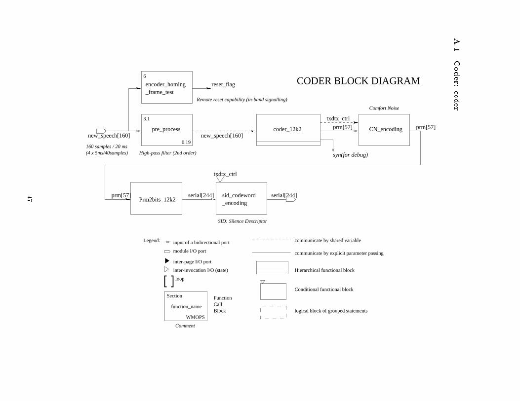
A.1
Coder:
coder
Section
WMOPS
function_name
sid_codeword_encoding
encoder_homing_frame_test
reset_flag
txdtx_ctrl
pre_process coder_12k2 CN_encoding
txdtx_ctrl
communicate by shared variable
communicate by explicit parameter passing
Hierarchical functional block
Legend:
syn(for debug)
new_speech[160] new_speech[160]
serial[244] serial[244]
prm[57] prm[57]
prm[57]
input of a bidirectional port
module I/O port
inter-page I/O port
logical block of grouped statements
Prm2bits_12k2
CODER BLOCK DIAGRAM6
3.1
Remote reset capability (in-band signalling)
Conditional functional block
Comment
FunctionCallBlock
High-pass filter (2nd order)
Comfort Noise
SID: Silence Descriptor
0.19160 samples / 20 ms(4 x 5ms/40samples)
loop
inter-invocation I/O (state)
47

A.1.1 Encoding: coder 12k2
A.1.1.1 Linear prediction analysis
Windowing&
Autocorrelation
Short term analysis:
Convert LP parameters
Speech
R[]
Levinson-Durbin
A(z)
LSP
LSPQuantization
LSP, LSP’
Interpolation for1st and 3rd subframe
to Line Spectral Pairs
r_h r_l
rc
r_h r_l
Levinson
Lag_window
lsp_mid
3.2.1
3.2.1
3.2.2
0.12
3.2.3
0.45
3.2.5
3.2.6, 3.2.4 3.2.6, 3.2.4
1.29
0.21
Autocorr
0.01
lsp_mid_q lsp_new_q
txdtx_ctrl
Q_plsf_5
Az_lsp
Int_lpc20.7 1.3
Aq_tInt_lpc
scal_acf
p_window_mid
r_h r_l
rc
r_h r_l
scal_acf
Levinson
Lag_window
3.2.1
0.21
3.2.1
0.01
3.2.2
0.45
Autocorr
0.12
Az_lsp
VA
D
A_t A_t
A(z), A’(z)
3.2.3
F_gamma2
p_window
F_gamma1
A_t
Extract Linear Prediction (LP) Filter H(z) = 1/A(z) parameters (a0, a1, ..., a9)
lsp_newlsp_old
lsp_old_q
prm
lsp_old
lsp_old lsp_old_q
speech[160]
speech[-80..0]
new_speech[160]
48

A.1.1.2 Open-loop pitch analysis
3.3
0.03
Residu
3.3
0.01
Weight_Ai
3.3
0.01
Weight_Ai
Ap2(z) = A(z/gamma2)(ap2i = ai x gamma2, i = 0..9)
(ap1i = ai x gamma1, i = 0..9)Ap1(z) = A(z/gamma1)
Filter 1/Ap2(z)
(filter speech through perceptual weighting filter W
(z) = A
(z/gamm
a1)/A(z/gam
ma2))
Filter Ap1(z)(= reverse 1/Ap1(z))
lags[0] lags[1]
lags
3.3
1.0
Pitch_ol
3.3
0.04
Syn_filt
Ap1
Ap2
F_gamma1
F_gamma2
A_t[i]
A_t[i]
3.3
1.0
Pitch_ol
T0_max[0]
T0_min[0]
T0_max[1]
T0_min[1]
to VAD
lag estimatesopen-loop
find
Com
pute weighted input speech for 4 subfram
es
mem_w mem_w
wsp[i..i+40]
wsp[i..i+40]
speech[i-10..i+40]
wsp[-143..0]
wsp[-143..0]Shift weighted speech bufferto the left by 160 sampleswsp[18..160]
i=[0,40,80,120]
wsp[-143..80] wsp[-63..160]
Long Term/Pitch Analysis (adaptive codebook) 1 / 2
49

A.1.1.3 Closed loop pitch analysis
Pitch_fr61.44
3.6
Calculate residual r(n)(filter speech through A’(z))
Com
pute adaptive codebook (pitch) gain
Codebook gainquantization
Syn_filt
Residu0.03
0.04
3.5
3.5Ap2[i]
h1Ap1[i]
xn
h1 xn
T0_min[i/80]
T0_max[i/80]
0.01
3.6Enc_lag6
T0_frac
T0_min[i/80]
T0_max[i/80]
y1
gain_pit
Convolve
G_pitch
q_gain_pitch
3.6
3.6
3.6
3.6
0.21
0.07
0.02
Residu0.03
3.5
Syn_filt0.04
3.5Aq_t[i]
Ap1[i]
error
txdtx_ctrl
Com
pute
Im
puls
e R
espo
nse
of w
eigh
ted
synt
hesi
s fi
lter
H(z
)W(z
) (3
.4)
(Fil
ter
Ap1
(z)
thro
ugh
1/A
’(z)
and
1/A
p2(z
))
(filter residual through 1/A’(z) and A
p1(z)/Ap2(z))
Com
pute Target Signal x(n) for Search (3.5)
Compute gain tomatch x(n) and y(n)
y1 = exc[i] * h1y(n) = filtered v(n)
Target =
weighted speech plus effect of w
eighted synthesis filter
h1
y1
gain_pit
res2
Interpolatecodebookvector v(n)(excitation)
T0
T0
prm
prm
Syn_filt0.04
3.4
zero
Syn_filt0.04
3.4
mem_w0
mem_errzero
Pred_lt_6
(find best filtered past excitation)find best pitch lag
speech[i-10..i+40]
exc[i-154..i+39] exc[i-154..i+39]
exc[i..i+39]exc[i..i+39]
exc[i..i+39]
exc[i-154..i]0.05
Long Term/Pitch Analysis (adaptive codebook) 2 / 2
50
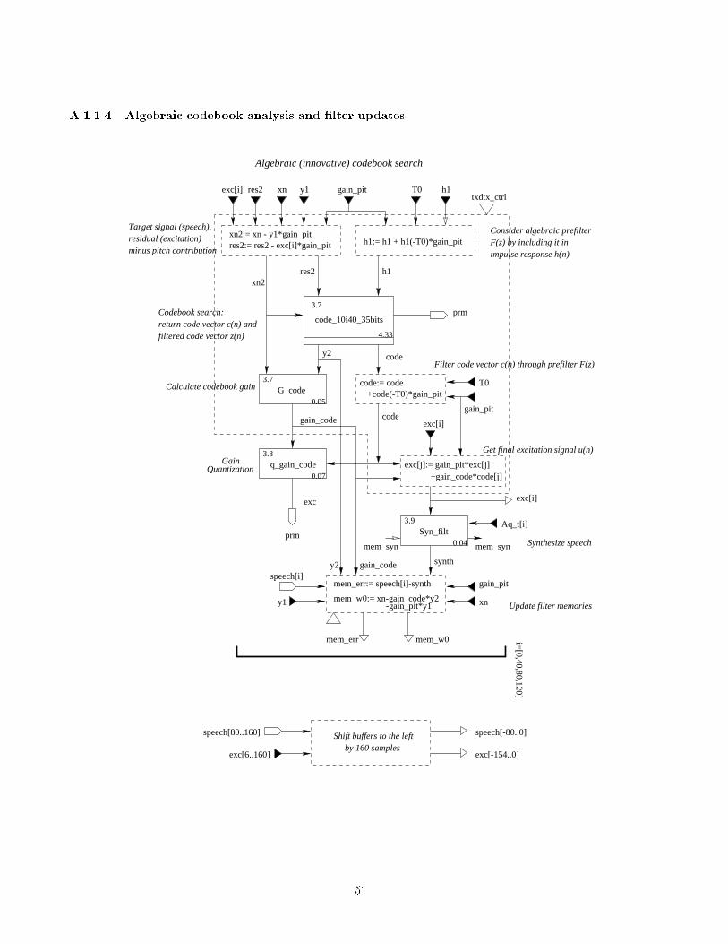
A.1.1.4 Algebraic codebook analysis and �lter updates
speech[80..160]
exc[6..160] exc[-154..0]
speech[-80..0]Shift buffers to the leftby 160 samples
exc[j]:= gain_pit*exc[j]+gain_code*code[j]
Algebraic (innovative) codebook search
minus pitch contribution
Target signal (speech), Consider algebraic prefilterF(z) by including it in impulse response h(n)
Filter code vector c(n) through prefilter F(z)
Calculate codebook gain
return code vector c(n) andCodebook search:
filtered code vector z(n)
Get final excitation signal u(n)
txdtx_ctrl
3.9
3.8
3.7
3.7
0.05
0.07
0.04
4.33
QuantizationGain
gain_pit h1T0
code_10i40_35bitsprm
h1res2xn2
G_code
exc
code
q_gain_code
prm
gain_code codegain_pit
T0
Syn_filt
mem_syn mem_syn
y2
synth
mem_w0:= xn-gain_code*y2-gain_pit*y1
mem_err:= speech[i]-synth
xn2:= xn - y1*gain_pit
code:= code+code(-T0)*gain_pit
h1:= h1 + h1(-T0)*gain_pit
mem_err mem_w0
y2
y1 xn
Aq_t[i]
speech[i]gain_pit
exc[i]
exc[i]
Synthesize speech
Update filter memories
res2:= res2 - exc[i]*gain_pit
exc[i] xn y1res2
residual (excitation)
gain_code
i=[0,40,80,120]
51

A.1.1.5
Codebooksearch
:code10i4035bits
set_sign
code_10i40_35bits
xn2
h1
res2
code
y2
prm
dncor_h_xxn2
h1
res2
search_10i40
dn
pos_max
ipos
sign rr
cor_hh1
sign
sign
h1build_code
codvec
0.313
0.171 2.643
0.146
1.034
d(n) = correlation between target x2(n) and impulse response h(n)
d’(n) = d(n)sign[b(n)]
Compute matrix of correlations of h(n)
Depth-first search (with pruning?)
Filter and encodecodebok vector
prm
y2
code
52

A.2
Decoder:
decoder
Section
WMOPS
function_name
decoder_12k2Bits2prm_12k2
6.2.1
Post_Filter
communicate by shared variable
communicate by explicit parameter passing
Hierarchical functional block
Legend: input of a bidirectional port
module I/O port
inter-page I/O port
logical block of grouped statements
Conditional functional block
Comment
FunctionCallBlock
loop
inter-invocation I/O (state)
DECODER BLOCK DIAGRAM
TAF
SID_flagserial[0..246]
serial[246]
serial[245]
Az_dec[0..43]
synth[0..159]
(4 x 5ms/40samples)160 samples / 20 ms
parm[0..57]
_frame_testdecoder_homing
reset_flag
Post filtering
synth[0..159]6.1
53

A.2.1 Decoding: decoder 12k2
D_p
lsf_
5
Int_
lpc
d_ga
in_c
ode
Pred
_lt_
6
Dec
_lag
6d_
gain
_pitc
hde
c_10
i40_
35bi
ts
agc2
Syn_
filt
0.01
0.05
0.01
0.01
0.01
0.02
0.04
1.3
parm
lsp_
old
lsp_
old
lsp_
new
lsp_
mid
T0
T0_
frac
code
:= c
ode
+ c
ode(
-T0)
*gai
n_pi
t
gain
_pit
code
gain
_cod
e
mem
_syn
mem
_syn
gain
_pit
code exc[
i]:=
exc
[i]*
gain
_pit
+ c
ode*
gain
_cod
e
excp
excpCom
pute
emph
asiz
ed e
xcit
atio
n
exc[
i..i+
39]
exc[
i..i+
39]
excp
synt
h[i]
exc[
i..i+
39]
Com
pute
exci
tati
on
Gai
n co
ntro
l
Synt
hesi
ze s
peec
h
exc[
i-15
4..i]
Ada
ptiv
e ve
ctor
i=[0
,40,
80,1
20]
Dec
ode
LSP
s
para
met
ers
Con
stru
ct fi
lter
A_t
A_t
[i]
Shift excitation buffer left by 160 samplesexc[-154..0] exc[6..160]
Decode adaptive codebook(pitch lag and gain)
codebook vector and gainDecode algebraic (fixed)
54

A.2.2 Post-processing: Post Filter
Weight_Ai
Syn_filt Weight_AiResidu
preemphasis
Syn_filt
agcsyn[i]
Az[i]
F_gamma3
Ap3
F_gamma4
Az[i]
zero
Ap4
hres2
res2
syn_pst[i]
temp2
h[11..22]=0
h[0..10]
syn_pst[i]
mem_syn mem_syn
syn[i-10..i+40]
syn[0..159]
syn[-10..0]syn[0..10]
syn[-10..0] := syn[0..10]
syn[0..159] := syn_pst[0..159]
6.2.1
Post_Filtersyn[0..159]
syn[0..159]
Az[0..44]
i=[0,40,80,120]
Post-filteredspeech
Tilt filter
Produce residual
Postfilterimpulseresponse
0.03
0.04
0.04
0.01
0.010.03
0.05
Computetilt factor
Adaptive Gain Control (AGC)
55

B Vocoder Speci�cation
This appendix describes the overall SpecC [1, 2, 4, 6] speci�cation of the GSM Enhanced Full Rate Vocoder [9].The SpecC blocks are directly derived from the blocks of C reference implementation (see Appendix A).
B.1 General (shared) behaviors
Syn filt Implement the LP �lter (synthesis �lter) 1=A(z).
Given an input sequence x(n), n = 0 : : :39, the LP �lter coe�cients a(k), k = 1 : : :10 and the �lter memoryy(m � 10) = mem(m), m = 0 : : :9, the output sequence is
y(n) = x(n)�10Xk=1
a(k)y(n � k); n = 0 : : :39:
In addition, the �lter memory can be updated, too:
mem(m) = y(30 +m); m = 0 : : :9:
Residu Implement the LP inverse �lter A(z) (to get the residual).
Given an input sequence x(n), n = �10 : : :39 and the LP �lter coe�cients a(k), k = 1 : : :10 the outputsequence is
y(n) = x(n) +10Xk=1
a(k)x(n� k); n = 0 : : :39:
56

B.2 Coder
Filter memory
update
Closed-loop
pitch search
pitch search
Open loop
Algebraic (fixed)
codebook search
Linear prediction
(LP) analysis
��������
��������
��������
��������
��������
��������
��������
������
������
��
��
��
����
��
����
����
����
����
����
����
�� ��
����
��������
��������
����
����
prm[57]
speech[160]
bits
pre_process
code_12k2
prm2bits_12k2
mem
ory
2x per fram
e
A(z)2 su
bfram
es
code_12k2
prm
speech[160]
sample coder
Figure 58: Coder
Encoding is based on �nding the parameters for the speech synthesis model at the receiving side which willthen be transmitted to the decoder over the medium.
The speech synthesis model is code-excited linear predictive (CELP) model: to synthesize speech in the decodera 10th order linear predictive (LP) synthesis �lter H(z) = 1=A(z) (responsible for the short term e�ects) is excitedwith a signal constructed by adding two vectors from two codebooks:
� The so-called adaptive codebook is based on a pitch synthesis �lter which is responsible for covering longterm e�ect. The output of the pitch �lter is simply a previous excitation signal delayed by a certain amount(lag) and scaled with a certain gain. Since the delay/lag of the pitch �lter can be fractional the delayedexcitation has to be interpolated (using a FIR �lter) between the two adjacent (delayed by an integer lag)excitation values.
� The so-called �xed or algebraic codebook covers any remaining pulse excitation sequence left after removingthe short-term and long- term contributions. The �xed codebook contains 5 tracks with 8 possible positionseach. For each track two positions are chosen (10 pulses all together) and transmitted.
In general, the parameters for the two codebooks are chosen such that the error between the synthesized speech(at the output of the LP synthesis �lter!) and the original speech is minimized. However, for the codebooksearches the original speech is weighted (by a weighting �lter W (z)) in order to account for the special propertiesof human acoustic perception.
57

B.2.1 Preprocessing: pre process
The pre-processing consists of high-pass �ltering and signal down-scaling (dividing the signal by two to reduce thepossibility of over ows) of the input speech samples. The high-pass �lter Hh1(z) is as given in the speci�cation.
Given the input signal x(n) and the �lter coe�cients a and b the output sequence y(n) of the pre-processingstep is
y(n) =b02x(n) +
b12x(n� 1) +
b22x(n� 2) + a1y(n � 1) + a2y(n � 2):
B.2.2 Linear prediction analysis and quantization
��
��
LSP -> A(z)Interpolation &
�������������������������
�������������������������
�������������������������
�������������������������
������
������
�����
�����
�� ��
����
�� ��
�� ��
����
���� ����
������������������������
������������������������
������������������
������������������
�� ��
��
����
������������������������������������������������������������������
������������������������������������������������������������������
������������������������������
������������������������������
��
��
����
���� ���� ����������
��������
��
����������
����������
��������
�����
�����
��������
��������
��������
Windowing &Autocorrelation
Windowing &Autocorrelation
A1(z) A2(z)
LSP
A(z) -> LSP
QuantizationLSP
A(z) Aq(z) prm
LSP -> Aq(z)Interpolation &
LevinsonLevinson
speech
�����
�����
����
��������
�� ��
�� ��
���� ����
������������
������������
����������
����������
����
����
��
��
����
������
������
�� ��
��
��
��
������
������
������������������
����������
��
��
���� ����
����
����
�������������������������
�������������������������
�� ������
������
��
��
�� �������������������������
����������������������������������
�������������
�����
�����
��������
��������
��������
Levinson Levinson
Az_LSP
Az_LSP
A1(z) A2(z)
LSP2LSP1
Int_lpc2
Int_lpc
Q_plsf_5
Lag_window Lag_window
Autocorr Autocorr
speech
A(z) Aq(z) prm
Figure 59: LP Analysis
Determine the parameters (coe�cients) of the LP (short term) synthesis �lter twice per frame, encode themfor transmission and recompute the coe�cients for every subframe (e.g. to include the e�ects due to encodinglosses):
Autocorr Windowing and autocorrelation computation.
Two �xed windows (see speci�cation) w(n) are applied to 80 samples from the past speech frame plus the160 samples from the current frame to get the windowed speech
s0(n) = s(n)w(n); n = 0 : : :239:
The autocorrelation r(k) of the windowed speech is then computed as
r(i) =239Xn=i
s0(n)s0(n� i); i = 0 : : :10:
58

In addition, the C reference implementation normalizes r(i) and checks for over ows.
Lag window Lag windowing of the autocorrelations.
r(k) = r(k)wlag(k); k = 1 : : :10
where the �xed window wlag(k) is as given in the speci�cation.
Levinson Levinson-Durbin algorithm to recursively compute the LP (linear prediction) �lter coe�cients a(k),k = 1 : : :10.
Az lsp Convert LP �lter coe�cients to line spectral pairs (LSPs) q(k), k = 1 : : :10.
Q plsf 5 Quantization of the two set of line spectral pairs (LSPs) per frame.
Int lpc, Int lpc2 Interpolation of the quantized and unquantized LSPs for intermediate subframes and re-conversion of the LSPs to LP �lter coe�cients.
The two sets of LSPs, q2(k) and q4(k) previously computed are used directly for the 2nd and 4th subframes.For the 1st and 3th subframe two sets of LSPs are calculated by linearly interpolating the LSPs fromadjacent subframes
q1(k) = 0:54q4;old(k) + 0:5q2(k);q3(k) = 0:5q2(k) + 0:54q4(k); k = 1 : : :10:
For the unquantized case of the 2nd and 4th subframes the LP �lter coe�cients are already directly available.For all other cases (quantized LSPs and unquantized but interpolated LSPs for 1st and 3rd subframes):
Lsp Az Convert the LSPs back to LP �lter coe�cients.
Once the LP �lter parameters are found in the next steps the signals at the input of the LP �lter, i.e. the twocodebook conttributions have to be found.
B.2.3 Open-loop pitch analysis
��
��
pitch delayFind open loop
��
���� ������
��������
����
��
����
����
������������
������
��������
������������
speechWeighted
2 su
bfr
ames
speech A(z)
wsp
T0 min/max Aw(z)
�����
�����
���� ��
���� ��
���� ����
������
�������������������������
�������������������������
�������������������������
�������������������������
�����
�����
����
����
����
����
����
����
���������������������������
���������������������������
��������
��������
��������
��������
������������
WeightedCoefficients
WeightedCoefficients
speech
Aw1(z) Aw2(z)
Filter Aw1(z)
Filter 1/Aw2(z)
A(z)
wsp
Figure 60: Open-loop pitch analysis
Open-loop pitch analysis determines delay/lag estimates for the (closed-loop) calculation of the pitch �lterparameters in order to narrow the actual adaptive codebook search.
59

Weight Ai Calculate the two sets of weighted �lter coe�cients for the implementation of the weighting �lter:
ai(k) = a(k) i(k); k = 1 : : :10; i = 1; 2
where the spectral expansion factors i(k) are given as in the speci�cation.
Residu, Syn filt, weighted coe�cients For each of the 4 subframes �lter the speech signal through the
weighting �lter W (z) = A(z= 1)A(z= 2)
to obtain the weighted speech signal.
Pitch ol Perform open-loop pitch analysis based on the weighted speech twice per frame to obtain two pitch lagestimates Top(s), s = 0; 1.
Open-loop pitch analysis is done by �nding maximal correlations in the weighted speech signal.
Finally, using the two open-loop pitch lag (pitch delay) estimates the closed-loop pitch analysis search ranges[T0min; T0max] for the 1st and 3rd subframes are preset to
T0min(s) = Top(s) � 3; T0min(s) � 18;
T0max(s) = Top(s) + 3; T0max(s) � 143; s = 0; 1:
B.2.4 Closed loop pitch analysis
��������
��������
��������
��������
��������
��������
prm h(n) gain_pit x(n) v(n) T0
��
���
���
����
����
����
��������
��������
�������� ����
�� ��
��
����
��
��
����
��
����
����
����
����
���
���
����
����������������
��������
��������
Targetsignal
Impulseresponse
Computecode vector
pitch gainCalculate
pitch delayFind
x(n)h(n)
Aq(z) Aw(z) speech T0 min/max
Figure 61: Closed loop pitch search.
Based on the open-loop lag estimates search for the pitch �lter parameters in the given intervals.
B.2.4.1 Impulse response computation For each subframe the impulse response h(n) of the weighted
synthesis �lter H(z)W (z) = A(z= 1)
A(z)A(z= 2)is computed by
Syn filt, quantized coe�cients a(k), zero-�lled memory Filtering of the weighted �lter coe�cientsa1(k) = a(k) 1(k) through the quantized synthesis �lter 1=A(z).
60

Syn filt, weighted coe�cients a2(k) = a(k) 2(k), zero memory Filtering of the intermediate resultthrough the weighted �lter 1=A(z= 2).
The impulse response is needed in the codebook searches to model the e�ects a certain excitation vector will haveon the error at the output of the LP synthesis �lter.
B.2.4.2 Residual computation For each subframe the residual signal resLP (n) is calculated by
Residu, quantized coe�cients a(k) Filter the speech signal s(n) through the inverse quantized synthesis �lterA(z).
The residual is basically the signal needed at the input of the LP �lter in order to get the original speech back atits output.
B.2.4.3 Target signal computation For each subframe calculate the target signal x(n) (weighted speechminus e�ect of weighted synthesis �lter H(z)W (z)) for the adaptive codebook search:
Syn filt, quantized coe�cients a(k) Filter the residual resLP (n) through the quantized synthesis �lter1=A(z).
Residu, Syn filt, weighted coe�cients Filter the result through the weighting �lter W (z) = A(z= 1)A(z= 2)
.
The �lters for the target signal computation use a special memory which is updated separately using additional�lters (see B.2.6).
B.2.4.4 Adaptive codebook search For each subframe compute the adaptive codebook parameters (de-lay/lag and gain of the pitch �lter).
First, the pitch delay/lag is found and encoded for transmission:
Pitch fr6 Closed-loop search to �nd the best pitch delay/lag T0 (integer and fractional parts) such that theerror between the target signal x(n) (original speech) and the past LP �ltered excitation (past excitationconvolved with impulse response h(n)) at delay T0 is minimized.
First, the integer part of the lag is found. Then, the fractional part (with resolution 1=6) is found byinterpolating the error between the adjacent integer boundaries.
Since the past excitation for delays inside the current subframe is not known yet the excitation bu�er forthe current subframe is initialized with the residual resLP (n).
Enc lag6 Encoding of the pitch lag T0 into 9 bits (1st and 3rd subframes) or 6 bits (2nd and 4th subframes). Ifnecessary, adjusts the fractional part of T0 for the following gain calculations.
For the 1st and 3rd subframes the lag is encoded with a resolution of 1=6 in the range [1736 ; 9436 ] and integers
only in the range [95; 143]. In the latter case the fractional part of the pitch lag is set to zero.
For the 2nd and 4th subframes the lag is encoded with a resolution of 1=6 in an interval around the lag inthe previous (1st or 3rd) frame.
In addition, in the 1st and 3rd subframes the search ranges [T0min; T0max] are updated for upcoming searchesin the 2nd and 4th subframes, respectively.
T0min(s) = [T0]� 5; T0min(s) � 18;
T0max(s) = [T0] + 4; T0max(s) � 143; s = 0; 1:
In the 2nd and 4th subframe the search ranges are based on the integer pitch lag parts [T0] found in the 1st and3rd subframe.
Then, the actual adaptive codevector is calculated in order to compute the adaptive codebook gain:
61

Pred lt 6 Compute the adaptive codebook vector v(n) by interpolating the past excitation at T0 using two FIR�lters.
Convolve Filter the adaptive codebook vector v(n) through the weighted synthesis �lter H(z)W (z) by convolvingit with the impulse response h(n): y(n) = v(n) � h(n), i.e.
y(n) =nXi=0
x(i)h(n� i); n = 0 : : :39:
G pitch Calculate the adaptive codebook gain
gp =
P39n=0 x(n)y(n)qP39n=0 y(n)y(n)
; 0 � gp � 1:2
q gain pitch Quantize the adaptive codebook gain for transmission.
B.2.5 Algebraic (�xed) codebook analysis
��
�� ��
��
���� ����
���� ���� ����
�� ��
����
����
��
���� ����
��
���� ����
��
�� ��
���� ����
����
��������
��������
��������
��������
��������
��
����
��
����
����
��������
��������
��������
��������
Prefilterresponse
Updatetarget
codebook
gain_pit x(n) v(n)h(n)T0
h(n) x2(n)
z(n)code
Prefiltercode vector
Calculatecodebook gain
prm code gain_code z(n)
Search
Figure 62: Algebraic (�xed) codebook search
B.2.5.1 Update target signal and residual The remaining target signal x2(n) and residual resLTP (n)(after removing long-term prediction contributions) are computed for the �xed codebook search by subtractingthe adaptive codebook e�ects:
x2(n) = x(n)� gpy(n); resLTP (n) = resLP (n) � v(n); n = 0 : : :39:
where x(n) and resLP (n) are the target signal and the residual for the adaptive codebook search (see B.2.4.3)and B.2.4.2), gp is the quantized adaptive codebook gain and v(n) is the adaptive codebook vector.
62

B.2.5.2 Update impulse response The impulse response h(n) is updated for the �xed codebook search byincluding a pre�lter FE(z) =
1
1�g�[T 0]p
(where gp, gp � 1:0 is the quantized pitch gain and [T0] is the integer part
of the pitch lag) which enhances spectral components to improve quality:
hE(n) = h(n) +gp8h(n� [T0]); n = [T0] : : :39:
B.2.5.3 Codebook search: code 10i40 35bits
cor h x Compute the correlation between the target x2(n) and the impulse response hE(n):
d(n) =39Xi=n
x2(n)hE (i� n); n = 0 : : :39:
The vector d(n) corresponds to the backward �ltered target signal.
The C reference implementation adds some normalization of d(n) such that the sum of the maxima of d(n)for each of the 5 tracks will not saturate.
set sign Calculate the pulse sign information
sign(n) = sign[en(n)]; n = 0 : : :39
with en(n) being the sum of the normalized long term residual and the normalized correlation vector d(n):
en(n) =resLTP (n)qP39i=0 res
2LTP (n)
+d(n)qP39i=0 d
2(n); n = 0 : : :39:
The sign information is then included into d(n):
d(n) = d(n)sign(n); n = 0 : : :39:
Also, the position with maximum correlation in each of the 5 tracks is computed:
posmax(t) = p s.t. en(p)sign(p) = maxj=t;t+5;:::;39
en(j)sign(j); t = 0 : : :4:
Finally, the starting positions of each pulse are calculated:
ipos(0) = ipos(5) = t s.t. posmax(t) = maxj=0:::4
posmax(j);
ipos(i) = ipos(i + 5) = (ipos(0) + i) mod 5; i = 1 : : :4:
cor h Compute the matrix of correlations of the impulse response hE(n) and include the sign information in it:
rr(i; j) =
39Xn=i
hE(n � i)hE (n� j)
!sign(i)sign(j); i � j; i; j = 0 : : :39:
search 10i40 Search the algebraic (�xed) codebook to �nd the optimal pulse positions mj :
/* Fix position of �rst pulse to global maximum position */i0 = posmax(ipos(0));/* Four iterations over local maxima in other tracks */for each track t = 1 : : :4 do
i1 = posmax(ipos(1)); /* max. pos. in track */
63

/* Successively add pulses in pairs */for each pair (a; b) = (2; 3); (4; 5); (5;7); (8;9) do
/* Search pair positions to maximize mean square error A */for ia = ipos(a) : : :39, step 5 do
for ib = ipos(b) : : :39, step 5 do
C =Pb
j=0 d(ij);
ED = 116
Pbj=0 rr(ij; ij) +
18
Pbj=0
Pj�1k=0 rr(ik; ij);
if C2
ED>
C2max
ED;maxthen
Cmax = C; ED;max = ED;iamax = ia; ibmax = ib;
end ifend for
end for/* Set pair positions to maximizer */ia = iamax; ib = ibmax;
end for/* All pulse positions assigned, is it global maximum? */
ifC2max
ED;max> Amax then
Amax =C2max
ED;max;
/* Remember pulse positions */for j = 0 : : :9 do mj = ij end for
end if/* Cyclically shift starting positions for next iteration */ipos(1 : : :9) = ipos(2 : : :9; 1);
end for
build code Given the positions and signs of the 10 pulses build the �xed codebook vector c(n) and encode it fortransmission.
In addition, the �xed codebook vector is �ltered by convolving with the impulse response hE(n):
z(n) =nXi=0
c(i)hE (n� i); n = 0 : : :39:
B.2.5.4 Codebook gain
G code Calculate the �xed codebook gain
gc =
P39n=0 x2(n)z(n)P39n=0 z(n)z(n)
B.2.5.5 Quantization of �xed codebook gain In a preprocessing step, the �xed codebook vector c(n) is�ltered through the pre�lter FE(z):
cE(n) = c(n) +gp8c(n� [T0]); n = [T0] : : :39:
(see B.2.5.2) followed by:
q gain code Quantize the �xed codebook gain for transmission.
64
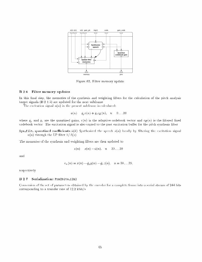
��
��
��
��
��
�� ����
����
����
����
����
����
����
����
��
��������
��������
��������
��������
��������
��������
��������
��������
��������
Synthesizespeech
Quantizecodebook gain
memoriesUpdate filter
gain_codecode
prmmemory
Aq(z)v(n) gain_pitx(n) z(n)
Figure 63: Filter memory update
B.2.6 Filter memory updates
In this �nal step, the memories of the synthesis and weighting �lters for the calculation of the pitch analysistarget signals (B.2.4.3) are updated for the next subframe.
The excitation signal u(n) in the present subframe is calculated:
u(n) = gpv(n) + gccE (n); n = 0 : : :39
where gp and gc are the quantized gains, v(n) is the adaptive codebook vector and cE(n) is the �ltered �xedcodebook vector. The excitation signal is also copied to the past excitation bu�er for the pitch synthesis �lter.
Syn filt, quantized coe�cients a(k) Synthesized the speech s(n) locally by �ltering the excitation signalu(n) through the LP �lter 1=A(z).
The memories of the synthesis and weighting �lters are then updated to
e(n) = s(n) � s(n); n = 30 : : :39
and
ew(n) = x(n)� gpy(n) � gcz(n); n = 30 : : :39;
respectively.
B.2.7 Serialization: Prm2bits 12k2
Conversion of the set of parameters obtained by the encoder for a complete frame into a serial stream of 244 bitscorresponding to a transfer rate of 12:2 kbit/s.
65

Pre
filt
erp
itch
_co
ntr
G_c
od
eP
refi
lter
cor_
h_x
set_
sig
n
cor_
h
sear
ch_1
0i40
bu
ild_c
od
e
Co
deb
oo
k
Syn
_filt
up
d_m
em
exci
tati
on
q_g
ain
_co
de
Up
dat
e
En
c_la
g6
Pre
d_l
t_6
Co
nvo
lve
G_p
itch
q_g
ain
_pit
ch
Res
idu
Syn
_filt
Res
idu
Syn
_filt
Syn
_filt
Syn
_filt
Clo
sed
_lo
op
Pit
ch_f
r6
2 su
bfr
ames
Res
idu
Syn
_filt
Wei
gh
t_A
iW
eig
ht_
Ai
2 subframes
Op
en_l
oo
p
Pit
ch_o
l
Az_
lsp
Az_
lsp
LP
_an
alys
is
Lev
inso
nL
evin
son
Au
toco
rr
Lag
_win
do
w
Au
toco
rr
Lag
_win
do
w
Q_p
lsf_
5
Int_
lpc
Int_
lpc2
2x p
er f
ram
e
cod
e_12
k2
Pre
_pro
cess
prm
2bit
s_12
k2
Figure 64: Coder block diagram.
66

B.3 Decoder
����
����
����
����
���
���
��
���
���
��
��
��
��������
������
������
decode_12k2
Post_Filter
Bits2prm_12k2
Decode
LP parameters4 su
bfram
es
bits
speech[160]
A(z)
synth[40]
synth[40]
prm[57]
prm[13]
decoder
Figure 65: Decoder
Decoding is basically the reverse process of encoding in the sense that simply the synthesis model described inB.2 is implemented. Therefore, the steps are very similar to the routines described in the encoding part and thereader is referred to the �rst part for details.
B.3.1 Parameter extraction: Bits2prm 12k2
Extract the decoder parameter set from the serial stream of 244 bits for a complete frame.
B.3.2 Decoding of LP �lter parameters
��
���� ��
DecodeLSPs
��������
��
���� ��
��������
Interpolatefilter coeff.
LSP
prm[5]
A(z)
Figure 66: LSP decoding
For each complete frame:
67

D plsf 5 The received LSP indices are used to reconstruct the two LSPs for the 2nd and 4th subframes.
Int lpc Interpolation of the LSPs for the 1st and 3rd subframes and conversion of the LSPs to LP �lter coe�cientsa(k), k = 1 : : :10 for all 4 subframes.
B.3.3 Decoding subframe and synthesizing speech
��
���� ��
Computeadaptive vector
��
����
����
��
ExcitationEmphasize
��
�� ��
����
���� ������
������������
���� ��
���� ������
��
����
��
����
��
���� ������
������������
������
��
��������
����
����
����
����
����
���� ��
��������
����
����
������
����
����
����
��������
������������
��������
Decode Decode Decodepitch gain code vectorpitch lag
Prefiltercode vector
Decodecode gain
ExcitationCompute
Adaptivegain control
Synthesizespeech
synth[40]
prm[13] A(z)
gain_code
code
code
excp[40]
exc[40]
gain_pit
Figure 67: Subframe decoding
B.3.3.1 Decoding of the adaptive codebook vector For each subframe, the received pitch lag is decodedand used to construct the adaptive codebook vector v(n) from the past excitation bu�er.
Dec lag6 Decode the received pitch index to construct the integer and fractional parts of the pitch lag T0.
Pred lt 6 Compute the adaptive codebook vector v(n) by interpolating the past excitation at T0.
B.3.3.2 Decoding of the adaptive codebook gain For each subframe:
d gain pitch Decode the received gain index to construct the adaptive codebook gain gp.
B.3.3.3 Decoding of the algebraic codebook vector For each subframe:
dec 10i40 35bits The received �xed codebook index is used to reconstruct the signs and positions of the 10pulses which then give the �xed codebook vector c(n).
After decoding, the pre�lter FE(z) (see B.2.5.2) is applied to the �xed codebook vector:
cE(n) = c(n) +gp8c(n� [T0]); n = [T0] : : :39
where gp and [T0] are the previously decoded pitch gain and integer part of the pitch lag.
68

B.3.3.4 Decoding of the algebraic codebook gain For each subframe:
d gain code Given the codebook vector cE(n) and the received gain index the �xed codebook gain gc is calculated.
B.3.3.5 Computing the reconstructed speech In each subframe, the basic excitation at the input of theLP synthesis �lter is
u(n) = gpv(n) + gccE (n); n = 0 : : :39
given the previously decoded codebook vectors and gains.If gp > 0:5 then the excitation is modi�ed to emphasize the contribution of the adaptive codebook vector:
u(n) = u(n) +gp16gpv(n); n = 0 : : :39
is calculated and the excitation u(n) is updated by
agc2 Adaptive gain control to compensate for the di�erence between u(n) and u(n).
The gain scaling factor is
� =
sP39n=0 u
2(n)P39n=0 u
2(n)
and the �nal excitation signal is then calculated to
u(n) = �u(n); n = 0 : : :39:
In other cases (gp � 0:5) the excitation signal u(n) is not modi�ed.
Finally, the speech is synthesized by passing the excitation through the synthesis �lter 1=A(z):
Syn Filt, coe�cients a(k), k = 1 : : :10 Filter the excitation signal u(n) through the LP synthesis �lter to getthe reconstructed speech signal s(n).
B.3.4 Post-�ltering: Post Filter
In each of the 4 subframes a post-�ltering of the synthesized speech is performed.
Weight Ai Calculate the weighted �lter coe�cients
an(k) = a(k) n(k);
ad(k) = a(k) d(k); k = 1 : : :10:
for the formant post�lter Hf (z) = =fracA(z= n)A(z= d).
B.3.4.1 Produce residual signal
Residu, coe�cients an Filter the speech s(n) through the LP inverse �lter A(z= n) to get the residual r(n).
B.3.4.2 Tilt compensation �lter First, calculate the truncated impulse response hf (n) of the formantpost�lter:
Syn filt, coe�cients ad, zero memory Filter the coe�cients an(k) through the LP �lter 1=A(z= d).
69
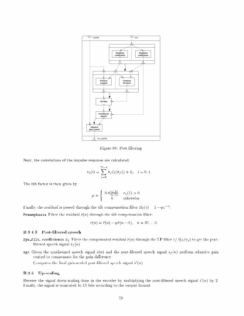
��
�� ��
����
����
��
����
Weightedcoefficients
Weightedcoefficients
����
����
��
Adaptivegain control
����
���� ����
��
��
��
����
������
����
��
����
��
��
��
���
���
��������
��������
��������
residualProduce Compute
tilt factor
Tilt filter
speechPostfiltered
syn[40] A(z)
syn_pst[40]
Figure 68: Post �ltering
Next, the correlations of the impulse response are calculated:
rh(i) =21�iXj=0
hf (j)hf (j + i); i = 0; 1:
The tilt factor is then given by
� =
(0:8 rh(1)rh(0)
; rh(1) > 0
0 otherwise
Finally, the residual is passed through the tilt compensation �lter Ht(z) = 1� �z�1:
Preemphasis Filter the residual r(n) through the tilt compensation �lter:
r(n) = r(n)� �r(n� 1); n = 39 : : :0:
B.3.4.3 Post-�ltered speech
Syn filt, coe�cients ad Filter the compensated residual r(n) through the LP �lter 1=A(z= d) to get the post-�ltered speech signal sf (n).
agc Given the synthesized speech signal s(n) and the post-�ltered speech signal sf (n) perform adaptive gaincontrol to compensate for the gain di�erence.
Computes the �nal gain-scaled post-�ltered speech signal s0(n).
B.3.5 Up-scaling
Reverse the signal down-scaling done in the encoder by multiplying the post-�ltered speech signal s0(n) by 2.Finally, the signal is truncated to 13 bits according to the output format.
70

d_g
ain
_pit
chD
ec_l
ag6
dec
_10i
40
Em
ph
asiz
e agc2
Syn
_filt
Exc
itat
ion
dec
od
e_12
k2
Pre
d_l
t_6
Pre
filt
er
d_g
ain
_co
de
Wei
gh
t_A
iW
eig
ht_
Ai
Res
idu
tilt
_fac
Syn
_filt
pre
emp
has
is
Syn
_filt
agc
Po
st_F
ilter
D_p
lsf_
5
Int_
lpc
D_l
sp
Bit
s2p
rm_1
2k2
4 su
bfr
ames
Figure 69: Decoder block diagram.
71

C Simulation Results
C.1 Software
The following tables list the cycle-accurate results obtained for simulating the coder and decoder on the ISS forthe Motorola DSP5600. Tables are given for unoptimized, initial code and for the software after optimizations.
72

Routine calls cycles instructionsmax total avg. max total avg
FAutocorr 18ae 6 104958 629748 104958 53938 323628 53938FAz lsp 16df 6 41258 246714 41119 24798 148315 24719FChebps 1822 628 322 202216 322 200 125600 200FCoder 12k2 11cc 3 2715917 8142878 2714292 1561164 4680860 1560286FConvolve 19a0 24 29702 712848 29702 16181 388344 16181FEnc lag6 2852 12 99 928 77 52 503 41FG code 2bd2 12 937 11244 937 842 10104 842FG pitch 28ae 12 2826 33818 2818 1625 19449 1620FGet lsp pol 36c4 36 1530 55080 1530 963 34668 963FInt lpc 30e4 3 14879 44629 14876 9471 28409 9469FInt lpc2 3140 3 7618 22840 7613 4866 14591 4863FInterpol 6 37e6 70 270 18340 262 134 9180 131FInv sqrt 3788 252 135 30946 122 77 17668 70FLag max 25b0 18 86950 916735 50929 60707 641995 35666FLag window 2fd2 6 443 2658 443 318 1908 318FLevinson 2cb7 6 18650 111788 18631 10373 62168 10361FLsf lsp 358b 6 404 2421 403 239 1434 239FLsf wt 34af 6 419 2490 415 293 1758 293FLsp Az 363b 18 3628 65195 3621 2300 41347 2297FLsp lsf 35bc 6 1960 11616 1936 945 5606 934FNorm Corr 271b 12 64233 733169 61097 39419 448217 37351FPitch fr6 2669 12 66638 757923 63160 40623 460564 38380FPitch ol 248b 6 158656 946007 157667 111212 664359 110726FPre Process 383c 3 15248 45744 15248 10268 30804 10268FPred lt 6 2c34 12 21995 263828 21985 11516 138150 11512FPrm2bits 12k2 3013 3 9599 28592 9530 4731 14152 4717FQ plsf 5 318f 3 116512 348864 116288 75269 225521 75173FReorder lsf 361c 6 207 1239 206 126 756 126FResidu 29d0 36 12528 451008 12528 8063 290268 8063FSet zero 34f7 9 1299 3119 346 1289 3029 336FSyn �lt 306f 72 11124 792192 11002 5885 418248 5809FVq subvec 3331 12 22498 184014 15334 14900 122334 10194FVq subvec s 33be 3 48033 143853 47951 30655 91860 30620FWeight Ai 2a20 48 132 6336 132 110 5280 110Fbuild code 2363 12 5730 68159 5679 3190 37976 3164Fcode 10i40 35bits 19f7 12 246805 2957399 246449 132574 1589235 132436Fcor h 1c25 12 80454 965331 80444 44758 537033 44752Fcor h x 1a74 12 31074 371601 30966 17096 204580 17048Fencoder reset 47a3 1 3553 3553 3553 3322 3322 3322Fq gain code 2a7d 12 2471 28688 2390 1415 16661 1388Fq gain pitch 2a40 12 584 6450 537 299 3402 283Fq p 1bf7 120 60 6360 53 31 3120 26Fsearch 10i40 1d21 12 124153 1485073 123756 64517 772537 64378Fset sign 1b17 12 4633 55127 4593 2673 31697 2641
Table 8: Initial delays for coder behaviors.
73
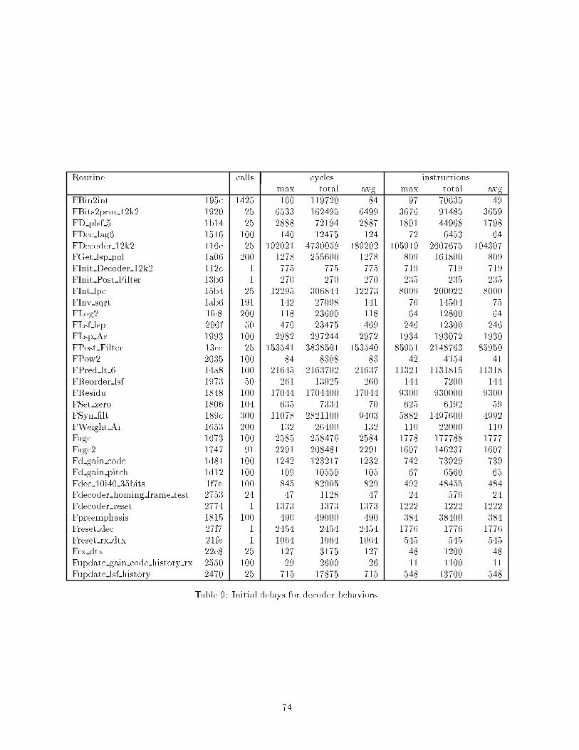
Routine calls cycles instructionsmax total avg. max total avg
FBin2int 195c 1425 160 119720 84 97 70635 49FBits2prm 12k2 1920 25 6533 162495 6499 3676 91485 3659FD plsf 5 1b14 25 2888 72194 2887 1801 44968 1798FDec lag6 1516 100 140 12475 124 72 6453 64FDecoder 12k2 116c 25 192021 4730059 189202 105919 2607675 104307FGet lsp pol 1a06 200 1278 255600 1278 809 161800 809FInit Decoder 12k2 112c 1 775 775 775 719 719 719FInit Post Filter 13b6 1 270 270 270 235 235 235FInt lpc 15b4 25 12295 306844 12273 8009 200022 8000FInv sqrt 1ab6 191 142 27098 141 76 14504 75FLog2 1fe8 200 118 23600 118 64 12800 64FLsf lsp 206f 50 470 23475 469 246 12300 246FLsp Az 1993 100 2982 297244 2972 1934 193072 1930FPost Filter 13cc 25 153541 3838501 153540 85951 2148763 85950FPow2 2035 100 84 8308 83 42 4154 41FPred lt 6 14a8 100 21645 2163702 21637 11321 1131815 11318FReorder lsf 1973 50 261 13025 260 144 7200 144FResidu 1848 100 17044 1704400 17044 9300 930000 9300FSet zero 1806 104 635 7334 70 625 6192 59FSyn �lt 189c 300 11078 2821100 9403 5882 1497600 4992FWeight Ai 1653 200 132 26400 132 110 22000 110Fagc 1673 100 2585 258476 2584 1778 177788 1777Fagc2 1747 91 2291 208481 2291 1607 146237 1607Fd gain code 1d81 100 1242 123217 1232 742 73929 739Fd gain pitch 1d12 100 109 10550 105 67 6560 65Fdec 10i40 35bits 1f7e 100 845 82905 829 492 48455 484Fdecoder homing frame test 2753 24 47 1128 47 24 576 24Fdecoder reset 2774 1 1373 1373 1373 1222 1222 1222Fpreemphasis 1815 100 490 49000 490 384 38400 384Freset dec 27f7 1 2454 2454 2454 1776 1776 1776Freset rx dtx 21fe 1 1064 1064 1064 545 545 545Frx dtx 22e8 25 127 3175 127 48 1200 48Fupdate gain code history rx 2550 100 29 2609 26 11 1100 11Fupdate lsf history 2470 25 715 17875 715 548 13700 548
Table 9: Initial delays for decoder behaviors.
74

Routine calls cycles instructionsmax total avg. max total avg
FAutocorr 1888 12 6228 74736 6228 5806 69672 5806FAz lsp 16cc 12 34209 405440 33786 18818 223085 18590FChebps 1820 1244 251 312244 251 142 176648 142FCoder 12k2 11c9 6 1437055 8610119 1435019 812501 4866760 811126FConvolve 4077 48 2297 110256 2297 1926 92448 1926FEnc lag6 2680 24 98 1860 77 51 1007 41FG code 2963 24 1231 29544 1231 805 19320 805FG pitch 26da 24 2448 58585 2441 1291 30903 1287FGet lsp pol 41cf 72 1276 91872 1276 807 58104 807FInt lpc 2cc5 6 11911 71466 11911 7746 46476 7746FInt lpc2 2d15 6 6096 36576 6096 3969 23814 3969FInterpol 6 30ca 154 259 38478 249 124 18568 120FInv sqrt 306c 504 142 68625 136 76 36765 72FLag max 4033 36 13620 290418 8067 12517 265881 7385FLag window 2c3a 12 226 2712 226 187 2244 187FLevinson 29d5 12 14092 168872 14072 7549 90443 7536FLsf lsp 2fb2 12 470 5634 469 246 2952 246FLsf wt 2ee4 12 379 4470 372 231 2746 228FLsp Az 4166 36 2898 104286 2896 1882 67752 1882FLsp lsf 2fe0 12 2572 30364 2530 1216 14372 1197FNorm Corr 25ad 24 15928 352299 14679 10859 241341 10055FPitch fr6 2505 24 18283 403716 16821 11979 265867 11077FPitch ol 23f5 12 28097 328942 27411 24770 291140 24261FPre Process 311d 6 10766 64596 10766 7226 43356 7226FPred lt 6 408a 24 2319 55617 2317 1938 46486 1936FQ plsf 5 2d58 6 53627 321478 53579 37723 226206 37701FReorder lsf 304c 12 261 3126 260 144 1728 144FResidu 401f 72 1457 104904 1457 1126 81072 1126FSet zero 2f20 9 339 908 100 328 809 89FSyn �lt 3fec 144 1692 239712 1664 1263 179664 1247FVq subvec 40ae 24 9020 149286 6220 6694 110736 4614FVq subvec s 40f5 6 20551 123306 20551 15150 90900 15150FWeight Ai 27db 96 102 9792 102 80 7680 80Fbuild code 22ea 24 5326 126266 5261 2809 66806 2783Fcode 10i40 35bits 18eb 24 248694 5958414 248267 128118 3070280 127928Fcor h 1af7 24 82634 1983120 82630 42753 1026024 42751Fcor h x 1965 24 28544 682536 28439 14511 347144 14464Fencoder homing frame test 3f46 6 25 150 25 12 72 12Fencoder reset 3f59 1 1242 1242 1242 999 999 999Fq gain code 282f 24 2194 50136 2089 1097 25578 1065Fq gain pitch 27f8 24 566 12840 535 267 6160 256Fq p 1adc 240 41 8400 35 18 3480 14Fsearch 10i40 1bdc 24 126468 3023685 125986 65225 1560428 65017Fset sign 1a00 24 5199 122983 5124 2640 61886 2578
Table 10: Coder delays after software optimization.
75

Routine calls cycles instructionsmax total avg. max total avg
FBin2int 17da 1425 143 109285 76 78 57010 40FBits2prm 12k2 179e 25 6099 152060 6082 3131 77860 3114FD plsf 5 186c 25 2588 64694 2587 1501 37468 1498FDec lag6 148a 100 140 12475 124 72 6453 64FDecoder 12k2 1168 25 72030 1736836 69473 44869 1087593 43503FGet lsp pol 26f6 200 1276 255200 1276 807 161400 807FInit Decoder 12k2 1128 1 283 283 283 225 225 225FInit Post Filter 139e 1 120 120 120 83 83 83FInt lpc 1528 25 11911 297775 11911 7746 193650 7746FInv sqrt 180e 191 142 27104 141 76 14507 75FLog2 1cf2 200 118 23600 118 64 12800 64FLsf lsp 1d79 50 470 23475 469 246 12300 246FLsp Az 268d 100 2898 289675 2896 1882 188200 1882FPost Filter 13b4 25 29825 745607 29824 21315 532866 21314FPow2 1d3f 100 84 8308 83 42 4154 41FPred lt 6 25b1 100 2319 231729 2317 1938 193686 1936FReorder lsf 17ee 50 261 13025 260 144 7200 144FResidu 2546 100 1457 145700 1457 1126 112600 1126FSet zero 1753 104 173 3392 32 162 2146 20FSyn �lt 2513 300 1692 433400 1444 1263 322600 1075FWeight Ai 15bb 200 102 20400 102 80 16000 80Fagc 15d8 100 2228 222782 2227 1421 142091 1420Fagc2 16a0 91 1934 175994 1934 1250 113750 1250Fd gain code 1aac 100 1097 108717 1087 597 59429 594Fd gain pitch 1a40 100 97 9350 93 55 5360 53Fdec 10i40 35bits 1c8e 100 711 69505 695 357 34955 349Fdecoder homing frame test 2421 25 47 1175 47 24 600 24Fdecoder reset 2442 1 646 646 646 489 489 489Fpreemphasis 175e 100 372 37200 372 266 26600 266Freset dec 24b9 1 1629 1629 1629 938 938 938Freset rx dtx 1e� 1 966 966 966 440 440 440Frx dtx 1fe3 25 127 3175 127 48 1200 48Fupdate gain code history rx 222f 100 29 2609 26 11 1100 11Fupdate lsf history 215b 25 505 12625 505 338 8450 338
Table 11: Decoder delays after software optimization.
76