design of a refrigerator abdallah soliman masih ahmed ryan
TRANSCRIPT

Design of a Refrigerator
Department of Aerospace and Mechanical Engineering
Abdallah Soliman
Masih Ahmed
Ryan Seballos
EMAE 355 – Project 4
Professor
Dr. J.R. Kadambi
Teaching Assistants
Bo Tan
Henry Brown
December 4, 2015

Abstract:
The engineering team has been tasked with designing a refrigeration
system for a relocating restaurant. The design requirements were to keep the
refrigerated room at 20o F, shielded from the ambient air temperature is 80o F.
Using an environmentally friendly refrigerant - R 134a - the design team
completed the review with positive results. The final design outcome and
procedures are detailed in the following report. The total estimated cost is $
907.51, with a , , a , and a of 147 kJ/kgqL of 80.06 kJ/kgqH − 1 of 33.06win
.OP of 4.44646C

Table of Contents
Section 1: Introduction
Section 2: Methods
Section 3: Results
Section 4: Discussion
Section 5: Conclusions
Section 6: Acknowledgements
References
Academic Integrity Statement
Appendices
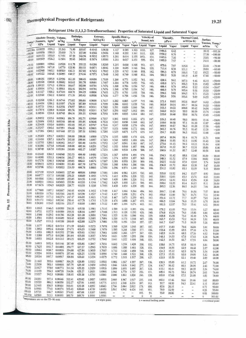
A1: R134a Tables
A2: P-h Diagrams
A3: Moody Diagram

Nomenclature
Symbol Description Units
COP Coefficient of Performance -
h Specific enthalpy kJ/kg
ṁ Mass flow rate kg/s
P Pressure MPa
q Specific heat kJ/kg
s Specific entropy kJ/kg-K
T Temperature ℃
w Specific work done by the compressor kJ/kg
ρ Density kg/m3
L Length m
Subscripts
Symbol Description
1 State between the evaporator and compressor
2 State between the compressor and condenser
3 State between the condenser and expansion valve
4 State between the expansion valve and evaporator
Carnot The maximum COP value that can, theoretically, be obtained
H Refers to a highest temperature, which is where the condenser transfer energy to
in Refers to specific work transferred into the system by the compressor
L Refers to a lowest temperature, which is where the evaporator transfer heat from

1. Introduction:
A very popular restaurant is planning to move into a new location. Based
upon the recommendation of the architect, they need a refrigeration system
with the load capacity of 1.25 tons (1 ton=12000Btu/hr) to keep the perishable
food storage room at 20o F. The ambient air temperature is 80o F. The team has
been selected to design an efficient refrigeration system for the restaurant.
Environmentally friendly refrigerant was to be used (e.g. R 134a).

2. Methods:
2.1.1 Assumptions
● The mass flow rate remains constant throughout the system ● Maximum density is used for Power loss calculations
2.1.2 Material Selection
Components:
After a final design space was picked, final components were picked based off the specifications required from each state.
Pipes:
Stainless steel is durable, long lasting, and most importantly, has a low roughness factor and will therefore lead to low pressure drops overall. For this reason, Stainless steel was selected as the material for the pipes.
2.1.3 Calculation Procedure
Before the calculations were carried out, a basic understanding of the refrigeration cycle chosen needs to be had or achieved. This design utilizes a vapor-compression refrigeration cycle. The physical components, as well as the defined and numbered states, are provided below:
Figure 2.1: Components and states of a vapor-compression refrigeration cycle

Now that the basic states and components are known or have been decided upon, knowledge
of the general vapor-compression cycle will be of great use in designing our refrigeration system. The
pressure-enthalpy diagram as well as temperature-entropy diagrams are provided below:
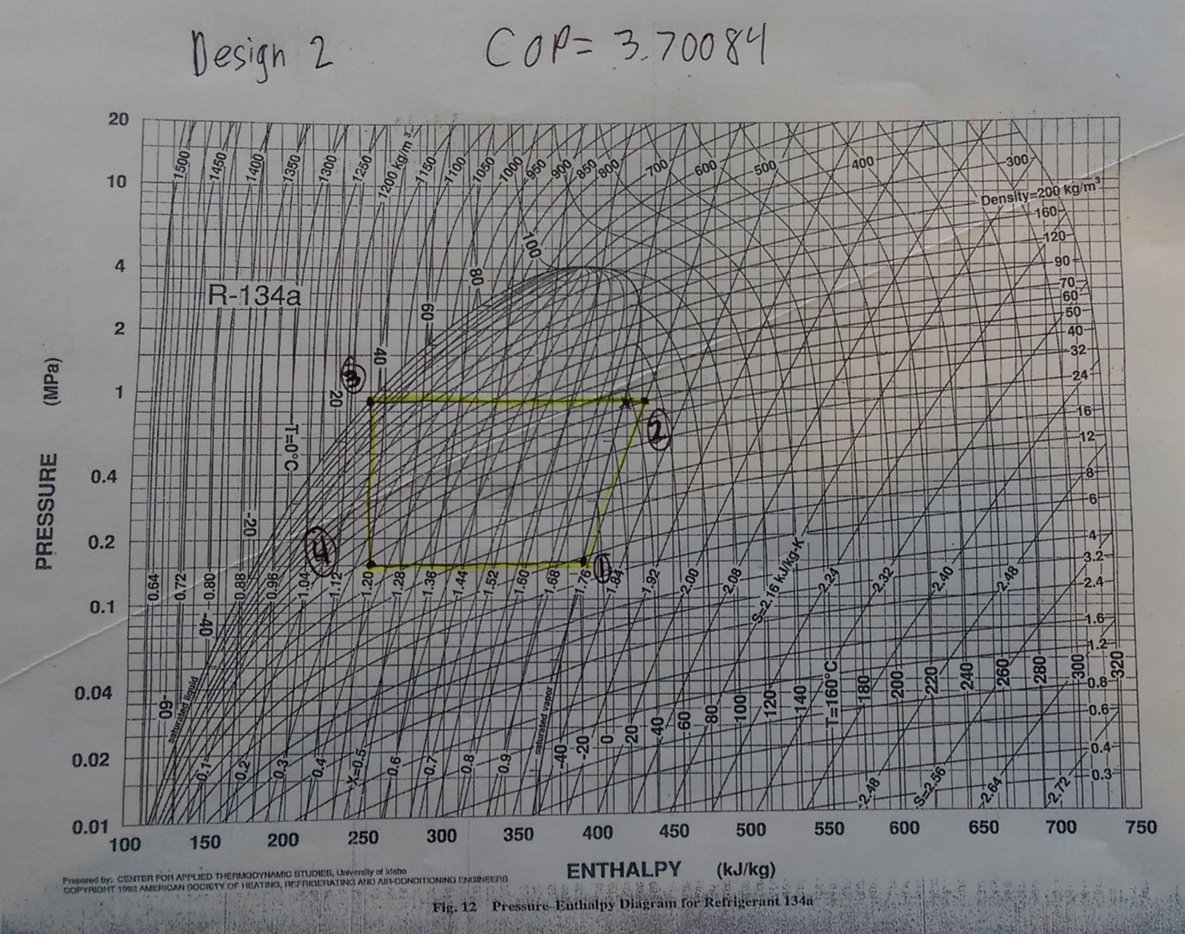
Figure 2.2: General pressure-specific enthalpy diagram with state numbers marked
First a temperature shall be chosen such that it is lower than the temperature of theT 1
refrigerated room (20 ℉ or -6.7 ℃). Next, a temperature shall be chosen such that it is higher thanT 3
the temperature of the ambient air that is exterior of the refrigerator (80 ℉ or 26.7 ℃). Using the
temperature for and the saturated vapor/liquid tables in Appendix A1, the specific enthalpy,T 1
specific entropy, absolute pressure, and density can be found under the saturated vapor columns that
are in line with the respective temperature for . Once this is done, using the temperature for T 1 T 3
and the saturated vapor/liquid tables in Appendix A1, the specific enthalpy, specific entropy, absolute
pressure, and density can be found under the saturated liquid columns that are in line with the
respective temperature for . Once this has been accomplished, the pressure for states 4 and 2 canT 3
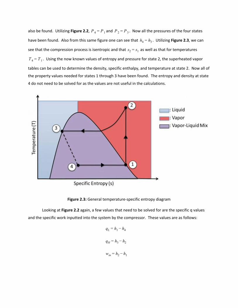
also be found. Utilizing Figure 2.2, and . Now all the pressures of the four statesP 4 = P 1 P 2 = P 3
have been found. Also from this same figure one can see that . Utilizing Figure 2.3, we canh4 = h3
see that the compression process is isentropic and that as well as that for temperaturess2 = s1
. Using the now known values of entropy and pressure for state 2, the superheated vaporT 4 = T 1
tables can be used to determine the density, specific enthalpy, and temperature at state 2. Now all of
the property values needed for states 1 through 3 have been found. The entropy and density at state
4 do not need to be solved for as the values are not useful in the calculations.
Figure 2.3: General temperature-specific entropy diagram
Looking at Figure 2.2 again, a few values that need to be solved for are the specific q values
and the specific work inputted into the system by the compressor. These values are as follows:
qL = h1 − h4
qH = h3 − h2
win = h2 − h1

Now that the q values and specific work have numerically been found, a coefficient of
performance (COP) can be calculated as such:
OP C = h −h2 1
h −h1 4 = qLwin
To evaluate how efficient the design is, the COP of the Carnot cycle (or the theoretically
largest possible COP) can be calculated as such:
COP carnot =TL
T −TH L
The temperature values of and are the temperatures of the refrigerated room andT L TH
ambient air, respectively. Note that, realistically, the COP will never reach the Carnot cycle COP.
Mass Flow Rate Determination
To determine the required mass flow rate, the load capacity is first divided by qL and then by qH,
resulting in two, distinct mass flow rates.
mdot = qload capacity
The mass flow rate chosen must be greater than both of the resulting mass flow rates.
Power Loss Calculations
To calculate pressure losses and power required to overcome the losses in , the following equations were used:
Although the density is changing throughout the system, the highest density can be picked for a worst case scenario of power loss.
Power = Pressure *Volumetric flow rate
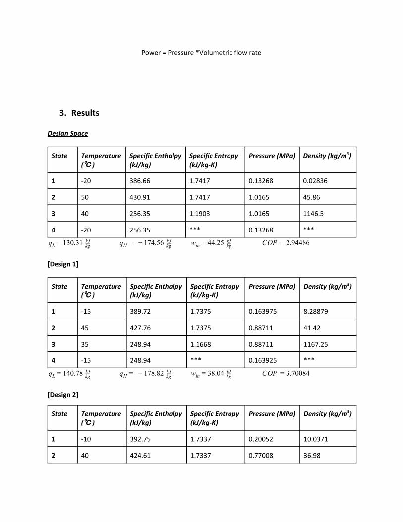
3. Results
Design Space
State Temperature (℃ )
Specific Enthalpy (kJ/kg)
Specific Entropy (kJ/kg-K)
Pressure (MPa) Density (kg/m3)
1 -20 386.66 1.7417 0.13268 0.02836
2 50 430.91 1.7417 1.0165 45.86
3 40 256.35 1.1903 1.0165 1146.5
4 -20 256.35 *** 0.13268 ***
30.31 qL = 1 kgkJ 74.56 qH = − 1 kg
kJ 4.25 win = 4 kgkJ OP .94486C = 2
[Design 1]
State Temperature (℃ )
Specific Enthalpy (kJ/kg)
Specific Entropy (kJ/kg-K)
Pressure (MPa) Density (kg/m3)
1 -15 389.72 1.7375 0.163975 8.28879
2 45 427.76 1.7375 0.88711 41.42
3 35 248.94 1.1668 0.88711 1167.25
4 -15 248.94 *** 0.163925 ***
40.78 qL = 1 kgkJ 78.82 qH = − 1 kg
kJ 8.04 win = 3 kgkJ OP .70084C = 3
[Design 2]
State Temperature (℃ )
Specific Enthalpy (kJ/kg)
Specific Entropy (kJ/kg-K)
Pressure (MPa) Density (kg/m3)
1 -10 392.75 1.7337 0.20052 10.0371
2 40 424.61 1.7337 0.77008 36.98

3 30 241.65 1.1432 0.77008 1187.2
4 -10 241.65 *** 0.20052 ***
51.1 qL = 1 kgkJ 82.96 qH = − 1 kg
kJ 1.86 win = 3 kgkJ OP .74262C = 4
[Design 3]
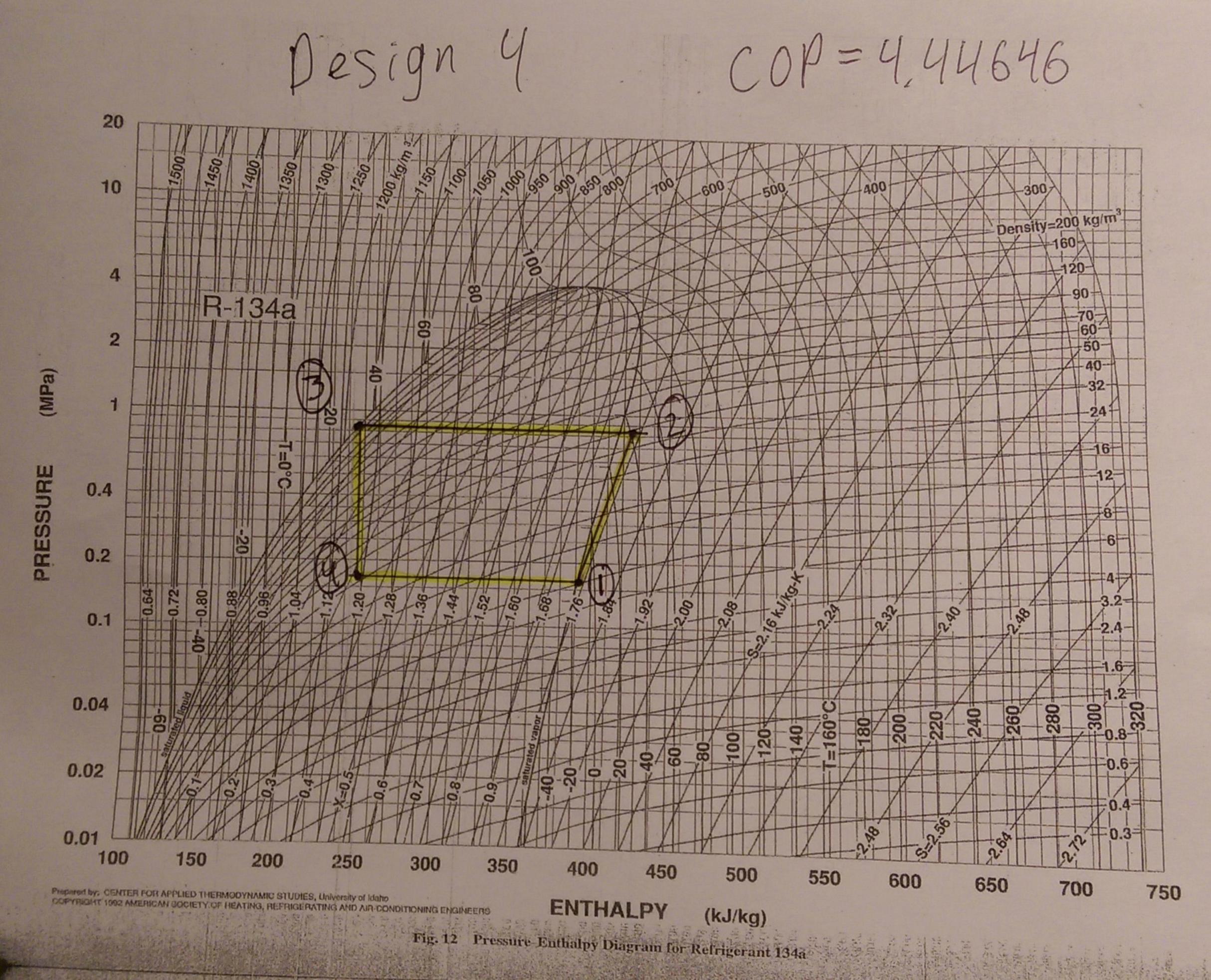
State Temperature (℃ )
Specific Enthalpy (kJ/kg)
Specific Entropy (kJ/kg-K)
Pressure (MPa) Density (kg/m3)
1 -12 391.55 1.7351 0.18516 9.30319
2 40 424.61 1.7351 0.81530 36.98
3 32 244.55 1.1527 0.81530 1179.3
4 -12 244.55 *** 0.18516 ***
47 qL = 1 kgkJ 80.06 qH = − 1 kg
kJ 3.06 win = 3 kgkJ OP .44646C = 4
[Design 4]
The fourth design space was selected.
Mass Flow Rate Determination
The provided load capacity is given in units of BTU/hr. To use it in the analysis, it must
first be converted to kJ/s.
2, 00 (0.00029307) 3.5168 1 0 hrBTU = s
kJ
Using the equation defined above, the necessary mass flow rate is first determined for
qL as follows:
391.55 244.55) 47.0 qL = h1 − h4 = ( − kgkJ = 1 kg
kJ
.0239 ṁ = qLload capacity = 147.0 kg
kJ3.5168 s
kJ
= 0 skg

The process is then repeated for qH:
244.55 24.61) 82.06 qH = h3 − h2 = ( − 4 kgkJ = − 1 kg
kJ
.01932 ṁ = QHload capacity = 182.06 kg
kJ3.5168 s
kJ
= 0 skg
The selected mass flow rate must be larger than qL, the the greater of the two values.
Applying a factor of safety of 1.5, the resulting mass flow rate is:
.5 .0239 .0359 ṁ = 1 * 0 skg = 0 s
kg
Power Loss Determination
Assuming all components are connected by straight pipes allows for the
assumption that there will be no power loss due to minor head loss. Although
this may seem far fetched, the fact of the matter is that this design will cool a
large industrial room sized refrigerator, and so a design wherein there are no
bends apart from inside components is possible. Again, because of the large
area, a small length and relatively large diameter can be used.
Using Moody-Diagram[Appendix] - [Use properties at state 3]
L=characteristic length = l = 2 meters
D= diameter = .25 meters

Density = 1179.3 kg/m3
Area = (D/2)2*pi = .049 m2
Volumetric flow rate = mdot/density = 42.33 m3/s
Velocity = Volumetric Flow rate/Area = 862.48 m/s
Viscosity @ 32 degrees = 196 * 10-6 Pa*s
Reynolds Number = 1.03*1010
Roughness of steel=[0.000015 m]
Relative roughness = Roughness/Diameter = .00006
Using Moody Diagram, at Reynolds number of 1.03*1010 and relative roughness
of .0006, the friction factor was found to be .017.
Pressure Drop = (.017)*(2m/.025m)*Density*Velocity2/2
Pressure Drop = 5.96529*106 Pa
Power = Pressure Drop * Volumetric Flow Rate = 2505.42 kW
Discussion:
The mass flow rate varies based on the design space selected. The larger
qL or qH value, the smaller the required mass flow rate will be. A smaller mass
flow rate is desirable as it will require less power to pump the refrigerant
through the system. The selected design has a relatively low mass flow rate and
therefore met this criteria. A factor of safety of 1.5 was applied to the mass flow

rate to ensure that the overall load capacity would remain under the required
12,000 BTU given in the design specifications.
The pressure drop and Power losses were calculated to be massive, but
these values were calculated from worst case scenarios and the high densities of
state 3. Additionally, the refrigerator needs to be reliable and withstand long
periods of time. In reality, the real pressure loss will be negligible compared to
this value. Furthermore, many of the components will contain their own pump,
and as such, a seperate pump will not be purchased.
4. Conclusions:
The Carnot Cycle should have a COP of 8. The team would choose design 3 as it has the highest COP,
but the temperature difference between the evaporator and the storage room as well as the
temperature difference between the condenser and the ambient air is very small. Heat can only be
transferred from the refrigerator to the evaporator if the evaporator is at a lower temperature.
Likewise, the condenser has to be at a higher temperature than the ambient air for heat transfer to
occur in the direction from the condenser to the ambient air. The gap in temperatures in design 3 are
close enough that the system runs the risk of not working if there’s a slight variation in temperature.
Therefore, to ensure that the refrigerator works the team picked the next efficient design with a
larger temperature gap. This particular design was design 4:
State Temperature (℃ )
Specific Enthalpy (kJ/kg)
Specific Entropy (kJ/kg-K)
Pressure (MPa) Density (kg/m3)
1 -12 391.55 1.7351 0.18516 9.30319
2 40 424.61 1.7351 0.81530 36.98
3 32 244.55 1.1527 0.81530 1179.3
4 -12 244.55 *** 0.18516 ***

47 kJ/kg qL = 1 80.06 kJ/kg qH = − 1 3.06win = 3 OP .44646C = 4
Using the above points for Specific Enthalpy, minimum specifications for each component were
determined.
Compressor Wattage = Enthalpy [State 2 - State 1]*mass flow rate = .971 kW
Evaporator Wattage = Enthalpy [State 4 - State 1]*mass flow rate = 5.49 kW
Condenser Wattage = Enthalpy [State 2 - State 3]*mass flow rate = 6.46 kW
Final BOM:
Part Description Source Unit Price Qty Total Price
Compressor Embraco FF8.5HBK1
Grainger $ 276.75 1 $ 276.75
Condenser True 950663
Condensing Unit
webstaurantstore $ 319.99 1 $ 319.99
Evaporator Sears Part #: 5303918284
SearsPartsDirect $186.30
1 $186.30
Expansion Valve
DELFIELD 3516273
PartsTown $ 124.47 1 $ 124.47
Total Price: $ 907.51

Section 6: Acknowledgements
Our project team would like to thank the following people for their assistance during this project:
o Dr. J. R. Kadambi – for the useful R134a tables, pressure-enthalpy diagrams, and suggestions pertaining to the design process.

References
[1] S. Turns, Thermal-fluid sciences . Cambridge: Cambridge University Press, 2006.
[2] '1997 ASHRAE Fundamentals Handbook', Building Services Engineering Research and Technology , vol. 2, no. 4, 1997.

Academic Integrity Statement
This report was written in accordance with the academic integrity policy described in the student handbook of Case Western Reserve University. The following signatures verify that each group member adhered to these standards.
Abdallah Soliman ________________________________ Date: ____________________
Masih Ahmed ________________________________ Date: ____________________
Ryan Seballos ________________________________ Date: ____________________

A1: R134a Tables


A2: P-h Diagrams


A3: Moody Diagram

ESSOM CO., LTD. 510/1 Soi Taksin 22/1 Taksin Rd. Bukkalo Thonburi Bangkok 10600 Thailand Tel. +66 2476 0034 Fax. +66 2476 1500 E-mail : [email protected], http://www.essom.com
MOODY DIAGRAM
Fric
tion
fact
ors f
or a
ny ty
pe a
nd si
ze o
f pip
e. (F
rom
Pip
e Fr
ictio
n M
anua
l, 3r
d ed
., H
ydra
ulic
Inst
itute
, New
Yor
k, 1
961)