design of a wideband vivaldi antenna array for...
TRANSCRIPT

i
DESIGN OF A WIDEBAND VIVALDI ANTENNA ARRAY
FOR THE SNOW RADAR
by
Raviprakash Rajaraman
B.E. (Electronics & Communications Engg.), Coimbatore Inst. of Tech, India, 2001
Submitted to the Department of Electrical Engineering and Computer Science and the
Faculty of the Graduate School of the University of Kansas in partial fulfillment of the
requirements for the degree of Master of Science.
--------------------------------
Dr. Prasad Gogineni
-------------------------------- Dr. Glenn Prescott --------------------------------- Dr. Pannir Kanagaratnam 2nd February, 2004 --------------------------------- Date project defended

ii
To my parents and sisters

iii
ACKNOWLEDGEMENTS
I wish to express sincere thanks to my advisor, Dr. Prasad Gogineni, for giving me this
opportunity to work on this project. I would like to thank Dr. Glenn Prescott for agreeing
to serve on my defense committee.
I would also like to extend my gratitude to Dr. Pannir Kanagaratnam for not only serving
on my committee, but also for the invaluable time and effort that he has put into this
project. I would like to acknowledge that without his advice this project would not have
been completed in time. I also take this opportunity to thank Dennis Sundermeyer for
always being ready to help me out with the antenna assembly and also doing an
exceptional job at it.
It is also my pleasure to thank Sudarsan for being such a great help in making
measurements with the antenna both inside and outside the building. I would like to
extend my thanks Timothy Rink and Bharath for helping me with the pattern
measurements on the roof in not so friendly weather. I also thank Harish and Abhinay for
helping me with the measurements.
I am grateful to John Paden and Dr. Dawood for being ready to answer my numerous
questions anytime. Thanks are also due to all the people at Ansoft technical support for
assisting me with the simulations.
I would like to extend a word of thanks to all my friends who have made my stay in
Lawrence a pleasant and memorable one. I like to thank my parents and sisters, whose
unlimited love and support has made this effort possible. Finally, I thank Almighty God
for always being there to guide me through thick and thin.

iv
ABSTRACT
A 2-8 GHz FM-CW based radar was built at the University of Kansas to measure the
thickness of snow cover over sea ice. Two double-ridged waveguide TEM horn antennas
were used to transmit and receive the radar signals. Although these antennas performed
well for ground-based radar measurements it would be prudent to seek an antenna with a
narrower beamwidth for airborne experiments. A narrow beamwidth antenna would be
required for airborne applications to reduce the effects of off-angle clutter from the snow
surface. However, an array of horn antennas would be bulky due to its relatively large
size. It was then decided to design an array of Vivaldi antennas to obtain a narrower
beamwidth. The Vivaldi is extremely light weight and could be easily developed as an
array with relatively lower cost than the horn antennas.
The characteristics of the Vivaldi antenna were understood through extensive simulations
performed in Ansoft HFSS after which the Vivaldi antenna was built and tested at the
RSL. The gain and the S11 of the single element were found to be quite poor.
Subsequently, a 12-element array was built. A metal plate was fixed to the back of the
antenna to reflect any signals going in the backward direction. The S11 of the array was
found to be better than -7 dB almost throughout the desired bandwidth, except at about 3
GHz. The pattern measurements were also done on this array using the antenna range
(KUAR) on the roof of the building. These revealed a fairly narrow beamwidth on the E-
plane and a wide one on the H-plane throughout the bandwidth. The average half-power
beamwidth in the E-plane for the Vivaldi was 15° while it was about 50° for the TEM
horn. The realized gain was found to vary between 8.5 dB at the lower end to about 16
dB at the higher end of the bandwidth. However, since the measurements were done in

v
less than ideal conditions, they were prone to errors, both human and otherwise. Most of
the design requirements for this antenna were met. A few changes to the design with
regards to impedance matching would make it ready for installation and integration with
the rest of the radar equipment.

vi
Table of Contents
Chapter 1 Introduction........................................................................................................ 1
1.1 Significance of snow thickness measurements over sea ice..................................... 1
1.2 Objective................................................................................................................... 2
1.3 Organization.............................................................................................................. 3
Chapter 2 Vivaldi antenna.................................................................................................. 5
2.1 Characteristics........................................................................................................... 5
2.1.1 Construction....................................................................................................... 5
2.1.2 Principle of operation......................................................................................... 6
2.1.3 Radiation............................................................................................................ 7
2.1.4 Bandwidth.......................................................................................................... 7
2.2 Taper profiles............................................................................................................ 9
2.2.1 Types.................................................................................................................. 9
2.2.2 Effect of curvature on the TSA ........................................................................ 10
2.3 Feeding techniques.................................................................................................. 10
2.3.1 Coaxial-slotline transition................................................................................ 11
2.3.2 Microstrip-slotline transition ........................................................................... 13
2.4 Summary................................................................................................................. 16
Chapter 3 Antenna design................................................................................................. 17
3.1 Parameter study: An overview................................................................................ 17
3.2 Introduction............................................................................................................. 18
3.3 Substrate material.................................................................................................... 20
3.4 Feed mechanism...................................................................................................... 21

vii
3.4.1 Background...................................................................................................... 21
3.4.2 Stripline-slotline transition............................................................................... 22
3.5 Taper design............................................................................................................ 29
3.6 Array design............................................................................................................ 30
3.6.1 Introduction...................................................................................................... 30
3.6.2 Array factor...................................................................................................... 31
3.6.3 Mutual Coupling.............................................................................................. 32
3.6.4 Linear Vivaldi array......................................................................................... 33
3.7 Fabrication .............................................................................................................. 35
3.8 Summary................................................................................................................. 36
Chapter 4 Simulation ........................................................................................................ 38
4.1 Introduction............................................................................................................. 38
4.2 Description.............................................................................................................. 39
4.2.1 Single element Vivaldi antenna....................................................................... 40
4.2.2 Infinite Vivaldi array with backplane.............................................................. 46
Chapter 5 Test & Measurement ........................................................................................ 53
5.1 Background............................................................................................................. 53
5.2 Power divider .......................................................................................................... 54
5.3 Reflection measurements........................................................................................ 56
5.3.1 Test setup......................................................................................................... 56
5.3.1 Single element Vivaldi antenna....................................................................... 57
5.3.2 Twelve-element Vivaldi array ......................................................................... 60
5.4 Pattern measurements............................................................................................. 67

viii
5.4.1 Introduction...................................................................................................... 67
5.4.2 Setup ................................................................................................................ 69
5.4.3 Polarization...................................................................................................... 72
5.4.4 Gain measurement ........................................................................................... 73
5.4.5 Radiation pattern measurements...................................................................... 75
5.5 Summary................................................................................................................. 83
Chapter 6 Summary and recommendations...................................................................... 85
6.1 Summary................................................................................................................. 85
6.2 Recommendations................................................................................................... 88
Chapter 7 References........................................................................................................ 90
Chapter 8 Appendix .......................................................................................................... 93
8.1 Datasheets............................................................................................................... 93
8.2 Pictures.................................................................................................................... 93

ix
List of Figures
Figure 2-1: Vivaldi antenna................................................................................................ 5
Figure 2-2: Typical radiation pattern of TSAs[10] ............................................................. 7
Figure 2-3: Different taper-styles of the TSA: (a) Exponential (Vivaldi); (b) Linear-
constant; (c) Tangential; (d) Exponential-constant; (e) Parabolic; (f) Step-constant;
(g) Linear; (h) Broken-linear [12] ............................................................................... 9
Figure 2-4: Different feed techniques: (a) Coaxial line;(b) Microstrip; (c) CPW; (d) air-
bridge/GCPW, (e) FCPW/centre-strip, (f) FCPW/notch [12] .................................. 11
Figure 2-5: Coax-slotline feed .......................................................................................... 12
Figure 2-6: Coax-fed Vivaldi antenna [17]....................................................................... 12
Figure 2-7: Microstrip-slotline transition.......................................................................... 13
Figure 2-8: Microstrip-slotline transition using radial stubs [20] ..................................... 14
Figure 2-9: Antipodal Vivaldi antenna [22]...................................................................... 15
Figure 2-10: Balanced antipodal Vivaldi antenna [24] ..................................................... 16
Figure 3-1: Vivaldi notch element .................................................................................... 19
Figure 3-2: Microstrip-slotline transition.......................................................................... 22
Figure 3-3: Stripline Triplate Structure............................................................................. 24
Figure 3-4: Slotline structure – end and top views........................................................... 25
Figure 3-5: Double transition in HFSS[R].......................................................................... 27
Figure 3-6: (a) S11; (b) S21 - Simulation results of the transition ................................... 28
Figure 3-7: Vivaldi antenna parameters............................................................................ 29
Figure 3-8: AF of 2 isotropic sources with identical amplitude and phase currents spaced
one-half wavelength apart......................................................................................... 32

x
Figure 3-9: AF of an endfire 12-element linear array at 8 and 2 GHz.............................. 34
Figure 3-10: (a) Single element Vivaldi antenna; (b) 12-element Vivaldi array.............. 36
Figure 4-1: Single element Vivaldi model ........................................................................ 40
Figure 4-2: S11 of single element Vivaldi antenna .......................................................... 41
Figure 4-3: E-field plot of structure.................................................................................. 41
Figure 4-4: E & H field intensity vectors.......................................................................... 42
Figure 4-5: E & H plane cuts of Vivaldi antenna............................................................. 44
Figure 4-6: E & H plane rectangular plots........................................................................ 45
Figure 4-7: Infinite array Vivaldi model........................................................................... 48
Figure 4-8: E and H plane cuts ......................................................................................... 51
Figure 4-9: HPBW of 12 element linear array.................................................................. 51
Figure 5-1: Characteristics of 12-way power divider ....................................................... 55
Figure 5-2: S11 measurement setup.................................................................................. 56
Figure 5-3: S11 comparison.............................................................................................. 58
Figure 5-4: Reflection from target at 7ft from antenna..................................................... 58
Figure 5-5: Test setup for array antenna........................................................................... 61
Figure 5-6: Array reflection measurements...................................................................... 62
Figure 5-7: Vivaldi array setup......................................................................................... 63
Figure 5-8: Time-gating of reflected signal ...................................................................... 65
Figure 5-9: Radiation pattern measurement setup ............................................................ 68
Figure 5-10: Antenna Range setup ................................................................................... 71
Figure 5-11: Azimuth & Elevation cuts at 2.5 GHz ......................................................... 79
Figure 5-12: Azimuth & Elevation cuts at 5 GHz ............................................................ 81

xi
Figure 5-13: Azimuth and elevation cuts at 7.5 GHz ....................................................... 82
Figure 8-1: Vivaldi antenna array in (a) Horizontal, and (b) Vertical polarization.......... 94
Figure 8-2: Double-ridged waveguide horn - Vertically polarized .................................. 94

xii
List of Tables
Table 3-1: Dielectric characteristics................................................................................. 21
Table 3-2: Stripline parameters......................................................................................... 23
Table 3-3: Transition parameters...................................................................................... 27
Table 3-4: Antenna features.............................................................................................. 37
Table 4-1: General simulation settings in HFSS............................................................... 40
Table 4-2: Antenna parameters at 6 GHz ......................................................................... 46
Table 5-1: Network Analyzer settings.............................................................................. 59
Table 5-2: Single element antenna - reflection measurement........................................... 60
Table 5-3: Power ratio comparison................................................................................... 67
Table 5-4: Antenna range setup features .......................................................................... 72
Table 5-5: Horn gain measurements................................................................................. 75
Table 5-6: Vivaldi gain measurements............................................................................. 75
Table 5-7: Measurement results........................................................................................ 84

1
Chapter 1 Introduction
1.1 Significance of snow thickness measurements over sea ice
Sea ice plays a crucial role in the global climate system. As such, changes in sea ice
extent can foretell changes in the global climate system [1]. In addition, sea ice also has
an important role in the polar ecosystem. It is home to various algae and protozoa and
serves as a platform for seals, penguins and polar bears [2].
Due to its low thermal conductance, sea ice limits the amount of heat that is exchanged
between the ocean and the atmosphere. This is especially important in winter as it helps
the ocean to preserve its thermal energy. The presence of snow cover further reduces the
thermal loss from the ocean as it acts as a blanket to retain the heat. The snow cover also
regulates the amount of solar radiation that is absorbed by the underlying media. Like any
white surface, snow also reflects most of the solar radiation due its high reflectivity. The
degree of reflectivity is a measure of its albedo. A high albedo indicates a highly
reflective medium. Due to its high albedo, snow cover reflects about 80% of the solar
radiation back to space. This helps to keep the polar region colder than what it would be
if there was no snow or ice cover.
By continuously monitoring the sea ice extent and snow cover over the polar region
scientists will be able to understand the dynamics of snow, ice and ocean interaction. This
will also help scientists develop models to predict the changes that may occur in the
global climate. Due to these factors it is important for us to be able to observe the sea ice
extent and snow cover over the polar regions. The only effective means of doing this on a
global scale is via remote sensing techniques.

2
1.2 Objective
Markus et al. [3] have developed an algorithm to estimate the thickness of snow cover
from passive microwave data. However there are currently no effective means to test and
validate the algorithm over the footprint of a space-borne radiometer. A prototype ultra
wideband Frequency Modulated Continuous Wave (FMCW) radar has been developed at
the University of Kansas by Wong [4] to measure the thickness of snow over sea ice.
This radar operates from 2 to 8 GHz and has a vertical resolution of about 4 cm in snow.
The prototype was designed to operate on a sled to collect data over snow-covered sea
ice. TEM horn antennas were employed for transmitting and receiving the signals. The
transmitter and receiver, along with the antennas, were mounted approximately 1 m
above the top snow level. This radar was successfully tested in a ground-based
experiment during the fall of 2003 in Antarctica. While the TEM horn antennas were
adequate for a ground-based experiment it would be prudent to seek an antenna
configuration with a narrower beamwidth for airborne application. A narrow beamwidth
antenna would be required for airborne applications to reduce the effects of off-angle
clutter from the snow surface.
A narrow beamwidth can be obtained by arranging the antenna in an array configuration.
The TEM horn is too bulky and would have been difficult to use in an array configuration
owing to its relatively large size. The objective of this project is to design an array
antenna that would operate in the 2 to 8 GHz frequency range and that is not as bulky as
the horn. The Vivaldi antenna has a number of characteristics favorable for this
application. The Vivaldi antenna belongs to the class of tapered slot antennas with an
exponential taper profile and are aperiodic continuously scaled traveling-wave antenna

3
structures[5]. Exceedingly high bandwidths, of the order of more than two octaves could
be reached. The antenna could be designed in such a way that very low beamwidths could
be attained. When designed as an array, the beam switching and shaping could also be
done based on the requirements. Moreover, the cost of buying a horn antenna off the
shelf was very high and this was taken care of by the Vivaldi design which was
completely fabricated in the lab.
1.3 Organization
The report has been divided into a total of six chapters.
Chapter 2 begins with an introduction of the basic Vivaldi antenna. The characteristics
and design considerations will give an insight into the operations of the antenna. The
different types of tapers and their effects on the antenna performance have been
discussed. A literature study was also done on the two major feeding techniques at the
end of the chapter.
Chapter 3 provides an in depth look into the principles of design of the Vivaldi antenna.
The choice of the substrate, the type of feed mechanism and other design issues are
discussed here. The stripline and the slotline designs are discussed separately with
appropriate equations. The design procedure for the linear Vivaldi array is also given.
Finally, the procedure for fabricating the antenna has been described.
Chapter 4 discusses in detail the various simulations that were done in Ansoft HFSS[R] [6]
to understand the performance of the antenna and how the different design parameters
affect it. The S-parameter and the field pattern plots have been generated from the
simulation and have been displayed in this chapter.

4
Chapter 5 talks about the various measurements and calculations that were made with
both the single element as well as with the linear array antenna. Measurements were
made both inside the lab as well as on the roof.
Chapter 6 summarizes the whole project and provides a few areas to improve for the
future.

5
Chapter 2 Vivaldi antenna
This chapter begins with a discussion of the typical characteristics of the Tapered-Slot
Antenna (TSA). The Vivaldi antenna is a special type of TSA with an exponential flare
profile. It is then followed by a review of the various design principles to be taken into
consideration in the process of constructing this antenna. Finally, there is a brief
discussion on the different design methodologies that were proposed in the literature.
2.1 Characteristics
2.1.1 Construction
Figure 2-1: Vivaldi antenna
The Vivaldi (Figure 2.1) is a member of a class of aperiodic continuously scaled
traveling-wave antenna structures[5]. The terms “ tapered-notch” , “ flared-slot” , “ tapered-
slot” antennas have been used interchangeably in the literature. These antennas consist of
a tapered slot etched onto a thin film of metal. This is done either with or without a
dielectric substrate on one side of the film. Besides being efficient and lightweight, the
Wo
WA WE
WE - Input slot width
WA - Slot width at radiating area
WO - Output slot width

6
more attractive features of TSAs are that they can work over a large frequency bandwidth
and produce a symmetrical end-fire beam with appreciable gain and low side lobes[7]. An
important step in the design of the antenna is to find suitable feeding techniques for the
Vivaldi.
Understanding the characteristics of the Vivaldi is fundamental and would help a great
deal in designing the antenna. From research journals on the TSA, we can confirm that
TSAs generally have wide bandwidth, high directivity and are able to produce
symmetrical radiation patterns[8].
The feature that is common to all the different designs of this antenna is the exponentially
flared slot. This aspect is particularly analogous to the standard TEM horn antenna[9] –
the width of the flare increases with distance from the antenna feed. In fact, we could say
that the Vivaldi is the printed-circuit equivalent of the horn. The wave-guiding structure
here is the printed slotline that is tapered exponentially outwards. A more detailed
procedure of construction is explained in a later section.
2.1.2 Principle of operation
As stated earlier, the Vivaldi antenna is a type of a traveling-wave antenna of the
“surface-type” . The waves travel down the curved path of the flare along the antenna. In
the region where the separation between the conductors is small when compared to the
free-space wavelength, the waves are tightly bound and as the separation increases, the
bond becomes progressively weaker and the waves get radiated away from the antenna[5].
This happens when the edge separation becomes greater than half-wavelength ( /2). !
Radiation from high-dielectric substrates is very low and hence for antenna applications
significantly low dielectric constant materials are chosen.

7
2.1.3 Radiation
The tapered-slot antennas utilize a traveling wave propagating along the antenna structure
b ec au s e the p has e velo c i ty "ph i s les s than the velo c i ty o f l i ght i n f r ee s p ac e o r "ph < c (as
well as the li m i ti ng c as e when "ph = c) [5]. Therefore, the Vivaldi is characterized by
radiation in the endfire direction (Figure 2.2) at the wider end of the slot in preference to
o ther d i r ec ti o ns . T he li m i ti ng c as e o f "ph = c relates to the case of the antenna with air as
the dielectric and consequently the beamwidth and the sidelobe level are considerably
greater than with a dielectric present. Also, the phase velocity and the guide wavelength
!g vary with the change in the thickness, dielectric constant and taper design. Typically,
the beamwidth in the E-plane and the H-plane patterns are almost the same.
Figure 2-2: Typical radiation pattern of TSAs[10]
2.1.4 Bandwidth
At different frequencies, different parts of the antenna radiate, while the radiating part is
constant in wavelength[5]. Thus the antenna theoretically has an infinite bandwidth of
operation and can thus be termed frequency independent. As the wavelength varies,
radiation occurs from a different section which is scaled in size in proportion to the
wavelength and has the same relative shape. This translates into an antenna with very
large bandwidth. Again referring to Figure 2.1 it can be seen that the Vivaldi antenna is
divided into two areas:

8
• a propagating area defined by WE < W < WA
• a radiating region defined by WA < W < WO
Where,
W - Slot width
WE - Input width
WA - Slot width at radiating area
WO - Output width
The original Vivaldi antenna proposed by Gibson [5] employed a taper that opened up
real fast thus providing an almost constant beamwidth over the entire frequency range of
about two octaves when plotted with frequency or normalized length. For antennas with
smaller opening angles, the beam width becomes dependent upon the frequency, as
predicted by Zucker[11].
Theoretically, the TSA is capable of having an operating bandwidth within a frequency
range of 2 GHz to 90 GHz while practically the operating bandwidth is limited by the
transition from the feeding transmission line to the slot line of the antenna and by the
finite dimensions of the antenna. Thus to achieve a wider bandwidth, it is imperative for
the designer to have in mind the following two aspects:
• The transition from the main input transmission line to the slot line for feeding
the antenna. This is designed for a low reflection coefficient to match the
potential of the antenna.
• The dimensions and shape of the antenna, to obtain the required beam width, side
lobes and back lobes, over the operating range of frequencies.

9
2.2 Taper profiles
2.2.1 Types
Many taper profiles exist for a normal TSA. Figure 2.3 shows different planar designs
and we can observe that each antenna differs from the other only in the taper profile of
the slot[12]. Planar tapered slot antennas have two common features. The radiating slot
acts as the ground plane for the antenna and the antenna is fed by a balanced slotline.
However, drawbacks for a planar TSA come in the form of using a low dielectric
constant substrate and obtaining an impedance match for the slotline. By fabricating on a
low dielectric constant substrate, relatively high impedance is obtained for the slotline. If
a microstrip feed is chosen, it makes matching very difficult. Thus, the microstrip to slot
transition will limit the operating bandwidth of the TSA.
(a) (b)
(c) (d)
(e) (f)
(g) (h)
Figure 2-3: Different taper-styles of the TSA: (a) Exponential (Vivaldi); (b) L inear-
constant; (c) Tangential; (d) Exponential-constant; (e) Parabolic; (f) Step-constant;
(g) L inear ; (h) Broken-linear [12]

10
2.2.2 Effect of curvature on the TSA
Experiments conducted by Lee and Simons[13] have shown that the curvature of tapered
profile has a significant impact on the gain, beamwidth and bandwidth of tapered slot
antennas. In fact, it was shown that the half-power beamwidth (HPBW) on the E-plane
increases with a decrease in the radius of curvature while the opposite is true on the H-
plane. The cross polarization is generally improved with the decrease in the radius of the
curvature except for the E-plane, which will not show any improvement. Also the authors
have shown that the bandwidth of the antenna reduces with a decrease in the radius of
curvature which is exactly the opposite of what we want to focus on.
2.3 Feeding techniques
In theory, the bandwidth of the Vivaldi antenna is infinite; the only limitation on the
bandwidth is the physical size of the antenna and the fabrication capabilities. In fact, the
feed determines the high frequency limit while the aperture size the low frequency
limit[14]. As discussed earlier, a proper feed structure design becomes essential to
maximize the bandwidth.
Most microwave integrated circuits (MICs) are realized in microstrip transmission
medium. However, the transmission medium best suited for feeding the TSA is a slotline.
In order to couple microwave signals to the antenna from a planar microstrip circuit, a
transition is needed. These transitions should be very compact and have low loss. Some
feeding techniques and their transitions are shown in the Figure 2.5. The commonly used
methods are the coaxial line feed and the microstrip line feed. These will be illustrated
and discussed in the next two sub-sections.

11
(a) (b)
(c) (d)
(e) (f)
Figure 2-4: Different feed techniques: (a) Coaxial line;(b) Microstr ip; (c) CPW; (d)
air -br idge/GCPW, (e) FCPW/centre-str ip, (f) FCPW/notch [12]
2.3.1 Coaxial-slotline transition
A coaxial line feed provides a direct path for coupling of fields across the slot [14]. The
transition consists of a coaxial line placed perpendicular at the end of an open circuited
slot. The outer conductor of the cable is electrically connected to the ground plane on one
side of the slot while the inner conductor of the coaxial line forms a semicircular shape
over the slot[16]. This is shown in Figure 2-5. However, designing slotlines with very low
characteristic impedances is difficult as the width has to then be too narrow and hence
etching becomes inaccurate.

12
Figure 2-5: Coax-slotline feed
Using double-clad, i.e., etching the slotline on both sides of the substrate, rather than
single-clad, reduces the characteristic impedance of the slotline so that better matching
with the coaxial line becomes possible. Weedon et al [17] have used this idea to design a
Vivaldi antenna (Figure 2.6) and has shown a pattern bandwidth of at least 9:1.
Figure 2-6: Coax-fed Vivaldi antenna [17]
#r
Zcl

13
2.3.2 Microstrip-slotline transition
As stated earlier, the microstrip transmission medium is used extensively in MICs.
However, research shows that the slotline would be the medium best suited for feeding
the TSA. The microstrip is an unbalanced transmission line while the medium used for
feeding the Vivaldi is a slotline which is a balanced medium. The success of the whole
design is thus hinged on the design of a proper balun for this transition. The objective is
thus to design a balun that would work over a wide frequency range or ideally be
frequency independent.
A microstrip to slot transition consists of a slot, etched on one side of the substrate,
crossing an open circuited microstrip line, located on the opposite side, at a right
angle[16]. The slot extends to one quarter of a wavelength (!s) beyond the microstrip and
the m i c r o s tr i p ex tend s o ne q u ar ter o f a wavelength (!m) beyond the slot[18] as shown in
Figure 2.7. A more detailed description of the transition and the design procedure is given
in the next chapter.
Figure 2-7: Microstr ip-slotline transition
!s/4
!m/4

14
A major drawback for this kind of a transition is its reduced operating bandwidth. A
number of ways have been suggested in the literature that improves this microstrip-
slotline transition [18], [19], [20]. These methods have not only shown a marked
improvement in the bandwidth but sometimes have shown better radiation characteristics.
These variations have been discussed below in brief. A more detailed description is
available with the stated references and would serve to complete the understanding of the
concepts involved.
2.3.2.1 Non-uniform stubs
Schuppert[18] proposed the use of circular quarter-wave stubs in the design of microstrip-
slotline transitions. This enabled him to obtain a more wideband transition than from the
transitions with straight stubs. Subsequently, with the help of equations provided in [15],
[18] and [19], Sloan et al [20] came up with the idea of using radial stubs instead of the
circular ones as shown in Figure 2.8. A detailed design procedure is given in the next
chapter.
Figure 2-8: Microstr ip-slotline transition using radial stubs [20]

15
2.3.2.2 Antipodal slotline
The symmetric double-sided slotline, also referred to as the antipodal slotline was first
suggested by Gazit[21]. In this case, the transition from the microstrip to the slotline was
realized through a parallel stripline as shown in Figure 2.9. The microstrip was used as
the input feed, the slotline for radiating purposes while the paired-strip served primarily
as the transition region thus critically affecting the antenna performance. This design also
helped avoid the slot hole that was necessary in the earlier designs. Noronha et al [22] have
used this idea to construct a Vivaldi antenna and have shown good results over a wide
frequency range. They have also empirically discovered that the transition region should
be three to five wavelengths long to prevent a sharp discontinuity between the feed and
the radiating regions.
Figure 2-9: Antipodal Vivaldi antenna [22]
2.3.2.3 Balanced antipodal slotline
It was found that the previous design did not have a really good cross-polarization
characteristic. This was even more pronounced at high frequencies, when the angle of the
E-field skew with respect to the physical axis of the antenna increased considerably.
Hence, there was a severe polarization tilt as the frequency of operation was increased.
Microstrip Feed
Paired strip
Slotline
16
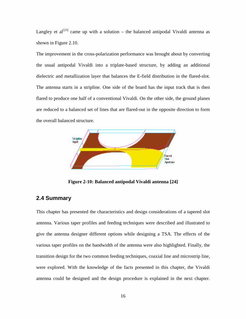
Langley et al [23] came up with a solution – the balanced antipodal Vivaldi antenna as
shown in Figure 2.10.
The improvement in the cross-polarization performance was brought about by converting
the usual antipodal Vivaldi into a triplate-based structure, by adding an additional
dielectric and metallization layer that balances the E-field distribution in the flared-slot.
The antenna starts in a stripline. One side of the board has the input track that is then
flared to produce one half of a conventional Vivaldi. On the other side, the ground planes
are reduced to a balanced set of lines that are flared-out in the opposite direction to form
the overall balanced structure.
Figure 2-10: Balanced antipodal Vivaldi antenna [24]
2.4 Summary
This chapter has presented the characteristics and design considerations of a tapered slot
antenna. Various taper profiles and feeding techniques were described and illustrated to
give the antenna designer different options while designing a TSA. The effects of the
various taper profiles on the bandwidth of the antenna were also highlighted. Finally, the
transition design for the two common feeding techniques, coaxial line and microstrip line,
were explored. With the knowledge of the facts presented in this chapter, the Vivaldi
antenna could be designed and the design procedure is explained in the next chapter.

17
Chapter 3 Antenna design
This chapter describes the step-by-step procedure to design a Vivaldi antenna based on
the specifications for the antenna. The stripline-fed Vivaldi antenna was chosen from all
the other possible designs mainly because of the varied research accomplished on it.
Also, not much work has been done on antenna arrays with feed mechanisms other than
the stripline feed. A single-element antenna was first designed, fabricated and tested
before developing a twelve-element linear array. This design has been based on the
parameter study of the stripline-fed Vivaldi antenna arrays performed by Schaubert[25].
3.1 Parameter study: An overview
As will be stated frequently in this document, the parameter study performed by
Schaubert and Shin has been followed extensively in this design. The objective of the
study was to analyze the various design parameters of the stripline-fed Vivaldi array
antennas so that the wideband performance could be improved in a systematic procedure.
The following were some of the parameters taken into consideration in the parameter
study:
• Diameter of the slotline cavity and the stripline stub
• Input stripline and slotline width
• Taper profile
• Aperture height
The effect of varying these parameter values on the antenna performance (S11 and
pattern) was discussed. Particularly, it was found out that through proper change in the
design parameters, the antenna resistance could be increased and subsequently resulting

18
in a decrease in the minimum operating frequency of the antenna. The higher end of the
bandwidth was set by the onset of grating lobes and hence only way to improve the
bandwidth was by decreasing the lower cutoff. Thus the parameters were varied one at a
time, with all others being constant, and the subsequent effect on the antenna impedance
in a large array was predicted. Hence, this study helps the antenna designer by identifying
some of the most important relationships between the design of the antenna and the
performance of each of the elements in an array.
The above parameters were studied for different combinations of substrate thickness and
stripline & slotline characteristic impedances. Of all the different design possibilities that
were tested in the study, the one that was claimed to have the largest bandwidth and at the
same time, displayed a better performance (S11/ antenna resistance) was chosen for the
actual design. The reader is referred to the stated publication [25] for greater detail.
3.2 Introduction
The stripline-fed Vivaldi notch antenna comprises:
• The stripline-to-slotline transition.
• The stripline open circuit stub and slotline short circuit cavity.
• The radiating tapered slot.
Figure 3.1 is a snapshot of the triplate-structured Vivaldi notch element as modeled in
HFSS. The outside layers, viz., the top and the bottom layers (in red) are identical tapered
slotlines which also act as ground planes for this antenna. The middle layer is the stripline
plane (in green) that is used as the connection to the signal input or any test equipment.
These three layers together form the Vivaldi-notch antenna. The input signal is fed to the
stripline input and is then magnetically coupled to the slotline on either sides of the

19
board. The input impedance of the antenna is dictated by the stripline while the operating
bandwidth of the antenna is governed by the stripline-to-slotline transition.
Figure 3-1: Vivaldi notch element
It was shown by Yngvesson[9] and Gibson[5] that single-element Vivaldi antennas work
best when they are over a wavelength long and when the height of the antenna aperture is
greater than one-half wavelength. In the case of arrays, on the other hand, good
performance is obtained from antennas that are less than a wavelength long and when the
element heights are much less than a wavelength. Typically, a single element in an array
is unmatched almost throughout the bandwidth of interest. However, by proper array
design, mutual coupling between the elements can be constructively used and very
wideband behavior could be accomplished. The balanced-antipodal Vivaldi [24] was also
fabricated and tested, but its behavior in an array was not well documented. Hence this
particular design was not considered.
The succeeding sections will discuss about the specifics of the design of the Vivaldi
notch element. The design of a single-element is first considered after which the linear

20
array design is discussed. Antenna simulations done in Ansoft HFSS[R] are discussed in
the next chapter.
3.3 Substrate material
The choice of dielectric substrate plays an important role in the design and simulation of
transmission lines as well as antennas. Some important dimensions of the dielectric
substrate are, in no specific order:
• The dielectric constant.
• The dielectric loss tangent that sets the dielectric loss.
• The thickness of the copper surface.
• The thermal expansion and conductivity.
• Cost and manufacturability.
There are numerous types of substrates that can be used for the design of antennas. They
often have different characteristics and their dielectric constants normally range from 2.2
$ #r $ 1 2. T hi c k s u b s tr ates wi th lo w r elati ve d i elec tr i c c o ns tants ar e o f ten u s ed as they
provide better efficiency and a wider bandwidth. However, using thin substrates with
high dielectric constant would result in smaller antenna size. But this also results
negatively on the efficiency and bandwidth. Therefore, there must be a design trade-off
between antenna size and good antenna performance[26].
There are basically two types of losses that occur in any microstrip transmission line –
the conductor and the dielectric losses, both of which increase with frequency. At low
frequencies, the conductor losses dominate while at higher frequencies the loss due to the
dielectric starts to become predominant. Dielectric loss is related to the fact that all
dielectrics contain polarized molecules that move in the presence of EM fields. High-

21
frequency fields oscillate very quickly and as the polar molecules move in sync with the
field, they begin to heat the dielectric material. There's only one possible source for the
heat — the energy of the signal itself. It turns out that dielectric loss increases relentlessly
with higher frequencies and in direct proportion to signal frequency.
Hence, to keep the dielectric losses low at the frequency of operation, the low-dielectric
c o ns tant (#r = 2.22) Rogers Duroid[R] 5880 PTFE material with a low loss-tangent
(0.0009) was chosen for this design. Table 3.1 gives a gist of the major properties of the
material. A datasheet with more details on the different electrical and mechanical
characteristics is provided in the Appendix of this report.
Character istic Value
Dielectric thickness 2*0.062”
D i elec tr i c c o ns tant, #r 2.22
D i s s i p ati o n f ac to r , tan % 0.0009
Thermal coefficient -125 ppm/°C
Thermal conductivity 0.20 W/m/K
Conductor thickness 1 oz. (1.4 mil)
Table 3-1: Dielectr ic character istics
3.4 Feed mechanism
3.4.1 Background
As noted in the previous chapter, the design of the feed mechanism forms the most
critical part of the antenna design as it essentially determines the bandwidth of the
antenna. The different methods of accomplishing this were also discussed. In this section,

22
the design of a stripline-slotline transition as a feed mechanism is described. This design
has been implemented based on the parametric study performed by Schaubert and
Shin[25], which basically makes use of the stripline-slotline feed mechanism. The
microstrip-slotline transition has a lot of advantages over the other mechanisms. This
transition can be easily fabricated by normal photo-etching processes. Also, two-sided
circuit boards are possible with the microstrip on one side and the slotline on the other.
Moreover, the authors have parameterized the antenna and hence the design is a lot easier
to fabricate than the other designs. All these factors helped me in deciding the type of
feed mechanism for the antenna.
3.4.2 Stripline-slotline transition
A detailed introduction to the microstrip/stripline-slotline transition has been done in the
previous chapter. The issues pertaining to the actual design of this transition will be
discussed in this section. As the name suggests, the microstripline/microstrip-to-slotline
transition (Figure 3.2) basically consists of,
• Stripline, used as a connection to the transmitter/receiver circuitry.
• Slotline, which is flared outwards from the feed.
Figure 3-2: Microstr ip-slotline transition
23
Previously, transitions were reported with both straight uniform stubs as well as non-
uniform circular ones. The radial stub was used here which eliminated the problem of
overlapping of the stubs and also provided a better bandwidth than the other two. The
microstrip-to-slotline transition design was adapted from the design by Sloan et al. [20].
As previously discussed, the stubs extend a quarter-wavelength further from the crossing
point. Due to this quarter-wavelength transformation at the overlap, the stripline open
circuit stub appears as a short circuit while the slotline short circuit appears as an open
circuit at the crossing reference plane. Designing a good quarter-wavelength stub is
crucial to obtain a fairly wideband transition.
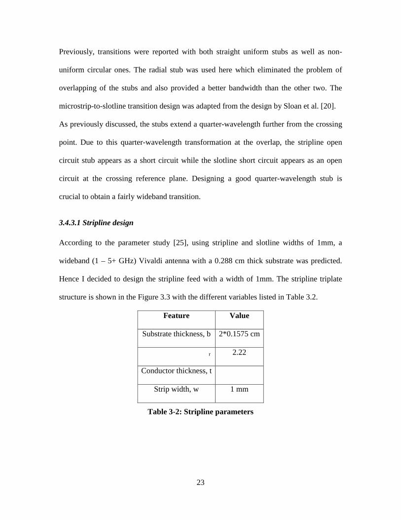
3.4.3.1 Stripline design
According to the parameter study [25], using stripline and slotline widths of 1mm, a
wideband (1 – 5+ GHz) Vivaldi antenna with a 0.288 cm thick substrate was predicted.
Hence I decided to design the stripline feed with a width of 1mm. The stripline triplate
structure is shown in the Figure 3.3 with the different variables listed in Table 3.2.
Feature Value
Substrate thickness, b 2*0.1575 cm
D i elec tr i c c o ns tant, #r 2.22
Conductor thickness, t 3 5 . 5 6 m&
Strip width, w 1 mm
Table 3-2: Str ipline parameters

24
Figure 3-3: Str ipline Tr iplate Structure
Based on the formula given in Wadell [28] (Eqn 3.1) and using LineCalcTM routine in ADS
EESof[R], the c har ac ter i s ti c i m p ed anc e o f the s tr i p l i ne f eed was f o u nd to b e 8 1 . 6 1 . I f '
the conductor thickness was neglected, the characteristic impedance was obtained as
8 4 . 6 1 . T he s tr u c tu r e, wi th the c o p p e r thi c k nes s neglec ted , was then s i m u lated u s i ng '
Ansoft HFSS[R] and the p o r t c har ac ter i s ti c i m p ed anc e was f o u nd to b e 8 5 . 4 5 2 , whi c h '
agrees well with the calculated value.
2.3
0.5ln
0.2
27.60.80.80.8
5.00.1ln0.2
'
2
'''0
0
=∆
∆+=
=
+
++=
t
b
t
w
tt
www
bh
w
b
w
b
w
bZ
rπππεπ
η
Here,
‘b’ : Thickness of the stripline substrate; ‘ t’ : Thickness of conductor; ‘w’ : Stripline width;
( #r) *: D i elec tr i c c o ns tant; 0: 3 7 7 and Z' 0: Characteristic impedance of the stripline.
#r t b
w

25
The stripline open circuit stub was chosen to be of length 8 mm as specified in the paper
[25]. It was shown that stripline radial stub reactance varied from large capacitive values
at the lower frequencies through a near-zero reactance in the mid-band region to
inductive values in the upper band[25].
This behavior of the stub reactance results in favorable compensation of the antenna
reactance, contributing to the wideband performance. The use of the radial/circular stubs
have been shown to achieve a significantly better bandwidth than the uniform stubs [18],
[20]. Moreover, designing non-uniform stubs is easier with modern etching processes.
3.4.3.2 Slotline design
The slotline plane of the antenna consists of the circular slotline cavity, the uniform
slotline input and the tapered radiating slot. The general configuration of a slotline is
shown in Figure 3.4.
Figure 3-4: Slotline structure – end and top views
The slotline width at the transition region was chosen to be 1 mm. As reported by
Schaubert, this transition setup worked well in a frequency range between 1 GHz and 5
W
#r hW

26
GHz [25]. The slotline wavelength and the characteristic impedance were calculated
using formulae given in [15].
The formulae specified are empirical and not in any case exact. The center frequency of 5
GHz is chosen for all the calculations with the substrate parameters being the same as
that o f the s tr i p li ne c as e. T he s l o tli ne wavelength !S was found to be 5.2 cm and the
c har ac ter i s ti c i m p ed anc e was c alc u lated to b e 1 3 0 . 7 8 . '
( )( )
( ) ( )
( ) ( )
( )[ ]( )
( ) ( )( )
( )20
0
00
0
945.0
0
0
0
85.006.2ln18.0148.12ln028.11.131
100lnln48.4011.0181.2
10ln5.13336.2
22.2sin69.360
2.3.ln100
95.081.8148.0
100238
3.6ln365.0045.1
06.0006.0
0.10015.0
8.922.2
hW
hW
h
hh
W
WZ
Eqnh
hW
hW
h
W
r
rr
rr
rr
S
r
rr
rs
r
+−++−+
+−+
+
−
+=
•
+−−
++−=
≤≤
≤≤
≤≤
εελε
λεε
λεπε
λεεε
ελλ
λ
λ
ε
��
Based on [25], I chose the slotline cavity diameter as 1 cm with a uniform slotline
extension of 5 mm. It was shown that increasing the size of the cavity decreased the
lowest frequency of operation of the antenna (when in an array) thus essentially widening
the bandwidth.
To test the frequency response of the transition, two transitions were cascaded together
on a RT/Duroid 5880 substrate. This setup was then modeled in Ansoft HFSS[R] using the
same substrate material, substrate and conductor thickness as mentioned in Table 3.2.

27
The model is shown in Figure 3.5. H-plane symmetry has been used and hence only half
of the model has been modeled to save memory and simulation time.
Design Feature Value
Substrate RT/Duroid[R] 5880
Height 2*0.062”
Stripline width 1 mm
Slotline width at cross plane 1 mm
Stripline stub length 8 mm
Slotline cavity length 10 mm
Length of uniform slotline 3.4 cm
Table 3-3: Transition parameters
Figure 3-5: Double transition in HFSS[R]
28
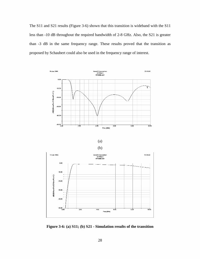
The S11 and S21 results (Figure 3-6) shown that this transition is wideband with the S11
less than -10 dB throughout the required bandwidth of 2-8 GHz. Also, the S21 is greater
than -3 dB in the same frequency range. These results proved that the transition as
proposed by Schaubert could also be used in the frequency range of interest.
(a)
(b)
Figure 3-6: (a) S11; (b) S21 - Simulation results of the transition

29
3.5 Taper design
As discussed in the previous chapter, the TSA with an exponential taper is referred to as
the Vivaldi antenna. Numerous exponentials have been used in the literature[3], [18], [20], [25].
Schaubert, in his design, has used the following exponential relations to design the taper.
With reference to Figure 3-7, R is defined as the opening rate and the points P1(z1,y1)
and P2(z2,y2) are the two end points of the taper profile. A closer look will reveal that P1
is actually the point where the slotline starts to flare after a short of uniform line from the
cavity. The difference z2 – z1 is the flare length L, as shown in the picture below. It is
worth mentioning that when R becomes zero, the slope of the taper becomes constant
resulting in a linearly tapered profile, commonly referred to as the LTSA.
22
22
22
212
121
21
RzRz
RzRz
RzRz
Rz
ee
eyeyc
ee
yyc
where
cecy
−−
=
−−=
+=
P2
P1
H
d
L
Figure 3-7: Vivaldi antenna parameters
A taper length L of 4.5 cm and an aperture height H of 1.7 cm were chosen for this
design based on the parameter study. As the length of the taper is increased, for the same
30
aperture height, the flare angle is reduced correspondingly. It was reported [25] that for
small flare angles, the lowest operating frequency of the array reduces and subsequently
the bandwidth increases. Similar study was also done for the opening rate R of the
exponential flare. For larger opening rates, the flare angle becomes small at the origin and
the lowest frequency of operation reduces as before. Further increase produces significant
improvement in the SWR at the higher operating frequencies. A value of 0.3 was finally
chosen for R based on the data given in [25]. All these values were chosen based on the
plots given in the referred publication by comparing the VSWR and antenna resistance
characteristics.
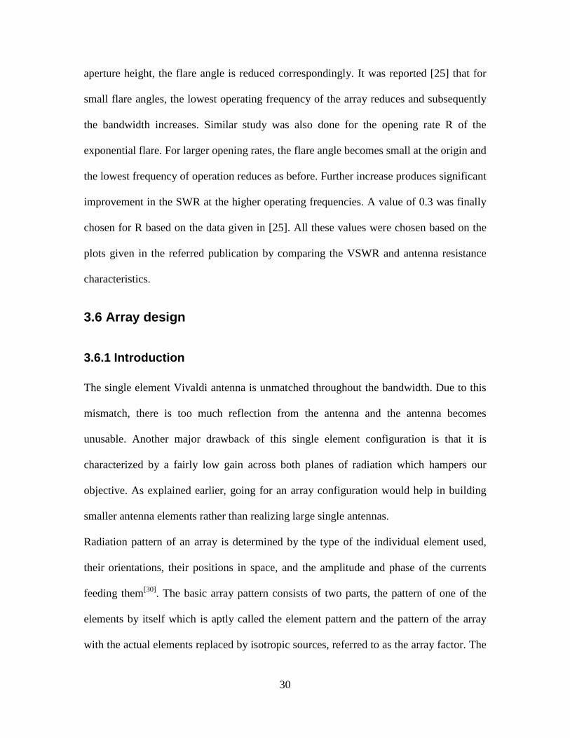
3.6 Array design
3.6.1 Introduction
The single element Vivaldi antenna is unmatched throughout the bandwidth. Due to this
mismatch, there is too much reflection from the antenna and the antenna becomes
unusable. Another major drawback of this single element configuration is that it is
characterized by a fairly low gain across both planes of radiation which hampers our
objective. As explained earlier, going for an array configuration would help in building
smaller antenna elements rather than realizing large single antennas.
Radiation pattern of an array is determined by the type of the individual element used,
their orientations, their positions in space, and the amplitude and phase of the currents
feeding them[30]. The basic array pattern consists of two parts, the pattern of one of the
elements by itself which is aptly called the element pattern and the pattern of the array
with the actual elements replaced by isotropic sources, referred to as the array factor. The

31
total pattern of the array is then the product of the element pattern and the array factor.
The procedure just explained is often referred to as pattern multiplication.
3.6.2 Array factor
The basic configuration of an array antenna is the linear array. As the name suggests, it is
an arrangement of the antenna elements in a single straight line with the appropriate feed
network and phase shifters, if needed. To determine the array factor, the elements are
assumed to be point sources that radiate equally in all directions, commonly known as
isotropic radiators, but retaining their respective locations, their input feeds and phase
differences in them, if any. The distance of separation between the elements is very
crucial in the proper design of the array. This distance dictates the phase difference
between the elements and is inherent to the array.
It is really intuitive to arrive at the array factor for a small linear array, given its setup and
input feed characteristics by what is called the inspection method. Consider a linear array
of two elem ents (p o i nt s o u r c es ) s ep ar ated b y a d i s tanc e o f /2 wi th eq u all y ex c i ted i np u ts !
and no additional phase shifting given on the inputs. At the far-field of the antennas, the
waves arriving from the elements on an axis perpendicular to the line joining the two
sources, add in phase and hence we would see a field maximum in that region. On the
other hand, along the axis of the array, the waves cancel each other at the far-field due to
the phase difference created by the separation between the two sources. A picture of the
two element linear array just described and its array factor is shown in Figure 3-9. The
polar plot would reveal what was described earlier in this paragraph.

32
Figure 3-8: AF of 2 isotropic sources with identical amplitude and phase currents spaced one-half wavelength apar t
3.6.3 Mutual Coupling
The inspection method, though intuitive cannot be used for more complex arrays with
more number of elements and complex phase differences and distance of separation.
Moreover, all these derivations have been based on the assumption that all the elements
are isolated from each other and from external sources. However, in practice, this is
rarely the case. Each element interacts with all the other elements in the array creating
what is known as the mutual coupling which causes changes in the current magnitude,
phase, and distribution on each element. The end result is that the total array pattern is
different from the no-coupling case.
Mutual coupling not only depends on the proximity of the elements, but also on the
frequency and scan direction. Also, it was found that mutual coupling decreases as the
!/2
1 1

33
spacing between elements increases and that the coupling strength is predicted by the far-
field pattern of each of the elements. The input impedance of the ‘m’ th element in the
presence of all other elements and with mutual coupling included is expressed as[26],
mIN
I
mNZ
mI
I
mZ
mI
I
mZ
mIm
V
mZ +++== �
22
11
This is referred to as the driving-point impedance. It is evident that input impedance of
each element depends on the mutual impedances with the other elements in the array and
the terminal currents.
3.6.4 Linear Vivaldi array
As discussed earlier, the inspection method would be easy to work with only for the
simplest of linear array configurations. Hence, a Matlab[R] code written by [31] was used
to plot out the array factor for arbitrary linear arrays. It was observed that the array factor
is a pattern that has rotational symmetry about the line of the array. Hence, its complete
structure is determined b y i ts valu es f o r 0 < < , k no wn as the vi s i b le r egi o n. W hen the + ,
element spacing is one-half wavelength, exactly one period of the array factor appears in
the visible region. The dimensions of the Vivaldi single element would make this
impossible for us to achieve. Less than one period is visible when the spacing is less than
!/2 whi c h wo u l d d ef eat the p u r p o s e o f havi ng thi s ar r ay . W hen the elem ent s p ac i ng
b ec o m es gr eater than /2, m o r e than o ne m aj o r l o b e b ec o m es vi s i b le d e p end i ng o n the !
element phasings. Any other lobe equal in intensity to the major lobe is referred to as a
grating lobe and its presence is undesirable.
In the case of the Vivaldi array, a linear configuration of twelve (12) elements was
chosen. The next logical step was to decide the element spacing. In this specific
34
application, where the antenna was either going to be mounted underneath an helicopter,
the vertical distance was expected to go up to 500 ft. Taking note of this, different array
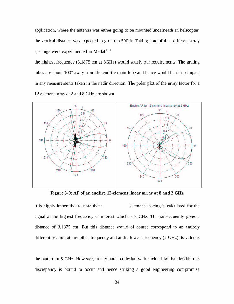
spacings were experimented in Matlab[R] and i t was f o u nd o u t that a s p ac i ng o f 0 . 8 5 at !
the highest frequency (3.1875 cm at 8GHz) would satisfy our requirements. The grating
lobes are about 100° away from the endfire main lobe and hence would be of no impact
in any measurements taken in the nadir direction. The polar plot of the array factor for a
12 element array at 2 and 8 GHz are shown.
Figure 3-9: AF of an endfire 12-element linear array at 8 and 2 GHz
It is highly imperative to note that the 0 . 8 5 i nter! -element spacing is calculated for the
signal at the highest frequency of interest which is 8 GHz. This subsequently gives a
distance of 3.1875 cm. But this distance would of course correspond to an entirely
different relation at any other frequency and at the lowest frequency (2 GHz) its value is
then 0 .21 25 . O b vi o u s l y , thi s valu e wo u l d then p r o d u c e a to tally d i f f e r ent p atter n than !
the pattern at 8 GHz. However, in any antenna design with such a high bandwidth, this
discrepancy is bound to occur and hence striking a good engineering compromise

35
essentially becomes the catch. This compromise would again differ, based on the
application for which the antenna is being designed. For our application, the value of
0 . 8 5 tu r! ned out to be good choice, since the grating lobes were more than 90° away
from the main end-fire lobe and hence it was decided to have it as the inter-element
spacing in the 12-element array.
3.7 Fabrication
The Vivaldi antenna was fabricated as a stripline-fed triplate structure using the LPK
Protomat® milling machine in the Remote Sensing Lab at the ITTC. The input feed to the
stripline was accomplished by an SMA edge connector to realize a coaxial input. The
outer ground pins of the SMA receptacle were shorted to the slotline ground planes of the
antenna. The center pin of the SMA was then soldered to the stripline transmission line.
A wedge/notch had to be made on the copper-less face of one of the dielectrics so that the
center pin of the SMA sits in between the two boards with no air-gaps. Since it was a
triplate structure, the two 0.062” RT/Duroid™ 5880 boards had to be bonded together at
very high temperatures of the order of 220°C with the special-purpose Rogers 3001
bonding film. A similar procedure was followed for fabricating the array antenna.
One major addition that was done to the array antenna was the back ground plane. The
application required that most radiation be oriented in the direction along the flared slot.
The purpose of the backplane, which was made of metal, was to reflect any radiation
going in a direction opposite to that of the required. This would then effectively increase
the forward radiation thus contributing to the gain of the antenna structure.
A picture of the single-element Vivaldi antenna as well as the twelve-element linear array
is shown in the below.

36
(a)
(b)
Figure 3-10: (a) Single element Vivaldi antenna; (b) 12-element Vivaldi array
3.8 Summary
The most crucial aspect of the design of the Vivaldi antenna – the feed mechanism, was
designed and simulated using Ansoft HFSS and then incorporated into the antenna
Vivaldi
Backplane
Power divider

37
design. The transition was found to be of very wide bandwidth. The input impedance of
the antenna was f o u nd o u t to b e ar o u nd 8 5 . T he var i o u s p ar am eter s i nvo lved i n the '
design like the taper width, opening rate, flare angle, size of slotline cavity as discussed
by [25] were considered and based on the reported performance, the nominal values were
chosen. The S11 was measured and the results are shown in Chapter 5 of this report. The
12-element Vivaldi array antenna was then designed with an inter-element spacing of
0 . 8 5 at the hi g! hest frequency (8 GHz) which turned out to be 3.1875 cm. The metal
backplane was then added to the array so that any signal going in the backward direction
would be reflected. The design features are summarized in the table below.
Feature Descr iption/Value
Material R T /D u r o i d 5 8 8 0 , - #r 2.22, 2*0.062” thick
Antenna length 6.4 cm
Antenna width 2.1 cm
Aperture height 1.7 cm
Taper length 4.5 cm
Opening rate 0.3
Stripline & slotline input width 0.1 cm
Backwall offset 0.5 cm
Array spacings 1 2 elem ents at d = 0 . 8 5 a! t 8 GHz
Table 3-4: Antenna features

38
Chapter 4 Simulation
4.1 Introduction
Antenna designs, however efficient they might be, could be understood a lot better when
their performance is simulated. Generally in antenna problems, the actual practical result
might not be the same as the one predicted by theory and a better understanding of the
functionality of the structure in terms of the reflection and radiation characteristics is
warranted. In this project, the High Frequency Structure Simulator (HFSS) of Ansoft has
been used extensively to perform antenna simulations.
Ansoft HFSS is an interactive software package for calculating the electromagnetic
behavior of a structure. The software also includes post-processing commands for
analyzing the electromagnetic behavior of a structure in more detail. Using Ansoft HFSS,
one can compute:
• Basic electromagnetic field quantities and, for open boundary problems, radiated
near and far fields.
• Characteristic port impedances and propagation constants.
• Generalized S-parameters and S-parameters renormalized to specific port
impedances.
The task at hand for the antenna designer is to first draw the structure, specify material
characteristics for each object and identify ports and special surface characteristics. The
system then generates the necessary field solutions and associated port characteristics and
S-parameters. As we sets up the problem, Ansoft HFSS allows us to specify whether to
solve the problem at one specific frequency or at several frequencies within a range. We
39
may choose to perform a fast frequency sweep that generates a unique full-field solution
for each division within a frequency range, a discrete frequency sweep that generates
field solutions at specific frequency points in a frequency range, or an interpolating
frequency sweep that estimates a solution for an entire frequency range.
This chapter describes the simulations that were performed on the different antenna
configurations with HFSS. The following section describes the different setups that were
simulated and presents and discusses the results of the S-parameter and field plots.
Antenna parameters like the peak gain, peak directivity, etc could also be calculated
using HFSS and are displayed at appropriate places.
4.2 Description
A number of simulations were done in HFSS with a variety of Vivaldi antenna
configurations. Considering their relevance to the final result only a few of them are
going to be discussed here in this section. The different designs that will be discussed are
listed below.
• The single element stripline-fed triplate-structured Vivaldi antenna.
• The Vivaldi infinite array with a backplane (ground) which could then be
approximated for a finite array configuration.
All the different designs are modeled based on the same principles. The common features
of the design are listed below and further modifications are explained in the respective
sections. Each design is described with the help of plots, figures and parameter values
generated after the simulation. Table 4-1 lists the general settings that were used in the
simulation.

40
Feature Setting
Symmetry H-plane (only half of the actual structure is modeled)
Stripline/Slotline Perfect E
Radiation absorber Perfectly Matched Layers (PMLs), at typicall y /4 f r o m the antenna!
Port Waveport (integration line defined)
Orientation XY plane with maximum radiation towards negative X-direction
Adaptive Freq. At 6 GHz, typically with 10-15 passes for the mesh to converge
Sweep 2-8 GHz interpolating sweep with 201 points
E plane; H plane . + + . = 0 ° f o r all valu es o f ; = 9 0 ° f o r all
Outputs S-parameters, port Z0, pattern cuts, half-power beamwidth (HPBW)
Table 4-1: General simulation settings in HFSS
4.2.1 Single element Vivaldi antenna
The basic setup of the antenna is shown below.
Figure 4-1: Single element Vivaldi model

41
The S11 looking into the input port of this antenna is shown below. It is obvious that the
antenna has a very poor match for frequencies less than 7 GHz. The characteristic
impedance was found to be 8 5 . 5 4 2 whi c h i s p r etty c l o s e to the theo r eti c al valu e o f '
8 4 . 6 1 . '
Figure 4-2: S11 of single element Vivaldi antenna
Figure 4-3: E-field plot of structure
Figure 4-3 shows the E-field plot of the antenna structure with red being the highest in
the intensity scale and blue the lowest. From the plot it is clear that the maximum
-X direction

42
radiation intensity (in red hue) in on the negative-x direction or in other words, the
antenna exhibits endfire radiation.
Figure 4-4: E & H field intensity vectors

43
From the plots shown above, the orientation of the E and H field vectors becomes clear.
Considering the principal direction of radiation (main lobe) in both cases, the E/H-plane
is the plane containing the E/H-vector and passing through the origin. Thus the XY plane
is the E-plane while the XZ plane is the H-plane.
The E-plane and H-plane cuts for the frequencies of 2, 4, 6 and 8 GHz are shown below.
The plots shown below are for the total absolute gain of the antenna at the above
mentioned frequencies. It is seen that the gain is clearly a function of frequency and that
the pattern is definitely a smooth one as it has a couple of sidelobes.

44
Figure 4-5: E & H plane cuts of Vivaldi antenna
The Half-Power Beam Width (HPBW) is plotted in the figure below in both the H and E
planes. This plot along with the polar plots shown in the previous page show that the
Vivaldi is an end-fire radiating type of antenna. This further agrees with the theory as

45
discussed in the literature. It is also seen that the peak gain on the E-plane (3.927) is only
slightly greater than that of the H-plane (2.687).
Figure 4-6: E & H plane rectangular plots
The antenna parameters that typically describe any antenna are listed below. The
parameters are for a signal frequency of 6 GHz which was frequency at which the

46
software created its mesh. The HPBW in both the H and E planes are exactly same, as
predicted by Gibson [5]. The radiation efficiency of 0.98 obtained is particularly very
good. This concludes the single-element simulation of the Vivaldi antenna.
Antenna Parameter (6 GHz) Value
Max. radiation intensity, Umax 0.158 W/Sr
Peak directivity 2.9
Peak gain 2.84
Realized gain 1.98
Radiated power 0.68 W
Accepted power 0.7 W
Input power 1.0 W
Radiation efficiency 0.98
HPBW (E-plane) 96°
HPBW (H-plane) 96°
Table 4-2: Antenna parameters at 6 GHz
4.2.2 Infinite Vivaldi array with backplane
Once the single element simulation is completed, the next step was to try and simulate the
antenna in the array configuration. Ideally, we would like to simulate an array with
twelve elements so that the measurements could be compared with the simulation.
However, simulating 12 elements in HFSS at the frequency of our interest was highly
difficult as the memory requirements exceeded even the most powerful computer in the
lab. For the sake understanding, the single element simulation sweep took almost a day to

47
get over. To circumvent this problem, the concept of infinite array simulation using
periodic boundary conditions was used in HFSS.
In this method, the model is setup similar to the single-element simulation. To be precise,
just one element is modeled in the design layout. The only difference between the two is
that the sides of the model which lie (or expect to) on the axis of the array, are defined
Linked Boundary Conditions (LBCs). The heart of the simulation is the setting up of the
two types of LBCs in the model, namely the master and slave boundaries. These enable
one to model planes of periodicity where the E-field on one surface matches the E-field
on another to within a phase difference. In other words, the LBCs force the E-field at
each point on the slave boundary to match the E-field to within a phase difference at each
corresponding point on the master boundary.
These boundaries are also called periodic boundary conditions. The advantage of using
these is that by modeling just a single element, the pattern for an infinite array could be
determined. All the effects of mutual coupling are also included with this setup. Once the
simulation is done, the user could then define an array of arbitrary size and the pattern
specific for that configuration could then be obtained.
It is important to note that the realization of the antenna characteristics with the custom
array setup is just an approximation that is arrived from the infinite array model. This
approximation gives good results if the array size is huge. For relatively small arrays, like
the one designed in this project with 12 elements, the approximation might become
erroneous or in some invalid. However, this configuration was attempted just to verify
how the pattern looks like and to get a rough estimate of the gain of the 12 element array
antenna.

48
A further addition to the original single element Vivaldi is the metal backplane. This
feature was suggested by Schaubert [25] and was basically used to reflect any signal
power going in the backward direction. This would then reduce the backlobe in the
model , if not completely.
The infinite array was then modeled in HFSS with the new master-slave settings and the
backplane with the other settings remaining the same. The model is shown below.
Master
Slave
Backplane
Figure 4-7: Infinite array Vivaldi model
The radiation pattern plots obtained from the 12 element array approximation are shown
in the next page. As previously explained, this model is just a rough approximation and it
has its own shortcomings. The driving-point impedance, as defined earlier, could not be
determined for this configuration. For obtaining this value, a simulation with all the 12
elements should be carried out which the solver is not capable of doing even with the
most powerful computer resources available in the lab.

49
The E and H field intensity vectors resemble that of the single element and are hence not
shown to save space. The 3-D radiation pattern is shown below. At 6 GHz, it is seen that
the main beam has become narrow in the E-plane and that is essentially due to the array
configuration. In addition, two side lobes are seen in the pattern.
To revisit the discussion that we had in the previous chapter - It is well known that the
element spacing in any array is very crucial in deciding its radiation characteristics. This
is obvious at lower frequencies like 2 and 4 GHz. It must be noted that the spacing of
0 . 8 5 was o nl y f o r the hi ghes t f r eq u enc y s i gnal and no t f o r o ther s . F o r ex am p le, 0 . 8 5 at ! !
8 G H z r es u lts i n a s p ac i ng o f 3 . 1 8 7 5 c m b etween the elem ents whi c h i s j u s t 0 .21 25 at !
the lowest frequency 2 GHz. This enormous discrepancy results in a lot of variations in
the resultant array beam pattern and the results are shown below in the 2-D field cuts. It is
understood that this is a compromise that we would have to make in order to design an
antenna with such a huge bandwidth.
The E-plane cut does not reveal much as the patterns look similar at the various
frequencies. However, it is clear that the beamwidth in the E-plane is very narrow (of the
order of degrees) which suggests the adding up of signals from the different elements of
the array in that direction. This makes sense considering the configuration of the array.
The H-plane cut at different frequencies as shown in the next page. It is seen that as we
go higher in frequency (from 2 to 8 GHz), the H-plane pattern becomes narrower and
grating lobes begin to show up. For example, the pattern at 8 GHz breaks into two grating
lobes, each at about 30° away and 3 dB above the lobe in the endfire direction, while the
pattern at 2 GHz has a single broad beam.

50
The effect of the grating lobe on any measurements taken with the antennas could be
understood better with the help of the following simple calculation based on
trigonometry. The antenna was first assumed to be mounted at a height of 500 ft from the
top of the snow surface and looking down. The principal direction of interest would then
be the nadir direction and anything else would have to be removed. For a grating lobe 30°
away from the nadir, the range to the ground would be about 577 ft. Therefore, any
unwanted returns resulting from the grating lobe, referred to as off-angle clutter, would
still be located about 77 ft. further from the signal return from the main nadir direction.
Thus, for a maximum snow thickness of 20 ft. (say), this off-angle clutter would appear
about 57 ft. away from the snow returns which should not affect the measurement in any
way. Thus, even with a performance as bad as the one at 8 GHz, meaningful
measurements could be made with the current setup.

51
Figure 4-8: E and H plane cuts
Figure 4-9: HPBW of 12 element linear array

52
The half-power beamwidth at 6 GHz was found out from the pattern plot on the
rectangular scale shown above. It showed a total gain of 17.79 d B at = 9 0 ° and a H P B W +
of about 48°. The twin grating lobes were about 4.5 dB down and 74° away from the
main lobe. Assuming the same setup as earlier, with the antenna mounted about 500 ft.
above the top snow surface, the signal return due to the grating lobe at 74° would be
located at about 1800 feet. Again, for a maximum snow thickness of 20 ft., this off-angle
clutter should not bring errors into the measurements.
This completes the simulation of the infinite array of Vivaldi elements. A look at the
antenna parameters gave me a peak gain of about 60 and a realized gain of about 28. This
means that if the antenna was perfectly matched at its input, a gain of about 60 is
possible. The realized gain is the actual gain of the antenna after accounting for any loss
due to mismatch at the port.
Thus, the pattern cuts have been studied for a 12-element array and they are found to vary
as we go through the bandwidth of interest. Particularly, the pattern plots at 8 GHz
revealed that two lobes of equal magnitude (grating lobes) at 30° away from the endfire
direction. This could result in errors in the measurement when the antenna is used with
the snow radar. The next task in hand is to cut the planes and measure the radiation
pattern for the antenna array. This whole exercise was to just report the method of
implementing the linked-boundary condition for simulating infinite arrays using HFSS.
As explained earlier, it still remains a problem to simulate the full array due to computer
resource issues.

53
Chapter 5 Test & Measurement
5.1 Background
Testing the antenna’s characteristics forms one of the most important activities in the
whole process. Moreover, of all the measurements that is made with any kind of circuit,
the most difficult and least understood are those of antennas. This is because, in the case
of circuits like filters, amplifiers, etc., enough accuracy can be achieved even with bench-
top measurements. However, in the case of antennas, the surrounding environment plays
a major role in deciding the accuracy of the tests being conducted and bench-top
measurements are not feasible in most cases.
Generally, any antenna should be tested only in a place far removed from any objects that
may cause spurious reflections, such that it is effectively in outer space. Since this is not
possible under usual circumstances, at least a controlled environment is essential to make
good antenna measurements[32]. The most deleterious effect that any physical structure
present in the test site would have on the measurement is that of multipath. This occurs
when the signal bounces off from surrounding objects and interferes with the received
signal from the direct path, resulting in a wrong measurement.
The following tests are typical of any antenna measurement setup.
• S-parameter, typically the reflection coefficient.
• Gain, with reference to an isotropic source
• Radiation pattern, both azimuth and elevation cuts.
• Polarization.

54
5.2 Power divider
One of the most important issues to be considered in any antenna test setup is the feed
network. Each port of the twelve-element linear Vivaldi antenna has to be fed with the
same input power level and phase offset. The antenna array can be driven from a single
source by using a 1:12 power divider. We used a 12-way power divider from Midwest
Microwave (Part # PWD-5522-12-SMA-79) for our feed network. This power divider
was characterized by an insertion loss of 1.4 dB and an isolation of 15 dB over the
frequency range 2-8 GHz. The data sheet of the power divider is attached in the
Appendix.
The theoretical power split of a power divider depends on the number of splits
accomplished in the divider. For an N-way power splitter, the power split would be 10
log (N) dB, hence for a 12-way divider; the power split would then be 10.8 dB. The
insertion loss of 1.4 dB that is specified in the datasheet is in addition to the theoretical
power split of 10.8 dB. Hence the total insertion loss from the input port to any one of the
output ports with the other ports matched would be 10.8 + 1.4 = 12.2 dB. This component
could be used both as a power divider as well as a combiner depending on the
application.
The power divider was tested in the lab with the NA and the insertion loss and isolation
characteristics were determined. It can be seen that the power divider works well in the
lower frequency end while at the higher end; the insertion loss begins to increase. In fact,
at 8 GHz, the measured insertion loss was about 14.5 dB, which was more than 2 dB
higher than the loss specified by the manufacturers for the same frequency. The insertion
loss and the isolation characteristic plots are shown in the figure below.

55
Figure 5-1: Character istics of 12-way power divider

56
5.3 Reflection measurements
5.3.1 Test setup
Figure 5-2: S11 measurement setup
The first test that we did was to verify its S-parameters, typically the S11. Figure 5-1
shows the setup for the S11 measurement as well as a reflection test from a metal plate.
This gives an idea how well the antenna is matched to the input over the frequency of
operation. Ideally, S11 less than -10 dB would be good for an antenna operating over a
wide bandwidth. However, this value depends on the kind of application for which the
antenna is being designed.
Cable
Antenna
Network
Analyzer
Controlled
Environment
(1)
(2)
Al Target
Network
Analyzer

57
The Network Analyzer (NA) was calibrated to the input of the antenna (or end of the
cable) over the 2-8 GHz frequency range. The following sections describe the reflection
measurements that were taken with the single element as well as the twelve-element
Vivaldi antenna.
Referring to the figure, in the first setup the antenna under test (AUT) was placed outside
the building in an environment with minimal clutter. The S11 measurement was then
taken. In the second measurement, the antenna was pointed at a flat aluminum plate that
was located at various distances from the antenna and the S11 measurements were taken
at these points. The reflections from the target at each of these points were then plotted in
the time domain to observe the specular target response of the antenna.
5.3.1 Single element Vivaldi antenna
The single element Vivaldi antenna was first connected the Port 1 of the NA and pointed
straight ahead, with no major reflector around other than the ground below. The NA was
calibrated to sample 201 points over the 2 to 8 GHz frequency range. This corresponds
to a maximum unambiguous range of just over 5 meters. In other words, the range to a
single target within this distance could be determined without any ambiguity. The S11
measurement vs. frequency was then plotted and compared with the result obtained from
the simulation in HFSS as shown in Figure 5-3. It is obvious that the simulation and the
measured values match well. Any difference in the two plots could be due to mismatch
between the cable and the antenna input as this was not accounted for in the simulation. .
The time domain plot (Figure 5-4) of the S11 reveals a lot more interesting facts about
the antenna than the frequency plot. The antenna is unmatched to the input port in
throughout the bandwidth and hence most of the input power is reflected back from the

58
antenna itself with very little reaching the outside world. This is clearly evident in the
plot near zero range, where the reflections from the antenna are seen as high peaks in the
reflection profile. The other values seen across the entire range are reflections coming out
of surrounding objects and the ground below.
Figure 5-3: S11 compar ison
Figure 5-4: Reflection from target at 7ft from antenna

59
NA Parameter Setting
Sweep 2-8 GHz
Power output -10 dBm
Sample points 201
Unambiguous. range 19 ft.
Table 5-1: Network Analyzer settings
Setup 2 was then arranged in the lab to look at the reflections from an aluminum plate on
the NA. An input power of -10 dBm is fed into the antenna from the NA. The target was
placed at 7 ft. from the outside edge of the antenna and the S11 was measured with the
NA. The measured values are then converted to time domain as shown in the Figure 5-4.
Referring to the figure, it can be seen that the reflection from the target is way down in
magnitude and almost embedded in the noise floor. Even though the reflection peak from
the target aluminum plate is discernible, it is about 44 dB below the peak return. This is
mainly because; the gain of the antenna is very low, as predicted by the simulation. The
radar equation (given below) could be used to verify this measurement. The received
power Prec from a target could be determined as:
( ) ( )
( )
ettandradarbetweenceDisR
ettfrompowerceivedP
wavelengthatantennatheofGainG
dividerpowertoinputPowerP
tcoefficienreflectionMaximum
poweroutputAnalyzerNetworkP
PP
where
R
GPP
rec
in
NA
NAin
inrec
argtan
argRe
:
:
:
:
||1
,
24
||
2
22
222
==
Γ
Γ−=
∗Γ∗∗∗
=
λ
πλ

60
PNA
(dBm)
!
(m)
| |/2
Pref
(dBm)
G R
(ft)
Prec
(dBm)
Pref - Prec
(dB)
(theoretical)
Pref - Prec
(dB)
(measured)
-10 0.15 0.76 -11.2 2.5 7 -59 -47.8 -44
Table 5-2: Single element antenna - reflection measurement
From the above table, it is seen that the reflection measurement from the target located at
about 7 ft. from the antenna matched its theoretical value with an error of just over 3 dB.
This error could be attributed to the inaccurate measurement of the distance between the
antenna and the target. Also, the gain of 2.5 was obtained from the HFSS simulation,
which could be erroneous. To improve the SNR, the antenna has to have more gain and
this was one of the reasons for building an array of Vivaldi elements.
The reflection characteristics of the antenna were thus studied and compared with that of
the simulation. The measurements validated the claim made by the simulation that the
gain of the single element is quite low.
5.3.2 Twelve-element Vivaldi array
The Vivaldi array was first tested for its reflection characteristics in the lab with the NA.
The test setup used with this array is shown. This is just an extension of the single
element setup. Since all the 12 elements need to be fed with the input signal, the test port
of the NA has to be hooked up to the 12-way power divider. Each output of the power
divider is then connected to each of the antenna element in the array. It is important to
ensure that the cables connecting to the array elements are of the same length and

61
characteristics. This assures that there is minimal difference in the amplitude and phase of
the input signal fed to each of the antenna elements.
Figure 5-5: Test setup for array antenna
Using a similar setup to the single element antenna test case we measured the reflection
from the aluminum plate placed at different distances (3ft., 5ft. and 7ft.)
Network
Analyzer
12-element array Metal Target
Power
Divider

62
Figure 5-6: Array reflection measurements

63
The time-domain plots of the S11 for all three distances are shown in Figure 5-6.
There are several features that are apparent in the figure above:
• The initial feature with the twin peaks is from the input and the output of the
power divider respectively.
• The next two features, which have the highest reflections, are reflections from the
antenna itself – the first one at the antenna input while the other one from the
output of the antenna. The picture of the 12-element array (including the power
divider) is shown again here for quick reference.
Figure 5-7: Vivaldi array setup
• The subsequent peaks are those of the surrounding objects with the larger ones
from the target aluminum reflector placed at different distances. In particular, the
‘green’ peak corresponds to the reflection from the target at about 3 feet away
PD I/P PD O/P
Antenna I/P
Antenna O/P

64
from the antenna, the ‘blue’ peak is from the target at 5 feet and the ‘ red’ is from
the target located approximately 7 feet from the antenna.
• The following are the differences (in dB) between each of the peak reflections as
seen from the NA and depicted in the figure.
§ Input of the antenna and target at 3 feet: 16.9 dB
§ Target at 3 feet and at 5 feet: 4.6 dB
§ Target at 5 feet and 7 feet: 3.4 dB
The reflection profile of the 12-element Vivaldi array antenna measured in the lab
contains clutter reflections in addition to the reflection from the mismatch at the antenna
input. To determine the S11 of the antenna we will need to filter out the reflection due to
clutter. The time-domain plot helps us to identify the regions that we need to remove. A
‘Butterworth’ bandpass filter of order 5 was used to isolate the antenna reflection. The
resultant time signal corresponds to the reflection from the antenna feed and when
transformed into the frequency domain, would provide us with the S-parameter (S11) plot
for the antenna with respect to frequency as shown in Figure 5-8.

65
Figure 5-8: Time-gating of reflected signal
Removing the unwanted reflections from the objects in the lab gives us a cleaner
frequency-domain plot of the S11 profile. This is essentially the reflection coefficient of
the antenna by itself with no outside disturbances. The maximum reflection coefficient

66
for the antenna is no greater than –5 dB over the entire bandwidth which means that, in
the worst case, 68.4% of the input power is actually being transmitted by the antenna.
The next task in hand is to verify if these measurements conform to theory. To do this the
calculation of the received power based on the radar range equation was carried out once
again.
Going by the worst-case scenario, the maximum reflection coefficient is considered for
these calculations. This was observed to occur at a frequency of 2.99 GHz with a
magnitude-squared value of 0.405. A simulation was then done in Ansoft HFSS using
LBC and the peak gain was found out. It has already been stated that this procedure is
really a very crude method of simulating the array. However, this was done purely to aid
us in putting down a value for the gain in the radar equation. The exact value for the gain
is irrelevant at this stage anyway as we are interested only in the relative magnitude of
reflection and not the absolute values. Subsequently, the following parameters are
determined from the above relations and settings:
( )
( )
.7.5.,3
99.227
10595.0
405.0||
1010
||1
4
2
4
2
ftandftftR
reflectorfrompowerreceivedP
simulationHFSSfromGHzfatG
WattsP
WattsordBmP
PP
rec
in
NA
NAin
==
==×=
=Γ
−=
Γ−=
−
−
The power ratio in each of the cases was then obtained as:
dBP
PdB
P
PdB
P
P
ft
ft
ft
ft
ft
antenna 92.2log10;43.4log10;93.16log107
5
5
3
3
=
∗=
∗=
∗

67
Comparing these values (Table 5-2) to those obtained from the measurement reveals that
there is a good agreement between the measured and theoretical predictions.
Theoretical power ratio Measured power ratio
Antenna/target at 3 ft 16.93 dB 16.9 dB
Target at 3 ft/target at 5ft 4.43 dB 4.6 dB
Target at 5 ft/target at 7 ft 2.92 dB 3.4 dB
Table 5-3: Power ratio compar ison
This concludes the reflection measurements taken with the twelve-element linear Vivaldi
array. Based on these measurements, it is clear that the antenna is conforming to the
simulated and theoretical expectations.
5.4 Pattern measurements
The knowledge of the exact beam directivity/gain pattern of the antenna will help us in
determining the antenna performance in a cluttered environment. The antenna pattern
helps us to gauge the amount of clutter that is going to be intercepted and their relative
power levels.
5.4.1 Introduction
“An antenna pattern is a graphical representation of the field magnitude at a fixed
distance from an antenna as a function of direction” [30]. Antenna pattern measurements
typically consist of the ‘Antenna Under Test’ (AUT) and a standard antenna with a
known S11, radiation and polarization characteristics. As a result of reciprocity of
transmit and receive patterns of antennas, measurements of gain and radiation patterns
can be made with the test antenna used either as a transmitting or a receiving antenna.
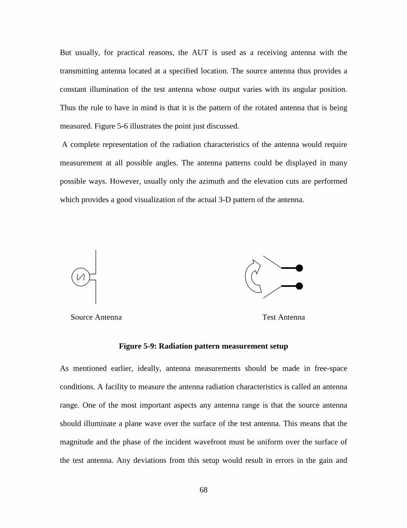
68
But usually, for practical reasons, the AUT is used as a receiving antenna with the
transmitting antenna located at a specified location. The source antenna thus provides a
constant illumination of the test antenna whose output varies with its angular position.
Thus the rule to have in mind is that it is the pattern of the rotated antenna that is being
measured. Figure 5-6 illustrates the point just discussed.
A complete representation of the radiation characteristics of the antenna would require
measurement at all possible angles. The antenna patterns could be displayed in many
possible ways. However, usually only the azimuth and the elevation cuts are performed
which provides a good visualization of the actual 3-D pattern of the antenna.
Figure 5-9: Radiation pattern measurement setup
As mentioned earlier, ideally, antenna measurements should be made in free-space
conditions. A facility to measure the antenna radiation characteristics is called an antenna
range. One of the most important aspects any antenna range is that the source antenna
should illuminate a plane wave over the surface of the test antenna. This means that the
magnitude and the phase of the incident wavefront must be uniform over the surface of
the test antenna. Any deviations from this setup would result in errors in the gain and
Source Antenna Test Antenna

69
pattern measurement. The source should also have sufficient beamwidth so that it is able
to illuminate the whole of the test antenna with very little reaching the surroundings and
at the same time, not being so narrow that it induces an amplitude taper across the test
antenna[30]. By positioning both the source as well as the test antennas well beyond their
respective far-field distances, the spherical wavefront, having traversed so far away from
its source, could be assumed as a plane wavefront.
Another major aspect in any antenna range setup is the proximity to potential clutter. This
could be a major factor influencing the antenna measurements as a reflection from the
ground/objects could interfere with the direct-path signal and cause erroneous nulls/peaks
resulting in errors in the measurement. Hence, care should be taken to mount the two
antennas as far removed from any obstacles in the vicinity. With the knowledge of the
distance between the two antennas, their height above the ground could then be
determined such that any multipath signal reaching the test antenna would have no
detrimental effect on the received signal.
5.4.2 Setup
The pattern measurements on the Vivaldi array antenna were done at the antenna range
facility at KU (KUAR), located on the top of the roof of Nichols Hall. A double-ridged
waveguide TEM horn antenna was chosen as the transmit antenna. This antenna was used
in the 2003 Antarctica experiment as a part of the Snow Radar. The gain and reflection
profile was already known (from datasheets) and hence this was used as the standard
antenna.
Before proceeding with the measurements, the far-field distance should be calculated for
the test antenna – the 12-element linear Vivaldi array. The minimum range distance

70
required for the radiating fields to dominate, referred to as the far-field region, is given
by: λ
22Dr ff = , where D is the maximu m d i m ens i o n o f the tes t antenna and i s the !
smallest wavelength of interest. The maximum dimension of the Vivaldi array was found
to be 15” (38 cm approx.) and considering the highest frequency of 8 GHz, the far-field
distance was found out to be about 7.8 meters.
The KUAR facility was used for the pattern measurements. The facility consists of the
following main parts:
• Source and test antenna assemblies on top of the East and the West stairwell
towers respectively.
• A Graphic User Interface (GUI) on a PC inside the building that remotely controls
the working of the system through connecting cables.
The source and the test antenna mounts in the KUAR facility are separated by a distance
of 100 ft (31.4 m), which is greater than the minimum required distance for being in the
far-field of the antenna. Hence it could be assumed that the test antenna is illuminated by
a plane wavefront. The block diagram of the antenna range setup is shown below.

71
Figure 5-10: Antenna Range setup
The NA - HP 8522D is operated in the continuous-wave (CW) mode at the desired
frequency with an output power level of -5 dBm so that it could be used to feed the
transmitting antenna. The NA is connected to the transmitting antenna through a 10 feet
UTiFLEX cable. At the receiver end, the outputs of the Vivaldi antenna are connected to
the power combiner which is connected to a spectrum analyzer (SA) for measuring the
power level at the transmit frequencies. The noise floor of the SA is set to a minimum to
increase the sensitivity of the spectrum analyzer.
With the above described setup, the three major antenna measurements, viz., polarization,
radiation pattern and the absolute gain, were performed. The constituent features of the
antenna range setup are listed below. Detailed data sheets on off-the-shelf components
listed below have been attached in the Appendix.
Spectrum
Analyzer
Test Antenna
Network
Analyzer
Source Antenna
10 ft. cable 10 ft. cable
Receiver Section Transmitter Section
100 ft.

72
Block Type Feature
Transmitter NA HP8522D CW mode; -5 dBm output power;
2.5, 5, 7.5 GHz
Source
antenna
Double-ridged waveguide horn
ETS-Lindgren Model 3115
Standard antenna; 1meter
Calibrated data available
Receive
antenna(s)
(1) 12-element linear Vivaldi
array; (2) Same as source antenna
(1) Test antenna
(2) Standard antenna for gain
measurement
Power divider Midwest Microwave 12-way
PWD-5522-12-SMA-79
Operated as a combiner; 3 dB
insertion loss (max); 15 dB isolation
Cables Utiflex UFA210A; 10 feet Insertion loss 0.08 dB/ft at 1 GHz
and 0.28dB/ft at 10 GHz
Table 5-4: Antenna range setup features
5.4.3 Polarization
It was found from both the simulation (refer Chapter 4) and measurements that the E-
field vector was directed horizontal since the element was oriented horizontally. The E-
field vectors in fact run between the opposite metal portions of the slotline of the antenna.
Most of the power from the antenna is radiated in this particular polarization. However,
there is some signal power that is being transmitted with vertical polarization as well. A
cross-polarization experiment with a vertically polarized Vivaldi array and a horizontally
polarized TEM horn revealed that the signal power was approximately 10-15 dB less than
the co-polarized value.

73
5.4.4 Gain measurement
Most gain measurements are made using an antenna of known gain, called a standard-
gain antenna. This technique is generally referred to as the gain comparison method.
Having established a suitable range, the signal level with the test antenna in its optimum
location is noted. Then the test antenna is replaced with the standard-gain antenna and is
placed with its aperture at the center of the location where the test antenna was located.
The difference in the received signal power between the standard and the test antenna is
computed and is added to or subtracted from the gain of the standard-gain to obtain the
gain of the test antenna.
The double-ridged TEM horns were used as the standard-gain antennas with the test
antenna being the Vivaldi array. To begin with, the source and the receiver standard-gain
antennas were first aligned so that the test antenna was illuminated by the maximum
radiation from the source. To achieve this, the receiver antenna was scanned for about 40
degrees on either side of the center and the position where the received power was the
highest was noted. This process was repeated for the test antenna for the three desired
frequencies - 2.5, 5 and 7.5 GHz. In each case, the peak received power is measured for a
transmitted power of -5 dBm.
The gain of the standard-gain antenna was obtained from the calibrated data available
from the manufacturers – ETS Lindgren (See Appendix). It should be noted that the
absolute gains (as specified in the datasheet) had been determined from a 1.0 meter
calibration with horizontal polarization. The calibration is usually done in near-perfect
conditions and the gain values could be assumed to be ideal. By connecting this standard-
gain antenna on the receiver side, it is possible to compare the gain that we actually

74
measure with the current range setup to the ideal gain values listed in the datasheet. This
would roughly give us an idea as to the error in the system.
The Friis power equation provides us with a method to determine the power received
when the transmitted power, gain of the two antennas, their distance of separation and the
frequency of operation is known. In the case when both the antennas are of the same type,
a little work of algebra will reveal an equation to determine its gain when all the other
parameters in the equation are known.
( )
∗=
==
∗∗∗=
λπ
πλ
R
P
PG
GGGwhenand
R
GGPP
t
r
tr
trtr
4
,
4 2
2
Since both the antennas were connected to the input/output units by 10 feet long cables, it
became necessary to take into consideration the loss inherent in them. The attached
datasheet of the UTiFLEX cable suggested a loss 0.08 dB/ft at 1 GHz and 0.28 dB/ft at
10 GHz. A linear interpolation was done to obtain the loss for frequencies between 1 and
10 GHz.
The standard TEM horn antenna was then replaced by the AUT at exactly the same
position. A similar set of measurements were taken for the Vivaldi array antenna. The
inclusion of the power combiner in this setup comes with the insertion loss associated
with it. However, this was not included in the gain calculation mainly because of the fact
that the power divider was actually a part of the array and in order to look at the antenna
as a one-port device, any loss occurring between the feed port of the power divider and
the inputs to the individual antenna elements should be disregarded. The results obtained
for both the horn and the Vivaldi are shown below.
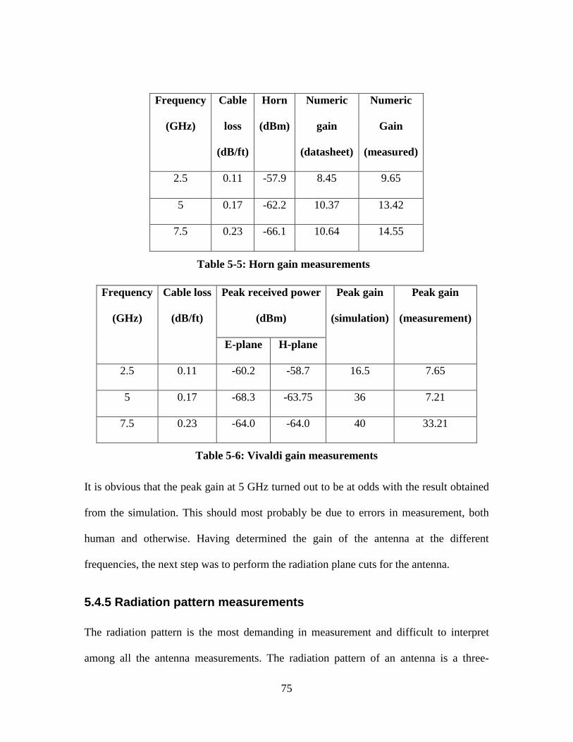
75
Peak received power
(dBm)
Frequency
(GHz)
Cable loss
(dB/ft)
E-plane H-plane
Peak gain
(simulation)
Peak gain
(measurement)
2.5 0.11 -60.2 -58.7 16.5 7.65
5 0.17 -68.3 -63.75 36 7.21
7.5 0.23 -64.0 -64.0 40 33.21
Table 5-6: Vivaldi gain measurements
It is obvious that the peak gain at 5 GHz turned out to be at odds with the result obtained
from the simulation. This should most probably be due to errors in measurement, both
human and otherwise. Having determined the gain of the antenna at the different
frequencies, the next step was to perform the radiation plane cuts for the antenna.
5.4.5 Radiation pattern measurements
The radiation pattern is the most demanding in measurement and difficult to interpret
among all the antenna measurements. The radiation pattern of an antenna is a three-
Frequency
(GHz)
Cable
loss
(dB/ft)
Horn
(dBm)
Numer ic
gain
(datasheet)
Numer ic
Gain
(measured)
2.5 0.11 -57.9 8.45 9.65
5 0.17 -62.2 10.37 13.42
7.5 0.23 -66.1 10.64 14.55
Table 5-5: Horn gain measurements

76
dimensional representation of the magnitude, phase and polarization of the radiation
emanating from it. Typically, the radiation in two perpendicular planes is measured to get
an idea about the field pattern of the antenna. One measurement is done on the plane of
polarization and the other in a plane perpendicular to the plane of polarization. The
polarization plane is also referred to as the E-plane as it is parallel to the E-field and the
latter is described as the H-plane for similar reasons. When taking pattern measurements
over real earth, the terms azimuth and elevation are generally used[32]. In the case of the
horizontally polarized Vivaldi antenna, the E-field becomes parallel to the ground and
hence the azimuth plane is also the E-plane and subsequently the elevation is the H-plane.
Before venturing into the description of the procedure used in taking the pattern
measurements, it would be worthwhile exercise to form a prediction of the results for
comparison with the measured results. To be more specific: based on the measurements
performed in the previous section, the gain of the 12-element Vivaldi could be calculated.
Knowing the gain of the TEM horn at the desired frequency, the loss in the cables and the
distance of separation between the two antennas, the received power could be arrived at
by making use of the Friis transmission equation. The following exercise is for the sole
purpose of making an educated guess as to what the received power might be.

77
( )
( )
( )
dBm
dBdBm
lossCablePP
dBmP
mftR
GHzfatm
tmeasuremenfromG
datasheetfromG
dBmdBdBmlossCablePP
where
R
GGPP
rSA
r
t
r
NAt
trtr
02.66
7.132.64
32.64
4.31.100
506.0
)(21.7
37.10
7.67.15
,
4 2
2
−=−−=
−=−=
===
==
−=−−=−=
∗∗∗=
λ
πλ
The above calculation predicts a received power of -66.02 dBm at the Spectrum Analyzer
(SA) for the given specifications.
The setup used to measure the radiation pattern of the Vivaldi antenna has already been
described earlier in this chapter. The horizontally polarized Vivaldi (AUT) was operated
as the receiver and mounted on top the West tower while the transmitter was the TEM
horn mounted on top of the East tower with the same polarization. The transmit power is
set as -5 dBm and a continuous wave at the desired frequency is fed to the transmit
antenna by the Network Analyzer (NA). The AUT is then rotated in the azimuth direction
in desired angle increments and the power received at each increment is noted down from
the Spectrum Analyzer (SA). Measurements were taken with two-degree increments for
50° on either side of the major lobe and in five-degree increments for the rest of the scan.
This process is carried out for the three frequencies – 2.5, 5 and 7.5 GHz. This concludes
the azimuth scan and subsequently the elevation sweep has to be done.
The KUAR does not have the facility to scan the antenna in the elevation direction. Thus
the antenna was removed from the current mounting and it was rotated by 90° around the

78
axis that is the line connecting the two antennas. The antenna was thus oriented
perpendicular to the real earth and effectively vertically polarized. If the orientation of the
transmit horn antenna is not changed, then any pattern measurement taken subsequently
will be one of cross-polarization. Even though this would have been an interesting
experiment on its own, it was not pursued further due to the lack of time. To copy the
effect of taking the elevation cut, the transmit antenna should also be rotated so that it is
also vertically polarized and subsequently we return to taking co-polarization elevation
measurements. The vertically polarized AUT was then rotated in the H-plane to obtain
the elevation cut. This process is performed with the same NA settings for the same
frequencies individually. A total of 240° was swept in both planes for the signal
frequencies of 2.5 GHz and 7.5 GHz while for the 5 GHz signal, the azimuth cut was
swept for the entire 360° with again a 240° sweep for the elevation plane cut. This was
not only done to save time but also for the reason that we were not really interested in
knowing about the pattern in the direction diametrically opposite to the main lobe. At
each sweep angle the power was measured with the SA. The SA was setup so that the
noise floor was well below the signal power level. The receiver bandwidth was set such
that even the lowest amplitude signal was discernible.
The “ received power versus angle” data obtained from the measurement was loaded into
Matlab for further processing. The radiation plots obtained for each frequency is then
normalized to the maximum power measured for that frequency. The following are the
plots generated from data taken from the pattern measurements done on the roof.
The azimuth cut taken at the frequency of 2.5 GHz is shown below. The antenna was
swept over a 110° angle on either side of the center. It is seen that the first side lobe is

79
close to 13 dB below the main lobe. A HPBW of 23° was observed from the
measurement. The gain of the Vivaldi array antenna at this frequency was 8.84 dB.
Figure 5-11: Azimuth & Elevation cuts at 2.5 GHz
The elevation cut reveals a broader beam with a HPBW of around 130° with a twin-peak
feature suggesting the breaking of the main lobe. In this case, a sweep of 120° on either
side of the center position is performed. Also, no side lobes were seen on this sweep.

80
An azimuth cut at 5 GHz revealed a lot of sidelobes and subsequently the main lobe was
fairly narrow. This was generated from a 360° sweep measurement with the Vivaldi
array. A HPBW of 14° is obtained from this measurement. The gain realized at this
frequency was 8.58 dB. This was below the gain obtained from the simulation by about 7
dB, which is not particularly good. This could probably be due to error in the
measurements.
An elevation cut at the same frequency once again gave a wide beamwidth pattern with a
HPBW close to 120°. Once again, the twin-peaks are observed on either side of the center
position.

81
Figure 5-12: Azimuth & Elevation cuts at 5 GHz
The same procedure was repeated for a frequency of 7.5 GHz for both the azimuth and
the elevation sweep. The HPBW in the azimuth was still small, with a value of about 12°.
The sidelobes increase in number with a corresponding decrease in their magnitude
levels. Discrepancies will be explained later in this section. The gain was found out to be
15.21 dB in this case. Finally, the elevation cut for 7.5 GHz is shown below. The HPBW
is obtained as 85°. Two sidelobes were observed in the pattern.

82
Figure 5-13: Azimuth and elevation cuts at 7.5 GHz
The pattern measurements prove that the beam is really narrow on the azimuth plane or
the E-plane while on the perpendicular elevation plane; the beam width is relatively large.
This is essentially due to the effect of the configuration of the antenna elements as a
linear (1-D) array. The main lobe was effectively centered on the angles 6° to 10°. A 0°
center was not obtained due to the inability to align the two antennas exactly on the same

83
line. This was further affected by extremely windy conditions that resulted in unstable
antenna mounts leading to potentially erroneous measurements.
One of the most important causes for errors in the pattern measurements was the presence
of the roof floor on one side of the antenna. Moreover, the store room on the roof also
caused reflections that got back to the receiver antenna. These concrete structures create
multipath signals that could have interfered with the direct path signals in a multitude of
ways. This would result in unusually large power at the receiver or on the other hand
might also cause severe nulls at points where a particularly high signal power was
expected. This could be the reason why the patterns were not symmetrical about the
maximum radiation point. Particularly, the sidelobes were not symmetrical with each
other. The first sidelobes on either sides of the main beam, in some cases, were not of
same magnitude. This means that more power was received on one side of the antenna
than the other. Again, the most probable cause would be the effect of multipath signals
5.5 Summary
Antenna measurements form one of the most important aspects of any antenna design.
Since the antenna is basically a device radiating in all directions, bench-top
measurements become highly error prone. To characterize an antenna, controlled
conditions are necessary. Otherwise, the environment would cause potentially severe
errors in the measurement. The reflection and the target-return measurements were done
in the lab with the NA as the input feed generator and a flat aluminum plate as the target.
Time-gating was also accomplished to remove the effect of the surroundings in the S11
measurement. These measurements were done both for the single as well as the array
Vivaldi antenna. The pattern measurements were however performed only for the array

84
antenna. The antenna range on the roof of the building was used for these measurements.
A double-ridged TEM horn antenna was used as the immobile standard transmit antenna
while the twelve-element Vivaldi array was used as the movable receiving antenna. The
movement was controlled remotely from the computer in the lab and the test antenna was
rotated in the azimuth direction to obtain the plane cut. The gain and polarization of the
antenna were also determined using the same range setup.
The results that were obtained from the different measurements performed with the
antenna array are listed below.
Parameter Value
S11 <=-7 dB, except for a brief region around 3 GHz
Polarization Linear, with E-field lines running between the opposite sides of the slot
Frequency 2.5 GHz 5 GHz 7.5 GHz
Gain 8.84 dB 8.58 dB 15.8 dB
HPBW E-plane 23° 14° 12°
HPBW H-plane 130° 120° 85°
Table 5-7: Measurement results
85
Chapter 6 Summary and recommendations
6.1 Summary
The Vivaldi is a member of a class of aperiodic continuously scaled traveling-wave
antenna structures. Besides being efficient and lightweight, the more attractive features of
this antenna are that it can work over a large frequency bandwidth and produce a
symmetrical end-fire beam with appreciable gain and low side lobes. The design of the
antenna is very simple and could be completed in the lab with limited resources and
labor. This antenna design hence costs less than the horn antenna. Since the antenna
worked best in an array, additional beam-forming and adaptive signal processing could
be done with this design. These were the basic reasons that led us to investigate the use
of the Vivaldi antenna in this particular application.
The antenna was first modeled and simulated using HFSS. Considering frequencies with
S11 lesser than -7 dB, the simulation yielded an antenna with a bandwidth of about 10-
15%, suggesting that the antenna was primarily unmatched at the port. The model was
then fabricated and its S11 was measured in the lab using the Network Analyzer (NA) HP
8722D. It was seen that the simulated and the measured S11 results matched. The
simulation revealed a very low antenna gain of 2.48, which subsequently led us to design
an array of Vivaldi elements.
The array antenna was modeled in HFSS with a grounded backplane which reflected any
signals going in the backward direction. A gain of about 16 dB was obtained for a signal
frequency of 7.5 GHz. The array was built and the S11 was measured in the lab. The
clutter was gated out and the resulting antenna had close to a 2.5:1 bandwidth, defined for

86
S11 lesser than -7 dB. This was definitely a marked improvement from the single element
case, but of course not good enough. However, “ -10 dB bandwidth” definition would
reduce the usable bandwidth of the antenna to four chunks of around 1 GHz width each
within the desired 2-8 GHz frequency band. This shows that the antenna was not really as
wideband as we sought out to be. One of the possible causes for this behavior could be
the feed mechanism which was only simulated and not really built and tested.
Theoretically, the S11 of the single transition (in the antenna) should have been better
than that of the double-transition. However, in practice, exactly the opposite was seen.
Another major issue was that of input impedance matching. Each of the elements had an
input impedance of around 8 5 , b u t the d r i vi ng' -point impedance of each of the element
in the entire array was not known. A 12-element simulation would have given me an idea
about the active impedance. The reflections between the antenna port and the power
divider ports should be substantial as to cause a significant amount of loss.
The pattern measurements taken in the roof yielded a peak gain value of around 15 dB (at
7.5 GHz) which was pretty close to the value obtained from simulation. However, the
gain at 5 GHz varied by a significantly larger amount (7 dB). This discrepancy might be
an error in measurement, because the simulation predicted a steady increase of gain with
frequency as is usually the case with most antennas. Also, the pattern cuts were not
entirely symmetrical about the main lobe in some of the plane cuts. In fact, in some cases,
the main lobe was steeper on one side than the other and in some others; the sidelobes
were not symmetrical on both sides. The sidelobes on one side were of larger magnitude
than the other, basically due to the fact that more power was received on one of the sides.

87
This was also probably due to some error in the measurement caused by multipath signals
reaching the receiver and interacting with the signal from the direct path. The presence of
the roof top and the store room on one side of the antenna range could have resulted in
signals being reflected and reaching the receiver out of phase with the direct path signal.
Moreover, the experiments were performed in inclement weather and the excessive wind
could have changed the orientation of the antennas. Even a slight variation could result in
potentially wrong measurements.
The pattern measurements, in general, yielded fairly narrow beamwidths of close to 15°
on the E-plane with a wide beamwidth of around 100° on the perpendicular H-plane,
which was basically due to setting up the linear array. Such very low beamwidths would
greatly benefit the measurement of snow thickness from a large height above the ground,
which was one of the aims of this project. Also, the mutual coupling influences the
strength of the radiation of the signals from each of the elements. However, a measure of
the coupling effects was made impossible with the inability to simulate the full array.
Thus, the twelve-element Vivaldi array was modeled, designed and tested entirely at the
lab. The gain of the array seemed to be on the lines of that of the double-ridged
waveguide horn that was used as the standard source antenna. Hence, it could readily
replace the horn in the current setup of the Snow Radar. A better performance could be
attained with a more detailed study of the working of the Vivaldi element and a thorough
simulation of the array configuration. This project, I hope, would serve as the first step in
using the Vivaldi antenna for effective snow thickness measurement.

88
6.2 Recommendations
As discussed in the previous section, a lot of improvements / modifications could be done
to the design so that better S11 and pattern characteristics could be obtained.
• The feed mechanism should be analyzed more thoroughly. Particularly, by
fabricating and testing the transition, it could be found out as to why the single
transition behaves worse than the double transition.
• A more powerful computer with a large enough RAM should be used to run the
twelve-element simulation. This would enable us to determine the effect of
mutual coupling on the driving-point impedance of the array elements.
Subsequently, a matching network could be designed so that the ports of the
power divider could be matched to the driving-point impedance of each of the
element. These two modifications would go a long way in improving the S11 of
the antenna and the realized gain of the antenna would also increase
correspondingly.
• The pattern measurement process could have been simplified if the automated
system was used, rather than manually noting down the readings from the roof-
top. However, this required enough amplifiers to boost the signal levels to
compensate for the exorbitant loss in the cables. Also, the reflections from the
roof floor and the walls could have been time-gated so that their effects do not
mask the original signal.
• The process of bonding the two antenna boards together to make the triplate
structure involved some real tough procedures that could not be followed strictly
in the lab. Having the boards made outside is an option, though costly.

89
• The measured insertion loss of the power divider matched that of the
specifications at the lower side of the frequency range. However, at the higher end
of the bandwidth, the insertion loss was worse by 3 dB. A better power divider
would have improved the gain of the Vivaldi array significantly

90
Chapter 7 References
[1] Vinnikov, K. Y., A. Robock, R. J. Stouffer, J. E. Walsh, C. L. Parkinson, D. J.
Cavalieri, J. F. B. Mitchell, D. Garrett, and V. F. Zakharov, “Global Warming and
Northern Hemisphere Sea Ice Extent,” Science, vol. 286, 1999, pp. 1934-1937.
[2]
http://earthobservatory.nasa.gov/Newsroom/MediaResources/aqua_sci_writers_guide.pdf
[3] Markus, T. and D. Cavalieri, “Snow Depth Distribution over Sea Ice in the Southern
Ocean from Satellite Passive Microwave Data. Antarctic Sea Ice: Physical Processes,
Interactions, and Variability,” Antarctic Research Series, Washington, DC, 74:19-39,
1998.
[4] Wong: “Development of a Prototype of a 2-8 GHz FMCW Radar for Snow Thickness
Measurement on Sea Ice,” M.S Thesis, University of Kansas, 2003.
[5] Gibson, P.J., “The Vivaldi aerial,” Proc. 9th European Microwave Conference, 1979,
pp. 103-105.
[6] http://www.ansoft.com
[7] H.Y. Wang et al, “Rigorous analysis of Tapered Slot Antennas on dielectric
substrates,” 10th International Conference on Antennas and Propagation, 1997.
[8] R. Janaswamy and D.H. Schaubert, “Analysis of a Tapered Slot Antenna,” IEEE
Transactions on Antennas and Propagation, Vol. AP-35, No. 9, September 1987, pp.
1058-1065.
[9] Yngvesson et al, “The tapered slot antenna – A new integrated element for
millimeter-wave applications,” IEEE Transactions on Microwave Theory and
Techniques, Vol. 37, No. 2, February 1989, pp. 365-374.

91
[10] Oraizi and Jam, “Optimum design of TSA profile,” IEEE Trans. on Antennas and
Propagation, Vol. 51, No. 8, August 2003, pp. 1987-1995.
[11] H. Jasik, Antenna Engineering Handbook, McGraw-Hill, 1961.
[12] R.Q. Lee and R.N. Simons, “Advances in Microstrip and Printed Antennas,” John
Wiley and Sons, 1997.
[13] R.Q. Lee and R.N. Simons, “Effect of Curvature on Tapered Slot Antennas,”
Antennas and Propagation Society International Symposium, 1996, AP-S. Digest ,
Vol.1, pp. 188 –191.
[14] J.P. Weem et al, “Vivaldi antenna arrays for SKA,” Antennas and Propagation
Society International Symposium, Vol.1, July 2000, pp. 174-177.
[15] K.C. Gupta, R. Garg and I.J. Bahl, “Microstrip Lines and Slotlines,” Artech House,
Dedham, MA, 1979.
[16] Knorr, J.B., “Slotline transitions,” IEEE Trans., Vol. MTT-22, 1974, pp. 548-554.
[17] Weedon et al, “A step-frequency radar imaging system for microwave
nondestructive evaluation,” Progress in electromagnetic research, 2000, pp. 121-146.
[18] Schuppert, “Microstrip/slotline transitions: Modeling and experimental
investigations,” IEEE Trans., Vol. MTT-36, 1988, pp. 1272-1282.
[19] A. H. Atwater, ‘ ‘The Design of the Radial Line Stub: A Useful Microstrip Circuit
Element,’ ’ Microwave Journal, Vol. 28, 1985, pp.149-156.
[20] Sloan et al, “A broadband microstrip-to-slotline transition,” Microwave and optical
technology letters, Vol. 18, No. 5, August 1998, pp. 339-342.
[21] Gazit, “ Improved design of a Vivaldi antenna,” IEEE Proc. H, 1988, pp 89-92.

92
[22] Noronha et al, “Designing antennas for UWB systems,” Microwaves & RF Journal,
June 2003, pp. 53-61.
[23] Langley et al, “Novel ultrawide-bandwidth Vivaldi antenna with low cross-
polarization,” Electronic Letters, Vol. 29, No. 23, 1993, pp. 2004-2005.
[24] The 2000 CAD Benchmark, Microwave Engineering Europe,
http://img.cmpnet.com/edtn/europe/mwee/pdf/CAD.pdf
[25] Schaubert & Shin, “A parameter study of stripline-fed Vivaldi notch-antenna
arrays,” IEEE Trans. on Antennas and Propagation, Vol. 47, No. 5, May 1999, pp. 879-
886.
[26] Advanced circuit materials - Technical Tips, Rogers Corporation website,
http://www.rogerscorporation.com/mwu/techindx.htm
[27] Bhartia et al, “Microstrip Antenna Design Handbook,”
[28] Wadell, “Transmission Line Design Handbook,” Artech House, 1991.
[29] Taflove and Thiele, “FD-TD analysis of Vivaldi flared-horn antennas and arrays,”
IEEE Trans. on Antennas and Propagation, Vol. 42, No. 5, May 1994, pp. 633-641.
[30] Stutzman and Thiele, “Antenna theory and design,” 2nd Edition, John Wiley & Sons,
1998.
[31] Dr. Pannirselvam Kanagaratnam, Research Assistant Professor, Electrical
Engineering and Computer Science, The University of Kansas, Lawrence.
[32] Turin, “The ARRL Antenna Book,” 19th Edition, Chapter 28, pp. 46-52

93
Chapter 8 Appendix
8.1 Datasheets
Par t Datasheet
Rogers Substrate http://www.rogerscorporation.com/mwu/pdf/5000data.pdf
Power divider http://ebiz.midwest-microwave.com/cgi-bin/mmb2c/PWD-5522-
12-SMA-79.html
UTiFLEX Cables http://www.micro-coax.com/utiflex/utiflex_lowloss.htm
Double-Ridged
Waveguide horn
http://www.ets-lindgren.com/Manuals/3115.pdf
8.2 Pictures
(a)
Power divider
Vivaldi Antenna
Backplane

94
(b)
Figure 8-1: Vivaldi antenna array in (a) Hor izontal, and (b) Ver tical polar ization
Figure 8-2: Double-r idged waveguide horn - Ver tically polar ized
UTiFLEX cable
Vertically polarized horn

95
Vivaldi Antenna
Horn antenna
100 ft.