design of next-generation tbps turbo codes
TRANSCRIPT

Design of Next-Generation Tbps Turbo Codes
Vinh Hoang Son Le
December 21, 2020

Contents
Contents i
Acronyms iv
1 Introduction 11.1 Motivation and Challenges . . . . . . . . . . . . . . . . . . . . . . . . . . . 21.2 Objectives, Contribution and Outline . . . . . . . . . . . . . . . . . . . . 3
2 Convolutional Codes and Turbo Codes 62.1 Short Introduction to Channel Coding . . . . . . . . . . . . . . . . . . . . 72.2 Convolutional Codes . . . . . . . . . . . . . . . . . . . . . . . . . . . . . . 9
2.2.1 Convolutional Encoding . . . . . . . . . . . . . . . . . . . . . . . . 92.2.2 The Trellis Diagram Representation of Convolutional Encoders . . . 112.2.3 High-Rate Convolutional Codes . . . . . . . . . . . . . . . . . . . . 12
2.3 Decoding Algorithms for Convolutional Codes . . . . . . . . . . . . . . . . 142.3.1 The Viterbi Algorithm . . . . . . . . . . . . . . . . . . . . . . . . . 142.3.2 The Soft-Output Viterbi Algorithm . . . . . . . . . . . . . . . . . . 162.3.3 MAP-Based Algorithms . . . . . . . . . . . . . . . . . . . . . . . . 17
2.4 Turbo Codes . . . . . . . . . . . . . . . . . . . . . . . . . . . . . . . . . . . 212.4.1 Turbo Encoding . . . . . . . . . . . . . . . . . . . . . . . . . . . . . 212.4.2 The Interleaver . . . . . . . . . . . . . . . . . . . . . . . . . . . . . 22
2.5 Turbo Decoding . . . . . . . . . . . . . . . . . . . . . . . . . . . . . . . . . 232.5.1 Principle . . . . . . . . . . . . . . . . . . . . . . . . . . . . . . . . . 232.5.2 Comparison of Constituent Codes Decoding Algorithms . . . . . . . 24
2.6 Summary . . . . . . . . . . . . . . . . . . . . . . . . . . . . . . . . . . . . 25
3 High-Throughput Turbo Decoders 263.1 Basic Turbo Decoders . . . . . . . . . . . . . . . . . . . . . . . . . . . . . 27
3.1.1 Generic Components of SISO Decoders . . . . . . . . . . . . . . . . 283.1.2 Scheduling SISO decoding . . . . . . . . . . . . . . . . . . . . . . . 293.1.3 Sliding Window Decoding . . . . . . . . . . . . . . . . . . . . . . . 303.1.4 State Metric Initialization . . . . . . . . . . . . . . . . . . . . . . . 323.1.5 Evaluation of Basic Key Performance Indicators for Turbo Decoders 32
3.2 High-Throughput Architectures . . . . . . . . . . . . . . . . . . . . . . . . 343.2.1 The PMAP Architecture . . . . . . . . . . . . . . . . . . . . . . . . 343.2.2 The XMAP Architecture . . . . . . . . . . . . . . . . . . . . . . . . 353.2.3 High-Radix Schemes . . . . . . . . . . . . . . . . . . . . . . . . . . 363.2.4 High-Throughput Turbo Decoders: State of the Art . . . . . . . . . 38
i

3.3 Ultra-High-Throughput Architectures . . . . . . . . . . . . . . . . . . . . . 383.3.1 The Fully-Parallel MAP (FPMAP) Architecture . . . . . . . . . . . 393.3.2 The Iteration Unrolled XMAP (UXMAP) Architecture . . . . . . . 40
3.4 Summary . . . . . . . . . . . . . . . . . . . . . . . . . . . . . . . . . . . . 42
4 The Local-SOVA 444.1 Introduction . . . . . . . . . . . . . . . . . . . . . . . . . . . . . . . . . . . 454.2 The Max-Log-MAP algorithm from the SOVA viewpoint . . . . . . . . . . 454.3 The Local-SOVA . . . . . . . . . . . . . . . . . . . . . . . . . . . . . . . . 48
4.3.1 Reliability Update Rules . . . . . . . . . . . . . . . . . . . . . . . . 484.3.2 Commutative and Associative Properties of the Merge Operation . 494.3.3 The MLM Algorithm as an Instance of the Merge Operation . . . . 514.3.4 The Soft Output Computation Algorithm . . . . . . . . . . . . . . 534.3.5 Radix-2 Local-SOVA Decoder Architecture . . . . . . . . . . . . . . 55
4.4 High-Radix Decoding Algorithms Using Local-SOVA . . . . . . . . . . . . 584.4.1 Radix-4 Local-SOVA Decoder with Minimum Complexity ACSU . . 594.4.2 Radix-8 local-SOVA Decoder Using a Simplified Reliability Update
Operator . . . . . . . . . . . . . . . . . . . . . . . . . . . . . . . . . 604.4.3 Simulation Results . . . . . . . . . . . . . . . . . . . . . . . . . . . 624.4.4 Computational Complexity Analysis . . . . . . . . . . . . . . . . . 644.4.5 Radix-16 Local-SOVA Decoder for Convolutional Codes with Mem-
ory Length ν = 3 . . . . . . . . . . . . . . . . . . . . . . . . . . . . 664.5 Conclusion . . . . . . . . . . . . . . . . . . . . . . . . . . . . . . . . . . . . 68
5 The Local-SOVA in Unrolled-XMAP Architecture 705.1 Introduction . . . . . . . . . . . . . . . . . . . . . . . . . . . . . . . . . . . 715.2 Fixed-Point Implementation of the Radix-4 MLM/UXMAP Decoder . . . . 72
5.2.1 Computational Units Implementation . . . . . . . . . . . . . . . . . 725.2.2 Metrics Quantization . . . . . . . . . . . . . . . . . . . . . . . . . . 745.2.3 Performance of the MLM/UXMAP Architecture . . . . . . . . . . . 78
5.3 High-Radix Local-SOVA in UXMAP Architecture . . . . . . . . . . . . . . 795.3.1 Metric Quantization in the Local-SOVA . . . . . . . . . . . . . . . 805.3.2 Radix-4 Computational Units . . . . . . . . . . . . . . . . . . . . . 805.3.3 Radix-8 Computational Units . . . . . . . . . . . . . . . . . . . . . 835.3.4 Radix-16 Computational Units . . . . . . . . . . . . . . . . . . . . 86
5.4 Conclusion . . . . . . . . . . . . . . . . . . . . . . . . . . . . . . . . . . . . 90
6 SISO Decoding Algorithms Using the Dual Trellis 926.1 Introduction . . . . . . . . . . . . . . . . . . . . . . . . . . . . . . . . . . . 936.2 The Dual Trellis and the MAP-Based Algorithms on the Dual Trellis . . . 94
6.2.1 The Dual Trellis . . . . . . . . . . . . . . . . . . . . . . . . . . . . . 946.2.2 The Dual-MAP and Dual-Log-MAP algorithms . . . . . . . . . . . 100
6.3 Constructing the Dual Trellis for Punctured Convolutional Codes . . . . . 1036.3.1 Equivalent Non-Systematic Generator Matrix of Punctured Convo-
lutional Codes . . . . . . . . . . . . . . . . . . . . . . . . . . . . . . 1046.3.2 Reciprocal Parity-Check Matrix of Punctured Convolutional Codes 1056.3.3 Example and Numerical Results . . . . . . . . . . . . . . . . . . . . 1076.3.4 Simulation Results and Discussion . . . . . . . . . . . . . . . . . . . 109
ii

6.4 The Dual-Max-Log-MAP Algorithm . . . . . . . . . . . . . . . . . . . . . . 1106.4.1 Drawbacks of the Dual-Log-MAP Algorithm . . . . . . . . . . . . . 1116.4.2 Max-Log Approximation for the Extrinsic Information Calculation . 1126.4.3 Extrinsic Information Calculation using the Local-SOVA . . . . . . 1146.4.4 The Dual-Max-Log-MAP Algorithm . . . . . . . . . . . . . . . . . 1156.4.5 Complexity Analysis and Simulation Results . . . . . . . . . . . . . 117
6.5 Conclusion . . . . . . . . . . . . . . . . . . . . . . . . . . . . . . . . . . . . 119
7 Conclusion and Future Works 1217.1 Conclusion . . . . . . . . . . . . . . . . . . . . . . . . . . . . . . . . . . . . 1217.2 Future Works . . . . . . . . . . . . . . . . . . . . . . . . . . . . . . . . . . 122
Bibliography 125
iii

Acronyms
ACQ AcquisitionACS Add-Compare-SelectACSU Add-Compare-Select UnitARP Almost Regular PermutationAPP A Posteriori ProbabilityAWGN Additive White Gaussian Noise
BCH Bose–Chaudhuri–HocquenghemBCJR Bahl-Cocke-Jelinek-RavivBER Bit Error RateBMU Branch Metric UnitBPSK Binary Phase Shift KeyingBR Battail Rule
CS Compare-Select
Dual-LM Dual-Log-MAPDual-MLM Dual-Max-Log-MAPDVB Digital Video BroadcastingDVB-RCS Digital Video Broadcasting - Return Channel via SatelliteDVB-SH Digital Video Broadcasting - Satellite Handheld
ESF Extrinsic Scaling Factor
FB Forward-BackwardFEC Forward Error CorrectionFER Frame Error RateFPMAP Fully-Parallel MAPFSM Finite State Machine
HI Half-IterationHR Hagenauer RuleHSPA High Speed Packet Access
KPI Key Performance Indicators
LDPC Low Density Parity Check
iv

LLR Log-Likelihood RatioLM Log-MAPLTE Long Term EvolutionLUT Lookup Table
MAP Maximum A PosterioriML Maximum LikelihoodMLM Max-Log-MAP
NII Next Iteration Initialization
PMAP Parallel MAP
QPP Quadratic Permutation Polynomial
RSC Recursive Systematic Convolutional
SIHO Soft-Input Hard-OutputSISO Soft-Input Soft-OutputSM Sign-MagnitudeSMA Sign-Magnitude AdditionSMD Sign-Magnitude DivisionSMM Sign-Magnitude MultiplicationSNR Signal-to-Noise RatioSOU Soft-Output UnitSOVA Soft-Output Viterbi Algorithm
UMTS Universal Mobile Telecommunications SystemUXMAP Unrolled XMAP
VA Viterbi Algorithm
WiMAX Worldwide Interoperability for Microwave Access
XMAP Pipelined MAP
v

Chapter 1
Introduction
Digital wireless communications can be considered as the most dynamic area in the com-munication field today. The last few decades have seen a surge of research and industrialactivities in the area. A combination of several factors can explain this surge. The firstand most obvious is the demand for wireless connectivity. Cordless devices are now ableto communicate efficiently with each other and can access the information without ge-ographical boundaries. Furthermore, the development of the semiconductor technology,which is governed by Moore’s law [1], allows sophisticated signal processing algorithmsto be integrated into the devices with small area and low power consumption. Last butnot least, the development of information theory, pioneered by Claude Shannon in hisoriginal article [2], paved the way for efficient communication systems to be implementedwith high reliability.
Subsequently, the success of the second generation (2G) of mobile communication stan-dards was a concrete demonstration that good wireless digital communication systems canbe achieved. However, the 2G system still concentrates mostly on voice communication,as it can only provide a bidirectional communication link with a maximum throughputof 9.6 kb/s. Then, the demand for data transmission with increasingly high data rates,including video telephony, drove the world of wireless communications. It is these chal-lenges and also the related interests that have fascinated many researchers and attractedthem to this field. In 1999, the UMTS technology [3] was introduced, which allows a datarate of 384 kb/s to be achieved. Since then, transmission with increased data throughputhas been one of the most important aspects of wireless communications. As a result, adata rate of 84 Mb/s can be reached by the HSPA+ technology [4], released in 2007, andthe LTE standard [5] can transmit with a maximum data rate of 300 Mb/s. With themost recent mobile standards, LTE Advanced Pro [6] and the 5G New Radio [7], through-puts from a few Gb/s to a few tens of Gb/s can be achieved. Following this trend, thethroughput of mobile broadband communications will be in the order of hundreds of Gb/sand up to Tb/s in the near future, especially with the advent of THz communications.
As part of the communication system, channel coding, or forward error correction(FEC), plays a critical role in enabling the communication link. A channel code addsredundant information to the original information to be transmitted. Thanks to the re-dundancy, corrupted information due to noise and channel impairments can be correctedto recover the message at the receiver side. Sophisticated channel codes can drasticallyimprove the reliability of the communication, thus allowing efficient data transmissionbetween devices with limited transmit power. Many channel codes can be found in the
1

literature as well as in industrial communication standards. The two classic code familiesare block codes, such as Hamming, Golay, BCH, or Reed-Solomon codes, and convolu-tional codes [8]. Then, in the nineties came the turbo codes with iterative decoding [9],the rediscovery of low-density parity-check (LDPC) codes [10] and more recently the polarcodes [11]. The invention of turbo codes by C. Berrou in 1991 is considered as one of themost important milestones of the channel coding research. They were the first practicalcodes able to operate within a fraction of a dB of the Shannon limit. Since then, turbocodes have been chosen as the channel code in many digital communication standards,such as the 3G/4G mobile standards and the digital video broadcasting DVB-RCS/RCS2and DVB-SH standards [12]. Furthermore, the iterative decoding of these codes and theconcept of extrinsic information have had influences on the decoding of LDPC codes butalso on many other elements of the communication chain, like modulation, equalization,and multi-antenna techniques.
1.1 Motivation and Challenges
For the time being, wireless digital communications using the LTE Advanced Pro or thenewly 5G standards can provide up to tens of Gb/s communication links. As a result,we can enjoy high-quality media material and streaming while on the move with ourmobile phones. Nevertheless, as technologies develop, so do applications. Therefore,the demand for even higher data rates of hundreds of Gb/s or Tb/s can be foreseen inthe future. Yet, new use cases of this “ultra-high-throughput” era have already beenidentified. Several examples can be cited, such as wireless intra-devices communication[13], mobile augmented/virtual reality communications [14], wireless backhaul/fronthaul[15], communications in data centers [16], hybrid fiber-wireless networks [17], and high-throughput satellites communications [18].
The increase of throughput up to Tb/s comes with the need to move to frequencies atthe THz range (0.1 THz − 10 THz) as well as with having the appropriate correspondingbaseband processing, especially for FEC. To this end, the European H2020 project EPIC(Enabling Practical Wireless Tb/s Communications with Next Generation Channel Cod-ing, https://epic-h2020.eu/) lent itself to develop a set of new implementation-readyFEC technologies that meet the cost and performance requirements of a variety of futurewireless Tb/s use cases.
In the past, steady progress in silicon technology – as governed by Moore’s law –could be regarded as the enabler of large leaps in data rates without the need for majoralgorithmic innovations on the FEC design part. However, a key finding of EPIC isthe prediction that the upgrade to Tb/s wireless data rates will not be smooth: theimprovements carried by silicon technology progress in the next decade will significantlyfall short of meeting the Tb/s FEC challenge [19]. Therefore, the EPIC project is basedon the thesis that major algorithmic and architectural innovations will be required in thedesign and implementation of FEC algorithms to make Tb/s wireless communicationsfeasible. As candidates for the FEC technologies, the EPIC project considered three codeclasses: turbo codes, LDPC codes, and polar codes, as their error correction performancecome close to the Shannon limit.
This thesis focuses on the development of turbo codes in the framework of the EPICproject. Efficiently achieving ultra-high throughput (up to Tb/s) for turbo codes is verychallenging, since turbo codes are inherently serial at the component decoder level. Be-
2

sides the main requirement in throughput, within the EPIC project framework, additionalconstraints such as chip area, area efficiency, power density, code flexibility, and bit errorrate (BER) should also be met [20]. Table 1.1 shows the main FEC Key PerformanceIndicators (KPI) in the EPIC context under 28 nm technology node. Addressing allthese constraints requires the exploration of new decoding algorithms and highly parallelarchitecture templates.
Applications BER Flexibility LatencyThroughput
(Gb/s)
Area eff.
(Gb/s/mm2)
Power dens.
(W/mm2)
Energy eff.
(pJ/bit)
Virtual Reality 10−6 high 0.5 ms 500 50 0.02 0.48
Intra-Device Com. 10−12 low 100 ns 500 50 0.13 1.00
Fronthaul 10−13 medium 25 ns 1000 100 0.17 0.60
Backhaul 10−8 medium 100 ns 250 25 0.09 3.60
Data Center > 10−12 medium 100 ns 1000 100 0.20 0.75
Hybrid Fiber-Wireless 10−12 medium 200 ns 1000 100 0.23 1.13
High Throughput Sat. 10−10 medium 10 ms 100 - 1000 100 0.27 0.50
Table 1.1: Summary of FEC level KPI for different use cases under 28 nm technologynode.
1.2 Objectives, Contribution and Outline
The objective of this thesis is to explore innovative turbo decoding techniques, allow-ing the decoder to achieve or approach very high-throughput transmission (Tb/s). Thecontribution of the thesis is shown as follows.
• The discovery of a new soft-input soft-output (SISO) decoding algorithm based onthe manipulation of paths in the trellis diagram, namely the Local-SOVA. It exhibitsa lower computational complexity than the conventional maximum a posteriori algo-rithm with Max-Log approximation (Max-Log-MAP) when employed for high-radixdecoding in order to increase throughput, while having the same error correctionperformance even when used in a turbo decoding process. Furthermore, with somesimplifications, it offers various trade-offs between error correction performance andcomputational complexity.
• The application of the Local-SOVA in an associated hardware architecture, theUnrolled-XMAP (UXMAP). This architecture combines iteration unrolled and spa-tial parallelism with fully pipelined component decoders. Since complete decodedframes are produced in each clock cycle, the UXMAP architecture guarantees a veryhigh-throughput for the turbo decoder. The Local-SOVA helps lower the area costof the UXMAP architecture in high-radix schemes, which can translate into a higherdecoder throughput. The high-radix Local-SOVA also proposes several low latencysolutions to the UXMAP architecture.
• The exploration of decoding algorithms based on the dual trellis of the convolutionalcodes. To this end, we generalized the method for constructing the dual trellis, given
3

a convolutional code with arbitrary code rate k/n. Furthermore, a new decodingalgorithm using the dual trellis was proposed with a lower complexity than thestate-of-the-art algorithms.
The remainder of this thesis is structured as follows:
• Convolutional Codes and Turbo Codes (Chapter 2): This chapter first in-troduces the concept of channel coding in a point-to-point communication context.It further presents convolutional codes, the process of encoding as well as the de-coding algorithms using the trellis diagram. Then, it gives an overview of turbocodes consisting of the encoding process, the role of interleavers, and the iterativedecoding process.
• High-Throughput SISO Decoders (Chapter 3): This chapter first providesseveral key performance indicators for the turbo decoders such as throughput, la-tency, complexity, error performance, and flexibility. Furthermore, the chapter de-scribes well-known techniques employed in turbo decoders to increase the through-put and to lower the complexity. Then, several parallelism architectures applicableto turbo decoders are discussed. Notably, for high-throughput, the PMAP andXMAP architectures are considered, and for very-high-throughput, the FPMAPand the UXMAP architectures are discussed and compared to each other.
• The Local-SOVA (Chapter 4): The Max-Log-MAP algorithm has been em-ployed extensively for decoding the component convolutional codes in a turbo code.When consider high-radix schemes, the complexity of the Max-Log-MAP algorithmincreases rapidly with the radix orders. Therefore, in this chapter, we propose a newdecoding algorithm and name it the Local-SOVA. The Local-SOVA can operate ina similar manner to the Max-Log-MAP algorithm, and exhibits a lower computa-tional complexity with the same error performance. Thus, the Local-SOVA can beemployed in various turbo decoder architectures. For high-radix schemes such asradix-4 and radix-8, we investigate the saving in complexity that the Local-SOVAcan provide compared to the Max-Log-MAP. Furthermore, the Local-SOVA enableseven higher radix orders (radix-16, radix-32) to be implemented efficiently.
The results of this work were published in the IEEE Transaction on Communications[21].
• The Local-SOVA in Unrolled-XMAP Architecture (Chapter 5): Basedon the computational complexity analysis of the Local-SOVA, this chapter focuseson the analysis of several Local-SOVA implementations in the UXMAP architec-ture. The chapter first gives an overview of the UXMAP architecture coupled withthe Max-Log-MAP algorithm. Then, the implementation of the Local-SOVA com-putational units are carried out and compared with the Max-Log-MAP algorithmin terms of throughput and area complexity. The chapter also provides differentLocal-SOVA schemes with different radix orders to further exploit the possibility ofusing the Local-SOVA in the context of a high throughput, low latency UXMAParchitecture.
• SISO Decoding Algorithms with The Dual-Trellis (Chapter 6): For de-coding a convolutional codes with high code rates, the decoder usually employs
4
the trellis of the mother code in case of puncturing at the encoder side. This ap-proach has the advantages of flexibility but the throughput of the decoder is alwaysbounded by the throughput of decoding the mother code. To this end, decoding ahigh-rate convolutional codes on the dual trellis provides a high-throughput solution.This chapter first introduces the concept of dual trellis and presents the decodingalgorithms for the dual trellis in the literature. Then, we generalize the methodof constructing the dual trellis for a given convolutional codes with arbitrary coderates. Secondly, a new decoding algorithm is proposed with a lower complexity thanthe state-of-the-art algorithms in exchange with a sub-optimal error performance.
The contributions discussed in this chapter were published and presented in thefollowing conferences and workshop [22], [23], and [24].
• Conclusion and Future Works (Chapter 7): This chapter concludes the thesisand gives an perspective to the future works that can be done with the Local-SOVAand the decoding algorithm using the dual trellis.
5

Chapter 2
Convolutional Codes and TurboCodes
This chapter aims at giving the necessary background information about convolutionalcodes and turbo codes in the context of a point-to-point digital communication chain.Special attention will be given to the different decoding algorithms for these codes.
The rest of this chapter is organized as follows. First, Section 2.1 introduces the trans-mission system model considered throughout this thesis with a specific focus on channelcoding. Then, Section 2.2 gives an overview of convolutional codes: the convolutionalencoding process, the main techniques to achieve high coding rates, the trellis diagramrepresentation of the encoder. Decoding algorithms for these codes are reviewed in Sec-tion 2.3 consisting of the Viterbi algorithm, the soft-output Viterbi algorithm, and theMAP-based algorithms. Next, Section 2.4 introduces turbo codes, their encoding process,and the role of the interleaver is explained. The principle of turbo decoding and the choiceof the decoding algorithm are discussed in Section 2.5. Finally, Section 2.6 summarizesthe chapter.
6

2.1 Short Introduction to Channel Coding
Figure 2.1 depicts the simplified diagram of a point-to-point digital communication chainused to convey information between the source and the destination (or the sink).
Figure 2.1: Simplified block diagram of a digital communication system with channelcoding.
The source generates information in packets of length K represented by vector u =[u0, . . . , uK−1]. This information is provided in digital format that could come from atext, an image, a video, or could be the sample of an analog signal, possibly after acompression step. After that, channel encoding is used to map the input informationonto a codeword c = [c0, . . . , cN−1] of length N . Note that N should be greater than Ksince the role of the channel code is to add redundant information to the original messageso that at the receiver, the redundant information can be used to recover the corrupted ordistorted message information. The ratio R = K/N denotes the code rate of the channelcode. Then, the channel codeword is modulated to convert the digital sequence to ananalog waveform compatible with the transmission channel. The channel here is modeledto mimic the physical channel. Noise, distortion, interference can be elements of a channelthat cause degradation in the received signal.
At the receiver, reverse processing blocks are employed to recover the transmittedmessage. The received symbol sequence y is first demodulated to provide the conditionalprobabilities or the log-likelihood ratios to the channel decoder. The channel decoderthen employs specific decoding algorithms to get the estimate of transmitted messageinformation or the decoded message denoted by u = [u0, . . . , uK−1].
In this work, a simple modulation/demodulation scheme and channel model have beenchosen to facilitate the assessment of our study. However, the work done and the achievedresults are also valid for other modulations and channels. For modulation, binary phaseshift keying (BPSK) is employed. The modulator maps a codeword bit ck ∈ {0, 1} toa modulated symbol xk ∈ {−1,+1}. Moreover, the channel is assumed to be additivewhite Gaussian noise (AWGN) with zero mean and variance σ2. Thus, the received noisysymbol is
yk = xk + wk, for k = 0, 1, . . . , N − 1, (2.1)
7

where wk ∼ N (0, σ2). The conditional probability of the received symbol yk is
Pr{yk|xk} =1√
2πσ2exp
(−(yk − xk)2
2σ2
). (2.2)
Then, the likelihood ratio can be derived as
Pr{yk|xk = 1}Pr{yk|xk = −1}
= exp
(−(yk − 1)2
2σ2+
(yk + 1)2
2σ2
)= exp
(2ykσ2
). (2.3)
Finally, the log-likelihood ratio (LLR) is obtained by taking the natural logarithm of (2.3)
L {yk|xk} =2ykσ2
. (2.4)
In order to assess the performance of a communication system, bit-error rate (BER)and frame-error rate (FER) measurements are usually employed. These metrics are usu-ally obtained by Monte-Carlo simulations where the decoded message u is compared withthe original message u. Furthermore, the performance of the system varies with thesignal-to-noise ratio (SNR). In digital communication systems, the SNR is described byEb/N0, where Eb is the bit energy and N0 represents the power spectrum density (PSD)of the white noise. The general expression for the SNR is
Eb/N0 =Es
R×M×N0
, (2.5)
where Es is the symbol energy, R is the code rate of the channel code, and M is thenumber of bit per modulated symbol. In the case of BPSK modulation, M is equal toone bit per symbol.
In simulations, for a given Eb/N0, the symbol energy Es is assumed to have a nominalvalue of 1 Joule, then the noise PSD is
N0 =1
R×Eb/N0
(Watt/Hz). (2.6)
Consequently, the variance of the band-limited AWGN is
σ2 =N0
2=
1
2R×Eb/N0
, (2.7)
and is used to generate the Gaussian noise added to the transmitted symbols.Figure 2.2 shows the performance in BER of different communication settings with
and without the use of channel coding. The channel code employed in the figure is aconvolutional code with various code rates. The first observation is that compared to theuncoded scheme, using channel coding tends to have higher BER at low SNR region (from0 ∼ 1 dB, as shown in the figure). However, as the SNR increases, the performances ofthe coded schemes are far superior to the uncoded one. It is also important to observethat different code rates yield different performance at a given SNR. For high code rates,although the bit energy Eb is higher, the amount of redundant information is less thanthe lower code rates. Thus, the performance is worse as the code rate increases. Nonethe-less, the use of less redundant information means that more message information can betransmitted for a fixed bandwidth. Therefore, high code rates produce higher data ratesat the expense of performance deterioration.
8

0 2 4 6 8 10Eb/N0 in dB
10 9
10 8
10 7
10 6
10 5
10 4
10 3
10 2
10 1
Bit E
rror R
ate
R = 1/2R = 2/3R = 4/5R = 8/9uncoded
Figure 2.2: Performance amelioration due to convolutional codes.
2.2 Convolutional Codes
The field of channel coding is traditionally partitioned into two categories: block codesand convolutional codes. In block codes, each input message u of length K is mapped to acodeword c of length N by linear combinations. These linear combinations are often rep-resented by a K×N generator matrix G. Each input message is encoded independently;hence, the encoding process of block codes is memoryless.
In convolutional codes, the information message of length K is divided into M infor-mation chunks of k bits. Then, for each k input bits, the convolutional encoder producesn output bits generated by a linear combination of the k current information inputs andthe previous information through ν steps of code memories, known as the memory lengthof the convolutional code. The value (ν + 1) is also usually referred as the constraintlength of the convolutional code. Therefore, a convolutional code can be denoted as a3-tuple (ν, k, n). Moreover, for each message of length K, the encoding process producesin total M chunks of n output bits, and the codeword length is N = n×M . Thus, forconvolutional codes, the code rate R can be described by k/n = K/N .
Convolutional codes were first proposed in 1955 by Elias [25]. But it was not until1967 when Viterbi proposed a maximum-likelihood decoding algorithm with reasonablecomplexity [26], that convolutional codes started to be widely employed.
2.2.1 Convolutional Encoding
A (ν, k, n) convolutional code can be described by a generator matrix G, or its D-transformnotation G(D). While the former can be seen as a K×N generator matrix as in blockcodes, the latter is more convenient to represent convolutional codes.
The matrix G(D) is referred as the polynomial generator matrix consisting of k×n
9
polynomials gi,j(D)
G(D) =
g0,0(D) g0,1(D) . . . g0,n−1(D)g1,0(D) g1,1(D) . . . g1,n−1(D)
......
. . ....
gk−1,0(D) gk−1,1(D) . . . gk−1,n−1(D)
. (2.8)
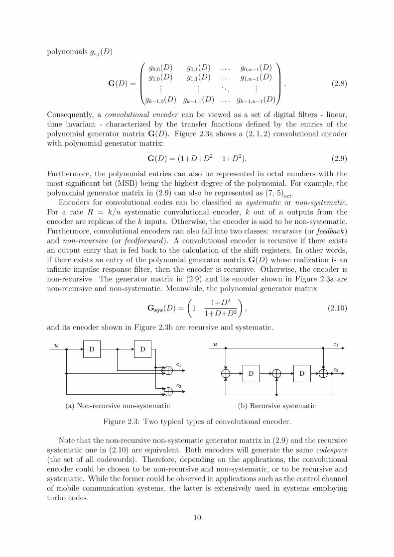
Consequently, a convolutional encoder can be viewed as a set of digital filters - linear,time invariant - characterized by the transfer functions defined by the entries of thepolynomial generator matrix G(D). Figure 2.3a shows a (2, 1, 2) convolutional encoderwith polynomial generator matrix:
G(D) = (1+D+D2 1+D2). (2.9)
Furthermore, the polynomial entries can also be represented in octal numbers with themost significant bit (MSB) being the highest degree of the polynomial. For example, thepolynomial generator matrix in (2.9) can also be represented as (7, 5)oct.
Encoders for convolutional codes can be classified as systematic or non-systematic.For a rate R = k/n systematic convolutional encoder, k out of n outputs from theencoder are replicas of the k inputs. Otherwise, the encoder is said to be non-systematic.Furthermore, convolutional encoders can also fall into two classes: recursive (or feedback)and non-recursive (or feedforward). A convolutional encoder is recursive if there existsan output entry that is fed back to the calculation of the shift registers. In other words,if there exists an entry of the polynomial generator matrix G(D) whose realization is aninfinite impulse response filter, then the encoder is recursive. Otherwise, the encoder isnon-recursive. The generator matrix in (2.9) and its encoder shown in Figure 2.3a arenon-recursive and non-systematic. Meanwhile, the polynomial generator matrix
Gsys(D) =
(1
1+D2
1+D+D2
), (2.10)
and its encoder shown in Figure 2.3b are recursive and systematic.
(a) Non-recursive non-systematic (b) Recursive systematic
Figure 2.3: Two typical types of convolutional encoder.
Note that the non-recursive non-systematic generator matrix in (2.9) and the recursivesystematic one in (2.10) are equivalent. Both encoders will generate the same codespace(the set of all codewords). Therefore, depending on the applications, the convolutionalencoder could be chosen to be non-recursive and non-systematic, or to be recursive andsystematic. While the former could be observed in applications such as the control channelof mobile communication systems, the latter is extensively used in systems employingturbo codes.
10

2.2.2 The Trellis Diagram Representation of Convolutional En-coders
A convolutional encoder consists of a set of shift registers, and the output is calculatedas a linear combination of the input and the contents of the shift registers. Therefore,the convolutional encoder can be viewed as a finite state machine (FSM). Then the trellisdiagram is simply a cascade over time of the state diagram of the state machine. Thetrellis diagram is a useful representation of a convolutional code since it helps to visualizethe encoding process as well as the decoding process of the code.
Given an encoder of a (ν, k, n) convolutional code, the process of constructing thetrellis diagram is as follows. First, the FSM of the encoder is obtained: for each of the 2ν
states s of the FSM and for each input symbol, the next state s′ and the output symbolsare computed. Figure 2.4 depicts the FSM of the convolutional encoder shown in Figure2.3b. Then, the trellis diagram of the convolutional code is deduced from the FSM, asshown in Figure 2.5 for the same code.
Figure 2.4: FSM of the convolutional encoder in Figure 2.3b.
The trellis diagram can be viewed as a two-dimensional plane. The horizontal axisconsists of time instants, and the vertical axis consists of the values of the encoder states.In this work, we consider mostly binary convolutional codes (ν, k, n). Therefore, if aninput message has K information symbols, the trellis diagram of the encoder consistsof (K/k + 1) time instants. At each time instant t, the state st can take a value in[0, 2ν−1]. The interval between time instants t and (t+1) is called trellis section t. Thestates at instant t are connected to states at instant (t+1) in trellis section t by branchesin the trellis diagram. In the case of binary convolutional codes with k = 1 as shownin Figure 2.5, there are two branches coming out of any state s at instant t, each beingconnected to a state at instant (t+1). Of the two branches, one is associated with inputbit ut = 0 (dashed line) and the other with input bit ut = 1 (solid line). An aggregationof continuous successive branches forms a state sequence which defines a path in the trellisdiagram. The concept of path is extensively useful for decoding convolutional codes usingthe well-known Viterbi algorithm.
In the case of packet transmission, the convolutional code can be made into a blockcode by the means of trellis termination. There are two main termination methods thatare used: force-to-zero [27] and tailbiting [28]. Terminating with force-to-zero introducesadditional dummy bits at the end of the message to force the trellis from state s atinstant K to a known state (usually state 0) at instant K+ν. On the other hand, with
11

Figure 2.5: Trellis diagram of the convolutional encoder in Figure 2.3b.
the tailbiting technique, the initial state of the trellis diagram is found based on the inputsequence. This initial state is obtained to ensure that the final state will be equal to theinitial state, thus making the trellis diagram circular.
2.2.3 High-Rate Convolutional Codes
For high-throughput transmission, the redundancy part of the channel encoder is usuallylimited so that higher number of information can be transmitted with the same transmis-sion resources. This is generally referred to as high coding rate schemes.
For convolutional codes, high coding rates can be achieved with two methods: withtrue high-rate encoders or by puncturing a mother encoder with lower coding rate.
2.2.3.1 True High-Rate Convolutional Encoding
A first method to achieve high coding rates is the direct use of true high-rate convolutionalencoders. The convolutional encoder is characterized by a k×n polynomial generatormatrix. Common coding rates values are of the form R = k/(k+1), i.e. n = k + 1. Fora systematic convolutional codes, this corresponds to the case where 1 output symbol iscomputed for very k-symbol chunk.
Good convolutional codes with high coding rates have been studied in the literaturefor both non-systematic [29, 30] and systematic codes [31]. The following example is takenfrom table IV in [31], where a (3, 4, 5) recursive systematic convolutional code is described
12

by the following systematic generator matrix:
Gsys(D) =
1 0 0 0 1+D+D2+D3
1+D+D3
0 1 0 0 1+D+D2
1+D+D3
0 0 1 0 1+D2+D3
1+D+D3
0 0 0 1 1+D3
1+D+D3
(2.11)
The corresponding encoder is shown in Figure 2.6. The recursive systematic encoderwith code rate k/(k + 1) can also be represented by a vector of octal numbers, wherethe first k entries are the numerator polynomials and the last entry is the denominatorpolynomial of the last column of Gsys(D). For this example, the corresponding octalvector is (17, 7, 15, 11, 13)oct.
Figure 2.6: Recursive systematic encoder of (17, 7, 15, 11, 13)oct convolutional code.
2.2.3.2 High-Rate Codes Obtained by Puncturing
Besides the use of true high-rate convolutional encoders, puncturing a low-rate motherencoder is an alternative technique to obtain a high-rate convolutional code. The messageis first encoded using a rate R = 1/n convolutional code (the mother code), but the codedsymbols are not all transmitted over the transmission channel. For ease of specificationand implementation, the discarded symbols can be periodically removed (or punctured)following a periodic pattern, called the puncturing pattern represented by a n×p matrix F,where p is the puncturing period. The successive rows of matrix F describe the patternapplied for the n outputs of the mother code. For example, a rate-4/5 code can beobtained from a rate-1/2 mother code using the following puncturing pattern:
F =
(1 1 1 11 0 0 0
). (2.12)
The search for good puncturing patterns has been intensively studied in [32, 33] forfeedforward convolutional codes and in [31, 34] for recursive systematic convolutional(RSC) codes, employed in turbo codes.
The main advantage of the puncturing technique over the true high-rate encoder isthe flexibility in changing the code rate. Indeed, a wide range of code rates can be easilyachieved by changing the puncturing pattern. Meanwhile, changing code rates in the truehigh-rate method requires different encoders, each for a specific code rate. Furthermore,since punctured high-rate codes solely employ the trellis diagram of the mother code, onesingle decoder for the mother code can be used for various code rates. On the contrary,different decoders should be employed for each code rate with true high-rate codes. That
13

is why, in most transmission systems using convolutional codes, puncturing is the chosensolution for achieving high coding rates. In return, true high-rate codes show better errorcorrection performance than punctured high-rate codes [31].
2.3 Decoding Algorithms for Convolutional Codes
In communication systems, a convolutional code can be employed as a stand-alone code, orit can be concatenated in serial or in parallel with an outer code. Therefore, depending onthe case, two main types of decoders can be used: soft-input hard-output (SIHO) decodersand soft-intput soft-output (SISO) decoders. In this section, the Viterbi algorithm (VA) isintroduced as a candidate for SIHO decoders. For SISO decoders, the soft-output Viterbialgorithm (SOVA) and the maximum a posteriori (MAP) based family algorithms willbe presented. Note that these algorithms uses the code trellis diagram for decoding. Forother decoding algorithms, readers can refer to [8] for a full reference. Furthermore, forthe sake of simplicity, we restricted ourselves to binary convolutional codes with code rateR = 1/n.
2.3.1 The Viterbi Algorithm
The VA was first introduced in 1967 by Andrew Viterbi [26] as a decoding algorithm withreasonable complexity for convolutional codes. Then, in 1973, the VA was recognized asa maximum-likelihood decoder by Forney in [35]. Since then, the VA and its derivativesplay a major role in decoding convolutional codes.
The VA decodes by exclusively employing the trellis diagram of the convolutional code.The trellis diagram is used to represent a finite-state discrete-time Markov process ob-served in white noise. Using the channel LLRs introduced in (2.4), the VA finds the statesequence s in the trellis diagram that maximizes the log-likelihood function ln Pr {y|s}.Then, from the estimated state sequence, the codeword as well as the message can be re-trieved. The decoding algorithm consists of two processes: the recursive path propagationprocess and the traceback process.
2.3.1.1 The Path Propagation Process
Let us denote Mt(s) the path metric at instant t for state s ∈ [0; 2ν − 1] in the trellisdiagram. To compute the path metrics at instant t, the VA recursively calculates thepath metrics from the initial instant t = 0. In case the trellis diagram starts from thestate zero, the 2ν path metrics are initialized as
M0(s) =
{+∞, if s = 0,
0, otherwise,(2.13)
and in case in case the initial state is not known in advance, they are initialized as
M0(s) = 0, ∀s ∈ [0; 2ν−1]. (2.14)
Assuming there are 2ν paths at instant t, the VA then calculates the path metric forthe next instant t+1. For binary convolutional codes, there are two branches comingfrom two different states s0
t and s1t at instant t that merge to state st+1 at instant t+1.
14

Therefore, there are two candidate paths for state st+1. The path metric of each candidateis computed as
Mt(sit) + Γt(s
it, st+1), i = 0, 1, (2.15)
where Γt(sit, st+1) is the metric of the branch connecting sit and st+1. The branch metric
is calculated as
Γt(sit, st+1) =
n(t+1)−1∑
j=nt
cj(sit, st+1)× L{yj|xj}, (2.16)
where cj(sit, st+1) ∈ {0, 1} is the j-th output bit labelling branch (sit, st+1), and L{yj|xj}
is the j-th channel LLR. The path metric for state sk+1 is selected as the most probablepath between the candidates as
Mt+1(st+1) = max(Mt(s
0t ) + Γt(s
0t , st+1),Mt(s
1t ) + Γt(s
1t , st+1)
). (2.17)
The selected path is usually referred to as the surviving path and the other path is consid-ered as the discarded path. Based on its elementary operators, equation (2.17) is widelyrecognized as the add-compare-select (ACS) operation. Furthermore, the VA use the ACSoperation for each state st+1 ∈ [0; 2ν−1] at instant t+1, resulting in 2ν new path metrics.The VA then stores these metrics to calculate the path metrics for the next instant t+ 2.As a result, the path metrics for every instant can be calculated recursively using thesame computation unit, denoted as the add-compare-select unit (ACSU). The process ofcalculating recursively the path metrics is the path propagation process.
2.3.1.2 The Traceback Process
When the path propagation has reached the end of the trellis diagram, the maximum-likelihood (ML) path can be obtained. If the trellis diagram is terminated by forcing tozero, then the surviving path at state 0 is the ML path. Otherwise, if the ending state isnot known in advance, the ML path should be the path with the highest metric. Then,from the ML path, the ML state sequence and the ML codeword can be retrieved. Thiscan be done by allowing the ACSU, while selecting the surviving paths at instant t, to storealso the corresponding output bits of the branches in the trellis section t. Consequently,the ML state and ML bits can be recursively obtained from the ending state of the MLpath and the stored surviving bits. However, this procedure may require a large amountof memory to store the surviving bits for every trellis section and may also introduce alarge additional latency to the decoder. To this end, the VA employs a low complexitytraceback.
Assuming that the surviving paths have reached the time instant t, the path con-vergence property of convolutional codes [35] dictates that all these surviving paths atinstant t originate from a state s at time instant (t−D). With the stored surviving bits,this state s can be traced back from any surviving path, and it is considered as the MLstate at instant (t−D). The value of D should be chosen large enough to ensure thatthe convergence property is satisfied with sufficiently high probability [36]. As a result,memories of only size D are necessary for storing the surviving bits of D previous trellissections to perform the traceback.
15

2.3.2 The Soft-Output Viterbi Algorithm
The Soft-Output Viterbi Algorithm (SOVA) was proposed by Hagenauer in 1989 in orderto meet the need for a soft-output convolutional decoder [37]. In addition to the harddecisions provided by the VA, the SOVA also produces reliability values for these decisions.In general, a SOVA decoder is made of two parts: a conventional VA decoder and areliability update unit to produce the reliability values.
The reliability update process can be demonstrated from the perspective of the bit utin the trellis section t as shown in Figure 2.7. Assuming that the path propagation of theVA has reached instant (t+D+1) as depicted in Figure 2.7a, then the traceback processprovides the ML state s at instant (t+1). Then, the metric difference ∆t+1(s) betweenthe surviving path and the discarded path at instant t for state s is the very first estimateon the reliability of the decision on bit ut in section t
Lt = ∆t+1(s). (2.18)
Note that this metric difference can be obtained by two approaches. In an intuitive way,the values of ∆t+1(s) can be stored in memory when the ACSU of the VA calculatesthe path metrics at instant (t+1). The second approach involves recomputing the metricdifference by performing two traceback processes, one for the surviving path and one forthe discarded path [38].
(a) First update where Lt = ∆t+1(s)
(b) Second update of the reliability value of ut using HR
Figure 2.7: SOVA process of finding the reliability value of bit ut in trellis section t.
Next, the VA moves to instant (t+D+2) and produces the ML state s′ for instant (t+2)as shown in Figure 2.7b. Similarly, the metric difference ∆t+2(s′) between the survivingpath and the discarded path at instant (t+2) is obtained. Furthermore, denoting by ust
16

and udt the sought bit decision of the surviving path and the discarded path, respectively,the reliability of bit ut can be updated using the following rule known as the Hagenauerrule (HR)
Lt =
{min (∆t+2(s′),Lt) , if ust 6= udt ,
Lt, if ust = udt .(2.19)
Subsequently, as the VA continues tracking the ML state for subsequent instants, thereliability of bit ut is be consecutively updated with the HR. Finally, the LLR of bit ut iscomputed as
L{ut} = (2ut − 1)× Lt, (2.20)
where ut is the hard decision of the t-th bit provided by the VA. The quality of thereliability value of a bit in the SOVA depends on the number of updates, denoted byU . In [39], the authors proposed that for ν = 3, with U = 24 and D = 32, there is nosignificant difference in performance compared to the global traceback and update case.
2.3.3 MAP-Based Algorithms
The decoding algorithms based on the MAP criterion are very popular alternatives forSISO decoding. Different from the Viterbi-based algorithms, these algorithms focus onfinding the most likely transmitted symbol rather than finding the most likely sequence.The algorithm was proposed in 1974 to decode linear codes, and the name of the algorithmis given after the names of the authors, the Bahl-Cocke-Jelinek-Raviv (BCJR) algorithm[40].
The BCJR algorithm estimates the a posteriori probability (APP) for each data sym-bol, and then the hard decision is chosen that corresponds to the maximum APP. Theimplementation of the BCJR algorithm proceeds somewhat like the path propagation ofthe Viterbi Algorithm but in both directions over the trellis diagram. It involves tworecursive processes called forward recursion for the propagation from left-to-right andbackward recursion for the propagation from right-to-left in the trellis diagram, respec-tively. Once both recursions have been completed, the APP and the hard decision can beobtained for each data symbol. Furthermore, in practice, applying the BCJR algorithmin the logarithmic domain (Log-MAP algorithm) and possibly simplifying it using themax-log approximation (Max-Log-MAP or MLM algorithm) makes it more suitable forhardware implementation.
2.3.3.1 The BCJR Algorithm
Assuming a binary convolutional code with rate R = 1/n, and y being the received vectorof length N , the APP of bit ut in trellis section t is expressed as [40]
Pr{ut; y} =∑
(s′,s)|ut
Pr {st = s′, st+1 = s; y} , (2.21)
which is equivalent to the sum of probability of all the sequence having ut ∈ {0, 1}.The BCJR algorithm defines the following probability functions where yji = [yi, yi+1, . . . , yj]
17

is the sub-vector from index i to j (0 ≤ i < j ≤ N−1) of vector y
σt(s′, s) = Pr {st = s′, st+1 = s; y} , (2.22)
αt+1(s) = Pr{st+1 = s; y
n(t+1)−10
}, (2.23)
βt+1(s) = Pr{
yN−1n(t+1) | st+1 = s
}, (2.24)
γt(s′, s) = Pr
{st+1 = s; y
n(t+1)−1nt | st = s′
}. (2.25)
Furthermore, the probability σt(s′, s) can be decomposed as
σt(s′, s) = Pr
{st = s′; ynt−1
0
}Pr{st+1 = s; yN−1
nt | st = s′}
= αt(s′)Pr
{st+1 = s; y
n(t+1)−1nt | st = s′
}Pr{
yN−1n(t+1) | st+1 = s
}
= αt(s′)γt(s
′, s)βt+1(s). (2.26)
As a result, from (2.21) and (2.26), the APP is
Pr{ut; y} =∑
(s′,s)|ut
αt(s′)γt(s
′, s)βt+1(s), (2.27)
where γt(s′, s), αt(s
′), and βt+1(s) are the branch metric, the forward state metric, andthe backward state metric, respectively. The branch metric γt(s
′, s) can be derived from(2.25) as
γt(s′, s) = Pr {st+1 = s | st = s′}Pr
{yn(t+1)−1j=nt | st = s′; st+1 = s
}
= Pr {st+1 = s | st = s′}Pr{
yn(t+1)−1j=nt | cn(t+1)−1
j=nt (s′, s)}
= Pr {st+1 = s | st = s′}n(t+1)−1∏
j=nt
Pr {yi | cj(s′, s)} , (2.28)
where Pr {st+1 = s | st = s′} is the probability having st+1 = s, given st = s′. Note thatif no a priori information is given, this probability is equal for all branches (s′, s) inthe trellis and it can be omitted since it does not affect the final MAP decision. Thebranch metric in (2.28) can be calculated locally per trellis section from the conditionalprobability of the received symbol given in (2.2). Moreover, the forward state metric iscomputed as
αt+1(s) =∑
s′
Pr{st = s′; st+1 = s; y
n(t+1)−10
}
=∑
s′
Pr{st = s′; ynt−1
0
}Pr{st+1 = s; y
n(t+1)−1nt | st = s′
}
=∑
s′
αt(s′)γt(s
′, s). (2.29)
18

Similarly, the backward state metric can be expanded as
βt(s′) =
∑
s
Pr{st+1 = s; yN−1
nt | st = s′}
=∑
s
Pr{
yN−1n(t+1) | st+1 = s
}Pr{st+1 = s; y
n(t+1)−1nt | st = s′
}
=∑
s
βt+1(s′)γt(s′, s). (2.30)
It is important to note that the state metrics in (2.29) and (2.30) can be calculatedrecursively during the forward recursion and backward recursion, respectively. Once theforward and backward state metrics are available for each instant t, the final step of theBCJR algorithm is to find the MAP decision, which can be derived from (2.27) as
ut = arg maxut∈{0,1}
∑
(s′,s)|ut
αt(s′)γt(s
′, s)βt+1(s). (2.31)
Operating in the probability domain, the BCJR algorithm employs multiplications in(2.25), (2.29), (2.30) and (2.26) making it not attractive for implementation. To circum-vent this shortcoming, the BCJR can be applied in logarithmic domain, resulting in theLog-MAP (LM) algorithm.
2.3.3.2 The Log-MAP Algorithm
The LM algorithm is the implementation of the BCJR algorithm in the logarithmic do-main. Therefore, similarly to the BCJR algorithm, it consists of four steps: the branchmetric calculation, the forward recursion, the backward recursion, and the soft-outputcalculation. Furthermore, instead of computing probability functions, the LM algorithmemploys LLRs as the basis for every calculation, using the channel LLRs obtained fromEq. (2.4).
In the LM algorithm, the branch metric is denoted as Γt(s′, s) = ln γt(s
′, s) and iscalculated as
Γt(s′, s) = ln Pr {st+1 = s | st = s′}+
n(t+1)−1∑
j=nt
cj(s′, s)L{yj|xj}. (2.32)
Now, since the convolutional code is binary, each branch (s′, s) in trellis section t isattached to an information bit ut(s
′, s) having its value in {0, 1}. Assuming that thedecoder has the following a priori information on bit ut,
La{ut} = lnPr{ut = 1}Pr{ut = 0}
, (2.33)
the logarithm probability of branch (s′, s) is derived as
ln Pr {st+1 = s | st = s′} = ln Pr{ut = ut(s′, s)}, (2.34)
and can be normalized as
ln Pr {st+1 = s | st = s′} = lnPr{ut = ut(s
′, s)}Pr{ut = 0}
+ ln Pr{ut = 0} (2.35)
=
{La{ut}, if ut(s
′, s) = 1
0, if ut(s′, s) = 0.
(2.36)
19

Note that from (2.35) to (2.36), the term ln Pr{ut = 0} is omitted since it will be cancelledout in the subsequent calculations. As a result, equation (2.32) can be transformed into
Γt(s′, s) = ut(s
′, s)× La{ut}+
n(t+1)−1∑
j=nt
cj(s′, s)× L{yj|xj}. (2.37)
The forward state metric in the LM algorithm, denoted as At+1(s) = ln(αt+1(s)), iscomputed by applying the logarithm function to Eq. (2.29)
At+1(s) = ln
(∑
s′
αt(s′)γt(s
′, s)
)= ln
(∑
s′
eAt(s′)+Γt(s′,s)
). (2.38)
Following [41], (2.38) can be reformulated using the Jacobian logarithm defined as
ln(eδ1 + eδ2) = max*(δ1, δ2) = max(δ1, δ2) + ln(1+e−|δ1−δ2|
), (2.39)
where the logarithmic correction term ln(1+e−|δ1−δ2|
)can be easily pre-calculated and
stored in a lookup table for implementation. Note that the Jacobian logarithm can beextended to any number of inputs greater than two by successively using (2.39). As aresult, the forward state metric can be expressed as
At+1(s) = max*s′
(At(s′) + Γt(s
′, s)) . (2.40)
Similarly, using the Jacobian logarithm in the backward recursion yields
Bt(s′) = max*
s(Bt+1(s) + Γt(s
′, s)) . (2.41)
In terms of the soft output, the LM algorithm produces the LLR of the APP of bit utas
L(ut) = ln
∑(s′,s)|ut=1 αt(s
′)γt(s′, s)βt+1(s)
∑(s′,s)|ut=0 αt(s
′)γt(s′, s)βt+1(s). (2.42)
By using the max* operation, it turns into
L(ut) = max*(s′,s)|ut=1
(At(s′) + Γt(s
′, s) +Bt+1(s))
− max*(s′,s)|ut=0
(At(s′) + Γt(s
′, s) +Bt+1(s)) .(2.43)
Moreover, the hard decision of bit ut can be derived as
ut =
{0, if L(ut) < 0,
1, if L(ut) ≥ 0.(2.44)
2.3.3.3 The Max-Log-MAP Algorithm
The MLM algorithm is considered as a sub-optimal version of the LM algorithm but withlower complexity [41]. The algorithm uses the max-log approximation
ln(eδ1 + eδ2 + . . .+ eδk
)≈ max (δ1, δ2, . . . , δk) , (2.45)
20

which discards the correction term in the max* operation and turns it into a max oper-ation. As a result, the forward recursion, the backward recursion, and the soft-outputcalculation in the MLM algorithm are performed as follows
At+1(s) = maxs′
(At(s′) + Γt(s
′, s)) (2.46)
Bt(s′) = max
s(Bt+1(s) + Γt(s
′, s)) (2.47)
L(ut) = max(s′,s)|ut=1
(At(s′) + Γt(s
′, s) +Bt+1(s))
− max(s′,s)|ut=0
(At(s′) + Γt(s
′, s) +Bt+1(s)) . (2.48)
In spite of a slight loss in performance compared to the LM algorithm due to themax-log approximation, the MLM algorithm gets rid of the use of lookup tables for thecorrection terms. Therefore, it is attractive due to its lower complexity. In practice, forturbo codes, the decoders employ mostly the MLM algorithm to decode the constituentconvolutional codes.
2.4 Turbo Codes
Turbo codes were first proposed by Berrou et al. in 1993 [9] as convolutional parallelconcatenated codes. For the past two decades, turbo codes have been adopted as chan-nel codes in several wireless communication standards thanks to their outstanding errorcorrection capabilities with a high degree of flexibility, in terms of block length and coderate. Notably, turbo codes were chosen for the third and fourth generations (3G and4G) of wireless mobile telecommunications as well as WiMAX, but also in digital videobroadcasting standards such as DVB-RCS/RCS2 and DVB-SH [12].
2.4.1 Turbo Encoding
A turbo encoder generally consists of two recursive systematic convolutional (RSC) en-coders concatenated in parallel and separated by an interleaver. Figure 2.8 shows thediagram of a typical turbo encoder. Let RSC1 and RSC2 be the first and second RSCencoder. Then the information message u is encoded by RSC1 producing the systematicpart and the first parity part of the codeword, denoted by cs and cp1 , respectively. On theother hand, the information message is also passed through the interleaver to produce theinterleaved information uπ. This sequence is then encoded by the second encoder RSC2
to produce the second parity part of the codeword cp2 . Note that encoder RSC2 doesnot produces any systematic part, since the systematic bits need to be transmitted onlyonce. In the end, the systematic, the first parity and the second parity parts are groupedtogether to make the turbo codeword c = [cs, cp1 , cp2 ]. Furthermore, assuming that thecode rate of RSC1 and RSC2 are R1 and R2, the code rate of the turbo code is
R =R1R2
R1 +R2 −R1R2
. (2.49)
If both RSC codes are identical with the same code rate R′, then the code rate of theturbo code is R = R′/(2−R′). Furthermore, if they are binary RSC codes with R′ = 1/2,then the turbo rate is R = 1/3.
21

Figure 2.8: Turbo encoder as the parallel concatenation of two convolutional encoders.
Similarly to convolutional codes, high-rate turbo codes can be achieved by employingtrue high-rate RSC codes or by puncturing low-rate RSC mother codes. In most commu-nication standards that employ turbo codes, the puncturing technique is chosen since itprovides flexibility in changing the code rate and it allows the reuse of the same decoder.
2.4.2 The Interleaver
The interleaver is placed in-between the two RSC component encoders of the turbo code.It plays the basic role of scrambling the information message before passing it to the secondRSC2 encoder. Given the information sequence in natural order u = [u0, u1, . . . , uK−1],the interleaved sequence is uπ = [uπ(0), uπ(1), . . . , uπ(K−1)], where j = π(i) is the in-terleaver function. Reversely, as the interleaver function is bijective, the deinterleaverfunction can be defined as i = π−1(j).
The interleaver is a key component of turbo codes. Its first purpose is the time-spreading of errors that could be produced in bursts over the transmission channel. Sec-ondly, the interleaver design has a great impact on the error correction performance ofthe turbo code and especially on its minimum Hamming distance.
In the literature, interleavers are generally classified into two categories: random-basedinterleavers and structured interleavers. The random-based interleaving function is gen-erated using random or pseudo-random methods. Hence, their practical implementationinvolves the process of memorizing the addresses of the interleaving/deinterleaving func-tions. As a result, the required memory increases the power consumption and area costof the turbo encoder and decoder, especially for large frame sizes.
On the contrary, for structured interleavers, the interleaving/deinterleaving functionsare generally obtained by simple algebraic equations, only requiring the storage of a smallset of parameters. Furthermore, their structure is more appropriate for hardware imple-mentations of turbo decoders, and for parallel architectures if they have the contention-freeproperty [42]. The most popular structured interleavers are quadratic permutation poly-nomial (QPP) interleavers [43] and almost regular permutation (ARP) interleavers [44].The QPP interleavers have been adopted in the LTE standard and are defined as
π(i) = (f1i+ f2i2) modK, ∀i = 0, 1, . . . , K − 1, (2.50)
where f1 and f2 are predefined interleaver coefficients for each information size. On theother hand, the ARP interleavers have been adopted in communication standards such asDVB-RSC/RSC2 and are defined as follows
π(i) = (Pi+ SimodQ) modK, (2.51)
22

where P and Q are the interleaver period and the disorder degree, respectively. Also,S = [S0, . . . , SQ−1] is a vector of length Q called the shift vector.
2.5 Turbo Decoding
2.5.1 Principle
The basic turbo decoder structure was proposed by Berrou in [9]. It consists of twoSISO decoders connected through an interleaver and a deinterleaver, which exchangeinformation through an iterative process. The turbo decoding process is depicted inFigure 2.9. Generally, it starts with the first SISO decoder, named SISO1, whose inputsare the systematic part received from the channel, Ls, the received first parity part Lp1
and the a priori information La provided by the other SISO decoder, if available. Then,SISO1 computes the a posteriori LLRs, denoted by L, and the extrinsic information Le
is extracted as follows:
Lei = Li − (Lsi + Lai ), ∀i = 0, 1, . . . , K−1. (2.52)
The extrinsic information was originally proposed by Berrou as the additional but notrepetitive information to be provided by a SISO decoder to the other in the iterativeprocess. Therefore, the extrinsic information extracted from SISO1 is interleaved andused as a priori information for the second decoder SISO2.
Figure 2.9: Turbo decoder consisting of two SISO decoders with the exchange of extrinsicinformation.
Then, SISO2 performs a similar decoding process with inputs consisting of the in-terleaved systematic and the second parity parts received from the channel and of theextrinsic information provided by the first decoder and used as a priori information.SISO2 decoder also computes a posteriori information as well as extrinsic information.Then, the extrinsic information is de-interleaved and used by the first decoder to start asecond iteration.
Conventionally, the process of decoding one constituent RSC code is counted as onehalf-iteration (HI) and a complete two HIs is considered as a full-iteration or iterationfor short. The iterative process of turbo decoding continues until a predefined number
23

of iterations is reached or until a stopping criterion is fulfilled. In mobile standards, theuse of cyclic redundancy check (CRC) codes [6] to detect decoding errors can serve as thestopping criteria.
From the decoding principle, the turbo decoder is affected by the choice of the con-stituent SISO decoders. Different SISO decoding algorithms can be used and, thus, havedifferent effects on the performance, complexity, throughput, etc. of the turbo decoder.
2.5.2 Comparison of Constituent Codes Decoding Algorithms
In this section, we compare the error correction performance of three candidates for theconstituent SISO decoding algorithm of turbo decoders: the LM algorithm, the MLMalgorithm, and the SOVA. These algorithms have been already detailed in section 2.3.Note that for turbo decoding with iterative process, the branch metric calculation is nowincluding the a priori information as in equation (2.37).
In order to make the comparison, the following setting is carried out for the turbocode. First, the (13, 15)oct constituent RSC code of the LTE standard is chosen withgenerator matrix
GLTE =
(1
1+D+D3
1+D2+D3
)(2.53)
and the encoder shown in Figure 2.10. We also use the QPP interleaver defined in theLTE standard. The information length is set to K = 256, and the code rate of theturbo code is R = 1/3, yielding codewords of length N = 768. The codewords arethen transmitted using BPSK modulation through the AWGN channel. The number ofiterations for turbo decoder is set to eight, and all the SISO decoding algorithms use afloating-point arithmetic representation of data.
Figure 2.10: Constituent RSC encoder of the LTE standard.
Figure 2.11 shows the turbo decoder performance for the three decoding algorithms.We can observe that, at 10−6 BER, the LM and the MLM algorithms outperform theSOVA by a gap of 0.7 dB and 1 dB, respectively. Thus, although the SOVA is claimedto require half of the number of computational operators compared to LM and MLM[41], the interest of this algorithm for turbo decoding remains limited due to its lowerperformance. Furthermore, the serial processing of traceback and reliability update inthe SOVA make it not inherently suitable for parallel processing.
Regarding the comparison between the LM and MLM algorithms, the LM outperformsthe MLM algorithm by about 0.3 dB at the expense of higher complexity and latency dueto the additional correction terms (2.39). However, MLM can be easily improved with
24

0.0 0.5 1.0 1.5 2.0 2.5 3.0Eb/N0 in dB
10 6
10 5
10 4
10 3
10 2
10 1
Bit E
rror R
ate
SOVALMMLMMLM with ESF = 0.75
Figure 2.11: Performance comparison of decoding algorithms in turbo decoder
the introduction of an extrinsic scaling factor (ESF) to compensate for the overestimationof the extrinsic information caused by the max-log approximation [45]. Extrinsic scalingwith the ESF allows the gap between the LM and the MLM to drop under 0.1 dB, asshown in Figure 2.11. Usually, the ESF is set to 0.75 for easy hardware implementation.Additionally, another advantage of the MLM over the LM algorithm is that the MLM isinsensitive to a bad estimation of the SNR, making it more robust than the LM algorithm[46].
In conclusion, throughout this work, we will use the MLM algorithm with ESF = 0.75as the baseline for the SISO decoders employed in turbo decoding processes.
2.6 Summary
In this chapter, we provided the necessary background information about convolutionalcodes and turbo codes in the context of a point-to-point digital communication chain.In particular, we described the main decoding algorithms for these codes and especiallythe SISO algorithms that are usually used for turbo decoding, namely the BCJR, theLog-MAP, and the Max-Log-MAP algorithms, as well as the SOVA that served as a basisfor a part of our work. Furthermore, we made a brief review of turbo codes, a familyof codes consisting of a parallel concatenation of two recursive systematic convolutionalcodes separated by an interleaver. The turbo decoding principle was explained, andwe introduced the concept of extrinsic information. Finally, a performance comparisonbetween the main SISO decoding algorithms was carried out in the context of turbo codes,which led to the choice of the Max-Log-MAP algorithm as the baseline decoding algorithmfor the next chapters.
25

Chapter 3
High-Throughput Turbo Decoders
As presented in the previous chapter, SISO decoder plays a fundamental part of a turbodecoder architecture. However, inherently, the component SISO decoder is serial in naturedue to the recursive calculation of the state metrics using the MLM algorithm. As a result,the SISO decoder requires a relatively large amount of memory for storing the statemetrics, and its throughput is very limited. This, in turns, also limits the throughputof the turbo decoder. Therefore, this chapter presents several techniques and decoderarchitectures that have been proposed in the literature in order to design turbo decoderswith a throughput up to 100 Gb/s.
The chapter starts by introducing in Section 3.1 the basic turbo decoding process withseveral basic techniques making a practical decoder feasible. We also define a set of usefulmetrics to analyze and evaluate the advantages and disadvantages of each technique orarchitecture. Then, in Section 3.2, techniques to increase the throughput of the decoderare presented, such as splitting the trellis into sub-trellises and processing with parallel orpipelined architectures. High-radix schemes are also considered because they allow severaltrellis sections to be aggregated, so as to be processed in a single clock cycle, thus furtherincreasing the throughput. Next, ultra-high-throughput architectures that examine fullyparallel or fully pipelined solutions are reviewed in Section 3.3. Finally, we summarizethe contents of the chapter in Section 3.4.
26

3.1 Basic Turbo Decoders
The turbo decoding process is carried out through an iterative process where two com-ponent SISO decoders exchange extrinsic information. The two component decoders canprocess in serial (sequential decoding) or in parallel (shuffle decoding) as shown in Figure3.1a and 3.1b, respectively. The former has been described in the previous chapter wherethe completion of one component decoding is referred to as one half-iteration (HI). Inthe latter, two SISO decoders process simultaneously, thus, each decoder acquires the apriori information more quickly than in the sequential decoding, which translates into afaster convergence of the decoding algorithm. The drawback of shuffle decoding is thatit requires two SISO decoders in the implementation, while only one SISO decoder isemployed in sequential decoding, since it can be reused for all HIs. Therefore, double theamount of hardware resources is needed for shuffle decoding. As a result, in this work,unless stated otherwise, we only consider the sequential decoding schedule.
Figure 3.1: Decoding process of turbo codes with 2 iterations using (a) sequential decodingand (b) shuffle decoding
The main objective of this work is to design a very high throughput turbo decoder.Hence, the decoder throughput is considered as the main performance indicator that needsto be optimized. The decoder throughput is defined as the number of decoded bits pertime unit. Since the turbo decoder consists of component SISO decoders, the throughputof the turbo decoder can easily be derived from that of a SISO decoder. Additionally, inthe framework of the EPIC project, other criteria should be taken into account to validatean architectural solution such as:
• Complexity: it can be measured by the algorithmic computational complexityand/or architectural complexity. The former is very useful in the phase of algorithmdevelopment to provide an overview and estimate of the architectural complexity.It determines the number of elementary operations performed by the decoding algo-rithm. In the case of the MLM algorithm, additions and compare-select operations
27

are considered as the elementary operations. Also, the amount of required mem-ory should also be counted in this phase. Then, the architectural complexity can bemeasured as the number of hardware resources required to implement the developedalgorithm. If an application-specific integrated circuit (ASIC) is targeted, the area(in mm2) is a direct measure of the complexity. If a field-programmable gate array(FPGA) is targeted, the complexity is measured as the number of functional unitsoccupied by the algorithm (LUTs, RAM blocks, Flip-Flops).
• Error correction performance: it is measured in terms of BER and/or FERat a given SNR as explained in Section 2.1. In the context of high throughputdecoding, some operations can be carried out in parallel and approximations canbe introduced into the decoding algorithm, thus degrading the error performanceof the decoder. If such a degradation is not tolerated, additional iterations can berequired or counteracting techniques can be introduced, which translate into a highercomplexity or a throughput decrease. Depending on the context, some applicationsaccept the error performance degradation in exchange for a throughput gain.
• Latency: this is the elapsed time between the moment the decoder receives aninput frame and the moment the decoding process has been completed. Among theuse cases defined by the EPIC project [20], some applications have a very stringentlatency requirement such as wireless connectivity in data centers (0.1 µs), hybridfiber-wireless networks (0.2 µs), while others have more relaxed requirements likemobile virtual reality (500 µs) or communications through high-throughput satellites(10000 µs).
• Flexibility: it is characterized by the scalability of the architecture in terms offrame size and coding rate (rate compatibility). In other words, it is given by thenumber of code lengths and code rates that the decoder architecture can supportwithout changing its structure.
• Other metrics: others metrics have also to be taken in account, such as the areaefficiency (in bit/s/mm2, throughput per unit area), the energy efficiency (in pJ/bit,energy required for decoding one information bit) or the power density (in W/mm2,power dissipation per unit area), which must be admissible with respect to thethermal dissipation of the device.
3.1.1 Generic Components of SISO Decoders
When considering the Max-Log-MAP algorithm, the SISO decoding process involvesbranch metric calculations (Eq. (2.37)), a forward recursion (Eq. (2.46)), a backwardrecursion (Eq. (2.46)), and the soft output calculation (Eq. (2.48)). These calculationsare carried out respectively by the following computation units: the branch metric unit(BMU), the forward and the backward ACSUs, and the soft-output unit (SOU). Figure3.2a illustrates the decoding process mapped on the trellis diagram of an RSC code.
Intuitively, one can schedule the decoding process as shown in Figure 3.2b. First, theforward state metrics are recursively calculated by the BMU and the forward ACSU. Thecalculated state metrics are stored in the memory. Then, after reaching the end of thetrellis diagram, the backward state metrics are calculated by the BMU and the backwardACSU. In the same time, the forward state metrics Ak(s) are loaded from the memory, and
28

are added to the intermediate values of (Bk+1(s′)+Γk(s, s′)). The sums are then fed to the
SOU for calculating the a posteriori and extrinsic LLRs. The architecture implementingthis scheduling is depicted in Figure 3.3, and the structures of the component computationunits are shown in Figure 3.4. Note that the presence of the feedback loop of the ACSUfor the state metrics recursion prevents this unit from being pipelined or parallelized [47].Therefore, the ACSU contains the critical path of the decoder, which limits the maximumoperating frequency.
Figure 3.2: Metric calculations in the Max-Log-MAP algorithm.
Figure 3.3: Basic SISO decoder architecture.
3.1.2 Scheduling SISO decoding
In the Max-Log-MAP algorithm, the order of execution of the forward recursion, backwardrecursion and soft ouput computation can vary, depending on the scheduling. There aretwo basic types of scheduling: Forward-Backward (FB) scheduling and butterfly schedul-ing [48, 49]. FB scheduling corresponds to the intuitive way of running MAP-basedalgorithms and has already been introduced in the previous section and illustrated byFigure 3.3(b): the forward state metrics are recursively calculated and stored in mem-ories. Then, the backward ACSU calculates the backward state metrics, and the softoutput can be computed on the fly. Another equivalent alternative is backward-forwardscheduling, which reverses the order of forward and backward recursions.
29

Max
Max
Max
Max
Max
Max
Figure 3.4: Generic computation units in a SISO decoder for a binary RSC with ν = 2.
Butterfly scheluding is shown in Figure 3.5 where the forward and backward statemetrics are calculated in parallel. At halfway, two SOUs are necessary for producing thesoft output along with the state metric calculation in both directions.
The soft output produced by the two types of scheduling is the same; hence, theyyield the same error correction performance. Furthermore, the computational complexityof both schedulings is similar and the amount of memory needed to store the state metricsis the same. However, in terms of hardware complexity, butterfly scheduling requires twoACSU in parallel and two SOUs to operate compared to only one ACSU and one SOUfor FB scheduling, making it more complex. Nevertheless, butterfly scheduling inherentlyoffers a higher throughput and a lower latency due to the fact that it can decode inK recursion steps compared to 2K recursion steps for FB scheduling. Therefore, theconstraints and requirements of the target application dictate the type of scheduling, FBor butterfly, to be applied.
3.1.3 Sliding Window Decoding
We can observe from Figures 3.2b and 3.5 that the amount of memory required to storethe state metrics of a SISO decoder increases linearly with the trellis length K, whichcan be a limiting factor for long frame sizes. Therefore, the sliding window technique wasproposed [50] to overcome this drawback. The trellis of length K is split into windowsof length W and the decoding schedule is applied at window level, thus reducing thememory requirements: the amount of storage required for the state metrics is linear with
30

Figure 3.5: Butterfly scheduling.
W intead of K. Figure 3.6 shows the overall decoding schedule with sliding windows forboth considered types of scheduling. Note that there is a continuity of forward recursionsbetween consecutive windows, while the data dependency of the backward recursions isloosened due to the discontinuity at the window borders. This raises the question of theinitialization of the backward metrics for each window.
The sliding window technique can be coupled with either FB scheduling or butterflyscheduling as depicted in Figure 3.6a and 3.6b, respectively. We can observe that, for bothtypes of scheduling, the amount of storage is reduced by a factor of K/W . Furthermore,for FB scheduling, using sliding window reduces the decoding latency from 2K recursionsteps down to (K+W ) steps. For butterfly schedule, the decoding latency with slidingwindow is still K recursion steps. From the memory requirement and latency points ofview, a low window size W is better. However if the window is too small, the errorcorrecting performance of the decoder can be degraded [51]. For applications where thevalue of K/W is relatively large, sliding window is usually employed with FB schedulingsince it generates nearly the same throughput and latency while having lower complexitythan butterfly scheduling.
Figure 3.6: Decoding with sliding windows(a) FB scheduling (b) butterfly scheduling.
31

3.1.4 State Metric Initialization
If the backward state metrics at the border of the sliding windows are initialized withequiprobable values, this can result in poor error correction performance of the decoder,especially if W is low. Therefore, initializing the state metrics with reliable values at thewindow border is necessary. Two main techniques can be found in the literature [48]:Acquisition (ACQ) and next iteration initialization (NII).
The use of ACQ initialization combined with FB scheduling and sliding window isshown in Figure 3.7a, in dashed line: LACQ recursion steps are performed prior to theregular resursion steps to initialize the state metric values at the beginning of each win-dow. The ACQ step can be regarded as a tool to enrich the backward state metrics beforethe decoder starts producing the soft outputs. Using the ACQ stage prevents the errorcorrection performance of the decoder to be degraded, at the expense of increased hard-ware complexity, due to an additional BMU and ACSU. This is all the more importantfor high coding rates R obtained with puncturing. This can be explained by the factthat the frequency of parity bits in the punctured codeword is low for high coding rates.Therefore, in this case, the ACQ length LACQ should cover at least several non-puncturedparity bit positions so that the resulting state metric is reliable enough.
NII is another technique to obtain good estimates for the initial state metrics as shownin Figure 3.7b. The principle is based on storing the last calculated state metric at theend of a window and using it as the initial value for the next window at the next iteration.Therefore, at the cost of extra memory to store the final state metric values, the errorcorrection performance can be improved without extra processing unlike in the case ofACQ. On the other hand, since the initial state metrics cannot benefit from NII at thefirst iteration, one additional iteration can be needed to obtain the same performance aswith ACQ. Therefore, a combination of ACQ and NII can be employed and is particularlyuseful for punctured high rate codes to limit the number of iterations. Figure 3.7c depictsan example of combining ACQ and NII in a turbo decoding process.
3.1.5 Evaluation of Basic Key Performance Indicators for TurboDecoders
This section shows the analytical evaluation of basic key performance indicators (KPI)for turbo decoders using the MLM SISO decoding algorithm. The basic turbo decoderuses sequential decoding as shown in Figure 3.1 with only one SISO decoder for differenthalf-iterations. This means that the LLRs output from the channel and the extrinsicinformation from each half-iteration are stored in the memory. For each half-iteration,the SISO decoder reads those values from the memory and performs the MLM decodingalgorithm. Furthermore, we assume that the SISO decoder performs FB scheduling withsliding window and that the state metrics are initialized using combined ACQ and NII asshown in Figure 3.7c.
First of all, in terms of throughput and latency, we assume the maximum operatingfrequency is f and it is limited by the critical path of the ACSU. Then, by neglecting theI/O latency, the latency of the decoder can be roughly estimated as
Latency =1
f× (K +W )× nHI, (3.1)
where nHI is the number of half iterations performed by the decoding process. The
32

Figure 3.7: State metric initialization by (a) ACQ, (b) NII, and (c) combining bothmethods.
throughput of the decoder is then expressed as
Throughput =K
(K +W )× nHI
× f. (3.2)
Note that one can increase the throughput by decreasing W or nHI but it will yield adegradation in the error correction performance. Furthermore, we can see that the decoderthroughput is a monotonic function increasing with the frame size K. Asymptotically,the throughput of the decoder as K goes to infinity is
limK→∞
1
1 +W/K× f
nHI
=f
nHI
, (3.3)
and is bounded by the operating frequency f . For a turbo decoder with 6 iterations(nHI = 12), with the operating frequency f of 800 MHz, the asymptotic throughput ofthis decoder is about 67 Mb/s.
The algorithmic computational complexity of each decoded bit in the component SISOdecoder in each half iteration is shown in Table 3.1 for a binary RSC code with rate 1/2
33

and ν memory elements. Note that for each decoded bit, the branch metric calculationand the ACS operation are performed three times (ACQ, forward and backward), and thesoft output calculation is performed once. For implementation, this basic turbo decoderrequires 3 BMU, 3 ACSU and 1 SOU with W memory units for the state metrics. Notethat these computation and memory units are reused for each half iteration in a sequentialdecoding fashion, thus, resulting in a relatively low complexity decoder. Furthermore, thisimplementation can support any frame size that is a multiple of the window size W , andcan support any code rate with puncturing. Intuitively, one can increase the throughput
AdditionComparison-
selectionTotal
Branch metrics calculation(forward & backward)
2 0 2
State metrics recursion(forward & backward)
2×2ν 2ν 3×2ν
Soft-output calculation 2×2ν + 1 2×(2ν−1 − 1) 3×2ν − 1
Computational complexityper decoded bit
8×2ν + 7 4×2ν − 2 12×2ν + 5
Table 3.1: Computational complexity per decoded bit of the MLM algorithm with FBscheduling, sliding window and ACQ according to Figure 3.7c. Convention for complexity:one addition equals one compare-select operation and is counted as one computationalunit.
of the decoder by applying direct spatial parallelism, i.e. by using multiple instanceof the basic decoder running in parallel. However, this method does not reduce thelatency and the area efficiency (throughput/complexity) remains unchanged. Therefore,in the subsequent sections, we introduce alternative parallelism techniques to increase thethroughput of the decoder, at the architectural and algorithmic levels.
3.2 High-Throughput Architectures
The basic turbo decoder architecture considered in the previous section can only achievea throughput of tens of Mb/s [47, 52]. However, due to the increasing throughput demandover time, new techniques and architectures have to be devised. The literature on parallelarchitectures for turbo codes mainly considers splitting the trellis into sub-trellises andthen processing it using a parallel MAP (PMAP) architecture architecture [53] or theso-called XMAP architecture [54]. On top of that, the algorithmic parallelism techniqueconsisting in processing several trellis sections at the same time and called high-radixprocessing [55] is also considered to help further increase the decoding throughput.
3.2.1 The PMAP Architecture
A straightforward method to help increase the throughput is to divide the trellis intosub-trellis of length KP , and having each sub-trellis decoded independently in parallel.This architecture is generally referred to as the PMAP architecture [53]. Denoting byP = K/KP the number of sub-trellises, by neglecting the I/O latency and the latency
34

due to metric initialization, the latency of the PMAP architecture can be estimated interms of clock cycles as
LatencyPMAP = (KP +W )× nHI, (3.4)
and the throughput of the PMAP architecture is
ThroughputPMAP =K
(KP +W )× nHI
× f. (3.5)
With a fixed frame size K, the throughput increases inversely with KP , i.e. it increaseswith the number of parallel sub-trellises P . As K goes to infinity, the asymptotic through-put of the PMAP architecture is
limK→∞
1
(KP/K +W/K)
f
nHI
=Pf
nHI
. (3.6)
As an example, with P = 64 independent SISO cores, f = 800 MHz and nHI = 12 (6iterations), the asymptotic throughput of the PMAP architecture is about 4.2 Gb/s.
Figure 3.8: The PMAP architecture with P = 4.
On the other side, to implement the PMAP architecture, the amount of hardwareresources increases by a factor P since each sub-trellis is processed by an independentSISO decoder. Figure 3.8 shows the scheduling and the architectural overview of thePMAP decoder. Note that Figure 3.8a shows the PMAP employing sliding window andFB scheduling, but the butterfly scheduling can also be used instead. Furthermore, NIIand/or ACQ initialization can be used to compensate for the loss in data dependency dueto sub-trellis division, thus preserving the inherent error correction performance of theturbo decoder.
3.2.2 The XMAP Architecture
Given P sub-trellises of length KP , the XMAP architecture [54] processes a single sub-trellis at a time. Sub-trellises are time-multiplexed into a pipeline consisting of a chain of
35

computation units (BMU, ACSU and SOU) connected through pipeline registers. As aresult, for each clock cycle, the decoder can produce KP soft-output values. Note that theXMAP architecture only differs from the PMAP architecture in the way each individualsub-trellis is processed.
An example of the XMAP architecture with 4 sub-trellises is shown in Figure 3.9 withthe scheduling on the left and the architectural overview on the right. Furthermore, theX-shaped architecture of the XMAP core is shown in Figure 3.10. By neglecting the I/Olatency and the latency due to metric initialization, the latency in clock cycles of theturbo decoder with XMAP architecture is
LatencyXMAP = (KP + P − 1)× nHI, (3.7)
and the throughput is
ThroughputXMAP =K
(KP + P − 1)× nHI
× f. (3.8)
Since the XMAP core consists of a chain of computation units setting up in a pipelinefashion, its complexity increases linearly with the sub-trellis length KP . Particularly,given the architecture shown in Figure 3.10, the XMAP core requires 2KP BMUs, 2KP
ACSUs, KP SOUs, as well as the pipeline registers for the state metrics, the channel andthe a priori information. Furthermore, if ACQ initialization is employed, the pipelineregisters and the number of BMUs and ACSUs will increase with the ACQ length.
Figure 3.9: The XMAP decoder with P = 4 with (a) the scheduling with the delayof 1 clock cycle between sub-trellis processing and (b) the architectural overview of thecorresponding XMAP decoder.
3.2.3 High-Radix Schemes
For SISO decoding algorithms based on the trellis diagram, like the SOVA and the MAP-based algorithms, the state metrics are calculated recursively by the ACSU. As a result,the decoder processes one trellis section per clock cycle. This is a bottleneck for a high
36

Figure 3.10: The XMAP core comprising chain of computation units and pipeline registers.
throughput implementation of SISO decoding algorithms. To overcome this problem, theauthors in [55] proposed a high-throughput computation of the state metrics by aggregat-ing successive trellis sections. This technique was first proposed for the Viterbi Algorithmand then was applied to the SOVA and the MAP-based algorithms.
For a binary RSC code with rate 1/n, the original trellis is in radix-2 form since thereare two branches coming in and out of a state. Then, the aggregation of two successiveradix-2 trellis sections results in a radix-4 trellis section as there are four branches comingin and going out of a state. Similarly, the aggregation of three and four radix-2 trellissections leads to a radix-8 and radix-16 trellis section, respectively. Figure 3.11 shows anexample of a radix-4 trellis section of a binary RSC code with ν = 2.
Figure 3.11: A radix-4 trellis section made of two consecutive radix-2 trellis sections.
37

Denoting by T the radix order, the forward state metrics calculation of the radix-2T
(T > 1) scheme for the Max-Log-MAP algorithm is obtained as follows
Ak+T (s) = maxs′
(Ak(s
′) + Γk→k+T (s′, s)), (3.9)
where Γk→k+T (s′, s) is the radix-2T branch metric connecting state s′ at instant k andstate s at instant k+T , and is calculated as the accumulation of T component radix-2branch metrics. As a result, a high-radix BMU has to compute all the combinations ofthe component radix-2 branch metrics to obtain the high-radix branch metrics providedto the ACSU. Furthermore, the a posteriori LLR of bit uk in radix-2T is calculated as
L(uk) = max(s′,s)|uk=1
(Ak(s′) + Γk→k+T (s′, s) +Bk+T (s))
− max(s′,s)|ut=0
(Ak(s′) + Γk→k+T (s′, s) +Bk+T (s)) , (3.10)
where the set of branches (s′, s) for each max operator has 2ν+T−1 elements, which in-creases exponentially with the radix order.
In terms of advantages, using radix-2T schemes produces T soft-output in a singleclock cycle. Hence, ideally, it helps increase the throughput of the decoder by a factor Twhile keeping the same error correction performance. However, radix-2T schemes requirean increase in complexity in terms of computation units (BMU, ACSU, SOU) as shownin (3.9) and (3.10). Furthermore, as shown in (3.9), the size of the set of state for themax operation in the ACSU increases with the radix order. This induces an increase inthe critical path of the ACSU, which in turns lowers the maximum operating frequency,thus decreasing the throughput of the decoder.
For the MLM algorithm, the use of radix-4 has been demonstrated to provide a higherthroughput than radix-2 schemes at the expense of a higher decoder complexity for theLTE turbo code [56]. However, radix orders greater than 2 (radix-8, radix-16 and above)were shown to be inefficient due to the increased complexity and longer critical path [57].
3.2.4 High-Throughput Turbo Decoders: State of the Art
Table 3.2 provides an overview of state-of-the-art turbo decoder implementations reportedin the literature, which use the high-throughput techniques described in the previoussections. This table shows that, by employing the PMAP or XMAP architecture with orwithout the use of high-radix schemes, turbo decoders can achieve data rates in the orderof several Gb/s.
3.3 Ultra-High-Throughput Architectures
Previous architectures and techniques can support applications with throughput require-ments up to several Gb/s. However, in the context of the EPIC project, throughputsof tens of Gb/s up to hundreds of Gb/s are required in several use cases. As far as weknow, there are two architectures that can meet such high-throughput constraints: thefully-parallel MAP [64] and the unrolled-XMAP architectures.
1Throughput measured at the maximum number of iterations
38

Reference [58] [59] [60] [60] [61] [62] [63]
Code - Flexibility LTE-A LTE-A LTE-A LTE-A LTE-AK =4096
LTE-A
Max block size 6144 6144 6144 6144 6144 4096 6144
Architecture PMAP PMAP PMAP PMAP PMAP PMAP XMAP
Radix/P 4/16 4/32 2/64 2/64 2/64 16/32 4/192
Window size 32 192 96 96 64 32 32
No. iterations max 5.5 6 8 5.5 6 8 7
Technology (nm) 65 65 90 90 65 90 28
Throughput (Gb/s)1 1.0 2.2 2.3 3.3 1.3 1.4 1.1
Frequency (MHz) 410 450 625 625 400 175 625
Area (mm2) 2.5 7.7 19.8 19.8 8.3 9.6 0.49
Area efficiency(Gb/s/mm2)
0.41 0.3 0.1 0.2 0.2 0.1 2.3
Table 3.2: Comparison of high-throughput turbo decoder implementations.
3.3.1 The Fully-Parallel MAP (FPMAP) Architecture
The FPMAP architecture combines shuffle decoding with a splitting of the trellis into sub-trellises of size KP = 1, which can be seen as an extreme case of the PMAP architecturewith P = K. The approach was first presented in [64] and an implementation based onthe LTE turbo codes was published in [65].
A schematic of the FPMAP architecture is shown in Figure 3.12. It employs 2K pro-cessing elements (PE). Each PE computes the branch metrics, the forward and backwardstate metrics and the extrinsic information for one trellis step in one clock cycle. Thecalculated state metrics at the border are then exchanged with neighbouring PEs, andthe calculated extrinsic information is fed to the interleaved/deinterleaved PEs.
Figure 3.12: The FPMAP architecture.
For the LTE turbo code, the use of the odd-even QPP interleaver helps split thePEs into two groups, where each group can be processed independently. The first group
39

consists of K/2 PEs of the SISO1 with even index and K/2 PEs of the SISO2 with oddindex (shown by grey blocks in Figure 3.12). The second group is made of K/2 PEsof the SISO1 with odd index and K/2 PEs of of the SISO2 with even index (shown bywhite blocks in Figure 3.12). Then, one complete iteration is the decoding process ofa group, with the alternation of the first and the second group. This setting halves theimplementation complexity [64] since one PE can be used to process two consecutive trellissections. However, this setting also halves the throughput of the decoder as it now takestwo clock cycles to finish an iteration. By neglecting the I/O latency, the decoder latencyin clock cycles of the FPMAP is
LatencyFPMAP = 2× nI, (3.11)
where nI is the number of iterations. The throughput of the FPMAP decoder is calculatedas
ThroughputFPMAP =K × f2× nI
, (3.12)
In [65], the authors showed that for K = 6144, the throughput of the FPMAP with 39iterations and a clock frequency of 100 MHz is 15.8 Gb/s in 65 nm CMOS. Furthermore,with this implementation the area complexity of the FPMAP decoder is 109 mm2, thus,the area efficiency is 0.145 Gb/s/mm2. Therefore, although the FPMAP can achieve ahigh throughput, the price to pay is a decrease in area efficiency compared to the PMAParchitectures [58, 59] shown in Table 3.2.
Moreover, other drawbacks of the FPMAP architecture should be the lack of flexibilitywith respect to code block sizes. Furthermore, the combination of sub-trellis size of 1 andshuffle decoding degrades the error correction performance of the decoder. At low coderates such as R = 1/3, the FPMAP requires 16 to 32 iterations to compensate for theperformance loss. However, for high code rates such as 8/9 and 18/19, it is shown in [57]that the number of iterations increases drastically up to 80.
3.3.2 The Iteration Unrolled XMAP (UXMAP) Architecture
Starting from the XMAP core shown in Figure 3.10, using multiple cores in parallel andunrolling the iterations of the turbo decoding process leads to the fully-pipelined UXMAParchitecture shown in Figure 3.13. Assuming a completely filled pipeline, by neglecting theI/O latency and the latency due to the metric initialization, the decoder produces a com-plete decoded frame of K bits per clock cycle, thus resulting in the following throughputexpression:
ThroughputUXMAP = K × f. (3.13)
Note that this throughput is only limited by the frame size and the achievable clockfrequency. In terms of flexiblity, the UXMAP architecture is rate-flexible with puncturing,and the frame-flexible aspect of the UXMAP was treated in [66].
Figure 3.14 shows the UXMAP architecture in more details, displaying the differentcomputations units and the pipeline registers. For a radix-2 sub-trellis of size KP , eachXMAP component employs 2KP BMUs, KP ACSUs for the forward state metrics, KP
ACSUs for the backward state metrics, and KP SOUs for the computation of the extrinsicinformation. Besides, pipeline registers are employed extensively to carry the channel
40

Figure 3.13: The UXMAP architecture with two iterations.
values, the calculated state metrics and the extrinsic information throughout the UXMAPdecoder. The latency of the decoder can be derived in clock cycles from Figure 3.14 as
LatencyUXMAP = nHI × (TBMU +KP + TSOU), (3.14)
where TBMU and TSOU are the number of clock cycles required for processing the firstBMU and the last SOU, respectively. Moreover, the ACSU takes one clock cycle to finisha trellis section, thus, it takes KP clock cycles to finish a sub-trellis. Furthermore, theinterleaving and the deinterleaving functions of the UXMAP architecture are hardwiredbetween the XMAP components [57], so that it provides no processing latency duringextrinsic exchange between HIs in the decoder.
Employing high radix schemes in the fully pipelined UXMAP architecture has a par-ticular impact. Increasing the number of trellis sections processed in a clock cycle leadsto a reduction in the number of pipeline stages for all the pipeline registers (state metrics,channel and extrinsic information). Hence, using radix-4 instead of radix-2 yields an areasaving of about 50% and halves the overall pipeline latency. However, as we increase theradix order, the area overhead in the computation units also increases. For Max-Log-MAP decoders using radix-8 and radix-16 processing, this overhead supersedes the areasavings in the pipelines, making the use of radix greater than 4 unattractive [57].
Table 3.3 shows the comparison between the FPMAP and the UXMAP architecturesboth implemented in 28 nm CMOS technology and reported in [57, 66]. For K = 128,the UXMAP can achieve a throughput of 102.4 Gb/s with an area of 23.61 mm2 withonly one XMAP core per HI [57], and with an area of 16.52 mm2 with 4 XMAP coresin parallel per HI [66]. The FPMAP, on the other hand, can only achieve 39.86 Gb/sin throughput with similar area consumption (24.09 mm2) for K = 6144. Beside, forK = 128, the FPMAP can only achieve 1.6 Gb/s with an area consumption of 1.04 mm2.Therefore, in terms of area efficiency, the UXMAP architecture outperforms the FPMAParchitecture by a factor of 2.6 – 4.0.
41

Figure 3.14: The detailed UXMAP architecture with 2 iterations (4 HIs) and with 4XMAP cores per HI. The area complexity of the decoder can be reduced with the increas-ing number of XMAP cores employed in parallel [67].
3.4 Summary
This chapter presents an overview of the techniques required for the hardware implementa-tion of turbo decoders, such as scheduling, sliding window, and state metric initialization.When high data rates are needed, the throughput of the turbo decoder can be increasedby employing various parallel or pipelined architectures like PMAP, XMAP, FPMAP, andUXMAP, combined with a high-radix processing of the code trellis. As a result, dependingon the chosen techniques and architecture, the throughput of a turbo decoder can rangefrom hundreds of Mb/s up to 100 Gb/s.
Moreover, a set of metrics have been defined in order to evaluate these architecturesand several turbo decoder implementations reported in the literature have been provided.Although we focus on the throughput metric in this work, one should also take accountof the complexity and the latency of the decoder. To this end, it has been shown thatthe UXMAP architecture combined with a radix-4 processing of the trellis sections canachieve 102.4 Gb/s with a relatively high area efficiency of 4.32 Gb/s/mm2. Therefore,the UXMAP was chosen as our main architecture template for our work towards thedesign of an ultra high-throughput turbo decoder.
42

Architecture UXMAP [57] UXMAP [66] FPMAP [57] FPMAP [65]
K 128 128 128 6144
Radix/P 4/1 4/4 2/128 2/6144
Frequency (MHz) 800 800 500 252
Throughput (Gb/s) 102.4 102.4 1.6 39.86
Area (mm2) 23.61 16.52 1.04 24.09
Area Eff. (Gb/s/mm2) 4.34 6.20 1.53 1.65
Table 3.3: Comparison of the implementation results of the UXMAP and FPMAP archi-tectures in 28 nm CMOS technology.
43

Chapter 4
The Local-SOVA
This chapter is dedicated to the description of a completely new algorithm that I developedin my thesis, which I called the local Soft-Output Viterbi algorithm (local-SOVA). Thealgorithm, the corresponding hardware architecture, and its application to high-radixSISO decoding are presented thoroughly.
The rest of this chapter is organized as follows. Section 4.1 gives an overview of high-radix schemes and provides the motivation for the introduction of the local-SOVA. Section4.2 recalls the MLM algorithm and analyzes it from the SOVA perspective. Section 4.3describes the local-SOVA and a corresponding hardware architecture. It is also shownthat the MLM algorithm can be seen as an instance of the proposed local-SOVA. High-radix turbo decoders using local SOVA are then considered with new simplifications inSection 4.4 and simulation results and a computational complexity analysis are providedto illustrate the advantages of the local-SOVA. Finally, Section 4.5 concludes the chapter.
44

4.1 Introduction
In this chapter, we mainly focus on how to enable high-order radix decoding schemesfor turbo decoders. Previous works in the literature, such as [68, 69], mainly tried toincrease the throughput of BCJR-based SISO decoders, without specifically consideringthe complexity reduction of the studied algorithm. Only in [70], a low-complexity radix-16 SISO decoder for the MLM algorithm was proposed, with the introduction of specificprocessing to limit the resulting error correction degradation at high signal-to-noise ratios.
On the other hand, the SOVA [37] has been recently reconsidered as an efficient SISOcandidate for turbo decoding [71, 72]. However, the interest in this algorithm remainslimited. This is because, first of all, the MLM algorithm outperforms the SOVA by about0.75 dB when used for turbo decoding [41] and, second, the serial nature of the SOVAis even more pronounced when compared to the MLM algorithm due to the involvedtraceback and the soft output update procedures. Nevertheless, the SOVA provides analternative way to perform the soft output computation for SISO decoding. In [73], theauthors proposed the modified SOVA that combines two update rules, the Hagenauerrule [37] and the Battail rule [74, 75]. This modified algorithm performs better than theclassical SOVA [37] where only the Hagenauer rule is employed. Nonetheless, the decoderin [73] is a SOVA-like decoder involving the soft output update procedure, which is aserial process in nature. The modified SOVA is able to achieve the same performance asthe MLM algorithm but the decoder has then to perform the soft output update for eachbit in each path every time it calculates the metric difference in the trellis. Consequently,it exhibits higher complexity and memory consumption than the classical SOVA.
In this section, we propose the local-SOVA, a combination between the MLM algorithmand the two above-mentioned update rules, the Hagenauer rule (HR) and the Battail rule(BR). More specifically, the proposed algorithm first performs the forward and backwardstate metric recursions as in the MLM algorithm. Then, for each trellis section, while theMLM generates the soft output as the difference between the maximum cumulated metriccorresponding to the value 1 of the considered bit and the maximum cumulated metriccorresponding to the value 0 of the considered bit, the proposed local-SOVA applies adifferent computational process using both update rules. Note that both methods resultinto the same soft output value. In fact, we will show that the MLM generation of softoutput appears to be a particular case of the local-SOVA method. Moreover, the proposedalgorithm does not involve either the traceback nor the soft output update of the classicalSOVA and it applies computation steps closer to the MLM algorithm except for the softoutput calculation. When applied to high-radix orders, the algorithm reveals to be quitedifferent from the MLM and SOVA algorithms. Indeed, it performs high-radix decoding ofconvolutional codes in an efficient way, simplifying the high-throughput implementationsof turbo decoders.
4.2 The Max-Log-MAP algorithm from the SOVA
viewpoint
Referring to Section 2.3.3.3, the Max-Log-MAP (MLM) algorithm consists of the followingsteps: branch metric calculation, forward recursion, backward recursion and soft-outputcomputation. For an RSC code with coding rate r = 1/2, these processes are expressed
45

as follows:
Γk(s, s′) = csk(s, s
′)×(Lak + Lsk
)+ cpk(s, s
′)× Lpk, (4.1)
Ak+1(s′) = maxs
(Ak(s) + Γk(s, s′)) , (4.2)
Bk(s) = maxs′
(Bk+1(s′) + Γk(s, s′)) , (4.3)
LMLM(uk) = max(s,s′)|uk=1
(Ak(s) + Γk(s′, s) +Bk+1(s))
− max(s,s′)|uk=0
(Ak(s′) + Γk(s
′, s) +Bk+1(s)) , (4.4)
where
• csk(s, s′), cpk(s, s
′) are the systematic and the parity symbols labeling the trellis branch(s, s′);
• Lsk, Lak, Lpk are the systematic, the a priori and the parity LLRs for trellis section k;
• Γk(s, s′) is the metric of branch (s, s′) for trellis section k;
• Ak(s) is the forward state metric of state s at instant k, Bk+1(s′) is the backwardstate metric of state s′ at instant k + 1;
• LMLM(uk) is the soft-output calculated by the MLM algorithm for the decoded bituk.
Let us take as an example the estimation of the soft output related to uk at trellissection k in Fig. 4.1, using the MLM algorithm. The forward and backward propagationsprovide all the values for Ak(s), s = 0, . . . , 3 and Bk+1(s′), s′ = 0, . . . , 3. Then, assumingthat (s, s′) = (0, 0) is the most likely trellis branch for uk = 0 (bold, dashed line) and that(s, s′) = (2, 1) is the most likely trellis branch for uk = 1 (bold, solid line), LMLM(uk) canbe written as:
LMLM(uk) = (Ak(2) + Γk(2, 1) +Bk+1(1))− (Ak(0, 0) + Γk(0, 0) +Bk+1(0)) (4.5)
Ak(0)
Ak(1)
Ak(2)
Ak(3)
Γk(0,0)
Γk(2,1)
Bk+1(0)
k k+1 k+3
Timeindex
k+2
Δ
Bk+1(1)
k+4
Bk+4(0)
Δ
k-1k-2
Trellissectionk
Ak-1(1)
Ak-2(2)
k-3 k+5
Forwardpropagation Backwardpropagation
Bk+2(0)
Bk+2(1)
Bk+2(2)Bk+1(2)
Bk+1(3)
Bk+3(0)
Bk+3(1)
Ak-1(3)
State
(3)
(2)
(1)
(0)
Figure 4.1: Trellis representation of a convolutional code with ν = 2. Dashed branchescorrespond to data bits equal to 0 and solid branches to data bits equal to 1.
46

On the other hand, the LLRs provided by the MLM algorithm can also be seen in adifferent way, involving paths in the trellis diagram. From section 2.2.2, a path is a statesequence corresponding to a particular input bit sequence in the trellis. Furthermore,performing the forward state metrics recursion in the MLM from instant 0 to instant kis equivalent to performing the path propagation process of the VA (see Section 2.3.1.1)from instant 0 to k. As a result, at instant k, there are 2ν values of Ak that can beconsidered as 2ν surviving paths. Similarly, the backward state metric recursion can alsobe considered as a path propagation process but in the backward direction and one canidentify another set of 2ν surviving paths after calculating Bk+1.
Furthermore, thanks to the path convergence property of convolutional codes [35], thesurviving paths can be truncated to some manageable length L to limit the amount ofmemory necessary for their storage, without any noticeable impact on the error correctionperformance. For a truncation length of L trellis sections, the VA needs to process thetrellis paths until instant k to take the decision on the information bit at instant (k−L).The value of L should be chosen large enough so that the 2ν surviving paths from theforward propagation originate from a single state at instant (k−L) with sufficiently highprobability [36]. The same rule applies if a backward propagation is carried out: in thiscase, the VA needs to process the trellis paths until instant k′ to take the decision on theinformation bit at instant (k′ + L).
Now, let us consider that both forward and backward propagations are carried outthrough the trellis. Then, for trellis section k, there are 2ν surviving paths at instant kresulting from the forward propagation and 2ν surviving paths at instant k + 1 resultingfrom the backward propagation. Connecting these two sets of paths with the 2ν+1 trellisbranches yields a total number of 2ν+1 surviving paths for trellis section k. The pathgoing through state s at instant k and through state s′ at instant k+1 has its path metricequal to Ak(s)+Γk(s, s
′)+Bk+1(s′). Moreover, because of the path convergence property,all 2ν+1 paths originate from a single state at instant k′ such that max(0, k−L) ≤ k′ < kin the forward propagation and from a single state at instant k′′ such that k + 1 < k′′ ≤min(k + L+ 1, K) in the backward propagation. So, these 2ν+1 paths merge together attimes indexes k′ and k′′.
Now, with the concept of path merging exploited in the SOVA [37], for each pair ofmerging paths, we can obtain the metric difference between these two paths by subtractingthe lower path metric from the higher one. Then, we can manipulate these resulting metricdifferences between paths to get the soft estimate of bit uk for trellis section k.
Taking the example in Fig. 4.1, the forward propagation and the backward propaga-tion provide us with four forward surviving paths at instant k and four backward survivingpaths at instant k+1, respectively. So, eight paths have to be considered for trellis sectionk, and as shown in Fig. 4.1, these paths merge into state 2 at instant k′ = k− 2 and intostate 0 at instant k′′ = k+4. Furthermore, if we denote by P0 the path going through thebranch (0,0) and by P1 the path going through the branch (2,1) in trellis section k, theLLR of bit uk can be estimated as the metric difference ∆ between these two paths wherethe path metric M0 of P0 is M0 = (Ak(0) + Γk(0, 0) +Bk+1(0)) and the path metric M1 ofP1 is M1 = (Ak(2) + Γk(2, 1) + Bk+1(1)). The result is then equal to the LLR estimatedby the MLM algorithm in (4.5).
Based on this equivalence, we can reformulate the MLM algorithm. In the trellis dia-gram, each trellis section k involves 2ν+1 paths going through 2ν+1 branches and mergingtogether. If a path goes through the branch (s, s′), its path metric Mk is then expressed
47

asMk(s, s
′) = Ak(s) + Γk(s, s′) +Bk+1(s′). (4.6)
The soft output related to bit uk is then equal to the metric difference between the pathwith the largest path metric carrying uk = 1 and the path with the largest path metriccarrying uk = 0. In the next section, we define the path merge operation, present itsproperties and show how it can be used to reformulate the MLM algorithm.
4.3 The Local-SOVA
Conventionally, a path in a trellis diagram is defined as a sequence of states and is as-sociated with an input bit sequence and a path metric. Starting from this section, wewill adopt an alternative mathematical definition of a path, with a more local sense, thatfocuses on a particular trellis section k. In the following, all the derivations focus on trellissection k. Therefore, for sake of simplicity, we will omit k in the notations.
We define a path P as a 3-tuple consisting of a path metric denoted by M , a harddecision denoted by u and a reliability value related to u, denoted by L:
P = {M,u, L} ∈ R× {0, 1} × R+, (4.7)
where R is the set of real numbers and R+ is the set of positive real numbers.As stated in the previous section, if path P goes through branch (s, s′) at trellis section
k, its path metric M is given by (4.6) where we omit (s, s′) for the sake of simplicity.Moreover, the hard decision u is the data bit carried by the corresponding branch in thetrellis diagram (0 for a dashed line or 1 for a solid line in Fig. 4.1). The reliability of thehard decision, L, is initialized to +∞ or to the largest possible value achievable with theused quantization.
We further define the merge operation
M : {R× {0, 1} × R+}2 → R× {0, 1} × R+, (4.8)
taking two paths as arguments and producing one path as output. Pa = {Ma, ua, La} andPb = {Mb, ub, Lb} being two paths, determining path Pc such that Pc =M(Pa, Pb) involvesthree procedures: finding Mc, uc and Lc. The output path metric Mc and hard decision uccan be obtained by comparing the path metrics Ma and Mb. Let p = arg maxa,b(Ma,Mb),then Mc = Mp and uc = up. Through that mechanism, if several paths merge at atrellis stage, the resulting output path will be assigned the largest path metric and willbe considered as the ML path. Then, the hard decision carried by the ML path is thedecision with highest path metric, and this is also the hard decision provided by thedecoder. Furthermore, in order to find Lc, we employ the two well-known reliability HRand BR update rules [37, 74, 75]. Both rules were proposed independently in the late 80’sfor SOVA decoders.
4.3.1 Reliability Update Rules
Let Pa and Pb be two paths to be merged and let us define p and p′ as
p = arg maxa,b
(Ma,Mb); p′ = arg mina,b
(Ma,Mb), (4.9)
48

and the metric difference between Pa and Pb as ∆p,p′ = Mp −Mp′ . Note that the metricdifference between two paths is always positive. Then, if Pc =M(Pa, Pb), Lc is calculatedas follows:
1. If ua 6= ub, apply HRLc = min
(Lp,∆p,p′
). (4.10)
2. If ua = ub, apply BRLc = min
(Lp,∆p,p′ + Lp′
). (4.11)
These two update rules can be summarized using the following update function φ:
Lc = φ(Lp, Lp′ ,∆p,p′ , up, up′
)
= min(Lp,∆p,p′ + δ(up, up′)Lp′
), (4.12)
where
δ(up, up′) =
{1, if up = up′
0, otherwise.(4.13)
The combination of these two rules for SOVA decoding was already proposed in [73]and the authors proved the equivalence with the MLM algorithm. However, in [73], theauthors only considered forward propagation. To estimate the reliability of the hardwaredecision at trellis section k, the algorithm carries out a forward propagation up to trellisstage k + L and then performs a traceback procedure. Thus, a large number of pathsshould be considered, which translates into a massive use of function φ and also into largememory for storing the reliability values after each update.
We propose an alternative algorithm that uses both forward and backward propaga-tions and hence limits the number of paths considered for trellis section k to 2ν+1, thusreducing the use of function φ.
4.3.2 Commutative and Associative Properties of the MergeOperation
As already mentioned earlier, the merge path operation described above involves threeprocedures: 1) selecting the output path metric 2) selecting the related hard decisionand 3) updating the related reliability value using function φ in (4.12). We show in thissection that the merge operation has the commutative and associative properties.
Theorem 4.1. The merge operation is commutative and associative.
• Commutative property: let Pa, Pb be two merging paths, then
M(Pa, Pb) =M(Pb, Pa), (4.14)
• Associative property: let Pa, Pb, and Pc be three merging paths, then
M(M(Pa, Pb), Pc) =M(Pa,M(Pb, Pc)). (4.15)
The “=” operator between two paths is defined as the equality between all the elements intheir tuples.
49

Proof. We will prove the commutative and associative properties of the three above-mentioned procedures of the merge operation.
For the commutative property, let us define p and p′ as in (4.9). The path metric of theoutput path is then MM(Pa,Pb) = Mp, the hard decision is uM(Pa,Pb) = up, and accordingto (4.12), the reliability value is then updated as
LM(Pa,Pb) = min(Lp, δ(up, up′)Lp′ + ∆p,p′). (4.16)
Since p and p′ do not depend on the order of Pa and Pb, the merge operation is commu-tative.
For the associative property, we can easily show that selecting a path metric andproviding a hard decision are associative procedures because they get the values of thepath with the largest metric and the maximum function is associative since
max(Ma,max(Mb,Mc)) = max(max(Ma,Mb),Mc).
Concerning the reliability update procedure, without loss of generality, we assume thatMc is the largest path metric and we define p and p′ as in (4.9). The updated reliabilityvalues of M(Pa,M(Pb, Pc)) and M(M(Pa, Pb), Pc) in (4.15) are respectively derived as
LM(Pa,M(Pb,Pc)) = min(
min(Lc, δ(uc, ub)Lb + ∆c,b
), δ(uc, ua)La + ∆c,a
)
= min(Lc, δ(uc, ub)Lb + ∆c,b, δ(uc, ua)La + ∆c,a
), (4.17)
LM(M(Pa,Pb),Pc) = min(Lc, δ(uc, up) min
(Lp, δ(up, up′)Lp′ + ∆p,p′
)+ ∆c,p
)
= min(Lc, δ(uc, up)Lp + ∆c,p, δ(uc, up)δ(up, up′)Lp′ + δ(uc, up)∆p,p′ + ∆c,p).(4.18)
Note that both δ(uc, up) and δ(up, up′) can take value in {0, 1} as defined by (4.13), theproof is then divided into four cases:
1. δ(uc, up) = 1 and δ(up, up′) = 1, then (4.18) becomes
min(Lc, Lp + ∆c,p, Lp′ + ∆p,p′ + ∆c,p) = min(Lc, Lp + ∆c,p, Lp′ + ∆c,p′), (4.19)
where ∆c,p + ∆p,p′ = ∆c,p′ . Moreover, (4.17) becomes
min(Lc, Lb + ∆c,b, La + ∆c,a). (4.20)
We can see that (4.19) is equivalent to (4.20).
2. δ(uc, up) = 1 and δ(up, up′) = 0, then (4.18) becomes
min(Lc, Lp + ∆c,p,∆c,p + ∆p,p′) = min(Lc, Lp + ∆c,p,∆c,p′). (4.21)
Without loss of generality, assuming that p = b and p′ = a, then δ(uc, ub) = 1 andδ(uc, ua) = 0, and (4.17) becomes
min(Lc, Lp + ∆c,p,∆c,p′), (4.22)
which is the same as (4.21).
50
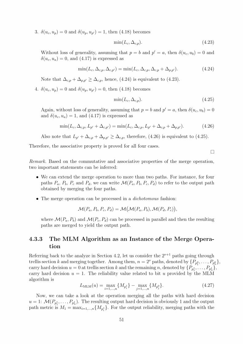
3. δ(uc, up) = 0 and δ(up, up′) = 1, then (4.18) becomes
min(Lc,∆c,p). (4.23)
Without loss of generality, assuming that p = b and p′ = a, then δ(uc, ub) = 0 andδ(uc, ua) = 0, and (4.17) is expressed as
min(Lc,∆c,p,∆c,p′) = min(Lc,∆c,p,∆c,p + ∆p,p′). (4.24)
Note that ∆c,p + ∆p,p′ ≥ ∆c,p, hence, (4.24) is equivalent to (4.23).
4. δ(uc, up) = 0 and δ(up, up′) = 0, then (4.18) becomes
min(Lc,∆c,p). (4.25)
Again, without loss of generality, assuming that p = b and p′ = a, then δ(uc, ub) = 0and δ(uc, ua) = 1, and (4.17) is expressed as
min(Lc,∆c,p, Lp′ + ∆c,p′) = min(Lc,∆c,p, Lp′ + ∆c,p + ∆p,p′). (4.26)
Also note that Lp′ + ∆c,p + ∆p,p′ ≥ ∆c,p, therefore, (4.26) is equivalent to (4.25).
Therefore, the associative property is proved for all four cases.
Remark. Based on the commutative and associative properties of the merge operation,two important statements can be inferred:
• We can extend the merge operation to more than two paths. For instance, for fourpaths Pa, Pb, Pc and Pd, we can writeM(Pa, Pb, Pc, Pd) to refer to the output pathobtained by merging the four paths.
• The merge operation can be processed in a dichotomous fashion:
M(Pa, Pb, Pc, Pd) =M(M(Pa, Pb),M(Pd, Pc)
),
whereM(Pa, Pb) andM(Pc, Pd) can be processed in parallel and then the resultingpaths are merged to yield the output path.
4.3.3 The MLM Algorithm as an Instance of the Merge Opera-tion
Referring back to the analyze in Section 4.2, let us consider the 2ν+1 paths going throughtrellis section k and merging together. Among them, n = 2ν paths, denoted by {Pp01 , . . . , Pp0n},carry hard decision u = 0 at trellis section k and the remaining n, denoted by {Pp11 , . . . , Pp1n},carry hard decision u = 1. The reliability value related to bit u provided by the MLMalgorithm is
LMLM(u) = maxi=1,...,n
{Mp1i} − max
j=1,...,n{Mp0j
}. (4.27)
Now, we can take a look at the operation merging all the paths with hard decisionu = 1: M(Pp11 , . . . , Pp1n). The resulting output hard decision is obviously 1 and the outputpath metric is M1 = maxi=1,...,n{Mp1i
}. For the output reliability, merging paths with the
51

same hard decision value requires the application of BR (4.11). Since the reliabilityvalues are all initialized at +∞, applying (4.11) yields an output reliability also equalto +∞. Similarly, merging together all the paths carrying hard decision u = 0 applyingM(Pp01 , . . . , Pp0n) results in an output hard decision 0, an output path metric equal toM0 = maxi=1,...,n{Mp0i
} and an output reliability at +∞.Then, if we merge the two resulting paths:
M(M(Pp11 , . . . , Pp1n),M(Pp01 , . . . , Pp0n)
), (4.28)
the computation of the output reliability amounts to the application of HR (4.10):
LM = min(
+∞,∣∣M1 −M0
∣∣)
=∣∣M1 −M0
∣∣, (4.29)
which is the absolute value of the expression of LMLM in (4.27). If we denote by uM theoutput hard decision deriving from (4.28), then LMLM is equal to
LMLM(uk) = (2uM − 1)× LM. (4.30)
Therefore, the result of the MLM algorithm can be interpreted as the outcome of a mergeoperation applied to all the paths.
On another note, thanks to the commutative and associative properties of the mergeoperation stated in (4.14) and (4.15), the operation merging all the paths (4.28) canbe performed in a different order for a better match with efficient software or hardwareimplementations. In particular, instead of first merging the paths with the same harddecision, one can start by merging pairs of paths with different hard decisions (Pp1i , Pp0i ),i = 1, . . . , n as
M(M(Pp11 , Pp01), . . . ,M(Pp1n , Pp0n)
). (4.31)
Moreover, if Pp1i and Pp0i are chosen in such a way that the corresponding trellis branchesat trellis section k, (sp1i , s
′p1i
) and (sp0i , s′p0i
) verify s′p1i
= s′p0i
= s′, the merge operation of
the pair of paths yields the following path metric
Mpi = max(Mp1i,Mp0i
)
= max(Ak(sp1i ) + Γk(sp1i , s
′) +Bk+1(s′), Ak(sp0i ) + Γk(sp0i , s′) +Bk+1(s′)
)
= max(Ak(sp1i )+Γk(sp1i , s
′), Ak(sp0i )+Γk(sp0i , s′))
+Bk+1(s′) (4.32)
= Ak+1(s′) +Bk+1(s′), (4.33)
and since up1i 6= up0i , the updated reliability with HR is
Lpi = min(
+∞,∆p1i ,p0i
)= ∆p1i ,p
0i
(4.34)
where
∆p1i ,p0i
=∣∣∣Mp1i
−Mp0i
∣∣∣ =∣∣∣(Ak(sp1i ) + Γk(sp1i , s
′))−(Ak(sp0i ) + Γk(sp0i , s
′))∣∣∣. (4.35)
The output hard decision upi is provided by the path, Pp0i or Pp1i , with the higher pathmetric.
We can see from (4.32) and (4.33) that, with the proposed merge ordering, the cal-culation of the output path metric for this scheduling proposal M(Pp1i , Pp0i ) includes the
52

derivation of the forward state metric Ak+1(s′) as in the forward recursion (4.2). There-fore, there is no need to perform a preliminary calculation of the forward state metrics.Only the backward state metrics need to be computed in advance. Similarly, one canshow that if the paths Pp1i and Pp0i are chosen in such a way that the corresponding trel-lis branches at trellis section k are stemming from the same state (sp1i = sp0i = s), thecalculation of the output path metric includes the same derivation of the backward statemetric Bk(s) as in the backward recursion (4.3). Then, there is no need to perform apreliminary calculation of the backward state metrics and only the forward state metricsneed to be computed in advance.
For a convolutional code with memory length ν, the overall merge operation for thecomputation of the soft output for the decoder can be carried out in a dichotomousfashion: the merge operation then requires a binary tree of 2ν+1 − 1 elementary mergeoperators organized in ν + 1 layers. Taking Fig. 4.1 as an example, ν = 2 and the softoutput related to bit uk is obtained by a binary tree consisting of ν + 1 = 3 layers ofmerge operators, as shown in Fig. 4.2.
�✁✂✄✁
� \ � 7^l
�
i
�
� \ � 7^l
�
i
�
�✁✂✄✁
� \ � 7^l
�
i
�
� \ � 7^l
�
i
�
�✁✂✄✁
� \ � 7^l
�
i
�
� \ � 7^l
�
i
�
�✁✂✄✁
� \ � 7^l
�
i
�
� \ � 7^l
�
i
�
�✁✂✄✁
�✁✂✄✁
�✁✂✄✁
☎✆✝✞ ✆✟✞✠✟✞
✡☛☞✁✂ ✌ ✡☛☞✁✂ ✍ ✡☛☞✁✂ ✎
Figure 4.2: Binary tree architecture used for the soft output computation in the local-SOVA decoder for the code of Fig.4.1.
The next section describes the overall algorithm implementing this particular arrange-ment for the merge operations.
4.3.4 The Soft Output Computation Algorithm
The soft output calculation using the merge operations in a dichotomous fashion can beperformed according to Algorithm 1. Note that this algorithm is a generic version thatassumes that all the forward and backward state metrics are pre-computed and stored ina memory.
Specific simplifications can be made for the local-SOVA. First, at the initialization step,we can organize the set of transitions T so that two adjacent transitions (s2i−1, s
′2i−1) and
(s2i, s′2i) have the same state on the left, i.e. s2i−1 = s2i, for i = 1, . . . , 2ν . Then, in line 4
of the Algorithm 1, we can initialize path metrics Mp(0) to be Γk(s, s′) +Bk+1(s′) instead
53

Algorithm 1 The generic local-SOVA
Assumption: The values of Γk(s, s′), Ak(s), Bk+1(s′) are available for all k =
0, . . . , K − 1, and for all pair of (s, s′).Initialization: T = [T (1) . . . T (2ν+1)] is the set of 2ν+1 transitions of the trellissection defined by the pairs of states (s, s′);
1: for each trellis section k = 0, . . . , K − 1 do2: for each path p = 1, . . . , 2ν+1 do3: (sp, s
′p) = T (p)
4: Mp(0) = Ak(sp) + Γk(sp, s′p) +Bk+1(s′p);
5: up(0) = data bit on transition (sp, s′p);
Initialize path Pp,p = 1, . . . , 8,for layer l = 06: Lp(0) = +∞;
7: end for
8: for each layer l = 1, . . . , ν + 1 do9: for each path p = 1, . . . , 2(ν−l+1) in layer l do
10: a = arg maxj∈{2p−1,2p}{Mj(l − 1)};11: b = arg minj∈{2p−1,2p}{Mj(l − 1)};12: ∆a,b = Ma(l − 1)−Mb(l − 1);13: Mp(l) = Ma(l − 1);
Process the(ν+1)-layerbinary tree14: up(l) = ua(l − 1);
15: Lp(l) = φ(La(l − 1), Lb(l − 1),∆a,b,ua(l − 1), ub(l − 1)
);
16: end for17: end for18: uk = u1(ν + 1); . Hard output19: L(uk) = (2uk − 1)×L1(ν + 1); . Soft output20: end for
of Ak(s) + Γk(s, s′) +Bk+1(s, s′). The resulting path metric Ma(1) at layer l = 1 is equal
to Bk(s), thus allowing the backward recursion to be incorporated into the soft outputcomputation. To compensate for omitting Ak(s) in the expression of Mp(0), the outputpath metric Mp(1) in line 13 should be taken equal to
Mp(1) = Ma(1) + Ak(s). (4.36)
Furthermore, in line 15 of Algorithm 1, the output reliability Lp(1) can be directly assigned∆a,b and the calculation of the reliability value at the first layer can be replaced by a simpleassignment operation, making the initial assignment to infinity in line 6 unnecessary. Afterlayer l = 1, the subsequent layers should be carried out following Algorithm 1 withoutany modification.
As mentioned in Chapter 3, for a practical application of SISO decoding algorithms,a scheduling (FB or Butterfly) has to be chosen and a sliding window technique can beapplied to limit the memory consumption. To achieve high throughputs, parallel archi-tectures have to be implemented. Therefore, like the MLM algorithm, the local-SOVAshould be compatible with these techniques and architectures. In fact, this is not a prob-lem since the only difference between the proposed local-SOVA and the MLM algorithm
54
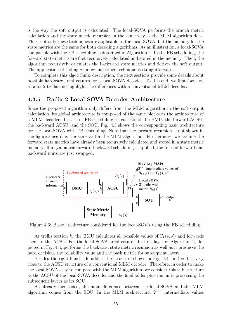
is the way the soft output is calculated. The local-SOVA performs the branch metriccalculation and the state metric recursion in the same way as the MLM algorithm does.Thus, not only these techniques are applicable to the local-SOVA, but the memory for thestate metrics are the same for both decoding algorithms. As an illustration, a local-SOVAcompatible with the FB scheduling is described in Algorithm 2. In the FB scheduling, theforward state metrics are first recursively calculated and stored in the memory. Then, thealgorithm recursively calculates the backward state metrics and derives the soft output.The application of sliding window and other technique is straightforward.
To complete this algorithmic description, the next sections provide some details aboutpossible hardware architectures for a local-SOVA decoder. To this end, we first focus ona radix-2 trellis and highlight the differences with a conventional MLM decoder.
4.3.5 Radix-2 Local-SOVA Decoder Architecture
Since the proposed algorithm only differs from the MLM algorithm in the soft outputcalculation, its global architecture is composed of the same blocks as the architecture ofa MLM decoder. In case of FB scheduling, it consists of the BMU, the forward ACSU,the backward ACSU, and the SOU. Fig. 4.3 shows the corresponding basic architecturefor the local-SOVA with FB scheduling. Note that the forward recursion is not shown inthe figure since it is the same as for the MLM algorithm. Furthermore, we assume theforward state metrics have already been recursively calculated and stored in a state metricmemory. If a symmetric forward-backward scheduling is applied, the roles of forward andbackward units are just swapped.
BMU ACSU
SOU
StateMetricMemory
a-priori&channelinformation
softoutput
Max-Log-MAP:intermediatevaluesof
LocalSOVA:pathswith
metric
Backwardrecursion
Figure 4.3: Basic architecture considered for the local-SOVA using the FB scheduling.
At trellis section k, the BMU calculates all possible values of Γk(s, s′) and forwards
them to the ACSU. For the local-SOVA architecture, the first layer of Algorithm 2, de-picted in Fig. 4.4, performs the backward state metric recursion as well as it produces thehard decision, the reliability value and the path metric for subsequent layers.
Besides the right-hand side adder, the structure shown in Fig. 4.4 for l = 1 is veryclose to the ACSU structure of a conventional MLM decoder. Therefore, in order to makethe local-SOVA easy to compare with the MLM algorithm, we consider this sub-structureas the ACSU of the local-SOVA decoder and the final adder plus the units processing thesubsequent layers as its SOU.
As already mentioned, the main difference between the local-SOVA and the MLMalgorithm comes from the SOU. In the MLM architecture, 2ν+1 intermediate values
55

Algorithm 2 The local-SOVA compatible with FB scheduling
Assumption: The values of Ak(s), are available for all k = 0, . . . , K − 1 from theforward recursion;Initialization: T = [T (1) . . . T (2ν+1)] is the set of 2ν+1 transitions of the trellis sec-tion defined by the pairs of states (s, s′) so that two adjacent transitions (s2i−1, s
′2i−1)
and (s2i, s′2i) have the same state on the left, i.e. s2i−1 = s2i, for i = 1, . . . , 2ν ;
1: Initialize BK(s);2: for each trellis section k = K − 1, . . . , 0 do3: Calculate Γk(s, s
′) according to (4.1);4: for each path p = 1, . . . , 2ν+1 do5: (sp, s
′p) = T (p);
6: Mp(0) = Γk(sp, s′p) +Bk+1(s′p);
7: up(0) = data bit on transition (sp, s′p);
8: if (p mod 2 = 0) then9: a = arg maxj∈{p−1,p}{Mj(0)};
10: b = arg minj∈{p−1,p}{Mj(0)};
Initialize paths,process layer l = 1,recursion of Bk(s)11: q = p/2;
12: Mq(1) = Ma(0) + Ak(sq)13: uq(1) = ua(0);14: Lq(1) = Ma(0)−Mb(0);15: Bk(sq) = Ma(0);16: end if17: end for
18: for each layer l = 2, . . . , ν + 1 do19: for each path p = 1, . . . , 2(ν−l+1) in layer l do20: a = arg maxj∈{2p−1,2p}{Mj(l − 1)};21: b = arg minj∈{2p−1,2p}{Mj(l − 1)};22: ∆a,b = Ma(l − 1)−Mb(l − 1);23: Mp(l) = Ma(l − 1);
Process thenext ν layers
24: up(l) = ua(l − 1);25: Lp(l) = φ
(La(l − 1), Lb(l − 1),∆a,b,ua(l − 1), ub(l − 1)
);
26: end for27: end for28: uk = u1(ν + 1); . Hard output29: L(uk) = (2uk − 1)×L1(ν + 1); . Soft output30: end for
Bk+1(s′) + Γk(s, s′) computed in the ACSU are added to Ak(s). Then, the most reli-
able branch for bit uk = 1 and for bit uk = 0 are selected using two 2ν-input maximumselection operators and the LLR is obtained by computing the difference between theterms Ak(s) + Γk(s, s
′) +Bk+1(s′) for these two branches as shown in Fig. 4.5a for ν = 2.On the other hand, the local-SOVA SOU takes the 2ν values of Bk(s), adds them to 2ν
corresponding values of Ak(s) to provide the path metrics. The hard decisions and their
56
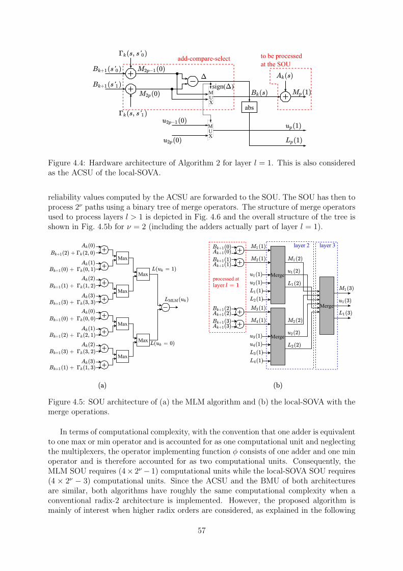
sign( )
abs
add-compare-select tobeprocessedattheSOU
MUX
MUX
Figure 4.4: Hardware architecture of Algorithm 2 for layer l = 1. This is also consideredas the ACSU of the local-SOVA.
reliability values computed by the ACSU are forwarded to the SOU. The SOU has then toprocess 2ν paths using a binary tree of merge operators. The structure of merge operatorsused to process layers l > 1 is depicted in Fig. 4.6 and the overall structure of the tree isshown in Fig. 4.5b for ν = 2 (including the adders actually part of layer l = 1).
Merge
Merge
Merge
processedatlayer
layer2 layer3
Max
Max
Max
Max
Max
Max
Figure 4.5: SOU architecture of (a) the MLM algorithm and (b) the local-SOVA with themerge operations.
In terms of computational complexity, with the convention that one adder is equivalentto one max or min operator and is accounted for as one computational unit and neglectingthe multiplexers, the operator implementing function φ consists of one adder and one minoperator and is therefore accounted for as two computational units. Consequently, theMLM SOU requires (4× 2ν − 1) computational units while the local-SOVA SOU requires(4 × 2ν − 3) computational units. Since the ACSU and the BMU of both architecturesare similar, both algorithms have roughly the same computational complexity when aconventional radix-2 architecture is implemented. However, the proposed algorithm ismainly of interest when higher radix orders are considered, as explained in the following
57

sign( )
Min
abs
function
compareselect mergeoperation
MUX
MUX
MUX
MUX
Figure 4.6: Generic hardware architecture of a merge operation M of two paths indexed2p and 2p− 1 at layer l > 1.
section.
4.4 High-Radix Decoding Algorithms Using Local-
SOVA
In the previous section, we have been considering the conventional radix-2 trellis diagram.In this section, we will concentrate on higher radix orders. Recall that in a radix-2T trellisdiagram, T > 1, there are 2T branches coming in and out of a state s at instant k. Thisis obtained by aggregating T consecutive radix-2 trellis sections. Hence, a branch in aradix-2T trellis stage is now labeled with T systematic bits and we have to reconsider thedefinition of a path and its corresponding merge operation.
01
10
11
Figure 4.7: A radix-4 stage for an convolutional code with ν = 2.
For a radix-2T trellis diagram, we define a radix-2T path P going through the branch(s, s′) as
P = {M,u1, . . . , uT , L1, . . . , LT} ∈ R× {0, 1}T × {R+}T (4.37)
where M is the path metric, u1, . . . , uT are the T hard decisions attached to branch (s, s′),and L1, . . . , LT are the reliability values for each hard decision and are initialized to +∞.
58

We also define the radix-2T merge operationM as in Section 4.3 with three procedures:path metric selection, hard decision selection and update of the reliability values. Theselection of the path metric remains unchanged. The only difference is now that we haveto select T hard decisions instead of one, and to update T reliability values using functionφ, one for each hard decision. Note that the merge operation for high-radix paths is alsocommutative and associative, therefore, the order of the paths in the merge operationdoes not affect the output. To this end, if we arrange wisely the input paths, we canreduce complexity when compared to a straightforward implementation.
4.4.1 Radix-4 Local-SOVA Decoder with Minimum ComplexityACSU
A branch in a radix-4 trellis diagram is the aggregation of two consecutive branches in aradix-2 diagram, as illustrated in Fig. 4.7 for an convolutional code with ν = 2. Frominstant k + 2 to instant k, four branches are leaving and merging into each trellis state,corresponding to the transmission of two systematic bits with possible values 00, 10, 01 and11. Therefore, at instant k, there are four radix-4 paths, denoted by {P00, P01, P10, P11},merging into each state s. Since these four paths have the same Ak(s) value, as in section4.3.4 we can initialize the corresponding path metrics with Γk→k+2(s, s′)+Bk+2(s′), whereΓk→k+2(s, s′) is the sum of the two successive branch metrics at sections k and k + 1 inthe equivalent radix-2 trellis diagram. Then, we perform the radix-4 merge operation:
M(P00, P01, P10, P11
). (4.38)
The path metric resulting from this layer-1 merge operation is also the backward statemetric of state s at instant k, Bk(s). Hence, we can consider the operator implementing(4.38) as the radix-4 ACSU of the local-SOVA decoder.
An important property of the radix-4 local-SOVA ACSU is that its complexity dependson the processing order of the paths in the merge operation (4.38). If we implement (4.38)as
M(M(P00, P01),M(P10, P11)
)(4.39)
with the hardware architecture shown in Fig. 4.8, only one φ operator has to be imple-mented. Actually, we do not need to resort to function φ in the first layer since the outputreliability is +∞ or the metric difference between the two paths, depending whether BRor HR is employed.
On the other hand, if we implement (4.38) as
M(M(P00, P11),M(P01, P10)
), (4.40)
we can use HR for both bits at the first layer but have to use a φ operation for each bitat the second layer since we do not know a priori which hard decision will be selected.Therefore, the implementation of (4.39) is less complex than the one of (4.40) and it hasminimum complexity. Note that (4.39) is not unique, since other processing orders of thepaths can also yield the same complexity, such as M
(M(P00, P10),M(P01, P11)
).
At the output of the radix-4 ACSU, 2ν radix-4 paths are forwarded to the radix-4 SOU.First of all, each path metric is added to the appropriate Ak(s) since it has been omittedin the ACSU. Then, a ν-layer tree of radix-4 merge operators is employed to produce the
59

Merge1st bit:
BR2nd bit:
HR
Merge1st bit:
BR2nd bit:
HR
Merge1st bit:
HR2nd bit:
-func
Figure 4.8: Radix-4 local-SOVA ACSU architecture implementing 2-bit merge operatorsaccording to (4.39).
final hard decision along with its reliability value. Note that the radix-4 merge operationrequires two φ operators for updating the reliability values, one for each bit.
When radix orders higher than 4 are considered, techniques for further reducing com-plexity can be considered, as explained in the following section.
4.4.2 Radix-8 local-SOVA Decoder Using a Simplified Reliabil-ity Update Operator
In this section, we introduce a sub-optimal but less complex version of the function φ,called ω. Consequently, by combining the corresponding operator with the minimumcomplexity ACSU previously described in Section 4.4.1, we propose a number of local-SOVA architectures with different complexity-performance tradeoffs.
A radix-8 trellis section aggregates three consecutive radix-2 trellis sections. Eachpath is now composed of a path metric, three hard decisions and their three reliabilityvalues. From instant k + 3 to instant k, eight radix-8 branches are leaving and merginginto each trellis state. Therefore, at instant k, there are eight radix-8 paths merginginto each state s, denoted by {P000, P001, . . . , P111}, where the indices represent the harddecisions associated with each path. Similarly to the previous cases, when applying theradix-8 merge operation to this set of paths
M(P000, P001, . . . , P111
), (4.41)
the resulting path metric is also the backward state metric of state s at time index k,Bk(s). This merging step can therefore be considered as the ACSU of the radix-8 local-SOVA decoder. Then the output path is processed by the SOU to produce the softdecision.
The minimum complexity radix-8 ACSU can be obtained by implementing (4.41) as
M(M(M(P000, P001),M(P010, P011)
),M
(M(P100, P101),M(P110, P111)
)). (4.42)
60

We can see from (4.42) that the first bit in M(M(P000, P001),M(P010, P011)
)is always
zero, hence, we can resort to a radix-4 merge operation for the last two bits using onlyone φ operator. Similarly, the first bit inM
(M(P100, P101),M(P110, P111)
)is always one,
then again, only one φ operator is necessary. In the second stage, the first bit is alwaysdifferent in the two input paths, thus only the second and the third bits require theimplementation of a φ operator. In total, four φ operators have to be implemented in aminimum complexity radix-8 ACSU.
However, employing φ operators has two main drawbacks. First of all, they consistof one adder and one min operator, therefore prohibitively increasing the complexity ofthe decoder if used excessively. Second and more importantly, the adder and the minoperators are connected serially. This is not desirable since the ACSU dictates the criticalpath of the decoder [47]. Therefore, we propose a lower complexity, lower latency, sub-optimal update operator, based on new update function, called function ω.
4.4.2.1 The Function ω
Motivated by the the possibility of using only HR as in [37], one can substitute a simplifiedfunction ω for function φ. Assuming that paths P2p−1 and P2p are to be merged at layerl − 1, the output reliability is then computed as:
Lp(l) = ω(La,∆a,b, u2p−1(l − 1), u2p(l − 1)
)
=
{min(La,∆a,b), if u2p−1(l − 1) 6= u2p(l − 1)
Lp, if u2p−1(l − 1) = u2p(l − 1)(4.43)
where a, b and ∆a,b are defined at lines 10, 11 and 12, respectively, in Algorithm 1.Fig. 4.9 shows the architecture of the elementary path merging operator using functionω. The ω operator is less complex than the φ operator since it uses only a min operationand a multiplexer resulting in a computational complexity of about one unit. However,the price to pay is a degradation of error correction performance. Indeed, a performancedegradation of 0.5 dB is observed between the conventional SOVA that uses only functionsφ [73] and the one that uses functions ω [37].
sign( )
Min
abs
function
compareselect
MUX
MUX
MUX
MUX
mergeoperationwithfunction
Figure 4.9: Generic hardware architecture of path merging operation using function ω.
Unlike the classical SOVA, the local-SOVA can mix both types of functions. There-fore, this provides the flexibility of several complexity/correction performance trade-offs.
61

However, care must be taken in making substitutions so that paths with high metricsare not eliminated from the selection process due to simplification. This is less likely tohappen if the simplifications are made in the first layers of the tree, where the number ofpaths to be processed is high. Consequently, we observed that if we only substitute theω operators for the φ operators in the first layers, we can significantly reduce complexitywithout degrading the performance of the decoder.
4.4.2.2 Radix-8 ACSU and SOU using ω operators
For a binary convolutional code with ν = 3, the first 3 layers of the path merge binarytree are in the ACSU while the last 3 layers are processed by the SOU.
As already mentioned above, the radix-8 ACSU requires 4 φ operators to update thereliability values. Substituting the ω operators for the φ operators reduces the complexityby 4 computational units. For ν = 3, the use of 2ν = 8 ACSUs saves 32 computationunits.
For the 3 layers of the binary tree implementing the radix-8 SOU, 7 radix-8 mergeoperations are required, resulting in the use of 21 φ operators (3 per merge operation).Replacing φ operators with ω operators reduces complexity but is expected to penalizethe performance of the decoder.
4.4.3 Simulation Results
Simulations were carried out to assess the error performance of the radix-8 local-SOVAand its variants for the LTE turbo code, in order to compare them with the radix-8MLM algorithm. For radix-2 and radix-4 local-SOVA, we proved in Section 4.3.3 that theLLR produced by the local-SOVA is the same as with the MLM algorithm. Therefore,their performance should be identical. Nevertheless, we first simulated the radix-8 local-SOVA with only φ operators to confirm this fact. Then, we gradually substituted ωoperators for φ operators to observe the impact on error correction when simplificationsare made to the radix-8 local-SOVA. We use the notations ACSU-(i, j) and SOU-(i, j) torepresent the different configurations, where i and j are the number of layers where ω andφ operators are employed, respectively. For example, ACSU-(2,1) means that ω operatorsare implemented in the two first layers of the ACSU and that φ operators are used in thelast layer of the ACSU. Similarly, if we use SOU-(1,2), it means that we use ω operatorsin the first layer of the SOU and use φ operators in the last two layers of the SOU.
We simulated the following seven configurations for the SISO decoding algorithms,where L-SOVA is an abbreviation for local-SOVA:
• DEC 1: MLM algorithm.
• DEC 2: L-SOVA with ACSU-(0,3) and SOU-(0,3).
• DEC 3: L-SOVA with ACSU-(3,0) and SOU-(0,3).
• DEC 4: L-SOVA with ACSU-(3,0) and SOU-(1,2).
• DEC 5: L-SOVA with ACSU-(3,0) and SOU-(2,1).
• DEC 6: L-SOVA with ACSU-(3,0) and SOU-(3,0).
62

• DEC 7: classical SOVA.
The simulations were carried out with information frames of K = 1056 bits, encoded withthe non-punctured r = 1/3 LTE turbo code, modulated by BPSK and transmitted overthe AWGN channel. A floating point representation of data is used in the decoder. Theresulting bit error rate (BER) is measured after 5.5 decoding iterations. Fig. 4.10 showsthat, as expected, the local-SOVA with only φ operators (DEC 2) has the same perfor-mance as the MLM algorithm. Moreover, by substituting ω operators for φ operators inthe ACSUs, i. e. in the first three layers, (DEC-3) the simulated curves confirm thatthe error correction performance of the decoder is not degraded, thus providing a lowcomplexity alternative to the original local-SOVA decoder. By gradually replacing theφ operators in the SOU, the performance is degraded by 0.05 dB at BER = 10−6 whenω operators are used in the first two layers and by about 0.3 dB when only ω operatorsare implemented. Fig. 4.10 also shows that the classical SOVA (DEC 7) performs 0.1dB worse than the local-SOVA with only ω operators (DEC 6). According to [73], usingφ operators instead of ω operators in the both the classical and local-SOVAs would beequivalent to apply the MLM algorithm (DEC 1). However, contrary to the classicalSOVA, the operations in the local-SOVA are arranged so as to minimize the number ofused φ operators. Therefore the performance gap between DEC 6 and DEC 7 is explainedby the fact that the number of sub-optimal ω operators needed in DEC 7 is greater thanin DEC 6.
0.0 0.2 0.4 0.6 0.8 1.0 1.2 1.4 1.6Eb/No in dB
10−6
10−5
10−4
10−3
10−2
10−1
Bit E
rror R
ate
DEC 1: MLMDEC 2: L-SOVA ACSU-(0,3) SOU-(0,3)DEC 3: L-SOVA ACSU-(3,0) SOU-(0,3)DEC 4: L-SOVA ACSU-(3,0) SOU-(1,2)DEC 5: L-SOVA ACSU-(3,0) SOU-(2,1)DEC 6: L-SOVA ACSU-(3,0) SOU-(3,0)DEC 7: classic SOVA
Figure 4.10: BER performance of a LTE decoder using radix-8 MLM algorithm, local-SOVA and its variant with K = 1056, r = 1/3 after 5.5 iterations. AWGN channel, BPSKmodulation.
63

4.4.4 Computational Complexity Analysis
In this section, we perform the comparison between the local-SOVA and the MLM al-gorithm in terms of complexity for different radix orders. To quantify complexity, wecalculate the number of additions and the number of compare select (CS) operations andconsider again one adder or CS operator as one computational unit. In this comparison,we use the FB scheduling and we do not take the memory requirements into account andonly consider computational complexity. As aforementioned, the difference between thelocal-SOVA decoder and the MLM decoder resides in the way it calculates the soft output.Therefore, the memory for the channel information, the state metrics and the extrinsicinformation is the same as in the MLM decoder. Moreover, sliding window techniques ordifferent decoding schedules can also be applied to the local-SOVA, hence, the memoryconsumption of the decoder depends on the hardware architecture.
In this analysis, we use a convolutional code with 8 states (ν = 3). The decodingcomplexity, denoted by C, is reported for one trellis section consisting of eight forwardACSUs, eight backward ACSUs, and one SOU as
C = (8× CF ) + (8× CB) + CS, (4.44)
where CF , CB and CS denote the computational complexity of the forward ACSU, thebackward ACSU, and the SOU, respectively. Note that we excluded the BMU in theexpression since the calculation of branch metrics is the same for the local-SOVA and theMLM algorithm. For the MLM algorithm, the forward and backward ACSUs have thesame computational complexity. Since we are considering the FB schedule, the forwardACSU of the local-SOVA is the same as in the MLM algorithm. However, the backwardACSU of the local-SOVA not only calculates the state metrics but also take part in thesoft output calculation with φ and ω operators. Therefore, there will be some differencecompared to the backward ACSU of the MLM algorithm.
Firstly, we perform the complexity comparison between the local-SOVA employingonly φ operators and the MLM algorithm to observe the change of the complexity differ-ence versus the radix order. Then, for radix-8, we perform further complexity analysisfor cases where φ operators are gradually replaced by ω operators.
4.4.4.1 Radix-2 local-SOVA and radix-2 MLM algorithm
As shown in Section 4.3.5, the forward ACSUs of the local-SOVA and the MLM algorithmare identical. Therefore, for both algorithms, the forward ACSU and the backward ACSUhave the same complexity and consist of two adders and one CS operator. For the SOU,the structures are shown in Fig. 4.5a and Fig. 4.5b for the MLM algorithm and thelocal-SOVA, respectively. With ν = 3, the MLM SOU consists of 17 adders and 14 CSoperators, whereas the SOU of the local-SOVA requires 22 adders and 7 CS operators. Intotal, applying (4.44), the complexity of the MLM decoder is 79 computational units andthe complexity of the local-SOVA decoder is 77 computational units.
4.4.4.2 Radix-4 local-SOVA and radix-4 MLM algorithm
For the MLM algorithm, the backward and the forward ACSUs have the same complexityand consist of 4 adders and 3 CS operators. Furthermore, the SOU of the MLM algorithmbegins by adding 32 intermediate values of Γk→k+1(s, s′) + Bk+2(s′) to Ak(s), using 32
64

adders. Next, two maximum selection trees for each systematic bit, each consisting of15 CS operators, are needed. Finally, each LLR value is obtained by using one extrasubtractor (adder). In total, MLM decoding requires 98 adders and 108 CS operators, i.e.206 computational units.
As for the local-SOVA, the forward ACSU is the same as for the MLM algorithm.Apart from the calculation of the state metric, the backward ACSU of the local-SOVArequires one extra φ operator (one adder and one CS operator) to update the reliabilityvalues, as shown in Section 4.4.1. Therefore, the backward ACSU of the local-SOVAconsists of 5 adders and 4 CS operators. For the SOU, the Ak(s) values are added to 8path metrics using 8 adders. Then, a 3-layer tree of radix-4 merge operators is employed,which consists of 7 CS operators and (2×7) φ operators (to decode 2 bits). Therefore,the total complexity of the SOU for the local-SOVA is 22 adders and 21 CS operators.Finally, from (4.44), the complexity of the radix-4 local-SOVA is 151 computational units.
4.4.4.3 Radix-8 local-SOVA and radix-8 MLM algorithm
For the MLM algorithm, the forward/backward ACSU requires 8 adders and 7 CS oper-ators. The MLM SOU uses 64 adders to add Ak(s) to the intermediate values providedby the backward ACSU. Then, two maximum selection trees, each consisting of 31 CSoperators, are employed for each systematic bit. Finally, 3 extra subtractors are requiredto compute the LLR of the 3 bits. In total, the complexity of the radix-8 MLM decoderis 493 computational units.
On the other hand, for the local-SOVA, the backward ACSU requires 4 extra φ op-erators to update the reliability values. For the SOU, 8 adders are first required to addthe values of Ak(s) to the path metrics. Then, a 3-layer tree of radix-8 merge operatorsis employed, which consists of 7 CS operators and (3×7) φ operators (to decode 3 bits).Thus, in total, the complexity of the radix-8 local-SOVA decoder is 361 computationalunits.
Table 4.1 summarizes the results of the complexity analysis for radix-2, radix-4 andradix-8 schemes. CMLM and CLSOVA denote the computational complexity of the MLMalgorithm and the local-SOVA, respectively. For radix-2, the MLM algorithm and thelocal-SOVA have roughly the same complexity, while for radix-4 and radix-8 schemes,the local-SOVA is less complex. For high-radix schemes (4 and 8), using the local-SOVAreduces complexity by 27%.
Table 4.1: Comparison of the computational complexity of the MLM algorithm and thelocal-SOVA for various radix schemes (Add: adder; CS: compare-select).
Radix
schemes
Max-Log-MAP local-SOVACLSOVA
CMLM8×CF 8×CB CS CMLM
8×CF 8×CB CS CLSOVAAdd CS Add CS Add CS Add CS Add CS Add CS
Radix-2 16 8 16 8 17 14 79 16 8 16 8 22 7 77 0.975
Radix-4 32 24 32 24 34 60 206 32 24 40 32 22 21 151 0.733
Radix-8 64 56 64 56 67 186 493 64 56 96 88 29 28 361 0.732
Furthermore, the complexity per decoded bit of the MLM algorithm increases from 79to 206/2 = 103 computational units when moving from radix 2 to radix 4. In contrast, itdecreases from 77 to 75.5 computational units for the local-SOVA. Therefore, using the
65

local-SOVA for radix-4 schemes can further increase the efficiency of the decoder. Onthe other hand, for radix-8 schemes, although the local-SOVA is less complex than theMLM algorithm, its complexity per decoded bit is raised to 120.3 computational units.It is higher than for radix 4 but enables a throughput increase. Moreover, it can besignificantly reduced by replacing the φ operators by ω operators, as shown in the follows.
4.4.4.4 Radix-8 local-SOVA with ω operators
The complexity analysis of the local-SOVA for a radix-8 scheme was reiterated by grad-ually replacing φ operators by ω operators in the backward ACSUs and in the SOU. Weconsidered the same configurations and notations as in Section 4.4.3, and the computa-tional complexity is still calculated based on (4.44).
The complexity comparison is shown in Table 4.2, where the MLM decoding complex-ity is taken as a reference for complexity normalization and performance comparison. Wecan observe that if we use ω operators instead of φ operators in the backward ACSUs(DEC 3), the resulting complexity is reduced to 67% of the complexity of the referencedecoder compared to 73% if only φ operators are used, with no noticeable impact on thecorrection performance. If a lower complexity is desired, the local-SOVA with ACSU-(3,0) and SOU-(2,1) (DEC 5) can be employed to reach 63% of the reference complexity,at the cost of a performance degradation of 0.05 dB. Table 4.2 also shows that usingonly ω operators (DEC 6) further reduces the complexity by 1% but the resulting 0.3 dBperformance loss makes this configuration less attractive.
Table 4.2: Comparison of the computational complexity of various radix-8 algorithms(CS: compare-select).
Algorithm8× CB 8× CF CS Computational
complexity C
Complexity
normalization
Performance loss
at BER 10−6 (dB)Add CS Add CS Add CS
MLM 64 56 64 56 67 186 493 1 −
DEC 2 64 56 96 88 29 28 361 0.73 0.0
DEC 3 64 56 64 88 29 28 329 0.67 < 0.01
DEC 4 64 56 64 88 17 28 317 0.64 0.05
DEC 5 64 56 64 88 11 28 311 0.63 0.05
DEC 6 64 56 64 88 8 28 308 0.62 0.3
4.4.5 Radix-16 Local-SOVA Decoder for Convolutional Codeswith Memory Length ν = 3
In this section, we extend the previous study by considering a particular implementationof the radix-16 local-SOVA for ν = 3 (8-state) convolutional codes. A section of a radix-16trellis diagram is the aggregation of four consecutive sections in a radix-2 trellis diagramor, equivalently, of two consecutive sections in a radix-4 trellis diagram. With the latterrepresentation, a pair of states s and s′ between two instants k and k + 4 are connectedby two parallel branches as illustrated in Fig. 4.11 between s = 2 and s′ = 4.
66

Figure 4.11: A radix-16 trellis section made of two radix-4 trellis sections.
Intuitively, one could decode this code with a radix-16 ACSU using 16-input max-selectoperations to produce the state metrics. However, increasing the number of inputs of themax-select operators results in a longer propagation path in the ACSU, thus lengtheningthe critical path of the decoder. To get around this problem, the authors of [70] suggestedthat we can select the branch with larger branch metric Γk→k+4(s, s′) among the twoparallel branches connecting two states, and discard the other one. Since this task couldbe done in the BMU to reduce by half the number of branches, we can then use radix-8 ACSUs for the calculation of the state metrics. However, the main drawback of thisapproach when applied to the MLM algorithm is that the branches selected after theBMU might carry either uj = 1 or uj = 0, for j = k, . . . , k + 3, which we cannot knowin advance. This creates a ratio between the number of branches having uj = 1 and thenumber of branches having uj = 0 that varies over different trellis sections and differentreceived frames. This causes a major problem for the MLM SOU since it naturally employsmax-select operations with a constant number of inputs referring to hard decisions 1 and0.
On the other hand, from the local-SOVA perspective, the two parallel branches pro-cessed by the BMU can be considered as the merge of two paths. Hence, we can use thepath merging operation to produce one path carrying the selected hard decision and theupdated reliability value. The BMU can then forward 64 paths to radix-8 ACSUs, whichin turn produce 8 output paths for the SOU to finally compute the soft output. So, inthe radix-16 local-SOVA decoder, the BMU, the ACSU and the SOU constitute a pathmerging binary tree with 7 layers: the first layer is in the BMU, and thus not in thecritical path, the three next layers are in the ACSU, and the last three layers in the SOUthat are also not in the critical path. In addition, since the order of the input paths doesnot affect the result of the merge operations, the local-SOVA is immune to the problemof the non-static ratio of hard decision value mentioned above for the MLM algorithm.
Extensive simulations with the radix-16 local-SOVA were also carried out. Similarly tothe radix-8 case, we first performed a radix-16 local-SOVA with only φ operators. Then,we gradually substituted ω operators for φ operators in order to observe the behavior ofthe decoder. The results are shown in Fig. 4.12. We can observe that we can still replaceφ operators by ω operators in the ACSU and in the first layer of the SOU with a negligibledegradation in performance. However, further substitutions are not recommended sincea penalty of 0.4 dB at 10−4 of BER can be observed if we use solely ω operators.
When considering higher radix orders such as 32 and 64 for the same convolutional
67

0.0 0.2 0.4 0.6 0.8 1.0 1.2 1.4 1.6Eb/No i dB
10−6
10−5
10−4
10−3
10−2
10−1
Bit E
rror R
ate
Radix-16 MLMRadix-16 L-SOVA ACSU-(0,3), SOU-(0,3)Radix-16 L-SOVA ACSU-(3,0), SOU-(0,3)Radix-16 L-SOVA ACSU-(3,0), SOU-(1,2)Radix-16 L-SOVA ACSU-(3,0), SOU-(2,1)Radix-16 L-SOVA ACSU-(3,0), SOU-(3,0)
Figure 4.12: BER performance of a LTE decoder using radix-16 MLM algorithm, local-SOVA and its variants with K = 1056, r = 1/3 after 5.5 iterations. AWGN channel,BPSK modulation.
code, there are respectively 4 and 8 parallel branches connecting two states in each high-radix trellis section. In this case, the BMU selects the path with the largest path metricamong the 4 or 8 paths. Moreover, since the BMU does not involve a recursive loop asin the ACSU, it can be pipelined to ensure that the critical path always resides in theACSU. However, since the complexity of the decoder increases exponentially with thenumber of bits decoded simultaneously, it is then necessary to find the processing orderof the paths with the best compromise between throughput and complexity. Nonetheless,using local-SOVA with high-radix orders provides an ultra high throughput solution forconvolutional and turbo codes since the critical path of the decoder can always remainsin the radix-8 ACSU while decoding an increasing number of systematic bits in a singleclock cycle.
4.5 Conclusion
In this chapter, we have introduced a new SISO decoding algorithm for convolutionalcodes: the local-SOVA. The decoder architecture for the local-SOVA is shown to exhibita more hierarchical structure and a lower computational complexity than the conventionalMax-Log-MAP algorithm.
We observed that using local-SOVA in radix-8 LTE turbo decoders significantly re-duces the computational complexity of the decoder compared to the respective radix-8Max-Log-MAP architecture. For instance, employing the local-SOVA algorithm for radix-8 decoding of the LTE turbo code reduces the complexity by 33% without any performancedegradation and by 36% with a slight penalty of only 0.05 dB. Moreover, the local-SOVAmakes it possible to increase the radix-order without penalizing the error correction per-
68

formance or the critical path of the decoder, but at the cost of added complexity. Theseadvantages make local-SOVA our first-choice algorithm for developing high-radix turbodecoders.
The study of the proposed algorithm and its results were published in the IEEETransaction on Communications [21].
69

Chapter 5
The Local-SOVA in Unrolled-XMAPArchitecture
The previous chapter showed that, when used with high radix orders, the local-SOVAdecoder has a lower computational complexity than the MLM decoder. Therefore, thischapter deals with the implementation of the computational units of radix-4, radix-8 andradix-16 local-SOVA decoders in the UXMAP architecture introduced in Section 3.3.2 forhigh-throughput applications. For each radix order, hardware architectures are proposedand implemented to observe how the computational complexity savings translate into areasavings.
The rest of the chapter is organized as follows. Section 5.1 briefly describes theUXMAP architecture and provides an overview of the benefits of employing the local-SOVA in the UXMAP architecture. Then, the state-of-the-art UXMAP architecture withthe MLM algorithm is described in Section 5.2. Section 5.3 presents the implementationof the radix-4, radix-8 and radix-16 local-SOVA decoders. These high-radix schemes arealso compared with the standard MLM decoder and with each other in terms of areacomplexity, error correction performance and latency/throughput. Finally, Section 5.4concludes the chapter.
70

5.1 Introduction
It was recently shown that a turbo decoder using the UXMAP architecture and imple-mented in CMOS 28 nm technology could achieve a throughput of 100 Gp/s for K = 128with the radix-4 MLM algorithm and 4 decoding iterations (8 HIs) [57, 67]. According toEq. (3.13) in Section 3.3.2, the throughput of a turbo decoder with the UXMAP archi-tecture increases linearly with K since it produces K decoded bits in a single clock cyclewhen the pipeline is full. Therefore, a throughput of 1 Tb/s can in theory be achievedwith the UXMAP architecture when K ≈ 1280. However, for a given number of decodingiterations, the area complexity of the UXMAP decoder also increases with the frame sizeK. Nonetheless, when K increased, the correlation between the two constituent RSCdecoders is reduced provided the interleaver is well designed [34] and the error correctionperformance is improved. On that basis, the authors in [67] showed that the UXMAParchitecture with K = 256 and K = 512 only needs 3 and 2.5 decoding iterations, re-spectively, to achieve the same correction performance as in the case of K = 128 with 4iterations. As a result, for K = 512, the decoder throughput is increased by 4 times, whilethe area complexity is only increased by 2.5 times, thus, resulting in an area efficiencyincreased by 1.6 times.
Furthermore, the previous chapter showed that the local-SOVA has a lower compu-tational complexity than the MLM algorithm, expecially for high radix orders. For theradix-4 case, the analysis in Chapter 4 led to a reduction of 27% in computational com-plexity. Assuming that this computational complexity saving can be translated into areasaving, one can expect that embedding a radix-4 local-SOVA in the UXMAP architecturecan reduce the decoder area by 25 to 30% compared to a radix-4 MLM UXMAP decoder.Equivalently, keeping the same area complexity as the MLM decoder, we can increase Kby 1.4 times by using the local-SOVA decoder instead, and thus, have a throughput gainand an area efficiency gain of 1.4.
The promising results of Chapter 4 encouraged us to consider using even higher radixschemes (radix-8, radix-16) with the UXMAP architecture. There are then several aspectsto be taken into account. Assuming that using higher radix schemes does not lower theoperating frequency, then the latency of the decoder can be reduced, since more bits areprocessed in a clock cycle. This characteristic is particularly interesting for applicationsrequiring low processing latency. Using higher radix schemes also means that the numberof computational units (BMU, ACSU, SOU) and registers in the pipeline of the UXMAPcan be decreased, leading to a reduction in the area complexity. But, on the other hand,the complexity of the computational units also increases with the radix order. Therefore,the actual impact of increasing the radix order can only be meaningfully assessed throughimplementing these high radix local-SOVA decoders in an UXMAP architecture.
In the next section, the fixed-point implementation of the UXMAP with the radix-4 MLM algorithm is discussed. This will serve as a basis for the design of our local-SOVA/UXMAP decoder and for comparisons. All the implementations and comparisonswere carried out for the LTE turbo code using rate-1/2 RSC component codes.
71

5.2 Fixed-Point Implementation of the Radix-4
MLM/UXMAP Decoder
This section describes the implementation of turbo decoders using the UXMAP archi-tecture with the radix-4 MLM decoding algorithm. As described in Section 3.3.2, thefully pipelined UXMAP architecture unrolls the decoding iterations and applies a spatialparallelization of the XMAP cores where each XMAP core processes a sub-trellis of lengthKP within a half-iteration. The authors in [67] have shown that KP = 32 is the optimallength for each XMAP core as smaller lengths entail a performance degradation, whichin turns requires more iterations to be compensated for. It is also shown in [67] that,compared to higher sub-trellis lengths (KP = 64 or KP = 128), using KP = 32 with asmall ACQ length at the first iteration does not degrade the error correction performanceand up to 40% of the area complexity can then be saved. Moreover, using KP = 32 alsoenables frame size flexibility to support K = 128, 64, 32 [66].
The XMAP core is made of computational units and pipeline registers as described inSection 3.3.2. Three distinct computational units, BMU, ACSU and SOU, constitute thebackbone of the XMAP core and hence of the UXMAP architecture. The next sectiondeals with the implementation of these computational units.
5.2.1 Computational Units Implementation
5.2.1.1 Branch Metric Unit
The BMU calculates all the branch metrics of the current trellis section and send themto the ACSU for further process. The constituent RSC code has coding rate R = 1/2.Therefore, for a radix-2 trellis section k, there are one systematic bit and one parity bit,and we have 4 branch metrics values:
Γk(00) = 0
Γk(01) = LpkΓk(10) = Lsk + LakΓk(11) = Lsk + Lak + Lpk
(5.1)
This representation suppose that all the branch metrics are normalized by subtractingthe metric of the all-zeros branch.
The radix-4 branch metrics can be directly calculated from the radix-2 branch metricsof sections k and k+1. The implementation of the radix-4 BMU is therefore a network ofadders and can be straightforwardly implemented.
5.2.1.2 Add Compare Select Unit
The ACSU receives the branch metrics from the BMU and computes the forward andbackward state metrics recursively. For instance, the forward state metric calculation inradix-4 scheme is expressed as
Ak+2(s) =∑
s′
(Ak(s
′) + Γk→k+2(s′, s)), (5.2)
72

where the size of the set of state s′ in the summation is 4. Equation (5.2) is implementedby an ACS operator. The radix-4 ACS operator can be implemented as a tree-like struc-ture as shown in Figure 5.1a or can be carried out by six compare-select (CS) operatorsfollowed by a look-up table (LUT) [56, 76, 77] as shown in Figure 5.1b. The tree-likestructure has lower complexity but it has higher critical path [56]. Moreover, the tree-like architecture could not be pipelined because it would have the same throughput andlatency compared to the radix-2 case but with higher complexity. On the other hand,although the implementation using LUT in Figure 5.1b is more complex (6 CS operators)than to the tree-like implementation (3 CS operators), this architecture shortens the crit-ical path of the ACSU by about 50% as shown in [56]. Therefore, it is the one that wechose to be implemented in the UXMAP architecture, since we are seeking high operatingfrequency for high throughput and low latency.
Figure 5.1: The schematic of the radix-4 Max-Log-MAP ACS operator using (a) a tree-likearchitecture, and (b) a LUT approach.
5.2.1.3 Soft Output Unit
The input of the SOU are metrics Ak(s), Γk→k+2(s, s′), and Bk+2(s′). It performs the softoutput calculation for two bits uk and uk+1 as follows:
L(ui) = max(s′,s)|ui=1
(Ak(s′) + Γk→k+2(s′, s) +Bk+2(s))
− max(s′,s)|ui=0
(Ak(s′) + Γk→k+2(s′, s) +Bk+2(s)) , i = k, k+1. (5.3)
Then, the extrinsic information of the systematic bits can be derived from the soft outputby subtracting the a priori LLR La(ui) and the channel LLR Lc(ui) from the soft output
Le(ui) = L(ui)−(La(ui) + Lc(ui)
). (5.4)
Finally, an extrinsic scaling factor of 0.75 is applied to the extrinsic information.
73

An architecture for the radix-4 SOU was proposed in [59] and is shown in Figure 5.2where CS-2 denotes a CS operator with two inputs and CS-4 denotes a CS operator withfour inputs. Note that the SOU should be pipelined (through the use of the pipelineregisters) to ensure that its critical path is smaller than that of the ACSU. In this case,the CS-4 stage of the SOU can be carried out by using the LUT approach as in theACSU which takes only one clock cycle since its critical path is equal to the critical pathof the ACSU. Alternatively, it can be implemented with the tree-like architecture whereanother extra pipeline stage should be added between two layers of the tree to ensurethat its critical path is always smaller than that of the ACSU. As a result, dependingon the choice of the CS-4 architecture, the SOU takes 4 or 5 clock cycles to produce twoextrinsic LLRs for bit uk and uk+1.
Figure 5.2: The architecture schematic of the radix-4 MLM SOU that produces twoextrinsics.
5.2.2 Metrics Quantization
In this work, we only considered uniform quantization to represent the different metrics.It is defined by two parameters: the range of the metric and the number of bits usedto represent that metric, also referred as to the metric bitwidth. For a metric in thedecoder with a fixed range of values, the bitwidth should be chosen very carefully since thehardware complexity increases linearly with the defined bitwidth but, on the other hand,the error correction performance of the decoder worsens when the bitwidth decreases.
For the computational units in the UXMAP, there are 4 types of metrics that should beconsidered for quantization: the channel metrics representing the LLRs of the systematicand parity bits, the branch metrics, the state metrics, and the extrinsic information (whichis also the input a priori information). To this end, we only needs to define the rangeof the channel metrics since other metrics are calculated based on the channel metrics.However, the bitwidth for each metric should be defined very carefully to avoid usingmore bits or less bits than necessary.
74

5.2.2.1 Quantization of Channel Values and Extrinsic Information
The turbo decoder receives the channel LLRs computed by the demodulator. Assuming atransmission over an AWGN channel using BPSK modulation, the received channel LLRsat the receiver are
Lci =2yiσ2, i = 0, . . . , N − 1 (5.5)
where σ is the variance of the additive white Gaussian noise. Note that in order tocalculate the channel LLRs in (5.5), receiver needs to estimate of the noise variance σ2.This estimation is not required with the MLM algorithm [46] since a constant multiplierto the channel LLRs does not affect the decoder performance. The MLM decoder cantherefore directly perform the quantization of the received values yi, i = 0, . . . , N − 1.
In the fixed-point implementation of the UXMAP, the two’s complement representa-tion of numbers is used. The reason is that it facilitates the modulo normalization of thestate metrics (see Section 5.2.2.3). Let A be the interval of the quantization, meaningthat yi is quantized between [−A,A). With the bitwidth of w bits, the two’s complementquantization function Q is defined as
yQi = Q(yi) = sat
(⌊yi
2w − 1
A+ 0.5
⌋, 2w), (5.6)
where bxc is the floor function returns the greatest integer less than or equal to x, andthe saturation function sat(a, b) is defined as
sat(a, b) =
a, if a ∈ [−b, b− 1]
b− 1, if a > b− 1
−b, if a < −b(5.7)
The value of A should be chosen so that it provides the optimal performance of thecode. If A is too large, most of uncertain values around zero would be quantized to zero.On the contrary, if A is too small, the saturation function prevents the quantized valuefrom taking high reliability values. In [78], the authors proposed that, for a rate 1/2 turbocode, the value of A could be taken around 1.2. Furthermore, as the code rate increases,the value of A can be decreased.
On the other hand, the choice of the channel bitwidth w depends on the target errorperformance and the decoder architecture. Typical values of w are between 3 to 6 bits[78]. For the UXMAP architecture, a quantization of 6 bits for the channel LLRs waschosen in [57, 66, 67]. From the chosen channel bitwidth w, the bitwidth for the extrinsicinformation (and also the a priori information) is then w+ 1 = 7 bits [67, 78]. Therefore,the value of the extrinsic information is in the range of [−2A, 2A), and if the SOU producesan extrinsic value out of this range, it should be saturated as given by (5.7) with b = 2w+1
before sending to the other constituent decoder.
5.2.2.2 Quantization of Branch Metrics
The bitwidth of the branch metrics can be directly deduced from the branch metriccalculation. For a radix-2 trellis section k, according to (5.1), if Lsk and Lpk are quantizedwith w bits and Lak is quantized with (w + 1) bits, the bitwidth of the radix-2 branchmetric should be w + 2.
75

The bitwidth of the high-radix branch metrics can then be obtained from the bitwidthof radix-2 branch metrics. For example, the bitwidth of the radix-4 branch metrics isw + 3, and the bitwidth of the radix-8 branch metrics is w + 4. Table 5.1 provides thebitwidth of the branch metrics for different radix orders with the channel bitwidth w = 6bits.
Radix Branch Metric Bitwidth
Radix-2 w + 2 = 8
Radix-4 w + 3 = 9
Radix-8 w + 4 = 10
Radix-16 w + 5 = 11
Table 5.1: Bitwidth of the branch metrics given the channel bitwidth w = 6 bits
Another important metric that we need to exploit is the maximum difference betweenthe branch metrics, denoted by ∆Γ. This metric will be used later to decide the bitwidthof the state metrics. Similarly to the process of finding the bitwidth of the branch metrics,this maximum difference can be deduced by setting the extreme case where all the channelvalues and a priori information reach their minimum values. In this case, the maximumdifference is the difference between the branch with all bits equal to one and the branchwith all bits equal to zero. The resulting value is ∆Γ = 2 × 2w for the radix-2 scheme,4× 2w for the radix-4 scheme, 6× 2w for the radix-8 scheme, and 8× 2w for the radix-16scheme.
5.2.2.3 Quantization of State Metrics
In order to determine the number of bits to represent the state metrics, the authors in [79]showed that for the Viterbi algorithm, the difference between path metrics was boundedby a value at any time instant on the trellis diagram. Since the forward and backward statemetric recursion share the same process as the path propagation in the Viterbi algorithm,the difference between forward state metrics and the difference between backward statemetrics are also bounded at any time instant. We denote this bound value for the statemetric as ∆SM
Furthermore, since the state metrics are calculated recursively, if no normalization isused, the metrics would increase over time. Therefore, metric normalization should be em-ployed in fixed-point implementation. A straightforward normalization method involvessubtracting the minimum state metric from all the state metrics. Then, the minimumnumber of bits required to represent the state metric is dlog2(∆SM)e [78]. However, thismethod implies that additional hardware resources are needed to find the minimum met-ric and then to subtract it from all the metrics. This increases both the complexity andthe critical path of the recursion unit.
Another method to normalize the state metrics consists in using directly two’s com-plement arithmetic where modulo normalization corresponds to the overflow mechanismof adders [79]. The advantage of this method is that there is no additional hardwarecost provided that the state metric range is sufficiently large. For a given set of metrics
76

{m1(t), . . . ,mn(t)} that change over time, let us assume that the difference between thesemetrics is always bounded by ∆max, i.e. at any time instant t,
|mi(t)−mj(t)| ≤ ∆max, ∀i, j ∈ 1, . . . , n. (5.8)
Then, if we want to represent these metrics with W bits with two’s complement repre-sentation ranging in [−2W−1, 2W−1 − 1), the following condition has to be met [79]:
∆max ≤ 2W−1 − 1. (5.9)
Figure 5.3 shows two examples of a valid and a non-valid bitwidth value W . Note that theset of possible values for the quantized metrics are equally spaced on the circumferenceof the circle. As the metrics increase over time, their two’s complement quantized valuesrotate counter-clockwise over the circle. Condition (5.9) ensures that, at a given timeinstant, the difference between two metrics is always less than or equal to ∆max as shownin Figure 5.3a, and does not take value 2W−1−
(∆max mod 2W−1
)as shown in Figure 5.3b.
Figure 5.3: Example of (a) a valid value of bitwidth W , and (b) a non-valid value ofbitwidth W which causes a wrong result.
For trellis section k, the MLM algorithm calculates:
Ak+1(s) = max(Ak(s0) + Γk(s0, s), Ak(s1) + Γk(s1, s)
). (5.10)
If we assume that, at time instant k, the difference between the state metrics Ak(s0) andAk(s1) reaches the bound value ∆SM and the difference between two branch metrics alsoreaches the maximum value of ∆Γ mentioned in the previous section, then, the bitwidthfor Ak+1(s) has to be large enough to support a difference equal to (∆SM + ∆Γ).
Moreover, for the soft output calculation, we use two intermediate values Ak(s0) +Γk(s0, s) and Ak(s1)+Γk(s1, s
′), which are added up to Bk+1(s) and Bk+1(s′) respectively.Now, if the differences between the two forward state metrics, between the two branchmetrics and between the two backward state metrics reach their corresponding boundvalues, then, the bitwidth of the state metric has to be large enough to support thedifference of (2∆SM + ∆Γ) since for the representation of the a posteriori LLR.
Consequently, for the MLM algorithm, the maximum difference ∆max that the statemetrics have to support while fulfilling condition (5.9) is
∆max = 2∆SM + ∆Γ, (5.11)
77

and the bitwidth of the state metric, denoted as wSM, can be obtained from (5.9) as
wSM = dlog2 (2∆SM + ∆Γ + 1) + 1e, (5.12)
where dxe is the ceiling function that returns the least integer greater than or equal to x.As explained in 5.2.2.2, the value of ∆Γ is 2T × 2w, where T is the radix order and
w is the bitwidth of the channel values. Regarding the value of ∆SM, there are severalbounds derived in the literature [79, 78, 49]. Nonetheless, to derive the exact bound of thestate metric, the authors in [49] proposed a process using simulation. By starting fromall-zero state metrics, we perform the state metric recursion with all the channel valuesand a priori information having their corresponding minimum values, until the systemreaches a steady state. Then, the maximum difference between state metrics is ∆SM. Forthe LTE constituent RSC code [5], the simulation method provided a value of ∆SM equalto 4× 2w.
Table 5.2 shows the resulting bitwidths for the state metrics representation in theMLM algorithm for radix-2, radix-4, radix-8 and radix-16 LTE RSC code with the channelbitwidth w = 6. We can observe that the bitwidth for the state metrics remains 11 bitsfor radix-2, radix-4 and radix-8 schemes, despite the changes in the value of ∆max, andonly the radix-16 scheme requires a state metrics bitwidth of 12 bits.
Radix ∆Γ ∆SM ∆max wSM
Radix-2 128 256 640 11 bits
Radix-4 256 256 768 11 bits
Radix-8 384 256 896 11 bits
Radix-16 512 256 1024 12 bits
Table 5.2: Maximum values for ∆Γ, ∆SM, ∆max and minimum bitwidth of the state metricsfor various radix orders for the MLM algorithm, given the channel bitwidth is w = 6 bits
5.2.3 Performance of the MLM/UXMAP Architecture
In this section, we take the architecture of the computation units as well as their corre-sponding quantization schemes into account, and perform simulation to assess the perfor-mance. It is important to note that the results from the simulation are bit-true. Therefore,an implementation of the solution in hardware should produce the same performance.
We simulated three settings of an MLM/UXMAP turbo decoder (KP = 32) for differ-ent frame sizes K = 128, 256, 512 and 8, 6, 5 HIs respectively. These settings are chosenbecause they provide similar correcting performances while having different number ofiterations. The coding rate 1/3 LTE turbo code with QPP interleaver is considered [5].The modulation scheme is BPSK and the channel is AWGN. Furthermore, the channelLLRs are quantized using w = 6 bits. The corresponding BER curves are shown in Figure5.4. We can clearly see that the three settings provide similar performance with a 0.25 dBcoding gain for K = 256 with 6 HIs, and 0.25 dB performance degradation for K = 512with 5 HIs, compared to the case of using K = 128 with 8 HIs.
Concerning area and throughput, the implementation of the decoder with K = 128and 8 HIs was reported in [66] with an area complexity of 16.54 mm2 and a throughput
78

of 102.4 Gb/s for a clock frequency equal to 800 MHz in CMOS 28 nm technology node.Therefore, the area and throughput of the two other decoders can be deduced from thesevalues. The estimates of the throughput of the decoder for K = 256 and K = 512 are204.8 Gb/s and 409.6 Gb/s, respectively. The estimated area for the case K = 256 and6 HIs is 24.81 mm2, and 41.35 mm2 for the case K = 512 with 5 HIs. As a result, usingthe setting K = 512 and 5 HIs provides an area efficiency of 9.91 Gb/s/mm2, which isgreater than the area efficiency of the setting K = 256 and 6 HIs (8.25 Gb/s/mm2) andalmost twice the area efficiency of the setting K = 128 and 8 HIs (6.19 Gb/s/mm2).
0.0 0.5 1.0 1.5 2.0 2.5 3.0 3.5Eb/N0 in dB
10 7
10 6
10 5
10 4
10 3
10 2
10 1
Bit E
rror R
ate
K128 - 8 HIsK256 - 6 HIsK512 - 5 HIs
Figure 5.4: BER performance of UXMAP decoder with KP = 32 for different settings.
5.3 High-Radix Local-SOVA in UXMAP Architec-
ture
This section focuses on the application of the local-SOVA to the UXMAP architecture.As shown in Section 4.4.4, the computational complexities of the local-SOVA and MLMalgorithm are similar for radix 2, but the local-SOVA is less complex for radices 4 and 8.Therefore, we skipped the radix-2 implementation and we focused directly on the radix-4,radix-8 and radix-16 implementations of the local-SOVA.
In this section, we first perform the analysis on the bitwidth of the state metric forthe local-SOVA. Then, we implemented the three computational units (BMU, ACSU andSOU) for the local-SOVA and compared them with the MLM units in terms of areacomplexity. Moreover, in order to perform area complexity comparisons between radix-4, radix-8 and radix-16 local-SOVA implementations, we implemented the equivalent of12 radix-2 trellis sections, which correspond to 6 radix-4 trellis sections, 4 radix-8 trellissections and 3 radix-16 trellis sections, respectively.
79

5.3.1 Metric Quantization in the Local-SOVA
For the local-SOVA, since the decoding process is different from the MLM algorithm,the analysis related to the bitwidth of state metrics has to be carried out again. In thelocal-SOVA, the ACSU also performs the maximum selection for the state metric as in(5.10). Therefore, the bitwidth of the state metrics should also support the difference of∆SM + ∆Γ. However, for the soft output calculation, the local-SOVA employs the metrics(Ak+1(s)+Bk+1(s)) instead of (Ak(s
′)+Γk(s′, s)+Bk+1(s′)) in the MLM algorithm. So, the
maximum difference that the state metrics have to support in the SOU of the local-SOVAis only 2∆SM. Consequently, the value of ∆max in the local-SOVA is
∆max = max(∆SM + ∆Γ, 2∆SM
)(5.13)
Table 5.3 shows the resulting bitwidths for the state metrics representation in thelocal-SOVA algorithm for radix-2, radix-4, radix-8 and radix-16 LTE RSC code with thechannel bitwidth w = 6. We can observe that the bitwidth for the state metrics remains11 bits for all radix orders, despite the changes in the value of ∆max.
Radix ∆Γ ∆SM ∆max wSM
Radix-2 128 256 512 11 bits
Radix-4 256 256 512 11 bits
Radix-8 384 256 640 11 bits
Radix-16 512 256 768 11 bits
Table 5.3: Maximum values for ∆Γ, ∆SM, ∆max and minimum bitwidth of the state metricsfor various radix orders for the local-SOVA , given the channel bitwidth is w = 6 bits
5.3.2 Radix-4 Computational Units
For the radix-4 local-SOVA, the BMU operates in the same way as for the MLM algorithm.Therefore, we only focus on the implementation of the ACSU and the SOU for the radix-4local-SOVA in this section.
5.3.2.1 The radix-4 ACSU
Section 4.4.1 mentioned the possibility of implementing the radix-4 ACSU through a treeof merge operations. However, for the same reason as for the radix-4 maximum selection inthe MLM decoder, the tree-like architecture introduces long critical paths into the ACSU,thus drastically limiting the maximum operating frequency of the decoder. Therefore, oneneed to resort to the radix-4 ACSU using the LUT approach. The local-SOVA ACSU,apart from calculating the next state metrics (the surviving paths), also has to find thereliability values for each surviving path to be provided to the SOU. To this end, theauthors in [76] proposed a method for calculating the reliability values that is compatiblewith the LUT approach. Different from the original method that updates the reliabilityvalues by the HR and BR using the metric differences, the proposed method acts on the
80

absolute value of the metrics and provides the reliability values represented by the pathmetrics of the contenders of the surviving path.
Let us denote by {P0, P1, P2, P3} the set of 4 paths considered for the selection of thesurviving path for state s′ at instant k+ 2 in the radix-4 ACSU. Each path Pi is a 3-tupleconsisting of the path metric Mi, the set of two hard decisions ui and the set of tworeliability values li. For a forward ACSU, each path metric corresponds to the sum ofthe forward state metric Ak(s) and the branch metric Γk→k+2(s, s′). The hard decisionsare the two systematic bits labeling the corresponding branch. The ACSU takes these 4paths and produce a surviving path
P s′ = {M s′ ,us′, ls′}, (5.14)
where M s′ = Ak+2(s′) and us′
= {us′0 , us′
1 } are the surviving path metric and the harddecisions. The values of ls
′= {ls′0 , ls
′1 } are defined as the metrics of the contender paths,
which are interpreted as the highest path metrics having different hard decisions withrespect to us
′0 and us
′1 , respectively. This new definition of the reliability values is different
from the original definition L in Section 4.3, which is based on the difference betweenpath metrics. Nonetheless, we will come back to the L values later in the next sectiondealing with the SOU.
With the LUT approach, the ACSU first computes the set of difference values betweenthe path metrics as in the MLM algorithm. Then, from the sign of these metric differences,the index of the path with the highest metric and its corresponding hard decisions areretrieved. For the computation of the reliability values, the input paths can be arrangedin a pre-determined order according to the hard decisions. Therefore, from the index ofthe maximum path and the signs of the path metric differences, the index of the contenderpaths can the deduced, and the reliability values computed. For example, we can arrangethe input paths according to the hard decisions such that u0 = {0, 0}, u1 = {0, 1},u2 = {1, 0}, and u3 = {1, 1}, and from the LUT we know that M1 is the highest pathmetric. Then, metric of the contender path for the first bit is either M2 or M3 and canbe decided by the sign of the difference between them. Similarly, the metric of contenderpath for the second bit is either M0 or M2 and is decided by the sign of (M0 − M2).Note that the resulting reliability values produced by this approach are equivalent to theoriginal approach shown in Figure 4.8 in Section 4.4.1.
Figure 5.5 shows the hardware architecture of the radix-4 ACSU producing one survingpath. For a convolutional codes with 2ν states, the ACSU should employ 2ν replicaof Figure 5.5. Compared to the radix-4 MLM architecture, the radix-4 ACSU of thelocal-SOVA has a complexity overhead for the LUTs for the contender paths and themultiplexers for the selection of these paths.
5.3.2.2 The radix-4 SOU
According to the original local-SOVA that we have studied in Chapter 4, for a code with2ν states, the SOU receives 2ν surviving paths from the forward ACSU, and it also receives2ν values of Bk+2(s′) from the pipeline registers in the UXMAP. First, the SOU adds thevalues of Ak+2(s′) to Bk+2(s′) to compute the new path metrics for the 2ν paths. Then,the merge operators are applied in a dichotomous fashion to produce the soft output. Theupdate rules in the merge operators can be either only HR (ω operator) or both HR andBR (φ operator).
81
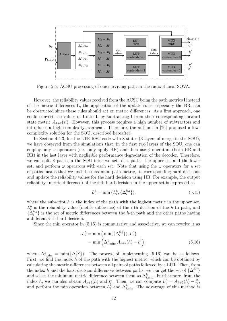
Figure 5.5: ACSU processing of one surviving path in the radix-4 local-SOVA.
However, the reliability values received from the ACSU being the path metrics l insteadof the metric differences L, the application of the update rules, especially the BR, canbe obstructed since these rules should act on metric differences. As a first approach, onecould convert the values of l into L by subtracting l from their corresponding forwardstate metric Ak+2(s′). However, this process requires a high number of subtractors andintroduces a high complexity overhead. Therefore, the authors in [76] proposed a low-complexity solution for the SOU, described hereafter.
In Section 4.4.3, for the LTE RSC code with 8 states (3 layers of merge in the SOU),we have observed from the simulations that, in the first two layers of the SOU, one canemploy only ω operators (i.e. only apply HR) and then use φ operators (both HR andBR) in the last layer with negligible performance degradation of the decoder. Therefore,we can split 8 paths in the SOU into two sets of 4 paths, the upper set and the lowerset, and perform ω operators with each set. Note that using the ω operators for a setof paths means that we find the maximum path metric, its corresponding hard decisionsand update the reliability values for the hard decision using HR. For example, the outputreliability (metric difference) of the i-th hard decision in the upper set is expressed as
Lhi = min(Lhi , {∆
h,ji }), (5.15)
where the subscript h is the index of the path with the highest metric in the upper set,Lhi is the reliability value (metric difference) of the i-th decision of the h-th path, and{∆h,j
i } is the set of metric differences between the h-th path and the other paths havinga different i-th hard decision.
Since the min operator in (5.15) is commutative and associative, we can rewrite it as
Lhi = min(
min({∆h,ji }), Lhi
)
= min(
∆hi,min, Ak+2(h)− lhi
), (5.16)
where ∆hi,min = min({∆h,j
i }). The process of implementing (5.16) can be as follows.First, we find the index h of the path with the highest metric, which can be obtained bycalculating the metric differences between all pairs of paths followed by a LUT. Then, fromthe index h and the hard decision differences between paths, we can get the set of {∆h,j
i }and select the minimum metric difference between them as ∆h
i,min. Furthermore, from theindex h, we can also obtain Ak+2(h) and lhi . Then, we can compute Lhi = Ak+2(h) − lhi ,and perform the min operation between Lhi and ∆h
i,min. The advantage of this method is
82

that we only have to convert the value of lhi into the value of Lhi for the h-th path. Theprocess can be generalized to other bit decisions and to the lower set of paths (denotedby subscript g).
After having selected the path metric and the hard decisions, the application of (5.16)to the set of upper paths and to the sets of lower paths gives two paths for the last layerof the SOU. We then can employ the φ operator to find the final hard decisions and thea posteriori LLRs, and from that, the scaled extrinsic information can be obtained.
The architecture of the SOU is depicted in Figures 5.6a and 5.6b. In order to reducethe critical path of the decoder, the implementation of Eq. (5.16) is divided into the firstclock cycle cycle (Figure 5.6a) and the second clock cycle (Figure 5.6b). Note that Figure5.6a shows the architecture for the set of upper paths. The architecture for the set oflower paths is identical but with different inputs. Overall, the SOU takes 4 clock cyclesto produce the extrinsic information. Therefore, for the set of upper and lower paths,intermediate registers are required to hold the values of Ak+2(h), lh, and the values of ∆h
as the metric difference between the h-th path and other paths.
5.3.2.3 Error correction performance and implementation results
We have simulated the error correction performance of the fixed-point implementations ofthe LTE turbo decoder using a radix-4 local-SOVA decoder and the UXMAP architecture.The simulation settings are the same as in Section 5.2.3. Figure 5.7 compares the resultingperformance curves with those obtained using the MLM algorithm. We can see that thelocal-SOVA with the use of ω operators in the first two layers of the SOU only entails aneligible performance degradation (less than 0.05 dB) compared to the MLM algorithmfor all three settings.
The computational units (BMU, ACSU, and SOU) of the radix-4 local-SOVA wereimplemented in VHDL, and the designs were placed and routed with Synopsis IC Com-piler for a CMOS 28 nm process under PVT (Process/Voltage/Temperature) worst caseconstraints and a target clock frequency of 800 MHz. For comparison, the respectiveBMU, ACSU and SOU of the radix-4 MLM algorithm were also implemented, placed androuted. The resulting area complexity comparison is shown in Table 5.4. We can see that,as expected, the BMU complexity is the same for both algorithms and that the area ofthe local-SOVA ACSU is a little higher due to the LUTs and multiplexers required forthe contender paths. In return, the SOU of the local-SOVA decoder occupies only half ofthe area of the MLM SOU.
To decode 6 radix-4 trellis sections (equivalent to 12 radix-2 trellis sections), the radix-4 scheme needs 6 BMUs, 6 ACSUs and 6 SOUs. The overall complexity of the radix-4MLM and the radix-4 local-SOVA decoders is shown in the last column of Table 5.4. Fromthese results, we can state that using the local-SOVA yields a complexity reduction of33% compared to the MLM, which is in line with the computational complexity analysisperformed in Section 4.4.4.
5.3.3 Radix-8 Computational Units
The radix-8 XMAP core consists of the implementation of a radix-8 BMU, a radix-8 ACSUand a radix-8 SOU. For a convolutional code with 8 states, the radix-8 trellis is fullyconnected but there are no parallel branches. Then, the radix-8 BMU of the local-SOVA
83

Figure 5.6: The SOU architecture for the radix-4 local-SOVA with (a) the hardwareprocessing the first part of (5.16) for the set of upper paths (the process for the lowerpaths is identical) and (b) the hardware processing the second part of (5.16) for bothupper paths and lower paths, and then applying the φ operation and calculating theextrinsic information.
and the MLM decoder should be the same and their implementation is straightforwardfrom the branch metric calculation.
The ACSU of the local-SOVA takes 8 input paths and produces one surviving pathfor each state s′ at time instant k + 3. The surviving path can be described similarly to(5.14), except that each path has now 3 hard decisions as well as 3 contender paths, onefor each hard decision. The input paths can also be organized in a predetermined orderaccording to the hard decisions. Then, the metric differences of path pairs are computed,and LUTs are employed to find the index of the surviving path as well as the indices of thecontender paths. The architecture of the radix-8 ACSU is similar to the radix-4 ACSU
84

0.0 0.5 1.0 1.5 2.0 2.5 3.0 3.5Eb/N0 in dB
10 7
10 6
10 5
10 4
10 3
10 2
10 1
Bit E
rror R
ate
MLM K128 - 8 HIsMLM K256 - 6 HIsMLM K512 - 5 HIsLSOVA K128 - 8 HIsLSOVA K256 - 6 HIsLSOVA K512 - 5 HIs
Figure 5.7: BER performance comparison between the radix-4 local-SOVA and the radix-4MLM algorithm employed in the UXMAP decoder with KP = 32 for frame sizes K = 128,K = 256 and K = 512.
Algorithm BMU ACSU SOU 6 radix-4 trellissections
Max-Log-MAP 1200 3885 10485 93420
Local-SOVA 1200 4076 5267 63258
Local-SOVAMax-Log-MAP 1.0 1.05 0.5 0.677
Table 5.4: Post place & route area of computational units (in µm2) in radix-4 MLM andradix-4 local-SOVA decoders.
architecture shown in Figure 5.5, except that 26 subtractors are required compared to 6subtractors for the radix-4 ACSU, since there are 8 path metrics. Furthermore, the sizeof the LUTs and multiplexers required to find and select a path among 8 is also increased.Nonetheless, despite these changes, the critical path of the radix-8 ACSU does not limitthe target frequency of 800 MHz.
Concerning the SOU, the radix-8 architecture is also similar to the radix-4 one shownin Figure 5.6. The only changes is that some operators now require 3 units instead of2 in order to process the 3 bits of the radix-8 unit in parallel. Therefore, it is expectedthat the complexity of the radix-8 SOU does not exceed 1.5 times the complexity of theradix-4 SOU.
Overall, the radix-8 local-SOVA uses the same decoding structure as the radix-4 local-SOVA, where φ operators are employed in the ACSUs and in the last layer of the SOUand ω operators are used in the first two layers of the SOU. Therefore, the error correctionperformance of the UXMAP turbo decoder using radix-8 local-SOVA is not expected todiffer from the radix-4 case, shown in Figure 5.7.
85

The area complexity resulting from the implementation of the radix-8 computationalunits is shown in Table 5.5 for the local-SOVA and MLM decoders. There is an overheadof 29% in the ACSU of the local-SOVA decoder due to the LUTs for the contenders.However, an area reduction of 73% is observed for the SOU of the local-SOVA decodercompared to the MLM decoder. Overall, to decode 4 radix-8 trellis sections (equivalentto 12 radix-2 trellis sections) using the local-SOVA decoder yields an area complexityreduction of 42%. On the other hand, when compared to the radix-4 local-SOVA decoder,the radix-8 local-SOVA decoder is approximately 1.5 times more complex. Note that thisincrease in complexity is traded for a decrease in latency and an increase in throughputsince a radix-8 decoder decodes a frame 1.5 times faster than a radix-4 decoder, if weneglect the I/O latency.
Algorithm BMU ACSU SOU 4 radix-8 trellissections
Max-Log-MAP 5341 9022 26444 163228
Local-SOVA 5341 11673 6792 95224
Local-SOVAMax-Log-MAP 1.0 1.29 0.26 0.58
Table 5.5: Post place & route area of computational units (in µm2) in radix-8 MLM andradix-8 local-SOVA decoders.
5.3.4 Radix-16 Computational Units
This section describes the implementation of the radix-16 local-SOVA decoder for thesame code as above.
5.3.4.1 Straightforward approach
Intuitively, one can implement the radix-16 computational units with the same structuresas for the radix-4 and radix-8 cases. In the straightforward radix-16 implementation, theBMU calculates 128 branch metrics and pass them to the ACSU. The ACSU adds thestate metrics to the branch metrics, calculates 128 metric differences and uses a LUT tofind the maximum state metric. For comparison, in the radix-4 and radix-8 cases, 6 metricdifferences and 28 metric differences have to be considered, respectively. Therefore, theradix-16 SOU can be implemented with a structure similar to the radix-4 and radix-8SOUs but with an increased complexity due to the higher number of bits to be processedin parallel (4 bits).
Table 5.6 shows the area complexity of the computational units for the local-SOVAand the MLM algorithm, as well as the area required to decode 3 radix-16 trellis sections(equivalent to 12 radix-2 trellis sections). Compared to the radix-4 local-SOVA, thecomplexity of the radix-16 local-SOVA decoder is 3.7 times higher while the latency isdivided by only a factor of 2 (and consequently the throughput is doubled). Therefore,modifications should be introduced to the radix-16 local-SOVA architecture to make itmore efficient.
According to Section 4.4.5, since there are two parallel branches connecting two statesin a radix-16 trellis section, the BMU can actually select one branch and discard the
86

Algorithm BMU ACSU SOU 3 radix-16 trellissections
Max-Log-MAP 22457 26301 64574 339996
Local-SOVA 22457 45800 8949 231618
Local-SOVAMax-Log-MAP 1.0 1.74 0.14 0.68
Table 5.6: Post place & route area of computational units (in µm2) in radix-16 MLM andradix-16 local-SOVA decoders without specific optimization.
other based on the branch metric. This means that it only passes 64 branch metrics tothe ACSU, and the ACSU can use the radix-8 structure to calculate the state metricsand calculate the reliability values. Note that this is already a saving in area since thismethod can be directly applied to the first half process of the XMAP core, where we onlyneed to calculate the state metrics and do not need to calculate the reliability values.However, for the second half, care should be taken to the radix-16 BMU, ACSU and SOUfor calculating the reliability values.
5.3.4.2 Optimized radix-16 BMU
For a radix-16 trellis section of the LTE RSC code, all pairs of parallel branches havehard decisions in the form u = {u0, u1, u2, u3} and u′ = {u0, u1, u2, u3}, where ui is thelogical not of the bit ui ∈ 0, 1. This means that the metric difference between two parallelbranches, denoted by ∆BMU, is given by the reliability values of bits at positions 0, 2, and3 for the surviving branch. These reliability values could then be passed to the ACSUwith the surviving branch metrics and be used to compute the output reliability values asdescribed in Section 4.4.5. However, as the the computation of the reliability values in theACSU is already a complex process, adding another layer to update the reliability valueswould result in an excessive complexity overhead and a longer critical path. Instead, thevalues of ∆BMU can be pushed into pipelined registers, and only be used at the end ofthe SOU, where the maximum-likelihood path has already been determined. In this case,the SOU will select the ∆BMU corresponding to the maximum-likelihood path to updatethe final reliability values (for the bits at positions 0, 2 and 3) before calculating theextrinsic information. The ACSU can then ignore these metric differences and processthe 64 branches from the BMU as if there were no a priori reliability values.
The structure of the radix-16 BMU that selects one out of two parallel branches wasproposed in [70] and is depicted in Figure 5.8. As mentioned above, the systematic bitsare the same for both parallel branches at position 1 and they are different at otherpositions. The same can be observed for the parity bits, where the parity bits are thesame for both parallel branches at position 2 and they are different at other positions.Therefore, out of 12 values (4 values of systematic LLRs, 4 values of parity LLRs, and 4values of a priori LLRs), we only need 9 values to calculate the metric difference ∆BMU
and to select the surviving branch metric. Furthermore, although there are 64 pairs ofparallel branches, there are only 16 values of metric difference ∆BMU due to repetition.The adopted radix-16 BMU needs two clock cycles to produce the branch metrics sinceit has to select 16 surviving metrics before calculating 64 branch metrics.
87

Figure 5.8: Selected BMU architecture for the radix-16 local SOVA decoder.
5.3.4.3 Optimized radix-16 ACSU
As mentioned earlier, the structure of the radix-8 ACSU can be used in order to implementthe radix-16 ACSU for the local-SOVA decoder. However, in the radix-8 ACSU, the harddecisions of each path are known in advance, which facilitates the selection of the contenderpaths. In the radix-16 case, except for the position 1, the hard decisions of the branchescoming from the BMU are not known in advance due to the merge in the BMU. Theuncertainty about hard decisions makes the selection for the contender paths much morecomplex. Hence, this translates into more complex LUTs for contender paths than in theradix-8 case. We called the ACSU which implements this approach type-I ACSU.
Another alternative structure which can be considered for the radix-16 ACSU isthe use of four radix-2 CS operators whose outputs are passed to a radix-4 CS opera-tor implemented using the LUT approach, similarly to [70]. The corresponding archi-tecture is shown in Figure 5.9. In order to avoid additional complexity in the LUTsfor contender paths, the metric differences ∆ACSU and decision differences dACSU ={dACSU,0, dACSU,1, dACSU,2, dACSU,3}1 obtained from the radix-2 CS operators are passedto the SOU to be processed later. ∆ACSU and dACSU can be selected according to themaximum-likelihood path founded in the SOU. Then, the SOU can use them to updatethe final reliability values with the HR. Concerning the ACSU, the reliability values ofthe surviving paths are note updated during the radix-2 CS. Only the path metrics andand hard decisions are selected for the surviving paths. We called the correspondingarchitecture type-II ACSU.
5.3.4.4 Radix-16 SOU
The radix-16 SOU can reuse the architecture shown in Figure 5.6 for the radix-4 case.However, the SOU architecture in Figure 5.6b has to be slightly modified to update thereliability values after finding the maximum-likelihood path using the 16 metric differences∆BMU provided by the BMU. To prevent the critical path from being increased by the
1dACSU,i = 1 means that the ith hard decisions between two paths are different.
88

Figure 5.9: Type-II ACSU architecture for radix-16 local SOVA decoder.
SOU, we had to add another pipeline stage to perform the final update process right beforethe extrinsic calculation and scaling. Furthermore, when the type-II radix-16 ACSU isimplemented, the SOU has to include the metric difference ∆ACSU in the final update ofthe reliability values.
Let us denote by LML = {LML0 , LML
1 , LML2 , LML
3 } the reliability values of the maximum-likelihood path before the final update taking account of ∆BMU, ∆ACSU and dACSU. Atthis stage, from the maximum-likelihood path, we can choose the corresponding metricdifference ∆ML
BMU from the BMU and the corresponding metric difference ∆MLACSU and deci-
sion difference dMLACSU from the ACSU (in the case of type-II ACSU). Then the reliability
values of the maximum-likelihood path are updated using HR as follows:
LMLi (type-II) =
{min
(LMLi ,∆ML
BMU, dMLACSU,i×∆ML
ACSU
), i = 0, 2, 3
min(LMLi , dML
ACSU,i×∆MLACSU
), i = 1
(5.17)
The update process for LML1 does not include ∆ML
BMU because in the merge of the BMU,the hard decisions at position 1 are the same. If the type-I ACSU is employed, the finalreliability updates are
LMLi (type-I) =
{min
(LMLi ,∆ML
BMU
), i = 0, 2, 3
LMLi , i = 1
(5.18)
5.3.4.5 Area complexity and error correction performance
We described the hardware architecture of radix-16 local-SOVA computational units inVHDL language and implemented them. The designs were placed and routed with Syn-opsis IC Compiler for a CMOS 28 nm process under worst case PVT constraints and atarget clock frequency of 800 MHz. The resulting area complexity for type-I radix-16and type-II radix-16 is shown in Table 5.7. The area of the BMU in both cases is thesame. However, with the use of a simpler architecture consisting of 4 radix-2 CS and a
89

radix-4 CS, the type-II ACSU yields a lower complexity (55%) compared to the type-IACSU. Although the type-II SOU is slightly more complex than the type-I SOU (4.5%),the overall area for 3 radix-16 trellis sections (equivalent to 12 radix-2 trellis sections) oftype-II local-SOVA is only 70% of the area of the type-I solution. Furthermore, the type-II radix-16 local-SOVA decoder has the same area complexity as the radix-8 local-SOVAdecoder, while providing a lower latency and higher throughput solution.
Architecture BMU ACSU SOU 3 radix-16 trellissections
Radix-16 type-I 5491 30860 8778 135387
Radix-16 type-II 5491 16996 9174 94983
Table 5.7: Post place & route area of computational units (in µm2) in type-I and type-IIradix-16 local-SOVA decoders.
The error correction performance of the type-I and type-II radix-16 local-SOVA de-coder is shown in Figure 5.10, where it is also compared with the radix-4 MLM algorithm.For the type-I radix-16 local-SOVA, since we omit the initial reliability values in the BMUand only use them for an update at the end of the process, the performance is slightlydegraded with less than 0.1 dB loss for all settings. Meanwhile, the type-II radix-16local-SOVA further skips the reliability update in the first layer of the ACSU and alsouses them for the final update, the performance is then further degraded resulting in anoverall loss of about 0.1 dB.
Compared to the radix-4 local-SOVA decoder, the area complexity of the type-II radix-16 local-SOVA decoder is 1.5 times higher, but the latency of the decoder is divided by2 times and the throughput doubled. Therefore, the UXMAP architecture with type-II radix-16 local-SOVA is recommended for applications requiring low latency and highthroughput and tolerating a small performance loss (about 0.1 dB) as well as a highercomplexity.
5.4 Conclusion
In this chapter, we have first reviewed the implementation of turbo decoders using UXMAParchitecture with the MLM algorithm. The corresponding computational units (BMU,ACSU, SOU) are described in the case of the radix-4 MLM algorithm. The area com-plexity and the error correction performance of the UXMAP architecture with the radix-4MLM algorithm were also shown, which served as the baseline to compare with our im-plementations of the local-SOVA in the UXMAP architecture.
The radix-4 local-SOVA decoder was first presented with the architecture of the com-putational units. Compared to the radix-4 MLM decoder, the radix-4 local-SOVA decoderemployed in the UXMAP architecture provides a lower complexity solution with a savingof 33% in area complexity, at the cost of a slight performance loss (smaller than 0.05dB). In light of this complexity reduction, the radix-8 and radix-16 local-SOVA were alsoinvestigated. Both schemes yield a higher area complexity than the radix-4 scheme, buthave the advantage of a lower latency. The radix-8 scheme is 1.5 times more complexbut provides a 1.5 gain in latency/throughput and no performance loss compared to the
90

1.0 1.5 2.0 2.5 3.0 3.5Eb/N0 in dB
10 7
10 6
10 5
10 4
10 3
10 2Bi
t Erro
r Rat
e
MLM K128 - 8 HIsMLM K256 - 6 HIsMLM K512 - 5 HIsLSOVA r16 type-I K128 - 8 HIsLSOVA r16 type-I K256 - 6 HIsLSOVA r16 type-I K512 - 5 HIsLSOVA r16 type-II K128 - 8 HIsLSOVA r16 type-II K256 - 6 HIsLSOVA r16 type-II K512 - 5 HIs
Figure 5.10: BER performance comparison between the MLM algorithm and the radix-16local-SOVA employed in the UXMAP decoder with KP = 32 for frame sizes K = 128,K = 256 and K = 512.
radix-4 scheme. Even better, the radix-16 scheme is also 1.5 times more complex butcan still increase the latency/throughput gain to a factor of 2, at the cost of a very smalldegradation in performance (about 0.1 dB) compared to the radix-4 scheme. Therefore,depending on the requirements of the application, the radix-4, radix-8 or radix-16 schemesof the local-SOVA can be can be beneficially employed instead of the MLM decoder inthe UXMAP architecture.
91

Chapter 6
SISO Decoding Algorithms Usingthe Dual Trellis
In search of decoding algorithms for high-throughput contexts, a part of my thesis workwas devoted to the efficient decoding of high-rate convolutional codes. Therefore, thischapter focuses on decoding convolutional codes with high coding rates (r > 1/2) usingthe trellis of the corresponding dual codes, i. e., the dual trellis.
The authors in [80] have proposed a derivation of the BCJR algorithm based on thedual code which is perfectly equivalent to the BCJR algorithm applied to the originalconvolutional code. For a code with rate r = k/n, the dual code has rate (n − k)/n. Ifk > n/2, i.e. if r > 1/2, the dual code has a rate lower than the original one. Therefore,the dual trellis is less complex than the original trellis since it has fewer branches pertrellis section. Thus, it is expected that if the BCJR algorithm is applied to the dualtrellis, the process of finding the a posteriori probability estimate and then convert it intothe original code is also less complex than the straightforward application of the BCJRto the original code.
The rest of the chapter is organized as follows. Section 6.1 introduces the benefitsof using the dual trellis to decode a convolutional code. Then, Section 6.2 describesthe state-of-the-art method for constructing the dual trellis, given a convolutional codewith rate k/(k + 1). The application of the BCJR algorithm and its logarithmic versionto the dual trellis are also presented and it is shown that they could provide a higherthroughput compared to the MLM algorithm. Section 6.3 then provides a method thatwe have proposed to derive the dual trellis for a convolutional code with arbitrary ratek/n. The construction method can be applied to a punctured convolutional code so thatdecoding on the dual trellis can be applied. Then, a new sub-optimal low-complexitydecoding algorithm based on the dual trellis is presented and analyzed in Section 6.4. Itis shown that despite a minor loss of about 0.2 dB in performance, the new decodingalgorithm significantly reduces the decoder complexity compared to the state-of-the-artalgorithm. Finally, Section 6.5 concludes the chapter.
92

6.1 Introduction
In communication systems requiring high data throughput, channel coding using highrates is preferred as the number of transmitted redundancy bits is limited. For a (k, n, ν)convolutional code, high coding rates (r = k/n > 1/2) can be achieved by puncturing orby using true high-rate convolutional encoders.
With the former approach, the information message is encoded by a low-rate mothercode (e.g. with code rate 1/n). Then, the output from the mother code is puncturedusing a puncturing pattern P to shorten the code length and achieve the desired codingrate. At the receiving side, the decoder first sets the LLR of the punctured bits to 0.Then, the decoder can use the MLM algorithm, the SOVA, or the local-SOVA on thetrellis of the low-rate mother code to compute the a posteriori LLRs.
The advantage of puncturing is that the decoder structure designed for the originalmother code can be reused for the high-rate punctured codes. Therefore, the complex-ity for decoding high-rate punctured codes is about the same as for the original code.Moreover, the code enjoys the flexibility to change the code rate by applying differentpuncturing patterns at the encoder, without changing the decoder structure. However,this also implies that, for high rates, the decoder inherits the throughput and decodinglatency of the mother code. In other words, regardless of the coding rate, the decoderarchitecture always employs the trellis of the mother code, and thus, its throughput andlatency are defined by this trellis. Furthermore, as mentioned in Section 3.1.4, the de-coders designed for high coding rates usually adopt the ACQ initialization technique withlong acquisition lengths to maintain the performance. Hence, the decoding latency isfurther increased and the throughput is reduced. In [81], the authors proposed a solutionto mitigate the long acquisition lengths, namely the trellis compression. However, thesolution requires extra hardware resources for the ACQ steps [63]. As a consequence, forhigh-rate schemes, other code families such as LDPC codes may provide a better perfor-mance in terms of decoding complexity, throughput and latency compared to turbo codesemploying puncturing.
As mentioned earlier, another alternative to achieve a high code rate k/n is to use antrue high-rate encoder, characterized by a k × n generator matrix. However, the maindrawback of this method is the complexity of the trellis diagram of the code. Consider a(k, n, ν) convolutional codes, then for a state s ∈ {0, . . . , 2ν − 1}, there are 2k branchescoming in and out, and there are 2k+ν branches in total for each trellis section. Processingsuch a trellis section is equivalent to processing the radix-2k scheme for a code with rate1/n. Since the complexity of the MLM algorithm increases exponentially with the radixorder, which is equal to k in this case, for high coding rates (e.g. k > 4), decodingalgorithms based on the trellis of the true high-rate encoder are not necessarily attractive.
To overcome the high complexity drawback in the original trellis, decoding a truehigh-rate convolutional code can be carried out with the dual trellis of the code. Fora convolutional code C with rate k/n encoded by generator matrix G(D), there exists
an associated dual code C⊥ with rate (n − k)/n generated by matrix H(D) such that
GH> = 0. In other words, any codeword generated by G(D) should be orthogonal with
all codewords generated by H(D). The generator matrix H(D) is usually referred to as thereciprocal parity-check matrix since it is the reciprocal of the parity-check matrix H(D) of
the code C. Then, the reciprocal dual trellis is constructed according to H(D), and we willrefer it as the dual trellis for short. In contrast, we will refer to the trellis generated by
93

the generator matrix G(D) as the original trellis. A very interesting property of the dualtrellis is that there are 2(n−k+ν) branches in a trellis section. As the code rate increases,the value of (n− k) decreases, and for a convolutional code with rate k/(k+ 1), there are2ν+1 branches, which corresponds to the conventional radix-2 scheme.
6.2 The Dual Trellis and the MAP-Based Algorithms
on the Dual Trellis
As in Chapter 2, we begin with a presentation related to the dual trellis and the MAP-based algorithms performed on the dual trellis. In this section, we only consider the caseof true high-rate convolutional codes with rate k/(k + 1) unless stated otherwise. Thegeneralization to arbitrary code rates k/n and punctured high-rate codes will be dealtwith in subsequent sections.
6.2.1 The Dual Trellis
As already stated in Section 2.2.1, a (k, n, ν) convolutional code C can be characterizedby a polynomial generator matrix G(D) with rank k, consisting of k×n polynomialsgi,j(D) ∈ F2(D):
G(D) =
g0,0(D) g0,1(D) . . . g0,n−1(D)g1,0(D) g1,1(D) . . . g1,n−1(D)
......
. . ....
gk−1,0(D) gk−1,1(D) . . . gk−1,n−1(D)
, (6.1)
where F2(D) is the field of formal Laurent series with binary coefficients. We furtherdefine the constraint length of the ith input of the generator matrix G(D) as
λj = max0≤j<n
{deg(gi,j(D))
}, (6.2)
where deg(gi,j(D)) denotes the degree of the polynomial gi,j(D). Then, we define theoverall constraint length of the generator matrix as the sum of the constraint lengths forall inputs
λ =k∑
i=0
λi (6.3)
Let us denote by u = (u0,u1, . . .) and c = (c0, c1, . . .) the input sequence and outputsequence of the encoder, respectively, where ui = (u0
i , u1i , . . . , u
k−1i ) is the ith input vector
consisting of k bits and ci = (c0i , c
1i , . . . , c
n−1i ) is the ith output vector consisting of n bits.
The sequence u and c can be written as
u(D) =∞∑
i=0
uiDi ∈ F k(D), (6.4)
and
c(D) =∞∑
i=0
ciDi ∈ F n(D), (6.5)
94

where Fm(D) is the m-dimensional vector space over F (D). Then, the encoder processcan be written as
c(D) = u(D)G(D). (6.6)
Given a convolutional code C encoded with an encoder characterized by the generatormatrix G(D) of size k × (k + 1), we are seeking to find the parity-check matrix H(D) of
this generator matrix in order to derive the reciprocal parity-check matrix H(D). To doso, we first try to find a systematic version of G(D), denoted by Gsys(D), and then, theparity check matrix can be directly derived from Gsys(D).
6.2.1.1 Generator matrix equivalence
Two convolutional codes are said to be equivalent if they generate the same codeword spaceC. Two convolutional encoders are equivalent if their generator matrices are equivalent,i. e.represent equivalent convolutional codes.
Theorem 6.1. Two rate k/n convolutional generator matrices G(D) and G′(D) areequivalent if and only if there exists a k × k non-singular matrix T(D) such that
G(D) = T(D)G′(D). (6.7)
Proof. If (6.7) holds, then for any input u(D) ∈ F k(D), we have
u(D)G(D) = u(D)T(D)G′(D) (6.8)
= u′(D)G′(D), (6.9)
where u′(D) = u(D)T(D). Therefore, G(D) and G′(D) are equivalent.Conversely, suppose that G(D) and G′(D) are equivalent. Then, there exists an input
ui(D) ∈ F k(D) such that
gi(D) = ui(D)G′(D), i = 0, . . . , k−1 (6.10)
where gi(D) ∈ F n(D) is the ith row of G(D). Then, by denoting
T(D) =
u0(D)u1(D)
...uk−1(D)
, (6.11)
we have
G(D) = T(D)G′(D). (6.12)
Since G(D) and G′(D) are generator matrix, they have rank k. Therefore, T(D) also hasrank k and, hence, is non-singular.
6.2.1.2 Equivalent systematic encoders
Let T(D) be a k×k non-singular sub-matrix of G(D), where G(D) is a non-systematicgenerator matrix of rate-k/(k + 1) convolutional code C. Without loss of generality, we
95

assume that T(D) consists of the k left-most columns of G(D). Then, the systematicgenerator matrix can be obtained as
Gsys(D) = T−1(D)G(D) =(Ik z(D)
), (6.13)
where Ik is the k×k identity matrix and z(D) is a k×1 column vector, which is theproduct of the matrix T−1(D) with the last column of G(D). Since T−1 is also non-singular, according to the Theorem 6.1, Gsys(D) is equivalent to G(D). Furthermore, theelements of z(D) may be rational polynomials with the same denominator; hence, theresulting systematic encoder may become recursive.
Example 6.1. Consider a rate r = 2/3 non-systematic convolutional encoder with gen-erator matrix
G(D) =
(1+D2 1 1+D+D2
D 1+D 1
). (6.14)
Let T(D) be the matrix consisting of the first two columns of G(D) as
T(D) =
(1+D2 1D 1+D
). (6.15)
Since T(D) is full rank, the determinant of T(D) is non zero and det(T(D)) = 1+D2+D3.Therefore, the inverse of T(D) is
T−1(D) =1
1+D2+D3
(1+D 1D 1+D2
). (6.16)
By multiplying G(D) with T(D), we obtain the systematic encoding matrix Gsys(D)equivalent to G(D) as
Gsys(D) =1
1+D2+D3
(1+D 1D 1+D2
)(1+D2 1 1+D+D2
D 1+D 1
)
=
1 0D3
1+D2+D3
0 11+D+D3
1+D2+D3
. (6.17)
In this case, the systematic encoder is also recursive.
6.2.1.3 Parity-check matrix and reciprocal parity-check matrix
A (n − k)×n polynomial matrix H(D) is the parity-check matrix corresponding to thek×n generator matrix G(D) if
G(D)H>(D) = 0, (6.18)
where > is the matrix transpose operator.In the case of a k×(k+1) systematic generator matrix Gsys(D), we can rewrite it as
Gsys(D) =(Ik z(D)
)=
(Ik
1
q(D)p(D),
)(6.19)
96

where p(D) is the column vector consisting of the numerators of z(D), and q(D) is thecommon denominator of the elements of z(D). Then, the 1×(k + 1) parity-check matrixH(D) can be obtained as
H(D) =(p>(D) q(D)
). (6.20)
We can verify that
Gsys(D)H>(D) =
(Ik
1
q(D)p(D)
)(p(D)q(D)
)=(Ikp(D) + p(D)
)= 0. (6.21)
Given a convolutional code C generated by the encoder with the k×n generator matrixG(D), the dual code C⊥ of C is defined as the set of codewords c⊥ such that
c(c⊥)> = 0, ∀c ∈ C, c⊥ ∈ C⊥. (6.22)
It is important to note that the dual code C⊥ can be generated using the (n−k)×ngenerator matrix H(D), where H(D) is the reciprocal of the parity-check matrix H(D)
[82]. The generator matrix H(D) is often referred to as the reciprocal parity-check matrix.
The procedure for obtaining the reciprocal parity-check matrix H(D) from the parity-check matrix H(D) is as follows.
Let λi be the constraint length of the ith row hi(D) of H(D), i = 0, . . . , (n−k). Then,
the ith row of H(D), denoted by hi(D) is
hi(D) = Dλihi(D−1). (6.23)
Example 6.2. Given the systematic generator matrix obtained from Example 6.1
Gsys(D) =
1 0D3
1+D2+D3
0 11+D+D3
1+D2+D3
, (6.24)
the parity-check matrix can be derived according to (6.20) as
H(D) =(D3 1+D+D3 1+D2+D3
). (6.25)
Then, by using (6.23), the reciprocal parity-check matrix is
H(D) = D3H(D−1)
=(1 1+D2+D3 1+D+D3
)(6.26)
Fig. 6.1 shows the original trellis constructed from Gsys(D) and the dual trellis con-
structed from H(D). We can observe that a section of the original trellis has the form ofradix-4, with 4 branches entering and leaving each state. Meanwhile, a section of the dualtrellis has the form of radix-2, with only half the number of branches. This can be furthergeneralized to k > 2: the original trellis of a rate k/(k+ 1) code has the form of radix-2k;hence, its complexity increases exponentially with k. The dual trellis, on the other hand,always has the form of radix-2 and is much less complex than the original one. Therefore,for values of k larger than 2, it seems attractive to resort to the dual trellis for decodinghigh-rate convolutional codes.
97

Figure 6.1: Comparison between a section of the original trellis generated from Gsys(D)
and a section of the dual trellis generated from H(D) (Example 6.2).
6.2.1.4 Decoding with the dual trellis
In this section, we take a retrospective look at the decoding process of a convolutionalcode and we make the connection with the dual code.
Recalling from Section 2.3.3, a systematic convolutional encoder with rate k/n takesinput u = (u0, . . . , uK−1) and produces codeword c = (c0, . . . , cN−1). Then, we assumethat the codeword is transmitted over an AWGN channel using BPSK modulation. Atthe receiver side, the LLR is computed for each bit cj, using the received vector y =(y0, . . . , yN−1):
LI(cj; yj) = lnPr{cj = 1; yj}Pr{cj = 0; yj}
(6.27)
= lnPr{yj|cj = 1}Pr{yj|cj = 0}
+ lnPr{cj = 1}Pr{cj = 0}
(6.28)
= Lc(yj|cj) + La(cj), (6.29)
where Lc(yj|cj) is the channel LLR, obtained from the demodulator after the zero-meanAWGN channel with variance σ2, and is calculated according to Eq. (2.4) as
Lc(yj|cj) =2ykσ2
. (6.30)
Furthermore, La(ck) is the a priori LLR, which is zero with the assumption that cj ∈ {0, 1}is equiprobable. However, in the context of conventional turbo decoding, then the a prioriLLR of the systematic bits might be non zero. Therefore, the previous LLR is derived as
LI(cj; yj) =
{Lc(yj|cj) + La(cj), if cj is an systematic bit
Lc(yj|cj), if cj is a parity bit(6.31)
The soft output of the decoder is the a posteriori LLR of the jth decoded bit cj,which can be estimated via the original code C by taking into account the codewords
98

c ∈ C having cj = 1 and the codewords c ∈ C having cj = 0, respectively. Therefore, foreach decoded systematic bit cj, the output LLR is computed as
L(cj) = ln
∑
c∈C|cj=1
N−1∏
l=0
exp(LI(cl; yl)×cl
)
∑
c∈C|cj=0
N−1∏
l=0
exp(LI(cl; yl)×cl
)
= ln
∑
c∈C|cj=1
exp(LI(cj; yj)×cj
) N−1∏
l=0,l 6=j
exp(LI(cl; yl)×cl
)
∑
c∈C|cj=0
exp(LI(cj; yj)×cj
) N−1∏
l=0,l 6=j
exp(LI(cl; yl)×cl
)
= LI(cj; yj) + ln
∑
c∈C|cj=1
N−1∏
l=0,l 6=j
exp(LI(cl; yl)×cl
)
∑
c∈C|cj=0
N−1∏
l=0,l 6=j
exp(LI(cl; yl)×cl
), (6.32)
where the second term from (6.32) is the extrinsic LLR provided by the decoder, whichhas already been introduced in Chapter 2.
Alternatively, the value of L(uj) can also be calculated using the dual code C⊥ of C as[80]
L(cj) = LI(cj; yj) + ln
∑
c⊥∈C⊥
(− 1)c⊥j
N−1∏
l=0,l 6=j
tanh(LI(cl; yl)/2
)c⊥l
∑
c⊥∈C⊥
N−1∏
l=0,l 6=j
tanh(LI(cl; yl)/2
)c⊥l, (6.33)
where c⊥ = (c⊥0 , . . . , c⊥N−1) denotes codewords of C⊥. By comparing (6.32) and (6.33),
we can see that both equations perform a sum over all codewords in their respective set.However, the dimension of C is k, and the dimension of C⊥ is (n−k). Therefore, for highcode rates such that n− k < k, i.e. r > 1/2, C⊥ has less codewords than C.
Furthermore, we have seen in Chapter 2 that (6.32) can be obtained using the BCJRor the log-MAP algorithm, which operates on the trellis of the original encoding matrixG(D). Equivalently, (6.33) could also be implemented using the BCJR algorithm or its
logarithmic version on the trellis of the reciprocal parity-check matrix H(D), since H(D)generates the codewords of the dual code C⊥. This trellis is referred to as the dual trellis,and the decoding algorithms operating on the dual trellis are referred to as the dual-MAPand dual-Log-MAPalgorithms, corresponding to their counterparts on the original trellis.
99

6.2.2 The Dual-MAP and Dual-Log-MAP algorithms
6.2.2.1 The dual-MAP algorithm
In the original trellis, the BCJR algorithm consists of the following steps: branch metriccalculation, forward recursion, backward recursion and soft-output calculation. Equiv-alently, the same steps can be applied into the dual trellis resulting in the dual-MAPalgorithm.
Given the received vector y of length N as the modulated and noisy version of thecodeword c, encoded by a rate k/n convolutional code with input message of length K, theintrinsic LLRs {LI(cj; yj)}0≤j<N are calculated as in (6.31). According to (6.33), the firststep towards the decoding of the convolutional codes using the dual trellis is to convertthe intrinsic LLRs into bit metrics {dj}0≤j<N as
dj = tanh(LI(cj; yj)/2
). (6.34)
With the dual trellis, the received frame of length N is decomposed into T = N/ntrellis sections. Then, the bit metrics related to a specific section t, 0 ≤ t < T , are{dnt+1, . . . , dnt+n}. Let (st, st+1) denote a branch between state st at instant t and st+1
at instant t+1, and let {c⊥nt+1(st, st+1), . . . , c⊥nt+n(st, st+1)} ∈ {0, 1}n be the bit decisionscarried by the branch (st, st+1).
In this section, we reuse the notation of the metrics in the original trellis for the dualtrellis. Therefore, γt(st, st+1) is the metric of branch (st, st+1), βt(st) is the backwardstate metric of state st at instant t, and αt+1(st+1) is the forward state metric of statest+1 at instant t+1. The branch metric calculation related to trellis section t in the dualtrellis yields
γt(st, st+1) =nt+n∏
j=nt+1
(dj)c⊥j (st,st+1)
. (6.35)
Then, the forward and backward state metrics can be recursively calculated as
αt+1(st+1) =∑
st
αt(st)γt(st, st+1), (6.36)
βt(st) =∑
st+1
βt+1(st+1)γt(st, st+1). (6.37)
Note that, as in the original trellis, the forward state metric recursion in the dual trellisalso starts at instant t = 0 and moves up to t = N+1. Conversely, the backward recursionstarts at instant t = N+1 and the backward state metrics are then calculated recursivelydown to t = 0. However, the initialization of the state metrics is different from theinitialization in the original trellis.
Recall that, in the original trellis, there are two widely employed methods to terminatethe trellis: force-to-zero and tailbiting. With the former termination method, the forwardstate metrics at the trellis start and the backward state metrics at the trellis end areinitialized according to an impulse distribution δ(s, 0), where
δ(s, i) =
{1, if the state s = i,
0, otherwise.(6.38)
100

For the tailbiting convolutional codes in the original trellis, the forward state metrics andthe backward state metrics are initialized according to a uniform distribution with equalvalues for all states s.
The state metrics in the original trellis and the dual trellis exhibit a Fourier transformrelation [83]. Therefore, an impulse (resp. uniform) state metric distribution in theoriginal trellis corresponds to a uniform (resp. impulse) state metric distribution in thedual trellis. Thus, if force-to-zero is used in the original trellis, the initialization of thestate metrics in the dual trellis is
α0(s) = 1, ∀s, (6.39)
βN+1(s) = 1, ∀s. (6.40)
Conversely, if tailbiting is used in the original trellis, the initialization of the statemetrics in the dual trellis is
α0(s) = δ(s, 0), (6.41)
βN+1(s) = δ(s, 0). (6.42)
For trellis section t, after having computed γt(st, st+1), αt(st), and βt+1(st+1), the a pos-teriori likelihood ratio for each bit c⊥j of the dual code, denoted by zj, j ∈ {nt+1, . . . , nt+n}is computed as
zj =q1j
q0j
=
∑
(st,st+1)|c⊥j (st,st+1)=1
αt(st)γt(st, st+1)βt+1(st+1)
∑
(st,st+1)|c⊥j (st,st+1)=0
αt(st)γt(st, st+1)βt+1(st+1), (6.43)
where q1j and q0
j are the summations of all the metrics of codeword c⊥ in C⊥ havingc⊥j = 1 and c⊥j = 0, respectively. By applying q0
j and q1j into the sums in the numerator
and denominator of (6.33), the a prosteriori LLR of the decoded bit cj in the originaltrellis is obtained as
L(cj) = LI(cj; yj) + lnq0j − q1
j/dj
q0j + q1
j/dj
= LI(cj; yj) + ln1− zj/dj1 + zj/dj
= LI(cj; yj) + ln1− uj1 + uj
, (6.44)
where uj = zj/dj is the extrinsic information in the dual domain.
Equation (6.44) shows that one can completely derive the soft output related to de-coded bit cj using the dual trellis. However, similar to the BCJR algorithm, the dual-MAPalgorithm requires a large number of multiplications and divisions and is therefore toocomplex, taken as it is, for practical hardware implementations. Consequently, to makethe decoding on the dual trellis feasible, the application of the dual-MAP algorithm in thelogarithmic domain was investigated in [84], which we call the dual-Log-MAP algorithm.
101

6.2.2.2 The dual-Log-MAP algorithm with sign-magnitude
The input bit metric of the dual-MAP decoder expressed in (6.34) can take positive ornegative values. Therefore, one can resort to the sign-magnitude (SM) representation asin [84] to represent it in the logarithmic domain. Using the SM representation, a realnumber x is expressed as
x = (−1)Xs exp(Xm) , [Xs;Xm], (6.45)
where Xs ∈ {0, 1} and Xm = log(|x|) are the sign and the magnitude of x, respectively.Then, the arithmetic operations involved in the decoding algorithm can be expressed asfollows, using the SM representation:
• Sign-magnitude multiplication (SMM):
xy , [Xs ⊕ Ys;Xm + Ym]. (6.46)
• Sign-magnitude division (SMD):
x/y , [Xs ⊕ Ys;Xm − Ym]. (6.47)
• Sign-magnitude addition (SMA):
x+ y ,
{[Xs;Xm − log
(1 + (−1)Xs+Ys exp(Ym −Xm)
)], if Xm > Ym,[
Ys;Ym − log(1 + (−1)Xs+Ys exp(Xm − Ym)
)], otherwise.
(6.48)
With this representation, the multiplication and division operators used by the dual-MAP decoder are replaced by SMM and SMD operators.
Furthermore, from (6.44), the extrinsic information in the original trellis can be ob-tained as [85]
ln1− (−1)Uj,s exp(Uj,m)
1 + (−1)Uj,s exp(Uj,m)=
ln tanh
(∣∣∣∣Uj,m
2
∣∣∣∣), if Uj,s = 0
− ln tanh
(∣∣∣∣Uj,m
2
∣∣∣∣), otherwise
, (6.49)
where Uj,s and Uj,m are the sign and the magnitude of the extrinsic information in thedual domain uj, respectively.
When considering the decoding algorithm in the logarithmic domain, the dual-Log-MAP (dual-LM) decoder is more hardware friendly than the dual-MAP decoder: Themultiplications and divisions are now replaced by adders and subtractors and the SMAcan be implemented with a compare-select operator and two LUTs, while the extrinsicinformation conversion can be implemented with one LUT for the logarithm of hyperbolictangent function.
In [85], two hardware implementations of a dual-LM decoder and a conventional radix-4 MLM decoder are reported and compared in terms of throughput and circuit area, forturbo codes using rate k/(k+1) component convolutional codes with k = 2, 4, 8, 16. Figure6.2 taken from [85], shows the comparison of the implementation results. Note that theturbo decoder used in [85] is a PMAP architecture with two parallel SISO decoders usingforward-backward scheduling, sliding windows and ACQ initialization.
102

Figure 6.2: Implementation comparison between dual-LM and radix-4 MLM decoders [85].
From Figure 6.2, we can see that for a medium code rate such as r = 2/3, bothalgorithms yield the same throughput but the circuit area of the dual-MAP decoder ismore than twice compared to the radix-4 MLM decoder. However, for higher code ratessuch as r = 4/5 or r = 8/9, the throughput of the MLM decoder remains unchanged whilethe circuit area increases with the code rate. This is due to the need of longer decodingwindows and/or long acquisition sequences for state metric initialization to avoid anycorrection performance loss. On the contrary, the throughput of the dual-LM decoderis doubled from r = 2/3 to r = 4/5 and from r = 4/5 to r = 8/9, while its circuitarea only increases from 140 kgates at r = 2/3 to 180 kgates at r = 8/9. This can beexplained by the fact that, for a code rate k/(k+1), the dual-LM decoder is able to processsimultaneously k bits while the conventional radix-4 MLM decoder can only process 2 bitsat each trellis stage. These are the main advantages of decoding using the dual trellisinstead of the original trellis for high-rate convolutional codes.
6.3 Constructing the Dual Trellis for Punctured Con-
volutional Codes
In the previous section, we explained that the dual-LM algorithm employed on the dualtrellis had a better area efficiency than the MLM in the original trellis, when consideringtrue high-rate convolutional codes with rate k/(k+1), for k > 4. With that motivation,this section proposes a fully generic procedure to construct the dual trellis for high-ratepunctured convolutional codes, so that they can also be decoded using the dual-LM algo-rithm. This method is based on transformations proposed by Forney in [86].
The generic procedure is presented in Figure 6.3. The main idea of the procedure isthat, given a mother code (e.g. r = 1/2) and a puncturing pattern to achieve code ratek/n, we first find the non-systematic generator matrix Gns(D) of size k×n equivalent tothe original punctured convolutional code of rate k/n. Then, parity-check matrix H(D)
103

and its reciprocal H(D) can be derived and the dual trellis is constructed directly from
matrix H(D). The dual-LM algorithm then decodes the received codeword based on thedual trellis yielding the soft estimate on the punctured codeword.
Low rate CC(e.g. r = 1/2)
G(D)
Puncturingpattern
P
Equivalentnon-systematicgenerator matrix
Gns(D)
Invariant factordecomposition
Gns(D) = A(D)Γ(D)B(D)
Basic parity-checkmatrix H(D)
Minimum basicparity-check
matrix Hmb(D)
Reciprocalparity-check matrix
H(D)Dual trellis
Figure 6.3: Procedure for obtaining the reciprocal dual trellis of a high-rate puncturedconvolutional code.
6.3.1 Equivalent Non-Systematic Generator Matrix of Punc-tured Convolutional Codes
The first step towards the reciprocal dual trellis involves converting the punctured con-volutional code into a non-systematic encoding form, as described in [87]. This transfor-mation has previously been used to assess the performance of convolutional codes, sinceall equivalent forms share the same Hamming weight spectrum.
In order to get a punctured convolutional code k/n, we start from the following generalform of an generator matrix of a mother code with rate 1/m as
G(D) =(g0(D) g1(D) . . . gm−1(D)
)(6.50)
where gi(D), i = 0, . . . ,m − 1 are the polynomials of the generator matrix. This convo-lutional code can also be viewed as a rate-k/(km) code, for any value of k. Therefore,we can derive a k × (km) generator matrix G′(D) that is equivalent to the generatormatrix of the mother code. This k × (km) matrix can be defined by km polynomialsobtained by splitting each polynomial gi(D), i = 0, . . . ,m − 1 into k sub-polynomialsfi,j(D), j = 0, . . . , k − 1 as follows
gi(D) =k−1∑
j=0
Djfi,j(Dk). (6.51)
The element of the resulting k × (km) generator matrix G′(D) at row p and column q,g′p,q(D), is defined as:
{g′p,q(D) = fqmodn,bq/mc−p(D), if p×m ≤ q
g′p,q(D) = D×fqmodn,bq/mc−p+k(D), if p×m > q(6.52)
where mod is the modulo operation. The generator matrix of the rate-k/n code is thenobtained by selecting n out of (km) columns in G′(D) according to a selected puncturingpattern.
104

Example 6.3. Given the generator matrix of a rate 1/2 mother code as G(D) = (g0(D), g1(D)),the procedure to obtain an equivalent 3×6 generator matrix is as follows. With m = 2and k = 3, two polynomials g0(D) and g1(D) can be each decomposed into three sub-polynomials: {f0,j(D)}j=0,1,2 and {f1,j(D)}j=0,1,2, respectively. The generator matrixG′(D) of the equivalent rate-3/6 code is
G′(D) =
f0,0(D) f1,0(D) f0,1(D) f1,1(D) f0,2(D) f1,2(D)D×f0,2(D) D×f1,2(D) f0,0(D) f1,0(D) f0,1(D) f1,1(D)D×f0,1(D) D×g1,1(D) D×f0,2(D) D×f1,2(D) f0,0(D) f1,0(D)
.
(6.53)The non-systematic punctured generator matrix Gns(D) of the rate-k/n code is thenobtained by selecting n columns out of kN in G′(D), according to a selected puncturingpattern. For instance, if columns 1, 2, 3 and 5 in G′(D) are selected, the following matrixgenerates a rate-3/4 code
Gns(D) =
f0,0(D) f1,0(D) f0,1(D) f0,2(D)D×f0,2(D) D×f1,2(D) f0,0(D) f0,1(D)D×f0,1(D) D×f1,1(D) D×f0,2(D) f0,0(D)
. (6.54)
6.3.2 Reciprocal Parity-Check Matrix of Punctured Convolu-tional Codes
6.3.2.1 Invariant-factor decomposition of the generator matrix
Let us start with the definition of a basic encoding matrix. An encoding matrix G(D) iscalled basic if it has a right inverse G−1(D). The right inverse existence of an encodingmatrix ensures that the encoder is a bijective function. Therefore, given any two differentinputs, the basic encoder always yields two different codewords.
Based on the invariant-factor theorem, as in [86], or on the Smith form, as in [88],the invariant-factor decomposition of the generator matrix G(D) of a convolutional codewith rate k/n gives
G(D) = A(D)Γ(D)B(D), (6.55)
where A(D) is a k × k polynomial matrix with unit determinant; B(D) is a n× n poly-nomial matrix with unit determinant, thus having an polynomial matrix inverse B−1(D);and Γ(D) is a k × n diagonal matrix, whose elements are called the invariant factorsof G(D) and are unique. In fact, matrix Γ(D) is obtained by permuting and linearlycombining the rows and the columns of matrix G(D). Since the permutation or linearcombination of rows (or columns) can be represented by the pre- (or post-) multiplica-tion of a square matrix with unit determinant by G(D), A(D) is the result of all rowoperations and matrix B(D) is the result of all column operations.
As pointed out in [86], matrix U(D) consisting of the first k rows of B(D) is a basicencoding matrix equivalent to G(D). Since the polynomial matrix B(D) has a polynomialinverse B−1(D), the matrix consisting of the last (n − k) columns of B−1(D) is thetranspose of the parity-check matrix, i.e., H>(D). This can be explained by the factthat B(D)B−1(D) = In where In is the n × n identity matrix. Then, the inner productbetween row i ∈ {0, . . . , k − 1} of B(D) and column j ∈ {n− k, . . . , n− 1} of B−1(D) isthe element at row i and column j of the identity matrix In. Since (In)i,j = 0 for j > i,U(D)H>(D) = 0 and consequently, G(D)H>(D) = 0. Note that matrix H(D) is basic
105

since it has a right inverse which is the transpose of the matrix consisting of the last(n− k) rows of B(D).
6.3.2.2 Minimal basic parity-check matrix
According to Theorem 7 in [86], if G(D) is a basic encoder with overall constraint lengthλ, then there exists an associated basic parity-check matrix H(D) with overall constraintlength λ. Recall from (6.3) that the overall constraint length of a polynomial matrix isthe sum of the constraint lengths for all rows.
However, we observed that, in the previous decomposition, the parity-check matrixH(D) consisting of the last (n− k) columns of B−1(D) usually has an overall constraintlength greater than λ, the overall constraint length of G(D). Therefore, we need to findthe minimal basic parity-check matrix Hmb(D) with overall constraint length λ that isequivalent to H(D). To this end, the authors in [88] proposed an algorithm for findingthe minimal basic form of an encoding matrix, called Algorithm MB. The main idea ofthis algorithm is to lower gradually the constraint length of the parity-check matrix bylinearly combining multiple rows. Then, after a number of steps, its overall constraintlength becomes equal to λ. Since the operation of linearly combining matrix rows can berepresented by the pre-multiplication of a unit determinant matrix by H(D), the resultingminimal basic parity-check matrix Hmb(D) is equivalent to H(D).
Assuming that G(D) is a k × n encoding matrix, let [G(D)]h be a (0,1)-matrix with1 in the position (i, j) if deg
(gi,j(D)
)= λi and 0 otherwise. The algorithm MB proceeds
as follows:
• Step 1: If [G(D)]h has full rank, then G(D) is a minimal basic encoding matrixand the algorithm stops; otherwise go to Step 2.
• Step 2: [G(D)]h does not have full rank, meaning that there are at least two linearlydependent rows in [G(D)]h. Without loss of generality, we let [ri1 ], [ri2 ], . . . , [rid ]denote the set of linearly dependent rows in [G(D)]h such that λid ≥ λij , j =0, . . . , d − 1. Then, if we let ri1 , ri2 , . . . , rid be the corresponding set of rows inG(D), we can lower the constraint lengths by adding
Dλid−λi1ri1 +Dλid−λi2ri2 + . . .+Dλid−λid−1rid−1
to the id-th row of G(D). Return to Step 1.
6.3.2.3 Reciprocal parity-check matrix
After having derived the minimal basic parity-check matrix Hmb(D), the reciprocal parity
check matrix H(D) can be directly obtained by
Hi(D) = DλiHmbi(D−1), 0 ≤ i < n− k (6.56)
where Hi(D) and Hmbi(D) are respectively the ith row of H(D) and Hmb(D).
Matrix H(D) is the encoder generating the dual codeword v that is orthogonal to anycodeword v generated by the original high-rate punctured convolutional encoder. Thedual-MAP algorithm can be run using the dual trellis generated by H(D) to yield thesoft estimates related to codeword v.
To summarize, the procedure to obtain the dual trellis starting from the original high-rate punctured convolutional code can be described as follows:
106

• Find the equivalent high-rate non-systematic generator matrix Gns(D);
• Perform the invariant-factor decomposition
Gns(D) = A(D)Γ(D)B(D);
• Find the inverse matrix B−1(D), then the parity-check matrix H(D) is the transposeof the matrix consisting of the last (n− k) columns of B−1(D);
• Apply Algorithm MB to derive the equivalent minimal basic parity-check matrixHmb(D) from H(D);
• Deduce the reciprocal parity-check matrix H(D) according to (6.56) and construct
the dual trellis based on H(D).
6.3.3 Example and Numerical Results
6.3.3.1 An example of dual trellis construction
In this section, we provide an example of derivation of the dual trellis from a high-ratepunctured convolutional code. The considered convolutional code is the constituent RSCcode of the LTE turbo code [5], punctured to achieve rate 5/7
GLTE(D) =(
1 1+D+D3
1+D2+D3
); P =
(1 1 1 1 11 0 0 1 0
),
thus yielding a rate-5/9 turbo code. In order to derive the dual trellis of the convolutioncode, we first convert the recursive systematic generator matrix into a non-recursive form
G(D) = (1 +D2 +D3)(
1 1+D+D3
1+D2+D3
)
=(1 +D2 +D3 1 +D +D3
)
and according to (6.7), GLTE(D) and G(D) are equivalent.
6.3.3.2 Equivalent non-systematic generator matrix
First, we find the equivalent non-punctured rate-5/10 generator matrix. According to(6.51), we decompose G0(D) = 1 + D2 + D3 and G1(D) = 1 + D + D3 into 5 sub-polynomials each
g0,0(D) = 1, g0,1(D) = 0, g0,2(D) = 1, g0,3(D) = 1, g0,4(D) = 0,g1,0(D) = 1, g1,1(D) = 1, g1,2(D) = 0, g1,3(D) = 1, g1,4(D) = 0.
Then, the non-punctured rate-5/10 generator matrix G′(D) is
1 1 0 1 1 0 1 1 0 00 0 1 1 0 1 1 0 1 1D D 0 0 1 1 0 1 1 0D 0 D D 0 0 1 1 0 10 D D 0 D D 0 0 1 1
107

The length of puncturing pattern P is 5. When applying it periodically to G(D), everysecond, third and fifth parity bits are punctured. Since these parity bits are equivalentlygenerated by the even columns of G′(D), applying pattern P to G′(D) amounts to re-moving columns 4, 6 and 10 from G′(D). The resulting non-systematic rate-5/7 generatormatrix Gns(D) is then:
Gns(D) =
1 1 0 1 1 1 00 0 1 0 1 0 1D D 0 1 0 1 1D 0 D 0 1 1 00 D D D 0 0 1
6.3.3.3 Reciprocal parity-check matrix
For the sake of simplicity, we do not show all the details of the invariant-factor decom-position here. Readers may refer to Example 2.4 in [88] for a detailed example. Theinvariant-factor decomposition of Gns(D) results in A(D)Γ(D)B(D) as
1 0 0 0 00 1 0 0 0D 0 1 0 0D D D 1 00 D 1+D 0 1
︸ ︷︷ ︸A(D)
1 0 0 0 0 0 00 1 0 0 0 0 00 0 1 0 0 0 00 0 0 1 0 0 00 0 0 0 1 0 0
︸ ︷︷ ︸Γ(D)
1 1 0 1 1 1 00 0 1 0 1 0 10 0 0 1+D D 1+D 10 D 0 D2 1+D2 1+D2 00 D 0 1+D+D2 D2 1+D2 00 1 0 0 D D 00 0 0 1 0 0 0
︸ ︷︷ ︸B(D)
Then, the inverse matrix B−1(D) is derived from B(D) by Gaussian elimination
B−1(D) =
1 0 0 1+D 0 1+D+D2 1+D2+D3
0 0 0 D 0 1+D2 D3
0 1 1 1+D 0 D+D2 1+D+D2+D3
0 0 0 0 0 0 10 0 0 1 1 0 1+D0 0 0 0 1 D 1+D+D2
0 0 1 D 1 D+D2 D2+D3
(6.57)
The code rate of the dual code is 2/7. Therefore, the parity-check matrix H(D) is obtainedfrom the last 2 columns of B−1(D) as
H(D) =
(1+D+D2 1+D2 D+D2 0 0 D D+D2
1+D2+D3 D3 1+D+D2+D3 1 1+D 1+D+D2 D2+D3
)(6.58)
We can observe that the overall constraint length of H(D) in (6.58) is 5 while theoverall constraint length of Gns(D) in (6.3.3.2) is only 3. Therefore, one should applyalgorithm MB to matrix H(D). We first derive the following matrix
[H(D)]h =
(1 1 1 0 0 0 11 1 1 0 0 0 1
). (6.59)
108

Table 6.1: Parity puncturing pattern for K = 400
Turbo rate Parity puncturing pattern
8/11 1100000000000010
4/5 0100000000000010
8/9 0100000000000000
Table 6.2: ARP interleaver parameters for K = 400
Q P(S(0), . . . , S(Q− 1)
)
16 383(8, 80, 311, 394, 58, 55, 250, 298,
56, 197, 280, 40, 229, 40, 136, 192)
Row 1 and row 2 of [H(D)]h are linearly dependent. Therefore, applying Step 2 ofalgorithm MB, row 2 is changed according to
[Row 2]⇐= [Row 2] +D × [Row 1]
resulting in the minimal basic parity-check matrix whose overall constraint length is 3
Hmb(D) =
(1+D+D2 1+D2 D+D2 0 0 D D+D2
1+D D 1+D 1 1+D 1+D 0
)(6.60)
Finally, applying (6.56) yields the reciprocal parity-check matrix H(D) as
H(D) =
(1+D+D2 1+D2 1+D 0 0 D 1+D
1+D 1 1+D D 1+D 1+D 0
)(6.61)
6.3.4 Simulation Results and Discussion
We present simulation results that compare the error performance of turbo codes imple-menting the conventional BCJR algorithm and the dual-LM algorithm based on the dualtrellis, for three high coding rates using puncturing. The mother code is the rate-1/2constituent RSC code of the LTE turbo code. Data are transmitted in AWGN channel,using BPSK modulation. The information frame length is K = 400 bits. The systematicbits are not punctured. The puncturing patterns of the parity bits (Table 6.1) and theinternal ARP interleaver have been jointly optimized according to the method describedin [34]. The interleaver is defined by
π(i) =(Pi+ S
(i mod Q
))mod K. (6.62)
and the corresponding parameters are given in Table 6.2.The simulations were carried out with floating point representation of data and the
number of iterations is set to 8. Fig. 6.4 shows that both decoding approaches yieldsimilar error correction performance for the turbo code. From simulation results, wecan assure that for any given high-rate convolutional code, obtained by true-high-rateencoding matrix or puncturing, the corresponding dual-trellis can always be founded
109

1 2 3 4 5 6Eb/No in dB
10−5
10−4
10−3
10−2
10−1
100
Block Error R
ate
R=8/11 originalR=8/11 dualR=4/5 originalR=4/5 dualR=8/9 originalR=8/9 dual
Figure 6.4: Performance comparison between MAP and dual-MAP algorithms for varioushigh-rate schemes for K = 400. AWGN channel and BPSK modulation.
and the dual-LM algorithm produces the same performance as the BCJR (or log-MAP)algorithm.
Furthermore, the decoder throughput can be enhanced using the dual-LM algorithm,as explained in Section 6.2.2.2 at the expense of a higher hardware complexity. It turnsout that this hardware complexity can be reduced by allowing some degradation in theerror performance of the decoder. The motivation for such a solution is the same thatled to the sub-optimal MLM algorithm with the original trellis. In the next section, wederive a sub-optimal but less complex version of the dual-LM algorithm, also using thedual trellis.
6.4 The Dual-Max-Log-MAP Algorithm
For convolutional codes with high coding rates k/n, since the dual trellis is shorter thanthe original one, the decoding throughput of the dual-LM decoder increases with thecoding rate, while the decoding throughput of the MLM decoder remains unchanged.The price to pay for a higher throughput is a larger circuit area of the dual-LM decoderfor all considered coding rates, since the dual-LM algorithm has to process a large numberof systematic and extrinsic information values in parallel. This area increase is currentlyregarded as the main obstacle to the extensive implementation of the dual-LM algorithm.
In this section, a new decoding algorithm based on the dual trellis is proposed, calleddual-Max-Log-MAP (dual-MLM). Compared to the dual-LM algorithm, it exhibits a lowercomplexity while keeping the high-throughput property. More specifically, the number ofLUTs required in the SOU is significantly reduced, compared to the dual-LM algorithm.This reduction results in a decrease of the decoder circuit area at the cost of a minorpenalty in performance.
110

6.4.1 Drawbacks of the Dual-Log-MAP Algorithm
Recalling from Section (6.2.2), if the SM representation of real numbers is adopted:
x = (−1)Xs exp(Xm) , [Xs;Xm], (6.63)
the different processing steps of the dual-LM algorithm are the branch metric calculation(6.35), the forward metric recursion (6.36), the backward metric recursion (6.37), and softoutput calculation (6.43).
Therefore, multiplications and divisions between two real numbers can be carried outby adding and subtracting their corresponding SM representations, respectively. However,in order to implement the addition of two real numbers, the SMA is performed as
x+ y ,
{[Xs;Xm − log
(1 + (−1)Xs+Ys exp(Ym −Xm)
)], if Xm > Ym,[
Ys;Ym − log(1 + (−1)Xs+Ys exp(Xm − Ym)
)], otherwise.
(6.64)
This implementation requires the use of LUTs to perform the two following functions:
f(∆) = log(1 + exp(−∆)
), (6.65)
g(∆) = log(1− exp(−∆)
), (6.66)
where ∆ is a positive real number. Functions f(∆) and g(∆) are shown in Fig. 6.5and the hardware architecture of the SMA is shown in Fig. 6.6. In the original trellis,only function f(∆) is employed and it can be replaced in practice by a scaling factor inthe MLM decoder [45]. Differently, the bit metrics in the dual-MAP algorithm can benegative, thus requiring the use of function g(∆). Function g(∆) is not bounded when ∆goes to zero, therefore, it can not be discarded or approximated as in the case of functionf(∆) in the MLM or LM decoder.
0.0 0.5 1.0 1.5 2.0 2.5 3.0 3.5 4.0Δ
−3
−2
−1
0
fΔΔ)gΔΔ)
Figure 6.5: The function f(∆) converges to√
2 when ∆ goes to zero, while the functiong(∆) does not converge and is −∞ as ∆ = 0.
The required use of two LUTs to implement an SMA operator has a penalizing impacton the dual-LM decoder implementation. In order to achieve the highest possible through-put, the SOU in charge of computing the a posteriori likelihood ratios, has to perform
111

LUT�(Δ)
LUT�(Δ)
Δ
sign(Δ)�
�
��
��
��
��
��
Figure 6.6: Hardware architecture of an SMA operator performing z = x+ y.
simultaneously the computation of (6.43) for every information bit in a section of thedual trellis. The corresponding architecture is shown in Fig. 6.7 for a radix-2 dual trelliswith 4 states. Furthermore, the number of required SMA operators employed increaseswith the number of states and with the rate of the original convolutional code: if thecode has 2ν states and rate r = k/n, the number of SMA operators required for the SOUof the dual-LM decoder is 2k × (2ν − 1). Since each SMA operator requires two LUTs,the SOU consists of a total of 4k × (2ν − 1) LUTs. Consequently, the implementation ofthe dual-LM decoder is only of interest for very high coding rates: it was reported in [85]that, for a rate-8/9 turbo code, the SOUs occupy more than 30 % the circuit area of theturbo decoder.
SMA SMA
SMA
SMA SMA
SMA
SMD
Routingnetworkforbitatposition�
�0
��1
�
��
8valuesof( ( ) ( , ) ( ))�� �� �� �� ��+1 �� ��+1
Figure 6.7: Hardware architecture for the calculation of (6.43) for bit at position j.
6.4.2 Max-Log Approximation for the Extrinsic Information Cal-culation
The complexity of the dual-LM decoder can be lowered by limiting the use of LUTsto compute (6.65) and (6.66). These LUTs are mainly used to derive the soft outputsaccording to (6.43) in the SOUs. Therefore, we consider approximating the calculationin the logarithmic domain of q0
j and q1j for each bit at position j in the trellis section t,
112

where
q0j =
∑
(st,st+1)|c⊥j (st,st+1)=1
αt(st)γt(st, st+1)βt+1(st+1), (6.67)
q1j =
∑
(st,st+1)|c⊥j (st,st+1)=0
αt(st)γt(st, st+1)βt+1(st+1) (6.68)
For the calculation of q0j , if the trellis section has N branches having bit decision equal
to zero at position j, we denote by Sj = {1, . . . ,N} the index set of those branches andby ws the metric of branch s ∈ Sj corresponding to state transition (st, st+1):
ws = αt(st)γt(st, st+1)βt+1(st+1). (6.69)
Then, (6.67) can be rewritten as:
q0j =
∑
s∈Sj
ws. (6.70)
The value of ws can be negative or positive and the corresponding sign is not knowna priori. Therefore, with the SM representation, one cannot apply the max-log approxi-mation for a set of positive numbers
log( N∑
i=1
exi)≈ max
i=1,...,N{xi},
to the summation in (6.70). However, if we denote by S+j and S−j the index sets of branches
having positive metrics and negative metrics, respectively, (6.70) can be expressed as
q0j =
( ∑
r∈S+j
wr
)+( ∑
p∈S−j
wp
). (6.71)
Since the elements in the two summations terms in (6.71) have the same sign value, thesesummations can be expressed in SM representation as
∑
r∈S+j
wr =[0; log
( ∑
r∈S+j
eWr,m)], (6.72)
∑
p∈S−j
wp =[1; log
( ∑
r∈S−j
eWp,m)]. (6.73)
where Wr,m and Wp,m are the magnitudes of wr and wp, respectively. Then, based on themax-log approximation, (6.72) and (6.73) can be approximated in the SM domain as
∑
r∈S+j
wr ≈[0; max
r∈S+j(Wr,m) (6.74)
∑
p∈S−j
wp ≈[1; max
p∈S−j(Wp,m)
](6.75)
113

Finally, by substituting (6.74) and (6.75) into (6.71), the SM representation of q0j after
the SMA operation can be written as
Q0j,s = Wlj ,s, (6.76)
Q0j,m ≈ Wlj ,m − log(1− e−∆j), (6.77)
where lj = arg mini∈Sj{Wi,m} and ∆j = |maxr∈S+j {Wr,m} − maxp∈S−j {Wp,m}|. We can
observe that the calculation of (6.77) involves only one LUT for function g(∆j), regardlessof the number of considered branches. Consequently, through branch rearrangement, wecan significantly reduce the number of LUTs employed by the dual MAP decoder.
However, another problem arises when implementing (6.77). Intuitively, (6.77) can becomputed by finding the minimum metric in S+
j and the minimum metric in S−j . Then,∆j and Wlj ,s are the results of a subtraction and a sign detection, respectively. However,the number of branches in S+
j and S−j is not constant. It depends on the considereddual trellis section and varies with each received frame. Therefore, a predefined hardwareimplementation for finding the minimum values in these two sets is not feasible in practice.This problem can be solved by resorting to the local-SOVA (see Section 4.3), to computeWlj ,s, Wlj ,m and ∆j in (6.77).
6.4.3 Extrinsic Information Calculation using the Local-SOVA
The algorithm presented in this section is a variant of the original local-SOVA shown inChapter 4. The local-SOVA performs operations on 3-tuple entities, called paths. A pathP consists of a metric value denoted by M , a sign value S, and a reliability value relatedto S, denoted by R:
P = {M,S,R} ∈ R× {0, 1} × R+, (6.78)
where R is the set of real numbers and R+ is the set of positive real numbers.Given a set of N paths, each has a sign value which is positive (S = 0) or negative
(S = 1). Also, each path has a pre-computed path metric M and its initial reliability valueR is set to +∞ or to the largest possible value achievable with quantization. Then, thelocal-SOVA processes as shown in Algorithm 3. The outcome of the algorithm is the pathwith the minimum metric value among all paths. The corresponding sign and metric areprovided as well as the associated reliability value, which is the minimum metric amongthe set of competing paths having a different sign value.
When using Algorithm 3 to calculate (6.76) and (6.77), the number of paths N to beconsidered is the cardinality of set Sj. The metric of path p ∈ Sj is wp, which is writtenas [Wp,s,Wp,m] using the SM representation. The N paths are initialized as
Pp = {Mp, Sp, Rp} = {Wp,m,Wp,s,+∞}, p = 1 · · · N . (6.79)
After having processed the local-SOVA according to Algorithm 3, the output path is{M1, S1, R1}. If lj = arg maxp∈Sj{Wp,m}, and if we assume that lj ∈ S+
j , then we have:
M1 = Wlj ,m = maxr∈S+j{Wr,m}, (6.80)
S1 = Wlj ,s, (6.81)
R1 = maxp∈S−j{Wp,m}. (6.82)
114

Algorithm 3 The local-SOVA for extrinsic information approximation
1: Initialization: N paths {P1, . . . , PN};2: Pi = {Mi, Si, Ri}, for i = 1, . . . ,N ;3: L = log2(N ) as the number of layers;4: for each layer l = 1, . . . ,L do5: for each path p = 1, . . . , 2(L−l) do6: a = arg maxj∈{2p−1,2p}{Mj};7: b = arg minj∈{2p−1,2p}{Mj};8: if Sa = Sb then9: Rp = min(Ra, Rb);
10: else11: Rp = min(Ra,Mb);12: end if13: Mp = Ma; Sp = Sa;14: end for15: end for16: Output:17: M1: maximum metric among all paths,18: S1: sign value of the path with maximum metric,19: R1: maximum metric among paths having sign value different from S1.
If lj ∈ S−j , S+j and S−j have to be swapped in (6.80) and (6.82). The value of ∆j in (6.77)
is then∆j = |max
r∈S+j{Wr,m} −max
p∈S−j{Wp,m}| = |M1 −R1|. (6.83)
To summarize, the computation of q0j using the local-SOVA results in:
Q0j,s = S1 (6.84)
Q0j,m = M1 − log
(1− e−|M1−R1|
)(6.85)
In addition, the practical implementation of the local-SOVA can be carried out in adichotomous fashion using elementary merge operations. In Algorithm 3, two paths P2p−1
and P2p at layer l− 1 are merged into a resulting path Pp at layer l. The overall extrinsicinformation calculation can therefore be implemented as a tree structure composed ofelementary merge operators. For example, the overall structure using the local-SOVAto calculate (6.76) and (6.77) with N = 4 paths is described in Fig. 6.8 in the form ofa binary tree with L = log2(N ) = 2 layers. A possible architecture for the elementarymerge operator is described in Fig. 6.9.
6.4.4 The Dual-Max-Log-MAP Algorithm
Based on the above analysis, we propose the new low-complexity dual-MLM algorithmto decode high coding rates convolutional codes using their dual trellis. The decodingprocedure is described as follows. Note that we skip the branch metric calculation sinceit is not different from the dual-LM algorithm.
As expressed in (6.36) and (6.37), the metric recursion involves summations of realvalues. The number of required additions depends on the dual trellis structure. If a
115

Merge
Merge
= { , , + ∞}�1 �1,� �1,�
MergeLUT
= { , , + ∞}�2 �2,� �2,�
= { , , + ∞}�3 �3,� �3,�
= { , , + ∞}�4 �4,� �4,�
�
�
�
�0�,�
�0�,�
Figure 6.8: Proposed hardware architecture of a local-SOVA decoder used to compute(6.76) and (6.77) for N = 4.
�2�−1
MininumSelection
��
��
��
��
��
��
��
��
�2�
�2�
�2�−1
�2�
�2�−1
Merge
Figure 6.9: Hardware architecture of a merge operator that selects the minimum metricwith its corresponding sign and updates the reliability value.
radix-2T dual trellis (2T state transitions enter and leave each state) is considered, thedecoder needs (2T − 1) adders for each backward or forward metric recursion. With theSM representation, two LUTs are required for each SMA operator. Hence, a total numberof 2×(2T −1) LUTs are necessary for a straightforward implementation of each recursion.
However, thanks to the proposed SMA approximation and using the the local-SOVAfor its implementation, the number of LUTs needed to implement each recursion usingthe SM representation is reduced to one.
The extrinsic information calculation for each bit in a dual trellis section is given by(6.43). It involves the calculation of q0
j and q1j for each position j as expressed in (6.67) and
(6.68), respectively. The corresponding calculation has already been dealt with the max-log approximation and the local-SOVA implementation solution. Then, the a posterioriinformation zj can be easily derived using an SMD operator.
As a final step, the conversion of the extrinsic information from the dual trellis domainto the original trellis domain (6.49) is necessary. However, due to the above-mentionedapproximations, the resulting extrinsic information values in the dual trellis domain are
116

found to be over-estimated, which in turn produce under-estimated values in the originaltrellis domain. Therefore, we employed two scaling factors, denoted by φ1 and φ2, tomitigate this over-estimation problem. Notice that the idea of using scaling factors iscommonly used with sub-optimal SISO decoding algorithms such as the MLM [45] orSOVA [89] algorithms.
The expression used for the conversion of the extrinsic information into the originaltrellis domain is therefore:
Le(cj) =
φ1 log
(∣∣ tanh(φ2Uj,m
2)∣∣), if Uj,s = 1,
−φ1 log(∣∣ tanh(φ2
Uj,m
2)∣∣), otherwise.
(6.86)
In practice, the optimal values for the scaling factors were found empirically. We per-formed a computer search in an effort to find the values of φ1 and φ2 providing the besterror correcting performance.
6.4.5 Complexity Analysis and Simulation Results
In order to illustrate the benefits of the proposed dual-MLM algorithm, we first perform ananalysis of the complexity savings due to the simplifications and then present simulationsresults to assess its error correction performance.
First, a simplified complexity comparison, in terms of number of adders and LUTsrequired by the decoder, is carried out between the dual-LM and the proposed dual-MLMalgorithms, for an 8-state (3 memory elements) convolutional code with various codingrates k/(k+1). In this comparison, we exclude the calculation of the branch metrics sinceit is the same for both algorithms. As shown in Table 6.3, despite a minor increase in thenumber of adders, the dual-MLM algorithm uses significantly less LUTs than the dual-MLalgorithm. More specifically, due to the max-log approximation, the use of function f(∆)is no longer needed in (6.65) and the use of function g(∆) is also limited, thanks to thelocal-SOVA. As the coding rate increases, the percentage of LUTs saved in the dual-MLMdecoder also increases. For instance, with coding rate 4/5, the total number of LUTs usedin the dual-LM decoder is 144, compared to 24 LUTs in the dual-MLM decoder. Whenraising the coding rate up to 8/9, dual-MLM decoding requires only 32 LUTs comparedto 256 for dual-LM decoding.
Next, we conducted several numerical simulations to assess and compare the perfor-mance of the dual-LM and the dual-MLM algorithms. For validation purposes, we alsoincluded the performance of the MLM decoder on the original trellis as a reference.
In the simulations, information frames are encoded by the turbo code consisting oftwo identical LTE constituent RSC codes [5] with generator matrix
GLTE(D) =(
1 1+D+D3
1+D2+D3
). (6.87)
For the internal interleaver, we chose the ARP interleaver defined by
π(i) =(Pi+ S
(i mod Q
))mod K, i = 1, . . . , K. (6.88)
The parameters of the ARP interleaver are given in Table 6.4. Furthermore, puncturingwas employed to achieve different high coding rates, and the puncturing patterns of the
117

Table 6.3: Complexity comparison between the dual-LM and the dual-MLM decoders forvarious coding rates
Coding
rate
dual-Log-MAP dual-Max-Log-MAP
AddersLUTs
AddersLUTs
f(∆) g(∆) f(∆) g(∆)
4/5 168 72 72 184 0 24
8/9 288 128 128 320 0 32
16/17 528 240 240 592 0 48
Table 6.4: ARP interleaver parameters
Q P(S(0), . . . , S(Q− 1)
)
16 383(8, 80, 311, 394, 58, 55, 250, 298,
56, 197, 280, 40, 229, 40, 136, 192)
Table 6.5: Parity puncturing patterns for various coding rates
Turbo rate CC rate Parity puncturing pattern
2/3 4/5 1000
4/5 8/9 01000000
8/9 16/17 0100000000000000
118

parity bits were jointly optimized with the ARP interleaver as described in [34]. Table6.5 shows the puncturing patterns used in the simulations for the coding rates 4/5, 8/9and 16/17 of the constituent convolutional code.
The encoded frames are modulated using a BPSK modulation and are sent throughan AWGN channel. All three decoding algorithms were carried out with a fixed-pointrepresentation of data, the channel values being quantized on 6 bits. The number ofiterations is set to 8 for all decoders. For the dual-MLM decoder, the values of the scalingfactors (φ1, φ2) are (1.3, 0.75) for r = 2/3, and (1.15, 0.75) for r = 4/5 and r = 8/9.The simulation results are shown in Fig. 6.10 and Fig. 6.11 for information frame sizesK = 400 bits and K = 992 bits, respectively. We can see that the dual-LM and the MLMalgorithms yield similar error rate, as expected. However, the dual-MLM algorithm entailsa loss of about 0.2 − 0.3 dB compared to the dual-LM algorithm at coding rate r = 2/3but this loss reduces to 0.1 − 0.2 dB at coding rates r = 4/5 and r = 8/9. Therefore,the dual-MLM algorithm can be regarded as a sub-optimal but low-complexity decodingalgorithm compared to the dual-LM algorithm.
1 2 3 4 5 6Eb/No in dB
10−6
10−5
10−4
10−3
10−2
10−1
Bit E
rror R
ate
r=2/3, MLMr=2/3, dual-LMr=2/3, dual-MLMr=4/5, MLMr=4/5, dual-LMr=4/5, dual-MLMr=8/9, MLMr=8/9, dual-LMr=8/9, dual-MLM
Figure 6.10: Performance comparison between the MLM, the dual-LM and the dual-MLMalgorithms with K = 400 bits.
6.5 Conclusion
In this chapter, we have shown that a high code rate (r > 1/2) convolutional code canbe decoded using the dual trellis, i. e. the trellis of the corresponding dual code. A high-rate convolutional code can be acquired by two means: using a true high-rate encodingmatrix or puncturing. For both cases, we have shown a generic procedure to constructthe dual trellis for a given high code rate convolutional code. Then, the BCJR algorithmand its logarithmic version can be used onto the dual trellis to decode the high-rateconvolutional code and produce the extrinsic information. Since these algorithms areperformed on the dual trellis, they are referred to as the dual-MAP and the dual-LMalgorithms. Numerical results have shown that these algorithms using the dual trellis
119

0.5 1.5 2.5 3.5 4.5 5.5Eb/No in dB
10 6
10 5
10 4
10 3
10 2
10 1
Bit Error Rate
r=2/3, MLMr=2/3, dual-LMr=2/3, dual-MLMr=4/5, MLMr=4/5, dual-LMr=4/5, dual-MLMr=8/9, MLMr=8/9, dual-LMr=8/9, dual-MLM
Figure 6.11: Performance comparison between the MLM, the dual-LM and the dual-MLMalgorithms with K = 992 bits.
yield the same error correction performance as the BCJR and log-MAP algorithms, evenin the turbo iterative decoding process.
Furthermore, as shown in [85], using the dual trellis offers the advantage of highthroughput decoding for high-rate coding schemes and the ratio of throughput to chiparea is largely increased compared to decoding using the original trellis of the mother code.Nevertheless, the circuit area of the decoder using the dual-LM algorithm is still higherthan the MLM decoder since the extrinsics for all systematic bits in a dual trellis sectionhave to be processed at the same time. Each extrinsic information calculation, in turns,involves a large number of LUTs to operate. Therefore, an abundant number of LUTsare required for the dual-LM algorithm. However, we have shown that the state metricrecursions and the extrinsic information calculations can then be reformulated using themax-log approximation and can be implemented with the local-SOVA architecture. Withthese solutions, we came up with a new algorithm for the dual trellis, namely the dual-MLM algorithm. A complexity analysis was conducted, showing that the number of LUTsemployed in the decoder can then be considerably reduced compared to the dual-LMalgorithm. Also, based on numerical simulations, we observed that dual-MLM decodingyields only a minor loss of about 0.2 dB in performance at 10−6 of bit error rate comparedto dual-LM decoding. Therefore, it can be considered as a viable and practical low-complexity sub-optimal decoding algorithm.
The generalization of the dual trellis construction method was published and presentedat the 30th International Symposium on Personal, Indoor and Mobile Radio Communica-tions (PIMRC 2019) [22]. A presentation on this subject was also given in the GdR ISISWorkshop: Enabling Technologies for sub-TeraHertz and TeraHertz communications [23].
Furthermore, the proposed low-complexity dual trellis decoding algorithm was pub-lished and presented at the Wireless Communications and Networking Conference (WCNC2020) [24].
120

Chapter 7
Conclusion and Future Works
7.1 Conclusion
In this thesis, we have studied and implemented a new decoding algorithm that can beemployed in the turbo decoder with low complexity and provide several trade offs betweencomplexity, latency, and error correction performance. Furthermore, the decoding processusing the dual trellis was investigated, where a generalized dual trellis constructing methodand a new low complexity decoding algorithm was addressed.
First, a review on turbo codes and decoding algorithms employed in turbo codeswas given. We then focused further on techniques and architectures employed in turbodecoders to increase the throughput and lower the complexity of the decoder. For the usecases defined in the H2020 EPIC project, the requirement in throughput were in the orderof 500 Gb/s up to 1 Tb/s. Therefore, the UXMAP architecture was chosen to achievethis goal in turbo decoding due to its ability to provide very-high-throughput with higharea efficiency.
Originally, the UXMAP architecture was coupled with the Max-Log-MAP decodingalgorithm and their combination has already led to a very high-throughput turbo decoder(up to 400 Gb/s). Nevertheless, we investigated its combination with a new decodingalgorithm that we proposed and called Local-SOVA. Le local-SOVA can deliver the sameerror correction performance as the MLM algorithm but with a lower complexity. Theanalysis related to the local-SOVA was carried out in Chapter 4 revealing that the MLMalgorithm is actually an instance of the Local-SOVA and that the Local-SOVA can have alower computational complexity in high-radix schemes and can provide numerous trade-offs between complexity and error performance.
The implementation of the Local-SOVA in the UXMAP architecture in Chapter 5 con-solidated the analysis provided in Chapter 4. The first implementation was the radix-4Local-SOVA decoder. In comparison with the radix-4 MLM decoder, the Local-SOVA de-coder brings a saving in area complexity of 33% with negligible performance loss (smallerthan 0.05 dB). For the UXMAP architecture, this saving in area can be translated intoan increase in throughput by using larger frame sizes. Furthermore, we also investigatedthe radix-8 and radix-16 local-SOVA decoders. Both schemes provide a lower latencysolution to the UXMAP architecture at the expense of area complexity and error correc-tion performance. The radix-16 Local-SOVA has a 2 times lower latency than the radix-4Local-SOVA, and this is traded with an increase of 50% in area complexity and a errorcorrection performance degradation of 0.1 dB.
121

On the other hand, the development of the dual trellis and of decoding algorithmsusing the dual trellis were studied in Chapter 6. The main advantage of decoding aconvolutional code using its dual trellis is that the decoding throughput increases withthe coding rate. On the contrary, when the decoding process uses the trellis of the mothercode through puncturing, the throughput of the decoder is almost the same for every coderates. Therefore, we first generalized the method for constructing the dual trellis for high-rate punctured convolutional codes. The decoding algorithm can then be applied to theresulting dual trellis to produce the extrinsic information. One main drawback of theconventional decoding algorithm using the dual trellis is the high number of LUTs thatare required for its hardware implementation, which leads to a high complexity decoder.To this end, we introduced a new variant, namely dual-MLM, that can decrease drasticallythe use of the LUTs. Although a small performance degradation of 0.1 − 0.2 dB can beobserved, the new decoding algorithm provides a lower complexity solution to the decodingprocess using the dual trellis for high-rate convolutional codes.
7.2 Future Works
The work presented in this thesis showed that the local-SOVA has a very high potential asa decoding algorithm for a SISO decoders of convolutional codes and turbo codes. Fromnow on, when considering a decoding algorithm for convolutional and turbo codes, thelocal-SOVA shall be one candidate to compete with the MLM, LM or SOVA algorithms.
In particular, with the UXMAP architecture, it is obvious that the local-SOVA shouldnow replace the MLM algorithm. Nevertheless, the current implementations of the local-SOVA are only a few realizations out of many possibilities that can be carried out, sincenumerous trade-offs between complexity and error correction performance can be done.The implemented radix-4 local-SOVA currently employs φ operators in the ACSU and amix of ω and φ operators in the SOU. Further simplifications without foreseeable impacton the error performance, as shown in Chapter 4, should be investigated. However, eachsolution should come with an efficient hardware implementation to leverage its advantages,and this needs further investigation. For the radix-8 and radix-16 local-SOVA, furtherinvestigation on other implementations can be carried out to minimize the increase incomplexity and reduce the performance loss. Furthermore, with the local-SOVA, one canalso consider the implementation of the radix-32 or even radix-64 schemes for applicationsthat require very low latency. As far as we know, these high-radix schemes are not feasiblein practice for the MLM algorithm. For the local-SOVA, the target should be to limit theincrease in complexity while providing an acceptable error correction performance.
For other turbo decoder architectures, the local-SOVA clearly deserves more attentionand could be employed instead of the MLM algorithm. Moreover, for applications in-volving a trellis diagram with a high number of states, the local-SOVA can be consideredas a candidate besides the SOVA [76]. These applications can be demodulation, equal-ization, and decoding in communication and storage systems. Compared to the SOVA,the local-SOVA can have a lower latency due to the absence of the traceback and updateprocedures. Furthermore, with a high number of states in the tellis diagram, the savingin complexity using the local-SOVA can be more pronounced.
On another note, for high-rate convolutional codes, a thorough investigation of thehardware implementation of the dual-MLM algorithm shall be considered in the future.The performed analysis has already led to a lower complexity algorithm but a hardware
122

implementation is required to complete the study of the dual-MLM algorithm. If theimplementation results are in line with the preliminary analysis, then the dual-MLMalgorithm can be considered as a first choice decoding algorithm for high-throughputhigh-rate convolutional and turbo decoders.
123

124

Bibliography
[1] G. E. Moore, “Cramming more components onto integrated circuits,” 1965.
[2] C. E. Shannon, “A mathematical theory of communication,” The Bell System Tech-nical Journal, vol. 27, no. 3, pp. 379–423, 1948.
[3] 3rd Generation Partnership Project (3GPP);Technical Specification Group (TSG)Radio Access Network (RAN); Working Group 1 (WG1); Multiplexing and channelcoding (FDD), 3GPP TS 25.212 V1.0.0, April 1999.
[4] 3rd Generation Partnership Project; Technical Specification Group Radio Access Net-work; Multiplexing and channel coding (FDD) (Release 7), 3GPP TS 25.212 V7.7.0,Nov. 2007.
[5] 3rd Generation Partnership Project; Technical Specification Group Radio Access Net-work; Evolved Universal Terrestrial Radio Access (E-UTRA); Multiplexing and chan-nel coding (Release 8), 3GPP TS 36.212 V8.5.0, Dec. 2008.
[6] LTE; Evolved Universal Terrestrial Radio Access (E-UTRA); Multiplexing and chan-nel coding (3GPP TS 36.213 version 13.1.0 Release 13), 3GPP TS 36.213 V13.1.0,Apr. 2016.
[7] 5G; NR; User Equipment (UE) radio access capabilities (3GPP TS 38.306 version15.2.0 Release 15), 3GPP TS 38.306 V15.2.0, Sep. 2018.
[8] T. K. Moon, Error correction coding: mathematical methods and algorithms. JohnWiley & Sons, 2005.
[9] C. Berrou, A. Glavieux, and P. Thitimajshima, “Near Shannon limit error-correctingcoding and decoding: Turbo-codes,” in Proc. IEEE Int. Conf. Commun., vol. 2, May1993, pp. 1064–1070.
[10] R. Gallager, “Low-density parity-check codes,” IRE Trans. Info. Theory, vol. 8, no. 1,pp. 21–28, 1962.
[11] E. Arikan, “Channel polarization: A method for constructing capacity-achievingcodes for symmetric binary-input memoryless channels,” IEEE Trans. Info. Theory,vol. 55, no. 7, pp. 3051–3073, 2009.
[12] C. Douillard and M. Jezequel, “Chapter 1. Turbo codes: from first principles to recentstandards,” in Channel Coding: Theory, Algorithms, and Applications. AcademicPress, July 2014, pp. 1–53.
125

[13] V. Petrov, A. Pyattaev, D. Moltchanov, and Y. Koucheryavy, “Terahertz band com-munications: Applications, research challenges, and standardization activities,” inInt. Congress Ultra Modern Telecom. Control Systems Workshops, 2016, pp. 183–190.
[14] T. Braud, F. H. Bijarbooneh, D. Chatzopoulos, and P. Hui, “Future networkingchallenges: The case of mobile augmented reality,” in ICDCS, 2017, pp. 1796–1807.
[15] T. S. Rappaport, Y. Xing, G. R. MacCartney, A. F. Molisch, E. Mellios, and J. Zhang,“Overview of millimeter wave communications for fifth-generation (5g) wireless net-works—with a focus on propagation models,” IEEE Trans. Antennas Propagation,vol. 65, no. 12, pp. 6213–6230, 2017.
[16] Y. Cui, H. Wang, X. Cheng, and B. Chen, “Wireless data center networking,” IEEEWireless Comm., vol. 18, no. 6, pp. 46–53, 2011.
[17] ITU-T, “G.709: Interfaces for the optical transport network,” http://https://www.itu.int/rec/T-REC-G.709/, 2016.
[18] H. Caleb, “Dankberg: Viasat-3 satellite will have more capacity than the rest of theworld combined,” Satellite Today, vol. 10, 2016.
[19] C. Kestel, M. Herrmann, and N. Wehn, “When channel coding hits the implemen-tation wall,” in IEEE 10th International Symposium on Turbo Codes and IterativeInformation Processing (ISTC), Hong Kong, Dec. 2018, pp. 1–6.
[20] EPIC, “D1.2 B5G Wireless Tb/s FEC KPI Requirement and Tech-nology Gap Analysis,” https://epic-h2020.eu/downloads/EPIC-D1.2-B5G-Wireless-Tbs-FEC-KPI-Requirement-and-Technology-Gap-Analysis-PU-M07.pdf, 2018.
[21] V. H. S. Le, C. A. Nour, E. Boutillon, and C. Douillard, “Revisiting the Max-Log-Map algorithm with SOVA update rules: new simplifications for high-radix SISOdecoders,” IEEE Trans. Comm., vol. 68, no. 4, pp. 1991–2004, 2020.
[22] ——, “Dual trellis construction for high-rate punctured convolutional codes,” inIEEE 30th International Symposium on Personal, Indoor and Mobile Radio Com-munications (PIMRC Workshops), Istanbul, Turkey, Sept. 2019, pp. 1–7.
[23] V. H. S. Le, “Dual trellis construction for high-rate punctured convolutional codes(invited talk),” in GdR ISIS Workshop: Enabling Technologies for sub-TeraHertz andTeraHertz communications, Maisons-Alfort, France, Sept. 2019.
[24] V. H. S. Le, C. A. Nour, E. Boutillon, and C. Douillard, “A low-complexity dual trellisdecoding algorithm for high-rate convolutional codes,” in IEEE Wireless Communi-cations and Networking Conference (WCNC), Seoul, South Korea, May 2020.
[25] P. Elias, “Coding for noisy channels,” IRE Conv. Rec., vol. 3, pp. 37–46, 1955.
[26] A. Viterbi, “Error bounds for convolutional codes and an asymptotically optimumdecoding algorithm,” IEEE Trans. Information Theory, vol. 13, no. 2, pp. 260–269,1967.
126

[27] D. Divsalar and F. Pollara, “Turbo codes for PCS applications,” in IEEE Int. Conf.Comm., vol. 1, 1995, pp. 54–59 vol.1.
[28] H. Ma and J. Wolf, “On tail biting convolutional codes,” IEEE Trans. Comm., vol. 34,no. 2, pp. 104–111, 1986.
[29] Hung-Hua Tang and Mao-Chao Lin, “On (n, n-1) convolutional codes with low trelliscomplexity,” IEEE Trans. Comm., vol. 50, no. 1, pp. 37–47, 2002.
[30] M. Tuchler and A. Dholakia, “New rate-(n-1)/n convolutional codes with optimalspectrum,” in IEEE Int. Symp. Info. Theory,, 2002, pp. 396–.
[31] A. Graell i Amat, G. Montorsi, and S. Benedetto, “Design and decoding of optimalhigh-rate convolutional codes,” IEEE Trans. Inf. Theory, vol. 50, no. 5, pp. 867–881,May 2004.
[32] J. Hagenauer, “Rate-compatible punctured convolutional codes (RCPC codes) andtheir applications,” IEEE Trans. Commun., vol. 36, no. 4, pp. 389–400, April 1988.
[33] G. Begin, D. Haccoun, and C. Paquin, “Further results on high-rate punctured convo-lutional codes for Viterbi and sequential decoding,” IEEE Trans. Commun., vol. 38,no. 11, pp. 1922–1928, Nov 1990.
[34] R. Garzon-Bohorquez, C. Abdel Nour, and C. Douillard, “Protograph-based inter-leavers for punctured turbo codes,” IEEE Trans. Commun., vol. 66, no. 5, pp. 1833–1844, May 2018.
[35] G. D. Forney, “The Viterbi algorithm,” Proceedings of the IEEE, vol. 61, no. 3, pp.268–278, 1973.
[36] F. Hemmati and D. Costello Jr, “Truncation error probability in Viterbi decoding,”IEEE Trans. Commun., vol. 25, pp. 530–532, 06 1977.
[37] J. Hagenauer and P. Hoeher, “A Viterbi algorithm with soft-decision outputs and itsapplications,” in Proc. IEEE GLOBECOM, Nov 1989, pp. 1680–1686 vol.3.
[38] C. Berrou, P. Adde, E. Angui, and S. Faudeil, “A low complexity soft-output Viterbidecoder architecture,” in IEEE Int. Conf. Comm., vol. 2, 1993, pp. 737–740.
[39] Zhongfeng Wang and K. K. Parhi, “High performance, high throughput turbo/SOVAdecoder design,” IEEE Trans. Comm., vol. 51, no. 4, pp. 570–579, 2003.
[40] L. Bahl, J. Cocke, F. Jelinek, and J. Raviv, “Optimal decoding of linear codes forminimizing symbol error rate (corresp.),” IEEE Trans. Inf. Theory, vol. 20, no. 2,pp. 284–287, March 1974.
[41] P. Robertson, E. Villebrun, and P. Hoeher, “A comparison of optimal and sub-optimal MAP decoding algorithms operating in the log domain,” in Proc. IEEE Int.Conf. Commun., vol. 2, June 1995, pp. 1009–1013 vol.2.
[42] A. Giulietti, L. van der Perre, and A. Strum, “Parallel turbo coding interleavers:avoiding collisions in accesses to storage elements,” Electronics Letters, vol. 38, no. 5,pp. 232–234, 2002.
127

[43] J. Sun and O. Y. Takeshita, “Interleavers for turbo codes using permutation poly-nomials over integer rings,” IEEE Trans. Inf. Theory, vol. 51, no. 1, pp. 101–119,2005.
[44] C. Berrou, Y. Saouter, C. Douillard, S. Kerouedan, and M. Jezequel, “Designinggood permutations for turbo codes: towards a single model,” in IEEE Int. Conf.Comm., vol. 1, 2004, pp. 341–345.
[45] J. Vogt and A. Finger, “Improving the max-log-MAP turbo decoder,” ElectronicsLetters, vol. 36, no. 23, pp. 1937–1939, Nov 2000.
[46] A. Worm, P. Hoeher, and N. Wehn, “Turbo-decoding without SNR estimation,”IEEE Comm. Letters, vol. 4, no. 6, pp. 193–195, 2000.
[47] C. Benkeser, A. Burg, T. Cupaiuolo, and Q. Huang, “Design and optimization ofan HSDPA turbo decoder ASIC,” IEEE J. Solid-State Circuits, vol. 44, no. 1, pp.98–106, Jan 2009.
[48] O. Muller, A. Baghdadi, and M. Jezequel, “Exploring parallel processing levels forconvolutional turbo decoding,” in Proc. 2nd ICTTA Conf., April 2006, pp. 2353–2358.
[49] E. Boutillon, W. J. Gross, and P. G. Gulak, “Vlsi architectures for the MAP algo-rithm,” IEEE Trans. Comm., vol. 51, no. 2, pp. 175–185, 2003.
[50] S. Benedetto, D. Divsalar, G. Montorsi, and F. Pollara, “A soft-input soft-outputmaximum a posteriori (MAP) module to decode parallel and serial concatenatedcodes,” TDA progress report, vol. 42, no. 127, pp. 1–20, 1996.
[51] O. D. S. Gonzalez, “Towards higher speed decoding of convolutional turbocodes,”Ph.D. dissertation, Telecom Bretagne, 2013.
[52] M. Bickerstaff, L. Davis, C. Thomas, D. Garrett, and C. Nicol, “A 24mb/s radix-4logMAP turbo decoder for 3GPP-HSDPA mobile wireless,” in IEEE Int. Solid-StateCircuits Conference, 2003, pp. 150–484 vol.1.
[53] M. J. Thul, F. Gilbert, T. Vogt, G. Kreiselmaier, and N. Wehn, “A scalable systemarchitecture for high-throughput turbo-decoders,” Journal of VLSI signal processingsystems for signal, image and video technology, vol. 39, no. 1-2, pp. 63–77, 2005.
[54] A. Worm, H. Lamm, and N. Wehn, “A high-speed MAP architecture with optimizedmemory size and power consumption,” in IEEE Workshop Signal Proc. Systems,2000, pp. 265–274.
[55] G. Fettweis and H. Meyr, “Parallel Viterbi algorithm implementation: breaking theACS-bottleneck,” IEEE Trans. Commun., vol. 37, no. 8, pp. 785–790, Aug 1989.
[56] C. Studer, C. Benkeser, S. Belfanti, and Q. Huang, “Design and implementation ofa parallel turbo-decoder ASIC for 3GPP-LTE,” IEEE Journal Solid-State Circuits,vol. 46, no. 1, pp. 8–17, 2011.
128

[57] S. Weithoffer, C. A. Nour, N. Wehn, C. Douillard, and C. Berrou, “25 Years of TurboCodes: From Mb/s to beyond 100 Gb/s,” in IEEE 10th International Symposium onTurbo Codes and Iterative Information Processing (ISTC), Hong Kong, Dec. 2018,pp. 1–6.
[58] A. Nimbalker, Y. Blankenship, B. Classon, and T. K. Blankenship, “ARP and QPPinterleavers for LTE turbo coding,” in IEEE Wireless Communications NetworkingConference, 2008, pp. 1032–1037.
[59] T. Ilnseher, F. Kienle, C. Weis, and N. Wehn, “A 2.15GBit/s turbo code decoderfor LTE advanced base station applications,” in IEEE 7th International Symposiumon Turbo Codes and Iterative Information Processing (ISTC), Gothenburg, Sweden,Aug. 2012, pp. 21–25.
[60] R. Shrestha and R. P. Paily, “High-throughput turbo decoder with parallel architec-ture for LTE wireless communication standards,” IEEE Trans. Circuits Systems I:Regular Papers, vol. 61, no. 9, pp. 2699–2710, 2014.
[61] Y. Sun and J. R. Cavallaro, “Efficient hardware implementation of a highly-parallel3GPP LTE/LTE-advance turbo decoder,” Integration VLSI Journal, vol. 44, no. 4,pp. 305–315, 2011.
[62] C. Wong and H. Chang, “High-efficiency processing schedule for parallel turbo de-coders using QPP interleaver,” IEEE Trans. Circuits Systems I: Regular Papers,vol. 58, no. 6, pp. 1412–1420, 2011.
[63] S. Weithoffer, F. Pohl, and N. Wehn, “On the applicability of trellis compression toturbo-code decoder hardware architectures,” in IEEE 9th International Symposiumon Turbo Codes and Iterative Information Processing (ISTC), Brest, France, Sept.2016, pp. 61–65.
[64] R. G. Maunder, “A fully-parallel turbo decoding algorithm,” IEEE Trans. Commun.,vol. 63, no. 8, pp. 2762–2775, Aug 2015.
[65] A. Li, L. Xiang, T. Chen, R. G. Maunder, B. M. Al-Hashimi, and L. Hanzo, “VLSIimplementation of fully parallel LTE turbo decoders,” IEEE Access, vol. 4, pp. 323–346, 2016.
[66] S. Weithoffer, O. Griebel, R. Klaimi, C. A. Nour, and N. Wehn, “Advanced hardwarearchitectures for turbo code decoding beyond 100 Gb/s,” in IEEE Wireless Commu-nications and Networking Conference (WCNC), Seoul, South Korea, May 2020, pp.1–6.
[67] S. Weithoffer, R. Klaimi, C. A. Nour, N. Wehn, and C. Douillard, “Fully pipelinediteration unrolled decoders the road to Tb/s turbo decoding,” in IEEE InternationalConference on Acoustics, Speech and Signal Processing (ICASSP), Barcelona, Spain,May 2020, pp. 5115–5119.
[68] C. Tang, C. Wong, C. Chen, C. Lin, and H. Chang, “A 952ms/s Max-Log MAPdecoder chip using radix-4× 4 ACS architecture,” in Proc. IEEE Asian Solid-StateCircuits Conf., Nov 2006, pp. 79–82.
129

[69] K. Shr, Y. Chang, C. Lin, and Y. Huang, “A 6.6pj/bit/iter radix-16 modified log-MAP decoder using two-stage ACS architecture,” in Proc. IEEE Asian Solid-StateCircuits Conf., Nov 2011, pp. 313–316.
[70] O. Sanchez, C. Jego, M. Jezequel, and Y. Saouter, “High speed low complexity radix-16 Max-Log-MAP SISO decoder,” in Proc. IEEE ICECS, Dec 2012, pp. 400–403.
[71] F. J. Martin-Vega, F. Blanquez-Casado, F. J. Lopez-Martınez, G. Gomez, and J. T.Entrambasaguas, “Further improvements in SOVA for high-throughput parallel turbodecoding,” IEEE Commun. Lett., vol. 19, no. 1, pp. 6–9, Jan 2015.
[72] Q. Huang, Q. Xiao, L. Quan, Z. Wang, and S. Wang, “Trimming soft-input soft-output Viterbi algorithms,” IEEE Trans. Commun., vol. 64, no. 7, pp. 2952–2960,July 2016.
[73] M. P. C. Fossorier, F. Burkert, and J. Hagenauer, “On the equivalence between SOVAand Max-Log-MAP decodings,” IEEE Commun. Lett., vol. 2, no. 5, pp. 137–139, May1998.
[74] G. Battail, “Ponderation des symboles decodes par l’algorithme de Viterbi,” Ann.Telecommun., vol. 42, no. 1-2, pp. 31–38, Jan 1987.
[75] L. Lin and R. S. Cheng, “Improvements in SOVA-based decoding for turbocodes,”in Proc. IEEE Int. Conf. on Commun., vol. 3, June 1997, pp. 137–139.
[76] S. Weithoffer, R. Klaimi, A. Charbel, N. Wehn, and C. Douillard, “Low-complexitycomputational units for the local-SOVA decoding algorithm,” in IEEE InternationalSymposium on Personal, Indoor and Mobile Radio Communications (PIMRC), Lon-don, United Kingdom, Aug. 2020.
[77] T. Ilnseher, “Standard compliant ultra high throughput turbo code decoders,” Ph.D.dissertation, Department of Electrical Engineering and Information Technology, Uni-versity of Kaiserslautern, 2013.
[78] E. Boutillon, C. Douillard, and G. Montorsi, “Iterative decoding of concatenatedconvolutional codes: Implementation issues,” IEEE Proc., vol. 95, no. 6, pp. 1201–1227, 2007.
[79] A. P. Hekstra, “An alternative to metric rescaling in Viterbi decoders,” IEEE Trans.Comm., vol. 37, no. 11, pp. 1220–1222, 1989.
[80] J. Hagenauer, E. Offer, and L. Papke, “Iterative decoding of binary block and con-volutional codes,” IEEE Trans.s Inf. Theory, vol. 42, no. 2, pp. 429–445, 1996.
[81] E. Boutillon, J. Sanchez-Rojas, and C. Marchand, “Simplified compression of redun-dancy free trellis sections in turbo decoder,” IEEE Commun. Lett., vol. 18, no. 6,pp. 941–944, June 2014.
[82] S. Riedel, “MAP decoding of convolutional codes using reciprocal dual codes,” IEEETrans. Inf. Theory, vol. 44, no. 3, pp. 1176–1187, May 1998.
130

[83] S. Srinivasan and S. S. Pietrobon, “Decoding of high rate convolutional codes usingthe dual trellis,” IEEE Trans. Inf. Theory, vol. 56, no. 1, pp. 273–295, Jan 2010.
[84] G. Montorsi and S. Benedetto, “An additive version of the SISO algorithm for thedual code,” in Proc. IEEE Int. Symp. Inf. Theory, June 2001, p. 27.
[85] C. Lin, C. Wong, and H. Chang, “A 40 nm 535 Mbps multiple code-rate turbo decoderchip using reciprocal dual trellis,” IEEE J. Solid-State Circuits, vol. 48, no. 11, pp.2662–2670, Nov 2013.
[86] G. Forney, “Convolutional codes I: Algebraic structure,” IEEE Trans. Inf. Theory,vol. 16, no. 6, pp. 720–738, November 1970.
[87] H. Sasano and S. Moriya, “A construction of high rate punctured convolutionalcodes,” in Int. Symp. Inf. Theory Applications, Oct 2012, pp. 662–666.
[88] R. Johannesson and K. S. Zigangirov, Fundamentals of convolutional coding. Pis-cataway, NJ: IEEE Press, 1999.
[89] Chuan Xiu Huang and A. Ghrayeb, “A simple remedy for the exaggerated extrinsicinformation produced by the sova algorithm,” IEEE Trans. Wireless Comm., vol. 5,no. 5, pp. 996–1002, May 2006.
131