design of slotted waveguide antennas with low sidelobes...

Progress In Electromagnetics Research C, Vol. 56, 15–28, 2015

Design of Slotted Waveguide Antennas with Low Sidelobes for HighPower Microwave Applications

Hilal M. El Misilmani1, *, Mohammed Al-Husseini2, and Karim Y. Kabalan1

Abstract—Slotted waveguide antenna (SWA) arrays offer clear advantages in terms of their design,weight, volume, power handling, directivity, and efficiency. For broadwall SWAs, the slot displacementsfrom the wall centerline determine the antenna’s sidelobe level (SLL). This paper presents a simpleinventive procedure for the design of broadwall SWAs with desired SLLs. For a specified number ofidentical longitudinal slots and given the required SLL and operating frequency, this procedure finds theslots length, width, locations along the length of the waveguide, and displacements from the centerline.Compared to existing methods, this procedure is much simpler as it uses a uniform length for all theslots and employs closed-form equations for the calculation of the displacements. A computer programhas been developed to perform the design calculations and generate the needed slots data. Illustrativeexamples, based on Taylor, Chebyshev and the binomial distributions are given. In these examples,elliptical slots are considered, since their rounded corners are more robust for high power applications.A prototype SWA has been fabricated and tested, and the results are in accordance with the designobjectives.

1. INTRODUCTION

Rectangular Slotted Waveguide Antennas (SWAs) [1] radiate energy through slots cut in a broad ornarrow wall of a rectangular waveguide. This means the radiating elements are an integral part of thefeed system, which is the waveguide itself, leading to a simple design not requiring baluns or matchingnetworks. The other main advantages of SWAs include relatively low weight and small volume, theirhigh power handling, high efficiency, and good reflection coefficient [2]. For this, they have been idealsolutions for many radar, communications, navigation, and high power microwave applications [3].

SWAs can be resonant or non-resonant depending on the way the wave propagates inside thewaveguide, which is a standing wave in the former case and a traveling-wave in the latter [4, 5]. Thetraveling-wave SWA has a larger bandwidth, but it requires a matched terminating load to absorb thewave and prevent it from being reflected, which reduces its efficiency. It also has the shortcoming of thedependency of the main beam direction on the operating frequency. Resonant SWAs, on the other hand,have the end of the waveguide terminated with a short circuit, which results in a higher efficiency due tono power loss at the waveguide end. In addition, the main beam is normal to the array independentlyof the frequency, but these advantages come at the cost of a narrower operation band.

The design of a resonant SWA is generally based on the procedure described by Stevenson andElliot [4, 6–9], by which the waveguide end is short-circuited at a distance of a quarter-guide wavelengthfrom the center of the last slot, and the inter-slot distance is one-half the guide wavelength. Forrectangular slots, the slot length should be about half the free-space wavelength. However, sincesharp corners aggravate the electrical breakdown problems, slot shapes that avoid sharp corners are

Received 19 December 2014, Accepted 22 January 2015, Scheduled 30 January 2015* Corresponding author: Hilal M. El Misilmani ([email protected]).1 ECE Department, American University of Beirut, Beirut, Lebanon. 2 Beirut Research and Innovation Center, Lebanese Center forStudies and Research, P. O. Box 11-0236, Beirut 1107 2020, Lebanon.

16 El Misilmani, Al-Husseini, and Kabalan

more suitable, especially for high power microwave applications. Elliptical slots are thus an excellentcandidate for such applications [10, 11].

The resulting sidelobe level (SLL) for antenna arrays is related to the excitations of the individualelements. In SWAs, the excitation of each slot is proportional to its conductance. For the case oflongitudinal slots in the broadwall of a waveguide, the slot conductance varies with its displacementfrom the broadface centerline [6]. Hence, for each desired SLL, a suitable set of slots displacementsshould be determined.

In his well-known procedure, Elliott has proposed two main equations that should be solvedsimultaneously to determine the values of the displacement and length for each slot. These two equationsare based on Stevenson equations and Babinet’s principle, and also rely on Tai’s formula [12] and Oliner’slength adjustment factor [13], in addition to Stegen’s assumption of the universality of the resonant slotlength [14]. In brief, the existing resonant SWA design procedures are complex, and mostly rely onnumerically solving several equations to deduce both the displacement and length of each slot. Thispaper presents a simplified procedure by which all the slots have the same uniform length, and closed-form equations are used to determine the slots non-uniform displacements, for a desired SLL. The otherparameters such as the slots inter-spacing along the length of the waveguide, and their distances fromboth the feed port and the shorted end, are obtained from the guidelines set by Elliott and Stevenson.

For rectangular slots, the slot length is about half the free-space wavelength. However, for ellipticalslots, as the ones used in this work, the exact length is to be optimized. For a desired SLL, theconductances of the slots are obtained from a certain distribution, Chebyshev, Taylor, or Binomial;then an equation that relates these conductances to the displacements from the centerline is used todeduce these displacements. A computer program written in Python has been developed to performthe design calculations and output the resulting slots dimensions and coordinates. Several examples aregiven in this paper to illustrate the presented procedure. An S-band SWA with 10 elliptical slots is usedfor these examples. For each example, results for the obtained displacements, reflection coefficients andradiation patterns are presented. A prototype SWA with 7 elliptical slots, operating at a frequency of3.4045 GHz, has been designed, fabricated, and measured, and the results show good analogy with thesimulated ones.

2. CONFIGURATION AND GENERAL GUIDELINES

For the illustrative examples, an S-band WR-284 waveguide with dimensions a = 2.84′′ and b = 1.37′′ isused. The design is done for the 3 GHz frequency. Ten elliptical slots are made to one broadwall. Thewaveguide is shorted at one end and fed at the other.

2.1. Slots Longitudinal Positions

There are general rules for the longitudinal positions of the slots on the broadwall:• The center of the first slot, Slot 1, is placed at a distance of quarter guide wavelength (λg/4), or

3λg/4, from the the waveguide feed,• The center of the last slot, Slot 10, is placed at λg/4, or 3λg/4, from the waveguide short-circuited

side,• The distance between the centers of two consecutive slots is λg/2.

The guide wavelength is defined as the distance between two equal phase planes along the waveguide.It is a function of the operating wavelength (or frequency) and the lower cutoff wavelength, and iscalculated according to the following equation:

λg =λ0√

1 −(

λ0

λcutoff

) =c

f× 1√

1 −(

c

2a · f) (1)

where λ0 is the free-space wavelength calculated at 3GHz, and c is the speed of light. In this case,λg = 138.5 mm.

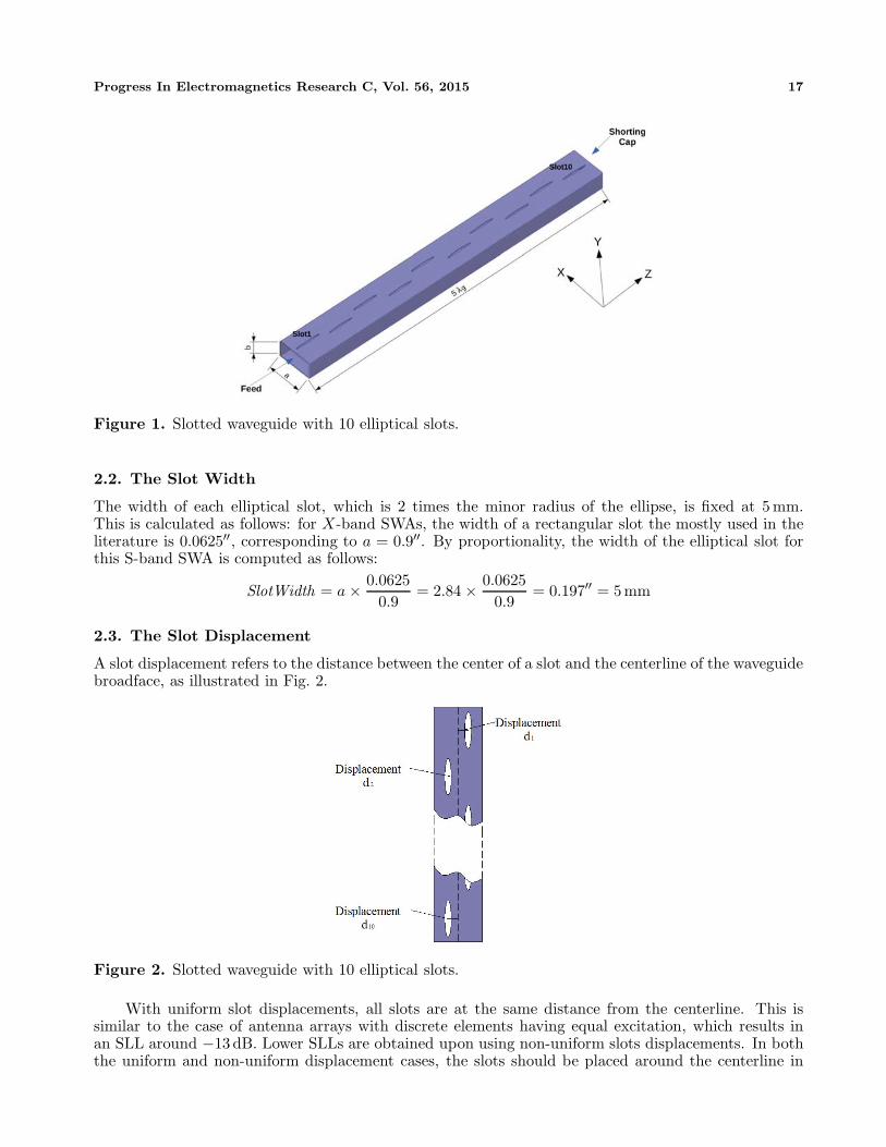
Based on the above guidelines, the total length of the SWA is 5λg, as shown in Fig. 1.

Progress In Electromagnetics Research C, Vol. 56, 2015 17

Figure 1. Slotted waveguide with 10 elliptical slots.

2.2. The Slot Width

The width of each elliptical slot, which is 2 times the minor radius of the ellipse, is fixed at 5 mm.This is calculated as follows: for X-band SWAs, the width of a rectangular slot the mostly used in theliterature is 0.0625′′, corresponding to a = 0.9′′. By proportionality, the width of the elliptical slot forthis S-band SWA is computed as follows:

SlotWidth = a × 0.06250.9

= 2.84 × 0.06250.9

= 0.197′′ = 5mm

2.3. The Slot Displacement

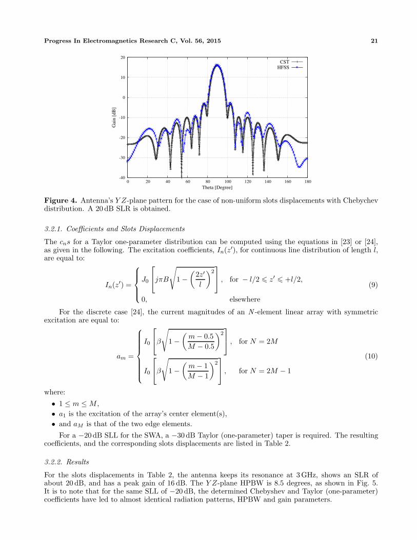
A slot displacement refers to the distance between the center of a slot and the centerline of the waveguidebroadface, as illustrated in Fig. 2.

Figure 2. Slotted waveguide with 10 elliptical slots.

With uniform slot displacements, all slots are at the same distance from the centerline. This issimilar to the case of antenna arrays with discrete elements having equal excitation, which results inan SLL around −13 dB. Lower SLLs are obtained upon using non-uniform slots displacements. In boththe uniform and non-uniform displacement cases, the slots should be placed around the centerline in


an alternating order. This is done to ensure that all slots radiate in phase and hence result in higherefficiency of the antenna.

The value of the uniform slot displacement that leads to a good reflection coefficient is givenby [15, 16]:

du =a

π

√arcsin

[1

N × G

](2)

where:

G = 2.09 × a

b× λg

λ0×

[cos

(0.464π × λ0

λg

)− cos(0.464π)

]2

(3)

In Equation (2), N is the number of slots, which is equal to 10. In Equation (3), λ0 = 100 mm at3GHz. Combining Equations (2) and (3), du is found to be 7.7 mm.

2.4. The Slot Length

For rectangular slots, the length is usually 0.98×λ0/2 � λ0/2. Because of the narrower ends of ellipticalslots, their length (double the major radius) is expected to be slightly larger than λ0/2. The optimizedelliptical slot length is determined as follows: the SWA, having 10 slots, is modeled assuming a uniformdisplacement (du = 7.7 mm); this 10-slot SWA is used to obtain the optimized slot length which takesinto account the effect of mutual coupling on the slot resonant length. An initial length of 0.98 × λ0/2per slot; the length is increased while inspecting the computed reflection coefficient S11 until the antennaresonates at 3GHz with a low S11 value. In our case, the elliptical slot length is found to be 54.25 mm.

For these uniform displacement and slot length, the resulting sidelobe level ration (SLR) is around13 dB, which is as expected. The reflection coefficient S11 and the Y Z-plane gain pattern in this case aregiven in Figs. 3(a) and 3(b), respectively. A peak gain of 16.6 dB and an SLR of 13.2 dB are recorded.The half-power beamwidth (HPBW) in this plane is 7.2 degrees. These values are obtained using CSTMicrowave Studio, and then verified with ANSYS HFSS.

-40

-30

-20

-10

0

10

20

0 20 40 60 80 100 120 140 160 180

Gai

n [d

B]

Theta [Degree]

CSTHFSS

-35

-30

-25

-20

-15

-10

-5

0

2.6 2.8 3 3.2 3.4

Ref

lect

ion

Coe

ffic

ient

[dB

]

Frequency [GHz]

CSTHFSS

(a) (b)

Figure 3. Antenna’s reflection coefficient and Y Z-plane pattern for the case of uniform slotdisplacement. (a) S11 for uniform slots displacement. (b) Pattern in the Y Z plane.

3. NON-UNIFORM DISPLACEMENT CALCULATION PROCEDURES

The simulations performed in this paper have proven that the resonating length of the elliptical slots isnot very sensitive to the slots displacements calculated using the method proposed in this paper. This


will be addressed again in later sections. For this, in the next calculations the length of all slots is fixedat 54.25 mm. The displacement of the nth slot is related to its normalized conductance gn by [15, 17–19]:

dn =a

πarcsin

√√√√√ gn

2.09λg

λ0

a

bcos2

(πλ0

2λg

) (4)

gn =cn

N∑n=1

cn

. (5)

In Equation (5), N is the number of slots, and cns are the distribution coefficients that should be

determined to achieve the desired SLL. Equation (5) guarantees thatN∑

n=1gn = 1.

Several distributions (tapers) well-known in discrete antenna arrays can be used to generate thecns (e.g., Taylor and Chebyshev). However, the resulting SLL of the SWA is always higher than theSLL used for the discrete array distribution. To reach the desired SWA SLL, a few iterations of thesimulation setup are required, where in each the SLL of the discrete array used to generate the tapervalues is decreased. Illustrative examples are shown below to further highlight this design procedure.

3.1. Example 1: 20 dB SLR with Chebyshev Distribution

In this example, the target is an SLR of 20 dB, where the cns are selected according to a Chebyshevdistribution.

3.1.1. Coefficients and Slots Displacements

The coefficients cns for a Chebyshev distribution are calculated from equations in [20, 21], as given inthe following. The array factor of a generalized Chebyshev array can be written as:

f(u) =p∏

n=1

(1

RnTNn−1

(γn cos

u

2

))=

1R

p∏n=1

(TNn−1

(γn cos

u

2

))(6)

where:

• Tx denotes a Chebyshev polynomial of order x,• γn = cosh[cosh−1(Rn)/(Nn − 1)],• u = 2π(d/λ)(cos θ − cos θ0) with d being the inter-element spacing and θ0 the elevation angle of

maximum radiation,• Rn is the sidelobe level ratio of the nth basis Chebyshev array,• and Nn is the number of elements of the nth basis array.

For a uniform spacing and an amplitude symmetrical about the center, the array factor can bewritten as:

f(u) =

⎧⎪⎪⎪⎪⎪⎪⎨⎪⎪⎪⎪⎪⎪⎩

2N/2∑m=1

Im cos[(m − 1/2)u], for N even

(N+1)/2∑m=1

εmIm cos[(m − 1)u], for N odd

(7)


where εm equals 1 for m = 1 and equals 2 for m �= 1. Finally, the excitation coefficients are found using:

Im =

⎧⎪⎪⎪⎪⎪⎪⎪⎨⎪⎪⎪⎪⎪⎪⎪⎩

2NR

N/2∑q=1

f [u = p ] cos[q], for N even

1NR

N+12∑

q=1

εqf [u = v] cos[w], for N odd

(8)

where:• p = 2π/N(q − 1/2),• q = 2π/N(m − 1/2)(q − 1/2),• v = 2π/N(q − 1),• and w = 2π/N(m − 1)(q − 1)

Equation (8) uses Chebyshev polynomials and the computed excitation currents result in anormalized array factor.

For a −35 dB Chebyshev taper, the cns and their corresponding slots displacements, calculatedfrom Equation (8), are given in Table 1. The −35 dB Chebyshev taper has been selected after somesimulation iterations, as it provides the desired −20 dB SLL for the SWA. A −20 dB Chebyshev taperleads to SWA sidelobes higher than the −20 dB goal.

Table 1. −35 dB Chebyshev taper coefficients and corresponding slots displacements leading to anSWA SLL of −20 dB.

Slot Number Chebyshev Coefficient Displacement (mm)1 1 3.742 2.086 5.423 3.552 7.114 4.896 8.45 5.707 9.116 5.707 9.117 4.896 8.48 3.552 7.119 2.086 5.4210 1 3.74

It is clear from Table 1 that the slots near the two waveguide ends are closest to the broadfacecenter line, whereas those toward the waveguide center have the largest displacement. This propertyapplies to all the examples.

3.1.2. Results

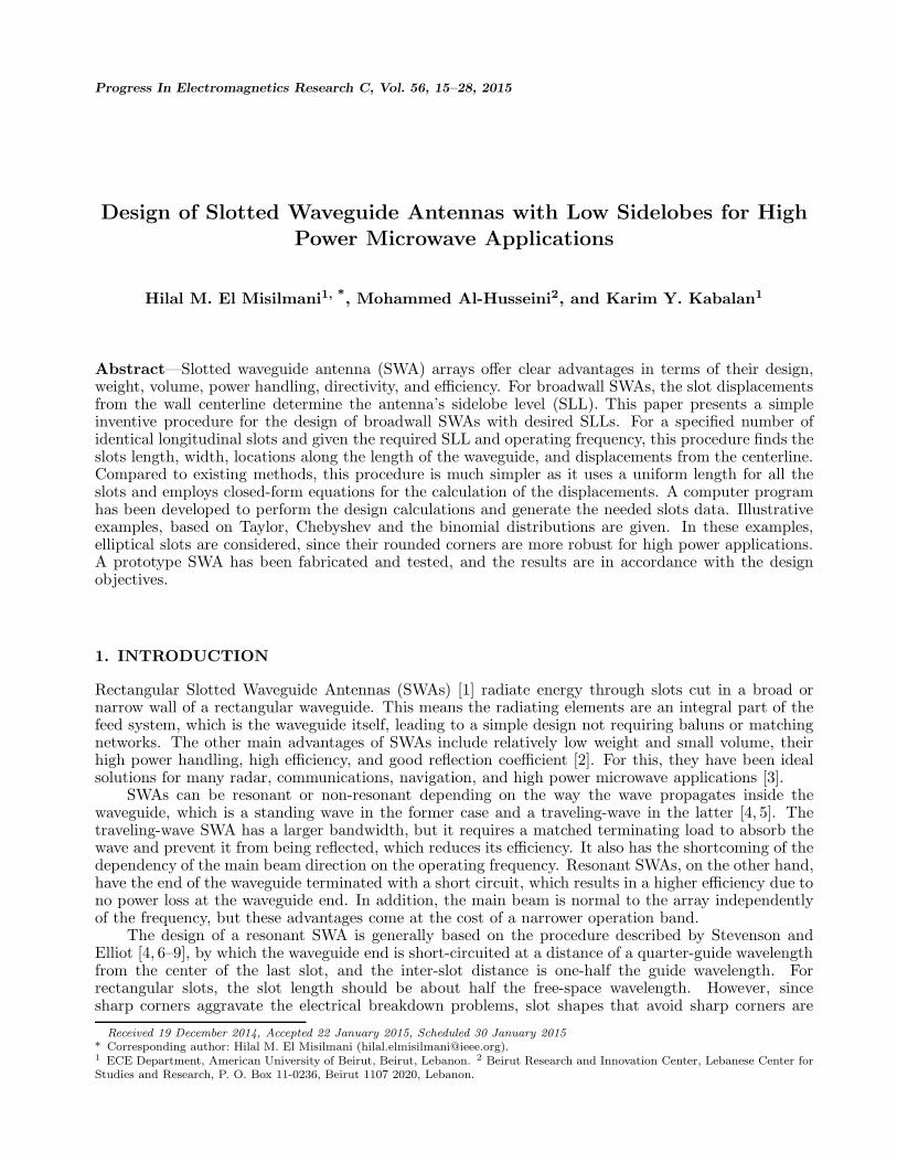
For the previously determined slot parameters (length, width, and coordinates), the SWA computedresults show a resonance at 3 GHz, an SLR of 20 dB, and a peak gain of 16.1 dB. The Y Z-plane HPBWhas increased to 8.4 degrees, compared to the uniform displacement case, as shown in Fig. 4. Thebroadening of the main beam is expected since the sidelobes have been forced to go lower.

3.2. Example 2: 20 dB SLR with Taylor (One-parameter) Distribution

In this example, the SWA is designed to have an SLR of 20 dB, where the cns will be obtained from aTaylor one-parameter distribution [22].


-40

-30

-20

-10

0

10

20

0 20 40 60 80 100 120 140 160 180

Gai

n [d

B]

Theta [Degree]

CSTHFSS

Figure 4. Antenna’s Y Z-plane pattern for the case of non-uniform slots displacements with Chebychevdistribution. A 20 dB SLR is obtained.

3.2.1. Coefficients and Slots Displacements

The cns for a Taylor one-parameter distribution can be computed using the equations in [23] or [24],as given in the following. The excitation coefficients, In(z′), for continuous line distribution of length l,are equal to:

In(z′) =

⎧⎪⎪⎨⎪⎪⎩

J0

⎡⎣jπB

√1 −

(2z′

l

)2⎤⎦ , for − l/2 � z′ � +l/2,

0, elsewhere

(9)

For the discrete case [24], the current magnitudes of an N -element linear array with symmetricexcitation are equal to:

am =

⎧⎪⎪⎪⎪⎪⎪⎨⎪⎪⎪⎪⎪⎪⎩

I0

⎡⎣β

√1 −

(m − 0.5M − 0.5

)2⎤⎦ , for N = 2M

I0

⎡⎣β

√1 −

(m − 1M − 1

)2⎤⎦ , for N = 2M − 1

(10)

where:

• 1 ≤ m ≤ M ,• a1 is the excitation of the array’s center element(s),• and aM is that of the two edge elements.

For a −20 dB SLL for the SWA, a −30 dB Taylor (one-parameter) taper is required. The resultingcoefficients, and the corresponding slots displacements are listed in Table 2.

3.2.2. Results

For the slots displacements in Table 2, the antenna keeps its resonance at 3GHz, shows an SLR ofabout 20 dB, and has a peak gain of 16 dB. The Y Z-plane HPBW is 8.5 degrees, as shown in Fig. 5.It is to note that for the same SLL of −20 dB, the determined Chebyshev and Taylor (one-parameter)coefficients have led to almost identical radiation patterns, HPBW and gain parameters.


Table 2. −30 dB Taylor (one-parameter) coefficients and corresponding slots displacements leading toan SWA SLL of −20 dB.

Slot Number Taylor-based Coefficient Displacement (mm)1 1 3.4932 2.467 5.5183 4.137 7.1944 5.597 8.4195 6.449 9.0706 6.449 9.0707 5.597 8.4198 4.137 7.1949 2.467 5.51810 1 3.493

-40

-30

-20

-10

0

10

20

0 20 40 60 80 100 120 140 160 180

Gai

n [d

B]

Theta [Degree]

CSTHFSS

Figure 5. Antenna’s Y Z-plane pattern for the case of non-uniform slot displacement with Taylor(one-parameter) distribution for an SLR of 20 dB.

3.3. Example 3: 30 dB SLR with Taylor (One-Parameter) Distribution

In this example, a Taylor (one-parameter) distribution is used to obtain an SWA SLR of 30 dB. Forthis, the taper coefficients for a −40 dB Taylor (one-parameter) distribution are required, and theseare listed in Table 3 alongside their corresponding slots displacements. The results show an antennaresonance at 3 GHz, and a peak gain of 15.3 dB. The −30 dB SLL has been attained, and the Y Z-planeHPBW has increased to 10 degrees. The Y Z-plane gain pattern is shown in Fig. 6.

3.4. Example 4: Binomial Excitation

Although it is not directly possible to use a binomial distribution to control the SLL, it is interesting touse the cns from a Binomial distribution and observe the resulting SWA SLL. The binomial coefficientsare obtained from the binomial expansion:

(1 + x)m−1 = 1 + (m − 1)x +(m − 1)(m − 2)

2!x2 (m − 1)(m − 2)(m − 3)

3!x3 + . . . (11)


Table 3. −40 dB Taylor (one-parameter) coefficients and corresponding slots displacements leading toan SWA SLL of −30 dB.

Slot Number Taylor-based Coefficient Displacement (mm)1 1 1.6312 6.611 4.2153 16.828 6.7854 28.573 8.9375 36.519 10.1816 36.519 10.1817 28.573 8.9378 16.828 6.7859 6.611 4.21510 1 1.631

-40

-30

-20

-10

0

10

20

0 20 40 60 80 100 120 140 160 180

Gai

n [d

B]

Theta [Degree]

CSTHFSS

Figure 6. Antenna’s Y Z-plane pattern for the case of non-uniform slots displacements with TaylorLine-Source distribution for an SLR of 30 dB.

Table 4. Binomial coefficients and corresponding slots displacements.

Slot Number Binomial Coefficient Displacement (mm)1 1 0.9642 9 2.9003 36 5.8474 84 9.0695 126 11.2686 126 11.2687 84 9.0698 36 5.8479 9 2.90010 1 0.964


For the case of 10 slots, the binomial coefficients and the resulting slots displacements are listed inTable 4. For these displacements values, the obtained SLR is 33.5 dB, and the peak gain is 15 dB. TheY Z-plane HPBW increases to 11.1 degrees, as shown in Fig. 7.

-40

-30

-20

-10

0

10

20

0 20 40 60 80 100 120 140 160 180

Gai

n [d

B]

Theta [Degree]

CSTHFSS

Figure 7. Antenna’s Y Z-plane pattern for the case of non-uniform slots displacements with binomialdistribution.

3.5. Reflection Coefficients

The S11 plots for the four examples are shown in Fig. 8. For all the studied examples where all theslots have a fixed length of 54.25 mm, the SWAs retain resonance at 3 GHz, despite the different slotsdisplacements used. This is evident by comparing the S11 plot for the case of uniform displacements inFig. 3(a) to those of the four SWA examples in Fig. 8, where the resonating length of the elliptical slotsproved insensitive to the slots displacements.

-30

-25

-20

-15

-10

-5

0

2.6 2.8 3 3.2 3.4

Ref

lect

ion

Coe

ffic

ient

[dB

]

Frequency [GHz]

Chebyshev with -35 dBTaylor with -30 dBTaylor with -40 dB

Binomial

Figure 8. Reflection coefficient plots for the four illustrated examples in case of non-uniformdisplacements (using CST).


4. COMPUTER PROGRAM

A computer program written in Python has been written to generate the slots displacements for a desiredSLL. The program takes as input the design frequency, waveguide dimensions a and b, the number ofslots, and the highest allowable SLL. It computes and outputs λ0, λg, the total needed waveguidelength, the resonant length of a rectangular slot (which serves as a starting point in optimizing thelength of any used slot shape), the width of the slot (which is kept the same for any slot type), the tapercoefficients (Chebyshev or Taylor), and the corresponding slots displacements. The units are indicatedon the program graphical user interface (GUI). A screenshot of the program output is given in Fig. 9.This program was used for the examples in Section 3, and for the design in Section 5. Improvements tothe program interface are still being done.

Figure 9. A screenshot of the python program output.

5. FABRICATION AND MEASUREMENTS

In order to validate the procedure illustrated in this paper, a prototype SWA array has been fabricatedand tested. The waveguide in hand has a length of 50 cm. This length is not enough to fit 10 slotsrespecting the different slot distance and length guidelines, so the design has been made with 7 slots,of elliptical shape. To avoid the two edge slots intersecting the waveguide flanges, the distance betweeneach of these two slots and the nearby waveguide edge has been increased from λg/4 to 3λg/4, leadingto a total SWA length of 4.5λg. This change was accounted for in the Python computer program, whichwas used for this design. To keep the waveguide length of 50 cm, the SWA is designed for a frequency of3.4045 GHz. At this frequency, λg = 111.11 mm, and 4.5λg = 50 cm. After initially designing the SWAwith the correct uniform distribution displacement, the elliptical slot length has been optimized to getto this resonance frequency. It is found equal to 48 mm. With this optimized length, and for a slotwidth of 5 mm, the SWA has later been designed to radiate with a sidelobe level of less than −20 dB.A Chebyshev distribution of −35 dB has been used to calculate the excitation coefficients in this case.These coefficients and the corresponding slots displacements are listed in Table 5.


Table 5. Normalized Chebyshev taper coefficients and corresponding slots displacements.

Slot Number Chebyshev Coefficient Displacement (mm)1 1 6.7592 2.588 11.1493 4.262 14.7464 4.981 16.1715 4.262 14.7466 2.588 11.1497 1 6.759

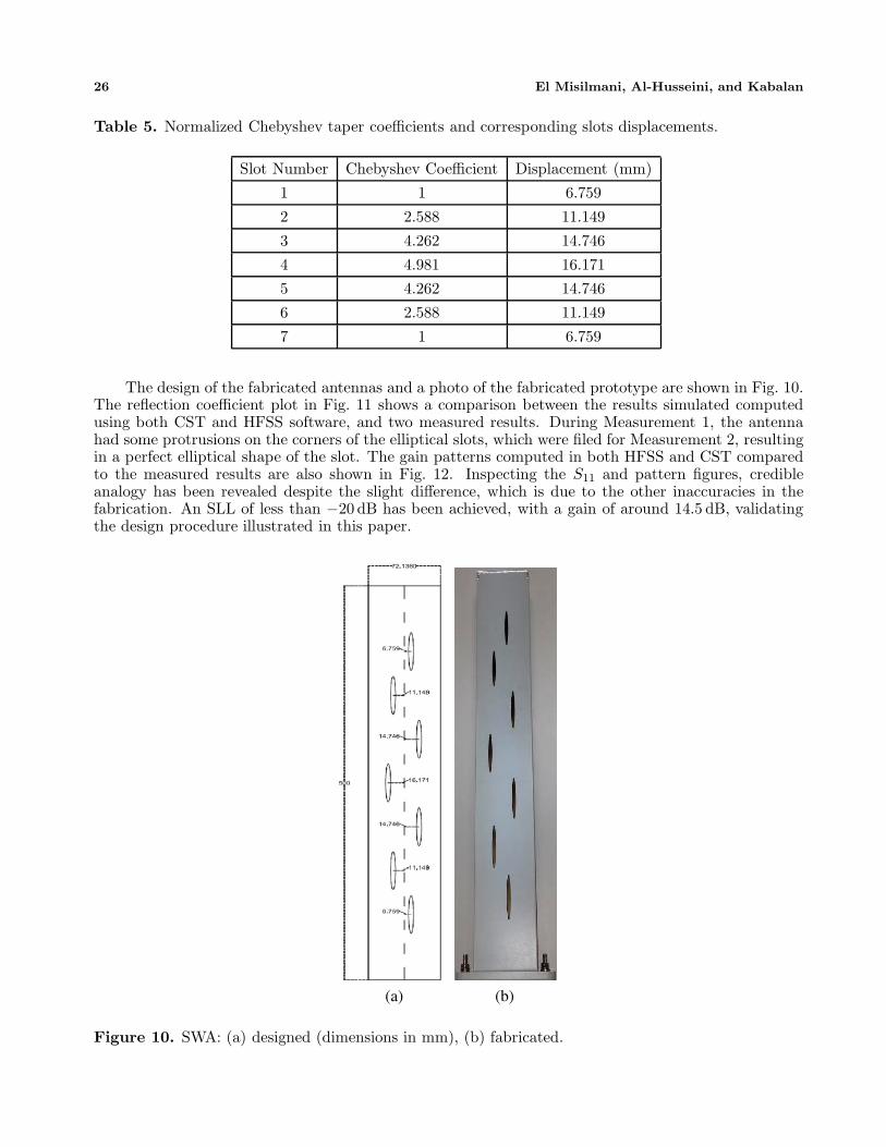
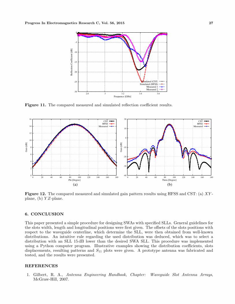
The design of the fabricated antennas and a photo of the fabricated prototype are shown in Fig. 10.The reflection coefficient plot in Fig. 11 shows a comparison between the results simulated computedusing both CST and HFSS software, and two measured results. During Measurement 1, the antennahad some protrusions on the corners of the elliptical slots, which were filed for Measurement 2, resultingin a perfect elliptical shape of the slot. The gain patterns computed in both HFSS and CST comparedto the measured results are also shown in Fig. 12. Inspecting the S11 and pattern figures, credibleanalogy has been revealed despite the slight difference, which is due to the other inaccuracies in thefabrication. An SLL of less than −20 dB has been achieved, with a gain of around 14.5 dB, validatingthe design procedure illustrated in this paper.

(a) (b)

Figure 10. SWA: (a) designed (dimensions in mm), (b) fabricated.


-30

-25

-20

-15

-10

-5

0

2.8 3 3.2 3.4 3.6

Ref

lect

ion

Coe

ffic

ient

[dB

]

Frequency [GHz]

Measured 1Measured 2

Simulated (CST)Simulated (HFSS)

Figure 11. The compared measured and simulated reflection coefficient results.

0

2

4

6

8

10

12

14

16

0 20 40 60 80 100 120 140 160 180

Gai

n [d

B]

Phi [Degree]

CSTHFSS

Measured

-40

-30

-20

-10

0

10

20

0 20 40 60 80 100 120 140 160 180

Gai

n [d

B]

Theta [Degree]

CSTHFSS

Measured

(a) (b)

Figure 12. The compared measured and simulated gain pattern results using HFSS and CST: (a) XY -plane, (b) Y Z-plane.

6. CONCLUSION

This paper presented a simple procedure for designing SWAs with specified SLLs. General guidelines forthe slots width, length and longitudinal positions were first given. The offsets of the slots positions withrespect to the waveguide centerline, which determine the SLL, were then obtained from well-knowndistributions. An intuitive rule regarding the used distribution was deduced, which was to select adistribution with an SLL 15 dB lower than the desired SWA SLL. This procedure was implementedusing a Python computer program. Illustrative examples showing the distribution coefficients, slotsdisplacements, resulting patterns and S11 plots were given. A prototype antenna was fabricated andtested, and the results were presented.

REFERENCES

1. Gilbert, R. A., Antenna Engineering Handbook, Chapter: Waveguide Slot Antenna Arrays,McGraw-Hill, 2007.


2. Mailloux, R. J., Phased Array Antenna Handbook, Artech House, 2005.3. Rueggeberg, W., “A multislotted waveguide antenna for high-powered microwave heating systems,”

IEEE Trans. Ind. Applicat., Vol. 16, No. 6, 809–813, 1980.4. Elliott, R. S. and L. A. Kurtz, “The design of small slot arrays,” IEEE Trans. Antennas Propagat.,

Vol. 26, 214–219, March 1978.5. Elliott, R. S., “The design of traveling wave fed longitudinal shunt slot arrays,” IEEE Trans.

Antennas Propagat., Vol. 27, No. 5, 717–720, September 1979.6. Stevenson, A. F., “Theory of slots in rectangular waveguides,” Journal of Applied Physics, Vol. 19,

24–38, 1948.7. Elliott, R. S., “An improved design procedure for small arrays of shunt slots,” IEEE Trans.

Antennas Propagat., Vol. 31, 48–53, January 1983.8. Elliott, R. S. and W. R. O’Loughlin, “The design of slot arrays including internal mutual coupling,”

IEEE Trans. Antennas Propagat., Vol. 34, 1149–1154, September 1986.9. Elliott, R. S., “Longitudinal Shunt Slots in Rectangular Waveguide: Part I, Theory,” Tech. Rep.,

Rantec Report No. 72022-TN-1, Rantec, Calabasas, CA, USA.10. Baum, C. E., “Sidewall waveguide slot antenna for high power,” Sensor and Simulation Note,

Vol. 503, August 2005.11. Al-Husseini, M., A. El-Hajj, and K. Y. Kabalan, “High-gain S-band slotted waveguide antenna

arrays with elliptical slots and low sidelobe levels,” PIERS Proceedings, Stockholm, Sweden,August 12–15, 2013.

12. Tai, C. T., Characteristics of Liner Antenna Elements, Antenna Engineering Handbook, H. Jasik(ed.), McGraw-Hill, 1961.

13. Oliner, A. A., “The impedance properties of narrow radiating slots in the broad face of rectangularwaveguides,” IEEE Trans. Antennas Propagat., Vol. 5, No. 1, 4–20, 1058.

14. Stegen, R. J., “Longitudinal shunt slot characteristics,” Hughes Technical Memorandum, No. 261,4–20, Culver City, CA, November 1951.

15. Stevenson, R. J., “Theory of slots in rectangular waveguide,” J. App. Phy., Vol. 19, 4–20, 1948.16. Watson, W. H., “Resonant slots,” Journal of the Institution of Electrical Engineers — Part IIIA:

Radiolocation, Vol. 93, 747–777, 1946.17. Coburn, W., M. Litz, J. Miletta, N. Tesny, L. Dilks, C. Brown, and B. King, “A slotted-waveguide

array for high-power microwave transmission,” Army Research Laboratory, January 2001.18. Cullen, A. L., “Laterally displaced slot in rectangular waveguide,” Wireless Eng., 3–10,

January 1949.19. Hung, K. L. and H. T. Chou, “A design of slotted waveguide antenna array operated at X-band,”

IEEE international Conference on Wireless Information Technology and System, 1–4, 2010.20. Safaai-Jazi, A., “A new formulation for the design of Chebyshev arrays,” IEEE Trans. Antennas

Propag., Vol. 42, 439–443, 1980.21. El-Hajj, A., K. Y. Kabalan, and M. Al-Husseini, “Generalized Chebyshev arrays,” Radio Science,

Vol. 40, RS3010, June 2005.22. Taylor, T. T., “One parameter family of line-sources producing modified sin(πu)/πu patterns,”

Hughes Aircraft Co. Tech., Mem. 324, Culver City, Calif., Contract AF 19(604)-262-F-14,September 4, 1953.

23. Balanis, C. A., Antenna Theory Analysis and Design, Wiley, 2005.24. Kabalan, K. Y., A. El-Hajj, and M. Al-Husseini, “The bessel planar arrays,” Radio Science, Vol. 39,

No. 1, RS1005, January 2004.

design of slotted waveguide antennas with low sidelobes...

Documents