DESIGN OF STEEL STRUCTURES

DESIGN OF STEEL STRUCTURES Elias G. Abu·Saba Associate Professor of Architectural Engineering North Carolina Agricultural and Technical State University

SPRINGER-SCIENCE+BUSINESS MEDIA, B.v

DESIGN OF STEEL STRUCTURES Elias G. Abu·Saba Associate Professor of Architectural Engineering North Carolina Agricultural and Technical State University

SPRINGER-SCIENCE+BUSINESS MEDIA, B.v

Copyright © 1995 Springer Science+Business Media Dordrecht Original1y pub1ished by Chapman & Hall in 1995 Softcover reprint ofthe hardcover 1st edition 1995

All rights reserved. No part of this work covered by the copyright hereon may be reproduced or used in any form or by any means-graphic, electronic, or mechanical, including photocopying, recording, taping, or information storage and retrieval systems-without the written permission of the publisher.

1 234567 8 9 10 XXX 01 009997 9695

Library of Congress Cataloging-in-Publication Data

Abu-Saba, Elias G., Design of steel structures / by Elias G. Abu-Saba.

p. cm. Includes bibliographical references and index. ISBN 978-1-4613-5864-0 ISBN 978-1-4615-2079-5 (eBook) DOI 10.1007/978-1-4615-2079-5 1. Building, Iron and steel. 2. Structural design. 3. Load factor design. 1. Title.

TA684.A144 1995 693' .71-dc20 94-48546

CIP

I dedicate this book to the memory of my parents, Jurjis and Sabat Abu-Saba, who did not have the privilege to go to school. Yet they believed in the power of knowledge and provided us, their children, with the opportunity to learn and grow.

The infinite spans the human mind. The spirit spins free of space and time. The joy and sadness of life are a wink In the eternal flow. The stream cascades and meanders To merge and be lost in the greater sea.

ELIAS G. ABU-SABA

November 6. 1994

Contents

Preface xiii

1 Introduction 1

1.1 Introduction 1 1.2 Structural Steel and Its Properties in Construction 4 1.3 Applications 7 1.4 Loads, Load Factors, and Load Combinations 13

2 Tension Members 14

2.1 Introduction 14 2.2 Design Criteria 14 2.3 ASD Method 15 2.4 LRFD Method 17 2.5 Effective Area of Riveted and Bolted Tension Members 20 2.6 Effective Area for Staggered Holes of Tension Members 21 2.7 Tension Rods in Design of Purlins 27 2.8 Limitation of Length of Tension Members on Stiffness:

Slenderness Ratio 25 2.9 Applications 25

3 Compression Members

3.1 Introduction 3.2 Derivation of Euler's Formula 3.3 Design Criteria for Compression Members Under

oncentric Load: ASD Method 3.4 Effective Length and Slenderness Ratio 3.5 Design Criteria for Compression Members

Under Concentric Load: LRFD Method

46

46 47

49 51

54

ix

x Contents

3.6 SI LRFD Design Criteria (Axial Compression) 60 3.7 Compression Members in Braced Frames: ASD Method 63 3.8 Axial Compression and Bending: ASD Method 64 3.9 Reduction in Live Loads 65 3.10 Columns Subject to Bending and Axial Force in a

Braced System: LRFD Method 3.11 Design of Columns for Braced and Unbraced Frames:

ASDMethod 82

4 Designs of Bending Members 106

4.1 Introduction 106 4.2 Simple Bending 106 4.3 Design of Beams and Other Flexural Members:

ASD Allowable Bending Stress 109 4.4 Deflections and Vibrations of Beams in Bending 116 4.5 Design for Flexure: LRFD Method 124 4.6 Use of the Load Factor Design Selection Table Zx

for Shapes Used as Beams 1128 4.7 Serviceability Design Considerations and the

LRFDMethod 132

5 Torsion and Bending 133

5.1 Introduction 133 5.2 Torsional Stresses 133 5.3 Plane Bending Stresses 137 5.4 Combining Torsional and Bending Stresses 137 5.5 Torsional End Conditions 138 5.6 Torsional Loading and End Conditions 139 5.7 Applications 144

6 Design of Bracings for Wind and Earthquake Forces 150

6.1 Introduction 150 6.2 Wind Forces 150 6.3 Wind Velocity Pressure 151 6.4 Selection of Basic Wind Speed (mph) 155

6.5 External Pressures and Combined External and Internal Pressures

6.6 Wind Pressure Profile Against Buildings 6.7 Analysis of Braced Frames for Wind Forces 6.8 Introduction to Seismic Design 6.9 Equivalent Static Force Procedure

Contents xi

155 165 166 175 177

7 Connections 187

7.1 Introduction 187 7.2 Types of Connections 187 7.3 Framed Beam Connection: Bolted 190 7.4 Framed Beam Connection: Welded E70XX Electrodes for

Combination with Table II and Table III Connections 196

8 Anchor Bolts and Baseplates 201

8.1 Introduction 201 8.2 Design of Column Baseplates 201

9 Built-Up Beams: Plate Girders 210

9.1 Introduction 9.2 Design of Plate Girders by ASD Method 9.3 Approximate Method for Selection of Trial Section

10 Composite Construction

10.1 Introduction 10.2 Design Conceptualization and Assumptions 10.3 Development of Section Properties 10.4 Short-Cut Method for Determining Sxbc

10.5 Shear Connectors 10.6 Bethlehem Steel Table for Selecting Shear Connectors 10.7 LRFD Method: Design Assumptions 10.8 LRFD Flexural Members

210 210 214

246

246 246 249 264 282 284 285 287

xii Contents

11 Plastic Analysis and Design of Structures 294

11.1 Introduction 294 11.2 Bending of Beams 294 11.3 Design of Beams: Failure Mechanism Approach 301 11.4 Fixed End Beam 308 11.5 Plastic Hinges: Mechanism of Failure 310 11.6 Fixed End Beam with Multiple Concentrated Loads 317 11.7 Continuous Beams 319 11.8 Portal Frames 329 11.9 Minimum Thickness (Width-Thickness Ratio) 332 11.10 Plastic Analysis of Gabled Frames 337

12 Influence of Axial Forces on Plastic Moment 340

12.1 Introduction 340 12.2 Influence of Axial Forces on Plastic Moment Capacity 340

13 Rigid Connections 350

13.1 Introduction 351 13.2 Straight Corner Connection 355 13.3 Stiffener for a Straight Corner Connection 357 13.4 Haunched Connections 364 13.5 Haunched Connections with Concentrated Loads 368 13.6 Design Guides: Connections

14 Multistory Buildings: Plastic Design

14.1 Introduction 14.2 Allowable Stress vs. Plastic Design Methods 14.3 Application to Multistory Buildings

Index

375

375

376 376 379

389

Preface

This book is intended for classroom teaching in architectural and civil engineering at the graduate and undergraduate levels. Although it has been developed from lecture notes given in structural steel design, it can be useful to practicing engineers. Many of the examples presented in this book are drawn from the field of design of structures.

Design of Steel Structures can be used for one or two semesters of three hours each on the undergraduate level. For a two-semester curriculum, Chapters 1 through 8 can be used during the first semester. Heavy emphasis should be placed on Chapters 1 through 5, giving the student a brief exposure to the consideration of wind and earthquakes in the design of buildings. With the new federal requirements vis a vis wind and earthquake hazards, it is beneficial to the student to have some under­standing of the underlying concepts in this field. In addition to the class lectures, the instructor should require the student to submit a term project that includes the complete structural design of a multi-story building using standard design procedures as specified by AISC Specifications. Thus, the use of the AISC Steel Construction Manual is a must in teaching this course. In the second semester, Chapters 9 through 13 should be covered. At the undergraduate level, Chapters 11 through 13 should be used on a limited basis, leaving the student more time to concentrate on composite construction and built-up girders.

Chapters 6, 11, 12, 13, and 14 can be used for a graduate course. As a prerequisite for the graduate course, the student must have a minimum of three credit hours in the design of steel structures. The instructor will go into more depth in the presentation of Chapters 6, 11, 12, and 13. The student should be required to submit a term project using rigid frames in multi story buildings. Chapter 14 provides a simple method which can easily be computerized, allowing the student the facility of designing medium- to high-rise buildings using steel frames. U. S. customary units are used throughout, although some examples are presented with S. I. units. To help students convert from U. S. units to S. I. units, tables of conversion are provided in Chapter 1.

The allowable stress design method (ASD) is used predominantly in this book. To help the student appreciate the load and resistance factored

xiii

xiv Preface

design method (LRFD), the text includes discussions and examples utiliz­ing this method.

Fundamental principles of steel design are presented in logical order to encourage the student to tackle the problem of design with a more general perspective. Tables, graphs and other design aids are introduced to help facilitate the design process. The selection of sections in the design of composite construction is made easier by a short-cut approach, thus eliminating the tediousness of the trial-and-error method.

The author gratefully acknowledges Robert M/ Hackett of the Univer­sity of Mississippi, Joseph P. Colaco of CBM Engineers, Inc., Ramesh Malia of the University of Conneticut, and Mahesh Pendey of the Univer­sity of Waterloo, Ontario for their comments during the development of the book.

The author expresses his appreciation to the hundreds of students who have attended his classes at North Carolina Agricultural and Technical State University. Without them this book could not have been material­ized.

Finally, the author wishes to thank his wife, Dr. Mary Bentley Abu-Saba, for her continued support and encouragement.

DESIGN OF STEEL STRUCTURES

1 Introduction

1.1 INTRODUCTION

Conversion Factors

The building industry in the United States is gradually adopting the new metric-based system referred to as SI units (for System International). For many years, the Congress of the United States has tried to legislate the use of the metric system without success. At present, scientific and technical periodicals and journals in this country are requiring the use of both systems in their publications. In this book, illustrations and example problems use both the SI and U.S. systems. Table 1.1 lists the standard units for both systems.

To help the reader make the transition from one system to another, conversion factors are provided in Table 1.2.

Design Philosophy

The design of structures is a creative process. At the same time, the structural designer must have a basic understanding of the concepts of solid mechanics and be able to work harmoniously with the architect who is in charge of the project, the contractor who will perform the construc­tion, and the owner who will bear the cost of the project and use it. The principal goals of the structural designer are to provide a safe and reliable structure that will serve the function for which it was intended, an

1

2 Introduction

TABLE 1.1 Units of Measurement

Length

Foot

Inch

Area

Name of Unit

Square feet Square inches

Volume

Cubic feet

Cubic inches

Force, Mass

Pound Kip Pounds per foot Kips per foot Pounds per square foot Kips per square foot Pounds per cubic foot

Stress

Pounds per square inch Kips per square inch

Length

Meter

Millimeter

Area Square meter Square millimeter

Abbreviation

U.S. System

ft

in.

lb k lb/ft k/ft lb 1ft 2 or psf k/ft2 or ksf Ib/ft 3 or pcf

Ib/in.2 or psi k/in? or ksi

Sf System

m

mm

Use

Large dimensions, building plans, beam spans

Small dimensions, size of member cross sections

Large areas Small areas, properties of

cross sections

Large volumes, quantities of materials

Small volumes

Specific weight, force, load 1000lb Linear load as on a beam Linear load as on a beam Distributed load on a surface Distributed load on a surface Relative density, weight

Stress in structures Stress in structures

Large dimensions, building plans, beam spans

Small dimensions, size of member cross sections

Large areas Small areas, properties of

cross sections

Introduction 3

Name of Unit Abbreviation Use

Volume

Cubic meter m3 Large volumes, quantities of materials

Cubic millimeter mm3 Small volumes

Mass Kilogram kg Mass of materials Kilograms

per cubic meter kg/m3 Density

Force (Load on Structures)

Newton N Force or load Kilonewton kN 1000 N

Stress Pascal Pa Stress or pressure

(1 Pa = 1 N/m2) Kilopascal kPa 1000 Pa Megapascal MPa 1,000,000 pascal Gigapascal GPa 1,000,000,000 pascal

economical structure that can be built and maintained within the specified budget, and a structure that is aesthetically acceptable.

Design Loads Design loads for buildings include dead and live loads. Dead loads

consist of the weight of all permanent constructions, including fixed equipment that is placed on the structure. In bridges, it includes the weight of decks, sidewalks, railings, utility posts and cables, and the bridge frame. Live loads are dynamic and vary in time. They include vehicles, snow, personnel, movable machinery, equipment, furniture, merchandise, wind and earthquake forces, and the like. Once a building frame has been selected on the basis of dead and live loads, a check must be made using a combination of these loads. In some regions, a check must include the seismic forces. Member sizes may have to be modified from the initial selection to meet the wind and seismic forces.

Live load tables are provided by almost all building codes. In unusual cases, the design load intensity is established to the satisfaction of a building official. However, the actual distribution of the live load for maximum effect is the responsibility of the design engineer. Table 1.3 lists live load intensities for various occupancies.

4 Introduction

TABLE 1.2 Conversion Factors for Measurement Units

To Convert from U.S. To Convert from SI Units to SI Units, Units to U.S. Units,

Multiply by U.S. Units SI Units Multiply by

25.4 in. mm 0.03937 0.3048 ft m 3.281

645.2 in.2 mm2 1.550 X 10- 3

16.39 X 103 in.3 mm3 61.02 X 10- 6

416.2 X 103 in.4 mm4 2.403 X 10- 6

0.09290 ft2 m2 10.76 0.02832 ft3 m3 35.31 0.4536 lb (mass) kg 2.205 4.448 lb (force) N 0.2248 4.448 k (force) kN 0.2248 1.356 ft-lb (moment) N-m 0.7376 1.356 k-ft (moment) kN-m 0.7376 1.488 lb /ft (mass) kg/m 0.6720

14.59 lb/ft (force) N/m 0.06853 14.59 k/ft (force) kN/m 0.06853 6.895 Ib/in.2 (force/unit area) kPa 0.1450 6.895 k/in.2 (force/unit area) MPa 0.1450 0.04788 Ib/ft 2 (force/unit area) kPa 20.93

47.88 k/ft2 (force/unit area) MPa 0.02093 16.02 Ib/ft 3 (density) kg/m3 0.6242

1.2 STRUCTURAL STEEL AND ITS PROPERTIES IN CONSTRUCTION

Historically, the use of steel in construction for commercial buildings has been widely adopted in the United States. The availability of steel makes it much easier to use. In addition, steel has many characteristics that make it more advantageous than concrete. Structural steel takes less time to erect. The combination of high strength, light weight, ease of fabrication and erection, and many other favorable properties makes steel the material of choice for construction in this country. These properties will be discussed briefly in the following paragraphs.

High Strength

The strength of a construction material is defined by the ratio of the weight it carries to its own weight. When compared with other building

TABLE 1.3 Minimum Uniformly Distributed Live Loads

Occupancy or Use

Apartments (see residential) Armories and drill rooms Assembly halls and other places of assembly

Fixed seats Movable seats

Balcony (exterior) Bowling alleys, poolrooms, and similar recreational areas Corridors

First floor Other floors, same as occupancy served except as indicated

Dance halls Diningrooms and restaurants Dwellings (see residential) Garages (passenger cars)a Grandstands (see reviewing stands) Gymnasiums, main floors and balconies Hospitals

Operating rooms Private rooms Wards

Hotels (see residential) Libraries

Reading rooms Stackrooms

Manufacturing Marquees Office buildings

Lobbies Offices

Penal institutions Cell blocks Corridors

Residential Multifamily Houses

Corridors Private apartments Public rooms

Dwellings First floor Second floor and habitable attics Unhabitable attics

Introduction 5

Live Load (Ib /ft 2 )

150

60 100 100 75

100

100 100

100

100

60 40 40

60 150 125 75

100 80

40 100

60 40 100

40 30 20

a Floors shall be designed to carry 150% of the maximum wheel load anywhere on the floor. (cont'd.)

6 Introduction

TABLE 1.3 (cont'd.)

Occupancy or Use

Hotels Corridors serving public rooms Guest rooms Private corridors Public rooms Public corridors

Reviewing stands and bleachersb

Schools Classrooms Corridors

Sidewalks, vehicular driveways, and yards subject to trucking Skating rinks Stairs' fire escapes and exitways Storage warehouse

Heavy Light

Stores Retail

First floor, rooms Upper floors

Wholesale Theaters

Aisles, corridors, and lobbies Balconies Orchestra floors Stage floors

Yards and terraces, pedestrians

Live Load (Ib Ift2)

100 40 40 100 60

40 100 250 10 100

250 125

100 75 125

100 60 60 150 100

b For detailed recommendations, see American Standard Places of Outdoor Assembly, Grandstands and Tents, Z20.3 1950, or the latest revision thereof approved by the American Standard Association, Inc., National Fire Protection Association, Boston, MA. Source: Minimum Uniformly Distributed Live Loads ASCE 7-88 (Formerly ANSI A58.1), Table 2, p. 4.

materials, steel is considered to have a high strength ratio. This is impor­tant in the construction of long-span bridges, tall buildings, and buildings that are erected on relatively poor soil.

Strength and ductility are the two properties that make steel suitable for building structures that otherwise could not have been possible. The strength of steel provides buildings with a minimum number of columns and relatively small members. Its ductility relieves overstressing in certain

Introduction 7

Stress

Strain

Figure 1.1 Typical stress-strain curve.

members in a given structure by allowing redistribution of stresses due to yielding.

A typical stress-strain diagram for structural steel is shown in Figure 1.1. If we look at this diagram, it can be observed that steel obeys Hooke's law up to the first yield. In this region, stress is directly proportional to strain. Beyond this point, steel experiences a plastic condition momentarily and then enters into the strain-hardening state. At failure, the strain ranges from 150 to 200 times the elastic strain. During strain hardening, the stress continues to increase to a maximum and then drops slightly before failure. At the end of the strain-hardening state, the cross section of the tension specimen is reduced. This characteristic is referred to as necking.

1.3 APPLICATIONS

The diagram shown in Figure 1.2 represents a typical interior panel of a library stack room's framing system. It has a reinforced concrete floor slab 4t in. thick. Tiling weighs 1 lb 1ft 2, and ceiling loads are equivalent to 10 lb/ft2.

Example 1.1

(a) Determine the uniform load on a typical beam and express it in pounds per linear foot.

8 Introduction

-~

--U

U 0

0 C\I

Typical Girder

E (\j Q)

ro Cij. (J .a.. >-I-

4 @ 6' - 0" on c. = 24' - 0"

Figure 1.2 Floor plan: typical interior bay,

-.-

...1-

:I I

(b) Assuming that the typical beam and its fireproof coating weighs 50 Ib Ilinear ft, find the concentrated loads on a typical girder.

(c) Show the loading system on the members in (a) and (b).

(d) Do part (a) and (b) using the S1 measurement units.

Solution

Typical Beam

In Figure 1.3a, the strip that is 1 ft X 6 ft represents the tributary area for the loading per linear foot on the beam shown in Figure 1.3b. Thus, the uniform load from each load component will be equal to the intensity of that load component times the tributary area. Calculation of the loads on the beam is presented as follows.

Dead Loads

Slab 1 X 6 X 4.5 X fI X 150 = 337.5 Ib 1ft Ceiling load 1 X 6 X 10.0 = 60.0 Tiling load 1 X 6 X 1 = 6.0 Subtotal = 403.5 Ib / ft

Introduction 9

l' wide

I .... 20' - a" ~I Figure 1.3 Typical beam. (a) Loading strip; (b) simply supported beam.

Live Loads

From Table 1.3, the intensity of the live load is 150 Ib/ft2. Thus, the uniform live load on the beam is calculated as follows:

Live load 1 X 6 X 150 = 900.0 lb 1ft Total (dead + live) = 1303.S Ib I ft

The intensity of the uniform load on the typical beam shown in Figure 1.4 is therefore found to be 1303.5 lb 1ft.

10 Introduction

E o

cO

-r-Typical Interior Girder

-I-

E !II (])

co (ij u .n. :>. I-

-I-

_L..

4 @ 1.83 m = 7.32 m

Figure 1.4 Typical interior girder with concentrated loads from typical beams.

Concentrated Loads on Typical Interior Girder

Calculate reaction R at the end of the beam

L 1 R = (DL + LL) x 2 + "2 x weight of beam

20 1 = 1303.5 x 2 + "2 X 20 X 50

= 13,035 + 500 = 13,5351b

Or expressed in kips, R = 13.58 k.

-.... -l-

-I-

-'--

~I

Since an interior girder shown in Figure 1.5 supports typical beams on both sides, the reaction on the girder is double the reaction from one beam. Hence, the concentrated loads on the girder will have the magni­tude P of

Example 1.2

SI Measurement Units

P = 13.54 X 2 = 27.1 k

Repeat the above problem using the SI measurement units showing the floor plan, typical beam, and girder. From Table 1.2, all measurements are

Introduction 11

27 k 27 k 27 k

24' - 0" ~I Figure 1.5 Floor plan: typical interior bay in SI units.

converted into S1 units. A summary of the results for the above problem is shown below.

Loads u.s. Units (Ib 1ft) Conversion Factor SI Units (N 1m)

Dead Loads

Slab 337.5 14.59 4924 Ceiling 60.0 875 Tiling 6.0 88 Subtotal 403.5 5887

Live Load

Floor 900.0 13,131

Weight of Beam

Beam plus coating 50.0 730

Total Unifonn Load on Beam Including Its Weight

1303.5 19,748

Determine the reaction at the end of the beam.

Reaction at end of beam R

p= 2R P 11000

U.S. Units (Ib) Conversion Factor

13,535 4.448

Concentrated Loads on Girder 27,070

27.1 k

SI Units (N)

60,204

120,408 120.4 kN

.... N

• _

'_

_

" _

_ v

•••

----------~----~

Fig

ure

1.6

Snow

loa

d in

pou

nd-f

orce

per

squ

are

foot

on

the

gro

und,

5-y

ear

mea

n re

curr

ence

int

erva

l.

Introduction 13

1.4 LOADS, LOAD FACTORS, AND LOAD COMBINATIONS

In 1986, the AISC introduced the first edition of a manual for steel construction using the load and resistance factor design method (LRFD). It will not be long before designers for steel construction are expected to use this method in preference to the allowable strength method currently in use. LRFD proportions the various members in a given structural system so that no single member or part may exceed the applicable limit state when the structure is subjected to all appropriate factored load combinations. The design strength of each structural member or assem­blage must exceed the required strength based on the factored nominal loads.

The following nominal loads are considered in the design of steel structures:

D = dead load due to the weight of the structural element and

permanent features on the structure

L = live load due to occupancy and movable equipment

Lr = roof live load

W = wind load

S = snow load (see Figure 1.6 for snow loads in the United States)

E = earthquake load

R = load due to initial rainwater or ice exclusive of the ponding contribution

The required strength of the structure and its elements must be deter-mined from the appropriate critical combination of factored loads listed below:

I.4D

1.2D + 1.6L + O.5(L,., S, or R)

1.2D + 1.6(L,., S, or R) + (0.5L or 0.8W)

1.2D + 1.3W + 0.5L + 0.5(L r , S, or R)

1.2D + 1.5E + (0.5L or 0.2S)

0.9D - (l.3W or 1.5E)

(Ll)

(1.2)

(1.3)

(1.4)

(1.5)

(1.6)

Exception: The load factor on L in combinations (1.3), (1.4), and (1.5) shall equal 1.0 for garages, areas occupied as places of public assembly, and all areas where the live load is greater than 100Ib/ft 2 •

2 Tension Members

2.1 INTRODUCTION

Tension members are simple to design once the forces in these members have been determined. They occur in trusses used for bridges and roofs, towers, bracing systems, cables, and various other applications. A tension member carries only direct axial forces that tend to stretch it. The basic requirement in the selection of a tension member is that it provides enough cross-sectional area so that its maximum carrying capacity is equal to or greater than the designated capacity for a particular design method such as the allowable stress design (ASD) or load and resistance factor design (LRFD).

Figure 2.1 presents two structural systems that include tension mem­bers, Structural steel sections of a variety of shapes may be used in the design of tension members. In the past, round bars were used frequently as tension members. Presently, they are not as popular because of the large drift that they cause during a wind storm and the disturbing noise induced by vibrations. Figure 2.2 includes a few examples of the various types of tension members in use in the construction of steel buildings.

2.2 DESIGN CRITERIA

In design, the basic requirement is to provide an assemblage of elements that can resist a given load or combination of loads without exceeding

14

Tension Members 15

(a)

II / (b)

Figure 2.1 Typical structures with tension members.

levels of stress or deformation as specified by the building code. The responsibility of the structural designer is to determine the loads that the structure as a whole and with its individual members separately may be subjected to within its life span. As the body of knowledge of the behavior of building materials increases and methods of structural analysis with the availability of sophisticated computer systems are improved, building codes change frequently. Until recently, the AISC had advocated the use of the ASD method. In 1986, AISC introduced the LRFD method as an alterna­tive one. In this text, we will use both methods simultaneously.

2.3 ASD METHOD

The allowable stress F; shall not exceed O.60Fy on the gross area, nor O.50Fu on the effective net area. For pin-connected members, the allow­able stress shall not exceed 0.45Fy on the effective net area. The bearing stress on the projected area of a pin shall be equal to or less than O.90Fy' In calculating the effective net area of a member in tension, the bolt or

16 Tension Members

L ~L (a)

(e)

Angle Double Angles Structural Tee W or S Beam Channel Built-up Section

(c)

II

(f)

Figure 2.2 Structural steel sections used in construction.

I (d)

rivet hole diameter shall be ft in. greater than that of the bolt or rivet (AISC, B2). During fabrication, the area around the hole is damaged due to punching. An allowance of fi in. radially around the hole is made for such damage. Hence, the hole diameter is i in. greater than the nominal diameter of the fastener. The determination of the net area of tension members is discussed in another section.

The design strength of a tension member shall be the lower of the two values obtained from Equations (2.1) and (2.2).

For strength based on the gross section

P = O.60FyAg

For strength based on the net section

P = O.50FuAe

where

A g = the gross sectional area of a tension member Ae = the effective cross-sectional area of a tension member

(2.1)

(2.2)

Tension Members 17

When the load is transmitted directly to each of the cross-sectional elements by connectors, the effective area Ae is equal to the net area An" If the load is transmitted by bolts or rivets through some but not all the cross-sectional elements of the member, the effective net area Ae is computed by

where

An = net area of the member (in?)

U = reduction coefficient

The following values of U are taken from the AISC specifications, LRFD and ASD, B3:

(a) W, M, or S shapes with flange widths not less than two-thirds the depth and structural tees cut from these shapes, provided the connection is to the flanges. Bolted or riveted connections shall have no fewer than three fasteners per line in the direction of the stress: U = 0.90.

(b) W, M, or S shapes not meeting the conditions of the above, structural tees cut from these shapes and all other shapes, including built-up cross sections. Bolted or riveted connections shall have no fewer than three fasteners per line in the direction of the stress: U = 0.85.

(c) All members with bolted or riveted connections having only two fasteners per line in the direction of the stress: U = 0.75.

For pin-connected members

(2.3)

The allowable bearing load on the pin

(2.4)

where D and t are the diameter of the pin and thickness of the plate, respectively.

2.4 LRFD METHOD

Structural steel is a ductile material as shown in Figure 2.3. Due to strain hardening, a member without holes and subjected to purely tensile forces

18

(/) (/)

~ (/)

Tension Members

Plastic Flow

E

First Yield

Elastic

Strain

Strain Hardening

Figure 2.3 Stress vs. strain for structural steel.

can resist a load larger than the product of its cross-sectional area and yield stress. For design purposes, the AISC specifications stipulate that the design strength of a tension member be limited to a value lower than its nominal axial strength Pn . If the ultimate design load is denoted by Pu ,

then the relationship between the nominal and ultimate design load is expressed by Equation (2.5).

(2.5)

According to the LRFD specification (Dr), the ultimate design load is the lower of the two values obtained from Equations (2.6b) and (2.7b).

For yielding in the gross section

¢t = 0.90

For fracture in the net section

¢t = 0.75

(2.6a)

(2.6b)

(2.7a)

(2.7b)

where the symbols have the same meaning as in the AISC nomenclature. When the load is transmitted by bolts or rivets through some but not all

Tension Members 19

the cross-sectional elements of the member, the effective net area Ae shall be computed as

(2.7c)

The strength in bearing of milled surfaces, pins in reamed, drilled or bored holes as stated in LRFD specification (18) is

CPt = 0.75 (2.8a)

C2.8b)

For eyebars and pin-connected members, the design strength shall be the lowest of the following limit states:

(a) Tension on the effective area

(b) Shear on the effective area

(c) Bearing on the projected area

where

CPt = 0.75

CPs! = 0.75

cP = 1.0

C2.9a)

(2.9b)

C2.9c)

(2.9d)

C2.ge)

(2.9f)

a = shortest distance from edge of the pin to the edge of the member measured parallel to the direction of the force Cin.)

Apb = projected bearing area Cin.2)

As! = 2tCa + dj2) Cin.2 )

heff = 2t + 0.63, but not more than the actual distance from the edge of the hole to the edge of the part measured in the direction normal to the applied force (in.)

d = pin diameter Cin.)

= thickness of the plate Cin.)

20 Tension Members

2.5 EFFECTIVE AREA OF RIVETED AND BOLTED TENSION MEMBERS

Under static loading, the stress around a hole for riveted and bolted members is raised many folds. However, the stress is redistributed due to plastic conditioning before yielding. When a single row of bolts is placed in a tension member as shown in Figure 2.4, the net effective area for load capacity determination is based on the product of the thickness of the plate and the effective width. According to the AISC specification (B3), bolted and riveted splice and gusset plates and other connection fittings subject to tensile forces shall be designed in compliance with the provi­sions of specification (Dl) as listed above. The net effective area shall be taken as the actual net area, except that, for the purpose of design calculations, it shall not exceed 85% of the gross area.

Example 2.1

Determine the net area of the plate shown in Figure 2.4 with the dimensions of t in. X 10 in. The diameter of the bolt is % in.

Solution

Effective area = A e

= (D X (10) - (t + V X i = 4.56 in.2

" p

Figure 2.4 Single-bolt connection.

Tension Members 21

In determining the net area, the diameter of the hole is considered to be t in. larger than that of the fastener. This is to allow for the damage in punching of the hole and clearance to facilitate construction. Table 2.1 can be used to obtain the reduction in the area once the thickness of the material and nominal diameter of the hole are known.

Example 2.2

A tension member is made up of a single angle 8 in. X 6 in. X ~ in. with a gross area of 8.36 in.2 Two rows of ~-in.-diameter bolt are used. Find the net area. See Figure 2.5.

Solution

Gross area = 8.36 in.2

Diameter of hole (t + i) = ~ in. Thickness of the leg of the angle = i in. Reduction of area (Table 2.1), 2 at 0.547 = 1.094 in.2

Net area = 7.266 in.2

2.6 EFFECTIVE AREA FOR STAGGERED HOLES OF TENSION MEMBERS

When there is more than one row of bolts and rivets, it is more efficient to stagger the holes. In the case of no stagger, the net area is determined by subtracting the area taken by the holes from the gross area, as has been shown in Section 2.5. In Figure 2.6a or 2.6b, the net area is the product of the thickness of the plate and the effective width that is obtained by subtracting the sum of the diameter of the holes existing in one column from the gross width of the plate.

For staggered holes as in Figure 2.7, the net width is obtained by deducting from the gross width the sum of the diameters of all holes in the chain, and adding for each gage space in the chain the quantity

where

s = longitudinal center-to-center spacing (pitch) of any two consecutive holes (in.)

g = transverse center-to-center spacing (gage) between fastener gage lines (in.)

22 Tension Members

TABLE 2.1 Reduction of Area for Holes

Diameter of Hole (in.)

Thickness (in.) 3 13 7 15 1 1ft 11. Ill. "4 16 "8 16 8 16

3 0.141 0.152 0.164 0.176 0.188 0.199 0.211 0.223 16 1 0.188 0.203 0.219 0.234 0.250 0.266 0.281 0.297 "4 5 0.234 0.254 0.273 0.293 0.313 0.332 0.352 0.371 16

3 0.281 0.305 0.328 0.352 0.375 0.398 0.422 0.445 "8 7 0.328 0.355 0.383 0.410 0.438 0.465 0.492 0.520 16 1 0.375 0.406 0.438 0.469 0.500 0.531 0.563 0.594 2 9 0.422 0.457 0.492 0.527 0.563 0.598 0.633 0.668 16

5 0.469 0.508 0.547 0.586 0.625 0.664 0.703 0.742 "8 11 0.516 0.559 0.602 0.645 0.688 0.730 0.773 0.816 16 3 0.563 0.609 0.656 0.703 0.750 0.797 0.844 0.891 "4 13 0.609 0.660 0.711 0.762 0.813 0.863 0.914 0.965 16 7 0.656 0.711 0.766 0.820 0.875 0.930 0.984 1.04 "8 15 0.703 0.762 0.820 0.879 0.938 0.996 1.05 1.11 16 1 0.750 0.813 0.875 0.938 1.00 1.06 1.13 1.19 1 0.797 0.863 0.930 0.996 1.06 1.13 1.20 1.26 16

1 0.844 0.914 0.984 1.05 1.13 1.20 1.27 1.34 "8 3 0.891 0.965 1.04 1.11 1.19 1.26 1.34 1.41 16 1 0.938 1.02 1.09 1.17 1.25 1.33 1.41 1.48 "4 5 0.984 1.07 1.15 1.23 1.31 1.39 1.48 1.56 16

3 1.03 1.12 1.20 1.29 1.38 1.46 1.55 1.63 "8 7 1.08 1.17 1.26 1.35 1.44 1.53 1.62 1.71 16

1. 1.13 1.22 1.31 1.41 1.50 1.59 1.69 1.78 2 9 1.17 1.27 1.37 1.46 1.56 1.66 1.76 1.86 16

5 1.22 1.32 1.42 1.52 1.63 1.73 1.83 1.93 "8 11 1.27 1.37 1.48 1.58 1.69 1.79 1.90 2.00 16 3 1.31 1:42 1.53 1.64 1.75 1.86 1.97 2.08 "4 13 1.59 1.170 1.81 1.93 2.04 2.15 16 7 1.64 1.76 1.88 1.99 2.11 2.23 "8 15 1.70 1.82 1.94 2.06 2.18 2.30 16 2 1.75 1.88 2.00 2.13 2.25 2.38 1 1.80 1.93 2.06 2.19 2.32 2.45 16

1 1.86 1.99 2.13 2.26 2.39 2.52 "8 3 1.91 2.05 2.19 2.32 2.46 2.60 16 1 1.97 2.11 2.25 2.39 2.53 2.67 "4 5. 2.02 2.17 2.31 2.46 2.60 2.75 16

Tension Members 23

Diameter of Hole (in.)

Thickness (in.) 3 13 7 15 1 1ft 11 III 4" 16 "8 16 8 16

3 2.08 2.23 2.38 2.52 2.67 2.82 "8 7 2.13 2.29 2.44 2.52 2.74 2.89 16

1 2.19 2.34 2.50 2.66 2.61 2.97 "2 5 2.30 2.46 2.63 2.79 2.95 3.12 "8 3 2.41 2.58 2.75 2.92 3.09 3.27 4" 7 2.52 2.70 2.88 3.05 3.23 3.41 "8 3 2.63 2.81 3.00 3.19 3.38 3.56

Area in square inches = diameter of hole X thickness of material

Source: Courtesy of AISC Steel Manual, Ninth Edition, pp. 4-98.

In calculating the net area for the member as in Figure 2.7, several paths should be considered, and the one with the smallest net area controls.

2.7 TENSION RODS IN DESIGN OF PURLINS

For a steep roof slope, purl ins must be supported laterally to account for the component of the vertical load acting in the weak plane of the purlin. Sag rods are installed in the plane of the slope. See Figures 2.8 and 2.9. Usually, there are two sag rods in each bay. They are attached to the ridge purlins that may be constructed of I-beam sections or channels as shown in

I I I

000 0 0000

(a) (b)

Figure 2.5 Multiple-bolt connection. (a) Cross section. (b) Side view.

24 Tension Members

.....

o

o o

, '8

(a)

o o

o

'A

, Q

CD

'8 (b)

o o

Figure 2.6 Typical connection. (a) Single row. (b) Two nonstaggered rows.

A I

, 'e ,

I I ,

CD D 0 0 0 , , , ' , , , , , , , , Q

, 'Q 0 0 , E ,

I , ' , , , , , , , , , , , , , I

c:pF ,

0 0 0 , , , , , I

, , B

,G 'H

Figure 2.7 Typical staggered bolt connection.

... ""

..

Tension Members 2S

Figure 2.8 Roof truss framing system.

Sag rods ~

....... -;.~~ ....... " ... :' ',' , , ,

" , I ,. " , , " :t"-~~,

Figure 2.9b. Even though the sag rods cut the span of the purlins in the weak direction, the stress in that direction can be significant and must be accounted for.

2.8 LIMITATION OF LENGTH OF TENSION MEMBERS ON STIFFNESS: SLENDERNESS RATIO

Tension members are not subjected to buckling, and hence the slenderness ratio is not critical in their design. However, to prevent excessive deflection and/or vibration, the AISC specifications impose a limit on the slender­ness ratio of 300 (LRFD, First Edition, Part 6, Section B7; ASD, Ninth Edition, Part 5, Section B7). The maximum ratio of 300 is not applicable to rods, which is left to the judgment of the designer.

2.9 APPLICATIONS

Example 2.3

Figure 2.10 shows the plan and a typical truss for the roof system of a warehouse. The warehouse is located in the central United States. The roof is to be constructed of lightweight materials such as corrugated steel sheets. All structural members are to be sprayed with fireproof material good for 1 hr. Determine the loads on the truss, analyze the truss,

26 Tension Members

TIT .~. yplca russ

~

Typical Sag rod

Typical Purlrn (a)

(b)

Ri dge Purlin

V

Figure 2.9 Roof purlin and tie-rod system. (a) Plan of roof frame. (b) Sag rods for roof purlins.

Tension Members 27

1

I~ 10 @ 8' • 0" = 80' • 0"

(al

b c :e c

" ~ 0..

;;. N

0.. 0;

'" .:.6.. .g> I- a:

b

'" @I M

0

:.,. N

b

'" @I M

(bl

Figure 2.10 Long-span roof truss system. (a) Typical roof truss. (b) Plan of roof framing system.

determine member forces, and design a typical tension member in each of the following categories: chord, diagonal, and strut.

Solution

First, show the truss members with their geometrical characteristics: length and slope. Second, because of symmetry, only one-half the truss is considered. Third, calculate the roof and ceiling loads and then determine the equivalent node loads. Fourth, determine the reactions at the end of

28 Tension Members

the truss. Fifth, analyze the truss and find the member forces. Then design a typical tension member in each of the following categories: chord, diagonal, and strut.

From Figure 2.lOb, the tributary area for each purlin is

Dead Load Calculations

Ap = 8 x 24

= 192 ft 2

Weight of steel deck = 3.5 Ib /ft 2 (see Table 2.2 based on gage 14) Weight of fire coating = 1.5 Ib /ft2 (estimate) Equivalent weight of purlin

on top chord =3Ib/ft 2 (estimate) Equivalent weight of truss

on top chord Three-ply ready roofing Total dead load on top

chord Total dead load on top

chord joint 192 X 10.5

Equivalent weight of truss on lower chord

Total dead load on lower chord 192 X 1.5

Live Load Calculations

=1.5Ib/ft 2 (estimate) = 11b/ft2

=10.5Ib/ft 2

= 2016 Ib, say, 2 k

= 1.5lb/ft 2

= 288 Ib, say, ~ k

Live load on roof = 25 Ib /ft 2

Total live load on top chord 192 X 25 = 4800 Ib, 4.8 k

Ceiling live load = 10 Ib /ft2 Total live load on

lower chord 192 X 10 = 1920 Ib, say, 2 k

Summary of Loads on Top and Bottom Truss Joints

Top (dead + live) = 6.8 k Bottom (dead + live) = 2.5 k

N ~

TA

BL

E 2

.2

Pro

per

ties

of 2~

in.

X ~ i

n. C

orr

ug

ated

Ste

el S

hee

ts

Unc

oate

d G

alva

nize

d

bPro

pert

ies

bpro

pert

ies

per

Fo

oto

! pe

r Fo

oto

!

U.S

. E

quiv

. C

orru

gate

d W

idth

G

alv

aniz

ed

Equ

iv.

Cor

ruga

ted

Wid

th

Mfr

.'s

Thi

ckne

ss

a W

eig

ht

A

I S

Sh

eet

Th

ick

nes

s a W

eig

ht

A

I S

Gag

e (i

n.)

(Ib /f

t2)

(in.

2)

(in.

4)

(in.

3)

Gag

e (i

n.)

(Ib /f

t2)

(in.

2 )

(in.

4)

(in

?)

12

0.10

46

4.77

1.

365

0.04

10

0.13

6 12

0.

1084

4.

94

1.37

9 0.

0417

0.

138

14

0.07

47

3.41

0.

968

0.02

88

0.10

0 14

0.

0785

3.

58

0.99

1 0.

295

0.10

2 16

0.

0598

7 2.

73

0.77

5 0.

0229

0.

0818

16

0.

0635

2.

90

0.79

7 0.

0236

0.

0839

18

0.

0478

2.

18

0.62

0 0.

0182

0.

0665

18

0.

0516

2.

35

0.64

3 0.

0189

0.

0688

20

0.

0359

1.

64

0.46

5 0.

0136

0.

0509

20

0.

0396

1.

81

0.48

7 0.

0413

0.

0532

22

0.

0299

1.

36

0.38

8 0.

0113

0.

0428

22

0.

0336

1.

53

0.41

0 0.

0120

0.

0451

24

0.

0239

1.

09

0.31

0 0.

0090

6 0.

0346

24

0.

0276

1.

26

0.33

2 0.

0097

1 0.

0369

26

0.

0179

0.

82

0.23

2 0.

0067

8 0.

0262

26

0.

0217

0.

99

0.25

5 0.

0074

6 0.

0287

28

0.

0149

0.

68

0.19

3 0.

0056

4 0.

0219

28

0.

0187

0.

85

0.21

6 0.

0063

2 0.

0245

a W

eigh

t fo

r ro

ofin

g st

yle (2

7~ i

n. w

ide)

and

no

allo

wan

ce f

or s

ide

or e

nd o

verl

aps.

b St

eel

thic

knes

s on

whi

ch s

ecti

onal

pro

pert

ies

wer

e ba

sed

was

obt

aine

d by

sub

trac

ting

0.0

020

in.

from

the

gal

vani

zed

shee

t th

ickn

ess

liste

d. T

his

thic

knes

s al

low

ance

app

lies

part

icul

arly

to

the

1.25

-oz.

coa

ting

cla

ss (

com

mer

cial

ly).

Sour

ce:

Fro

m M

anua

l of

Ste

el C

onst

ruct

ion,

Sev

enth

Edi

tion

, by

Am

eric

an I

nsti

tute

of

Stee

l C

onst

ruct

ion,

p.

6-5.

30 Tension Members

The slopes for the truss members are shown in Figure 2.11. The sum of the total loads on the truss is simply the product of the truss chord nodes and the total load oil each one. Since there are nine such nodes, the reaction R at the end of the truss is one-half the total

R = t x 9 x (6.8 + 2.5)

= 41.85, say, 41.9 k

The truss loads and reactions are shown acting on the truss in Figure 2.12. The analysis of the truss, being a determinate one, proceeds using the method of joints. Beginning with joint A and summing the forces in the x and y directions to zero yield the required results as shown in Figure 2.13. At joint G, there are two unknown forces. Thus, a two-equation system is written as

-O.29Fl + O.29F2 + 32.6 = 0

- O.96Fl - O.96F2 + 138.7 = 0

The solution of these two equations yields

Fl = 128.4 k

F2 = 16.1 k

The procedure is continued for each joint to cover the whole truss. At joint K, the horizontal force is found to be 77.0 k. The same result can be obtained by taking moments around joint K. The last step is used as a check for the accuracy of the method. All the member forces are shown in

.96

A 8' 8' 8' D 8' E 8' Figure 2.11 Typical loading on roof truss.

Tension Members 31

I I L _______ 04

(a)

(b)

Typical DL = 2 k LL = 4.8 k

Typical DL = 0.5 k Ceiling L = 2 k t9k

Figure 2.12 Member direction cosines for truss system. (a) Truss connection. (b) Truss loading.

Figure 2.14. The maximum tensile forces for each category of members are listed as follows:

Chord ABC F = 138.7 k

Diagonal EK F = 27.9 k

Strut BG, DI, and FK F = 2.5 k

Use a %-in. ct> bolt, N, STD A-325 steel. Employ the ASD method. Based on the gross section, from Equation

(2.1)

32 Tension Members

r t C

2.5 K 2.5 K 41.9 K

138.7 k

~ 13B.7 k ~'9k i 41.9 k 144.9 k In compo

Joint A

~6'8k .96Fl

41,9 k

.29 F2

138.7 k 2.5 k .96 F2

Joinl G

.76 F3 4.7 k

.29 Fl

~5.4 k 6'l k .74F3

~ ~F4

2.5 k

Joint C

27,9 k 6.8 k 92.4 k

r L-5i 279 k

9~ t

t 6.B k

Joint J

p J:-2.5 K 2.5 K

(a)

2.5 k

t 130.7 k

138.7 k~ +. -

(b)

Joint B

,6.8 k

3k--t--43

k

7.2 k

123.3 k t 6.8 k

Joint H

Joint I

~ 34 k

~'"~-". 154 k

233k 12k

Joint K

Figure 2.13 Resolution of member forces in the truss.

Tension Members 33

107.8 107.8

Figure 2.14 Member forces in the truss system.

For the chord member ABC, the required gross section is

P A =--

g 0.60Fy

138.7

0.60 x 36

= 6.42 in.2

Try 2Ls6 X 3~ X i; the gross sectional area is 6.84 in. 2

77.0

For the strength based on the net section, it is required to find the net area for a staggered bolt connection as shown in Figure 2.15. For two holes, the net area is obtained from the AISC Manual, 4-97.

An = 5.53 in?

: 0:: I I I

I ............ .2 .. 1 ~ ____ ~L-__________ ~

000 o 0

000

o 0 0: o 0 I

o 0 0

Figure 2.15 Lower chord connection.

-

34 Tension Members

From Table 2.1, the reduction in area for one hole is 0.328 in.2 There are four holes in a double-angle combination associated with every row of two rivets. Hence, the net area is

An = 6.84 - 4 X 0.328

= 5.53 in.2

For the strength based on the net area

P = 0.50FuAn

= 0.50 X 58 X 5.53 = 160.4 k > 138.7

Check for the staggered condition. The product of the term s 2/4 g and the thickness of the leg is added to

the reduced area based on the presence of several holes along a particular path. Note that the above product is multiplied by the number of occur­rences that take place along the path of failure

Ae = 6.84 - 6 X 0.305 + 4s 2j4g X t

Using s = g = 2.5 in., we find the effective area

Ae = 6.84 - (6 X 0.328) + 2.5 X ~

= 5.81 in?

The AISC specifications state that the net area for a connection should not exceed 85% of the gross area

0.85 X 6.84 = 5.81 in.2

Notice that the effective area for the path through two holes controls. As a final check, consider the limitation of the slenderness ratio of 300 as required by the AISC specifications for tension members

Ix = 96 in.

I y = 192 in.

For the double angles of 6 in. X 3~ in. X ~ in. and a gusset plate ~ in. thick, the radii of gyrations from the AISC Manual, Ninth Edition, 1-78 are

rx = 1.94 in.

ry = 1.39 in.

The slenderness ratio with respect to both axes is

Ijrx = 96/1.94

= 49

Iy/ry = 192/1.39

= 138

Tension Members 35

The selection meets all the AISC specification requirements.

Diagonals

The largest force in the diagonals is a tensile force in member EK. Since the force is relatively small, the bolt holes will be placed in a single file. Hence, the reduction for the net area is taken from Table 2.1. If we enter the hole size and read vertically down to meet the row that represents the thickness of the plate, a reduction of 0.328 in.2 is determined.

Based on the gross section, the required area is

Ag = P /0.60Fy

= 27.9/(0.60 x 36)

= 1.29 in.2

Try a single angle of 3 X 2 X ~. The physical properties of the section are

Ag = 1.730 in.2

rx = 0.940 in.

ry = 0.559 in.

rz = 0.430 in.

Ix = ly = lz = 173.0 in.

Note that the slenderness ratio with respect to the z axis exceeds the maximum requirement of 300.

Try another size for a second trial. To minimize the trial-and-error procedure, use the minimum radius of gyration that is admissible

rmin = 1/300

= 173/300

= 0.577 in.

36 Tension Members

Using this number, search the table for a single angle of equal legs or unequal legs that has a minimum r value of 0.577 in. The angle 3 X 3 X t seems to fit this requirement

Ag = 1.44 in.2

rx = 0.930 in.

ry = 0.930 in.

rz = 0.592 in.

The maximum slenderness ratio for this section is

lz/rz = 173/0.592

= 292

Next, check the strength based on the gross area and net area

P = Ag x 0.60 x Fy

= 1.44 x 0.60 x 36

= 31.1 k

The net area of the section with a single hole is

An = Ag - 0.328

= 1.44 - 0.328

= 1.112 in.2 controls

Consider 85% of the gross area

0.85 x 1.44 = 1.224 in.2

P = 0.50Fu x An

= 0.50 x 58 x 1.112

= 32.2 k

The capacity of the angle 3 X 3 X t is established to be 31.1 k. At this juncture in the course, the student has not yet been taught how to design connections. Thus, the shear and bearing strength considerations are not included in the solution. These topics will be covered later in this text.

The design of the strut members will be controlled by the slenderness ratio for member FK. Its length is 144 in. Using the maximum slenderness ratio of 300 will require a radius of gyration r of 144/300. It means that

Tension Members 37

the minimum acceptable value of r is 0.48 in. A single angle 2i X 2i X -fts provides a minimum r of 0.495 in. and an area of 0.902 in.2

Example 2.4

LRFD Method of Design

Figure 2.16a shows the plan of a sports arena. The live and dead loads on the steel joists are given as 194 and 60 lb 1ft, respectively. The typical truss is shown in Figure 2.16b. Calculate the truss loads and show then on the upper and lower nodes. Analyze the truss to determine the member forces and then design the tension members in the chord, diagonal, and strut categories. The truss is represented in Figure 2.16b.

Solution

Given Loads

Uniform roof dead load (lightweight roof) = 7.5lb Ift2 Uniform roof live load = 15.0 lb Ift2 Ceiling live loads = 10.0 lb Ift2 Weight of steel joist (assumed) = 20 lb 1ft Weight of truss (assumed) = 60 lb 1ft

Calculate uniform loads on the steel joist. From Figure 2.16c, the tributary area for the loading on the joist is

A = 8 xl

= 9 ft2

The uniform loads on the steel joist are

Roof dead load = 7.5 X 8 = 60 lb/ft

Roof live load = 15.0 X 8 = 120 lb/ft

Ceiling live load = 10 X 8 = 80 lb/ft

Joist dead load = 20 lb 1ft

Calculation of Truss Loads

The loads at the nodes in the truss are equal to the sum of the reactions at the end of the joist for an interior truss and one-half that at an exterior

38 Tension Members

- .... Ty I T u pIca r 55

-'-Vi ~ a;

" iii c:

" Cl. 0 (ij <)

'0. ,., I-- ....

-'-Vi ~ a; oS C/)

c:

" Cl. 0 (ij <)

'0. ~

-f-_L...

20 @ 2.5 m (8 I!) = 50 m ( 160 I! )

PLAN

Typical Node Loads Are Shown on Top and Bottom Chords

t l-c

10@ 161!

(a)

160 I!

(b)

!

-11- 1

=j I 1<

65 I!

(e)

I!

LL = 16 k DL = 10 k

LL = 10.5 k DL = 2 k

----

-f--f-

-f-_ ....

~I

~I

'" <0

E o N

t

t

Figure 2.16 (a) Roof plan for a sports arena. (b) Typical node loads on top and bottom chords. (c) Tributary area per foot length of a typical interior truss.

Tension Members 39

one. Note also that the dead load from the weight of the joist and the truss is divided equally between the top and bottom chord nodes in the truss. This is a simplification that is reasonable.

Top Chord Loads

Total roof dead load on the joist 65 X 60 = 3900 lb One-half the weight of the joist ~ X 65 X 20 = 650 lb Subtotal = 4550 lb Two joists for every truss panel 2 X 4550 = 9100 lb Load from truss weight 2 X 8 X ~ X 60 = 480 lb Total dead load on top truss node = 9580 lb, say, 10 k Live load from one joist 65 X 120 = 7800 lb Two joists for every truss panel 2 X 7800 = 15,600 lb, say, 16 k Total live load on top truss node = 16 k

Bottom Chord Loads

Dead load from joist ~ X 65 X 20 = 650 lb Two joists per truss panel 2 X 650 = 1300 lb Load from truss weight 16 X ~ X 60 = 480 lb Subtotal = 1780 lb, say, 2 k Total dead load on bottom truss node = 2 k Live load on bottom chord of the joist 80 X 65 = 5200 lb Two joists per panel 2 X 5200 = 10,400 lb, say, 10.5 k Total live load on bottom truss node = 10.5 k

The factored loads for the top and lower nodes are based on the LRFD specifications (A4-2)

Pu = 1.2D + 1.6L

where D and L represent the service dead and live loads, respectively. The factored loads for the nodes are Top node

Lower node

Pu = 1.2 X 10 + 1.6 X 16

= 37.6 k

Pu = 1.2 X 2 + 1.6 X 10.5

= 19.2 k

Place these loads on the truss and start analyzing for member forces. See Figure 2.16b. From the given loads on the truss, the reactions can easily be found as seen in Figure 2.17a.The method of joints provides a

40 Tension Members

3'7.6 k Typical

255.6 k 255.6 k Factorod loads

(a)

length/cos 16'/0.85 19.2 k

JOINT ANALYSIS t 4~8.6k

255.6 k A _ 8 I 408.6 k 408.6k_~_

Lk 255.6 k 37.6 k

255.~k M ~k 318.1 k -408.6 k ~

19.2 k 198.8 k

198.8 k

~37.6 k

142k

-726.7 k

N I 37.6 k

t 726.7 k

----ir-----

~19.2 k

r8.2 k

____ ~O~I------9~ ~ 19.2 k

+ 37.6 k 1090.2 k

,-:;;~--''7io;;:--- -1090.2 k- ----T\---+__ ~ 19.2 k

85.2 k

19.2 k

(b)

Figure 2.17 (a) Factored load on the truss system. (b) Resolution of member forces for the truss system. (c) Member Forces in the truss.

Tension Members 41

19.2 k ~

953.9 k ~----~~--_ 1135.6 k

28.4 k ~~~ F i 1135.6 k

~ 19.2 k

19.2 k

37.6 k

1090.2 k Q 1090.2 k

------~.------~~~---

45.4 k

19.2 k

37.6 k 37.6 k 37.6 k 37.6 k

1135.6 K

19.2 K 19.2 K .9.6 k

I 255.6 K

(c)

Figure 2.17 (cant'd.)

solution for the member forces. See Figures 2.17b and 2.17c. Because of the symmetry in the truss geometry and loading, the member forces to the right of the centerline will be a mirror image of the forces to the left as shown in Figure 2.17 c. The lower chord will be designed in five sections. The middle section will stretch from F to G. The other sections will include the members AC, CE, and their counterparts on the right. The lower chord is subjected to tension and bending stresses. Their design will be left to a later chapter where bending members are discussed. The

42 Tension Members

remaining tension members are the two diagonals and three struts as shown in Figure 2.17c.

Let us consider the design of member eM. The tension in this member is 375.3 k. The factored load-induced force in the member is

Pu = 375.3 k

From Equation (2.5),

where

and Pn = Fy XAg

from which the expression for the gross area is expressed as

375.3

0.90 x 36

= 11.58 in.2

The strength based on the net section is given by Equations (2.7a) and (2.7b). To find the effective net area, the three paths of the fracture must be discussed. Path one goes through a single hole. Path two goes through a pair of holes, and path three through three staggered holes as shown in Figure 2.18. It is evident that path one is ruled out. For path two, the reduction in the area is

Ar = 2 x (2 x t x d,,)

For the third path,

Ar = 2 x [3 x t x dh - 2 x t x (s2j4g)]

where t and dh are the thickness of the plate and diameter of the hole, respectively. The other terms are as defined before. The larger of the two values will be subtracted from the gross area to provide the equivalent area.

Using a t-in.-diameter bolt, A325-N, STD steel in double shear yields the following result. Use a thickness of t in. for double angles

A, = 2 x [2 x 0.75 x (~ + i)]

= 2.625 in.2 controls

Tension Members 43

Figure 2.18 Diagonal tension member in the truss system.

and

Ar = [3 x (~ + V - x 2 x (2.5 2/4 x 2.5)] x 2 x 0.75

= 2.0625 in?

Thus, the effective area is

An = Ag - 2.625

= 11.58 - 2.625

= 8.955 in.2

Based on the gross area, the capacity is

~l = 0.90 x 36 x 11.58

= 375.2 k

Using the fracture criterion as a basis for strength (LRFD B3-l), we obtain

Pu = 0.85 x 0.75 x 58 x 9.5175

= 351.9 k

The first of the two values controls.

44 Tension Members

Based on the above results, a WT12 X 42 with a gross cross-sectional area of 12.4 in.2 will suffice.

Example 2.5

SILRFD

The factored load on the diagonal member in Figure 2.19 is given as 1112 kN. Select a section that can carry this load.

Solution

From Equations (2.5) through (2.7) and based on the tensile strength in the gross section,

1112 X 103

0.90 X 300 MPa

1.112 =--m2

270

= 4118.5 mm2

Choosing from the Canadian Institute of Steel Construction (CISC), Third Edition, try 2Ls100 X 75 X 13 with an area of 4210 mm2 • The radii

t

$ $

Figure 2.19 Tension member using the SI system of measurement.

Tension Members 45

of gyration with respect to the x and y axes are 31.1 and 33.6 mm, respectively.

Based on the net section,

Pu = 0.85<Pt A n Fu

= 0.85 x 0.75 x 450 MPa An

The required net area is

If we use bolts 20 mm in diameter, the net area is

An = 4210 - [(20 + 2) x 10] x 2

= 3770 mm2

Since this is smaller than required, the needed gross area can be obtained from

Ag = 3867.5 + [(20 + 2) x 10] x 2

= 4307.5 mm2

Select 2L s90 X 90 X 13, A g = 4340 mm2 , and the radii of gyration are rx = 27.2 mm and ry = 42.2 mm.

3 Compression Members

3.1 INTRODUCTION

Compression members differ behaviorally from those in tension under load. Whereas tension members remain straight under all levels of loading until they fail, members in compression tend to fail at levels lower than their yield capacity. The inability of compression members to reach yield is attributed to their slenderness. Under compressive loads, a member de­flects in a direction perpendicular to that of the load. The deflection occurs along the weaker of the two axes of the section. There are several types of compression members: column, strut, post, stanchion, and top chords of trusses.

It is well established from the basic mechanics of materials that only very short members can reach their yield capacity under compressive loading. Usually, buckling due to instability occurs before the material reaches its full strength. In the middle of the eighteenth century, a Swiss mathematician by the name of Leonhard Euler wrote a significant paper concerning the buckling of compression members. The failure load for a compression member came to be known as the Euler buckling load. Euler's paper marked the beginning of the theoretical and experimental investigation of columns. Research in the theory of column behavior is extensive, and many formulas have been introduced for predicting column behavior under compression. The Euler formula is derived in the next section.

46

Compression Members 47

3.2 DERIVATION OF EULER'S FORMULA

Euler's formula applies to a straight, concentrically loaded, homogeneous, long slender member with simply supported ends as shown in Figure 3.1. The x and y axes are oriented as shown in Figure 3.1. The bending moment in the column about the z axis at any point y is given by

(3.1)

It is known from the theory of beams that

(3.2)

Substituting Equation (3.1) into (3.2) and rearranging the terms yield

(3.3)

p

D---~-----r---------X

p

y

Figure 3.1 Critical axial column load.

48 Compression Members

Equation (3.3) is an ordinary second-order homogeneous linear differ­ential equation, the solution of which may be expressed as

where

x = A sin ky + B cos ky

P k 2 = -

El

(3.4)

Applying the end conditions of zero deflection at x = 0 and x = L leads to three conclusions:

1. B = 0

2. A = 8

3. kL = N7T

where N represents the number of buckling mode. Thus,

(3.5)

Using the first buckling load (N = 1), we obtain

(3.6)

The average compression stress is

(3.7)

Using 1= Agr2 where Ag and r represent the gross area of the section and its radius of gyration, respectively, yields the buckling compression stress

(3.8)

The term (L Ir) is known as the slenderness ratio that plays a signifi­cant role in the design of structural members both in tension and compres­sion. The slenderness ratio must be multiplied by a factor of K that

Compression Members 49

reflects the support condition as seen in Figure 3.2. Thus, Equation (3.8) is modified as follows:

(3.9)

Early investigators of column behavior observed the discrepancy be­tween theoretical results based on the Euler formula and those obtained from test data. The Euler approach ignores a number of factors that affect the behavior of a column under a compression load. These factors are listed as follows:

1. The stress-strain properties do not remain constant throughout the section. 2. Residual stresses due to cooling after rolling the steel section and those

imposed by welding during construction exist in the section before loading. 3. The column may not be perfectly straight as the load is applied to it. 4. Due to construction details, the load is not perfectly concentric. S. End conditions vary from case to case. 6. Secondary stresses due to bending are developed in the section due to a

small deflection in the column. 7. Twisting may occur during loading.

3.3 DESIGN CRITERIA FOR COMPRESSION MEMBERS UNDER CONCENTRIC LOAD: ASD METHOD

According to AISC specifications, the allowable stress on the gross section of an axially loaded member is

where

and

(1 - ~A2)Fy

Fa = % + ~A - tA3

(Kllr) A=-­

Cc

(3.10)

50 Compression Members

Buckled shape of columns shown by dashed line

Theoretical K value

Recommended design valuewhen ideal conditions are approximated

End condition code

(a)

0.5

0.65

,. ?

(b) (c) (d) (e) (f)

0.7 1.0 1.0 2.0 2.0

0.80 1.20 1.0 2.10 2.0

Rotation fixed and translation fixed

Rotation free and translation fixed

Rotation fixed and translation free

Rotation free and tanslation free

Figure 3.2 Column effective length. (Figure C-C2-1 from Manual of Steel Construction, ASD, 9th Edition, 1989 by American Institute of Steel Construction.)

Compression Members 51

for A equal or less than 1,

(3.11)

for A greater than 1. Equations (3.10) and (3.11) are used to prepare Table 3.1 (AISC, Ninth

Edition, Table C-36).

3.4 EFFECTIVE LENGTH AND SLENDERNESS RATIO

The design of columns and other compression members conforms with the latest AISC specifications, Section E1 through E6. The effective length factor is determined from Section C2 and can be obtained from Figure 3.2. In determining the slenderness ratio of a member axially loaded, the length is taken as its effective length KI and r as the corresponding radius of gyration. Compression members consisting of two or more rolled shapes separated by intermittent fillers need to be connected to these fillers at intervals such that the slenderness ratio Kljr of either element, between the fasteners, does not exceed % times the governing slenderness ratio of the built-up member. The smallest radius of gyration r is used in comput­ing the slenderness ratio of each component part. A minimum of two intermediate connectors is recommended to be used along the length of the built-up member. In truss systems, the AISC ASD commentary recom­mends that K = 1 for truss members to be used in determining the effective length of a compression member, and that the slenderness ratio of compression members be limited to 200.

Example 3.1

In Example 2.3, the member AG has a compression force of 144.9 k. Assuming a purely concentric action and using A-36 steel, select an adequate member to carry this· load. Use double angles. The length of member AG is 8.35 ft. See Figure 2.11.

1 2'

Solution

From the double-angle column load tables, AISC, 3-68, try 2L s 6 X 4 X

Klx = 8.35 ft

Pcr = 172 k

Kly = 8.35 ft

Pcr = 155 k

52 Compression Members

TABLE 3.1 Allowable Stress for Compression Members A-36 Yield Stress Steel: ASD Method

Fa Fa Fa Fa Fa Kljr (kjin.2) Kljr (kjin.2) Kljr (kjin.2 ) Kljr (kjin.2 ) Kljr (kjin.2 )

1 21.56 41 19.11 81 15.24 121 10.14 161 5.76 2 21.52 42 19.03 82 15.13 122 9.99 162 5.69 3 21.48 43 18.95 83 15.02 123 9.85 163 5.62 4 21.44 44 18.86 84 14.90 124 9.70 164 5.55 5 21.39 45 18.78 85 14.79 125 9.55 165 5.49

6 21.35 46 18.70 86 14.67 126 9.41 166 5.42 7 21.30 47 18.61 87 14.56 127 9.26 167 5.35 8 21.25 48 18.53 88 14.44 128 9.11 168 5.29 9 21.21 49 18.44 89 14.32 129 8.97 169 5.23

10 21.16 50 18.35 90 14.20 130 8.84 170 5.17

11 21.10 51 18.26 91 14.09 131 8.70 171 5.11 12 21.05 52 18.17 92 13.97 132 8.57 172 5.05 13 21.00 53 18.08 93 13.84 133 8.44 173 4.99 14 20.95 54 17.99 94 13.72 134 8.32 174 4.93 15 20.89 55 17.90 95 13.60 135 8.19 175 4.88

16 20.83 56 17.81 96 13.48 136 8.07 176 4.82 17 20.78 57 17.71 97 13.35 137 7.96 177 4.77 18 20.72 58 17.62 98 13.23 138 7.84 178 4.71 19 20.66 59 17.53 99 13.10 139 7.73 179 4.66 20 20.60 60 17.43 100 12.98 140 7.62 180 4.61

21 20.54 61 17.33 101 12.85 141 7.51 181 4.56 22 20.48 62 17.24 102 12.72 142 7.41 182 4.51 23 20.41 63 17.14 103 12.59 143 7.30 183 4.46 24 20.35 64 17.04 104 12.47 144 7.20 184 4.41 25 20.28 65 16.94 105 12.33 145 7.10 185 4.36

26 20.22 66 16.84 106 12.20 146 7.01 186 4.32 27 20.15 67 16.74 107 12.07 147 6.91 187 4.27 28 20.08 68 16.64 108 11.94 148 6.82 188 4.23 29 20.01 69 16.53 109 11.81 149 6.73 189 4.18 30 19.94 70 16.43 110 11.67 150 6.64 190 4.14

31 19.87 71 16.33 111 11.54 151 6.55 191 4.09 32 19.80 72 16.22 112 11.40 152 6.46 192 4.05 33 19.73 73 16.12 113 11.26 153 6.38 193 4.01 34 19.65 74 16.01 114 11.13 154 6.30 194 3.97 35 19.58 75 15.90 115 10.99 155 6.22 195 3.93

36 19.50 76 15.79 116 10.85 156 6.14 196 3.89 37 19.42 77 15.69 117 10.71 157 6.06 197 3.85 38 19.35 78 15.58 118 10.57 158 5.98 198 3.81 39 19.27 79 15.47 119 10.43 159 5.91 199 3.77 40 19.19 80 15.36 120 10.28 160 5.83 200 3.73

When an element's width-to-thickness ratio exceeds the noncompact section limits of Section BS.1, see Appendix BS.

Note: Cc = 126.1.

Source: AISC Manual, Ninth Edition, Table C-36.

The section properties are

Area = 9.50 in.2

rx = 1.91 in.

ry = 1.64 in.

Compression Members 53

The section properties of a single L6 X 4 X ~ are

rx = 1.86 in.

ry = 1.86 in.

rz = 1.18 in.

Check the slenderness ratio of the built-up section

Klx - = 8.35 x 12/1.91 rx

= 52 Kl -y = 8.35 x 12/1.86 ry

= 54 controls

From Table 3.1, the allowable compression stress is found to be equal to 17.99 kjin.2 Thus, the capacity of the member is calculated as follows:

P = 9.50 x 17.99 = 170.9 k

The maximum slenderness of the individual angle is

a - = 0.75 x 54 rz

= 41

where

a = the distance between two connectors to the pair of angles rz = the radius of gyration round the z axis

The above slenderness ratio represents the maximum allowable one for an individual angle. Use two intermediate connectors spaced equally. The slenderness ratio of the individual angle is

8.35 x 12 -,------,- = 28 (3 x 1.180)

54 Compression Members

This value is less than t times the slenderness ratio of the built-up section. The selection satisfies the design requirements.

3.5 DESIGN CRITERIA FOR COMPRESSION MEMBERS UNDER CONCENTRIC LOAD: LRFD METHOD

The design strength of compression members is a function of the material and geometrical properties of the section. For members whose elements have a width-thickness ratio less than An the design strength is ¢cPn' where

76 A =--

r (F )1/2 Y

and

¢c = 0.85

For A-36 yield steel, A, is 12.7. The factored load Pu is given by

Since

then

where

Ag = gross area of member Gn.2) Fer = critical stress (k/in.2)

The critical stress is obtain from

for Ae ~ 1.5 at Kljr = 134 and

(3.12)

(3.13)

(3.14)

(3.15)

(3.16)

(3.17)

(3.18)

Compression Members SS

for Ac > 1.5,

where

= 0.0112 x (Kllr)

Equations (3.17) and (3.18) are expressed in Table 3.2 for A-36. A similar table can be prepared from the above equations for any yield-stress steel. Compression members composed of two or more components need to have connectors so that the ljr ratio for either component, between connectors, does not exceed the governing slenderness ratio of the built-up member. For buckling about the x-x axis, both angles move parallel to each other so that the connectors do not have any effect on the strength of the built-up member. On the other hand, for buckling about the y-y axis, the presence of intermediate connectors reduces the slenderness ratio and thus increases the strength of the built-up member. Tabulated loads assume a gusset plate of ~ in. between the angles.

To ensure that shear forces in the connectors between individual shapes remain under control, the modified column slenderness ratio (Kl jr)m needs to be checked in accordance with AISC, E4.

(a) For snug-tight bolted connectors

(3.19)

(b) For welded connectors and fully bolted connectors as required for slip­critical joints

With alri > 50

(kl)2 (a )2 -;: + ~ - 50 (3.20)

With a Iri .s; 50

(3.21)

56 Compression Members

TABLE 3.2 Design Stress for Compression Members of A-36 Steel: LRFDMethod

cf>cFcr cf>cFcr cf>cFu cf>cFcr cf>cFu Kljr (kjin.2 ) Kljr (kjin.2 ) Kljr (kjin.2 ) Kljr (kjin.2 ) Kljr (kjin.2 )

1 30.60 41 28.01 81 21.66 121 14.16 161 8.23 2 30.59 42 27.89 82 21.48 122 13.98 162 8.13 3 30.59 43 27.76 83 21.29 123 13.80 163 8.08 4 30.57 44 27.64 84 21.11 124 13.62 164 7.93 5 30.56 45 27.51 85 20.92 125 13.44 165 7.84

6 30.54 46 27.37 86 20.73 126 13.27 166 7.74 7 30.52 47 27.24 87 20.54 127 13.09 167 7.65 8 30.50 48 27.11 88 20.36 128 12.92 168 7.56 9 30.47 49 26.97 89 20.17 129 12.74 169 7.47

10 30.44 50 26.83 90 19.98 130 12.57 170 7.38

11 30.41 51 26.68 91 19.79 131 12.40 171 7.30 12 30.37 52 26.54 92 19.60 132 12.23 172 7.21 13 30.33 53 26.39 93 19.41 133 12.06 173 7.13 14 30.29 54 26.25 94 19.22 134 11.88 174 7.05 15 30.24 55 26.10 95 19.03 135 11.71 175 6.97

16 30.19 56 25.94 96 18.84 136 11.54 176 6.89 17 30.14 57 25.79 97 18.65 137 11.37 177 6.81 18 30.08 58 25.63 98 18.46 138 11.20 178 6.73 19 30.02 59 25.48 99 18.27 139 11.04 179 6.66 20 29.96 60 25.32 100 18.08 140 10.89 180 6.59

21 29.90 61 25.16 101 17.89 141 10.73 181 6.51 22 29.83 62 24.99 102 17.70 142 10.58 182 6.44 23 29.76 63 24.83 103 17.51 143 10.43 183 6.37 24 29.69 64 24.67 104 17.32 144 10.29 184 6.30 25 29.61 65 24.50 105 17.13 145 10.15 185 6.23

26 29.53 66 24.33 106 16.94 146 1O.q1 186 6.17 27 29.45 67 24.16 107 16.75 147 9.87 187 6.10 28 29.36 68 23.99 108 16.56 148 9.74 188 6.04 29 29.28 69 23.82 109 16.37 149 9.61 189 5.97 30 29.18 70 23.64 110 16.19 150 9.48 190 5.91

31 29.09 71 23.47 111 16.00 151 9.36 191 5.85 32 28.99 72 23.29 112 15.81 152 9.23 192 5.79 33 28.90 73 23.12 113 15.63 153 9.11 193 5.73 34 28.79 74 22.94 114 15.44 154 9.00 194 5.67 35 28.69 75 22.76 115 15.26 155 8.88 195 5.61

36 28.58 76 22.58 116 15.07 156 8.77 196 5.55 37 28.47 77 22.40 117 14.89 157 8.66 197 5.50 38 28.36 78 22.22 118 14.70 158 8.55 198 5.44 39 28.25 79 22.03 119 14.52 159 8.44 199 5.39 40 28.13 80 21.85 120 14.34 160 8.33 200 5.33

Compression Members 57

where

(K1lr)o = column slenderness ratio of built-up member acting as a unit

alri = largest column slenderness of individual components

(Kl Ir)m = modified column slenderness of built-up members a = distance between connectors

ri = minimum radius of gyration of individual component

Example 3.2

The site for the building shown in Figure 3.3 is in the northern region of the United States. Roof dead load is estimated at 10 Ib/ft 2. The dead and live load at the ceiling are estimated at 2 and 10 Ib/ft 2, respectively. Calculate the loads on the top and lower nodes for the truss shown in Figure 3.3b; analyze the truss and design member GH using the LRFD method and A-36 yield steel.

Solution

The snow load for the northern region of the United States is 30 Ib/ft2. The loads at nodes G and B for the typical interior truss are calculated below.

Top node G

The factored load

Lower node B

Live load = 10 X 10 X 30

= 3000lb

Dead load = 10 X 10 X 10

= 1000lb

P" = 1.2 ,X 1000 + 1.6 X 3000

= 6000lb

=6k

Live load = 10 X 10 X 10

= 1000lb

Dead load = 10 X 10 X 2

= 200lb

58 Compression Members

-~ • - -~ -~ • - -~

Typical Interior Truss

-... • ~ • -_ .... • ... --

I~ 2 @ 40' = 80'

~I (a)

:Lt:r$JZQIzt\k1S1 } I : : 8 @ 10' = 80' I ~ I I ~

I I I I (b) I I I I I I

-It- - - - - .... I I G I

I

I

- - - - - _I ..

(e)

Figure 3.3 Building floor plan.

The factored load

Compression Members 59

Pu = 1.2 x 200 + 1.6 x 1000

= 1840lb = 1.84 k

Referring to Figure 3.4a and 3.4b and taking moments around H yield

FGH = 31.36 kjin.2

Try a Kllr of 120. From Table 3.2, the design compression stress is 14.34 k/in.2 Using Equation (3.16) yields a gross area of 2.19 in. 2. Select 2L s 3 X 2i X t. The section properties are

A = 2.63 in.2

rx = 0.945 in.

ry = 1.12 in.

6 k s 6 k 6 k .

1.84 K 1.84 K 1.84 K

4 @ 10' = 40' 11.76 K

(a)

6 k s

I I

F G : H ....------:..1---i - - - - - - , ....... l-- 31.4 K

I I

I I ~-___ -+-_-"-- - -- - ... ~ 31.11 K

1.84 K t B : C

11.76 K (b)

Figure 3.4 Typical truss load system.

60 Compression Members

and for the single angle

rz = 0.528 in.

Check the slenderness ratio for this selection. The length I is 10 ft.

10 X 12

0.945

= 127 controls 10 X 12 --- = 107

1.12

The compression strength taken from Table 3.2 is

Fer = 13.09 kjin.2

Pu = 2.63 X 13.09

= 34.4 k > 31.6 k

Using a connector at midpoint between the supports for the above selection yields a slenderness ratio of

lz ± X 10 X 12

rz 0.528

= 114 < 127

Check that the modified slenderness ratio does not govern. Since lz/rz > 50, use Equation (3.20)

( K~lx ) m = /(07)2 + 014 - 50)2

= 125 < 127

The selection of 2Ls 3 X 2~ X t satisfies the LRFD specification requirements.

3.6 SI LRFD DESIGN CRITERIA (AXIAL COMPRESSION)

The factored axial compressive strength for rolled structural steel shapes manufactured in Canada is obtained from the following

Kl (a) 0 < - < 13

r

Kl (b) 13 < - < 89

r

Kl (c) 89 < - < 178

r

Kl (d) 178 < - < 320

r

Kl (e) 320 < -

r

where for A-36 steel

Kl Ac = 0.0112-

r

Compression Members 61

(3.24)

(3.25)

Table 3.3 is based on the Canadian code. It is calculated in accordance with Clause 13.3.1 of CAN3-S16.1-M7S. CPc = 0.90.

Example 3.3

Find the factored compressive resistance of a W14 X 257 column of ASTM A-36 steel. The column has an unsupported length in the x and y directions of 11 ft, 7 in. Use the SI system.

62 Compression Members

TABLE 3.3 Design Stress for Compression Members Fy = 248 MPa

KIll' Fer KIll' Fcr KIll' Fcr KIll' Eer KIll' Eer

1 223 41 200 81 149 121 90.4 161 59.8 2 223 42 199 82 148 122 89.4 162 59.3 3 223 43 198 83 146 123 88.4 163 58.7 4 223 44 197 84 145 124 87.4 164 58.2 5 223 45 196 85 143 125 86.4 165 57.7 6 223 46 195 86 142 126 85.5 166 57.1 7 223 47 194 87 140 127 84.5 167 56.6 8 223 48 192 88 138 128 83.6 168 56.1 9 223 49 191 89 137 129 82.70 169 55.6

10 223 50 190 90 135 130 81.8 170 55.1 11 223 51 189 91 133 131 80.9 171 54.6 12 223 52 188 92 131 132 80.0 172 54.1 13 223 53 187 93 129 133 79.2 173 53.6 14 223 54 186 94 127 134 78.3 174 53.1 15 222 55 184 95 126 135 77.5 175 52.6 16 221 56 183 96 124 136 76.7 176 52.2 17 221 57 182 97 122 137 75.9 177 51.7 18 220 58 181 98 121 138 75.1 178 51.3 19 219 59 180 99 119 139 74.3 179 50.6 20 218 60 178 100 117 140 73.6 180 50.1 21 218 61 177 101 116 141 72.8 181 49.6 22 217 62 176 102 114 142 73.0 182 49.0 23 216 63 174 103 113 143 71.3 183 48.5 24 215 64 173 104 111 144 70.6 184 48.0 25 214 65 172 105 110 145 70.8 185 47.5 26 214 66 171 106 108 146 69.2 186 47.0 27 213 67 169 107 107 147 68.5 187 46.6 28 212 68 168 108 106 148 67.9 188 46.1 29 211 69 167 109 104 149 67.2 189 45.6 30 210 70 165 110 103 150 66.5 190 45.2 31 209 71 164 111 102 151 65.9 191 44.7 32 208 72 162 112 101 152 65.2 192 44.3 33 208 73 161 113 99.4 153 64.6 193 43.8 34 207 74 160 114 98.2 154 64.0 194 43.4 35 206 75 158 115 97.0 155 63.4 195 43.0 36 205 76 157 116 95.9 156 62.8 196 42.6 37 204 77 155 117 94.8 157 62.2 197 42.2 38 203 78 154 118 93.7 158 61.6 198 41.8 39 202 79 152 119 92.6 159 61.0 199 41.4 40 201 80 151 120 91.5 160 60.4 200 41.0

Source: Adapted from Canadian Handbook of Steel Construction, CAN3-S16.1-M78, clause 13.3.1.

Compression Members 63

Solution

The section properties for both the U.S. and SI systems are listed below.

U.S. System SI System

A 75.6 in.2 48,774mm2

l< 3400 in.4 1415 X 106 mm4

ly 1290 in.4 537 ry 4.13 in. 105mm rx/ry 1.62 1.62 lx,ly 139 in. 3531 mm

The slenderness ratio of the column (using K = 1) is controlled by the y-axis characteristic

Kl/ry = 34

Fer = 223 MPa

Puer (compressive load capacity) = 10,876.6 kN (2445 k)

3.7 COMPRESSION MEMBERS IN BRACED FRAMES: ASD METHOD

So far, the discussion of compression members has dealt with truss systems. Although trusses are quite prevalent in the construction industry, columns play a more significant role. Steel columns in buildings receive their loads from beams and girders that frame into them. Forces and moments are transmitted to columns through the beams and girders at each floor or roof level in the structure. In braced frames with standard connections, the beams and girders are assumed to be simply supported. Hence, they have zero moments at their ends. However, the connection between beam and column dictates that the reactions transmitted from the beams and girders act outside the centroidal axes of the column. For the purpose of illustration, see Figure 3.5. If the reactions on both sides are equal, the moment M will be identical to zero. An imbalanced condition of the moments in the column at the connection develops when the live load is removed from one side and not from the other when both spans are equal. Another imbalanced moment condition arises when the spans of the girders or beams are unequal, or the live loads on both sides of the column differ by more than 25%.

64 Compression Members

~ .1 R1 1' '1' ""'1 R2

====In R1 f ~ J~I:::====

P = R1 + R2

M = ( d/2 + 2")( R1 - R2)

Figure 3.5 Beam/girder column reactions.

3.8 AXIAL COMPRESSION AND BENDING: ASD METHOD

When the column in a braced system that uses standard connections is exposed to bending moments in addition to axial loads, it must be designed to satisfy the following AISC requirements:

~ ~xhx ~yhy - + -:"(----:-) - + -'(---'---i-) - :s; 1.0 Fa 1- ~ F 1 - ~ F

F' bx F' by ex ey

(3.26)

~ + Ibx + Iby .::;; 1.0 (3.27) 0.60Fy Fbx Fby

When fa/Fa S 0.15, Equation (3.28) is permitted instead of Equations (3.26) and (3.27)

(3.28)

Compression Members 65

where

Fa = axial compressive stress that would be permitted if axial force alone existed (k/ in. 2)

Fb = compressive bending stress that would be permitted if bending moment alone existed (k/in.2)

F; = 127T 2E/23(Klb/Tb)2

= Euler stress divided by a factor of safety (k/in.2). (In the expression for F;, lb is the actual unbraced length in the plane of bending and Tb the corresponding radius of gyration. F; may be increased by t for wind and earthquake forces.)

fa = computed axial stress (k/in.2) fb = computed compressive bending stress at the point under consideration

(k/in.2)

em = a coefficient whose value is taken from the following:

(a) For compression members in frames subject to translation (sideways), em = 0.85.

(b) For rotationally restrained compression members in frames braced against joint translation and not subject to transverse loading between their sup­ports in the plane of bending, em = 0.6 - 0.4(MdM2), where MdM2 is the ratio of the smaller to larger moments at the ends of that portion of the member unbraced in the plane of bending under consideration. MdM2 is positive when the member is bent in reverse curvature, negative when bent in single curvature.

(c) For compression members in frames braced against joint translation in the plane of loading and subjected to transverse loading between their supports, the value of em may be determined by an analysis. However, in lieu of such analysis, the following values are permitted: (i) For members whose ends are restrained against rotation in the plane of

bending, em = 0.85. (ij) For members whose ends are unrestrained against rotation in the plane

of bending, em = 1.0.

3.9 REDUCTION IN LIVE LOADS

Live load reduction applied to members with an influence area of 400 ft2 or more is designed for reduced live load determined by the following equation:

(3.29)

66 Compression Members

- .... - - -r- .... - f- A

I YPlcal JOisl Spacea \ijl 5 0 cenlers

.... - l- I- In f- ,......

II

In N

I- .... l- I- -l-@; -C")

l- I- ~ I- r-,

I-

I~ 5 @ 30' = 150' ~I Figure 3.6 Seven-story building.

where

L = reduced design live load per square foot of area supported by the member

Lo = unreduced design live load per square foot of area supported by the member (see Table 1.3)

A I = influence area (ft 2)

The influence area A I is four times the tributary area for a column, two times the tributary area for a beam, and equal to the panel area for a two-way slab. The reduced live load cannot be less than 50% of the unit live load Lo for members supporting one floor nor less than 40% of the unit live load La otherwise.

Example 3.4

The drawings in Figure 3.6 and 3.7 show the plan and elevations of a seven-story office building. The building is located in the northern region of the United States. Determine the roof and typical floor loads on an interior column. See the sketch in Figure 3.8 for the orientation of the open steel joists.

Compression Members 67

Elevation A

Elevation B Figure 3.7 Elevation of seven-story building.

Solution

Referring to Figure 3.8, we see that the column with a dotted rectangle around it represents the typical interior column. The dotted lines include the influence loading area for this type of column.

Since the building is located in the northern region of the United States, the snow load is 30 Ibjft2. The live load is 80 Ibjft 2 , which includes partition loads (see Table 1.3). There will be no reduction in the live load

68 Compression Members

r--------------

.4 ,.. Direction of joists

Figure 3.8 Direction of steel joists.

on the roof. The live load on an interior column at the first floor must be reduced in accordance to Equation (3.29). The tributary area for one floor is 25 ft X 30 ft = 750 ft2. Then the reduced live load is obtained as follows:

L = L (0.25 + 15 ) o V25 x 30 x 4 x 6

= 0.362Lo < 0.40

Use a live load reduction of 0.4

Roof Loads

L = 80 x 0.4

= 321b/ft2

Live load (snow) = 30 lb /ft2 Dead loads (assumed) = 151b/ft2

Compression Members 69

Floor Loads

Reduced live load = 32lb /ft 2

3~-in. reinforced concrete slab on a metal deck =45Ib/ft 2

Calculation of the Loads on a Typical Joist

Roof

Floor

Live load = 1 X 5 X 30/1000

= 0.150 k/ft

Dead load = 1 X 5 X 15/1000

= 0.075 k/ft

Live load = 1 X 5 X 32/1000

= 0.160 k/ft

Dead load = 1 X 5 X 45/1000

= 0.225 k/ft

The reaction at each end of the joist is Roof

Floor

Live load = 0.15 X 30/2

= 2.25 k

Dead load = 0.D75 X 30/2

= 1.125 k

Live load = 0.16 X 30/2

= 2.4 k

Dead load = 0.225 X 30/2

= 3.375 k

The above reactions are placed on the joists for both roof and floor loads as shown in Figure 3.9. For the reactions on the interior column from the roof and a typical floor, see Figure 3.10.

70 Compression Members

Roof Load

LL = 0.15 kIlt

DL = 0.075 klft

Typical Floor Load

tL L = 0.16 kilt

t D L = 0.225 kilt

DLR = 1.125 k ~ 30' '" DLR = 3.375 k LLR = 2.25 k rl"'l<r-----...;;..;;------~>I LLR = 2.4 k

Figure 3.9 Loads on a typical roof or floor joist.

The joist reactions are placed on the column as shown in Figure 3.10. Thus, the load on a typical interior column at the first floor is the sum of the roof loads and the six levels below it.

Total roof loads = 33.75 k

Total floor loads 6 X 57.75 = 346.5 k

The grand total = 380.2 k

If we consider an unsupported length of the column to be 10 ft, the selection of a column for the first floor or any succeeding one would require load analysis to determine the worst loading condition. Assume that the live loads in one quadrant have been removed from every floor except the roof. The reduction in the axial load is 6.0 k for every floor. The loading condition for this case is summarized below

9.0 k

P = 380.2 - 6 X 6

= 344.2 k

9.6 k L '( girder Vt girder

2.25 k t 4.5k

1·:;;7""'1'1.125 k ;0;"

4.5 k t

2.4 k t 13.5 V 3.375 k L~

-.......L. -x-::--- joist .£ h.375 k

t 2.25 k

9.0 k

/ -:13.5 I\} I 2.4 k '( 9.6 k

(a) (b)

Figure 3.10 Loads on a typical interior column. (a) Roof loads. (b) Floor loads.

and

Mx = 6 x 4.8( ~ + 2) in. k

My = 6 X 1.2 X 2 in. k

Compression Members 71

Two inches are assumed to be the distance from the back of the column flange or its web to the position of the reaction at the end of the beam or girder.

A third loading pattern that has to be checked is the case of no live loads in two adjacent quadrants. The loads resulting from this condition are

P = 380.2 - 12 X 6

= 308 k

Mx = 6 X 9.6( ~ + 2) in. k

My = 0

Having determined the loads for each of the three cases, we see that a column design analysis provides the optimum section.

For an unsupported length of 10 ft, try Wl2 X 79 (AISC Manual, Section 3-28). Pa is the capacity of the column and is 466 k. The ratio (P I P) = (fa I F).

fa 380.2

Fa 446

= 0.852 > 0.15

Check Equations (3.26) and (3.27) (AISC, Hl-l, Hl-2).

From paragraph Hl, Cmx and Cmy are taken to be 1.0 for the purpose of simplification. The properties of this section are listed in the AISC

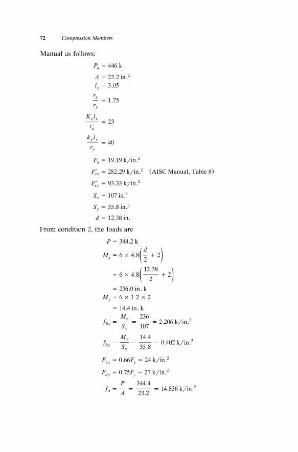
72 Compression Members

Manual as follows:

Pa = 446 k

A = 23.2 in? ly = 3.05

r ~ = 1.75 ry

K)x -- =23

rx

Fa = 19.19 k/in.2

F;x = 282.29 k/in.2 (AISC Manual, Table 8)

F:y = 93.33 k/in.2

Sx = 107 in?

Sy = 35.8 in.3

d = 12.38 in.

From condition 2, the loads are

P = 344.2 k

Mx = 6 x 4.8( ~ + 2) ( 12.38 )

= 6 x 4.8 -2- + 2

= 236.0 in. k My = 6 X 1.2 X 2

= 14.4 in. k

Mx 236 . 2 fb = - = - = 2.206k/m.

x Sx 107

My 14.4 fby = S = 358 = 0.402 k/in.2

y .

Fbx = 0.66Fy = 24 k/in.2

Fby = 0.75Fy = 27 k/in.2

P 344.4 f. = - = -- = 14.836 k/in.2

a A 23.2

Compression Members 73

Applying these values in Equation (3.26) yields the following:

14.836 --+ 19.19

1.0 x 2.206

( 14.836 ) 1- -- 24

282.29

1.0 x 0.402

+ ( 14.836) 1- -- 27 93.33

Check the loading for condition 3

P = 308 k

Mx = 6 X 9.6 X C2~38 + 2)

X 472in.k

472

= 0.88 < 1.0

308 1 X -10-7 -44-6 + ....,(----:3'""0"'"8----:)- = 0.883 < 1

1 - 24 282.29 X 23.2

The column section satisfies the AISC specification. Use W12 X 79.

3.10 COLUMNS SUBJECT TO BENDING AND AXIAL FORCE IN A BRACED SYSTEM: LRFD METHOD

In a braced frame, columns may be subjected to bending about one axis or both due to the unequal loads on the sides of the column. This condition arises from the removal of the live load from one side of the column and not the other. The interaction of axial and flexural stresses in symmetric shapes is given by the following equations:

For Pu/1>cPn ;::: 0.2

(3.30)

(3.31)

74 Compression Members

where

Pu = required compressive strength (k)

Pn = nominal compressive strength determined from Equation (3.15) or col­umn selection table (k)

Mu = required flexural strength determined (k-in.)

M" = nominal flexural strength (k-in.), where Mn is obtained from Equation (4.23b)

CPc = resistance factor for compression, 0.85

CPb = resistance factor for flexure, 0.90

The design of columns under the combined action of bending and axial forces is a trial-and-error procedure. A trial section is checked for compli­ance with formulas HI-a and HI-b. A simplified and fast method is to assume an effective axial load on the basis of which the trial section will carry the bending and axial forces adequately

where

Pu = actual factored load (k)

Mux = actual factored moment about the strong axis (k-ft) M lly = actual factored moment about the minor axis (k-ft)

m = factor taken from Table B, LRFD, p. 2-10 U = factor taken from column load table

The procedure is summarized in the following steps:

(3.32)

1. With the known KL (effective unbraced length), select values for m and U. 2. Solve for Plleff •

3. Make the appropriate selection from the column load table. 4. Based on the selection of Step 3, select the appropriate values for m

and U. 5. With these values, solve for Pueff '

6. Repeat Steps 3 and 4 until the values of m and U converge.

On the basis of elastic analysis, Mu is determined from

(3.33)

Compression Members 75

where

Cm = 0.85 for members whose ends are restrained Cm = 1.0 for members whose ends are unrestrained

AgFy Pe = -2- or from Table 9, LRFD

Ac

Example 3.5

(3.34)

Figure 3.11 shows part of a building frame. The building has 11 stories. The first story is 15 ft, 0 in. high. All others are 10 ft, 6 in. high. The loads are as follows:

Typical floor loads

Snow load = 201b/ft 2

Roof dead load = 45 Ib /ft 2

Live load = 50 Ib /ft 2

Partition load = 25 Ib /ft 2

Ceiling load = 51b/ft 2

Floor dead load = 551b/ft 2

Use A-36 steel to choose the column size. Splice columns every third floor. Use the LRFD method.

Solution

Load Calculations

Roof Loads

1 Dead load on typical beam = 45 X 7.5 ft X 1000

= 0.338 k/ft

1 Live load = 20 X 7.5 ft X 1000

= 0.150 k/ft

76 Compression Members

A

I 1: II' \

I . ,

I

/ 2

\\-\ -'------H-I------'------I-+I

/

-I--

\I"~"'" 40' I 40'

Figure 3.11 Typical interior column tributary area.

Typical floor load

1 Dead load + ceiling load = 60 X 7.5 ft X --

1000

= 0.45 kjft

1 Live + partition load = 75 X 7.5 ft X --

1000

= 0.562 kjft

......

Compression Members 77

The tributary area for a typical interior column is 30 ft X 40 ft = 1200 ft2. Live load reduction applies to a member with an influence area that exceeds 400 ft2. There will be no reduction in the roof live load. The tributary area of the lightest (the uppermost column) column section is three times the tributary area for that column per floor

Al = 3 x 4 x 1200

= 14,400 ft2

L = 75 X (0.25 +

= 28.1Ib/ft 2

15 ) V14,400

Check the minimum reduction allowed in the live load. The reduced live load should not be less than 40% of the actual live load. Thus, the total live load on the column from a group of three columns is 30 lb /ft2.

Beam reactions

Roof

Typical floor

40 1.2 X dead load = 1.2 X 0.338 X ""2

= 8.1 k

40 1.6 X live load = 1.6 X 0.150 X ""2

= 4.8k

40 1.2 X dead load = 1.2 X 0.450 X ""2

= 10.8 k

40 1.6 X live load = 1.6 X 0.225 X ""2

= 7.2k

To understand the action of the loads on an interior column, refer to Figures 3.11 and 3.12. The loads are transmitted to the column at four different points as shown in Figures 3.12c and 3.12d.

78 Compression Members

,-, ,

-------~--------

12.2

.. 7.2

Roof

(e)

~

I I

}-

(b)

LL - 0.150 kilt

DL = 0.338 kilt

40'

Roof

LL = 0.225 klft

DL = 0.45 klft

40'

Typical beam

7.2 t 10.8 t

Typical floor

(d)

I I

~t

~t

Reactions, k

Working Load

DL 6.76

LL 3

DL 9.0 LL 4.5

Factored Load

8.1

4.8

10.8 7.2

Figure 3.12 Typical load calculation on an interior column.

Design of the Column on the First Floor

Three loading conditions will be considered. First, the live load exists in all quadrants. Second, the live load is removed from the first quadrant. Third, the live load is removed from two adjacent quadrants.

Condition 1

Live load in all quadrants

Pu = Roof load + 10 X typical floor load

= 64.6 + 10 X 90

= 964.6 k

= 15 ft

Compression Members 79

From the column selection table, try W14 X 159

Condition 2

The live load is removed from quadrant I. Load removed from each floor = 9 k

For 10 floors = 90 k

LPu = 964.6 - 90 = 874.6 k

Load removed along the x axis = 5.4 X 10 = 54 k

= 54 x 2

= 108 k-in.

The reaction is assumed to be applied 2 in. from the extreme edge of the column to where the connection reaction is supposed to take place.

Load removed along the y axis = 3.6 X 10 = 36 k

Mux = Pu y ( ~ + 2 in.)

( 14.98 ) = 36 -2- + 2

= 341.4 k-in.

If we consider no intermediate stiffners, Lb = 15 ft. Also, it is assumed that there is no torsion.

List the column load requirements:

P" = 874.6 k

Mux = 341.4 k-in.

= 28.5 k-ft

M"y = 108 k-in.

= 9 k-ft

lb = 15 ft

Cmx = 0.85

Cmy = 0.85

S{) Compression Members

Step 1. For Kl = 15 ft, from Table B (LRFD, p. 2-10) and the column selection table as a first trial

Step 2. From Equation (3.32)

m = 2.6

U = 1.26

Peff = 874.6 + 2 X 28.5 + 2 X 1.26 X 9

= 954.3 k

Step 3. From the column load tables, select W14 X 120 (¢cPn = 956).

Step 4. Adopt W14 X 120. With m = 2 and U = 1.35,

Peff = 874.6 + 2 X 28.5 + 2 X 1.35 X 9

= 956 k

A = 35.3 in.2

rx = 6.25 in.

ry = 3.74 in.

Kl 15 X 12

ry 3.74

= 48

Kl 15 X 12

rx 6.25

= 29

29 J36 Acx = -; V 29,000

= 0.325

48 J36 Acy = -; V 29,000

= 0.538

35.3 X Ey Pex = ------=-2--'-­

Acx

35.3 X 36

0.3252

= 12,031 k

35.3 X 36

0.538 2

== 4390 k

em Bx= --~ Pu

1- -Pex

0.85

874.6 1---

12,031

Compression Members 81

= 0.917 (use Bx = 1.0)

0.85

874.6 1- --

4390

= 1.061

= 1.0 X 28.5

= 28.5 k-ft

= 1.061 X 9

= 9.6 k-ft

Apply the above values to Equation (3.30).

-- + - - + - = 0.983 < 1.0 874.6 8 ( 28.5 9.6 )

956 9 636 306

300ry Lp = {F;

= 16.67 ft

Lb < Lp

300 X 4.0

f36 = 200 in.

No intermediate stiffners are needed in the column.

82 Compression Members

3.11 DESIGN OF COLUMNS FOR BRACED AND UNBRACED FRAMES: ASD METHOD

In a braced frame, lateral stability is provided by diagonal bracing as shown in Figure 3.13. When the beams or girders are rigidly connected to the column, the use of an alignment chart is used to simplify the sizing of the column. These charts were developed for the elastic column. However, by multiplying the G values from the alignment chart by the proper reduction factor, the charts may be used for the inelastic column. The procedure is outlined as follows:

1. Determine the axial load on the column. 2. Select a column size and calculate fa'

L 0.70L<KL<L

(a)

L 0.50 L < KL < 0.7 L

(b)

Figure 3.13 Braced frames. (a) Hinged support. (b) Fixed support.

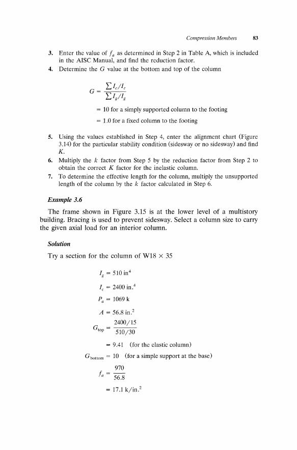
Compression Members 83

3. Enter the value of fa as determined in Step 2 in Table A, which is included in the AISC Manual, and find the reduction factor.

4. Determine the G value at the bottom and top of the column

= 10 for a simply supported column to the footing

= 1.0 for a fixed column to the footing

5. Using the values established in Step 4, enter the alignment chart (Figure 3.14) for the particular stability condition (sidesway or no sidesway) and find K.

6. Multiply the k factor from Step 5 by the reduction factor from Step 2 to obtain the correct K factor for the inelastic column.

7. To determine the effective length for the column, multiply the unsupported length of the column by the k factor calculated in Step 6.

Example 3.6

The frame shown in Figure 3.15 is at the lower level of a multistory building. Bracing is used to prevent sidesway. Select a column size to carry the given axial load for an interior column.

Solution

Try a section for the column of W18 X 35

Ig = 510 in4

Ie = 2400 in.4

Pa = 1069 k

A = 56.8 in.2

2400/15 G =---

top 510/30

= 9.41 (for the elastic column)

Gbottom = 10 (for a simple support at the base)

970 fa = 56.8

= 17.1 k/in.2

84 Compression Members

Gil

50~0' 10.0_ 5.0 4.0 3.0 2.0

1.0 0.9 0.8 0.7 0.6

0.5

0.4

100.0 50.0 30.0 cO. a -

-10.0 _ 'i.0-X.O 7.0 -('.0

,.0 4.0

\3.0

c.O

1.0

0-

0.3

0.2

0.1

1.0

0.9

-0.8

0.7

0.6

0.5

(a)

K

/= Fe ,0.0 - 10.0

- 5.0

4.0

3.0

2.0

- 1.5

- 1.0

(b)

Gll

/,~ _ 50.0

10.0 5.0

3.0

2.0

1.0 0.9 0.8 0.7 0.6 0.5

0.4

0.3

0,2

0.1

,= 100.0 50.0 30.0

20.0

r- 10.0 r- 9.0 I- 8.0 I- 7.0 I- 6.0

5.0

I- 4.0

r 3.0

I- C.O

r- 1.0

LO

Figure 3.14 Chart for the K column factor. (a) Sidesway inhibited. (b) Sidesway uninhibited.

Compression Members 85

485 k 970k 485

W 18 X 35 W 18 X 35

30' 30' ~I Figure 3.15 Braced frame of a multistory building.

From Table A in the AISC Manual, the reduction factor is found to be 0.460

Ginelastic = 0.460 x 9.41

= 4.3

Use the values of 4.3 and 10 for the G values at the top and bottom of the column, respectively, in the alignment chart in Figure 3.14 for no sidesway to obtain a K value of 0.95. Hence, the effective slenderness ratio of the column is

Klx 0.95 x 15 x 12

rx 6.5

= 27

Enter this value in Table 3.1 to obtain a value of Fa = 20.15 kjin.2 that is higher than required. The selection meets the load requirements and those of the AISC specifications.

Example 3.7

Consider the sidesway in the frame shown in Figure 3.15 to be uninhib­ited. See Figure 3.16. Check the frame as designed in Example 3.6.

GA inelastic = 4.3

86 Compression Members

485 k 170k 970k 485

~ W 18 x 35 W 18 x 35 W 18 x 35

Ie 30' ~Ie 30' ~I· 30' ~I

Figure 3.16 Unbraced frame of a multistory building.

Solution

Use these values with the alignment chart in Figure 3.14 for an uninhibited sidesway. The K factor is found to be 2.5. The slenderness ratio for the column is

K)x 2.5 x 15 x 12

rx 6.5

= 69

The allowable compression stress corresponding to this slenderness ratio is Fa = 16.53 kjin.2 < 17.1 kjin.2 (required). Try a stronger section, W14 X 211.

The compression stress is

A = 62 in.2

Ix = 2660 in.4

ly = 1030 in.4

ry = 4.07 in.

d = 15.72 in.

970 fa = 62

= 15.64 kjin.2

Compression Members 87

The corresponding reduction factor is obtained from Table A, AISC Manual, p. 3-8 and found to be equal to 0.626 by interpolation. Then the inelastic g factor for the top of the column is determined

GA inelastic = 0.626 X GA elastic

2660/15 GA elastic = 510/30

= 10.43

GA inelastic = 0.626 X 10.43

= 6.5

With the modified value for the g-factor at the top of the column, enter the alignment chart in Figure 3.14 for the uninhibited sidesway to obtain a k factor of 2.7. The new slenderness ratio is

K)x 2.7 X 15 X 12

rx 4.07 X 1.61

= 74

Fa = 16.01 k/in.z > 15.64 k/in.z

Use W14 X 211.

Example 3.8

The building shown in Figure 3.17 is eight stories high. The frames are braced against lateral movement as shown in the figure. Design an interior column for the first floor. The tributary area is indicated by dashed lines in the diagram.

Solution

Use the ASD method for A-36 steel.

At = 35 X 25

= 875 ftz

The influence area A I for an interior column is

Al = 4 XA t

= 4 X 875

= 3500 ftz > 400 ftz

88 Compression Members

.~ · · • r;t

I . • 0-

r···· At : · I L · rl · r . · . ....... .. .. .......

. I I •

· -. r.,

· r

· • · . r ••

· . -.

b o

<;> in C\I

Rool Loads:

Dead Load = 45 psI

Snow Load = 30 psI

Typical Floor Loads:

Dead Load = 55 psI

Live Load = 50 psI

Partition Load = 20 psI

25'-0': I 35' - 0" 35' - 0" 25'-0"

I 1120, ,-- ..

At = Tributary area lor an interior column on the lirst floor

~--~--------------~+---~'--~

25' - 0" 70' - 0" 25')-30: ~·~1 .. ~--____________ ~ .. ~11~~~

b First Floor Plan

in C\I

M

Figure 3.17 Floor and elevation of a seven-story building.

Compression Members 89

Reduction in the live load for column loading must be used in the design. The total influence area for an interior column on the first floor is 3500 X 7 = 24,500 ft2. The reduced live load on the floors is computed as follows:

L = 70(0.25 + ~) 24,500

Note that the partition load is considered a live load

L = 0.346 x 70

= 24.21b Ift 2

The minimum live load reduction for an interior column is limited to 40%.

L = 0.40 x 70

= 28lb/ft 2 controls

The joist loads are shown in Figures 3.18a and 3.18b. The joists run in the short direction at 5 ft on center. The calculations of the loads carried by the joists are included below.

Roof loads

Typical floor loads

Snow load = 0.03 x 5

= 0.15 k/ft

Dead load = 0.045 X 5

= 0.225 k/ft

Live load = 0.028 X 5

= 0.14 k/ft

Dead load = 0.055 X 5

= 0.275 k/ft

Determine the reactions at the end of the joists:

Roof joists (total DL and LL)

R = (0.15 + 0.225) X 25/2

= 4.7k

90 Compression Members

~~~~~~~I LL ~ 0.15 kill .f 1 DL = 0.225 k/ft

~!<Ii;:--__ 2-,-5_' -_~~. R = 4.7 k

(a)

4.7k{ 7 128.2~ ~

___ ---'-t-:;;,~.I'I:-_'2I'- Girder ,.- 7 _-'---1--""-'=

/ '1'28.2 k

/~4.7k (c) Roof

LpL 112.6 \0'''''-

L ~75.6 k D L t 28.5

DLI171 k ~ 'I' .., ",_--. ___ Girder

/ 7 ~171 k DL

/~28.5 k DL ~ 75.6 k LL

~ 12.6 k L L

(e) First floor total column load

[;;1 ~~~~~~~I LL = 0.14 k ~ I DL • 0.275 k

li"1o(t--~25,-,--)o~~ RD= 3.4 k

t t RL =1.8 k

L L~1.8 k . ",'-

L~10.8 k DL 3.4 v a'

DLI 20.4 k ~ 'I' .., ~---r--- Girder

~7 1

'I' 20.4 k D L

t 3.4 k D L ~ 10.8 k L L

~1.8 k LL

(d) Typical floor

Figure 3.18 Interior column load calculations for the first floor. (a) Typical roof joist loads. (b) Typical floor joist loads. (c). Roof. (d) Typical floor. (e) First floor total column load.

Typical floor joist (dead and live loads are separate):

RDL = 0.275 x 25/2

=3.4k RLL = 0.140 x 25/2

= 1.8 k

Impose these reactions on the interior column. See Figures 3.18c and 3.18d. Note that the girder supports reactions from a set of three pairs of joists, Hence, the load on the girder is three times that of one joist. The total load components acting on an interior column on the first floor are shown in Figure 3,18e.

Compression Members 91

Load Calculations for the First Floor Interior Column

From the girders

Floor

Roof

DL = 7 x 20.4

= 142.8 k

LL = 7 X 10.8

= 75.6 k

DL + LL = 28.2k

Total roof and floor loads

From the joists

Floor

Roof

DL = 142.8 + 28.2

= 171 k

LL = 75.6 k

DL = 7 X 3.4

= 23.8 k

LL = 7 X 1.8

= 12.6 k

DL + LL = 4.7k

Total roof and floor loads

DL = 23.8 + 4.7

= 28.5 k

LL = 12.6 k

The column can be subjected to any of several loading conditions in its life span. As discussed before, these conditions are listed as follows:

1. Live load exists everywhere.

2. Live load is removed uniformly from one quadrant from every floor.

3. Live load is removed from two adjacent quadrants.

92 Compression Members

I I

Figure 3.19 Interior column-girder connection.

For condition 1, the load is concentric. The column can be selected on that basis and later checked for the other two conditions.

Condition 1 P=575.4k

Mx = 0

My = 0

The girders are rigidly connected to the columns as shown in Figure 3.19. Because of the bracing, the frame is inhibited from moving laterally. As a first attempt, try W14 X 132.

Column Properties

Ie = 1530 in.4

A = 38.8 in.2

ry = 3.76 in.

r -...:. = 1.67 ry

d = 14.66 in. Pa = 719 k

Since the column is simply supported to the foundation,

GB = 10

Compression Members 93

The elastic G factor at the top of the column is obtained from the following expression:

1530/15 G =---

A 1830/35

= 1.95

The compression stress in the column is

575.4 fa = 38.8

= 14.83 k/in?

The reduction factor to multiply the elastic GA in order to obtain the equivalent inelastic factor is determined from Table A in the AISC Manual, ASD. Thus, the reduction factor is found by interpolation to be 0.71

GA = 0.71 x 1.95

= 1.38

Enter the GB and modified GA values in Figure 3.14a to obtain the K factor

K = 0.88

The slenderness ratio for this column is

Kx1x 15 x 12 x 0.88

rx 3.76 x 1.67

= 25

From Table 3.1,

Fa = 20.28 k/in? > 14.83 k/in.2

Condition 2

List the load requirements and stress intensities for this condition. The change in the load is equal to one-half of each of the live load components on the joist and girder adjacent to the quadrant from which the live load has been removed. The load change is as follows:

From the joist

AP = t x 12.6

= 6.3 k

94 Compression Members

From the girder

;j,p = ~ x 75.6

= 37.8 k

The total change in the load on the column is

L ;j,p = 6.3 + 37.8

= 44.1 k

The magnitude of the load for condition 2 is

P = 575.4 - 44.1

= 531.3 k

Refer to Figure 3.21e to determine the moments about the x and y axes, respectively. Note that the y axis is parallel to the web and the x axis perpendicular to it.

Mx = 37.8 x (14~66 + 2)

= 353 in. k

Similarly, the moment about the y axis is

My = 6.3 x 2

= 12.6 in. k

Fa = 20.28 kjin.2

531.3 fa = 38.8

= 13.69 kjin.2

Sx = 209 in?

Sy = 74.5 in?

353 fbx = 209

= 1.689 kjin.2

12.6 fby = 74.5

= 0.169 kjin.2

Compression Members 95

Check Equations (3.26) and (3.27).

and

Fbx = 24 kjin.2

Fby = 27 kjin.2

Cmxfbx Cmyfby

(1 - ~)F + (1 - ~)F Cmx = 1

Cmy = 1

Ky =Kx

= 0.88

F, bx F by ex ey'

< 1.0

Fex' = 238.8 kjin,z (from Table 8, AISC ASD)

kyly 15 X 12 X 0.88

ry 1.67 X 3.76

= 42

Fey' = 84.65 kjin.2 (from Table 8, AISC ASD)

13.69 --+ 20.28

1.689 0.169

( 13.69) + ( 13.69) = 0.757 < 1.0

1 - -- 24 1 - -- 27 238.93 84.65

~ + fbx + fby < 1.0 0.60Fy Fbx Fby

13.69 1.689 0.169 ---- + -- + -- = 0.71 < 1.0 0.60 X 36 24 27

The column seems to be a little oversized. For a more economical design, the process can be repeated with W14 X 120 or W14 X 109.

Example 3.9

Design an interior column adjacent to the exterior bay as indicated in Figure 3.20 on the first floor.

96 Compression Members

17' - 6" 12' - 6"

(a)

L~L ,12.6 \O\~' L ~75.6 k 0 L t 28.5

DLI171 k ~ t _ t ..1'.-" Girder

~ ~ ---~~11-4-k-DL

/~28.5 k DL ~ 50.4 k LL

~ 12.6 k L L

(b)

Figure 3.20 Exterior column load calculations. (a) Typical interior column adjacent to exterior bay. (b) Loads on a typical interior column.

Solution

Calculate the tributary area

At = 25 x 35 + 25

2

= 750 ft2

AI = 4 x 750

= 3000ft 2 > 400ft 2 per floor

Compression Members 97

Live load reduction must be utilized in determining the size of the column. For the first floor column, the tributary area is

AI = 7 x 3000

= 21,000 ft2

The reduced live load is

L = 70(0.25 + ~) 21,000

= 24.7lb /ft2

O.4La = 70 x 0.4

= 28lb/ft 2

The loads on this column differ from the previous example only by the difference on the right girder. The reactions on the right girder are two-thirds what they were in the previous problem. Examine the loads as shown in Figure 3.20b. Two loading conditions will be considered.

Condition 1

Live load covers the entire space around the column

P = 493.1 k

Mx = 82.2( ~ + 2)

= 740 in. k (for d approximately 14 in.)

My = 0

Select W14 X 109 for the first trial. The section properties are listed as follows:

Pa = 592 k

Ix = 1240 in.4

ry = 3.73 in.

A = 32 in.2

d = 14.32 in.

Sx = 173 in?

98 Compression Members

The girders on the left and right have the sections W24 X 68 and W21 X 44, respectively. From these sizes, the G factors are obtained in the usual procedure as developed before

1240 X 2/15 GA elastic = (1830/35 + 843/25)

= 1.92

493.1 fa= 32

= 15.41 k/in.2

The stiffness reduction factor is found to be equal to 0.653. The equivalent GA inelastic factor is

GA inelastic = 0.653 X 1.92

= 1.25

The k factor is obtained from the alignment chart

K = 0.88

Klx - =26 rx

Fa = 20.22 k/in.2 > 15.41

Next, check the column interaction equation

493.1 fa= 32

= 15.41k/in.2

740 fbx = 173

= 4.58 k/in,z

Fex' = 220.9 k/in,z (Table 8, AISC Manual)

fa Cmxfbx Fa + """(--fa--'-) - = 0.967 < 1.0

1 - - Fbx Fex'

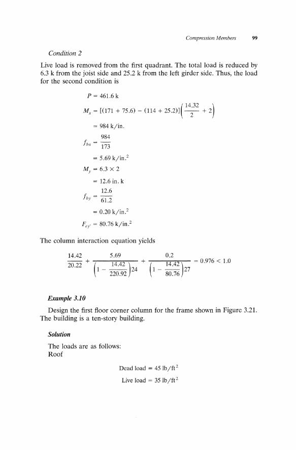
Compression Members 99

Condition 2

Live load is removed from the first quadrant. The total load is reduced by 6.3 k from the joist side and 25.2 k from the left girder side. Thus, the load for the second condition is

P = 461.6 k

( 14.32 ) Mx = [(171 + 75.6) - (114 + 25.2)] -2- + 2

= 984 k/in.

984 fbx = 173

= 5.69 k/in.2

My = 6.3 x 2

= 12.6in.k

12.6 fby = 61.2

= 0.20 k/in.2

Fey' = 80.76 k/in.2

The column interaction equation yields

14.42 --+ 20.22

Example 3.10

5.69 0.2

( 14.42) + ( 14.42) = 0.976 < 1.0

1 - -- 24 1 - -- 27 220.92 80.76

Design the first floor corner column for the frame shown in Figure 3.21. The building is a ten-story building.

Solution

The loads are as follows: Roof

Dead load = 45lb /ft 2

Live load = 351b/ft 2

100 Compression Members

m ------h-I------h-I--0 1------------

gl---------------I---------------II

o~--------------

@J II) r---20-' --~

Floor

Use A-36 steel.

R L 9.6 k

~ D L54.0 k

~ LL39.6k

R~ ~

DL27.0k

~ L L 19.8 k

Figure 3.21 Corner column load calculations.

Dead load = 50lb/ft 2

Live load = 80 lb Ift2

The tributary are for the corner column is

At = 10 x 15

= 150 ft2

The influence area is four times the tributary area for a column

AI = 600 ft2 > 400

Compression Members 101

Use reduction in the live load on the floors. The reduced live load is

L = L O(0.25 + ~) 4 XA t

= SO(0.25 + J 15 ) 4 x 150 x 9

= 36.31b/ft 2

Roof Loads

When we enter the flange of the column, the load is

(35 + 45)

1000

= 4.Sk

x 6 x 10

When we enter the web of the column, the load is

----x6xlO __ 2 x [(35 + 40) ] 1000

= 9.6k

Dead Floor Loads

When we enter the flange of the column, the load is

50 = 1000 x6xlOx9

= 27k

When we enter the web of the column, the load is

Live Floor Loads

50 =2x--x6xlOx9

1000

= 54k

When we enter the flange of the column, the load is

36.3 =--x6xlOx9

1000

= 19.5 k

102 Compression Members

When we enter the web of the column, the load is

36.3 =2x 1000 x6xlOx9

= 39.6 k

Show the placement of the loads on the column on the first floor. See Figure 3.21b. Total load on the column is

Refer to Figure 3.22.

9

L Pi = 145.2k i~ 1

My = 93.6 x 2

= 187.2 in. k

Mx = 51.6 x (dj2 + 2)

For an unsupported length of 11.5 with respect to the y axis and from the selection table for column capacity, try W8 X 58.

Pa = 288 k

A = 17.1 in.2

145.2 fa = 17.1

= 8.50 kjin.2

ry = 2.10 in.

rx = 3.65 in.

lx 11.5 X 12

rx 3.65

= 39

Fex' = 98.2 kjin.2

~ 11.5 X 12

ry 2.10

= 66

Fey' = 34.3 kjin.2

Sx = 52.0 in?

Sy = 18.3 in.3

Mx = 51.6 X 6.375

= 329 in. k

329 fbx = 52

= 6.326 kjin.2

187.2 fby = 18.3

= 10.23 kjin.2

fa P

1462

288

= 0.508 > 0.15

Compression Members 103

Check only Equations Hl-l and Hl-2, AISC Manual, p. 5-54. Examine Hl-2 first.

fa fbx fby 8.50 6.326 10.23 --+-+-=--+--+--0.6Fy Fbx Fby 21.6 24 27

= 1.04> 1.00

The results are not satisfactory. Try a larger section, W8 X 67. The section properties and requirements are as follows:

Pa = 334 k

A = 19.7 in.2

ry = 2.12 in.

rx = 1.75 X 2.12 in.

104 Compression Members

Check Equation Hl-2 first.

Ix 11.5 X 12

rx 2.12 X 1.75

= 37 I -.Z = 37 X 1.75 ry

= 65

Fex' = 109.1 kjin.2

Fey' = 35.34 kjin.2

Sx = 60.4 in.3

Sy = 21.4in.3

d = 9.0 in. My = 187.2 in. k

Mx = 51.6 X 6.5

= 335 in. k 45.2

fa = 19.7

335 fbx = 60.4

187.2 fby = 21.4

7.421 5.546 8.748 -- + -- + -- = 0.90 < 1.0 21.6 24 27

Examine Hl-l next.

X _fb_X + -,-_C_m.:....y --:- X fby :s; 1.0 Fbx ( 1 - fa ) Fby

Fey'

Substituting the proper values for the terms in Hl-l yields

7.421 0.85 5.546 0.85 8.745

-16-.9-4 + '7( 1-_--;7:;"".4;-;;2:7'17") X ~ + (1 - 7.421 )

109.8 35.34

X 2:7 = 0.997

Use W8 X 67.

Compression Members 105

Example 3.11

Given the column shown in Figure 3.22, select an adequate size using the ASD method with A-36 steel. The unsupported length of the column with respect to the x and y axes is 10.5 ft.

The solution is left to the student.

x

y kips

y

x

Eccentricity on each side = 2" + d/2

y

Figure 3.22 Determination of eccentricity of a typical column beam connection.

4 Design of Bending

Members

4.1 INTRODUCTION

In buildings, loads of any kind have to be carried down to the foundation. Dead loads (the weight of the building elements and other permanent fixtures in the building) and live loads (furniture, snow, people, and movable equipment) are usually called gravity loads. Wind and earthquake forces acting against buildings are known as lateral loads. Structural members subjected to loads acting perpendicularly to their longitudinal axis are known as flexural (bending) members. In construction, they are referred to as beams, girders, joists, purlins, etc. Such members constitute the major and minor components of almost all types of structures.

Beams and girders are used interchangeably. A girder may suggest a more important role in terms of load-carrying capacity. However, both are subjected to tension and compression stresses due to bending. See Figure 4.1.

4.2 SIMPLE BENDING

The theory of the bending of beams is based on the principle that a plane section before bending remains very nearly plane after bending (Figure 4.2) and that within the elastic range stress is proportional to strain. When a beam is loaded, it deflects as shown in Figure 4.1a. At each point along the length of the beam, its axis has a definite radius of curvature p that

106

Design of Bending Members 107

(a)

(b)

(c)

Figure 4.1 Beam deflection due to bending.

108 Design of Bending Members

I I I L _______ -' I I I

Before Bending After Bending

Figure 4.2 Beam section before and after bending.

varies from point to point. Considering a small part of the beam before and after loading as seen in Figure 4.2, we notice that the fibers across the section of the beam are subjected to compression in the upper fibers and tension in the lower ones. For a symmetrical section, the neutral axis falls in the middle of the section and the compression and tension stresses are equally distributed. By using the equations of equilibrium, simple equa­tions for normal and shearing stresses in the beam (Figure 4.3) are obtained when bending takes place about a principal axis in the absence of twisting of the section

where

Ib = the fiber stress in bending Mx= the bending moment about the x axis along the length of the beam y = the fiber position along the y axis

Ix = the moment of inertia about the x axis

II! = shear stress at a distance y from the neutral axis

Yy = the total shear at any point along the longitudinal axis of the beam

Qx = the first moment of area at y about the x axis b = the width of the section at the point under consideration

(4.1)

(4.2)

Design of Bending Members 109

7'c::::::-.,,-=::;:::::/ ~~_~===x =~~ r ~------lOo-Z ----~ Mx

~I (a)

y

z

fv max (b)

Figure 4.3 (a) Normal bending stress. (b) Sheer bending stress.

4.3 DESIGN OF BEAMS AND OTHER FLEXURAL MEMBERS: ASD ALLOWABLE BENDING STRESS

Beams are differentiated from plate girders by the fact that the ratio of h / tw is lower than 760/ {F;, where Fb is the allowable bending stress. The allowable shear stresses and stiffener requirements are given in Chapter F of the ASIC specifications. It applies to singly or doubly symmetric beams, including hybrid beams and girders loaded in the plane of symmetry.

The allowable stress for compact members loaded in the plane of their minor axis and symmetrical about the same is

(4.3)

110 Design of Bending Members

provided the flanges are connected continuously to the web and the unsupported length of the compression flange L b does not exceed L c'

where

or 20,000

L =--c d

-F A Y f

(4.4a)

(4.4b)

In addition to the above restrictions, the width-thickness ratios of its compression elements must not exceed the applicable limiting width­thickness ratios from Table 4.1 (AISC Manual, Table B5.1). For members that meet the requirements of F1.1 except that their flanges are noncom­pact (excluding built-up members and those with yield points greater than 65 k/in.2), the allowable yield stress is

(4.5)

For the members described above (in addition, their webs are noncom pact), the allowable stress is

where

4.05

kc = (h ) tw 0.46

Otherwise, kc = 1.0.

if h - > 70 tw

(4.6)

(4.7)

For noncompact sections not covered above and loaded through the shear center and braced laterally in the region of compression stress at intervals not exceeding the limit set in Equation (4.4), the allowable bending stress is

(4.8)

Design of Bending Members 111

TABLE 4.1 Limiting Width-Thickness Ratios for Compression Elements

Description of Elements

Flanges of I-shaped rolled beams and channels in flexure a

Flanges of I-shaped welded beams in flexure

Outstanding legs of pairs of angles in continuous con­tact; angles or plates pro­jecting from rolled beams or columns; stiffeners on plate girders

Angles or plates projecting from girders, built-up columns, or other compres­sion members; compression flanges of plate girders

Stems of tees

Unstiffened elements simply supported along one edge, such as legs of single-angle struts, legs of double-angle struts with separators, and star-shaped sections

Flanges of square and rectan­gular box and hollow struc­tural selections of uniform thickness subject to bending or compression b flange cover plates and diaphram plates between lines of fas­teners or welds

Unsupported width of cover plates perforated with a suc­cession of access holesd

All other uniformly com­pressed stiffened elements, i.e., supported along two edges

Width-Thickness

Ratio

bit

bit

bit

bit

d/t

bit

bit

bit

bit h/tw

Limiting Width-Thickness Ratios

Compact NoncompactC

651fF;

651fF;

NA 95/fF;

NA 95/..jFylkc

NA 127/fF;

NA 761fF;

190/fF; 238/fF;

NA 317/fF;

NA 253/fF;

(cont'd.)

112 Design of Bending Members

TABLE 4.1 (cont'd.)

Width-Thickness Limiting Width-Thickness Ratios

Description of Elements Ratio Compact Noncompact C

Webs in flexural compression a d/t 640/ fF;

Webs in combined flexural and

axial compression

Circular hollow sections in axial compression in flexure

h/tw

D/t D/t

For (ta/Fy < 0.16) 640 fa

X -(1 - 3.74-) fF; Fy

For fa/Fy > 0.16

257/fF;

3300/Fy

3300/Fy

a For hybrid beams, use the yield strength of the flange FYI instead of Fy .

b See also Section F3.1, AISC Manual, Ninth Edition.

760/M

760/M

cFor the design of slender sections that exceed the noncompact limits, see Appendix B5, AISC Manual, Ninth Edition.

dAssume the net area of the plate's widest hole.

e kc = 4.05 /(h /1)0.46 if h > 70. Otherwise, kc = 1.0

Source: AISC Steel Manual, ASD, Ninth Ed., Table B5.1

For members with compact or noncompact sections with unbraced length in the compression region greater than L c' the allowable bending stress in tension is determined from Equation (4.8). For members that are loaded in the plane which includes an axis of symmetry in their web, the allowable bending stress in compression is determined as the larger value from Equations (4.9) or (4.10) and (4.11)

(4.9)

when

170 X 10 3Cb Fb = ----,,---

(l/rT )2 (4.10)

Design of Bending Members 113

where

For any value of IlrT

I 510 X 10 3Cb -> rT Fy

12 X 103Cb Fb = I < 0.60Fy

d

At

(4.11)

Equation (4.11) applies only to sections with a compression flange that is solid and approximately rectangular in cross section and that has an area not less than the tension flange. The symbols used in Equations (4.9), (4.10), and (4.11) are listed below.

= distance between cross sections braced against twist or lateral displace­ment of the compression flange (in.). For cantilevers braced only against twist at the support, I may be taken conservatively as the actual length.

r T = radius of gyration of a section comprising the compression flange plus one-third of the compression web area, taken about an axis in the plane of the web (in.).

At = area of the compression flange (in. 2 ).

Cb = 1.75 + 1.05(M1/M2 ) + 0.3(MJ/M2 f, but no more than 2.3. It is conser­vative to consider Cb as unity. For values of Cb less than 2.3, see Table 4.2

TABLE 4.2 Values of C" for Use in Equations (4.9), (4.10), and (4.11)

MdM 2 Cb MdM 2 Cb M J/M2 Cb

- 1.00 1.00 -0.45 1.34 0.10 1.86 -0.95 1.02 -0.40 1.38 0.15 1.91 -0.90 1.05 -0.35 1.42 0.20 1.97

-0.85 1.07 -0.30 1.46 0.25 2.03 -0.80 1.10 -0.25 1.51 0.30 2.09 -0.75 1.13 -0.20 1.55 0.35 2.15

-0.70 1.16 -0.15 1.60 0.40 2.22 -0.065 1.19 -0.10 1.65 0.45 2.28 -0.60 1.23 -0.05 1.70 > 0.47 2.30

-0.55 1.26 0 1.75 -0.50 1.30 0.05 1.80

Source: AISC Manual, Ninth Edition, Table 6.

114 Design of Bending Members

(Table 6, AISC Manual, Ninth Edition). M J is the smaller and M2 the larger bending moment at the ends of the unbraced length, taken about the strong axis of the member, and where MdM2' the ratio of end moments, is positive when M j and M2 have the same sign (reverse curvature bending) and negative when they are of opposite signs (single curvature bending). When the bending moment at any point within an unbraced length is larger than that at both ends of this length, the values of Cb is taken as unity.

Members with compact sections, doubly symmetrical 1- and H-shapes, solid round and square bars, and solid rectangular bars bent about their weaker axes have an allowable bending stress of

(4.12)

for Fy < 65 kjin.2 • For noncompact shapes bent about their minor axis, the allowable bending stress is

(4.13)

for Fy < 65 kjin.2. For doubly symmetrical 1- and H-shapes having non­compact flanges and Fy > 65 kjin.2 , the allowable bending stress about the weaker axes is

Fb = Fy (l.075 - O.005!L fF;) 2tt

(4.14)

Box members, rectangular tubes, and circular tubes that are compact have an allowable bending stress of

(4.15)

To qualify as a compact section, the box-shaped member must meet the requirements of compactness set before. In addition, its depth must not exceed six times its width, its flange be no greater than two times its web thickness, and its laterally unsupported length Lb be less than or equal to

(4.16)

except that it need not be less than 1200 (b j Fy). The conditions for M j

and M2 are the same as mentioned before. For box-type and tubular

Design of Bending Members 115

flexural members that meet the noncompact requirements previously out­lined here, the allowable stress is

(4.17)

Allowable Shear Stress

The allowable shear stress for flexural members is

(4.18)

for h/tw equal or less than 380/ jF;. For h/tw > 380/ jF;, the allow­able shear stress in the web is

Fv should not exceed OAOFy '

when Cu is less than 0.8.

when Cv is more than 0.8.

when a/h is less than 1.0.

5.34 ku = 4.00 + --2

(a/h)

4.00 ku = 5.34 + --2

(a/h)

when a/h is more than 1.0.

tw = thickness of web (in.) a = clear distance between transverse stiffeners (in.)

(4.19)

h = clear distance between flanges at the section under investigation (in.)

116 Design of Bending Members

Intermediate stiffeners are required whenever the ratio h/tw exceeds 260 and the maximum web shear stress fv is greater than the limit set by Equation (4.19). When required, the spacing of the intermediate stiffeners shall be such that the web shear does not exceed the value for Fv given by Equation (4.19) and

a [260]2 - < -(--) < 3.0 h hjtw

4.4 DEFLECTIONS AND VIBRATIONS OF BEAMS IN BENDING

(4.20)

In addition to strength considerations, serviceability of the structural members in building plays a significant role. As beams take on long spans, deflection restrictions may control the design. Excessive deflections will cause damage to plastered ceilings and other non structural elements attached to the building frame. On flat roofs, a relatively large deflection can be catastrophic due to ponding. The deflected roof structure forms a bowl-shaped volume that will retain rain water unless properly drained. Thus, deflection increases due to the accumulation of rain water. This process continues, unless checked, leading to an unstable condition when collapse occurs. Various building codes limit the maximum live load deflections to 1/360 and 1/240 of the span for plastered and nonplastered ceilings, respectively.

For a symmetrical and uniformly loaded simply supported beam, the maximum deflection is

where

~ = deflection (in.)

5W13

~=--384E1

W = total uniform load, including weight of beam (k) I = span of beam (in.)

(4.21)

For E = 29,000 k/in.2 and a specific value of Fb , this equation reduces to the expressions shown in Table 4.3. In this table, L = span (in feet) and d = depth of beam (in inches).

Design of Bending Members 117

TABLE 4.3 Maximum Deflection of Beams

Deflection (in.)

Fy = 36 k/in.2

Fy = 50 k/in?

23.8 21.6

33 30

Source: AlSC Steel Manual, ASD, Ninth Ed., p. 2-32.

Example 4.1

0.02458 L21d 0.02234L2 I d 0.03414L21d 0.03103L2Id

Given the framing plane of Figure 4.4, design a typical beam using the ASD method, assuming the beam to be simply supported:

Design Data for 4-in. concrete slab

Solution

Live load = 50lb/ft 2

Partitions = 20 lb 1ft 2

Consider a 1-ft strip as shown in Figure 4.Sa to calculate the uniform loads on a typical beam. Having determined the magnitude of the uniform

I 48'

~I-_____ ~II Typical Beam

f-!-I----------- f-!-I Figure 4.4 Typical floor bay.

118 Design of Bending Members

I~ l' strip

- r-- ,..... ~

- Typical Beam CD

, - I-- i...-

I~ 48' ~

(a)

i i i i i i i i i , LL+ DL

t I· 48' ·1

(b)

Figure 4.5 Load calculations on a typical beam.

load and placed it on the beam as shown in Figure 4.Sb, we can readily obtain the maximum bending moment:

Dead load (DL)

4 150 Weight of the slab = 12 X 1 ft X 6 ft X 1000

= 0.30 klft Assumed weight of beam = 0.05 k/ft Total DL = 0.35 klft

Live load (LL):

50 Live load on the strip = 1 ft X 6 ft X 1000

= 0.30 klft

Design of Bending Members 119

Partition loads (PL)

Partition loads on the strip 20

= 1ft X 6ft x--1000

= 0.12 kjft Total uniform load on the beam = 0.77 kjft

For a simply supported beam with a uniformly distributed load, the maximum bending moment occurs at the center of the span

0.77 X 48 2

8

= 221.8 k ft

In Equation (4.1), the stress is given for any point in the section. For the purpose of designing, it is required that the maximum stress which occurs at the point furthest from the neutral axis be determined. Let that distance be denoted bye. Then Equation (4.1) is modified as

If we let lje be denoted by Sx, the section modulus, the above equation can be expressed as

Designing for the maximum allowable stress Fb , we find that the required section modulus for a beam to resist the given moment is

M s=-

x Fb

By assuming a compact section, the maximum allowable bending stress is Fb = O.66Fy from Equation (4.3). For structural steel with a yield point of 36 kjin.2 , Fb = 24 kjin.2 .

120 Design of Bending Members

The required section for this case is

s = x

221.8 x 12

24

= 110.9 in.3

Examine the allowable stress design selection table and find the nearest tabulated value of Sx = 114 in.3, which corresponds to W24 X 55. Table 4.4 is taken from the allowable stress design selection table that appears in the AISe Manual, Ninth Edition, Section 2.

Since the above selection is based on the assumption that the section is compact, a check for compactness is in order. Table 4.5 extracted from the AISe Manual, Part 1, "Dimensions and Properties of W Shapes" is used to provide the check for compactness. The properties of W24 X 55 listed in Table 4.5 are

and from Table 4.5

bl = 7.005 in.

b -.L = 6.9 2tf

d - = 59.7 tw

d - = 6.66 Af

Lc=7.0ft

The limiting width-thickness ratios for compression elements are given in Table 4.1 (AISe Manual, Table B5.1). A summary of those limits that are pertinent to this case is found in Table 4.6.

The selection of W24 X 55 confirms the compactness assumption made earlier. The compression flange must be supported laterally every 6 ft. In other words, place seven intermediate stiffeners at 6-ft intervals. The maximum shear occurs at the support

wI Vrnax = :2

= 0.77 X 48/2

= 8.5 k

Design of Bending Members 121

TABLE 4.4 Allowable Stress Design Selection for Shapes Used as Beams

Fy = 50 kjin.2 Fy = 36 kjin.2

Lc Lu MR Sx Depth d Lc Lu MR (ft) (ft) (k-ft) (in?) Shape (in.) F' y (ft) (ft) (k-ft)

8.1 8.6 484 176 W24 X 76 23i 9.5 11.8 348 9.3 20.2 481 175 W16 X 100 17 11.0 28.1 347

13.1 29.2 476 173 W14 X 100 14i 58.6 15.4 40.6 343

7.5 10.9 470 171 W21 X 83 21i 8.8 15.1 339

9.9 15.5 457 166 W18 X 86 18i 11.7 21.5 329

13.0 26.7 432 157 W14 X 99 14i 48.5 15.4 37.0 311

9.3 18.0 426 155 W16 X 89 16~ 10.9 25.0 307

7.4 8.5 424 154 W24 X 68 23% 9.5 10.2 305

7.4 9.6 415 151 W21 X 73 21i 8.8 13.4 299

9.9 13.7 402 146 W18 X 76 18i 64.2 11.6 19.2 289 13.0 24.5 385 143 W14 X 90 14 40.4 15.3 34.0 283

7.4 8.9 385 140 W21 X 68 21i 8.7 12.4 277

9.2 15.8 369 134 W16 X 77 16~ 10.9 21.9 265

5.8 6.4 360 131 W24 X 62 23% 7.4 8.1 259

7.4 8.1 349 127 W21 X 62 21 8.7 11.2 251 6.8 11.1 349 127 W18 X 71 18~ 8.1 15.5 251

9.1 20.2 338 123 W14 X 82 14i 10.7 28.1 244

10.9 26.0 325 118 W12 X 87 12~ 12.8 36.2 234

6.8 10.4 322 117 W18 X 65 18~ 8.0 14.4 232

9.2 13.9 322 117 W16 X 67 16i 10.8 19.3 232

5.0 6.3 314 114 W24 X 55 23~ 7.0 7.5 226

9.0 18.6 308 112 W14 X 74 14~ 10.6 25.9 222 5.9 6.7 305 111 W21 X 57 21 6.9 9.4 220 6.8 9.6 297 108 W18 X 60 18i 8.0 13.3 214

10.8 24.0 294 107 W12 X 79 12i 62.6 12.8 33.3 212 9.0 17.2 283 103 W14 X 68 14 10.6 23.9 204

Source: Adapted from data in Manual of Steel ConstlUction, 9th Ed., American Institute of Steel Construction.

122 Design of Bending Members

TABLE 4.5 Section Dimensions and Properties

Area A Depth Web tw Flange tf Flange bf Ix Sx Sy Designation (in.2 ) (in.) (in.) (in.) (in.) (in.4) (in?) Gn.3 )

W24 X 76 22.4 23.92 0.440 0.680 8.990 2100 176 18.4 W16 X 100 29.4 16.97 0.585 0.985 10.425 1490 175 35.7 W14 X 109 32.0 14.32 0.525 0.860 14.605 1240 173 61.2 W21 X 83 24.3 21.43 0.515 0.835 8.355 1830 171 19.5 W18 X 86 25.3 18.39 0.480 0.770 11.090 1530 166 31.6 W14 X 99 29.1 14.16 0.485 0.780 14.565 1110 157 55.2 W16 X 89 26.2 16.75 0.525 0.875 10.365 1300 155 31.4

W24 X 68 20.1 23.73 0.415 0.585 8.965 1830 154 15.7 W21 X 73 21.5 21.24 0.455 0.740 8.295 1600 151 17.0 W18 X 76 22.3 18.21 0.425 0.680 11.035 1330 146 27.6 W14 X 90 26.5 14.02 0.440 0.710 14.520 999 143 49.9

W21 X 68 20.0 21.13 0.430 0.685 8.270 1480 140 15.7 W16 X 77 22.6 16.52 0.455 0.760 10.295 1110 134 26.9

W24 X 62 18.2 23.74 0.430 7.040 0.590 1550 131 9.80

W21 X 62 18.3 20.99 0.400 0.615 8.240 1330 127 13.9 W18 X 71 20.8 18.47 0.495 0.810 7.635 1170 127 15.8 W14 X 82 24.1 14.31 0.510 0.855 10.130 882 123 29.3 W12 X 87 25.6 12.53 0.515 0.810 12.125 740 118 39.7 W18 X 65 19.1 18.35 0.450 0.750 7.590 1070 117 14.4 W16 X 67 19.7 16.33 0.395 0.665 10.235 954 117 23.2

W24 X 55 16.2 23.57 0.395 0.505 7.005 1350 114 8.30 W14 X 74 21.8 14.17 0.450 0.785 10.070 796 112 26.6 W21 X 57 16.7 21.06 0.405 0.650 6.555 1170 111 9.35 W18 X 60 17.6 18.24 0.415 0.695 7.555 984 108 13.3 W12 X 79 23.2 12.38 0.470 0.735 12.080 662 107 35.8 W14 X 68 20.0 14.04 0.415 0.720 10.035 723 103 24.2

Source: Adapted from data in Manual of Steel Construction, ASD 9th Ed., 1989, by American Institute of Steel Construction.

Design of Bending Members 123

TABLE 4.6 Summary of Limiting Width-Thickness Ratios for W24 X 55

Limits

65

P; 640

P; 76bf

L =-cp; 20,000

L =--c d

-F A Y f

10.8> 6.9

106> 59.7

7.39 ft, use Lb = 6.0 ft

6.95 ft, use Lb = 6.0 ft

From Equation (4.2), the shear stress is

18.5 X Qx fu=---­

Itw

Qx' I, and tw are obtained from the tables for W-shape dimensions and properties in Part 1 of the AISC Manual

Qx = 67.1 in.3

1= 1350 in.4

tw = 0.395 in.

18.5 X 67.1

fv = 1350 X 0.395

= 2.33 kjin.2 < Oo4OFy = 1404 kjin.2

One last check remains and that is for the stability of the beam with regard to deflection. Building code requirements recommend that the live load deflection not exceed 1/360 of the span of the beam

Ll max = 48 X 12

360

= 1.60 in.

124 Design of Bending Members

The maximum deflection due to live and partion loads at midspan is

5WI 3

& = 384E1 x 1728

where

W= kjft I = length (ft)

E = Young's modulus of elasticity (kjin.2)

1 = moment of inertia Gn.4)

5 X (0.30 + 0.12) X 48 X (48)3 ---------- 1728

384 X 29,000 X 1350 & = 1.281 in. < 1.60

The same result may be obtained by using Table 4.3 after adjusting for the bending stress. Note that the partition load is included with the live load in the determination of the maximum deflection. This may not be necessary when the partitions constructed are of a permanent nature.

Thus, the selection of W24 X 55 has met the three requirements of bending stress, shear stress, and deflection serviceability.

4.5 DESIGN FOR FLEXURE: LRFD METHOD

LRFD is a method of proportioning structural elements in such a manner that no applicable limit state is exceeded when the structure is subjected to all possible factored loads during its life time. Strength limit is concerned with safety and applies to maximum load-carrying capacity.

The flexural design strength as determined by the limit state of lateral­torsional buckling is

(4.22)

where

Mn = nominal strength (h = resistance factor for flexure, 0.90

Compact Section Members with Lb :::;; Lr

The nominal beam strength in bending for laterally unsupported com­pact section members bent about the major axis is

[ Lb - Lp] Mn = Cb Mp - (Mp - Mr) ::0; Mp L, - Lp

(4.23)

Design of Bending Members 125

where

Cb = 1.75 + 1.05(MdM2) + 0.3(MdM2)2 :0:; 2.3, where M J is the smaller and M2 the larger end moment in the unbraced segment of the beam; M J/M2 is positive when the moments cause reverse curvature and negative when bent in single curvature

Cb = 1.0 for unbraced cantilevers and members where the moment within a significant portion of the unbraced segment is greater than or equal to the larger-segment end moments

Lb = distance between points braced against lateral displacement of the com­pression flange, or between points braced to prevent twist of the cross section

Mp = plastic bending moment (k-in.)

Lr = limiting laterally unbraced length for inelastic lateral-torsional buckling (in.)

Mr = limiting buckling moment when A = Ar and Cb = 1.0 (k-in.)

A = the width-thickness ratio

Ar = the limiting width-thickness ratio for buckling

The limiting laterally unbraced length Lp for developing the full plastic bending a moment with Cb = 1.0, is

300ry L =-­P{F;; (4.24)

for I-shaped members including hybrid sections and channels bent about their major axis.

For solid bars and box beams, the limiting laterally unbraced length is

3750rJIA L =--'------

p Mp

where

FYi = specified minimum yield strength of the flange (k/in.2)

ry = radius of gyration about the y axis (in.)

A = cross-sectional area (in.2)

J = torsional constant (in.4)

(4.25)

The values of Lp and Mr are obtained from the following expressions:

(a) For I-shaped members, doubly and singly symmetric with the compression flange larger than or equal to the tension flange, and channels loaded in the

126 Design of Bending Members

plane of the web

Cw ( Sx )2 X =4--2 Iy GJ

where

Sx = section modulus about the major axis (in?)

E = modulus of elasticity of steel (29,000 kjin.2 )

G = shear modulus of elasticity of steel (11,000 kjin.2 )

Fyw= yield stress of web (kjin.2 )

Iy = moment of inertia about the y axis (in.4 )

Cw = warping constant (in.6 )

(4.26)

(4.27)

(4.28)

(4.29)

Fr = compressive residual stress in flange; 10 kjin.2 for rolled shapes, 16.5 kjin. 2 for welded shapes)

(b) For singly symmetric, I-shaped sections with compression flange larger than the tension flange, use Sxc in place of Sx in Equations (4.27) through (4.29). Sx is the section modulus with respect to the compression flange.

(c) For a symmetric box section bent about the major axis and loaded in the plane of symmetry, Mr and Lr are determined from Equations (4.27) and (4.30), respectively.

(d) For solid rectangular bars bent about the major axis,

57 ,000r y I.I4 L = -----'---

r Mr (4.30)

(4.31)

Compact Section Members with Lb > Lr When the compression flange of compact sections bent about the major

axis is not supported laterally, the nominal bending strength is determined from

(4.32)

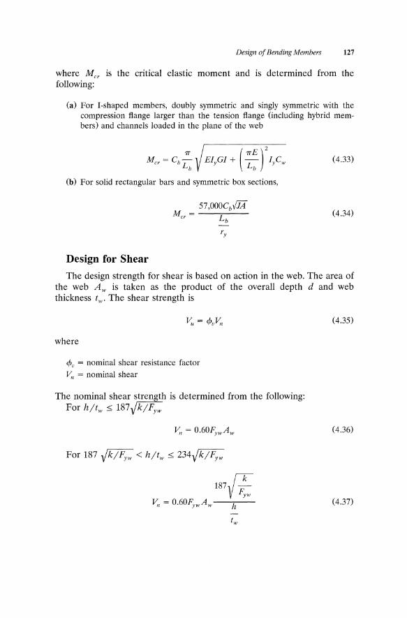
Design of Bending Members 127

where Mer is the critical elastic moment and is determined from the following:

(a) For I-shaped members, doubly symmetric and singly symmetric with the compression flange larger than the tension flange (including hybrid mem­bers) and channels loaded in the plane of the web

(4.33)

(b) For solid rectangular bars and symmetric box sections,

57,OOOCbvlA Mer = L

b (4.34)

Design for Shear The design strength for shear is based on action in the web. The area of

the web Aw is taken as the product of the overall depth d and web thickness two The shear strength is

where

cPu = nominal shear resistance factor v;, = nominal shear

The nominal shear strength is determined from the following: For h/tw .:0; 187Jk/Fyw

For 187 Jk/Fyw < h/tw .:0; 234Jk/Fyw

(4.35)

(4.36)

(4.37)

128 Design of Bending Members

For hjtw > 234JkjFyw

where k = the web buckling coefficient

5 =5+ --

(~ r

(4.38)

(4.39)

When ajh exceeds 3.0, k is taken as 5.0. This applies to all rolled sections. Thus, the limit for hjtw for a rolled section is 70.0 and Equation (4.36) applies when checking the nominal for a rolled section.

4.6 USE OF THE LOAD FACTOR DESIGN SELECTION TABLE Zx FOR SHAPES USED AS BEAMS

Table Zx in Part 3 of the LRFD Manual applies to the selection of braced beams with unbraced lengths not exceeding L r • For beams with unbraced lengths exceeding L p ' it is more convenient to use the unbraced beam charts provided in the manual.

Once the ultimate moment Mu has been determined, the required plastic section modulus Zx is obtained from

12Mu Z = -- (4.40)

x cfJbFy

Enter the column head Zx in the table and find a value equal to or greater than the plastic section modulus required. The beam opposite the required Zx and all beams above have sufficient capacity in bending based only on these parameters. The first beam appearing in boldface represents the most economical section. After the beam has been selected, the following check is required. If the lateral bracing of the compressive flange exceeds L p ' but is less than L" the design moment may be calculated by the following equation:

(4.41)

where

(4.42)

Design of Bending Members 129

If the bracing length Lb is significantly greater than Lp, i.e., Lb > L r , it is recommended that the unbraced beam charts be used.

Example 4.2

Given the information in Example 4.1, use the LRFD method to select a typical beam.

Solution

Consider the partition load as a live load. The ultimate load is

Wu = 1.2D + 1.6L

= 1.2 x 0.35 + 1.6 x 0.42

= 1.09 kjft

The ultimate bending moment is

48 2

M =109x-u· 8

= 314.5 kjft

From Equation (4.40), the required section modulus based on the LRFD method is

12 x 314.5

0.90 x 36

= 116.5 in.3

From the load factor design selection table, select W24 X 55 with the following properties:

BF = 12.7k

L, = 16.6 ft

Lp = 5.6 ft

CPbMr = 222 k-ft

CPbMp = 362 k-ft

hjtw = 54.6

Aw = 8.91 in.2

130 Design of Bending Members

Use seven intermediate stiffeners spaced equally, i.e., 5 ft center to center of the stiffeners. Since Lb = 5 ft < Lp = 5.6, there is no need to use the check as required by Equation (4.41)

CPbMn = CPbMp

CPbMn > 314.5 k-ft = Mu

If we check for shear, Equation (4.36) is used since h/tw = 54.6 < 70

Vu :s; = CPuv" = 0.6Fyw A w

wu L V=-

u 2

1.09 x 48

2

= 26.2 k

0.6FywAw = 0.6 x 36 x 8.91

= 192 k > Vu = 26.2 k

The selection of W24 X 55 proves satisfactory.

Alternate Solution

Mp Method

Knowing that the required factored moment Mu = 314.5 k-ft, find cfJbMp in the load factor design selection table and choose a section with a value of 314.5 or larger. W24 X 55 provides a value of 362 k-ft and Lb < Lp.

Example 4.3

Determine the moment capacity of W27 X 84 for Fy = 36 k/in.2 with the compression flange braced at intervals of 10 ft (Cb = 1.0).

Solution

Examine the load factor design table and observe that for W27 X 84, Fy = 36 k/in.2

CPbMp = 659 k-ft

Lp = 8.6ft

Lr = 24.9 ft

BF = 15.0k

Design of Bending Members 131

From Equation (4.41),

Example 4.4

cPbMn = Cb[ cPbMp - BF(Lb - Lp)] ::;; cPbMp

= 1.0 x [659 - 15.0 x (10 - 8.6)]

= 638 k-ft

Select a beam of Fy = 50 k/in.2 steel subjected to service loads of MD = 156 k-ft and ML = 257 k-ft. Its compression flange is braced at intervals of 8.0 ft (Cb = 1.0).

Solution

Zx Method

Assume that the shape is compact and Lb :::;; Lp. The factored moment is

Mu = 1.2MD + 1.6M1

= 1.2 x 156 + 1.6 x 257

= 598.4 k-ft

The required section modulus is

12 x 598.4

0.90 x 50.0

= 159.6 in.3

Examine the load factor design selection table and note that for W24 X 68 with Fy = 50 k/in.2, the maximum resisting moment 4>bMn listed in the 4>bMp column is 664 k-ft > Mu = 598.4 k-ft. Further note that

cPbMn = 664 k-ft

Lp = 6.6 ft

Lr = 17.4 ft

BF= 18.7k

132 Design of Bending Members

Use W24 X 68.

Alternate Solution

Mp Method

cfJbMn = Cb[cfJbMp - BF(Lb - Lp)]

= 1.0[664 - 18.7(8.0 - 6.6)]

= 637.8 k-ft 2:: 598.4

With a given factored moment of 598.4 k-ft, review the selection table and note that in the column of ¢bMi¢bMn .::; ¢bMp) values for W24 X 68, Fy = 50 kjin.2, the value of ¢bMp is 664 k-ft, which is greater than the given factored moment. This section has Lp = 6.6 ft, Lr = 17.4 ft, and BF = 18.7 k. Since Lb = 8.0 ft,

cfJbMn = 1.0[664.0 - 18.7(8.0 - 6.6)]

= 637.8 k-ft

The selection of W24 X 68 is adequate.

4.7 SERVICEABILITY DESIGN CONSIDERATIONS AND THE LRFD METHOD

The concept of serviceability is developed in design to ensure that disrup­tions of a structure's functional use or damage to it during normal everyday use are extremely unlikely. Although malfunctions in the service­ability of a structure may not lead to its collapse, they can seriously impair its usefulness or in some cases incrue significant repair costs. The use of high-strength materials in design provides relatively flexible structures.

It is stated in the ASD method that serviceability checks are required for live loads, wind and earthquake forces, human activities such as walking and dancing, temperature fluctuations, and vibrations induced by machinery within the building. The LRFD specifications do not provide limiting deflections for individual members or structural assemblies. These limits depend on the function of the structure.

5 Torsion and Bending

5.1 INTRODUCTION

When the transverse forces acting on the beam do not pass through the shear center of its cross section, the beam will experience torsional stresses in addition to those caused by bending. Beams and girders that are placed on the periphery of the building support floor as well as wall loads. These members will experience stresses due to bending and, in addition, torsion. This chapter is intended to present a brief discussion of the theory of torsion and the use of tables and charts to determine the magnitude of stresses caused by torsion.

5.2 TORSIONAL STRESSES

In Figure 5.la, the cross section of the member is subjected to pure torsional shear stresses, warping shear stresses, and warping normal stresses in addition to normal and shear bending stresses. Figure 5.lb is a vectorial representation of the beam shown in Figure 5.la. When a structural member is subjected to loads applied outside the shear center of its cross section as shown above, the cross section tends to rotate about its longitu­dinal axis. See Figure 5.2.

The distribution of torsional stresses along the length of the beam shown in Figure 5.1 depends on the length of the beam, its torsional rigidity, and its end conditions. In Figure 5.3, several types of end con-

133

134 Torsion and Bending

w klft

J J J 1 * J JIll l&-=t::::::: .................... ~ .............................. ::r:----

(a)

m, kip-in per ft

Figure 5.1 Uniform load applied outside of the plane of symmetry of a beam.

ditions are illustrated. Only ideal fixed, pinned, or free torsional end conditions will be considered in this text.

Pure Torsional Shear Stresses

Pure torsional shear stresses vary linearly across the thickness of an element of the cross section and act in a direction parallel to the edge of the element. See Figure S.2c. At the two edges, the stresses are maximum and equal but of opposite direction. The stress at the edge of the element is determined by the formula

(5.1)

In a section that consists of several elements, pure torsional shear stresses will be largest in the thickest element of the cross section.

Warping Shear Stresses

Warping shear stresses are constant across the thickness of the element of the cross section, but vary in magnitude along the length of the element.

Torsion and Bending 135

o y

Applied Torque

z (a)

z

d/2

d/2

(b)

(e)

-- ---

--.... ----(d)

(e)

Figure 5.2 Torsional stresses and stress orientation. (a) General orientation of beam. (b) Positive angle of rotation. (c) Pure torsional shear. (d) Warping shear stresses. (e) Warping normal stresses.

136 Torsion and Bending

- Rigid Support

(a) <1>" = 0

(b)

(c)

(d)

L.......---(e) (f)

Figure 5.3 Bending stresses. (a) Ideal. (b) Ideal. (c) and (d) Schematic representations. (e) and (0 Structural connections.

See Figure S.2d. The magnitude of the warping stresses is determined by the formula

(5.2)

Warping Normal Stresses Warping normal stresses act perpendicular to the surface of the cross

section. See Figure S.2e. They are constant across the thickness of an element of the cross section, but vary in magnitude along the length of the element. These stresses are given by the following formula:

(5.3)

Torsion and Bending 137

5.3 PLANE BENDING STRESSES

In addition to the stresses due to torsion, the section may be subjected to bending stresses (Tb and shear stresses Tb due to plane bending already existing in the structural member. These stresses are obtained from Equations (4.1) and (4.2).

Mby ¢b = -1-

VQ Tb = It

(5.4)

(5.5)

These stresses are illustrated in Figure 5.4 for a wide flange and T-section members.

5.4 COMBINING TORSIONAL AND BENDING STRESSES

In order to determine the total stress condition of a structural member subjected to both torsion and bending, the stresses are added algebraically as long as they remain in the elastic range. It is imperative that the direction of the stresses be carefully noted. The positive direction of the torsional stresses is indicated in Figures 5.2 and 5.4. In the diagrams accompanying each figure, the stresses are shown acting on a section of the member located a distance Z from the left support and viewed in the direction indicated by the general orientation of Figure 5.2. In all the diagrams shown in Figure 5.4, the moment acts about the major axis of the cross section of the member and causes compression in the top flange and tension in the bottom one. Furthermore, the applied shear is assumed to act vertically downward along the minor axis of the cross section.

For wide-flange sections, (Tws and (Tb are both at their maximum values at the edges of the flanges as shown in Figures 5.2 and 5.4. Likewise, there are two flange tips where these stresses are added regardless of the directions of the applied torsional and bending moments. Thus, for wide­flange shapes, (Tws and (Tb should be added to determine the maximum longitudinal stress on the cross section. Also for wide-flange sections, the maximum values of TI' Tws ' and Tb in the flanges can be added at some point regardless of the direction of the applied torsional moment and vertical shear to give the maximum shear stress in the flange. The value of Tb computed using Qf from the torsional properties tables given in the Ninth Edition of the AISC Manual, Part 1, pp. 117 through 133, is the

138 Torsion and Bending

% flange

~ 'tb flange

Figure 5.4 Torsional end conditions.

theoretical value at the edge of the web. It is within the accuracy of the method presented in this book to combine the resulting theoretical value with the torsional shearing stress calculated for the point at the intersection of the web and flange centerlines. In the web, the maximum value of the shear stress T b is added to the value of Tt , regardless of the direction of loading, to give the maximum shear in the web.

5.5 TORSIONAL END CONDITIONS

The distribution of torsional stresses along the length of the member and the torsional rigidity depend on the end conditions. This book only considers ideal fixed, pinned, or free torsional end conditions. When the ideal conditions do not apply, it may be necessary to interpolate between conditions or, conservatively, to assume the worst possible conditions.

Torsion and Bending 139

The fixed end condition is satisfied when rotation and warping of the cross section at the end of the member are prevented. A connection approximating this condition is shown in Figures 5.3a, 5.3c, and 5.3e. The pinned end condition occurs when the cross section at the end of the member is prevented from rotating, but is allowed to warp freely. The common simple structural connection shown in Figures 5.3b, 5.3d, and 5.3f is a reasonable example of this condition. For the free end condition, both rotation and warping of the cross section are unrestrained. The unsup­ported end of a cantilever beam illustrates this condition.

5.6 TORSIONAL LOADING AND END CONDITIONS

The series of charts given in Figures 5.5a through .5.5b provide the values for the angle of rotation and its derivatives [<p', (f/', and <p'" used in Equations (5.1), (5.2), and (5.3)] for any point along the length of the member. These terms are given in nondimensional form, i.e., each term is multiplied by a factor dependent on the torsional properties of the member and magnitude of the applied torsional moment. This product is called the torsional function.

The charts apply to 12 combinations of torsional loading and end restraints. A case chart listing is given in Figure 5.6. Each chart presents a series of curves for the torsional functions depending on different values of L / a, L being the length of the member and a the torsional property of its cross section.

For each case of loading, there are two charts. One provides values for <p and <p", and the other for <p' and <p"'. Each chart shows the value of the torsional function (on the vertical scale) plotted against the location of the cross section (on the horizontal scale) from the left support.

How to Use the Charts

For the given cross section and span length, compute the value of L / a using L in inches and a as given in Table 5.1 for torsional properties, where a = VECw/GJ in inches. With L/a, Z/L, and the case for torsional loading and end conditions lmown, enter the appropriate chart to obtain the torsional functions <p, <p', <p", or <p"'. This result may then be used appropriately in Equations (5.1), (5.2), and (5.3).

Sign Convention

The case charts are based on applied torsional moments shown in the sketch accompanying each chart. In all cases, the torsional moment is

140

.... ... ....

Tors

iona

l Fu

nctio

ns

+.2

+.1 o

~~,,

~,~.

~' ~~~ ..

,~

~It_

~ __

:ttt

iitt

t!i-

-Ij

ittt

ttt,

t-'j-t!

·'·m~-:'

.oj.

" It!

: "~

~lfIT

!~iJl]j,

!,- IT

.s _

_

W

0 2

CA

SE

3

a=

0.5

</>

,</>"

"'R-

--+-

CC'~

o+-+

~-::

+1 ~:

-i

f­:~

1-1

L rrIT

+4.-'-

..... ,,.

,, ;. I.

fli

i':: ....

.. r-

.;.'-o ..

.. ..;v

y-X

i!!

P1

m"

~ ::r

...... ~

k:;

t;7

M

1i11

1'!:

mH::

~~ i ';

:r r~~ ~"::;~; ~~~.\

~WII ~~k/'~~I

"""'

f~,.

, kT

, -,1

2 __ ~~

.... ,·;:

it l'iJ

-

p R;~:lkl

~&:L

A ~

9ill ~

';:;

1:'

'.,

I ",

" Iii

!)

',I

~, ~<!Iii

! ';·1

::, '.

',I.

.,t

"i"

11'0)

I;

V

.WV

' I.ii"f

!o

"?riL

' ~. Ii IK

li~rJi~r h

il

••. ,. !!~

1'4

L+

,,:J

11 iii

! V.

Iff

1,1

Iii

~.~J.W

1 J

"L P

rr:TI

iii H

i;) lY

lIUiL

U

' '~1! ~L

lJ'

'1£ '0

1

R. J.il

. ,"

.,:

II!! i

ll M

i.!!

IJ ::t

l I!,

'iii ji[

ljl

~~: F

!I Vi!

:' I

i' ·t

rrll

it·,

.,~

liE

L

Iii"

I'i t:=

.' •...

.6

.7

11

.9

1.0

Fra

dio

n o

f S

pan

Le

ng

th-{-

Fig

ure

5.5

(a)

Tor

sion

al f

unct

ions

. (b

) T

orsi

onal

fun

ctio

ns.

(Cha

rts

from

Tor

sion

al A

naly

sis

of

Ste

el M

embe

rs b

y A

mer

ican

In

stit

ute

of

Ste

el C

onst

ruct

ion'

)

142 Torsion and Bending

Torsional End Restraints

Case Torsional Loading Remarks Page Left End Right End

I eM ~f' Free Free Concentrated torques at ends of 1 <P ~ <P" ~ 0 <P" ~ 0 member with free ends 21

~M M

~ d~ Fixed Fixed Concentrated torques at ends of 2 <P ~ <P' ~ 0 <P' ~ 0 member with fixed ends 22

~ al

M

~ Concentrated torque at rx = 0.1,

Ib l(l·a)

Pinned Pinned 3 <P ~ <P" ~ 0 <P ~ <P" ~ 0

0.3, or 0.5 on member with pin-ned ends 24

m Pinned Pinned Uniformly distributed torque on

4 ~ ~ <P ~ <P" ~ 0 <P ~ <P" ~ 0 member with pinned ends 30

M ~ m(Z/l) m ::l Pinned Pinned linearly varying torque on memo

5 ~ ~ <P ~ <P" ~ 0 <P ~ <P" ~ 0 ber with pinned ends 32

~ ~Ml(l.") ~ Concentrated torque at a = 0.1,

Fixed Fixed 6 <P ~ <P' ~ 0 <P ~ <P' ~ 0

0.3, or 0.5 on member with fixed

I al I ends 34

m Fixed Uniformly distributed torque on

~ ~ Fixed

7 <P ~ <P' ~ 0 <P ~ <P' ~ 0 member with fixed ends 40

M ~ m(Z/l)

~ Fixed Fixed linearly varying torque on mern-a ~ <P ~ <P' ~ 0 <P ~ <P' ~ 0 ber with fixed ends 42

~M I Fixed Free Concentrated torque at 0: = 0.1,

9 <P ~ <P' ~ 0 <P" ~ 0 0.3,0.5,.0.7,0.9, or 1.0 on memo ber with fixed and free ends 44

~ m Partial uniformly distributed torque

10 I Fixed Free along 0: = 0.1, 0.3, 0.5, 0.7,0.9,

al I '" ~ <P' ~ 0 <P" ~ 0 or 1.0 with fixed end and free end 56 I

M - m(Z/l)

~ Free Fixed Linearly varying torque on memo 11 I <P" ~ 0 <P ~ <P' ~ 0 ber with free and fixed ends 68

m Uniformly distributed torque on

~ ~ Fixed Pinned

member with fixed and pinned 12 <P ~ <P' ~ 0 <P ~ <P" ~ 0 ends 70

Figure 5.6 Case chart listing for beams in torsion. (Charts from Torsional Analysis of Steel Members by American Institute of Steel Construction.)

shown acting in a counterclockwise direction when viewed toward the left end of the member. This is considered to be a positive moment. If the applied torsional moment occurs in the opposite direction, it should be assigned a negative value for computational purposes. A positive stress or rotation computed with the formulas and torsional constants of this book acts in the direction shown in the cross-sectional view in Figure 5.2. A negative value indicates the opposite sense. In some of the case charts, the applied torsional moment is indicated by a vector notation using a line with two arrowheads as shown in Figure 5.6. This notation uses the

TA

BL

E 5

.1

Tor

sion

al P

rope

rtie

s: W

sha

pes

Nor

mal

ize

d W

arpi

ng

Tor

sion

al

War

ping

VEC

wa

W

arpi

ng

Sta

tica

l C

onst

ant

Con

stan

t G

J C

onst

ant

Mom

ent

Sta

tica

l M

omen

t

Sec

tion

J

Gn.

4)

Cw

(in.

6)

(in.

) W

ns

(in

?)

Sw O

n.4)

Q

f (i

n.3

) Q

w (

in.3

)

W24

X

84

3.70

12

,800

94

.8

52.6

91

.3

39.0

11

2.0

W24

X

62

1.71

46

20

83.7

40

.7

42.3

23

.2

76.6

W

24 X

55

1.

18

3870

82

.0

40.4

35

.7

19.8

67

.1

W21

X

62

1.83

59

60

91.8

42

.0

53.2

25

.1

72.2

W

18 X

46

1.

22

1710

60

.3

26.4

24

.2

15.3

45

.3

W12

X

50

1.78

18

80

52.3

23

.3

30.2

14

.7

36.2

Sour

ce:

Ada

pted

fro

m d

ata

in t

he M

anua

l o

f Ste

el C

onst

ruct

ion,

ASD

9th

ed.

198

9 A

mer

ican

Soc

iety

of

Stee

l C

onst

ruct

ion .

..... e

144 Torsion and Bending

"right-hand rule," whereby if the thumb of the right hand is extended and pointed in the direction of the vector, the remaining fingers of the right hand would curve in the direction of the moment.

5.7 APPLICATIONS

Example 5.1

A W12 X 50 section is used on a 20-ft span to support a lO-k load applied eccentrically at midspan as shown in Figure 5.7. Determine the stresses in the member and torsional rotation at midspan.

Solution

The eccentric load is resolved into a torsional moment and a load applied through the shear center of the section as shown in Figures 5.7c and 5.7d. The stresses due to plane bending and torsion are then deter­mined independently.

P = 10k

10' - 0" 9k

M" Pe" 40 k.;'.i+ e = 4"

:£1'Ok

L20' - 0"

(a) (b)

J10k M = 40 k-in.

fS.Ok +~ r <f s.oJ • I

(c) (d)

Figure 5.7 Simply supported beam in torsion.

Torsion and Bending 145

The torsional properties of the section are obtained from Table 5.1. A similar table can be found in the AISC Manual.

1. Plane Bending Stresses

J = 1.78 in.4

a = 52.3 in.

Cw = 1880 in.6

w"s = 23.3 in.2

Sw[ = 30.2 in.4

Qf = 14.7 in?

Qw = 36.2 in.3

Ix = 394 in.4

Sx = 64.7 in.3

tw = 0.370 in.

d = 12.19 in. tf = 0.640 in.

b = 8.08 in.

(a) Maximum longitudinal bending stresses. These occur in the extreme fibers at midspan of the beam

PL Mb=4

10 X 12 X 12

4

= 600 k-in.

Mb 600 G'b = - = -- = 9.20 k (compression at top and tension at bottom)

Sx 64.7

(b) Maximum web shear stresses at the supports.

VQ 7'b = It

5 X 36.2

394 X 0.370

= 1.24 k/in,z

146 Torsion and Bending

(c) Maximum flange shear stresses.

5.0 X 14.7

394 X 0.640

= 0.290 kjin.2

For this loading, the shear stresses are constant from the support to the load point.

2. Torsional Stresses

(a) Torsional functions. The web angle connection is assumed to provide a torsional pinned end condition. Case 3 with IX = 0.50 should therefore be used for this problem

20 X 12

a 52.3

= 4.6

From the chart at the centerline (Z j L = 0.5),

GJ 1 cjJ X - X - = +0.15

M L

GJ

LM cjJ = +0.15 GJ

cjJ" X - X a = - 0.48 M

M cjJ" = -0.48-

GJa

GJ cjJ' X - =0

M

cjJ' = 0

GJ cjJlII X - X a2 = -0.50

M

t/J'" =

M -0.50-­

GJa2

At the support (ZjL = 0),

GJ 1 cjJXMXL=O

cjJ=O

GJ cjJ" X - X a = 0

M

cjJ" = 0

GJ cjJ' X M = +0.40

GJ

M cjJ' = +0.40 GJ

cjJ'" X - X a2 = - 0.10 M

4;>'" = M

-0.10 X-­GJa2

M -40

GJ 11.2 X 103 X 1.78

Torsion and Bending 147

-2.01 X 10- 3

In accordance with the sign convention of this book, the applied torsional moment is negative.

(b) Pure torsional shear stresses.

from Equation (5.1). At the centerline of the beam,

cjJ' = 0

At the support,

Web T t = 11.2 X 103 X 0.370 X 0.40 X (-2.01 X 10- 3 )

= - 3.3 kjin.2

Flange T t = 11.2 X 103 X 0.64 X 0.40 X (-2.01 X 10-3 )

= -5.8 kjin?

148 Torsion and Bending

Warping nonnal stresses. These are maximum at the tips of the flanges

At the centerline of the beam,

O"ws = 29 X 103 X 23.3 X (-0.48) X

= 12.44 k/in.2

-2.01 X 10- 3

52.3

At the support,

¢" = 0

O"ws = 0

Warping shear stresses. These are maximum at the center of the flanges

At the centerline of the beam,

30.2 - 2.01 X 10- 3

Tw = 29 X 103 X -- X (- 0.50) X ---.".--1 0.64 52.32

-0.50 k/in?

At the support,

30.2 - 2.01 X 10- 3

Tw = 29 X 103 X -- X (-0.10) X ---.".--1 0.64 52.3 2

= -0.10 k/in.2

3. Maximum Combined Stresses

A summary of stresses is presented as shown below.

(a) The maximum normal stresses occur at midspan. Refer to Figure 5.8. At point 1,

O"b = 12.44 + 9.27

= 21.71 k/in.2 (compression)

At point 5,

O"b = 12.44 + 9.27

= 21.71 k/in.2 (tension)

Torsion and Bending 149

1 i<-

-T I

3 - --5 4 ... . • -

Figure 5.8 Stress location designation for beams in torsion.

(b) The maximum shear stresses occur at the support. At point 2,

'TWj = -5.80 - 0.10 - 0.29

- 6.19 kjin.2 (acts toward the right)

At point 4,

'TW4 = - 6.19 kjin.2 (acts toward the left)

At point 3,

'TW3 = -3.3 - 1.24

-4.54 kjin.2 (acts downward)

4. Torsional Rotation at Midspan

The angle of rotation at midspan is calculated as follows:

cp = 0.15 x 20 x 12( -2.01 x 10- 3 )

-0.072 rad (4.126 deg)

For other cases the reader is referred to a publication by AISC, "Torsional Analysis of Steel Structures". There are twelve cases which include a variety of loading and support conditions as shown in Figure 5.6. Associated with these cases, there are fifty charts that provide the values of the torsional functions. This method of analysis is simple and can be accomplished with a minimum of calculations.

6 Design of Bracings for

Wind and Earthquake

Forces

6.1 INTRODUCTION

Lateral loads acting on a structure are mostly attributed to wind and earthquake forces. Ordinarily, in designing a building, members are first selected on the basis of gravity loads and then checked for a combination of loading patterns that include wind and/or earthquake forces. The magnitude of these forces is a matter of judgment and reliance on local and national code requirements. Rational analyses can be made using certain parametric assumptions and design criteria. The designer has the responsibility of using judiciously the guidelines of the code. Such action does not release him/her from the necessity of more elaborate analyses depending on specific building requirements and functions.

6.2 WIND FORCES

All exposed structures, including low-rise buildings, are affected by wind forces. Wind loads are a function of the site and the region in which the building is situated. The region determines the wind velocity as the fastest-mile wind speed in miles per hour calculated from the national meteorological records. Wind forces are resisted by a frame or assemblage of structural elements that work together to transfer wind load acting on the building as a whole to the foundation. Bracings, shear walls, roof and

150

Design of Bracings for Wind and Earthquake Forces 151

floor diaphrams are the structural components that conduct the transfer of the wind load to the foundation.

As wind blows against a building, the outer shell of the building experiences the effect of the wind force. Purlins in roof systems, girts, and wall studs receive the impact of the wind load against the building skin and transfer this load to the main frame system. Rigid connections, bracings, or a combination of both transfer these forces to girders and columns and eventually the foundation. Wind-resisting structural components act as a part of a structural system. However, they have to be designed as individu­ally loaded members. The structural engineer would have to appropriate the load to these members and design them accordingly. A tributary area is the wind loading surface area of a definite structural element. When using braced frames in a building, the tributary area for the braced frame may come from several panels (see Figure 6.1).

The tributary area for the wind-resisting frame in the long direction is

75 A = "2 X 147

= 5512.5 ft2

Consider an average wind pressure against the building of 25 lb / ft 2. The total wind load against the building is

25 P = 5512.5 X --

1000

= 137.8 ks

6.3 WIND VELOCITY PRESSURE

The design wind speed is converted to a velocity pressure from:

where

(6.1)

v = basic mean design wind speed in mph (fastest mile) at a height above mean ground of 10 m (33 ft) for terrain exposure category C (see Table 6.1)

I = importance factor, a coefficient used to modify wind speed to provide a somewhat consistent level of risk based on usage (see Table 6.2)

152 Design of Bracings for Wind and Earthquake Forces

-r- -r- ---- -f- -- -r- ---:-

L In r---f- -- -f- - " -I- -I- -I- - a

In N

-f- -f- -f- -f- - @; M

:-1- -I- -r- -I- -

-f- f- -I- -f- -- , -'-

I 4 @ 30' - 0" = 120' - 0"

I --- Signifies Bracing in Panel

Direction of Wind

(a)

Roof

<::> , N C')

6

" 5 N

@J

(b)

Figure 6.1 Wind against a multistory building. (a) Plan. (b) Elevation.

Design of Bracings for Wind and Emthquake Forces 153

TABLE 6.1 Exposure Category Constants

Exposure Category a Zg

A 3.0 1500 B 4.5 1200 C 7.0 900 D 10.0 700

Source: Table C6 from Minimum Design Loads for Buildings and Other Structures, 1990 by American Society of Civil Engineers.

K z = velocity pressure exposure coefficient as a function of height (Table 6.3) or from Equations (6.2) and (6.3)

The constant 0.00256 reflects the mass density of air at standard conditions. The velocity pressure exposure coefficient K z is given as a function of the height above the surface of the ground. It is obtained from

( ria K z = 2.58 :g for Z :2: 15 ft

C5r/a = 2.58 - for Z ::;; 15 ft Zg

where a and Zg are obtained from Table 6.1 and Figure 6.2.

TABLE 6.2 Importance Factors

Building Use Category

I II III IV

Importance Factor I

100 mi inland Hurricane coastline

1.00 1.07 1.07 0.95

1.05 1.11 1.11 1.00

(6.2)

(6.3)

Source: Table 5 from Minimum Design Loads for Buildings and Other Structures, 1990 by American Society of Civil Engineers.

154 Design of Bracings for Wind and Earthquake Forces

TABLE 6.3 Velocity Pressure Exposure Coefficient K z

K z

Height z Exposure A Exposure B Exposure C Exposure D

0-15 0.12 0.37 0.80 1.20 20 0.15 0.42 0.87 1.27 25 0.17 0.46 0.93 1.32 30 0.19 0.50 0.98 1.37 40 0.23 0.57 1.06 1.46 50 0.27 0.63 1.13 1.52 60 0.30 0.68 1.19 1.58 70 0.33 0.73 1.24 1.63 80 0.37 0.77 1.29 1.67 90 0.40 0.82 1.34 1.71

100 0.42 0.86 1.38 1.75 120 0.48 0.93 1.45 1.81 140 0.53 0.99 1.52 1.87 160 0.58 1.05 1.58 1.92 180 0.63 1.11 1.63 1.97 200 0.67 1.16 1.68 2.01 250 0.78 1.28 1.79 2.10 300 0.88 1.39 1.88 2.18 350 0.98 1.49 1.97 2.25 400 1.07 1.58 2.05 2.31 450 1.16 1.67 2.12 2.36 500 1.24 1.75 2.18 2.41

Source: Table 6 from Minimum Design Loads for Buildings and Other Structures, 1990 by American Society of Civil Engineers.

The regional basic wind speed is given for exposure C at a height of 10 m (33 ft) above the mean elevation of the ground. The wind speed for other exposures is obtained from the following equation:

(6.4)

where

~) = the wind speed for exposure C

For the purpose of assigning wind, snow, and seismic loads, certain categories are provided for buildings and other structures. These cate­gories have an importance factor as given in Table 6.4. The importance

Design of Bracings for Wind and Earthquake Forces 155

-' 161 MPH (Gradient Wind Speed) w

~ 1500 FT l;,

0

., [ ",. (To) Vo: !:?:1511 Z 1200 FT :J

0 \0 a: 0 fG8 (t;) Vo: lS;1511 Z 900 FT

~ ~ 700 FT w > 118 MPH 0 ro <

100 MPH

r ~I :r: 72 MPH 0 W

45 MPH :r:

Terrain Exposure

Figure 6.2 Wind velocity chart for the United States and Alaska. (Fig. A4.2 from Low Rise Building Systems Manual, 1986 by Metal Building Manufacturers Association, Inc.)

factors are given in Table 6.2. The numerical values of K z are listed in Table 6.3 for up to 500 ft above mean ground level. For greater heights, use Equation (6.2).

6.4 SELECTION OF BASIC WIND SPEED (mph)

The selection of the basic wind speed depends on the site location of the building. Once the location of the building has been identified, the basic wind speed Vo is obtained from Figure 6.3. To determine the design wind speed, it is not enough to know the general location of the building. The site must be identified relative to the exposure category as shown in Figure 6.2. Equation (6.4) is used to calculate V33 • From Figure 6.2, it is observed that the selection of an appropriate category will define the wind speed design value. Exposure categorization requires an understanding of the terrain immediately surrounding the building site.

6.5 EXTERNAL PRESSURES AND COMBINED EXTERNAL AND INTERNAL PRESSURES

The pressure on a building is given by

pz = qGCp (6.5)

156 Design of Bracings for Wind and Earthquake Forces

TABLE 6.4 Classification of Buildings and Other Structures in Terms of Importance When Used with Wind, Snow, and Seismic Loads

Type of Occupancy Category

All buildings and structures except those listed below

Buildings and structures where the primary occupancy is one in which more than 300 people congregate in one area

Buildings and structures designated as essential facilities, including but not limited to Hospitals and other medical facilities having surgery or

emergency treatment area Fire or rescue and police stations Primary communication facilities and disaster operation

centers Power stations and other utilities required in an emergency Structures having critical national defense capabilities

Buildings and structures that represent a low hazard to human life or property in the event of failure, such as agricultural buildings, certain temporary facilities, and minor storage facilities

II

III

IV

Source: Table 1 from Minimum Design Loads for Buildings and Other Structures, 1990 by American Society of Civil Engineers.

where

q = velocity pressure [Equation (6.1)]

G = gust factor [Table 6.6 or Equations (6.6) through (6.10)]

Cp = pressure coefficient averaged over some time interval (Table 6.5)

The pressure coefficient Cp varies from one location to another in relation to the building. See Tables 6.5 and 6.6 and Figure 6.4.

IMPORTANT NOTES

1. For main wind-resisting systems, use building or structure height h = z.

2. Linear interpolation is acceptable for intermediate values of z.

3. For heights above ground of more than 500 ft, Equation (6.5) may be used.

.....

<Jt "

I , ~.

~'

-\--,

\ •

, x

, c '1

10

'

.. I

GU

LF

O

F

--\'

---E

3-B

aS

iC win~ed 7

0 m

ph

m

Spec

ial

win

d ~eg

ion

I I

I "

No

tes

: 1

. V

alu

es

are

fa

ste

st-

mil

e s

pe

ed

s a

t 3

3 f

t.(1

0m

) a

bo

ve

gro

un

d f

or

ex

po

su

re.

ca

teg

ory

C a

nd

are

as

so

cia

ted

wit

h a

n a

nn

ua

l p

rob

ab

ilit

y o

f 0

.02

.

Fig

ure

6.3

Win

d sp

eed

vari

atio

n w

ith

heig

ht f

or v

ario

us s

ite

expo

sure

s. (

Fig.

1 f

rom

Min

imum

Des

ign

Loa

ds

for

Bui

ldin

gs a

nd O

ther

Str

uctu

res,

199

0 by

Am

eric

an S

ocie

ty o

f C

ivil

Eng

inee

rs.)

158 Design of Bracings for Wind and Earthquake Forces

TABLE 6.5 Wall Pressure Coefficients Cp

Surface L/B Cp For use with

Windward wall All values 0.8 qz 0-1 -0.5

Leeward wall 2 -0.3 q" ~4 -0.2

Side walls All values -0.7 qh

Source: Adapted from Minimum Design Loads for Buildings and Other Struc­tures, 1990 by American Society of Civil Engineers.

4. The value of the gust response factor shall not be less than 1.0. The gust response factors listed in Table 6.7 are calculated from Equation (6.6)

Gz = 0.65 + 3.65Tz (6.6)

where

2.35(Do)1/2 T = ----;--,--

z (Z/30)1/" (6.7)

The gust response factor for a building is calculated on the basis of the mean roof height of that building. The appropriate value can be obtained from Table 6.7. This value will be used for the entire wind-foree-resisting system. For structural systems with a fundamental natural frequency of 1 Hz or less, the dynamic amplification becomes a factor that needs to be accounted for. For buildings and structures with a natural frequency f < 1 Hz, the gust response factor is

_ [p (3.32T1 )2 S ]1/2 G = 0.65 + - + -:-------,-

f3 (1 + 0.002e) (6.8)

For a latticed framework like television and radio towers, towers for power distribution, and any other similar structure, the gust response factor is determined from

_ [ 1.25P (3.32T1 )2 S ]1/2 G = 0.65 + -- + -,-------,-

f3 (1 + 0.002e) (6.9)

.... UI

'C

TA

BL

E 6

.6

Roo

f Pre

ssur

e C

oeff

icie

nts

Cp

for

Use

with

qh

Win

d di

rect

ion

hjL

0

10-1

5

Nor

mal

to

:::; 0

.3

-0.7

0.

2 ri

dge

-0.9

0.

5 -0

.7

-0.9

1.

0 -0

.7

-0.9

>

1.5

-0

.7

-0.9

Par

alle

l h

jB o

r h

jL ::

:; 2.

5 to

rid

ge

hjB

or h

jL >

2.5

Win

dwar

d

Ang

le 0

(de

g)

20

30

40

0.2

0.3

0.4

-0.7

5

-0.2

0.

3 -0

.75

-0

.2

0.3

-0.9

-0

.9

-0.3

5

-0.7

-0

.8

50

> 6

0

0.5

0.01

0

0.5

0.10

0 0.

5 0.

100

0.2

0.01

0

Lee

war

d

-0.

7 fo

r al

l val

ues

of h

jL a

nd 0

-0.7

-0

.8

Sour

ce:

Fig

ure

2 fr

om M

inim

um D

esig

n L

oads

for

Bui

ldin

gs a

nd O

ther

Str

uctu

res,

199

0 by

Am

eric

an S

ocie

ty o

f C

ivil

Eng

inee

rs .

160 Design of Bracings for Wind and Earthquake Forces

(a)

(b)

Figure 6.4 Wind drag coefficients for ordinary buildings. (a) Plan. (b) Elevation.

Design of Bracings for Wind and Earthquake Forces

TABLE 6.7 Gust Response Factors G h and Gz

Height above G h and Gz Ground Level

z (ft) Exposure A Exposure B Exposure C Exposure D

0-15 2.36 1.65 1.32 1.15 20 2.20 1.59 1.29 1.14 25 2.09 1.54 1.27 1.13 30 2.01 1.51 1.26 1.12 40 1.88 1.46 1.23 1.11 50 1.79 1.42 1.21 1.10 60 1.73 1.39 1.20 1.09 70 1.67 1.36 1.19 1.08 80 1.63 1.34 1.18 1.08 90 1.59 1.32 1.17 1.07

100 1.56 1.31 1.16 1.07 120 1.50 1.28 1.15 1.06 140 1.46 1.26 1.14 1.05 160 1.43 1.24 1.13 1.05 180 1.40 1.23 1.12 1.04 200 1.37 1.21 1.11 1.04 250 1.32 1.19 1.10 1.03 300 1.28 1.16 1.09 1.02 350 1.25 1.15 1.08 1.02 400 1.22 1.13 1.07 1.01 450 1.20 1.12 1.06 1.01 500 1.18 1.11 1.06 1.00

Source: Table 8 from Minimum Design Loads for Buildings and Other Structures. 1990 by American Society of Civil Engineers.

where

h = building height (ft)

c = building width (ft)

f = building fundamental natural frequency (Hz) f3 = structural damping factor (percentage of critical damping)

S = structure factor from Figure 6.5

s = surface friction factor obtained from Table 6.8 J = pressure profile factor as a function of ratio 'Y from Figure 6.5

'Y = ratio obtained from Table 6.8

161

P = probability of exceeding design wind speed during a specified number of years n

162 Design of Bracings for Wind and Eanhquake Forces

1. 4 ...----r--,,,----,..,-,--r-r"T"'T.,..,---;-----,-r,-rr"'"'T""-,-,.,-rr-..,-..,

1.3

1.2

1.1

1.0

S 0.9

0.8

0.7

0.6

0.5

A

B C

0.4 L---I._.L.-.L.-L........L-'---'--J.....L....L..J'-'-_-'----'---'---'-.J.....L----L--'-....L...J-I-L----J'---J

10 20 30 40 50 60 80 100 200 300 400500600800 1000 2000 h(ft)

Figure 6.5 Structure size factor S. (Fig. C8 from Minimum Design Loads for Buildings and Other Structures, 1990 by American Society of Civil Engineers.)

Y = resonance factor as a function of y and the ratio c jh from Figure 6.6a Do = surface drag coefficient from Table 6.8 Tl = exposure factor evaluated at two-thirds of the mean roof height

The values of P and f are obtained from Equations (6.10) and (6.11)

P =flV

_ lO.5fh f = ----:;:v

TABLE 6.8 Parameters s, y, and Do

Exposure Category s

A 1.46 B 1.33 C 1.00 D 0.85

y Do

8.20jh 0.025 3.28jh O.OlO 0.23jh 0.005 0.02jh 0.003

Source: Table C9 from Minimum Design Loads for Buildings and Other Structures, 1990 by American Society of Civil Engineers.

(6.10)

(6.11)

Design of Bracings for Wind and Earthquake Forces 163

(a)

Figure 6.6a Pressure profile factor. (Fig. C6 from Minimum Design Loads for Buildings and Other Structures, 1990 by American Society of Civil Engineers.)

Example 6.1

The basic design wind speed for a certain site is 80 mph; the type of exposure is B.

Building height h = 450 ft

Building width c = 80 ft

Building fundamental frequency f = 0.56 Hz

Building damping coefficient f3 = 0.025

Determine the dynamic-response factor.

Solution _ 1O.5fh f= --;v-

10.5 x 0.56 x 450

1.33 x 80

= 24.868

164 Design of Bracings for Wind and Earthquake Forces

I .

10 " .. NOTE: The four sets of curves correspond to four different values of the ratio c/h.

(b)

Figure 6.6b Resonance factor. (Fig. C7 from Minimum Design Loads for Buildings and Other Structures, 1990 by American Society of Civil Engineers.)

For exposure E,

3.28 "Y = 450

c 80

h 450

0.178

0.00729

Design of Bracings for Wind and Earthquake Forces 165

Given the values of 'Y, j, and c / h, use Figures 6.5 and 6.6 to obtain the parameters J, Y, and S

J = 0.0103

Y = 0.0030

S = 0.84

2.35 x (0.01)°.5 Tl =

( 33000 ) 1/4.5

= 0.141

P = 24.868 x 0.0103 x 0.0030

= 0.000768

[0.000768 (3.32 x 0.141)2 X 0.84]1/2

= 0.65 + + --------0.025 1 + 0.002 x 80

G = 1.119

6.6 WIND PRESSURE PROFILE AGAINST BUILDINGS

The equivalent static wind pressure against closed buildings is determined from Equation (6.5), in which Cp represents the difference between positive pressure on the windward side and negative pressure on the leeward side. For values of these constants, refer to Table 6.5. Once the gust response factor has been determined, the equivalent static pressure against the building along its height can be calculated.

Example 6.2

In Example 6.1, the length of the building is 100 ft. The structure is located more than 100 mi from the coastline and is used as an office building. Calculate the pressure diagram along the height of the building.

Solution

From Table 6.1, the building category is I. Hence, the influence factor I is unity. From Equation (6.1),

qz = 0.00256K/IV)2

= 0.00256 x (1 X 80)2

= 16.4Kz lb /ft 2

166 Design of Bracings for Wind and Earthquake Forces

and

where Cp and Cn represent the positive and negative coefficients as given in Table 6.5. Then,

pz = 16.4Kz x 1.119 x [0.8 - (-0.5)]

= 23.9Kz lb/ft 2

With Table 6.3, the pressure diagram is completed as shown in Table 6.9. From this pressure distribution, the lateral forces at the level of each story can be determined.

6.7 ANALYSIS OF BRACED FRAMES FOR WIND FORCES

Buildings are subjected to wind forces frequently during their life time, but it is usually tall buildings (three or more stories high) that are designed

TABLE 6.9 Pressure Diagram

Height Exposure B, K z pz

0-15 0.37 8.8 20 0.42 10.0 25 0.46 11.0 30 0.50 12.0 40 0.57 13.6 50 0.63 15.1 60 0.68 16.2 70 0.73 17.4 80 0.77 18.4 90 0.82 19.6

100 0.86 20.6 120 0.93 22.2 140 0.99 23.7 160 1.05 25.1 180 1.11 26.5 200 1.16 27.7 250 1.28 30.6 300 1.39 33.2 350 1.49 35.6 400 1.58 37.8 450 1.67 39.9

Design of Bracings for Wind and Earthquake Forces 167

with a special consideration given to wind loads. Wind forces are dynamic in nature. Some assumptions based on theoretical and experimental stud­ies have been made available to simplify the evaluation of wind forces against buildings and other structures. One such assumption is that wind forces are transferred to the columns and from there to the foundation through a rigid floor structure and bracing frame system. The wind forces are considered concentrated loads applied against the braced frames at each story level. See Figure 6.7. Simple joint-by-joint analysis yields the distribution of the wind load in the frame system. Further, it is assumed that the bracing members will experience only tension. This assumption is made for simplifying the analysis. For all practical purposes, the results thus obtained are satisfactory for the design.

Example 6.3

Calculate the wind force against the building given in Example 6.2 for the same parameters in Example 6.1. The structure used is an office building.

Solution

The classification of the building is obtained from Table 6.4. It is classified as category 1. The importance factor I = 1.0; it is determined from Table 6.2. For a B exposure, a = 4.5 and Zg = 1200 ft; these values are obtained from Table 6.1. The wind velocity pressure as given by Equation (6.1) is

Given the basic wind speed for the region (airport records), the equiva­lent basic wind speed for any other exposure is provided by Equation (6.4)

Then

= >/2.58 (~) 415 X 80

1200

= 57.8 mph

Z qz = 0.00256(1 x 57.8) K z

= 8.56Kz Ib Ift z

168 Design of Bracings for Wind and Earthquake Forces

I .. 4 @ 25' = 100'

--- .-- "-J ~ -,:; 1,;,- -;;: - r-

<::> CD -

II - -f- -f- - -I-

L I -f- -l- i- -I- N - --~ -,", r- -I-

- .... - - I- t Plan Wind Direction

Fa ~ 1===:::::j;.t;ii==;:I:=====I======l ---r-

F7 ~

F6---4~~ -----~~~---4~~------+-------4

F5 __ ~~-----~~~~~------~----~

F2 ~1----~kIfC:""""'-a.O::...l-----I-------I

~---4~~~------~~----~~------~------1

Figure 6.7 Transfer of wind forces into the building frame system of braced frames with standard bolt connections.

Design of Bracings for Wind and Earthquake Forces 169

In Equation (6.5), the static wind pressure against the building is

The constant C p is given in Table 6.5

Cp = [0.8 - (-0.5)]

= 1.33

Since the building has a basic fundamental frequency f == 0.56 Hz that is less than 1.0, the dynamic gust response factor G as determined in Example 6.1 is 1.119. The factor is used for all heights of the building. Thus, the wind static pressure against the building is written as

pz = 8.56 x 1.119 x 1.13Kz

= 12.45Kz Ib 1ft 2

Consider that the wind pressure against the building conforms to a step pattern and these steps change at elevations of 30, 50, 100, and 200 ft. The elevation coefficient K z is obtained from Table 6.3. A summary of the static wind pressure against the building is given below. The wind pressure per foot along the height of each exterior frame is obtained from the product of the wind pressure in pounds per square feet at that height and one-half the width of the building that is perpendicular to the direction of the wind:

z (ft) Kz pz (tb Ift 2 ) pz (tb/ft)

30 0.50 6.2 186 50 0.63 7.8 234

100 0.86 10.7 321 200 1.16 14.4

The wind pressure against the building is resisted by the two exterior frames since they are the only ones that are braced. Each frame receives one-half of the total wind load against the building. Thus, the pressure diagram for the wind load acting on each frame is the product of the wind pressure summarized above and one-half the width.

170 Design of Bracings for Wind and Earlhquake Forces

The calculation of the forces at the various story levels proceeds as follows:

15 + 10 186 FI = x--

2 1000

= 2.32 k

10+10 186 F2 = x--

2 1000

= 1.86 k

10 + 10 234 F3 = x--

2 1000

= 2.34 k

10+10 234 F4 = x--

2 1000

= 2.34 k

10+10 321 Fs = x--

2 1000

= 3.21 k

10+10 321 F6 = x--

2 1000

= 3.21 k

10 + 10 321 F7 = x--

2 1000

= 3.21 k

10 321 F =-x--

8 2 1000

= 1.60 k

The wind forces against each story are shown in Figure 6.S. The next step is to analyze the forces in the braced bay. The method of joints is used. Because braces can be very slender, it is assumed that they will carry tension forces only, so the frame is analyzed with one diagonal, which makes it a determinate structure. At every level, the horizontal component of the force in the bracing is equal to the sum of the wind forces above it. See Figure 6.9.

The horizontal components of the diagonals and the diagonal forces are shown in Table 6.10. The girders are subjected to axial forces due to wind.

Design of Bracings for Wind and Earthquake Forces 171

F8 =1.60k ~

321 pit F7 = 3.21 k .. F6 = 3.21 k ~

F5 = 3.21 k .. 234 pit

F4 = 2.34 k .. F3 = 2.34 k ~

F2 = 1.86 k .. 186 pit ~ = 2.32 k ..

Figure 6.8 Wind shear against building floors.

The horizontal component of the diagonal force is

n

Fjx = L ~. j~l

The force in the diagonal is

L. n

Fj = t- L Fjx jx j~ 1

The force in the column on the leeward side is

n

Fjcl = L Fjy j~ 1

(6.12)

(6.13)

(6.14)

(6.14)

~~}~--~~~--~~ F8 = 1.60 k7

Figure 6.9 Resolution of wind shear in the braced frame.

172 Design of Bracings for Wind and Eal1hquake Forces

TABLE 6.10 Diagonal Forces Due to Wind

Story Wind Force (k) Fx (k)

8th 1.60 1.60

7th 3.21 4.81

6th 3.21 8.02

5th 3.21 11.23

4th 2.34 13.57

3rd 2.34 15.91

2nd 1.86 17.77

1st 2.32 20.09

The force in the column on the windward side is

Fncw = 0.0

Diagonal Force F (k)

1.72

5.18

8.64

12.09

14.61

17.14

18.45

23.42

(6.15)

(6.16)

(6.17)

where the symbols in Equations (6.12) through (6.16) define the members as indicated in Figure 6.10.

Example 6.4

A 21-story building is located in the vicinity of O'Hare Airport in Chicago, Illinois. The structure is an office building. The plan and braced frame of the building are given in Figure 6.11. Calculate the wind pressure profile against the building.

Solution

The basic wind speed for the location is 75 mph (Figure 6.2). The building category is I (Table 6.4). The importance factor based on the building category is 1.05 (the coastline). The Cp factor is the sum of the

Design of Bracings for Wind and Earthquake Forces 173

---I~" +-'=-------",./

----II~~ 1"""--------~

PJ· ~

~cw Figure 6.10 Braced frame nomenclature.

absolute values for the windward and leeward side coefficients (Table 6.5). The wind pressure at any height z is

where K z and Gz are obtained from Tables 6.3 and 6.6, respectively

pz = O.00256K/1.05 X 75)21.3Gz

= 20.639Kz Gz Ib/ft 2

By using Tables 6.3 and 6.6 in the equation for the wind pressure, the pressure profile can be obtained as shown below. To determine the pressure at each story level due to the parabolic pressure distribution, Simpson's rule is used as indicated

h p = - x (p + 4p + P )

z 6 Z2/1l-2 Z2m-l 22m (6.18)

174 Design of Bracings for Wind and Earthquake Forces

~--~----+---~r---~~~18

*""--,-__ 225'

215.5'

205'

194.5'

183'

1---

Elevation

5 @ 24' = 120'

Plan ~I

15

13

12

1 1

9

8

7

6

5

4

3

2

0 (\j

II

~ 0

@! 0 N

Lo

172.5'

162'

151.5'

141 '

130.5'

120'

109.5'

99'

88.5'

78'

67.5'

57'

46.5'

36'

25.5'

15'

_....lIL __ '--_ 0

Figure 6.11 Twenty-one-story building frame system.

Design of Braeings for Wind and Earthquake F orees

TABLE 6.11 Pressure Profile for Building in Example 6.4

z (ft) Kz Gz pz Ob/ft2)

0-15 0.80 1.32 21.8 25.5 0.93 1.27 24.4 36 1.02 1.22 25.7 46.5 1.10 1.22 27.7 57 1.17 1.20 29.0 67.5 1.23 1.19 30.2 78 1.28 1.18 31.2 88.5 1.34 1.17 32.4 99 1.38 1.16 33.0

109.5 1.42 1.16 34.0 120 1.45 1.15 34.4 130.5 1.48 1.14 34.8 141 1.52 1.14 35.8 151.5 1.55 1.13 36.1 162 1.58 1.13 36.8 172.5 1.60 1.12 37.0 183 1.64 1.12 37.9 193.5 1.66 1.11 38.0 204 1.69 1.11 38.7 214.5 1.71 1.10 38.8 225 1.74 1.10 39.5

where

m = a number that indicates the number of a particular story; m = 1, n n = number of stories in the building

175

Pz = intensity of wind pressure Ob 1ft) along the width of the building and at the level of that particular story

P z = the pressure Ob 1ft 2), as given in Table 6.11, induding the interpolated values at half-story height for each story6.11

h = the story height (ft)

The wind pressure profile is summarized in Table 6.11. The wind force against each story along the height of the building is shown in Table 6.12.

6.8 INTRODUCTION TO SEISMIC DESIGN

An earthquake causes ground motions at the base of the structure. Depending on the type of the structure, its response to ground motion will determine the magnitude of displacements and level of stresses in the frame of the structure. Thus, seismic design will require the determination

176 Design of Bracings for Wind and Earthquake Forces

TABLE 6.12 Wind Forces

n Pn (lb Ift2) W(lb/ft 2 ) m Pm (k)

0 21.8 1 21.8 22.0 1 22.2 2 23.1 3 24.4 24.3 2 24.5 4 25.0 5 25.7 25.8 3 26.0 6 26.7 7 27.7 27.6 4 27.8 8 28.4 9 29.0 29.0 5 29.2

10 29.6 11 30.2 30.2 6 30.4 12 30.7 13 31.2 31.2 7 31.4 14 31.8 15 32.4 32.4 8 32.7 16 32.7 17 33.0 33.0 9 33.3 18 33.5 19 34.0 34.0 10 34.3 20 34.2 21 34.4 34.4 11 34.7 22 34.6 23 34.8 34.8 12 35.1 24 35.1 25 35.8 35.7 13 36.0 26 36.0 27 36.1 36.1 14 36.4 28 36.4 29 36.8 36.8 15 37.1 30 36.9 31 37.0 37.0 16 37.3 32 37.4 33 37.9 37.8 17 38.1 34 38.0 35 38.0 38.1 18 38.4 36 38.4 37 38.7 38.7 19 39.0 38 38.8 39 38.8 38.9 20 39.2 40 39.2 41 39.5 32.9 21 33.2

Design of Bracings for Wind and Earthquake Forces 177

of seismic forces that act on the structure and the selection of member sizes to resist these forces in order to keep deflections within prescribed limits. The various seismic zones in the United States are shown in Figure 6.12.

The determination of seismic forces can be achieved by an equivalent static force procedure or a dynamic analysis approach. In this book, the former procedure will be used. However, the design engineer must use sound judgment on when the dynamic approach should be used in the prediction of earthquake forces against a building.

6.9 EQUIVALENT STATIC FORCE PROCEDURE

In this method, a step-by-step procedure is outlined in accordance with the ANSI building code. The following symbols and notations will be used throughout the procedure:

C = numerical coefficient for the base share

Cp = numerical coefficient used in determining the lateral force for parts or portions of buildings or other structures

D = the dimension of the building in the direction of the earthquake

d i = deflection at level i relative to the base due to the applied lateral forces

Fi , Fn, Fx = lateral force applied to level i, n, or x, respectively Fp = lateral force on a part of the structure and in the direction under

consideration F, = that portion of V, the total shear force at the base due to earth-

quake motion, considered concentrated at the top of the structure in addition to F;,

g = acceleration due to gravity

hi' hn' hx = height above the base to level i, n, or x, respectively I = occupancy importance factor K = numerical coefficient related to stiffness of the structure

N = the total number of stories above the base to level n S = numerical coefficient for site-structure resonance

T = fundamental elastic period of vibration of structure in seconds per cycle in the direction under consideration

Ts = characteristic site period V = total lateral force or shear at the base of the building due to

earthquake motion

W = the total dead load and applicable portions of other loads Z = seismicity coefficient

178 Design of Braeings for Wind and Earthquake F orees

~ Zones.

Guam Tutulla ThaVlrginlslands

MILES

ALASKA

HAWAII PUERTO RICO o '00 =

Figure 6.12 Seismic zone chart for the United States and its territories. (Courtesy of American Society of Civil Engineers, Minimum Design Loads for Buildings and Other Structures.)

Design of Bracings for Wind and Earthquake Forces 179

TABLE 6.13 The Seismic Zone Coefficient Z

Seismic Zone from Figure 6.12 Z

4 1 3 3/4 2 3/8 1 3/16 o 1/8

Source: Table 21 from Minimum Design Loads for Buildings and Other Structures, 1990 by American Society of Civil Engineers.

The predicted earthquake forces against buildings are a function of the intensity of the earthquake, site characteristics, type of materials and method of construction used in the building, and function of the building. The total lateral seismic force against a building and in the direction of the seismic motion is expressed by the following formula:

V= ZIKCSW (6.19)

The factors in Equation (6.19) have to be determined for each building. They can be obtained from Tables 6.13 through 6.16. The product CS need not exceed 0.14, or for soil profile type III in seismic zones 3 and 4, it need not exceed O.ll.

The value of C depends on the dynamic characteristics of the structural system and is obtained from the following equation:

1 C=--

15{i

The value of C must not exceed 0.12.

TABLE 6.14 Occupancy Importance Factor I

Category I

I. All other buildings not in II and III 1.0 II. Assembly of 300 people or more 1.25

III. Essential facilities 1.5 IV. 14 NA

Source: Table 22 from Minimum Design Loads for Buildings and Other Structures, 1990 by American Society of Civil Engineers.

(6.20)

180 Design of Bracings for Wind and Earthquake Forces

TABLE 6.15 Horizontal Stiffness Factor K for Buildings and Other Structures

Type of Lateral-Force-Resisting Building System K

Bearing wall systems

Walls provide for all or the major part of the vertical loads and resist the seismic force:

Reinforced concrete shear walls or braced frames 1.33 Masonry walls 1.33 One-, two, or three-story light wood or metal

frame-wall systems 1.00

Building frame systems

A structural system with an essentially complete space frame providing seismic force resistance by shear walls or braced frames 1.00

Moment-resistingframe systems

A structural system with an essentially complete space frame providing support for vertical loads. Seismic forces are resisted by moment-resist­ing frames:

For ordinary steel frames 1.00 For special frames 0.67 For intermediate reinforced concrete frames 1.25

Dual systems

A complete space frame to support vertical loads; special moment­resisting frames and shear walls or braced frames to resist seismic forces:

Special moment-resisting frame 0.80 Intermediate moment-resisting frame 1.00

Elevated tanks

Tanks plus full contents, where tanks are supported on their own tower and on a building 2.50

Structures other than buildings 2.00

Source: Table 23 from Minimum Design Loads for Buildings and Other Structures, 1990 by American Society of Civil Engineers.

T is the period of the structural frame system reslstmg the seismic horizontal forces and is a function of the structural material used in the frame and type of construction used in assembling the frame system. The

Design of Bracings for Wind and Earthquake Forces 181

TABLE 6.16 Soil Profile Coefficients S

Soil Profile Type S

Type I: Rock 1.0 Type II: Stiff clay greater than 200 ft in thickness 1.2 Type III: Soft to medium stiff clays and sand 1.5

Source: Table 24 from Minimum Design Loads for Buildings and Other Structures, 1990 by American Society of Civil Engineers.

determination of the period of a structural system is a complex problem. It can be computed using the Raleigh-Ritz method expressed in the follow­ing formula:

(6.21)

in which the values of F;, FI' 0;, and dn are determined from the base shear V distributed according to Equations (6.22), (6.23), and (6.24).

The distribution of the lateral shear force V is expressed as

n

V=Ft+LF; ;~ 1

(6.22)

The force Ft is a concentrated force applied at the top of the building to account for the parapet and any other appertenances that may exist on the roof. This force is expressed as a function of the period of the frame system and the total lateral force acting against the building. It is given by the following equation:

Ft = 0.07TV (6.23)

The remainder of the lateral force is distributed linearly between the top and bottom of the building as follows:

(V - Ft)h n Fn = -"""n---

LW;h; ;~ 1

(6.24)

In the absence of a rational analysis for the determination of the period T as shown above, it can be evaluated based on the type of frame under

182 Design of Bracings for Wind and Earthquake Forces

consideration. For braced frames, an approximate equation can be used for moderately high buildings

where

O.05H T=--

ViS

H = the height of the building above the ground D = the width of the building in the direction of the earthquake

(6.25)

For a 100% ductile-moment frame resisting the lateral forces, the period of the building is

T = D.WN (6.26)

where

N = the number of stories

It has been found that Equation (6.26) yields poor results for low-rise buildings. It is reasonably accurate for buildings in the 40-story range. Otherwise, one must use the Raleigh-Ritz equation. As an initial approxi­mation, Teal's formula (Edward Teal, Teal's Method or Formula, AISC Engineering Journals, Second and Fourth Quarters, 1975) provides reason­able results

(6.27)

where

C1 = ZICS Ll = the lateral deflection at the top of the building

One can begin by assuming a deflection at the top of the building that is equal to two-thirds of the maximum allowable drift stipulated by the local building code. Use that value in Equation (6.27). By using an average value for S between 1 and 1.5, which is the range presented in Table 6.16, and lZ, as known from the site and function of the building, a relationship

Design of Bracings for Wind and Earthquake Forces 183

between the period T and factor C is established from Equations (6.27) and (6.20). The result is expressed as follows:

1 T= -

4 (6.28)

Knowing the values of Z, I, and S will provide a value for T. Use this value in the procedure to obtain V and the subsequent forces Ft and F; against the building. With these forces at hand, the deflection of the frame can be obtained. Use the deflection in the Raleigh-Ritz formula and compare the results for T with the one obtained from Equation (6.28). For any significant difference, the calculated T can be used to determine a new set of deflections to calculate a value for T. The process converges rapidly.

Example 6.5

Consider a lO-story hospital in Los Angeles, California. It is essentially a steel space frame with braced frames in the N-S direction and ductile­moment frames in the E-W direction. The roof and floors are constructed of reinforced concrete slab (3± in. with a 3-in. metal deck) placed on open steel joists. Floor-to-floor height is 10 ft, 6 in. The plan and elevation of the building are shown in Figure 6.13. Determine the distribution of the seismic forces against the building in the N-S orientation. The site consists of sand and moderately stiff clay.

Solution

Loads

1. Roof

(a) Roofing and insulation

(b) Metal deck (c) Concrete slab

(d) Ceiling

(e) Steel framing

Total roof dead load (f) Live load (reducible)

8.0 Ib/ft 2

3.0

45.0

5.0

8.0 69.0Ib/ft 2

20.0 Ib /ft2

184 Design of Bracings for Wind and Earthquake Forces

,

b o N

I I

in N

OX)

,

I

,

,

,

,

,

,

~-4----t~~

loe: 6 @ 25' = 150'

(a) (b)

Figure 6.13 Ten-story building for seismic design. (a) Plan. (b) Elevation N-S.

2. Typical Floor Loading

(a) Metal deck (b) Concrete slab (c) Ceiling (d) Partitions (e) Steel framing with fire retardant

Total dead load (f) Live load (reducible) average

3. Curtain Walls

(a) Average weight

Lateral Force Analysis

3.0Ib/ft 2

45.0

5.0 20.0 13.0

86.0Ib/ft 2

85.5Ib/ft 2

15.0Ib/ft 2

From Equation (6.19), we write the expression for the seismic force against the building

V= ZIKCSW

Z = 1.0

Los Angeles is in region 4; see Figure 6.12.

1=1.5

Design of Bracings for Wind and Earthquake Forces 185

The building is a hospital; see Table 6.14.

K = 1.00

The frame is steel and braced; see Table 6.15.

S = 1.5

The soil is category 3; see Table 6.16.

The frame is braced

Then from Equation (6.20),

0.05H T=--

ID

0.05 x 107.5 T = --;y'I50=15=0-

= 0.44 sec

1 c= --==

15,10.44

= 0.10

The product of CS is 0.15. However, in zones 3 and 4, it need not exceed 0.14. Hence, the seismic force against the building is

v = 1 x 1.5 x 1 x 0.14W

= 0.21W

Calculate the total dead load of the building. Note that the building dimensions to the building lines are 202.5 ft X 152.5 ft.

Typical Floor Load

Floor: 202.5 X 152.5 X 0.086 = 2656 k Curtain Walls: 2(202.5 + 152.5)0.015 X 10.75 = 114 k

Total per floor =2770 k

186 Design of Bracings for Wind and Earthquake Forces

TABLE 6.17 Distribution of Seismic Force Against One Typical Frame

Height Weight wnh n (wnhn/L wnhn) Level (ft) wn (k) (k/1000) I/L wnh n X (V-ft) Fi

R 107.5 2220 238.65 0.150 207.2 251.2 9 96.75 2770 280.00 0.176 243.0 243.0 8 86.00 238.22 0.150 207.2 207.2 7 75.25 208.44 0.131 180.9 180.9 6 64:5 178.66 0.112 154.7 154.7 5 53.75 148.88 0.094 129.8 129.8 4 43.00 119.11 0.075 103.6 103.6 3 32.25 3389.0 0.056 77.3 77.3 2 21.50 59.56 0.037 51.1 51.1 1 10.75 29.78 0.019 26.2 26.2 0

Roof Load

Roof 202.5 X 152.5 X 0.069 =2131 k Wall and 3-ft parapet 2(202.5 + 152.5)8.375 X 0.015 = 89 k

Total for roof

Thus, the total weight of the building

9 X 2770 + 2220 = 27,150 k

The seismic force against the building is

v = 0.21 X 27,150 = 5701.5 k

=2220 k

Let the building be braced in the short direction at the 1st, 4th, 6th, and 9th line. Then, the seismic force resisted by one single frame is one-fourth the total horizontal force (5701.5/4 = 1425 k). The force Ft is

Ft = 0.Q7 x 0.44 X 1425

= 44k V - F, = 1425 - 44

= 1381 k

The distribution of this force is accomplished by using Equation (6.24). Arrange the results in tabular form. See Table 6.17. With these results the frame can be analyzed structurally.

7 Connections

7.1 INTRODUCTION

The behavior of connections IS the least understood in the field of structural engineering. Most connections are designed on the basis of experience rather than theoretical analysis. Rational analysis of joints is intricate and highly indeterminate. Most failures in steel structures occur because of inadequate connections. It is common practice in design engineering to leave the detailing of connections to the fabricator, hence adding to the confusion of who is responsible in the event of failure. However, the structural engineer who designs the structure is responsible for the design of the connections. It is of the utmost importance then that the engineer be proficient in connection design.

Until fairly recently, welding and riveting dominated the field of connec­tions. Modern steel structures are constructed with welded connections, bolted ones with high-strength or common bolts, or a combination of both. Figure 7.1 is a representation of a column splice that is designed to transfer axial as well as bending loads.

7.2 TYPES OF CONNECTIONS

There are several types of connections, the use of which depends on the magnitude and importance of the job. Figure 7.2 shows various types of

187

188 Connections

I I, " " " " "

" I

.r:: U)

&U-kip-It ~

It? 9 x 3/4

Figure 7.1 Column splice.

Connections 189

(a) (b)

(e)

.~ • • • •

(d)

Figure 7.2 Standard column connections.

190 Connections

connections that are used currently in the building industry or have been employed in the past.

For standard connections, the "AISC Specifications for Structural Steel Buildings," Section J4 (ASD) stipulates that the effective area to resist failure due to shear and tension when present is obtained by deducting the area of the standard holes along the minimum net failure surface. A standard hole is defined by the nominal fastener diameter plus 1.8 in. (ft for clearance and ft for cracks due to punching).

7.3 FRAMED BEAM CONNECTION: BOLTED

The standard practice in the design engineering of building is to show the reactions for simply supported beams on the contract drawing. Fabricators then can specify the standard connection in accordance with the AISC specifications to meet the load requirements. However, the engineer must be familiar with the basic assumptions behind this practice and be able to verify it by analysis. The AISC specifications require that several condi­tions be checked to identify the allowable capacity of the framed beam connection. These conditions are bolt shear, bolt bearing on the connect­ing material, beam web tear-out known as block shear, shear on the net area of the connecting angles or plates, and local bending stresses due to eccentricity and other factors.

Example 7.1

The diagram in Figure 7.3 represents an interior bay of a floor system. The live and dead loads are 80 and 55 lb / ft 2, respectively. The girder size that is required to carry these loads adequately is W33 X 118. Design the beam column standard connection. See Figure 7.4.

Solution

The reaction at the end of the girder is 48 k.

1. Check for shear in the bolts. From the AISC Manual, Table I-D, "Shear," for A325-N bolts with double shear, the capacity of one bolt is 18.6 k

48 n= --

18.6

=3

Pa = 55.8k > 48

Connections 191

--H-!----i----i----r---

in C\I

-- \-H----..:...--;..-.--~-

I ... 4 @ 10' - 0" = 40' - 0"

~I Figure 7.3 Typical interior bay framing system.

2. Check the net area in the angles. Use Table H-C and a i-in. angle and ~-in.-diameter bolt

Pa = 52.7 k

3. Check the bearing capacity should slip occur. By using Table I-F at Fu =

58 kjin.2 and with a ~-in.-diameter bolt and I v = 1 ~ in. or greater, the allowable load for one fastener with a I-in. thick plate is 52.2 k

Pa = 52.2 X 3 X 0.55

= 86.1 k

A W 33x 118

2L 4x 31/2 x 114 x 8 1/2 Section at A

Figure 7.4 Typical beam-to-column connection.

192 Connections

Since the beam is coped, block shear must be checked. The resistance to block shear according to AISC ASD, Section 14, is

and lh = 2 in.

From Table I-G, the coefficients C1 and C2 are 1.38 and 0.99, respectively. Then the allowable block shear resistance is

RES = (1.38 + 0.99) x 58 x 0.55

= 137.5 k > 48

The connection as given is adequate. Other allowances must be estab­lished to conform to the AISC requirements. These are listed as follows:

(a) Insertion and tightening clearances can be checked in the table of assem-bling clearances (AISe Manual, Part 4).

(b) Need for reinforcement at the coped section in bending. (c) Adequacy of this connection with respect to the supporting member. (d) If a smaller gage on the outstanding leg of the connection angles is

required, the bolts must be staggered with those in the web. An even stagger will permit the use of a 5-in. gage with 3~ X 3~ X * X 0 ft, 10 in. The stagger portion of the table of stagger for tightening (AISe Manual, Part 4) is used in verifying clearances.

Example 7.2

The diagram in Figure 7.5 represents an interior bay of a library stackroom's floor system. The live and dead loads are 150 and 65 lb/ft 2

respectively. The girder size required to carry these loads adequately is W40 X 324. Design the beam column standard connection. See Figure 7.6.

Solution

The reaction at the end of the girder is 171 k.

1. Check/or shear in the bolts. From the AISe Manual, Table I-D, "Shear," for A325-N bolts with double shear, the capacity of one bolt is 18.6 k

171 n= --

18.6

= 10

Pa = 186 k > 171

Connections 193

hrl-----.------.------.------~----_.------

~~-----+_----_+------+_----_+------+_----hrl

I-'-i------'-----:...-------'------....:.--------.:-----I-'-i

I~ 6 @ 10' - 0" = 60' - 0"

in

'"

Figure 7,5 Plan view of a typical standard column-girder connection.

" >

7 5/8

1/2"

Ih • 1 1/2 + 4 112

W 40 x 324 o ...

"' o ...

'"

SECTION AT 0

""-___ 2 ~6 x 4 x 3/8 x 2' - 6"

Figure 7.6 Typical beam column standard connection.

194 Connections

2. Check the net area in the angles. Use Table II-C and a ~-in. angle and ~-in.-diameter bolt

Pa = 279 k

3. Check the bearing capacity should slip occur. By using Table I-F at F;, =

58 kjin.2 and with a ~-in.-diameter bolt and Iv = 1~ in. or greater, the allowable load for one fastener with a 1 in. thick plate is 52.2 k

Pa = 52.2 X 10 X 1.00

= 522k

Since the beam is coped, block shear must be checked. The resistance to block shear according to AISC ASD, Section 14, is

and Ih=2in., n=IO

From Table I-G, the coefficients C1 and C2 are 1.38 and 5.58, respectively. Then the allowable block shear resistance is

RES = (1.38 + 5.58) X 58 x 1.00

= 403.6 k > 171

The connection as given is adequate. Other allowances must be estab­lished to conform to the AISC requirements. These are listed as described above.

Example 7.3

Given the beam as shown in Figure 7.7, the selection of W36 X 393 satisfies the requirements of the beam design. See Figure 7.8. Design a

1230 K

4 @ S' - 0" = 32' - 0"

Figure 7.7 Large concentrated loads on a 32-ft girder.

Connections 195

W 36 x 393

+ Section at 0

12 3/4 21_6x4x5/82'-9

Figure 7.8 Standard column-girder connection.

standard connection in accordance with the AISC specifications. We are given the following data given:

Beam size: W36 X 393, tw = 1.220 in. (Ii)

A 572 Grade 50 (Fy = 50 kjin.2 and Fu = 65 kjin. 2)

Beam reaction = 351 k

Bolts: 1-in.-diameter A325-N

Holes: 1 eft X 1 fir in. (short slots), long axis perpendicular to transmitted force

Use 2Ls 6 X 4 X ~ X 2 ft, 9 in.

Solution

1. Check for shear in the bolts. A 1-in.-diameter bolt A325-N in double shear has a capacity of 33 k (Table I-D). The number of required bolts is

351 n= --

33.0

=11

Pa = 11 X 33

= 363 k > 351 k

2. Check the net area in the angles. Use Table H-C and a ~-in. angle and 1-in.-diameter bolt. The table is based on an allowable shear of 0.3Eu (17.4 kjin.2 for A36 angles) for the net area of the area of the two angles.

196 Connections

Net area of the two angles An

An = 2 X [33 X % - 11(1 + lr,) X %1

= 26.641 in.2

Pa = 17.4 X 26.641

= 463.5 k > 351 k

Check the capacity of the A36 connection angles using Table I-F with Fu = 58 k/in.2 and Iv = l~-in. edge distance. The top bolt has a material bearing value of 43.5 k/in. and each succeeding bolt has a material bearing value of 69.6 k/in. The allowable bearing on the connection angles is then

Pa = % X (43.5 + 10 X 69.6) X 2

= 924 k > 351 k

3. Check the beam web tear-out. From Table I -G with I v = 1 ~ in. and I h = 2 in., C1 = 1.45 and C2 = 4.81

RES = (1.45 + 4.81) X 581.22

= 443 k > 351 k

The connection as given is adequate. Other allowances must be estab­lished to conform to the AISC requirements. These are listed as described above.

7.4 FRAMED BEAM CONNECTION: WELDED E70XX ELE€TRODES FOR COMBINATION WITH TABLE II AND TABLE III CONNECTIONS

Connections may have bolted and welded parts requiring the use of Table II with Table III from the AISC Manual, Part 4. * To accommodate typical gages, angle leg widths will generally be 4 X 3~ in., the 4 in. being the outstanding leg. There are two cases for this type of connection. Case I is shown in Figure 7.9 in which the weld type A is shown in the web of the girder, while the other legs of the pair of angles are bolted to the flanges of the column. In case II (see Figure 7.10), the opposite is true. The pair of angles are welded to the flanges of the column, and the other set of legs is bolted to the web of the girder.

* All tables mentioned here refer to those in AISC ASD Manual, Ninth Edition.

Connections 197

w eb thickness _ l- ~~~==1/=2==============:j •• 0 0

0 0

...

~ .- -4 --3 11

c..i

~ f/)

L

c.,

.. ... ..

Varies

Figure 7.9 Typical welded connection: Case I.

....--------r----- Length of return

~ I~ ~17r ~2 x=w=e=ld=Si=ze=====~

3 1/2

~--~21/4

Case II

Figure 7.10 Typical welded connection: Case II.

198 Connections

The following AISC recommendations are used in the design of welded connections for cases I and II:

1. Width of web legs in case I may be reduced optionally from 3~ to 3 in. 2. Width of outstanding legs in case II may be reduced optionally from 4 to 3

in. for values of L = 5~ in. through 1 ft, 5~ in. 3. Angle thickness is equal to weld size plus -k in., or thickness of angle from

the applicable Table II whichever is greater.

4. Angle length L must be as tabulated in Table III. 5. When holes for bolts are used, investigate the bearing capacity of the

supporting member. 6. Welded connections type A and B can be chosen from Table IV. This table

provides greater economy and allows more flexibility in the section of angle lengths and connection capacities.

7. Allowable capacity for weld A is based on the center solution presented in the AISC ASD Manual for the development of Tables XIX through XXVI, "Eccentric Loads on Weld Groups> For Weld B." Traditional vector analysis is used.

Example 7.4

Given the frame shown in Figure 7.11 and floor loads of 120 lb/ft 2 total dead and live loads, design a connection ofthe Case I type. Use A-36 steel,

I I ....

---r---T-------:---1 1

Girder

Girder

4 @ 12' - 6" = 50' - 0" ~I Figure 7.11 Typical floor framing system.

Connections 199

~-in.-diameter A325-N bolts and E70XX electrodes for combination with Table II and Table III connections.

Solution

We are given the following data:

Beam: W27 X 161 (not coped)

Reaction: 90 k

tw = 0.660 in.

Fy = 36 kjin.2

Fv = 14.5 kjin.2

Bolts: ~-in.-diameter ASTM A325-N Welds: E70XX

Examine the data under weld A and note that a value of 92.1 k satisfies the reaction. It requires -ft-in. welds and 8~ in. long angles. The thickness of the thinner part to be welded must be at least larger than the weld (AISC ASD Manual, Specifications, Section J2-2b). Use an angle thickness of t in. minimum. The 0.660-in. web thickness exceeds the minimum required 0.64 in., so the increase in capacity is (0.660/0.640) X 92.1 =

95 k. Note in Table II-A that the angle provides three rows and 75.8-k

capacity. Hence, use 11- ~-in. angle length with four rows and a capacity of 101 k.

DATA

Two angles: L4 X 3t X ~ X 11 tin. Fy = 36 kjin? Eight ~-in.-diameter ASTM A325-N bolts (threads included in shear plane)

-ft.-in. fillet weld, E70XX

Example 7.5

We are given the following data:

Beam: W18 X 40 (not coped)

tw = 0.315 in.

Reaction: 22.5 k Bolts: ~-in.-diameter ASTM A325-N Welds: E70XX

200 Connections

Solution

Note in Table II-A that two rows of i-in.-diameter ASTM A325-N bolts provide a capacity of 50.5 k and require an angle of L4 X 3i X i X 7 in. In Table III, an 8t in. long angle requires a -k-in. weld and minimum web thickness of 0.38. The reduced capacity for the web is calculated as follows: (0.315/0.38) X 55.3 = 45.8. The thickness of the angle must be larger than the size of the weld by tr in. Hence, use an angle thickness of ± in.

Two angles: L4 X 3~ X i X 8~ Fy = 36 k/in.2

DATA

Six ~-in.-diameter ASTM A325-N bolts

fr;--in. fillet weld, E70XX

For more complicated connections, the AISC ASD Manual provides ample resource material for design purposes.

8 Anchor Bolts and

Baseplates

8.1 INTRODUCTION

Compressive stresses for structural steel members are much higher than the corresponding values of masonry or reinforced concrete on which the steel members may be supported. In order to avoid crushing of the concrete or masonry from bearing stresses that are imposed by the steel members, an intermediate material is used to spread the compressive stresses in the steel to an acceptable level for the concrete of masonry. The analysis for the determination of the stress bearing on the support under a column or beam is a very complex problem. Instead, a simple assumption is used in which the stress is considered to spread uniformly on the support.

8.2 DESIGN OF COLUMN BASEPLATES

All superstructures must be anchored to their support system to prevent sliding or overturning. Columns might rest on pile caps, reinforced con­crete mats, individual concrete footings or pads. Floor frames that are supported on bearing walls have to have some type of anchoring system to prevent uplift or horizontal movement. See Figure 8.1 for a beam-bearing wall support. In each of these cases, the transfer of stress from the superstructure to its support system requires rational design so as not to exceed the bearing capacity of these systems.

201

202 Anchor Bolts and Baseplates

(a) (b)

Figure 8.1 Beam baseplate.

For the transfer of loads from the column to its base, the AISC ASD Manual outlines a procedure that is rational and simple to follow. Figure 8.2 presents the dimensions used in the baseplate design. The notation used below is the same as in the AISC ASD Manual

P = total column load (k)

Al = B X N = gross area of the baseplate (in.2) A 2 = full cross-sectional area of the supporting concrete member Fb = allowable bending stress in the steel plate (k/in.2) Fp = allowable bearing pressure on support (k/in.2) fp = actual bearing pressure (k/in.2) f: = compressive strength of concrete (k/in,z) t p = thickness of the plate (in.)

For relatively large values of m and n, the baseplate is designed as a cantilever beam, fixed at the edges of a rectangle whose dimensions are outlined by the dashed lines in Figure 8.2. The column load is assumed to be distributed uniformly on the supporting pedestal. This is a simplification

Anchor Bolts and Baseplates 203

m

0.95 d

m

" " " II II

" II

" II II II

_L.- 1--____ --1

~ B ~I

N

Figure 8.2 Column baseplate: AlSC procedure.

that yields conservative results and has been proven to be reliable. See Figure 8.3.

The thickness of the plate is obtained from the following equations:

(8.1)

(8.2)

204 Anchor Bolts and Baseplates

p

Base plate in bending

Foundation Support

Figure 8.3 Baseplate foundation interaction.

Use the larger value of tp as obtained from the above equations. The baseplate is optimized when m and n are equal. This condition

warrants that

N={A;+I::.. (8.3)

and

I::.. = O.5(O.95d - O.80br) (8.4)

Al (8.5) B=-

N

For small values of m and n, the model presented in Figure 8.4 is used in the stress analysis of the baseplate. The column load is assumed to be transferred to the concrete over the shaded area, including the area of the cross section of the column

A = 2(d + b - 2L)L (8.6)

Anchor Bolts and Baseplates 205

I I

~: 2L .... ;-c:Il---

A

L

(a)

(b)

Figure 8.4 Stress action pattern on a baseplate.

206 Anchor Bolts and Baseplates

where

d = depth of the column (in.)

b = flange width of column section (in.)

Equating the sum of the pressure over the shaded area A to the column load yields

P F =------

p 2(d + b - 2L)L (8.7)

Assuming a cantilever model as shown in Figure 8Ab and considering a strip of the plate 1 in. wide, we determine the bending moment to be

L2 Mmax = /P2

and Mmax = SFb

where 1

S = -t 2

6

Letting fp = Fb and combining Equations (8.7) through (8.10) yield

t=LV 3/ p

Fb

The allowable bearing strength of concrete is

Fp = 0.35/c '

but

(8.8)

(8.9)

(8.10)

(8.11)

(8.12)

(8.13)

The limits for the areas Aj and A z are given in the AISC ASD Manual as follows:

P A >--

1 = 0.70/c'

p Az~ --­

- 0.175/c '

A>~(_P)2 1 = A z 0.35/c'

(8.14)

(8.15)

(8.16)

Anchor Bolts and Baseplates 207

The procedure for designing column baseplates is as follows.

Step 1. Calculate p

(a) A -1 - 0.70[c'

1 ( P )2 (b)A j = - ---A2 0.35[c'

where

P A 2 = ---

0.175[c'

Use the larger of these two.

Step 2. Determine Nand B

where

t; = 0.5(0.95d - 0.80b)

and

Step 3. Determine the actual bearing pressure on concrete

Step 4. Determine m, n, and n'

where

m = O.5(N - 0.95d)

n = 0.5(B - 0.80b)

b-t .1 1 n' = TV 1 + 3.20'3

0'=

208 Anchor Bolts and Baseplates

The subscripts wand f refer to the web and flange, respectively. Step 5. Use the larger of the values m, n, or n' to solve for t by using the appropriate formula

.~ = ny 0.25Fy

,~ = n y 0.25Fy

Example 8.1

We are given a column W12 X 120, of A-36 steel, carrying a concentric load of 590 k. The concrete strength is 3 k/in.z. Design the baseplate and specify the dimensions for the pedestal under the plate.

Solution

List the section properties

Begin the procedure.

Step 1. Calculate

(a)

(b)

d = 13.12 in. b = 12.32 in.

tw = 0.710 in.

tf = 1.105 in.

590 A) = 0.70 X 3

= 281 in.2

590 A z = 0.175 X 3

= 1157 in.2

1 ( 590 )2 A) = 1157 0.35 X 3

= 273 in.2

Anchor Bolts and Baseplates 209

Use Al = 281 in.2. Step 2. Determine Nand B

Ll = 0.5(0.95 X 13.12 - 0.80 X 12.32)

= 1.30 in.

N = V2s1 + 1.30

= 18.06 (use N = 18 in.)

281 B=-

18

= 15.6 (use B = 16 in.)

Step 3. Calculate Ip

590 Ip = 16 X 18

= 2.05 k/in.2 < 0.70Ic ' = 2.1 k/in.2

Step 4. Calculate m, n, and n'

12.32 - 0.710 Q'= -------

2(13.12 - 2 X 1.105)

= 0.53

n' = 12.32 - 0.710 .1 1

2 V 1 + 3.2 X 0.533

= 4.78 in.

n = 0.5(16 - 0.80 X 12.32)

= 3.07 in.

m = 0.5(18 - 0.95 X 13.12)

= 2.77 in.

Use n' = 4.78 in.

Step 5. Calculate tp

tp = 4.78 2.05

0.25 X 36

= 2.2813 in. (use tp = 2ft)

Use the following baseplate: 1 ft, 4 in. X 1 ft, 6 in. X 2ft.

The area of the pier is calculated in Step 1 and found to be 1157 in? Use the dimensions of 30 in. X 35 in. for an area of 1150 in. 2•

9 Built-Up Beams:

Plate Girders

9.1 INTRODUCTION

A plate girder is distinguished from a rolled beam by the web slenderness ratio h/tw' When spans are long and loads are relatively large, it is more economical to use plate girders rather than rolled sections. With the introduction of railroads in the middle of the nineteenth century, riveted plate girders were commonly used in bridge designs spanning 50 to 150 ft. Later with the introduction of welding, riveted plate girders became less and less frequently used. Plate girders may have a constant section throughout their span or a variable section. Several plate girder sections are shown in Figure 9.1

9.2 DESIGN OF PLATE GIRDERS BY ASD METHOD

In addition to meeting the bending stress requirements, in the design of plate girders, flange and web instability requirements must be met to ensure that the girder reaches its optimum strength. Slenderness limita­tions are applied whenever no stiffeners are used in the girder or when stiffeners are placed at a distance greater than 1 ~ times h, the distance between the flanges

h 14,000 -<-----r===== tw - -/Fy/Fy! + 16.5)

(9.1)

210

Built-Up Beams: Plate Girders 211

(a)

for a/h ~ 1~

for a/h < 1~,

where

(b)

Figure 9.1 Typical plate girder construction.

h 2000 -<--tw - [F;;

h = distance between the flanges

tw = thickness of the web a = distance between the stiffeners

Fyf = steel yield stress in the flange

Allowable Bending Stress Requirements

(e)

(9.2)

The maximum bending stress in the compression flange Fb , is given by

for (h/tw ) ~ (760/ [il;), where

(9.3)

Fb = applicable bending stress given III Chapter 4 (ArSC Manual, Ninth Edition, Chapter F) (kjin.2 )

212 Built-Up Beams: Plate Girders

Aw (h 760 ) RpG = 1 - 0.0005 At t - {F; ~ 1.0 (9.4)

[12 + ~(3a - ( 3 )]

( ) < 1.0

12 + 2 X Aw -Af

(9.5)

For nonhybrid girders, Re = 1.0 and

Aw = area of web at the section under consideration (in,z)

Af = area of compression flange (in,z)

Allowable Shear Stress with Tension Field Action The maximum web shear stress under any loading applied to the plate

girder may not exceed the value given in Equations (4.18) or (4.19). For nonhybrid plate girders stiffened in accordance with the provisions of Section G4, if the coefficient Cv ~ 1.0, the allowable shear including tension field is given by

(9.6)

where

190 fiu = h - when Cu is greater than 0.8

_ Fy tw

5.34 kv = 4.00 + --2 when ajh is less than 1.0

(~) 4.00

ku = 5.34 + --2 when ajh is greater than 1.0

(~)

Built-Up Beams: Plate Girders 213

tw = thickness of web (in.) a = clear distance between transverse stiffeners (in.) h = clear distance between flanges at the section under investigation (in.)

Transverse Stiffeners

When the ratio h/tw exceeds 260 and the maximum web shear stress Iv is greater than that allowable (as given by the AISC Manual, Section F4-2), stiffeners are used to provide web and flange stability. The spacing of the stiffeners is given by

a [260]2 h:S; (h/tw )

and 3.0 (9.7)

When stiffeners are provided in pairs, the total gross area of the stiffener is

A = -- - - YDht 1 - Cu [a (a/h)2 1 sf 2 h VI + (a/h)2 w

where

Y = ratio of yield stress of web steel to that of stiffener steel Y = 1.0 for the case when the same steel is used in the web and stiffeners D = 1.0 for stiffeners used in pairs

= 1.8 for single angle stiffeners = 2.4 for single plate stiffeners

The maximum allowable shear stress in the stiffener is

(9.8)

(9.9)

Bolts or rivets used to connect stiffeners to the web are spaced not more than 12 in. on center. For weld connections, the intermittent fillet welds are used at a maximum clear distance between the welds not more than 16 times the web thickness nor more than 10 in.

Stiffeners may run from the compression flange to a point not closer than 4 in. nor further than 6 in. from the near toe of the fillet weld at the tension flange. When single stiffeners are used, they shall be attached to the compression flange to prevent torsion in the web. Lateral bracing must

214 Built-Up Beams: Plate Girders

be attached to the compression flange to transmit 1 % of the total flange stress, unless the flange is made only of angles.

The moment of inertia of a single or double intermediate stiffener is limited as follows:

( h )4 I > -

sl - 50

Combined Shear and Tension Stress

(9.10)

The bending stress in the web of a plate girder is limited to a maximum of O.60Fy or

( fv ) fb = 0.825 - 0.375 Fu Fy (9.11)

where

fv = computed average web shear stress (total shear divided by web area) (kjin.2 )

Fv = allowable web shear stress according to Equation (9.6)

When the plate girder is built of steel with a yield point greater than 65 kjin.2 , the allowable shear stress may not be more than the value given in Equation (4.18) or (4.19), whichever is smaller.

9.3 APPROXIMATE METHOD FOR SELECTION OF TRIAL SECTION

To minimize the time for the design of plate girders, an approximate method of stress calculation is presented in the following paragraphs. It is observed that in plate girders the moment of inertia of the section is provided mostly by the flanges. The contribution of the web theoretically is given by f2twh 3, and tw and h are the thickness of the web and clear distance between the flanges, respectively. Noting that the area of the web is twh, we can write the expression for the moment of inertia as f2Awh2. If a fraction of the web area is lumped with the flange area, the contribution of that is Aw/n(h/2)2. Then the moment of inertia of the section is the sum of the contribution of the flanges and web

(9.12)

Built-Up Beams: Plate Girders 215

Note that the second term on the right in Equation (9.11) can be written as

-A h2 = 2 x ~ -1 A (h)2 12 w 6 2

(9.13)

which yields n = 6. Substituting Equation (9.13) into (9.12) and simplifying result in

I=2XAf(~r +2x ~w(~r

=(Af+A;)X2(~r (9.14)

The section modulus S x is given by I I(d 12), where d "" h for deep girders. Then,

(9.15)

The bending stress is limited to 0.60Fy in order to accommodate the combined shear and tension stress in the web, as provided in Equation (9.10) (AISe Manual, Section G5-l).

Example 9.1

Design a welded plate girder shown in Figure 9.2 to support a uniform load of 2.8 k/ft and two concentrated loads of 80 k located 20 ft from each end. The compression flange will be supported laterally only at points of the concentrated loads.

Solution

1. Trial Section Selection

For no reduction in the compression flange stress,

h 760 -<--tw - {if;

as noted in the AISe Manual, Section G2. Using A36, we obtain

h - = 162 tw

216 Built-Up Beams: Plate Girders

80 kips ~ 2.8 kips/ft

I I I I I

20 ft

169.6 kips

169.6 kips

24 ft

480 kips

I I I I I I

~I.... 20 It

169.6 kips

169.6 kips M max = 3,033.6 k-ft

M1 = 2,832

Figure 9.2 Plate girder loading, shear, and bending moment diagrams.

Built-Up Beams: Plate Girders 217

The ratio of the outstanding projection of a plate from the web of the girder to its thickness is given by

95 -- (AISC Manual, Section B5-2) p;

For A36 steel, bltf = 31.6. Using the approximation of tf = 2tw yields hlb ~ 2.6.

From Equation (9.14), we obtain

Letting tf = 2tw and b = h13, we can express the above relationship for the section modulus as

S = 2x-x-+-- h ( h h 1 h 2 )

x 3 162 6 162

Solving for h yields

3 h = 5.793 ;;S;

Given the maximum moment of 3033.6 k-ft and Fb = 0.60Fy (A-36 steel, Fb = 22 k/in.2), the required modulus is

Then,

3033.6 x 12 S = ---- = 16547 in 3 x 22 ..

3 h = 5.793;;S; = 68.5, say, 70 in.

70 tw = 162 = 0.432 in. (use 0.4375 in.)

tf = 2tw = 0.875 in.

h b =-

3 or b = 23.3 in. (use b = 24 in.)

The section is shown in Figure 9.3. Another fast way of determining the required height of the web, thus

meeting AISC requirements, is a graphical approach. Having determined

218 Built-Up Beams: Plate Girders

I'" 24"

~I

7/16+

Section is symmetrical

7/8" -L _ ..... ---Figure 9.3 Plate girder section.

the required section modulus based on the given loads and span of the girder and choosing a ratio of h/tw as an average value between the lower and upper limits specified by the AISC specifications, examine the graph shown in Figure 9.12. Go vertically from the Sx axis to intersect the curve for the appropriate h/tw ratio. Then project a straight line horizontally to intersect the h axis. This determines the value of h in inches.

2. Section Properties

The calculation of the section properties is shown in Table 9.1.

(a) Calculate the moment of inertia.

(b) The furnished section modulus is

63,955 = 1827.3 in.3

35

TABLE 9.1 Section Properties for Example 9.1

n A Y I: AiY?

Section (in.2 ) (in.) i~ 1

Web ft X 70 30.62

1 flange i X 24 21.00 35.00 25,725

1 flange i X 24 21.00 35.00 25,725 Moment of inertia

10 (in.4)

12,505

1

1

Igr

Cin.4)

12,505

25,725

25,725 63,955

Built-Up Beams: Plate Girders 219

3. Check Flange Stresses

Check bending at midspan

72.62 590 Weight of section = 144 X 1000

= 0.298 k/ft

642

Moment due to weight of beam = 0.298 X 8

= 152.6 klft

(3033.6 + 152.6) X 12 fb = ---1-8-27-.-3 ---

= 20.9 k/in.2 < 22

4. Check Spacing Between Stiffeners

where

243

loy = 0.875 X 12

= 1008 in.3

loy = moment of inertia of the flange about the y axis

= /1008 rT 21

= 6.928 in. = radius of gyration of the flange

24 X 12

rT 6.928

= 42.6 < 53..jC; = 53

No intermediary stiffeners are needed between the panel points. Allowable stresses are based on lateral buckling criteria

Fb = 0.60Fy

= 21.6 k/in.2

220 Built-Up Beams: Plate Girders

Reduced allowable bending stress in the compression flange is

( Aw) (h 760 ) R = 1 - 0.0005 - - - --PG A t fF

f V'b

= 1 - 0.0005 x - -- - -- = 1.0 21.0 (70 760 ) 30.6 0.4375 /21.6

Since the section is nonhybrid, Re = 1.0

Fb , = Fb = 21.6 kjin.2 > 20.9 kjin.2

5. Check Bending Stress in 20-ft Panel

Maximum bending stress

where

Then,

and

2832 x 12

1827.3

= 18.6 kjin.2

{ }2

M j M) Cb = 1.75 + 1.05- + 0.3 -

M2 M2

Cb = 1.75

I 20 x 12

rT 6.928

= 34.6 < 53[C; = 70.1

Allowable stress in the 20-ft panel is based on lateral buckling criteria

Fb = 0.60Fy

= 21.6 kjin.2 > 18.6 kjin.2

No stress reduction in the compression flange is needed.

6. Stiffener Requirements

Bearing Stiffeners

Built-Up Beams: Plate Girders 221

(a) Bearing stiffeners are required at the girder ends. (b) Check the bearing under concentrated loads. Assume point bearing and

±-in. web-to-flange welds. Local web yielding is as follows: When the web load to be resisted is a concentrated load producing tension or compression, applied at a distance from the member end that is greater than the depth of the member,

where

R = concentrated load or reaction (k)

tw = thickness of web (in.) N = length of bearing (not less than k for end reactions) k = distance from outer face of flange to web toe of fillet (in.)

k = ~ + ± = It in. (AISC Manual, Equation KI-2)

80 0.4375(0 + 5 X 1.125) = 32.5 kjin.2

> 0.66 X 36

Provide bearing stiffeners under concentrated loads.

Intermediate Stiffeners

(a) Check the shear stress in an unstiffened end panel

h - = 160 tw

a 20 X 12

h 70

= 3.429

222 Built-Up Beams: Plate Girders

From Equation (4.19), the maximum allowable shear is

Fv F---xC

v - 2.89 v

45,000kv Cv = 2 (when Cv is less than 0.8)

FyChjtw )

4 Kv = 5.34 + 3.4292 = 5.68

Cv = 45,000 X 5.68

36 X 160 2 = 0.277

F = v 36 X 0.277

2.89 = 3.45 kjin.2

169.6 Iv = 0.4375 X 70

= 5.52 kjin.2 > 3.45 kjin.2

Provide intermediate stiffeners. (b) For the end panel stiffener (tension field action not permitted), by using

Equation (4.19 or Table 1-36 from the AISC Manual, a value of ajh is found to be equal to unity. Hence, a = 70 in. or 5 ft, 10 in.

(c) Check for additional stiffeners. The shear at the first intermediate stiffener is

v = 169.6 - (2.8 X ~~)

Iv

= 153.3 k 153.3

30.62

= 5.01 kjin.2

Using the same procedure as in part (b) yields the value for a

a h = 1.2

a = 70 X 1.2 = 84 in. or 7ft,Oin.

The maximum ajh from Equation (9.7) and the AISC Manual, Section F-5, is

: = (~~~ r = 2.64 > 1.2

Built-Up Beams: Plate Girders 223

Sym.

Figure 9.4 Stiffener spacing for plate girder.

Check the distance between the second stiffener and the concentrated load for the maximum allowable ajh

a 86 h 70

= 1.23 < 2.64 V= 113.6k

113.6 fv = 30.62

= 3.71 kjin.2 < 4.9 kjin. 2 (AISC Manual, Table 1-36)

Fu = 4.9 kjin.2

Figure 9.4 shows the beam with stiffeners.

Combined Shear and Tensile Stress

Check the interaction at the concentrated load in the tension field panel. Plate girder webs that depend On tension field action, as provided in Equation G3-1 in the AISC Manual, shall be proportioned such that the bending tensile stress, due to moment in the plane of the girder web, shall not exceed O.60Fy nor

( j~ ) Fb = 0.825 - 0.375- Fy Fy

( 3.71 ) = 0.825 - 0.375 X - X 36

4.9

= 19.48 kjin.2

fb = 18.6 kjin.2 < 19.48 kjin.2

224 Built-Up Beams: Plate Girders

Stiffener Size

For an Intermediate Stiffener

(a) Area required (single plate stiffener). The size of the stiffener is determined from Equation (9.8) (AISC Manual, Section G4-l)

Since the shear force is maximum at the support, the size of the stiffener is controlled by the shear at the support. The ratio of the distance between the support and first intermediate stiffener and the height of the web a /h = 1

4 ku = 5.34 + --2 = 9.34

(~) 45,000

Cu = 2 X 9.34 = 0.456 36(160)

For the same material in the web and the stiffener, Y = 1. For a single plate stiffener, D = 2.4

1 - 0.456 ( 1) Ast = 2 1 - Ii X 1 X 2.4 X 30.62

= 5.85 in.2

Try one bar ~ X 8

As, = 7.0 in? > 5.85 in.2

(b) Check the width-thickness ratio.

8 0.875 = 9.1 < 15.8

(c) Check the moment of inertia.

Irequired = (70/50)4 = 3.84 in.4

Iproved = i(O.875 X 83 ) = 149.3 in.4 > 3.84 in.4

Built-Up Beams: Plate Girders 225

(d) The minimum length required. From the AISe Manual, Section G-4, the length of the stiffener is 70 - t - (6 X 0.4375) = 67.125 in. (67~). Use for intermediate stiffeners one plate ~ X 8 in. X 5 ft and 7~ in. fillet-weld to the compression flange and web.

Design Bearing Stiffeners (AISC Manual, Section K1.8)

For the end of the girder stiffeners, design for the end reaction. Try two plates, t X 8 in. bars.

(a) Check the width-thickness ratio (AISC Manual, Section B5.1).

8 0.875 = 9.1 < 15.8

(b) Check the compressive stress (AISC Manual, Section Kl.8).

16.43753 . 4 1= 0.875 X 12 = 323.8 m.

Aeff = 2 X 8 X 0.875 + 12 X 0.43752

= 16.3 in?

r = /323.8 = 4.46 in. 16.3

Kl 0.75 X 70

r 4.46

= 11.8

Allowable stress

Fa = 21.06 k/in.2

169.6 . 2 . 2 fa = -- = 10.40 kim. < 21.06 kim.

16.3

Use for the bearing stiffeners at the end of the girder and under the concentrated loads, two plates ~ X 8 in. X 5 ft. and 9~ fillet-weld. See Figure 9.5.

Example 9.2

Repeat the same problem as in Example 9.1, but use a ratio of

h = 322 (AISe Manual, Section Gl-l)

tw

226 Built-Up Beams: Plate Girders

stiffeners

Figure 9.5 End bearing stiffener for plate girder.

Solution

1. Trial Section Selection

Allow a reduction in the compression flange

h 14,000 - = J = 322 (AISC Manual, Section G 1-1) tw Fy(Fy + 16.5)

Recall that the required Sx = 1654.7 in.3. Given a certain girder section, its section modulus is

Using the ratios of h/tw = 322 and b = h/6 yields

3~ 3~ h = 8.62 ySx = 8.62 v1654.7 = 101.7 in.

Use h = 96 in.

96 tw = 322 = 0.2981 in. (use tw = -ft = 0.3125 in.)

h 96 - = -- = 307 tw 0.3125

Built-Up Beams: Plate Girders 227

2. Section Properties

For the calculations of section properties, refer to Figure 9.6 and Table 9.2.

(a) Section modulus from the above table.

(b) Approximate method.

80,640 S =--

x 48

= 1680 in.4

Note that both methods yield identical results.

3. Check Stresses

Check Flange Stress

(a) Check the bending stress in a 24-ft panel. The maximum bending stress at midspan is

<0 OJ

Figure 9.6 Plate girder section dimensions.

228 Built-Up Beams: Plate Girders

TABLE 9.2 Section Properties for Example 9.2

n 10 Igr A Y LAiY?

Section (in.2) (in.) i~ 1 (in.4 ) Gn.4)

Web -ft X 96 30.00 23,040 23,040

1 flange ~ X 20 12.50 48.00 28,800 1 28,800

1 flange ~ X 20 12.50 48.00 28,800 1 28,800 Moment of inertia 80,640

3033.6 X 12 fb = 1680 = 21.7 k/in,z

The moment of inertia of flange plus t of the web about the Y-Y axis is obtained as follows:

5 20 3

loy = '8 X 12 = 416.7 in.4

(AI + ~w ) = (12.5 + 5) = 17.5 in.2

fWI16.7 rT = -- = 4.88 in.

17.5

Mmax > M J and M2 then, C = 1.0.

24 X 12

rT 4.88 = 59.0

102 X 10 3Cb = 53

Fy

510 X 10 3Cb

Fy = 119

Built-Up Beams: Plate Girders 229

Allowable stress based on lateral buckling criteria is

Fb = 0.60Fy = 21.6 kjin.2

The reduced allowable stress bending in the compression flange is

Aw ( h 760 ) RpG = 1 - 0.0005- - - --At tw {F;,

= 1 - 0.0005- -- - -- = 0.828 30 (96 760 ) 12.5 0.3125 /21.6

Since the same material is used in the web and flanges, Re = 1.0. The reduced allowable stress in the compression flange is

F£ = FbRPGRe = 21.6 X 0.828 X 1.0 = 17.88 kjin.2 < 21.7 kjin.2

The size of the section must be increased. This can be done by changing the thickness of the web to k See Figure 9.7. The new section modulus is

(1.25 + i X 0.4375 X 96) X 96 = 1872 in?

3033.6 X 12 fb = ---- = 19.45 kjin.2

1872

h 96 - = -- = 219.4 tw 0.4375

42 (96 760 ) RpG = 1 - 0.0005- -- - /rM7 = 0.906 12.5 0.4375 v21.6

F£ = FbRPGRe = 21.6 X 0.906 X 1.0 = 19.57 kjin.2 > 19.45 kjin,z

(b) Check the bending stress in a 20-ft panel. The maximum bending stress is

2832 X 12 fb = = 18.15 kjin.2

1872

( )2

M) M) Cb = 1.75 + 1.05- + 0.3 -

M2 M2

230 Built-Up Beams: Plate Girders

7/16

CD OJ

Figure 9.7 Plate girder section.

where Ml = 0; then, (MdM2) = 0 and Cb = 1.75

(Af + iAw) = 12.5 + 7 = 19.5 in.2

JOy = 416.7 in.4

f[fI16.7 rT = -- = 4.62 in.

19.5

20 X 12 --- = 51.9 < 53{C; = 70.1

4.62

Allowable stress in a 20-ft panel based on lateral buckling criteria is

Fb = 0.60Fy = 21.6 kjin.2

The reduced allowable bending stress in the compression flange is

F~ = 19.57 kjin.2 > 18.15 kjin.2

The trial section conforms to AISC specifications. Use for the web, one plate -k X 96 in., and for flanges, two plates % X 20 in.

Built-Up Beams: Plate Girders 231

4. Stiffener Requirements

Bearing Stiffeners

(a) Bearing stiffeners are required at both ends of the girder. (b) Check the bearing under concentrated loads. Assume point bearing and i-in.

web-to-flange welds.

Local web yielding

R tw(N + 5k) ::::; 0.66Fy (AISe Manual, Section Kl-2)

k = i + i = 0.S75 in.

Since point bearing is assumed, N = o.

SO -0-.4-37-5-(-0-+-5-X-0-.S-75-) = 41.S0 kjin.2, which is greater than 0.66Fy

= 23.S kjin.2

Provide bearing stiffeners under concentrated loads.

Intermediate Stiffeners

(a) Check the shear stress in the unstiffened end panel.

h 96

tw 0.4375 = 220

a 20 X 12

h 96 = 2.5

From AISe Table 1-36 and by interpolation, we obtain

Fv = 2.0 kjin.2

169.6 fv = 0.4375 X 96 = 4.04 kjin.2 > 2.0

Use intermediate stiffeners.

232 Built-Up Beams: Plate Girders

(b) End panel stiffener spacing (tension field action not pennitted, AISC Manual, Table 1-36.

Fv ~ fL. = 4.05 kjin,z

h a - = 220 h = 0.7, Fv = 4.8 kjin.2

tw

a = 0.7 X 96 = 67.2 in.

Use a = 5 ft, 7 in.

(c) Check for additional stiffeners. Shear at the first intermediate stiffener is

v = 169.6 - 2.8 X 5.83 = 154 k

154 fv = 0.4375 X 96 = 3.67 kjin.2

Using Table 1-36 and keeping Fv ~ 3.67 require a ratio ajh of 0.85 by interpolation

a = 0.85 X 96 = 81.6 in.

Use a = 81 in. (6 ft, 9 in.).

(d) Check the panel between the second intennediate stiffener and concentrated load. Shear at the second intermediate stiffener is

v = 169.6 - 2.8 X 12.33 = 135.1 k

135 fv = 0.4375 X 96 = 3.22 kjin,z

Keeping Fv ~ 3.22 requires a ratio of 0.95

a = 0.95 X 96 = 91.2 in. (7 ft, 7.2 in.)

The distance between the second stiffener and concentrated load is 7 ft, 8 in. Therefore, no additional stiffener is required.

(e) Check the middle panel for stiffeners.

33.6 fv = = 0.80 kjin.2

0.4375 X 96

Without a stiffener in the 24-ft panel, the required ratio a jh = 3. This means that there is an allowable shear stress Fv of 1.7 kjin.2 ~ 0.80 kjin.2.

Built-Up Beams: Plate Girders 233

Combined Shear and Tension Stress

Check interaction at the concentrated load in the tension field panel

113.6 Iv = 0.4375 x 96 = 2.70 k/in.2

2832 X 12 Ib = ---- = 18.2 k/in.2

1872

Fu = 3.20 k/in.2

( from Table 1-36, ~ = 0.85 and ~ = 322) h tw

The allowable bending stress is

( 2.7 ) Fb = 0.825 - 0.375 X - X 36 = 18.31 k/in.2 > 18.2 3.20

A summary of space stiffeners is given below.

Stiffener Size

Intermediate Stiffeners

(a) Area required using a single plate.

Ast = 1 -2 Cv [-ha - -,==(a=/=h)=2====-]YDhtw VI + (a/h)2

45,000kv Cu = 1

FyCh/tw t 5.34

ku = 4 + ---2 (a/h)

For the first intermediate stiffener,

a h = 0.7

ku = 15.0

45,000 X 15 Cv = = 0.387

36(220)2

234 Built-Up Beams: Plate Girders

1 - 0.387 [ (0.7)2 1 AS! = 2 0.70 - V YDhtw

1 + 0.72

= 0.0915 X YDhtw

Y = 1 for the same material in web and stiffener

D = 2.4 for single plate stiffener

AS! = 0.0915 X 1.0 X 2.4 X 96 X 0.4375 = 9.224 in?

The width of the flange is 20 in. The width of the stiffener is obtained by subtracting the thickness of the web from the width of the flange and then dividing the remainder by 2

Use one bar 1~ X 9 in.

AS! = 1.125 X 9 = 10.125 in.2 > 9.78 in.2

(b) Check the width-thickness ratio.

9 1.125 = 8.0 < 15.8

(c) Check the moment of inertia of the stiffener.

4 Irequired = (96/50) (ArSe Manual, Section 04-1)

Irequired = 13.60 in.4

Ifurnishcd = t X 1.125 X (9)3 = 273.4 in.4 > 13.6 in.4

(d) Minimum length required. The end of the stiffener should not be closer than four times nor more than six times the thickness of the web from the near toe of the web-to-flange weld. With a t weld, the stiffener length is

96 - t - 6 X (ft) = 93.125 in. 7ft, 9 ~ in.

See Figure 9.8a for final stiffener locations.

5'-7"

1 1/8 X 9

1 1/8 X 9

Built-Up Beams: Plate Girders 235

24' - 0" k r 71 7

(al

~w ¢:!===:I=====::::::=:JT 12tw

(b)

Figure 9.8 End bearing stiffener. (a) Modified dimensions. (b) Stiffener spacing.

Design Bearing Stiffeners

At the end of the girder, design for an end reaction. Try two bars, It X

9 in.

(a) Check the width-thickness ratio.

b 9 - = --8 < 15.8 tw 1.125

(b) Check the compressive stress.

1.125 3 1= ---u- X (18.4375) = 587.4 in.4

Aeff = 2 X 9 X 1.125 + 6 X 0.4375 X 0.4375

= 22.55 in.2

236 Built-Up Beams: Plate Girders

The radius of gyration r is given by

r = (T = V 587.4 = 5.104 in. V A 22.55

Kl = 0.75 X 96 = 72 in.

Kl 72 - = -- = 14.1 r 5.104

The allowable compressive stress is

Fa = 20.9 kjin.2 (AISC Manual, Table C-36)

The compressive stress at the support is

169.6 fa = 22.55 = 7.52 kjin.2 < 20.9 kjin2

Use for bearing stiffeners two plates Ii X 9 in. X 7 ft with 9-i- in. fillet . weld. See Figure 9.Sb. Use the same-size stiffeners under concentrated loads.

Example 9.3

Given the frame as shown in Figure 9.9, design a plate girder to carry the building loads above the first floor. The frames are located 30 ft

0, ,

C\i t--

II

<:;> C\i .-

@I (!)

It L 4 @ 25' - 0" = 100' - 0" ~

Figure 9.9 Seven-story building with no interior columns on first floor.

Built-Up Beams: Plate Girders 237

on center. The total dead and live load on a typical floor and the roof is 140 Ib/ft2.

Solution

First, determine the load at the bottom of each interior column. The tributary area is

A=30x25

= 750 ft2

The dead load can be assumed to be 55 lb 1ft 2, and that leaves a combination of live loads of 85 Ib/ft 2 • The next step is to determine the reduction factor for the live loads from the equation

L=LO(0.25+ ;)

where A I is four times the tributary area of the column, and L and La are the reduced and initial live loads, respectively. L should not be less than 40% of La. Since each interior column carries loads from six levels, the tributary area must be multiplied by 6. Hence,

L = L O(0.25 + J 15 ) 6 x 4 x 750

= 0.362Lo (use 0.40Lo)

= 85 X 0.40

= 341b/ft 2

The sum of the dead load and reduced live load is 89 lb 1ft 2. The load at the bottom of each interior column in kips is

P = 750 X 0.089 X 6

= 400k

The uniform load on the plate girder will come from the weight of the girder itself and the loads from the second floor. The reduction factor for a

238 Built-Up Beams: Plate Girders

beam is obtained by considering that the influence A I is twice the tributary area. The tributary area for the girder is 100 X 30 ft2. Then,

L = Lo( 0.25 +

= 0.444Lo

The uniform load on the girder is

15 ) ,)2 X 3000

w = 55 + 0.444 X 85

= 92.71b 1ft 2

Find the maximum bending moment. See Figure 9.10. It is obvious from the above that the maximum moment occurs at the middle of the span9.10

100 2

Mmax = 400 X 1.5 X 50 - 400 X 25 + 2.782 X -8-

= 23,480 k.ft

The required section modulus to resist this moment for A-36 steel is

Assume the weight of the girder to be on the order of 0.6 klft. The maximum moment from the weight of the girder is

w

1002

mmax = 0.6 X -8-

= 750 ft k

4 @ 25' - 0" = 100' - 0"

Figure 9.10 Loading on the plate girder for the first floor.

Built-Up Beams: Plate Girders 239

The required section modulus for resisting this moment is

Sx = 375 in?

The total required section modulus is the sum of the two

A girder section can be assumed; it is then checked. Since the height of the girder is limited to 6 ft, the dimensions of the flange and web thickness and the flange width must be relatively large. Begin by assuming a section as shown in Figure 9.11.

o <0

I 32" I "II( ..

4.5" -*'-~"~ , "

,--l __ ----'I n" ~ 32" .. I

Figure 9.11 Trial dimensions for the plate girder.

240 Built-Up Beams: Plate Girders

The moment of inertia for this section is

60 3

I = 2 x 32 x 6 X 33 2 + 4.5 x 12

= 499,176 in.4

The section modulus is given by the expression

I S =­

x hj2

= 13,866 in? > 12,115

Check the weight of the section. The area of the section is

A = 2 x 32 x 6 + 4.5 x 60

= 654 in.2

Steel weighs 490 Ib/ft3. Then the weight of the section is

654 w = 144 x 0.490

= 2.225 kjft

Notice that the assumed weight of the girder is 0.6 k/ft. The difference between the actual and assumed weight is

~w = 1.625 kjft

1002

~m = 1.625 x -8-

= 2030 ft k

~SX = 1016 in?

The adjusted section modulus is

Sx = 1016 + 12,115

= 13,131 in.3 < 13,866

Example 9.4

Given a span of 60 ft and moment due to superimposed loads of 3850 kip ft, design a plate girder in accordance with the AISC specifications using the ASD method. The depth of the girder is limited to 8 ft.

Built-Up Beams: Plate Girders 241

Solution

In addition to the given moment, the weight of girder itself exerts an influence that must be added to the moment. An increment of 5% on top of the given moment will accommodate the contribution due to the weight of the girder. Hence, the total moment for the purpose of selection is

Mtotal = 4042 k ft

If we assume an allowable stress of 22 k/in?, the required section modulus is

s x. required = 2205 in?

The general equation for the section modulus can be expressed as m Equation (9.15)

where h is an average value between the depth of the web and the total depth of the beam. For a plate girder to be noncompact, the range of values for h /tw is as follows:

Assume a ratio of 190

or

h 162 < - < 322

tw

h - = 190 tw

h t =-w 190

For noncompact sections, the ratio for the projected part of the flange and its thickness is obtained from AISC Table B5.1

b 95

2tt = 1Ti'

242 Built-Up Beams: Plate Girders

where

4.05

kc = (h) tw 0.46

for all values of h/tw greater than 70. Then kc for the above ratio is

and

or

kc = 0.362

b - =9.5 2tt

b - = 19 tt

If we assume that tt = tw provides a relationship between hand b,

or

h - = 5 b

h b = -

5

The expression for S x can now be put strictly in terms of h

3 = 6.947{S;

We are given the fact that Sx is required as above to yield a value for h of 90.7 in. Use a value of h = 90 in. From this, the values of b, tt' and tw are found to be 18, 1, and 0.5 in. The calculated Sx turns out to be 2280 in.3, which is greater than the required value of 2205 in.3

Another method for determining h is to use the required S x and an r = h/tw ratio smaller than 200. Examine the graph in Figure 9.12 and note the required depth.

Built-Up Beams: Plate Girders 243

? = :E .~ :t:

HEIGHT VS. SECTION MODULUS

200 _____ _

....... - -----::.-....... ...::.-

150

100

2000 4000 6000 8000

Sx (In.3)

10,000 12.000 14,000 18,000

Figure 9.12 Trial height charts for plate girders.

- - - - hI (r=I60)

- - - - h2(r=I70)

- - - - h3(r=I80)

- - - - h4(r=I90)

--hS(r=200)

- - - - h6(r=220)

- - - - h7(r=240)

- - - - h8(r=260)

- - - - h9(r=2BO)

--hl0(r=300)

- - - - hll(r=320)

Having determined the size of the section, we can next find the actual weight of the plate girder. The cross-sectional area is

A = 18 x 1 x 2 + 0.5 x 89

= 80.5 in.2

The weight in kips per foot of the beam is

80.5 W = 144 x 0.490 kjft

= 0.273 kjft

The moment due to the weight of the beam is

The actual total moment is

M = 0.274 x

= 219 kjft

MIOI = 3850 + 219

= 4069 kjft

244 Built-Up Beams: Plate Girders

I~<--:>~I L 1"

A

1 / 2"

o OJ

~ 18" IL111 ~I<-~:>

Figure 9.13 Final dimensions for the plate girder.

Built-Up Beams: Plate Girders 245

Check the bending stress in the flange

4069 x 12

2280

= 21.42 kjin.2

A value for the allowable bending stress of 22 kjin.2 having been used, it is necessary to check for the reduced value of the allowable stress in the bending of plate girders. From the AISC Manual, Section G2-1, the reduced value of the allowable stress is

Aw ( h 760 ) RpG = 1 - 0.0005- - - --

At tw [F;,

Re = 1 for nonhybrid girder

For the above section.

RpG = 0.965

Fh = 0.965 x 22

= 21.24 kjin.2

Fj, is slightly lower than the flexural stress calculated in the flange of the girder due to the loads. This slight difference may be ignored, or a slight increase in the size of the section may be effected. The final section is shown in Figure 9.13.

10 Composite Construction

10.1 INTRODUCTION

The slab and beam type of construction is commonly used in bridge and building construction. In recent years, such construction has been im­proved by letting the slab participate with the steel section in carrying loads. The slab-beam interaction is made possible through the use of shear connectors that are welded to the top flange. Figure 10.1 shows various types of shear connectors.

Composite structures are stronger and stiffer than noncomposite ones in which the steel section carries the given loads independently of the concrete slab. There are a number of advantages to using composite construction:

(a) Savings in steel by using lighter sections.

(b) Savings in overhead space by using shallower sections. (c) For long spans, savings in the structural steel are significant.

10.2 DESIGN CONCEPTUALIZATION AND ASSUMPTIONS

In composite construction, the slab is mobilized by means of shear connec­tors to act with the steel section in resisting the given loads. Thus, the steel

246

Composite Construction 247

I T T T T T T 1

(a) Studs

LLLL

(b) Angles

J (c) Spirals

Figure 10.1 Types of shear connectors. (a) Studs. (b) Angles. (c) Spirals.

beam behaves like a T-beam with the slab or part of it acting as a flange in compression. The effective width of the slab that is mobilized to act with the steel beam is obtained in accordance with the ACI code. The effective width bE is equal to the smallest of the following:

(a) One-fourth the length of the beam

(b) The distance from center to center of the beams

(c) Sixteen times the thickness of the slab plus the width of the flange of the steel beam

When the beam is an exterior one, the slab exists only on one side of it. The effective width is obtained from the following:

(a) One-twelfth the span of the beam (b) One-half the center-to-center distance between the beams (c) Six times the thickness of the slab plus the width of the flange of the steel

section.

To illustrate the above assumptions, see Figure 1O.2a and lO.2b.

248 Composite Construction

I bE

~ 1 T T

I I~ s *1 s ~I

(a)

I~ bE ,

T#~ 1 (b)

Figure 10.2 Section showing composite construction.

The American Association of State Highway and Transportation Offi­cials (AASHTO) requirements are the same a those specified by the American Concrete Institute (AC!), except for the effective width of an interior beam. The effective width of an interior beam shall not exceed 12 times the thickness of the slab.

A further assumption for composite construction is that bond between the shear connectors and slab is perfect, i.e., no slippage between the top flange of the steel beam and slab is permitted. In determining the section properties, it is more convenient to transform the concrete slab into an equivalent steel section. This is accomplished by dividing the area of the concrete section by the modular ratio n

where

Es = modulus of elasticity of steel, 29,000 kjin.2

Ec = modulus of elasticity of concrete, 57..f1[ kjin.2

f~ = compression strength of concrete (Ib j in. 2 )

(10.1)

Composite Construction 249

The rest of the analysis is carried out as if the section were made of a homogeneous material. Stresses in the composite beam must not exceed the maximum allowable stresses for each material.

Loading on the composite beam is limited to the same requirements as the homogeneous beam. The loads are:

(a) Dead load

(b) Live load

(c) Deformational loads such as creep, shrinkage, and thermal

The dead load from the concrete slab can be either shored or unshored. In each case, the section properties must reflect the type of construction. All dead loads placed on the structure after the concrete has attained 75% of its strength at 28 days are assumed to be carried by the composite section. For un shored construction, all other dead loads are carried by the steel section.

10.3 DEVELOPMENT OF SECTION PROPERTIES

First, consider the case of a rolled section with a cover plate attached to the bottom flange. See Figure 10.3.

As = area of steel section

A p = area of cover plate

Ys = distance from center of steel section to centroid of the composite section

x __ _ x x __ _ x

x---- --:~--x

(a) (b)

A = As + Ap Figure 10.3 Cover plates.

250 Composite ConstlUetion

From the mechanics of materials, we determine that the centroid of the section is located a distance Ys from the center of the steel section, as shown in Figure lO.3b

where

d = overall depth of the steel section

t p = thickness of cover plate

The moment of inertia of the composite section is written as

where

Is = moment of inertia of the steel section

Ie = moment of inertia of the composite section

The section modulus of the beam is given by

(10.2)

(10.3)

Referring to Figure lOA, we can express the positions of the extreme fibers in the composite section as follows:

d Yts = "2 + Ys (10.4)

Ybs = ~d + tp - Yts (10.5)

x Y s -=:L -=--_- __ ~x

Figure 10.4 Neutral axis of W-fiange sections with cover plates.

Composite Construction 251

where

Yts = the fiber at the top of the beam Ybs= the fiber at the bottom of the cover plate

The section modulii of the beam in Figure 10.4 with respect to the top and bottom fibers are

Ie Sxts = -

Yts (10.6)

(10.7)

When concrete is made to participate in the structural function of a floor system by using shear connectors, the cover plate is equivalent to the transformed area of the concrete. The physical properties of a composite section of a steel beam and concrete slab depend on the properties of the steel and concrete components, as will be demonstrated later. In addition to the modular ratio given in Equation (10.1), another parameter k is introduced that will account for the type of loading applied to the compos­ite structure. The parameter k = 3 is used with long-term dead loads, whereas k = 1 is used with live loads. Long-term dead loads induce creep deformation in concrete structure. The higher value of k compensates for the creep effect.

Consider the composite system shown in Figure 10.5 and introduce the same concept that has been used when a cover plate is added to the steel beam.

When the slab and steel beam act together, the centroidal axis shifts upward an amount Ye . This upward shift depends on the transformed area

~Yl~C----"~~.r----~ ~c-1 ~ _ ---c. A.

Yc _ - -- N.A.

Figure 10.5 CentroidaI axis of composite section.

252 Composite Construction

of concrete. The section properties are determined using the step-by-step method outlined below:

1. Determine the effective slab width that acts with the steel beam

(a) bE = L/4 (b) bE = S

(c) bE = 16t + b

where

L = the length of the beam S = the spacing from center to center of successive beams t = thickness of the slab

b = width of the flange of the steel beam

Use the smallest of the three values. 2. Determine the effective area of concrete to act with the steel beam

3. Transform the concrete section into steel

where

k = a load factor to account for creep in concrete n = modular ratio as defined in Equation (10.1)

(a) For live loads, k = 1

(b) For long-term dead loads, k = 3

4. Sum the areas of the various components in the composite section

Al =As +Atl

A2 =As +At2

(10.8)

(10.9a)

(l0.9b)

Composite Construction 253

5. Determine the location of the centroidal axis for the composite section

1 At! Yc1 = "2 A + A X (d + t)

II s (l0.10a)

1 At2

Yc2 = "2 A + A X (d + t) t2 s

(l0.10b)

where

d = depth of the steel beam

6. Determine the moment of inertia for the composite section

b'lt 3 b'lt 2 2 () lei = Is + A sYc1 + 12 + 4 d + 1yc1 (lO.lla)

b' t 3 b' t 2 2 2 ( )2

Ie2 = Is +A sYe2 + 12 + 4 d + lye2 (lO.11b)

where

Is = moment of inertia of steel section about its centroidal axis b'I ,2 = the transformed width of the slab for cases 1 and 2, respectively

Y c1, 2 = the shift in the centroidal axis for cases 1 and 2, respectively

7. Determine the distances from the centroidal axis for the composite section to all critical points in the section

d Ybl = "2 + Yc1 (l0.12)

d, (10.13) Ytl = 2' - Yel

d Yeel = "2 - Yel + t (10.14)

d Yb2 = "2 + Yc2 (10.15)

d Yt2 = 2' - Yc2 (10.16)

d Yec2 = "2 - Ye2 + t (10.17)

254 Composite Construction

8. Determine the section modulus for each component of the composite section

Ie1 Sxeb1 =­

Yb1

Ie! Sxetl = -

Ytl

Ie! Sxee! = -

Ye!

Ie2 Sxeb2 = -

Yb2

Ie2 Sxet2 = -

Yt2

Ie2 Sxcc2 = -

Yc2

(10.18)

(10.19)

(10.20)

(10.21)

(10.22)

(10.23)

9. Determine the fiber stresses in the composite section

The final stress in any fiber across the cross section of the beam is the sum of all stress components. Thus,

(10.24)

where

fbs = the stress in the bottom flange carried by the steel section before composite action takes place

fbe! = the stress in the bottom flange due to live loads carried by the composite action of the section

fbc2 = the stress in the bottom flange due to long dead loads carried by the composite of the section Given the various moment components in the beam due to differ­ent loadings, the expressions for the fiber stresses are as follows:

Ms fbs = S

xs (10.25)

(10.26)

(10.27)

Composite Construction 255

Example 10.1

Given the floor plan as shown III Figure 10.6, calculate the section properties for composite action.

Solution

Use the step-by-step method outlined in the text above.

Step 1. Determine the width bE

(a) L/4 = 72 in. Cb) S = 72 in. (center-to-center spacing of beams)

Cc) b + 16t = 62 in. controls

-I-

3 @ 6' - 0" = 18' - 0"

1/2"

~-

A- 36 steel

n = 8

L = 24'

Figure 10.6 Typical floor frame: Interior bay.

256 Composite Construction

Step 2. Determine the effective area of the slab that will act with the steel section

Ac = 62 X 3.5

= 217

= in.2

Step 3. Transform the concrete section into steel

62 X 3.5

8

= 27.1 in.2

62 X 3.5

k = 1

A'2=---8 X 3

= 9.0 in.z

k=3

Step 4. Sum the areas of the various components in the composite section

A1 = 27.1 + 10.3

= 37.40 in.z

A z = 9.04 + 10.3

= 19.34 in.2

Step 5. Determine the location of the centroid for the composite section

27.1 = 37.40 X ±(3.5 + 17.7)

= 7.682 in.

A z Y2 = -21(d+t)

c A2 = As

9.04 = 19.34 X ±(3.5 + 17.7)

= 4.954 in.

Composite Construction 257

Step 6. Determine the moment of inertia for the composite section

2 7.75 X 3.53 27.12 2 = 510 + 10.3(7.682) + 12 + -4-(17.7 + 3.5 - 2 X 7.682)

= 1376 in.4

b' (3 b' t 2 2 2 ( )2 Ie2 = Is + A sYe2 + 12 + 4 d + ( - 2Ye2

2 2.583 X 3.53 9.04 2 = 510 + 10.3(4.954) + 12 + -4-07.7 + 3.5 - 2 X 4.954)

= 1061 in.4

Step 7. Determine the distances from the centroidal axis for the composite section to all critical points in the section

d Yb! = "2 + Ye!

17.7 = -2- + 7.682

= 16.532 in.

d Ytl = "2 - Yc1

17.7 = -2- - 7.682

= 1.168 in.

d Yee! = "2 + t - Yc1

17.7 = - + 3.5 - 7.682

2

= 4.668 in.

d Yb2 = "2 + Ye2

17.7 = -2- + 4.954

= 13.804 in.

258 Composite Construction

d Yt2 = "2 - Ye2

17.7 = - - 4954 2 .

= 3.646 in.

d Y cc 2 = "2 + t - Ye2

17.7 = - + 3.5 - 4.954

2

= 7.396 in.

Step 8. Determine the section modulus for each component of the composite section

1376

16.532

= 83.2 in.3

1376

1.168

= 1178 in?

1376 S =--

xec1 4.668

= 294.8 in.3

1061

13.804

= 76.9 in.3

Example 10.2

1061

3.646

= 291 in.3

1061 S =--

xcc2 7.396

= 143.5 in.3

Composite Construction 259

Given the following loads on the composite section of Example 10.1, check the bending stresses in the composite section and make recommen­dations for change if needed. The construction is shored.

Loads

Weight of steel beam = 0.035 k/ft Weight of slab (3.5 X 12.5 X 6)/1000 =0.262k/ft Partition load 20 Ib/ft 2 X 6/1000 =0.120 k/ft Ceiling load 51b/ft 2 X 6/1000 =0.030 k/ft Total long-range dead load =0.412 k/ft Live load 50 Ib/ft 2 X 6/1000 =0.300 k/ft

Corresponding bending moments

Ms (due to steel section) = 0.035 X 242

8

= 2.52 ft k

MD (due to long-range dead loads) = 0.412 X 242

8

= 29.66 ft k

ML (due to live loads) = 0.300 X 242

8

= 21.6 ft k

260 Composite Construction

Solution

Since the construction is shored, the slab and other long-range dead loads will be carried by the composite section. Bending stresses are obtained as follows:

fbs = the bending stress in the lower flange due to the weight of the steel section

fbc1 = the bending stress in the bottom flange of the composite section due to the live load

fbc2 = the bending stress in the bottom flange of the composite section due to long-range dead loads

fb = the bending stress in the bottom flange of the composite section due to all the loads on the beam

= fbs + fbe! + fbc2

2.52 X 12 12 12 + 29.66 X - + 21.6 X -

57.9 76.9 83.2 = 8.263 kjin.2 « 24 kjin. 2

Based on the above result in the bending stress of the bottom flange of the composite section, it is recommended that a smaller steel section be used.

If the steel beam were to carry these loads singly with composite action, the required section modulus would be

J

LMn S=~

x Fb

j = 3 in this case

53.8 X 12

24

= 26.9 in.3

The section modulus of the steel beam that would meet the bending requirement of the loads need not not be more than the one shown above, but it can be smaller. Two such sections meet these requirements: W12 X 19 and M14 X 18. Try the latter section. Its physical properties are listed below:

As = 5.10 in.2

d = 14.00 in. b = 4.00 in.

Sxs = 21.1 in.3

Is = 148 in.4

Step 1. Determine the effective width of the slab:

24 X 12

4 = 72 in.

(b) bE = 6 X 12

= 72 in.

(r) bE = 16 X 3.5 + 4

= 60 in. controls

Step 2. Determine the area of the concrete

Ac = 60 X 3.5

= 210 in.2

Composite Construction 261

Step 3. Determine the transformed area of concrete

210 A = -- (for live loads)

I 1 X 8

= 26.2 in.2 (for long-range dead loads)

210 A z = 3 X 8

= 8.75 in?

Step 4. Calculate the total composite area for the composite section

Al = 26.2 + 5.10

= 31.3 in?

Az = 8.75 + 5.1

= 13.85 in.z

Step 5. Determine the position of the centroidal axis for the composite section

1 26.25 Yc1 = "2 X 31.3 (14.0 + 3.5)

= 7.234 in.

1 8.75 Ycz = "2 X 13.85 (14.0 + 3.5)

= 5.528 in.

262 Composite Construction

Step 6. Determine the moment of inertia for the composite section

lei = 148 + 5.1(7.237)2 + 26.2

2 7.5 X 3.53

X ~(14.0 + 3.50 - 2 X 7.237) + '12

= 497.5 in.4

le2 = 148 + 5.1(5.528)2 + 8.75

2 2.5 X 3.53

X ~(14.0 + 3.50 - 2 X 5.528) + ----12

= 403.6 in.4

Step 7. Determine the distances from the centroidal axis for the composite section to all critical points in the section

d Ybl = 2" + Yel

14.0 = -2- + 7.237

= 14.237 in.

d Ytl = 2" - Yel

14.0 = -2- - 7.237

= -0.237 in

d Yeel = 2" + t - Yc1

14.0 = - + 3.5 - 7.237

2

= 3.263 in.

d Yb2 = 2" + Yc2

14.0 = -2- + 5.528

= 12.528 in.

d Yt2 = "2 - Yc2

14.0 = - - 5528 2 .

= 1.472 in.

d Ycc2 = "2 + t - Yc2

14.0

Composite Construction 263

= - + 3.5 - 5.528 2

= 4.972 in.

Step 8. Determine the section modulus for each component of the composite section

497.5

14.237

= 34.94 in.3

Ie! Sxetl = -

Ytl

497.5

-0.263

-2099 in.3

497.5 S =--

xee! 3.263

= 152.5 in.3

403.6

12.528

= 32.2in.3

264 Composite Construction

fe2 Sxet2 = -

Yt2

403.6

1.472

= 274.2 in.3

403.6 Sxcc2 = 4.972

= 81.2 in.3

Step 9. Determine the bending stresses. Lower flange

2.52 X 12 29.66 X 12 21.6 X 12 ------- + + -----

21.1 32.22 34.94

= 20.0 kjin? < 24

Top of concrete

fcc = MD ML

Sxee2 X k X n +

Sxecl X n X k

29.66 X 12 21.6 X 12

81.2 X 3 X 8 +

152.5 X 1 X 8

= 0.45 kjin.2 < 1.8

The section M12 X 18 satisfies the required conditions.

10.4 SHORT -CUT METHOD FOR DETERMINING S xbc

In a composite section, the sum of the various stress components should not exceed the maximum allowable bending stress for steel and concrete. The bending stress in a composite beam is

MDJ MDl ML fb= -- + --+-

SB Sbe3 Sbcl 00.28)

where

S B = section modulus of the steel beam M D1 = moment due to dead loads carried by steel section alone before compos­

ite action takes place

Composite Constnlction 265

MD2 = moment due to long-range dead loads carried by composite action

ML = moment due to live loads carried by composite action

Since at all times Fb ~ fb'

00.29)

The section modulii Sbe3 and Sbe! signify the use of k = 3 and k = 1, respectively, in the calculations of the section properties for the composite beam. Let

Then,

Equation (10.30) may be expressed as follows:

Let

and

Then,

12 Sxbc:2: 1 - 11

(10.30)

00.31)

00.32)

This procedure consists of calculating f2 based on the given moments and the allowable steel bending stress, and selecting a steel section that yields an f1 of about 2 to 4% for shored construction. For unshored construction, f1 is approximately equal to the ratio MDl/(MDl + ML). Then solve Equation (10.32) and find a section in Table 10.1 that has a section modulus S xbc equal to or greater than that calculated above.

N '"

TA

BL

E 1

0.1

Sec

tion

Pro

pert

ies

of

Com

posi

te B

eam

s '"

Are

a o

f D

epth

of

Mom

ent

Sla

b T

hick

ness

3 1

12 in

.

Ste

el

Ste

el

Sec

tion

o

f In

erti

a b

in =

4

bin

=

6 b

in =

8

bin

=

10

bin

=

12

Sec

tion

A

s d

(in.

) Ix

S

xb

c

Y bc

(in.

) S

xb

c

Y bc

(in.

) S

xb

c

Yb

c (i

n.)

Sxb

c

Y hc

(in.

) S

xb

c

Yb

c (i

n.)

W36

X

160

47

36.0

1 97

50

620.

0 22

.54

640.

3 24

.11

855.

1 25

.38

666.

3 26

.44

675.

1 27

.33

W36

X

150

44.2

35

.85

9040

58

1.3

22.5

6 60

0.6

24.2

6 61

4.5

25.5

6 62

5.0

26.6

2 63

3.2

27.5

1 W

36 X

13

5 39

.7

35.5

5 78

00

514.

3 22

.87

532.

3 24

.53

545.

0 25

.85

554.

4 26

.92

561.

7 27

.81

W33

X

141

41.6

33

.3

7450

51

7.3

21.2

8 53

4.4

22.8

2 54

6.5

24.0

5 55

5.6

25.0

6 56

2.8

25.8

9 W

33 X

13

0 38

.3

33.0

9 67

10

473.

6 21

.44

489.

5 23

.02

500.

7 24

.27

509.

0 25

.28

515.

4 26

.11

W33

X

118

34.7

32

.86

5900

42

5.3

21.6

6 44

0.0

23.2

8 45

0.1

24.5

5 45

7.6

25.5

6 46

3.3

26.3

9

W30

X

116

34.2

30

.01

4930

38

9.1

19.8

7 40

2.4

21.3

8 41

1.6

22.5

5 41

8.3

23.4

8 42

3.5

24.2

4 W

30 X

10

8 31

.7

29.8

3 44

70

358.

7 20

.02

371.

1 21

.56

379.

6 22

.73

385.

7 23

.66

390.

4 24

.41

W30

X

99

29.1

29

.65

3990

32

6.6

20.2

1 33

8.2

21.7

7 34

5.9

22.9

5 35

1.5

23.8

8 35

5.7

24.6

2

W27

X

94

27.7

26

.92

3270

29

2.8

18.5

7 30

2.5

20.0

2 30

8.9

21.1

1 31

3.6

21.9

5 31

7.1

22.6

3 W

27 X

84

24

.8

26.7

1 28

50

260.

9 18

.81

269.

5 20

.28

275.

2 21

.37

279.

2 22

.20

282.

3 22

.85

W24

X

94

27.7

24

.31

2700

26

6.2

16.8

2 27

7.2

18.1

5 28

3.1

19.1

4 28

7.5

19.9

2 29

0.7

20.5

3 W

24 X

84

24

.7

24.1

23

70

239.

8 17

.04

247.

6 18

.39

252.

7 19

.38

256.

4 20

.14

259.

2 20

.74

W24

X

76

22.4

23

.92

2100

21

6.7

17.2

3 22

3.7

18.5

9 22

8.2

19.5

8 23

1.5

20.3

2 23

3.9

20.9

0 W

24 X

68

20

.1

23.7

3 18

30

193.

3 17

.45

199.

5 18

.82

203.

5 19

.79

206.

3 20

.51

208.

5 21

.07

W24

X

62

18.2

23

.74

1550

17

0.4

17.7

9 17

6.4

19.1

7 18

0.1

20.1

2 18

2.8

20.8

3 18

4.7

21.3

7 W

24 X

55

16

.22

23.5

7 13

50

151.

7 18

.06

156.

8 19

.43

160.

1 20

.36

162.

3 21

.04

164.

0 21

.55

W21

X

68

20

21.1

3 14

80

175.

4 15

.64

181.

1 16

.87

184.

7 17

.75

187.

3 18

.40

189.

2 18

.91

W21

X

62

18.3

20

.99

1330

16

0.3

15.8

0 16

5.4

17.0

4 16

8.6

17.9

0 17

0.9

18.5

4 17

2.6

19.0

2 W

21 X

57

16

.7

21.0

6 11

70

144.

6 16

.13

149.

3 17

.37

152.

3 18

.22

154.

5 18

.84

156.

1 19

.32

W21

X 50

14

.7

20.8

3 98

4 12

6.0

16.3

5 13

0.0

17.5

7 13

2.6

18.3

9 13

4.4

18.9

8 13

5.8

19.4

3 W

21 X

44

13

20

.66

843

110.

9 16

.59

114.

4 17

.79

116.

6 18

.58

118.

2 19

.14

119.

4 19

.55

W18

x 5

5 16

.2

18.1

1 89

0 12

6.6

14.0

6 13

0.6

15.1

5 13

3.1

15.9

0 13

4.9

16.4

4 13

6.3

16.8

5 W

18 X

50

14

.7

17.9

9 80

0 11

5.4

14.2

4 11

8.8

15.3

2 12

1.0

16.0

4 12

2.6

16.5

6 12

3.9

16.9

5 W

18 X

46

13

.5

18.0

6 71

2 10

5.0

14.5

2 10

8.3

15.5

9 11

0.3

16.3

0 11

1.8

16.8

1 11

3.0

17.1

9 W

18 X

40

11

.8

17.9

61

2 92

.1

14.7

6 94

.8

15.8

0 96

.6

16.4

8 97

.8

16.9

5 98

.8

17.3

0 W

18 X

35

10

.3

17.7

51

0 79

.6

14.9

6 81

.9

15.9

6 83

.4

16.6

0 84

.5

17.0

4 85

.4

17.3

6

Wl6

X

50

14.7

16

.26

659

106.

0 12

.95

109.

3 13

.94

111.

5 14

.61

113.

0 15

.09

114.

2 15

.45

W16

X

45

13.3

16

.13

586

96.0

13

.10

98.9

14

.07

100.

8 14

.72

102.

1 15

.18

103.

2 15

.52

W16

X

40

11.8

16

.01

518

85.8

13

.30

88.3

14

.25

89.9

14

.87

91.1

15

.30

92.0

15

.62

W16

X

31

9.12

15

.88

375

65.7

13

.81

67.6

14

.70

68.8

15

.25

69.8

15

.63

70.5

15

.90

W16

X

26

7.68

15

.69

301

55.0

14

.04

56.5

14

.87

57.5

15

.37

58.3

15

.71

59.0

15

.96

W14

X

38

11.2

14

.1

385

73.8

11

.94

76.0

12

.79

77.5

13

.34

78.6

13

.72

79.5

14

.00

W14

X

34

10

13.9

8 34

0 66

.2

12.0

9 68

.1

12.9

1 69

.4

13.4

3 70

.3

13.7

9 71

.2

14.0

5 W

14 X

30

8.

85

13.8

4 29

1 58

.3

12.2

3 59

.9

13.0

2 61

.1

13.5

1 62

.0

13.8

4 62

.7

14.0

8 W

14 X

26

7.

69

13.9

1 24

5 50

.5

12.5

7 52

.0

13.3

3 53

.0

13.7

8 53

.8

14.0

9 54

.5

14.3

1 W

14 X

22

6.

49

13.7

4 19

9 42

.5

12.7

6 43

.8

13.4

5 44

.6

13.8

7 45

.4

14.1

4 46

.0

14.3

4

W12

X

30

8.79

12

.34

238

53.6

11

.04

55.1

11

.75

56.3

12

.20

57.2

12

.50

57.9

12

.72

W12

X 26

7.

65

12.2

2 20

4 46

.8

11.1

9 48

.2

11.8

7 49

.2

12.2

8 50

.0

12.5

6 50

.7

12.7

6 W

12 X

22

6.

48

12.3

1 15

6 38

.7

11.5

6 39

.9

12.2

0 40

.8

12.5

7 41

.6

12.8

3 42

.3

13.0

0 W

12 X

19

5.

57

12.1

6 13

0 33

.3

11.6

8 34

.3

12.2

7 35

.2

12.6

1 35

.9

12.8

3 36

.5

12.9

9 W

12 X

16

4.

71

11.9

9 10

3 27

.9

11.7

9 28

.8

12.3

2 29

.6

12.6

2 30

.2

12.8

2 30

.9

12.9

6

WlO

X

26

7.61

10

.33

144

40.9

9.

64

42.2

10

.24

43.3

10

.60

44.1

10

.85

44.9

11

.02

WlO

X

22

6.49

10

.17

118

34.8

9.

76

36.0

10

.31

36.9

10

.63

37.7

10

.85

38.5

11

.01

WlO

X

19

5.62

10

.24

96.3

29

.9

10.0

2 31

.0

10.5

4 31

.9

10.8

4 32

.7

11.0

4 33

.4

11.1

8

WlO

xIS

4.

41

9.99

68

.9

23.3

10

.12

24.2

10

.57

25.0

10

.82

25.7

10

.99

26.4

11

.10

W8

X

21

6.16

8.

28

75.3

28

.9

8.23

30

.1

8.69

31

.1

8.97

32

.0

9.15

32

.8

9.28

W

8 X

18

5.

26

8.14

61

.9

24.8

8.

30

25.9

8.

72

26.8

8.

97

27.7

9.

13

28.5

9.

24

W8

X

15

4.44

8.

11

48

20.8

8.

46

21.8

8.

85

22.7

9.

07

23.5

9.

21

24.3

9.

31

N

W8

X

13

3.84

7.

99

39.6

18

.0

8.50

19

.0

8.85

19

.9

9.05

20

.7

9.17

21

.4

9.26

a-

, (c

ont'd

.)

'"

N '='

TA

BL

E 1

0.1

(con

t'd.)

Q

O

Are

a o

f D

epth

of

Mom

ent

Sla

b T

hick

ness

4 in

.

Ste

el

Ste

el

Sec

tion

o

f In

erti

a b

in =

4

bin

= 6

b

in =

8

bin

= 1

0 b

in =

12

Sec

tion

A

s d

(in.

) Ix

S

xb

c

Yb

c (i

n.)

Sxb

c

Y bc

(in

.)

Sxb

c

Yb

c (i

n.)

S

xb

c

Ybc

(in

.)

Sxb

c

Y bc

(in

.)

W36

X

160

47

36.0

1 87

50

630.

2 23

.09

651.

7 24

.77

666.

9 26

.11

678.

3 27

.20

687.

1 28

.11

W36

X

150

44.2

35

.85

9040

59

1.1

23.2

2 61

1.4

24.9

4 62

5.7

26.2

9 83

6.3

27.3

9 64

4.5

28.3

0 W

36 X

13

5 39

.7

35.5

5 78

00

523.

6 23

.46

542.

4 25

.23

555.

3 26

.60

564.

8 27

.70

572.

1 28

.60

W33

X

141

41.8

33

.3

7450

52

6.4

21.8

3 54

4.3

23.4

7 55

6.7

24.7

6 56

5.9

25.7

9 57

3.0

26.6

4 W

33 X

13

0 38

.3

33.0

9 67

10

482.

2 22

.01

498.

8 23

.69

510.

2 24

.99

518.

6 26

.02

525.

0 26

.88

W33

X

118

34.7

32

.86

5900

43

3.4

22.2

5 44

8.6

23.9

7 45

8.9

25.2

7 46

6.4

26.3

0 47

2.0

27.1

3

W30

X

116

34.2

30

.01

4930

39

6.7

20.4

2 41

0.6

22.0

2 41

9.9

23.2

2 42

6.7

24.1

7 43

1.9

24.9

3 W

30 X

10

8 31

.7

29.8

3 44

70

385.

9 20

.59

378.

8 22

.20

387.

4 23

.41

393.

5 24

.35

398.

2 25

.10

W30

X

99

29.1

29

.65

3990

33

3.5

20.7

9 34

5.3

22.4

3 35

3.1

23.6

4 35

8.7

24.5

6 36

2.9

25.3

0

W27

X

94

27.7

26

.92

3270

29

8.9

19.1

2 30

8.9

20.6

4 31

5.5

21.7

5 32

0.2

22.5

9 32

3.8

23.2

6 W

27 X

84

24

.8

26.7

1 28

50

266.

5 19

.38

275.

4 20

.91

281.

1 22

.01

285.

2 22

.83

288.

3 23

.48

W24

X

94

27.7

24

.31

2700

27

4.2

17.3

4 28

3.5

18.7

3 28

9.6

19.7

4 29

4.0

20.5

2 29

7.4

21.1

3 W

24 X

84

24

.7

24.1

23

70

245.

2 17

.57

253.

2 18

.97

258.

5 19

.98

262.

2 20

.74

265.

1 21

.33

W24

X 76

22

.4

23.9

2 21

00

221.

7 17

.78

228.

9 19

.18

233.

5 20

.17

236.

8 20

.91

239.

3 21

.48

W24

X

68

20.1

23

.73

1830

19

7.9

18.0

1 20

4.3

19.4

1 20

8.3

20.3

8 21

1.2

21.0

9 21

3.4

21.6

4 W

24 X

62

18

.2

23.7

4 15

50

174.

8 18

.36

180.

8 19

.76

184.

7 20

.71

187.

3 21

.40

189.

4 21

.93

W24

X

55

16.2

23

.57

1350

15

5.7

18.8

3 16

0.9

20.0

1 16

4.1

20.9

4 16

6.4

21.6

0 16

8.2

22.0

9

W21

X

68

20

21.1

3 14

80

179.

9 16

.15

185.

7 17

.42

189.

4 18

.30

192.

1 18

.94

194.

1 19

.43

W21

X

62

18.3

20

.99

1330

16

4.4

16.3

2 16

9.6

17.5

8 17

3.0

18.4

4 17

5.4

19.0

7 17

7.2

19.5

4 W

21 X

57

16

.7

21.0

6 11

70

148.

5 16

.66

153.

4 17

.92

156.

4 18

.76

158.

7 19

.37

160.

4 19

.83

W21

X

50

14.7

20

.83

984

129.

5 16

.89

133.

7 18

.11

136.

3 18

.92

138.

2 19

.49

139.

7 19

.92

W21

X

44

13

20.6

6 84

3 11

4.1

17.1

3 11

7.7

18.3

3 12

0.0

19.1

0 12

1.6

19.6

4 12

2.9

20.0

3

W18

x 5

5 16

.2

18.1

1 89

0 13

0.3

14.5

5 13

4.4

15.6

6 13

7.1

16.3

9 13

9.0

16.9

2 14

0.5

17.3

2 W

18 X

50

14.7

17

.99

800

118.

7 14

.73

122.

3 15

.81

124.

7 16

.53

126.

4 17

.04

127.

8 17

.41

W18

X 4

6 13

.5

18.0

6 71

2 10

8.2

15.0

1 11

1.6

16.0

9 11

3.8

16.7

9 11

5.4

17.2

8 11

6.7

17.6

4 W

18 X

40

11.8

17

.9

612

94.9

15

.25

97.8

16

.29

99.6

16

.95

101.

0 17

.41

102.

1 17

.74

W18

X 3

5 10

.3

17.7

51

0 82

.1

15.4

5 84

.6

16.4

4 86

.2

17.0

6 87

.4

17.4

8 88

.4

17.7

8

W16

X 5

0 14

.7

16.2

6 65

9 10

9.4

13.4

1 11

2.9

14.4

1 11

5.1

15.0

7 11

6.8

15.5

4 11

8.2

15.8

9 W

18 X

45

13.3

16

.13

586

99.0

13

.56

102.

1 14

.54

104.

1 15

.17

105.

7 15

.62

106.

9 15

.95

W16

X 4

0 11

.8

16.0

1 51

8 88

.6

13.7

6 91

.2

14.7

1 93

.0

15.3

1 94

.3

15.7

3 95

.4

16.0

4 W

16 X

31

9.12

15

.88

375

68.0

14

.27

70.0

15

.14

71.4

15

.68

72.5

16

.03

73.4

16

.29

W16

X 2

6 7.

88

15.6

9 30

1 56

.9

14.5

0 58

.6

15.3

0 59

.8

15.7

8 60

.8

16.1

0 61

.8

16.3

3

W14

X 3

8 11

.2

14.1

38

5 76

.4

12.3

7 78

.9

13.2

2 80

.5

13.7

5 81

.8

14.1

2 82

.9

14.3

9 W

14 X

34

10

13.9

8 34

0 68

.6

12.5

2 70

.7

13.3

4 72

.1

13.8

4 73

.3

14.1

8 74

.3

14.4

3 W

14 X

30

8.85

13

.84

291

60.5

12

.66

62.3

13

.44

63.7

13

.91

64.7

14

.22

65.7

14

.45

W14

X 2

6 7.

69

13.9

1 24

5 52

.5

13.0

0 54

.2

13.7

4 55

.4

14.1

7 56

.4

14.4

7 57

.3

14.6

7 W

14 X

22

8.49

13

.74

199

44.3

13

.18

45.7

13

.85

46.8

14

.24

47.7

14

.50

48.5

14

.68

W12

X 3

0 8.

79

12.3

4 23

8 55

.8

11.4

4 57

.6

12.1

5 58

.9

12.5

8 60

.0

12.8

7 61

.0

13.0

8 W

12 X

26

7.65

12

.22

204

48.8

11

.60

50.4

12

.26

51.6

12

.66

52.6

12

.92

53.6

13

.11

W12

X 2

2 6.

48

12.3

1 15

6 40

.5

11.9

6 41

.9

12.5

8 43

.1

12.9

4 44

.0

13.1

7 45

.0

13.3

4 W

12 X

19

5.

57

12.1

6 13

0 34

.9

12.0

7 36

.2

12.6

4 37

.2

12.9

6 38

.2

13.1

7 39

.0

13.3

2 W

12 X

16

4.71

11

.99

103

29.3

12

.17

30.5

12

.68

31.5

12

.96

32.4

13

.15

33.2

13

.28

WlO

X 2

6 7.

61

10.3

3 14

4 42

.9

10.0

2 44

.6

10.6

1 45

.9

10.9

5 47

.0

11.1

8 48

.0

11.3

5 W

lO X

22

8.49

10

.17

118

36.7

10

.13

38.1

10

.66

39.3

10

.98

40.4

11

.18

41.4

11

.33

WlO

X

19

5.62

10

.24

96.3

31

.6

10.3

9 33

.0

10.8

9 34

.1

11.1

8 35

.2

11.3

6 36

.1

11.4

9 W

lO X

15

4.

41

9.99

68

.9

24.8

10

.48

26.0

10

.90

27.0

11

.14

28.0

11

.30

29.0

11

.40

W8

X 2

1 6.

16

8.28

75

.3

30.8

8.

57

32.4

9.

03

33.7

9.

29

34.9

9.

46

36.0

9.

58

W8

X 18

5.

26

8.14

61

.9

26.5

8.

64

27.9

9.

05

29.2

9.

28

30.4

9.

43

31.5

9.

54

W8

X 15

4.

44

8.11

48

22

.4

8.79

23

.7

9.16

24

.9

9.37

26

.1

9.51

27

.2

9.60

W

8 X

13

3.

84

7.99

N

39

.6

19.5

8.

83

20.8

9.

16

22.0

9.

35

23.1

9.

46

24.2

9.

55

'" (c

on

t'd.)

\C

N .....

TA

BL

E 1

0.1

(con

t'd.)

0

Are

a o

f D

epth

of

Mom

ent

Sla

b T

hick

ness

4 1

12 in

.

Ste

el

Ste

el

Sec

tion

o

f In

erti

a b

in =

4

bin

=

6 b

in =

8

bin

=

10

bin

=

12

Sec

tion

A

s d

(in.

) Ix

S

xb

c

Yb

c (i

n.)

Sxb

c

Ybc

(in

.)

Sxb

c

Yb

c (i

n.)

Sxb

c

Ybc

(in

.)

Sxb

c

Yb

c (i

n.)

W36

X

160

47

36.0

1 97

50

640.

3 23

.61

662.

8 25

.40

678.

4 26

.79

689.

9 27

.91

698.

8 28

.83

W36

X

150

44.2

35

.85

9040

60

0.8

23.7

6 62

2.0

25.5

8 63

6.6

26.9

8 64

7.3

28.1

0 65

5.6

29.0

2 W

36 X

13

5 39

.7

35.5

5 78

00

532.

7 24

.02

552.

1 25

.88

565.

3 27

.30

574.

9 28

.41

582.

1 29

.32

W33

X

141

41.6

33

.3

7450

53

5.3

22.3

6 54

4.0

24.0

9 56

6.7

25.4

2 57

6.0

26.4

7 58

3.1

27.3

3 W

33 X

13

0 38

.3

33.0

9 67

10

490.

6 22

.55

507.

9 24

.32

519.

5 25

.65

527.

9 26

.70

534.

4 27

.54

W33

X

118

34.7

32

.86

5900

44

1.3

22.8

1 45

7.0

24.6

0 46

7.4

25.9

4 47

4.9

26.9

8 48

0.6

27.8

0

W30

X

116

34.2

30

.01

4930

40

4.3

20.9

6 41

8.6

22.6

2 42

8.1

23.8

5 43

5.0

24.8

1 44

0.2

25.5

7 W

30 X

10

8 31

.7

29.8

3 44

70

373.

0 21

.13

366.

3 22

.81

395.

0 24

.04

401.

3 24

.99

406.

0 25

.73

W30

X

99

29.1

29

.85

3990

34

0.2

21.3

5 35

2.3

23.0

4 36

0.3

24.2

7 36

5.9

25.1

9 37

0.1

25.9

2

W27

X

94

27.7

26

.92

3270

30

5.0

19.6

5 31

5.4

21.2

1 32

2.1

22.3

4 32

6.8

23.1

8 33

0.5

23.8

4 W

27 X

84

24

.8

26.7

1 28

50

272.

1 19

.92

281.

2 21

.49

287.

1 22

.59

291.

2 23

.42

294.

4 24

.05

W24

X

94

27.7

24

.31

2700

28

0.1

17.8

3 28

9.8

19.2

7 29

6.1

20.3

0 30

0.6

21.0

7 30

4.0

21.8

8 W

24 X

84

24

.7

24.1

23

70

250.

6 18

.08

258.

9 19

.52

264.

3 20

.53

268.

2 21

.28

271.

1 21

.86

W24

X

76

22.4

23

.92

2100

22

6.6

18.2

9 23

4.1

19.7

3 23

8.9

20.7

2 24

2.3

21.4

5 24

4.9

22.0

0 W

24 X

68

20

.1

23.7

3 18

30

202.

5 18

.53

209.

0 19

.96

213.

2 20

.92

216.

2 21

.62

218.

5 22

.15

W24

X

62

18.2

23

.74

1550

17

9.2

18.8

9 18

5.3

20.3

0 18

9.2

21.2

5 19

2.0

21.9

2 19

4.2

22.4

3 W

24 X

55

16

.2

23.5

7 13

50

159.

6 19

.17

164.

9 20

.56

168.

3 21

.46

170.

7 22

.10

172.

5 22

.58

W21

X

68

20

21.1

3 14

80

184.

3 16

.64

190.

4 17

.93

194.

2 18

.80

197.

0 19

.44

199.

2 19

.92

W21

X

62

18.3

20

.99

1330

16

8.6

16.8

1 17

4.0

18.0

9 17

7.4

18.9

4 18

0.0

19.5

6 18

1.9

20.0

1 W

21 X

57

16

.7

21.0

6 11

70

152.

4 17

.16

157.

4 18

.43

160.

6 19

.26

163.

0 19

.85

164.

8 20

.29

W21

X 50

14

.7

20.8

3 98

4 13

3.0

17.3

9 13

7.3

18.6

2 14

0.1

19.4

1 14

2.1

19.9

6 14

3.8

20.3

7 W

21 X

44

13

20

.66

843

117.

3 17

.63

121.

0 18

.82

123.

4 19

.57

125.

2 20

.09

126.

6 20

.47

W18

x 5

5 16

.2

18.1

1 89

0 13

4.0

15.0

1 13

8.3

16.1

2 14

1.2

16.8

5 14

3.3

17.3

7 14

5.0

17.7

5 W

18 X

50

14.7

17

.99

800

122.

1 15

.18

125.

9 16

.28

128.

4 16

.98

130.

3 17

.47

131.

9 17

.83

W18

X 4

6 13

.5

18.0

6 71

2 11

1.4

15.4

8 11

5.0

16.5

5 11

7.3

17.2

3 11

9.1

17.7

1 12

0.6

18.0

5 W

18 X

40

11.8

17

.9

612

97.8

15

.72

100.

8 16

.74

102.

8 17

.39

104.

4 17

.82

105.

7 18

.14

W18

X 3

5 10

.3

17.7

51

0 84

.7

15.9

1 87

.3

16.8

8 89

.1

17.4

8 90

.5

17.8

8 91

.7

18.1

7

W16

X 5

0 14

.7

16.2

6 65

9 11

2.8

13.8

4 11

6.5

14.8

5 11

9.0

15.5

0 12

0.9

15.9

5 12

2.5

16.2

9 W

16 X

45

13.3

16

.13

586

102.

2 14

.00

105.

5 14

.98

107.

7 15

.60

109.

5 16

.03

110.

9 16

.34

W16

X 4

0 11

.8

16.0

1 51

8 91

.4

14.2

0 94

.3

15.1

4 96

.2

15.7

3 97

.8

16.1

3 99

.1

16.4

2 W

16 X

31

9.12

15

.88

375

70.3

14

.70

72.5

15

.56

74.1

16

.07

75.4

16

.41

76.6

16

.66

W16

X 2

6 7.

68

15.6

9 30

1 59

.0

14.9

2 60

.9

15.7

0 62

.3

16.1

7 63

.5

16.4

7 64

.6

16.6

8

W14

X 3

8 11

.2

14.1

38

5 79

.2

12.7

8 81

.9

13.6

2 83

.8

14.1

4 85

.3

14.5

0 86

.7

14.7

5 W

14 X

34

10

13.9

8 34

0 71

.1

12.9

3 73

.4

13.7

3 75

.2

14.2

2 76

.6

14.5

5 77

.9

14.7

9 W

14 X

30

8.85

13

.84

291

62.8

13

.07

64.9

13

.83

66.5

14

.28

87.8

14

.58

69.0

14

.80

W14

X 2

6 7.

69

13.9

1 24

5 54

.6

13.4

0 56

.5

14.1

2 58

.0

14.5

4 59

.2

14.8

2 60

.4

15.0

1 W

12 X

22

6.49

13

.74

199

46.1

13

.57

47.8

14

.22

49.1

14

.60

50.3

14

.84

51.4

15

.01

W12

X 3

0 8.

79

12.3

4 23

8 58

.1

11.8

3 60

.2

12.5

2 61

.8

12.9

4 63

.2

13.2

1 64

.5

13.4

1 W

12 X

26

7.65

12

.22

204

50.9

11

.98

52.8

12

.62

54.3

13

.00

55.6

13

.26

56.8

13

.43

W12

X 2

2 6.

48

12.3

1 15

6 42

.4

12.3

4 44

.1

12.9

3 45

.5

13.2

8 46

.8

13.5

0 48

.0

13.6

6 W

12 X

19

5.

57

12.1

6 13

0 36

.6

12.4

4 38

.2

12.9

9 39

.5

13.2

9 40

.8

13.4

9 41

.9

13.6

3 W

12 X

16

4.

71

11.9

9 10

3 30

.9

12.5

3 32

.4

13.0

2 33

.6

13.2

9 34

.8

13.4

6 36

.0

13.5

8

WlO

X 2

6 7.

61

10.3

3 14

4 45

.1

10.3

8 47

.1

10.9

5 48

.7

11.2

9 50

.2

11.5

1 51

.6

11.6

6 W

lO X

22

6.49

10

.17

118

38.7

10

.48

40.5

11

.00

42.0

11

.30

43.4

11

.50

44.8

11

.63

WlO

X 1

9 5.

62

10.2

4 96

.3

33.5

10

.74

35.2

11

.22

36.6

11

.49

38.0

11

.67

39.3

11

.80

WlO

X 15

4.

41

9.99

68

.9

26.4

10

.81

27.9

11

.22

29.3

11

.45

30.7

11

.59

32.0

11

.69

W8

X 2

1 6.

16

8.28

75

.3

32.9

8.

90

34.9

9.

34

36.6

9.

60

38.2

9.

76

39.7

9.

88

W8

X 18

5.

26

8.14

61

.9

28.4

8.

96

30.3

9.

36

31.9

9.

58

33.5

9.

73

35.0

9.

83

W8

X 15

4.

44

8.11

48

24

.1

9.11

25

.9

9.47

27

.5

9.67

29

.1

9.79

30

.6

9.88

N

W

8 X

13

3.

84

7.99

39

.6

21.2

9.

14

22.9

9.

46

24.5

9.

64

26.0

9.

75

27.5

9.

83

....., ,..

(con

t·d.)

N '" N

TA

BL

E 1

0.1

(con

t'd.)

Arc

a o

f D

epth

of

Mom

ent

Sla

b T

hick

ness

5 i

n.

Ste

el

Ste

el

Sec

tion

o

f In

erti

a b

jn =

4

bjn

= 6

b

jn =

8

bjn

=

10

bjn

=

12

Sec

tion

A

s d

(in.

) Ix

S

xb

c

Yb

c (i

n.)

Sxb

c

Yb

c (i

n.)

Sxb

c

Yb

c (i

n.)

Sxb

c

Yb

c (i

n.)

Sxb

c

Yb

c (i

n.)

W36

X

160

47

36.0

1 97

50

650.

4 24

.13

673.

7 25

.99

689.

7 27

.43

701.

3 28

.57

710.

3 29

.50

W36

X

150

44.2

35

.85

9040

61

0.4

24.2

9 63

2.4

26.1

8 64

7.3

27.6

3 65

8.1

28.7

7 66

6.4

29.6

9 W

38 X

13

5 39

.7

35.5

5 78

00

541.

7 24

.57

561.

7 26

.50

575.

1 27

.95

584.

7 29

.08

592.

0 29

.98

W33

X

141

41.6

33

.3

7450

54

4.2

22.8

7 56

3.5

24.6

7 57

6.5

26.0

4 58

6.0

27.1

0 59

3.2

27.9

6 W

33 X

13

0 38

.3

33.0

9 67

10

499.

1 23

.08

516.

8 24

.91

528.

7 26

.27

537.

2 27

.33

543.

6 28

.17

W33

X

118

34.7

32

.86

5900

44

9.1

23.3

5 46

5.3

25.2

1 47

5.9

26.5

7 48

3.4

27.6

0 48

9.1

28.4

2

W30

X

116

34.2

30

.01

4930

41

1.8

21.4

6 42

6.6

23.1

8 43

6.3

24.4

4 43

3.2

25.4

0 44

8.5

26.1

5 W

30 X

10

8 31

.7

29.8

3 44

70

380.

1 21

.65

393.

8 23

.38

402.

6 24

.83

408.

9 25

.57

413.

7 26

.31

W30

X

99

29.1

29

.85

3990

34

6.8

21.8

8 35

9.3

23.6

2 36

7.3

24.8

5 37

3.0

25.7

8 37

7.4

26.4

9

W27

X

94

27.7

26

.92

3270

31

1.1

20.1

5 32

1.8

21.7

6 32

8.6

22.8

9 33

3.5

23.7

3 33

7.3

24.3

6 W

27 X

84

24

.8

26.7

1 28

50

277.

7 20

.43

287.

1 22

.03

293.

0 23

.14

297.

3 23

.95

300.

6 24

.57

W24

X

94

27.7

24

.31

2700

28

6.1

18.3

0 29

6.1

19.7

7 30

2.6

20.8

1 30

7.3

21.5

9 31

0.9

22.1

8 W

24 X

84

24

.7

24.1

23

70

256.

0 18

.56

264.

6 20

.03

270.

2 21

.05

274.

2 21

.79

277.

3 22

.36

W24

X

76

22.4

23

.92

2100

23

1.7

18.7

8 23

9.3

20.2

4 24

4.3

21.2

3 24

7.8

21.9

5 25

0.6

22.4

9 W

24 X

68

20

.1

23.7

3 18

30

207.

1 19

.03

213.

8 20

.47

218.

1 21

.43

221.

3 22

.11

223.

7 22

.63

W24

X

62

18.2

23

.74

1550

18

3.5

19.3

9 18

9.9

20.8

1 19

3.9

21.7

5 19

6.8

22.4

1 19

9.1

22.9

0 W

24 X

55

16

.2

23.5

7 13

50

163.

5 19

.68

169.

0 21

.06

172.

5 21

.95

175.

0 22

.57

177.

0 23

.03

W21

X

68

20

21

.13

1480

18

8.8

17.1

0 19

5.1

18.4

0 19

9.2

19.2

8 20

2.2

19.9

0 20

4.6

20.3

6 W

21 X

62

18

.3

20.9

9 13

30

172.

8 17

.28

178.

4 18

.57

182.

0 19

.41

184.

7 20

.01

186.

9 20

.45

W21

X 57

16

.7

21.0

6 11

70

156.

4 17

.63

161.

6 18

.90

165.

0 19

.72

167.

5 20

.30

169.

5 20

.72

W21

X

50

14.7

20

.83

984

136.

6 17

.86

141.

1 19

.08

144.

0 19

.86

146.

3 20

.40

148.

1 20

.79

W21

X

44

13

20.6

6 84

3 12

0.5

18.1

1 12

4.4

19.2

8 12

7.0

20.0

1 12

9.0

20.5

1 13

0.6

20.8

8

W18

x 5

5 16

.2

18.1

1 89

0 13

7.7

15.4

4 14

2.3

16.5

6 14

5.4

17.2

8 14

7.8

17.7

8 14

9.7

18.1

5 W

18 X

50

14

.7

17.9

9 80

0 12

5.6

15.6

2 12

9.6

16.7

1 13

2.4

17.4

0 13

4.5

17.8

8 13

6.3

18.2

3 W

18 X

46

13

.5

18.0

6 71

2 11

4.7

15.9

1 11

8.5

16.9

8 12

1.1

17.6

5 12

3.1

18.1

1 12

4.8

18.4

4 W

18 X

40

11

.8

17.9

61

2 10

0.7

16.1

5 10

4.0

17.1

7 10

6.2

17.7

9 10

8.0

18.2

1 10

9.6

18.5

2 W

18 X

35

10

.3

17.7

51

0 87

.4

16.3

4 90

.2

17.3

0 92

.2

17.8

8 93

.9

18.2

6 95

.3

18.5

4

W16

X

50

14.7

16

.26

659

116.

3 14

.26

120.

3 15

.26

123.

1 15

.90

125.

2 16

.34

127.

1 16

.67

W16

X

45

13.3

16

.13

586

105.

4 14

.41

109.

0 15

.38

111.

5 15

.99

113.

5 16

.41

115.

2 16

.71

W16

X

40

11.8

16

.01

518

94.4

14

.61

97.5

15

.54

99.7

16

.12

101.

5 16

.50

103.

1 16

.78

W16

X

31

9.12

15

.88

375

72.8

15

.11

75.2

15

.95

77.1

16

.44

78.7

16

.77

80.2

17

.00

W16

X

26

7.68

15

.69

301

61.1

15

.32

63.3

16

.08

65.0

16

.52

66.5

16

.81

67.9

17

.02

W14

X

38

11.2

14

.1

385

82.1

13

.17

85.1

14

.00

87.3

14

.51

89.1

14

.85

90.8

15

.10

W14

X

34

10

13.9

8 34

0 73

.7

13.3

2 76

.4

14.1

1 78

.4

14.5

8 80

.2

14.9

0 81

.8

15.1

2 W

14 X

30

8.

85

13.8

4 29

1 65

.2

13.4

5 67

.6

14.1

9 69

.5

14.6

3 71

.2

14.9

2 72

.7

15.1

3 W

14 X

26

7.

69

13.9

1 24

5 56

.8

13.7

8 59

.0

14.4

8 60

.8

14.8

9 62

.4

15.1

5 63

.9

15.3

4 W

14 X

22

6.

49

13.7

4 19

9 48

.1

13.9

4 50

.1

14.5

7 5

l.7

14

.93

53.3

15

.16

54.7

15

.33

W12

X 30

8.

79

12.3

4 23

8 60

.6

12.1

9 63

.0

12.8

8 65

.0

13.2

8 66

.8

13.5

4 68

.4

13.7

3 W

12 X

26

7.

65

12.2

2 20

4 53

.2

12.3

4 55

.4

12.9

7 57

.2

13.3

4 58

.9

13.5

8 60

.5

13.7

5 W

12 X

22

6.

48

12.3

1 15

6 44

.5

12.6

9 46

.5

13.2

7 48

.3

13.6

0 49

.9

13.8

2 51

.5

13.9

7 W

12 X

19

5.

57

12.1

6 13

0 38

.5

12.7

9 40

.4

13.3

2 42

.1

13.6

1 43

.7

13.8

0 45

.2

13.9

3 W

12 X

16

4.

71

11.9

9 10

3 32

.6

12.8

7 34

.4

13.3

4 36

.1

13.6

0 37

.6

13.7

6 39

.2

13.8

7

WlO

X

26

7.61

10

.33

144

47.5

10

.72

49.9

11

.28

52.0

11

.60

53.8

11

.82

55.6

11

.97

WlO

X

22

6.49

10

.17

118

40.8

10

.81

43.1

11

.32

45.0

11

.61

46.8

11

.80

48.6

11

.93

WlO

X

19

5.62

10

.24

96.3

35

.5

11.0

7 37

.6

11.5

4 39

.5

11.8

0 41

.3

11.9

7 43

.0

12.0

9 W

lO X

15

4.

41

9.99

68

.9

28.2

11

.14

30.1

11

.53

32.0

1l

.75

33.7

11

.88

35.5

11

.98

W8

X

21

6.16

8.

28

75.3

35

.2

9.22

37

.6

9.65

39

.8

9.89

41

.9

10.0

5 43

.9

10.1

6 W

8 X

18

5.

26

8.14

61

.9

30.6

9.

27

32.9

9.

66

35.0

9.

88

37.1

10

.01

39.1

10

.11

W8

X

15

4.44

8.

11

48

26.1

9.

42

28.3

9.

76

30.4

9.

96

32.5

10

.08

34.5

10

.16

... W

8 X

13

3.

84

7.99

39

.6

23.0

9.

44

25.2

9.

75

27.3

9.

92

29.3

10

.03

31.4

10

.10

;:;l

(con

t'd.)

N '"

TA

BL

E 1

0.1

(con

t'd.)

....

Are

a o

f D

epth

of

Mom

ent

Sla

b T

hick

ness

6 in

.

Ste

el

Ste

el

Sec

tion

o

f In

erti

a b

in =

4

bin

=

6 b

in =

8

bin

=

10

bin

=

12

Sec

tion

A

s d

(in.

) Ix

S

xbc

Yb

c (i

n.)

Sxb

c Y

bc

(in.

) S

xhc

Yhc

(in

.)

Sxh

c Y h

c (i

n.)

Sxb

c Y

bc

(in.

)

W36

X

160

47

36.0

1 97

50

670.

4 25

.11

695.

3 27

.12

711.

8 26

.62

723.

8 29

.78

733.

0 30

.71

W36

X

150

44.2

35

.85

9040

62

9.6

25.2

9 65

2.9

27.3

2 66

8.3

28.8

2 67

9.4

29.9

7 68

7.8

30.8

9 W

36 X

13

5 39

.7

35.5

5 78

00

559.

6 25

.60

580.

6 27

.65

594.

3 29

.15

604.

1 30

.28

611.

6 31

.17

W33

X

141

41.6

33

.3

7450

56

2.0

23.8

4 58

2.5

25.7

7 59

6.1

27.1

8 60

5.8

28.2

5 61

3.2

29.1

0 W

33 X

13

0 38

.3

33.0

9 67

10

515.

8 24

.07

534.

6 26

.01

546.

8 27

.42

555.

6 28

.47

562.

3 29

.30

W33

X

118

34.7

32

.86

5900

46

4.8

24.3

7 48

1.6

26.3

2 49

2.6

27.7

1 50

0.3

28.7

4 50

6.3

29.5

4

W30

X

116

34.2

30

.01

4930

42

6.8

22.4

3 44

2.4

24.2

4 45

2.5

25.5

2 45

9.8

26.4

7 46

5.3

27.2

1 W

30 X

10

8 31

.7

29.8

3 44

70

394.

3 22

.63

408.

7 24

.44

417.

9 25

.70

424.

5 26

.64

429.

6 27

.35

W30

X

99

29.1

29

.65

3990

26

0.2

22.8

8 37

3.2

24.6

8 38

1.5

25.9

2 38

7.5

26.8

3 39

2.1

27.5

2

W27

X

94

27.7

26

.92

3270

32

3.5

21.1

0 33

4.7

22.7

6 34

2.0

23.9

0 34

7.3

24.7

2 35

1.4

25.3

5 W

25 X

84

24

.8

26.7

1 28

50

289.

0 21

.40

298.

9 23

.04

305.

2 24

.14

309.

9 24

.93

313.

5 25

.52

W24

X

94

27.7

24

.31

2700

29

8.3

19.1

9 30

9.0

20.7

2 31

6.0

21.7

6 32

1.1

22.5

2 32

5.1

23.1

0 W

24 X

84

24

.7

24.1

23

70

267.

1 19

.47

276.

3 20

.98

282.

3 21

.99

286.

8 22

.71

290.

3 23

.26

W24

X

76

22.4

23

.92

2100

24

1.9

19.7

0 25

0.1

21.1

8 25

5.5

22.1

6 25

9.5

22.8

5 26

2.7

23.3

7 W

24 X

68

20

.1

23.7

3 18

30

216.

4 19

.95

223.

7 21

.40

228.

5 22

.34

232.

0 23

.00

235.

0 23

.49

W24

X

62

18.2

23

.74

1550

19

2.4

20.3

3 19

9.2

21.7

5 20

3.6

22.6

5 20

7.0

23.2

8 20

9.7

23.7

4 W

24 X

55

16

.2

23.5

7 13

50

171.

8 20

.61

177.

4 21

.98

181.

3 22

.84

184.

3 23

.43

186.

8 23

.85

W21

X

68

20

21.1

3 14

80

198.

1 17

.96

205.

0 19

.29

209.

6 20

.14

213.

1 20

.74

216.

0 21

.18

W21

X

62

18.3

20

.99

1330

18

1.4

18.1

5 18

7.6

19.4

4 19

1.8

20.2

7 19

5.0

20.8

4 19

7.8

21.2

6 W

21 X

57

16

.7

21.0

6 11

70

164.

5 18

.51

170.

3 19

.77

174.

2 20

.57

177.

2 21

.11

179.

8 21

.51

W21

X

50

14.7

20

.83

984

143.

9 18

.73

149.

0 19

.94

152.

4 20

.68

155.

2 21

.19

157.

6 21

.56

W21

X

44

13

20.6

6 84

3 12

7.2

19.9

8 13

1.6

20.1

2 13

4.7

20.8

2 13

7.3

21.2

9 13

9.5

21.6

2

W18

x 5

5 16

.2

18.1

1 89

0 14

5.7

16.2

5 15

0.9

17.3

7 15

4.6

18.0

7 15

7.6

18.5

5 16

0.2

18.9

0 W

18 X

50

14

.7

17.9

9 80

0 13

2.9

16.4

3 13

7.6

17.5

1 14

1.0

18.1

8 14

3.8

18.6

3 14

6.3

18.9

6 W

18 X

46

13

.5

18.0

6 71

2 12

1.6

16.7

3 12

6.0

17.7

8 12

9.3

18.4

2 13

1.9

18.8

5 13

4.3

19.1

6 W

18 X

40

11

.8

17.9

61

2 10

6.9

16.9

6 11

0.8

17.9

5 11

3.7

18.5

4 11

6.2

18.9

4 11

8.4

19.2

2 W

18 X

35

10

.3

17.7

51

0 93

.0

17.4

96

.5

18.0

6 99

.1

18.6

1 10

1.5

18.9

6 10

3.6

19.2

2

W16

X

50

14.7

16

.26

659

123.

8 15

.03

128.

5 16

.03

132.

0 16

.65

134.

8 17

.07

137.

4 17

.37

W16

X

45

13.3

16

.13

586

112.

3 15

.18

116.

6 16

.14

119.

9 16

.73

122.

6 17

.12

125.

1 17

.40

W16

X 40

11

.8

16.0

1 51

8 10

0.6

15.3

8 10

4.5

16.2

9 10

7.4

16.8

4 11

0.0

17.2

0 11

2.4

17.4

6 W

16 X

31

9.

12

15.8

8 37

5 78

.0

15.8

7 81

.2

16.6

7 83

.8

17.1

3 86

.2

17.4

4 88

.4

17.6

5 W

16 X

26

7.

68

15.6

9 30

1 65

.8

16.0

6 68

.7

16.7

8 71

.2

17.1

9 73

.4

17.4

6 75

.6

17.6

4

W14

X

38

11.2

14

.1

385

88.4

13

.90

92.1

14

.72

95.2

15

.20

97.8

15

.52

100.

3 15

.75

W14

X

34

10

13.9

8 34

0 79

.5

14.0

4 83

.0

14.8

1 85

.9

15.2

6 88

.4

15.5

5 90

.9

15.7

6 W

14 X

30

8.

85

13.8

4 29

1 70

.5

14.1

7 73

.8

14.8

8 76

.5

15.3

0 79

.0

15.5

6 81

.4

15.7

5 W

14 X

26

7.

69

13.9

1 24

5 61

.7

14.4

9 64

.7

15.1

6 67

.3

15.5

4 69

.7

15.7

8 72

.1

15.9

5 W

14 X

22

6.

49

13.7

4 19

9 52

.5

14.6

4 55

.3

15.2

3 57

.8

15.5

6 60

.2

15.7

8 62

.5

15.9

2

W12

X

30

8.79

12

.34

238

66.1

12

.88

69.4

13

.54

72.3

13

.92

75.0

14

.17

77.6

14

.34

W12

X

26

7.85

12

.22

204

58.2

13

.02

61.3

13

.62

64.1

13

.97

66.7

14

.19

69.3

14

.35

W12

X

22

6.48

12

.31

156

49.1

13

.36

52.1

13

.91

54.7

14

.22

57.3

14

.42

59.8

14

.55

W12

X

19

5.57

12

.16

130

42.7

13

.45

45.6

13

.94

48.2

14

.22

50.7

14

.39

53.2

14

.51

W12

X

16

4.71

11

.99

103

36.5

13

.51

39.3

13

.95

41.9

14

.19

44.4

14

.34

46.9

14

.44

WlO

X

26

7.61

10

.33

144

52.9

11

.36

56.3

11

.91

59.4

12

.21

62.4

12

.41

65.2

12

.55

WlO

X

22

6.49

10

.17

118

45.8

11

.45

49.1

11

.94

52.1

12

.21

55.0

12

.38

57.8

12

.50

WlO

X

19

5.62

10

.24

96.3

40

.0

11.7

0 43

.2

12.1

4 46

.2

12.3

9 49

.0

12.5

4 51

.9

12.6

5 W

lO X

15

4.

41

9.99

68

.9

32.3

11

.75

35.3

12

.12

38.2

12

.32

41.1

12

.44

43.9

12

.53

W8

X

21

6.16

8.

28

75.3

40

.4

9.82

44

.1

10.2

4 47

.5

10.4

7 50

.9

10.6

2 54

.2

10.7

2 W

8 X

18

5.

26

8.14

61

.9

35.4

9.

87

39.0

10

.24

42.4

10

.44

45.8

10

.57

49.1

10

.66

W8

X

15

4.44

8.

11

48

30.6

10

.01

34.1

10

.34

37.5

10

.51

40.8

10

.62

44.1

10

.70

N

W8

X

13

3.84

7.

99

39.6

27

.3

10.0

3 30

.8

.... 10

.32

34.1

10

.47

37.5

10

.57

40.8

10

.64

til

(con

t'd.)

N

-..l

TA

BL

E 1

0.1

(con

t'd.)

C

\

Are

a o

f D

epth

of

Mom

ent

Sla

b T

hick

ness

7 i

n.

Ste

el

Ste

el

Sec

tion

o

f In

erti

a b

jn =

4

bjn

= 6

b

jn =

8

bjn

= 1

0 b

jn =

12

Sec

tion

A

s d

(in.

) Ix

S

xb

c

Yb

c (i

n.)

Sxb

c

Yb

c (i

n.)

Sxb

c

Yb

c (i

n.)

Sxb

c Y

bc

(in.

) S

xb

c

Y bc

(in.

)

W36

X

160

47

36.0

1 97

50

690.

6 26

.03

716.

7 28

.15

734.

0 29

.70

746.

3 30

.87

755.

8 31

.79

W36

X

150

44.2

35

.85

9040

64

8.9

26.2

3 67

3.3

28.3

6 68

9.2

29.9

0 70

0.7

31.0

6 70

9.5

31.9

6 W

36 X

13

5 39

.7

35.5

5 78

00

577.

5 26

.57

599.

4 28

.71

613.

5 30

.22

623.

7 31

.35

631.

4 32

.22

W33

X

141

41.6

33

.3

7450

58

0.0

24.7

6 60

1.6

26.7

7 61

5.7

28.2

1 62

5.8

29.2

9 63

3.6

30.1

3 W

33 X

13

0 38

.3

33.0

9 67

10

532.

7 25

.01

552.

4 27

.03

565.

1 28

.45

574.

3 29

.50

581.

4 30

.31

W33

X

118

34.7

32

.86

5900

48

0.4

25.3

3 49

8.1

27.3

4 50

9.4

28.7

4 51

7.6

29.7

5 52

3.9

30.5

3

W30

X

116

34.2

30

.01

4930

44

2.1

23.3

4 45

8.5

25.2

0 46

9.2

26.4

9 47

6.9

27.4

4 48

2.9

28.1

6 W

30 X

10

8 31

.7

29.8

3 44

70

408.

7 23

.55

423.

8 25

.41

433.

5 26

.67

440.

6 27

.59

446.

1 28

.28

W30

X

99

29.1

29

.65

3990

37

3.6

23.8

1 38

7.3

25.6

5 39

6.1

26.8

8 40

2.5

27.7

7 40

7.8

28.4

4

W27

X

94

27.7

26

.92

3270

33

6.1

21.9

9 34

8.1

23.6

8 35

5.9

24.8

1 36

1.7

25.6

1 36

6.4

26.2

1 W

27 X

84

24

.8

26.7

1 28

50

300.

6 22

.29

311.

1 23

.95

318.

0 25

.04

323.

2 25

.80

327.

4 26

.37

W24

X

94

27.7

24

.31

2700

31

1:0

20.0

2 32

2.5

21.5

9 33

0.1

22.6

3 33

5.9

23.3

7 34

0.5

23.9

3 W

24 X

84

24

.7

24.1

23

70

278.

5 20

.31

288.

5 21

.84

295.

2 22

.84

300.

3 23

.54

304.

5 24

.07

W24

X

76

22.4

23

.92

2100

25

2.5

20.5

5 26

1.5

22.0

4 26

7.5

23.0

0 27

2.1

23.6

7 27

6.0

24.1

7 W

24 X

68

20

.1

23.7

3 18

30

226.

2 20

.81

234.

1 22

.26

239.

5 23

.17

243.

8 23

.80

247.

4 24

.26

W24

X

62

18.2

23

.74

1550

20

1.6

21.1

9 20

9.0

22.5

9 21

4.0

23.4

7 21

8.1

24.0

7 22

1.5

24.5

0 W

24 X

55

16

.2

23.5

7 13

50

179.

9 21

.47

186.

4 22

.82

191.

0 23

.64

194.

6 24

.20

197.

8 24

.60

W21

X

68

20

21.1

3 14

80

207.

9 18

.77

215.

6 20

.09

220.

9 20

.93

225.

2 21

.50

228.

9 21

.93

W21

X

62

18.3

20

.99

1330

19

0.5

18.9

6 19

7.5

20.2

4 20

2.4

21.0

4 20

6.5

21.5

9 .

210.

0 21

.99

W21

X 57

16

.7

21.0

6 11

70

173.

1 19

.32

179.

6 20

.57

184.

2 21

.34

188.

0 21

.86

191.

4 22

.23

W21

X

50

14.7

20

.83

984

151.

7 19

.54

157.

5 20

.72

161.

7 21

.44

165.

3 21

.92

168.

5 22

.26

W21

X 44

13

20

.66

843

134.

3 19

.77

139.

5 20

.89

143.

3 21

.55

146.

7 21

.99

149.

7 22

.31

W18

x 5

5 16

.2

18.1

1 89

0 15

4.2

17.0

1 16

0.3

18.1

2 16

4.9

18.7

9 16

8.8

19.2

5 17

2.3

19.5

8 W

18 X

50

14

.7

17.9

9 80

0 14

0.8

17.1

9 14

6.4

18.2

5 15

0.7

18.8

9 15

4.4

19.3

2 15

7.7

19.6

3 W

18 X

46

13

.5

18.0

6 71

2 12

9.1

17.4

8 13

4.4

18.5

1 13

8.5

19.1

3 14

2.0

19.5

3 14

5.3

19.8

3 W

18 X

40

11

.8

17.9

61

2 11

3.7

17.7

1 11

8.4

18.6

7 12

2.3

19.2

3 12

5.6

19.6

0 12

8.8

19.8

7 W

18 X

35

10

.3

17.7

51

0 99

.2

17.8

8 10

3.5

18.7

7 10

7.1

19.2

8 11

0.4

19.6

2 11

3.5

19.8

5

W16

X 50

14

.7

16.2

6 65

9 13

1.8

15.7

6 13

7.6

16.7

4 14

2.0

17.3

4 14

5.9

17.7

4 14

9.4

18.0

3 W

16 X

45

13

.3

16.1

3 58

6 11

9.9

15.9

1 12

5.1

16.8

5 12

9.4

17.4

1 13

3.1

17.7

8 13

6.6

18.0

5 W

16 X

40

11

.8

16.0

1 51

8 10

7.5

16.1

0 11

2.4

16.9

9 11

6.3

17.5

1 11

9.9

17.8

5 12

3.3

18.0

9 W

16 X

31

9.

12

15.8

8 37

5 83

.9

16.5

7 88

.1

17.3

4 91

.7

17.7

8 95

.1

18.0

6 98

.3

18.2

6 W

16 X

26

7.

68

15.6

9 30

1 71

.1

16.7

5 75

.0

17.4

4 78

.5

17.8

2 81

.8

18.0

7 85

.0

18.2

4

W14

X

38

11.2

14

.1

385

95.3

14

.59

100.

2 15

.38

104.

3 15

.84

108.

1 16

.14

11.7

16

.36

W14

X

34

10

13.9

8 34

0 86

.0

14.7

2 90

.6

15.4

6 94

.5

15.8

9 98

.3

16.1

7 10

1.8

16.3

6 W

14 X

30

8.

85

13.8

4 29

1 76

.5

14.8

4 80

.9

15.5

3 84

.8

15.9

2 88

.4

16.1

7 92

.0

16.3

5 W

14 X

26

7.

69

13.9

1 24

5 67

.2

15.1

6 71

.4

15.7

9 75

.1

16.1

5 78

.7

16.3

8 82

.1

16.5

3 W

14 X

22

6.

49

13.7

4 19

9 57

.6

15.2

9 61

.5

15.8

5 65

.2

16.1

6 68

.7

16.3

6 72

.1

16.5

0

W12

X

30

8.79

12

.34

238

72.3

13

.53

76.9

14

.17

81.0

14

.53

85.0

14

.76

88.8

14

.92

W12

X

26

7.65

12

.22

204

63.9

13

.66

68.3

14

.24

72.4

14

.56

76.3

14

.77

80.1

14

.92

W12

X

22

6.46

12

.31

156

54.4

14

.00

58.6

14

.52

62.5

14

.81

66.3

14

.99

70.1

15

.12

W12

X

19

5.57

12

.16

130

47.7

14

0.7

51.8

14

.54

55.7

14

.79

59.5

14

.95

63.2

15

.06

W12

X

16

4.71

11

.99

103

41.1

14

.12

45.2

14

.53

49.0

14

.75

52.8

14

.89

56.6

14

.99

WlO

X

26

7.61

10

.33

144

59.1

11

.98

63.9

12

.50

68.4

12

.79

72.8

12

.98

77.1

13

.11

WlO

X

22

6.49

10

.17

118

51.5

12

.05

56.2

12

.52

60.7

12

.78

65.0

12

.94

69.3

13

.05

WlO

X

19

5.62

10

.24

96.3

45

.4

12.3

0 50

.0

12.7

2 54

.4

12.9

5 58

.7

13.1

0 62

.9

13.2

0 W

lO X

15

4.

41

9.99

68

.9

37.1

12

.33

41.7

12

.68

46.0

12

.87

50.4

12

.99

54.7

13

.07

W8

X

21

6.16

8.

28

75.3

46

.6

10.4

0 51

.9

10.8

0 57

.0

11.0

2 62

.0

11.1

6 66

.9

11.2

6 W

8 X

18

5.

26

8.14

61

.9

41.2

10

.44

46.4

10

.80

51.5

10

.99

56.5

11

.11

61.5

11

.19

W8

X

15

4.44

8.

11

48

36.0

10

.58

41.2

10

.89

46.3

11

.06

51.3

11

.16

56.2

11

.23

N

W8

X

13

3.84

7.

99

39.6

32

.5

10.5

9 37

.6

10.8

6 42

.7

11.0

1 47

.7

11.1

0 52

.8

11.1

6 o..

.l (c

on

t'd.)

o.

..l

N

-..J

T

AB

LE

10.

1 (c

ont'd

.)

oc

Are

a o

f D

epth

of

Mom

ent

Sla

b T

hick

ness

8 in

.

Ste

el

Ste

el

Sec

tion

o

f In

erti

a b

in =

4

bin

=

6 b

in =

8

bin

=

10

bin

=

12

Sec

tion

A

s d

(in.

) Ix

S

xb

c

Ybc

(in

.)

Sxb

c

Yhc

(in

.)

Sxb

c

Ybc

(in

.)

Sxh

c

Ybc

(in

.)

Sxh

c

Yb

c (i

n.)

W36

x

160

47

36.0

1 97

50

711.

0 26

.92

738.

4 29

.12

756.

3 30

.69

769.

2 31

.87

779.

2 32

.78

W36

x

150

44.2

35

.85

9040

66

8.3

27.1

3 69

3.9

29.3

4 71

0.5

30.8

9 72

2.4

32.0

5 73

1.7

32.9

4 W

36 x

13

5 39

.7

35.5

5 78

00

595.

5 27

.49

618.

3 29

.69

633.

0 31

.21

643.

6 32

.22

651.

9 33

.18

W33

x

141

41.6

33

.3

7450

59

8.3

25.6

3 62

1.0

27.7

1 63

5.8

29.1

7 64

8.5

30.2

4 65

4.9

31.0

6 W

33 x

13

0 38

.3

33.0

9 67

10

549.

9 25

.90

570.

5 29

.97

583.

9 29

.40

593.

6 30

.44

60l.

3 31

.23

W33

x

118

34.7

32

.86

5900

49

6.3

26.2

3 51

4.8

28.2

9 52

6.8

29.6

8 53

5.5

30.6

8 54

2.4

31.4

4

W30

x

116

34.2

30

.01

4930

45

7.7

24.1

9 47

5.0

26.1

0 48

6.4

27.3

9 49

4.7

26.3

2 50

1.4

29.0

2 W

30 x

10

8 31

.7

29.8

3 44

70

423.

4 24

.42

439.

2 26

.31

449.

7 27

.56

457.

4 28

.46

483.

6 29

.13

W30

x

99

29.1

29

.65

3990

38

7.4

24.6

8 40

1.8

26.5

4 41

l.3

27.7

7 41

8.4

28.6

3 42

4.2

29.2

7

W27

x 9

4 27

.7

26.9

2 32

70

349.

1 22

.82

362.

0 24

.53

370.

6 25

.65

377.

2 26

.43

382.

6 27

.01

W27

x 8

4 24

.8

26.7

1 28

50

312.

5 23

.13

323.

9 24

.80

331.

5 25

.86

337.

5 26

.60

342.

5 27

.15

W24

x 9

4 27

.7

24.3

1 27

00

324.

1 20

.81

336.

6 22

.40

345.

1 23

.43

351.

8 24

.16

357.

3 24

.69

W24

x 8

4 24

.7

24.1

23

70

290.

5 21

.11

301.

5 22

.65

309.

0 23

.63

315.

0 24

.31

320.

1 24

.82

W24

x 7

6 22

.4

23.9

2 21

00

263.

6 2l

.35

273.

5 22

.84

280.

4 23

.78

285.

9 24

.43

290.

7 24

.90

W24

x 6

8 20

.1

23.7

3 18

30

236.

4 21

.61

245.

2 23

.05

251.

5 23

.94

256.

7 24

.54

261.

2 24

.98

W24

x

62

18.2

23

.74

1550

21

1.2

21.9

9 21

9.4

23.3

8 22

5.4

24.2

3 23

0.3

24.8

0 23

4.6

25.2

1 W

24 X

55

16.2

23

.57

1350

18

8.7

22.2

6 19

6.0

23.5

9 20

1.5

24.3

8 20

6.1

24.9

1 21

0.2

25.2

9

W21

X 6

8 20

21

.13

1480

21

8.2

19.5

3 22

6.9

20.8

5 23

3.3

21.6

6 23

8.6

22.2

2 24

3.3

22.6

2 W

21 X

62

18.3

20

.99

1330

20

0.2

19.7

2 20

8.2

20.9

9 21

4.1

21.7

7 21

9.2

22.2

9 22

3.7

22.6

7 W

21 X

57

16.7

21

.06

1170

18

2.2

20.0

8 18

9.7

2l.3

1 19

5.3

22.0

5 20

0.1

22.5

5 20

4.5

22.9

1 W

21 X

50

14.7

20

.83

984

160.

0 20

.29

166.

8 21

.45

172.

1 22

.14

176.

7 22

.59

180.

9 22

.92

W21

X 4

4 13

20

.66

843

141.

9 20

.52

148.

1 21

.61

153.

0 22

.24

157.

4 22

.66

161.

5 22

.95

Wll

) x

55

16.2

18

.11

890

163.

3 17

.72

170.

6 18

.82

176.

4 19

.47

181.

4 19

.91

186.

1 20

.23

W18

X 50

14

.7

17.9

9 80

0 14

9.3

17.9

0 15

6.1

18.9

4 16

1.5

19.5

6 16

6.4

19.9

7 17

1.0

20.2

6 W

18 X

46

13

.5

18.0

6 71

2 13

7.1

18.1

9 14

3.6

19.2

0 14

8.9

19.7

9 15

3.6

20.1

8 15

8.1

20.4

5 W

18 X

40

11

.8

17.9

61

2 12

1.0

18.4

1 12

7.0

19.3

4 13

2.0

19.8

8 13

6.6

20.2

4 14

0.9

20.4

8 W

18 X

35

10

.3

17.7

51

0 10

5.9

18.5

7 11

1.5

19.4

3 11

6.3

19.9

2 12

0.8

20.2

3 12

5.1

20.4

5

W16

X

50

14.7

16

.26

659

140.

6 16

.44

147.

6 17

.42

153.

3 17

.99

158.

5 18

.38

163.

4 18

.65

W16

X 45

13

.3

16.1

3 58

6 12

8.1

16.5

9 13

4.6

17.5

1 14

0.1

18.0

5 14

5.2

18.4

1 15

0.0

18.6

6 W

16 X

40

11

.8

16.p

1 51

8 11

5.1

16.7

8 12

1.3

17.6

4 12

6.5

18.1

4 13

1.4

18.4

7 13

6.1

18.7

0 W

16 X

31

9.

12

15.8

8 37

5 90

.4

17.2

3 95

.9

17.9

7 10

0.8

18.3

9 10

5.5

18.6

6 11

0.1

18.8

4 W

16 X

26

7.

68

15.6

9 30

1 77

.1

17.4

0 82

.3

18.0

6 87

.1

18.4

2 91

.7

18.6

5 96

.3

18.8

1

W14

X

38

11.2

14

.1

385

103.

0 15

.24

109.

3 16

.01

114.

9 16

.45

120.

1 16

.74

125.

2 16

.95

W14

X

34

10

13.9

8 34

0 93

.1

15.3

6 99

.2

16.0

9 10

4.6

16.4

9 10

9.8

16.7

6 11

4.8

16.9

4 W

14 X

30

8.

85

13.8

4 29

1 83

.3

15.4

7 89

.1

16.1

4 94

.4

16.5

1 99

.6

16.7

5 10

4.6

16.9

2 W

14 X

26

7.

69

13.9

1 24

5 73

.5

15.7

9 79

.1

16.4

0 84

.3

16.7

3 89

.3

16.9

5 94

.3

17.1

0 W

14 X

22

6.

49

13.7

4 19

9 63

.3

15.9

1 68

.7

16.4

5 73

.9

16.7

4 78

.9

16.9

2 83

.8

17.0

5

W12

X

30

8.79

12

.34

238

79.3

14

.15

85.5

14

.77

91.2

15

.11

96.8

15

.33

102.

2 15

.49

W12

X

26

7.65

12

.22

204

70.5

14

.27

76.5

14

.83

82.1

15

.14

87.7

15

.34

93.1

15

.47

W12

X

22

6.48

12

.31

156

60.4

14

.60

66.3

15

.10

71.8

15

.38

77.2

15

.55

82.6

15

.67

W12

X

19

5.57

12

.16

130

53.4

14

.67

59.1

15

.11

64.6

15

.35

70.0

15

.50

75.4

15

.61

W12

X

18

4.71

11

.99

103

46.5

14

.71

52.2

15

.10

57.7

15

.30

63.1

15

.43

68.5

15

.52

WlO

X 26

7.

61

10.3

3 14

4 66

.1

12.5

7 72

.8

13.0

8 79

.1

13.3

6 85

.3

13.5

3 91

.4

13.6

6 W

lO X

22

6.

49

10.1

7 11

8 58

.1

12.6

4 64

.6

13.0

9 70

.9

13.3

3 77

.1

13.4

9 83

.2

13.5

9 W

lO X

19

5.

62

10.2

4 96

.3

51.6

12

.88

58.0

13

.28

64.2

13

.50

70.4

13

.64

76.4

13

.74

WlO

X

15

4.41

9.

99

68.9

42

.9

12.9

0 49

.2

13.2

3 55

.5

13.4

1 61

.7

13.5

2 67

.8

13.5

9

W8

X

21

6.16

8.

28

75.3

53

.6

10.9

7 61

.0

11.3

5 68

.2

11.5

7 75

.3

11.7

0 82

.4

11.7

9 W

8 X

18

5.

26

8.14

61

.9

47.9

11

.00

55.2

11

.34

62.4

11

.53

69.6

11

.64

76.7

11

.72

W8

X

15

4.44

8.

11

48

42.4

11

.13

49.7

11

.43

56.8

11

.59

64.0

11

.69

71.1

11

.75

W8

X

13

3.84

7.

99

39.6

38

.6

11.1

3 45

.9

11.4

0 53

.1

11.5

4 60

.3

11.6

2 67

.4

11.6

8

N '""

Sour

ce:

Tab

les

prod

uced

by

How

ard

Reg

inal

d L

ee.

Ie

280 Composite Constmetion

C\J -... "0

C\J -... "0

L b E I

I

Vc· . N. A. of steel section

I~

Y le~ Ycc

----

Y be

b .. I

; t

Centroi dal axis of site section compo

Figure 10.7 Location of neutral axis of a composite section.

Example 10.3

The floor system in Figure 10.8 is for a stackroom in a public library. The slab is 4.5 in. thick. The live load in the stackroom is 150 lb /ft 2 and the ceiling load 10 lb /ft 2. The construction is shored. Select a steel beam that will carry these loads economically using composite construction and the ASD method.

Solution

(a) Moment calculation. Assume a beam load of 35 lb jft. The moment due to the weight of the steel section is

242 Ms = 0.035 X 8

= 2.52 kjft

The moment due to the weight of the slab and the ceiling loads is

( 4.5 ) 242

MD = 12 X 1000 X 150 + 0.010 X 6 X 8

= 28.6 kjft

The moment due to the live load is

150 242 M L = 1000 X 6 X 8

= 64.8 kjft

Composite Construction 281

-r- -r-

-I- -I-

-I- -I-

-"- -"-

I 3 @ 6' = 18' - 0" I .... ,..

(b) Determine bE/no

Figure 10.8 Floor frame: Typical Bay.

L/4 = 72 in.

S = 72 in. 16t + b = 72 + b

bE = 72 in.

For a concrete strength of 4000 Ib/in.2 , n = 8. Then, bE /8 = 9.

(e) Use the short-cut method.

MD+ML 12 = ---'--------'­Fb

= X 12 (28.6 + 64.8 )

24

= 46.7 in.3

Since it is a shored construction, the assumed value of 11 should be about 2 to 4%. Using the lower limit yields

12 S >-­

xbc - 1 - 11

:2: 46.6 in.3

From Table 10.1 and by using 9 for bE/n, W14 X 22 is observed to have a section modulus of 49.0 in.3. The section modulus of the steel beam is 29.0 in.3. For a trial section, W14 X 22 will be used.

282 Composite Construction

The step-by-step method calculations yield the following results:

Sxcb! = 49.5 in.3

Sxeb2 = 44.8 in?

Sxce! = 208.3 in.3

Sxce2 = 112.3 in.3

The final stresses are calculated as follows:

2.52 x 12

29 +

26.5 x 12

44.8

= 23.44 kjin.2 < 24

The stress at the top of the slab is

MD ML fcc = --- + ---

nkSxee2 nkSxcc1

+ 64.8 x 12

49.5

26.5 x 12

8 x 3112.3

64.8 x 12 +

1 x 8 x 208.3

= 0.585 kjin.2 < 0.45f; = 1.8 kjin.2

Use W14 X 22.

10.5 SHEAR CONNECTORS

The basic assumption in the design of composite structures is that no slippage occurs between concrete and steel when subjected to external or internal loading. One way of obtaining this is by providing shear connec­tors at the top flange of the steel section. See Figure 10.9. The function of shear connectors is to transfer horizontal shear, thus preventing the relative movement between concrete and the steel section. Shear connec­tors must be designed to transfer the stresses in both the horizontal and vertical directions.

The capacity of a shear connector at working stress for studs is

00.33)

and for channels

00.34)

(al

(c)

~-------------------~ -(el

Composite Construction 283

(bl

(d)

(f')

Figure 10.9 Types of shear connectors. where

d s = stud diameter (in.)

h s = stud height (in.)

f~ = compressive strength of concrete (Ib / in. 2 )

tf = thickness of the flange of the channel

tw = thickness of the web of the channel c = the length of the channel

284 Composite Construction

The allowable shear capacity of connectors may be obtained from Table 14.1 of the AISC specifications.

The total horizontal shear to be resisted between the points of maxi­mum and zero moments must be equal to the smaller of the values given by the two equations that follow. These equations are based on the ultimate capacity for concrete and steel.

and

where

Ac = actual effective concrete area On.2 )

As = area of steel beam Gn.2 )

f~ = concrete strength (kjin.2 )

(10.35)

(10.36)

The number of shear connectors over one-half the beam for full composite action is given by

V N=­

Q

10.6 LRFD METHOD: DESIGN ASSUMPTIONS

(10.37)

With the LRFD method, several assumptions are made to simplify the design procedure:

1. Force detennination. Forces in a composite member are calculated on the basis of the effective area.

2. Elastic analysis. In the elastic analysis of prismatic members, the stiffness of the member is considered uniform throughout its length. The stiffness is calculated with a moment of inertia based on the transformed section.

3. Plastic stress distribution. For a slab in the positive moment region, the concrete stress is 0.85f~ distributed uniformly in the compression block. The steel stress is Fy throughout the steel section.

Composite Construction 285

4. Fully composite beam. Either the tensile yield strength of the steel section or compressive strength of the slab governs the maximum flexural strength of a fully composite beam subjected to a positive moment. Shear connectors are provided in sufficient numbers to develop the maximum flexural com­posite beam capacity. No slip is allowed between concrete and steel.

10.7 LRFD FLEXURAL MEMBERS

The considerations for the effective width of the slab are the same as those with the ASD method. The strength of the composite beam with shear connectors is

00.38)

where

M" = the moment determined from the plastic stress distribution (h = 0.85, with Mn determined from the plastic stress distribution on the

composite section for hjtw :s; 640/ {F;; ¢b = 0.90, with Mn determined from the superposition of elastic stresses,

considering the effect of shoring or non shoring for hjtw > 640/ {F;;

The plastic stress distribution for the composite beam is shown in Figure lD.lD. The design flexural strength of a composite beam depends on the position of the neutral axis.

Plastic Neutral Axis in Web

Plastic Neutral Axis in Flange

Plastic Ne utral Axis in Slab

Figure lD.lD Use of plastic stress method in composite beams.

286 Composite ConstlUction

t PNA

hr d/2 + h r + t c- a/2

-I (a)

t t cf 2 C-r PNA ---- ~r d/2 + h r -

-I t cf 2

(b)

Figure 10.11 Neutral axis of composite sections using the plastic method.

Case 1. Plastic neutral axis (PNA) falls in the slab (fully plastic). For an analysis of this case, refer to Figure 1O.l1a

C = 0.85f;bE a

T=C

T =AsFy

AsFy a=

0.85f;bE

Mn = AJy ( ~ + h, + tc - ~)

(10.39)

(10.40)

Case 2. The neutral axis falls between the slab and top of the steel section. Referring to Figure 1O.l1b, we observe that the nominal plastic moment is

(10.41)

Other possibilities for the PNA are in the flange and/or web of the

Composite Construction 287

steel beam. The above two cases represent the upper limit for the nominal plastic moment of the composite beam.

10.8 SHEAR CONNECTORS: LRFD METHOD

The compressive force developed in the slab of a fully plastic composite section is the smallest of

c = 0.85f~Ac

where

Ac = area of concrete slab within the effective width Gn.2 )

Asw = area of steel web Gn.2 )

As! = area of steel flange Gn.2)

Fyw = minimum specified yield stress of web steel (kjin.2 )

Fy! = minimum specified yield stress of flange steel (kjin.2 )

(10.42)

(10.43)

(10.44)

The nominal capacity of shear connectors between the point of maxi­mum moment and zero moment is

(10.45)

where

Asc = cross-section of a stud shear connector Gn.2 )

f~ = specified compressive strength of concrete (kjin.2 )

F;, = minimum specified tensile strength of a stud shear connector (kjin.2 )

Ee = modulus of elasticity of concrete (kjin.2 )

= (w 15 )/f[ w = unit weight of concrete (Ib jft 3)

f~ = concrete strength (kjin.2 )

The nominal shear strengths of i-in. headed studs embedded in concrete slab are given in Table. 10.2

288 Composite Construction

TABLE 10.2 Nominal Stud Shear Strength Qn (k) for ~-in. headed studs

W

f: (k/in.2) (lb /ft 3 ) Qn (k)

3.0 115 17.7 3.0 145 21.0 3.5 115 19.8 3.5 145 23.6 4.0 115 21.9 4.0 145 26.1

Source: Courtesy of AISC, Manual of Steel Construction, LRFD, First Edition, Section 4, p. 7, Table. 4.1.

For stud shear connectors embedded in a slab on a formed steel deck, a reduction factor is applied to the nominal shar strength of the stud. The factor is applicable only to the strength calculated on the basis of the concrete capacity. The reduction factor is

R = - - - - 1 :s; 1.0 ( 0.85 ) wI' ( Hs ) Nr hI' hr

where

Nr = number of stud connectors in one rib :s; 3

wr = average width of rib (in.)

hr = nominal rib height (in.)

Hs = length of stud connector after welding limited to hI' + 3 in.

(10.46)

To use the LRFD composite design selection table as provided by the AISC, reference to Figure 10.12 is required. A preliminary section selec­tion formula is

WT = x 3.4 [ M,,(12) ]

(d/2 + Yeon - a/2)cjJFy (10.47)

Composite Construction 289

bE I'" --I _1:/ 2

'I -----====:-:==::i-I-= -J} ~ TFL (pt. 1)

t "- BFL (pt. 5)

'l1 (varies - see Fig. 10.12 b

(al

G) !.-o

4 equal spaces ® Beam top ® flange ®

-@

TFL

If

BFL

(bl

Figure 10.12 Composite sections by LRFD. (Figure 4.3 from LRFD, Manual of Steel Construction, first edition, 1986, by American Institute of Steel Construction p.5.)

where

WT = weight of steel beam (lb Ift 3 )

Example 10.5

A ftoorplan shows bays of 25 X 30 ft as depicted in Figure 10.13. Typical beams run at 10 ft on centers in the short direction. The slab is 4 in. thick supported by a steel deck 3 in. high and 6 in. wide ribs. The ribs are placed perpendicular to the beams. The concrete strength is 4 k/in.2. The

290 Composite Construction

T------- T_-.--

U')

C\I

T--:.----=---T -of-

~ 3 @ 10' = 30' ~I

Figure 10.13 Typical floor bay.

construction is unshored. Live load on the floor is 85 Ib/ft2. Select a beam size using the LRFD method. A-36 steel is used. For shear connectors, use ~-in. headed studs

Solution

Load Calculations

Slab load -tz X 0.15 X 10 = 0.50 kjft Steel deck (assumed) 0.003 X 10 = 0.03 kjft Steel beam (assumed) 0.05 = 0.05 kjft Total dead load = 0.58 kjft Live load 0.085 X 10 = 0.85 kjft

Factored Load Calculation

Moment Calculation

u = 1.2D + 1.6L

= 1.2 X 0.58 + 1.6 X 0.85

= 2.06 kjft

252

Mu = 2.06 X 8

= 170 kjft

Composite Construction 291

TABLE 10.3 Preliminary Section Selection

d Mu(12)(3.4)

4>Ey dj2 ~on - aj2 WT

16 226.7 8 6 16.2 18 226.7 9 6 15.1 14 226.7 7 6 17.4 12 226.7 6 6 18.9

Preliminary Selection of Section

WT = x 3.4 [ MuC12) ]

(dj2 + ~on - aj2)4>Fy

where

~on = 3 + 4 = 7 in.

aj2 = 1 in. (assumed)

4> = 0.85

Fy = 36 kjin. 2

From the above results and Table 10.3, W12 X 19 seems to be the more likely section.

Calculations of Shear Connectors

The nominal strength of one stud is

Qn = 0.5 x 0.44V4 x 1451.5/4 [Equation (10.45)]

= 26.1 k

Let the total shear provided by the connectors be

l:Qn = AsFy

= 5.57 x 36

= 200.5 k

292 Composite Construction

Since C is the compression force in the slab and it is transferred to the steel section by the connectors, then

200.5 a=---

0.85bE f: 25 x 12

4

= 75 in. controls

bE = 10 X 12

= 120 in.

Then, the depth of the compression zone is

200.5 a=-----

0.085 X 75 X 4

= 0.786 in.

0.786 Y2 = 7 - -2-

= 6.60 in.

By interpolation from the composite selection table in AISC, LRFD Manual, First Edition for W14 X 22 and a value of 6.60 in. for Y2

cfJMn = 179 + (0.ljO.5)(186 - 179)

= 180.4 kjft > M" = 170 kjft

Computation of the Number of Studs

Using a stud connector that protudes 2.5 in. above the top of the rib, we obtain

R = 0; X ~ ( 5 ~5 _ 1) x1.416

No reduction is required.

Composite Construction 293

From Table 10.2, we see that the nominal strength of one stud connec­tor is 26.1 k. The number of stud connectors required is

N= L Q" Qn

200.5

26.1

= 7.7

Use 8 studs over one-half the span or a total of 18 studs for the entire length of the beam. The studs should be spaced uniformly.

11 Plastic Analysis and Design of Structures

11.1 INTRODUCTION

This chapter deals with the design of structural members based on their behavior beyond the elastic limit, with a particular emphasis on collapse loads. In treating the subject of the plastic design of structures, resistance to bending action is the primary means by which the loads are supported. The application of this method is best suited to the analysis of continuous beams and rigid frames.

Except for very tall buildings, the most significant stresses are bending stresses when deformations are relatively small. The effect of shear stresses, except for column members under special conditions, can be neglected in the determination of the collapse load without loss of accuracy. The behavior of the material beyond the elastic range is very highly variable. For structural steel, because of its high ductility, collapse of the structure occurs with very large deformation. The plastic design approach takes advantage of this unique property. Evidence of the ductility of steel is made clear by examining the stress-strain diagram obtained from a simple tension or compression test shown in Figure 11.1.

Ordinarily, the strain in the plastic range is more than 15 times higher than that of the elastic one. To simplify the analysis, the stress-strain diagram of structural steel is idealized as shown in Figure 11.1b.

11.2 BENDING OF BEAMS

In the elastic range, the analysis of beams in bending is based on simplified assumptions and conditions. These same assumptions are used in the

294

Plastic Analysis and Design of Structures 295

(J (J

(a) (b)

Figure 11.1 Stress vs. strain curve for structural steel. (a) Real. (b) Ideal.

analysis of bending of beams in the plastic range. The assumptions are as follows:

1. Strain is proportional to the distance from the neutral axis.

2. Stress-strain is idealized to consist of two straight lines as shown in Figure l1.1b

u = Ec:,

3. Strains are small enough so that ¢ (angle of curvature) is equal to tan ¢. 4. The equilibrium conditions stipulates that the internal forces and moments

are obtainable as explained below.

The normal force is given by

F=f udA Area

and the bending moment by

M= f y·udA Area

Consider the bending of a beam with a rectangular cross section as shown in Figure 11.2. For relatively small loads, the maximum fiber stress

296 Plastic Analysis and Design of Structures

1-4 b

~I

r_2 ----,lilt- -,- .... 0lil1---

(2/3) d:..f---1-__ _

d/2 -'-

T

Figure 11.2 Stress distribution diagram: Elastic range.

is below the yield. Additional loads leading to an extreme fiber stress of (J' = (J' Y maintain the elastic stress condition in Figure 11.3.

The internal bending moment for this level of stress condition is denoted by My. From the condition of equilibrium, the resisting moment can be expressed as follows:

1 ( d tf) My = 2btf x '2 X (O'y + O'f) X '2 - '2

+ 2t x - x - - t X - X - - t· O'f (d ) 2 (d ) )V 2 2 f 3 2 f

(11.1)

With assumptions 1 and 2, the expression for the stress at the bottom of the flange (J'f is expressed as

(11.2a)

2

I'" b

~I

-.-- ........... ---

(2/3 ) d~---I----

c

--If-- 1 d '_2 _-----,,....

~T

Figure 11.3 Stress distribution: Yield limit.

Plastic Analysis and Design of Structures 297

In simplified form,

(ll.2b)

Substituting Equation (l1.2b) in Equation (11.1) and simplifying the result yield

(11.3)

Further simplification reduces Equation (11.3)

(11.4)

Note that Equation (11.4) is valid for both wide-flange sections and rectangular ones. To use it for a rectangular section, let tw be replaced by band tf maCle equal to zero. Then,

bd2 M =0'.-

Y Y 6 (11.5)

This is the same equation for a rectangular section. Let the section modulus about the x axis be denoted by Sx; the bending moment expres­sion becomes

where

for a rectangular section.

bd2

S =-x 6

(11.6)

(11.7)

By a similar procedure, the moment of inertia for both wide-flange and rectangular sections can be expressed as

(11.8)

298 Plastic Analysis and Design of Structures

The section modulus can be obtained by dividing Equation (11.8) by d /2 or by substitution between Equations (11.4) and (11.6) to yield

(11.9)

As the loading continues beyond the state of yield in the first fibers, the yield condition penetrates deeper and deeper into the section. See Figure 11.4.

In the fully plastic state, all fibers throughout the entire cross section reach the yield condition. See Figure 11.5.

Similarly, the equations for the plastic moment and plastic section modulus are written as follows:

(11.10)

and

(11.11)

For a rectangular section, substituting tf = 0 and tw = b yields

(11.12)

::::::::::::: -----:.:-:-:-:-:-:-:-:-:-:-:-:-: ~ ~ t u - no u no no _-_-_-_-_-_-_~-_-_-_-_-_-_-_-:_-_-_- ~;~ t 2f

~~§ .. -.-.. : ............. -.-.---.-----.-. ~.1 ---'-1'IIIa1 .... r-..::::b--l~pl cry

(a) (b) (c)

Figure 11.4 Stress distribution: Plastic-elastic range.

Plastic Analysis and Design of Structures 299

and

--- ----------- -------.----1----'"------------

I'" b

(a)

~I '--~-.-------------------cry

(b)

Figure 11.5 Stress distribution: Fully plastic state.

bd2

Z =­p 4

(e)

(11.13)

For a ductile material like structural steel, a member reaching yield at the extreme fibers retains a reserve of strength that varies with the shape factor. The shape factor is defined as the ratio of the plastic moment Mp to the maximum elastic moment My.

For a rectangular section, the shape factor is

bd2

O"Y4 f = ---z;;j2 = 1.5

O"Y6 (11.14)

In general, the shape factor is determined from the ratio of the plastic section modulus to the elastic section modulus. Using Equations (11.11) and (11.9) results in the following expression for the shape factor:

f= (11.15)

300 Plastic Analysis and Design of Structures

.or Diamond 2.00

o Round 1.70 o Rectangle 1.50 o Tube 1.27 I Wide Flange 1.14

cy Figure 11.6 Shape factors for various sections.

It is determined from Equation (11.15) that the shape factor for wide-flange sections varies from a low of 1.08 to a high of 1.23, with 1.14 being the most common value. The same procedure is applied to deter­mine the shape factors of other shapes. Figure 11.6 illustrates these variations.

Example 11.1

Find the shape factor for a circular tube as shown in Figure 11.7.

Solution

The element of force is given by

dF" = trdf3uh

'14----,- - - - - - - - - - - - - - -.

------• t,- ----------_._--------

...-.----l---- - - - - - - - - -- - - --- - --.

Figure 11.7 Hollow tube section.

where

The shape factor is

Example 11.2

Plastic Analysis and Design of Structures 301

t = thickness of tube

f3 = angle from the zero axis

r = radius of the tube

h u= -()",

r y

dFh = thuy df3

dMy = th 2uy d f3

h = r sin f3

dMy = tr 2uy sin2 f3 df3

2 f1T/2 . 2 My = 4tr Uy sm f3 df3 f3~O

dFp = tTUy d f3

dMp = trh uy d f3

= 1.27

Find the shape factor of a solid circular section as shown in Figure 11.8. Let yield take place at the extreme fibers. The moment about a centroidal axis can be written in terms of the yield stress O'y and the parameters r

302 Plastic Analysis and Design of Structures

cry -r-....::--~------- ---------

*= dF

1 ___ --:.. _________________ - - - - - - - - - - -

Figure 11.8 Circular section.

and h. Consider the area dA h and the stress U h • The equation for the element of moment dMy is written as follows.

Solution

dMy = 2h 2u y cos f3 dh

h = r sin f3

dh = r cos f3 d f3

dMy = 2r 3uy sin2 f3 cos2 f3 df3

Similarly, with U = OJ for all fibers,

When all appropriate substitutions are made,

and

Example 11.3

Plastic Analysis and Design of Structures 303

4rh M =--y

p 3

Mp f=-

My

4dTy

3 = r3a: 7T

y

4

= 1.70

Find the shape factor of a diamond shaped cross section as shown in Figure 11.9.

Solution

By a similar procedure,

and

dMy = 2 x dhO"hh

x H- h

b H b

x=-(H-h) H

h O"h = HO"Y

2b dMy = H2 (H - h)h~y dh

bH 2

My = -3-O"Y

4bH 2

-6-O"Y f = ----=:...,,-- = 2.00

bH 2

-3-O"Y

304 Plastic Analysis and Design of Structures

H

H

Figure 11.9 Diamond section.

11.3 DESIGN OF BEAMS: FAILURE MECHANISM APPROACH

Designing structural members with the ASD approach, we consider the member to have reached its limit whenever the extreme fibers have reached the maximum allowable stress

(11.16)

Consider a simply supported beam having a rectangular section and carrying a concentrated load at the center of the span. See Figure 11.10. As the extreme fibers at the center of the span reach yield, any further loading will be carried by the fibers below. A plastic node is formed that radiates downward and to the sides as loading progresses to produce the partial plastic condition as shown in Figure l1.lOd. Additional loading can be applied to the beam up to the point of failure as shown in Figure 11.1Ot. That load will constitute the collapse load, and the service loading condi­tion can be obtained by dividing the collapse load by an appropriate factor of safety.

Example 11.4

Use a simply supported beam with a rectangular section carrying a concentrated load at midspan. See Figure 11.11. The section has 4 in. X 8

Fy

0.66 Fy

Plastic Analysis and Design of Structures 305

L

(a)

1.....----------1 ... £

(b)

(d) (e) Fy

(f) (g)

Figure 11.10 Development of the plastic hinge.

306 Plastic Analysis and Design of Structures

r r 5' ... OS"

t J (a)

4" 10'

(b)

Figure 11.11 Simply supported beam with a concentrated load at midspan.

in. dimensions. Find the load-carrying capacity of the beam using the:

(a) Elastic method

(b) Plastic method

Solution

With the ASD method, the maximum allowable stress for A-36 steel is 24 kjin.2

PL Mmax = 4

The load is expressed as follows:

bd2

S =-x 6

Plastic Analysis and Design of Structures 307

= 42.7 in.3

P= 4 X 42.7 X 24

10 X 12

= 34.2 k, (maximum allowable load)

Use the plastic method. The moment diagram is assumed to be the same as in the elastic method

bd2 Z = - = 64 in 3 x 4 .

4 X 64 X 36 Pc =

4

= 76.8 k

Using a factor of safety of 1.5 yields a maximum allowable load of 50.7 k that the beam can carry. The ratio of the loads obtained by the two methods for rectangular sections is 1.5, which is the same as the shape factor. It should be noticed that using the plastic method in the design of rectangular sections in steel provides a 50% advantage. On the average, the advantage of using the plastic method with wide-flange sections is about 14%.

The analysis and design of beams using the plastic method are based on the following assumptions:

1. A plastic hinge forms at a point of maximum moment where the moment is Mp.

2. The plastic moment is the product of the plastic section modulus and yield stress Fy-

3. The shape factor (f = Zx/S) determines the reserve strength that can be utilized beyond the elastic limit.

308 Plastic Analysis and Design of Structures

11.4 FIXED END BEAM

The example of a fixed end beam with a constant section and uniform gravity load serves as a good illustration of the concepts of plastic analysis and design of structural members. Figure 11.12 provides a diagrammatic explanation of how moment redistribution takes place during loading beyond the elastic limit. In addition to the modest increase of loading that results from the formation of plastic hinges at the support, redistribution of the moments will enhance the capacity of the beam.

As the load is increased, the moment redistribution will go through different stages as indicated by Figure 11.12. A pattern of deflection is associated with each of the moment conditions. Figure l1.12b represents a

I~

~ lllll

(a)

M , , Ice=:::::==-' I

~ Elastic condition "'\j M (c)

M : ,..........-::---'Ir--:-:::..-...... '

Mp.( "'\ .. Mp , Plastic condition at supports :

(e) ,

Plastic condition at supports and center

(g)

M

(b)

(d)

,

--==-~ , , , ,

, , k: ___ -:::::A

(f)

(h)

Figure 11.12 Fixed end beam with a uniform load on entire span.

Plastic Analysis and Design of Structures 309

pictorial conceptualization of the relationship between moment and de­flection. Note that the region between 1 and 2 describes the moment state when plastic hinges have formed at the supports. This condition transforms the beam into a simply supported one for the remainder of the loading condition.

It is of interest to compare the load-carrying capacity of the fixed end beam using the ASD and plastic methods. Let wa and wp represent the allowable and collapse loads, respectively. The maximum moment occurs at the supports, and it is given by

The allowable uniform load is

W L2 M=_a_

12 (11.17)

(11.18)

From Figure 11.12g, the sum of the negative and positive moments is equal to the moment of a simply supported beam with a uniform load that induces collapse in the beam. Hence,

and

W L2 2M = _c_

p 8

W L2 M =_c_

p 16

With the ASD method, the maximum allowable moment is

where

For the plastic condition, the moment capacity is

(11.19)

(11.20)

(11.21)

(11.22)

(11.23)

310 Plastic Analysis and Design of Structures

The ratio of the collapse and allowable loads is

where

16Zx Fy

We L2 = 2/

Wa 12Sx O.66Fy

L2

Zx - = / (the shape factor) Sx

(11.24)

For a wide-flange beam, the average shape factor is 1.14. Then, the ratio of the collapse load to the service load is

W --.':... = 2.28 (11.25) wa

Designing a fixed end beam by the plastic method and employing a factor of safety of 1.5 provide a 52% advantage for using a wide-flange section.

11.5 PLASTIC HINGES: MECHANISM OF FAILURE

A structure is considered to be stable and hence functional until a sufficient number of plastic hinges have been formed to render the structure unstable. As soon as the structure reaches an unstable condition, it is considered to have failed. Segments of the beam between the plastic hinges are able to move excessively without additional loads. This condi­tion in a member is called a mechanism. The concepts of mechanism formation in a structure due to loading beyond the elastic limit and virtual work are used in the analysis and design of steel structures.

Example 11.5

The fixed end beam shown in Figure 11.13 is loaded with a concentrated load at midspan. Find the moment that produces a failure mechanism in the beam. Use the concepts of virtual work.

Solution

The principle of virtual work states that for small displacements, inter­nal work is identically equal and opposite to external work for a structure.

Plastic Analysis and Design of Structures 311

Figure 11.13 Fixed end beam with a concentrated load at midspan.

Internal work is defined as the product of all internal forces mobilized within the structure to resist the action of all external forces acting on the structure. Since work is defined as the product of the force and its displacement in the direction of the force, it is reasonable to use this concept in mapping out all the external and internal work in the above example.

Let external work be denoted by WE and internal work by ~. Then,

(11.26)

The internal work ~ is the result of the moments Mp at the support and midspan. Similarly,

(11.27)

Note that between points A and C, the member is a straight line. Hence, for a small displacement, the tangent of the angle is equal to the angle itself in radians. Thus,

L ~=f3X-

2

Substituting Equation (11.28) into (11.26) yields

(11.28)

(11.29)

Equating the right-hand side of equations (11.27) and (11.29) results in the following:

(11.30)

312 Plastic Analysis and Design of Structures

p

L _JIo • ...1 C T----J L

(a)

(b)

(c)

B

Figure 11.14 Failure mechanism of a fixed end beam with a concentrated load at midspan.

The same results may be obtained by using the moment equilibrium in the beam at the collapse condition. See Figure 11.14. It is noticed from Figure 11.14c that the sum of positive and negative moments is equal to that of a simply supported beam with a concentrated load applied at midspan

(11.31)

and

(11.32)

Plastic Analysis and Design of Structures 313

Note that the same results have been obtained with both methods. Deciding which of the methods to use in a particular case will depend on the simplicity of one compared to the other in each individual case.

Example 11.6

Use a uniform load applied to a fixed end beam as shown in Figure 11.15. Find the moment capacity of the beam by plastic analysis using the failure mechanism and moment equilibrium approaches.

Solution

With the failure mechanism, the expressions for the external and internal work are written as follows:

(a)

Figure 11.15 Failure mechanism of a fixed end beam with a uniformly distributed load.

314 Plastic Analysis and Design of Structures

External work WE

(11.33)

Note that the total load is multiplied by the average displacement in this case. The displacement is

Then,

Internal work

L 11={3x-

2

Combining Equations (11.35) and (11.36) yields

From Figure 11.15c, it is noticed that

L2 2M = w X-

p c 8

from which the same result is obtained for Mp.

Example 11.7

(11.34)

(11.35)

(11.36)

(11.37)

Place a concentrated load at any point kL from the left support on a fixed end beam as shown in Figure 11.16. Write the general expression for the moment capacity Mp using the failure mechanism concept.

Solution

The assumption that plastic hinges are developed at points of maximum moment is used in locating the mechanisms of failure in the above

Plastic Analysis and Design of Structures 315

r~ ~kL} 1 ~!'~~

11"41-: -~-... -( -~ k_)L_-.: I P

(a)

Figure 11.16 Fixed end beam with one single concentrated load at any point.

structure. Next, we develop the geometric relationship between the angles of rotation at the plastic hinges:

and

k a = --f3

1 - k

1 a + f3 = --f3

1 - k

The virtual work equation is written as follows:

Equation (11.40) yields

(11.38)

(11.39)

(11.40)

(11.41)

When the load is located in the middle of the span, k = ~. The value of the plastic moment is reduced to Mp = Pe L/8, which is the same as in Equation (11.30).

Example 11.8

Design a fixed end beam with a concentrated collapse load placed at one-third of the span from the left support. The beam length is 27 ft and carries a load of 30 k. The load factors are as follows:

Gravity loads

F = 1.70

316 Plastic Analysis and Design of Structures

Lateral loads

F = 1.30

Solution

From Equation (11.41),

where k = ~, Pc = 1.70 X 30 k, with

1(1 - 1)27 M = 3 3 X 30 x 1. 70

p 2

= 153 ft k

Mp Z =-

x Fy

153 =- x 12

36

= 51.0 in.3

From the AISC selection table, it is clear that W16 X 31 with a plastic section modulus of 54 in.3 is the most economical section.

With the ASD method, the maximum moment occurs at the left support

where

The section modulus is

a = kL

b = (1 - k)L

9 X 18 2

M = - X 30 272

-120 ft k

120 X 12

0.66Fy

= 60 in.3

Plastic Analysis and Design of Structures 317

The ASD selection table indicates W16 X 40 or W18 X 40 is the most economical section that can be used. A savings of about 22% results with the plastic method.

Example 11.9

Design a beam having the same length and support conditions as in Example 11.8 with a uniform load of 2.0 k/ft.

Solution

From Equation (11.37), the plastic moment is

W L2 M =_C_

p 16

1.7 x 2 X 272

16

= 154.9 ft k

154.9 x 12

36 z = x

= 51.6 in?

Use W16 X 31 with a plastic section modulus of 54.0 in. 3. The maximum moment obtained from the elastic analysis is

WL2 M=-

12

2 x 272

12

= 121.5 ft k

W16 X 40 or W18 X 40 will satisfy the requirements.

11.6 FIXED END BEAM WITH MULTIPLE CONCENTRATED LOADS

In the following section, the general equation is derived for the plastic moment of a fixed end beam with two concentrated loads PI and Pz at klL and kzL, respectively, from the left support. See Figure 11.17.

318 Plastic Analysis and Design of Structures

(a)

Figure 11.17 Fixed end beam with two concentrated loads.

The loading condition illustrated in Figure 11.17a leads to two possible failure patterns, as shown in Figures 11.17b and 11.17c. The analysis is performed for each case, and the one that produces the larger plastic moment is considered for the purpose of design.

The external work for the failure depicted in Figure 11.17b is

where

and

Then,

III = f3k l L

112 = 0'(1 - k 2 )L

WE = PI f3k J L + P2 O'(1 - k 2 )L

kl 0'= --f3

1 - kl

The expression for the internal work is

Simplified, Equation (11.45) is written as follows:

(11.42)

(11.43)

(11.44)

(11.45)

(11.46)

(11.47)

(b)

(c)

Plastic Analysis and Design of Stnlctures 319

Substituting Equation (11.44) in Equation (11.47) yields

Mp = ~kjL[Pl(1 - k j ) + PzO - k z)) (11.48)

A similar procedure for the failure pattern shown in Figure 11.17c yields the following expression for the plastic moment:

01.49)

Example 11.10

A fixed end beam is loaded with two concentrated loads as shown in Figure 11.17. We are given the following:

k1 = 0.30,

k z = 0.60,

P1 = 15 k

Pz = 20 k

Find the design plastic moment.

Solution

From Equation (11.48),

Mp = ~(0.30)[150 - 0.3) + 200 - 0.6)]30

= 83.2 ft k

From Equation (11.49),

Mp = ~(0.40)[15 x 0.3) + 20 XO.6))30

= 99 ft k

Note that the pattern failure shown in Figure 11.17c controls selection and/or design. Use W14 x 22; Mp = 100 ft k.

11.7 CONTINUOUS BEAMS

In analyzing continuous beams by the plastic method, certain assumptions are necessary to simplify the solution. These assumptions are as follows:

1. Deformations are sufficiently small so that an equilibrium condition can be formulated for the undeformed structure.

2. The structure remains stable up to the point of attainment of the ultimate load.

320 Plastic Analysis and Design of Structures

3. The connections remain functional to provide full continuity. 4. Shear and normal forces are small enough to have a negligible effect on the

plastic moment Mp-5. Loading on the structure can increase equally for all the nodes or individual

members as long as no local failure occurs.

There are two methods for the plastic analysis of structures: the statical (moment equilibrium) and failure mechanism methods. In the statical methods of analysis, the objective is to find an equilibrium moment condition for which M < Mp ' such that a mechanism of failure is formed. The procedure is outlined step by step as follows:

1. Select the redundant or redundants if more than one exists in the structure.

2. Draw the moment diagram for the determinate structure. 3. Draw the moment diagram for the structure loaded with the redundants.

4. Superimpose the diagram from Step 3 on that from Step 2. 5. Compute the value of the ultimate load from the equilibrium equation

constructed in Step 4.

6. Check that the moment M :S: Mp for all positions in the structure.

The method of failure mechanism is based on the same set of assump­tions as the former method of analysis. With the assumption of a small deformation, the principle of virtual work is utilized to establish the relationship between the ultimate load and plastic moment. It can be applied to continuous beams with constant or variable sections. If the load is uniform along the beam, the correct value of the plastic moment is obtained by determining the location of the point of maximum moment. Consider the beam in Figure 11.18.

For complicated frames, the statical method of analysis is more difficult, and finding the correct equilibrium equation becomes illusive. In these cases, the mechanism method is more practical. In a continuous frame, more than one mechanism is considered. The mechanism pattern with the largest plastic moment requirement represents the correct failure mecha­nism. The moment will not exceed the plastic moment anywhere in the frame. The procedure is outlined as follows:

1. Determine the location of the plastic hinge. It falls at the point of maximum moment.

2. Select possible independent and combined mechanisms.

3. Solve the equilibrium equation using virtual work.

4. M:s: Mp at all locations in the frame.

Plastic Analysis and Design of Structures 321

(a)

(b)

Figure 11.18 Continuous beam at one end and fixed at the other with variable sections and a uniformly distributed load.

There are two possibilities depending on the value of n:

1. n = 1 and n > 1: The plastic hinge falls to the left of C.

2. n < 1: The plastic hinge falls to the right of c.

Let the plastic hinge between the supports fall a distance i from the left support as shown in Figure 11.18b. For the case n ;:::: 1, the internal work is

and

Then,

i a= --(3

L -i

L ((3 + a) = ---(3

L -x

L Uj = 2Mp L _ i (3

WE = ~wLi(3

(11.50)

(11.51)

(11.52)

(11.53)

(11.54)

322 Plastic Analysis and Design of Structures

from which

Mp = iwx(L - x)

dMp -- = a = L - 2x

dx

x = 0.50L

(11.55)

This is the same result that was obtained for a fixed end beam with a uniform load.

For n < 1, the internal work is given by

Jtf = Mpf3 + Mp( f3 + a) + nMpa

1 = Mp[2L + (n - 1)x]--_ f3

L -x

The expression for the external work is unchanged. Then,

1 ~wLxf3 = Mp[2L + (n - l)x]--_ f3

L -x

Simplifying the above equation and solving for the moment yield

wL x(L -x) M = - ----,---.,-

p 2 2L + x(n - 1)

(11.56)

(11.57)

When the equation is differentiated with respect to x and the differen­tial is equated to zero, the following quadratic equation is obtained:

The solution for x is 2L2 - 4Lx - (n - 1)x2 = a

1 x = --[J4 + 2(n -1) - 2]L

n - 1

(11.58)

(11.59)

Equation (11.59) is the general solution for the distance from the left support at which the maximum moment occurs.

For n = 1, x = 0/0. This is an indeterminate case. Use L'Hopital's rule to determine the value of x

x = lim -J(4 + 2(n - 1)) -en - 1)L d jd n~l dn dn

= 0.50L (11.60)

Plastic Analysis and Design of Structures 323

This corresponds to the same results for a fixed end beam. For a value of n = 0.75, i = 0.52L.

Consider the case of a continuous beam with a simple support and uniform load as shown in Figure 11.19. The expression for internal work is

The external work is

L (f3+ex)=--_f3

L -x

X ex = --f3

L -x

(11.61)

(11.62)

(11.63)

(11.64)

Substituting Equations (11.63) and (11.64) in Equation (11.61) and simpli­fying yield

Combining Equations (11.62) and (11.65) gives

I~

x(L - x) Mp = ~wL (L + ni)

L

(11.65)

(11.66)

Figure 11.19 Continuous beam at one end and simply supported at the other with variable sections and a uniformly distributed load.

324 Plastic Analysis and Design of Stnletures

Differentiate the moment with respect to x and solve for x to obtain

1 x = -(-1 + )(1 + n))L (1l.67) n

For n = 1, x = OA14L. For n = 0, the limit of x using L'Hopital's rule is O.SL.

Example 11.11

A continuous beam carries a uniform load of 1 k/ft between points A and B and a concentrated load of 20 k placed as shown in Figure 11.20. Find an optimum beam size to carry the given loads.

Solution

From the given information, n = ~. There are two possibilities for the collapse of the system. They are demonstrated in Figures l1.20b and 11.20c.

1 k/ft

I~ 30'

(a)

(b)

(c)

Figure 11.20 Failure mechanism of a continuous beam, two spans.

Plastic Analysis and Design of Stntctures 325

Considering the case in Figure I1.20b, we obtain the value of i from Equation (11.67)

The collapse load is

1 x = -(-1 + V(1 + n»L

n

= 0.436L

= 0.436 x 30

= 13.08 ft

We = 1.70w

= 1.70 k/ft

Having obtained the values of n, we> and i, we can determine the moment Mp from Equation (11.66)

Mp = 145.8 ft k

The collapse mechanism in Figure 11.20c requires a different moment. The external and internal work expressions are as follows:

WE = Pc kLf3

Wr = Mp f3 + Mp( f3 + a)

k a=l_k f3

(11.68)

(11.69)

(11.70)

Combining Equations (11.68), (11.69), and (11.70) and solving for Mp yield

kL(1 - k) Mp = Pc (2 _ k)

k=~ (11.71)

L = 18 ft

Pc = 1.7 x 20 = 34 k

Substituting the above values in the moment equation results in

Mp = 81.6 ft k

The section capacity on the left is equivalent to ~ of that on the right. The moment capacity for AB is equal to 122.4 ft k. Thus, the first failure mechanism controls.

326 Plastic Analysis and Design of Structures

From the plastic design selection table, we observe that W16 X 31 has a capacity of 162 ft k. This section is the optimum size meeting the load requirement.

The equilibrium of moments will be applied to the same problem given in Example 11.10. The moment diagram for the continuous beam is shown in Figure 11.21.

The moment diagrams above the horizontal line represent the redun­dant moments. The determinate moments on each span are shown below the line. For the left span,

30 2

= 1.7 x 1 x ~

= 191.2 ft k

From Figure 11.21, the following moment relationships are established:

3Mp = 191.2 - Mp

and

For the right span,

Mp = 47.Sftk

3Mp = 143.4 ft k

6 x 12 = 20 x 1.7 x ~

= 136 ft k

191.2 ft k

Figure 11.21 Equilibrium of moments approach.

and

Plastic Analysis and Design of StlUctures 327

2M - 136 - 1M p 3 p

Mp = 40.8 ft k

3Mp = 122.4 ft k

Note that the moment equilibrium on the left controls. It agrees with the results obtained by the failure mechanism method.

Example 11.12

Given the continuous beam shown in Figure 11.22, design the beam for the most economical combination of sizes in the two different spans.

Solution

Apply failure to the left span with n = 0.50. From Equation (11.67), the value of x is

1 x= -(~ -l)L n

= 0.450L

The expression for the moment is given by Equation (11.66)

1 x(L -x) M =-wL---

p 2 L+ni

w = 1.3 x 1.7 (the factored load for gravity loads)

Substituting the values of n, L, W, and x above yields Mp = 357 ft k and nMp = 178.

1.3 k/ft

j) 1 1 Mp ! IJ:IJp l~

r 40' ~r 25' I ~I

Figure 11.22 Two-span continuous beam with a variable section and uniformly dis­tributed load.

328 Plastic Analysis and Design of Structures

If we consider failure in the right span, n = 1 since both plastic hinges appear in that beam. From Equation (11.67), i = OA14L. It yields a value of Mp = 118 ft k. If the beams are designed for their failure capacity and not any higher, the ratio n = 118/357 = 0.333 and not 0.500. Try the solution for the new value of n. The second and third cycle iterations yield values for Mp in the left span of 382 and 384 ft k, respectively. The optimum beam sizes are W24 X 55 for the left span and W14 X 26 for the right span with capacities of 402 and 121 ft k, respectively.

Example 11.13

Design the continuous beam shown in Figure 11.23.

Solution

First, assume that the beam is uniform throughout its length. Consider a value of n = 1 for the sections AB and CD.

For AB, we apply Equations (11.66) and (11.67) for Mp and n, respec­tively. For n = 1, the value i is OA14L

1 x(L -x)

Mp = 2wcL L + nX

1 0.414(1 - 0.414) = - x 1.7 x 3 X 302------

2 1 + 0.414

= 393.7 ft k

Look for the failure in section BC. Equation (11.30) gives the moment as

PeL M =-

p 8

1.7 X 30 X 20

8

= 127.5 ft k

1 1 '1 40'

Figure 11.23 Three-span continuous beam.

2.5 k/ft

Plastic Analysis and Design of Strnctures 329

Check the failure moment in section CD. Use Equation (11.60) to show that i = 0.5L. Then, the value of Mp is determined from Equation (11.37)

W L2 M =_C_

p 16

40 2 =17x25x-. . 16

= 425 ft k controls

Note that were the beam to have a uniform section, the middle section would be grossly overdesigned. A reasonable approach is to assume that the exterior sections have the same size, whereas the middle section takes on a smaller size. Let the ratio of the moment capacities between the external sections and the middle one be 0.33.

From Equations (11.57) and (11.59) for CD and (11.66) and (11.67) for AB, the required ultimate moments for the beam are listed as follows:

AB

Mp = 495 ft k

BC

Mp = 166 ft k

CD

Mp = 504 ft k

From the first assumption of a uniform section, Mp = 425 ft k. Make the size selection for both cases and compare the overall weight. Use W24 X 68 for the exterior span and W18 X 35 for a total weight of 5464 lb. For a constant section selection of all spans, use W21 X 62 and a total weight of 5580 lb. The first scheme is lighter, but may not be cheaper since the savings in weight are small.

11.8 PORTAL FRAMES

The concept of failure mechanism is extended to frames of which the rectangular frame is but one example. The frame shown in Figure 11.24 represents a portal frame. The moment diagram is drawn on the frame. In the case of continuous beams, the possible failure mechanisms were obvious. However, there are several possibilities for failure mechanisms

330 Plastic Analysis and Design of StlUctures

L-t :~ ..l..- I} ~ .A 2

\j ~ [1 ~ ~

L ~' l' (a) (d)

(e)

f /1Mp

~ VMP

(f)

Figure 11.24 Portal frame.

when dealing with frames. There are two primary mechanisms as shown in Figures 11.24c and 11.24d. A third mechanism is a secondary one, and sometimes it is called a combined mechanism. Using the principle of virtual work with each mechanism and solving for Mp is considered the most straightforward method.

Beam Mechanism (P2 is at L /2)

Column Mechanism

P2 /::" = Mp {3 + Mp2{3 + Mp {3

L P2Z {3 = 4Mp {3

L Mp = P28

PI/::" = Mp{3 + Mp{3

P j H{3 = 2Mp {3

H M =P j -

p 2

(11.72)

(11.73)

(11.74)

(11.75)

Plastic Analysis and Design of Structures 331

Combined Mechanism

Example 11.14

P1!:..1 + P2 !:..2 = Mp2{3 + Mp2{3

L 4Mp = P1H{3 + P2Z {3

Mp=~(PIH+P2~)

(11.76)

Consider a portal frame as in Figure 11.24. We are given the following:

PI = 10 k

P2 = 30 k

H = 20 ft

L=40ft

The frame has a constant section throughout. Find an optimum size to use in the columns and the beam.

Solution

Beam Mechanism

1.7 x 30 x 40 Mp = 8

= 255 ft k

Column Mechanism

1.3 x 10 x 20 Mp = 2

= 130 ft k

Combined Mechanism

1.3 ( 40 ) Mp = 4 10 x 20 + 30 x 2

= 260 ft k controls

Use W24 x 55. The beam should be checked in accordance with AISC Specification N7.

332 Plastic Analysis and Design of Structures

11.9 MINIMUM THICKNESS (WIDTH-THICKNESS RATIO)

When using the plastic method in the design of steel structures, the width-thickness ratio for rolled W, M, or S shapes and similar built-up, single-web shapes subjected to compression involving hinge rotation under ultimate load should be maintained at values not exceeding those listed in Table 11.1.

The width-thickness ratio for a compression flange in a box section should not exceed 190/ [F;.

For members subjected to ultimate loads, the depth-thickness ratio shall not exceed the values given by Equations (N7-1) or (N7-2) as the case may require (see AISC Manual)

~ = 412 (1 - 1.4~) when t {F; Py

d 257

{F; when

P - > 0.27 Py

P - s 0.27 Py

(11.77)

(11.78)

Consider the rectangular frame with loads applied as shown in Figure 11.25.

There are four possible failure mechanisms as shown in Figure 11.26. The beam and column mechanisms are simple to predict. Refer to Figures 11.26a, 11.26b, and 11.26c

TABLE 11.1 Limiting flange dimensional proportions

Fy bt /2tt

36 8.5 42 8.0 45 7.4 50 7.0 55 6.6 60 6.3 65 6.0

Source: Data on p. 5-96 from Man­ual of Steel Construction, Ninth Edition, 1989 by American Institute of Steel Construction.

Plastic Analysis and Design of Structures 333

H

/ L

Figure 11.25 Portal frame with concentrated loads at any point on column and girder.

11 l~

1 /

Beam Mechanism Column Mechanism

(a) (b)

Beam Mechanism in Column Combined Mechanism

(c) (d)

Figure 11.26 Failure mechanism of the portal frame. (a) Beam mechanism. (b) Column mechanism. (c) Beam mechanism in column. (d) Combined mechanism.

334 Plastic Analysis and Design of Structures

Beam Mechanism

and

1 Jifj = 2Mpf3--k-

1 - 2

Equations (11.79) and (11.80) yield

Column Mechanism

and

k 2(1 - k 2 )P2 L M =-----

p 2

WE = P)k)Hf3

Jifj = 2Mp f3

Beam Mechanism in the left column

and

Jifj = Mp(a + f3) + Mpa

k) a= --f3

1 - k)

1 + k) Jifj = Mp""l="k f3

)

(11.75)

(11.79)

(11.80)

(11.81)

(11.82)

(11.83a)

(11.83b)

(11.84)

(11.85)

(11.86)

(11.87)

To determine the displacements that occur in the combined mechanism, refer to Figure 11.27.

Combined Mechanism

IC = the instantaneous center ABECD = undeformed structure

A I B I E I C I D = deformed structure

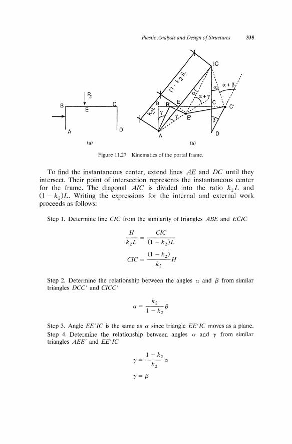
Plastic Analysis and Design of Stnlctures 335

--1 r2 c E

10 A 0 A

(a) (b)

Figure 11.27 Kinematics of the portal frame.

To find the instantaneous center, extend lines AE and DC until they intersect. Their point of intersection represents the instantaneous center for the frame. The diagonal AIC is divided into the ratio k2L and (1 - k 2 )L. Writing the expressions for the internal and external work proceeds as follows:

Step 1. Determine line CIC from the similarity of triangles ABE and ECIC

H CIC

k2L (1 - k 2)L

(1 - kz) CIC= H

k2

Step 2. Determine the relationship between the angles a and 13 from similar triangles DCC' and CICC'

k2 a= --13

1 - kz

Step 3. Angle EE'IC is the same as a since triangle EE'IC moves as a plane.

Step 4. Determine the relationship between angles a and y from similar triangles AEE' and EE'IC

1 - k2 y= ---a

k2

y=f3

336 Plastic Analysis and Design of Structures

This is true when the height of the columns is the same on both sides. Step 5. Add the angles a and f3 and 'Y and a

and

1 'Y + a = --f3

1 - k2

From the above relationships and by using the concept of virtual work, the expressions for external and internal work are

1 W1 = 2Mp--f3

1 - k2

WE = P1k j H j + P2(1 - k 2 )Lf3

(1 - k 2 ) Mp = 2 [kjPjH + (1 - k 2 )P2L]

When k2 = t and kl = 1,

Example 11.15

(11.88)

(11.89)

(11.90)

Given a frame that has a span of 75 ft and height of 20 ft with loads P2 = 30 k applied 25 ft from the left column and PI = 10 k applied 16 ft from the support on the left column, design the frame.

Solution

k j = 0.80 and

With the values of the k's established, proceed with the application. Beam mechanism

kzC1 - k 2 )P2 L Mp = 2 [from Equation (11.81)]

0.333(1 - 0.333)1.7 X 30 X 75

2

= 425 ft k

Plastic Analysis and Design of Structures 337

Column mechanism

P1k1H Mp = -2- [from Equation (11.83)]

1.3 X 0.80 X 10 X 20

2

= 104 ft k

Beam mechanism in the left column

0.8(1 - 0.8) X 1.3 X 10 X 20

2

= 22.9 ft k

Combined mechanism

( 0.333 ) = (1 - 0.333) 0.667 X 10 X 20 + 30 X 75 X 1.3

= 679 ft k controls

Use W27 X 84, Mp = 732 ft k.

11.10 PLASTIC ANALYSIS OF GABLED FRAMES

The geometric relationship between rotations for the various failure mech­anisms, displacements, and virtual work is more complicated for gable frames than for continuous beams and portal frames. The method of instantaneous center is used to assist in formulating these relationships. For the structure shown in Figure 11.28, the angle of rotation b will be assigned an arbitrary value and all other rotations and displacements found in terms of it.

The failure mechanisms and principle of virtual work are applied to the gable structure shown in Figure 11.28. The three basic failure mechanisms are presented in Figure 11.29.

338 Plastic Analysis and Design of Structures

Figure 11.28 Gable frame.

Ie

(a) (b)

F'

(d)

Figure 11.29 Kinematics of the gable frame.

Plastic Analysis and Design of StlUctures 339

The diagrams in Figures l1.29a and l1.29b represent the beam mecha­nism in the girders. The expression for the plastic moment is taken from Equation (11.41). For the left girder,

(11.91)

For the right girder,

(11.92)

For a symmetrical system in which L1 = L2 = L/2, k1 = k2 = k, and P2 = P3 = P, the plastic moment is

k(1 - k)PL Mp = 4 (11.93)

where

L = the span of the frame

For an unsymmetrical frame, the larger of the moments as given by Equations (11.91) and (11.92) is used in representing the beam failure mechanism.

Since lateral forces are relatively small when compared with gravity loads, the moment from the column mechanism will not control the design.

12 Influence Of Axial Forces

on Plastic Moment

12.1 INTRODUCTION

In Chapter 11, the analysis is based on the principle of pure bending. Although this assumption is valid for continuous beams, other secondary effects have to be included in the analysis and design of frames. Secondary effects are attributed to a number of factors such as axial forces, shear forces, buckling (local, lateral, column), repeated loading (fatigue), and brittle fracture. In this text, only the effect of axial loads and shear forces will be included in considering a plastic failure in members of a structural system. The analysis of plastic failure is based on the theory of small deformations.

The procedure for the analysis and design of frames begins with the selection of structural members on the basis of pure bending. The effects of axial and shear forces are introduced, and a check on the adequacy of selected members is made based on AISC specifications. If the initial selection is found inadequate, new sizes are selected and checked. The final selection must satisfy bending, axial, and shear force requirements.

12.2 INFLUENCE OF AXIAL FORCES ON PLASTIC MOMENT CAPACITY

When a member is subjected to axial forces in addition to bending, the magnitude of the plastic moment of that member is reduced. For ordinary

340

Influence of Axial Forces on Plastic Moment 341

portal frames, the axial load is small and its effect may be ignored. However, in cases for which the axial forces are relatively large, their effect must be included in the analysis of the frame.

Figure 12.1 shows the stress pattern under a combination of bending and axial forces. Consider the stress diagram depicted in Figure 12.lf that represents the plastic condition at failure. As illustrated in Figure 12.2b, a part of the stress distribution in this diagram is caused by the axial force. The remainder is due to bending. The stress diagram is divided into two diagrams. The one representing the axial force consists of a core symmetri­cally distributed about the centroidal axis and is as shown in Figure 12.2d. The second part is presented in Figure 12.2c and is equivalent to the moment MpC' the failure moment under the combined action of bending and axial loads.

For the case when the stress due to P is confined to the web only, the magnitude of P is expressed as

(12.1)

"-'-'"7- - - --- - -- -- r4--""1" <tb

.... ...... C.A.

~

1=======:::1 --------....... -~ O"t b <ta

(a) (b) (el

O"y cry r4---!:::.-~ - - - - - - - - - - ,-----r - - - - - - - - - "1--":""---,

Io.-...~-=:-__ ' ____________ •

cry (d) (e) (fJ

Figure 12.1 Neutral axis falling in the web for combined axial force and bending on beams in the plastic range.

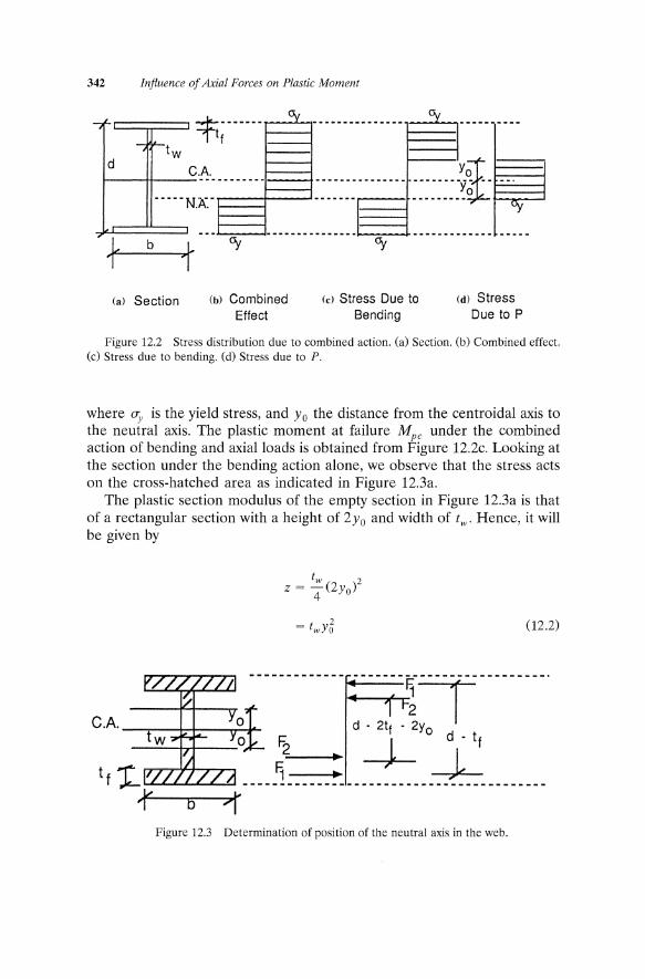
342 Influence of Axial Forces on Plastic Moment

1f-C::=~-;~='t=W:::J 't.;"""""" Oy """"""""""""""" §""""" I-d_-I+_--=-C,!',: _________ 1_--+ ________________ -_-_-_-_-_-_-_~_"~" l==::]

-----N.A~ -r===,--' -- ............ - .......... _-- --- ........... _---- ..........

~ b 'r 0y 0y

1

(a) Section (b) Combined (e) Stress Due to (d) Stress Effect Bending Due to P

Figure 12.2 Stress distribution due to combined action. (a) Section. (b) Combined effect. (c) Stress due to bending. (d) Stress due to P.

where iJy is the yield stress, and Yo the distance from the centroidal axis to the neutral axis. The plastic moment at failure Mpc under the combined action of bending and axial loads is obtained from Figure 12.2c. Looking at the section under the bending action alone, we observe that the stress acts on the cross-hatched area as indicated in Figure 12.3a.

The plastic section modulus of the empty section in Figure 12.3a is that of a rectangular section with a height of 2yo and width of two Hence, it will be given by

(12.2)

CA --,---++--,.,r.., .....

-------~-~---------.

1 t-2.. I d - 2tj - 2y

'2=--__ .. ~ -J- o~ t f :LL.L...o<....L.L-L.-L...~ ____ !!_-_-__ -_-_~~ ___________________________ _

v 1 b

Figure 12.3 Determination of position of the neutral axis in the web.

Influence of Axial Forces on Plastic Moment 343

The plastic section modulus for the equivalent section that is represented by Figure 12.3a is

Zpc = Z - z (12.3)

where

Z = plastic section modulus of the full section Zpc = plastic section modulus for the section under the cmbined action of axial

and bending forces z = Plastic section modulus for the empty section shown in Figure 12.3a

The plastic moment can be expressed as

(12.4)

The value of Yo IS obtained from Equation (12.1) and substituted in Equation (12.4)

(12.5)

Note that

(12.6)

Simplifying Equation (12.5) yields

(12.7)

Dividing both sides of Equation (12.7) by Mp gives

(12.8)

Substituting Equation (12.6) in Equation (12.8) and noting that A O'y = Py ,

we can express Equation (12.8) as follows:

(12.9)

344 Influence of Axial Forces on Plastic Moment

I l-=:lif

C.A.

f-.~tw N.A.

cry

(a)

'1

T' I --

~ c 2yo

/

1-1 ~ L I Uy

(c) Bending (e) compression

Figure 12.4 Determination of the neutral axis in the flange (a) Beam cross section. (b) Stress diagram. (c) Bending. (d) Area under compression. (e) Compression.

Equation (12.9) applies only when the following equation is satisfied:

(12.10)

When the neutral axis falls in the flange as in Figure 12.4a, a different expression for P is developed.

The value of the axial force can be obtained once the cross-hatched area is defined. Let the equivalent area be denoted by Ac

(12.11)

Influence of Axial Forces on Plastic Moment 345

.-r b • .r r -----,- -,------ l/ b 1/ 1.1'-----~1

d r il-------J--------

(a) (b)

Figure 12.5 Generalized section.

and

(12.12)

Consider that Figure 12.4d consists of two rectangles having a width of b and heights of d and 2yo, respectively. The inner rectangle is void of any bending stress. Thus, its plastic section modulus can be considered a negative quantity. See Figure 12.5.

The plastic section modulus for the section shown in Figure 12.5 is given by the equation

Zpc = ZI - Z2 (12.13)

where

bd2

ZI=-4

(12.14)

and

Z2 = by~ (12.15)

Then,

Mpc = bCTy ( d: _ y~) (12.16)

346 Influence of Axial Forces on Plastic Moment

The expression for Yo is obtained from Equation (12.12)

YO=~-~(A-~) 2 2b u y

Combining Equations (12.16) and (12.17) yields

Mpc = uy [d(A -~) - ~(A - ~)2l 2 u y 2b u y

Equation (12.18) can be expressed in nondimensional form as

Mpc = ~[d(l _~) -~(1 -~)2l Mp 2Z Py 2b Py

where

Z = the plastic section modulus On.3 )

Py= uyA

The above equation should conform to the following condition:

Example 12.1

(12.17)

(12.18)

(12.19)

(12.20)

Given the frame shown in Figure 12.6, design the columns and girder using the plastic method for A-36 steel. Check for the effect of axial load on the moment capacity.

Solution

For the beam mechanism type of failure, refer to Figure 12.6b. The external work WE is

WE = 1.7 X 2 X 40 X 20e X ~

= 13,60e kip ft.

Influence of Axial Forces on Plastic Moment 347

40'

(a)

(c)

Figure 12,6 Portal frame design example.

The internal work ~ is

TfJ = Mp() + 3Mp(2()) + Mp()

= 8Mp()

Equating external with internal work yields

Mp = 170 kip ft.

(b)

(d)

Next, check the column mechanism type of failure as shown in Figure 12.6c

WE = 1.3 x 20 x 20()

= 520() kip ft.

The expression for internal work is written as follows:

348 Influence of Axial Forces on Plastic Moment

From the geometry of the frame in Figure 12.6c, the value of f3 is determined from the following relationship:

Then,

and

Mp = 156 kip ft.

The combined mechanism of failure is shown in Figure 12.6d. From the geometry of the frame in its failure position, the relationship between f3 and e is established

The expressions for external and internal work are

WE = 1.3 x 2 x 40 x 20 x {3 x ~ + 1.3 x 20 x 20{3

= 1560{3 k/ft

ftJ = 8Mp {3 + Mp{}

= ~M {3 3 p

Then, the value of the moment is obtained for the combined mechanism

Mp = 167 kip ft.

It is clear from the three mechanisms of failure that the beam mecha­nism controls design.

Selection of Sizes

The girder size is obtained with

Mp = 3 x 170

= 510 kip ft.

Use W24 X 68; Mp = 530 kip ft. for the column size. Try W18 X 35; Mp = 200 kip ft. Check for the effect of the axial load on the plastic moment capacity.

Influence of Axial Forces on Plastic Moment 349

The load carried by each column is

P = 68 k

and the ultimate capacity Py is

The above value for Py is obtained from the AISC plastic design selection table given in Part 2 of the Manual.

From the section physical properties given in the AISC Manual, Part 1, the following section properties are determined for the column:

d = 17.70 in.

tw = 0.300 in.

tf = 0.425 in.

Z = 66.5 in.3

A = 10.3 in.2

Use Equation (12.10) to verify whether the neutral axis falls in the web or not

P 68

Py 371

= 0.187

tw(d - 2tf ) 0.300 x (17.70 - 2 x 0.425)

A 10.3

= 0.491 > 0.183

From the above result and Equation (12.10), it can be concluded that the neutral axis indeed falls in the web of the column.

Equation (12.9) gives the relationship between the moment capacity without the axial load and that with one

M A2 (p)2 ;;; = 1 - 4twZ Py

Substituting the appropriate values of the terms in the above equation yields a value of Mpc = 191 k/ft.

13 Rigid Connections

13.1 INTRODUCTION

The method of plastic analysis is based on the premise that connections are rigid. Thus, connections play a significant role in the design of indeterminate structures. The basic requirements for the condition of rigid connections are:

1. Sufficient strength of the connections to absorb (resist) the moments in the frame as a result of the given loads.

2. Adequate rotation capacity in the joints to provide sufficient redistribution of the moments.

3. Attainment of an overall stiffness for the structure to keep the displace­ments relatively small.

4. Cost of fabrication must remain economical to provide an overall reduction in the cost of construction.

There are a variety of connections commonly used in steel construction. These are listed as follows:

350

1. Corner connection 2. Tee connection 3. Cross connection 4. Column or beam slice connection s. Column anchorage connection 6. Miscellaneous connections

Rigid Connections 351

13.2 STRAIGHT CORNER CONNECTION

In a typical frame, beams and columns are connected at right angles as shown in Figure 13.1. A free-body diagram for the corner, including the points for zero moment, is shown in Figure 13.2. B is chosen at the point of counterflexure in the beam, which is commonly L /4 in the fully developed plastic condition. In the absence of any lateral forces on the frame,

(13.1)

The shear in the column is assumed to be resisted by the column web

(13.2)

For a square corner, the column and beam have the same depth. A free-body diagram of the beam alone is presented in Figure 13.3. Summing the moments acting on the free-body diagram in Figure 13.3 to zero yields

(13.3)

where Vb is the shear force in the beam. From the diagram in Figure 13.2b, the shear force in the beam is shown to be equal to the shear in the column

(13.4)

and

(13.5)

Combining Equations (13.1), (13.3), (13.4), and (13.5) yields

T = Mp (1 _~) o d 2L

(13.6)

A free-body diagram of the flange at the corner provides the following relationship:

(13.7)

Substituting Equation (13.7) in Equation (13.6) and rearranging the terms yield

(13.8)

352 Rigid Connections

I I H

I / L , I I I I

(a)

(b)

.. ~ To ...

~J ~ ~r J ~ ... '1:- Ti

To T I (c) (d)

Figure 13.1 Straight corner connection.

Rigid Connections 353

8 Nb ...

de Vb .. To

V7- N

Ve ~ t;-" IN,

M To

L (a) (b)

Figure 13.2 Free-body diagram of corner connection.

Simplifying Equation (13.8) results in the following:

(13.9)

For a square corner in which de = db = d,

(13.10)

Substituting Tw = (J"y/ ..f3 in Equation (13.10) yields

(13.11)

~ ______ ~L~ __________ ~I Vb

Figure 13.3 Free-body diagram of one leg of a straight corner connection.

354 Rigid Connections

Example 13.1

A portal frame with a span of 60 ft and height of 20 ft carries a uniform load of 0.6 k/ft and wind force of 8 k applied at the top of the column. See Figure 13.4. The frame has a constant section throughout its length. Use plastic analysis to design the frame (constructed of A-36 steel).

Solution

The beam mechanism yields Mp = 230 ft k and the combined mecha­nism Mp = 227 ft k. It is obvious that the moment for the column mechanism is smaller than both. Hence, the frame must be designed for Mp = 230 ft k. Try W18 X 40.

Mp = 235 ft k.

d = 17.9 in.

tw = 0.315 in.

L = ~ X span = 15 ft

From Equation (13.11), the required thickness of the web is

{3 x 230 x 12 ( 17.9) tw= 36x17.92 1-2X15X12

= 0.394 > 0.315

The size selection is not satisfactory. Either choose a larger section or stiffen the web. Stiffening the web is the subject of the next section.

0.6 klft

8~~1==========================~

60'

Figure 13.4 Portal frame example.

o C\J

Rigid Connections 355

13.3 STIFFENER FOR A STRAIGHT CORNER CONNECTION

Replacing Mp in Equation (13.11) by ZfTy yields

t = {3 Z(1 _ ~) W d 2 2L

and

Z = Sxf

where

f = shape factor of the section Sx = section modulus Gn.3)

Equation (13.12) is rewritten as

t = {3 j.S (1 - ~) W d2 x 2L

(13.12)

(13.13)

(13.14)

For most commonly used wide-flange sections, the product of 1(1 -d12L) is almost equal to unity. Thus, the required thickness of the web at the corner is expressed by

(13.15)

When the beam and column are of different sizes, then the thickness becomes

(13.16)

To meet the required strength at the corner without increasing the size of the section, a stiffener is needed at the corner. See Figure 13.5. From a free-body diagram of the top flange as shown in Figure 13.5, the sum of the horizontal forces is expressed as follows:

(13.17)

356 Rigid Connections

~========~==============~-----~~~ To

t;:;::=====~~============~ ..... -<<----- Tj

Figure 13.5 Stiffener design for corner connections.

U sing the yield strength of the stiffener and a square corner in which () = 45 deg and 'Ty = CTy/ IS, we can rewrite the above equation as

(13.18)

substituting Equation (13.6) in Equation (13.18) yields

(13.19)

Representing the left term in Equation (13.19) by

Sxf(I_~)a: d 2L y

Rigid Connections 357

and simplifying as before, the following expression is obtained:

bsts Sx twd Ii d-{3 (13.20)

The required area of the stiffener that is needed to strengthen the corner is derived from Equation (13.20)

(13.21)

Example 13.2

Consider the frame in Example 13.1. Design the stiffener for the corner. Use W18 x 40.

Solution

Sx = 68.4 in?

d = 17.9 in.

tw = 0.315 in.

_ ",(68.4 _ 0.315 X 17.9) bsts - v2 17.9 {3

= 0.80 in?

In welding the stiffeners to the web, the thickness of the stiffener must be of the same magnitude as that of the web. For a stiffener thickness of 0.25 in., the width of a double stiffener is 1.6 in. Use a width of 2 in. on each side of the web.

13.4 HAUNCHED CONNECTIONS

Haunches whether tapered or curved are pleasing to the eye, and they modify the section to follow more closely the shape of the moment diagram for the elastic and plastic conditions. The haunch helps to reduce the size of the main member considerably. If the cost of fabricating the haunch is high, it may offset the savings from the reduction of the member size. A feasibility study is recommended before deciding to use a haunched connection. The method of analysis of the frame remains the same with or without haunches.

358 Rigid Connections

L - 2 m ~~1~ ____________________________ ~.1 m I

1 h

", " L

(a)

Beam Mechanism

Column Mechanism One

(c)

Figure 13.6 Haunched corner connection.

Consider the portal frame with haunched corners as depicted in Figure 13.6.

Beam Mechanism

The beam mechanism is shown in Figure 13.6b. The plastic moment Mp is given by

(13.22)

Rigid Connections 359

Column Mechanism Two

(d)

29

Combined Mechanism One

(e)

Combined Mechanism Two

(f)

Figure 13.6 (cont'd.)

Column Mechanism

The external work due to the lateral load consists of two parts. The top m feet displace an equal amount, and the lower h - m feet displace a varying amount as illustrated in Figure 13.6c. The expressions for external and internal work are written as follows:

(13.23)

(13.24)

360 Rigid Connections

Combining Equations (13.23) and (13.24) yields

(13.25)

Another possibility for a column mechanism is shown in Figure 13.6d. The rotation at the bottom of the column is e, whereas the rotation of the plastic hinge in the beam is e + (3. The relationship between e and (3 is given by

2m {3= e

L - 2m (13.26)

and L

(}+{3= () L - 2m

(13.27)

Then, the expressions for external and internal work are written as follows:

and

where

WuL = factored lateral load

wuv = factored vertical load

Thus,

1 [ h2 ] (L - 2m ) Mp = - w uL - + wuv(L - m)m

4 2 L - m

Combined Mechanism

(13.28)

(13.29)

(13.30)

The combined mechanism mode of failure has two possibilities as shown in Figure 13.6e and 13.6f. The plastic moment for each of these two cases is the same and is given by the following:

h 2 L2 Mp = wuL 12 + wuv 24 (13.31)

Rigid Connections 361

Example 13.3

A portal frame carries a gravity load of 0.6 k/ft and may be exposed to a wind force of 0.5 k/ft. The frame has a span of 60 ft and height of 20 ft. Design the frame employing A-36 steel. Use plastic analysis.

Solution

1. Analysis

(a) Factored loads.

Gravity Load

Wuv = 1.7 X 0.6

= 1.02 kjft

Wind Load

WuL = 1.3 X 0.5

= 0.65 kjft

Combined Load

Assume the length of the corner connection to be 5 ft. (b) Beam mechanism.

(c) Column mechanism.

First column mechanism

w)L - 2m)2 M =-----

p 16

1.02(60 - 2 X 5)2

16

= 159.4 ft k

= t X 0.65(202 - 52)

= 30.5 ft k

362 Rigid Connections

Second column mechanism

1 [ h2 ] ( L - 2m ) Mp = - WuL - + wUV(L - m)m

4 2 L - m

x ~ [0.65 2~2 + 1.02(60 _ 5)5] ( 6600 -=- 150 )

= 96.2 ft k

(d) Combined mechanism.

2. Selection of Sizes

Try W18 X 35.

h 2 L2

Mp = wuL 12 + wuv 24

= 0.65 ( 21~2) + 1.02( ~042 ) = 174.7 ft k control

Mp = 200 ft k

tw = 0.300 in.

d = 17.7 in.

Sx = 57.6in.3

A = 10.3 in.3

(a) Check the adequacy of the web at the comer.

13 = --2 57.6

17.7

= 0.318 in. > 0.300

A stiffener must be used at the corner to strengthen it

h(SX twd) bsts = v2 d - 13

= {2 (57.6 _ 0.300 X 17.7) 17.7 13

= 0.27in.2

Use a stiffener Ii in. X i in. on one side only. (b) Check the flange.

b - = 7.1 < 8.5 2tt

Rigid Connections 363

(c) Check the effect of axial load on the capacity of the column. The axial load is

P = 1.02 X 30

= 30.6 k

Py = *371 k

An asterisk requires checking shape for compliance with Equations (N7-1) or (N7-2), Sect. N7 AISC ASD Specifications. Assume that girts are placed at 5 ft. on centers; check for the slenderness ratio

The y direction controls

ly = 5 ft

Ix = 20 ft

ry = 1.22 in.

rx = 7.04 in.

ly 5 X 12

ry 1.22

= 49

Ix 20 X 12

rx 7.04

= 34

Fa = 18.44 kjin?

Pcr = 1.7Fa A

= 1.7 X 18.44 X 10.3

= 322.9 k

Fe' = 62.2 kjin,z

23 X 62.2 X 10.3

12

= 1280 k

364 Rigid Connections

The interaction formulas in the AISC specifications are

30.6 --+ 322.9

em = 0.85

0.85 X 174.7

( 30.6 ) = 0.86 < 1.0

1 - -- 200 1280

30.6 174.7 371 + 1.18 X 200 = 0.82 < 1.0

The selection satisfies the required specifications. The next item to consider is the design of haunched connection.

13.5 HAUNCHED CONNECTIONS WITH CONCENTRATED LOADS

Figure 13.7 shows the various failure mechanisms for haunched portal frames subjected to concentrated loads.

Beam Mechanism

Figure 13.7b illustrates the failure mode for the beam mechanism

Then,

L - 2m WE = PI 2 ()

TVr = 4Mp

PI M = -(L - 2m)

p 8 (13.32)

Rigid Connections 365

L

(b)

( d ) (d)

(e)

(f)

Figure 13.7 Failure mechanism for a haunched corner connection in a portal frame.

366 Rigid Connections

Column Mechanism

(a) Failure in the column.

(b) Failure in the beam.

WE = P2(h - m)()

UJ = 4Mp()

Pz M = -(h - m)

p 4

WE = P2h()

(13.33)

If the angle swept by the column is considered to be (J, then the angle swept by the beam must be (J + {3. Then from Figure 13.7d, the relation­ship between (J and {3 is established as follows:

2m {3= ()

L - 2m

and L

{3+()= () L - 2m

The internal work is given by

Then,

P1h L - m M =----

p 4 L - 2m

Combined Mechanism

(13.34)

If the failure were to occur in the beam as shown in Figure 13.7e, the plastic moment is

L - 2m Mp = (~LPI + P2h)

6L - 8m (13.35)

For the failure mode depicted in Figure 13.7f, the plastic moment is given by the expression

(13.36)

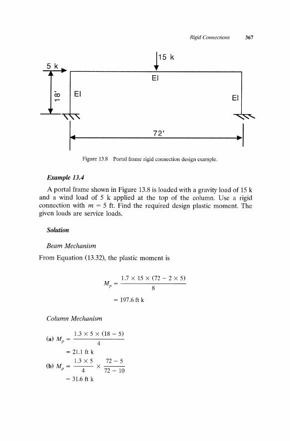
Rigid Connections 367

~15 k

EI

EI

72'

Figure 13.8 Portal frame rigid connection design example.

Example 13.4

A portal frame shown in Figure 13.8 is loaded with a gravity load of 15 k and a wind load of 5 k applied at the top of the column. Use a rigid connection with m = 5 ft. Find the required design plastic moment. The given loads are service loads.

Solution

Beam Mechanism

From Equation (13.32), the plastic moment is

Column Mechanism

M= p

1.7 x 15 x (72 - 2 x 5)

8

= 197.6ftk

1.3 x 5 x (18 - 5) (a) Mp = ---4---

= 21.1 ft k

1.3x5 72-5 (b) Mp = -4- x 72 _ 10

= 31.6 ft k

368 Rigid Connections

Combined Mechanism

72-2x5 (a) Mp = 1.3 X (~ X 72 X 15 + 5 X 18)

6x72-8x5

= 129.5 ft k

18 - 5 ( 15 X 72 ) (b) Mp = 1.3 X X 2 + 5 X 18

6 X 18 - 2 X 5

= 108.6 ft k

The beam mechanism controls. Hence,

Mp = 197.6 ft k

13.6 DESIGN GUIDES: CONNECTIONS

To develop full Mp at point H (see Figure 13.9), the required thickness of the web at the corner is

S being the section modulus of the given section.

...... -H "Ii~

I

IV

Ie b 4' , C:::::;:::;::=::l

Figure 13.9 Design of stiffeners for rigid connections.

(13.37)

d

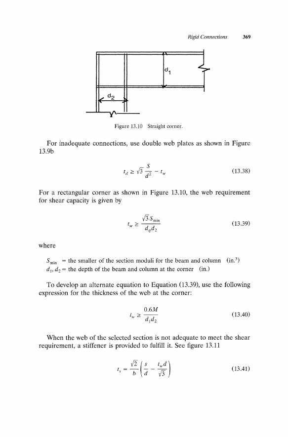
Rigid Connections 369

d 1 4-". d 2

A lI'

Figure 13.10 Straight corner.

For inadequate connections, use double web plates as shown in Figure 13.9b

(13.38)

For a rectangular corner as shown in Figure l3.1O, the web requirement for shear capacity is given by

where

V3Smin t >--­w - d d

q 2

(13.39)

Smin = the smaller of the section moduli for the beam and column (in.3)

d 1, d 2 = the depth of the beam and column at the corner (in.)

To develop an alternate equation to Equation (13.39), use the following expression for the thickness of the web at the corner:

(13.40)

When the web of the selected section is not adequate to meet the shear requirement, a stiffener is provided to fulfill it. See figure l3.11

t = 12 (!.- _ fwd) S b d V3 (13.41)

370 Rigid Connections

Figure 13.11 Stiffener for a straight corner.

where

b t <­s - 17

A conservative approach is to assume that ts = t, where

ts = the thickness of the stiffener t = the thickness of the tension flange for the beam or column

(13.42)

Tapered haunch connections are designed on the same basis. See Figure 13.12. The procedure is a step-by-step method.

1. Select the general layout. Brace at sections R, H, and P. See Figure 13.12.

2. Check the strength at section 1. Develop Mp at point 1

(13.43)

where

(13.44)

Rigid Connections 371

Figure 13.12 Haunched corner rigid connection for a gabled frame.

3. For Z = M1/sy, check haunch stability according to the following possible alternatives:

(a) For sib :s; 4.0,

t t =-­c cos f3

(13.45)

(b) For sib> 4.0, use Equation (13.45) and provide intermediate bracing or alternatively, the following.

(c) 4.0 < sib < 17.0

where

t 1 t =-­e cos f3

t 1 = thickness of tension flange

te = thickness of compression flange

(13.46)

(d) At point 1, the relationship Z1 » M11 l.Ty must be maintained and f3 > 24 deg.

372 Rigid Connections

t, = t

t, t =-­c cos f3

(13.47)

S. The thickness of the web for the connection is equal to that of the member.

6. The selection of bracing is discussed under the following heading.

Stiffeners for Tapered Haunch Connections

Refer to Figure 13.13. The following requirements must be met in the design of haunched and tapered connections:

M twd, ts ~ v2t, - 0.82 -b-

t s ~ Ii (1 - tan f3)t

b t >­s - 17

tr ~ tc tan f3

b t, ~ 17

One can use a conservative approximation by assuming that

Figure 13.13 Haunched corner rigid connection proportions.

(13 .48)

(13.49)

(13.50)

(13.51)

(13.52)

(13.53)

Rigid Connections 373

Figure 13.14 Curved haunched rigid connection.

Curved Tapered Connections

Figure 13.14 illustrates a curved connection. The design of a curved haunched rigid connection is outlined as follows:

1. Select the general layout of the connection and brace at points G, H, and C.

2. Check the haunch radius

4b R<­

a (13.54)

for 4 < R alb < 17, increase the tension and compression flange thickness according to

or provide additional bracing.

3. Select flange thickness to provide plastic moment at C or G

dm t=t=--

t c 2 d~b

-------4(b - tw)

(13.55)

(13.56)

374 Rigid Connections

where

dm = d + 0.02R

Mm = moment at am = 0.2 rad

One approximation that may be used is

4. Check cross-bending

(13.57)

5. Use for the haunch web thickness and width of the flange the same dimensions as those of the rolled section.

6. Select stiffeners according to Equations (13.48) through (13.53).

14 Multistory Buildings:

Plastic Design

14.1 INTRODUCTION

The use of plastic design concepts in the design of multistory steel building frames provides the structural engineer with yet another powerful tool in analysis and design. The concepts involved in this method have been well documented through several research projects sponsored by the AISC, Canadian Institute of Steel Construction (CISC), and several other na­tional facilities, private as well as military, that are connected to the building industry.

The purpose of this chapter is to acquaint the student and practitioner with the theory behind plastic design methods for braced frames. It is hoped that this introductory chapter may stimulate interest in exploring further the development of a viable procedure in the design of multistory buildings for braced frames, as well as moment-connected ones.

High-rise buildings have been constructed in this country for many years. However, the rapid urbanization of American society over the past few decades has forced developers to construct high-rise buildings in many more locations other than large cities. The continuous increase in the population and the even greater rise in land costs make the use of tall buildings more economical in housing and urban planning. Structural steel frames with the use of plastic design methods may offer savings over buildings utilizing other materials or steel frames designed by the allow­able stress methods.

375

376 Multistory Buildings: Plastic Design

To provide an organic design, the building process at present demands the integrated effort of several engineering teams: architects, and electri­cal, mechanical, and structural engineers. Each of these groups must understand the other disciplines in order to fully understand the total function of a building. Conduits both vertical and horizontal for the purpose of electrical and mechanical needs in the building must be provided for without adverse effects on the structural integrity of the frame or certain economic and spacial constraints. In the end, the frame must safely support all gravity and lateral forces due to wind, and to a certain extent earthquake forces, and remain aesthetically appropriate and complementary to the existing environment in which the building is lo­cated.

Fortunately, the structural engineer has at his or her hands the knowl­edge of more elaborate methods of analysis, new materials that are stronger than those used in the past, and the availability of computers. New high-strength carbon steel, high-strength bolts, welding equipment, and composite design using steel and concrete in floor construction pro­duce more economical buildings.

14.2 ALLOWABLE STRESS VS. PLASTIC DESIGN METHODS

The AISC has introduced LRFD as a viable method of design, to replace ASD at some point in the future. LRFD uses the elastic method of analysis, thus requiring sophisticated computational procedures for analyz­ing structural systems. The allowable stress method uses the same ap­proach to analysis as LRFD, but it is based on the assumption that the usefulness of a structural element is reached once a particular characteris­tic in that element attains its allowable limit. Other points in the structural system remain understressed, which renders this approach uneconomical. When a certain point in an indeterminate structural system reaches yield, redistribution of the internal forces takes place, allowing understressed members in the system to acquire more resistance to the applied loads. When this process is utilized in the design of indeterminate frames, a more economical system is obtained.

The plastic method for the analysis and design of indeterminate frames recognizes the above phenomenon in the behavior of structural systems subjected to external loads. The focus for the usefulness of a structure is shifted to the ultimate load limit that can be reached before a failure mechanism is induced, thus initiating the unrestrained deformation of the

Multistory Buildings: Plastic Design 377

structure. The ultimate load represents the strength capacity of the entire structure. The ratio of the ultimate load to the working stress load is known by the load factor F. Let the ultimate moment capacity of the structural system be denoted by Mp ' where

Mp = uyZ

uy = the yield stress (k/in.2) (14.1)

Z = the plastic section modulus Gn.3 )

and the working stress moment capacity by Ma , where

Ma = uaSx

S = the yield section modulus (in?)

Ua = the allowable stress (k/in.2)

(14.2)

Since the load factor has been defined by the ratio of the ultimate capacity to the allowable one, it is determined as follows:

(14.3)

Substituting Equations (14.1) and (14.2) in Equation (14.3) yields

(14.4)

The ratio of the plastic section modulus to the elastic one is known by /, the shape factor. Then, the load factor is expressed by

uyf F=- (14.5)

The average shape factor for American wide-flange sections is about 1.12. According to the AISC specification, the allowable stress for gravity

loads is

Then, Uy x 1.12

F= -'---0.66uy

= 1.70

(14.6)

The allowable stress for wind or earthquake forces and a combination of these forces with gravity loads is raised by 33% above that for the gravity loads. Thus, the load factor for lateral loads and a combination of

378 Multistory Buildings: Plastic Design

lateral and vertical loads is obtained from Equation (14.5) as follows:

or

-' ~

0 C')

"'f;" 0 (\J

..l~

0 C')

20' 1 25'

~

-%ists I

%'ists I

-----------

G"y x 1.12 F= --'-----

0.66 X 1.33G"y

= 1.276

F = 1.3

"'l 25'

A 4 ~A

I

., 20' -----------

----_ ... _----

CD ® ® - - - - - - - - - - - - - - - - - - - - Indicates bracing

2 1/2" Lt. wI. concrete slab (120 Iblft)

1 1/2" fire rated

Section A-A at exterior girders

Figure 14.1 Building floorplan and section of an exterior girder.

-(0

-CD

-0

-0

Multistory Buildings: Plastic Design 379

14.3 APPLICATION TO MULTISTORY BUILDINGS

Consider the building presented in Figures 14.1 and 14.2. The design process involves four stages. Stage 1 considers the design of the unbraced bent for gravity loads only. Stage 2 involves the design of braced bents for combined loads. Stage 3 consists of checking columns, girders, bracing, shear, and uplift. The final stage will include the design of connections.

The structure under consideration is an office building located in downtown, Greensboro, North Carolina. The building loads are tabulated below:

FLOOR LOADS

3t-in. reinforced concrete slab Floor finish Ceiling Partitions Joists

MECHANICAL

Total dead load Live load Total load Exterior walls: 60 Ib/ft 2 X 9.67 ft Parapet: 60 Ib /ft 2 X 4 ft

ROOF LOADS

3t-in. reinforced concrete slab Roofing Insulation Ceiling Joists

MECHANICAL

Total dead load Live load Total load Exterior walls: 60 Ib /ft 2 X 9.67 ft Parapet: 60 Ib/ft 2 X 4 ft

431b/ft 2

1 5

20 4

5lb/ft 2

78 50

128 580 250

43 3 5 5 2

5lb/ft 2

63 20 83

580 250

For the wind, use the ASCE 7-88 Standard of 10 lb jft 2 throughout the height of the building.

The design of floor girders is similar to those of the roof. In designing floor girders, the working live loads must be modified by applying the following reduction factor:

380 Multistory Buildings: Plastic Design

~ 3' - 0" Parapet

Figure 14.2 Evaluation of 27-story building.

The design of columns in multistory buildings is controlled by the factored load placed on every girder. It is sufficient for a preliminary design to use the axial loads and moments obtained from this loading condition. A "checkerboard" live load condition will produce different moment and end-restraint conditions. Unless the ratio of dead load to total load is less than 0.75 and the adjacent girders have almost equal spans and loads, the checkerboard loading condition can be neglected.

The design of roof and floor girders for the unbraced bent A is given in Tables 14.1 and 14.2, respectively. Table 14.3 presents a summary of the loads from the roof and a typical floor for interior and exterior columns.

The-oolttmIi load calculations are listed in Tables 14.4 and 14.5. The increments for the dead and live loads on an exterior column are 46.3 and 18.75 k, respectively. For an interior column, these increments are 56.4 and 40.63 k, respectively.

Multistory Buildings: Plastic Design 381

TABLE 14.1 Design of Roof Girders: Unbraced Bent A

Bay

Line Item Unit Operation Exterior Interior

Bay span ft 30 20 2 Bent spacing ft 25 25 3 Unit DL + LL on roof Ib/ft 2 83 83 4 Estimated column depth ft 1.0 1.0 5 Clear span ft (1)-(4) 29 19 6 Roof load on girder k/ft (2) X (3) 2.08 2.08 7 Estimated DL of girder k/ft 0.04 0.03 8 Working load k/ft (6) + (7) 2.12 2.11 9 Factored load F = 1.7 k/ft (8) X 1.7 3.60 3.59

10 Required Mp k/ft (9) X (5)2/16 189.2 81.0 11 Required Z in.3 (10) X 12/36 63.0 27 12 Section W18 X 35 W14 X 22 13 Z provided in.3 66.5 33.2

Column Moments

The equilibrium of moments at the girder-column connection is ex­pressed as follows:

where

Mjt = moment at the top of the column for joint j

Mjb = moment at the bottom of the column for joint j

MjL = moment in the girder at the left end

MjR = moment in the girder at the right end

Mje = moment in the column due to eccentric loading

(14.7)

The left-hand side of Equation (14.7) represents the total moment transferred from the girders to the column. The columns will also resist bending moments imposed on them by the girder end moments and shears. From Figure 14.3, the total moment at the centerline of the column from each girder is given by the equation

(14.8)

(14.9)

382 Multistory Buildings: Plastic Design

TABLE 14.2 Design of Floor Girders: Unbraced Bent A

Line Item Unit

Bay span ft 2 Bent spacing ft 3 Unit DL on floor lb Ift2 4 Unit LL on floor lb Ift2

Live Load Reduction

5 Floor area ft2

6 Minimum reduced live load lb Ift2

7 L = Lo ( 0.25 + ; ) lb Ift2

8 Selection of reduced LL lb Ift2 9 Estimated column depth ft

10 Clear span ft 11 Floor, DL on girder k/ft 12 Estimated DL of girder ft 13 Reduced LL on girder k/ft 14 Working load k/ft 15 Factored load k/ft 16 Required Mp k/ft 17 Required Z in.3

18 Selected section 19 Capacity of girder (given Z) in. 3

where

de = the depth of the column (in.)

L g = the length of the girder

Bay

Operation Exterior Interior

30 20 25 25 78 78 50 70

(1) X (2) 750 500 0.5 X (4) 25 35

Lx (4) 31.9 50.7

Largest of (6) or (7) 31.9 50.7 1.0 1.0

(1)-(9) 29 19 (2) X (3) 1.95 1.95

0.05 0.04 (8) X (2) 0.80 1.27 (11) + (12) + (13) 2.80 3.26 1.7 X (14) 4.76 5.54 (15) X (1W 116 250.2 125.0 (16) X 12/36 83.4 41.7

W21 X 44 W16 X 26 95.4 44.2

MjR and MjL represent the moments at the column ends. They have opposite signs when forming a single curvature. For double curvature in the column, the moment signs are both positive. Equations (14.8) and (14.9) are introduced to the calculations of column moments and are summarized in Table 14.6. The moment diagram for the columns is shown in Figure 14.4.

Multistory Buildings: Plastic Design 383

TABLE 14.3 Column Loads: Unbraced Bent A

Column

Line Item Unit Operation Exterior Interior

Tributary area per floor.

1 From exterior bay (15 X 25) ft2 375 375 2 From interior bay (12.5 X 25) ft2 312.5 3 Total ft2 (1) + (2) 375 687.5 4 Unit roof load (DL + LL) lb Ift 2 83 83

Unit floor loads

5 Exterior bay: Dead-live lb Ift2 78 78 6 lb Ift2 50 50 7 Interior bay: Dead-live lb Ift2 78 8 Ib/ft2 70

Loads below roof

9 DL + LL from roof k (3) X (4) 31.1 57.1 10 DL of girder k 0.53 0.81 11 Estimated DL of column k 2.0 2.0 12 DL of parapet at 0.25 k/ft k 0.25 X 25 6.25 13 Working load below roof k Sum (9) to (12) 39.9 59.9

Loads per floor

14 DL from floor: Exterior bay k (1) X (5) 29.25 29.25 15 DL from floor: Interior bay k (2) X (7) 24.38 16 DL of girder k 0.53 0.81 17 DL exterior wall 0.58 k/ft k 0.58 X 25 14.5 18 Estimated DL of column k 2.0 2.0 19 Total DL per floor k Sum (16) to (19) 46.3 56.4 20 LL from floor: Exterior bay k (1) X (6) 18.75 18.75 21 LL from floor: Interior bay k (2) X (8) 21.88 22 Total LL per floor k (20) + (21) 18.75 40.63

EFFECT OF AXIAL FORCE ON PLASTIC MOMENT CAPACITY

Previously, it has been demonstrated that axial force reduces the plastic moment capacity in a structural member under combined effect. This relationship is given by the equation

- = 1.18 1 --Mpc (P ) Mp Py

(14.10)

w

TA

BL

E 1

4.4

Ext

erio

r C

olum

n co

"'" T

ribu

tary

R

educ

ed

Sum

of

DL

1.

7 X

S

um

1.3

X S

um

DL

A

rea

Red

ucti

on

Sum

of

LL

C

olum

n +

Red

uced

D

L +

Red

uced

D

L +

Red

uced

L

evel

(k

) (f

t2)

Fac

tor

(k)

LL

(k)

L

L (

k)

LL

(k)

L

L (

k)

Roo

f 26

39

.9

375

0.80

18

.75

15.0

0 54

.9

93.3

71

.4

25

86.2

75

0 0.

64

37.5

0 24

.00

110.

2 18

7.3

143.

3 24

13

2.5

1125

0.

57

56.2

5 32

.1

164.

6 27

9.8

214.

0 23

17

8.8

1500

0.

52

75.0

0 39

.0

217.

8 37

0.3

283.

1 22

22

5.1

1875

0.

49

93.7

5 45

.3

271.

0 46

0.7

352.

3 21

27

1.4

2250

0.

47

112.

5 52

.9

324.

3 55

1.3

421.

6 20

31

7.7

2625

0.

46

131.

25

60.4

37

8.1

642.

8 49

1.5

19

364.

0 30

00

0.44

15

0.0

66.0

43

0.0

731.

0 55

9.0

18

410.

3 33

75

0.43

16

8.75

72

.6

482.

9 82

0.9

627.

8 17

45

6.6

3750

0.

42

187.

50

78.8

53

5.4

910.

2 69

6.0

16

502.

9 41

25

0.42

20

6.25

86

.6

589.

5 10

02.2

76

6.4

15

549.

2 45

00

0.41

22

5.0

92.2

64

1.4

1090

.4

833.

8 14

59

5.5

4875

0.

40

243.

75

97.5

69

3.0

1178

.1

900.

9 13

64

1.8

5250

26

2.50

10

5.0

746.

8 12

69.6

97

0.8

12

688.

1 56

25

281.

25

112.

5 80

0.6

1361

.0

1040

.8

11

734.

4 60

00

300.

00

120.

0 85

4.4

1452

.5

1110

.7

10

780.

7 63

75

318.

75

127.

5 90

8.2

1543

.9

1180

.7

09

827.

0 67

50

337.

50

135.

0 96

2.0

1635

.4

1250

.6

08

873.

3 71

25

356.

25

142.

5 10

15.8

17

26.9

13

20.5

07

91

9.6

7500

37

5.00

15

0.0

1069

.6

1818

.3

1390

.5

06

965.

9 78

75

393.

75

157.

5 11

23.4

19

09.8

14

60.4

05

10

12.2

82

50

412.

5 16

5.0

1177

.2

2001

.2

1530

.4

04

1058

.5

8625

43

1.25

17

2.5

1231

.0

2092

.7

1600

.3

03

1104

.8

9000

45

0.00

18

0.0

1284

.8

2184

.2

1670

.2

02

1151

.1

9375

46

8.75

18

7.5

1338

.6

2275

.6

1740

.2

01

1197

.4

9750

48

7.50

19

5.0

1392

.4

2367

.1

1810

.1

00

1243

.7

10,1

25

506.

25

202.

5 14

46.2

24

58.5

18

80.1

TA

BL

E 1

4.5

Inte

rior

Col

umn

Tri

buta

ry

Red

uced

S

um o

f D

L

1.7

X S

um

1.3

X S

um

DL

A

rea

Red

ucti

on

Sum

of

LL

C

olum

n +

Red

uced

D

L +

Red

uced

D

L +

Red

uced

L

evel

(k

) (f

t2)

Fac

tor

(k)

LL

(k)

L

L (

k)

LL

(k)

L

L (

k)

Ro

of

26

59.9

75

0 0.

52

40.6

3 21

.1

81

137.

7 10

5.3

25

116.

3 15

00

0.44

81

.3

35.7

15

2.0

258.

4 19

7.6

24

172.

7 22

50

0.4

121.

9 48

.8

221.

5 37

6.6

288.

0 23

22

9.1

3000

0.

4 16

2.5

65.0

29

5.1

500.

0 38

2.3

22

285.

5 20

3.2

81.3

36

6.8

623.

6 47

6.9

21

341.

5 24

3.8

97.5

43

9.4

747.

0 57

1.2

20

398.

3 28

4.4

113.

8 51

2.1

870.

6 66

5.8

19

454.

7 32

5.1

130.

0 58

4.7

994.

0 76

0.0

18

511.

1 36

5.7

146.

3 65

7.4

1117

.6

854.

6 17

56

7.5

406.

3 16

2.5

730.

0 12

41.0

94

9.0

16

623.

9 44

6.9

178.

8 80

2.7

1364

.5

1043

.4

15

680.

3 48

7.6

195.

0 87

5.3

1488

.0

1137

.9

14

736.

7 52

8.2

211.

3 94

8.0

1611

.6

1232

.4

13

793.

1 56

8.8

227.

5 10

20.6

17

35.0

13

26.8

12

84

9.5

609.

5 24

3.8

1093

.3

1858

.6

1421

.8

11

905.

9 65

0.1

260.

0 11

65.9

19

82.0

15

15.6

10

96

2.3

690.

7 27

6.3

1238

.3

2105

.1

1609

.8

09

1018

.7

731.

4 29

2.6

1311

.3

2229

.0

1704

.7

08

1075

.1

772.

0 30

8.8

1383

.9

2352

.6

1799

.0

07

1131

.5

812.

6 32

5.0

1456

.5

2476

.1

1893

.5

06

1187

.9

853.

2 34

1.3

1529

.0

2599

.6

1987

.9

05

1244

.3

893.

9 35

7.6

1601

.9

2723

.2

2082

.4

04

1300

.7

934.

5 37

3.8

1674

.5

2846

.6

2176

.8

03

1357

.1

975.

0 39

0.0

1747

.1

2970

.0

2271

.2

02

1413

.5

1015

.8

406.

3 18

79.8

31

95.6

24

43.7

t.

-01

14

69.9

10

56.4

42

2.6

1892

.5

3217

.2

2460

.2

QC

00

15

26.3

10

97.0

43

8.8

1965

.1

3340

.7

2554

.6

<II

386 Multistory Buildings: Plastic Design

v

(a)

(- M8

~(,)f J8 ~A

Mj8 rd2c .... (b)

Figure 14.3 Girder-column moment and shear designation.

where

Equation (14.10) may be expressed as follows:

(14.11)

(14.12)

(14.13)

Combining Equations (14.9) through (14.11) and using the value of Z/S = 1.12 for wide-flange sections (average value) and rx = 0.43d yield the following relationship:

(14.14)

TA

BL

E 1

4.6

Col

umns

Mom

ents

, Fac

tore

d G

ravi

ty L

oads

Col

umn

Lin

e It

em

Uni

ts

Ope

rati

on

Ext

erio

r In

teri

or

1 L

eft

gird

er r

equi

red

Mp

k ft

Tab

le 1

4.1

(10)

18

9.2

2 E

stim

ated

del

Lg

Tab

le 1

4.1

(4)/

(5)

0.03

45

3 A

t cen

tral

col

umn

MjB

= M

il +

4d c

/Lg

) k

ft

215.

3 4

Rig

ht g

irde

r re

quir

ed M

p k

ft

Tab

le 1

4.1

(10)

-1

89

.2

-81

.0

5 E

stim

ated

del

Lg

0.03

45

0.05

26

6 C

olum

n c

MjA

= M

il +

4d c

/Lg

) k

ft

-21

5.3

-9

8.0

7

Spa

ndre

l (6.

2 X

0.5

X 1

.7)

kft

14

.3 (

12)

dc/L

g +

5.3

8 C

olum

n m

omen

t at

roo

f k

ft

-[(3

) +

(6)

+ (7

) +

210

-11

7.3

Mom

ent a

t Lev

el 2

6-1

9 L

eft g

irde

r re

quir

ed M

p k

ft

Tab

le 1

4.2

(16)

+

250.

2 10

E

stim

ated

dc/

Lg

Tab

le 1

4.1

(4)/

(5)

0.03

45

11

Col

umn

c M

jB =

Mil

+ 4

d c/L

g)

kft

+

284.

7 12

G

irde

r ri

ght

kft

T

able

14.

2 +

250.

2 +

125.

0 13

E

stim

ated

dc/

Lg

0.03

45

0.05

26

14

Col

umn

c M

jA =

Mil

+ 4

d c/L

g)

kft

-2

84

.7

-15

1.3

15

S

pand

rel

14.5

(de

le)

1.7

14.5

X 0

.5 X

1.7

+

12.3

16

N

et g

irde

r m

omen

t on

join

t k

ft

-[(

11)

+ (1

4) +

(15

) 27

2.4

-13

3.4

17

C

olum

n m

omen

t 0.

5 X

(16

) +

136.

2 -6

6.7

... QC

....

388 Multistory Buildings: Plastic Design

117

136 136 67

136 136 67

136 136 67

136

67

Figure 14.4 Column moment diagrams.

The term Py in Equation (14.14) is an equivalent axial load that can be computed directly from the axial loads as determined in Tables 14.4 and 14.5. Then, the design of the column can follow the routine procedure outlined in the AISC Manual for concentric loads. Next, a check for wind on the stability of the structure will be conducted. It is not within the scope of this book to accomplish that.

Index

A

Allowable stress design, 13, 14, 15-17 Air, 201 Anchor bolts, 201 Architects, 375 Axial forces, 340-341, 383 Axial loads, 187, 340

B

Bars, 14 Base plates, 202-209 Beams:

analysis, 294-295 bending, 106, 118-120 compact members, 109-110, 114, 120 connections, 190 deflections, 116-117 exterior, 247 fixed end, 308, 311 flange buckling, 126 girders, 109 LRFD, 128-132 mechanism, 358 rolled beams, 210 section dimensions, 122 serviceability, 132 torsion (see Torsion) shear, 109, 115, 123, 127 stiffeners, 109 stress, 109, 121 symmetric, 109

Bending members, 106, 124, 133, 187, 210, 294-295, 340-341

Bolts: in tension members, 20 in building connections, 187

Bracing, 150-151 Bridge, 210, 246 Buckling, 46, 340

c

Columns: compression, 46, 63ff connections, 189 mechanism, 359-360, 366 steel, 6

Composite construction: advantages, 246 exterior beam, 247 loads, 249 LRFD flexural members, 285-286 LRFD method, 284-285 section properties, 266-279 shear connectors, 246-247, 251,

282-284, 287 slippage, 248, 282 stress, 259, 264

Compression members: ASD method, 49-50, 63-65 braced and unbraced frames, 82-105 columns, 63ff design stress, 60-62 Eulers formula, 47-49 flexural buckling, 73-75, 124 LRFD method, 54-60 slenderness ratio, 51-53

Connections: combined mechanism, 360-364,

366-368 corner, 351, 369 design guides, 368 framed beam, 190-200 haunch, 357-358, 364-365 joints, 187

389

390 Index

Connections (Cant.) responsibility, 187 rigid connections, 350 riveting, 187 stiffener, 355-357, 368 types, 350 welding, 187

Compression, 344 Computers, 376 Concrete, 201, 251, 376

E

Earthquake load, 13, 150ff, 175-186, 376

Euler, Leonard, 46 Euler's formula, 47-49

F

Fatigue, 340 Flange, 210 Fracture, 340 Framed beam connection, 190

G

Gages, 196 Girders, 196 Girts, 151

H

High rise, 375 Hooke's law, 7

L

Loads: axial, 187 collapse loads, 294

M

dead, 3-6, 13, 28, 106 design loads, 3-4 factors, 13 floor, 70 gravity loads, 106, 150 interior columns, 77-78 lateral, 150 live, 3-6, 13, 28, 65-68, 106 roof,70

Masonry, 201

N

Noise, 14

p

Plastic analysis: collapse, 294, 304 continuous beams, 319-329 elastic moment, 299-300 loads, 317-319 modulus, 299 plastic moment, 299, 320, 383 shape factor, 299-300 stress, 298-299 virtual-work, 336, 337 width-thickness, 332 yield, 298

Plastic design: ASD method, 309 assumptions, 307 beams, 304-306 braced frames, 375 frames, 320 gabled frames, 337-338 hinge, 305, 310 LRFD,376 mechanism, 310, 312-313, 320, 329,

330-331

moment diagrams, 384-385, 387-388 multistory buildings, 375, 379-380 portal frames, 329, 333, 335

Plastic failure, 340 Plastic moments, 340-349 Plate girders:

bending stress, 210-211, 214 bolted and riveted, 20 flanges, 210,214 shear, 212,214, 223 slenderness, 210 stiffeners, 210, 213 tensile field action, 212 tensile stress, 223 web, 210, 213

Post, 45 Purlin, 23, 26, 151

R

Railroads, 210 Riveting, 187, 210 Rods, 25 Roof, 150

s

Sag rods, 23, 25, 26 Seismic design, 175-186 Shear forces, 340 Shear walls, 150 Slab-beam, 246 Snow loads, 12, 13, 106, 154 Span, 210 Splices, 187-188

Stanchion, 46 Stress, 210 Stress-strain diagram, 7 Structural steel:

advantages, 4 ductility, 6-7 savings, 375 strength, 6 stress-strain, 294-295 tension members, 14

Strut, 46

T

Tension members: bolts, 20 buckling, 25 slenderness, 25 staggered holes, 21 stiffness, 25

Torsion, 133-149 Towers, 158 Truss, 25, 46

v

Vibration, 25

w

Warping, 136-137 Web, 210 Welding, 187, 196, 210 Wide-flange sections, 377 Wind load, 13, 150ff, 388

Index 391