design of steering wheel force feedback...
TRANSCRIPT

DESIGN OF STEERING WHEEL FORCE FEEDBACK SYSTEM WITH
FOCUS ON LANE KEEPING ASSISTANCE APPLIED IN DRIVING
SIMULATOR
Master’s Thesis in the Systems control and Mechatronics
Abolfazl Tahmasebi Inallu
Department of Signals and Systems
Division of Automatic control, Automation and Mechatronics
Mechatronics group
CHALMERS UNIVERSITY OF TECHNOLOGY
Göteborg, Sweden 2014
Master’s thesis 2014: EX063/2014

MASTER’S THESIS IN SYSTEMS CONTROL AND MECHATRONICS
DESIGN OF STEERING WHEEL FORCE FEEDBACK SYSTEM WITH
FOCUS ON LANE KEEPING ASSISTANCE APPLIED IN DRIVING
SIMULATOR
Systems control and Mechatronics
Abolfazl Tahmasebi Inallu
Department of Signals and Systems
Division of Automatic control, Automation and Mechatronics
Mechatronics group
CHALMERS UNIVERSITY OF TECHNOLOGY
Göteborg, Sweden 2014


I
DESIGN OF STEERING WHEEL FORCE FEEDBACK SYSTEM WITH
FOCUS ON LANE KEEPING ASSISTANCE APPLIED IN DRIVING
SIMULATOR
Systems control and Mechatronics
Abolfazl Tahmasebi Inallu
© ABOLFAZL TAHMASEBI INALLU 2014
Master’s Thesis 2014: EX063/2014
ISSN 1652-8557
Department of Signals and Systems
Division of Automatic control, Automation and Mechatronics
Mechatronics group
Chalmers University of Technology
SE-412 96 Göteborg
Sweden
Cover: Chalmers driving Simulator which was used in this project
Repro service / Department of Signals and Systems
Göteborg, Sweden 2014

II
III
DESIGN OF STEERING WHEEL FORCE FEEDBACK SYSTEM WITH
FOCUS ON LANE KEEPING ASSISTANCE APPLIED IN DRIVING
SIMULATOR
Master’s Thesis in the Systems control and Mechatronics
Abolfazl Tahmasebi Inallu
Department of Signals and Systems
Division of Automatic control, Automation and Mechatronics
Mechatronics group
Chalmers University of Technology
ABSTRACT
In recent years driving simulators are being widely used by automotive manufactures and
researchers especially related in Human-In-The Loop (HIL) experiments. Simulators help
researchers reduce prototyping time and cost. Simulators provide unlimited parameterization,
more safety and enhanced repeatability. They play an important role in studies of the driver’s
behaviour in unstable vehicle conditions and manoeuvres.
The goal of this thesis is to create a more real steering feeling for drivers in simulators. Increasing
the reality of the steering enhance the driving experience on simulator. The work is divided into
two parts; the first part is development of a steering wheel force feedback and the second part is
development of a Lane Keeping Assistance System (LKAS), where the steering wheel force
feedback system is a component. The steering force feedback system developed includes effect of
the kingpin and caster angles on tire forces and self-aligning torque, which have been shown to be
important factors for realizing good steering feeling.
In the second part an LKAS is proposed, the idea is to apply an assistance torque depending of
lateral offset and heading error in order to minimize trajectory overshoot. The calculated lane
keeping assistance torque is added to the steering system feedback torque. Chalmers simulator is
used to evaluate the proposed steering force feedback system and the LKAS. The simulator results
demonstrate that the LKAS reduces lateral offset of a vehicle and driver’s need to interfere with
the system and that the steering feeling is improved.
Key words: Steering Wheel feedback torque, driving simulator, lane-keeping assisting

IV

V
TABLE OF CONTENTS
Page
TABLE OF CONTENTS V
1. INTRODUCTION 1
1.1 Chalmers driving simulator 1 1.1.1 Computing component 1
1.1.2 Software for the simulator 2 1.1.3 Motion hardware 2
1.2 Master thesis’s goal 4
1.3 Model characteristics 5
1.4 Model limitations 5
2. VEHICLE DYNAMICS MODEL 7
2.1 VDM structure of XC90 Volvo used in this report 7
2.2 Coordinate systems 9
2.3 Model inputs and outputs 11
2.4 Model terminology 13
2.5 Tire modelling 14
2.5.1 TMEasy tire model 16
2.5.2 Longitudinal forces 16
2.5.3 Lateral force 17 2.5.4 Self-aligning torque 19
2.6 Vehicle model 21 2.6.1 Equations of motion 21
3. STEERING SYSTEM MODELING 23
3.1 Steering system overview 23
3.2 Mathematical modelling of steering system 29 3.2.1 Steering system forces and moments 30 3.2.2 Mathematical modelling of tire forces 32
3.2.3 Mathematical modelling of steering column 35
3.3 Friction torque modelling 37
3.4 Power steering modelling 38
4. LANE-KEEPING ASSISTANCE SYSTEM 43
4.1 Lane-keeping controller 44 4.1.1 Vehicle-road model 45 4.1.2 Lane-departure prevention controller 48
4.2 Modelling of force feedback generation for lane-keeping assistance torque 51
VI
5. STEERING WHEEL FORCE FEEDBACK IMPLEMENTATION ON DRIVING
SIMULATOR 53
5.1 PWM generation 54
5.2 Steering wheel feedback torque command 59
6. MODEL VALIDATION 61
6.1 Comparison model with measurement data 61
6.2 Steering response evaluating in driving simulator 63
6.3 Tests for evaluating the lane keeping assistance torque functionality in driving
simulator 66
7. CONCLUSION 69
8. RECOMMENDATION AND FUTURE WORK 70
REFERENCES 71
APPENDICES 73
APPENDIX A 74
APPENDIX B 75
APPENDIX C 77
APPENDIX D 80
VII
Preface
This Master’s thesis was carried out from October 2012 to December 2013 at the
Department of Signals and Systems at Chalmers University of Technology and
Electronics department of Istanbul Technical University.
This work wouldn’t have been possible without the enormous support provided by my
supervisor, Jonas Fredriksson, who supported me all the time during the thesis. I
would like to thank Jonas Sjöberg, research group leader of Mechatronics group for
his support in relation to driving simulator equipment problems.
I would also thank my advisor in Istanbul Technical University, Dr. Müştak Erhan Yalçın
who gave me the opportunity to work on my thesis at Chalmers University of Technology.
I also would like to thank my friends Alberto Morando, Artem Kusachov, Faouzi Al
Mouatamid, Gonçalo Salazar, Pontus Petersson, for helping me during the implementation
of model on the driving simulator.
My greatest appreciation and friendship goes to my closest friends, Mohammad
Kazem Hosseini and Toumaj Kohandel, who was always a great support in all my
struggles during my life.
Finally I owe special thanks to my girlfriend, Faezeh Navvab who supported me, I will
never forget it!
Göteborg January 2014
Abolfazl Tahmasebi Inallu

VIII

IX
Notations
ay Lateral acceleration
ax Longitudinal acceleration
az Verticalacceleration
AServo Area of the piston in the servo assistance cylinder
br Rack damping coefficient
bs Steering Wheel damping coefficient
bTB Torsion bar damping
Cf Front tires cornering stiffness
Cr Rear tires cornering stiffness
Cservo Steering servo assistance
CF Dahl model coulomb fricition level
D Steering wheel and coulmn damping
Drack Rack damping
FLong Longitudinal force of front left and right tires
FLat Lateral force of front left and right tires
Fp Force acting on the pinion
Fr Force on the rack
Frolling i Rolling resistance force at wheel i.
Fyf Lateral force of front tire
Fyr Lateral force of rear tire
FServo Servo assistance force
FL Front left
FR Front right
FXi Total tire force in longitudinal direction
FYi Total tire force in lateral direction
FZi Total tire force in verical direction
JSW Steering wheel moment of inertia.
JZ Vehicle moment of inertia with respect to z axis.
KS Steering wheel stifness constant
KTB Torsion bar stifness constant
X
l Vehicle length
Larm Steering arm lever length
lf Distance between front tire and COG
lr Distance between rear tire and COG
m Vehicle mass
MZ Self-aligning torque
rp Pinion radius
rKP Scrub radius
R Radius of tire
Rl Rear left
Rnom Tire nominal radius.
RR Rear right
S Longitudinal tire slip
u Longitudinal velocity of COG
v Lateral velocityoF COG
Vx Longitudinal velocity of vehicle
Vy Lateral velocity of vehicle
xr Rack displacement
rx Rack velocity
γ King pin angle
𝛉SW Steering wheel angle
𝛅 Steering angle
𝛔 Dahl stiffness coefficient
ψ , Yaw angle and yaw rate
τ Torque
θP Pinion angle
β Side slip angle
αf ,r Front and rear tire slip angle
𝛚 Rotational velocity
CHALMERS, Signals and Systems, Master’s Thesis 2014: 1
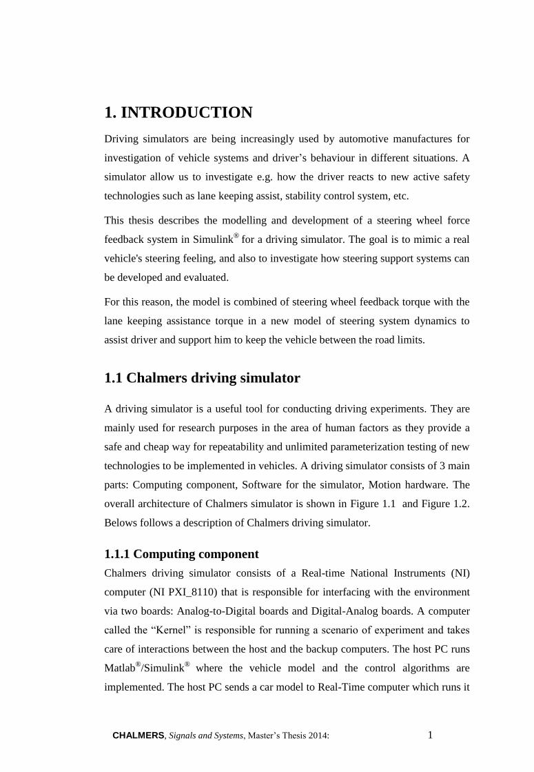
1. INTRODUCTION
Driving simulators are being increasingly used by automotive manufactures for
investigation of vehicle systems and driver’s behaviour in different situations. A
simulator allow us to investigate e.g. how the driver reacts to new active safety
technologies such as lane keeping assist, stability control system, etc.
This thesis describes the modelling and development of a steering wheel force
feedback system in Simulink®
for a driving simulator. The goal is to mimic a real
vehicle's steering feeling, and also to investigate how steering support systems can
be developed and evaluated.
For this reason, the model is combined of steering wheel feedback torque with the
lane keeping assistance torque in a new model of steering system dynamics to
assist driver and support him to keep the vehicle between the road limits.
1.1 Chalmers driving simulator
A driving simulator is a useful tool for conducting driving experiments. They are
mainly used for research purposes in the area of human factors as they provide a
safe and cheap way for repeatability and unlimited parameterization testing of new
technologies to be implemented in vehicles. A driving simulator consists of 3 main
parts: Computing component, Software for the simulator, Motion hardware. The
overall architecture of Chalmers simulator is shown in Figure 1.1 and Figure 1.2.
Belows follows a description of Chalmers driving simulator.
1.1.1 Computing component
Chalmers driving simulator consists of a Real-time National Instruments (NI)
computer (NI PXI_8110) that is responsible for interfacing with the environment
via two boards: Analog-to-Digital boards and Digital-Analog boards. A computer
called the “Kernel” is responsible for running a scenario of experiment and takes
care of interactions between the host and the backup computers. The host PC runs
Matlab®/Simulink
® where the vehicle model and the control algorithms are
implemented. The host PC sends a car model to Real-Time computer which runs it

2 CHALMERS, Signals and Systems, Master’s Thesis 2014:
and sends the car state interaction to Kernel. The Kernel sends the received
information (car’s positions, accelerations, speeds...) to another computer called
gateway/backup computer. Basically, the motion platform is controlled by these
four computers.
1.1.2 Software for the simulator
Software from Matlab®/ Simulink
® and NI Veristand (Lab View) is used for the
operation of the simulator. The vehicle dynamics is configured in Matlab®/
Simulink® model, with 14 DOF (Degree Of Freedom) model which has been
developed as a master thesis by Benito& Nilsson in Chalmers at 2006. All
characteristics of the model such as constants and relevant information has been
derived to reasonable a Volvo XC90 specification. It incorporates steering
geometry, vehicle control, powertrain, brakes, wheels, suspension dynamics,
steering system model, chassis, etc. The Vehicle Dynamics Model (VDM) is being
executed at 1 kHz at the “slave” board.
1.1.3 Motion hardware
The driving simulator can render inertial and steering feel through the motion
platform and the Force Feedback Steering Wheel (FFSW) respectively. The
motion platform consists of two main parts: Cockpit, where the driver is seated
and a Moog Stewart platform. The cockpit consists of a quarter of a Volvo S80,
which is mounted on an electrically powered six degree of freedom Stewart
platform and provides the interaction between the driver and the vehicle system.
The Moog stewart platform consists of two platforms and six linear actuators
connecting through universal joints. The stewart platform has 6 DOF, which gives
the possibility to perform different forms of displacements.
The steering wheel feedback plays an important role to create high reality feel of
driving in driving simulator. Chalmers simulator employs a brushless DC servo
motor to create a steering wheel feedback torque on the steering wheel. The motor
is mounted on the shaft behind steering wheel.

CHALMERS, Signals and Systems, Master’s Thesis 2014: 3
Figure 1.1: Simulator architecture

4 CHALMERS, Signals and Systems, Master’s Thesis 2014:
Figure 1.2: Chalmers S2 driving simulator
1.2 Master thesis’s goal
The main goal of this thesis is to develop a new model of the steering system in
order to improve the steering wheel force feedback in Chalmers driving simulator.
The previous model is developed in Simulink®, see [2]. The model works well, but
the steering geometry model can be improved in Steering system model.
CHALMERS, Signals and Systems, Master’s Thesis 2014: 5
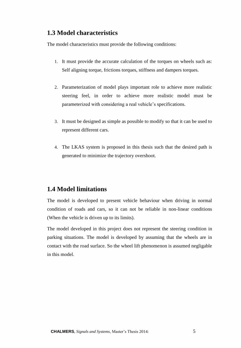
1.3 Model characteristics
The model characteristics must provide the following conditions:
1. It must provide the accurate calculation of the torques on wheels such as:
Self aligning torque, frictions torques, stiffness and dampers torques.
2. Parameterization of model plays important role to achieve more realistic
steering feel, in order to achieve more realistic model must be
parameterized with considering a real vehicle’s specifications.
3. It must be designed as simple as possible to modify so that it can be used to
represent different cars.
4. The LKAS system is proposed in this thesis such that the desired path is
generated to minimize the trajectory overshoot.
1.4 Model limitations
The model is developed to present vehicle behaviour when driving in normal
condition of roads and cars, so it can not be reliable in non-linear conditions
(When the vehicle is driven up to its limits).
The model developed in this project does not represent the steering condition in
parking situations. The model is developed by assuming that the wheels are in
contact with the road surface. So the wheel lift phenomenon is assumed negligable
in this model.

6 CHALMERS, Signals and Systems, Master’s Thesis 2014:

CHALMERS, Signals and Systems, Master’s Thesis 2014: 7
2. VEHICLE DYNAMICS MODEL
The aim of this section is to describe the vehicle model used in this thesis. As
mentioned earlier, the model, [2], is implemented in Matlab®/Simulnik®. The
model is made out of seven sub-blocks consisting of Steering geometry, vehicle
control, power train, brakes, suspensions, chassis and wheels.
The Simulink® model exists in two versions: offline and online.The differences
between the two models are in the input and output sources.
Online model or Hardware-in-the-loop mode can be used in Real-Time
simulations. The inputs in this mode are real signals that are transmitted from the
driver through steering wheel, acceleration pedal and brake pedals to the National
Instruments (NI) data acquire system.
Offline model is usually used during the early development phases before
connecting to the data acquiring system, when frequent changes are need to
configure the model.
2.1 VDM structure of XC90 Volvo used in this report
The model consists of 7 sub-blocks that model the steering geometry, power train,
brakes, wheels, suspension, chassis, vehicle control. The vehicle control block
consists of an active safety system used during simulation. Figure 2.1 shows a
schematic of the used VDM model in the report.

8 CHALMERS, Signals and Systems, Master’s Thesis 2014:
Figure 2.1: VDM structured in sub-blocks used in this project
The main sub-blocks are:
1. Steering geometry: This block is established to calculate the steering angle
of the wheels by using the steering wheel angle as input. Outputs of this
block are the wheel angle for front and rear tires of the model in
consideration of steering system forces and road condition.
2. Power train: The main goal of this block is calculation of the engine speed
and engine torque required in this model. In order to simulated the power
train of the simulated vehicle, The model is supplied with a 2,5 liter engine
and the corresponding automatic transmission system from Volvo cars.
3. Brakes: This block is used to model the actual braking torque applied to
the brakes for each wheel of the simulated vehicle. Brakes block contains a
simplified modeling of hydraulic brake.
4. Wheels: This block contains 4 subsystems for front and rear tires to
calculate the tire forces during steering. All the required information about

CHALMERS, Signals and Systems, Master’s Thesis 2014: 9
the tire forces and self aligning torque is calculated in this block. For this
reason this block has an important role in this project. In this item TMEasy
tire model is used as a virtual tire model. More details about the model are
presented in the tire model item.
5. Suspension: This block computes the load transfers and the individual
vertical load generated on each tire. In this model the toe and camber
angles for the wheel are constant. The absence of changing in toe and
camber angles would have led to a high fidelity model. But no big effects
were expected in the result of this project, because this project is focused
on the steering system.
6. Chassis: This block is used for calculation of the vehicle velocities,
accelerations and corresponding coordinate of the vehicle position in IOS
coordinate system and world coordinate system. The outputs of this sub-
system are the vehicle accelerations, velocities and positions.
7. Vehicle control: All the safety development modeling of the vehicle are
located as sub-systems in this block. The main active safety systems to be
developed such as Anti-lock Brake System (ABS), Electronic Stability
Control (ESC) And Electrical Power Steering Assisted system (EPSA) are
located in this subsystem.
2.2 Coordinate systems
In the following section, the basic concepts of the coordinate systems used in this
project will be presented. In this model, the ISO coordinate systems are used. They
are based on the seven coordinate systems as following:
Earth (X, Y, Z)
The global coordinate system describes the entire environment of the model. It is
used as the position reference for the vehicle because of the global coordinate
system which does not move during simulation.

10 CHALMERS, Signals and Systems, Master’s Thesis 2014:
Vehicle (x, y, z)
The Center of Gravity (COG) coordinate system describes the position of COG
during simulation. In this coordinate system, the x-axis is parallel to the
longitudinal movement of the vehicle and points to the front of the vehicle. The y-
axis is parallel to the lateral movement of the vehicle and the Z axis is parallel to
the vertical movement of the vehicle.
Wheel (xw, yw, zw)
The wheel coordinate system is located in the center of each wheel. In this
coordinate system, the x-axis points to the heading of the wheel.
Path (xp, yp, zp)
The velocity coordinate system is fixed to the center of gravity of the vehicle .The
difference of the center of gravity positions follows the velocity vector of the
vehicle such as: longitudinal velocity (in x axis direction), Lateral velocity (in y
axis direction), vertical velocity (in z axis direction)
Yaw (ψ)
Yaw is the rotation around the vertical axis (z-axis) through the center of gravity
of the vehicle. The yaw can be felt in skidding or spin movement.
Pitch (φ)
Pitch is the rotation around the lateral axis (y-axis) through the center of gravity of
the vehicle. It can be felt in acceleration or braking movement around (y-axis) of
vehicle.
Roll (ϴ)
Roll is the rotation around the longitudinal axis (x-axis) through the center of
gravity of the vehicle. This rotation can be felt during lateral acceleration (side-to-
side movement) of the vehicle.
The overall scheme of ISO coordinate system is shown in Figure 2.2.

CHALMERS, Signals and Systems, Master’s Thesis 2014: 11
COG
Z axis Vertical
Yaw
Y axis
PitchLateral
Roll
X axis
Longitudinal
Figure 2.2: Overall scheme of ISO coordinate system for vehicle
2.3 Model inputs and outputs
Identification of the inputs and outputs for the Vehicle Dynamics Model (VDM) is
one of the basic steps needed to develop the model. The received information from
the simulator platform and Kernel PC, to the VDM is known as model input. The
information generated by the VDM and sent to the simulator system is known as
model output.
The VDM inputs related to driver behavior that are acquired by National
Instruments Digital /Analog and Analog / Digital boards, are listed in Table 2.1.
In order to run an experiment on a driving simulator, it is necessary to have some
calculated information from VDM such as vehicle velocities, steering wheel
torque, vehicle acceleration. The model developed to calculate the different
requirements of the special experiments as VDM outputs.

12 CHALMERS, Signals and Systems, Master’s Thesis 2014:
Table 2.1: VDM inputs
Input Description
Steering wheel angle Steering wheel position. Values between [-360, 360],
[degree]. Negative for left turn
Acceleration pedal
position
Accelerator pedal position. Values between [0, 1]
being1 for full acceleration
Brake pedal position Brake pedal position. Values between [0 ,1]Being1
for full brake.
Table 2.2 shows the some required outputs in related to this project.
Table 2.2: VDM outputs
Output Description
Vehicle
velocities
3 components of the vehicle velocity in IOS coordinate system
(Longitudinal, Lateral, Vertical), measured in SI units, [m/s]
Steering wheel
torque
Force feedback torque to be generated on steering wheel,
measured in SI units, [Nm]
Vehicle
Accelartions
3 components of the vehicle acceleration in IOS coordinate
system (Longitudinal, Lateral, Vertical) rate, measured in SI
units, [m/s2]
Vehicle slip
angle
Difference between the travelling direction of vehicle and the
direction that the body of vehicle is pointing. measured in SI
units, [rad]
Vehicle
angular
velocities
3 components of the vehicle angular velocity in IOS
coordinate system (Yaw, Roll, Pitch), measured in SI units,[
rad/s]
Vehicle
angular
accelerations
3 components of the vehicle angular acceleration in IOS
coordinate system (Yaw, Roll, Pitch) rate, measured in SI
units, [rad/s2]
Offset from
middle road
Distance between the COG and middle of road, measured in
SI units [m]

CHALMERS, Signals and Systems, Master’s Thesis 2014: 13
The outputs of VDM are sent to the Kernel PC in order to control the simulator
platform motion and graphic controlling. The information contains 3 components
of vehicle velocities and accelerations, which are used to control the motion
platform. Steering wheel torque is generated by a dc servo motor mounted on the
steering shaft.
2.4 Model terminology
In this part, vehicle dynamics terminology used in this project is shown in Figure
2.3 and descrined respectively.
x
COG
xV
yV
wx
wx
wy
Figure 2.3: Vehicle dynamics terminology used in this project
Wheel angle (𝛅)
The Wheel angle (δ) is the angle between the longitudinal axis of the wheel (xw)
and the longitudinal axis of the center of gravity (x) of the vehicle.
Self aligning torque (Mz)
Self aligning torque (SAT) is a torque created by tire when it is rotated around its
vertical axis.Self aligning torque is one of the important parts of the steering wheel
force feedback that the driver can sense on the steering wheel. In order to create a
high fidelity of steering feel on a driving simulator, the tires modeling need to be
developed accurately.
Side slip angle (β)

14 CHALMERS, Signals and Systems, Master’s Thesis 2014:
The side slip angle(β) is the angle between the longitudinal axis of the path
coordinate system (xp) and the longitudinal axis of the center of gravity (x) of the
vehicle.
The side slip angle shows sliding rate of the vehicle, and plays an important role
in vehicle safety studying.
Under steering
The under steering is what occurs when the car does not turn enough to stay on the
road. In other words under steering is what happens when the vehicle’s side slip
angle is less than the steering angle intended by the driver.
Over steering
The over steering is what occurs when the car turns more sharply than intended by
the driver which can get it into a spin. In over steering terms the vehicle side slips
angle is more than the amount commanded by the driver.
2.5 Tire modelling
Tire modeling plays an important role in vehicle dynamics modeling. Calculation
of tires forces is important to create a high reality steering feel for the driver. Tires
are the only part of a vehicle which have contact with the road, so the generated
forces between tires and road have an effect on the vehicle motion. On the other
hand, tire modeling provides useful information about the road condition by the
steering wheel force feedback through the steering wheel. Regarding to this fact
that the knowledge of tire forces and individually self aligning torque are essential
and valuable for steering systems modeling, the tire modeling should be carefully
validated.
The information of direction, magnitude and limit of the forces generated inside
the contact path between the tires and road are valuable to compute the self
aligning torque for each tire. Self aligning torque also known as aligning moment
is the resultant of the tire lateral force and the trial arm of the tire. Self aligning
torque attempt to decrease and return the wheel states to zero slip angles.
Tire feedback forces are a combination of two forces:
Friction (sliding) in the contact path between tire and road surface.
CHALMERS, Signals and Systems, Master’s Thesis 2014: 15
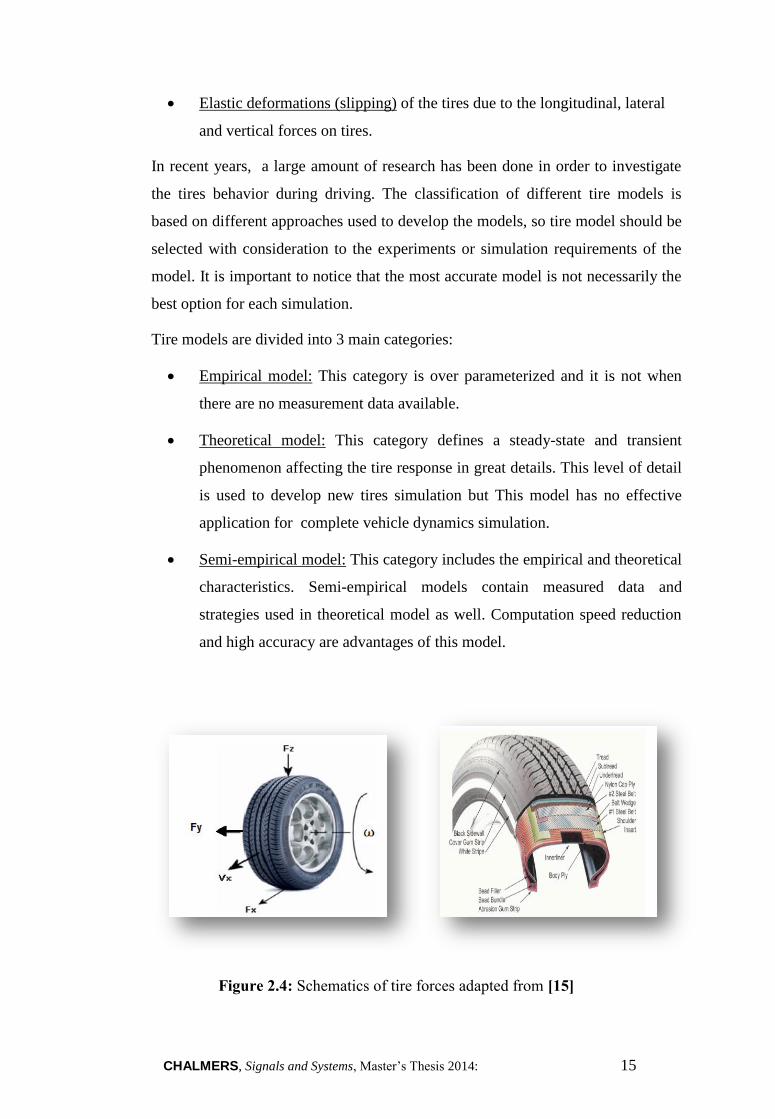
Elastic deformations (slipping) of the tires due to the longitudinal, lateral
and vertical forces on tires.
In recent years, a large amount of research has been done in order to investigate
the tires behavior during driving. The classification of different tire models is
based on different approaches used to develop the models, so tire model should be
selected with consideration to the experiments or simulation requirements of the
model. It is important to notice that the most accurate model is not necessarily the
best option for each simulation.
Tire models are divided into 3 main categories:
Empirical model: This category is over parameterized and it is not when
there are no measurement data available.
Theoretical model: This category defines a steady-state and transient
phenomenon affecting the tire response in great details. This level of detail
is used to develop new tires simulation but This model has no effective
application for complete vehicle dynamics simulation.
Semi-empirical model: This category includes the empirical and theoretical
characteristics. Semi-empirical models contain measured data and
strategies used in theoretical model as well. Computation speed reduction
and high accuracy are advantages of this model.
Figure 2.4: Schematics of tire forces adapted from [15]

16 CHALMERS, Signals and Systems, Master’s Thesis 2014:
2.5.1 TMEasy tire model
Considering the importance of tire model in vehicle dynamics modeling and
regarding to requirements of this project e.g. lateral and longitudinal forces and
self aligning torque, the The TMeasy tire model is based on a semi-empirical
approach.
TMEasy tire model was chosen for these reasons:
This model has ability to accurately simulate the interaction between
longitudinal and lateral forces.
In vertical load changing of vehicle, TMEasy model takes into account the
non linear response of the tires as well.
This model combines the advantages of the mathematical approaches with
a experimental parameter set of physical meaning and the model runtime is
close to Real-time execution time.
This model simulates characteristics that are physically comprehensible for
the user.
This model is being used by Volvo cars, so it allows us to access some
measurement data for the tires.
2.5.2 Longitudinal forces
The longitudinal forces are generated between tire and road, due to the difference
in velocity between road and tire, when accelerating and braking. This difference
between the rotational speed of tire (ω) and vehicle longitudinal speed (v) is called
longitudinal slip or slip rate (s) .The tread elements in the tire will deform when
the slip is non zero. This deformation generates a force on the tire that causes the
vehicle move. The slip rate is different for acceleration and braking. The slip rate
can be calculated as follows:
for braking
for acceleration
. ,
.
, .
(R. < )
(R. > )
v R
vs
R v
R
v
v
(2.1)
where ω is the rotational velocity and R is the radius of tire, v is the longitudinal
velocity of the vehicle. The value of the longitudinal slip is limited such
CHALMERS, Signals and Systems, Master’s Thesis 2014: 17
that 1S .For braking, axle speed is used in denominator of equation so that the
longitudinal slip is 1 for ω=0 (braking).
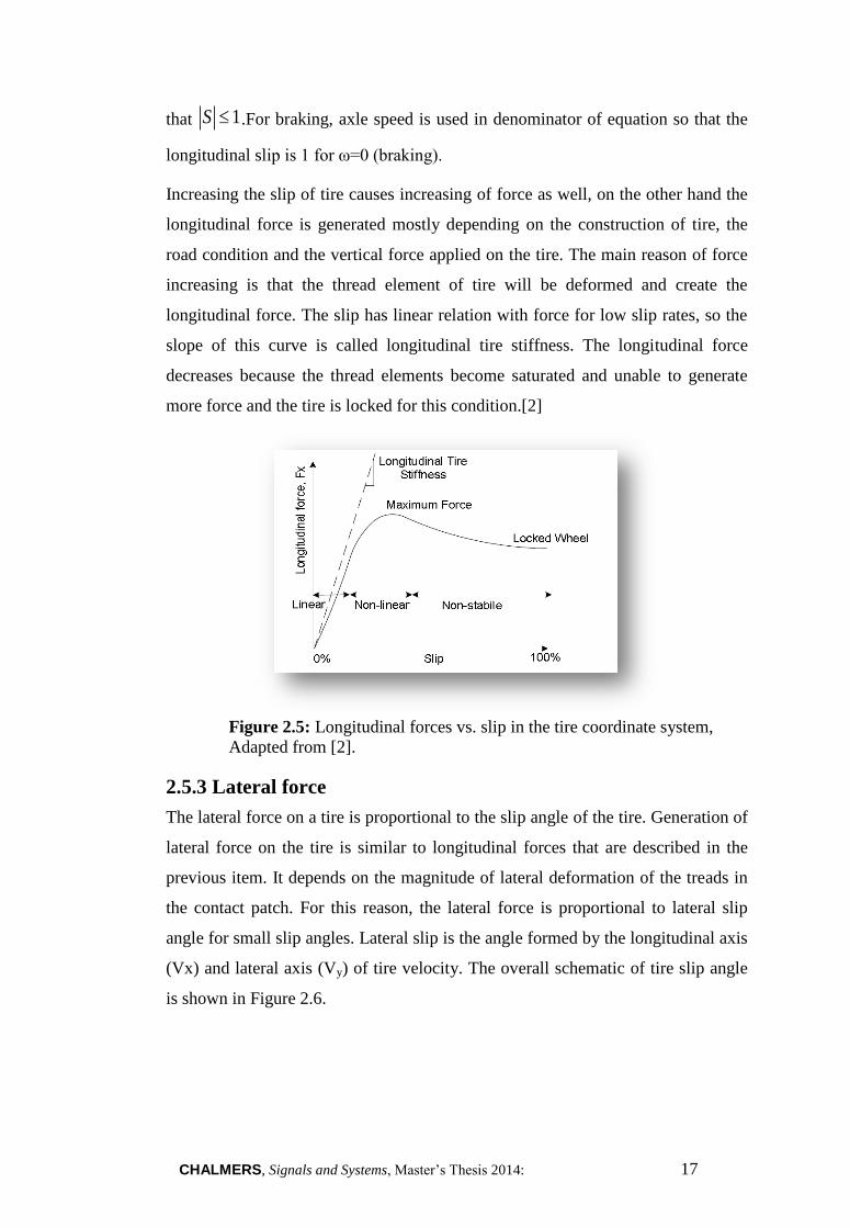
Increasing the slip of tire causes increasing of force as well, on the other hand the
longitudinal force is generated mostly depending on the construction of tire, the
road condition and the vertical force applied on the tire. The main reason of force
increasing is that the thread element of tire will be deformed and create the
longitudinal force. The slip has linear relation with force for low slip rates, so the
slope of this curve is called longitudinal tire stiffness. The longitudinal force
decreases because the thread elements become saturated and unable to generate
more force and the tire is locked for this condition.[2]
Figure 2.5: Longitudinal forces vs. slip in the tire coordinate system,
Adapted from [2].
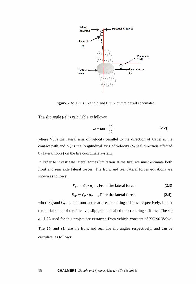
2.5.3 Lateral force
The lateral force on a tire is proportional to the slip angle of the tire. Generation of
lateral force on the tire is similar to longitudinal forces that are described in the
previous item. It depends on the magnitude of lateral deformation of the treads in
the contact patch. For this reason, the lateral force is proportional to lateral slip
angle for small slip angles. Lateral slip is the angle formed by the longitudinal axis
(Vx) and lateral axis (Vy) of tire velocity. The overall schematic of tire slip angle
is shown in Figure 2.6.
18 CHALMERS, Signals and Systems, Master’s Thesis 2014:
Figure 2.6: Tire slip angle and tire pneumatic trail schematic
The slip angle (α) is calculable as follows:
1tan y
x
V
V (2.2)
where Vy is the lateral axis of velocity parallel to the direction of travel at the
contact path and Vy is the longitudinal axis of velocity (Wheel direction affected
by lateral force) on the tire coordinate system.
In order to investigate lateral forces limitation at the tire, we must estimate both
front and rear axle lateral forces. The front and rear lateral forces equations are
shown as follows:
𝐹𝑦𝑓 = 𝐶𝑓 ∙ 𝛼𝑓 , Front tire lateral force (2.3)
𝐹𝑦𝑟 = 𝐶𝑟 ∙ 𝛼𝑟 , Rear tire lateral force (2.4)
where Cf and Cr are the front and rear tires cornering stiffness respectively, In fact
the initial slope of the force vs. slip graph is called the cornering stiffness. The Cf
and Cr used for this project are extracted from vehicle constant of XC 90 Volvo.
The αf and αr are the front and rear tire slip angles respectively, and can be
calculate as follows:

CHALMERS, Signals and Systems, Master’s Thesis 2014: 19
1Front slip angle,
. .tan ( ) or ,
f ff f
y l l
x v
(2.5)
1Rear slip angle,
. .tan ( ) or ,
r rr r
y l l
x v
(2.6)
where δ is the steering angle and is the side slip angle at the COG that can be
calculated by using equation 2.7 is shown in the following.The y and x are the
derivative of lateral and longitudinal displacement respectively.The is vehicle
yaw rate at the COG.
1sinu
v (2.7)
where u is the x-axis of longitudinal velocity and v is the COG of the car’s
velocity.
2.5.4 Self-aligning torque
Self-aligning torque is the torque that the tire creates when the side slip angle is
not zero. In fact, the tire develops this torque when it is turning around the vertical
axis, this torque intends to steer the tire direction toward the traveling direction of
COG. In fact, it should be considered that the lateral forces do not affect exactly at
the center of contact patch, rather it acts at the longitudinal distance between the
resulting force and hub’s vertical projection known as the tire pneumatic trail (tp).
Pneumatic trail is caused by lateral force at the tire along the length of the contact
patch creating a torque about the steer axis known as self-aligning torque [2].

20 CHALMERS, Signals and Systems, Master’s Thesis 2014:
Figure 2.7: Lateral force& self-aligning torque vs. tire slip angle,
from [2].
Figure 2.7 shows how self-aligning torque and lateral force depend on the slip
angle. The maximum self-aligning torque occurs for a lower slip angle than the
maximum lateral force. This means that a decrease in self-aligning torque occurs
before the maximum lateral force is reached, see e.g. [2].
As previously mentioned the self-aligning torque can be calculated by product of
lateral force and moment arm. The moment arm generated by pneumatic trail (tp)
and the mechanical (caster) trail (tm).Mechanical trail is a function of steering
geometry and can be determined as a function of the steer angle [4]. So, the self-
aligning torque can be calculated as follows:
.( )z y p mM F t t (2.8)
Figure 2.7 shows how the lateral force and self aligning torque are changed with
the slip angle, the pneumatic trail will decrease when the self aligning torque
decreases to become negative for a very high slip angle. It can be shown the self
aligning torque and lateral force decrease when maximum lateral force has been
reached, in other words the pneumatic trail has been decreased after maximum
lateral force has been reached as well.

CHALMERS, Signals and Systems, Master’s Thesis 2014: 21
2.6 Vehicle model
There are numerous vehicle models to take into consideration for degrees of
freedom. A very simple model of the vehicle is a two degree of freedom, bicycle
model associated a linear tire model that represents the linear lateral and yaw
motions. This model is commonly used for vehicle control studies and it is an easy
way to understand the basic concepts of vehicle modeling. An overall schematic of
the bicycle model is shown in Figure 2.8.
.
Figure 2.8: Bicycle model schematic
In the following section, the tire forces will be presented. Calculation of the tire
forces is the first step of steering modeling in order to study of vehicle behavior.
The bicycle model is a linear model and the cornering stiffness is the only
parameter used to model the tire.
2.6.1 Equations of motion
As mentioned before, the two DOF bicycle model are mostly used for studying the
vehicle motions behavior. The vehicle velocities and acceleration can be
calculated by applying Newton’s equations for balance of the forces and torques of
the complete vehicle.
The equilibrium of torque balance and lateral force balance applying Newton
Equations are shown as follows :
= y arm0 , F . l Z yf f yr rlJ F l F , torque balance (2.9)
. y yF m a . .( )yf yrF F m v , lateral force balance (2.10)
where Fyf and Fyr are the lateral forces of front and rear tires respectively:
𝐹𝑦𝑓 = 𝐶𝑓 ∙ 𝛼𝑓 , Front tire lateral forces, (2.11)
𝐹𝑦𝑟 = 𝐶𝑟 ∙ 𝛼𝑟 , Rear tire lateral forces

22 CHALMERS, Signals and Systems, Master’s Thesis 2014:
The equation of slip angles for front and rear tires are described in 2.5.3 and can
be calculated from equation 2.2.The 3-D schematic of the chassis forces is shown
in Figure 2.9.
Figure 2.9: Schematic 3D-view of a two-track vehicle, from Luque, Álvarez
(2005)

CHALMERS, Signals and Systems, Master’s Thesis 2014: 23
3. STEERING SYSTEM MODELING
In this chapter, the steering system used in this thesis is described. As mentioned
before, steering system modeling is one of the most important issues in driving
simulation. The high fidelity of steering system simulation is useful to achieve high
reality steering feel for the driver during driving simulation.
The steering system modeled during this project consists of two main parts: steering
geometry and steering wheel feedback torque. Steering geometry is created to
transmit the steering wheel angle applied by the driver as an input to virtual wheels
angles as output. Steering wheel feedback torque has the main purpose of transmitting
the torque created in a tire (self-aligning torque, friction torque…) to the steering
wheel. In other words, steering system model receives the steering wheel position
which is applied by the driver as input and provides the steering wheel feedback
torque as output.
3.1 Steering system overview
The steering system transfers the steering wheel angle to the wheels through a
mechanical system composed by a series of rods and pivots linkages. In this case
when the driver turns the steering wheel, the steering wheel’s rotation is transmitted
through the steering column (steering shaft) to the pinion, the pinion convert the
rotation to the linear displacement through the rack and pinion. The created linear
movement is transferred to the uprights through the tie roads. The created linear
movement at upright generates the steering angle in the wheels. The steering
mechanism between the steering box and the steering angle in the wheels presents a
transmission rate which is called steering ratio. It is important to notice that the
steering wheel angle and wheel angle relates via a steering ratio coefficient.
Rack and pinion steering system is commonly used in conventional cars. In this
project, the power steering assistance system is used as well as the rack and pinion
system. A power steering assist system helps drivers by decreasing the driver’s effort

24 CHALMERS, Signals and Systems, Master’s Thesis 2014:
in the steering wheel. The power steering assistance system is comprised of a DC
motor and a control unit, so that the control unit calculates if a steering assistance is
required for the driver. More information about the power steering assistance will be
presented in the last part of this chapter. The rack and pinion steering system is shown
in Figure 3.1 and steering box is shown in Figure 3.2 respectively.
Figure 3.1: Steering systems (rack and pinion).
Figure 3.2: Steering gear schematic. Adapted from [16]
In this project the steering ratio of XC 90 Volvo is used to calculate the wheel angles.
The mechanical linkage between the steering box and the wheels usually conform to
an Ackermann steering system.

CHALMERS, Signals and Systems, Master’s Thesis 2014: 25
Ackerman steering geometry is the term used to describe the behavior of the front
wheel when the vehicle is driven around a corner. In the corner when the front tires
turn, the inner wheels radius is smaller than the outer wheels and that means the
steering wheel is needed to generate the wheel angle for the inner wheels which are
larger than the outer wheels, otherwise the inner wheel tends to slide over the road
[3].The Ackerman geometry neglects the effect of road on tire, so it is not completely
suitable for modern cars. The wheels behavior interface corner turning can be seen in
Figure 3.3.
Figure 3.3: Ackerman steering geometry
As can be seen in the Figure, the inner wheel angle is larger than the outer wheel,
when the vehicle turns around a circle.
δw2 > δw1
It is important to notice that the wheels behavior analysis is a very important point to
accurately simulate tire forces. For this reason, all the parameters which can affect the
tires must take into account in tire modeling. The static toe angles for tires are other
main characteristics of tires which should be considered in the modeling of the tire.
Toe angle is the initial symmetric steering angle that each tire makes with the
longitudinal axis of the vehicle, even when the steering wheel is not turned. The
steerable wheels are set to have the toe angles as a function of the static steering
geometry and kinematic effects of steering system and tires. Regarding the application

26 CHALMERS, Signals and Systems, Master’s Thesis 2014:
of the steering system, the toe angle can be positive or negative. It can be measured as
an angular deflection of the tire at the front of the tire.
Toe-in or positive toe is the angle between the centerline of the tire and vehicle when
the tires are pointing in towards the centerline of the vehicle. Toe in can be useful in
order to improve the vehicle stability of the road car for straight driving and vehicle
response in a turn.
Toe-out or negative toe is the angle between the centerline of the tire and vehicle
when the tires are pointing away from the centerline of the vehicle. Toe out is used for
racing cars only, because it can increase the vehicles stability in turning position but it
is unstable for straight driving. Toe- in and toe -out of the front tires are shown in
Figure 3.4.
Figure 3.4: Toe-in and Toe- out for front tire, adapted from [17]
Other properties that should be considered when modeling a steering system are the
effect of caster angle, camber angle and kingpin inclination. Caster angle is the
angular displacement of the steering axis from vertical axis in the longitudinal plane
(in the side view of tire).The positive caster angle is achieved when the steering axis
is inclined toward the rear tires of the vehicle (in the side view) and the negative
caster angle is achieved when the steering axis is inclined to the front side of the
vehicle.
Caster angle affect the steering feel by creating a self-centering torque to reduce the
toughness of steering. For example when the caster angle is positive and the wheel is
steered, the lateral forces will create a torque around the steering axis and will
increase the self-aligning torque of the tire. Increasing of self-aligning torque causes
the steering wheel to align quickly. Furthermore positive caster improves the stability

CHALMERS, Signals and Systems, Master’s Thesis 2014: 27
of vehicle in a turn and reduces under-steering situation of the vehicle when the
vehicle is exiting from a turn. Positive caster angle will increases handling of the
vehicle when the vehicle is turning but it causes the steering wheel to be tougher to
move.
When the caster angle is negative the lateral forces will produce a torque that helps
steering. Consequently, the entry of the turn is improved as well as the directionality
in low-speed turns, but more over- steering will be presented while exiting from a
turn. The advantage is that the steering wheel will be less tough to move, and the
disadvantage is that the steering wheel becomes more unstable at a high speed. The
value of the caster trail is a compromise between these two exigencies [7].The
professional drivers adjust caster angle in order to improve their vehicle handling
stability. The positive and negative caster angles are shown in Figure 3.5.
Figure 3.5: Negative and positive caster angles at the top in the side view
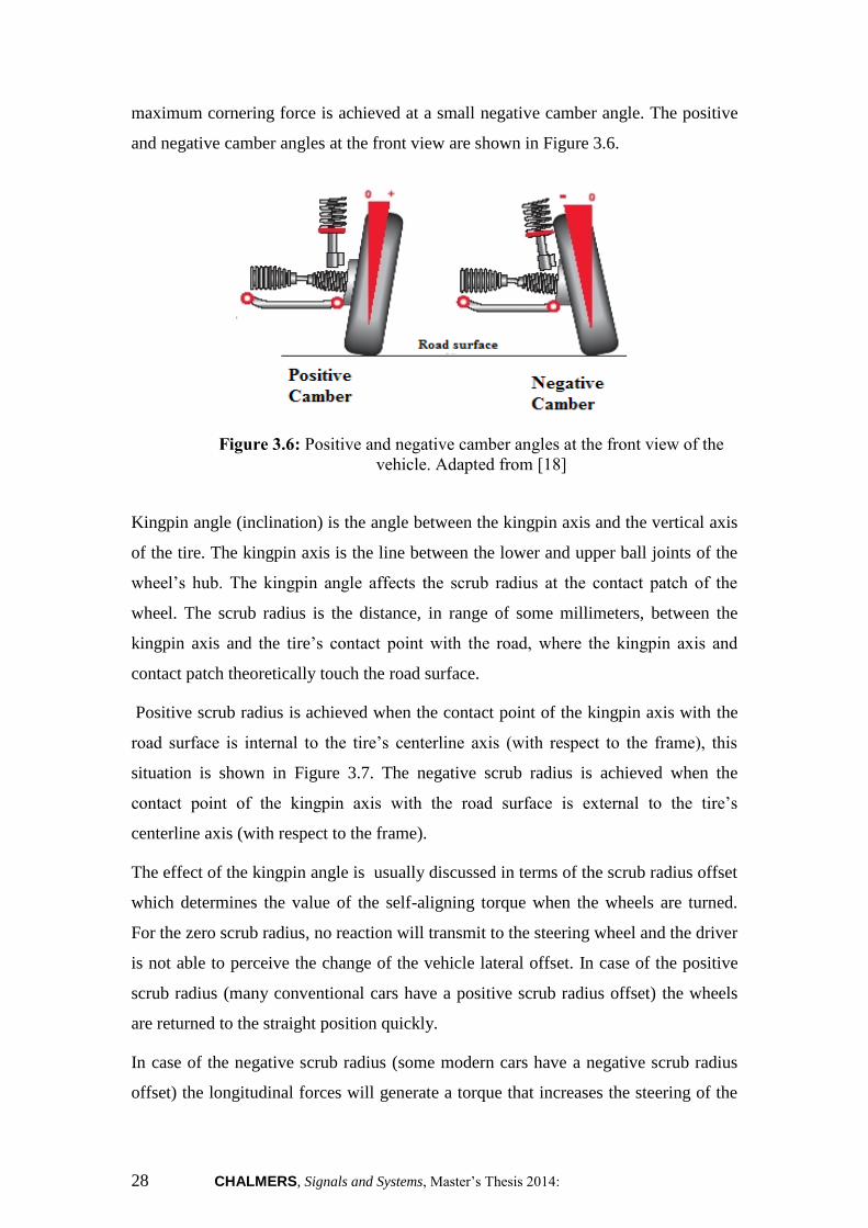
The camber angle is the angle made by the wheel between the vertical axis of the
wheel and the vertical axis of the steering axis at the top of the front or rear view.
Positive caster angle is achieved when the top of the wheel is leaning outward farther
than the bottom (at the front view of tire), and if the top of the tire is leaning inward
toward the centerline of the vehicle, the negative caster angle is achieved (at the front
view of tire). It is important to notice that the cornering force of the tires mostly
dependent on theire angle relative to the road surface condition, so that the generated
28 CHALMERS, Signals and Systems, Master’s Thesis 2014:
maximum cornering force is achieved at a small negative camber angle. The positive
and negative camber angles at the front view are shown in Figure 3.6.
Figure 3.6: Positive and negative camber angles at the front view of the
vehicle. Adapted from [18]
Kingpin angle (inclination) is the angle between the kingpin axis and the vertical axis
of the tire. The kingpin axis is the line between the lower and upper ball joints of the
wheel’s hub. The kingpin angle affects the scrub radius at the contact patch of the
wheel. The scrub radius is the distance, in range of some millimeters, between the
kingpin axis and the tire’s contact point with the road, where the kingpin axis and
contact patch theoretically touch the road surface.
Positive scrub radius is achieved when the contact point of the kingpin axis with the
road surface is internal to the tire’s centerline axis (with respect to the frame), this
situation is shown in Figure 3.7. The negative scrub radius is achieved when the
contact point of the kingpin axis with the road surface is external to the tire’s
centerline axis (with respect to the frame).
The effect of the kingpin angle is usually discussed in terms of the scrub radius offset
which determines the value of the self-aligning torque when the wheels are turned.
For the zero scrub radius, no reaction will transmit to the steering wheel and the driver
is not able to perceive the change of the vehicle lateral offset. In case of the positive
scrub radius (many conventional cars have a positive scrub radius offset) the wheels
are returned to the straight position quickly.
In case of the negative scrub radius (some modern cars have a negative scrub radius
offset) the longitudinal forces will generate a torque that increases the steering of the

CHALMERS, Signals and Systems, Master’s Thesis 2014: 29
wheels in a longitudinal direction. For this reason, the vehicle becomes more
oversteering when the scrub radius offset is negative, thus the driver is not able to
sense the self-aligning torque effect correctly. The used scrub radius for this project is
extracted from XC 90 Volvo measurement data.
Figure 3.7: Kingpin inclination with the positive scrub radius
3.2 Mathematical modelling of steering system
In this section the mathematical modeling of the steering system used in this project is
considered. The steering system is divided into the following two sub-systems:
The steering geometry block which helps to compute the steering angles
measured for each wheel from steering wheel angles as an input. In this part
the Ackerman steering system is used, and additionally the effect of the rear
toe-in angle has been added to the model in order to improve the stability of
the vehicle. The steering geometry used in this project is explained in
appendix A.
The torque feedback block which helps to calculate the steering wheel
feedback torque due to the created forces and torques in the tires and steering
system (rack and pinion). In this block the mathematical modeling of the
30 CHALMERS, Signals and Systems, Master’s Thesis 2014:
steering system is used. In order to achieve a steering feel as close as possible
to real steering, the torque that the driver feels in the steering wheel is
important. The steering wheel feedback torque is a result of the tire forces and
the steering geometry which is filtered through the power steering sub-system.
3.2.1 Steering system forces and moments
In the modeling of the steering wheel feedback torque, six sources of forces and
torques were taken into consideration, they are described as follows:
Longitudinal forces (FLong): These forces create a torque in the tire when the
vehicle accelerates or brakes. The created torque in the tire due to a
longitudinal forces is the product of the longitudinal forces and the moment
arm. The moment arm in this case is the scrub radius caused by the
longitudinal forces effect, which would be sensed in the steering wheel. In this
project, the scrub radius is set to a very small value in order to avoid
interacting with the braking forces effect when the ESP (Electronic Stability
Control) is active. The torque due to the longitudinal forces can be calculated
from :
scrub radiusWhl Long Whl LongF (3.1)
Lateral forces (FLat): These forces create a torque at the contact patch of the
tire with the ground. The distance caused by the lateral forces acts as a lever
arm and is the sum of the static offset and pneumatic trail which is explained
in the 2.5.5. The torque due to the lateral force is the product of the lateral
forces and the static offset. This torque is calculated in the
Vehicle/wheels/self-Align-Torque torque sub-block. The torque due to the
lateral forces can be computed as follows:
_ _ Wheel offsetLWhl Lat Whl LatF (3.2)
Linear damping (b): linear damping of the steering column damper (bs) and
the rack (br) generates an opposing torque with respect to the steering wheel
rotation direction. The torque due to the linear damping is a product of the
damping and the rational speed of the steering wheel.

CHALMERS, Signals and Systems, Master’s Thesis 2014: 31
sw( ). damp s rb b (3.3)
Inertial effects: inertial effects of the steering system component such as the
steering column, the rack-pinion mass, the wheel carriers and the hubs
increase the resisting torque in accelerating and braking. The torque created by
the inertial effects is specially noticeable in the rapid reaction of the driver
(evasion maneuvers or over reactions in accidents). The torque due to inertial
effects is the product of the steering wheel acceleration (SW ) and a constant
factor for inertia (Js) from XC 90 Volvo measurement data.
.inertia s swJ (3.4)
Front lift: suspension compliance of the car generates the additional steering
angle in the wheels. In order to achieve the high realiability model of the
vehicle steering system for the Chalmers driving simulator this part of the
model was developed. In this model, the suspension linkage is used to connect
the wheels to the body of the car. As mentioned previously, the front wheels of
the cars are lifted or lowered due to the caster and kingpin (KPI) angles. The
rack and pinion mechanism is used to calculate the proper suspension
compliance effect. The model used by the [2] is developed for this project by
adding the effect of the caster and KPI angles, which is added to the XC90
model. The suspension compliance used for this model adapted from the
vehicle dynamics which was written as [7].
Friction: friction is one of the important components of the steering system
modeling which should be considered in modeling process. In the model used
by Benito& Nilsson a constant friction is applied as a dry friction between the
road surface and the steerable wheels. The friction modeling for this project
was developed through adding the friction that comes from the rack-pinion
contact and bearings of the steering systems. Dahl friction model is used to
model the rack-pinion component friction, because it is simple and most
useful. The Dahl friction model proposed that the relationship between

32 CHALMERS, Signals and Systems, Master’s Thesis 2014:
frictional force and position would be analogous to a stress-strain curve and
hysteresis. Modeling of the stress-strain curve can be extracted as:
( ) ( )
( ) . 1 ( ( )) . 1 . ( ( )) ( )[ ] ( ).f f
f
c c
F t F tF t sign x t sign sign x t x t
F F
(3.5)
where σ is the stiffness coefficient, Ff (t) is the Dahl friction force, Fc is the coulomb
friction force, ( )x t is the velocity between two surfaces and λ is the shape parameter.
More information about the friction modeling in this project can be found in friction
modeling 3.3.
3.2.2 Mathematical modelling of tire forces
Mathematical model of the steering wheel should be adopted the forces and moments
which described in 3.2.1.The steering system model considered is based on the
torques and forces and is presented in Figure 3.8.
Figure 3.8: Mathematical scheme of steering system. Adapted from [5]
Regarding to the steering system moments, the starting point of the modeling is to
calculate the forces in the tires. The longitudinal and lateral forces of the front tires
can be calculated by using:
,For longitudinal forces
cos( ) sin( ) with i=1,2( ) ,
m ax
xi rollingi wi yi wiFX F F F
Fx
(3.6)

CHALMERS, Signals and Systems, Master’s Thesis 2014: 33
where Fx and Fy are the longitudinal and forces of tire respectively which are derived
from TMEasy tire’s model (An overall view on TMEasy tire’s model can be found in
appendix B).The Frolling is the force generated by tire rolling resistance, the Frolling can
be calculated from:
min(1, ) ( )rolling r Vx sign VxF f m g (3.7)
where fr is the rolling resistance coefficient, the m is the vehicle curb mass adding the
driver mass (75Kg), g is gravity acceleration and Vx is the longitudinal axis of car’s
velocity.
The total forces around the steering axle along y direction are:
with i=1,2
,For lateral forces
cos( ) + sin( )
m
( ) ,
y
yi wi xi rollingi wi
Fy a
FY F F F
(3.8)
The total torque generated around the steering axis by FX can be calculated starting
from Figure 3.9.
Figure 3.9: Scheme used to calculate the resistant torque generated by FX.
Adapted from [7]
As Figure 3.9 shows the total resistant torque generated around the steering axis due
to FX can be computed from :
cos( ) [ cos( ) sin( )]FX KP nomFX r R (3.9)
The total resistant torque generated due to FY is calculated by taking into account the
effect of the caster and kingpin angles in the contact patch between tire and road
surface. The moment arm created due to the caster and KPI is shown in Figure 3.10.

34 CHALMERS, Signals and Systems, Master’s Thesis 2014:
Figure 3.10: Scheme used to calculate the resistant torque generated by
FX. Adapted from [7]
Figure 3.10 shows the caster and KPI effect on the lateral forces of tire. So the
generated torque due to FY around the steering axis can be determined from:
cos( ) [ cos( ) sin( )]FY nomFY t R (3.10)
t = tp+tm
The vertical force and moment generated due to FZ is calculated starting from Figure
3.11.
Figure 3.11: Scheme used to calculate the resistant torque generated by FZ.
Adapted from [7]
The torque produced due to Fz can be computed from:
sin( ) cos( ) sin( ) {cos( ) [ tan( )]}FZ Z W KPnom
F r R (3.11)
So the total resistant torque generated around the left and right tires of front steering
axis can be computed as:

CHALMERS, Signals and Systems, Master’s Thesis 2014: 35
1 1 11
1 1
1
1
cos( ) [ cos( ) sin( )]
+ cos( ) [ cos( ) sin( )]
+ sin( ) cos( ) sin( ) {cos( ) [ tan( )]}
W FX FY FZ
W KP
W KP
align
align nom
nom
nom
FX r R
FY t R
FZ r R
(3.12)
2 2 2 2
2 2
2
2
cos( ) [ cos( ) sin( )]
+ cos( ) [ cos( ) sin( )]
+ sin( ) cos( ) sin( ) {cos( ) [ tan( )]}
W FX FY FZ
W KP
W KP
nom
nom
nom
align
align FX r R
FY t R
FZ r R
(3.13)
3.2.3 Mathematical modelling of steering column
In the modeling of the steering column the rack forces should be taking into account.
The total torques on the steering axis is mentioned in 3.2.2. The resulting
displacement of the rack, xr, derives from the torque applied by driver and the torques
generated by the steering axis and tires on the rack. The rack through the lever arm is
connecting to the wheels. The self-aligning torque around the steering axis is
transmitted to the rack through the lever arm.
The mathematical modeling of the steering column with these assumptions can be
represented in Figure 3.12.

36 CHALMERS, Signals and Systems, Master’s Thesis 2014:
Figure 3.12: Scheme of steering column modelling
The Figure 3.12 shows the steering column torque is composed of the torque applied
by the driver (τd), the assisting torque generated by the assist motor and the resistant
torque generated around the steering axis which is transmitted to the rack through the
lever arm.The steering column torque can be computed as:
s SW d assist TB fJ (3.14)
So to compute the assisting torque and in order to calculate the torque acting on the
steering wheel we need to calculate the steering column torque as:
( ) ( )TB TB
r rTB SW SW
p p
x xk b
r r (3.15)
The pinion torque is:
, pinion torque TB p pF r (3.16)
The total force transmitted to the rack can be computed from:
1 2( )p r r r r r r assistF m x b x F F F (3.17)
The forces on the rack can be calculated from as:
,with i=1,2 Walign i
i
arm
FrL
(3.18)

CHALMERS, Signals and Systems, Master’s Thesis 2014: 37
And the pinion angle is:
,pinion angle r
p
p
x
r (3.19)
Now that the forces acting on the steering column are known, the torques on steering
column can be computed from:
SW s SW s SW p p fJ b F r (3.20)
where τf is the produced torque due to friction. The detailed view of the friction
torque can be found in 3.3.
3.3 Friction torque modelling
As mentioned in 3.2, the friction modeling has an important influence in center-
aligning torque of steering axis, so that the friction torque can be affect on tire
direction in small steering angle. For this reason the torque is caused by the friction of
the rack-pinion contact.
Rotation in different components of torsion bar and dry friction between tire and road
surface should be taken into account in steering system modeling.
As described in 3.2 the Dahl friction model was developed for this project. The stress-
strain curve is modeled in base of equation 3.21:
( ) ( )
( ) . 1 ( ( )) . 1 . ( ( )) ( )[ ] ( ).f f
f
c c
F t F tF t sign x t sign sign x t x t
F F
(3.21)
where σ is the stiffness coefficient, Ff (t) is the Dahl friction force, Fc is the coulomb
friction force, ( )x t is the velocity between two surfaces and λ is the shape parameter.
The stiffness coefficient for steering wheel can be computed from equation 3.22:
2
SW
s s
s
b k
k
j
(3.22)
38 CHALMERS, Signals and Systems, Master’s Thesis 2014:
Dahl friction does not include of the Stribeck effect, In fact the Stribeck effect has a
small value and the driver does not perceive it. So the hysteresis in the system should
be modeled to compute the friction torque effect. In order to compute the friction
torque, the friction forces parameters should be replaced with the friction torques and
the velocity between two surfaces should be replaced with the steering wheel velocity.
So the friction torque equation can be written as equation 3.23 :
1 ( )( )f
f SW SW
c
sign sign
(3.23)
Where the τf is the steering wheel friction torque and τc is the coulomb friction level
and SW is the steering wheel angular velocity.
3.4 Power steering modelling
The function of power steering is widely installed in modern cars. The power steering
function is used to reduce the effort applied to the steering wheel by the driver,
especially when completing a cornering or correction of a car’s steering direction at
low speed. The power steering systems are categorized in two control methods:
Hydraulic Power Assisted Steering (HPAS) and Electric Power Assisted Steering
system (EPAS). The power steering system improves the vehicle’s safety and helps
the driver steering to control a car in unstable maneuvering . In addition the system
reduces the driver fatigue during driving, because the power steering system reduces
the steering effort of the driver by adding a certain amount of assisting torque to
driver’s torque (with a relevant amount of the resistant torque through the steering
wheel torque). In base of the available measurement data from Volvo, a hydraulic
power steering system is modeled in this project.
The basic principle of the HPAS is using an ordinary hydro-mechanical servo parallel
to mechanical connection between steering wheel shaft and torsion bar. In HPAS, the
steering wheel is connected to the steering rack via the valve which is used to control
the amount and direction of the delivered fluid to the cylinder in the steering system
closed loop. In this closed loop system, the displacement of the valve and hydraulic
adjust the pressure in the cylinder such that appropriate assistance is added to the
steering rack [10]. It is important to consider that the driver needs to feel the forces

CHALMERS, Signals and Systems, Master’s Thesis 2014: 39
acting on the steering rack, so the hydraulic system is parallel to steering system. The
overall scheme of the hydraulic power steering closed loop is shown in Figure 3.13.
Figure 3.13: Hydraulic power steering closed loop
In the HPAS the fluid is sent to a double acting hydraulic cylinder through the
hydraulic system pomp, the piston uses the cylinder to produce a force is acting in the
steering gear. The structure of the hydraulic power steering system is shown in Figure
3.14.
Figure 3.14: Structure of hydraulic power steering system [14]
The attitude of the assisting torque can be determined from the characteristic curve in
relation between servo pressure and steering wheel torque. In fact, tuning the assisting
torque value is a complicated process because in order to compute an accurate amount
of assisting torque we should take into account different factors such as: vehicle types,
driving environments, driving styles etc. The amount of the assisting torque would be
changed for different condition of driving. For instance when parking, a large amount
of assisting torque is needed to make steering wheel as soft as possible, despite the
fact that it beeing not necessary to generate a large amount of assisting torque for

40 CHALMERS, Signals and Systems, Master’s Thesis 2014:
direction corrections or lane changing maneuvers in high speeds. For these reason the
typical characteristic between steering wheel torque and boost pressure is shown in
Figure 3.15
Figure 3.15: Relation between servo pressure and steering wheel torque for
different driving condition. Adapted from [10]
The relationship between servo assistance pressure generated by the hydraulic power
steering and steering wheel torque can be modeled as:
2( ) ( )servo assist SW SWP A sign (3.24)
So the created force by servo can be computed as:
-servo servo assist assist pM P A r (3.25)
where Aassist is the cylinder working area and rp is the pinion radius.
The relation between servo pressure and torsion bar torque extracted from XC 90
Volvo is shown in Figure 3.16.

CHALMERS, Signals and Systems, Master’s Thesis 2014: 41
Figure 3.16: Relation between servo pressure and torsion bar torque
The structure of assisting torque function used in this project is shown is Figure 3.17.
In this structure the driver’s torque is used as an input to power steering boost
function from which the resulting assisting torque is computed. The calculated torque
is subtracted from the torque that is created by the tires, either by hydraulic circuit [2].
Figure 3.17: Power steering scheme
As Figure 3.17 shows, the steering column torque is input into the system and it is at
the same time a direct function of assisting torque output. So this loop requires high
computing time. This loop can be able to mange in an off-line simulation, but it is not
possible to solve in real-time application [2]. So the layout implemented by [2] is used
-6 -4 -2 0 2 4 6-15
-10
-5
0
5
10
15
Steering coulmn torque [Nm]
Serv
o p
ressu
re [
MP
a]
Steering column torque Assisting torqueTorque caused by tires forces
and steering geometry
1
Steering column torque
Power Steering boost function
1

42 CHALMERS, Signals and Systems, Master’s Thesis 2014:
for this project .In this simplified layout the torque is caused by the tires forces and
steering geometry is used as input for a look-up table, which computes the steering
column torque. The driver feels both the steering column torque and the lane-keeping
assistance torque in the steering wheel. The implemented layout is shown in Figure
3.18.
Figure 3.18: Implemented power steering system
More information about power steering can be found in [2],[10]
CHALMERS, Signals and Systems, Master’s Thesis 2014: 43
4. LANE-KEEPING ASSISTANCE SYSTEM
In recent years, improvment to the traffic system safety is widely considered by
automotive manufacturers and researchers to reduce the vehicle fatalities. Traffic
system safety can be divided into three main factors: human, vehicle and road. The
vehicle parameter is investigated in this chapter. Safety of the vehicles can be divided
into two areas:
Passive safety: passive safety provides the safety in structural design of
the vehicle in order to reduce the vehicle fatalities when an accident
occurs. Passive safety develops the vehicle’s chassis and body where
no action or intervention by the driver comes into play. Passive safety
system intervenes when a crash occurs, for instance airbags and seat-
belt tension in the event of a crash.
Active safety: active safety provides safety of the vehicle stability to
avoid accidents. Active safety increases the handling of the car by
improving the vehicle stability and driver response. Nowadays, the
automotive manufacturers introduce some electronically controlled
devices such as : Lane Keeping Assistance(LKA), Hydraulic Power
Assisted steering system (HPAS),Electric Power Assisted Steering
System(EPAS),Anti-Lock Brake System(ABS),Electronic stability
program (ESP).
According to the statistics, more than 50% of vehicle fatalities are the result of
unintended lane departure which is caused by the driver’s lack of attention. So the
lane keeping assistance can be useful to decrease the unintended lane departures as an
active safety system. The strategies of LKA can be divided into three parts:
development of the functions to determine dangerous situation, design of driver
warning system and development of the intervention control strategies to assist driver.
The lane keeping system used in this project applies a corrective force to the vehicle
based on the lateral offset and heading deviation from the middle lane of the road. In

44 CHALMERS, Signals and Systems, Master’s Thesis 2014:
this system, driver still can intervene by providing a torque in the steering wheel and
the driver command is added to the lane keeping assistance command. The lane
keeping assistance system analyzed in this project is supposed to keep vehicle in the
road in the absence of driver steering command.
Most investigations on the steering wheel force feedback have focused on transmitting
the mechanical self-aligning torques which is caused by steering geometry and
steering system moments to the driver. In order to to keep the vehicle in the lane, the
developed model combines the steering system torque and the lane keeping assistance
torque computed by the controller. In this project, a noise is used to warn the driver of
an imminent road departure. Some of the warning systems use a warning torque to the
driver of imminent lane departure, Sato et al. [11] found that a torque warning to the
driver is more effective than sounds while Suzuki [12] found that a torque warning
can cause the driver to steer in the wrong direction if not design correctly. [13]
4.1 Lane-keeping controller
The lane keeping controller system is based on the lateral offset and heading distance
of vehicle COG. This controller seeks to keep the vehicle between road lanes through
the correction of wheel angle by generation a torque in the steering wheel. In this
system, the lane keeping assistance torque should be changed when the position of the
vehicle changes between lanes. For instance, the system provides zero torque in center
lane and increases the torque when the car moves from the specified path. So the lane
keeping controller has two parameters: The assistance gain, Kass, which represents the
effective torque constant, and a look-ahead distance, xla ,which represents the gain of
the heading error of vehicle from road’s middle lane.
In order to compute a correct value of lane keeping assistance torque, modeling of the
vehicle’s behavior in unstable condition is necessary. Investigation of the vehicle’s
behavior before entering a road curve can be useful to study the vehicle’s condition
before lane keeping occurs. The scheme of the vehicle characteristics before curve is
shown in Figure 4.1.

CHALMERS, Signals and Systems, Master’s Thesis 2014: 45
Figure 4.1: Vehicle and road-curve frames.
4.1.1 Vehicle-road model
The modeling of the vehicle-road characteristic is one the important parts of the
vehicle’s behavior Studying in order to prevent of vehicle road departure. In the
following chapter, the characteristic of vehicle velocities is calculated as a function of
the yaw angle, longitudinal and lateral forces. It is important to know that this model
is suitable for highway traffic so that a slow steering action, slow velocity and small
pitch and roll angles are considered. The components of the vehicle velocity in the x-
y coordinate read as:
sin( ) cos( )
sin( ) cos( )
V V
V V
x
y
V v u
V u v
(4.1)
where Vy ,Vx are the lateral and longitudinal axis of the vehicle velocity before
entering to road-curve, and ψv is the yaw angle of the vehicle with respect to the
centerline before entering to the road-curve.
The time derivative of lateral offset (yla) of the vehicle center with respect to the
center-line can be calculated as follows:
sin( ) [ ( )] cos( )R Rlala Vx yy V V x (4.2)
by substituting equation 4.1 in 4.2 one can obtain:

46 CHALMERS, Signals and Systems, Master’s Thesis 2014:
[ sin( ) cos( )] sin( )
[ ( ) cos( ) ( )] cos( )
V V R
V V V Rla
lay v u
u sin v x
(4.3)
where ψR is the yaw angle of vehicle center in the road-curve. Assuming ψV, ψR are
small enough and R is the road curvature, so that:
sin( ) , sin( ) , 0
, ( / )
( )
( )
V V R R R V
VR V R VR V xV R
(4.4)
The equation 4.3 can be summarized as:
( )VR Vla lay v u x (4.5)
The described model can be written in state space as follows:
x Ax Bu Ew
y Cx
(4.6)
where the state vector [ , , , ]VRT
lax v r y contains the vehicle lateral velocity
v,the yaw rate ,r, the lateral offset of COG , yla, and relative yaw angle ψVR. The
system’s input u, is the front wheel angle and w is the road curvature. A, B, C, D
can be computed from 4.7 and 4.8:
11 12 11
21 22 21
0 0 0 0
0 0 0 0 , B= , E= , C=
1 0 0 0 1
0 1 0 0 0 0
la
a a b
a a bA
x u
u
(4.7)
11 12
2 221 22
11 12 ,
( ) / , ( ) /
( ) / , ( ) /
/ , / , 1/
f r f f r r
f f r r f f r r zz
f f f z
a C C mu a l C l C u mu
a l C l C I u a l C l C I u
b C m b l C I u w R
(4.8)
The transfer function from wheel angle δ , to lateral offset yla, as follows:

CHALMERS, Signals and Systems, Master’s Thesis 2014: 47
2 1 0
22 1 0
21
2
( )( ) ( )
( ) ( )
lay s n s n s nG s C sI A B
s s d s d s d
(4.9)
Where two integrators are due to positional situation of the vehicle and two poles
arise from vehicle handling .Equation 4.10 reads the transfer function regarding to XC
90 Volvo:
2
2
2 2
1.68 10.6 5.24( ) 10
(0.175 1.41 2.39)
s sG s
s s s
(4.10)
The Bode diagram of the transfer function is shown in Figure 4.2:
Figure 4.2: Transfer function from wheel angle to lateral offset bode diagram
The nominal parameters used in the model, regarding the XC 90 Volvo data are
presented in Table 4.1.
-50
0
50
100
150
Magnitu
de (
dB
)
10-2
10-1
100
101
102
-180
-170
-160
-150
-140
Phase (
deg)
Bode Diagram
Frequency (rad/sec)

48 CHALMERS, Signals and Systems, Master’s Thesis 2014:
Table 4.1: Nominal value and parameter description
Parameter Description and range Nominal value
m
Cf
Cr
Iz
Vx
Lf
Lr
xla
Vehicle mass
Cornering stiffness of front axle
Cornering stiffness of rear axle
Vehicle moment of inertia around yaw axis
Longitudinal velocity of vehicle in range [20-
130km/h]
Distance between front axle and COG of vehicle
Distance between rear axle and COG of vehicle
Look-ahead distance of the vehicle’ COG in road-
curve
2081 [Kg]
70000 [N/rad]
140000 [N/rad]
4512.6 [Kg.m2]
90 [km/h]
1.32484 [m]
1.532 [m]
25 [m]
4.1.2 Lane-departure prevention controller
As mentioned before, lane-departure is an important factor of serious injuries
accidents. According to statistics, more than 1790,000 fatal crashes are recorded
relevant to the lane-departure around the world per year. The lane-departure occurs
usually by the driver’s sleepness, negligence, fatigue and improper reaction of driver
in an emergency situation. So the automotive manufacturing such as Nissan, Toyota,
Honda have been offering a lane keeping system with audible feedback that sounds if
the vehicle begins crossing the lane limit. Since 2002, Toyota and Honda have been
offering their lane keeping assist systems that apply steering wheel torque to help
drivers to keep the vehicle in the lane [5].Most lane-departure warning systems utilize
a camera to estimate the vehicle position relevant to the roadsides. In this project, a
C++ program is used to compute the distance between the centerline of the roads and
vehicle COG. The aim of this chapter is to investigate the lane-departure prevention
system in emergency maneuver by using the RDP controller developed by Alirezaei et
al [1] .The controller determines the correcting wheel angle using the steering wheel
angle and vehicle’s velocity. The overall schematic of RDP controller is shown in
Figure 4.3.

CHALMERS, Signals and Systems, Master’s Thesis 2014: 49
Figure 4.3 : Scheme of road-departure prevention system
In Figure 4.3, block G represents the vehicle dynamics from the front wheel angle δ to
lateral offset yla. Block G is an estimate of G which was used to account for
modeling errors due to correcting angle, G function is computed by equation 4.16.
The lateral offset yla can be calculated from equation 4.5 and 4.11 as well, where C
is the GC controller’s correcting angle and d is the front-wheel steering angle
deriving from driver’s steering wheel angle SW .The estimated desire lateral offset
ˆlady is computed as follows.
when k =1 ( ) la la d cy G y G (4.11)
ˆˆlad la cy y G (4.12)
The desired lateral offset yd can be calculated from equation 4.13, where yl is the
lateral limit (road width).The input of the controller yin is given by equation 4.14.
ˆ
ˆ
ˆ ˆ
ˆ
d lad
l lad l
d lad lad l
l lad l
y y
y if y y
y y if y y
y if y y
(4.13)
in d lay y y (4.14)
Depending on the status of the saturation, the lateral offset function of the wheel angle
and road limit can be computed as:

50 CHALMERS, Signals and Systems, Master’s Thesis 2014:
ˆ( )1 1
ˆ( )
ˆ( )1 1
clad l la d l
c c
lad l la d
clad l la d l
c c
G GGif y y y y
GG GG
if y y y y
G GGif y y y y
GG GG
(4.15)
The order of model’s tranfer function calculated by 4.9 can be reduced. In order to
design a robust controller, Alirezaei et al.[1] the Reduced order transfer function is
described as follows:
1 0
2ˆ ( )
m s mG s
s
(4.16)
where 0 2
1
/ x ro
ml V K
, 1 0
( )la r
x
x lm m
V
f rl l l and ( ) /ro r r f f f rK m l C l C l C C
ˆ ( )G s function was used to calculate the desired lateral offset in look-ahead distance.
According to the Figure 4.3 when 0c and that yla is within the road limits
d lay y , so yin=0 and therefore the controller has no effect on the vehicle. When the
wheel’s angle points the vehicle outside the road limits, so d lay y and controller
input yin is not zero, therefore the controller Gc becomes active ( 0c ) .The
Simulink model of vehicle dynamic can compute the look-ahead position and lateral
offset of the COG with respect to the road limits. The look-ahead distance in 25 m/s
velocity when the time is set to 0.5 is equal to xla=12.5m.
In this section, the correcting wheel angle where is the first point of the required lane-
keeping assist torque calculated for controller.The correcting angle can be determined
as represented:
2
_ ( )c ro x VR VR y Loff lasteering ratiok V l w k k y (4.17)
where KVR and Ky_Loff are the lane-keeping constant coefficient that they are tuned
during the test process, ylais the lateral error between vehicle COG and middle lane of

CHALMERS, Signals and Systems, Master’s Thesis 2014: 51
road. Ψ is the heading error of the vehicle and middle lane of the road and w is the
road curvature.
The force feedback based on the lane keeping assistance is proportional to the
corrective wheel angle, so the torque caused by the correcting wheel angle can be
calculated as shown:
c c
K steering ratiolka (4.18)
where lka is an advisory steering torque for lane-keeping which is product of
correcting wheel angle c (resulting from controller function Gc).The Steering ratio is
the ratio between steering wheel angle and wheel angle SW
w
. This ratio is obtained
from XC 90 Volvo measurement data(15.9/1).In emergency maneuver, the correcting
Wheel angle can be increased quickly, to avoid a high magnitude impulse torque on
the Steering wheel .Therefore, lka was designed to be limited, where Kc =0.5
Nm/rad)
4.2 Modelling of force feedback generation for lane-keeping
assistance torque
The system can be modeled as a mass damper system and implemented as a torque
input from the motor. So the model can be described as inertia of the steering wheel
and motor. The system can be expressed by:
s SW s s SW motorJ b (4.19)
where τSW is zero if the driver’s hands are off the steering wheel. τmotor Contains
various force feedback components represented as follow:
( )motor Lka assist align inertia damper f (4.20)
Lka is the advisory lane keeping assistance torque which is described in 4.1.2.
assist is the power assist torque designed as a function of a driver torque .

52 CHALMERS, Signals and Systems, Master’s Thesis 2014:
align is the self-aligning torque caused by the tire forces, the self align torque can be
calculated from 3.2.2 equation.
inertia is the torque due to moving parts such as steering wheel and rack inertia
which can be calculated as follow:
1 2 1 or
0.05 1 0.05 1inertia s SW inertia s
p
J Js r s
(4.21)
damper is the torque due to the artificial damping which is purely a function of the
steering wheel velocity:
1 2 1
or 0.05 1 0.05 1
damper s SW damper sp
b bs r s
(4.22)
f is the friction torque described in 3.3.
Thus, motor can be imposed to the velocity-controlled force feedback motor to create
feedback torque on steering wheel. The more details regarding to implementation of
force feedback torque via velocity-controlled motor is described in chapter 5.

CHALMERS, Signals and Systems, Master’s Thesis 2014: 53
5. STEERING WHEEL FORCE FEEDBACK
IMPLEMENTATION ON DRIVING
SIMULATOR
The main goal of the following section is design and implementation of a force
feedback steering wheel on driving simulator. In recent years, driving simulator is
widely considered within the automotive manufacturing to increase the safety of
vehicle in emergency situations. Driving simulations is preferred to real cars of
experiments in unstable condition, because it provides safety, repeatability
experiments, various parameterizations of vehicle dynamics for vehicle and the
environment conditions.
The validity of the acquired measurement data depends on the reality of the simulator.
Therefore, improving the driving simulators reality is considered by researcher to
increase the driving feel of driver in experiments. Driving simulator reality is usually
described by the quality of its motion cueing and visual components. So the control
properties and hardware function of the simulator must be taking into account to
increase the reliability of the experiments. In this section the schematic of the
hardware, control properties and the method to overcome the electromagnetic
interfaces are described.
In this study closed loop control method was considered to compute the steering
wheel feedback torque. As mentioned in chapter 3 the real car steering system is
supposed to compute the forces and moments on the steering system (rack and pinion)
for real car. After that, the created torque caused by tires and steering axis is
calculated in 3.2.In chapter 4, the lane-keeping assistance torque was calculated to
prevent the road departure. According to the publication from Switkes et al.[13] the
lane-keeping assistance was calculated in 4.2.The calculated torque is implemented
via a brushed DC motor which is mounted on the steering shaft.
The overall schematic of the force feedback system is shown in Figure 5.1.

54 CHALMERS, Signals and Systems, Master’s Thesis 2014:
Figure 5.1: Overall schematic of force feedback system
Figure 5.1 shows the components used in a servo system to control the position,
velocity or acceleration of the motor.
5.1 PWM generation
The drive represents the electronic power converter that drives the motor according to
the controller reference signals. There exist a lot of ways to amplify the electrical
signals; Pulse Width Modulation (PWM) is the most efficient approach.The PWM
servo drive is a current loop circuit that controls the output current by varying the duty
cycle of the output power stage. The PWM current control circuit is shown in Figure
5.2.
Figure 5.2: PWM Current control circuit
The diodes shown in Figure 5.2 are used to control the current continuity in system
and the RC is used to measure the output current. The transistors (MOSFET or IGBT)
I
S4S3
Command
S1 D1
+HV
D4D3
+
-
OUT
0
Switching Logic
S2 D2
Motor
Rc
CurrentControl
Controller Servo Drive Motor Feedback Load Feedback
Reference Current

CHALMERS, Signals and Systems, Master’s Thesis 2014: 55
are used to switch on and off the diodes. For instance, when switch S1 and S4 (or S2
and S3) are activated, current will flow in the positive (or negative) direction and
increase. When switch S1 is off and S4 is on (or S2 off and S3 on) current will flow in
the positive (or negative) direction and decrease (via one of the diodes). The switch
“on” time can be computed by the difference between the actual current and demand
current. The Current control circuit compares both signals (Actual and demand
current) by the switching logic circuit and activate the switches. Overall dependency
between the pulse width (on time) and the current pattern is shown in Figure 5.3.
Figure 5.3: Relation of output current and duty cycle [19]
Maxon DC motor 168505 series is used as force feedback actuator for Chalmers
driving simulator. Motor current and voltage requirements are computed based on the
maximum required torque and velocity respectively. The relations between velocity,
torque and power curves are shown in Figure 5.4.
Current
Time
On time
Pulse width

56 CHALMERS, Signals and Systems, Master’s Thesis 2014:
Figure 5.4: Relations between velocity, Torque and power curves [19]
The power is equal to Torque * Speed of the motor. The motor voltage (Vm) and
current (Im) should be chosen where power is maximum. The DC motor current (Im) in
amps is function of the torque needed to move the load, it can be computed as
follows:
M
T
TorqueI
K (5.1)
where KT is motor’s torque constant. So the motor current is proportional to the motor
shaft torque, and the motor voltage is proportional to the motor speed and can be
calculated as shown :
(5.2)
where E is the motor back–EMF voltage and Ke is the voltage constant and ωm is the
maximum speed of motor. Figure 5.5 represents transformer is used to transform the
Velocity
Torque
RMS
Power
Time
Time
Time
1 Cycle
Dwell Dwell
m m m
e m
V R I E
E K

CHALMERS, Signals and Systems, Master’s Thesis 2014: 57
AC, DC voltage will charge the capacitor. The point should be noticed that during
braking, most of the stored mechanical energy is fed back into the power supply,
which charges the output capacitor to a higher voltage. If the charge reaches the
drive’s over- voltage shutdown point, motor control and braking cease. To ensure
smooth braking of large inertial loads the shunt regulator is used. Thereby, when the
DC bus reaches the shunt voltage of the shunt regulator, the voltage comparator unit
turns on the electronic switch, which connects the R (47Ω) power resistor across the
DC bus which dissipates the energy from the DC bus. After the bus voltage is reduced
to less than the shunt voltage setting, the resistor is disconnected from the bus.
Figure 5.5: Schematic of the motor’s power supply and servo drive used for
Chalmers simulator
The power supply current is based on the maximum required current by the system
which is defined as follows:
(0.98)
M MPS
PS
V II
V
(5.3)
where IPS ,VPS are the current and voltage of power supply respectively . Figure 5.6
represents the overall schematic of voltage and current changing for motor, diode and
capacitor regarding to the MOSFET switch. The power supply power is
approximately equal to drive output power plus 3 to 5%. As shown in, the power
supply current is a pulsed DC current, so that when the MOSFET switch is on, the
motor current is equal to power supply current; when the MOSFET is off,it is zero.
Therefore the power supply current is a function of the motor current and PWM duty
cycle. As shown in Figure 5.5, the servo drive is located between DC motor and
2200u
Servo Drive
Id220 Vac
100
Vm
Ip
100
TX1
Im
+-
4
1
2
3
47
Motor
0.1

58 CHALMERS, Signals and Systems, Master’s Thesis 2014:
power supply. The servo drive is used in order to generate the calculated torque
(τmotor) which is determined in section 4.2.As mentioned before, the motor’s torque
and speed are proportional to the motor current and voltage respectively. For this
reasons, motor’s torque and speed are based on the motor controller outputs (Voltage
and current). So, the brushed DC motor’s torque is controlled by servo
Controller which creates the PWM signals according the command torque from
National Instruments D/A converter. In this project, ADVANCED motion controller
25A8 series is used as motor controller on simulator. The motion control reference
command is computed by the model which is created in order to calculate the steering
system feedback torque.
Figure 5.6: Overall schematics of motor inputs and servo drive outputs
Vm
Im
Id
Ip
Vcapacitor
PWM
Switching Time MOSFET ON
MOSFETOFF
Ripple current
Average
Time
Time
Time
Time
Time
Average
50μsec
CHALMERS, Signals and Systems, Master’s Thesis 2014: 59
5.2 Steering wheel feedback torque command
The developed model of XC90 Volvo computes generated torques by steering system
during driving and dictates the steering wheel velocitySW constituting the command
sent to the velocity control DC motor as follows:
0
( )t d Lka assist align f speed s SW
SW
s
bd
J
(5.4)
where τd is the torque applied by driver, τLka is the lane keeping assistance which is
determined in section 4.2.τalign is the self-aligning torque which is computed in
section 3.2.2.
τf is the torque caused by the friction of steering system which is determined in
section 3.3. The bs is the steering column damper and Js is the steering wheel moment
of inertia. τspeed represents a feedback torque which is a product of speed stiffness
term Ks ,the longitudinal velocity Vx and steering wheel angle θSW. The τspeed can be
determined as follows:
speed s x SWK V (5.5)
The electric noise sampled from the A/D board with the DC motor illustrates the
undesired noise when the motor is enabled .So, first order low-pass Butterworth active
filtering is used to reduce the noise for the sensors in the model. On the other hand,
the command signals from D/A board need to amplify. In order to amplify the
reference command the difference amplifier is used for command signals. The
schematic of the difference amplifier and second order low-pass filter are shown in
Figure 5.7.

60 CHALMERS, Signals and Systems, Master’s Thesis 2014:
Figure 5.7: First order low-pass filter (left) and difference amplifier (right)
where Vout_filter and Vout_amp can be calculated as follows:
22 1
1
_ ( ) ( ) ( )( )out amp
RV s V s V s
R (5.6)
_ 1
2 1
1( ) ( )
1out filterV s V s
SR C
(5.7)
In this section some information in related to the implementation of force feedback
torque on driving simulator has been provided.
.
R2R2
+
-
OUT
+
-
OUT
- Ref In
R4
0
50k
R1
0
V2
V1
20k
C1
1000u
50k
Vout_amp
V1
50k
+ Ref In
V2
20k
R3Vout_filter
20k
R1

CHALMERS, Signals and Systems, Master’s Thesis 2014: 61
6. MODEL VALIDATION
Model validation for this project is divided into two parts: the first part is included the
vehicle dynamics model validation and the second part is the lane keeping assistance
system validation. The vehicle dynamics model validation procedure done by
comparison with XC 90 Volvo measurement data. The proposed lane keeping
assistance system has been validated by testing the function activity in the driving
simulator. The vehicle dynamics model parameters are tuned to reduce the difference
between matching of the measurement data from Volvo and to increase the drivability
in the Chalmers driving simulator.
6.1 Model comparison with measurement data
The measurement data from Volvo were available in three maneuvers. In the
following sections only the significant parameters which are developed within the
project are represented. The extracted measurement data are recorded in quick
transient maneuvers. Note that the time sample of measurement data and developed
model were not match. The time sample of measurement data was 20ms while the
sample time of model was 1ms.In order to fix this problem, the model parameter
regarding to the measurement data time sample is selected. The transient response of
the vehicle can be evaluated by driving car at constant speed in a straight direction,
where sinusoidal steering wheel inputs of different frequencies applied (0.2-2.5 Hz).
Thus the validation of the lateral velocity and acceleration would be feasible to
determine it in the open-loop test method, since the lateral force of tire is function of
the lateral acceleration. In the first part, the developed model will be compared by the
measurements data at 81km/h or 22.5 m/s. The steering wheel input to the model and
measurement data are shown in Figure 6.1.

62 CHALMERS, Signals and Systems, Master’s Thesis 2014:
Figure 6.1: Steering wheel angles, at 81Km/h
In order to evaluate the model, the steering wheel angle measured from measurement
data is used as input to the model.
The steering wheel response is mainly related to the steering system forces such as:
forces on tires and rack-pinion. Self-aligning torque has important role in steering
response.
During this project the self aligning torque of the previous model is developed
regarding to the caster and kingpin angle effect. The tire’s self-aligning torque is
function of lateral force of front tires, the lateral torque of front left and right tires are
shown in Figure 6.2 and 6.3 respectively.
Figure 6.2: Transient response of lateral moment for front left tire, at
81Km/h
0 0.5 1 1.5 2 2.5 3 3.5 4 4.5-50
-40
-30
-20
-10
0
10
20
30
40
Steering Wheel angle
Time [s]
Ste
ering w
heel angle
[deg]
Measurment Data
Model
0 0.5 1 1.5 2 2.5 3 3.5 4 4.5-0.12
-0.1
-0.08
-0.06
-0.04
-0.02
0
0.02
0.04
Lateral Moment of front left tire
Time [s]
Late
ral M
om
ent
[Nm
]
Measurment data
Model
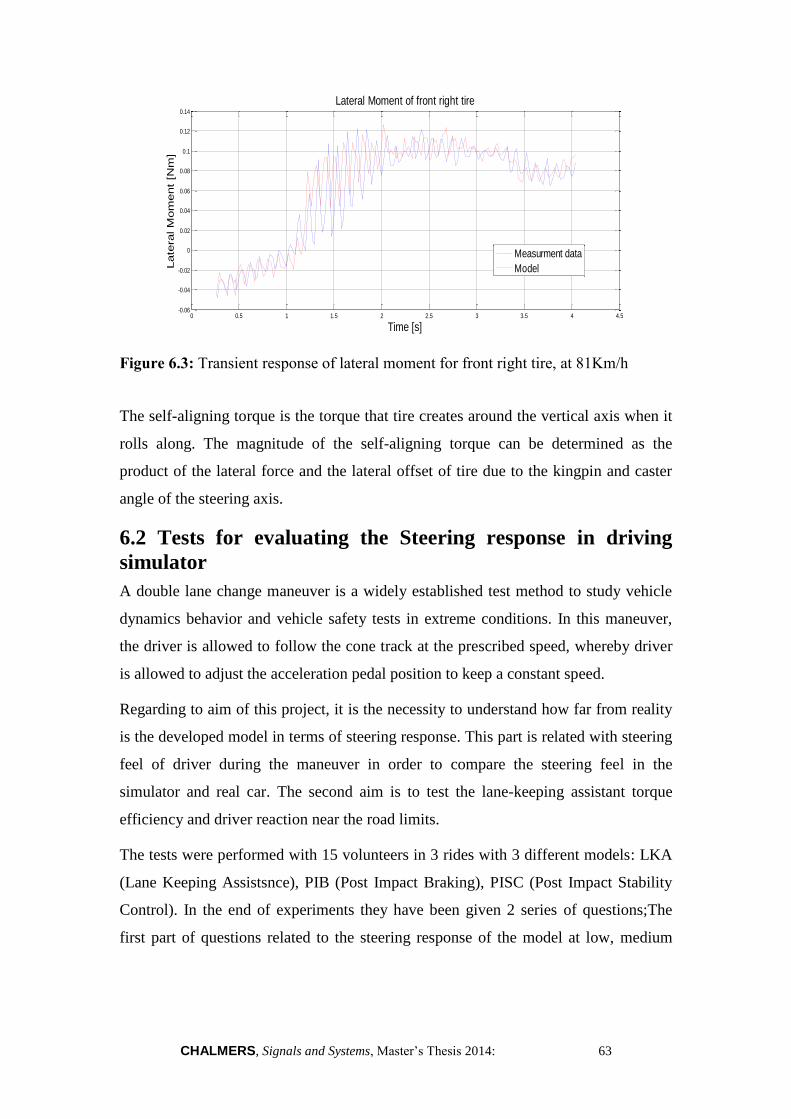
CHALMERS, Signals and Systems, Master’s Thesis 2014: 63
Figure 6.3: Transient response of lateral moment for front right tire, at 81Km/h
The self-aligning torque is the torque that tire creates around the vertical axis when it
rolls along. The magnitude of the self-aligning torque can be determined as the
product of the lateral force and the lateral offset of tire due to the kingpin and caster
angle of the steering axis.
6.2 Tests for evaluating the Steering response in driving
simulator
A double lane change maneuver is a widely established test method to study vehicle
dynamics behavior and vehicle safety tests in extreme conditions. In this maneuver,
the driver is allowed to follow the cone track at the prescribed speed, whereby driver
is allowed to adjust the acceleration pedal position to keep a constant speed.
Regarding to aim of this project, it is the necessity to understand how far from reality
is the developed model in terms of steering response. This part is related with steering
feel of driver during the maneuver in order to compare the steering feel in the
simulator and real car. The second aim is to test the lane-keeping assistant torque
efficiency and driver reaction near the road limits.
The tests were performed with 15 volunteers in 3 rides with 3 different models: LKA
(Lane Keeping Assistsnce), PIB (Post Impact Braking), PISC (Post Impact Stability
Control). In the end of experiments they have been given 2 series of questions;The
first part of questions related to the steering response of the model at low, medium
0 0.5 1 1.5 2 2.5 3 3.5 4 4.5-0.06
-0.04
-0.02
0
0.02
0.04
0.06
0.08
0.1
0.12
0.14
Lateral Moment of front right tire
Time [s]
Late
ral M
om
ent
[Nm
]
Measurment data
Model

64 CHALMERS, Signals and Systems, Master’s Thesis 2014:
and high speed turning. The second part of questions are related to lane-keeping
assistant function efficiency.
The volunteers were asked to drive the simulator in 3 rides for 2-3 minutes per each
ride without knowing what model they were driving. The drivers also had the
opportunity to drive 3 models in a double-lane change manoeuvre like the one
performed at the test track. The drivers tested 3 different vehicle dynamics models to
express their judgment on different speeds; After driving in 3 rides, the drivers filled
in a questionnaire, show in Appendix C, they were asked to give a point for each
model from 0 to10. In the following sections the results of these tests are reported.
The results described in terms of the mean value obtained by the models at different
speeds. The average of the sample which can be calculted from equation 6.1:
1
N
i
i
S
SN
(6.1)
The steering feel score of models in different speed is shown in Figure 6.6.
Figure 6.6: Low, medium and high speed steering feel of PISC model (blue),
Developed model-LKA model (red) and PIB model (green).
5 4,93
4,13
7,26 7
6,8
5,73 5,73 5,6
Low speed Medium speed High speed
Steering response of models at different speeds
PISC Model Developed Model(LKA model) PIB Model

CHALMERS, Signals and Systems, Master’s Thesis 2014: 65
The PIB model has an aligning torque which is more “elastic”, with a high self-
aligning-torque and without considering the power steering system. For this reaosn we
asked participants to compare the models in terms of vehicle stability reponse athigh
speeds. The PISC model is considered without steering wheel feedback effect.
The developed model (LKA model) appears to be more realistic, with the steering
wheel returning in centre position. During the tuning process before experiments,
many efforts have been put to tune the effect of requlating friction and power steering
assistance on steering wheel force feedback torque.
In questionnaire 1 we also asked participants to give a point (0-10) for simulator
stability when steering wheel is turing fast. This question purpose was to determine
the vehicle stability reponse of 3 models when the steering wheel is turning fast. The
scores of simulator response stability for 3 models are shown in Figure 6.7.
Figure 6.7: High speed vehicle stability response of PISC model (blue),
Developed model-LKA model (red) and PIB model (green).
4,6
9,06
5,8
Simulator stability response
Vehicle stability response at high turning
speed
PISC Model Developed Model(LKA model) PIB Model

66 CHALMERS, Signals and Systems, Master’s Thesis 2014:
6.3 Tests for evaluating the lane keeping assistance torque
functionality in driving simulator
In order to test this function, 15 participants have been asked to drive simulator on a
test track.They have not beeen informed that the LKA system is active in which
model.They have been asked to drive in the low speed line of highway at speed more
than 75km/h for one minute and cease the steering wheel turning like sleepless
position. They have been asked to do the first reaction after alarm sound. The alarm
sound was set to activate when the vehicle is close the road limits. This experiments
helps us to evaluate the reaction of drivers when they hear the alarm sound and to
understand the usefulness of this function for drivers in extreme conditions. Driver’s
comments must be qualified LKA systems functionality after experiments.
Participants have been asked to fill questionnaire1 in related to compare the stability
control of vehicle when it is close the road limits. In the questionnaire 2, participants
have beed asked to explain the first reaction after sound alarm when the vehicle was
close the roadsides. Questionaaire 2 contained some question about usefulness of the
function.[appandix 3]
One of the questions was related with the first reaction of drivers when they noticed
the position of the vehicle near the road limits. The participants have been asked to
select between the brake, turning the steering wheel and get lost. The asnwers of
fifteen participates are shown in Figure 6.8.
Figure 6.8: The rate of drivers reaction when they noticed the position of the vehicle
near the road limits
Brake 7%
Turning the steering wheel
93%
Get lost 0%
0%
Driver reaction
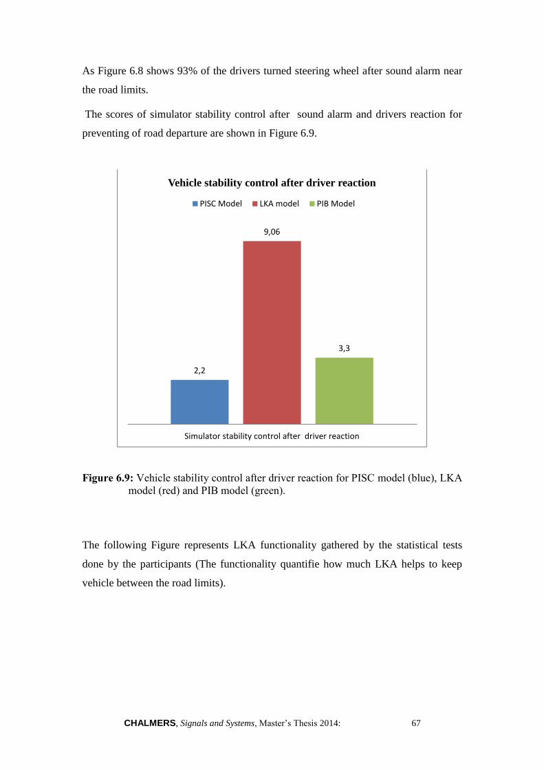
CHALMERS, Signals and Systems, Master’s Thesis 2014: 67
As Figure 6.8 shows 93% of the drivers turned steering wheel after sound alarm near
the road limits.
The scores of simulator stability control after sound alarm and drivers reaction for
preventing of road departure are shown in Figure 6.9.
Figure 6.9: Vehicle stability control after driver reaction for PISC model (blue), LKA
model (red) and PIB model (green).
The following Figure represents LKA functionality gathered by the statistical tests
done by the participants (The functionality quantifie how much LKA helps to keep
vehicle between the road limits).
2,2
9,06
3,3
Simulator stability control after driver reaction
Vehicle stability control after driver reaction
PISC Model LKA model PIB Model
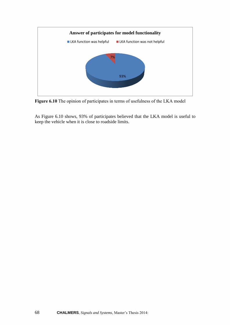
68 CHALMERS, Signals and Systems, Master’s Thesis 2014:
Figure 6.10 The opinion of participates in terms of usefulness of the LKA model
As Figure 6.10 shows, 93% of participates believed that the LKA model is useful to
keep the vehicle when it is close to roadside limits.
93%
7%
Answer of participates for model functionality
LKA function was helpful LKA function was not helpful

CHALMERS, Signals and Systems, Master’s Thesis 2014: 69
7. CONCLUSION
The main conclusions obtained in this master thesis was the development of the
steering wheel force feedback with focus on LKA in Chalmers driving simulator.The
steering wheel force feedback concerns to improvement in two area:
development of steering wheel feedback torque to improve the steering feel of
driver in driving simulator
verification of derived lane-keeping assistance function by adding the
calculated LKA torque to steering wheel feedback torque and test in Chalmers
driving simulator
The model has been developed using Matlab®
/Simulink® as programming language
and it has been validated both with a comparison versus measurments data (coming
from Volvo) and with simulations performed in the Chalmers simulator.
The LKA model can be seen as an evolution of XC 90 Volvo vehicle dynamics model
which is currently used in the Chalmers simulator.This model uses a closed-loop
control system to keep the vehicle in road limits regarding the lateral offset and
heading error between the vehicle’s COG and the road centerline.This function
reduces the lateral offset of vehicle by providing the correction wheel angle through
the steering wheel torque.
70 CHALMERS, Signals and Systems, Master’s Thesis 2014:
8. RECOMMENDATION AND FUTURE WORK
This chapter consists of some recommendations for future work and further
development.
Deeper study realted with the suspension in order to improve vertical
behaviour of the vehicle in terms of acceleration and vibratios.
Improve the powertrain subsystem, to increase the vehicle behaviourfor initial
acceleration.
Model the friction of rack as variable in function of the rack deisplacement.
Deeper study to model the steering feedback dependency in function of the
vehicle speed.
Improve the audio and the quality graphic of the senario to provide a better
feel for driver.
Improve the interaction of driver and simulator by adding a touchpanel to the
simulator cockpit.

CHALMERS, Signals and Systems, Master’s Thesis 2014: 71
REFERENCES
[1] Alirezaei, M., Corno, M., Katzourakis, D., Ghaffari, A., Kazemi, R. (2012). A
Robust Steering Assistance Sysytem for Road Departure Avoidance.
IEEE Transactions on Vehicular Technology, Vol. 61, No.6, (2012).
[2] Benito, G. & Nilsson, H. (2006). Vehicle Stability Control for Roadside Departure
Incidents by Steering Wheel Torque Superposition, Master’s Thesis,
department of Applied Mechanics & Signals and Systems, Chalmers
Uinversity of Technology, Göteborg, Sweden.
[3] Gómez Fernández, J. (2012). A Vehicle Dynamic Model for Driving Simulators.
Master’s Thesis, department of Applied Mechanics, division of Vehicle
Engineering and Autonomous Systems, Chalmers Univesrity of
Technology, Göteborg, Sweden
[4] Judy Hsu, Y.H. (2009). Estimation and Controlof Lateral Tire Forces Using
Steering Torque. PhD. Thesis, department of mechanical engineering,
Stanford University, Stanford, United states of America
[5] Katzourakis, D. (2012). Driver Steering Support Interfaces near the Vehicle’s
Handling Limit. PhD. Thesis, Technische Universiteit Delft, Delft,
Netherlands.
[6] Kusachov, A., Al Moutamid, F. (2012). Post Impact Braking Verification in
Motion Platform Simulator. Master’s Thesis, department of Applied
Mechanics, division of Vehicl Engineeringand and Autonomous Systems,
Vehicle Dynamics Group, Chalmers University of Technology, Göteborg,
Sweden.
[7] Obialero, E. (2013). A Refined Vehicle Dynamic Model for Driving Simulators.
Master’s Thesis, department of Applied Mechanics, division of Vehicle
Engineering and Autonomous Systems, Chalmers University of
Technology, Göteborg, Sweden.
[8] Pacejka, H.B. (2005). Tire and Vehicle Dynamics (2th edition.) SAE International,
Englewood Cliffs, New Jersey.
[9] Pohl, J. & Ekmark, J. (2007). SYN3: A Lane Keeping Assist System for
Passenger Cars, Design Aspects of the user interfce, Volvo Car
Corporatio Report, Paper No. 529, Göteborg, Sweden.
[10] Rösth, M. (2007). Hydraulic Power Steering Design in Road Vehicles.
Dissertation No. 1068, Division of Fluid and Mechanical Engineering
Systems, Department of Mechanical Enginnering, Linköping, Sweden.
[11] Sato, K., Goto, T., Kubota, Y., Amno, Y. & Fukui, K. (1998). A study on a
Lane Departure Warning System using a Steering Torque as Warning
Signal. In Proceeding of the International Symposium on Advanced
Vehicle Control (AVEC) (1998), pp.479-484.

72 CHALMERS, Signals and Systems, Master’s Thesis 2014:
[12] Suzuki, K. (2002). Analysis of drivers steering behaviour during auditory or
haptic warnings in lane departure situations. In Proceeding of the
International Symposium on Advanced Vehicle Control (AVEC)
(2002), pp.243-248.
[13] Switkes, J. P.,Rossetter, E. J.,Coe, I. A.&Gerdes, J. C. (2006).
Handweel Force Feedback for Lanekeeping Assistance:Combined
Dynamics and Stability. Jornal of Dynamic System, Measurment and
Control, Vol. 128, pp. 532-542 (2006).
[14] Url-1<http://www.agcoauto.com>, date retrieved 30.10.2013.
[15] Url-2< http://www.mathworks.se/help/physmod/sdl/drive/tire.html>, date
retrieved 20.10.2013.
[16] Url-3< http://www.carbibles.com/steering_bible.html>, date retrieved
20.09.2013.
[17] Url-4< http://www.discounttiredirect.com/direct/infoAlignment.do>, date
retrieved 21.09.2013.
[18] Url-5< http://www.bestcoiloverguide.com/coilover-parts/camberplates/ >,
date retrieved 10.10.2013.
[19] Advanced Motion Controls, Analog Drives for servo Systems and
Hardware Installation manual, 25A8Servo drive datasheet, Date
retrieved: 20.10.2013, adress: http://www.a-m-
c.com/download/manual/AMC_AnalogDrives_InstallManual.pdf

CHALMERS, Signals and Systems, Master’s Thesis 2014: 73
APPENDICES
APPENDIX A: Steering Geometry
APPENDIX B: TMEasy Tire model
APPENDIX C: The pictures of Chalmers driving simulator and simulator control
computers
APPENDIX D: Instruction Paper and Questionnaire 1, 2

74 CHALMERS, Signals and Systems, Master’s Thesis 2014:
APPENDIX A
Steering geometry calculates the wheel angle with regarding to the steering wheel
angle.Real steerig ration from the XC 90 Volvo is used to calculate the wheel angles
in this model.This block is modified to approximate the characteristics of an
Ackermann steering system.The steering geometry block can be found in
Vehicle/Steering Geometry block of Vehicle Dynamics model.It is shown in Figure
A.1 also.
Figure A.1: Steering Geometry sub-system to calculate the wheel angle for each
wheel
2
FBout
1
FFoutAn_SteWhlRev s
Wheel Position
An_SteWhlRev s1
An_SteWhlBus
Steering Geometry
Ground
2
FBin
1
Inputs
Steering geometry<Wheel Position>
<An_SteWhlRev s>
An_SteWhlBus

CHALMERS, Signals and Systems, Master’s Thesis 2014: 75
APPENDIX B
One of the important parts of the vehicle dynamics model is the physical model for
tires.This part of vrhicle dynamics has an important role in accuracy of final result.
For this reason, everything are related to wheels should be take into account in tire
modeling.The TMEasy model was chosen for this project and the main idea behind
the model is to characterize the forces vs. slip relation by use the 5 and an optional
sixth constant are listed below:
Slip rat or slip angle for which this maximum force is achieved.
Maximum force generated by the tire
Cornering stiffness
Slip rate or slip angle after considering the full sliding or spinning Condition
Force generated by the tire at full sliding or spinnin situations
(Optional) Rate of looses force by each tire at higher slip rate or slip angle
The generated slip angle by tire can be calculated from following equations:
(A.1.1)
22
_ max
_ max
2 2 2 2_ max _ max
_ max _ max
_ max
_ max
2 2 2 2_ max _ max
_ max _ max
ˆ ˆ
ˆ( ) ( )
ˆ( ) ( )
yx
x y
x
x xx
x yx y
x x
y
y
x
x yx y
x x
SSS
S S
F
S dFS
S S F F
dF dF
F
S dFyS
S S F F
dF dF

76 CHALMERS, Signals and Systems, Master’s Thesis 2014:
The TMEasy tire model can be found in Vehicle/Wheels/FL block of Vehicle
Dynamics model.It is shown in Figure A.1 also.
Figure B.1: TMEasy tire model sub-system, to calculate the lateral and longitudinal
forces on tires
The More information about TMEasy tire model can be found in [2]
3
Offset
2
Fy
1
Fx
u[1]*u[3]
sin
u[1]*u[2]
cos
Fz Consts
Weight Interpolation
Scope1
S
NewCurv eF
Resulting Force
Sy
Fz
Of f set
Offset Calc
Combined
Original
NewCurv e
New Constants
Sx
Sy
Consts
S
Combined
Compound slip
f(u)
Add static offset
4
Consts
3
Sy
2
Sx
1
Fz
<cos>
<sin>

CHALMERS, Signals and Systems, Master’s Thesis 2014: 77
APPENDIX C
In the following section, some pictures of Chalmers driving simulator are shown.This
Simulator was used to test the model
Figure C.1: Chalmers driving simulator control computers
The Figure C.1 shows the computers which are used to control the simulator. The
middle PC is the Host PC which is described in chapter 1.1.1. The right PC is Kernel
and the Left PC is Backup PC.

78 CHALMERS, Signals and Systems, Master’s Thesis 2014:
The Patforms and cockpit of Chalmers driving simulator are shown in Figure C.2.
Figure C.2: Chalmers driving simulator platform and cockpit
Figure C.2 shows the platform and cockpit of the Chalmers driving simulator which
Is described in chapter 1.1.3.

CHALMERS, Signals and Systems, Master’s Thesis 2014: 79
The Graphical part and screen of Chalmers driving simulator are shown in Figure
C.3.
Figure C.3: Graphical screen of Chalmers driving simulator

80 CHALMERS, Signals and Systems, Master’s Thesis 2014:
APPENDIX D
Instruction paper
Hello Dear driver
You are invited to make a test drive on Chalmers Driving simulator in the scope of a
Master’s Thesis project .This paper will give you a short background and introduction
about the ongoing experiment.
The aim of the test is to study the different aspects of the car and driver’s behavior,
like:
Test an overall vehicle simulation model (and its separate parts) behavior,
especially how well it works with the current steering system.
Check how realistic the simulator is in both normal driving and limit handling
cases.
Record and analyze the driver’s reaction and the vehicle control parameters on
the unusual, unforeseen and stressful events.
So the experiment will consist of 3rides, at the first ride the Model 1 will be run; In
the second ride the Model 2 will be test and in the third ride the model 3 will be run.
During each ride, you will be given the instruction about the desired driving behavior
(like “try to drive with certain speed” or “zigzagging “).Please try to follow the
instruction carefully in order to help us to collect the best data set. Try to imagine that
you are riding a real car and behave appropriately- avoid collisions, respect the traffic
rules and so on.
NOTE: Speedometer has two scales- mph (outer one) and Kph (inner one); we
are operating only with Kph.
At the beginning of the experiment, you will be given some2-3 minutes to drive the
simulator in the way you want, so as to feel and test the overall fidelity of the
simulator. You can do any braking, steering or combined maneuvers. You will be
given a small questionnaire after this ride.

CHALMERS, Signals and Systems, Master’s Thesis 2014: 81
In the end of the experiment you will be given another questionnaire with more
specific questions.
NOTE: Everything that you see or feel in the simulator is caused made and
sanctioned by us and is part of the experiment!
Please do not worry about the simulator capability. We will inform you to pause in
experiment if needed. Please, do not leave the simulator before the platform is parked
down.
Also, opening the door of the car will caused the stop of the simulation .So, Please do
not open it during the experiment unless you feel a need.
Please, fasten your seat belt before start the simulation and don’t change the
handbrake position. The Simulator gear is shifting automatically, so you don’t need to
shift it.
Questionnaire 1
Driver Information
Test Case#:
Name:
Gender:
Driving License: Yes/No
Driving Experience: Years
How many km do you drive per year? 0-10.000 10.000-20.000 More
than 20.000
How many times have you used a simulator before? Never 1_3 More
than 3
Do you play car related video games? Yes/No
Date and Time of experiment:

82 CHALMERS, Signals and Systems, Master’s Thesis 2014:
Model Comparison
How do you perceive the steering response when negotiating low speed turn? (From 0
to10)
Model 1: Model 2: Model 3:
How do you perceive the steering response when negotiating medium speed turn?
(From 0 to10)
Model 1: Model 2: Model 3:
How do you perceive the steering response when negotiating high speed turn? (From
0 to10)
Model 1: Model 2: Model 3:
How do you perceive the simulator stability when steering wheel is turning? (From 0
to10)
Model 1: Model 2: Model 3:
How do you perceive the simulator stability control for road departure? (From 0 to10)
Model 1: Model 2: Model 3:
What should be improved in the models? (Model 1, Model 2, Model 3):

CHALMERS, Signals and Systems, Master’s Thesis 2014: 83
Questionnaire 2
Name:
Test case#:
Date and time:
Questions:
As you probably noticed, at one part of experiments you had an assistance torque to
keep the vehicle between the roadsides. The real aim of this experiment was to test the
Lane-keeping assistance torque we derived. This function partly takes the control of
the vehicle path near the road limits when the driver doesn’t have any reaction to
avoid of road departure.
So now, knowing all the background if you don’t have any question, please answer
these questions:
1. Can you describe briefly the unusual events when the vehicle is near the road
limits (Alarm, assistance torque)?
2. How did you react when you noticed the position of the vehicle near the road
limits (Brake? turning the steering? Get lost? )
3. If you knew about the existing this function, would you react differently?

84 CHALMERS, Signals and Systems, Master’s Thesis 2014:
4. Are you satisfied with your reaction on road departure position?
5. On which side of road limits did you feel the assistance torque?
6. Do you think this function helped you? Why?
Additional Comments (thoughts, suggestions, etc):
Thanks in advance for your participation in these experiments.