design of the renewable heat incentive - nera · pdf filethe rhi subsidy levels are calculated...
TRANSCRIPT
February 2010
Design of the Renewable Heat Incentive Study for the Department of Energy & Climate Change
Ref: URN 10D/544

Project Team
Daniel Radov Per Klevnäs Martina Lindovska
NERA Economic Consulting 15 Stratford Place London W1C 1BE United Kingdom Tel: +44 20 7659 8500 Fax: +44 20 7659 8501 www.nera.com

Design of the Renewable Heat Incentive Contents
NERA Economic Consulting
Contents
Acknowledgements i
Executive Summary i
1. Introduction 1
2. Summary of Modelling Methodology 2 2.1. Technologies 2 2.2. Supply Industry and Resource Constraints 3 2.3. Demand Segmentation and Suitability Assessment 3 2.4. Technology Characteristics and Input Assumptions 4 2.5. Discount Rates and Capital Cost 5 2.6. Modelling of Uptake 5 2.7. Modelling of Policy Objectives 6 2.8. Description of lead scenario 6
3. Approach to Calculating Subsidies 8 3.1. Definition of Bands: Technology and Size Thresholds 8 3.2. Reference Installations and Determination of Subsidy 11 3.3. Subsidy Scenarios 14
4. Modelling Results 16 4.1. Headline Modelling Results 16 4.2. Detailed Modelling Results 17 4.3. Alternative Policy Designs 25 4.4. Sensitivity Analyses of Inputs and Key Assumptions 35
5. Summary and Conclusions 41
References 43
Appendix A. Additional Modelling Results 44
Appendix B. Updated Supply Curve Assumptions 45
Appendix C. Updated Supply Curve Assumptions 49 C.1. Market Potential Curves 49 C.2. Reference Installation Characteristics: Lead Scenario 52 C.3. Cost curves identifying reference installations 52

Design of the Renewable Heat Incentive Contents
NERA Economic Consulting
Appendix D. Differentiation of Support and Banding 54
D.1. Motivations for and Consequences of Banding 54
Appendix E. Flexibility of Instrument and Robustness to Changes 66
E.1. Uncertainty and Policy Learning 66 E.2. The Difficulty of Commitment 67

Design of the Renewable Heat Incentive List of Tables
NERA Economic Consulting
List of Tables
Table ES-1 Summary of Lead scenario proposed size bands and subsidy levels (2008 Prices) iv
Table ES-2 Headline modelling results for Lead scenario v Table 2.1 Modelling inputs and assumptions for Lead scenario 7 Table 3.1 Banding size thresholds 11 Table 3.2 Lead scenario subsidy levels by banding segment (2008 prices) 15 Table 4.1 Headline modelling results for the Lead scenario 16 Table 4.2 Comparison of key costs and shares by technology (Lead scenario) 21 Table 4.3 Subsidy by banding segment 27 Table 4.4 Headline modelling results for alternative subsidy scenarios 28 Table 4.5 Headline results: sensitivity to fuel prices (excluding CHP) 36 Table 4.6 Headline results: sensitivity to discount rates (excluding CHP) 38 Table 4.7 Solar thermal subsidy requirements under different discount rate assumptions 39 Table A.1 Composition of ARR by technology and end-user sector 44 Table B.1 Summary of changes to July 2009 renewable heat supply curve 45 Table B.2 Summary of revisions to technology assumptions 46 Table B.3 Summary of supply growth assumptions 47 Table B.4 Technology assumptions for liquid biofuels 47 Table C.1 Characteristics of reference installations (Lead scenario) 52

Design of the Renewable Heat Incentive List of Figures
NERA Economic Consulting
List of Figures
Figure 3.1 Market potential curves for biomass boilers 9 Figure 3.2 Market potential curves and size bands for biomass boilers 10 Figure 3.3 Reference installation for medium biomass boilers 12 Figure 4.1 Composition of additional renewable resource in Lead scenario 18 Figure 4.2 Composition of ARR, resource cost, and subsidies by technology (Lead
scenario) 20 Figure 4.3 Composition of resource cost and subsidies by technology and size (Lead
scenario) 22 Figure 4.4 Economic rents in Lead scenario 24 Figure 4.5 Implied renewable heat share in new heating equipment, 2011-2020 (Lead
scenario) 25 Figure 4.6 Distribution of ARR, subsidies, and resource cost with and without banding (by
technology) 31 Figure 4.7 Distribution of ARR, subsidies, and resource cost with and without banding (by
size band) 32 Figure B.1 Updated renewable heat supply curve and modelling projections 48 Figure C.1 Reference installations and market potential curves by banding segment 53 Figure D.1 Hypothetical renewable heat cost curve 55 Figure D.2 Illustration of undifferentiated subsidy 56 Figure D.3 Illustration of “idealised” banding 57 Figure D.4 Illustration of “imperfect” banding 59 Figure D.5 Effective supply curve under “imperfect” banding 60

Design of the Renewable Heat Incentive List of Figures
NERA Economic Consulting
Acknowledgements
This work has been funded by DECC. It has benefited from the substantial input of DECC officials, notably Stella Matakidou and Erich Scherer. Joanna Greasley, Ewa Kmietowicz, and Jackie Honey also contributed to various stages of the work. The modelling described in this report also has relied for its inputs on data and technical expertise provided by AEA Technology, including contributions from Mahmoud Abu-Ebid and Nick Barker. The authors are grateful for the contributions from both DECC and AEA. As always, responsibility for any errors or omissions rests with the authors.

Design of the Renewable Heat Incentive Executive Summary
NERA Economic Consulting i
Executive Summary
DECC has commissioned NERA Economic Consulting to assist with the design of the Renewable Heat Incentive. This research builds on previous work for DECC by NERA and AEA to investigate the supply curve for renewable heat (reported in NERA and AEA, 2009).
The current project has had three main outputs:
1. An updated supply curve for renewable heat, with revised input assumptions incorporating stakeholder feedback and other information.
2. Proposed RHI subsidy levels for technologies to be covered by the RHI, based on a methodology specified by DECC and implemented by NERA.
3. Modelling of the resulting renewable heat deployment, along with calculations of the associated subsidy, cost, emissions benefits and other quantities relevant to a cost-benefit analysis of the overall proposed RHI policy.
We provide additional detail on each of these three tasks below.
Update to Renewable Heat Supply Curve
Based on feedback from stakeholders and additional research, NERA and AEA have made revisions to the renewable heat supply curve originally published in July 2009. The following are the most significant revisions to the renewable heat supply curve model that forms the basis for the calculation of the RHI subsidies:
§ inclusion of liquid biofuels among the modelled technologies;
§ inclusion of larger ground-source heat pumps;
§ revision of solar thermal performance assumptions, demand-side barriers, and consumer discount rates;
§ improvement in the projected future coefficient of performance for all heat pumps;
§ revisions of the capital cost of biomass boilers, including biomass district heating;
§ inclusion of renewable CHP, through a separate modelling exercise undertaken by AEA Technology (AEA 2010);
§ update of biomass, fossil fuel, and electricity price assumptions; and
§ update of heat demand projections.
The revised solar thermal assumptions have been provided by DECC based on manufacturers data under the Low Carbon Buildings Program. Heat demand projections as well as fossil fuel and electricity price assumptions are based on DECC’s Updated Energy Projections. Biomass fuel price assumptions have been provided by DECC based on new research by E4Tech. Other technology revisions have been developed by AEA, taking into account stakeholder feedback.

Design of the Renewable Heat Incentive Executive Summary
NERA Economic Consulting ii
Approach to Calculating Subsidies
The approach to calculating subsidies has been developed by DECC, using inputs provided by NERA. NERA has implemented the methodology using its renewable heat supply curve model. We summarise the main elements of the methodology below.
Overview of methodology
The methodology developed by DECC for the calculation of subsidies proceeds in three steps:
1. Banding: eligible renewable heat measures are assigned to categories (“bands”), defined by the renewable heat technology and the size (capacity) of the equipment.
2. Reference installations: in each band, a “reference installation” is identified, chosen so its costs are higher than approximately half of the market potential of the band.1
3. Subsidy calculation: the RHI subsidy level is calculated using the characteristics of the reference installation, characteristics of the counterfactual (incumbent) heating technology, assumptions about fuel and other input costs, as well as other inputs.
Calculation of subsidies
The RHI subsidy levels are calculated based on the difference between the cost of the reference installation and that of the counterfactual heating technology. The subsidies reflect an element based on the difference in ongoing costs (fixed opex, fuel and other input costs, and ongoing demand-side barrier costs), and another based on the difference in up-front costs (capex and up-front barrier costs).
One of the discretionary inputs in this methodology is the interest or discount rate used to calculate the ongoing payment that is financially equivalent to a given up-front capital expenditure (i.e., to “levelise the capex”). We refer to this rate as the modified rate of return (MRoR); it is one of the main parameters that determine subsidy levels.
The subsidy level includes an element reflecting the higher barriers of renewable heat technologies. However, the rate used to levelise up-front barrier costs is zero in all cases (i.e., no “rate of return” is provided on up-front barriers).
Eligibility and exceptions to methodology
Subsidies for some bands are calculated using a methodology that differs from the standard approach described above. For some technology bands, the RHI subsidy is calculated so that it is equivalent to RHI subsidies provided to other technologies, or to subsidies provided by other policies. This applies to the following:
1 See section 3.2.1 for details of the rules used to identify the reference installations.

Design of the Renewable Heat Incentive Executive Summary
NERA Economic Consulting iii
§ Biogas injection: subsidies have been calculated to provide an incentive for biogas injection similar to that provided for electricity generation from anaerobic digesters under the Feed-In Tariff proposals.
§ Biomass boilers: Large biomass boilers (including boilers for district heating) are provided a subsidy similar to the implied support for heat from renewable CHP under the Renewables Obligation.2
In addition, DECC has indicated that the use of liquid biofuels will not be eligible for RHI subsidy outside the domestic sector.
Lead subsidy scenario: Proposed bands and subsidy levels
We investigate a Lead scenario based on the above methodology and with the following characteristics:
§ Technology characteristics, discount rates, fuel prices, and other input assumptions are based on the main scenario developed and described in NERA and AEA (2009), with the updates noted above.
§ For technologies other than solar thermal, subsidies are calculated with a 12 percent MRoR.
§ Solar thermal subsidy levels are calculated using a 6 percent MRoR. The subsidy includes no element to compensate for demand-side barriers.
Table ES-1 summarises the proposed size bands and subsidy levels in this scenario.
2 The support of renewable CHP through the Renewables Obligation and the Renewable Heat Incentive has been
analysed by AEA, see AEA (2010).

Design of the Renewable Heat Incentive Executive Summary
NERA Economic Consulting iv
Table ES-1 Summary of Lead scenario proposed size bands and subsidy levels (2008
Prices)
Technology Size RHI level Size bandp/kWh kW
Biomass boilers Small 8.7 0-45Biomass boilers Medium 6.2 45-500Biomass boilers Large 2.5 > 500Biomass DH Medium 6.2 45-500Biomass DH Large 2.5 > 500Liquid Biofuels1 Small 6.5 0-45ASHP Small 7.6 0-45
ASHP Medium 1.8 45-350GSHP Small 7.1 0-45GSHP Medium 5.5 45-350GSHP Large 1.3 > 350Solar Thermal Small 17.5 0-20Solar Thermal Medium 16.4 20-100CHP Large 2.5 N/ABiogas on-site combustion Small N/A 0-45Biogas on-site combustion Medium 5.5 45-200Biogas injection All 4.0 All Notes:
1. Subsidies are calculated per kWh renewable energy (so for biofuels, a subsidy of 6.5 p/kWh, using a 30 percent FAME blend, implies a subsidy of 1.95 p/kWh total heat output).
2. We do not calculate subsidy levels for some bands, including district heating below 45 kW, liquid biofuels above 45 kW, solar thermal above 100 kW, and ASHP above 350 kW. See DECC (2010) for a discussed treatment of these combinations under the RHI.
3. Subsidy levels are reported in 2008 prices, whereas the DECC RHI Impact Assessment (DECC 2010b) reports values in 2009 prices.
Renewable Heat Modelling and Findings
We model the uptake of renewable heat using the model described more fully in NERA and AEA (2009). In sum, this consists of a supply curve and model of consumers’ choices when faced with a range of heating options with different features and cost. The model relies on a range of input assumptions about consumer behaviour, technology cost and characteristics, barriers to the uptake of renewable heat, and fuel and other input costs. The modelling also accounts for a range of constraints including the suitability of technologies for particular applications, the biomass resource available for biogas and biomass combustion, the feasible expansion in supply capacity, the level of heat demand and turnover of heating equipment stock, and the constraints imposed by the interaction of different renewable heat measures.
The RHI is represented in the modelling as an annual payment for (possibly estimated) renewable heat output, consistent with current proposals for this policy.

Design of the Renewable Heat Incentive Executive Summary
NERA Economic Consulting v
Headline modelling results
Table ES-2 shows the headline modelling results for the Lead scenario. Results are shown on an annual basis for 2020, and in terms of the lifetime cumulative NPV. NPV results are discounted using the Government recommended discount rate of 3.5 percent, whereas 2020 results are undiscounted. All results are presented in 2008 real terms.3
Table ES-2 Headline modelling results for Lead scenario
Variable Units 2020Lifetime cumulative
NPV
Additional renewable resource1 TWh 73 1,300Proportion of ARR in total heat % 11.9 N/A
CO2 emissions abatement MtCO2 16.7 297.9Covered by EU ETS MtCO2 2.0 24.6Not covered by EU ETS MtCO2 14.7 273.4
Number of installations million 1.9 1.9
Resource cost, variable prices2 £m 2,200 23,000
Technology costs £m 1,900 20,000Barrier costs £m 320 3,300Resource cost, retail prices £m 1,900 20,000Value of CO2 emissions abated £m 910 11,000Total subsidies £m 3,400 34,000
Average subsidy3 £/MWh 47 26
Resource cost / MWh2 £/MWh 31 18
Average CO2 abatement cost4 £/tCO2 134 77 Notes:
1. ARR is the “additional renewable resource” as it counts towards the UK’s obligations under relevant EU legislation. Actual heat output may differ (i.e. it may be higher or lower), depending on the combination of technologies.
2. Resource cost is calculated using the “variable component” of fuel prices. 3. Average subsidy is reported in £ per MWh heat output (rather than ARR). 4. Average CO2 abatement cost is obtained by dividing total resource cost (at variable prices)
by the total CO2 emissions abatement. 5. Values are reported in 2008 prices.
The Lead scenario achieves additional renewable resource (“ARR”, defined in the table above) of 73 TWh, or 12 percent of total heat in 2020, generated from nearly two million installations of renewable heat technologies. The annual resource cost in 2020 is £2.2 billion, the large majority of which is accounted for by higher technology costs (capex, fixed opex, and input costs) associated with the use of renewable heat, whereas costs to overcome barriers are a relatively small component of the total. The subsidies in 2020 are £3.4 billion, or £47/MWh (4.7 p/kWh) on average. The RHI achieves emissions reductions of just under
3 The RHI Consultation document reports values in 2009 prices.
Design of the Renewable Heat Incentive Executive Summary
NERA Economic Consulting vi
17 MtCO2 / year, at an average abatement cost of £134 / tCO2. The total benefit from the emissions reductions is £910 million / year in 2020.
Achieving this level of renewable heat deployment faces several challenges, discussed in more detail in our previous report (NERA and AEA, 2009). These include a significant expansion of the renewable heat supply industry capacity, and subsidies sufficient to make renewable heat technologies the default choice for new heating equipment investments in many applications and sectors by the end of the decade.
Alternative policy designs
We have investigated other potential policy designs for the RHI, exploring four main issues.
Alternative subsidy scenarios. We investigate two other banding variants, exploring the implications of using a higher MRoR when calculating subsidies to small-scale installations, as well as different assumptions about solar thermal. By raising subsidies to small installations (typically in the domestic sector), an increase in ARR of 2.2 TWh can be achieved (from non-solar thermal technologies), at an additional cost of £180 million (excluding solar thermal). The average cost of these measures thus is £82 / MWh, significantly higher than the average cost of measures in the Lead scenario (£31/MWh). Further details of these scenarios are provided in the main report.
Banding vs. uniform subsidy. We also investigate the impact of banding (paying different levels of subsidy to different measures). As expected, the use of banding increases resource cost but reduces the total subsidies required to reach a given level of output.4 A policy offering the same subsidy to all measures would need to offer a subsidy of 7 p / kWh to achieve the same level of additional renewable resource. The subsidies paid in the uniform support approach in 2020 would be £1.6 billion (or 32 percent) higher than is required in the Lead banding approach, but the resource cost in 2020 in the uniform support case is actually £1 billion (or around 85 percent) less than with banding, because some higher-cost renewable heat options are not supported. A uniform subsidy also would result in concentration of uptake in certain end-user segments. Under the uniform subsidy approach, if it proved more difficult than we have assumed to achieve uptake in particularly important segments, then a uniform subsidy could make it more difficult to guard against a risk of not meeting the 2020 target.
Time structure of subsidies. We also investigate the impact of “front-loading” RHI payments, rather than paying them in equal annual instalments over the lifetime of the equipment. The rationale for front-loading payment is to offset the higher initial cost that often is associated with renewable heat technologies. As the private discount rates assumed in the modelling in most cases are significantly higher than the government discount rate of 3.5 percent, front-loading the subsidies so that they are paid out over a seven- or ten-year period (and increasing the annual amount commensurately) results in a lower net present value of the subsidies required. Accelerating subsidy payments to a period of 7-10 years could reduce the policy lifetime NPV of subsidies by 20-30 percent. Against this, the
4 See Appendix D for a discussion of the implications of banding.

Design of the Renewable Heat Incentive Executive Summary
NERA Economic Consulting vii
payments in individual years would be higher earlier in the policy, increasing the amount to be raised through the RHI funding mechanism.
Subsidy degression. Finally, we have investigated the implications of a gradual and pre-determined reduction in subsidies over time (often referred to as “degression”). In a simple scenario with 3 percent annual reductions in subsidies to key technologies, total uptake in 2020 is reduced by 3 percent (because some options are no longer cost-effective at the reduced subsidy levels) while subsidies decline by around 25 percent. However, these results do not account for potential disadvantages of pre-determined reductions in subsidies that are not flexible to changes in circumstances.
Sensitivity analysis
The above modelling results are sensitive to the input assumptions used. We investigate fuel prices, discount rates, and assumptions about feasible supply growth. The sensitivity analysis is carried out by recalculating implied subsidy levels with the new assumptions. Total heat output and additional renewable resource therefore stays nearly constant, but the cost and subsidy required changes.
Sensitivity to fuel prices. The lead scenario uses DECC’s “central” fuel price scenario. Renewable heat measures are less financially attractive in the “low” fuel price scenario, and costs therefore increase by 23 percent. In the “high-high” fuel price case, by contrast, the higher costs of conventional heating options mean that the cost of the renewable heat measures falls by as much as 55 percent. The revisions to subsidies required to deliver a similar level of renewable heat are more modest, varying by around 13 percent up or down in the low and high cases, respectively.
Sensitivity to discount rates. The results also are sensitive to assumptions about the extent to which consumers demand higher future compensation in order to make early capital investments, captured in the model through discount rate assumptions. Leaving assumptions about solar thermal unchanged but assuming a 20 percent discount rate for all other sectors (corresponding to a requirement of investment “payback” of just under five years) results in 2020 costs of £3.2 billion, or 50 percent higher than the Lead scenario. Subsidies need to be revised up accordingly, and increase by 35 percent to £4.5 billion per year. A lower discount rate of 10 percent (and corresponding subsidy levels) instead leads to a modest reduction in both costs and subsidies by £0.2-0.3 billion (because it is relatively close to the assumed discount rate for non-domestic end-users). Overall, the modelling suggests that, if consumers are less willing (than assumed in the Lead scenario) to incur up-front costs against the prospect of future RHI subsidies, then both the cost of the policy and the subsidy levels required could increase substantially.
Sensitivity to solar thermal discount rate. Solar thermal is even more sensitive than other technologies to assumptions about discount rates. If the same discount rate assumptions are applied to solar thermal as to other technologies, and the MRoR is set to match these discount rates, then subsidies increase from £430 million per year to £820 million per year for the same level of uptake.
Sensitivity to supply capacity growth assumptions. Finally, the amount of renewable heat achieved depends on the feasible expansion of the supply capacity. The Lead scenario uses a

Design of the Renewable Heat Incentive Executive Summary
NERA Economic Consulting viii
“higher” growth scenario. A “central” growth scenario results in less 14 TWh less additional renewable resource, corresponding to 10 percent of total heat by 2020 (rather than 12 percent).
Summary
A banding approach, where subsidies are set according to the cost of each band, results in widely varying subsidies. The levels in the currently proposed methodology range from 1.3 p/kWh for large GSHPs, to 17.5 p/kWh for small solar thermal installations.
Overall, the modelling suggests that the proposed RHI subsidies may achieve just over 70 TWh of additional renewable resource from heat by 2020. The findings are sensitive to a number of assumptions. Important uncertainties include the feasible expansion in renewable heat supply, and whether the proposed policy is sufficient to achieve the gradual establishment of renewable heat technologies as the dominant choice in large parts of the UK heat market. The subsidies required also are sensitive to fuel prices, consumer discount rates, and other factors.

Design of the Renewable Heat Incentive Introduction
NERA Economic Consulting
1
1. Introduction
Under EU renewables policy the UK has taken on a target to increase the share of renewables in the energy mix from current levels of around 2 percent to 15 percent of energy use by 2020. As indicated in DECC’s 2009 Renewable Energy Strategy, reaching this target is likely to require a very substantial increase in the use of renewables to generate heat, where they currently account for around 1 percent of energy consumption. Anticipating the need for a significant increase in the use of renewable energy for heating, the 2008 Energy Act laid the foundation for a renewable heat incentive (RHI) to support a large-scale increase in renewable heating technologies
This report describes the outcome of research carried out by NERA Economic Consulting (NERA) with support from AEA Technology (AEA) to assist with the design of the RHI subsidy. Chapter 2 briefly outlines the framework developed to model renewable heat costs, potential, and uptake, also reporting the modifications carried out since our previous report in July 2009 (NERA and AEA, 2009). Chapter 3 sets out the methodology used to calculate proposed RHI subsidy levels proposed by DECC and implemented by NERA. Finally, Chapter 4 reports the results from our modelling when we apply the RHI subsidy levels to UK heat markets, including results relevant for a cost-benefit analysis of the proposed policy.
Annexes A, B, and C provide additional information on the underlying technology assumptions and their associated growth rates as well as more detailed modelling outputs. Annex D provides some conceptual background on the advantages and disadvantages of banding, and Annex E discusses options for designing flexibility into the structure of the RHI.

Design of the Renewable Heat Incentive Summary of Modelling Methodology
NERA Economic Consulting
2
2. Summary of Modelling Methodology
Last year DECC commissioned NERA and AEA technology to undertake research on the UK supply curve for renewable heat. The output of this work (NERA and AEA, 2009) was an estimate of the potential for renewable heat and its cost across a range of sectors and technologies, showing resource costs and potential output.
The renewable heat supply curve depends on a range of input assumptions about technology cost and characteristics, barriers to the uptake of renewable heat, and fuel and other input costs. It also accounts for a range of constraints including the suitability of technologies for particular applications, the biomass resource available for biogas and biomass combustion, the feasible expansion in supply capacity, the level of heat demand and turnover of heating equipment stock, and the constraints imposed by the interaction of different renewable heat measures. Following stakeholder consultation on the renewable heat supply curve NERA and AEA have updated it to reflect the latest available information about various technologies.
In the sections below, we summarise the overall methodology for constructing the supply curve – further details can be found in NERA and AEA 2009. We highlight changes that have been made to the previous supply curve, as well as the assumptions underlying the subsidy scenarios that are discussed in more detail in chapter 3. We also describe the modelling of consumer uptake when faced with different heating options with different features and cost.
2.1. Technologies
The previously published supply curve covered the following renewable heating technologies:
§ Air source heat pumps (ASHPs)
§ Biogas for injection into the gas grid
§ Biomass boilers
§ Biomass district heating (Biomass DH)
§ Ground source heat pumps (GSHPs)
§ Solar thermal
Following stakeholder feedback, we have included two additional technologies. First, the supply curve now includes the use of liquid biofuels for heating (modelled as a 30 percent biofuel blend). Second, additional modelling of renewable CHP (above 5 MW capacity) has been carried out by AEA, which has been incorporated into the results presented in this report.
In addition to these two technologies, we have also developed information on the costs of using biogas for on-site combustion, as opposed to injection into the gas grid. Although we have not attempted to estimate the TWh potential for use of biogas in this way, we have used the costs to calculate required subsidy levels for this use of the fuel.

Design of the Renewable Heat Incentive Summary of Modelling Methodology
NERA Economic Consulting
3
2.2. Supply Industry and Resource Constraints
Many renewable heat technologies start from a very small UK base, and the adoption of high levels of renewable heat by 2020 depends on the rapid development of a supply industry. However, there are several potential constraints on supply growth, including shortage of skilled workers, limited infrastructure, small number of companies, institutions, and other elements of the supply chain required to deploy renewable heat.
To account for these constraints the modelling incorporates scenarios for the maximum feasible expansion until 2020. In this report we make use the “higher” and “central” growth rate scenarios, detailed in NERA and AEA (2009). The maximum feasible growth rates constraints have been relaxed somewhat for biogas injection and for biomass DH – full details are shown in Table B.3 in Appendix B.
Additionally, for the technologies involving biological feedstock (biomass boilers, biomass district heating, biogas injection, and liquid biofuels), there may be an overall resource constraint (which also will be affected by policies governing imports as well as “sustainability” criteria). The total amount of biomass, including material available for production of biogas, is restricted not to exceed estimates of the total available resource. These estimates, in turn, are derived from E4tech (2009) as well as additional estimates developed by AEA.
Following stakeholder feedback, the growth assumptions for biomass district heating and biogas injection have been revised, with the new assumptions detailed in Appendix B, Table B.3. The other supply industry and resource constraints used in this report are unchanged from those in the previously published supply curve.
2.3. Demand Segmentation and Suitability Assessment
The cost and potential for renewable heat is calculated for a large number of different consumer and end-user segments, including:
§ End-use sector (commercial/public, domestic, and industrial)
§ Counterfactual fuel (natural gas, electricity, and non net-bound fuels including coal and oil)
§ House type (in the domestic sector)
§ Process heat vs. space heating (in industry)
§ Large and small loads (in commercial/public, and industry sectors)
§ Location (urban, suburban, or rural)
§ Building age (pre-1990 and post-1990, including new build)
This segmentation captures a rich set of variation in end-user characteristics that are relevant to the suitability and cost of the various renewable heat technologies. In addition to an assessment of the suitability of each technology for each end-user application, the modelling also includes data on the cost and performance of the different technologies in different circumstances. Examples of relevant factors include the size of the heat load, the nature of

Design of the Renewable Heat Incentive Summary of Modelling Methodology
NERA Economic Consulting
4
the incumbent heating fuel, the typical load factor, the amount of additional adaptation of heating systems required, and various other considerations.
Three changes have been made from the previously published estimates of renewable heat potential and cost. First, the overall heat projection has been updated for all sectors, following updated projections from DECC’s United Energy Projections modelling. This results in somewhat higher overall heat demand in 2020 and most other years. Second, some technology and end-user combinations that previously were not modelled have now been classified as suitable, following feedback from stakeholders. Third, we have adjusted the heat loads used to account for the incorporation of renewable CHP in the analysis. This has entailed separating heat loads suitable primarily for CHP and above certain size thresholds from the heat loads for which other technologies are more appropriate. This additional segmentation has reduced the total heat load available to other technologies, and has the greatest impact on the potential for large biomass boilers.5
2.4. Technology Characteristics and Input Assumptions
The modelling calculates the levelised additional cost of renewable heat, relative to the relevant incumbent or other relevant counterfactual heating technology. This makes use of data on typical installation size and cost, efficiency and performance, utilisation, lifetime, and other technology characteristics. The data have been developed by AEA from a wide range of sources, and updated following stakeholder feedback. The revisions since the previous supply curve include some applications of ground-source heat pumps (size, cost, suitability, and coefficient of performance), air-source heat pumps (coefficient of performance), district heating (lifetime), and solar thermal (size, up-front and operating costs, implied output). The revised solar thermal assumptions have been supplied by DECC and are based on manufacturers’ data provided under the Low Carbon Buildings Program. We summarise these changes in Table B.2 and Table B.4 in Appendix B.
The cost calculations also make use of various other input assumptions. DECC has provided an updated (since the previous supply curve) set of scenarios with price projections for fossil and biomass fuels, electricity, and emissions allowances (for sources covered by the EU ETS). The biomass prices are detailed in E4tech (2010). The costs accounted for also include various demand-side “barriers” to renewable heat (such as hassle or time costs), as well as administrative time costs. These are based on Enviros Consulting (2008), Element Energy (2008), and NERA (2008) and are unchanged from the previous supply curve except in the case of solar thermal where the assumptions have been adjusted for some scenarios to reflect different behavioural patterns suggested by DECC.
5 As with conventional fossil-fired CHP, the choice between using biomass to run either a boiler or a CHP plant is one
that will depend on the relative prices of fuels and electricity, and on the support policies that are relevant to each technology. The current work has investigated neither the choice between biomass boilers and biomass CHP nor the advantages and disadvantages, from the government’s perspective, for supporting one or the other technology.

Design of the Renewable Heat Incentive Summary of Modelling Methodology
NERA Economic Consulting
5
2.5. Discount Rates and Capital Cost
The calculation of cost requires a method for characterising consumers’ willingness to incur up-front costs in exchange for deferred benefits (such as energy cost savings or subsidies). Factors influencing consumer valuation of future income or expenditure include: the fact that the consumer may not be in a position to enjoy all of the future benefit of the subsidy (e.g., if moving house); interest rates on loans taken to finance capital investment; the use of “payback” or similar criteria in commercial organisations to reflect capital constraints and other factors; and high individual time preference rates in the case of households. In the modelling, these factors are captured through a set of discount rates used by consumers when making investment decisions.
It is uncertain what discount rates will be employed by consumers evaluating options to adopt renewable heat under the RHI. For most of the modelling reported here we use discount rates of 16 percent for the domestic sector and 12 percent for non-domestic sectors. For a 15-year investment lifetime, these rates result in investment decisions that are the same as would be taken if “payback” criteria of just under six or seven years were applied, respectively. That is, end-users will make an investment decision if, given their individual characteristics, the rate of return offered by a particular technology (including any associated subsidy), exceeds the discount rate that they are assumed to apply. (This decision is also subject to other constraints, including suitability and availability restrictions, as well as the possibility that other alternative technologies would offer an even higher rate of return.)
These values correspond to a “mid-low” scenario of those developed in our previous work, where rates ranged from a “low” scenario of 8 percent to a “high” scenario of 32 percent (corresponding to “payback” criteria of around 9 and 3 years, respectively.) In this report, we also investigate other values in sensitivity analyses. This gives some indication of what levels of support might be required if some or all end-users have discount rates that are higher or lower than these assumptions.
We discuss potential motivations for different discount rate values in more detail in NERA and AEA (2009).
In addition to variation between different types of consumer, there is likely to be some variation within consumer groups, reflecting factors such as access to capital, preferences, or risk attitudes. However, we are not aware of empirical evidence that could clarify what the extent of variability or distribution of discount rates is likely to look like.
2.6. Modelling of Uptake
The above data are used jointly to model consumer uptake of renewable heat, subject to the constraints identified. The main steps include the following:
§ Technical potential: account for technology suitability and available heat demand.
§ Market potential: restrict heat demand to the size of replacement heating equipment (with exceptions for certain technologies, including solar thermal, biogas from anaerobic digestion, and liquid biofuels, which do not entail the replacement of existing heating systems).
Design of the Renewable Heat Incentive Summary of Modelling Methodology
NERA Economic Consulting
6
§ Economic potential: restrict market potential to the portion of market potential that can be more profitably served by each relevant renewable technology than by another heating technology, whether “conventional” (fossil fuel or electric) or renewable.
§ Demand potential: restrict market potential by accounting for demand already taken up by other renewable heat technologies.
§ Supply potential: restrict overall uptake to be consistent with supply capacity and resource constraints.
2.7. Modelling of Policy Objectives
The final uptake of renewable heat is used to calculate a range of different policy-relevant variables and to carry out a cost-benefit analysis of achieving different levels and patterns of renewable heat uptake. The following are the main differences between the private perspective of the uptake modelling and the social perspective of the cost-benefit analysis.
2.7.1. Additional renewable resource
Although all of the technologies that we model have the potential to contribute to meeting the UK’s renewable energy target, they do not contribute on an equal basis. To avoid confusion with heat output, we refer to the contribution toward the renewable energy target as the additional renewable resource (ARR). In brief, heat pumps contribute less than their full heat output (to account for the electricity used as an input), biomass combustion contributes a greater amount (equivalent to the fuel input used), while the rules for other technologies vary.
2.7.2. Social vs. private fuel costs
The retail cost of fuels is used to calculate all uptake decisions by consumers. In addition, we have been provided by DECC with a set of fuel prices that include only the “variable component” of fuel and electricity prices (see DECC 2010b). This excludes from the retail price various items, including taxes, network costs, and emissions allowance costs. For consistency with DECC guidelines we use these lower prices to calculate resource costs.6
2.7.3. Benefits from CO2 emissions reductions
We value CO2 emissions reductions following the guidance in DECC (2009c), including the Shadow Prices of Carbon given in this publication. For sources covered by the EU ETS, we use EU ETS allowance price forecasts provided by DECC.
2.8. Description of lead scenario
The majority of the modelling assumptions for the Lead scenario are unchanged relative to the previously published supply curve. The table below indicates whether parameters have been revised, which scenario is used, and the nature of any revisions.
6 In the long-term it is not clear that network costs should be excluded from calculations of social cost, particularly if
policy choices affect the level of network costs.

Design of the Renewable Heat Incentive Summary of Modelling Methodology
NERA Economic Consulting
7
Table 2.1 Modelling inputs and assumptions for Lead scenario
Modelling parameter Unchanged / revised? Scenario / changes
Supply industry and resource constraints
Supply growth rate Revised “Higher” supply growth rate scenario with minor revisions as outlined in section 2.2.
Biomass supply constraint Unchanged Central scenario
Liquid biofuels constraint: New technology No supply-side constraint for liquid biofuels.
Technology characteristics and input assumptions
Technology characteristics Revised Details of revisions are found in Appendix B.
Fuel prices (fossil and biomass) Revised Updated central scenario, see (DECC 2010c)
CO2 prices Unchanged Central scenario
Heat loads Revised New overall heat load projection; heat loads adjusted to account for CHP modelling.
Barriers to uptake
Non-solar thermal demand-side barriers
Unchanged Central scenario
Solar thermal demand-side barriers
Revised Barriers reduced to half of original value.
Discount rates
Non-solar thermal discount rate Unchanged “Mid-low” scenario (16 percent for domestic sector; 12 percent for non-domestic sector).
Solar thermal discount rate Revised 6 percent discount rate for all segments.
The most significant change from the previous supply curve is the change in the discount rate used to evaluate uptake of solar thermal, and the demand-side barriers applying to this technology. These inputs have been proposed DECC, and are intended to reflect behavioural parameters applicable to a subset of possible solar thermal installations. On the basis of historical uptake of solar thermal technologies in the UK when these technologies were supported by grant schemes, DECC believes that required internal rates of return for solar thermal will be lower than those for other technologies. The discount rate for solar thermal has therefore been set at six percent in the Lead scenario. DECC does not expect this lower discount rate to apply to all potential consumers. It is highly uncertain what proportion of the population might evaluate solar thermal using a discount rate at this level, and as noted in section 2.5, we are not aware of any empirical evidence that could be used to inform this issue. The uptake of solar thermal associated with this scenario therefore is highly uncertain.
Design of the Renewable Heat Incentive Approach to Calculating Subsidies
NERA Economic Consulting
8
3. Approach to Calculating Subsidies
This section describes the method used to calculate RHI subsidies. The methodology has been developed by DECC, using qualitative advice and modelling provided by NERA. A discussion motivating the approach can be found in DECC’s RHI Impact Assessment (DECC 2010b).
The approach consists of three steps: first, renewable heat options are categorised into technology and size combinations referred to as subsidy “bands”. Second, for each band, a “reference installation” is identified. Third, rates of return to be provided by the subsidy are set and these are applied to the characteristics of the reference installations to calculate the subsidy level applicable to the relevant band. Once subsidies have been set in this way, they are applied to the uptake model as described in Chapter 2 above; the model results are discussed in Chapter 4.
DECC has developed various scenarios to assess the level of subsidies for each technology band. One of these, referred to as the “Lead” scenario, is the basis for most of the subsequent analysis in this report. We present the general approach to setting subsidies in the Lead case in this chapter. In the next chapter, we also present various alternative subsidies calculated using two other policy variants (differing in the “modified rate of return” provided to domestic installations and in the assumptions about solar thermal that were discussed in the previous chapter) and using different assumptions about a number of other input parameters.
3.1. Definition of Bands: Technology and Size Thresholds
The bands proposed by DECC are defined first by the renewable heat technology, and then by separating each technology depending on the capacity of the equipment. The first step in determining the level of subsidy is to identify the technology size bands that will be used to set the differentiated levels of support.
The main consideration in selecting the size bands is the cost of the technology at different sizes, as this is the most important factor in determining the subsidy required to promote uptake. The amount of potential is also relevant, as a segment that appears very small may matter less for the determination of the band groupings than a larger segment.
To help in the determination of band size thresholds we have developed charts for each technology showing the cost structure of each installation size category. An example for biomass boilers is shown in Figure 3.1. As various interactions that influence uptake are not accounted for, this is not a “supply curve” for the renewable heat market as a whole, in the sense of an assessment of the amount of biomass boilers that could realistically come forward at a given cost. Instead, it shows the market potential for, and associated cost of, an individual renewable technology. As indicated in section 2.6, this is evaluated without considering competing technologies (except the current incumbent heating technology).7
7 The market potential accounts for technical suitability, the size of heat loads, and the proportion of heating equipment
that is replaced in a single year. It does not account for some important constraints, however, so it is significantly greater than the potential that is likely to be taken up for any given technology. In particular, the market potential does not account for the relative cost of other technologies (which may be preferred) or for supply constraints. In any given
Design of the Renewable Heat Incentive Approach to Calculating Subsidies
NERA Economic Consulting
9
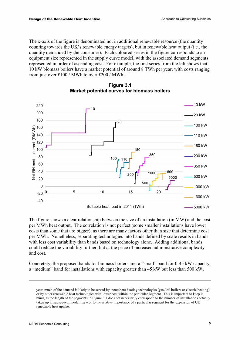
The x-axis of the figure is denominated not in additional renewable resource (the quantity counting towards the UK’s renewable energy targets), but in renewable heat output (i.e., the quantity demanded by the consumer). Each coloured series in the figure corresponds to an equipment size represented in the supply curve model, with the associated demand segments represented in order of ascending cost. For example, the first series from the left shows that 10 kW biomass boilers have a market potential of around 8 TWh per year, with costs ranging from just over £100 / MWh to over £200 / MWh.
Figure 3.1 Market potential curves for biomass boilers
10
20
100 110
180
200
350
500
1000 16005000
-40
-20
0
20
40
60
80
100
120
140
160
180
200
220
0 5 10 15 20 25
Suitable heat load in 2011 (TWh)
Net
RH
cos
t -- c
urre
nt (£
/MW
h)
10 kW
20 kW
100 kW
110 kW
180 kW
200 kW
350 kW
500 kW
1000 kW
1600 kW
5000 kW
The figure shows a clear relationship between the size of an installation (in MW) and the cost per MWh heat output. The correlation is not perfect (some smaller installations have lower costs than some that are bigger), as there are many factors other than size that determine cost per MWh. Nonetheless, separating technologies into bands defined by scale results in bands with less cost variability than bands based on technology alone. Adding additional bands could reduce the variability further, but at the price of increased administrative complexity and cost.
Concretely, the proposed bands for biomass boilers are: a “small” band for 0-45 kW capacity; a “medium” band for installations with capacity greater than 45 kW but less than 500 kW;
year, much of the demand is likely to be served by incumbent heating technologies (gas / oil boilers or electric heating), or by other renewable heat technologies with lower cost within the particular segment. This is important to keep in mind, as the length of the segments in Figure 3.1 does not necessarily correspond to the number of installations actually taken up in subsequent modelling – or to the relative importance of a particular segment for the expansion of UK renewable heat uptake.
Design of the Renewable Heat Incentive Approach to Calculating Subsidies
NERA Economic Consulting
10
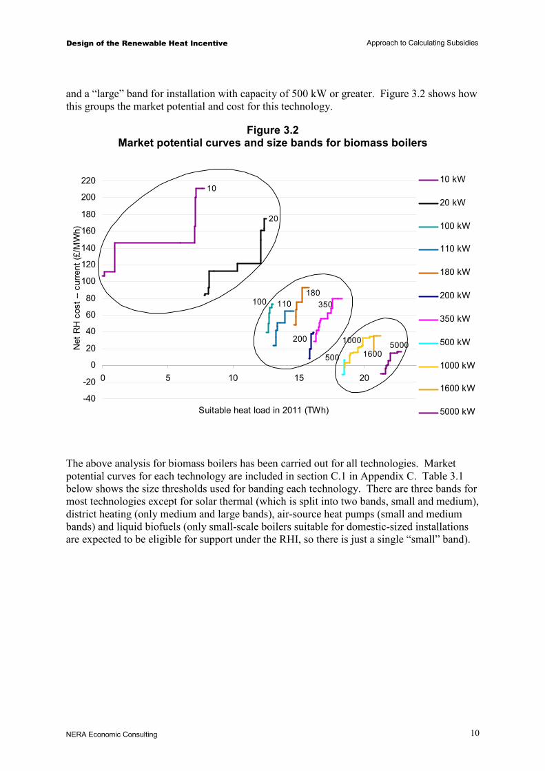
and a “large” band for installation with capacity of 500 kW or greater. Figure 3.2 shows how this groups the market potential and cost for this technology.
Figure 3.2 Market potential curves and size bands for biomass boilers
10
20
100 110180
200
350
500
1000
16005000
-40
-20
0
20
40
60
80
100
120
140
160
180
200
220
0 5 10 15 20 25
Suitable heat load in 2011 (TWh)
Net
RH
cos
t -- c
urre
nt (£
/MW
h)
10 kW
20 kW
100 kW
110 kW
180 kW
200 kW
350 kW
500 kW
1000 kW
1600 kW
5000 kW
The above analysis for biomass boilers has been carried out for all technologies. Market potential curves for each technology are included in section C.1 in Appendix C. Table 3.1 below shows the size thresholds used for banding each technology. There are three bands for most technologies except for solar thermal (which is split into two bands, small and medium), district heating (only medium and large bands), air-source heat pumps (small and medium bands) and liquid biofuels (only small-scale boilers suitable for domestic-sized installations are expected to be eligible for support under the RHI, so there is just a single “small” band).

Design of the Renewable Heat Incentive Approach to Calculating Subsidies
NERA Economic Consulting
11
Table 3.1 Banding size thresholds
Technology Size Size bandkW
Biomass boilers Small 0-45Biomass boilers Medium 45-500Biomass boilers Large > 500Biomass DH Medium 45-500Biomass DH Large > 500Liquid Biofuels Small 0-45ASHP Small 0-45
ASHP Medium 45-350GSHP Small 0-45GSHP Medium 45-350GSHP Large > 350Solar Thermal Small 0-20Solar Thermal Medium 20-100CHP Large N/ABiogas on-site combustion Small 0-45Biogas on-site combustion Medium 45-200Biogas injection All All
3.2. Reference Installations and Determination of Subsidy
The next step in calculating subsidies is to identify a “reference installation” – i.e., the individual demand segment whose cost and other characteristics are used to calculate the subsidy level. Section 3.2.1 explains how the reference installation is identified. The methodology used to determine the level of the subsidy is set out in section 3.2.2, below.
3.2.1. Identification of reference installation
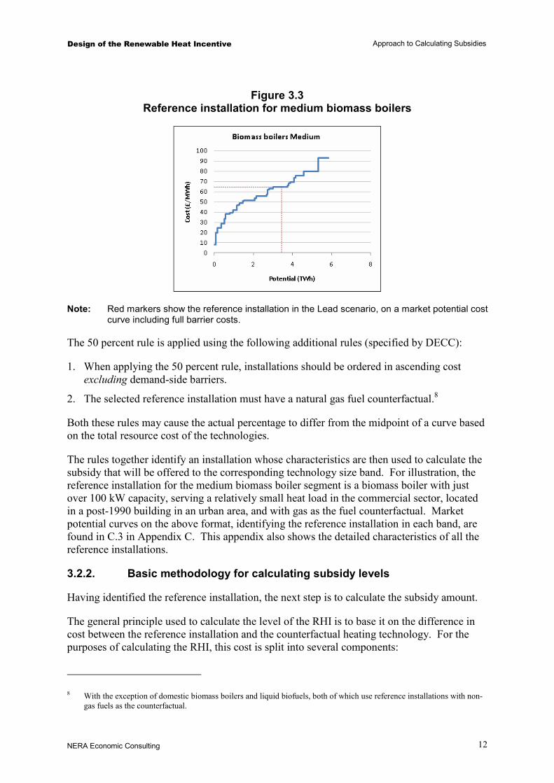
The starting point for identifying the reference installation is to order the costs of all demand segments within a technology size band in ascending order. We then identify the segment whose lower bound lies as close as possible to half of the market potential. That is, the reference installation’s costs are such that the cumulative potential of all segments with lower costs is as close as possible to 50 percent of the total heat market potential in the given banding segment. (We refer to this as “the 50 percent rule”.) This is illustrated for the medium biomass band in Figure 3.3, showing the total market potential of all sizes of biomass boilers above 45 kW but no larger than 500 kW, as well as associated costs. The total market potential is just under 6 TWh per year. The 50 percent rule identifies a segment whose upper bound is at around 3.5 TWh but lower bound is around 3 TWh. This in turn has a net resource cost (i.e. a cost relative to its counterfactual) of approximately £65 / MWh, as indicated by the horizontal dotted line.
Design of the Renewable Heat Incentive Approach to Calculating Subsidies
NERA Economic Consulting
12
Figure 3.3 Reference installation for medium biomass boilers
Note: Red markers show the reference installation in the Lead scenario, on a market potential cost curve including full barrier costs.
The 50 percent rule is applied using the following additional rules (specified by DECC):
1. When applying the 50 percent rule, installations should be ordered in ascending cost excluding demand-side barriers.
2. The selected reference installation must have a natural gas fuel counterfactual.8
Both these rules may cause the actual percentage to differ from the midpoint of a curve based on the total resource cost of the technologies.
The rules together identify an installation whose characteristics are then used to calculate the subsidy that will be offered to the corresponding technology size band. For illustration, the reference installation for the medium biomass boiler segment is a biomass boiler with just over 100 kW capacity, serving a relatively small heat load in the commercial sector, located in a post-1990 building in an urban area, and with gas as the fuel counterfactual. Market potential curves on the above format, identifying the reference installation in each band, are found in C.3 in Appendix C. This appendix also shows the detailed characteristics of all the reference installations.
3.2.2. Basic methodology for calculating subsidy levels
Having identified the reference installation, the next step is to calculate the subsidy amount.
The general principle used to calculate the level of the RHI is to base it on the difference in cost between the reference installation and the counterfactual heating technology. For the purposes of calculating the RHI, this cost is split into several components:
8 With the exception of domestic biomass boilers and liquid biofuels, both of which use reference installations with non-
gas fuels as the counterfactual.
Design of the Renewable Heat Incentive Approach to Calculating Subsidies
NERA Economic Consulting
13
First, there is an ongoing cost component of the RHI, reflecting three categories of cost:
§ Fuel / electricity costs;
§ Maintenance costs (fixed opex); and
§ Ongoing demand-side barrier / administrative costs.
These in turn are calculated using the relevant characteristics of the reference installation and the counterfactual conventional technology (fixed opex, efficiency / performance, and barrier / administrative cost assumptions), and using the fuel and electricity price assumptions in the Lead scenario. In some applications of heat pumps, the use of the renewable heat technology entails a net saving on ongoing costs; in these cases, the ongoing cost component is set to zero.
Second, there is an up-front cost component. Again, this is calculated to reflect the difference between the renewable heat technology and the counterfactual (incumbent) conventional heating technology. It has two components:
§ Equipment and other capital costs (capex)
§ Up-front barrier / administrative costs
As the RHI is provided on an ongoing basis, the up-front costs are calculated on a levelised basis—i.e., as an equivalent annual payment. Two different discount or interest rates are applied to the two different components of the up-front cost. To annualise the capex we apply a discount rate that is specified as an input parameter, and that varies by policy scenario. To annualise the demand demand-side barriers / administrative costs, by contrast, we assume a rate equal to zero.
The rates used in these calculations therefore are not (necessarily) the same as the discount rate that we assume consumers apply in their decision making.
Using terminology from investment appraisal, the rate used to calculate the annualised up-front component of the RHI can be viewed as a “rate of return” (RoR) on the initial up-front payment. In subsequent discussions, we refer to the rate used to levelise the net capex cost as the “modified rate of return” (MRoR). The MRoR is one of the main parameters defining different subsidy scenarios.
There are two important qualifications to the use of the “rate of return” terminology:
§ First, the MRoR applies only to the capex component of costs. It can differ from the overall implied RoR, both because barrier costs are levelised with a zero discount rate, and because, as noted above, some technologies provide a net saving on ongoing costs.
§ Second, the MRoR applies only to the reference installation. The heterogeneity of costs within each banding segment means that a given subsidy will result in different implied rates of return for different heat consumers—with higher implied RoR for installations with costs lower than that of the reference installation.
For both these reasons, the MRoR thus differs from the rate of return that can be expected by “typical” or “average” heat consumers that switch to renewable heat.

Design of the Renewable Heat Incentive Approach to Calculating Subsidies
NERA Economic Consulting
14
3.2.3. Modified subsidy calculation for selected technologies
In addition to the standard methodology described above, there are two cases in which the RHI is set using a different approach.
3.2.3.1. Subsidies calculated for parity with other policy / technologies
Some subsidies are calculated based not on reference installation costs, but so they provide parity with the level of support offered by other policies. This applies to the following:
§ Large biomass boilers: RHI subsidy is set at a level similar to the incremental support provided to the heat portion of renewable CHP under the Renewables Obligation.9
§ Biomass District Heating: RHI subsidy set to the level of biomass boilers with the same capacity.
§ Biogas injection: the subsidy is set for parity, per unit of gas produced, with the support provided to anaerobic digestion of biogas proposed for the Feed-In Tariff.
3.2.3.2. Treatment of solar thermal
In addition, the subsidy to solar thermal is calculated using slightly different principles. First, the MRoR differs from what is provided to other technologies, reflecting DECC’s assumptions about the discount rate used by consumers to evaluate the decision to adopt solar thermal (details are provided below). Additionally, unlike for other technologies, the Lead scenario solar thermal subsidy contains no component to reflect assumed demand-side barriers / administrative costs.
3.3. Subsidy Scenarios
The Lead scenario applies a MRoR of 12 percent for installations other than solar thermal, and a 6 percent MRoR for solar thermal installations. (Up-front barrier costs are levelised using a zero discount rate, as described above.)
For installations other than solar thermal the RHI level is the sum of the ongoing cost components, fixed opex costs, levelised capex costs and levelised upfront barriers. For solar thermal installations, the subsidy reflects only the ongoing costs, fixed opex costs and levelised capex costs, but does not reflect estimated administrative costs or the costs of overcoming barriers.
Table 3.2 shows the resulting Lead scenario subsidy levels.
9 For the purposes of the modelling presented in this report, the RHI for large biomass boilers is set equal to 2.5 p/kWh
which is at the upper end of the range presented in the RHI consultation document (1.6-2.5 p/kWh). If we were to use the same reference-installation methodology for large biomass boilers as we use for other segments (as described above in section 3.2.2), the RHI level would be at the lower end of the range in the consultation document.

Design of the Renewable Heat Incentive Approach to Calculating Subsidies
NERA Economic Consulting
15
Table 3.2 Lead scenario subsidy levels by banding segment (2008 prices)
Technology Size RHI level Size bandp/kWh kW
Biomass boilers Small 8.7 0-45Biomass boilers Medium 6.2 45-500Biomass boilers Large 2.5 > 500Biomass DH Medium 6.2 45-500Biomass DH Large 2.5 > 500Liquid Biofuels1 Small 6.5 0-45ASHP Small 7.6 0-45
ASHP Medium 1.8 45-350GSHP Small 7.1 0-45GSHP Medium 5.5 45-350GSHP Large 1.3 > 350Solar Thermal Small 17.5 0-20Solar Thermal Medium 16.4 20-100CHP Large 2.5 N/ABiogas on-site combustion2
Small N/A 0-45Biogas on-site combustion Medium 5.5 45-200Biogas injection All 4.0 All
Notes:
1. All subsidies are calculated per kWh renewable energy output (n.b. not ARR). For liquid biofuels, a subsidy of 6.5 p/kWh, using a 30 percent FAME blend, implies a subsidy of 1.95 p/kWh total heat output. No subsidies are envisaged for non-domestic use of liquid biofuel.
2. No subsidy is calculated for biogas on-site combustion below 45 kW. 3. Values are reported in 2008 prices.
In addition to this scenario, we model two other policy variants. We describe these in more detail in section 4.3.
Design of the Renewable Heat Incentive Modelling Results
NERA Economic Consulting
16
4. Modelling Results
In this section we present headline results for the Lead scenario described above.
We first show headline modelling results, before presenting more detailed results for the composition of additional renewable resource, resource costs, and implied subsidy payments. We then show results for different policy design options.
These modelling results are of course subject to a wide range of potential uncertainty. We investigate the sensitivity of the results to some of these uncertainties (such as discount rates and input prices) in section 4.4. Other types of uncertainty have less systematic impacts and their influence more difficult to determine through modelling.
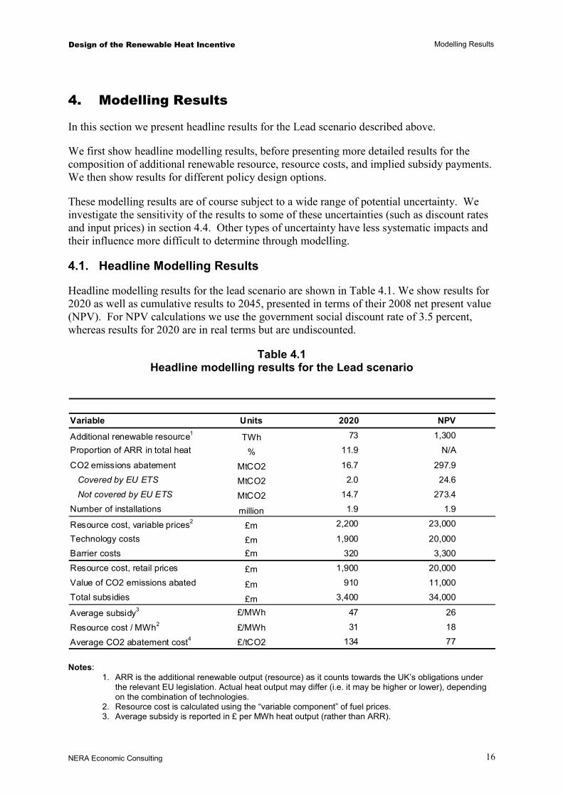
4.1. Headline Modelling Results
Headline modelling results for the lead scenario are shown in Table 4.1. We show results for 2020 as well as cumulative results to 2045, presented in terms of their 2008 net present value (NPV). For NPV calculations we use the government social discount rate of 3.5 percent, whereas results for 2020 are in real terms but are undiscounted.
Table 4.1 Headline modelling results for the Lead scenario
Variable Units 2020Lifetime cumulative
NPV
Additional renewable resource1 TWh 73 1,300Proportion of ARR in total heat % 11.9 N/A
CO2 emissions abatement MtCO2 16.7 297.9Covered by EU ETS MtCO2 2.0 24.6Not covered by EU ETS MtCO2 14.7 273.4
Number of installations million 1.9 1.9
Resource cost, variable prices2 £m 2,200 23,000
Technology costs £m 1,900 20,000Barrier costs £m 320 3,300Resource cost, retail prices £m 1,900 20,000Value of CO2 emissions abated £m 910 11,000Total subsidies £m 3,400 34,000
Average subsidy3 £/MWh 47 26
Resource cost / MWh2 £/MWh 31 18
Average CO2 abatement cost4 £/tCO2 134 77 Notes:
1. ARR is the additional renewable output (resource) as it counts towards the UK’s obligations under the relevant EU legislation. Actual heat output may differ (i.e. it may be higher or lower), depending on the combination of technologies.
2. Resource cost is calculated using the “variable component” of fuel prices. 3. Average subsidy is reported in £ per MWh heat output (rather than ARR).
Design of the Renewable Heat Incentive Modelling Results
NERA Economic Consulting
17
4. Average CO2 abatement cost is obtained by dividing total resource cost (at variable prices) by the total CO2 emissions abatement.
5. Values are reported in 2008 prices.
The results reported above are limited to measures installed in the 2011-2020 period. When they reach the end of their useful life we assume that these measures will cease to generate heat (for example, installations installed in 2011 with a 15 year lifetime would not be expected to generate heat after 2025). In all of the Lead scenarios, installations receive subsidies for their full expected lifetime. By 2045, very little heat is generated from the installations installed up to 2020, so the cumulative values (in NPV terms, where appropriate) represent an estimate of the total costs over the entire RHI policy lifetime.
The modelling suggests the Lead scenario would result in 73 TWh of additional renewable resource by 2020, or a 12 percent share of renewable energy in total heat. By 2020, close to two million installations would be supported by the RHI. The policy would reduce CO2 emissions by just under 17 MtCO2 of annual emissions, mostly from emissions sources not covered by the EU ETS. On average, these reductions are achieved at a cost of £130 / tCO2, although the spread is very large and the highest-cost measures (some small-scale solar thermal installations) have CO2 abatement costs in excess of £800/tCO2.
The total annual resource cost in 2020 is £2.2 billion, or £31 / MWh ARR. This refers to the social resource cost. The cost incurred by consumers differs somewhat from this as the calculation uses retail energy prices (see section 2.7.2), and is £1.9 billion per year in the Lead scenario.
This level of deployment is achieved by paying subsidies amounting to £3.4 billion per year in 2020, or an average of £47 / MWh ARR. The actual subsidies paid per MWh vary significantly by band, as outlined in section 2.7.1 above. The difference between subsidies paid and the cost incurred by consumers is referred to as “rents”, and amounts to approximately £1.4 billion in 2020.
Over the lifetime of the policy, the NPV resource costs are £23 billion, while subsidies are £34 billion. On the benefit side, the value of cumulative CO2 emissions abated is £11 billion.
4.2. Detailed Modelling Results
This section presents modelling results for the Lead scenario at the level of each subsidy band.
4.2.1. Composition of additional renewable resource
4.2.1.1. Composition of ARR by technology and scale
Figure 4.1 shows the composition of additional renewable resource by technology and scale for the Lead scenario. The left-most bar shows the total 2020 ARR of 73 TWh / year, split by technology. This is further grouped by banding size – small, medium, and large – in the subsequent three bars.

Design of the Renewable Heat Incentive Modelling Results
NERA Economic Consulting
18
Figure 4.1 Composition of additional renewable resource in Lead scenario
0
10
20
30
40
50
60
70
80
Total Small Medium Large
Add
ition
al re
new
able
reso
urce
(TW
h)
Biomass boilers Biomass DH ASHP GSHP Solar thermal Biogas injection CHP Liquid biofuels
Source: NERA modelling as explained in text
The dominant technology is biomass boilers, which contribute 27 TWh. Heat pumps make up a similar quantity, split between air-source (14 TWh) and ground-source (13 TWh). CHP and biogas injection each contribute 7 TWh. There also are smaller contributions from solar thermal and biomass district heating, each at around 2.5 TWh.
The modelling results suggest that a limited amount of biomass DH is taken up, despite the fact that the technology does not receive any “uplift” relative to a stand-alone biomass boiler of the same size. This is because the underlying data suggest that, for a limited number of circumstances, the cost of biomass DH is quite low compared to the counter-factual technology. However, the barriers and commercial requirements relevant to biomass district heating are complex and differ in many respects from those faced by other, stand-alone heating options. The financial modelling framework used here does not capture all of these barriers. Nonetheless, the results are consistent with a scenario where there is increased use of district heating in general, and the presence of the RHI makes the use of biomass instead of fossil fuel attractive in some proportion of cases at the subsidy levels being considered. With higher or lower scenarios for overall deployment of district heating, the deployment of biomass district heating also would change.
The uptake of solar thermal also is modelled on a different basis from other technologies, as noted in section 2.8. The assumption of a lower discount rate restricts the potential incentivised to a sub-segment of the market—viz., in modelling terms, the proportion evaluating a potential investment in solar thermal at an implied discount rate of six percent, or lower. Although some restrictions have been made to limit total uptake by 2020, the model has not been directly modified to account for the possibility of different potential

Design of the Renewable Heat Incentive Modelling Results
NERA Economic Consulting
19
distributions of discount rates. In general, the results for solar thermal uptake therefore are more likely to be biased upwards than are the results for other technologies.10
The breakdown by scale shows that the medium segment – in which installation sizes range from 20 kW to 500 kW, depending on technology – accounts for the largest share of output, with 36 TWh ARR. This is followed by the large segment, with 27 TWh. The domestic-sized small segment accounts for around 10 TWh. In the small and medium segments, the contribution from individual technologies is relatively evenly split, except for a low contribution of biomass boilers in the small band. By contrast, the large segment is dominated by biomass boilers and CHP which together represent 84 percent of large-segment ARR. This is because much of the heat demand in this segment is higher-temperature industrial process heat, which can be served only biomass boilers and CHP; by comparison, large installations of district heating, ground-source heat pumps, and biogas have relatively small potential.
The type of consumer is closely correlated with the size bands. The small segment includes all of the domestic sector, while nearly all of the large segment is in the industrial sector. The medium sector is dominated by commercial and public sector installations, although it also contains some industrial space heating. A more detailed breakdown of ARR output by technology and end-user sector is found in Table A.1 in Appendix A.
4.2.2. Distribution of subsidies and resource cost
Although the distribution of ARR is relatively evenly distributed across technologies, the distribution of costs and subsidies by technology is much more uneven.
The distribution is shown in Figure 4.2. The first bar shows ARR by technology, denominated in TWh, with the scale shown on the left vertical axis. The next two bars show resource cost and subsidy in £m, with the scale indicated on the right vertical axis. All numbers relate to annual, undiscounted quantities in 2020.
10 2.5 TWh corresponds to around 1 million solar thermal installations by 2020, mostly in the domestic sector. We do not
know of empirical information that would allow us to test the assumption that there are this many households that would be willing to take up solar thermal applying a discount or hurdle rate (“rate of return”) of six percent or lower.

Design of the Renewable Heat Incentive Modelling Results
NERA Economic Consulting
20
Figure 4.2 Composition of ARR, resource cost, and subsidies by technology
(Lead scenario)
0
10
20
30
40
50
60
70
80
Additional renewableresource
Subsidies paid Total resource cost
TWh
(AR
R)
0
500
1000
1500
2000
2500
3000
3500
4000
£ m
illio
n
Biomass boilers Biomass DH ASHP GSHP
Solar Thermal Biogas Injection CHP Liquid Biofuels
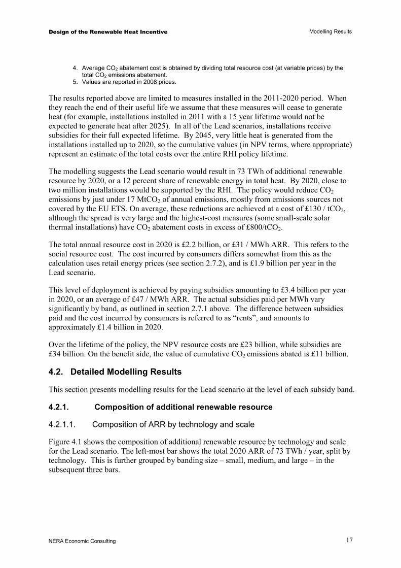
The figure illustrates several differences between the technologies. At one end of the spectrum, biomass boilers account for some 27 TWh of ARR at a cost of £600 million, for an average cost of £22 / MWh ARR; at the other end, solar thermal produces 2.5 TWh of ARR at a cost of £400 million, for an average cost over £160 /MWh ARR.
A more detailed comparison is shown in Table 4.2. The first two columns show average resource cost and subsidy, calculated by summing the total annual cost/subsidy in 2020, and dividing by the total additional renewable resource in that year.11 The average resource cost of biomass boilers, biomass CHP, and ASHPs is similar, at £22-24/MWh ARR all of them are below the overall average of £31 / MWh ARR. Biogas injection has the lowest cost under the particular assumptions used here.12 By contrast, the cost of GSHPs is higher than average, at just above £50 / MWh ARR, and the resource cost of solar thermal stands out as substantially higher than that of technologies, at an average of £166/ MWh ARR. Note that,
11 This is the “social” resource cost rather than the cost as perceived by the consumer. We discuss this distinction in 2.7.2.
We further discuss the issue of “rents” – i.e., payments in excess of the amount required to induce consumers to switch to renewable heat – in section 4.2.2.2
12 The cost of biogas injection is only £1/MWh. This resource cost is very dependent on assumptions about the level of the “gate fee” for receiving waste. The cost is substantially higher if the revenue from gate fees is lower – either because of competition for the resource or because other types of feedstock (whether other types of waste or energy crops) are used.
Design of the Renewable Heat Incentive Modelling Results
NERA Economic Consulting
21
as the quantities in this table are denominated in terms of ARR rather than heat output, they differ from average subsidies per MWh heat output. Also, the numbers for individual technologies combine measures of very varying sizes.13
Table 4.2 Comparison of key costs and shares by technology (Lead scenario)
TechnologyAverage
resource costAverage subsidy
Proportion of total ARR
Proportion of total resource
costProportion of
subsidies£/MWh ARR £/MWh ARR % % %
Biomass boilers 22 33 37% 27% 26%Biomass DH 26 44 4% 3% 3%ASHP 24 44 19% 15% 18%GSHP 52 75 18% 30% 28%Solar Thermal 166 172 3% 18% 12%Biogas Injection 1 40 10% 0% 8%CHP 23 20 9% 7% 4%Liquid Biofuels N/A N/A N/A N/A N/ATotal 31 47 100% 100% 100% Source: NERA modelling Note: Subsidies are reported in £ per MWh ARR (see footnote 14),
Correspondingly, these differences mean that technologies’ share in total ARR (their contribution towards the overall renewable target) can differ substantially from their share in total resource cost or subsidies. This is illustrated by the last three columns in the table. For example, biomass boilers account for 37 percent of total ARR, but only 27 percent of cost, making them less costly than the average. By contrast, solar thermal accounts for just 3 percent of ARR, but 18 percent of cost.
The distribution of subsidies tells a similar story, with CHP and biomass boilers receiving subsidies below the average of £47 / MWh; ASHPs, biomass DH, and biogas injection close to average; and GSHPs and solar thermal receiving substantially above-average subsidies.14
4.2.2.1. Additional breakdown by technology and size
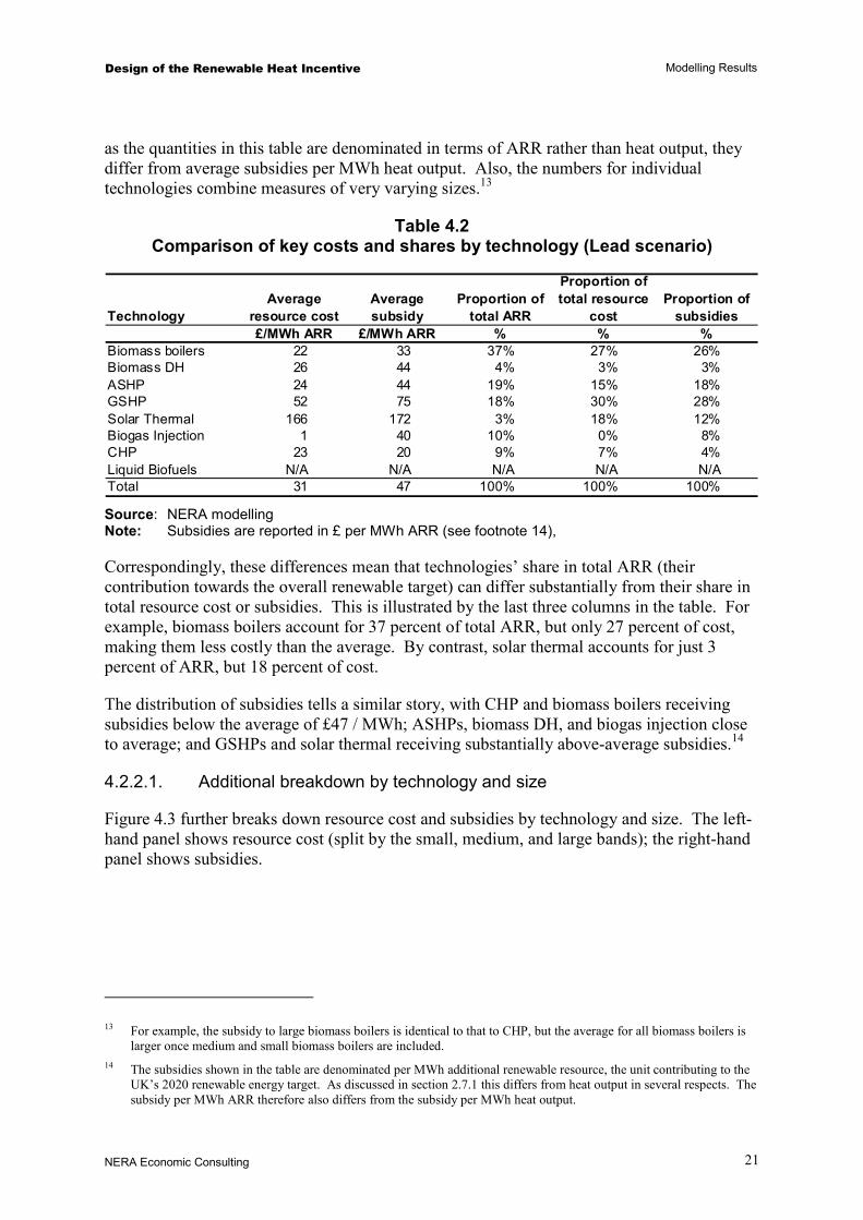
Figure 4.3 further breaks down resource cost and subsidies by technology and size. The left-hand panel shows resource cost (split by the small, medium, and large bands); the right-hand panel shows subsidies.
13 For example, the subsidy to large biomass boilers is identical to that to CHP, but the average for all biomass boilers is
larger once medium and small biomass boilers are included. 14 The subsidies shown in the table are denominated per MWh additional renewable resource, the unit contributing to the
UK’s 2020 renewable energy target. As discussed in section 2.7.1 this differs from heat output in several respects. The subsidy per MWh ARR therefore also differs from the subsidy per MWh heat output.
Design of the Renewable Heat Incentive Modelling Results
NERA Economic Consulting
22
Figure 4.3 Composition of resource cost and subsidies by technology and size
(Lead scenario)
-200
0
200
400
600
800
1,000
1,200
1,400
1,600
1,800
Small Medium Large Small Medium Large
Total resource cost Subsidies paid
£mill
ion
Biomass boilers Biomass DH ASHP GSHPSolar thermal Biogas injection CHP Liquid biofuels
As the figure illustrates, small installations undertaken under the RHI are more expensive than are large ones, accounting for around a third of resource cost but only 13 percent of the ARR (see Figure 4.1). A significant share of the resource cost in the small band is due to solar thermal. The reverse holds for large installations, which contribute just over a third of ARR but only account for 17 percent of the resource costs.
With some exceptions, subsidies follow a similar pattern to costs. The differences are largest where subsidies are set to create parity with other existing policies, rather than on the basis of modelled cost of heat generation (notably, for biogas).15
4.2.2.2. Rents
An important motivation for banding is the ability to reflect differences in underlying costs, and thus avoid paying lower-cost technologies the higher subsidies required for more expensive technologies (see Appendix D for a discussion). As discussed in section 3.2.2, however, the division into bands does not fully eliminate the variability in cost, and therefore also does not fully eliminate payment in excess of cost (“rents”).
15 In both the medium and large segments, biogas injection stands out as having a low resource cost (it is actually negative
in the large band). As noted, this depends on assumptions about the composition of feedstock and the gate fee paid for waste.

Design of the Renewable Heat Incentive Modelling Results
NERA Economic Consulting
23
One complication in calculating rents is the distinction between “social” and “private” resource cost introduced in section 2.7.2. For rents, the relevant quantity is how payments compare to the costs as perceived by the consumer, so based on retail fuel prices. On this basis, out of the total Lead scenario subsidy of £3.4 billion paid in 2020, £1.4 billion accrue as rents.
The amount of rents in an individual band depends on a number of factors. The most important is the variability of cost in each segment. In some cases, the grouping into size and technology leads to relatively homogenous costs (and therefore lower rents), whereas in others there is substantial market potential with costs lower than the reference installation (higher rents). Another factor is that rents tend to be higher when subsidies are set not on the basis of cost, but for parity with other policies (e.g., in the case of biogas and large biomass boilers).
Figure 4.4 shows the average rent in each band, expressed per MWh of heat output (not per MWh ARR):
§ Biogas injection stands out as receiving substantial rents (large biogas injection installations receive the full £40 / MWh as rents), driven by the fact that subsidies are set at the level paid to biogas electricity under the FIT (rather than at the level implied by the standard “rate of return” approach), whereas the estimated net resource costs is much lower (reflecting in part gate fees for food waste, as noted in footnote 12).
§ The modelling suggests that rents to large and medium biomass boilers also are relatively high, in the region of £25-35 / MWh. In the case of large-scale biomass boilers, the rents are high because, as for biogas injection, the subsidy is set on the basis of parity (with the support provided to CHP under the RO), rather than on the basis of required “rate of return”. The resulting subsidy of 2.5 p/kWh is higher than the amount derived through the standard subsidy calculation methodology (as noted, the actual proposed RHI level is yet to be determined, but is proposed in the range 1.6-2.5 p/kWh).
§ In the case of medium biomass boilers, the relatively high rents reflects the fact that the reference installation has much higher costs than some other applications of medium-scale biomass boilers, whereas our modelling suggests that these less expensive options are likely to dominate in actual deployment.
§ Solar thermal rents, especially in the medium segment, also are relatively large on a per-MWh basis. This is due in part to assumed reductions in the costs of solar thermal technology over time, rather than being due to higher-than-required subsidies being offered at the start of the scheme.16 It is also worth bearing in mind that the rents shown for solar thermal represent a relatively small proportion of the subsidy paid to this technology, which is higher than what is offered to other technologies.
16 We discuss options for reducing rents in section 4.3, below.

Design of the Renewable Heat Incentive Modelling Results
NERA Economic Consulting
24
Figure 4.4 Economic rents in Lead scenario
0
5
10
15
20
25
30
35
40
45
S M M L S M L S M L S M
ASHP Biogas injection Biomass boilers GSHP Solar Thermal
£/M
Wh
Notes: Rents are reported in £ / MWh heat output (not additional renewable resource). The figure shows rents relative to costs in 2015, which is around the time that DECC is proposing to review RHI subsidy levels.
For other technologies, the modelling results suggest that average rents will be smaller. For domestic-scale heat pumps and medium biomass boilers the cost can vary substantially within each band, so overpayment to some low-cost applications drives up the average rents to around £10-20 / MWh. For the remaining technologies, average rents typically are small, below £10 / MWh.
Rents could be reduced by reducing subsidy payments – either initially, or over time (e.g. through a pre-defined “degression” of support or through periodic review of support levels). The above rents are calculated on the basis of costs projected for 2015, the year after the first proposed revision to RHI subsidy levels. Because RHI subsidy levels are expected to be reviewed throughout the period to 2020, there will be opportunities to limit overpayment to less than the amounts suggested by the above calculations.
4.2.3. Demand-side implications and renewable heat market share
The final share of additional renewable heat output achieved in the Lead scenario is 12 percent. However, the implied share of renewables in new heating equipment sales is much higher. This is both because not all heating equipment in place in 2011 is expected to be replaced before 2020, and because the ramp-up starts from a low base and only gradually reaches high level of penetration.
Figure 4.5 shows the annual market share in terms of head demand of renewable technologies under the Lead scenario. Overall, renewable heat technology sales are low to start with, but by 2020 reach over 40 percent of the heat market. For the RHI to succeed in delivering the renewable heat share indicated above, it therefore has to succeed in making renewable heat technologies achieve nearly as high a share of heating equipment as conventional gas and oil

Design of the Renewable Heat Incentive Modelling Results
NERA Economic Consulting
25
boilers, by 2020. (The numbers exclude solar thermal, as this is a discretionary and supplementary technology rather than a replacement for conventional heating.)
The overall average masks significant variation between sectors. The highest market share is in the commercial and public sectors, where sales of renewable heat equipment in 2020 almost entirely replaces sales of conventional boilers, reaching close to 90 percent of the total new heating equipment market by 2020. In the industrial sector, the majority of heat load served by new sales in 2020 likewise is of renewable heat technologies, achieved in large part through expansion of biomass boilers and biomass CHP. By contrast, penetration in the domestic sector is smaller, with renewable heat technologies representing 18 percent of the market share. In the non-domestic sectors in particular, these levels of uptake will require very significant changes to the market for heating equipment.
Figure 4.5 Implied renewable heat share in new heating equipment, 2011-2020
(Lead scenario)
0%
10%
20%
30%
40%
50%
60%
70%
80%
90%
100%
2012 2013 2014 2015 2016 2017 2018 2019 2020
Mar
ket S
hare
(%)
Commercial / Public Domestic Industrial Total
4.3. Alternative Policy Designs
In the course of developing the Lead scenario, we investigated the implications of a number of other potential policy designs and structures for the RHI subsidy. Some of main issues investigated include:
§ The level of the “modified rate of return” used to set subsidies;
§ The assumptions for solar thermal uptake and subsidies;
§ The use of banding vs. a uniform subsidy to all installations;
§ The payment of the RHI subsidy on an ongoing basis vs. a more “front-loaded” payment structure; and
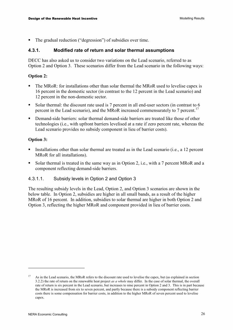
Design of the Renewable Heat Incentive Modelling Results
NERA Economic Consulting
26
§ The gradual reduction (“degression”) of subsidies over time.
4.3.1. Modified rate of return and solar thermal assumptions
DECC has also asked us to consider two variations on the Lead scenario, referred to as Option 2 and Option 3. These scenarios differ from the Lead scenario in the following ways:
Option 2:
§ The MRoR: for installations other than solar thermal the MRoR used to levelise capex is 16 percent in the domestic sector (in contrast to the 12 percent in the Lead scenario) and 12 percent in the non-domestic sector.
§ Solar thermal: the discount rate used is 7 percent in all end-user sectors (in contrast to 6 percent in the Lead scenario), and the MRoR increased commensurately to 7 percent.17
§ Demand-side barriers: solar thermal demand-side barriers are treated like those of other technologies (i.e., with upfront barriers levelised at a rate if zero percent rate, whereas the Lead scenario provides no subsidy component in lieu of barrier costs).
Option 3:
§ Installations other than solar thermal are treated as in the Lead scenario (i.e., a 12 percent MRoR for all installations).
§ Solar thermal is treated in the same way as in Option 2, i.e., with a 7 percent MRoR and a component reflecting demand-side barriers.
4.3.1.1. Subsidy levels in Option 2 and Option 3
The resulting subsidy levels in the Lead, Option 2, and Option 3 scenarios are shown in the below table. In Option 2, subsidies are higher in all small bands, as a result of the higher MRoR of 16 percent. In addition, subsidies to solar thermal are higher in both Option 2 and Option 3, reflecting the higher MRoR and component provided in lieu of barrier costs.
17 As in the Lead scenario, the MRoR refers to the discount rate used to levelise the capex, but (as explained in section
3.2.2) the rate of return on the renewable heat project as a whole may differ. In the case of solar thermal, the overall rate of return is six percent in the Lead scenario, but increases to nine percent in Option 2 and 3. This is in part because the MRoR is increased from six to seven percent, and partly because there is a subsidy component reflecting barrier costs there is some compensation for barrier costs, in addition to the higher MRoR of seven percent used to levelise capex.

Design of the Renewable Heat Incentive Modelling Results
NERA Economic Consulting
27
Table 4.3 Subsidy by banding segment
Lead Option 2 Option 3Technology Size RHI level RHI level RHI level
p/kWh p/kWh p/kWhBiomass boilers Small 8.7 9.9 8.7Biomass boilers Medium 6.2 6.2 6.2Biomass boilers Large 2.5 2.5 2.5Biomass DH Medium 6.2 6.2 6.2Biomass DH Large 2.5 2.5 2.5Liquid Biofuels Small 6.5 6.8 6.5ASHP Small 7.6 9.2 7.6ASHP Medium 1.8 1.8 1.8GSHP Small 7.1 9.2 7.1GSHP Medium 5.5 5.5 5.5GSHP Large 1.3 1.3 1.3Solar Thermal Small 17.5 22.3 22.3Solar Thermal Medium 16.4 19.5 19.5CHP Large 2.5 2.5 2.5Biogas on-site combustion1
Small N/A N/A N/ABiogas on-site combustion Medium 5.5 5.5 5.5Biogas injection All 4.0 4.0 4.0 Source: NERA calculations based on DECC methodology.
Notes: 1. There is no subsidy calculated for small biogas on-site combustion

Design of the Renewable Heat Incentive Modelling Results
NERA Economic Consulting
28
4.3.1.2. Headline modelling results for Option 2 and Option 3
Headline results for Option 2 and Option 3 are shown and contrasted with the Lead scenario in Table 4.4
Table 4.4 Headline modelling results for alternative subsidy scenarios
Variable Units Lead Option 2 Option 3 Lead Option 2 Option 3
Additional renewable resource1 TWh 73 76 74 1,300 1,400 1,300
Proportion of ARR in total heat % 11.9 12.4 12.1 N/A N/A N/ACO2 emissions abatement MtCO2 16.7 17.4 16.9 298 311 303
Covered by EU ETS MtCO2 2.0 2.1 2.0 25 25 25Not covered by EU ETS MtCO2 14.7 15.4 14.9 273 285 278
Number of installations million 1.9 2.6 2.4 1.9 2.6 2.4
Resource cost, variable prices2 £m 2,200 2,700 2,600 23,000 28,000 26,000Technology costs £m 1,900 2,300 2,100 20,000 23,000 22,000Barrier costs £m 320 460 420 3,300 4,800 4,400Resource cost, retail prices £m 1,900 2,400 2,200 20,000 25,000 24,000Value of CO2 emissions abated £m 910 950 920 11,000 11,000 11,000
Total subsidies £m 3,400 4,200 3,800 34,000 42,000 38,000
Average subsidy3 £/MWh 47 54 51 26 30 28
Resource cost / MWh2 £/MWh 31 36 35 18 21 20
Average CO2 abatement cost4 £/tCO2 134 158 152 77 90 87
Lifetime cumulative NPV2020
Notes: See notes to Table 4.1
4.3.1.3. Main features of Option 2 headline results
The Option 2 scenario uses the same input assumptions as Lead but applies a higher MRoR to installations in the small band (covering domestic-sized installations), in line with the assumed household discount rate of 16 percent. The scenario also treats solar thermal differently. The solar thermal discount rate is 7 rather than 6 percent, and barrier costs are higher. Subsidies to solar thermal also differ, calculated using a 7 percent MRoR to match the discount rate, and accounting for barrier cost in the same way as for other technologies.
The higher subsidies to small installations and revised treatment of solar thermal result in somewhat higher levels of ARR, reaching 76 TWh per year in 2020, compared to 73 TWh in Lead. This is accompanied by higher resource cost, reaching £2.7 billion per year in 2020, as compared with £2.2 billion in the Lead scenario. The increase of £500 million arises partly because of increased uptake of renewable heat among (higher-cost) domestic installations (£200 million), and partly because the uptake of solar thermal costs consumers more (£300 million). Meanwhile, subsidies are £600 million per year higher, reaching £4.2 billion per year in 2020.

Design of the Renewable Heat Incentive Modelling Results
NERA Economic Consulting
29
The increased domestic sector deployment under the Option 2 scenario comes at an increase in average costs, because the additional measures are more expensive than those previously taken up. Overall, excluding solar thermal, the additional measures taken up under the Option 2 scenario have an average cost of £82/ MWh (significantly higher than the £31 / MWh average cost in the Lead scenario). The higher subsidies necessary to incentivise uptake of these measures are also paid to those that were already being installed in the Lead scenario, so the subsidy cost per additional MWh of non-solar technologies goes as high as £172 / MWh, or 17 p/kWh (compared with the average of £47 / MWh, or 4.7 p/kWh, paid in the Lead scenario). (Note that a comparison including solar thermal is not directly relevant, as the assumptions about discount rates and barriers change between scenarios.) In policy lifetime terms, the NPV resource cost is £28 billion (compared to £23 billion in the Lead scenario), NPV subsidies are £42 billion (£34 billion in the Lead scenario), and the NPV benefits of CO2 emissions abated is £11 billion, which is very similar to the Lead scenario.
4.3.1.4. Main features of Option 3 headline results
The Lead and Option 3 scenarios differ only in the treatment of solar thermal. In Option 3, the same approach is taken as in Option 2, with less optimistic assumptions about solar thermal uptake (higher discount rate and barriers), matched by higher MRoR and some compensation for demand-side barriers.
Overall, the Option 3 scenario results in a higher level of solar thermal deployment than in the Lead scenario, adding nearly half a million installations accounting for 1 TWh of ARR per year by 2020. The total ARR in 2020 thus is 74 TWh per year. This comes at an additional cost of £400 million per year, or some £400 / MWh, while subsidies increase by £400 million (in both cases a combination of assumed higher cost and higher solar deployment).
The scenario thus illustrates that the overall cost and subsidy are sensitive to assumptions about solar thermal cost. The high per-MWh cost of this technology means that even relatively small changes in absolute ARR have a large impact on the overall cost and subsidy required. We further discuss the implications of alternative assumptions for solar thermal in section 4.4.2.1.
4.3.1.5. Composition of renewable heat uptake
The Option 2 and Option 3 scenarios differ in the composition of ARR in the following ways:
The Option 2 scenario achieves a higher level of ARR (3 TWh) in the small band (domestic sector) as a result of higher subsidies. This increase is achieved chiefly through an increase in biomass boilers (1.5 TWh) and solar thermal (1 TWh), and liquid biofuels (0.5 TWh) in 2020. The uptake of heat pumps is close to unchanged.
The Option 3 scenario differs from Lead only in the treatment of solar thermal technology. As a result of higher subsidies to solar thermal, Option 3 achieves 1 TWh ARR more than the Lead scenario. The contribution to ARR from all other technologies remains identical to the Lead scenario.

Design of the Renewable Heat Incentive Modelling Results
NERA Economic Consulting
30
4.3.2. Uniform support
As discussed in more detail in Appendix D, the use of banding has both advantages and disadvantages. Its advantages include the reduction of rents, and the ability to bring forward more expensive technologies without overpaying less costly options. This in turn could be desirable for a number of reasons, whether to ensure that renewable heat be used in all sectors of the economy, or to guard against the risk of unexpectedly low growth in some sectors and the associated failure to meet UK renewable heat target.
Against this, banding typically drives up the cost of the renewable heat options deployed. This is because some cost-effective ways of adding to the renewables target are excluded by setting some bands lower than others. In terms of the market potential curve shown in Figure 3.3, some of the market potential with cost higher than the reference installation is likely to have lower cost than the subsidies offered to other, higher-cost bands. However, these lower cost measures will not be undertaken, so total cost increases.18
To quantify the additional resource cost associated with banding vs. not banding, one can compare the results of the Lead scenario to one that achieves the same level of ARR output by offering the same subsidy to all installations.19 The results for ARR, subsidies, and resource cost is shown in Figure 4.6 (where the results are organised by technology) and in Figure 4.7 (by scale). The non-banding scenario is labelled “uniform subsidy”, and corresponds to a subsidy of £70 / MWh (or 7 p/kWh) offered to all installations. As with previous figures, the results presented are undiscounted annual quantities for the year 2020.
18 If costs and future uptake were known with certainty it would be possible to set bands and subsidy levels in a way that
would reduce subsidies “perfectly” without sacrificing efficiency – that is, without leaving out some of the relatively low-cost measures. In practice bands cannot be set perfectly.
19 Economic theory suggests that applying a uniform charge or subsidy for some output (e.g. MWh ARR, or in other contexts, tCO2, etc.) will lead to the efficient – i.e., lowest resource cost – way of achieving a target related to that output. However, for a subsidy scheme such as the RHI the lower resource cost may be accompanied by higher total subsidy payments than a policy that differentiates support. We discuss these issues in more detail in Appendix D.

Design of the Renewable Heat Incentive Modelling Results
NERA Economic Consulting
31
Figure 4.6 Distribution of ARR, subsidies, and resource cost with and without banding
(by technology)
0
10
20
30
40
50
60
70
80
Lead Uniformsubsidy
Lead Uniformsubsidy
Lead Uniformsubsidy
Additional renewableresource
Subsidies paid Total resource cost
TWh
(AR
R)
0
1000
2000
3000
4000
5000
6000
£ m
illio
n
Biomass boilers Biomass DH ASHP GSHP
Solar Thermal Biogas Injection CHP Liquid Biofuels
Design of the Renewable Heat Incentive Modelling Results
NERA Economic Consulting
32
Figure 4.7 Distribution of ARR, subsidies, and resource cost with and without banding
(by size band)
0
10
20
30
40
50
60
70
80
Lead Uniformsubsidy
Lead Uniformsubsidy
Lead Uniformsubsidy
Additional renewableresource
Subsidies paid Total resource cost
TWh
(AR
R)
0
1000
2000
3000
4000
5000
6000
£ m
illio
n
Small Medium Large
As expected, a uniform subsidy leads to higher subsidies but lower resource cost. Total subsidies paid increase by £1.6 billion, from £3.4 billion to £5 billion. Most of this is an increase in the payments to heat pumps (£1.1 billion) and biomass boilers (£600 million). This is offset in part by eliminating the subsidies paid to solar thermal (-£400 million), as the costs of solar thermal are not sufficiently compensated by the £70 / MWh or 7 p/kWh subsidy level, so the technology is not taken up. Meanwhile, resource costs are almost halved, dropping by almost £1 billion. The modelling thus suggests that the use of banding saves £1.6 billion in annual subsidy cost by 2020, but that this is traded against an increase in the resource cost (not accounting for the potential “insurance” benefit of encouraging multiple technologies and sectors) of £1 billion per year by 2020.
The technology mix also changes. Solar thermal disappears from the mix in the uniform subsidy scenario, while there is the addition of a small amount of liquid biofuels. These shifts are minor, however, and the most notable feature is that significant contributions from all technologies remain at a uniform £70 / MWh subsidy. From a technology point of view, the insurance benefits of banding therefore may be limited, as the use of banding does not significantly alter the composition of technologies brought forward.
However, there is a significant change in the distribution between sizes (and therefore sectors). The contribution from small and medium installations shrinks from 46 TWh to 26

Design of the Renewable Heat Incentive Modelling Results
NERA Economic Consulting
33
TWh, with a corresponding increase in large installations, from 27 TWh to 47 TWh. Much of the additional contribution in the large segment is from industry, and the achievement of this level of ARR from renewable heat thus would depend to a large extent on the successful scaling up of biomass boilers in industrial applications (about 25 TWh ARR would need to come forward, 5 TWh more than in Lead scenario). There also is increased reliance on commercial / public ground-source heat pumps (almost 3 TWh more). These two segments alone would contribute over 36 TWh in 2020, or half of the total.
4.3.3. Up-front support / time-limited subsidies
The policy modelled in the Lead scenarios is one of ongoing subsidies throughout the expected lifetime of each technology. An alternative would be to provide the subsidy over a shorter time period. This can be done by paying (some share of) subsidies up-front. Alternatively, a stream of subsidies with the same NPV value to the consumer can be provided over a shorter time period (say, five or ten years).
In brief, the main motivation for front-loading the subsidy would be to overcome the factors that cause consumers to demand high future compensation in order to make early capital investments.
These factors are captured in the modelling through the use of discount rates, as set out in section 2.5. The discount rates in the Lead scenario are 12 percent for non-domestic organisations and 16 percent for households, whereas the government discount rate is significantly lower, at 3.5 percent. The higher the discount rate, the higher are the ongoing subsidies required to compensate for up-front expenditure. Viewed purely from the perspective of the total net present value of costs and subsidies, the government therefore would prefer not to have to pay the higher subsidy levels required by private parties when they receive subsidies over an extended time period.
To investigate the impact of front-loading subsidies, we have modelled a scenario where subsidies are divided into two tiers, one consisting of the up-front components (Tier 1), and another of the ongoing cost components (Tier 2). Tier 2 would be paid throughout the lifetime of the equipment, whereas Tier 1 would be paid per MWh over a shorter time period (with commensurate increases per MWh as required to make the NPV value the same as in the Lead scenario).
By construction, rescheduling of subsidies that are equivalent in NPV terms does not have any effect on total ARR or on total resource costs. However, the NPV subsidy cost is significantly affected. For example, paying off up-front expenditures over 10 years (rather than over the full lifetime of a measure) reduces the cumulative NPV of subsidies to 2030 by about 1.5 percent, and compressing the capital repayment into 7 years reduces the NPV of subsidies by almost 10 percent. The effect becomes stronger over time, and the reduction in the NPV of subsidies to 2045 can be reduced by as much as 20 to 30 percent by front-loading the subsidy payments.
Against this, shortening the period over which subsidies are paid leads to higher payments in each individual year. For example, a 7-year payment schedule would increase payments in the year 2020 by around one-third. This in turn would increase the amount of money to be

Design of the Renewable Heat Incentive Modelling Results
NERA Economic Consulting
34
raised through the RHI funding mechanism – at least until all subsidies for up-front expenses were paid off.20
4.3.4. Degression
The Lead scenario results are calculated on the assumption of a fixed level of subsidy for each technology-band for the duration of the RHI until 2020. It would also be possible for subsidies to change over time. The process of reducing subsidies in a step-wise fashion over time (usually at a pre-determined rate) is known as “degression”, and has been used in a number of schemes, perhaps most prominently in German FITs.
There are several potentially attractive features of degression: first, it may motivate investors to bring forward their purchase of renewable heat equipment, in order to benefit from a higher subsidy level. This could counteract any incentive to postpone renewable equipment purchase until more efficient technologies are available. Reducing subsidies over time would also reduce the NPV of the lifetime subsidies from the government perspective (this effect similar to the upfront subsidies described in section 4.3.3.
Second, rents to heat users installing renewable technologies are likely to fall, as subsidies more accurately reflect the evolution of renewable heat costs over time. For example, the efficiency of heat pumps is expected to increase over the coming years, and degression would reduce the rents accruing to late-adopters.
It has also been suggested that degression could encourage innovation, by signalling the need to reduce the costs of renewable technologies. (This argument assumes that manufacturers and installers of renewables technologies do not already have incentives to reduce costs as a way to increase their profitability, given a fixed subsidy payment.)
Degression also may have disadvantages. First, given uncertainties about the development of technology costs, degression may reduce subsidies faster than costs actually decline over time – this would risk undermining the renewable heat supply chain if projections of future cost reductions (which are inherently less certain than estimates of current cost) prove optimistic. Second, because a number of renewable heat technologies are characterised by significant ongoing costs, in addition to capital costs, there is less certainty about the direction of movement in the requirement for support. It may therefore be preferable to plan for periodic reviews in the level of support offered.21
To investigate the potential impact of degression, we have modelled a scenario where a 3 percent degression rate is applied to air-source and ground-source heat pumps and solar thermal segments (selected because costs of these technologies are expected to fall most). This reduces the total ARR in 2020 by around 2 TWh (because some installations were no
20 If the RHI were to be discontinued in 2020 this would imply declining funding requirements from 2021-2027, as the
Tier 1 component of the levy was eliminated. However, if the RHI were not expected to be available to new installations after 2020 it is unlikely that the growth rates assumed here would ever be achieved.
21 If support levels were reviewed periodically, or on an ad-hoc basis, there is a risk that this will increase investor uncertainty, particularly if subsidy review is ad-hoc. Increased risk would reduce investors’ willingness to invest in renewable heat technologies and businesses, and higher subsidies could be required to counteract this effect. We have not modelled the impacts of ad-hoc adjustments to subsidy levels.
Design of the Renewable Heat Incentive Modelling Results
NERA Economic Consulting
35
longer attractive to end-users), whereas subsidies are reduced by some 25 percent in 2020 (mostly coming from GSHPs and solar thermal, but also from ASHPs) and total resource cost also is reduced. Total lifetime NPV of subsidies (until 2045) decreases by over 35 percent.
4.4. Sensitivity Analyses of Inputs and Key Assumptions
Many of the inputs to the modelling are highly uncertain. We have explored the significance of this uncertainty through sensitivity analysis of various inputs, and present some of the more important results in this section.
It is possible to reflect the uncertainty in two ways – either holding subsidies constant and modelling the effects on uptake (and other headline quantities) or by holding the target or method of setting subsidies constant and then calculating the resulting subsidies required.
For example, higher fossil fuel prices would make many renewable heat options more attractive.22 At a given subsidy level this would lead to higher deployment of renewable heat. Alternatively, it could lead to a downward revision in the subsidy offered to renewable technologies. We focus our sensitivity analysis on the latter – i.e. the impact on subsidies given changes in the uncertain variables.
Concretely, our broad approach has been to calculate the subsidy the reference installation in each band would receive under the subsidy-setting approach discussed in Chapter 2 if a particular input differed. We then model uptake using the new set of subsidies and the revised fuel prices
4.4.1. Impact of fuel price assumptions: fossil fuels and biomass prices
The first quantity that we investigate is fuel prices. We use the “low” and “high high” fossil fuel price projections derived from DECC’s Updated Energy Projections and provided by DECC, while keeping biomass prices constant (central). We also investigate low and high biomass price scenarios provided by DECC, while keeping the fossil fuel prices constant (central).
The sensitivity of headline results to changes in these inputs is shown in Table 4.5. The results are presented excluding renewable CHP. This is because the CHP modelling was undertaken separately, using a different methodology to investigate the sensitivity of the results to fuel prices. The overall quantity of ARR in the Lead scenario therefore is lower, at 66 TWh. This varies somewhat between scenarios, reflecting different responses within bands to the changes in fuel prices. However, the variations are minor (65-68 TWh) and do not significantly alter the conclusions from direct comparisons of quantities in the table.
22 Heat pumps complicate this example. Heat pumps use electricity, and the price of this in turn depends on fossil fuel
prices. Both the cost of heat pumps and of the counterfactual they replace changes when fossil fuel prices change, so the relative attractiveness of heat pumps depends on the movement of electricity prices relative to other fossil fuel prices.

Design of the Renewable Heat Incentive Modelling Results
NERA Economic Consulting
36
Table 4.5 Headline results: sensitivity to fuel prices (excluding CHP)
Variable Units Lead
Low Fossil Fuel Price
High high
Fossil Fuel Price
Low Biomass
Price
High Biomass
Price
Additional renewable resource1 TWh 66 66 68 67 65
Proportion of ARR in total heat % 10.8 10.8 11.1 10.9 10.6
CO2 emissions abatement MtCO2 16.0 15.9 16.5 16.2 15.5
Covered by EU ETS MtCO2 1.3 1.3 1.8 1.5 0.9
Not covered by EU ETS MtCO2 14.6 14.5 14.7 14.7 14.6
Number of installations million 1.9 1.9 1.9 1.9 1.9
Resource cost, variable prices2 £m 2,100 2,600 940 1,900 2,300
Technology costs £m 1,800 2,300 630 1,600 2,000
Barrier costs £m 320 310 310 310 330
Resource cost, retail prices £m 1,800 2,300 560 1,600 2,000
Value of CO2 emissions abated £m 890 880 900 900 880
Total subsidies £m 3,300 3,700 2,800 3,200 3,500
Average subsidy3 £/MWh 48 55 41 46 53
Resource cost / MWh2 £/MWh 32 39 14 29 35
Average CO2 abatement cost4 £/tCO2 131 162 57 120 148
NPV Cumulative resource cost to 2045 £m 23,000 26,000 13,000 22,000 24,000
NPV Cumulative subsidies to 2045 £m 34,000 37,000 32,000 35,000 35,000 Notes: See notes to Table 4.1.
As the table shows, when fossil fuel prices are low it increases the total annual resource cost in 2020 relative to the Lead scenario by about £500 million, from £2.1 billion to £2.6 billion. (Around half of this difference is accounted for by an increase in the resource cost of medium and large biomass boilers.)23 Subsidies increase by £400 million (again, some £240 million of this is attributable to biomass boilers).
The “high high” fossil fuel prices have the reverse effect. Total annual resource costs in 2020 are reduced by over £1 billion, from £2.1 billion to £940 million. Again, the impact is most pronounced for biomass boilers whose costs are reduced by £600 million. Under the “high high” scenario, (assuming biomass fuel prices are not affected) the resource cost of some large biomass boilers becomes negative. Subsidies fall by £500 million, from £3.3 billion to 2.8 billion.
23 This is due to the effects noted in footnote 22, viz., that the exposure of heat pumps to the electricity price makes these
technologies less sensitive to changes in fossil fuel prices.
Design of the Renewable Heat Incentive Modelling Results
NERA Economic Consulting
37
The effect of biomass prices is qualitatively similar: low biomass prices decrease the total resource costs (by £200 million) and subsidies (by £100 million). The “high” biomass prices lead to an increase in resource costs and subsidies by a similar quantity (around £200 million). These changes are almost entirely due to changes in the cost of technologies using biomass fuel, but there are also some small changes to the uptake of other technologies.
As noted, CHP has been excluded from the headline results. Separate modelling undertaken by AEA suggests that CHP is highly sensitive to fossil fuel price assumptions. Under a scenario where the subsidy paid to CHP remains at the level of £25 / MWH (or 2.5 p/kWh) but the low fossil fuel prices are used, the total ARR from CHP is reduced from 7 TWh to just 0.7 TWh. By contrast, using “high high” fossil fuel prices increases ARR to 16 TWh. CHP uptake is also sensitive to biomass prices: high biomass prices reduce CHP uptake significantly, to just 2 TWh ARR, whereas low biomass prices increases the ARR from CHP to 12 TWh (AEA, 2010)
4.4.2. Impact of discount rate assumptions
Another important but uncertain input is how heat users trade off up-front costs against expected ongoing costs. We reflect this trade-off (which reflects both the time value of money, uncertainties, and possibly other costs) in the discount rate that end-users apply to evaluate their heating technology options. Some of the relevant considerations are discussed in sections 2.5 and 4.3.3.
We compare the Lead assumptions (16 percent domestic discount rate; 12 percent non-domestic discount rate) to two alternative assumptions about discount rate, a “high” scenario with a uniform 20 percent discount rate and a “low” scenario with a 10 percent discount rate.24 These alternative discount rates apply to both domestic and non-domestic end-users, with the exception of those adopting solar thermal, where we use the assumptions specified by DECC for the Lead scenario. For a typical equipment lifetime of 15 years, 10 and 20 percent discount rates yield investment decisions equivalent to those produced by requirements to meet “payback” periods of just under eight and five years, respectively.
We use the same methodology as in the fuel price sensitivity analysis, adjusting subsidies and keeping renewable heat output close to the level in the Lead scenario. (This approach therefore amounts to a change in the “modified rate of return” implicit in the subsidy.)
Table 4.6 shows how the subsidies, resource costs and other headline variables change in these scenarios. Total ARR stays nearly the same, by construction.25 As above, the analysis excludes renewable CHP, which is modelled separately and uses different discount rate assumptions.
24 This differs from the analysis presented in the RHI IA (DECC 2010), which tests a 12 percent discount rate. 25 Small differences in the ARR and the number of installations arise because there is some uptake of liquid biofuels in the
domestic-sector under the discount rate sensitivity scenarios.

Design of the Renewable Heat Incentive Modelling Results
NERA Economic Consulting
38
Table 4.6 Headline results: sensitivity to discount rates (excluding CHP)
Variable Units LeadHigh discount
rateLow discount
rate
Additional renewable resource1 TWh 66 67 67Proportion of ARR in total heat in 2020 % 10.8 10.9 10.9CO2 emissions abatement MtCO2 16.0 16.1 16.2
Covered by EU ETS MtCO2 1.3 1.2 1.6Not covered by EU ETS MtCO2 14.6 14.9 14.6
Number of installations million 1.9 2.0 2.0
Resource cost, variable prices2 £m 2,100 3,200 1,800
Technology costs £m 1,800 2,700 1,500Barrier costs £m 320 440 270Resource cost, retail prices £m 1,800 2,900 1,500Value of CO2 emissions abated £m 890 900 890Total subsidies £m 3,300 4,500 3,100
Average subsidy3 £/MWh 48 66 45
Resource cost / MWh2 £/MWh 32 48 26
Average CO2 abatement cost4 £/tCO2 131 198 108 Notes: See notes to Table 4.1
The table shows that discount rate assumptions have a large impact on costs and on subsidies. Annual subsidies in the high discount rate scenario increase from £3.3 billion to £4.5 billion, while the resource cost increases by more than half, from £2.1 billion to £3.2 billion in 2020.
The low discount rate scenario is a smaller change from the original Lead scenario assumptions, so the changes are smaller. Nonetheless, the total resource cost falls from £2.1 billion to £1.8 billion in 2020, most of which is accounted for by a reduction in domestic sector costs (£0.2 billion), and also in medium sector (£0.1 billion).
Overall, the modelling suggests that, if consumers are less willing (than assumed in the Lead scenario) to incur up-front costs against the prospect of future RHI subsidies, then the cost of the policy could increase substantially.
4.4.2.1. Treatment of solar thermal
The Lead scenario treats solar thermal differently from other technologies. As noted in Chapter 3, the differences include a lower discount rate for the modelling of consumer uptake as well as a reduction of the demand-side barriers to solar thermal. The revised inputs have been specified by DECC, and correspond to an assumption that a proportion of the potential market for solar thermal will apply a discount rate of six percent or lower, and will face lower demand-side barriers, when evaluating the decision whether to adopt the technology.
As noted in section 2.8 there is significant uncertainty about what proportion of households or businesses may be willing to adopt solar thermal using these criteria. To investigate the
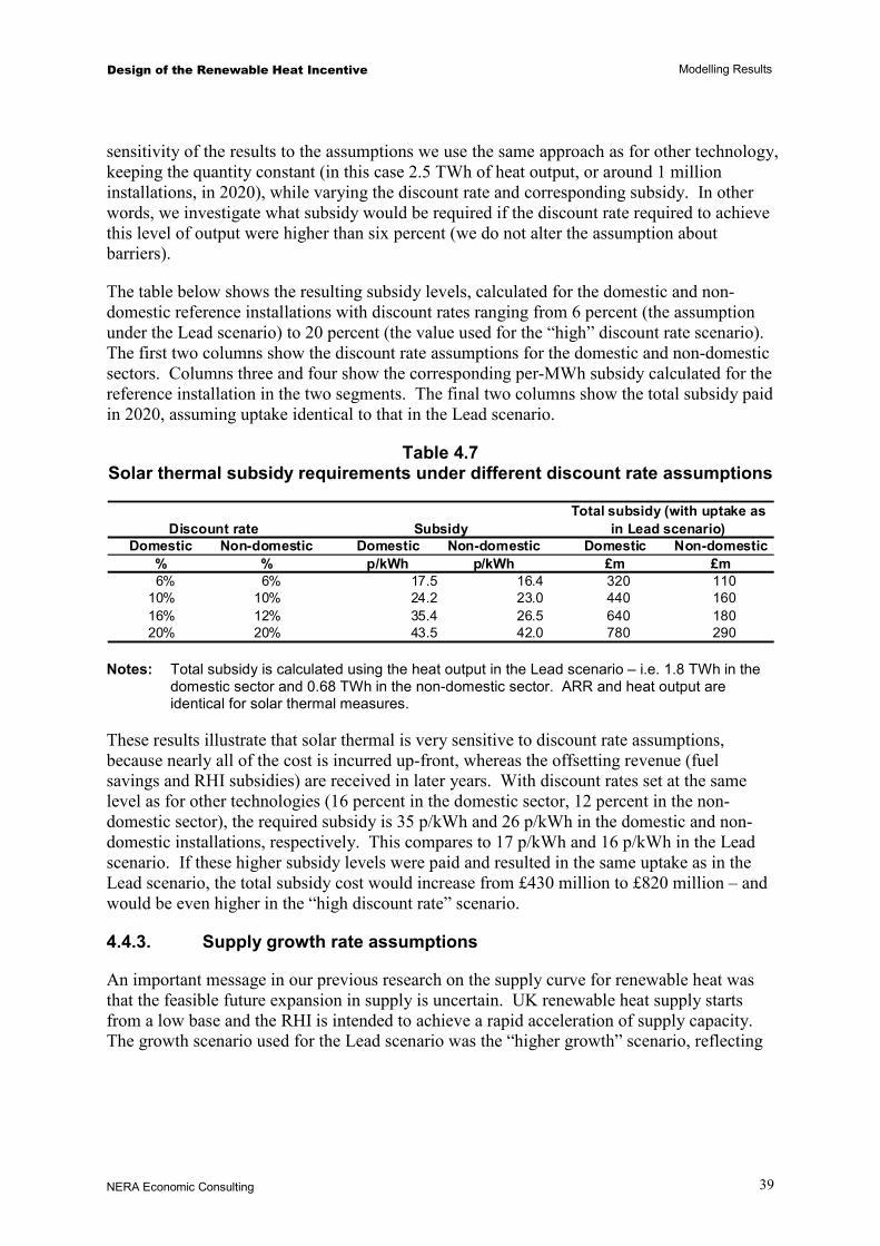
Design of the Renewable Heat Incentive Modelling Results
NERA Economic Consulting
39
sensitivity of the results to the assumptions we use the same approach as for other technology, keeping the quantity constant (in this case 2.5 TWh of heat output, or around 1 million installations, in 2020), while varying the discount rate and corresponding subsidy. In other words, we investigate what subsidy would be required if the discount rate required to achieve this level of output were higher than six percent (we do not alter the assumption about barriers).
The table below shows the resulting subsidy levels, calculated for the domestic and non-domestic reference installations with discount rates ranging from 6 percent (the assumption under the Lead scenario) to 20 percent (the value used for the “high” discount rate scenario). The first two columns show the discount rate assumptions for the domestic and non-domestic sectors. Columns three and four show the corresponding per-MWh subsidy calculated for the reference installation in the two segments. The final two columns show the total subsidy paid in 2020, assuming uptake identical to that in the Lead scenario.
Table 4.7 Solar thermal subsidy requirements under different discount rate assumptions
Domestic Non-domestic Domestic Non-domestic Domestic Non-domestic% % p/kWh p/kWh £m £m6% 6% 17.5 16.4 320 110
10% 10% 24.2 23.0 440 16016% 12% 35.4 26.5 640 18020% 20% 43.5 42.0 780 290
Total subsidy (with uptake as in Lead scenario)SubsidyDiscount rate
Notes: Total subsidy is calculated using the heat output in the Lead scenario – i.e. 1.8 TWh in the domestic sector and 0.68 TWh in the non-domestic sector. ARR and heat output are identical for solar thermal measures.
These results illustrate that solar thermal is very sensitive to discount rate assumptions, because nearly all of the cost is incurred up-front, whereas the offsetting revenue (fuel savings and RHI subsidies) are received in later years. With discount rates set at the same level as for other technologies (16 percent in the domestic sector, 12 percent in the non-domestic sector), the required subsidy is 35 p/kWh and 26 p/kWh in the domestic and non-domestic installations, respectively. This compares to 17 p/kWh and 16 p/kWh in the Lead scenario. If these higher subsidy levels were paid and resulted in the same uptake as in the Lead scenario, the total subsidy cost would increase from £430 million to £820 million – and would be even higher in the “high discount rate” scenario.
4.4.3. Supply growth rate assumptions
An important message in our previous research on the supply curve for renewable heat was that the feasible future expansion in supply is uncertain. UK renewable heat supply starts from a low base and the RHI is intended to achieve a rapid acceleration of supply capacity. The growth scenario used for the Lead scenario was the “higher growth” scenario, reflecting

Design of the Renewable Heat Incentive Modelling Results
NERA Economic Consulting
40
ambitious expansion. We also have modelled a “central” scenario where available supply is more limited.26
Under this scenario, the total ARR falls from 73 TWh to 59 TWh (a drop of 14 TWh, or 19 percent) assuming subsidies are set as in the Lead scenario (because the underlying costs and other parameters used to set subsidies do not change this implies the same set of subsidies). This amount of renewable heat is just below 10 percent of total heat demand in 2020. The total resource cost falls commensurately by around £400 million to £1.8 billion per year in 2020, while subsidies fall by £400 million to £3 billion per year in 2020. The CO2 emissions reductions in 2020 also decrease, from 17 MtCO2 to 14 MtCO2.27
26 See NERA and AEA (2009) for detailed descriptions of these assumptions. 27 As noted, CHP has been modelled separately and the amount of renewable CHP does not change between the Lead
scenario and the central-growth scenario.

Design of the Renewable Heat Incentive Summary and Conclusions
NERA Economic Consulting
41
5. Summary and Conclusions
The current project has had three main outputs:
First, it has updated the supply curve for renewable heat documented in NERA and AEA (2009), incorporating revised input assumptions to reflect stakeholder feedback and other information.
Second, it has developed a banding structure for technologies to be covered by the RHI based on technology and equipment size, and calculated proposed RHI subsidy levels. This has been based on a methodology specified by DECC and implemented by NERA, with subsidy levels in each band calculated from derived from the cost characteristics of a “reference installation” in each band along with various input assumptions. The resulting subsidies range widely between 1.3 p / kWh and 17.5 p / kWh heat output.
Finally, the project has included modelling of the renewable heat deployment that may result from these subsidies. Our modelling projects renewable heat output corresponding to 73 TWh of additional renewable resource by 2020. This in turn corresponds to a 12 percent share of renewable energy in UK heat supply.
The renewable heat deployment modelled would require annual subsidies of £3.4bn 2020, and would entail a resource cost of some £2.2bn per year. It would cut annual CO2 emissions by some 17 MtCO2 by 2020, at an average abatement cost of around £130 / tCO2 and with associated benefits of £0.9bn / year.
The results show a mix of technologies taken up across a range of end-user segments. The largest contribution comes from biomass boilers and heat pumps. The mix also includes renewable CHP, biogas injection, district heating powered by biomass, and solar thermal. To achieve the levels indicated, renewable heat technologies would need to command much of the market for replacement heating equipment, especially in the commercial and public sectors in latter years to 2020. Uptake for industrial process heat and (to a lesser extent) the heating of residential dwellings also would be required. The modelling of options for additional uptake in the domestic sector suggests this would come at a relatively high cost.
We also have investigated various policy designs. As expected, the use of banding reduces the total subsidy required to achieve the levels of renewable heat uptake indicated, relative to a policy offering the same subsidy level to all technologies, but increases the resource cost by stimulating the adoption of relatively high-cost measures. Modelling results for other policy variations suggests that the net present value of subsidies could be reduced by paying off the additional up-front costs of renewable heat measures over a shorter (and earlier) period, but this would increase the amount of funding to be raised in the early years of the scheme. The modelling also suggests that, if reductions in the cost of renewable heat technologies can be achieved, there is scope to reduce the total subsidy payments by lowering the amount paid to new projects at later stages in the policy.
The results are sensitive to a number of input assumptions. UK renewable heat supply starts from a low base and achieving the projected uptake would depend on achieving significant expansion of the renewable heat supply chain capacity. In a less optimistic scenario, uptake is lower by some 14 TWh in 2020, and average cost also increases. Variation in fossil fuel

Design of the Renewable Heat Incentive Summary and Conclusions
NERA Economic Consulting
42
prices also influences the required subsidy and / or uptake from the policy, by changing the relatively attractiveness of renewable and fossil-fuel fired heating options. Another uncertain factor is the payment required to induce end-users to incur higher up-front costs of many renewable heat technologies, in exchange for subsidies that they do not receive until the renewable heat output is produced. The model suggests that the time structure of costs and subsidies is a significant determinant of the amount of subsidy required and of the resource cost of renewable heat. For example, discount rates in the region of 20 percent would increase resource costs as well as subsidies required by some 40-50 percent on the Lead scenario. (Costs are higher under the assumption that the discount rates reflect real costs that are costs to society, rather than a form of irrational behaviour by end-users). Conversely, if consumers applied lower discount rates, then costs and subsidies would be lower.

Design of the Renewable Heat Incentive References
NERA Economic Consulting
43
References
The study draws on research reflected in NERA (2008) and NERA and AEA (2009), and we refer to the references contained therein. The following are additional references to work used to inform this study and referred to in the text:
AEA (2010) ‘Interaction between different incentives to support renewable energy and their effect on CHP: the Renewables Obligation and Renewable Heat Incentive’, report for DECC.
DECC (2009) ‘The UK Renewable Energy Strategy 2009: An Analytical Annex’.
DECC (2009b) ‘Greenhouse Gas Policy Evaluation and Appraisal in Government Departments’.
DECC (2010a) ‘Renewable Heat Incentive, Consultation on the proposed RHI financial support scheme’.
DECC (2010b) ‘Impact Assessment of the Renewable Heat Incentive’.
DECC (2010c) ‘Analytical Annex on the RHI IA’.
E4Tech (2009) ‘The Biomass Supply Curve for the UK’, report for DECC.
E4tech (2010) ‘Biomass prices for the heat and electricity sectors in the UK’, report for DECC.
Element Energy (2008), ‘The growth potential for Microgeneration in England, Wales and Scotland’.
Enviros Consulting (2008a) ‘Barriers to renewable heat part 1: supply side’, report for BERR.
Enviros Consulting (2008b) ‘Barriers to renewable heat part 1: demand side’, report for BERR.
NERA (2008) ‘Evaluation of Financial Instruments for Renewable Heat’, Report for the Department for Business, Enterprise and Regulatory Reform.
NERA and AEA (2009) ‘The UK Supply Curve for Renewable Heat’, report for DECC.

Design of the Renewable Heat Incentive Appendix A
NERA Economic Consulting
44
Appendix A. Additional Modelling Results
Table A.1 below provides more detailed composition of ARR by technology and sector (domestic and non-domestic), as well as number of units installed by year 2020 for the Lead scenario.
Table A.1 Composition of ARR by technology and end-user sector
Technology Sector
TWh 1000 unitsASHP Domestic 3.4 293ASHP Non-Domestic 10.5 16GSHP Domestic 4.0 434GSHP Non-Domestic 8.9 63Biomass boilers Domestic 0.5 25Biomass boilers Non-Domestic 26.8 26Biomass DH Domestic 1.2 1Biomass DH Non-Domestic 1.3 2Solar thermal Domestic 1.8 976Solar thermal Non-Domestic 0.7 37Liquid biofuels Domestic - -Liquid biofuels Non-Domestic - -Biogas Injection Domestic - -Biogas Injection Non-Domestic 7.2 0CHP Domestic - N/ACHP Non-Domestic 6.6 N/ASubtotal Domestic 11 1,728Subtotal Non-Domestic 62 144Total - 73 1,872
Lead scenario
Source: NERA modelling.
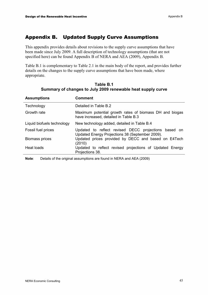
Design of the Renewable Heat Incentive Appendix B
NERA Economic Consulting
45
Appendix B. Updated Supply Curve Assumptions
This appendix provides details about revisions to the supply curve assumptions that have been made since July 2009. A full description of technology assumptions (that are not specified here) can be found Appendix B of NERA and AEA (2009), Appendix B.
Table B.1 is complementary to Table 2.1 in the main body of the report, and provides further details on the changes to the supply curve assumptions that have been made, where appropriate.
Table B.1 Summary of changes to July 2009 renewable heat supply curve
Assumptions Comment
Technology Detailed in Table B.2
Growth rate Maximum potential growth rates of biomass DH and biogas have increased, detailed in Table B.3
Liquid biofuels technology New technology added, detailed in Table B.4
Fossil fuel prices Updated to reflect revised DECC projections based on Updated Energy Projections 38 (September 2009).
Biomass prices Updated prices provided by DECC and based on E4Tech (2010)
Heat loads Updated to reflect revised projections of Updated Energy Projections 38.
Note: Details of the original assumptions are found in NERA and AEA (2009)
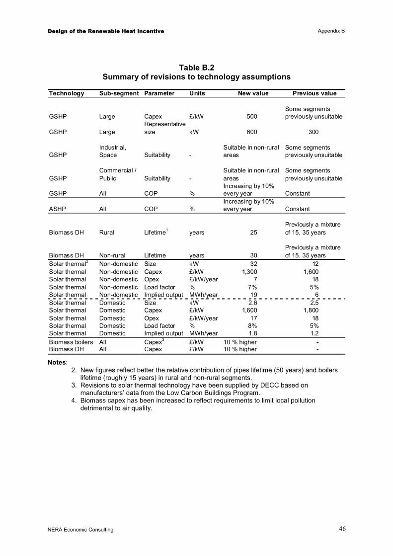
Design of the Renewable Heat Incentive Appendix B
NERA Economic Consulting
46
Table B.2 Summary of revisions to technology assumptions
Technology Sub-segment Parameter Units New value Previous value
GSHP Large Capex £/kW 500Some segments previously unsuitable
GSHP LargeRepresentative size kW 600 300
GSHPIndustrial, Space Suitability -
Suitable in non-rural areas
Some segments previously unsuitable
GSHPCommercial / Public Suitability -
Suitable in non-rural areas
Some segments previously unsuitable
GSHP All COP %Increasing by 10% every year Constant
ASHP All COP %Increasing by 10% every year Constant
Biomass DH Rural Lifetime1 years 25Previously a mixture of 15, 35 years
Biomass DH Non-rural Lifetime years 30Previously a mixture of 15, 35 years
Solar thermal2 Non-domestic Size kW 32 12Solar thermal Non-domestic Capex £/kW 1,300 1,600Solar thermal Non-domestic Opex £/kW/year 7 18Solar thermal Non-domestic Load factor % 7% 5%Solar thermal Non-domestic Implied output MWh/year 19 6Solar thermal Domestic Size kW 2.6 2.5Solar thermal Domestic Capex £/kW 1,600 1,800Solar thermal Domestic Opex £/kW/year 17 18Solar thermal Domestic Load factor % 8% 5%Solar thermal Domestic Implied output MWh/year 1.8 1.2Biomass boilers All Capex3 £/kW 10 % higher -Biomass DH All Capex £/kW 10 % higher - Notes:
2. New figures reflect better the relative contribution of pipes lifetime (50 years) and boilers lifetime (roughly 15 years) in rural and non-rural segments.
3. Revisions to solar thermal technology have been supplied by DECC based on manufacturers’ data from the Low Carbon Buildings Program.
4. Biomass capex has been increased to reflect requirements to limit local pollution detrimental to air quality.

Design of the Renewable Heat Incentive Appendix B
NERA Economic Consulting
47
Table B.3 Summary of supply growth assumptions
Technology Sector 2010 2015 2020 2011-2015 2016-2020TWh TWh TWh % %
ASHP Non-domestic 0.3 2.3 16.0 51% 47%ASHP Domestic 0.1 0.8 5.3 51% 47%Liquid Biofuels Non-domestic N/A N/A N/A N/A N/ALiquid Biofuels Domestic N/A N/A N/A N/A N/ABiomass boilers Non-domestic 2.8 6.5 25.3 18% 31%Biomass boilers Domestic 0.0 1.0 7.0 90% 48%Biomass DH Non-domestic 0.5 1.1 2.1 16% 13%Biomass DH Domestic 0.5 1.1 1.9 16% 12%GSHP Non-domestic 0.5 4.0 17.0 52% 33%GSHP Domestic 0.2 1.3 5.6 52% 33%Solar Thermal Non-domestic 0.1 0.3 0.8 25% 18%Solar Thermal Domestic 0.2 1.9 4.6 51% 20%Biogas injection - 0.2 1.0 7.4 41% 49%Total - 6 21 93 27% 29%
PotentialGrowth rates (% per
year)
Note: Changes from the last report (NERA and AEA, 2009) have been highlighted in bold – they
affect biogas injection and biomass DH only.
In addition to the changes listed above, the replacement of oil with liquid biofuels has been added as a technology. A summary of liquid biofuels technology assumptions is provided in Table B.4 below.
Table B.4 Technology assumptions for liquid biofuels
Segment Capex Fixed Opex EfficiencyLoad factor Size Lifetime
Implied output
£/kW £/kWh/year % % kW years MWh/yearCommercial / Public 65-105 1.1-3.3 80% 20% 50-3000 15 90-5300Domestic 155-180 9 80% 5 -10% 20 15 9-18Industrial 31-66 0.22 80% 20 -82% 1000 15 1800-7200
The above assumptions have been incorporated to the overall renewable heat market model. Figure B.1 shows the supply curve for renewable heat under these assumptions. The figure shows renewable heat potential in 2020 on the horizontal axis, measured in TWh of additional renewable resource. The vertical axis shows the associated cost per MWh ARR (calculated using the variable component of fuel prices). The curve labelled “original ranking” shows the renewable heat supply curve on the assumption that the cost ranking of different renewable heat options is not affected by policy, showing close to 90 TWh of renewable heat potential by 2020. The curve labelled “banding” shows the actual uptake projected under the lead bandings scenario described in the main body of this report. This only shows the segments that are projected to be taken up given the proposed subsidy structure, for a total of 66 TWh.

Design of the Renewable Heat Incentive Appendix B
NERA Economic Consulting
48
Figure B.1 Updated renewable heat supply curve and modelling projections
0
10
20
30
40
50
60
1ASHP Biogas injection Biomass boilers Biomass DHGSHP Solar thermal Liquid Biofuels
-50
-25
0
25
50
75
100
125
150
175
200
0 5 10 15 20 25 30 35 40 45 50 55 60 65 70 75 80 85 90Additional Renewable Resource in 2020 (TWh)
Res
ourc
e Co
st (£
/MW
h)
Banding
Original ranking
Note: The results exclude renewable CHP.
The difference between the two curves provides an illustration of the impacts of banding discussed in section 4.3.2 and in Appendix D: in particular, the resource costs of meeting a particular target (especially at levels above 30 TWh ARR) are higher with banding. As noted elsewhere, these results provide a snapshot given current expectations about prices; they do not attempt to take into account the possibility that subsidies may be reviewed over time, or any potential “insurance value” derived from banding.

Design of the Renewable Heat Incentive Appendix C
NERA Economic Consulting
49
Appendix C. Updated Supply Curve Assumptions
This appendix provides additional details about the reference installations used to calculate subsidy levels. The procedure of identifying the reference installations is described in section 3.2. Section C.1 provides details about market potential curves, while in section C.2 we characterise the reference installations used in the Lead scenario.
C.1. Market Potential Curves
Market potential curves are shown for each technology separately. The first one, biomass boilers, replicates Figure 3.2 from the main body of the report.
C.1.1. Biomass boilers
10
20
100 110180
200
350
500
1000
16005000
-40
-20
0
20
40
60
80
100
120
140
160
180
200
220
0 5 10 15 20 25
Suitable heat load in 2011 (TWh)
Net
RH
cos
t -- c
urre
nt (£
/MW
h)
10 kW
20 kW
100 kW
110 kW
180 kW
200 kW
350 kW
500 kW
1000 kW
1600 kW
5000 kW

Design of the Renewable Heat Incentive Appendix C
NERA Economic Consulting
50
C.1.2. Air-source heat pumps
10
15
60 300
-40
-20
0
20
40
60
80
100
120
140
160
180
200
220
0 5 10 15 20 25
Suitable heat load in 2011 (TWh)
Net
RH
cos
t -- c
urre
nt (£
/MW
h)
10 kW
15 kW
60 kW
300 kW
C.1.3. Ground-source heat pumps
610
60
600
-40
-20
0
20
40
60
80
100
120
140
160
180
200
220
0 5 10 15 20 25
Suitable heat load in 2011 (TWh)
Net
RH
cos
t -- c
urre
nt (£
/MW
h) 6 kW
10 kW
60 kW
600 kW

Design of the Renewable Heat Incentive Appendix C
NERA Economic Consulting
51
C.1.4. Solar thermal
330
-40
-20
0
20
40
60
80
100
120
140
160
180
200
220
0 5 10 15 20 25
Suitable heat load in 2011 (TWh)
Net
RH
cos
t -- c
urre
nt (£
/MW
h)
3 kW
30 kW
C.1.5. Liquid biofuels
20
0
5
10
15
20
25
30
35
0 5 10 15 20 25Suitable heat load in 2011 (TWh)
Net
RH
cos
t -- c
urre
nt (£
/MW
h)
20 kW

Design of the Renewable Heat Incentive Appendix C
NERA Economic Consulting
52
C.2. Reference Installation Characteristics: Lead Scenario
Table C.1 provides the description of the reference installations used to calculate subsidies in the Lead scenario.
Table C.1 Characteristics of reference installations (Lead scenario)
Technology SizeConsumer segment
Fuel counterfactual Sub-segment Location
Building age
Biomass boilers Small Domestic NNB Other House (semi-, terraced) Rural Pre-1990Biomass boilers Medium Com/Pub Gas Small private Urban Post-1990Biomass boilers Large Industrial Gas Large, low-temperature process Suburban Post-1990Liquid Biofuels Small Domestic NNB Detached Rural Pre-1990ASHP Small Domestic Gas Other House (semi-, terraced) Urban Pre-1990ASHP Medium Com/Pub Gas Small public Rural Post-1990GSHP Small Domestic Gas Detached Rural Post-1990GSHP Medium Com/Pub Gas Small public Suburban Post-1990GSHP Large Com/Pub Gas Large public Suburban Post-1990Solar Thermal Small Domestic Gas Other House (semi-, terraced) Urban Pre-1990Solar Thermal Medium Com/Pub Gas Small private Urban Pre-1990 Notes: Subsidies to biomass district heating and biogas installations are not determined through
the use of a reference installation but according to the principles described in section 3.2.3 in the main text. There are no installations in the “large” ASHP category.
C.3. Cost curves identifying reference installations
Table C.1 indicates the installations used as reference installations in the Lead scenario within the market potential for the relevant subsidy band. As discussed in the main text of the report, the reference installations are identified by a segment of a cost curve excluding barrier / administrative costs. By contrast, the cost curves presented here show the total cost perceived by the consumer, including full demand-side barrier and administrative costs. This illustrates more clearly what proportion of the market potential has lower cost than the reference installation.
In some cases the difference between the two curves causes the reference installation to deviate from the mid-way point by a large amount. One factor causing this is where the cost curve is very flat, so that a small vertical movement results in an apparently large horizontal shift; medium ASHPs is an example of this, as is small Liquid Biofuels. Another factor is where barriers are a significant proportion of cost, so the two cost curves (with and without barriers) differ significantly; examples, such as in the case of small Biomass Boilers and small GSHPs.

Design of the Renewable Heat Incentive Appendix C
NERA Economic Consulting
53
Figure C.1 Reference installations and market potential curves by banding segment
-200
20406080
100120140160180200220
0 5 10 15 20
Cost
(£/M
Wh)
Potential (TWh)
Biomass boilers Small
020406080
100120140160180200220
0 5 10 15 20Co
st (£
/MW
h)
Potential (TWh)
Biomass boilers Medium
-200
20406080
100120140160180200220
0 5 10 15 20
Cost
(£/M
Wh)
Potential (TWh)
Biomass boilers Large
-200
20406080
100120140160180200220
0 5 10 15 20
Cost
(£/M
Wh)
Potential (TWh)
ASHP Small
-200
20406080
100120140160180200220
0 5 10 15 20
Cost
(£/M
Wh)
Potential (TWh)
ASHP Medium
-200
20406080
100120140160180200220
0 5 10 15 20
Cost
(£/M
Wh)
Potential (TWh)
GSHP Small
-200
20406080
100120140160180200220
0 5 10 15 20
Cost
(£/M
Wh)
Potential (TWh)
GSHP Medium
-200
20406080
100120140160180200220
0 5 10 15 20
Cost
(£/M
Wh)
Potential (TWh)
GSHP Large
-200
20406080
100120140160180200220
0 5 10 15 20
Cost
(£/M
Wh)
Potential (TWh)
Solar Thermal Small
-200
20406080
100120140160180200220
0 5 10 15 20
Cost
(£/M
Wh)
Potential (TWh)
Solar thermal Medium
-200
20406080
100120140160180200220
0 5 10 15 20
Cost
(£/M
Wh)
Potential (TWh)
Liquid biofuels small

Design of the Renewable Heat Incentive Appendix D
NERA Economic Consulting
54
Appendix D. Differentiation of Support and Banding
Policies to support renewable energy often differentiate the support they provide, depending on technology. It is a feature of most feed-in tariff schemes, and of the UK Renewables Obligation (RO). In the RO, this will be implemented by awarding a differing number of certificates for different technologies: established technologies receive 0.25-0.5 RO Certificates (ROCs) per MWh of electricity generated; “reference” technologies receive 1 ROC / MWh, and post-demonstration and emerging technologies receive 1.5 and 2 ROCs / MWh, respectively. The Renewable Heat Incentive will not award certificates, but will instead provide a direct, pre-determined subsidy payment per unit of eligible renewable heat generated or gas injected. “Banding” in this context thus can be achieved by directly varying the per-unit subsidy level by type of project.
D.1. Motivations for and Consequences of Banding
There are two main potential motivations for the differentiation of support. First, a uniform payment to all eligible categories of projects can mean that some are paid more than would be required to make them viable. Total subsidy costs therefore could be reduced if the payments to these projects could be set below the level required to make more expensive projects viable. Second, a uniform payment can result in the dominance of one or a few technologies. If the rapid deployment of capacity is limited – for example, because it requires lengthy planning processes, or because the development of new supply chains or infrastructure has long lead times – this focus on a single technology can result in slower expansion than in cases where multiple technologies are deployed simultaneously.28
D.1.1.1. Implications of uniform support
To understand the implications of differentiating support it is useful to consider a situation where all projects are paid the same level of subsidy per MWh. This is a “pure” market-based mechanism, in the sense that it is neutral with respect to technology and other factors, so that the selection of projects depends only on the subsidy level and on the (private) information that project developers have about their costs. Under standard assumptions, this will minimise the cost of reaching the resulting output level.
To illustrate the implications of uniform support, as well as various types of banding below, we use a hypothetical supply curve for renewable heat, shown in Figure D.1. This is a deliberately stylised representation of features relevant to the UK supply curve of renewable heat, including the existence of multiple categories of measures, and variation of costs within each category. However, it does not correspond to the representation of actual supply curve
28 Banding in the Renewables Obligation aims to § “Bring on additional deployable technologies by providing appropriate levels of support and certainty for
future investments through the RO within acceptable costs to consumers; § Protect the position of existing renewable energy projects and investors and also those projects under
construction or which come into operation prior to the introduction of the new regime; and § Allow adjustments to the RO to avoid over-subsidy of technologies as costs and revenues evolve.”
We discuss the issue of protecting existing projects and providing certainty in Appendix E.

Design of the Renewable Heat Incentive Appendix D
NERA Economic Consulting
55
data, or an analysis of banding on the basis of actual data (refer to section 4.3.2 for such an analysis).
In the figure, the horizontal axis of the figure shows hypothetical annual renewable heat output potential denominated in tera-watt hours (TWh) per year. The vertical axis shows the additional cost of renewable heat relative to its relevant counterfactual29 technology, expressed in pounds per mega-watt hour (£/MWh). The supply illustrated in the figure is hypothetical, illustrating total available renewable heat potential of 100 TWh, at additional cost ranging from just over zero to £100 / MWh. In addition, the underlying projects can be categorised into three types, indicated as Category I (blue), II (red), and III (yellow) in the figure. These could correspond to different technologies, consumer groups, or other features by which the cost of renewable heat varies. In general, Category I is lower-cost than is Category II, and Category II cheaper than Category III. However, there is no perfect correlation between categories and cost.
Figure D.1 Hypothetical renewable heat cost curve
0
20
40
60
80
100
120
0 20 40 60 80 100 120
Renewable Heat Potential (TWh)
Mar
gina
l Cos
t (£/
MW
h)
Figure D.1 shows the impact of introducing a uniform subsidy in this situation. With this supply curve a subsidy around £25 / MWh would be required to achieve renewable heat output of 50 TWh. A policy providing a single payment at this level would have several notable features. First, this is the least-cost way of achieving the target given this cost curve. No projects with a cost greater than £25 / MWh are undertaken, meaning that costs are minimised. At the same time, £25 / MWh is the minimum payment required to meet the
29 The “counterfactual” technology is the conventional heating technology that would be used to deliver the same output
in the absence of the renewable heat support policy.

Design of the Renewable Heat Incentive Appendix D
NERA Economic Consulting
56
target, as insufficient projects would be undertaken at lower payment levels. Total costs thus are the area under the supply curve, up to actual output of just over 50 TWh.
Second, this uniform £25 / MWh payment would mean a large share of projects received a subsidy significantly in excess of their cost (“infra-marginal rents”, or just “rents”). In the figure, the rents correspond to the area between the £25 / MWh line and the supply curve. As the figure shows, rents are a very significant proportion of the total subsidy. In this (again, hypothetical) example, the total subsidy is £1,280 million (£25 / MWh for around 51 TWh); however, costs are only around £380 million, leading to rents of £890 million. The policy thus has a significant redistributive effect, amounting to a net transfer from the party paying the subsidy to those who undertake (low-cost) renewable heat projects and receive the subsidy. In the context of an RHI, both the party paying and the party receiving the subsidy would be heat consumers, with consumers who continue to use fossil fuel for heating paying those heat consumers who switch to renewables.30
Figure D.2 Illustration of undifferentiated subsidy
Target: 50 TWh
0
20
40
60
80
100
120
0 20 40 60 80 100 120
Renewable Heat Potential (TWh)
Mar
gina
l Cos
t (£/
MW
h)
RentsCost
A third feature is that not all technologies are used. This is illustrated in stylised form in the above figure, where all projects in Category III remain more expensive than their relevant counterfactual even with the subsidy is place. If one of the policy objectives is to ensure that particular technologies are deployed (or that certain segments of consumers receive renewable heat, or that certain fuels are displaced, etc.), or that a diversity of technologies
30 In fact, the rents accruing to the use of renewable heat may be divided along the renewable heat “value chain”,
depending on the relative bargaining position of renewable heat consumers and the relevant “suppliers”—where “suppliers” here includes equipment providers, installers, creditors / financial backers, biomass / waste / other renewable fuel suppliers. In theory rents may accrue to consumers or any of these suppliers.
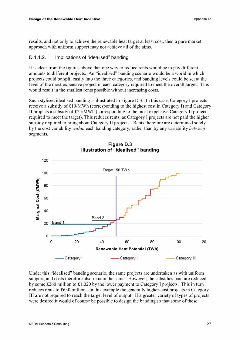
Design of the Renewable Heat Incentive Appendix D
NERA Economic Consulting
57
results, and not only to achieve the renewable heat target at least cost, then a pure market approach with uniform support may not achieve all of the aims.
D.1.1.2. Implications of “idealised” banding
It is clear from the figures above that one way to reduce rents would be to pay different amounts to different projects. An “idealised” banding scenario would be a world in which projects could be split easily into the three categories, and banding levels could be set at the level of the most expensive project in each category required to meet the overall target. This would result in the smallest rents possible without increasing costs.
Such stylised idealised banding is illustrated in Figure D.3. In this case, Category I projects receive a subsidy of £19/MWh (corresponding to the highest cost in Category I) and Category II projects a subsidy of £25/MWh (corresponding to the most expensive Category II project required to meet the target). This reduces rents, as Category I projects are not paid the higher subsidy required to bring about Category II projects. Rents therefore are determined solely by the cost variability within each banding category, rather than by any variability between segments.
Figure D.3 Illustration of “idealised” banding
Target: 50 TWh
0
20
40
60
80
100
120
0 20 40 60 80 100 120
Renewable Heat Potential (TWh)
Mar
gina
l Cos
t (£/
MW
h)
Band 2Band 1
Under this “idealised” banding scenario, the same projects are undertaken as with uniform support, and costs therefore also remain the same. However, the subsidies paid are reduced by some £260 million to £1,020 by the lower payment to Category I projects. This in turn reduces rents to £630 million. In this example the generally higher-cost projects in Category III are not required to reach the target level of output. If a greater variety of types of projects were desired it would of course be possible to design the banding so that some of these

Design of the Renewable Heat Incentive Appendix D
NERA Economic Consulting
58
projects were viable as well (at higher resource cost, and at the expense of some measures in Categories I and/or II).
D.1.1.3. Implications of “imperfect” banding
In practice, however, it is likely to be very difficult to achieve such idealised banding levels. The first reason is that, even if categories can be easily identified, it will be difficult to define the “correct” level of a band. As we discuss in more detail below, the net resource cost of a given renewable heat project depends on a range of factors, many of which are idiosyncratic rather than systematically related to easily identifiable categories of project. Many factors (such as fuel prices) also change over time, meaning that relative cost differences for different projects also change over time. At any one point in time it therefore is likely that bands will be set too low to support some of the potential projects within a category, or alternatively too high.
Second, although the figure shows a stylised example with just three categories, cost can vary depending on a wide range of factors (counterfactual heat source, consumer segment, technology, size of heat load, etc.). Even if government did not have the disadvantage of incomplete information, it could be administratively difficult or even infeasible to vary support with the specifics of project circumstances across the multiple potentially relevant categories.
This means that, in practice, a banding approach is likely to forego some of the cost-minimising efficiency of a “pure” market-based approach. This is illustrated in Figure D.4, where payments are set at £10, £25, and £55 / MWh for the three categories of project. In contrast to the assumption in the idealised case presented in the preceding section, here, the banding levels are not set at the level of the most expensive instance of the particular technology required to meet the target. Instead, the subsidy for Category I is set “too low”; that for Category II is set at the same level; and that for Category III substantially higher (Category III was not required at all in the preceding example).
Note that the mismatch between support levels and actual costs could be due to a number of factors, as we discuss below.31 The impact is to make some of the projects that previously went ahead unviable, illustrated by the hashed segments in the Figure. In addition, some more expensive potential that was unviable under uniform support or idealised banding is now rendered viable and therefore undertaken.
31 Briefly, reasons could include changes in fossil fuel prices; slower development of supply chains than had been
expected (resulting in higher than expected costs); unrepresentative cost information used to set the banding levels; greater cost variability among projects than previously believed – or any other factors that caused a mismatch between support levels and actual project cost.

Design of the Renewable Heat Incentive Appendix D
NERA Economic Consulting
59
Figure D.4 Illustration of “imperfect” banding
Target: 50 TWh
0
20
40
60
80
100
120
0 20 40 60 80 100 120
Renewable Heat Potential (TWh)
Mar
gina
l Cos
t (£/
MW
h)
Band 1
Band 2
Band 3
The exclusion of some segments of the supply curve results in a new effective supply curve, with some of the potential not longer incentivised (and therefore effectively removed). This is illustrated in Figure D.5, alongside the three support levels.

Design of the Renewable Heat Incentive Appendix D
NERA Economic Consulting
60
Figure D.5 Effective supply curve under “imperfect” banding
Target: 50 TWh
0
20
40
60
80
100
120
0 20 40 60 80 100 120
Renewable Heat Potential (TWh)
Mar
gina
l Cos
t (£/
MW
h)
Comparing this with the uniform payment in Figure 3.2 illustrates several features that are likely to be relevant to real-world banding of support. First, total cost is higher; in this example, it rises from £380 million to £650 million. This results both because some low-cost projects are not undertaken and because some higher-cost projects have to be undertaken to substitute for the excluded low-cost potential. Second, despite the higher cost the total subsidy is in fact smaller, falling from £1,280 to £1,060 million, despite the high payments to Category III projects. As a consequence, rents also fall, from £890 to £410 million. Third, projects in all three categories are undertaken, as the highest subsidy level is sufficient for some of the projects in Category III. Fourth, although this example has been constructed to keep total output at the same level with and without banding, the risk the existence of multiple bands is likely to increase the difficulty of predicting the overall level of output. (This uncertainty is always a feature of a price instrument like the RHI, but is likely to be greater with a more complex support structure.)
D.1.1.4. Implications for principles for banding
The above suggests that the gains from banding may be greater if:
1. There are likely to be high rents from uniform support. This in turn is more likely if:
§ There is low-cost potential is but there is reason to believe that the low-cost potential is insufficient to meet objectives.
– either because potential is limited in absolute terms (e.g., limited suitability, overall resource constraints) or

Design of the Renewable Heat Incentive Appendix D
NERA Economic Consulting
61
– likely to be slow to develop (e.g., long lead times to deployment);
2. The efficiency penalty of banding is likely to be small. This is more likely if:
§ There are systematic cost differences between identifiable categories of project;
§ Future uncertainty about factors affecting systematic cost differences is small;
§ Idiosyncratic cost heterogeneity within categories is limited (e.g., because projects are standardised and equally suitable across a large range of situations);
§ There is little uncertainty in government’s estimates of cost (or, of cost variation);
§ Early deployment is likely to result in future cost savings that could partly offset initial higher costs.
3. Technology diversity is likely to be limited with uniform support. This is more likely if:
§ The low-cost potential is concentrated in a small number of dominant categories of project (consumer groups, technologies), resulting in limited deployment of higher-cost categories of project.
4. Banding can be administered easily and without creating perverse incentives. This is more likely if
§ There is a small number of categories, and these meet the criteria in 3.
§ These categories can be observed easily and verified without undue administrative overhead
5. The risk of not meeting the overall target is small. This is more likely if:
§ Available feasible potential is known to exceed target levels; and
§ there is confidence that the subsidy will be sufficient to bring forward sufficient overall renewable heat output.
The above principles form a basis for analysing the application of banding to a prospective RHI. We discuss each in turn as they are likely to apply, at a high level, to renewable heat.
D.1.2. Size of rents with uniform support
As noted, the preference for banding is likely to be stronger the higher the infra-marginal rents from uniform support. NERA’s analysis of the supply curve for renewable heat suggests that such rents could be a very significant feature of a non-banded RHI, for two main reasons.
1. The cost of switching to renewable heat varies significantly between different projects (both within and across technologies). This reflects of the diverse set of circumstances among potential renewable heat applications. In particular,
– there are different renewable heat technologies, with very different characteristics and factors influencing cost; and

Design of the Renewable Heat Incentive Appendix D
NERA Economic Consulting
62
– the economic viability of a given technology varies significantly with factors including available conventional fossil fuels; the size of the heat load; and various localised barriers including space constraints and air quality regulations (see below).
These features combine to generate a wide range of costs for different renewable heating options.
2. Rents may be large because of limited availability of low-cost potential. Broadly speaking, “barriers” to an increase in renewable heat fall into three overall categories.
– First, some of the low-cost technologies are not suitable for parts of the heating market, for a range of reasons.
– Second, there may be an aggregate resource constraint, notably in the case of biological feedstock (biomass, biogas, and liquid biofuels).
– Third, starting from a low base, UK renewable heat supply depends on the development of new supply chains—including infrastructure, expertise, and institutions. The requirement to develop new supply capacity may limit how quickly each of the different renewable heat technologies can be made available.
Taken together, these factors limit the extent to which low-cost potential can be realised, and again previous research suggested that this may be a significant constraint on the extent to which policy targets can be achieved with the technologies that otherwise appear to offer the lowest-cost renewable heat options. The need to rely on higher-cost technologies, and the resulting rents, therefore will be greater the more ambitious is the renewable heat output target.
D.1.3. Efficiency penalty of banding
D.1.3.1. Sources of systematic cost variability
There are various potential sources of systematic cost variability between renewable heat projects that could serve as the basis for defining banding categories. Some of the most prominent include:
§ Technology / fuel: there are low-cost applications of biomass boilers and (air-source) heat pumps that can be less expensive on average than other technologies; whereas solar thermal, in particular, has high costs relative to the relevant conventional technology.
§ Counterfactual fuel: the subsidy requires depends on the cost of the relevant conventional technology, which in turn depends on the fossil fuels available.
§ End-user characteristics: The high discount factors used by domestic consumers raise the required subsidy for a range of renewable heat technologies with high upfront costs, as compared to the subsidy required in other consumer groups with lower discount factors.
§ Size of heat load: renewable heat technologies often have higher capital costs that make them less attractive (compared to conventional heating technologies) the smaller is the load served.
Design of the Renewable Heat Incentive Appendix D
NERA Economic Consulting
63
D.1.3.2. Sensitivity of systematic cost variability to uncertain variables
The cost within any one of the above categories is by necessity uncertain. The experience within the UK of most of the key technologies is very limited, and the basis for estimating the feasibility and cost associated with a rapid expansion of renewable heat therefore is weaker than for many other technologies where there is significant existing experience (such as energy efficiency measures, or large-scale renewable electricity generation). In particular, both the potential and cost of renewable heat projects are likely to depend on the development of new supply chains for renewable heat, with uncertain associated feasibility and cost.32
The list below highlights some of the more important uncertain factors influencing the relative net cost of renewable heat projects.
§ Capital costs: Future equipment costs are uncertain. The potential for renewable heat combines some relatively mature technologies (e.g., pellet boilers) with ones that depend on future technological development (e.g., biogas injection). The relative cost at a future point in time therefore is uncertain.
§ Relative input prices: Fuel prices influence the relative net cost of renewable heat projects, both because they influence counterfactual costs and because they can influence the cost of renewable heat (for example, because electricity used for heat pumps depends on underlying fossil fuel prices, and because biomass prices are likely to be correlated to some extent with fossil fuel prices). The relative net cost of renewable heat projects thus depends directly on relative fuel prices.
§ Potential and technology suitability: The constraints on renewable heat potential – including suitability and performance of particular technologies for different heat loads and the aggregate biomass resource constraint – influence different technologies and consumer segments. Uncertainty about these factors thus also creates uncertainty about the appropriate banding levels.
§ Consumer preferences, risk, and “demand-side barriers”: consumer preferences for renewable heat technologies are highly uncertain and may vary. Widespread adoption in short time period may require substantial subsidy payment to overcome perceived risks of unfamiliar technologies.
D.1.3.3. Sources of idiosyncratic cost heterogeneity
In addition to variability between potential banding categories, there also will be variability within segments. For a given customer segment, type and size of heat load, technology, etc. the cost and performance can vary with a range of idiosyncratic circumstances.
Examples of such factors include the difficulty of getting planning permission; characteristics of pre-existing heating systems; the extent of disruption of production of other business activity; the local nature of some biomass markets; the performance of technologies for particular application (e.g., grade of heat or system efficiency) and many other factors. As a 32 Additionally, if potential is constrained by supply-side considerations but there is significant demand, there is the
possibility that scarcity rents in the supplier market drive the cost to consumers, and thus the required subsidy.

Design of the Renewable Heat Incentive Appendix D
NERA Economic Consulting
64
rough estimate, AEA has indicated that a variability of cost by up to 30 percent of the average cost can be expected, even once factors including customer segment, sub-segment (type of house, size of load, process vs. space heat), location (urban, rural, suburban), and building age (post/pre-1990) have been taken into account.
D.1.3.4. Implications for efficiency penalty of banding
Overall, the currently available data – notably the research on the UK supply curve for renewable heat presented in NERA and AEA (2009) – indicate that the cost variability within “simple” banding options (e.g., single technologies) can be relatively large. More detailed banding combinations (e.g., technology and size) can reduce this, but some residual variability is likely to remain.
Ex-ante modelling of these issues can tell us only so much, and it seems very likely that much better information will become available within a few years of the start of any new policy. This is particularly the case for issues such as the stability of relative costs of categories over time, and the potential attributable to low vs. high-cost projects
D.1.4. Implications of uniform support for project diversity
As expected, our modelling suggests that the diversity of projects would be lower with uniform support than with banding. The main factor appears to be not the dominance of single technologies, but rather that renewable heat can be significantly cheaper in large-scale than in small-scale applications. The main increase in project diversity from banding therefore is likely to be an increase in domestic-scale renewable heat options.
It is difficult to gauge how significant this would be for the UK ambition to increase renewable heat deployment. However, it seems likely that banding is necessary to achieve any significant deployment in the domestic sector.
D.1.5. Administrative implications of banding
The heterogeneity of the renewable heat sector is both a major reason that banding may be desirable and potentially a challenge to its implementation; especially as the available information suggests that relatively finely graded banded categories may be required in order to reduce rents without risking an increase in cost. The administrative implications of a large number of different RHI levels therefore are a further consideration in determining bands of support.
One concern is that a large number of categories would increase the complexity of scheme rules, making it more difficult for prospective project developers to ascertain the level of support to which they would be entitled. Another is that the verification procedures required to categorise projects become more important when the level of support depends on precise project characteristics. Both of these could have a negative impact on uptake of the RHI subsidy, but the concern would be reduced if bands are based on easily observable characteristics. A related consideration is that banding may distort technology choices; for example, banding on the basis of size may cause projects to be under- or over-sized in order to access a different subsidy level. This, too, can be reduced by ensuring both that the differences in support levels of adjacent bands are not too large, and that the band definitions used correspond as far as possible to natural distinctions between projects.

Design of the Renewable Heat Incentive Appendix D
NERA Economic Consulting
65
Another consideration is how banding interacts with the achievement of the overall output target. Banding adds another layer of complexity to this, as total renewable heat output depends not just on a single subsidy level, but on multiple support levels and the interactions between them. In a situation where the output that results from the policy is falling short of the target level, it is more difficult to determine which bands are set at the “wrong” level, and which ones should be increased so that rents remain as low as feasible while also delivering the target. Similar difficulties would arise where targets appear to be over-shot.33
D.1.6. Summary
The following are summary points related to the differentiation of support via banding:
§ In principle, differentiation can reduce total amount of subsidy paid by the policy, relative to a policy with a uniform support level.
§ Total resource costs with banding are very likely to be higher than with uniform support, but the significance of this reduced cost-effectiveness is an empirical question to be investigated given currently available data, and ideally to be revised over time.
– This effect counteracts some of the reduction in subsidies achieved by differentiation, by making necessary support of a larger share of high-cost projects.
§ For both of the above reasons, the infra-marginal rents created by the RHI are likely to be smaller in the case of a banded policy than in the case of uniform support.
§ Banding could be used to encourage a greater diversity of technologies, or to promote the uptake of RH technologies across a greater diversity of consumer segments, than would occur under a uniform support. This in turn may reduce the risk of missing a target of renewable heat deployment because particular categories of project prove more difficult to achieve than anticipated.
§ On the other hand, the addition of banding is likely to increase administrative costs (of policy design, implementation and revision for government, but also potentially of enforcement, monitoring and reporting, and other aspects falling under administrative costs).
33 As a complication, government may face an incentive problem at the policy design (and review) stage(s) as it attempts
to improve its knowledge about the true cost of technologies and thus the correct levels for bands. Given that banding levels may be based on the information supplied to government, stakeholders may have an incentive both to overstate the cost, as this may lead to a higher banded payment, and to overstate potential, as a separate band may be more important if it is thought that a particular technology or other type of project is able to make a significant contribution towards the overall renewable heat target.

Design of the Renewable Heat Incentive Appendix E
NERA Economic Consulting
66
Appendix E. Flexibility of Instrument and Robustness to Changes
As discussed above, the costs of increasing renewable heat deployment through the RHI are uncertain. The experience with the Renewables Obligation for renewable electricity generation, as well as experience with other policies, suggests that it is likely that Government will want to modify some policy parameters over time as new information comes to light about the costs, potential, and barriers facing particular renewable heat technologies.
This section considers how the RHI could be designed to provide flexibility while also ensuring that the smooth operation of the policy is not disrupted.
E.1. Uncertainty and Policy Learning
The RHI is likely to be a complex policy with no direct precedents. Inevitably this will mean that Government may wish to modify it over time. Such revisions, when put into effect, may change the relative attractiveness of different renewable heating technologies to different customer segments.
Equally important, however, is the effect that the expectation of revisions could have on the uptake of renewable heat technologies. In particular:
§ If, when considering whether or not to make an initial investment, heat consumers (or investors) believe there is a reasonable chance that support could be reduced, potential consumers may prefer not to undertake the renewable heat project. To overcome this uncertainty about the level of support that will be available in the future, it may be necessary to offer consumers or investors a higher subsidy to convince them to undertake a particular measure. When investors perceive a risk that support will be reduced, fewer projects will be undertaken.
§ Conversely, if, when considering an investment, heat users believe that support levels could rise, this may give them an incentive to wait until the higher support level is in place.34
§ These two considerations suggest the following principles:
– When reducing the level of support, apply the reduction only to new projects undertaken after the change in support levels have been announced, but “grandfather” the previous level of support to existing projects.
– When increasing the level of support, apply this increase to all projects—including those that have already been undertaken.
34 This can be thought of as an option value to waiting, the value of which is in proportion to the probability that support
will be increased as well as the magnitude of the expected increase. In the case of heating equipment, this risk is lower than in some other cases because much new investment is likely to be necessary replacement of equipment nearing the end of its useful life, leaving only limited discretion about timing.

Design of the Renewable Heat Incentive Appendix E
NERA Economic Consulting
67
§ This does not mean that government could – or should – guard heat market participants against all sources of risk—for example, all heat users already face the risk of changes in fuel prices, and ought not to expect the government to take on the risk that these will change. However, it is desirable to minimise, as far as possible, the risk attributable to changing “the rules of the game” that are under government control.
E.2. The Difficulty of Commitment
One difficulty that the government has when setting RHI support levels is that it may be difficult to signal credible commitment to a policy that turns out to set the wrong support level. For example, if setting the RHI at a certain level (whether under a uniform support scheme or banded scheme) turns out to result in high rents (or perceived rents), there may be pressure on the government to “claw back” these subsidies. (Similar issues have arisen, for example, in the case of free allocation and the EU ETS.) Despite these pressures, it may not be feasible for the government to reclaim subsidies in a way that does not render some projects unprofitable, or that does not deter investment in the longer run.
In the case of renewable heat, the high level of uncertainty may make it more difficult for the government to make a credible commitment. It seems important for the government to acknowledge the uncertainty from the start and to put in place procedures to try to ensure a consistent protocol for changing support levels or other features of the RHI. It may also be important for the government to acknowledge that the targets are ambitious and that given supply chain constraints, paying rents to certain technologies may be the only way to incentivise sufficiently rapid uptake to meet the targets.
As noted, one way of providing assurances to investors that the rules will not be changed after the fact is to “grandfather” support levels to existing equipment any time a reduction of support levels is implemented. This is the principle upon which the planned revisions to the RO that will band the support it offers are based. Such a provision is only really relevant if the policy offers ongoing support, rather than up-front support. Moreover, while it is feasible to implement such a policy for large-scale electricity generating operations that number in the hundreds, it would entail substantially higher administrative costs for a policy that applied to millions of small installations.
On top of this, there are further difficulties associated with applying grandfathering principles to biomass or other technologies where the amount of fuel delivered is monitored or incentivised. As noted above, one way of avoiding relatively high administrative costs associated with ongoing support for biomass would be for biomass fuel suppliers to report their sales and to receive the subsidy directly based on sales. If support levels were differentiated among different “vintages” of heating system, suppliers would need to know these vintages for each of their customers. Given the possibility of changing fuel supplier, it would be necessary for biomass users to have certificates that they would present to their suppliers, and suppliers would need to keep a record of where they supplied their fuel to allow verifiers to ensure that they received the correct subsidy payment for their fuel supply. Without such procedures it would be more likely that the system could be abused by the sale and resale of biomass fuel to those eligible for the higher subsidy levels.

Design of the Renewable Heat Incentive Appendix E
NERA Economic Consulting
68
These requirements that suppliers understand who their customers are is similar to the issue noted in section Appendix D in relation to banding. In effect, introducing different levels of support through grandfathering amounts to a further dimension of banding along a time dimension.

NERA Economic Consulting 15 Stratford Place London W1C 1BE United Kingdom Tel: +44 20 7659 8500 Fax: +44 20 7659 8501 www.nera.com
NERA UK Limited, registered in England and Wales, No 3974527 Registered Office: 15 Stratford Place, London W1C 1BE