Chapter 7Design Theory of the RelationalModel

Goal: a relational schema that suitably represents an excerpt of the real world.

• Real world implies integrity constraints (we have seen e.g. keys and referential integrityas relational concepts)

• Base of such concepts: data dependencies

• Representation must cope with these dependencies (from this design, keys are obtained,and referential integrity constraints).

323

DESIGN STEPS

Real World

ER-schema

set of (preliminary) relation schemata,set of dependencies

The more exact the ER model,the better the preliminary rela-tional schema.

equivalent set of “good” relation schemata

Application Analysis

Transformation

relational design

324

MOTIVATION

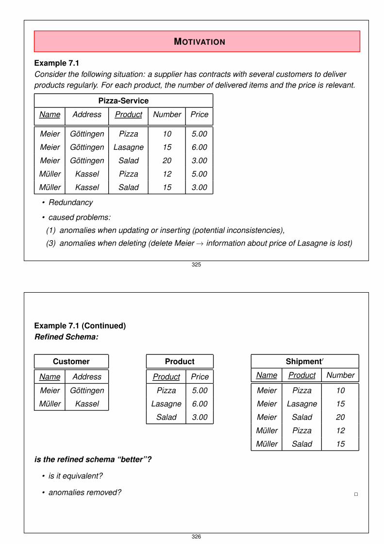
Example 7.1Consider the following situation: a supplier has contracts with several customers to deliverproducts regularly. For each product, the number of delivered items and the price is relevant.

Pizza-Service

Name Address Product Number Price

Meier Göttingen Pizza 10 5.00

Meier Göttingen Lasagne 15 6.00

Meier Göttingen Salad 20 3.00

Müller Kassel Pizza 12 5.00

Müller Kassel Salad 15 3.00

• Redundancy

• caused problems:

(1) anomalies when updating or inserting (potential inconsistencies),

(3) anomalies when deleting (delete Meier → information about price of Lasagne is lost)

325

Example 7.1 (Continued)Refined Schema:

Customer

Name Address

Meier Göttingen

Müller Kassel

Product

Product Price

Pizza 5.00

Lasagne 6.00

Salad 3.00

Shipment′

Name Product Number

Meier Pizza 10

Meier Lasagne 15

Meier Salad 20

Müller Pizza 12

Müller Salad 15

is the refined schema “better”?

• is it equivalent?

• anomalies removed? ✷

326

REQUIRED NOTIONS

1. Analysis of relevant dependencies

2. criterion when to decompose a relation schema (and when a decomposition is equivalent)(based on (1))

3. measure for “quality” of a schema(in terms of (1))

327

7.1 Functional Dependencies

• Data dependencies that describe a functional relationship.

Let V a set of attributes and r ∈ Rel(V ), X, Y ⊆ V .r satisfies the functional dependency (FD) X → Y if for all t, s ∈ r,

t[X] = s[X ] ⇒ t[Y ] = s[Y ] .

For Y ⊆ X, X → Y is a trivial dependency (satisfied by every relation r ∈ Rel(V )).

Refined Definition of “Relation Schema”

A relation schema R(X,ΣX) consists of a name (here, R) and a finite setX = {A1, . . . , Am}, m ≥ 1 of attributes:

• X is the format of the schema.

• ΣX is a set of functional dependencies over X.

A relation r ∈ Rel(X) is an instance of R if it satisfies all dependencies in ΣX .The set of all instances of R is denoted by Sat(X,ΣX).

328

Example 7.2Consider again Example 7.1.

The given instance is in Sat(X,ΣX) for the following set ΣX of FDs:

Name → Address

Product → Price

(Name, Product) → Number

“Intuitive” ER-model of the problem:

Customer

AddressName

Product

NamePrice

buys

Number

✷

329

7.1.1 Decomposition Based on Functional Dependencies

• Does a “good” ER-model already guarantee all desirable properties of the relationalmodel?

NO(at least not completely - The more exact the ER model, the better the preliminaryrelational schema)

• is a formal dependency analysis necessary?

YES• theory: based on normal forms of relational schemata

330

ANALYSIS OF ENTITY SETS

Example 7.3 (FDs of entity attributes)Consider a staff database in a university. Persons (professors and lecturers) have names,ranks, and salaries.

Person

name

rank

salary

Person

Name Rank Salary

G full prof. 5000

T full prof. 5000

S associate prof. 4000

W assistant 3000

P assistant 3000

There is a functional dependency Rank → Salary.

Refined schema: Person(Name, Rank)

SalaryTable(Rank, Salary)

✷

331

ANALYSIS OF RELATIONSHIP SETS

Example 7.4 (FDs of ternary relationships)Students attend courses that are given by lecturers.

Student attends Course

Lecturer

Name Name

Name

attends

Student Course Lecturer

Stud1 Telematics Ho

Stud2 Telematics Ho

Stud2 Mobile Comm Ho

Stud3 Mobile Comm Ho

Stud3 Databases WM

Stud4 Databases WM

Stud1 Databases WM

There is a functional dependency Course → Lecturer.

Refined schema: reads(Course, Lecturer)

attends’(Student, Course)

✷

332

7.1.2 Functional Dependency Theory

Let R(V ,F) a relation schema where X, Y ⊆ V , and F is a set of functional dependenciesover V .Definition 7.1

• F implies a functional dependency X → Y , written as F |= X → Y , if and only if everyrelation r ∈ Sat(V ,F) satisfies X → Y .

• F+ = {X → Y | F |= X → Y } is the closure of F . ✷

Definition 7.2Let V = {A1 . . . An}. X is a key of V (wrt. F) if and only if

• X → A1 . . . An ∈ F+,

• Y ( X ⇒ Y → A1 . . . An /∈ F+.

For a key X, each Y ⊇ X is a superkey. ✷

For an attribute A such that A ∈ X for any key X, A is a key attribute. If there is no key X

such that A ∈ X, then A is a non-key attribute.

333

CLOSURE OF FDS

Problem: How to decide whether X → Y ∈ F+? (Membership Test)

The test is based on the Armstrong-Axioms:

Let F a set of FDs over V and r ∈ Sat(V ,F).

(A1) Reflexivity: If Y ⊆ X ⊆ V , then r satisfies X → Y .

(A2) Augmentation: If X → Y ∈ F and Z ⊆ V , then r satisfies XZ → Y Z.

(A3) Transitivity: If X → Y and Y → Z ∈ F , then r satisfies X → Z.

The Armstrong-Axioms can be used as inference rules for FDs.

Theorem 7.1The Armstrong-Axioms are correct, i.e., all derived FDs are in F+, and they are complete,i.e., all FDs in F+ can be derived. ✷

334

CLOSURE OF FDS (CONT’D)

Armstrong Axioms can especially be used for searching which attributes depend on a givenX ⊆ V .

Definition 7.3For X ⊆ V , X+ is the set of all A ∈ V such that X → A can be derived by the Armstrongaxioms. X+ is called the (Attribute-)closure of X (wrt. F). ✷

Exercise 7.1Consider a relation schema R(V ,F) such that K is a key. What is K+? ✷

335

Proof of Theorem 7.1: correctness is obvious.Completeness: it has to be shown that if X → Y ∈ F+, then X → Y can be derived by(A1)–(A3) from F .

It will be shown: if X → Y is not derivable by (A1)–(A3), then X → Y 6∈ F+, i.e., there is anr ∈ Sat(V ,F) that does not satisfy X → Y .

Assume X → Y cannot be derived. Consider a relation r as below:

1 1 . . . 1 1 1 . . . 1

1 1 . . . 1︸ ︷︷ ︸ 0 0 . . . 0︸ ︷︷ ︸attributes in X+ all other attributes

(i) First it will be shown that r satisfies F :Assume that there is a Z → W ∈ F , such that r does not satisfy Z → W . This is onlypossible if Z ⊆ X+ and W 6⊆ X+. Since Z ⊆ X+, there is X → Z and Z → W , and thusW ⊆ X+, a contradiction.

(ii) Next, it will be shown that r does not satisfy X → Y :For any X → Y that is satisfied by r, Y ⊆ X+. This would mean that X → Y can bederived from (A1)–(A3).

336

MEMBERSHIP PROBLEM

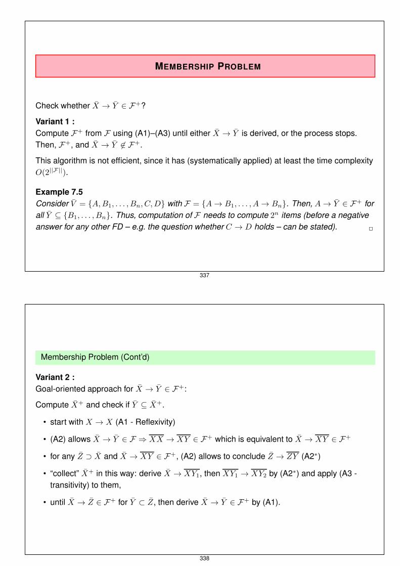
Check whether X → Y ∈ F+?

Variant 1 :Compute F+ from F using (A1)–(A3) until either X → Y is derived, or the process stops.Then, F+, and X → Y 6∈ F+.

This algorithm is not efficient, since it has (systematically applied) at least the time complexityO(2||F||).

Example 7.5Consider V = {A,B1, . . . , Bn, C,D} with F = {A → B1, . . . , A → Bn}. Then, A → Y ∈ F+ forall Y ⊆ {B1, . . . , Bn}. Thus, computation of F needs to compute 2n items (before a negativeanswer for any other FD – e.g. the question whether C → D holds – can be stated). ✷

337

Membership Problem (Cont’d)

Variant 2 :Goal-oriented approach for X → Y ∈ F+:

Compute X+ and check if Y ⊆ X+.

• start with X → X (A1 - Reflexivity)

• (A2) allows X → Y ∈ F ⇒ XX → XY ∈ F+ which is equivalent to X → XY ∈ F+

• for any Z ⊃ X and X → XY ∈ F+, (A2) allows to conclude Z → ZY (A2∗)

• “collect” X+ in this way: derive X → XY1, then XY1 → XY2 by (A2∗) and apply (A3 -transitivity) to them,

• until X → Z ∈ F+ for Y ⊂ Z, then derive X → Y ∈ F+ by (A1).

338

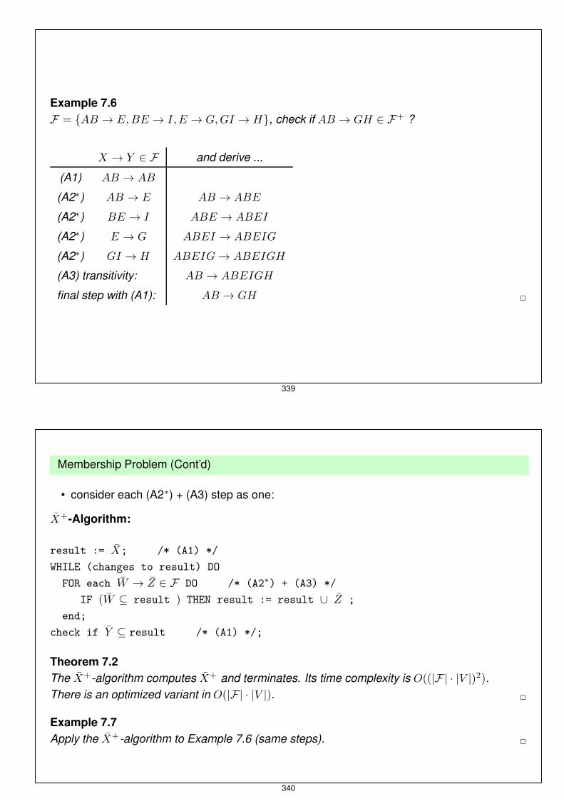
Example 7.6F = {AB → E,BE → I, E → G,GI → H}, check if AB → GH ∈ F+ ?

X → Y ∈ F and derive ...

(A1) AB → AB

(A2∗) AB → E AB → ABE

(A2∗) BE → I ABE → ABEI

(A2∗) E → G ABEI → ABEIG

(A2∗) GI → H ABEIG → ABEIGH

(A3) transitivity: AB → ABEIGH

final step with (A1): AB → GH ✷

339

Membership Problem (Cont’d)

• consider each (A2∗) + (A3) step as one:

X+-Algorithm:

result := X; /* (A1) */WHILE (changes to result) DOFOR each W → Z ∈ F DO /* (A2∗) + (A3) */

IF (W ⊆ result ) THEN result := result ∪ Z ;end;

check if Y ⊆ result /* (A1) */;

Theorem 7.2The X+-algorithm computes X+ and terminates. Its time complexity is O((|F| · |V |)2).There is an optimized variant in O(|F| · |V |). ✷

Example 7.7Apply the X+-algorithm to Example 7.6 (same steps). ✷

340

AN EQUIVALENT SET OF RULES

Lemma 7.1Consider a relation schema R(V ,F) such that A ∈ V and X, Y , Z, W ⊆ V , and F is a set offunctional dependencies over V , and r ∈ Sat(V ,F). Then:

(A4) Union: If X → Y and X → Z ∈ F , then r satisfies X → Y Z.

(A5) Pseudo-transitivity: If X → Y and WY → Z ∈ F , then r satisfies XW → Z.

(A6) Decomposition: If X → Y ∈ F and Z ⊆ Y , then r satisfies X → Z.

(A7) Reflexivity: r satisfies X → X

(A8) Accumulation: If X → Y Z and Z → AW ∈ F , then r satisfies X → Y ZA. ✷

Lemma 7.2The rule sets {(A1), (A2), (A3)} and {(A6), (A7), (A8)} are equivalent, i.e., for given F , thesame set of FDs can be derived. ✷

• (A8) covers the combination of (A2∗) and (A3) (consider W = ∅).

341

Example 7.8F = {AB → E,BE → I, E → G,GI → H}, check if AB → GH ∈ F+ ?

Derivation by Intermediate result Xi

(A7)–(A8) of the X+-algorithm

(A7) AB → AB X0 = {A,B}(A8) [ AB → E ]

AB → ABE X1 = {A,B,E}(A8) [ BE → I ]

AB → ABEI X2 = {A,B,E, I}(A8) [ E → G ]

AB → ABEIG X3 = {A,B,E, I,G}(A8) [ GI → H ]

AB → ABEIGH X4 = {A,B,E, I,G,H}final step with (A6):

(A6) AB → GH ✷

342

DETERMINING A KEY

Consider a relation schema R = (V ,F).

• The X+-algorithm allows for determining a key of R in time O(|F| |V |2):Start with the superkey V and try to delete attributes as long as the closure of theremaining attributes is still the whole V . If no more attributes can be deleted, a key isfound.

• In the general case, it is not possible to determine all keys of a relation schema efficiently.Note that the problem “is there a key with at most k attributes?” is NP-complete.

343

ASIDE: UNIQUE KEYS

Theorem 7.3Let F = {X1 → Y1, . . . , Xp → Yp}.Let Zi = Yi \ Xi for 1 ≤ i ≤ p.

R(V ) has a unique key if and only if V \ (Z1 ∪ . . . ∪ Zp) is a superkey.(note that K is a superkey if K+ = V ).(Proof: next slide) ✷

Note:

• Z1 ∪ . . . ∪ Zp contains those attributes that are fd from any other attribute.

• V \ (Z1 ∪ . . . ∪ Zp) contains those attributes that are not fd from any other attribute.

• V \ (Z1 ∪ . . . ∪ Zp) is subset of all keys of a relation.

Example 7.9Consider the relation Country(name,code,population, area) with FDsname→ code,population,area and code→ name,population,area.Here, name and code are keys.V \ (...) = ∅ ✷

344

ASIDE: UNIQUE KEYS (CONT’D)

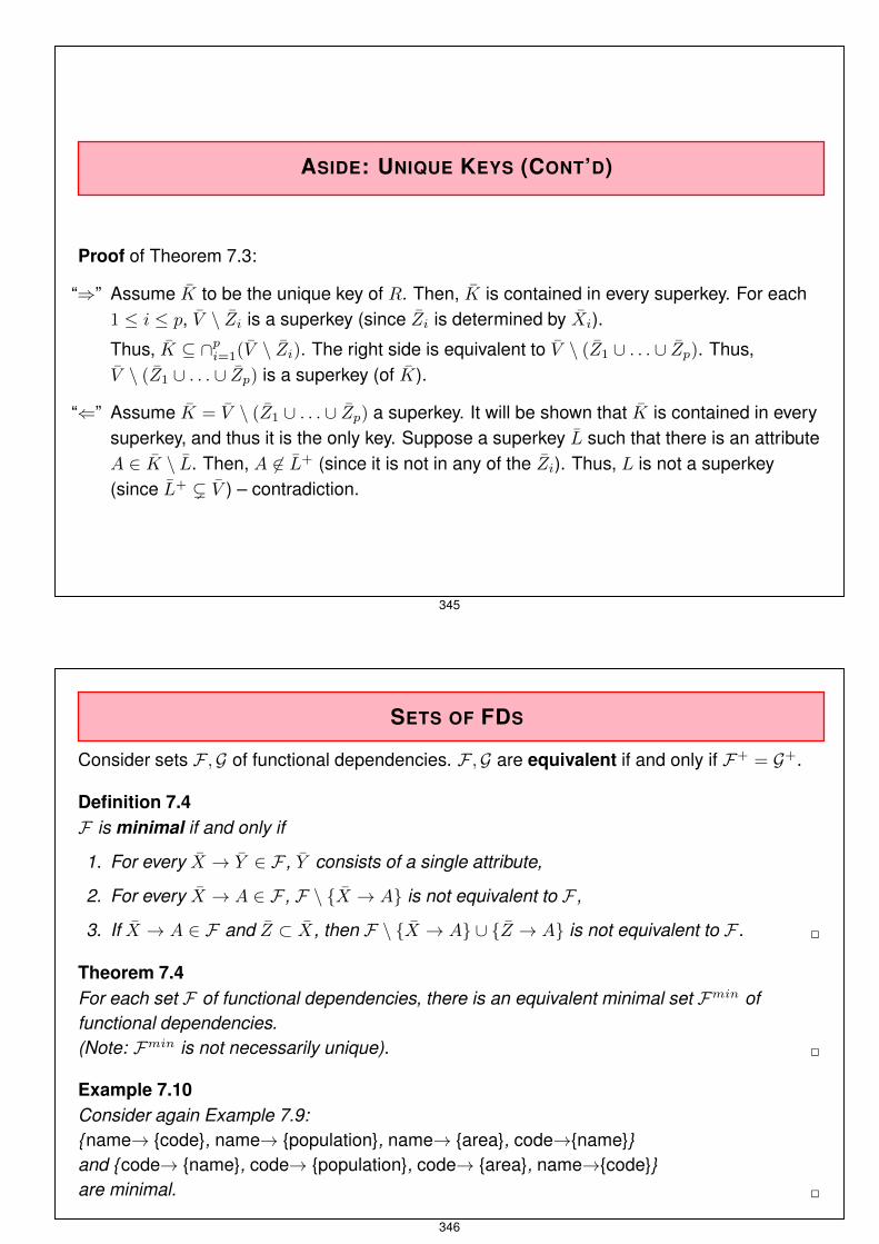
Proof of Theorem 7.3:

“⇒” Assume K to be the unique key of R. Then, K is contained in every superkey. For each1 ≤ i ≤ p, V \ Zi is a superkey (since Zi is determined by Xi).

Thus, K ⊆ ∩pi=1(V \ Zi). The right side is equivalent to V \ (Z1 ∪ . . . ∪ Zp). Thus,

V \ (Z1 ∪ . . . ∪ Zp) is a superkey (of K).

“⇐” Assume K = V \ (Z1 ∪ . . . ∪ Zp) a superkey. It will be shown that K is contained in everysuperkey, and thus it is the only key. Suppose a superkey L such that there is an attributeA ∈ K \ L. Then, A 6∈ L+ (since it is not in any of the Zi). Thus, L is not a superkey(since L+ ( V ) – contradiction.

345

SETS OF FDS

Consider sets F ,G of functional dependencies. F ,G are equivalent if and only if F+ = G+.

Definition 7.4F is minimal if and only if

1. For every X → Y ∈ F , Y consists of a single attribute,

2. For every X → A ∈ F , F \ {X → A} is not equivalent to F ,

3. If X → A ∈ F and Z ⊂ X, then F \ {X → A} ∪ {Z → A} is not equivalent to F . ✷

Theorem 7.4For each set F of functional dependencies, there is an equivalent minimal set Fmin offunctional dependencies.(Note: Fmin is not necessarily unique). ✷

Example 7.10Consider again Example 7.9:{name→ {code}, name→ {population}, name→ {area}, code→{name}}and {code→ {name}, code→ {population}, code→ {area}, name→{code}}are minimal. ✷

346

MINIMAL SETS OF FDS

• Fmin can be computed by the X+-algorithm (without computing F+) in polynomial time.

Consider a schema R(V ,F) with |V | = n and |F| = f .

1. Decompose all X → Y ∈ F such that each right side consists of a single attribute; get F ′

with |F ′| ≤ nf in O(f · n) steps.

2. Delete all ϕ ∈ F ′ that follow from the others (iteratively), using the X+ algorithm.Each application of X+ requires O(f · n) steps, thus, altogether O(f2 · n2).

3. Delete in each remaining FD {x1 . . . , xn} → y stepwise as many attributes on the left sideas possible. For each step, check, whether y is still in the remaining {x1 . . . , xk}+.The X+-algorithm is applied |F ′| · n = O(f · n2) times, thus, this step is in O(f2 · n3).

4. The algorithm is in O(f2 · n3), i.e., polynomial.

347

7.2 Decomposition of Relation Schemata

In Example 7.1 (Slide 325), a relation has been decomposed for yielding a better behavior.

Definition 7.5• Let V a set of attributes. Then, ρ = {X1, . . . , Xn} s.t. X1 ∪ . . . ∪ Xn = V and for each i,Xi ⊆ V is a decomposition of V . ✷

Example 7.11Consider again Example 7.1. There, V = {Name,Address,Product,Number,Price}.

E.g., ρ = {{Name,Address}, {Product,Price}, {Name,Product,Number}}. is adecomposition. ✷

Lemma 7.3Consider a relation r ∈ Rel(V ) and a decomposition ρ = {X1, . . . , Xk} of V .

Then,

r ⊆ π[X1](r) ⊲⊳ . . . ⊲⊳ π[Xk](r) . ✷

348

PROPERTIES OF DECOMPOSITIONS

Losslessness: The complete tuples must be reconstructable by joining the decomposedrelations without getting additional tuples that have not been there originally.

Example 7.12Consider again Example 7.4, now with a decomposition into hears(Student,Lecturer) andattends’(Student, Course).

Then, the join hears ⊲⊳ attends’ yields a tuple (DStud1,Databases,Ho). ✷

Definition 7.6Consider a relation schema R(V ,F) and a decomposition ρ = {X1, . . . , Xn} of R.

ρ is lossless if and only if for every relation r ∈ Sat(V ,F),

r = π[X1](r) ⊲⊳ . . . ⊲⊳ π[Xk](r) . ✷

349

PROPERTIES OF DECOMPOSITIONS (CONT’D)

dependency-preservation: the dependencies can be tested using the decomposed tablesonly, i.e., without having to recompute the join.

Definition 7.7Consider a relation schema R(V ,F) and a decomposition ρ = {X1, . . . , Xn} of R.

π[Z](F) = {X → Y ∈ F+ | XY ⊆ Z} is the projection of F to Z.

ρ is dependency-preserving if and only if for all i,

n⋃

i=1

π[Xi](F) ≡ F .✷

Dependency-preservation means that FDs can be distributed over the decompositionwithout losing anything:If the projections of F+ are asserted, the (joined) database contents satisfies F .

We will first discuss losslessness.

350

7.2.1 Lossless Decompositions

• The problem is not to lose tuples by (wrong) decompositions, but to lose “information”about relationships.

Example 7.13Consider again Examples 7.4 and 7.12.

1. attends = π[Course, Lecturer](attends)︸ ︷︷ ︸reads

⊲⊳ π[Student,Course](attends)︸ ︷︷ ︸attends′

2. attends ( π[Student, Lecturer](attends)︸ ︷︷ ︸hears

⊲⊳ π[Student,Course](attends)︸ ︷︷ ︸attends′

(DStud1,Databases,Ho) ∈ hears ⊲⊳ attends’. ✷

351

TEST FOR LOSSLESSNESS (CHASE-ALGORITHM FOR FDS)

Input: a relation schema R(V ,F), where V = {A1, . . . , An}, ρ = {X1, . . . , Xk}.

Algorithm: (Aho, Beeri, Ullman, TODS 1979)

Idea: take a tuple (a1, . . . , an), decompose it according to ρ. Create a “test table” thatrepresents the requirements of a tuple (a1, . . . , an) in the re-join of the decomposed tables.Add the knowledge from the FDs about the attribute values of this tuple. The goal is to showthat this tuple must have been already present in the original table.

Construct a table T with n columns and k rows.Column j stands for Aj , row i for Xi as follows:

• T(i,j) = aj if Aj ∈ Xi,

• otherwise T(i,j) = bij (“any value”).

(see next slide)

352

Chase-Algorithm for FDs (Cont’d)

As long as T changes, do the following:

Consider a FD X → Y ∈ F . If there are rows z1, z2 ∈ T which coincide for all X-columns, butnot in all Y -columns, then make their Y -values the same:

• For each Y -column j:

• if one of the symbols is aj , then replace every occurrence of the other symbol globally byaj .

• if both symbols are of the form bij, then replace arbitrarily one of them globally by theother.

Note: The algorithm corresponds to enforcing the FDs.(since they are known to hold in T , this constrains the occurrences of other values)

Result: ρ is lossless if and only if (a1, . . . , an) ∈ T .

353

Example 7.14 (Chase)V = ABCDE, ρ = (AD,AB,BE,CDE,AE);F = {A → B,B → D,DE → C,E → A}

A B C D E

from AD: a1 b12 b13 a4 b15

from AB: a1 a2 b23 b24 b25

from BE: b31 a2 b33 b34 a5

from CDE: b41 b42 a3 a4 a5

from AE: a1 b52 b53 b54 a5

chase−→

A B C D E

a1 a2 b13 a4 b15

a1 a2 b23 a4 b25

a1 a2 a3 a4 a5

a1 b42 a3 a4 a5

a1 b52 b53 b54 a5

The process is finished when the following table is reached:

A B C D E

a1 a2 a3 a4 b15

a1 a2 a3 a4 b25

a1 a2 a3 a4 a5

a1 a2 a3 a4 a5

a1 a2 a3 a4 a5

Note that only for columns thatdo not occur on the right side ofa FD, the bs remain.

✷

354

Theorem 7.5The above algorithm for testing losslessness is correct. ✷

Proof:

Notation:

• for a decomposition ρ = {X1, . . . , Xk} of V and a relation r, the re-join of thedecomposed tables is denoted by mρ(r) = ⊲⊳ki=1 π[Xi](r).

• T0 and T ∗ denote the table before and after execution of the algorithm.

The algorithm terminates since the number of different symbols decreases with every step.

(A) It has to be shown that if ρ is lossless, (a1, . . . , an) ∈ T ∗.

Due to the construction of T0, each π[Xi](T0) contains a row that consists only of ais. Thus,(a1, . . . , an) ∈ mρ(T0).

This property is preserved by the chase steps, thus (a1, . . . , an) ∈ mρ(T∗). The chase

process also guarantees that T ∗ ∈ Sat(V ,F). From the assumption that ρ is lossless,T ∗ = mρ(T

∗) and (a1, . . . , an) ∈ T ∗.

355

(B) (uses Relational Calculus)

It will be shown that if (a1, . . . , an) ∈ T ∗, ρ is lossless.

Consider relations r over R(V ) (as structures). Consider the formula of the calculus

F0 = (∃b11) . . . (∃bkn)(R(w1) ∧ . . . ∧R(wk))

where wi is the i-th row of T0 and all ai and bjk’s are interpreted as variables. The freevariables in F0 are a1, . . . , an. Note that every member R(wi) of the conjunction in F0

corresponds to a projection to Xi. Then,

mρ(r) = answers(F0(a1, . . . an)) .

Consider only relations r ∈ Sat(V ,F). Since r satisfies F ,

F0(a1, . . . an) ≡F F1(a1, . . . an) ≡F . . . ≡ F ∗(a1, . . . an)

where each Fi corresponds to the table after i chase steps. For given r, the answer set to F ∗

is the same as the answer set to F0.

Since F ∗(a1, . . . an) is of the form (∃b11) . . . (∃bkm)(R(a1, . . . , an) ∧ . . .) ,its answer set is a subset (or equal) of r.

Altogether, mρ(r) ⊆ r. Since mρ(r) ⊇ r by Lemma 7.3, mρ(r) = r, i.e., ρ is lossless.

356

Corollary 7.1 (Decomposition into two relations)Consider a set V of attributes, a set F of functional dependencies, and a decompositionρ = {X1, X2} of V . ρ is lossless if and only if

(X1 ∩ X2) → (X1 \ X2) ∈ F+, or (X1 ∩ X2) → (X2 \ X1) ∈ F+ .✷

Proof:The table T for ρ is

X1 ∩ X2 X1 \ X2 X2 \ X1

X1 a . . . a a . . . a b . . . b

X2 a . . . a b . . . b a . . . a

1. Assume (a1, . . . , an) ∈ T ∗. Consider an attribute A whose column contains a b. If thealgorithm exchanges it by an a, then A ∈ (X1 ∩ X2)

+. Due to the assumption that(a1, . . . , an) ∈ T ∗, there is one line where this happens for all attributes – thus all theseattributes are in (X1 ∩ X2)

+.

2. Assume (w.l.o.g.) that (X1 ∩ X2) → (X1 \ X2) ∈ F+, i.e., X1 \ X2 ⊆ (X1 ∩ X2)+.

Consider the steps for deriving this by the X+-algorithm. For each such step there is acorresponding chase-step. Thus, the chase replaces each b of an attribute in X1 \ X2 byan a, leading to (a1, . . . , an) ∈ T ∗.

357

Example 7.15Consider again Examples 7.4, 7.12 and 7.13 whith the schema

attends((Student, Course, Lecturer), {Course → Lecturer})

• ρ1 = {{Course, Lecturer}, {Student,Course}} is lossless.

• ρ2 = {{Student, Lecturer}, {Student,Course}} is not lossless. ✷

General conclusion for ternary relations:

• for any (useful) decomposition into two binary relations, there is one attribute A that iscontained in both relations.

• the decomposition is lossless if at least one of the other attributes is functionallydependent only on A.

In the above example, the functional dependency Course → Lecturer which made thedecomposition possible.

358

7.2.2 Dependency Preservation

Example 7.16Consider again Examples 7.1 and 7.11 with the schema

Pizza-Service( {Name,Address,Product,Number,Price},{Name → Address, Product → Price, (Name,Product) → Number})

and the decomposition

ρ = {{Name,Address}, {Product,Price}, {Name,Product,Number}} .

Recall that π[Z](F) = {X → Y ∈ F+ | XY ⊆ Z}

π[Name,Address](F) ⊇ {Name → Address}π[Product,Price](F) ⊇ {Product → Price}π[Name, Product, Number](F) ⊇ {(Name,Product) → Number

So, all FD’s immediately survive. ✷

359

Another, abstract Example

Example 7.17V = {A,B,C,D}, ρ = {AB,BC}F = {A → B,B → C,C → A}

ρ is dependency-preserving (check whether C → A is preserved).

Recall again that π[Z](F) = {X → Y ∈ F+ | XY ⊆ Z}

(F+ contains A → ABC, B → ABC, C → ABC)

π[AB](F) ⊇ {A → B,B → A}π[BC](F) ⊇ {B → C,C → B}C → A ∈ (π[AB](F) ∪ π[BC](F))

+✷

360

DEPENDENCY PRESERVATION

There are lossless decompositions that are not dependency-preserving:

Example 7.18Consider R = (V ,F), where V = {City, Address, Zip}, andF = {(City,Address) → Zip, Zip → City}.

The decomposition R1(Address, Zip) and R2(City, Zip) is lossless since(R1 ∩R2) → (R2 \R1) ∈ F , but is not dependency-preserving.

(note that the keys of R are (Address, Zip) and (City, Address).)

R City Address Zip

FR Herdern 79106

FR Flughafen 79110

FR Mooswald 79110

S Flughafen 70629

R1 Address Zip

Herdern 79106

Flughafen 79110

Mooswald 79110

Flughafen 70629

R2 City Zip

FR 79106

FR 79110

S 70629

Insert (FR,Herdern,79100) and check the FDs:The original FD (City,Address) → Zip is not satisfied. ✷

361

... and now to a systematic characterization:

• some properties have been identified that should hold for a decomposition,

• algorithms have been giving for testing them;

• is it possible to express properties of such decompositions based on schema information?

• how to find such decompositions?

362

7.3 Normal Forms based on FDs

Task:

Consider a schema R = (V ,F). Find a decomposition ρ = (X1, . . . , Xn) of R such that

1. each Ri = (Xi, π[Xi](F)), 1 ≤ i ≤ n is in some normal form,

2. ρ is lossless and (if possible) dependency-preserving,

3. n is minimal.

363

Non-normalized Data

Nested Relations:Nested_Languages

Code Name Languages

D Germany German 100

CH Switzerland German 65

French 18

Italian 12...

......

Non-atomic values:Products

Code GDP Products

D 1452200 steel, coal, chemicals, machinery, vehicles

CH 158500 machinery, chemicals, watches...

......

364

1ST NORMAL FORM (1NF)

Definition 7.8A relation schema is in 1NF if and only if its attribute domains are atomic. ✷

Non-normalized relations are transformed into 1NF by expanding groups.

Note that redundancy arises (expressed by functional dependencies).

Example 7.19

Languages

Code Name Language Percent

D Germany German 100

CH Switzerland German 65

CH Switzerland French 18

CH Switzerland Italian 12...

......

...

F = {Code → Name,

Name → Code,

(Code, Language) → Percent,

(Name, Language) → Percent}

✷

365

Example 7.20

Economy

Code GDP Product

D 1452200 steel

D 1452200 coal

D 1452200 chemicals

D 1452200 machinery

D 1452200 vehicles

CH 158500 machinery

CH 158500 chemicals

CH 158500 watches...

......

F = {(Code,Product) → (Code, Product, GDP), Code → GDP}

Key: (Code, Product) ✷

366

2ND NORMAL FORM (2NF)

• In Example 7.20, the GDP information (e.g., (D, 1452200)) is stored redundantly.

• Problem: Code → GDP, but Code alone is not a key.

2NF forbids non-trivial FDs, where a non-key attribute A is functionally dependent on some X

that is a proper subset of a key. Such FDs cause the above redundancy.

Definition 7.9A relation schema R = (V ,F) is in 2NF if and only if every non-key attribute A is fullydependent on each candidate key:

• Let K be a candidate key of R, A an attribute that is not contained in any candidate key.Then, there is no X ( K s.t. X → A ∈ F . ✷

Example 7.21Consider again Example 7.20: Split the Economy relation into relations Economy’(Code,GDP) and Products(Code, Product). ✷

367

2ND NORMAL FORM (CONT’D)

The above example was motivated by normalizing a multivalued attribute.

The same situation can occur when mapping a multivalued relationship inaccurately:

• non-key attributes of one of the participating entity types is mixed with the relationship.

Student Courseattends< 0, ∗ > < 4, ∗ >

Name Name room

attends

Student Course room

Alice Databases E105

Bob Databases E105

Alice Telematics E105

Carol Telematics E105

Bob Programming E203

(Student, Course) is (the only) candidate key.

F = { Course → Room,

(Student, Course) → Room }• The table contains redundancies

• 2NF Decomposition: Separate the

relationship from the entity.

368

2ND NORMAL FORM (CONT’D)

Separate the relationship from the entity:

attends

Student Course room

Alice Databases E105

Bob Databases E105

Alice Telematics E105

Carol Telematics E105

Bob Programming E203

split

attends’

Student Course

Alice Databases

Bob Databases

Alice Telematics

Carol Telematics

Bob Programming

Course

Name room

Databases E105

Telematics E105

Programming E203

Is that all?

No. The idea is clear, but the formulation is not yet perfectly accurate.

369

... 2NF covers only FDs from keys.

Consider the following situation when mapping a multivalued, n : 1-relationship inaccurately:

Course Lecturerread_by< 1, 1 > < 1, ∗ >

Name Name phone

read_by

Course Lecturer phone

Telematics Ho 14401

Mobile Comm Ho 14401

Databases WM 14412

SSD&XML WM 14412

Course is (the only) candidate key.

F = { Course → Lecturer

Course → phone

Lecturer → phone }

• the table contains redundancies

• the table is in 2NF

• Lecturer → phone does not violate 2NF because Lecturer is not contained in anycandidate key – this case is not covered by 2NF.

370

3RD NORMAL FORM (3NF)

Definition 7.10A relation schema R = (V ,F) is in 3NF if and only if for each non-key attribute A:

• For each X → A ∈ F such that A is not contained in any candidate key, X contains acandidate key. ✷

Now, all FDs for non key A must be “complete key → A”

3NF Decomposition: Split again.

Separate the relationship from the entity:

read_by

Course Lecturer phone

Telematics Ho 14401

Mobile Comm Ho 14401

Databases WM 14412

SSD&XML WM 14412

split:

read_by’

Course Lecturer

Mobile Comm Ho

Telematics Ho

Databases WM

SSD&XML WM

Lecturer

Lecturer phone

Ho 14401

WM 14412

3NF-Decomposition is always lossless and dependency-preserving.

371

NORMAL FORMS

Compare: why can the relationship and the entity be combined in in the following case?

Country Cityis_capital< 1, 1 > < 0, 1 >

name code name pop.

372

BOYCE-CODD NORMAL FORM (BCNF)

• In Example 7.19 (Languages), the name (e.g., D, Germany) is stored redundantly.(Note that Name is a key attribute there – thus 3NF is not applicable.)

BCNF extends 3NF for key attributes:

Definition 7.11A relation schema R = (V ,F) is in BCNF if and only if for each attribute A:

• For each X → A ∈ F such that A 6∈ X, X contains a key. ✷

Example 7.22Consider again Example 7.19: Name depends on Code, but Code does not contain a key.

Split the Languages relation into relations Country(Code,Name) andLanguages’(Code,Language,Percent).

In this case, the decomposition is lossless and dependency-preserving. ✷

373

BCNF (CONT’D)

• BCNF-Decomposition is always lossless, but not necessarily dependency-preserving.

Example 7.23Consider again Example7.18:

R = (V ,F), where V = {City, Address, Zip}, and F = {(City,Address) → Zip, Zip → City}.

R is in 3NF, but not in BCNF.

The decomposition R1(Address, Zip) and R2(City,Zip) transforms it in a BCNF schema.

It has been shown that this decomposition is lossless, but not dependency-preserving. ✷

374

PROPERTIES OF BCNF AND 3NF

Theorem 7.6If a relation schema R has exactly one key, then R is in BCNF if and only if R is in 3NF.

Proof: Obviously, BCNF implies 3NF. Assume R in 3NF and K its only key. Assume a FDX → A ∈ F .

We show that X → A is trivial (i.e., A ∈ X). Since R is in 3NF, it is sufficient to consider thecase where A is a key attribute.

(K − A) ∪ X is a superkey (since X → A and A is part of K). Thus, there is a keyK ′ ⊆ (K −A) ∪ X. Since there is only a single key, K = K ′. Thus, since A ∈ K, also A ∈ K ′

– thus it must be in X. ✷

375

PROPERTIES OF BCNF AND 3NF (CONT’D)

Lemma 7.4A relation schema R = (V ,F) is in BCNF if and only if for each non-trivial FD X → A ∈ F+,X is a superkey.

Proof:

• “if” is obvious.

• It will be shown that if X → A ∈ F+ and A /∈ X, then X → V ∈ F+.

Since A ∈ X+ \ X, there is a non-trivial FD Y → A ∈ F that is used by the X+-algorithmfor adding A to X+. For this, Y ⊆ X+, i.e., X → Y ∈ F+.

Since R is in BCNF, Y is a superkey. Since X → Y ∈ F+, X must already be a superkey– i.e., X → V ∈ F+. ✷

Corollary 7.2A relation schema R = (V ,F) is in BCNF if and only if R′ = (V ,F+) is in BCNF. ✷

• Lemma 7.4 and Corollary 7.2 analogously hold for 3NF.

376

PRACTICAL ASPECTS

• BCNF can be tested in polynomial time.

Sketch: Use the X+-algorithm for each FD X → Y to check if X is a superkey.

• Testing 3NF is NP-complete

– polynomially check if BCNF – if “yes”, OK

– if ”no”, the check whether A is a key attribute is exponential.

• Consider a set F of FDs over V , and X ⊆ V .

Then, for computing π[X](F), only algorithms are known that are (in the worst case)exponential in |X|.Sketch: For every Y ⊆ X, compute Y + and add Y → (Y + ∩ X) to π[X](F)+

(no way to compute π[X](F) without the closure).

377

PRACTICAL ASPECTS (CONT’D)

Lemma 7.5For a relation schema R = (V ,F) s.t. there is a FD X → Y where X ∩ Y = ∅, thedecomposition ρ = (R \ Y , XY ) is lossless. ✷

Proof Proof: Use Corollary 7.1 (Slide 7.1):(R \ Y ) ∩XY = X, XY \ (R \ Y ) = Y , and thus X → Y . ✷

... this can now be used for an algorithm.

378

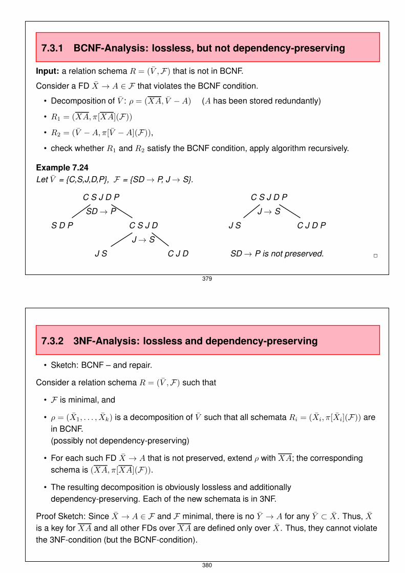
7.3.1 BCNF-Analysis: lossless, but not dependency-preserving

Input: a relation schema R = (V ,F) that is not in BCNF.

Consider a FD X → A ∈ F that violates the BCNF condition.

• Decomposition of V : ρ = (XA, V −A) (A has been stored redundantly)

• R1 = (XA, π[XA](F))

• R2 = (V −A, π[V −A](F)),

• check whether R1 and R2 satisfy the BCNF condition, apply algorithm recursively.

Example 7.24Let V = {C,S,J,D,P}, F = {SD → P, J → S}.

C S J D P

SD → P

S D P C S J D

J → S

J S C J D

C S J D P

J → S

J S C J D P

SD → P is not preserved. ✷

379

7.3.2 3NF-Analysis: lossless and dependency-preserving

• Sketch: BCNF – and repair.

Consider a relation schema R = (V ,F) such that

• F is minimal, and

• ρ = (X1, . . . , Xk) is a decomposition of V such that all schemata Ri = (Xi, π[Xi](F)) arein BCNF.(possibly not dependency-preserving)

• For each such FD X → A that is not preserved, extend ρ with XA; the correspondingschema is (XA, π[XA](F)).

• The resulting decomposition is obviously lossless and additionallydependency-preserving. Each of the new schemata is in 3NF.

Proof Sketch: Since X → A ∈ F and F minimal, there is no Y → A for any Y ⊂ X. Thus, Xis a key for XA and all other FDs over XA are defined only over X. Thus, they cannot violatethe 3NF-condition (but the BCNF-condition).

380

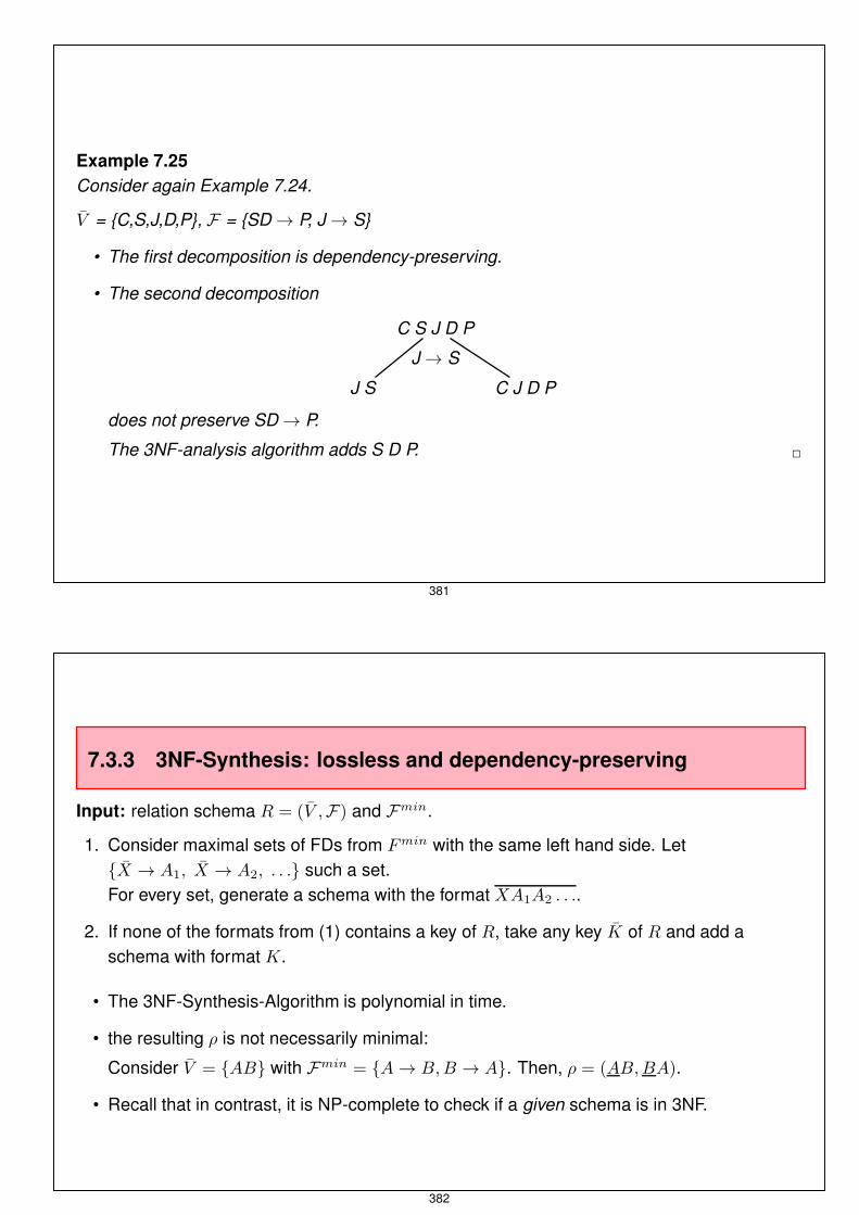
Example 7.25Consider again Example 7.24.

V = {C,S,J,D,P}, F = {SD → P, J → S}

• The first decomposition is dependency-preserving.

• The second decomposition

C S J D P

J → S

J S C J D P

does not preserve SD → P.

The 3NF-analysis algorithm adds S D P. ✷

381

7.3.3 3NF-Synthesis: lossless and dependency-preserving

Input: relation schema R = (V ,F) and Fmin.

1. Consider maximal sets of FDs from Fmin with the same left hand side. Let{X → A1, X → A2, . . .} such a set.For every set, generate a schema with the format XA1A2 . . ..

2. If none of the formats from (1) contains a key of R, take any key K of R and add aschema with format K.

• The 3NF-Synthesis-Algorithm is polynomial in time.

• the resulting ρ is not necessarily minimal:

Consider V = {AB} with Fmin = {A → B,B → A}. Then, ρ = (AB,BA).

• Recall that in contrast, it is NP-complete to check if a given schema is in 3NF.

382

Correctness

• Using Fmin, the generated schemata are in 3NF.

• ρ is dependency-preserving since for every X → Y ∈ Fmin, a format is generated thatcontains XY .

• ρ is lossless since ρ contains a key of the original schema. Using this tuple, in T ∗ (cf.Theorem 7.5) contains a row that consists of ais:

Consider the steps of the X+-algorithm that add – w.l.o.g. – the attributes A1, A2, . . . , Ak

from V \ X to X+. Show by induction that column of Ai in the row of X is set to ai.

– i = 0: nothing to show.

– i− 1 → i: Ai is added to X+ due to a FD Y → Ai where Y ⊆ X ∪ {A1, . . . , Ai−1}.Furthermore, Y Ai ⊆ X ′ for some X ′ ∈ ρ (generated by step (1)) and the rows of Xand X ′ coincide for Y (only as). Then, the chase copies the ai from the row of X ′ tothe row of X.

383

7.4 Join Dependencies and Multivalued Dependencies

Example 7.26

Consider the following Non-1NF table:

cco

Country Continents Organizations

D Europe NATO, EU, UN

TR Europe, Asia NATO, UN

R Europe, Asia UN

USA America UN

... expand the groups as before to 1NF ...

384

Join Dependencies and Multivalued Dependencies (Cont’d)

Example 7.26 (Continued)the expanded table:

cco

Country Continent Organization

D Europe NATO

D Europe EU

D Europe UN

TR Europe NATO

TR Europe UN

TR Asia NATO

TR Asia UN

R Europe UN

R Asia UN

USA America UN

There is some redundancy ...called multivalued dependenciescco satisfies

• country →→ continent and

• country →→ organization.

385

Join Dependencies and Multivalued Dependencies (Cont’d)

Example 7.26 (Continued)

cco

Country Continent Organization

D Europe NATO

D Europe EU

D Europe UN

TR Europe NATO

TR Europe UN

TR Asia NATO

TR Asia UN

R Europe UN

R Asia UN

USA America UN

Actually, cco is a join of

encompasses

Country Cont.

D Europe

TR Europe

TR Asia

R Europe

R Asia

USA America

and

isMember

Country Org.

D EU

D NATO

D UN

TR UN

TR NATO

R UN

USA UN

cco = π[Country,Cont](cco) ⊲⊳ π[Country,Org](cco)

= encompasses ⊲⊳ isMember

✷

386

JOIN DEPENDENCIES (CONT’D)

Consider a set V of attributes, a relation r ∈ Rel(V ), and a decomposition ρ = {X1, . . . , Xn}of V .

r satisfies the join dependency (JD) ⊲⊳ [X1, . . . , Xn] if and only if

r = ⊲⊳ni=1 π[Xi](r) .

In case that n = 2, the JD is also called a multivalued dependency (MVD), written as

X1 ∩ X2 →→ X1 \ X2, or, symmetrically X1 ∩ X2 →→ X2 \ X1 .

Note: X1 = (X1 ∩ X2) ∪ (X1 \ X2), and X2 = (X1 ∩ X2) ∪ (X2 \ X1).

387

7.4.1 4. Normal Form (4NF)

Goal: mutually independent facts should not be represented in a single relation.

Consider a relation schema R = (V ,D) where D is a set of MVDs and FDs. Let D+ theclosure of D.

• for the closure D+ for MVDs see literature.

• FDs are special cases of MVDs.

• MVDs satisfy the following complement property:If X →→ Y ∈ D+, then also X →→ (V \ (X ∪ Y )) ∈ D+.

• trivial MVDs are of the form X →→ Y for Y ⊆ X, and X →→ V \ X.

Definition 7.12A relation schema R = (V ,D) is in 4NF if and only if for every non-trivial X →→ Y ∈ D+, Xcontains a key. ✷

Example 7.27Consider again Example 7.26. It is not in 4NF.Decomposition is lossless and dependency-preserving. ✷

388

Exercise 7.2Experiment with join dependencies using the following ER diagram that describes restaurantsthat offer multiple choices of 2-course meals and accessoires (note that these attributes aremultivalued):

Restaurant

Name City

aperitifs

starters

1st courses 2nd courses

desserts

drinks

389

7.5 Summary

• Analogous considerations for join dependencies lead to 5NF.

• 1NF ⇐ (2NF) ⇐ 3NF ⇐ BCNF ⇐ 4NF (⇐ 5NF)(other directions do not hold).

• 2NF is only of historical interest.

• In all cases there exists a lossless decomposition in 4NF (5NF).

• In the general case, all decompositions further than 3NF are not dependency-preserving.

390

7.6 Inclusion Dependencies

Consider sets X1 and X2 of attributes, and relations r1 ∈ Rel(X1) and r2 ∈ Rel(X2) withY ⊆ X1 ∩ X2.

r1, r2 satisfy the inclusion dependency (ID) R1[Y ] ⊆ R2[Y ] if and only if

π[Y ](r1) ⊆ π[Y ](r2) .

391

7.7 Schema Design

1. Generate an ER-model. This means a thorough discussion of the data engineers and thespecialists of the application area.

2. Note that keys, functional dependencies, multivalued dependencies, and inclusiondependencies belong to this stage!

Candidates can be found by data analysis, but the semantic aspect must be confirmed bythe domain specialists.

3. Transformation to a relational schema

4. Normalization to 3NF

5. Manual decomposition to 4NF

6. enhanced ER design.

392

IMPORTANCE OF A CORRECT ER-DESIGN

Example 7.28Employees are associated (uniquely) with departments. For every employee, the id, name,and the parking area must be stored. For each department, the name, the number, and thebudget of the department are stored, together with the hiring date of each of the employees.

(A) An ER model:

Employee

EmpNo

EName

PArea

Dept

DeptNo

DName

Budget

worksIn< 1, 1 > < 1, ∗ >

since

(B) Dependency Analysis

The FD DeptNo → PArea is detected.

Inter-relational FDs are not allowed?

⇒ Re-Design ✷

393