designing a framework to improve time series data of ... · pdf filealgorithms article...
TRANSCRIPT
algorithms
Article
Designing a Framework to Improve Time Series Dataof Construction Projects: Application of a SimulationModel and Singular Spectrum Analysis
Zahra Hojjati Tavassoli 1, Seyed Hossein Iranmanesh 1,* and Ahmad Tavassoli Hojjati 2
1 School of Industrial Engineering, College of Engineering, University of Tehran, Tehran, 11155/4563, Iran;[email protected]
2 Centre for Transport Strategy, School of Civil Engineering, The University of Queensland, Brisbane,Queensland 4072, Australia; [email protected]
* Correspondence: [email protected]; Tel.: +98-21-8833-5605
Academic Editor: Tom BurrReceived: 21 March 2016; Accepted: 7 June 2016; Published: 18 July 2016
Abstract: During a construction project life cycle, project costs and time estimations contribute greatlyto baseline scheduling. Besides, schedule risk analysis and project control are also influenced bythe above factors. Although many papers have offered estimation techniques, little attempt hasbeen made to generate project time series data as daily progressive estimations in different projectenvironments that could help researchers in generating general and customized formulae in furtherstudies. This paper, however, is an attempt to introduce a new simulation approach to reflect the dataregarding time series progress of the project, considering the specifications and the complexity ofthe project and the environment where the project is performed. Moreover, this simulator can equipproject managers with estimated information, which reassures them of the execution stages of theproject although they lack historical data. A case study is presented to show the usefulness of themodel and its applicability in practice. In this study, singular spectrum analysis has been employedto analyze the simulated outputs, and the results are separated based on their signal and noise trends.The signal trend is used as a point-of-reference to compare the outputs of a simulation employingS-curve technique results and the formulae corresponding to earned value management, as well asthe life of a given project.
Keywords: project management; project progress simulation; singular spectrum analysis; S-curvetechnique; earned value management
1. Introduction
Research in the field of Project scheduling mainly consisting of mathematical operations dates backto the late 1950s, and was used to approximately predict the times on when to start and when to finishactivities of the project in terms of priority and constraints in resources, while simultaneously pursuingto achieve a particular optimized project objective. Subsequently, a stockpile of research was conducted,accounting for scheduling and planning of projects in different areas (see, for example [1–4]).
While extensive research has been carried out during the last two decades resulting in models ofproject scheduling with different features, the bulk of research has mainly focused on fundamentalprinciples of project scheduling. This limitation can possibly be explained by the project schedulefailure, due to limited capability, to overcome the uncertainty and different risks which characterizethe actual and practical execution of the project.
However, as a significant role in a project life cycle and in its failure or success, project scheduling(in combination with other new techniques) can improve the results [5]. In other words, a construction
Algorithms 2016, 9, 45; doi:10.3390/a9030045 www.mdpi.com/journal/algorithms

Algorithms 2016, 9, 45 2 of 24
project schedule has to be considered as a predictive model that can be used with other techniquessuch as Earned Value (EV) indices to improve resource efficiency calculations, risk analysis, projectplanning and control and performance measurement.
For more than fifty years, managers have been using Earned Value Management Systems (EVMS)to cope with the complicated task of controlling and adjusting project schedule baseline as theproject is being executed, according to total project budget, timed delivery, and account projectscope. There is a general consensus over using this well-known management system to use indiceslike Cost Performance Index (CPI) and Schedule Performance Index (SPI) to account for cost, scheduleand technical performance integratively. Besides, this system allows for the calculation of costs,performance indices, schedule variances, forecast project costs and schedule duration. Cioffi proposedprevious and new formalism as well as a new notation to be used in earned value analysis [6].
Research in this area has grown slightly, while forecasting techniques and their applications inareas such as price forecasting have grown rapidly. It seems that the lack or inaccessibility of projectdata is a major barrier to utilizing new forecasting techniques in project management. Applying newforecasting methods requires periodic, progressive time series data, as well as sufficient historicaldata from similar projects. Hence, in many construction projects, this data is not sufficient to applyforecasting methods and risk analysis. Refer to [5,7,8] for more details.
This paper contributes to serve two objectives. First, it mainly intends to review the literatureon project management control research using earned value management and efforts to investigateproject time and cost estimates. Although a large number of papers have proposed estimation methods,little attempt has been made to apply these methods to generate project time series data as dailyprogressive estimations in different project environments. Therefore, a new simulation approach asa novel framework is offered here to reflect the data regarding time-series progress of the project,considering the specifications and the complexity of the project and the environment where the projectis performed.
The output can explain the future progress and financial situation of the project at different timescale. This simulator is a powerful tool that can provide daily progressive estimated information whichreassures project managers of execution stages of the project although they lack historical data thatcould help researchers in generating general and customized formulae in further studies.
Secondly, the additional aim of this paper is to use both fictitious and empirical data to obtain andthen validate results by using Singular Spectrum Analysis (SSA) and S-Curve techniques. Specificationsof this simulator are extracted from the literature or arise from the author’s experiences. Thus,researchers can both adjust their ideas to generally investigate project estimations by setting theirinputs and study the outputs of the simulator.
This paper has been structured to include the following sections: Section 2 gives brief reviewson project estimates and controls which refer to sources as significant research studies in the relatedliterature; further details are offered on their usage in the experiments related to simulation. In thefirst subsection, the most important parameters employed in Earned Value Management (EVM) arebriefly reviewed, and some resources on the latest literature concerning time and cost performancemeasurement are displayed. A second subsection deals with the basic concept of SSA approach toanalysis and forecast nonparametric time series. The third subsection surveys simulations techniqueswith reference to previous research studies in the field of project management and its recent advances.Section 3 describes the methodology, the new proposed framework and input and output descriptionsand introduces the validation method in three subsections. The simulator has two main inputsdescribed in Section 4. The following section calculates results containing construction projectinformation which are fictitious project data and empirical data. Finally, Section 6 draws conclusionsand paves the ground for future research.

Algorithms 2016, 9, 45 3 of 24
2. Literature Review
In this section, we start with a short review of project estimates and controls with references tothe earlier most important studies conducted in the literature. The subsections that follow offer furtherdetails about the simulation experiments presented in this study, specifically on their usage.
Plans and project schedules are usually developed for each project to make sure that activities areconducted to meet the specifications of the quality expected along with the budget and the allowedtime. Many projects lose substantial financial resources every year due to delays in their progress andrequire additional time and costs for implementation or to reach completion. One of the main concernsof project managers is to fulfill a project within a pre-determined schedule and allocated budget. Whendifferences between planned and actual work performances become considerable, extra managementof tasks would be required to bring indices back on course to stay on the planned schedule and budget.During the implementation phase, project progress should be frequently monitored and checkedagainst the planned project schedule so that we can identify and measure any divergences. Exactcontrol of a project depends on suitable and timely access to the project’s information, such as the costand time status of the project.
2.1. EVM
In 1967, the U.S. Federal Government agencies played a significant role in introducing EVM forthe first time and using it in programs like large acquisition ones [9]. The U.S. Federal Governmentwas also able to successfully take advantage of EVM in its widespread projects. Project managers couldbenefit from EVM the most as it keeps them informed of the early indications and procedures of aproject’s execution and alerts them to eventual corrective action if needed. A large number of researchinvestigations have been devoted to this area, as shown in [5,10], since EVM was introduced. AlthoughEVM was employed to investigate time and cost both, the cost aspect has been the center of attentionin most research studies. In a study, EVM was discussed from a price tag perspective [11]. In a laterstudy, it is focused on predicting how long an activity takes by proposing a reliable methodology andusing SPI [12] and a formula for estimating project time according to (EDAC) is proposed, i.e., Estimateof Duration at Completion.
During the life cycle of a project, a point of reference is needed for EVM to measure the project’sexecution periodically. This fixed reference point is supplied by its project’s baseline schedule. Inorder to obtain the time and costs of a project performance, the three key parameters of EVM must becompared to each other and the time and cost performance measures as below:
� Budgeted Cost of Work scheduled (BCWS)� Actual Costs Work Performed (ACWP)� Budgeted Cost of Work Performed (BCWP)� Earned schedule (ES)� Schedule Variance (SV = BCWP´ BCWS)� Schedule Performance Index (SPI = BCWP
BCWS )� Cost Variance (CV = BCWP´ACWP)� Cost Performance Index (CPI = BCWP
ACWP )� EDAC = PD/SPI
Lipke questioned the classic metrics of SV and SPI previously used since they failed to reliablyforecast ending point of time of a project [10]. In this study, however, a time-based measure wasdesigned to cope with false and unreliable behavior, which is dependent on similar principles tothose of earned value method, but which renders the money-related metrics into a time aspect. Hetransformed the time performance metrics SV and SPI to SV(t) and SPI(t) and indicated that theyshowconsistent and reliable behavior throughout the project life cycle.

Algorithms 2016, 9, 45 4 of 24
EVM was also used for forecasting project duration, comparing the indicators of previous earnedvalue performance, namely SV and SPI, with the recently developed indicators of earned scheduleperformance SV(t) and SPI(t) and later compared them with the results of time performance measuredthrough the three methods of obtaining time performance in a project [13]. Their results indicatedthat a general schedule forecasting formula could apply to various project situations. Later, it wastried to evaluate EV-based methods by reviewing them as they are commonly used to forecast totalduration of a project [14]. They delicately controlled the uncertainty level of project to conduct anextensive simulation survey in which they tried to account for the accuracy of forecasts as influencedby the network structure of project, and the reliable and accurate results obtained from the EV-basedmeasures within time perspective. In their study, they investigated the capability of a newly designedmethod, and the schedule method earned, which hones the relationship between EV metrics andduration forecasts of the project.
A new formula to calculate the (EAC) is presented [15], i.e., Estimate At Completion, of projects tohone EVMS. Their new method contains a formula which is composed of four variables: SPI, ScheduledPercent Complete by Duration (SPCD), Actual Percent Complete by Duration (APCD), and Sum ofDurations to Due Time (SDDT).
Studies measuring time performance of the project and/or the concept of earned schedule havebeen the focus of some publications issued in the popular and academic literature. Empirical data wasmanipulated by using statistical procedures involved in validation of time performance indices andstability investigations [10].
After all, sensitivity or risk analysis and EVM (whose results were validated using a simulator)were concepts already studied and examined in previous research investigations [5,14,16].
In conclusion, although research in this area has increased only minimally, there is still widespreadinterest in the need to introduce new indices and formulae into forecasting. Additionally, the use ofsimulation techniques and simulators has emerged as an effective tool to generate varied experiments.
2.2. SSA
SSA is a component of the more inclusive classification of methods called Principal ComponentAnalysis (PCA), is a powerful technique used to analyze and predict non-parametric time series thatinclude non-stationarity data elements with complex seasonal components and is superior to classicaltechniques. On the other hand, SSA is a technique used for the analysis of time series that are observed,and it is capable of exposing the main features of the predictability of time series.
The traditional models, namely ARMA, ARIMA, Box–Jenkins and artificial intelligence, suchas fuzzy models, etc., demand certain assumptions as restrictive distributional, structural ones andadequate historical data. A new method inspired by genetic colonial theory is introduced to forecastand filter time series [17] This method has many similarity with SSA. However, SSA does not use anystatistical assumptions, namely the series stationarity or residuals normality, and it need not rely onany parametric model to find out the trend or oscillations. Moreover, contrary to many other methods,it is independent of sample size, even small sample sizes.
The theoretical underpinnings and practical background of the SSA technique were introducedby Golyandina et al. in 2001 [18] and further by Hassani [19,20] and Viljoen for common timeseries [21]. The applications of this technique are many and various, for example, in meteorology,physics, economics, and financial mathematics. In recent years, SSA has been designed and employedto various practical problems, for instance, in industrial production [22], by Afshar et al. [23] to loadforecasting in the electricity market as well as other markets, for forecasting CO2 emissions [24], and forsignal extraction in a genetics related application [25]. Moreover, a forecasting method was presentedwith Artificial Neural Network and SSA [26] and a hybrid model Coupled with SSA was used toforecast rainfall [27]. Finally, SSA is introduced and reviewed the separability techniques and windowlength [28].

Algorithms 2016, 9, 45 5 of 24
The SSA technique is composed of two steps that are complementary to each other, decompositionand reconstruction.
Figure 1 presents, the standard SSA, which includes two main stages and four subsets. Byreconstructing the original series after decomposition, it is possible to remove noise.Algorithms 2016, 9, 45 5 of 24
Figure 1. The standard Singular Spectrum Analysis (SSA) steps.
The first stage is the decomposition stage, which has two steps:
Step 1, embedding:
Embedding is similar to mapping and can be regarded as a form of mapping. This form of mapping, i.e., embedding, turns a time series that is one-dimensional, = ( , , … , ),into series that are multi-dimensional, , , … , , using vectors, = ( ,… , )ϵ .
= ⋯⋮ ⋱ ⋮⋯
Embedding has certain assumptions: K = T − L + 1; the window length, L, as the single parameter or an integer that should be 2 ≤ L ≤ T. Besides, the L or window length must be big enough. This step results in a matrix called a Hankel matrix, = ( ,… , ), which has equal elements on the diagonal, and the linear space that is spanned by columns of H is called the trajectory.
Step 2, SVD:
The second step is called the SVD step, which sums up elementary matrices of rank-one bi-orthogonal to obtain the singular value decomposition of the trajectory, = +⋯+ , where = and and are eigenvalues and eigenvectors of matrix, , = and ⋯ 0. The set ( , , ) is referred to as a value of the matrix X called the i-th eigentriple, in which si represents the singular value of X or its i-th value (whose value is equal to the square root of the i-th eigenvalue of matrix XXT); Ui is the i-th left singular vector of X (equivalent to the i-th eigenvector of XXT); and Vi is the i-th right singular vector of X (equivalent to the i-th eigenvector of XTX). A group of r eigenvectors determines an r-dimensional hyperplane in the L-dimensional space, RL of vectors, Xj.
The second stage is the reconstruction stage, which consists of two steps: grouping and diagonal averaging. The grouping step refers to dividing the elementary matrices, X , into some categories and adding the matrices in each group. Imagine that I = i , … , i is a set of indices i , … , i .Therefore, the matrix, X , related to the set I, is presented as X = i + ⋯+ i . The decomposition of the set of indices, J = 1,… , d, into the disjoint subsets, I , … , I , corresponds to the matrix called X, which is represented by X = X +⋯+ X . Eigentriple grouping is the process of selecting the sets I , … , I .
Diagonal averaging turns every single matrix I into a time series. A time series is an element commonly added to the initial series Y . If z represents a component of a matrix Z, then the k-th term of the obtained series is calculated by averaging z over all I, j in such a way that i + j = k + 2. The above procedure is known as diagonal averaging or, to put it differently, the Hankelization of the matrix Z. By applying diagonal averaging or the Hankelization procedure to all matrix elements of X ,… , X , another expansion is achieved: X = X +⋯+ X . This expansion is equal to the decomposition of the first original series Y = (y , y , Thiy )into a total m series: = ∑ y ( ), where Y ( ) = (y ( ), … , y ( )) matches the matrix X .
•Transformation of the one-dimensional time series into a Henkel matrix
•Singular Value Decomposition (SVD) of the Hankel matrix
Decomposition
•PCA and selection of the dominant features by grouping the SVD components
•Reconstruction of the original time series using the selected features
Reconstruction
Figure 1. The standard Singular Spectrum Analysis (SSA) steps.
The first stage is the decomposition stage, which has two steps:
Step 1, embedding:
Embedding is similar to mapping and can be regarded as a form of mapping. This form ofmapping, i.e., embedding, turns a time series that is one-dimensional, YT “ py1, y2, . . . , yTq, intoseries that are multi-dimensional, X1, X2, . . . , Xk, using vectors, Xi “ pyi, . . . , yi`L´2q P RL.
X “
¨
˚
˝
y0 ¨ ¨ ¨ yK´1...
. . ....
yL´1 ¨ ¨ ¨ yT´1
˛
‹
‚
Embedding has certain assumptions: K = T ´ L + 1; the window length, L, as the single parameteror an integer that should be 2 ď L ď T. Besides, the L or window length must be big enough. Thisstep results in a matrix called a Hankel matrix, H “ pX1, . . . , XKq , which has equal elements on thediagonal, and the linear space that is spanned by columns of H is called the trajectory.
Step 2, SVD:
The second step is called the SVD step, which sums up elementary matrices of rank-onebi-orthogonal to obtain the singular value decomposition of the trajectory, X “ E1 ` . . .` Ed, whereEi “
a
λiUiVi and λi and Ui are eigenvalues and eigenvectors of matrix, XX, Vi “ XUi{a
λi andλ1 ě λ2 ě . . . ě λL ě 0. The set (λi, Ui, Vi) is referred to as a value of the matrix X called the i-theigentriple, in which si represents the singular value of X or its i-th value (whose value is equal to thesquare root of the i-th eigenvalue of matrix XXT); Ui is the i-th left singular vector of X (equivalent to thei-th eigenvector of XXT); and Vi is the i-th right singular vector of X (equivalent to the i-th eigenvectorof XTX). A group of r eigenvectors determines an r-dimensional hyperplane in the L-dimensionalspace, RL of vectors, Xj.
The second stage is the reconstruction stage, which consists of two steps: grouping and diagonalaveraging. The grouping step refers to dividing the elementary matrices, Xi, into some categories andadding the matrices in each group. Imagine that I “
i1, . . . , ip(
is a set of indices i1, . . . , ip. Therefore,the matrix, XI, related to the set I, is presented as XI “ i1 ` . . .` ip. The decomposition of the set of
Algorithms 2016, 9, 45 6 of 24
indices, J “ 1, . . . , d, into the disjoint subsets, I1, . . . , Im, corresponds to the matrix called X, which isrepresented by X “ XI1 ` . . .`XIm . Eigentriple grouping is the process of selecting the sets I1, . . . , Im.
Diagonal averaging turns every single matrix I into a time series. A time series is an elementcommonly added to the initial series YT. If zij represents a component of a matrix Z, then the k-thterm of the obtained series is calculated by averaging zij over all I, j in such a way that i + j = k + 2.The above procedure is known as diagonal averaging or, to put it differently, the Hankelization ofthe matrix Z. By applying diagonal averaging or the Hankelization procedure to all matrix elementsof XI1 , . . . , XIm , another expansion is achieved: X “ ĂXI1 ` . . .`ĄXIm . This expansion is equal to thedecomposition of the first original series YT “
`
y1, y2, ThiyT˘
into a total m series: yt “řm
k“1 rytpkq,
where ĂYTpkq“ p ry1
pkq, . . . , ĂyTpkqqmatches the matrix XIk .
Two parameters are needed for the SSA method: the number of elementary matrices r and thewindow length L. It is necessary that we choose an appropriate window length L since it is essentialfor improving the accuracy of the SSA. If the points of different vectors, Xi and Xj (i ‰ j) are linearlyindependent, then the value of L is calculated. The structure of the data and how we perform theanalysis determine our choice of these parameters following particular selection rules.
2.3. Simulation Project Techniques
Simulation is also one of the most useful and effective techniques to analyze a complex anddynamic project, which helping the decision maker to recognize the effect of various dependentvariables and complex scenarios on the project’s behavior. Furthermore, project simulation can be usedin different aspects of project management, can help researchers to gain many accurate and realisticoutputs according to set inputs and also to investigate different scenarios as summarized below.
As described in Section 2.1, the use of simulation techniques and simulators has emerged as aneffective tool to generate varied experiments in this area. A method called Special Purpose Simulation(SPS) is utilized [29] which is a tool to optimize workforce forecast loading and leveling resources.SPS is a simulation model manages to optimize resource supplies and requirements for conductinga petrochemical project, considering standard discipline necessities and involvements. A projectmodel has been designed [30] which simulates the developmental process of the project in a realisticmanner and produces information concerning three different monitoring systems. In this paper, factorsinfluencing the total cost and performance of project are also accounted for by changes occurringin the project plan and rates of inflation. In a similar vein, a research framework was developed toenable project managers to approximately calculate completion time of the project and dive deepinto the main factors which influence the estimation for complex engineering projects being executedconcurrently [31]. Their proposed framework is composed of three main procedures: data gathering,simulation, and data analysis with ANOVA.
A number of studies have been developed to scrutinize various factors affecting project costestimations. Akintoye focused on understanding different factors influencing project contractors’ costestimating practices [32]. In this study, 24 factors were identified by conducting a comparative studyanalyzing 84 UK contractors categorized into four classes ranging from very small, small, medium tolarge firms. Bashir and Thomson presented a thorough quantitative estimation approach which canoffer initial along with updated project estimates from manageability or feasibility study until projectcompletion [33]. A dynamic simulation-based crashing methodology was introduced to assess projectnetworks and determine the optimum crashing configuration that reduces the average project cost to aminimum level because of delayed penalties and crashing costs [34]. Their dynamic method allows usto assess the project network to design a crashing strategy at the very onset of the project executionand also during the time that the project is being performed.
As described in Section 2.2, EVM concepts were used as a basis to analyze simulation techniques ina number of research investigations. In a study, the efficiency of controlling a project was analyzed [5].A Monte-Carlo simulation was used to validate the project data of the study whether fictitious orempirical. Upon noticing warning control parameters, we must take corrective actions to put the

Algorithms 2016, 9, 45 7 of 24
project back into the correct path whenever a problem occurs. This set of information offered by theSchedule Risk Analyses (SRA) along with EVM information which is mostly the sensitivity informationis obtained during project control. The effects of different activities on risk and the expected completiontime of the project were described [8].
In another study, Elshaer used Planned Value Management (PVM), Earned Duration Management(EDM) and Earned Schedule Management (ESM) as the three earned value methods to study theprediction of project duration in EVM [16].
In conclusion, it can be seen that, to a considerable degree, these studies were conducted with theaim of designing a project simulator. In many cases, simulation studies have been used to validateproject scheduling solutions or to estimate project specification in some part of the project, for instanceproject completion cost and time estimations or risk measurements. However, none of the prior studieshas considered daily project information as a time series. On this basis, the purpose of this paper is todesign a novel project progress simulator that can convert the project into its time series as efficientinformation, which can help other researchers to generate new formulae.
3. Methodology
The methodology employed in the computational and conceptual experiment includes a newframework in order to generate project progress time series data, thereby introducing valuableinformation about projects and preparing an appropriate context for introducing new indices andformulae, varied experiments and further research. In the following subsections, the frameworkstructure, its components and sources and why and how these sources (project progress simulator andSSA) can be used together in project control are explained.
3.1. Project Progress Generator Framework
Computer-assisted simulation is a powerful method to analyze complex and dynamic projects byanalyzing large data size, and this precise and flexible technique has been used in much of the researchin the field of project management (see, for example, [14,29]). Simulation software can predict the setof expected costs and the duration of the project, depending on input parameters. These inputs controlactivity duration, cost estimation and the effect of risks when producing cost estimates.
However, as mentioned before, the idea of generating project progress simulators has not beenmentioned in the prior studies. Therefore, the aim of this paper is to introduce this simulator andto optimize the resulting time series with SSA. The combination of simulation techniques and SSAanalysis with different inputs will help project managers to obtain a realistic estimation of project costand time in different sectors of the project and will reduce the delay risks. Furthermore, insight isgained into project progress behavior, deviations during project execution, the appropriate use of EACformulas and identifying areas for additional research.
The important aspect of the SSA is that it has two advantages over other methods, which makes itmore beneficial in project control. One feature of the SSA is that it can be applied to series with smallsample sizes. The other important aspect is that, unlike other methods, the SSA does not need anystatistical assumptions, such as the stationarity of the series or the normality of the residuals. Thebasic concepts of the project progress generator have been shown by Iranmanesh and Tavassoli [15]. Inthis paper, the well-developed model with more details is presented. The project progress generatorframework has four main steps (as shown in Figure 2). The process starts with the project entry, whichcan be a given project or selected from a fictitious database and scheduling baseline.
Algorithms 2016, 9, 45 8 of 24
Algorithms 2016, 9, 45 7 of 24
the prior studies has considered daily project information as a time series. On this basis, the purpose of this paper is to design a novel project progress simulator that can convert the project into its time series as efficient information, which can help other researchers to generate new formulae.
3. Methodology
The methodology employed in the computational and conceptual experiment includes a new framework in order to generate project progress time series data, thereby introducing valuable information about projects and preparing an appropriate context for introducing new indices and formulae, varied experiments and further research. In the following subsections, the framework structure, its components and sources and why and how these sources (project progress simulator and SSA) can be used together in project control are explained.
3.1. Project Progress Generator Framework
Computer-assisted simulation is a powerful method to analyze complex and dynamic projects by analyzing large data size, and this precise and flexible technique has been used in much of the research in the field of project management (see, for example, [14,29]). Simulation software can predict the set of expected costs and the duration of the project, depending on input parameters. These inputs control activity duration, cost estimation and the effect of risks when producing cost estimates.
However, as mentioned before, the idea of generating project progress simulators has not been mentioned in the prior studies. Therefore, the aim of this paper is to introduce this simulator and to optimize the resulting time series with SSA. The combination of simulation techniques and SSA analysis with different inputs will help project managers to obtain a realistic estimation of project cost and time in different sectors of the project and will reduce the delay risks. Furthermore, insight is gained into project progress behavior, deviations during project execution, the appropriate use of EAC formulas and identifying areas for additional research.
The important aspect of the SSA is that it has two advantages over other methods, which makes it more beneficial in project control. One feature of the SSA is that it can be applied to series with small sample sizes. The other important aspect is that, unlike other methods, the SSA does not need any statistical assumptions, such as the stationarity of the series or the normality of the residuals. The basic concepts of the project progress generator have been shown by Iranmanesh and Tavassoli [15]. In this paper, the well-developed model with more details is presented. The project progress generator framework has four main steps (as shown in Figure 2). The process starts with the project entry, which can be a given project or selected from a fictitious database and scheduling baseline.
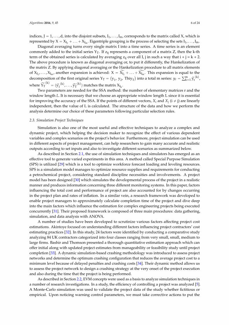
Figure 2. Project progress generator framework and its steps. PSC, Progress Simulation for Time; PST, Progress Simulation for Time.
Figure 2. Project progress generator framework and its steps. PSC, Progress Simulation for Time; PST,Progress Simulation for Time.
The project progress with the proposed simulator can be considered from two main perspectives:
‚ Progress Simulation for Time (PST): PST calculates different indices in various time sections andfocuses on time parameters to simulate the progress of projects.
PST consists of the following steps:
a. Determining the input project and parameters;b. Constructing project scheduling;c. Updating the project’s progress daily;d. Computing the project’s actual progress daily, based on the set inputs. Suppose ℵ
represents the random impact of risk overall, then ℵ P p0, 1s . The impact of risk events, X,integrated with the above task progress is shown as follows:
pXiqj “ pXiqj´1 ` pPiqs ˚Di ˚ pℵiqj
where i and j represent the number of tasks and days, respectively. The random overallimpact, pℵiqj, shows the risk of each task in each day from its start to finish. Furthermore,pPiqs and Di are daily scheduled progress in a planned day, s, and experts’ proposed statusfor the task, i.
e. Calculating different measurement indices (i.e., EVM measurements);f. Continuing until the project is entirely completed.
‚ Progress Simulation for Cost (PSC): PSC simulates the progress of projects via cost progressduring project execution, calculates different indices in different time sections and focuses oncost parameters. PSC is developed mainly based on the PST structure and focuses on the costparameters. The following is a list of other principles of PSC.
1. Determining the input costing parameters;2. Calculating planned cost progress based on a general specification (i.e., inflation rate) and
each task’s specifications (i.e., costs of resources);3. The daily cost of each task is calculated based on resource consumption of the task on that
day and other costing parameters;4. The daily project cost is calculated until the project is finished.
The simulator outputs are time and cost time series that indicate the progressive behavior ofthe project’s cost and time. These outputs are then used as inputs of the SSA method. SSA analyzesthese inputs and separates the main trend from noise, then identifies if there is any special trend in

Algorithms 2016, 9, 45 9 of 24
the time series, such as seasonal behaviors. The output, or “trend time series”, can be used for furtherestimations if the project is repeated or not completed.
3.2. Input Parameters
The proposed simulator considers several parameters that are identified as affecting the project’sprogress. Hence, these parameters are presented as samples for the designed model, and many otherscan be considered in this framework with different types of projects. These input parameters, whichshould be fed to the simulator by the user, are as follows:
Input project type: As mentioned before, the input project can be a fictitious project or a given one.Project discipline: In regard to project management, the concept of ‘discipline’ is defined as an
area of work or activity that demands enormous knowledge. It peculiarly corresponds to the area ofwork or focus where unique and static sets of rules and regulations need to be closely followed in theprocesses of the conduct and completion of that work or activity.
As Figure 3 presents, the project structure is divided into some separated disciplines, and eachdiscipline comprises certain tasks, each of which utilizes project resources to be accomplished.
Algorithms 2016, 9, 45 9 of 24
each discipline have the same work contour property, named back-loaded. The shape of different work contours is pointed out in the different behaviors of tasks and disciplines during the project.
Expert’s comments: To generate actual information, some task specifications are needed. As a case in point, each task’s progress status is needed in order to process whether the task progress has overtaken the plan and to determine the degree of variation existing between them. This simulator is a powerful tool for project managers. Therefore, they are the main users of this system, and they should enter their comments about how projects can progress in their environments.
Inflation rate: Inflation rates are assumed to be linear and fixed during the project.
Figure 3. Project disciplines and their relations to project resources.
3.3. Output Validation
S-Curve displays accumulated efforts or costs of a project and represents the function of time or cost. In fact, this curve was employed to control and check progress in a set of projects related to each other. Moreover, it is showed that this is possible to characterize the progression of the overall cost of any project [35]. The results of the study inductively concluded that the rising slope in the S-curve, and the point of time when half of the total funds have been consumed, are two numbers that represent this curve.
In the absence of data, we can characterize an equation to illustrate project S-curves with three parameters:
• The total cost of the project (Y1); • The total life time of the project (t1); • The point of time when the project has spent half of its total funds (t1/2).
Estimating the three above parameters, an S-curve equation that can specify in what way labor or funds could be represented during the project at the start of any project can be established for project management purposes.
Define as the proportion = / , and term the specific where Y = 0.5Y1 as / where Y indicates the project cost, given the condition that 0 < / < 1. If a project whose distribution is front-loaded, where the funds are spent earlier rather than later, / will be nearer to the beginning of the project. Other projects tend to have this time closer to the middle ( / = 0.5). For back-loaded projects, in which funds are disbursed nearer to the end of the project, / would be greater than 0.7.
A gentle rise, a steep slope and a gradual path to the asymptote are the three parts of a typical S-curve. Suppose that the steep slope in the middle portion includes two-thirds of the rise from point Y = 0 to Y = , where is the highest level of the project cost. One-third of the rise remaining
Project
Structure
Figure 3. Project disciplines and their relations to project resources.
Disciplines’ work contour: The work contour is a kind of property that demonstrates how everysingle task is spread over the assignment duration. In this research, it is assumed that all tasks in eachdiscipline have the same work contour property, named back-loaded. The shape of different workcontours is pointed out in the different behaviors of tasks and disciplines during the project.
Expert’s comments: To generate actual information, some task specifications are needed. As acase in point, each task’s progress status is needed in order to process whether the task progress hasovertaken the plan and to determine the degree of variation existing between them. This simulator is apowerful tool for project managers. Therefore, they are the main users of this system, and they shouldenter their comments about how projects can progress in their environments.
Inflation rate: Inflation rates are assumed to be linear and fixed during the project.
3.3. Output Validation
S-Curve displays accumulated efforts or costs of a project and represents the function of time orcost. In fact, this curve was employed to control and check progress in a set of projects related to eachother. Moreover, it is showed that this is possible to characterize the progression of the overall cost ofany project [35]. The results of the study inductively concluded that the rising slope in the S-curve, andthe point of time when half of the total funds have been consumed, are two numbers that representthis curve.
In the absence of data, we can characterize an equation to illustrate project S-curves withthree parameters:

Algorithms 2016, 9, 45 10 of 24
‚ The total cost of the project (Y1);‚ The total life time of the project (t1);‚ The point of time when the project has spent half of its total funds (t1/2).
Estimating the three above parameters, an S-curve equation that can specify in what way labor orfunds could be represented during the project at the start of any project can be established for projectmanagement purposes.
Define β as the proportion β “ t{t1, and term the specific β where Y = 0.5Y1 as β1{2 where Yindicates the project cost, given the condition that 0 < β1{2 < 1. If a project whose distribution isfront-loaded, where the funds are spent earlier rather than later, β1{2 will be nearer to the beginning ofthe project. Other projects tend to have this time closer to the middle (β1{2 “ 0.5). For back-loadedprojects, in which funds are disbursed nearer to the end of the project, β1{2 would be greater than 0.7.
A gentle rise, a steep slope and a gradual path to the asymptote are the three parts of a typicalS-curve. Suppose that the steep slope in the middle portion includes two-thirds of the rise from pointY = 0 to Y = Y8, where Y8 is the highest level of the project cost. One-third of the rise remaining takesplace over the two gently rising portions. Factor r is defined as a parameter that displays the large sizeof the rise in the third middle and enables the project manager to freely select an approximation to thiscentral slope, and r0.67 is defined through:
r “23
r0.67
Assume that the project manager selected desired β and r0.67, so the value of γ throughEquation (1) can be calculated. The project manager can then plot the project’s S-curve using Equation (2).
ln pγ` 2q “ 8 β1{2r0.67 (1)
Finally, the S-curve equation, in regard to the ratio y = Y/Y1, is defined as follows:
ypβq “ y81´ exp p´8r0.67βq
1` γexp p´8r0.67βq(2)
where y8 “ Y8{Y1 ą 1. Theoretically, y = 1 shows that the project is complete, and at β “ β1{2, y “ Y8
2 .
Algorithms 2016, 9, 45 10 of 24
takes place over the two gently rising portions. Factor is defined as a parameter that displays the large size of the rise in the third middle and enables the project manager to freely select an approximation to this central slope, and 67.0r is defined through:
0.672
3r r=
Assume that the project manager selected desired and . , so the value of through Equation (1) can be calculated. The project manager can then plot the project’s S-curve using Equation (2). ln( + 2) = 8 β / . (1)
Finally, the S-curve equation, in regard to the ratio y = Y/Y1, is defined as follows:
y(β)=y∞ ( . )( . ) (2)
where = > 1⁄ . Theoretically, y = 1 shows that the project is complete, and at β = β / , y = Y2 . If the manager is willing to say that y = 1/2 at β = 1/2, conducting the calculation will obtain a
new β / that will meet the desired situation. Figure 4 represents the flowchart for using this technique to plot a project’s S-curve.
In the next section, the behavior of simulator results is compared to project life cycle trends, using an S-curve trend to verify these results.
Figure 4. S-curve technique flowchart.
4. Data Description
As mentioned before, the framework has two project data sources: fictitious and given projects. In this subsection, we describe both fictitious and empirical project data and their specifications.
4.1. Fictitious Project Data
As there has been great progress in the models and methods of project scheduling (especially intelligent approaches), the need for data instances to evaluate the solution procedure increases. Therefore, a large number of research studies on project scheduling during the past several years has been attempting to focus on designing and developing benchmark series of project networks to
No
Yes
Start
Project manager chooses β / and
Calculate γ based on Equations (1) and plot the S-curve using Equation (2)
Calculate new β / and corresponding γ and plot the
new S-curve using Equation (2)
Finish
Does project manager insist on β = 1/2 at
y = 1/2?
Figure 4. S-curve technique flowchart.

Algorithms 2016, 9, 45 11 of 24
If the manager is willing to say that y = 1/2 at β = 1/2, conducting the β calculation will obtain anew β1{2 that will meet the desired situation. Figure 4 represents the flowchart for using this techniqueto plot a project’s S-curve.
In the next section, the behavior of simulator results is compared to project life cycle trends, usingan S-curve trend to verify these results.
4. Data Description
As mentioned before, the framework has two project data sources: fictitious and given projects.In this subsection, we describe both fictitious and empirical project data and their specifications.
4.1. Fictitious Project Data
As there has been great progress in the models and methods of project scheduling (especiallyintelligent approaches), the need for data instances to evaluate the solution procedure increases.Therefore, a large number of research studies on project scheduling during the past several years hasbeen attempting to focus on designing and developing benchmark series of project networks to equipusers and researchers with successful project planning and evaluating equipment to visualize variousprojects and to benchmark solution procedures for single and multi-mode project scheduling problemsthat are resource-constrained.
Generally, if we want to employ intelligent forecasting methods to predict the time and cost ofprojects, it is essential that we generate basic time series as the scientific representations of variousprojects. These representations, referred to as standard datasets, are always formed based on theknown concept of project networks, explaining the activities, characteristics and precedence constraintsof each project using a directed non-cyclic connected graph to prove that the project is manageable.
Comprehensive surveys of these datasets and comparisons between them can be foundin [23,25–27]. In the current study, we use the ProGen standard dataset. The simulator was usedin 480 projects with 92 tasks and 4 resources [36].
As mentioned before, the purpose of this study is to introduce a project progressive simulatorframework and generate project time series data. Hence, structural network parameters such as thetopological structure, the criticality of a network or resources are not investigated in this study. On thisbasis, fictitious project data are used just as an input project.
4.2. Empirical Project Data
Javadieh is one of the areas situated in the southwest of Tehran in Iran. An underpass project wasconducted in Javadieh. This project includes two bridges, one overpass measuring 90 m in length and8.20 m in width and one underpass of 80 m in length and 8.20 m in width. Besides, two entry rampsand one exit ramp meet this railway, which cross with the northern city network (Shoosh Avenue) andsouthern city network (Noori Street).
Engineering, procurement, destruction and construction are the four main disciplines employedin the whole project. The construction discipline consists of some main sub-disciplines, namelyexcavation, formwork, concreting, waterproofing, embankment, pavement and other minor workactivities, like curbs, signs, signaling and lighting.
This project was estimated to be completed within six months with 223 tasks over the fourmentioned disciplines. The price agreed for this contract was fixed, approximately 66,869,542,003 Rials(equal to $2.3 million at writing). The project network was thought to be an activity-on-the-nodeproject network whose project data determined the precedence relations between the tasks. The projectwas scheduled from 24 April 2013 to 20 October 2013; after five months, only 60% of the project hadbeen completed, and the delays made them reschedule the project. Therefore, it was necessary forthem to continuously analyze the project condition, measurement factors and daily progress status inorder to evaluate the project’s efficiency and risk effects. That way, the project can be rescheduled in arealistic way, since this monitoring and controlling equipment enabled the project manager to measurethe remaining project cost and time, to provide adequate resources and to take other factors, such ascontrol risks, into account.
Algorithms 2016, 9, 45 12 of 24
5. Simulation Result
The progress simulator is demonstrated as a software program including PSC and PST conceptsby the use of Visual Basic for Application (VBA) in the environment of Microsoft Project 2010 (MSP)and SSA method using CaterPillar SSA 3.40 to analyze the results [37].
In this section, the results of a randomly selected project from the ProGen dataset and a givenproject are presented. The selected project is just used for presenting the methodology, and thistechnique can be applied on several projects. Moreover, simulating several runs with different inputparameters can help project managers to forecast precisely different situations. The results are thencompared to the S-curve technique and SSA, based on the simulator output. The influences ofinput parameters are then examined in different circumstances. Section 5.1 presents the steps ofgenerating fictitious project progress time series and Section 5.2 demonstrates the simulated results fora given project.
5.1. Fictitious Project Results
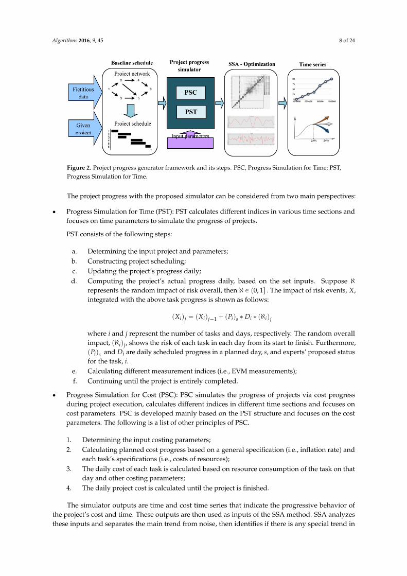
Figure 5 shows the results of the simulator on one randomly selected project from the ProGendataset. In this diagram, the daily progresses of physical and actual percent completion were compared.The S-curve shape can be seen in these two diagrams; however, this simulated project includes adelay of 56 days. This project has 92 tasks and is scheduled for 87 days, and it is simulated by theseinput parameters:
- The project has four disciplines comprising 20%, 10%, 40% and 30% of all of the tasks, andback-loaded, flat, front-loaded and bell are their work contours, respectively.
- Eighty percent of task delays are in the range of 10% of scheduled progress.- The project was simulated with a 20% inflation rate for the last six months.
Algorithms 2016, 9, 45 12 of 24
5.1. Fictitious Project Results
Figure 5 shows the results of the simulator on one randomly selected project from the ProGen dataset. In this diagram, the daily progresses of physical and actual percent completion were compared. The S-curve shape can be seen in these two diagrams; however, this simulated project includes a delay of 56 days. This project has 92 tasks and is scheduled for 87 days, and it is simulated by these input parameters:
- The project has four disciplines comprising 20%, 10%, 40% and 30% of all of the tasks, and back-loaded, flat, front-loaded and bell are their work contours, respectively.
- Eighty percent of task delays are in the range of 10% of scheduled progress. - The project was simulated with a 20% inflation rate for the last six months.
Figure 5. Percent completion of the simulated project.
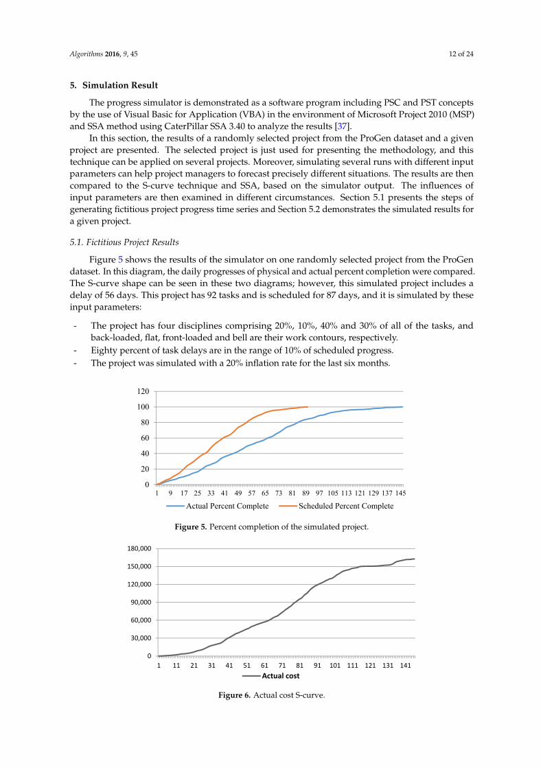
To validate the simulator, another randomly selected project from the ProGen dataset is used, taking the results and comparing them to the S-curve technique’s results. The simulator inputs are set, as all tasks are in one discipline with a normal distribution, a 20% inflation rate for last six months and 80% of task delays in the range of 10% of scheduled progress. Figure 6 shows the actual cost S-curve.
This actual time series is now used as an example to illustrate the selection of the SSA parameters and to show the reconstruction of the original series in detail.
Figure 6. Actual cost S-curve.
• Selection of the window length L: At the decomposition stage, the window length L is a single parameter that has to be chosen
and achieving sufficient separation of the components is crucial in selecting L. As stated above, the window length is the dimension of the Euclidean space that the time series is developed. Moreover,
0
20
40
60
80
100
120
1 9 17 25 33 41 49 57 65 73 81 89 97 105 113 121 129 137 145
Actual Percent Complete Scheduled Percent Complete
0
30,000
60,000
90,000
120,000
150,000
180,000
1 11 21 31 41 51 61 71 81 91 101 111 121 131 141Actual cost
Figure 5. Percent completion of the simulated project.
Algorithms 2016, 9, 45 12 of 24
5.1. Fictitious Project Results
Figure 5 shows the results of the simulator on one randomly selected project from the ProGen dataset. In this diagram, the daily progresses of physical and actual percent completion were compared. The S-curve shape can be seen in these two diagrams; however, this simulated project includes a delay of 56 days. This project has 92 tasks and is scheduled for 87 days, and it is simulated by these input parameters:
- The project has four disciplines comprising 20%, 10%, 40% and 30% of all of the tasks, and back-loaded, flat, front-loaded and bell are their work contours, respectively.
- Eighty percent of task delays are in the range of 10% of scheduled progress. - The project was simulated with a 20% inflation rate for the last six months.
Figure 5. Percent completion of the simulated project.
To validate the simulator, another randomly selected project from the ProGen dataset is used, taking the results and comparing them to the S-curve technique’s results. The simulator inputs are set, as all tasks are in one discipline with a normal distribution, a 20% inflation rate for last six months and 80% of task delays in the range of 10% of scheduled progress. Figure 6 shows the actual cost S-curve.
This actual time series is now used as an example to illustrate the selection of the SSA parameters and to show the reconstruction of the original series in detail.
Figure 6. Actual cost S-curve.
• Selection of the window length L: At the decomposition stage, the window length L is a single parameter that has to be chosen
and achieving sufficient separation of the components is crucial in selecting L. As stated above, the window length is the dimension of the Euclidean space that the time series is developed. Moreover,
0
20
40
60
80
100
120
1 9 17 25 33 41 49 57 65 73 81 89 97 105 113 121 129 137 145
Actual Percent Complete Scheduled Percent Complete
0
30,000
60,000
90,000
120,000
150,000
180,000
1 11 21 31 41 51 61 71 81 91 101 111 121 131 141Actual cost
Figure 6. Actual cost S-curve.
Algorithms 2016, 9, 45 13 of 24
To validate the simulator, another randomly selected project from the ProGen dataset is used,taking the results and comparing them to the S-curve technique’s results. The simulator inputs are set,as all tasks are in one discipline with a normal distribution, a 20% inflation rate for last six months and80% of task delays in the range of 10% of scheduled progress. Figure 6 shows the actual cost S-curve.
This actual time series is now used as an example to illustrate the selection of the SSA parametersand to show the reconstruction of the original series in detail.
‚ Selection of the window length L:
At the decomposition stage, the window length L is a single parameter that has to be chosen andachieving sufficient separation of the components is crucial in selecting L. As stated above, the windowlength is the dimension of the Euclidean space that the time series is developed. Moreover, in literatureconsiderable attempt and various methods have been presented for choosing the optimal value of L,for example, L = T/4 as a recommended one and L can be larger but not larger than T/2 [19]. Morerecently, the selection of L was optimized based on the minimization of a loss function [38]. Largervalue of L leads to a more detailed decomposition and resolving longer period oscillations so L hasbeen set at a larger value (L = T/2) in these analyses. In this example L = 38.
‚ Selection of r:
In this method, some auxiliary information and diagrams generated by Caterpillar SSA could beapplied to select the parameters L and r. Here, there is a brief explanation of the method which mightbe beneficial in separating the signal from noise in the time series, which is offered by controllingbreaks in the eigenvalue spectra. Furthermore, a pure noise series typically generates a graduallyreducing sequence of singular values. It is noteworthy that there are alternate methods for the selectionof r, refer to Hassani et al. (2016) for instance [20].
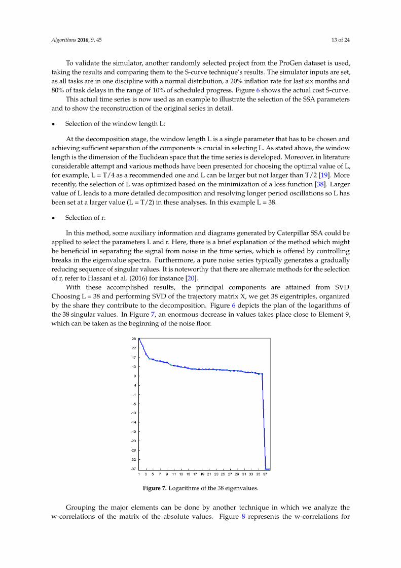
With these accomplished results, the principal components are attained from SVD.Choosing L = 38 and performing SVD of the trajectory matrix X, we get 38 eigentriples, organizedby the share they contribute to the decomposition. Figure 6 depicts the plan of the logarithms ofthe 38 singular values. In Figure 7, an enormous decrease in values takes place close to Element 9,which can be taken as the beginning of the noise floor.
Algorithms 2016, 9, 45 13 of 24
in literature considerable attempt and various methods have been presented for choosing the optimal value of L, for example, L = T/4 as a recommended one and L can be larger but not larger than T/2 [19]. More recently, the selection of L was optimized based on the minimization of a loss function [38]. Larger value of L leads to a more detailed decomposition and resolving longer period oscillations so L has been set at a larger value (L = T/2) in these analyses. In this example L = 38.
• Selection of r:
In this method, some auxiliary information and diagrams generated by Caterpillar SSA could be applied to select the parameters L and r. Here, there is a brief explanation of the method which might be beneficial in separating the signal from noise in the time series, which is offered by controlling breaks in the eigenvalue spectra. Furthermore, a pure noise series typically generates a gradually reducing sequence of singular values. It is noteworthy that there are alternate methods for the selection of r, refer to Hassani et al. (2016) for instance [20].
With these accomplished results, the principal components are attained from SVD. Choosing L = 38 and performing SVD of the trajectory matrix X, we get 38 eigentriples, organized by the share they contribute to the decomposition. Figure 6 depicts the plan of the logarithms of the 38 singular values. In Figure 7, an enormous decrease in values takes place close to Element 9, which can be taken as the beginning of the noise floor.
Figure 7. Logarithms of the 38 eigenvalues.
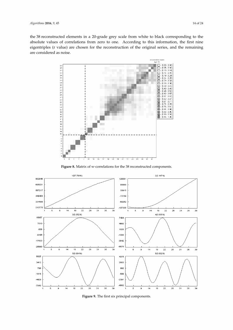
Grouping the major elements can be done by another technique in which we analyze the w-correlations of the matrix of the absolute values. Figure 8 represents the w-correlations for the 38 reconstructed elements in a 20-grade grey scale from white to black corresponding to the absolute values of correlations from zero to one. According to this information, the first nine eigentriples (r value) are chosen for the reconstruction of the original series, and the remaining are considered as noise.
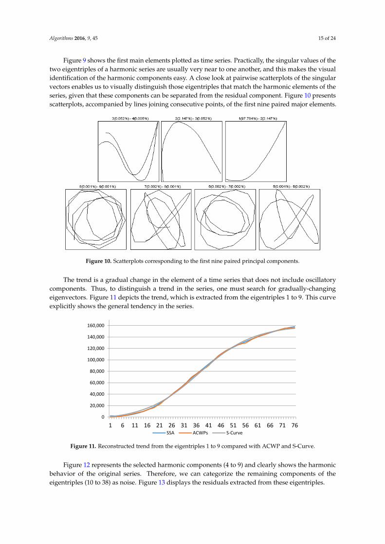
Figure 9 shows the first main elements plotted as time series. Practically, the singular values of the two eigentriples of a harmonic series are usually very near to one another, and this makes the visual identification of the harmonic components easy. A close look at pairwise scatterplots of the singular vectors enables us to visually distinguish those eigentriples that match the harmonic elements of the series, given that these components can be separated from the residual component. Figure 10 presents scatterplots, accompanied by lines joining consecutive points, of the first nine paired major elements.
Figure 7. Logarithms of the 38 eigenvalues.
Grouping the major elements can be done by another technique in which we analyze thew-correlations of the matrix of the absolute values. Figure 8 represents the w-correlations for
Algorithms 2016, 9, 45 14 of 24
the 38 reconstructed elements in a 20-grade grey scale from white to black corresponding to theabsolute values of correlations from zero to one. According to this information, the first nineeigentriples (r value) are chosen for the reconstruction of the original series, and the remainingare considered as noise.Algorithms 2016, 9, 45 14 of 24
Figure 8. Matrix of w-correlations for the 38 reconstructed components.
The trend is a gradual change in the element of a time series that does not include oscillatory components. Thus, to distinguish a trend in the series, one must search for gradually-changing eigenvectors. Figure 11 depicts the trend, which is extracted from the eigentriples 1 to 9. This curve explicitly shows the general tendency in the series.
Figure 9. The first six principal components.
Figure 8. Matrix of w-correlations for the 38 reconstructed components.
Algorithms 2016, 9, 45 14 of 24
Figure 8. Matrix of w-correlations for the 38 reconstructed components.
The trend is a gradual change in the element of a time series that does not include oscillatory components. Thus, to distinguish a trend in the series, one must search for gradually-changing eigenvectors. Figure 11 depicts the trend, which is extracted from the eigentriples 1 to 9. This curve explicitly shows the general tendency in the series.
Figure 9. The first six principal components. Figure 9. The first six principal components.
Algorithms 2016, 9, 45 15 of 24
Figure 9 shows the first main elements plotted as time series. Practically, the singular values of thetwo eigentriples of a harmonic series are usually very near to one another, and this makes the visualidentification of the harmonic components easy. A close look at pairwise scatterplots of the singularvectors enables us to visually distinguish those eigentriples that match the harmonic elements of theseries, given that these components can be separated from the residual component. Figure 10 presentsscatterplots, accompanied by lines joining consecutive points, of the first nine paired major elements.Algorithms 2016, 9, 45 15 of 24
Figure 10. Scatterplots corresponding to the first nine paired principal components.
Figure 11. Reconstructed trend from the eigentriples 1 to 9.compared with ACWP and S-Curve
Figure 12 represents the selected harmonic components (4 to 9) and clearly shows the harmonic behavior of the original series. Therefore, we can categorize the remaining components of the eigentriples (10 to 38) as noise. Figure 13 displays the residuals extracted from these eigentriples.
Figure 12. Harmonic from the eigentriples 4 to 9.
0
20,000
40,000
60,000
80,000
100,000
120,000
140,000
160,000
1 6 11 16 21 26 31 36 41 46 51 56 61 66 71 76SSA ACWPs S-Curve
Figure 10. Scatterplots corresponding to the first nine paired principal components.
The trend is a gradual change in the element of a time series that does not include oscillatorycomponents. Thus, to distinguish a trend in the series, one must search for gradually-changingeigenvectors. Figure 11 depicts the trend, which is extracted from the eigentriples 1 to 9. This curveexplicitly shows the general tendency in the series.
Algorithms 2016, 9, 45 15 of 24
Figure 10. Scatterplots corresponding to the first nine paired principal components.
Figure 11. Reconstructed trend from the eigentriples 1 to 9.compared with ACWP and S-Curve
Figure 12 represents the selected harmonic components (4 to 9) and clearly shows the harmonic behavior of the original series. Therefore, we can categorize the remaining components of the eigentriples (10 to 38) as noise. Figure 13 displays the residuals extracted from these eigentriples.
Figure 12. Harmonic from the eigentriples 4 to 9.
0
20,000
40,000
60,000
80,000
100,000
120,000
140,000
160,000
1 6 11 16 21 26 31 36 41 46 51 56 61 66 71 76SSA ACWPs S-Curve
Figure 11. Reconstructed trend from the eigentriples 1 to 9 compared with ACWP and S-Curve.
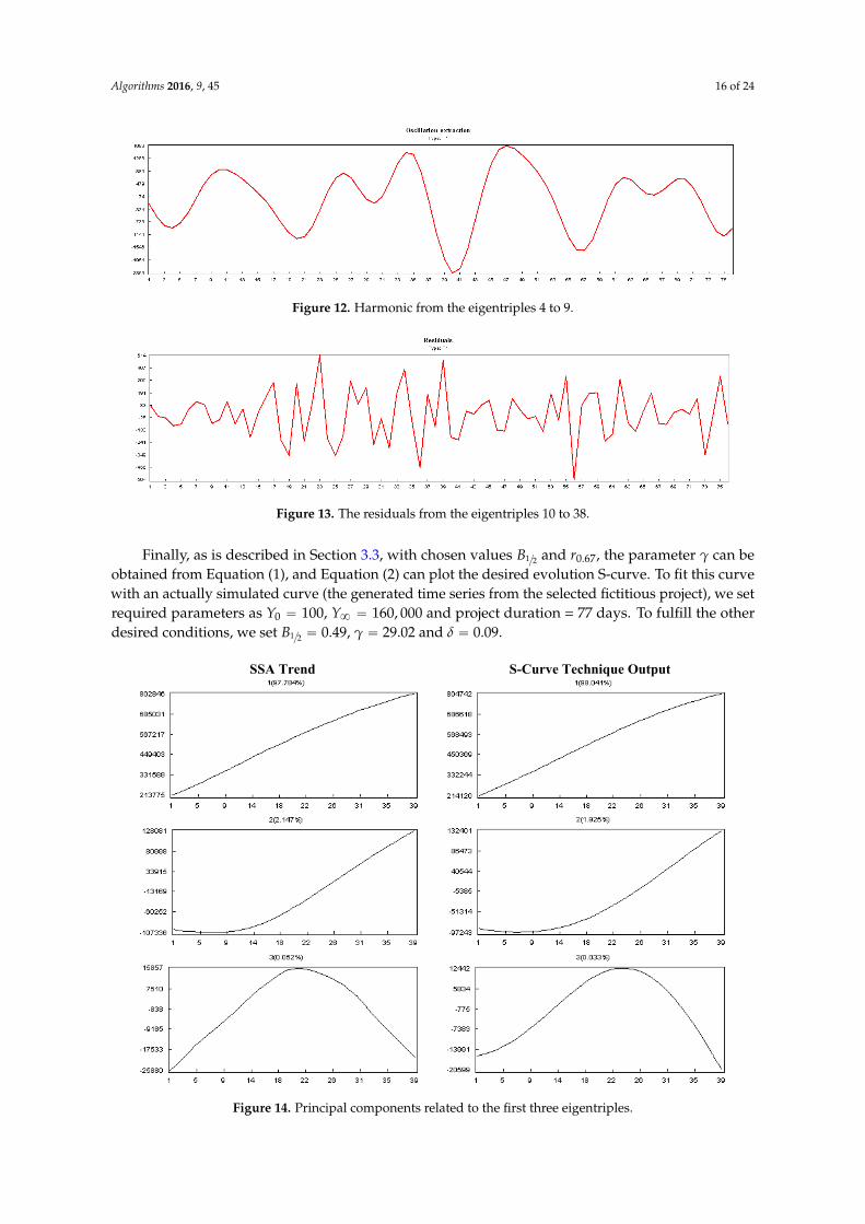
Figure 12 represents the selected harmonic components (4 to 9) and clearly shows the harmonicbehavior of the original series. Therefore, we can categorize the remaining components of theeigentriples (10 to 38) as noise. Figure 13 displays the residuals extracted from these eigentriples.
Algorithms 2016, 9, 45 16 of 24
Algorithms 2016, 9, 45 15 of 24
Figure 10. Scatterplots corresponding to the first nine paired principal components.
Figure 11. Reconstructed trend from the eigentriples 1 to 9.compared with ACWP and S-Curve
Figure 12 represents the selected harmonic components (4 to 9) and clearly shows the harmonic behavior of the original series. Therefore, we can categorize the remaining components of the eigentriples (10 to 38) as noise. Figure 13 displays the residuals extracted from these eigentriples.
Figure 12. Harmonic from the eigentriples 4 to 9.
0
20,000
40,000
60,000
80,000
100,000
120,000
140,000
160,000
1 6 11 16 21 26 31 36 41 46 51 56 61 66 71 76SSA ACWPs S-Curve
Figure 12. Harmonic from the eigentriples 4 to 9.Algorithms 2016, 9, 45 16 of 24
Figure 13. The residuals from the eigentriples 10 to 38.
Finally, as is described in Section 3.3, with chosen values 1
2B and
0 .6 7r , the parameter γ
can be obtained from Equation (1), and Equation (2) can plot the desired evolution S-curve. To fit this curve with an actually simulated curve (the generated time series from the selected fictitious project), we set required parameters as 1000 =Y , 000,160=∞Y and project duration = 77 days.
To fulfill the other desired conditions, we set 49.02
1 =B , 02.29=γ and 09.0=δ
In the next step, the analysis of the S-curve technique time series was implemented similarly to the previously mentioned selected project by SSA method. To show the similarity of these two time series, principal components of two time series, simulator output and S-curve technique output are extracted and compared. The most important components concerning the first three eigentriples, for both the simulator and S-curve technique series, are shown in Figure 14. As shown, these two series have quite similar components. Accordingly, we can conclude that the simulator and S-curve technique time series have the same structure, and this verifies the accuracy of the simulator result.
S-Curve Technique Output SSA Trend
Figure 14. Principal components related to the first three eigentriples.
The deviations between the trend of simulated results (SSA trend) and the S-curve technique with the first generated time series are shown in Figure 15. Clearly, these two deviations have the
Figure 13. The residuals from the eigentriples 10 to 38.
Finally, as is described in Section 3.3, with chosen values B1{2 and r0.67, the parameter γ can beobtained from Equation (1), and Equation (2) can plot the desired evolution S-curve. To fit this curvewith an actually simulated curve (the generated time series from the selected fictitious project), we setrequired parameters as Y0 “ 100, Y8 “ 160, 000 and project duration = 77 days. To fulfill the otherdesired conditions, we set B1{2 “ 0.49, γ “ 29.02 and δ “ 0.09.
Algorithms 2016, 9, 45 16 of 24
Figure 13. The residuals from the eigentriples 10 to 38.
Finally, as is described in Section 3.3, with chosen values 1
2B and
0 .6 7r , the parameter γ
can be obtained from Equation (1), and Equation (2) can plot the desired evolution S-curve. To fit this curve with an actually simulated curve (the generated time series from the selected fictitious project), we set required parameters as 1000 =Y , 000,160=∞Y and project duration = 77 days.
To fulfill the other desired conditions, we set 49.02
1 =B , 02.29=γ and 09.0=δ
In the next step, the analysis of the S-curve technique time series was implemented similarly to the previously mentioned selected project by SSA method. To show the similarity of these two time series, principal components of two time series, simulator output and S-curve technique output are extracted and compared. The most important components concerning the first three eigentriples, for both the simulator and S-curve technique series, are shown in Figure 14. As shown, these two series have quite similar components. Accordingly, we can conclude that the simulator and S-curve technique time series have the same structure, and this verifies the accuracy of the simulator result.
S-Curve Technique Output SSA Trend
Figure 14. Principal components related to the first three eigentriples.
The deviations between the trend of simulated results (SSA trend) and the S-curve technique with the first generated time series are shown in Figure 15. Clearly, these two deviations have the
Figure 14. Principal components related to the first three eigentriples.

Algorithms 2016, 9, 45 17 of 24
In the next step, the analysis of the S-curve technique time series was implemented similarlyto the previously mentioned selected project by SSA method. To show the similarity of these twotime series, principal components of two time series, simulator output and S-curve technique outputare extracted and compared. The most important components concerning the first three eigentriples,for both the simulator and S-curve technique series, are shown in Figure 14. As shown, these twoseries have quite similar components. Accordingly, we can conclude that the simulator and S-curvetechnique time series have the same structure, and this verifies the accuracy of the simulator result.
The deviations between the trend of simulated results (SSA trend) and the S-curve technique withthe first generated time series are shown in Figure 15. Clearly, these two deviations have the samebehavior over time, with the exception of the start and end points. However, SSA results show a lowerchange range. Generally, these two deviations are near to one another, which results in the fact that thesimulated fictitious results have a high accuracy and that this accuracy can be confirmed by similartests on empirical data.
Algorithms 2016, 9, 45 17 of 24
same behavior over time, with the exception of the start and end points. However, SSA results show a lower change range. Generally, these two deviations are near to one another, which results in the fact that the simulated fictitious results have a high accuracy and that this accuracy can be confirmed by similar tests on empirical data.
Figure 15. Deviations between the SSA trend and the S-curve method with the generated time series.
To validate deviations between SSA and the S-curve method, two measures, RMSE and R, are employed that assess the quality of the generated time series. These two measures, R and RMSE, are used to determine the extent to which the model fits the data and are calculated as below:
= ∑( − )( − )∑( − ) ∑( − ) = 1 ( − ) (3)
Table 1 presents the results of the two measures for SSA trend and the S-curve method with the generated time series. These two measures prove that the generated time series fit the actual trend better than the standard S-curve. Both RMSE values are less than 5% of the maximum member of each series that prove the validity of estimated time series. RMSE of the SSA trend is less than half of the S-curve one. Although the R measure is perfect in both, SSA is judged slightly better.
Table 1. Deviations between SSA trend and the S-curve method with the generated time series.
MAX RMSE R ACWP 156,015.81
SSA 158,153.98 1050.64 0.92 S-Curve 155,155.24 2166.50 0.93
5.1.1. Effect of Input Parameters on the Simulator Results
The sensitivity analysis of some important input parameters is presented in this section. Resource constraints, work contours and changes in the progress status are considered as changing factors, and their effects on simulator outputs are studied.
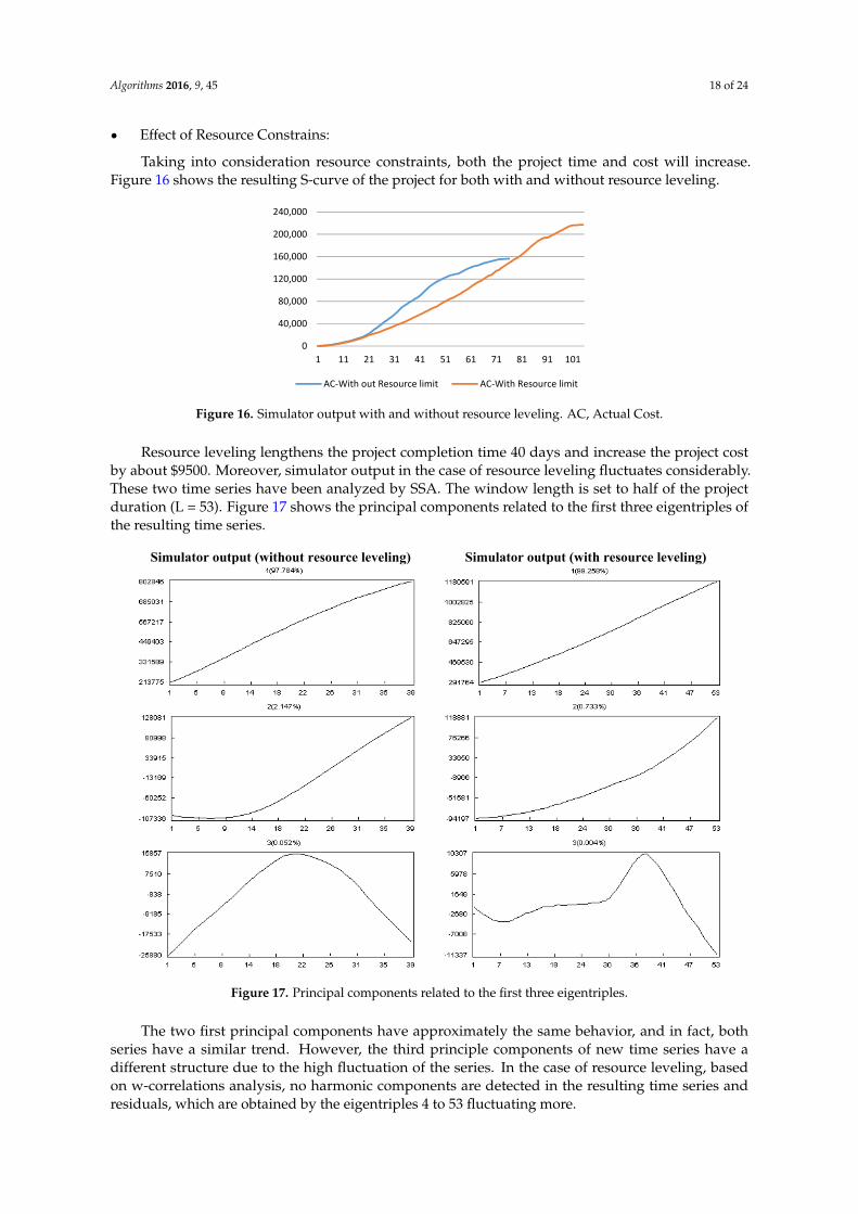
• Effect of Resource Constrains:
Taking into consideration resource constraints, both the project time and cost will increase. Figure 16 shows the resulting S-curve of the project for both with and without resource leveling.
Figure 15. Deviations between the SSA trend and the S-curve method with the generated time series.
To validate deviations between SSA and the S-curve method, two measures, RMSE and R, areemployed that assess the quality of the generated time series. These two measures, R and RMSE, areused to determine the extent to which the model fits the data and are calculated as below:
R “ř
`
yi ´ yi˘
pyi ´ yiqb
ř`
yi ´ yi˘2 ř
pyi ´ yiq2
RMSE “
c
1N
ÿ
pyi ´ yiq2 (3)
Table 1 presents the results of the two measures for SSA trend and the S-curve method with thegenerated time series. These two measures prove that the generated time series fit the actual trendbetter than the standard S-curve. Both RMSE values are less than 5% of the maximum member of eachseries that prove the validity of estimated time series. RMSE of the SSA trend is less than half of theS-curve one. Although the R measure is perfect in both, SSA is judged slightly better.
Table 1. Deviations between SSA trend and the S-curve method with the generated time series.
MAX RMSE R
ACWP 156,015.81SSA 158,153.98 1050.64 0.92
S-Curve 155,155.24 2166.50 0.93
5.1.1. Effect of Input Parameters on the Simulator Results
The sensitivity analysis of some important input parameters is presented in this section. Resourceconstraints, work contours and changes in the progress status are considered as changing factors, andtheir effects on simulator outputs are studied.
Algorithms 2016, 9, 45 18 of 24
‚ Effect of Resource Constrains:
Taking into consideration resource constraints, both the project time and cost will increase.Figure 16 shows the resulting S-curve of the project for both with and without resource leveling.
Algorithms 2016, 9, 45 18 of 24
Figure 16. Simulator output with and without resource leveling. AC, Actual Cost.
Resource leveling lengthens the project completion time 40 days and increase the project cost by about $9500. Moreover, simulator output in the case of resource leveling fluctuates considerably. These two time series have been analyzed by SSA. The window length is set to half of the project duration (L = 53). Figure 17 shows the principal components related to the first three eigentriples of the resulting time series.
The two first principal components have approximately the same behavior, and in fact, both series have a similar trend. However, the third principle components of new time series have a different structure due to the high fluctuation of the series. In the case of resource leveling, based on w-correlations analysis, no harmonic components are detected in the resulting time series and residuals, which are obtained by the eigentriples 4 to 53 fluctuating more.
Simulator output (with resource leveling) Simulator output (without resource leveling)
Figure 17. Principal components related to the first three eigentriples.
0
40,000
80,000
120,000
160,000
200,000
240,000
1 11 21 31 41 51 61 71 81 91 101
AC-With out Resource limit AC-With Resource limit
Figure 16. Simulator output with and without resource leveling. AC, Actual Cost.
Resource leveling lengthens the project completion time 40 days and increase the project costby about $9500. Moreover, simulator output in the case of resource leveling fluctuates considerably.These two time series have been analyzed by SSA. The window length is set to half of the projectduration (L = 53). Figure 17 shows the principal components related to the first three eigentriples ofthe resulting time series.
Algorithms 2016, 9, 45 18 of 24
Figure 16. Simulator output with and without resource leveling. AC, Actual Cost.
Resource leveling lengthens the project completion time 40 days and increase the project cost by about $9500. Moreover, simulator output in the case of resource leveling fluctuates considerably. These two time series have been analyzed by SSA. The window length is set to half of the project duration (L = 53). Figure 17 shows the principal components related to the first three eigentriples of the resulting time series.
The two first principal components have approximately the same behavior, and in fact, both series have a similar trend. However, the third principle components of new time series have a different structure due to the high fluctuation of the series. In the case of resource leveling, based on w-correlations analysis, no harmonic components are detected in the resulting time series and residuals, which are obtained by the eigentriples 4 to 53 fluctuating more.
Simulator output (with resource leveling) Simulator output (without resource leveling)
Figure 17. Principal components related to the first three eigentriples.
0
40,000
80,000
120,000
160,000
200,000
240,000
1 11 21 31 41 51 61 71 81 91 101
AC-With out Resource limit AC-With Resource limit
Figure 17. Principal components related to the first three eigentriples.
The two first principal components have approximately the same behavior, and in fact, bothseries have a similar trend. However, the third principle components of new time series have adifferent structure due to the high fluctuation of the series. In the case of resource leveling, basedon w-correlations analysis, no harmonic components are detected in the resulting time series andresiduals, which are obtained by the eigentriples 4 to 53 fluctuating more.

Algorithms 2016, 9, 45 19 of 24
‚ Effect of discipline and work contour:
In this section, the simulator is run in two different settings of work contour: front loaded andback loaded and with the assumption of resource leveling. Principal components related to the firstthree eigentriples of the resulting time series are presented in Figure 18.
Algorithms 2016, 9, 45 19 of 24
• Effect of discipline and work contour:
In this section, the simulator is run in two different settings of work contour: front loaded and back loaded and with the assumption of resource leveling. Principal components related to the first three eigentriples of the resulting time series are presented in Figure 18.
In this case, the two first components of the resulted series are similar, but the third component has a different shape. Besides, the third component has more fluctuation in the front-loaded work contour setting than the back-loaded one.
Although the residuals of these time series have various behaviors and structures, these series have a similar harmonic component, as well.
Simulator output (Front loaded) Simulator output (Back loaded)
Figure 18. Principal components related to the first three eigentriples of the time series in two different settings: front-loaded and back-loaded work contour.
• Effect of the changes in the progress status:
To evaluate the impacts of activities’ progress status on actual progress and the simulator output, the simulator is run in two various statuses:
The actual progress of tasks fluctuates ±0.2 of their plan progress. The actual progress of tasks fluctuates ±0.3 of their plan progress.
Moreover, it is assumed that the project has a flat work contour and resource leveling. When the interval range increases, project completion time and cost raise, while project progress fluctuates more
Figure 19 presents the first three eigentriple components of the resulting time series. The increase of this range results in a large fluctuation in the time series. This is apparent in the second and third principle components. However, the first principle component of the two series has approximately the same structure, and therefore, the two series have generally similar trends.
Figure 18. Principal components related to the first three eigentriples of the time series in two differentsettings: front-loaded and back-loaded work contour.
In this case, the two first components of the resulted series are similar, but the third componenthas a different shape. Besides, the third component has more fluctuation in the front-loaded workcontour setting than the back-loaded one.
Although the residuals of these time series have various behaviors and structures, these serieshave a similar harmonic component, as well.
‚ Effect of the changes in the progress status:
To evaluate the impacts of activities’ progress status on actual progress and the simulator output,the simulator is run in two various statuses:
� The actual progress of tasks fluctuates ˘0.2 of their plan progress.� The actual progress of tasks fluctuates ˘0.3 of their plan progress.
Moreover, it is assumed that the project has a flat work contour and resource leveling. When theinterval range increases, project completion time and cost raise, while project progress fluctuates more.
Figure 19 presents the first three eigentriple components of the resulting time series. The increaseof this range results in a large fluctuation in the time series. This is apparent in the second and thirdprinciple components. However, the first principle component of the two series has approximately thesame structure, and therefore, the two series have generally similar trends.

Algorithms 2016, 9, 45 20 of 24Algorithms 2016, 9, 45 20 of 24
Simulator output (interval range ±0.2) Simulator output (interval range ±0.3)
Figure 19. Principal components related to the first three eigentriples of the time series for two different interval ranges.
5.2. Case Study Results
Figure 20 simulates an experiment on a construction project whose project duration was six months, and its Budget at Completion (BAC) was = 66,869,542,003 Rials (around $2.3 million at writing). About 34% of the project was not completed due to delays for about five months since the project started, and the project was executed under a situation with high risks; the inflation rate was estimated to be 30% for six months. As already stated, the project was supposed to follow the four main disciplines and seven sub-disciplines corresponding to the fourth main discipline. Here, we suppose that all tasks have a uniform (flat) distribution.
The baseline schedule is used when the project was planned at the very beginning, which is shown in the Gantt chart formed. In this paper, the simulation is conducted by the use of the project progress simulator described earlier. After all, other input parameters have been treated based on present actual information. After 150 days of the project have passed, the simulation begins to match the actual curve with actual project progress; thus, the completion trends can be forecasted and measured.
As seen in Figure 20, the project is scheduled to be completed in 306 days (about 10 months) with a cost overrun. As a result, the budget must rise from 66,869,542 to 100,750,109,952 Rials, i.e., by about 35%. Besides, Figure 20 displays the progress information of another project. Therefore, EVM calculations are now able to be measured daily.
The progress simulator equips us with forecast and control methods that lead to reliable results, and which make daily and completion date forecasting simple to a large extent. If these initial warning signals are appropriately analyzed properly in comparison with the project schedule, they pave the way for us to take corrective actions on those activities that are not on the right track (particularly, those tasks that are on the critical path).
Figure 19. Principal components related to the first three eigentriples of the time series for two differentinterval ranges.
5.2. Case Study Results
Figure 20 simulates an experiment on a construction project whose project duration was sixmonths, and its Budget at Completion (BAC) was = 66,869,542,003 Rials (around $2.3 million atwriting). About 34% of the project was not completed due to delays for about five months since theproject started, and the project was executed under a situation with high risks; the inflation rate wasestimated to be 30% for six months. As already stated, the project was supposed to follow the fourmain disciplines and seven sub-disciplines corresponding to the fourth main discipline. Here, wesuppose that all tasks have a uniform (flat) distribution.
The baseline schedule is used when the project was planned at the very beginning, which is shownin the Gantt chart formed. In this paper, the simulation is conducted by the use of the project progresssimulator described earlier. After all, other input parameters have been treated based on present actualinformation. After 150 days of the project have passed, the simulation begins to match the actual curvewith actual project progress; thus, the completion trends can be forecasted and measured.
As seen in Figure 20, the project is scheduled to be completed in 306 days (about 10 months)with a cost overrun. As a result, the budget must rise from 66,869,542 to 100,750,109,952 Rials, i.e., byabout 35%. Besides, Figure 20 displays the progress information of another project. Therefore, EVMcalculations are now able to be measured daily.
The progress simulator equips us with forecast and control methods that lead to reliable results,and which make daily and completion date forecasting simple to a large extent. If these initial warningsignals are appropriately analyzed properly in comparison with the project schedule, they pave theway for us to take corrective actions on those activities that are not on the right track (particularly,those tasks that are on the critical path).
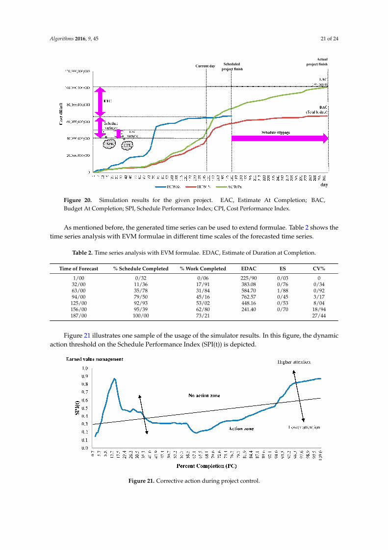
Algorithms 2016, 9, 45 21 of 24Algorithms 2016, 9, 45 21 of 24
Figure 20. Simulation results for the given project. EAC, Estimate At Completion; BAC, Budget At Completion; SPI, Schedule Performance Index; CPI, Cost Performance Index.
As mentioned before, the generated time series can be used to extend formulae. Table 2 shows the time series analysis with EVM formulae in different time scales of the forecasted time series.
Table 2. Time series analysis with EVM formulae. EDAC, Estimate of Duration at Completion.
Time of Forecast % Schedule Completed % Work Completed EDAC ES CV% 1/00 0/32 0/06 225/90 0/03 0
32/00 11/36 17/91 383.08 0/76 0/34 63/00 35/78 31/84 584.70 1/88 0/92 94/00 79/50 45/16 762.57 0/45 3/17 125/00 92/93 53/02 448.16 0/53 8/04 156/00 95/39 62/80 241.40 0/70 18/94 187/00 100/00 73/21 27/44
Figure 21 illustrates one sample of the usage of the simulator results. In this figure, the dynamic action threshold on the Schedule Performance Index (SPI(t)) is depicted.
Figure 21. Corrective action during project control.
Figure 20. Simulation results for the given project. EAC, Estimate At Completion; BAC,Budget At Completion; SPI, Schedule Performance Index; CPI, Cost Performance Index.
As mentioned before, the generated time series can be used to extend formulae. Table 2 shows thetime series analysis with EVM formulae in different time scales of the forecasted time series.
Table 2. Time series analysis with EVM formulae. EDAC, Estimate of Duration at Completion.
Time of Forecast % Schedule Completed % Work Completed EDAC ES CV%
1/00 0/32 0/06 225/90 0/03 032/00 11/36 17/91 383.08 0/76 0/3463/00 35/78 31/84 584.70 1/88 0/9294/00 79/50 45/16 762.57 0/45 3/17125/00 92/93 53/02 448.16 0/53 8/04156/00 95/39 62/80 241.40 0/70 18/94187/00 100/00 73/21 27/44
Figure 21 illustrates one sample of the usage of the simulator results. In this figure, the dynamicaction threshold on the Schedule Performance Index (SPI(t)) is depicted.
Algorithms 2016, 9, 45 21 of 24
Figure 20. Simulation results for the given project. EAC, Estimate At Completion; BAC, Budget At Completion; SPI, Schedule Performance Index; CPI, Cost Performance Index.
As mentioned before, the generated time series can be used to extend formulae. Table 2 shows the time series analysis with EVM formulae in different time scales of the forecasted time series.
Table 2. Time series analysis with EVM formulae. EDAC, Estimate of Duration at Completion.
Time of Forecast % Schedule Completed % Work Completed EDAC ES CV% 1/00 0/32 0/06 225/90 0/03 0
32/00 11/36 17/91 383.08 0/76 0/34 63/00 35/78 31/84 584.70 1/88 0/92 94/00 79/50 45/16 762.57 0/45 3/17 125/00 92/93 53/02 448.16 0/53 8/04 156/00 95/39 62/80 241.40 0/70 18/94 187/00 100/00 73/21 27/44
Figure 21 illustrates one sample of the usage of the simulator results. In this figure, the dynamic action threshold on the Schedule Performance Index (SPI(t)) is depicted.
Figure 21. Corrective action during project control. Figure 21. Corrective action during project control.
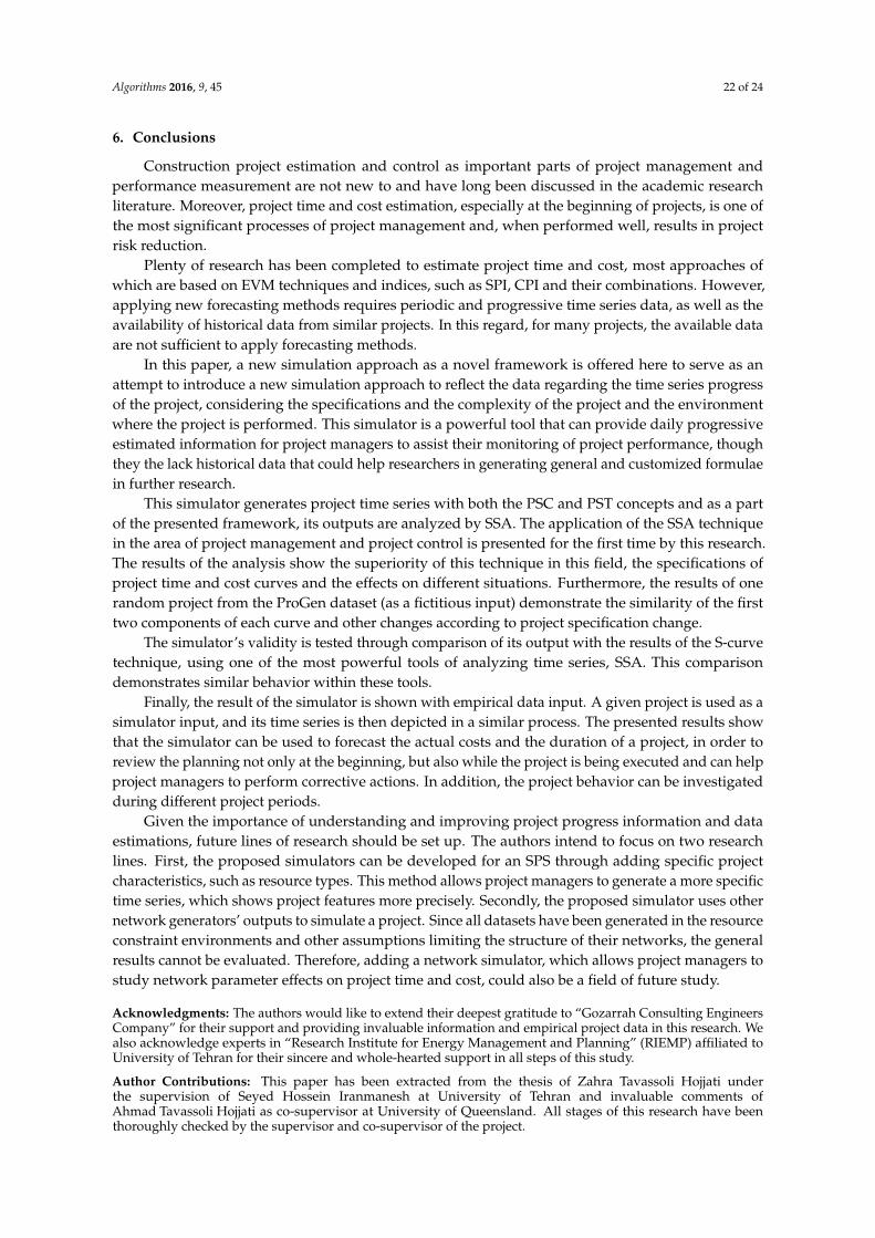
Algorithms 2016, 9, 45 22 of 24
6. Conclusions
Construction project estimation and control as important parts of project management andperformance measurement are not new to and have long been discussed in the academic researchliterature. Moreover, project time and cost estimation, especially at the beginning of projects, is one ofthe most significant processes of project management and, when performed well, results in projectrisk reduction.
Plenty of research has been completed to estimate project time and cost, most approaches ofwhich are based on EVM techniques and indices, such as SPI, CPI and their combinations. However,applying new forecasting methods requires periodic and progressive time series data, as well as theavailability of historical data from similar projects. In this regard, for many projects, the available dataare not sufficient to apply forecasting methods.
In this paper, a new simulation approach as a novel framework is offered here to serve as anattempt to introduce a new simulation approach to reflect the data regarding the time series progressof the project, considering the specifications and the complexity of the project and the environmentwhere the project is performed. This simulator is a powerful tool that can provide daily progressiveestimated information for project managers to assist their monitoring of project performance, thoughthey the lack historical data that could help researchers in generating general and customized formulaein further research.
This simulator generates project time series with both the PSC and PST concepts and as a partof the presented framework, its outputs are analyzed by SSA. The application of the SSA techniquein the area of project management and project control is presented for the first time by this research.The results of the analysis show the superiority of this technique in this field, the specifications ofproject time and cost curves and the effects on different situations. Furthermore, the results of onerandom project from the ProGen dataset (as a fictitious input) demonstrate the similarity of the firsttwo components of each curve and other changes according to project specification change.
The simulator’s validity is tested through comparison of its output with the results of the S-curvetechnique, using one of the most powerful tools of analyzing time series, SSA. This comparisondemonstrates similar behavior within these tools.
Finally, the result of the simulator is shown with empirical data input. A given project is used as asimulator input, and its time series is then depicted in a similar process. The presented results showthat the simulator can be used to forecast the actual costs and the duration of a project, in order toreview the planning not only at the beginning, but also while the project is being executed and can helpproject managers to perform corrective actions. In addition, the project behavior can be investigatedduring different project periods.
Given the importance of understanding and improving project progress information and dataestimations, future lines of research should be set up. The authors intend to focus on two researchlines. First, the proposed simulators can be developed for an SPS through adding specific projectcharacteristics, such as resource types. This method allows project managers to generate a more specifictime series, which shows project features more precisely. Secondly, the proposed simulator uses othernetwork generators’ outputs to simulate a project. Since all datasets have been generated in the resourceconstraint environments and other assumptions limiting the structure of their networks, the generalresults cannot be evaluated. Therefore, adding a network simulator, which allows project managers tostudy network parameter effects on project time and cost, could also be a field of future study.
Acknowledgments: The authors would like to extend their deepest gratitude to “Gozarrah Consulting EngineersCompany” for their support and providing invaluable information and empirical project data in this research. Wealso acknowledge experts in “Research Institute for Energy Management and Planning” (RIEMP) affiliated toUniversity of Tehran for their sincere and whole-hearted support in all steps of this study.
Author Contributions: This paper has been extracted from the thesis of Zahra Tavassoli Hojjati underthe supervision of Seyed Hossein Iranmanesh at University of Tehran and invaluable comments ofAhmad Tavassoli Hojjati as co-supervisor at University of Queensland. All stages of this research have beenthoroughly checked by the supervisor and co-supervisor of the project.

Algorithms 2016, 9, 45 23 of 24
Conflicts of Interest: The authors declare no conflict of interest.
References
1. Kolisch, R.; Sprecher, A. PSPLIB—A project scheduling problem library. Eur. J. Oper. Res. 1996, 96, 205–216.[CrossRef]
2. Kolisch, R.; Padman, R. An Integrated Survey of Project Management Scheduling; Technical Report; Heinz Schoolof Public Policy and Management, Carnegie Mellon University: Pittsburgh, PA, USA, 1997.
3. Hartmann, S.; Briskorn, D. A survey of variants and extensions of the resource-constrained project schedulingproblem. Eur. J. Oper. Res. 2010, 207, 1–15. [CrossRef]
4. Kolisch, R.; Hartmann, S. Experimental investigation of heuristics for resource-constrained project scheduling:An update. Eur. J. Oper. Res. 2006, 174, 23–37. [CrossRef]
5. Vanhoucke, M. Measuring the efficiency of project control using fictitious and empirical project data. Int. J.Proj. Manag. 2012, 30, 252–263. [CrossRef]
6. Cioffi, D. Designing project management: A scientific notation and an improved formalism for earned valuecalculations. Int. J. Proj. Manag. 2006, 24, 136–144. [CrossRef]
7. Iranmanesh, S.H.; Kimiagari, S.; Mojir, N. A new formula to estimate at completion of a project’s timeto improve earned value management system. In Proceedings of the IEEE International Conference onIndustrial Engineering and Engineering Management (IEEM), Singapore, 2–4 December 2007; pp. 1014–1020.
8. Madadi, M.; Iranmanesh, H. A management-oriented approach to reduce project duration and its risk(variability). Eur. J. Oper. Res. 2012, 215, 751–761. [CrossRef]
9. Fleming, Q.W.; Koppleman, J.M. Earned Value Project Management; Project Management Institute: NewtownSquare, PA, USA, 1996.
10. Lipke, W.; Zwikael, O.; Henderson, K.; Anbari, F. Prediction of project outcome: the application of statisticalmethods to earned value management and earned schedule performance indexes. Int. J. Proj. Manag. 2009,27, 400–407. [CrossRef]
11. Fleming, Q.; Koppelman, J. What’s your project’s real price tag? Harv. Bus. Rev. 2003, 81, 20–21.12. Jacob, D.S.; Kane, M. Forecasting schedule completion using earned value metrics. Meas. News 2004,
3, 11–17.13. Vandevoorde, S.; Vanhoucke, M. A comparison of different project duration forecasting methods using
earned value metrics. Int. J. Proj. Manag. 2006, 24, 289–302. [CrossRef]14. Vanhoucke, M.; Vandevoorde, S. A simulation and evaluation of earned value metrics to forecast the project
duration. J. Oper. Res. Soc. 2007, 58, 1361–1374. [CrossRef]15. Iranmanesh, S.H.; Tavassoli, H.Z. Intelligent systems in project performance measurement and evaluation.
In Engineering Management, intelligent systems references library 87; Springer International Publishing: Basel,Switzerland, 2015. [CrossRef]
16. Elshaer, R. Impact of sensitivity information on the prediction of project’s duration using earned schedulemethod. Int. J. Proj. Manag. 2013, 31, 579–588. [CrossRef]
17. Hassani, H.; Ghodsi, Z.; Silva, E.S.; Heravi, S. From nature to maths: Improving forecasting performance insubspace-based methods using genetics Colonial Theory. Dig. Signal Process. 2016, 51, 101–109. [CrossRef]
18. Golyandina, N.; Nekrutkin, V.; Zhigljavsky, A. Analysis of Time Series Structure: SSA and Related Techniques;Chapman & Hall/CRC: Boca Raton, FL, USA, 2001.
19. Hassani, H. Singular Spectrum Analysis: Methodology and comparison. J. Data Sci. 2007, 5, 239–257.20. Hassani, H.; Zokaei, M.; von Rosen, D.; Amiri, S.; Ghodsi, M. Does noise reduction matter for curve fitting in
growth curve models? Comput. Methods Progr. Biomed. 2009, 96, 173–181. [CrossRef] [PubMed]21. Viljoen, H.; Nel, D.G. Common singular spectrum analysis of several time series. J. Stat. Plan. Inference 2010,
140, 260–267. [CrossRef]22. Hassani, H.; Heravi, S.; Zhigljavsky, A. Forecasting European industrial production with singular spectrum
analysis. Int. J. Forecast. 2009, 25, 103–118. [CrossRef]23. Afshar, K.; Bigdeli, N. Data analysis and short-term load forecasting in Iran’s electricity market using singular
spectral analysis (SSA). Energy 2011, 36, 2620–2627. [CrossRef]24. Silva, E.S. A combination forecast for energy-related CO2 emissions in the United States. Int. J. Energy Stat.
2013, 1, 269–279. [CrossRef]

Algorithms 2016, 9, 45 24 of 24
25. Ghodsi, Z.; Silva, E.S.; Hassani, H. Bicoid signal extraction with a selection of parametric and nonparametricsignal processing techniques. Genom. Proteom. Bioinform. 2015, 13, 183–191. [CrossRef] [PubMed]
26. Wu, C.L.; Chau, K.W. Rainfall-Runoff Modeling Using Artificial Neural Network Coupled with SingularSpectrum Analysis. J. Hydrol. 2001, 399, 394–409. [CrossRef]
27. Chau, K.W.; Wu, C.L. A Hybrid Model Coupled with Singular Spectrum Analysis for Daily RainfallPrediction. J. Hydroinform. 2010, 12, 458–473. [CrossRef]
28. Hassani, H.; Mahmoudvand, R.; Zokaei, M. Separability and window length in singular spectrum analysis.C. R. Acad. Sci. Paris Ser. I. 2011, 349, 987–990. [CrossRef]
29. Hanna, M.; Ruwanpura, J.Y. Simulation tool for manpower forecast loading and resource leveling.In Proceedings of the 2007 Winter Simulation Conference, Washington, DC, USA, 9–12 December 2007;pp. 2099–2103.
30. Al-Jibouri, S.H. Monitoring systems and their effectiveness for project cost control in construction. Int. J.Proj. Manag. 2003, 21, 145–154. [CrossRef]
31. Huang, E.; Chen, S.J. Estimation of project completion time and factors analysis for concurrent engineeringproject management: A simulation approach. Concurr. Eng. Res. Appl. 2006, 14, 329–341. [CrossRef]
32. Akintoye, A. Analysis of factors influencing project cost estimating practice. Constr. Manag. Econ. 2000, 18,77–89. [CrossRef]
33. Bashir, H.A.; Thomson, V. Project estimation from feasibility study until completion: A quantitativemethodology. Concurr. Eng. Res. Appl. 2001, 9, 257–269. [CrossRef]
34. Kuhl, M.; Radhames, A.; Pena, T. A dynamic crashing method for project management usingsimulation-based optimization. In Proceedings of the 40th Conference on Winter Simulation, Austin,TX, USA, 7–10 December 2008; pp. 2370–2376.
35. Cioffi, D.F. A tool for managing projects: An analytic parameterization of the S-Curve. Int. J. Proj. Manag.2005, 23, 215–222. [CrossRef]
36. The ProGen standard dataset. Available online: http://129.187.106.231/psplib/main.html (accessed on13 July 2016).
37. Caterpillar-SSA Software. Available online: http://www.gistatgroup.com/cat/index.html (accessed on13 July 2016).
38. Hassani, H.; Webster, A.; Silva, E.S.; Heravi, S. Forecasting U.S. tourist arrivals using optimal SingularSpectrum Analysis. Tour. Manag. 2015, 46, 322–335. [CrossRef]
© 2016 by the authors; licensee MDPI, Basel, Switzerland. This article is an open accessarticle distributed under the terms and conditions of the Creative Commons Attribution(CC-BY) license (http://creativecommons.org/licenses/by/4.0/).