designing an emissions trading system in mexico: …...designing an emissions trading system in...

Designing an Emissions Trading System in Mexico: Options for Setting an Emissions Cap


is publication presents the results of the study

Designing an Emissions Trading System in Mexico:Options for Setting an Emissions Cap,

which was elaborated by Öko-Institut e.V.

Its contents were developed under the coordination of the Ministry for the Environment and Natural Resources (Secretaría de Medio Ambiente y Recursos Naturales,

SEMARNAT), and the project "Preparation of an Emissions Trading System in Mexico" (SiCEM) of the Deutsche Gesellschaft für Internationale Zusammenarbeit (GIZ)

GmbH on behalf of the German Federal Ministry for the Environment, Nature Conservation and Nuclear Safety.

Designing an Emissions Trading System in Mexico:

Options for Setting an Emissions Cap

Contents

Abbreviations 5

Executive summary 6

Resumen ejecutivo 7

1. Introduction 10

2. Data 132.1. Inputs from SEMARNAT 132.2. National Registry of Emissions (RENE) 13

2.2.1. Historical emissions 13 2.3. Nationally Determined Contribution (NDC) for Mexico 15

2.3.1. Emissions baseline 152.3.2. Unconditional target emissions 152.3.3. Conditional target emissions 17

2.4. National Electric System Development Program (PRODESEN) 182.4.1. Projected emissions for the electricity sector 18

3. Methodology 203.1. Options for cap setting 20

3.1.1. Applying a Linear Reduction Factor (LRF) 203.1.2. Applying a deviation from a selected emission projection 203.1.3. Defining the cap setting scenarios 21

3.2. Options for setting emission thresholds 223.3. Balance between the supply and demand of allowances 22

4. Results 244.1. Options for cap setting 24

4.1.1. LRF approach 244.1.2. Deviation from projection approach 25

4.2. Options for setting emission thresholds 274.3. Balance between the supply and demand of allowances 29

5. Discussion 325.1. Safeguard and flexibility options 325.2. Safeguarding ambition and integrity in the long-term 34

5.2.1. General considerations 345.2.2. Applicability to the Mexican context 345.2.3. Steps to implementation 36

5.3. Making the system responsive to short-term shocks 375.3.1. General considerations 375.3.2. Applicability to the Mexican context 375.3.3. Steps to implementation 41

6. Conclusion 45

7. Publication bibliography 48

List of Figures

Figure 2-1: Comparison of emission projections for electricity generation 18Figure 4-1: Scenario 1: Increase in the annual LRF of + 1% between 2019 and 2030 24Figure 4-2: Scenario 2: Decrease in the annual LRF of - 1% between 2019 and 2030 25Figure 4-3: Scenario 3: Annual caps based upon an emission pathway that meets the unconditional NDC target in 2030 26Figure 4-4: Scenario 4: Annual caps based upon an emission pathway that meets the conditional NDC target in 2030 27Figure 4-5: Impact of uncertain emission projections on the balance of the supply and demand for allowances for the electricity generation sector 30Figure 5-1: Long-term and short-term options for adjusting an ETS cap 33Figure 5-2: Comparing the impact of rebasing the cap and increasing the LRF for the power generation sector 35Figure 5-3: Example price path for potential Mexican floor and ceiling prices when linking to WCI is considered 42

List of Tables

Table 2-1: Historical CO2 emissions from the RENE database 14Table 2-2: NDC baseline emissions (Mt CO2e) 15Table 2-3: NDC unconditional target emissions (Mt CO2e) 16Table 2-4: NDC conditional target emissions (Mt CO2e) 17Table 4-1: Sensitivity analysis of applying different emission thresholds to determine the scope of the Mexican ETS 28Table 5-1: Allowance supply and demand in the first years of operation (EU ETS, California ETS) 32Table 5-2: Options for adjusting the cap in the long-term 34Table 5-3: Price management options (minimum price) 39Table 5-4: Price management options (maximum price) 40Table 5-5: Quantity management options 41

Abbreviations

BAU: Business as Usual

COA: Annual Operational Certificate

ETS: Emissions Trading System

EU ETS: European Union Emissions Trading System

GDP: Gross Domestic Product

GHG: Greenhouse Gas

ICAP: International Carbon Action Partnership

INECC: National Institute of Environment and Climate Change of Mexico

LRF: Linear Reduction Factor

MSR: Market Stability Reserve

NDC: Nationally Determined Contribution

PRODESEN: National Electric System Development Program

PMR: Partnership for Market Readiness

RENE: National Emissions Register

RGGI: Regional Greenhouse Gas Initiative

SEMARNAT: Ministry for the Environment

WCI: Western Climate Initiative

Designing an Emissions Trading System in Mexico: Options for Setting an Emissions Cap 5

Executive summary

The Mexican government is considering the implementa-tion of an Emissions Trading System (ETS) as an instru-ment for cost-efficient mitigation to contribute towards their Nationally Determined Contribution (NDC). It is expected that market rules for a Mexican ETS will be published by the end of 2018. After a pilot phase that will run until December 2021, the rules will then be up-dated for the start of the second phase (i.e. formal phase), which will also be consistent with the start of the first accounting period under the Paris Agreement in 2021 (ICAP 2018a).

This study has developed a Cap Setting Tool in order to support policy makers with the setting of an ETS cap for Mexico. The results from four illustrative cap setting sce-narios have been presented, which were based upon two approaches for defining an absolute cap that contribute to the achievement of two different levels of mitigation ambition (i.e. the unconditional and conditional NDC target level in 2030):

1. Linear Reduction Factor (LRF) approach: The ETS cap is adjusted annually by a specified rate over the duration of the trading period;

2. Deviation from a projection approach: The ETS cap is adjusted annually relative to a selected emis-sions projection over the duration of the trading period.

The Cap Setting Tool has been made available to the Mexican government to further modify the options for an absolute ETS cap, which were outlined in this report, when further decisions on the design of the ETS have been taken. At the time of writing, decisions on the final scope of the Mexican ETS and, importantly, the emis-

sion thresholds to apply, were not yet agreed upon. Based upon an analysis of the 2016 CO2 emissions data from the RENE, the study finds that emission thresholds could be set by ETS sector to cover over 80 % of CO2 emissions whilst only covering under half of the total number of ETS installations. This may represent a pragmatic balan-ce between ensuring a high coverage of emissions and limiting the administrative burden associated with ETS implementation.

Regardless of the cap setting approach selected, it is es-sential that any future cap is accompanied by appropriate flexibilities and safeguards. Experience has shown that ETSs are often over-supplied with allowances at the start of their lifetime. Preliminary projections suggest that this may also be the case for the Mexican system if the cap is set in accordance with the unconditional NDC tar-get. In order to safeguard effectiveness and long-term efficiency, it may therefore be necessary to readjust the cap downwards between ETS phases. Short-term flexi-bility options should also be implemented in order to im-prove the resilience of the Mexican ETS to unexpected shocks. Price-based mechanisms may represent the more appropriate, simpler to implement, option for Mexico, as it already has a price instrument in place: the carbon tax. Furthermore, a price-based flexibility mechanism may aid price stability and price discovery in the pilot pha-se and provide security to (inexperienced) market par-ticipants. Flexibility options should certainly be trialled during the pilot phase in order to help future decision making on the design of the Mexican ETS at the start of the formal phase.

6

Resumen ejecutivo

El gobierno de México está considerando la implemen-tación de un Sistema de Comercio de Emisiones (SCE) como un instrumento costo eficiente de mitigación que puede contribuir al logro de su Contribución Determi-nada a nivel Nacional (NDC). Se espera que las bases del mercado relativas al SCE mexicano se publiquen a finales de 2018. Después de un programa de prueba que se llevará a cabo hasta diciembre de 2021, se actualizará la normativa para el inicio de la fase formal, que también será compatible con el inicio del primer período contable en el marco del Acuerdo de París en 2021 (ICAP 2018a).

El presente estudio desarrolló una herramienta para el diseño del tope de emisiones, con el fin de apoyar a los tomadores de decisión en el establecimiento del tope para el SCE en México. Se presentan los resultados de cuatro escenarios ilustrativos para la definición de un tope de emisiones absoluto. Estos están basados en dos niveles de ambición de reducción de emisiones (es decir, el objeti-vo incondicional y condicional de la NDC mexicana en 2030), así como en dos diferentes enfoques para alcanzar dichas metas:

1. Enfoque del factor de reducción lineal (LRF): el tope del SCE se ajusta anualmente con una tasa específica a lo largo de la duración del periodo de comercio;

2. Enfoque de desviación con respecto a una proyec-ción: el tope del SCE se ajusta anualmente en re-lación con una proyección de emisiones definida, durante la totalidad del periodo de comercio.

La herramienta de diseño del tope se ha puesto a dispo-sición del gobierno mexicano para que este pueda modi-ficar las opciones de configuración del tope absoluto del SCE, en cuanto se hayan tomado decisiones definitivas sobre el diseño del SCE. En el momento de redactar este documento, aún no se habían acordado los paráme-tros sobre el ámbito de aplicación ni sobre los umbrales

de emisión del SCE de México. Como resultado de un análisis de los datos de emisiones de CO2 de 2016 del RENE, el estudio encuentra que los umbrales de emi-sión se podrían establecer por sector del SCE para cubrir más del 80% de las emisiones de CO2, con menos de la mitad del número total de instalaciones del SCE. Esto puede representar un equilibrio pragmático entre una alta cobertura de emisiones y limitar la carga administrativa asociada con la implementación del SCE.

Independientemente del enfoque elegido para establecer el tope de emisiones, es esencial que cualquier tope este acompañado de garantías y mecanismos de flexibilidad apropiados. La experiencia ha demostrado que los SCE reciben demasiados derechos de emisión en la fase inicial de su implementación. Las proyecciones preliminares su-gieren que este también puede ser el caso para el sistema mexicano si el tope se establece de acuerdo con el objetivo incondicional de la NDC. Con el fin de salvaguardar la efectividad y eficiencia a largo plazo, puede ser necesario volver a ajustar el tope hacia abajo entre las fases del SCE. También deben ser implementadas opciones de flexibi-lidad a corto plazo, con el fin de mejorar la capacidad de recuperación del SCE mexicano ante choques ines-perados de mercado. Los mecanismos basados en precios pueden ser la opción más adecuada y sencilla de imple-mentar para México, pues ya cuenta con un instrumento basado en precios: el impuesto al carbono. Además, un mecanismo de flexibilidad basado en el precio puede ayu-dar a mantener la estabilidad de los mismos, al descubri-miento de precios en la fase piloto y puede proporcionar seguridad a los participantes del mercado (que aún no tienen experiencia en sistemas de comercio de emisiones). Sin duda, las opciones de flexibilidad deben ser puestas a prueba durante el programa de prueba con el fin de ayu-dar a la toma de decisiones futuras para el diseño del SCE al inicio de la fase formal.


Introduction

1. Introduction

According to the Climate Action Tracker (2017), ‘pro-gress in policy planning and institution building over re-cent years [in Mexico] has been remarkable’.

Mexico announced in 2015 its Nationally Determined Contribution (NDC) of - 22% GHG mitigation (- 36% conditional upon international support) until 2030 com-pared to Business as Usual (BAU) (México 2015). The NDC outlines the expected contribution of different sectors of the economy towards the achievement of the GHG mitigation target. Mexico also published in 2016 a Mid-Century Strategy, which includes indicative emis-sions trajectories that allows the country to shift from current emissions levels to achieve either the uncondi-tional or conditional NDC target in 2030 and to then subsequently reach a 50% GHG reduction compared to 2000 levels by 2050 (SEMARNAT-INECC 2016).

The Climate Change Law in 2012 originally allowed the Ministry for the Environment (SEMARNAT), with the participation of the Inter-Ministerial Commission on Climate Change and Council on Climate Change, to es-tablish a (voluntary) Emissions Trading System (ETS). Following a recent amendment to the Climate Change Law by the Mexican Parliament on the 12th of December 2017 (ICAP 2018a), which was subsequently approved by the Mexican Senate on the 26th of April 2018, the Se-cretariat of Environment and Natural Resources has been directed to adopt the preliminary basis for a mandatory ETS no less than ten months after the regulation comes into force (Carbon Pulse 2018). Given that President Peña Nieto is expected to sign the bill (i.e. passing it into law) ahead of the presidential elections on the 1st of July, 2018, a three-year pilot phase of an ETS is planned to start in 2019 and will be followed by a mandatory phase from 2022 onwards (aligning with the implementation of the Paris Agreement).

Against this policy background, SEMARNAT is ex-ploring an ETS as an instrument for cost-efficient mi-tigation to contribute towards their NDC. The ability of emitters to trade permits that correspond to an overall limit on emissions set by an ETS cap ensures, in theory, that emission reductions are achieved in a cost-effective manner (i.e. emitters with high abatement costs purchase permits from emitters with lower abatement costs). SE-MARNAT plans that the market rules for an ETS will be published by the end of 2018. After a pilot phase that will run until December 2021, the rules will then be up-

dated for the start of the second phase (i.e. formal phase), which will also be consistent with the start of the first accounting period under the Paris Agreement in 2021 (ICAP 2018a).

Fundamental to the development of the market rules for the ETS will be the establishment of a cap on emissions. The setting of a cap depends upon both the quality of the dataset available, and importantly, the political con-text. The PMR & ICAP (2016) recommends that the fo-llowing two design issues should be carefully considered when setting an ETS cap:

1. Cap ambition, i.e. the extent of emission reductions under an ETS are influenced by

• the trade-offs between emission reductions and system costs;

• aligning cap ambition with the target ambition by top-down and/or bottom-up approaches (depending upon data quality and availability);

• taking into account the share of total GHG mitigation abatement expected by ETS cove-red sectors (reflecting differences in marginal abatement costs by sector);

• taking into account the interaction of the ETS with other policies such as the carbon tax on selected fossil fuels in Mexico (Mehling & Di-mantchev 2017).

2. Type of cap i.e. the setting of an absolute or inten-sity cap, which is influenced by

• the alignment between the cap and the ove-rarching mitigation target (i.e. an absolute emissions reduction target for the economy as a whole will correspond more easily with an absolute cap);

• the extent to which certainty of emissions outcome is desired (i.e. under an absolute cap, compliance cost will fluctuate if emission pro-jections differ but the emission reductions will still, in theory, take place),

• data considerations (i.e. an intensity cap requi-res further inputs such as production or GDP growth rates);

10

• the ability to link to other ETSs. For example, the Western Climate Initiative (WCI) recom-mends the use of an absolute cap (WCI 2010).

In this study, the ambition of an absolute cap was aligned to the unconditional and conditional targets expressed in the Mexican NDC (México 2015). These emission reduction targets have already been domestically agreed upon after consideration of the trade-off between emis-sion reductions and system costs. The contribution of the ETS towards the achievement of these emission reduc-tion targets will be determined by its scope, which initia-lly focuses on energy and industrial emitters of CO2. At the time of writing, decisions on the final scope of the Mexican ETS and, importantly, the emission thresholds to apply, were not yet agreed upon. Therefore, options on how to set emission thresholds were also provided within this study in addition to the provision of options for im-plementing different cap setting approaches. This study shows how an ETS absolute cap could be set based upon simple, transparent assumptions (that will be updated); however the actual ETS cap for the pilot phase in Mexi-co is yet to be determined. This study also assessed the most appropriate safeguarding and flexibility measures to accompany the absolute cap. Given the uncertainty associated with cap setting, the ability to adjust the cap or implement a flexibility mechanism to accommodate (limited) shocks to the system is often implemented in other ETSs.

The aim of this study was to provide technical support for the setting of an absolute ETS cap in Mexico. In a first step, the quality of the datasets available for defining the cap was assessed (Section 2). In a second step, a me-thodology for setting the cap was established (Section 3). In a third step, options for cap setting approaches (based on the development of a Cap Setting Tool) and the se-tting of emission thresholds were assessed. A sensitivity analysis was also completed to show the impact of diffe-rent emission projections on the possible supply of, and demand for, allowances in the electricity sector (Section 4). In a fourth step, a review of the literature on flexibility and safeguarding measures implemented in other ETSs was conducted in order to assess suitable options for the Mexican ETS (Section 5). The conclusion of this study summarised the key findings and put forward several re-commendations for the setting of an absolute cap for the Mexican ETS.


2. Data

(1) Refer to Table 4: https://www.gob.mx/cms/uploads/attachment/file/166842/mexico_mcs_final_cop22nov16_red.pdf(2) This difference in emissions for the oil and gas sector is explained by the scope of the Mexican ETS, which only includes CO2 emissions from the RENE while the NDC baseline includes both CO2 and non-CO2 emissions.

To assist policy makers with the setting of an ETS cap in Mexico, a Cap Setting Tool has been developed to facili-tate the evaluation of different options. All of the infor-mation sources that were used in the cap setting exercise are outlined in the following sub-sections.

2.1. Inputs from SEMARNAT

In order to set an ETS cap for Mexico it was necessary to ascertain from SEMARNAT confirmation of several important ETS design elements in advance of the cap setting exercise. The following information was provided:

• As a starting point, the ambition of the ETS cap should be based on the sectoral targets that are outlined in Mexico’s unconditional NDC target and can be extrapolated further to also reach the conditional NDC target (this may however be subsequently revised following fur-ther stakeholder engagement);

• Only options for an absolute ETS cap should be considered in the assessment;

• The scope of the ETS should include the elec-tricity sector and the following industrial sec-tors that are covered in the RENE (i.e. cement, chemical, glass, iron & steel, lime, mining, oil & gas, oil refining, petrochemical and pulp & paper). This suggested scope for the ETS is however subject to final political approval;

• Only CO2 emissions will initially be included in the ETS cap;

• At the time of writing, no information was provided on the emission thresholds to apply in the Mexican ETS. It was decided by the project team to therefore not apply emission thresholds in the proposed options for cap set-ting. When there is political agreement on the emission thresholds to apply in the ETS, the cap setting options should be updated.

2.2. National Registry of Emissions (RENE)

Following the introduction of the General Law of Cli-mate Change in 2012, the RENE was subsequently esta-blished in Mexico. Establishments, which are defined as a ‘set of fixed and mobile sources with which a produc-tive, commercial or service activity is performed, whose operation generates direct or indirect GHG emissions’ (Mosqueda et al. 2017) are now required under Article 7 of the RENE to report their GHG emissions in the An-nual Operational Certificate (COA); if their emissions are greater than the current reporting threshold establi-shed by the RENE of 25,000 tCO2/year (Mosqueda et al. 2017) The emissions in the RENE are collected ba-sed upon bottom-up approaches (i.e. standard emission factor approach or direct measurement approach) and is the main data source for historical emissions used in this study.

2.2.1. Historical emissions

Table 2-1 provides an overview of the historic CO2 emis-sions (for both energy and industrial processes) from the RENE. The time series of the data from the RENE starts in 2014 and is currently available for three years (i.e. 2014, 2015 and 2016).

The majority of energy related CO2 emissions origina-te from electricity generation accounting for 141 Mt or 55% of the total reported in the RENE in 2016. This va-lue is similar to the GHG emissions that were estimated for electricity generation in 2016 using Mexico’s NDC emissions baseline (Table 2-2 in Section 2.3.1).

Oil and gas accounted for 16% of the energy related CO2 emissions reported in the RENE in 2016, which corres-ponds to 41 Mt and this is of a similar magnitude to the CO2 emissions previously reported for oil and gas in the inventory (1). This value accounts for around half of the GHG emissions that were estimated for the oil and gas sector in 2016(2) using Mexico’s NDC emission baseline (Table 2-2 in Section 2.3.1).


The remaining sectors in Table 2-1 accounted for 76 Mt of energy related CO2 emissions and 28 Mt of process related CO2 emissions in 2016. This is of a similar mag-nitude to the CO2 emissions reported for the industrial sector in the inventory(3). In aggregate, this is a lower va-lue than the industrial GHG emissions in 2016(4) estima-

(3) Refer to Table 4: https://www.gob.mx/cms/uploads/attachment/file/166842/mexico_mcs_final_cop22nov16_red.pdf(4) This difference in emissions for the industrial sector is explained by the scope of the Mexican ETS, which only includes CO2 emissions from the RENE while the NDC baseline includes both CO2 and non-CO2 emissions.

ted using Mexico’s NDC emission baseline (Table 2-2 in Section 2.3.1). As the industrial sector is not further disaggregated in Mexico’s NDC emission baseline, a di-rect comparison with the reported industrial emissions in the RENE is not possible.

Table 2-1: Historical CO2 emissions from the RENE database

Energy emissions (Mt CO2) Process emissions (Mt CO2)

2014 2015 2016 2014 2015 2016Power generation 126 133 141 0 0 0Oil and Gas 45 35 41 0 0 0Cement 10 10 10 16 18 18Iron and Steel 18 15 14 7 5 5Food and beverages 25 11 14 0 0 0Chemical Industry 4 7 16 1 1 2Petrochemical 3 3 3 4 4 3Mining 3 11 3 0 0 0Pulp and paper 3 3 4 0 0 0Automotive 1 4 4 0 0 0Glass 2 2 3 0 0 0Metallurgical Industry 1 1 3 0 0 0Miscellaneous Manufacturing 0 1 2 0 0 0Lime 1 1 1 0 0 0Textile 0 0 0 0 0 0Wood 0 0 0 0 0 0Source: SEMARNAT (2018)

The scope of the Mexican ETS is currently limited to only CO2 emissions from both energy and industrial sec-tors. As a consequence, the absolute cap on emissions in the Mexican ETS will be lower than the absolute emis

sion levels outlined for 2030 according to the unconditio-nal and conditional targets in Mexico’s NDC, which will be further described in the following sub-sections.

14

2.3. Nationally Determined Contribution (NDC) for Mexico

The Paris Agreement requests each country to outli-ne and communicate their post-2020 climate actions, known as their NDCs. In 2015, Mexico published their own NDC that provided information on both uncondi-tional and conditional GHG reduction targets (relative to a BAU baseline). The unconditional and conditional GHG targets cover carbon dioxide, methane, nitrous oxide, hydrofluorocarbons, perfluorocarbons, and sulphur hexafluoride. In this study, the ambition of the options proposed for setting the Mexican ETS cap was defined by the absolute emission reductions that are associated with the achievement of either the unconditional or con-ditional NDC target.

2.3.1. Emissions baseline

Mexico’s unconditional and conditional GHG reduction targets are defined relative to a BAU baseline, which re-presents the expected development of emissions by sector ‘in the absence of climate change policies’ (México 2015). The expected development of GHG emissions in the BAU baseline for the sectors that are likely to participate in the Mexican ETS includes:

• Electricity generation: GHG emissions increa-se by 59% in 2030 relative to 2013 levels;

• Oil & gas: GHG emissions increase by 71% in 2030 relative to 2013 levels;

• Industry: GHG emissions increase by 43% in 2030 relative to 2013 levels.

Given that baseline emissions are only provided in the NDC for the years 2013, 2020, 2025 and 2030, the inter-vening years have been simply interpolated in Table 2-2 in order to complete the time series.

Table 2-2: NDC baseline emissions (Mt CO2e)

2013

2014

2015

2016

2017

2018

2019

2020

2021

2022

2023

2024

2025

2026

2027

2028

2029

2030

Transport 174 180 185 191 197 203 208 214 219 223 228 232 237 243 249 254 260 266

Electricity generation 127 129 132 134 136 138 141 143 151 158 166 173 181 185 189 194 198 202Residential/commercial 26 26 26 26 27 27 27 27 27 27 27 27 27 27 27 28 28 28Oil and gas 80 86 92 98 105 111 117 123 125 127 128 130 132 133 134 135 136 137Industry 115 116 118 119 121 122 124 125 129 133 136 140 144 148 152 157 161 165Agriculture 80 81 82 83 85 86 87 88 88 89 89 90 90 91 91 92 92 93Waste 31 32 34 35 36 37 39 40 41 42 43 44 45 46 47 47 48 49Sub-total 633 651 669 687 706 724 742 760 779 798 818 837 856 873 890 907 924 941LULUCF 32 32 32 32 32 32 32 32 32 32 32 32 32 32 32 32 32 32Total 665 683 701 719 738 756 774 792 811 830 850 869 888 905 922 939 956 973Source: México (2015); Own calculation

2.3.2. Unconditional target emissions

Mexico’s unconditional target corresponds to a 22% re-duction in GHG emissions below BAU by 2030 and this will be achieved using the country’s own resources (Mé-xico 2015). The contribution of each sector to the achie-vement of this target varies. The unconditional targets in 2030 for the sectors that are likely to participate in the Mexican ETS include:Electricity generation: 31.2% re-duction in GHG emissions below BAU in 2030;

• Oil & gas: 13.9% reduction in GHG emissions below BAU in 2030;

• Industry: 4.8% reduction in GHG emissions below BAU in 2030.


The NDC for Mexico only provides sectoral emissions under the unconditional target for 2030, it was there-fore necessary to estimate the sectoral emissions for the years prior to 2030. Table 2-3 shows the estimated GHG emissions under the unconditional target pathway by sector. The GHG emissions by sector for 2020 and 2025 from the NDC baseline (Table 2-2) were scaled based

(5) Derived from Figure 4 of the NDC: https://www.gob.mx/cms/uploads/attachment/file/162973/2015_indc_ing.pdf(6) Refer to Figure 4: https://www.gob.mx/cms/uploads/attachment/file/162973/2015_indc_ing.pdf

upon the sectoral targets for 2030 and the deviation in total emissions between the BAU baseline and the un-conditional target pathway(5). The sectoral emissions for the intervening years were then simply interpolated. As a consequence, the peak in emissions occurs in 2025 in this estimation rather than in 2026 as illustrated in Mexico’s NDC(6).

Table 2-3: NDC unconditional target emissions (Mt CO2e)

2013

2014

2015

2016

2017

2018

2019

2020

2021

2022

2023

2024

2025

2026

2027

2028

2029

2030

Transport 174 179 183 188 192 197 202 206 209 212 215 218 221 220 220 219 219 218

Electricity generation 127 128 129 130 131 132 133 134 139 144 149 155 160 155 151 147 143 139Residential/commercial 26 26 26 26 26 26 26 26 26 26 26 25 25 25 24 24 23 23Oil and gas 80 86 91 97 103 108 114 120 121 122 123 124 125 124 122 121 119 118Industry 115 116 118 119 120 121 123 124 127 131 134 138 141 144 148 151 154 157Agriculture 80 81 82 83 84 85 86 87 87 87 87 87 87 87 87 87 86 86Waste 31 32 33 34 35 36 37 38 38 39 39 40 40 39 38 37 36 35Sub-total 633 647 662 676 690 705 719 733 747 760 773 786 799 794 790 785 781 776LULUCF 32 32 32 32 32 32 32 32 32 32 32 32 32 23 14 4 -5 -14Total 665 679 694 708 722 737 751 765 779 792 805 818 831 817 803 790 776 762Source: México (2015); Own calculation

The unconditional NDC pathway is likely to vary con-siderably by sector. For example, based upon the estima-ted sectoral emission pathways in Table 2-3, while the emissions from electricity generation will start to decline from 2025 onwards, the emissions from industrial sectors

will still be able to increase their emissions every year, in absolute terms, up until 2030. The electricity sector will thus be expected to compensate for the increasing emis-sions from the industrial sector, in order to achieve an overall peak in national emissions.

16

2.3.3. Conditional target emissions

Mexico’s conditional target corresponds to a 36% reduc-tion in GHG emissions below BAU by 2030 and this will be implemented if a new multilateral climate regime is adopted and if additional resources and the transfer of technology are made available through international coo-peration (México 2015).

No further information is provided on the emission pa-thway to target or the distribution of the overall target by sector. It was therefore simply assumed that the ad-ditional mitigation in comparison to the unconditional target is equally distributed across the ETS sectors (i.e. so that by 2030 sectoral emissions under the conditional target are an additional 18% lower than corresponding emissions under the unconditional target).

Based upon this approach the sectors that are likely to participate in the Mexican ETS would have the following

more ambitious emission reduction targets:

• Electricity generation: 44% reduction in GHG emissions below BAU in 2030;

• Oil & gas: 30% reduction in GHG emissions below BAU in 2030;

• Industry: 22% reduction in GHG emissions below BAU in 2030.

The emission pathway to the conditional target also implies a net emissions peak starting from 2026 as it is assumed to the follow the same emission profile as the unconditional target albeit with a higher level of emission reductions. However, this peak is not represented in Ta-ble 2-4 as it was necessary to interpolate emission values between 2025 and 2030. Therefore, the peak in emissions occurs in 2025 based upon these estimated values.

Table 2-4: NDC conditional target emissions (Mt CO2e)

2013

2014

2015

2016

2017

2018

2019

2020

2021

2022

2023

2024

2025

2026

2027

2028

2029

2030

Transport 174 177 179 182 184 186 189 191 191 192 192 192 192 189 187 184 181 178

Electricity generation 127 127 126 126 125 125 125 124 127 130 133 136 139 134 129 123 118 114Residential/commercial 26 26 25 25 25 25 24 24 24 23 23 22 22 21 21 20 19 19Oil and gas 80 85 89 94 98 102 107 111 110 110 110 109 109 106 104 101 99 96Industry 115 115 115 115 115 115 115 114 116 118 120 122 123 124 125 126 127 128Agriculture 80 80 80 80 80 80 80 80 79 79 78 77 76 75 74 73 71 70Waste 31 32 32 33 33 34 34 35 35 35 35 35 35 34 32 31 30 29Sub-total 633 640 647 654 661 667 673 678 682 686 690 693 696 683 671 659 646 634LULUCF 32 32 31 31 31 30 30 30 29 29 29 28 28 20 12 4 -4 -11Total 665 672 679 685 691 697 703 708 712 715 718 721 724 703 683 662 642 623Source: México (2015); Own calculation


2.4. National Electric System Development Program (PRODESEN)

The National Electric System Development Program (PRODESEN) is the main tool to plan and design the electric infrastructure that Mexico will require in order to cover its energy demand, on a 15-year period. In this study, emission projections from the PRODESEN de-velopment plan for 2016-2030 (PRODESEN 2016) are available to use as the basis for cap setting in the power sector under the deviation from projection approach (re-fer to Section 3.1.2).

It is important to add that the Cap Setting Tool has been specifically designed to also incorporate emission projec-tions from other sectoral stakeholders in the future.

2.4.1. Projected emissions for the electricity sector

Figure 2-1 compares the historic emissions of electricity generation with several emissions projections. The PRO-DESEN projection (i.e. illustrated by the purple dotted line) forecasts that emissions from electricity generation will correspond to 132 Mt CO2 in 2030. This represents a decline of 34.7% relative to the NDC baseline for 2030. This is lower than the unconditional target set for electri-city sector (i.e. illustrated by the blue-green dotted line) in Mexico’s NDC (i.e. 31.2% lower than the NDC base-line in 2030).

An explanation for the more ambitious emission reduc-tions under the PRODESEN projection may be due to the fact that it assumes that the renewables and climate targets of Mexico will be achieved (and possibly even ex-ceeded). However, for the emission projection of PRO-DESEN to be fully realised the abatement will still need to take place between 2019 and 2030. Interestingly, the pathway of emissions development in the PRODESEN projection differs markedly from the development of emissions envisaged under the NDC unconditional tar-get pathway.

Figure 2-1: Comparison of emission projections for electricity generation

202

139

132

0

50

100

150

200

250

2014 2015 2016 2017 2018 2019 2020 2021 2022 2023 2024 2025 2026 2027 2028 2029 2030

Mt

tCO

2

Historic emissions NDC baseline

NDC unconditional target path PRODESEN projection

Source: México (2015); PRODESEN (2016); SEMARNAT (2018); Own calculation

18

Methodology

3. Methodology

Following a review of the information available and after a consultation with SEMARNAT, three tasks were iden-tified that needed to be addressed in the study.

1. Development of different approaches for the set-ting of an absolute ETS cap;

2. Information to support decision making on the se-tting of emission thresholds;

3. Sensitivity analysis to show the impact of different emission projections on the future supply of, and demand for, allowances.

The methodological approaches undertaken for each of these tasks is described in the following sub-sections.

3.1. Options for cap setting

The Cap Setting Tool has been developed for SEMAR-NAT to enable policy makers to propose options for de-fining an absolute cap on CO2 emissions, which could be implemented in a future Mexican ETS. The Cap Setting Tool calculates annual caps for both energy and process CO2 emissions for a range of different sectors based upon two approaches.

3.1.1. Applying a Linear Reduction Factor (LRF)

For each three year period proposed for the Mexican ETS (2019-2021, 2022-2024, 2025-2027 and 2028-2030) a LRF is applied. The ETS cap is calculated for each sec-tor by multiplying the LRF with the latest available CO2 emissions data for 2016 by installation (i.e. bottom-up data) from the RENE dataset (Section 2.2).

There are a number of variables within the Cap Setting Tool, which the user can change in order to set an ETS cap based upon the LRF approach:

• Sector: Select from the eleven sectors available within the tool (i.e. power, cement, chemical, glass, iron & steel, lime, mining, oil & gas, oil refining, petrochemical and pulp & paper sec-tors). Individual sector caps can be subsequent-ly combined in an aggregator tool that accom-panies the Cap Setting Tool to determine the total ETS cap;

• Threshold: Set an emission threshold to limit ETS coverage to only installations with higher emissions. Limiting the number of installations covered by the ETS may help to lower admi-nistrative costs but a balance needs to be struck to ensure that the coverage of the ETS remains high (Section 4.2);

• Growth rate 2017/18: Given that emissions data is currently only available up until 2016 and the pilot phase of the Mexican ETS is only expected to commence in 2019, it is necessary to select an emissions growth rate for the in-tervening years;

• LRF: Set the rate of change in the annual cap from the previous year and this may lead to both a reduction in emissions if it is a negati-ve value and an increase in emissions if it is a positive value. The determination of the LRF is ultimately a political decision; however illus-trative LRF emission pathways are shown in Section 4.1.1.

3.1.2. Applying a deviation from a selected emission projection

A deviation from a selected emission projection, in terms of a percentage change, can be set annually from 2019 up until 2030. This annual deviation is then calculated against the selected emissions projection for that year. This is more of a top-down approach to cap setting, which uses sectoral emission projections to calculate the annual caps for the ETS.

There are a number of variables within the Cap Setting Tool, which the user can change to set an ETS cap based upon the deviation from a selected emission projection approach:

• Projection: A number of projections can be se-lected for setting the cap:

• NDC baseline: The emission pathway for the baseline is only outlined in the NDC for the years 2013, 2020, 2025 and 2030. Emissions in the intervening years were therefore interpola-ted (Table 2-2). For electricity generation the NDC baseline emissions outlined in Table 2-2 were applied. For the remaining sectors, the

20

annual growth rates from the NDC baseline for industry (Table 2-2) were instead applied to the CO2 emissions of the installations for each ETS sector in 2016 that was available in the RENE dataset (Table 2-1);

• NDC unconditional or conditional target path: The emission pathway for the uncondi-tional and conditional target was estimated ba-sed on the information available in the NDC. For electricity generation, the unconditional emission pathway (Table 2-3) and the con-ditional emission pathway (Table 2-4) was applied. For the remaining sectors, the annual growth rates from the NDC unconditional and conditional emission pathways for indus-try were instead applied to the CO2 emissions of the installations for each ETS sector in 2016 that were available in the RENE dataset (Table 2-1);

• Sector projections: The PRODESEN emis-sion projection for electricity generation (Sec-tion 2.4.1) was also available to select within the Cap Setting Tool and further emission projections from other sectors may be added in the future;

• Deviation from projection: For each year of the trading period the user can input a per-centage deviation from the selected emission projection;

• Sector: Refer to the description in Section 3.1.1;

• Threshold: Refer to the description in Section 3.1.1;

• Growth rate 2017/18: Refer to the description in Section 3.1.1.

3.1.3. Defining the cap setting scenarios

In order to support policy makers with the setting of an absolute cap for the Mexican ETS, this study has deve-loped four scenarios based upon two different approa-ches that reflect both different levels of ambition and pathways to target:

1. LRF approach:

a. + 1 % LRF to achieve the unconditional NDC target in 2030;

b. - 1 % LRF to achieve the conditional NDC target in 2030.

2. Deviation from projection approach:

a. Emissions peaking in 2025 following the de-viation from the NDC baseline set by the un-conditional NDC target pathway;

b. Emissions peaking in 2025 following the de-viation from the NDC baseline set by the con-ditional NDC target pathway.

The results from the cap setting scenarios in Section 4.1 are dependent upon several important assumptions, which are outlined below and may be subject to further revision:

• It is assumed that the unconditional and con-ditional NDC targets are based on expected emission reductions from both existing and planned policies. For the unconditional NDC target, it is assumed that the sectoral targets specified in Mexico’s NDC are implemented (Section 2.3.2). For the conditional NDC tar-get the additional mitigation is equally distri-buted across the ETS sectors (Section 2.3.3);

• The scope of the Mexican ETS is assumed to include the CO2 emissions of eleven sec-tors (i.e. power, cement, chemical, glass, iron & steel, lime, mining, oil & gas, oil refining, petrochemical and pulp & paper). The NDC baseline, unconditional and conditional target pathways were scaled in order to match the total CO2 emissions for these sectors that are available in the RENE;

• No emission thresholds have been applied to the installation data from the RENE (which only includes emission data from installations that annually emit over 25,000 tCO2) in the cap setting scenarios. It is likely, however, that emission thresholds will be applied in line with the recommendations provided in Section 4.2, which will lead to a reduction in the absolute level of the emissions cap;

• The starting point for the cap is based upon the assumption that emissions will increase by 1% in both 2017 and 2018 (compared to the pre-vious year). This assumption is not based on any economic forecast. It is likely to either underes-timate or over-estimate the actual development of emissions in the years prior to the start of the ETS pilot phase and may therefore need to be subsequently adjusted.


Given that it is likely that some or all of the above as-sumptions may change, the cap setting options that are provided in Section 4.1 simply provide examples of how an absolute ETS cap could be set and what parameters influence levels of ambition.

3.2. Options for setting emission thresholds

Emission thresholds can be applied in an ETS to lower the number of installations that are covered by the poli-cy instrument. By focusing on a fewer number of larger emitters, the administrative costs of an ETS can be con-siderably reduced.

In order to support any future decisions on how emission thresholds could be set in the Mexican ETS, a modelling exercise was completed to calculate the emission thres-holds necessary to cover a certain share of the total ETS emissions. The modelling exercise built upon the previous input from SEMARNAT (Section 2.1) by calculating emission thresholds to apply to the CO2 emissions of eleven sectors based upon 2016 data from the RENE.

The modelling exercise assessed the impact of setting a range of different emission thresholds in Mt CO2 by sec-tor in terms of both:

1. the share of total emissions covered by the ETS sectors and;

2. the number of installations covered by the ETS sectors.

The modelling exercise consisted of five scenarios, whe-reby the share of total emissions covered by each of the ETS sectors were restricted to at least 95%, 90%, 80%, 70% and 50%. Based upon these emission constraints, the model solved the emission thresholds necessary for each sector in order to achieve the specified emission le-vel. This involved multiple model runs (i.e. automatically inputting a higher or lower emission threshold value) to find the correct emission threshold to solve each problem (i.e. to reach a certain percent of ETS emissions coverage

for each sector). In some circumstances, emissions were slightly above the threshold for certain sectors, whereby an installation with large emissions needed to be inclu-ded to ensure that emissions were not lower than the spe-cified emission level

The outcome of the modelling exercise is illustrated for all of the emission threshold scenarios in Table 4-1 in Section 4.2.

3.3. Balance between the supply and demand of allowances

In order to illustrate the uncertainty associated with cap setting, a sensitivity analysis has been completed for the electricity sector.

• The starting point for the analysis was to show the expected development of emissions in the electricity sector up until 2030 based upon in-formation provided by PRODESEN;

• An emission cap was then set to decline below this emission projection by a certain percenta-ge each year up until 2030 and the cumulative deficit in allowances for the time period was quantified;

• Two additional emission projection scenarios were then developed to show emission projec-tions that are either higher or lower than the expected emissions under the PRODESEN projection. The cumulative deficit or surplus of allowances up until 2030 under these two sce-narios were then also quantified.

The pupose of the exercise was to simply show the poten-tial impacts of setting the cap incorrectly and the need to include the flexibility to adjust the cap in the future, in order to respond to shocks to the system. The outcome of the sensitivity analysis is illustrated in Figure 4-5 in Section 4.3.

22

Results

4. Results

The results of the study for the three tasks referred to in the methodology section are now outlined in detail in the following sub-sections.

4.1. Options for cap setting

4.1.1. LRF approach

Based upon the LRF approach (Section 3.1.1) the cap is adjusted annually by a specified rate over the duration of

the trading period. In Scenario 1, the LRF is simply set to increase each year by 1% of the total ETS emissions in 2016 (i.e. the latest year of emissions data available). This represents an absolute increase each year of 2.6 Mt CO2. Figure 4-1 shows that if this LRF would be applied to the cap (i.e. illustrated by the green bars) each year between 2019 and 2030, absolute emissions would increase from 271 Mt CO2 in 2019 to 300 Mt CO2 by 2030. This emis-sion level would only be slightly higher than the 294 Mt CO2 target level of emissions set under a scaled version of the unconditional NDC target for 2030 (illustrated by the yellow dotted line).

Figure 4-1: Scenario 1: Increase in the annual LRF of + 1% between 2019 and 2030

271 273 276 279 281 284 286 289 292 294 297 300

370

294

0

50

100

150

200

250

300

350

400

2014 2015 2016 2017 2018 2019 2020 2021 2022 2023 2024 2025 2026 2027 2028 2029 2030

Mt

CO

2

Historic emissions Estimated 2017/18 emissionsCap NDC baselineNDC target path (unconditional) NDC target path (conditional)

Source: México (2015); SEMARNAT (2018); Own calculation

As an alternative, the LRF in Scenario 2 is set to decrease each year by 1% of the total ETS emissions in 2016. This represents an absolute decrease each year of 2.6 Mt CO2. Figure 4-2 shows that if this LRF would be applied to the cap (i.e. illustrated by the green bars) each year between 2019 and 2030, absolute emissions would decrease from

265 Mt CO2 in 2019 to 236 Mt CO2 by 2030. This emis-sion level would be slightly lower than the 240 Mt CO2 target level of emissions set under a scaled version of the conditional NDC target for 2030 (i.e. illustrated by the blue dotted line).

24

Figure 4-2: Scenario 2: Decrease in the annual LRF of - 1% between 2019 and 2030

265 263 260 258 255 252 250 247 244 242 239 236

370

240

0

50

100

150

200

250

300

350

400

2014 2015 2016 2017 2018 2019 2020 2021 2022 2023 2024 2025 2026 2027 2028 2029 2030

Mt

CO

2

Historic emissions Estimated 2017/18 emissionsCap NDC baselineNDC target path (unconditional) NDC target path (conditional)


4.1.2. Deviation from projection approach

Based upon the deviation from projection approach (Sec-tion 3.1.2), the cap is adjusted annually relative to a selec-ted emissions projection (i.e. NDC baseline emissions) over the duration of the trading period. In Scenario 3, the extent to which the annual cap in Figure 4-3 deviates from the NDC baseline (i.e. illustrated by the green do-

tted line) is determined by the emissions pathway of the unconditional NDC target (i.e. illustrated by the yellow dotted line). According to this emission pathway, ETS emissions will increase from 263 Mt CO2 in 2019 to a peak of 307 Mt CO2 in 2025 before subsequently decli-ning in order to achieve the scaled 2030 unconditional NDC target of 294 Mt CO2.


Figure 4-3: Scenario 3: Annual caps based upon an emission pathway that meets the unconditional NDC target in 2030

263 267 275 283 291 299 307 305 302 299 297 294

370

294

0

50

100

150

200

250

300

350

400

2014 2015 2016 2017 2018 2019 2020 2021 2022 2023 2024 2025 2026 2027 2028 2029 2030

Mt

CO

2

Historic emissions Estimated 2017/18 emissions

Cap NDC baseline

NDC target path (unconditional) NDC target path (conditional)


In Scenario 4, the extent to which the annual cap in Fi-gure 4-4 deviates from the NDC baseline (i.e. illustrated by the green dotted line) is determined by the emissions pathway of the conditional NDC target (i.e. illustrated by the blue dotted line). In comparison to the 2030 un-conditional NDC target, the 2030 conditional NDC tar-get requires a further 18% reduction in emissions relative to BAU. This additional mitigation effort is distributed

evenly across the ETS sectors (Section 2 and 3). As a result, the profile of the emission pathway for Scenario 4 is the same as under the previous Scenario 3, albeit with a greater level of ambition. ETS emissions will increase from 246 Mt CO2 in 2019 to a peak of 267 Mt CO2 in 2025 before subsequently declining in order to achieve the scaled 2030 conditional NDC target of 240 Mt CO2.

26

Figure 4-4: Scenario 4: Annual caps based upon an emission pathway that meets the conditional NDC target in 2030

246 247 252 256 260 264 267 262 256 251 246 240

370

240

0

50

100

150

200

250

300

350

400

2014 2015 2016 2017 2018 2019 2020 2021 2022 2023 2024 2025 2026 2027 2028 2029 2030

Mt

tCO

2

Historic emissions Estimated 2017/18 emissions

Cap NDC baseline

NDC target path (unconditional) NDC target path (conditional)


4.2. Options for setting emission

thresholds

Table 4-1 shows the outcome of a sensitivity analysis, which modelled the impact of setting a range of different emission thresholds in Mt CO2 by sector.

The setting of the emission thresholds to determine the scope of the ETS is ultimately a political decision, which needs to take into account the cost of implementation as well as the overall coverage of emissions. Table 4-1 shows that as the emission thresholds increase, the number of installations and total emissions covered by the ETS de-clines. However, the number of installations covered by the ETS decreases at a faster rate in each of the scenarios than the total emissions covered by the ETS. For exam-ple, the share of installations covered by the ETS declines by around 20% compared to only a 5% reduction in emis-sions coverage between the >95% threshold scenario and the >90% threshold scenario.

Over 80% of total emissions could be covered by under half of the total number of installations in the ETS

sectors.

Interestingly, over 80% of total emissions could be cove-red by under half of the total number of installations in the ETS sectors (refer to the >80% thresholds outlined in Table 4-1) and this may represent a pragmatic balance between a high level of emissions coverage whilst also ensuring that the cost of implementation is not prohibi-tively high.


Table 4-1: Sensitivity analysis of applying different emission thresholds to determine the scope of the Mexican ETS

Power

Cem

ent

Chem

ical

Glass

Iron & Steel

Lime

Mining

Oil and G

as

Oil R

efining

Petrochemical

Pulp & Paper

Total

No. Installations 112 29 46 25 17 13 29 95 6 7 39 418

Emissions [Mt CO2] 141 28 17 3 18 1 3 27 14 6 4 263

>95% Thresholds [Mt CO2] 0.5 0.5 0.0 0.0 0.3 0.0 0.0 0.0 2.0 0.2 0.0


Share [%] 55 86 100 100 53 100 100 100 100 57 100 84

Emissions [Mt CO2] 135 27 17 3 18 1 3 27 14 6 4 255

Share [%] 96 96 100 100 96 100 100 100 100 97 100 97

>90% Thresholds [Mt CO2] 0.9 0.6 0.1 0.0 0.8 0.0 0.0 0.1 2.0 1.2 0.0


Share [%] 46 79 46 100 35 100 100 53 100 43 100 64

Emissions [Mt CO2] 128 26 16 3 17 1 3 25 14 6 4 241

Share [%] 91 92 92 100 90 100 100 92 100 93 100 92

>80% Thresholds [Mt CO2] 1.5 0.8 0.3 0.1 1.9 0.0 0.0 0.2 2.4 1.2 0.0


Share [%] 33 62 22 64 24 100 100 27 83 43 100 48

Emissions [Mt CO2] 113 23 14 3 15 1 3 22 11 6 4 215

Share [%] 80 81 81 86 82 100 100 82 85 93 100 82

>70% Thresholds [Mt CO2] 1.8 0.9 0.6 0.1 6.4 0.0 0.1 0.4 2.4 2.5 0.0


Share [%] 26 52 13 64 12 100 41 17 83 29 100 37

Emissions [Mt CO2] 101 21 12 3 13 1 2 20 11 5 4 192

Share [%] 72 72 72 86 72 100 73 72 85 77 100 73

>50% Thresholds [Mt CO2] 3.1 1.2 2.3 0.1 6.4 0.1 0.1 1.5 2.8 3.2 0.1


Share [%] 12 38 7 40 12 31 24 5 50 14 23 16

Emissions [Mt CO2] 72 17 10 2 13 1 1 15 8 3 2 143

Share [%] 51 58 57 67 72 56 52 54 59 50 53 54

Source: SEMARNAT (2018); Own calculation

28

4.3. Balance between the supply and demand of allowances

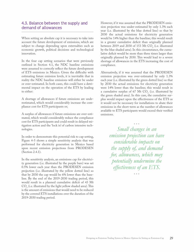
When setting an absolute cap it is necessary to take into account the future development of emissions, which are subject to change depending upon externalties such as economic growth, political decisions and technological innovation.

In the four cap setting scenarios that were previously outlined in Section 4.1, the NDC baseline emissions were assumed to correctly reflect the future development of ETS emissions in Mexico. Given the difficulty with estimating future emission levels, it is inevitable that in reality the NDC baseline emissions will either be under or over-estimated. In both cases, this could have a detri-mental impact on the operation of the ETS by leading to either:

A shortage of allowances if future emissions are unde-restimated, which would considerably increase the com-pliance cost for ETS participants or;

A surplus of allowances if future emissions are over-esti-mated, which would considerably reduce the compliance cost for ETS participants and could result in delayed mi-tigation action and the ‘lock in’ of carbon intensive tech-nologies.

In order to demonstrate this potential risk to cap setting, Figure 4-5 shows a simple sensitivity analysis that was performed for electricity generation in Mexico based upon recent emission projections from PRODESEN (Section 2.4.1).

In the sensitivity analysis, an emissions cap for electrici-ty generation (i.e. illustrated by the purple bars) was set 0.5% lower each year than the PRODESEN emission projection (i.e. illustrated by the yellow dotted line) so that by 2030 the cap would be 6% lower than the base-line. By the end of the 2019-2030 trading period, this would result in a planned cumulative deficit of 43 Mt CO2 (i.e. illustrated by the light yellow shaded area). This is the amount of emissions that would need to be reduced by the covered ETS installations over the duration of the 2019-2030 trading period.

However, if it was assumed that the PRODESEN emis-sion projection was under-estimated by only 1.3% each year (i.e. illustrated by the blue dotted line) so that by 2030 the actual emissions for electricity generation would be 14% higher than the baseline; this would result in a greater cumulative deficit than originally planned between 2019 and 2030 of 153 Mt CO2 (i.e. illustrated by the blue shaded area). In this circumstance, the cumu-lative deficit would be more than three times larger than originally planned by 2030. This would lead to a severe shortage of allowances in the ETS increasing the cost of compliance.

Alternatively, if it was assumed that the PRODESEN emission projection was over-estimated by only 1.3% each year (i.e. illustrated by the green dotted line) so that by 2030 the actual emissions for electricity generation were 14% lower than the baseline; this would result in a cumulative surplus of 67 Mt CO2 (i.e. illustrated by the green shaded area). In this case, the cumulative sur-plus would impact upon the effectiveness of the ETS as it would not be necessary for installations to abate their emissions in the short-term as the number of allowances available to ETS participants would exceed their verified emissions.

Small changes in an emission projection can have

considerable impacts on the supply of, and demand for, allowances, which may potentially undermine the effectiveness of an ETS.


The key outcome of this sensitivity analysis is to simply underline the uncertainty associated with cap setting and how relatively small changes in an emission projection can have considerable impacts on the supply of, and de-mand for, allowances, which may potentially undermine the effectiveness of an ETS. In order to address this

inherent risk to cap setting, it is necessary to therefore introduce flexibilities and safeguards so that ETS autho-rities have the ability to adjust the cap in response to both shorter-term fluctuations and longer-term policy develo-pments.

Figure 4-5: Impact of uncertain emission projections on the balance of the supply and demand for allowances for the electricity generation sector

-153

-43

-200

-150

-100

-50

0

50

100

150

200

2019 2020 2021 2022 2023 2024 2025 2026 2027 2028 2029 2030

Mt

CO

2

Real cumulative deficit (higher) Real cumulative deficit (lower)Planned cumulative deficit CapProjection (PRODESEN) Projection under-estimated emissionsProjection over-estimated emissions

0

67

0

67

Source: PRODESEN (2016); Own calculation

30

Discussion

5. Discussion

5.1. Safeguard and flexibility options

In theory, if the ultimate reduction goal and reduction pathways are set in an efficient manner, it should be pos-sible to set ETS caps decades in advance without having to intervene in the market (Neuhoff et al. 2015). Howe-ver, experience with ETSs to date has shown that this is infeasible and that some degree of market intervention is likely to be necessary for a number of reasons.

• The data quality, in particular at the beginning of an ETS, may be low and it may therefore be impossible to set an effective and efficient cap;

• The ambition of the trading system is not alig-ned with long-term reduction requirements, or long-term reductions may change (i.e. fo-llowing the Paris Agreement’s global stocktake process to raise the ambition of future NDCs);

• The cap does not (fully) anticipate emission reductions achieved by complementary poli-cies. System-wide shocks, e.g. to the economy, fuel prices or technology can lead to a structu-ral imbalance between supply and demand of allowances.

Table 5-1 shows the cap, (allowed) use of international offsets and emissions for the EU ETS in its first two pha-ses and the Californian cap-and-trade program in its first phase and the first two years of the second phase. For the EU ETS actual international credit use is applied, for the Californian cap and trade program allowed use (i.e. 8% of compliance) is shown. The over-supply in both systems is remarkable. In the EU, this situation has prompted an increase in the LRF governing the cap and the setting up of a Market Stability Reserve (MSR), which includes a cancellation mechanism for allowances (European Union (EU) 2018). Since California has an auction reserve price in place, the over-supply of allowances meant that not all allowances offered at auction were bought and entered the market. However, California, to date, has no mecha-nism for cancelling the non-required allowances.

Table 5-1: Allowance supply and demand in the first years of operation (EU ETS, California ETS)

Cap Offset use Emissions OversupplyEU ETS (2005-07) 6 370 Mt - 6 215 Mt 155 Mt (2%)EU ETS (2008-2012) 10 411 Mt 1 048 Mt 9 710 Mt 1 756 Mt (18%)California (2013-14) 323 Mt 23 Mt 292 Mt 54 Mt (19%)California (2015-16) 777 Mt 53 Mt 665 Mt 166 Mt (25%)Source: EEA (2017); ICAP (2018b); ARB (2017b)

In a similar development, the Regional Greenhouse Gas Initiative (RGGI) started out with a yearly cap of 150 Mt reducing by 2.5% each year in 2009. By 2012, reductions of more than 40% below this cap were achieved promp-ting the cap to be reduced to about 83 Mt (91 million short tons) in 2014. In more recent developments, the re-duction factor is to be increased from 2.5% to 3% (ICAP 2018c).

Current projections and analyses suggest that a Mexican ETS with a cap based on the unconditional NDC tar-get is likely to lead to very limited abatement incentives (Mehling & Dimantchev 2017) and potential over-su-pply of allowances.

32

Current projections and analyses suggest that a

Mexican ETS with a cap based on the unconditional

NDC target is likely to lead to very limited abatement

incentives and potential over-supply of allowances.

Figure 5-1 illustrates two types of cap adjustments, which are categorised based on whether the adjustment to the ETS cap has a long or short-term impact.

• On the one hand, in order to safeguard long-term ambition and effectiveness of the system, avoiding lock-in and increasing investor cer-tainty, the regulator may wish to reduce the overall cap. This would usually be done between trading phases. Reasons could be an increase in ambition, accounting for emission reductions of complementary policies or improved data quality (in particular at the start of a scheme);

• On the other hand, one may consider setting up on-going flexibility mechanisms to accom-modate (limited) shocks to the system, e.g. re-lated to economic or fuel price development. They would also bridge the gap until a more general adjustment of the cap can take place at the beginning of the next trading phase.

In the following sections, the different options illustrated below will be assessed, outlining their advantages and li-mitations and their applicability in the Mexican context.

Figure 5-1: Long-term and short-term options for adjusting an ETS cap

Source: Own illustration


5.2. Safeguarding ambition and integrity in the long-term

5.2.1. General considerations

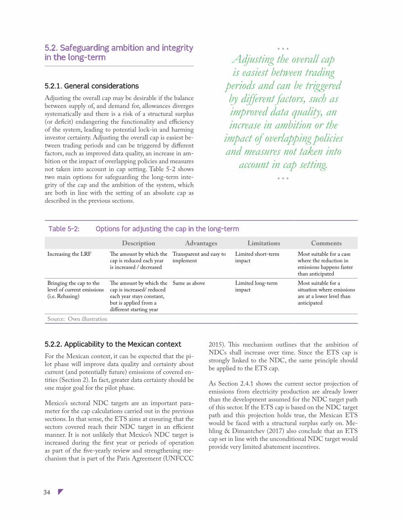
Adjusting the overall cap may be desirable if the balance between supply of, and demand for, allowances diverges systematically and there is a risk of a structural surplus (or deficit) endangering the functionality and efficiency of the system, leading to potential lock-in and harming investor certainty. Adjusting the overall cap is easiest be-tween trading periods and can be triggered by different factors, such as improved data quality, an increase in am-bition or the impact of overlapping policies and measures not taken into account in cap setting. Table 5-2 shows two main options for safeguarding the long-term inte-grity of the cap and the ambition of the system, which are both in line with the setting of an absolute cap as described in the previous sections.

.

Adjusting the overall cap is easiest between trading

periods and can be triggered by different factors, such as improved data quality, an increase in ambition or the

impact of overlapping policies and measures not taken into

account in cap setting.

Table 5-2: Options for adjusting the cap in the long-term

Description Advantages Limitations CommentsIncreasing the LRF The amount by which the

cap is reduced each year is increased / decreased

Transparent and easy to implement

Limited short-term impact

Most suitable for a case where the reduction in emissions happens faster than anticipated

Bringing the cap to the level of current emissions (i.e. Rebasing)

The amount by which the cap is increased/ reduced each year stays constant, but is applied from a different starting year

Same as above Limited long-term impact

Most suitable for a situation where emissions are at a lower level than anticipated


5.2.2. Applicability to the Mexican context

For the Mexican context, it can be expected that the pi-lot phase will improve data quality and certainty about current (and potentially future) emissions of covered en-tities (Section 2). In fact, greater data certainty should be one major goal for the pilot phase.

Mexico’s sectoral NDC targets are an important para-meter for the cap calculations carried out in the previous sections. In that sense, the ETS aims at ensuring that the sectors covered reach their NDC target in an efficient manner. It is not unlikely that Mexico’s NDC target is increased during the first year or periods of operation as part of the five-yearly review and strengthening me-chanism that is part of the Paris Agreement (UNFCCC

2015). This mechanism outlines that the ambition of NDCs shall increase over time. Since the ETS cap is strongly linked to the NDC, the same principle should be applied to the ETS cap.

As Section 2.4.1 shows the current sector projection of emissions from electricity production are already lower than the development assumed for the NDC target path of this sector. If the ETS cap is based on the NDC target path and this projection holds true, the Mexican ETS would be faced with a structural surplus early on. Me-hling & Dimantchev (2017) also conclude that an ETS cap set in line with the unconditional NDC target would provide very limited abatement incentives.

34

.

For the Mexican context, it can be expected that the

pilot phase will improve data quality and certainty about

current (and potentially future) emissions of covered entities. In fact, greater data certainty should be one major

goal for the pilot phase.

The Mexican government may also want to introduce additional energy and climate policy instruments that impact the demand for allowances and are not reflected in the initial modelling of the cap. As these policy ins-truments, e.g. in the area of renewable energy of energy efficiency, are likely to reduce the demand for allowances in a systematic and long lasting manner, the overall cap should be reduced in line with this impact.

Choosing whether to increase the LRF or rebase the cap depends on the specific situation at hand. Figure 5-2 illustrates a situation for the electricity generation sector. For the example, the ETS cap for electricity generation is set using a LRF of -1% (i.e. illustrated by the green bars). According to electricity sector projections, this situation would amass a sizeable surplus until 2021. If the cap is rebased to the projected emissions level in 2022 (i.e. illus-trated by the yellow dotted line), it is straight away in line with actual emissions, providing a short-term remedy to the situation (see also FTI-CL Energy 2017). Increasing the LRF to -2% (i.e. illustrated by the purple dotted line), on the other hand, does not immediately align the cap with current emissions, but has a more pronounced effect in the longer term.

Figure 5-2: Comparing the impact of rebasing the cap and increasing the LRF for the power generation sector

143 141 140 138 137 136 134 133 131 130 129 127

117

133

110

128

0

20

40

60

80

100

120

140

160

2014 2015 2016 2017 2018 2019 2020 2021 2022 2023 2024 2025 2026 2027 2028 2029 2030

Mt

CO

2

Historic emissions Cap with LRF of -1%Rebased Cap in 2022 Cap with increased LRF of -2%Sector projection

Source: PRODESEN (2016); SEMARNAT (2018); Own calculation


TThe choice between these two options depends on the cause of the over-supply and expected future develop-ments. If, for example, improved data shows that emis-sions in electricity generation were over-estimated by 10%, it makes sense to rebase the cap. If the overall am-bition of the system in the long-term is to be increased, it makes sense to increase the LRF. The two options can also be combined. In order to increase policy certainty and avoid lengthy political processes, these long-term adjustments should – as far as possible - be based on ru-les and previously defined parameters (PMR & ICAP 2016). It is helpful to define these rules and parameters in the initial design of the ETS.

5.2.3. Steps to implementation

In light of the data quality issues (Section 2) and sector projections that already suggest a surplus (Section 2.4.1), it would be good to make clear at the start of the scheme that adjustments to the cap may take place in 2022 and which rules and parameters these adjustments will be ba-sed on. In line with the requirements set out in the Paris Agreement and in order to fulfil international commit-ments, it should be the rule that the ambition of the ETS shall increase over time and that therefore that rebasing can only take place to a lower emissions level and that the LRF can only be increased (rather than decreased).

The ambition of the ETS shall increase over time.

As emissions for the last year of the pilot phase are li-kely to be reported only in 2022, rebasing for 2022 would most likely have to use 2019 and 2020 emission levels. If these are lower than the cap by a substantial amount (what this means should be specified in the initial de-sign), rebasing of the cap in 2022 could take place. It should be ascertained that this lower level of emissions is not due to short-term effects (e.g. outages, etc.), but rather systematic (e.g. due to data quality issues or the impact of overlapping policies).

If it becomes clear during the pilot phase that i) the am-bition of the Mexican NDC is increased (e.g. as part of the Facilitative Dialogue in 2018) or that ii) the contri-bution of the ETS sectors in helping Mexico achieve its climate targets is to be increased, an increase of the LRF would make sense.

One has to keep in mind the principle of the LRF, i.e. that it is applied to a base year or period and the resulting absolute reduction year-on-year held constant. To facili-tate the choice of a more ambitious LRF in 2022, already at the inception of the system, different scenarios using different LRFs could be presented and the resulting increase in ambition, for example to the unconditional NDC target or beyond, be calculated. Mehling & Di-mantchev (2017), for example, present a 26% reduction beyond BAU as one of their main scenarios, which would go beyond the unconditional NDC target.

There could also be pre-defined rules on how to adjust the LRF based on distance to NDC path, e.g. if emis-sions are x% below NDC path, LRF should be increased by x%-points. This would take account of the fact that the sector is apparently able to contribute to a greater extent to Mexico reaching its climate targets.

The relatively short length of trading phases (potentia-lly 3 years) planned for the Mexican system also allows the regulator to more quickly respond to and carry out downward adjustments.

36

5.3. Making the system responsive to short-term shocks

5.3.1. General considerations

In addition to more long-lasting changes to emissions and / or ambition, entities covered by an ETS may also face short-term emission variations related to, for exam-ple, unanticipated changes in economic development or fuel price development. The unanticipated impact of complementary policies can also lead to an imbalance be-tween the demand and supply of allowances if the supply is inflexible. To address these short-term imbalances and also to bridge the gap until a more long-term adjustment to the cap can be made, several short-term flexibility op-tions are available. These options can be differentiated by the triggers used, which may be based on price or quan-tity of allowances and further by the steps taken when these trigger points are reached, for example direct cance-llation of allowances or putting allowances into a market integrity reserve (Figure 5-1).

The unanticipated impact of complementary policies can also lead to an imbalance between the demand and

supply of allowances if the supply is inflexible.

5.3.2. Applicability to the Mexican context

In a dynamic economy such as Mexico’s it is not unlikely that short-term imbalances between demand and supply of allowances occur. Furthermore, international develop-ments, such as fuel price variations also have short-term impacts on ETS emissions. In the following, the different options will be discussed, illustrating their application, empirical examples, advantages and limitations.

The advantage of an auction reserve price is that it

safeguards market stability if the demand for allowances is lower than anticipated. It

also provides price certainty to emitters.

Auction reserve price If an auction reserve price is in place, allowances at auc-tion are only sold if a certain price level is reached. Se-veral trading systems have a reserve price in place, such as the California, Québec and Ontario systems (ICAP 2018b). RGGI has opted for a step-wise approach with two different trigger prices starting in 2021 (Burtraw et al. 2018). The advantage of an auction reserve price is that it safeguards market stability if the demand for allowan-ces is lower than anticipated. It also provides price cer-tainty to emitters, which may be particularly important at the start of a scheme and bolsters government revenue, as allowances are not auctioned at excessively low prices.


In order to apply an auction reserve price to the Mexi-can ETS, it is important that a substantial amount of allowances is auctioned. Since there is already a carbon price in place in Mexico, i.e. the carbon tax, the mecha-nism should be familiar and easy to understand for emi-tters. What is more, since the WCI systems have an auc-tion reserve price in place, a link to these systems is likely facilitated if Mexico also introduces an auction reserve price (of a similar magnitude).

Allowances not auctioned because the reserve price is not reached can either be cancelled directly or set aside in a market integrity reserve. Direct cancelling has the largest climate benefit. A reserve that releases allowances back into the market at a later point in time carries the dan-ger of compromising climate integrity in the long-term. Therefore, some form of cancellation mechanism should be in place. This can be achieved through the definition of vintages with a limited lifespan or a pre-defined me-chanism that caps the overall size of the reserve, as is the case for the MSR in the EU ETS (cf. European Union (EU) 2015). It is also important that the auction reserve price rises over time.

Surrender chargeIf a surrender charge is in place, at compliance, emitters have to pay a top-up charge representing the difference between the market price of allowances and a set mini-mum price. The UK has implemented a surrender charge in order to guarantee a minimum price for CO2 in the electricity sector (Hirst 2018). In contrast to a unilateral auction reserve price, the surrender charge is compatible with the overall structure of the EU ETS, where the re-maining 30 countries covered do not have a minimum price in place.

This mechanism provides price certainty to covered enti-ties and ensures government revenue for those allowances that are surrendered. Since entities can still buy allowan-ces at lower prices (at auction or on the market) and bank them for later use, the climate benefit of this mechanism is unclear and depends on the way in which the surrender charge rises over time. There is a risk that entities amass a substantial bank of allowances, which undermines caps in later years.

Mehling & Dimantchev (2017) suggest that incorpo-rating the current Mexican carbon tax into the ETS by way of a surrender charge ‘allows for the continuation of carbon pricing revenues, and for the introduction of an ETS that introduces higher certainty of achieving clima-te mitigation goals.’ Similar to the auction reserve price, it is important that the surrender charge is increased by a substantial amount each year. Both for a surrender charge and a price ceiling (next section), the regulator needs to define a reference price against which the top-up is cal-culated.

38

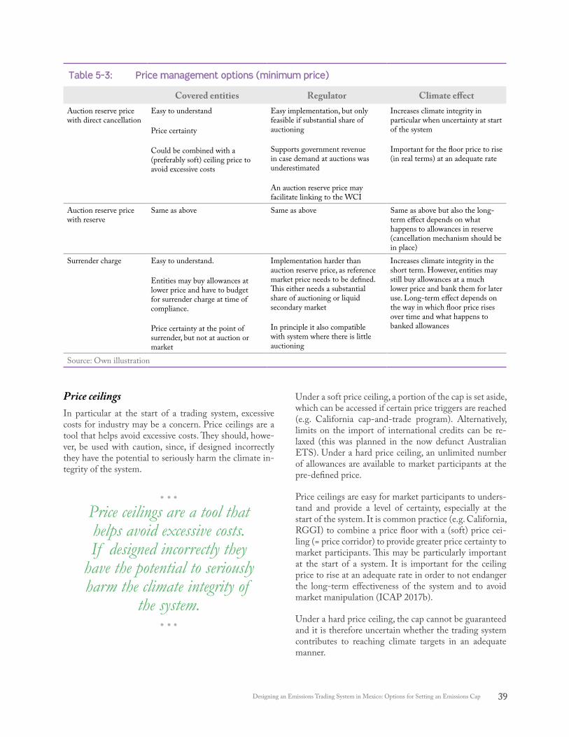
Table 5-3: Price management options (minimum price)

Covered entities Regulator Climate effectAuction reserve price with direct cancellation

Easy to understand

Price certainty

Could be combined with a (preferably soft) ceiling price to avoid excessive costs

Easy implementation, but only feasible if substantial share of auctioning

Supports government revenue in case demand at auctions was underestimated

An auction reserve price may facilitate linking to the WCI

Increases climate integrity in particular when uncertainty at start of the system

Important for the floor price to rise (in real terms) at an adequate rate

Auction reserve price with reserve

Same as above Same as above Same as above but also the long-term effect depends on what happens to allowances in reserve (cancellation mechanism should be in place)

Surrender charge Easy to understand.

Entities may buy allowances at lower price and have to budget for surrender charge at time of compliance.

Price certainty at the point of surrender, but not at auction or market

Implementation harder than auction reserve price, as reference market price needs to be defined. This either needs a substantial share of auctioning or liquid secondary market

In principle it also compatible with system where there is little auctioning

Increases climate integrity in the short term. However, entities may still buy allowances at a much lower price and bank them for later use. Long-term effect depends on the way in which floor price rises over time and what happens to banked allowances


Price ceilingsIn particular at the start of a trading system, excessive costs for industry may be a concern. Price ceilings are a tool that helps avoid excessive costs. They should, howe-ver, be used with caution, since, if designed incorrectly they have the potential to seriously harm the climate in-tegrity of the system.

Price ceilings are a tool that helps avoid excessive costs. If designed incorrectly they

have the potential to seriously harm the climate integrity of

the system.

Under a soft price ceiling, a portion of the cap is set aside, which can be accessed if certain price triggers are reached (e.g. California cap-and-trade program). Alternatively, limits on the import of international credits can be re-laxed (this was planned in the now defunct Australian ETS). Under a hard price ceiling, an unlimited number of allowances are available to market participants at the pre-defined price.

Price ceilings are easy for market participants to unders-tand and provide a level of certainty, especially at the start of the system. It is common practice (e.g. California, RGGI) to combine a price floor with a (soft) price cei-ling (= price corridor) to provide greater price certainty to market participants. This may be particularly important at the start of a system. It is important for the ceiling price to rise at an adequate rate in order to not endanger the long-term effectiveness of the system and to avoid market manipulation (ICAP 2017b).

Under a hard price ceiling, the cap cannot be guaranteed and it is therefore uncertain whether the trading system contributes to reaching climate targets in an adequate manner.


Table 5-4: Price management options (maximum price)

Covered entities Regulator Climate effectSoft price ceiling Can be combined with floor

price to safeguard against excessive costs, in particular if there is uncertainty at start of the system

Regulator needs to define reference price that the ceiling price is evaluated against. This either needs a substantial share of auctioning or liquid secondary market

Price ceiling needs to rise at an adequate rate in order to not endanger climate integrity

Hard price ceiling Same as above Same as above Could seriously harm climate integrity, as cap and thus contribution of covered sectors to long- term targets is not guaranteed


Quantity managementRather than using price triggers (e.g. auction reserve pri-ce, soft price ceiling), quantity triggers can also be used to activate a market integrity reserve. Instead of having a floor and ceiling price, a minimum and maximum accep-table size of the surplus is defined and if these quantity triggers are reached, allowances are cancelled directly, ad-ded to or released from a market integrity reserve. Typi-cally, allowances are taken from and reintroduced into the auctioning budget. The most prominent example of such a mechanism is the MSR in the EU ETS (Euro-pean Union (EU) 2015).

Quantity management also increases resilience of the sys-tem to shocks and supports the ETS price signal. Howe-ver, price certainty is somewhat lower than under a price management system, since the price impact of quantity management may be hard to predict for participants. Si-milar to price management, quantity management should be rule-based and predictable. Which of the two is cho-sen depends on political preferences of the country or re-gion (e.g. the EU where it was / is infeasible to manage the price of the ETS directly).

Similar to setting an adequate price under a price ma-nagement system, it is important to adequately set the trigger levels under quantity management and to adjust these over time. In the EU’s MSR, for example, the quan-tity thresholds are set based on assumptions about the hedging demand and behaviour of electricity generators covered by the system. Hedging demand and behaviour is changing over time depending on the share of renewables

in the market and the electricity market structure (e.g. the importance of short vs. long-term contracts). Inade-quate trigger levels (thresholds) may seriously harm the efficiency of the system.

As noted above, it is important to combine any kind of reserve with a cancellation mechanism (as is the case for the EU’s MSR) to avoid the build-up of a large reserve leading to higher emissions in future years and endange-ring long-term reduction targets.

It is important to combine any kind of reserve with a

cancellation mechanism as is the case for the EU’s MSR to avoid the build-up of a

large reserve leading to higher emissions in future years

and endangering long-term reduction targets.

40

Table 5-5: Quantity management options

Covered entities Regulator Climate effectQuantity management with direct cancellation.

More certainty on the amount of allowances available

More complex than price management and price effect is less certain

Several parameters governing quantity management need to be set and monitored

Can support government revenue

Linking to WCI likely easier under price management

Increases climate integrity if parameters governing quantity management are set, evaluated and adjusted adequately

Quantity management with reserve

More certainty on the amount of allowances available

More complex than price management and price effect is less certain

Several parameters governing quantity management need to be set and monitored

Can support government revenue

Linking to WCI likely easier under price management

Increases climate integrity if parameters governing quantity management are set, evaluated and adjusted adequately

Long-term effect depends on what happens to allowances in reserve (some cancellation mechanism should be in place)


5.3.3. Steps to implementation

This section is intended to provide a first overview of the necessary steps toward implementation of the different options rather than a complete elaboration of a specific option.

Price managementIf the Mexican ETS is to include a price management mechanism, it may make sense to introduce this mecha-nism already in the pilot phase. In fact, as price uncertain-ty may be high in the pilot phase, a minimum price may help increase price certainty (and ensure government re-venue). What is more, Mexico already has a carbon price in place – the carbon tax. This could be combined with a (soft) price ceiling to avoid excessively high costs to en-tities.

First, the level of the floor price needs to be set. A floor price is only effective and efficient if it is set at an adequa-te level. The current level of the carbon tax, floor prices in

other ETSs and / or calculations and projections regar-ding abatement costs can be used in setting the floor pri-ce. The current level of the carbon tax of 75 MXN/t (3.5 USD/t) is below the current Californian auction reserve price of 13.57 USD/t in 2017. In general, floor prices should rise (in real terms) to continue being effective and efficient. In the Californian cap-and-trade program, the floor price rises by 5% each year (ICAP 2017).

If linking to the WCI is considered, it would be natural to let the Mexican floor price rise incrementally to meet the WCI floor price (in fact, floor prices in California, Ontario and Québec differ very slightly, the Californian floor price is used as the target price here). Similarly, Ca-lifornia’s three-tiered soft price ceiling (50.69 USD/t, 57.04 USD/t and 63.37 USD/t in 2017, rising at 5% in real terms each year, ICAP 2018b) could be used as a reference for a Mexican (soft) price ceiling. Figure 5-3 provides an example of how this could be achieved.


Figure 5-3: Example price path for potential Mexican floor and ceiling prices when linking to WCI is considered

0

20

40

60

80

100

120

140

2018 2019 2020 2021 2022 2023 2024 2025 2026 2027 2028 2029 2030

US$

(20

14)

/ tC

O2

Mexican ceilingprice tier 1



Californian ceilingprice tier 1



Californian auctionreserve price

Mexican floor price

Source: PRODESEN (2016); SEMARNAT (2018); Own calculation

Starting in 2021, California is planning to replace its soft price ceiling with a hard one. The actual price to be set has not been determined yet (C2ES 2017).

In order to avoid the build-up of a large reserve that harms long-term effectiveness and

climate integrity, it would be important to either directly cancel allowances when the floor price is triggered or introduce a reserve with a

cancelling mechanism.

As noted above, in order to avoid the build-up of a large reserve that harms long-term effectiveness and climate integrity, it would be important to either directly cancel allowances when the floor price is triggered or introdu-ce a reserve with a cancelling mechanism. There are two main options to introduce a cancelling mechanism wi-thin a reserve:

• Vintages: Allowances receive a time-stamp for their year of creation and only have a limited, pre-defined lifetime after which they are no longer valid and would also be cancelled from the reserve;

• Setting a cap on the overall size of the reserve. In the EU’s MSR, for example, the reserve can-not grow above the previous year’s total auction amount.

42

When introducing a soft price ceiling, Mexico would also need to determine the amount of allowances to be set asi-de that would be available to the entities if ceiling prices are reached. In fact, a fraction of the allowances put into a reserve when the auction reserve price is triggered, could be used for this purpose.

In the case of a surrender charge and a soft ceiling price, the regulator needs to define a (market) reference price – against which the set floor or ceiling price is evaluated. This reference price may, for example, be related to out-comes at auctions or published market prices of liquid market platforms. In California, the auction settlement price is used as a reference price (ARB 2017a). For the UK Carbon Floor price government projections are used as the reference price (Hirst 2018).

Quantity managementIn order to set up a reserve with quantity-based triggers, a number of parameters need to be defined. As an indica-tion, the following lists the parameters defining the MSR (European Union (EU) 2015, 2018):

• Amount of allowances in circulation: Needs to be calculated on the basis of total supply and total demand in a pre-defined time span;

• Thresholds: The amount of allowances in cir-culation is evaluated against the thresholds to determine whether the reserve is triggered. In the EU, these thresholds are set according to assumptions about the hedging demand of electricity generators and the resulting ‘neces-sary surplus’ on the market. Since hedging de-mand is likely to change over time (due to, for example, changes in electricity demand or the generation mix) thresholds should be adjusted periodically;

• Amount put into reserve / released from re-serve if thresholds are triggered: In the EU, the amount to be put into the reserve is defined as a % of the amount of allowances in circula-tion, while the amount to be released is defi-ned as an absolute number. If these thresholds are not set adequately, a structural surplus may persist;

• Cancellation provisions: Allowances are cancelled from the MSR if the total stock of allowances in the MSR is higher than the pre-vious years auctioned amount. The difference is then cancelled from the MSR. Another option discussed in the EU was a fixed amount to be cancelled in a certain year.


Conclusion

6. Conclusion

This study has developed a Cap Setting Tool in order to support policy makers with the setting of an ETS cap for Mexico. The results from four illustrative cap setting scenarios have been presented in Section 4.1, which were based upon two approaches for defining an absolute cap (i.e. LRF and deviation from projection) that contribute to the achievement of two different levels of mitigation ambition (i.e. the unconditional and conditional NDC target level in 2030).

These four cap setting scenarios all assumed, for simpli-city, that no emission thresholds would be applied (i.e. all installations in ETS sectors that are included in the RENE were covered). However, in reality it would make sense to further limit the scope of the ETS to reduce the administrative burden. Indeed, the analysis conducted in Section 4.2 demonstrated that the application of certain emission thresholds by sector could reduce the number of installations participating in the ETS by half whilst still ensuring that over 80% of the emissions from these ETS sectors were covered. Furthermore, the cap setting scena-rios all simply assumed a 1% growth in emissions in 2017 and 2018. Therefore the starting level of CO2 emissions for the ETS pilot in 2019 will need to be revised based upon updated data from the RENE when available.

In this study, LRFs from Scenario 1 and 2 were applied to 2016 CO2 emissions from the RENE. However, the most appropriate base year(s) to use under the LRF approach should be re-assessed as the time series of the RENE increases. The LRF approach to cap setting is relatively straightforward, providing high levels of transparency and greater certainty to market participants over future levels of ambition. This approach also provides flexibili-ty for setting the cap that could reflect either increasing or decreasing emissions. However, the setting of a LRF needs to always take into account the expected emissions development to ensure that the approach does not lead to an over-supply of allowances in the market.

The deviation from a projection approach to cap setting used in Scenario 3 and 4 may be more politically accep-table as it could follow an emission pathway that has al-ready been agreed upon (i.e. such as the unconditional and conditional 2030 targets in the Mexican NDC). The extent to which the annual cap should deviate from an emission projection should always be set so that the mi-tigation potential and associated cost is taken into ac-count to ensure that any ETS cap is both technically and economically feasible. This approach is highly dependent upon the quality of the emission projection selected. If the ETS cap is based upon a deviation from an emis-sion projection that is over-estimated, this may result in a build-up of surplus allowances if the target is not suffi-ciently ambitious. This potential risk was illustrated in a sensitivity analysis in Section 4.3.

The extent to which the annual cap should deviate from an emission projection should always be set so that the mitigation potential and associated cost is taken into account to ensure that any

ETS cap is both technically and economically feasible.


Regardless of the cap setting approach selected, it is es-sential that any future cap is accompanied by appropriate flexibilities and safeguards (as discussed in Section 5). Experience has shown that ETSs are often over-supplied with allowances at the start of their lifetime. Prelimi-nary projections suggest that this may also be the case for the Mexican system if the cap is set in accordance with the unconditional NDC target. In order to safe-guard effectiveness and long-term efficiency, it may the-refore be necessary to re-adjust the cap downwards be-tween ETS phases. Short-term flexibility options should also be implemented in order to improve the resilience of the Mexican ETS to unexpected shocks. Price-based mechanisms may represent the more appropriate, sim-pler to implement, option for Mexico, as it already has a price instrument in place: the carbon tax. Furthermore, a price-based flexibility mechanism may aid price stability and price discovery in the pilot phase and provide se-curity to (inexperienced) market participants. Flexibility options should certainly be trialled during the pilot phase in order to help future decision making on the design of the Mexican ETS at the start of the formal phase.

.

Regardless of the cap setting approach selected, it is essential that any future

cap is accompanied by appropriate flexibilities and

safeguards

46

Publicationbibliography

7. Publication bibliography

ARB (2017a): December 2017 Reserve Sale Will Not Be Offered. California Air Resources Board (ARB). Avai-lable online at https://www.arb.ca.gov/cc/capandtrade/reservesale/dec-2017/status_update.pdf, checked on 12/16/2017.

ARB (2017b): Mandatory GHG Reporting - Repor-ted Emissions. California Air Resources Board (ARB). Available online at https://ww2.arb.ca.gov/our-work/programs/mandatory-greenhouse-gas-emissions-repor-ting/data.

Burtraw, Dallas; Holt, Charles; Palmer, Karen; Paul, Anthony; Shobe, William (2018): Quantities with Pri-ces. Resources for the Future (RFF WP, 18-08). Avai-lable online at http://www.rff.org/files/document/file/RFF%20WP%2018-08.pdf, checked on 4/13/2018.

C2ES (2017): Summary of California’s Extension of its Cap and Trade Program. C2ES. Available online at https://www.c2es.org/site/assets/uploads/2017/09/sum-mary-californias-extension-its-cap-trade-program.pdf, checked on 5/20/2018.

Carbon Pulse (2018): Mexican senate approves bill to bolster emissions trading plans. Carbon Pulse. Available online at https://carbon-pulse.com/51336/.

Climate Action Tracker (2017): Mexico: Assessment. Ecofys; Climate Analytics; PIK; NewClimate Institute. Available online at http://climateactiontracker.org/coun-tries/mexico.html.

EEA (2017): EU Emissions Trading System (ETS) data viewer. European Environment Agency (EEA). Availa-ble online at http://www.eea.europa.eu/data-and-maps/data/data-viewers/emissions-trading-viewer, checked on 7/11/2017.

European Union (EU) (2015): Decision (EU) 2015/1814 of the European Parliament and of the Council of 6 Oc-tober 2015 concerning the establishment and operation of a market stability re-serve for the Union greenhouse gas emission trading scheme and amending Directive 2003/87/EC. In OJ L 264, pp. 1–5, checked on 6/7/2017.

European Union (EU) (2018): Directive (EU) 2018/410 of the European Parliament and of the Council of 14 March 2018 amending Directive 2003/87/ EC to en-hance cost-effective emission reductions and low-car-bon investments, and Decision (EU) 2015/1814. In OJ L 76, pp. 3–27. Available online at https://eur-lex.europa.eu/legal-content/EN/TXT/PDF/?uri=CE-LEX:32018L0410&rid=1, checked on 4/10/2018.

FTI-CL Energy (2017): Wake Up Reforming EU ETS. Available online at Most suitable for a case where the reduction in emissions happens faster than anticipated., checked on 4/11/2018.

Hirst, David (2018): Carbon Price Floor (CPF) and the price support mechanism. House of Com-mons Library. London (Briefing Paper, No. 05927). Available online at http://researchbriefings.files.parliament.uk/documents/SN05927/SN05927.pdf, checked on 2/15/2018.

ICAP (2017): USA - California Cap-and-Trade Pro-gram. International Carbon Action Partnership (ETS Detailed Information). Available online at https://icap-carbonaction.com/en/?option=com_etsmap&task=ex-port&format=pdf&layout=list&systems=45, checked on 12/16/2017.

ICAP (2018a): Mexico. General Information. Interna-tional Carbon Action Partnership. Available online at https://icapcarbonaction.com/en/?option=com_etsma-p&task=export&format=pdf&layout=list&systems%-5b%5d=59, checked on 4/3/2018.

48

ICAP (2018b): USA - California Cap-and-Trade Pro-gram. International Carbon Action Partnership (ICAP). Available online at https://icapcarbonaction.com/en/?option=com_etsmap&task=export&format=pdf&la-yout=list&systems=45, checked on 4/12/2018.

ICAP (2018c): USA - Regional Greenhouse Gas Initia-tive (RGGI). International Carbon Action Partnership (ICAP). Available online at https://icapcarbonaction.com/en/?option=com_etsmap&task=export&format=p-df&layout=list&systems=50, checked on 4/16/2018.

Mehling & Dimantchev (2017): Achieving the Mexi-can Mitigation Targets: Options for an Effective Carbon Pricing Policy Mix. Mexican-German Climate Change Alliance. Available online at http://climate.blue/down-load/GIZ%202017%20-%20Options%20for%20a%20Carbon%20Pricing%20Policy%20Mix%20Mexico(2).pdf, checked on 12/4/2017.

México (2015): Intended nationally determined con-tribution. Submission under the UNFCCC. Avail-able online at http://www4.unfccc.int/submissions/INDC/Published%20Documents/Mexico/1/MEXICO%20INDC%2003.30.2015.pdf.

Mosqueda, Elizabeth; Buchner, Lisa; Wasilewski, Alexandra; Tharan, Doris (2017): Emissions Trad-ing in Mexico - Recommendations for a Monitoring, Repor-ting and Verification (MRV) system for a future Mexi-can emissions trading system (ETS). DEHSt, checked on 4/9/2018.

Neuhoff, Karsten; Acworth, William; Betz, Regina; Burtraw, Dallas; Cludius, Johanna; Fell, Harrison et al. (2015): Is a Market Stability Reserve likely to impro-ve the functioning of the EU ETS? Evi-dence from a model comparison exercise. Climate Strategies. Availa-ble online at http://climatestrategies.org/wp-content/uploads/2015/02/Climate-Strategies-MSR-Report-Fi-nal1.pdf, checked on 8/14/2015.

PMR & ICAP (2016): Emissions Trading in Practice: A Handbook on Design and Implementation. Interna-tional Bank for Reconstruction and Development / The World Bank. Washington. Availa-ble online at https://icapcarbonaction.com/en/?option=com_attach&task=-download&id=364, checked on 12/5/2017.

PRODESEN (2016): National Electric System De-velopment Programme 2016- 2030. Available onli-ne at https://www.gob.mx/cms/uploads/attachment/file/102165/PRODESEN_2016-2030_2.pdf.

SEMARNAT (2018): National Registry of Emissions (RENE).

https://www.gob.mx/semarnat/acciones-y-programas/registro-nacional-de-emisiones-rene

SEMARNAT-INECC (2016): Mexico’s Climate Chan-ge Mid-Century Strategy. Ministry of Envi-ronment and Natural Resources (SEMARNAT) and National Institu-te of Ecology and Climate Change (INECC). Mexico City, Mexico, checked on 4/3/2018.

UNFCCC (2015): Paris Agreement. Available online at http://unfccc.int/files/essential_background/convention/application/pdf/english_paris_agreement.pdf, checked on 10/20/2017.

WCI (2010): Guidance for Developing WCI Partner Jurisdiction Allowance Budgets. Western Cli-mate Ini-tiative (WCI), checked on 4/3/2018.


Designing an Emissions Trading System in Mexico: Options for Setting an Emissions Cap,

which was elaborated by Öko-Institut e.V.

Its contents were developed under the coordination of the Ministry for the Environment and Natural Resources (Secretaría de Medio Ambiente

y Recursos Naturales, SEMARNAT), and the project “Preparation of an Emissions Trading System in Mexico” (SiCEM) of the Deutsche

Gesellschaft für Internationale Zusammenarbeit (GIZ) GmbH on behalf of the German Federal Ministry for the Environment, Nature Conservation

and Nuclear Safety.

Editorial design and creative direction by: Edgar Javier González Castilloand La Estación de Servicio.

Published by: Deutsche Gesellschaft für

Internationale Zusammenarbeit (GIZ) GmbH

Friedrich-Ebert-Alle 36+4053113 Bonn, Deutschland

T +49 228 44 60-0F +49 228 44 60-17 66

Dag Hammarskjöld-Weg 1-565760 Eschborn, Deutschland

T +49 61 96 79 0F +49 61 96 79 11 15

E [email protected] www.giz.de

Project:Preparation of an Emissions Trading

System in Mexico (SiCEM)

Av. Insurgentes Sur No. 826, PH03100 Col. del Valle, CDMX México

E [email protected] [email protected]

Secretaría de Medio Ambiente y RecursosNaturales (SEMARNAT)

Avenida Ejército Nacional 223, piso 19Del. Miguel Hidalgo, Col. Anáhuac

11320 Ciudad de MéxicoE [email protected]