designing an intelligent decision support system for

Decision Support Systems 96 (2017) 49–66

Contents lists available at ScienceDirect

Decision Support Systems

j ourna l homepage: www.e lsev ie r .com/ locate /dss

Designing an intelligent decision support system for effectivenegotiation pricing: A systematic and learning approach

Xin Fua, Xiao-Jun Zengb, Xin(Robert) Luoc, Di Wangd, Di Xua,*, Qing-Liang Fane

aDepartment of Management Science, School of Management, Xiamen University, Xiamen 361005, ChinabSchool of Computer Science, University of Manchester, M13 9PL, U.K.cAnderson School of Management, The University of New Mexico, 1924 Las Lomas NE, MSC05 3090, Albuquerque, NM 87131, United StatesdEBTIC, Khalifa University, Abu Dhabi, United Arab EmirateseWang Yanan Institute for Studies in Economics (WISE), Xiamen University, Xiamen 361005, China

A R T I C L E I N F O

Article history:Received 17 October 2015Received in revised form 27 January 2017Accepted 5 February 2017Available online 10 February 2017

Keywords:Decision support systemsHierarchical fuzzy systemsNegotiation pricing

A B S T R A C T

Automatic negotiation pricing and differential pricing aim to provide different customers with products/services that adequately meet their requirements at the “right” price. This often takes place with thepurchase of expensive products/services and in the business-to-business context. Effective negotiation pric-ing can help enhance a company’s profitability, balance supply and demand, and improve the customersatisfaction. However, determining the “right” price is a rather complex decision-making problem that puz-zles pricing managers, as it needs to consider information from many constituents of the purchase channel.To further advance this line of research, this study proposes a systematic and learning approach that consistsof three different types of fuzzy systems (FSs) to provide intelligent decision support for negotiation pric-ing. More specifically, the three FSs include: 1) a standard FS, which is a typical multiple inputs and singleoutput FS that forms a mathematical mapping from the input space to the output space; 2) an SFS-SISOM,which is a linear fuzzy inference model with a single input and a single output module; and 3) a hierarchicalFS, which consists of several FSs in a hierarchical manner to perform fuzzy inference. To address the existingproblem of a standard FS suffering from the high-dimensional problem with a large number of influentialfactors, a generalized type of FS (named hierarchical FS), including its mathematical models and suitabil-ity for tackling the negotiation pricing problem, is introduced. In particular, a proof-of-concept prototypesystem that integrates these three FSs is also developed and presented. From a system design perspective,this artifact provides immense potential and flexibility for end users to choose the most suitable modelfor the given problem. The utility and effectiveness of this proposed system is illustrated and examined bythree experimental datasets that vary from dimensionality and data coverage. Moreover, the performancesof three different approaches are compared and discussed with respect to some important properties ofdecision support systems (DSSs).

© 2017 Elsevier B.V. All rights reserved.

1. Introduction

Intelligent negotiation pricing and differential pricing are preva-lent in retailing and business-to-business (B2B), and it is playing anincreasingly important role in electronic businesses. In traditionalretailing, it is natural to provide standard products and services toall customers at a standard price. In recent years, with the rapid

* Corresponding author.E-mail addresses: [email protected] (X. Fu), [email protected] (X.-J. Zeng),

[email protected] (X. Luo), [email protected] (D. Wang), [email protected] (D. Xu),[email protected] (Q.-L. Fan).

development of marketing science, it is well recognized that differ-ent marketing and pricing strategies should be applied to differentsegments of customers, because differential pricing can substantiallyenhance organizational profitability and improve customer satis-faction. This emerging phenomenon often occurs in the purchaseof expensive products/services (e.g., cars, houses, and systems). Inparticular, tailor-made products/services require a sales process tonegotiate and settle the final price with customers individually.Furthermore, the outcomes of negotiation pricing and differentialpricing often have a long-term impact on the organizational supplychain relationship and the reputation of business in the B2B arena.In supply chain management, for instance, price negotiation takesplace during annual price reviews, thereby providing an opportu-nity for suppliers to adjust prices in response to recent changes in

http://dx.doi.org/10.1016/j.dss.2017.02.0030167-9236/© 2017 Elsevier B.V. All rights reserved.

http://dx.doi.org/10.1016/j.dss.2017.02.003

http://www.ScienceDirect.com/

http://www.elsevier.com/locate/dss

http://crossmark.crossref.org/dialog/?doi=10.1016/j.dss.2017.02.003&domain=pdf

mailto: [email protected]






http://dx.doi.org/10.1016/j.dss.2017.02.003

50 X. Fu et al. / Decision Support Systems 96 (2017) 49–66

costs, as well as the customer relationships [20,21]. Many examplesof this scenario can be found in the industry. For example, broad-band wireless service providers may provide differentiated servicesto their customers with a variety of customized prices [9]; theatersprovide personalized prices of last-minute tickets depending on thetime remaining and the customer’s location [15].

To increase the effectiveness and efficiency of negotiation pricing,companies often delegate certain degrees of pricing authority to salesrepresentatives who have direct contact with and better knowledgeof customers. The agreed price will then be approved by the pricingmanager. However, the salespeople may have different sales skillsand preferences, as empirical findings have revealed that sales rep-resentatives might offer too many price concessions in order toensure the order [30]. Therefore, from the perspective of pricingmanagers, disclosing the reservation price to all human agents isunfavorable. In essence, decision-making for negotiation pricing isa rather complicated process because it needs to consider informa-tion from a plethora of organizational dimensions to identify theright price for the company. It is worth noting that negotiation pric-ing does not support the entire dynamic and interactive process ofprice negotiation. Instead, it supports the most fundamental problemin the price negotiation process, which helps pricing managers toidentify the right price when offering the unique product/service toeach individual customer.

Prior research efforts have been devoted to providing decisionsupport for negotiation pricing through different techniques,including game theory (GT) [9,34], neural networks [2,20], expertsystems [4], case-based reasoning [15], and fuzzy logic [12,17,18].Notwithstanding, certain drawbacks and challenges still exist withthese approaches because some hypothetical assumptions aredifficult to achieve in real scenarios, and the assessment of utilityfunctions is not feasible in many studies due to heterogeneityand incidental parameters problems. Expert systems are heavilyreliant on expert knowledge and/or static negotiation strategies.Hence, capturing knowledge in manual ways for the resultantsystem would be less flexible and inefficient to handle the dynamicchanges and new cases in negotiations. Similarly, the neural networkapproach [2,20] is limited in its interpretability, and its derivedresults are questionable for the end users.

These extant approaches should resort to adequate and preciseinformation provided by negotiation parties for decision making.However, uncertain information is often inherent in the dynamicnegotiation environments of real negotiation scenarios. The involve-ment of uncertain information is an extremely imperative but oftenunder-addressed issue in negotiation pricing. Fuzzy set theory [32]is well regarded as a useful tool for handling uncertain informa-tion, and preserving transparency and interpretability in modeling.Recently, several research efforts [12,17,18,34] have employed thistechnique to provide decision support for negotiation pricing. Inessence, the majority of the existing approaches either focus on therepresentation of involved uncertain attributes by using linguisticterms, or employ expert knowledge to build static fuzzy rule-basedsystems for reasoning. Yet, slight changes in negotiation conditionsmay necessitate substantial expert interventions to modify thecorresponding rules to reflect the new conditions. Moreover, it isdifficult to validate and assess the quality of knowledge capturedfrom experts. Therefore, it is more desirable to build a fuzzy sys-tem (FS) that would automatically learn from historical records togenerate the fuzzy rules, rather than completely depending on exter-nal knowledge. Additionally, when the number of influential factorsis large, a standard FS easily suffers from the problem of dimension-ality, since the number of required modeling parameters and fuzzyrules exponentially increases with the number of involved attributes.As such, dealing with uncertain information within negotiation pric-ing is of particular interest to researchers and practitioners. Giventhe different features (e.g., dimensionality and data coverage) of

the available historical dataset, choosing the most appropriate FSsis another crucial task faced by the end users of decision supportsystems (DSSs).

In an effort to remedy these pressing issues and challenges, thisstudy substantially extends the initial work of [8], and proposes asystematic and learning approach to provide decision support fornegotiation pricing through FS theory. In essence, this study con-cerns bilateral negations on the price, and considers the negotiationpricing problem particularly from the seller’s point of view to pro-vide intelligent decision support for pricing managers. Given a setof historical records, mathematical relationships between influentialfactors and the proposed price will be built by both learning from thedata itself and integrating expert knowledge. It is believed that theproposed model can be leveraged to better predict the will-to-payand other reference prices (e.g., reservation price, target price, andinitial price) for unforeseeable transactions. Beyond the simplifiedFS with a single input and a single output module (SFS-SISOM) thathas been presented in [8], this work employs the hierarchical fuzzysystem (HFS) approach, which is effective for tackling the dimen-sionality problem to build predictive models for negotiation pricing.The performances of three approaches (i.e., standard FS, SFS-SISOM,and HFS) are further compared and discussed from different perspec-tives, including interpretability, accuracy, generality, computationalcost, and applicability. Moreover, a prototype of an intelligent DSSfor negotiation pricing is designed and developed with an integrationof these three fuzzy approaches. The IT artifact provides substantialpotential and flexibility for end users to choose the most suitablemodel for the existing negotiation pricing problem.

In the general context of DSS, it is worth distinguishing thefeatures of the proposed negotiation pricing DSS. Most extant studieshave been devoted to finding, from a set of known feasible deci-sions, the best decision to fit with the given set of decision criteriaor maximizing the known utility functions. Therefore, these stud-ies can be regarded as DSS with complete and certain information,and the dominant approaches in DSS are decision analysis, ranking,and optimization methods. For the negotiation pricing DSS, however,the situation is very different because the best decision is attain-able, and it is the highest price a customer is willing to pay. Yet, theactual problem is that the highest willing-to-pay price is unknown.Therefore, this type of decision-making problem requires DSS withuncertain information. As the distinguishing feature here is the infor-mation’s uncertainty, the dominant approaches in most existing DSSare no longer applicable and a new approach is needed.

This paper is organized as follows: Section 2 reviews the relatedwork of negotiation pricing decision support, and introduces the HFSand its challenges. In Section 3, a systematic approach employingthree different types of FS is proposed and presented to provide deci-sion support for intelligent negotiation pricing. The applicability andutility of the proposed approach is demonstrated and tested againstthree datasets in Section 4, and the derived results are comparedand discussed in Section 5. In Section 6, a prototype system is devel-oped and presented to provide a proof-of-concept for the proposedwork. The final section concludes this paper and suggests furtherwork directions.

2. Related work

2.1. Negotiation pricing decision support

Negotiation is a crucial activity in business, and is a complex,time consuming, and iterative process which might involve intensiveinformation exchange and processing. In most business negotiations,price is the most important attribute. According to utility theory,in a multi-issue negotiation problems, a utility function can beemployed to model price, such that multi-criteria can be convertedand evaluated by one dimension [13]. Negotiation pricing aims to

X. Fu et al. / Decision Support Systems 96 (2017) 49–66 51

identify a mutually beneficial price for both seller and buyer. This canoften be achieved by iterative one-to-one interactions. An effectivenegotiation pricing DSS may offer many benefits, such as maximizingthe company’s profitability, maintaining good customer relations,balancing supply and demand, and improving inventory manage-ment. Much work has been done recently on negotiation pricingdecision support in the areas of influential factor identification,modeling negotiation behavior, user utility elicitation, and price pre-diction by employing various techniques. A summary of recent workson decision support for negotiation pricing is presented in Table 1.

For identifying and analyzing the underlying relationshipsbetween influential factors and the negotiation price, the pioneeringwork of [10] investigates the relationship between car price andbuyer attributes (e.g., income, race, and gender). Recently, moreefforts have been conducted to explore how reference prices influ-ence the final price in negotiations and analyze their importance(e.g., [1,13,20-22]). The reference prices can refer to the initialprice, participants’ reservation prices (i.e., the walk-away prices),and participants’ target prices. Having recognized the importanceof these reference prices, some works aim to employ both parties’references prices to accelerate and improve the negotiation pro-cess. A common approach is to require both the buyer and theseller to report their reference prices to a third-party before negoti-ations. If the zone of potential agreement is empty, the negotiationwill not be launched (e.g., [13]). A classic approach to model thenegotiation behavior of participants is the well-known GT, whichemphasizes the interactions between buyers and sellers, and hasbeen widely applied in bargaining problems [9,24,34]. Some ofthese game-theoretical models often assume that participants wouldbehave rationally and strategically to optimize their negotiation out-come based on symmetrically available information. However, suchassumptions are difficult to achieve in real scenarios, and limit theapplicability of GT approaches for solving realistic negotiation prob-lems. In principle, GT is a utility-based approach that relies on amathematical concept of optimal convergence where both parties’utility functions are defined and optimized. However, the assessmentof utility functions is a time-consuming and error-prone process.

The above approaches mainly rely on adequate and preciseinformation for negotiation pricing decision support. In recent years,researchers have become increasingly recognizant of the impor-tance of the uncertain information inherent in dynamic negotia-tion environments. For instance, it is not easy to precisely mea-sure certain influential factors of negotiation pricing, such as cus-tomer values, customer’s knowledge about the product, and thedegree of product popularity. In literature, FSs have been widelyregarded as appropriate tools for handling uncertain information,and they have been employed to deal with the negotiation pricingproblem [12,17,18,34]. The majority of the existing systems gen-erally either employs linguistic terms to represent and fuzzify theinvolved uncertain attributes, or rely on expert knowledge and/ora static strategy to generate decision-making rules. However, suchexpert-defined and static fuzzy rules are rather limited. It has beenreported in [26] that only when the problem domain is certain, small,and loosely coupled, can the knowledge be captured through man-ual methods such as interviews and observations. Also, these staticfuzzy rules are inefficient to response the changes of negotiationconditions.

To sum up, providing efficient and intelligent decision supportfor negotiation pricing is not an easy task. This is evident in theaforementioned drawbacks and challenges of existing approaches.Applying computational intelligent methods to support negotiationpricing decision making is gaining increased interest. In particular,the approach, which employs computational intelligence and softcomputing to discover negotiation pricing patterns and behaviorsfrom historical data and human knowledge, seems appropriate toovercome the existing limitations and handle the problem at hand.

2.2. Hierarchical fuzzy systems

The hierarchical fuzzy system (HFS) was firstly proposed tocontrol a steam generator’s drum level [23]. It has been proved thatthe HFS is capable of approximating any non-linear function on acompact set to arbitrary accuracy [29]. As such, HFS has been applied,together with other machine learning techniques, to a variety ofapplication areas (e.g., [14,16,19]). Besides its universal approxima-tion, HFS is also capable of relieving the high-dimensional problemby reducing the number of required fuzzy rules [11,29]. More specif-ically, a special case of an incremental hierarchical structure [5] andthe Takagi-Sugeno-Kang (TSK) FS [25] was proposed in [29], and hasbeen proved that the number of required fuzzy rules in HFS increaseslinearly with the number of involved input attributes, rather thanexponential as in a standard FS. However, since the THEN part ofTSK FS is a polynomial of the input attributes, more parameters areneeded to achieve a good universal approximation capability. In [11],the outputs of the lower level sub-FSs are fed as the THEN part intothe connected higher level sub-FS, such that more parameters arerequired to compute the THEN part of each sub-FS. Since both theabove methods move the dimensional complexity of fuzzy rules fromthe IF part to the THEN part, the proposed hierarchical structuresin [11,29] still suffer from the curse of dimensionality in terms of thenumber of parameters.

To overcome the parameter dimensionality problems andenhance the transparency and interpretability, a standard FS is usedin [33] to analyze the universal approximation of HFS. The resultsshow that the HFS is superior to a standard FS by using fewer param-eters and fuzzy rules in terms of achieving the same approximationaccuracy. Hence, the proposed HFS in [33] is employed in this work.Unlike a standard FS, which uses a flat high-dimensional FS to modelthe given problem, the underlying mechanism of HFS is to groupseveral low-dimensional sub-FSs (in the form of a standard FS) in ahierarchical manner to model the problem. A general structure of anHFS consists of several levels that jointly contribute to computing thefinal output. Each level can consist of sub-FSs and/or original inputattributes. In general, the lowest level’s sub-FSs receive the origi-nal input attributes, and then produce the outputs that feed to theirupper level. Note that, the sub-FSs in the upper level not only canreceive the outputs from its lower level sub-FSs, but also the originalinput attributes. The outputs from the same level’s sub-FSs are thenpropagated as inputs to the upper level sub-FSs, until they reach thehighest level to derive the final output.

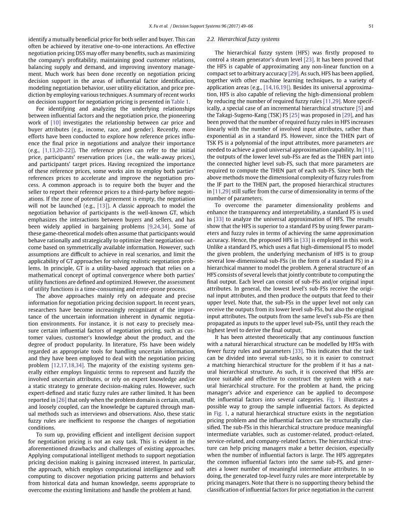
It has been attested theoretically that any continuous functionwith a natural hierarchical structure can be modelled by HFSs withfewer fuzzy rules and parameters [33]. This indicates that the taskcan be divided into several sub-tasks, so it is easier to constructa matching hierarchical structure for the problem if it has a nat-ural hierarchical structure. As such, it is conceived that HFSs aremore suitable and effective to construct the system with a nat-ural hierarchical structure. For the problem at hand, the pricingmanager’s advice and experience can be applied to decomposethe influential factors into several categories. Fig. 1 illustrates apossible way to group the sample influential factors. As depictedin Fig. 1, a natural hierarchical structure exists in the negotiationpricing problem and the influential factors can be structurally clas-sified. The sub-FSs in this hierarchical structure produce meaningfulintermediate variables, such as customer-related, product-related,service-related, and company-related factors. The hierarchical struc-ture can help pricing managers make a better decision, especiallywhen the number of influential factors is large. The HFS aggregatesthe common influential factors into the same sub-FS, and gener-ates a lower number of meaningful intermediate attributes. In sodoing, the generated top-level fuzzy rules are more interpretable bypricing managers. Note that there is no supporting theory behind theclassification of influential factors for price negotiation in the current


Table 1Review of literature drawing on negotiation pricing decision support.

Author(s) & year Method(s) Application domain and datasets Aims and results

Giacomazzi et al. [9] (2012) Game-theoretical approach Simulated dataset in broadbandwireless access

A bilateral negotiation algorithm is proposed to identifythe price of the wireless bandwidth services.

Zhao and Wang [34] (2015) Game-theoretical approach Simulated dataset This work investigates the pricing problem and servicedecisions in a supply chain under fuzzy uncertainty con-ditions. Expected value models are presented to identifythe optimal pricing and service strategies under threedifferent scenarios.

Carbonneau et al. [2] (2008) Neural networks Data obtained from conductingbilateral negotiation experimentsin the Inspire system

This work presents a neural network approach to estimatethe opponents’ responses in negotiations.

Chan et al. [4] (2011) Customer segmentation &expert systems (generatepricing rules by experts) &empirical analysis

Computers and peripherals onlineshop

This work applies customer segmentation, and offers moreprice discounts to more valuable customers. The experi-ment results reveal that the use of differential pricing andpromotion strategies can improve the total sales withoutgreatly reducing the company’s revenues.

Lee et al. [15] (2012) Case based reasoning & fuzzycognitive map

Simulation experiments This paper proposes an agent-based mobile negotiationframework for personalized pricing of last minutes theatertickets whose values are dependent on the time remain-ing until the performance and the locations of potentialcustomers.

Moosmayer et al. [20] (2013) Three layer neural network &questionnaire to collect data

Business-to-business contexts This work explores the importances and significance ofthe influential factors of negotiation pricing. The obtainedorder of significance is: target price, initial price, walk-away price and the size of the relationships.

Wilken et al. [30] (2010) Empirical method Questionnaire survey This work presents how pricing managers can influencesalespeople’s pricing behaviors through information con-trol. A theoretical model is proposed and tested against thecollected dataset.

Kolomvatsos et al. [12] (2014) Fuzzy inference Simulation experiments This work proposes a fuzzy logic (FL) based approach fornegotiation decision support for sellers. Initially, the sellercan use FL reasoning to estimate negotiation time androunds, and then reason based on user-defined FL rules toaccept/reject decisions.

Lin et al. [17] (2011) Fuzzy expert systems (user-defined fuzzy rules)

Internet auction An agent-based price negotiation system is proposed inthis work. Within the system, end users are allowedto customize their negotiation pricing strategies throughuser pre-defined fuzzy rules.

Lin and Chang [18] (2008) Fuzzy approach and fixed/flexible quantity mixedinteger programming (MIP)models

Numerical examples This work develops a fuzzy approach to evaluating buy-ers. The results are employed to support the order selec-tion and final pricing decisions. The more valuable buyersreceive more discounts.

work. The classification of influential factors is actually case driven,and it relies on expert knowledge to construct the hierarchical struc-ture, rather than automatically generating the structure from anyclassification theory.

3. The proposed approach

Fuzzy set theory has become an increasingly prevalent method-ology for representing and dealing with uncertain information, andhas been successfully applied to many IT contexts, such as controlengineering, soft computing, and intelligent DSSs [6,7]. The merits ofutilizing fuzzy sets for representing subjective expertise/knowledge,handling uncertainty, and modeling reasoning processes have beenwidely discussed and verified [31]. This study proposes a systematicand learning approach based on FSs to support negotiation pric-ing. One of the major contributions of this study is shedding lighton investigating the features of three different types of FSs, namelystandard FS, SFS-SISOM, and HFS, especially on their applicabilitiesin handling different negotiation pricing problems. As illustrated inFig. 2, the proposed approach is a data-driven method that aimsto learn from historical transactions. These three types of FSs arethereby integrated into a single prototype system for pricing man-agers. This section presents the mathematical models of these FSs,as well as their associated learning algorithms. Since the standardFS and the SFS-SISOM have been reported in [8], this paper places aparticular focus on the technical details of the HFS.

This study advances the understanding of the bilateral negotia-tion which involves the one-to-one pricing problem. The model aimsto offer the right price to the right customer. Suppose that a series ofinfluential factors is X = (x1, · · · , xn), and the offered price is y; thenthe given problem is to build the mathematical relationship betweenprice y and the vector of influencing factors X. So it is denoted as:

y = P(X) = P(x1, · · · , xn) (1)

If the relationship P(X) can be learned from historical data, then foreach new customer, the right negotiation price can be estimated byusing P(X) based on this customer’s values of the influential factors.As uncertainties are inherent in negotiation pricing, they may exist inthe measure of influential factors, and/or the relationships betweeninfluential factors and the proposed price. Thus an FS approachbecomes suitable and useful herein.

Note that the current study employs expert knowledge to man-ually group the input attributes in the HFS. It is possible to developalgorithms to allow for more automatic grouping of the inputattributes, which may improve the prediction accuracy in somecases. Also, clustering is another plausible and useful approach togrouping the input attributes. One main reason for utilizing the man-ual grouping of the input attributes is due to the consideration ofthe application. Since most of the automatic grouping algorithmsare driven by historical data, they are likely to lead to less rele-vant attributes being selected in the same group. Consequently, the


Fig. 1. The factors influencing negotiation pricing.

intermediate variables will become meaningless and the resultingHFS will lose its interpretability. For example, to consider a DSS forhouse negotiation pricing, if the floor number of the apartment andlocal crime rate are classified in the same group by an algorithm,the corresponding intermediate variables will not be meaningful andthe resulting HFS will just be a numerical model. On the other hand,by allowing a pricing manager to manually group input attributes,he/she may select the floor number and condition of an apartment

in the same group, and include crime rate and closeness to the shop-ping center in the same group. In this manner, the correspondingintermediate variables can be regarded as the house facility indexand location index, which are meaningful. Further, the resulting HFSwill show the impacts of the house facility index and location indexon the price of an apartment. As such, the manual grouping of inputattributes is very useful from an application point of view. For thisreason, it is perhaps a better choice than an algorithm grouping, since

Fig. 2. The proposed approach for negotiation pricing decision support.


it enables a user to build a negotiation pricing model that fits his/herthinking and ensures interpretability and understandability.

3.1. Standard fuzzy system

A MISO standard FS builds a mathematical relationship betweenn input variables and one output variable. It is known in [8] thata complete fuzzy rule base of a standard FS requires K =

∏nj=1 Nj

fuzzy rules, where Nj is the number of fuzzy sets of the jth input vari-able (xj ∈ Uj ⊂ R; j = 1, 2, . . . , n). In order to enhance the model’stransparency, the triangular membership functions that used in [8]are employed in all three types of FSs in this study. Given inputX = (x1, x2, · · · , xn) and output y, the standard FS can be representedas:

y = f (X) =∑

i1 ···in∈I

⎛⎝ n∏

j=1

ljij

(xj)

⎞⎠ yi1 ···in , (2)

where I is the index set that represented as I = {i1, · · · , in|ij =1, 2, · · · , Nj; j = 1, 2, · · · , n}, i1i2 · · · in is the index of fuzzy rule, andl

jij

(xj) is the membership degree of the ithj fuzzy set in the jth inputvariable fired by the input value xj.

In Eq. (2), parameters yi1 ···in are learned from the recursive leastsquare (RLS) learning algorithm [28] whose technical details forimplementation can be found in [8]. To start the learning process, adisturbance parameter (i.e., s) needs to be identified, and it is oftena large number (e.g., 100,000). This parameter is introduced to tuneand balance the fitting to the historical data and to the initial param-eters. During the learning process, the parameters are iterativelyupdated to minimize the sum of errors. In the end, the recursivelearning process terminates either by achieving a satisfied error rate(i.e., e) or reaching the maximum iteration number (i.e., T).

3.2. SFS-SISOM

To address the curse of dimensionality problem in standard FSs,a novel SFS-SISOM has been proposed in [8]. Rather than modelingthe complete combination of all input variables and the output vari-able, the SFS-SISOM resolves the complex model by building a linearcombination of several simple sub-models, and each sub-model rep-resents the relationship between an input variable and the outputvariable. Therefore, a fuzzy rule in the SFS-SISOM only contains oneinput variable and the output variable, and it only requires S =∑n

j=1 Nj (i.e., Nj is the number of fuzzy sets in the jth input variable)fuzzy rules to cover the whole input space.

Mathematically speaking, the SFS-SISOM is formed by severalSISO standard FSs, and the outputs of such SISO FSs contribute tothe final output of the SFS-SISOM by carrying different importantweights. Thus, the SFS-SISOM can be represented as:

y =n∑

j=1

wj

⎛⎝ Nj∑

ij=1

ljij

(xj)yjij

⎞⎠ =

n∑j=1

Nj∑ij=1

wjyjijl

jij

(xj) =n∑

j=1

Nj∑ij=1

C jijl

jij

(xj),

(3)

where wj represents the important weight of the jth input vari-able/SISO standard FS, and y j

ijis the central point of the corre-

sponding fuzzy set of the output variable when given the ithj fuzzy

set in the jth input variable (i.e., xj). These two parameters form anew parameter C j

ijwhich is learned from a RLS algorithm [8], and

its implementation steps are similar to the standard FS, with the

main differences exist in the construction of input matrix, parametervector, and output vector.

3.3. Hierarchical fuzzy system

3.3.1. The model of the hierarchical fuzzy systemThe mathematical model of the standard FS has been introduced

in Section 3.1, and the HFS consists of several standard FSs in a hier-archical manner. As shown in Fig. 3, the ath sub-FS in the hth level (i.e.,SFSh

a) contains several intermediate attributes (i.e., y h,a1 · · · , yh,a

nh,a), and

original attributes (i.e., xh,a1 , · · · , xh,a

mh,a). In this model, x refers to the

original input attributes, while y refers to the output of the sub-FS. The output of SFSh

a , denoted as oh,a, is used as an intermediateattribute (i.e., yh+1,b

1 ) of its upper level’s standard FS, so that the SFSha

can be represented as:

oh,a = y h+1,b1 = fh,a(y h,a

1 , · · · , y h,anh,a

, xh,a1 , · · · , xh,a

mh,a)

=

∑j1 j2 ···jnh,a i1 i2 ···imh,a

y h,aj1 j2 ···jnh,a i1 i2 ···imh,a

∏nh,ak=1 l

h,a,kjk

(yh,ak )

∏mh,ak=1 wh,a,k

ik(xh,a

k )∑j1 j2 ···jnh,a i1 i2 ···imh,a

∏nh,ak=1 l

h,a,kjk

(yh,ak )

∏mh,ak=1 wh,a,k

ik(xh,a

k ).

(4)

In Eq. (4), nh,a is the number of intermediate attributes of SFSha and

mh,a represents the number of the SFSha ’s original input attributes.

yh,anh,a

is the output of the sub-FS in the h − 1 level, and it is used asthe nth

h,a intermediate input attribute of the SFSha; and xh,a

mh,ais the mth

h,aoriginal input attribute of the SFSh

a . Also, j1j2 · · · jnh,a i1i2 · · · imh,a is theindex of fuzzy rules in the SFSh

a , and lh,a,kjk

(yh,ak ) stands for the corre-

sponding output of the jthk fuzzy set of the kth intermediate attributeof the SFSh

a , while wh,a,kik

(xh,ak ) is the output of the ithk fuzzy set in the kth

original input attribute of the SFSha .

By employing the triangular membership functions in the HFS, Eq.(4) can derive that:

∑j1j2 ···jnh,a i1 i2 ···imh,a

nh,a∏k=1

l h,a,kjk

(y h,a

k

) mh,a∏k=1

w h,a,kik

(x h,a

k

)= 1. (5)

Fig. 3. Mathematical model of HFS.


Eq. (4) can be rewritten as:

oh,a =∑

j1 j2 ···jnh,a i1 i2 ···imh,a

⎡⎣nh,a∏

k=1

lh,a,kjk

(yh,a

k

) mh,a∏k=1

w h,a,kik

(xh,a

k

)⎤⎦ yh,a

j1 j2 ···jnh,a i1 i2 ···imh,a.

(6)

The number of fuzzy rules in the HFS can be represented as:

H =L∑

i=1

⎡⎣ Si∑

j=1

⎛⎝ ni,j∏

k=1

Nki,j

mi,j∏k=1

Nki,j

⎞⎠

⎤⎦ (7)

where L is the number of levels in the hierarchical structure and Si

is the number of sub-FSs in the ith level. ni,j and mi,j, respectively,represent the number of intermediate attributes and the number oforiginal input attributes of the jth sub-FS in the ith level (i.e., SFSi

j). Nki,j

is the number of fuzzy sets in the kth input attribute (can be either anintermediate attribute or an original input attribute) of the SFSi

j.

3.3.2. Gradient descent learning algorithmDifferent from the standard FS and SFS-SISOM, the HFS employs

the gradient descent learning algorithm to learn from historicalrecords in this work. Although RLS is capable of finding the globaloptima, it is not applicable to HFS due to the existence of interme-diate attributes. Since an HFS consists of several lower-level sub-FSs,the final output is nonlinearly dependent on the non-top sub-FSs,and the gradient descent learning algorithm is employed herein tooptimize the HFS’s parameters. The objective function of the gradi-ent decent algorithm only minimizes the error based on the currentdata instance (i.e., r):

er =12

[ f (Xr) − yr]2. (8)

In [27], an improved gradient descent algorithm is proposed andit is adapted in this work. This algorithm aims to minimize the localerror by updating the parameters and integrates a normalization stepto handle the intermediate attributes in the HFS. Given an HFS, thefinal error back propagates from the top level to the lower levels, andthe error derived from the upper level is used to update the parame-ters of the neighboring lower level. Assume t is the learning iterationindex; the final error of a HFS is written as:

eL,1(t) = oL,1(t) − y(t), (9)

where L is the total number of levels in an HFS, and oL,1(t) is thepredicted output of the top-level sub-FS in the tth learning iteration,while y(t) is the target output provided in the given dataset. Givena hierarchical structure as shown in Fig. 3, the error of SFSh+1

b ispropagated to SFSh

a in the following way:

eh,a(t) = eh+1,b(t) × ∂oh+1,b(t)∂oh,a(t)

. (10)

For simplicity, the level index (e.g., h and h + 1) is omitted. Hence,Eq. (10) is rewritten as:

ea(t) = eb(t) × ∂ob(t)∂oa(t)

. (11)

Also, the HFS as shown in Eq. (6) can be simplified as:

oa =∑

j1 j2 ···jna i1 i2 ···ima

[ na∏k=1

la,kjk

(ya

k

) ma∏k=1

wa,kik

(xa

k

)]ya

j1j2 ···jna i1i2 ···ima. (12)

The fuzzy rule index j1j2 · · · jna i1i2 · · · ima of the SFSha is denoted as

Ia, and∏na

k=1 la,kjk

(yak)

∏mak=1 wa,k

ik(xa

k) is denoted as AaIa

. Therefore, the

output of the SFSha is represented as:

oa =∑

Ia

AaIa ya

Ia . (13)

Eq. (11) can then be represented as:

ea(t) = eb(t) ×∂∑

IbAb

Ib(t)yb

Ib(t)

∂oa(t)

= eb(t) ×∑

Ib

ybIb

(t)∂Ab

Ib(t)

∂oa(t), (14)

in which∂Ab

Ib(t)

∂oa(t) =Ab

Ib(t)

lb,1j1

(yb1,t)

× ∂lb,1j1

(yb1,t)

∂oa(t) . As shown in Fig. 3, the output

of SFSha (i.e., oa) is the first intermediate attribute (i.e., yb

1) of SFSh+1b .

In addition, since oa = yb1, Eq. (14) can be written as:

∂AbIb

(t)

∂oa(t)=

AbIb

(t)

lb,1j1

(oa, t)×

∂lb,1j1

(oa, t)

∂oa(t). (15)

According to the definition of triangular membership functions, itis derived that:

∂lb,1j1

(oa, t)

∂oa(t)=

⎧⎪⎪⎨⎪⎪⎩

1 oa ∈ [cjk−1, cjk ]

−1 oa ∈ [cjk , cjk+1]

0 otherwise.

(16)

where cjk is the central point of the jthk fuzzy set of the kth attribute in

SFSb. This results in that the propagated error can be represented as:

ea(t) =

⎧⎪⎪⎪⎪⎪⎨⎪⎪⎪⎪⎪⎩

eb(t) × ∑Ib

ybIb

(t)AbIb

(t)

lb,1j1

(oa ,t)oa ∈ [cjk−1, cjk ]

−eb(t) × ∑Ib

ybIb

(t)AbIb

(t)

lb,1j1

(oa ,t)oa ∈ [cjk , cjk+1]

0 otherwise.

(17)

Given the previous iteration results (e.g., yaIa

(t)), the gradientdescent learning algorithm iteratively updates the parameters of thecurrent iteration by:

yaIa (t + 1) = ya

Ia (t) − k × ∂oa(t)∂ya

Ia(t)

× ea(t) (18)

where k is the learning rate parameter, and according to Eq. (13),

∂oa(t)∂ya

Ia(t)

=∂(

∑Ia Aa

Ia(t)ya

Ia(t))

∂yaIa

(t)= Aa

Ia (t). (19)

Therefore, Eq. (18) can be rewritten as:

yaIa (t + 1) = ya

Ia (t) − k × AaIa (t) × ea(t). (20)


To sum up, according to the mathematical model of the HFS (i.e.,Eq. (6)) and gradient descent algorithm (i.e., Eqs. (17) and (20)), thelearning process of the HFS can be described as:

Step 1: Construction of the hierarchical structureThis task involves identifying the number of hierarchical levels,

the number of sub-FSs in each level, the allocation of original inputattributes, and the segmentation of the associated input attributes toconstruct a sub-FS. This is currently identified by the end user.

Step 2: Initialization of the learning parametersThe initial parameters for each sub-FS (e.g., yh,a

Ia(0) for SFSh

a) caneither be initialized by experts or use default values. These param-eters will be iteratively updated in the learning process. Since thegradient descent learning algorithm may converge to a local optima,the choice of initial parameters becomes essential. If the initialparameters are close to the global optima, the algorithm stands agood chance of finding the global optima. Also, the learning rateparameter (i.e., k) and two termination parameters (i.e., the maxi-mum number of iteration T, and the error threshold n) need to beinitialized herein.

Step 3: Update of the parameters by using the recursive gradi-ent descent algorithm

Based on the given initial parameters, calculate the final output ofthe HFS and the error. After that, the error is back propagated fromthe top level to the lowest level by using Eq. (17), and the error foreach sub-FS (e.g., eh,a) can be calculated, respectively. Then apply Eq.(20) to update the parameters for each sub-FS.

Step 4: Normalization of the intermediate parametersIntermediate attributes are a newly introduced problem in the

HFS. In many cases, the intermediate attributes do not have seman-tical meanings. Thus, this may result in the universe of discourseof the derived intermediate attribute being unpredictable and diffi-cult to pre-define. It has been proved in [27] that the approximationaccuracy of the HFS is independent of the definition domain ofintermediate attributes. Therefore, a method is proposed in [27] toovercome this problem by normalizing the domains of intermediateattributes into [0, 1]. The normalization process can be described as:

yh,aIa

=yh,a

Ia− min(yI)

max(yI) − min(yI)(21)

where min(yI) is the minimal value of the intermediate attribute out-puts within all non-top level sub-FSs, while max(yI) is the maximumvalue. This ensures that the value of yh,a

Iaalways lies within [0, 1].

Step 5: Termination of the learning processSimilar to RLS, the recursive learning terminates either by reach-

ing the maximum iteration number T, or reaching a predefined errorthreshold n. Calculate the overall error E(t) = 1

2 ×∑Mr=1(oL,1

r (t)−yr(t));if E(t) < n or t > T, the learning terminates. Otherwise, go back toStep 3 with t = t + 1 and set r = 1 to start a new iteration.

4. Empirical results

4.1. Experimental data

Three negotiation pricing related datasets, which vary from thenumber of instances to dimensionalities, were used in this study. Asummary of these three datasets are presented in Table 2.

4.1.1. DS1 - MP3 player datasetA questionnaire survey was conducted at a major British univer-

sity to collect this dataset. The questionnaire consists of two parts:Part 1 introduces the background scenario, in which a MP3 companyconducts a promotion to provide potential buyers with customizeddiscounts, with the aim to boost the product sales; Part 2 containstwo questions that capture participants’ demographic attributes and

four sets of questions that are associated with the four influentialattributes (i.e., importance, budget, usefulness, and knowledge aboutthe product) of product purchase. Participants were asked to answerthe questions along a five-point Likert-type scale. Furthermore, ifthe product was deemed too expensive at its current price, the par-ticipants were asked to suggest a minimal numeric discount thatwould persuade them to reconsider of the purchase, and the speci-fied discount was also regarded as the reservation price for pricingmanagers. The questionnaires were sent out by hand or electroni-cally distributed via a mailing list to students and academic staff atthe university. A total of 500 questionnaires were send out and 248valid responses were returned and processed for further analysis.

4.1.2. DS2 - Boston house datasetThis is a publicly available dataset that captures the residential

property price for house sales in Boston in 1976.1 In this dataset, 11influential factors (see Table 2) were considered when identifying thehouse price. Given the house properties, the right negotiation pricecan be predicted by employing the proposed models. This dataset,in particular, was chosen to testify to the utility of the proposedapproach in handling relatively high-dimensional problems.

4.1.3. DS3 - California datasetThis dataset collects house information from the 1990 Census

in California, and it is publicly available.2 The dataset includes allblock groups in California and each block group on average includes1,425.5 individuals living in a geographically compact area. The dis-tances among the centroids of each block group as measured inlatitude and longitude were computed. In addition, all the blockgroups reporting zero entities for the observed attributes were fil-tered out. In total, this dataset records 20,640 observations on eightindependent attributes (i.e., median income, housing median age,total rooms, total bedrooms, population, households, latitude, andlongitude) and the dependent variable is ln(median house value).Note that, this dataset does not report individual house information,as it instead captures the aggregated information for all block groups.

4.2. Experimental results

The selection of initial values of learning parameters is a com-mon problem in literature of machine learning. In this work, theinitializations of learning parameters are mainly determined by thecombination of expertise and pre-experiments with the goal toachieve the optimal prediction results (i.e., cross validation basedon least APE and RMSE). In different FSs, different sets of initialvalues of learning parameters were tested in pre-experiments, andonly the learning parameters that produce the optimal results arereported. More specifically, the initializations of the different learn-ing parameters are explained as follows: 1) Error threshold: in orderto monitor the best performance of different FSs, the error thresholdis set to be very small (i.e., 0.01) for all experiments; 2) Number ofiterations: within the pre-experiment, how the error changes withthe increase of iterations can be observed and plotted. The itera-tion parameter that produces the stable prediction performance isselected; 3) Learning rate: it is taken within the range of [0, 1] toavoid missing out the optima, as a small value (e.g., 0.02) of learningrate is selected in this work. A set of the combinations of iterationand learning rate parameters were tested in the pre-experiments;4) Disturbance parameter: this parameter is used to construct thedisturbance matrix in the RLS learning. As suggested by [28], a reallarge number (e.g., 100,000) is often used for the initial value ofthis parameter. The performances standard FSs and SFS-SISOMs are

1 http://lib.stat.cmu.edu/datasets/boston.2 http://lib.stat.cmu.edu/datasets/houses.zip.

http://lib.stat.cmu.edu/datasets/boston

http://lib.stat.cmu.edu/datasets/houses.zip


Table 2Summary of experimental datasets.

Dataset No. of input attributes No. of instances Input attributes Output attribute

DS1 - MP3 player dataset 4 248 1. Usefulness; 2. Importance; 3. Budget;4. Knowledge

Discount

DS2 - Boston house dataset 11 499 1. Crime; 2. Education; 3. Population; 4. Airquality; 5. Zone proportion; 6. No. of rooms;7. Age; 8. Tax; 9. Convenience; 10. Distance;11. Accessibility to highway

Property value

DS3 - California dataset 8 20,640 1. Median income; 2. Housing median age;3. Total rooms; 4. Total bedrooms; 5. Population;6. Households; 7. Latitude; 8. Longitude

ln(median house value)

quite sensitive to this parameter. Therefore, several pre-experimentswere conducted to select the appropriate disturbance parameter fordifferent FSs.

4.2.1. DS1 - MP3 player datasetIn this experiment, three FSs were all employed to predict diverse

situations, which varied in the number of training/testing instances(i.e., 50, 100, and 248 samples were used in different situations,respectively) and fuzzy attribute partitions. In the HFS, a hierarchicalstructure with 2 sub-systems and no free parameters are employedfor all experiments. More specially, Usefulness and importance aregrouped to construct a sub-standard FS, whereas financial capabilityand knowledge are grouped to construct another standard FS. Thelearning rate is set to 0.02 and the error threshold is set to 0.01. Thenumber of iterations for the standard FS and the SFS-SISOM is set to100. Since the input matrixes of the SFS-SISOM and the standard FSare different, the selection of the disturbance parameter (s) valuecould be different. In this study, pre-experiments revealed that thestandard FS and SFS-SISOM achieve optimal results when setting thes = 9999999 and 99999, respectively. The reason for setting a larger

s for the standard FS is that it has more parameters, so a smaller 1/sis needed to weigh down the impact of the initial parameters of thestandard FS model to fit the data better.

The obtained results, as listed in Tables 3 through 5, reveal thatall three FSs perform well when the divided sub-spaces are wellcovered by training samples. The derived results mirror some inter-esting findings: First, the standard FS suffers from the over-fittingproblem when there is an insufficient number of training data sam-ples (e.g., Exp3, Exp10, and Exp12 in Table 3). However, by increasingthe number of training data samples to include all 248 instancesbeing used, the over-fitting problem for the standard FS is removedgradually. Second, when the number of training data samples issufficient to cover the divided sub-spaces, the standard FS, among thethree FSs, performs the best in the sense of goodness of fitting (i.e.,better accuracy for training data or smaller training error). However,the SFS-SISOM and the HFS both obtain better testing accuracy (i.e.,smaller error for testing data) than the standard FS. This is verified,respectively, by the Exp1, Exp7, and Exp13 in Tables 3 and 4. Moreover,compared with the HFS, the SFS-SISOM can obtain similar testingaccuracy with fewer fuzzy rules and a lower number of learning

Table 3Results of using the standard FS in the MP3 player dataset [8].

Experiment Training dataset (#) Testing dataset (#) # of rules Partitions Training APE (%) Training RMSE Testing APE (%) Testing RMSE Running time (second)

Exp1 31–100 (70) 1–30 (30) 36 1,2,1,2 6.6283 1.1305 15.7317 1.7482 1.81Exp2 1–70 (70) 71–100 (30) 36 1,2,1,2 6.5245 0.7582 14.7936 2.4849 1.75Exp3 1–40 (40) 41–100 (60) 36 1,2,1,2 1.6495 0.1739 80.3334 7.8112 1.30Exp4 11–50 (40) 1–10 (10) 36 1,2,1,2 3.2771 0.3826 21.4055 2.5766 1.28Exp5 21–50 (30) 1–20 (20) 36 1,2,1,2 1.1137 0.2591 18.9492 2.8863 1.13Exp6 1–5; 21–50 (35) 6–20 (15) 36 1,2,1,2 1.2440 0.2680 21.3402 3.4829 1.20Exp7 51–248 (198) 1–50 (50) 36 1,2,1,2 8.3482 1.2396 12.6061 1.2643 3.73Exp8 51–248 (198) 1–50 (50) 144 2,3,2,3 3.4679 0.8347 42.5941 3.2094 107.39Exp9 1–30; 91–248 (188) 31–90 (60) 36 1,2,1,2 8.0517 1.0080 14.5664 2.0378 2.08Exp10 1–30; 91–248 (188) 31–90 (60) 144 2,3,2,3 2.5822 0.3812 63.6023 12.2093 101.11Exp11 1–120 (120) 121–248 (128) 36 1,2,1,2 8.6280 1.1464 12.5673 1.7509 2.57Exp12 1–120 (120) 121–248 (128) 144 2,3,2,3 1.7404 0.2948 24.8623 4.6594 111.01Exp13 1–150; 241–248 (158) 151–240 (90) 36 1,2,1,2 9.1615 1.2624 10.2230 1.4241 3.11Exp14 1–150; 241–248 (158) 151–240 (90) 144 2,3,2,3 3.3248 0.7825 24.8890 4.9452 120.21

Table 4Results of using the SFS-SISOM in the MP3 player dataset [8].

Experiment Training dataset (#) Testing dataset (#) # of rules Partitions Training APE (%) Training RMSE Testing APE (%) Testing RMSE Running time (second)

Exp1 31–100 (70) 1–30 (30) 10 1,2,1,2 16.2000 1.7012 12.3035 1.2875 0.47Exp2 1–70 (70) 71–100 (30) 10 1,2,1,2 16.2004 1.6322 12.5001 1.5594 0.42Exp3 1–40 (40) 41–100 (60) 10 1,2,1,2 12.7127 1.0876 16.1389 1.9536 0.29Exp4 11–50 (40) 1–10 (10) 10 1,2,1,2 16.6560 1.3656 6.1107 1.0769 0.22Exp5 21–50 (30) 1–20 (20) 10 1,2,1,2 21.3886 1.4440 7.4940 1.1040 0.19Exp6 1–5; 21–50 (35) 6–20 (15) 10 1,2,1,2 20.4390 1.3806 8.5950 1.1521 0.20Exp7 51–248 (198) 1–50 (50) 10 1,2,1,2 9.8862 1.3894 12.1184 1.4428 0.77Exp8 51–248 (198) 1–50 (50) 14 2,3,2,3 7.9622 1.2033 13.0766 1.2628 0.94Exp9 1–30; 91–248 (188) 31–90 (60) 10 1,2,1,2 9.7417 1.2073 11.7267 1.8978 0.77Exp10 1–30; 91–248 (188) 31–90 (60) 14 2,3,2,3 7.8455 0.9967 10.8846 1.7643 0.88Exp11 1–120 (120) 121–248 (128) 10 1,2,1,2 13.4239 1.5468 10.4996 1.3152 0.61Exp12 1–120 (120) 121–248 (128) 14 2,3,2,3 10.7789 1.3717 8.5867 1.2005 0.74Exp13 1–150; 241–248 (158) 151–240 (90) 10 1,2,1,2 11.1983 1.4857 9.1089 1.3065 0.66Exp14 1–150; 241–248 (158) 151–240 (90) 14 2,3,2,3 10.1013 1.3206 7.6733 1.0936 0.88


Table 5Results of using the HFS in the MP3 player dataset.

Experiment Training dataset(#)

Testing dataset(#)

# of rules Partitions Iterations Training APE (%) Training RMSE Testing APE (%) Testing RMSE Running time(second)

Exp1 31–100 (70) 1–30 (30) 16 1 2; 1 2; 1 1 10,000 9.9741 0.9404 12.7680 1.8076 2.12Exp2 31–100 (70) 1–30 (30) 21 1 2; 1 2; 2 2 6000 10.8963 1.7663 11.7490 1.6266 1.36Exp3 31–100 (70) 1–30 (30) 28 1 2; 1 2; 3 3 10,000 10.4902 1.5118 12.8370 1.8318 2.06Exp4 1–70 (70) 71–100 (30) 16 1 2; 1 2; 1 1 10,000 10.1038 1.2613 12.6070 1.8312 2.06Exp5 1–70 (70) 71–100 (30) 21 1 2; 1 2; 2 2 10,000 9.5615 1.1274 12.2300 1.9679 2.08Exp6 1–70 (70) 71–100 (30) 28 1 2; 1 2; 3 3 10,000 10.5901 1.2619 12.8150 1.9052 2.03Exp7 1–40 (40) 41–100 (60) 16 1 2; 1 2; 1 1 10,000 10.3302 1.5111 12.5770 1.8197 1.24Exp8 1–40 (40) 41–100 (60) 21 1 2; 1 2; 2 2 10,000 11.4601 1.0948 14.9430 2.9411 1.27Exp9 1–40 (40) 41–100 (60) 28 1 2; 1 2; 3 3 10,000 13.8669 1.7309 25.7410 5.6944 1.26Exp10 11–50 (40) 1–10 (10) 16 1 2; 1 2; 1 1 10,000 11.2670 1.2055 6.6900 0.7983 1.27Exp11 11–50 (40) 1–10 (10) 16 1 2; 1 2; 1 1 3000 14.4835 1.4092 10.6896 1.6482 0.53Exp12 11–50 (40) 1–10 (10) 21 1 2; 1 2; 2 2 10,000 16.1273 1.6353 12.9130 1.6091 1.29Exp13 11–50 (40) 1–10 (10) 28 1 2; 1 2; 3 3 10,000 11.8673 1.0891 15.6870 3.7580 1.31Exp14 21–50 (30) 1–20 (20) 16 1 2; 1 2; 1 1 10,000 13.7768 1.1744 8.7620 1.2906 0.99Exp15 21–50 (30) 1–20 (20) 16 1 2; 1 2; 1 1 3000 13.4583 1.3571 12.3371 1.8762 0.45Exp16 21–50 (30) 1–20 (20) 21 1 2; 1 2; 2 2 10,000 12.0021 1.0689 13.0840 2.2542 1.02Exp17 21–50 (30) 1–20 (20) 28 1 2; 1 2; 3 3 10,000 10.8501 0.9221 14.5210 4.8472 1.04Exp18 51–248 (198) 1–50 (50) 16 1 2; 1 2; 1 1 10,000 8.8865 1.3633 12.5860 1.4644 5.40Exp19 51–248 (198) 1–50 (50) 22 2 2; 2 2; 1 1 6000 8.4084 1.3067 13.1501 1.3202 3,40Exp20 51–248 (198) 1–50 (50) 21 1 2; 1 2; 2 2 10,000 8.5953 1.3225 13.9480 1.4482 5,38Exp21 51–248 (198) 1–50 (50) 28 1 2; 1 2; 3 3 10,000 8.9526 1.3174 15.3150 1.3774 5.47Exp22 1–30; 91–248 (188) 31–90 (60) 16 1 2; 1 2; 1 1 6000 9.1456 1.2401 11.1345 1.8376 3.14Exp23 1–30; 91–248 (188) 31–90 (60) 22 2 2; 2 2; 1 1 6000 8.6851 1.1210 12.7091 1.9002 3.30Exp24 1–30; 91–248 (188) 31–90 (60) 21 1 2; 1 2; 2 2 6000 8.0572 1.1163 15.2720 1.8671 3.20Exp25 1–30; 91–248 (188) 31–90 (60) 28 1 2; 1 2; 3 3 6000 8.1971 1.1077 16.0640 1.9446 3.21Exp26 1–120 (120) 121–248 (128) 16 1 2; 1 2; 1 1 6000 10.6254 1.5046 9.9050 1.6352 2.11Exp27 1–120 (120) 121–248 (128) 22 2 2; 2 2; 1 1 6000 10.7058 1.4687 9.9592 1.6921 2.15Exp28 1–120 (120) 121–248 (128) 21 1 2; 1 2; 2 2 6000 11.4216 1.7332 11.6220 2.0507 2.12Exp29 1–120 (120) 121–248 (128) 28 1 2; 1 2; 3 3 6000 10.5594 1.4292 11.5960 1.8939 2.10Exp30 1–150; 241–248 (158) 151–240 (90) 16 1 2; 1 2; 1 1 6000 10.2264 1.4780 9.9200 1.5209 2.70Exp31 1–150; 241–248 (158) 151–240 (90) 22 2 2; 2 2; 1 1 6000 9.9087 1.4225 9.1745 1.3747 2.74Exp32 1–150; 241–248 (158) 151–240 (90) 21 1 2; 1 2; 2 2 6000 10.6577 1.5578 10.1140 1.5967 2.69Exp33 1–150; 241–248 (158) 151–240 (90) 28 1 2; 1 2; 3 3 6000 10.3626 1.5206 10.4050 1.6123 2.74

iterations. Thus, it can be concluded that the SFS-SISOM performs thebest in this experiment.

4.2.2. DS2 - Boston house datasetIn this dataset, there were 499 historical samples with 11 input

attributes. For such a relatively high-dimensional but limited sampledataset, the standard FS was not usable as it requires 211 = 2048fuzzy rules, even when applying the simplest partition in which eachattribute contains only two fuzzy sets. Therefore, only the SFS-SISOMand the HFS were applied in this experiment. The available datasetwas randomly decomposed into training/testing datasets, in which414 samples were randomly selected to form the training datasetand the other 85 records were used as the testing dataset. A natu-ral hierarchical structure (as depicted in Fig. 4) is associated with thegiven problem. Three meaningful intermediate attributes, namelyliving environments, house property, and convenience, construct thetop level standard FS. Hence, the experiments in HFS all employ thesame hierarchical structure which consists of three sub-systems withno free parameters. In addition, the learning rate is set to 0.02 anderror threshold is set to 0.01 for all experiment in the HFS. In the

SFS-SISOM, the disturbance parameter is set to be 99,999 and thenumber of iterations is set to 100. The pre-experiments show thatthe obtained results are very similar when employing different num-ber of iterations (i.e., 10, 100, and 1000), therefore, only the resultsof running the 100 iterations are reported. The results of using theSFS-SISOM and the HFS, together with the employed parameters, arereported in Tables 6 and 7. Note that, in Table 7, when the partitionparameter is set to “n′ ′, this indicates that the original and interme-diate attributes were all divided into n sub-spaces (e.g., Exp2); whenthe partition parameter is set to “n, m′ ′, the original attributes werepartitioned into n sub-spaces, and the intermediate attributes weredivided into m sub-spaces (e.g., Exp1 and Exp3).

It can be concluded from the experimental results that both theSFS-SISOM and the HFS performed well in this dataset, and can beused as effective decision support models. Both approaches achievedapproximately 84% − 88% prediction accuracy in the testing dataset.In general, the HFS performs slightly better than the SFS-SISOM interms of predictability (i.e., Testing APE(%)). On the other hand, thestandard FS was incapable of dealing with this dataset due to thecurse of dimensionality.

Fig. 4. Hierarchical structure for Boston house dataset.


Table 6Results of using the SFS-SISOM in the Boston house dataset [8].

Experiment # of sub-spaces in attributes # of rules Training APE (%) Training RMSE Testing APE (%) Testing RMSE Running time (second)

1 2 3 4 5 6 7 8 9 10 11

Exp1 2 2 3 2 3 2 3 2 2 2 2 25 12.4817 3.6516 14.3455 5.3367 6.53Exp2 3 3 5 3 5 3 5 3 3 3 3 90 12.4064 3.3852 13.1579 5.1074 13.22Exp3 3 3 3 3 3 3 3 3 3 3 3 44 12.0596 3.6064 14.0818 5.1709 9.98Exp4 1 1 2 1 2 1 2 1 1 1 1 25 13.0903 3.7723 13.1299 5.2278 3.62Exp5 2 2 2 2 2 2 2 2 2 2 2 33 14.9134 4.1978 16.5419 6.0427 5.53

Table 7Results of using the HFS in the Boston house dataset.

Experiment # of rules Partitions Iterations Training APE (%) Training RMSE Testing APE (%) Testing RMSE Running time (second)

Exp1 253 2,3 6000 13.6606 4.1415 12.8858 5.5013 66.93Exp2 48 1 6000 15.3197 4.5951 15.2067 6.7762 59.48Exp3 104 1,3 6000 14.0024 4.8466 13.4519 6.5981 61.96Exp4 116 1 3 1 3; 1 2 1 2; 1 1 1; 1 1 1 6000 12.2817 3.6230 13.9064 5.9200 60.25Exp5 212 1 3 1 3; 1 2 1 2; 3 3 3; 3 3 2 6000 14.1919 3.6930 13.7923 5.5817 63.53Exp6 212 1 3 1 3; 1 2 1 2; 3 3 3; 3 3 2 3000 13.1382 3.4611 14.4630 6.0849 32.92

4.2.3. DS3 - California datasetIn this dataset, 20,640 observations were randomly partitioned

into two subsets, in which 70% (i.e., 14,448) were used for trainingand 30% (i.e., 6,192) were used for testing. The eight input attributescan be naturally grouped into two standard sub-FSs: the medianincome, population and households reflect the block group properties,while the housing median age, total rooms, total bedrooms, lati-tude, and longitude represent the house properties. Then these twomeaningful intermediate attributes (i.e., block group properties andthe house properties) construct the top-level standard FS. Thus, thesub-FSs construction setting is: 1 5 6; 2 3 4 7 8. The experiments ofthe HFS in this dataset all employ the above hierarchical structurethat consists of two sub-FSs with no free parameters. In addition,the learning parameters of the HFS were set to: learning rate = 0.02,error threshold = 0.01, and iterations = 1000. In the standard FS, inorder to obtain the result within an hour, the number of iteration isset to 1 because the computational cost is very high (see more detailsin Section 5.4). The results of using the three FSs, together with theused parameters, are reported in Tables 8 through 10.

The results reveal that in general all three FSs can achieve verygood performances in terms of training and testing prediction accu-racy (i.e., 96.3% –98.2%). However, the standard FS and the SFS-SISOMare quite sensitive to the disturbance parameter. If an inappropriatedisturbance parameter was employed, the performance drops dra-matically and even fails to derive the results (e.g., Exp3 in Table 8;Exp4 and Exp8 in Table 9). In addition, although the standard FS canproduce good prediction results, the flexibility of dividing the inputspace is quite limited due to its high computational complexity. Asshown in Table 8, when 384 fuzzy rules are involved, it takes over45 min to derive the results. It is time consuming and even impracti-cal to employ the standard FS when some attributes are required tobe finely divided. The HFS produces slightly better prediction perfor-mance than the SFS-SISOM, but with far more fuzzy rules. Althoughthe number of required fuzzy rules is large, the running time toderive the result is short because the HFS requires much less space

computational cost. Moreover, the HFS is less sensitive to the learn-ing parameters, it produces more stable prediction performances inthis experiment. This dataset involves relatively high dimensions,and the HFS outperforms the other two FSs with respect to theinterpretability for the following reasons: 1) the standard FS jointlyconsiders eight attributes in a fuzzy rule, and the derived fuzzy rulemight be too complicated for end users to understand. Also, onlya small number of fuzzy sets (i.e., 1 or 2) is employed to describean attribute due to the curse of dimensionality; 2) the SFS-SISOMonly considers one attribute in a fuzzy rule. Instead, the HFS decom-poses the high-dimensional problem into three sub-SFSs, therefore,the negotiation behaviors can be better explained and understoodby considering diverse modeling granularities. Further from Exp5 inTable 10, it shows that by uneven partitions for different attributes,the number of rules in the HFS can be reduced significantly. The dis-tinguishing merit of the SFS-SISOM is the modeling efficiency, as itcan produce good prediction accuracy by using fewer fuzzy rules anditerations as long as the right learning parameters are identified.

In summary, this experiment shows that both the SFS-SISOM andthe HFS can handle high dimensional and large data effectively. Thedataset is based on the block group rather than individual house, asit is less complicated and less non-linear, therefore the linear model(i.e., the SFS-SISOM) performs well. However, it is expected that, ifthe dataset with the individual houses is available, the HFS can bemore useful and effective. Therefore, the proposed three FSs providea comprehensive set of model choices and are able to handle variousneeds to accurately model the negotiation pricing behavior.

5. Discussion

5.1. Interpretability and transparency

In regard to the development of DSSs, interpretability/transparency is one of the most crucially desirable features. It is ofparamount importance for researchers to further apply this insight

Table 8Results of using the standard FS in the California dataset.

Experiment # of rules Partitions Disturbance parameter Training APE (%) Training RMSE Testing APE (%) Testing RMSE Running time (second)

Exp1 256 1,1,1,1,1,1,1,1 999 1.9407 0.3120 1.9653 0.3156 1,013.79Exp2 256 1,1,1,1,1,1,1,1 99999 1.8963 0.3057 1.9432 0.3322 511.17Exp3 256 1,1,1,1,1,1,1,1 9999999 14.6492 8.1259 15.5764 10.5383 543.34Exp4 384 2,1,1,1,1,1,1,1 999 1.8679 0.3022 1.8922 0.3040 2,754.45Exp5 384 2,1,1,1,1,1,1,1 99999 1.8248 0.2963 1.8728 0.3185 2,785.24


Table 9Results of using the SFS-SISOM in the California dataset.

Experiment # of sub-spaces in attributes # of rules Disturbance parameter Iterations Training APE (%) Training RMSE Testing APE (%) Testing RMSE Running time

1 2 3 4 5 6 7 8 (second)

Exp1 1 1 1 1 1 1 1 1 16 999 10 2.2763 0.3913 2.2711 0.3653 9.13Exp2 1 1 1 1 1 1 1 1 16 999 1000 2.2699 0.3574 2.2657 0.3591 519.16Exp3 1 1 1 1 1 1 1 1 16 9999 10 2.4640 0.3837 2.4566 0.3848 9.01Exp4 1 1 1 1 1 1 1 1 16 99,999 10 N/A N/A N/A N/A 8.89Exp5 2 2 2 2 2 2 2 2 24 999 10 2.1638 0.3446 2.1531 0.3419 13.04Exp6 2 2 2 2 2 2 2 2 24 999 1000 2.1590 0.3436 2.1498 0.3413 1,409.67Exp7 2 2 2 2 2 2 2 2 24 9999 10 2.2233 0.3508 2.2170 0.3487 13.23Exp8 2 2 2 2 2 2 2 2 24 99,999 10 18050.908 2838.5105 18183.354 2866.5483 13.05Exp9 3 3 3 3 3 3 3 3 32 999 10 2.0386 0.3263 2.0354 0.3247 21.06Exp10 3 3 3 3 3 3 3 3 32 9999 10 2.1547 0.3414 2.1586 0.3413 20.62Exp11 3 3 3 3 3 3 3 3 32 99,999 10 N/A N/A N/A N/A 20.39Exp12 4 4 4 4 4 4 4 4 40 999 10 2.0918 0.3340 2.0752 0.3296 30.35Exp13 4 4 4 4 4 4 4 4 40 9999 10 2.2093 0.3486 2.1936 0.3448 30.68Exp14 4 4 4 4 4 4 4 4 40 99,999 10 8.9838 1.6173 9.1614 1.6408 30.74

to the predicament of negotiation pricing. The proposed FS approachnot only enables effective knowledge discovery, but also efficientknowledge representation in the form of linguistic IF-THEN fuzzyrules, which are understandable and interpretable. When the dimen-sion is low, the standard FS has the best interpretability, because itcan explain the complete conditions of input attributes within onefuzzy rule. On the contrary, the SFS-SISOM can merely representone influential aspect and the outcome in the derived fuzzy rules.However, the standard FS and the SFS-SISOM offer a flat view in thesense that all attributes are listed at the same level, and the impactsof different attributes become less apparent when a large numberof attributes and rules are involved. In the HFS, individual and lessimportant attributes are aggregated (by the lower level sub-FS)into the higher-level indexes, which are combined with importantattributes to form a top-level sub-FS to derive the system output(i.e., the negotiation price). For example, in DS2, the higher-levelsub-FS shows the aggregated impacts (in terms of intermediatevariables) of living environments, house property, and convenienceon the house price. In this manner, the top-level sub-FS providesa high-level overview and interpretation (i.e., from a forest pointof view), while the lower-level sub-FS represents a more detailedview of how each index is formed or formulated (i.e., how the forestis formed from trees). In other words, the fuzzy rules derived fromthe HFS present comprehensive multi-views to understand negoti-ation pricing behaviors. Such a feature of HFSs, which can provideboth tree and forest views, is very useful for complicated negotia-tion pricing problems to ensure and enable the interpretability andtransparency.

5.2. Accuracy

The APE (%) and the RMSE were employed in this study to mea-sure performance accuracy. Such performance is dependent on howwell the partitioned sub-spaces are covered by the training data. Inorder to analyze this point, consider the case where n input attributesexist and the input space of each attribute is partitioned by m sub-spaces (i.e., m+1 fuzzy sets). As such, there are mn and m×n dividedsub-spaces in the standard FS and the SFS-SISOM, respectively. Inthe HFS, the total number of the divided sub-spaces is the same as

the number of the divided sub-spaces in the hierarchical level thatcontains the maximum number of attributes. Suppose there are Llevels in the structure and ni attributes in the ith level; then thetotal number of divided sub-spaces can be represented as:

∑Li=1 mni .

Since n =∑L

i=1 ni, in most cases, the number of the divided sub-spaces in the SFS-SISOM (i.e., m × n) and the number in the HFS (i.e.,∑L

i=1 mni ) is smaller than that of the standard FS (i.e., mn). Thus, thedivided sub-spaces in the SFS-SISOM and the HFS stands a betterchance of being covered when given the same training dataset andpartitions. This explains why the testing accuracy of the standardFS is lower than the other two FSs in some cases. Besides the num-ber of required data samples, the selected learning algorithms alsocontribute to the model’s performance. The RLS learning algorithmsfor standard FSs and SFS-SISOMs ensure that the global optima arefound. However, the gradient decent algorithm used in HFSs maylead to a local optima. If the selected initial parameters diverge to theglobal optima, the performance of the HFS can be affected.

5.3. Generality

Generality relates not only to the capability of handling wideproblem domains, but also the capability of satisfying various mod-eling requirements. In general, compared to the SFS-SISOM and theHFS, the standard FS is less generic in handling high-dimensionalproblems due to the large number of learning parameters and fuzzyrules it requires. In order to cover the divided input space, the num-ber of required training samples should be at least as many as thenumber of required fuzzy rules; otherwise, the standard FS may suf-fer from the high-dimensional problem. This drawback is clearlyevident in some experiments in DS1 (e.g., Exp12 in Table 3) and theinability to build usable models on DS2. In addition, from the appli-cation point of view, in some cases the user would like to partitionthe input variable into a specified number of sub-spaces, such thatthe negotiation behavior in a certain sub-space could be observed.The capability of the standard FS to satisfy various modeling require-ments is also bounded by the dimensionality problem. For instance,in the DS1, the standard FS fails to produce acceptable predictiveresults when the input attributes need to be partitioned into “2,3,2,2”sub-spaces (i.e., Exp8, Exp10, and Exp12 in Table 3). Under the same

Table 10Results of using the HFS in the California dataset.

Experiment # of rules Partitions Iterations Training APE (%) Training RMSE Testing APE (%) Testing RMSE Running time (second)

Exp1 76 1 1 1;1 1 1 1 1;5 5 1000 2.5533 0.3977 2.6233 0.4107 226.16Exp2 306 2 2 2;2 2 2 2 2;5 5 1000 2.1122 0.3413 2.1939 0.3581 328.81Exp3 1124 3 3 3;3 3 3 3 3;5 5 1000 1.9511 0.3160 2.039 0.3320 395.49Exp4 3286 4 4 4;4 4 4 4 4;5 5 1000 1.866 0.3084 1.9342 0.3160 636.48Exp5 780 5 1 1;1 4 1 5 5;5 5 1000 1.9082 0.3111 1.9908 0.3257 355.71


Table 11Summary of running time.

Standard FS SFS-SISOM HFS

No. of rules (iterations) running time (second) No. of rules (iterations) running time (second) No. of rules (iterations) running time (second)

DS1 36 (100) 1.99 10 (100) 0.46 16−28 (6000) 2.56114 (100) 109.93 14 (100) 0.86 16−28 (10000) 2.19

DS2 N/A 25−90 (10) 7.78 48−212 (6000) 62.43DS3 256 (1) 689.43 16−48 (100) 23.59 76−1124 (1000) 326.54

384 (1) 2,769.84 16−48 (1000) 964.42 3286−8028 (1000) 875.30

circumstance, SFS-SISOM and HFS are still capable of accomplish-ing such tasks. As such, the SFS-SISOM and the HFS are superiorto the standard FS in terms of model generality. Further, HFSs areuniversal approximators and, therefore, can represent any nonlinearnegotiation pricing models, whereas SFS-SISOMs are not universalapproximators and cannot accurately model some highly nonlinearscenarios.

5.4. Computational cost

The computational cost concerns both the space and time com-plexity in this study. For space complexity, both standard FSs andSFS-SISOMs need to construct the input matrix. Hence, the requiredspace for standard FSs is O(MK), where M is the number of instances,K =

∏nj=1 Nj is required number of fuzzy rules, and Nj is the num-

ber of fuzzy sets of the jth attribute, while the required space forSFS-SISOMs is O(MS), where S =

∑nj=1 Nj is the required num-

ber of fuzzy rules for SFS-SISOMs. Since HFSs employ the gradientdecent algorithm for learning, the learning parameters are updatedby instances. Therefore, the required computational space of HFSs ismuch less than the other two FSs, and it is O(H), where H (see Eq. (7))is the number of required fuzzy rule of HFSs.

In the proposed approach, triangular membership functions areselected in order to achieve the interpretability and computing effec-tiveness. Triangular membership functions are basically piecewiselinear functions, and their derivatives are simple to calculate. GivenT iterations, the time complexity of standard FSs is either O(KMT) orO(KMn

−2) (depends on which termination condition reaches first),where n is the error threshold. The time complexity of SFS-SISOMsis either O(SMT) or O(SMn

−2). In HFSs, although there are multi-levelsub-FSs, all computations only involve the derivatives of triangu-lar membership functions and some simple algebraic manipulations.The time complexity of HFS can be represented as either O(HMT) orO(HMn

−2) [3]. In this study, all the experiments were conducted ona laptop with Mac OS X 10.7.4, processor 1.7 GHz Intel Core i5, 4 GBmemory, and the running time of different FSs on different datasets

Fig. 5. Applicability of different FSs.

are summarized in Table 11. Table 11 shows that the proposed mod-els can obtain the results within a few seconds in most cases, and thestandard FSs take the longest time to derive the result, which is con-sistent with the above analyses. In DS3, the standard FS takes over45 min when 384 rules are involved. For SFS-SISOMs, if the numberof iteration is small, it is quick to derive the result. For HFSs, althoughthey involve a large number of fuzzy rules in DS3, the space complex-ity is small, therefore, the running time of each iteration of the HFSsis actually less than the standard FSs and SFS-SISOMs.

5.5. Applicability

One of the main contributions of this work is examining the appli-cability of three FSs in dealing with negotiation pricing. In this study,no approach can always outperform the others. The above experi-mental results reveal that the applicability of three FSs can differ, sounderstanding their applicabilities would be beneficial to select theappropriate approach for the given problem. Generally speaking, thestandard FS is a better approach for low-dimensional problems withsufficient data samples (i.e., dense data coverage). The main reasonbehind this is that the required number of partitioned sub-spaces inthe input space is relatively small when modeling low-dimensionalproblems, and such sub-spaces are more likely to be well coveredby training samples. This would help to improve prediction per-formance. Moreover, in the standard FS, complete combinations ofinput conditions are linked through fuzzy intersection operators andare represented in the form of fuzzy rules. As such, it is more suitableto select the standard FS when it is required to emulate and observedifferent aspects of negotiation pricing behaviors. On the contrary,the SFS-SISOM is a better approach for high-dimensional problemswith insufficient data samples (i.e., sparse data coverage). In the SFS-SISOM, the mathematical relationship between the input attributesand the output attributes is individually emulated. This results inrequiring far fewer fuzzy rules when modeling the high-dimensionalproblems. The applicability of three FSs are depicted in Fig. 5.

The performance of the HFS lies between the standard FS and theSFS-SISOM, as both the standard and the SFS-SISOM FSs can be rep-resented as special cases of HFS (as shown in Fig. 6). When thereare no free parameters in the hierarchical structure and each original

Fig. 6. Special cases of HFSs.


Table 12Summary of the properties of three FS approaches.

Approach Interpretablity Computational cost Generality Flexibility

Low-dimensional high-dimensional

Standard FS A C C C CSFS-SISOM C B A B BHFS B A B A A

input attribute constructs a sub-FS (e.g., SFS11, SFS1

2, and SFS13 in Fig. 6),

the HFS becomes a SFS-SISOM. On the other hand, when only onesub-FS exists (i.e., the top level sub-FS) in the hierarchical structure,and all original input attributes contribute to the top level sub-FS,the HFS can be treated as a standard FS. Consequently, HFSs providemore flexibility in building the predictive model, as the hierarchicalstructure can be modified according to the features of the availabledatasets. Compared with the other two FSs, HFSs can be more easilyadapted to meet various modeling requirements. The discussions ofthe properties of three FSs are summarised in Table 12 in which ‘A’indicates the best performance and ‘C’ indicates the worst.

The newly introduced HFS is important for the following rea-sons: First, compared to standard FSs, which can represent anycontinuous function to any degree of accuracy (i.e., universal approx-imators) but suffer from the problem of dimensionality, HFSs areuniversal approximators and are capable of overcoming the problemof dimensionality. Second, from the learning mechanism point ofview, although both SFS-SISOMs and HFSs can handle the high-dimensional data, the mechanism behind is vastly different. TheSFS-SISOM is a simplified approach by omitting certain impacts ofpricing attributes and more complicated behaviors (in particular, theaggregated cross or 1 + 1 > 2 effect), so that it can be learned from

less data. However, the SFS-SISOM is unable to represent some com-plicated systems or behaviors (i.e., not universal approximators) dueto their inherent structure. On the other hand, the HFS does not omitpricing component, but employs the transfer learning mechanismto handle data coverage problem. Take the DS2 for an example, aslong as there are sufficient data to learn the relationship between thethree intermediate variables and the house price, as well as how eachof the above three intermediate variables are formed, the knowledgefrom one data sample of good living environment, property, and con-venience can be transferred to represent other cases of good livingenvironment, property, and convenience even if these other casesare good due to different reasons (i.e., the values of the attributes inthese cases are different from the available data sample). In short,rather than using the simplification or omitting attributes as SFS-SISOMs, the transfer mechanism enables HFSs to work effectivelywhen training samples don’t densely cover the input space. Thus,HFSs as universal approximators are capable of representing anycomplicated systems and providing a flexible structure to representany given negotiation pricing system with the right complexity anddesired accuracy if designed properly. Third, in the case of a largenumber of negotiation attributes, HFSs can be designed to developinterpretable systems where the lower-level sub-systems represent

Fig. 7. Prototype system - model design.


the impact from the raw attributes, and the higher-level sub-systemsprovide a small number of human-understandable indexes whichaggregate the impacts from a set of raw attributes.

6. Developing a prototype system

In this section, a prototype system has been developed and pre-sented. The system is a standalone Java application that providesintelligent decision support for a series of negotiation pricing tasks.The system allows pricing managers to load dataset, design, train, andtest the fuzzy model, and then predict the negotiation price/discountfor a new transaction. The graphic user interface (GUI) consists offive components: menu, toolbar panel, display panel, tab controlpanel, and status display panel (see Fig. 7). The menu groups thebasic functions of the system, and the toolbar panel provides a moreconvenient way to access these functions. Once a user clicks thefunctional buttons on the toolbar panel, the tab control panel willautomatically switch to the corresponding tab. When the system isin use, the current status and instructions are displayed on the statusdisplay panel. The basic functions are presented below:

• Open and view dataset: At the beginning, a pricing managercan select the dataset which will be modeled from the Openbutton. Before the system is in use, the user should ensurethe training dataset and the corresponding testing dataset willbe readily available and are named correctly in the predefinedway (i.e., filename + “-Test” indicates the testing dataset).The loaded dataset, including the training dataset and testingdataset, can then be displayed in the display panel.

• Design the model: When the user clicks the Design buttonon the toolbar panel, a design panel, as shown in Fig. 7, isprovided and allows the user to identify the model type andspecify different learning parameters. The design panel con-tains two parts: the SFS panel for the design of standard and

SFS-SISOM FSs, and the HFS panel for the design of HFSs.Once the model type is selected, only the corresponding designpanel is enabled. The learning parameters and the hierarchi-cal structure of HFSs must be entered in a predefined format.A tooltip with the format instructions is also provided for eachparameter. The raw dataset will be reconstructed according tothe defined structure (e.g., attributes that in the same sub-FSwill be grouped together). The reconstructed dataset can bechecked via the “Processed Data” option in the “View” menu.

• Train and test the model: Once the design of the predictivemodel is accomplished, the user can click the Train button totrain the designed model. The learning algorithm and definedparameters are employed to learn the fuzzy rules from thetraining dataset. The training results and generated rules willthen be displayed. Consequently, the generated fuzzy rules(see Fig. 8) are used in conjunction with the testing datasetto further validate the built model. The testing results, includ-ing target values, predicted value, error, APE, and RMSE, areshown in Fig. 9. The plot of the target value and the predictedvalue provides the user with a clear and intuitive view of modelperformance.

• Prediction: A suggested negotiation price/discount can be pro-vided by the system to assist the pricing manager when givena new transaction. In the prediction panel, the user can manu-ally enter the information of a new transaction, and then clickthe Predict button. The predicted price will be displayed (anexample is shown in Fig. 10). This proposed price can be usedas a baseline or resistance point in the price negotiation.

7. Conclusions

This study proposes a systematic and learning approach con-sisting of three different FSs (i.e., standard FS, SFS-SISOM, and

Fig. 8. Prototype system - generated fuzzy rules.


Fig. 9. Prototype system - model testing.

HFS) to provide intelligent decision support for negotiation pricing,in particular under the high-dimensional and uncertain scenarios.The effectiveness and applicability of the proposed approaches aredemonstrated by three experimental datasets, varying from dimen-sionality to data coverage. The main contributions of this workinclude: 1) Instead of tackling the difficult and unrealistic tasks toidentify and maximize the utility functions in negotiation pricing,this work proposes a new learning approach that concentrates onidentifying the right negotiation pricing by learning from historicaldata. The proposed approach also is capable of learning the differentinfluential factors for different customers, gaining a good customerrelationship by offering the right price to the right customer; 2) Tohandle the uncertain information in negotiation pricing, a system-atic and comprehensive set of fuzzy models is proposed, developed,and compared. Their advantages and capabilities under differentapplication scenarios are analyzed and discussed with respect to thecrucial properties of DSSs: interpretability and transparency, accu-racy, generality, computational cost, and applicability; and 3) A DSSprototype integrating the three FSs is developed and validated. Thesystem illustrates how the negotiation pricing DSS based on theproposed approach can be designed and implemented for practicaluses.

This research has several significant implications for researchand practice. First, interpretability and transparency is one of themost desirable features for DSSs. Compared with other data min-ing techniques (e.g., neural networks), the FS-based approach iscapable of transforming the acquired negotiation pricing knowledgeinto human understandable IF-THEN fuzzy rules. The derived fuzzyrules can serve as unified guidance in negotiation pricing and alsobe employed to train new sales representatives. Second, this studyendeavors to draw more attention to the dimensionality problem innegotiation pricing, which has yet to be thoroughly investigated in

the literature. It has been proven both theoretically and practicallythat the standard FS is more susceptible to the problem of dimen-sionality. This study has shown that the other two types of FSs canbe used as a means to complement the standard FS in handling high-dimensional problems. Third, this study reveals the properties andfeatures of the three FSs. The proposed approach and the integratedplatform can provide immense potential and flexibility for end usersto choose the most suitable model for any particular problem.

Like many prior empirical studies, this research inevitably hasseveral limitations that may trigger further research. With the rapiddevelopment and promising results of e-negotiations, the proposedapproach can be integrated into e-negotiation platforms. In addition,the current prototype is not role-based and it does not distinguishdifferent groups of targeted users (e.g., data operators, model train-ers, salespeople, and managers). It is an important direction toimprove the prototype by separating different tasks for differentgroups of users, and providing clear visuals that guide users to theappropriate and applicable parts of the system. Moreover, since dif-ferent users may have different preferences on the model properties,it is difficult for the intelligent DSS to determine the most appropri-ate FS model on behalf of the decision maker. One plausible way toautomate the model selection is to allow the user to specify his/hermodel preferences in the prototype system, then an overall perfor-mance score can be derived. Finally, it will be interesting to extendthe current model to support multi-issue and bilateral negotiationdecision support for future studies. If the historical data of biddingand offering during the price negotiation process were available, itwill be possible to build two additional models to learn the bid-ding behavior and successful offering strategy. Then the system willbe not only able to predict the final agreement prices proposed inthis study, but also guide the offering strategy based on the biddingbehavior.


Fig. 10. Prototype system - model prediction.

Acknowledgments

This work is supported by the National Natural Science Foun-dation of China (No. 71301133, 71572166, 71671153, 71671149,and 71202059) and the Fundamental Research Funds for theCentral Universities (Project No. 20720161044). The authors aregrateful to the reviewers and editor for their invaluable and insight-ful comments that have helped to improve this work. Thanks alsogo to all participants who have helped completed the MP3 datasetquestionnaire.

References

[1] M. Cao, X. Luo, X.R. Luo, X. Dai, Automated negotiation for e-commerce deci-sion making: a goal deliberated agent architecture for multi-strategy selection,Decis. Support. Syst. 73 (2015) 1–14.

[2] R. Carbonneau, G.E. Kersten, R. Vahidov, Predicting opponent’s moves in elec-tronic negotiations using neural networks, Expert Syst. Appl. 34 (2) (2008)1266–1273.

[3] C. Cartis, N.I.M. Gould, P.L. Toint, On the complexity of steepest descent,Newton’s and regularized Newton’s methods for nonconvex unconstrainedoptimization problems, SIAM J. Optim. 20 (6) (2010) 2833–2852.

[4] C.-C.H. Chan, C.-B. Cheng, W.-C. Hsien, Pricing and promotion strategies of anonline shop based on customer segmentation and multiple objective decisionmaking, Expert Syst. Appl. 38 (2011) 14585–14591.

[5] F.-L. Chung, J.-C. Duan, On multistage fuzzy neural network modeling, IEEETrans. Fuzzy Syst. 8 (2) (2000) 125–142.

[6] X. Fu, Q. Shen, Fuzzy compositional modelling, IEEE Trans. Fuzzy Syst. 18 (4)(2010) 823–840.

[7] X. Fu, Q. Shen, Fuzzy complex numbers and their application for classifiersperformance evaluation, Pattern Recogn. 44 (7) (2011) 1403–1417.

[8] X. Fu, X. Zeng, D. Wang, D. Xu, L. Yang, Fuzzy system approaches to negotiationpricing decision support, J. Intell. Fuzzy Syst. 29 (2) (2015) 685–699.

[9] P. Giacomazzi, I. Stanojev, G. Verticale, A negotiation-based scheme for servicelevel pricing for wireless access, Comput. Commun. 35 (4) (2012) 444–453.

[10] P.K. Goldberg, Dealer price discrimination in new car purchases: evidence fromthe consumer expenditure survey, J. Polit. Econ. 104 (3) (June 1996) 622–654.

[11] M. Joo, J. Lee, Universal approximation by hierarchical fuzzy system withconstraints on the fuzzy rule, Fuzzy Sets Syst. 130 (2002) 175–188.

[12] K. Kolomvatsos, C. Anagnostopoulos, S. Hadjiefthymiades, Sellers in e-marketplaces: a fuzzy logic based decision support system, Inf. Sci. 278 (2014)267–284.

[13] S. Kwon, B. Yoo, J. Kim, W. Shang, G. Lee, Reservation price reporting mech-anisms for online negotiations, Decis. Support. Syst. 46 (4) (2009) 755–762.

[14] V. López, A. Fernández, M.J. del Jesus, F. Herrera, A hierarchical genetic fuzzysystem based on genetic programming for addressing classification with highlyimbalanced and borderline data-sets, Knowl.-Based Syst. 38 (2013) 85–104.

[15] K.C. Lee, H. Lee, N. Lee, Agent based mobile negotiation for personalized pricingof last minute theatre tickets, Expert Syst. Appl. 39 (10) (2012) 9255–9263.

[16] I.-H. Li, L.-W. Lee, A hierarchical structure of observer-based adaptive fuzzy-neural controller for MIMO systems, Fuzzy Set. Syst. 185 (1) (2011) 52–82.

[17] C.-C. Lin, S.-C. Chen, Y.-M. Chu, Automatic price negotiation on the web: anagent-based web application using fuzzy expert system, Expert Syst. Appl. 38(5) (2011) 5090–5100.

[18] H.-T. Lin, W.-L. Chang, Order selection and pricing methods using flexible quan-tity and fuzzy approach for buyer evaluation, Eur. J. Oper. Res. 187 (2) (2008)415–428.

[19] D. Linkens, J. Shieh, J. Peacock, Hierarchical fuzzy modelling for monitoringdepth of anaesthesia, Fuzzy Sets Syst. 79 (1) (1996) 43–57.

[20] D.C. Moosmayer, A.Y.-L. Chong, M.J. Liu, B. Schuppar, A neural networkapproach to predicting price negotiation outcomes in business-to-businesscontexts, Expert Syst. Appl. 40 (8) (2013) 3028–3035.

[21] D.C. Moosmayer, B. Schuppar, F.U. Siems, Reference prices as determinantsof business-to-business price negotiation outcomes: an empirical perspectivefrom the chemical industry, J. Supply Chain Manag. 48 (1) (2012) 92–106.

[22] S. Park, G.E. Bolton, L. Rothrock, J. Brosig, Towards an interdisciplinary perspec-tive of training intervention for negotiations: developing strategic negotiationsupport contents, Decis. Support. Syst. 49 (2010) 213–221.

[23] G.V.S. Raju, J. Zhou, R. Kisner, Hierarchical fuzzy control, Int. J. Control. 54 (5)(1991) 1201–1216.

[24] A. Rubinstein, Perfect equilibrium in a bargaining model, Econometrica 50 (1)(1982) 97–109.

[25] T. Takagi, M. Sugeno, Fuzzy identification of systems and its applicationsto modeling and control, IEEE Trans. Syst. Man Cybern. SMC-15 (1) (1985)116–132.

[26] E. Turban, J.E. Aronson, T.-P. Liang, Decision Support Systems and IntelligentSystems (7th Edition), Prentice-Hall, Inc., Upper Saddle River, NJ, USA, 2004.

[27] D. Wang, X. Zeng, J.A. Keane, Intermediate variable normalization for gradientdescent learning for hierarchical fuzzy system, IEEE Trans. Fuzzy Syst. 17 (2)(2009) 468–476.

[28] L.-X. Wang, A Course in Fuzzy Systems and Control, Prentice Hall PTR. 1997.[29] L.-X. Wang, Universal approximation by hierarchical fuzzy systems, Fuzzy Sets

Syst. 93 (2) (1998) 223–230.

http://refhub.elsevier.com/S0167-9236(17)30019-2/rf0005






























[30] R. Wilken, M. Cornelien, K. Backhaus, C. Schmitz, Steering sales reps throughcost information: an investigation into the black box of cognitive referencesand negotiation behavior, Int. J. Res. Mark. 27 (1) (2010) 69–82.

[31] L. Zadeh, J. Kacprzyk, Computing with Words in Information/Intelligent Sys-tems: Foundations. Studies in Fuzziness and Soft Computing, Physica-Verlag.1999.

[32] L.A. Zadeh, Fuzzy sets, Inf. Control. 8 (1965) 338–353.[33] X. Zeng, J.A. Keane, Approximation capabilities of hierarchical fuzzy systems,

IEEE Trans. Fuzzy Syst. 13 (5) (2005) 659–672.[34] J. Zhao, L. Wang, Pricing and retail service decisions in fuzzy uncertainty

environments, Appl. Math. Comput. 250 (0) (2015) 580–592.

Xin Fu is an Associate Professor in the School of Man-agement, Xiamen University, China. She received her PhDdegree in Computer Science from Aberystwyth Univer-sity, UK. Her research interests include decision supportsystems, fuzzy and qualitative modelling, business intel-ligence, and predictive toxicology. Her research has beenpublished in journals including Decision Support Systems,Information & Management, IEEE Transactions on FuzzySystems, Pattern Recognition, Journal of Cheminformatics,etc.

Xiao-Jun Zeng received the B.Sc. degree in mathemat-ics and the M.Sc. degree in control theory and operationresearch from Xiamen University, China, and the Ph.D.degree in computation from the University of Manchester,U.K. He has been with the University of Manchester since2002, where he is currently a Senior Lecturer with theSchool of Computer Science. His current research interestsinclude computational intelligence, machine learning anddata mining, decision support systems and game theorywith the applications to energy demand side manage-ment and pricing. In these areas, he has published morethan 120 papers in international journals and conferenceproceedings. His research impact case Intelligent pricingdecision support systems has been selected as one of 20impact cases studies to highlight impact made by UK aca-

demic Computer Science Research within UK and world over the period 2008-2013.Dr. Zeng is an Associate Editor of the IEEE Transactions on Fuzzy Systems and a mem-ber of the peer review college of the U.K. Engineering and Physical Sciences ResearchCouncil. With KSS Ltd, UK, his research won the European Information Society Tech-nologies Award in 1999 and the Microsoft European Retail Application DeveloperAwards in 2001 and 2003.

Xin (Robert) Luo is an Endowed Regents Professor andAssociate Professor of MIS and Information Assurance inthe Anderson School of Management at the University ofNew Mexico, USA. He received his Ph.D. in MIS from Mis-sissippi State University, USA. He has published researchpapers in leading journals including European Journal ofInformation Systems, Decision Support Systems, Communi-cations of the ACM, Journal of the AIS, Journal of StrategicInformation Systems, Information Systems Journal, Informa-tion & Management, and Computers & Security, etc. Heis currently serving as an Ad-hoc Associate Editor for MISQuarterly and an Associate Editor for Decision Sciences,European Journal of Information Systems, Electronic Com-merce Research, Journal of Electronic Commerce Research,and International Conference on Information Systems. His

research interests center around information assurance, innovative technologies forstrategic decision-making, and global IT management.

Di Wang received the Bachelors degree in computerscience and technique from Tianjin University, Tianjin,China, in 2001 and the Ph.D. degree in computer engineer-ing form Nanyang Technological University, Singapore, in2005. Currently Dr Wang is a senior research with EBTIC,Khalifa University. Her primary research focus has beenon social media analytics and specifically, short messageanalysis. Dr. Wang developed a customer service proto-type for Etisalat from tweets. She has also developed atraffic analysis engine using tweets for the department oftransport in the UK. In addition, she is also working onan application for smart transport as part of MK Smart,a smart city project in the UK. Dr. Wang has about 50publications and 2 patent inventions under filling.

Di Xu is a Full Professor of management science and Asso-ciate Dean of School of Management at Xiamen University,China. He received his PhD from Xiamen University. Hisresearch interests are in the areas of information systemsand ecommerce.

Qingliang Fan is currently an Assistant Professor of Eco-nomics at the Wang Yanan Institute for Studies in Eco-nomics and School of Economics, Xiamen University,China. He earned his Ph.D. in North Carolina State Uni-versity. His research interests are theoretical and appliedeconometrics, high dimensional econometrics and bigdata analysis on consumers and investors behaviors. Hehas publications in both international and domestic jour-nals, such as Journal of Econometrics. He also developedSTATA user defined ado files for some of the methods hepublished.






designing an intelligent decision support system for

Documents