designing and back-testing a trading strategy for stocks
TRANSCRIPT
Designing and back-testing a trading strategy for stocks combining LPPLS
signal and fundamentals
Master Thesis
Xingyu Yang
June, 2019
Supervisor: Prof. Sornette Didier, Dr. Ke Wu

Acknowledgements
ii
Acknowledgements I would like to express my gratitude to my supervisor Dr. Ke Wu for the expert guidance of my master thesis and to the support that my professor Sornette Didier has provided me throughout my study in the master’s program.
Abstract
iii
Abstract The goal of this thesis is to back-test the effectiveness of a trading strategy based on the Bubble Score and Value Score which comes from the LPPLS model and ROIC valuation framework, respectively. According the Bubble Score and Value Score, stocks can be categorized into 4 types, thus correspond buy/sell decisions will be made. We use the LPPLS output and quarterly fundamental data of S&P500 index constituents from 20 years ago till 12/2018 to back-test the strategy. By changing the holding period as 3, 6, 9, and 12 months, and impose constraints regarding the market cap, P/E ratio, Bubble Score, Value Score and Growth Score, we could further improve the performance of initial strategy and find out the optimal trading condition for each portfolio. Our trading strategy outperforms the benchmark to different extent, where the contrarian long stock portfolio always has higher annualized return than the trend-following long stock portfolio. By combining the all or a subset of trend-following long stock portfolio, contrarian long stock portfolio, trend-following short stock portfolio and contrarian short stock portfolio, a self-financing portfolio can be constructed which is less sensitive to the trend of the broad market. A modification on ROIC curve is presented and proved to be effective to improve the valuation power.
Table of content
iv
Table of content Acknowledgements ...................................................................................................... ii
Abstract ........................................................................................................................ iii
Table of content .......................................................................................................... iv
List of Tables .............................................................................................................. vi
List of Figures ............................................................................................................. vii
Notation ...................................................................................................................... xi
1 Introduction ........................................................................................................... 1
2 Methodology ......................................................................................................... 3
2.1 LPPLS Model .................................................................................................. 4
Bubble mechanics ................................................................................................ 4
Assumptions of LPPLS model .............................................................................. 5
Derivation of LPPLS model .................................................................................. 5
2.2 Value Score ..................................................................................................... 6
ROIC as a viable screening factor ........................................................................ 7
EV/IC vs. ROIC regression ................................................................................... 8
Exclusion of financial sector ............................................................................... 10
2.3 Growth Score ................................................................................................ 10
3 Derive and back-test a trading strategy .............................................................. 11
3.1 Trading strategy ............................................................................................ 11
3.2 Exploration of statistical characteristics of trading strategies ........................ 12
3.3 Back-test the trading strategy ....................................................................... 30
Base strategy ...................................................................................................... 30
Add a constraint on the market cap (Strategy 1) ................................................ 33
Change the weight of each stock in the portfolio ................................................ 35
Add a constraint on the P/E Ratio (Strategy 4) ................................................... 40
Add a constraint regarding the scores ................................................................ 43
A summary of strategies ..................................................................................... 51
3.4 Look back at the ROIC Valuation Framework ............................................... 54
4 Conclusion .......................................................................................................... 61
5 Outlook ............................................................................................................... 62
6 Appendix ............................................................................................................. 63

Table of content
v
Data ........................................................................................................................ 63
Bibliography ............................................................................................................... 64

List of Tables
vi
List of Tables Table 3.1 6 cases mentioned above and their description ........................................ 15
Table 3.2 Optimal holding period and constraint for 4 portfolios according to the boxplots shown above, which tells us the direction of how to improve the performance of the strategy. ........................................................................................................... 30
Table 3.3 Sharpe ratio for base strategy ................................................................... 31
Table 3.4 Calmar ratio for base strategy ................................................................... 32
Table 3.5 Sharpe ratio and Calmar ratio for Strategy 1 ............................................. 34
Table 3.6 Sharpe ratio and Calmar ratio for Strategy 2 ............................................. 36
Table 3.7 Sharpe ratio and Calmar ratio of Strategy 3 .............................................. 39
Table 3.8 Sharpe ratio and Calmar ratio of Strategy 4 .............................................. 41
Table 3.9 Sharpe ratio and Calmar ratio of Strategy 5 .............................................. 44
Table 3.10 Sharpe ratio and Calmar ratio of strategy 6 ............................................. 47
Table 3.11 Sharpe ratio and Calmar ratio of strategy 7 ............................................. 49
Table 3.12 Strategies and description ....................................................................... 51
Table 3.13 Comparison of strategies ......................................................................... 52
Table 3.14 Evaluation metrics of the above portfolio ................................................. 54

List of Figures
vii
List of Figures Figure 2.1 Categorizing stocks into 4 quadrants, stocks with strong positive bubble signals and strong (weak) fundamentals are assigned to quadrant 1 (2, respectively), stocks with strong negative bubble signals and weak (strong) fundamentals are assigned quadrant 3 (4, respectively). ......................................................................... 4
Figure 2.2 The ROIC curve for S&P500 constituent stocks. The blue markers are the real market value of ln(EV/IC) vs. ROIC for single stocks, and the red line is the fitted linear model between ln(EV/IC) and ROIC. In the title of the figure, “slope” is the coefficient of ROIC, and “intercept” is the constant in the model. ................................ 9
Figure 3.1 ROIC-based valuation curve for individual industries on 31/10/2018. The title of each figure includes the sector name and parameters of the regression model. The robust regression model is in the form of ln𝐸𝑉𝐼𝐶 = 𝛽 ∙ 𝑅𝑂𝐼𝐶 + 𝑐, where 𝛽 corresponds to the “slope” in the title and 𝑐 corresponds to the “intercept” in the title. The scatter plot is the real ROIC and ln(EV/IC) plotted on the xy-plane, and the red line is the fitted linear relationship between the ROIC and ln(EV/IC) obtained from the model. ........................................................................................................................ 14
Figure 3.2 Trend-following long stock portfolio, annualized return vs. Bubble Score range. The panel 1 - 6 is corresponding to Case 1 - 6 respectively, where the bars colored by blue, green, red and turquoise represent holding period being 3, 6, 9 and 12 months respectively. The black line across the bar is the median of the corresponding annualized return, and the red spot is the mean of the corresponding annualized return. ...................................................................................................... 17
Figure 3.3 Trend-following long stock portfolio, annualized return vs. Value Score range. The format is same as in Figure 3.1. .............................................................. 19
Figure 3.4 Contrarian short stock portfolio, annualized return vs. Bubble Score range. The format is same as in Figure 3.1. ......................................................................... 20
Figure 3.5 Contrarian short stock portfolio, annualized return vs. Value Score range. The format is same as in Figure 3.1. ......................................................................... 22
Figure 3.6 Trend following short stock portfolio, annualized return vs. Bubble Score range. The format is same as in Figure 3.1. .............................................................. 24
Figure 3.7 Trend following short stock portfolio, annualized return vs. Value Score range. The format is same as in Figure 3.1. .............................................................. 26
Figure 3.8 Contrarian long stock portfolio, annualized return vs. Bubble Score range. The format is same as in Figure 3.1. ......................................................................... 27
Figure 3.9 Contrarian long stock portfolio, annualized return vs. Value Score range. The format is same as in Figure 3.1. ......................................................................... 29
Figure 3.10 The cumulative returns of four portfolios vs. the benchmark S&P500 from Jan. 2000 to Nov. 2018. The lines colored by blue, green, red, gold and black represent the cumulative of trend-following long stock portfolio, contrarian long stock portfolio, trend-following short stock portfolio, contrarian short stock portfolio and

List of Figures
viii
S&P500, respectively. Panel a – d manifest the situation of holding portfolios for 3, 6, 9, and 12 months respectively. .................................................................................. 31
Figure 3.11 The cumulative returns of the portfolio which combines the four portfolios equally. The blue line draws the cumulative return of the combined portfolio, and the black line is the cumulative return of the bench mark S&P500 index. .......... 32
Figure 3.12 Combine 4 portfolios equally with their own optimal holding period for base strategy. The TFLSP, CLSP, TFSSP and CSSP are hold for 9, 6, 3 and 9 months respectively. The format is same as in Figure 3.11 ................................................... 33
Figure 3.13 Strategy 1, remove stocks with market cap lower than 0.05 quantile at every rebalance date. The format is same as in Figure 3.10. .................................... 34
Figure 3.14 The cumulative returns of the portfolio which combines he four portfolios equally for strategy 1. The format is same as in Figure 3.11. .................................... 35
Figure 3.15 Combine 4 portfolios equally with their own optimal holding period for strategy 1. The TFLSP, CLSP, TFSSP and CSSP are hold for 9, 6, 3 and 9 months respectively. The format is same as in Figure 3.11. .................................................. 35
Figure 3.16 Strategy 2, remove stocks with market cap lower than 0.05 quantile at every rebalance date, assign the equal weight to stocks. The format is same as in Figure 3.10. ................................................................................................................ 36
Figure 3.17 The cumulative returns of the portfolio which combines the four portfolios equally for strategy 2. The format is same as in Figure 3.11. .................................... 37
Figure 3.18 Combine 4 portfolios equally with their own optimal holding period for strategy 2. The TFLSP, CLSP, TFSSP and CSSP are hold for 6, 6, 3 and 9 months respectively. The format is same as in Figure 3.11. .................................................. 38
Figure 3.19 Strategy 3, remove stocks with market cap lower than 0.05 quantile at every rebalance date, assign the weight as reversely proportional to the market ca of the stock. The format is same as in Figure 3.10. ....................................................... 39
Figure 3.20 The cumulative returns of the portfolio which combines the four portfolios equally for strategy 3. The format is same as in Figure 3.11. .................................... 40
Figure 3.21 Combine 4 portfolios equally with their own optimal holding period for strategy 3. The TFLSP, CLSP, TFSSP and CSSP are hold for 3, 6, 3 and 9 months respectively. The format is same as in Figure 3.11. .................................................. 40
Figure 3.22 Strategy 4, only select stocks with P/E ratio below 0.6 quantile in the corresponding industry for long stock portfolio (type 1 and 4 stocks), and stocks with P/E ratio over 0.4 quantile in the corresponding industry for short stock portfolio (type 2 and 3 stocks). The format is same as in Figure 3.10. ............................................. 41
Figure 3.23 The cumulative returns of the portfolio which combines the four portfolios equally for strategy 4. The format is same as in Figure 3.11. .................................... 42
Figure 3.24 Combine 4 portfolios equally with their own optimal holding period for strategy 4. The TFLSP, CLSP, TFSSP and CSSP are hold for 6, 6, 3 and 9 months respectively. The format is same as in Figure 3.11. .................................................. 43

List of Figures
ix
Figure 3.25 Strategy 5, only select absolute value of bubble score below 0.4 for trend-following portfolio (type 1 and 3 stocks) and select absolute value of bubble score over 0.6 for contrarian portfolio (type 2 and 4 stocks). The format is same as in Figure 3.10. ................................................................................................................................... 44
Figure 3.26 Strategy 5, holding period = 1 month, the format is same as in Figure 3.10. The TFLSP, CLSP, TFSSP and CSSP are hold for 3, 1, 3 and 9 months respectively. The format is same as in Figure 3.11. ....................................................................... 44
Figure 3.27 Combine 4 portfolios equally with their own optimal holding period for strategy 5. Panel a – e is the cumulative return of the combined portfolio in which each portfolio is hold for same period. Panel f is the cumulative return of the combined portfolio in which each portfolio is hold for its optimal period. The TFLSP, CLSP, TFSSP and CSSP are hold for 3, 1, 3 and 9 months respectively. The format is same as in Figure 3.11. ....................................................................................................... 46
Figure 3.28 Strategy 6, only select stocks with Value Score over 0.8 for long stock portfolios (type 1 and 4 stocks) and stocks with Value Score below 0.2 for short stocks portfolios (type 2 and 3 stocks). The format is same as in Figure 3.10. .................... 47
Figure 3.29 The cumulative returns of the portfolio which combines the four portfolios equally for strategy 6. The format is same as in Figure 3.11. .................................... 48
Figure 3.30 Combine 4 portfolios equally with their own optimal holding period for strategy 6. The TFLSP, CLSP, TFSSP and CSSP are hold for 6, 6, 3 and 3 months respectively. The format is same as in Figure 3.11. .................................................. 48
Figure 3.31 Strategy 7, only select stocks with Growth Score over 0.6 for long stock portfolios (type 1 and 4 stocks) and stocks with Growth Score below 0.4 for short stocks portfolios (type 2 and 3 stocks). The format is same as in Figure 3.10. .................... 49
Figure 3.32 The cumulative returns of the portfolio which combines the four portfolios equally for strategy 7. The format is same as in Figure 3.11. .................................... 50
Figure 3.33 Combine 4 portfolios equally with their own optimal holding period for strategy 7. The TFLSP, CLSP, TFSSP and CSSP are hold for 6, 6, 3 and 9 months respectively. The format is same as in Figure 3.11. .................................................. 50
Figure 3.34 The cumulative return of a combination of different portfolios mentioned above (this is a self- financing portfolio). The blue line is the cumulative return of the combination, the black line is the cumulative return of the benchmark S&P500. ...... 54
Figure 3.35 An example of the anomaly for energy stocks (01/05/2000). The Slope of the linear regression for Energy sector is negative, indicating the negative correlation between the ROIC and ln(EV/IC), which is opposite of the theory and truth. ............ 56
Figure 3.36 Regression results for ROIC-based valuation framework (panel a) and (ROIC - WACC) based valuation framework (panel b) considering stocks from all the industries. The format is same as in Figure 3.1 except that this figure is for the broad market which includes all the sectors except Financial sector. ................................. 56
Figure 3.37 Regression results for ROIC-based valuation framework (panel a) and (ROIC - WACC) based valuation framework (panel b) for each individual industry. The format is same as in Figure 3.1. ................................................................................ 58

List of Figures
x
Figure 3.38 Comparison of the portfolios in the section 3.3.6 between the same strategies based on ROIC and (ROIC-WACC) respectively. The black line is the original cumulative return of the portfolios starting from 01/2016 till 12/2018, and the blue line is the cumulative returns of the portfolios from 21/2016 to 12/2018 after adjusting the ROIC by deducting WACC. Panels a – d are for the 4 types of portfolios included in the combined portfolios, and the panel e is for the combined portfolio. .. 59
Notation
xi
Notation Abbreviation
Symbol Meaning LPPLS Log-Period Power-Law Singularity TFLSP Trend-following long stock portfolio CLSP Contrarian long stock portfolio TFSSP Trend-following short stocks portfolio CSSP Contrarian short stock portfolio
Introduction
1
1 Introduction Making predictions about stock prices has been an essential goal for hedge funds and individual investors. There has existed various theories and methods regarding stock market prediction among which the efficient market hypothesis (EMH) and the random walk view have found favor among financial academics. As posited by EMH, the stock prices are a function of rational expectation and information, which implies that the current prices have reflected all the publicly known information as well as the price history, and stock prices fluctuate responding to the release of the new information, changes in the market generally and random movements around the intrinsic value. The intrinsic value is essentially the level that the price of a stock moves around, which is the market’s expected discounted present value of the future cash flow associated with the stock. The random movements, which is later described by the “random walk” process make it impossible to predict the stock prices accurately as the deviation from the central value is random and unpredictable.
Attempting to rigorously challenge key propositions of EMH, “rational bubbles” theory demonstrates that, even with rational expectations and behavior, “rational” deviations in stock prices from their intrinsic values – rational bubbles – would be possible [1]. Rational bubbles emerge when stock prices diverge gradually faster from the path determined by its economic fundamentals. The formation and growth of rational bubbles reflect the presence of arbitrary and self-confirming expectations about future increases in stock prices, that is, investors buy stocks solely with the expectation that they would be resold at higher prices to other investors who are willing to buy them for the same reason. Hence, an explosive deviation from the intrinsic value would be possible even if investors held rational expectations and the rational arbitrage conditions were fulfilled.
Both the EMH and rational bubbles theories could explain the stock prices to some extent; however, they fail to explain large stock prices crashes, not to mention identifying the bubbles ex-ante. An alternative approach to model the financial bubbles is to fit a Log-Period Power-Law Singularity (LPPLS) to asset prices. In the standpoint of LPPLS model [2], financial bubble is defined as a strong deviation from the intrinsic value which will result in the unsustainable growth staggered along corrections and rebounds. As the bubbles growing, the crash risk is increasing and finally the financial market crashes once the bubble matures at a critical time.
The phenomena that the bubble matures and crashes might be caused by positive feedback mechanism, imitation and herding behavior, bounded rationality and moral hazard theories [3]. The positive feedback mechanism could be explained by the self-confirming expectation mentioned above which indicates that investors buy an overvalued stock on purpose not for the intrinsic value but for the sake of selling it to other investors at a higher price instead. Herding behavior refers to the tendency for an individual to imitate the actions of a larger groups, whether those actions are rational or not, which implies that investors tend to price the stocks according to other’s expectations rather than their intrinsic values. Bounded rational theory represents that people make more or less reasonable decisions that are usually not optimal due to the

Introduction
2
limited time and available information. Moral hazard occurs when investors know that someone else will bear the risk which in turn gives him the incentive to act in a riskier way. The US real estate bubble is a good example of moral hazard theory. Serious financial bubbles can trigger problems in a larger scale and spread catastrophic effects to global economy after burst. Understanding the financial bubbles and identifying them ex-ante is of big significance.
Contrary to the traditional models which assume an exponential growth in stock prices with a static growth rate, the LPPLS model takes into consideration the positive feedback mechanism and herding behavior, which in turn fits better for stock prices that follow a hyperbolic curve which is led by non-linear dynamics of the financial markets where many intelligent and interacting players are involved in a hierarchical network structure who affect one another continuously [4]. LPPLS model detects the bubbles and regime changes in financial markets. It assumes that as a bubble emerges, due to the positive feedback mechanism caused by the herding behavior, the stock price follows a certain type of oscillations superposed on faster-than-exponential growth.
At the platform Financial Crisis Observatory, an FCO Cockpit report is published on a monthly basis, synthesizing the global bubble status. As a part of this report, a set of US stocks is analyzed by calculating the bubble risk as well as the fundamental value and the expected growth potential. Combining the bubble status and the fundamental values, trading decisions could be made along with the growth and crash of stocks and a factor model could be thus developed. This can be compared to the Fama and French Factor Model which adds size risk and value risk factors to the market risk factor in the capital asset pricing model (CAPM) [5]. This model considers the fact that value and small-cap stocks outperform markets on a regular basis [6]. In the same spirit, the reality that stocks follow a faster-than-exponential growth outperform market in all probability makes it reasonable to add the bubble factor to the traditional valuation and growth assessment of stocks. This turns out a trading strategy which combines bubble score, values score and growth score, which is thought to be a better tool for adjusting for herding behavior and evaluating the stocks.
In this thesis, the methodology regarding the LPPLS model and ROIC-based valuation framework will be first explained in section 2. In section 3, according to this stock selection and valuation method, boxplot will be presented to look for a direction for developing a trading strategy. Based on this descriptive statistical analysis, a series of trading strategies will be back-tested and discussed. Portfolios will be constructed corresponding to the strategies. By comparing the evaluation metrics such as Sharpe ratio, we find the optimal holding period and trading strategy for each of the portfolios. Then we look back at the ROIC curve which is used to derive the Value Score, and make a little modification, which is then proved to be effective to better value stocks. In section 4, we finally give conclusions about the trading strategies and portfolios we’ve been working on.
Methodology
3
2 Methodology During a bubble, the observed price of a stock deviates from its fundamental value; where during a positive bubble, there is excessive demand, while during a negative bubble, there is disproportionate selling [7]. Bubbles usually leave some traces behind which makes it possible to diagnose them timely. Here comes the LPPLS model to hunt for the distinct fingerprint of financial bubbles. It detects whether the price follows super-exponential curve and whether it is now still in the unsustainable growth.
Financial strength of a stock is evaluated by two indicators: value score and growth score. These two scores, ranging from zero to one where one being the best and zero the worst, demonstrate how a stock is ranked among the set of stocks, that is, the higher the score, the higher the financial strength. Value score is based on the linear model of ROIC (return on invested capital) versus EV (enterprise value) per unit of invested capital, calculated by sorting the ROIC level versus EV/IC in each industry. The growth score has characteristics similar to the PEG ratio, which is the price to earnings (P/E) ratio normalized by the expected growth of the earnings per share (EPS).
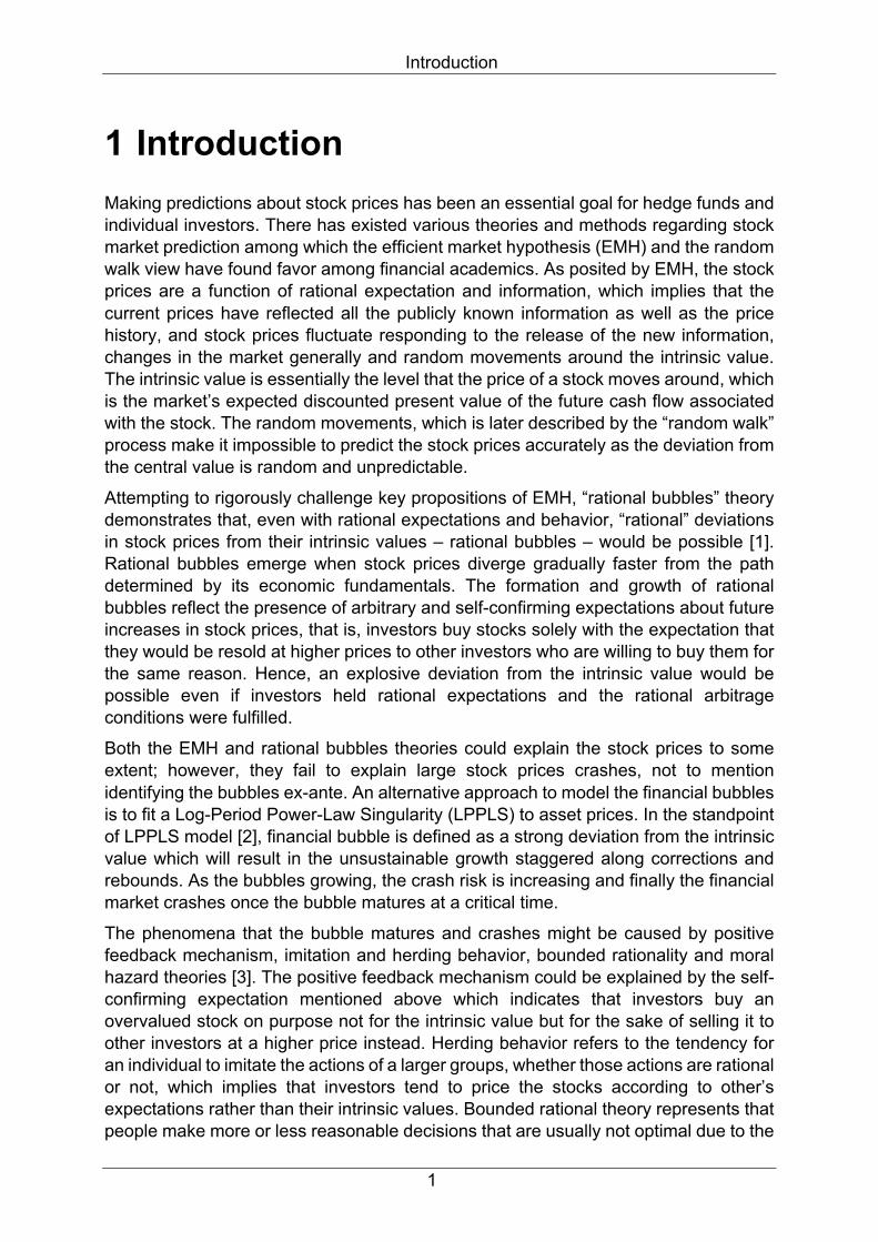
The stocks can thus be classified into four quadrants by plotting the aggregated bubble score against the value score. The four quadrants in turns represent four types of investors:
1. Quadrant 1: Stocks with a strong value score are considered cheap relative to their earning potential. A strong positive bubble score is a momentum indicator resulting from a repricing based on the fundamentals. As an investor, one could be a trend-following buyer.
2. Quadrant 2: Stocks with a weak value score considered expensive relative to their earning potential. A strong positive bubble score indicates the sentiment and herding behavior are increasing the price until it is not linked to the fundamental value anymore. As an investor, one could be a contrarian seller.
3. Quadrant 3: Stocks with a weak value score are expensive relative to their earning potential. A strong negative bubble score is considered as falling knives, which is a strong indicator for the price to drop drastically. As an investor, one could be a trend-following seller.
4. Quadrant 4: Stocks with a strong value score are cheap relative to their earning potential. However, there are clearly negative bubbles due to the sentiment and herding behavior. Such stocks are considered oversold. As an investor, one could be a contrarian buyer.
For each of the quadrants, a portfolio can be constructed based on the classification of the stocks. Note that a strong positive signal is identified if bubble score is larger than 0, and a strong negative bubble signal is identified if bubble score is smaller than 0. A strong value score is identified if value score is larger than 60%, and a weak value score is identified if value score is smaller than 40%.

Methodology
4
Figure 2.1 Categorizing stocks into 4 quadrants, stocks with strong positive bubble signals and strong (weak) fundamentals are assigned to quadrant 1 (2, respectively), stocks with strong negative bubble signals and weak (strong) fundamentals are assigned quadrant 3 (4, respectively).
2.1 LPPLS Model
Bubble mechanics
A bubble is essentially an unsustainable process where the positive feedback mechanism is involved. Consequently, the growth rate is not constant anymore and itself grows, which causes the price to follow a hyperbolic power law trajectory ending in some critical point or singularity where the it’s very likely that a crash or a correction happens.
A bubble starts with a new opportunity or expectation which can be a breakthrough in technology, the access to a new market, or in the realm of trading, a breaking of a support level. In all probability, a promising future in any of these cases will ensue. Attracted by the prospect of the expected high return, more investors surge in, which will push the price up. The increase in price further attracts more investors; the demand increases as the prices moves up, and the price moves up further as the demand increases, this is the so-called positive feedback, which is the essential ingredient that triggers an unsustainable growth process. The positive feedback is often caused by imitation: the herding behavior pushes the price up, and the increasing price leads to higher demand, which results in the break of the equilibrium of supply and demand.
In reality, the unsustainable growth process is not smooth. Usually, due to the specific dynamic and structural features of the market, typical patterns of oscillations can be observed. According to the study of the social structure [8], traders and investors are interacting in the way that they imitate each other which leaves an impact on their coordinated buy and sell orders. This discrete social structure has a real effect on the pricing mechanism during the phases of strong herding and creates a specific pattern in price with accelerating oscillations. As a consequence, the increasing oscillations with decreasing amplitude will be observed in the price due to the discrete temporal hierarchy imitation. This is the so-called log-periodicity.
The unsustainable faster-than-exponential growth will necessarily end, which can be the burst of the bubble, or the fading of the bubble.
Quadrant 1: trend-following buyer
Quadrant 2:
Contrarian seller
Quadrant 4: contrarian buyer
Quadrant 3: trend-following seller
Value Score
Aggregated Bubble Score

Methodology
5
Assumptions of LPPLS model
We use the Log-Periodic Power Law Singularity (LPPLS) model to hunt for the distinct fingerprint of financial bubbles. Basic assumptions of the model are as follows:
1. When the positive (negative) bubbles is growing, the price increases (decreases) faster than exponentially. Hence, the logarithm of the price increases faster than linearly.
2. Accelerating log-periodic oscillations are constantly emerging around the super-exponential price evolution that represents the increasing volatility towards the crash of the bubble.
3. When the bubble is coming to the end, the so-called critical time 𝑡0, a finite time singularity takes place after which the bubble crashes.
Derivation of LPPLS model
The LPPLS model is developed based on the Johansen-Ledoit-Sornette (JLS) model [9]. The price dynamics of an asset during a bubble phase can be described as:
12323= 𝜇(𝑡)𝑑𝑡 + 𝜎9𝑑𝑊9 − 𝜘𝑑𝑗 (2.1)
where𝜇(𝑡) is the expected return, 𝜎9 is the volatility, 𝑊9 is a standard Brownian motion, 𝑑𝑊9 represents an infinitesimal change in a Brownian motion over the next instant time, 𝑑𝑗 represents a discontinuous jump in the asset price where 𝑑𝑗 = 0 and 𝑑𝑗 = 1 correspond to before and after the crash, respectively, and 𝜘 represents the size of a possible crash or rebound. The dynamics of jumps are controlled by the hazard rate ℎ(𝑡), which measures how much the bubble is likely to crash. Specifically, ℎ(𝑡)𝑑𝑡 implies the probability that a crash will occur between 𝑡 and 𝑡 + 𝑑𝑡 under the condition that the crash has not happened yet, which yields that Et[𝑑𝑗] = 1 × ℎ(𝑡)𝑑𝑡 + 0 × (1 −ℎ(𝑡)𝑑𝑡), thus the expectation of 𝑑𝑗 can be written as
Et[𝑑𝑗] = ℎ(𝑡)𝑑𝑡 (2.2)
Note that if the expected return 𝜇(𝑡) is constant, and the discontinuous jump is missing, the price process is a geometric Brownian motion, resulting in that the deterministic part of the asset price is the standard differential equation for exponential price growth.
Under the arbitrage-free condition, the price process is a martingale, that is E9[𝑑𝑝9] =0. Multiplying the equation (2.1) with 𝑝9 on both sides and taking the expectation yields
Et[𝑑𝑝9] = 𝜇(𝑡)𝑝9𝑑𝑡 + 𝜎9𝑝9Et[𝑑𝑊9] − 𝜘𝑝9Et[𝑑𝑗] = 0 (2.3)
Noting that Et[𝑑𝑊9] = 0 and combining equation (2.2) and (2.3), we can obtain that
𝜇(𝑡) = 𝜘ℎ(𝑡) (2.4)
The equation (2.4) shows that the expected return is proportional to the hazard rate ℎ(𝑡). Recall that the hazard rate ℎ(𝑡) represents the probability that a bubble crashes, which is in accordance with the common sense that the investors are compensated for higher risk with higher expected return. When the jump has not occurred (𝑑𝑗 = 0), the equation (2.1) becomes
12323= 𝜇(𝑡)𝑑𝑡 + 𝜎9𝑑𝑊9 = 𝜘ℎ(𝑡)𝑑𝑡 + 𝜎9𝑑𝑊9 (2.5)

Methodology
6
Integrating and taking the expectation of the above equation yields
E9[ln2323G]=𝜘 ∫ ℎ(𝑥)9
9G𝑑𝑥 (2.6)
It can be seen from the above equation that under the condition that the price follows the martingale process, the higher the risk of bubble crashing, the faster the price increases. In other words, the price growth is driven by the growth of the hazard rate ℎ(𝑡). Recall that the unsustainable price growth process is caused by the positive feedback and herding behavior, so the hazard rate ℎ(𝑡) is supposed to reflect the herding behavior and the hierarchical structure of the financial markets. As posited in Johansen et al. [10], the hazard rate should be in the following form:
ℎ(𝑡) = 𝛼(𝑡0 − 𝑡)KLM(1 + 𝛽cos(𝜔ln(𝑡0 − 𝑡) − 𝜙S)) (2.7)
The equation (2.7) reveals that the risk of a bubble crashing can be broken down to a power law singularity 𝛼(𝑡0 − 𝑡)KLM and the accelerating oscillations that are periodic in the logarithm at the critical time 𝑡0. The power law singularity part corresponds to the positive feedback mechanism, where the power law reaches its singularity at 𝑡 = 𝑡0, captured by the exponent 𝑚. The accelerating oscillations represent the competition between the value traders and trend followers who drive the price to deviate from the fundamental value in a faster-than-exponential growth rate as approaching critical time 𝑡0 [11].
Substituting equation (2.7) to ℎ(𝑥) in the equation (2.6), the log-period power law (LPPL) equation can be obtained:
E[ln(𝑝9)] = 𝐴 + 𝐵(𝑡0 − 𝑡)K + 𝐶(𝑡0 − 𝑡)K cos(𝜔ln(𝑡0 − 𝑡) − 𝜙) (2.8)
Where 𝐴 = ln(𝑝9W) represents the finite peak (valley) log-price at critical time 𝑡0 when the positive (negative) bubble comes to the end. 𝐵 = −XY
K (with 𝐵 < 0) stands for the
power law intensity, that is, B measures the increase in the logarithmic price before the crash. 𝐶 = − XY[
√K]^_] is the magnitude coefficient of the log-periodic accelerating
oscillations. 𝜔 is the log-periodic angular frequency of the log-period oscillations.
The LPPL equation works for the price dynamics before the critical time 𝑡0, and the bubble phase is terminated when we reach the singularity of the power law. The breakdown the equation (2.7) at the critical time 𝑡0 features the end of the bubble regime and the transition into a new regime that can be a crash or a rebound, which is of great significance [12].
2.2 Value Score
A value score is based on the Return on Invested Capital (ROIC) taking into consideration the Enterprise Value (EV) to normalize for high/low market valuations. Value scores are calculated by comparing ROIC level versus the Enterprise Value per Invested Capital (EV/IC) within a certain industry.

Methodology
7
ROIC as a viable screening factor
At the most basic level, a firm’s theoretical value equals to the present value of its future cash flows [13], according to the valuation framework developed by Merton Miller and Franco Modigliani, five drivers of the valuation include:
1. Normalized net operating profit after tax (NOPAT) acts as the current cash flow generation of the firm, which doesn’t consider the future reinvestment opportunities.
2. Return on invested capital (ROIC). 3. Reinvestment rate (growth) stands for the growth rate of NOPAT, equal to ROIC
less the amount distributed to the firm’s investors such as dividends, share buybacks and debt service.
4. Weighted average cost of capital (WACC) represents the return expected by investors as the remuneration of the fundamental risk of the firm’s cash flows.
5. Competitive advantage period (CAP) measures how long the firm can generate ROIC which exceeds the firm’s WACC as only the part that the ROIC exceeds WACC will add value to the shareholders’ investments.
Among the above five key components, ROIC is selected for valuation screening due some attributes:
1. Measurability. ROIC and the relevant historical data can be readily read from most of the existing financial database.
2. Automation. ROIC can be compiled into an automated system when screening a large set of companies efficiently.
3. Fundamental insight. ROIC offers the fundamental insight about the type and quality of the business being valued.
4. Cross-factor correlation. ROIC offers some incremental information regarding other valuation stimulus. Taking the firm’s growth rate as an example, a sustainable growth for a firm without raising additional capital is the subject to the ROIC less the amount distributed the firm’s investor such as dividends, which means that the growth rate is somewhat correlated with ROIC.
5. Efficacy. In the paper the ROIC Curve, Valuation Framework, ROIC has back-tested and proven to be an effective selection standard based which the selection of stocks could yield positive alpha over time.
Other valuation drivers are important and effective during the overall valuation process, but fail to have one or more attributes mentioned above, for example, WACC doesn't have the attributes measurability and automation. Hence, for the initial screening, we will only focus on ROIC.
Besides, the profitability being measured by ROIC under this valuation framework is of significance due to two reasons. First, ROIC is superior to such profitability metrics which are based on profit margin as pre-tax margin or net income margin in respect that ROIC accounts for the capital required to generate profits, while pre-tax margin at best depicts the cost of debt capital via the expensing of interest costs. Second, ROIC captures the return to all investors in the firm, regardless debt or equity, which is superior to such measure as ROE (return on equity) that doesn’t take into consideration different use of financial leverage among different firms at the same level of equity profitability.

Methodology
8
Regarding metric of the market valuation, we will use EV/IC as both the numerator and denominator are adjusted for the firm’s debt level. EV accounts for the capital structure of the company, and IC measures the profitability of the entire entity to both debt and equity holders. The adjustment is important as the future cash flow that equity investors expect to receive is subject to the creditors. Such metrics as P/B or P/E ratio fail to consider the different debt loads among firms, which causes the overlook in terms risk aspect when comparing firms. In addition, cash is excluded from EV which makes it more reasonable to value ongoing operating business.
The formulaic definitions of ROIC and EV/IC are as the following:
1. 𝐼𝐶 = 𝑏𝑜𝑜𝑘𝑣𝑎𝑙𝑢𝑒𝑜𝑓𝑒𝑞𝑢𝑖𝑡𝑦 + 𝑏𝑜𝑜𝑘𝑣𝑎𝑙𝑢𝑒𝑜𝑓𝑑𝑒𝑏𝑡 2. 𝐸𝑉 = 𝑚𝑎𝑟𝑘𝑒𝑡𝑣𝑎𝑙𝑢𝑒𝑜𝑓𝑒𝑞𝑢𝑖𝑡𝑦 + 𝑏𝑜𝑜𝑘𝑣𝑎𝑙𝑢𝑒𝑜𝑓𝑑𝑒𝑏𝑡 −
𝑐𝑎𝑠ℎ&𝑠ℎ𝑜𝑟𝑡𝑡𝑒𝑟𝑚𝑖𝑛𝑣𝑒𝑠𝑡𝑚𝑒𝑛𝑡𝑠 3. 𝑅𝑂𝐼𝐶 = 𝐸𝑎𝑟𝑛𝑖𝑛𝑔𝑠𝑝𝑒𝑟𝑠ℎ𝑎𝑟𝑒 × 𝑡𝑜𝑡𝑎𝑙𝑐𝑜𝑚𝑚𝑜𝑛𝑠ℎ𝑎𝑟𝑒𝑠𝑜𝑢𝑡𝑠𝑡𝑎𝑑𝑖𝑛𝑔 ÷ 𝐼𝐶
EV/IC vs. ROIC regression
We draw conclusion about whether there is potential overvaluation or undervaluation in the stock by calculating the current EV/IC based on market price and comparing it with the “warranted” EV/IC obtained in the regression model of EV/IC and ROIC where EV/IC is the response variable and ROIC is the independent variable. The warranted EV/IC can be obtained relative to one of three benchmark ROIC Curves: 1) the broad market, 2) the subject company’s industry, and 3) the company’s own history (adjusting for any changes in ROIC over time).
Conditioned on the same risk profile and growth outlook, the company should be valued the same regardless of what the actual output is. Hence, if there is a big discrepancy between the subject company’s EV/IC and the warranted EV/IC derived from the one of the three benchmark ROIC Curves mentioned above, there is a potential mispricing of the security. Defining “delta Y” as this discrepancy, a large positive delta Y indicates overvaluation of the subject company, while a large negative delta Y indicates undervaluation. Note that negative delta Y doesn’t guarantee undervaluation of a security due to the fact that the ROIC Curve fails to capture the other four components of Miller & Modigliani’s theoretical valuation framework, however, these four components could be significantly higher or lower than the benchmark group of companies against which we are comparing the subject company.
We construct the ROIC Curve by placing the ROIC on the abscissa and ln(EV/IC) on the ordinate. It can be observed from the flowing figure which depicts the ROIC curve for the broad market that there is a clear functional relationship between ln(EV/IC) and ROIC. The figure shows that the more the retained earnings a company can generate per unit of invested capital, the higher the enterprise value per unit of invested capital can be, which is in accordance with the fact that the more profitable the company is, the more it should be worth. The reason that we take the logarithm of EV/IC is that ln(EV/IC) yields a cumulative return on investment so that we are comparing return as an enterprise value component ln(EV/IC) and return as an earning component (ROIC).
Methodology
9
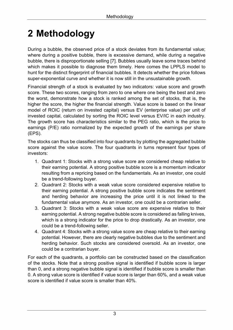
Figure 2.2 The ROIC curve for S&P500 constituent stocks. The blue markers are the real market value of ln(EV/IC) vs. ROIC for single stocks, and the red line is the fitted linear model between ln(EV/IC) and ROIC. In the title of the figure, “slope” is the coefficient of ROIC, and “intercept” is the constant in the model.
We do the following regression:
ln rstuvw = 𝛽 ∙ 𝑅𝑂𝐼𝐶 + 𝑐 (2.9)
In the example in Figure 2.2, the regression yields that 𝛽 = 17.65, 𝑐 = 0.36. Different from the example, we will apply the regression model with the subject company’s industry, these industries include consumer discretionary, communication service, consumer staples, industrials, energy, health care, information technology, materials, and utilities.
Robust regression is used here in order not to be overly affected by violations of assumptions by the underlying data-generating process. As we can see from Figure 2.2, some outliers exist which obviously do not follow the pattern of other observations; in addition, the variance of the error terms is not the same for all the values of ROIC., hence, applying the ordinary least squares regression will affect the validity of the regression results. Robust regression is a good method to deal with the heteroskedasticity of the variance of the error terms and the outliers that don't come from the same data generating process.
We then define Financial Strength as what delta Y is defined, that is,
𝐹𝑖𝑛𝑎𝑛𝑐𝑖𝑎𝑙𝑆𝑡𝑟𝑒𝑛𝑔𝑡ℎ = r����w
∗Lr����w
(���� )∗
(2.10)
Financial Strength gives in percentage terms the degree of overvaluation (negative being undervaluation) of the observed Enterprise Value with regards to the warranted EV/IC calculated from the regression model. Once we get the financial strength for each stock, we rank them across all the industries, so the value score is finally obtained. A score of 1, which is a potential undervalued signal, is given to the stock with the best
Methodology
10
financial strength of the set, and a score of 0, which is a potential overvalued signal, is given to the stock with the worst financial strength.
Exclusion of financial sector
The two largest financial sectors – banking and insurance – have unique characteristics compared to industrial sectors that require the exclusion of the financial sector from the ROIC Curve. In the banking industry, the high degree of the financial leverage makes it not meaningful to calculate the ROIC. In the insurance industry, “leverage” has more operating instead of financial attributes because the key leverage statistic is premium to written to equity. This type of leverage is unlikely to capture in the ROIC Curve. Besides, both banks and insurance companies have remarkable uncertainty in profit reporting due to the heavy use of accruals, which usually causes financial services companies to trade at a significant discount to the broader market.
2.3 Growth Score
Earnings per Share (EPS) is the portion of a company’s profit allocated to each share of common stock. It is served as an indicator of a company’s profitability. The direction of EPS can to some degree indicate the direction of the stock price. Thus, we use the expected EPS growth to quantify the growth strength. A growth score is used as a supplementary factor to further select stocks based on the four-quadrant framework. It is calculated in the following way:
𝐺𝑟𝑜𝑤𝑡ℎ𝑆𝑡𝑟𝑒𝑛𝑔𝑡ℎ = s�9�K�9�������9���s������L����s�������v�������0�
(3.1)
Growth Strength gives a value to represent the discrepancy between the estimated future EPS and the real EPS. The higher the Growth Strength is, the more likely that the EPS will increase., thus the stock price/ Once we get the Growth Strength of each individual stock, we rang them within the complete set the stocks, so the growth score is finally obtained. Same as the value score being interpreted, growth score being 1 means the price of the stock has the biggest potential to increase, while growth score being 0 means the price of the stock has the biggest potential to decrease.

Derive and back-test a trading strategy
11
3 Derive and back-test a trading strategy
Some existing master theses of the Chair of Entrepreneurial Risks have developed and back-tested some trading strategies based on the LPPLS model and the Financial Crisis Observatory output. The master thesis [15] developed the “Dragon-Hunting” and “Bubble Overlay” trading strategies, focusing on the long time-scale Early Bubble Warning and Bubble End Flag indicators. The first strategy aimed to capture the financial bubbles called Dragon Kings [15] which are very rare but significantly powerful in impact and size. Distinct from the Black Swans [16], Dragon Kings are to some extent predictable. The second strategy focused on avoiding negative bubbles instead of capturing positive bubbles. Both the strategies outperformed the buy-and-hold strategy with regard to Sharpe Ratio, which can be mainly attributed to the two large bubbles that occurred in the last two decades. The master thesis [17] incorporated the short time-scale indicators to further improve the performances of the mentioned trading strategy. In addition to outperforming the buy-and-hold benchmark in most cases in terms of the Sharpe ratio, this strategy remarkably reduced drawdowns during the dot-com and the US real estate bubbles.
Different from the theses mentioned above, this thesis will formulate a bubble score based on the LPPLS model as a measure of the bubble status, a value score to represent the how much the security is overvalued or undervalued, and a growth score to quantify the growth potential of the price. Incorporating these three scores, a trading strategy is thus developed which is rather long-term. Based on the four-quadrant framework which sort stocks according to their Bubble Score and Value Score, four portfolios are built. The holding period and the supplement of other constraints will be examined to look for the optimal portfolio construction methods.
3.1 Trading strategy
For this investment strategy, we will construct four types of portfolios based on the stocks in four quadrants identified above:
1. Trend-Following Long Stock Portfolio (TFLSP) consists of stocks that have a positive bubble score and a strong value score which is higher than 0.6 (that locate in quadrant 1 shown in Figure 2.1).
2. Contrarian Short Stock Portfolio (CSSP) consists of stocks that have a positive bubble and a weak value score which is lower than 0.4 (that locate in quadrant 2 shown in Figure 2.1).
3. Trend-Following Short Stock Portfolio (TFSSP) consists of stocks that have a negative bubble score and a weak value score which is lower than 0.4(that locate in quadrant 3 shown in Figure 2.1).
4. Contrarian Long Stock Portfolio (CLSP) consists of stocks that have a negative bubble score and a strong value score which is higher than 0.6 (that locate in quadrant 4 shown in Figure 2.1).

Derive and back-test a trading strategy
12
Suppose the first day of a month is t, and the last business day before t is t-1, for each month, we read all the data including the quarterly financial report and price history until t-1, and make long/short decisions on t. For all 4 portfolios, we will hold them for 3, 6, 9 and 12 months to see how long the holding period is the portfolios will perform relatively better. The weight of each stock is proportional to its company market capitalization within each portfolio. This is designated as the base strategy. The growth score is not used in the initial stage of portfolio construction, but it will be a supplementary factor to further improve the performances of the portfolios.
We will present the cumulative return of each portfolio in a monthly basis and compare it with the cumulative return of index S&P500. Further, we use such statistics as Sharpe ratio and Calmar ratio to compare the trading strategies with the benchmark. The Sharpe ratio is used to help investors understand the return of an investment adjusted by its risk, which quantifies the average return earned in excess of the risk-free rate per unit of volatility or total risk. Subtracting the risk-free rate from the mean return allows an investor to better isolate the profits corresponding to the risk-taking activities. It is defined as follows:
𝑆ℎ𝑎𝑟𝑝𝑒𝑟𝑎𝑡𝑖𝑜 =𝑅2 − 𝑅�𝜎2
Where 𝑅2 is the return of the portfolio, 𝑅� is the risk-free rate (we use a 3-month U.S. treasury bill), 𝜎2 is the standard deviation of the portfolio’s excess return which equals to �Var[𝑅2 − 𝑅�]. In general, the greater value of the Sharpe ratio, the more attractive the risk-adjusted return. However, only using the Sharpe ratio to compare the performance of different trading strategies might be misleading, as the Sharpe ratio uses the standard deviation of the excess return of the portfolio to assess the risk. However, this standard deviation does not account for tail risks and for correlated returns that accumulate in a drawdown. The common risk-adjusted return gauges such as the Sharpe ratio are adjusted by a certain medium-sized risk, as we are dealing with the bubbles and dramatic dynamics in financial markets, we need an augmentation of the traditional risk-return relationship. The Calmar ratio is defined as follows:
𝐶𝑎𝑙𝑚𝑎𝑟𝑟𝑎𝑡𝑖𝑜 =𝐴𝑛𝑛𝑢𝑎𝑙𝑖𝑧𝑒𝑑𝑡𝑜𝑡𝑎𝑙𝑟𝑒𝑡𝑢𝑟𝑛|𝑀𝑎𝑥𝑖𝑚𝑢𝑚𝑑𝑟𝑎𝑤𝑑𝑜𝑤𝑛|
Where the Maximum drawdown is the percentage term calculated by the maximum loss of the portfolio from its peak value. A higher Calmar ratio indicates that the return of the portfolio has not been at risk of large drawdowns. Besides, the inverse of the Calmar ratio illustrates how many years it will take to recover the average maximum drawdown. Thus, we would prefer portfolios with higher Calmar ratio.
3.2 Exploration of statistical characteristics of trading strategies
The trading strategy starts from calculating the Bubble Score and the Value Score, which comes from the existing LPPLS model and the ROIC valuation framework respectively. As explained before, the Value Score is based on the deviation of the market enterprise value from the warranted enterprise value which is calculated by the robust regression model taking ROIC as the independent variable. We run the robust

Derive and back-test a trading strategy
13
regression model for each industry sector except the financial sector at the reliance date. Below (Figure 3.1) is an example of the ROIC curve derived from the ROIC valuation framework.
From Figure 3.1, it can be observed that on 31/10/2018, according the quarterly fundamental data and the close price of each stock, the robust regression model could to some extent measure how much the market value deviates from the warranted value. For such sectors as Information Technology, Consumer Discretionary, Consumer Services, Consumer Staples, Health Care, and Industrials, the linear relationship between the ROIC and ln(EV/IC) is significant, whereas for such sectors as Material, Utilities, and Energy, the linear relationship is not significant. However, noting that the slope for all the industries are more than zero, which is in accordance with the underlying theory that the higher the ROIC is, the more the company should be valued. Although for certain sectors the linear relationship is not significant, it does act as an effective way to value stocks from the fundamental perspective.

Derive and back-test a trading strategy
14
Figure 3.1 ROIC-based valuation curve for individual industries on 31/10/2018. The title of each figure includes the sector name and parameters of the regression model. The robust regression model is in the form of ln rst
uvw = 𝛽 ∙ 𝑅𝑂𝐼𝐶 + 𝑐, where 𝛽 corresponds to the “slope”
in the title and 𝑐 corresponds to the “intercept” in the title. The scatter plot is the real ROIC and ln(EV/IC) plotted on the xy-plane, and the red line is the fitted linear relationship between the ROIC and ln(EV/IC) obtained from the model.
The four types of the portfolios –TFLSP, CSSP, TFSSP, and CLSP -- are constructed and rebalanced in the beginning of each month according to the Bubble Score and the Value Score of each stock. Upon this construction method, some manipulation regarding the holding period and weight of stocks can be exerted; besides, some constraints could be applied to further filter out some stocks that we think might be detrimental to the corresponding portfolio. Here we treat the time series data from 20 years ago until now as panel data and assign equal weight to stocks. We will use boxplot, which depicts the annualized return through the quartiles corresponding to the Bubble Score and the Value Score to check the efficacy of the trading strategy and compare the different constraints.
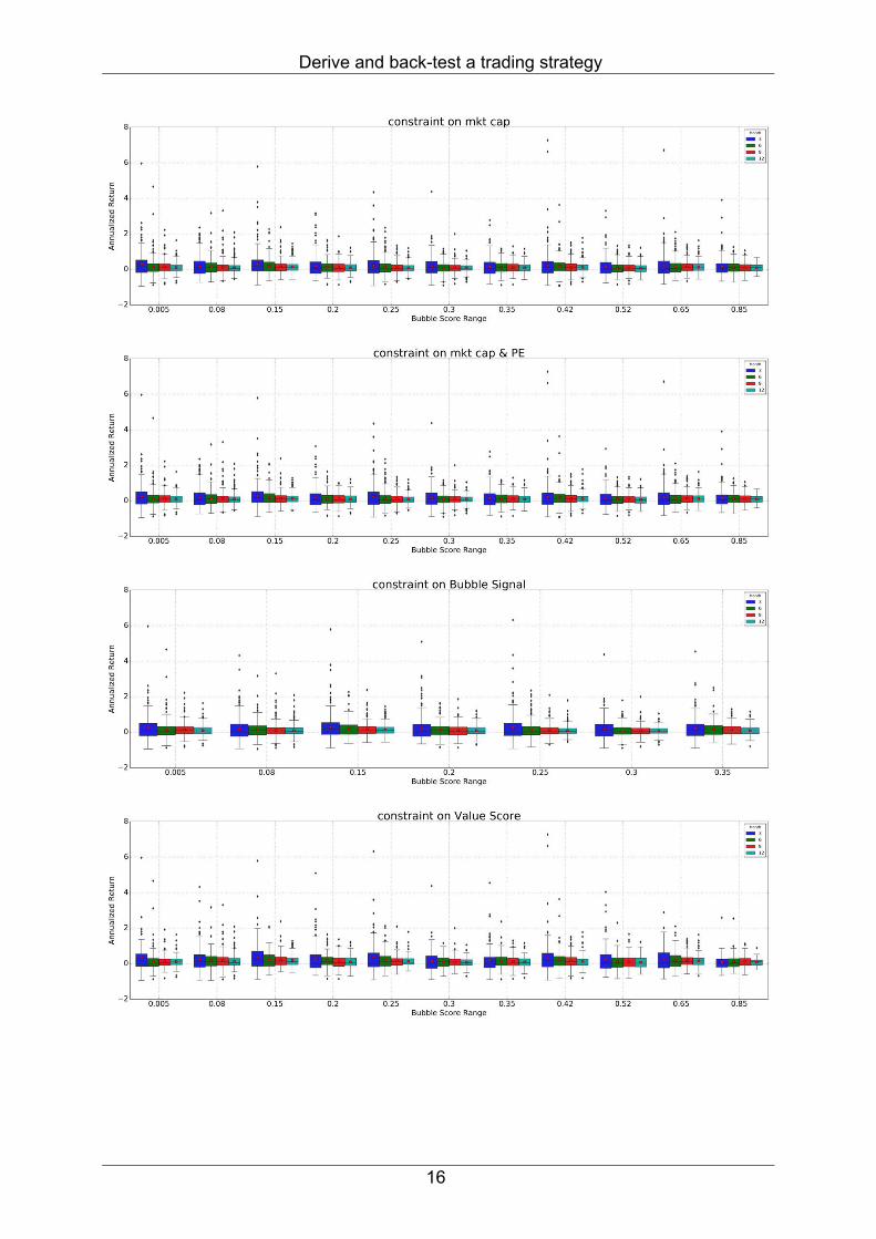
First, the four portfolios are constructed in the way mentioned above, and they are hold for 3, 6, 9 and 12 months respectively. Second, we add a constraint on the market cap of stocks. In each month, we filter out the stocks with market cap lower than 0.05 quartile among all the stocks selected in four quadrants for the sake of higher liquidity of the portfolio. Third, based on the second situation, we add one more constraint on the P/E ratio, which filters out the stocks with too high P/E ratio for long stock portfolios and stocks with too low P/E ratio short stocks portfolios. Doing this, we think that it’s more likely for stocks with strong fundamentals to appreciate and for stocks with weak fundamentals to depreciate in the future. We distinguish the “high” and “low” P/E ratio by the quartile of P/E ratio of all the stocks in each industry in each month being 0.6 and 0.4 respectively. Forth, we remove the aforementioned two constraints and add a constraint regarding the threshold of three scores. Here come three methods which are based on the Bubble Score, Value Score and the Growth Score, respectively:
1. select stocks with bubble signals (the absolute value of the Bubble Score) lower than 0.4 for trend-following portfolios which contain type 1 and 3 stocks as we want to capture the trend thus the bubble shouldn’t be too strong otherwise bubbles are very likely to crash, and select stocks with bubble signals (the absolute value of the Bubble Score) higher than 0.6 for the contrarian portfolios which contain type 2 and 4 stocks as we are looking for corrections thus the bubble should be as strong as enough.
2. For the two long stock portfolios which contain type 1 and 4 stocks, select stocks with the Value Score over 0.8 as the stronger the fundamentals are, the more likely the stocks will appreciate. For the two short stock portfolios which contains type 2 and 3 stocks, select stocks with Value Score below 0.2 as the weaker the fundamentals are, the more likely the stocks are overvalued currently.
3. For two long stock portfolios which contain type 1 and 4 stocks, select stocks with the Growth Score over 0.6 as the more growth potential indicates higher returns the stocks might have. For the two short stock portfolios which contains type 2 and 3 stocks, select stocks with Growth Score below 0.4 lower growth potential is beneficial for the short stock positions.
Derive and back-test a trading strategy
15
The aforementioned cases are shown in the following table in order to present them more clearly. We will then grope about the statistical characteristics of each case. Table 3.1 6 cases mentioned above and their description
Case Description
1 Four portfolios are constructed according the 4-quadrant framework, stocks are equal weighted, no other constraints for the stock selection process
2 Based on Case 1, filter out stocks with market cap lower than 0.05 quantile among all the S&P500 constituent stocks at every rebalance date
3
Based on Case 2, filter out stocks with P/E ratio higher than 0.6 quantile for long stock portfolio and stocks with P/E ratio lower than 0.4 quantile for short stock portfolio among all the S&P500 constituent stocks at every rebalance date.
4
Based on Case 1, for the two trend-following portfolios (which contain type 1 and 3 stocks), select stocks with the absolute value of Bubble Score below 0.4, and for two contrarian portfolios (which contain type 2 and 4 stocks), select stocks with the absolute value of Bubble Score over 0.6.
5
Based on Case 1, for the two long stock portfolios (which contain type 1 and 4 stocks), select stocks with Value Score over 0.8, and for two short stock portfolios (which contain type 2 and 3 stocks), select stocks with Value Score below 0.2.
6
Based on Case 1, for the two long stock portfolios (which contain type 1 and 4 stocks), select stocks with Growth Score over 0.6, and for two short stock portfolios (which contain type 2 and 3 stocks), select stocks with Growth Score below 0.4.
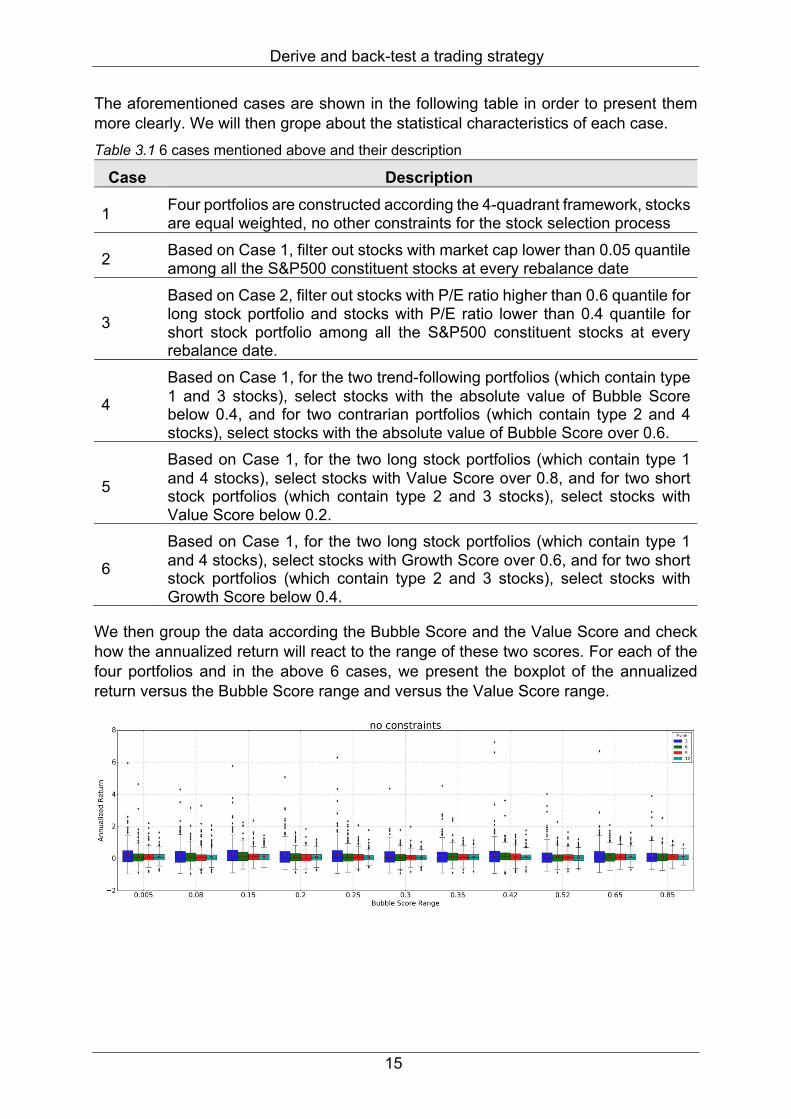
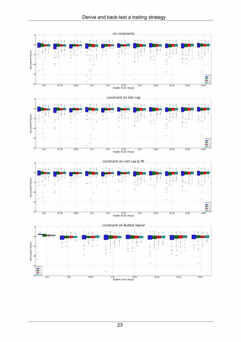
We then group the data according the Bubble Score and the Value Score and check how the annualized return will react to the range of these two scores. For each of the four portfolios and in the above 6 cases, we present the boxplot of the annualized return versus the Bubble Score range and versus the Value Score range.
Derive and back-test a trading strategy
16

Derive and back-test a trading strategy
17
Figure 3.2 Trend-following long stock portfolio, annualized return vs. Bubble Score range. The panel 1 - 6 is corresponding to Case 1 - 6 respectively, where the bars colored by blue, green, red and turquoise represent holding period being 3, 6, 9 and 12 months respectively. The black line across the bar is the median of the corresponding annualized return, and the red spot is the mean of the corresponding annualized return.
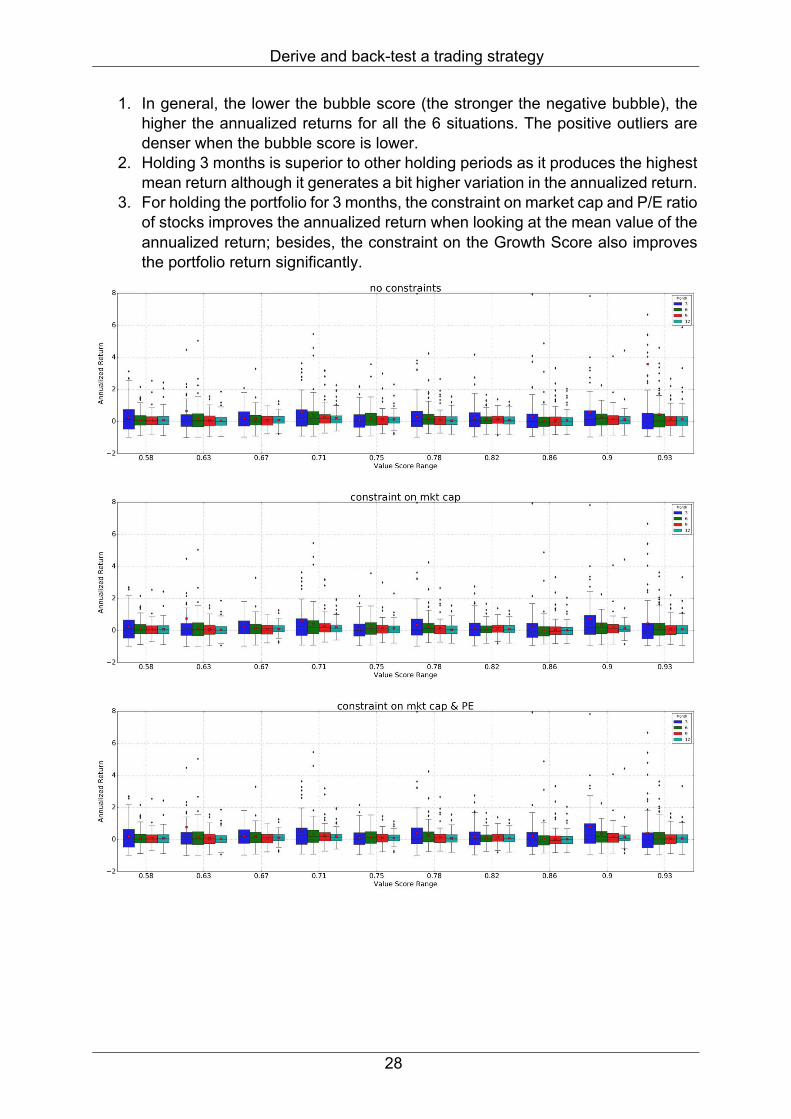
From the Figure 3.2, following conclusions can be made:
1. The mean and median of the annualized returns are always bigger than zero for all 4 types of holding period and under all these situations; there are much more positive outliers than negative outliers.
2. The maximum and mean value of the annualized returns are a bit higher when the bubble score is low than when the bubble score is high. Besides, the positive outliers are denser when the bubble score is lower.
3. Among four choices of holding period (3, 6, 9, 12 months), holding 3 months has the biggest variation in returns for all 6 cases, whereas in terms of the variation in returns, holding 6, 9 and 12 months are almost the same. In terms of the median of the annualized returns, holding 6 months is superior to other holding periods.
4. Compared to the “no constraint” condition, two constrains regarding the market cap and P/E ratio don’t seem to improve the annualized returns obviously. However, the constraint on the Value Score and the Growth Score increases the mean of the annualized return for all 4 holding periods, and the negative outliers are less compared to the “no constraints” cases.
5. Among three cases regarding the scores, the “Growth Score filter” generates the least variation in the annualized returns compared to the others.

Derive and back-test a trading strategy
18
Derive and back-test a trading strategy
19
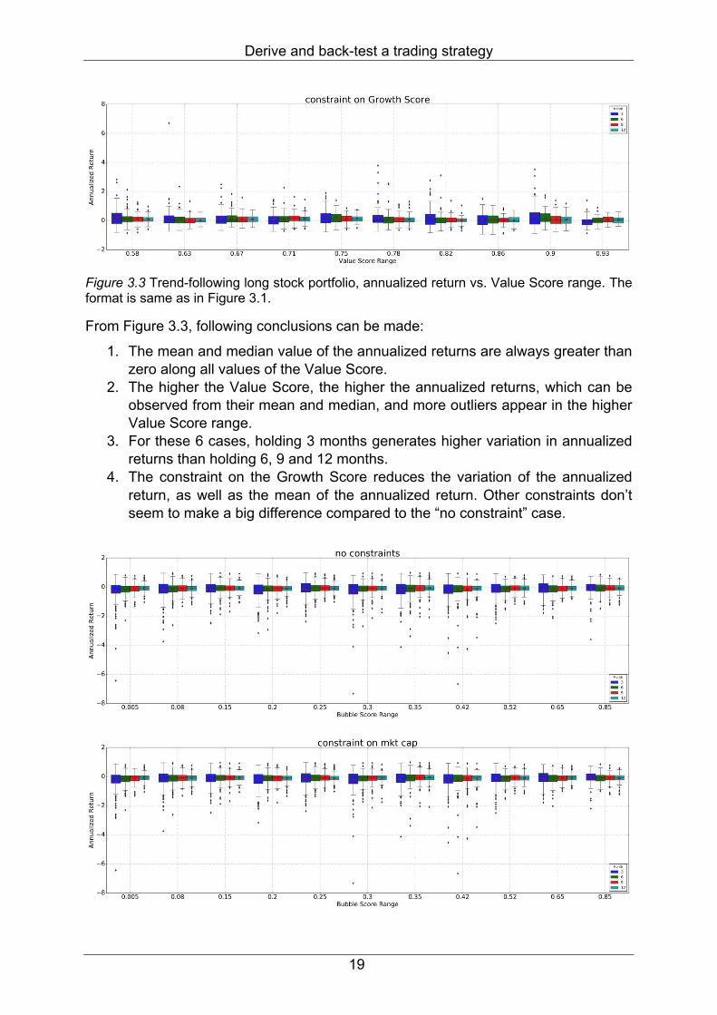
Figure 3.3 Trend-following long stock portfolio, annualized return vs. Value Score range. The format is same as in Figure 3.1.
From Figure 3.3, following conclusions can be made:
1. The mean and median value of the annualized returns are always greater than zero along all values of the Value Score.
2. The higher the Value Score, the higher the annualized returns, which can be observed from their mean and median, and more outliers appear in the higher Value Score range.
3. For these 6 cases, holding 3 months generates higher variation in annualized returns than holding 6, 9 and 12 months.
4. The constraint on the Growth Score reduces the variation of the annualized return, as well as the mean of the annualized return. Other constraints don’t seem to make a big difference compared to the “no constraint” case.

Derive and back-test a trading strategy
20
Figure 3.4 Contrarian short stock portfolio, annualized return vs. Bubble Score range. The format is same as in Figure 3.1.
From the Figure 3.4, following conclusions can be made:

Derive and back-test a trading strategy
21
1. The Mean and median of the annualized returns are not always bigger than zero, and more negative outliers appear.
2. In general, the higher the bubble score, the higher the mean, median and minimum value of the annualized returns and the less variation in the returns.
3. Holding 3 months is a bit more volatile than other holding periods, which is a bit different from the Trend Following Long Stock Portfolio.
4. For holding period being 6 months, it is obvious that when the bubble score is in the highest range, the portfolio has the highest return.
Derive and back-test a trading strategy
22
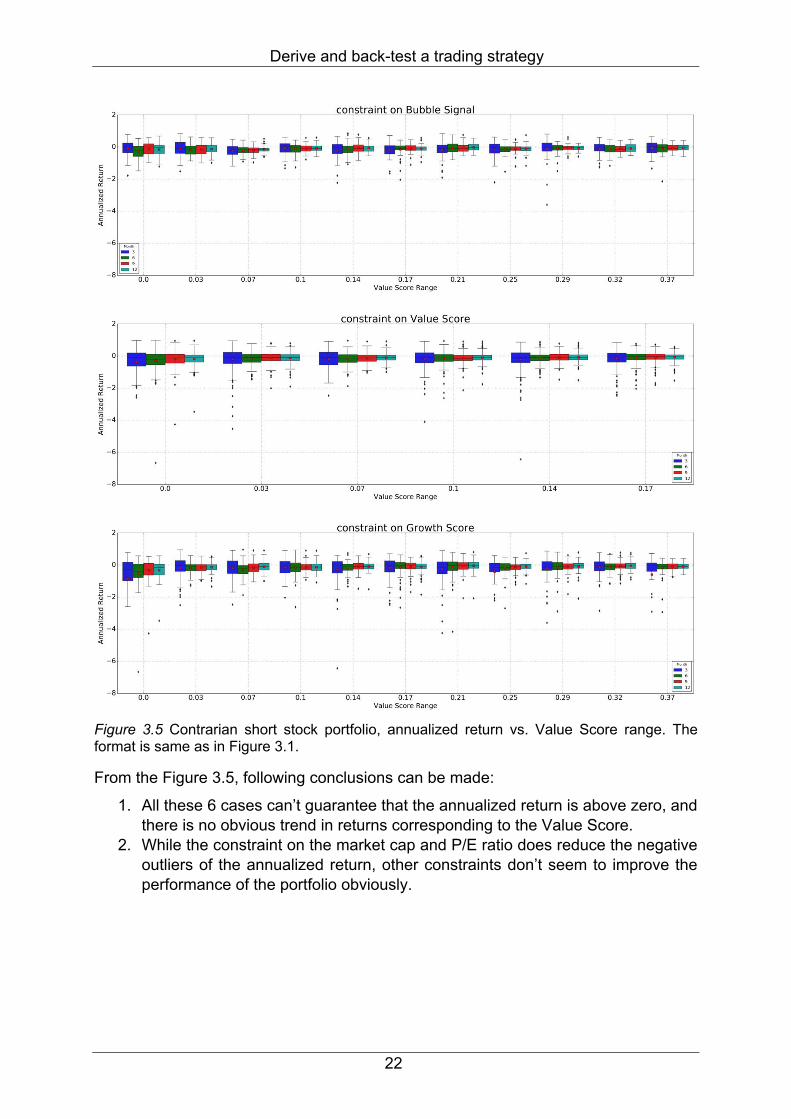
Figure 3.5 Contrarian short stock portfolio, annualized return vs. Value Score range. The format is same as in Figure 3.1.
From the Figure 3.5, following conclusions can be made:
1. All these 6 cases can’t guarantee that the annualized return is above zero, and there is no obvious trend in returns corresponding to the Value Score.
2. While the constraint on the market cap and P/E ratio does reduce the negative outliers of the annualized return, other constraints don’t seem to improve the performance of the portfolio obviously.
Derive and back-test a trading strategy
23

Derive and back-test a trading strategy
24
Figure 3.6 Trend following short stock portfolio, annualized return vs. Bubble Score range. The format is same as in Figure 3.1.
From Figure 3.6, following conclusions can be made:
1. Holding 3 months is the most volatile compared to other holding periods, and always has the negative mean and median value of the annualized return, which makes holding 3 months a bad choice for this portfolio. Holding 6, 9, and 12 months are not so different in terms of the variation in returns.
2. For holding 6 months, more negative outliers appear when the bubble score is higher (when the negative bubble is weaker).
3. The exerted constraints don't seem to improve the annualized returns of the portfolio significantly.

Derive and back-test a trading strategy
25

Derive and back-test a trading strategy
26
Figure 3.7 Trend following short stock portfolio, annualized return vs. Value Score range. The format is same as in Figure 3.1.
From Figure 3.7, following conclusions can be made:
1. The lower the Value Score is, the higher the annualized return is, which can be observed for the mean and median. More negative outliers appear in the higher Value Score range.
2. Holding 3 months generates more variation in returns compared other holding periods.
3. The constraints on the market cap and P/E ratio decrease the variation a lot compared to the “no constraints” situation and reduces the negative outliers as well.
Derive and back-test a trading strategy
27
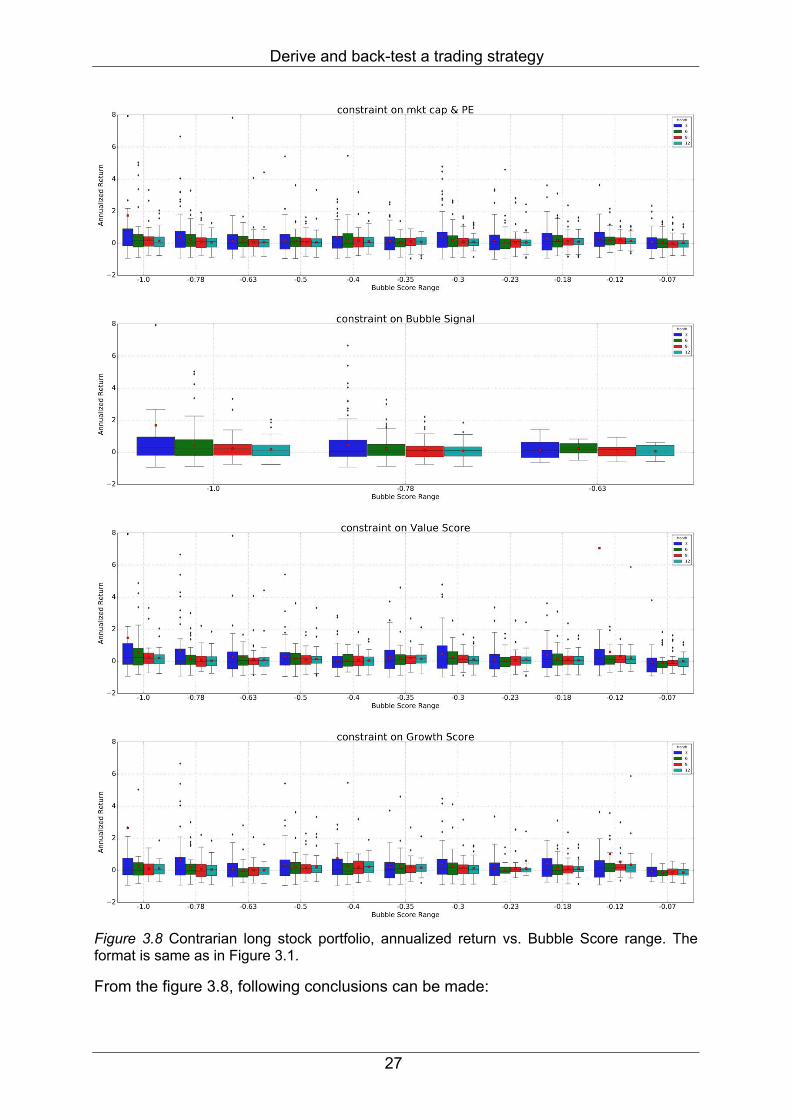
Figure 3.8 Contrarian long stock portfolio, annualized return vs. Bubble Score range. The format is same as in Figure 3.1.
From the figure 3.8, following conclusions can be made:
Derive and back-test a trading strategy
28
1. In general, the lower the bubble score (the stronger the negative bubble), the higher the annualized returns for all the 6 situations. The positive outliers are denser when the bubble score is lower.
2. Holding 3 months is superior to other holding periods as it produces the highest mean return although it generates a bit higher variation in the annualized return.
3. For holding the portfolio for 3 months, the constraint on market cap and P/E ratio of stocks improves the annualized return when looking at the mean value of the annualized return; besides, the constraint on the Growth Score also improves the portfolio return significantly.
Derive and back-test a trading strategy
29
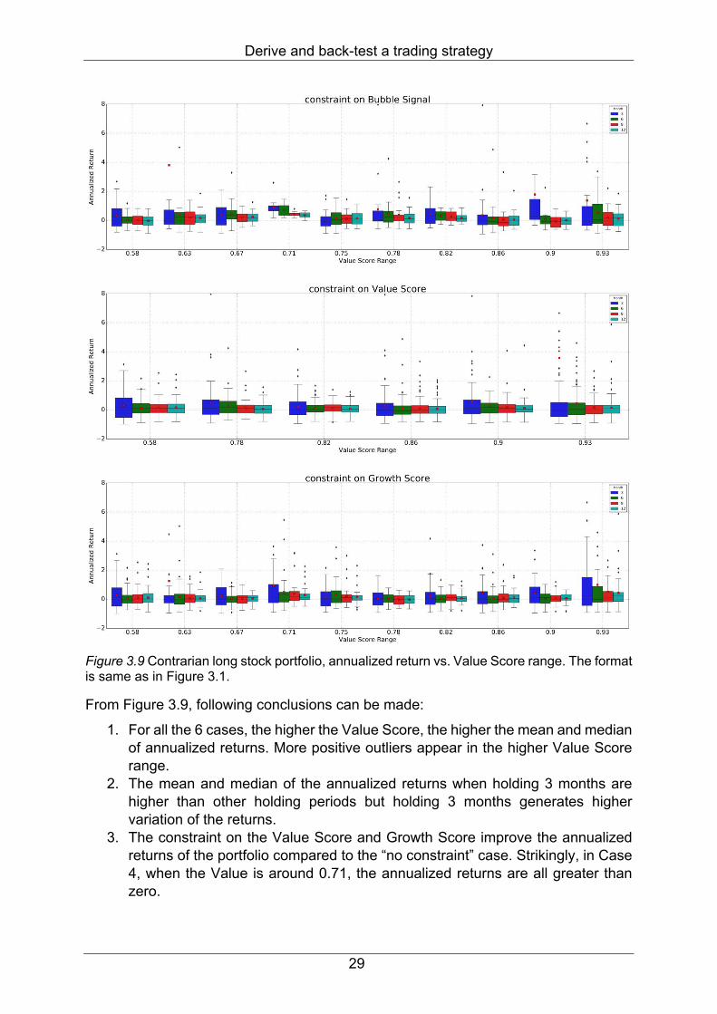
Figure 3.9 Contrarian long stock portfolio, annualized return vs. Value Score range. The format is same as in Figure 3.1.
From Figure 3.9, following conclusions can be made:
1. For all the 6 cases, the higher the Value Score, the higher the mean and median of annualized returns. More positive outliers appear in the higher Value Score range.
2. The mean and median of the annualized returns when holding 3 months are higher than other holding periods but holding 3 months generates higher variation of the returns.
3. The constraint on the Value Score and Growth Score improve the annualized returns of the portfolio compared to the “no constraint” case. Strikingly, in Case 4, when the Value is around 0.71, the annualized returns are all greater than zero.
Derive and back-test a trading strategy
30
Overall, the above discussion about the boxplot verifies the effectiveness of the strategy and our intuition about the indication of the Bubble Score and the Value Score, which proves that for the stronger the bubble is, the higher returns of the trend following (long stock and short stock) portfolios, and higher the Value Score is, the higher the return of the (trend following and contrarian) long stock portfolios. This strategy is rather long-term, as holding 3 months always generates the highest variation which makes it not favorable, and holding 6, 9 or 12 months doesn’t have big difference, hence for the following discussion, we will present all the strategies for holding 3, 6, 9 and 12 months, respectively. In addition, the two short stocks portfolios perform worse than the two long stocks portfolios. Besides, the contrarian long stocks portfolio seems to have the best performance as the mean value of the annualized returns is significantly higher than zero which is not the case for other portfolios. Moreover, change the holding period and applying the different constraints have the different effect on 4 portfolios, which indicates that these 4 types of the portfolios may perform their best in different cases. Below is the table for the potential best holding period and constraints concluded from the boxplots. Table 3.2 Optimal holding period and constraint for 4 portfolios according to the boxplots shown above, which tells us the direction of how to improve the performance of the strategy.
Portfolio Holding period Constraints TFLSP 6 months stocks selected based on the Bubble Score CSSP 6 months Not obvious TFSSP 6 months Not obvious CLSP 3 months Market Cap and P/E ratio; Growth Score.
3.3 Back-test the trading strategy
The above section gives us a direction about the methods of constructing the portfolio and further improving the performance. However, from the boxplot sometimes it is not obvious and which holding period is optimal, which constraints should be applied and how the weight is assigned to each stock to generate the highest annualized return. Hence, we will back test the above trading strategy to see which situation works the best for these 4 types pf portfolios. Note that in this thesis, we assume that there are no transaction costs, and each stock can be long or short for any amount.
Base strategy
Base strategy is to construct 4 portfolios according to the 4-quadrant framework and assign the weight of each stock proportional to the market cap in its corresponding portfolio. The Below is the back-test result of the base strategy, holding portfolios for 3, 6, 9 and 12 months, respectively.
It can be observed that the two short stock portfolios perform well when the benchmark is going down, and in general, the TFSSP generates higher return than the other one, especially when hold for 3 months; the two long stock portfolios almost always generate higher cumulative return compared to the benchmark. Besides, these four

Derive and back-test a trading strategy
31
portfolios react differently to different holding period: TFLSP performs relatively better if the stocks are bought and hold for at least 9 months; CLSP performs relatively better if the stocks are bought and hold for 6 months. Overall, there is no big difference for TFSSP and CSSP in terms of the cumulative return unless there is a significant drawdown in the benchmark, for example, the TFSSP generates the greatest cumulative return from the year 2000 to the year 2003.
a) holding period = 3 months
b) Holding period = 6 months
c) Holding period = 9 months
d) Holding period = 12 months
Figure 3.10 The cumulative returns of four portfolios vs. the benchmark S&P500 from Jan. 2000 to Nov. 2018. The lines colored by blue, green, red, gold and black represent the cumulative of trend-following long stock portfolio, contrarian long stock portfolio, trend-following short stock portfolio, contrarian short stock portfolio and S&P500, respectively. Panel a – d manifest the situation of holding portfolios for 3, 6, 9, and 12 months respectively.
Considering the Sharpe ratio (as shown in the Table 3.3), the TFLSP is the best among all 4 portfolios and performs the best when hold for 9 or 12 months. The CLSP performs the best when hold 6 months, whereas the TFSSP 3 months. The CSSP is the worst.
Table 3.3 Sharpe ratio for base strategy
TFLSP CLSP TFSSP CSSP S&P500 Hold 3 months 0.34 0.23 0.00 -0.44 0.30 Hold 6 months 0.46 0.42 -0.07 -0.53 0.30 Hold 9 months 0.52 0.36 -0.21 -0.46 0.30 Hold 12 months 0.53 0.25 -0.18 -0.49 0.30
Derive and back-test a trading strategy
32
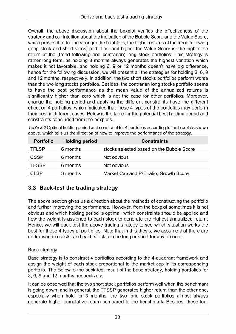
When looking into the Calmar ratio, the TFLSP is superior to other 3 portfolios, especially when hold for 6 months. The TFLSP works much better than the CLSP along all holding periods. The CSSP is still the worst in terms of the Calmar ratio.
Table 3.4 Calmar ratio for base strategy
TFLSP CLSP TFSSP CSSP S&P500 Hold 3 months 1.63 0.53 -0.03 -0.09 0.64 Hold 6 months 11.73 0.46 -0.04 -0.10 0.64 Hold 9 months 3.57 0.50 -0.07 -0.09 0.64 Hold 12 months 1.98 0.29 -0.06 -0.09 0.64
When considering combining the 4 portfolios to form a self-financing portfolio, we have the following cumulative return curves of the combined portfolios, among which holding 6 months is optimal due to its high annualized return, whereas holding 9 months is the worst.
a) Holding period = 3 months
b) Holding period = 6 months
c) Holding period = 9 months
d) Holding period = 12 months
Figure 3.11 The cumulative returns of the portfolio which combines the four portfolios equally. The blue line draws the cumulative return of the combined portfolio, and the black line is the cumulative return of the bench mark S&P500 index.
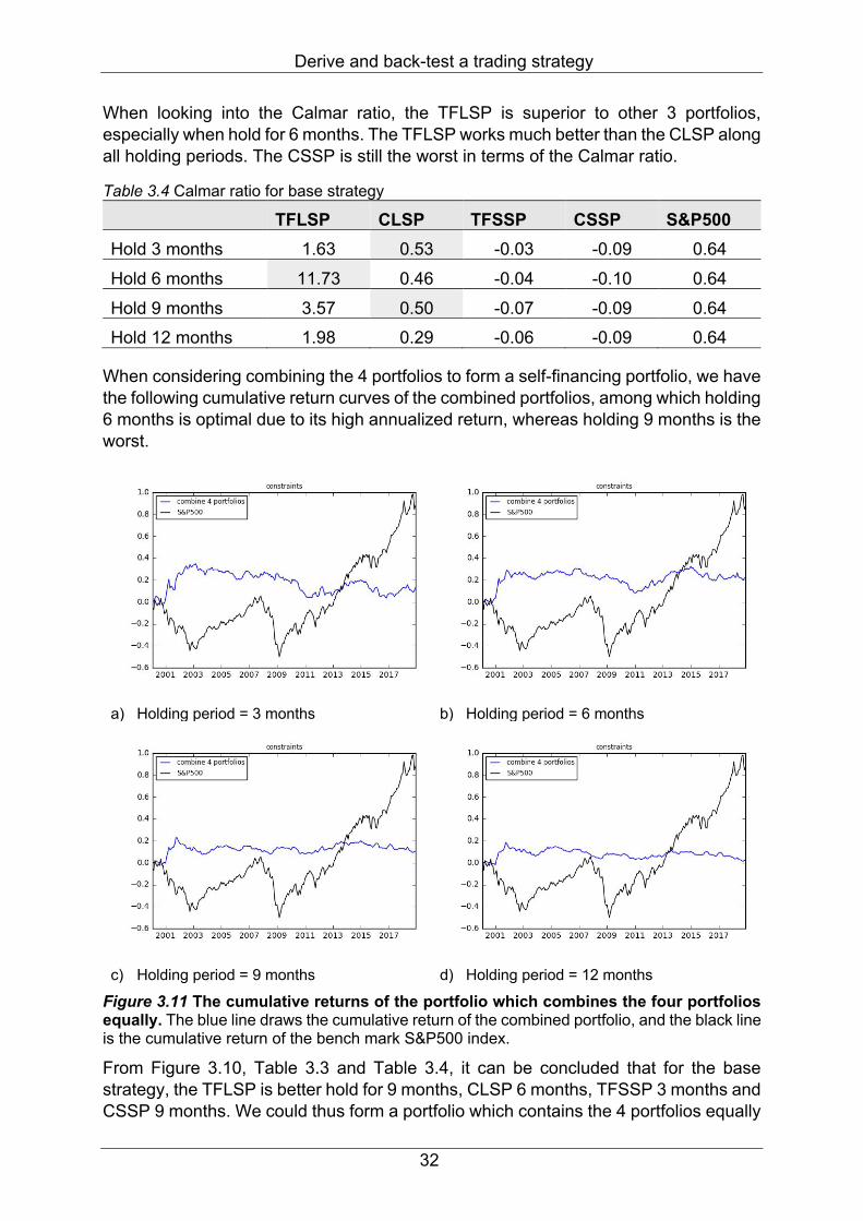
From Figure 3.10, Table 3.3 and Table 3.4, it can be concluded that for the base strategy, the TFLSP is better hold for 9 months, CLSP 6 months, TFSSP 3 months and CSSP 9 months. We could thus form a portfolio which contains the 4 portfolios equally
Derive and back-test a trading strategy
33
under their own optimal situation. Figure 3.12 depicts the cumulative return of such a portfolio. It can be observed that the combined portfolios generated higher returns compared to the one when portfolios are combined under the same situation.
Figure 3.12 Combine 4 portfolios equally with their own optimal holding period for base strategy. The TFLSP, CLSP, TFSSP and CSSP are hold for 9, 6, 3 and 9 months respectively. The format is same as in Figure 3.11
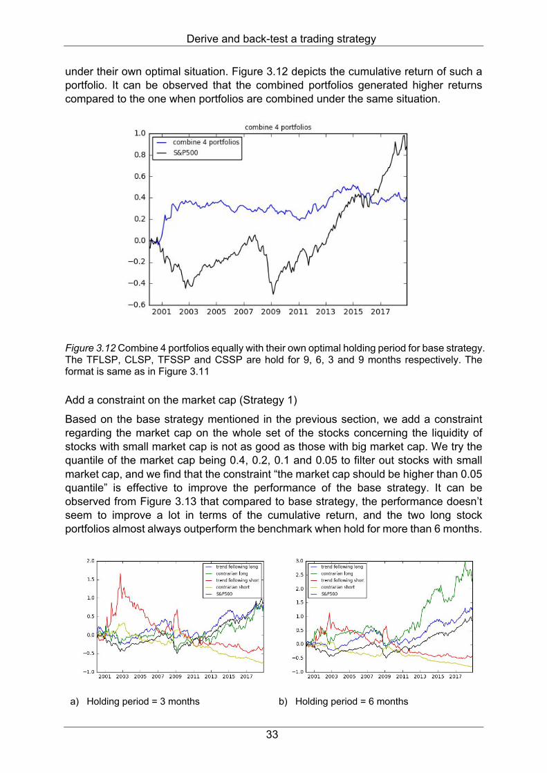
Add a constraint on the market cap (Strategy 1)
Based on the base strategy mentioned in the previous section, we add a constraint regarding the market cap on the whole set of the stocks concerning the liquidity of stocks with small market cap is not as good as those with big market cap. We try the quantile of the market cap being 0.4, 0.2, 0.1 and 0.05 to filter out stocks with small market cap, and we find that the constraint “the market cap should be higher than 0.05 quantile” is effective to improve the performance of the base strategy. It can be observed from Figure 3.13 that compared to base strategy, the performance doesn’t seem to improve a lot in terms of the cumulative return, and the two long stock portfolios almost always outperform the benchmark when hold for more than 6 months.
a) Holding period = 3 months
b) Holding period = 6 months

Derive and back-test a trading strategy
34
c) Holding period = 9 months
d) Holding period = 12 months
Figure 3.13 Strategy 1, remove stocks with market cap lower than 0.05 quantile at every rebalance date. The format is same as in Figure 3.10.
However, when looking at the risk-adjusted returns, the Calmar of increased a bit, which proves the effectiveness of this constraint. Table 3.5 Sharpe ratio and Calmar ratio for Strategy 1
Holding Period TFLSP CLSP TFSSP CSSP S&P500
Sharpe ratio
3 0.31 0.24 0.02 -0.44 0.30 6 0.43 0.43 -0.06 -0.53 0.3 9 0.50 0.38 -0.21 -0.46 0.30
12 0.52 0.26 -0.18 -0.49 0.30
Calmar ratio
3 1.09 0.60 -0.03 -0.09 0.64 6 12.14 0.48 -0.04 -0.1 0.64 9 3.46 0.56 -0.07 -0.09 0.64
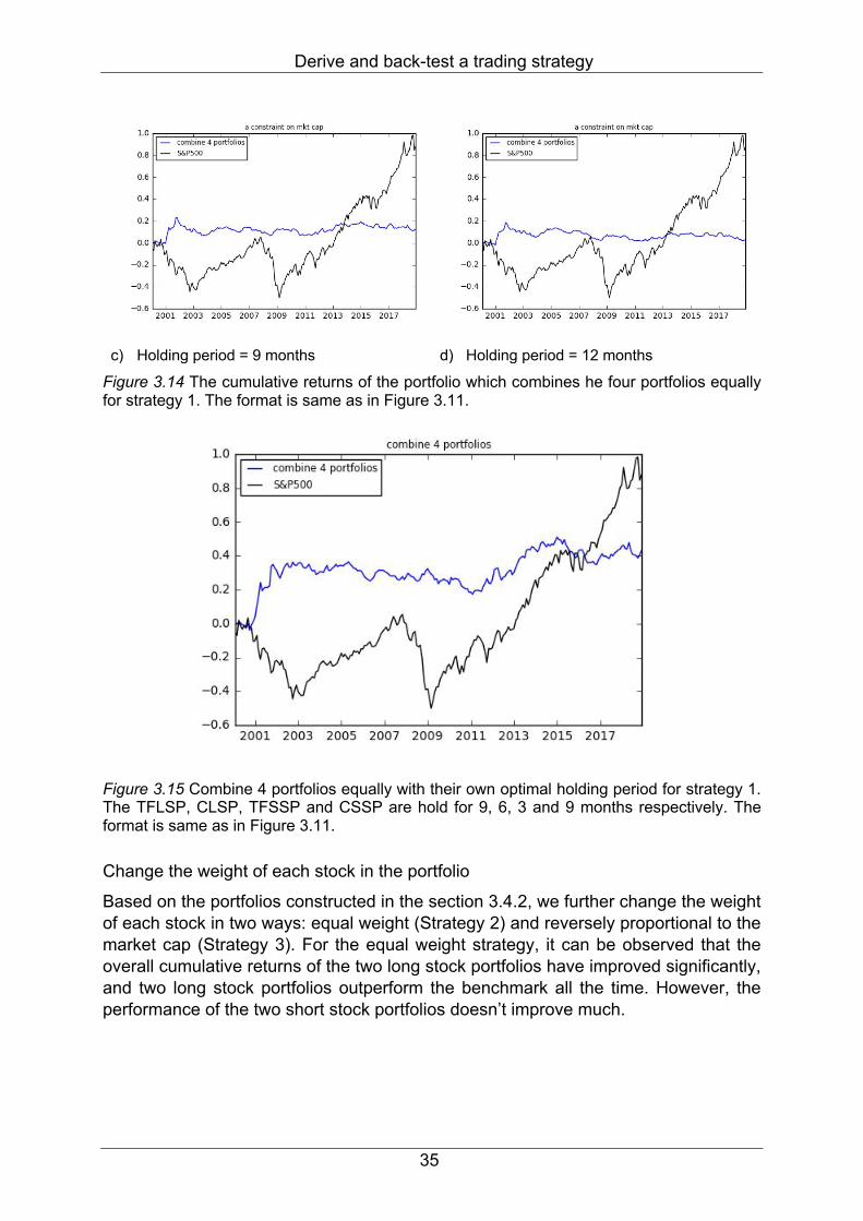
12 1.93 0.31 -0.06 -0.09 0.64 We then follow the same process in the previous section to construct the combined portfolio under the same holding period and under individual optimal holding period, which indicates holding the TFLSP for 9 months, CLSP 6 months, TFSSP 3 months, and CSSP 9 months. The results are shown in Figure 3.14 and Figure 3.15.
a) Holding period = 3 months
b) Holding period = 6 months
Derive and back-test a trading strategy
35
c) Holding period = 9 months
d) Holding period = 12 months
Figure 3.14 The cumulative returns of the portfolio which combines he four portfolios equally for strategy 1. The format is same as in Figure 3.11.
Figure 3.15 Combine 4 portfolios equally with their own optimal holding period for strategy 1. The TFLSP, CLSP, TFSSP and CSSP are hold for 9, 6, 3 and 9 months respectively. The format is same as in Figure 3.11.
Change the weight of each stock in the portfolio
Based on the portfolios constructed in the section 3.4.2, we further change the weight of each stock in two ways: equal weight (Strategy 2) and reversely proportional to the market cap (Strategy 3). For the equal weight strategy, it can be observed that the overall cumulative returns of the two long stock portfolios have improved significantly, and two long stock portfolios outperform the benchmark all the time. However, the performance of the two short stock portfolios doesn’t improve much.

Derive and back-test a trading strategy
36
a) Holding period = 3 months
b) Holding period = 6 months
c) Holding period = 9 months
d) Holding period = 12 months
Figure 3.16 Strategy 2, remove stocks with market cap lower than 0.05 quantile at every rebalance date, assign the equal weight to stocks. The format is same as in Figure 3.10.
The Sharpe ratio and of the two long portfolios increase a bit, while those of the two short portfolios decrease a bit. This confirms that changing the weight as equal after removing stocks with too small market cap can further improve the performance of two long stock portfolios with regards to the cumulative return and the risk-adjusted return. Table 3.6 Sharpe ratio and Calmar ratio for Strategy 2
Holding Period TFLSP CLSP TFSSP CSSP S&P500
Sharpe ratio
3 0.52 0.25 -0.07 -0.60 0.30 6 0.56 0.47 -0.17 -0.64 0.30 9 0.55 0.39 -0.30 -0.50 0.30
12 0.58 0.33 -0.30 -0.56 0.30
Calmar ratio
3 1.51 0.29 -0.05 -0.11 0.64 6 1.63 0.49 -0.07 -0.11 0.64 9 1.05 0.71 -0.09 -0.10 0.64
12 1.00 0.53 -0.09 -0.10 0.64
From Figure 3.16 and Table 3.6, it can be concluded that the TFLSP, CLSP, TFSSP and CSSP are better hold for 6, 6, 3, and 9 months respectively. The combined
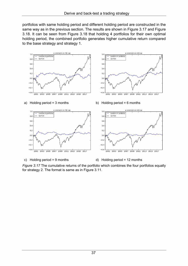
Derive and back-test a trading strategy
37
portfolios with same holding period and different holding period are constructed in the same way as in the previous section. The results are shown in Figure 3.17 and Figure 3.18. It can be seen from Figure 3.18 that holding 4 portfolios for their own optimal holding period, the combined portfolio generates higher cumulative return compared to the base strategy and strategy 1.
a) Holding period = 3 months
b) Holding period = 6 months
c) Holding period = 9 months
d) Holding period = 12 months
Figure 3.17 The cumulative returns of the portfolio which combines the four portfolios equally for strategy 2. The format is same as in Figure 3.11.
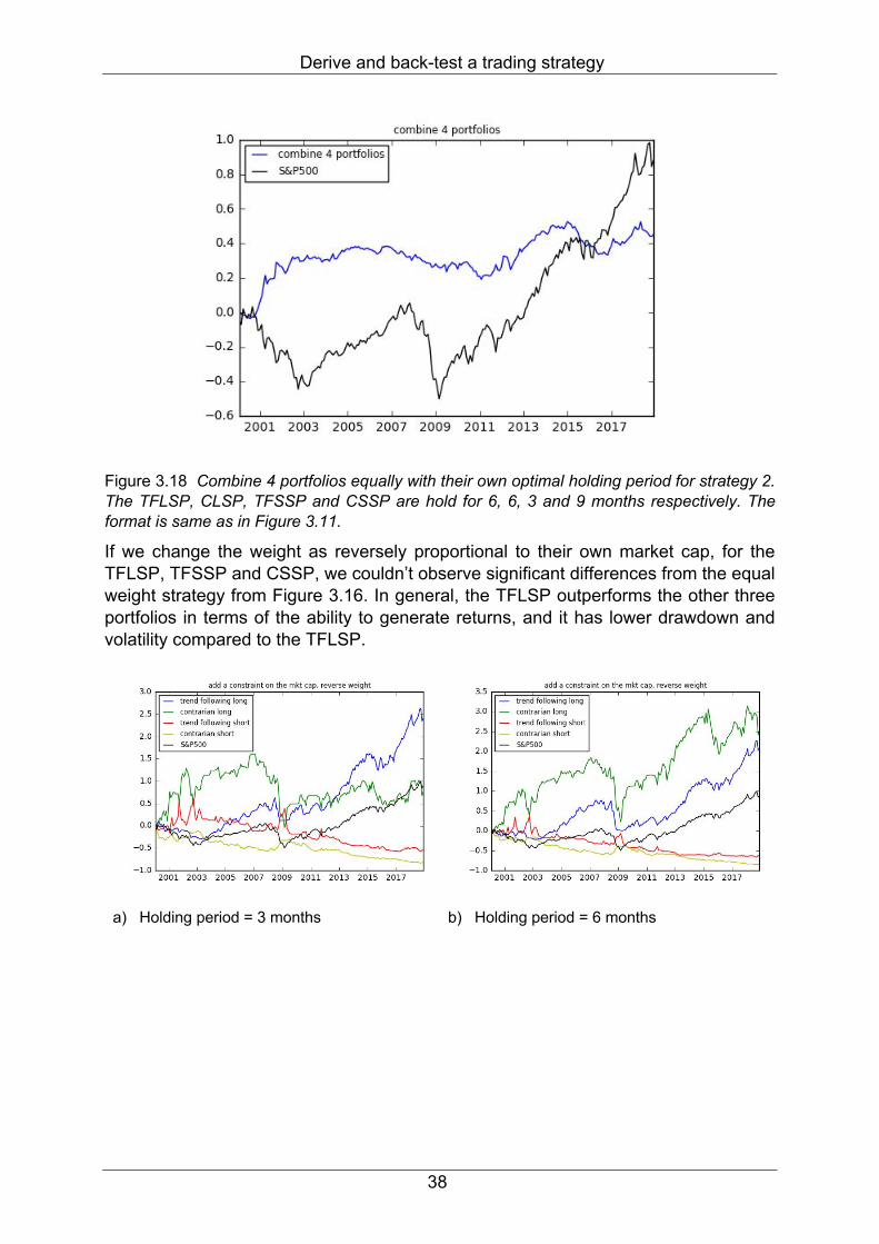
Derive and back-test a trading strategy
38
Figure 3.18 Combine 4 portfolios equally with their own optimal holding period for strategy 2. The TFLSP, CLSP, TFSSP and CSSP are hold for 6, 6, 3 and 9 months respectively. The format is same as in Figure 3.11.
If we change the weight as reversely proportional to their own market cap, for the TFLSP, TFSSP and CSSP, we couldn’t observe significant differences from the equal weight strategy from Figure 3.16. In general, the TFLSP outperforms the other three portfolios in terms of the ability to generate returns, and it has lower drawdown and volatility compared to the TFLSP.
a) Holding period = 3 months
b) Holding period = 6 months

Derive and back-test a trading strategy
39
c) Holding period = 9 months
d) Holding period = 12 months
Figure 3.19 Strategy 3, remove stocks with market cap lower than 0.05 quantile at every rebalance date, assign the weight as reversely proportional to the market ca of the stock. The format is same as in Figure 3.10.
Table 3.7 Sharpe ratio and Calmar ratio of Strategy 3
Holding Period TFLSP CLSP TFSSP CSSP S&P500
Sharpe ratio
3 0.55 0.24 -0.09 -0.57 0.30 6 0.50 0.43 -0.20 -0.65 0.30 9 0.47 0.41 -0.30 -0.49 0.30
12 0.51 0.39 -0.33 -0.53 0.30
Calmar ratio
3 1.09 0.09 -0.06 -0.11 0.64 6 1.09 0.47 -0.07 -0.11 0.64 9 0.72 0.77 -0.09 -0.09 0.64
12 0.73 1.03 -0.09 -0.10 0.64 From Table 3.7, it can be seen that the risk-adjusted returns are lower than that in strategy 2. In strategy 3, the TFLSP, CLSP, TFSSP and CSSP are better hold for 3, 6, 3, and 9 months respectively. The results of the combined portfolios are shown in the following Figure 3.20 and 3.21.
a) Holding period = 3 months
b) Holding period = 6 months

Derive and back-test a trading strategy
40
c) Holding period = 9 months
d) Holding period = 12 months
Figure 3.20 The cumulative returns of the portfolio which combines the four portfolios equally for strategy 3. The format is same as in Figure 3.11.
Figure 3.21 Combine 4 portfolios equally with their own optimal holding period for strategy 3. The TFLSP, CLSP, TFSSP and CSSP are hold for 3, 6, 3 and 9 months respectively. The format is same as in Figure 3.11.
After making the above two changes on the weight of each stock, we can conclude that equal weight strategy performs better that the other strategy due to higher risk-adjusted return. Thus, we will make other changes based on the equal weight strategy.
Add a constraint on the P/E Ratio (Strategy 4)
Based on the previous section which adds a constraint on the market cap and change the weight of each stocks as equal, we now add an additional constraint on the P/E ratio for the sake of further improvement of the portfolio’s performance.
The Price-to-Earnings (P/E ratio) is the ratio for valuing a company that measures its current share price relative to its per-share earnings (EPS). The P/E ratio shows whether a company stock price is overvalued or undervalued compared to its industry group. A high P/E ratio indicate that a stock’s price is high relative to earnings and

Derive and back-test a trading strategy
41
possibly overvalued. Thus, for two long stock portfolios, we will filter out stocks with high P/E ratio, and for two short stock portfolios, we will filter out stocks with low P/E ratio.
Within each industry, we set lower bound being 0.4 quantile of P/E ratio of all the stocks belong to this industry, and upper bound being 0.6 quantile. For long stock portfolio, the P/E ratio of stocks should be lower than upper bound (0.6 quantile) as we are looking for undervalued stocks that will very likely appreciate in the future, and for short stock portfolio, the P/E ratio of stocks should be higher than the lower bound (0.4 quantile) as we are looking for overvalued stocks that will depreciate in the future.
It can be observed that the performance of each portfolio is almost same as the equal weight strategy in section 3.4.3, which means that the constraint regarding P/E ratio doesn’t filter out too many stocks
a) Holding period = 3 months
b) Holding period = 6 months
c) Holding period = 9 months
d) Holding period = 12 months
Figure 3.22 Strategy 4, only select stocks with P/E ratio below 0.6 quantile in the corresponding industry for long stock portfolio (type 1 and 4 stocks), and stocks with P/E ratio over 0.4 quantile in the corresponding industry for short stock portfolio (type 2 and 3 stocks). The format is same as in Figure 3.10.
Table 3.8 Sharpe ratio and Calmar ratio of Strategy 4
Holding Period TFLSP CLSP TFSSP CSSP S&P500
Sharpe ratio
3 0.52 0.25 -0.06 -0.54 0.30 6 0.56 0.47 -0.14 -0.62 0.30

Derive and back-test a trading strategy
42
9 0.55 0.39 -0.30 -0.51 0.30 12 0.58 0.33 -0.30 -0.57 0.30
Calmar ratio
3 1.51 0.29 -0.05 -0.10 0.64 6 1.63 0.49 -0.05 -0.11 0.64 9 1.05 0.71 -0.08 -0.09 0.64
12 1.00 0.53 -0.08 -0.10 0.64
From Figure 3.22 and Table 3.8, it can be concluded that the TFLSP, CLSP, TFSSP and CSSP perform relatively better when hold for 6, 6, 3, and 9 months, respectively. The results of combining 4 portfolios with same holding period and with individual optimal holding period are shown in the following Figure 3.23 and Figure 3.24.
a) Holding period = 3 months
b) Holding period = 6 months
c) Holding period = 9 months
d) Holding period = 12 months
Figure 3.23 The cumulative returns of the portfolio which combines the four portfolios equally for strategy 4. The format is same as in Figure 3.11.

Derive and back-test a trading strategy
43
Figure 3.24 Combine 4 portfolios equally with their own optimal holding period for strategy 4. The TFLSP, CLSP, TFSSP and CSSP are hold for 6, 6, 3 and 9 months respectively. The format is same as in Figure 3.11.
Add a constraint regarding the scores
Back to the base strategy, and change the weight of stocks as equal, we further add a constraint on the scores. Stocks can be selected in a couple of ways: 1) add a threshold on the Bubble Signal; 2) add a threshold on the Value Score; 3) add a threshold on the Growth Score. For each of the selection method, we filter out stocks that don't reach the threshold.
1) Select stocks based on the Bubble Signal (Strategy 5)
In this section, we select stocks based on the Bubble Signal which is the absolute value of the Bubble Score, that is, for the two trend following portfolios, we select stocks with the Bubble Signal below 0.4 as we want to capture the trend thus the current bubble shouldn’t be too strong; for the contrarian portfolio, we select the stocks with the Bubble Signal over 0.6 as we want to spot the correction, the stronger the bubble, the more likely it crashes.
a) Holding period = 3 months
b) Holding period = 6 months
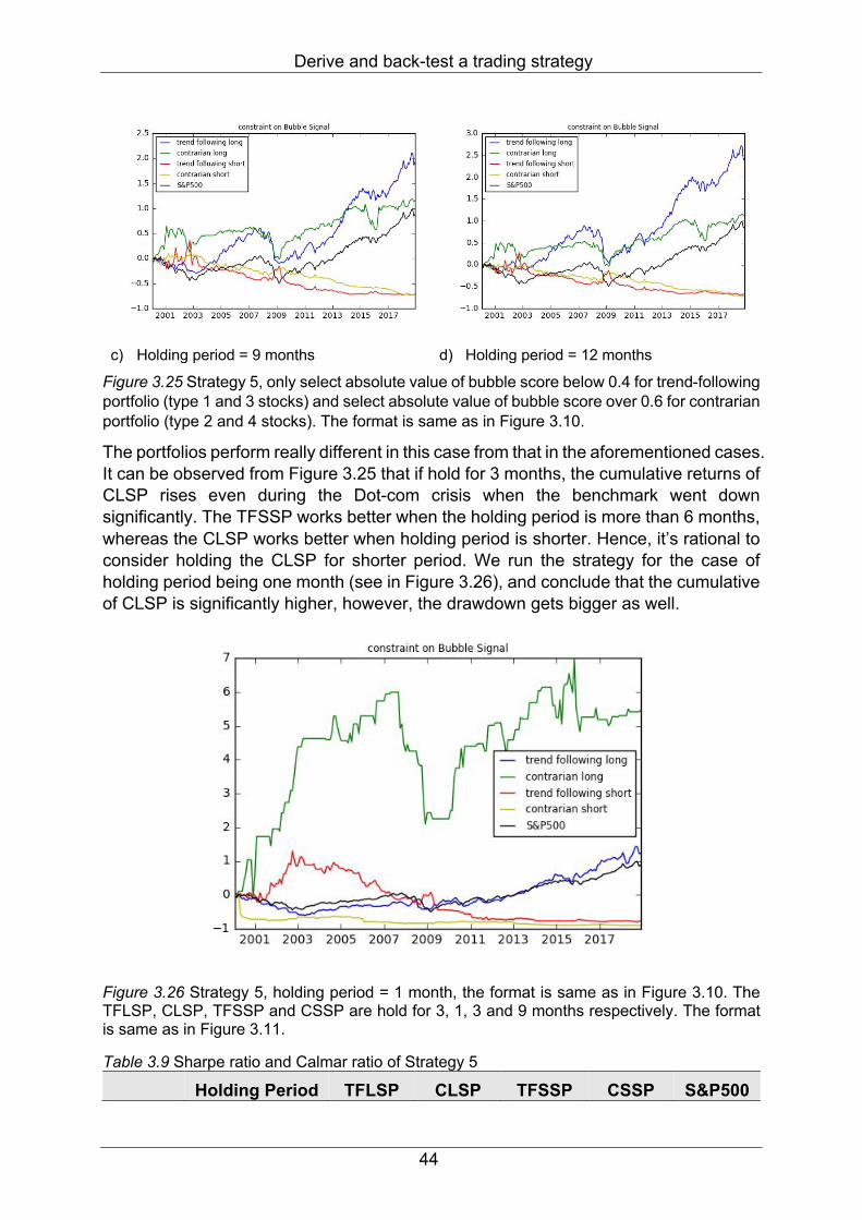
Derive and back-test a trading strategy
44
c) Holding period = 9 months
d) Holding period = 12 months
Figure 3.25 Strategy 5, only select absolute value of bubble score below 0.4 for trend-following portfolio (type 1 and 3 stocks) and select absolute value of bubble score over 0.6 for contrarian portfolio (type 2 and 4 stocks). The format is same as in Figure 3.10.
The portfolios perform really different in this case from that in the aforementioned cases. It can be observed from Figure 3.25 that if hold for 3 months, the cumulative returns of CLSP rises even during the Dot-com crisis when the benchmark went down significantly. The TFSSP works better when the holding period is more than 6 months, whereas the CLSP works better when holding period is shorter. Hence, it’s rational to consider holding the CLSP for shorter period. We run the strategy for the case of holding period being one month (see in Figure 3.26), and conclude that the cumulative of CLSP is significantly higher, however, the drawdown gets bigger as well.
Figure 3.26 Strategy 5, holding period = 1 month, the format is same as in Figure 3.10. The TFLSP, CLSP, TFSSP and CSSP are hold for 3, 1, 3 and 9 months respectively. The format is same as in Figure 3.11.
Table 3.9 Sharpe ratio and Calmar ratio of Strategy 5
Holding Period TFLSP CLSP TFSSP CSSP S&P500
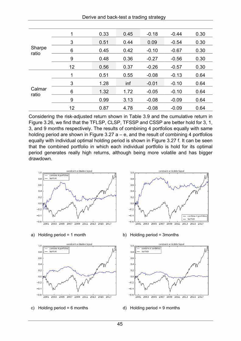
Derive and back-test a trading strategy
45
Sharpe ratio
1 0.33 0.45 -0.18 -0.44 0.30 3 0.51 0.44 0.09 -0.54 0.30 6 0.45 0.42 -0.10 -0.67 0.30 9 0.48 0.36 -0.27 -0.56 0.30
12 0.56 0.37 -0.26 -0.57 0.30
Calmar ratio
1 0.51 0.55 -0.08 -0.13 0.64 3 1.28 inf -0.01 -0.10 0.64 6 1.32 1.72 -0.05 -0.10 0.64 9 0.99 3.13 -0.08 -0.09 0.64
12 0.87 4.78 -0.08 -0.09 0.64
Considering the risk-adjusted return shown in Table 3.9 and the cumulative return in Figure 3.26, we find that the TFLSP, CLSP, TFSSP and CSSP are better hold for 3, 1, 3, and 9 months respectively. The results of combining 4 portfolios equally with same holding period are shown in Figure 3.27 a – e, and the result of combining 4 portfolios equally with individual optimal holding period is shown in Figure 3.27 f. It can be seen that the combined portfolio in which each individual portfolio is hold for its optimal period generates really high returns, although being more volatile and has bigger drawdown.
a) Holding period = 1 month
b) Holding period = 3months
c) Holding period = 6 months
d) Holding period = 9 months
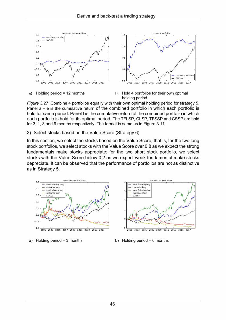
Derive and back-test a trading strategy
46
e) Holding period = 12 months
f) Hold 4 portfolios for their own optimal
holding period Figure 3.27 Combine 4 portfolios equally with their own optimal holding period for strategy 5. Panel a – e is the cumulative return of the combined portfolio in which each portfolio is hold for same period. Panel f is the cumulative return of the combined portfolio in which each portfolio is hold for its optimal period. The TFLSP, CLSP, TFSSP and CSSP are hold for 3, 1, 3 and 9 months respectively. The format is same as in Figure 3.11.
2) Select stocks based on the Value Score (Strategy 6)
In this section, we select the stocks based on the Value Score, that is, for the two long stock portfolios, we select stocks with the Value Score over 0.8 as we expect the strong fundamentals make stocks appreciate; for the two short stock portfolio, we select stocks with the Value Score below 0.2 as we expect weak fundamental make stocks depreciate. It can be observed that the performance of portfolios are not as distinctive as in Strategy 5.
a) Holding period = 3 months
b) Holding period = 6 months

Derive and back-test a trading strategy
47
c) Holding period = 9 months
d) Holding period = 12 months
Figure 3.28 Strategy 6, only select stocks with Value Score over 0.8 for long stock portfolios (type 1 and 4 stocks) and stocks with Value Score below 0.2 for short stocks portfolios (type 2 and 3 stocks). The format is same as in Figure 3.10.
Table 3.10 Sharpe ratio and Calmar ratio of strategy 6
Holding Period TFLSP CLSP TFSSP CSSP S&P500
Sharpe ratio
3 0.48 0.33 -0.05 -0.45 0.30 6 0.50 0.49 -0.13 -0.65 0.30 9 0.50 0.42 -0.22 -0.52 0.30
12 0.57 0.38 -0.27 -0.58 0.30
Calmar ratio
3 1.47 0.57 -0.05 -0.09 0.64 6 1.28 0.86 -0.06 -0.12 0.64 9 1.03 1.53 -0.08 -0.10 0.64
12 0.89 1.72 -0.08 -0.10 0.64 From Figure 3.28 and Table 3.10, it can be concluded that the TFLSP, CLSP, TFSSP and CSSP perform better in terms of the cumulative return and risk-adjusted return if hold for 6, 6, 3 and 3 months respectively. Combining 4 portfolios with same holding period and individual optimal holding period, respectively, the results are shown in Figure 3.29 and Figure 3.30.
a) Holding period = 3 months
b) Holding period = 6 months

Derive and back-test a trading strategy
48
c) Holding period = 9 months
d) Holding period = 12 months
Figure 3.29 The cumulative returns of the portfolio which combines the four portfolios equally for strategy 6. The format is same as in Figure 3.11.
Figure 3.30 Combine 4 portfolios equally with their own optimal holding period for strategy 6. The TFLSP, CLSP, TFSSP and CSSP are hold for 6, 6, 3 and 3 months respectively. The format is same as in Figure 3.11.
3) Select stocks based on the Growth Score (Strategy 7)
In this section, for two long stock portfolios, we select stocks with the Growth Score over 0.6 as the higher the growth potential is, the more likely the stocks appreciate; for two short stock portfolios, we select stocks with the Growth Score below 0.4 as the lower the growth potential is, the more beneficial to the short stock portfolio.
From Figure 3.31 and Table 3.11, it can be observed that this strategy couldn’t yield as lucrative returns as other strategy do. The TFLSP, CLSP, TFSSP and CSSP are better hold for 6, 6, 3, and 9 months respectively.
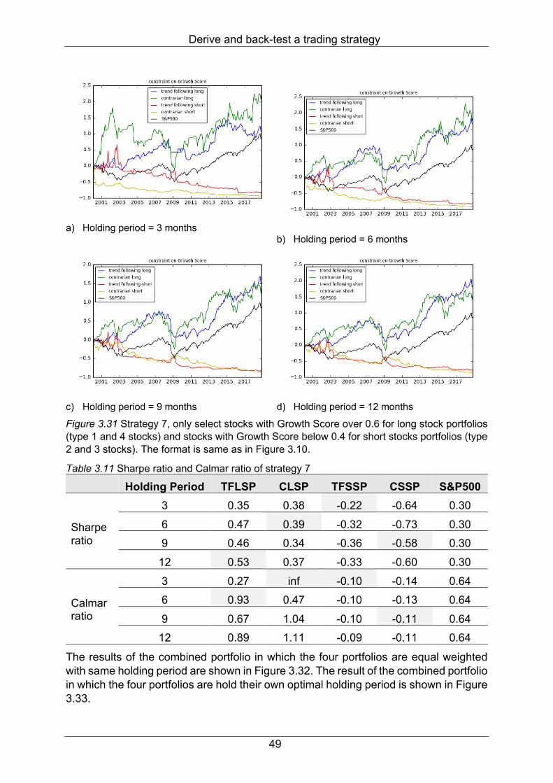
Derive and back-test a trading strategy
49
a) Holding period = 3 months
b) Holding period = 6 months
c) Holding period = 9 months
d) Holding period = 12 months
Figure 3.31 Strategy 7, only select stocks with Growth Score over 0.6 for long stock portfolios (type 1 and 4 stocks) and stocks with Growth Score below 0.4 for short stocks portfolios (type 2 and 3 stocks). The format is same as in Figure 3.10.
Table 3.11 Sharpe ratio and Calmar ratio of strategy 7
Holding Period TFLSP CLSP TFSSP CSSP S&P500
Sharpe ratio
3 0.35 0.38 -0.22 -0.64 0.30 6 0.47 0.39 -0.32 -0.73 0.30 9 0.46 0.34 -0.36 -0.58 0.30
12 0.53 0.37 -0.33 -0.60 0.30
Calmar ratio
3 0.27 inf -0.10 -0.14 0.64 6 0.93 0.47 -0.10 -0.13 0.64 9 0.67 1.04 -0.10 -0.11 0.64
12 0.89 1.11 -0.09 -0.11 0.64
The results of the combined portfolio in which the four portfolios are equal weighted with same holding period are shown in Figure 3.32. The result of the combined portfolio in which the four portfolios are hold their own optimal holding period is shown in Figure 3.33.
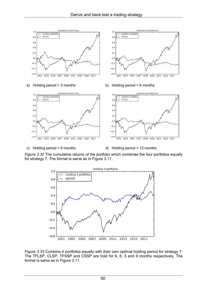
Derive and back-test a trading strategy
50
a) Holding period = 3 months
b) Holding period = 6 months
c) Holding period = 9 months
d) Holding period = 12 months
Figure 3.32 The cumulative returns of the portfolio which combines the four portfolios equally for strategy 7. The format is same as in Figure 3.11.
Figure 3.33 Combine 4 portfolios equally with their own optimal holding period for strategy 7. The TFLSP, CLSP, TFSSP and CSSP are hold for 6, 6, 3 and 9 months respectively. The format is same as in Figure 3.11.

Derive and back-test a trading strategy
51
A summary of strategies
Starting from the base strategy, we have tried some changes regarding the constraints on market cap, P/E ratio, three scores, weight of each stock for the sake of further improvements of the cumulative and risk-adjusted return. The strategies that we back test in turns are as follows: Table 3.12 Strategies and description
Strategy Description
Base
The TFLSP, CLSP, TFSSP and CSSP are constructed based on the 4-quadrants framework which considers the Bubble Score and Value, weight of a stock is proportional to its market cap in the corresponding portfolio.
1 Based on the Base Strategy, impose a constraint regarding the market cap of stocks, filter out stocks with market cap lower than 0.05 quantile in order for better liquidity of the stocks.
2 Based on Strategy 1, change the weight of stocks as equal.
3 Based on Strategy 1, change the weight of stocks as reversely proportional to its market cap.
4
Based on Strategy 1, add one more constraint regarding the P/E ratio, remove stocks in TFLSP and CLSP with P/E ratio higher than 0.6 quantile within its corresponding industry, and remove stocks in TFSSP and CSSP with P/E ratio lower than 0.4 quantile within its corresponding industry, stocks are equal weighted.
5 Based on Base Strategy, only keep stocks in the TFLSP and TFSSP with Bubble Signal below 0.4, and only keep stocks in the CLSP and CSSP with Bubble Signal over 0.6. Stocks are equal weighted.
6 Based on Base Strategy, only keep stocks in the TFLSP and CLSP with Value Score over 0.8, and only keep stocks in the TFSSP and CSSP with Value Score below 0.2. Stocks are equal weighted.
7 Based on Base Strategy, only keep stocks in the TFLSP and CLSP with Growth Score over 0.8, and only keep stocks in the TFSSP and CSSP with Growth Score below 0.2. Stocks are equal weighted.
Below is the comparison among these strategies. In order to compare the different strategies from a comprehensive perspective, we present the following table which calculates important metrics to evaluate the strategies. For each of the strategies, the optimal holding period for the four portfolios has been decided according to the discussion in previous sections. The table only contains the cases of optimal holding period.
Recall that the metrics are computed as follows:
• 𝐶𝑢𝑚𝑢𝑙𝑎𝑡𝑖𝑣𝑒𝑅𝑒𝑡𝑢𝑟𝑛9 = ∏ (1 +𝑀𝑜𝑛𝑡ℎ𝑙𝑦𝑅𝑒𝑡𝑢𝑟𝑛�)9M
• 𝐴𝑛𝑛𝑢𝑎𝑙𝑖𝑧𝑒𝑑𝑅𝑒𝑡𝑢𝑟𝑛9 = 𝐶𝑢𝑚𝑢𝑙𝑎𝑡𝑖𝑣𝑒𝑅𝑒𝑡𝑢𝑟𝑛9�]3
• 𝑉𝑜𝑙𝑎𝑡𝑖𝑙𝑖𝑡𝑦 = 𝑆𝑡𝑎𝑛𝑑𝑎𝑟𝑑𝐷𝑒𝑣𝑖𝑎𝑡𝑖𝑜𝑛𝑜𝑓𝑀𝑜𝑛𝑡ℎ𝑙𝑦𝑅𝑒𝑡𝑢𝑟𝑛
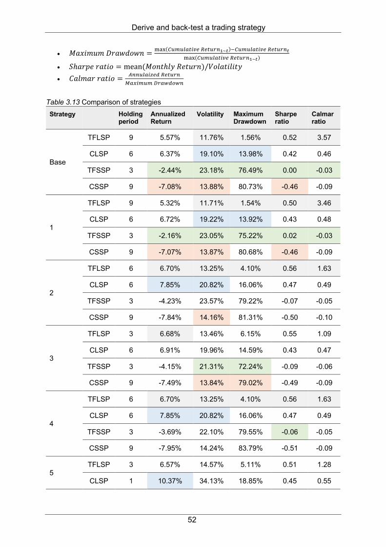
Derive and back-test a trading strategy
52
• 𝑀𝑎𝑥𝑖𝑚𝑢𝑚𝐷𝑟𝑎𝑤𝑑𝑜𝑤𝑛 = � ¡(v�K���9�¢���9����~3)Lv�K���9�¢���9���3� ¡(v�K���9�¢���9����~3)
• 𝑆ℎ𝑎𝑟𝑝𝑒𝑟𝑎𝑡𝑖𝑜 = mean(𝑀𝑜𝑛𝑡ℎ𝑙𝑦𝑅𝑒𝑡𝑢𝑟𝑛)/𝑉𝑜𝑙𝑎𝑡𝑖𝑙𝑖𝑡𝑦 • 𝐶𝑎𝑙𝑚𝑎𝑟𝑟𝑎𝑡𝑖𝑜 = §������¨�1��9���
©�ª�K�K«��¬1�¬�
Table 3.13 Comparison of strategies Strategy Holding
period Annualized Return
Volatility Maximum Drawdown
Sharpe ratio
Calmar ratio
Base
TFLSP 9 5.57% 11.76% 1.56% 0.52 3.57
CLSP 6 6.37% 19.10% 13.98% 0.42 0.46
TFSSP 3 -2.44% 23.18% 76.49% 0.00 -0.03
CSSP 9 -7.08% 13.88% 80.73% -0.46 -0.09
1
TFLSP 9 5.32% 11.71% 1.54% 0.50 3.46
CLSP 6 6.72% 19.22% 13.92% 0.43 0.48
TFSSP 3 -2.16% 23.05% 75.22% 0.02 -0.03
CSSP 9 -7.07% 13.87% 80.68% -0.46 -0.09
2
TFLSP 6 6.70% 13.25% 4.10% 0.56 1.63
CLSP 6 7.85% 20.82% 16.06% 0.47 0.49
TFSSP 3 -4.23% 23.57% 79.22% -0.07 -0.05
CSSP 9 -7.84% 14.16% 81.31% -0.50 -0.10
3
TFLSP 3 6.68% 13.46% 6.15% 0.55 1.09
CLSP 6 6.91% 19.96% 14.59% 0.43 0.47
TFSSP 3 -4.15% 21.31% 72.24% -0.09 -0.06
CSSP 9 -7.49% 13.84% 79.02% -0.49 -0.09
4
TFLSP 6 6.70% 13.25% 4.10% 0.56 1.63
CLSP 6 7.85% 20.82% 16.06% 0.47 0.49
TFSSP 3 -3.69% 22.10% 79.55% -0.06 -0.05
CSSP 9 -7.95% 14.24% 83.79% -0.51 -0.09
5 TFLSP 3 6.57% 14.57% 5.11% 0.51 1.28
CLSP 1 10.37% 34.13% 18.85% 0.45 0.55

Derive and back-test a trading strategy
53
TFSSP 3 -0.41% 23.10% 63.73% 0.09 -0.01
CSSP 9 -6.71% 11.20% 75.54% -0.56 -0.09
6
TFLSP 6 6.62% 15.17% 5.16% 0.50 1.28
CLSP 6 8.19% 20.00% 9.58% 0.49 0.86
TFSSP 3 -4.07% 23.96% 78.36% -0.05 -0.05
CSSP 3 -8.11% 15.82% 86.24% -0.45 -0.09
7
TFLSP 6 5.32% 12.94% 5.71% 0.47 0.93
CLSP 6 5.76% 19.42% 12.15% 0.39 0.47
TFSSP 3 -9.12% 26.69% 90.15% -0.22 -0.10
CSSP 9 -9.57% 15.21% 85.18% -0.58 -0.11
From Table 3.13, it is obvious that the TFSSP is always better to be hold for 3 months, and the CSSP is always better to be hold for 9 months, except in strategy 6 which selects stocks based on the Value Score. The TFLSP and CLSP are hold for longer term except in strategy 5, which select stocks based on the Bubble Signal, CLSP is hold for 1 month. Back to 20 years ago, the TFLSP and CLSP have accumulated higher returns than the other two portfolios, and in the same case, the CLSP always performs better than the TFLSP. The CSSP doesn’t perform well no matter which strategy is applied, thus it could be considered useless.
For each of the portfolio, we mark some cells in which the metrics are relatively good. We can thus conclude that for TFLSP, the strategy 2 and 4 are relatively better; for CLSP, the strategy 2, 4 and 6 are relatively better; for TFSSP, the base strategy, strategy 1 and 5 are relatively better.
Although for most of time, the CLSP has higher return than TFLSP, it has higher volatility and maximum drawdown, hence in order to construct a self-financing portfolio, one could combine CLSP, TFLSP and TFSSP together to lower the volatility, protect against the broad market going down and yield relatively high return. For example, we could consider the following combination:
a) One CLSP, strategy 6, hold 6 months b) One CLSP, strategy 5, hold 1 month c) One TFLSP, strategy 2, hold 6 months d) Three TFSSP, strategy 3, hold 3 months
According to the following Figure 3.14 and Table 3.15, the performance of this combined portfolios is good due to its high risk-adjusted return and low volatility.

Derive and back-test a trading strategy
54
Figure 3.34 The cumulative return of a combination of different portfolios mentioned above (this is a self- financing portfolio). The blue line is the cumulative return of the combination, the black line is the cumulative return of the benchmark S&P500.
Table 3.14 Evaluation metrics of the above portfolio
Annualized Return Volatility Maximum Drawdown Sharpe ratio Calmar ratio
4.13% 8.89% 5.84% 0.5 0.71
3.4 Look back at the ROIC Valuation Framework
Although the combined portfolio has shown the effectiveness of our trading strategies, when we look into details of the ROIC curve which are generated during the process of calculating the Value Score, we find some anomalies. Overall, the ROIC curve makes sense as it depicts the positive relation between the ROIC and EV/IC, which is in accordance with the common sense – the more profitable the company is, the more it should be worth. However, when we plot the ln(EV/IC) vs. ROIC curve from 20 years ago until now, there does exist some months in which the positive relation between ln(EV/IC) and ROIC doesn’t hold for the energy stocks (an example is shown in figure 3.19). Specifically, these anomalies appear only in the energy industry from 05/2000 to 06/2001 and from 04/2003 to 05/2003.
Some reasons could be attributed to this anomaly is energy industry. The relationship between the oil and gas supply and global demand plays a significant role in the energy market and is a crucial factor driving the price of the oil and gas. Oil and gas have prices depending on the location type. They trade at different prices due to the refinability as well as the regional issues. Because oil prices can differ significantly, oil producers in some regions make less money than others. Besides, OPEC, which is an intergovernmental organization currently made up of 14 oil-producing nations that work together to coordinate and unify their oil prices. Those counties combine to produce about 40% of global oil supplies, which gives OPEC lots of sway over the oil market.
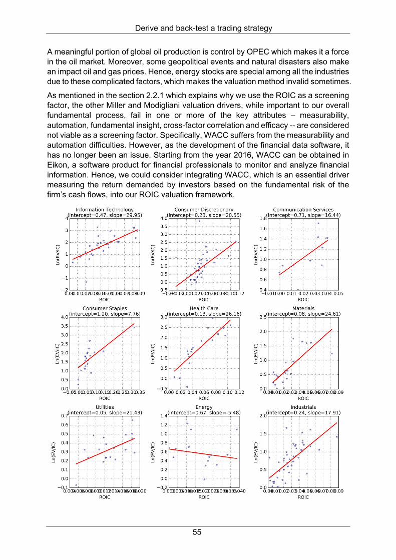
Derive and back-test a trading strategy
55
A meaningful portion of global oil production is control by OPEC which makes it a force in the oil market. Moreover, some geopolitical events and natural disasters also make an impact oil and gas prices. Hence, energy stocks are special among all the industries due to these complicated factors, which makes the valuation method invalid sometimes.
As mentioned in the section 2.2.1 which explains why we use the ROIC as a screening factor, the other Miller and Modigliani valuation drivers, while important to our overall fundamental process, fail in one or more of the key attributes – measurability, automation, fundamental insight, cross-factor correlation and efficacy -- are considered not viable as a screening factor. Specifically, WACC suffers from the measurability and automation difficulties. However, as the development of the financial data software, it has no longer been an issue. Starting from the year 2016, WACC can be obtained in Eikon, a software product for financial professionals to monitor and analyze financial information. Hence, we could consider integrating WACC, which is an essential driver measuring the return demanded by investors based on the fundamental risk of the firm’s cash flows, into our ROIC valuation framework.
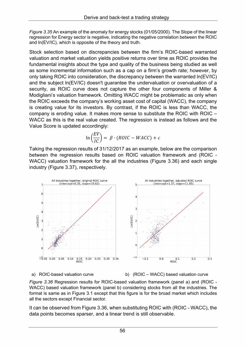
Derive and back-test a trading strategy
56
Figure 3.35 An example of the anomaly for energy stocks (01/05/2000). The Slope of the linear regression for Energy sector is negative, indicating the negative correlation between the ROIC and ln(EV/IC), which is opposite of the theory and truth.
Stock selection based on discrepancies between the firm’s ROIC-based warranted valuation and market valuation yields positive returns over time as ROIC provides the fundamental insights about the type and quality of the business being studied as well as some incremental information such as a cap on a firm’s growth rate; however, by only taking ROIC into consideration, the discrepancy between the warranted ln(EV/IC) and the subject ln(EV/IC) doesn't guarantee the undervaluation or overvaluation of a security, as ROIC curve does not capture the other four components of Miller & Modigliani’s valuation framework. Omitting WACC might be problematic as only when the ROIC exceeds the company’s working asset cost of capital (WACC), the company is creating value for its investors. By contrast, if the ROIC is less than WACC, the company is eroding value. It makes more sense to substitute the ROIC with ROIC – WACC as this is the real value created. The regression is instead as follows and the Value Score is updated accordingly:
ln 𝐸𝑉𝐼𝐶 ® = 𝛽 ∙ (𝑅𝑂𝐼𝐶 −𝑊𝐴𝐶𝐶) + 𝑐
Taking the regression results of 31/12/2017 as an example, below are the comparison between the regression results based on ROIC valuation framework and (ROIC - WACC) valuation framework for the all the industries (Figure 3.36) and each single industry (Figure 3.37), respectively.
a) ROIC-based valuation curve
b) (ROIC – WACC) based valuation curve
Figure 3.36 Regression results for ROIC-based valuation framework (panel a) and (ROIC - WACC) based valuation framework (panel b) considering stocks from all the industries. The format is same as in Figure 3.1 except that this figure is for the broad market which includes all the sectors except Financial sector.
It can be observed from Figure 3.36, when substituting ROIC with (ROIC - WACC), the data points becomes sparser, and a linear trend is still observable.
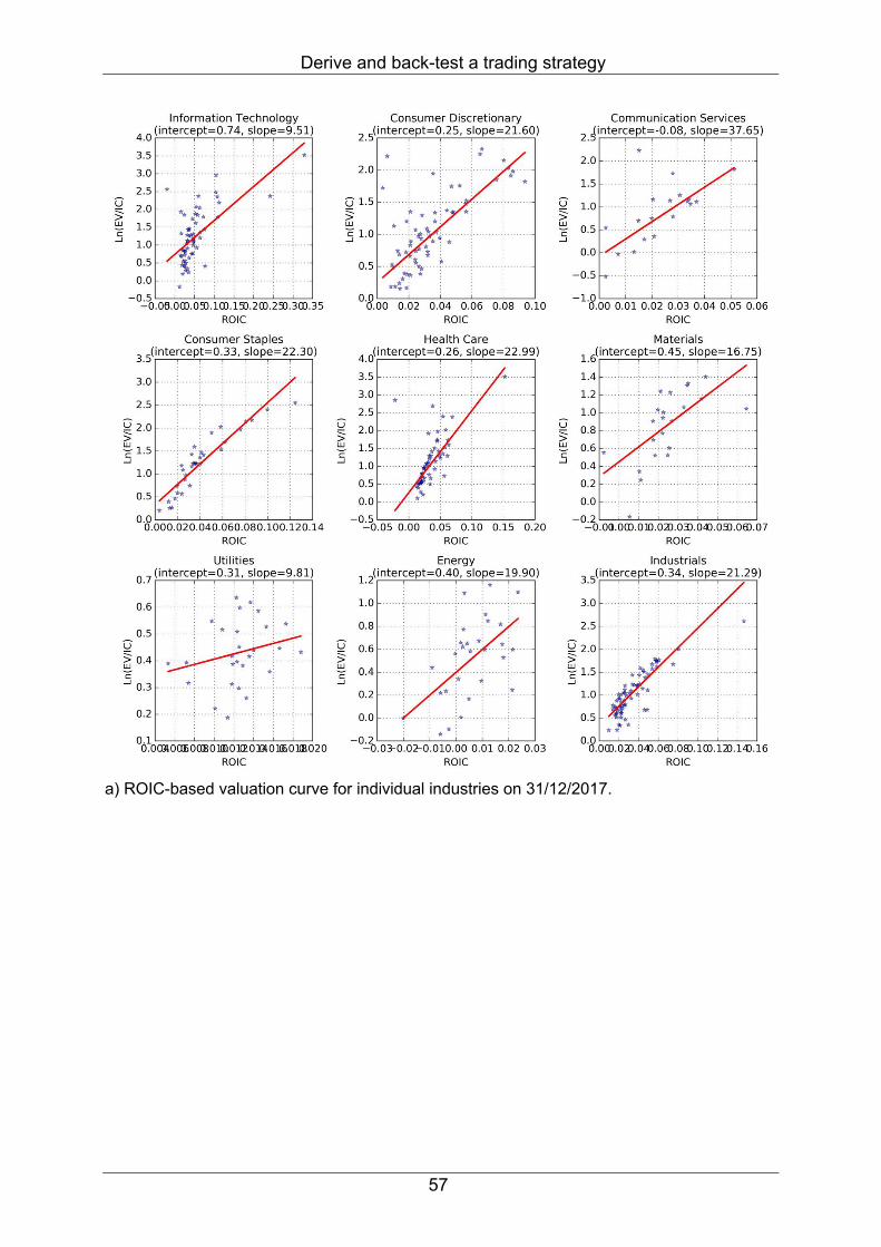
Derive and back-test a trading strategy
57
a) ROIC-based valuation curve for individual industries on 31/12/2017.

Derive and back-test a trading strategy
58
b) (ROIC – WACC) based valuation curve for individual industries on 31/12/2017.
Figure 3.37 Regression results for ROIC-based valuation framework (panel a) and (ROIC - WACC) based valuation framework (panel b) for each individual industry. The format is same as in Figure 3.1.
From Figure 3.37, it can be observed that the extent of the deviation of the real market value from the warranted value changes significantly, thus the Value Score will change accordingly. We then evaluate the effect of adding (-WACC) into the original model by rerun the back-testing for the 4 portfolios in the combined portfolio in section 3.3.6.

Derive and back-test a trading strategy
59
a) CLSP, strategy 6, hold 6 months
b) CLSP, strategy 5, hold 1 month
c) TFLSP, strategy 2, hold 6 months
d) TFSSP, strategy 1, hold 3 months
e) Combined portfolio (which contains one a, one b, one c and three d)
Figure 3.38 Comparison of the portfolios in the section 3.3.6 between the same strategies based on ROIC and (ROIC-WACC) respectively. The black line is the original cumulative return of the portfolios starting from 01/2016 till 12/2018, and the blue line is the cumulative returns of the portfolios from 21/2016 to 12/2018 after adjusting the ROIC by deducting WACC. Panels a – d are for the 4 types of portfolios included in the combined portfolios, and the panel e is for the combined portfolio.
From Figure 3.38, it can be observed that by adjusting the ROIC by deducting WACC, the performance of portfolio a and c doesn't change a lot, while the performance of portfolio b and d does improve a lot, thus the performance of the combined portfolio

Derive and back-test a trading strategy
60
improves as well. The (ROIC-WACC) based valuation framework is proved to be effective.

Conclusion
61
4 Conclusion The emergence of bubble is due to the positive feedback and herding behavior. The Bubble Score is based on the LPPLS model which detects the emergence and burst of bubbles ex-ante. The Value Score is derived from the ROIC valuation framework which measures the deviation of the market value from the ROIC-based warranted value. By categorizing stocks according these two stocks, it is possible to capture the trend and identify the corrections.
The trading strategy based on the Bubble Score and Value Score which updates these two scores and rebalance on a monthly basis is proved to be effective for trading constituents of S&P500. Our back-test starts from 01/2000 until 12/2018. During the two massive correction which happened in 2000 and 2008 respectively, the trend-following short stock portfolio and the contrarian short stock portfolio yield positive returns while except for these two bubble crashes, the trend-following long stock portfolio and contrarian long stock portfolio continuously outperform the benchmark, which confirms that the Bubble Score does possess the predictive power which could help investors to chase the trend or spot corrections, and under the help of the fundamental valuation, the current status of stocks can be better interpreted – strong positive (negative) bubble and strong (weak) fundamental indicate a fast growing trend, while strong positive(negative) bubble and weak (strong) fundamental indicate a potential correction.
Among all the strategies we have tested, the contrarian long stock portfolio always performs better than the trend-following long stock portfolio, which implies for S&P500, it is more profitable to trade the stocks follow a faster-than-exponential growth but with little support of fundamental. This kind stocks are usually ignored by investors until the correction happens. This thesis successfully finds out this kind of stocks and trading them turn out to be more profitable than chasing the trend.
By changing the holding period and impose some constraints on the initial strategy, we further improve the performance and find out the optimal trading method for each portfolio. A self-financing portfolio can thus be constructed by combining the portfolios with different strategy.
Moreover, in the end of this thesis, we present a method to improve the ROIC valuation framework. By substituting the ROIC with (ROIC - WACC) in the framework, the cumulative of the portfolio increases, which indicates subtracting the WACC from ROIC makes it clearer if the company is creating value for investors.
Outlook
62
5 Outlook In the LPPLS model, only bubble signal is used in our trading strategy, while other confidence indicators are not taken into consideration, they might play a role for improving the performance of the portfolios. The critical time tc, for example, could be used to determine the holding period.
In the ROIC framework, due the measurability and automation issues, some valuations drivers are omitted for now, but they might have a significant impact on the valuation process. With the development of the financial database, more data of key drivers will be available which can be further integrated in the valuation framework.
Our trading strategy is mainly for S&P500 constituents, it could be applied on the constituents of other indices as well.
Appendix
63
6 Appendix Data
The LPPLS data is obtained from the existing FCO platform. The fundamental data are fetched through the Eikon API, which is provided by Thomsen Reuters for financial professionals to monitor and analyze financial information. For each of stocks, the most recent fundamental data coming from the quarterly financial report are used as the input of the strategy. Specifically, at the rebalance date, we get the following fields from via Eikon:
1. Earnings Per Share – Actual (EPSa, “TR.EPSACTVALUE”) 2. Earnings Per Share – Mean Estimate (EPSm, “TR.EPSMeanEstimate”) 3. Company Market Cap (MC, Reuters: “TR.CompanyMarketCap”) 4. Total Long Term Debt (LTD, “TR.TotalLongTermDebt”) 5. Common Shareholder Equity (CSE, “TR.CommShareholdersEqty”) 6. Number of Shares Outstanding – Mean (S,
“TR.NumberofSharesOutstandingMean”)
From this direct input we calculate the following factors:
1. The Enterprise Value: EV = MC + LTD; 2. The Invested Capital: IC = CSE + LTD; 3. The Return on Invested Capital: ROIC = S * EPSm /IC; 4. The expected growth in ROIC: DROIC = S * (EPSm – EPSa)/IC; 5. The expected growth in ROIC: DROIC = S * (EPSm – EPSa)/IC;

Bibliography
64
Bibliography [1]. Modern Approaches to Asset Price Formation: A survey of Recent Theoretical Literature, International Department and Economic Research Department, Reserve Bank of Australia.
[2]. Sornette, Didier and Cauwels, Peter, Financial Bubbles: Mechanisms and Diagnostics (April 8, 2014). Swiss Finance Institute Research Paper No. 14-28.
[3]. Yip, P. (2018). Some Important Characteristics of Asset Bubbles and Financial Crises. Modern Economy, 09(07), pp.1137-1168.
[4]. Sornette, D. and Johansen, A. (1998). A hierarchical model of financial crashes. Physica A: Statistical Mechanics and its Applications, 261(3-4), pp.581-598.
[5]. E. Fama. Efficient markets: a review of theory and empirical work. Journal of Finance, 25:383–417, 1970.
[6]. E. Fama. Efficient capital markets. Journal of Finance, 46:1575–1618, 1991.
[7]. Bao, T., Hommes, C. and Makarewicz, T. (2015). Bubble Formation and (In)Efficient Markets in Learning-to-Forecast and -Optimise Experiments. SSRN Electronic Journal.
[8]. Massoud, N. and Bernhardt, D. (1999). Stock market dynamics with rational liquidity traders. Journal of Financial Markets, 2(4), pp.359-389.
[9]. Sornette, D., Woodard, R., Yan, W. and Zhou, W. (2011). Clarifications to Questions and Criticisms on the Johansen-Ledoit-Sornette Bubble Model. SSRN Electronic Journal.
[10]. A. Johansen, O. Ledoit, and D. Sornette, Crashes as critical points. International Journal of Theoretical and Applied Finance, 3:329-225, 2000.
[11]. Demirer, R., Demos, G., Gupta, R. and Sornette, D. (2018). On the predictability of stock market bubbles: evidence from LPPLS confidence multi-scale indicators. Quantitative Finance, 19(5), pp.843-858.
[12]. Sornette, D. and Woodard, R. (2009). Financial Bubbles, Real Estate Bubbles, Derivative Bubbles, and the Financial and Economic Crisis. SSRN Electronic Journal.
[13]. The ROIC Curve, Valuation Framework
[14]. N.-P. Pham Huu. Back-testing of trading strategies based on financial crisis observatory output. Master’s thesis, ETH Zurich, 2018.
[15]. T. Mamageishvili. Back-testing of Trading Strategies Using Financial Crisis Observatory Output. Master’s thesis, ETH Zurich, 2019.
[16]. D. Sornette. Dragon-kings, black swans and the prediction of crises. International Journal of Terraspace Science and Engineering, 2(1):1–18, 2009.
[17]. N.-N. Taleb. The Black Swan: the impact of the highly improbable. London: Penguin, 2012.