designing and maintaining essbase cubes · the essbase solution for creating optimized databases...

Oracle® CloudDesigning and Maintaining Essbase Cubes

E70190-10January 2019

Oracle Cloud Designing and Maintaining Essbase Cubes,

E70190-10

Copyright © 1996, 2019, Oracle and/or its affiliates. All rights reserved.

Primary Author: Essbase Information Development Team

This software and related documentation are provided under a license agreement containing restrictions onuse and disclosure and are protected by intellectual property laws. Except as expressly permitted in yourlicense agreement or allowed by law, you may not use, copy, reproduce, translate, broadcast, modify,license, transmit, distribute, exhibit, perform, publish, or display any part, in any form, or by any means.Reverse engineering, disassembly, or decompilation of this software, unless required by law forinteroperability, is prohibited.

The information contained herein is subject to change without notice and is not warranted to be error-free. Ifyou find any errors, please report them to us in writing.

If this is software or related documentation that is delivered to the U.S. Government or anyone licensing it onbehalf of the U.S. Government, then the following notice is applicable:

U.S. GOVERNMENT END USERS: Oracle programs, including any operating system, integrated software,any programs installed on the hardware, and/or documentation, delivered to U.S. Government end users are"commercial computer software" pursuant to the applicable Federal Acquisition Regulation and agency-specific supplemental regulations. As such, use, duplication, disclosure, modification, and adaptation of theprograms, including any operating system, integrated software, any programs installed on the hardware,and/or documentation, shall be subject to license terms and license restrictions applicable to the programs.No other rights are granted to the U.S. Government.

This software or hardware is developed for general use in a variety of information management applications.It is not developed or intended for use in any inherently dangerous applications, including applications thatmay create a risk of personal injury. If you use this software or hardware in dangerous applications, then youshall be responsible to take all appropriate fail-safe, backup, redundancy, and other measures to ensure itssafe use. Oracle Corporation and its affiliates disclaim any liability for any damages caused by use of thissoftware or hardware in dangerous applications.

Oracle and Java are registered trademarks of Oracle and/or its affiliates. Other names may be trademarks oftheir respective owners.

Intel and Intel Xeon are trademarks or registered trademarks of Intel Corporation. All SPARC trademarks areused under license and are trademarks or registered trademarks of SPARC International, Inc. AMD, Opteron,the AMD logo, and the AMD Opteron logo are trademarks or registered trademarks of Advanced MicroDevices. UNIX is a registered trademark of The Open Group.

This software or hardware and documentation may provide access to or information about content, products,and services from third parties. Oracle Corporation and its affiliates are not responsible for and expresslydisclaim all warranties of any kind with respect to third-party content, products, and services unless otherwiseset forth in an applicable agreement between you and Oracle. Oracle Corporation and its affiliates will not beresponsible for any loss, costs, or damages incurred due to your access to or use of third-party content,products, or services, except as set forth in an applicable agreement between you and Oracle.

Contents

Preface

Audience xxviii

Documentation Accessibility xxviii

Related Resources xxviii

Conventions xxix

1 Case Study: Designing a Single-Server, Multidimensional Database

Process for Designing a Database 1-1

Case Study: The Beverage Company 1-2

Analyzing and Planning 1-2

Analyzing Source Data 1-3

Identifying User Requirements 1-3

Planning for Security in a Multiple User Environment 1-4

Creating Database Models 1-4

Identifying Analysis Objectives 1-4

Determining Dimensions and Members 1-5

Analyzing Database Design 1-8

Drafting Outlines 1-13

Dimension and Member Properties 1-14

Dimension Types 1-15

Member Storage Properties 1-15

Checklist for Dimension and Member Properties 1-16

Designing an Outline to Optimize Performance 1-16

Optimizing Query Performance 1-17

Optimizing Calculation Performance 1-17

Meeting the Needs of Both Calculation and Retrieval 1-18

Loading Test Data 1-18

Defining Calculations 1-18

Consolidation of Dimensions and Members 1-19

Effect of Position and Operator on Consolidation 1-20

Consolidation of Shared Members 1-20

Checklist for Consolidation 1-21

iii

Tags and Operators on Example Measures Dimension 1-21

Accounts Dimension Calculations 1-22

Time Balance Properties 1-22

Variance Reporting 1-23

Formulas and Functions 1-23

Dynamic Calculations 1-24

Two-Pass Calculations 1-25

Checklist for Calculations 1-26

Defining Reports 1-27

Verifying the Design 1-27

2 Understanding Multidimensional Databases

OLAP and Multidimensional Databases 2-1

Dimensions and Members 2-2

Outline Hierarchies 2-3

Dimension and Member Relationships 2-3

Parents, Children, and Siblings 2-4

Descendants and Ancestors 2-5

Roots and Leaves 2-5

Generations and Levels 2-5

Generation and Level Names 2-6

Standard Dimensions and Attribute Dimensions 2-6

Sparse and Dense Dimensions 2-6

Selection of Dense and Sparse Dimensions 2-7

Dense-Sparse Configuration for Sample.Basic 2-8

Dense and Sparse Selection Scenarios 2-9

Data Storage 2-15

Data Values 2-15

Data Blocks and the Index System 2-17

Multiple Data Views 2-21

The Essbase Solution for Creating Optimized Databases 2-22

3 Creating Applications and Databases

Understanding Applications and Databases 3-1

Understanding Database Artifacts 3-1

Understanding Database Outlines 3-2

Understanding Source Data 3-2

Understanding Rule Files for Data Load and Dimension Build 3-2

Understanding Calculation Scripts 3-2

iv

Creating an Application and Database 3-3

Using Substitution Variables 3-3

Rules for Setting Substitution Variable Names and Values 3-4

Setting Substitution Variables 3-5

Deleting Substitution Variables 3-5

Updating Substitution Variables 3-6

Copying Substitution Variables 3-6

Using Location Aliases 3-6

4 Creating and Changing Database Outlines

Process for Creating Outlines 4-1

Creating and Editing Outlines 4-2

Locking and Unlocking Outlines 4-2

Setting the Dimension Storage Type 4-2

Positioning Dimensions and Members 4-3

Moving Dimensions and Members 4-3

Sorting Dimensions and Members 4-3

Verifying Outlines 4-4

Saving Outlines 4-5

Saving an Outline with Added Standard Dimensions 4-5

Saving an Outline with One or More Deleted Standard Dimensions 4-5

Creating Sub-Databases Using Deleted Members 4-5

5 Creating and Working With Duplicate Member Outlines

Creating Duplicate Member Names in Outlines 5-1

Restrictions for Duplicate Member Names and Aliases in Outlines 5-2

Syntax for Specifying Duplicate Member Names and Aliases 5-2

Using Fully Qualified Member Names 5-3

Qualifying Members by Differentiating Ancestor 5-3

Using Shortcut Qualified Member Names 5-3

Using Qualified Member Names in Unique Member Name Outlines 5-4

Working with Duplicate Member Names in Clients 5-4

6 Setting Dimension and Member Properties

Setting Dimension Types 6-1

Creating a Time Dimension 6-1

Creating an Accounts Dimension 6-2

Setting Time Balance Properties 6-2

Setting Skip Properties 6-3

v

Setting Variance Reporting Properties 6-4

Creating Attribute Dimensions 6-4

Setting Member Consolidation 6-5

Calculating Members with Different Operators 6-5

Determining How Members Store Data Values 6-6

Understanding Stored Members 6-7

Understanding Dynamic Calculation Members 6-7

Understanding Label Only Members 6-7

Understanding Shared Members 6-7

Understanding the Rules for Shared Members 6-8

Understanding Shared Member Retrieval During Drill-Down 6-9

Setting Aliases 6-11

Alias Tables 6-12

Creating Aliases 6-12

Creating and Managing Alias Tables 6-12

Creating an Alias Table 6-12

Setting an Alias Table as Active 6-13

Copying an Alias Table 6-13

Renaming an Alias Table 6-13

Clearing and Deleting Alias Tables 6-13

Importing and Exporting Alias Tables 6-14

Setting Two-Pass Calculations 6-14

Creating Formulas 6-15

Naming Generations and Levels 6-15

Creating UDAs 6-15

Adding Comments to Dimensions and Members 6-16

7 Working with Attributes

Process for Creating Attributes 7-1

Understanding Attributes 7-2

Understanding Attribute Dimensions 7-3

Understanding Members of Attribute Dimensions 7-4

Understanding the Rules for Base and Attribute Dimensions and Members 7-4

Understanding the Rules for Attribute Dimension Association 7-5

Understanding the Rules for Attribute Member Association 7-5

Understanding Attribute Types 7-5

Comparing Attribute and Standard Dimensions 7-6

Solve Order and Attributes 7-8

Understanding Two-Pass Calculations on Attribute Dimensions 7-9

Comparing Attributes and UDAs 7-9

vi

Designing Attribute Dimensions 7-11

Using Attribute Dimensions 7-11

Using Alternative Design Approaches 7-12

Optimizing Outline Performance 7-13

Building Attribute Dimensions 7-13

Setting Member Names in Attribute Dimensions 7-14

Setting Prefix and Suffix Formats for Member Names of Attribute Dimensions 7-14

Setting Boolean Attribute Member Names 7-15

Changing the Member Names in Date Attribute Dimensions 7-15

Setting Up Member Names Representing Ranges of Values 7-16

Changing the Member Names of the Attribute Calculations Dimension 7-17

Calculating Attribute Data 7-17

Understanding the Attribute Calculations Dimension 7-18

Understanding the Default Attribute Calculations Members 7-19

Viewing an Attribute Calculation Example 7-20

Accessing Attribute Calculations Members in Smart View 7-20

Optimizing Calculation and Retrieval Performance 7-21

Using Attributes in Calculation Formulas 7-21

Understanding Attribute Calculation and Shared Members 7-22

Differences Between Calculating Attribute Members and Non-Attribute (Storedand Dynamic Calc) Members 7-23

Non-Aggregating Attributes 7-23

Submitting Data for Valid Attribute Combinations in the Grid 7-23

Suppressing Invalid Attribute Combinations in the Grid 7-24

8 Working with Typed Measures

About Typed Measures 8-1

Working with Text Measures 8-1

Text Measures Workflow 8-2

Text List Objects and Text List Members 8-2

Working with Date Measures 8-3

Implementing Date Measures 8-3

Functions Supporting Date Measures 8-3

Performing Database Operations on Text and Date Measures 8-4

Loading, Clearing, and Exporting Text and Date Measures 8-4

Consolidating Text and Date Measures 8-6

Retrieving Data With Text and Date Measures 8-6

Limitations of Text and Date Measures 8-6

Working with Format Strings 8-6

Implementing Format Strings 8-7

MDX Format Directive 8-7

vii

Functions Supporting Format Strings 8-8

Limitations of Format Strings 8-8

9 Designing Partitioned Applications

Understanding Partitioning 9-1

Partition Types 9-1

Parts of a Partition 9-2

Data Sources and Data Targets 9-3

Attributes in Partitions 9-5

Version and Encoding Requirements 9-6

Partition Design Requirements 9-6

Benefits of Partitioning 9-7

Partitioning Strategies 9-7

Guidelines for Partitioning a Database 9-7

Guidelines for Partitioning Data 9-8

Security for Partitioned Databases 9-9

Setting up End-User Security 9-9

Setting up Administrator Security 9-9

Replicated Partitions 9-10

Rules for Replicated Partitions 9-10

Advantages of Replicated Partitions 9-11

Disadvantages of Replicated Partitions 9-11

Performance Considerations for Replicated Partitions 9-12

Replicated Partitions and Port Usage 9-12

Transparent Partitions 9-13

Rules for Transparent Partitions 9-14

Advantages of Transparent Partitions 9-15

Disadvantages of Transparent Partitions 9-15

Performance Considerations for Transparent Partitions 9-16

Calculating Transparent Partitions 9-17

Performance Considerations for Transparent Partition Calculations 9-17

Transparent Partitions and Member Formulas 9-18

Transparent Partitions and Port Usage 9-18

10

Creating and Maintaining Partitions

Choosing a Partition Type 10-1

Setting up a Partition Data Source 10-1

Setting the User Name and Password 10-2

Defining a Partition Area 10-2

viii

Mapping Members in Partitions 10-2

Mapping Members with Different Names 10-3

Mapping Data Cubes with Extra Dimensions 10-3

Mapping Shared Members 10-5

Mapping Attributes Associated with Members 10-5

Creating Advanced Area-Specific Mappings 10-6

Validating Partitions 10-7

Populating or Updating Replicated Partitions 10-8

Viewing Partition Information 10-9

Partitioning and SSL 10-9

Troubleshooting Partitions 10-9

11

Understanding Data Loading and Dimension Building

Introduction to Data Loading and Dimension Building 11-1

Process for Data Loading and Dimension Building 11-2

Data Sources 11-2

Supported Source Data Types 11-2

Items in a Data Source 11-3

Valid Dimension Fields 11-4

Valid Member Fields 11-4

Valid Data Fields 11-5

Valid Delimiters 11-6

Valid Formatting Characters 11-7

Rule Files 11-7

Situations that Do and Do Not Need a Rules File 11-8

Data Sources that Do Not Need a Rule File 11-9

Formatting Ranges of Member Fields 11-10

Setting Ranges Automatically 11-10

Handling Out of Range Data Values 11-11

Interpreting Duplicate Members in a Range 11-11

Reading Multiple Ranges 11-11

Formatting Columns 11-12

Symmetric Columns 11-12

Asymmetric Columns 11-12

Security and Multiple-User Considerations 11-13

12

Working with Rule Files

Process for Creating Data Load Rule Files 12-1

Process for Creating Dimension Build Rules Files 12-1

ix

Creating Rule Files 12-2

Setting File Delimiters 12-2

Naming New Dimensions 12-3

Selecting a Build Method 12-3

Setting and Changing Member and Dimension Properties 12-3

Using the Data Source to Work with Member Properties 12-3

Setting Field Type Information 12-5

Field Types and Valid Build Methods 12-6

Rules for Assigning Field Types 12-7

Setting Dimension Build Operational Instructions 12-8

Defining Data Load Field Properties 12-9

Performing Operations on Records, Fields, and Data 12-9

Validating Rules Files 12-10

Requirements for Valid Data Load Rule Files 12-10

Requirements for Valid Dimension Build Rule Files 12-11

13

Using a Rules File to Perform Operations on Records, Fields, andData

Performing Operations on Records 13-1

Selecting Records 13-1

Rejecting Records 13-1

Combining Multiple Select and Reject Criteria 13-2

Setting the Records Displayed 13-2

Defining Header Records 13-2

Data Source Headers 13-3

Valid Data Source Header Field Types 13-3

Performing Operations on Fields 13-4

Ignoring Fields 13-4

Ignoring Strings 13-4

Arranging Fields 13-5

Moving Fields 13-5

Joining Fields 13-5

Creating a Field by Joining Fields 13-5

Copying Fields 13-6

Splitting Fields 13-6

Creating Additional Text Fields 13-6

Mapping Fields 13-6

Changing Field Names 13-6

Replacing Text Strings 13-7

Placing Text in Empty Fields 13-7

x

Changing the Case of Fields 13-7

Dropping Leading and Trailing Spaces 13-7

Converting Spaces to Underscores 13-7

Adding Prefixes or Suffixes to Field Values 13-7

Performing Operations on Data 13-8

Defining Columns as Data Fields 13-8

Adding to and Subtracting from Existing Values 13-8

Clearing Existing Data Values 13-9

Replacing All Data 13-9

Scaling Data Values 13-10

Flipping Field Signs 13-10

14

Performing and Debugging Data Loads or Dimension Builds

Prerequisites for Data Loads and Dimension Builds 14-1

Performing Data Loads or Dimension Builds 14-1

Stopping Data Loads or Dimension Builds 14-2

Tips for Loading Data and Building Dimensions 14-2

Performing Deferred-Restructure Dimension Builds 14-2

Determining Where to Load Data 14-3

Dealing with Missing Fields in a Data Source 14-4

Loading a Subset of Records from a Data Source 14-4

Debugging Data Loads and Dimension Builds 14-5

Verifying that Essbase Server Is Available 14-5

Verifying that the Data Source Is Available 14-5

Checking Error Logs 14-6

Resolving Problems with Data Loaded Incorrectly 14-6

Creating Rejection Criteria for End of File Markers 14-7

Understanding How Essbase Processes a Rules File 14-8

Understanding How Essbase Processes Missing or Invalid Fields During a DataLoad 14-9

Missing Dimension or Member Fields 14-9

Unknown Member Fields 14-9

Invalid Data Fields 14-10

15

Understanding Advanced Dimension Building Concepts

Understanding Build Methods 15-1

Using Generation References 15-2

Using Level References 15-5

Using Parent-Child References 15-8

Adding a List of New Members 15-9

xi

Adding Members Based On String Matches 15-9

Adding Members as Siblings of the Lowest Level 15-11

Adding Members to a Specified Parent 15-12

Building Attribute Dimensions and Associating Attributes 15-14

Building Attribute Dimensions 15-15

Associating Attributes 15-15

Updating Attribute Associations 15-17

Removing Attribute Associations 15-17

Working with Multilevel Attribute Dimensions 15-18

Working with Numeric Ranges 15-20

Building Attribute Dimensions that Accommodate Ranges 15-21

Associating Base Dimension Members with Their Range Attributes 15-22

Ensuring the Validity of Associations 15-23

Reviewing the Rules for Building Attribute and Base Dimensions 15-24

Building Shared Members by Using a Rules File 15-25

Sharing Members at the Same Generation 15-27

Using Generation References to Create Same Generation Shared Members15-27

Using Level References to Create Same Generation Shared Members 15-28

Using Parent-Child References to Create Same Generation SharedMembers 15-29

Sharing Members at Different Generations 15-29

Using Level References to Create Different Generation Shared Members 15-30

Using Parent-Child References to Create Different Generation SharedMembers 15-31

Sharing Non-Level 0 Members 15-31

Using Level References to Create Non-Level 0 Shared Members 15-32

Using Parent-Child References to Create Non-Level 0 Shared Members 15-33

Building Multiple Roll-Ups by Using Level References 15-34

Creating Shared Roll-Ups from Multiple Data Sources 15-35

Building Duplicate Member Outlines 15-36

Uniquely Identifying Members Through the Rules File 15-36

Building Qualified Member Names Through the Rules File 15-37

16

Modeling Data in Private Scenarios

Testing Changes with a Sandbox Dimension 16-1

Merging Sandbox Data Changes 16-2

xii

17

Calculating Essbase Databases

About Database Calculation 17-1

Outline Calculation 17-2

Calculation Script Calculation 17-3

About Multidimensional Calculation Concepts 17-3

Setting the Default Calculation 17-7

Calculating Databases 17-7

Canceling Calculations 17-7

Parallel and Serial Calculation 17-8

Security Considerations 17-8

18

Developing Formulas for Block Storage Databases

Using Formulas and Formula Calculations 18-1

Understanding Formula Syntax 18-2

Operators 18-4

Dimension and Member Names 18-4

Constant Values 18-4

Nonconstant Values 18-5

Basic Equations 18-5

Checking Formula Syntax 18-6

Using Functions in Formulas 18-7

Conditional Tests 18-9

Examples of Conditional Tests 18-11

Mathematical Operations 18-12

Member Relationship Functions 18-13

Range Functions 18-14

Financial Functions 18-15

Member-Related Functions 18-16

Specifying Member Lists and Ranges 18-16

Generating Member Lists 18-17

Manipulating Member Names 18-20

Working with Member Combinations Across Dimensions 18-21

Value-Related Functions 18-22

Using Interdependent Values 18-22

Calculating Variances or Percentage Variances Between Actual and BudgetValues 18-23

Allocating Values 18-24

Forecasting Functions 18-25

Statistical Functions 18-25

Date and Time Function 18-26

xiii

Calculation Mode Function 18-26

Using Substitution Variables in Formulas 18-27

Using Formulas on Partitions 18-27

Displaying Formulas 18-28

19

Reviewing Examples of Formulas for Block Storage Databases

Calculating Period-to-Date Values in an Accounts Dimension 19-1

Calculating Rolling Values 19-2

Calculating Monthly Asset Movements 19-3

Testing for #MISSING Values 19-4

Calculating an Attribute Formula 19-5

20

Defining Calculation Order

Data Storage in Data Blocks 20-1

Member Calculation Order 20-3

Understanding the Effects of Member Relationships 20-3

Determining Member Consolidation 20-4

Ordering Dimensions in the Database Outline 20-5

Placing Formulas on Members in the Database Outline 20-5

Using the Calculation Operators *, /, and % 20-5

Avoiding Forward Calculation References 20-6

Block Calculation Order 20-8

Data Block Renumbering 20-10

Cell Calculation Order 20-11

Cell Calculation Order: Example 1 20-11




Cell Calculation Order for Formulas on a Dense Dimension 20-16

Calculation Passes 20-16

Calculation of Shared Members 20-18

21

Understanding Intelligent Calculation

About Intelligent Calculation 21-1

Benefits of Intelligent Calculation 21-1

Intelligent Calculation and Data Block Status 21-2

Marking Blocks as Clean 21-2

Marking Blocks as Dirty 21-3

Maintaining Clean and Dirty Status 21-3

xiv

Limitations of Intelligent Calculation 21-3

Considerations for Essbase Intelligent Calculation on Oracle Exalytics In-Memory Machine 21-4

Using Intelligent Calculation 21-4

Turning Intelligent Calculation On and Off 21-4

Using Intelligent Calculation for a Default, Full Calculation 21-4

Calculating for the First Time 21-5

Recalculating 21-5

Using Intelligent Calculation for a Calculation Script, Partial Calculation 21-5

Using the SET CLEARUPDATESTATUS Command 21-5

Understanding SET CLEARUPDATESTATUS 21-6

Choosing a SET CLEARUPDATESTATUS Setting 21-6

Reviewing Examples That Use SET CLEARUPDATESTATUS 21-6

Example 1: CLEARUPDATESTATUS AFTER 21-7

Example 2: CLEARUPDATESTATUS ONLY 21-7

Example 3: CLEARUPDATESTATUS OFF 21-7

Calculating Data Blocks 21-7

Calculating Dense Dimensions 21-8

Calculating Sparse Dimensions 21-8

Level 0 Effects 21-8

Upper-Level Effects 21-9

Unnecessary Calculation 21-9

Handling Concurrent Calculations 21-9

Understanding Multiple-Pass Calculations 21-10

Reviewing Examples and Solutions for Multiple-Pass Calculations 21-10

Example 1: Intelligent Calculation and Two-Pass 21-10

Example 2: SET CLEARUPDATESTATUS and FIX 21-11

Example 3: SET CLEARUPDATESTATUS and Two CALC DIM Commands 21-11

Example 4: Two Calculation Scripts 21-12

Understanding the Effects of Intelligent Calculation 21-14

Changing Formulas and Accounts Properties 21-14

Using Relationship and Financial Functions 21-14

Restructuring Databases 21-14

Copying and Clearing Data 21-15

Converting Currencies 21-15

22

Dynamically Calculating Data Values

Understanding Dynamic Calculation 22-1

Understanding Dynamic Calc Members 22-1

Retrieving the Parent Value of Dynamically Calculated Child Values 22-2

Benefitting from Dynamic Calculation 22-2

xv

Using Dynamic Calculation 22-2

Choosing Values to Calculate Dynamically 22-3

Dense Members and Dynamic Calculation 22-3

Sparse Members and Dynamic Calculation 22-3

Two-Pass Members and Dynamic Calculation 22-4

Parent-Child Relationships and Dynamic Calculation 22-4

Calculation Scripts and Dynamic Calculation 22-4

Formulas and Dynamically Calculated Members 22-4

Scripts and Dynamically Calculated Members 22-5

Dynamically Calculated Children 22-5

Understanding How Dynamic Calculation Changes Calculation Order 22-6

Calculation Order for Dynamic Calculation 22-6

Calculation Order for Dynamically Calculating Two-Pass Members 22-7

Calculation Order for Asymmetric Data 22-7

Reducing the Impact on Retrieval Time 22-9

Displaying a Retrieval Factor 22-9

Displaying a Summary of Dynamically Calculated Members 22-10

Increasing Retrieval Buffer Size 22-10

Using Dynamic Calculator Caches 22-10

Reviewing Dynamic Calculator Cache Usage 22-11

Using Dynamic Calculations with Standard Procedures 22-11

Creating Dynamic Calc Members 22-12

Restructuring Databases 22-12

Dynamically Calculating Data in Partitions 22-13

Custom Solve Order in Hybrid Aggregation Mode 22-13

23

Calculating Time Series Data

Calculating First, Last, and Average Values 23-1

Specifying Accounts and Time Dimensions 23-2

Reporting the Last Value for Each Time Period 23-2

Reporting the First Value for Each Time Period 23-3

Reporting the Average Value for Each Time Period 23-3

Skipping #MISSING and Zero Values 23-4

Considering the Effects of First, Last, and Average Tags 23-4

Placing Formulas on Time and Accounts Dimensions 23-5

Calculating Period-to-Date Values Using Dynamic Time Series Members 23-5

Using Dynamic Time Series Members 23-5

Enabling and Disabling Dynamic Time Series Members 23-7

Specifying Alias Names for Dynamic Time Series Members 23-7

Applying Predefined Generation Names to Dynamic Time Series Members 23-8

xvi

Retrieving Period-to-Date Values 23-8

Using Dynamic Time Series Members in Transparent Partitions 23-9

24

Developing Calculation Scripts for Block Storage Databases

Using Calculation Scripts 24-1

Understanding Calculation Script Syntax 24-3

Adding Comments to Calculation Scripts 24-6

Checking Syntax 24-6

Using Calculation Commands 24-7

Calculating the Database Outline 24-7

Controlling the Flow of Calculations 24-7

Declaring Data Variables 24-8

Specifying Global Settings for a Database Calculation 24-9

Using Formulas in Calculation Scripts 24-10

Basic Equations 24-11

Conditional Equations 24-11

Interdependent Formulas 24-12

Using a Calculation Script to Control Intelligent Calculation 24-12

Grouping Formulas and Calculations 24-13

Calculating a Series of Member Formulas 24-13

Calculating a Series of Dimensions 24-13

Using Substitution, Runtime Substitution, and Environment Variables in CalculationScripts 24-14

Using Substitution Variables in Calculation Scripts 24-14

Using Runtime Substitution Variables in Calculation Scripts Run in Essbase 24-14

Specifying Data Type and Input Limit for Runtime Substitution Variables inCalculation Scripts Run in Essbase 24-17

Logging Runtime Substitution Variables 24-17

Using Runtime Substitution Variables in Calculation Scripts Run in Smart View 24-18

Example: Runtime Substitution Variable Set to POV 24-19

XML Tag Reference—Calculation Scripts with Runtime SubstitutionVariables for Smart View 24-20

Clearing and Copying Data 24-21

Clearing Data 24-21

Copying Data 24-22

Calculating a Subset of a Database 24-23

Calculating Lists of Members 24-23

Using the FIX Command 24-23

Using the Exclude Command 24-26

Exporting Data Using the DATAEXPORT Command 24-26

Advantages and Disadvantages of Exporting Data Using a Calculation Script 24-28

xvii

Enabling Calculations on Potential Blocks 24-29

Using DATACOPY to Copy Existing Blocks 24-29

Using SET CREATENONMISSINGBLK to Calculate All Potential Blocks 24-30

Using Calculation Scripts on Partitions 24-31

Writing Calculation Scripts for Partitions 24-31

Controlling Calculation Order for Partitions 24-31

Saving, Executing, and Copying Calculations Scripts 24-32

Saving Calculation Scripts 24-32

Executing Calculation Scripts 24-33

Copying Calculation Scripts 24-33

Checking Calculation Results 24-33

25

Reviewing Examples of Calculation Scripts for Block StorageDatabases

About These Calculation Script Examples 25-1

Calculating Variance 25-1

Calculating Database Subsets 25-2

Loading New Budget Values 25-3

Calculating Product Share and Market Share Values 25-4

Allocating Costs Across Products 25-5

Allocating Values within a Dimension 25-6

Allocating Values Across Multiple Dimensions 25-8

Goal-Seeking Using the LOOP Command 25-10

Forecasting Future Values 25-13

26

Using Hybrid Aggregation

About Hybrid Aggregation 26-1

Comparison of Hybrid Aggregation, Block Storage, and Aggregate Storage 26-1

Getting Started with Hybrid Aggregation 26-2

Optimizing the Database for Hybrid Aggregation 26-3

Limitations and Exceptions to Hybrid Mode 26-3

27

Using Parallel Calculation

About Parallel Calculation 27-1

Using CALCPARALLEL Parallel Calculation 27-1

Essbase Analysis of Feasibility 27-2

CALCPARALLEL Parallel Calculation Guidelines 27-2

Relationship Between CALCPARALLEL Parallel Calculation and Other EssbaseFeatures 27-3

xviii

Retrieval Performance 27-3

Formula Limitations 27-3

Calculator Cache 27-4

Transparent Partition Limitations 27-4

Checking Current CALCPARALLEL Settings 27-4

Enabling CALCPARALLEL Parallel Calculation 27-4

Identifying Additional Tasks for Parallel Calculation 27-5

Tuning CALCPARALLEL with Log Messages 27-6

Monitoring CALCPARALLEL Parallel Calculation 27-6

Using FIXPARALLEL Parallel Calculation 27-7

28

Writing MDX Queries

About Writing MDX Queries 28-1

Understanding Elements of a Query 28-2

Introduction to Sets and Tuples 28-2

Exercise: Running Your First Query 28-3

Rules for Specifying Sets 28-4

Introduction to Axis Specifications 28-5

Exercise: Running A Two-Axis Query 28-6

Exercise: Querying Multiple Dimensions on a Single Axis 28-7

Cube Specification 28-8

Using Functions to Build Sets 28-8

Exercise: Using the MemberRange Function 28-8

Exercise: Using the CrossJoin Function 28-9

Exercise: Using the Children Function 28-11

Working with Levels and Generations 28-12

Exercise: Using the Members Function 28-12

Using a Slicer Axis to Set Query Point-of-View 28-13

Exercise: Limiting the Results with a Slicer Axis 28-14

Common Relationship Functions 28-14

Performing Set Operations 28-15

Exercise: Using the Intersect Function 28-16

Exercise: Using the Union Function 28-17

Creating and Using Named Sets and Calculated Members 28-17

Calculated Members 28-18

Exercise: Creating a Calculated Member 28-18

Named Sets 28-20

Using Iterative Functions 28-20

Working with Missing Data 28-21

Using Substitution Variables in MDX Queries 28-22

xix

Querying for Properties 28-23

Querying for Member Properties 28-24

The Value Type of Properties 28-25

NULL Property Values 28-26

29

Exporting Data

Exporting Data Using MaxL 29-1

Exporting Text Data Using Calculation Scripts 29-1

30

Controlling Access to Database Cells Using Security Filters

About Security Filters 30-1

Defining Permissions Using Security Filters 30-1

Creating Filters 30-2

Filtering Members Versus Filtering Member Combinations 30-3

Filtering Members Separately 30-4

Filtering Member Combinations 30-4

Filtering Using Substitution Variables 30-5

Filtering with Attribute Functions 30-5

Metadata Filtering 30-6

Dynamic Filtering 30-6

Managing Filters 30-6

Assigning Filters 30-7

Overlapping Filter Definitions 30-7

Overlapping Metadata Filter Definitions 30-7

Overlapping Access Definitions 30-8

31

Using MaxL Data Definition Language

32

Optimizing Database Restructuring

Database Restructuring 32-1

Implicit Restructures 32-1

Explicit Restructures 32-2

Conditions Affecting Database Restructuring 32-2

Restructuring Requires a Temporary Increase in the Index Cache Size 32-3

Optimization of Restructure Operations 32-3

Actions That Improve Performance 32-3

Parallel Restructuring 32-4

xx

Options for Saving a Modified Outline 32-4

Outline Change Quick Reference 32-4

33

Optimizing Data Loads

Understanding Data Loads 33-1

Grouping Sparse Member Combinations 33-2

Making the Data Source as Small as Possible 33-4

Making Source Fields as Small as Possible 33-5

Positioning Data in the Same Order as the Outline 33-5

Loading from Essbase Server 33-5

Using Parallel Data Load 33-6

Understanding Parallel Data Load 33-6

Enabling Parallel Data Load With Multiple Files 33-6

34

Optimizing Calculations

Designing for Calculation Performance 34-1

Block Size and Block Density 34-1

Order of Sparse Dimensions 34-2

Incremental Data Loading 34-2

Database Outlines with Multiple Flat Dimensions 34-2

Formulas and Calculation Scripts 34-3

Monitoring and Tracing Calculations 34-3

SET MSG SUMMARY and SET MSG DETAIL 34-3

SET NOTICE 34-3

Using Simulated Calculations to Estimate Calculation Time 34-4

Performing a Simulated Calculation 34-4

Estimating Calculation Time 34-5

Factors Affecting Estimate Accuracy 34-6

Variations Due to a Chain of Influences 34-6

Variations Due to Outline Structure 34-6

Changing the Outline Based on Results 34-6

Estimating Calculation Effects on Database Size 34-7

Using Formulas 34-8

Consolidating 34-8

Using Simple Formulas 34-8

Using Complex Formulas 34-9

Optimizing Formulas on Sparse Dimensions in Large Database Outlines 34-10

Constant Values Assigned to Members in a Sparse Dimension 34-10

Nonconstant Values Assigned to Members in a Sparse Dimension 34-11

xxi

Using Cross-Dimensional Operators 34-11

On the Left of an Equation 34-12

In Equations in a Dense Dimension 34-12

Managing Formula Execution Levels 34-13

Using Bottom-Up Calculation 34-13

Bottom-Up and Top-Down Calculation 34-13

Bottom-Up Calculations and Simple Formulas 34-13

Top-Down Calculations and Complex Formulas 34-14

Forcing a Bottom-Up Calculation 34-14

Hybrid Aggregation Mode in Block Storage Databases 34-15

Managing Caches to Improve Performance 34-15

Working with the Block Locking System 34-16

Managing Concurrent Access for Users 34-16

Using Two-Pass Calculation 34-17

Understanding Two-Pass Calculation 34-17

Reviewing a Two-Pass Calculation Example 34-17

Understanding the Interaction of Two-Pass Calculation and IntelligentCalculation 34-19

Scenario A 34-19

Scenario B 34-19

Choosing Two-Pass Calculation Tag or Calculation Script 34-20

Enabling Two-Pass on Default Calculations 34-20

Creating Calculation Scripts for Two-Pass and Intelligent Calculation 34-21

Intelligent Calculation with a Large Index 34-21

Intelligent Calculation with a Small Index 34-23

Intelligent Calculation Turned Off for a Two-Pass Formula 34-23

Choosing Between Member Set Functions and Performance 34-24

Consolidating #MISSING Values 34-24

Understanding #MISSING Calculation 34-24

Changing Consolidation for Performance 34-25

Removing #MISSING Blocks 34-26

Identifying Additional Calculation Optimization Issues 34-27

35

Comparison of Aggregate and Block Storage

Inherent Differences 35-1

Outline Differences 35-2

Calculation Differences 35-4

Data Load Differences 35-4

Query Differences 35-5

Feature Differences 35-6

xxii

Hybrid Aggregation 35-6

36

Aggregate Storage Applications, Databases, and Outlines

Process for Creating Aggregate Storage Applications 36-1

Creating Aggregate Storage Applications, Databases, and Outlines 36-1

Hierarchies 36-2

Stored Hierarchies 36-3

Dynamic Hierarchies 36-4

Alternate Hierarchies 36-5

Attribute Dimensions 36-7

Design Considerations for Attribute Queries 36-8

Design Considerations for Aggregate Storage Outlines 36-9

Query Design Considerations for Aggregate Storage 36-9

64-bit Dimension Size Limit for Aggregate Storage Database Outline 36-9

Understanding the Compression Dimension for Aggregate Storage Databases 36-12

Maintaining Retrieval Performance 36-12

Viewing Compression Estimation Statistics 36-13

Verifying Aggregate Storage Outlines 36-14

Outline Paging 36-14

Outline Paging Limits 36-14

Dimension Build Limit 36-15

Loaded Outline Limit 36-15

Compacting the Aggregate Storage Outline File 36-16

Developing Formulas on Aggregate Storage Outlines 36-16

Using MDX Formulas 36-16

Formula Calculation for Aggregate Storage Databases 36-18

Formula Syntax for Aggregate Storage Databases 36-19

Creating Formulas on Aggregate Storage Outlines 36-20

Composing Formulas on Aggregate Storage Outlines 36-20

Basic Equations for Aggregate Storage Outlines 36-20

Members Across Dimensions in Aggregate Storage Outlines 36-21

Conditional Tests in Formulas for Aggregate Storage Outlines 36-21

Specifying UDAs in Formulas in Aggregate Storage Outlines 36-21

37

Aggregate Storage Time-Based Analysis

About Aggregate Storage Time-Based Analysis 37-1

Understanding Date-Time Dimensions 37-1

Understanding Linked Attributes 37-2

Designing and Creating an Outline for Date-Time Analysis 37-4

xxiii

Preparing for Creating Date-Time Dimensionality 37-4

Understanding Date-Time Calendars 37-5

Modifying or Deleting Date-Time Dimensions 37-6

Verification Rules for Date-Time Dimensions 37-7

Verification Rules for Linked Attribute Dimensions 37-7

Loading Data Mapped to Dates 37-8

Analyzing Time-Based Data 37-9

Using Smart View to Analyze Time-Related Data 37-9

Analyzing Time-Based Metrics with MDX 37-9

38

Loading, Calculating, and Retrieving Aggregate Storage Data

Sample Aggregate Storage Outline 38-1

Preparing Aggregate Storage Databases 38-3

Building Dimensions in Aggregate Storage Databases 38-3

Rules File Differences for Aggregate Storage Dimension Builds 38-3

Data Source Differences for Aggregate Storage Dimension Builds 38-4

Building Alternate Hierarchies in Aggregate Storage Databases 38-5

Understanding Exclusive Operations on Aggregate Storage Databases 38-5

Loading Data into Aggregate Storage Databases 38-6

Incrementally Loading Data Using a Data Load Buffer 38-7

Controlling Data Load Buffer Resource Usage 38-9

Setting Data Load Buffer Properties 38-10

Resolving Cell Conflicts 38-11

Performing Multiple Data Loads in Parallel 38-11

Listing Data Load Buffers for an Aggregate Storage Database 38-12

Creating a Data Slice 38-13

Merging Incremental Data Slices 38-14

Replacing Database or Incremental Data Slice Contents 38-15

Viewing Incremental Data Slices Statistics 38-16

Managing Disk Space For Incremental Data Loads 38-16

Using Smart View 38-17

Data Source Differences for Aggregate Storage Data Loads 38-17

Rules File Differences for Aggregate Storage Data Loads 38-17

Clearing Data from an Aggregate Storage Database 38-18

Clearing Data from Specific Regions of Aggregate Storage Databases 38-18

Clearing All Data from an Aggregate Storage Database 38-22

Copying an Aggregate Storage Application 38-22

Combining Data Loads and Dimension Builds 38-22

Calculating Aggregate Storage Databases 38-22

Outline Factors Affecting Data Values 38-23

xxiv

Block Storage Calculation Features That Do Not Apply to Aggregate StorageDatabases 38-23

Calculation Order 38-24

Solve Order Property 38-24

Example Using the Solve Order Property 38-25

Aggregating an Aggregate Storage Database 38-28

Understanding Aggregation-Related Terms 38-28

Performing Database Aggregations 38-29

Fine-Tuning Aggregate View Selection 38-30

Selecting Views Based on Usage 38-32

Understanding User-Defined View Selection 38-33

Working with Aggregation Scripts 38-34

Optimizing Aggregation Performance 38-35

Clearing Aggregations 38-35

Replacing Aggregations 38-36

Performing Time Balance and Flow Metrics Calculations in Aggregate StorageAccounts Dimensions 38-36

Using Time Balance Tags in Aggregate Storage Accounts Dimensions 38-36

Using Flow Tags in Aggregate Storage Accounts Dimensions 38-37

Restrictions on Alternate Hierarchies 38-38

Aggregating Time-Balance Tagged Measures 38-39

Effect of Attribute Calculations on Time Balance Measures in AggregateStorage Databases 38-39

Retrieving Aggregate Storage Data 38-40

Attribute Calculation Retrievals 38-40

Retrieval Tools Supporting Aggregate Storage Databases 38-40

39

Performing Custom Calculations and Allocations on AggregateStorage Databases

About Performing Custom Calculations and Allocations on Aggregate StorageDatabases 39-1

Custom Calculations on Aggregate Storage Databases 39-2

List of Custom Calculations Criteria 39-3

Writing Custom Calculations 39-3

Executing Custom Calculations 39-4

Sample Use Case for Custom Calculations 39-4

Optimizing Custom Calculations by Skipping Empty Tuples 39-6

Custom Allocations on Aggregate Storage Databases 39-7

List of Allocation Criteria 39-8

Understanding Regions 39-10

Specifying Allocation Criteria 39-10

xxv

Using Shared Members 39-11

Using Duplicate Members 39-11

Setting the POV 39-11

Setting the Range 39-12

Setting the Amount 39-12

Setting the Basis 39-14

Setting the Target 39-15

Setting the Allocation Method 39-16

Setting the Rounding Method 39-18

Setting the Offset 39-19

Balancing Allocations 39-19

Understanding Settings for Basis and Target Time Span 39-19

Example 1: Basis and Target Time Span—Empty or Single Member 39-20

Example 2: Basis Time Span—Empty or Single Member; Target Time Span—Multiple Members 39-20

Example 3: Basis Time Span—Multiple Members; Target Time Span—Empty or Single Member 39-22

Example 4: Basis and Target Time Span—Multiple Members; Basis TimeSpan Option—Split 39-23

Example 5: Basis and Target Time Span—Multiple Members; Basis TimeSpan Option—Combine 39-25

Examples of Aggregate Storage Allocations 39-27

Sample Use Case for Aggregate Storage Allocations 39-28

Scenario 1: Aggregate Storage Allocations 39-29

Scenario 2: Aggregate Storage Allocations 39-29

Avoiding Data Inconsistency When Using Formulas 39-30

Understanding Data Load Buffers for Custom Calculations and Allocations 39-31

Understanding Offset Handling for Custom Calculations and Allocations 39-31

Understanding Credit and Debit Processing for Custom Calculations and Allocations39-32

40

Managing Aggregate Storage Applications and Databases

Aggregate Storage Security 40-1

Managing the Aggregate Storage Cache 40-1

Improving Performance When Building Aggregate Views on Aggregate StorageDatabases 40-2

Aggregate Storage Database Restructuring 40-3

Levels of Aggregate Storage Database Restructuring 40-4

Outline-Change Examples 40-8

Example: No Change in the Number of Stored Levels in a Hierarchy 40-8

Example: Change in the Number of Stored Levels in a Hierarchy 40-9

Example: Changes in Alternate Hierarchies 40-10

xxvi

Example: Addition of Child Members 40-10

Example: Addition of Child Branches 40-11

Exporting Aggregate Storage Databases 40-12

Calculating the Number of Stored Dimension Levels in an Aggregate StorageOutline 40-12

A Limits

Name and Related Artifact Limits A-1

Data Load and Dimension Build Limits A-3

Aggregate Storage Database Limits A-3

Block Storage Database Limits A-4

Drill-through to Oracle Applications Limits A-6

Other Size or Quantity Limits A-6

B Naming Conventions for Essbase

Naming Conventions for Applications and Databases B-1

Naming Conventions for Dimensions, Members, and Aliases B-2

Naming Conventions for Dynamic Time Series Members B-4

Naming Conventions for Attribute Calculations Dimension Member Names B-4

Naming Conventions in Calculation Scripts, Report Scripts, Formulas, Filters, andSubstitution and Environment Variable Values B-5

List of Essbase System-Defined Dimension and Member Names B-6

List of MaxL DDL Reserved Words B-6

xxvii

Preface

Learn how to get started with Oracle Analytics Cloud – Essbase.

Topics

• Audience

• Documentation Accessibility

• Related Resources

• Conventions

AudienceDesigning and Maintaining Essbase Cubes is intended for business users, analysts,modelers, and decision-makers across all lines of business within an organization whouse Oracle Analytics Cloud – Essbase.

Use this document as an in-depth resource and reference guide for designing andmaintaining Essbase cubes.

Documentation AccessibilityFor information about Oracle's commitment to accessibility, visit the OracleAccessibility Program website at http://www.oracle.com/pls/topic/lookup?ctx=acc&id=docacc.

Access to Oracle Support

Oracle customers that have purchased support have access to electronic supportthrough My Oracle Support. For information, visit http://www.oracle.com/pls/topic/lookup?ctx=acc&id=info or visit http://www.oracle.com/pls/topic/lookup?ctx=acc&id=trsif you are hearing impaired.

Related ResourcesUse these related resources to expand your understanding of Oracle Analytics Cloud -Essbase.

• Oracle Public Cloud http://cloud.oracle.com

• Using Oracle Analytics Cloud - Essbase

• Technical Reference for Oracle Analytics Cloud - Essbase

• Accessibility Guide for Oracle Analytics Cloud - Essbase

Preface

xxviii

http://www.oracle.com/pls/topic/lookup?ctx=acc&id=docacc

http://www.oracle.com/pls/topic/lookup?ctx=acc&id=docacc

http://www.oracle.com/pls/topic/lookup?ctx=acc&id=info

http://www.oracle.com/pls/topic/lookup?ctx=acc&id=info

http://www.oracle.com/pls/topic/lookup?ctx=acc&id=trs

• Getting Started with Oracle Analytics Cloud

• Administering Oracle Analytics Cloud in a Customer-Managed Environment

ConventionsThe following text conventions are used in this document:

Convention Meaning

boldface Boldface type indicates graphical user interface elements associatedwith an action, or terms defined in text or the glossary.

italic Italic type indicates book titles, emphasis, or placeholder variables forwhich you supply particular values.

monospace Monospace type indicates commands within a paragraph, URLs, codein examples, text that appears on the screen, or text that you enter.

Preface

xxix

1Case Study: Designing a Single-Server,Multidimensional Database

This case study provides an overview of the database planning process and discussesworking rules that you can follow to design a single-server, multidimensional databasesolution for your organization.

• Process for Designing a Database

• Case Study: The Beverage Company

• Analyzing and Planning

• Drafting Outlines

• Loading Test Data

• Defining Calculations

• Defining Reports

• Verifying the Design

Process for Designing a DatabaseTo implement a multidimensional database, you design and create an application anddatabase. You analyze data sources and define requirements carefully and decidewhether a single-server approach or a partitioned, distributed approach better servesyour needs. For criteria that you can review to decide whether to partition anapplication, see Guidelines for Partitioning a Database.

This case study provides an overview of the database planning process and discussesworking rules that you can follow to design a single-cube, multidimensional databasesolution for your organization. See Creating Applications and Databases.

The process of designing a database includes the following basic steps:

1. Analyze business needs and design a plan.

The application and database that you create must satisfy the information needs ofyour users and your organization. Therefore, you identify source data, define userinformation access needs, review security considerations, and design a databasemodel. See Analyzing and Planning.

2. Draft a database outline.

The outline determines the structure of the database—what information is storedand how different pieces of information interrelate. See Drafting Outlines.

3. Load test data into the database.

After an outline and a security plan are in place, you load the database with testdata to enable the later steps of the process. See Loading Test Data.

4. Define calculations.

1-1

You test outline consolidations, write and test formulas, and define calculationscripts for specialized calculations. See Defining Calculations.

5. Verify with users.

To ensure that the database satisfies your user goals, solicit and carefully considertheir feedback. See Verifying the Design.

6. Repeat the process.

To fine-tune the design, repeat steps 1 through 5.

Case Study: The Beverage CompanyThis case study bases the database planning process on the needs of a fictitiouscompany, The Beverage Company (TBC), as an example for how to build an Essbasedatabase. TBC is a variation of the Sample.Basic application that is included with theEssbase installation.

TBC manufactures, markets, and distributes soft drink products internationally.Analysts at TBC prepare budget forecasts and compare performance to budgetforecasts monthly. The financial measures that analysts track are profit, loss, andinventory.

TBC uses spreadsheet packages to prepare budget data and perform variancereporting. Because TBC plans and tracks a variety of products over several markets,the process of deriving and analyzing data is tedious. Last month, analysts spent mostof their time entering and rekeying data and preparing reports.

TBC has determined that Essbase is the best tool for creating a centralized repositoryfor financial data. The data repository will reside on a server that is accessible toanalysts throughout the organization. Users can load data from various sources andretrieve data as needed. TBC has a variety of users, so TBC expects that differentusers will have different security levels for accessing data.

Analyzing and PlanningThe design and optimization of an Essbase multidimensional database are key toachieving a well-tuned system that enables you to analyze business informationefficiently. Given the size of multidimensional databases, developing an optimizeddatabase is critical. A detailed plan that outlines data sources, user needs, andprospective database elements can save you development and implementation time.

The planning and analysis phase involves these tasks:

• Analyzing Source Data

• Identifying User Requirements

• Planning for Security in a Multiple User Environment

• Creating Database Models

When designing a multidimensional application, consider these factors:

• How information flows within the company—who uses which data for whatpurposes

• The types of reporting the company does—what types of data must be included inthe outline to serve user reporting needs

Chapter 1Case Study: The Beverage Company

1-2

Note:

Defining only one database per application enhances memory usageand ease of database administration.

Analyzing Source DataFirst, evaluate the source data to be included in the database. Think about where thedata resides, data accessibility for the cloud, and the frequency and size of the update.This up-front research saves time when you create the database outline and load datainto the Essbase database.

Determine the scope of the database. If an organization has numerous productfamilies containing a vast number of products, you may want to store data values onlyfor product families. Interview members from each user department to find out whatdata they process, how they calculate and report data today, and how they want to doit in the future. You should store in Essbase only what is needed for multi-dimensionalpivot reporting and drill-through. The remainder of the data can remain in a relationaldatabase and be partitioned in (federated) or drilled through.

Carefully define reporting and analysis needs.

• How do users want to view and analyze data?

• How much detail should the database contain?

• Does the data support the desired analysis and reporting goals?

• If not, what additional data do you need, and where can you find it?

Determine the location of the current data.

• Where does each department currently store data?

• Is data in a form that Essbase can use?

• Do departments store data in relational databases on Windows or UNIX servers,or in Excel spreadsheets?

• Who updates the database and how frequently?

• Do those who need to update data have access to it?

Ensure that the data is ready to load into Essbase.

• Does data come from a single source or multiple sources?

• Is data in a format that Essbase can use? For a list of valid data sources that youcan load into Essbase, see Data Sources.

• Is all data that you want to use readily available?

Identifying User RequirementsDiscuss information needs with users and request sample reports from them. Reviewthe information they use and the reports they must generate for review by others.Determine the following requirements:

• What types of analysis do users require?

Chapter 1Analyzing and Planning

1-3

• Do users require ad-hoc (pivot style) reporting and structured reports?

• What summary and detail levels of information do users need?

• Do some users require access to information that other users should not see?

Planning for Security in a Multiple User EnvironmentConsider user information needs when you plan how to set up security permissions.End your analysis with a list of users and permissions.

Use this checklist to plan for security:

• Who are the users and what permissions should they have for reading or writingdata in the database?

• Who should have load data permissions?

• Who should have permission to execute calculations?

• Which users can be grouped and assigned similar permissions?

See About User and Role Management in Oracle Analytics Cloud – Essbase.

Creating Database ModelsCreate a model of the database. To build the model, identify the perspectives andviews that are important to your business. These views translate into the dimensionsof the database model.

Many businesses analyze the following views:

• Time periods

• Measures

• Scenarios

• Products

• Customers

• Geographical regions

• Business units

Use the following topics to help you gather information and make decisions.

Identifying Analysis ObjectivesAfter you identify the major views of information in a business, the next step indesigning an Essbase database is deciding how the database enables data analysis.

• If analyzing by time, which time periods are needed? Should the analysis includeonly the current year or multiple years? Should the analysis include quarterly andmonthly data? Should it include data by season?

• If analyzing by geographical region, how do you define the regions? Do you defineregions by sales territories? Do you define regions by geographical boundaries,such as states and cities?

• If analyzing by product line, should you review data for each product? Can yousummarize data into product classes?


1-4

Regardless of the business views, you must determine the perspective and detailneeded in the analysis. Each business area that you analyze provides a different viewof the data.

Determining Dimensions and MembersYou can represent each business view as a separate standard dimension in thedatabase. You may hear business analysts refer to the "bys" of their business, such asby product, by geography, and by time period. If you need to analyze a business viewby classification or attribute, such as by the size or color of products, you can useattribute dimensions or properties to represent the classification views.

The dimensions that you choose determine what types of analysis you can perform onthe data. With Essbase, you can use as many dimensions as you need for analysis.

When you know approximately what dimensions and members you need, review thefollowing topics and develop a tentative database design:

• Relationships Among Dimensions

• Example Dimension-Member Structure

• Checklist for Determining Dimensions and Members

After you determine the dimensions of the database model, choose the elements oritems within each dimension. These elements become the hierarchies and members oftheir respective dimensions. For example, a time hierarchy may include the timeperiods that you want to analyze, such as quarters, and within quarters, months. Eachquarter and month becomes a member of the dimension that you create for time.Quarters and months represent a two-level hierarchy of members and their children.Months within a quarter can consolidate to a total for each quarter.

Relationships Among DimensionsNext, consider the relationships among the dimensions. The structure of an Essbasedatabase makes it easy for users to analyze information from many perspectives. Afinancial analyst, for example, may ask the following questions:

• What are sales for a particular month? How does this figure compare to sales inthe same month over the last five years?

• By what percentage is profit margin increasing?

• How close are actual values to budgeted values?

In other words, the analyst may want to examine information from three dimensions—time, account, and scenario. The sample database in Figure 1-1 represents thesethree dimensions, with one dimension represented along each of the three axes:

• A time dimension, which comprises Jan, Feb, Mar, and the total for Qtr1, isdisplayed along the X-axis.

• An accounts dimension, which consists of accounting figures such as Sales,COGS, Margin, and Margin%, is displayed along the Y-axis.

• Another dimension, which provides a different point of view, such as Budget forbudget values and Actual for actual values, is displayed along the Z-axis.


1-5

Figure 1-1 Cube Representing Three Database Dimensions

The cells within the cube, where the members intersect, contain the data relevant to allthree intersecting members; for example, the actual sales in January.

Example Dimension-Member StructureTable 1-1 shows a summary of the TBC dimensions. The application designer createdthree columns, with the dimensions in the left column and members in the two rightcolumns. The members in column 3 are subcategories of the members in column 2. Insome cases, members in column 3 are divided into another level of subcategories; forexample, the Margin of the Measures dimension is divided into Sales and COGS.

Table 1-1 TBC Sample Dimensions

Dimensions Members Child Members

Year Qtr1 Jan, Feb, Mar

Year Qtr2 Apr, May, Jun

Year Qtr3 Jul, Aug, Sep

Year Qtr4 Oct, Nov, Dec

Measures Profit Margin: Sales, COGS

Total Expenses: Marketing,Payroll, Miscellaneous

Measures Inventory Opening Inventory, Additions,Ending Inventory

Measures Ratios Margin %, Profit %, Profit perOunce

Product Colas (100) Cola (100‑10), Diet Cola(100‑20), Caffeine Free Cola(100‑30)


1-6

Table 1-1 (Cont.) TBC Sample Dimensions


Product Root Beer (200) Old Fashioned (200‑10), DietRoot Beer (200‑20),Sarsaparilla (200‑30), BirchBeer (200‑40)

Product Cream Soda (300) Dark Cream (300‑10), VanillaCream (300‑20), Diet CreamSoda (300‑30)

Product Fruit Soda (400) Grape (400‑10), Orange(400‑20), Strawberry (400‑30)

Market East Connecticut, Florida,Massachusetts, NewHampshire, New York

Market West California, Nevada, Oregon,Utah, Washington

Market South Louisiana, New Mexico,Oklahoma, Texas

Market Central Colorado, Illinois, Iowa,Missouri, Ohio, Wisconsin

Scenario Actual N/A

Scenario Budget N/A

Scenario Variance N/A

Scenario Variance % N/A

In addition, the application designer added the following attribute dimensions to enableproduct analysis based on size and packaging:

Table 1-2 TBC Sample Attribute Dimensions


Ounces Large

Small

64, 32, 20

16, 12

Pkg Type Bottle

Can

N/A

Checklist for Determining Dimensions and MembersUse the following checklist when determining the dimensions and members of yourmodel database:

• What are the candidates for dimensions?

• Do any of the dimensions classify or describe other dimensions? Thesedimensions are candidates for attribute dimensions.

• Do users want to qualify their view of a dimension? The categories by which theyqualify a dimension are candidates for attribute dimensions.

• What are the candidates for members?


1-7

• How many levels does the data require?

• How does the data consolidate?

Analyzing Database DesignWhile the initial dimension design is still on paper, you should review the designaccording to a set of guidelines. The guidelines help you fine-tune the database andleverage the multidimensional technology. The guidelines are processes or questionsthat help you achieve an efficient design and meet consolidation and calculation goals.

The number of members needed to describe a potential data point should determinethe number of dimensions. If you are not sure whether you should delete a dimension,keep it and apply more analysis rules until you feel confident about deleting or keepingit.

Use the information in the following topics to analyze and improve your databasedesign.

Dense and Sparse DimensionsWhich dimensions are sparse and which dense affects performance. See:

• Sparse and Dense Dimensions

• Designing an Outline to Optimize Performance

Standard and Attribute DimensionsFor simplicity, the examples in this topic show alternative arrangements for what wasinitially designed as two dimensions. You can apply the same logic to all combinationsof dimensions.

Consider the design for a company that sells products to multiple customers overmultiple markets; the markets are unique to each customer:

Cust A Cust B Cust CNew York 100 N/A N/AIllinois N/A 150 N/ACalifornia N/A N/A 30

Cust A is only in New York, Cust B is only in Illinois, and Cust C is only in California.The company can define the data in one standard dimension:

Market New York Cust A Illinois Cust B California Cust C

However, if you look at a larger sampling of data, you may see that many customerscan be in each market. Cust A and Cust E are in New York; Cust B, Cust M, and CustP are in Illinois; Cust C and Cust F are in California. In this situation, the companytypically defines the large dimension, Customer, as a standard dimension and the


1-8

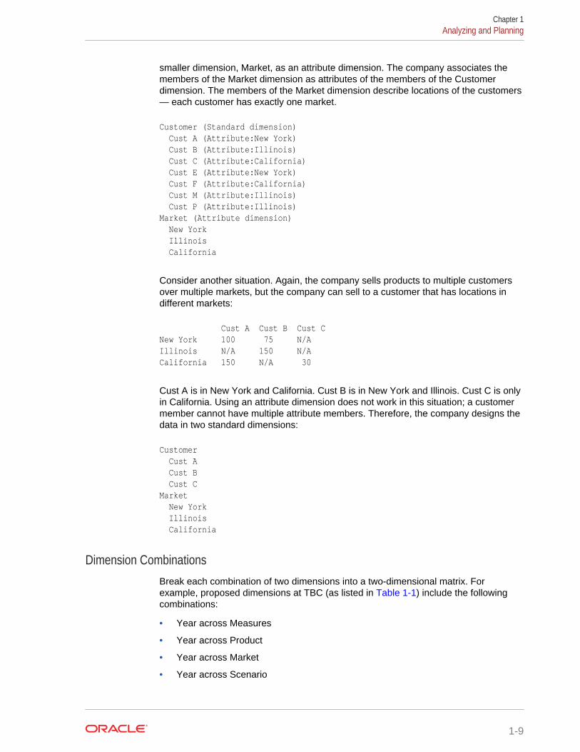
smaller dimension, Market, as an attribute dimension. The company associates themembers of the Market dimension as attributes of the members of the Customerdimension. The members of the Market dimension describe locations of the customers— each customer has exactly one market.

Customer (Standard dimension) Cust A (Attribute:New York) Cust B (Attribute:Illinois) Cust C (Attribute:California) Cust E (Attribute:New York) Cust F (Attribute:California) Cust M (Attribute:Illinois) Cust P (Attribute:Illinois)Market (Attribute dimension) New York Illinois California

Consider another situation. Again, the company sells products to multiple customersover multiple markets, but the company can sell to a customer that has locations indifferent markets:

Cust A Cust B Cust CNew York 100 75 N/AIllinois N/A 150 N/ACalifornia 150 N/A 30

Cust A is in New York and California. Cust B is in New York and Illinois. Cust C is onlyin California. Using an attribute dimension does not work in this situation; a customermember cannot have multiple attribute members. Therefore, the company designs thedata in two standard dimensions:

Customer Cust A Cust B Cust CMarket New York Illinois California

Dimension CombinationsBreak each combination of two dimensions into a two-dimensional matrix. Forexample, proposed dimensions at TBC (as listed in Table 1-1) include the followingcombinations:

• Year across Measures

• Year across Product

• Year across Market

• Year across Scenario


1-9

• Measures across Product

• Measures across Market

• Measures across Scenario

• Market across Product

• Market across Scenario

• Scenario across Product

• Ounces across Pkg Type

Ounces and Pkg Type, as attribute dimensions associated with the Product dimension,can be considered with the Product dimension.

To help visualize each dimension, draw a matrix and include a few of the first-generation members. Figure 1-2 shows a simplified set of matrixes for threedimensions.

Figure 1-2 Analyzing Dimensional Relationships

For each combination of dimensions, ask three questions:

• Does it add analytic value?

• Does it add utility for reporting?

• Does it avoid an excess of unused combinations?

For each combination, the answers to the questions help determine whether thecombination is valid for the database. Ideally, the answer to each question is yes. Ifnot, consider rearranging the data into more-meaningful dimensions. As you workthrough this process, discuss information needs with users.


1-10

Repetition in OutlinesThe repetition of elements in an outline often indicates a need to split dimensions. Thefollowing examples show you how to avoid repetition.

In Figure 1-3, the left column, labeled “Repetition,” shows Profit, Margin, Sales,COGS, and Expenses repeated under Budget and Actual in the Accounts dimension.The right column, labeled “No Repetition,” separates Budget and Actual into anotherdimension (Scenario), leaving just one set of Profit, Margin, Sales, COGS, andExpenses members in the Accounts dimension. This approach simplifies the outlineand provides a simpler view of the budget and actual figures of the other dimensions inthe database.

Figure 1-3 Example of Eliminating Repetition By Creating a ScenarioDimension

In Figure 1-4, the left column, labeled “Repetition,” uses shared members in the Dietdimension to analyze diet beverages. Members 100–20, 200–20, and 300–20 arerepeated: once under Diet, and once under their respective parents. The right column,labeled “No Repetition,” simplifies the outline by creating a Diet attribute dimension oftype Boolean (True or False). All members are shown only once, under theirrespective parents, and are tagged with the appropriate attribute (“Diet: True” or “Diet:False”).


1-11

Figure 1-4 Example of Eliminating Repetition By Creating an AttributeDimension

Attribute dimensions also provide additional analytic capabilities. See DesigningAttribute Dimensions.

Interdimensional IrrelevanceInterdimensional irrelevance occurs when many members of a dimension areirrelevant across other dimensions. Essbase defines irrelevant data as data thatEssbase stores only at the summary (dimension) level. In such a situation, you may beable to remove a dimension from the database and add its members to anotherdimension or split the model into separate databases.

For example, TBC considered analyzing salaries as a member of the Measuresdimension. But salary information often proves irrelevant in the context of a corporatedatabase. Most salaries are confidential and apply to individuals. The individual andthe salary typically represent one cell, with no reason to intersect with any otherdimension.

TBC considered separating employees into a separate dimension. Table 1-3 shows anexample of how TBC analyzed the proposed Employee dimension for interdimensionalirrelevance. Members of the proposed Employee dimension (represented in the tableheader row) are compared with members of the Measures dimension (represented inthe left-most column). The Measures dimension members (such as Revenue) apply toAll Employees; only the Salary measure is relevant to individual employees.

Table 1-3 Example of Interdimensional Irrelevance

Joe Smith Mary Jones Mike Garcia All Employees

Revenue Irrelevance Irrelevance Irrelevance Relevance

Variable Costs Irrelevance Irrelevance Irrelevance Relevance

COGS Irrelevance Irrelevance Irrelevance Relevance

Advertising Irrelevance Irrelevance Irrelevance Relevance

Salaries Relevance Relevance Relevance Relevance

Fixed Costs Irrelevance Irrelevance Irrelevance Relevance


1-12

Table 1-3 (Cont.) Example of Interdimensional Irrelevance

Joe Smith Mary Jones Mike Garcia All Employees

Expenses Irrelevance Irrelevance Irrelevance Relevance

Profit Irrelevance Irrelevance Irrelevance Relevance

Reasons to Split DatabasesBecause individual employee information is irrelevant to the other information in thedatabase, and also because adding an Employee dimension would substantiallyincrease database storage needs, TBC created a separate Human Resources (HR)database. The new HR database contains a group of related dimensions and includessalaries, benefits, insurance, and 401(k) plans.

There are many reasons for splitting a database; for example, suppose that acompany maintains an organizational database that contains several internationalsubsidiaries in several time zones. Each subsidiary relies on time-sensitive financialcalculations. You can split the database for groups of subsidiaries in the same timezone to ensure that financial calculations are timely. You can also use a partitionedapplication to separate information by subsidiary.

Checklist to Analyze the Database DesignUse the following checklist to analyze the database design:

• Have you minimized the number of dimensions?

• For each dimensional combination, did you ask:

– Does it add analytic value?

– Does it add utility for reporting?

– Does it avoid an excess of unused combinations?

• Did you avoid repetition in the outline?

• Did you avoid interdimensional irrelevance?

• Did you split the databases as necessary?

Drafting OutlinesNow you can create the application and database and build the first draft of the outlinein Essbase. The draft defines all dimensions, members, and consolidations. Use theoutline to design consolidation requirements and identify where you need formulas andcalculation scripts.

Note:

Outlines are a part of an Essbase database (or cube), which exists inside anEssbase application.

Chapter 1Drafting Outlines

1-13

The TBC application designer issued the following draft for a database outline. In thisplan, Year, Measures, Product, Market, Scenario, Pkg Type, and Ounces aredimension names. Observe how TBC anticipated consolidations, calculations andformulas, and reporting requirements. The application designers also used productcodes rather than product names to describe products.

• Year. TBC needs to collect data monthly and summarize the monthly data byquarter and year. Monthly data, stored in members such as Jan, Feb, and Mar,consolidates to quarters. Quarterly data, stored in members such as Qtr1 andQtr2, consolidates to Year.

• Measures. Sales, Cost of Goods Sold, Marketing, Payroll, Miscellaneous,Opening Inventory, Additions, and Ending Inventory are standard measures.Essbase can calculate Margin, Total Expenses, Profit, Total Inventory, Profit %,Margin %, and Profit per Ounce from these measures. TBC needs to calculateMeasures on a monthly, quarterly, and yearly basis.

• Product. The Product codes are 100‑10, 100‑20, 100‑30, 200‑10, 200‑20, 200‑30,200‑40, 300‑10, 300‑20, 300‑30, 400‑10, 400‑20, and 400‑30. Each productconsolidates to its respective family (100, 200, 300, and 400). Each consolidationallows TBC to analyze by size and package, because each product is associatedwith members of the Ounces and Pkg Type attribute dimensions.

• Market. Several states make up a region; four regions make up a market. Thestates are Connecticut, Florida, Massachusetts, New Hampshire, New York,California, Nevada, Oregon, Utah, Washington, Louisiana, New Mexico,Oklahoma, Texas, Colorado, Illinois, Iowa, Missouri, Ohio, and Wisconsin. Eachstate consolidates into its region—East, West, South, or Central. Each regionconsolidates into Market.

• Scenario. TBC derives and tracks budget versus actual data. Managers mustmonitor and track budgets and actuals, as well as the variance and variancepercentage between them.

• Pkg Type. TBC wants to see the effect that product packaging has on sales andprofit. Establishing the Pkg Type attribute dimension enables users to analyzeproduct information based on whether a product is packaged in bottles or cans.

• Ounces. TBC sells products in different sizes in ounces in different markets.Establishing the Ounces attribute dimension helps users monitor which sizes sellbetter in which markets.

The following topics present a review of the basics of dimension and memberproperties and a discussion of how outline design affects performance.

Dimension and Member PropertiesThe properties of dimensions and members define the roles of the dimensions andmembers in the design of the multidimensional structure. These properties include thefollowing:

• Dimension types and attribute associations. See Dimension Types.

• Data storage properties. See Member Storage Properties.

• Consolidation operators. See Consolidation of Dimensions and Members.

• Formulas. See Formulas and Functions.

For a complete list of dimension and member properties, see Setting Dimension andMember Properties.


1-14

Dimension TypesA dimension type is a property that Essbase provides that adds special functionality toa dimension. The most commonly used dimension types: time, accounts, and attribute.This topic uses the following dimensions of the TBC database to illustrate dimensiontypes.

Database:Design Year (Type: time) Measures (Type: accounts) Product Market Scenario Pkg Type (Type: attribute) Ounces (Type: attribute)

Table 1-4 defines each Essbase dimension type.

Table 1-4 Dimension Types

Dimension Types Description

None Specifies no particular dimension type.

Time Defines the time periods for which you reportand update data. You can tag only onedimension as time. The time dimensionenables several accounts dimension functions,such as first and last time balances.

Accounts Contains items that you want to measure,such as profit and inventory, and makesEssbase built-in accounting functionalityavailable. Only one dimension can be definedas accounts.

For discussion of two forms of accountdimension calculation, see AccountsDimension Calculations.

Attribute Contains members that can be used todescribe members of another, so-called basedimension.

For example, the Pkg Type attribute dimensioncontains a member for each type ofpackaging, such as bottle or can, that appliesto members of the Product dimension.

Member Storage PropertiesYou can specify data storage properties for members; data storage properties definewhere and when consolidations are stored. For example, by default, members aretagged as store data. Essbase sums the values of store data members and stores theresult at the parent level.

You can change the default logic for each member by changing the data storageproperty tag for the member. For example, you can change a store data member to a


1-15

label only member. Members with the label only tag, for example, do not have dataassociated with them.

Table 1-5 describes the effect that Essbase data storage properties have on members.

Table 1-5 Essbase Data Storage Properties

Data Storage Properties Effects on Members

Store data Data for the member is stored in the database.Store data is the default storage property.

Dynamic Calc The data associated with the member iscalculated when requested by a user query.The calculated data is not stored; it isdiscarded after the query request iscompleted.

Shared member The data associated with the member comesfrom another member with the same name.

Label only Although a label only member has no dataassociated with it, a label only member candisplay a value. The label only tag groupsmembers and eases navigation and reporting.Typically, label only members are notcalculated.

For example, in the Measures dimension, themember Ratios has three children, Margin%,Profit%, and Profit per Ounce. The memberRatios defines a category of members. Whenconsolidated, Margin%, Profit%, and Profit perOunce do not roll up to a meaningful figure forRatios. Hence, Ratios is tagged as label only.

Checklist for Dimension and Member Properties• Can you identify a time dimension?

• Can you identify an accounts dimension?

• Can you identify qualities or characteristics of dimensions that should be definedas separate attribute dimensions?

• Which members require special data storage properties?

Designing an Outline to Optimize PerformancePosition attribute dimensions at the end of the outline. Position dense dimensionsbefore sparse dimensions.

The position of dimensions in an outline and the storage properties of dimensions canaffect two areas of performance—how quickly calculations are run and how long ittakes users to retrieve information.

See these topics to understand performance optimization basics:

• Optimizing Query Performance

• Optimizing Calculation Performance


1-16

• Meeting the Needs of Both Calculation and Retrieval

Optimizing Query PerformanceTo optimize query performance, use the following guidelines when you design anoutline:

• If the outline contains attribute dimensions, ensure that the attribute dimensionsare the only sparse Dynamic Calc dimensions in the outline.

• In the outline, place the more-queried sparse dimensions before the less-queriedsparse dimensions.

The outline in Figure 1-5 is designed for optimum query performance:

• Because the outline contains attribute dimensions, the storage property forstandard dimensions and all standard dimensions members is set as store data.

• As the most-queried sparse dimension, the Product dimension is the first of thesparse dimensions. Base dimensions are typically queried more than otherdimensions.

Figure 1-5 Designing an Outline for Optimized Query Times

Optimizing Calculation PerformanceTo optimize calculation performance, order the sparse dimensions in the outline bytheir number of members, starting with the dimension that contains the fewest.

See Designing for Calculation Performance.

The outline in Figure 1-6 is designed for optimum calculation performance:

• The smallest standard dimension that is sparse, Market, is the first of the sparsedimensions in the outline.

• The largest standard dimension that is sparse, Product, is immediately above thefirst attribute dimension. If the outline did not contain attribute dimensions, theProduct dimension would be at the end of the outline.


1-17

Figure 1-6 Designing an Outline for Optimized Calculation Times

Meeting the Needs of Both Calculation and RetrievalAlthough they contain the same dimensions, the example outlines in Figure 1-5 and Figure 1-6 are different. To determine the best outline sequence for a situation,prioritize the data retrieval requirements of the users against the time needed to runcalculations on the database. How often do you expect to update and recalculate thedatabase? What is the nature of user queries? What is the expected volume of userqueries?

A possible workaround is to initially position the dimensions in the outline to optimizecalculation. After you run the calculations, you can manually resequence thedimensions to optimize retrieval. When you save the outline after you reposition itsdimensions, choose to restructure the database by index only. Before you runcalculations again, resequence the dimensions in the outline to optimize calculation.

Loading Test DataBefore you can test calculations, consolidations, and reports, you need data in thedatabase. During the design process, loading mocked-up data or a subset of real dataprovides flexibility and shortens the time required to test and analyze results.

See the following topics for detailed instructions for loading data:

• Understanding Data Loading and Dimension Building

• Working with Rule Files

If you’re satisfied with your database design after the preliminary test, load thecomplete set of real data with which you’ll populate the final database. Use the testrules files, if possible. This final test may reveal source data problems that were notanticipated during earlier design phases.

Defining CalculationsCalculations are essential to derive certain types of data. Data that is derived from acalculation is called calculated data; source data that is not calculated is called inputdata.

Chapter 1Loading Test Data

1-18

The following topics use the Product and Measures dimensions of the TBC applicationto illustrate several types of common calculations that are found in many Essbasedatabases.

• Consolidation of Dimensions and Members

• Tags and Operators on Example Measures Dimension

• Accounts Dimension Calculations

• Formulas and Functions

• Dynamic Calculations

• Two-Pass Calculations

• Checklist for Calculations

Consolidation of Dimensions and MembersWhen you define members of standard dimensions, Essbase automatically tags themembers with the + consolidation operator (plus sign representing addition), meaningthat during consolidation members are added to derive their parent's value. Asappropriate, you can change a member consolidation property to one of the operatorsshown in Table 6-2, which defines Essbase consolidation operators.

Consolidation is the most frequently used calculation in Essbase. This topic uses theProduct dimension to illustrate consolidations.

The TBC application has several consolidation paths:

• Individual products roll up to product families, and product families consolidate intoProduct. The TBC outline also requires multiple consolidation paths; someproducts must consolidate in multiple categories.

• States roll up to regions, and regions consolidate into Market.

• Months roll up into quarters, and quarters consolidate into Year.

The following topics discuss consolidation in greater detail:

• Effect of Position and Operator on Consolidation

• Consolidation of Shared Members

• Checklist for Consolidation

Consolidation operators define how Essbase rolls up data for each member in abranch to the parent. For example, using the default addition (+) operator, Essbaseadds 100‑10, 100‑20, and 100‑30 and stores the result in their parent, 100, as shownin Figure 1-7.

Chapter 1Defining Calculations

1-19

Figure 1-7 TBC Product Dimension

The Product dimension contains mostly addition (+) operators, which indicate thateach group of members is added and rolled up to the parent. Diet has a tilde (~)operator, which indicates that Essbase does not include the Diet member in theconsolidation to the parent, Product. The Diet member consists entirely of membersthat are shared. The TBC product management group wants to be able to isolate Dietdrinks in reports, so TBC created a separate Diet member that does not impact overallconsolidation.

Effect of Position and Operator on ConsolidationEssbase calculates the data of a branch in top-down order. For example, if you have,in order, two members tagged with an addition (+) operator and a third member taggedwith a multiplication (*) operator, Essbase adds the first two and multiplies that sum bythe third.

Because Essbase always begins with the top member when it consolidates, the orderand the labels of the members is important. See Calculating Members with DifferentOperators.

See Table 6-2, which defines Essbase consolidation operators.

Consolidation of Shared MembersShared members also affect consolidation paths. The shared member conceptenables two members with the same name to share the same data. The sharedmember stores a pointer to data contained in the other member, so Essbase storesthe data only once. Shared members must be in the same dimension. Data can beshared by multiple members.


1-20

Checklist for ConsolidationUse the following checklist to help define consolidation:

• Did you identify the consolidations in the outline?

• Did you tag each member with the proper consolidation operator?

• Did you specify a shared member tag for designated members?

• Would shared members be more efficient if designed within an attribute dimension(other than shared)?

Tags and Operators on Example Measures DimensionThe Measures dimension is the most complex dimension in the TBC outline because ituses both time and accounts data. It also contains formulas and special tags to helpEssbase calculate the outline. This topic discusses the formulas and tags that TBCincluded in the Measures dimension (the dimension tagged as accounts).

Look closely at the Measures dimension tags defined by TBC (in Figure 1-8). Many ofthe properties of the Measures dimension are discussed in previous topics: addition(+), subtraction (–), and no consolidation (~) operators, and accounts and label onlytags:

• The Inventory and Ratios member names assist the user in data navigation. Theydo not contain data, and therefore receive a label only tag.

• The Measures dimension itself has a label only tag. Some members of Measureshave a Dynamic Calc tag. See: Dynamic Calculations.

• Some members of Measures have a time balance tag (TB First or TB Last). See: Setting Time Balance Properties.

Figure 1-8 TBC Measures Dimension


1-21

Accounts Dimension CalculationsThis topic discusses two forms of calculations for a dimension tagged as accounts.

• Time Balance Properties

• Variance Reporting

Time Balance PropertiesNote the two tags in the Measures dimension of Table 1-7—TB first and TB last.These tags, called time balance tags or properties, provide instructions to Essbaseabout how to calculate the data in a dimension tagged as accounts. Using the tagsrequires a dimension tagged as accounts and a dimension tagged as time. The first,last, average, and expense tags are available exclusively for use with accountsdimension members.

In the TBC Measures dimension, Opening Inventory data represents the inventory thatTBC carries at the beginning of each month. The quarterly value for Opening Inventoryequals the Opening value for the first month in the quarter. Opening Inventory requiresthe time balance tag, TB first.

Ending Inventory data represents the inventory that TBC carries at the end of eachmonth. The quarterly value for Ending Inventory equals the ending value for the lastmonth in the quarter. Ending Inventory requires the time balance tag, TB last. Table 1-6 defines the time balance tags for the accounts dimension.

Table 1-6 Accounts Member Tags

Tags Description

Time Balance Last The value for the last child member is carriedto the parent. For example, March is carried toQtr1.

Time Balance First The value for the first child is carried to theparent. For example, Jan is carried to Qtr1.

In Table 1-7, Qtr1 (second column from the right) and Year (right-most column) showhow consolidation in the time dimension is affected by time balance properties in theaccounts dimension. Data is shown for the first quarter only.

Table 1-7 TBC Consolidations Affected by Time Balance Properties

Dimensions Jan Feb Mar Qtr1 Year

AccountsMember1

11 12 13 36 Qtr1 + Qtr2 +Qtr3 + Qtr4

AccountsMember2 (TBFirst)

20 25 21 20 20

AccountsMember3 (TBLast)

25 21 30 30 Value of Qtr4


1-22

Normally, the calculation of a parent in the time dimension is based on theconsolidation and formulas of children of the parent. However, if a member in anaccounts branch is marked as TB First, any parent in the time dimension matches themember marked as TB First.

For examples, see Setting Time Balance Properties.

Variance ReportingOne TBC Essbase requirement is the ability to perform variance reporting on actualversus budget data. The variance reporting calculation requires that any item thatrepresents an expense to the company must have an expense reporting tag. Inventorymembers, Total Expense members, and the COGS member each receive an expensereporting tag for variance reporting.

Essbase provides two variance reporting properties—expense and nonexpense(default). Variance reporting properties define how Essbase calculates the differencebetween actual and budget data in members with the @VAR or @VARPER function intheir member formulas.

When you tag a member as expense, the @VAR function calculates Budget – Actual.For example, if the budgeted amount is $100 and the actual amount is $110, thevariance is –10.

Without the expense reporting tag, the @VAR function calculates Actual – Budget. Forexample, if the budgeted amount is $100 and the actual amount is $110, the varianceis 10.

Formulas and FunctionsFormulas calculate relationships between members in the database outline. You canapply formulas to members in the outline, or you can place formulas in a calculationscript. This topic explains how TBC optimized the performance of its database byusing formulas.

Functions are predefined routines that perform specialized calculations and return setsof members or sets of data values. Formulas comprise operators and functions, aswell as dimension names, member names, and numeric constants.

Essbase supports the following operators:

• Mathematical operators , which perform arithmetic operations

• Conditional operators, which build logical conditions into calculations

• Cross-dimensional operators, which point to data values of specific databasemember combinations

The Essbase functions include more than 175 predefined routines to extend thecalculation capabilities of Essbase. Essbase supports the following functions:

• Boolean functions, which provide a conditional test by returning a TRUE or FALSEvalue

• Mathematical functions, which perform specialized mathematical calculations

• Relationship functions, which look up data values within a database during acalculation based on the position of the current member


1-23

• Range functions, which declare a range of members as an argument to anotherfunction or to a command

• Financial functions, which perform specialized financial calculations

• Member set functions, which are based on a specified member and whichgenerate lists of members

• Allocation functions, which allocate values that are input at a parent level acrosschild members

• Forecasting functions, which manipulate data for the purpose of smoothing data,interpolating data, or calculating future values

• Statistical functions, which calculate advanced statistics

• Date and time functions, which use date and time characteristics in calculationformulas

• Calculation mode functions, which specify the calculation mode that Essbase usesto calculate a formula

The Measures dimension uses the following formulas:

• Margin = Sales – COGS

• Total Expenses = Marketing + Payroll + Miscellaneous

• Profit = Margin – Total Expenses

• Profit % = Profit % Sales

• Margin % = Margin % Sales

• Profit per Ounce = Profit / @ATTRIBUTEVAL(@NAME(Ounces))

Essbase uses consolidation operators to calculate the Margin, Total Expenses, andProfit members. The Margin% formula uses a % operator, which means “expressMargin as a percentage of Sales.” The Profit% formula uses the same % operator. TheProfit per Ounce formula uses a division operator (/) and a function(@ATTRIBUTEVAL) to calculate profitability by ounce for products sized in ounces.

Note:

In the Profit per Ounce formula, the @NAME function is also used to processthe string “Ounces” for the @ATTRIBUTEVAL function.

For a complete list of operators, functions, and syntax, see Technical Reference forOracle Essbase. Also see Developing Formulas for Block Storage Databases.

Dynamic CalculationsWhen you design the overall database calculation, you may want to define a memberas a Dynamic Calc member. When you tag a member as Dynamic Calc, Essbasecalculates the combinations of that member when you retrieve the data, instead ofprecalculating the member combinations during the regular database calculation.Dynamic calculations shorten regular database calculation time, but may increaseretrieval time for dynamically calculated data values.


1-24

In Figure 1-9, the TBC Measures dimension contains several members tagged asDynamic Calc—Profit, Margin, Total Expenses, Margin %, and Profit %.

Figure 1-9 TBC Measures Dimension, Dynamic Calc Tags

When an overall database calculation is performed, the Dynamic Calc members andtheir corresponding formulas are not calculated. These members are calculated whena user queries them, for example, from Smart View. Essbase does not store thequeried values; it recalculates the values for every subsequent query.

To decide when to calculate data values dynamically, consider your priorities in thefollowing areas:

• Optimum regular calculation time (batch calculation)

• Low disk space usage

• Reduced database restructure time

• Speedy data retrieval for users

• Reduced backup time

See Dynamically Calculating Data Values.

Two-Pass CalculationsIn the TBC database, Margin % and Profit % contain the label two-pass. This labelindicates that some member formulas must be calculated twice to produce the desiredvalue. The two-pass property works only on members of the dimension tagged asaccounts and on members tagged as Dynamic Calc.

The following example illustrates why Profit % (based on the formula Profit % Sales)has a two-pass tag. The tables have five columns (column headers are labeled left toright as Dimension, Jan, Feb, Mar, and Qtr1) and three rows (labeled as Profit, Sales,and Profit %). Jan, Feb, Mar, and Qtr1 are members of the Year dimension. Profit,Sales, and Profit % are members of the Measures (accounts) dimension.


1-25

Table 1-8 defines the initial data to load into Essbase. The data values for Profit ->Jan, Profit -> Feb, and Profit -> Mar are 100. The data value for Sales -> Jan, Sales ->Feb, and Sales -> Mar are 1000.

Table 1-8 Data Loaded into Essbase

Dimension Jan Feb Mar Qtr1

Profit 100 100 100 N/A

Sales 1000 1000 1000 N/A

Profit % N/A N/A N/A N/A

First, Essbase calculates the Measures dimension. In Table 1-9, the data values forProfit % -> Jan, Profit % -> Feb, and Profit % -> Mar are 10%.

Table 1-9 Data After Essbase Calculates the Measures Dimension


Profit 100 100 100

Sales 1000 1000 1000

Profit % 10% 10% 10% N/A

Next, Essbase calculates the Year dimension. The data rolls up across the dimension.In Table 1-10, the data values for Profit -> Qtr1 (300) and Sales -> Qtr1 (3000) arecorrect. The data value for Profit % -> Qtr1 (30%) is incorrect because Profit % istagged as a two-pass calculation.

Table 1-10 Data After Essbase Calculates the Year Dimension


Profit 100 100 100 300

Sales 1000 1000 1000 3000

Profit % 10% 10% 10% 30%

Essbase then recalculates profit percentage at each occurrence of the member Profit%. In Table 1-11, the data value for Profit % -> Qtr1 (10%) is correct after the secondpass.

Table 1-11 Data After Essbase Recalculates Profit Percentage


Profit 100 100 100 300

Sales 1000 1000 1000 3000

Profit % 10% 10% 10% 10%

Checklist for CalculationsUse the following checklist when you define a calculation:


1-26

• Does the default calculation logic achieve accurate results?

• Which members require formulas?

• Which members require time balance tags?

• Which members require variance reporting?

• Which members require two-pass calculation?

• Which members can be tagged as Dynamic Calc?

Defining ReportsTo ensure that the design meets user information requirements, you must view data asusers view it. Users typically view data through spreadsheets, printed reports, orreports published on the Web. Oracle and its partners offer many tools for producingreporting systems for users.

Several tools can help you display and format data quickly, and test whether thedatabase design meets user needs. For example, those who are familiar withspreadsheets can use Smart View.

During the design phase, check the following:

• Grouping and sequencing of data. Do the intersections enabled by the designprovide the data that users need?

• Levels of totals. What consolidation levels are required by, for example, a SmartView user who drills down and up through the hierarchy of the outline design?

• Attribute reporting. Does the database design facilitate an analysis that is basedon the characteristics or attributes of specific dimensions or members? Forexample, do you need to compare sales by specific combinations of size andpackaging, such as comparing the sales of 16‑ounce bottled colas with the salesof 32‑ounce bottled colas?

Be sure to use the appropriate tool to create and test predesigned use reports againsttest data. The reports that you design should provide information that meets youroriginal objectives. The reports should be easy to use, providing the right combinationsof data, and the right amount of data. Because reports with too many columns androws are difficult to use, you may need to create several reports instead of oneall‑inclusive report, or pivot a dimension to the point of view of the report so that eachuser can choose a different member from that dimension without viewing all members.

Verifying the DesignAfter you analyze the data and create a preliminary design, check all aspects of thedesign with users. You should already have verified that the database satisfies theusers’ analysis and reporting needs. Ensure that the database satisfies all of theirgoals.

Do the calculations provide the information they need? Are they able to generatereports quickly? Are they satisfied with consolidation times? In short, ask users if thedatabase works for them.

Near the end of the design cycle, test with real data. Does the outline build correctly?Does all data load? If the database fails in any area, repeat the steps of the designcycle to identify the cause of the problem.

Chapter 1Defining Reports

1-27

Essbase provides several sources of information to help you isolate problems.Sources include application and Essbase Server logs, and exception logs. Look atdocumentation topics relevant to your problem; for example, topics about security,calculations, reports, or general error messages.

Most likely, you will need to repeat one or more steps of the design process to arrive atthe ideal database solution.

Chapter 1Verifying the Design

1-28

2Understanding MultidimensionalDatabases

Online analytical processing (OLAP) is a multidimensional, multiuser, client-servercomputing environment for users who need to analyze enterprise data. Key features ofOLAP applications include multidimensional views of data and calculation-intensivecapabilities. Review the topics in this chapter to understand basic concepts of anEssbase database.

• OLAP and Multidimensional Databases

• Dimensions and Members

• Data Storage

• The Essbase Solution for Creating Optimized Databases

Some information in this chapter applies only to block storage databases and is notrelevant to aggregate storage databases. Also see Comparison of Aggregate andBlock Storage.

OLAP and Multidimensional DatabasesFinance departments use OLAP for applications such as budgeting, activity-basedcosting (allocations), financial performance analysis, and financial modeling. Salesdepartments use OLAP for sales analysis and forecasting. Marketing departments useOLAP for market research analysis, sales forecasting, promotions analysis, customeranalysis, and market/customer segmentation. Typical manufacturing OLAPapplications include production planning and defect analysis.

Important to all of these applications is the ability to provide managers the informationthat they need to make effective decisions about an organization's strategic directions.A successful OLAP application provides information as needed; that is, it provides“just-in-time” information for effective decision-making.

Providing such information requires more than a base level of detailed data. Just-in-time information is computed data that usually reflects complex relationships and isoften calculated on the fly. Analyzing and modeling complex relationships are practicalonly if response times are consistently short. In addition, because the nature of datarelationships may not be known in advance, the data model must be flexible. A trulyflexible data model ensures that OLAP systems can respond to changing businessrequirements as needed for effective decision making.

Although OLAP applications are found in widely divergent functional areas, all requirethe following key features:

• Multidimensional views of data

• Calculation-intensive capabilities

• Time intelligence

2-1

Key to OLAP systems are multidimensional databases, which not only consolidate andcalculate data; but also provide retrieval and calculation of a variety of data subsets. Amultidimensional database supports multiple views of data sets for users who need toanalyze the relationships between data categories. For example, a marketing analystmight ask following questions:

• How did Product A sell last month? How does this figure compare to sales in thesame month over the last five years? How did the product sell by branch, region,and territory?

• Did this product sell better in particular regions? Are there regional trends?

• Did customers return Product A last year? Were the returns due to productdefects? Did the company manufacture the products in a specific plant?

• Did commissions and pricing affect how salespeople sold the product? Did certainsalespeople sell more?

In multidimensional databases, the number of data views is limited only by thedatabase outline, the structure that defines all elements of the database. Users canpivot the data to see information from a different viewpoint, drill down to find moredetailed information, or drill up to see an overview.

Dimensions and MembersThis section introduces the concepts of outlines, dimensions, and members within amultidimensional database. If you understand dimensions and members, you are wellon your way to understanding the power of a multidimensional database.

A dimension represents the highest consolidation level in the database outline. Thedatabase outline presents dimensions and members in a tree structure to indicate aconsolidation relationship. For example, Year is a dimension (of type Time) and Qtr1 isa member:

Year Time Qtr1 (+) Jan (+)......Feb (+)......Mar (+)

There are two types of dimensions: standard and attribute.

• Standard dimensions represent the core components of a business plan and oftenrelate to departmental functions. Typical standard dimensions: Time, Accounts,Product Line, Market, and Division. Dimensions change less frequently thanmembers.

• Attribute dimensions are associated with standard dimensions. Through attributedimensions, you group and analyze members of standard dimensions based onthe member attributes (characteristics). For example, you can compare theprofitability of noncaffeinated products that are packaged in glass to theprofitability of noncaffeinated products packaged in cans.

Members are the individual components of a dimension. For example, Product A,Product B, and Product C might be members of the Product dimension. Each memberhas a unique name. Data associated with a member can be stored (referred to as astored member in this chapter), or the data can be dynamically calculated when a userretrieves it.

Chapter 2Dimensions and Members

2-2

Outline HierarchiesDatabase development begins with creating a database outline, which accomplishesthe following objectives:

• Defines the structural relationships between members in the database.

• Organizes data in the database.

• Defines the consolidations and mathematical relationships between items.

The concept of members is used to represent data hierarchies. Each dimensionconsists of one or more members. The members, in turn, may consist of othermembers. When you create a dimension, you define how to consolidate the values ofits individual members. Within the tree structure of the database outline, aconsolidation is a group of members in a branch of the tree.

For example, many businesses summarize their data monthly, rolling up monthly datato obtain quarterly figures and rolling up quarterly data to obtain annual figures.Businesses may also summarize data by zip code, city, state, and country. Anydimension can be used to consolidate data for reporting purposes.

In the Sample.Basic database, for example, the Year dimension comprises fivemembers: Qtr1, Qtr2, Qtr3, and Qtr4, each storing data for an individual quarter, plusYear, storing summary data for the year. Qtr1 comprises four members: Jan, Feb, andMar, each storing data for a month, plus Qtr1, storing summary data for the quarter.Similarly, Qtr2, Qtr3, and Qtr4 comprise the members that represent the individualmonths plus the member that stores the quarterly totals.

The following hierarchical structure represents the data consolidations andrelationships in Qtr, as described in the previous paragraph.

Year Time Qtr1 (+) Jan (+)......Feb (+)......Mar (+)

Some dimensions consist of relatively few members, while others may have hundredsor even thousands of members.

Dimension and Member RelationshipsHierarchical (generations and level; and roots and leaves) and family history (parents,children, and siblings; and descendants and ancestors) terms are used to describe theroles and relationships of the members in a database outline. The subtopics in thissection reference the outline shown in Figure 2-1 in describing the position of themembers in the outline.


2-3

Figure 2-1 Member Generation and Level Numbers

• Parents, Children, and Siblings

• Descendants and Ancestors

• Roots and Leaves

• Generations and Levels

• Generation and Level Names

Parents, Children, and SiblingsFigure 2-1 illustrates the following parent, child, and sibling relationships:

• A parent is a member that has a branch below it. For example, Margin is a parentmember for Sales and Cost of Goods Sold.

• A child is a member that has a parent above it. For example, Sales and Cost ofGoods Sold are children of the parent Margin.

• Siblings are child members of the same immediate parent, at the same generation.For example, Sales and Cost of Goods Sold are siblings (they both have theparent Margin), but Marketing (at the same branch level) is not a sibling, becauseits parent is Total Expenses.


2-4

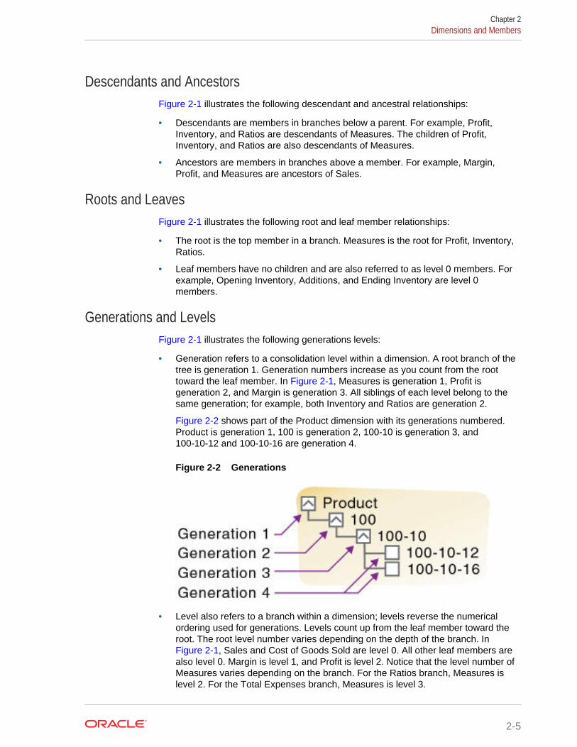
Descendants and AncestorsFigure 2-1 illustrates the following descendant and ancestral relationships:

• Descendants are members in branches below a parent. For example, Profit,Inventory, and Ratios are descendants of Measures. The children of Profit,Inventory, and Ratios are also descendants of Measures.

• Ancestors are members in branches above a member. For example, Margin,Profit, and Measures are ancestors of Sales.

Roots and LeavesFigure 2-1 illustrates the following root and leaf member relationships:

• The root is the top member in a branch. Measures is the root for Profit, Inventory,Ratios.

• Leaf members have no children and are also referred to as level 0 members. Forexample, Opening Inventory, Additions, and Ending Inventory are level 0members.

Generations and LevelsFigure 2-1 illustrates the following generations levels:

• Generation refers to a consolidation level within a dimension. A root branch of thetree is generation 1. Generation numbers increase as you count from the roottoward the leaf member. In Figure 2-1, Measures is generation 1, Profit isgeneration 2, and Margin is generation 3. All siblings of each level belong to thesame generation; for example, both Inventory and Ratios are generation 2.

Figure 2-2 shows part of the Product dimension with its generations numbered.Product is generation 1, 100 is generation 2, 100-10 is generation 3, and100-10-12 and 100-10-16 are generation 4.

Figure 2-2 Generations

• Level also refers to a branch within a dimension; levels reverse the numericalordering used for generations. Levels count up from the leaf member toward theroot. The root level number varies depending on the depth of the branch. In Figure 2-1, Sales and Cost of Goods Sold are level 0. All other leaf members arealso level 0. Margin is level 1, and Profit is level 2. Notice that the level number ofMeasures varies depending on the branch. For the Ratios branch, Measures islevel 2. For the Total Expenses branch, Measures is level 3.


2-5

Figure 2-3 shows part of the Product dimension with its levels numbered. 100 islevel 2, 100-10 is level 1, and 100-10-12 and 100-10-16 are level 0.

Figure 2-3 Levels

Generation and Level NamesTo ease report maintenance, you can assign a name to a generation or level and thenuse the name as a shorthand for all members in that generation or level. Becausechanges to an outline are automatically reflected in a report, when you use generationand level names, you do not need to change the report if a member name is changedor deleted from the database outline.

Standard Dimensions and Attribute DimensionsEssbase has standard dimensions and attribute dimensions. This chapter focuses onstandard dimensions, because Essbase does not allocate storage for attributedimension members. Instead, it dynamically calculates the members when the userqueries data associated with them.

An attribute dimension is a special type of dimension that is associated with a standarddimension. See Working with Attributes.

Sparse and Dense DimensionsMost data sets of multidimensional databases have two characteristics:

• Data is not smoothly and uniformly distributed.

• Data does not exist for the majority of member combinations. For example, allproducts may not be sold in all areas of the country.

Essbase maximizes performance by dividing the standard dimensions of anapplication into two types: dense dimensions and sparse dimensions. This divisionallows Essbase to cope with data that is not smoothly distributed, without losing theadvantages of matrix-style access to the data. Essbase speeds data retrieval whileminimizing memory and disk requirements.

Most multidimensional databases are inherently sparse; they lack data values for themajority of member combinations. A sparse dimension is one with a low percentage ofavailable data positions filled.

For example, the outline of the Sample.Basic database in Figure 2-4 includes theYear, Product, Market, Measures, and Scenario dimensions. Product represents theproduct units, Market represents the geographical regions in which the products are


2-6

sold, and Measures represents the accounts data. Because not every product is soldin every market, Market and Product are chosen as sparse dimensions.

Multidimensional databases also contain dense dimensions. A dense dimension has ahigh probability that one or more cells is occupied in every combination of dimensions.For example, in the Sample.Basic database, accounts data exists for almost allproducts in all markets, so Measures is chosen as a dense dimension. Year andScenario are also chosen as dense dimensions. Year represents time in months, andScenario represents whether the accounts values are budget or actual values.

Caffeinated, Intro Date, Ounces, Pkg Type and Population are attribute dimensions.See Working with Attributes.

When an Essbase database is stored on disk, the cartesian product of dense membercombinations form units of storage called blocks, and a block is written to disk forevery sparse member combination in the database.

Figure 2-4 Sample.Basic Database Outline

Selection of Dense and Sparse DimensionsIn most data sets, existing data tends to follow predictable patterns of density andsparsity. If you match patterns correctly, you can store the existing data in a


2-7

reasonable number of fairly dense data blocks, rather than in many highly sparse datablocks.

By default, a new dimension is set to sparse. Attribute dimensions are always sparsedimensions. Keep in mind that you can associate attribute dimensions only with sparsestandard dimensions.

Dense-Sparse Configuration for Sample.BasicConsider the Sample.Basic database, which represents data for The BeverageCompany (TBC).

Because TBC does not sell every product in every market, the data set is reasonablysparse. Data values do not exist for many combinations of members in the Productand Market dimensions. For example, if Caffeine Free Cola is not sold in Florida, datavalues do not exist for the combination Caffeine Free Cola (100-30) -> Florida, soProduct and Market are sparse dimensions. Therefore, if no data values exist for aspecific combination of members in these dimensions, a data block is not created forthe combination.

However, consider combinations of members in the Year, Measures, and Scenariodimensions. Data values almost always exist for some member combinations on thesedimensions. For example, data values exist for the member combination Sales ->January -> Actual, because at least some products are sold in January. Thus, Yearand, similarly, Measures and Scenario, are dense dimensions.

The sparse-dense configuration of the standard dimensions in the Sample.Basicdatabase may be summarized:

• The sparse standard dimensions are Product and Market.

• The dense standard dimensions are Year, Measures, and Scenario.

A data block is created for each unique combination of members in the Product andMarket dimensions (see Data Storage). Each data block represents data from thedense dimensions. The data blocks likely will have few empty cells.

For example, consider the sparse member combination Caffeine Free Cola (100-30),New York, in Figure 2-5:

• If accounts data (represented by the Measures dimension) exists for thiscombination for January, it probably exists for February and for all members in theYear dimension.

• If a data value exists for one member on the Measures dimension, it is likely thatother accounts data values exist for other members in the Measures dimension.

• If Actual accounts data values exist, it is likely that Budget accounts data valuesexist.


2-8

Figure 2-5 Dense Data Block for Sample.Basic Database

Dense and Sparse Selection ScenariosIn the following scenarios, you'll see how a database is affected when you selectdifferent standard dimensions. Assume that these scenarios are based on typicaldatabases with at least seven dimensions and several hundred members.

• Scenario 1: All Sparse Standard Dimensions

• Scenario 2: All Dense Standard Dimensions

• Scenario 3: Dense and Sparse Standard Dimensions

• Scenario 4: A Typical Multidimensional Problem

Scenario 1: All Sparse Standard DimensionsIf you make all dimensions sparse, Essbase creates data blocks that consist of singledata cells that contain single data values. An index entry is created for each data blockand, therefore, in this scenario, for each existing data value.

This configuration produces an index that requires a large memory. The more indexentries, the longer Essbase searches for a specific block.


2-9

Figure 2-6 Database with All Sparse Standard Dimensions

Scenario 2: All Dense Standard DimensionsIf you make all dimensions dense, as shown in Figure 2-7, Essbase creates one indexentry and one large, sparse block. In most applications, this configuration requiresthousands of times more storage than other configurations. Essbase must load theentire database into memory when it searches for any data value, which requiresenormous memory.


2-10

Figure 2-7 Database with All Dense Standard Dimensions

Scenario 3: Dense and Sparse Standard DimensionsBased on your knowledge of your company’s data, you have identified all your sparseand dense standard dimensions.

Essbase creates dense blocks that can fit into memory easily and creates a relativelysmall index, as shown in Figure 2-8. Your database runs efficiently using minimalresources.


2-11

Figure 2-8 An Ideal Configuration with Combination of Dense and SparseDimensions

Scenario 4: A Typical Multidimensional ProblemConsider a database with four standard dimensions: Time, Accounts, Region, andProduct. In the following example, Time and Accounts are dense dimensions, andRegion and Product are sparse dimensions.

The two-dimensional data blocks shown in Figure 2-9 represent data values from thedense dimensions: Time and Accounts. The members in the Time dimension are J, F,M, and Q1. The members in the Accounts dimension are Rev, Exp, and Net.

Figure 2-9 Two-dimensional Data Block for Time and Accounts

Essbase creates data blocks for combinations of members in the sparse standarddimensions (providing that at least one data value exists for the member combination).


2-12

The sparse dimensions are Region and Product. The members of the Regiondimension are East, West, South, and Total US. The members in the Productdimension are Product A, Product B, Product C, and Total Product.

Figure 2-10 shows 11 data blocks. No data values exist for Product A in the West andSouth, for Product B in the East and West, or for Product C in the East. Therefore,Essbase has not created data blocks for these member combinations. The data blocksthat Essbase has created have few empty cells. This example effectively concentratesall sparseness into the index and concentrates all data into fully utilized blocks. Thisconfiguration provides efficient data storage and retrieval.

Figure 2-10 Data Blocks Created for Sparse Members on Region and Product

Next, consider a reversal of the dense and sparse dimension selections. In thefollowing example, Region and Product are dense dimensions, and Time andAccounts are sparse dimensions.

In Figure 2-11, the two-dimensional data blocks represent data values from the densedimensions: Region and Product. In the West region, data is not available for ProductA and Product B. Data is also not available for Total Product in US.


2-13

Figure 2-11 Two-Dimensional Data Block for Region and Product

Essbase creates data blocks for combinations of members in the sparse standarddimensions (providing that at least one data value exists for the member combination).The sparse standard dimensions are Time and Accounts.

Figure 2-12 shows 12 data blocks. Data values exist for all combinations of membersin the Time and Accounts dimensions; therefore, Essbase creates data blocks for allmember combinations. Because data values do not exist for all products in all regions,the data blocks have many empty cells. Data blocks with many empty cells store datainefficiently.

Figure 2-12 Data Blocks Created for Sparse Members on Time and Accounts


2-14

Data StorageEach data value in a multidimensional database is stored in one cell. A particular datavalue is referenced by specifying its coordinates along each standard dimension.

Note:

Essbase does not store data for attribute dimensions. Essbase dynamicallycalculates attribute dimension data when a user retrieves the data.

Consider the simplified database shown in Figure 2-13. This database has threedimensions: Accounts, Time, and Scenario:

• The Accounts dimension has four members: Sales, COGS, Margin, and Margin%.

• The Time dimension has four quarter members, and Qtr1 has three monthmembers

• The Scenario dimension has two child members: Budget for budget values andActual for actual values.

Figure 2-13 A Multidimensional Database Outline

Data ValuesThe intersection of one member from one dimension with one member from each ofthe other dimensions represents a data value. The example in Figure 2-14 has threedimensions (Accounts, Time, and Scenario); therefore, the dimensions and datavalues in the database can be represented as a cube.

Chapter 2Data Storage

2-15

Figure 2-14 Three-Dimensional Database

As illustrated in Figure 2-15, when you specify Sales, you are specifying the slice ofthe database that contains eight Sales values, where Sales intersect with Actual andBudget.

Figure 2-15 Sales Slice of the Database

Slicing a database amounts to fixing one or more dimensions at a constant value whileallowing the other dimensions to vary.

As illustrated in Figure 2-16, when you specify Actual Sales, you are specifying theslice of the database that contains four Sales values, where Actual and Salesintersect.


2-16

Figure 2-16 Actual, Sales Slice of the Database

A data value is stored in one cell in the database. To refer to a specific data value in amultidimensional database, you specify its member on each dimension. In Figure 2-17,the cell containing the data value for Sales, Jan, Actual is shaded. The data value canalso be expressed using the cross-dimensional operator (->) as Sales -> Actual -> Jan.

Figure 2-17 Sales->Jan->Actual Slice of the Database

Data Blocks and the Index SystemEssbase uses two types of internal structures to store and access data: data blocksand the index system.


2-17

Essbase creates a data block for each unique combination of sparse standarddimension members (providing that at least one data value exists for the sparsedimension member combination). The data block represents all the dense dimensionmembers for its combination of sparse dimension members.

Essbase creates an index entry for each data block. The index represents thecombinations of sparse standard dimension members. It contains an entry for eachunique combination of sparse standard dimension members for which at least onedata value exists.

For example, in the Sample.Basic database outline shown in Figure 2-18, Product andMarket are sparse dimensions.

Figure 2-18 Product and Market Dimensions from the Sample.Basic Database

If data exists for Caffeine Free Cola in New York, Essbase creates a data block and anindex entry for the sparse member combination of Caffeine Free Cola (100-30) -> NewYork. If Caffeine Free Cola is not sold in Florida, Essbase does not create a data blockor an index entry for the sparse member combination: Caffeine Free Cola (100-30) ->Florida.

The data block Caffeine Free Cola (100-30) -> New York represents all the Year,Measures, and Scenario dimensions for Caffeine Free Cola (100-30) -> New York.

Each unique data value can be considered to exist in a cell in a data block. WhenEssbase searches for a data value, it uses the index to locate the appropriate datablock. Then, within the data block, it locates the cell containing the data value. Theindex entry provides a pointer to the data block. The index handles sparse dataefficiently because it includes only pointers to existing data blocks.

Figure 2-19 shows part of a data block for the Sample.Basic database. Eachdimension of the block represents a dense dimension in the Sample.Basic database:Time, Measures, and Scenario. A data block exists for each unique combination ofmembers of the Product and Market sparse dimensions (providing that at least onedata value exists for the combination).


2-18

Figure 2-19 Part of a Data Block for the Sample.Basic Database

Each data block is a multidimensional array that contains a fixed, ordered location foreach possible combination of dense dimension members. Accessing a cell in the blockdoes not involve sequential or index searches. The search is almost instantaneous,resulting in optimal retrieval and calculation speed.

Essbase orders the cells in a data block according to the order of the members in thedense dimensions of the database outline.

A (Dense) a1 a2B (Dense) b1 b11 b12 b2 b21 b22C (Dense) c1 c2 c3D (Sparse) d1


2-19

d2 d21 d22E (Sparse) e1 e2 e3

The block in Figure 2-20 represents the three dense dimensions from within thecombination of the sparse members d22 and e3, from the preceding database outline.In Essbase, member combinations are denoted by the cross-dimensional operator.The symbol for the cross-dimensional operator is ->, so d22 -> e3 denotes the blockfor d22 and e3. The intersection of A, b21, and c3 is written as A -> b21 -> c3.

Figure 2-20 Data Block Representing Dense Dimensions for d22 -> e3

Essbase creates a data block for every unique combination of the members of thesparse dimensions D and E (providing that at least one data value exists for thecombination).

Data blocks, such as the one in Figure 2-20, may include cells that do not contain datavalues. A data block is created if at least one data value exists in the block. Essbasecompresses data blocks with missing values on disk, expanding each block fully as itbrings the block into memory. Data compression is optional but is enabled by default.


2-20

By carefully selecting dense and sparse standard dimensions, you can ensure thatdata blocks do not contain many empty cells, minimizing disk storage requirementsand improving performance. In Essbase, empty cells are known as #MISSING data.

Multiple Data ViewsA multidimensional database supports multiple views of data sets for users who needto analyze the relationships between data categories. Slicing the database in differentways gives you different perspectives of the data. For example, in Figure 2-21, theslice for Jan examines all data values for which the Year dimension is fixed at Jan.

Figure 2-21 Data for January

The slice in Figure 2-22 shows data for the month of Feb:


2-21

Figure 2-22 Data for February

The slice in Figure 2-23 shows data for profit margin:

Figure 2-23 Data for Profit Margin

The Essbase Solution for Creating Optimized DatabasesTo create an optimized database, ask:

• How does your company use the data?

• How will you build and order the dimensions?

Chapter 2The Essbase Solution for Creating Optimized Databases

2-22

• How will you create and order calculations?

See these topics:

• Planning the development of your multidimensional database, see Case Study:Designing a Single-Server, Multidimensional Database.

• Selecting dense and sparse dimensions, see Selection of Dense and SparseDimensions.

• Loading data, see Understanding Data Loading and Dimension Building.

• Calculating your database, see Calculating Essbase Databases.

Chapter 2The Essbase Solution for Creating Optimized Databases

2-23

3Creating Applications and Databases

After you familiarize yourself with applications, and the databases contained withinthem, you can proceed to create them.

• Understanding Applications and Databases

• Understanding Database Artifacts

• Creating an Application and Database

• Using Substitution Variables

• Using Location Aliases


Understanding Applications and DatabasesAn application is a management structure that contains one or more databases andrelated files. Block storage applications can contain multiple databases; aggregatestorage applications can contain one database only. Even for block storagedatabases, Oracle recommends creating one database per application. An Essbaseservice can store multiple applications and databases.

The database is a data repository that contains a multidimensional data storage array.A multidimensional database supports multiple views of data so that users can analyzethe data and make meaningful business decisions. See UnderstandingMultidimensional Databases.

Note:

Some information in this chapter applies only to block storage databases andis not relevant to aggregate storage databases. Also see:

• Comparison of Aggregate and Block Storage

• Aggregate Storage Applications, Databases, and Outlines

Understanding Database ArtifactsFiles that are related to databases are called artifacts (or objects). Database artifactsperform actions against one or more databases, such as defining calculations. Bydefault, artifacts are stored in their associated database folder, and can also be savedto a client computer or to other available network directories.

Common artifact types:

3-1

• A database outline (a storage structure definition)

• Source data files

• Rules for loading data and building dimensions dynamically (rule files)

• Scripts that define how to calculate data (calculation scripts)

• Partition definitions

Understanding Database OutlinesDatabase outlines define the structure of a multidimensional database, including all thedimensions, members, aliases, properties, types, consolidations, and mathematicalrelationships. The structure defined in the outline determines how data is stored in thedatabase.

When a database is created, an outline for that database is created automatically.

See Creating an Application and Database and Creating and Changing DatabaseOutlines.

Understanding Source DataSource data is external data that is loaded into an Essbase database. Common typesof source data include the following:

• Text files

• External databases, such as an SQL database

See Supported Source Data Types.

Understanding Rule Files for Data Load and Dimension BuildAn Essbase database contains no data when it is created. Data load rule files are setsof operations that Essbase performs on data from an external source as the data isloaded, or copied, into the Essbase database. Dimension build rule files create ormodify the dimensions and members in an outline based on data in an external datasource. Rules files are typically associated with a particular database, but you candefine rules for use with multiple databases. One rule file can be used for both dataloads and dimension builds. Rule files have a .rul extension.

See Rule Files and Working with Rule Files.

Understanding Calculation ScriptsCalculation scripts are text files that contain sets of instructions telling Essbase how tocalculate data in the database. Calculation scripts perform calculations different fromthe consolidations and mathematical operations that are defined in the databaseoutline. Because calculation scripts perform specific mathematical operations onmembers, they are typically associated with a particular database. You can, however,define a calculation script for use with multiple databases. Calculation scripts fileshave a .csc extension.

See Developing Calculation Scripts for Block Storage Databases.

Chapter 3Understanding Database Artifacts

3-2

Creating an Application and DatabaseCreate an application and its database.

You can easily create an application and database using an Excel-based applicationworkbook. You can use a sample application workbook and modify it for your use. See About Application Workbooks in Using Oracle Analytics Cloud - Essbase.

If you already created an application and database, and you want to base a newapplication and database on it with some modifications, export the application anddatabase to an application workbook. After you make the changes to the applicationworkbook, you can then import the new application and database. See Creating aCube from an Application Workbook in Using Oracle Analytics Cloud - Essbase.

You can use MaxL statements to create applications and databases:, you can use thecreate application MaxL statement.

• create application

• create database

Before naming applications and databases, see Naming Conventions for Applicationsand Databases.

Using Substitution VariablesSubstitution variables are global placeholders for regularly changing information.Because changes to a variable value are reflected everywhere the variable is used,manual changes are reduced.

For example, many reports depend on reporting periods; if you generate a reportbased on the current month, you must update the report script manually every month.With a substitution variable, such as CurMnth, set on the server, you can change theassigned value each month to the appropriate time period. When you use the variablename in a report script, the information is dynamically updated when you run the finalreport.

You can use substitution variables with both aggregate storage and block storageapplications (unless otherwise noted) in the following areas:

• Aggregate storage outline formulas

See Using MDX Formulas.

• Block storage outline formulas

See Using Substitution Variables in Formulas.

• Calculation scripts (block storage databases only)

Substitution variables and runtime substitution variables are supported incalculation scripts. See Using Runtime Substitution Variables in CalculationScripts Run in Essbase and Using Runtime Substitution Variables in CalculationScripts Run in Smart View.

• Data load rules file header definitions and field definitions. You can enter variablenames for dimension and member names.

• Data source name (DSN) specifications in rules files for SQL data sources

Chapter 3Creating an Application and Database

3-3

• SELECT, FROM, or WHERE clauses in rules files for SQL data sources

• Security filters

See Filtering Using Substitution Variables.

• MDX statements

See Using Substitution Variables in MDX Queries.

• Smart View

See Working with Oracle Smart View for Office 11.1.2.5.720.

You can set substitution variables at these levels:

• Cloud service: Provides access to the variable from all applications and databaseson the cloud service instance.

• Application: Provides access to the variable from all databases within theapplication.

• Database: Provides access to the variable within the specified database.

Rules for Setting Substitution Variable Names and ValuesThe following rules apply to substitution variable names and values:

• The substitution variable name must comprise alphanumeric characters orunderscores ( _ ) and cannot exceed the limit specified in Limits.

• The substitution variable name cannot include nonalphanumeric characters, suchas hyphens (-), asterisks (*), and slashes (/). Do not use spaces, punctuationmarks, or brackets ([ ]) in substitution variable names used in MDX.

• If substitution variables with the same name exist at server, application, anddatabase levels, the order of precedence for the variables: a database-levelsubstitution variable supersedes an application-level variable, which supersedes aserver-level variable.

• The substitution variable value may contain any character except a leadingampersand (&). The substitution variable value cannot exceed the limit specified in Limits.

• To set a substitution variable value to a duplicate member name, use the qualifiedmember name enclosed in double quotation marks; for example, a value for&Period could be “[2006].[Qtr1]”.

• When specifying use of a substitution variable, do not insert a substitution variableas a part of a qualified name. For example, it is invalid to specify “[2004].[&CurrentQtr]”.

• If a substitution variable value is a member name that begins with a numeral orcontains spaces or any of the special characters listed in Naming Conventions inCalculation Scripts, Report Scripts, Formulas, Filters, and Substitution andEnvironment Variable Values, different rules apply for how you enter the variable:

– Enclose the member-name value in brackets ([ ]) if it is used in MDXstatements.

– Enclose the member-name value in quotation marks (“ ”) if it is not used inMDX statements.

Chapter 3Using Substitution Variables

3-4

• If a substitution variable value is numeric, different rules apply for how you enterthe variable:

– If it is not used in MDX statements, enclose a substitution variable value inquotation marks; for example, if the variable name is Month, and itscorresponding value is 01 (corresponding to January), place quotation marksaround 01 (“01”). Substitution variables usually are used with block storagedatabases; they are not used in MDX statements.

– If it is used in MDX statements only, such as in formulas in aggregate storageoutlines, and the value is numeric or a member name, do not enclose thevalue in quotation marks.

Note:

If a substitution variable value is numeric or a member name startingwith a numeral or containing the special characters referred to aboveis to be used both in MDX and non-MDX situations, create twosubstitution variables, one without the value enclosed in quotationmarks and one with the value in quotation marks.

Setting Substitution VariablesYou can set substitution variables at the server, application, or database level. Beforesetting a substitution variable, see Rules for Setting Substitution Variable Names andValues.

When you add or update substitution variables, they are sent to the application anddynamically resolved.

To set a substitution variable, see Using Variables in Using Oracle Analytics Cloud -Essbase. You can also use application workbook to set at the application level, or usethese MaxL statements:

• alter system

• alter application

• alter database

Deleting Substitution VariablesYou may need to delete a substitution variable that is no longer used.

To delete a substitution variable, you can remove it from your application workbook,delete it using the Web UI, or use these MaxL statements:

• alter system


• alter database

Chapter 3Using Substitution Variables

3-5

Updating Substitution VariablesYou can modify or update existing substitution variables. Before updating asubstitution variable, see Rules for Setting Substitution Variable Names and Values.

To update a substitution variable, you can use these MaxL statements:

• alter system


• alter database

Copying Substitution VariablesYou can copy substitution variables to any Essbase Server, application, or database towhich you have appropriate access.

Using Location AliasesA location alias is a descriptor for a data source. A location alias maps an alias namefor a database to the location of that database. A location alias is set at the databaselevel and specifies an alias, a server, an application, a database, a user name, and apassword. Set the location alias on the database on which the calculation script is run.

After you create a location alias, you can use the alias to refer to that database. If thelocation of the database changes, edit the location definition accordingly.

You can use location aliases only with the @XREF and @XWRITE functions. With@XREF, you can retrieve a data value from another database to include in acalculation on the current database. In this case, the location alias points to thedatabase from which the value is to be retrieved. With @XWRITE, you can writevalues to another Essbase database, or to the same database. See TechnicalReference for Oracle Essbase.

The following considerations apply when using location aliases in secure (SSL) mode:

• To enable Essbase to use SSL connectivity, you must setENABLESECUREMODE to TRUE.

• If the location alias is set up to a secure port, you must append :secure to theserver name specification.

For example, using MaxL:

create location alias EasternDB from Sample.Basic to East.Sales at Easthost:6423:secure as User1 identified by password1;

You can create a location alias for a particular database. To create a location alias,you can use the create location alias MaxL statement.

You can edit or delete location aliases that you created. To edit or delete a locationalias, you can use these MaxL statements:

• display location alias

• drop location alias

Chapter 3Using Location Aliases

3-6

4Creating and Changing Database Outlines

The database outline defines the structure of the database. The outline includesdimensions and members, and their properties.

• Creating and Editing Outlines

• Locking and Unlocking Outlines

• Setting the Dimension Storage Type

• Positioning Dimensions and Members

• Verifying Outlines

• Saving Outlines


All examples in this chapter are based on the Sample.Basic database, which you cancreate using the Block Storage Sample (Stored) application workbook(Sample_Basic.xlsx). See About Application Workbooks in Using Oracle AnalyticsCloud - Essbase.

Process for Creating OutlinesThis section provides an overview of creating outlines. For basic information aboutoutlines, see Understanding Multidimensional Databases.

1. Create a database. The new database automatically contains a blank outline.

See Creating Applications and Databases.

2. Open the outline.

See Creating and Editing Outlines.

3. Add dimensions and members to the outline.

4. Set each dimension as dense or sparse.

See Setting the Dimension Storage Type.

5. Position dimensions and members in the outline.

See Positioning Dimensions and Members.

6. Set dimension and member properties.

See Setting Dimension and Member Properties.

7. If necessary, create attribute dimensions and associate them with the appropriatebase dimensions.

See Working with Attributes.

8. Verify and save the outline.

4-1

See Figure 4-1 and Saving Outlines.

Creating and Editing OutlinesYou can create content in the new outline in the following ways:

• Create a new application and cube, and add dimensions and members, byimporting an Excel-based application workbook.

See About Application Workbooks in Using Oracle Analytics Cloud - Essbase.

• Open the empty outline created by default when you create a database and addcontent manually.

See Adding Dimensions to Outlines Manually and Adding Members to OutlinesManually in Using Oracle Analytics Cloud - Essbase.

• Build dimensions using a flat file and a rules file.

See Building Dimensions Using a Rules File in Using Oracle Analytics Cloud -Essbase.

• Import tabular data and allow Essbase to create a cube

• Import an On Premises application using LCM utility export and CLI import.

You can create an outline using the create database MaxL statement.

You can copy an outline using the create database as MaxL statement.

Locking and Unlocking OutlinesWhen an outline is locked, other users are not allowed to save over, rename, delete,or edit the outline.

You can review a list of the modifications that you made. When you are finishedediting the outline, you can either save or revert your modifications.

Note:

Essbase uses a different process for locking and unlocking outlines than forother database artifacts.

The outline is automatically unlocked upon saving it.

Setting the Dimension Storage TypeIf you are using an application workbook to design the database, you assign thestorage type for each dimension in the Essbase.Cube worksheet. See Understandingthe Essbase.Cube Worksheet in Using Oracle Analytics Cloud - Essbase.

In the Web UI, you can also assign the storage type for each dimension in the outline.

Chapter 4Creating and Editing Outlines

4-2

Positioning Dimensions and MembersThe following sections describe how to position dimensions and members in theoutline.

• Moving Dimensions and Members

• Sorting Dimensions and Members

Moving Dimensions and MembersAfter you create dimensions and members, you can rearrange them within the outline.Before moving members and dimensions in an outline, consider the followinginformation:

• The positions of dimensions and members in an outline can affect performance.

See Optimizing Outline Performance.

• Moving dimensions and members can affect the performance of calculations andretrievals.

See Designing an Outline to Optimize Performance.

• Moving members could move a shared member before the actual member in theoutline (which is not recommend).

• If you add, delete, or move nonattribute dimensions or members, Essbaserestructures the database, and you might need to recalculate the data.

• Position attribute dimensions at the end of the outline.

Sorting Dimensions and MembersYou can have Essbase arrange dimensions within an outline or members within adimension in alphabetical order (A–Z) or reverse alphabetical order (Z–A). For a list ofconsequences of sorting dimensions and members, see Moving Dimensions andMembers.

When you sort level 0 members of numeric attribute dimensions in outlines, themembers are sorted by their values. For example, Figure 4-1 shows text and numericversions of the Sizes attribute dimension after sorting the members in ascendingorder. The members of the numeric attribute dimension (on the right) are sequencedby the numeric values of the members; the member 8 is before the other members. Inthe text attribute dimension (on the left), because the characters are sorted left to right,the member 8 is after the member 24.

Figure 4-1 Sorting Numeric Versus Text Attribute Dimension in AscendingOrder

Chapter 4Positioning Dimensions and Members

4-3

You cannot sort Boolean attribute dimensions. See Understanding Attribute Types.

Verifying OutlinesWhen you save an outline, the outline is automatically verified. When verifying anoutline, the following items are checked:

• All member and alias names are valid. Members and aliases cannot have thesame name as other members, aliases, generations, or levels, in non-duplicatemember outlines.

See Naming Conventions for Applications and Databases.

• Only one dimension is tagged as accounts or time.

• Shared members are valid.

See Understanding the Rules for Shared Members.

• Level 0 members are not tagged as label only or Dynamic Calc (unless themember has a formula).

• Label-only members have not been assigned formulas.

• A descendant of a label only member is not tagged as Dynamic Calc.

See Understanding Label Only Members.

• Parent members with only one Dynamic Calc child, are Dynamic Calc.

• Parent members with only oneDynamic Calc child, which is two-pass, the parentmember must also be Dynamic Calc, two-pass.

• The two names of members of Boolean attribute dimensions are the same as thetwo Boolean attribute dimension member names defined for the outline.

• The level 0 member name of a date attribute dimension matches the date formatname setting (mm-dd-yyyy or dd-mm-yyyy).

• The level 0 member name of a numeric attribute dimension is a numeric value.

• Attribute dimensions are located at the end of the outline, following all standarddimensions.

• Level 0 Dynamic Calc members of standard dimensions have a formula.

• Formulas for members are valid.

Note:

An outline with Boolean, numeric or date type attribute dimensions that haveno members (the attribute dimension is empty) is allowed but should only beused in an interim outline. The results of queries, calculations, and gridoperations on empty attribute dimensions can be unpredictable.

During outline verification, the following conversions to appropriate numeric attributedimension member names are made in the outline:

• It moves minus signs in member names from the front to the end of the name; forexample, –1 becomes 1–.

Chapter 4Verifying Outlines

4-4

• It strips out leading or trailing zeroes in member names; for example, 1.0 becomes1, and 00.1 becomes 0.1.

See Understanding Attribute Types.

Saving OutlinesWhen you save changes to an outline, the outline is restructured. For example, if youchange a member name from Market to Region, the data stored in Market is moved toRegion. Each time that you save an outline, the outline is verified to ensure that it iscorrect.

Saving an Outline with Added Standard DimensionsIf you add one or more new standard (nonattribute) dimensions, any data that existedpreviously in the database must be mapped to a member of each new dimensionbefore the outline can be saved. For example, adding a dimension called Channel tothe Sample.Basic outline implies that all previous data in Sample.Basic is associatedwith a particular channel or the sum of all channels.

Saving an Outline with One or More Deleted Standard DimensionsIf you delete one or more standard (nonattribute) dimensions, the data associated withonly one member of each deleted dimension must be retained and associated with amember of one of the other dimensions. For example, removing a dimension calledMarket from the outline implies that all of the data that remains in the database afterthe restructure operation is associated with a single, specified member of the Marketdimension.

If you delete an attribute dimension, Essbase deletes the associations to its basedimension. See Working with Attributes.

Creating Sub-Databases Using Deleted Members1. Delete a dimension from an existing outline.

2. Save the database using a different name, and specify the member to keep.

Only one member can be kept when a dimension is deleted. See Saving anOutline with One or More Deleted Standard Dimensions.

Chapter 4Saving Outlines

4-5

5Creating and Working With DuplicateMember Outlines

When you enable duplicate member names in an outline, multiple members using thesame name can be displayed in the outline.

• Creating Duplicate Member Names in Outlines

• Restrictions for Duplicate Member Names and Aliases in Outlines

• Syntax for Specifying Duplicate Member Names and Aliases

• Working with Duplicate Member Names in Clients

The information in this chapter applies to block storage and aggregate storagedatabases. Also see Comparison of Aggregate and Block Storage.

Creating Duplicate Member Names in OutlinesYou can use duplicate names in an outline only if the outline has the allow duplicatemembers option enabled.

When you enable duplicate member names in an outline, Essbase displays multiplemembers in the outline using the same name. Create the names in the usual way. See Naming Conventions for Dimensions, Members, and Aliases.

When you save the outline, Essbase validates and saves the outline with the duplicatemember names. A qualified name format differentiates the duplicate member names.

Figure 5-1 shows an example of a duplicate member outline in which the New Yorkstate member and the New York city member appear in the outline as New York.

Figure 5-1 Duplicate Member Name “New York”

The qualified member names for the example in Figure 5-1 are [State].[New York] and[City].[New York]. See Syntax for Specifying Duplicate Member Names and Aliases.

To create an outline that enables duplicate member names, use the create databaseMaxL statement with using non_unique_members. Or, if you build the cube from anapplication workbook, on the Cube.Settings tab, set the Outline Type property toDuplicate.

5-1

When you create a duplicate member outline, by default, all dimensions in the outlineare tagged as duplicate.

When duplicate members are enabled in a dimension, you can tag particulargenerations or levels within the dimension as unique. If a member is assignedconflicting properties, the unique property takes precedence.

Note:

Duplicate member outline attribute dimensions do not have prefixes orsuffixes attached that apply to attribute dimensions in unique outlines. Forexample, in a duplicate member Boolean attribute dimension, members donot include dimension, parent, grandparent, or ancestors affixed to the TRUEand FALSE members. See Setting Prefix and Suffix Formats for MemberNames of Attribute Dimensions.

Restrictions for Duplicate Member Names and Aliases inOutlines

When creating duplicate member names and aliases in database outlines, thefollowing must always be unique:

• Dimension names

• Generation names and level names

• Siblings under a parent member

If you are using aliases, this additional restriction applies: an alias table that containsduplicate alias names is valid only with a duplicate member outline.

Note:

Do not use quotation marks (" "), brackets ([ ]), or tabs in member,dimension, or alias names. For example, you cannot create a member name“[New York].[Area 1]”. Outline verification does not display an error formember names that contain the invalid sequence of characters, and you cansave the outline; however, Essbase cannot accurately query the data.

Syntax for Specifying Duplicate Member Names and AliasesAlthough duplicate member names appear in the outline, each nonshared membername uniquely identifies a member in the database. A qualified name formatdifferentiates the duplicate member names. A qualified name must be used to specifya duplicate member name.

A qualified member or alias name can be specified in any of the following formats:

• Fully qualified member name

Chapter 5Restrictions for Duplicate Member Names and Aliases in Outlines

5-2

• Member name qualified by differentiating ancestor

• Shortcut qualified member name

Note:

A qualified name must comprise all alias names or all member names. Youcannot mix member names and alias names in a qualified name.

Using Fully Qualified Member NamesA fully qualified member name comprises the duplicate member or alias name and allancestors up to and including the dimension name. Each name must be enclosed inbrackets ([ ]) and separated by a period (.). The syntax is as follows:

[DimensionMember].[Ancestors...].[DuplicateMember]

For example:

[Market].[East].[State].[New York][Market].[East].[City].[New York]

Qualifying Members by Differentiating AncestorA member name qualified by differentiating ancestor uses the member or alias nameand all ancestors up to and including the ancestor that uniquely identifies the duplicatemember or alias. The top ancestor in the path will always be a unique member name.Each name must be enclosed in brackets ([ ]) and separated by a period (.). Thesyntax is as follows:

[DifferentiatingAncestor].[Ancestors...].[DuplicateMember]

For example:

[State].[New York][City].[New York]

Using Shortcut Qualified Member NamesEssbase internally constructs shortcut qualified names for members in duplicatemember outlines. You can manually insert shortcut qualified names into scripts,spreadsheets, or MDX queries.

Essbase uses the syntax shown in Table 5-1 to construct shortcut qualified names.Using the same syntax that Essbase uses when you reference members in scripts,spreadsheets, and MDX queries is optimal but not required.

Chapter 5Syntax for Specifying Duplicate Member Names and Aliases

5-3

Table 5-1 Shortcut Qualified Name Syntax

Scenario Qualified Name Syntax Example

Duplicate member names exist atgeneration 2

[DimensionMember].[DuplicateMember]

[Year].[Jan]

[Product].[Jan]

Duplicate member names exist in anoutline but are unique within adimension

[DimensionMember]@[DuplicateMember]

[Year]@[Jan]

Duplicate member names have aunique parent

[ParentMember].[DuplicateMember]

[East].[New York]

Duplicate member names exist atgeneration 3

[DimensionMember].[ParentMember].[DuplicateMember]

[Products].[PersonalElectronics].[Televisions]

Duplicate member names exist at anamed generation or level, and themember is unique at its generation orlevel

[DimensionMember]@[GenLevelName]|[DuplicateMember]

[2006]@[Gen1]|[Jan]

In some scenarios, the differentiatingancestor method is used as ashortcut.

[DifferentiatingAncestor].[Ancestors...].[DuplicateMember]

[2006].[Qtr1].[Jan]

Using Qualified Member Names in Unique Member Name OutlinesQualified member names are also applicable for referencing member names in aunique member name outline (an outline with duplicate member names not enabled).Qualified member names can be used to differentiate shared members from theiroriginal members.

For example, in the Sample Basic database, the member [100-20] is an originalmember under parent [100], and has a shared member associated with it under parent[Diet]. The shared member [100-20] can be referred to explicitly, using the uniquename [Diet].[100-20], as shown in the following query:

SELECT {Sales} ON COLUMNS, {[[Diet]].[100-20]]]} PROPERTIES MEMBER_UNIQUE_NAMEON ROWSFROM Sample.Basic;

The double closing brackets in the example are needed as escape characters. Formore details about the MDX syntax, see MDX Syntax for Specifying Duplicate MemberNames and Aliases in Technical Reference for Oracle Analytics Cloud - Essbase.

Working with Duplicate Member Names in ClientsTo specify duplicate member names in Smart View, see Oracle Smart View for OfficeUser’s Guide

Chapter 5Working with Duplicate Member Names in Clients

5-4

To use duplicate member names in MDX and MaxL, see Technical Reference forOracle Essbase.

Note:

If an alias name and member name are the same but do not represent thesame member, searching by alias name is not supported in clients.

Chapter 5Working with Duplicate Member Names in Clients

5-5

6Setting Dimension and Member Properties

When you tag a dimension as a specific type, such as accounts, time, or attribute, thedimension can access built-in functionality designed for that type. You can set memberproperties to specify member consolidation, how data values are stored, memberaliases, and UDAs. You can also create member formulas.

• Setting Dimension Types

• Setting Member Consolidation

• Calculating Members with Different Operators

• Determining How Members Store Data Values

• Setting Aliases

• Setting Two-Pass Calculations

• Creating Formulas

• Naming Generations and Levels

• Creating UDAs

• Adding Comments to Calculation Scripts


Setting Dimension TypesWhen you tag a dimension as a specific type, the dimension can access built-infunctionality designed for that type. For example, if you define a dimension asaccounts, you can specify accounting capabilities for members in that dimension.Essbase calculates the two primary dimension types, time and accounts, before otherdimensions in the database. By default, all dimensions are tagged as none.

To set a dimension type, see Setting Information Properties in Using Oracle AnalyticsCloud - Essbase.

Creating a Time DimensionTag a dimension as time if it contains members that describe how often you collectand update data. In the Sample.Basic database, for example, the Year dimension istagged as time. The time dimension also enables several functions on accountdimension members, such as first and last time balances.

Rules when tagging a dimension as time:

• You can tag only one dimension in an outline as time.

• All members in the time dimension inherit the time property.

• You can add time members to dimensions that are not tagged as time.

6-1

• You can create an outline that does not have a time dimension.

To tag a dimension as time, see Understanding the Essbase.Cube Worksheet in UsingOracle Analytics Cloud - Essbase.

Creating an Accounts DimensionTag a dimension as accounts if it contains facts that you want to analyze, such asprofit or inventory.

Rules when tagging a dimension as accounts:

• You can tag only one dimension in an outline as accounts.

• All members in the accounts dimension inherit the accounts property.

• You can specify that members of the accounts dimension are calculated on thesecond pass through an outline. See Setting Two-Pass Calculations.

• You can create an outline that does not have an accounts dimension.

To tag a dimension as accounts, see Understanding the Essbase.Cube Worksheet inUsing Oracle Analytics Cloud - Essbase.

The following sections describe built-in functionality for accounts dimensions.

• Setting Time Balance Properties

• Setting Skip Properties

• Setting Variance Reporting Properties

Setting Time Balance PropertiesIf an accounts dimension member uses the time balance property, it affects howEssbase calculates the parent of that member in the time dimension. By default, aparent in the time dimension is calculated based on the consolidation and formulas ofits children. For example, in the Sample.Basic database, the Qtr1 member is the sumof its children (Jan, Feb, and Mar). However, setting a time balance property causesparents, for example Qtr1, to roll up differently.

To set time balance properties, see Understanding Dimension Worksheets in UsingOracle Analytics Cloud - Essbase.

Example 6-1 Example of Time Balance as None

None is the default value. When you set the time balance property as none, Essbaserolls up parents in the time dimension in the usual way—the value of the parent isbased on the formulas and consolidation properties of its children.

Example 6-2 Example of Time Balance as First

Set the time balance as “first” when you want the parent value to represent the valueof the first member in the branch (often at the beginning of a time period).

For example, assume that a member named OpeningInventory represents theinventory at the beginning of the time period. If the time period was Qtr1,OpeningInventory represents the inventory at the beginning of Jan; that is, theOpeningInventory for Qtr1 is the same as the OpeningInventory for Jan. For example,if you had 50 cases of Cola at the beginning of Jan, you also had 50 cases of Cola atthe beginning of Qtr1.

Chapter 6Setting Dimension Types

6-2

Tag OpeningInventory as first, as shown in the following example consolidation:

OpeningInventory (TB First), Cola, East, Actual, Jan(+), 50OpeningInventory (TB First), Cola, East, Actual, Feb(+), 60OpeningInventory (TB First), Cola, East, Actual, Mar(+), 70OpeningInventory (TB First), Cola, East, Actual, Qtr1(+), 50

Example 6-3 Example of Time Balance as Last

Set the time balance as “last” when you want the parent value to represent the valueof the last member in the branch (often at the end of a time period).

For example, assume that a member named EndingInventory represents the inventoryat the end of the time period. If the time period is Qtr1, EndingInventory represents theinventory at the end of Mar; that is, the EndingInventory for Qtr1 is the same as theEndingInventory for Mar. For example, if you had 70 cases of Cola at the end of Mar,you also had 70 cases of Cola at the end of Qtr1.

Tag EndingInventory as last, as shown in the following example consolidation:

EndingInventory (TB Last), Cola, East, Actual, Jan(+), 50EndingInventory (TB Last), Cola, East, Actual, Feb(+), 60EndingInventory (TB Last), Cola, East, Actual, Mar(+), 70EndingInventory (TB Last), Cola, East, Actual, Qtr1(+), 70

Example 6-4 Example of Time Balance as Average

Set the time balance as “average” when you want the parent value to represent theaverage value of its children.

For example, assume that a member named AverageInventory represents the averageof the inventory for the time period. If the time period was Qtr1, then AverageInventoryrepresents the average of the inventory during Jan, Feb, and Mar.

Tag AverageInventory as average, as shown in the following example consolidation:

AverageInventory (TB Average), Cola, East, Actual, Jan(+), 60AverageInventory (TB Average), Cola, East, Actual, Feb(+), 62AverageInventory (TB Average), Cola, East, Actual, Mar(+), 67AverageInventory (TB Average), Cola, East, Actual, Qtr1(+), 63

Setting Skip PropertiesIf you set the time balance as first, last, or average, set the skip property to tellEssbase what to do when it encounters missing values or values of 0.

Table 6-1 Skip Properties

Setting Essbase Action

None Does not skip data when calculating the parentvalue.

Missing Skips #MISSING data when calculating theparent value.


6-3

Table 6-1 (Cont.) Skip Properties

Setting Essbase Action

Zeros Skips data that equals zero when calculatingthe parent value.

Missing and Zeros Skips #MISSING data and data that equalszero when calculating the parent value.

If you mark a member as last with a skip property of missing or missing and zeros, theparent of that time period matches the last nonmissing child. In the following example,EndingInventory is based on the value for Feb, because Mar does not have a value.

Cola, East, Actual, Jan, EndingInventory (Last), 60Cola, East, Actual, Feb, EndingInventory (Last), 70Cola, East, Actual, Mar, EndingInventory (Last), #MICola, East, Actual, Qtr1, EndingInventory (Last),70

To set skip properties, see Understanding Dimension Worksheets in Using OracleAnalytics Cloud - Essbase.

Setting Variance Reporting PropertiesVariance reporting properties determine how Essbase calculates the differencebetween actual and budget data in a member with the @VAR or @VARPER functionin its member formula. Any member that represents an expense to the companyrequires an expense property.

When you are budgeting expenses for a time period, the actual expenses should beless than the budget. When actual expenses are greater than budget expenses, thevariance is negative. The @VAR function calculates Budget – Actual. For example, ifbudgeted expenses are $100, and you spend $110, the variance is -10.

When you are budgeting nonexpense items, such as sales, the actual sales should bemore than the budget. When actual sales are less than budget, the variance isnegative. The @VAR function calculates Actual – Budget. For example, if budgetedsales were $100, and you made $110 in sales, the variance is 10.

By default, members are nonexpense.

To set variance reporting properties, see Setting Information Properties in UsingOracle Analytics Cloud - Essbase.

Creating Attribute DimensionsUse attribute dimensions to report and aggregate data based on characteristics ofstandard dimensions. In the Sample.Basic database, for example, the Productdimension is associated with the Ounces attribute dimension. Members of the Ouncesattribute dimension categorize products based on their size in ounces.

Review the rules for using attribute dimensions in Working with Attributes.

To tag a dimension as an attribute, see Understanding the Essbase.Cube Worksheetin Using Oracle Analytics Cloud - Essbase.


6-4

Setting Member ConsolidationMember consolidation properties, which are listed in Table 6-2, determine howchildren roll up into their parents. By default, new members are given the addition (+)operator, meaning that members are added. For example, Jan, Feb, and Mar figuresare added and the result stored in their parent, Qtr1.

Note:

Essbase does not use consolidation properties with members of attributedimensions. See Calculating Attribute Data.

Table 6-2 Consolidation Operators

Operator Description

+ Adds the member to the resulting value fromcalculations performed on prior memberswithin the branch. + is the default operator.

- Multiplies the member by –1 and adds it to thesum of previous calculations performed onother members.

* Multiplies the member by the result of previouscalculations performed on other members.

/ Divides the member into the result of previouscalculations performed on other members.

% Divides the member into the sum of previouscalculations performed on other members. Theresult is multiplied by 100 to yield apercentage value.

~ Does not use the member in the consolidationto its parent.

^ Does not use the member in any consolidationin any dimension except attribute dimensions.

To set member consolidation properties, see Understanding Dimension Worksheets inUsing Oracle Analytics Cloud - Essbase.

Calculating Members with Different OperatorsWhen siblings have different operators, Essbase calculates the data in top-downorder. Consider the following members:

Parent1 Member1 (+) 10 Member2 (+) 20 Member3 (-) 25 Member4 (*) 40 Member5 (%) 50

Chapter 6Setting Member Consolidation

6-5

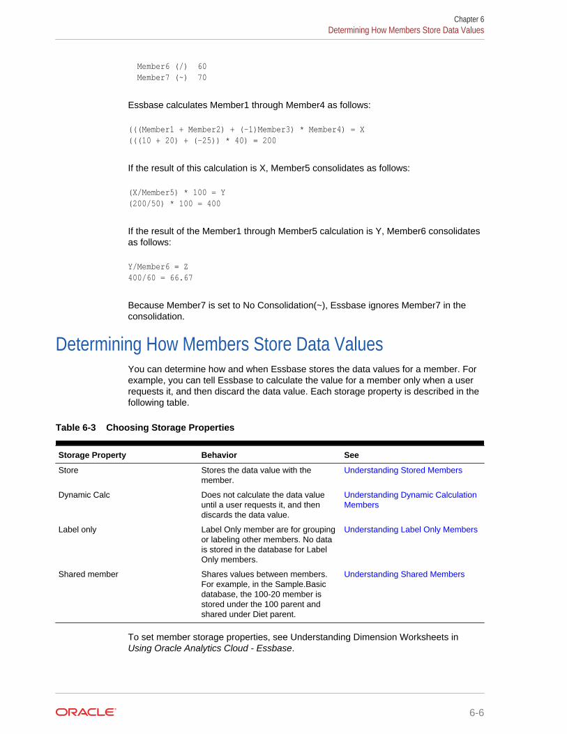
Member6 (/) 60 Member7 (~) 70

Essbase calculates Member1 through Member4 as follows:

(((Member1 + Member2) + (-1)Member3) * Member4) = X(((10 + 20) + (-25)) * 40) = 200

If the result of this calculation is X, Member5 consolidates as follows:

(X/Member5) * 100 = Y(200/50) * 100 = 400

If the result of the Member1 through Member5 calculation is Y, Member6 consolidatesas follows:

Y/Member6 = Z400/60 = 66.67

Because Member7 is set to No Consolidation(~), Essbase ignores Member7 in theconsolidation.

Determining How Members Store Data ValuesYou can determine how and when Essbase stores the data values for a member. Forexample, you can tell Essbase to calculate the value for a member only when a userrequests it, and then discard the data value. Each storage property is described in thefollowing table.

Table 6-3 Choosing Storage Properties

Storage Property Behavior See

Store Stores the data value with themember.

Understanding Stored Members

Dynamic Calc Does not calculate the data valueuntil a user requests it, and thendiscards the data value.

Understanding Dynamic CalculationMembers

Label only Label Only member are for groupingor labeling other members. No datais stored in the database for LabelOnly members.

Understanding Label Only Members

Shared member Shares values between members.For example, in the Sample.Basicdatabase, the 100-20 member isstored under the 100 parent andshared under Diet parent.

Understanding Shared Members

To set member storage properties, see Understanding Dimension Worksheets inUsing Oracle Analytics Cloud - Essbase.

Chapter 6Determining How Members Store Data Values

6-6

Understanding Stored MembersStored members contain calculated values that are stored with the member in thedatabase after calculation. By default, members are set as stored.

To define a member as stored, see Understanding Dimension Worksheets in UsingOracle Analytics Cloud - Essbase.

Understanding Dynamic Calculation MembersWhen a member is Dynamic Calc, Essbase does not calculate the value for thatmember until a user requests it. After the user views it, Essbase does not store thevalue for that member.See Dynamically Calculating Data Values.

Essbase automatically tags members of attribute dimensions as Dynamic Calc. Youcannot change this setting.

To tag a member as Dynamic Calc, see Understanding Dimension Worksheets inUsing Oracle Analytics Cloud - Essbase.

Understanding Label Only MembersLabel only members have no associated data. Use them to group members or to easenavigation and reporting from Smart View. Typically, you should give label onlymembers the “no consolidation” property. See Setting Member Consolidation.

You cannot associate attributes with label only members. If you tag a base dimensionmember that has attribute associations as label only, Essbase removes the attributeassociations and displays a warning message.

A descendent of a label only member cannot be tagged as Dynamic Calc. In thefollowing example, when verifying the outline, Essbase issues an error messageindicating that ChildB cannot be tagged as label only:

ParentA = Label Only ChildB = Label Only DescendantC = Dynamic Calc

Tagging DescendantC as Store Data resolves the issue.

To tag a member as label only, see Understanding Dimension Worksheets in UsingOracle Analytics Cloud - Essbase.

Understanding Shared MembersThe data values associated with a shared member come from another member withthe same name, called the referenced member. The shared member stores a pointerto data contained in the referenced member, and the data is stored only once. Todefine a member as shared, a referenced member of the same name must exist. Forexample, in the Sample.Basic database, the 100-20 member under 100 stores thedata for that member. The 100-20 member under Diet points to that value.


6-7

Shared members typically are used to calculate the same member across multipleparents; for example, to calculate a Diet Cola member in both the 100 and Dietparents.

Using shared members lets you use members repeatedly throughout a dimension.Essbase stores the data value only once, but it displays in multiple locations. Storingthe data value only once saves space and improves processing efficiency.

To tag a member as shared, see Understanding Dimension Worksheets in UsingOracle Analytics Cloud - Essbase.

Read the following sections to learn more about shared members.

• Understanding the Rules for Shared Members

• Understanding Shared Member Retrieval During Drill-Down

Note:

Members with the same name may be duplicate members instead of sharedmembers. See Creating and Working With Duplicate Member Outlines.

Understanding the Rules for Shared MembersRules when creating shared members:

• Shared members must be in the same dimension as their referenced member. Forexample, both 100-20 members in the Sample.Basic database are in the Productdimension.

• The reference member must precede the shared member in the outline order.

• Shared members cannot have children.

• An unlimited number of shared members can have the same name.

• UDAs or formulas cannot be assigned to shared members.

• You can create a shared member for a member with a duplicate member name.

• Attributes cannot be associated with shared members.

• If accounts properties are assigned to shared members, the values for thoseaccounts properties are taken from the referenced member, even if the accountsproperties on the shared member are changed.

• Aliases can be assigned to shared members.

• If an alias for a shared member is empty, Essbase uses the stored member’salias.

• If you assign an alias for a shared member and you change the alias for areferenced member, the shared member’s alias doesn’t change.

• A referenced member must be located in a dimension before its shared member.

• Avoid complex relationships between referenced and shared members that will bepart of an attribute calculation, or a calculation may return unexpected results. See Understanding Attribute Calculation and Shared Members.


6-8

Note:

You cannot place a shared member its referenced member under the sameparent. In a duplicate member outline, siblings must be unique.

In grid clients (for example, Smart View), shared members can easily bedifferentiated from their referenced members, because you can specify forthem to be displayed with a qualified name (for example, [Parent].[Child]).Shared members can be displayed with qualified names even if you have notset the outline to enable duplicate member names. Additionally, you can usequalified member names to search for shared members in the grid or usingmember selection.

Understanding Shared Member Retrieval During Drill-DownEssbase retrieves shared members during drill-down, depending on their location inthe spreadsheet. Essbase follows three rules during this type of retrieval:

• Essbase retrieves referenced members (not their shared member counterparts) bydefault.

• Essbase retrieves from the bottom of a spreadsheet first.

• If the parent of a shared member is a sibling of the referenced membercounterpart of one of the shared members, Essbase retrieves the referencedmember.

Example of Shared Members from a Single Dimension

If you create a test dimension with all shared members based on the referencedmembers of the dimension East from the Sample.Basic outline, the outline would besimilar to the one shown in Figure 6-1:


6-9

Figure 6-1 Shared Members from a Single Dimension

If you retrieve only the children of East, all results are from referenced membersbecause Essbase retrieves referenced members by default.

If, however, you retrieve data with the children of test above it in the spreadsheet,Essbase retrieves the shared members:

New YorkMassachusettsFloridaConnecticutNew Hampshiretest

If you move test above its last two children, Essbase retrieves the first three childrenas shared members, but the last two as referenced members. Similarly, if you insert amember in the middle of the list above which was not a sibling of the shared members(for example, California inserted between Florida and Connecticut), Essbase retrievesshared members only between the nonsibling and the parent (in this case, betweenCalifornia and test).

Example of Retrieval with Crossed Generation Shared Members

You can modify the Sample.Basic outline to create a shared member whosereferenced member counterpart is a sibling to its own parent, as shown in Figure 6-2:


6-10

Figure 6-2 Retrieval with Crossed Generation Shared Members

If you create a spreadsheet with shared members in this order, Essbase retrieves allthe shared members, except it retrieves the referenced member West, not the sharedmember west:

WestNew YorkMassachusettsConnecticutNew Hampshiretest

Essbase retrieves the members in this order because test is a parent of west and asibling of its referenced member counterpart, West.

Setting AliasesThe information about aliases and alias tables applies to block storage and aggregatestorage databases.

An alias is an alternate name for a member or shared member. For example,members in the Product dimension in the Sample.Basic database are identified bothby product codes, such as 100, and by more descriptive aliases, such as Cola.Aliases, stored in alias tables, can improve the readability of outlines or reports.

You can set multiple aliases for a member using alias tables. For example, you canuse different aliases for different kinds of reports—users may be familiar with 100-10as Cola, but advertisers and executives may be familiar with it as The Best Cola. This

Chapter 6Setting Aliases

6-11

list shows products in the Sample.Basic database that have two descriptive aliasnames:

Product Default Long Names100-10 Cola The Best Cola100-20 Diet Cola Diet Cola with Honey100-30 Caffeine Free Cola All the Cola, none of the Caffeine

Alias TablesAliases are stored in one or more tables as part of a database outline. An alias tablemaps a specific, named set of alias names to member names. When you create adatabase outline, Essbase creates an empty alias table named Default. If you do notcreate any other alias tables, the aliases that you create are stored in the Default aliastable.

An alias table applies to all members in the outline, although you don't have to providean alias name for every member unless you need it. You may use up to 56 alias tablesif you require more than one name for any members in the outline. A common use ofmultiple alias tables is for language conversion. Users in different countries can set theappropriate alias table to read the outline in their language.

Creating AliasesYou can provide an alias for any member. Alias names must follow the same rules asmember names. See Naming Conventions for Dimensions, Members, and Aliases.

You can use any of the following methods to create aliases in an existing alias table:

• Manually assign an alias to a member while editing an outline.

To open the outline management interface, see Setting Dimension and MemberProperties in Using Oracle Analytics Cloud - Essbase.

• Use Cube Designer and an application workbook to create alias tables and to addaliases to alias tables.

• Use dimension build and a data source to add aliases to an alias table.

• Import alias values from an alias table source file created in a predefined format.

In the Web interface, you cannot manage alias tables.

Creating and Managing Alias TablesAlias tables enable you to display different aliases.


Creating an Alias TableAn alias table contains a list of aliases to use for outline members. Theserequirements apply:

• You can create up to 56 alias tables for a block storage or aggregate storageoutline.


6-12

• The naming conventions for alias table names are the same as those fordimensions.

See Naming Conventions for Dimensions, Members, and Aliases.

• The name of the system-generated default alias table, which is Default, cannot bechanged; however, the name of alias tables that you create can be changed.

• (Optional.) You can specify multiple language codes for an alias table. When youcreate an alias table, a language code is not specified.

A new alias table is empty. To add aliases to an alias table and assign them tomembers, see Creating Aliases.

See these topics in Using Oracle Analytics Cloud - Essbase:

• Understanding the Cube.Setting Worksheet: Alias Tables

• Creating Aliases

Setting an Alias Table as ActiveThe active alias table contains the aliases that Essbase currently displays in theoutline.

To view a list of alias tables in the outline and to set the current alias table, you canuse the MaxL statements query database get active alias_table and alter databaseset active alias_table .


Copying an Alias TableTo copy an alias table, the table must be persisted in the database directory.

You can copy alias tables using the alter object MaxL statement.


Renaming an Alias TableYou can rename an alias table using the alter object MaxL statement.


Clearing and Deleting Alias TablesYou can delete an alias table from the outline, or you can clear all the aliases from analias table without deleting the alias table itself.

When you clear the aliases from an alias table, language codes associated with thatalias table are removed.

You can delete an alias table using the MaxL statement alter database unloadalias_table.



6-13

Importing and Exporting Alias TablesYou can import a correctly formatted text file into Essbase as an alias table. Alias tableimport files have the .alt extension. Alias table import files should have the followingstructure:

• The first line in the file starts with $ALT_NAME. Add one or two spaces followedby the name of the alias table. If the alias table name contains a blank character,enclose the name in single quotation marks.

• The last line of the file must be $END.

• Each line between the first and the last lines contains two values separated by oneor more spaces or tabs. The first value must be the name of an existing outlinemember; the second value is the alias for the member.

• Any member or alias name that contains a blank or underscore must be enclosedin double quotation marks.

The following is an example of an alias table import file:

$ALT_NAME 'Quarters'Qtr1 Quarter1Jan JanuaryFeb FebruaryMar March$END

You can also export an alias table from the Essbase outline to a text file. The exportfile contains aliases and the corresponding member names—qualified member namesfor duplicate members.

You can import and export alias tables using the MaxL statement alter database loadalias_table and unload alias_table.

Setting Two-Pass CalculationsBy default, Essbase calculates outlines from the bottom up—first calculating thevalues for the children and then the values for the parent. Sometimes, however, thevalues of the children may be based on the values of the parent or the values of othermembers in the outline. To obtain the correct values for these members, Essbasemust first calculate the outline and then recalculate the members that are dependenton the calculated values of other members. The members that are calculated on thesecond pass through the outline are called two-pass calculations.

See Using Bottom-Up Calculation.

For example, to calculate the ratio between Sales and Margin, Essbase needs first tocalculate Margin, which is a parent member based on its children, including Sales. Toensure that the ratio is calculated based on a freshly calculated Margin figure, tag theMargin % ratio member as a two-pass calculation. Essbase calculates the databaseonce and then calculates the ratio member again. This calculation produces thecorrect result.

Although two-pass calculation is a property that you can give to any nonattributemember, it works only on the following members:

Chapter 6Setting Two-Pass Calculations

6-14

• Accounts dimension members

• Dynamic Calc members

If two-pass calculation is assigned to other members, Essbase ignores it.

To tag a member as two-pass, see Understanding Dimension Worksheets and SettingTwo-Pass Calculation Properties in Using Oracle Analytics Cloud - Essbase.

Creating FormulasYou can apply formulas to standard dimensions and members. You cannot setformulas for attribute dimensions and their members. The formula determines howEssbase calculates the outline data. See Developing Formulas for Block StorageDatabases.

To add formulas to a dimension or member, see Understanding DimensionWorksheets and Creating Member Formulas in Using Oracle Analytics Cloud -Essbase.

Naming Generations and LevelsYou can create names for generations and levels in an outline, such as a word orphrase that describes the generation or level. For example, you might create ageneration name called Cities for all cities in the outline. See Dimension and MemberRelationships.

Use generation and level names in calculation scripts or report scripts wherever youneed to specify either a list of member names or generation or level numbers. Forexample, you could limit a calculation in a calculation script to all members in aspecific generation. See Developing Calculation Scripts for Block Storage Databases.

You can define only one name for each generation or level. When you namegenerations and levels, follow the same naming rules as for members. See NamingConventions for Dimensions, Members, and Aliases.

To name generations and levels, see Naming Generations and Levels in Using OracleAnalytics Cloud - Essbase.

Creating UDAsYou can create user-defined attributes (UDA) for members. For example, you mightcreate a UDA called Debit. Use UDAs in the following places:

• Calculation scripts. After you define a UDA, you can query a member for its UDAin a calculation script. For example, you can multiply all members with the UDADebit by –1 so that they display as either positive or negative (depending on howthe data is currently stored). See Developing Calculation Scripts for Block StorageDatabases.

• Data loading. You can change the sign of the data as it is loaded into the databasebased on its UDA.

To perform a calculation, selectively retrieve data based on attribute values, or providefull crosstab, pivot, and drill-down support in the spreadsheet, create attributedimensions instead of UDAs. See Comparing Attributes and UDAs.

Chapter 6Creating Formulas

6-15

Note:

On aggregate storage databases, using UDAs to define member groupsgreatly decreases the execution speeds of Essbase functions. To avoid thisperformance loss, use attribute dimensions to define member groups.

Rules when creating UDAs:

• You can define multiple UDAs per member.

• You cannot set the same UDA twice for one member.

• You can set the same UDA for different members.

• A UDA name can be the same as a member, alias, level, or generation name.Follow the same naming rules as for members. See Naming Conventions forDimensions, Members, and Aliases.

• You cannot create a UDA on shared members.

• You cannot create a UDA on members of attribute dimensions.

• A UDA applies to the specified member only. Descendants and ancestors of themember do not automatically receive the same UDA.

See Creating User-Defined Attributes in Using Oracle Analytics Cloud - Essbase.

Adding Comments to Dimensions and MembersYou can add comments to dimensions and members in a dimension worksheet in anapplication workbook that you plan to import to create a cube or in the cube outline.Comments can contain 255 characters maximum.

Chapter 6Adding Comments to Dimensions and Members

6-16

7Working with Attributes

You use attributes to describe characteristics of data, such as product size and color.Through attributes, you can group and analyze members of dimensions based on theircharacteristics.

• Process for Creating Attributes

• Understanding Attributes

• Understanding Attribute Dimensions

• Designing Attribute Dimensions

• Building Attribute Dimensions

• Setting Member Names in Attribute Dimensions

• Calculating Attribute Data

• Non-Aggregating Attributes

• Submitting Data for Valid Attribute Combinations in the Grid

• Suppressing Invalid Attribute Combinations in the Grid


Process for Creating Attributes1. Create a dimension.

In an application workbook on the Essbase.Cube Worksheet, or in the outlineeditor, position the attribute dimensions after all standard dimensions.

2. Tag the dimension as an attribute dimension and set attribute dimension type astext, numeric, Boolean, or date.

See Creating Attribute Dimensions.

3. Consider whether non-aggregating attributes would be useful in your database.See Non-Aggregating Attributes.

4. Add members to the attribute dimension.

5. Associate a base dimension with the attribute dimension.

See Understanding the Rules for Attribute Dimension Association.

6. Associate members of the base dimension with members of the attributedimension.

See Understanding the Rules for Attribute Member Association.

7. If necessary, set up the attribute calculations.

See Calculating Attribute Data.

7-1


• Understanding the Essbase.Cube Worksheet

• Understanding Cube.Settings Worksheet: Attribute Settings

• Working with Attributes

• Setting Attribute Associations

Understanding AttributesYou can use the Essbase attribute feature to retrieve and analyze data not only fromthe perspective of dimensions, but also in terms of characteristics, or attributes, ofthose dimensions. For example, you can analyze product profitability based on size orpackaging, and you can make more effective conclusions by incorporating marketattributes, such as the population of each market region, into the analysis.

Such an analysis could tell you that decaffeinated drinks sold in cans in small markets(populations less than 6,000,000) are less profitable than you anticipated. For moredetails, you can filter the analysis by specific attribute criteria, including minimum ormaximum sales and profits of different products in similar market segments.

A few ways analysis by attribute provides depth and perspective, supporting better-informed decisions:

• You can select, aggregate, and report on data based on common features(attributes).

• By defining attributes as having a text, numeric, Boolean, or date type, you canfilter (select) data using type-related functions such as AND, OR, and NOToperators and <, >, and = comparisons.

• You can use the numeric attribute type to group statistical values by attributeranges; for example, population groupings such as <500,000, 500,000–1,000,000,and >1,000,000.

• Through the Attribute Calculations dimension automatically created by Essbase,you can view sums, counts, minimum or maximum values, and average values ofattribute data. For example, when you enter Avg and Bottle into a spreadsheet,Essbase retrieves calculated values for average sales in bottles for all the columnand row intersections on the sheet.

• You can perform calculations using numeric attribute values in calculation scriptsand member formulas; for example, to determine profitability by ounce for productssized by the ounce.

• You can create crosstabs of attribute data for the same dimension, and you canpivot and drill down for detail data in spreadsheets.

An attribute crosstab is a report or spreadsheet showing data consolidationsacross attributes of the same dimension. The crosstab example below displaysproduct packaging as columns and the product size in ounces as rows. At theirintersections, you see the profit for each combination of package type and size.

From this information, you can see which size-packaging combinations were mostprofitable in the Florida market.

Product Year Florida Profit Actual

Chapter 7Understanding Attributes

7-2

Bottle Can Pkg Type ====== ===== ======== 32 946 N/A 946 20 791 N/A 791 16 714 N/A 714 12 241 2,383 2,624Ounces 2,692 2,383 5,075

Understanding Attribute DimensionsProducts have attributes that are characteristics of the products, such as a product'ssize and packaging. Attribute members reside in attribute dimensions.

An attribute dimension has the letter A next to its name in the outline.

The image below shows part of the Sample.Basic outline featuring the Productdimension and some attribute dimensions: Caffeinated, Ounces, Pkg Type, and IntroDate.

In the Properties panel for the Product dimension, you can see which attributedimensions are associated with the Product dimension.

Attributes are associated with sparse, non-attribute dimensions, called basedimensions. In the example above, the Product dimension is the base dimension forthe attribute dimensions.

Chapter 7Understanding Attribute Dimensions

7-3

Note:

Attribute dimensions and members are Dynamic Calc (with the exception ofnon-aggregating attributes), so Essbase calculates attribute information atretrieval time. Attribute data is not stored in the database.

Understanding Members of Attribute DimensionsMembers of an attribute dimension are potential attributes of the members of theassociated base dimension. After you associate a base dimension with an attributedimension, you associate members of the base dimension with members of theassociated attribute dimension. The Market dimension member Connecticut isassociated with the 6000000 member of the Population attribute dimension. Thatmakes 6000000 an attribute of Connecticut.

Understanding the Rules for Base and Attribute Dimensions andMembers

Rules regarding members of attribute dimensions and their base dimensions:

• You can tag only sparse dimensions as attribute dimensions.

• Before you can save an outline to the server, each attribute dimension must beassociated with a standard, sparse dimension as its base dimension.

• Attribute dimensions must be the last dimensions in the outline.

• Attribute dimensions have a type setting—text, numeric, Boolean, or date. Text isthe default setting. Although assigned at the dimension level, the type applies onlyto the level 0 members of the dimension. See Understanding Attribute Types.

• If you remove the attribute tag from a dimension, Essbase removes prefixes orsuffixes from its member names. Prefixes and suffixes are not visible in theoutline. See Setting Prefix and Suffix Formats for Member Names of AttributeDimensions.

• A base dimension member can have many attributes, but only one attribute fromeach attribute dimension.

For example, product 100-10 can have size and packaging attributes, but only onesize and only one type of packaging.

You can use attribute values in calculations in the following comparisons:

• > (greater than)

• >= (greater than or equal to)

• < (less than)

• <= (less than or equal to)

• == (equal to)

• <> or != (not equal to)

• IN


7-4

Understanding the Rules for Attribute Dimension AssociationWhen you associate an attribute dimension with a standard dimension, the standarddimension is the base dimension for that attribute dimension.

• An attribute dimension must be associated with a sparse standard dimension.

• A standard dimension can be a base dimension for multiple attribute dimensions.

• An attribute dimension can be associated with only one base dimension.

For example, you might have a Size attribute dimension with members Small,Medium, and Large. If you associate the Size attribute dimension with the Productdimension, you cannot also associate the Size attribute dimension with the Marketdimension. Tracking size-related information for the Market dimension requiresanother attribute dimension with a different name; for example, MarketSize, withthe MarketSize attribute dimension associated with the Market dimension.

Understanding the Rules for Attribute Member AssociationWhen you associate a member of an attribute dimension with a member of a basedimension, follow these rules:

• You cannot associate multiple members from the same attribute dimension withthe same base dimension member. For example, the Bottle and Can packagetypes cannot both be associated with the product 100-30.

• You can associate members from different attribute dimensions with the samemember of a base dimension. For example, a decaffeinated cola product (100-30)sold in 16-ounce bottles has three attributes: Caffeinated:False; Ounces:16; andPkg Type:Bottle.

• Essbase does not require that each member of a base dimension be associatedwith a member of an attribute dimension.

• Attributes can be assigned only to level zero members.

• The level 0 members of attribute dimensions are the only members that you canassociate with base dimension members.

For example, in the Population attribute dimension, you can associate only level 0members such as 3000000, 6000000, and 9000000, with members of the Marketdimension. You cannot associate a level 1 member such as Small.

The name of the level 0 member of an attribute dimension is the attribute value.The only members of attribute dimensions that have attribute values are level 0members.

You can use the higher-level members of attribute dimensions to select and groupdata. For example, you can use Small, the level 1 member of the Populationattribute dimension, to retrieve sales in both the 3000000 and 6000000 populationcategories.

Understanding Attribute TypesAttribute dimensions have a text, numeric, Boolean, or date type that enables differentfunctions for grouping, selecting, or calculating data. Although assigned at the


7-5

dimension level, the attribute type applies only to level 0 members of the attributedimension.

• The default attribute type is text. Text attributes enable the basic attribute memberselection and attribute comparisons in calculations. When you perform suchcomparisons, Essbase compares characters. For example, the package typeBottle is less than the package type Can, because B precedes C in the alphabet.In Sample.Basic, Pkg Type is an example of a text attribute dimension.

• The names of level 0 members of numeric attribute dimensions are numericvalues. You can include the names (values) of numeric attribute dimensionmembers in calculations. For example, you can use the number of ouncesspecified in the Ounces attribute to calculate profit per ounce for each product.

You can also associate numeric attributes with ranges of base dimension values;for example, to analyze product sales by market population groupings—states with3,000,000 population or less in one group, states with a population between3,000,001 and 6,000,000 in another group, and so on. See Setting Up MemberNames Representing Ranges of Values.

• All Boolean attribute dimensions in a database contain only two members. Themember names must match the settings for the database; for example, True andFalse. If multiple Boolean attribute dimensions exist, specify a prefix or suffixmember name format to ensure unique member names; for example,Caffeinated_True and Caffeinated_False. See Setting Boolean Attribute MemberNames.

• You can use date attributes to specify the date format—month-day-year or day-month-year—and to sequence information accordingly. See Changing the MemberNames in Date Attribute Dimensions. You can use date attributes in calculations.For example, you can compare dates in a calculation that selects product salesfrom markets established since 10-12-1999.

Essbase supports date attributes from January 1, 1970, through January 1, 2038.

Comparing Attribute and Standard DimensionsIn general, attribute dimensions and their members are similar to standard dimensionsand their members. You can provide aliases and member comments for attributes.Attribute dimensions can include hierarchies, and you can name generations andlevels. You can perform the same spreadsheet operations on attribute dimensions andmembers as on standard dimensions and members; for example, to analyze data fromdifferent perspectives, you can retrieve, pivot, and drill down in the spreadsheet.

Table 7-1 describes major differences between attribute and standard dimensions andtheir members.

Table 7-1 Differences Between Attribute and Standard Dimensions

Functionality Attribute Dimensions Standard Dimensions

Storage Sparse. An attribute dimension'sbase dimension also must be sparse

Can be dense or sparse

Storage property Can be Dynamic Calc only.Therefore, not stored in thedatabase. The outline does notdisplay this property.

Can be Store Data, Dynamic Calc, orLabel Only


7-6

Table 7-1 (Cont.) Differences Between Attribute and Standard Dimensions


Position in outline Must be the last dimensions in theoutline

Must be above all attributedimensions in the outline

Partitions Cannot be defined along attributedimensions, but you can useattributes to define a partition on abase dimension

Can be defined along standarddimensions

Formulas (on members) Cannot be associated Can be associated

Shared members Not allowed Allowed

Two-pass calculation memberproperty

Not available Available

Two-pass calculation with runtimeformula

If a member formula contains aruntime-dependent functionassociated with an attribute membername, and the member with theformula is tagged as two-pass,calculation skips the member andissues a warning message. Runtime-dependent functions include:@CURRMBR, @PARENT,@PARENTVAL, @SPARENTVAL,@MDPARENTVAL, @ANCEST,@ANCESTVAL, @SANCESTVAL,and @MDANCESTVAL.

See Understanding Two-PassCalculations on AttributeDimensions.

Calculation is performed on standardmembers with runtime formulas andtagged two-pass.

Two-pass, multiple dimensions:Calculation order

Order of calculation of memberstagged two-pass depends on order inoutline. The last dimension iscalculated last.

Calculation result is not dependenton outline order for members taggedtwo-pass in multiple dimensions.

Two-pass calculation with nomember formula

Calculation skipped, warningmessage issued. Therefore, memberintersection of two-pass taggedmembers and upper-level membersmay return different results fromcalculation on standard dimensions.

See Understanding Two-PassCalculations on AttributeDimensions.

Available


7-7

Table 7-1 (Cont.) Differences Between Attribute and Standard Dimensions


Dense Dynamic Calc members innonexisting stored blocks

Calculations skip dense dimensionsif they are on nonexisting storedblocks.

For attributes to work on densemembers, data blocks for the densemembers must exist. When retrievingdata on a dense member that has aDynamic Calc formula and noattributes, Essbase dynamicallycreates the data block and returns avalue. However, if the Dynamic Calcdense member has an attribute,doing a retrieve on the attributemember results in #MISSING,because Essbase skips the dynamiccalculation on the dense memberand, therefore, the data block is notcreated.

To identify nonexisting stored blocks,export the database or run a query tofind out whether the block has data.

Available

UDAs on members Not allowed Allowed

Consolidations For all members, calculated throughthe Attribute Calculations dimensionmembers: Sum, Count, Min, Max,and Avg. Consolidation operators inthe outline are ignored duringattribute calculations.

Consolidation operation indicated byassigning the desired consolidationsymbol to each member

Member selection facilitated by Level0 member typing

Available types include text, numeric,Boolean, and date.

All members treated as text

Associations Must be associated with a basedimension

N/A

Spreadsheet drill-downs List the base dimension dataassociated with the selectedattribute. For example, drilling downon the attribute Glass displays salesfor each product packaged in glass,where Product is the base dimensionfor the Pkg Type attribute dimension.

List lower or sibling levels of detail inthe standard dimensions. Forexample, drilling down on Qtr1displays a list of products and theirsales for that quarter.

Solve Order and AttributesIf hybrid aggregation mode is enabled, you can set the solve order for attributedimensions and their base dimensions, eliminating the need to tag members as two-pass. In hybrid aggregation mode, the default calculation order (also known as solveorder) matches that of block storage databases, with some enhancements. If you wishto use a non-default solve order, you can set a custom solve order for dimensions andmembers.

For more information about hybrid aggregation mode, see Using Hybrid Aggregation.


7-8

Understanding Two-Pass Calculations on Attribute DimensionsThe following example, based on the Product dimension in the Sample.Basicdatabase, illustrates how two-pass calculations work on attribute dimensions. Assumemember “400–30” is tagged as two-pass.

If member “400-30” has the following member formula:

=”400–10”;

Essbase executes the formula when performing a retrieve on “400-30.”

If “400-30” has the following member formula:

=@CURRMBR("Market");

Essbase skips the calculation because the formula includes the @CURRMBR runtimefunction, which is not allowed, and issues the following error message:

Two-pass calc skipped on member [400-30] in attribute calc”

If “400-30” does not have a member formula, the same error message is generatedbecause a member tagged as two-pass must have a formula.

Comparing Attributes and UDAsAttributes and UDAs enable analysis based on characteristics of the data. Attributesprovide greater capability than UDAs. The tables in this topic describe the differencesbetween attributes and UDAs in these areas of functionality:

• Data storage (Table 7-2)

• Data retrieval (Table 7-3)

• Data conversion (Table 7-4)

• Calculation scripts (Table 7-5)

Table 7-2 Data Storage—Comparing Attributes and UDAs

Data storage Attributes UDAs

You can associate with sparsedimensions.

Supported Supported

You can associate with densedimensions.

Not supported Supported


7-9

Table 7-3 Data Retrieval—Comparing Attributes and UDAs

Data Retrieval Attributes UDAs

You can group and retrieveconsolidated totals by attribute orUDA value. For example, associatethe value High Focus Item to variousmembers of the Product dimensionand use that term to retrieve totalsand details for only those members.

Supported

Simple

Supported

More difficult to implement, requiringadditional calculation scripts orcommands

You can categorize attributes in ahierarchy and retrieve consolidatedtotals by higher levels in the attributehierarchy; for example, if eachproduct has a size attribute such as8, 12, 16, or 32, and the sizes arecategorized as small, medium, andlarge. You can view the total sales ofsmall products.

Supported Supported

More difficult to implement

You can create crosstab viewsdisplaying aggregate totals ofattributes associated with the samebase dimension.

Supported

You can show a crosstab of allvalues of each attribute dimension.

Not supported

You can retrieve only totals based onspecific UDA values.

You can use Boolean operatorsAND, OR, and NOT with attributeand UDA values to refine a query.For example, you can selectdecaffeinated drinks from the 100product group.

Supported Supported

Because attributes have a text,Boolean, date, or numeric type, youcan use appropriate operators andfunctions to work with and displayattribute data. For example, you canview sales totals of all productsintroduced after a specific date.

Supported Not supported

You can group numeric attributesinto ranges of values and let thedimension building processautomatically associate the basemember with the appropriate range.For example, you can group sales invarious regions based on ranges oftheir populations—less than 3million, between 3 million and 6million, and so on.


Through the Attribute Calculationsdimension, you can viewaggregations of attribute values assums, counts, minimums,maximums, and averages.



7-10

Table 7-3 (Cont.) Data Retrieval—Comparing Attributes and UDAs

Data Retrieval Attributes UDAs

You can use an attribute in acalculation that defines a member.For example, you can use the weightof a product in ounces to define theprofit per ounce member of theMeasures dimension.


You can retrieve specific basemembers using attribute-relatedinformation.

Supported

Powerful conditional and value-based selections

Supported

Limited to text string matches only

Table 7-4 Data Conversion—Comparing Attributes and UDAs

Data Conversion Attributes UDAs

Based on the value of a UDA, youcan change the sign of the data as itis loaded into the database. Forexample, you can reverse the sign ofall members with the UDA Debit.

Not supported Supported

Table 7-5 Calculation Scripts—Comparing Attributes and UDAs

Calculation Scripts Attributes UDAs

You can perform calculations on amember if its attribute or UDA valuematches a specific value. Forexample, you can increase the priceby 10% of all products with theattribute or UDA of Bottle.

Supported Supported

You can perform calculations onbase members whose attribute valuesatisfies conditions that you specify.For example, you can calculate theProfit per Ounce of each basemember.


Designing Attribute DimensionsEssbase provides multiple ways to design attribute information into a database. Mostoften, defining characteristics of the data through attribute dimensions and theirmembers is the best approach. The following sections discuss when to use attributedimensions, when to use other features, and how to optimize performance when usingattributes.

Using Attribute DimensionsFor the most flexibility and functionality, use attribute dimensions to define attributedata. Using attribute dimensions provides the following features:

Chapter 7Designing Attribute Dimensions

7-11

• Sophisticated, flexible data retrieval

You can view attribute data only when you want to; you can create meaningfulsummaries through crosstabs; and, using type-based comparisons, you canselectively view only the data that you want to see.

• Additional calculation functionality

Not only can you perform calculations on the names of members of attributedimensions to define members of standard dimensions, you can also access fivetypes of consolidations of attribute data—sums, counts, averages, minimums, andmaximums.

• Economy and simplicity

Because attribute dimensions are sparse, Dynamic Calc, they are not stored asdata. Compared to using shared members, outlines using attribute dimensionscontain fewer members and are easier to read.

See Understanding Attributes.

Using Alternative Design ApproachesIn some situations, consider one of the following approaches:

• Hybrid aggregation mode. If you enable hybrid aggregation mode, you can usenon-aggregating attributes if needed, and you can set a custom solve orderinstead of using two-pass calculation. See Non-Aggregating Attributes. For moreinformation about hybrid aggregation, see the ASODYNAMICAGGINBSO topic inTechnical Reference for Oracle Essbase.

• UDAs. Although UDAs provide less flexibility than attributes, you can use them togroup and retrieve data based on its characteristics. See Comparing Attributesand UDAs.

• Shared members. For example, to include a seasonal analysis in the Yeardimension, repeat the months as shared members under the appropriate season;Winter: Jan (shared member), Feb (shared member), and so on. A majordisadvantage of using shared members is that the outline becomes large if thecategories repeat many members.

• Standard dimensions and members. Additional standard dimensions provideflexibility but add storage requirements and complexity to a database. Forguidelines on evaluating the impact of additional dimensions, see Analyzing andPlanning.

Table 7-6 describes situations in which you might consider an alternative approach tomanaging attribute data in a database.

Table 7-6 Considering Alternatives to Attribute Dimensions

Situation Alternative

Analyze attributes of dense dimensions UDAs or shared members

Perform batch calculation of data Shared members or members of separate,standard dimensions

Define the name of a member of an attributedimension as a value that results from aformula

Shared members or members of separate,standard dimensions

Chapter 7Designing Attribute Dimensions

7-12

Table 7-6 (Cont.) Considering Alternatives to Attribute Dimensions

Situation Alternative

Define attributes that vary over time Members of separate, standard dimensions.For example, to track product maintenancecosts over time, the age of the product at thetime of maintenance is important. However,using the attribute feature, you could associateonly one age with the product. You needmultiple members in a separate dimension foreach time period that you want to track.

Minimize retrieval time with large numbers ofbase-dimension members

Batch calculation with shared members ormembers of separate, standard dimensions.

Perform cross-dimensional analysis with lowperformance impact

Non-aggregating attributes

Optimizing Outline PerformanceOutline layout and content can affect attribute calculation and query performance. Forgeneral outline design guidelines, see Designing an Outline to Optimize Performance.

To optimize attribute query performance, consider the following design tips:

• Ensure that attribute dimensions are the only sparse Dynamic Calc dimensions inthe outline.

• Locate sparse dimensions after dense dimensions in the outline. Place the most-queried dimensions at the beginning of the sparse dimensions and attributedimensions at the end of the outline. In most situations, base dimensions arequeried most.

See Optimizing Calculation and Retrieval Performance.

Building Attribute DimensionsTo build an attribute dimension, tag the dimension as an attribute and assign thedimension a type. Then associate the attribute dimension with a base dimension.Finally, associate each level 0 member of the attribute dimension with a member of theassociated base dimension.

You can view the dimension, attribute value, and attribute type of a specific attributemember using the query database MaxL statement.


• Understanding the Essbase.Cube Worksheet

• Understanding Cube.Settings Worksheet: Attribute Settings

• Working with Attributes

• Setting Attribute Associations

Chapter 7Building Attribute Dimensions

7-13

Setting Member Names in Attribute DimensionsWhen you use the attribute feature, Essbase establishes default member names; forexample, the system-defined True and False precludes other member names of Trueand False. You can change these system-defined names for the database. Dateattributes and numeric attributes also can be duplicated. To avoid duplicate nameconfusion, you can establish settings for qualifying member names in attributedimensions. The outline does not show the fully qualified attribute names, but you cansee the full attribute names anywhere you select members, such as when you definepartitions or select information to be retrieved.

Define the member name settings before you define or build the attribute dimensions.Changing the settings after the attribute dimensions and members are defined couldresult in invalid member names.

The following sections describe how to work with the names of members of attributedimensions:

• Setting Prefix and Suffix Formats for Member Names of Attribute Dimensions

• Setting Boolean Attribute Member Names

• Changing the Member Names in Date Attribute Dimensions

• Setting Up Member Names Representing Ranges of Values

• Changing the Member Names of the Attribute Calculations Dimension

Note:

If you partition an outlines containing attribute dimensions, the name formatsettings of members described in this section must be identical in the sourceand target outlines.

Setting Prefix and Suffix Formats for Member Names of AttributeDimensions

The information in this section does not apply to duplicate member attributedimensions.

The names of members of Boolean, date, and numeric attribute dimensions arevalues. It is possible to encounter duplicate attribute values in different attributedimensions.

• Boolean example

If you have multiple Boolean attribute dimensions in an outline, the two membersof each of those dimensions have the same names, by default, True and False.

• Date example

If you have multiple date attribute dimensions, some member names in bothdimensions could be the same. For example, the date on which a store opens in acertain market could be the same as the date on which a product was introduced.

Chapter 7Setting Member Names in Attribute Dimensions

7-14

• Numeric example

The attribute value for the size of a product could be 12, and 12 also could be thevalue for the number of packing units for a product. This example results in twomembers with the name 12.

You can define unique names by attaching a prefix or suffix to member names inBoolean, date, and numeric attribute dimensions in the outline. You can affix thedimension, parent, grandparent, or all ancestors to the attribute name. For example,by setting member names of attribute dimensions to include the dimension name asthe suffix, attached by an underscore, the member value 12 in the Ounces attributedimension assumes the unique, full attribute member name 12_Ounces.

By default, Essbase assumes that no prefix or suffix is attached to the names ofmembers of attribute dimensions.

The convention that you select applies to the level 0 member names of all numeric,Boolean, and date attribute dimensions in the outline. You can define aliases for thesenames if you want to display shorter names in retrievals.

See Understanding Cube.Settings Worksheet: Attribute Settings in Using OracleAnalytics Cloud - Essbase.

Setting Boolean Attribute Member NamesWhen you set the dimension type of an attribute dimension as Boolean, Essbaseautomatically creates two level 0 members with the names specified for the Booleanattribute settings. The initial Boolean member names in a database are set as Trueand False. To change these default names, for example, to Yes and No, define themember names for Boolean attribute dimensions before you create Boolean attributedimensions in the database.

Before you can set an attribute dimension type as Boolean, you must delete allexisting members in the dimension.


Changing the Member Names in Date Attribute DimensionsYou can change the format of members of date attribute dimensions. For example,you can use the following date formats:

• mm-dd-yyyy: October 18, 2007 is displayed as 10-18-2007.

• dd-mm-yyyy: October 18, 2007 is displayed as 18-10-2007.

If you change the date member name format, the names of existing members of dateattribute dimensions may be invalid. For example, if the 10-18-2007 member exists,and you change the format to dd-mm-2007, outline verification will find this memberinvalid. If you change the date format, you must rebuild the date attribute dimensions.



7-15

Setting Up Member Names Representing Ranges of ValuesMembers of numeric attribute dimensions can represent single numeric values orranges of values:

• Single-value example: the member 12 in the Ounces attribute dimensionrepresents the single numeric value 12; you associate this attribute with all 12-ounce products. The outline includes a separate member for each size; forexample, 16, 20, and 32.

• Range of values example: the Population attribute dimension, as shown in Figure 7-1:

Figure 7-1 Population Attribute Dimension and Members

In this outline, the members of the Population attribute dimension representranges of population values in the associated Market dimension. The 3000000member represents populations from zero through 3,000,000; the 6000000member represents populations from 3,000,001 through 6,000,000; and so on. Asetting for the outline establishes that each numeric member represents the top ofits range.

You can also define this outline setting so that members of numeric attributedimensions are the bottoms of the ranges that they represent. For example, ifnumeric members are set to define the bottoms of the ranges, the 3000000member represents populations from 3,000,000 through 5,999,999, and the6000000 member represents populations from 6,000,000 through 8,999,999.

When you build the base dimension, Essbase automatically associates members ofthe base dimension with the appropriate attribute range. For example, if numericmembers represent the tops of ranges, Essbase automatically associates theConnecticut market, with a population of 3,269,858, with the 6000000 member of thePopulation attribute dimension.

In the dimension build rules file, specify the size of the range for each member of thenumeric attribute dimension. In the above example, each attribute represents a rangeof 3,000,000.


7-16

Note:

Oracle recommends that numeric attribute dimension member namescontain no more than six decimal positions. Otherwise, because of precisionadjustments, an outline may not pass verification.


Changing the Member Names of the Attribute Calculations DimensionTo avoid duplicating names in an outline, you may need to change the name of theAttribute Calculations dimension or its members.

Sum, Count, Min, Max, and Avg—the names of the members that Essbase creates inthe Attribute Calculations dimension—are not considered reserved words because youcan change these names in the Attribute Calculations dimension and then use thedefault name in an attribute or standard dimension. Follow these guidelines:

• If the outline is tagged as a duplicate member outline, you can use the defaultnames to name other base or attribute members.

• If the outline is tagged as a unique member outline, you should avoid using Sum,Count, Min, Max, and Avg as member names. For example, if you use Max in astandard dimension and then create an attribute dimension, in which Essbasecreates the Max member in the Attribute Calculations dimension, Essbase detectsa duplicate name and returns an error message indicating the name is already inuse.

Regardless of the name that you use for a Attribute Calculations dimension member,its function remains the same. For example, Count, the second member, alwayscounts.


Calculating Attribute DataEssbase calculates attribute data dynamically at retrieval time, using members from asystem-defined dimension created by Essbase. Using this dimension, you can applydifferent calculation functions, such as a sum or an average, to the same attribute. Youcan also perform specific calculations on members of attribute dimensions; forexample, to determine profitability by ounce for products sized by the ounce.

The following information assumes that you understand the concepts of attributedimensions and Essbase calculations, including dynamic calculations. See thefollowing sections.

• Understanding the Attribute Calculations Dimension

• Understanding the Default Attribute Calculations Members

• Viewing an Attribute Calculation Example

• Accessing Attribute Calculations Members in Smart View

Chapter 7Calculating Attribute Data

7-17

• Optimizing Calculation and Retrieval Performance

• Using Attributes in Calculation Formulas

• Understanding Attribute Calculation and Shared Members

• Differences Between Calculating Attribute Members and Non-Attribute (Stored andDynamic Calc) Members

Understanding the Attribute Calculations DimensionWhen you create the first attribute dimension in the outline, Essbase also creates theAttribute Calculations dimension comprising five members with the default namesSum, Count, Min (minimum), Max (maximum), and Avg (average). You can use thesemembers in spreadsheets or in reports to dynamically calculate and report on attributedata, such as the average yearly sales of 12-ounce bottles of cola in the West.

The Attribute Calculations dimension is not visible in the outline. You can see itwherever you select dimension members, such as in Smart View.

The attribute calculation dimension has the following properties:

• System-defined

When you create the first attribute dimension in an application, Essbase createsthe Attribute Calculations dimension and its members (Sum, Count, Min, Max, andAvg). Each member represents a type of calculation to be performed for attributes.

See Understanding the Default Attribute Calculations Members.

• Label only

Like all label only dimensions, the Attribute Calculations dimension shares thevalue of its first child, Sum.

See Member Storage Properties.

• Dynamic Calc

The data in the Attribute Calculations dimension is calculated when a userrequests it and is then discarded. You cannot store calculated attribute data in adatabase.

See Dynamically Calculating Data Values.

• Not displayed in Outline Editor

The Attribute Calculations dimension is not displayed in Outline Editor. Membersfrom this dimension can be viewed in spreadsheets and in reports.

There is no consolidation along attribute dimensions. You cannot tag members fromattribute dimensions with consolidation symbols (for example, + or -) or with memberformulas in order to calculate attribute data. As Dynamic Calc members, attributecalculations do not affect the batch calculation in terms of time or calculation order.

To calculate attribute data at retrieval time, Essbase performs the following tasks:

1. Finds the base-dimension members associated with the attribute-dimensionmembers present in the current query

2. Dynamically calculates the sum, count, minimum, maximum, or average for theattribute-member combination for the current query

3. Displays the results in the spreadsheet or report


7-18

4. Discards the calculated values—that is, the values are not stored in the database

Note:

Essbase excludes #MISSING values when calculating attribute data.

For example, as shown in Figure 7-2, a spreadsheet user specifies two members ofattribute dimensions (Ounces_16 and Bottle) and an Attribute Calculations member(Avg) in a spreadsheet report. Upon retrieval, Essbase dynamically calculates theaverage sales values of all products associated with these attributes for the currentmember combination (Actual -> Sales -> East -> Qtr1):

Figure 7-2 Retrieving an Attribute Calculations Member

See Accessing Attribute Calculations Members in Smart View.

Understanding the Default Attribute Calculations MembersThe Attribute Calculations dimension contains five members (Sum, Count, Min, Max,and Avg) that are used to calculate and report attribute data:

• Sum—Calculates a sum, or total, of the values for a member with an attribute orcombination of attributes.

• Count—Calculates the number of members with the specified attribute orcombination of attributes, for which a data value exists. Count includes only thosemembers that have data blocks in existence. To calculate a count of all memberswith certain attributes, regardless of whether they have data values, use the@COUNT function in combination with the @ATTRIBUTE function. See TechnicalReference for Oracle Essbase.

• Avg—Calculates a mathematical mean, or average, of the nonmissing values foran specified attribute or combination of attributes (Sum divided by Count).

• Min—Calculates the minimum data value for a specified attribute or combination ofattributes.

• Max—Calculates the maximum data value for a specified attribute or combinationof attributes.

Note:

Each of these calculations excludes #MISSING values.


7-19

You can change these default member names, subject to the same namingconventions as standard members. See Changing the Member Names of the AttributeCalculations Dimension.

Viewing an Attribute Calculation ExampleAs an example of how Essbase calculates attribute data, consider the following yearlysales data for the East:

Table 7-7 Sample Attribute Data

Base-Dimension Member Associated Attributes Sales Value for Attribute-Member Combination

Cola Ounces_12, Can 23205

Diet Cola Ounces_12, Can 3068

Diet Cream Ounces_12, Can 1074

Grape Ounces_32, Bottle 6398

Orange Ounces_32, Bottle 3183

Strawberry Ounces_32, Bottle 5664

Figure 7-3 shows how calculated attribute data might look in a spreadsheet report.You can retrieve multiple Attribute Calculations members for attributes. For example,you can calculate Sum, Count, Avg, Min, and Max for bottles and cans.

Figure 7-3 Sample Spreadsheet with Attribute Data

Accessing Attribute Calculations Members in Smart ViewYou can access members from the Attribute Calculations dimension in Smart View.From the spreadsheet, users can view Attribute Calculations dimension membersusing any of the following methods:

• Entering members directly into a sheet

• Selecting members from the Query Designer

• Entering members as an EssCell parameter

See Oracle Smart View for Office User’s Guide.


7-20

Optimizing Calculation and Retrieval PerformanceTo optimize attribute calculation and retrieval performance, consider the following:

• The calculation order for attribute calculations is the same as for dynamiccalculations. For an outline, see Calculation Order for Dynamic Calculation.

• Because Essbase calculates attribute data dynamically at retrieval time, attributecalculations do not affect the performance of the overall (batch) databasecalculation.

• Tagging base-dimension members as Dynamic Calc may increase retrieval time.

• When a query includes the Sum member and an attribute-dimension memberwhose associated base member is tagged as two-pass, retrieval time may beslow.

• To maximize attribute retrieval performance, use any of the following techniques:

– Configure the outline using the tips in Optimizing Outline Performance.

– Drill down to the lowest level of base dimensions before retrieving data. Forexample, in Smart View, turn on the Navigate Without Data feature, drill downto the lowest level of the base dimensions included in the report, and thenretrieve data.

– When the members of a base dimension are associated with several attributedimensions, consider grouping the members of the base dimension accordingto their attributes. For example, in the Sample.Basic database, you can groupall 8-ounce products.

Using Attributes in Calculation FormulasIn addition to using the Attribute Calculations dimension to calculate attribute data, youcan use calculation formulas on members of standard or base dimensions to performspecific calculations on members of attribute dimensions; for example, to determineprofitability by ounce for products sized by the ounce.

You cannot associate formulas with members of attribute dimensions.

Note:

Some restrictions apply when using attributes in formulas associated withtwo-pass members. See the rows about two-pass calculations in Table 7-1and Understanding Two-Pass Calculations on Attribute Dimensions.

Table 7-8 lists functions you can use to perform specific calculations on attributes:


7-21

Table 7-8 Functions That Calculate On Attributes

Function Type of Calculation

@ATTRIBUTE Generate a list of all base members with aspecific attribute. For example, generate a listof members that have the Bottle attribute, andthen increase the price for those members.

@ATTRIBUTEVAL

@ATTRIBUTEBVAL

@ATTRIBUTESVAL

Return the value of the level 0 attributemember that is associated with the basemember being calculated.

• From a numeric or date attributedimension (using @ATTRIBUTEVAL)

• From a Boolean attribute dimension(using @ATTRIBUTEBVAL)

• From a text attribute dimension (using@ATTRIBUTESVAL)

For example, return the numeric value of asize attribute (for example, 12 for the member12 under Ounces) for the base member beingcalculated (for example, Cola).

For an additional example using@ATTRIBUTEVAL in a formula, see Calculating an Attribute Formula.

@TODATE Convert a date string to numbers for acalculation. For example, use @TODATE incombination with the @ATTRIBUTEVALfunction to increase overhead costs for storesopened after a certain date.

@WITHATTR Generate a list of base dimension membersassociated with attributes that satisfy theconditions that you specify. For example,generate a list of products that are greaterthan or equal to 20 ounces, and then increasethe price for those products.

Understanding Attribute Calculation and Shared MembersAttribute calculations start at level 0 and stop at the first stored member. Therefore, ifyour outline has placed a stored member between two shared members in an outlinehierarchy, the calculation results may not include the higher shared member.

In the following example, when an attribute calculation is performed, the calculationstarts with level 0 Member 2 and stops when it encounters the first stored member,which is Member A. Therefore, Member 1 would not be included in the calculation.

Member 1 (stored) Member A (stored) Member 2 (shared)Member B (stored) Member 1 (shared member whose referenced member is Member 1 above)

To avoid unexpected results with attribute calculation, avoid mixing shared and storedmembers. For this example, if Member 2 were not shared, or Member 1 did not have a


7-22

corresponding shared member elsewhere in the outline, calculation results would notbe as expected.

Differences Between Calculating Attribute Members and Non-Attribute(Stored and Dynamic Calc) Members

The calculation of attribute dimension members is designed to work differently than thecalculation of stored or Dynamic Calc members in standard dimensions.

The basis of this difference:

• Members in standard dimensions: The value of a parent member is based onaggregating the values of the parent member's child members, whether the childmembers are level 0 or upper-level members. All child member values contributeto the value of the parent member.

• Members in attribute dimensions: For each parent member for which anattribute aggregation is requested, the parent member's descendant list isexpanded to include the dependent level 0 data blocks that need to be aggregatedto calculate the value of the parent member.

Given these differences, the result of aggregating attribute dimension members mightdiffer from the result of aggregating standard dimension members, if shared membersare involved and there are multiple aggregation paths.

To workaround this issue, remove duplicate shared members under the aggregatingattribute hierarchy or remodel the outline so that there are not multiple aggregationpaths.

Non-Aggregating AttributesNon-aggregating attributes are supported only in hybrid aggregation mode. If you setan attribute member as non-aggregating, then it will not be rolled up.

Non-aggregating attributes enable your analyses to benefit from the association of across-dimensional attribute. You can pivot the attribute across the base dimension toidentify valid combinations, while avoiding the performance hit of dynamic aggregation.

Non-aggregating attributes only present values when the base dimension member isexplicitly tagged as non-aggregating. If the base member is not tagged, then the topmember in the attribute dimension also needs to be included in the query.

Mixing non-aggregating and standard attribute dimensions on the same grid is notsupported. If mixed, all the attribute dimensions on the grid will behave as non-aggregating attributes.

Submitting Data for Valid Attribute Combinations in the GridEssbase allows submitting data on the grid for valid attribute combinations. A validattribute combination is the result of an intersection of a dimension member for whichan attribute is assigned. Invalid attribute combinations are represented on the grid with#invalid.

An invalid attribute combination is the result of an intersection of a dimension memberfor which an attribute is not assigned or, if an attribute is assigned to the member, the

Chapter 7Non-Aggregating Attributes

7-23

attribute combination is not within the scope of the grid query or the assigned attributeis incorrect.

This functionality applies to block storage and aggregate storage databases.

See Suppressing Invalid Attribute Combinations in the Grid.

Suppressing Invalid Attribute Combinations in the GridAn invalid attribute combination is the result of an intersection of a dimension memberfor which:

• An attribute is not assigned to the member

• The assigned attribute is not within the scope of the grid query

• The attribute assigned to the member is incorrect

On the grid, invalid attribute combinations are represented by #invalid. You canconfigure Essbase to suppress #invalid values by setting theGRIDSUPPRESSINVALID configuration setting to TRUE. Invalid attributecombinations are suppressed when the row contains all #invalid values. Validcombinations with #MISSING values are not suppressed.

This functionality applies to block storage and aggregate storage databases.

Consider the following outline:

Product (Color, Size) sku1 (Color: Red; Size: Small) sku2 (Color: Blue; Size: Small) sku3 (Color: Blue; Size: Medium)SupplierGeo (Dynamic Calc)Customer (Dynamic Calc)YearTime (Dynamic Calc)Measures AccoutsSize Attribute [Type: Text] Small Medium...LargeColor Attribute [Type: Text] Red Blue Green

The Size attribute dimension values are Small, Medium, and Large. The Color attributedimension values are Red, Blue, and Green. In the Product dimension, each memberis assigned a Color and Size attribute:

• Member sku1 is assigned the color Red and the size Small attributes

• Member sku2 is assigned the color Blue and the size Small attributes

• Member sku3 is assigned the color Blue and the size Medium attributes

When drilling down on the Product, Color, and Size dimensions, all combinations—including invalid combinations—are displayed on the grid. As shown, the values in the

Chapter 7Suppressing Invalid Attribute Combinations in the Grid

7-24

Supplier column are either #MISSING (these are valid combinations) or #invalid (theseare invalid combinations):

Table 7-9 Suppress Invalid Attribute Combinations: Grid 1

Supplier

Small Red sku1 #MISSING

Small Red sku2 #invalid

Small Red sku3 #invalid

Small Blue sku1 #invalid

Small Blue sku2 #MISSING

Small Blue sku3 #invalid

Small Green sku1 #invalid



Medium Red sku1 #invalid



Medium Blue sku1 #invalid

Medium Blue sku2 #MISSING

Medium Blue sku3 #invalid

When Essbase is configured to suppress invalid attribute combinations, the grid showsonly valid attribute combinations, which are the combinations with a value of#MISSING, as shown:


Supplier

Small Red sku1 #MISSING

Small Blue sku2 #MISSING

Medium Blue sku2 #MISSING

Invalid combinations are not suppressed when there are values other than #invalid in arow. Consider this example of a grid, in which some rows have all #invalid values andsome rows have #invalid and #MISSING values:


Red Blue Green

Supplier Supplier Supplier

Small sku1 #MISSING #invalid #invalid

Small sku2 #invalid #MISSING #invalid

Small sku3 #invalid #invalid #invalid


7-25

Table 7-11 (Cont.) Suppress Invalid Attribute Combinations: Grid 3

Red Blue Green

Medium sku1 #invalid #invalid #invalid

Medium sku2 #invalid #invalid #invalid

Medium sku3 #invalid #MISSING #invalid

Large sku1 #invalid #invalid #invalid



Essbase suppresses all of the rows that contain the #invalid value only, which leavesthe rows that contain a mixture of #invalid and #MISSING values, as shown:


Red Blue Green

Supplier Supplier Supplier

Small sku1 #MISSING #invalid #invalid

Small sku2 #invalid #MISSING #invalid

Medium sku3 #invalid #MISSING #invalid

Consider this outline:

Year Time (Active Dynamic Time Series Members: H-T-D, Q-T-D) (Dynamic Calc)Measures Accounts (Label Only)Product {A, B, Caffeinated, Intro Date, Ounces, Pkg Type} P1 (+) {A: aa1; B: True} P2 (+) {B: True} P3 (+) {A: aa3} 100 (+) (Alias: Colas) 200 (+) (Alias: Root Beer) 300 (+) (Alias: Cream Soda) 400 (+) (Alias: Fruit Soda) Diet (~) (Alias: Diet Drinks)Market {Population}Scenario (Label Only)Caffeinated Attribute [Type: Boolean]Ounces Attribute [Type: Numeric]Pkg Type Attribute [Type: Text]Population Attribute [Type: Numeric]Intro Date Attribute [Type: Date]A Attribute [Type: Text] aa1 aa2 aa3B Attribute [Type: Boolean]


7-26

True False

The A attribute dimension values are aa1, aa2, and aa3. The B attribute dimensionvalues are True and False. In the Product dimension, the P1, P2, and P3 members areassigned one or two attributes:

• Member P1 is assigned the A aa1 attribute and the B True attribute

• Member P2 is assigned the B True attribute

• Member P3 is asssigned the A aa3 attribute

Consider this example of a grid, in which there is only one valid attribute combination—member P1, which is assigned the A aa1 attribute. The attributes assigned tomembers P2 (True) and P3 (aa3) are not represented in the grid; therefore, thoseattribute combinations are invalid.


Market Scenario

Year

Measures

aa1 P1 #MISSING

aa1 P2 #invalid

aa1 P3 #invalid

aa2 P1 #invalid

aa2 P2 #invalid

aa2 P3 #invalid

When Essbase is configured to suppress invalid attribute combinations, the grid showsonly the valid attribute combination for member P1:


Market Scenario

Year

Measures

aa1 P1 #MISSING


7-27

8Working with Typed Measures

You can use typed measures to extend the analytical capabilities of Essbase. Inaddition to numeric values, measures can also be associated with text- or date-typedvalues.

• About Typed Measures

• Working with Text Measures

• Working with Date Measures

• Performing Database Operations on Text and Date Measures

• Working with Format Strings

About Typed MeasuresTyped measures extend the analytical capabilities of Essbase. In addition to numericvalues, measures can also be associated with text- or date-typed values.

Text measures are tagged as “text” in whichever dimension measures arerepresented. They enable cell values to contain one of an enumerated list of textlabels. These labels are defined, at the outline level, using a mapping artifact called atext list.

Date measures are tagged as “date” in the dimension where measures arerepresented. Date measures enable cell values in the form of a formatted date.

The following general guidelines apply to both text and date measures:

• Add them to the existing measures dimension; for example, Accounts.

• Do not consolidate them. By default, text and date measures are assigned thenever consolidate operator (^).

• If the measure is not designed to be consolidated, queries should be made at thesame level at which data was loaded.

• After you enable an outline to support typed measures, it cannot be reverted backto an outline that does not support typed measures.

• Text and date measures functionality applies to both aggregate storage and blockstorage applications.

Working with Text MeasuresText measures extend the analytical capabilities of Essbase beyond numerical data totext-based content. Storage and analysis of textual content can be useful when a cellneeds to have one of a finite list of textual values; for example, a product may be soldin five different colors. The color is a text measure whose value must be one of thosefive colors. Any color not represented in the finite list would be considered by Essbaseto be out of range.

8-1

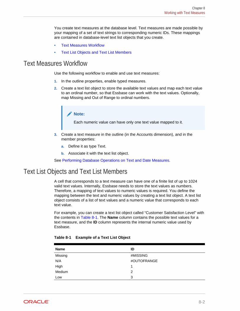
You create text measures at the database level. Text measures are made possible byyour mapping of a set of text strings to corresponding numeric IDs. These mappingsare contained in database-level text list objects that you create.

• Text Measures Workflow

• Text List Objects and Text List Members

Text Measures WorkflowUse the following workflow to enable and use text measures:

1. In the outline properties, enable typed measures.

2. Create a text list object to store the available text values and map each text valueto an ordinal number, so that Essbase can work with the text values. Optionally,map Missing and Out of Range to ordinal numbers.

Note:

Each numeric value can have only one text value mapped to it.

3. Create a text measure in the outline (in the Accounts dimension), and in themember properties:

a. Define it as type Text.

b. Associate it with the text list object.

See Performing Database Operations on Text and Date Measures.

Text List Objects and Text List MembersA cell that corresponds to a text measure can have one of a finite list of up to 1024valid text values. Internally, Essbase needs to store the text values as numbers.Therefore, a mapping of text values to numeric values is required. You define themapping between the text and numeric values by creating a text list object. A text listobject consists of a list of text values and a numeric value that corresponds to eachtext value.

For example, you can create a text list object called “Customer Satisfaction Level” withthe contents in Table 8-1. The Name column contains the possible text values for atext measure, and the ID column represents the internal numeric value used byEssbase.

Table 8-1 Example of a Text List Object

Name ID

Missing #MISSING

N/A #OUTOFRANGE

High 1

Medium 2

Low 3

Chapter 8Working with Text Measures

8-2

Each text value must map to a unique numeric value. Any text value that does not mapto an integer in the text list object is considered by Essbase to be invalid.

The first two IDs, #MISSING and #OUTOFRANGE, are for handling cases where thetextual data is invalid or empty. For example, if a user attempted to load an unmappedvalue such as “Average” to a text measure, the cell value would not be updated, andwould display as #MISSING in a subsequent query. If a user loads a numerical cellvalue which is unmapped, the subsequent query would return N/A.

Aside from #MISSING and #OUTOFRANGE , all of the other IDs must be integers.

Working with Date MeasuresDate measures enable members to be associated with date-type values. The ability toprocess dates in the measures dimension can be useful for types of analysis that aredifficult to represent using the Time dimension.

For example, an application that analyzes asset depreciation may need to trackacquisition dates for a series of capital assets. The company has been in business forfifty years, so the acquisition dates span too large a period to allow for feasible Timedimension modeling (the Time dimension only covers five years).

In addition to their ability to represent values spanning large time periods, datemeasures can also capture date values with smaller granularity than is captured in theTime dimension, such as hours and minutes.

• Implementing Date Measures

• Functions Supporting Date Measures

Implementing Date MeasuresDate measures are supported for aggregate and block storage databases. You createdate measures at the database level.

Use the following workflow to enable and use date measures:


2. In the outline properties, select a date format (for example, yyyy-mm-dd). All datemeasures in the outline must use the same format.

3. Create a date measure in the outline (in the Accounts dimension), and in themember properties, define it as type Date.

For example, in ASOsamp.Sample, you can enable typed measures for the outline,select a date format, and add a measure named IntroDate defined as type Date.

The date values are stored internally as numeric values, although you load them intoEssbase as formatted date strings. When queried, date measures are displayedaccording to the selected date format.

See Performing Database Operations on Text and Date Measures.

Functions Supporting Date MeasuresThe following MDX functions are useful for calculations based on date measures.

• DateDiff

Chapter 8Working with Date Measures

8-3

• DatePart

• DateRoll

• FormatDate

• GetFirstDate

• GetLastDate

• ToDate

• ToDateEx

• Today

The following calculation functions are useful for calculations based on date measures.

• @DATEDIFF

• @DATEPART

• @DATEROLL

• @FORMATDATE

• @TODATEEX

• @TODAY

For information about these functions and commands, see Technical Reference forOracle Essbase.

Performing Database Operations on Text and DateMeasures

You can perform these common database operations when using text and datemeasures:

• Loading, Clearing, and Exporting Text and Date Measures

• Consolidating Text and Date Measures

• Retrieving Data With Text and Date Measures

• Limitations of Text and Date Measures

Loading, Clearing, and Exporting Text and Date MeasuresTo load data to text or date measures, follow the same procedure as for loading datato members with numeric measures. The input data should contain formatted datevalues, or text values corresponding to the text list object that is associated with thetext measure.

If you attempt to load text values that are not present in the text list object associatedwith that member, Essbase issues a warning message.

In aggregate storage databases, values can only be loaded at the input level; thisrestriction applies equally to text and date measures. In block storage databases, textand date values can be loaded at any level.

Use the following guidelines when loading text and date values into an aggregatestorage database. These guidelines will help eliminate invalid aggregations.

Chapter 8Performing Database Operations on Text and Date Measures

8-4

• Use Replace mode.

Note:

Replace mode is set when committing the buffer. In MaxL, use theoverride values grammar of the import data statement. In the EssbaseJava API, use the commitType parameter of theIEssCube.loadBufferTerm method. In the C API, use the ulCommitTypefield of the EssLoadBufferTerm function.

• Use a single load buffer to load all values associated with date/text measures.

• Use the aggregate_use_last aggregation method.

Caution:

The aggregate_use_last method has significant performance impact,and is not intended for large data loads. If your data load is larger thanone million cells, consider separating the numeric data into a separatedata load process (from any typed measure data). The separate dataload can use aggregate_sum instead.

Aggregate_use_last is set when creating the load buffer. In MaxL, see the PROPSterminal that is part of the initialize load_buffer grammar in the alter databasestatement. In the Essbase Java API, use the duplicateAggregationMethodparameter of the IEssCube.loadBufferInit method. In the C API, use theulDuplicateAggregationMethod field of the EssLoadBufferInit function.

• Avoid loading #MISSING values to text/date measures in incremental data loadmode. When a #MISSING value is loaded to a cell with a non-Missing value inincremental load, it is replaced with a zero value. The zero value may not have thesame meaning as the #MISSING value for date/text measures. Use full data load ifyou need to load #MISSING values to date/text measures.

If mixed (numeric and text or date) data are being loaded, either ensure that Replacemode is sufficient for your numeric data, or create a separate data load process for thenumeric data.

You can load text or date values with or without rules files. When a rules file is notused, you must distinguish text or date values from member names by enclosing thetext values in double quotation marks and prefixing them with the string #Txt:.

Here is an example of a line of data in a free-form data load file:

"100-10" "New York" "Cust Index" #Txt:"Highly Satisfied"

The text value "Highly Satisfied" is pre-fixed with #Txt:to differentiate it from membernames such as "New York".

The "#Txt" prefix is also required for date measures when a rules file is not used fordata load.

Chapter 8Performing Database Operations on Text and Date Measures

8-5

You can clear, lock and send, and export text or date values just as you perform thoseoperations on numeric values.

Consolidating Text and Date MeasuresBy default, text measures are assigned the ^ operator (never consolidate). Text anddate measures are not consolidated to higher level members along non Accountsdimensions.

If you tag a text or date measure with an operator other than ^, it will be consolidatedalong other dimensions based on its internal numeric value. This is not recommendedfor aggregate storage databases, because only the + operator is supported, and theaggregated values likely will not have any validity for text or date measures.Additionally, Essbase does not translate out-of-range values to #OUTOFRANGEduring consolidation.

For block storage databases, you can write calculation scripts that consolidate textmeasures in a custom fashion. You might want to consolidated text measures whenthey represent ranking measures. For example, consider a text list named"CustomerSatisfaction", which contains mappings such as Excellent=5, Good=4,Fair=3, Poor=2, Bad=1. The values are loaded at level 0. You can consolidate valuesto parent levels by taking an average of values at child levels. For example, the valueof “CustomerSatisfaction” at [Qtr1] is the average of values at [Jan], [Feb], [Mar].

Retrieving Data With Text and Date MeasuresText or date measures can be queried in the same way as numerical measures, usingSmart View and MDX. The corresponding cells are displayed with the appropriate textvalues or formatted date values.

The MDX function EnumValue and the calculation function @ENUMVALUE aredesigned specifically for getting the text value of text measures. These functions canbe useful in MDX scripts, calc scripts, or formulas, when you need to do operationsbased on the text value of a member rather than its internally stored numeric value.See Technical Reference for Oracle Essbase.

Limitations of Text and Date MeasuresAn outline restructure does not restructure text lists. If the mapping of numeric to textvalues in a text list is changed, the change will be reflected in the text data alreadypresent in the database for that text list. Therefore, when adding items to a text list,add them to the top or bottom of the list so as to avoid altering the mapping numbersof existing text list items.

Text and date measures are not supported across partitions.

Shared members inherit the text or date type of the referenced member.

Working with Format StringsUsing format strings, you can format the values (cell contents) of Essbase databasemembers in numeric type measures so that they appear, for query purposes, as text,dates, or other types of predefined values. The resultant display value is the cell’sformatted value (FORMATTED_VALUE property in MDX).

Chapter 8Working with Format Strings

8-6

The underlying real value is numeric, and this value is unaffected by the associatedformatted value. Format strings enable you to display more meaningful values in placeof raw numeric values. For example, using a text based formatted value, you mightdisplay data cells as “High,” “Medium,” and “Low.”

Text and date type values are additionally supported using the built-in text and datemeasure types. Format strings add more flexibility to your implementation, in that youcan apply format strings to members in multiple dimensions, whereas with text anddate measures, you can only apply one or the other to a single measures dimension.You can apply format strings to numeric dimensions; you do not have to type thedimension as text or date.

Format strings can be applied to either aggregate storage or block storage databases.

Format strings can be defined on the following members:

• All members in Measures dimension

• Members associated with explicit formula strings on other dimensions

Topics:

• Implementing Format Strings

• MDX Format Directive

• Functions Supporting Format Strings

• Limitations of Format Strings

Implementing Format StringsFormat strings are supported for aggregate and block storage databases. Youimplement format strings at the database level.

Use the following workflow to enable and use format strings:


2. In the Accounts dimension, create a measure whose members you want to format,and in its member properties, edit the Associate Format String field to create anMDX format directive. For the syntax to create an MDX format directive, see MDXFormat Directive.

MDX Format DirectiveA format string is defined by the following syntax:

format_string_expression = MdxFormat (string_value_expression)

string_value_expression is a valid MDX string value expression as described in theMDX specification documented in Technical Reference for Oracle Essbase.

Most MDX expressions can be used to specify format strings; however, format stringscannot contain references to values of data cells other than the current cell valuebeing formatted. The current cell value can be referenced using the MDX CellValuefunction.


8-7

Essbase treats members with invalid format strings as if there is no format stringdefined. Outlines can be saved with invalid format strings. Essbase generates awarning if a query consists of a member with an invalid format string.

If a member is not associated with a format string, default format rules are applied.The default format rules format a cell based on whether the measure is numeric, text,or date type. For numeric measures, the default formatted value is the text version ofthat number. For text measures, the default formatted value is the text value based onthe associated text list object. For date values, the default format is a date stringformatted according the date format string defined in the outline properties.

Functions Supporting Format StringsThe following MDX functions can be useful when applying format strings to a measure.Format strings are applied as MDX expressions, in both aggregate and block storagedatabases.

• EnumText, returns the text list label associated with the internal numeric value.

• EnumValue, returns the internal numeric value for a text list label.

• CellValue, returns the internal numeric value of the current cell.

• NumToStr, converts a value to a decimal string.

The @ENUMVALUE calculation function can be useful when writing calculation scriptsfor a block storage database that has text measures or format strings. This functionreturns the text list label associated with the internal numeric value.

The MaxL alter session set dml_output statement has a clause setformatted_value on | off. By default, formatted values are displayed in queries, butthis statement can be used to turn off the display of formatted values.

For information about these functions, commands, and statements, see TechnicalReference for Oracle Essbase.

Limitations of Format StringsFormat strings are not supported across partitions.

Shared members cannot have separate format strings; they inherit the format string ofthe referenced member.

Maximum length of a format string: 256 characters.


8-8

9Designing Partitioned Applications

A partition is the region of a database that is shared with another database.Partitioning can provide many benefits. Carefully review the design requirements tohelp you determine whether partitioning can meet your objectives.

• Understanding Partitioning

• Partition Design Requirements

• Replicated Partitions

• Transparent Partitions

Understanding PartitioningA partition is the region of a database that is shared with another database. AnEssbase partitioned application can span multiple servers, processors, or computers.

See:

• Partition Types

• Parts of a Partition

• Data Sources and Data Targets

• Attributes in Partitions

• Version and Encoding Requirements

Partition TypesTable 9-1 lists the types of partitions that are supported in Essbase:

Table 9-1 Partition Types

Partition Type Description Applies To

Replicated A copy of a portion of the datasource that is stored in the datatarget.

See Replicated Partitions.

Block storage databases

Aggregate storage databases

Transparent Allows users to access data from thedata source as though it were storedin the data target. The data is,however, stored at the data source,which can be in another applicationor Essbase database, or on anotherEssbase Server.

See Transparent Partitions.

Block storage databases

Aggregate storage databases

Use the information in Table 9-2 to help you choose which type of partition to use:

9-1

Table 9-2 Features Supported by Partition Type

Feature Replicated Transparent

Up-to-the-minute data x

Reduced network traffic x

Reduced disk space x

Increased calculation speed x

Smaller databases x

Improved query speed x

Invisible to end users x x

Easier to recover x

Ability to query data based onits attributes

x

Ability to use front-end toolsthat are not distributed OLAP-aware

x x

Easy to perform frequentupdates and calculations

x

Ability to update data at thedata target

x

Perform batch updates andsimple aggregations

x

Parts of a PartitionPartitions contain the following parts, as illustrated in Figure 9-1 and described in Table 9-3.

Figure 9-1 Parts of a Partition

Chapter 9Understanding Partitioning

9-2

Table 9-3 Parts of a Partition

Part Description

Type of partition A flag indicating whether the partition isreplicated or transparent.

Data source information The server, application, and database name ofthe data source.

Data target information The server, application, and database name ofthe data target.

Login and password The login and password information for thedata source and the data target. Thisinformation is used for internal requestsbetween the two databases to executeadministrative and end-user operations.

Shared areas A definition of one or more areas, or regions,shared between the data source and the datatarget. To share multiple noncontiguousportions of a database, define multiple areas ina single partition. This information determineswhich parts of the data source and data targetare shared so that Essbase can put the properdata into the data target and keep the outlinesfor the shared areas synchronized.

Member mapping information A description of how the members in the datasource map to members in the data target.Essbase uses this information to determinehow to put data into the data target if the datatarget and the data source use different namesfor some members and dimensions.

State of the partition Information about whether the partition is up-to-date and when the partition was lastupdated.

Data Sources and Data TargetsPartitioned databases contain at least one data source (the primary site of the data)and at least one data target (the secondary site of the data). One database can serveas the data source for one partition and the data target for another partition. Whendefining a partition, you map cells in the data source to their counterparts in the datatarget.


9-3

Figure 9-2 Data Source and Data Target

An Essbase database can contain many partitions, as well as data that is not sharedwith any other Essbase database. You can define partitions between the followingdatabases:

• Different databases in different applications, as long as each database uses thesame language and the same Unicode-related mode.

The applications can be on the same computer or different computers.

• Different databases in one block storage application.

This practice is not recommended, because the full benefits of partitioningdatabases are realized when each database is in a separate application.

One database can serve as the data source or data target for multiple partitions. Toshare data among many databases, create multiple partitions, each with the samedata source and a different data target, as shown in Figure 9-3:


9-4

Figure 9-3 Data Shared at Multiple Targets

Table 9-4 lists the combinations of block storage and aggregate storage databases asdata target and data source that are supported by each partition type:

Table 9-4 Combinations of Data Sources and Data Targets Supported byPartition Type

Source Target Replicated Transparent

Block storage Block storage Yes Yes

Aggregate storage Block storage No Yes

Aggregate storage Aggregate storage No Yes

Block storage Aggregate storage Yes Yes

Attributes in PartitionsFor block storage databases, you can use attribute functions for partitioning onattribute values, but you cannot partition an attribute dimension. Use attribute values topartition a database to access members of a dimension according to theircharacteristics.

For example, in the Sample.Basic database, you cannot partition the Pkg Typeattribute dimension, but you can create a partition that contains all the members of the


9-5

Product dimension that are associated with either or both members (Bottle and Can) ofthe Pkg Type dimension. If you create a partition that contains members associatedwith Can, you can access data only on Product members that are packaged in cans;namely, 100-10, 100-20, and 300-30.

Note:

Retrieving data on attribute members of block storage databases may resultin missing data. See the entry for "Dense Dynamic Calc members innonexisting stored blocks" in Table 7-1.

You can use the @ATTRIBUTE command and the @WITHATTR command to definepartitions.

For example, to extract data on all members of the Product dimension that areassociated with the Caffeinated attribute dimension, you can create a partition such as@ATTRIBUTE (Caffeinated). But you cannot partition the Caffeinated attributedimension.

Based on the previous example, this partition is correct:

Source Target@ATTRIBUTE(Caffeinated) @ATTRIBUTE(Caffeinated)

This partition is incorrect:

Source TargetCaffeinated Caffeinated

For more information about these commands, see the Technical Reference for OracleEssbase.

Also see Working with Attributes.

Version and Encoding RequirementsVersion and encoding requirements for transparent and replicated partitions:

• Version: Both ends (the source and target) of the partition must be on the samerelease level.

• Encoding: Both ends of the partition must be in Unicode-mode.

Partition Design RequirementsUse the information in this section to carefully design partitions before implementingthem.

• Benefits of Partitioning

• Partitioning Strategies

• Guidelines for Partitioning a Database

Chapter 9Partition Design Requirements

9-6

• Guidelines for Partitioning Data

• Security for Partitioned Databases

Benefits of PartitioningPartitioning can provide the following benefits:

• For block storage databases, data synchronization across multiple databases

Essbase tracks changes made to data values in a partition and provides tools forupdating the data values in related partitions.

• Ability for user navigation between databases with differing dimensionality

When users drill across to the new database, they can drill down to more-detaileddata.

Partitioning StrategiesBased on user requirements, select a partitioning strategy:

• Partition applications from the top down.

Use top-down partitioning to split a database onto multiple processors, servers, orcomputers, which can improve the scalability, reliability, and performance ofdatabases. To achieve the best results with top-down partitioning, create aseparate application for each partitioned database.

• Partition applications from the bottom up.

Use bottom-up partitioning to manage data flow between multiple relateddatabases, which can improve the quality and accessibility of the data indatabases.

• Partition databases according to attribute values associated with base dimensions(a standard dimension associated with one or more attribute dimensions).

Use this strategy to extract data based on the characteristics of a dimension, suchas flavor or size.

Note:

You cannot partition attribute dimensions. See Attributes in Partitions.

Guidelines for Partitioning a DatabaseUse the following information to help you determine whether to partition a database.

• Partition a database when:

– The data should be closer to the people who are using it.

– A single failure would be catastrophic.

– It takes too long to perform calculations after new data is loaded, and you wantto improve performance by spreading calculations across multiple processorsor computers.


9-7

– Users want to see the data in different application contexts, and you want tocontrol how users navigate between databases.

– You need to synchronize information from different sources.

– You plan to add new organizational units that would benefit from having theirown databases.

– Users must wait as other users access the database.

– You want to save disk space by giving users access to data stored in a remotelocation.

– You want to reduce network traffic by replicating data in several locations.

– You need to control database outlines from a central location.

– You need client write-back functionality on an aggregate storage database.

• Do not partition a database when:

– You have disk space, network bandwidth, and administrative resourceconcerns.

– You perform complex allocations where unit level values are derived from totalvalues.

– You are required to keep all databases online at all times.

Keeping databases online can be a problem if you have databases in severaltime zones, because peak user load may differ between time zones. Usingtransparent partitions exacerbates this problem, but using replicated partitionsmight help.

– Databases are in different languages or Unicode-related modes.

Essbase can partition databases only if each database uses the samelanguage, or each database uses the same Unicode or non-Unicode mode.

Guidelines for Partitioning DataWhen designing a partitioned database, use the following information to help youdetermine which data to include in each partition:

• Which database should be the data source and which the data target? Thedatabase that “owns” the data, where the data is updated and where most of thedetail data is stored, should be the data source.

• Are some parts of the database accessed more frequently than others?

• What data can you share among sites?

• How granular must the data be at each location?

• How frequently is the data accessed, updated, or calculated?

• What are the available resources: disk space, CPUs, and network resources?

• How much data must be transferred over the network? How long does it take?

• Is the data stored in one or multiple locations?

• Is the data accessed in one or multiple locations?

• Is there information in separate databases that should be accessed from a centrallocation? How closely are groups of data related?


9-8

Security for Partitioned DatabasesUsers accessing partitions may need to view data stored in multiple databases. Thefollowing sections describe how to set up security so that users do not view or changeinappropriate data.

• Setting up End-User Security

• Setting up Administrator Security

Setting up End-User SecurityCreate the required end users with the correct filters.

1. Create accounts for users at the data target.

2. Create read and write filters at the data target to determine what end users canview and update.

See Controlling Access to Database Cells Using Security Filters.

3. If you are creating a replicated partition, determine whether users can makechanges to a replicated partition at the data target. The update setting (whichallows or disallows updates) overrides user filters that allow users to update data.

When creating replicated partitions using the create replicated partition MaxLstatement, if you do not specify the update allow grammar, replicated partitionscannot be updated by default.

Setting up Administrator SecurityThe administrative account performs all read and write operations requested by thedata target for the data source. For example, when end users request data at the datatarget, the administrative account retrieves the data. When end users update data atthe data target, the administrative account logs into the data source and updates thedata there.

You can create filters on the administrative account and on the end users. Filters onthe administrative account can ensure that no one at the data target can view orupdate inappropriate data. For example, the administrator at the corporate databasecan restrict write access on certain cells to avoid relying on administrators in theregions to set up security correctly for each end user.

Create the required administrative users with the correct filters.

1. Create an administrative account at the data source and data target.

See Setting the User Name and Password.

Essbase uses this account to log onto the data source to retrieve data.

2. Create read and write filters to determine which data administrators can view andupdate.

See Controlling Access to Database Cells Using Security Filters.

• For replicated partitions, set up read filters at the data source to determinewhich data Essbase reads when replicating, and set up write filters at the datatarget to determine which data Essbase writes to when replicating.


9-9

• For transparent partitions, set up read filters at the data source to determinewhich data Essbase retrieves for end users, and set up write filters at the datasource to determine which data Essbase updates for end users.

Replicated PartitionsA replicated partition is a copy of a portion of the data source that is stored in the datatarget. Some users can then access the data in the data source while others access itin the data target.

For example, in the Samppart and Sampeast sample applications, the DBA at TheBeverage Company (TBC) created a replicated partition between the East databaseand the Company database containing Actual, Budget, Variance, and Variance%.Users in the eastern region now store their budget data locally. Because they do nothave to retrieve this data live from corporate headquarters, response times are faster,and they have more control over the downtimes and administration of local data.

Changes to the data in a replicated partition flow from the data source to the datatarget. Changes made to replicated data in the data target do not flow back to the datasource. If users change the data at the data target, Essbase overwrites their changeswhen the DBA updates the replicated partition.

When a replicated partition is defined, the DBA can select a setting to prevent the datain the replicated portion of the data target from being updated. The update setting(which allows or disallows updates) takes precedence over access provided bysecurity filters and is also honored by batch operations, such as data load andcalculation. See Setting up End-User Security.

Use a replicated partition to achieve any of the following goals:

• Decrease network activity

• Decrease query response times

• Decrease calculation times

• Recover more easily from system failures

Rules for Replicated PartitionsReplicated partitions must follow these rules:

• You must be able to map the shared replicated areas of the data source and datatarget outlines, although the shared areas need not be identical. You must tellEssbase how each dimension and member in the data source maps to eachdimension and member in the data target.

The data source and data target outlines for the non-shared areas do not have tobe mappable.

• Because none of the areas that you use as a replicated partition target can comefrom a transparent partition source, you cannot create a replicated partition on topof a transparent partition, as shown in Figure 9-4:

Chapter 9Replicated Partitions

9-10

Figure 9-4 Invalid Replicated Partition

• The cells in the data target of a replicated partition cannot come from two datasources; the cells in one partition must come from one database. To replicate cellsfrom multiple databases, create a different partition for each data source.

The cells in a data target can be the data source for a different replicated partition.For example, if the Samppart.Company database contains a replicated partitionfrom the Sampeast.East database, you can replicate the cells in Sampeast.Eastinto a third database, such as Sampwest.West.

• You cannot use attribute members to define a replicated partition. For example,associated with the Market dimension, the Market Type attribute dimensionmembers are Urban, Suburban, and Rural. You cannot define a partition onUrban, Suburban, or Rural, because a replicated partition contains dynamic data,not stored data. Therefore, an attempt to map attributes in replicated partitionsresults in an error message. However, you can use the WITHATTR command toreplicate attribute data.

Advantages of Replicated Partitions• Because data is stored closer to end users, in the data target, replicated partitions

can decrease network activity, resulting in improved retrieval times for users.

• The data is more easily accessible to all users. Some users access the data at thedata source, others at the data target.

• Failures are not as catastrophic. Because the data is in multiple places, if onedatabase fails, only the users connected to that database are unable to access theinformation. Data is still available at and can be retrieved from the other sites.

• Local DBAs can control the downtime of their local databases. For example,because users in the eastern region are accessing their own replicated datainstead of the Company database, DBAs can bring down the Company databasewithout affecting users in the eastern region.

• Because only the relevant data is kept at each site, databases can be smaller. Forexample, users in the eastern region can replicate only the eastern budgetinformation, instead of accessing a larger company database containing budgetinformation for all regions.

Disadvantages of Replicated Partitions• You need more disk space because data is stored in multiple locations.


9-11

• Because the DBA must manually refresh data regularly, users may not see thelatest version of the data.

Performance Considerations for Replicated PartitionsTo improve the performance of replicated partitions, follow these guidelines:

• Do not replicate members that are dynamically calculated in the data source,because Essbase must probe the outline to find dynamically calculated membersand their children to determine how to perform the calculation.

• Do not replicate derived data from the data source. Instead, replicate the lowestpractical level of each dimension and perform the calculations on the data targetafter you complete the replication.

For example, to replicate the database along the Market dimension:

– Define the shared area as the lowest-level members of the Market dimensionthat you care about, for example, East, West, South, and Central and the level0 members of the other dimensions.

– After you complete the replication, calculate the values for Market and theupper-level values in the other dimensions at the data target.

Sometimes you cannot calculate derived data at the data target. In that case,replicate it from the data source. For example, you cannot calculate deriveddata at the data source if the data meets any of the following criteria:

* Requires that data outside the replicated area be calculated.

* Requires calculation scripts from which you cannot extract only the portionto be calculated at the data target.

* Is being replicated onto a computer with little processing power, such as alaptop.

• Partitioning along a dense dimension takes longer than partitioning along a sparsedimension. When Essbase replicates data partitioned along a dense dimension, itmust access every block in the data source and then create each block in the datatarget during the replication operation.

• You cannot replicate data into a member that is dynamically calculated at the datatarget. Essbase does not load or replicate into Dynamic Calc members, becausethese members do not contain data until a user requests it at runtime. Essbaseavoids sending replicated data for both dynamic dense and dynamic sparsemembers on the replication target, because this data is not stored on the datatarget.

To replicate only the data values that have changed instead of the entire partition,see Populating or Updating Replicated Partitions.

Replicated Partitions and Port UsageWith replicated partitions, users connect to the target database only. When data isupdated on the target database, the process of replicating data from the sourcedatabase to the target database utilizes one port and this connection is based on theuser name declared in the partition definition (partition user).


9-12

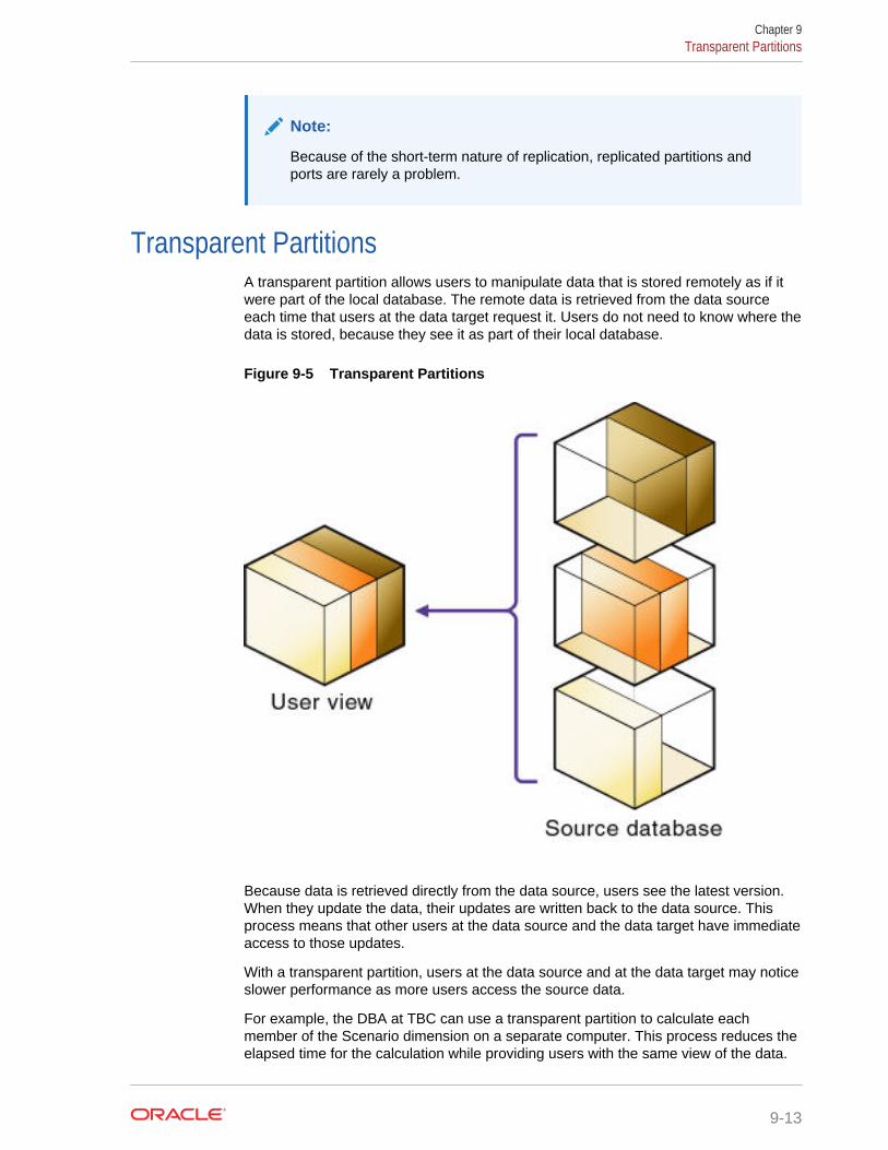
Note:

Because of the short-term nature of replication, replicated partitions andports are rarely a problem.

Transparent PartitionsA transparent partition allows users to manipulate data that is stored remotely as if itwere part of the local database. The remote data is retrieved from the data sourceeach time that users at the data target request it. Users do not need to know where thedata is stored, because they see it as part of their local database.

Figure 9-5 Transparent Partitions

Because data is retrieved directly from the data source, users see the latest version.When they update the data, their updates are written back to the data source. Thisprocess means that other users at the data source and the data target have immediateaccess to those updates.

With a transparent partition, users at the data source and at the data target may noticeslower performance as more users access the source data.

For example, the DBA at TBC can use a transparent partition to calculate eachmember of the Scenario dimension on a separate computer. This process reduces theelapsed time for the calculation while providing users with the same view of the data.

Chapter 9Transparent Partitions

9-13

Use a transparent partition to achieve the following goals:

• Show users the latest version of the data

• Allow users at the data target to update data

• Decrease disk space

Rules for Transparent PartitionsTransparent partitions must follow these rules:

• The shared transparent areas of the data source and data target outlines need notbe identical, but you must be able to map the dimensions in them. You must tellEssbase how each dimension and member in the data source maps to eachdimension and member in the data target.

• The data source and data target outlines for the nonshared areas need not bemappable, but attribute associations must be identical. Otherwise, users can getincorrect results for some retrievals. For example, if product 100-10-1010 isassociated with the Grape Flavor attribute on the source, but product 100-10-1010is not associated with Grape on the target, the total of sales for all Grape flavors inNew York is incorrect.

• The partition definition must contain only stored members. You cannot useattribute dimensions or members to define a transparent partition. For example,the Market Type attribute dimension, which is associated with the Marketdimension, has members Urban, Suburban, and Rural. You cannot define apartition on Urban, Suburban, or Rural.

• If a cell is mapped from the data source to an aggregate storage database as thetarget, all the cell's dependents must also be mapped to the same partitiondefinition.

• You can create a transparent partition on top of a replicated partition. In otherwords, you can create a transparent partition target using a replicated partitionsource, as shown in Figure 9-6

Figure 9-6 Valid Transparent Partition

• As illustrated in Figure 9-7, you cannot create a transparent partition on top ofmultiple other partitions. In other words, you cannot create a transparent partitiontarget from multiple sources because each cell in a database must be retrievedfrom only one location—either the local disk or a remote disk.


9-14

Figure 9-7 Invalid Transparent Partition

• Carefully consider any formulas you assign to members in the data source anddata target.

Advantages of Transparent PartitionsTransparent partitions can solve many database problems, but transparent partitionsare not always the ideal partition type.

• You need less disk space, because you are storing the data in one database.

• The data accessed from the data target is always the latest version.

• When the user updates the data at the data source, Essbase makes thosechanges at the data target.

• Individual databases are smaller, so they can be calculated more quickly.

• The distribution of the data is invisible to the end user and the end user’s tools.

• You can load the data from either the data source or data target.

Disadvantages of Transparent PartitionsIf these disadvantages are too serious, consider using replicated partitions instead.

• Transparent partitions increase network activity, because Essbase transfers thedata at the data source across the network to the data target. Increased networkactivity results in slower retrieval times for users.

• Because more users are accessing the data source, retrieval time may be slower.


9-15

• If the data source fails, users at both the data source and the data target areaffected. Therefore, the network and data source must be available wheneverusers at the data source or data target need them.

• You can perform some administrative operations only on local data. For example,if you archive the data target, Essbase archives only the data target and not thedata source. The following administrative operations work only on local data inblock storage databases:

– CLEARDATA calculation command

– DATACOPY calculation command

– EXPORT command

– VALIDATE command

– BEGINARCHIVE and ENDARCHIVE commands

• When you perform a calculation on a transparent partition, Essbase performs thecalculation using the current values of the local data and transparent dependents.Essbase does not recalculate the values of transparent dependents, because theoutlines for the data source and the data target may be so different that such acalculation is inaccurate. To calculate all partitions, issue a CALC ALL commandfor each individual partition, and then perform a CALC ALL command at the toplevel using the new values for each partition.

Consider this example:

– The data target outline contains a Market dimension with East, West, South,and Central members

– The data source outline contains an East dimension with New York and NewJersey members

If you tried to calculate the data target outline, you would assume that East was alevel 0 member. In the data source, however, East is derived by adding New Yorkand New Jersey. Any calculations at the data target, however, would not know thisinformation and could not reflect changes made to New York and New Jersey inthe data source. To perform an accurate calculation, therefore, calculate East inthe data source and then calculate the data target.

• Formulas assigned to members in the data source may produce calculated resultsthat are inconsistent with formulas or consolidations defined in the data target, andvice versa.

Performance Considerations for Transparent PartitionsTo improve the performance of transparent partitions, consider the following guidelineswhen creating the partition:

• Partitioning along dense dimensions in a transparent partition can greatly slowperformance, because dense dimensions are used to determine the structure andcontents of data blocks. If a database is partitioned only along a dense dimensionat the target, Essbase must compose data blocks by performing network calls forthe remote data in the transparent partition and to the disk I/O for the local portionof the block.

To improve performance, consider including one or more sparse dimensions in thearea definition so that the number of blocks required is limited to combinations withthe sparse members.


9-16

• Basing transparent partitions on the attribute values of a dimension can increaseretrieval time, because attributes are associated with sparse dimensions. In suchcases, partitioning at a level higher than the level that is associated with attributesimproves retrieval time. For example, in the Product dimension of theSample.Basic database, if children 100-10, 200-10, and 300-10 (level 0) areassociated with attributes, then partition their parents 100, 200, and 300 (level 1)for better retrieval performance.

• Loading data into the data source from the data target can greatly slowperformance. If possible, load data into the data source locally.

• Retrieval time is slower because users access the data over the network.

• When the transparent partition target is an aggregate storage database, you canspecify the maximum size of the request grid and the response grid, using the MAX_REQUEST_GRID_SIZE and MAX_RESPONSE_GRID_SIZE configurationsettings.

• Partitioning base dimensions can greatly slow performance.

• See Performance Considerations for Transparent Partition Calculations.

Calculating Transparent PartitionsWhen you perform a calculation on a transparent partition, Essbase performs thecalculation using the current values of the local data and transparent dependents.When calculating local data that depends on remote data, Essbase performs a bottom-up calculation. The bottom-up calculation can be done only if the calculator cache onthe target database is used properly. See Using Bottom-Up Calculation.

Increasing the memory assigned to the calculator cache greatly improves calculationperformance with transparent partitions. When a calculation is started, a message inthe application log file indicates whether the calculator cache is enabled or disabled onthe target database. Using the calculator cache on the target database reduces thenumber of blocks that are requested from the data source during calculation. Reducingthe blocks requested, in turn, reduces the network traffic that is generated bytransferring blocks across the network.

Performance Considerations for Transparent Partition CalculationsCalculating data on the data target can greatly slow performance when the data targetmust retrieve each dependent data block across the network, and then perform thecalculation.

Performance with transparent calculations also may slow if Essbase must perform atop-down calculation on any portion of the data target that contains top-down memberformulas. When the data target does not contain top-down member formulas, Essbasecan perform a bottom-up calculation on the data target, which is much faster.

When Essbase performs the calculation on the data source, it can always perform abottom-up calculation. For a comparison of top-down and bottom-up calculations, see Using Bottom-Up Calculation.

Consider using these calculation alternatives:

• If you are absolutely sure that a target partition calculation script does not involveaccess to remote data, you can use the SET REMOTECALC OFF calculationcommand in the calculation script to stop retrieval efforts from the source partition.


9-17

• Dynamic Calc members as parents of the transparent data so that the data iscalculated on the fly when it is retrieved. This process reduces the batchprocessing time. Essbase performs the calculation only when users request it.

• A replicated layer between the low-level transparent data and high-level local data.

Consider these performance strategies:

• Keep the partition fully within the calculator cache area, which means that anysparse members in the partition definition must be contained within the calculatorcache. For example, in the Sample.Basic database, if a partition definition includes@IDESC(East), all descendants of East must be within the calculator cache.

• Enable the calculator cache, and assign a sufficient amount of memory to it.

• Do not use complex formulas on any members that define the partition. Forexample, in Sample.Basic, assigning a complex formula to New York or NewJersey (both children of East) forces Essbase to use the top-down calculationmethod. See Bottom-Up and Top-Down Calculation.

Transparent Partitions and Member FormulasIf the data target and data source outlines are identical except for different memberformulas, ensure that the partition definition produces the calculation results you want.

For example, suppose that the data source and data target outlines both contain aMarket dimension with North and South members, and children of North and South.On the data target, Market is calculated from the data for the North and Southmembers (and their children) on the data source. If any of these members on the datasource contains member formulas, these formulas are calculated, affecting thecalculated value of Market on the data target. These results may be different from howthe Market member are calculated from the North and South members on the datatarget, where these formulas may not exist.

Ensure that any formulas you assign to members in the data source and data targetproduce the results you want.

Transparent Partitions and Port UsageOne port is used for every unique user and machine combination. If a user definesseveral transparent partitions on one server, using the same user name, then only oneport is occupied.

In a transparent partition, when a user (user1) drills into an area in the target thataccesses source data, user1 is using the user name declared in the partition definition(partition user) to access the data from the source database. This access causes theuse of an additional port because different users (user1 and partition user) areconnecting to the application.

If a second user (user2) connects to the target database and drills down to accesssource data, user2 also uses the user name declared in the partition definition(partition user). Because the partition user is already connected to the sourcedatabase, an additional port is not needed for the partition user, as long as user2 isaccessing the same source database.


9-18

10Creating and Maintaining Partitions

When you build a partition, each database in the partition uses a partition definition fileto record all information about the partition, such as its data source, data target, andthe areas to share. Partition creation requires Database Manager permissions orhigher. After you have created a partition, load and calculate the database thatcontains the partition. Loading and calculating the partition may require you to changeexisting rules files and calculation scripts.

For information about using the Web interface to create and maintain partitions, see Linking Cubes Using Partitions and Location Aliases in Using Oracle Analytics Cloud -Essbase.

• Choosing a Partition Type

• Setting up a Partition Data Source

• Setting the User Name and Password

• Defining a Partition Area

• Mapping Members in Partitions

• Validating Partitions

• Populating or Updating Replicated Partitions

• Viewing Partition Information

• Partitioning and SSL

• Troubleshooting Partitions

Choosing a Partition TypeDecide which type of partition to create:

• Replicated

• Transparent

See Partition Types.

Setting up a Partition Data SourceYou define partitions in the context of the data target. You must be logged in on thetarget cube. Select your data source, which can be another cube, or a federatedsource.

Single-Instance Partitioning – All source cubes and the target cube are in the sameEssbase instance. You select a source cube from the list of available cubes in theinstance. There is no need to specify any host connection information, as everythingwithin the same instance is inferred.

10-1

Cross-Instance Partitioning – At least some source cubes are from a differentEssbase instance than the target cube. To access these sources from the target, youmust first create a connection, and select it while creating the partitions.

See also:

• Linking Cubes Using Partitions and Location Aliases

• Using Connections and Data Sources

Setting the User Name and PasswordYou must specify a user name and password for Essbase to use when itcommunicates between the data source and the data target. The user name andpassword must be identical on the data source and the data target. Essbase uses thisuser name and password to:

• Transfer data between the data source and the data target for replicated andtransparent partitions. Local security filters apply to prevent end users from seeingprivileged data.

• Synchronize database outlines for all partition types.

See Security for Partitioned Databases.

Defining a Partition AreaYou can define or edit the areas of the data source to share with the data target in apartition. An area is a subcube within a database and a partition comprises one ormore areas. For example, an area could be all Measures at the lowest level for Actualdata in the Eastern region.

When you define a replicated area, ensure that the data source and data targetcontain the same number of cells. The shape of the two partitions must match. Forexample, if the area in the data source covers 18 cells, the data target should containan area covering 18 cells into which to put those values. The cell count does notinclude the cells of attribute dimensions.

Note:

Use member names instead of their aliases to create area definitions.Although Essbase validates the aliases, the partitions will not work.

Mapping Members in PartitionsTo create a partition, Essbase must be able to map all shared data source members todata target members. Oracle recommends that data source member names and datatarget member names are the same to reduce maintenance requirements for thepartition, especially when the partition is based on member attributes.

If the data source and data target contain the same number of members and use thesame member names, Essbase automatically maps the members. You need only

Chapter 10Setting the User Name and Password

10-2

validate, save, and test the partitions. If Essbase cannot map automatically, you mustmap manually.

Map data source members to data target members in any of the following ways:

• Enter or select member names manually. (When you type a duplicate membername, type the qualified member name and enclose it in double quotation marks;for example, “[State].[New York]”

• Import the member mappings from an external data file.

• Create area-specific mappings.

Topics in this section:

• Mapping Members with Different Names

• Mapping Data Cubes with Extra Dimensions

• Mapping Shared Members

• Mapping Attributes Associated with Members

• Creating Advanced Area-Specific Mappings

Mapping Members with Different NamesIf the data source outline and data target outline contain different members, or if themembers have different names in each outline, you must map the data sourcemembers to the data target members. In the following example, the first two membernames are identical, but the third member name is different:

Source TargetProduct Product Cola ColaYear Year 1998 1998Market Market East East_Region

Because you know that East in the data source corresponds to East_Region in thedata target, map East to East_Region. Then, all references to East_Region in the datatarget point to East in the data source. For example, if the data value for Cola, 1998,East is 15 in the data source, the data value for Cola, 1998, East_Region is 15 in thedata target.

Mapping Data Cubes with Extra DimensionsThe number of dimensions in the data source and data target may vary. The followingexample illustrates a case where there are more dimensions in the data source outlinethan in the data target outline:

Source TargetProduct Product Cola ColaMarket Market East EastYear

Chapter 10Mapping Members in Partitions

10-3

1999 1998 1997

You can map member 1997 of the Year dimension to Void in the data target. First,define the areas of the data source to share with the data target:

Source Target@DESCENDANTS(Market), 1997 @DESCENDANTS(Market)

Then, map the data source member to Void in the data target:

Source Target1997 Void

“Void” is displayed automatically; manually entering “Void” may cause errors.

If you do not include at least one member from the extra dimension in the areadefinition, you will receive an error message when you attempt to validate the partition.

Note:

When you map a member from an extra dimension, the partition resultsreflect data only for the mapped member. In the above example, the Yeardimension contains three members: 1999, 1998, and 1997. If you mapmember 1997 from the data source to the data target, the partition resultsreflect Product and Market data only for 1997. Product and Market data for1998 and 1999 will not be extracted.

The following example illustrates a case where the data target includes moredimensions than the data source:

Source TargetProduct Product Cola Cola Market EastYear Year 1997 1997

In such cases, first define the shared areas of the data source and the data target:

Source Target@IDESCENDANTS(Product) @IDESCENDANTS(Product), East


10-4

You can then map member East from the Market dimension of the data target to Voidin the data source:

Source TargetVoid East

If member East from the Market dimension in the data target is not included in thetarget areas definition, you will receive an error message when you attempt to validatethe partition.

Mapping Shared MembersWhen you create a replicated or transparent partition using a shared member, use thereferenced member names in the mapping. Essbase maps the referenced memberfrom the data source.

Mapping Attributes Associated with MembersYou must accurately map attribute dimensions and members from the data source tothe data target to ensure that the partition is valid.

You can map attributes in transparent partitions. See Attributes in Partitions.

In the following example, the outline for the data source contains a Product dimensionwith a member 100 (Cola). Children 100-10 and 100-20 are associated with memberTRUE of the Caffeinated attribute dimension, and child 100-30 is associated withmember FALSE of the Caffeinated attribute dimension.

The data target outline has a Product dimension with a member 200 (Cola). Children200-10 and 200-20 are associated with member Yes of the With_Caffeine attributedimension, and child 200-30 is associated with No of the With_Caffeine attributedimension.

First define the areas to be shared from the data source to the data target:

Source Target@DESCENDANTS(100) @DESCENDANTS(200)@DESCENDANTS(East) @DESCENDANTS(East)

Then map the attributes:

Source Target100–10 200–10100–20 200–20100–30 200–30Caffeinated With CaffeineCaffeinated_True With_Caffeine_TrueCaffeinated_False With_Caffeine_False

If you map attribute Caffeinated_True to attribute With_Caffeine_No, you receive anerror message during validation. You must associate caffeinated cola from the datasource to caffeinated cola in the data target.


10-5

An attribute dimension or an attribute member can exist in the outline of the datasource but not in the outline of the data target, or in the outline of the data target butnot in the outline for the data source. For example:

Source TargetCaffeinated True False

In such cases, you have the following choices:

• Create the Caffeinated attribute dimension and its members in the outline of thedata target and associate them with the Product dimension. You can then map theattributes from the data source to the data target.

• Map the Caffeinated attribute dimension in the data source to Void in the datatarget.

Creating Advanced Area-Specific MappingsIf you can map all of the members in your data source to their counterparts in the datatarget using standard member mapping, you need not perform advanced area-specificmapping.

If, however, you need to control how Essbase maps members at a more granularlevel, you may need to use area-specific mapping, which maps members in one areato members in another area only in the context of a particular area map.

Use area-to-area mapping to do the following:

• Map data differently depending on where it is coming from.

• Map multiple members in the data source to a single member in the data target.

Because Essbase cannot determine how to map multiple members in the data sourceto a single member in the data target, you must logically determine how to divide yourdata until you can apply one mapping rule to that subset of the data. Then use thatrule in the context of area-specific mapping to map the members.

Example 10-1 Example 1: Advanced Area-Specific Mapping

The data source and data target contain the following dimensions and members:

Source TargetProduct Product Cola ColaMarket Market East EastYear Year 1998 1998 1999 1999 Scenario Actual Budget

The data source does not have a Scenario dimension. Instead, it assumes that pastdata is actual data and future data is forecast, or budget, data.


10-6

You know that 1998 in the data source should correspond to 1998, Actual in the datatarget and 1999 in the data source should correspond to 1999, Budget in the datatarget. So, for example, if the data value for Cola, East, 1998 in the data source is 15,the data value for Cola, East, 1998, Actual in the data target should be 15.

Because mapping works on members, not member combinations, you cannot simplymap 1998 to 1998, Actual. Define the area (1998 and 1998, Actual) and then createarea-specific mapping rules for that area.

Because the data source does not have Actual and Budget members, you also mustmap these members to Void in the data target.

Example 10-2 Example 2: Advanced Area-Specific Mapping

You also can use advanced area-specific mapping if the data source and data targetare structured very differently but contain the same kind of information.

This strategy works, for example, if your data source and data target contain thefollowing dimensions and members:

Source TargetMarket Customer_Planning NY NY_Actual CA NY_Budget CA_Actual CA_BudgetScenario Actual Budget

You know that NY and Actual in the data source should correspond to NY_Actual inthe data target and NY and Budget in the data source should correspond toNY_Budget in the data target. So, for example, if the data value for NY, Budget in thedata source is 28, the data value for NY_Budget in the data target should be 28.

Because mapping works on members, not member combinations, you cannot simplymap NY, Actual to NY_Actual. Define the area (NY and Actual, and NY_Actual) andthen create area-specific mapping rules for that area.

Because the data target does not have NY and CA members, you must also mapthese members to Void in the data target so that the dimensionality is complete whengoing from the data source to the data target.

Validating PartitionsWhen you create a partition, validate it to ensure its accuracy before you use it.Database Manager permissions or higher are required. After you validate, save thepartition definition. If necessary, you can edit an existing partition.

When Essbase validates a partition definition, it checks on the Essbase Server for thedata source and the data target to ensure that:

• The area definition is valid (contains no syntax errors).

• The specified data source members are valid and map to valid members in thedata target.

Chapter 10Validating Partitions

10-7

• All connection information is correct; that is, the server names, database names,application names, user names, and password information.

• For replicated and transparent partitions, a replication target does not overlap witha replication target; a replication target does not overlap with a transparent target;and a transparent target does not overlap with a transparent target.

• For replicated and transparent partitions, the cell count for the partition is the sameon the data source and the data target.

• For replicated and transparent partitions, the area dimensionality matches the datasource and the data target.

• You must validate a transparent partition that is based on attribute values toensure that the results are complete. Essbase does not display an error messagewhen results are incomplete.

Populating or Updating Replicated PartitionsWhen you edit a partition, you use the same interface as for creating the partition.

The administrator should regularly update data in a replicated partition. How frequentlyyou update replicated partitions depends on user requirements for up-to-the-minutedata. Essbase keeps track of when the data source was last changed and when thedata target was last updated so that you can determine when to update replicatedpartitions. This information is saved at the data source. The administrator of either thedata source site or data target site can be responsible for replicating data.

Essbase also tracks which cells in a partition are changed:

• Faster—Only the cells that have changed since the last replication

• Slower—All cells

The slower update is useful under certain conditions; for example, updating allcells to recover lost data at the target.

Follow these guidelines:

• Unless you update all cells, replication does not update target data when thesource data has not changed since the last replication.

• By default, Essbase replicates #MISSING cells.

• If you deleted data blocks on the data source, Essbase updates all data cells atthe data target, even if you choose to update only changed cells. You can deletedata blocks at the data source using any of these methods:

– Using the CLEARDATA command in a calculation script

– Using “Clear combinations” in your rules file during a data load

– Restructuring the database keeping only level 0 or input data

– Deleting sparse members

You can replicate:

• All data targets connected to a data source.

For example, if you replicate all data targets connected to the Sampeast.Eastdatabase, Essbase updates the Budget, Actual, Variance, and Variance %members in the Samppart.Company database:

Chapter 10Populating or Updating Replicated Partitions

10-8

• From all data sources connected to a data target.

For example, if you replicate from all data sources connected to theSamppart.Company database, Essbase pulls the Budget, Actual, Variance, andVariance % members from the Sampeast.East database and updates them in theSamppart.Company database.

To update a replicated partition, you can use the refresh replicated partition MaxLstatement.

Viewing Partition InformationTo view information about a partition, you can use the display partition MaxLstatement.

For information about using the Web interface for partitioning, see Linking CubesUsing Partitions and Location Aliases in Using Oracle Analytics Cloud - Essbase.

Partitioning and SSLThe following considerations apply when partitioning in secure (SSL) mode:

• The partition source and target must have the same security protocol; for example,both or neither use SSL.

• To enable Essbase to use SSL connectivity, you must setENABLESECUREMODE to TRUE.

• Consider setting CLIENTPREFERREDMODE to SECURE.

If CLIENTPREFERREDMODE is not set, or is set to FALSE, butENABLESECUREMODE is set to TRUE, you can securely create and refreshpartitions in MaxL by adding :secure to the HOST-NAME string. For example:

login esbuser esbpassword on “localhost:6423:secure”;

Troubleshooting PartitionsThe following table lists common problems that you may encounter when usingpartitions.

Table 10-1 Troubleshooting Problems with Partitions

Symptom Possible Cause Solution

When replicating to multiple datatargets, some are not replicated.

The connection between the datasource and one of the data targetswas lost during the replicationoperation.

Retry the replication operation. If onedatabase is unavailable, replicateinto only the available databases.

A new or recently changed partitionis validated and saved but does notfunction.

The partition may have a circulardependency. If database A is thesource for database B, database Bcannot be source for database A forthe same slice.

Edit the partition definition to removethe circular dependency.

Chapter 10Viewing Partition Information

10-9

Table 10-1 (Cont.) Troubleshooting Problems with Partitions

Symptom Possible Cause Solution

When you try to access a partition,you cannot connect to it.

Someone has deleted, renamed, ormoved the application containing thedatabase to which you are trying toconnect.

Edit the partition having problems tospecify the new application name orlocation.

Essbase overwrites user edits. Users are changing data at areplicated partition that you overwriteeach time you update the partition.

Set the partition to disallow userupdates, or explain to users whytheir data disappears.

Data is confusing. Your partition may not be set upcorrectly.

Check your partition to ensure thatyou are partitioning the data that youneed.

Chapter 10Troubleshooting Partitions

10-10

11Understanding Data Loading andDimension Building

Loading data is the process of adding data values to a database from a data source.Building dimensions is the process of loading dimensions and members to a databaseoutline by using a data source and a rule file.

• Introduction to Data Loading and Dimension Building

• Process for Data Loading and Dimension Building

• Data Sources

• Rule Files

• Situations that Do and Do Not Need a Rules File

• Data Sources that Do Not Need a Rule File

• Security and Multiple-User Considerations

The information in this chapter applies to block storage databases and aggregatestorage database. Because some rule file options and data source requirements varyfor aggregate storage databases, also see Preparing Aggregate Storage Databases.

Introduction to Data Loading and Dimension BuildingAn Essbase database contains dimensions, members, and data values.

• Loading data is the process of adding data values to an Essbase database from adata source, such as a Microsoft Excel spreadsheet or SQL database. If the datasource is not perfectly formatted, you need a rules file to load the data values. See Rule Files.

• Building dimensions is the process of loading dimensions and members to anEssbase database outline by using a data source and a rules file. You can alsouse Outline Editor to add dimensions and members manually.

• If you use the Essbase API, XML outline editing enables you to use an XML file tomake basic changes to the database outline without needing to use a rules file norinvoke the Outline API. To perform XML outline editing, you reference aprovided .xsd file, create an .xml file, and call the C Main API functionEssBuildDimXML (or the Java API method buildDimensionXml). For moreinformation, see EssBuildDimXML in the Oracle Essbase API Reference.

To use the XML outline editing feature, aggregate storage outlines that werecreated in an earlier release of Essbase must first be migrated to the currentrelease. Once an aggregate storage outline is migrated, it cannot be edited in anearlier release client. Block storage outlines created in an earlier release ofEssbase can use XML outline editing without needing to migrate the outline.

In the remainder of this chapter, all content pertains to non-API methods of dataloading and dimension building.

11-1

Process for Data Loading and Dimension BuildingTo load data values or dimensions and members into an Essbase database:

1. Set up the data source. If you are not using a rules file, you must set up the datasource outside Essbase.

See Data Sources.

2. Set up the rule file.

See Rule Files.

3. Perform the data load or dimension build.

Data SourcesData sources contain the information that you want to load into the Essbase database.A data source can contain:

• Data values

• Information about members, such as member names, member aliases, formulas,and consolidation properties

• Generation and level names

• Currency name and category

• Data storage properties

• Attributes

• UDAs

The following sections describe the components of any kind of data source.

Supported Source Data TypesEssbase supports the following types of data sources:

• Text files (flat files) from text backups or external sources

• SQL data sources

• Essbase export files (export files do not need a rules file to load)

• Microsoft Excel-based application workbook files

Note:

If you’re working with an application workbook to build your cube, rulesfor dimension build and data load, and their associated text files, arecreated as part of the process, assuming there are both dimension anddata sheets in your application workbook. See About ApplicationWorkbooks in Using Oracle Analytics Cloud - Essbase.

• Oracle database sources

Chapter 11Process for Data Loading and Dimension Building

11-2

Items in a Data SourceAs illustrated in Figure 11-1, a data source comprises records, fields, and fielddelimiters.

• A record is a structured row of related fields.

• A field is an individual value.

• A delimiter indicates that a field is complete and that the next character in therecord starts another field. In the illustration, the default delimiter appears as aspace.

Essbase reads data sources starting at the top and proceeding from left to right.

Figure 11-1 Records and Fields

As illustrated in Figure 11-2, data sources can contain dimension fields, memberfields, member combination fields, and data fields.

Figure 11-2 Kinds of Fields

• Dimension fields identify the dimensions of the database, such as Market. Usedimension fields to tell Essbase the order of the dimensions in the data source. In Figure 11-2, for example, the dimension fields are Market, Product, Year,Measures, and Scenario. Fields in the Market column, such as Texas, aremembers of the Market dimension, and fields in the Product column, such as100-10, are members of the Product dimension. If the dimension fields are not inthe file-based data source, you can set dimension fields in the rule file.

Chapter 11Data Sources

11-3

• Member fields identify the members or member combinations of the specifieddimensions. Use member fields to tell Essbase to which members to map newdata values, or which members to add to the outline. In Figure 11-2, for example,Texas, 100-10 (for dim build), Jan, Sales, and Actual are member fields (for dataload).

• Data fields contain the numeric data values that are loaded into the intersectionsof the members of the database. Each data value must map to a dimensionmember. Figure 11-2, for example, 42 is the data value that corresponds to theintersection of Texas, 100-10, Jan, Sales, and Actual.

You can specify information in the header and in an individual record. Onemember from every standard dimension on the outline must be associated withevery data value being loaded into Essbase. In the following example, 100 is thedata value associated with Jan, Actual, Cola, East, Sales, and 200 is the datavalue associated with Jan, Actual, Cola, West, Sales.

Jan, ActualCola East Sales 100Cola West Sales 200Cola South Sales 300

Data fields are used only for data loading; dimension builds ignore data fields.

The following sections describe each item in a data source.

Valid Dimension FieldsIn a data load, if the data source does not identify every dimension in the Essbasedatabase, the rules file must identify the missing dimensions. For example, theSample.Basic database has a dimension for Year (where Level 0 of year is Month). Ifseveral data sources arrive with monthly numbers from different regions, the monthitself might not be specified in the data sources. (Here, all data sources contain thesame month’s data, and we have only one rule file.) You must specify the month in thedata source header of the rules file.

A dimension field must contain a valid dimension name. If you are not performing adimension build, the dimension must already exist in the database. If you areperforming a dimension build, the dimension name can be new, but the new namemust be specified in the rules file.

Valid Member FieldsA member field can contain the name of a valid member or an alias. In Figure 11-2, forexample, Texas and Ohio are valid members of the Market dimension. A blankmember field inherits the member name from the previous record. Essbase must knowhow to map each member field of the data source to a member of the database.

To be valid, a member field must meet the following criteria:

• The member field must contain or inherit a valid member name or memberproperty. See Using the Data Source to Work with Member Properties. If you arenot performing a dimension build, the member must already exist in the outline. Ifyou are performing a dimension build, the member can be new.

• Either the data source or the rules file must specify which dimension each memberfield maps to.


11-4

• A member field can map to a single member name, such as Jan (which is amember of the Year dimension), or to a member combination, such as Jan, Actual(which are members of the Year and Scenario dimensions).

• Member names that contain the same character as the file delimiter must besurrounded by double quotation marks. For example, if the data source isdelimited by spaces, ensure that a member containing spaces, such as “NewYork,” is enclosed by double quotation marks. If you are performing a data loadwithout a rules file, member names containing some other characters also must beenclosed by quotation marks. See Data Sources that Do Not Need a Rule File.

When a rules file is not used, blank dimension and member fields are valid. WhenEssbase encounters a blank dimension or member field while loading data without arules file, it uses the last dimension or member name encountered for that dimensionor member column.

Note:

While it processes each record in a data source for a data load, Essbasedoes not check to ensure that a member specified in a member field belongsto the dimension specified for the dimension field. Essbase loads the datavalue to the data cell identified by the member combination in the record. In Figure 11-2, for example, if the second record reversed Jan and Sales(Texas, ‘100-10’, Sales, Jan, Actual, 42), Essbase would load 42 to thecorrect data cell.

Valid Data FieldsIf you are performing a dimension build, skip this section. Data fields are ignoredduring a dimension build.

The combination of the data source and the rule file must contain enough informationfor Essbase to determine where to put each data value. A data field contains the datavalue for its intersection in the database. In Figure 11-2, for example, 42 is a data field.It is the dollar sales of 100-10 (Cola) in Texas in January, and Actual.

In a data field, Essbase accepts numbers and their modifiers, with no spaces orseparators between them, and the text strings #MI and #MISSING, as listed in Table 11-1.

Table 11-1 Valid Data Field Modifiers

Valid Modifiers Examples

Currency symbols:

• Dollar $• Euro • Yen ¥

$12 is a valid value.

$ 12 is not a valid value because there is aspace between the dollar sign and the 12.

Parentheses around numbers to indicate anegative number

(12)

Minus sign before numbers. Minus signs afternumbers are not valid.

-12


11-5

Table 11-1 (Cont.) Valid Data Field Modifiers

Valid Modifiers Examples

Decimal point 12.3

Large numbers with or without commas 1,345,218 and 1345218 are valid values.

#MI or #MISSING to represent missing orunknown values

#MI

If the data source contains a member field for every dimension and one field thatcontains data values, you must define the field that contains data values as a data fieldin the rule file. To read the following data source into the Sample.Basic database, forexample, define the last field as a data field.

Jan Cola East Sales Actual 100Feb Cola East Sales Actual 200

If the data source contains blank fields for data values, replace them with #MI or#MISSING. (If #MI is in a data field, it is loaded and the data field value becomes#MISSING.) If there is no value in the data field (or the value is #MISSING), Essbasedoes not change the existing data value in the database, and Essbase does notreplace current values with empty values. If the value int he data field ins #MI,

Valid DelimitersYou must separate fields from each other with delimiters. If you are loading datawithout a rule file, you must use spaces to delimit fields.

If you are using a rule file, delimiters can be any of the following:

• Tabs (default)

• Spaces

• New lines

• Carriage returns

• Commas

Extra Delimiters Without a Rule FileIn data sources that are loaded without a rule file, Essbase ignores extra delimiters. Inthe following example, the fields are separated by spaces. Essbase ignores the extraspaces between the fields.

East Cola Actual Jan Sales 10East Cola Actual Feb Sales 21East Cola Actual Mar Sales 30

Extra Delimiters with a Rules FileIn data sources that are loaded with a rules file, Essbase reads extra delimiters asempty fields. For example, if you try to use a rules file to load the file below into the


11-6

Sample.Basic database, the load fails. Essbase reads the extra comma between Eastand Cola in the first record as an extra field. Essbase then puts Cola into Field 3. Inthe next record, however, Cola is in Field 2. Essbase expects Cola to be in Field 3 andstops the data load.

East,,Cola,Actual,Jan,Sales,10East,Cola,Actual,Feb,Sales,21East,Cola,Actual,Mar,Sales,30

To resolve the problem, delete the extra delimiter from the data source.

Valid Formatting CharactersEssbase views some characters in the data source as formatting characters only.Essbase ignores the characters listed in Table 11-2:

Table 11-2 Valid Formatting Characters

Formatting Character Description

== Multiple equal signs, such as for doubleunderlining

-- Multiple minus signs, such as for singleunderlining

_ _ Multiple underscores

== Multiple IBM PC graphic double underlines(ASCII character 205)

_ _ Multiple IBM PC graphic single underlines(ASCII character 196)

Ignored fields do not affect the data load or dimension build.

For example, Essbase ignores the equal signs in the following data source and loadsthe other fields normally.

East Actual "100-10" Sales Marketing ===== =========Jan 10 8Feb 21 16

Rule FilesRules define operations that Essbase performs on data values or on dimensions andmembers when it processes a data source. Use rules to map data values to anEssbase database or to map dimensions and members to an Essbase outline.

Chapter 11Rule Files

11-7

Figure 11-3 Loading Data Sources Through Rules Files

Rules are stored in rule files. A rule file defines which build method to use ([builddimension or load data), whether data values or members are sorted or in randomorder, and how to transform data values or members before loading them. It is best tocreate a separate rule file for each dimension.

Essbase reads the data values or members in the data source, changes them basedon the rules in the rule file, and loads the changed data values into the database andthe changed members into the outline. Essbase does not change the data source. Youcan reuse a rule file with any data source that requires the same set of rules.

Situations that Do and Do Not Need a Rules FileYou need a rules file if the data source does not map perfectly to the database or ifyou are performing any of the following tasks:

• Loading data from a SQL data source

• Building dimensions

– Adding dimensions and members to the database

– Changing existing dimensions and members in the database

• Changing the data in any way, including the following:

– Ignoring fields or strings in the data source

– Changing the order of fields by moving, joining, splitting, or creating fields

– Mapping the data in the data source to the database by changing strings

– Changing the data values in the data source by scaling data values or byadding data values to existing data values in the data source

– Setting header records for missing values

– Rejecting an invalid record and continuing the data load

Chapter 11Situations that Do and Do Not Need a Rules File

11-8

You do not need a rules file if you are performing a data load and the data sourcemaps perfectly to the database. See Data Sources that Do Not Need a Rule File.

Note:

If you are using a rules file, the number of fields in each record in the rulesfile must match.

Data Sources that Do Not Need a Rule FileIf you are building dimensions, it requires a rule file

If a data source contains all of the information required to load the data values in it intothe database, you can load the data source directly in a free-form data load.

To load a data value successfully, Essbase must encounter one member from eachdimension before encountering the data value. For example, in Figure 11-2, Essbaseloads the data value 42 into the database with the members Texas, 100-10, Jan,Sales, and Actual. If Essbase encounters a data value before a member of eachdimension is specified, it stops loading the data source.

To map perfectly, a data source must contain all of the following and nothing else:

• One or more valid members from each dimension. A member name must beenclosed in quotation marks if it contains any of the following:

– Spaces

– Numeric characters (0–9)

– Dashes (minus signs, hyphens)

– Plus signs

– Ampersands (&)

If you are performing a data load without a rule file, when Essbase encountersan invalid member field, it stops the data load even if the Abort on Error flag isnot set to true. Essbase loads all fields read before the invalid field into thedatabase, resulting in a partial load of the data values.

• One or more valid data values. See Valid Data Fields.

If the data source contains blank fields for data values, replace the blank fieldswith #MI or #MISSING. Otherwise, the data values may not load correctly.

• Valid delimiters. See Valid Delimiters.

The fields in the data source must be formatted in an order that Essbase understands.The simplest way to format a record is to include a member from each dimension anda data field, as illustrated below:

Sales "100-10" Ohio Jan Actual 25Sales "100-20" Ohio Jan Actual 25Sales "100-30" Ohio Jan Actual 25

Chapter 11Data Sources that Do Not Need a Rule File

11-9

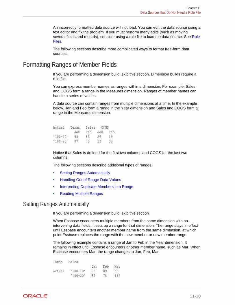
An incorrectly formatted data source will not load. You can edit the data source using atext editor and fix the problem. If you must perform many edits (such as movingseveral fields and records), consider using a rule file to load the data source. See RuleFiles.

The following sections describe more complicated ways to format free-form datasources.

Formatting Ranges of Member FieldsIf you are performing a dimension build, skip this section. Dimension builds require arule file.

You can express member names as ranges within a dimension. For example, Salesand COGS form a range in the Measures dimension. Ranges of member names canhandle a series of values.

A data source can contain ranges from multiple dimensions at a time. In the examplebelow, Jan and Feb form a range in the Year dimension and Sales and COGS form arange in the Measures dimension.

Actual Texas Sales COGS Jan Feb Jan Feb"100-10" 98 89 26 19"100-20" 87 78 23 32

Notice that Sales is defined for the first two columns and COGS for the last twocolumns.

The following sections describe additional types of ranges.

• Setting Ranges Automatically

• Handling Out of Range Data Values

• Interpreting Duplicate Members in a Range

• Reading Multiple Ranges

Setting Ranges AutomaticallyIf you are performing a dimension build, skip this section.

When Essbase encounters multiple members from the same dimension with nointervening data fields, it sets up a range for that dimension. The range stays in effectuntil Essbase encounters another member name from the same dimension, at whichpoint Essbase replaces the range with the new member or new member range.

The following example contains a range of Jan to Feb in the Year dimension. Itremains in effect until Essbase encounters another member name, such as Mar. WhenEssbase encounters Mar, the range changes to Jan, Feb, Mar.

Texas Sales Jan Feb MarActual “100-10" 98 89 58 “100-20” 87 78 115


11-10

Handling Out of Range Data ValuesIf you are performing a dimension build, skip this section.

When Essbase encounters a member range, it assumes that there is a correspondingrange of data values. If the data values are not in the member range, the data loadstops. Essbase loads any data fields read before the invalid field into the database,resulting in a partial data load.

The following example contains more data fields than member fields in the definedrange of members. The data load stops when it reaches the 10 data field. Essbaseloads the 100 and 120 data fields into the database.

Cola Actual East Jan FebSales 100 120 10COGS 30 34 32

Interpreting Duplicate Members in a RangeIf you are performing a dimension build, skip this section.

Structure ranges in the source data so that Essbase interprets them correctly. If amember appears more than once in a range, Essbase ignores the duplicates.

The first table below shows duplicate members for Actual, Budget, Sales, and COGSand two ranges: Actual to Budget and Sales to COGS. Essbase ignores the duplicateinstances of Actual, Budget, Sales, and COGs (for example, in the second line in theexample, the second Actual and second Budget are ignored):

Cola East Actual Budget Actual Budget Sales Sales COGS COGSJan 108 110 49 50Feb 102 120 57 60

For Actual, the first member of the first range, Essbase maps data values to eachmember of the second range (Sales and COGS). Essbase then proceeds to the nextvalue of the first range, Budget, similarly mapping values to each member of thesecond range. As a result, Essbase interprets the file as shown below:

Cola East Actual Budget Sales COGS Sales COGSJan 108 110 49 50Feb 102 120 57 60

Reading Multiple RangesIf you are performing a dimension build, skip this section.


11-11

As Essbase scans a file, it processes the most recently encountered range first whenidentifying a range of data values. The example above contains two ranges: Actualand Budget and Sales and COGS. While reading the file from left to right and top tobottom, Essbase encounters the Actual and Budget range first and the Sales andCOGS range second.

Formatting ColumnsIf you are performing a dimension build, skip this section. Dimension builds require arule file.

Files can contain columns of fields. Essbase supports loading data from symmetriccolumns or asymmetric columns.

• Symmetric Columns

• Asymmetric Columns

Symmetric ColumnsIf you are performing a dimension build, skip this section. Dimension builds require arules file.

Symmetric columns have the same number of members under them. In the followingexample, each dimension column has one column of members under it. For example,Product has one column under it (100-10 and 100-10) and Market has one columnunder it (Texas and Ohio).

Product Measures Market Year Scenario "100-10" Sales Texas Jan Actual 112"100-10" Sales Ohio Jan Actual 145

The columns in the following file are also symmetric, because Jan and Feb have thesame number of members under them:

Jan Feb Actual Budget Actual Budget"100-10" Sales Texas 112 110 243 215"100-10" Sales Ohio 145 120 81 102

Asymmetric ColumnsIf you are performing a dimension build, skip this section.

Asymmetric columns have different numbers of members under them. In the followingexample, the Jan and Feb columns are asymmetric because Jan has two columnsunder it (Actual and Budget) and Feb has one column under it (Budget):

Jan Jan Feb Actual Budget Budget"100-10" Sales Texas 112 110 243"100-10" Sales Ohio 145 120 81


11-12

If a file contains asymmetric columns, label each column with the appropriate membername.

The example above is valid because the Jan label is now over Actual and Budget. It isclear to Essbase that both columns map to Jan.

The following example is not valid because the column labels are incomplete. The Janlabel must appear over the Actual and Budget columns.

Jan Feb Actual Budget Budget"100-10" Sales Texas 112 110 243"100-10" Sales Ohio 145 120 81

Security and Multiple-User ConsiderationsEssbase supports concurrent users reading and updating the database; therefore,users can use the database while you are dynamically building dimensions, loadingdata, or calculating the database.

• Security Issues

The security system prevents unauthorized users from changing the database.Only users with write access to a database can load data values or adddimensions and members to the database. Write access can be provided globallyor by using filters.

• Multi-User Data Load Issues

You can load data values while multiple users are connected to a database.Essbase uses a block locking scheme for handling multi-user issues. When youload data values, Essbase does the following:

– Locks the block it is loading into so that no one can write to the block.

– Updates the block.

• Multi-User Dimension Build Issues

You cannot build dimensions while other users are reading or writing to thedatabase. After you build dimensions, Essbase restructures the outline and locksthe database for the duration of the restructure operation.

Chapter 11Security and Multiple-User Considerations

11-13

12Working with Rule Files

Data load rule files are sets of operations that are performed on data from an externaldata source file as the data is loaded, or copied, into the database. Dimension buildrule files create or modify the dimensions and members in an outline dynamicallybased on data in an external data source.

• Process for Creating Data Load Rule Files

• Process for Creating Dimension Build Rules Files

• Combining Data Loads and Dimension Builds

• Creating Rule Files

• Setting File Delimiters

• Naming New Dimensions

• Selecting a Build Method

• Setting and Changing Member and Dimension Properties

• Using the Data Source to Work with Member Properties

• Setting Field Type Information

• Setting Dimension Build Operational Instructions

• Defining Data Load Field Properties

• Performing Operations on Records, Fields, and Data

• Validating Rules Files

Process for Creating Data Load Rule Files1. Create a rules file.

2. Set the file delimiters for the data source.

See Setting File Delimiters.

3. Map each rule file field to the data source and define field properties.

See Defining Data Load Field Properties.

4. If necessary, set record, field, and data operations to change the data in the datasource during loading.

See Using a Rules File to Perform Operations on Records, Fields, and Data.

5. Validate and save the rule file.

See Setting Dimension Build Operational Instructions.

Process for Creating Dimension Build Rules FilesTo create a dimension build rules file:

12-1

1. Create a rules file.

2. Set the file delimiters for the data source.

See Setting File Delimiters.

3. If you are creating a dimension, name the dimension.

See Naming New Dimensions.

4. Select the build method.

See Selecting a Build Method.

5. If necessary, change or set the properties of members and dimensions you arebuilding.

See Setting and Changing Member and Dimension Properties.

6. If necessary, set record and field operations to change the members in the datasource during loading.

7. Set field type information, including field type, field number, and dimension.

See Setting Field Type Information.

8. Validate and save the rules file.

See Setting Dimension Build Operational Instructions.

Creating Rule FilesA rule files specifies the changes to make to the data source and outline during a dataload or dimension build. If you are creating the rule file on the service, connect to theserver.

Note:

In rule files, record size is limited to 64 KB.

Setting File DelimitersA file delimiter is the character (or characters) used to separate fields in the datasource. By default, a rules file expects fields to be separated by tabs. You can set thefile delimiter as a comma, tab, whitespace, or custom value. Acceptable custom valuesare characters in the standard ASCII character set, numbered from 0 through 127.Usually, setting file delimiters is what you do first after opening a data source.

Note:

You do not need to set file delimiters for SQL data.

Chapter 12Creating Rule Files

12-2

Naming New DimensionsIf you’re not creating a dimension in the rule file, skip this section.

If you’re creating a dimension, you must name it in the rule file. See NamingConventions for Dimensions, Members, and Aliases.

If you’re creating an attribute dimension, the base dimension must be a sparsedimension already defined in the outline or the same rule file. See Working withAttributes.

Selecting a Build MethodIf you are not performing a dimension build, skip this section.

If you are building a new dimension or adding members to an existing dimension, youmust specify a build method for each dimension that you are creating or modifying.See Understanding Build Methods.

In application workbooks, you set the build method for a dimension on the dimensionworksheet (Dim.dimname). See Understanding Dimension Worksheets in UsingOracle Analytics Cloud - Essbase.

Setting and Changing Member and Dimension PropertiesIf you’re not performing a dimension build, skip this section.

If you’re performing a dimension build, you can set or change the properties of themembers and dimensions in the outline. Some changes affect all members of theselected dimension, some affect only the selected dimension, and some affect alldimensions in the rule file.

You can change the member properties in the data source.

Using the Data Source to Work with Member PropertiesYou can modify the properties of new and existing members during a dimension buildby:

• Including member properties in a field in the data source

• Leaving the data source field empty to reset the property to the default value, or toremove the formula or UDA

In the data source, put the properties in the field directly following the field containingthe members that the properties modify. For example, to specify that member Margin% not roll up into its parent and not be shared:

1. Position the ~ property (which indicates that the member should not roll up into itsparent) and the N property (which indicates that the member should not beshared) after the Margin% field. For example:

Margin% Margin% ~ N Sales

Chapter 12Naming New Dimensions

12-3

Note:

Margin % being repeated because of Alias.

2. Set the field type for the properties fields to Property.


Removing a formula, UDA, or attribute, or resetting a property to its default value,includes the following additional step: Leave the field NULL or empty in the datasource.

Table 12-1 lists all member codes used in the data source to assign properties to blockstorage outline members. (For a list of properties that can be assigned to aggregatestorage outline members, see Rules File Differences for Aggregate Storage DimensionBuilds.)

Table 12-1 Member Property Codes for Block Storage Outlines

Code Description

% Express as a percentage of the current total ina consolidation

* Multiply by the current total in a consolidation

+ Add to the current total in a consolidation

- Subtract from the current total in aconsolidation

/ Divide by the current total in a consolidation

~ Exclude from the consolidation

^ Exclude from all consolidations in alldimensions

A Treat as an time balance average item(applies to accounts dimensions only)

B Exclude data values of zero or #MISSING inthe time balance (applies to accountsdimensions only)

E Treat as an expense item (applies to accountsdimensions only)

F Treat as a time balance first item (applies toaccounts dimensions only)

G Reset two-pass calculation to false (applies toaccounts dimensions only). Also see propertycode T in this table.

J Reset expense item to false (applies toaccounts dimensions only). Also see propertycode E in this table.

K Reset the time balance property to NONE(applies to accounts dimensions only). Alsosee property codes A, F, and L in this table.

L Treat as a time balance last item (applies toaccounts dimensions only)

Chapter 12Using the Data Source to Work with Member Properties

12-4

Table 12-1 (Cont.) Member Property Codes for Block Storage Outlines

Code Description

M Exclude data values of #MISSING from thetime balance (applies to accounts dimensionsonly)

N Never allow data sharing

O Tag as label only (store no data)

P Reset the time balance skip option to NONE(applies to accounts dimensions only). Alsosee property codes B, M and Z in this table.

S Set member as stored member (non-DynamicCalc and not label only)

T Require a two-pass calculation (applies toaccounts dimensions only)

X Create as Dynamic Calc

Z Exclude data values of zero from the timebalance (applies to accounts dimensions only)

Setting Field Type InformationIf you are not performing a dimension build, skip this section.

In a dimension build, each field in the data source is part of a column that describes anoutline member. Fields can contain information about:

• Member names

• Member properties

• Attribute associations

For Essbase to process this information, you must specify the following informationwhen setting field types:

• Field type

The type of field to expect in that column, such as a generation field or an aliasfield. The field type depends on the data source and the build method (see Understanding Build Methods).

• Dimension

The dimension to which the members of that column belong.

• Generation or level number

The generation or level number of the members of that column.

See:

• Field Types and Valid Build Methods

• Rules for Assigning Field Types

Chapter 12Setting Field Type Information

12-5

Field Types and Valid Build MethodsTable 12-2 lists field types and valid build methods.

Table 12-2 Field Types and Valid Build Methods

Field Type1 What the Field Contains Valid Build Methods

Alias An alias

Note:

Thealiasvaluewill notbeassigned to thenewmember ifMemberupdatedimensionbuild isset toRemoveunspecifiedand thedatasourcefor anewmembercontains thealiasvalueof aremovedmember.

Generation, level, and parent-childreferences

See Rules for Assigning Field Types.

Property A member property.

See Table 12-1.

Formula A formula


12-6

Table 12-2 (Cont.) Field Types and Valid Build Methods

Field Type1 What the Field Contains Valid Build Methods

Currency name (Block storage outlines only) Acurrency name

Currency category (Block storage outlines only) Acurrency category

UDA A UDA

Attribute parent In an attribute dimension, the nameof the parent member of the attributemember in the following field

The name of a specific attributedimension

A member of the specified attributedimension. This member isassociated with a specifiedgeneration or level of the selectedbase dimension.

Generation The name of a member in thespecified generation

Generation references

Duplicate generation The name of a member with ashared member as a child

Duplicate generation alias The alias for the shared member

Level The name of a member in a level Level references

Duplicate level The name of a member with ashared member as a child

Duplicate level alias The alias for the shared member

Parent The name of a parent Parent-child reference

Child The name of a child

1 Field types whose names begin with duplicate (such as duplicate generation and duplicate level alias), are not related toduplicate member names described in Creating and Working With Duplicate Member Outlines.

Rules for Assigning Field TypesEach build method has rules for assigning field types.

• Generation build method rules:

– If GEN numbers do not start at 2, the first member of the specified generationmust exist in the outline.

– GEN numbers must form a contiguous range. For example, if GEN 3 and GEN5 exist, you must also define GEN 4.

– Put DUPGEN fields immediately after GEN fields.

– Put DUPGENALIAS fields immediately after DUPGEN fields.

– Group GEN fields sequentially within a dimension. For example:

GEN2,PRODUCT GEN3,PRODUCT GEN4,PRODUCT

– Put attribute association fields after the base field with which they areassociated, and specify the generation number of the associated basedimension member. For example:


12-7

GEN2,PRODUCT GEN3,PRODUCT OUNCES3,PRODUCT

The generation number must correspond to the generation of the member inthe outline for which the field provides values. For example, the 3 inGEN3,PRODUCT shows that the values in the field are third-generation membersof the Product dimension. The 2 in ALIAS2,POPULATION shows that the valuesin the field are associated with the second-generation member of thePopulation dimension.

Note:

When using the generation build method to create a duplicate memberdimension, the maximum number of generations is 20.

• Level build method rules:

– Put DUPLEVEL fields immediately after LEVEL fields.

– Put DUPLEVELALIAS fields immediately after the DUPLEVEL fields.

– Each record must contain a level 0 member. If a level 0 member is repeatedon a new record with a different parent, Essbase rejects the record unless youselect the Allow Moves member property.

– Group level fields sequentially within a dimension.

– Put the fields for each roll-up in sequential order.

– Use a single record to describe the primary and secondary roll-ups.

– Put attribute association fields after the base field with which they areassociated, and specify the level number of the associated base dimensionmember. For example:

LEVEL3,PRODUCT OUNCES3,PRODUCT LEVEL2,PRODUCT

– The level number must correspond to the level of the member in the outline forwhich the field provides values. For example, the 3 in LEVEL3,PRODUCTshows that the values in the field are level 3 members of the Productdimension. The 2 in ALIAS2,POPULATION shows that the values in the field areassociated with the second level of the Population dimension.

• Attribute dimension name build method rules:

The generation or level number must correspond to the generation or level of theassociated base member in the outline. For example, the 3 in OUNCES3,PRODUCTshows that the values in the field are the members of the Ounces attributedimension that are associated with the third-generation member of the Productdimension in the same source data record.

If necessary, move the fields to the required locations.

Setting Dimension Build Operational InstructionsIf you are not performing a dimension build, skip this section.

Within the rules file, you define operations to be performed after the data source hasbeen read:

Chapter 12Setting Dimension Build Operational Instructions

12-8

• Whether to sort members after Essbase has processed and added all membersfrom the data source

• Whether to add the members to the existing outline or to remove unspecifiedmembers from the outline

Removing unspecified members is available only with the generation reference,level reference, and parent-child reference build methods.

Note:

Outlines are invalid if removing members results in level 0 Dynamic Calcmembers without formulas.

Defining Data Load Field PropertiesYou must map each rules file field to the corresponding outline member, or as a datafield or ignored field. Other field characteristics may also apply.

For duplicate member outlines, you must specify the method (level reference,generation reference, or dimension reference) that Essbase uses to map the field.

• Level and generation references: The data source contains multiple fields withinthe duplicate member dimension to uniquely identify duplicate members.

– Use the level reference method when fields within a dimension are organizedbottom-up in the data source.

– Use the generation reference method when fields within a dimension areorganized top-down in the data source. For example:

gen2,Market, gen3,Market, Product, Year, Measures, Scenario, *data*State,"New York","100-10",Jan,Sales,Actual,42City,"New York","100-20",Jan,Sales Actual,82State,Texas,"100-10",Jan,Sales,Actual,37

• Dimension reference: If an outline contains a duplicate member name in differentdimensions—for example, a member name such as Other can be meaningful indifferent dimensions—you can use the dimension reference method. When youset a field to use the dimension reference method, you also identify the dimensionto which members in that field belong. When the dimension reference method isspecified for a field, Essbase checks to ensure that members in the field belong tothe dimension specified for the field.

Performing Operations on Records, Fields, and DataA rules file enables you to perform operations on records, fields, and data valuesbefore loading them into the database without changing the data source.

See Using a Rules File to Perform Operations on Records, Fields, and Data.

Chapter 12Defining Data Load Field Properties

12-9

Validating Rules FilesRules files are validated to ensure that the members and dimensions in the rules filemap to the outline. Validation cannot ensure that the data source loads properly.

If the rules file is correct, you can perform a data load or dimension build.

If the rules file is not valid, see the appropriate topic for each rules file type:

• Data load: Requirements for Valid Data Load Rule Files

• Dimension build: Requirements for Valid Dimension Build Rule Files

Requirements for Valid Data Load Rule FilesFor a data load rule file to validate, all of the following questions must be answered“yes.”

• Is the rule file associated with the correct outline?

• Does each record in the data source contain only one member from eachdimension?

See Items in a Data Source.

• Are all member and dimension names spelled correctly?

• Are all members surrounded by quotation marks if they contain spaces, numbers,or file delimiters?

See Valid Member Fields.

• Are there no extra delimiters in the data source?

See Extra Delimiters with a Rules File.

• Is the member that each data field maps to spelled correctly in the rules file?

See Changing Field Names.

• Are the file delimiters correctly placed?

See Valid Delimiters.

• Is the member in the field name a valid member?

See Mapping Fields.

• Is the dimension name used in only one field (for example, not in a field name andthe header)?

You can map a single data value to only one set of members.

• Is only one field defined as a data field?

See Defining Columns as Data Fields.

• Is the UDA used for sign flipping in the associated outline?

See Flipping Field Signs.

Chapter 12Validating Rules Files

12-10

Requirements for Valid Dimension Build Rule FilesFor a dimension build rule file to validate, all of the following questions must beanswered “yes.”

• Is the rule file associated with the correct outline?

• Does each record contain only one member from each dimension?

See Items in a Data Source.

• Are all member and dimension names spelled correctly?

• Are all members enclosed in quotation marks if they contain spaces, numbers, orfile delimiters?

See Valid Member Fields.

• Are there no extra delimiters in the data source?

See Extra Delimiters with a Rules File.

• Are the reference numbers sequential?


• Are there no repeated generations?


• Is each field type valid for the build method?

See Field Types and Valid Build Methods.

• Are all the fields in correct order?


• Does each child field have a parent field?

• Do all dimension names exist in the outline or the rule file?

• Are any dimensions specified in both the header record in the rules file and theheader record in the data source?

Dimensions can be specified in either the header in the rule file or the header inthe data source, but not in both.

See Defining Header Records.

Chapter 12Validating Rules Files

12-11

13Using a Rules File to Perform Operationson Records, Fields, and Data

You can use rules files to perform operations on records, fields, and data. Forexample, at the record-level, you can include criteria for selecting and rejectingrecords in the rules file. At the field-level, you can set a rule for mapping data sourcefields to member names in the database. At the data-level, you can add to or subtractfrom existing values, or clear existing data values.

• Performing Operations on Records

• Performing Operations on Fields

• Performing Operations on Data

Performing Operations on RecordsYou can perform operations at the record level. For example, you can reject certainrecords before they are loaded into the database. See:

• Selecting Records

• Rejecting Records

• Combining Multiple Select and Reject Criteria

• Defining Header Records

Selecting RecordsYou can specify which records Essbase loads into the database or uses to builddimensions by setting selection criteria. Selection criteria are string and numberconditions that must be met by one or more fields within a record for Essbase to loadthe record. If a field or fields in the record do not meet the selection criteria, Essbasedoes not load the record. You can define one or more selection criteria. For example,to load only 2003 Budget data from a data source, create a selection criterion to loadonly records in which the first field is Budget and the second field is 2003. If you defineselection criteria on multiple fields, you can specify how Essbase combines thecriteria. See Combining Multiple Select and Reject Criteria.

Rejecting RecordsYou can specify which records Essbase ignores by setting rejection criteria. Rejectioncriteria are string and number conditions that, when met by one or more fields within arecord, cause Essbase to reject the record. You can define one or more rejectioncriteria. If no field in the record meets the rejection criteria, Essbase loads the record.For example, to reject Actual data from a data source and load only Budget data,create a rejection criterion to reject records in which the first field is Actual.

13-1

Combining Multiple Select and Reject CriteriaWhen you define select and reject criteria on multiple fields, you can specify howEssbase combines the rules across fields: whether the criteria are connected logicallywith AND or with OR. If you select AND from the Boolean group, the fields must matchall of the criteria. If you select OR, the fields must match only one of the criteria. Theglobal Boolean setting applies to all select or reject operations in the rules file, for dataload and dimension build fields.

Note:

If selection and rejection criteria apply to the same record (you define selectand reject criteria on the same record), the record is rejected.

Setting the Records DisplayedYou can specify the number of records, and the first record, that Essbase displays inthe rules editor in the Web UI. When you specify the first record, Essbase skips allpreceding records. For example, if you enter 5 as the starting record, Essbase doesnot display records 1 through 4.

Note:

Essbase treats header records the same as data records when counting therecords to skip.

Defining Header RecordsData sources can contain:

• Data records, which contain member fields and data fields

• Header records, which describe the contents of the data source and how to loadvalues from the data source to the database

Note:

When loading SQL data, the data load rules file cannot have headerrecords.

Rules files contain records that translate the data of the data source to map it to thedatabase. As part of that information, rules files can also contain header records. Forexample, the Sample.Basic database has a dimension for Year. If several datasources arrive with monthly numbers from different regions, the month itself might notbe specified in the data sources. You must set header information to specify themonth.

Chapter 13Performing Operations on Records

13-2

You can create a header record using one of the following methods:

• Define header information in the rules file.

Rules file headers are used only during data loading or dimension building and donot change the data source. Header information set in a rules file is not used if therules file also points to header records in the data source.

• Define header information in the data source and, in the rules file, point to theheader records.

Placing header information in the data source makes it possible to use the samerules file for multiple data sources with different formats, because the data sourceformat is specified in the data source header (not in the rules file).

When you add one or more headers to the data source, you must also specify inthe rules files the location of the headers in the data source. The rules file tellsEssbase to read the header information as a header record (not as a data record).You can also specify the type of header information in each header record.

Header information defined in the data source takes precedence over headerinformation defined in the rules file.

Data Source HeadersYou can build dimensions dynamically by adding header information to the top recordof the data source and by specifying the location of the header record in the rules file.

The header record lists field definitions for each field. The field definition includes thefield type, the field number, and the dimension name into which to load the fields. Figure 13-1 illustrates the format of a header record:

Figure 13-1 Header Record with Three Field Definitions

If the file delimiter is a comma, enclose each field definition in quotation marks (" ").

After you set the header information in the data source, you must specify the locationof the header information in the rules file. If a rules file refers to header information in adata source, Essbase uses the information in the data source—rather than theinformation in the rules file—to determine field types and dimensions.

Valid Data Source Header Field TypesValid field types, which must be in capital letters:

• GEN, DUPGEN, and DUPGENALIAS

Chapter 13Performing Operations on Records

13-3

• LEVEL, DUPLEVEL, and DUPLEVELALIAS

• PARENT, CHILD

• PROPERTY

• ALIAS

• FORMULA

• CURNAME

• CURCAT

• UDA

• ATTRPARENT

• The name of an attribute dimension, such as CAFFEINATED

Each field type that you set requires a field number. When the field type is the name ofan attribute dimension, the field number cannot be greater than 9. See Setting FieldType Information.

Performing Operations on FieldsYou can perform operations at the field level. For example, you can move a field to anew position in the record.

See:

• Ignoring Fields

• Ignoring Strings

• Arranging Fields

• Mapping Fields

• Changing Field Names

Ignoring FieldsYou can ignore all fields of a specified column of the data source. The fields still existin the data source, but they are not loaded into the Essbase database. For example,the Sample.Basic database has five standard dimensions: Year, Product, Market,Measures, and Scenario. If the data source has an extra field that is not a member ofany dimension, such as Salesperson, you can tell Essbase to ignore the Salespersonfield.

Ignoring StringsYou can ignore any field in the data source that matches a string, called a token.When you ignore fields based on string values, the fields are ignored everywhere theyappear in the data source, not just in a particular column. For example, in a datasource that is a computer-generated report in text format, special ASCII charactersmight be used to create horizontal lines between pages or boxes around headings.These special characters can be defined as tokens to be ignored.

Chapter 13Performing Operations on Fields

13-4

Arranging FieldsYou can set the order of the fields in the rules file to be different from the order of thefields in the data source. The data source is unchanged.

See:

• Moving Fields

• Joining Fields

• Creating a Field by Joining Fields

• Copying Fields

• Splitting Fields

• Creating Additional Text Fields

Moving FieldsYou can move fields to a different location using a rules file. For example, you canspecify the first field in the data source to be the third field during the data load ordimension build.

In some instances, moved fields may appear to merge. If you move a field thatcontains empty cells, and the moved field becomes the last field in the record, asshown below, the field may merge with the field to its left.

1<tab>2<tab>31<tab>2<tab>(null)

To prevent merging, replace the empty cell with a delimiter.

Joining FieldsYou can join multiple fields into one field. The new field is given the name of the firstfield in the join. For example, if a data source has separate fields for product number(100) and product family (-10), you must join the fields (100-10) before loading theminto the Sample.Basic database.

Before you join fields, move the fields to join into the order in which you want themjoined.

Creating a Field by Joining FieldsYou can join fields by placing the joined fields into a new field. This procedure leavesthe original fields intact. Creating a field is useful if you need to concatenate fields ofthe data source to create a member.

For example, if a data source has separate fields for product number (100) andproduct family (-10), you must join the fields (100-10) before you load them into theSample.Basic database. If, however, you want to preserve the two existing fields in thedata source, you can create a field (100-10) using a join. The data source nowincludes all three fields (100, -10, and 100-10).


13-5

Before you join fields, move the fields to join into the order in which you want themjoined.

Copying FieldsYou can create a copy of a field while leaving the original field intact. For example, if,during a single dimension build, you want to define a multilevel attribute dimension andassociate attributes with members of a base dimension, you must copy some of thefields. See Working with Multilevel Attribute Dimensions.

Splitting FieldsYou can split a field into two fields. For example, if a data source for the Sample.Basicdatabase has a field containing UPC100-10-1, you can split “UPC” out of the field andignore it. Then, only 100-10-1, the product number, is loaded.

Creating Additional Text FieldsYou can create a text field between two fields. You might create a text field to inserttext between fields that are to be joined. For example, if one field contains 100 andone contains 10-1, you can insert a text field with a dash between the two fields andthen join the three fields to create the 100-10-1 member of the Product dimension.

Mapping FieldsThis section applies to data load only. If you are performing a dimension build, skipthis section.

You use a rules file to map data source fields to Essbase member names during adata load. You can map fields in a data source directly to fields in the Essbasedatabase during a data load by specifying which field in the data source maps to whichmember or member combination in the Essbase database. The data source is notchanged.

Note:

When you open a SQL data source, the fields default to the SQL data sourcecolumn names. If the SQL column names and the Essbase dimensionnames are the same, you need not map the column names.

Changing Field NamesTo load a data source, you must specify how the fields of the data source map to thedimensions and members of the database. Rules files can translate fields of the datasource so that the fields match member names each time the data source is loaded.This process does not change the data source.

The rules file:

• Maps member fields of the data source to dimensions and members of thedatabase


13-6

• Maps data fields of the data source to member names or member combinations(such as Jan, Actual) of the database

See:

• Replacing Text Strings

• Placing Text in Empty Fields

• Changing the Case of Fields

• Dropping Leading and Trailing Spaces

• Converting Spaces to Underscores

• Adding Prefixes or Suffixes to Field Values

Replacing Text StringsYou can replace text strings so that the fields map to Essbase member names duringa data load or dimension build. The data source is not changed. For example, if thedata source abbreviates New York to NY, you can have the rules file replace each NYwith New York.

Placing Text in Empty FieldsYou may want to replace empty fields in a column with text. For example, if emptyfields in the column represent default values, you can insert the default values or insert#MI to represent missing values.

Changing the Case of FieldsYou can change the case of a field so that the field maps to Essbase member namesduring a data load or dimension build. The data source is not changed. For example, ifthe data source capitalizes a field (for example, JAN) that is in lowercase in thedatabase (jan), you can have the rules file change the field to lowercase.

Dropping Leading and Trailing SpacesYou can drop leading and trailing spaces from around fields of the data source. A fieldvalue containing leading or trailing spaces does not map to a member name, even ifthe name within the spaces is an exact match.

By default, Essbase drops leading and trailing spaces.

Converting Spaces to UnderscoresYou can convert spaces in fields of the data source to underscores to make the fieldvalues match the member names of the database.

Adding Prefixes or Suffixes to Field ValuesYou can add prefixes and suffixes to each field value of the data source. For example,you can add 2017 as the prefix to all member names in the Year dimension.


13-7

Performing Operations on DataThis section applies to data load only. If you are performing a dimension build, skipthis section.

You can perform operations on the data in a field; for example, moving a field to a newposition in the record.

See:

• Defining Columns as Data Fields

• Adding to and Subtracting from Existing Values

• Clearing Existing Data Values

• Replacing All Data

• Scaling Data Values

• Flipping Field Signs

Defining Columns as Data FieldsThis section applies to data load only. If you are performing a dimension build, skipthis section.

If each record in the data source contains a column for every dimension and one datacolumn, you must define the data column as a data field, as shown in the followingexample:

Market, Product, Year, Measures, ScenarioTexas 100-10 Jan Sales Actual 42Texas 100-20 Jan Sales Actual 82Texas 100-10 Jan Sales Actual 37

You can define only one field in a record as a data field.

Adding to and Subtracting from Existing ValuesThis section is for data load only. If you are performing a dimension build, skip thissection.

By default, Essbase overwrites the existing values of the database with the values ofthe data source, but you can determine how newly loaded data values affect existingdata values.

You can use incoming data values to add to or subtract from existing database values.For example, if you load weekly values, you can add them to create monthly values inthe database.

Using this option makes recovery more difficult if the database crashes while loadingdata, although Essbase lists the number of the last row committed in the applicationlog.

Chapter 13Performing Operations on Data

13-8

For block storage databases, set the Commit Row database transaction option to 0 toprevent difficult recoveries. This setting causes Essbase to view the entire load as asingle transaction and to commit the data only when the load is complete.

Using the import data (aggregate storage) MaxL statement, you can only add to andsubstract from existing values in aggregate storage databases only.

Clearing Existing Data ValuesThis section is for data load only. If you are performing a dimension build, skip thissection.

You can clear existing data values from the database before you load new values. Bydefault, Essbase overwrites the existing values of the database with the new values ofthe data source. If you are adding and subtracting data values, however, Essbaseadds or subtracts the new data values to and from the existing values.

Before adding or subtracting new values, make sure that the existing values arecorrect. Before loading the first set of values into the database, make sure that there isno existing value.

For example, assume that the Sales figures for January are calculated by adding thevalues for each week in January:

January Sales = Week 1 Sales + Week 2 Sales + Week 3 Sales + Week 4 Sales

When you load Week 1 Sales, clear the database value for January Monthly Sales. Ifthere is an existing value, Essbase performs the following calculation:

January Sales = Existing Value + Week 1 Sales + Week 2 Sales + Week 3 Sales + Week 4 Sales

You can also clear data from fields that are not part of the data load. For example, if adata source contains data for January, February, and March, and you want to loadonly the March data, you can clear January and February data.

Replacing All DataThis section applies to loading data into an aggregate storage database only. If youare loading data into a block storage database or performing a dimension build, skipthis section.

In an aggregate storage database, Essbase can remove all of the data in the databaseor all of the data in each incremental data slice in a database, and replace the datawith the contents of a specified data load buffer. This functionality is useful whenworking with data sets that are small enough to reload completely, or when workingwith data that can be separated into large, static data sets that are never updated andsmall, volatile data sets in which you need to track changes.

To replace all data, see Replacing Database or Incremental Data Slice Contents.


13-9

Scaling Data ValuesThis section is for data load only. If you are performing a dimension build, skip thissection.

You can scale data values if the values of the data source are not in the same scale asthe values of the database.

For example, assume the real value of sales is $5,460. If the Sales data source tracksthe values in hundreds, the value is 54.6. If the Essbase database tracks the realvalue, you must multiply the value coming in from the Sales data source (54.6) by 100to have the value display correctly in the Essbase database (as 5460).

Flipping Field SignsThis section is for data load only. If you are performing a dimension build, skip thissection.

You can reverse, or flip, the value of a data field by flipping its sign. Sign flips arebased on the UDAs of the outline. When loading data into the accounts dimension, forexample, you can specify that any record whose accounts member has a UDA ofExpense change from a plus sign to a minus sign. See Creating UDAs.


13-10

14Performing and Debugging Data Loads orDimension Builds

You can load data or members from one or more external data sources to an Essbasedatabase. You can load data without updating the outline, update the outline withoutloading data, or load data and build dimensions simultaneously.

• Prerequisites for Data Loads and Dimension Builds

• Performing Data Loads or Dimension Builds

• Stopping Data Loads or Dimension Builds

• Tips for Loading Data and Building Dimensions

• Debugging Data Loads and Dimension Builds

Prerequisites for Data Loads and Dimension BuildsBefore you load data or build dimensions, ensure that the following items are in place:

• An Essbase database

• A connection to the appropriate Essbase Server

• One or more valid data sources

See Data Sources.

• A rules files, if you are using one

See Rule Files.

• If you are not using a rules file, a data source correctly formatted for free-form dataloading

See Data Sources that Do Not Need a Rule File.

Performing Data Loads or Dimension BuildsWhen you perform a data load or dimension build, the process runs in the backgroundso that you can continue working during the load or build. You can then check thestatus of the background process to see when the load or build has completed.

If you are using multiple data sources in a dimension build, to reduce total processingtime you can perform a deferred-restructure dimension build. See PerformingDeferred-Restructure Dimension Builds.

14-1

Note:

If you are loading data into a transparent partition, follow the same steps asfor loading data into a local database.

You can load data or build dimensions using these MaxL statements:

• For data loading: import data

• For dimension building: import dimensions

Stopping Data Loads or Dimension BuildsYou can stop a data load or dimension build before it completes. You should not stopa data load or dimension build unless it is necessary. If a data load or dimension buildprocess is terminated, Essbase displays the file name as partially loaded.

If you initiate a data load or dimension build from a client and terminate the data loador dimension build from the server, it could take time before the client responds to thetermination request. Because Essbase reads the source file until all source data isread, the amount of time depends on the file size and the amount of source data thatEssbase has processed. If the process is terminated from the computer that initiated it,termination is immediate.

To stop a data load or dimension build before it completes, you can use the altersystem kill request MaxL statement.

Tips for Loading Data and Building DimensionsSee these topics to help you load data and build dimensions:

• Performing Deferred-Restructure Dimension Builds

• Determining Where to Load Data

• Dealing with Missing Fields in a Data Source

• Loading a Subset of Records from a Data Source

Performing Deferred-Restructure Dimension BuildsSkip this section if you are loading data only or are using a single data source for adimension build.

By default, each time you make changes to an outline, Essbase considers the type ofchange and restructures the database if needed. Restructuring the database rebuildsthe database, which takes time, requires more disk space for its process, and cancause file defragmentation. For information about the types of changes and types ofrestructuring that can be required, see the following topics:

• For block storage outlines, see Optimizing Database Restructuring.

• For aggregate storage outlines, see Aggregate Storage Database Restructuring.

Chapter 14Stopping Data Loads or Dimension Builds

14-2

Deferred-restructure dimension builds, also known as incremental dimension builds,read multiple data sources for dimension builds and delay restructuring until all datasources have been processed.

MaxL enables you to include all of the data sources within one import databasestatement. You can control whether outline validation is performed for each file. Youmust enable outline validation for the last file. See import database and importdimensions in Technical Reference for Oracle Essbase.

In all cases, the data sources are processed in the order in which they are listed.

Note:

MaxL enables you to enforce or suppress outline verification for each file. Toensure a valid outline, ensure that the last build verifies the outline.

Determining Where to Load DataSkip this section if you are building dimensions or working with an aggregate storagedatabase.

If you load data into a parent member, when you calculate the database, theconsolidation of the children’s data values can overwrite the parent data value. Toprevent overwriting:

• If possible, do not load data directly into a parent.

• If you must load data into a parent member, ensure that Essbase knows not toconsolidate #MISSING values from the children of the parent into the parent.

You can set the consolidation operator in an application workbook, the outline orcalculation scripts:

• Application workbook: See Understanding Dimension Worksheets in Using OracleAnalytics Cloud - Essbase.

• Outline: See Setting Information Properties in Using Oracle Analytics Cloud -Essbase.

• Calculation script: Use the SET AGGMISSG calculation command. See TechnicalReference for Oracle Analytics Cloud - Essbase.

You can set the consolidation using the alter database MaxL statement.

The methods in this table work only if the child values are empty (#MISSING). If thechildren have data values, the data values overwrite the data values of the parent. See Consolidating #MISSING Values.

Note:

You cannot load data into Dynamic Calc or attribute members. For example,if Year is a Dynamic Calc member, you cannot load data into it. Instead, loaddata into Qtr1, Qtr2, Qtr3, and Qtr4, which are not Dynamic Calc members.

Chapter 14Tips for Loading Data and Building Dimensions

14-3

Dealing with Missing Fields in a Data SourceEach record in the data source must have the same number of data value fields toperform a data load. If data values are missing, the data load processes incorrectly.

For example, the following file is invalid, because there is no value under Apr:

Actual Ohio Sales ColaJan Feb Mar Apr10 15 20

To fix the file, insert #MISSING or #MI into the missing field:

Actual Ohio Sales ColaJan Feb Mar Apr10 15 20 #MI

See Placing Text in Empty Fields.

Note:

If a dimension field or member field is missing, Essbase uses the value that itused previously for that dimension or member field. See Missing Dimensionor Member Fields.

If a rules file has extra blank fields, join the empty fields with the field next to them.See Joining Fields.

In aggregate storage databases, values can be loaded only to level 0 cells. Specifying#MISSING or #MI as a value in the data source removes the associated cell if it ispresent in the database. For information about data load differences for aggregatestorage databases, see Preparing Aggregate Storage Databases.

Loading a Subset of Records from a Data SourceYou can load a subset of records in a data source during a data load or a dimensionbuild. For example, you can load records 250 to 500 without loading the other recordsof the data source.

To load a subset of records:

1. Using a text-editing tool, number the records in the data source.

2. Set the rules file to ignore the column containing the record number.

See Ignoring Fields.

3. Define a rejection criterion that rejects all records except those that you want toload.

For example, reject all records for which the ignored column is fewer than 250 orgreater than 500. See Rejecting Records.

Chapter 14Tips for Loading Data and Building Dimensions

14-4

Debugging Data Loads and Dimension BuildsIf a data source does not correctly load into Essbase Server, ensure that you areconnected to the appropriate application and database and that you are loading thecorrect data source.

If you still encounter problems, see these topics:

• Verifying that Essbase Server Is Available

• Verifying that the Data Source Is Available

• Checking Error Logs

• Resolving Problems with Data Loaded Incorrectly

• Creating Rejection Criteria for End of File Markers

• Understanding How Essbase Processes a Rules File

• Understanding How Essbase Processes Missing or Invalid Fields During a DataLoad

After you correct the problems, you can reload the records that did not load byreloading the error log.

Verifying that Essbase Server Is AvailableTo help identify that the problem is with Essbase and not with the server or network,try to access the server without using Essbase. Check whether:

• The server is running.

Try connecting to the server without using Essbase. If you cannot, check with yoursystem administrator.

• Essbase Server is running.

Check with your Essbase administrator.

• The client is connected to the server.

Try connecting to the server from the client without using Essbase.

Verifying that the Data Source Is AvailableIf Essbase cannot open the data source that you want to load, ensure that thefollowing conditions are true:

• The data source is open (for example, is someone editing the data source?).

Essbase can load only data sources that are not locked by another user orapplication.

• The data source has the correct file extension.

Text files must have a .txt extension; rules files must have an .rul extension.

• The data source name and the path name are correct.

Check for misspellings.

• The data source is in the specified location.

Chapter 14Debugging Data Loads and Dimension Builds

14-5

Ensure that no one has moved or deleted the data source.

• If you are using a SQL data source:

– The connection information (such as the user name, password, and databasename) is correct.

– You can connect to the SQL data source without using Essbase.

Checking Error LogsIf a data load or dimension build fails, the error log can be a valuable debugging tool.

If there is no error log, check whether the following conditions exist:

• The person running the data load set up an error log.

By default, when using a rules file, Essbase creates an error log.

• The data source and Essbase Server are available.

See Verifying that Essbase Server Is Available and Verifying that the Data SourceIs Available

• Essbase Server crashed during the data load.

If so, you probably received a timeout error on the client.

• The application log exists.

If the error log exists but is empty, Essbase does not think that an error occurredduring loading. Check whether the following conditions exist:

• The rules file contains selection or rejection criteria that rejected every record inthe data source.

See Selecting Records and Rejecting Records.

• The rules file validates properly.

See Requirements for Valid Data Load Rule Files and Requirements for ValidDimension Build Rule Files.

Resolving Problems with Data Loaded IncorrectlyIf the data source loads without error, but the data in the database is wrong, checkwhether the following conditions exist:

• You loaded the correct data source.

If so, check the data source again to make sure that it contains the correct values.

• There are blank fields in the data source.

You must insert #MI or #MISSING into a data field that has no value. Otherwise,the data source may not load correctly. To replace a blank field with #MI or#MISSING using a rules file, see Placing Text in Empty Fields.

• The data source is formatted correctly.

– All ranges are set up properly.

– The data is clean. For example, as it processes the data source, Essbaserecognizes member names and knows the dimensions they belong to. If adata source record inadvertently includes a member from a dimension for


14-6

which there is a member named in the header record, the new member namereplaces the header record member for that dimension. In the followingexample data source, Essbase recognizes Florida as a member of the Marketdimension. The values in the last four records are interpreted as Florida valuesinstead of Texas values.

Jan Actual Texas Sales "100-10" 51.7 "100-20" 102.5 "100-20" 335.0 Florida 96.7 "200-20" 276.0 "200-20" 113.1 "200-10" 167.0

• You added incoming data to existing data instead of replacing incoming data withexisting data.

See Adding to and Subtracting from Existing Values.

• You selected or rejected any records that you did not intend to select or reject.

See Selecting Records and Rejecting Records.

• The sign is reversed (for example, a minus sign instead of a plus sign) andwhether you performed sign flips on any UDAs.

See Flipping Field Signs.

• You cleared data combinations that you did not intend to clear.

See Clearing Existing Data Values.

• You scaled the incoming values incorrectly.

See Scaling Data Values.

• All member and alias names are fewer than 79 characters long.

To check data in Smart View, see the Oracle Smart View for Office User’s Guide.

Creating Rejection Criteria for End of File MarkersA SQL data source may have an end of file marker made up of special characters thatcause a data load or dimension build to fail. To fix this problem, define a rejectioncriterion to reject the problem record.

To define rejection criteria:

1. Find the end of file marker in the SQL data source.

2. Determine how to search for the end of file marker using the Essbase searchcommand.

This task may be difficult, because the end of file marker may be composed of oneor more special characters.

3. Define a rejection criterion that rejects the end of file marker.


14-7

Understanding How Essbase Processes a Rules FileSometimes, you can track down problems with dimension builds by understandinghow Essbase initializes the rules file and processes the data source.

Essbase performs the following steps to initialize a rules file:

1. Validates the rules file against the associated outline.

2. Validates the dimensions. This process includes ensuring that the build methodand field types are compatible and that each dimension name is unique. Membernames must be either unique or shared.

3. Adds new dimensions defined in the rules file to the outline.

4. Reads header records specified in the data source.

Then Essbase performs the following operations on each record of the data sourceduring a data load or dimension build:

1. Sets the file delimiters for all records.

2. Applies field operations to the data in the order in which the operations are definedin the rules file.

Field operations include joins, moves, splits, and creating fields using text andjoins. To see the order in which field operations are defined in the rules file, see Performing Operations on Fields.

3. Essbase applies all properties for each field, applying all properties to field1 beforeproceeding to field2. Essbase applies field properties in the following order:

a. Ignores fields set to be ignored during data load

b. Ignores fields set to be ignored during dimension build

c. Flags the data field

d. Applies field names

e. Applies field generations

f. Performs all replaces in the order in which they are defined in the rules file

g. Drops leading and trailing spaces

h. Converts spaces to underscores

i. Applies suffix and prefix operations

j. Scales data values

k. Converts text to lowercase

l. Converts text to uppercase

4. Adds members, or member information, or both, to the outline

5. If you chose to skip lines, Essbase skips the number of lines that you specified;otherwise, Essbase proceeds to the first record.

6. Essbase performs selection or rejection criteria in the order in which the criteriaare defined in the rules file. Essbase loads or rejects individual records of the datasource based on the specified criteria.


14-8

Understanding How Essbase Processes Missing or Invalid FieldsDuring a Data Load

See these topics to understand how Essbase processes invalid fields during a dataload.

• Missing Dimension or Member Fields

• Unknown Member Fields

• Invalid Data Fields

Missing Dimension or Member FieldsIf a dimension or member field is missing, Essbase uses the value that it usedpreviously for that dimension or member field. If there is no previous value, Essbaseaborts the data load.

For example, when you load the following file into the Sample.Basic database,Essbase maps the Ohio member field into the Market dimension for all records,including the records that have Root Beer and Diet Cola in the Product dimension.

Jan Sales Actual Ohio Cola 25 "Root Beer" 50 "Diet Cola" 19

Essbase stops the data load if no prior record contains a value for the missing memberfield. For example, if you try to load the following file into the Sample.Basic database,the data load stops, because the Market dimension (Ohio, in the previous example) isnot specified.

Jan Sales Actual Cola 25 "Root Beer" 50 "Diet Cola" 19

Unknown Member FieldsIf you are performing a data load and an unknown member name is encountered, theentire record is rejected. If there is a prior record with a member name for the missingmember field, Essbase continues to the next record. If there is no prior record, thedata load stops. For example, when you load the following file into the Sample.Basicdatabase, the record containing Ginger Ale is rejected because it is not a validmember name. The records containing Cola, Root Beer, and Cream Soda are loaded.If Ginger Ale were in the first record, however, the data load would stop.

Jan, Sales, ActualOhio Cola 2 "Root Beer" 12 "Ginger Ale" 15 "Cream Soda" 11


14-9

Note:

If you are performing a dimension build, you can add the new member to thedatabase. See Performing Data Loads or Dimension Builds.

Invalid Data FieldsIf you are performing a data load, the data load stops if an invalid data field isencountered. All fields that are read before the invalid field are loaded into thedatabase, resulting in a partial data load. For example, in the following file, the dataload stops when it encounters the 15- data value. The Jan and Feb Sales records areloaded but not the Mar and Apr Sales records.

East Cola Actual

Sales Jan $10

Feb $21

Mar $15-

Apr $16


14-10

15Understanding Advanced DimensionBuilding Concepts

The build method that you select depends on the type of data in the data source anddetermines the algorithm that is used to add, change, or remove dimensions,members, and aliases in the outline. All examples in this chapter are based on theSample.Basic database.

• Understanding Build Methods

• Using Generation References

• Using Level References

• Using Parent-Child References

• Adding a List of New Members

• Building Attribute Dimensions and Associating Attributes

• Building Shared Members by Using a Rules File

• Building Duplicate Member Outlines

All examples in this chapter are based on the Sample.Basic database, which you cancreate using the Block Storage Sample (Stored) sample application workbook(Sample_Basic.xlsx). See About Application Workbooks in Using Oracle AnalyticsCloud - Essbase.

Understanding Build MethodsUse the guidelines in Table 15-1 to select the appropriate build method for the datasource:

Table 15-1 Build Method Guidelines

Type of Data inEach Record

Examples Desired Operation Build Method1 Field TypeInformation

Top-down data

Each record specifiesthe parent’s name,the child’s name, thechildren of that child,and so on.

Year, Quarter, Month Modify the propertiesof existingdimensions andmembers

Generationreferences

The generationnumber for each field.

15-1

Table 15-1 (Cont.) Build Method Guidelines

Type of Data inEach Record

Examples Desired Operation Build Method1 Field TypeInformation

Bottom-up data

Each record specifiesthe name of themember, the name ofits parent, the nameof its parent’s parent,and so forth.

Month, Quarter, Year • Create sharedmembers thatroll up intodifferentgenerations

• Modify theproperties ofexistingdimensions andmembers

Level references The level number foreach field.

Parent followed by itschild

Each record specifiesthe name of theparent and the nameof the new childmember, in thatorder, although theycan specify otherinformation as well.

Cola, Diet Cola • Create sharedmembers thatroll up intodifferentgenerations

• Share non-level0 members

• Modify propertiesof existingdimensions andmembers

Parent-childreferences

Whether a field isparent or child. Thefield number is 0.

A list of newmembersEach data sourcelists new members;the data source doesnot specify where inthe outline themembers belong.Essbase providesalgorithms thatdetermine where toadd these members.

Jan, Feb, Mar, April Add all members aschildren of an existingparent (possibly a“dummy” parent)

Add as child of thespecified parent

800-10, 800-20 Add all members atthe end of thedimension

Add as sibling at thelowest level

800-10, 800-20 Add each newmember to thedimension thatcontains similarmembers

Add as sibling to amember with amatching string

A list of basedimension membersand their attributes

Cola 16oz Can, RootBeer 14oz Bottle

Add members to anattribute dimensionand associate theadded members withthe appropriatemembers of the basedimension

Generation, level, orparent-childreferences,depending on theorganization of thesource data

The number for eachfield.

The number is eitherthe generation orlevel number of theassociated memberof the basedimension or zero.

1 Using a level references build, you cannot create an alias that has the same name as its member. This restriction does notapply if you use other build methods, including the generation references build method.

Using Generation ReferencesTop-down data sources are organized left to right from the highest level to the lowestlevel. Each record begins with the most general information and progresses to themost specific information. The name of the new member is at the end of the record.

Chapter 15Using Generation References

15-2

When using a top-down data source, use the generation references build method. Inthe rules file, specify the generation number and the field type of each field of the datasource.

Essbase numbers members within a dimension according to the hierarchical positionof the member within the dimension. The numbers are called generation references. Adimension is always generation 1. All members at the same branch in a dimension arecalled a generation. Generations are numbered top-down according to their positionrelative to the dimension; that is, relative to dimension 1.

For example, as illustrated in Figure 15-1, the Product dimension is generation 1.Product has a 100 member, which is generation 2. 100 has members, such as 100-10,which are generation 3. To use the generation references build method, specify thegeneration reference number in the rules file.

Figure 15-1 Generations

The top half of Figure 15-2 shows a top-down data source (GENREF.TXT). The datasource is used to build the Product dimension. The bottom half shows the rules file forthe data source (GENREF.RUL). The rules file specifies the generation number for eachfield in the data source. See Setting Field Type Information.

Figure 15-2 Rules File for Generation Build

Figure 15-3 shows the tree that Essbase builds from the GENREF.TXT data source andGENREF.RUL rules file:


15-3

Figure 15-3 Generation References

Dealing with Empty Fields

When you use the generation references build method, you can choose to process nullvalues. Null processing specifies what actions Essbase takes when it encountersempty fields, also known as null fields, in the data source.

If null processing is not enabled, Essbase rejects all records with null values andwrites an error to the error log.

If null processing is enabled, Essbase processes nulls as in the following ways:

• Missing field: If the null occurs where Essbase expects a GENERATION field,Essbase promotes the next GENERATION field to replace the missing field.

In the following example, there is no field in the GEN3,Products column:

GEN2,Products GEN3,Products GEN4,Products100 100-10a

When Essbase reads the record, it promotes the GEN4 field (100-10a) to GEN3,as if the data source looked like the following example:

GEN2,Products GEN3,Products GEN4,Products100 100-10a

• Missing field before secondary field: If a null occurs directly before a secondaryfield, Essbase ignores the secondary field. (Secondary field types are alias,property, formula, duplicate generation, duplicate generation alias, currency name,currency category, attribute parent, UDA, and name of an attribute dimension.)


15-4

In the following example, there is no field in the GEN2, Products or theALIAS2,Products column:

GEN2,Products ALIAS2,Products GEN3,Products GEN4,Products Cola 100-10 100-10a

When Essbase reads the record, it ignores the ALIAS2 field and promotes theGEN3 field (100-10) to GEN2 and the GEN4 field (100-10a) to GEN3, as if thedata source looked like the following example:

GEN2,Products ALIAS2,Products GEN3,Products GEN4,Products100-10 Cola 100-10a

• Missing secondary field: If the null occurs where Essbase expects a secondaryfield, Essbase ignores the secondary null field and continues loading.

In the following example, there is no field in the ALIAS2, Products column:

GEN2,Products ALIAS2,Products GEN3,Products GEN4,Products100 100-10 100-10a

When Essbase reads the record, it ignores the ALIAS2 field and loads the otherfields.

Using Level ReferencesIn a bottom-up data source, each record defines a single member of a dimension. Thedefinition begins with the most specific information about the member and providesprogressively more general information. A typical record specifies the name of the newmember, then the name of its parent, then its parent’s parent, and so forth.

Levels are defined from a bottom-up hierarchical structure. For example, in the outlinein Figure 15-4, the lowest-level members are at the bottoms of the branches of theProduct dimension.

Figure 15-4 Generation and Level Numbers

To build the outline in Figure 15-4, you can use the following bottom-up data source:

100-10-12 100-10 100100-20-12 100-20 100

Chapter 15Using Level References

15-5

In a level reference build, the lowest-level members are sequenced left to right. Level0 members are in the first field, level 1 members are in the second field, and so on.This organization is the opposite of how data is presented for generation references(top-down).

In the following example, the rules file uses the level reference build method to addmembers to the Product dimension. The rules file specifies the level number and thefield type for each field of the data source (see Setting Field Type Information). Thefirst column of the data source contains new members (600-10-11, 600-20-10, and600-20-18). The second column contains the parents of the new members (600-10and 600-20), and the third column contains parents of the parents (600).

Figure 15-5 Rules File for Level Build

For example, to build the tree in Figure 15-6, use Figure 15-5 to set up the data source(LEVEL.TXT) and the rules file (LEVEL.RUL).

Figure 15-6 Levels


15-6

Dealing with Empty Fields

When you use the level references build method, you can choose to process nullvalues. Null processing specifies what actions Essbase takes when it encountersempty fields, also know as null fields, in the data source.

If null processing is not enabled, Essbase rejects all records with null values andwrites an error to the error log.

If null processing is enabled, Essbase processes nulls in the following ways:

• Missing field: If a null occurs where Essbase expects a LEVEL field, Essbasepromotes the next LEVEL field to replace the missing field.

In the following example, there is no field in the LEVEL0, Products column:

LEVEL0,Products LEVEL1,Products LEVEL2,Products 100-10 100

When Essbase reads the record, it promotes the LEVEL1 field (100-10) toLEVEL0 and the LEVEL2 field (100) to LEVEL1, as if the data source looked likethe following example:

LEVEL0,Products LEVEL1,Products LEVEL2,Products100-10 100

• Missing field before a secondary field: If a null occurs directly before asecondary field, Essbase ignores the secondary field. (Secondary field options arealias, property, formula, duplicate level, duplicate level alias, currency name,currency category, attribute parent, UDA, and a name of an attribute dimension.)

In the following example, there is no field in the LEVEL0, Products column:

LEVEL0,Products ALIAS0,Products LEVEL1,Products LEVEL2,Products Cola 100-10 100

When Essbase reads the record, it ignores the ALIAS0 field and promotes theLEVEL1 field (100-10) to LEVEL0 and the LEVEL2 field (100) to LEVEL1, as if thedata source looked like the following example:

LEVEL0,Products ALIAS0,Products LEVEL1,Products LEVEL2,Products100-10 Cola 100

• Missing secondary field: If a null occurs where Essbase expects a secondaryfield, Essbase ignores the secondary null field and continues loading.

In the following example, there is no field in the ALIAS0, Products column:

LEVEL0,Products ALIAS0,Products LEVEL1,Products LEVEL2,Products100-10a 100-10 100

When Essbase reads the record, it ignores the ALIAS0 field and loads the otherfields.


15-7

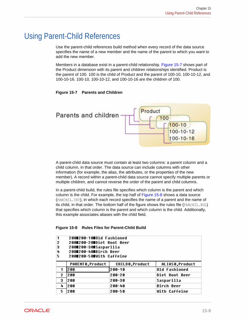
Using Parent-Child ReferencesUse the parent-child references build method when every record of the data sourcespecifies the name of a new member and the name of the parent to which you want toadd the new member.

Members in a database exist in a parent-child relationship. Figure 15-7 shows part ofthe Product dimension with its parent and children relationships identified. Product isthe parent of 100. 100 is the child of Product and the parent of 100-10, 100-10-12, and100-10-16. 100-10, 100-10-12, and 100-10-16 are the children of 100.

Figure 15-7 Parents and Children

A parent-child data source must contain at least two columns: a parent column and achild column, in that order. The data source can include columns with otherinformation (for example, the alias, the attributes, or the properties of the newmember). A record within a parent-child data source cannot specify multiple parents ormultiple children, and cannot reverse the order of the parent and child columns.

In a parent-child build, the rules file specifies which column is the parent and whichcolumn is the child. For example, the top half of Figure 15-8 shows a data source(PARCHIL.TXT), in which each record specifies the name of a parent and the name ofits child, in that order. The bottom half of the figure shows the rules file (PARCHIL.RUL)that specifies which column is the parent and which column is the child. Additionally,this example associates aliases with the child field.

Figure 15-8 Rules Files for Parent-Child Build

Chapter 15Using Parent-Child References

15-8

Figure 15-9 shows the tree that Essbase builds from this data source and rules file.

Figure 15-9 Parents and Children

Note:

For duplicate member situations, the parent field must contain the qualifiedmember name. See Building Qualified Member Names Through the RulesFile.

Adding a List of New MembersIf a data source consists of a list of new members and does not specify theirancestors, Essbase must decide where in the outline to add them. Essbase providesthe following build methods for this type of data source:

• Add each new member as a sibling of the existing member whose text mostclosely matches its own.

See Adding Members Based On String Matches.

• Add each new member as a sibling of the lowest-level existing member.

See Adding Members as Siblings of the Lowest Level.

• Add all new members as children of a specified parent (generally a “dummy”parent).

See Adding Members to a Specified Parent.

After Essbase adds all new members to the outline, it may be necessary to move thenew members into their correct positions using Outline Editor. See PositioningDimensions and Members.

Note:

Essbase does not support concurrent attribute association with the Add asbuild methods.

Adding Members Based On String MatchesYou can add new members from a data source to an existing dimension by matchingstrings with existing members. When Essbase encounters a new member in a data

Chapter 15Adding a List of New Members

15-9

source, it scans the outline for a member name with similar text and adds the newmember as a sibling of the member with the closest string match.

For example, the data source in Figure 15-10 (SIBSTR.TXT) contains two newmembers (100-11 and 200-22) to add to the Product dimension. The new membersare similar to strings in the Product dimension: they contain three digits, one dash, andtwo digits.

To add the example members to the database, set the values in Table 15-2 in therules file:

Table 15-2 Example of Adding Members Using String Matches

Field Value More Information

Field 1 (Product) • Do not select a field type for thefield

• Set the dimension for the field toProduct (field 1 is displayed asProduct, as shown in Figure 15-9)

Setting Field Type Information

Fields 2 through 6 Ignore the fields Ignoring Fields

Product dimension Select the Add as sibling of matchingstring build method

Selecting a Build Method

Figure 15-10 Rules File Fields Set to Add Members as Siblings with StringMatches

Figure 15-11 shows the tree that Essbase builds from this data source and rules file.100-11 is added as a sibling of 100 and 200-22 is added as a sibling of 200.


15-10

Figure 15-11 Tree for Adding Members as Siblings with String Matches

Adding Members as Siblings of the Lowest LevelYou can add new members from a data source as siblings of members that reside atthe lowest level of a dimension—at the level 0 branch. When Essbase encounters anew member in a data source, it scans the outline for the level 0 branch of membersand adds the new member as a sibling of these members.

Note:

If the outline contains multiple groups of members at this level, Essbaseadds the new member to the first group of members that it encounters.

For example, the data source (SIBLOW.TXT) and the rules file (SIBLOW.RUL) in Figure 15-12 contain new members (A100-10 and A100-99) to add to the Measuresdimension.

Figure 15-12 Rules File Fields Set to Add Members as Siblings of the LowestLevel

To add the example members dynamically to the database, set the values shown in Table 15-3 in the rules file:


15-11

Table 15-3 Example of Adding Members as Siblings of the Lowest Level


Field 3 (Measures) • Do not select a field type for thefield

• Set the dimension for the field toMeasures (field 3 is displayed asMeasures, as shown in Figure 15-12)


Fields 1, 2, 4, 5, and 6 Ignore the fields You can ignore all fields of aspecified column of the data source.


Measures dimension Select the Add as sibling of lowestlevel build method


Figure 15-13 shows the tree that Essbase builds from this data source and rules file.A100–20 and A100–99 are added as siblings of Margin.

Figure 15-13 Tree for Adding Members as Siblings of the Lowest Level

Adding Members to a Specified ParentYou can add all new members as children of a specified parent, generally a “dummy”parent.

After Essbase adds all new members to the outline, review the added members andmove or delete them in the outline.

When Essbase encounters a new member in the data source, it adds the new memberas a child of the parent that you define. The parent must be part of the outline beforeyou start the dimension build.

For example, the data source in Figure 15-14 (SIBPAR.TXT) contains two newmembers (600-54 and 780-22) for the Product dimension (field 1). Assume that youpreviously added a member called NewProducts under the Products dimension.


15-12

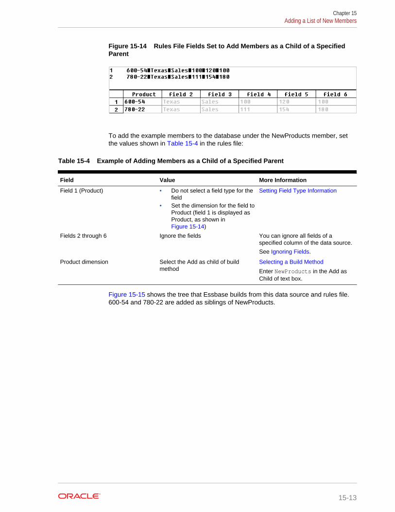
Figure 15-14 Rules File Fields Set to Add Members as a Child of a SpecifiedParent

To add the example members to the database under the NewProducts member, setthe values shown in Table 15-4 in the rules file:

Table 15-4 Example of Adding Members as a Child of a Specified Parent


Field 1 (Product) • Do not select a field type for thefield

• Set the dimension for the field toProduct (field 1 is displayed asProduct, as shown in Figure 15-14)


Fields 2 through 6 Ignore the fields You can ignore all fields of aspecified column of the data source.


Product dimension Select the Add as child of buildmethod


Enter NewProducts in the Add asChild of text box.

Figure 15-15 shows the tree that Essbase builds from this data source and rules file.600-54 and 780-22 are added as siblings of NewProducts.


15-13

Figure 15-15 Tree for Adding Members as a Child of a Specified Parent

Building Attribute Dimensions and Associating AttributesWhen a data source contains attribute information, you must use one or more rulesfiles to build attribute dimensions and to associate attributes with members of theirbase dimensions.

You can use rules files to build attribute dimensions dynamically, to add and deletemembers, and to establish or change attribute associations.

Working with attributes involves the following operations:

• If the base dimension does not exist, you must build it.

• You must build the attribute dimension.

• You must associate members of the base dimension with members of the attributedimension.

You can use any of the following approaches to perform these operations:

• Build the base and attribute dimensions and perform the associations allsimultaneously. Doing so, you use a single rules file to build the base dimensionand one or more attribute dimensions to associate each attribute with theappropriate member of the base dimension. Because this approach uses a singlerules file, it can be the most convenient. Use this approach if the base dimensiondoes not exist and each source data record contains all attribute information foreach member of the base dimension.

• Build the attribute dimension and perform the associations in one rules file.Assuming that the base dimension is built in a separate step or that the basedimension already exists, you can build an attribute dimension and associate theattributes with the members of the base dimension in one step. You need only todefine the attribute associations in the rules file. See Associating Attributes.

Chapter 15Building Attribute Dimensions and Associating Attributes

15-14

• Build the attribute dimension and then perform the associations using separaterules files. Assuming that the base dimension is built in a separate step or that thebase dimension already exists, you can build an attribute dimension and associatethe attributes with the members of the base dimension in separate steps. Build theattribute dimension, and then associate the attribute members with members ofthe base dimension. Use this approach when you build numeric attributedimensions that are multilevel or that have members that represent different-sizedranges.

See:

• Building Attribute Dimensions

• Associating Attributes

• Updating Attribute Associations

• Working with Multilevel Attribute Dimensions

• Working with Numeric Ranges

• Reviewing the Rules for Building Attribute and Base Dimensions

Building Attribute DimensionsBefore you build attribute dimensions in a database, you must define the attributemember name formats for the outline. See Setting Member Names in AttributeDimensions.

You can build attribute dimensions in one of the following ways:

• The same way in which you build standard dimensions.

SeeProcess for Data Loading and Dimension Building.

• Simultaneously, as you associate attributes with members of the base dimension.

See Associating Attributes.

Essbase does not support concurrent attribute association with the Add as buildmethods.

When you define the rules file for building attribute dimensions, specify the basedimension and the name of the attribute dimension file.

Associating AttributesWhether you build the attribute dimension and associate the attribute members withthe members of the base dimension in one step or in separate steps, define the fieldsas described in this section.

Note:

If you are working with a multilevel attribute dimension or with an attributedimension of the type numeric, Boolean, or date, the rules file requires anadditional field. See Working with Multilevel Attribute Dimensions.


15-15

Every record of the source data must include at least two columns: one for themember of the base dimension and one for the attribute value of the base dimensionmember. In the same source data record you can include additional columns for otherattributes that you want to associate with the member of the base dimension. Youmust position the field for the member of the base dimension before any of the fieldsfor the members of the attribute dimension.

Define the field type for the attribute dimension member as the name of the attributedimension, use the generation or level number of the associated member of the basedimension, and specify the base dimension name. For example, as shown in theATTRPROD.RUL file in Figure 15-16, the field definition Ounces3,Product specifies thatthe field contains members of the Ounces attribute dimension. Each member of thisfield is associated with the data field that is defined as the generation 3 member of thebase dimension Product. Based on this field definition, Essbase associates theattribute 64 with the 500-10 member.

Figure 15-16 Rules File for Associating Attributes

You can have Essbase use the attribute columns to build the members of the attributedimensions.

When you are working with numeric ranges, you may need to build attributedimensions and perform associations in separate steps. See Working with NumericRanges.

The Caffeinated3,Product field in Figure 15-16 shows how to associate attributes fromadditional single-level attribute dimensions. Because the base dimension is alreadyspecified, you need only to define an additional field for each attribute that you want toassociate with the member of the base dimension.

The file in Figure 15-16 associates attributes as shown in the outline in Figure 15-17.Member 64 is a new member of the Ounces attribute dimension. Members 500,500-10, and 500-20 are new members of the base dimension, Product, and areassociated with member 64.


15-16

Figure 15-17 Associating Attributes

See Setting Attribute Associations in Using Oracle Analytics Cloud - Essbase.

Updating Attribute AssociationsYou can also use the rules file shown in Figure 15-16 to change attribute associations.Ensure that you allow association changes.

Note:

For duplicate member situations, the field to which the attribute is associatedmust contain the qualified member name. See Building Qualified MemberNames Through the Rules File.

See Setting Attribute Associations in Using Oracle Analytics Cloud - Essbase.

Removing Attribute AssociationsTo remove attribute associations, use the same process as for updating them, plus thefollowing steps:

• In the Dimension Build Properties tab of the Field Properties dialog box, selectDelete when the field is empty for the attribute field. (This option is ignored ifAllow association changes is not selected.)

• Leave the field empty or NULL in the data source.


15-17

Working with Multilevel Attribute DimensionsMultilevel, numeric, Boolean, and date attribute dimensions can have duplicate level 0members. For example, associated with a Product dimension, you can have a Sizeattribute dimension with two levels. Level 1 categorizes sizes by men or by women.The level 0 members (attributes) are the actual sizes. You can have a member named8 under Women and member named 8 under Men.

When an attribute is part of a multilevel numeric, Boolean, or date attribute dimension,the source data must include columns for all generations or levels of the attributedimension. In the rules file, you must make copies of all fields that comprise the levelsof the attribute dimension. Define the first set of attribute fields to build the attributedimension. Define the second set of attribute fields to associate the attributes with theappropriate base dimension members. To ensure association with the correct attribute,indicate the parent field for the attribute field by making a copy of the parent field andsetting the copy of the parent field as the field type Attribute Parent.

The position of the fields in the rules file is important.

• Place the copied attribute dimension field or fields that define the associationimmediately to the right of the field for the members of the base dimension.

• For a multilevel attribute dimension, place the attribute parent field immediately tothe left of the field that is the child of the attribute parent.

The following steps describe how to define the fields in the rules file to build amultilevel attribute dimension and associate its members with members of its basedimension. This example uses the level references build method.

1. In the rules file, in field 1 and field 2, define the attribute dimension fields in thesame way in which you define standard dimensions; specify type (level orgeneration), number, and dimension name.

Essbase uses field1 and field2 to build the attribute dimension.

2. Define the fields for building the base dimension.

In the following example, you are defining the level 0 and level 1 fields for theProduct dimension. Figure 15-18 shows the fields of the rules file at this stage.

Figure 15-18 Defining Multilevel Attribute Dimensions Before Adding theAssociation Fields


15-18

3. To define the association, make a copy of the field that contains the level 0attribute.

In the current example, make a copy of field 1.

a. Use the attribute dimension name as the field type and specify the generationor level number of the member of the base dimension with which Essbaseassociates the attribute; for example, Size0.

b. Specify the base dimension; for example, Product.

c. Move the new field immediately to the right of the field for the base dimensionwith which Essbase associates the attribute.

In the current example, move the new field to the right of the field Level0,Product.

4. Make a copy of the field containing the parent of the attribute field.

In the current example, make a copy of field 2.

a. Set the field type of the new field as Attribute Parent and specify thegeneration or level number of the base member with which you want Essbaseto associate the attribute; for example, ATTRPARENT0.

b. Specify the attribute dimension; for example, Size.

c. Move the ATTRPARENT field immediately to the left of the attributeassociation field that you created in step 3.

As shown in Figure 15-19, the rules file now contains the field definitions to build theattribute dimension Size and to associate the members of Size with the appropriatemembers of the base dimension Product.

Figure 15-19 Source Data and Rules File for Building a Multilevel AttributeDimension

When you run a dimension build with the data shown in Figure 15-19, Essbase buildsthe Size attribute dimension and associates its members with the appropriatemembers of the base dimension. Figure 15-20 shows the updated outline.


15-19

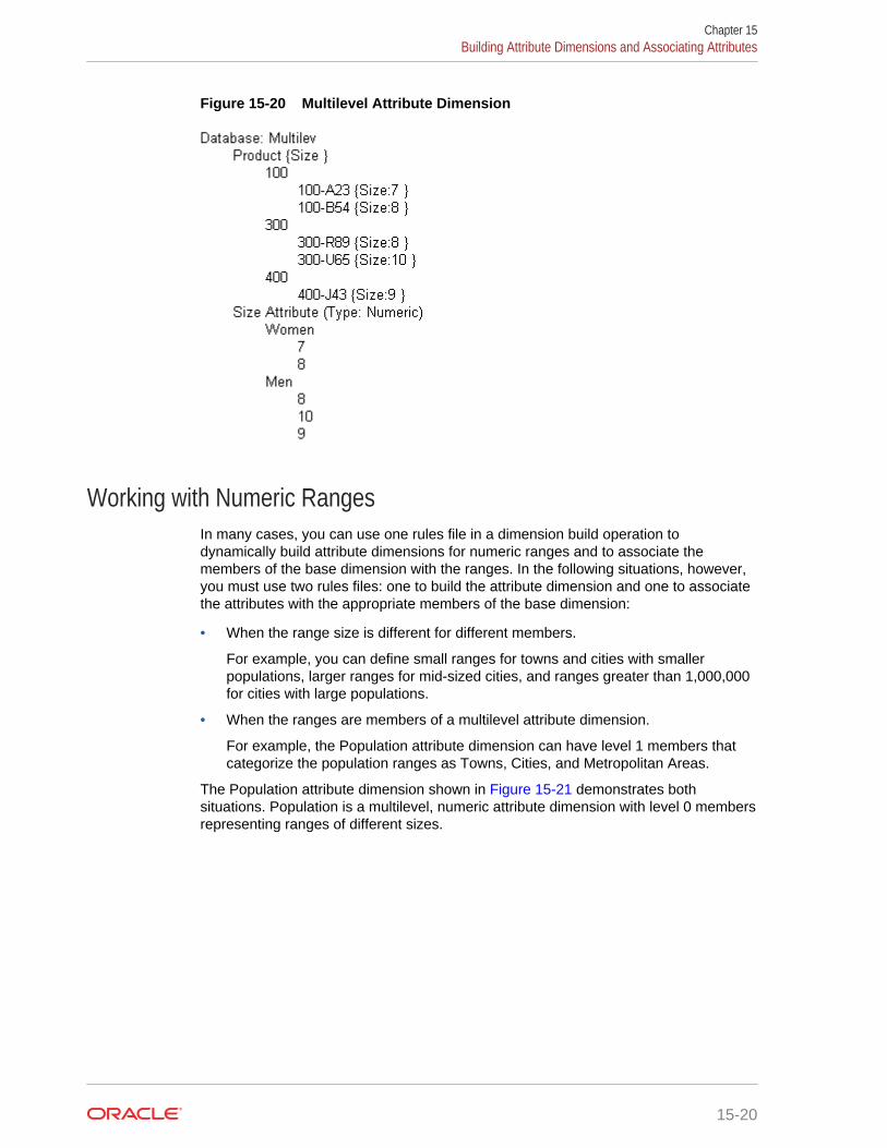
Figure 15-20 Multilevel Attribute Dimension

Working with Numeric RangesIn many cases, you can use one rules file in a dimension build operation todynamically build attribute dimensions for numeric ranges and to associate themembers of the base dimension with the ranges. In the following situations, however,you must use two rules files: one to build the attribute dimension and one to associatethe attributes with the appropriate members of the base dimension:

• When the range size is different for different members.

For example, you can define small ranges for towns and cities with smallerpopulations, larger ranges for mid-sized cities, and ranges greater than 1,000,000for cities with large populations.

• When the ranges are members of a multilevel attribute dimension.

For example, the Population attribute dimension can have level 1 members thatcategorize the population ranges as Towns, Cities, and Metropolitan Areas.

The Population attribute dimension shown in Figure 15-21 demonstrates bothsituations. Population is a multilevel, numeric attribute dimension with level 0 membersrepresenting ranges of different sizes.


15-20

Figure 15-21 Numeric Attribute Dimension with Different-Sized Ranges

You must use one rules file to build the Population dimension and another rules file toassociate the Population dimension members as attributes of members of the basedimension.

Building Attribute Dimensions that Accommodate RangesFirst, create a rules file that uses the generation, level, or parent-child build method tobuild the attribute dimension. In the rules file, specify the following information:

• The name of the attribute dimension and its associated base dimension.

• The fields for building the attribute dimension.


The source data must be in attribute sequence, in ascending order. If ranges havedifferent sizes, the source data must include a record for every attribute range.

Note:

In later builds, you cannot insert attribute members between existingmembers.

To use the generation method to build the outline in Figure 15-21, you must sequencethe source data in ascending sequence, based on the numeric attribute value. Definethe fields in a rules file as shown in Figure 15-22. Additionally, Figure 15-22 showshow to associate aliases with attributes.


15-21

Figure 15-22 Rules File for Building a Numeric Attribute Dimension withRanges

Associating Base Dimension Members with Their Range AttributesAfter you build the numeric attribute dimension ranges, you need a rules file toassociate the members of the base dimension with their attributes. The source dataincludes fields for the members of the base dimension and fields for the data valuesthat Essbase uses to associate the appropriate Population attribute.

Define the rules file as shown in Figure 15-23.

Figure 15-23 Rules File for Associating Numeric Range Attributes


15-22

When you define the association field (for example, Population3, Market), place theattribute members within a range.

Note:

Figure 15-23 includes a city, Boston, whose population of 3,227,707 isoutside the ranges of the attribute dimension in Figure 15-21, where theranges extend only to 3,000,000. To allow for values in the source data thatare outside the ranges in the attribute dimension, enter a range size, such as1000000. Essbase uses the range size to add members to the attributedimension above the existing highest member or below the existing lowestmember, as needed.

Caution:

After you associate members of the base dimension with members of theattribute dimension, if you manually insert new members into the attributedimension or rename members of the attribute dimension, you mayinvalidate existing attribute associations. Consider an example wherenumeric range attributes are defined as “Tops of ranges” and an attributedimension contains members 100, 200, 500, and 1000. A base dimensionmember with the value 556 is associated with the attribute 1000. If yourename a attribute dimension member from 500 to 600, the base dimensionmember with the value 556 now has an invalid association. This basemember is still associated with the attribute 1000 when it should beassociated with the attribute 600. If you manually insert new members orrename existing members, to ensure that associations are correct, rerun thedimension build procedure and associate the base members with thechanged attribute dimensions. For example, rerunning the attributeassociation procedure correctly associates the member of the basedimension with the value 556 with the new attribute 600.

Ensuring the Validity of AssociationsTo ensure the validity of attribute associations, you must select the correct dimensionbuilding options and perform the builds in the proper sequence.

• Adding or Changing Members of the Attribute Dimension: After you associatemembers of a base dimension with their numeric attribute ranges, if you manuallyinsert new members or rename existing members in the attribute dimension,ensure that associations between attributes and base members are correct byperforming one of the following tasks:

– Rerun the dimension build procedure that associates the base members withthe changed attribute dimension.

– Use Outline Editor to manually review and fix, as needed, the associations ofall base dimensions.

• Deleting Members from the Attribute Dimension: You can delete all membersof an attribute dimension so that you can rebuild the dimension with new data.


15-23

• Adding Members to the Base Dimension: You can use the same rules file toadd new members to the base dimension and to associate the new members withtheir numeric range attributes simultaneously. Provide a value for the range size.

If Essbase encounters a base dimension value that is greater than the highestattribute member by more than the range size or is lower than the lowest attributemember by more than the range size, it creates members in the attributedimension to accommodate the out-of-range values.

For example, in Figure 15-24, the numeric range attributes are defined as “Tops ofranges.” The highest value member of the Population attribute dimension is3000000. If the source data includes a record with the population 4,420,000, andthe range size is 1000000, Essbase adds two members to the attribute dimension,4000000 and 5000000, and associates the base member with the value of4,420,000 with the 5000000 attribute.

Figure 15-24 Dynamically Adding Attribute Range Members

When you add range members and base dimension members simultaneously,Essbase does not create aliases for the new members of the attribute dimension. Ifyou want aliases that describe the range values for the new members of the attributedimension, you must add the aliases in a separate operation.

Reviewing the Rules for Building Attribute and Base DimensionsThe information in this section describes areas unique to defining and associatingattributes through a dimension build.

Getting Ready

• Before running a dimension build, you must define the attribute member nameformats for the outline.

See Setting Member Names in Attribute Dimensions.

• Defining new attribute dimensions in a rules file is different from defining newstandard dimensions in a rules file.


15-24

Defining Fields in Rules Files

Rules files that are used to build single-level attribute dimensions require fewer fieldtypes than rules files that build and associate members of multilevel attributedimensions.

• For single-level attribute dimensions, define the field that contains the attributevalues as the field to be associated with the members of the base dimension. Adimension build uses the defined field to add new members to the attributedimension.

See Associating Attributes.

• For multilevel attribute dimensions, Essbase requires fields that define eachgeneration or level in the attribute dimension and fields that define theassociations. Use the new field type, Attribute Parent, to identify fields that areparent members for the attribute members being associated.

See Working with Multilevel Attribute Dimensions.

Controlling Adding New Attribute Members

When Essbase encounters attribute data values that are not members of the attributedimension, it automatically adds the values as new members.

To prevent adding new members to attribute dimensions, select the Do not createmembers option for the attribute dimension.

Controlling Associations

You can control the following associations:

• Making changes to attribute associations

Select the Allow association changes option for the attribute dimension.

• Enabling automatic association of base members with attributes that representranges of values

Define the size of the range.


• Concurrent attribute associations

Use any build method except the Add as build methods.

See Understanding Build Methods.

Note:

Because attributes are defined only in the outline, the data load processdoes not affect them.

Building Shared Members by Using a Rules FileThe data associated with a shared member comes from a referenced member with thesame name as the shared member. Because the shared member stores a pointer to

Chapter 15Building Shared Members by Using a Rules File

15-25

data contained in the referenced member, the data is shared between the membersand is stored only once.

For example, member 100-20 (Diet Cola) rolls up into the 100 family and into the Dietfamily.

Figure 15-25 Shared Members in the Sample.Basic Database

You can share members among as many parents as you want. Diet Cola has twoparents (100 and Diet), but you can define it to roll up into more parents.

You can share members at multiple generations in the outline. In Figure 15-25, DietCola is shared by two members at generation 2 in the outline, but it can be shared bya member at generation 3 and a member at generation 4, as shown in Figure 15-30.

Creating shared members at different generations in the outline is easy in OutlineEditor; creating shared members using dimension build is more difficult. You must pickthe build method and format the data source carefully.

The following sections describe how to build shared members in the outline by using adata source and a rules file.

• Sharing Members at the Same Generation

• Sharing Members at Different Generations

• Sharing Non-Level 0 Members

• Building Multiple Roll-Ups by Using Level References

• Creating Shared Roll-Ups from Multiple Data Sources


15-26

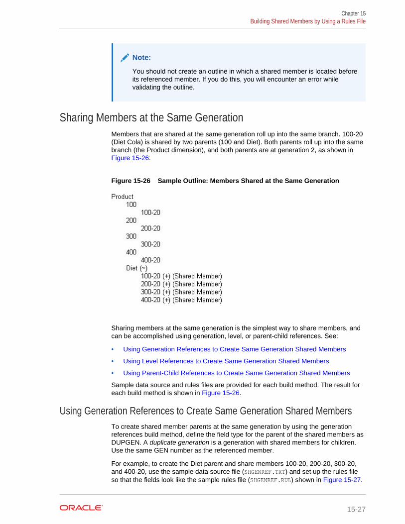
Note:

You should not create an outline in which a shared member is located beforeits referenced member. If you do this, you will encounter an error whilevalidating the outline.

Sharing Members at the Same GenerationMembers that are shared at the same generation roll up into the same branch. 100-20(Diet Cola) is shared by two parents (100 and Diet). Both parents roll up into the samebranch (the Product dimension), and both parents are at generation 2, as shown in Figure 15-26:

Figure 15-26 Sample Outline: Members Shared at the Same Generation

Sharing members at the same generation is the simplest way to share members, andcan be accomplished using generation, level, or parent-child references. See:

• Using Generation References to Create Same Generation Shared Members

• Using Level References to Create Same Generation Shared Members

• Using Parent-Child References to Create Same Generation Shared Members

Sample data source and rules files are provided for each build method. The result foreach build method is shown in Figure 15-26.

Using Generation References to Create Same Generation Shared MembersTo create shared member parents at the same generation by using the generationreferences build method, define the field type for the parent of the shared members asDUPGEN. A duplicate generation is a generation with shared members for children.Use the same GEN number as the referenced member.

For example, to create the Diet parent and share members 100-20, 200-20, 300-20,and 400-20, use the sample data source file (SHGENREF.TXT) and set up the rules fileso that the fields look like the sample rules file (SHGENREF.RUL) shown in Figure 15-27.


15-27

100 is the Cola family, 200 is the Root Beer family, 300 is the Cream Soda family, and-20 appended to the family name (for example, 100–20) indicates a diet version of thesoda.

Figure 15-27 Sample Rules File: Members Shared at the Same GenerationUsing Generation References

Using Level References to Create Same Generation Shared MembersTo create shared members of the same generation by using the level references buildmethod, first ensure that the primary and any secondary roll-ups are specified in onerecord. You can specify as many secondary roll-ups as you want, as long as they areall in one record.

Define the field type for the shared member as LEVEL. Then enter the level number.To create a shared member of the same generation, set the level number of thesecondary roll-up to have the same number of levels as the primary roll-up. Whileprocessing the data source, Essbase creates a parent at the specified level andinserts the shared members under it.

For example, to create the shared members 100-20 (Diet Cola), 200-20 (Diet RootBeer), 300-20 (Diet Cream Soda), and 400-20 (Diet Fruit Soda), use the sample datasource file (SHLEV.TXT) and set up the rules file so that the fields look like the samplerules file (SHLEV.RUL) shown in Figure 15-28.

Figure 15-28 Sample Rules File: Members Shared at the Same GenerationUsing Level References


15-28

Using Parent-Child References to Create Same Generation Shared MembersTo create shared members of the same generation by using the parent-childreferences build method, define the PARENT and CHILD field types. Ensure thatEssbase is set up to allow sharing. When sharing is enabled, Essbase automaticallycreates duplicate members under a new parent as shared members.

Figure 15-29 Sample Rules File: Members Shared at the Same GenerationUsing Parent-Child References

Sharing Members at Different GenerationsSometimes you want shared members to roll up into parents that are at differentgenerations in the outline. For example, in Figure 15-30, the shared members roll upinto parents at generation 2 (Diet) and at generation 3 (TBC and Grandma’s). Thisoutline assumes that TBC (The Beverage Company) buys some beverages fromoutside vendors: it buys 200-20 (Diet Root Beer) from a vendor named Grandma’s.


15-29

Figure 15-30 Sample Outline: Members Shared at Different Generations

Sharing members at different generations can be accomplished using level or parent-child references. See:

• Using Level References to Create Different Generation Shared Members

• Using Parent-Child References to Create Different Generation Shared Members


Using Level References to Create Different Generation Shared MembersTo create shared members of different generations by using the level references buildmethod, ensure that primary and secondary roll-ups are specified in one record. Youcan specify as many secondary roll-ups as you want, as long as they are all in onerecord.

Define the field type for the shared member as LEVEL. Then enter the level number.While processing the data source, Essbase creates a parent at the specified level andinserts the shared members under it.

For example, to share the products 100-20, 200-20, and 300-20 with a parent calledDiet and two parents called TBC and Grandma’s, use the sample data file and therules file shown in Figure 15-31:

Figure 15-31 Sample Rules File: Members Shared at Different GenerationsUsing Level References


15-30

Using Parent-Child References to Create Different Generation SharedMembers

To create shared members at different generations using the parent-child referencesbuild method, define the PARENT and CHILD field types. Ensure that Essbase is setup to allow sharing. When sharing is enabled, Essbase automatically creates duplicatemembers under a new parent as shared members.

Figure 15-32 Sample Rules File: Members Shared at Different GenerationsUsing Parent-Child References

Sharing Non-Level 0 MembersSometimes you want to share non-level 0 members (members that are not at thelowest generation). For example, in Figure 15-33, 100, 200, and 300 are shared byTBC and Grandma's. This outline assumes that TBC buys some of its product linesfrom outside vendors; it buys 200 (all root beer) from a vendor named Grandma's.


15-31

Figure 15-33 Sample Outline: Non-Level 0 Members Shared at DifferentGenerations

Sharing non-level 0 members can be accomplished using level or parent-childreferences. See:

• Using Level References to Create Non-Level 0 Shared Members

• Using Parent-Child References to Create Non-Level 0 Shared Members


Using Level References to Create Non-Level 0 Shared MembersTo create shared non-level 0 members by using the level references build method,ensure that primary and secondary roll-ups are specified in one record. You canspecify unlimited secondary roll-ups, as long as they are all in one record.

Define the field type for the parent of the shared member as duplicate level(DUPLEVEL), and then enter the level number. To create a shared member of thesame generation, set the level number of the secondary roll-up to have the samenumber of levels as the primary roll-up. While processing the data source, Essbasecreates a parent at the specified level and inserts the shared members under it.

For example, to share the product lines 100, 200, and 300 with a parent called Sodaand parents called TBC and Grandma’s, use the sample data file and rules file shownin Figure 15-34. This data source and rules file work only if the Diet, TBC, andGrandma’s members exist in the outline. The DUPLEVEL field is always created as achild of the dimension (at generation 2), unless the named level field already exists inthe outline.


15-32

Figure 15-34 Sample Rules File: Non-Level 0 Members Shared at DifferentGenerations Using Level References

Using Parent-Child References to Create Non-Level 0 Shared MembersThe parent-child references build method is the most versatile for creating sharedmembers. It does not have any restrictions on the position of the shared members inthe outline, unlike the generation references and level references build methods.

To create non-level 0 shared members at the same generation using the parent-childreferences build method, define the PARENT and CHILD field types. Ensure thatEssbase is set up to allow sharing. When sharing is enabled, Essbase automaticallycreates duplicate members under a new parent as shared members.

Figure 15-35 Sample Rules File: Non-Level 0 Members Shared at the SameGeneration Using Parent-Child References


15-33

Building Multiple Roll-Ups by Using Level ReferencesTo enable the retrieval of totals from multiple perspectives, you can also put sharedmembers at different levels in the outline by using the level references build method.For example, the rules file (LEVELMUL.RUL) shown in Figure 15-36 and Figure 15-37specifies build instructions for levels in the Product dimension:

Figure 15-36 Sample Rules File: Multiple Roll-Ups at Different Levels UsingLevel References

Because the record is so long, this second graphic shows the rules file scrolled to theright to show the extra members:

Figure 15-37 (Continuation) Sample Rules File: Multiple Roll-Ups at DifferentLevels Using Level References

When you run the dimension build using the data in Figure 15-37, Essbase builds theoutline shown in Figure 15-38:


15-34

Figure 15-38 Sample Outline: Multiple Roll-Ups at Different Levels

This example enables analysis not only by package type (Cans), but also bypackaging material (comparing sales of aluminum cans and steel cans).

Because Product is a sparse dimension, you can use an alternative outline design toenable retrieval of the same information. For example, consider creating a multilevelattribute dimension for package type with Steel and Aluminum as level 0 membersunder Can. For outline design guidelines, see Analyzing Database Design.

Creating Shared Roll-Ups from Multiple Data SourcesIn many situations, the data for a dimension is in multiple data sources. If you arebuilding dimensions from multiple data sources and want to create multiple roll-ups,load the first data source using the most appropriate build method, and then load allother data sources using the parent-child references build method. Ensure thatEssbase is set up to allow sharing.

For example, using the following Product data source:

"Soft Drinks" Cola"Soft Drinks" "Root Beer"Cola TBC"Root Beer" Grandma’s

Essbase builds the outline illustrated in Figure 15-39:


15-35

Figure 15-39 Sample Outline: Soft Drinks

Then load the second data source below to relate the products to the vendors usingthe parent-child build method. Ensure that Essbase is set up to allow sharing.

Vendor TBCVendor Grandma’s

Essbase builds the outline illustrated in Figure 15-40:

Figure 15-40 Sample Outline: Vendors (Shared Roll-Ups)

Building Duplicate Member OutlinesDuplicate member outlines contain multiple members with the same name, where thevalues are not shared. In unique member outlines, only shared members can have thesame name. See Creating and Working With Duplicate Member Outlines.

The rules file enables you to set whether dimensions, levels, and generations in aduplicate member outline are unique or can include duplicate members.

Uniquely Identifying Members Through the Rules FileTo ensure that duplicate member outline hierarchies are built correctly, use qualifiedmember names in the data source or use the rules file to construct qualified membernames from fields in the data source.

In most situations, the reference method and arrangement of fields provide enoughinformation for Essbase to map data source columns to members in a duplicatemember outline. The dimension build rules file for duplicate member is similar to therules file for unique member outlines.

The following operations require more complex rules files for qualified member names:

Chapter 15Building Duplicate Member Outlines

15-36

• Parent-child dimension builds: The parent-child build method requires twofields, one for parent and one for child. For duplicate member situations the parentfield must contain the qualified member name. Parent-child dimension builds onduplicate member outlines do not support attribute association. To ensure thatattributes are associated with the correct members, perform the associations in aseparate pass, using a generation-reference or level-reference rules file.

• Association of attributes to existing members in the outline: For duplicatemember situations, the field to which the attribute is associated must contain thequalified member name.

Building Qualified Member Names Through the Rules FileIf the data source does not contain the qualified member name as a field, you can usethe rules file to edit and join multiple fields resulting in qualified member names.

To create qualified member names, use the Field Edits tab of the Data SourceProperties dialog box to copy, move, and join fields, and to create brackets andperiods. For example, you can assign population attributes to existing city members ina duplicate member dimension. You can use move, join, and create operations to buildthe qualified name.

For example, the cities in the following data source already exist in the outline. Youwant to associate with the cities the population attributes in the last column of this four-column data source:

Central "Kansas City" Kansas 706010Central "Kansas City" Missouri 1070052East "New York" "New York" 8104079

Editing this source through the rules file to build qualified names and sequence thefield columns properly involves the following edits:

• Using Create using text operations, create one field each for the following textelements:

– [

– ].[

– ].[

– ]

• Using Move operations, move the fields to the following sequence:

1 2 3 4 5 6 7 8[ Central ].[ Kansas ].[ Kansas City ] 706010

• Using Join operations, join together fields 1 2 3 4 5 6 7 to create the single field towhich the attributes are to be associated: [Central].[Kansas].[Kansas City]. Therules file now shows two fields:

1 2 [Central].[Kansas].[Kansas City] 706010

Chapter 15Building Duplicate Member Outlines

15-37

16Modeling Data in Private Scenarios

Using the scenario-management feature, you can use the Sandbox dimension to testand model hypothetical data, without the storage overhead that would be required toreplicate data from your working environment. Modeling scenarios applies only tohybrid aggregation mode databases.

• Testing Changes with a Sandbox Dimension

• Merging Sandbox Data Changes

Testing Changes with a Sandbox DimensionA sandbox dimension allows collaborating database planners to model data usingSmart View or MDX, without the storage overhead replicating large amounts ofmodeled data. A sandbox dimension provides an experimental, testing, ordevelopment environment in which to safely model changes to a production or workingenvironment, without necessarily committing those changes to the workingenvironment.

The sandbox dimension has one base member and usually multiple (up to 1000)sandbox members. Each sandbox member is, initially, an exact mirror of whatever is inthe base. Whenever you submit values to the base, the changes are seen, but notstored, in each sandbox. When you make changes to a sandbox, the base remainsunaffected, unless you deliberately merge the sandbox to the base. Unlike the basevalues, changes you make in the sandbox are stored in the sandbox.

Line 2 n the following grid shows members of the sandbox dimension, the basemember and two sandbox members, sb1 and sb2.

Members p1, p2, and p3 are base periods. Q1 and Time are dynamically calculatedmembers.

On row 4, columns C, D and E have values, while the rest are #Missing. Because thedata exists in the base, those same values are shown in the sandboxes.

On row 5, a user has submitted the value 100 into column H. As you can see, thisnumber exists only in the sandbox sb1. This value is stored in sb1.

On line 6, column C has a base value, but someone has modified the mirror value insb1, column H. Column M in sb2 shows the same value that is seen in the base.

16-1

Merging Sandbox Data ChangesIf, after working in a sandbox environment, you decide to commit the changes to thebase or working environment, then you need to merge the sandbox to the base target.You can also use another sandbox as a merge target.

Only populated (non-#Missing) cells from the source sandbox will be merged to thebase or sandbox target.

See Applying or Discarding Data Changes in Using Oracle Analytics Cloud - Essbase.

Chapter 16Merging Sandbox Data Changes

16-2

17Calculating Essbase Databases

A database contains input data, and values calculated from input data. Essbase offerstwo methods for calculating a database: an outline or a calculation script.

• About Database Calculation

• About Multidimensional Calculation Concepts

• Setting the Default Calculation

• Calculating Databases

• Canceling Calculations

• Parallel and Serial Calculation

• Security Considerations

The information in this chapter applies only to block storage databases and is notrelevant to aggregate storage databases.

About Database CalculationA database contains two types of values:

• Values that you enter, called input data

• Values that are calculated from input data

For example:

• You enter regional sales figures for a variety of products. You calculate the totalsales for each.

• You enter the budget and actual values for the cost of goods sold for severalproducts in several regions. You calculate the variance between budget and actualvalues for each product in each region.

• The database contains regional sales figures and prices for all products. Youcalculate what happens to total profit if you increase the price of one product inone region by 5%.

Small differences in the precision of cell values may occur between calculations run ondifferent platforms, due to operating system math library differences.

17-1

Note:

Most computers represent numbers in binary, and therefore can onlyapproximately represent real numbers. Because binary computers cannothold an infinite number of bits after a decimal point, numeric fractions suchas one-third (0.3333...) cannot be expressed as a decimal with a terminatingpoint. Fractions with a denominator of the power of two (for example, 0.50) orten (0.10) are the only real numbers that can be represented exactly. SeeIEEE Standard 754 for Floating-Point Representation (IEEE, 1985).

Essbase offers two methods for calculating a database:

• Outline calculation

• Calculation script calculation

The method that you choose depends on the type of calculation that you want toperform.

Outline CalculationOutline calculation is the simplest calculation method. Essbase bases the calculationof the database on the relationships between members in the database outline and onany formulas that are associated with members in the outline.

For example, Figure 17-1 shows the relationships between the members of the Marketdimension in the Sample.Basic database. The values for New York, Massachusetts,Florida, Connecticut, and New Hampshire are added to calculate the value for East.The values for East, West, South, and Central are added to calculate the total valuefor Market.

Figure 17-1 Relationship Between Members of the Market Dimension

Figure 17-2 shows the Scenario dimension from the Sample.Basic database. TheVariance and Variance % members are calculated by using the formulas attached tothem.

Chapter 17About Database Calculation

17-2

Figure 17-2 Calculation of Variance and Variance %

It may be more efficient to calculate some member combinations when you retrievethe data instead of calculating the member combinations during the regular databasecalculation. You can use dynamic calculations to calculate data at retrieval time. See Dynamically Calculating Data Values.

Calculation Script CalculationCalculation script calculation is the second method of calculation. Using a calculationscript, you can choose exactly how to calculate a database. For example, you cancalculate part of a database or copy data values between members.

A calculation script contains a series of calculation commands, equations, andformulas. For example, the following calculation script increases the actual marketingexpenses in the New York region by 5%.

FIX (Actual, “New York”) Marketing = Marketing *1.05;ENDFIX;

See Developing Calculation Scripts for Block Storage Databases.

About Multidimensional Calculation ConceptsFigure 17-3, which is based on a simplified database, illustrates the nature ofmultidimensional calculations:

Figure 17-3 Calculating a Multidimensional Database

Chapter 17About Multidimensional Calculation Concepts

17-3

The database has three dimensions—Accounts, Time, and Scenario.

The Accounts dimension has four members:

• Sales and COGS are input values

• Margin = Sales - COGS

• Margin% = Margin % Sales (Margin as a percentage of Sales)

The Time dimension has four quarters. The example displays only the members inQtr1—Jan, Feb, and Mar.

The Scenario dimension has two child members—Budget for budget values andActual for actual values.

The outline in Figure 17-3 is illustrated as a three-dimensional cube in Figure 17-4:

Figure 17-4 Illustration of a Three-Dimensional Database

An intersection of members (one member on each dimension) represents a datavalue; a data value is stored in one cell in the database. To refer to a specific datavalue in a multidimensional database, you must specify each member on eachdimension. In Essbase, member combinations are denoted by a cross-dimensionaloperator (->). Create the cross-dimensional operator using a hyphen (-) and a greater-than symbol (>). Do not include a space between the cross-dimensional operator andmembers.

The single cell containing the data value for Sales, Jan, Actual, as shown in Figure 17-5, is written as Sales -> Jan -> Actual.


17-4

Figure 17-5 Sales, Jan, Actual Slice of the Database

When you refer to Sales, you are referring to a slice of the database containing eightvalues, as shown in Figure 17-6, which are:

• Sales -> Jan -> Actual

• Sales -> Feb -> Actual

• Sales -> Mar -> Actual

• Sales -> Qtr1 -> Actual

• Sales -> Jan -> Budget

• Sales -> Feb -> Budget

• Sales -> Mar -> Budget

• Sales -> Qtr1 -> Budget


17-5

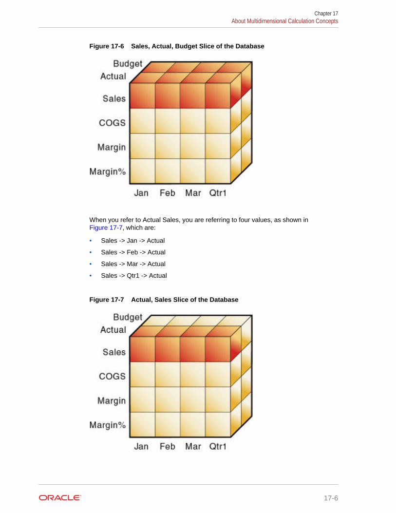
Figure 17-6 Sales, Actual, Budget Slice of the Database

When you refer to Actual Sales, you are referring to four values, as shown in Figure 17-7, which are:

• Sales -> Jan -> Actual

• Sales -> Feb -> Actual

• Sales -> Mar -> Actual

• Sales -> Qtr1 -> Actual

Figure 17-7 Actual, Sales Slice of the Database


17-6

When Essbase calculates the formula “Margin% = Margin % Sales,” it takes eachMargin value and calculates it as a percentage of its corresponding Sales value.

Essbase cycles through the database and calculates Margin% as follows:

1. Margin -> Jan -> Actual as a percentage of Sales -> Jan -> Actual.

The result is placed in Margin% -> Jan -> Actual.

2. Margin -> Feb -> Actual as a percentage of Sales -> Feb -> Actual.

The result is placed in Margin% -> Feb -> Actual.

3. Margin -> Mar -> Actual as a percentage of Sales -> Mar -> Actual.

The result is placed in Margin% -> Mar -> Actual.

4. Margin -> Qtr1 -> Actual as a percentage of Sales -> Qtr1 -> Actual.

The result is placed in Margin% -> Qtr1 -> Actual.

5. Margin -> Jan -> Budget as a percentage of Sales -> Jan -> Budget.

The result is placed in Margin% -> Jan -> Budget.

6. Essbase continues cycling through the database until it has calculated Margin%for every combination of members in the database.

See Defining Calculation Order.

Setting the Default CalculationBy default, the calculation for a database is a CALC ALL of the database outline.CALC ALL consolidates all dimensions and members and calculates all formulas in theoutline.

You can, however, specify any calculation script as the default database calculation.Thus, you can assign a frequently used script to the database rather than loading thescript each time you want to perform its calculation. If you want a calculation script towork with calculation settings defined at the database level, you must set thecalculation script as the default calculation.

To set the default calculation, you can use the alter database MaxL statement.

Calculating DatabasesUsers with the Database Update role have access to run the default calculation on thecube, but no access to run any specific calculation scripts. Users with the ApplicationManager or Database Manager roles have calculation privileges and rights to executeall calculations. See About Calculating Data in Using Oracle Analytics Cloud -Essbase.

To calculate a database, you can use the execute calculation MaxL statement. SeeTechnical Reference for Oracle Analytics Cloud - Essbase.

Canceling CalculationsTo stop a calculation before Essbase completes it, click the Cancel button while thecalculation is running.

Chapter 17Setting the Default Calculation

17-7

When you cancel a calculation, Essbase performs one of the following operations:

• Reverts all values to their previous state

• Retains any values calculated before the cancellation

Parallel and Serial CalculationEssbase supports parallel and serial calculations:

• Serial calculation (default): All steps in a calculation run on a single thread. Eachtask is completed before the next is started.

• Parallel calculation: The Essbase calculator can analyze a calculation, and, ifappropriate, assign tasks to multiple CPUs (up to four).

See Using Parallel Calculation.

Security ConsiderationsTo calculate a database, you must have the Database Update role for the databaseoutline. You can calculate any value in the database, and you can calculate a valueeven if a security filter denies you read and update permissions. Carefully considerproviding users with the Database Update role.

Chapter 17Parallel and Serial Calculation

17-8

18Developing Formulas for Block StorageDatabases

Formulas calculate relationships between members in a database outline. You canapply formulas to members in the database outline or include formulas in calculationscripts.

• Using Formulas and Formula Calculations

• Understanding Formula Syntax

• Using Functions in Formulas

• Using Substitution Variables in Formulas

• Using Formulas on Partitions

• Displaying Formulas


All of the examples in this chapter are based on the Sample.Basic application anddatabase.

For more information about the functions referenced in this chapter, see CalculationFunctions in Technical Reference for Oracle Analytics Cloud - Essbase.

Using Formulas and Formula CalculationsFormulas calculate relationships between members in a database outline. Withformulas, you can:

• Apply formulas to members in the database outline. Use this method if you do notneed to control database calculations carefully for accuracy or performance. Thismethod limits formula size to less than 64 KB.

See Using Functions in Formulas.

• Place formulas in a calculation script. Use this method if you need to controldatabase calculations carefully.

See Using Formulas in Calculation Scripts.

Figure 18-1 shows the Measures dimension from the Sample.Basic database. TheMargin %, Profit %, and Profit per Ounce members are calculated using the formulasapplied to them.

Figure 18-1 Calculation of Margin %, Profit %, and Profit per Ounce

18-1

For formulas applied to members in a database outline, Essbase calculates formulaswhen you perform the following actions:

• Run a default (CALC ALL) calculation of a database.

• Run a calculation script that calculates the member containing the formula; forexample, a CALC DIM of the dimension containing the member, or the memberitself. See Developing Calculation Scripts for Block Storage Databases.

For a formula in a calculation script, Essbase calculates the formula when it occurs inthe calculation script.

If a formula is associated with a dynamically calculated member, Essbase calculatesthe formula when the user requests the data values. In a calculation script, you cannotcalculate a dynamically calculated member or make a dynamically calculated memberthe target of a formula calculation. See Dynamically Calculating Data Values.

Using dynamically calculated members in a formula on a database outline or in acalculation script can significantly affect calculation performance. Performance isaffected because Essbase interrupts the regular calculation to perform the dynamiccalculation.

You cannot use substitution variables in formulas that you apply to the databaseoutline. See Using Substitution Variables in Formulas.

Understanding Formula SyntaxWhen you create member formulas, follow these rules:

• End each statement in the formula with a semicolon (;). For example:

Margin % Sales;

• Use only saved outline member names. If a substitution variable is used for amember name, the substitution variable value must be a saved outline membername.

• Enclose a member name in double quotation marks (“”) if the member namemeets any of the following conditions:

– Contains spaces. For example:

"Opening Inventory" = "Ending Inventory" - Sales + Additions;

– Is the same as an operator, function name, or keyword.

See Naming Conventions in Calculation Scripts, Report Scripts, Formulas,Filters, and Substitution and Environment Variable Values.

– Includes any nonalphanumeric character. For example, hyphens (-), asterisks(*), and slashes (/).

– Is all numeric or starts with one or more numerals. For example, "100" or"10Prod"

For a full list of member names that must be enclosed in quotation marks, see Naming Conventions in Calculation Scripts, Report Scripts, Formulas, Filters, andSubstitution and Environment Variable Values.

• End each IF statement in a formula with an ENDIF statement.

Chapter 18Understanding Formula Syntax

18-2

For example, the following formula contains a simple IF...ENDIF statement. Youcan apply this formula to the Commission member in a database outline:

IF(Sales < 100) Commission = 0;ENDIF;

If you are using an IF statement nested within another IF statement, end each IFwith an ENDIF. For example:

"Opening Inventory"(IF (@ISMBR(Budget)) IF (@ISMBR(Jan)) "Opening Inventory" = Jan; ELSE "Opening Inventory" = @PRIOR("Ending Inventory"); ENDIF;ENDIF;)

• You do not need to end ELSE or ELSEIF statements with ENDIFs. For example:

IF (@ISMBR(@DESCENDANTS(West)) OR @ISMBR(@DESCENDANTS(East) Marketing = Marketing * 1.5;ELSEIF(@ISMBR(@DESCENDANTS(South))) Marketing = Marketing * .9;ELSE Marketing = Marketing * 1.1;ENDIF;

Note:

If you use ELSE IF (with a space) rather than ELSEIF (one word) in aformula, you must supply an ENDIF for the IF statement.

• Ending ENDIF statements with a semicolon (;) is not required, but it is a goodpractice.

When writing formulas, you can check the syntax using the Formula Editor syntaxchecker. See Checking Formula Syntax.

See:

• Operators

• Dimension and Member Names

• Constant Values

• Nonconstant Values

• Basic Equations

• Checking Formula Syntax


18-3

OperatorsTable 18-1 lists the types of operators you can use in formulas:

Table 18-1 List of Operator Types

Operator Type Description

Mathematical Perform common arithmetic operations.

For example, you can add, subtract, multiply,or divide values.

See Mathematical Operations.

Conditional Control the flow of formula executions basedon the results of conditional tests.

For example, you can use an IF statement totest for a specified condition.

See Conditional Tests.

Cross-dimensional Point to the data values of specific membercombinations.

For example, you can point to the sales valuefor a specific product in a specific region.

See Working with Member CombinationsAcross Dimensions.

For information about using operators with #MISSING, zero, and other values, seeTechnical Reference for Oracle Essbase.

Dimension and Member NamesYou can include dimension and member names in a formula. For example:

• Scenario

• 100-10

• Feb

Constant ValuesYou can assign a constant value to a member. For example:

California = 120;

In this formula, California is a member in a sparse dimension and 120 is a constantvalue. Essbase automatically creates all possible data blocks for California andassigns the value 120 to all data cells. Many thousands of data blocks may be created.

To assign constants in a sparse dimension to only those intersections that require avalue, use a FIX statement. See Constant Values Assigned to Members in a SparseDimension.


18-4

Nonconstant ValuesIf you assign anything other than a constant to a member in a sparse dimension, andno data block exists for that member, new blocks may not be created unless Essbaseis enabled to create blocks on equations. By default, Create Blocks on Equations isdisabled.

For example, to create blocks for West that did not exist before running the calculation,you must enable Create Blocks on Equations for this formula:

West = California + 120;

Note:

If Create Blocks on Equations is disabled for a database and data blocksexist for members on either the left- or right-side of the equation, the formulaproduces results.

You can enable Create Blocks on Equations at the database level, whereby blocks arealways created, or you can control block creation within calculation scripts using theSET CREATEBLOCKONEQ ON | OFF calculation command.

Because unnecessary blocks can be created when Create Blocks on Equations isenabled at the application or database level, calculation performance can be affected.To control block creation within a calculation script, use the SETCREATEBLOCKONEQ ON | OFF calculation command. See Nonconstant ValuesAssigned to Members in a Sparse Dimension.

To enable the Create Blocks on Equations feature for all calculation scripts for aspecific database, you can use the alter database MaxL statement.

Basic EquationsYou can apply a mathematical operation to a formula to create a basic equation. Theequation can be in the database outline or in a calculation script.

The syntax for an equation:

member = mathematical_operation;

member is a member name from the database outline and mathematical_operation isany valid mathematical operation.

In the following example, Essbase cycles through the database, subtracting the valuesin COGS from the values in Sales, and placing the results in Margin:

Margin = Sales - COGS;


18-5

The following example shows how to use an equation in the database outline and in acalculation script. In the outline, apply the following formula to a Markup member:

(Retail - Cost) % Retail;

Then, in a calculation script, use this formula:

Markup = (Retail - Cost) % Retail;

Essbase cycles through the database, subtracting the values in Cost from the valuesin Retail, calculating the resulting values as a percentage of the values in Retail, andplacing the result in Markup.

Checking Formula SyntaxEssbase includes formula syntax checking that tells you about syntax errors informulas. For example, Essbase tells you if you have mistyped a function name.

A syntax checker cannot tell you about semantic errors in a formula. Semantic errorsoccur when a formula does not work as you expect. To find semantic errors, run thecalculation and check the results to ensure that they are as you expect.

Essbase displays the syntax checker results at the bottom of the Formula Editor. IfEssbase finds no syntax errors, it displays the “No errors” message.

If Essbase finds one or more syntax errors, it displays the number of the line thatincludes the error and a brief description of the error. For example, if you do notinclude a semicolon end-of-line character at the end of a formula, Essbase displays amessage similar to the following message:

Error: line 1: invalid statement; expected semicolon

If a formula passes validation in Formula Editor or Outline Editor, but Essbase Serverdetects semantic errors when the outline is saved, check the following:

• The incorrect formula is saved as part of the outline, even though it containserrors.

• Essbase Server writes a message in the application log that indicates what theerror is and displays the incorrect formula.

• Essbase Server writes an error message to the comment field of the memberassociated with the incorrect formula. The message indicates that the incorrectformula was not loaded. You can view this comment in Outline Editor by closingand reopening the outline.

• If you do not correct the member formula, and a calculation that includes thatmember is run, the formula is ignored during the calculation.

After you have corrected the formula and saved the outline, the message in themember comment is deleted. You can view the updated comment when you reopenthe outline.


18-6

Using Functions in FormulasFunctions are predefined routines that perform specialized calculations and return setsof members or data values. Table 18-2 lists the types of functions you can use informulas:

Table 18-2 List of Function Types

Function Type Description

Boolean Provide a conditional test by returning a TRUE(1) or FALSE (0) value.

For example, you can use the @ISMBRfunction to determine whether the currentmember matches any members specified.

See Conditional Tests.

Mathematical Perform specialized mathematicalcalculations.

For example, you can use the @AVG functionto return the average value of a list ofmembers.

See Mathematical Operations.

Relationship Look up data values within a database duringa calculation.

For example, you can use the @ANCESTVALfunction to return the ancestor values of aspecified member combination.

See Member Relationship Functions.

Range Declare a range of members as an argumentto another function or command.

For example, you can use the @SUMRANGEfunction to return the sum of all memberswithin a specified range.

See Range Functions.

Financial Perform specialized financial calculations.

For example, you can use the @INTERESTfunction to calculate simple interest or the@PTD function to calculate period-to-datevalues.

See Financial Functions.

Specifying member lists and ranges Specify multiple members or a range ofmembers.

For example, the @ISMBR function tests tosee if a member that is currently beingcalculated matches any of a list or range ofspecified members.

See Specifying Member Lists and Ranges.

Chapter 18Using Functions in Formulas

18-7

Table 18-2 (Cont.) List of Function Types


Generating member lists Generate a list of members that is based on aspecified member.

For example, you can use the @ICHILDRENfunction to return a specified member and itschildren.

See Generating Member Lists.

Character string manipulation Manipulate character strings for member anddimension names.

For example, you can generate membernames by adding a character prefix to a nameor removing a suffix from a name, or bypassing the name as a string.

See Manipulating Member Names.

Member combinations across dimensions Point to data values of specific membercombinations by using the cross-dimensionaloperator (->).

See Working with Member CombinationsAcross Dimensions.

Interdependent values For formulas that require values frommembers of the same dimension, but for whichthe required values have not yet beencalculated.

See Using Interdependent Values.

Variances and variance percentages Calculate a variance or percentage variancebetween budget and actual values.

See Calculating Variances or PercentageVariances Between Actual and Budget Values.

Allocation Allocate values that are input at a parent levelacross child members. You can allocatevalues within the same dimension or acrossmultiple dimensions.

For example, you can use the @ALLOCATEfunction to allocate sales values that are inputat a parent level to the children of the parent;the allocation of each child is determined by itsshare of the sales of the previous year.

See Allocating Values.

Forecasting Manipulate data for the purposes of smoothingor interpolating data, or calculating futurevalues.

For example, you can use the @TRENDfunction to calculate future values that arebased on curve-fitting to historical values.

See Forecasting Functions.

Statistical Calculate advanced statistics. For example,you can use the @RANK function to calculatethe rank of a specified member or a specifiedvalue in a data set.

See Statistical Functions.


18-8

Table 18-2 (Cont.) List of Function Types


Date and time Use date and time characteristics incalculation formulas.

For example, you can use the @TODATEfunction to convert date strings to numbersthat can be used in calculation formulas.

See Date and Time Function.

Calculation mode Specify calculation modes that Essbase is touse to calculate a formula—cell, block, bottom-up, and top-down.

See Calculation Mode Function.

Note:

Abbreviations of functions are not supported. Some commands may work inan abbreviated form, but if another function has a similar name, Essbasemay use the wrong function. Use the complete function name to ensurecorrect results.

Conditional TestsYou can define formulas that use a conditional test or a series of conditional tests tocontrol the flow of calculation.

The IF and ENDIF commands define a conditional block. The formulas between the IFand the ENDIF commands are executed only if the test returns TRUE (1). If the testreturns FALSE (0), you can use the ELSE and ELSEIF commands to specifyalternative actions. The formulas following each ELSE command are executed only ifthe previous test returns FALSE (0). Conditions following each ELSEIF command aretested only if the previous IF command returns FALSE (0). See UnderstandingFormula Syntax.

When you use a conditional formula in a calculation script, enclose it in parenthesesand associate it with a member in the database outline, as shown in the examples inthis section.

In conjunction with an IF command, you can use functions that return TRUE or FALSE(1 or 0, respectively) based on the result of a conditional test. These functions areknown as Boolean functions.

Use Boolean functions to determine which formula to use. The decision is based onthe characteristics of the current member combination. For example, to restrict acertain calculation to the members in the Product dimension that contain input data,preface the calculation with an IF test based on @ISLEV(Product,0).

If one of the function parameters is a cross-dimensional member, such as@ISMBR(Sales -> Budget), all of the parts of the cross-dimensional member mustmatch the properties of the current cell to return a value of TRUE (1).


18-9

Table 18-3 lists Boolean functions that specify conditions:

Table 18-3 List of Boolean Functions That Test Conditions

Function Condition

@ISACCTYPE Current member has a specified accounts tag(for example, an Expense tag)

@ISANCEST Current member is an ancestor of thespecified member

@ISIANCEST Current member is an ancestor of thespecified member, or the specified memberitself

@ISCHILD Current member is a child of the specifiedmember

@ISICHILD Current member is a child of the specifiedmember, or the specified member itself

@ISDESC Current member is a descendant of thespecified member

@ISIDESC Current member is a descendant of thespecified member, or the specified memberitself

@ISGEN Current member of the specified dimension isin the generation specified

@ISLEV Current member of the specified dimension isin the level specified

@ISMBR Current member matches any of the specifiedmembers

@ISPARENT Current member is the parent of the specifiedmember

@ISIPARENT Current member is the parent of the specifiedmember, or the specified member itself

@ISSAMEGEN Current member (of the same dimension asthe specified member) is in the samegeneration as the specified member

@ISSAMELEV Current member (of the same dimension asthe specified member) is in the same level asthe specified member

@ISSIBLING Current member is a sibling of the specifiedmember

@ISISIBLING Current member is a sibling of the specifiedmember, or the specified member itself

@ISUDA A specified UDA exists for the current memberof the specified dimension

When you place formulas on the database outline, you can use only the IF, ELSE,ELSEIF, and ENDIF commands and Boolean functions to control the flow of thecalculations. You can use additional control commands in a calculation script.

For information about how to develop calculation scripts and how to use them tocontrol how Essbase calculates a database, see Developing Calculation Scripts for


18-10

Block Storage Databases. For information on individual Essbase functions andcalculation commands, see Technical Reference for Oracle Essbase.

Examples of Conditional TestsYou can apply the following formula to a Commission member in the database outline.

In the following example, the formula calculates commission at 1% of sales if the salesare greater than 500000:

IF(Sales > 500000) Commission = Sales * .01;ENDIF;

If you place the formula in a calculation script, you must associate the formula with theCommission member as shown:

Commission (IF(Sales > 500000) Commission = Sales * .01;ENDIF;)

Essbase cycles through the database, performing these calculations:

1. The IF statement checks to see if the value of Sales for the current membercombination is greater than 500000.

2. If Sales is greater than 500000, Essbase multiplies the value in Sales by 0.01 andplaces the result in Commission.

In the next example, the formula tests the ancestry of the current member and thenapplies the appropriate Payroll calculation formula:

IF(@ISIDESC(East) OR @ISIDESC(West)) Payroll = Sales * .15;ELSEIF(@ISIDESC(Central)) Payroll = Sales * .11;ELSE Payroll = Sales * .10;ENDIF;

If you place the formula in a calculation script, you must associate the formula with thePayroll member as shown:

Payroll(IF(@ISIDESC(East) OR @ISIDESC(West)) Payroll = Sales * .15;ELSEIF(@ISIDESC(Central)) Payroll = Sales * .11;ELSE Payroll = Sales * .10;ENDIF;)

Essbase cycles through the database, performing the following calculations:


18-11

1. The IF statement uses the @ISIDESC function to check whether the currentmember on the Market dimension is a descendant of either East or West.

2. If the current member on the Market dimension is a descendant of East or West,Essbase multiplies the value in Sales by 0.15 and moves on to the next membercombination.

3. If the current member is not a descendant of East or West, the ELSEIF statementuses the @ISIDESC function to check whether the current member is adescendant of Central.

4. If the current member on the Market dimension is a descendant of Central,Essbase multiplies the value in Sales by 0.11 and moves to the next membercombination.

5. If the current member is not a descendant of East, West, or Central, Essbasemultiplies the value in Sales by 0.10 and moves to the next member combination.

See About Multidimensional Calculation Concepts. For information on the @ISIDESCfunction, see Technical Reference for Oracle Essbase.

Mathematical OperationsTable 18-4 lists mathematical functions, which allow you to perform manymathematical operations in formulas:

Table 18-4 List of Mathematical Functions

Function Operation

@ABS Return the absolute value of an expression

@AVG Return the average value of the values in thespecified member list

@EXP Return the value of e (the base of naturallogarithms) raised to power of the specifiedexpression

@FACTORIAL Return the factorial of an expression

@INT Return the next-lowest integer value of amember or expression

@LN Return the natural logarithm of a specifiedexpression

@LOG Return the logarithm to a specified base of aspecified expression

@LOG10 Return the base-10 logarithm of a specifiedexpression

@MAX Return the maximum value among theexpressions in the specified member list

@MAXS Return the maximum value among theexpressions in the specified member list, withthe ability to skip zero and #MISSING values

@MIN Return the minimum value among theexpressions in the specified member list

@MINS Return the minimum value among theexpressions in the specified member list, withthe ability to skip zero and #MISSING values


18-12

Table 18-4 (Cont.) List of Mathematical Functions

Function Operation

@MOD Return the modulus produced by the divisionof two specified members

@POWER Return the value of the specified memberraised to the specified power

@REMAINDER Return the remainder value of an expression

@ROUND Return the member or expression rounded tothe specified number of decimal places

@SUM Return the summation of values of all specifiedmembers

@TRUNCATE Return the truncated value of an expression

@VAR Return the variance (difference) between twospecified members.


@VARPER Return the percentage variance (difference)between two specified members.


Member Relationship FunctionsTable 18-5 lists relationship functions, which allow you to use the member combinationthat Essbase is currently calculating to look up specific values:

Table 18-5 List of Member Relationship Functions

Function Look-up Value

@ANCESTVAL Ancestor values of the specified membercombination

@ATTRIBUTEVAL Numeric value of the attribute from thespecified numeric or date attribute dimensionassociated with the current member

@ATTRIBUTESVAL Text value of the attribute from the specifiedtext attribute dimension associated with thecurrent member

@ATTRIBUTEBVAL Value (TRUE or FALSE) of the attribute fromthe specified Boolean attribute dimensionassociated with the current member

@CURGEN Generation number of the current membercombination for the specified dimension

@CURLEV Level number of the current membercombination for the specified dimension

@GEN Generation number of the specified member

@LEV Level number of the specified member


18-13

Table 18-5 (Cont.) List of Member Relationship Functions

Function Look-up Value

@MDANCESTVAL Ancestor values of the specified membercombination across multiple dimensions

@SANCESTVAL Shared ancestor values of the specifiedmember combination

@PARENTVAL Parent values of the specified membercombination

@MDPARENTVAL Parent values of the specified membercombination across multiple dimensions

@SPARENTVAL Shared parent values of the specified membercombination

@XREF Data value from another database to be usedfor calculation of a value from the currentdatabase

@XWRITE Used to write values to another Essbasedatabase, or to the same database

For information about specific functions, see Technical Reference for Oracle Essbase.

Range FunctionsTable 18-6 lists range functions, which allow you to execute a function for a range ofmembers:

Table 18-6 List of Range Functions

Function Calculation

@AVGRANGE The average value of a member across arange of members

@CURRMBRRANGE A range of members that is based on therelative position of the member combinationEssbase is currently calculating

@MAXRANGE The maximum value of a member across arange of members

@MAXSRANGE The maximum value of a member across arange of members, with the ability to skip zeroand #MISSING values

@MDSHIFT The next or nth member in a range ofmembers, retaining all other membersidentical to the current member across multipledimensions

@MINRANGE The minimum value of a member across arange of members

@MINSRANGE The minimum value of a member across arange of members, with the ability to skip zeroand #MISSING values


18-14

Table 18-6 (Cont.) List of Range Functions


@NEXT The next or nth member in a range ofmembers

@NEXT The next or nth member in a range ofmembers, with the option to skip #MISSING,zero, or both values

@PRIOR The previous or nth previous member in arange of members

@PRIORS The previous or nth previous member in arange of members, with the option to skip#MISSING, zero, or both values

@SHIFT

In some cases, @SHIFTPLUS or@SHIFTMINUS

The next or nth member in a range ofmembers, retaining all other membersidentical to the current member and in thespecified dimension

@SUMRANGE The summation of values of all specifiedmembers across a range of members

Financial FunctionsTable 18-7 lists financial functions, which allow you to include financial calculations informulas:

Table 18-7 List of Financial Functions


@ACCUM An accumulation of values up to the specifiedmember

@COMPOUND The proceeds of a compound interestcalculation

@COMPOUNDGROWTH A series of values that represent thecompound growth of the specified memberacross a range of members

@DECLINE Depreciation for a specific period, calculatedusing the declining balance method

@DISCOUNT A value discounted by the specified rate, fromthe first period of the range to the period inwhich the amount to discount is found

@GROWTH A series of values that represents the lineargrowth of the specified value

@INTEREST The simple interest for a specified member ata specified rate

@IRR The Internal Rate of Return on a cash flow thatis calculated across the time dimension or aspecified range of members and must containat least one investment (negative) and oneincome (positive). Includes an initial guess of0.07 (the initial guess cannot be configured).


18-15

Table 18-7 (Cont.) List of Financial Functions


@IRREX The Internal Rate of Return on a cash flow thatis calculated across the time dimension or aspecified range of members and must containat least one investment (negative) and oneincome (positive). Includes functionality toconfigure the initial guess and the number ofiterations the algorithm can make.

@NPV The Net Present Value of an investment(based on a series of payments and incomes)

@PTD The period-to-date values of members in thedimension tagged as time

@SLN The amount per period that an asset in thecurrent period may be depreciated (calculatedacross a range of periods).

The depreciation method used is straight-linedepreciation.

@SYD The amount per period that an asset in thecurrent period may be depreciated (calculatedacross a range of periods).

The depreciation method used is sum of theyear's digits.

Note:

One member formula cannot contain multiple financial functions (forexample, @NPV and @SLN, or multiple instances of @NPV). A memberformula that requires multiple financial functions must be broken intoseparate formulas so that each formula contains only one financial function(for example, MemberName(@NPV(...));Membername(@NPV(...))).

Member-Related FunctionsThis section discusses creating formulas that refer to members.

• Specifying Member Lists and Ranges

• Generating Member Lists

• Manipulating Member Names

• Working with Member Combinations Across Dimensions

Specifying Member Lists and RangesIn some functions, you may need to specify multiple members, or you may need tospecify a range of members. For example, the @ISMBR function tests to see if amember that is currently being calculated matches any of a list or range of specifiedmembers.


18-16

Table 18-8 lists the syntax for specifying members:

Table 18-8 Syntax for Specifying Member Lists and Ranges

Member List or Range Syntax

One member The member name.

For example:

Mar2001

A list of members A comma-delimited (,) list of member names.

For example:

Mar2001, Apr2001, May2001

A range of all members at the same level,between and including the two definingmembers

The two defining member names separated bya colon (:). For example:

Jan2000:Dec2000

A range of all members in the samegeneration, between and including the twodefining members

The two defining member names separated bytwo colons (::).

For example:

Q1_2000::Q4_2000

A function-generated list of members or arange of members

For a list of member list contents andcorresponding functions, see GeneratingMember Lists.

A combination of ranges and list Separate each range, list, and function with acomma (,).

For example:

Q1_97::Q4_98, FY99, FY2000

or

@SIBLINGS(Dept01), Dept65:Dept73, Total_Dept

If you do not specify a list of members or a range of members in a function thatrequires either, Essbase uses the level 0 members of the dimension tagged as time. Ifno dimension is tagged as time, Essbase displays an error message.

Generating Member ListsMember set functions allow you to generate member lists that are based on aspecified member or member list. Table 18-9 lists member set functions:


18-17

Table 18-9 List of Member Set Functions

Function Contents of Member List

@ALLANCESTORS All ancestors of the specified member,including ancestors of the specified memberas a shared member. This function does notinclude the specified member.

@IALLANCESTORS All ancestors of the specified member,including ancestors of the specified memberas a shared member. This function includesthe specified member.

@ANCEST The ancestor of the specified member at thespecified generation or level

@ANCESTORS All ancestors of the specified member(optionally, up to the specified generation orlevel), but not the specified member

@IANCESTORS All ancestors of the specified member(optionally, up to the specified generation orlevel), including the specified member

@LANCESTORS All ancestors of the specified list of members(optionally, up to the specified generation orlevel), but not including the specified members

@ILANCESTORS All ancestors of the specified list of members(optionally, up to the specified generation orlevel), including the specified members

@ATTRIBUTE All base-dimension members that areassociated with the specified attribute-dimension member

@WITHATTR All base members that are associated withattributes that satisfy the specified conditions

@BETWEEN All members whose name string value fallbetween, and are inclusive of, two specifiedstring tokens

@CHILDREN All children of the specified member, but notincluding the specified member

@ICHILDREN All children of the specified member, includingthe specified member

@CURRMBR The current member being calculated for thespecified dimension

@DESCENDANTS All descendants of the specified member(optionally, up to the specified generation orlevel), but not the specified member nordescendants of shared members

@IDESCENDANTS All descendants of the specified member(optionally, up to the specified generation orlevel), including the specified member, but notdescendants of shared members

@LDESCENDANTS All descendants of the specified list ofmembers (optionally, down to the specifiedgeneration or level), but not including thespecified members


18-18

Table 18-9 (Cont.) List of Member Set Functions


@ILDESCENDANTS All descendants of the specified list ofmembers (optionally, down to the specifiedgeneration or level), including the specifiedmembers

@RDESCENDANTS All descendants of the specified member(optionally, up to the specified generation orlevel), including descendants of sharedmembers, but not the specified member

@IRDESCENDANTS All descendants of the specified member(optionally, up to the specified generation orlevel), including the specified member anddescendants of shared members

@EQUAL Member names that match the specified tokenname

@NOTEQUAL Member names that do not match thespecified token name

@EXPAND Expands a member search by calling amember set function for each member in amember list

@GENMBRS All members of the specified generation in thespecified dimension

@LEVMBRS All members of the specified level in thespecified dimension

@LIKE Member names that match the specifiedpattern.

@LIST Separate lists of members to be processed byfunctions that require multiple list arguments

@MATCH All members that match the specified wildcardselection

@MBRCOMPARE Member names that match the comparisoncriteria

@MBRPARENT Parent of the specified member

@MEMBER The member with the name that is provided asa character string

@MERGE A merged list of two member lists to beprocessed by another function

@PARENT The parent of the current member beingcalculated in the specified dimension

@RANGE A member list that crosses the specifiedmember from one dimension with the specifiedmember range from another dimension

@REMOVE A list of members from which some membershave been removed

@RELATIVE All members of the specified generation orlevel that are above or below the specifiedmember


18-19

Table 18-9 (Cont.) List of Member Set Functions


@SHARE A member list that identifies all sharedmembers among the specified members

@SIBLINGS All siblings of the specified member, but notthe specified member

@ISIBLINGS All siblings of the specified member, includingthe specified member

@LSIBLINGS All siblings that precede the specified memberin the database outline, but not the specifiedmember

@RSIBLINGS All siblings that follow the specified member inthe database outline, but not the specifiedmember

@ILSIBLINGS All siblings that precede the specified memberin the database outline, including the specifiedmember

@IRSIBLINGS All siblings that follow the specified member inthe database outline, including the specifiedmember

@SHIFTSIBLING The sibling at the specified distance from themember

@NEXTSIBLING The next, or right-most, sibling of the member

@PREVSIBLING The previous, or left-most, sibling of themember

@UDA All members that have a common UDAdefined on Essbase Server

@XRANGE A member list that identifies the range ofmembers between (and inclusive of) twospecified single or cross-dimensionalmembers at the same level

Manipulating Member NamesYou can work with member names as character strings. Table 18-10 lists characterstring manipulation functions:

Table 18-10 List of Character String Manipulation Functions

Function Character String Manipulation

@CONCATENATE Create a character string that is the result ofappending a member name or specifiedcharacter string to another member name orcharacter string

@NAME Return a member name as a string

@SUBSTRING Return a substring of characters from anothercharacter string or from a member name


18-20

Working with Member Combinations Across DimensionsUse the cross-dimensional operator to point to data values of specific membercombinations. Create the cross-dimensional operator using a hyphen (-) and a greater-than symbol (>). Do not include a space between the cross-dimensional operator andmembers.

Figure 18-2 is a simplified illustration of a multidimensional cube, in which Jan is thefirst column on the X axis, Sales is the fourth and top-most row on the Y axis, andActual is the first row on the Z axis. In this example, Sales -> Jan -> Actual is theintersection of a single data value.

Figure 18-2 Specifying a Single Data Value

The following example, which allocates miscellaneous expenses to each product ineach market, illustrates how to use the cross-dimensional operator. The value ofMisc_Expenses for all products in all markets is known. The formula allocates apercentage of the total Misc_Expenses value to each Product -> Market combination.The allocation is based on the value of Sales for each product in each market.

Misc_Expenses = Misc_Expenses -> Market -> Product *

(Sales / ( Sales -> Market -> Product));


1. Divides the Sales value for the current member combination by the total Salesvalue for all markets and all products (Sales -> Market -> Product).

2. Multiplies the value calculated in step 1 by the Misc_Expenses value for allmarkets and all products (Misc_Expenses -> Market -> Product).


18-21

3. Allocates the result to Misc_Expenses for the current member combination.

Using the cross-dimensional operator can have significant performance implications.For optimization guidelines, see Using Cross-Dimensional Operators.

Value-Related FunctionsThis section discusses formulas related to values.

• Using Interdependent Values

• Calculating Variances or Percentage Variances Between Actual and BudgetValues

• Allocating Values

Using Interdependent ValuesEssbase optimizes calculation performance by calculating formulas for a range ofmembers in the same dimension simultaneously. Some formulas, however, requirevalues from members of the same dimension, and Essbase may not yet havecalculated the required values.

A good example is that of cash flow, in which the opening inventory is dependent onthe ending inventory from the previous month.

The values for Opening Inventory and Ending Inventory must be calculated on amonth-by-month basis. Assume you want to achieve the results shown in Table 18-11:

Table 18-11 Data Values for Cash Flow Example

Jan Feb Mar

Opening Inventory 100 120 110

Sales 50 70 100

Addition 70 60 150

Ending Inventory 120 110 160

Assuming that the Opening Inventory value for January is loaded into the database,the following calculations are required to get the results in Table 18-11:

1. January Ending = January Opening – Sales + Additions2. February Opening = January Ending3. February Ending = February Opening – Sales + Additions4. March Opening = February Ending5. March Ending = March Opening – Sales + Additions

You can calculate the required results by applying interdependent, multiple equationsto one member in the database outline.

The following formula, applied to the Opening Inventory member in the databaseoutline, calculates the correct values:

IF(NOT @ISMBR (Jan)) "Opening Inventory" = @PRIOR("Ending Inventory");


18-22

ENDIF;"Ending Inventory" = "Opening Inventory" - Sales + Additions;

If you place the formula in a calculation script, you must associate the formula with theOpening Inventory member as shown:

"Opening Inventory"(IF(NOT @ISMBR (Jan)) "Opening Inventory" = @PRIOR("Ending Inventory");ENDIF;)"Ending Inventory" = "Opening Inventory" - Sales + Additions;

Essbase cycles through the months, performing the following calculations:

1. The IF statement and @ISMBR function check that the current member on theYear dimension is not Jan. This step is necessary because the Opening Inventoryvalue for Jan is an input value.

2. If the current month is not Jan, the @PRIOR function obtains the value for theEnding Inventory for the previous month. This value is then allocated to theOpening Inventory of the current month.

3. The Ending Inventory is calculated for the current month.

Note:

To calculate the correct results, you must place the above formula on onemember, Opening Inventory. If you place the formulas for Opening Inventoryand Ending Inventory on their separate members, Essbase calculatesOpening Inventory for all months and then Ending Inventory for all months.This organization means that the value of the Ending Inventory of theprevious month is not available when Opening Inventory is calculated.

Calculating Variances or Percentage Variances Between Actual and BudgetValues

You can use the @VAR and @VARPER functions to calculate a variance orpercentage variance between budget and actual values.

You may want the variance to be positive or negative, depending on whether you arecalculating variance for members on the accounts dimension that are expense ornonexpense items:

• Expense items. You want Essbase to show a positive variance if the actual valuesare less than the budget values (for example, if actual costs are less thanbudgeted costs).

• Nonexpense items. You want Essbase to show a negative variance if the actualvalues are less than the budget values (for example, if actual sales are less thanbudgeted sales).

By default, Essbase assumes that members are nonexpense items and calculates thevariance accordingly.


18-23

When you use the @VAR or @VARPER functions, Essbase shows a positive varianceif the actual values are less than the budget values. For example, in Sample.Basic, thechildren of Total Expenses are expense items. The Variance and Variance %members of the Scenario dimension calculate the variance between the Actual andBudget values. See Figure 18-3.

Figure 18-3 Variance Example

See Setting Variance Reporting Properties.

Allocating ValuesAllocation functions allow you to allocate values that are input at the parent levelacross child members in the same dimension or in different dimensions. The allocationis based on a variety of specified criteria.

Table 18-12 List of Allocation Functions

Function Allocated Values

@ALLOCATE Values from a member, cross-dimensionalmember, or value across a member list withinthe same dimension.

@MDALLOCATE Values from a member, cross-dimensionalmember, or value across multiple dimensions.

For examples of calculation scripts using @ALLOCATE, see Allocating Costs AcrossProducts; using @MDALLOCATE, see Allocating Values Across Multiple Dimensions.


18-24

Forecasting FunctionsForecasting functions allow you to manipulate data for the purposes of interpolatingdata or calculating future values. Table 18-13 lists the functions that forecast values:

Table 18-13 List of Forecasting Functions

Function Data Manipulation

@MOVAVG Apply a moving average to a data set andreplace each term in the list with a trailingaverage.

This function modifies the data set forsmoothing purposes.

@MOVMAX Apply a moving maximum to a data set andreplace each term in the list with a trailingmaximum.


@MOVMED Apply a moving median to a data set andreplace each term in the list with a trailingmedian.


@MOVMIN Apply a moving minimum to a data set andreplace each term in the list with a trailingminimum.


@MOVSUM Apply a moving sum to a data set and replaceeach term with a trailing sum.


@MOVSUMX Apply a moving sum to a data set and replaceeach term with a trailing sum. Specify how toassign values to members before you reachthe number to sum.


@SPLINE Apply a smoothing spline to a set of datapoints.

A spline is a mathematical curve that is usedto smooth or interpolate data.

@TREND Calculate future values and base thecalculation on curve-fitting to historical values.

For information about specific Essbase functions, see Technical Reference for OracleEssbase.

Statistical FunctionsStatistical functions allow you to calculate advanced statistics in Essbase.


18-25

Table 18-14 List of Statistical Functions

Function Calculated Value

@CORRELATION The correlation coefficient between twoparallel data sets

@COUNT The number of values in the specified data set

@MEDIAN The median, or middle number, in thespecified data set

@MODE The mode, or the most frequently occurringvalue, in the specified data set

@RANK The rank of the specified member or value inthe specified data set

@STDEV The standard deviation, based upon a sample,of the specified members

@STDEVP The standard deviation, based upon the entirepopulation, of the specified members

@STDEVRANGE The standard deviation, crossed with a rangeof members, of the specified members

@VARIANCE The variance, based upon a sample, of thespecified data set

@VARIANCEP The variance, based upon the entirepopulation, of the specified data set

Date and Time FunctionThe date function allows you to use dates with other functions.

@TODATE: Convert date strings to numbers that can be used in calculation formulas

Calculation Mode FunctionThe calculation mode function allows you to specify which calculation mode thatEssbase uses to calculate a formula.

@CALCMODE: Specify the calculation mode (cell, block, bottom-up, or top-down) thatEssbase uses to calculate a formula

Note:

You can also use the configuration setting CALCMODE to set calculationmodes to BLOCK or BOTTOMUP at the database, application, or serverlevel. See Technical Reference for Oracle Essbase.


18-26

Using Substitution Variables in FormulasSubstitution variables act as placeholders for information that changes regularly; forexample, time-period information. You can use substitution variables in formulas thatyou apply to the database outline.

When the outline is calculated, Essbase replaces the substitution variable with thevalue that you have assigned to it. You can create and assign values to substitutionvariables using MaxL or ESSCMD shell.

You can set substitution variables at the server, application, and database levels.Essbase must be able to access the substitution variable from the application anddatabase on which you are running the calculation scripts. See Using SubstitutionVariables.

To use a substitution variable in a formula, enter an ampersand (&), followed by thesubstitution variable name.

Essbase treats any text string preceded by & as a substitution variable.

For example, assume that the substitution variable UpToCurr is defined as Jan:Jun.You can use the following @ISMBR function as part of a conditional test:

@ISMBR(&UpToCurr)

At the time Essbase calculates the outline, it replaces the substitution variable, asshown:

@ISMBR(Jan:Jun)

Note:

Substitution variables used in formulas for new outline members do not passverification unless the outline is saved.

Using Formulas on PartitionsA partitioned application can span multiple service instances, processors, orcomputers.

You can use formulas in partitioning, just as you use formulas on your local database.If, however, a formula you use in one database references a value from anotherdatabase, Essbase must retrieve the data from the other database when calculatingthe formula; therefore, ensure that the referenced values are up-to-date and carefullyconsider the performance impact on the overall database calculation. See WritingCalculation Scripts for Partitions.

With transparent partitions, carefully consider how you use formulas on the datatarget. See Transparent Partitions and Member Formulas and PerformanceConsiderations for Transparent Partitions.

Chapter 18Using Substitution Variables in Formulas

18-27

Displaying FormulasTo display a formula, see Creating Member Formulas in Using Oracle Analytics Cloud- Essbase.

You can also use the query database MaxL statement. See Technical Reference forOracle Analytics Cloud - Essbase.

Chapter 18Displaying Formulas

18-28

19Reviewing Examples of Formulas for BlockStorage Databases

These examples of formulas can help you develop your own formulas.

• Calculating Period-to-Date Values in an Accounts Dimension

• Calculating Rolling Values

• Calculating Monthly Asset Movements

• Testing for #MISSING Values

• Calculating an Attribute Formula


Calculating Period-to-Date Values in an AccountsDimension

If the outline includes a dimension tagged as accounts, you can use the @PTDfunction to calculate period-to-date values.

This example uses the Inventory branch of the Measures dimension from theSample.Basic database, as shown:

Inventory (~) (Label Only) Opening Inventory (+) (TB First) (Expense Reporting) IF(NOT @ISMBR(Jan)) Additions (~) (Expense Reporting) Ending Inventory (~) (TB Last) (Expense Reporting)

To calculate period-to-date values for the year and for the current quarter, add twomembers to the Year dimension: QTD for quarter-to-date and YTD for year-to-date.For example:

QTD (~) @PTD(Apr:May)YTD (~) @PTD(Jan:May);

Assuming that the current month is May, add this formula to the QTD member:

@PTD(Apr:May);

And add this formula on the YTD member:

@PTD(Jan:May);

19-1

Essbase sums the values for the range of months, as appropriate. Opening Inventory,however, has a time balance tag, First, and Ending Inventory has a time balance tag,Last. Essbase takes these values and treats them accordingly. See Calculating First,Last, and Average Values.

Table 19-1 provides an example of the calculation results for the members in theInventory branch and for the Sales member:

Table 19-1 Results: Example Calculation Script for Calculating Period-to-Date Values

Measures->Time

Jan Feb Mar Apr May QTD YTD

OpeningInventory

100 110 120 110 140 110 100

Additions 110 120 100 160 180 340 670

Sales 100 110 110 130 190 320 640

EndingInventory

110 120 110 140 130 130 130

The values for Sales and Additions have been summed.

Opening Inventory has a First tag. For QTD, Essbase takes the first value in thecurrent quarter, which is Apr. For YTD, Essbase takes the first value in the year, whichis Jan.

Ending Inventory has a Last tag. For QTD, Essbase takes the last value in the currentquarter, which is May. For YTD, Essbase takes the last value in the year, which is alsoMay.

Note:

You can also use Dynamic Time Series members to calculate period-to-datevalues. See Calculating Time Series Data.

Calculating Rolling ValuesYou can use the @AVGRANGE function to calculate rolling averages and the@ACCUM function to calculate rolling year-to-date values.

For example, assume that a database contains monthly Sales data values and that thedatabase outline includes the members AVG_Sales and YTD_Sales.

You would add this formula to the AVG_Sales member:

@AVGRANGE(SKIPNONE, Sales, @CURRMBRRANGE(Year, LEV, 0, , 0));

And you would add this formula on the YTD_Sales member:

@ACCUM(Sales);

Chapter 19Calculating Rolling Values

19-2

Essbase calculates the average Sales values across the months in the dimensiontagged as time. The SKIPNONE parameter means that all values are included, even#MISSING values. Essbase places the results in AVG_Sales. See Consolidating#MISSING Values.

Table 19-2 shows the results when Essbase calculates the cumulative Sales valuesand places the results in YTD_Sales:

Table 19-2 Results: Example Calculation Script for Calculating Rolling Values

Measures -> Time Jan Feb Mar Qtr1

Sales 100 200 300 600

AVG_Sales 100 150 200 #MISSING

YTD_Sales 100 300 600 #MISSING

The values for AVG_Sales are averages of the months-to-date. For example,AVG_Sales -> Mar is an average of Sales for Jan, Feb, and Mar.

The values for YTD_Sales are the cumulative values up to the current month. SoYTD_Sales -> Feb is the sum of Sales -> Jan and Sales -> Feb.

Calculating Monthly Asset MovementsYou can use the @PRIOR function to calculate values based on a previous month’svalue.

For example, assume that a database contains assets data values that are stored on amonth-by-month basis. You can calculate the difference between the assets values ofsuccessive months (the asset movement) by subtracting the previous month’s valuefrom the present month’s value.

Assume these three members manage the asset values for the database:

• Assets for the monthly asset values

• Asset_MVNT for the asset movement values

• Opening_Balance for the asset value at the beginning of the year

For Jan, the Asset_MVNT value is calculated by subtracting the Opening_Balancevalue from the Jan value.

You would add this formula on the Asset_MVNT member:

IF(@ISMBR(Jan)) Asset_MVNT = Assets - Opening_Balance; ELSE Asset_MVNT = Assets - @PRIOR(Assets);ENDIF;

Table 19-3 shows the results when Essbase calculates the difference between thevalues of assets in successive months:

Chapter 19Calculating Monthly Asset Movements

19-3

Table 19-3 Results: Example Calculation Script for Calculating Monthly Asset Movements

Assets -> Time Opening_Balance Jan Feb Mar

Assets 1200 1400 1300 1800

Asset_MVNT 200 -100 500

Essbase cycles through the months, performing these calculations:

1. The IF statement and @ISMBR function check whether the current member on theYear dimension is Jan. This check is necessary because the Asset_MVNT valuefor Jan cannot be calculated by subtracting the previous month’s value.

2. If the current member on the Year dimension is Jan, Essbase subtracts theOpening_Balance from the Jan -> Assets value and places the result in Jan ->Asset_MVNT.

3. If the current member on the Year dimension is not Jan, the @PRIOR functionobtains the value for the previous month’s assets. Essbase subtracts the previousmonth’s assets from the current month’s assets. It places the result in the currentmonth’s Asset_MVNT value.

Testing for #MISSING ValuesYou can test for #MISSING values in a database. See Consolidating #MISSINGValues.

Assume that a database outline contains a member called Commission. Commissionis paid at 10% of sales when the Sales value for the current member combination isnot #MISSING. When applied to a Commission member in the database outline, thefollowing formula calculates Commission:

IF(Sales <> #MISSING) Commission = Sales * .1; ELSE Commission = #MISSING;ENDIF;

If you place the formula in a calculation script, you must associate it with theCommission member as shown:

Commission(IF(Sales <> #MISSING) Commission = Sales * .1; ELSE Commission = #MISSING;ENDIF;);


1. The IF statement checks the value of the Sales member for the current membercombination.

2. If Sales is not #MISSING, Essbase multiplies the value in the Sales member by0.1 and places the result in the Commission member.

3. If Sales is #MISSING, Essbase places #MISSING in the Commission member.

Chapter 19Testing for #MISSING Values

19-4

Calculating an Attribute FormulaYou can perform specific calculations on attribute-dimension members in a database.See Calculating Attribute Data.

For example, to calculate profitability by ounce for products sized in ounces, you canuse the @ATTRIBUTEVAL function in a calculation formula. In the Sample.Basicdatabase, the Ratios branch of the Measures dimension contains a member calledProfit per Ounce. The formula on this member:

Profit/@ATTRIBUTEVAL(@NAME(Ounces));

Essbase cycles through the Products dimension, performing the following calculations:

1. For each base member that is associated with a member from the Ouncesattribute dimension, the @ATTRIBUTEVAL function returns the numeric attributevalue (for example, 12 for the member 12 under Ounces).

Note:

The @NAME function is required to process the string “Ounces” beforepassing it to the @ATTRIBUTEVAL function.

2. Essbase then divides Profit by the result of @ATTRIBUTEVAL to yield Profit perOunce.

Note:

See Using Attributes in Calculation Formulas. For more information about the@ATTRIBUTEVAL function, see Technical Reference for Oracle Essbase.

Chapter 19Calculating an Attribute Formula

19-5

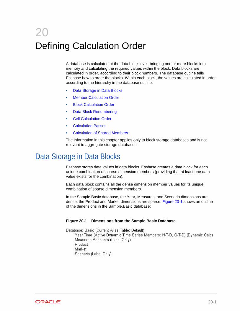
20Defining Calculation Order

A database is calculated at the data block level, bringing one or more blocks intomemory and calculating the required values within the block. Data blocks arecalculated in order, according to their block numbers. The database outline tellsEssbase how to order the blocks. Within each block, the values are calculated in orderaccording to the hierarchy in the database outline.

• Data Storage in Data Blocks

• Member Calculation Order

• Block Calculation Order

• Data Block Renumbering

• Cell Calculation Order

• Calculation Passes

• Calculation of Shared Members


Data Storage in Data BlocksEssbase stores data values in data blocks. Essbase creates a data block for eachunique combination of sparse dimension members (providing that at least one datavalue exists for the combination).

Each data block contains all the dense dimension member values for its uniquecombination of sparse dimension members.

In the Sample.Basic database, the Year, Measures, and Scenario dimensions aredense; the Product and Market dimensions are sparse. Figure 20-1 shows an outlineof the dimensions in the Sample.Basic database:

Figure 20-1 Dimensions from the Sample.Basic Database

20-1

Note:

Sample.Basic also contains five attribute dimensions. These dimensions aresparse, Dynamic Calc, meaning that attribute data is not stored in thedatabase. See Working with Attributes.

Essbase creates a data block for each unique combination of members in the Productand Market dimensions (providing that at least one data value exists for thecombination). For example, it creates one data block for the combination of 100-10,New York. This data block contains all the Year, Measures, and Scenario values for100-10, New York. Figure 20-2 shows an outline of the Product and Marketdimensions in the Sample.Basic database:

Figure 20-2 Product and Market Dimensions from the Sample.Basic Database

In Essbase, member combinations are denoted by the cross-dimensional operator.The symbol for the cross-dimensional operator is -> (a hyphen followed by a greater-than symbol). So 100-10, New York is written as 100-10 -> New York.

You can categorize data blocks in the following ways:

• Input

These blocks are created by loading data to cells in a block. Input blocks can becreated for (1) sparse, level 0 member combinations or (2) sparse, upper-levelmember combinations, when at least one of the sparse members is a parent-levelmember. Input blocks can be level 0 or upper-level blocks.

• Noninput

These blocks are created through calculations. For example, in Sample.Basic, theEast -> Cola block is created during a sparse calculation process (that is, the blockdid not exist before calculation).

• Level 0

These blocks are created for sparse member combinations when all of the sparsemembers are level 0 members. For example, in Sample.Basic, New York -> Colais a level 0 block because New York and Cola are level 0 members of theirrespective sparse dimensions. Level 0 blocks can be input or noninput blocks; forexample, a level 0 noninput block is created during an allocation process, wheredata is loaded at a parent level and then allocated down to level 0.

Chapter 20Data Storage in Data Blocks

20-2

• Upper level

These blocks are created for sparse member combinations when at least one ofthe sparse members is a parent-level member. Upper-level blocks can be input ornoninput blocks.

See Generations and Levels and Data Blocks and the Index System.

Member Calculation OrderEssbase calculates a database at the data block level, bringing one or more blocksinto memory and calculating the required values within the block. Essbase calculatesthe blocks in order, according to their block numbers. The database outline tellsEssbase how to order the blocks. Within each block, Essbase calculates the values inorder according to the hierarchy in the database outline. Therefore, overall, Essbasecalculates a database based on the database outline.

When you perform a default calculation (CALC ALL) on a database, Essbasecalculates the dimensions in this order:

• If both a dimension tagged as accounts and a dimension tagged as time exist, andif formulas are applied to members on the accounts dimension, Essbasecalculates in this order:

1. Dimension tagged as accounts

2. Dimension tagged as time

3. Other dense dimensions (in the order in which they are displayed in thedatabase outline)

4. Other sparse dimensions (in the order in which they are displayed in thedatabase outline)

• Otherwise, Essbase calculates in this order:

1. Dense dimensions (in the order in which they are displayed in the databaseoutline)

2. Sparse dimensions (in the order in which they are displayed in the databaseoutline)

Note:

Attribute dimensions, which are not included in the database consolidation,do not affect calculation order. See Working with Attributes.

In the Sample.Basic database, the dimensions are calculated in this order: Measures,Year, Scenario, Product, and Market.

You can override the default order by using a calculation script. See DevelopingCalculation Scripts for Block Storage Databases.

Understanding the Effects of Member RelationshipsThe order of calculation within each dimension depends on the relationships betweenmembers in the database outline. Within each branch of a dimension, level 0 values

Chapter 20Member Calculation Order

20-3

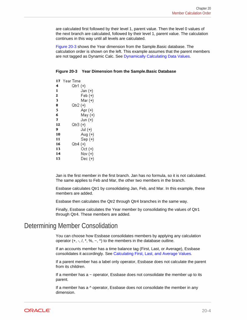
are calculated first followed by their level 1, parent value. Then the level 0 values ofthe next branch are calculated, followed by their level 1, parent value. The calculationcontinues in this way until all levels are calculated.

Figure 20-3 shows the Year dimension from the Sample.Basic database. Thecalculation order is shown on the left. This example assumes that the parent membersare not tagged as Dynamic Calc. See Dynamically Calculating Data Values.

Figure 20-3 Year Dimension from the Sample.Basic Database

Jan is the first member in the first branch. Jan has no formula, so it is not calculated.The same applies to Feb and Mar, the other two members in the branch.

Essbase calculates Qtr1 by consolidating Jan, Feb, and Mar. In this example, thesemembers are added.

Essbase then calculates the Qtr2 through Qtr4 branches in the same way.

Finally, Essbase calculates the Year member by consolidating the values of Qtr1through Qtr4. These members are added.

Determining Member ConsolidationYou can choose how Essbase consolidates members by applying any calculationoperator (+, -, /, *, %, ~, ^) to the members in the database outline.

If an accounts member has a time balance tag (First, Last, or Average), Essbaseconsolidates it accordingly. See Calculating First, Last, and Average Values.

If a parent member has a label only operator, Essbase does not calculate the parentfrom its children.

If a member has a ~ operator, Essbase does not consolidate the member up to itsparent.

If a member has a ^ operator, Essbase does not consolidate the member in anydimension.


20-4

Note:

If you use dynamic calculations, Essbase may use a different calculationorder. See Calculation Order for Dynamic Calculation.

Ordering Dimensions in the Database OutlineTo ensure the required calculation results, consider the calculation order of thedimensions in the database outline if you do either of these tasks:

• Use calculation operators to divide (/), multiply (*), or calculate percentages (%) formembers in the database outline.

• Place formulas on members in the database outline.

You need not consider calculation order if you use only calculation operators to add (+)and subtract (–) members in the database outline and you do not use formulas in theoutline.

See:

• Placing Formulas on Members in the Database Outline

• Using the Calculation Operators *, /, and %

Placing Formulas on Members in the Database OutlineIf you place formulas on members in the database outline, consider the calculationorder of the dimensions. A formula that is attached to a member on one dimensionmay be overwritten by a subsequent calculation on another dimension.

For example, the Sample.Basic database has a Measures dimension, tagged asaccounts, and a Year dimension, tagged as time. Measures is calculated first and Yearsecond. If you attach a formula to Margin on the Measures dimension, Essbasecalculates the formula when it calculates the Measures dimension. Essbase thenoverwrites the formula when it consolidates the Year dimension. See Cell CalculationOrder.

Using the Calculation Operators *, /, and %If you use calculation operators to multiply ( * ), divide ( / ), and calculate percentages( % ) for members in the database outline, consider the calculation order of thedimensions. The required calculated values may be overwritten by a subsequentcalculation on another dimension.

For example, the Sample.Basic database has a Measures dimension, tagged asaccounts, and a Year dimension, tagged as time. Measures is calculated first and Yearsecond. If you multiply members on the Measures dimension, the calculated resultsmay be overwritten when Essbase consolidates values on the Year dimension. See Cell Calculation Order.

When you use a multiplication ( * ), division ( / ), or percentage ( % ) operator toconsolidate members, carefully order the members in the branch to achieve therequired result.


20-5

Figure 20-4 shows calculations operators as they appear in an outline. Assume thatthe user wants to divide the total of Child 2 and Child 3 by Child 1. However, if Child 1is the first member, Essbase starts with Child 1, starting with the value #MISSING, anddividing it by Child 1. The result is #MISSING. Essbase then adds Child 2 and Child 3.Obviously, this result is not the required one.

Figure 20-4 Calculation Operators in the Database Outline

To calculate the correct result, make Child 1 the last member in the branch.

You can apply a formula to a member on the database outline to achieve the sameresult. However, it is far more efficient to use these calculation operators on membersas shown in Figure 20-4.

Avoiding Forward Calculation ReferencesTo obtain the calculation results you expect, ensure that the outline does not containforward calculation references. Forward calculation references occur when the valueof a calculating member is dependent on a member that Essbase has not yetcalculated. In these cases, Essbase may not produce the required calculation results.

For example, consider the Product dimension shown in Figure 20-5, which has threeforward calculation references: two shared members (P100–20 and P300–20) and onenonshared member (P500–20):

Figure 20-5 Product Dimension with Forward Calculation References


20-6

In Outline Editor, when you verify the outline, Essbase identifies shared members withforward calculation references. Verifying the outline does not identify nonsharedmembers that have forward calculation references. You can save and use an outlinecontaining forward calculation references.

Consider the five members under Diet. The members P100-20, P300-20, and P500-20have forward calculation references:

• P100-20 (+) (Shared Member): Essbase calculates the shared member P100-20before it calculates the referenced member P100-20. Because the referencedmember P100-20 has children, Essbase must calculate the referenced member byadding its children before it can accurately calculate the shared member P100-20.

• P300-20 (+) (Shared Member): Essbase calculates the shared member P300-20before it calculates the referenced member P300-20. Because the referencedmember P300-20 has a formula, Essbase must calculate the referenced memberbefore it can accurately calculate the shared member P300-20.

• P500-20 (+) (“P200-20” + “P300-20”): The formula applied to P500-20 refers tomembers that Essbase has not yet calculated. One such referenced member,P300-20, has its own formula, and Essbase must calculate P300-20 before it canaccurately calculate P500-20. The members P200-20 and P400-20 calculatecorrectly, because they do not have forward calculation references.

• P200-20 (+) (Shared Member): P200-20 is not a forward calculation reference,although Essbase calculates the shared member P200-20 before it calculates thereferenced member P200-20. The referenced member P200-20 has no calculationdependencies (no children and no formula). Therefore, Essbase does not need tocalculate the referenced member before the shared member. Essbase simplytakes the value of the referenced member.

• P400-20 (+) (“P200-10” * 2): P400-20 is not a forward calculation reference,although the formula that is applied to P400-20 references a member that Essbasehas not yet calculated. The member referenced in the formula does not itself havecalculation dependencies. P200-10 is the only member in the formula, andP200-10 does not itself have children or a formula. Essbase accurately calculatesP400-20.

To get accurate calculation results for P100-20, P300-20, and P500-20, change theorder of members in the outline. By placing the Diet shared members after the Regularmembers, as shown in Figure 20-6, you ensure that Essbase calculates the membersin the required order.


20-7

Figure 20-6 Changed Product Dimension Without Forward CalculationReferences

Now Essbase calculates:

• The referenced member P100-20 before it calculates the shared memberP100-20. So, P100-20 no longer has a forward calculation reference.

• The referenced member P300-20 before the shared member P300-20. So,P300-20 no longer has a forward calculation reference.

• The member with a formula, P300-20, before the member P500-20. So, P500-20no longer has a forward calculation reference.

Block Calculation OrderEssbase calculates blocks in the order in which the blocks are numbered. Essbasetakes the first sparse dimension in a database outline as a starting point. It defines thesparse member combinations from this first dimension.

In the Sample.Basic database, Product is the first sparse dimension in the databaseoutline.

Figure 20-7 Dimensions in the Sample.Basic Database

Chapter 20Block Calculation Order

20-8

Note:

The attribute dimensions in the Sample.Basic outline (not shown in the figureabove), are not included in the database consolidation and do not affectblock calculation order. See Working with Attributes..

As shown in Figure 20-8, Product has 19 members (excluding the shared members,for which Essbase does not create data blocks). Therefore, the first 19 data blocks inthe database are numbered according to the calculation order of members in theProduct dimension.

Figure 20-8 Product Dimension from the Sample.Basic Database

The other sparse dimension is Market. The first 19 data blocks contain the firstmember to be calculated in the Market dimension, which is New York. Table 20-1shows the sparse member combinations of each Product member and New York, forthe first five of these 19 data blocks:

Table 20-1 Sparse Member Combinations: Data Blocks 0 Through 4

Block Number Product Member Market Member

0 Cola (100-10) New York

1 Diet Cola (100-20) New York

2 Caffeine Free Cola (100-30) New York

3 Colas (100) New York

Chapter 20Block Calculation Order

20-9

Table 20-1 (Cont.) Sparse Member Combinations: Data Blocks 0 Through 4


4 Old Fashioned (200-10) New York

The next member in the Market dimension is Massachusetts. Essbase creates thenext 19 data blocks for sparse combinations of each Product member andMassachusetts. Table 20-2 shows the sparse member combinations for the blocknumbers 19 through 23:

Table 20-2 Sparse Member Combinations: Data Blocks 19 Through 23


19 Cola (100-10) Massachusetts

20 Diet Cola (100-20) Massachusetts

21 Caffeine Free Cola (100-30) Massachusetts

22 Colas (100) Massachusetts

23 Old Fashioned (200-10) Massachusetts

Essbase continues until blocks have been created for all combinations of sparsedimension members for which at least one data value exists.

Essbase creates a data block only if at least one value exists for the block. Forexample, if no data values exist for Old Fashioned Root Beer (200-10) inMassachusetts, then Essbase does not create a data block for 200-10 ->Massachusetts. However, Essbase does reserve the appropriate block number for200-10 -> Massachusetts in case data is loaded for that member combination in thefuture.

When you run a default calculation (CALC ALL) on a database, each block isprocessed in order, according to its block number. If you have Intelligent Calculationturned on, and if the block does not need to be calculated, then Essbase skips theblock and moves to the next block. For information about how intelligent calculation isused to optimize performance, see Understanding Intelligent Calculation.

Data Block RenumberingEssbase renumbers the data blocks when you make any of these changes:

• Move a sparse dimension

• Add a sparse dimension

• Change a dense dimension to a sparse dimension

• Move any member in a sparse dimension

• Delete any member in a sparse dimension

• Add a member to a sparse dimension

Chapter 20Data Block Renumbering

20-10

Cell Calculation OrderEach data block contains all the dense dimension member values for its uniquecombination of sparse dimension members. Each data value is contained in a cell ofthe data block.

The order in which Essbase calculates the cells within each block depends on howyou have configured the database. How you have configured the database defines themember calculation order of dense dimension members within each block. It alsodefines the calculation order of blocks that represent sparse dimension members.

See the following examples:

Cell Calculation Order: Example 1In this example, which is the simplest case, these conditions are true:

• No dimensions have time or accounts tags.

• The setting for consolidating #MISSING values is turned on.

• Market and Year are dense dimensions.

Essbase calculates dense dimensions in the order in which they are defined in thedatabase outline. Assume that the Year dimension is positioned in the databaseoutline before the Market dimension and is calculated first.

Table 20-3 shows a subset of the cells in a data block:

Table 20-3 Calculation Order Example 1: Input Cells and Calculated Cells

Year-Market New York Massachusetts East

Jan 112345 68754 3Feb 135788 75643 4Mar 112234 93456 5Qtr1 1 2 6

Data values have been loaded into the following input cells:

• Jan -> New York

• Feb -> New York

• Mar -> New York

• Jan -> Massachusetts

• Feb -> Massachusetts

• Mar -> Massachusetts

Essbase calculates the following cells. In Table 20-3, the calculation order for thesecells is represented by the numbers 1 through 6 that appear in the cells:

1. Qtr1 -> New York

2. Qtr1 -> Massachusetts

3. Jan -> East

Chapter 20Cell Calculation Order

20-11

4. Feb -> East

5. Mar -> East

6. Qtr1 -> East

Qtr1 -> East has multiple consolidation paths; it can be consolidated on Market or onYear. When consolidated on Market, it is a consolidation of Qtr1 -> New York and Qtr1-> Massachusetts. When consolidated on Year, it is a consolidation of Jan -> East,Feb -> East, and Mar -> East.

Essbase knows that Qtr1 -> East has multiple consolidation paths. Therefore, itcalculates Qtr1 -> East only once by consolidating the values for Qtr1 and uses theconsolidation path of the dimension calculated last (in this example, the Marketdimension), as shown in Table 20-4.

Table 20-4 Calculation Order Example 1: Results


Jan 112345 68754 181099Feb 135788 75643 211431Mar 112234 93456 205690Qtr1 360367 237853 598220

Based on the calculation order, if you place a member formula on Qtr1 in the databaseoutline, Essbase ignores it when calculating Qtr1 -> East. If you place a memberformula on East in the database outline, the formula is calculated when Essbaseconsolidates Qtr1 -> East on the Market consolidation path.

If required, you can use a calculation script to calculate the dimensions in the orderyou choose. See Developing Calculation Scripts for Block Storage Databases.

Cell Calculation Order: Example 2In this example, these conditions are true:


• The setting for consolidating #MISSING values is turned off (the default).




Table 20-5 Calculation Order Example 2: Input Cells and Calculated Cells


Jan 112345 68754 4Feb 135788 75643 5Mar 112234 93456 6Qtr1 1 2 3/7


20-12

Data values have been loaded into the following input cells:

• Jan -> New York

• Feb -> New York

• Mar -> New York

• Jan -> Massachusetts

• Feb -> Massachusetts

• Mar -> Massachusetts

Essbase calculates the Qtr1 cells for New York, Massachusetts, and East and theEast cells for Jan, Feb, and March. In Table 20-5, the calculation order for these cellsis represented by the numbers 1 through 7 that appear in the cells:

1. Qtr1 -> New York

2. Qtr1 -> Massachusetts

3. Qtr1 -> East

4. Jan -> East

5. Feb -> East

6. Mar -> East

7. Qtr1 -> East

Qtr1 -> East is calculated on both the Year and Market consolidation paths. First, Qtr1-> East is calculated as a consolidation of Qtr1 -> New York and Qtr1 ->Massachusetts. Second, Qtr1 -> East is calculated as a consolidation of Jan -> East,Feb -> East, and Mar -> East.

The results, as shown in Table 20-6, are identical to the results for example 1 (see Table 20-4). However, Qtr1 -> East has been calculated twice. This fact is significantwhen you need to load data at parent levels (see Cell Calculation Order: Example 3).



Jan 112345 68754 181099Feb 135788 75643 211431Mar 112234 93456 205690Qtr1 360367 237853 598220

Based on the calculation order, if you place a member formula on Qtr1 in the databaseoutline, its result is overwritten when Essbase consolidates Qtr1 -> East on the Marketconsolidation path. If you place a member formula on East in the database outline, theresult is retained, because the Market consolidation path is calculated last.





20-13

• Data values have been loaded at parent levels.




Table 20-7 Calculation Order Example 3: Input Cells and #MISSING Values


Jan #MISSING #MISSING 181099Feb #MISSING #MISSING 211431Mar #MISSING #MISSING 205690Qtr1 #MISSING #MISSING

The cells are calculated in the same order as in Cell Calculation Order: Example 2.Qtr1 -> East is calculated on both the Year and Market consolidation paths.

Because the setting for consolidating #MISSING values is turned off, Essbase doesnot consolidate the #MISSING values. Thus, the data that is loaded at parent levels isnot overwritten by the #MISSING values below it.

However, if any of the child data values are not #MISSING, these values areconsolidated and overwrite the parent values. For example, if Jan -> New Yorkcontains 50000.00, this value overwrites the values loaded at parent levels.

The results, as shown in Table 20-8, show that Essbase first correctly calculates theQtr1 -> East cell by consolidating Jan -> East, Feb -> East, and Mar -> East, and thencalculates on the Market consolidation path. However, it does not consolidate the#MISSING values in Qtr1 -> New York and Qtr1 -> Massachusetts; therefore, thevalue in Qtr1 -> East is not overwritten.



Jan #MISSING #MISSING 181099Feb #MISSING #MISSING 211431Mar #MISSING #MISSING 205690Qtr1 #MISSING #MISSING 598220

Essbase must calculate the Qtr1 -> East cell twice to ensure that a value is calculatedfor the cell. If Qtr1 -> East is calculated according to only the last consolidation path,the result is #MISSING, which is not the required result.


• The Year dimension is tagged as time.

• The Measures dimension is tagged as accounts.


20-14

Essbase calculates a dimension tagged as accounts first, followed by a dimensiontagged as time. Therefore, in this example, Measures is calculated before Year.


• The Marketing, Payroll, and Misc Expenses values have been loaded at the Qtr1,parent level.

Figure 20-9 shows the Profit branch of the Measures dimension in the Sample.Basicdatabase. This example assumes that Total Expenses is not a Dynamic Calc member.

Figure 20-9 Profit Branch of the Measures Dimension


Table 20-9 Calculation Order Example 4: Input Cells, #MISSING Values, and Calculated Cells

Measures/Year Jan Feb Mar Qtr1

Sales 31538 32069 32213 13COGS 14160 14307 14410 14Margin 1 4 7 10/15Marketing #MISSING #MISSING #MISSING 15839

Payroll #MISSING #MISSING #MISSING 12168

Misc #MISSING #MISSING #MISSING 233

Total Expenses 2 5 8 11/16Profit 3 6 9 12/17

The following cells have multiple consolidation paths:

• Margin -> Qtr1

• Total Expenses -> Qtr1

• Profit -> Qtr1

Because the setting for consolidating #MISSING values is turned off, Essbase doesnot consolidate the #MISSING values. Thus, any data that is loaded at parent levels isnot overwritten by the #MISSING values and Essbase calculates the cells with multipleconsolidation paths twice.

The results are shown in Table 20-10:


20-15



Sales 31538 32069 32213 95820COGS 14160 14307 14410 42877Margin 17378 17762 17803 52943Marketing #MISSING #MISSING #MISSING 15839

Payroll #MISSING #MISSING #MISSING 12168

Misc #MISSING #MISSING #MISSING 233

Total Expenses 28240Profit 17378 17762 17803 12/17

Based on the calculation order, if you place a member formula on, for example, Marginin the database outline, its result is overwritten by the consolidation on Qtr1.

Cell Calculation Order for Formulas on a Dense DimensionThe cell calculation order within a data block is not affected by formulas on members.When Essbase encounters a formula in a data block, it locks any other required datablocks, calculates the formula, and proceeds with the data block calculation.

When placing a formula on a dense dimension member, carefully consider the cellcalculation order. As described in the examples above, the dimension calculated lastoverwrites previous cell calculations for cells with multiple consolidation paths. Ifrequired, you can use a calculation script to change the order in which the dimensionsare calculated. See Developing Calculation Scripts for Block Storage Databases and Developing Formulas for Block Storage Databases.

Calculation PassesWhenever possible, Essbase calculates a database in one calculation pass throughthe database. Thus, it reads each of the required data blocks into memory only once,performing all relevant calculations on the data block and saving it. However, in somesituations, Essbase must perform multiple calculation passes through a database. Onsubsequent calculation passes, Essbase brings data blocks back into memory,performs further calculations on them, and saves them again.

When you perform a default, full calculation of a database (CALC ALL), Essbaseattempts to calculate the database in one calculation pass. If you have dimensions thatare tagged as accounts or time, Essbase may have to do multiple calculation passesthrough the database.

Table 20-11 shows the number of calculation passes Essbase performs if you havedimensions that are tagged as time or accounts, and you have at least one formula onthe accounts dimension:

Chapter 20Calculation Passes

20-16

Table 20-11 Calculation Passes For Accounts and Time Dimension

Dimension TaggedAs Accounts

Dimension TaggedAs Time

Calculation Passes During eachcalculation pass,Essbase calculatesbased on:

Dense or Sparse None 1 All dimensions

Dense Dense 1 All dimensions

Dense Sparse 2 Pass 1: Accounts andtime dimensions

Pass 2: Otherdimensions

Sparse Sparse 2 Pass 1: Accounts andtime dimensions


Sparse Dense 2 Pass 1: Accountsdimension


If you are using formulas that are tagged as Two-Pass, Essbase may need to do anextra calculation pass to calculate these formulas. See Using Two-Pass Calculation.

When you use a calculation script to calculate a database, the number of calculationpasses Essbase needs to perform depends upon the calculation script. See Calculation Passes and Understanding Multiple-Pass Calculations. Also see GroupingFormulas and Calculations.

If the isolation level is set for committed access, and multiple passes are required,Essbase writes data values at the end of each pass. Data retrievals that occurbetween passes can pick up intermediate values.

When you calculate a database, Essbase automatically displays the calculation orderof the dimensions for each pass through the database and tells you how many timesEssbase has cycled through the database during the calculation. Essbase displaysthis information in the ESSCMD shell window and in the application log.

For each data block, Essbase decides whether to do a dense or a sparse calculation.The type of calculation it chooses depends on the type of values within the data block.When you run a default calculation (CALC ALL) on a database, each block isprocessed in order, according to its block number.

Essbase calculates the blocks using this procedure:

• If you have Intelligent Calculation turned on, and if the block does not need to becalculated (if it is marked as clean), Essbase skips the block and moves to thenext block. See Understanding Intelligent Calculation.

• If the block needs recalculating, Essbase checks to see if the block is a level 0, aninput, or an upper-level block. See Data Storage in Data Blocks.

• If the block is a level 0 block or an input block, Essbase performs a densecalculation on the block. Each cell in the block is calculated. See Cell CalculationOrder.

Chapter 20Calculation Passes

20-17

• If the block is an upper-level block, Essbase either consolidates the values orperforms a sparse calculation on the data block.

The sparse member combination of each upper-level block contains at least oneparent member. Essbase consolidates or calculates the block based on the parentmember’s dimension. For example, if the upper-level block is for Product -> Floridafrom the Sample.Basic database, then Essbase chooses the Product dimension.

If the sparse member combination for the block has multiple parent members,Essbase chooses the last dimension in the calculation order that includes a parentmember. For example, if the block is for Product -> East, and you perform adefault calculation on the Sample.Basic database, Essbase chooses the Marketdimension, which contains East. The Market dimension is last in the defaultcalculation order because it is placed after the Product dimension in the databaseoutline. See Member Calculation Order.

Based on the chosen sparse dimension, Essbase either consolidates the values orperforms a sparse calculation on the data block:

– If a formula is applied to the data block member on the chosen sparsedimension, Essbase performs a formula calculation on the sparse dimension.Essbase evaluates each cell in the data block. The formula affects only themember on the sparse dimension, so overall calculation performance is notsignificantly affected.

– If the chosen sparse dimension is a default consolidation, Essbaseconsolidates the values, taking the values of the previously calculated childdata blocks.

Calculation of Shared MembersShared members are those that share data values with other members. For example,in the Sample.Basic database, Diet Cola, Diet Root Beer, and Diet Cream areconsolidated under two parents: under Diet and under their product types—Colas,Root Beer, and Cream Soda. The members under the Diet parent are sharedmembers, as shown in Figure 20-10. See Understanding Shared Members.

Chapter 20Calculation of Shared Members

20-18

Figure 20-10 Calculating Shared Members

A calculation on a shared member is a calculation on its referenced member. If youuse the FIX command to calculate a subset of a database and the subset includes ashared member, Essbase calculates the referenced member.

Chapter 20Calculation of Shared Members

20-19

21Understanding Intelligent Calculation

By default, when Essbase performs a full calculation of a database, it tracks whichdata blocks it calculates. If you then load a subset of data, on subsequent calculations,Essbase calculates only the data blocks that have not been calculated and thecalculated blocks that require recalculation because of the new data. This process iscalled Intelligent Calculation.

• About Intelligent Calculation

• Using Intelligent Calculation

• Using the SET CLEARUPDATESTATUS Command

• Calculating Data Blocks

• Understanding the Effects of Intelligent Calculation

About Intelligent CalculationBy default, when Essbase performs a full calculation of a database, it tracks whichdata blocks it calculates. If you then load a subset of data, on subsequent calculations,Essbase calculates only the data blocks that have not been calculated and thecalculated blocks that require recalculation because of the new data. This process iscalled Intelligent Calculation.

By default, Intelligent Calculation is turned on.

You can also turn Intelligent Calculation on or off in a calculation script. See TurningIntelligent Calculation On and Off.

For information on other calculation optimization methods, see:

• Designing Partitioned Applications

• Dynamically Calculating Data Values

• Optimizing Calculations

Benefits of Intelligent CalculationIntelligent Calculation is designed to provide significant calculation performancebenefits for these types of calculations:

• A full calculation of a database (CALC ALL), with some exceptions.

See Limitations of Intelligent Calculation.

• A calculation script that calculates all members in one CALC DIM statement.

• For database calculations that cannot use Intelligent Calculation for the fullcalculation, you may be able to use Intelligent Calculation for part of thecalculation.

21-1

For example, to significantly improve calculation performance for a case in whichyou calculate a database by doing a default consolidation and then an allocation ofdata, enable Intelligent Calculation for the default consolidation and then disableIntelligent Calculation for the allocation.

Assuming that Intelligent Calculation is turned on (the default), create a calculationscript to perform these steps for a partial Intelligent Calculation:

– Enable Intelligent Calculation, if it is disabled

– Use CALC ALL to calculate the database

– Use the SET UPDATECALC command to disable Intelligent Calculation

– Allocate data

– Optionally, enable Intelligent Calculation again

Intelligent Calculation and Data Block StatusTo provide Intelligent Calculation, Essbase checks the status of the data blocks in adatabase. Data blocks have a calculation status of clean or dirty. Essbase marks adata block as clean after certain calculations.

When Intelligent Calculation is enabled, Essbase calculates only dirty blocks and theirdependent parents. When disabled, Essbase calculates all data blocks, regardless ofwhether they are marked as clean or dirty.

Marking Blocks as CleanEssbase marks data blocks as clean in these types of calculations:

• A full calculation (CALC ALL) of a database (the default calculation).

• A calculation script that calculates all the dimensions in one CALC DIM statement.

For example, the following calculation script calculates all members in theSample.Basic database:

CALC DIM(Measures, Product, Market, Year, Scenario);

Compare this calculation script to a calculation script that calculates all themembers with two CALC DIM statements:

CALC DIM(Measures, Product);CALC DIM(Market, Year, Scenario);

Using two CALC DIM statements causes Essbase to do at least two calculationpasses through the database. In this calculation, Essbase does not, by default, markthe data blocks as clean. Because Intelligent Calculation depends on accurate cleanand dirty status, you must manage these markers carefully. See Maintaining Cleanand Dirty Status.

Essbase marks calculated data blocks as clean only in the situations described above,unless you use the SET CLEARUPDATESTATUS command in a calculation script.See Using the SET CLEARUPDATESTATUS Command.

Chapter 21About Intelligent Calculation

21-2

Marking Blocks as DirtyEssbase marks a data block as dirty in these situations:

• Calculating the data block for a partial calculation of the database only if SETCLEARUPDATESTATUS AFTER is not part of the partial calculation statement inthe calculation script

• Loading data into the data block

• Restructuring the database (for example, by adding a member to a densedimension)

• Copying data to the data block; for example, using DATACOPY

Maintaining Clean and Dirty StatusTo use Intelligent Calculation when calculating a subset of a database or whenperforming multiple calculation passes through a database, consider carefully theimplications of how Essbase marks data blocks as clean. When using IntelligentCalculation, you must accurately maintain the clean and dirty status of the data blocksto ensure that Essbase recalculates the database as efficiently as possible.

For example, when you calculate a subset of a database, the newly calculated datablocks are not marked as clean by default. You can ensure that the newly calculatedblocks are marked as clean by using the SET CLEARUPDATESTATUS AFTERcommand in a calculation script. Before creating the calculation script, see Using theSET CLEARUPDATESTATUS Command and Technical Reference for OracleEssbase.

Limitations of Intelligent CalculationConsider the following limitations and situations when using Intelligent Calculation:

• Intelligent Calculation works on a data block level and not on a cell level. Forexample, if you load a data value into one cell of a data block, the whole datablock is marked as dirty.

• A CALC ALL that requires two passes through the database may calculateincorrectly. The problem occurs because blocks that are marked clean during thefirst pass are skipped during the second pass. To avoid this problem, turnIntelligent Calculation off or perform a CALC DIM for each dimension (rather thana CALC ALL for the database). A CALC ALL requires two passes through thedatabase in either of these situations:

– When the accounts dimension is sparse

– When the accounts dimension is dense, the time dimension is sparse, andthere is at least one more dense dimension in the outline

• Changing a formula on the database outline or changing an accounts property onthe database outline does not cause Essbase to restructure the database.Therefore, Essbase does not mark the affected blocks as dirty. You mustrecalculate the appropriate data blocks. See Changing Formulas and AccountsProperties.

• Whenever possible, Essbase calculates formulas that are tagged as two-pass andin the dimension tagged as accounts as part of the main calculation of a database.

Chapter 21About Intelligent Calculation

21-3

You may, however, need to use a calculation script to calculate some formulastwice. When you use a calculation script, disable Intelligent Calculation beforerecalculating formulas.

• When SET CREATENONMISSINGBLK is set to ON in a calculation script,Intelligent Calculation is turned off, and affected blocks are calculated whetherthey are marked clean or dirty.

Considerations for Essbase Intelligent Calculation on Oracle ExalyticsIn-Memory Machine

The following functionality applies only to Essbase running on an Oracle Exalytics In-Memory machine.

Status bits for Intelligent Calculation on a block storage database are not persisted.Therefore, Intelligent Calculation works as intended only if both of the followingconditions are true:

• The whole index fits in the index cache

• Related calculation scripts that use Intelligent Calculation complete within thelifetime of the Essbase Server

For Intelligent Calculation, set the index cache size large enough to fit the whole indexand to account for future index growth due to data load or calculation.

Using Intelligent CalculationThis section provides information on turning Intelligent Calculation on and off andusing Intelligent Calculation with different types of calculations.

See:

• Turning Intelligent Calculation On and Off

• Using Intelligent Calculation for a Default, Full Calculation

• Using Intelligent Calculation for a Calculation Script, Partial Calculation

Turning Intelligent Calculation On and OffBy default, Intelligent Calculation is turned on.

To turn Intelligent Calculation on and off for the duration of a calculation script, use theSET UPDATECALC command in a calculation script.

See Technical Reference for Oracle Essbase.

Using Intelligent Calculation for a Default, Full CalculationIntelligent Calculation provides significant performance benefits when you do a fullcalculation (CALC ALL) of a database. If you do a full calculation, leave IntelligentCalculation turned on (the default) to take advantage of its performance benefits.

Chapter 21Using Intelligent Calculation

21-4

Caution:

When using Intelligent Calculation, note the information in Limitations ofIntelligent Calculation.

Calculating for the First TimeWhen you do the first full calculation of a database, Essbase calculates every block.The performance is the same whether Intelligent Calculation is on or off.

RecalculatingWhen you do a full recalculation of a database with Intelligent Calculation turned on,Essbase checks each block to see whether it is marked as clean or dirty. See Intelligent Calculation and Data Block Status.

Checking data blocks has a 5% to 10% performance overhead, which is insignificantwhen compared to the performance gained by enabling Intelligent Calculation.

If, however, you recalculate a database in which more than approximately 80% of thevalues have changed, the overhead of Intelligent Calculation may outweigh thebenefits. In this case, disable Intelligent Calculation.

Using Intelligent Calculation for a Calculation Script, Partial CalculationEssbase marks a data block as clean when it calculates the data block on a fullcalculation (CALC ALL) or when it calculates all dimensions in one CALC DIMcommand. See Marking Blocks as Clean.

In any other calculations, Essbase does not mark calculated data blocks as clean,unless you use the SET CLEARUPDATESTATUS command in a calculation script.For example, if you calculate a subset of a database or calculate a database in twocalculation passes, Essbase does not mark the calculated blocks as clean, unless youuse the SET CLEARUPDATESTATUS command.

The following calculation scripts do not cause Essbase to mark the calculated datablocks as clean:

FIX(“New York”) CALC DIM(Product, Measures);ENDFIX

CALC DIM(Measures, Product);CALC DIM(Market, Year, Scenario);

Use SET CLEARUPDATESTATUS to avoid unnecessary recalculations.

Using the SET CLEARUPDATESTATUS CommandIn some cases, Essbase does not mark calculated blocks as clean; for example, if youcalculate a subset of a database or calculate a database in two calculation passes. To

Chapter 21Using the SET CLEARUPDATESTATUS Command

21-5

manually mark data blocks as clean for purposes of Intelligent Calculation, use theSET CLEARUPDATESTATUS command in a calculation script. Read this section, andalso see Intelligent Calculation and Data Block Status.

Understanding SET CLEARUPDATESTATUSThe SET CLEARUPDATESTATUS command has three parameters—AFTER, ONLY,and OFF.

• SET CLEARUPDATESTATUS AFTER;

Essbase marks calculated data blocks as clean, even if it is calculating a subset ofa database.

• SET CLEARUPDATESTATUS ONLY;

Essbase marks the specified data blocks as clean but does not calculate the datablocks. This parameter provides the same result as AFTER, but withoutcalculation.

• SET CLEARUPDATESTATUS OFF;

Essbase calculates the data blocks but does not mark the calculated data blocksas clean. Data blocks are not marked as clean, even on a full calculation (CALCALL) of a database. The existing clean or dirty status of the calculated data blocksremains unchanged.

Choosing a SET CLEARUPDATESTATUS SettingWhen you use the SET CLEARUPDATESTATUS command to mark calculated datablocks as clean, be aware of these recommendations before selecting the parameter(AFTER, ONLY, OFF):

• Only calculated data blocks are marked as clean.

• Do not use the SET CLEARUPDATESTATUS AFTER command with concurrentcalculations unless you are certain that the concurrent calculations do not need tocalculate the same data block or blocks. If concurrent calculations attempt tocalculate the same data blocks, with Intelligent Calculation enabled, Essbase doesnot recalculate the data blocks if the data blocks are already marked clean by theother concurrent calculation. See Handling Concurrent Calculations.

• When Essbase calculates data blocks on a first calculation pass through adatabase, it marks the data blocks as clean. If you try to calculate the same datablocks on a subsequent pass with Intelligent Calculation enabled, Essbase doesnot recalculate the data blocks, because they are already marked as clean.

Reviewing Examples That Use SET CLEARUPDATESTATUSAssume a scenario using the Sample.Basic database:

• Sparse dimensions are Market and Product.

• New York is a member on the sparse Market dimension.

• Intelligent Calculation is turned on (the default).

These examples show different ways of using SET CLEARUPDATESTATUS:

Chapter 21Using the SET CLEARUPDATESTATUS Command

21-6

Example 1: CLEARUPDATESTATUS AFTER

SET CLEARUPDATESTATUS AFTER;FIX(“New York”) CALC DIM(Product);ENDFIX

In this example, Essbase searches for dirty parent data blocks for New York (forexample New York -> Colas, in which Colas is a parent member on the Productdimension). It calculates these dirty blocks and marks them as clean. Essbase doesnot mark the level 0 data blocks as clean, because they are not calculated. Forinformation on level 0 blocks, see Defining Calculation Order.

Example 2: CLEARUPDATESTATUS ONLY

SET CLEARUPDATESTATUS ONLY;FIX(“New York”) CALC DIM(Product);ENDFIX

Essbase searches for dirty parent data blocks for New York (for example New York ->Colas, in which Colas is a parent member on the Product dimension). Essbase marksthe dirty parent data blocks as clean but does not calculate the data blocks. Essbasedoes not mark the level 0 data blocks as clean because they are not calculated. Forexample, if New York -> 100-10 (a level 0 block) is dirty, it remains dirty.

Example 3: CLEARUPDATESTATUS OFF

SET CLEARUPDATESTATUS OFF;CALC ALL;CALC TWOPASS;SET CLEARUPDATESTATUS ONLY;CALC ALL;

In this example, Essbase first calculates all the dirty data blocks in the database. Thecalculated data blocks remain dirty. Essbase does not mark them as clean.

Essbase then calculates the members tagged as two-pass that are in the dimensiontagged as accounts. Because the data blocks are still marked as dirty, Essbaserecalculates them. Again, it does not mark the calculated data blocks as clean.

Essbase then searches for all the dirty blocks in the database and marks them asclean. It does not calculate the blocks, although a CALC ALL command is used.

Calculating Data BlocksEssbase creates a data block for each unique combination of sparse dimensionmembers, provided that at least one data value exists for the combination. Each datablock represents all dense dimension member values for that unique combination ofsparse dimension members.

Chapter 21Calculating Data Blocks

21-7

For example, in the Sample.Basic database, the Market and Product dimensions aresparse. Therefore, the data block New York -> Colas represents all the member valueson the Year, Measures, and Scenario dimensions for the sparse combination NewYork -> Colas.

These sections assume that you are familiar with the concepts of upper-level, level 0,and input data blocks. See Data Storage in Data Blocks.

Calculating Dense DimensionsWhen you calculate a dense dimension and do not use a FIX command, Essbasecalculates at least some of the data values in every data block in the database.

For example, the following calculation script is based on the Sample.Basic database:

SET CLEARUPDATESTATUS AFTER;CALC DIM(Year);

This script calculates the Year dimension, which is a dense dimension. Because Yearis dense, every data block in the database includes members of the Year dimension.Therefore, Essbase calculates data values in every data block. Because the scriptuses the SET CLEARUPDATESTATUS AFTER command, Essbase marks all datablocks as clean.

Calculating Sparse DimensionsWhen you calculate a sparse dimension, Essbase may not need to calculate everydata block in the database.

For example, the following calculation script is based on the Sample.Basic database:

SET CLEARUPDATESTATUS AFTER;CALC DIM(Product);

This script calculates the Product dimension, which is a sparse dimension. BecauseProduct is sparse, a data block exists for each member on the Product dimension. Forexample, one data block exists for New York -> Colas and another for New York ->100-10.

Level 0 EffectsThe data block New York -> 100-10 is a level 0 block; it does not represent a parentmember on either sparse dimension (Market or Product). The data values for NewYork -> 100-10 are input values; they are loaded into the database. Therefore,Essbase does not need to calculate this data block. Nor does Essbase mark the datablock for New York -> 100-10 as clean, even though the script uses the SETCLEARUPDATESTATUS AFTER command.


21-8

Note:

Essbase calculates level 0 data blocks if a corresponding sparse, level 0member has a formula applied to it.

If you load data into a database, the level 0 data blocks into which you load data aremarked as dirty. If you subsequently calculate only a sparse dimension or dimensions,the level 0 blocks remain dirty, because Essbase does not calculate them. Therefore,when you recalculate only a sparse dimension or dimensions, Essbase recalculates allupper-level data blocks, because the upper-level blocks are marked as dirty if theirchild blocks are dirty, although the upper-level blocks were originally clean.

Upper-Level EffectsColas is a parent-level member on the Product dimension. Essbase must calculatevalues for Colas, so Essbase calculates this data block. Because the script uses theSET CLEARUPDATESTATUS AFTER command, Essbase marks the data block asclean.

When Essbase calculates a sparse dimension, it recalculates an upper-level datablock if the block is dependent on one or more dirty child blocks.

Unnecessary CalculationYou can avoid unnecessary calculation by calculating at least one dense dimension.When you calculate a dense dimension and do not use the FIX command, data valuesare calculated in every data block, including the level 0 blocks. So the level 0 blocksare marked as clean.

Handling Concurrent CalculationsIf concurrent calculations attempt to calculate the same data blocks, and IntelligentCalculation is turned on, Essbase may not recalculate the data blocks, because theyare already marked as clean.

In the following example, based on the Sample.Basic database, Actual and Budget aremembers of the dense Scenario dimension. Because Scenario is dense, each datablock in the database contains Actual and Budget values. If User 1 runs the followingcalculation script, Essbase calculates the Actual values for all data blocks thatrepresent New York. Essbase marks the calculated data blocks as clean, although notall the data values in each calculated block have been calculated. For example, theBudget values have not been calculated.

SET CLEARUPDATESTATUS AFTER;FIX(“New York”, Actual) CALC DIM(Product, Year);ENDFIX


21-9

If User 2 runs the following calculation script to calculate the Budget values for NewYork, Essbase does not recalculate the specified data blocks, because they arealready marked as clean. The calculation results for Budget are not correct.

SET CLEARUPDATESTATUS AFTER;FIX(“New York”, Budget) CALC DIM(Product, Year);ENDFIX

One way to solve this problem is to make the Scenario dimension sparse. Then theActual and Budget values are in different data blocks; for example, New York -> Colas-> Actual and New York -> Colas -> Budget. In this case, the second calculation scriptcorrectly calculates Budget data block.

Running concurrent calculations might require an increase in the data cache.

Understanding Multiple-Pass CalculationsWhenever possible, Essbase calculates a database in one calculation pass throughthe database. See Calculation Passes.

When you use a calculation script to calculate a database, the number of calculationpasses that Essbase performs depends upon the calculation script. See IntelligentCalculation and Data Block Status and Grouping Formulas and Calculations.

For example, assume that Essbase calculates data blocks on a first calculation passthrough a database and marks them as clean. If you attempt to calculate the samedata blocks on a subsequent pass and Intelligent Calculation is enabled, Essbasedoes not recalculate the data blocks, because they are already marked as clean.

Reviewing Examples and Solutions for Multiple-Pass CalculationsThese examples describe situations that produce incorrect calculation results andprovide a solution to obtain correct results. They are based on the Sample.Basicdatabase and assume that Intelligent Calculation is turned on.

Example 1: Intelligent Calculation and Two-PassThis calculation script does a default calculation and then a two-pass calculation:

CALC ALL;CALC TWOPASS;

Error

Essbase calculates the dirty data blocks in the database and marks all the data blocksas clean. Essbase then needs to recalculate the members tagged as two-pass in thedimension tagged as accounts. However, Essbase does not recalculate the specifieddata blocks because they are already marked as clean. The calculation results are notcorrect.


21-10

Solution

You can calculate the correct results by disabling Intelligent Calculation for the two-pass calculation.

Example 2: SET CLEARUPDATESTATUS and FIXThis calculation script calculates data values for New York. The calculation is basedon the Product dimension:

SET CLEARUPDATESTATUS AFTER;FIX(“New York”) CALC DIM(Product);ENDFIXCALC TWOPASS;

Error

Essbase performs the following processes:

1. Essbase cycles through the database calculating the dirty data blocks thatrepresent New York. The calculation is based on the Product dimension. Thus,Essbase calculates only the blocks that represent a parent member on the Productdimension (for example, New York -> Colas, New York -> Root Beer, and NewYork -> Fruit Soda), and then only calculates the aggregations and formulas forthe Product dimension.

2. Because the SET CLEARUPDATESTATUS AFTER command is used, Essbasemarks the calculated data blocks as clean, although not all data values in eachcalculated block have been calculated.

3. Essbase should recalculate the members tagged as two-pass in the dimensiontagged as accounts; however, some of these data blocks are already marked asclean from the calculation in the previous step. Essbase does not recalculate thedata blocks that are marked as clean. The calculation results are not correct.

Solution

You can calculate the correct results by disabling Intelligent Calculation for the two-pass calculation.

Example 3: SET CLEARUPDATESTATUS and Two CALC DIM CommandsThis calculation script bases the database calculation on the Product and Yeardimensions. Because two CALC DIM commands are used, Essbase does twocalculation passes through the database:

SET CLEARUPDATESTATUS AFTER;CALC DIM(Product);CALC DIM(Year);

Error

Essbase performs the following processes:


21-11

1. Essbase cycles through the database calculating the dirty data blocks. Thecalculation is based on the Product dimension, as in Example 2: SETCLEARUPDATESTATUS and FIX.

2. Because the SET CLEARUPDATESTATUS AFTER command is used, Essbasemarks the calculated data blocks as clean, although not all data values in eachcalculated block have been calculated.

3. Essbase should recalculate the data blocks. The recalculation is based on theYear dimension. However, as a result of the calculation in the previous step, somedata blocks are already marked as clean, and Essbase does not recalculate them.The calculation results are not correct.

Solution

You can calculate the correct results by using one CALC DIM command to calculatethe Product and Year dimensions. Essbase calculates both dimensions in onecalculation pass through the database.

The following calculation script calculates the correct results:

SET CLEARUPDATESTATUS AFTER;CALC DIM(Product, Year);

Note:

When you calculate several dimensions in one CALC DIM command,Essbase calculates the dimensions in the default calculation order and not inthe order in which you list them in the command. See Member CalculationOrder.

Example 4: Two Calculation ScriptsThis example calculates data values for New York but calculates based on twodimensions using two calculation scripts. The first calculation script calculates theProduct dimension:

SET CLEARUPDATESTATUS AFTER;FIX(“New York”) CALC DIM(Product);ENDFIX

Essbase calculates the data blocks that include New York. Because the calculation isbased on the Product dimension, Essbase calculates only the dirty blocks that includea parent member on the Product dimension (for example, New York -> Colas, NewYork -> Root Beer, and New York -> Fruit Soda), and calculates only the aggregationsand formulas for the Product dimension.

Because of the CLEARUPDATESTATUS AFTER command, Essbase marks thecalculated data blocks as clean, although not all data values in each calculated blockhave been calculated.


21-12

The second calculation script calculates the Year dimension:

SET CLEARUPDATESTATUS AFTER;FIX(“New York”) CALC DIM(Year);ENDFIX

Essbase calculates the data blocks that represent New York. Because the calculationis based on the Year dimension, which is a dense dimension, Essbase shouldcalculate all data blocks that include New York, although within each block Essbasecalculates only the aggregations and formulas for the Year dimension.

Error

As a result of the first calculation, some data blocks for New York are already markedas clean. Essbase does not recalculate these data blocks with the second calculationscript because the data blocks are marked as clean. The calculation results are notcorrect.

Solution

You can calculate the correct results by telling Essbase not to mark the calculateddata blocks as clean. The following calculation script calculates the correct results:

SET CLEARUPDATESTATUS OFF;FIX(“New York”) CALC DIM(Product);ENDFIXSET CLEARUPDATESTATUS AFTER;FIX(“New York”) CALC DIM(Year);ENDFIX

With the SET CLEARUPDATESTATUS OFF command, Essbase calculates dirty datablocks but does not to mark them as clean, unlike the SET CLEARUPDATESTATUSAFTER command.

This solution assumes that the data blocks are not marked as clean from a previouspartial calculation of the database.

You can ensure that all data blocks are calculated, regardless of their status, bydisabling Intelligent Calculation. The following calculation script calculates all specifieddata blocks, regardless of their clean or dirty status:

SET UPDATECALC OFF;FIX(“New York”) CALC DIM(Year, Product);ENDFIX

Because you have not used the SET CLEARUPDATESTATUS AFTER command,Essbase does not mark calculated data blocks as clean.


21-13

Understanding the Effects of Intelligent CalculationUsing Intelligent Calculation may have implications for how you administer a database.This section discusses the implications of each action.

Changing Formulas and Accounts PropertiesBecause neither changing a formula in the database outline nor changing an accountsproperty in the database outline causes Essbase to restructure the database, datablocks affected by such a change are not marked as dirty. For example, if you changea time balance tag in the dimension tagged as accounts, Essbase does not restructurethe database and does not mark the affected blocks as dirty.

When you subsequently run a default calculation with Intelligent Calculation turned on,the changes are not calculated. To recalculate the appropriate data blocks, use acalculation script to perform any of the following tasks:

• Disable Intelligent Calculation and calculate the member formula that haschanged.

• Disable Intelligent Calculation and use the FIX command to calculate theappropriate subset of a database.

• Disable Intelligent Calculation and perform a default CALC ALL on a database.

Using Relationship and Financial FunctionsIf you use relationship functions (for example, @PRIOR or @NEXT) or financialfunctions (for example, @ACCUM, @NPV, or @INTEREST) in a formula on a sparsedimension or a dense dimension, Essbase always recalculates the data block thatcontains the formula.

See Technical Reference for Oracle Essbase.

Restructuring DatabasesWhen you restructure a database (for example, by adding a member to a densedimension), all data blocks potentially need recalculating. Therefore, Essbase marksall data blocks as dirty. When you calculate the restructured database, all blocks arecalculated.

Note:

Changing a formula in the database outline or changing an accountsproperty in the database outline does not cause Essbase to restructure thedatabase. You must recalculate the appropriate data blocks. See ChangingFormulas and Accounts Properties.

Chapter 21Understanding the Effects of Intelligent Calculation

21-14

Copying and Clearing DataWhen you copy values to a data block by using the DATACOPY command, theresulting data block is marked as dirty. Essbase calculates the block when yourecalculate a database.

When you clear data values by using the CLEARDATA and CLEARBLOCKcommands, Essbase clears all the blocks regardless of how they are marked.

Converting CurrenciesWhen you convert currencies using the CCONV command, the resulting data blocksare marked as dirty. Essbase calculates all converted blocks when you recalculate adatabase.

Chapter 21Understanding the Effects of Intelligent Calculation

21-15

22Dynamically Calculating Data Values

When you design the overall database calculation, it may be more efficient to calculatesome member combinations when you retrieve their data, instead of precalculating themember combinations during a batch database calculation. Dynamically calculatingsome values in a database can significantly improve the performance of an overalldatabase calculation.

• Understanding Dynamic Calculation

• Benefitting from Dynamic Calculation

• Using Dynamic Calculation

• Choosing Values to Calculate Dynamically

• Understanding How Dynamic Calculation Changes Calculation Order

• Reducing the Impact on Retrieval Time

• Using Dynamic Calculations with Standard Procedures

• Creating Dynamic Calc Members

• Restructuring Databases

• Dynamically Calculating Data in Partitions

• Custom Solve Order in Hybrid Aggregation Mode


Understanding Dynamic CalculationWhen you design the overall database calculation, it may be more efficient to calculatesome member combinations when you retrieve their data, instead of precalculating themember combinations during a batch database calculation. Dynamically calculatingsome values in a database can significantly improve the performance of an overalldatabase calculation.

In Essbase, you can define a member to have a dynamic calculation. This definitiontells Essbase to calculate a data value for the member as users request it. Dynamiccalculation shortens batch database calculation time, but may increase retrieval timefor the dynamically calculated data values. See Reducing the Impact on RetrievalTime.

In Essbase you specify dynamic calculations on a per-member basis. See Understanding Dynamic Calc Members

Understanding Dynamic Calc MembersFor a member tagged as Dynamic Calc, Essbase does not calculate its data valueduring a batch database calculation (for example, during a CALC ALL). Instead,

22-1

Essbase calculates the data value upon retrieval (for example, when you retrieve thedata into Smart View.)

Specifically, Essbase calculates a data value dynamically when you request the datavalue in either of two ways:

• By retrieving the data value into Smart View

• By running a report script that displays the data value

Essbase does not store the calculated value; it recalculates the value for eachsubsequent retrieval.

Retrieving the Parent Value of Dynamically Calculated Child ValuesIf you retrieve a parent value that is calculated from Dynamic Calc child members,Essbase must dynamically calculate the child member combinations before calculatingthe parent value.

Benefitting from Dynamic CalculationDynamically calculating some database values can significantly improve theperformance of an overall database calculation.

By calculating some data values dynamically, you reduce:

• Batch calculation time of the database, because Essbase has fewer membercombinations to calculate.

• Disk usage, because Essbase stores fewer calculated data values. Database sizeand index size are also reduced.

• Database restructure time. For example, adding or deleting a Dynamic Calcmember in a dense dimension does not change the data block size, so Essbasedoes not need to restructure the database. See Restructuring Databases.

• Time required to back up the database. Because database size is reduced,Essbase takes less time to perform a backup.

Data values that Essbase calculates dynamically can take longer to retrieve. You canestimate the retrieval time for dynamically calculated members. See Reducing theImpact on Retrieval Time.

Using Dynamic CalculationYou can tag any member as Dynamic Calc, except the following members:

• Level 0 members that do not have a formula

• Label-only members

• Shared members

Which members you choose to calculate dynamically depends on the databasestructure and on the balance between (1) the need for reduced calculation time anddisk usage and (2) the need for speedy data retrieval for users. See Choosing Valuesto Calculate Dynamically.

In Outline Editor, you can see which members are Dynamic Calc. Figure 22-1 showsDynamic Calc members.

Chapter 22Benefitting from Dynamic Calculation

22-2

Figure 22-1 Sample.Basic Outline Showing Dynamic Calc Members

In Smart View, users can display visual cues to distinguish dynamically calculatedvalues. See the Oracle Smart View for Office User’s Guide.

When developing spreadsheets that include dynamically calculated values,spreadsheet designers may want to use the spreadsheet Navigate Without Dataoption, so that Essbase does not dynamically calculate and store values while testspreadsheets are built.

Choosing Values to Calculate DynamicallyDynamically calculating some data values decreases calculation time and disk usageand reduces database restructure time but increases retrieval time for dynamicallycalculated data values.

Use the guidelines described in the following sections when deciding which membersto calculate dynamically.

Dense Members and Dynamic CalculationConsider making the following changes to members of dense dimensions:

• Tag upper-level members of dense dimensions as Dynamic Calc.

• Try tagging level 0 members of dense dimensions with simple formulas asDynamic Calc, and assess the increase in retrieval time.

Simple formulas do not require Essbase to perform an expensive calculation.Formulas containing financial functions or cross-dimensional operators (->) arecomplex formulas.

Sparse Members and Dynamic CalculationConsider making the following changes to members of sparse dimensions:

• Tag some upper-level members of sparse dimensions that have six or fewerchildren as Dynamic Calc.

• Tag sparse-dimension members with complex formulas as Dynamic Calc.

A complex formula requires Essbase to perform an expensive calculation. Forexample, any formula that contains a financial function is a complex formula. See Using Complex Formulas

• Tag upper-level members in a dimension that you frequently restructure asDynamic Calc.

• Do not tag upper-level, sparse-dimension members that have 20 or moredescendants as Dynamic Calc.

Chapter 22Choosing Values to Calculate Dynamically

22-3

Two-Pass Members and Dynamic CalculationTo reduce the time needed to perform batch calculations, tag two-pass members asDynamic Calc. You can tag any Dynamic Calc member as two-pass, even if it is not onan accounts dimension. See Using Two-Pass Calculation.

For information about the interaction of members tagged as two-pass and attributemembers, see Comparing Attribute and Standard Dimensions.

For information about how querying on a two-pass member in a dense dimensionimpacts the dynamic calculator cache, see Two-Pass Members and DynamicCalculation.

Parent-Child Relationships and Dynamic CalculationIf a parent member has one child member, and you tag the child as Dynamic Calc, youmust also tag the parent as Dynamic Calc.

However, if a parent member has one child member, and the parent is a Dynamic Calcmember, you do not have to tag the child as Dynamic Calc.

Calculation Scripts and Dynamic CalculationWhen Essbase calculates a CALC ALL or CALC DIM statement in a calculation script,it bypasses the calculation of Dynamic Calc members.

Similarly, if a member set function (for example, @CHILDREN or @SIBLINGS) is usedto specify the list of members to calculate, Essbase bypasses the calculation of anyDynamic Calc members in the resulting list.

If you specify a Dynamic Calc member explicitly in a calculation script, the calculationscript fails. You cannot do a calculation script calculation of a Dynamic Calc member.To use a calculation script to calculate a member explicitly, do not tag the member asDynamic Calc.

For example, the following calculation script is valid only if Qtr1 is not a Dynamic Calcmember:

FIX (East, Colas) Qtr1;ENDFIX

Formulas and Dynamically Calculated MembersYou can include a dynamically calculated member in a formula when you apply theformula to the database outline. For example, if Qtr1 is a Dynamic Calc member, youcan place the following formula on Qtr1 in the database outline:

Qtr1 = Jan + Feb;

You cannot make a dynamically calculated member the target of a formula calculationin a calculation script; Essbase does not reserve memory for a dynamically calculatedvalue and, therefore, cannot assign a value to it. For example, if Qtr1 is a Dynamic


22-4

Calc member, Essbase displays a syntax error if you include the following formula in acalculation script:

Qtr1 = Jan + Feb;

If Qtr1 is a Dynamic Calc member and Year is not, you can use the following formulain a calculation script:

Year = Qtr1 + Qtr2;

This formula is valid because Essbase does not assign a value to the dynamicallycalculated member.

Note:

When you reference a dynamically calculated member in a formula in thedatabase outline or in a calculation script, Essbase interrupts the regularcalculation to do the dynamic calculation. This interruption can significantlyreduce calculation performance.

Scripts and Dynamically Calculated MembersThe preprocessing phase of a calculation script cannot determine whether an outlinecontains dense Dynamic Calc members. If a script contains runtime-dependentformulas, Essbase must calculate all dense Dynamic Calc members when the script isexecuted. Using the SET FRMLRTDYNAMIC OFF calculation command improvesperformance by stopping calculation of these Dynamic Calc members.

Dynamically Calculated ChildrenIf the calculation of a member depends on the calculation of Dynamic Calc childmembers, Essbase must calculate the child members first during the batch databasecalculation in order to calculate the parent. Therefore, regular calculation time is notreduced. This requirement applies to members of sparse dimensions and members ofdense dimensions.

For example, in Figure 22-2, Qtr1 is a Dynamic Calc member. Its children, Jan, Feb,and Mar, are not dynamic members. Its parent, Year, is not a dynamic member. WhenEssbase calculates Year during a batch database calculation, it must consolidate thevalues of its children, including Qtr1. Therefore, it must take the additional time tocalculate Qtr1, although Qtr1 is a Dynamic Calc member.

Figure 22-2 Sample.Basic Outline, Showing Qtr1 as a Dynamic Calc Member


22-5

Understanding How Dynamic Calculation ChangesCalculation Order

Using dynamically calculated data values changes the order in which Essbasecalculates the values and can have implications for how you administer a database.

Calculation Order for Dynamic CalculationWhen Essbase dynamically calculates data values, it calculates the data in an orderdifferent from the batch database calculation order.

During batch calculations, Essbase calculates the database in the following order:

1. Dimension tagged as accounts

2. Dimension tagged as time

3. Other dense dimensions (in the order in which they appear in the databaseoutline)

4. Other sparse dimensions (in the order in which they appear in the databaseoutline)

5. Two-pass calculations

See Defining Calculation Order.

For dynamically calculated values, on retrieval, Essbase calculates the values bycalculating the database in the following order:

1. Sparse dimensions

• If the dimension tagged as time is sparse and the database outline uses timeseries data, Essbase bases the sparse calculation on the time dimension.

• Otherwise, Essbase bases the calculation on the dimension that it normallyuses for a batch calculation.

2. Dense dimensions

a. Dimension tagged as accounts, if dense

b. Dimension tagged as time, if dense

c. Time series calculations

d. Remaining dense dimensions

e. Two-pass calculations

f. Attributes

If your data retrieval uses attribute members, the last step in the calculation order isthe summation of the attributes. Attribute calculation performs on-the-fly aggregationon data blocks that match the attribute members specified in the query. When thequery contains two-pass calculation members, attribute calculation applies the two-pass calculation member formula after all the aggregated values are collected. Thistwo-pass calculation uses the data values from the attribute calculation, not the valuesin a real data block.

Chapter 22Understanding How Dynamic Calculation Changes Calculation Order

22-6

The use of attribute members in your query causes Essbase to disregard the value ofthe Time Balance member in the dynamic calculations. During retrievals that do notuse attributes, the value of the Time Balance member is applied to the calculations.The difference in calculation procedure between the use and nonuse of attributemembers generates different results for any upper-level time members that aredynamically calculated.

During retrievals that do not use attributes, these dynamically calculated members arecalculated in the last step and, therefore, apply the time balance functionality properly.However, during retrievals that do use attributes, the summation of the attribute is thelast step applied. The difference in calculation order produces two different,predictable results for upper-level time members that are dynamically calculated.

Calculation Order for Dynamically Calculating Two-Pass MembersConsider the following information to ensure that Essbase produces the requiredcalculation result when it dynamically calculates data values for members tagged astwo-pass (see Using Two-Pass Calculation).

If multiple Dynamic Calc dense dimension member are tagged as two-pass, Essbaseperforms the dynamic calculation in the first pass, and then calculates the two-passmembers in this order:

1. Two-pass members in the accounts dimension, if any exist

2. Two-pass members in the time dimension, if any exist

3. Two-pass members in the remaining dense dimensions in the order in which thedimensions appear in the outline

For example, in the Sample.Basic database, assume the following:

• Margin% in the dense Measures dimension (the dimension tagged as accounts) istagged as Dynamic Calc and two-pass.

• Variance in the dense Scenario dimension is tagged as Dynamic Calc and two-pass.

Essbase calculates the accounts dimension member first. So, Essbase calculatesMargin% (from the Measures dimension) and then calculates Variance (from theScenario dimension).

If Scenario is a sparse dimension, Essbase calculates Variance first, following theregular calculation order for dynamic calculations. Essbase then calculates Margin%.See Calculation Order for Dynamic Calculation.

This calculation order does not produce the required result, because Essbase needsto calculate Margin % -> Variance using the formula on Margin %, and not the formulaon Variance. You can avoid this problem by making Scenario a dense dimension. Thisproblem does not occur if the Measures dimension (the accounts dimension) issparse, because Essbase still calculates Margin% first.

Calculation Order for Asymmetric DataBecause the calculation order used for dynamic calculations differs from thecalculation order used for batch database calculations, in some database outlines, youmay get different calculation results if you tag certain members as Dynamic Calc.These differences happen when Essbase dynamically calculates asymmetric data.


22-7

Symmetric data calculations produce the same results no matter which dimension iscalculated.

Using the data set in Table 22-1, the calculation for Qtr1-> Profit produces the sameresult whether you calculate along the dimension tagged as time or the dimensiontagged as accounts. Calculating along the time dimension, add the values for Jan,Feb, and Mar:

50+100+150=300

Calculating along the accounts dimension, subtract Qtr1 -> COGS from Qtr1 -> Sales:

600–300=300

Table 22-1 Example of a Symmetric Calculation

Time -> Accounts Jan Feb Mar Qtr1

Sales 100 200 300 600

COGS 50 100 150 300

Profit (Sales –COGS)

50 100 150 300

Asymmetric data calculations calculate differently along different dimensions.

Using the data set in Table 22-2, the calculation for East -> Sales produces the correctresult when you calculate along the Market dimension, but produces an incorrect resultwhen you calculate along the accounts dimension. Calculating along the Marketdimension, adding the values for New York, Florida, and Connecticut produces thecorrect results:

50 + 100 + 100 = 250

Calculating along the accounts dimension, multiplying the value East -> Price by thevalue East -> UnitsSold produces incorrect results:

15 * 50 = 750

Table 22-2 Example of an Asymmetric Calculation

Market -> Accounts New York Florida Connecticut East

UnitsSold 10 20 20 50

Price 5 5 5 15

Sales (Price *UnitsSold)

50 100 100 250

In the following outline, East is a sparse dimension, and Accounts is a densedimension:


22-8

If East and Sales are tagged as Dynamic Calc, Essbase calculates a different resultthan it does if East and Sales are not tagged as Dynamic Calc.

If East and Sales are not Dynamic Calc members, Essbase produces the correct resultby calculating these dimensions:

1. Dense Accounts dimension—calculating the values for UnitsSold, Price, and Salesfor New York, Florida, and Connecticut

2. Sparse East dimension—aggregating the calculated values for UnitsSold, Price,and Sales for New York, Florida, and Connecticut to obtain the Sales values forEast

If East and Sales are Dynamic Calc members, Essbase produces an incorrect resultby calculating these dimensions:

1. Sparse East dimension—aggregating the values for UnitsSold, Price, and Salesfor New York, Florida, and Connecticut to obtain the values for East

2. Values for East -> Sales—taking the aggregated values in the East data blocksand performing a formula calculation with these values to obtain the value forSales

To avoid this problem and ensure that you obtain the required results, do not tag theSales member as Dynamic Calc.

Reducing the Impact on Retrieval TimeThe increase in retrieval time when you dynamically calculate a member of a densedimension is not significant unless the member contains a complex formula. Theincrease in retrieval time may be significant when you tag members of sparsedimensions as Dynamic Calc.

The following sections discuss ways you can analyze and manage the effect ofDynamic Calc members on a database.

Note:

For a list of functions that have the most significant effect on query retrieval,see Choosing Between Member Set Functions and Performance.

Displaying a Retrieval FactorTo help you estimate any increase in retrieval time, Essbase calculates a retrievalfactor for a database outline when you save the outline. Essbase calculates this

Chapter 22Reducing the Impact on Retrieval Time

22-9

retrieval factor based on the dynamically calculated data block that is the mostexpensive for Essbase to calculate. The retrieval factor takes into account onlyaggregations. It does not consider the retrieval impact of formulas.

The retrieval factor is the number of data blocks that Essbase must retrieve from thedisk or from the database to calculate the most expensive block. If the database hasDynamic Calc members in dense dimensions only (no Dynamic Calc members insparse dimensions), the retrieval factor is 1.

An outline with a high retrieval factor (for example, greater than 2000) can cause longdelays when users retrieve data. However, the actual impact on retrieval time alsodepends on how many dynamically calculated data values a user retrieves. Theretrieval factor is only an indicator. In some applications, using Dynamic Calcmembers may reduce retrieval time because the database size and index size arereduced.

Essbase displays the retrieval factor value in the application log.

A message similar to this sample indicates a retrieval factor:

[Wed Sep 20 20:04:13 2000] Local/Sample///Info (1012710)Essbase needs to retrieve [1] Essbase kernel blocks in orderto calculate the top dynamically-calculated block.

This message tells you that Essbase needs to retrieve one block to calculate the mostexpensive dynamically calculated data block.

Displaying a Summary of Dynamically Calculated MembersWhen you add Dynamic Calc members to a database outline and save the outline,Essbase provides a summary of how many members are tagged as Dynamic Calc.Essbase displays the summary in the application log.

Increasing Retrieval Buffer SizeBy default, the retrieval buffer size is 10 KB. However, you may speed retrieval time ifyou set the retrieval buffer size greater than 10 KB.

Using Dynamic Calculator CachesBy default, when Essbase calculates a Dynamic Calc member in a dense dimension(for example, for a query), it writes all blocks needed for the calculation into an area inmemory called the dynamic calculator cache. When Essbase writes these blocks intothe dynamic calculator cache, it expands them to include all Dynamic Calc members inthe dense dimensions.

If a query includes a two-pass calculation member in a dense dimension, the queryneeds one dynamic calculator cache for each block retrieved.

Using the Essbase dynamic calculator cache enables centralized control of memoryusage for dynamic calculations. Managing data blocks in the dynamic calculator cachealso reduces the overall memory space requirement and can improve performance byreducing the number of calls to the operating system to do memory allocations.

Chapter 22Reducing the Impact on Retrieval Time

22-10

Note:

The dynamic calculator cache and the calculator cache use differentapproaches to optimizing calculation performance.

Reviewing Dynamic Calculator Cache UsageEssbase writes two messages to the application log for each data retrieval. In thefollowing example, the first message describes the total time required for the retrieval:

[Thu Aug 03 14:33:00 2005]Local/Sample/Basic/aspen/Info(1001065)Regular Extractor Elapsed Time : [0.531] seconds

[Thu Aug 03 14:33:00 2005]Local/Sample/Basic/aspen/Info(1001401)Regular Extractor Big Blocks Allocs -- Dyn.Calc.Cache : [30] non-Dyn.Calc.Cache : [0]

If a dynamic calculator cache is used, a second message displays the number ofblocks calculated within the data calculator cache (Dyn.Calc.Cache: [n]) and thenumber of blocks calculated in memory outside dynamic calculator cache (non-Dyn.Calc.Cache: [n]).

To determine whether the dynamic calculator cache is being used effectively, reviewboth messages and consider your configuration settings. For example, if the messageindicates that blocks were calculated outside and in a dynamic calculator cache, youmay increase the DYNCALCCACHEMAXSIZE setting.

You can use the query database MaxL statement with the performance statisticsgrammar to view a summary of dynamic calculator cache activity.

Using Dynamic Calculations with Standard ProceduresUsing dynamic calculations with standard Essbase procedures affects theseprocesses:

• Clearing data and data blocks

The CLEARDATA command has no effect on data values for Dynamic Calcmembers.

• Copying data

You cannot copy data to a dynamically calculated data value. You cannot specifya Dynamic Calc member as the target for the DATACOPY calculation command.

• Loading data

When you load data, Essbase does not load data into member combinations thatcontain a Dynamic Calc member. Essbase skips these members during data loadand does not display an error message.

• Exporting data

Essbase does not calculate dynamically calculated values before exporting data.Essbase does not export values for Dynamic Calc members.

Chapter 22Using Dynamic Calculations with Standard Procedures

22-11

• Including dynamic members in calculation scripts

When calculating a database, Essbase skips the calculation of any Dynamic Calcmembers. Essbase displays an error message if you attempt to do a membercalculation of a Dynamic Calc member in a calculation script. See CalculationScripts and Dynamic Calculation.

Creating Dynamic Calc MembersYou can create Dynamic Calc members in these ways:

• In an application workbook, enter the appropriate property value in the Storagefield.

See Understanding Dimension Worksheets in Using Oracle Analytics Cloud -Essbase.

• In the outline, select the Data Storage Type.

See Setting Information Properties in Using Oracle Analytics Cloud - Essbase.

• In a dimension build data file, enter the appropriate property value.

See Using the Data Source to Work with Member Properties.

Restructuring DatabasesWhen you add a Dynamic Calc member to a dense dimension, Essbase does notreserve space in the data block for the member’s values. Therefore, Essbase does notneed to restructure the database.

When you add a Dynamic Calc member to a sparse dimension, Essbase updates theindex but does not change the relevant data blocks.

Essbase can save changes to the database outline significantly faster if it does nothave to restructure the database.

In the following cases, Essbase does not restructure the database or change the index(Essbase saves only the database outline, which is very fast):

• Add, delete, or move a dense dimension Dynamic Calc member.

• Change the storage property of a sparse dimension Dynamic Calc member to anondynamic storage property.

• Rename any Dynamic Calc member.

In the following cases, Essbase does not restructure the database but does restructurethe database index, which is significantly faster:

• Add, delete, or move sparse dimension Dynamic Calc members.

In the following cases, Essbase restructures the database:

• Change the storage property of a nondynamic member in a dense dimension toDynamic Calc.

• Change the storage property of a dense dimension from Dynamic Calc member toa nondynamic value.

• Change the storage property of a nondynamic member in a sparse dimension toDynamic Calc.

Chapter 22Creating Dynamic Calc Members

22-12

See Implicit Restructures and Explicit Restructures.

Dynamically Calculating Data in PartitionsYou can define Dynamic Calc members in transparent or replicated regions of thepartitions.

In a transparent partition, the definition on the remote database takes precedence overany definition on the local database. For example, if a member is tagged as DynamicCalc in the local database but not in the remote database, Essbase retrieves the valuefrom the remote database and does not do the local calculation.

Note:

When Essbase replicates data, it checks the time stamp on each source datablock and each corresponding target data block. If the source data block ismore recent, Essbase replicates the data in the data block. However, fordynamically calculated data, data blocks and time stamps do not exist.Therefore, Essbase always replicates dynamically calculated data.

Custom Solve Order in Hybrid Aggregation ModeWhen hybrid aggregation mode is enabled, the default calculation order (also knownas solve order) matches that of block storage databases, with some enhancements. Ifyou wish to use a non-default solve order, you can set a custom solve order fordimensions and members in hybrid aggregation mode.

The default solve order in hybrid aggregation mode is easier to decipher than standardblock-storage calculation order, for these scenarios:

• Forward references, in which a dynamic member formula references a memberthat comes later in the outline order. There is no outline order dependency inhybrid mode.

• Aggregation of child values based on outline order more closely matchesaggregation using equivalent formulas.

• Dynamic dense members as dependencies inside sparse formulas. If a sparseformula references a dense dynamic member, the reference is ignored in hybridmode, because by default, sparse dimensions are calculated first. You can changethis behavior by assigning a custom solve order to the sparse dimension that ishigher than (calculated later than) the dense dimension’s solve order.

Chapter 22Dynamically Calculating Data in Partitions

22-13

23Calculating Time Series Data

Time series calculations assume that you have Dynamic Time Series membersdefined in the outline. Calculating time series data is helpful in tracking inventory bycalculating the first and last values for a time period, and in calculating period-to-datevalues.

• Calculating First, Last, and Average Values

• Calculating Period-to-Date Values Using Dynamic Time Series Members

• Using Dynamic Time Series Members in Transparent Partitions


Calculating First, Last, and Average ValuesUsing time balance and variance reporting tags on the dimension tagged as accounts,you can tell Essbase how to perform time balance calculations on accounts data.

Essbase usually calculates a dimension tagged as time by consolidating or calculatingthe formulas on the parent’s children. However, you can use accounts tags, such astime balance and variance reporting tags, to consolidate a different kind of value. Forexample, if you tag a parent member in the accounts dimension with a time balanceproperty of First, Essbase calculates the member by consolidating the value of themember’s first child. For example, in the Sample.Basic database, the OpeningInventory member in the Measures dimension (the accounts dimension) has a timebalance property of First. This member represents the inventory at the beginning of thetime period. If the time period is Qtr1, Opening Inventory represents the inventoryavailable at the beginning of Jan (the first member in the Qtr1 branch).

To use accounts tags, you must have a dimension tagged as accounts and adimension tagged as time. You use the First, Last, and Average tags (time balanceproperties) and the Expense tag (variance reporting property) only on members of adimension tagged as accounts. The dimensions you tag as time and accounts can beeither dense or sparse dimensions.

For cells of time balance account members, a member in any dimension other than thetime dimension that is set with the ^ consolidation operator is excluded from theAverage calculation; the member is, however, included in First and Last calculations.

Note:

If you are using Intelligent Calculation, changing accounts tags in thedatabase outline does not cause Essbase to restructure the database. Youmay have to tell Essbase explicitly to recalculate the required data values.See Changing Formulas and Accounts Properties.

23-1

Specifying Accounts and Time DimensionsWhen you tag a dimension as accounts, Essbase knows that the dimension containsmembers with accounts tags. When you tag a dimension as time, Essbase knows thatthis dimension is the one on which to base the time periods for the accounts tags.

As shown in Figure 23-1, the Measures dimension is tagged as accounts, and theYear dimension is tagged as time.

Figure 23-1 Sample.Basic Outline Showing Accounts and Time Tags

See Creating a Time Dimension and Creating an Accounts Dimension.

Reporting the Last Value for Each Time PeriodFor an accounts dimension member, you can tell Essbase to move the last value foreach time period up to the next level. To report the last value for each time period, setthe member’s time balance property as Last. (The tag displays as TB Last in thedatabase outline.)

As shown in Figure 23-2, the accounts member Ending Inventory is tagged as TBLast. Ending Inventory consolidates the value for the last month in each quarter anduses that value for that month’s parent. For example, the value for Qtr1 is the same asthe value for Mar.

Figure 23-2 Sample.Basic Outline Showing Last Tag

Chapter 23Calculating First, Last, and Average Values

23-2

For information on tagging an accounts member as Last, see Setting Time BalanceProperties.

By default, Essbase does not skip #MISSING or zero (0) values when calculating aparent value. You can choose to skip these values. For a discussion of how and whyto skip #MISSING values, see Skipping #MISSING and Zero Values.

Reporting the First Value for Each Time PeriodFor an accounts dimension member, you can tell Essbase to move the first value foreach time period up to the next level. To report the first value for each time period, setthe member’s time balance property as First. (The tag displays as TB First in thedatabase outline.)

As shown in Figure 23-3, the accounts member Opening Inventory is tagged as TBFirst. Opening Inventory consolidates the value of the first month in each quarter anduses that value for that month’s parent. For example, the value for Qtr1 is the same asthe value for Jan.

Figure 23-3 Sample.Basic Outline Showing First Tag

For information on tagging an accounts member as First, see Setting Time BalanceProperties.

By default, Essbase does not skip #MISSING or zero (0) values when calculating aparent value. You can choose to skip these values. See Skipping #MISSING and ZeroValues.

Reporting the Average Value for Each Time PeriodFor an accounts dimension member, you can tell Essbase to average values acrosstime periods and consolidate the average up to the next level. For example, you cantell Essbase to average the values for Jan, Feb, and Mar and then use that value forthe Qtr1 value. To report the average value for each time period, set the member’stime balance property as Average.

For information on tagging an accounts member as Average, see Setting TimeBalance Properties.


23-3

By default, Essbase does not skip #MISSING or zero (0) values when it calculates aparent value. Thus, when it calculates the average, Essbase aggregates the childvalues and divides by the number of children, regardless of whether the children have#MISSING or zero values. You can tell Essbase to skip #MISSING and zero values.See Skipping #MISSING and Zero Values.

Skipping #MISSING and Zero ValuesYou can tell Essbase how to treat #MISSING and zero (0) values when doing timebalance calculations. A #MISSING value is a marker in Essbase that indicates that thedata in this location does not exist, does not contain any meaningful value, or wasnever entered.

By default, Essbase does not skip #MISSING or 0 (zero) values when calculating aparent value.

You can override this default by setting a skip property. See Setting Skip Properties.

For example, if you tag an accounts dimension member as Last and Skip Missing,then Essbase consolidates the last nonmissing child to the parent. Consider theexample in Table 23-1:

Table 23-1 Example of the Effects of the Skip Missing

Accounts -> Time Jan Feb Mar Qtr1

Accounts Member(Last, Skip Missing)

60 70 #MI 70

Tagging an account as Average and Skip Missing may produce different results fromtagging that account as Average and Skip None. A calculation performed with Averageand Skip None produces correct results because no data is skipped. But becausegrandparents with children are consolidated by summing the averages, results of acalculation on an account with Average and Skip Missing is incorrect unless you useDynamic Calc or Two-Pass tags.

Considering the Effects of First, Last, and Average TagsTable 23-2 shows how Essbase consolidates the time dimension based on the timebalance (TB) First, Last, and Average tags on accounts dimension members.

Table 23-2 Example of the Effects of (TB) First, Last and Average

Accounts ->Time

Jan Feb Mar Qtr1 Consolidation

AccountsMember1

11 12 13 36 Value of Jan +Feb + Mar

AccountsMember2 (TBFirst)

20 25 21 20 Value of Jan

AccountsMember3 (TBLast)

25 21 30 30 Value of Mar


23-4

Table 23-2 (Cont.) Example of the Effects of (TB) First, Last and Average

Accounts ->Time

Jan Feb Mar Qtr1 Consolidation

AccountsMember4 (TBAverage)

20 30 28 26 Average of Jan,Feb, Mar

Placing Formulas on Time and Accounts DimensionsIf you place a member formula on a time or accounts dimension, it may be overwrittenby a time balance calculation.

Table 23-3 shows an example in which Opening Inventory is tagged as First:

Table 23-3 Example of the Effects of (TB) First

Measures -> Year Jan Feb Mar Qtr1

Opening Inventory:First

30000 28000 27000 30000

Because Opening Inventory is tagged as First, Essbase calculates Opening Inventoryfor Qtr1 by taking the Opening Inventory for Jan value. Any member formula that isplaced on Qtr1 in the database outline is overwritten by this time balance calculation.

Calculating Period-to-Date Values Using Dynamic TimeSeries Members

You can calculate period-to-date values for data. For example, you can calculate thesales values for the current quarter up to the current month. If the current month isMay, using a standard calendar quarter, the quarter total is the total of the values forApril and May.

In Essbase, you can calculate period-to-date values in the following ways:

• During a batch calculation, using the @PTD function

• Dynamically, when a user requests the values, using Dynamic Time Seriesmembers

• As part of an MDX query, using the DTS function

This section explains how to use Dynamic Time Series members to dynamicallycalculate period-to-date values. Using Dynamic Time Series members is almostalways the most efficient method. For an example, see Calculating Period-to-DateValues in an Accounts Dimension.

Using Dynamic Time Series MembersTo calculate period-to-date values dynamically, you must use a Dynamic Time Seriesmember for a period on the dimension tagged as time. See Specifying Accounts andTime Dimensions.

Chapter 23Calculating Period-to-Date Values Using Dynamic Time Series Members

23-5

You do not create the Dynamic Time Series member directly in the database outline.Instead, you enable a predefined Dynamic Time Series member and associate it withan appropriate generation number.

For example, to calculate quarter-to-date values, you enable the Q-T-D member andassociate it with the generation to which you want to apply the Dynamic Time Seriesmember. In Sample.Basic, the generation containing quarters is generation number 2,which contains the Qtr1, Qtr2, Qtr3, and Qtr4 members. Essbase creates a DynamicTime Series member called Q-T-D and associates it with generation 2. The Q-T-Dmember calculates monthly values up to the current month in the quarter. see Enabling and Disabling Dynamic Time Series Members.

Dynamic Time Series members are not displayed as members in the database outline.Instead, Essbase lists the currently active Dynamic Time Series members in acomment on the time dimension. In the outline in Figure 23-4, H-T-D (history-to-date)and Q-T-D (quarter-to-date) are active. H-T-D is associated with generation 1; Q-T-Dis associated with generation 2.

Figure 23-4 Sample.Basic Outline Showing Dynamic Time Series

Essbase provides eight predefined Dynamic Time Series members:

• HTD (history-to-date)

• Y-T-D (year-to-date)

• S-T-D (season-to-date)

• P-T-D (period-to-date)

• Q-T-D (quarter-to-date)

• M-T-D (month-to-date)

• W-T-D (week-to-date)

• D-T-D (day-to-date)

These members provide up to eight levels of period-to-date reporting. How many andwhich members you use depends on the data and the database outline.

For example, if the database contains hourly, daily, weekly, monthly, quarterly, andyearly data, you can report day-to date (D-T-D), week-to-date (W-T-D), month-to-date(M-T-D), quarter-to-date (Q-T-D), and year-to-date (Y-T-D) information.

If the database contains monthly data for the last five years, you can report year-to-date (Y-T-D) and history-to-date (H-T-D) information, up to a specific year.

If the database tracks data for seasonal time periods, you can report period-to-date (P-T-D) or season-to-date (S-T-D) information.


23-6

You can associate a Dynamic Time Series member with any generation in the timedimension except the highest generation number, regardless of the data. For example,you can use the P-T-D member to report quarter-to-date information. You cannotassociate Dynamic Time Series members with level 0 members of the time dimension.

Note:

Oracle recommends that you avoid assigning time balance properties (First,Last, Average, Skip Missing) to members set for dynamic calculations if youplan to use these members in Dynamic Time Series calculations. Doing somay retrieve incorrect values for the parent members in your accountsdimension.

Enabling and Disabling Dynamic Time Series MembersTo use a predefined Dynamic Time Series member, you must enable the member andassociate it with an appropriate generation number. See Understanding theCube.Settings Worksheet: Dynamic Time Series in Using Oracle Analytics Cloud -Essbase.

Note:

The number of generations displayed depends on the number of generationsin the time dimension. You cannot associate Dynamic Time Series memberswith the highest generation (level 0 members).

After you enable Dynamic Time Series members in the database outline, Essbaseadds a comment to the dimension tagged as time; for example, the Year dimensionfrom Sample.Basic showing H-T-D and Q-T-D defined:

Year Time (Active Dynamic Time Series Members: H-T-D, Q-T-D) (Dynamic Calc)

If required, you can specify aliases for Dynamic Time Series members. See SpecifyingAlias Names for Dynamic Time Series Members.

To disable Dynamic Time Series members, tell Essbase not to use the predefinedmember.

Specifying Alias Names for Dynamic Time Series MembersYou can specify alias names for predefined Dynamic Time Series members, such asQtrToDate, for the Q-T-D Dynamic Time Series member. You can then use the aliasnames to retrieve the Dynamic Time Series members in Smart View or in a report.

You can create up to eight alias names for each Dynamic Time Series member.Essbase saves each alias name in the Dynamic Time Series alias table that youspecify.

For information on specifying and displaying alias names, see Setting Aliases.


23-7

Applying Predefined Generation Names to Dynamic Time SeriesMembers

When you enable a Dynamic Time Series member and associate it with a generationnumber, Essbase creates a predefined generation name for that generation number.See Naming Generations and Levels.

Table 23-4 lists the Dynamic Time Series members and their correspondinggeneration names:

Table 23-4 Dynamic Time Series Members and Corresponding GenerationNames

Member Generation Name

D-T-D Day

H-T-D History

M-T-D Month

P-T-D Period

Q-T-D Quarter

S-T-D Season

W-T-D Week

Y-T-D Year

These member and generation names are reserved for use by Essbase.

For example, in Sample.Basic, you can enable Dynamic Time Series for a generationcalled Quarter. Quarter contains quarterly data in the members Qtr1, Qtr2, and so on.If you enable Dynamic Time Series for Quarter, Essbase creates a Dynamic TimeSeries member called Q-T-D.

Retrieving Period-to-Date ValuesWhen you retrieve a Dynamic Time Series member, you must tell Essbase the timeperiod up to which you want to calculate the period-to-date value. This time period,known as the latest time period, must be a level 0 member on the time dimension.

Use the following methods to specify the latest time period:

• For a specific member, in Smart View, specify the latest period member name.Place that name after the Dynamic Time Series member or alias name. Forexample, Q-T-D(May) returns the quarter-to-date value by adding values for Apriland May.

• For a retrieval, specify the Select DTS Member option in Smart View.

In the example in Figure 23-5, Q-T-D(May) displays the period-to-date value for Maythat is obtained by adding the values for Apr and May (8644 + 8929 = 17573).


23-8

Figure 23-5 Spreadsheet Showing Period-To-Date Value for May

Using Dynamic Time Series Members in TransparentPartitions

To optimize query time across transparent partitions for outlines containing DynamicTime Series members, use the configuration setting TARGETTIMESERIESOPT.

See the Technical Reference for Oracle Analytics Cloud - Essbase .

Chapter 23Using Dynamic Time Series Members in Transparent Partitions

23-9

24Developing Calculation Scripts for BlockStorage Databases

You can write calculation scripts to perform calculations other than those defined bythe database outline. The calculation script that you create can contain a series ofcalculation commands, equations, and formulas.

• Using Calculation Scripts

• Understanding Calculation Script Syntax

• Using Calculation Commands

• Using Formulas in Calculation Scripts

• Using a Calculation Script to Control Intelligent Calculation

• Grouping Formulas and Calculations

• Using Substitution, Runtime Substitution, and Environment Variables inCalculation Scripts

• Clearing and Copying Data

• Calculating a Subset of a Database

• Exporting Data Using the DATAEXPORT Command

• Enabling Calculations on Potential Blocks

• Using Calculation Scripts on Partitions

• Saving, Executing, and Copying Calculations Scripts

• Checking Calculation Results


Using Calculation ScriptsA calculation script, which contains a series of calculation commands, equations, andformulas, allows you to define calculations other than those defined by the databaseoutline.

In a calculation script, you can perform a default calculation (CALC ALL) or acalculation of your choosing (for example, you can calculate part of a database or copydata values between members).

You must write a calculation script to perform any of the following tasks:

• Calculate a subset of a database

See Calculating a Subset of a Database.

• Change the calculation order of the dense and sparse dimensions in a database

24-1

• Perform a complex calculation in a specific order or perform a calculation thatrequires multiple iterations through the data (for example, some two-passcalculations require a calculation script)

• Perform any two-pass calculation on a dimension without an accounts tag

See Using Two-Pass Calculation.

• Calculate member formulas that differ from formulas in the database outline(formulas in a calculation script override formulas in the database outline)

• Use an API interface to create a custom calculation dynamically

• Use control of flow logic in a calculation (for example, to use the IF…ELSE…ENDIF or the LOOP…ENDLOOP commands)

• Clear or copy data from specific members

See Copying Data.

• Define temporary variables for use in a database calculation

See Declaring Data Variables.

• Force a recalculation of data blocks after you have changed a formula or anaccounts property on the database outline

• Control how Essbase uses Intelligent Calculation when calculating a database

See Understanding Intelligent Calculation.

The following calculation script calculates the Actual values from the Year, Measures,Market, and Product dimensions:

FIX (Actual)

CALC DIM(Year, Measures, Market, Product);

ENDFIX

Using the Scripts page editor, you can create calculation scripts by:

• Entering the calculation script in the text area of the script editor

• Using the user interface features of the script editor to build the script

• Creating the script in a text editor and pasting the script text into the script editor

See Creating Calculation Scripts in Using Oracle Analytics Cloud - Essbase.

If you run a calculation script from Smart View, the file must have a .csc extension.However, because a calculation script is a text file, you can use MaxL to run any textfile as a calculation script.

A calculation script can also be a string defined in memory and accessed through theAPI on an Essbase client or an Essbase Server. Therefore, from dialog boxes, youcan dynamically create a calculation script that is based on user selections.

All of the examples in this chapter are based on the Sample.Basic database. For moreinformation about the calculation commands referenced in this chapter, see TechnicalReference for Oracle Analytics Cloud - Essbase.

Chapter 24Using Calculation Scripts

24-2

Understanding Calculation Script SyntaxEssbase provides a flexible set of commands that you can use to control how adatabase is calculated. You can construct calculation scripts from commands andformulas.

When you create a calculation script, you must apply the following rules:

• End each formula or calculation script command with a semicolon (;). Forexample:

Example 1

CALC DIM(Product, Measures);

Example 2

DATACOPY Plan TO Revised_Plan;

Example 3

"Market Share" = Sales % Sales -> Market;

Example 4

IF (Sales <> #MISSING)

Commission = Sales * .9;

ELSE

Commission = #MISSING;

ENDIF;

Chapter 24Understanding Calculation Script Syntax

24-3

You do not need to end the following commands with semicolons:

IF

ENDIF

ELSE

ELSIF

FIX

ENDFIX

EXCLUDE

ENDEXCLUDE

LOOP

ENDLOOP

Note:

Although not required, Oracle recommends ending each ENDIFstatement in a formula with a semicolon.

• Enclose a member name in double quotation marks (" "), if that member namemeets any of the following conditions:

– Contains spaces.

For example, in the following formula, Opening Inventory and Ending Inventoryare enclosed in double quotation marks:

"Opening Inventory" = "Ending Inventory" - Sales + Additions;

– Is the same as an operator, function name, or keyword.


– Includes any nonalphanumeric character, such as a hyphen ( - ), asterisk ( * ),or slash ( / ).


24-4


– Contains only numerals or starts with a numeral.

For example: “100” or “10Prod”

– Begins with an ampersand (&). The leading ampersand (&) is reserved forsubstitution variables. If a member name begins with &, enclose the name inquotation marks.

Note:

Do not enclose substitution variables in quotation marks in acalculation script.

– Contains a dot (.).

For example: 1999.Jan or .100

• If you are using an IF statement or an interdependent formula, enclose the formulain parentheses to associate it with the specified member.

For example, the following formula is associated with the Commission member inthe database outline:

Commission(IF(Sales < 100) Commission = 0;ENDIF;)

• End each IF statement in a formula with an ENDIF statement.

For example, the previous formula contains a simple IF...ENDIF statement.

• If you are using an IF statement that is nested within another IF statement, endeach IF with an ENDIF statement.

For example:

"Opening Inventory"(IF (@ISMBR(Budget)) IF (@ISMBR(Jan)) "Opening Inventory" = Jan; ELSE "Opening Inventory" = @PRIOR("Ending Inventory"); ENDIF;ENDIF;)

• You do not need to end ELSE or ELSEIF statements with ENDIF statements.

For example:

Marketing(IF (@ISMBR(@DESCENDANTS(West)) OR @ISMBR(@DESCENDANTS(East))) Marketing = Marketing * 1.5;ELSEIF(@ISMBR(@DESCENDANTS(South))) Marketing = Marketing * .9;


24-5

ELSE Marketing = Marketing * 1.1;ENDIF;)

Note:

If you use ELSE IF (with a space) rather than ELSEIF (one word) in aformula, you must supply an ENDIF for the IF statement.

• End each FIX statement with an ENDFIX statement.

For example:

FIX(Budget,@DESCENDANTS(East)) CALC DIM(Year, Measures, Product);ENDFIX

• End each EXCLUDE statement with an ENDEXCLUDE statement.

When you write a calculation script, use the Calculation Script Editor syntax checker tovalidate the syntax. See Checking Syntax.

Adding Comments to Calculation ScriptsYou can include comments to annotate calculation scripts. Comments are ignoredwhen the calculation script runs.

To include a comment, start the comment with /* and end the comment with */. Forexample:

/* This calculation script comment spans two lines. */

Checking SyntaxEssbase includes a syntax checker that flags syntax errors (such as a mistypedfunction name) in a calculation script.

If syntax errors are not found, Essbase indicates the syntax check succeeded.

If syntax errors are found, Essbase indicates the syntax check failed and displays oneerror at a time. Typically, an error message includes the line number in which the erroroccurred and a brief description.

See Creating Calculation Scripts in Using Oracle Analytics Cloud - Essbase.


24-6

Note:

The syntax checker cannot determine semantic errors, which occur when acalculation script does not work as you expect. To find semantic errors, runthe calculation and check the results to ensure they are as you expect. See Checking Calculation Results.

Using Calculation CommandsThe topics in this section discuss calculation commands, grouped by functionality.See:

• Calculating the Database Outline

• Controlling the Flow of Calculations

• Declaring Data Variables

• Specifying Global Settings for a Database Calculation

Calculating the Database OutlineTable 24-1 lists the calculation commands that perform a database calculation basedon the structure and formulas in the database outline.

Table 24-1 List of Commands for Calculating a Database

Command Calculation

CALC ALL The entire database, based on the outline

CALC DIM A specified dimension or dimensions

CALC TWOPASS All members tagged as two-pass on thedimension tagged as accounts

membername The formula applied to a member in thedatabase outline, where membername is thename of the member to which the formula isapplied

CALC AVERAGE All members tagged as Average on thedimension tagged as accounts

CALC FIRST All members tagged as First on the dimensiontagged as accounts

CALC LAST All members tagged as Last on the dimensiontagged as accounts

CCONV Currency conversions

Controlling the Flow of CalculationsTable 24-2 lists the commands that manipulate the flow of calculations:

Chapter 24Using Calculation Commands

24-7

Table 24-2 List of Commands to Control the Flow of Calculations

Command Calculation

FIX…ENDFIX Calculate a subset of a database by inclusion

EXCLUDE…ENDEXCLUDE Calculate a subset of a database by exclusion

LOOP…ENDLOOP Specify the number of times that commandsare iterated

FIXPARALLEL...ENDFIXPARALLEL Enable parallel calculation on a block ofcommands

You can also use the IF and ENDIF commands to specify conditional calculations.

Note:

Essbase does not allow branching from one calculation script to anothercalculation script.

Declaring Data VariablesTable 24-3 lists the commands that declare temporary variables and, if required, settheir initial values. Temporary variables store the results of intermediate calculations.

You can also use substitution variables in a calculation script. See Using SubstitutionVariables in Calculation Scripts.

Table 24-3 List of Commands for Declaring Data Variables

Command Calculation

ARRAY Declare one-dimensional array variables

VAR Declare a temporary variable that contains asingle value

THREADPARVAR and TASKPARVAR Declare a temporary variable that can be usedwithin a FIXPARALLEL block.

Values stored in temporary variables exist only while the calculation script is running.You cannot report on the values of temporary variables.

Variable and array names are character strings that contain any of the followingcharacters:

• Letters a–z

• Numerals 0–9

• Special characters: $ (dollar sign), # (pound sign), and _ (underscore)

Typically, arrays are used to store variables as part of a member formula. The size ofthe array variable is determined by the number of members in the corresponding


24-8

dimension. For example, if the Scenario dimension has four members, the followingcommand creates an array called Discount with four entries:

ARRAY Discount[Scenario];

You can use multiple arrays at a time.

Specifying Global Settings for a Database CalculationTable 24-4 lists the commands that define calculation behavior:

Table 24-4 List of Commands for Defining Calculation Behavior

Command Calculation

SET AGGMISSG Specify how Essbase treats #MISSING valuesduring a calculation.

SET CACHE Adjust the default calculator cache size.

SET CALCPARALLEL Enable parallel calculation. See EnablingCALCPARALLEL Parallel Calculation.

SET CALCTASKDIMS Increase the number of dimensions used toidentify tasks for parallel calculation. See Identifying Additional Tasks for ParallelCalculation.

SET CLEARUPDATESTATUS Control how Essbase marks data blocks forIntelligent Calculation. See Using the SETCLEARUPDATESTATUS Command.

SET CREATEBLOCKEQ Turn on and turn off the Create Blocks onEquation setting, which controls the creation ofblocks when you assign nonconstant values tomembers of a sparse dimension. See Nonconstant Values Assigned to Members ina Sparse Dimension.

SET CREATENONMISSINGBLK Enable calculations on potential data blocksand save these blocks when the result is not#MISSING.

SET FRMLBOTTOMUP Optimize the calculation of sparse dimensionformulas in large database outlines. See Optimizing Formulas on Sparse Dimensions inLarge Database Outlines.

SET MSG

SET NOTICE

Display messages to trace a calculation.

SET RUNTIMESUBVARS Declare runtime substitution variables that areused in a calculation script. See UsingRuntime Substitution Variables in CalculationScripts Run in Essbase and Using RuntimeSubstitution Variables in Calculation ScriptsRun in Smart View

SET UPDATECALC Turn on and turn off Intelligent Calculation.See Turning Intelligent Calculation On and Off.

A SET command in a calculation script stays in effect until the next occurrence of thesame SET command.


24-9

In the following calculation script, Essbase displays messages at the detail level (SETMSG DETAIL;) when calculating the Year dimension and displays messages at thesummary level (SET MSG SUMMARY;) when calculating the Measures dimension:

SET MSG DETAIL;CALC DIM(Year);

SET MSG SUMMARY;

CALC DIM(Measures);

Some SET calculation commands trigger additional passes through the database.

In the following calculation script, Essbase calculates member combinations for Qtr1with SET AGGMISSG turned on, and then does a second calculation pass through thedatabase and calculates member combinations for East with SET AGGMISSG turnedoff:

SET AGGMISSG ON;Qtr1;SET AGGMISSG OFF;

East;

Also see Using Two-Pass Calculation.

Using Formulas in Calculation ScriptsYou can place member formulas in a calculation script. When you do, the formulaoverrides conflicting formulas that are applied to members in the database outline.

In a calculation script, you can perform both of these operations:

• Calculate a member formula on the database outline

• Define a formula

To calculate a formula that is applied to a member in the database outline, use themember name followed by a semicolon (;). For example, the following commandcalculates the formula applied to the Variance member in the database outline:

Variance;

To override values that result from calculating an outline, manually apply a formulathat you define in a calculation script. For example, the following formula cyclesthrough the database, adding the values in the members Payroll, Marketing, and Misc,and placing the result in the Expenses member. The formula overrides any formulaplaced on the Expenses member in the database outline:

Expenses = Payroll + Marketing + Misc;

Chapter 24Using Formulas in Calculation Scripts

24-10

Note:

You cannot apply formulas to shared members or label only members.

See:

• Basic Equations

• Conditional Equations

• Interdependent Formulas

Also see Developing Formulas for Block Storage Databases.

Basic EquationsYou can use equations in a calculation script to assign a value to a member. Thesyntax for an equation:

member = mathematical_expression;

member is a member name from the database outline and mathematical_expression isany valid mathematical expression.

Essbase evaluates the expression and assigns the value to the specified member.

In the following example, Essbase cycles through the database, subtracting the valuesin COGS from the values in Sales, and placing the result in Margin:

Margin = Sales - COGS;

In this example, Essbase cycles through the database, subtracting the values in Costfrom the values in Retail, calculating the resulting values as a percentage of the valuesin Retail, and placing the results in Markup:

Markup = (Retail - Cost) % Retail;

You can also use the > (greater than) and < (less than) logical operators in equations.

In the following example, if February sales are greater than January sales, SalesIncrease Flag results in a value of 1; if false, the result is a value of 0:

Sales Increase Flag = Sales -> Feb > Sales -> Jan;

Conditional EquationsWhen you use an IF statement as part of a member formula in a calculation script, youmust:

• Associate the IF statement with a single member

• Enclose the IF statement in parentheses

Chapter 24Using Formulas in Calculation Scripts

24-11

In the following example, the entire IF…ENDIF statement is enclosed in parenthesesand associated with the Profit member, Profit (IF(...)...):

Profit(IF (Sales > 100) Profit = (Sales - COGS) * 2;ELSE Profit = (Sales - COGS) * 1.5;ENDIF;)

Essbase cycles through the database and performs the following calculations:

1. The IF statement checks whether the value of Sales for the current membercombination is greater than 100.

2. If Sales is greater than 100, Essbase subtracts the value in COGS from the valuein Sales, multiplies the difference by 2, and places the result in Profit.

3. If Sales is less than or equal to 100, Essbase subtracts the value in COGS fromthe value in Sales, multiplies the difference by 1.5, and places the result in Profit.

Interdependent FormulasWhen you use an interdependent formula in a calculation script, the same rules applyas for the IF statement. You must:

• Associate the formula with a single member

• Enclose the formula in parentheses

In the following example, the entire formula is enclosed in parentheses and associatedwith the Opening Inventory member:

"Opening Inventory"(IF(NOT @ISMBR (Jan)) "Opening Inventory" = @PRIOR("Ending Inventory");ENDIF;)"Ending Inventory" = "Opening Inventory" - Sales + Additions;

Using a Calculation Script to Control Intelligent CalculationAssume that you have a formula on a sparse dimension member, and the formulacontains either of the following type of function:

• Relationship (for example, @PRIOR or @NEXT)

• Financial (for example, @NPV or @INTEREST)

Essbase always recalculates the data block that contains the formula, even if the datablock is marked as clean for the purposes of Intelligent Calculation.

See Calculating Data Blocks and Understanding Intelligent Calculation.

Chapter 24Using a Calculation Script to Control Intelligent Calculation

24-12

Grouping Formulas and CalculationsYou may achieve significant calculation performance improvements by carefullygrouping formulas and dimensions in a calculation script. See:

• Calculating a Series of Member Formulas

• Calculating a Series of Dimensions

Calculating a Series of Member FormulasWhen you calculate formulas, be sure to use parentheses correctly.

In the following example, incorrectly placed parentheses causes Essbase to performtwo calculation passes through the database: once calculating the formulas on themembers Qtr1 and Qtr2; and once calculating the formula on Qtr3:

(Qtr1;Qtr2;)Qtr3;

In contrast, the following configurations cause Essbase to cycle through the databaseonly once, calculating the formulas on the members Qtr1, Qtr2, and Qtr3:

Qtr1;Qtr2;Qtr3;

or

(Qtr1;Qtr2;Qtr3;)

Similarly, the following formulas cause Essbase to cycle through the database once,calculating both formulas in one pass:

Profit = (Sales - COGS) * 1.5;Market = East + West;

Calculating a Series of DimensionsWhen calculating a series of dimensions, you can optimize performance by groupingthe dimensions wherever possible.

For example, the following formula causes Essbase to cycle through the database onlyonce:

CALC DIM(Year, Measures);

Chapter 24Grouping Formulas and Calculations

24-13

In contrast, the following syntax causes Essbase to cycle through the database twice,once for each CALC DIM command:

CALC DIM(Year);CALC DIM(Measures);

Using Substitution, Runtime Substitution, and EnvironmentVariables in Calculation Scripts

Substitution variables are used to reference information that changes frequently;environment variables are used as placeholders for user-specific system settings.

For general information on substitution variables, see Using Substitution Variables.

Using Substitution Variables in Calculation ScriptsWhen you include a substitution variable in a calculation script, Essbase replaces thesubstitution variable with the value you specified for the substitution variable.Substitution variables are useful, for example, when you reference information or listsof members that change frequently.

You can create substitution variables at the server, application, and database levels.To use a substitution variable in a calculation script, the substitution variable must beavailable to the calculation script. For example, a database-level substitution variableis available only to calculation scripts within the database; a server-level substitutionvariable is available to any calculation script on the server.

In a calculation script, insert an ampersand (&) before a substitution variable. Essbasetreats any string that begins with a leading ampersand as a substitution variable,replacing the variable with its assigned value before parsing the calculation script.

For example, in Sample.Basic, to calculate Qtr1 as the current quarter:

• Create a substitution variable for the current quarter (&CurQtr) and assign it thevalue Qtr1

• Create a calculation script that uses the &CurQtr substitution variable. Forexample:

FIX(&CurQtr) CALC DIM(Measures, Product);ENDFIX

Also see Using Runtime Substitution Variables in Calculation Scripts Run in Essbase.

Using Runtime Substitution Variables in Calculation Scripts Run inEssbase

Similar to substitution variables, a runtime substitution variable can be included in acalculation script wherever substitution variables are allowed. In the calculation script,an ampersand (&) must precede the name of the runtime substitution variable.

Chapter 24Using Substitution, Runtime Substitution, and Environment Variables in Calculation Scripts

24-14

Runtime substitution variables are different from substitution variables in that everyruntime substitution variable used in a calculation script must be declared in the SETRUNTIMESUBVARS calculation command, with a name and default value.

Note:

If a default value is not included in the runtime substitution variabledeclaration in SET RUNTIMESUBVARS, an error occurs when thecalculation script is validated. Oracle recommends that you provide a defaultvalue to avoid the validation error and, when running the calculation script,provide the expected value. However, if you do not provide a default value,you can still provide a value at runtime using the execute calculation MaxLstatement with the with runtimesubvars grammar.

A description of the runtime substitution variable's data type and data input limit is astring in the <RTSV_HINT>rtsv_description</RTSV_HINT> tag. This tag is optional whenthe calculation script with runtime substitution variables is run in Essbase; see Specifying Data Type and Input Limit for Runtime Substitution Variables in CalculationScripts Run in Essbase. The <RTSV_HINT> tag, with additional metadata, is requiredwhen the calculation script with runtime substitution variables is run in Smart View.See Using Runtime Substitution Variables in Calculation Scripts Run in Smart View.

In this example of SET RUNTIMESUBVARS, three runtime substitution variables aredeclared: myMarket, salesNum, and PointD. Default values are specified for eachruntime substitution variable (for example, the value of myMarket is "New York"). Thisexample applies to a calculation script that is run in Essbase:

SET RUNTIMESUBVARS{ myMarket = "New York"; salesNum = 10; pointD = "Actual"->"Final";};

At runtime, the default values that are specified in the SET RUNTIMESUBVARScommand can be overwritten, using one of these methods:

• execute calculation MaxL statement with the with runtimesubvars grammar, inwhich runtime substitution variables are specified as a string of key/value pairs.

Using the SET RUNTIMESUBVARS example above, at runtime you can overwritethe salesNum default value of 10 with 500 by using the following MaxL statement:

execute calculation appname.dbname.calcScriptName with runtimesubvars 'salesNum=500';

Using this MaxL statement also allows you to provide values for runtimesubstitution variables that do not have a default value in the SETRUNTIMESUBVARS declaration.

• An API call in which runtime substitution variables are specified as a string of key/value pairs: IEssCube.calcFileWithRunTimeSubVars (Java API) orEssCalcWithRuntimeSubVars (C API)


24-15

• An API call in which runtime substitution variables can be specified in a text file onthe client computer or as a string of key/value pairs:IEssCube.calcFileWithRunTimeSubVarFile (Java API) orEssCalcFileWithRuntimeSubVars (C API)

When specifying runtime substitution variables as a string of key/value pairs, the stringmust be enclosed with single quotation marks, and key/value pairs must be separatedby a semicolon, including a semicolon after the last runtime substitution variable in thestring and before the terminal single quotation mark. In this example of a runtimesubstitution variable string, the name and value of four runtime substitution variablesare specified (for example, the value of the runtime substitution variable named "a" is100):

'a=100;b=@CHILDREN("100");c="Actual"->"Final";d="New York";'

When specifying runtime substitution variables in a text file, create the text file withan .rsv extension on the client computer. (Essbase does not support runtimesubstitution variable files located on the Essbase Server computer.) Each line in thefile specifies one runtime substitution variable as a key/value pair and must end with asemicolon. In this example of an .rsv file, the name and value of four runtimesubstitution variables are specified:

a=100;b=200;c=@CHILDREN("100");d=@TODATE("DD/MM/YY","10/11/12");

When a calculation is executed, runtime substitution variable values are determined inthe following order:

1. Values specified through the execute calculation MaxL statement with the withruntimesubvars grammar, or the APIs (IEssCube.calcFileWithRunTimeSubVarsor IEssCube.calcFileWithRunTimeSubVarFile Java APIs;EssCalcWithRuntimeSubVars or EssCalcFileWithRuntimeSubVars C APIs).

2. Default values specified in the SET RUNTIMESUBVARS calculation command.

Consider these guidelines when using runtime substitution variables:

• If you declare a runtime substitution variable in SET RUNTIMESUBVARS but donot use the runtime substitution variable in the calculation script, Essbase ignoresthe unused runtime substitution variable declaration (no warning or exception isgenerated).

• Runtime substitution variables have a higher precedence than substitutionvariables. Therefore, if a substitution variable and a runtime substitution variablehave the same name (for example, myProduct), the value of the runtimesubstitution variable overwrites the value of the substitution variable.

• If multiple runtime substitution variables have the same name but have differentvalues, only the value of the first instance of the runtime substitution variable isused; all other subsequent values are ignored.

The rules for setting names and values for runtime substitution variables are the sameas for substitution variables. See Rules for Setting Substitution Variable Names andValues.


24-16

Specifying Data Type and Input Limit for Runtime Substitution Variables inCalculation Scripts Run in Essbase

The information in this topic applies to running a calculation script with runtimesubstitution variables in Essbase. Also see Using Runtime Substitution Variables inCalculation Scripts Run in Smart View.

In the SET RUNTIMESUBVARS calculation command, the runtime substitutionvariable declaration can include the <RTSV_HINT>rtsv_description</RTSV_HINT> tag, inwhich rtsv_description is a string that describes the data type and data input limit (forexample, an integer not greater than 100) for the runtime substitution variable. Thertsv_description string is not used in the calculation.

The IEssIterator.getCalcFileRunTimeSubVars orIEssIterator.getCalcRunTimeSubVars Java API methods or EssGetRuntimeSubVars CAPI retrieves all of the information (name, default value, and description) that isspecified in the runtime substitution variable declaration in SET RUNTIMESUBVARS.The rtsv_description string can then be used to prompt a user to input a value atruntime or to validate input data before passing the value to the calculation script.

In this example of SET RUNTIMESUBVARS, each declaration specifies the name,default value, and description of the runtime substitution variable:

SET RUNTIMESUBVARS{ myMarket = "New York" <RTSV_HINT>myMarket: Input the value as a member name, such as "New York"</RTSV_HINT>; salesNum = 10 <RTSV_HINT>salesNum: Input the value as an integer, such as 100</RTSV_HINT>; pointD = "Actual"->"Final" <RTSV_HINT>pointD: Input the value as a member combination, such as "Actual"->"Final"</RTSVVAR_HINT>;};

Logging Runtime Substitution VariablesTo log runtime substitution variables that are used in a calculation script, set theENABLERTSVLOGGING configuration setting to TRUE. Logging can be implementedat the Essbase Server, application, or database level.

Runtime substitution variable log entries are written to the application log file. Essbasewrites one entry to the application log for each string of key/value pairs (or a list of key/value pairs specified in an .rsv file when using theIEssCube.calcFileWithRunTimeSubVarFile Java API orEssCalcFileWithRuntimeSubVars C API).

In the following example, two runtime substitution variables (Entity and Currency) andtheir values are logged in one entry:

Executing calc script 'calcprofit.csc' with runtime substitution variables {Entity = “MyCompany”; Currency = “USD”;}


24-17

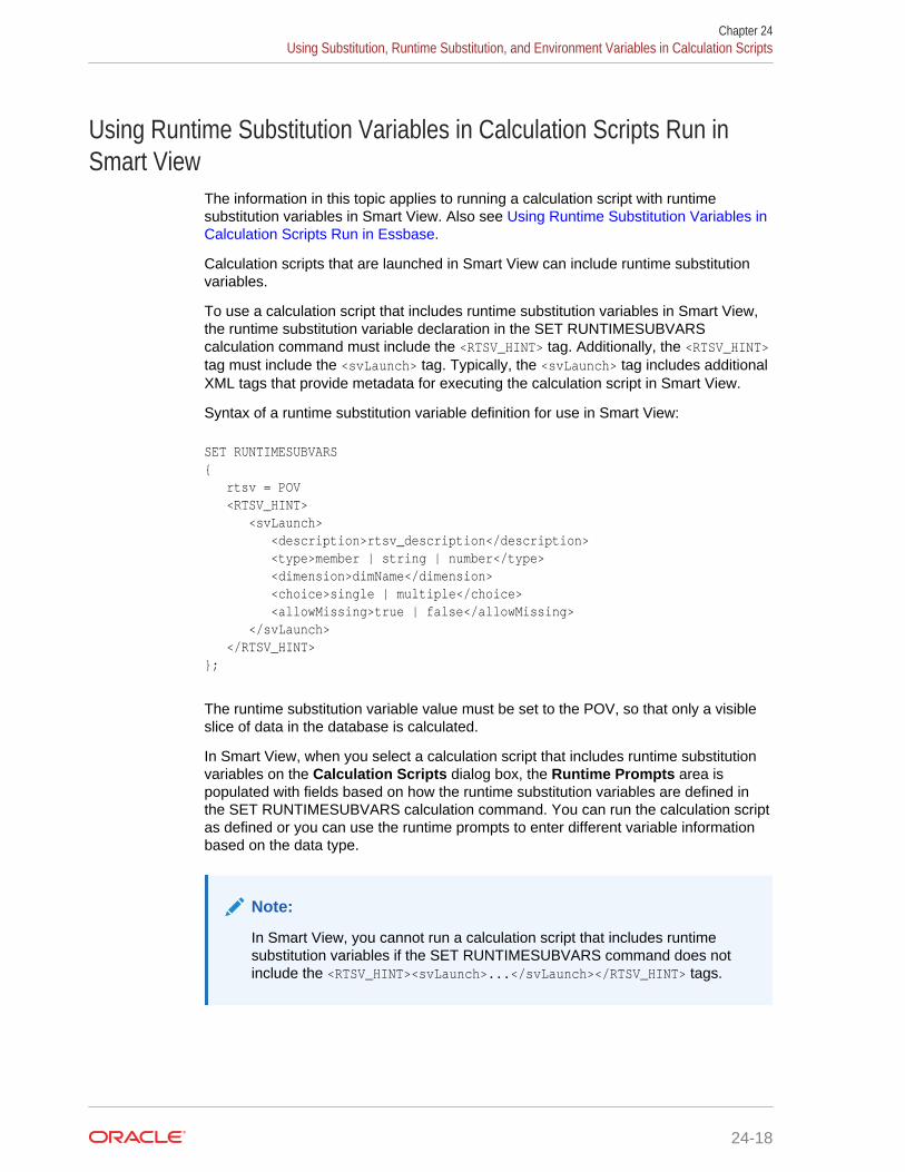
Using Runtime Substitution Variables in Calculation Scripts Run inSmart View

The information in this topic applies to running a calculation script with runtimesubstitution variables in Smart View. Also see Using Runtime Substitution Variables inCalculation Scripts Run in Essbase.

Calculation scripts that are launched in Smart View can include runtime substitutionvariables.

To use a calculation script that includes runtime substitution variables in Smart View,the runtime substitution variable declaration in the SET RUNTIMESUBVARScalculation command must include the <RTSV_HINT> tag. Additionally, the <RTSV_HINT>tag must include the <svLaunch> tag. Typically, the <svLaunch> tag includes additionalXML tags that provide metadata for executing the calculation script in Smart View.

Syntax of a runtime substitution variable definition for use in Smart View:

SET RUNTIMESUBVARS{ rtsv = POV <RTSV_HINT> <svLaunch> <description>rtsv_description</description> <type>member | string | number</type> <dimension>dimName</dimension> <choice>single | multiple</choice> <allowMissing>true | false</allowMissing> </svLaunch> </RTSV_HINT>};

The runtime substitution variable value must be set to the POV, so that only a visibleslice of data in the database is calculated.

In Smart View, when you select a calculation script that includes runtime substitutionvariables on the Calculation Scripts dialog box, the Runtime Prompts area ispopulated with fields based on how the runtime substitution variables are defined inthe SET RUNTIMESUBVARS calculation command. You can run the calculation scriptas defined or you can use the runtime prompts to enter different variable informationbased on the data type.

Note:

In Smart View, you cannot run a calculation script that includes runtimesubstitution variables if the SET RUNTIMESUBVARS command does notinclude the <RTSV_HINT><svLaunch>...</svLaunch></RTSV_HINT> tags.


24-18

Example: Runtime Substitution Variable Set to POVTo set a runtime substitution variable to the POV, the value of the runtime substitutionvariable must be set to "POV" and the data type must be set to member.

By default, the calculation script uses the active member in the POV at runtime unlessthe Smart View user specifies a different member in the runtime prompt.

In this example, assume that the database has these dimensions: Account, Entity,Period and Scenario. Three runtime substitution variables are defined (named Entity,Scenario, and Period) and the value for each variable is set to POV. The runtimesubstitution variables are referenced in the FIX statement as &Entity, &Scenario, and&Period.

SET RUNTIMESUBVARS { Entity = POV <RTSV_HINT> <svLaunch> <description>Entities to Copy</description> <type>member</type> <dimension>Entity</dimension> <allowMissing>false</allowMissing> <choice>multiple</choice> </svLaunch> </RTSV_HINT>; Scenario = POV <RTSV_HINT> <svLaunch> <description>Scenarios to Copy</description> <type>member</type> <allowMissing>false</allowMissing> <dimension>Scenario</dimension> <choice>multiple</choice> </svLaunch> </RTSV_HINT>; Period = POV <RTSV_HINT> <svLaunch> <description>Period to Copy</description> <type>member</type> <allowMissing>false</allowMissing> <dimension>Period</dimension> <choice>single</choice> </svLaunch> </RTSV_HINT>;}FIX(&Entity, &Scenario, &Period)“Opening Balance” (@PREV(“Closing Balance”);)


24-19

Note:

In Essbase, you cannot run a calculation script that includes a runtimesubstitution variable that is set to POV.

XML Tag Reference—Calculation Scripts with Runtime Substitution Variablesfor Smart View

Runtime substitution variables for Smart View XML tags defined:

• <RTSV_HINT>

Required tag for defining runtime substitution variables for use in Smart View.

• <svLaunch>

Required tag that indicates that the runtime substitution variable is defined for usein Smart View.

This tag is the parent tag for these tags: <description>, <type>, <dimension>,<choice>, and <allowMissing>.

• <description>rtsv_description</description>

The rtsv_description is a string that describes the runtime substitution variable.The string is not used in the calculation.

• <type>value</type>

Valid data type values are:

– member—The runtime substitution variable value must be defined as amember (a single member name or a comma separated list of membernames), or POV.

Note:

Member names must be enclosed in quotes; for example, "NewYork" (single member) or "New York","Florida" (a comma separatedlist of member names).

If the runtime substitution variable value is set to POV, the <type>value must be member. Also see the <choice> tag.

In Essbase, you cannot run a calculation script that includes aruntime substitution variable that is set to the POV.

– string—The runtime substitution variable value can be defined as a singlemember name, a comma separated list of member names (for example, "NewYork","Florida"), or a date.

When using the string data type, the Member Selection dialog box is notavailable; therefore, the Smart View user must be sure to use the correctsyntax (enclosing a member name in quotes, separating multiple membernames with a comma, or, for a date, matching the format of the date string to


24-20

the format that is defined in the calculation script—mm-dd-yyyy or dd-mm-yyyy).

– number—The runtime substitution variable value must be defined as a number

• <dimension>dimName</dimension>

Name of the dimension.

Note:

This XML tag is supported only if the <type> value is member.

• <choice>value</choice>

Valid choice values are:

– single:

* If there is a single member on the grid or POV, that member is used.

* If a dimension is on the POV, the active member is used.

* If a dimension is on the POV and there are multiple members, an erroroccurs.

– multiple—All dimension members on the grid or the POV are used.

Note:

This XML tag is supported only if the <type> value is member.

• <allowMissing>boolean</allowMissing>

Specifies whether to allow or suppress data cells for which no data exists in thedatabase.

Valid values: true and false.

Clearing and Copying DataYou can clear a subset of data from a database and copy data values from one set ofmembers to another set of members.

Clearing DataTable 24-5 lists the commands that clear data:

Chapter 24Clearing and Copying Data

24-21

Table 24-5 List of Commands for Clearing Data

Command Calculation

CLEARDATA Change the values of the cells you specify to#MISSING; the data blocks are not removed.

Use the FIX command with the CLEARDATAcommand to clear a subset of a database.

CLEARBLOCK Remove the entire contents of a block,including all the dense dimension members.

Essbase removes the entire block, unlessCLEARBLOCK is inside a FIX command onmembers within the block.

CLEARBLOCK UPPER Remove consolidated level blocks.

CLEARBLOCK NONINPUT Remove blocks containing derived values.Applies to blocks that are completely createdby a calculation operation, not to blocks intowhich any values were loaded.

CLEARBLOCK EMPTY Remove empty blocks.

The following calculation script command yields different results depending on whetherthe Scenario dimension is dense or sparse:

FIX(Actual) CLEARBLOCK NONINPUT;ENDFIX

• Dense: The command removes all data cells that do not contain input data valuesand that intersect with the member Actual from the Scenario dimension.

• Sparse: The command removes only the blocks whose Scenario dimensionmember is Actual.

The following formula clears all the Actual data values for Colas:

CLEARDATA Actual -> Colas;

Copying DataThe DATACOPY calculation command copies data cells from one range of membersto another range of members in a database. The two ranges must be the same size.For example, the following formula copies Actual values to Budget values:

DATACOPY Actual TO Budget;

You can use the FIX command to copy a subset of values. For example, the followingformula copies Actual values to Budget values for the month of January only:

FIX (Jan) DATACOPY Actual TO Budget;ENDFIX

Chapter 24Clearing and Copying Data

24-22

See Using the FIX Command.

Calculating a Subset of a DatabaseTo calculate a subset of a database, use one of the following methods:

• Create a formula using member set functions to calculate lists of members.

See Calculating Lists of Members.

• Use the FIX...ENDFIX commands to calculate a range of values by inclusion.

See Using the FIX Command.

• Use the EXCLUDE...ENDEXCLUDE commands to calculate a range of values byexclusion.

See Using the Exclude Command.

Note:

When Intelligent Calculation is turned on, the newly calculated data blocksare not marked as clean after a partial calculation of a database. When youcalculate a subset of a database, you can use the SETCLEARUPDATESTATUS AFTER command to ensure that the newlycalculated blocks are marked as clean. Using this command ensures thatEssbase recalculates the database as efficiently as possible using IntelligentCalculation. See Understanding Intelligent Calculation.

Calculating Lists of MembersMember set functions generate a list of members that is based on a member youspecify. For example, the @IDESCENDANTS function generates a list of all thedescendants of a specified member. When you use a member set function in aformula, Essbase generates a list of members before calculating the formula.

In the following example, using the @IDESCENDANTS command on the memberTotal Expenses generates a list of these members—Total Expenses, itself, and itsdescendants, which are Marketing, Payroll, and Misc:

@IDESCENDANTS("Total Expenses");

Using the FIX CommandUse the FIX command to define which members to include in the calculation.

The following example calculates only the Budget values for only the descendants ofEast (New York, Massachusetts, Florida, Connecticut, and New Hampshire):

FIX(Budget,@DESCENDANTS(East)) CALC DIM(Year, Measures, Product);ENDFIX

Chapter 24Calculating a Subset of a Database

24-23

The following example fixes on member combinations for the children of East thathave a UDA of New Mkt:

FIX(@CHILDREN(East) AND @UDA(Market,"New Mkt")) Marketing = Marketing * 1.1;ENDFIX

The following example uses a wildcard match (???) to fix on member names that endin the characters -10, which are members 100-10, 200-10, 300-10, and 400-10:

FIX(@MATCH(Product, "???-10")) Price = Price * 1.1;ENDFIX

When you use the FIX command only on a dense dimension, Essbase retrieves theentire block that contains the required value or values for the members that youspecify. I/O is not affected, and the calculation performance time is improved.

When you use the FIX command on a sparse dimension, Essbase retrieves the blockfor the specified sparse dimension members. I/O may be greatly reduced.

Essbase cycles through the database once for each FIX command that you use ondense dimension members. When possible, combine FIX blocks to improve calculationperformance.

For example, by using one FIX command, the following calculation script causesEssbase to cycle through the database only once, calculating both the Actual and theBudget values:

FIX(Actual,Budget) CALC DIM(Year, Measures);ENDFIX

In contrast, by using two FIX commands, the following calculation script causesEssbase to cycle through the database twice: once calculating the Actual data valuesand once calculating the Budget data values:

FIX(Actual) CALC DIM(Year, Measures);ENDFIXFIX(Budget) CALC DIM(Year, Measures);ENDFIX

You cannot FIX on a subset of a dimension that you calculate within a FIX command.For example, the following calculation script returns an error message because theCALC DIM operation calculates the entire Market dimension, although the FIX above itfixes on specific members of the Market dimension:

FIX(@CHILDREN(East) AND @UDA(Market,"New Mkt")) CALC DIM(Year, Measures, Product, Market);ENDFIX


24-24

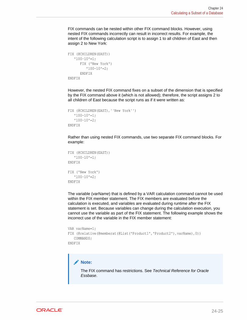
FIX commands can be nested within other FIX command blocks. However, usingnested FIX commands incorrectly can result in incorrect results. For example, theintent of the following calculation script is to assign 1 to all children of East and thenassign 2 to New York:

FIX (@CHILDREN(EAST)) "100-10"=1; FIX ("New York") "100-10"=2; ENDFIXENDFIX

However, the nested FIX command fixes on a subset of the dimension that is specifiedby the FIX command above it (which is not allowed); therefore, the script assigns 2 toall children of East because the script runs as if it were written as:

FIX (@CHILDREN(EAST),''New York'') "100-10"=1; "100-10"=2;ENDFIX

Rather than using nested FIX commands, use two separate FIX command blocks. Forexample:

FIX (@CHILDREN(EAST)) "100-10"=1;ENDFIX

FIX ("New York") "100-10"=2;ENDFIX

The variable (varName) that is defined by a VAR calculation command cannot be usedwithin the FIX member statement. The FIX members are evaluated before thecalculation is executed, and variables are evaluated during runtime after the FIXstatement is set. Because variables can change during the calculation execution, youcannot use the variable as part of the FIX statement. The following example shows theincorrect use of the variable in the FIX member statement:

VAR varName=1;FIX (@relative(@memberat(@List("Product1","Product2"),varName),0)) COMMANDS;ENDFIX

Note:

The FIX command has restrictions. See Technical Reference for OracleEssbase.


24-25

Using the Exclude CommandUse the EXCLUDE...ENDEXCLUDE command to define which members to excludefrom the calculation. Sometimes it is easier to specify which members not to include ina calculation than to define which members to include.

Note:

The EXCLUDE command has restrictions. See Technical Reference forOracle Essbase.

Exporting Data Using the DATAEXPORT CommandThe DATAEXPORT command enables calculation scripts to export data in binary ortext, or directly to a relational database. A set of data-export-related calculationcommands qualify what data to export and provide various output and formattingoptions.

Note:

DATAEXPORT to binary files is not supported across Essbase releases, andis only supported between 64-bit operating systems.

The following command sequence shows the typical calculation script structure forexporting data:

SET DATAEXPORTOPTIONS { DATAEXPORTLEVEL parameters; DATAEXPORTDYNAMICCALC ON | OFF; DATAEXPORTNONEXISTINGBLOCKS ON | OFF; DATAEXPORTDECIMAL n; DATAEXPORTPRECISION n; DATAEXPORTCOLFORMAT ON | OFF; DATAEXPORTCOLHEADER dimensionName; DATAEXPORTDIMHEADER ON | OFF; DATAEXPORTRELATIONALFILE ON | OFF; DATAEXPORTOVERWRITEFILE ON | OFF; DATAEXPORTDRYRUN ON | OFF; };DATAEXPORTCOND parameters;FIX (fixMembers) DATAEXPORT parameters;ENDFIX;

Chapter 24Exporting Data Using the DATAEXPORT Command

24-26

The following tables list the SET DATAEXPORTOPTIONS commands, which are alloptional:

Table 24-6 SET DATAEXPORTOPTIONS Commands: Content Options

Command Calculation

DATAEXPORTLEVEL Specify a data value: ALL, LEVEL0, or INPUT

In specifying the data value for theDataExportLevel option, use these guidelines:

• The values are case-insensitive. Forexample, you can specify LEVEL0 orlevel0.

• Enclosing the value in quotation marks isoptional. For example, you can specifyLEVEL0 or "LEVEL0".

• If the value is not specified, Essbase usesthe default value of ALL.

• If the value is incorrectly expressed (forexample, LEVEL 0 or LEVEL2), Essbaseuses the default value of ALL.

DATAEXPORTDYNAMICCALC Control export of dynamically calculatedvalues

DATAEXPORTNONEXISTINGBLOCKS Specify whether to export data from allpotential data blocks or only from existing datablocks

DATAEXPORTDECIMAL Specify the number of decimal positions in theexported values

DATAEXPORTPRECISION Specify the total number of positions in theexported values

Table 24-7 SET DATAEXPORTOPTIONS Commands: Output Format Options

Command Calculation

DATAEXPORTCOLFORMAT Specify columnar or noncolumnar format

DATAEXPORTCOLHEADER Specify a dense dimension for the columnheader

DATAEXPORTDIMHEADER Include a header record that lists all dimensionnames in the same order as the data in the file

DATAEXPORTRELATIONALFILE Format the text export file for importing thedata into a relational database

Table 24-8 SET DATAEXPORTOPTIONS Commands: Processing Options

Command Calculation

DATAEXPORTOVERWRITEFILE Specify whether an existing file with the samename and location is replaced

DATAEXPORTDRYRUN Enable validating the set of calculationcommands and viewing export statistics—including a time estimate—without having toperform the entire export process

To develop a calculation script that exports a subset of data:


24-27

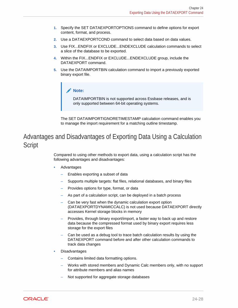
1. Specify the SET DATAEXPORTOPTIONS command to define options for exportcontent, format, and process.

2. Use a DATAEXPORTCOND command to select data based on data values.

3. Use FIX...ENDFIX or EXCLUDE...ENDEXCLUDE calculation commands to selecta slice of the database to be exported.

4. Within the FIX...ENDFIX or EXCLUDE...ENDEXCLUDE group, include theDATAEXPORT command.

5. Use the DATAIMPORTBIN calculation command to import a previously exportedbinary export file.

Note:

DATAIMPORTBIN is not supported across Essbase releases, and isonly supported between 64-bit operating systems.

The SET DATAIMPORTIGNORETIMESTAMP calculation command enables youto manage the import requirement for a matching outline timestamp.

Advantages and Disadvantages of Exporting Data Using a CalculationScript

Compared to using other methods to export data, using a calculation script has thefollowing advantages and disadvantages:

• Advantages

– Enables exporting a subset of data

– Supports multiple targets: flat files, relational databases, and binary files

– Provides options for type, format, or data

– As part of a calculation script, can be deployed in a batch process

– Can be very fast when the dynamic calculation export option(DATAEXPORTDYNAMICCALC) is not used because DATAEXPORT directlyaccesses Kernel storage blocks in memory

– Provides, through binary export/import, a faster way to back up and restoredata because the compressed format used by binary export requires lessstorage for the export files

– Can be used as a debug tool to trace batch calculation results by using theDATAEXPORT command before and after other calculation commands totrack data changes

• Disadvantages

– Contains limited data formatting options.

– Works with stored members and Dynamic Calc members only, with no supportfor attribute members and alias names

– Not supported for aggregate storage databases


24-28

– Cannot export data directly to the client

– Can significantly impact performance when exporting dynamic calculation data(DATAEXPORTDYNAMICCALC) is used, unlessDATAEXPORTNONEXISTINGBLOCKS is set to ON.

Enabling Calculations on Potential BlocksWhen you use a formula on a dense member in a dense dimension, if the resultantvalues are from a dense dimension and the operand or operands are from a sparsedimension, Essbase does not automatically create the required blocks.

In the following example, assume that you want to create budget sales and expensedata from existing actual data. Sales and Expenses are members in the denseMeasures dimension; Budget and Actual are members in the sparse Scenariodimension.

FIX(Budget) (Sales = Sales -> Actual * 1.1; Expenses = Expenses -> Actual * .95;)ENDFIX

Sales and Expenses, the results of the equations, are dense dimension members; theoperand, Actual, is in a sparse dimension. Because Essbase executes dense memberformulas only on existing data blocks, the calculation script does not create therequired data blocks and Budget data values are not calculated for blocks that do notalready exist.

You can solve the problem using the following techniques:

• Using DATACOPY to Copy Existing Blocks

• Using SET CREATENONMISSINGBLK to Calculate All Potential Blocks

Using DATACOPY to Copy Existing BlocksUse the DATACOPY command to create a block for each existing block, and thenperform calculations on the new blocks. For example:

DATACOPY Sales -> Actual TO Sales -> Budget;DATACOPY Expenses -> Actual TO Expenses -> Budget;FIX(Budget) (Sales = Sales -> Actual * 1.1; Expenses = Expenses -> Actual * .95;)ENDFIX

Essbase creates blocks that contain the Budget values for each corresponding Actualblock that exists. After the DATACOPY commands are finished, the remaining part ofthe script changes the values.

Using DATACOPY works well in these situations:

• There is a mathematical relationship between values in existing blocks and theircounterparts created by the DATACOPY.

Chapter 24Enabling Calculations on Potential Blocks

24-29

For example, in the preceding example, the Budget values can be calculatedbased on the existing Actual values.

Caution:

DATACOPY creates the new blocks with identical values in all cells fromthe source blocks. If the formula performs only on a portion of the block,these copied cells remain at the end of the calculation, potentiallyresulting in unwanted values.

• None of the blocks that are copied contain only #MISSING values.

If #MISSING values exist, blocks are written that contain only #MISSING values.Unneeded #MISSING blocks require Essbase resource and processing time.

Using SET CREATENONMISSINGBLK to Calculate All PotentialBlocks

If you are concerned about unwanted values, instead of using DATACOPY, you canuse the SET CREATENONMISSINGBLK ON calculation command, which calculatesall potential blocks in memory and then stores only the calculated blocks that containdata values. The SET CREATENONMISSINGBLK calculation command can be usefulwhen calculating values on dense or sparse dimensions.

The following example creates budget sales and expense data from existing actualdata. Sales and Expenses are members in the dense Measures dimension; Budgetand Actual are members in the sparse Scenario dimension.

FIX(Budget)SET CREATENONMISSINGBLK ON (Sales = Sales -> Actual * 1.1; Expenses = Expenses -> Actual * .95;)ENDFIX

Note:

If SET CREATEBLOCKONEQ ON is set for sparse dimensions, SETCREATENONMISSINGBLK ON temporarily overrides SETCREATEBLOCKONEQ ON until a SET CREATENONMISSINGBLK OFFcommand is encountered or the calculation script is completed. See Nonconstant Values Assigned to Members in a Sparse Dimension.

The advantage of using the SET CREATENONMISSINGBLK command is that, whenapplied on dense members, only data cells that are affected by the member formulaare saved. The disadvantage is that too many potential blocks may be materialized inmemory, possibly affecting calculation performance. When you use this command,limit the number of potential blocks; for example, by using FIX to restrict the scope ofthe blocks to be calculated.

Chapter 24Enabling Calculations on Potential Blocks

24-30

Using Calculation Scripts on PartitionsA partitioned application can span multiple servers, processors, or computers. You canachieve significant calculation performance improvements by partitioning applicationsand running separate calculations on each partition.

See:

• Writing Calculation Scripts for Partitions

• Controlling Calculation Order for Partitions

Writing Calculation Scripts for PartitionsWhen writing calculation script for partitions, review these guidelines:

• Evaluate the performance impact on the overall database calculation. To improveperformance, you can:

– Redesign the overall calculation to avoid referencing remote values that are ina transparent partition in a remote database.

– Dynamically calculate a value in a remote database.

See Dynamically Calculating Data in Partitions.

– Replicate a value in the database that contains the applicable formula.

For example, if replicating quarterly data for the Eastern region, replicate onlythe values for Qtr1, Qtr2, Qtr3, and Qtr4, and calculate the parent Year valueslocally.

• Ensure that a referenced value is up-to-date when Essbase retrieves it. Chooseone of the options previously discussed (redesign, dynamically calculate, orreplicate) or calculate the referenced database before calculating the formula.

Controlling Calculation Order for PartitionsYou must calculate databases in a specific order to ensure that Essbase calculates therequired results.

Figure 24-1 illustrates partitions in which you view information from the West, Central,and East databases transparently from the Corporate database:

Chapter 24Using Calculation Scripts on Partitions

24-31

Figure 24-1 Calculating Partitions

West, Central, and East contain only actual values. Corporate contains actual andbudgeted values. Although you can view West, Central, and East data in theCorporate database, the data exists only in the West, Central, and East databases—itis not duplicated in the Corporate database.

Therefore, when Essbase calculates Corporate, it must take the latest values fromWest, Central, and East. To obtain the required results, you must calculate West,Central, and East before you calculate Corporate.

Saving, Executing, and Copying Calculations ScriptsYou can create calculation scripts in the Web UI and save it. You can also upload acalculation script file to the Web UI. You run a calculation script as a job in the Web UI.You can reuse a calculation script by uploading it to other databases.

• Saving Calculation Scripts

• Executing Calculation Scripts

• Copying Calculation Scripts

Saving Calculation ScriptsYou save a calculation script as an artifact for the database that you plan to calculate.If a calculation script is intended to be executed on multiple databases, you mustupload the calculation script to each database.

If a calculation script is created in a text file and saved on a client computer, you canpaste the script into the editor on the Scripts page in the Web UI and then save thescript, or you can upload the calculation script file from the client computer to adatabase on the cloud service.

See Creating Calculation Scripts and Uploading Files to a Cube in Using OracleAnalytics Cloud - Essbase.

Chapter 24Saving, Executing, and Copying Calculations Scripts

24-32

Executing Calculation ScriptsBefore you can execute a calculation script in the Web UI, the calculation script mustbe saved as an artifact for the database that you plan to calculate. When you run thejob type to execute the calculation, the job runs in the background. You can see thestatus of the calculation. See Executing Calculations in Using Oracle Analytics Cloud -Essbase.

To execute a calculation script in Smart View, see Calculating Data in the OracleSmart View for Office User’s Guide.

To execute a calculation script, you can use the execute calculation MaxL statement.

Copying Calculation ScriptsYou can copy a calculation script to any database on the cloud service instance. See Uploading Files to a Cube in Using Oracle Analytics Cloud - Essbase.

To copy a calculation script, you can use the create calculation as MaxL statement.

Checking Calculation ResultsAfter you execute a calculation script, you can check the results of the calculation inSmart View.

Essbase provides the following information about the executed calculation script:

• Calculation order of the dimensions for each pass through the database

• Total calculation time

To display more-detailed information, you can use the SET MSG SUMMARY, SETMSG DETAIL, and SET NOTICE commands in a calculation script. See SpecifyingGlobal Settings for a Database Calculation.

You can use these messages to understand how the calculation is performed and totune it for the next calculation.

Where you view this information depends on the tool used to execute the calculationscript.

• Smart View—Application log

• MaxL—Standard output (command-line window)

The amount of information depends on the message level set in MaxL Shell.

Chapter 24Checking Calculation Results

24-33

25Reviewing Examples of Calculation Scriptsfor Block Storage Databases

These examples of calculation scripts can help you develop your own calculationscripts.

• About These Calculation Script Examples

• Calculating Variance

• Calculating Database Subsets

• Loading New Budget Values

• Calculating Product Share and Market Share Values

• Allocating Costs Across Products

• Allocating Values within a Dimension

• Allocating Values Across Multiple Dimensions

• Goal-Seeking Using the LOOP Command

• Forecasting Future Values


About These Calculation Script ExamplesAll examples in this chapter are based on the Sample.Basic database.

For examples that use the Intelligent Calculation commands SET UPDATECALC andSET CLEARUPDATESTATUS, see Reviewing Examples That Use SETCLEARUPDATESTATUS and Reviewing Examples and Solutions for Multiple-PassCalculations.

Calculating VarianceThis example includes a calculation of the variance percentage between Budget andActual values.

Figure 25-1 shows an outline in which Variance and Variance % are tagged asDynamic Calc, two-pass members.

Figure 25-1 Variance and Variance % in the Scenario Dimension

25-1

During a default calculation, Essbase aggregates the values on the Market andProduct dimensions. Because percentage values do not aggregate correctly, theVariance % formula must be recalculated after the default calculation.

Because Variance % is tagged as a Dynamic Calc, two-pass member, Essbasedynamically calculates Variance % values when they are retrieved. The dynamiccalculation overwrites the incorrect values with the correctly calculated percentages.

If you choose not to tag Variance % as a Dynamic Calc, two-pass member, use thefollowing calculation script—which assumes that Intelligent Calculation is turned on(the default)—to perform a default calculation and to recalculate the formula onVariance %:

CALC ALL;SET UPDATECALC OFF;SET CLEARUPDATESTATUS AFTER;"Variance %";

Essbase performs the following actions:

1. Performs a default calculation of the database (CALC ALL).

Alternatively, you can run a default calculation of the database outline withoutusing a calculation script.

2. Turns off Intelligent Calculation (SET UPDATECALC OFF).

3. Marks the calculated blocks calculated by the variance formula of the calculationscript as clean, even though the variance calculation is a partial calculation of thedatabase (CLEARUPDATESTATUS AFTER).

By default, data blocks are marked as clean only after a full calculation of thedatabase.

4. Cycles through the database calculating the formula for Variance %.

See Choosing Two-Pass Calculation Tag or Calculation Script and Using Two-PassCalculation.

For information on calculating statistical variance, see Technical Reference for OracleEssbase.

Calculating Database SubsetsThis example shows how a regional Marketing manager can calculate her respectivearea of the database. The calculation script uses @DESCENDENTS(East) to limit thecalculations to the East region, as it calculates the Year, Measures, and Productdimensions for each child of East.

Figure 25-2 shows an outline of the East, West, South, and Central members in theMarket dimension:

Chapter 25Calculating Database Subsets

25-2

Figure 25-2 East, West, South, and Central Members in the Market Dimension

Example script:

/* Calculate the Budget data values for the descendants of East */

FIX(Budget, @DESCENDANTS(East)) CALC DIM(Year, Measures, Product);ENDFIX

/* Consolidate East */

FIX(Budget) @DESCENDANTS(East);ENDFIX


1. Fixes on the Budget values of the descendants of East.

2. Calculates the Year, Measures, and Product dimensions in one pass of thedatabase for all Budget values of the descendants of East.

3. Fixes on the Budget values for all members on the other dimensions.

4. Aggregates the descendants of East and places the result in East.

Loading New Budget ValuesThis example calculates Budget values and then recalculates the Variance andVariance % members.

Example script:

/* Calculate all Budget values */

FIX(Budget) CALC DIM(Year, Product, Market, Measures);ENDFIX

/* Recalculate the Variance and Variance % formulas, which requires two passes */

Variance;"Variance %";


Chapter 25Loading New Budget Values

25-3

1. Fixes on the Budget values.

2. Calculates all Budget values.

The CALC DIM command is used to calculate all the dimensions except for theScenario dimension, which contains Budget.

3. Calculates the formula applied to Variance in the database outline.

4. Calculates the formula applied to Variance % in the database outline.

Calculating Product Share and Market Share ValuesThis example calculates product share and market share values for each market andeach product. The share values are calculated as follows:

• Each member as a percentage of the total

• Each member as a percentage of its parent

Assume that you added four members to the Measures dimension:

• Market Share

• Product Share

• Market %

• Product %

Example script:

/* First consolidate the Sales values to ensure that they are accurate */

FIX(Sales) CALC DIM(Year, Market, Product);ENDFIX

/* Calculate each market as a percentage of the total market for each product */

"Market Share" = Sales % Sales -> Market;

/* Calculate each product as a percentage of the total product for each market */

"Product Share" = Sales % Sales -> Product;

/* Calculate each market as a percentage of its parent for each product */

"Market %" = Sales % @PARENTVAL(Market, Sales);

/* Calculate each product as a percentage its parent for each market */

"Product %" = Sales % @PARENTVAL(Product, Sales);


1. Fixes on the Sales values and consolidates all the Sales values.

Chapter 25Calculating Product Share and Market Share Values

25-4

The CALC DIM command is used to calculate the Year, Market, and Productdimensions. The Measures dimension contains the Sales member and therefore isnot consolidated. The Scenario dimension is label only and therefore does notneed to be consolidated.

2. Cycles through the database and calculates Market Share by taking the Salesvalue for each product in each market for each month and calculating this Salesvalue as a percentage of total Sales in all markets for each product (Sales ->Market).

3. Calculates Product Share by taking the Sales value for each product in eachmarket for each month and calculating this Sales value as a percentage of totalSales of all products in each market (Sales -> Product).

4. Calculates Market % by taking the Sales value for each product in each market foreach month and calculating this Sales value as a percentage of the Sales value ofthe parent of the current member on the Market dimension.

The @PARENTVAL function is used to obtain the Sales value of the parent on theMarket dimension.

5. Calculates Product % by taking the Sales value for each product in each marketfor each month, and calculating this Sales value as a percentage of the Salesvalue of the parent of the current member on the Product dimension.

The @PARENTVAL function is used to obtain the Sales value of the parent on theProduct dimension.

Allocating Costs Across ProductsThis example allocates overhead costs to each product in each market for eachmonth. Overhead costs are allocated based on each product’s Sales value as apercentage of the total Sales for all products.

Assume that you added two members to the Measures dimension:

• OH_Costs for the allocated overhead costs

• OH_TotalCost for the total overhead costs

Example script:

/* Declare a temporary array called ALLOCQ based on the Year dimension */

ARRAY ALLOCQ[Year];

/* Turn the Aggregate Missing Values setting off. If this is your system default, omit this line */

SET AGGMISSG OFF;

/* Allocate the overhead costs for Actual values */

FIX(Actual) OH_Costs (ALLOCQ=Sales/Sales->Product; OH_Costs = OH_TotalCost->Product * ALLOCQ;);

/* Calculate and consolidate the Measures dimension */

Chapter 25Allocating Costs Across Products

25-5

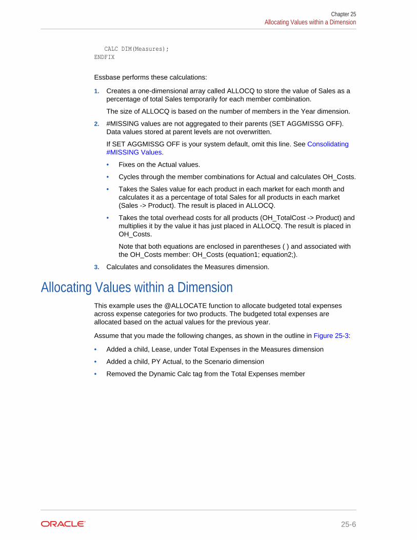
CALC DIM(Measures);ENDFIX

Essbase performs these calculations:

1. Creates a one-dimensional array called ALLOCQ to store the value of Sales as apercentage of total Sales temporarily for each member combination.

The size of ALLOCQ is based on the number of members in the Year dimension.

2. #MISSING values are not aggregated to their parents (SET AGGMISSG OFF).Data values stored at parent levels are not overwritten.

If SET AGGMISSG OFF is your system default, omit this line. See Consolidating#MISSING Values.

• Fixes on the Actual values.

• Cycles through the member combinations for Actual and calculates OH_Costs.

• Takes the Sales value for each product in each market for each month andcalculates it as a percentage of total Sales for all products in each market(Sales -> Product). The result is placed in ALLOCQ.

• Takes the total overhead costs for all products (OH_TotalCost -> Product) andmultiplies it by the value it has just placed in ALLOCQ. The result is placed inOH_Costs.

Note that both equations are enclosed in parentheses ( ) and associated withthe OH_Costs member: OH_Costs (equation1; equation2;).

3. Calculates and consolidates the Measures dimension.

Allocating Values within a DimensionThis example uses the @ALLOCATE function to allocate budgeted total expensesacross expense categories for two products. The budgeted total expenses areallocated based on the actual values for the previous year.

Assume that you made the following changes, as shown in the outline in Figure 25-3:

• Added a child, Lease, under Total Expenses in the Measures dimension

• Added a child, PY Actual, to the Scenario dimension

• Removed the Dynamic Calc tag from the Total Expenses member

Chapter 25Allocating Values within a Dimension

25-6

Figure 25-3 Modified Measures and Scenario Dimensions

Assume that data values of 1000 and 2000 are loaded into Budget -> Total Expensesfor Colas and Root Beer, respectively. These values must be allocated to eachexpense category, evenly spreading the values based on the nonmissing children ofTotal Expenses from PY Actual. The allocated values must be rounded to the nearestdollar.

Example script:

/* Allocate budgeted total expenses based on prior year */

FIX("Total Expenses") Budget = @ALLOCATE(Budget->"Total Expenses", @CHILDREN("Total Expenses"),"PY Actual",, spread,SKIPMISSING,roundAmt,0,errorsToHigh)ENDFIX

The results of the calculation script:

Budget PY ActualColas Marketing 334 * 150 Payroll #MI #MI Lease 333 200 Misc 333 100 Total Expenses 1000 450Root Beer Marketing 500 300 Payroll 500 200 Lease 500 200 Misc 500 400 Total Expenses 2000 1100

* Rounding errors are added to this value.

Chapter 25Allocating Values within a Dimension

25-7


1. Fixes on the children of Total Expenses.

Using a FIX statement with @ALLOCATE may improve calculation performance.

2. For Budget -> Colas -> Marketing, divides 1 by the count of nonmissing values foreach expense category in PY Actual -> Colas for each month.

In this case, 1 is divided by 3, because there are 3 nonmissing expense values forBudget -> Colas.

3. Takes the value from step 2 (.333), multiplies it by the value for Budget -> Colas ->Total Expenses (1000), and rounds to the nearest dollar (333). The result is placedin Budget -> Colas -> Marketing.

4. Repeats steps 2 and 3 for each expense category for Budget -> Colas and thenfor Budget -> Root Beer.

5. As specified in the calculation script, rounds allocated values to the nearest wholedollar.

Essbase makes a second pass through the block to make the sum of the roundedvalues equal to the allocation value (for example, 1000 for Budget -> Colas ->Total Expenses). In this example, there is a rounding error of 1 for Budget ->Colas -> Total Expenses, because the expense categories add up to 999, not1000, which is the allocation value. Because all allocated values are identical(333), the rounding error of 1 is added to the first value in the allocation range,Budget -> Colas -> Marketing (thus a value of 334).

Allocating Values Across Multiple DimensionsThis example uses the @MDALLOCATE function to allocate a loaded value forbudgeted total expenses across three dimensions. The budgeted total expenses areallocated based on the actual values of the previous year.

Assume that you made the following changes:

• Added a child, PY Actual, to the Scenario dimension

• Copied data from Actual into PY Actual

• Cleared data from Budget

For this example, a value of 750 (for Budget -> Total Expenses -> Product -> East ->Jan) must be allocated to each expense category for the children of product 100across the states in the East. The allocation uses values from PY Actual to determinethe percentage share that each category should receive.

Example script:

/* Allocate budgeted total expenses based on prior year, across 3 dimensions */

SET UPDATECALC OFF;FIX (East, “100”, “Total Expenses”) BUDGET = @MDALLOCATE(750,3,@CHILDREN(“100”),@CHILDREN("Total Expenses"),@CHILDREN(East),"PY Actual",,share);ENDFIX

Chapter 25Allocating Values Across Multiple Dimensions

25-8

The values for PY Actual:

Jan PY Actual Marketing Payroll Misc Total Expenses100–10 New York 94 51 0 145 Massachusetts 23 31 1 55 Florida 27 31 0 58 Connecticut 40 31 0 71 New Hampshire 15 31 1 47100-20 New York 199 175 2 376 Massachusetts #MI #MI #MI #MI Florida #MI #MI #MI #MI Connecticut 26 23 0 49 New Hampshire #MI #MI #MI #MI100-30 New York #MI #MI #MI #MI Massachusetts 26 23 0 49 Florida #MI #MI #MI #MI Connecticut #MI #MI #MI #MI New Hampshire #MI #MI #MI #MI100 New York #MI #MI #MI #MI Massachusetts 12 22 1 35 Florida 12 22 1 35 Connecticut 94 51 0 145 New Hampshire 23 31 1 55 East 237 220 3 460


1. Fixes on East, the children of 100, and Total Expenses.

Using a FIX statement with @MDALLOCATE may improve calculationperformance.

2. Before performing the allocation, determines what share of 750 (the value to beallocated) each expense category should receive, for each product-statecombination, using the shares of each expense category from PY Actual. Startingwith PY Actual -> 100-10 -> New York, Essbase divides the value for the firstexpense category, Marketing, by the value for PY Actual-> 100-10 -> East -> TotalExpenses to calculate the percentage share of that category.

For example, Essbase divides the value for PY Actual -> 100-10 -> New York ->Marketing (94) by the value for PY Actual -> 100-10 -> East -> Total Expenses(460), which yields a percentage share of approximately 20.4% for the Marketingcategory.

3. Repeats step 2 for each expense category, for each product-state combination.

4. During the allocation, Essbase uses the percentage shares calculated in step 2and step 3 to determine what share of 750 should be allocated to each child ofTotal Expenses from Budget, for each product-state combination.

For example, for Marketing, Essbase uses the 20.4% figure calculated in step 2,takes 20.4% of 750 (approximately 153), and places the allocated value in Budget-> 100-10 -> New York -> Marketing (see the results that follow this procedure).

Chapter 25Allocating Values Across Multiple Dimensions

25-9

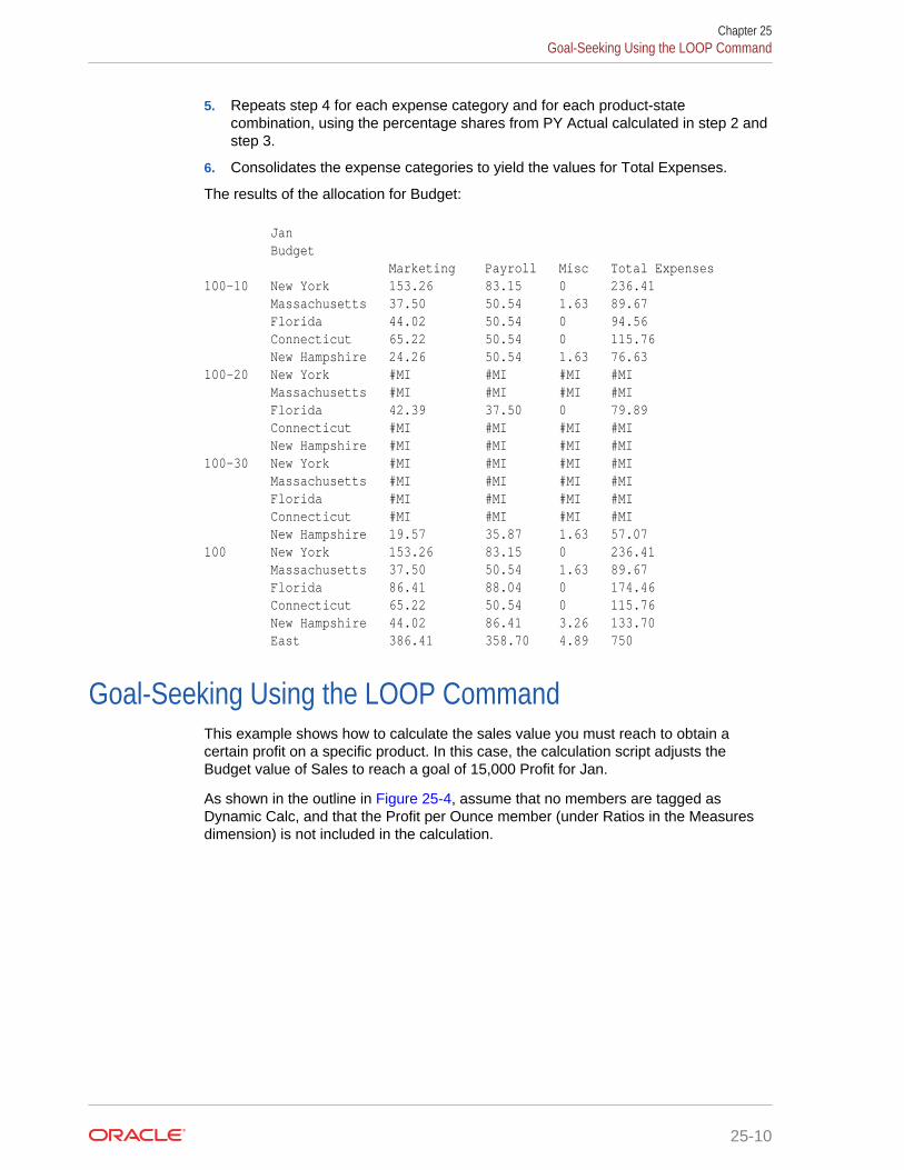
5. Repeats step 4 for each expense category and for each product-statecombination, using the percentage shares from PY Actual calculated in step 2 andstep 3.

6. Consolidates the expense categories to yield the values for Total Expenses.

The results of the allocation for Budget:

Jan Budget Marketing Payroll Misc Total Expenses100–10 New York 153.26 83.15 0 236.41 Massachusetts 37.50 50.54 1.63 89.67 Florida 44.02 50.54 0 94.56 Connecticut 65.22 50.54 0 115.76 New Hampshire 24.26 50.54 1.63 76.63100-20 New York #MI #MI #MI #MI Massachusetts #MI #MI #MI #MI Florida 42.39 37.50 0 79.89 Connecticut #MI #MI #MI #MI New Hampshire #MI #MI #MI #MI100-30 New York #MI #MI #MI #MI Massachusetts #MI #MI #MI #MI Florida #MI #MI #MI #MI Connecticut #MI #MI #MI #MI New Hampshire 19.57 35.87 1.63 57.07100 New York 153.26 83.15 0 236.41 Massachusetts 37.50 50.54 1.63 89.67 Florida 86.41 88.04 0 174.46 Connecticut 65.22 50.54 0 115.76 New Hampshire 44.02 86.41 3.26 133.70 East 386.41 358.70 4.89 750

Goal-Seeking Using the LOOP CommandThis example shows how to calculate the sales value you must reach to obtain acertain profit on a specific product. In this case, the calculation script adjusts theBudget value of Sales to reach a goal of 15,000 Profit for Jan.

As shown in the outline in Figure 25-4, assume that no members are tagged asDynamic Calc, and that the Profit per Ounce member (under Ratios in the Measuresdimension) is not included in the calculation.

Chapter 25Goal-Seeking Using the LOOP Command

25-10

Figure 25-4 Measures Dimension

Assume that, before running the goal-seeking calculation script, the data values are:

Product, Market, Budget JanProfit 12,278.50 Margin 30,195.50 Sales 49,950.00 COGS 19,755.00 Total Expenses 17,917.00 Marketing 3,515.00 Payroll 14,402.00 Misc 0Inventory Label Only memberRatios Label Only member Margin % 60.45 Profit % 24.58

Example script:

/* Declare the temporary variables and set their initial values*/

VAR Target = 15000, AcceptableErrorPercent = .001, AcceptableError, PriorVar, PriorTar, PctNewVarChange = .10, CurTarDiff, Slope, Quit = 0, DependencyCheck, NxtVar;

/*Declare a temporary array variable called Rollback based on the Measures dimension */

ARRAY Rollback [Measures];


25-11

/* Fix on the appropriate member combinations and perform the goal-seeking calculation*/

FIX(Budget, Jan, Product, Market) LOOP (35, Quit) Sales (Rollback = Budget; AcceptableError = Target * (AcceptableErrorPercent); PriorVar = Sales; PriorTar = Profit; Sales = Sales + PctNewVarChange * Sales;); CALC DIM(Measures); Sales (DependencyCheck = PriorVar - PriorTar; IF(DependencyCheck <> 0) CurTarDiff = Profit - Target; IF(@ABS(CurTarDiff) > @ABS(AcceptableError)) Slope = (Profit - PriorTar) / (Sales - PriorVar); NxtVar = Sales - (CurTarDiff / Slope); PctNewVarChange = (NxtVar - Sales) / Sales; ELSE Quit = 1; ENDIF; ELSE Budget = Rollback; Quit = 1; ENDIF;); ENDLOOP CALC DIM(Measures);ENDFIX

Essbase performs the following calculations:

1. Declares the required temporary variables using the VAR command. Whereappropriate, the initial values are set.

2. Declares a one-dimensional array called Rollback to store the Budget values.

The size of Rollback is based on the number of members in the Measuresdimension.

3. Fixes on the Jan -> Budget values for all Product and Market members.

4. Ensures that the commands between LOOP and ENDLOOP are cycled through 35times for each member combination. If, however, the Quit variable is set to 1, theLOOP is broken and the calculation continues after the ENDLOOP command.

5. Cycles through the member combinations, performing the following calculations:

a. Places the Budget -> Sales value in the Rollback temporary array variable.

b. Calculates the acceptable error, by multiplying the Target value (15000) by theAcceptableErrorPercent value (0.001). The result is placed in theAcceptableError variable.

c. Retains the current Sales value, and places the Sales value for the currentmember combination in the PriorVar temporary variable.

d. Retains the current Profit value, and places the Profit value for the currentmember combination in the PriorTar temporary variable.


25-12

e. Calculates a new Sales value by multiplying the PctNewVarChange value(0.1) by the current Sales value, and adding the current Sales value. Theresult is placed in Sales.

f. Calculates and consolidates the Measures dimension.

g. Subtracts the PriorTar value from the PriorVar value, and places the result inthe DependencyCheck temporary variable.

h. Checks that DependencyCheck is not 0 (zero) (IF).

• If DependencyCheck is not 0, subtracts the Target value (15000) from thecurrent Profit and places the result in the CurTarDiff temporary variable.

The IF command checks whether the absolute value (irrespective of the +or – sign) of CurTarDiff is greater than the absolute value ofAcceptableError:

– If greater than AcceptableError, calculates the Slope, NxtVar, andPctNewVarChange temporary variables.

– If not greater than AcceptableError, breaks the LOOP command bysetting the value of Quit to 1. The calculation continues after theENDLOOP command.

• If DependencyCheck is 0, places the value in the Rollback array intoBudget. Essbase breaks the LOOP command by setting the value of Quitto 1. The calculation continues after the ENDLOOP command.

6. Calculates and consolidates the Measures dimension.

The results for product 100-10:

Product, Market, Budget JanProfit 15,000.00 Margin 32,917.00 Sales 52,671.50 COGS 19,755.00 Total Expenses 17,917.00 Marketing 3,515.00 Payroll 14,402.00 Misc 0Inventory Label Only memberRatios Label Only member Margin % 28.47839913 Profit % 62.49489762

Forecasting Future ValuesThis example uses a linear regression forecasting method to produce a trend(@TREND), or line, that starts with the known data values from selected previousmonths and continues with forecasted values based on the known values, and showshow to check the results of the trend for “goodness of fit” to the known data values. Inthis case, the calculation script forecasts sales data for June–December, assumingthat data currently exists only up to May.

Assume that the Measures dimension contains an additional child, ErrorLR, where thegoodness-of-fit results are placed.

Chapter 25Forecasting Future Values

25-13

Example script:

Sales(@TREND(@LIST(Jan,Mar,Apr),@LIST(1,3,4),, @RANGE(ErrorLR,@LIST(Jan,Mar,Apr)), @LIST(6,7,8,9,10,11,12), Jun:Dec,LR););

Table 25-1 describes the parameters used in the forecasting calculation script:

Table 25-1 Parameters Used in the Example Calculation Script for ForecastingFuture Values

Parameter Description

@LIST(Jan,Mar,Apr) Represents the Ylist, or the members thatcontain the known data values.

The @LIST function groups the threemembers as a comma-delimited list and keepsthe list separate from other parameters.

@LIST(1,3,4) Represents the Xlist, or the underlying variablevalues. Because Feb and May are skipped,Essbase numbers the Ylist values as 1,3,4.

, The extra comma after the Xlist parameterindicates that a parameter (weightList) wasskipped.

This example uses a default weight of 1.

@RANGE(ErrorLR,@LIST(Jan,Mar,Apr) Represents the errorList, or the member listwhere results of the goodness of fit of thetrend line to Ylist are placed.

The values placed in errorList are thedifferences between the data points in Ylistand the data points on the trend line that isproduced.

The @RANGE function combines the ErrorLRmember with Ylist (Jan, Mar, Apr) to produce amember list.

@LIST(6,7,8,9,10,11,12) Represents the XforecastList, or theunderlying variable values for which theforecast is sought. This example forecastsvalues consecutively for Jun–Dec, so thevalues are 6,7,8,9,10,11,12.

Jun:Dec Represents the YforecastList, or the memberlist into which the forecast values are placed.This example forecasts values for Jun–Dec,based on the values for Jan, Mar, and Apr.

LR Specifies the Linear Regression method.


1. Finds the known data values on which to base the trend (Sales for Jan, Mar, Apr),as specified by the Ylist and Xlist parameters.

2. Calculates the trend line using Linear Regression and places the results in Salesfor Jun–Dec, as specified by the YforecastList parameter.


25-14

3. Calculates the goodness of fit of the trend line for the data values for Jan, Mar,and Apr, and places the results in ErrorLR for those months.

For example, the value in ErrorLR for Jan (4.57) means that after Essbasecalculates the trend line, the difference between the Sales value for Jan (2339)and the Jan value on the trend line is 4.57. The ErrorLR values for Feb and Mayare #MISSING, because these months were not part of Ylist.

The results of the calculation script:

100 West Actual Sales ErrorLRJan 2339 4.57Feb 2298 #MIMar 2313 -13.71Apr 2332 9.14May 2351 #MIJun 2315.14 #MIJul 2311.29 #MIAug 2307.49 #MISep 2303.57 #MIOct 2299.71 #MINov 2295.86 #MIDec 2292 #MI


25-15

26Using Hybrid Aggregation

Hybrid aggregation for block storage databases is an aggregation model in whichblock storage data calculation executes with efficiency similar to that of aggregatestorage databases.

• About Hybrid Aggregation

• Comparison of Hybrid Aggregation, Block Storage, and Aggregate Storage

• Getting Started with Hybrid Aggregation

• Optimizing the Database for Hybrid Aggregation

• Limitations and Exceptions to Hybrid Mode

About Hybrid AggregationHybrid aggregation combines block storage functionality with aggregate storageperformance. Hybrid aggregation offers the benefit of fast performance by removingsparse aggregations, reducing size and memory footprint, and speeding up batchroutines. The deployment considerations are simplified, as you no longer have toconsider using block storage for heavy use of level 0 calculations, versus aggregatestorage for many upper-level aggregations, versus designing partitioned models inwhich the cube is split along dimensional lines to facilitate calculation performance.

The following are some scenarios where hybrid aggregation is likely to improvecalculation performance:

• A block storage database has sparse members that are not level 0, and arecalculated according to hierarchy (rather than by calculation scripts).

• A sparse Dynamic Calc member has more than 100 children.

• You are using a transparent partition between an empty aggregate storage targetand a block storage source. If the formulas on the aggregate storage target aresimple and translatable to block storage formula language, you can achieve fastresults on block storage using hybrid aggregation.

• You are using a transparent partition between two block storage databases, andcalculation performance is a concern.

The default calculation and query processor is hybrid aggregation mode. See OracleAnalytics Cloud - Essbase Calculation and Query Processor in Using Oracle AnalyticsCloud - Essbase.

Comparison of Hybrid Aggregation, Block Storage, andAggregate Storage

In block storage databases, large, sparse dimensions must be stored: making themdynamic would result in too much block I/O at query time, affecting performance. Verylarge stored sparse dimensions can lead to lengthy batch aggregation times, as well

26-1

as large database sizes that grow in relation to the number and size of the sparsedimensions. Even with such drawbacks, block storage is widely used for its powerfulfunctionality.

Aggregate storage is designed specifically to enable large databases with more andlarger dimensions. Unlike block storage, it does not require large sparse dimensions tobe pre-aggregated to achieve good query performance. The key lies in the aggregatestorage engine, which facilitates rapid dynamic aggregation across largedimensionality.

For all the benefits that aggregate storage offers, however, there are manyapplications that are simply better suited to block storage, such as the need to doallocations or currency conversion. In such cases, hybrid aggregation might be thesolution. Hybrid aggregation is a combination of the best features of block storage andaggregate storage:

• It enables full procedural calculation flexibility, and can eliminate the need toperform sparse aggregations.

• For queries accessing dynamic sparse members, Essbase utilizes the aggregatestorage engine to satisfy the request. For the small percentage of queries thatcannot be processed by the aggregate storage engine, Essbase employs theblock storage engine to satisfy the request. See Limitations and Exceptions toHybrid Mode.

• By marking sparse members as dynamic, eliminating the need for pre-aggregation, these are the benefits:

– Restructure performance improves

– Backup performance improves

– There is a reduction in disk space requirements

• You have better control of calculation sequence for dynamic members by usingsolve order, inclusive of attribute sequencing.

• You can use non-aggregating attributes if needed.

Note:

The aggregate storage query processor does not interface directly with theblock storage data and index files; rather, it brings the data into an aggregatestorage temporary tablespace. Just as with aggregate storage mode, thetemporary tablespace resides within the aggregate storage cache to thelargest extent possible, overflowing to the file system only as needed.Aggregate storage-level performance is achieved whenever the aggregatestorage query processor is used. In some cases, hybrid aggregation queryperformance may be even greater than the equivalent aggregate storageperformance.

Getting Started with Hybrid AggregationTo get started with hybrid aggregation, follow these guidelines:

Chapter 26Getting Started with Hybrid Aggregation

26-2

• Set up a development environment, and migrate existing block storageapplications to it.

• In Oracle Analytics Cloud - Essbase, hybrid aggregation mode is enabled by the ASODYNAMICAGGINBSO FULL configuration setting, which is set by default.See Oracle Analytics Cloud - Essbase Calculation and Query Processor in UsingOracle Analytics Cloud - Essbase.

• Where possible, make larger sparse dimensions dynamic. See also Optimizing theDatabase for Hybrid Aggregation.

• Run test queries and examine the application log, both before and after enablinghybrid aggregation. This activity can reveal the extent to which the aggregatestorage query processor was used, and the benefits of hybrid mode that weregained. For each query, the application log states Hybrid aggregation modeenabled or Hybrid aggregation mode disabled.

• If too many queries are logged with hybrid aggregation mode disabled, optimizethe application so that a greater percentage of queries can use the aggregatestorage query processor. See Limitations and Exceptions to Hybrid Mode toensure that your queries are supported in hybrid aggregation mode. See also Functions Supported in Hybrid Aggregation Mode in Technical Reference forOracle Analytics Cloud - Essbase.

Optimizing the Database for Hybrid AggregationTo use hybrid aggregation most effectively:

• If there are non-level-0 stored members that are batch calculated based solely ontheir hierarchy, Oracle recommends that you convert them to Dynamic Calcmembers.

• Avoid using two-pass calculation in hybrid aggregation mode. Use solve orderinstead.

• If the conversion to Dynamic Calc members affects solve order for dependentformulas, you may need to adjust the outline's order of dimensions to align thesolve order with the previous batch calculation order and two-pass calc settings.

• You may need to adjust the dimensions' dense or sparse configurations (appliesonly to block-storage engine utilization in cases where the aggregate storageengine cannot be used).

• Minimize the size of blocks, if possible. Consider adjusting the Create Blocks onEquations configuration setting, or in the case of calculation scripts, using the SETCREATEBLOCKONEQ ON|OFF command.

The default solve order for hybrid-aggregation-enabled databases matches thecalculation order of block storage databases, with some enhancements

For more information about solve order, see Calculation Order. Although the linkedtopic is about aggregate storage databases, the solve order information also applies tohybrid aggregation.

Limitations and Exceptions to Hybrid ModeIn some cases, a query is not supported in hybrid mode. Essbase detects when theseconditions are present, and calculates them in block storage mode. If a query mixes

Chapter 26Optimizing the Database for Hybrid Aggregation

26-3

supported and unsupported hybrid mode calculation types, Essbase defaults to blockstorage execution.

If enabled, hybrid aggregation is in effect for member formulas using any of thesupported functions. For a list of supported and unsupported functions, see FunctionsSupported in Hybrid Aggregation Mode in Technical Reference for Oracle Essbase.

The following types of calculations are not supported for hybrid mode:

• Dynamic Calc members with formulas that are a target of transparent partitions

• Queries which include both two-pass and one-pass dynamic calc members fromthe same dimension

• Queries where the shared member is outside the target partition definition and itsreferenced member is inside, or the reverse

• XOLAP

• Text measures/text lists

Attribute calculations are supported in hybrid mode, with these exceptions:

• Varying attributes

• Two-pass members

• Any attribute calculation other than sum

Formulas with dimension references can run in hybrid mode in the following cases(when the FULL parameter is used with the ASODYNAMICAGGINBSO configurationsetting):

• Sparse-to-Sparse: The formula is set on a sparse dimension member, and theformula only references member combinations from sparse dimensions.

• Dense-to-Dense: The formula is set on a dense dimension member, and theformula only references member combinations from dense dimensions.

• Sparse-to-Dense/Sparse: The formula is set on a sparse dimension member, andthe formula references member combinations from both dense and sparsedimensions. The dense dimension members must be stored.

Example: On a sparse Product dimension, a Dynamic Calc member [Stereo_HY1]has the formula @MINSRANGE("Stereo","Qtr1":"Qtr2");.

The formula depends on the dense Year dimension for [Qtr1] and [Qtr2], and thesparse Product dimension for [Stereo].

Chapter 26Limitations and Exceptions to Hybrid Mode

26-4

27Using Parallel Calculation

With serial calculation, each calculation pass is scheduled to run on a singleprocessor. If invoked from a calculation script, the calculations are executedsequentially in the order in which they appear in the calculation script. Parallelcalculation breaks each calculation pass into sub-tasks. The sub-tasks that can runindependently of one another are scheduled to run simultaneously on up 128 threads.Each thread may be on a different processor.

• About Parallel Calculation

• Using CALCPARALLEL Parallel Calculation

• Using FIXPARALLEL Parallel Calculation

About Parallel CalculationEssbase provides two ways of invoking a calculation on a block storage database:

• The calculation may be implicitly specified by the outline itself.

• The calculation may be explicitly specified by a calculation script that you create.The script contains formulas and calculation instructions.

Regardless of how a calculation is triggered, Essbase can execute the calculation inone of two modes:

• Serial calculation is the default. With serial calculation, each calculation pass isscheduled to run on a single processor. If invoked from a calculation script, thecalculations are executed sequentially in the order in which they appear in thecalculation script.

• Parallel calculation breaks each calculation pass into sub-tasks. The sub-tasksthat can run independently of one another are scheduled to run simultaneously onup 128 threads for block storage and aggregate storage databases running on 64-bit operating systems. Each thread may be on a different processor.

Note:

Parallel calculation operations do not dynamically create threads, but insteaduse a set number of threads from a pre-created pool of threads. You cancustomize the size of the thread pool. see the WORKERTHREADSconfiguration setting topic in Technical Reference for Oracle Essbase.

Using CALCPARALLEL Parallel CalculationTo change from the default serial calculation to CALCPARALLEL parallel calculation,you change one or two configuration settings and restart the server, or add aninstruction to the calculation script.

27-1

See Enabling CALCPARALLEL Parallel Calculation.

The following topics discuss the details of parallel calculation.

Essbase Analysis of FeasibilityEssbase evaluates whether using parallel calculation is possible before eachcalculation pass for which you have enabled parallel calculation.

Essbase analyzes the outline and the calculation requested for each calculation pass.Remember that one calculation may require multiple passes. Some situations maycreate the need for multiple passes, including dynamic calculation, the presence of amember tagged as two-pass, or calculations that create certain kinds ofinterdependencies. See Calculation Passes.

If Essbase determines that parallel calculation is possible, Essbase splits thecalculation into smaller tasks that are independent of each other. During thecalculation, Essbase performs the smaller tasks simultaneously.

However, Essbase uses serial calculation even if parallel calculation is enabled if thereare complex interdependencies between formulas that participate in the pass. Suchinterdependencies render parallel calculation impossible.

CALCPARALLEL Parallel Calculation GuidelinesOutline structure and application design determine whether enabling parallelcalculation can improve calculation performance. Before you enable CALCPARALLELparallel calculation, review the following guidelines, which will help you get the fullbenefit of parallel calculation:

• One or more formulas present in a calculation may prevent Essbase from usingCALCPARALLEL parallel calculation even if it is enabled. For a description offormulas that may force serial calculation regardless of parallel calculationsettings, see Formula Limitations.

• Calculation tasks are generated along the last n sparse dimensions of an outline.These sparse dimensions used to identify tasks are called task dimensions. Thenumber of task dimensions, n, is either selected dynamically by Essbase, or youcan override the number by specifying a value for the calculation command SETCALCTASKDIMS.

Order the sparse dimensions in an outline from smallest to largest, based onactual size of the dimension (as reported by the MaxL statement query databaseDBS-NAME get dbstats dimension). This ordering recommendation is consistentwith recommendations for optimizing calculator cache size and consistent withother outline recommendations. For a description of situations that may need touse additional dimensions (more than the last sparse dimension) and forinstructions on how to increase the number of sparse dimensions used, see Identifying Additional Tasks for Parallel Calculation.

• CALCPARALLEL parallel calculation is effective on non-partitioned applicationsand these partitioned applications:

– Replicated partitions

– Transparent partitions if the calculation occurs at the target database. Thenumber of sparse dimensions specified by SET CALCTASKDIMS in acalculation script must be set at 1. For information on limitations imposed by

Chapter 27Using CALCPARALLEL Parallel Calculation

27-2

the use of parallel calculation with transparent partitions, see TransparentPartition Limitations; for information on using SET CALCTASKDIMS, see Identifying Additional Tasks for Parallel Calculation.

• Update transactions, such as calculations and data updates, are more resource-consuming requests than MDX queries or report scripts.

Relationship Between CALCPARALLEL Parallel Calculation and OtherEssbase Features

The following topics discuss the relationship between CALCPARALLEL parallelcalculation and other Essbase functionality.

• Retrieval Performance

• Formula Limitations

• Calculator Cache

• Transparent Partition Limitations

Retrieval PerformancePlacing the largest sparse dimension at the end of the outline for maximum parallelcalculation performance may slow retrieval performance. See Optimizing QueryPerformance.

Formula LimitationsThe presence of some formulas may force serial calculation. The following formulaplacements likely will force serial calculation:

• A formula on a dense member, including all stored members and any DynamicCalc members upon which a stored member may be dependent, that causes adependence on a member of the dimension that is used to identify tasks forparallel calculation.

• A formula that contains references to variables declared in a calculation script thatuses @VAR, @ARRAY, @XREF, or @XWRITE. Consider using FIXPARALLEL.

• A sparse dimension member formula using @XREF, and the dimension for thesparse member is fully calculated. @XREF does not force serial calculation whenit is on dense Dynamic Calc members that are not dependent on other storedmembers during the batch calculation.

• A member formula that causes a circular dependence. For example, member Ahas a formula referring to member B, and member B has a formula referring tomember C, and member C has a formula referring to member A.

• A formula on a dense or sparse member with a dependency on a member ormembers from the dimension used to identify tasks for parallel processing.

• A sparse dimension member formula that contains references to members fromother sparse dimensions.

If you need to use a formula that might prevent parallel calculation, consider usingFIXPARALLEL. Otherwise, you can either mark the member of the formula asDynamic Calc, or exclude the formula from the scope of the calculation. To see


27-3

whether a formula is preventing parallel calculation, check the application log. Forrelevant error messages, see Monitoring CALCPARALLEL Parallel Calculation.

Calculator CacheAt the start of a calculation pass, Essbase checks the calculator cache size and thedegree of parallelism and then uses the calculator cache bitmap option appropriate formaximum performance. Therefore, the bitmap option used for parallel calculation maybe different from that used for serial calculation.

For example, assume Essbase performs a serial calculation and uses multiple bitmapsand a single anchoring dimension. Without explicit change of the calculator cache size,Essbase might perform a parallel calculation using only a single bitmap and a singleanchoring dimension.

You can determine the calculator cache mode that controls the bitmap options bychecking the application log at the start of each calculation pass for an entry similar tothe following:

Multiple bitmap mode calculator cache memory usage has a limit of [50000] bitmaps.

Transparent Partition LimitationsParallel calculation with transparent partitions has the following limitations:

• You cannot use parallel calculation across transparent partitions unless thecalculation occurs at the target.

• You must set SET CALCTASKDIMS to 1 so that there is only one task dimension.

• You must increase the calculator cache so that multiple bitmaps can be used. Youcan identify the calculator cache mode that controls the bitmap options bychecking the application log at the start of each calculation pass for an entrysimilar to the following:

Multiple bitmap mode calculator cache memory usage has a limit of [50000] bitmaps.

Checking Current CALCPARALLEL Settings

To check whether a calculation script sets parallel calculation, look for the SETCALCPARALLEL command. The number of threads that can simultaneously performtasks to complete a calculation is specified by a value between 1 and 128. Blockstorage and aggregate storage databases running on 64-bit platforms support up to128 threads. Review the script carefully, because the script may enable or disableparallel calculation more than once. Alternately, a script can use FIXPARALLELcommand blocks for parallel calculation.

Enabling CALCPARALLEL Parallel CalculationTo use CALCPARALLEL parallel calculation, add the appropriate calculationcommands, SET CALCPARALLEL and SET CALCTASKDIMS, to a calculation script.


27-4

Caution:

Read this entire chapter before attempting to enable parallel calculation.

To enable parallel calculation:

1. Add SET CALCPARALLEL to a calculation script.

2. If needed, enable Essbase to use more than the one sparse dimension to identifytasks for parallel calculation.

Use the process described in Identifying Additional Tasks for Parallel Calculationand Tuning CALCPARALLEL with Log Messages.

3. Run the calculation.

Oracle recommends that you set the value of SET CALCPARALLEL to be one lessthan the number of processors available for calculation. This extra processor can thenbe used by either the operating system or by the Essbase process responsible forwriting out dirty blocks from the cache.

Identifying Additional Tasks for Parallel CalculationBy default, Essbase uses an iterative technique to select the optimal number of taskdimensions to use for CALCPARALLEL parallel calculation.

If necessary, you can enable Essbase to use a specific number, n, of task dimensions.For example, if you have a FIX statement on a member of the last sparse dimension,you can include the next-to-last sparse dimension from the outline as well. Becauseeach unique member combination of these two dimensions is identified as a potentialtask, more and smaller tasks are created, increasing the opportunities for parallelprocessing and improving load balancing.

To specify the number of task dimensions for parallel calculation:

1. Use SET CALCPARALLEL at the top of the calculation script to enable parallelcalculation.

2. Optional: Essbase selects a default number, n, of task dimensions to use forparallel calculation and this number is printed in the application log file as aninformational message; for example: Parallelizing using [2] taskdimensions. To override the default n setting, use the calculation script command SET CALCTASKDIMS .

3. Run the calculation script.

Note:

In some cases, Essbase uses fewer dimensions to identify tasks than isspecified by SET CALCTASKDIMS.


27-5

Tuning CALCPARALLEL with Log MessagesIf you are using CALCPARALLEL parallel calculation, you may encounter the followinglog messages:

Current selection of task dimensions [n] will generate insufficient numberof tasks [n] for parallel calculation. See whether calculation time can beimproved by increasing the number of task dimensions by one (see SETCALCTASKDIMS topic in the Technical Reference). Also, consider usingFIXPARALLEL to make custom task selections that are different fromCALCPARALLEL.

If this message is encountered, it means that during a parallel calculation, Essbaserefrained from increasing the number of task dimensions, in case that would haveresulted in tasks becoming too small. When tasks become too small, calculationscheduling overhead could overtake the benefits of parallelism. However, when tasksare too large, there might not be enough tasks for parallel calculation threads to workon.

If the next potential task dimension is not the first sparse dimension, considerincreasing the number of task dimensions by one using SET CALCTASKDIMS, andobserve whether that improves the speed of the calculation. Also, consider usingFIXPARALLEL to make custom task selections that are different fromCALCPARALLEL (see Using FIXPARALLEL Parallel Calculation).

Current number of task dimensions [n] for parallel calculation might havecaused too many tasks [n] to be generated. See whether calculation timecan be improved by decreasing the number of task dimensions by one (seeSET CALCTASKDIMS topic in the Technical Reference). Also, consider usingFIXPARALLEL to make custom task selections that are different fromCALCPARALLEL.

For parallel calculation, having a sufficient number of tasks helps to reduce the effectsof data skew. However, too many tasks (even for appropriately sized tasks) can causethe scheduling overhead to outweigh the benefits. Essbase targets an optimal range. Ifyou see the above message, it means that Essbase tried to meet the recommendedminimum number of tasks by adding one more task dimension; in doing so, it ispossible that the upper boundary for task count may have been crossed.

If the last task dimension selected by Essbase is not the only task dimension, considerdecreasing task dimensions by one using SET CALCTASKDIMS, and observewhether that improves the speed of the calculation. Also, consider usingFIXPARALLEL to make custom task selections that are different fromCALCPARALLEL (see Using FIXPARALLEL Parallel Calculation).

Monitoring CALCPARALLEL Parallel CalculationYou can view events related to parallel calculation in the application log.

For each calculation pass, Essbase writes several types of information to theapplication log to support parallel calculation:


27-6

• If you have enabled parallel calculation and Essbase has determined that parallelcalculation can be performed, Essbase writes a message in the application log:

Calculating in parallel with n threads

n represents the number of concurrent tasks specified in SET CALCPARALLEL.

• For each formula that prevents parallel calculation (forces serial calculation),Essbase writes a message to the application log:

Formula on ((or backward dependence from) mbr memberName prevents calculation from running in parallel.

memberName represents the name of the member where the relevant formulaexists. You can look in the application log for such messages and considerremoving the formula or, if possible, tagging the relevant member or members asDynamic Calc so they do not feature in the calculation pass.

• Essbase writes a message to the application log specifying the number of tasksthat can be executed concurrently (based on the data, not the value of SETCALCPARALLEL):

Calculation task schedule [576,35,14,3,2,1]

The example message indicates that 576 tasks can be executed concurrently.After the 576 tasks complete, 35 more can be performed concurrently, and so on.

The benefit of parallel calculation is greatest in the first few steps and diminishesas fewer concurrent tasks are performed.

The degree of parallelism depends on the number of tasks in the task schedule.The greater the number, the more tasks that can run in parallel, and the greaterthe performance gains.

• Essbase writes a message to the application log file indicating how many tasks areempty (contain no calculations):

[Tue Jun 27 12:30:44 2007]Local/CCDemo/Finance/essexer/Info(1012681) Empty tasks [291,1,0,0,0,0]

In the example, Essbase indicates that 291 of the tasks at level 0 were empty.

If the ratio of empty tasks to the tasks specified in the calculation task schedule isgreater than 50% (for example, 291 / 576), parallelism may not be giving youimproved performance because of the high sparsity in the data model.

You can change dense-sparse assignments to reduce the number of empty tasksand increase the performance gains from parallel calculation.

Using FIXPARALLEL Parallel CalculationAlthough parallel calculation can be performed using the CALCPARALLEL method, incertain cases it might be beneficial to use the FIXPARALLEL command block method.

Chapter 27Using FIXPARALLEL Parallel Calculation

27-7

In a FIXPARALLEL command block, you input some commands to be executed, alongwith a number of threads (numThreads) and a member list (mbrList) specifying thedatabase regions (slices) to be calculated. Essbase creates a list of tasks from thecombinations in the member list, and divides the tasks across the threads.

The FIXPARALLEL method can be advantageous in the following cases:

• If you need to use temporary variables during parallel calculation.

• If you need to use the DATACOPY, DATAEXPORT, or CLEARBLOCK calculationcommands.

• In conjunction with the @XREF or @XWRITE functions.

• If you need to export regions of the database in parallel.

• In cases where CALCPARALLEL is not meeting performance requirements, andyour outline generates many empty tasks, or contains many task groupings withfewer tasks than threads made available to the calculation.

Chapter 27Using FIXPARALLEL Parallel Calculation

27-8

28Writing MDX Queries

MDX is a query language for multidimensional databases that can be used to executegrid retrievals. MDX expressions can also be used to define formulas on Essbaseaggregate storage databases, to query metadata, to qualify member names, and todescribe data or outline subsets.

• About Writing MDX Queries

• Understanding Elements of a Query

• Using Functions to Build Sets

• Working with Levels and Generations

• Using a Slicer Axis to Set Query Point-of-View

• Common Relationship Functions

• Performing Set Operations

• Creating and Using Named Sets and Calculated Members

• Using Iterative Functions

• Working with Missing Data

• Using Substitution Variables in MDX Queries

• Querying for Properties

About Writing MDX QueriesMDX, the data manipulation language for Essbase, is a query language formultidimensional databases that can be used to execute grid retrievals. MDXexpressions can also be used to define formulas on Essbase aggregate storagedatabases, to query metadata, to qualify member names, and to describe data oroutline subsets for conditional triggers and other Essbase functionality.

This chapter provides an introduction to MDX with a series of practice exercises.

To complete the exercises, which are based on the Sample.Basic database, use theMaxL Shell. Before continuing, start Essbase and log on to MaxL Shell. Additionally,be prepared to use a text editor to create the sample queries as presented in thischapter.

Note:

The instructions in this chapter use the MaxL Shell.

28-1

Understanding Elements of a QueryIn this section you will create a template to use as a basis for developing simplequeries.

Most queries can be built upon the following grammatical framework:

SELECT {}ON COLUMNSFROM Sample.Basic

SELECT in line 1 is the keyword that begins the main body of all MDX statements.

The braces { } in line 2 are a placeholder for a set. In the above query, the set isempty, but the braces remain as a placeholder.

To create a query template:

1. Create a folder to store sample queries that can be run against the Sample.Basicdatabase.

For example, create a folder called “queries.”

2. Using a text editor, type the following code into a blank file:

SELECT {}ON COLUMNSFROM Sample.Basic

3. Save the file as qry_blank.txt.

Introduction to Sets and TuplesA set is an ordered collection of one or more tuples that have the same dimensionality(see Rules for Specifying Sets for an explanation of dimensionality).

A tuple is a way to refer to a member or a member combination from any number ofdimensions. For example, in the Sample.Basic database, Jan is a tuple, as is (Jan,Sales), as is ([Jan],[Sales],[Cola],[Utah],[Actual]).

The member name can be specified in these ways:

• By specifying the actual name or the alias; for example:

– Cola

– Actual

– COGS

– [100]

If the member name starts with number or contains spaces, it should be withinbrackets; for example, [100]. Brackets are recommended for all member names,for clarity and code readability.

Chapter 28Understanding Elements of a Query

28-2

If the member name starts with an ampersand (&) , it should be within quotationmarks; for example, ["&xyz"]. This is because the leading ampersand is reservedfor substitution variables (see Using Substitution Variables in MDX Queries). Youcan also specify it as StrToMbr("&100").

For attribute members, the long name (qualified to uniquely identify the member)should be used; for example, [Ounces_12] instead of [12].

• By specifying dimension name or any one of the ancestor member names as aprefix to the member name; for example, [Product].[100-10] and [Diet].[100-10]. This practice is recommended for all member names, as it eliminatesambiguity and enables you to refer accurately to shared members.

Note:

Do not use multiple ancestors in the member name qualification.Essbase returns an error if multiple ancestors are included. For example,[Market].[New York] and [East].[New York] are valid names for NewYork; however, [Market].[East].[New York] returns an error.

• By specifying the name of a calculated member defined in the WITH section.

Exercise: Running Your First QueryRecall that the braces { } in line 2 of your query template are a placeholder for a set. Inthis exercise, we will add a set to the query and run it.

To run the query:

1. Open qry_blank.txt, the query template you created from UnderstandingElements of a Query.

2. Because a set can be as simple as one tuple, add Jan as a set to the querytemplate. Retain the braces (required for all set specifications except for sets thatare produced by a function call).

Type Jan inside the braces in line 2:

SELECT {Jan}ON COLUMNSFROM Sample.Basic

3. Save the query as qry_first.txt.

4. Ensure that Essbase is running.

5. In order for Essbase to receive MDX statements, pass the statements to Essbaseusing the MaxL Client or the Execute MDX option in the cloud platform service(available in the Analyze view for any cube). The examples in this chapter use theMaxL Client. In the cloud platform service, the above example does not work,because row and column axes must both be present. However, you can executeother example queries that do include ON COLUMNS and ON ROWS (see Exercise: Running A Two-Axis Query). Also, when using the cloud platformservice, do not terminate the MDX query with a semicolon.


28-3

Start the MaxL Client and log on with a valid user name and password. Forexample,

login admin1 password1 on https://hostname/essbase/agent;

6. Copy and paste the entire SELECT query into the MaxL shell, but do not pressEnter yet.

7. Enter a semicolon at the end, anywhere after Basic but before pressing Enter. Thesemicolon is not part of MDX syntax requirements, but it is required by the MaxLshell to indicate the end of a statement that is ready to execute.

8. Press Enter.

The results should be similar to the following:

Jan 8024

Rules for Specifying SetsAs described previously, a set is an ordered collection of one or more tuples.

For example, in the following query, {[100-10]} is a set consisting of one tuple.

SELECT {[100-10]}ON COLUMNSFROM Sample.Basic

In the following query, {([100-10], [Actual])} is a also a set consisting of one tuple,though in this case, the tuple is not one member name. Rather, ([100-10], [Actual])represents a tuple consisting of members from two dimensions, Product and Scenario.

SELECT {([100-10], [Actual])}ON COLUMNSFROM Sample.Basic

When a set has multiple tuples, the following rule applies: In each tuple of the set,members must represent the same dimensions as do the members of other tuples ofthe set. Additionally, the dimensions must be represented in the same order. In otherwords, each tuple of the set must have the same dimensionality. For example:

• The following set consists of two tuples of the same dimensionality:

{(West, Feb), (East, Mar)}

• The following set breaks the dimensionality rule, because Feb and Sales are fromdifferent dimensions:

{(West, Feb), (East, Sales)}


28-4

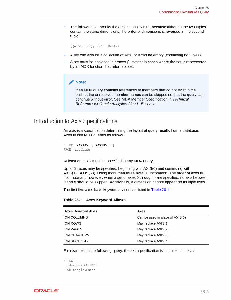
• The following set breaks the dimensionality rule, because although the two tuplescontain the same dimensions, the order of dimensions is reversed in the secondtuple:

{(West, Feb), (Mar, East)}

• A set can also be a collection of sets, or it can be empty (containing no tuples).

• A set must be enclosed in braces {}, except in cases where the set is representedby an MDX function that returns a set.

Note:

If an MDX query contains references to members that do not exist in theoutline, the unresolved member names can be skipped so that the query cancontinue without error. See MDX Member Specification in TechnicalReference for Oracle Analytics Cloud - Essbase.

Introduction to Axis SpecificationsAn axis is a specification determining the layout of query results from a database.Axes fit into MDX queries as follows:

SELECT <axis> [, <axis>...]FROM <database>

At least one axis must be specified in any MDX query.

Up to 64 axes may be specified, beginning with AXIS(0) and continuing withAXIS(1)...AXIS(63). Using more than three axes is uncommon. The order of axes isnot important; however, when a set of axes 0 through n are specified, no axis between0 and n should be skipped. Additionally, a dimension cannot appear on multiple axes.

The first five axes have keyword aliases, as listed in Table 28-1:

Table 28-1 Axes Keyword Aliases

Axes Keyword Alias Axes

ON COLUMNS Can be used in place of AXIS(0)

ON ROWS May replace AXIS(1)

ON PAGES May replace AXIS(2)

ON CHAPTERS May replace AXIS(3)

ON SECTIONS May replace AXIS(4)

For example, in the following query, the axis specification is {Jan}ON COLUMNS:

SELECT {Jan} ON COLUMNSFROM Sample.Basic


28-5

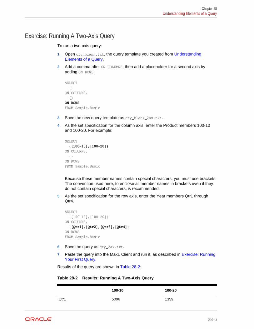
Exercise: Running A Two-Axis QueryTo run a two-axis query:


2. Add a comma after ON COLUMNS; then add a placeholder for a second axis byadding ON ROWS:

SELECT {}ON COLUMNS, {}ON ROWSFROM Sample.Basic

3. Save the new query template as qry_blank_2ax.txt.

4. As the set specification for the column axis, enter the Product members 100-10and 100-20. For example:

SELECT {[100-10],[100-20]}ON COLUMNS, {}ON ROWSFROM Sample.Basic

Because these member names contain special characters, you must use brackets.The convention used here, to enclose all member names in brackets even if theydo not contain special characters, is recommended.

5. As the set specification for the row axis, enter the Year members Qtr1 throughQtr4.

SELECT {[100-10],[100-20]}ON COLUMNS, {[Qtr1],[Qtr2],[Qtr3],[Qtr4]}ON ROWSFROM Sample.Basic

6. Save the query as qry_2ax.txt.

7. Paste the query into the MaxL Client and run it, as described in Exercise: RunningYour First Query.

Results of the query are shown in Table 28-2:

Table 28-2 Results: Running A Two-Axis Query

100-10 100-20

Qtr1 5096 1359


28-6

Table 28-2 (Cont.) Results: Running A Two-Axis Query

100-10 100-20

Qtr2 5892 1534

Qtr3 6583 1528

Qtr4 5206 1287

Exercise: Querying Multiple Dimensions on a Single AxisTo query multiple dimensions on a single axis:

1. Open qry_blank_2ax.txt, the query template you created from Exercise: RunningA Two-Axis Query.

2. On the column axis, specify two tuples, each of which is a member combinationrather than a single member. Enclose each tuple in parentheses, because multiplemembers are represented in each tuple.

SELECT {([100-10],[East]), ([100-20],[East])}ON COLUMNS, {}ON ROWSFROM Sample.Basic

3. On the row axis, specify four two-member tuples, nesting each Quarter with Profit:

SELECT {([100-10],[East]), ([100-20],[East])}ON COLUMNS, { ([Qtr1],[Profit]), ([Qtr2],[Profit]), ([Qtr3],[Profit]), ([Qtr4],[Profit]) }ON ROWSFROM Sample.Basic

4. Save the query as qry_1ax.txt.



Table 28-3 Results: Querying Multiple Dimensions on a Single Axis

100-10 100-20

East East

Qtr1 Profit 2461 212



28-7

Table 28-3 (Cont.) Results: Querying Multiple Dimensions on a Single Axis

100-10 100-20



Cube SpecificationA cube specification is the part of the query that determines which database is beingqueried. The cube specification fits into an MDX query as follows:

SELECT <axis> [, <axis>...]FROM <database>

The <database> section follows the FROM keyword and should consist of delimited ornondelimited identifiers that specify first an application name and a then databasename; for example, the following specifications are valid:

• FROM Sample.Basic

• FROM [Sample.Basic]

• FROM [Sample].[Basic]

• FROM'Sample'.'Basic'

Using Functions to Build SetsRather than creating sets member-by-member or tuple-by-tuple, you can use afunction that returns a set. MDX includes several functions that return sets and severalfunctions that return other values. For a complete reference of MDX functionssupported by Essbase, see MDX in Technical Reference for Oracle Analytics Cloud -Essbase.

Exercise: Using the MemberRange FunctionThe MemberRange MDX function returns a range of members inclusive of andbetween two specified members of the same generation. Its syntax is as follows:

MemberRange (member1, member2, [,layertype])

where the first argument you provide is the member that begins the range, and thesecond argument is the member that ends the range. The layertype argument isoptional.

Chapter 28Using Functions to Build Sets

28-8

Note:

An alternate syntax for MemberRange is to use a colon between the twomembers, instead of using the function name: member1 : member2.

To use the MemberRange function:


2. Delete the braces {}, which are unnecessary when you are using a function toreturn the set.

3. Use the colon operator to select a member range of Qtr1 through Qtr4:

SELECT [Qtr1]:[Qtr4]ON COLUMNS FROM Sample.Basic


Qtr1, Qtr2, Qtr3, and Qtr4 are returned.

5. Use the MemberRange function to select the same member range, Qtr1 throughQtr4.

SELECT MemberRange([Qtr1],[Qtr4])ON COLUMNSFROM Sample.Basic

6. Save the query as gry_member_range_func.txt.


Qtr1, Qtr2, Qtr3, and Qtr4 are returned.

Exercise: Using the CrossJoin FunctionThe CrossJoin function returns the cross product of two sets from differentdimensions. Its syntax is as follows:

CrossJoin(set,set)

The CrossJoin function takes two sets from different dimensions as input and createsa set that is a cross product of the two input sets, useful for creating symmetricreports.

To use the CrossJoin function:



28-9

2. Replace the braces {} from the columns axis with CrossJoin().

SELECT CrossJoin () ON COLUMNS, {}ON ROWSFROM Sample.Basic

3. Add two comma-separated pairs of braces as placeholders for the two setarguments you will provide to the CrossJoin function:

SELECT CrossJoin ({}, {})ON COLUMNS, {}ON ROWSFROM Sample.Basic

4. In the first set, specify the Product member [100-10]. In the second set, specifythe Market members [East], [West], [South], and [Central].

SELECT CrossJoin ({[100-10]}, {[East],[West],[South],[Central]})ON COLUMNS, {}ON ROWSFROM Sample.Basic

5. On the row axis, use CrossJoin to cross a set of Measures members with a setcontaining Qtr1:

SELECT CrossJoin ({[100-10]}, {[East],[West],[South],[Central]})ON COLUMNS, CrossJoin ( {[Sales],[COGS],[Margin %],[Profit %]}, {[Qtr1]} ) ON ROWSFROM Sample.Basic

6. Save the query as qry_crossjoin_func.txt.


When using CrossJoin, the order of arguments affects the order of tuples in the output.

Note:

Consider using CrossJoinAttribute if the input sets are a base dimension andits attribute dimension.


28-10


Table 28-4 Results: Using the CrossJoin Function

100-10 100-10 100-10 100-10

East West South Central

Sales Qtr1 5731 3493 2296 3425

COGS Qtr1 1783 1428 1010 1460

Margin % Qtr1 66.803 59.118 56.01 57.372

Profit % Qtr1 45.82 29.974 32.448 24.613

Exercise: Using the Children FunctionThe Children function returns a set of all child members of the given member. Use thissyntax:

Children (member)

Note:

An alternate syntax for Children is to use it as an operator on the inputmember, as follows: member.Children. We will use the operator syntax inthis exercise.

To use the Children function to introduce a shortcut in the first axis specification:

1. Open qry_crossjoin_func.txt, the query you built in Exercise: Using theCrossJoin Function.

2. In the second set of the column axis specification, replace [East],[West],[South],[Central] with [Market].Children.

SELECT CrossJoin ({[100-10]}, {[Market].Children})ON COLUMNS, CrossJoin ( {[Sales],[COGS],[Margin %],[Profit %]}, {[Qtr1]} )ON ROWSFROM Sample.Basic

3. Save the query as gry_children_func.txt.


You should see the same results as those returned for the Crossjoin exercise: Table 28-4.


28-11

Working with Levels and GenerationsIn MDX, layer refers to generations and levels in an Essbase hierarchy.

In Essbase, generation numbers begin counting with 1 at the dimension name; highergeneration numbers are those closest to leaf members in a hierarchy.

Level numbers begin with 0 at the leaf-most part of the hierarchy, and the highest levelnumber is a dimension name.

A number of MDX functions take a layer you specify as an input argument and performset operations based on the generation or level represented in the layer argument.

You can specify a layer argument in the following ways:

• Generation or level name; for example, States or Regions.

• The dimension name along with the generation or level name; for example,Market.Regions and [Market].[States].

• The Levels function with a dimension and a level number as input. For example,[Year].Levels(0).

• The Level function with a member as input. For example, [Qtr1].Level returnsthe level of quarters in Sample.Basic, which is level 1 of the Market dimension.

• The Generations function with a dimension and a generation number as input. Forexample, [Year].Generations (3).

• The Generation function with a member as input. For example,[Qtr1].Generation returns the generation of quarters in Sample.Basic, which isgeneration 2 of the Market dimension.

Note:

In the Sample.Basic database, Qtr1 and Qtr4 are in the same layer. Thismeans that Qtr1 and Qtr4 are also in the same generation. However, in adifferent database with a ragged hierarchy, Qtr1 and Qtr4 might notnecessarily be in the same level, although they are in the same generation.For example, if the hierarchy of Qtr1 drills down to weeks, and the hierarchyof Qtr4 stops at months, Qtr1 is one level higher than Qtr4, but they are stillin the same layer.

See Also

MDX Layer Specification in Technical Reference for Oracle Analytics Cloud - Essbase.

Exercise: Using the Members FunctionUse the Members function to return all members of a specified generation or level.When used with a layer argument, the syntax is:

Members (layer)

where the layer argument indicates the generation or level of members to return.

Chapter 28Working with Levels and Generations

28-12

Note:

An alternate syntax for Members is layer.Members.

To use the Members function:

1. Open qry_blank.txt, the query template you created from UnderstandingElements of a Query..

2. Delete the braces {}.

3. Use the Members function and the Levels function to select all level 0 members inthe Market dimension of Sample.Basic:

SELECT Members(Market.levels(0))ON COLUMNSFROM Sample.Basic

4. Save the query as qry_members_func.txt.


Results: All states in the Market dimension are returned.

Using a Slicer Axis to Set Query Point-of-ViewA slicer axis is a way to limit a query to apply to only a specific area of the database.The optional slicer, if used, must be in the WHERE section of an MDX query.Furthermore, the WHERE section must be the last component of the query, followingthe cube specification (the FROM section):

SELECT {set}ON axesFROM databaseWHERE slicer

Use the slicer axis to set the context of the query; it is usually the default context for allthe other axes.

For example, for a query to select only Actual Sales in the Sample.Basic database,excluding budgeted sales, the WHERE clause might look like the following:

WHERE ([Actual], [Sales])

Because (Actual, Sales) is specified in the slicer axis, you need not include them in theON AXIS(n) set specifications.

Chapter 28Using a Slicer Axis to Set Query Point-of-View

28-13

Note:

The same dimension cannot appear on other axes and the slicer axis. Tofilter an axis using criteria from its own dimension, you can use a sub select.

See Also

• MDX Slicer Specification in Technical Reference for Oracle Analytics Cloud -Essbase

• MDX Sub Select in Technical Reference for Oracle Analytics Cloud - Essbase

Exercise: Limiting the Results with a Slicer AxisTo use the slicer axis to limit results:

1. Open gry_crossjoin_func.txt, the query you built in Exercise: Using theCrossJoin Function.


Note the results in one of the data cells; for example, notice that the first tuple,([100-10],[East],[Sales],[Qtr1]), has a value of 5731.

3. Add a slicer axis to limit the data returned to budgeted values only.

SELECT CrossJoin ({[100-10]}, {[East],[West],[South],[Central]})ON COLUMNS, CrossJoin ( {[Sales],[COGS],[Margin %],[Profit %]}, {[Qtr1]} )ON ROWSFROM Sample.BasicWHERE (Budget)

4. Paste the query into the MaxL Client and run it.

5. Save the query as qry_slicer_axis.txt.

You should see different results for the two queries.

Common Relationship FunctionsTable 28-5 lists the relationship functions that return sets based on memberrelationships in the database outline:

Table 28-5 List of Relationship Functions That Return Sets

Relationship Function Description

Children Returns the children of the input member.

Siblings Returns the siblings of the input member.

Chapter 28Common Relationship Functions

28-14

Table 28-5 (Cont.) List of Relationship Functions That Return Sets


Descendants Returns the descendants of a member, withvarying options.

Table 28-6 lists the relationship functions that return a single member rather than aset:

Table 28-6 List of Relationship Functions That Return a Single Member


Ancestor Returns an ancestor at the specified layer.

Cousin Returns a child member at the same positionas a member from another ancestor.

Parent Returns the parent of the input member.

FirstChild Returns the first child of the input member.

LastChild Returns the last child of the input member.

FirstSibling Returns the first child of the input member’sparent.

LastSibling Returns the last child of the input member’sparent.

For examples using relationship functions, click the links to see the MDX examples inTechnical Reference for Oracle Analytics Cloud - Essbase.

Performing Set OperationsTable 28-7 lists the set functions that operate on input sets without deriving furtherinformation from a cube:

Table 28-7 List of Pure Set Functions

Pure Set Function Description

CrossJoin, CrossJoinAttribute Returns a cross-section of two sets fromdifferent dimensions.

Distinct Deletes duplicate tuples from a set.

Except Returns a subset containing the differencesbetween two sets.

Generate An iterative function. For each tuple in set1,returns set2.

Head Returns the first n members or tuples presentin a set.

Intersect Returns the intersection of two input sets.

Subset Returns a subset from a set, in which thesubset is a numerically specified range oftuples.

Chapter 28Performing Set Operations

28-15

Table 28-7 (Cont.) List of Pure Set Functions

Pure Set Function Description

Tail Returns the last n members or tuples presentin a set.

Union Returns the union of two input sets.

For examples using pure set functions, click the links to see the MDX examples inTechnical Reference for Oracle Analytics Cloud - Essbase.

Exercise: Using the Intersect FunctionThe Intersect MDX function returns the intersection two input sets, optionally retainingduplicates. Syntax:

Intersect (set, set [,ALL])

Use the Intersect function to compare sets by finding tuples that are present in bothsets.

To use the Intersect function:


2. Delete the braces {} from the axis, and replace them with Intersect(). Forexample:

SELECT Intersect (

)ON COLUMNSFROM Sample.Basic

3. Add two comma-separated pairs of braces to use as placeholders for the two setarguments you will provide to the Intersect function. For example:

SELECT Intersect ( { }, { } )ON COLUMNSFROM Sample.Basic

4. Specify children of East as the first set argument. For example:

SELECT Intersect ( { [East].children }, { }

Chapter 28Performing Set Operations

28-16

)ON COLUMNSFROM Sample.Basic

5. For the second set argument, specify all members of the Market dimension thathave a UDA of “Major Market.” For example:

SELECT Intersect ( { [East].children }, { UDA([Market], "Major Market") } )ON COLUMNSFROM Sample.Basic

6. Save the query as qry_intersect_func.txt.


All children of East that have a UDA of "Major Market" are returned. For example:

New York Massachusetts Florida

8202 6172 5029

Exercise: Using the Union FunctionThe Union MDX function joins two input sets, optionally retaining duplicates. Syntax:

Union (set, set [,ALL])

Use the Union function to lump two sets together into one set.

To use the Union function:

1. Open qry_intersect_func.txt, the query you built in Exercise: Using theIntersect Function.

2. Replace Intersect with Union.

3. Save the query as qry_union_func.txt.

4. Paste the query into the MaxL Client and run it.

While Intersect returned a set containing only those children of East that have a UDAof Major Market, Union returns all children of East AND all Market members that havea UDA of Major Market.

Creating and Using Named Sets and Calculated MembersCalculated members and named sets are logical entities in query that can be usedmultiple times during the life of the query. Calculated members and named sets cansave time in lines of code written as well as in execution time. The optional WITHsection at the beginning of an MDX query is where you define the calculated membersand/or named sets.

Chapter 28Creating and Using Named Sets and Calculated Members

28-17

See Also

MDX With Section

Calculated MembersA calculated member is a hypothetical member that exists for the duration of the queryexecution. Calculated members enable complex analysis without the need to addphysical members to the cube outline. Calculated members store calculation resultsperformed on physical members.

Use the following guidelines for calculated member names:

• Associate the calculated member with a dimension; for example, to associated themember MyCalc with the Measures dimension, name it [Measures].[MyCalc].

• Do not use actual member names to name calculated members; for example, donot name a calculated member [Measures].[Sales], because Sales alreadyexists in the Measures dimension.

Setting the solve order for each calculated member is recommended when you usemultiple calculated members to create ratios or custom totals. For more informationabout solve order, see MDX With Section in Technical Reference for Oracle AnalyticsCloud - Essbase.

Exercise: Creating a Calculated MemberThis exercise includes the Max MDX function, a common function for calculations. TheMax function returns the maximum of values found in the tuples of a set. Its syntax isas follows:

Max (set, numeric_value)

To create a calculated member,


2. On the row axis set, specify the children of Product. For example:

SELECT {}ON COLUMNS, {[Product].children}ON ROWSFROM Sample.Basic

3. At the beginning of the query, add a placeholder for the calculated memberspecification. For example:

WITH MEMBER [].[] AS ''SELECT {}ON COLUMNS,


28-18

{[Product].children}ON ROWSFROM Sample.Basic

4. To associate the calculated member with the Measures dimension and name itMax Qtr2 Sales, add this information to the calculated member specification. Forexample:

WITH MEMBER [Measures].[Max Qtr2 Sales] AS ''SELECT {}ON COLUMNS, {[Product].children}ON ROWSFROM Sample.Basic

5. After the AS keyword and inside the single quotation marks, define the logic for thecalculated member named Max Qtr2 Sales.

Use the Max function with the set to evaluate (Qtr2) as the first argument, and themeasure to evaluate (Sales) as the second argument. For example:

WITH MEMBER [Measures].[Max Qtr2 Sales] AS ' Max ( {[Year].[Qtr2]}, [Measures].[Sales] )'SELECT {}ON COLUMNS, {[Product].children}ON ROWSFROM Sample.Basic

6. The calculated member Max Qtr2 Sales is defined in the WITH section. To use itin a query, include it on one of the axes in the SELECT portion of the query. Selectthe predefined calculated member on the columns axis. For example:

WITH MEMBER [Measures].[Max Qtr2 Sales] AS ' Max ( {[Year].[Qtr2]}, [Measures].[Sales] )'SELECT {[Measures].[Max Qtr2 Sales]}ON COLUMNS, {[Product].children}ON ROWSFROM Sample.Basic

7. Save the query as gry_calc_member.txt.


28-19



Table 28-8 Results: Creating a Calculated Member

Max Qtr2 Sales

100 27187

200 27401

300 25736

400 21355

Diet 26787

Named SetsYou define named sets in the WITH section of the query. Doing so is useful becauseyou can reference the set by name when building the SELECT section of the query.

For example, the named set Best5Prods identifies a set of the five top-selling productsin December:

WITHSET [Best5Prods] AS 'Topcount ( [Product].members, 5, ([Measures].[Sales], [Scenario].[Actual], [Year].[Dec]) )'SELECT [Best5Prods] ON AXIS(0), {[Year].[Dec]} ON AXIS(1)FROM Sample.Basic

Using Iterative FunctionsTable 28-9 lists the functions that loop through sets of data, and perform searchconditions and results that you specify:

Table 28-9 List of Iterative Functions

Function Description

Filter Returns the subset of tuples in set for whichthe value of the search condition is TRUE.

IIF Performs a conditional test and returns anappropriate numeric expression or setdepending on whether the test evaluates toTRUE or FALSE.

Case Performs conditional tests and returns theresults you specify.

Chapter 28Using Iterative Functions

28-20

Table 28-9 (Cont.) List of Iterative Functions


Generate For each tuple in set1, returns set2.

Filter Function Example

The following query returns all Market dimension members for which the expressionIsChild([Market].CurrentMember,[East]) returns TRUE; the query returns allchildren of East.

SELECT Filter([Market].Members, IsChild([Market].CurrentMember,[East]) )ON COLUMNSFROM Sample.Basic

For more examples using iterative functions, click the links to see the MDX examplesin Technical Reference for Oracle Analytics Cloud - Essbase.

Working with Missing DataWhen you are querying an Essbase cube using MDX, you can use the NON EMPTYkeywords at the beginning of an axis specification to prevent cells containing no valuefrom being included the result of the query.

The following is the axis specification syntax with NON EMPTY:

<axis_specification> ::= [NON EMPTY] <set> ON COLUMNS | ROWS | PAGES | CHAPTERS | SECTIONS | AXIS (<unsigned_integer>)

Including the optional keywords NON EMPTY before the set specification in an axiscauses suppression of slices in that axis that would contain entirely #MISSING values.

For any given tuple on an axis (such as (Qtr1, Actual)), a slice consists of the cellsarising from combining this tuple with all tuples of all other axes. If all of these cellvalues are #MISSING, the NON EMPTY keyword causes elimination of the tuple.

For example, if even one value in a row is not empty, the entire row is returned.Including NON EMPTY at the beginning of the row axis specification would eliminatethe following row slice from the set returned by a query:

In addition to suppressing missing values with NON EMPTY, you can use the followingMDX functions to handle #MISSING results:

Chapter 28Working with Missing Data

28-21

• CoalesceEmpty, which searches numeric value expressions for non #MISSINGvalues

• IsEmpty, which returns TRUE if the value of an input numeric-value-expressionevaluates to #MISSING

• Avg, which omits missing values from averages unless you use the optionalIncludeEmpty flag

The NonEmptyCount MDX function returns the count of the number of tuples in a setthat evaluate to non-#Missing values. Each tuple is evaluated and included in thecount returned by this function. If the numeric value expression is specified, it isevaluated in the context of every tuple, and the count of non-#Missing values isreturned.

On aggregate storage databases only, the NonEmptyCount function is optimized sothat the calculation of the distinct count for all cells can be performed by scanning thedatabase only once. Without this optimization, the database is scanned as many timesas the number of cells corresponding to the distinct count. The NonEmptyCountoptimization is triggered when an outline member formula has the following syntax:

NONEMPTYCOUNT(set, measure, exclude_missing)

The exclude_missing parameter supports the NonEmptyCount optimization onaggregate databases by improving the performance of a query that queries metricsthat perform a distinct count calculation.

The NONEMPTYMEMBER and NONEMPTYTUPLE optimization properties enableMDX to query on large sets of members or tuples while skipping formula execution onnon-contributing values that contain only #MISSING data. See MDX OptimizationProperties in Technical Reference for Oracle Analytics Cloud - Essbase.

• Use a single NONEMPTYMEMBER property clause at the beginning of acalculated member or formula expression to indicate to Essbase that the value ofthe formula or calculated member is empty when any of the members specified innonempty_member_list are empty.

• Use a single NONEMPTYTUPLE property clause at the beginning of a calculatedmember or formula expression to indicate to Essbase that the value of the formulaor calculated member is empty when the cell value at the tuple given innonempty_member_list is empty.

Given an input set, the NonEmptySubset MDX function returns a subset of that inputset in which all tuples evaluate to non-empty. An optional value expression may bespecified for the non-empty check. This function can help optimize queries that arebased on a large set for which the set of non-empty combinations is known to besmall. NonEmptySubset reduces the size of the set in the presence of a metric; forexample, you might request the non-empty subset of descendants for specific Units.

Using Substitution Variables in MDX QueriesSubstitution variables act as global placeholders for information that changesregularly; you set the substitution variables at the Essbase cube, application, or globallevel, and assign a value to each variable. You can change the value anytime. Youmust have the role of at least Database Manager to set substitution variables. See Using Substitution Variables.

Chapter 28Using Substitution Variables in MDX Queries

28-22

To use a substitution variable in an MDX expression, consider:

• The substitution variable must be accessible from the application and cube youare querying.

• A substitution variable has two components: the name and the value.

• The variable name can be an alphanumeric combination whose maximum size isspecified in Name and Related Artifact Limits. Do not use spaces, punctuation, orbrackets ([ ]) in substitution variable names used in MDX.

• At the point in the expression where you want to use the variable, show thevariable name preceded by an ampersand (&); for example, where CurMonth is thename of the substitution variable set on the server, include &CurMonth in the MDXexpression.

• When you perform the retrieval, Essbase replaces the variable name with thesubstitution value, and that value is used by the MDX expression.

For example, the expression is written showing the variable name CurQtr precededwith the &:

SELECT {[&CurQtr]}ON COLUMNSFROM Sample.Basic

When the expression is executed, the current value (Qtr1) is substituted for thevariable name, and the expression that is executed is:

SELECT {[Qtr1]}ON COLUMNSFROM Sample.Basic

Querying for PropertiesIn MDX, properties describe certain characteristics of data and metadata. MDXenables you to write queries that use properties to retrieve and analyze data.Properties can be intrinsic or custom.

Intrinsic properties are defined for members in all dimensions. The intrinsic memberproperties defined for all members in an Essbase database outline areMEMBER_NAME, MEMBER_ALIAS, LEVEL_NUMBER, GEN_NUMBER,IS_EXPENSE, COMMENTS, and MEMBER_UNIQUE_NAME.

MDX in Essbase supports two types of custom properties: attribute properties andUDA properties. Attribute properties are defined by the attribute dimensions in anoutline. In the Sample.Basic database, the Pkg Type attribute dimension describes thepackaging characteristics of members in the Product dimension. This information canbe queried in MDX using the property name [Pkg Type].

Attribute properties are defined only for specific dimensions and only for a specificlevel in each dimension. For example, in the Sample.Basic outline, [Ounces] is anattribute property defined only for members in the Product dimension, and thisproperty has valid values only for the level 0 members of the Product dimension. The[Ounces] property does not exist for other dimensions, such as Market. The [Ounces]

Chapter 28Querying for Properties

28-23

property for a non level 0 member in the Product dimension is a NULL value. Theattribute properties in an outline are identified by the names of attribute dimensions inthat outline.

The custom properties also include UDAs. For example, [Major Market] is a UDAproperty defined on Market dimension members. It returns a TRUE value if [MajorMarket] UDA is defined for a member, and FALSE otherwise.

See Also

About MDX Properties in Technical Reference for Oracle Analytics Cloud - Essbase.

Querying for Member PropertiesProperties can be used inside an MDX query in two ways.

• You can list the dimension and property combinations for each axis set. When aquery is executed, the specified property is evaluated for all members from thespecified dimension and included in the result set.

For example, on the column axis, the following query returns the GEN_NUMBERinformation for every Market dimension member. On the row axis, the queryreturns MEMBER_ALIAS information for every Product dimension member.

SELECT [Market].Members DIMENSION PROPERTIES [Market].[GEN_NUMBER] on columns, Filter ([Product].Members, Sales > 5000) DIMENSION PROPERTIES [Product].[MEMBER_ALIAS] on rowsFROM Sample.Basic

When querying for member properties using the DIMENSION PROPERTIESsection of an axis, a property can be identified by the dimension name and thename of the property, or by using the property name itself. When a property nameis used by itself, that property information is returned for all members from alldimensions on that axis, for which that property applies. In the following query, theMEMBER_ALIAS property is evaluated on the row axis for Year and Productdimensions.

SELECT [Market].Members DIMENSION PROPERTIES [Market].[GEN_NUMBER] on columns, CrossJoin([Product].Children, Year.Children) DIMENSION PROPERTIES [MEMBER_ALIAS] on rowsFROM Sample.Basic

• Properties can be used inside value expressions in an MDX query. For example,you can filter a set based on a value expression that uses properties of membersin the input set.

The following query returns all caffeinated products that are packaged in cans.

SELECT Filter([Product].levels(0).members, [Product].CurrentMember.Caffeinated and [Product].CurrentMember.[Pkg Type] = "Can") xDimension Properties


28-24

[Caffeinated], [Pkg Type] on columnsFROM Sample.Basic

The following query calculates the value [BudgetedExpenses] based on whetherthe current Market is a major market, using the UDA [Major Market].

WITH MEMBER [Measures].[BudgetedExpenses] AS 'IIF([Market].CurrentMember.[Major Market], [Marketing] * 1.2, [Marketing])'

SELECT {[Measures].[BudgetedExpenses]} ON COLUMNS, [Market].Members ON ROWSFROM Sample.BasicWHERE ([Budget])

The Value Type of PropertiesThe value of an MDX property in Essbase can be a numeric, Boolean, or string type.MEMBER_NAME and MEMBER_ALIAS properties return string values.LEVEL_NUMBER, and GEN_NUMBER properties return numeric values.

The attribute properties return numeric, Boolean, or string values based on theattribute dimension type. For example, in Sample.Basic, the [Ounces] attributeproperty is a numeric property. The [Pkg Type] attribute property is a string property.The [Caffeinated] attribute property is a Boolean property.

Essbase allows attribute dimensions with date types. The date type properties aretreated as numeric properties in MDX. When comparing these property values withdates, use the TODATE function to convert date strings to numeric before comparison.

The following query returns all Product dimension members that have been introducedon date 03/25/2018. Because the property [Intro Date] is a date type, the TODATEfunction must be used to convert the date string “03-25-2018” to a number beforecomparing it.

SELECT Filter ([Product].Members, [Product].CurrentMember.[Intro Date] = TODATE("mm-dd-yyyy","03-25-2018"))ON COLUMNSFROM Sample.Basic

When a property is used in a value expression, you must use it appropriately based onits value type: string, numeric, or Boolean.

You can also query attribute dimensions with numeric ranges.

The following query retrieves Sales data for Small, Medium, and Large populationranges.

SELECT {Sales} ON COLUMNS, {Small, Medium, Large} ON ROWSFROM Sample.Basic


28-25

When attributes are used as properties in a value expression, you can use rangemembers to check whether a member's property value falls within a given range, usingthe IN operator.

For example, the following query returns all Market dimension members with thepopulation range in Medium:

SELECT Filter( Market.Members, Market.CurrentMember.Population IN "Medium" )ON AXIS(0)FROM Sample.Basic

NULL Property ValuesNot all members may have valid values for a given property name. For example, theMEMBER_ALIAS property returns an alternate name for a given member as defined inthe outline; however, not all members may have aliases defined. In these cases ANULL value is be returned for those members that do not have aliases.

In the following query,

SELECT [Year].Members DIMENSION PROPERTIES [MEMBER_ALIAS]ON COLUMNSFROM Sample.Basic

None of the members in the Year dimension have aliases defined for them. Therefore,the query returns NULL values for the MEMBER_ALIAS property for members in theYear dimension.

The attribute properties are defined for members of a specific dimension and a specificlevel in that dimension. In the Sample.Basic database, the [Ounces] property isdefined only for level 0 members of the Product dimension.

Therefore, if you query for the [Ounces] property of a member from the Marketdimension, as shown in the following query, you will get a syntax error:

SELECT Filter([Market].members, [Market].CurrentMember.[Ounces] = 32) ON COLUMNSFROM Sample.Basic

Additionally, if you query for the [Ounces] property of a non level 0 member of thedimension, you will get a NULL value.


28-26

When using property values in value expressions, you can use the function IsValid() tocheck for NULL values. The following query returns all Product dimension memberswith an [Ounces] property value of 12, after eliminating members with NULL values.

SELECT Filter([Product].Members, IsValid([Product].CurrentMember.[Ounces]) AND [Product].CurrentMember.[Ounces] = 12) ON COLUMNSFROM Sample.Basic


28-27

29Exporting Data

You can export data from a database to move data between Essbase databases.

Topics:

• Exporting Data Using MaxL

• Exporting Text Data Using Calculation Scripts

Also see Exporting a Cube to an Application Workbook and Exporting On-PremisesCubes to Import to the Cloud in Using Oracle Analytics Cloud - Essbase.

Exporting Data Using MaxLYou can export data from an Essbase database using the export data MaxLstatement. Data can be export serially or in parallel. If the data for a thread exceeds 2GB, Essbase may divide the export data into multiple files with numbers appended tothe file names.

• Block storage databases: You can export all data, level-0 data, or input-level data,which does not include calculated values.

To export data in parallel, specify a comma-separated list of export files, up to amaximum of 1024 file names. The number of file names determines the number ofexport threads. The number of available block-address ranges limits the number ofexport threads that Essbase actually uses. Essbase divides the number of actualdata blocks by the specified number of file names (export threads). If there arefewer actual data blocks than the specified number of export threads, the numberof export threads that are created is based on the number of actual data blocks.This approach results in a more even distribution of data blocks between exportthreads.

• Aggregate storage databases: You can export only level-0 data, which does notinclude calculated values. (Level-0 data is the same as input data in aggregatestorage databases.) You cannot perform upper-level data export or columnarexport on an aggregate storage database.

To export data in parallel, specify a comma-separated list of export files, from 1 to8 file names. The number of threads Essbase uses typically depends on thenumber of file names you specify. However, on a very small aggregate storagedatabase with a small number of data blocks, it is possible that only a single filewill be created (in effect, performing serial export), even though parallel export tomultiple files is requested.

Export files are stored in the database directory in the file catalog; for example, Files> applications > Sample > Basic.

Exporting Text Data Using Calculation ScriptsYou can use the following calculation commands to select and format a text import file: DATAEXPORT, DATAEXPORTCOND, SET DATAEXPORTOPTIONS, FIX...ENDFIX,

29-1

and EXCLUDE...ENDEXCLUDE. For general information about creating and running acalculation script, see Developing Calculation Scripts for Block Storage Databases.

Calculation script-based data export works with stored and dynamically calculatedmembers only and provides fewer formatting options than report scripts. However,calculation script-based data exports provide decimal- and precision-based formattingoptions and can be faster than report scripts. The DATAEXPORT calculationcommand also enables export directly to relational databases, eliminating the usualintermediate import step.

The following calculation script example produces a text file that contains a subset ofthe database.

SET DATAEXPORTOPTIONS{ DATAEXPORTLEVEL "ALL";DATAEXPORTCOLFORMAT ON;DATAEXPORTCOLHEADER Scenario;}; FIX ("100-10","New York","Actual","Qtr1"); DATAEXPORT "File" "," "actual.txt" "NULL";ENDFIX;

These commands specify inclusion of all levels of data and indicate that data is to berepeated in columns, with the Scenario dimension set as the dense dimension columnheader for the output. The FIX command defines the data slice, and then the data isexported to a text file actual.txt in the database directory. Commas are used asdelimiters, and missing data values are indicated by consecutive delimiters. Runningthis script against Sample.Basic generates the following data:

"Actual""100-10","New York","Sales","Qtr1",1998"100-10","New York","COGS","Qtr1",799"100-10","New York","Margin","Qtr1",1199"100-10","New York","Marketing","Qtr1",278"100-10","New York","Payroll","Qtr1",153"100-10","New York","Misc","Qtr1",2"100-10","New York","Total Expenses","Qtr1",433"100-10","New York","Profit","Qtr1",766"100-10","New York","Opening Inventory","Qtr1",2101"100-10","New York","Additions","Qtr1",2005"100-10","New York","Ending Inventory","Qtr1",2108"100-10","New York","Margin %","Qtr1",60.01001001001001"100-10","New York","Profit %","Qtr1",38.33833833833834"100-10","New York","Profit per Ounce","Qtr1",63.83333333333334

Chapter 29Exporting Text Data Using Calculation Scripts

29-2

30Controlling Access to Database CellsUsing Security Filters

When security levels defined for applications, databases, users, and groups areinsufficient, Essbase security filters give you more specific control. Filters enable youto control access to individual data within a database by defining what kind of accessis allowed to which parts of the database, and to whom these settings apply.

• About Security Filters

• Defining Permissions Using Security Filters

• Creating Filters

• Managing Filters

• Assigning Filters

About Security FiltersWhen security levels defined for applications, databases, users, and groups areinsufficient, Essbase security filters give you more specific control. Filters enable youto control access to individual data within a database by defining what kind of accessis allowed to which parts of the database, and to whom these settings apply.

If you have Administrator permissions, you can define and assign any filters to anyusers or groups. Filters do not affect you.

If you have Create/Delete Applications permissions, you can assign and define filtersfor applications that you created.

If you have Application Manager or Database Manager permissions, you can defineand assign filters within your applications or databases.

Defining Permissions Using Security FiltersFilters control security access to data values, or cells. You create filters toaccommodate security needs for specific parts of a database. When you define a filter,you designate restrictions on particular database cells. When you save the filter, yougive it a unique name to distinguish it from other filters. You can then assign the filtersto users or groups.

For example, a manager designs a filter named RED and associates it with a databaseto limit access to cells containing profit information. The filter is assigned to a visitinggroup called REVIEWERS, so that they can read, but cannot alter, most of thedatabase; they have no access to Profit data values.

Filters comprise one or more access settings for database members. You can specifythe following access levels and apply them to data ranging from a list of members toone cell:

30-1

• None: No data can be retrieved or updated for the specified member list.

• Read: Data can be retrieved but not updated for the specified member list.

• Write: Data can be retrieved and updated for the specified member list.

• Metaread: Metadata (dimension and member names) can be retrieved andupdated for the corresponding member specification.

Note:

The metaread access level overrides all other access levels. If additionalfilters for data are defined, they are enforced within any defined metareadfilters. If you have assigned a metaread filter on a substitution variable andthen try to retrieve the substitution variable, an unknown member erroroccurs, but the value of the substitution variable is displayed. This behavioris expected. Metadata security cannot be completely turned off in partitions.Therefore, do not set metadata security at the source database; otherwise,incorrect data may result at the target partition. When drilling up or retrievingon a member that has metadata security turned on and has shared membersin the children, an unknown member error occurs because the referencedmembers of the shared members have been filtered. To avoid this error, givethe referenced members of the shared members metadata security access.

Any cells that are not specified in the filter definition inherit the database access level.Filters can, however, add or remove access assigned at the database level, becausethe filter definition, being more data-specific, indicates a greater level of detail than themore general database access level.

Data values not covered by filter definitions default to the access levels defined forusers.

Calculation access is controlled by permissions granted to users and groups. Userswho have calculate access to the database are not blocked by filters—they can affectall data elements that the execution of their calculations would update.

Note:

During the calculation of MDX calculated members, cells to which a userdoes not have access are treated as #MISSING cells.

Creating FiltersYou can create a filter for each set of access restrictions you need to place ondatabase values. You need not create separate filters for users with the same accessneeds. After you have created a filter, you can assign it to multiple users or groups ofusers.

Chapter 30Creating Filters

30-2

Note:

If you use a calculation function that returns a set of members, such aschildren or descendants, and it evaluates to an empty set, the security filter isnot created. An error is written to the application log stating that the regiondefinition evaluated to an empty set.

Before creating a filter, perform the following actions:

• Connect to the server and select the database associated with the filter.

• Check the naming rules for filters in Limits.

See Creating Filters in Using Oracle Analytics Cloud - Essbase.

To create a filter, you can also use the create filter MaxL statement.

Filtering Members Versus Filtering Member CombinationsFigure 30-1 illustrates different ways to control access to database cells. Data can beprotected by filtering entire members or by filtering member combinations.

• Filtering members separately affects whole regions of data for those members.

• Filtering member combinations affects data at the member intersections.

Figure 30-1 How Filters Affect Data AND/OR Relationships

Note:

Filtering on member combinations (AND relationship) does not apply tometaread. Metaread filters each member separately (OR relationship).


30-3

Filtering Members SeparatelyTo filter all the data for one or more members, define access for each member on itsown row in Filter Editor. Filter definitions on separate rows of a filter are treated with anOR relationship.

For example, to block access to Sales or Jan, assume that user KSmith is assignedthe following filter:

• Access: None. Member specification: Sales.

• Access: None. Member specification: Jan.

The next time user KSmith connects to Sample.Basic, her spreadsheet view of theprofit margin for Qtr1 (Figure 30-2) shows that she has no access to data values forthe member Sales or the member Jan, which are marked with #NOACCESS. All datafor Sales is blocked from view, as well as all data for January, inside and outside of theSales member. Data for COGS (Cost of Goods Sold), a sibling of Sales and a child ofMargin, is available, with the exception of COGS for January.

Figure 30-2 Results of Filter Blocking Access to Sales or Jan

Filtering Member CombinationsTo filter data for member combinations, define the access for each membercombination using a row in Filter Editor. In filter definitions, two member setsseparated by a comma are treated as union of those two member sets (an ANDrelationship).

For example, assume that user RChinn is assigned the following filter: Access: None.Member specification: Sales, Jan.

The next time user RChinn connects to Sample.Basic, her spreadsheet view of theprofit margin for Qtr1 (Figure 30-3) shows that she has no access to the data value atthe intersection of members Sales and Jan, which is marked with #NoAccess. Salesdata for January is blocked from view. However, Sales data for other months isavailable, and non-Sales data for January is available.


30-4

Figure 30-3 Results of Filter Blocking Access to Sales, Jan

Filtering Using Substitution VariablesSubstitution variables enable you to more easily manage information that changesregularly. Each substitution variable has an assigned name and value. The DatabaseManager can change the value anytime. Where a substitution variable is specified in afilter, the substitution variable value at that time is used.

For example, if you want a group of users to see data only for the current month, youcan set up a substitution variable named CurMonth and define a filter (MonthlyAccess)wherein you specify access, using &CurMonth for the member name. Using anampersand (&) at the beginning of a specification identifies it as a substitution variableinstead of a member name to Essbase. Assign the MonthlyAccess filter to theappropriate users.

Each month, you need to change only the value of the CurMonth substitution variableto the member name for the current month, such as Jan, Feb, and so on. The newvalue will apply to all assigned users.

See Using Substitution Variables.

Filtering with Attribute FunctionsYou can use filters to restrict access to data for base members sharing a particularattribute. To filter data for members with particular attributes defined in an attributedimension, use the attribute member in combination with the @ATTRIBUTE functionor the @WITHATTR function.

Note:

@ATTRIBUTE and @WITHATTR are member set functions. Most memberset functions can be used in filter definitions.


30-5

For example, assume that user PJones is assigned this filter: Access: None. Memberspecification: @ATTRIBUTE(“Caffeinated_False”).

The next time user PJones connects to Sample.Basic, his spreadsheet view of first-quarter cola sales in California (Figure 30-4) shows that he has no access to the datavalues for any base dimension members associated with Caffeinated_False. Salesdata for Caffeine Free Cola is blocked from view. Note that Caffeine Free Cola is abase member, and Caffeinated_False is an associated member of the attributedimension Caffeinated (not shown in the above spreadsheet view).

Figure 30-4 Results of Filter Blocking Access to Caffeine-free Products

Metadata FilteringMetadata filtering provides data filtering and an additional layer of security. Withmetadata filtering, an administrator can remove outline members from a user's view,providing access only to those members that are of interest to the user.

When a filter is used to apply MetaRead permission on a member:

1. Data for all ancestors of that member are hidden from the filter user’s view.

2. Data and metadata (member names) for all siblings of that member are hiddenfrom the filter user’s view.

Dynamic FilteringYou can create dynamic filters based on external source data to reduce the number offilter definitions needed. You do this using dynamic filter definition syntax, including themethod @datasourceLookup and the variables $LoginUser and $LoginGroup.

For details, see Create Efficient Dynamic Filters in Using Oracle Analytics Cloud -Essbase.

Managing FiltersTo view a list of filters, you can use the display filter MaxL statement.

To edit, copy, or rename a filter, you can use the create filter MaxL statement.

You can copy filters to applications and databases on any Essbase Server, accordingto your permissions. You can also copy filters across servers as part of applicationmigration.

To delete a filter, you can use the drop filter MaxL statement.

Chapter 30Managing Filters

30-6

Assigning FiltersAfter you define filters, you can assign them to users or groups, which lets youmanage multiple users who require the same filter settings. Modifications to thedefinition of a filter are automatically inherited by users of that filter.

Filters do not affect users who have the Administrator role.

Overlapping Filter DefinitionsIf a filter contains rows that have overlapping member specifications, the inheritedaccess is set by the following rules, listed in order of precedence:

1. A filter that defines a more detailed dimension combination list takes precedenceover a filter with less detail.

2. If the preceding rule does not resolve the overlap conflict, the highest access levelamong overlapping filter rows is applied.

For example, this filter contains overlap conflicts:

• Access: Write. Member specification: Actual.

• Access: None. Member specification: Actual.

• Access: Read. Member specification: Actual, @IDESCENDANTS(“New York”).

The third specification defines security at a greater level of detail than the other two.Therefore, read access is granted to all Actual data for members in the New Yorkbranch.

Because write access is a higher access level than none, the remaining data values inActual are granted write access.

All other cells, such as Budget, are accessible according to the minimum databasepermissions.

If you have write access, you also have read access.

Note:

Changes to members in the database outline are not reflected automaticallyin filters. You must manually update member references that change.

Overlapping Metadata Filter DefinitionsYou should define a MetaRead filter using multiple rows only when the affectedmember set in any given row (the metaread members and their ancestors) has nooverlap with MetaRead members in other rows. It is recommended that you specifyone dimension per row in filters that contain MetaRead on multiple rows. However, aslong as there is no overlap between the ancestors and MetaRead members, it is stillvalid to specify different member sets of one dimension into multiple MetaRead rows.

For example, in Sample Basic, the following filter definition has overlap conflicts:

Chapter 30Assigning Filters

30-7

• Access: MetaRead. Member specification: California.

• Access: MetaRead. Member specification: West.

In the first row, applying MetaRead to California has the effect of allowing access toCalifornia but blocking access to its ancestors. Therefore, the MetaRead access toWest is ignored; users who are assigned this filter will have no access to West.

If you wish to assign MetaRead access to West, as well as California, the appropriatemethod is to combine them into one row: Access: MetaRead. Member specification:California, West.

Overlapping Access DefinitionsWhen the access rights of user and group definitions overlap, the following rules, listedin order of precedence, apply:

1. An access level that defines a more detailed dimension combination list takesprecedence over a level with less detail.

2. If the preceding rule does not resolve the overlap conflict, the highest access levelis applied.

Example 1:

User Fred is defined with the following database access:

FINPLAN RCAPPLAN WPRODPLAN N

He is assigned to Group Marketing, which has the following database access:

FINPLAN NCAPPLAN NPRODPLAN W

His effective rights are set as:

FINPLAN RCAPPLAN WPRODPLAN W

Example 2:

User Mary is defined with the following database access:

FINPLAN RPRODPLAN N

She is assigned to Group Marketing, which has the following database access:

FINPLAN NPRODPLAN W


30-8

Her effective rights are set as:

FINPLAN RPRODPLAN W

In addition, Mary uses the filter artifact RED (for the database FINPLAN). The filter hastwo filter rows:

• Access: Read. Member specification: Actual.

• Access: Write. Member specification: Budget, @IDESCENDANTS(“New York”).

The Group Marketing also uses a filter artifact BLUE (for the database FINPLAN). Thefilter has two filter rows:

• Access: Read. Member specification: Actual, Sales.

• Access: Write. Member specification: Budget, Sales.

Mary’s effective rights from the overlapping filters, and the permissions assigned to herand her group:

• R: Entire FINPLAN database.

• W: For all Budget data in the New York branch.

• W: For data values that relate to Budget and Sales.


30-9

31Using MaxL Data Definition Language

Using MaxL, you can automate administrative operations on Essbase databases. TheMaxL data definition language is an interface for making administrative requests toEssbase using statements.

See the following resources:

• Managing Essbase Using the MaxL Client in Using Oracle Analytics Cloud -Essbase

• MaxL in Technical Reference for Oracle Analytics Cloud - Essbase

31-1

32Optimizing Database Restructuring

Some changes to a database outline affect the data storage arrangement, forcing therestructuring of the database. Because changes that require restructuring thedatabase are time-consuming (unless you discard the data before restructuring),consider deciding on such changes based on how they affect performance.

• Database Restructuring

• Optimization of Restructure Operations

• Actions That Improve Performance

• Outline Change Quick Reference


Also see Positioning Dimensions and Members.

Database RestructuringAs your business changes, you change the Essbase database outline to capture newproduct lines, provide information on new scenarios, reflect new time periods, and soon. Some changes to a database outline affect the data storage arrangement, forcingEssbase to restructure the database.

Because changes that require restructuring the database are time-consuming (unlessyou discard the data before restructuring), consider deciding on such changes basedon how they affect performance. See:

• Implicit Restructures

• Explicit Restructures

• Conditions Affecting Database Restructuring

• Restructuring Requires a Temporary Increase in the Index Cache Size

Note:

For information about clearing data and thus avoiding some restructuring,see CLEARDATA and CLEARBLOCK in Technical Reference for OracleEssbase.

Implicit RestructuresEssbase initiates an implicit restructure of the database files after an outline ischanged using Outline Editor or Dimension Build. The type of restructure that isperformed depends on the type of changes made to the outline:

32-1

• Dense restructure: If a member of a dense dimension is moved, deleted, oradded, Essbase restructures the blocks in the data files and creates new datafiles. When Essbase restructures the data blocks, it regenerates the indexautomatically so that index entries point to the new data blocks. Empty blocks arenot removed. Essbase marks all restructured blocks as dirty, so after a denserestructure you must recalculate the database. Dense restructuring, the most time-consuming of the restructures, can take a long time to complete for largedatabases.

• Sparse restructure: If a member of a sparse dimension is moved, deleted, oradded, Essbase restructures the index and creates new index files. Restructuringthe index is relatively fast; the time required depends on the index size.

• Outline-only restructure: If a change affects only the database outline, Essbasedoes not restructure the index or data files. Member name changes, creation ofaliases, and dynamic calculation formula changes are examples of changes thataffect only the database outline.

Note:

How a database outline is changed (by using Outline Editor or usingdimension build) does not influence restructuring. Only the type ofinformation change influences what type of restructuring, if any, takes place.For information about outline changes and the type of restructures theycause, see Outline Change Quick Reference.

Explicit RestructuresWhen you manually initiate a database restructure, you perform an explicit restructure.An explicit restructure forces a full restructure of the database. A full restructurecomprises a dense restructure plus removal of empty blocks. All data load andcalculation transaction history is removed after an explicit restructure.

To initiate an full restructure, you can use the alter database MaxL statement.

Conditions Affecting Database RestructuringIntelligent Calculation, name changes, and formula changes affect databaserestructuring:

• If you use Intelligent Calculation in the database, all restructured blocks aremarked as dirty whenever data blocks are restructured. Marking the blocks as dirtyforces the next default Intelligent Calculation to be a full calculation.

• If you change a name or a formula, Essbase does not mark the affected blocks asdirty. Therefore, you must use a method other than full calculation to recalculatethe member or the database.

Use Table 32-1 for information about restructuring:

Chapter 32Database Restructuring

32-2

Table 32-1 Topics Related To Database Restructuring

Topic Related Information

Intelligent Calculation Restructuring Databases

Sparse and dense dimensions • Sparse and Dense Dimensions, Selectionof Dense and Sparse Dimensions

• Dense and Sparse Selection Scenarios

Attribute dimensions Designing Attribute Dimensions

Dimension building Understanding Data Loading and DimensionBuilding

Outline Editor Creating and Changing Database Outlines

Restructuring Requires a Temporary Increase in the Index Cache SizeRestructuring an Essbase database results in a temporary increase (double at most)of the index cache size. When the restructure is completed, the index cache sizereturns to the size before the restructure was performed.

Optimization of Restructure OperationsIf a database outline changes frequently, analyze the outline and the types of changesthat you are making. Changes to sparse dimensions or attribute dimensions arerelatively fast, because only the index changes. Changes to dense dimensions arerelatively slow, because data blocks are rebuilt.

These types of restructure operations are listed from fastest to slowest:

• Outline only (no index or data files)

• Sparse (only index files)

• Dense (index files and data files) as a result of adding, deleting, or movingmembers and other operations. See Outline Change Quick Reference

• Dense (index and data files) as a result of changing a dense dimension to sparseor changing a sparse dimension to dense

Actions That Improve PerformanceSeveral actions improve performance related to database restructuring:

• If you change a dimension frequently, make it sparse.

• Use incremental restructuring to control when Essbase performs a requireddatabase restructuring.

• Consider using parallel restructuring on multiprocessor systems.

• Select options when you save a modified outline that reduce the amount ofrestructuring required.

Chapter 32Optimization of Restructure Operations

32-3

Parallel RestructuringBy default, block storage restructuring is performed sequentially. Blocks arerenumbered and reshaped from first to last, a time-intensive process. Parallelrestructuring can reduce restructuring time by dividing block restructuring work acrossmultiple concurrent threads to use available processor cores. Because calculation isperformed separately from restructuring, each block can be restructured independentlyof other blocks.

Blocks are divided into n groups, where n is the number of restructuring threads. Thisdivision is performed by traversing the breadth of the index BTree until the number ofkeys at a level is equal to or greater than n. If there is no level with more than n keys,the number of restructuring threads is reduced accordingly.

The number of restructuring threads to use is defined using the RESTRUCTURETHREADS configuration setting. If RESTRUCTURETHREADS is notdefined, the default is one thread.

Options for Saving a Modified OutlineEssbase displays a dialog box when you save outline changes that trigger databaserestructuring (using Outline Editor). In the Restructure Database dialog box, you definehow data values are handled during restructure; for example, you can preserve alldata, preserve only level 0 or input data, or discard all data during restructure.

If the database contains data, you need enough free disk space on the server tocreate a backup copy of the database. Backup ensures that any abnormal terminationduring the restructure process does not corrupt the database.

Essbase may display a message that restructuring is not required, yet still perform anindex-only restructure. This event most likely occurs if you make changes to a sparsedimension. If you try to cancel a restructure operation, Essbase may issue a messageindicating that the operation cannot be canceled. If such a message is displayed,Essbase is performing final cleanup, and it is too late to cancel.

Outline Change Quick ReferenceThe tables in this section show all outline changes that affect calculation andrestructuring, including incremental restructuring.

Note:

If you are using Partitioning, restructuring affects only the database to whichyou are connected.

Chapter 32Outline Change Quick Reference

32-4

Table 32-2 Actions: Delete, Add, or Move Member

Action Calculation and StandardRestructure Effects

Incremental RestructuringApplies? (If Enabled)

Delete member of sparse dimension Data must be recalculated to reflectchanges to relationships.

Essbase deletes from the index fileall pointers to blocks represented bythe deleted member. Because theblocks are no longer pointed to, theybecome free space. No restructure.

For regular members, no. Essbaserestructures the index, overridingincremental restructure.

For label-only members, yes,restructuring is deferred.

Delete member of attributedimension

None No

Delete member of dense dimension Data must be recalculated to reflectchanges to relationships.

Essbase restructures the data files toreflect a changed block size.Essbase restructures the index.

Yes. Changes to data and index filesare deferred.

Delete shared member in sparse ordense dimension

Data must be recalculated. The dataremains associated with thereferenced member name, but,because the parent of the sharedmember may have depended onchild data, recalculation is needed.

No restructure.

No

Add member to sparse dimension Data for the new member must beloaded or calculated to derive newvalues.

Essbase restructures the index.


Add member to dense dimension Data for the new member must beloaded or calculated to derive newvalues. Data must be recalculated.

Essbase restructures the data files toreflect a changed block size.Essbase restructures the index.


Add member to attribute dimension None No

Add shared member to sparse ordense dimension

Data must be recalculated. The newshared member affects theconsolidation to its parent.

No restructure.

No

Move regular member within asparse dimension

Data must be recalculated to reflectchanges in consolidation.

Essbase restructures the index file.

No. Essbase restructures the indexfile, overriding incrementalrestructure.

Move regular member within a densedimension

Data must be recalculated to reflectchanges in consolidation.

Essbase restructures index and datafiles.


Move an attribute dimension member None No


32-5

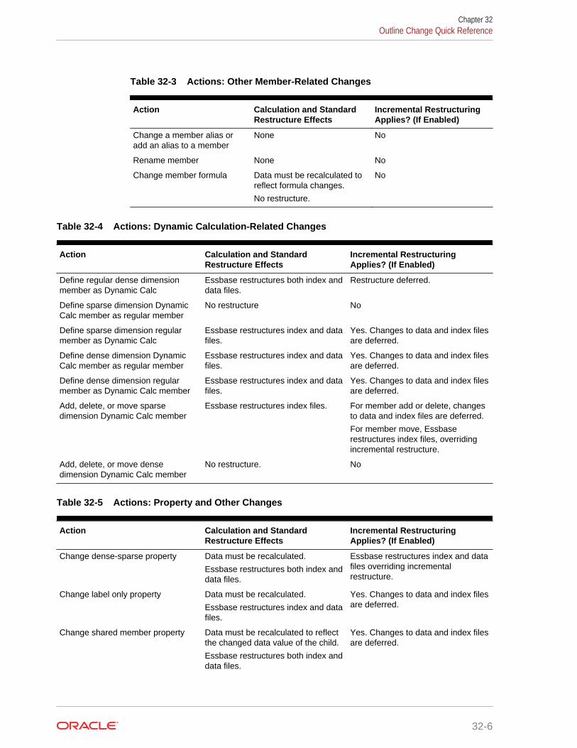
Table 32-3 Actions: Other Member-Related Changes



Change a member alias oradd an alias to a member

None No

Rename member None No

Change member formula Data must be recalculated toreflect formula changes.

No restructure.

No

Table 32-4 Actions: Dynamic Calculation-Related Changes



Define regular dense dimensionmember as Dynamic Calc

Essbase restructures both index anddata files.

Restructure deferred.

Define sparse dimension DynamicCalc member as regular member

No restructure No

Define sparse dimension regularmember as Dynamic Calc



Define dense dimension DynamicCalc member as regular member



Define dense dimension regularmember as Dynamic Calc member



Add, delete, or move sparsedimension Dynamic Calc member

Essbase restructures index files. For member add or delete, changesto data and index files are deferred.

For member move, Essbaserestructures index files, overridingincremental restructure.

Add, delete, or move densedimension Dynamic Calc member

No restructure. No

Table 32-5 Actions: Property and Other Changes



Change dense-sparse property Data must be recalculated.


Essbase restructures index and datafiles overriding incrementalrestructure.

Change label only property Data must be recalculated.



Change shared member property Data must be recalculated to reflectthe changed data value of the child.




32-6

Table 32-5 (Cont.) Actions: Property and Other Changes



Change properties other than dense-sparse, label, or shared

Data may need to be recalculated toreflect changed consolidationproperties, such as changing timebalance from first to last.

No

Change the order of two sparsedimensions

No calculation or data load impact.

Essbase restructures the index.

Essbase restructures the index,overriding incremental restructure.

Change the order of dimensions Data must be recalculated.


Essbase restructures index and datafiles (overrides incrementalrestructure).

Change the order of attributedimensions

None No

Create, delete, clear, rename, orcopy an alias table

None No

Import an alias table or set amember alias

None No

Change the case-sensitive setting None No

Name a level and generation None No

Create, change, or delete a UDA None No


32-7

33Optimizing Data Loads

You can shorten the time it takes too load data by minimizing the time spent onreading and parsing the data source, and reading and writing to the database

• Understanding Data Loads

• Grouping Sparse Member Combinations

• Making the Data Source as Small as Possible

• Making Source Fields as Small as Possible

• Positioning Data in the Same Order as the Outline

• Loading from Essbase Server

• Using Parallel Data Load


Understanding Data LoadsThis section does not apply to aggregate storage databases.

Loading a large data source into an Essbase database can take hours. You canshorten the data loading process by minimizing the time spent on these actions:

• Reading and parsing the data source

• Reading and writing to the database

To optimize data load performance, think in terms of database structure. Essbaseloads data block by block. For each unique combination of sparse dimensionmembers, one data block contains the data for all the dense dimension combinations,assuming that at least one cell contains data. For faster access to block locations,Essbase uses an index. Each entry in the index corresponds to one data block. See Sparse and Dense Dimensions, Selection of Dense and Sparse Dimensions, and Dense and Sparse Selection Scenarios.

When Essbase loads a data source, Essbase processes the data in five stages of apipeline.

For free form data load, the stages are:

1. Input—Essbase collects input from file or SQL connection

2. Tokenize—Essbase separates input fields from records, creating tokens

3. Convert—Essbase converts tokens into member items

4. Preparation—Essbase arranges the data in preparation for putting it into blocks

33-1

5. Write—Essbase puts the data into blocks in memory and then writes the blocks todisk, finding the correct block on the disk by using the index, which is composed ofpointers based on sparse intersections

For rules-file based data load, the stages are:

1. Input—Essbase collects input from file or SQL connection

2. Pre-Rule—Essbase reads data load records

3. Rule—Essbase applies rules, embedded in rules file, to data load records

4. Preparation—Essbase arranges the data in preparation for putting it into blocks

5. Write—Essbase puts the data into blocks in memory and then writes the blocks todisk, finding the correct block on the disk by using the index, which is composed ofpointers based on sparse intersections

Note:

On aggregate storage databases, the fifth stage does not apply.

This process is repeated until all data is loaded. By using one or more processingthreads in each stage, Essbase can perform some processes in parallel. See UsingParallel Data Load.

Examples in this chapter assume that you are familiar with the information in this topic: Data Sources.

Grouping Sparse Member CombinationsThis section does not apply to aggregate storage databases.

The most effective strategy to improve performance is to minimize the number of diskI/Os that Essbase must perform while reading or writing to the database. BecauseEssbase loads data block by block, organizing the source data to correspond to thephysical block organization reduces the number of physical disk I/Os that Essbasemust perform.

Arrange the data source so that records with the same unique combination of sparsedimensions are grouped together. This arrangement corresponds to blocks in thedatabase.

The examples in this chapter illustrate ways that you can organize the data followingthis strategy. These examples use a subset of the Sample.Basic database, as shownin Table 33-1:

Table 33-1 Dimensions and Values for Examples

Sparse, Nonattribute Dimensions Dense Dimensions

Scenario (Budget, Actual) Measures (Sales, Margin, COG, Profit)

Product (Cola, Root Beer) Year (Jan, Feb)

Market (Florida, Ohio)

Chapter 33Grouping Sparse Member Combinations

33-2

Note:

Because you do not load data into attribute dimensions, they are not relevantto this discussion although they are sparse.

Consider the following data source. Because it is not grouped by sparse-dimensionmember combinations, this data has not been sorted for optimization. As Essbasereads each record, it must deal with different members of the sparse dimensions.

JanActual Cola Ohio Sales 25Budget "Root Beer" Florida Sales 28Actual "Root Beer" Ohio Sales 18Budget Cola Florida Sales 30

This data loads slowly because Essbase accesses four blocks instead of one.

An optimally organized data source for the same Sample.Basic database showsdifferent records sorted by a unique combination of sparse-dimension members:Actual -> Cola -> Ohio. Essbase accesses only one block to load these records.

Actual Cola Ohio Jan Sales 25Actual Cola Ohio Jan Margin 18Actual Cola Ohio Jan COGS 20Actual Cola Ohio Jan Profit 5

You can use a data source that loads many cells per record. Ensure that records aregrouped together by unique sparse-dimension member combinations. Then order therecords so that the dimension in the record for which you provide multiple values is adense dimension.

The next data source example uses a header record to identify the members of theMeasures dimension, which is dense. The data is sorted first by members of the densedimension Year and grouped hierarchically by members of the other dimensions.Multiple values for the Measures dimension are provided on each record.

Sales Margin COG ProfitJan Actual Cola Ohio 25 18 20 5Jan Actual Cola Florida 30 19 20 10Jan Actual "Root Beer" Ohio 18 12 10 8Jan Actual "Root Beer" Florida 28 18 20 8

Notice that the heading and first data line that requires two lines in this example; theprevious example needs four lines for the same data.

For information about arranging data in source files before loading, see Data Sourcesthat Do Not Need a Rule File.

Chapter 33Grouping Sparse Member Combinations

33-3

Making the Data Source as Small as PossibleMake the data source as small as possible. The fewer fields that Essbase reads in thedata source, the less time is needed to read and load the data.

Group the data into ranges. Eliminating redundancy in the data source reduces thenumber of fields that Essbase must read before loading data values.

The following example data source is not organized in ranges. It includes unneededrepetition of fields. All values are Profit values. Profit must be included only at thebeginning of the group of data applicable to it. This example contains 33 fields thatEssbase must read to load the data values properly.

ProfitJan "New York" Cola 4Jan "New York" "Diet Cola" 3Jan Ohio Cola 8Jan Ohio "Diet Cola" 7Feb "New York" Cola 6Feb "New York" "Diet Cola" 8Feb Ohio Cola 7Feb Ohio "Diet Cola" 9

The next example provides the same data optimized by grouping members in ranges.By eliminating redundancy, this example contains only 23 fields that Essbase mustread in order to load the data values properly.

ProfitJan "New York" Cola 4 "Diet Cola" 3 Ohio Cola 8 "Diet Cola" 7Feb "New York" Cola 6 "Diet Cola" 8 Ohio Cola 7 "Diet Cola" 9

Essbase assigns the first value, 4, to Jan->New York->Cola; it assigns the next value,3, to Jan->New York->Diet Cola and so on.

Although sorted efficiently, the data source sorted and grouped by dense dimensionsshows a lot of repetition that can slow down the load process. You can further optimizethis data by grouping the data into ranges. The optimized data source beloweliminates the redundant fields, reducing processing time.

Sales Margin COG ProfitJan Actual Cola Ohio 25 18 20 5 Florida 30 19 20 10 "Root Beer" Ohio 18 12 10 8 Florida 28 18 20 8

See Formatting Ranges of Member Fields.

Chapter 33Making the Data Source as Small as Possible

33-4

Making Source Fields as Small as PossibleMaking fields in a data source smaller enables Essbase to read and load faster.

Make the fields in the data source as small as possible by performing the followingtasks:

• Remove excess white space in the data source. For example, use tabs instead ofblank spaces.

• Round computer-generated numbers to the precision you need. For example, ifthe data value has nine decimal points and you care about two, round the numberto two decimal points.

• Use #MI instead of #MISSING.

Positioning Data in the Same Order as the OutlineThis section does not apply to aggregate storage databases.

The index is organized in the same order as the sparse dimensions in the outline. Tofurther optimize the data source, with the sparse data combinations in the data sourcegrouped together, arrange the data so that sparse dimensions are in the same orderas the outline.

Essbase pages portions of the index in and out of memory as requested by the dataload or other operations. Arranging the source data to match the order of entries in theindex speeds the data load because it requires less paging of the index. Less pagingresults in fewer I/O operations.

The index cache size is used to determine how much of the index can be paged intomemory. Adjusting the size of the index cache may also improve data loadperformance.

Note:

If the index cache size is large enough to hold the entire index in memory,positioning data in the same order as the outline does not affect the speed ofdata loads.

Loading from Essbase ServerLoading the data source from Essbase Server is faster than loading from a clientcomputer. To load a data source from the server, move the data source to the serverand start the load.

Loading data from the server improves performance because the data need not betransported over the network from the client computer to the server computer.

Chapter 33Making Source Fields as Small as Possible

33-5

Using Parallel Data LoadThe following topics discuss parallel data load and how it might improve performancefor your site.

Understanding Parallel Data LoadOne aspect of parallel data load describes the pipeline optimization you can achieveby using the configuration settings DLTHREADSPREPARE and DLTHREADSWRITE.While the minimum and default number of threads allocated for a data load is 5 (onethread per stage of the pipeline), these settings enable you to add threads to selectedstages in the pipeline. For example, with the following configuration, you can increasethe threads used in the Prepare and Write stages from 1 each to 4 each:

DLSINGLETHREADPERSTAGE Sample Basic FALSEDLTHREADSPREPARE Sample Basic 4DLTHREADSWRITE Sample Basic 4

With the above configuration, the data load is set to run with 11 threads.

Another aspect of parallel data load refers to the concurrent loading of multiple datafiles into an Essbase database. When working with large data sets (for example, a setof ten 2 GB files), loading the data sources concurrently enables you to fully utilize theCPU resources and I/O channels of modern servers with multiple processors and high-performance storage subsystems.

You can also adjust the number of threads used in multiple-file data loads. Forexample, specifying the above configuration while also specifying two data files resultsin the creation of two data load pipelines, each having 11 threads.

Enabling Parallel Data Load With Multiple FilesTo enable parallel data load, specify multiple files as the data source, by using awildcard character (* and/or ?) to match all data sources files you intend to use. Seethe MaxL statement import data. If necessary, control the number of threads spawnedby the parallel data load, using the using max_threads grammar in the MaxLstatement.

Chapter 33Using Parallel Data Load

33-6

34Optimizing Calculations

You can configure a database to optimize calculation performance. The information inthis chapter applies only to block storage databases and is not relevant to aggregatestorage databases.

• Designing for Calculation Performance

• Monitoring and Tracing Calculations

• Using Simulated Calculations to Estimate Calculation Time

• Estimating Calculation Effects on Database Size

• Using Formulas

• Using Bottom-Up Calculation

• Hybrid Aggregation Mode in Block Storage Databases

• Managing Caches to Improve Performance

• Working with the Block Locking System

• Using Two-Pass Calculation

• Choosing Between Member Set Functions and Performance

• Consolidating #MISSING Values

• Removing #MISSING Blocks

• Identifying Additional Calculation Optimization Issues

Designing for Calculation PerformanceYou can configure a database to optimize calculation performance.

The best configuration for the site depends on the nature and size of the database.Use the information in the following topics as guidelines only.

Block Size and Block DensityA data block size of 8 Kb to 100 Kb provides optimal performance in most cases.

If data blocks are much smaller than 8 KB, the index is usually very large, forcingEssbase to write to and retrieve the index from disk. This process slows calculation.

If data blocks are much larger than 100 KB, Intelligent Calculation does not workeffectively. See Understanding Intelligent Calculation.

To optimize calculation performance and data storage, balance data block density anddata block size by rearranging the dense and sparse dimension configuration of thedatabase. Keep these suggestions in mind:

• Keep data block size between 8 KB and 100 KB with as high a block density aspossible.

34-1

• Run test calculations of the most promising configurations of a database thatcontains representative data. Check results to determine the configuration thatproduces the best calculation performance.

You can view information about a database, including the potential and actual numberof data blocks and the data block size.

To view data block information:

Use the GETDBINFO ESSCMD shell command.

Order of Sparse DimensionsYou may improve calculation performance by changing the order of standard (notattribute) sparse dimensions in the database outline. Order standard sparsedimensions by the number of members they contain, placing the dimension thatcontains the fewest members first. This arrangement provides many possibleimprovements, depending on the site:

• The calculator cache functions more effectively, providing approximately a 10%performance improvement if you have a database outline with a large dimension(for example, one containing 1000 members).

• Parallel calculation, if enabled, more likely will be used if the standard sparsedimension with the most members is the last standard sparse dimension in theoutline.

Incremental Data LoadingMany companies load data incrementally. For example, a company may load dataeach month for that month.

To optimize calculation performance when you load data incrementally, make thedimension tagged as time a sparse dimension. If the time dimension is sparse, thedatabase contains a data block for each time period. When you load data by timeperiod, Essbase accesses fewer data blocks because fewer blocks contain therelevant time period. Thus, if you have Intelligent Calculation enabled, only the datablocks marked as dirty are recalculated. For example, if you load data for March, onlythe data blocks for March and the dependent parents of March are updated.

However, making the time dimension sparse when it is naturally dense maysignificantly increase the size of the index, creating possibly slower performance dueto more physical I/O activity to accommodate the large index.

If the dimension tagged as time is dense, you still receive some benefit from IntelligentCalculation when you do a partial data load for a sparse dimension. For example, ifProduct is sparse and you load data for one product, Essbase recalculates only theblocks affected by the partial load, although time is dense and Intelligent Calculation isenabled.

For information on incremental loads, see Loading Data into Aggregate StorageDatabases.

Database Outlines with Multiple Flat DimensionsCalculation performance may be affected if a database outline has multiple flatdimensions. A flat dimension has very few parents, and each parent has many

Chapter 34Designing for Calculation Performance

34-2

thousands of children; in other words, flat dimensions have many members and fewlevels.

You can improve performance for outlines with multiple flat dimensions by addingintermediate levels to the database outline.

Formulas and Calculation ScriptsYou may achieve significant improvements in calculation performance by carefullygrouping formulas and dimensions in a calculation script. In this way, you can ensurethat Essbase cycles through the data blocks in the database as few times as possibleduring a calculation.

Order commands in calculation scripts to make the database calculation as simple aspossible. Consider applying all formulas to the database outline and using a defaultcalculation (CALC ALL). This method may improve calculation performance.

See Developing Calculation Scripts for Block Storage Databases and CalculationPasses.

Monitoring and Tracing CalculationsYou can display information in the application log about how Essbase is calculating thedatabase by using the following commands in a calculation script.

SET MSG SUMMARY and SET MSG DETAILYou can use the SET MSG SUMMARY and SET MSG DETAIL calculation commandsin a calculation script to do the following:

• Display calculation settings, for example, whether completion notice messages areenabled

• Provide statistics on the number of data blocks created, read, and written

• Provide statistics on the number of data cells calculated

SET MSG DETAIL also provides an information message every time Essbasecalculates a data block. SET MSG DETAIL is useful for reviewing the calculation orderof data blocks and for testing intelligent recalculations.

Caution:

Because SET MSG DETAIL causes a high processing overhead, use it onlyduring test calculations.

SET MSG SUMMARY causes a processing overhead of approximately 1% to 5%,depending on database size, and is therefore appropriate for all calculations.

SET NOTICEYou can use the SET NOTICE calculation command in a calculation script to displaycalculation completion notices that tell you what percentage of the database has been

Chapter 34Monitoring and Tracing Calculations

34-3

calculated. You can use the SET MSG SUMMARY command with the SET NOTICEcommand to show calculation progress between completion notices. Completionnotices do not significantly reduce calculation performance, except when used with avery small database.

Using Simulated Calculations to Estimate Calculation TimeYou can simulate a calculation using SET MSG ONLY in a calculation script. Asimulated calculation produces results that help you analyze the performance of a realcalculation that is based on the same data and outline.

By running a simulated calculation with a command such as SET NOTICE HIGH, youcan mark the relative amount of time each sparse dimension takes to complete. Then,by performing a real calculation on one or more dimensions, you can estimate howlong the full calculation will take, because the time a simulated calculation takes to runis proportional to the time that the actual calculation takes to run.

For example, if the calculation starts at 9:50:00 AM, and the first notice is time-stamped at 09:50:10 AM and the second is time-stamped at 09:50:20 AM, you knowthat each part of the calculation took 10 seconds. If you then run a real calculation ononly the first portion and note that it took 30 seconds to run, you know that the otherportion also will take 30 seconds. If there were two messages total, then you wouldknow that the real calculation will take approximately 60 seconds (20 / 10 * 30 = 60seconds).

Use the following topics to learn how to perform a simulated calculation and how touse a simulated calculation to estimate calculation time.

Performing a Simulated CalculationBefore you can estimate calculation time, you must perform a simulated calculation ona data model that is based on your actual database.

To perform a simulated calculation:

1. Create a data model that uses all dimensions and all levels of detail about whichyou want information.

2. Load all data. This procedure calculates only data loaded in the database.

3. Create a calculation script with these entries:

SET MSG ONLY;SET NOTICE HIGH;CALC ALL;

If you are using dynamic calculations on dense dimensions, substitute the CALCALL command with the specific dimensions that you need to calculate; forexample, CALC DIM EAST.

Note:

If you try to validate the script, Essbase reports an error. Disregard theerror.

Chapter 34Using Simulated Calculations to Estimate Calculation Time

34-4

4. Run the script.

5. Find the first sparse calculation message in the application log and note the time inthe message.

6. Note the time for each subsequent message.

7. Calculate the dense dimensions of the model that are not being dynamicallycalculated:

CALC DIM (DENSE_DIM1, DENSE_DIM2, …);

8. Calculate the sparse dimensions of the model:

CALC DIM (SPARSEDIM1, SPARSEDIM2, …);

9. Project the intervals at which notices will occur, and then verify against sparsecalculation results. You can then estimate calculation time.

Estimating Calculation TimeWhen you perform a simulated calculation, you record the results and use them toestimate actual calculation time.

To estimate total calculation time:

1. Note the times of all the intervals between application log messages generated bySET NOTICE HIGH.

See Table 34-1.

2. Use the following calculation to estimate the time for a real calculation:

Total time required for simulated calculation, divided by the first simulatedcalculation notice interval, multiplied by the first real calculation time interval.

Table 34-1 Sample Intervals Between Log Messages

Calculation Notice Number Simulated CalculationTime Interval (in seconds)

Sparse DimensionCalculation Interval (inseconds)

1 7 45

2 5

3 6

4 3

5 4

6 2

7 6

8 4

9 3

10 3

Total calculation time 43


34-5

In this example, 43 / 7 * 45 = 276.4 seconds, so the real calculation should take276.4 seconds.

Factors Affecting Estimate AccuracyThe simulated calculation should return a time accurate to about 5%, excluding thefollowing issues:

• Variations Due to a Chain of Influences

• Variations Due to Outline Structure

When these factors are present, this estimating technique more closely predictscalculation time when Essbase reaches 30%–40% of the simulated calculations (30%–40% of the messages generated by SET NOTICE HIGH). See Technical Reference forOracle Essbase.

Variations Due to a Chain of InfluencesUsing SET MSG ONLY as a calculation-time estimating technique should be validatedagainst later CALCNOTICE intervals. The results of this estimating technique varybecause of the following chain of influences:

1. Blocks differ in block density through the real consolidation process, therefore

2. The rate at which Essbase writes blocks to the disk differs, therefore

3. The rate at which blocks are processed in the cache differs, therefore

4. Actual results may differ from the predicted calculation time.

Variations Due to Outline StructureAnother factor that can make actual results diverge significantly from predicted is theoutline structure. Calculations based on CALCNOTICE intervals assume evenlybalanced processing time throughout the outline. Factors that can skew this balanceinclude the following situations:

• The model contains one or two sparse dimensions that are large in relation to theother sparse dimensions.

• Larger dimensions have member configurations that result in multiple shared roll-ups.

Changing the Outline Based on ResultsAfter you have estimated and analyzed a simulated calculation, you can makechanges in the outline to improve performance.

From top to bottom in the outline, order sparse dimensions to create the fewestpercentage increases in upper blocks:

• Level 0 blocks following full model load: 100,000

• Upper level blocks after consolidating only sparse dimension 1: 1,000,000




34-6

• Upper level blocks after consolidating only sparse dimension 4: 300,000


For example:

• #4 (members = 10,000, 4 levels)

• #1 (members = 500, 2 levels)

• #2 (members = 100, 4 levels)

• #5 (members = 10,000, 4 levels)

• #3 (members = 20, flat)

Use the simulated calculation to generate the upper block count. These numbers maybe accurate despite actual dimension sizes as noted next to the items above.

Caution:

The largest count of members is not always a good predictor.

Estimating Calculation Effects on Database SizeGiven the current number of blocks in a database, you can estimate the number ofblocks that a CALC ALL will produce.

To estimate the database size resulting from a calculation using interactive mode:

1. Load data and issue a CALC ALL command and note the average block size.

2. Start the MaxL shell, log on to Essbase, and start an application and database.For example:

essmsh login username password;alter system load application appname;alter application appname load database dbname;

3. Providing the application and database name, enter the following MaxL statementand note the value that is returned for the number of blocks:

query database appname.dbname get estimated size;

4. Multiply the number of blocks by the average size of the blocks in the database.

Results are accurate to ±10%.

Be aware of the following conditions when you query Essbase for an estimate of thefull size of a database:

• You must perform this query after a CALC ALL. Any other calculation will notproduce accurate results.

• You can obtain accurate results with formulas only if they are on sparsedimensions.

Chapter 34Estimating Calculation Effects on Database Size

34-7

• You cannot obtain accurate results with top-down calculations on any member incombination with a lock on data (committed access).

• If you need to estimate partitions, you must query Essbase for a database sizeestimate on every partition and add the results. If you query for the size of only thesource database, the estimate includes only the data on the source databaseserver.

Using FormulasYou may achieve significant improvements in calculation performance by carefullyusing formulas in the database outline. For example, you may achieve improvedcalculation performance by placing formulas on members in the database outlineinstead of placing the formulas in a calculation script. See Developing Formulas forBlock Storage Databases.

The following sections discuss how to handle formula issues that affect performance.

ConsolidatingUsing the database outline to roll up values is more efficient than using a formula tocalculate values. For example, the consolidation of members 100-10, 100-20, and100-30 into member 100, as shown in Figure 34-1, is more efficient than applying thefollowing formula to member 100:

100-10 + 100-20 + 100-30

Figure 34-1 Consolidation Example

Using Simple FormulasIf you use a simple formula, and block size is not unusually large, you can place theformula on a member of either a sparse or a dense dimension without significantlyaffecting calculation performance. The bigger the block size, the more impact simpleformulas have on calculation performance. For a discussion of the relationshipbetween block size and calculation performance, see Block Size and Block Density.

A simple formula is, for example, a ratio or a percentage and meets the followingrequirements:

• Does not reference values from a different dimension (sparse or dense). Forexample, a simple formula cannot reference Product -> Jan.

• Does not use range functions. For example, a simple formula cannot use@AVGRANGE, @MAXRANGE, @MINRANGE, or @SUMRANGE.

• Does not use relationship or financial functions. For example, a simple formulacannot use @ANCESTVAL, @NEXT, @PARENTVAL, @SHIFT, @ACCUM, or

Chapter 34Using Formulas

34-8

@GROWTH. For a complete list of relationship and financial functions, seeTechnical Reference for Oracle Essbase.

For information on how formulas affect calculation performance, see Bottom-Up andTop-Down Calculation.

Using Complex FormulasIf you use a complex formula, you can improve performance by applying the followingguidelines:

• If possible, apply the formula to a member in a dense dimension.

• Use the FIX command in a calculation script to calculate only required data blocks.See Using the FIX Command.

• Increase the density of the database (ratio of existing data blocks to possible datablocks).

See Block Size and Block Density.

A complex formula is one that meets any of the following requirements:

• References a member or members in a different dimension (sparse or dense); forexample, Product -> Jan.

• Uses one or more range functions, for example, @AVGRANGE, @MAXRANGE,@MINRANGE, or @SUMRANGE.

• Uses relationship or financial functions; for example, @ANCESTVAL, @NEXT,@PARENTVAL, @SHIFT, @ACCUM, or @GROWTH. For a complete list ofrelationship and financial functions, see Technical Reference for Oracle Essbase.

When applied to sparse dimension members, complex formulas create morecalculation overhead and therefore slow performance. This problem occurs becausethe presence of complex formulas requires Essbase to perform calculations on allpossible as well as all existing data blocks related to the member with the complexformula. The presence of a relationship or financial function on a sparse dimensionmember causes Essbase to perform calculations on all blocks, possible as well asexisting, increasing the overhead even more.

Thus, a complex formula that includes a relationship or financial function creates agreater overhead increase than does a complex formula that does not include arelationship or financial function.

For a discussion about how complex formulas affect calculation performance, see Bottom-Up and Top-Down Calculation.

Two examples illustrate complex formula overhead:

• If a database has 90 existing data blocks and 100 potential data blocks, theoverhead for complex formulas is not large, not more than 10 extra blocks to readand possibly write values to.

• If a database has 10 existing data blocks and 100 potential data blocks, theoverhead is as much as ten times what it would be without the complex formula(depending on the outline structure and other factors), as many as 90 extra blocksto read and possibly write to.

In all cases, the lower the ratio of existing data blocks to possible data blocks, thehigher the calculation performance overhead and the slower the performance.


34-9

Optimizing Formulas on Sparse Dimensions in Large DatabaseOutlines

You can use the SET FRMLBOTTOMUP calculation command to optimize thecalculation of formulas in sparse dimensions in large database outlines. With thiscommand, you can force a bottom-up calculation on sparse member formulas thatotherwise would be calculated top-down. See Forcing a Bottom-Up Calculation.

Forcing a bottom-up calculation on a top-down formula enables efficient use of theCALC ALL and CALC DIM commands. Review the discussions of the SETFRMLBOTTOMUP calculation command and the CALCOPTFRMLBOTTOMUPconfiguration setting in Technical Reference for Oracle Essbase.

Constant Values Assigned to Members in a Sparse DimensionIf you assign a constant to a member in a sparse dimension, Essbase automaticallycreates a data block for every combination of sparse dimension members thatcontains the member.

For example, assume that a member or a calculation script formula contains thefollowing expression:

California = 120;

In this formula, California is a member in a sparse dimension and 120 is a constantvalue. Essbase automatically creates all possible data blocks for California andassigns the value 120 to all data cells. Many thousands of data blocks may be created.To improve performance, create a formula that does not create unnecessary values.

To assign constants in a sparse dimension to only those intersections that require avalue, use FIX in a manner similar to the following example:

FIX(Colas,Misc,Actual) California = 120;ENDFIX

In this example, Colas is a member of the sparse dimension, Product; Actual is amember of the dense dimension, Scenario; and Misc is a member of the densedimension, Measures. The value 120 is assigned to any intersection of California (inthe Market dimension), Actual (in the Scenario dimension), Misc (in the Measuresdimension), Colas (in the Product dimension), and any member in the Year dimension,because a specific member of Year is not specified in the script.

Because Sample.Basic includes only two sparse dimensions, this example affects onlyone block. If more sparse dimensions existed, Essbase would ensure data blocks forall combinations of the sparse dimensions with California and Colas, creating blocks ifnecessary. Within the new blocks, Essbase sets Measures and Scenario values (otherthan those assigned the value 120) to #MISSING.


34-10

Nonconstant Values Assigned to Members in a Sparse DimensionIf you assign nonconstant values to members of a sparse dimension, blocks arecreated based on the Create Blocks on Equations setting. The Create Blocks onEquations setting is defined at the database level, as a database property. (See Nonconstant Values.)

Within calculation scripts, you can temporarily override the Create Blocks onEquations setting. Consider the effects of the following calculation when West doesnot have a value and Create Blocks on Equations is enabled:

West = California + 120;

Unneeded blocks may be created for all sparse-member intersections with West, evenif the corresponding block value is #MISSING for all of the children of West. Especiallyin a large database, creation and processing of unneeded blocks requires additionalprocessing time.

To control creation of blocks when you assign nonconstant values to members of asparse dimension, use the SET CREATEBLOCKONEQ ON | OFF calculationcommand, as shown in the following script:

FIX (Colas); SET CREATEBLOCKONEQ OFF West = California + 120; SET CREATEBLOCKONEQ ON East = “New York” + 100;ENDFIX

Because the Create Block on Equation setting is disabled at the beginning of thescript, West blocks are created only when values exist for the children of West. Later,because the Create Block on Equation setting is enabled, all blocks for East arecreated.

Note:

Using SET CREATEBLOCKONEQ affects only creation of blocks during theexecution of the calculation script that contains this command. Thiscommand does not change the overall database setting for Create Blocks onEquations.

Using Cross-Dimensional OperatorsUse caution when using a cross-dimensional operator ( -> ) in the following situations:

• On the Left of an Equation

• In Equations in a Dense Dimension


34-11

On the Left of an EquationFor faster calculation script performance, use FIX in the calculation script to qualify theuse of a formula rather than a formula that includes a cross-dimensional operator onthe left of an equation.

For example, assume that you want to increase the Jan -> Sales values inSample.Basic by 5%. To improve performance by calculating only the relevantcombinations of members, use the FIX command:

FIX(Jan) Sales = Sales * .05;ENDFIX

With the FIX command, Essbase calculates the formula only for specified membercombinations, in this example, for combinations that include Jan.

Compare this technique to using the slower cross-dimensional operator approach. Forthe previous example, you place the following formula on the Sales member in thedatabase outline:

Sales(Sales -> Jan = Sales -> Jan * .05;)

As Essbase cycles through the database, it calculates the formula for every membercombination that includes a member from the dimension tagged as time (Jan, Feb,Mar, and so on), although only January combinations need to be calculated.

See Using the FIX Command and the Technical Reference for Oracle Essbase.

In Equations in a Dense DimensionWhen you use a cross-dimensional operator in an equation in a dense dimension,Essbase does not automatically create the required blocks if both of these conditionsapply:

• Resultant values are from a dense dimension.

• The operand or operands are from a sparse dimension.

You can use the following techniques to create the blocks and avoid the performanceissue.

• Ensure that the results members are from a sparse dimension, not from a densedimension. In this example, the results member Budget is from a sparsedimension:

FIX(Sales) Budget = Actual * 1.1;ENDFIXFIX(Expenses) Budget = Actual * .95;ENDFIX

• Use the DATACOPY calculation command to create and then calculate therequired blocks. See Using DATACOPY to Copy Existing Blocks.


34-12

• Use a member formula that contains the dense member equations:

FIX(Sales, Expenses)Budget (Sales = Sales -> Actual * 1.1;Expenses = Expenses -> Actual * .95;)ENDFIX

Managing Formula Execution LevelsFormulas in a block storage outline can have dependencies on one another such thatthey cause a nested execution of formulas within one or more blocks. Such formulasare called recursive formulas. Sometimes recursive formulas result in large orunending loops that result in abnormal termination of the server.

To avoid abnormal termination, you can use the CALCLIMITFORMULARECURSIONconfiguration setting to stop a formula execution that reaches beyond a default numberof execution levels. See the Technical Reference for Oracle Essbase.

Using Bottom-Up CalculationA top-down calculation is less efficient than a bottom-up calculation, because moreblocks are calculated than is necessary. Although a top-down calculation is lessefficient than a bottom-up calculation, top-down calculations are necessary in somecases to ensure that calculation results are correct.

The following topics describe which calculation to use in different situations:

Bottom-Up and Top-Down CalculationEssbase uses one of two calculation methods to do a full calculation of a databaseoutline—bottom-up calculation or top-down calculation. By default, Essbase does abottom-up calculation.

For a bottom-up calculation, Essbase determines which data blocks must becalculated before it calculates the database. Essbase then calculates only the blocksthat must be calculated. The calculation begins with the existing block with the lowestblock number and works up through each block in number order until the existing blockwith the highest block number is reached. See Block Calculation Order.

If the database outline contains a complex member formula, Essbase performs a top-down calculation for the relevant member.

Use the following information to learn more about simple and complex formulainteractions with bottom-up and top-down calculation:

Bottom-Up Calculations and Simple FormulasFor simple formulas, Essbase does a bottom-up calculation to determine which blocksmust be calculated before running the full calculation. For example, for a simpleformula on a member (such as A = B + C), A is calculated only if B or C exists in thedatabase. That is, the dependency of the formula on B and C is known before thecalculation is started.

Chapter 34Using Bottom-Up Calculation

34-13

Top-Down Calculations and Complex FormulasBefore starting a calculation, Essbase searches the database outline and markscomplex formulas that require top-down calculation; for example, a member formulathat contains a cross-dimensional reference. When Essbase reaches a member with atop-down formula, it does a top-down calculation for the member.

When a formula on a member is complex, all possible blocks for the member must beexamined to see if an existing block must be changed or a new block created; it isdifficult to determine the dependency that blocks have on other blocks before the startof the calculation. The top-down method slows calculation performance becauseEssbase must search for appropriate blocks to calculate to execute the formula.

When a formula is compiled, if the formula is to be calculated top-down, Essbase logsa message in the application log file.

Consider the following complex formula:

A = B -> D + C -> D

To calculate the formula, Essbase must examine every combination of A to seewhether B -> D or C -> D exists.

See Using Complex Formulas.

Forcing a Bottom-Up CalculationIf it is appropriate for the site, you can force a bottom-up calculation on a top-downformula.

To force a bottom-up calculation, use the use one of the following methods:

• Calculation function—@CALCMODE in a formula

• Calculation script command—SET FRMLBOTTOMUP

• Configuration settings:

– CALCOPTFRMLBOTTOMUP

– CALCMODE

Forcing a bottom-up calculation on a formula usually increases performance time. Ifthe formula contains complex functions (for example, range functions) or if theformula's dependencies are not straightforward, a bottom-up calculation may produceresults different from those of a top-down calculation.

Caution:

Before changing the setting CALCOPTFRMLBOTTOMUP or using thecalculation script command SET FRMLBOTTOMUP in a productionenvironment, check the validity of calculation results by comparing, relativeto the same data, the results of a bottom-up calculation and the results of atop-down calculation.

Chapter 34Using Bottom-Up Calculation

34-14

Hybrid Aggregation Mode in Block Storage DatabasesHybrid aggregation mode is available for block storage databases. Hybrid aggregationfor block storage databases means that wherever possible, block storage datacalculation executes with efficiency similar to that of aggregate storage databases.See Using Hybrid Aggregation.

See also the ASODYNAMICAGGINBSO configuration setting topic in the TechnicalReference for Oracle Essbase.

Managing Caches to Improve PerformanceThe following section describes the caches that are used with block storagedatabases. For information about the aggregate storage cache, see Managing theAggregate Storage Cache.

When calculating a database, Essbase uses approximately 30 bytes of memory permember in the database outline. So if the database has 5,000 members, Essbaseneeds approximately 150 KB of memory to calculate the database.

Note:

You can avoid excess memory use by combining calculation scripts. You canobtain good performance by using parallel calculation with a singlecalculation script. See Using Parallel Calculation.

Essbase uses memory to optimize calculation performance, especially for largecalculations. The amount of memory used is not controllable, except by altering thesize of the database outline. However, you can ensure that the memory cache sizesenable Essbase to optimize the calculation.

Essbase uses memory caches to coordinate memory usage:

• Calculator cache. Ensure that the calculator cache is large enough to optimizecalculation performance.

• Dynamic calculator cache.

• Index cache. If the database is large, the default index cache is not large enoughto provide optimum calculation performance.

• Data cache.

• Data file cache.

• Application cache. If hybrid aggregation mode is used in block storage databases,the application cache can help you manage memory usage for retrievals. Theapplication cache is similar to the aggregate storage cache; for more information,see Managing the Aggregate Storage Cache.

Chapter 34Hybrid Aggregation Mode in Block Storage Databases

34-15

Note:

When you first calculate a database, the size of the calculator cache issignificant for calculation performance. If possible, ensure that the calculatorcache is large enough for Essbase to use the optimal calculator cacheoption.

Working with the Block Locking SystemWhen a block is calculated, Essbase locks the block and all blocks that contain thechildren of the block. Essbase calculates the block and then releases the block andthe blocks containing the children.

By default, Essbase locks up to 100 blocks concurrently when calculating a block. Thisnumber of block locks is sufficient for most database calculations. If you arecalculating a formula in a sparse dimension, Essbase works most efficiently if it canlock all required child blocks concurrently. Therefore, when calculating a formula in asparse dimension, you may want to set a lock number higher than 100 if you areconsolidating very large numbers of children (for example, more than 100). Byincreasing the number, you ensure that Essbase can lock all required blocks, andperformance is not impaired.

Note:

For consolidations in a sparse dimension, block locking is not aconsideration, because Essbase does not need to lock all blocks containingchildren concurrently.

Managing Concurrent Access for UsersEssbase uses the block locking system to manage concurrent access to users. Thissystem ensures that only one user at a time can update or calculate a particular datablock. How Essbase handles locking blocks and committing data depends on theisolation level setting.

When Essbase calculates a data block, it creates an exclusive lock; other userscannot update or calculate it, but they can have read-only access. When Essbasefinishes the calculation, it releases the block. Other users can then update the block ifthey have the appropriate security access.

When a user is updating a data block, the block is locked. If a database calculationrequires a data block that is being updated by another user, the calculation waits forone of the following conditions:

• For the data block to be released if the isolation level setting is UncommittedAccess.

• For the calculation to complete if the isolation level setting is Committed Access.

Essbase does not provide a message to say that the calculation is waiting for the datablock to be released.

Chapter 34Working with the Block Locking System

34-16

You can prevent calculation delays caused by waiting for locked blocks by usingEssbase security options to do either of the following:

• Deny access to other users

• Disconnect users from Essbase

Note:

When Essbase locks a block for calculation, it does not put an exclusive lockon the dependent child blocks, so another user can update values in thechild blocks. If necessary, you can use the above security options to preventsuch updates.

Using Two-Pass CalculationYou can improve performance significantly by tagging an accounts dimension memberas two-pass in the database outline, if it is appropriate for the application. Thecombination of data and calculation needs may require the use of a calculation scriptto calculate a formula twice, instead of two-pass tagging, to preserve accuracy.

Use these sections to understand more about two-pass calculation. Decide whetheryou can tag an accounts dimension member as two-pass to improve performance, orwhether you must use a calculation script to calculate a formula twice. This sectionalso provides information about how to enable two-pass calculation or create acalculation script for two-pass calculation.

For information about the interaction of two-pass calculation and attribute members,see Table 7-1.

Understanding Two-Pass CalculationYou can use a two-pass calculation on member formulas that must be calculated twiceto produce the correct value.

Whenever possible, two-pass formulas are calculated at the data block level,calculating the two-pass formulas simultaneously as the main calculation. Thus, anextra calculation pass through the database is not needed. However, in somesituations, an extra calculation pass through the database is needed.

How two-pass formulas are calculated depends on whether there is a dimensiontagged as time as well as a dimension tagged as accounts and on the dense-sparseconfiguration of the time and account dimensions.

Avoid using two-pass calculation in hybrid aggregation mode. Use solve order instead.

Reviewing a Two-Pass Calculation ExampleConsider this calculation required for Profit%:

Profit % = Profit % Sales

Chapter 34Using Two-Pass Calculation

34-17

Assume that Table 34-2 shows a subset of a data block with Measures and Year asdense dimensions. Measures is tagged as accounts, and Year is tagged as time. TheAGGMISSG configuration setting is turned off (the default).

Data values have been loaded into the input cells. Essbase calculates the cells inwhich the numbers 1 through 7 appear, in that order. For example, Profit % -> Jan iscalculated first; Profit% -> Qtr1 has multiple consolidation paths.

Table 34-2 Two-Pass Calculation Example: Data and Calculation Order

Measures -> Year Jan Feb Mar Qtr1

Profit 75 50 120 5

Sales 150 200 240 6

Profit% 1 2 3 4, 7

Note:

For information on how cell calculation order depends on databaseconfiguration, see Cell Calculation Order.

Essbase uses this calculation order:

1. Essbase calculates the formula Profit % Sales for Profit % -> Jan, Profit % ->Feb, Profit % -> Mar, and Profit % -> Qtr1 (1, 2, 3, 4 above).

2. Essbase calculates Profit -> Qtr1 and Sales -> Qtr1 by adding the values for Jan,Feb, and Mar (5, 6 above).

3. Essbase calculates Profit % -> Qtr1 by adding the values for Profit % -> Jan, Profit% -> Feb, and Profit % -> Mar (7 above). This addition of percentages producesthe value 125%, which is not the correct result.

Table 34-3 Two-Pass Calculation Example: Incorrect Results


Profit 75 50 120 245 (5)

Sales 150 200 240 590 (6)

Profit% 50% (1) 25% (2) 50% (3) 0% (4)125% (7)

4. If you tag Profit% as two-pass in the database outline, Essbase uses the Profit %Sales formula to recalculate the Profit% values and produce the correct results.


34-18

Table 34-4 Two-Pass Calculation Example: Correct Results


Profit 75 50 120 245 (5)

Sales 150 200 240 590 (6)

Profit% 50% (1) 25% (2) 50% (3) 0% (4)125% (7)42% (8)

For information about multiple calculation passes, see Calculation Passes.

Understanding the Interaction of Two-Pass Calculation and IntelligentCalculation

Two scenarios are described in detail in the following sections. If you are usingIntelligent Calculation, use the scenario that matches the configuration of thedatabase; each scenario tells you how to ensure that Essbase accurately calculatestwo-pass formulas.

These scenarios require that you understand the concepts of Intelligent Calculation.See Understanding Intelligent Calculation.

Scenario AIn this scenario, you place formulas in the outline and, as appropriate, tag specificformulas as two-pass for best performance.

No Extra Calculation Pass for Two-Pass FormulasBecause Essbase calculates the two-pass formulas while it is calculating the datablock, Essbase need not do an extra calculation pass through the database.

All Data Blocks Marked As CleanAfter the calculation, all data blocks are marked as clean for the purposes of IntelligentCalculation.

When you tag a member formula as two-pass in the outline, Essbase does the two-pass calculation while each data block is being calculated. However, when you repeata formula in a calculation script, Essbase must read the data blocks and write them tomemory to recalculate the formula.

Scenario BIn this scenario, you create a calculation script to perform the formula calculation forbest performance.

Extra Calculation Pass for Two-Pass FormulasEssbase calculates the database and then does an extra calculation pass to calculatethe two-pass formulas. Even though all data blocks are marked as clean after the first


34-19

database calculation, Essbase ignores the clean status on the blocks that are relevantto the two-pass formula and recalculates these blocks.

Data Blocks for Two-pass Formulas Not Marked As CleanAfter the first calculation, Essbase has marked all data blocks as clean for thepurposes of Intelligent Calculation. In a second calculation pass through the database,Essbase recalculates the required data blocks for the two-pass formulas. However,because the second calculation is a partial calculation of the database, Essbase doesnot mark the recalculated blocks as clean. When you recalculate the database withIntelligent Calculation turned on, these data blocks may be recalculated unnecessarily.

If the database configuration allows Essbase to use Scenario B, consider using acalculation script to perform two-pass formula calculations. If you use a calculationscript, Essbase still does an extra calculation pass through the database; however,you can ensure that Essbase has marked all the data blocks as clean after thecalculation. See Creating Calculation Scripts for Two-Pass and Intelligent Calculation.

Choosing Two-Pass Calculation Tag or Calculation ScriptAlthough tagging an accounts member as two-pass may bring performance benefits,some applications cannot use this method. Check these qualifications to see whetheryou should apply a two-pass tag or create a calculation script that performs acalculation twice for best performance and accuracy:

• You can tag a member as two-pass if it is in a dimension tagged as accounts.When you perform a default calculation on the database, Essbase automaticallyrecalculates any formulas tagged as two-pass if they are in the dimension taggedas accounts in the database outline.

• You can tag a member as two-pass if it is a Dynamic Calc member of anydimension. See Dynamically Calculating Data Values.

• You may need to use a calculation script to calculate a two-pass formula to obtainaccurate results, even if the two-pass tag would provide performance benefits.See Creating Calculation Scripts for Two-Pass and Intelligent Calculation.

• Use a calculation script instead of the two-pass tag to ensure efficient use ofIntelligent Calculation. See Understanding the Interaction of Two-Pass Calculationand Intelligent Calculation.

• You must use a calculation script to calculate a formula twice if the databaseconfiguration means that Essbase uses Scenario A, as described in Scenario A,and if the formula references values from another data block.

• You may want to use a calculation script to calculate two-pass formulas if thedatabase configuration means that Essbase uses Scenario B, as described in Scenario B.

Enabling Two-Pass on Default CalculationsA database setting enables two-pass calculation in default calculations. When youperform a default calculation on a database with two-pass calculation enabled (thedefault setting), Essbase automatically attempts to calculate formulas tagged as two-pass in the dimension tagged as accounts in the database outline. This is true even ifyou have customized the default calculation script.

In Using Oracle Analytics Cloud - Essbase, see these topics:


34-20

• Setting Advanced Cube Properties

• Setting Two-Pass Calculation Properties

To perform a default calculation, you can use the execute calculation MaxL statement.

To enable two-pass calculation, you can use the alter database MaxL statement.

Creating Calculation Scripts for Two-Pass and Intelligent CalculationUse these methods to create calculation scripts to perform two-pass calculations withIntelligent Calculation, so that the calculation is accurate and as fast as possible:

• Before the calculation script command that recalculates a two-pass formula, addthe SET UPDATECALC OFF command to disable Intelligent Calculation. If youhave Intelligent Calculation enabled (the default), Essbase calculates only the datablocks that are not marked as clean, but when you perform a default calculation ofthe database with Intelligent Calculation enabled, all data blocks are marked asclean, so Essbase does not perform the two-pass formula recalculation.

• When you use a calculation script, Essbase does not automatically recalculatetwo-pass formulas. Use the CALC TWOPASS command.

• If you have changed the default calculation of CALC ALL, and IntelligentCalculation is enabled, the data blocks may not be marked as clean after the firstcalculation. See Understanding Intelligent Calculation.

To obtain the performance benefits of Intelligent Calculation when performing the first,full calculation of the database, use one of these methods, depending on thecalculation needs and outline structure:

• Intelligent Calculation with a Large Index

• Intelligent Calculation with a Small Index

• Intelligent Calculation Turned Off for a Two-Pass Formula

These three options use the following example situation:

The outline has a dimension tagged as accounts, and it is a dense dimension. Youwant to calculate sales for each product as a percentage of sales for all products.Assume this formula should calculate the dimension:

Sales % Sales -> Product

When Essbase calculates the data block for each product, it has not yet calculated thevalue Sales -> Product, so the results for the sales of each product as a percentage oftotal sales are incorrect.

Intelligent Calculation with a Large IndexIf the index is large, and you want to use Intelligent Calculation, you can use any of thefollowing options for the best performance. All three options perform the same tasks.

1. Enable Intelligent Calculation.

2. Calculate the full database and marks the data blocks as clean.

3. Disable Intelligent Calculation.


34-21

4. Mark the recalculated blocks as clean, even though this calculation is a partialcalculation of the database. If you do not use the command SETCLEARUPDATESTATUS AFTER, Essbase marks data blocks as clean only aftera full calculation of the database.

5. Essbase cycles through the database, calculating only the formula for the relevantmember (Share of Sales in our example), or calculating all formulas tagged astwo-pass in the database outline.

Use a Calculation ScriptUse this model to create a calculation script that performs a full calculation of thedatabase with Intelligent Calculation enabled:

SET UPDATECALC ON;

CALC ALL;SET UPDATECALC OFF;SET CLEARUPDATESTATUS AFTER;"Share of Sales" = Sales % Sales -> Product;

Use a Calculation Script and the Two-Pass TagTo tag a member as two-pass, and use a calculation script to calculate first the fulldatabase, then the two-pass member:

1. Place a formula in the database outline and tag it as two-pass.

2. Place the formula on the appropriate member in the dimension tagged asaccounts, in our example, Share of Sales.

3. Create a calculation script that performs a full database calculation and then atwo-pass calculation:

SET UPDATECALC ON;CALC ALL;SET UPDATECALC OFF;SET CLEARUPDATESTATUS AFTER;CALC TWOPASS;

Use a Client and a Calculation ScriptTo perform a default calculation from a client and then use a calculation script toperform the formula calculation:

1. Enable Intelligent Calculation, if this default has been changed.

2. Perform a full calculation.

3. Use a calculation script similar to this example to disable Intelligent Calculationand calculate the formula:

SET UPDATECALC OFF;SET CLEARUPDATESTATUS AFTER;"Share of Sales" = Sales % Sales -> Product;


34-22

or:

SET UPDATECALC OFF;SET CLEARUPDATESTATUS AFTER;CALC TWOPASS;

See Understanding Intelligent Calculation, Developing Formulas for Block StorageDatabases, and Developing Calculation Scripts for Block Storage Databases.

In Using Oracle Analytics Cloud - Essbase, see Creating Calculation Scripts.

You can use the execute calculation MaxL statement.

Intelligent Calculation with a Small IndexTo use Intelligent Calculation when the index is small:

1. Create a calculation script to calculate the database, but tell Essbase not to markthe calculated data blocks as clean.

2. Mark all data blocks as clean and do not recalculate the data blocks.

SET CLEARUPDATESTATUS OFF;CALC ALL;CALC TWOPASS;SET CLEARUPDATESTATUS ONLY;CALC ALL;

3. Essbase performs these tasks:

a. The SET CLEARUPDATESTATUS OFF command tells Essbase not to markthe calculated data blocks as clean.

b. The first CALC ALL command causes Essbase to cycle through the database,calculating all dirty data blocks. Essbase does not mark the calculated datablocks as clean. Essbase does not automatically recalculate the formulastagged as two-pass in the database outline.

c. The CALC TWOPASS command causes Essbase to cycle through thedatabase, recalculating the formulas that are tagged as two-pass in thedimension tagged as accounts in the database outline. Essbase recalculatesthe formulas because the required data blocks are not marked as clean by theprevious CALC ALL. Essbase does not mark the recalculated data blocks asclean.

d. The SET CLEARUPDATESTATUS ONLY command tells Essbase to mark thedata blocks as clean but not to calculate the data blocks. This commanddisables calculation.

e. The last CALC ALL command causes Essbase to cycle through the databaseand mark all the data blocks as clean. Essbase searches the index and marksthe data blocks as clean. It does not calculate the data blocks.

Intelligent Calculation Turned Off for a Two-Pass FormulaTo turn Intelligent Calculation off for a Two-Pass formula, create a calculation scriptthat performs these tasks:

• Disables Intelligent Calculation.


34-23

• Performs a full calculation.

• Repeats the following two-pass formula:

SET UPDATECALC OFF;CALC ALL;"Share of Sales" = Sales % Sales -> Product;

Choosing Between Member Set Functions and PerformanceQueries and calculations that reference a member that has been tagged as DynamicCalc may be significantly slower than queries and calculations involving the samemembers, if the member has formulas involving any of these functions:

• @CURRMBR

• @PARENT

• @SPARENTVAL

• @ANCEST

• @SANCESTVAL

If you are experiencing slow performance, consider either removing the dynamiccalculation tag or removing these functions from the attached formula.

Consolidating #MISSING ValuesIf no data value exists for a combination of dimension members, Essbase gives thecombination a value of #MISSING. Essbase treats #MISSING values and zero (0)values differently.

Understanding #MISSING CalculationTable 34-5 shows how Essbase calculates #MISSING values. In this table, Xrepresents any number:

Table 34-5 How Essbase Treats #MISSING Values

Calculation/Operation Result

X + #MISSING X

X – #MISSING

#MISSING – X

X

-X

X * #MISSING #MISSING

X / #MISSING

#MISSING / X

X / 0

#MISSING

#MISSING

#MISSING

X % #MISSING

#MISSING % X

X % 0

#MISSING

#MISSING

#MISSING

X == #MISSING FALSE, unless X is #MISSING

Chapter 34Choosing Between Member Set Functions and Performance

34-24

Table 34-5 (Cont.) How Essbase Treats #MISSING Values

Calculation/Operation Result

X != #MISSING

X < > #MISSING

TRUE, unless X is #MISSING

TRUE, unless X is #MISSING

X <= #MISSING (X <= 0)

X >= #MISSING (X >= 0) or (X == #MISSING)

X > #MISSING (X > 0)

X < #MISSING (X < 0)

X AND #MISSING:

Y AND #MISSING, where Y represents anynonzero value

0 AND #MISSING

#MISSING AND #MISSING

#MISSING

0

#MISSING

X OR #MISSING:

Y OR #MISSING, where Y represents anynonzero value

0 OR #MISSING

#MISSING OR #MISSING

Y

#MISSING

#MISSING

IF (#MISSING) IF (0)

f (#MISSING) #MISSING for any Essbase function of onevariable

f (X) #MISSING for any X not in the domain of f andany EssbaseEssbase function of multiplevariables (except where specifically noted)

By default, Essbase does not roll up #MISSING values. However, if you always loaddata at level 0 and never at parent levels, you should enable the setting forconsolidating #MISSING values. This setting provides a calculation performanceimprovement of 1%–30%. The performance improvement varies, depending ondatabase size and configuration.

Caution:

The default, not consolidating #MISSING values, must be in effect if you loaddata at parent, rather than child, levels, if any child member combinationshave #MISSING values. If all child member combinations have any othervalues, including zero (0), Essbase rolls up the child values and overwritesthe parent values correctly, so you can safely change the default.

Changing Consolidation for PerformanceTo consolidate, enable the setting for consolidating #MISSING values by using one ofthe methods described above. The degree of performance improvement you achievedepends on the ratio between upper-level blocks and input blocks in the database.

Chapter 34Consolidating #MISSING Values

34-25

To change how #MISSING values are consolidated, you can use one of thesemethods:

• Select the Aggregate missing values cube option in the Web UI.

See Setting Advanced Cube Properties in the Using Oracle Analytics Cloud -Essbase

• In a calculation script, use the SET AGGMISSG calculation command.

See Technical Reference for Oracle Analytics Cloud - Essbase.

• Use the alter database MaxL statement.

See Technical Reference for Oracle Analytics Cloud - Essbase.

Note:

If you enable the setting for consolidating #MISSING values, the cellcalculation order within a data block changes. See Cell Calculation Order.

When the setting for consolidating #MISSING values is disabled, note that theperformance overhead is particularly high in the following situations:

• When the ratio of calculated data blocks to input data blocks is low

• When you load many data values at parent levels on sparse dimensions; forexample, in the Sample.Basic database, if you load many data values into East ina sparse Market dimension

In these situations, the performance overhead is 10%–30%. If calculation performanceis critical, you may want to reconsider the database configuration or how you loaddata.

See Consolidating #MISSING Values.

Removing #MISSING BlocksYou can use the CLEARDATA command to change the value of cells in a block to#MISSING. It does not remove the data blocks. These extra blocks can slow retrievaland calculation performance.

If the #MISSING blocks are slowing performance, perform either action:

• Use the CLEARBLOCK command to remove the data blocks.

• Export the data and re-import it (see the Oracle Enterprise PerformanceManagement System Backup and Recovery Guide).

Note:

Removing empty blocks improves performance when data values alreadyhave been loaded. However, data load process time increases if new valuesrequire that blocks be created.

Chapter 34Removing #MISSING Blocks

34-26

Identifying Additional Calculation Optimization IssuesThe relationship between calculation and performance is also described in thefollowing chapters:

• In Dynamically Calculating Data Values, see the following topics:

– Benefitting from Dynamic Calculation

– Reducing the Impact on Retrieval Time

– Dynamically Calculating Data in Partitions

• In Developing Calculation Scripts for Block Storage Databases, see the followingtopics:

– Specifying Global Settings for a Database Calculation

– Writing Calculation Scripts for Partitions

For the relationship of two-pass calculation and the SET CLEARUPDATESTATUScommand, see that topic in Technical Reference for Oracle Analytics Cloud - Essbase.

Chapter 34Identifying Additional Calculation Optimization Issues

34-27

35Comparison of Aggregate and BlockStorage

Review these differences between aggregate storage and block storage applicationsand databases.

• Inherent Differences

• Outline Differences

• Calculation Differences

• Data Load Differences

• Query Differences

• Feature Differences

• Hybrid Aggregation

Inherent DifferencesTable 35-1 Inherent Differences Between Aggregate Storage and Block Storage

Inherent Differences Aggregate Storage Block Storage

Storage kernel Architecture that supports rapidaggregation, optimized to supporthigh dimensionality and sparse data

Multiple blocks defined by dense andsparse dimensions and theirmembers, optimized for financialapplications

Create database Migrate a block storage outline ordefine after application creation

Note:

Do notuse thefilesystemto copya blockstorageoutlineinto anaggregatestorageapplication.

Define after application creation

35-1

Table 35-1 (Cont.) Inherent Differences Between Aggregate Storage and Block Storage

Inherent Differences Aggregate Storage Block Storage

Copy database Not supported Supported

Databases supported per application One Several (one recommended)

Application and database names Names reserved for tablespaces,cannot be used as application ordatabase names:

• default• log• metadata• tempSee Naming Conventions forApplications and Databases.

See Naming Conventions forApplications and Databases.

Configuration settings For a list of the settings that apply toaggregate storage databases, seeTechnical Reference for OracleEssbase

For a list of the settings that do notapply to block storage databases,see Technical Reference for OracleEssbase

Outline DifferencesTable 35-2 Outline Differences Between Aggregate Storage and Block Storage

Outline Functionality Aggregate Storage Block Storage

Dense or sparse dimensiondesignation

Not relevant Relevant

Multiple hierarchies enabled,dynamic hierarchy, or storedhierarchy designation

Relevant Irrelevant

Accounts dimensions and memberson dynamic hierarchies

Support with the followingexceptions:

• No two-pass calculation(however, for information onspecifying the calculation order,see Calculation Order)

• No association of attributedimensions with the dimensiontagged Accounts

• Additional restrictions for sharedmembers. See AlternateHierarchies.

Full support

Chapter 35Outline Differences

35-2

Table 35-2 (Cont.) Outline Differences Between Aggregate Storage and Block Storage

Outline Functionality Aggregate Storage Block Storage

Members on stored hierarchies Support with the followingexceptions:

• Support for the ~ (noconsolidation) operator(underneath label-only membersonly) and the + (addition)operator

• Cannot have formulas• Restrictions on label only

members (See Member storagetypes.)

• No Dynamic Time Seriesmembers

• Stored hierarchy dimensionscannot have shared members.Stored hierarchies within amultiple hierarchies dimensioncan have shared members. See Stored Hierarchies.

Full support

Member storage types Support with the followingexceptions:

• Dynamic Calc and Store notrelevant

• On stored hierarchies, twolimitations if a member is labelonly:

– All dimension members atthe same level as themember must be label only

– The parents of the membermust be label only.

– On dynamic hierarchies,ability to tag any member aslabel only

Support for all member storage typesin all types of dimensions exceptattribute dimensions

Ragged hierarchies and hierarchieswith more than 10 levels

Support, with possible performanceimpact

Support

Outline validation • When database is started• When outline is saved• When block storage outline is

converted to aggregate storageoutline

• When user requests

• When outline is saved• When user requests

Outline paging Support No support

Database restructure Levels of restructure; see AggregateStorage Database Restructuring

Levels of restructure; see OptimizingDatabase Restructuring

Chapter 35Outline Differences

35-3

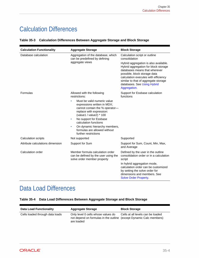
Calculation DifferencesTable 35-3 Calculation Differences Between Aggregate Storage and Block Storage

Calculation Functionality Aggregate Storage Block Storage

Database calculation Aggregation of the database, whichcan be predefined by definingaggregate views

Calculation script or outlineconsolidation

Hybrid aggregation is also available.Hybrid aggregation for block storagedatabases means that whereverpossible, block storage datacalculation executes with efficiencysimilar to that of aggregate storagedatabases. See Using HybridAggregation.

Formulas Allowed with the followingrestrictions:

• Must be valid numeric valueexpressions written in MDX;cannot contain the % operator—replace with expression:(value1 / value2) * 100

• No support for Essbasecalculation functions

• On dynamic hierarchy members,formulas are allowed withoutfurther restrictions

Support for Essbase calculationfunctions

Calculation scripts Not supported Supported

Attribute calculations dimension Support for Sum Support for Sum, Count, Min, Max,and Average

Calculation order Member formula calculation ordercan be defined by the user using thesolve order member property

Defined by the user in the outlineconsolidation order or in a calculationscript

In hybrid aggregation mode,calculation order can be customizedby setting the solve order fordimensions and members. See Solve Order Property.

Data Load DifferencesTable 35-4 Data Load Differences Between Aggregate Storage and Block Storage

Data Load Functionality Aggregate Storage Block Storage

Cells loaded through data loads Only level 0 cells whose values donot depend on formulas in the outlineare loaded

Cells at all levels can be loaded(except Dynamic Calc members)

Chapter 35Calculation Differences

35-4

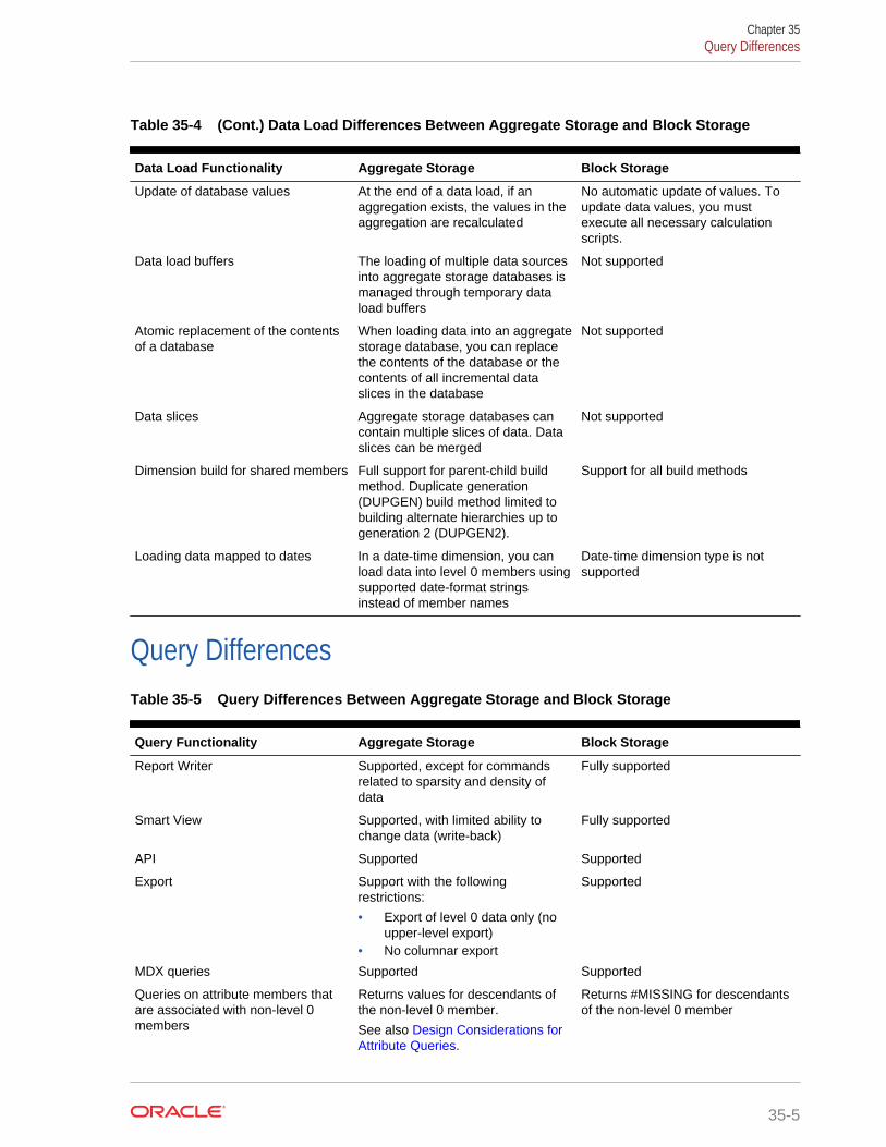
Table 35-4 (Cont.) Data Load Differences Between Aggregate Storage and Block Storage

Data Load Functionality Aggregate Storage Block Storage

Update of database values At the end of a data load, if anaggregation exists, the values in theaggregation are recalculated

No automatic update of values. Toupdate data values, you mustexecute all necessary calculationscripts.

Data load buffers The loading of multiple data sourcesinto aggregate storage databases ismanaged through temporary dataload buffers

Not supported

Atomic replacement of the contentsof a database

When loading data into an aggregatestorage database, you can replacethe contents of the database or thecontents of all incremental dataslices in the database

Not supported

Data slices Aggregate storage databases cancontain multiple slices of data. Dataslices can be merged

Not supported

Dimension build for shared members Full support for parent-child buildmethod. Duplicate generation(DUPGEN) build method limited tobuilding alternate hierarchies up togeneration 2 (DUPGEN2).

Support for all build methods

Loading data mapped to dates In a date-time dimension, you canload data into level 0 members usingsupported date-format stringsinstead of member names

Date-time dimension type is notsupported

Query DifferencesTable 35-5 Query Differences Between Aggregate Storage and Block Storage

Query Functionality Aggregate Storage Block Storage

Report Writer Supported, except for commandsrelated to sparsity and density ofdata

Fully supported

Smart View Supported, with limited ability tochange data (write-back)

Fully supported

API Supported Supported

Export Support with the followingrestrictions:

• Export of level 0 data only (noupper-level export)

• No columnar export

Supported

MDX queries Supported Supported

Queries on attribute members thatare associated with non-level 0members

Returns values for descendants ofthe non-level 0 member.

See also Design Considerations forAttribute Queries.

Returns #MISSING for descendantsof the non-level 0 member

Chapter 35Query Differences

35-5

Table 35-5 (Cont.) Query Differences Between Aggregate Storage and Block Storage

Query Functionality Aggregate Storage Block Storage

Queries on attribute members andshared members

A shared member automaticallyshares the attribute associations ofits referenced member

A shared member does not share theattribute associations of itsreferenced member

Query logging Supported Supported

Query performance Considerations when querying datafrom a dimension that has multiplehierarchies.

See Query Design Considerationsfor Aggregate Storage.

Hierarchies not relevant

Feature DifferencesTable 35-6 Feature Differences Between Aggregate and Block Storage

Features Aggregate Storage Block Storage

Aliases Supported Supported

Incremental data load Supported Supported

LROs Not supported Supported

Time balance reporting Support with the followingrestrictions:

• Skip Zeros is not supported• Time dimension must contain

only stored hierarchies• Shared members must be at

level zero

Supported

Triggers After-update triggers supported On-update triggers and after-updatetriggers supported

Unicode Supported Supported

Variance reporting Not supported Supported

Date-time dimension type and linkedattribute dimensions


User ability to change data (write-back)

Supported with the followingrestriction: Write back to anaggregate storage database must beto level 0 members.

Supported

Hybrid AggregationEssbase hybrid aggregation combines block storage functionality with aggregatestorage performance. In hybrid aggregation mode, you retain the use of block storageelements while enabling the use of more (and larger) sparse dimensions, while alsoreducing the database footprint and improving performance. See Using HybridAggregation.

Chapter 35Feature Differences

35-6

36Aggregate Storage Applications,Databases, and Outlines

Aggregate storage applications and databases and block storage applications anddatabases differ in concept and design. Some block storage outline features do notapply to aggregate storage. For example, the concept of dense and sparsedimensions does not apply.

• Process for Creating Aggregate Storage Applications

• Creating Aggregate Storage Applications, Databases, and Outlines

• Developing Formulas on Aggregate Storage Outlines

Also see Comparison of Aggregate and Block Storage.

Process for Creating Aggregate Storage ApplicationsThis topic provides a high-level process for creating an aggregate storage application.

1. Create an aggregate storage application, database, and outline.

See Creating Aggregate Storage Applications, Databases, and Outlines.

2. Specify the maximum size of the aggregate storage cache.

See Managing the Aggregate Storage Cache.

3. Load data into the aggregate storage database. A data load can be combined witha dimension build.

See Preparing Aggregate Storage Databases.

4. Precalculate chosen aggregations to optimize retrieval time.

See Calculating Aggregate Storage Databases.

5. View database statistics.

6. Write back to an aggregate storage database must be to level 0 members.

7. View data using Oracle tools (for example, Smart View) or third-party tools.

Creating Aggregate Storage Applications, Databases, andOutlines

You must create an aggregate storage application to contain an aggregate storagedatabase. An aggregate storage application can contain only one database. You cancreate an aggregate storage application, database, and outline in the following ways:

• Convert a block storage outline to an aggregate storage outline, and then createan aggregate storage application to contain the converted database and outline.

36-1

Essbase supports the following scenarios for converting block storage outlines toaggregate storage outlines:

– Non-Unicode block storage outline to non-Unicode aggregate storage outline

– Non-Unicode block storage outline to Unicode aggregate storage outline

– Unicode block storage outline to Unicode aggregate storage outline

The following conversion scenarios are not supported:

– Unicode block storage outline to non-Unicode aggregate storage outline

– Aggregate storage outline to a block storage outline

• Create an aggregate storage application and database. The aggregate storageoutline is created automatically when you create the database.

For information on loading dimensions and members into an aggregate storageoutline, see Building Dimensions in Aggregate Storage Databases and Loading Datainto Aggregate Storage Databases.

Aggregate storage application and database information differs from block storageinformation, and specific naming restrictions apply to aggregate storage applicationsand databases. See Table 35-1.

To convert a block storage outline to an aggregate storage outline, you can use thecreate outline MaxL statement.

Note:

Do not use the file system to copy a block storage outline into an aggregatestorage application.

To create an aggregate storage application or database, use these MaxL statements:

• create application

• create database

When creating aggregate storage applications, databases, and outlines, consider thedifferences between aggregate storage and block storage and issues specific toaggregate storage. See the following sections, and also see Aggregate Storage Time-Based Analysis.

HierarchiesIn aggregate storage outlines and block storage outlines, dimensions are structured tocontain one or more hierarchies of related levels and members within the levels. Forexample, the Time dimension in the ASOsamp.Sample database includes thehierarchies MTD, QTD, and YTD, as shown in Figure 36-1.

Chapter 36Creating Aggregate Storage Applications, Databases, and Outlines

36-2

Figure 36-1 Outline Showing Multiple Hierarchies and Members on the TimeDimension

In an aggregate storage database, you can create two types of hierarchies:

• Stored

• Dynamic

The two types of hierarchies have different advantages and restrictions. A dimensionmay contain both types of hierarchies. To use multiple hierarchies in a dimension(even if they are all stored hierarchies), you must enable multiple hierarchies for thatdimension.

In the Essbase web UI, you enable multiple hierarchies for a dimension as a cubeinformation property. See Setting Information Properties in Using Oracle AnalyticsCloud - Essbase.

You can also tag the dimension member as multiple-hierarchies-enabled by using theimport database MaxL statement.

When you tag a dimension member as multiple hierarchies enabled, it is automaticallytagged label only.

If you do not tag the dimension as multiple hierarchies enabled, the dimension isautomatically tagged as a stored hierarchy (except the dimension tagged as Accounts,which is automatically tagged as a dynamic hierarchy).

Note:

The first hierarchy in a multiple hierarchies enabled dimension must be astored hierarchy.

Stored HierarchiesMembers of stored hierarchies are aggregated according to the outline structure.Because aggregate storage databases are optimized for aggregation, the aggregationof data values for stored hierarchies is very fast. To allow this fast aggregation,members of stored hierarchies have the following restrictions:


36-3

• Stored hierarchies can have the no-consolidation (~) operator (only underneathlabel only members) or the addition (+) operator.

• Stored hierarchies cannot have formulas.

Stored hierarchies have restrictions on label only members. See Table 35-2.

In Figure 36-2, the All Merchandise hierarchy and the High End Merchandise hierarchyare stored hierarchies. The All Merchandise member and the High End Merchandisemember are the tops of the hierarchies and are both tagged as top of a storedhierarchy.

In the Essbase web UI, you specify a stored hierarchy as an information property. See Setting Information Properties in Using Oracle Analytics Cloud - Essbase.

You can tag the top member of the hierarchy as top of a stored hierarchy by using theimport database MaxL statement.

The following members can be tagged as top of a stored hierarchy:

• A dimension member (generation 1). If a dimension member is tagged as top ofa stored hierarchy, the entire dimension is considered a single stored hierarchy,and no other member in the dimension can be tagged as top of a stored hierarchyor top of a dynamic hierarchy.

• The children of the dimension member (generation 2). If a generation 2member is tagged as top of a stored hierarchy, all generation 2 members in thedimension also must be tagged as either top of a stored hierarchy or top of adynamic hierarchy. The first hierarchy in the dimension must be a storedhierarchy.

The dimension tagged as accounts is automatically considered a dynamic hierarchy.You cannot specify the accounts dimension as a stored hierarchy.

Dynamic HierarchiesTo evaluate a dynamic hierarchy, Essbase calculates, rather than aggregates, themembers and formulas. The order in which members and formulas are evaluated isdefined by the solve order property. See Calculation Order.

At the time of retrieval, Essbase calculates the required member combinations andcalculates any required outline member formulas. Because dynamic hierarchies arecalculated, the data retrieval time may be longer than for data retrieved from storedhierarchies. However, when you design your database, dynamic hierarchies providethe following advantages:

• They can contain any consolidation operator.

• They can have formulas.

In the Essbase web UI, you specify a dynamic hierarchy as an information property.See Setting Information Properties in Using Oracle Analytics Cloud - Essbase.

Tag the top member of the hierarchy as top of a dynamic hierarchy by using the importdatabase MaxL statement.

The following members can be tagged as top of a dynamic hierarchy:

• A dimension member (generation 1)—If a dimension member is tagged as top of adynamic hierarchy, the entire dimension is considered a single dynamic hierarchy,


36-4

and no other member in the dimension can be tagged as top of a dynamichierarchy or top of a stored hierarchy.

• The children of the dimension member (generation 2)—If a generation 2 memberis tagged as top of a dynamic hierarchy, all generation 2 members in thedimension must also be tagged as either top of a dynamic hierarchy or top of astored hierarchy. The first hierarchy in the dimension must be a stored hierarchy.

Note:

If a member has the no-consolidation operator (~) on all its children, themember must be tagged label only.

The dimension tagged accounts is automatically considered a dynamic hierarchy. Youcannot specify the accounts dimension as a stored hierarchy.

Essbase cannot select dynamic hierarchy members for an aggregate view. See Aggregating an Aggregate Storage Database.

Alternate HierarchiesAn alternate hierarchy may be modeled in either of the following ways:

• As an attribute dimension, which uses attributes to classify members logicallywithin the dimension (for example, a Product dimension can have attributes suchas Size and Flavor). See Working with Attributes.

Note:

If you use an attribute dimension to create an alternate hierarchy, youcan create a crosstab report query of members in the attribute dimensionwith members in the base dimension. For example, a crosstab report ofproduct sales information could show size attributes (such as small andlarge) as column headings and products as row headings. If you useshared members to create an alternate hierarchy, you cannot create anequivalent crosstab report query of the shared members with thereferenced members in the primary hierarchy.

• As a hierarchy of shared members. The alternate hierarchy has shared membersthat point to referenced members of previous hierarchies in the outline. Theshared members roll up according to a different hierarchy from the referencedmembers. Shared members on dynamic hierarchies can have formulas. See Understanding Shared Members. Table 36-1 shows the hierarchies for theASOsamp.Sample database. The Products dimension is shown in Figure 36-2.


36-5

Table 36-1 Example Hierarchies and Alternate Hierarchies for the ProductDimension of ASOsamp.Sample

Product Hierarchy Alternate Hierarchy(containing sharedmembers)

Flat Panel Products, All Merchandise,Personal Electronics, HomeEntertainment, Televisions

Products, High EndMerchandise

HDTV Products, All Merchandise,Personal Electronics, HomeEntertainment, Televisions

Products, High EndMerchandise

Figure 36-2 Aggregate Storage Outline Displaying the Alternate Hierarchy HighEnd Merchandise on the Product Dimension

The following restrictions apply when creating alternate hierarchies in aggregatestorage outlines:

• The referenced instance of the member must occur in the outline before anyshared instances of the member. For example, in Figure 36-2, the member HDTVoccurs in the All Merchandise hierarchy before it occurs as a shared member inthe alternate hierarchy of High End Merchandise.

• The first hierarchy in a dimension where multiple hierarchies are enabled cannotcontain a shared member.

• Stored hierarchy dimensions cannot have shared members. Stored hierarchieswithin a multiple hierarchies dimension can have shared members.

• To ensure that values are not double-counted, a stored hierarchy cannot containmultiple copies of the same shared member. For example, a stored hierarchycannot contain a shared member and any of its ancestors. In Figure 36-2, youcannot add the shared member “Televisions” as a child of “High EndMerchandise,” because doing so would make “Televisions” a sibling of its children,


36-6

shared members “Flat Panel” and “HDTV,” causing the values of “Flat Panel” and“HDTV” to be added twice.

• Referenced instances of a member must be in the same dimension as the sharedmember (same for block storage outlines).

• A stored hierarchy cannot contain a referenced instance and a shared instance ofthe same member.

• A stored hierarchy can contain a shared instance of a dynamic hierarchy memberonly if the dynamic hierarchy member is a level 0 member without a formula.

Note:

In an aggregate storage database, a shared member automatically sharesany attributes that are associated with its referenced member.

Attribute DimensionsThis topic provides information on the differences between aggregate storage andblock storage databases with regard to attribute dimensions. To use the information inthis topic, you should be familiar with attribute dimension concepts for block storagedatabases. See Working with Attributes.

The following information applies to attribute dimensions when used on aggregatestorage databases:

• Only the addition (+) consolidation operator is available for attribute dimensions.

• For a given attribute dimension, all associations must be with one level of the basedimension. For example, in the ASOsamp.Sample database, associations for theStore Manager attribute dimension are with level 0 of the Stores dimension. Thefollowing restrictions apply to attribute associations:

– Level 0: You can associate attributes with any level 0 member of a dynamic orstored hierarchy that does not have a formula.

– Non-level 0: You can associate attributes only to upper level members in theprimary stored hierarchy.

Attribute dimensions do not have hierarchy types. You cannot specify an attributedimension as a dynamic or stored hierarchy. Essbase treats attribute dimensions asstored alternate hierarchies of the base dimension. For example, in theASOsamp.Sample database, Essbase treats the Store Manager attribute dimensionas if the Store Manager dimension were a stored alternate hierarchy of the Storesdimension.

When using query tracking, Essbase considers queries on attribute dimension dataand may include attribute dimension members in aggregate view selections. See Selecting Views Based on Usage and Calculating Aggregate Storage Databases.


36-7

Note:

Queries on attribute members that are associated with non-level 0 membersreturn values for descendants of the non-level 0 member. This behavior ofqueries on attribute members in aggregate storage databases is differentfrom the behavior in block storage databases.

Design Considerations for Attribute QueriesWhen selecting and building views based on attribute query data, some queries onattribute data are always dynamically calculated at the time of retrieval, which mayaffect query performance.

Every query involving attribute dimension members must also include at least onemember from the base dimension. If the query involves a single attribute dimensionand a sum-of-all dimension member, Essbase aggregates the query data, potentiallyimproving query performance. In other cases, Essbase must calculate the query at thetime of retrieval.

Table 36-2 describes attribute query types and how Essbase calculates the query:

Table 36-2 Attribute Queries and Calculation Performance

Attribute Query Type Query Calculation Type

Query involves a sum-of-all base dimensionmember and members from one attributedimension.

Essbase can aggregate query data, potentiallyimproving query performance.

Query involves any member of the basedimension and members from multipleattribute dimensions.

Essbase calculates the query at the time ofretrieval based on the level 0 input data.

Query involves any child member of the basedimension member (or dimension member thatis tagged as label-only) and members fromone attribute dimension.

Essbase calculates the query at the time ofretrieval based on the level 0 input data, or ondata from aggregations on the basedimension.

In the outline displayed in Figure 36-3, RealDimension is the sum of all itsdescendents (it is not tagged as label-only). If a query involves one or more membersfrom a single attribute dimension (for example, AttributeDimension1), crossed with thebase dimension member (RealDimension), Essbase can build aggregate cells for thedata, potentially improving query performance.

The following queries, however, are always calculated at the time of retrieval:

• Any query requesting data for members from an attribute dimension (for exampleAttributeDimension1) and any of the children of RealDimension is calculateddynamically at retrieval time based on the level 0 input data or on data fromaggregations.

• Any query requesting data from multiple attribute dimensions (for exampleAttributeDimension1 and AttributeDimension2) and a base member dimension (forexample RealDimension) is calculated dynamically at retrieval time based on level0 input data.


36-8

Figure 36-3 Outline for Attribute Query Example

Design Considerations for Aggregate Storage OutlinesThis topic lists the key design considerations when you create aggregate storagedatabase outlines. For an example of implementing these design considerations, seethe ASOsamp.Sample database. Consider the following information when designingan aggregate storage outline:

• Use stored hierarchies (rather than dynamic hierarchies) as much as possible.

• Use alternate hierarchies (shared members) only when necessary.

• Minimize the number of hierarchies. (For example, each additional storedhierarchy slows down view selection and potentially increases the size of theaggregated data).

• If a hierarchy is a small subset of the first hierarchy, consider making the smallhierarchy a dynamic hierarchy. Considerations include how often the hierarchydata is queried and the query performance impact when it is dynamically queriedat the time of retrieval.

• The performance of attributes is the same as for members on a stored hierarchy.

• The higher the association level of an attribute to the base member, the faster theretrieval query. (See also, Design Considerations for Attribute Queries).

Query Design Considerations for Aggregate StorageWhen querying data from a dimension that has multiple hierarchies, queryperformance may improve if you query the data in the following way:

1. Select the hierarchy that you want to query.

2. Navigate to find the detailed data (for example, by zooming in on the hierarchy inSmart View).

Including dynamic hierarchy members and stored hierarchy members in the samequery may require a large internal memory cache, which decreases queryperformance.

64-bit Dimension Size Limit for Aggregate Storage Database OutlineAn aggregate storage database outline cannot exceed 64-bits per dimension.

The number of bits needed by a dimension is the maximum number of bits used byany level 0 child, including the level 0 children in alternate hierarchies and associatedattribute dimensions. For the purposes of member numbering, attribute dimensions aretreated as alternate hierarchies of their base dimensions.


36-9

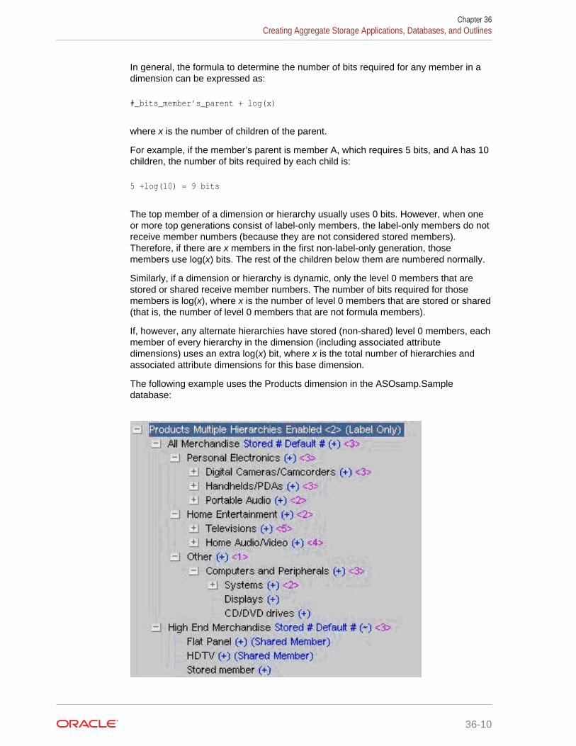
In general, the formula to determine the number of bits required for any member in adimension can be expressed as:

#_bits_member’s_parent + log(x)

where x is the number of children of the parent.

For example, if the member’s parent is member A, which requires 5 bits, and A has 10children, the number of bits required by each child is:

5 +log(10) = 9 bits

The top member of a dimension or hierarchy usually uses 0 bits. However, when oneor more top generations consist of label-only members, the label-only members do notreceive member numbers (because they are not considered stored members).Therefore, if there are x members in the first non-label-only generation, thosemembers use log(x) bits. The rest of the children below them are numbered normally.

Similarly, if a dimension or hierarchy is dynamic, only the level 0 members that arestored or shared receive member numbers. The number of bits required for thosemembers is log(x), where x is the number of level 0 members that are stored or shared(that is, the number of level 0 members that are not formula members).

If, however, any alternate hierarchies have stored (non-shared) level 0 members, eachmember of every hierarchy in the dimension (including associated attributedimensions) uses an extra log(x) bit, where x is the total number of hierarchies andassociated attribute dimensions for this base dimension.

The following example uses the Products dimension in the ASOsamp.Sampledatabase:


36-10

The Products dimension has two hierarchies: All Merchandise and High EndMerchandise, which is an alternate hierarchy. High End Merchandise has one storedlevel 0 member: Stored Member. The Products dimension does not have anyassociated attribute dimensions.

Members All Merchandise and High End Merchandise use log(2) = 1 bit.

Note:

If the alternate hierarchy High End Merchandise did not have any storedlevel 0 members, the top members of each hierarchy (and associatedattribute dimensions) would each use 0 bits.

The calculation of the number of bits required by each level 0 children:

All Merchandise = 1 bit Personal Electronics, Home Entertainment, Other = 1 + log(3) = 3 bits Digital Cameras/Camcorders, Handhelds/PDAs, Portable Audio = 3 + log(3) = 5 Children of Digital Cameras/Camcorders = 5 + log(3) = 7 Children of Handhelds/PDAs = 5 + log(3) = 7 Children of Portable Audio = 5 + log(2) = 6 Televisions, Home Audio/Video = 3 + log(2) = 4 Children of Televisions = 4 + log(5) = 7

Children of Home Audio/Video = 4 + log(4) = 6 Computers and Peripherals = 3 + log(1) = 3 ** Systems, Displays, CD/DVD drives = 3 + log(3) = 5 Children of Systems = 5 + log(2) = 6 High End Merchandise = 1 bit Flat Panel, HDTV, Stored Member = 1 + log(3) = 3 bits

Member Computers and Peripherals has the same number of bits (3) as its parentOther.

The maximum bits used by any level 0 children in the Products dimension is 7(Children of Digital Cameras and Children of Televisions). Therefore, Products uses 7bits, which is less than the dimension size limit of 64 bits.

If the dimension size exceeds 64 bits:

• Essbase generates the following error when saving the outline:

Hierarchy [DimensionName] is too complex. It exceeds the maximum member number width of 64 bits. See application log for details.

• Essbase logs messages similar to the following messages in the application log:

Member number for member [level0member] requires [65] bits to encodeMember [level0member] contributes [5] bits to member numberMember [level1parent] contributes [20] bits to member number


36-11

Member [level2parent] contributes [20] bits to member numberMember [level3parent] contributes [20] bits to member number

To fix the error, use one of these recommendations:

• If possible, delete some siblings of any of the members referenced in themessages. Reducing the number of siblings by a power of two saves one bit. Forinstance, assume that level0member, which contributes 5 bits to the membernumber, has 18 siblings, including itself. Reducing the number of siblings to 16 orfewer saves one bit because log(16) = 4. Similarly, reducing the number of siblingsto 8 or fewer saves two bits.

• Reclassify some siblings of members referenced in the messages. For example,move half of level0member’s 18 siblings to another parent that doesn’t have asmany children. Alternately, create a new parent as a sibling of level1parent andmove half of level1parent’s children under the new member. This approach savesone bit.

• Combine some intermediate levels. For instance, move level0member, and all ofits siblings, to be children of level2parent and then remove level1parent. Thisapproach is more involved but it can save many bits.

Understanding the Compression Dimension for Aggregate StorageDatabases

By default, the compression dimension in an aggregate storage database is theAccounts dimension. Changing the compression dimension triggers a full restructureof the database. Essbase requires the compression dimension to be a single dynamichierarchy. If the dimension has a different hierarchy setting, such as multiplehierarchies, it will be set to single dynamic hierarchy automatically. The originalhierarchy setting is lost (setting a different dimension as compression does not returnthe original hierarchy setting). Attribute dimensions cannot be compressiondimensions, nor can dimensions with attributes associated to them.

The choice of compression dimension can significantly affect performance. A goodcandidate for a compression dimension is one that optimizes data compression whilemaintaining retrieval performance. This topic provides information about choosing anoptimal compression dimension.

Note:

The information in this topic applies to loaded databases. See Loading Datainto Aggregate Storage Databases.

Maintaining Retrieval PerformanceBecause compression dimensions are dynamically calculated, you must take intoaccount design considerations for dynamically calculated dimensions when choosing acompression dimension. Dynamic dimensions are calculated at the time of retrieval, sothe data retrieval time is longer than for stored hierarchies.

If a dimension with a large number of level 0 members is tagged as compression,upper-level queries take longer because they require many level 0 members to be


36-12

retrieved. If users will be doing many upper-level retrievals on a large dimension, it isnot a good candidate for a compression dimension.

Viewing Compression Estimation StatisticsIn MaxL, you can view detailed compression and query statistics. You can view thenumber of stored level 0 members, which affects retrieval performance; the averagebundle fill and average value length, which affect compression; and the level 0 size.

To view detailed query and compression statistics, you can use the aggregate storageversion of the query database MaxL statement.

See these topics for a description of each of the compression and query relatedstatistics.

• Stored level 0 members

• Average bundle fill

• Average value length

• Expected level 0 size

Stored level 0 membersDimensions with a large number of stored level 0 members do not perform well iftagged Compression. As with any dynamically calculated dimension, upper-levelretrievals from compression dimensions generally are slow. See Maintaining RetrievalPerformance.

Average bundle fillCompression is more effective if values are grouped together in consecutive memberson dimensions or hierarchies rather than spread throughout the outline with lots of#MISSING data between values. Essbase saves memory by storing information aboutthe location and contents of the groups rather than storing it separately for each of themembers. The average bundle fill is the average number of values stored in thegroups. It can vary between 1 and 16, with 16 being the best. Choosing a compressiondimension that has a higher average bundle fill means that the database compressesbetter.

In some outlines, you can improve compression by ordering the numbers in thecompression dimension so that members that are frequently populated are groupedtogether. When populated members are grouped together, more values fit into eachbundle, increasing the average bundle fill and improving compression.

Average value lengthThe average value length is the average storage size, in bytes, required for the storedvalues in the cells. It can vary between 2 bytes and 8 bytes with 2 bytes being thebest. Without compression, it takes 8 bytes to store a value in a cell. Withcompression, it can take fewer bytes, depending on the value length. For example,10.050001 might take 8 bytes to store even when compressed, but 10.05 may onlytake 2 bytes (4 bytes to store when compressed). Dimensions with a smaller averagevalue length compress the database better.

Rounding the data values to no more that two digits after the decimal point can reducethe average value length, improving compression.


36-13

Expected level 0 sizeThis field indicates the estimated size of the compressed database. A smallerexpected level 0 size indicates that choosing this dimension is expected to enablebetter compression.

Verifying Aggregate Storage OutlinesAggregate storage outline files have the same file extension (.otl) as block storagedatabase outline files and are stored in an equivalent directory structure.

When you save an outline, Essbase verifies it for errors. You can also verify theaccuracy of an outline before you save it. Some block storage database features donot apply to aggregate storage databases, and the verification process considers therules for aggregate storage databases. See Comparison of Aggregate and BlockStorage.

Outline PagingAggregate storage database outlines are pageable. This feature may significantlyreduce memory usage for very large database outlines. For aggregate storagedatabases, Essbase preloads part of the database outline into memory. Then, duringdata retrieval, Essbase pages other parts of the outline into memory as required.

When you create an aggregate storage database, the outline is created in a pageableformat. When you use the Aggregate Storage Outline Conversion Wizard to convert anexisting block storage outline to aggregate storage, the outline is automaticallyconverted to a pageable format.

Paging an outline into memory enables Essbase to handle very large outlines (forexample, 10 million or more members) but potentially increases data retrieval time.

Note:

Aggregate storage databases that have pageable outlines contain memorypages, and therefore their outline files may be larger than binary blockstorage database outline files.

Outline Paging LimitsThe maximum size of a buildable outline (the number of members) depends onseveral factors:

• The available memory for Essbase

• The amount of memory in Essbase allocated for other uses

• The amount of memory required for each member (and aliases for each member)

Essbase uses about 40 MB of memory on startup. In addition, the various cachesrequire the following memory allocations:

• Outline paging cache: 8 MB


36-14

• Aggregate storage data cache: 32 MB

• Aggregate storage aggregation cache: 10 MB

Therefore, the initial memory footprint for Essbase is about 90 MB. In addition,memory must be allocated to process incoming query requests. Typical memory toreserve for this purpose is about 300 MB. The total memory allocated for Essbase istherefore 390 MB.

On a Windows system with 1.85 GB of addressable memory, the amount available tobuild and load the outline is about 1.46 GB (1.85 GB - 390 MB = 1.46 GB).

The maximum outline size depends on whether it is built using a dimension build orfrom an outline already loaded into Essbase.

Dimension Build LimitTo build the outline by using a dimension build, Essbase allocates about 100 bytes permember, plus the size of the member name, plus the size of all alias names for themember (up to 10 aliases are allowed).

For a sample outline (using a single byte codepage) where the average member nameis 15 characters and there is one alias (of 20 characters) per member, the memoryrequirement for each member that is added:

100 + 15 + 20 bytes = 135 bytes

The total number of members that can be added in a dimension build is the availablememory (1.46 GB, or 153,092,060 bytes) divided by the number of bytes per member(135), approximately 11 million members.

On systems with more than 2 GB of addressable memory, the outline can be larger inproportion to the extra memory that is available.

When the dimension build is complete, a dbname.otn file is saved in the databasedirectory. The .otn file is used as input for the outline restructuring process, whichreplaces the old outline with the new one. During restructuring, two copies of theoutline are loaded into memory, the old one (potentially empty), and the new one, sothe maximum size of an outline that can be restructured depends on the size of the oldoutline.

In a dimension build, which starts with an empty outline, only one outline is loaded intomemory.

Loaded Outline LimitThe memory requirement for an outline loaded into Essbase at runtime or duringrestructuring is different from the memory requirements for a dimension build. Essbaseallocates about 60 bytes per member, plus the size of the member name plus 5 bytes,plus the size of all alias names for the member (up to 10 aliases are allowed) plus 5bytes. For a sample outline where the average member name is 15 characters andthere is one alias (of 20 characters) per member, the memory requirement for eachmember that is added:

60 + 15 + 5 + 20 + 5 bytes = 105 bytes per member

Assuming 1.46 GB of available memory, the maximum size of an outline that can beloaded is one with 14 million members (1.46 GB/105 bytes).


36-15

The 14 million members are the sum of two outlines that are loaded duringrestructuring. For example, if an existing outline has 5 million members, the newoutline can have a maximum of 9 million members. In an incremental dimension build,it is recommended to build the smaller dimensions first and the larger ones last toallow for a maximum outline size.

Compacting the Aggregate Storage Outline FileThe outline file (.otl) for an aggregated storage outline increases in size as theoutline changes; for example, when members are added or deleted. You can decreasethe outline file size by compacting it. After the outline file is compacted, the filecontinues to grow as before, when members are added or deleted.

Compacting the outline file causes Essbase to restructure the outline and can takeplace only when no other users or processes are actively using the database.Compacting the outline does not cause Essbase to clear the data.

Note:

When a member is deleted from the outline, the corresponding record of thatmember in the outline file is marked as deleted but the record remains in theoutline file. Compacting the outline file does not remove the records ofdeleted members.

To compact an outline file, you can use the alter database MaxL statement.

Developing Formulas on Aggregate Storage OutlinesFormulas calculate relationships between members in a database outline. If you arefamiliar with using formulas on block storage outlines, consider the followingdifferences when using formulas on aggregate storage outlines:

• Essbase provides a native calculation language to write formulas on block storageoutlines. To write formulas for aggregate storage outlines, use the MDX(Multidimensional Expressions) language.

• Apply formulas directly to members in the database outline. For block storagedatabases, formulas can be placed in a calculation script. For aggregate storagedatabases, you cannot place formulas in a calculation script.

This chapter concentrates on using MDX to write formulas on aggregate storagedatabases. For information about using MDX to write queries, see Writing MDXQueries. For information about writing formulas for block storage outlines, see Developing Formulas for Block Storage Databases. For MDX syntax details, see MDXin Technical Reference for Oracle Analytics Cloud - Essbase.

Using MDX FormulasAn MDX formula must always be an MDX numeric value expression. In MDX, anumeric value expression is any combination of functions, operators, and membernames that does one of the following actions:

• Calculates a value

Chapter 36Developing Formulas on Aggregate Storage Outlines

36-16

• Tests for a condition

• Performs a mathematical operation

A numeric value expression is different from a set expression. A set expression isused on query axes and describes members and member combinations. A numericvalue expression specifies a value.

A numeric value expression is used in queries to build calculated members, which arelogical members created for analytical purposes in the WITH section of the query, butwhich do not exist in the outline.

The following query defines a calculated member and uses a numeric valueexpression to provide a value for it:

WITH MEMBER [Measures].[Prod Count]AS 'Count ( Crossjoin ( {[Units]}, {[Products].children} ) )', SOLVE_ORDER=1SELECT {[Geography].children}ON COLUMNS, { Crossjoin ( {[Units]}, {[Products].children} ), ([Measures].[Prod Count], [Products]) }ON ROWSFROM ASOsamp.Sample

In the sample query, the WITH clause defines a calculated member, Product Count, inthe Measures dimension, as follows:

WITH MEMBER [Measures].[Prod Count]

The numeric value expression follows the WITH clause and is enclosed in singlequotation marks. In the sample query, the numeric value expression is specified asfollows:

'Count ( Crossjoin ( {[Units]}, {[Products].children} ) )'


36-17

The SOLVE_ORDER property specifies the order in which members and formulas areevaluated. See Calculation Order.

Note:

For an explanation of the syntax rules used to build the numeric valueexpression in the example, see the documentation in the TechnicalReference for Oracle Essbase for the Count, CrossJoin, and Childrenfunctions.

A numeric value expression also can be used as an MDX formula to calculate thevalue of an existing outline member.

Therefore, rather than creating the example query, you can create an outline memberon the Measures dimension called Prod Count that is calculated in the outline in thesame way that the hypothetical Prod Count was calculated in the sample query.

To create a calculated member with a formula:

1. Create a member.

2. Attach an MDX formula to the member.

Assuming that you created the example Prod Count member, you would use thefollowing formula, which is the equivalent of the numeric value expression used tocreate the calculated member in the example query:

Count(Crossjoin ( {[Units]}, {[Products].children}))

3. Verify the formula by verifying the outline.

When you retrieve data from the aggregate storage database, the formula is usedto calculate the member value.

You can use substitution variables within formulas. For example, you could definea substitution variable named “EstimatedPercent” and provide differentpercentages as substitution variable values. See Using Substitution Variables.

Before applying formulas to members in the outline, you can write MDX queries thatcontain calculated members. When you can write an MDX query that returns thecalculated member results that you want, you are ready to apply the logic of thenumeric value expression to an outline member and validate and test the expression.See Writing MDX Queries. For syntax information about MDX, see the TechnicalReference for Oracle Essbase.

Formula Calculation for Aggregate Storage DatabasesEssbase calculates formulas in aggregate storage outlines only when data is retrieved.Calculation order may affect calculation results. Whenever you use MDX formulas onmultiple dimensions in an aggregate storage outline, it is good practice to set the solveorder for each member or dimension. See Calculation Order.


36-18

Note:

When designing an aggregate storage database calculation, consider thataggregate storage database members with MDX formulas are dynamicallycalculated. The dynamically calculated members have a value of #MISSINGuntil they are queried.

Formula Syntax for Aggregate Storage DatabasesWhen you create member formulas for aggregate storage outlines, observe thefollowing rules:

• Enclose member names in brackets ([]) if they meet any of the followingconditions:

– Start with a number or contains spaces; for example, [100]. Brackets arerecommended for all member names, for clarity and code readability.

– Are the same as an operator or function name. See the Technical Referencefor Oracle Essbase for a list of operators and functions.

– Include a nonalphanumeric character; for example, a hyphen (-), an asterisk(*), or a slash (/).

Note:

In formulas, member names starting with $ or & must be enclosed inquotation marks as well as brackets. For example, $testmember wouldbe expressed in the formula as ["$testmember"]/100

• Use the IIF function to write conditional tests with a single else condition. Thesyntax for the IIF function does not require an ELSEIF keyword to identify the elsecondition nor an ENDIF keyword to terminate the statement. You can nest IIFfunctions to create a more complex formula.

• Use the CASE, WHEN, THEN construct to write conditional tests with multipleconditions.

• Be certain that tuples are specified correctly. A tuple is a collection of memberswith the restriction that no two members can be from the same dimension. Enclosetuples in parentheses; for example, (Actual, Sales).

• Be certain that sets are specified correctly. A set is an ordered collection of one ormore tuples. When a set has multiple tuples, the following rule applies: In eachtuple of the set, members must represent the same dimensions as do themembers of other tuples of the set. Additionally, the dimensions must berepresented in the same order. In other words, all tuples of the set must have thesame dimensionality.

See Rules for Specifying Sets.

Enclose sets in braces, for example:

{ [Year].[Qtr1], [Year].[Qtr2], [Year].[Qtr3], [Year].[Qtr4] }


36-19

Creating Formulas on Aggregate Storage OutlinesFormulas are plain text. You can type the formulas directly into the formula editor, oryou can create a formula in any text editor and paste the text into the formula editor.

MDX-based syntax checking tells you about syntax errors in formulas; for example, amistyped function name or a nonexistent member. Unknown member names can bevalidated against a list of function names. If you are not connected to the serviceinstance or to the application associated with the outline, Essbase may connect you tovalidate unknown names.

Syntax checking occurs when validate or save a formula. Errors are displayed in theuser interface. If an error occurs, you choose to save or not save the formula. If yousave a formula with errors, you are warned when you save the outline. When youcalculate a formula with errors, the formula is ignored and the member is given a valueof $MISSING.

A syntax checker cannot warn you of semantic errors in a formula. Semantic errorsoccur when a formula does not work as you expect. One way to find semantic errors ina formula is to place the numeric value expression that defines the formula into aquery and run the query to verify that the results are as you expect. See Using MDXFormulas to see how to place a formula into a query.

You can include formulas in a dimension build data source. See Setting Field TypeInformation.

Composing Formulas on Aggregate Storage OutlinesThe following topics in this section discusses and give examples of how to write avariety of formulas for members in aggregate storage outlines.

Basic Equations for Aggregate Storage OutlinesYou can apply a mathematical operation to a formula to create a basic equation. Forexample, the following formula is applied to the Avg Units/Transaction member in theASOsamp.Sample database:

[Units]/[Transactions]

The formula in Avg Units/Transaction divides the number of units by the number oftransactions to arrive at the average number of units per transaction.

In aggregate storage outlines, members cannot be tagged as expense items.Therefore, functions in Calc, such as @VAR and @VARPER, which determine thedifference between two members by considering expense tags, are not relevant inaggregate storage outlines.

The MDX subtraction operator can be used to calculate the difference between twomembers. For example, the following formula can be applied to a new member, calledPrice Diff, in ASOsamp.Sample, to calculate the difference between the price paid andthe original price:

[Price Paid]-[Original Price]


36-20

Members Across Dimensions in Aggregate Storage OutlinesASOsamp.Sample provides a formula on a member called % of Total. This memberformula identifies the percentage of the Measures total that is produced byTransactions. The formula for % of Total:

Transactions/(Transactions,Years,Months,[Transaction Type],[Payment Type],Promotions,Age,[Income Level],Products,Stores,Geography)

The formula specifies a member (Transactions) divided by a tuple (Transactions,Years, ...). The formula lists a top member from every dimension to account for allTransaction data in the cube; that is, not Transaction data for the Curr Year memberbut Transaction data for all members of the Years dimension, not Transaction data formonths in the first two quarters but Transaction for all months, and so on. In this way,the value of % of Total represents the percentage of the Measures total that areproduced by Transactions.

Conditional Tests in Formulas for Aggregate Storage OutlinesYou can define a formula that uses a conditional test or a series of conditional tests todetermine the value for a member. Use the IIF function to perform a test with one elsecondition. You can nest IIF functions to create a more complex query.

The example specifies a formula for a member that represents the price the companymust pay for credit card transactions, which includes a 5% charge. The followingexample assumes that the Credit Price member has been added to the Measuresdimension of the ASOsamp.Sample database. Credit Price has the following formula,which adds 5% to Price Paid when the payment type is a credit card.

IIF ( [Payment Type].CurrentMember=[Credit Card], [Price Paid] * 1.05, [Price Paid])

Use the CASE, WHEN, THEN construct to create formulas with multiple tests and elseconditions.

The Filter function returns the tuples of the input set that meet the criteria of thespecified search condition. For example, to establish a baseline (100) for all products,you can add a Baseline member and create a formula for it, as follows:

Count(Filter(Descendants([PersonalElectronics],[Products].Levels(0)),[Qtr1] > 100.00))

Specifying UDAs in Formulas in Aggregate Storage OutlinesUDAs are words or phrases that you create for a member. For example, inSample.Basic, top-level members of the Market dimension have the UDA SmallMarket or the UDA Major Market.


36-21

The Major Market example used in this topic shows how to create a formula for amember that shows the sum of sales for all major market members. The exampleassumes that a new member (Major Market Total) has been added to Sample.Basic.

1. MDX provides a Boolean function, IsUDA, which Returns TRUE if a member hasthe associated UDA tag. The following syntax returns TRUE if the current memberof the Market dimension has the UDA “Major Market”:

IsUda([Market].CurrentMember, "Major Market")

2. A Filter function, when used with IsUDA (as shown in the following syntax), cyclesthrough each member of the Market dimension and returns a value for eachmember that has the Major Market UDA:

Filter([Market].Members, IsUda([Market].CurrentMember, "Major Market"))

3. The Sum function adds the values returned by the Filter function; for the MajorMarket example, the following formula is produced:

Sum (Filter([Market].Members, IsUda([Market].CurrentMember, "Major Market")))

This formula is attached to the Major Market Total member.


36-22

37Aggregate Storage Time-Based Analysis

Most data analysis includes a time (history) perspective. Aggregate storageapplications provide built-in time-based functionality through time dimensions anddate-time dimensions.

• About Aggregate Storage Time-Based Analysis

• Understanding Date-Time Dimensions

• Understanding Linked Attributes

• Designing and Creating an Outline for Date-Time Analysis

• Modifying or Deleting Date-Time Dimensions

• Loading Data Mapped to Dates

• Analyzing Time-Based Data

•

About Aggregate Storage Time-Based AnalysisThe information in this chapter applies only to aggregate storage databases and is notrelevant to block storage databases. Also see Comparison of Aggregate and BlockStorage.

Aggregate storage time dimensions are similar to block storage time dimensions. Theyenable tagging the accounts dimension for such time balance calculations as first, last,average, and to-date values. Time dimensions are easily modifiable.

Aggregate storage date-time dimensions enable the first, last, and average timebalance support.

The remainder of this chapter discusses date-time dimensions and the linked attributedimensions that can be associated with them. For information about time balancecalculations in aggregate storage outlines, see Performing Time Balance and FlowMetrics Calculations in Aggregate Storage Accounts Dimensions.

Understanding Date-Time DimensionsDate-time dimensions contain a date hierarchy based on the selection of one ofseveral standard corporate calendars. Dimension and member properties contain textstrings that are used to manage the hierarchy, as shown in Figure 37-1.

37-1

Figure 37-1 Sample Date-Time Hierarchy

The dimension member at the top of the hierarchy shows the comment:

/* TI-HIER,TP[3,1,4,5]!TI-MBR,TSPAN[1–1–2008,12–31–2009]! */.

The TI-MBR,TSPAN[date1, date2] information enclosed between exclamation points(!) defines the time range covered by the dimension; in this case two years, Jan. 1,2008–Dec. 31, 2009. Positioned in front of the time span, the array TI-HIER,TP[3,1,4,5] describes the hierarchy. The first number in the array, 3, indicatesthat the hierarchy contains three time periods. The remaining numbers in the arrayindicate what time periods are included, based on the following possible levels:

• 1—Year

• 2—Semester

• 3—Trimester

• 4—Quarter

• 5—Month

• 6—Period

• 7—Week

• 8—Day

Array TI-HIER,TP[3,1,4,5] indicates that the array contains three time periods: year,quarter, and month.

Using the same time span TI-MBR,TSPAN syntax, each member comments fielddefines the time range that it covers; for example, member Quarter 1 of GregorianYear 2008 covers Jan. 1, 2008–Mar. 31, 2008, and member Quarter 2 of GregorianYear 2008 covers Apr. 1, 2008–Jun. 30, 2008.

Understanding Linked AttributesAnalyzing data in terms of relative position within time periods can be useful; forexample, knowing that some costs increase in the last week of each quarter can helpyou balance expenditures. Linked attributes enable data analysis based on relativetime periods such as the first month of a quarter, or the fourth week of a month.

Linked attribute dimensions can be associated only with the date-time dimension.Defining linked attribute dimensions is part of the Create Date-Time Dimensionswizard. The linked attribute dimensions that you create are based on the time depthsyou select when you define the calendar for the date-time dimension. For example, asshown in Figure 37-2, if you select year, quarter, and month time depths and create

Chapter 37Understanding Linked Attributes

37-2

linked attributes, the wizard creates three linked attribute dimensions (defaultdimension names): Quarter by Year, Month by Year, and Month by Quarter. Eachattribute dimension contains members with sequential numeric names, indicating arelative position that will be used in analyzing the members associated with thatattribute.

Figure 37-2 Sample Date-Time Dimension with Linked Attributes

Linked attributes enable you to compare sales of the first month of a quarter againstsales of the second and third months of a quarter in a simple crosstab analysis, asshown:

Chapter 37Understanding Linked Attributes

37-3

Note:

Linked attributes cannot be assigned to year time-depth members.

Linked attribute dimensions reflect two time components, which are easier tounderstand if we use the default names; for example, Quarter by Year. Members ofthe Quarter by Year dimension are associated with quarter time-depth members suchas Quarter 1 of Gregorian Year 2008 in Figure 37-2. The first time component,Quarter, is called the association level, because it indicates the date-time dimensionmembers to which the attributes are associated.

The second time component in this example, Year, is called the attachment level. Theattachment level indicates a member level in the associated date-time dimension.Each member of the linked attribute dimension contains a number that indicates arelationship between the association level and the attachment level. Quarter by Year:1 is the first attribute member, Quarter by Year: 2 is the second member, and so on.

The date-time dimension members associated with linked attribute Quarter by Year: 1are the first quarters of their respective years. All date-time dimension members withthe attribute Month by Quarter: 1 are the first months of their respective quarters. Thuslinked attributes enable analysis of information based on a common periodicrelationship such as first, second, and third.

Designing and Creating an Outline for Date-Time AnalysisThe Create Date-Time Dimension wizard uses your option selections to design a time-analysis structure including date-time dimension through calendar templates. Youchoose a calendar type, customize it to your business requirements, and select otheroptions to fit your time-analysis needs. The wizard creates the following outlinecomponents:

• The date-time dimension.

See Understanding Date-Time Dimensions.

• (Optional) Linked attribute dimensions and member associations.

See Understanding Linked Attributes.

• (Optional) Attribute dimensions associated with day-level members. These arestandard Boolean or text attributes based on specific dates or days of the week.You can use these attributes to include or exclude day-level information. Forexample, the wizard enables defining the following types of situations:

– Assigning a Boolean attribute dimension such as Weekend to selected days ofthe week, resulting in every day of the week having a [Weekend].[True] or[Weekend].[False} attribute.

– Assigning attributes for special days or holidays that you designate.

– Assigning text attributes such as Monday and Tuesday to appropriateweekdays.

Preparing for Creating Date-Time DimensionalityBefore running the Create Date-Time Dimension wizard, consider the following points:

Chapter 37Designing and Creating an Outline for Date-Time Analysis

37-4

• What time period must the database model? You must provide the start and enddates.

• What type of calendar fits your business use?

See Understanding Date-Time Calendars.

• What time-period granularity should the database reflect in its outline? Doesbusiness analysis drill down to the week level, or can weeks be omitted becausereporting is by month or a higher level? Are any business measures analyzed andreported down to the day level? Are semester or trimester breakdowns required?

• Would analysis of data within time relationships be valuable? For example, withina business calendar containing quarters, would the ability to see trends for eachclosing quarter be useful, such as whether sales increase toward the close ofeach?

The Create Date-Time Dimension wizard is a powerful tool with many options.Consider some practice runs to better understand the dimensions it builds.

Understanding Date-Time CalendarsThe Create Date-Time Dimension wizard calendar templates determine thehierarchical structure of members in the date-time type of dimension. For all calendars,you must select a date-time dimension name, the calendar type, the first day of theweek, and the beginning and ending dates for which you want to build date-timedimension members. You also must select time depths, which determine the calendarmember hierarchy. The year time depth is required for all calendars. The availability ofother time depths depends on the calendar type and other time depths selected. Forexample, semester and trimester time depths are mutually exclusive.

If a time depth is selected, the wizard creates, within each year, a member for eachinstance of that time depth. For example, if the month time depth is selected, 12 monthmembers are created in the hierarchy under each year. A naming rule indicates anaming pattern for each member, which includes a number for the relative positionwithin its year ancestor. For example, in the Gregorian calendar shown in Figure 37-2,the month members follow a default naming pattern that includes the month numbersuch as Month 4 of Gregorian Year 2008.

Note:

When selecting naming rules for time dimensions, it is possible to createduplicate members. This can cause the create date-time dimensionprocedure to fail unless the outline is set to allow duplicate member names. Ifthe outline is not set to allow duplicate member names, you must avoidduplicates.

Depending on the calendar template and chosen time depths, you may need to defineyear, month, or period characteristics (semantic rules) such as period starting orending dates, week count, or how months or weeks are grouped within their parentmembers. These characteristics affect the rules by which members are built andnamed. For some calendars, availability of year, period, or month semantic rules isdependent on other year, period, or month options selected.

Chapter 37Designing and Creating an Outline for Date-Time Analysis

37-5

The Create Date-Time Dimension wizard provides templates for the following calendartypes:

• Gregorian

The Gregorian calendar is the standard 12-month calendar, January 1–December31. Time depths are year, semester, trimester, quarter, month, week, and day.

• Fiscal

Fiscal calendar definitions are based on company financial reporting requirementsand can start on any date. Weeks In fiscal calendars have seven days. The 12-month reporting period includes two months of four weeks and one month of fiveweeks, in a repeated three-month quarterly pattern, (4-4-5, 4-5-4, or 5-4-4 weeks).If the year has 53 weeks, one month can have an extra week.

The week definition determines how to divide the calendar year into weeks. Youcan adjust the week definition to make a 52 week or 53 week year. Time depthsare year, semester, trimester, quarter, month, week, and day.

• Retail

The retail calendar, from the National Retail Federation, is modeled to analyzeweek-over-week data across years. It has a 4-5-4 quarter pattern with leap weeksevery five to six years. The starting date differs from year to year but always fallsin early February. When comparing year over year, standard practice is to omit thefirst week of a 53-week year to normalize for the extra week while the years keepthe same holidays. Available time depths are year, semester, quarter, month,week, and day.

• Manufacturing

The manufacturing calendar defines a 13-period year, made up of seven-dayweeks. Manufacturing periods are divided into three quarters of three periods eachand one quarter of four periods. All periods have four weeks, except for 53-weekyears, in which one period has five weeks.

When you define the 13 periods, you specify which quarter has the extra period. Ifthe year has 53 weeks, you must specify which period will have the extra week. Ifyou specify that the year starts on a specific date, you must indicate whether theyear has 52 weeks or 53. If the year has 52 weeks, you may need to specify both52-week and 53-week options, to pare the weeks first down to 53, then pare themdown to 52. Available time depths are year, semester, quarter, period, week, andday.

• ISO 8601

The ISO 8601 calendar contains seven-day weeks. The year can start before orafter January 1 and is modeled to start on a day such that the first week of the ISOcalendar contains the first Thursday of January. The first day of the week isMonday. Year, week, and day time depths are required for the ISO calendar, withno additional time-depth options.

Modifying or Deleting Date-Time DimensionsThe only way to modify a date-time dimension is manually. Because of its tightstructure, modifying a date-time dimension can be risky. In most cases, it is better todelete the dimension and use the Create Date-Time Dimension wizard to recreate itwith the changes built in by the wizard, particularly if changes involve adding orremoving members.

Chapter 37Modifying or Deleting Date-Time Dimensions

37-6

Even for minor changes, you must be aware of the comments structure described in Understanding Date-Time Dimensions. The TI-HIER and TI-MBR,TSPAN sectionsmust be at the beginning of the comments field. You can add comments after the last !mark, such as:

TI-MBR,TSPAN[1-1-2006,1-31-2006]! This is the First Month

Note:

If you edit the TI-HIER and TI-MBR,TSPAN sections in member comments,you must ensure that the correct members exist throughout the hierarchy,and you must edit dependent ranges for ancestors or descendants. Forexample, if you change the span of a given month, you must also change thespan of the quarter.

If you delete a date-time dimension, also delete all associated attribute dimensions.Linked attributes have meaning only when they are whole; that is, all members existand be associated in the correct sequence. An outline is invalid if you disassociate alinked attribute from only a few members.

Be aware of the verification rules summarized in the following sections.

Verification Rules for Date-Time Dimensions• The dimension is tagged as “Date-Time”.

• The dimension is a single-hierarchy, stored dimension.

• The hierarchy is balanced; all level 0 members are of the same generation.

• Members are all tagged with the addition (+) consolidator.

• Member comment fields for each member contain the following information in theleft-most part of the comment. (Details are described in Understanding Date-TimeDimensions.)

– The member comment field for the top dimension member includes containsthe TI-HIER, TP[ ] specification that contains an array that describes thehierarchy structure.

– The member comment field for each member including the top dimensionmember contains the TI-MBR, TSPAN[ ] specification that includes the daterange for the member, with starting date preceding ending date.

• Along a generation, date ranges should be contiguous and should increase inascending order. For example, along the month generation, the date range foreach month member must have a starting date that logically follows from theending date of the previous period. There must be no time gaps, and the span ofthe parent member must equal the total time span of its children.

Verification Rules for Linked Attribute Dimensions• Linked attribute dimensions are tagged as “Linked Attribute.”

• Linked attribute dimensions are associated with the date-time dimension.

Chapter 37Modifying or Deleting Date-Time Dimensions

37-7

• Each linked attribute dimension has two levels only, the parent level and thechildren attribute members.

• Linked attribute member names are sequential numbers, starting with 1.

• If attribute dimensions exist, all combinations of attachment and association levelsfor the date-time dimension must exist. For example, if the date-time dimensionincludes year, semester, and month time depths, if you create linked attributedimensions you must create “Month by Year,” “Month by Semester,” and“Semester by Year.”

Loading Data Mapped to DatesYou can load data into the level 0 members of date-time dimensions using date stringsinstead of member names. Even if the date hierarchy does not span to the daygranularity level, the data source can be specified by individual dates. The loadprocess aggregates the values and stores them at the appropriate level.

Loading data based on date provides the following advantages:

• Data can be loaded from any day-level load file, as long as the data file dateformat is supported.

• If you set the data load to “Add to existing cells,” data can be loaded from a day-level load file to a less granular level in the hierarchy; for example to week ormonth level 0 cells.

Table 37-1 lists the date format strings you can use when you define the date field inthe data load rules file:

Table 37-1 Date Format Strings

Date Format String Example

mon dd yyyy Jan 15 2006

Mon dd yyyy January 15 2006

mm/dd/yy 01/15/06

mm/dd/yyyy 01/15/2006

yy.mm.dd 06.01.06

dd/mm/yy 15/01/06

dd.mm.yy 15.01.06

dd-mm-yy 15–01–06

dd Mon yy 15 January 06

dd mon yy 15 Jan 06

Mon dd yy January 15 06

mon dd yy Jan 15 06

mm-dd-yy 01–15–06

yy/mm/dd 06/01/15

yymmdd 060115

dd Mon yyyy 15 January 2006

dd mon yyyy 15 Jan 2006

Chapter 37Loading Data Mapped to Dates

37-8

Table 37-1 (Cont.) Date Format Strings

Date Format String Example

yyyy-mm-dd 2006–01–15

yyyy/mm/dd 2006/01/15

Long Name Sunday, January 15, 2006

Short Name 1/8/06 (m/d/yy)

Note:

Using extra white space not included in the internal format strings returns anerror. Trailing characters after the date format has been satisfied are ignored.If you erroneously use a date string of 06/20/2006 with date formatmm/dd/yy, the trailing 06 is ignored and the date is interpreted as June 20,2020. Long Name format is not verified for a day-of-week match to the givendate.

Analyzing Time-Based DataThe MDX and Smart View interfaces can take advantage of linked attributes foranalyzing periodic relationships within data.

Using Smart View to Analyze Time-Related DataSmart View provides use of linked attributes in several different ways:

• Working on the free-form grid. With a date-time member on the grid selected,using Member Selection shows Date-Time as a dimension type and lists themembers of that dimension. The Period and Range filters enable you to select anddisplay information using linked attributes.

• Using Query Designer.

– Selecting Date-Time dimension on the Query Designer Toolbar includes linkedattributes in the attributes list.

– Using the POV toolbar, you can select a linked attribute, drag it to the free-form grid, and execute the query.

For additional information, see Oracle Smart View for Office User’s Guide.

Analyzing Time-Based Metrics with MDXTable 37-2 lists the MDX functions that are provided for analysis of date hierarchies.For a complete description of these functions, see the Technical Reference for OracleEssbase.

Chapter 37Analyzing Time-Based Data

37-9

Table 37-2 MDX Functions for Analyzing Date Hierarchies


DateDiff Returns the difference between two inputdates.

DatePart Returns the date part (Year/Quarter/Month/Day/DayOfYear/Weekday) as anumber.

DateRoll To the given date, rolls (adds or subtracts) anumber of specific time intervals, returninganother date.

DateToMember Returns the date-hierarchy member specifiedby the input date.

FormatDate Returns a formatted date-string.

GetFirstDate Returns the start date for a date-hierarchymember.

GetLastDate Returns the end date for a date-hierarchymember.

Today Returns a number representing the currentdate on the Essbase computer.

ToDateEx Converts any date string to a date that can beused in calculations.

Chapter 37Analyzing Time-Based Data

37-10

38Loading, Calculating, and RetrievingAggregate Storage Data

The most common processes for working with database information includemaintaining the outline, loading data values to the database, calculating values, andretrieving database information. Performing these tasks with aggregate storagedatabases is different from performing them with block storage databases. Theinformation in this chapter applies only to aggregate storage databases and is notrelevant to block storage databases.

• Sample Aggregate Storage Outline

• Preparing Aggregate Storage Databases

• Calculating Aggregate Storage Databases

• Retrieving Aggregate Storage Data

Sample Aggregate Storage OutlineExamples in this chapter refer to the aggregate storage outline for theASOSamp.Sample database, as shown in Figure 38-1.

38-1

Figure 38-1 Sample Aggregate Storage Outline

The simplified aggregate storage outline in Figure 38-1 is not completely expanded. Aplus sign (+) node at the left of a member name indicates that the member haschildren that are not displayed.

Chapter 38Sample Aggregate Storage Outline

38-2

Preparing Aggregate Storage DatabasesThe topics in this section describe dimension build and data load process differencesbetween aggregate storage and block storage databases. You should be familiar withdata load, dimension build, and rules file concepts and procedures.

For information about using data sources to change outlines and to load data values,see Understanding Data Loading and Dimension Building and Performing andDebugging Data Loads or Dimension Builds.

For information on the maximum size of a buildable aggregate storage outline, see Outline Paging Limits.

Building Dimensions in Aggregate Storage DatabasesAggregate storage dimension build changes to the outline can result in all aggregateviews or all data values being cleared from the database when the dimension build isfinished. Aggregate Storage Database Restructuring describes the results of outlinechanges.

If you use multiple data sources to build dimensions, you can save processing time byperforming an incremental dimension build. Incremental dimension builds enable youto defer restructuring until all data sources have been processed.

For information about incremental dimension build, see Performing Deferred-Restructure Dimension Builds.

Differences between outline characteristics of block storage outlines and aggregatestorage outlines affect data sources and rules files. For example, defining a dimensionas sparse or dense is not relevant to aggregate storage outlines.

Rules File Differences for Aggregate Storage Dimension BuildsRules files for building aggregate storage outlines must define only outline propertiesand field types that apply to aggregate storage outlines. See Table 35-2.

After converting a block storage outline to aggregate storage, update the rules files byassociating them to the aggregate storage version of the outline.

Field Type Differences for Aggregate Storage Dimension BuildsThe field contains a number (0–127) that specifies the order in which the member isevaluated in the outline. Values less than 0 or greater than 127 are reset to 0 and 127,respectively. No warning message is displayed. For information on the solve orderproperty, see Calculation Order.

Valid build methods for solve order:

• Generation

• Level

• Parent-child references

Chapter 38Preparing Aggregate Storage Databases

38-3

Data Source Differences for Aggregate Storage Dimension BuildsTable 38-1 lists the member codes that are recognized in dimension build datasources as properties for members of aggregate storage database outlines. Any otherconsolidation code is ignored and + (add) is assumed. (Data sources for modifyingaggregate storage outlines should not include field values that apply only to blockstorage outlines. See Using the Data Source to Work with Member Properties.)

Table 38-1 Consolidation Codes for Members of Aggregate Storage Outlines

Code Description

% Expresses as a percentage of the current totalin a consolidation (applies only to members ofa dynamic hierarchy)

* Multiplies by the current total in a consolidation(applies only to members of a dynamichierarchy)

+ Adds to the current total in a consolidation(applies only to members of a dynamichierarchy)

- Subtracts from the current total in aconsolidation (applies only to members of adynamic hierarchy)

/ Divides by the current total in a consolidation(applies only to members of a dynamichierarchy)

~ Excludes from the consolidation (applies onlyto members of a dynamic hierarchy ormembers beneath Label Only members in astored hierarchy)

C Set member as top of a stored hierarchy(applies to dimension member or generation 2member)

D Set member as top of a dynamic hierarchy(applies to dimension member or generation 2member)

H Set dimension member as multiple hierarchiesenabled (applies to dimension member only)

K Reset the time balance property to NONE(applies to accounts dimensions only).

N Never allow data sharing

O Tag as label only

P Reset the time balance skip option to NONE(applies to accounts dimensions only).

Currency name and currency category field types are not supported for aggregatestorage outlines.

In aggregate storage outlines, formulas must be specified in the same format as MDXnumeric value expressions. See Developing Formulas on Aggregate Storage Outlines.


38-4

Building Alternate Hierarchies in Aggregate Storage DatabasesTo build shared members in an aggregate storage outline, make these selections inthe Rules Editor:

• On the Properties tab, select Auto Configuration

• On the Dimensions tab, under Dimension Properties, select Share on theGeneral tab

When auto configuration and sharing are enabled, duplicate members areautomatically created under a new parent as shared members. See Building SharedMembers by Using a Rules File.

Note:

There are restrictions on using the duplicate generation (DUPGEN) methodto build alternate hierarchies in aggregate storage outlines. See Table 35-4.

Caution:

In alternate hierarchies in aggregate storage databases, you can associateattributes only with level-0 members.

Understanding Exclusive Operations on Aggregate Storage DatabasesOn aggregate storage databases, multiple exclusive operations cannot be performedsimultaneously on the same database. If one exclusive operation is running and asecond exclusive operation is attempted simultaneously, the second operation isrejected with a message indicating that the operation cannot proceed while the firstoperation is in progress. For example, when performing a partial data clear on anaggregate storage database, a second partial data clear cannot run concurrently onthe database, even if the operations are clearing different regions in the database.While most exclusive operations are mutually exclusive, there are some exceptions.

Exclusive operations and exceptions:

• Export

Multiple export operations can run at the same time because export is a read-onlyoperation. Export operations can run at the same time as build aggregations andbackup, both of which are exclusive operations; however, export is not compatiblewith any other exclusive operation.

• Build aggregations

• Backup (putting the database in read-only archive mode)

• Data load (committing the contents of a load buffer to the database)

Creating an aggregate storage load buffer and loading data into the load buffer arenot exclusive operations. These operations can run concurrently with any other


38-5

operations. However, committing the data in the load buffer to the database is anexclusive operation.

• Spreadsheet send operations (for example, updating cells)

If a send operation is running while another exclusive operation is attempted, thenew operation waits for the send operation to finish before proceeding. Eventhough not compatible with the send operation, the new operation does not errorout because send operations are always assumed to be small and fast (<5seconds). This means it is possible for many users to perform spreadsheet sendoperations at the same time without those operations being rejected because theyare incompatible with each other.

Note:

In the case where multiple exclusive operations are attempted while asend operation is running, the order in which the new exclusiveoperations execute after the send operation completes is random; theorder is not based on the sequence in which the new exclusiveoperations were attempted. For example, if a send operation is runningand an exclusive operation of a different type is attempted, the newexclusive operation waits for the send operation to finish beforeproceeding. If, in the meantime, more send operations are attempted byother users, those send operations might be executed before the otherexclusive operation, even though they were attempted afterward.Therefore, the exclusive operation might wait indefinitely as long as thereis at least one send operation waiting to be executed.

• Merge slices

• Data clear operations (full, aggregates only, and partial)

Queries are allowed to run concurrently with all exclusive operations. However, if anoperation adds, changes, or removes any data in the database, the followingsequence takes place at the end of the operation, when the changes are made visibleto queries:

1. Any new queries are temporarily blocked from starting (the queries wait).

2. Existing queries finish running.

3. Data changes from the exclusive operation are committed to the database.

4. Queries that are waiting proceed.

Queries are never rejected or canceled because of an operation that changes data onan aggregate storage cube.

Loading Data into Aggregate Storage DatabasesFor general information about loading data, see Performing and Debugging DataLoads or Dimension Builds.

Aggregate storage databases facilitate analysis of very large dimensions containing upto a million or more members. To efficiently support loading data values into suchlarge databases, Essbase:


38-6

• Allows the processing of multiple data sources through temporary aggregatestorage data load buffers

• Allows you to control the percentage of resources a data load buffer uses

• Allows an aggregate storage database to contain multiple slices of data (a query tothe database accesses each slice, collecting all of the data cells)

• Provides an incremental data load process that completes in a length of time thatis proportional to the size of the incremental data

To load values to an aggregate storage databases, you can use the alter databaseand import data MaxL statements.

Note:

If values have been calculated and stored through an aggregation, Essbaseautomatically updates higher-level stored values when data values arechanged. No additional calculation step is necessary. The existence and sizeof an aggregation can affect the time it takes to perform a data load. See Aggregations.

You cannot export data when loading data into a database.

Incrementally Loading Data Using a Data Load BufferUsing the import database data MaxL statement to load data values from a singledata source does not involve the aggregate storage data load buffer.

If you use multiple import database data MaxL statements to load data values toaggregate storage databases, you can significantly improve performance by loadingvalues to a temporary data load buffer first, with a final write to storage after all datasources have been read.

In the aggregate storage data load buffer, Essbase sorts and commits the values afterall data sources have been read. If multiple (or duplicate) records are encountered forany specific data cell, the values are accumulated (see Resolving Cell Conflicts).Essbase then stores the accumulated values—replacing, adding to, or subtractingfrom existing data values in the database. Using the aggregate storage data loadbuffer can significantly improve overall data load performance.

Note:

When using the aggregate storage data load buffer, the choice for replacing,adding, or subtracting values is specified for the entire set of data sourceswhen loading the data buffer contents to the database.

While the data load buffer exists in memory, you cannot build aggregations or mergeslices, because these operations are resource-intensive. You can, however, load datato other data load buffers, and perform queries and other operations on the database.There might be a brief wait for queries, until the full data set is committed to thedatabase and aggregations are created.


38-7

The data load buffer exists in memory until the buffer contents are committed to thedatabase or the application is restarted, at which time the buffer is destroyed. Even ifthe commit operation fails, the buffer is destroyed and the data is not loaded into thedatabase. (You can manually destroy a data load buffer by using the alter databaseMaxL statement. See the Technical Reference for Oracle Essbase.)

Note:

Stopping the application before committing the buffer contents destroys thebuffer. In this situation, after restarting the application, you must initialize anew buffer and load the data to it.

To use the data load buffer for aggregate storage databases:

1. Prepare the data load buffer, where data values are sorted and accumulated byusing the alter database MaxL statement to initialize an aggregate storage dataload buffer. For example:

alter database ASOsamp.Sample initialize load_buffer with buffer_id 1;

2. Load data from your data sources into the data load buffer using the importdatabase MaxL statement. Use multiple statements to load data from multipledata sources. You can include any combination of data sources, such as .xlsfiles, text files, and SQL relational sources. Specify a rules file if the data sourcerequires one.

The following example loads three data sources, one of which uses a rules file,into the same data load buffer:

import database ASOsamp.Sample data from server data_file 'file_1.txt' to load_buffer with buffer_id 1 on error abort; import database ASOsamp.Sample data from server data_file 'file_2' using server rules_file ‘rule’ to load_buffer with buffer_id 1; on error abort;import database ASOsamp.Sample data from server excel data_file 'file_3.xls' to load_buffer with buffer_id 1 on error abort;

To load data into multiple load buffers simultaneously, see Performing MultipleData Loads in Parallel.

3. Use the import database MaxL statement to commit the data load buffer contentsto the database. For example:

import database ASOsamp.Sample data from load_buffer with buffer_id 1;


38-8

To commit the contents of multiple data load buffers into the database with oneMaxL statement, see Performing Multiple Data Loads in Parallel.

The following incremental data load example provides optimal performance when newdata values do not intersect with existing values:

1. Create a single data load buffer using the ignore_missing_values andignore_zero_values properties. For example:

alter database ASOsamp.Sample initialize load_buffer with buffer_id 1 property ignore_missing_values, ignore_zero_values;

If the database must be available for send data requests while the database isbeing updated, initialize the data load buffer with the resource_usage grammarset for 80%. For example:

alter database ASOsamp.Sample initialize load_buffer with buffer_id 1 resource_usage 0.8 property ignore_missing_values, ignore_zero_values;

2. Load the data into the buffer. For example:

import database ASOsamp.Sample data from server data_file 'file_1.txt' to load_buffer with buffer_id 1 on error abort; import database ASOsamp.Sample data from server data_file 'file_2' to load_buffer with buffer_id 1; on error abort;

3. Commit the contents of the data load buffer to the database by creating a slice andadding values. For example:

import database ASOsamp.Sample data from load_buffer with buffer_id 1 add values create slice;

Controlling Data Load Buffer Resource UsageWhen performing an incremental data load, Essbase uses the aggregate storagecache for sorting data. You can control the amount of the cache a data load buffer canuse by specifying the percentage. The percentage is a number between .01 and 1.0inclusive; only two digits after the decimal point are significant—for example, 0.029 isinterpreted as 0.02. By default, the resource usage of a data load buffer is set to 1.0,and the total resource usage of all data load buffers created on a database cannotexceed 1.0. For example, if a buffer of size 0.9 exists, you cannot create anotherbuffer of a size greater than 0.1.


38-9

Note:

Send operations internally create load buffers of size 0.2; therefore, a loadbuffer of the default size of 1.0 will cause send operations to fail because ofinsufficient data load buffer resources.

To set the amount of resources the buffer is allowed to use, use the alter databaseMaxL statement with the resource_usage grammar.

For example, to set the resource_usage to 50% of the total cache, use this statement:

alter database ASOsamp.Sample initialize load_buffer with buffer_id 1 resource_usage .5;

If you plan to run concurrent send operations, use the ASOLOADBUFFERWAITconfiguration setting and the alter database MaxL statement with thewait_for_resources grammar. ASOLOADBUFFERWAIT applies to the creation ofaggregate storage data load buffers with the wait_for_resources option, and appliesto allocations, custom calculations, and lock and send operations.

Setting Data Load Buffer PropertiesWhen loading data incrementally, you can specify how missing and zero values in thesource data are treated when loading the data into the data load buffer.

For resolving cell conflicts for duplicate cells, you can specify whether to use the lastcell loaded into the load buffer.

The data load buffer properties:

• ignore_missing_values: Ignores #MI values in the incoming data stream

• ignore_zero_values: Ignores zeros in the incoming data stream

• aggregate_use_last: Combines duplicate cells by using the value of the cell thatwas loaded last into the load buffer

Note:

When loading text and date values into an aggregate storage database,use the aggregate_use_last property to help eliminate invalidaggregations. For other guidelines, see Loading, Clearing, and ExportingText and Date Measures.

If you use multiple properties in the command and any conflict, the last property listedtakes precedence.

To set data load buffer properties, use the alter database MaxL statement with theproperty grammar.


38-10

For example:

alter database ASOsamp.Sample initialize load_buffer with buffer_id 1 property ignore_missing_values, ignore_zero_values;

Resolving Cell ConflictsBy default, when cells with identical keys are loaded into the same data load buffer,Essbase resolves the cell conflict by adding the values together.

To create a data load buffer that combines duplicate cells by accepting the value of thecell that was loaded last into the load buffer, use the alter database MaxL statementwith the aggregate_use_last grammar.

For example:

alter database ASOsamp.Sample initialize load_buffer with buffer_id 1 property aggregate_use_last;

Note:

When using data load buffers with the aggregate_use_last grammar, dataloads are significantly slower, even if there are not any duplicate keys.

Performing Multiple Data Loads in ParallelMultiple data load buffers can exist on an aggregate storage database. To save time,you can load data into multiple data load buffers simultaneously.

Although only one data load commit operation on a database can be active at anytime, you can commit multiple data load buffers in the same commit operation, whichis faster than committing buffers individually.

To load data into multiple data load buffers simultaneously, use separate MaxL Shellsessions. For example, in one MaxL Shell session, load data into a buffer with an ID of1:

alter database ASOsamp.Sample initialize load_buffer with buffer_id 1 resource_usage 0.5;import database ASOsamp.Sample data from data_file "dataload1.txt" to load_buffer with buffer_id 1 on error abort;

Simultaneously, in another MaxL Shell session, load data into a buffer with an ID of 2:

alter database ASOsamp.Sample initialize load_buffer with buffer_id 2 resource_usage 0.5;import database ASOsamp.Sample data


38-11

from data_file "dataload2.txt" to load_buffer with buffer_id 2 on error abort;

When the data is fully loaded into the data load buffers, use one MaxL statement tocommit the contents of both buffers into the database by using a comma-separated listof buffer IDs:

For example, this statement loads the contents of buffers 1 and 2:

import database ASOsamp.Sample data from load_buffer with buffer_id 1, 2;

Note:

When loading SQL data into aggregate storage databases, you can use upto eight rules files to load data in parallel. This functionality is different thanthe process described above. When preforming multiple SQL data loads inparallel, you can use one import database MaxL statement with the usingmultiple rules_file grammar. Essbase initializes multiple temporaryaggregate storage data load buffers (one for each rules file) and commits thecontents of all buffers into the database in one operation. See the OracleEssbase SQL Interface Guide.

Listing Data Load Buffers for an Aggregate Storage DatabaseMultiple data load buffers can exist on an aggregate storage database. For a list anddescription of the data load buffers that exist on an aggregate storage database, usethe query database MaxL statement with the list load_buffers grammar:

query database appname.dbname list load_buffers;

This statement returns the following information about each existing data load buffer:

Table 38-2 Data Load Buffer Information

Field Description

buffer_id ID of a data load buffer (a number between 1and 4,294,967,296).

internal A Boolean that specifies whether the data loadbuffer was created internally by Essbase(TRUE) or by a user (FALSE).

active A Boolean that specifies whether the data loadbuffer is currently in use by a data loadoperation.

resource_usage The percentage (a number between .01 and1.0 inclusive) of the aggregate storage cachethat the data load buffer is allowed to use.


38-12

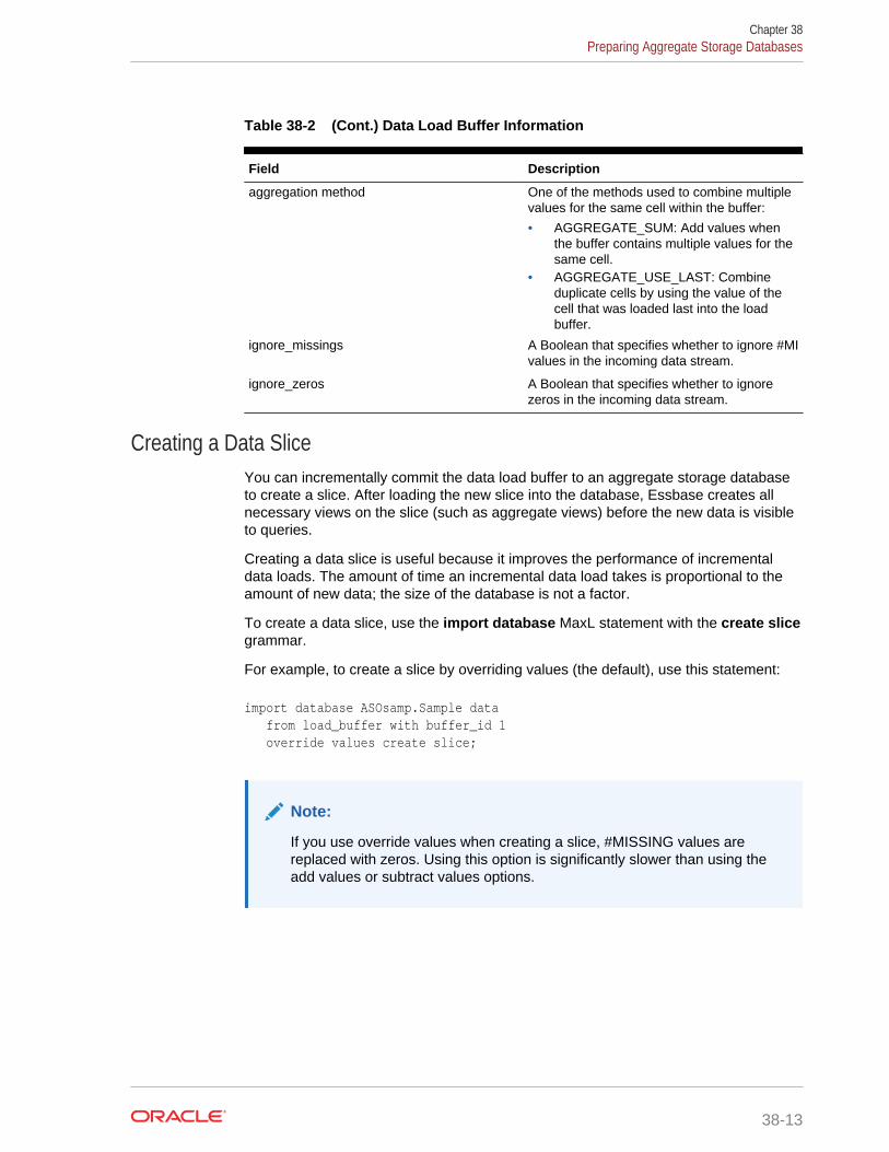
Table 38-2 (Cont.) Data Load Buffer Information

Field Description

aggregation method One of the methods used to combine multiplevalues for the same cell within the buffer:

• AGGREGATE_SUM: Add values whenthe buffer contains multiple values for thesame cell.

• AGGREGATE_USE_LAST: Combineduplicate cells by using the value of thecell that was loaded last into the loadbuffer.

ignore_missings A Boolean that specifies whether to ignore #MIvalues in the incoming data stream.

ignore_zeros A Boolean that specifies whether to ignorezeros in the incoming data stream.

Creating a Data SliceYou can incrementally commit the data load buffer to an aggregate storage databaseto create a slice. After loading the new slice into the database, Essbase creates allnecessary views on the slice (such as aggregate views) before the new data is visibleto queries.

Creating a data slice is useful because it improves the performance of incrementaldata loads. The amount of time an incremental data load takes is proportional to theamount of new data; the size of the database is not a factor.

To create a data slice, use the import database MaxL statement with the create slicegrammar.

For example, to create a slice by overriding values (the default), use this statement:

import database ASOsamp.Sample data from load_buffer with buffer_id 1 override values create slice;

Note:

If you use override values when creating a slice, #MISSING values arereplaced with zeros. Using this option is significantly slower than using theadd values or subtract values options.


38-13

Merging Incremental Data Slices

Automatically Merging Incremental Data Slices During a Data Load to an AggregateStorage Database

Using the AUTOMERGE and AUTOMERGEMAXSLICENUMBER configurationsettings, you can specify whether Essbase automatically merges incremental dataslices during a data load to an aggregate storage database.

AUTOMERGE configuration setting options:

• ALWAYS—Specifies to automatically merge incremental data slices during a dataload to an aggregate storage database. By default, merges are executed once forevery four consecutive incremental data slices. If, however, theAUTOMERGEMAXSLICENUMBER configuration setting is used, the auto-mergeprocess is activated when the AUTOMERGEMAXSLICENUMBER value isexceeded. The size of the incremental data slices is not a factor in selecting whichones are merged.

The default value is ALWAYS.

• NEVER—Specifies to never automatically merge incremental data slices during adata load to an aggregate storage database. To manually merge incremental dataslices, use the alter database MaxL statement with the merge grammar. See Manually Merging Incremental Data Slices.

• SELECTIVE—Specifies to activate the incremental data slice auto-merge processwhen the number of incremental data slices specified in theAUTOMERGEMAXSLICENUMBER configuration setting is exceeded. If thenumber of incremental data slices in the data load does not exceed the value ofAUTOMERGEMAXSLICENUMBER, the auto-merge process is not activated.

Manually Merging Incremental Data SlicesYou can merge all incremental data slices into the main database slice or merge allincremental data slices into a single data slice while leaving the main database sliceunchanged. To merge slices, you must have the same privileges as for loading data(Administrator or Database Manager permissions).

After the new input view is written to the database, Essbase creates the aggregateviews for the slice. The views created for the new slice are a subset of the views thatexist on the main database slice.

Note:

You cannot export data when performing a merge.

If you cleared data from a region using the logical clear region operation, which resultsin a value of zero for the cells you cleared, you can elect to remove zero value cellsduring the merge operation. See Clearing Data from Specific Regions of AggregateStorage Databases.


38-14

To perform merging operations, use the alter database MaxL statement with themerge grammar.

For example, to merge all incremental data slices into the main database slice, usethis statement:

alter database ASOsamp.Sample merge all data;

To merge all incremental data slices into the main database slice and remove zerovalue cells, use this statement:

alter database ASOsamp.Sample merge all data remove_zero_cells;

To merge all incremental data slices into a single data slice, use this statement:

alter database ASOsamp.Sample merge incremental data;

Note:

Before you copy an aggregate storage application, you must merge allincremental data slices into the main database slice. Data in unmergedincremental data slices is not copied. See Manually Merging IncrementalData Slices.

Replacing Database or Incremental Data Slice ContentsFor data sets that are small enough to reload completely while maintaining low datalatency, Essbase can remove the current contents of a database and replace thedatabase with the contents of a specified data load buffer. The atomic replacementfunctionality transitions querying the old contents of the database to the new contentswithout interrupting service. The newly loaded data set is aggregated to create thesame set of views that existed for the replaced data set.

Essbase also allows for atomically replacing the contents of all incremental data slicesin a database. Consider a situation in which data can be separated into a relativelylarge, static data set that is never updated and a relatively small, volatile data set forwhich the individual updates are difficult to identify but are confined to the volatile dataset. For example, the large, static data set consists of historical transaction data for thelast three years; however, for the transaction data for the past two months, users canchange a characteristic of a transaction in the source database. Tracking thesechanges can be prohibitively complex. You can load the static data set as the mainslice in a database and the volatile data set as one or more incremental slices.

Essbase removes the current contents of all incremental data slices and creates a newslice (using the add values grammar) with the contents of a specified data load buffer.The newly loaded data set is augmented with aggregated views based on the set ofviews that exist on the main slice.


38-15

Note:

To use the override grammar, create a data load buffer with theignore_missing_values property for optimal performance. Additionally, youmust ensure that there are not any conflicts between the static and volatiledata sets (for example, there should not be a value in each data set for thesame cell).

To replace the contents of a database or the incremental data slices in a database,use the import database MaxL statement with the override grammar.

For example, to replace the contents of a database, use this statement:

import database ASOsamp.Sample data from load_buffer with buffer_id 1 override all data;

To replace the contents of all incremental data slices with a new slice, use thisstatement:

import database ASOsamp.Sample data from load_buffer with buffer_id 1 override incremental data;

Note:

If the override replacement fails, Essbase continues to serve the old data set.

Viewing Incremental Data Slices StatisticsEssbase provides statistics on the size and number of incremental data slices, and thecost of querying the incremental data slices.

The time it takes for a query to access all of the incremental data slices is expressedas a percentage (between .01 and 1.0 inclusive). If a database has a main slice andmultiple incremental data slices, a query statistic of 0.66 means that two-thirds of thequery time was spent querying the incremental data slices and one-third was spentquerying the main data slice. If the cost of querying the incremental data slices is toohigh, you can merge the slices.

Managing Disk Space For Incremental Data LoadsIncremental data loads on aggregate storage databases may use disk space up to twotimes the size of your current data files. For example, assume that the size of adatabase .dat file is 1 GB and the size of the incremental data load is 200 MB, for atotal database size of 1.2 GB. During the incremental data load process, Essbasemight use up to 2.4 GB of disk space.


38-16

In cases where databases are larger than 2 GB, you can reduce disk space utilizationby setting the maximum file size of the default tablespace to no more than 2 GB..

To set the maximum file size of the default tablespace, you can use the altertablespace MaxL statement.

Using Smart ViewIn Smart View, the submit command is equivalent to using the incremental data loadfunctionality with the override grammar.

While performing a send operation, new requests for lock, unlock, and retrieve andlock will wait until the send operation is completed.

See the Oracle Smart View for Office User’s Guide.

Data Source Differences for Aggregate Storage Data LoadsWhile processing data source records for loading values into aggregate storagedatabases, Essbase processes source data records only for the level 0 dimensionintersections where the member does not have a formula.

The following example shows a data source with records for only level 0 intersections.The last field contains data values; the other fields are level 0 members of theirrespective dimensions.

Jan, Curr Year, Digital Cameras, CO, Original Price, 10784Jan, Prev Year, Camcorders, CO, Original Price, 13573

Essbase ignores records that specify upper-level members and, at the end of the dataload, displays the number of skipped records.

For example, the following record would be skipped because member Mid West is alevel 1 member:

Jan, Curr Year, Digital Cameras, Mid West, Original Price, 121301

Sorting data sources is unnecessary because Essbase Server reads and sorts recordsinternally before committing values to the database.

Rules File Differences for Aggregate Storage Data LoadsRules file specifications for loading values to aggregate storage databases reflect theaggregate storage data load process.

For block storage data loads, through the rules file, you choose for each data sourcewhether to overwrite existing values, add values in the data source to existing values,or subtract them from existing values.

For aggregate storage data loads using the aggregate storage data load buffer, youmake this choice for all data load sources that are gathered into the data load bufferbefore they are loaded to the database.


38-17

Clearing Data from an Aggregate Storage DatabaseYou can selectively clear data or clear all data from an aggregate storage database.

Also see Clearing Aggregations.

Clearing Data from Specific Regions of Aggregate Storage DatabasesYou can clear data from a specified region in an aggregate storage database andretain the data located in other regions. This feature is useful when you want to deletevolatile data (such as data corresponding to the last month) but retain historical data.You must have Database Manager or Administrator permission to clear data.

Methods for clearing data from a region:

• Physical

The input cells in the specified region are physically removed from the aggregatestorage database, as illustrated in Figure 38-2.

Figure 38-2 Physically Clearing a Region of Data

If there are multiple data slices in the database, the physical clear region operationautomatically merges all data slices into the main data slice. After data for thespecified region is cleared, Essbase materializes all aggregate views that werepresent in the main data slice before the clear region operation took place.

The process for physically clearing data completes in a length of time proportionalto the size of the input data, not to the size of the data being cleared. Therefore,you might use this method only when removing large slices of data.

To physically clear data, use the alter database MaxL statement with the cleardata in region grammar and the physical keyword:

alter database appname.dbname clear data in region 'MDX set expression' physical;

• Logical


38-18

The input cells in the specified region are written to a new data slice with negative,compensating values that result in a value of zero for the cells you want to clear,as illustrated in Figure 38-3.

Figure 38-3 Logically Clearing a Region of Data

The logical clear region operation automatically merges only the data slice withzero values into the main data slice; other data slices in the database are notmerged. After data for the specified region is cleared, Essbase materializesaggregate views only in the new data slice.

The process for logically clearing data completes in a length of time that isproportional to the size of the data being cleared. Because compensating cells arecreated, this option increases the size of the database.

To logically clear data, use the alter database MaxL statement with the clear datain region grammar but without the physical keyword:

alter database appname.dbname clear data in region 'MDX set expression';

Queries to the logically cleared region return zero values instead of #MISSINGvalues. You may need to update formulas that rely on #MISSING values for emptycells.

To remove cells with a value of zero, use the alter database MaxL statement withthe merge grammar and the remove_zero_cells keyword. See the TechnicalReference for Oracle Essbase.

Note:

Oracle does not recommend performing a second logical clear regionoperation on the same region, because the second operation does notclear the compensating cells created in the first operation and does notcreate new compensating cells.

In specifying the region to be cleared, follow these guidelines:

• The region must be symmetrical.


38-19

– {(Jan, Budget)} is a valid symmetrical region that clears all Budget data forJan.

– {(Jan, Forecast1),(Feb, Forecast2)} is an invalid region because it consists oftwo asymmetrical regions (Jan, Forecast1 and Feb, Forecast2).

• Individual members in any dimension in the region specification must be storedmembers.

• Members in the region cannot be:

– Dynamic members (members with implicit or explicit MDX formulas)

– From attribute dimensions

If you need to clear cells by an attribute, use the Attribute MDX function.

• Members in the region can be upper-level members in stored hierarchies, which isa convenient way to specify multiple level 0 members.

For example, you can specify Qrt1, which is the same as specifying Jan, Feb, andMar (the level 0 children of Qrt1):

The following two MaxL statements produce the same results:

alter database appname.dbname clear data in region '{Qtr1}';

alter database appname.dbname clear data in region '{Jan, Feb, Mar}';

• (Physically clearing data only) Members in the region can be upper-level membersin alternate hierarchies.

For example, you can specify High End Merchandise, which is the same asspecifying Flat Panel, HDTV, Digital Recorders, and Notebooks (the shared, level0 children of High End Merchandise):


38-20

The following two MaxL statements produce the same results:

alter database appname.dbname clear data in region '{High End Merchandise}';

alter database appname.dbname clear data in region '{[Flat Panel],[HDTV],[Digital Recorders],[Notebooks]}';

To specify members in alternate hierarchies when logically clearing data, use theDescendants MDX function.

Note:

When the region contains upper-level members from alternatehierarchies, you may experience a decrease in performance. In thiscase, consider using only level 0 members.

• The MDX set expression must be enclosed with single quotation marks.

For example, to clear all January data for Forecast1 and Forecast2 scenarios, use thisstatement:

alter database ASOsamp.Sample clear data in region 'CrossJoin({Jan},{Forecast1, Forecast2})';

During the clear region operation, you cannot perform operations that update thedatabase (such as loading data, merging data slices, or clearing data from anotherregion), nor export data. You can query the database; however, the query results arebased on the data set before the clear region operation.

The clear data in region grammar cannot clear data from the entire database. See Clearing All Data from an Aggregate Storage Database.


38-21

Clearing All Data from an Aggregate Storage DatabaseClearing all data from an aggregate storage database is the same as for a blockstorage database. To clear the entire database, use the alter database MaxLstatement with the reset grammar:

alter database appname.dbname reset;

Copying an Aggregate Storage ApplicationTo copy all of the data in an aggregate storage application, you must merge allincremental data slices into the main database slice. Data in unmerged incrementaldata slices is not copied.

See Manually Merging Incremental Data Slices.

Combining Data Loads and Dimension BuildsWhen using the aggregate storage data load buffer, you can combine data sourcesand rules files to add members to the outline and to load data values to the level 0cells. Regardless of the order in which you specify the files, Essbase makes theoutline changes and then loads the data values.

Note:

Oracle recommends that you separate dimension build operations from dataload operations, because some dimension builds clear data, which couldlead to data loss. See Building Dimensions in Aggregate Storage Databases.

Calculating Aggregate Storage DatabasesAggregate storage database values are calculated through the outline structure andMDX formulas. When a data load is complete, all the information needed to calculatean aggregate storage database is available. When a retrieval request is made,Essbase Server calculates the needed values by consolidating the values loaded forlevel 0 members and calculating formulas. Values calculated for retrievals are notstored.

To improve retrieval performance, Essbase can aggregate values and store themahead of time. However, aggregating and storing all values can be a lengthy processthat requires disk space for storage. Essbase provides an intelligent aggregationprocess that balances time and storage resources. See Aggregating an AggregateStorage Database.

To prepare an aggregate storage database for retrieval, you create the outline andload the level 0 values. Then you calculate the database by aggregating, and storingadditional values, with the remaining values to be calculated when retrieved.

Chapter 38Calculating Aggregate Storage Databases

38-22

Note:

If a database needs calculation scripts to handle special calculations anddata dependencies, consider altering the database design or making it ablock storage database.

See Table 35-3.

Outline Factors Affecting Data ValuesThe hierarchical structure of an aggregate storage outline determines how values arerolled up. Level 0 member values roll up to level 1 member values, level 1 membervalues roll up to level 2 member values, and so on.

Consolidation operators assigned to members of dynamic hierarchies define theoperations used in the roll-up: add (+), subtract (-), multiply (*), divide (/), percent (%),no operation (~), and (^) never consolidate. See Table 38-1.

Note:

Members of stored hierarchies can have only the addition (+) or the no-consolidation (~) operator.

For more complex operations, you can provide MDX formulas on members of dynamichierarchies. MDX formulas are written in the same format as MDX numeric valueexpressions. See Developing Formulas on Aggregate Storage Outlines.

Block Storage Calculation Features That Do Not Apply to AggregateStorage Databases

The following characteristics of calculating block storage databases do not apply toaggregate storage databases:

• Calculation script calculations

• Dynamic Calc member storage property

• Block storage formula syntax and predefined Essbase functions in formulas

• Formulas on members of dimensions other than members of aggregate storagedynamic hierarchies

• Preloaded values for member intersections above level 0

• Two-pass calculations tags

• Block storage performance features such as Intelligent Calculation


38-23

Calculation OrderAggregate storage calculation order and block storage calculation order differ. Foraggregate storage databases, Essbase calculates data in the following order:

1. Aggregates members of stored hierarchies and attribute dimensions. Theorder in which members and dimensions are aggregated is optimized internallyand changes according to the nature of the database outline and the existingaggregations. Because the aggregation is additive, the order in which Essbaseaggregates the dimensions and members does not affect the results.

Because the internal aggregation order for an aggregate storage database is notpredictable, any inherent rounding errors are also not predictable. These roundingerrors are expected behavior in computer calculation and are extremely small inrelation to the data values concerned.

2. Calculates dynamic hierarchy dimension members and formulas. The orderin which members and formulas are evaluated is defined by the solve orderproperty, which you can set for each member or dimension. Calculation order mayaffect calculation results.

Solve Order PropertyThe concept of solve order applies to query execution. When a cell is evaluated in amultidimensional query, the order in which the calculations should be resolved may beambiguous. To remove ambiguity, you can use the solve order property to specify therequired calculation priority.

Note:

It is good practice to specify the solve order for each member by setting thesolve order property. Members without formulas that do not have a specifiedsolve order inherit the solve order of their dimension. Members with formulasthat do not have a specified solve order have a solve order of zero.

To specify the solve order for a member, you can use the solve_order parameter inthe With section of an MDX query.

The value of the solve order property determines the priority with which Essbasecalculates the formulas. The formulas on the members that have a specified solveorder are calculated in order from the lowest solve order to the highest. (See ExampleUsing the Solve Order Property). You can specify a solve order between 0 and 127.The default is 0.

You can specify the solve order at the member level. Essbase uses the followinginformation to define calculation precedence:

1. Member solve order

2. Dimension solve order (members without formulas for which you do not specify amember solve order inherit the solve order of their dimension. Members withformulas for which you do not specify a member solve order have a solve order ofzero.)


38-24

If multiple members have the same solve order, the members are evaluated in thereverse order in which their dimensions occur in the database outline. Themember that occurs later in the outline takes precedence.

The tie situation calculation order is different for calculated members defined in anMDX query for block storage databases. See the Technical Reference for OracleEssbase.

Note:

When a member formula is dependant on the value of another member,the member with the formula must have a higher solve order than themember or members on which it depends. For example, in theASOsamp.Sample database outline in Figure 38-5, Avg Units/Transaction depends on the value of Units and of Transactions. AvgUnits/Transaction must have a higher solve order than Units andTransactions.

Example Using the Solve Order PropertyThe following example is based on the ASOsamp.Sample database. To removeambiguity in query results, the example uses the solve order property to specify therequired calculation priority.

The spreadsheet query in Figure 38-4 retrieves data for the number of units sold andthe number of transactions for January of the current year and for January of theprevious year. The Variance member shows the difference between the current yearand the previous year. The Avg Units/Transaction member shows a ratio of thenumber of units sold per transaction.

Figure 38-4 Results from Spreadsheet Query of ASOsamp.Sample databaseShowing the Variance Between Two Ratios (C12)


38-25

Figure 38-5 shows the database outline for these members and the formulas appliedto the Variance and Avg Units/Transaction members.

Figure 38-5 ASOsamp.Sample Database Showing the Measures, Years, andTime Dimensions

When calculating the variance of the average units per transaction (cell C12 in Figure 38-4), the result could be the variance between the two ratios, or the resultcould be the ratio of the two variances. The result depends on whether Essbase givesprecedence to the formula on Variance or the formula on Avg Units/Transaction.

The value of the solve order property, which is attached to the members in thedatabase outline, determines the priority with which Essbase evaluates the formulas.The formula on the member that has the higher solve order takes precedence.

In the example, if the Variance member has a higher solve order than the Avg Units/Transaction member, then the formula on the Variance member takes precedence andthe result is the variance between two ratios. This is the case in the ASOsamp.Sampledatabase, because the solve order of the Variance member is 20 and the solve orderof the Avg Units/Transaction member is 10. The formula on Variance takesprecedence, because the Variance member has the higher solve order. The result forcell C12 of the query in Figure 38-4 is the variance between the two ratios, as shownin Table 38-3:


38-26

Table 38-3 Using the Solve Order Property to Specify the Variance Between Two Ratios

Member Solve Order Formula Result of Intersection ofVariance and Avg Units/Transaction (cell C12 in Figure 38-4)

Variance 20 Curr Year - Prev Year Current year average units/transaction - previous yearaverage units/transaction0.94894382 (cell C6) -0.954252111 (cell C9) =-0.005308291 (cell C12)

Avg Units/Transaction 10 Units/Transactions

Alternatively, if you change the ASOsamp.Sample database, and you give the AvgUnits/Transaction member a higher solve order than the Variance member, then theformula on the Avg Units/Transaction member takes precedence, and the result is theratio of two variances, as shown in Table 38-4 and in Figure 38-6:

Table 38-4 Using the Solve Order Property to Specify the Ratio of Two Variances

Member Solve Order Formula Result of Intersection ofVariance and Avg Units/Transaction (cell C12 in Figure 38-6)

Variance 10 Curr Year - Prev Year Variance (current year toprevious year) of units /variance of transactions

10585 (cell C10) / 11340(cell C11) = 0.933421517(cell C12)

Avg Units/Transaction 20 Units/Transactions

Figure 38-6 Results from Spreadsheet Query of ASOsamp.Sample DatabaseShowing the Ratio of Two Variances (C12)


38-27

Aggregating an Aggregate Storage DatabaseAggregate storage databases require no separate calculation step after data valuesare loaded into the level 0 cells of the outline. From any point in the database, userscan retrieve and view values that are aggregated dynamically, for the current retrievalonly. Aggregate storage databases are smaller than block storage databases,enabling quick retrieval of data values.

As databases grow, retrievals must process more data values to satisfy the calculationneeds of the queries. For faster retrieval, Essbase enables you to precalculate datavalues and store those values in aggregations. If a database size nears one millionaggregate cells, you should strongly consider performing an aggregation. Dependingon database usage and the usage environment, you can achieve performance benefitsby precalculating smaller databases as well. Use MaxL to calculate an aggregatestorage database.

Understanding Aggregation-Related TermsThe following topics describe terms that are integral to an explanation of aggregatestorage database calculation.

Aggregate CellsCells for level 0 intersections across dimensions, without formulas, are called inputcells. Data values can be loaded to them. Higher-level cells involving members of theaccounts dimension or dynamic hierarchies are always calculated at retrieval. All otherhigher-level intersections across dimensions are aggregate cells. For example, for theoutline in Sample Aggregate Storage Outline, Price Paid > Curr Year > 1st Half >Portable Audio > CO is an aggregate cell; Original Price > Curr Year > Jan >Camcorders > CO is another aggregate cell. Values for aggregate cells must be rolledup from lower-level values.

Aggregate cell values are calculated for each request, or they can be precalculatedand stored on disk.

Aggregate ViewsWhen Essbase defines which aggregate cells to precalculate and store, it works withaggregate views. An aggregate view is a collection of aggregate cells. The collection isbased on the levels of the members within each dimension.

For example, consider one aggregate view for the outline in Sample AggregateStorage Outline. This aggregate view includes aggregate cells for the followingdimension levels:

• Measures dimension, level 0

• Years dimension, level 0

• Time dimension, level 1 of hierarchy 0

• Product dimension, level 2 of hierarchy 0

• Geography dimensions, level 0

The example aggregate view is shown as 0, 0, 1/0, 2/0, 0.


38-28

Each dimension is shown, left to right, in its sequence in the outline. If a dimensioncontains hierarchies, the notation specifies the member level within its hierarchy.Hierarchies within a dimension are numbered top-down, starting with hierarchy 0.

The 0, 0, 1/0, 2/0, 0 aggregate view contains aggregate cells that include the followingmember intersections:

Original Price, Curr Year, Qtr1, Personal Electronics, CO Original Price, Curr Year, Qtr1, Personal Electronics, KS Original Price, Curr Year, Qtr1, Home Entertainment, CO Original Price, Curr Year, Qtr1, Home Entertainment, KS Original Price, Curr Year, Qtr2, Personal Electronics, CO Original Price, Curr Year, Qtr2, Personal Electronics, KS Original Price, Curr Year, Qtr2, Home Entertainment, CO Original Price, Curr Year, Qtr2, Home Entertainment, KS Original Price, Curr Year, Qtr3, Personal Electronics, CO Original Price, Curr Year, Qtr3, Personal Electronics, KS Original Price, Curr Year, Qtr3, Home Entertainment, CO Original Price, Curr Year, Qtr3, Home Entertainment, KS Original Price, Curr Year, Qtr4, Personal Electronics, CO Original Price, Curr Year, Qtr4, Personal Electronics, KS Original Price, Curr Year, Qtr4, Home Entertainment, CO Original Price, Curr Year, Qtr4, Home Entertainment, KS Original Price, Prev Year, Qtr1, Personal Electronics, CO Original Price, Prev Year, Qtr1, Personal Electronics, KS Original Price, Prev Year, Qtr1, Home Entertainment, CO Original Price, Prev Year, Qtr1, Home Entertainment, KS and so on...

AggregationsAggregations are consolidations, based on outline hierarchy, of level 0 data values. Anaggregation contains one or more aggregate views. Essbase provides an intelligentaggregation process that selects aggregate views to be rolled up, aggregates them,and then stores the values for the cells in the selected views. If an aggregationincludes aggregate cells dependent on level 0 values that are changed through a dataload, the higher-level values are automatically updated at the end of the data loadprocess.

The term aggregation is used for the aggregation process and the set of values storedas a result of the process.

Aggregation ScriptsEach aggregation script is a file that defines a particular selection of aggregate viewsto be materialized. See Working with Aggregation Scripts.

Performing Database AggregationsUse MaxL statements to perform an aggregation. The aggregation process has twophases:

• Aggregate view selection.


38-29

• Calculation and storage of values for the selected aggregate views. This phase isalso called the materialization of the aggregation.

During the aggregate view selection phase, Essbase analyzes how calculating andstoring various combinations of aggregate views might affect average query responsetime. As input to the analysis, you can define physical storage and performancerequirements. You can also track data usage and provide the information to theanalysis process. See Selecting Views Based on Usage.

Based on their usefulness and resource requirements, Essbase creates a list ofaggregate views. Included with each view in the list is storage and performanceinformation that applies when that aggregate view plus all other aggregate views listedabove it are stored. You can choose to aggregate the listed views, select andaggregate a subset of the listed views, or rerun the selection process with differentinput criteria. You can also add to an aggregation the materialization of new views thatare based on new selection criteria. See Fine-Tuning Aggregate View Selection.

Whether or not you materialize the selection, you can save the selection of aggregateviews as an aggregation script. Aggregation scripts provide flexibility and can savetime because they enable you to bypass the selection process if the same selection isneeded again. See Working with Aggregation Scripts.

After the selection process is finished, the selected aggregate views are calculatedwhen you materialize the selected aggregate views into an aggregation.

The following process is recommended for defining and materializing aggregations:

1. After the outline is created or changed, load data values.

2. Perform the default aggregation.

Optional: Specify a storage stopping point.

3. Materialize the suggested aggregate views and save the default selection in anaggregation script.

4. Run the types of queries for which the aggregation is designed.

5. If query time or aggregation time is too long, consider fine-tuning the aggregation.See Fine-Tuning Aggregate View Selection.

6. (Optional) Save the aggregation selection as an aggregation script.

See Working with Aggregation Scripts.

To perform a database aggregation selection or materialization, you can use theseMaxL statements:

• execute aggregate process

• execute aggregate selection

• execute aggregate build

Also see Optimizing Aggregation Performance.

Fine-Tuning Aggregate View SelectionThe default selection of aggregate views proposed by Essbase provides excellentperformance. However, accepting all aggregate views in the selection list does notguarantee optimum performance. For the default selection, Essbase analyzes storedhierarchies and assumes an equal chance that any aggregate cell will be retrieved.Essbase cannot account for external factors such as the amount of available memory


38-30

at the time of a query. Available memory can be affected by such factors as the cachememory definition at retrieval time, or the memory other concurrent processes require.

You may want to track which data is most queried and include the results andalternate views in the aggregate view selection process. See Selecting Views Basedon Usage.

As you tune and test aggregations, consider the following points:

• Improving retrieval performance can increase disk storage costs and the time ittakes to materialize the aggregation.

• Tracking queries may result in a set of proposed aggregate views that providebetter performance for some queries than for others. Selecting proposedaggregate views can considerably improve performance time of some queries withothers experiencing little improvement—but never worse—as long as query typeand frequency are close to the type and frequency of queries performed during thetracking period.

• Optimizing aggregations may require an iterative, fine-tuning process.

Essbase provides information to help you select and store the right balance ofaggregate views for your database. Weigh this information against what you knowabout your database retrieval requirements and environment. Use the followinginformation to help you select aggregate views for an aggregation:

• The maximum storage requirement

You can specify a storage limit for selecting aggregate views in two ways:

– When the aggregation selection is initiated, you specify a maximum storagestopping value. Aggregate views are selected until the specified storage limit isreached or there are no more views to select.

When using the execute aggregate process MaxL statement with thestopping when total_size exceeds grammar, you can specify the maximumdisk space of the resulting data files, as a ratio of the current database size.For example, if the size of a database is 1 GB, specifying the total size as 1.2means that the size of the resulting data cannot exceed 20% of 1 GB, for atotal of 1.2 GB. See the Technical Reference for Oracle Essbase.

– After each analysis of the database, Essbase displays information about thelevel 0 input cell view followed by a list of suggested aggregate views.Displayed by each aggregate view is a storage number that includes thataggregate view and all other aggregate views it depends on. You can considerthis storage number as you select the aggregate views to be included in theaggregation.

• The relative “Query Cost” performance improvement

The Query Cost number that is displayed by each aggregate view in the listprojects an average retrieval time for retrieving values from the associatedaggregate view. The default view selection estimates the cost as the average of allpossible queries. When using query tracking, the estimated cost is the average forall tracked queries. The cost number for a specific aggregate view can be differentin different selection lists; for example, aggregate view 0, 0, 1/0, 2/0, 0 can show adifferent query cost in the default selection list than it would show in a selectionthat includes tracked queries in the analysis.

To compute the percentage improvement, divide the query cost value for theaggregate view into the query cost value shown for storing only level 0 input cells.


38-31

• Tracked usage

Before running an aggregate view selection, you can turn on query tracking todetermine which data is retrieved most often. After some period of databaseactivity, you can have Essbase include the usage statistics in the aggregationanalysis process. See Selecting Views Based on Usage.

• Aggregation time

The time it takes to perform an aggregation after the selection process completesincreases for each aggregate view materialized. To determine actual aggregationtime, you must perform the aggregation.

The following process is recommended for fine-tuning aggregations:

1. Perform the default aggregations described in Performing Database Aggregations.

2. Save the default selection in an aggregation script. See Working with AggregationScripts.

3. Turn on query tracking. See Selecting Views Based on Usage.

4. Have users perform their usual queries against the database or perform the batchquery operations for which the aggregation is being designed. Queries from allquery tools are tracked.

5. After sufficient time to capture data retrieval requirements, perform anotheraggregation including tracked data.

6. Analyze the proposed list of aggregate views to be stored, and select theaggregate views that you determine provide the best balance of system resourcesand retrieval performance.

7. Materialize the selected aggregate views and, if desired, save the selection in anaggregation script.

8. Working with aggregation scripts and various selection criteria, repeat the processuntil you think you have the optimum selection of aggregate views for yoursituation.

Note:

To optimize aggregations for different database retrieval situations, such asfor generating reports or user queries, you may need to repeat the tuningprocess, creating an aggregation script for each situation. See Working withAggregation Scripts.

Selecting Views Based on UsageEssbase enables you to capture retrieval statistics against a database. You can thenuse these statistics to build aggregations tailored to retrieval patterns in your company.Also, Essbase includes alternate hierarchies in its analysis of the database whenusage information is used in the aggregate view selection process.

Database usage for periodic reporting may be different than for ongoing userretrievals. To optimize different retrieval situations, consider tracking situational usagepatterns and creating aggregation scripts for each situation.


38-32

Before you begin the aggregation selection process, ensure that query tracking is onand that it has been on long enough to capture representative usage.

To track data query patterns, you can use the alter database MaxL statement.

Query tracking holds query usage information in memory. Performing any of thefollowing operations clears query usage information.

• Loading or clearing data

• Materializing or clearing an aggregation

• Turning off query tracking

Query tracking remains on until you turn it off, stop the application, or change theoutline.

Understanding User-Defined View SelectionBy default, Essbase uses internal mechanisms to decide how to create aggregations.User-defined view selection provides a way for you to influence default view selectionand view selection based on query data. See Selecting Views Based on Usage.

Administrators may apply view selection properties to stored hierarchies to restrictEssbase from choosing certain levels for aggregation.

Note:

Secondary hierarchies are either shared or attribute hierarchies.

Table 38-5 View Selection Properties

Property Effect

Default On primary hierarchies, Essbase considers alllevels. It does not aggregate on secondaryhierarchies unless alternative roll-ups areenabled.

Consider all levels Considers all levels of the hierarchy aspotential candidates for aggregation. This isthe default for primary hierarchies, but not forsecondary hierarchies.

Do not aggregate Does not aggregate along this hierarchy. Allviews selected by Essbase are at the inputlevel.

Consider bottom level only Applies only to secondary hierarchies.Essbase considers only the bottom level ofthis hierarchy for aggregation.

Consider top level only Applies only to primary hierarchies. Considersonly top level of this hierarchy for aggregation.

Never aggregate to intermediate levels Applies to primary hierarchies. Selects top andbottom levels only.


38-33

Note:

The bottom level of an attribute dimension consists of the zero-level attributemembers. When a secondary hierarchy is formed using shared members,the bottom level comprises the immediate parents of the shared members.

Essbase considers only views that satisfy the selected view selection properties.

You should be familiar with the dominant query patterns of databases before changingdefault properties; preventing selection of certain views will make queries to thoseviews slower while improving the speed of other queries. Similarly, enabling ConsiderAll Levels on a secondary hierarchy may speed queries to that hierarchy while makingother queries slower.

To define view selection properties, you can use these MaxL statements:

• execute aggregate process


Working with Aggregation ScriptsEach aggregation script represents a specific aggregate view selection against adatabase.

Aggregation scripts can save you time. For example, after loading new data valuesyou need not perform another aggregate view selection. You can speed theaggregation process by using the selection stored in an aggregation script tomaterialize the aggregation.

Aggregation scripts also give you flexibility. You can use them to save aggregate viewselections optimized for different retrieval situations; for example, you can use onescript to optimize retrievals in month-end reporting and another for daily retrievalrequirements.

Aggregation scripts for a database become invalid when the selection it contains isinvalid for the database. Create aggregation scripts when you create aggregations. Donot manually modify aggregation script files, which may cause unpredictable results.For information about when you must create aggregations and aggregation scripts,see Replacing Aggregations.

Creating Aggregation ScriptsSaved aggregation scripts enable you to split up the total aggregation process. Youcan materialize an aggregation at a different time than when the aggregate views forthe aggregation are selected. The aggregation script contains information derivedduring the aggregate view selection phase.

To create an aggregation script, you can use these MaxL statements:

• query database


Aggregation scripts are stored in the database directory as text files with the .cscextension and are valid as long as the dimension level structure in the outline has not


38-34

changed. For information about when aggregation selections are invalid, see Replacing Aggregations.

To avoid the potential clutter of invalid aggregation script files, manually deleteaggregation scripts when they are no longer useful.

Executing Aggregation ScriptsExecuting an aggregation script materializes the aggregate views specified within it.Although you can create multiple aggregation scripts, only one aggregation can bematerialized at a time.

To execute an aggregation script, you can use the execute aggregate build MaxLstatement.

Optimizing Aggregation PerformanceTo possibly improve aggregation performance time, you can use the CALCPARALLELconfiguration setting to increase the number of threads. Because each thread handlesa task of building an aggregate view, the number of threads you define establisheshow many aggregate views can be built concurrently. Even on single-CPU computers,increasing the CALCPARALLEL configuration setting may improve performance wherebuilding aggregates is I/O-bound, such as for databases too large to fit in memory.Because threads must share aggregate storage cache, the cache size must besufficiently large to support the number of threads defined. Otherwise, increasing thenumber of threads could degrade aggregation performance time.

Note:

For small databases, the performance of building aggregate views inEssbase 9.3.1 and later versions may be slower than Essbase versionsearlier than 9.3.1. However, Essbase 9.3.1 should perform better fordatabases larger than a few hundred million cells, especially on computerswith more than two processors and where the CALCPARALLELconfiguration setting has been chosen appropriately.

See the Technical Reference for Oracle Essbase.

Clearing AggregationsAt times you might want to manually clear aggregations from the disk; for example, tomake the disk space available for disk-intensive operations. Clearing aggregationsclears all data, except level 0 values, from the database, releasing the disk area forother use. After aggregations are cleared, queries calculate retrieved valuesdynamically from level 0 values.

For information about when Essbase Server automatically clears aggregated data, see“Database restructure” in Table 35-2.

To clear aggregations, you can use the alter database MaxL statement.


38-35

Replacing AggregationsYou can replace an aggregation by clearing the existing aggregation and materializinga different selection of aggregate views. You can perform a new aggregate viewselection and materialization process, or you can run an aggregation script. Considerreplacing the aggregation in the following situations:

• To fine-tune the selection of aggregate views to improve performance. See Fine-Tuning Aggregate View Selection.

• To create aggregations optimized for different database retrieval situations, suchas for generating reports or user queries.

• To optimize an aggregation after significant growth in database size. Gradually, asthe size of a database increases, an aggregation can become less efficient.Consider replacing an aggregation when performance degradation is noticeable orwhen the database size increases to about 150% of its original size.

• To optimize aggregations for new or different operational environments, such asmemory and disk resource availability changes.

You must replace an aggregation and associated aggregation scripts after the numberof levels in a dimension has been changed or one or more dimensions have beenadded or removed from the outline. See Performing Database Aggregations and Working with Aggregation Scripts.

Performing Time Balance and Flow Metrics Calculations in AggregateStorage Accounts Dimensions

The topics in this section explain how to perform time balance and flow metricscalculations on aggregate storage databases.

Using Time Balance Tags in Aggregate Storage Accounts DimensionsYou can set Time Balance properties on aggregate storage Accounts dimensions toprovide built-in calculations along the Time dimension. This saves time andperformance overhead of using member formulas to achieve time-balancefunctionality.

The following time-balance properties are supported on stored or formula-bearingAccounts dimension members:

• TB First, TB Last, TB Average

• SKIP NONE, SKIP MISSING

Consider a stored measure such as Headcount in a human-resources application.Within a Year-Quarter-Months hierarchy, Headcount data is loaded at the month level.


38-36

The desired yearly or quarterly Headcount value is not the sum of its months; rather, itshould be the last recorded value within a time period.

Tagging Headcount as TB Last with SKIPMISSING means that, for Year 2005, itsvalue is the last nonempty value of the headcount for its months. If Dec has anonmissing Headcount value, then that value will be returned; otherwise, the Novvalue will be checked and returned if nonmissing.

If a formula-bearing member has a time balance tag, the formula is executed only forlevel 0 Time members, and the Time dimension is aggregated according to the timebalance tag.

The time balance tags provide a built-in calculation along the Time dimension. Toperform other time-based calculations using formulas, such as period-to-date androlling averages, you can create a dimension called TimeView and write all time-basedformulas on that dimension. Doing so enables you to use Time Balance calculationfunctionality without losing the ability to perform other time-based calculations.

Using Flow Tags in Aggregate Storage Accounts DimensionsA Flow tag can be assigned to Accounts dimension members bearing formulas.

The following example describes the problem to be solved with flow metrics. Assumeyou have Sales and Additions figures for all 12 months. You want to perform anaggregation to populate each month’s beginning inventory.

Table 38-6 Inventory Calculation

Sales Additions Inventory

Jan 5 1 50

Feb 6 3 46

Mar 4 2 43

Apr 7 0 41


38-37

Table 38-6 (Cont.) Inventory Calculation

Sales Additions Inventory

... ... ... ...

You would use an MDX formula on the Beginning Inventory member in order tocalculate its value. Without flow metrics, to obtain each month’s beginning inventory,the calculator engine would have to reiterate the MDX formula exponentially.

Inventory = SUM(MemberRange(Jan:Time.CurrentMember), (Additions - Sales)) + Beg_Inventory

To optimize the illustrated example, assign the Inventory member the formula(Addition – Sales), and tag the member as Flow.

Restrictions on Alternate HierarchiesIf alternate hierarchies are used in the aggregate storage time dimension, the followingrestrictions apply when using Flow and TB tags on the Accounts dimension:

1. The shared level among alternate time hierarchies must be level 0.

2. The order of members at shared level among alternate time hierarchies must bethe same in all alternate hierarchies.

3. The number of shares for a stored member must not exceed that of its previoussibling. Previous sibling means the prior stored member in the outline, found at thesame generation.

For example, consider the following Year dimension. The alternate hierarchies arenot valid, because the number of shares for April (3) is greater than the number ofshares for March (1).


38-38

Aggregating Time-Balance Tagged MeasuresThe MDX Aggregate function can be used to aggregate measures tagged with timebalance tags. See the Technical Reference for Oracle Essbase.

Effect of Attribute Calculations on Time Balance Measures in AggregateStorage Databases

The following calculation logic applies if

1. The aggregate storage outline contains a time dimension or date-time dimensionwith one or more attribute or linked-attribute dimensions.

2. You perform queries on time balance tagged measures.

If the above cases are both true, MDX Aggregate() semantics are used to evaluate thecells.

For example, consider a scenario in which:

• Year is a time-date dimension with a day level hierarchy.


38-39

• Holiday is an attribute dimension on Year, with each date tagged withHoliday_TRUE or Holiday_FALSE.

• Opening Inventory is tagged as TBFirst.

The value of (Year, Holiday_TRUE, [Opening Inventory]) is evaluated according to thefollowing MDX logic:

Aggregate( {Set of dates that are holidays in Year}, [Opening Inventory])

Retrieving Aggregate Storage DataThe topics in this section describe how Essbase retrieves data from aggregate storagedatabases.

Also see Table 35-5.

Attribute Calculation RetrievalsAggregate storage applications support only the Sum member of the AttributeCalculations dimension. If you specify any other member name from the AttributeCalculations dimension, such as Min or Avg, an error is returned. See Understandingthe Attribute Calculations Dimension.

Retrieval Tools Supporting Aggregate Storage DatabasesEssbase provides the following programs and tools that enable data retrieval fromaggregate storage databases:

• MDX queries

• The export data using report_file MaxL statement

Note:

Commands that support block-storage-only features (for example, the<SPARSE Report Writer command) cannot be used with aggregate storagedatabases. MDX queries fully support aggregate storage features.

Chapter 38Retrieving Aggregate Storage Data

38-40

39Performing Custom Calculations andAllocations on Aggregate StorageDatabases

Custom calculations extend the analytical capabilities of Essbase by enabling theexecution of recurring calculations on aggregate storage databases. Allocations areused in the budgeting process to distribute revenues or costs.

• About Performing Custom Calculations and Allocations on Aggregate StorageDatabases

• Custom Calculations on Aggregate Storage Databases

• Custom Allocations on Aggregate Storage Databases

• Understanding Data Load Buffers for Custom Calculations and Allocations

• Understanding Offset Handling for Custom Calculations and Allocations

• Understanding Credit and Debit Processing for Custom Calculations andAllocations

The information in this chapter applies only to aggregate storage databases.

For information about performing custom calculations on block storage databases,see:

• Developing Calculation Scripts for Block Storage Databases

• Reviewing Examples of Calculation Scripts for Block Storage Databases

For more information about configuration settings discussed in this chapter, seeTechnical Reference for Oracle Essbase. If you are using Oracle Analytics Cloud –Essbase, you cannot use the Java APIs or C-APIs referenced in this chapter. You canuse MaxL statements.

About Performing Custom Calculations and Allocations onAggregate Storage Databases

Essbase provides separate API functions and structures for performing customcalculations (see Custom Calculations on Aggregate Storage Databases) andallocations (see Custom Allocations on Aggregate Storage Databases) on aggregatestorage databases. However, both features share the following common functionality:

• Aggregate storage data load buffers

See Understanding Data Load Buffers for Custom Calculations and Allocations.

• Credit and debit processing

See Understanding Credit and Debit Processing for Custom Calculations andAllocations.

39-1

• Offset handling

See Understanding Offset Handling for Custom Calculations and Allocations.

Custom Calculations on Aggregate Storage DatabasesCustom calculations extend the analytical capabilities of Essbase by enabling theexecution of recurring calculations on aggregate storage databases.

You can write custom calculations for aggregate storage databases that update targetlevel 0 cells. Custom calculation scripts are expressed in MDX.

Using custom calculations, you can do basic math on account balances in a generalledger and write the results to targeted level 0 members of an Essbase aggregatestorage database. You can perform calculations on account balances or on fixedamounts and can be scheduled to repeat every accounting period.

Custom calculations on aggregate storage databases can be useful when thedatabase is used for general ledger reporting, where double-entry accounting is ineffect. Debit items, such as assets and expenses, must balance with credit items, suchas equity and revenue.

Use the following workflow to create and execute custom calculations:

• Create a calculation script expressed in MDX.

See Writing Custom Calculations.

• Select an area of the database where the calculation will be executed. You providethe area at execution time using the target and POV (point of view) parameters.

• If you use debit and credit processing, select the debit and credit members in theoutline to write the positive and negative values. You provide these parameters atexecution time.

See Understanding Credit and Debit Processing for Custom Calculations andAllocations.

• If you use offsetting entries, select the area where offsetting entries should bemade. You provide this parameter at execution time using an MDX tuple. If anoffset is not specified or is empty, the offset calculation is not performed.

Note:

In general ledger bookkeeping, an offsetting entry is a counterbalancingmeasure on the opposite side of the ledger; for example, a $100 credit inJanuary may have a $100 offset added to the debit side of the ledger, sothe ledger can be balanced in preparation for an upcoming expense ofthat amount.

See Understanding Offset Handling for Custom Calculations and Allocations.

• Execute the custom calculation script using the Essbase API.

See Executing Custom Calculations.

Chapter 39Custom Calculations on Aggregate Storage Databases

39-2

List of Custom Calculations CriteriaCustom calculation functionality depends on a variety of specified criteria. Table 39-1provides a brief description of the criteria used to define custom calculations. Reviewthese terms before continuing.

Table 39-1 Description of Custom Calculations Criteria

Criteria Description

POV A symmetric region in the database thatdescribes the context in which customcalculations are performed.

Attribute members cannot be used for thisargument.

Calculation script A calculation script expressed in MDX.

Attribute members cannot be used in the leftside of the equation.

Target A tuple argument expressed in MDX thatdefines the region in the database wherecalculation results are written. This argumentis combined with left side of each formula andthe offset to determine where the results andoffset values are written.


(Optional) Offset The location in the database where anoffsetting value for each source amount iswritten.


(Optional) Credit and debit members In double-entry accounting, balancing journalentries for one transaction. Both are MDXmember expressions. The debit memberindicates a member to which positive resultvalues are written, and the credit memberindicates a member to which negative resultvalues are written.


Source region An MDX set expression specifying the regionof the cube referred to by the formulas in thescript.

Writing Custom CalculationsA custom calculation script is a file that you create and store with a .csc extension.Create the custom calculation script with one or a series of tuple-expression pairs inMDX, terminated by semicolons. The syntax:

tuple := numeric_value_expression;


39-3

The tuple is an MDX specification of one or more members where no two memberscan be from the same dimension. The tuple must be on the left side of the equationand is the primary factor in determining where results of the custom calculation arewritten.

Only member names are allowed in the tuple expression. The use of memberfunctions is not supported for custom calculation scripts.

Note:

The secondary factor determining the target for results is the targetparameter, and the third factor is the POV parameter. You specify thesecond and third parameters at calculation execution time, rather than aspart of the calculation script.

The numeric_value_expression is a simple MDX numeric value expression, such as anumber or an arithmetic operation. The expression must be on the right side of theequation. Only arithmetic operators are permitted. An error is returned if non arithmeticoperators (such as AND, OR, or IF statements) are used.

Member names can be used in the numeric value expression, but the use of memberfunctions is not supported for custom calculation scripts.

Attribute members cannot be used on the left side of the equation in a customcalculation script.

You must also define the source region, which serves as a performance hint forEssbase. Essbase pre-fetches the data specified in the source region, and uses that toperform the calculation specified in the script.

For an example of a custom calculation script, and more information about defining thesource region, see Sample Use Case for Custom Calculations.

Executing Custom CalculationsYou can execute custom calculations using the MaxL Execute Calculation (AggregateStorage) statement.

You can also execute custom calculation scripts using the API, by calling the Java APImethod IEssPerformCustomCalc.performCustomCalc, or the C API functionEssPerformCustomCalcASO.

You can also use Oracle Hyperion Calculation Manager to design a custom calculationand deploy it for execution to Enterprise Scheduling Services.

Sample Use Case for Custom CalculationsConsider an outline with the following dimensions:

• Company, containing CompanyA, CompanyB, and other children.

• Department, containing numbered departments such as 101, 102, 103.

• Account, in which Account 5740 is a rent expense account and SQFT is astatistical account used to record square footage for each department.


39-4

• Scenario, in which the Actual member is where data is posted, and the Allocationmember is where allocations and custom calculations are stored. The Scenariomember is a parent that aggregates the child members Actual and Allocation.

• Year, a time dimension organized by months and quarters.

• Geography, a dimension organized by states and cities.

• AmountType, in which Debit is the target, and Credit is the offset.

• Project, a dimension containing projects such as Proj1, Proj2.

The POV is an MDX set expression indicating where the custom calculation should beexecuted. It is specified as follows:

CrossJoin( { ( [Company], [101], [Jan], [Scenario] ) }, Descendants( Geography, Geography.Levels(0)) )

The DebitMember is an MDX member expression indicating a debit member to whichpositive result values should be written. It is specified as [BeginningBalance_Debit].

The CreditMember is an MDX member expression indicating a credit member to whichnegative and offsetting result values should be written. It is specified as[BeginningBalance_Credit].

Note:

The offset is written to the debit member in the case that the sum of all resultvalues is negative.

The offset is an MDX tuple expression indicating where offsetting entries should bemade. It is specified as ([Account_NA], [Project_NA]).

The offset expression is combined with Target and POV to determine the locationwhere offsetting entries are made. If dimensions overlap, the order for resolving theoffset location is the offset, the target, and the POV, in that order.

The target is an MDX tuple expression indicating where to write the results of thecustom calculation. It is specified as(Allocation).

The target expression is combined with POV, and the left side of each line in thecustom calculation script, to determine the location where results are written. Ifdimensions overlap, the order for resolving the target location is the left side of theequations, the target, and the POV, in that order. In this example, results are written tothe Allocation member, because the target overrides the Scenario member specified inthe POV.

The following is an example of a custom calculation script:

(AccountA,Proj1) := 100;([AccountB], [Proj1]) := ([AccountB], [Proj1]) * 1.1;(AccountC,Proj1) := ((AccountB,Proj1,2007) + (AccountB, Proj1)) / 2;(AccountA,Proj2) :=


39-5

((AccountD,Proj1) + (AccountB,Proj2)) / 2;

For each combination in the POV,

• The calculation script is executed in the context of the current POV combination.

• One offset value is written to the target location.

Note:

Each formula (line in the calculation script) is executed simultaneously,rather than sequentially. Therefore, you cannot use the result of one formulain a subsequent formula.

To define the source region, examine the custom calculation script and determinewhich members are referenced on the right sides of equations. At a minimum, thesource region should include all members from the right sides of the assignmentstatements in the custom calculation script.

Define the source region as a single MDX set. If the members on the right sides of theequations are from more than one dimension, you can use CrossJoin to create the setfrom two sets. CrossJoin only accepts two sets, so you may have to use nestedCrossJoins.

The source region for the above custom calculation script is:

Crossjoin( {[AccountB], [AccountD]}, Crossjoin( {[Proj1], [Proj2]}, {[2007]} ))

It is not necessary to include any members in the source region that are not assignedin the script. For example, if you added to the source region an [AccountC], which isnot used in the script, then it would be ignored, and could cause a slight detriment toperformance.

It is not necessary to account for numbers in the source region. For example, thefollowing assignment in a custom calculation script requires nothing to be added tosource region: ([Bud Var]):=10.

Optimizing Custom Calculations by Skipping Empty TuplesYou can optimize custom calculation scripts to conserve memory resources whencalculating over large, sparse data sets.

Because large data sets can be very sparse, using the NONEMPTYTUPLE property incustom calculation scripts can optimize your script to conserve memory resources.


39-6

You create a custom calculation script with one or a series of tuple-expression pairs inMDX, terminated by semicolons. You can optionally filter out empty result sets frombeing calculated, by including the NONEMPTYTUPLE property clause in the customcalculation script.

Using the NONEMPTYTUPLE property clause in a custom calculation script indicatesto Essbase that the cell value being calculated for a tuple is empty whenever the givennonempty_member_list is empty.

Syntax

use_optimized_way;tuple := [NONEMPTYTUPLE (nonempty_member_list)] numeric_value_expression;

Where

• use_optimized_way—a literal keyword, required to enable the use ofNONEMPTYTUPLE property in the calculation script. If omitted,NONEMPTYTUPLE directives are ignored.

• tuple—an MDX specification of one or more members, where no two memberscan be from the same dimension.

• NONEMPTYTUPLE—an optional property you can use to optimize calculationperformance. If used, then you must follow this literal property withnonempty_member_list.

• nonempty_member_list—one or more comma-separated member names fromdifferent dimensions.

• numeric_value_expression—a simple MDX numeric value expression, such as anumber or an arithmetic operation. The expression must be on the right side of theequation. Only arithmetic operators are permitted. An error is returned if nonarithmetic operators (such as AND, OR, or IF statements) are used.

Examples

The following custom calculation script examples include a NONEMPTYTUPLEproperty clause to filter out empty tuples from being included in the calculation pass.

use_optimized_way;([Balance].[Net Balance].[Net Change].[Allocation Out]):= NONEMPTYTUPLE ([Balance].[Remainder],[Rule]) -(([Balance].[Remainder],[Rule])*(20.24000/100));

([2014], [August], [Actual]):= NONEMPTYTUPLE ([2014], [January], [Actual]) ([2014], [January], [Actual]);

Custom Allocations on Aggregate Storage DatabasesAllocations are used in the budgeting process to distribute revenues or costs.

The allocations feature allows you to allocate a given source amount to a target rangeof cells in an aggregate storage database. The source amount can be allocated to the

Chapter 39Custom Allocations on Aggregate Storage Databases

39-7

target proportionately, based on a given basis, or the source amount can be spreadevenly to the target.

You can perform aggregate storage allocations using the MaxL execute allocationstatement.

You can also perform aggregate storage allocations by using the using the API, bycalling the Java API method IEssPerformAllocation.performAllocation or the C APIfunction EssPerformAllocationAso.

A single allocation has its own POV (point of view), range, amount, basis, target, and,optionally, offset. To perform allocations with different sets of values for theseparameters, you must make a sequence of individual API calls.

Allocations are performed in the allocation engine and then written back to theaggregate storage database using temporary data load buffers that Essbase creates.For general information about data load buffers, see Loading Data into AggregateStorage Databases. For information specific to allocations and custom calculations,see Understanding Data Load Buffers for Custom Calculations and Allocations.

List of Allocation CriteriaAllocations are based on a variety of specified criteria. Table 39-2 provides a briefdescription of the criteria used to define allocations. Review these terms beforecontinuing.

Table 39-2 Description of Allocation Criteria

Criteria Description See

POV A symmetric region in the databasethat describes the context in whichallocations are performed

Setting the POV

Range A symmetric region in the databasein which allocated values arecalculated and written

Setting the Range

(Optional) Excluded range Locations in the range where you donot want allocation values written

Setting the Range

Amount The amount to be allocated Setting the Amount

(Optional) Amount context Additional context, or specificity, forthe amount

Setting the Amount

(Optional) Amount time span One or more time periods to beconsidered for the amount

Setting the Amount

(Optional) Zero amount options Treatment of zero or #MISSINGamount values

Setting the Amount

Basis When combined with the range,defines the location of basis valuesthat determine how the amount isallocated

Setting the Basis

(Optional) Basis time span One or more time periods to beconsidered for the basis

Setting the Basis


39-8

Table 39-2 (Cont.) Description of Allocation Criteria


(Required if basis time span is set)

Basis time span option

Method for calculating the basisacross the basis time span:

• Combine• Split

Setting the Basis

Zero basis options Treatment of zero basis values Setting the Basis

(Optional) Negative basis options Treatment of negative basis values Setting the Basis

Target When combined with the range,defines the region in the databasewhere allocation values are written

Setting the Target

(Optional) Target time span One or more time periods to beconsidered for the target

Setting the Target

(Required if target time span is set)

Target time span option

Method for allocating values acrossthe target time span:

• Divide the amount• Repeat the amount

Setting the Target

Allocation method Method for allocating the amount:

• Share: Allocates the amountproportionately to the basisvalues

• Spread: Allocates the amountevenly

Setting the Allocation Method

(Optional) Spread skip options For spread allocation method,whether to skip basis values in therange that are zero, #MISSING, ornegative

Setting the Allocation Method

Rounding method Whether to round allocated values.

If you choose to round, specifies themethod for handling rounding errors:

• Discard rounding errors• Add the total rounding error to:

– The greatest allocatedvalue

– The lowest allocated value– A specific location

Setting the Rounding Method

(Optional) Round digits The number of decimal places towhich allocation values are rounded:

• To the nearest integer• To a specified number of

decimal places• To a power of 10


(Required if rounding method is setto a specific location)

Round to location

The location to which to add the totalrounding error


(Optional) Offset The location in the database wherean offsetting value for each sourceamount is written

Setting the Offset


39-9

Table 39-2 (Cont.) Description of Allocation Criteria


(Optional) Credit and debit members In double-entry accounting,balancing journal entries for onetransaction

Balancing Allocations

Understanding RegionsEssbase uses various regions in the database when performing allocations. Eachregion consists of at least one member from each dimension defined in the region.

Table 39-3 List of Regions Used in Allocations

Region Name Region Definition Description

Source (POV X amount [X amount context]X [amount time span])

The region containing the amountvalues that are to be allocated.

The source region and target regioncannot overlap.

Target (POV X target X debit member/creditmember X range X [target timespan])

The region containing the locationsto which allocated values are written.

The source region and target regioncannot overlap.

The target region need not need beempty before performing anallocation. Essbase overwrites non-empty cells either with allocationdata or with zeros. For cells with#MISSING, the cells remain#MISSING unless Essbase writesallocation data to those cells.

Basis (POV X basis X range X [basis timespan])

The region containing the basisvalues that are used to determinehow the source amount is allocated.

Basis might override part of the POV.

Offset (POV X offset X debitMember/creditMember)

The region containing the locationsto which offset values are written.

Specifying Allocation CriteriaAllocation parameter values can be expressed in the following ways:

• MDX member expression

• MDX set expression

• MDX tuple expression (where no two members can be from the same dimension)

• Constant

For more information about how to express allocation parameter values, see theOracle Essbase and Provider Services Java API Reference orOracle Essbase APIReference (C API).


39-10

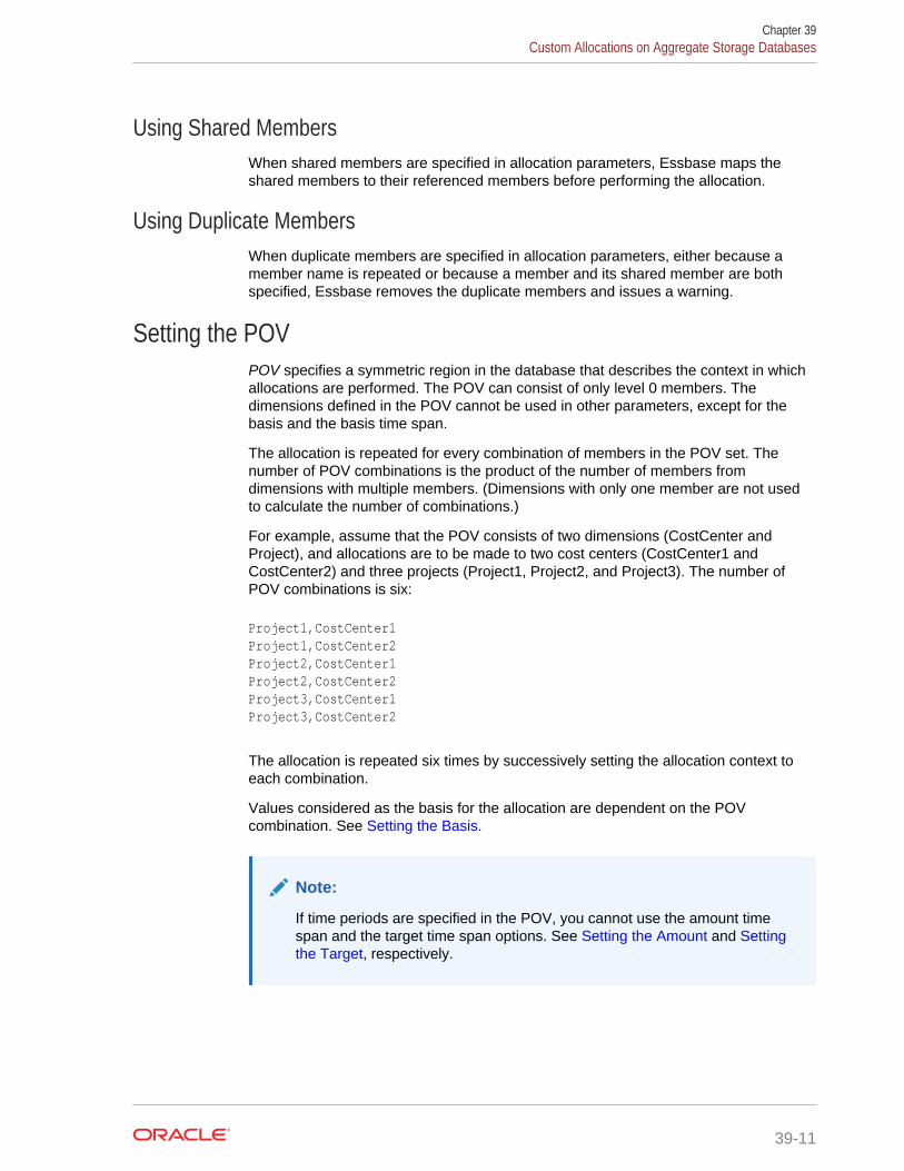
Using Shared MembersWhen shared members are specified in allocation parameters, Essbase maps theshared members to their referenced members before performing the allocation.

Using Duplicate MembersWhen duplicate members are specified in allocation parameters, either because amember name is repeated or because a member and its shared member are bothspecified, Essbase removes the duplicate members and issues a warning.

Setting the POVPOV specifies a symmetric region in the database that describes the context in whichallocations are performed. The POV can consist of only level 0 members. Thedimensions defined in the POV cannot be used in other parameters, except for thebasis and the basis time span.

The allocation is repeated for every combination of members in the POV set. Thenumber of POV combinations is the product of the number of members fromdimensions with multiple members. (Dimensions with only one member are not usedto calculate the number of combinations.)

For example, assume that the POV consists of two dimensions (CostCenter andProject), and allocations are to be made to two cost centers (CostCenter1 andCostCenter2) and three projects (Project1, Project2, and Project3). The number ofPOV combinations is six:

Project1,CostCenter1Project1,CostCenter2Project2,CostCenter1Project2,CostCenter2Project3,CostCenter1Project3,CostCenter2

The allocation is repeated six times by successively setting the allocation context toeach combination.

Values considered as the basis for the allocation are dependent on the POVcombination. See Setting the Basis.

Note:

If time periods are specified in the POV, you cannot use the amount timespan and the target time span options. See Setting the Amount and Settingthe Target, respectively.


39-11

Setting the RangeRange specifies a symmetric region in the database in which allocated values arecalculated and written.

If you do not want allocation values written to certain cells within the range, use theexcluded range parameter to express a symmetrical subset of the range. Even whenexcluding a subset of the range, Essbase uses all cells in the range to calculateallocated values.

When you exclude cells from the range, the sum of allocated values might be less thanthe value of the amount.

The following examples assume that the range consists of six member combinations,the amount is 6, and the allocation method is spread, in which Essbase evenlyallocates the amount across the range. The allocation spread amount is 1 (6/6 = 1).

As illustrated in Table 39-4, Essbase writes 1 in each cell in the range.

Table 39-4 Example: Allocating the Amount to Each Member in the Range

- CostCtr1 CostCtr2

Project1 1 1

Project2 1 1

Project3 1 1

As illustrated in Table 39-5, if the excluded range is set to the member combination of(Project2,CostCtr2), Essbase does not write the allocation spread amount to that cell.Therefore, the sum of allocated values (5) is less than the amount (6). The value of theexcluded cell after the allocation process is either #MISSING or zero.

Table 39-5 Example: Allocating the Amount to Only Some Members in theRange

- CostCtr1 CostCtr2

Project1 1 1

Project2 1

Project3 1 1

The range and excluded range can consist of only level 0 members.

Setting the AmountAmount specifies the source of the allocation. The amount value is allocated to cells inthe target region. The amount, which can consist of upper-level or level 0 members,can be expressed as a numeric value expression, a tuple, or a constant.

How you express the amount determines certain requirements:

• Numeric value expression:

– All members in the expression must be from the same dimension.

– Tuples cannot be used in the expression.


39-12

– Only arithmetic expressions (+, -, /, and *) can be used in the expression.

– MDX functions (such as Avg and Parent) are not allowed.

For example:

(Acc_1000 + Acc_2000)/2

AccA + AcctB

Balance * 1.1

• Tuple:

– The tuple must use one member from every dimension that is not specified inthe POV.

– The amount context must be empty.

For example:

(Balance,Cost_Center_00,Project_00)

(Balance,Cost_Center_00,Actual)

• Constant:

– The amount context must be empty.

– The amount time span must be empty.

For example:

100

You can use these parameters to further define the amount:

• (Optional) Amount context provides additional context, or specificity, for theamount. The amount context, which can consist of upper-level or level 0 members,can be expressed as a tuple. By specifying the amount context, you can include amember from a dimension that is not specified in the POV.

When using amount context, these requirements apply to the amount and theamount context:

– The parameters cannot refer to members in the same dimensions.

– Together, the parameters must use members from every dimension notspecified in the POV.

• (Optional) Amount time span specifies one or more time periods to be consideredfor the amount. The amount value is aggregated over the specified time periods,and the aggregated amount value is allocated. Time periods must be level 0members in a Time dimension.

When amount is specified using an arithmetic expression, and amount time spanis used, amount time span takes precedence over any formulas in the amount orany formula members used in the amount. For example, assume that the amount


39-13

is specified as Dept_A/Dept_B and amount time span is set to Jan, Feb, Mar, andApr for each department, as shown in Table 39-6. The amount to be allocated forthe POV is calculated by dividing the amount time span value for Dept_A (10) bythe amount time span value for Dept_B (20), which is 0.5.

Table 39-6 Example: Amount Time Span Takes Precedence Over Formulasin Amount

Members in Amount TimeSpan

Dept_A Dept_B

Jan 1 2

Feb 2 4

Mar 3 6

Apr 4 8

Total 10 20

• (Optional) Zero amount options specifies how to treat the amount if the value iszero or #MISSING. You can choose to allocate zero values (the default), skip tothe next nonzero or non-#MISSING amount value, or cancel the entire allocationoperation.

You can use amount context and amount time span to achieve the same result, asshown in following example. The amount is the value of Dept_A, but amount time spanis used to focus only on the months of Jan, Feb, Mar, and Apr for Dept_A. As shown in Table 39-7, the aggregated value of the members included in the amount time span(10) is the amount value that is allocated across the cells in the range.

Table 39-7 Example: Amount Time Span

Members in Amount Time Span Dept_A

Jan 1

Feb 2

Mar 3

Apr 4

Total 10

You can achieve the same amount value by specifying amount as an arithmeticexpression of Jan + Feb + Mar + Apr and setting the amount context as Dept_A, asshown in Table 39-8:

Table 39-8 Example: Amount Context

Amount Context Jan Feb Mar Apr Total

Dept_A 1 2 3 4 10

Setting the Basis(Optional) Basis, when combined with the range, defines the location of basis valuesthat determine how the amount is allocated. The basis can consist of upper-level orlevel 0 members.

You can use these parameters to further define the basis:


39-14

• (Optional) Basis time span specifies one or more time periods to be consideredfor the basis. Time periods must be level 0 members in a Time dimension.

• (Required if basis time span is set) Basis time span option specifies how the basisis calculated across the time periods specified by the basis time span. You canchoose to use the basis value for each time period individually (split) or use thesum of the basis values across the time periods specified by the basis time span(combine).

– If basis time span specifies multiple time periods and the target time spanspecifies one time period or is empty, you must set the basis time span optionto combine. Essbase ignores the target time span option.

– If basis time span and target time span specifies multiple time periods, andyou set the basis time span option to split, the periods specified by basis timespan and target time span must be identical. Essbase ignores the target timespan option.

See Understanding Settings for Basis and Target Time Span.

• Zero basis options specifies how to treat a zero basis value. You can choose toskip to the next nonzero or non-#MISSING amount value or cancel the entireallocation operation. Essbase processes the zero basis options setting based onthe allocation method. See Setting the Allocation Method.

• (Optional) Negative basis options specifies how to treat a negative basis value.The options available for the negative basis options depend on the allocationmethod used. See Setting the Allocation Method.

Note:

The basis is ignored when using the spread allocation method and you havenot set any spread skip options.

Setting the TargetTarget, when combined with the range, defines the region in the database whereallocation values are written. The target can consist of only level 0 members.

You can use these parameters to further define target:

• (Optional) Target time span specifies one or more time periods to be consideredfor the target. Time periods must be level 0 members in a Time dimension.

• (Required if target time span is set) Target time span option specifies the methodfor allocating values across the time periods specified in target time span. You canchoose to divide the amount value or repeat the amount value across the specifiedtime periods.

– If basis time span specifies multiple time periods, and the target time spanspecifies one time period or is empty, you must set the basis time span optionto combine. Essbase ignores the target time span option.

– If basis time span and target time span specifies multiple time periods, andyou set the basis time span option to split, the periods specified by the basistime span and target time span must be identical. Essbase ignores the targettime span option.


39-15

See Understanding Settings for Basis and Target Time Span.

Setting the Allocation MethodAllocation method specifies whether to allocate the amount evenly or proportionally.

• The share method allocates a percentage of the amount (alloc_share_amt) bydividing the basis value for the current member in the range (basis_mbr_value) bythe sum of the basis across the range (basis_range_sum). The allocated amountsare based on the number of valid basis values in the range. The algorithm forcalculating the allocation share amount:

alloc_share_amt = (basis_mbr_value/basis_range_sum) * amount

Basis values and Essbase action:

– Zero, Essbase writes a zero to the corresponding target cell.

If the sum of all basis values is zero (which would result in a division-by-zeroerror), Essbase uses the zero basis options setting. See Setting the Basis.

– #MISSING, Essbase either leaves the target cell as #MISSING, or, if the targetcell already has a value, overwrites the existing value with zero.

– A negative number, Essbase uses the negative basis options setting. You canchoose to use the negative basis value (the default), skip to the next amountvalue (no data is allocated for the current amount value, and Essbase skips tothe next POV combination), or cancel the entire operation.

The following examples illustrate the share allocation method. In both examples,the amount to allocate is 10.

In Table 39-9, assume that the amount (10) represents the rent expense for abuilding, and the basis represents the head count of each department in the range.Essbase uses the basis values for departments with non-#MISSING head count(Dept_A through Dept_D) to calculate the allocation share amounts, which is therent allocation.

The rent allocation for Dept_A is the basis value of Dept_A (3), divided by the sumof valid basis values across the range (3 + 2 = 5), multiplied by the amount (10):3/5 * 10 = 6. For Dept_D, the rent allocation is 2/5 * 10 = 4. The total of the targetcells in the range equals 10.

Table 39-9 Share Allocation Method Example

Members in Range Basis (Head Count) Target (Rent Allocation)

Dept_A 3 6

Dept_B

Dept_C 0 0

Dept_D 2 4

In Table 39-10, assume that all basis values are to be considered in calculatingthe share allocation amounts. The allocation for Mbr1 is the basis value of Mbr1(3), divided by the sum of valid basis values across the range (3 + -1 + 2 = 4),multiplied by the amount (10): 3/4 * 10 = 7.5. For Mbr3, the allocation is -1/4 * 10 =


39-16

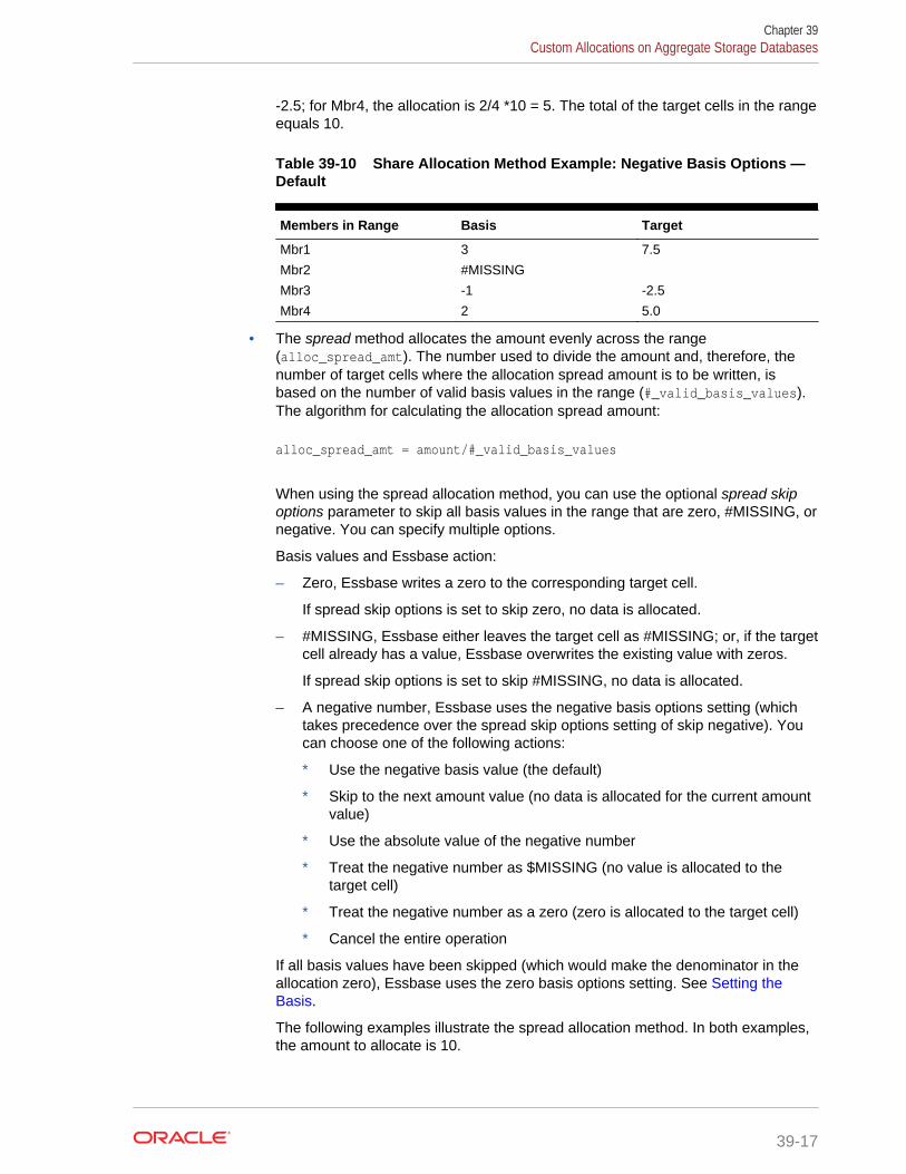
-2.5; for Mbr4, the allocation is 2/4 *10 = 5. The total of the target cells in the rangeequals 10.

Table 39-10 Share Allocation Method Example: Negative Basis Options —Default

Members in Range Basis Target

Mbr1 3 7.5

Mbr2 #MISSING

Mbr3 -1 -2.5

Mbr4 2 5.0

• The spread method allocates the amount evenly across the range(alloc_spread_amt). The number used to divide the amount and, therefore, thenumber of target cells where the allocation spread amount is to be written, isbased on the number of valid basis values in the range (#_valid_basis_values).The algorithm for calculating the allocation spread amount:

alloc_spread_amt = amount/#_valid_basis_values

When using the spread allocation method, you can use the optional spread skipoptions parameter to skip all basis values in the range that are zero, #MISSING, ornegative. You can specify multiple options.

Basis values and Essbase action:

– Zero, Essbase writes a zero to the corresponding target cell.

If spread skip options is set to skip zero, no data is allocated.

– #MISSING, Essbase either leaves the target cell as #MISSING; or, if the targetcell already has a value, Essbase overwrites the existing value with zeros.

If spread skip options is set to skip #MISSING, no data is allocated.

– A negative number, Essbase uses the negative basis options setting (whichtakes precedence over the spread skip options setting of skip negative). Youcan choose one of the following actions:

* Use the negative basis value (the default)

* Skip to the next amount value (no data is allocated for the current amountvalue)

* Use the absolute value of the negative number

* Treat the negative number as $MISSING (no value is allocated to thetarget cell)

* Treat the negative number as a zero (zero is allocated to the target cell)

* Cancel the entire operation

If all basis values have been skipped (which would make the denominator in theallocation zero), Essbase uses the zero basis options setting. See Setting theBasis.

The following examples illustrate the spread allocation method. In both examples,the amount to allocate is 10.


39-17

In Table 39-11, assume that the spread skip options parameter is not specified.Therefore, Essbase considers all four basis members in the range. Essbasedivides the amount (10), by the number of valid basis members in the range (4),and spreads that value (2.5) to each target cell in the range: 10/4 = 2.5.

Table 39-11 Spread Allocation Method Example: Do Not Skip Basis Values


Mbr1 2 2.5

Mbr2 #MISSING 2.5

Mbr3 3 2.5

Mbr4 -6 2.5

In Table 39-12, assume that the spread skip options parameter is set to ignore#MISSING and negative numbers. Therefore, Essbase considers only the twobasis members with positive values (Mbr1 and Mbr3). Essbase divides the amount(10), by the number of valid basis members in the range (2), and spreads thatvalue (5) to the Mbr1 and Mbr3 target cells: 10/2 = 5.

Table 39-12 Spread Allocation Method Example: Skip #MISSING andNegative Basis Values


Mbr1 2 5

Mbr2 #MISSING

Mbr3 3 5

Mbr4 -6

Setting the Rounding MethodThe rounding method specifies whether to round allocated values (the default is not toround).

If you choose to round values, the rounding method specifies how to handle roundingerrors. You can choose to discard rounding errors, or to round all allocated values andadd the total rounding error to the highest allocated value, the lowest allocated value,or to a specific cell. If you choose to add the rounding error to the highest or lowestallocated value, and there are multiple highest or lowest allocated values, Essbasechooses one of the highest or lowest values to which to add the rounding error.

If you choose to round allocation values, you can use these parameters to furtherdefine the rounding method:

• (Required if rounding allocated values) Round digits specifies the number ofdecimal places to which allocated values are rounded. You can choose to round tothe nearest integer (the default), to a specified number of decimal places, or to apower of 10.

Round digits must be a number from -100 to 100 and can be expressed as aninteger, an MDX numeric value expression, or a tuple.

Using an MDX numeric value expression is helpful when the setting for rounddigits is based on the currency of the allocated value. For example, assume thatthe database contains a dimension named Currency, which is part of the POV,


39-18

and an associated attribute dimension named NumCurrencyDigits, which specifieshow to round allocated values based on the currency of the allocated values. Youcan express round digits as:

Currency.currentMember.NumCurrencyDigits

Note:

If, for the rounding method, you choose not to round allocated values,the round digits parameter value must be 0 (which is the default). If youwant to round to 0 digits, the parameter value must be -1.

• (Required if rounding method is set to a specific location) Round to locationspecifies a cell to which to add the total rounding error. Expressed as a tuple, thecell must be in the range and have the same dimensionality as the range. Roundto location can consist of only level 0 members.

Note:

If, for the rounding method, you choose an option other than to round toa specific cell, the round to location parameter must be empty.

Setting the Offset(Optional) Offset specifies the location in the database where an offsetting value foreach source amount is written.

Offset works the same for allocations and custom calculations. See UnderstandingOffset Handling for Custom Calculations and Allocations.

Balancing Allocations(Optional) debitMember and creditMember can consist only of level 0 members.

The debit member and the credit member must be two different members from thesame dimension.

debitMember and creditMember work the same for allocations and customcalculations. See Understanding Credit and Debit Processing for Custom Calculationsand Allocations.

Understanding Settings for Basis and Target Time SpanThe number of members that are specified for the basis time span and target timespan affect how Essbase treats the basis time span option and target time spanoption, respectively, as summarized in Table 39-13. In situations where the basis ortarget time span is empty or set to a single time period, Essbase ignores any settingthat you might have set for the respective basis or target time span option. Insituations where one or both of the basis or target time spans are set to multiple time


39-19

periods, Essbase requires a particular setting for the respective basis or target timespan option.

Table 39-13 Summary: Basis and Target Time Span, and Basis and Time Span Option

Basis Time Span Target Time Span Basis Time SpanOption

Target Time SpanOption

See

Empty or singlemember


Ignored Ignored Example 1: Basis andTarget Time Span—Empty or SingleMember


Multiple members Ignored Divide or repeat Example 2: BasisTime Span—Emptyor Single Member;Target Time Span—Multiple Members

Multiple members Empty or singlemember

Combine Ignored Example 3: BasisTime Span—MultipleMembers; TargetTime Span—Emptyor Single Member

Multiple members Multiple members Split Ignored Example 4: Basis andTarget Time Span—Multiple Members;Basis Time SpanOption—Split

Multiple members Multiple members Combine Divide or repeat Example 5: Basis andTarget Time Span—Multiple Members;Basis Time SpanOption—Combine

Example 1: Basis and Target Time Span—Empty or Single MemberIn this example, the basis time span and target time span are not set or are set for onlyone time period. Essbase ignores any setting you might have chosen for the basistime span option or target time span option.

Example 2: Basis Time Span—Empty or Single Member; Target Time Span—Multiple Members

In this example, the basis time span is not set, and multiple time periods are specifiedfor the target time span. The basis time span option is ignored. For the target timespan option, you can select either divide or repeat.

Assume the amount is 1000. Table 39-14 shows that the basis for each department(Dept_1 = 1) and the total basis for the range (21):


39-20

Table 39-14 Example 2: Basis Values

Range Total

Dept_1 Dept_2 Dept_3 Dept_4 Dept_5 Dept_6

Basis 11 2 3 4 5 6 212

1 Basis for the member2 Total basis for the range

The setting for target time span option determines how the allocation is calculated.

• Repeat the allocated amount across the specified target time span periods:

In this scenario, Essbase performs the allocation for a single period and copies theallocated amount value to all members in the target time span.

The algorithm Essbase uses:

alloc_amt = (basis_mbr_value/basis_total_range) * amount

As shown in Table 39-15, for Dec 07,Dept_1, the member basis value (1) isdivided by the total basis across the range (21), and the result (0.04762) ismultiplied by amount (1000): (1/21) * 1000 = 47.62. Essbase copies 47.62 into thecells for Jan 08, Feb 08, Mar 08, and Apr 08. Essbase continues to performallocations for Dec 07 for each department. For each target time span, the sum ofthe allocated values across the range equals the amount (1000).

Table 39-15 Example 2: Allocation Using Target Time Span Option Set to Repeat

Range Total

Members inTarget TimeSpan


Dec 07 47.62 95.24 142.86 190.48 238.10 285.71 1000

Jan 08 47.62 95.24 142.86 190.48 238.10 285.71 1000

Feb 08 47.62 95.24 142.86 190.48 238.10 285.71 1000

Mar 08 47.62 95.24 142.86 190.48 238.10 285.71 1000

Apr 08 47.62 95.24 142.86 190.48 238.10 285.71 1000

50001

1 Total allocated values

The total allocated amount is the original amount value (1000) multiplied by thenumber of target time span members (5): 1000 * 5 = 5000.

• Divide the allocated amount across the specified target time span periods

In this scenario, Essbase performs the allocation for one period and evenly dividesthe allocated amount across all members in the target time span.


39-21


alloc_amt = ((basis_mbr_value/basis_total_range) * amount)/#_target_time_span_periods

As shown in Table 39-16, for Dec 07,Dept_1, Essbase performs the samecalculation as described for the repeat target time span option scenario to arrive at47.62. However, this amount is evenly divided across all five target time spanperiods for Dept_1; therefore, 9.52 is written in each target cell: 47.62/5 = 9.52.Essbase continues to perform allocations for each department. For each targettime span, the sum of the allocated values across the range equals (200).

Table 39-16 Example 2: Allocation Using Target Time Span Option Set to Divide

Range Total



Dec 07 9.52 19.05 28.57 38.10 47.62 57.14 200

Jan 08 9.52 19.05 28.57 38.10 47.62 57.14 200

Feb 08 9.52 19.05 28.57 38.10 47.62 57.14 200

Mar 08 9.52 19.05 28.57 38.10 47.62 57.14 200

Apr 08 9.52 19.05 28.57 38.10 47.62 57.14 200

10001


The total allocated values across the range is the original amount value (1000):200 * 5 = 1000.

Example 3: Basis Time Span—Multiple Members; Target Time Span—Emptyor Single Member

In this example, multiple time periods are specified for the basis time span, but thetarget time span is not set. The target time span option is ignored. The only validchoice for the basis time span option is combine.

Assume the amount is 1000. As shown in Table 39-17, the basis to be used for eachdepartment is the sum of the basis values for the basis time span (Dept_1 = 15); thetotal basis for the range is the sum of all department basis values (147):


Range Total

Members inBasis TimeSpan


Dec 07 1 2 3 4 5 6


39-22

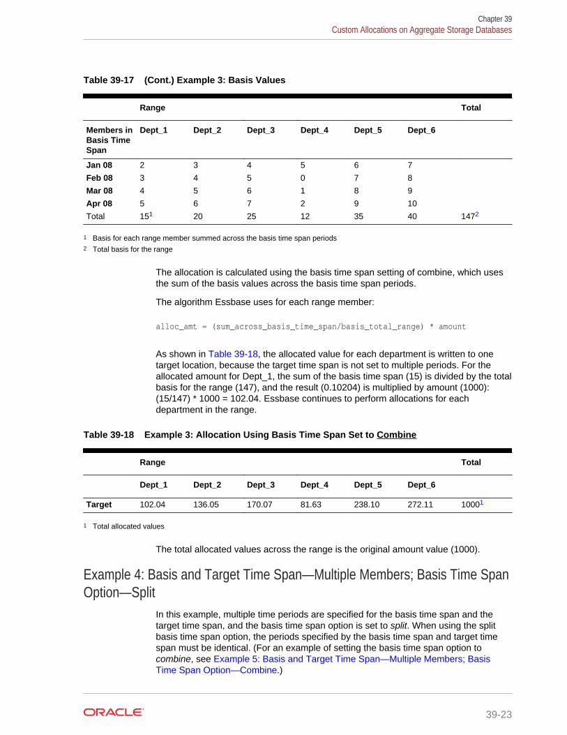
Table 39-17 (Cont.) Example 3: Basis Values

Range Total



Jan 08 2 3 4 5 6 7

Feb 08 3 4 5 0 7 8

Mar 08 4 5 6 1 8 9

Apr 08 5 6 7 2 9 10

Total 151 20 25 12 35 40 1472

1 Basis for each range member summed across the basis time span periods2 Total basis for the range

The allocation is calculated using the basis time span setting of combine, which usesthe sum of the basis values across the basis time span periods.

The algorithm Essbase uses for each range member:

alloc_amt = (sum_across_basis_time_span/basis_total_range) * amount

As shown in Table 39-18, the allocated value for each department is written to onetarget location, because the target time span is not set to multiple periods. For theallocated amount for Dept_1, the sum of the basis time span (15) is divided by the totalbasis for the range (147), and the result (0.10204) is multiplied by amount (1000):(15/147) * 1000 = 102.04. Essbase continues to perform allocations for eachdepartment in the range.

Table 39-18 Example 3: Allocation Using Basis Time Span Set to Combine

Range Total


Target 102.04 136.05 170.07 81.63 238.10 272.11 10001


The total allocated values across the range is the original amount value (1000).

Example 4: Basis and Target Time Span—Multiple Members; Basis Time SpanOption—Split

In this example, multiple time periods are specified for the basis time span and thetarget time span, and the basis time span option is set to split. When using the splitbasis time span option, the periods specified by the basis time span and target timespan must be identical. (For an example of setting the basis time span option tocombine, see Example 5: Basis and Target Time Span—Multiple Members; BasisTime Span Option—Combine.)


39-23

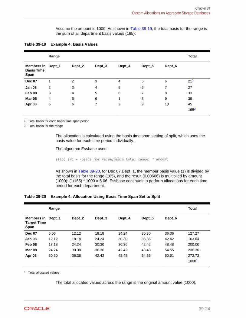
Assume the amount is 1000. As shown in Table 39-19, the total basis for the range isthe sum of all department basis values (165):


Range Total



Dec 07 1 2 3 4 5 6 211

Jan 08 2 3 4 5 6 7 27

Feb 08 3 4 5 6 7 8 33

Mar 08 4 5 6 1 8 9 39

Apr 08 5 6 7 2 9 10 45

1652

1 Total basis for each basis time span period2 Total basis for the range

The allocation is calculated using the basis time span setting of split, which uses thebasis value for each time period individually.


alloc_amt = (basis_mbr_value/basis_total_range) * amount

As shown in Table 39-20, for Dec 07,Dept_1, the member basis value (1) is divided bythe total basis for the range (165), and the result (0.00606) is multiplied by amount(1000): (1/165) * 1000 = 6.06. Essbase continues to perform allocations for each timeperiod for each department.

Table 39-20 Example 4: Allocation Using Basis Time Span Set to Split

Range Total



Dec 07 6.06 12.12 18.18 24.24 30.30 36.36 127.27

Jan 08 12.12 18.18 24.24 30.30 36.36 42.42 163.64

Feb 08 18.18 24.24 30.30 36.36 42.42 48.48 200.00

Mar 08 24.24 30.30 36.36 42.42 48.48 54.55 236.36

Apr 08 30.30 36.36 42.42 48.48 54.55 60.61 272.73

10001


The total allocated values across the range is the original amount value (1000).


39-24

Example 5: Basis and Target Time Span—Multiple Members; Basis Time SpanOption—Combine

In this example, multiple time periods are specified for the basis and target time spans;however, because the basis time span option is set to combine, the basis and targettime spans need not contain the same member set. (For an example of setting thebasis time span option to split, see Example 4: Basis and Target Time Span—MultipleMembers; Basis Time Span Option—Split.)

Assume the amount is 1000. As shown in Table 39-21, the basis to be used for eachdepartment is the sum of the basis values across the basis time span (Dept_1 = 10);the basis for the range is the sum of all department basis values (113):


Range Total



Dec 07 1 2 3 4 5 6

Jan 08 2 3 4 5 6 7

Feb 08 3 4 5 6 7 8

Mar 08 4 5 6 0 8 9

Total 101 14 18 15 26 30 1132

1 Basis for each range member summed across the basis time span periods2 Total basis for the range

The setting for target time span option determines how the allocation is calculated.

• Repeat the allocated amount across the specified target time periods:

In this scenario, Essbase performs the allocation for a single period and copies theallocated amount value to all members in the target time span.

The algorithm Essbase uses for each range member:

alloc_amt = (sum_across_basis_time_span/basis_total_range) * amount

As shown in Table 39-22, for Dec 07,Dept_1, the basis for Dept_1 (10) is dividedby the total basis for the range (113), and the result (0.0885) is multiplied byamount (1000): (10/113) * 1000 = 88.50. Essbase copies 88.50 into the cells forJan 08, Feb 08, Mar 08, and Apr 08. Essbase continues to perform allocations forDec 07 for each department. For each target time span, the sum of the allocatedvalues across the range equals the amount (1000).


39-25

Table 39-22 Example 5: Allocation Using Target Time Span Option Set to Repeat

Range Total



Dec 07 88.50 123.89 159.29 132.74 230.09 265.49 1000

Jan 08 88.50 123.89 159.29 132.74 230.09 265.49 1000

Feb 08 88.50 123.89 159.29 132.74 230.09 265.49 1000

Mar 08 88.50 123.89 159.29 132.74 230.09 265.49 1000

Apr 08 88.50 123.89 159.29 132.74 230.09 265.49 1000

50001


The total allocated values is the original amount value (1000) multiplied by thenumber of target time span members (5): 1000 * 5 = 5000.

• Divide the allocated amount across the specified target time periods:

In this scenario, Essbase performs the allocation for a single period and evenlydivides the allocated amount across all members in the target time span.


alloc_amt = ((basis_time_span/basis_total_range) * amount)/#_target_time_span_periods

As shown in Table 39-23, Essbase performs the same calculation as described forthe repeat target time span option scenario to arrive at 88.50. However, thisamount is evenly divided across all five target time span periods for Dept_1;therefore, 17.70 is written in each target cell: 88.50/5 = 17.70. Essbase continuesto perform allocations for each department. For each target time span, the sum ofthe allocated values across the range equals (200).

Table 39-23 Example 5: Allocation Using Target Time Span Option Set to Divide

Range Total



Dec 07 17.70 24.78 31.86 26.55 46.02 53.10 200

Jan 08 17.70 24.78 31.86 26.55 46.02 53.10 200

Feb 08 17.70 24.78 31.86 26.55 46.02 53.10 200

Mar 08 17.70 24.78 31.86 26.55 46.02 53.10 200

Apr 08 17.70 24.78 31.86 26.55 46.02 53.10 200

10001



39-26

The total allocated values across the range is the original amount value (1000):200 * 5 = 1000.

Examples of Aggregate Storage AllocationsThe following example illustrates how changing the POV combination affects thevalues considered as the basis for the allocation. The example, which uses the shareallocation method, allocates the total rent from the previous year to all cost centers inthe current year, based on each cost center's head count. Assume that the aggregatestorage database has four dimensions—Departments, Time, CostCenter, andMeasures—and the allocation criteria is specified as shown in Table 39-24:

Table 39-24 POV Example: Allocation Criteria

Criteria Definition

POV Dept_A, Dept_B

Amount 2007, CCNA, TotalRent

Assume that the amount values are:

• Dept_A = 1000• Dept_B = 2000

Basis Jan 2008, Head count

Target Jan 2008, RentalAllocation

Range Level 0 descendants of CostCenterAssume that the range evaluates to thefollowing cost centers:

• CostCenter1• CostCenter2• CostCenter3• CostCenter4

The allocation is performed for each of the POV combinations:

• Dept_A

• Dept_B

Each POV combination has its own set of basis values that are used in calculating theallocation: the head count for each cost center in the range and the total Jan 2008head count, as shown in Table 39-25:

Table 39-25 POV Example: Basis Values for Each POV Combination

Member Basis Values Range BasisValue

POV CostCenter1 CostCenter2 CostCenter3 CostCenter4 2008 HeadCount Total

Dept_A 1 2 3 5 11

Dept_B 5 0 10 15

For each POV, Essbase divides the head count of each cost center (the basis value ofeach member) by the total head count of the range (the basis value of the range), andthen multiplies that value by the total rental amount for each department (amount). For


39-27

example, for Dept_A,CostCenter1, the member basis value (1) is divided by the basisof the range (11), and the result (0.09090909) is multiplied by amount (1000): (1/11) *1000 = 90.90909. For Dept_B,CostCenter1, the allocated amount is 666.6667: (5/15) *2000 = 666.6667. Table 39-26 shows the allocated share amount for each cost center:

Table 39-26 POV Example: Target Values for Each POV Combination

Member Target Values Amount Value

POV CostCenter1 CostCenter2 CostCenter3 CostCenter4 RentalAllocation Total

Dept_A 90.90909 181.8182 272.7273 454.5455 1000

Dept_B 666.6667 0 1333.333 2000

Sample Use Case for Aggregate Storage AllocationsThe objective of this sample use case is to use the share allocation method toproportionally redistribute the total monthly rent expense across departments, basedon the square footage each department occupies.

Consider an outline with the following dimensions:

• Company: Contains multiple ledgers. The rent expense allocations take place inthe Vision US ledger.

• Department: Contains the following members:

– 100, which stores the total monthly rent expense, of $100,000, for Vision US.This amount is proportionally allocated to the children of department 999.

– 999, which is the parent of the following departments:

* 101, which receives 45% of the rent allocation



• Account: Contains the following members:

– 5740, which is a rent expense account

– SQFT, which is a statistical account used to record square footage for eachdepartment

• AmountType: Contains PeriodActivty, which is the parent of the followingmembers:

– PeriodActivityDebit, which is the target location

– PeriodActivityCredit, which is the offset location

You can accomplish the rent expense allocation in several ways, each with the sameresult. Two scenarios are presented. For each scenario, assume that the followingparameters are defined as follows:

• Allocation method: Share

• Range: The descendents of department 999:

– 101


39-28

– 102

– 103

No cells in the range are excluded.

• Basis: The square footage of each range member for the period of activity (whichis monthly).

SQFT,PeriodActivity

• Zero amount option: (Default) Allocate zero amount values.

• Zero basis option: If the basis value is zero, cancel the allocation operation.

• Basis time span option: (Default) Split, use the basis value for each time periodindividually.

• Rounding method: Round allocation values to the nearest 1,000 and add thetotal rounding error to department 101.

• Debit member: If the sum is positive, write the value to PeriodActivityDebit.

• Credit member: Write the value to PeriodActivityCredit.

Scenario 1: Aggregate Storage AllocationsFor scenario 1, assume the following parameters are defined as follows:

• POV: Consists of one member, Vision US, from the Company dimension.

Because only one member from one dimension is specified, the POV does notchange and, therefore, the allocation is performed only once.

• Amount: The source value of the allocation is from the following cross-dimensional member:

5740,100,Beginning Balance

• Target: Write allocated values to account 5740 for each department.

• Offset: Write the offsetting entry to member 5740,100.

Scenario 2: Aggregate Storage AllocationsFor scenario 2, assume the following parameters are defined as follows:

• POV: Consists of one member each from two dimensions:

– Vision US, from the Company dimension

– 5740, from the Amount dimension

In this scenario, account 5740 is a part of the POV. In the basis, account 5740is overridden with member SQFT.

Because only one member from each dimension is specified, the POV does notchange and, therefore, the allocation is performed only once.


39-29

• Amount: The source value of the allocation is from the following cross-dimensional member:

100,Beginning Balance

• Target: Not set. Because the combination of POV, target, debit member/creditmember, and range uses members from all dimensions, the target can be empty.

• Offset: Write the offset entry to department 100.

Avoiding Data Inconsistency When Using FormulasFormula members can be used in the amount and the basis but not in the target.However, because aggregate storage databases do not support transactionsemantics, you might experience data inconsistency issues when using formulamembers in the amount or the basis.

In the following example, User 1 posts revenue values for a set of departments andUser 2 performs an allocation of bonus money, for which the year-to-date revenue foreach department is basis of the allocation. The order in which these operations areperformed affects the result:

• Scenario 1: User 1 posts revenue before User 2 runs the allocation.

The allocation results are based on the updated revenue values.

• Scenario 2: User 2 runs the allocation before User 1 posts revenue.

The allocation results are based on prior revenue values, not on the updatedrevenue values.

• Scenario 3: User 1 posts revenue and User 2 runs the allocation concurrently.

The allocation results are based on the updated or prior revenue values,depending on which user operation started first.

Oracle does not recommend running these operations concurrently when usingformula members in the amount or the basis.

Also, assume that an MDX formula is used to calculate the year-to-date revenue forthe allocation. The complexity of the formula can affect the result:

• Scenario 4: The year-to-date revenue formula involves members from onedimension and uses only the following arithmetic expressions: +, -, /, and *.

The allocation results are based entirely on either the updated or prior revenuevalues.

Oracle recommends using simple MDX formulas, as described in scenario 4.

• Scenario 5: The year-to-date revenue formula is more complicated than theformula in scenario 4.

It is possible that some of the allocation results are based on the updated revenuevalues and some are based on the prior revenue values.


39-30

Understanding Data Load Buffers for Custom Calculationsand Allocations

When performing allocations or custom calculations on an aggregate storagedatabase, Essbase uses temporary data load buffers. If there are insufficientresources in the aggregate storage cache to create the data load buffers, Essbasewaits until resources are available.

Multiple data load buffers can exist on a single aggregate storage database. The dataload buffers that Essbase creates for allocations and custom calculations are notconfigurable. You can, however, configure the data load buffers that you create fordata loads and postings.

If you want to perform allocations and custom calculations concurrently with data loadsand postings, set the resource usage for the data load buffers that you create for dataloads and postings to a maximum of 0.8 (80%). The lower you set the resource usagesetting, the greater the number of allocations and custom calculations that can runconcurrently with data loads and postings. You can also configure the amount of timeEssbase waits for resources to become available in order to process load bufferoperations.

To configure data load buffers, use the alter database MaxL statement with theinitialize load_buffer grammar and ASOLOADBUFFERWAIT configuration setting.

Understanding Offset Handling for Custom Calculations andAllocations

In general ledger bookkeeping, an offsetting entry is a counterbalancing measure onthe opposite side of the ledger from a transaction of equal value. In this document, anoffsetting entry is referred to as an offset.

Specification of an offset is optional. An offset might be needed in case the sum ofcredits and the sum of debits are not equal. If the sum of credits and debits are notequal, the ledger is unbalanced. In such a case, an offset would serve to balance theledger.

For example, a $100 credit in January may need a $100 offset added to the debit sideof the ledger, so that the ledger can be balanced in preparation for a known upcomingexpense of that amount.

An offset is a location you specify in the form of a tuple, to which Essbase writes avalue offsetting the result of the custom calculation script.

In the following examples, assume the POV is Prod1, Prod2, AcctA, AcctB, Jan.

The following custom calculation script has a sum of 13.

mbr1 := 7;mbr2 := -4;mbr3 := 0;mbr4 := 10;

Chapter 39Understanding Data Load Buffers for Custom Calculations and Allocations

39-31

Therefore, if an offset is required, it must also be 13. Assume that an offset is writtento a member called “Offset_Member.”

Debit Creditmbr1 7 mbr2 4mbr3 0 mbr4 10 mbr_offset 13Total 17 17

When an offset is used, credit and debit processing is reversed. The followingcalculation sequence occurs when an offset is used with credit and debit processing:

1. For the given POV, get the sum of results written by the calculation script (in thiscase, 13).

2. If the sum is positive, write it to the credit member in the target database.

3. If the sum is negative, change it to a positive and write it to the debit member inthe target database.

Understanding Credit and Debit Processing for CustomCalculations and Allocations

Oracle General Ledger uses double-entry accounting, in which every transaction hastwo journal entries: a debit entry and a credit entry.

Thus, for every transaction, there are two accounts, represented as columns. The twoaccounts must balance; in other words, the sum of debit column must equal the sum ofthe credit column.

A debit member can be specified, to which the custom calculation writes positive resultvalues, and a credit member can be specified, to which the custom calculation writesnegative and offsetting result values. The debit member and the credit member mustbe two different members from the same dimension. For example, a dimension called“AmountType” may have two level 0 children named “Credit” and “Debit.”

Whenever the calculation would result in writing a positive number to a level 0 cell inthe target database, the positive value is written to the debit member.

Whenever the calculation would result in writing a negative number to a level 0 cell inthe target database, the sign is changed to a positive and is written to the creditmember.

Chapter 39Understanding Credit and Debit Processing for Custom Calculations and Allocations

39-32

40Managing Aggregate Storage Applicationsand Databases

Review the topics in this chapter to better understand how to manage aggregatestorage applications and databases.

• Aggregate Storage Security

• Managing the Aggregate Storage Cache

• Improving Performance When Building Aggregate Views on Aggregate StorageDatabases

• Aggregate Storage Database Restructuring

• Exporting Aggregate Storage Databases

• Calculating the Number of Stored Dimension Levels in an Aggregate StorageOutline

The information in this chapter applies only to aggregate storage databases and is notrelevant to block storage databases.

Aggregate Storage SecurityDefining and executing aggregations requires the App Manager role or higher.Dimension builds that clear database values require the DB Manager role.

Managing the Aggregate Storage CacheAggregate storage cache facilitates memory usage during data loads, aggregations,and retrievals. The cache memory locking feature is used only with block storageapplications.

When an aggregate storage outline is started, a small area in memory is allocated asthe aggregate storage cache for the relevant application. As additional cache area isneeded, the cache size incrementally increases until the maximum cache size is usedor the operating system denies additional allocations.

Note:

Denial of aggregate cache memory allocations does not deny increased useof existing memory.

You can view the current aggregate cache memory allocation and the maximumaggregate cache size setting. Changing the setting may optimize memory use. Thedefault maximum cache size, 32 MB, is the minimum setting size. You can use thesize of input-level data to determine when to increase the maximum size for the cache.

40-1

MaxL displays the size of input-level data as the aggregate storage database property:Size of level 0 values.

A 32 MB cache setting supports a database with approximately 2 GB of input-leveldata. If the input-level data size is greater than 2 GB by some factor, the aggregatestorage cache can be increased by the square root of the factor. For example, if theinput-level data size is 3 GB (2 GB * 1.5), multiply the aggregate storage cache size of32 MB by the square root of 1.5, and set the aggregate cache size to the result: 39.04MB.

For aggregation materialization performance, consider the number of threads set forparallel calculation. The aggregation materialization process uses multiple threads thatdivide the aggregate storage cache. Increasing the number of threads specified in theCALCPARALLEL configuration setting for aggregate storage applications ordatabases may require an increase in aggregate storage cache size. See theCALCPARALLEL configuration setting in the Technical Reference for Oracle Essbase.

To set aggregate storage cache size, you can use the query application and alterapplication MaxL statements:

Note:

Setting the number of threads higher than the number of processors mayimprove aggregate storage application performance.

Do not increase the maximum size of the aggregate storage cache beyondwhat is needed.

A changed aggregate storage cache setting becomes effective when theapplication is restarted.

Improving Performance When Building Aggregate Views onAggregate Storage Databases

You might encounter the following message while building aggregate views on anaggregate storage database:

For better performance, increase the size of aggregate storage cache

This message sometimes occurs when an aggregate storage database is larger than afew hundred million input cells.

To improve the performance of building aggregates, take the following steps.

1. Increase the size of the aggregate storage cache to at least 512 MB or 20% of theinput data size, whichever is smaller. (If the cache setting is already greater thanthis amount, proceed to the next step.) Use the following MaxL command:

alter application appname set cache_size xMB

This setting takes effect after you restart the application.

Chapter 40Improving Performance When Building Aggregate Views on Aggregate Storage Databases

40-2

2. If you still see the message when building aggregate views after increasing theaggregate storage cache, use the ASOSAMPLESIZEPERCENT configurationsetting. Syntax:

ASOSAMPLESIZEPERCENT [appname [dbname]] n

Gradually increase the n value until the message disappears and optimalaggregation performance is reached. For a database that contains:

• 20 million input cells, start with 5%

• 100 million cells, start with 1%

• More than 1 billion cells, start with 0.1%

Clear the aggregate views; then reselect and rebuild them. If the message stillappears, increase the setting and try again.

Performance of building aggregate views may not improve until the message nolonger occurs. When the message no longer occurs and performance no longerimproves, stop increasing the setting.

Note:

If you increase the ASOSAMPLESIZEPERCENT setting too high,performance will start to degrade again. The optimal setting for adatabase larger than 1 billion cells will probably be less than 3%. Formore information on ASOSAMPLESIZEPERCENT, see the TechnicalReference for Oracle Essbase.

Aggregate Storage Database RestructuringDatabase restructures may be forced by some aggregate storage database outlinechanges, including changes to hierarchies. A hierarchy comprises a top member andits descendants.

• A dynamic hierarchy includes only one stored level. The Accounts dimension is adynamic hierarchy.

• An attribute dimension is one hierarchy. The generation 1 member is the topmember of the hierarchy.

• If a standard dimension is not tagged as multiple hierarchies enabled, it is onehierarchy. The generation 1 member is the top member of the hierarchy.

• If a standard dimension is tagged as multiple hierarchies enabled, it containsmultiple hierarchies. The generation 2 members are the top members of thehierarchies. For example, the Products dimension in ASOsamp.Sample containstwo hierarchies. The top members are the generation 2 members All Merchandiseand High End Merchandise.

Chapter 40Aggregate Storage Database Restructuring

40-3

What outlines changes affect:

• Whether data must be cleared from the database before restructuring

• The time and storage required to restructure the outline

Levels of Aggregate Storage Database RestructuringTo minimize the time and storage needed for database restructures, if a databaseoutline changes frequently, analyze the outline and the types of outline changes.

Levels of restructuring for aggregate storage databases, listed from most to leastexpensive (in regard to time, storage, and data):

Table 40-1 Aggregate Storage Restructuring Levels

User-Outline Changes Essbase-Restructure Level Performance Impact

Add, delete, or move a standarddimension

Clears data and aggregate views,and performs full outline restructure

Very high

User must reload input (level 0) data,select the aggregate views, andrerun the database aggregation.


40-4

Table 40-1 (Cont.) Aggregate Storage Restructuring Levels


• Add, delete, or move ahierarchy.

• Change the number of storedlevels in a hierarchy.

See:

– Example: No Change in theNumber of Stored Levels ina Hierarchy

– Example: Change in theNumber of Stored Levels ina Hierarchy

• Change the top member of astored hierarchy from label-onlyto stored or from stored to label-only.

• Change a dynamic hierarchy toa stored hierarchy or a storedhierarchy to a dynamichierarchy.

• Change a primary or analternate hierarchy so that itmatches or no longer matchesits primary or alternatehierarchy.

All level 0 members of a primaryhierarchy must be representeddirectly or indirectly (forexample, a parent that is a sumof its children may represent itschildren) in all alternatehierarchies. The top level of theprimary hierarchy must equateto the top level of each alternatehierarchy. See Example:Changes in AlternateHierarchies.

Clears aggregate views, andperforms full outline restructure

Very high

Storage requirement is up to threetimes the size of the database file(.dat file).

User must select the aggregateviews and rerun the databaseaggregation.

Perform a change that is notincluded in other categories; forexample, delete or move a member,or add a member that is not the lastof its siblings

Performs full outline restructure High

Storage requirement is up to threetimes the size of the database file(.dat file).

Perform a light restructure change(described below) to an alternatehierarchy or an attribute dimension

Rebuilds all aggregate views that arebased on attribute dimensions oralternate hierarchies

Low

Storage requirement is up to threetimes the size of the affected views.Such aggregate views normally existonly if you used query tracking toselect views based on usage. See Selecting Views Based on Usage.


40-5



On nonattribute dimensions withoutstored level 0 members (for example,all level 0 members are shared orhave formulas), add a child or childbranch without changing the numberof levels in the hierarchy and withoutcrossing a power of 2 boundary.

Performs light outline restructure

Note:

If thenumberoflevelsin thehierarchychanges,Essbaseclearsallaggregateviewsandperforms a fulloutlinerestructure.Performanceimpactis VeryHigh.

If thenumberoflevelsin thehierarchydoesnotchange, butaddinga childor childbranchcrossesapowerof 2boundary,

Very low


40-6



Essbaseperforms a fulloutlinerestructure.Performanceimpactis High.

On nonattribute dimensions withstored level 0 members:

• Add a child as the last child of aparent without crossing a powerof 2 boundary (1, 2, 4, 8, 16, andso on). For example, if a parentmember has three children, youmay add a fourth child as thelast child of the parent.

• Add a child branch as the lastchild branch of an existingparent without crossing a powerof 2 boundary and withoutchanging the number of levels inthe hierarchy.

Examples:

• Renames a member• Changes a formula• Changes an alias• Changes a dynamic hierarchy

consolidation operator (forexample, from + to -)

Performs light outline restructure. Very low


40-7



On nonattribute dimensions withstored level 0 members:

• Add a child that crosses a powerof 2 boundary as the last child ofa parent. For example, if aparent member has threechildren and you add a fourthand fifth child, the fifth childcrosses the power of 2boundary. See Example:Addition of Child Members.

• For scenarios in which adding achild branch as the last childbranch of an existing parent thatcrosses a power of 2 boundaryor changing the number of levelsin the hierarchy, which triggers afull outline restructure, see Example: Addition of ChildBranches.

Clears aggregate views, andperforms full outline restructure

Very high

Outline-Change ExamplesThis sections contains examples of the more complicated outline changes described in Table 40-1.

Example: No Change in the Number of Stored Levels in a HierarchyIn ASOsamp.Sample, the Measures dimension is tagged as accounts. Therefore, as adynamic hierarchy, Measures includes only one stored level.

Adding the child member All to Ratios does not change the number of stored levels inthe Measures dimension. Saving the outline triggers a light restructure.


40-8

In ASOsamp.Sample, Income Level is a stored hierarchy dimension.

Adding a child member does not change the number of levels (two) in the hierarchy.Adding a seventh or eighth child member at the end is allowed; however, adding aninth child member crosses the power of 2 boundary (see Example: Addition of ChildMembers), requiring a full outline restructure.

Example: Change in the Number of Stored Levels in a HierarchyIn the Product dimension in ASOsamp.Sample, renaming Photo Printers to Printersand adding child members increases the number of levels in the All Merchandisehierarchy from four to five. When the outline is saved, Essbase clears all aggregateviews and performs a full outline restructure.


40-9

Example: Changes in Alternate HierarchiesIf you delete the shared member Orange under Drinks by Category and do not deleteits referenced member under Drinks, the alternate hierarchy Drinks by Category is nolonger a replica of the Drinks hierarchy. When the outline is saved, Essbase clears allaggregate views and performs a full outline restructure.

If you delete the shared and referenced Orange members, the alternate hierarchyDrinks by Category remains a replica of the Drinks hierarchy. When the outline issaved, Essbase performs a full outline restructure but does not clear aggregate views.

Example: Addition of Child MembersIn ASOsamp.Sample, adding a child member under Systems in the All Merchandisehierarchy increases the number of children under Systems to three, crossing thepower of 2 boundary. When the outline is saved, Essbase performs a full outlinerestructure.


40-10

However, adding a child member under Computers and Peripherals increases thenumber of children under Computers and Peripherals from three to four. Adding afourth child, which must be added after the existing members, does not cross theboundary of 2 or 4. The child must be added after existing members. When the outlineis saved, Essbase performs a light restructure.

Example: Addition of Child BranchesIn ASOsamp.Sample, adding a child branch under Computers and Peripherals in theAll Merchandise hierarchy increases the number of children to four. Adding this child,which must be added after the existing members, does not cross the power of 2boundary. The new member, called Other Peripherals, has two children. Systems(which is a sibling of Other Peripherals) has two children. Adding the child branchstays within the power of 2 boundary for children of sibling members at the same level.When the outline is saved, Essbase performs a light restructure.

Adding a child branch with three child members crosses the power of 2 boundary andmay require that Essbase perform a full outline restructure. However, if Systemsalready had three members, the power of 2 boundary would be four and, at most, fourchildren can be added to Other Peripherals without triggering a full outline restructure.


40-11

Exporting Aggregate Storage DatabasesIf you have read permission for an aggregate storage database, you can export level 0data from the database to a specified text file. The export file contains onlyuncompressed data, not control, outline, or security information. During data export,users can connect to Essbase Server and perform read-only operations on thedatabase.

Exported data can be reloaded without a rules file if there are no outline changes.Consider exporting data for the following reasons:

• To transfer data across platforms

• To create an exported file in text, rather than binary, format

• To create backups

The export file is created in the application folder. You can view this file in the Files tabof the application.

Aggregate storage database exports have limits:

• You can export only level 0 data (input data).

• You cannot perform columnar exports. In a columnar export, the output filedisplays a member name from each dimension in every row (and names can berepeated from row to row).

To avoid creating export files larger than 2 GB, Essbase may create multiple exportfiles that include a number suffix in the name, as follows: _1, _2, and so on. Forexample, if the first file name is /home/exportfile.txt, the next file is /home/exportfile_1.txt.

To improve performance, you can export data in parallel.

To export data, you can use the export data MaxL statement.

Calculating the Number of Stored Dimension Levels in anAggregate Storage Outline

To calculate the number of stored dimension levels in an outline:

1. Determine the stored-level factor for each dimension.

2. Multiply the dimension factors together; for example, a * b * c * d, and so on.

To determine the factor for each dimension, use the following guidelines:

• For dynamic dimensions, the factor is 1.

• For stored dimensions, for an initial dimension factor, count the nonlabel-onlylevels.

– If a stored dimension has attribute dimensions, count the levels in eachattribute dimension, and add that number to the dimension factor. Then, if alllevel 0 members of the dimension have an attribute from a specific attributedimension, subtract 1 for each attribute dimension in which this occurs.

Chapter 40Exporting Aggregate Storage Databases

40-12

– If a stored dimension has additional stored hierarchies, count the number ofnonlabel-only levels in each stored hierarchy, and add the count to thedimension factor. Do not count a level if it comprises only shared members.

– Dynamic hierarchies in a stored dimension do not affect the dimension factor.

For example, multiplying the factors for the 11 dimensions in ASOsamp.Sample, 1 * 1* 4 * 2 * 2 * 2 * 3 * 2 * 6 * 7 * 7 equals 56,448.

To view dimension level factors, use this MaxL command:

query database appname.dbname list aggregate_storage runtime_info;

Chapter 40Calculating the Number of Stored Dimension Levels in an Aggregate Storage Outline

40-13

ALimits

The cloud service supports Unicode applications only; therefore, you must follow theUnicode-mode limits. For onpremises instances, the term non-Unicode applicationsrefers to non-Unicode-mode applications, and applications on Essbase Servers thatare not Unicode-enabled.

• Name and Related Artifact Limits

• Data Load and Dimension Build Limits

• Aggregate Storage Database Limits

• Block Storage Database Limits

• Drill-through to Oracle Applications Limits

• Other Size or Quantity Limits

Name and Related Artifact LimitsTable A-1 lists limits for names and related artifacts.

Oracle Analytics Cloud - Essbase supports Unicode applications only.

Table A-1 Names and Related Artifacts

Artifact Limits

Alias name • Non-Unicode application limit: 1024 bytes• Unicode-mode application limit: 1024

characters

Alias table name • Non-Unicode application limit: 30 bytes• Unicode-mode application limit: 30

characters

Application name • Non-Unicode application limit: 8 bytes• Unicode-mode application limit: 30

characters

Application description • Non-Unicode application limit: 79 bytes• Unicode-mode application limit: 80

characters

Database name • Non-Unicode application limit: 8 bytes• Unicode-mode application limit: 30

characters

Database description • Non-Unicode application limit: 79 bytes• Unicode-mode application limit: 80

characters

Dimension name • Non-Unicode application limit: 1024 bytes• Unicode-mode application limit: 1024

characters

A-1

Table A-1 (Cont.) Names and Related Artifacts

Artifact Limits

Directory path

For example:

EPM_ORACLE_HOME/products/Essbase/EssbaseServer/bin

• Non-Unicode application limit: 255characters

• Unicode-mode application limit: 1024characters

Environment variable name • Non-Unicode application limit: 320 bytes• Unicode-mode application limit: 320

characters

Environment variable value • Non-Unicode application limit: 256 bytes• Unicode-mode application limit: 256

characters

Essbase Server name • Non-Unicode application limit: 1024 bytes• Unicode-mode application limit: 1024

characters

Filename for calculation scripts, report scripts,and rules files

• Non-Unicode application limit: 8 bytes• Unicode-mode application limit:

– If included within a path, the smallerof the following two values:

* 1024 bytes* The limit established by the

operating system– If not included within a path, as in

some MaxL statements, 1024 bytes.

Filename for text and Excel files Non-Unicode application limit: 8 bytes

Filter name • Non-Unicode application limit: 256 bytes• Unicode-mode application limit: 256

characters

Group name • Non-Unicode application limit: 256 bytes• Unicode-mode application limit: 256

characters

LRO cell note • Non-Unicode application limit: 600 bytes• Unicode-mode application limit: 600

characters

LRO URL 512 characters (always single-byte characters)

LRO description for URLs and files • Non-Unicode application limit: 80 bytes• Unicode-mode application limit: 80

characters

Member comment field • Non-Unicode application limit: 255 bytes• Unicode-mode application limit: 256

characters

Member name • Non-Unicode application limit: 1024 bytes• Unicode-mode application limit: 1024

characters

Qualified member name limit: the number oflevels that can be specified in a qualifiedmember name

20 levels

Appendix AName and Related Artifact Limits

A-2

Table A-1 (Cont.) Names and Related Artifacts

Artifact Limits

Password • Non-Unicode application limit: 100 bytes• Unicode-mode application limit: 100

characters

Runtime substitution variable name 320 bytes

Runtime substitution variable value 256 bytes

Substitution variable name 320 bytes

Substitution variable value 256 bytes

Maximum number of text values in a text listobject

32,766

Maximum length of the name of a text value 80

Trigger name • Non-Unicode application limit: 30 bytes• Unicode-mode application limit: 30

characters

UDA • Non-Unicode application limit: 1024 bytes• Unicode-mode application limit: 1024

characters

User name • Non-Unicode application limit: 256 bytes• Unicode-mode application limit: 256

characters

Data Load and Dimension Build LimitsTable A-2 lists limits related to data loading and dimension building.

Table A-2 Data Load and Dimension Build Limits

Artifact Limits

Selection and rejection criteria Number of characters that describe selectionand rejection criteria: combination of all criterialimited to 32 KB

Maximum number of generations allowedwhen building a duplicate member dimension

20

Maximum number of source files forincremental dimension build

64

Maximum number of levels in an outlinehierarchy

127

Aggregate Storage Database LimitsTable A-3 lists limits related to aggregate storage databases.

Appendix AData Load and Dimension Build Limits

A-3

Table A-3 Aggregate Storage Limits

Artifact Limits

Number of hierarchies in a single dimension ofan aggregate storage database

65535 (including all stored hierarchies,dynamic hierarchies, and any attributedimensions based on the dimension)

Number of members in an aggregate storageoutline

10,000,000 to 20,000,000 members,depending on available memory and othermemory requirements

Maximum file location size in an aggregatestorage database

4,294,967,295 MB

Number of cells that can be queried in anaggregate storage database that has a verysparse data set

264

The limit is based on the number of cells thatEssbase processes in the query, which is theproduct of the member count across alldimensions, not on the number of cellscontained in the output report.

You might encounter this limit when using aclient interface that suppresses missing data inorder to generate a relatively small reportcompared to the size of the query.

Number of alias tables 56

Number of parallel export threads 8

For information about how Essbase usesexport threads, see the data export MaxLcommand for block storage database and theEXPORTTHREADS configuration setting inthe Technical Reference for Oracle Essbase.

Number of dimensions in an aggregatestorage outline

255

When working with an aggregation storagedatabase outline, dimensions that you deletecount toward the total number of dimensionsbecause Essbase does not reclaim the ID ofdeleted dimensions. Therefore, if you createand then delete dimensions, the maximumnumber of dimensions is reduced by thenumber of deleted dimensions.

For example, if you create 10 dimensions inyour aggregate storage outline, and you thendelete two of those dimensions, the maximumnumber of dimensions of 255 becomes 253(255-2) for this outline.

Block Storage Database LimitsTable A-4 lists limits related to block storage databases.

Appendix ABlock Storage Database Limits

A-4

Table A-4 Block Storage Database Limits

Artifact Limits

Number of members in a block storage outline Approximately 1,000,000 explicitly definedmembers in an Essbase outline.

Longer member names, which can occur ifusing multibyte characters, decrease thenumber of members that are allowed.

Number of possible cells per block in a blockstorage database

64-bit: 228 -1 (268,435,455)

Number of possible sparse blocks in a blockstorage database

The product of the stored member count ofsparse dimensions cannot exceed thefollowing values:

64-bit: 2104

Number of Linked Reporting Objects in a blockstorage database

64-bit: 2104

Note:

When viewing orediting LinkedReportingObjects attachedto cells, you mayencounter alimitation prior to2104, if theoutline has non-stored members.If this occurs, thefollowing error isdisplayed: "Error1140013 InvalidCell AddressEntered" Youcan work aroundthe limit byreordering thedimensions inthe outline.

Number of alias tables 56

Number of parallel export threads 1024

For information about how Essbase usesexport threads, see the data export MaxLcommand for aggregate storage database andthe EXPORTTHREADS configuration settingin the Technical Reference for OracleEssbase.

Number of dimensions in a block storageoutline

254

Appendix ABlock Storage Database Limits

A-5

Drill-through to Oracle Applications LimitsTable A-5 lists limits related to drill-through URLs.

Table A-5 Drill-through to Oracle Applications Limits

Artifact Limits

Number of drill-through URLs per database 255

Number of drillable regions in a drill-throughURL

256

Number of characters per drillable region 65536

Other Size or Quantity LimitsTable A-6 lists other size and quantity limits.

Table A-6 Other Size or Quantity Limits

Artifact Limits

Formula size 65534 bytes

Number of security filters • Per Essbase Server: 65535• Per Essbase database: 32290

Number of users and groups (combined) 30,000

Exceeding this limit results in an error.

Rules file maximum record size 64 KB

Rules file SQL query maximum size 64 KB

MDX maximum query limits and set sizes See the MDX Query Limits topic in TechnicalReference for Oracle Essbase.

Maximum size for variable arrays in calculationscripts and formulas. Arrays temporarily storearguments to calculation functions, includingMEMBERS, NUMBERS, and STRINGS, orvalues associated with them.

Maximum integer value of 2,147,483,647

MaxL maximum statement length 81,920 characters or bytes

Maximum length of a format string 256 characters

Appendix ADrill-through to Oracle Applications Limits

A-6

BNaming Conventions for Essbase

Review these naming conventions for application, database, dimension, member, andalias names, and for reserved words.

• Naming Conventions for Applications and Databases

• Naming Conventions for Dimensions, Members, and Aliases

• Naming Conventions for Dynamic Time Series Members

• Naming Conventions for Attribute Calculations Dimension Member Names

• Naming Conventions in Calculation Scripts, Report Scripts, Formulas, Filters, andSubstitution and Environment Variable Values

• List of Essbase System-Defined Dimension and Member Names

• List of MaxL DDL Reserved Words

Naming Conventions for Applications and DatabasesWhen naming applications and databases, follow these rules:

• Use no more than 8 bytes when naming non-Unicode-mode applications anddatabases.

• Use no more than 30 characters when naming Unicode-mode applications anddatabases.

• Do not use spaces in the name.

• Do not use the characters listed in Table B-1 in the name:

Table B-1 List of Restricted Characters in Application and Database Names

Character Description

* asterisk

[] brackets

: colon

; semicolon

, comma

= equal sign

> greater-than sign

< less-than sign

. period

+ plus sign

? question mark

" double quotation mark

B-1

Table B-1 (Cont.) List of Restricted Characters in Application and DatabaseNames


‘ single quotation mark

/ forward slash

\ backslash

| vertical bars

[TAB] tabs

• For database names, do not use the:

– String drxxxxxx (not case-sensitive)

– Reserved word Replay

• For aggregate storage databases, do not use the following words as application ordatabase names:

DEFAULTLOGMETADATAREPLAYTEMP

Application and database names are not case-sensitive. However, on case-sensitivefile systems, the application or database name is created exactly as you enter it.Therefore, when creating, renaming, or copying applications and databases on case-sensitive file systems, Essbase ensures that the same application or database namebut with different case usage cannot be used. For example, if you create anapplication name with all uppercase letters (NEWAPP), you cannot then create anapplication with the same name but with mixed-case letters (Newapp). Also, whenmanually copying application and database files from one computer to another andthen creating an application or database, you must use the same case for theapplication and database directory names on both computers.

Naming Conventions for Dimensions, Members, and AliasesWhen naming dimensions, members, and aliases in the database outline, follow theserules:

• Use no more than 1024 bytes when naming non-Unicode-mode dimensions,members, or aliases.

• Use no more than 1024 characters when naming Unicode-mode dimensions,members, or aliases.

• Any character that can be used in a relational database field is allowed as part of amember name.

• Names are not case-sensitive unless case-sensitivity is enabled.

• Even when case-sensitivity is enabled, in an aggregate storage outline for whichduplicate member names is enabled, do not use matching names with only casedifferences for a dimension name. For example, do not name two dimensionsProduct and product.

Appendix BNaming Conventions for Dimensions, Members, and Aliases

B-2

Do not use these words as dimension, member, or alias names:

• Calculation script commands, operators, and keywords

• Function names and function arguments

• Names of other dimensions and members (unless the member is shared), andgeneration names, level names, and aliases in the database

• @_NULL, $$$UNIVERSE$$$, and #MISSING

• Words reserved for Sandbox dimensions, including "Base" or any name beginningwith "sb"

The following list of words are not strictly prohibited; however, Oracle recommendsthat you avoid using these words unless you are certain that doing so will not causeunanticipated problems:

ALLANDASSIGNAVERAGECALCCALCMBRCOPYFORWARDCROSSDIMCURMBRNAMEDIMDIMNAMEDIVDYNAMICEMPTYPARMEQEQOPEXCEPTEXPEXPERRORFLOATFUNCTIONGEGENGENRANGEGROUPGTIDIDERRORINTEGERLELEVELRANGELOOPBLOCKLOOPPARMSLTMBRMBRNAMEMBRONLYMINUSMISSINGMUL

Appendix BNaming Conventions for Dimensions, Members, and Aliases

B-3

MULOPNENONNONINPUTNOTORPARENPARENPARMPERCENTPLUSRELOPSETSKIPBOTHSKIPMISSINGSKIPNONESKIPZEROTOTOLOCALRATETRAILMISSINGTRAILSUMUMINUSUPPERVARORXMBRXMBRONLY#MI

Naming Conventions for Dynamic Time Series MembersIf you enable Dynamic Time Series members, do not use the following associatedgeneration names:

• History

• Year

• Season

• Period

• Quarter

• Month

• Week

• Day

Naming Conventions for Attribute Calculations DimensionMember Names

In unique member outlines that contain an attribute dimension (and, therefore, anAttribute Calculations dimension), do not use the following names unless you changethe default names in the Attribute Calculations dimension:

• Sum

• Count

Appendix BNaming Conventions for Dynamic Time Series Members

B-4

• Min

• Max

• Avg

If the outline is tagged as a duplicate member outline, you can use the default namesto name other base or attribute members.

See Changing the Member Names of the Attribute Calculations Dimension.

Naming Conventions in Calculation Scripts, Report Scripts,Formulas, Filters, and Substitution and EnvironmentVariable Values

In substitution variable values, environment variable values, calculation scripts, reportscripts, filter definitions, partition definitions, or formulas, you must enclose membernames in brackets ([ ]) when used within MDX statements, and otherwise in quotationmarks (" "), in these situations:

• Name starts with one or more numerals (for example, 100).

• Name contains spaces or any characters listed in Table B-2:

Table B-2 Characters that Require Member Name Enclosures


& ampersand

* asterisk

@ at sign

\ backslash

{ } braces

: colon

, comma

- dash, hyphen, or minus

! exclamation point

= equal sign

> greater than sign

< less than sign

() parentheses

% percent sign

. period

+ plus sign

; semicolon

/ slash

~ tilde

Appendix BNaming Conventions in Calculation Scripts, Report Scripts, Formulas, Filters, and Substitution and Environment Variable

Values

B-5

In calculation scripts and formulas, you must enclose these member names, which arealso Essbase keywords, in quotation marks (" ") for block storage databases, and inbrackets ([ ]) for aggregate storage databases:

BEGINDOUBLE ELSEENDFUNCTIONGLOBALIFMACROMEMBERRANGERETURNSTRINGTHEN

List of Essbase System-Defined Dimension and MemberNames

When using attribute dimensions, Essbase creates the following dimension andmembers names:

Member names in attribute dimensions:

• True

• False

Dimension name: Attribute Calculations

Member names in the Attribute Calculations dimension:

• Sum

• Count

• Min

• Max

• Avg

See Naming Conventions for Attribute Calculations Dimension Member Names.

List of MaxL DDL Reserved WordsSee Reserved Words List in Technical Reference for Oracle Essbase.

Appendix BList of Essbase System-Defined Dimension and Member Names

B-6

designing and maintaining essbase cubes · the essbase solution for creating optimized databases...

Documents