designing autonomic wireless multi-hop networks for delay
TRANSCRIPT
UNIVERSITY OF CALIFORNIA
Los Angeles
Designing Autonomic Wireless Multi-Hop Networks
for Delay-Sensitive Applications
A dissertation submitted in partial satisfaction of the
requirements for the degree Doctor of Philosophy
in Electrical Engineering
by
Hsien-Po Shiang
2009

© Copyright by Hsien-Po Shiang
2009

ii
The dissertation of Hsien-Po Shiang is approved.
____________________________________
Mario Gerla
____________________________________
Jason Speyer
____________________________________
Kung Yao
____________________________________
Mihaela van der Schaar, Committee Chair
University of California, Los Angeles
2009

iii
To my parents

iv
TABLE OF CONTENTS
1. Introduction 1
I. Dissertation Goal 1
II. Challenges in Dynamic Multi-hop Wireless Networks 3
III. Organization of the Dissertation 5
2. Cross-layer Optimization for Multimedia Streaming in Multi-Hop
Wireless Networks Based on Priority Queuing 12
I. Introduction 12
II. Multi-user Video Streaming Specification 18
A. Video priority classes 18
B. Network specification 20
C. Cross-layer joint transmission strategy vector 20
D. Problem formulation 22
III. A Distributed Packet-Based Solution Based on Priority Queuing 24
A. Required information feedback among network nodes for the distributed
solution 24
B. Self-learning policy for dynamic routing 25
C. Delay-driven policy for MAC/PHY 27
D. Complexity analysis in terms of route selection 28
IV. Multi-Hop Priority Queuing Analysis for Multimedia Transmission 29
A. Assumptions for priority queuing analysis 29
B. Priority queuing analysis for an elementary structure 31
C. Generalization to the multi-hop case 33
V. Priority Queuing Analysis Considering Interference of Wireless Networks
35
A. Incidence matrix and interference matrix 35
B. Priority queuing with virtual-queue service time modification 37

v
VI. Convergence Discussion 40
VII. Simulation Results 41
VIII. Conclusions 47
IX. Appendix 48
3. Autonomic Decision Making for Transmitting Delay-Sensitive Applications
Based on Markov Decision Process 49
I. Introduction 49
II. Autonomic Decision Making Problem Formulation 54
A. Delay-sensitive application characteristics 54
B. Autonomic multi-hop network setting 55
C. Actions of the autonomic wireless nodes 56
D. Problem formulation 56
III. Distributed Markov Decision Process Framework 59
A. States of the autonomic wireless nodes 60
B. Centralized Markov decision process formulation 62
C. Distributed Markov decision process formulation 63
D. Convergence of the distributed Markov decision process 65
IV. On-line Model-Based Learning for Solving the Distributed Markov decision
process 66
A. Model-free reinforcement learning 68
B. Model-based reinforcement learning 69
C. Upper and lower bounds of the model-based learning approach 72
V. Simulation Results 73
A. Simulation results for different network topologies 73
B. Comparisons of the learning approaches 75
C. Heterogeneous learning 79
D. Simulation results for the upper and lower bounds 80

vi
VI. Conclusions 81
VII. Appendix A 81
VIII. Appendix B 85
4. Adapting the Information Horizon – Risk-Aware Scheduling for
Multimedia Streaming over Multi-Hop W ireless Networks 87
I. Introduction 87
II. Problem Formulation and System Description 91
A. Overlay network specification 92
B. Centralized cross-layer optimization for multi-user wireless video
transmission 93
C. Proposed distributed cross-layer adaptation based on information
feedback 94
III. Impact of Accurate Network Status 97
A. Information feedback frequencies and information horizon 97
B. The impact of various information horizons 99
C. Distributed cross-layer adaptation based on information feedback with
larger information horizons 100
IV. Risk-Aware Scheduling for Multimedia Streaming 101
A. Risk estimation based on priority queuing analysis 102
B. Feedback-Driven Scheduling 104
V. Risk-Aware MAC Layer Retransmission Strategy 108
VI. Overhead Analysis for Information Feedback 109
VII. Simulation Results 110
VIII. Conclusions 114
5. Feedback-Driven Interactive Learning in Wireless Networks 115
I. Introduction 115
II. Network Settings and Problem Formulation 120

vii
A. Network settings 120
B. Actions and strategies 121
C. Utility function definition 122
D. Problem formulation 123
E. Learning efficiency 125
III. Information Feedback for Interactive Learning 126
A. Characterization of information feedback 126
B. Cost-efficiency tradeoff when adjusting the information feedback 128
IV. Interactive Learning with Private Information Feedback 130
A. Reinforcement learning based on private information feedback 131
B. Adaptive reinforcement learning 132
V. Interactive Learning with Public Information Feedback 133
A. Action learning based on public information feedback 134
B. Adaptive action learning 136
VI. Simulation Results 137
A. Comparisons among different learning approaches 138
B. Convergence of the learning approaches 141
C. Adaptive reinforcement learning using different time scales 141
D. Adaptive action learning from different neighboring users 143
E. Mobility effect on the interactive learning efficiency 144
VII. Conclusions 144
VIII. Appendix A 146
IX. Appendix B 147
X. Appendix C 148
XI. Appendix D 149
6. Resource Management in Single-Hop Cognitive Radio Networks 150
I. Introduction 150

viii
II. Modeling the Cognitive Radio Networks as Multi-Agent Interactions 154
A. Agents in cognitive radio networks 154
B. Models of the dynamic resource management problem 155
III. Dynamic Resource Management for Heterogeneous Secondary Users using
Priority Queuing 157
A. Prioritization of the users 157
B. Heterogeneous channel conditions 158
C. Goals of the heterogeneous users 158
D. Example of three priority classes with different utility functions 160
E. Priority virtual queue interface 161
IV. Priority Queuing Analysis for Delay-Sensitive Multimedia Users 163
A. Traffic models 164
B. Priority virtual queue analysis 166
C. Information overhead and aggregate virtual queue effects 168
V. Dynamic Channel Selection with Strategy Learning 170
VI. Simulation Results 174
A. Impact of the delay sensitive preference of the applications 175
B. Impact of the primary users 178
C. Comparisons with other cognitive radio resource management solutions
179
VII. Conclusions 181
VIII. Appendix 182
7. Resource Management in Multi-Hop Cognitive Radio Networks 184
I. Introduction 184
II. Main Challenges and Related Work 186
A. Main challenges in multi-hop cognitive radio networks 186
B. Related work 187

ix
III. Multi-Hop Cognitive Radio Network Settings 189
A. Network entities 189
B. Source traffic characteristics 190
C. Multi-hop cognitive radio network specification 191
D. Interference characterization 191
E. Actions of the nodes 194
IV. Resource Management Problem Formulation 195
V. Distributed Resource Management with Information Constraints 198
A. Considered medium access control 199
B. Benefit of acquiring information and information constraints 200
C. Cost of information exchange 204
VI. Distributed Resource Management Algorithms 206
A. Resource management algorithms 207
B. Adaptive fictitious play 210
C. Information exchange overhead reduction 213
VII. Simulation Results 214
A. Reward of cost of information exchange 216
B. Application layer performance with different information horizons and
interference ranges 216
C. Reducing the frequency of learning 219
D. Impact of the primary users 220
E. Impact of the mobility 221
VIII. Conclusions 222
8. Conjecture-Based Channel Selection in Multi-Channel Wireless Networks
224
I. Introduction 224
II. Problem Formulation for Foresighted Channel Selection 229

x
A. Network model 229
B. Conventional centralized decision making 231
C. Conventional distributed decision making 232
D. Foresighted decision making 234
III. Conjecture-Based Channel Selection Game and Conjectural Equilibrium235
IV. Distributed Channel Selection When There is Only One Foresighted User
237
A. Belief function when only one user is foresighted 237
B. Linear regression learning to model the belief function 239
C. Altruistic foresighted user 240
D. Self-interested foresighted user 242
V. Distributed Channel Selection When There Are Multiple Foresighted Users
245
A. Performance degradation when multiple users learn 245
B. Reaching system-wise Pareto optimal solution when every user builds
belief using a prescribed rule 246
C. On-line coordination of the foresighted channel selection 248
VI. Simulation Results 251
A. Single foresighted user scenario 252
B. Multiple foresighted user scenario 255
VII. Conclusions 257
VIII. Appendix A 258
IX. Appendix B 258
X. Appendix C 259
9. Conclusions 261
Bibliography 267

xi
LIST OF FIGURES
Fig. 1.1 The autonomic decision making framework for delay-sensitive applications. 3
Fig. 1.2 The organization of the dissertation. 5
Fig. 2.1 Illustrative example of the considered directed acyclic multi-hop networks. 20
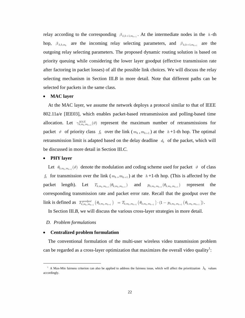
Fig. 2.2 Integrated block diagram of the proposed distributed per-packet algorithm. 25
Fig. 2.3 Priority queuing analysis system map. 31
Fig. 2.4 The elementary structure. 31
Fig. 2.5 (a) Network settings of the elementary structure. (b) Analytical average end-to-end waiting time of
the 8 video classes. 43
Fig. 2.6 (a) Network settings of the 6-hop overlay network (by cascading the elementary structure). (b)
Analytical average end-to-end waiting time of the 8 video classes. 45
Fig. 2.7 (a) Primary paths of the 6-hop overlay network using self-learning policy. (b) Analytical average
end-to-end waiting time of the 8 video classes. 46
Fig. 3.1 (a) Conventional distributed decision making of an agent. (b) Proposed foresighted decision
making of an agent. 58
Fig. 3.2 Expected delay evaluation and the required local information. 61
Fig. 3.3 Proposed decentralized Markov decision process framework and the necessary information
exchange among the agents. 64
Fig. 3.4 System diagram of the proposed model-based online learning approach at the agent hm . 67
Fig. 3.5 (a) 6-hop network topology (b) MDP delay values of the first five priority classes. 74
Fig. 3.6 (a) 2-cluster skewed network topology (b) MDP delay values of the first five priority classes. 75
Fig. 3.7 Comparisons of the MDP delay values using different learning approaches. 76
Fig. 3.8 Comparisons of the expected end-to-end delay using different learning approaches. 77
Fig. 3.9 Source node of packets in class 1C , 4C disappears after 60t = . 78
Fig. 3.10 The upper and the lower bounds of the MDP delay values for the first priority class traffic at
different hops. 80

xii
Fig. 4.1 The directed acyclic multi-hop overlay network for an exemplary wireless infrastructure. (a) Actual
network topology that has 2 source-destination pairs, 5 relay nodes. (b) Overlay network topology that
has 2 source-destination pairs, 6 relay nodes (with one virtual node in the 1-hop intermediate nodes). 93
Fig. 4.2 Illustrative example of an application layer overlay network with information horizon 2h =
. 96
Fig. 4.3 System map for the IFDS packet scheduling. 105
Fig. 4.4 Risk estimation vs. time interval for 2 users. 107
Fig. 4.5 Simulation settings of a 6-hop overlay network with 2 video sequences. 110
Fig. 4.6 Y-PSNR vs. various information horizon cases under different network transmission efficiencies
113
Fig. 5.1 (a) Conventional distributed power control. (b) Payoff-based interactive learning with private
information feedback. (c) Model-based interactive learning with public information feedback. 118
Fig. 5.2 System diagram of the dynamic joint power-spectrum resource allocation. 120
Fig. 5.3 (a) Throughput vB vs. vP in a selected frequency channel vf with fixed interference. (b) Utility
vu vs. vP in a selected frequency channel vf with fixed interference. 122
Fig. 5.4 Interactions among users and the foresighted decision making based on information feedback. 125
Fig. 5.5 Examples of different types of information feedback tvI . 127
Fig. 5.6 System block diagram for the adaptive interactive learning for dynamic resource management. 129
Fig. 5.7 Topology settings for the simulation. 137
Fig. 5.8 Average utility vs. time slot of the proposed algorithms when T = 700 Kbps. 141
Fig. 5.9 Performance of user 1m adopting adaptive reinforcement learning with private information
feedback using different 1ω . 142
Fig. 5.10 Performance of user 1m adopting adaptive action learning with public information feedback
using different 1tV . 143
Fig. 5.11 Average utility over time using the adaptive interactive learning when receivers have mobility (T
= 2100 Kbps) (a) 0.5ν = , (b) 1ν = , (c) 2ν = (m/time slot). 145
Fig. 6.1 An illustration of the considered network model. 155

xiii
Fig. 6.2 The architecture of the proposed dynamic resource management with priority virtual queue
interface. 162
Fig. 6.3 Actions of the secondary users ija and their physical queues for each frequency channel 164
Fig. 6.4 The block diagram of the priority virtual queue interface and dynamic strategy learning of a
secondary user. 172
Fig. 6.5 Analytical expected delay of the secondary users with various strategies in different frequency
channels, shadow part represents a bounded delay below the delay deadline (stable region). 176
Fig. 6.6 (a) Simulation results of the DSL algorithm – strategies of the secondary users and the utility
functions of less delay-sensitive applications ( 0.2iθ = , 0.05σ = , 0ijχ = ).(b) Simulation results of
the DSL algorithm – strategies of the secondary users and the utility functions of delay-sensitive
applications ( 0.8iθ = , 0.05σ = , 0ijχ = ). 177
Fig. 6.7 Steady state strategies of the secondary users and the utility functions vs. the normalized loading of
1PU for delay-sensitive applications ( 0.8iθ = , 0.05σ = , 0.02ijχ = ). 178
Fig. 7.1 A simple multi-hop cognitive radio network with three nodes and two frequency channels. 193
Fig. 7.2 Transmission time line at the node n with local information nL . 199
Fig. 7.3 Example of the static reward of information ( , ( ))n nJ k xI , dynamic reward of information
( , ( ))dn nJ k xI and optimal expected delay ( , )nK k x (where the information horizon ( , )nh k ν = 3,
average packet lengthkL =1000 bytes, and average transmission rate T = 6Mbps over the multi-hop
network). 201
Fig 7.4 (a) 2-hop information cell network without information exchange mismatch problem. (b) 1-hop
information cell network with information exchange mismatch problem. 204
Fig. 7.5 System diagram of the proposed distributed resource management. 206
Fig. 7.6 Block diagram of the proposed distributed resource management at network node n . 210
Fig. 7.7 (a). Block diagram of the proposed distributed resource management algorithm using the AFP. (b).
Impact of the network variation on the FP and the video performance. 211
Fig. 7.8 Wireless network settings for the simulation of two video streams. 215
Fig. 7.9 Reward dnJ and cost cnJ of different information horizon at different node for video 1V . 215

xiv
Fig. 7.10 (a) Packet loss rate vs. average transmission bandwidth using different approaches (InH = 80
meters). (b) Packet loss rate vs. average transmission bandwidth using different approaches (InH = 40
meters). 218
Fig. 7.11 Packet loss rate vs. learning frequency /nb c (average T =5.5 Mbps, InH = 80 meters). 219
Fig. 7.12 Packet loss rate vs. time fraction ρ of the primary users occupying frequency channel 1F around
network node n = 7, 11, 12 (average T =5.5Mbps, /nb c = 1, InH = 80 meters). 220
Fig. 7.13 Packet loss rate vs. mobility v of the secondary users (network relays) (average T = 8Mbps,
0ρ = , /nb c = 1, InH = 80 meters). 222
Fig. 8.1 Considered queuing model for multi-user channel access. 230
Fig. 8.2 Block diagram of the (a) myopic channel selection and (b) foresighted channel selection. 235
Fig. 8.3 An illustrative example of the solutions in the utility domain for a 2-user case (iv is the foresighted
user). 244
Fig. 8.4 Flowchart of the on-line foresighted channel selection procedure. 251
Fig. 8.5(a)(d) The action of the foresighted user 1v over time, while participating in the channel selection
game [(a) in network setting 1, (d) in network setting 2]. (b)(c)(e)(f) The actual remaining capacity
1jC and the estimated linear belief function 1jC , 1,2j = [(b)(c) in network setting 1, (e)(f) in
network setting 2]. 253
Fig. 8.6 Reaching the system-wise Pareto optimal solution and the Stackelberg Equilibrium. 254
Fig. 8.7 Delay of the foresighted user at different equilibrium for various numbers of myopic users in the
network. 255

xv
LIST OF TABLES
TABLE 2.1 THE CHARACTERISTIC PARAMETERS OF THE VIDEO CLASSES OF THE TWO VIDEO SEQUENCES. 41
TABLE 2.2 ANALYTICAL AND SIMULATION RESULTS FOR UNIFORM RELAY SELECTING PARAMETERS WITH
DIFFERENT NETWORK EFFICIENCIES OVER THE ELEMENTARY STRUCTURE. 43
TABLE 2.3 ANALYTICAL AND SIMULATION RESULTS FOR UNIFORM RELAY SELECTING PARAMETERS WITH
DIFFERENT NETWORK EFFICIENCIES OVER THE 6-HOP NETWORK. 45
TABLE 2.4 ANALYTICAL AND SIMULATION RESULTS FOR SELF-LEARNING POLICY RELAY SELECTING
PARAMETERS WITH DIFFERENT NETWORK EFFICIENCIES (THE ANALYTICAL RESULTS ARE
APPROXIMATED ACCORDING TO THE PRIMARY PATH SELECTED BY THE SELF-LEARNING POLICY). 46
TABLE 2.5 COMPARISON OF THE DYNAMIC SELF-LEARNING POLICY WITH THE CONVENTIONAL FIXED SINGLE-
PATH AND MULTI-PATH ALGORITHMS (USING THE SAME NETWORK SETTINGS AS IN TABLE 2.4). 47
TABLE 3.1. COMPLEXITY SUMMARY OF THE MODEL-FREE REINFORCEMENT LEARNING 69
TABLE 3.2. COMPLEXITY SUMMARY OF THE MODEL-BASED REINFORCEMENT LEARNING 71
TABLE 3.3. THE CHARACTERISTIC PARAMETERS OF THE DELAY-SENSITIVE APPLICATIONS. 73
TABLE 3.4 THE RESULTS OF HETEROGENEOUS LEARNING SCENARIOS. 79
TABLE 4.1 DESCRIPTIONS FOR THE FOUR CASES OF THE SIMULATION RESULTS ( 100SIt = ms). 111
TABLE 4.2 SIMULATION RESULTS FOR IFDS SCHEDULING WITH VARIOUS INFORMATION HORIZONS AND
DIFFERENT NETWORK EFFICIENCIES. 113
TABLE 5.1 COMPARISONS OF THE PROPOSED LEARNING ALGORITHMS. 137
TABLE 5.2 SIMULATION RESULTS OF THE FIVE SCHEMES WHEN T = 700 KBPS. 139
TABLE 5.3 SIMULATION RESULTS OF THE FIVE SCHEMES WHEN T = 2100 KBPS. 140
TABLE 5.5 SUMMARY OF THE USED NOTATIONS OF CHAPTER 5. 146
TABLE 6.1 SIMULATION PARAMETERS OF THE SECONDARY USERS. 175
TABLE 6.2 SIMULATION PARAMETERS OF THE PRIMARY USERS. 175
TABLE 6.3 COMPARISONS OF THE CHANNEL SELECTION ALGORITHMS FOR DELAY-SENSITIVE APPLICATIONS
WITH 6, 10N M= = . 180
xvi
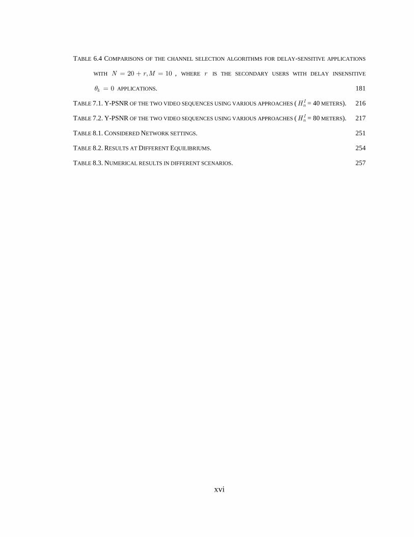
TABLE 6.4 COMPARISONS OF THE CHANNEL SELECTION ALGORITHMS FOR DELAY-SENSITIVE APPLICATIONS
WITH 20 , 10N r M= + = , WHERE r IS THE SECONDARY USERS WITH DELAY INSENSITIVE
0kθ = APPLICATIONS. 181
TABLE 7.1. Y-PSNR OF THE TWO VIDEO SEQUENCES USING VARIOUS APPROACHES ( InH = 40 METERS). 216
TABLE 7.2. Y-PSNR OF THE TWO VIDEO SEQUENCES USING VARIOUS APPROACHES ( InH = 80 METERS). 217
TABLE 8.1. CONSIDERED NETWORK SETTINGS. 251
TABLE 8.2. RESULTS AT DIFFERENT EQUILIBRIUMS. 254
TABLE 8.3. NUMERICAL RESULTS IN DIFFERENT SCENARIOS. 257

xvii
ACKNOWLEDGEMENTS
I would like to start by thanking my advisor Mihaela van der Schaar for her enthusiasm
and support through the course of my PhD. She has always encouraged me to look
beyond the details of specific problems and to see the big picture. Under her guidance, I
was able to complete papers on a wide range of research topics. Her breath and creativity
have been constant sources of inspiration for me throughout my stay here at UCLA.
I would also like to thank Professors Jason Speyer, Kung Yao, and Mario Gerla for
their interest in my work, and their time invested to be part of my committee. Their
helpful comments and advices have guided my work.
I would also like to thank my labmates Fangwen Fu, Hyunggon Park, Nick
Mastronarde, Brian Foo, Yi Su, and Zhichu Lin for helping me to think through many of
my research ideas, and for helping to peer review my papers before submission. I will
also treasure the personal times spent with each of them, and how they have enriched my
life through both meaningful and fun conversations. I would also like to thank my
supervisor at Intel, Dilip Krishnaswamy, for giving me the opportunity to do very
interesting research with them in their research group.
Finally, I would like to thank my family, my mom and dad, and my sister Judy, for
their continued love and support for me during the course of my PhD career. I would like
to dedicate my dissertation to my family.

xviii
VITA
2000 B.A., Electrical Engineering, National Taiwan University Taipei, Taiwan
2002 M.A., Electrical Engineering, Communications, National Taiwan University, Taipei, Taiwan Second Lieutenant, Information Office, Army
Taiwan Ministry of National Defense, Taiwan
2004 Software Engineer, High Tech Computer Corp. Taiwan
2005 Teaching Assistant, Electrical Engineering Dept., UCLA Joined the Multimedia Communication and System Lab.
under Prof. Mihaela van der Schaar. 2006 Teaching Assistant, Electrical Engineering Dept., UCLA
Summer interned at Intel Corp., Folsom, CA 2007 Received Award, Emerging Leaders in Multimedia,
from IBM T. J. Watson Research Center, Hawthorne, NY

xix
PUBLICATIONS
D. Krishnaswamy, H.-P. Shiang, J. Vicente, W. S. Conner, S. Rungta, W. Chan and K. Miao, “A Cross-Layer Cross-Overlay Architecture for Proactive Adaptive Processing in Mesh Networks,” in 2nd IEEE Workshop on Wireless Mesh Networks (WiMesh 2006), Sep 2006. Y.-L. Li, H.-H. Chen, Y. Chen, H.-P. Shiang, Y. Lee,"Low-Complexity Receiver Design for OFDM Packet Transmission with Mobility Support," IEEE Global Telecommunications Conference, vol. 1, pp. 599-604, Nov. 2002. H.-P. Shiang, D. Krishnaswamy, and M. van der Schaar, “Quality-aware Video Streaming over Wireless Mesh Networks with Optimal Dynamic Routing and Time Allocation,” in Proceedings of the 40th Asilomar Conference on Signals, Systems, and Computers, Oct 2006. H.-P. Shiang, J.-S. Liu, and Y.-R. Chien, "Estimate of minimum distance between convex polyhedra based on enclosed ellipsoids," in Proceedings of IEEE/RSJ International Conference on Intelligent Robots and Systems, 2000 (IROS 2000), vol. 1, pp. 739 - 744, Oct 2000. H.-P. Shiang, M. van der Schaar, “Multi-user Video Streaming over Multi-hop Wireless Networks: A Cross-layer Priority Queuing Approach,” in IEEE Conference on Intelligent Information Hiding and Multimedia Signal Processing (IIH-MSP 2006), pp. 255-258, Dec 2006. H.-P. Shiang, M. van der Schaar, “Multi-user Video Streaming over Multi-hop Wireless Networks: A Distributed, Cross-layer Approach Based on Priority Queuing,” IEEE Journal of Selected Areas in Communications, vol. 25, no. 4, pp. 770-785, May 2007. H.-P. Shiang, M. van der Schaar, “Informationally Decentralized Video Streaming over Multi-hop Wireless Networks,” IEEE Transactions on Multimedia, vol. 9, no. 6, pp. 1299-1313, Oct 2007. H.-P. Shiang, M. van der Schaar, “Queuing-Based Dynamic Channel Selection for Heterogeneous Multimedia Applications over Cognitive Radio Networks,” IEEE Transactions on Multimedia, vol. 10, no. 5, pp. 896-909, Aug. 2008.

xx
H.-P. Shiang, M. van der Schaar, “Delay-Sensitive Resource Management in Multi-hop Cognitive Radio Networks" in IEEE Dynamic Spectrum Access Networks (DySPAN 2008), Oct. 2008. H.-P. Shiang, M. van der Schaar, “Dynamic Channel Selection for Multi-user Video Streaming over Cognitive Radio Networks," in Proc. Int. Conf. On Image Processing. (ICIP 2008) Oct. 2008. H.-P. Shiang, M. van der Schaar, “Risk-aware scheduling for multi-user video streaming over wireless multi-hop networks,” in IS&T/SPIE Visual Communications and Image Processing (VCIP 2008), San Jose, Jan 2008. H.-P. Shiang, M. van der Schaar, “Conjecture-Based Channel Selection Game for Delay-Sensitive Users in Multi-Channel Wireless Networks" in International Conference on Game Theory for Networks (GameNets 2009), 2009. (Invited paper) H.-P. Shiang, W. Tu, M. van der Schaar, “Dynamic Resource Allocation of Delay Sensitive Users Using Interactive Learning over Multi-carrier Networks," in Proc. Int. Conf. Commun. (ICC 2008), May 2008. H.-P. Shiang, M. van der Schaar, “Distributed Resource Management in Multi-hop Cognitive Radio Networks for Delay Sensitive Transmission,” IEEE Transactions on Vehicular Technology, vol. 58, no. 2, pp. 941-953, Feb 2009. H.-P. Shiang, M. van der Schaar, “Feedback-Driven Interactive Learning in Dynamic Wireless Resource Management for Delay Sensitive Users,” IEEE Transactions on Vehicular Technology, to appear. H.-P. Shiang, M. van der Schaar, “Information-Constrained Resource Allocation in Multi-Camera Wireless Surveillance Networks,” submitted to IEEE Transactions on Circuits and Systems for Video Technology. H.-P. Shiang, M. van der Schaar, “Conjecture-Based Channel Selection for Autonomous Delay-Sensitive Users in Multi-Channel Wireless Networks,” submitted to IEEE Transactions on Networking. J. Wu, H.-P. Shiang, K. T. Chen,and H. W. Tsao," Delay and Throughput Analysis of the High Speed Variable Length Self-Routing Packet Switch," IEEE workshop on High Performance Switching and Routing (HPSR 2002), pp:314 - 318, May 2002.

xxi
ABSTRACT OF THE DISSERTATION
Designing Autonomic Wireless Multi-Hop Networks
for Delay-Sensitive Applications
by
Hsien-Po Shiang
Doctor of Philosophy in Electrical Engineering
University of California, Los Angeles, 2009
Professor Mihaela van der Schaar, Chair
Emerging multi-hop wireless networks provide a low-cost and flexible infrastructure
that can be simultaneously utilized by multiple users for a variety of applications,
including delay-sensitive applications, such as multimedia streaming, mission-critical
applications, etc. However, this wireless infrastructure is often unreliable and provides
dynamically varying resources with only limited QoS support.
To improve the performance of the delay-sensitive applications and to support timely
reaction to the network dynamics, the multi-hop network needs to be composed of
autonomic nodes (agents), which can adapt, make their own transmission decisions and
negotiate their wireless resources based on their available local information. Current
wireless networking research has focused on coping with the environment disturbances,

xxii
such as variations (uncertainties) of the wireless channel (e.g. fading) or source (e.g.
multimedia traffic) characteristics, while neglecting the coupling dynamics among nodes,
due to the shared nature of the wireless spectrum. However, characterizing and learning
the neighboring nodes’ actions and the evolution of these actions over time is vital in
order to construct an efficient and robust solution for delay-sensitive applications. Hence,
we propose and analyze various interactive learning schemes for these agents to learn the
network dynamics and, based on this knowledge, foresightedly adapt their cross-layer
transmission decisions such that they can efficiently utilize the shared, time-varying
network resources. We show that the foresighted decision making significantly improves
the agents' utilities under a variety of dynamic network scenarios (e.g. multimedia
streaming over WLAN, energy-efficient transmission in mobile ad hoc networks, joint
route/channel selection in multi-hop cognitive radio networks) and various network
topologies as compared to existing state-of-the-art solutions.
In conclusion, our research adds a new, “cognitive”, dimension to existing multi-hop
wireless networks that enables the autonomic nodes to dynamically forecast the expected
response to network dynamics of neighboring nodes and evaluate how specific forms of
explicit and implicit signaling impact the performance of delay-sensitive applications.

1
Chapter 1
Introduction
Emerging multi-hop wireless networks provide a low-cost and flexible infrastructure
that can be simultaneously utilized by multiple nodes for a variety of applications,
including delay-sensitive applications, which form the main focus in this dissertation.
These multi-hop wireless networks can be either constructed using passive nodes that
follow the coordination of a central coordinator (e.g. a network planner), which directs
their transmission strategies, or using autonomic nodes that can determine and adapt their
own transmission strategies to maximize the network utility. Such wireless networks are
referred to as autonomic wireless networks. These networks are established based on the
voluntary participation of autonomic wireless nodes (also interchangeably referred to as
agents in this dissertation), which interact with each other (i.e. make their own decisions)
in order to maximize their own utilities. Many features make such autonomic decision
making an appealing approach for driving the resource management and information
exchanges for delay-sensitive applications. First, in the multi-hop wireless environment,
the decisions on how to adapt the cross-layer transmission strategies at the various
sources and relays need to be performed in an informationally-decentralized manner,
because the tolerable delay does not allow propagating messages back and forth
throughout the network to a centralized coordinator. Second, even if information were
centralized, the centralized cross-layer optimizations are too complex to be solved in a
timely manner. This leads to a “decomposition” of the optimization which relies on the
dynamic reconfiguration of the autonomous nodes. Third, both the applications and the
wireless network conditions are time-varying and hence, it is necessary that the source
nodes and relay nodes self-organize to adapt to new environmental conditions.

2
I. DISSERTATION GOAL
This dissertation presents principles and design rules that enable autonomic nodes to
proactively construct multi-hop networks for the efficient transmission of delay-sensitive
applications. We study how these autonomic nodes can coordinate with the other nodes in
order to self-organize themselves to transmit delay-sensitive applications over a
multi-hop wireless network. Importantly, we discuss two main concepts that enable the
autonomic nodes to make autonomous decisions and maximize the applications’
performances:
• Foresighted cross-layer transmission strategies. In dynamic multi-user wireless
environments, the nodes’ strategies are coupled, since the transmission actions taken
by the nodes impact the utility of each other. Thus, nodes need to select their optimal
cross-layer strategies by anticipating the impact of their actions on both their
immediate utility as well as on their long term performance. For instance, a node’s
aggressive transmission strategy may be rewarded in the short term by a high utility
gain, but this will trigger the other nodes to respond by adapting their own
transmission strategies, which will ultimately impact its long term reward. Hence,
autonomic nodes need to build accurate models about the other wireless nodes’
response strategies to forecast future utilities and, based on this, make foresighted
decisions on which cross-layer transmission strategies they should adopt in real-time.
• Interactive learning. In order to build these accurate models about the other nodes,
the autonomic nodes can adopt interactive learning approaches to learn the strategies
of the other nodes based on local “observed information”. Such information is often
obtained through control message exchange mechanisms made possible by network
protocols. The autonomic nodes can proactively determine what messages they would
like to exchange with other nodes and, using these messages, negotiate and coordinate
with other nodes the usage of available network resources. Various classes of
interactive learning approaches can be adopted depending on the information
3
exchange mechanism, which results in different transmission overheads and
complexity costs that lead to different learning efficiency. This dissertation also
discusses the tradeoffs between the costs of the information exchanges, which are
necessary for the distributed coordination of nodes, and the learning efficiency, by
evaluating their impact on the nodes’ utilities.
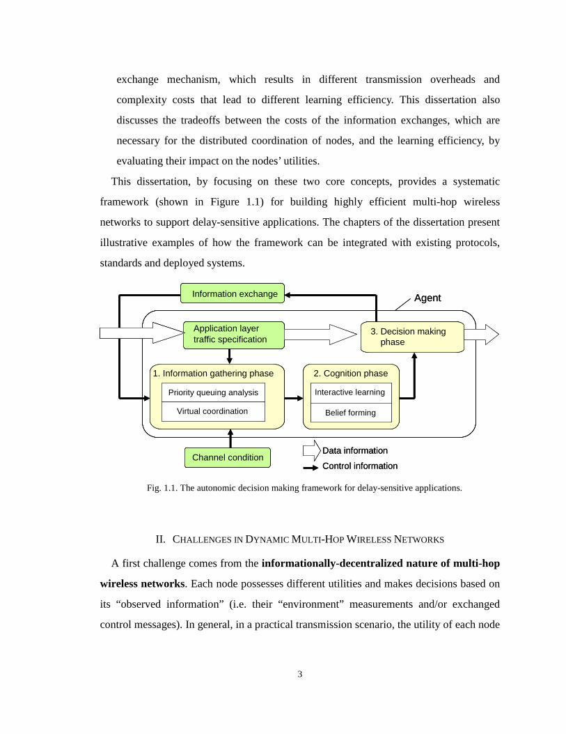
This dissertation, by focusing on these two core concepts, provides a systematic
framework (shown in Figure 1.1) for building highly efficient multi-hop wireless
networks to support delay-sensitive applications. The chapters of the dissertation present
illustrative examples of how the framework can be integrated with existing protocols,
standards and deployed systems.
Fig. 1.1. The autonomic decision making framework for delay-sensitive applications.
II. CHALLENGES IN DYNAMIC MULTI-HOP WIRELESS NETWORKS
A first challenge comes from the informationally-decentralized nature of multi-hop
wireless networks. Each node possesses different utilities and makes decisions based on
its “observed information” (i.e. their “environment” measurements and/or exchanged
control messages). In general, in a practical transmission scenario, the utility of each node
2. Cognition phase
Application layertraffic specification
Channel condition
Agent
Priority queuing analysis
Belief forming
1. Information gathering phase
Virtual coordination
Control information
Data information
3. Decision making phase
Interactive learning
Information exchange
2. Cognition phase
Application layertraffic specification
Channel condition
Agent
Priority queuing analysis
Belief forming
1. Information gathering phase
Virtual coordination
Control information
Data information
3. Decision making phase
Interactive learning
Information exchange

4
is not known by other nodes. Moreover, the nodes are not always directly aware of the
transmission strategies of other nodes. Different types of observations can be made by the
nodes depending on their adopted wireless protocols. Moreover, we highlight the
importance of considering the cost of the induced information overheads and their impact
on the nodes’ utilities.
The second challenge arises due to the delay-sensitive characteristics of the
applications. As the source characteristics are changing, the tolerable delays at the
application layer and the required utility (e.g. quality or fidelity) can vary significantly.
This influences the performance of the applications and, ultimately, the choice of the
optimal transmission strategy adopted by the node. Moreover, the delay-sensitive
characteristics of the applications also make a centralized solution impractical, since the
tolerable delay does not allow propagating control information back and forth throughout
the multi-hop network to a centralized decision maker. Hence, this further emphasizes the
need for developing informationally-decentralized resource management solutions, where
autonomic nodes coordinate their resource usage by proactively exchanging information.
Third, the wireless network is a highly dynamic transmission environment. The
transmission channel condition is unreliable and the network topology may vary over
time. To address this issue, it is important to provide distributed solutions that can timely
adapt to these changes in the network.
Finally, in a multi-user setting, the utility and the decision of a node varies depending
on both its experienced “environment” (e.g. application, source and channel
characteristics), and the other nodes’ strategies. Thus, a key challenge associated with
delay-sensitive transmission in ad-hoc wireless networks is the coupling of the wireless
nodes’ actions and their utility performances, as the individual decisions of the nodes
and that of their relaying peers will have a significant impact on each others’ utilities.
More challenges are arising when multiple delay-sensitive applications are
simultaneously utilizing the same wireless networks.

5
To cope with these challenges, the autonomic nodes need to coordinate with each other
to form a multi-hop network and optimize their cross-layer transmission strategies by
taking in to account the response of the other nodes. To do so, the nodes will need to
learn the other nodes responses to their strategies and correspondingly adapt their
strategies in real-time. To estimate the response of the other nodes, interactive learning
approaches can be deployed.
III. ORGANIZATION OF THE DISSERTATION
The subsequent chapters of the dissertation aim to address the abovementioned
challenges. Figure 1.2 shows the organization of the various chapters.
Fig. 1.2. The organization of the dissertation.
Chapter 2 discusses the cross-layer design of video streaming over multi-hop wireless
Decision process(Markov decision process)
Priority queuing analysis (virtual coordination
interface)
Interactive learning
Dynamic transmissionenvironment
Distributedinformation
Multi-userinteraction
Main challenges Proposed autonomicdecision making framework
Main concerns
Multimedia Transmission
inmulti-hopnetworks
Power controlad hoc mobile
networks
Resource management
incognitive radio
networks
Energy-efficienttransmission
Distributedcoordination
Cross-layeroptimization
Risk-awarescheduling
Adaptiverouting
Collaborative rule-basedresource management
Foresighteddecisionmaking
Conjecture gamemodeling
Informationexchange
Futureprediction
Ch. 2
Ch. 3
Ch. 4
Ch. 5
Ch. 6
Ch. 7
Ch. 8
Applications
Applicationcharacteristics
(priorities, delay deadlines)
Dynamic transmissionenvironment
Applicationcharacteristics
(priorities, delay deadlines)
Decision process(Markov decision process)
Priority queuing analysis (virtual coordination
interface)
Interactive learning
Dynamic transmissionenvironment
Distributedinformation
Multi-userinteraction
Main challenges Proposed autonomicdecision making framework
Main concerns
Multimedia Transmission
inmulti-hopnetworks
Power controlad hoc mobile
networks
Resource management
incognitive radio
networks
Energy-efficienttransmission
Distributedcoordination
Cross-layeroptimization
Risk-awarescheduling
Adaptiverouting
Collaborative rule-basedresource management
Foresighteddecisionmaking
Conjecture gamemodeling
Informationexchange
Futureprediction
Ch. 2Ch. 2
Ch. 3Ch. 3
Ch. 4Ch. 4
Ch. 5Ch. 5
Ch. 6Ch. 6
Ch. 7Ch. 7
Ch. 8Ch. 8
Applications
Applicationcharacteristics
(priorities, delay deadlines)
Dynamic transmissionenvironment
Applicationcharacteristics
(priorities, delay deadlines)

6
networks. Distributed packet-based cross-layer algorithms are presented to maximize the
decoded video quality of multiple nodes engaged in simultaneous real-time streaming
sessions over the same multi-hop wireless network. These algorithms explicitly consider
packet-based distortion impact and delay constraints in assigning priorities to the various
packets and then rely on priority queuing analysis to model the coupling impact from the
other nodes and to drive the optimization of the various nodes’ transmission strategies
across the protocol layers as well as across the multi-hop network. Solutions enabled by
the scalable coding of the video content (i.e. nodes can transmit and consume video at
different quality levels) will be discussed. The cross-layer strategies we consider in this
chapter include the application layer packet scheduling, the policy for choosing the routing
relays in network layer, the MAC retransmission strategies, and the PHY modulation and
coding schemes. The main component of the proposed solution is a low-complexity,
distributed, and dynamic routing algorithm referred to as self-learning policy, which relies
on prioritized queuing to select the path and time reservation for the various packets, while
explicitly considering instantaneous channel conditions, queuing delays and the resulting
interference. Based on the local information exchange, the cross-layer transmission
strategies are optimized at each node, in a fully distributed manner.
Chapter 3 addresses the network dynamics in multi-hop wireless networks. The
considered network dynamics include 1) time-varying traffic characteristics, 2)
time-varying channel conditions, and 3) inter-node coupling. We study how wireless
nodes learn the network dynamics and optimize their cross-layer transmission decisions to
support delay-sensitive applications, such as surveillance, security monitoring, and
mission-critical applications in military operations, etc. We consider the network delay
minimization problem in a dynamic multi-hop wireless network, where multiple source
nodes transmit simultaneously delay-sensitive data through relay nodes to one or multiple
decision makers (destinations). Again, since there is no time to propagate control
information back and forth to a central decision maker, the multi-hop network needs to be

7
built by autonomic nodes that can make their own transmission decisions. In such a
network, the nodes can be modeled as agents that can make timely transmission decisions
based on available local information. We formulate the autonomic decision making
problem as a Markov decision process (MDP). By decomposing the centralized MDP
formulation, we construct a distributed MDP framework, which takes into consideration
the decentralized nature of the multi-hop wireless network. We prove that the distributed
MDP converges to the same optimal cross-layer transmission policies of the agents as the
centralized MDP. We further propose an online model-based reinforcement learning
approach for agents to solve the distributed MDP at runtime, by modeling the network
dynamics using priority queuing. Specifically, we allow the agents to minimize the delays
of the applications by modeling the queuing delay and anticipating the network state
transition probabilities. We determine the upper and the lower bounds of the delays to
show the accuracy of the proposed model-based learning approach and show that they both
asymptotically converge to the optimal expected delay. Moreover, we compare the
proposed model-based reinforcement learning approach with the conventional model-free
reinforcement learning approaches.
In Chapter 4, we investigate risk-aware scheduling for autonomic nodes to transmit
packets of delay-sensitive applications in its queue. Various packet scheduling
approaches have been proposed to address multi-user multimedia streaming over
multi-hop wireless networks. However, these cross-layer transmission strategies can be
efficiently optimized only if they use accurate information about the network conditions
and hence, are able to timely adapt to network changes. Distributed solutions that adapt
the transmission strategies based on timely information feedback need to be considered. To
acquire this information feedback for cross-layer adaptation, we deploy an overlay
infrastructure, which is able to relay the necessary information about the network status
and incurred delays across different network “horizons” (i.e. across a different number of
hops in a predetermined period of time). Based on the information feedback, we can

8
estimate the risk that packets from different priority classes will not arrive at their
destination before their decoding deadline expires. In this chapter, we propose a
distributed risk-aware scheduling approach that is optimized based on the local
information feedback acquired from the various network horizons. We investigate the
distributed cross-layer adaptation at each wireless node by considering the advantages
resulting from an accurate and frequent network information feedback from larger
horizons as well as the drawbacks resulting from an increased transmission overhead.
Chapter 5 studies the interference coupling among the delay-sensitive applications
over wireless networks. We focus on a decentralized power control setting, where
wireless nodes make their own transmission decisions in order to maximize their
energy-efficient utilities as evaluated based on exchanged information. Specifically, two
types of information exchange are discussed in this chapter, which result in two different
classes of learning approaches. One is the private information feedback between a
transmitter-receiver pair. The other is the public information feedback among nodes (i.e.
different transmitter-receiver pairs). Due to the informationally-decentralized nature of
the wireless network, a node cannot have complete information about the transmission
actions of its interfering neighbors. However, the node can model implicitly or explicitly
the transmission strategies (power spectrum profile) of its major interference sources
based on the observed information. A node can adopt model-based learning schemes to
explicitly model the other nodes’ strategies if public information is available, or adopt
payoff-based learning schemes to implicitly model the impact of other nodes’ actions on
its utility if only private information is available. Based on these models, the node creates
beliefs and is able to strategically adapt its decisions to maximize its own utility.
Importantly, we investigate the cost-efficiency tradeoffs resulting from the information
gathered with different frequencies and from various nodes. By adjusting the information
exchange, the node can adapt its interactive learning scheme to approach the utility upper
bound. The energy efficiency of delay-sensitive nodes in mobile ad hoc networks can be

9
significantly improved by adopting the interactive learning schemes introduced in this
chapter.
In Chapter 6, we present the dynamic channel selection in single-hop cognitive radio
networks for transmitting delay-sensitive applications. The majority research in this area
seldom considers the requirement of the application layer. In this chapter, we present the
solutions especially suitable for heterogeneous multimedia applications with various rate
requirements and delay deadlines. Note that in a cognitive radio networks, the wireless
nodes usually possess private utility functions, application requirements, and distinct
channel conditions in different frequency channels. To efficiently manage available
spectrum resources in a decentralized manner, efficient information exchange
coordination among nodes is necessary. The term “cognitive” in this dissertation refers to
both the capability of the network nodes to achieve large spectral efficiencies by
dynamically exploiting available frequency channels as well as their ability to learn the
“environment” (the actions of interfering nodes) based on the designed information
exchange. Hence, we first introduce the priority virtual queuing interface that determines
the required information exchanges. With the primary nodes as the highest priority traffic,
each node evaluates its expected delays based on the information. Such expected delays
are important for multimedia applications due to their delay-sensitivity nature. The
expected delays are evaluated using priority queuing analysis that considers the wireless
environment, traffic characteristics, and build models of the other nodes’ behaviors in the
same frequency channel. Next, we discuss the Dynamic Strategy Learning (DSL)
algorithm that exploits the expected delay and dynamically adapts the channel selection
strategies to maximize the node’s utility function.
Chapter 7 studies the dynamic resource management in multi-hop cognitive radio
networks for transmitting delay-sensitive applications. Since the tolerable delay does not
allow propagating global information back and forth throughout the multi-hop network to
a centralized decision maker, the source nodes and relays need to adapt their actions
10
(transmission frequency channel and route selections) in a distributed manner, based on
local network information. We propose a distributed resource management algorithm that
allows network nodes to exchange information and that explicitly considers the delays
and cost of exchanging the network information over the multi-hop cognitive radio
networks. Note that the node competition is due to the mutual interference of neighboring
nodes using the same frequency channel. Based on this, we adopt a multi-agent learning
approach, adaptive fictitious play, which uses the available interference information. We
also discuss the tradeoff between the cost of the required information exchange and the
learning efficiency.
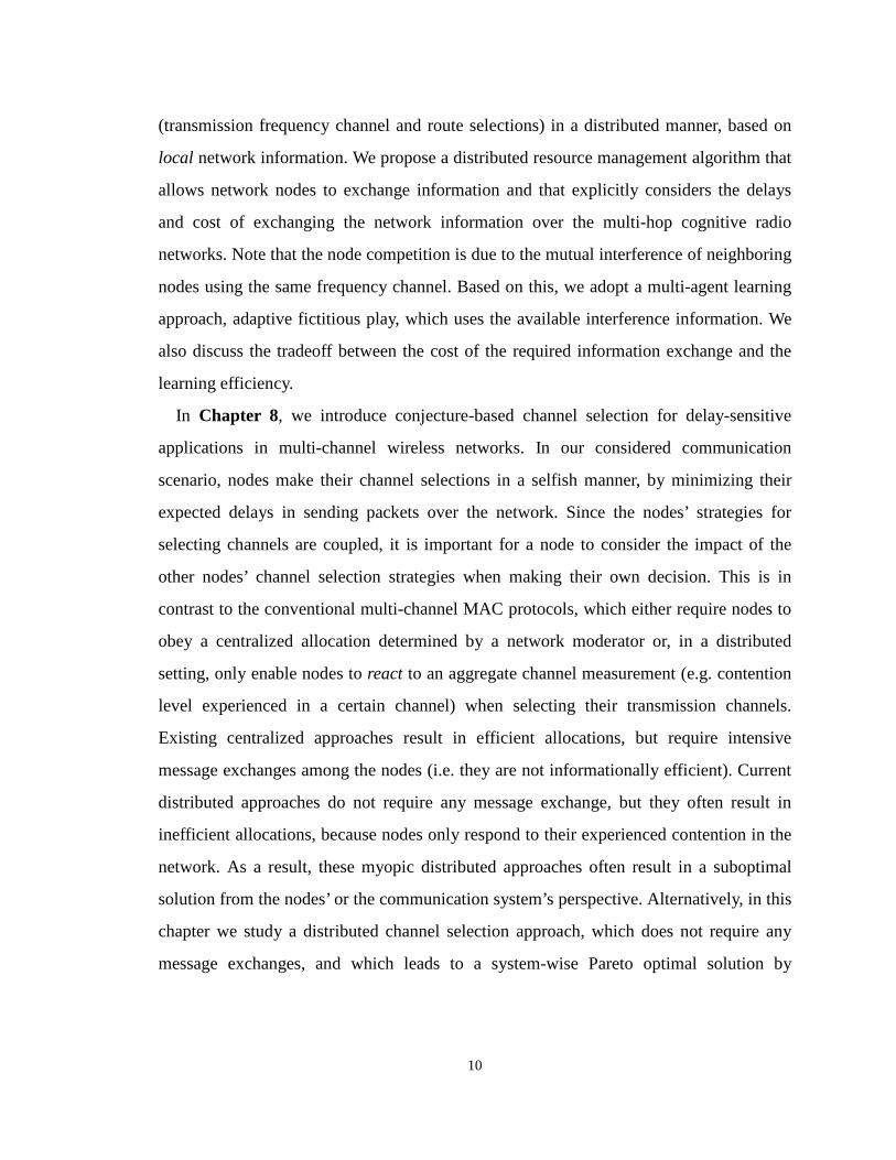
In Chapter 8, we introduce conjecture-based channel selection for delay-sensitive
applications in multi-channel wireless networks. In our considered communication
scenario, nodes make their channel selections in a selfish manner, by minimizing their
expected delays in sending packets over the network. Since the nodes’ strategies for
selecting channels are coupled, it is important for a node to consider the impact of the
other nodes’ channel selection strategies when making their own decision. This is in
contrast to the conventional multi-channel MAC protocols, which either require nodes to
obey a centralized allocation determined by a network moderator or, in a distributed
setting, only enable nodes to react to an aggregate channel measurement (e.g. contention
level experienced in a certain channel) when selecting their transmission channels.
Existing centralized approaches result in efficient allocations, but require intensive
message exchanges among the nodes (i.e. they are not informationally efficient). Current
distributed approaches do not require any message exchange, but they often result in
inefficient allocations, because nodes only respond to their experienced contention in the
network. As a result, these myopic distributed approaches often result in a suboptimal
solution from the nodes’ or the communication system’s perspective. Alternatively, in this
chapter we study a distributed channel selection approach, which does not require any
message exchanges, and which leads to a system-wise Pareto optimal solution by

11
enabling nodes to predict the implications (based on their beliefs) of their channel
selection on their expected future delays and thereby, foresightedly influence the resulting
multi-user interaction. We model the multi-user interaction as a channel selection game
and show how nodes can play an ε -consistent conjectural equilibrium by building
near-accurate beliefs and competing for the remaining capacities of the channels. We
study two different operation scenarios – 1) when the wireless system has only one
foresighted node acting as a leader, 2) when the wireless system has multiple foresighted
nodes. We analytically show that when the system has only one foresighted node, this
self-interested leader can deploy a linear belief function in each channel and manipulates
the equilibrium to approach the Stackelberg equilibrium. Alternatively, when the leader is
altruistic, the system will converge to the system-wise Pareto optimal solution. We
propose a low-complexity learning method based on linear regression for the foresighted
node to learn its belief functions. When the system has multiple foresighted nodes, we
show how these nodes can approach the system-wise Pareto optimal solution by
collaboratively complying with prescribed rules of building beliefs. An on-line
coordination procedure that enables the nodes to reach the system-wise Pareto optimal
solution in a distributed manner is provided.
Finally, we conclude the dissertation in Chapter 9.

12
Chapter 2
Cross-layer Optimization for Multimedia
Streaming in Multi-Hop Wireless Networks
I. INTRODUCTION
In this chapter, we focus on transmitting multiple delay-sensitive video bitstreams
across the same multi-hop wireless local area network (WLAN). Such wireless
infrastructures often provide dynamically varying resources with only limited support for
the Quality of Service (QoS) required by real-time multimedia applications. Hence,
efficient solutions for multimedia streaming must accommodate time-varying bandwidths
and probabilities of error introduced by the shared nature of the wireless medium and
quality of the physical connections. In the studied distributed transmission scenario, users
need to proactively collaborate in sharing the available wireless resources, in order to
ensure that the various multimedia applications are provided with the necessary QoS.
Such collaboration is needed due to the shared nature of the wireless infrastructure, where
the cross-layer transmission strategy deployed by one user impacts and is impacted by the
other users.
Prior research on multi-user multimedia transmission over multi-hop wireless networks
has focused on centralized, flow-based resource allocation strategies based on a
pre-determined rate-requirement [WZ02][SYZ05]. These solutions are not scalable to the
network size or the number of users and attempt to solve the end-to-end routing and path
selection problem as a combined optimization using algorithms designed for
Multi-Commodity Flow [AL94] problems. Such an optimization ensures that the
end-to-end utility function (benefit) is maximized while satisfying constraints on
individual link capacities. For instance, in [NMR05], a dynamic routing policy based on

13
queuing backpressure is proposed, which ensures that the average delay is bounded for
the various users as long as the transmission rates are inside the capacity region of the
network. However, the flow-based optimization does not guarantee that explicit
packet-based delay constraints are met for video applications. These network layer
research chapters do not consider the real-time adaptation to time-varying channel
conditions, video characteristics and encoding parameters (that influence packet-based
delay constraints). Importantly, they do not take into account the loss tolerance provided
by video applications, which can be exploited by the wireless network to support a larger
number of users. Therefore, these solutions often lead to inferior network efficiency and
suboptimal resulting qualities for the video users.
Alternatively, the majority of the video-centric research does not consider the
protection techniques available at lower layers of the protocol stack (MAC, PHY) and/or
optimizes the video transport using purely end-to-end metrics, thereby excluding the
significant gains of cross-layer design [BT05][WCZ05][DAB03]. Recent results on the
practical throughput and packet loss analysis of multi-hop wireless networks have shown
that the incorporation of appropriate utility functions (that take into account specific
parameters of the protocol layers such as the expected retransmissions, the error rate and
bandwidth of each link [DAB03], as well as expected transmission time [DPZ04]) can
significantly impact the actual performance. In [AMV06], an integrated cross-layer
optimization framework was proposed that considers the video quality impact. However,
the solution proposed in [AMV06] considers only the single user case, where a set of
paths and transmission opportunities are statically pre-allocated for each video
application. This leads to a sub-optimal, non-scalable solution for the multi-user case,
which ignores important problems such as inefficient routing and time allocation to avoid
interference among neighboring nodes. In summary, while significant contributions have
been made to enhance the separate performance of the various OSI layers, no framework
exists that integrates distributed and adaptive routing and resource allocation with
14
cross-layer optimization for efficient multi-user multimedia streaming over multi-hop
wireless networks.
In this chapter, we propose such an integrated cross-layer solution for multiple video
users. Our solution relies on the users’ agreement to collaborate by dynamically adapting
the quality of their multimedia applications to accommodate the more important
flows/packets of other users. Unlike commercial multi-user systems, where the incentive
to collaborate is minimal and there are often free-riders, we investigate the proposed
approach in an enterprise network setting where users exchange accurate and trustable
information about their applications (e.g. packet priorities). In our setting, the importance
of the packets is determined based on their contribution to the overall distortion of a
particular video as well as their delay deadlines. This information is encapsulated in the
header of each transmitted packet and is used by intermediate nodes to drive the
cross-layer transmission strategies. Moreover, our priority queuing approach also enables
path diversity gains due to the delay-optimized dynamic routing, since the packets of the
same application may be transmitted over different paths between the source and
destination nodes.
To increase the number of simultaneous users as well as to improve their performance
given time-varying network conditions, we deploy scalable video coding schemes that
enable a fine-granular adaptation to changing network conditions and a higher granularity
in assigning the packet priorities. In our set-up, each user has a distinct source-destination
pair. We assume a directed acyclic multi-hop overlay network [KV04] that can convey (in
real-time) information about the expected delay for each priority class from a specific
node to the destination. Each receiving node performs polling-based contention-free
media access [IEE03] that dynamically reserves a transmission opportunity interval in a
service interval (SI). The network topology and the corresponding channel condition of
each link are assumed to remain unchanged within the SI. Each node maintains a queue
containing video packets from various users and correspondingly determines the

15
transmission strategies based on the network information feedback from the neighbor
nodes of the next hop. At intermediate nodes, we select the next hop based on a
shortest-delay policy similar to the Bellman-Ford routing algorithm [BG87]. However, in
our approach, we explicitly consider the packet deadlines and their priorities. Based on
this intermediate node selection, we determine the expected delay for the packet and relay
this information via the overlay network to the previous nodes.
The main contributions of this chapter are listed below.
1. Packet-based vs. flow-based/layer-based solutions
We introduce a novel video streaming approach based on priority queuing that enables
us to optimize the cross-layer transmission strategies per packet. The proposed
cross-layer adaptation differs from existing solutions for multimedia transmission over
multi-hop networks, where the path (or limited multiple paths) is predetermined for the
entire bitstream or layer [AMV06]. Moreover, the MAC retransmission and PHY link
adaptation are often not considered for these flow-based/layer-based solutions [SYZ05].
Our approach is based on a multi-path routing algorithm that determines the next relay
per packet. The proposed priority and delay-driven approach allows us to avoid global
optimizations based on pre-determined rate requirements or path selections, which are not
adaptive to network changes, the number of users or streamed video content
characteristics.
2. Distributed solution based on dynamic routing vs. conventional centralized
solutions
Existing research [SYZ05][WCZ05] poses the problem of multi-user resource
allocation and cross-layer adaptation over ad-hoc wireless networks as a static,
centralized optimization that maximizes the utility (e.g. video quality) of the various
users given pre-determined channel (capacity) constraints [TG03] and video rate
requirements. These solutions have several limitations. First, the video bitstreams are
changing over time in terms of required rates, priorities and delays. Hence, it is difficult

16
to timely allocate the necessary bandwidths across the wireless network infrastructure to
match these time-varying application requirements. Second, the delay constraints of the
various packets are not explicitly considered in centralized solutions, as this information
cannot be relayed to a central resource manager in a timely manner. Third, the
complexity of the centralized approach grows exponentially with the size of the network
and number of video flows. Finally, the channel characteristics of the entire network (the
capacity region of the network) need to be known for this centralized, oracle-based
optimization. This is not practical as channel conditions are time-varying, and having
accurate information about the status of all the network links is not realistic.
Alternatively, in our solution, we optimize the cross-layer strategies (dynamic routing,
MAC retransmission limit, and PHY modulation and coding scheme) per packet at the
various intermediate nodes, in a distributed manner, which allows us to efficiently adapt
to changes in the video bitstream, channel characteristics, and network resource. This
approach is well suited for the informationally decentralized nature of the investigated
multi-user video transmission problem. We also discuss the required
information/parameters exchange among networks/layers for implementing such a
distributed solution.
3. Priority queuing analysis with interference consideration
Our solution aims at minimizing the packet loss rate of the packets in higher priority
video classes based on the proposed priority queuing analysis. The analysis is performed
for network environments with and without transmission interference consideration. To
cope with the interference problems that exist in multi-hop networks due to the broadcast
nature of the wireless medium, we adopt a polling-based, contention-free MAC that
allocates transmission opportunities at each node to the various classes/packets based on
their priorities [IEE03]. To analyze the expected waiting time for the various packets in
the presence of interference, we apply a novel virtual queuing method based on the
"service-on-vacation" queuing model.

17
4. Bottleneck identification
Using our priority queuing analysis, we can estimate the expected packet loss at the
transmitter side. This information can be used by the application layer to decide how
many quality layers are transmitted or to adapt its encoding parameters (in the case of
real-time encoding) to improve its video quality performance given the current number of
users, priorities of the competing streams and network conditions, but also, importantly,
to alleviate the network congestion. Note that our analysis provides this network
bottleneck identification for each priority class, which is used in our solution to simplify
the routing decision strategies. Furthermore, this information can be exploited to improve
the network infrastructure such that it can support various multimedia application
scenarios under different levels of network congestion.
The rest of this chapter is organized as follows. Section II introduces the multi-user
video streaming specification (video priority classes, network specification, cross-layer
parameters etc.) and subsequently gives the cross-layer optimization problem formulation
and highlights the need for a distributed per-packet solution. In Section III, we present
our distributed solution which involves dynamically selecting relays that minimize the
end-to-end packet loss probability of the higher priority video packets of the various
users. In Section IV, we present the queuing delay analysis required in the proposed
solution to determine the expected delay at each node. Based on the expected delay, a
relay will be dynamically selected. In this section, we do not consider the effect of
interference, as is the case in wireless networks where the nodes can simultaneously
transmit and receive in orthogonal channels. Subsequently, in Section V, our analysis is
extended to a wireless network environment where the transmission is performed in the
same channel, and thus the interference needs to be considered. In Section VI, we show
that the proposed distributed routing algorithm converges to a steady-state under certain
assumptions. Finally, Section VII presents our simulation results, and Section VIII
concludes the chapter.

18
II. MULTI-USER VIDEO STREAMING SPECIFICATION
A. Video priority classes
We assume that there are V video users (with distinct source-destination pairs)
sharing the same multi-hop wireless infrastructure. In [VAH06], it has been shown that
partitioning a scalable embedded video flow (stream) into several priority classes
(quality-layers) can improve the number of simultaneously admitted stations in a
congested 802.11a/e WLAN infrastructure, as well as the overall received quality.
Similarly, in this chapter, we categorize the video units (video packets, video subbands,
video frames) of the video bitstream into several priority classes. We adopt an embedded
3D wavelet codec [AMB04] and construct video classes by truncating the embedded
bitstream [VAH06]. We assume that the packets within each class have the same delay
deadline (see e.g. [VT07][VAH06] for more detail on how the delay is computed per
class). For a video sequence v , we assume there are vN classes, and these video classes
are characterized by:
• vλλλλ , a vector of the quality impact of the various video classes. We prioritize the video
classes based on this parameter. The video classes are organized in an embedded
bitstream in terms of their video quality impact, i.e. 1 2 ...vN
λ λ λ≥ ≥ ≥ .
• vR , a vector of the rate requirements of the various video classes.
• vd , a vector of the delay deadlines of the various video classes. Due to the
hierarchical temporal structure deployed in 3D wavelet video coders (see
[VT07][WV06]), the lower priority packets also have a less stringent delay
requirement, i.e. 1 2 ...vN
d d d≤ ≤ ≤ . This is the reason why we can prioritize the
video bitstream only in terms of the quality impact. However, if the used video coder
did not exhibit this property, we need to deploy alternative prioritization techniques
( , )videok k kdλ λ that jointly consider the distortion impact and delay constraints (see the
more sophisticated methods discussed in e.g. [CM06][JF07]).
• vL , a vector of the average packet lengths of the various video classes.

19
• succvP , a vector containing the probabilities of successfully receiving the packets in the
various video classes at the destination.
We denote the video classes using kf , which can be characterized by the elements
, , , , succk k k k kR d L Pλ in the above mentioned vectors.
At the client side, the expected received video quality for video v can be modeled
using any desirable video rate-distortion model:
( , , , , )rec succv v v v v v vQ F= R d L Pλλλλ , (1)
represented by the function ()vF ⋅ which can be computed as in e.g.
[VT07][OR98][WV06], based on the successfully received video classes.
We assume that the client implements a simple error concealment scheme, where the
lower priority packets are discarded whenever the higher priority packets are lost [VT07].
This is because the quality improvement (gain) obtained from decoding the lower priority
packets is very limited (in such embedded scalable video coders) whenever the higher
priority packets are not received. For example, drift errors can be observed when
decoding the lower priority packets without the higher priority packets [WV06]. Hence,
we can write: ' '0 ,if 1 and
(1 ) [ ( )], otherwise
succk k k
succk
k k k
P f fP
P E I D d
≠= − = ≤
≺
, (2)
where we use the notation in [CM06] -'k kf f≺ to indicate that the class kf depends on
'kf . Specifically, if kf and 'kf are classes of the same video stream, 'k kf f≺ means
'k k< due to the descending priority ('k kλ λ> ). This error concealment policy facilitates
our priority queuing solution, which will be discussed in Section III. kP represents the
end-to-end packet loss probability for the packets of class kf . kD represents the
experienced end-to-end delay for the packets of class kf . ()I ⋅ is an indicator function.
Note that the end-to-end probability succkP depends on the network resource, competing
users’ priorities as well as the deployed cross-layer transmission strategies vector, which
will be discussed in more detail in Section III.C.

20
B. Network specification
Let [ , ]ℜ = Γ C represent the network specification, where Γ represents the given
network graph, and C represents the interference matrix. The network graph Γ defines
the network nodes (including the source nodes, destination nodes and relays) and the
available transmission links in the multi-hop wireless network. The interference matrix
C defines whether or not two different links can transmit simultaneously, and will be
discussed in Section V in more detail. Besides the V source-destination pairs, we
assume the network graph Γ consists of H hops with hM intermediate nodes (relays)
at each h-th hop (0 1h H≤ ≤ − ). The number of source and destination nodes are the
same, i.e. 0 HM M V= = , and each node will be tagged with a distinct number hm
(1 h hm M≤ ≤ ) as shown in Figure 2.1. The other parameters in the figure will be defined
in the following subsection.
Fig. 2.1 Illustrative example of the considered directed acyclic multi-hop networks.
C. Cross-layer joint transmission strategy vector
Next, we define the transmission strategies of video units (video packets) at various
layers across the network. Let us define the cross-layer joint strategies vector
=STR , ( ) | =1 , h
toth mSTR Nϑ ϑ … 1 , and 0 1h hm M h H≤ ≤ ≤ ≤ − as a vector of
……
..…
…
1
……
..…
…
1
Hop h+1Hop h
..…. …
1
ASs
……
.
……
……
……
……
Mission-critical priority classes
DestinationsARs
1C
KChm
hM 1hM +
1hm +
……
0m
0M
Hm
HM
1
……
..…
…
1
……
..…
……
…..
……
1
……
..…
…
1
……
..…
……
…..
……
1
Hop h+1Hop h
..…. …
1
ASs
……
.
……
……
……
……
……
……
Mission-critical priority classes
DestinationsARs
1C
KChm
hM 1hM +
1hm +
……
0m
0M
Hm
HM
1

21
transmission strategies that can be deployed for packets present in the queue at the
various nodes. totN is the total number of packets. , ( )hh m kSTR fϑ ∈
1 1 1, , 1, , , ,[ , , ( ), ( )]h h h h h h
MAXh m k h m k m m k m mπ β γ ϑ θ ϑ
+ + ++= represents the cross-layer transmission
strategies for a packet ϑ at the intermediate node hm at the h-th hop. Next, we
describe the cross-layer transmission strategies.
• Application layer
The packet headers are extracted at the various relays, to determine the packet priority,
delay deadlines and packet lengths required for our cross-layer solution. Based on this
information, the packet scheduling , hh mπ should transmit a packet in the highest priority
class kf (i.e. the class with the highest quality impact) that is present in the queue at the
node hm . Thus, the packets with the largest quality contribution are scheduled first for
transmission. The packets for which the delay deadline has expired are discarded from
the queue. In other words, the higher priority packets are transmitted to the level that the
network can accommodate, while the lower priority packets are queued and will be
dropped if their delays exceed the delay deadline.
• Network layer
We define , , hk h mβ as the percentage of packets in priority class kf (fraction of time)
to select the node hm as its relay at the h-th hop. We refer to this term as the relay
selecting parameter. By assigning relays according to the relay selecting parameter,
multiple paths can be chosen for the packets in class kf , i.e. , ,0 1hk h mβ≤ ≤ . The relay
selecting parameters provide a routing description across the network with multi-path
capability. Whenever an intermediate node hm is not reachable for classkf , then
, , 0hk h mβ = . Since the total number of intermediate nodes in the h-th hop is hM , we have
, ,11h
hh
M
k h mmβ
==∑ . Note that since each class kf has a pre-determined destination (i.e.
Hm v= ), the relay selecting parameter at the last hop (, , Hk H mβ ) is equal to ‘1’, if Hm is
the destination of the class, and ‘0’, otherwise. Instead of selecting a fixed relay for all
packets of class kf , these video packets select the intermediate nodes 1hm + as their
22
relay according to the corresponding 1, 1, hk h mβ
++ . At the intermediate nodes in the h -th
hop, , , hk h mβ are the incoming relay selecting parameters, and 1, 1, hk h mβ
++ are the
outgoing relay selecting parameters. The proposed dynamic routing solution is based on
priority queuing while considering the lower layer goodput (effective transmission rate
after factoring in packet losses) of all the possible link choices. We will discuss the relay
selecting mechanism in Section III.B in more detail. Note that different paths can be
selected for packets in the same class.
• MAC layer
At the MAC layer, we assume the network deploys a protocol similar to that of IEEE
802.11a/e [IEE03], which enables packet-based retransmission and polling-based time
allocation. Let 1, , ( )
h h
MAXk m mγ ϑ
+ represent the maximum number of retransmissions for
packet ϑ of priority class kf over the link ( hm , 1hm + ) at the h +1-th hop. The optimal
retransmission limit is adapted based on the delay deadline kd of the packet, which will
be discussed in more detail in Section III.C.
• PHY layer
Let 1, , ( )
h hk m mθ ϑ+
denote the modulation and coding scheme used for packet ϑ of class
kf for transmission over the link (hm , 1hm + ) at the h +1-th hop. (This is affected by the
packet length). Let 1 1, , , ,( )
h h h hk m m k m mT θ+ +
and 1 1, , , ,( )
h h h hk m m k m mp θ+ +
represent the
corresponding transmission rate and packet error rate. Recall that the goodput over the
link is defined as ( )11 , ,, , h hh h
goodputk m mk m mT θ
++ ( ) ( )
1 1 1 1, , , , , , , ,(1 )h h h h h h h hk m m k m m k m m k m mT pθ θ
+ + + += ⋅ − .
In Section III.B, we will discuss the various cross-layer strategies in more detail.
D. Problem formulations
• Centralized problem formulation
The conventional formulation of the multi-user wireless video transmission problem
can be regarded as a cross-layer optimization that maximizes the overall video quality1:
1 A Max-Min fairness criterion can also be applied to address the fairness issue, which will affect the prioritization kλ values
accordingly.

23
1
argmax ( , , , , ( , ))V
opt rec succv v v v v v
v
Q=
= ℜ∑STR
STR R d L P STRλλλλ , (3)
with the constraint that all successfully received packets must have their end-to-end delay
kD smaller than their corresponding delay deadline kd (i.e. for every ϑ , kfϑ ∈ ,
( )k kD dϑ ≤ ).
Due to the informationally decentralized nature of the multi-users video transmission
over multi-hop networks, a centralized solution for this optimization problem is not
practical. For instance, the optimal solution depends on the delay incurred by the various
packets across the hops, which cannot be timely relayed to a central controller. Instead,
we propose a distributed packet-based solution to optimize the quality of the various
users sharing the same multi-hop wireless infrastructure.
• Proposed distributed problem formulation
Based on the proposed prioritized video classes and deployed error concealment
strategy, a distributed cross-layer optimization can be formulated as a per-hop
minimization of the end-to-end packet loss rate at the node hm of the h-th hop: * *
,,
*,
( ) argmax ( ( ), )
= argmin ( ( ), )
hh
h
opt succk k k h mh m
STR
k h mSTR
STR f R P STR
P STR
ϑ ϑ
ϑ
∈ = ⋅ ℜ
ℜ, (4)
where we minimize kP for the selected packet * kfϑ ∈ in the queue of the node hm
according to the scheduling , hh mπ , with the delay constraint *( )k kD dϑ ≤ .
Note that in a directed acyclic multi-hop network shown in Figure 2.1, the end-to-end
packet loss probability kP can be decomposed based on the hop-by-hop packet loss
probability ,k hP :
( )1
,0
1 1H
k k hh
P P
−
=
= − − ∏ , (5)
where ,k hP represents the packet loss probability incurred due to delay deadline
expiration during a specific hop h , given that the packet was not lost in the previous hop.
In the next section, we present our distributed cross-layer solution of equation (4) based
on the dynamic routing over such multi-stage overlay structure.

24
III. A DISTRIBUTED PACKET-BASED SOLUTION BASED ON PRIORITY QUEUING
In this section, we present our distributed packet-based solution. We show that the
packet priorities (determined by kλ for class kf ) and their delay constraints (kd ) drive
the selection of optimal transmission strategies at the different layers in a distributed
manner at each hop.
A. Required information feedback among network nodes for the distributed solution
The proposed distributed approach not only simplifies the proposed cross-layer
solution but also makes it adaptive to the varying network characteristics, as it does not
require feedback about the entire network status. At each node, the transmission strategies
for the prioritized video packets are determined based on the information feedback from
the neighboring nodes. In order to implement the mentioned distributed solution for
multimedia transmission based on priority queuing, the following two types of
information feedback to a node hm are provided:
• 1,[ ]
hk mE Delay+
: the expected delay from nodes 1hm + to the destination node of the
packets of class kf (this information can be relayed by the overlay infrastructure and
is required for the dynamic routing solution, which will be discussed in Section III.B).
• SINR : the Signal-to-Interference-Noise-Ratio (SINR) from the nodes 1hm + in the
next hop that are able to establish a link with node hm according to the network
graph Γ . This information can easily be extracted from existing 802.11 WLAN
standards [IEE03].
We provide a block diagram in Figure 2.2 that indicates the parameters/information
that need to be exchanged across layers/various nodes in the proposed cross-layer
transmission solution.
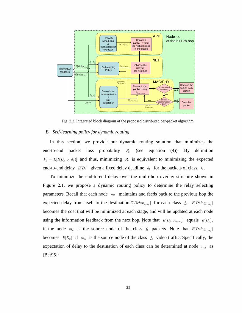
25
Fig. 2.2. Integrated block diagram of the proposed distributed per-packet algorithm.
B. Self-learning policy for dynamic routing
In this section, we provide our dynamic routing solution that minimizes the
end-to-end packet loss probability kP (see equation (4)). By definition
[ ( )]k k kP E I D d= > and thus, minimizing kP is equivalent to minimizing the expected
end-to-end delay [ ]kE D , given a fixed delay deadline kd for the packets of class kf .
To minimize the end-to-end delay over the multi-hop overlay structure shown in
Figure 2.1, we propose a dynamic routing policy to determine the relay selecting
parameters. Recall that each node hm maintains and feeds back to the previous hop the
expected delay from itself to the destination ,[ ]hk mE Delay for each class kf . ,[ ]
hk mE Delay
becomes the cost that will be minimized at each stage, and will be updated at each node
using the information feedback from the next hop. Note that ,[ ]hk mE Delay equals [ ]kE D ,
if the node hm is the source node of the class kf packets. Note that ,[ ]hk mE Delay
becomes [ ]kE D if hm is the source node of the class kf video traffic. Specifically, the
expectation of delay to the destination of each class can be determined at node hm as
[Ber95]:
Informationfeedback
Priorityscheduling
&packet header
extractor
Self-learningPolicy
Delay-drivenretransmission
&link
adaptation
Choose apacket from
the highest class in the queue
Choose therelay of
the next hop
Transmit the packet using
1, ,h hk m mθ+
Transmissionsuccess?
Reach retransmission
limit?
Remove thepacket from
queue
Drop the packet
yes
no
yesno
,,hk h mλ π
,k kd R
,k kL d
SINR
1, ,h h
goodputk m mT
+
1, ,h hk m mθ+
1, ,h h
MAXk m mγ
+
APP
NET
MAC/PHY
1, 1, hk h mβ++
Node at the h+1-th hop
hm
,[ ]hk mEDelay
1,[ ]hk mEDelay
+
*ϑ

26
1
1 1 11, 1, 1
1
, , , 1, , 1, ,, ,1
[ ] min [ ( , )] [ ]h
h h h h hh hk h mh
h
Mgoodput
k m k m k h m k h m k mk m mm
E Delay EW T E Delayβ
β β+
+ + +++ +
+
+ +=
= + ∑ , (6)
where 1,[ ]
hk mE Delay+
is given by the information feedback obtained from the nodes of the
next hop, and the relay selecting parameter 1, 1, hk h mβ
++ is chosen such that ,[ ]hk mE Delay is
minimized. ,[ ]hk mEW is the average queuing delay at the current relay queue, which can
be obtained using the priority queuing analysis introduced in Section IV. In a congested
network, equation (6) is dominated by the second term (the accumulated queuing delay in
the rest of the network). Thus, we can simplify this equation as: 1
1 1, 1, 1
1
, , , 1, ,1
[ ] [ ] min [ ]h
h h h hk h mh
h
M
k m k m k h m k m
m
E Delay EW E Delayβ
β+
+ ++ +
+
+=
= + ∑ (7)
To determine the relay selecting parameter 1, 1, hk h mβ
++ , we apply the following soft
minimum (probabilistic) policy to enable transmission across multiple paths:
1
1
, 1,,1 [ ]h
h
kk h m
k m
Coeff
E Delay ϕβκ+
+
+ =+
. (8)
kCoeff are normalized coefficients to make sure that the summation of the percentages
(fraction) equals to one:
11 , 1
1
,
1
1 [ ]hh k h
kk mm
CoeffE Delay ϕκ
++ +
−
∈
= +
∑M
, (9)
where κ and ϕ are constants. equation (8) is inspired from the balking arrival
probability in queuing theory [Kle75]. The value of κ is set depending on the arrival
rate according to [Kle75]. The term ϕ weighs the average delay 1,[ ]
hk mE Delay+
such
that the routing policy favors paths leading to significantly lower delays to the
destination. , 1k h+M represents a set of nodes 1hm + in the h+1-th hop that feedback the
information 1,[ ]
hk mE Delay+
. We set 1, 1, 0
hk h mβ++ = for the nodes whose information
feedback is not received, indicating that node 1hm + is not connected to node hm using
the overlay infrastructure [KV04]. We refer to this relay selecting policy as the
self-learning policy, since the decision of 1, 1, hk h mβ
++ will influence the future information
feedback. The complete algorithm of the proposed self-learning policy including the
information feedback is given in the Appendix of this chapter. The self-learning policy

27
will dynamically adapt the relay selection to minimize the delay through the network.
Finally, the next relay 1hm + can be determined for the packet *ϑ at the node hm
according to the percentage (time fraction) 1, 1, hk h mβ
++ .
This method is inspired by the Bellman-Ford shortest path (delay) routing algorithm
[BG87] that minimizes the end-to-end delay across the network. Our routing algorithm
reduces to the well-known Bellman-Ford algorithm when 1, 1, 1
hk h mβ++ = to the node
1hm + that feedbacks the smallest 1,[ ]
hk mE Delay+ (which can be implemented using a
large ϕ ). Note that our algorithm is prioritized and the delay of class kf will be
influenced by equal or higher priority traffic, which will be discussed in more details in
Section IV.
C. Delay-driven policy for MAC/PHY
If a node 1hm + is selected with probability 1, 1, hk h mβ
++ for the selected packet *ϑ at
each intermediate node hm , we can determine the corresponding transmission rate
1, ,h hk m mT+
and the packet error rate 1, ,h hk m mp
+ for the link by selecting
1, ,h hk m mθ+
based on
the link adaptation scheme presented in [QCS02]. To describe the channel conditions, we
assume as in [Kri02] that each wireless link is a memory-less packet erasure channel. The
link packet error rate for a fixed packet of length kL bits is
( )1 1 1, , , , , ,( , ) 1 1 ( ) k
h h h h h h
Lk m m k m m k k m mp L BERθ θ
+ + += − − , where
1, ,( )h hk m mBER θ
+ is the bit error
rate when the modulation scheme 1, ,h hk m mθ
+ is selected. Recall that the packet error rate
and the effective transmission rate (goodput) can be approximated using the sigmoid
function as in [Kri02]:
1 1, , , , ( )
1( , )
1h h h hk m m k m m k SINRp L
eζ δθ
+ + −=
+, (10)
( ) 1 1
1 1 1 11
, , , ,, , , , , , , ,, , ( )
( )1 ( , ) ( )
1 e
h h h h
h h h h h h h hh h
k m m k m mgoodputk m m k m m k k m m k m mk m m SINR
TT p L T
ζ δ
θθ θ + +
+ + + ++ − −= − =
+, (11)
where SINR is the Signal-to-Interference-Noise-Ratio, and ζ and δ are constants
corresponding to the modulation and coding schemes for a given packet length. This
method maximizes the goodput given the average packet length kL of the specific class

28
over a selected link 1( , )h hm m + based on the SINR feedback.
For a fixed 1, ,h h
goodputk m mT
+, we choose the retransmission limit
1, ,h h
MAXk m mγ
+ for the selected
packet *ϑ in the priority class kf such that the delay constraint is satisfied. Specifically,
let *, ( )
h
currh mdelay ϑ represent the current measured delay incurred by the selected packet
from the source to a current nodehm . The maximum retransmission limit for the packet
of class kf over the link from hm to 1hm + is determined based on the delay deadline
kd (where ⋅ is the floor operation) [VAH06]: ( )
1
1
*,, ,*
, ,
( )( ) 1
hh h
h h
goodput currk h mk m mMAX
k m mk
T d delay
L
ϑγ ϑ +
+
− = −
. (12)
D. Complexity analysis in terms of route selection
In this section, we compare the complexity of our proposed distributed solution with a
centralized approach.
• Complexity of a conventional centralized approach (exhaustive search)
Assume that we have a total of 1
V
vvK N
== ∑ classes across the users in an H-hop
network. Let us assume the maximum number of the intermediate nodes that can be
selected as a relay for a class kf packet at the h-th hop is ,k hC . The maximum
number of possible end-to-end paths is then ,1
Hk hh=∏ C . Thus, the total complexity (in
terms of the number of path combinations) of a centralized exhaustive search can be
up to ,1 1
K Hk hk h= =∏ ∏ C . Due to the informationally decentralized nature of the wireless
multi-hop network, the control overhead of the centralized approach can induce a
significant amount of delay (inefficient when the number of hops is large) for doing
the optimization. Hence, the distributed approach is proposed and its complexity is
also investigated.
• Complexity of the proposed distributed relay selecting algorithm
In our distributed approach, for a packet (of class kf ) at the node hm at the h-th hop,
the complexity is ,k hC (i.e. ,k hC is the number of relays that can be selected). Thus, the
complexity for the packet over the H hops is ,1
H
k hh=∑ C . Then, the total complexity by

29
considering all the different classes equals ,1 1
K H
k hk h= =∑ ∑ C .
Next, we investigate the delay analysis for the proposed distributed approach based on
priority queuing.
IV. MULTI-HOP PRIORITY QUEUING ANALYSIS FOR MULTIMEDIA TRANSMISSION
In this section, we present the analysis of the expected queuing delay ,[ ]hk mEW (that
forms ,[ ]hk mE Delay ) and packet loss probabilities , , hk h mP using queuing theory. Based on
these values, a relay will be dynamically selected. In this section, we do not consider the
effect of interference. In the next section, we extend our analysis to a network
environment where the interference is considered. Before introducing the queuing model,
several assumptions for the priority queuing analysis are made in Section IV.A. Then in
Section IV.B, we determine the end-to-end packet loss probability kP by considering a
simple 2-hop network structure (with only one set of intermediate nodes), which we refer
to as the “elementary structure”. We further extend this result by cascading the
elementary structure to create a general H -hop network (with 1H − sets of
intermediate nodes) in Section IV.C.
A. Assumptions for priority queuing analysis
The priority queuing analysis is based on the following assumptions:
1. We assume that the arrival traffic at each intermediate node is from various video
sources and is assumed to be a Poisson process. This approximation is reasonable if
the number of intermediate nodes is large enough and the selection of paths is
relatively balanced. We model the queues in the intermediate nodes as
preemptive-repeat priority M/G/1 queues [Kle75]. For our analysis, we do not apply
the non-preemptive model because when a packet with higher priority arrives at the
queue, it will interrupt future transmissions (i.e. the retransmission of the same packet
when this is lost or the transmission of a lower priority packet). The preempted packet
will be retransmitted later.

30
2. We assume the transmission rate and the packet error rate for each link are fixed in a
SI, as these are determined, as discussed in Section III, by selecting the appropriate
modulation and coding scheme using the link adaptation mechanism. As an example,
let us consider a link from node hm to node 1hm + . The selected 1, ,h hk m mθ
+
determines the physical transmission rate 1, ,h hk m mT
+(equation (11)) and packet error
rate 1, ,h hk m mp
+(equation (10)) for classkf over this link. Each packet will be
retransmitted until it is either successfully received or discarded because its delay
deadline kd was exceeded. In summary, assuming the packet length of a class kf is
fixed to be kL , with a header length HeaderL , we can formulate the service time for a
packet as a geometric distribution from these assumptions. If 1, ,h hk m mX
+ is the service
time, then the probability of there being exactly i transmissions (including
retransmissions) will be:
( )
1
1
1 1 1
, ,, ,
1, , , , , ,
Prob
1 , for 1
h h
h h
h h h h h h
k Headerk m m o
k m m
i MAXk m m k m m k m m
L LX i Time
T
p p i γ
+
+
+ + +
−
+ = × + =
− ≤ +
, (13)
where oTime denotes the time overhead including the time of waiting for the
acknowledgement, polling delay, and the expected background traffic in the
contention-based period, etc [IEE03].
3. We assume that the queue waiting time dominates the overall delay (i.e. the
transmission delay across the various network hops is relatively small).
Figure 2.3 illustrates the deployed priority queuing at each intermediate node. Given
the application layer video priorities and class characteristics, the relay selecting
parameters of the network layer, the retransmission strategy at the MAC layer, and the
modulation and coding scheme at the PHY layer, we can determine the average input rate
and the service time for the packets in a certain class, thereby obtaining a steady state
waiting time distribution for all video priority classes. In the next subsection, we analyze
the video quality problem using priority queuing analysis for our elementary structure
with only one set of intermediate nodes (a 2-hop structure).

31
Fig. 2.3. Priority queuing analysis system map.
B. Priority queuing analysis for an elementary structure
We first analyze the priority queuing model for an elementary structure. The
elementary structure is an overlay 2-hop network with V video streams and one set of
M intermediate nodes (relays) between sources and destinations, as illustrated in Figure
2.4. A packet of class kf will be routed from its source through an intermediate node m
with percentage ,k mβ toward its destination. Each intermediate node contains a queue
that schedules the waiting packets based on their header information (quality impact
parameterkλ and delay deadline kd ).
Fig. 2.4. The elementary structure.
Video stream statistics
(Network layer): Relay selecting parameter
Priority queuing
analysis at nodes
for class
Input rate analysis
Service time analysis
(MAC layer): Retransmission limit, (PHY layer): Modulation and coding scheme
kR
, ,k k kd Lλ
, , hk h mη
1, ,h hk m mX+
, , hk h mP
, , hk h mβ
1 1, , , ,,h h h hk m m k m mT p
+ +
hm kf
……
……
Video Classes m
…..
…..
1
M
...
1
V
v
......
1
V
v
1f
Kf
...
1f
kf...
Kf
...
1f
kf...
Kf
...
1f
kf...
Kf
...
, ,,k m k mT p
……
……
Video Classes m
…..
…..
1
M
...
1
V
v
......
1
V
v
......
1
V
v
1f
Kf
...
1f
kf...
Kf
...
1f
kf...
Kf
...
1f
kf...
Kf
...
1f
kf...
Kf
...
1f
kf...
Kf
...
1f
kf...
Kf
...
, ,,k m k mT p

32
From the geometric distribution assumption above, the first and second moment of the
service time at queue m are (using the approximation , 1, 1
MAXk m
k mpγ +
):
( ), 1, , , ,
,, , , , ,
ˆ ˆ1 ˆ[ ]
(1 ) (1 )
MAXk m
k m k m k m k mk m goodput
k m k m k m k m k m
L p L LE X
T p T p T
γ +−
= ≈ =− −
, (14)
2, ,2
, 2 2, ,
ˆ (1 )[ ]
(1 )
k m k mk m
k m k m
L pE X
T p
+≈
−. (15)
For a class kf , which is relayed through the intermediate node m , let ,k mL be the
effective packet “length”, which includes both the video packet length kL and the time
overhead ,o mTime (as in equation (13)). ,k mT and ,k mp are the transmission rate and
packet error rate for the packets of class kf that are transmitted through the intermediate
node m to the destination. Note that the modulation and coding strategy changes
depending on the chosen link status, and this will consequently impact2 ,k mT and ,k mp
(see equation (10), equation (11)).
Let ,k mη be the average arrival rate of the Poisson input traffic of queue m for class
kf . Given the relay selecting parameters ,k mβ , we have:
, , ,0(1 )k m k m k kR Pη β= − , (16)
where ,0 ,0( )k k kP PW d= > is the packet loss probability at the source queue due to packet
expiration and can be calculated from the queue waiting time ,0kW tail distribution for
each class.
Let ,[ ]k mEW be the average waiting time of class kf that goes through node m . For a
preemptive-priority M/G/1 queue, the priority queuing analysis gives the following result
[BG87]:
2, ,
1, 1
, , , ,1 1
[ ]
[ ]
2 1 [ ] 1 [ ]
k
i m i m
ik m k k
i m i m i m i m
i i
E X
EW
E X E X
η
η η
=−
= =
= − −
∑
∑ ∑. (17)
Based on this expected average waiting time, the probability of packet loss due to the
2 To simplify the notation, here as well as in the subsequent part of the chapter, we do not explicitly state the
dependency of the throughput, goodput, packet error rate etc. on the optimal modulation strategy chosen for that link, but assume that this is implicitly considered.

33
expiration can be calculated by the tail distribution of the waiting time:
( ), ,
1, , ,
,1
[ ]
Prob [ ] exp( )[ ]
K
i m i mKi
k m i m i mk mi
t E X
W t E XEW
η
η =
=
> ≈ −
∑∑ . (18)
In equation (18), we adopt the G/G/1 tail distribution approximation based on the work of
[JTK01][ACW95]. Let us now express this probability in terms of the packet delay
deadline kd . This probability of packet loss (at the intermediate node m ) is denoted
,k mP (recall that the waiting time is assumed to dominate the overall delay):
, , ,0Prob( [ ] )k m k m k kP W EW d= + > , (19)
where ,0[ ]kEW is the expected queuing delay of the packets at the source queue, which
depends on the number of packets of a class in one GOP. Then, the end-to-end packet loss
probability kP for class kf can be calculated as:
( ),0 , ,1
1 1 1M
k k k m k m
m
P P Pβ=
= − − − ∑ . (20)
We can observe from the above derivation that the resulting end-to-end packet loss
probability for each class kf is affected by the various cross-layer parameters (as shown
in equation (4)): the relay selecting parameters ,k mβ , the modulation and coding scheme
1, ,h hk m mθ+
that affects the average queue waiting time. Finally, the received video quality
can be estimated by substituting equation (20) into equation (1).
C. Generalization to the multi-hop case
We now extend our analysis to a general directed acyclic multi-hop overlay network
(as shown in Figure 2.1) by cascading the elementary structure. Importantly, note that the
deployed structure is very general and any multi-hop network that can be modeled as a
directed acyclic graph can be modified to fit into this overlay structure by introducing
virtual nodes [EM93]. We introduce virtual nodes with zero service time for users that
have a smaller number of hops, and fix the path for particular classes to pass through the
virtual node (by setting , , 1hk h mβ = ). Methods to construct such overlay structures given a
specific multi-hop network and a set of transmitting-receiving pairs can be found in

34
[WR03][Jan02].
The network is assumed to have H hops from sources to destinations. All the queues
in the intermediate nodes perform a preemptive-repeat priority M/G/1 model as
mentioned in the previous subsection. For the queue at node hm , let , , hk h mη be the
average arrival rate between the h-th hop and (h+1)-th hop (1 1h H≤ ≤ − ), and , 1k hP −
be the packet loss due to delay expiration from the previous hop. ,k hR is the updated
arrival rate of class kf for all the intermediate nodes between the h-th hop and (h+1)-th
hop, and we set ,0k kR R= for the source nodes. Then, the average arrival rates , , hk h mη
have the following recursive relationship:
, , 1 , 1(1 )k h k h k hR P R− −= − , (21)
, , , , ,h hk h m k h m k hRη β= . (22)
equation (21) illustrates that the video rate was reduced from hop to hop due to the packet
deadline expiration. equation (22) shows that the average input rate is distributed based
on the relay selecting parameters at the h-th hop.
Recall that , , hk h mX is the service time of the priority M/G/1 queue at node hm
between the h-th hop and (h+1)-th hop. Given the relay selecting parameters, we can
obtain the first two moments of the service time: 1
1
1 11
, , , 1,, , , ,1
ˆ[ ]
(1 )
h
h h
h h h hh
Mk
k h m k h mk m m k m mm
LE X
T pβ
+
+
+ ++
+=
≈−∑ ,
1
1
1
1 11
2, ,2
, , , 1, 2 2, , , ,1
ˆ (1 )[ ]
(1 )
h
h h
h h
h h h hh
Mk k m m
k h m k h mk m m k m mm
L pE X
T pβ
++
+
+ ++
+=
+≈
−∑ . (23)
Similarly, recall , hk mW is the queue waiting time at node hm for video class kf . Then,
the expected average value can be calculated similarly to equation (17):
2, , , ,
1, 1
, , , , , , , ,1 1
[ ]
[ ]
2 1 [ ] 1 [ ]
h h
h
h h h h
k
i h m i h m
ik m k k
i h m i h m i h m i h m
i i
E X
EW
E X E X
η
η η
=−
= =
= − −
∑
∑ ∑. (24)
Therefore, the expectation of the waiting time ,[ ]k hEW over the h-th hop for packets of
class kf is:

35
, , , ,1[ ] [ ]h
h hh
M
k h k h m k mmEW EWβ
== ∑ . (25)
The probability of packet loss due to the expiration becomes: 1
, , , ,0
1
, , , , ,0 1
, , , ,,1
Prob [ ]
[ ] [ ]
[ ] exp( )[ ]
h h
h h
h h
h
h
k h m k m k k j
j
h K
k k j i h m i h mKj i
i h m i h mk mi
P W d EW
d EW E X
E XEW
η
η
−
=
−
= =
=
= > −
− ≈ −
∑
∑ ∑∑
. (26)
Similar to equation (19), the probability of packet loss at the node m is the waiting time
tail distribution when the accumulated waiting time exceeds the delay deadline. Then, the
expected hop-by-hop packet loss probability of the hop h is:
, , , , ,1
h
h hh
M
k h k h m k h mmP Pβ
== ∑ . (27)
Recursively, we can write: 1
, 1 , 1 ,0
(1 ) (1 )H
k H k H k h kh
P R P R
−
− −=
− ⋅ = − ⋅∏ . (28)
Finally, the received video quality can be estimated by substituting equation (27) into
equation (5) and equation (1). Note that the model can be applied even for the 1-hop case,
the average waiting time at the source ,0[ ]kEW , and the packet loss probability
,0 ,0( )k k kP PW d= > can be obtained using the above equations.
V. PRIORITY QUEUING ANALYSIS CONSIDERING INTERFERENCE OF WIRELESS NETWORKS
In the Section IV, we determined the priority queuing analysis without considering the
interference of other simultaneous transmissions. This can be considered as being the
case in a network with multiple orthogonal channels for transmission. However, for
regular wireless networks, the interference is severely rooted in the broadcasting nature
of the medium. Hence, it is important to include the performance degradation due to the
interference effect. First, we introduce two matrices to describe the interference in
Section V.A. Then, in Section V.B, we present the priority queuing analysis with the
virtual-queue service time modification.
A. Incidence matrix and interference matrix
In [TG03], a rate matrix was introduced to describe the state of the network at a given

36
time. In [WCZ05], an elementary capacity graph was used to represent the physical layer
state of the various links. In [XJB04], a node-link incidence matrix was used. Here, we
assume a similar incidence matrix to describe a network with n nodes and l links. This
matrix is defined as [ ]ij n lA ×=A , where i is the nodes’ index, and j is the index of
directional links:
1 , if link flows into node
1 , if link flows out of node
0 , otherwise
ij
j i
A j i
= −
. (29)
The existence of links is determined by the SINR value, i.e. links having a SINR below a
predetermined value are not considered viable [Kri02].
Additionally, we introduce here a matrix C to characterize the interference in the
multi-hop network. Two types of interference are considered in this chapter. One type of
interference is the transmission rate decrease due to the SINR degradation. The other type
of interference, which is referred as the feasibility of simultaneous transmission links, is
from the fact that in a regular wireless network environment, a node cannot transmit and
receive data at the same time, and it cannot transmit two flows and receive two flows at
the same time due to the wireless radio limitation. First, let [ ] Tjk l lB ×= =B A A . If
0jkB > , there exists transmitter-receiver interference between link j and k. If 0jkB < ,
there exists transmitter-transmitter or receiver-receiver interference between link j and k.
If 0jkB = , there exists no second type of interference between link j and k. The
interference matrix [ ]jk l lC ×=C is defined as:
1, if 0
0, if 0
jk
jkjk
BC
B
== ≠
. (30)
Note that the interference matrix C is defined to observe the feasibility of simultaneous
transmission links. Link j and link k could transmit simultaneously if and only if 1jkC = .
Given the interference matrix C, the set zΦ = Φ represents all the combinations of
transmission links that can transmit simultaneously. A combination zΦ must satisfy the
following condition:

37
,
1z
jkj k
C∈ΦΠ = . (31)
We denote link 1( , )h h hl m m += to be the link connecting node hm with node 1hm + .
Denote the air-time fractions z
rΦ as the average time portion (a probability) for the link
combination zΦ to happen in a SI [IEE03]. Note that 1z
rΦΦ=∑ . In general, the
decision on the routing as well as the nodes participating in the video streaming session
depend largely on a number of system-related factors that transcend the video streaming
problem [AMV06] (e.g. node cooperation strategies/incentives and network coordination
and routing policies imposed by the utilized protocols). Hence, such information can be
provided by the negotiation and arbitration of the polling-based contention-free MAC
protocol statistically. We define ( ),z h
IlPRΦ as the probability that a particular combination
of links that simultaneously transmit (i.e. zΦ ) occurs, given that the link hl is
transmitting:
( ),
0, if
, if zz h
ih i
h z
Il
h z
l
l
rPRl
r
ΦΦ
Φ∈Φ
∉ Φ= ∈ Φ ∑
. (32)
B. Priority queuing with virtual-queue service time modification
Since our model has only one server per queue at each intermediate node, only one
transmission can take place at a time from the same queue. However, we still have to
avoid the case that a receiver simultaneously receives more than one packet from distinct
nodes. In fact, for a regular polling-based wireless network with a single channel, the
packets are kept in the servers while waiting for the interfering transmission to finish the
service. Hence, we assume that the servers at each intermediate node form a “virtual
queue” to the same destination [ML99]. In a virtual queue, packets of different queues
wait in turns at the servers to be transmitted to the same destination. The concept is
similar to the “service on vacation” [BG87] in queuing theory, and the waiting time of the
virtual queue can be regarded as the “vacation time”. The total sojourn time (queue
waiting time plus the transmission service time) of the virtual queue now becomes the
actual service time at each of the intermediate nodes. As the packet in the server is

38
waiting in the virtual queue, the node is able to receive packets from the previous hop.
For simplicity, we assume that the receiving process can still be approximated as a
regular Poisson process. In addition, the arrival process of the virtual queue is also
assumed to be an M/G/1 priority queue.
Let 1, hk mη +
be the average arrival rate of class k to the virtual M/G/1 queue that has
node 1hm + as its destination. Next, we denote all random variables for the virtual queues
with a tail on it.
1 1, , 1, ,h hk m k h m k hRη β
+ ++= , (33)
where ,k hR is the updated input rate after the h-th hop defined in equation (21).
Denote , ,h zk lX Φ as the service time of the priority M/G/1 queue in the node hm , when
the transmission is on the link 1( , )h h hl m m += in the combination zΦ . Both the first
moment and the second moment need to be modified, since the channel is different due
to the SINR degradation from simultaneous transmissions. 1, ,h hk m mT
+ is changed into
, ,h zk lT Φ , and 1, ,h hk m mp
+ is changed into , ,h zk lp Φ . Let , ,
ˆh zk lL Φ represent the new effective
packet length including the time overhead oTime for MAC operations similar to
equation (14). The first three moments of , ,h zk lX Φ become (assuming , 1, , 1
MAXk lh
h zk lpγ +
Φ ):
, ,, ,
, , , ,
ˆ[ ]
(1 )h z
h z
h z h z
k lk l
k l k l
LE X
T p
ΦΦ
Φ Φ
≈−
, ( )
( )
2, , , ,2
, , 22, , , ,
ˆ 1[ ]
1
h z h z
h z
h z h z
k l k lk l
k l k l
L pE X
T p
Φ ΦΦ
Φ Φ
+≈
−,
( )
( )
3 2, , , , , ,3
, , 33, , , ,
ˆ 1 4[ ]
1
h z h z h z
h z
h z h z
k l k l k lk l
k l k l
L p pE X
T p
Φ Φ ΦΦ
Φ Φ
+ +≈
−. (34)
Let 1, hk mS
+ be the service time of the virtual queue having destination node 1hm + . The
first moment of service time for class kf of this virtual M/G/1 queue can be obtained as:
1 , 1
( ), , , , , , , ,,
1 1
[ ] [ ] [ ]h h
h h h h h h zz h
h h
M MI
k m k h m k m m k h m k llm m z
E S E S PR E Xβ β+ + ΦΦ
= =
= =∑ ∑ ∑ , (35)
where 1, ,[ ]
h hk m mE S+
is the statistical average service time from intermediate node hm to
node 1hm + through all the possible transmission combinations zΦ . The second and the
third moment are similarly:
1
( )2 2, , , , ,,
1
[ ] [ ]h
h h h zz h
h
MI
k m k h m k llm z
E S PR E Xβ+ ΦΦ
=
= ∑ ∑ , 1
( )3 3, , , , ,,
1
[ ] [ ]h
h h h zz h
h
MI
k m k h m k llm z
E S PR E Xβ+ ΦΦ
=
= ∑ ∑ . (36)

39
Let random variable1, hk mW
+ be the waiting time of the virtual queue with node 1hm + as its
destination. From the Pollaczek-Khinchin formula, the first moment of 1, hk mW
+ for the
virtual queue [BG87] is:
1 1
1
1 1
2, ,
1,
, ,1
[ ]
[ ]
2 1 [ ]
h h
h
h h
k
i m i m
ik m k
i m i m
i
E S
EW
E S
η
η
+ +
+
+ +
=
=
= −
∑
∑
. (37)
Using the Takacs recurrence formula [Kle75], we have the second moment:
1 1
1 1
1 1
3, ,
2 2 1, ,
, ,1
[ ]
[ ] 2 [ ]
3 1 [ ]
h h
h h
h h
k
i m i m
ik m k m k
i m i m
i
E S
EW EW
E S
η
η
+ +
+ +
+ +
=
=
= + −
∑
∑
. (38)
The expected virtual queue waiting time 1,[ ]
hk mEW+
are the same through all the
intermediate nodes hm , since the packets eventually join the same virtual queue (to node
1hm + ). However, the sojourn time 1, ,h hk m mD
+ of the virtual queue will be different, since
the transmission time from various intermediate nodes hm to the same 1hm + are different.
The first moment and the second moment of the sojourn time are:
1 1 1, , , , ,[ ] [ ] [ ]h h h h hk m m k m k m mE D EW E S
+ + += + , (39)
1 1 1 1 1
2 2 2, , , , , , , ,[ ] [ ] 2 [ ] [ ] [ ]
h h h h h h h hk m m k m k m k m m k m mE D EW EW E S E S+ + + + +
≈ + + . (40)
Note that equation (40) is obtained by ignoring the correlation of the waiting and service
time. Finally, the service time of the priority M/G/1 queue at the intermediate nodehm can
be modified as (similar to equation (23)): 1
1 1
1
, , 1, , ,1
[ ] [ ]h
h h h h
h
M
k m k h m k m m
m
E X E Dβ+
+ +
+
+=
= ∑ , 1
1 , 1
1
2 2, , 1, ,
1
[ ] [ ]h
h h h h
h
M
k m k h m k m m
m
E X E Dβ+
+ +
+
+=
= ∑ . (41)
Let ( ), h
Ik mW be the waiting time for a packet of class kf that goes through an intermediate
node hm when the interference effect is considered:
2, ,
( ) 1, 1
, , , ,1 1
[ ]
[ ]
2 1 [ ] 1 [ ]
h h
h
h h h
k
i m i mI ik m k k
i m i m i m i m
i i
E X
EW
E X E X
η
η η
=−
= =
= − −
∑
∑ ∑
. (42)
The expectation of the waiting time over the h-th hop for packets of class kf is (as
40
equation (25)): ( ) ( )
, ,, ,1[ ] [ ]h
h hh
MI Ik h mk h k mm
EW EWβ=
= ∑ . (43)
The probability of packet loss of class kf at intermediate node hm due to the expiration
now becomes: 1
( ) ( )( ),, ,
0
1( )
, ,,0 1
, , ( )1 ,
Prob [ ]
[ ] [ ]
[ ] exp( )[ ]
hh
h h
h h
h
hI II
k m kk m k jj
h KI
k i m i mk jKj i
i m i m Ii k m
P W d EW
d EW E X
E XEW
η
η
−
=
−
= =
=
= > −
− ≈ −
∑
∑ ∑∑
. (44)
VI. CONVERGENCE DISCUSSION
Next, we show that the self-learning routing algorithm will converge to a steady-state
under certain assumptions:
Lemma: Given a set of fixed (pre-determined) outgoing relay selecting parameters
1, 1, 1 1 | 1, , 1, , hk h m h hm M k Kβ
++ + += =… … , the incoming relay selecting parameters
, , | 1, , 1, , hk h m h hm M k Kβ = =… … will converge to a steady-state, under the assumption
that the network condition is not changing over time, and given stationary statistics for
the video sources.
Proof:
Since all the 1, 1, hk h mβ
++ are fixed and the network condition is not changing, the first
two moments of the service time , ,[ ]hk h mE X and 2
, ,[ ]hk h mE X remain constant over time
(see equation (23)). Thus, the balking arrival queues converge to a steady state (see
[Kle75] for more details) having the average queue waiting times ,[ ]hk mEW . In addition,
the fixed 1, 1, hk h mβ
++ also implies that the expected delays 1,[ ]
hk mE Delay+
from the relay
1hm + (in the next hop) are fixed over time for every class of traffic. Consequently, from
equation (7), ,[ ]hk mE Delay will also converge to a steady state for every node hm (at
the current hop). This ensures that the incoming relay selecting parameters , , hk h mβ will
also have a steady-state, because they only depend on these ,[ ]hk mE Delay (see equation
(8)).

41
Theorem: The self-learning policy over an H -hop directed acyclic overlay network
will converge to a steady-state solution for the relay selecting parameters.
Proof:
Since the relay selecting parameters , , Hk H mβ at the last hop are fixed according to the
pre-determined destination node of each traffic class, the relay selecting parameters
1, 1, Hk H mβ−− will converge in time to a steady-state according to the above Lemma. Then,
starting from the last hop, the relay selecting parameters of the entire multi-hop
infrastructure will converge sequentially to a steady-state.
VII. SIMULATION RESULTS
In this section, two video sequences “Mobile”, and “Coastguard” (16 frames per
GOP at a frame rate of 30 Hz) are compressed using an embedded scalable video codec
[AMB04]. Each scalable bitstream is separated into 4 classes ( 4, 8vN K= = ). The
characteristic parameters of the video classes of the two video streams are given in Table
2.1 (see [VT07][VAH06] for more details on how to determine these parameters). In the
simulation, the packet length kL is up to 1000 bytes. No further fragmentation is
performed at the lower layers (network or MAC layer). The application playback delay
deadline is set to 0.533 seconds. We analyze the performance of our algorithms in terms
of the received video quality (PSNR) of the various users. We compare our analytical
results based on a steady-state analysis of the proposed distributed solution with the
simulation results obtained using a multi-hop overlay network test-bed [KV04].
TABLE 2.1 THE CHARACTERISTIC PARAMETERS OF THE VIDEO CLASSES OF THE TWO VIDEO SEQUENCES.
In our simulation, we captured the packet-loss pattern under different channel
conditions (described in the chapter by the link SINR) using our wireless streaming
Video Classes Video 1 “Mobile”
1668 Kbps Video 2 “Coastguard”
1500 Kbps
kf 1f 4f 6f 8f 2f 3f 5f 7f
kλ (dB/Kbps) 0.0170 0.0064 0.0042 0.0031 0.0105 0.0064 0.0048 0.0042
kR (Kbps) 556 333 334 445 500 300 300 400

42
test-bed [KV04]. In this way, we can assess the efficiency of our system under real
wireless channel conditions and link adaptation mechanisms currently deployed in
state-of-the-art 802.11a/g wireless cards with 802.11e extension. Link adaptation selects
one appropriate physical-layer mode (modulation and channel coding) depending on the
link condition, in order to continuously maximize the experienced goodput [KV04]. The
various efficiency levels are represented by varying the available time fraction for the
contention-free period in the polling-based MAC protocol, which induces the various
available transmission rates for the video packets over the links. In our elementary
structure, these network efficiency levels are represented by the transmission rate
multiplier Tm ranging from 0.3 Mbps to 0.6 Mbps. A larger transmission rate multiplier
gives a higher network efficiency.
In the analytical results, we determine the end-to-end packet loss rate based on the
average measured SINR and the average Tm obtained for each link from the test-bed over
the duration of the simulation experiments. Figure 2.5 shows the elementary structure
with the two video streams and four intermediate nodes. The analytical expected
end-to-end delays [ ]kE D of the packets in the eight classes are also shown for different
network efficiency levels. The dashed line represents the delay deadline. Once the
end-to-end delay exceeds the delay deadline, the packets in that class are dropped. Table
2.2 shows the results of the end-to-end packet loss probability for each video class using
our priority queuing approach. The almost-binary results (0 or 100%) obtained by our
packet loss analysis are due to the fact that in equation (44), we approximate , h
currk mdelay
(current delay, see equation (12)) using 1 ( ),0
[ ]h I
k jjEW
−
=∑ instead of 1 ( ),0
h Ik jj
W−
=∑ , i.e. we use
the expected waiting time instead of the exact waiting time, as this is only known
instantaneously, at each queue, during the streaming simulation. Note though that the
estimations of kP are accurate enough for the important classes, thereby leading to an
accurate video quality estimation.
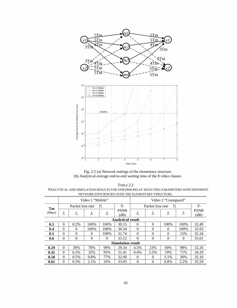
43
Fig. 2.5 (a) Network settings of the elementary structure. (b) Analytical average end-to-end waiting time of the 8 video classes.
TABLE 2.2
ANALYTICAL AND SIMULATION RESULTS FOR UNIFORM RELAY SELECTING PARAMETERS WITH DIFFERENT
NETWORK EFFICIENCIES OVER THE ELEMENTARY STRUCTURE. Video 1 “Mobile” Video 2 “Coastguard”
Packet loss rate kP Packet loss rate kP Tm
(Mbps) 1f 4f 6f 8f
Y- PSNR (dB) 2f 3f 5f 7f
Y- PSNR (dB)
Analytical result 0.3 0 8.2% 100% 100% 30.15 0 0 100% 100% 32.49 0.4 0 0 100% 100% 30.34 0 0 0 100% 33.93 0.5 0 0 0 100% 31.74 0 0 0 15% 35.34 0.6 0 0 0 0 33.12 0 0 0 0 35.61
Simulation result 0.29 0 39% 78% 99% 29.34 4.5% 23% 69% 98% 32.26 0.41 0 6.5% 32% 95% 31.41 0.4% 2.5% 19% 71% 34.29 0.50 0 0.5% 9.8% 77% 32.00 0 0 3.1% 30% 35.10 0.61 0 0.3% 2.1% 10% 33.05 0 0 0.8% 2.2% 35.59
v1
v2 v2
v1
m1
m2
m3
m4
5Tm
4Tm 5Tm
3Tm
5Tm
4Tm 5Tm
3Tm
3Tm 4Tm 5Tm 5Tm
4Tm
5Tm
3Tm
5Tm
1 2 3 4 5 6 7 810
-4
10-3
10-2
10-1
100
101
102
Video Class
Ave
rage
End
-to-
end
Wai
ting
Tim
e (s
ec)
Tm=0.3MbpsTm=0.4MbpsTm=0.5MbpsTm=0.6Mbps
deadline

44
In Figure 2.6, we consider a larger network (the 6-hop network) with the same network
settings as in Figure 2.5. By increasing the number of hops, both the average queue
waiting time and the end-to-end packet error rate increase. Comparing the results in Table
2.3 with the results in Table 2.2, the error between the analytical and simulation results
decreases, since the assumption that the waiting time dominates the overall delay is more
accurate in a larger network. The accuracy of the analysis could be further improved by
separating the video into a larger number of classes.
The results of the proposed self-learning policy are shown in Table 2.4. Note that in
Table 2.2 and Table 2.3, we use a uniform relay selection among the intermediate nodes
of each hop. The resulting primary paths are marked in bold arrows in the network plot of
Figure 2.7. We observe significant improvements in terms of end-to-end packet loss and
video qualities using the self-learning policy. Interestingly, similarly to the Bellman-Ford
algorithm, we found that this policy tries to transmit the two video streams over distinct
paths in order to limit the effect of interference and congestion among the flows.

45
Fig. 2.6. (a) Network settings of the 6-hop overlay network (by cascading the elementary structure).
(b) Analytical average end-to-end waiting time of the 8 video classes.
TABLE 2.3 ANALYTICAL AND SIMULATION RESULTS FOR UNIFORM RELAY SELECTING PARAMETERS WITH DIFFERENT
NETWORK EFFICIENCIES OVER THE 6-HOP NETWORK. Video 1 “Mobile” Video 2 “Coastguard”
Packet loss rate kP Packet loss rate kP Tm (Mbps) 1f 4f 6f 8f
Y- PSNR (dB) 2f 3f 5f 7f
Y- PSNR (dB)
Analytical result 0.3 0 100% 100% 100% 28.20 0 0.3% 100% 100% 32.48 0.4 0 0 100% 100% 30.34 0 0 0.4% 100% 33.92 0.5 0 0 0.1% 100% 31.74 0 0 0 100% 33.93 0.6 0 0 0 1% 33.12 0 0 0 0.1% 35.61
Simulation result 0.30 0 75% 97% 100% 28.39 7.7% 42% 88% 100% 31.86 0.39 0 21% 65% 99% 30.21 0.1% 11% 38% 93% 33.56 0.51 0 3.4% 12% 92% 31.35 0 1.6% 12% 64% 33.88 0.60 0 0 1.1% 39% 32.85 0 0 0.4% 10% 35.58
1 2 3 4 5 6 7 810
-4
10-3
10-2
10-1
100
101
102
Video Classes
Ave
rage
End
-to-
end
Wai
ting
Tim
e (s
ec)
Tm=0.3MbpsTm=0.4MbpsTm=0.5MbpsTm=0.6Mbps
deadline

46
Fig. 2.7. (a) Primary paths of the 6-hop overlay network using self-learning policy.
(b) Analytical average end-to-end waiting time of the 8 video classes.
TABLE 2.4 ANALYTICAL AND SIMULATION RESULTS FOR SELF-LEARNING POLICY RELAY SELECTING
PARAMETERS WITH DIFFERENT NETWORK EFFICIENCIES (THE ANALYTICAL RESULTS ARE APPROXIMATED
ACCORDING TO THE PRIMARY PATH SELECTED BY THE SELF-LEARNING POLICY).
Video 1 “Mobile” Video 2 “Coastguard”
Packet loss rate kP Packet loss rate kP Tm (Mbps) 1f 4f 6f 8f
Y- PSNR (dB) 2f 3f 5f 7f
Y- PSNR (dB)
Analytical result 0.3 0 0 100% 100% 30.34 0 0 100% 100% 32.49 0.4 0 0 0 100% 31.74 0 0 0 100% 33.93 0.5 0 0 0 0 33.12 0 0 0 0 35.61 0.6 0 0 0 0 33.12 0 0 0 0 35.61
Simulation result 0.31 0.4% 21% 53% 83% 30.42 0 8.3% 35% 66% 33.27 0.42 0 0 7.3% 48% 32.53 0 0 0.5% 14% 35.23 0.50 0 0 0 3.3% 33.10 0 0 0 1.2% 35.61 0.60 0 0 0 0 33.10 0 0 0 0 35.61
Primary Path
5Tm
5Tm 5Tm
5Tm
5Tm
5Tm
1 2 3 4 5 6 7 810
-4
10-3
10-2
10-1
100
101
102
Video Class
Ave
rage
End
-to-
end
Wai
ting
Tim
e (s
ec)
Tm = 0.3MbpsTm = 0.4MbpsTm = 0.5MbpsTm = 0.6Mbps
deadline
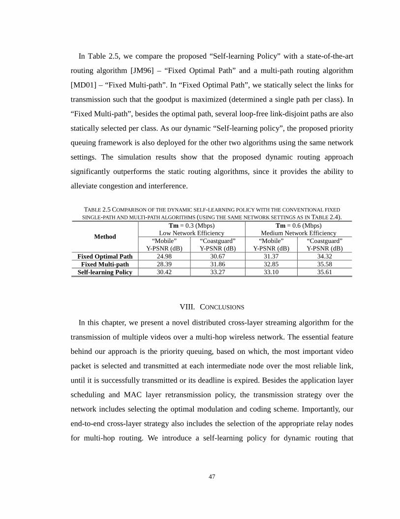
47
In Table 2.5, we compare the proposed “Self-learning Policy” with a state-of-the-art
routing algorithm [JM96] – “Fixed Optimal Path” and a multi-path routing algorithm
[MD01] – “Fixed Multi-path”. In “Fixed Optimal Path”, we statically select the links for
transmission such that the goodput is maximized (determined a single path per class). In
“Fixed Multi-path”, besides the optimal path, several loop-free link-disjoint paths are also
statically selected per class. As our dynamic “Self-learning policy”, the proposed priority
queuing framework is also deployed for the other two algorithms using the same network
settings. The simulation results show that the proposed dynamic routing approach
significantly outperforms the static routing algorithms, since it provides the ability to
alleviate congestion and interference.
TABLE 2.5 COMPARISON OF THE DYNAMIC SELF-LEARNING POLICY WITH THE CONVENTIONAL FIXED
SINGLE-PATH AND MULTI-PATH ALGORITHMS (USING THE SAME NETWORK SETTINGS AS IN TABLE 2.4). Tm = 0.3 (Mbps)
Low Network Efficiency Tm = 0.6 (Mbps)
Medium Network Efficiency Method “Mobile”
Y-PSNR (dB) “Coastguard” Y-PSNR (dB)
“Mobile” Y-PSNR (dB)
“Coastguard” Y-PSNR (dB)
Fixed Optimal Path 24.98 30.67 31.37 34.32 Fixed Multi-path 28.39 31.86 32.85 35.58
Self-learning Policy 30.42 33.27 33.10 35.61
VIII. CONCLUSIONS
In this chapter, we present a novel distributed cross-layer streaming algorithm for the
transmission of multiple videos over a multi-hop wireless network. The essential feature
behind our approach is the priority queuing, based on which, the most important video
packet is selected and transmitted at each intermediate node over the most reliable link,
until it is successfully transmitted or its deadline is expired. Besides the application layer
scheduling and MAC layer retransmission policy, the transmission strategy over the
network includes selecting the optimal modulation and coding scheme. Importantly, our
end-to-end cross-layer strategy also includes the selection of the appropriate relay nodes
for multi-hop routing. We introduce a self-learning policy for dynamic routing that

48
minimizes the end-to-end packet loss for each class of the video streams. The end-to-end
packet loss probabilities are estimated given the information feedback from the nodes of
the next hops. The proposed distributed algorithm is fully adaptive to changes in the
network, number of users, priorities of the users.
IX. APPENDIX
Algorithm 3.1 The Self-learning Algorithm
1. Initialization: Set , , hk h mβ as uniform distribution at each node of each hop
2. For each service interval 3. For each priority class 4. For hop h +1 (0 1h H≤ ≤ − ) at each node hm
5. Receive the 1,[ ]
hk mE Delay+
from all the nodes 1hm + at the end of this hop.
6. Determine 1, 1, hk h mβ
++ using the equation (3.8) and (3.9).
7. Estimate the ,[ ]hk mEW using equation (3.42).
8. Feedback to the nodes 1hm − of the previous hop h with ,[ ]hk mE Delay using equation (3.7).
9. Send packets according to 1, 1, hk h mβ
++ .
49
Chapter 3
Autonomic Decision Making for Transmitting Delay-Sensitive Applications Based on Markov
Decision Process
I. INTRODUCTION
Autonomic wireless networks are composed of autonomic wireless nodes (also
interchangeably referred to as agents in this chapter) endowed with the capability of
individually sensing the network environment, online learning the dynamic network
changes based on their local information, and promptly adapting their transmission
actions in an autonomous manner to optimize the utility of the applications which they
are serving. The dynamic network changes include variations in network topology,
wireless channel conditions, application requirements, etc.. When these network
dynamics occur, the autonomic nodes can self-configure themselves and immediately
react to these changes, without the need of propagating messages back and forth to a
centralized coordinator. Autonomic wireless networks are especially suitable for
delay-sensitive applications, since the autonomic behavior allows the wireless nodes to
promptly discover local network changes and instantaneously react to these changes, such
that the important data packets they are relaying will arrive at their destinations within
their predetermined delay deadlines. Moreover, autonomic wireless nodes endowed with
online learning capabilities can successfully model the network dynamics and
foresightedly adapt their packet transmission to maximize the utility of the
delay-sensitive applications.
In this chapter, we investigate how these agents in the multi-hop network optimize

50
their cross-layer transmission decisions to support delay-sensitive applications. There are
several challenges for optimizing the performance of the delay-sensitive applications in
such a context. First, optimizing the cross-layer strategies in a decentralized manner, by
each node, presents its own challenges. In the multi-hop network, a node’s decision
impacts and is impacted by the decisions of the neighboring nodes. We refer to this
coupling among the decision making performed by agents as the spatial dependency
among the multi-hop network’s nodes. To solve this coupling efficiently, we need to
determine the required information exchange among the agents and computing the
agents’ associated utility impact due to the information exchange. Various research
efforts have been devoted to optimally solving such spatial dependencies in the literature,
e.g. [KMT98][SV07a][XCR08]. The second challenge occurs when considering the
multi-hop network dynamics, e.g. time-variant wireless channel conditions, application
requirements. However, many existing solutions that consider the spatial dependency
ignore the dynamic nature of the networks. They react to experienced network dynamics
in a “myopic” way by optimizing the transmission decisions based only on the
information about the current network dynamics and application requirements. In the
dynamic multi-hop network, however, the agents need to adopt “foresighted” adaptation
by considering not only the immediate network status, but also how the network
dynamics evolve over time, in order to make optimal cross-layer transmission decisions.
Importantly, in addition to the spatial dependency, agents need also to consider the
temporal dependency among their sequential decisions (performed over time), since their
current decisions will also impact the information exchange in the future. By considering
both the spatial and temporal dependency, an agent can evaluate the immediate and future
expected delay and determines its optimal transmission action through real-time
adaptation.
The delay-sensitive applications require the network to support various transmission
priorities, security, robustness requirements, and stringent transmission delay deadlines
51
[TL08][GFX01]. In this chapter, we focus on minimizing the network delays of the
delay-sensitive applications, and rely on other literatures (such as [GFX01][HN08]) for
the security and reliability requirements of the delay-sensitive applications.
In the multi-hop network, the cross-layer transmission decisions, especially the route
selection, cannot be determined selfishly by the autonomic nodes. In [RT02], the authors
show that the performance degradation is unavoidable if the agents do not maximize the
network utility (minimizing the overall network delays) in a cooperative manner. To
maximize the overall performance of the applications, a Network Utility Maximization
(NUM) framework has been introduced for determining the optimal transmission actions
at various layers, see e.g. [KMT98][Low03][XCR08]. It has been shown that by allowing
users to cooperatively exchange information, they can determine their transmission
actions such that a Pareto-efficient solution can be reached in a distributed manner.
However, such solutions only consider the spatial dependency among the agents, but do
not address the dynamic nature (and hence, the temporal dependency) of the multi-hop
network. In [NMR05][GJ07], dynamic routing policies based on queuing backpressure
are proposed, which ensure that the expected delay is bounded for the delay-sensitive
applications as long as the transmission rates are inside the capacity region of the network.
However, computing the capacity region requires a high computational complexity
[TG03] and, moreover, does not guarantee that the required delay constraints of the
delay-sensitive applications are met.
Note that the network dynamics may not be known a priori in practice. Reinforcement
learning solutions have been proposed for the nodes to learn the network dynamics and
optimize the performance in routing [BL94][DCC05] and admission control [TB00]
solutions at runtime. However, these solutions do not minimize the delays of the
delay-sensitive applications. Moreover, the majority of these solutions focus on
model-free reinforcement learning approaches, which are not suitable for the
delay-sensitive applications due to their slow convergence rates [TO98].

52
In summary, there is no integrated framework that considers the spatio-temporal
dependency among the agents in the multi-hop network to minimize the network delays
of the delay-sensitive applications, based on application priorities, packet-based delay
deadlines, and the network dynamics. In this paper, we provide a systematic framework
based on which agents can optimize their cross-layer transmission actions and minimize
the delays of the delay-sensitive applications, while considering the spatio-temporal
dependencies among their actions. We assume that all the source and relay nodes are able
to make their own cross-layer transmission decisions, which are the packet-based
scheduling decisions in the application layer, the routing decisions in the network layer
and the modulation and coding scheme decisions in the physical layer, based on their
local information exchanges with their neighboring nodes. We propose that each agent
models the queuing delay using a preemptive-repeat priority M/G/1 queuing model
[SV07a] and models the network state transition over time, using maximum-likelihood
state transition probabilities [BBS95]. Using these models, the agents are able to forecast
the future network status and optimize their cross-layer transmission actions using a
Markov Decision Process (MDP) [Put94]. Based on the MDP, the agents are able to
perform foresighted decision making that considers the multi-hop network dynamics. The
role of the network designer becomes in this case the careful development of policies
such that the agents autonomously work towards minimizing the overall delays of the
delay-sensitive applications. In this chapter, we assume that agents minimize the
discounted sum of expected end-to-end delays of the delay-sensitive applications, which
is referred to in this chapter as the MDP delay value.
In summary, the chapter makes the following contributions:
1) Distributed MDP framework that considers the spatio-temporal dependency. To
account for the dynamic nature of the multi-hop network, we construct an MDP
framework which minimizes the MDP delay values of the delay-sensitive applications. To
address the informationally-decentralized nature of the multi-hop network, we further

53
decompose the MDP formulation into a distributed MDP, such that each agent in the
multi-hop network can deploy its own cross-layer transmission policy based on only local
information exchanges with its neighboring agents. We investigate the required local
information exchange among the agents in multi-hop network and prove that the
distributed MDP converges to the same optimal policy as the centralized MDP.
2) Model-based online learning approach to solve the distributed MDP. In practice, it
is not known a priori to the agents how the network dynamics change over time. We
propose an online model-based learning approach for the agents in multi-hop network to
solve the distributed MDP in real-time. Unlike the conventional model-free reinforcement
learning approaches for solving MDPs, the proposed model-based learning algorithm
takes advantage of the priority queuing model to solve the distributed MDP, and provides
a faster convergence rate and shorter delays for the delay-sensitive applications. The
upper and lower bounds of the resulting MDP delay value are provided to verify the
accuracy of the proposed model-based online learning approach at different network
locations. Moreover, we compare the proposed model-based reinforcement learning
approaches [BBS95][TO98] with the model-free reinforcement learning approaches
[WD92][Sut88] in terms of delay performance, computational complexity, and the
required information exchange overheads.
This chapter is organized as follows. In Section II, we discuss the network settings and
the cross-layer transmission actions of the autonomic wireless nodes in multi-hop
wireless networks, and formulate the autonomic decision making problem in the
multi-hop network. In Section III, we discuss the MDP framework for solving the
problem and study how to decompose the MDP into a distributed MDP to make the
framework suitable for an autonomic wireless network. In Section IV, we propose a
model-based online learning approach for the autonomic wireless nodes to implement the
distributed MDP. Section V provides simulation results. Section VI concludes the chapter.
54
II. AUTONOMIC DECISION MAKING PROBLEM FORMULATION
A. Delay-sensitive application characteristics
Unlike most cross-layer design chapters that consider only a single application, we
assume that there are multiple sources transmitting simultaneously delay-critical
information over the multi-hop network. Let iV=V represent the set of the
delay-sensitive applications. Each application has a certain number of packets to be
transmitted. We assume that the packets of an application iV are prioritized into iK
priority classes. The total number of the priority classes in the network is 1 ii
K K=
= ∑V .
Let , 1,..., kC k K= represent all the priority classes in the network. A priority class kC
is characterized by the following four parameters , , , k k k kD R Lλ :
kλ represents the impact factor of the class kC packets, which shows how critical
the packets are among the delay-sensitive applications. We prioritize the packets of
the delay-sensitive applications based on the impact factors. In the subsequent part
of the chapter, we label the K classes (across all applications) in descending order
of their priorities, i.e. 1 2 ... Kλ λ λ≥ ≥ ≥ .
kD represents the delay deadline of the packet class. A packet of a delay-sensitive
application is useful only if it is received at the destination before its delay deadline.
kR represents the average source rate of the packets in class kC . Based on the
source rate, the source node generates a certain number of packets per unit time,
which impacts the traffic load of the multi-hop network.
kL represents the average packet length of the packets in class kC . The length of a
packet directly impacts the packet error rate and the transmission rate of sending a
class kC packet.
As discussed in the introduction, we assume that the multi-hop network consists of
autonomic wireless nodes that make their own transmission decisions to transmit
delay-sensitive packets in different priority classes. Next, we discuss the settings of the
multi-hop network.

55
B. Autonomic multi-hop network settings
The multi-hop network is represented by a network graph ( , , )V M EG , where
1 ,..., m m= MM represents the set of agents and 1 ,..., e e= EE represents a set of
edges (transmission links) that connect the various agents. There are two types of agents
defined in this chapter:
Autonomic Source Agents (ASs). Each AS generates a delay-sensitive application
and would like to transmit the application to a predetermined destination node. The
ASs packetize their applications and only determine their own cross-layer
transmission actions to the next relays without specifying the cross-layer
transmission actions for the relays on the entire transmission paths until the
destinations.
Autonomic Relay Agents (ARs). ARs relay the packets from the AS to the
corresponding destination node. Unlike the ASs, the ARs do not generate their own
traffic. They make their cross-layer transmission decisions and forward the packets
for the ASs.
To enable us to better discuss the various networking solutions, we label the agents using
the same directed acyclic graph as shown in Figure 2.1, which consists of H hops from
the ASs to the destination nodes. Each agent at the h-th hop will be tagged with a distinct
number hm (1 h hm M≤ ≤ ). Let h ⊆M M represent the set of agents at the h-th hop.
The agent hm processes a priority queue and it can only transmit the packets in the
queue to a subset of ARs in 1h+M . Through periodic information exchange (e.g. hello
message exchange in [PB94]), we assume that each agent hm knows the existence of its
neighboring nodes (i.e. the other agents 'h hm ∈ M in the same hop and the agents
1 1h hm + +∈ M in the next hop), as well as the interference matrix of the current hop that
defines whether or not any of two different links 1( , )h hm m + can transmit simultaneously.

56
C. Actions of the autonomic wireless nodes
An agent’s cross-layer transmission action varies when transmitting different priority
class traffic. Denote , , h hm k m kA A C= ∀ as the cross-layer transmission action of agent hm ,
where 1 1, , , , , , 1 1 , , , ,
h h h h h h hk m k m k m m k m m h h k mA mπ β θ+ + + += ∈ ∈M A represents the action of
agent hm when sending packets in class kC . , hk mA represents the set of feasible actions
for the agent hm . In this chapter, we assume that the cross-layer transmission action
includes the application layer packet scheduling , hk mπ of transmitting packets in class
kC , the network layer relay selection parameter 1, ,h hk m mβ
+, which determines the
probability of selecting a node 1 1h hm + +∈ M in the next hop as the next relay, and
1, ,h hk m mθ+
represents the modulation and coding scheme chosen at the physical layer for
transmission over the link 1( , )h hm m + . The modulation and coding scheme determines the
packet error rate and the transmission rate when transmitting packets in class kC (see
Section III.A for more details). Denote , hm hA m= ∀ ∈A M as the actions of all the
agents in the multi-hop network. Note that the delay ( )kDelay A of packets in class kC is
a function of all agents’ actions.
D. Problem formulation
In this subsection, we discuss how to determine the cross-layer transmission decisions
for transmitting the delay-sensitive applications over the multi-hop network.
- Centralized decision making
The majority of the cross-layer design chapters assume that a central controller collects
all the network information and make transmission decisions for all the agents in the
multi-hop network, e.g. in [SYZ05]. The centralized optimization can be performed as a
rate-constrained optimization:
( ) argmax (1 ( , ))
s.t. [ (1 ( , )), ] i k i
optk k k
V C V
k k k
R P
R P C CR
λ∈ ∈
= −
− ∀ ∈
∑ ∑A
V
A A
A
G G
G
, (1)
where CR represents the capacity region of the network [TG03], and
( , ) Prob( ( , ) )k k kP Delay D= >A AG G represents the packet loss probability of class kC

57
traffic due to the delay deadline expiration. However, the above optimization is very
complicated in a multi-hop network (especially the computation of the capacity region).
Alternatively, delay-constrained optimization [CF06][SV07b] that minimize the
expected delay starting from the highest priority class to the lowest priority class traffic
are considered. Specifically, let ,[ , ]hk k m hA m= ∀ ∈A M
1 represent the actions of all the
agents sending class kC traffic. The following delay constrained optimization are
considered:
1 1 1 1
1 1
( ,..., , ) argmin [ ( , ,..., , )]
s.t. ( , ,..., , )k
suboptk k k kk
k k k k
E Delay
Delay D
− −
−
=
≤
AA A A A A A
A A A
G G
G. (2)
Based on the above equation, the actions for transmitting the priority class kC traffic can
be computed after the actions for the higher priority classes 1 1 ,..., k−A A are determined
and the action kA will not affect any of the actions for 1 1 ,..., k−A A . An advantage of
such delay-driven approach in equation (2) is that the optimization only needs to be done
for the higher priority classes, in which the delay constraints are satisfied. The packets
should be simply dropped for the lower priority classes. In addition, another advantage is
that the optimization can be decomposed into a fully distributed manner (as shown in the
previous chapter) that does not require the global information G to be gathered at a
central controller.
- Distributed decision making for the agent hm
Denote hm
L as the local information gathered by the agent hm . The agent hm can
minimize the expected delay for the highest priority class kC in its queue using the
following optimization:
,
, ,,
, , ,
( ) argmin [ ( , )]
s.t. ( , )
h h h hhk mh
h h h h
optm k m k m mk m
A
PASSk m k m m k k m
A E Delay A
Delay A D Delay
=
≤ −
L L
L
, (3)
1 The action 1 1, , , , , 1 1 , ,
h h h h hk m k m m k m m h hA mβ θ+ + + += ∈ M hereafter does not include the application layer
scheduling, since the greedy algorithm has selected the highest priority packet to be transmitted. To simplify the notation, we use the same notation for the cross-layer transmission actions and assume that the class kC is the highest priority class existing in the queue
of the agent hm when taking the action , hk mA .

58
where , h
PASSk mDelay represents the delay that has already passed when the class kC packet
arrives at the agent hm , which is encapsulated in the packet header.
, ,[ ( , )]h h hk m k m mE Delay A L represents the expected delay from hm to the destination node of
the class kC traffic. Figure 3.1 (a) illustrates how such a conventional distributed
decision making works. First, the agent evaluate utility (the expected delay
, ,[ ( , )]h h hk m k m mE Delay A L in this chapter) based on local information
hmL . Then, the agent
determines the transmission action using equation (3). The required local information
hmL for computing , ,[ ( , )]
h h hk m k m mE Delay A L will be discussed later in Section III.B.
Fig. 3.1 (a) Conventional distributed decision making of an agent.
(b) Proposed foresighted decision making of an agent.
However, due to the dynamic nature of the multi-hop network, the network dynamics
and hence, the local information is changing over time, it is important for the agents to
(a)
(b)
input rate, SINR
Utility evaluation
Determine transmission
action
Gather local information
Futureutility
evaluation
Gather local Information
State
Determine transmission
action
Agent
input rate, SINR
Wirelessnetworks
(other agents)
Wirelessnetworks
(other agents)
(a)
(b)
input rate, SINR
Utility evaluation
Determine transmission
action
Gather local information
Futureutility
evaluation
Gather local Information
State
Determine transmission
action
Agent
input rate, SINR
Wirelessnetworks
(other agents)
Wirelessnetworks
(other agents)
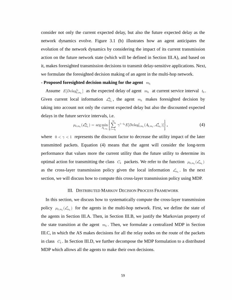
59
consider not only the current expected delay, but also the future expected delay as the
network dynamics evolve. Figure 3.1 (b) illustrates how an agent anticipates the
evolution of the network dynamics by considering the impact of its current transmission
action on the future network state (which will be defined in Section III.A), and based on
it, makes foresighted transmission decisions to transmit delay-sensitive applications. Next,
we formulate the foresighted decision making of an agent in the multi-hop network.
- Proposed foresighted decision making for the agent hm
Assume 0,[ ]
h
tk mE Delay as the expected delay of agent hm at current service interval 0t .
Given current local information 0h
tmL , the agent hm makes foresighted decision by
taking into account not only the current expected delay but also the discounted expected
delays in the future service intervals, i.e.
0 0
,0
, , ,( ) argmin [ ( , )]h h h h h
k mh
t t t t tk m m k m k m m
At t
E Delay Aµ γ
∞−
=
= ∑L L , (4)
where 0 1γ< < represents the discount factor to decrease the utility impact of the later
transmitted packets. Equation (4) means that the agent will consider the long-term
performance that values more the current utility than the future utility to determine its
optimal action for transmitting the class kC packets. We refer to the function , ( )h hk m mµ L
as the cross-layer transmission policy given the local information hm
L . In the next
section, we will discuss how to compute this cross-layer transmission policy using MDP.
III. DISTRIBUTED MARKOV DECISION PROCESS FRAMEWORK
In this section, we discuss how to systematically compute the cross-layer transmission
policy , ( )h hk m mµ L for the agents in the multi-hop network. First, we define the state of
the agents in Section III.A. Then, in Section III.B, we justify the Markovian property of
the state transition at the agent hm . Then, we formulate a centralized MDP in Section
III.C, in which the AS makes decisions for all the relay nodes on the route of the packets
in class kC . In Section III.D, we further decompose the MDP formulation to a distributed
MDP which allows all the agents to make their own decisions.
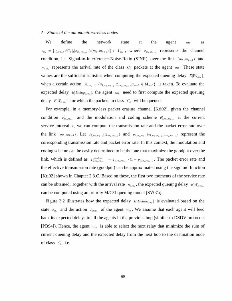
60
A. States of the autonomic wireless nodes
We define the network state at the agent hm as
1, , 1[ , ],[ , ( , )]h h h h hm k m k m m h h ms C x m mη
+ += ∀ ∀ ∈ X , where 1,h hm mx
+ represents the channel
condition, i.e. Signal-to-Interference-Noise-Ratio (SINR), over the link 1( , )h hm m + and
, hk mη represents the arrival rate of the class kC packets at the agent hm . These state
values are the sufficient statistics when computing the expected queuing delay ,[ ]hk mEW ,
when a certain action 1 1, , , , , 1 1 , ,
h h h h hk m k m m k m m h hA mβ θ+ + + += ∈ M is taken. To evaluate the
expected delay ,[ ]hk mE Delay , the agent hm need to first compute the expected queuing
delay ,[ ]hk mEW for which the packets in class kC will be queued.
For example, in a memory-less packet erasure channel [Kri02], given the channel
condition 1,h h
tm mx
+ and the modulation and coding scheme
1, ,h h
tk m mθ
+ at the current
service interval t , we can compute the transmission rate and the packet error rate over
the link 1( , )h hm m + . Let 1 1, , , ,( )
h h h hk m m k m mT θ+ +
and 1 1 1, , , , ,( , )
h h h h h hk m m k m m m mp xθ+ + +
represent the
corresponding transmission rate and packet error rate. In this context, the modulation and
coding scheme can be easily determined to be the one that maximize the goodput over the
link, which is defined as 1, ,h h
goodputk m mT
+
1 1, , , ,(1 )h h h hk m m k m mT p
+ += ⋅ − . The packet error rate and
the effective transmission rate (goodput) can be approximated using the sigmoid function
[Kri02] shown in Chapter 2.3.C. Based on these, the first two moments of the service rate
can be obtained. Together with the arrival rate , hk mη , the expected queuing delay ,[ ]hk mEW
can be computed using an priority M/G/1 queuing model [SV07a].
Figure 3.2 illustrates how the expected delay ,[ ]hk mE Delay is evaluated based on the
state hm
s and the action , hk mA of the agent hm . We assume that each agent will feed
back its expected delays to all the agents in the previous hop (similar to DSDV protocols
[PB94]). Hence, the agent hm is able to select the next relay that minimize the sum of
current queuing delay and the expected delay from the next hop to the destination node
of class kC , i.e.

61
' ' '
1 1 1
1
, , , ,'
, , , ,
[ ( , )] [ ( , )]
= [ ( , )] [ ( , )]
h h h h h h
h h h h h h
H
k m k m m k m k m m
h h
k m k m m k m k m m
E Delay A EW A
EW A E Delay A+ + +
−
=
=
+
∑L L
L L
. (5)
Importantly, the agent hm ’s transmission action will impact the information feedback
1,[ ]hk mE Delay+
, since it will select the next relay 1 1h hm + +∈ M that feeds back different
expected delay values. Moreover, the expected delay ,[ ]hk mE Delay will be fed back to the
agents in the previous hop and hence impact their transmission actions. Hence, the agent
hm ’s action , hk mA will affect its own future state hm
s and also will influence the future
expected delay as the network dynamics evolve. We denote the probability that the agent
hm has a state 1h
tms+ in service interval 1t + as 1( )
h
tmp s + , which is modeled as a function
of agent hm ’s current state h
tms and current action , h
tk mA , i.e.
11
,ˆ( ) ( , )th h hmh
t t tm m k ms
p s s A++ ≅ F . (6)
Note that the real 1( )h
tmp s + can be very complicated in a real network, since it is
impacted by the decisions of all the agents in the previous hop as well as the interference
among the agents in the current hop. Note that in our solution, the agents do not need to
know the exact form of 1( )h
tmp s + . Online learning approaches will be discussed in Section
IV for the agents to learn the state transition function in equation (6). Next, we formulate
the cross-layer optimization of the agent hm as an MDP for each class.
Fig. 3.2. Expected delay evaluation and the required local information.
State
Queuingdelay
analysis
Evaluateexpected
delay
Information feedbackfrom the next hop
Service timeanalysis
,[ ]hk mE Delay
,[ ]hk mEW, hk mη
1,h hm mx+
,[ ]hk mE X
1, 1 1 [ ], , hk m h h kE Delay m C+ + +∀ ∈ ∀M
Determinetransmission
decision
Packettransmission
hms
1 1, , , ,,h h h hk m m k m mβ θ
+ +
, hk mA
, hk mA
Local information hm
L
State
Queuingdelay
analysis
Evaluateexpected
delay
Information feedbackfrom the next hop
Service timeanalysis
,[ ]hk mE Delay
,[ ]hk mEW, hk mη
1,h hm mx+
,[ ]hk mE X
1, 1 1 [ ], , hk m h h kE Delay m C+ + +∀ ∈ ∀M
Determinetransmission
decision
Packettransmission
hms
1 1, , , ,,h h h hk m m k m mβ θ
+ +
, hk mA
, hk mA
Local information hm
LLocal information hm
L
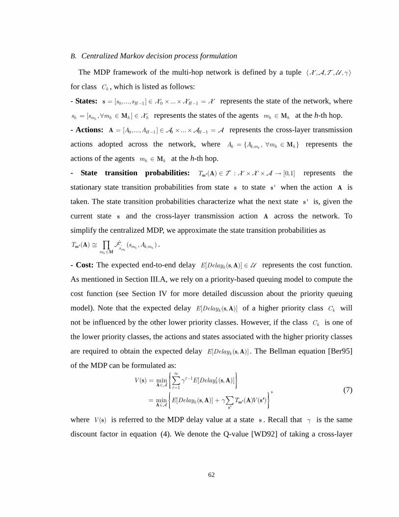
62
B. Centralized Markov decision process formulation
The MDP framework of the multi-hop network is defined by a tuple , , , ,γX A T U
for class kC , which is listed as follows:
- States: 0 1 0 1[ ,..., ] ...H Hs s − −= ∈ × × =s X X X represents the state of the network, where
[ , ]hh m h h hs s m= ∀ ∈ ∈M X represents the states of the agents h hm ∈ M at the h-th hop.
- Actions: 0 1 0 1[ ,..., ] ...H HA A − −= ∈ × × =A A A A represents the cross-layer transmission
actions adopted across the network, where , , hh k m h hA A m= ∀ ∈ M represents the
actions of the agents h hm ∈ M at the h-th hop.
- State transition probabilities: ( ) : [0,1]T ∈ × × →ss' A T X X A represents the
stationary state transition probabilities from state s to state 's when the action A is
taken. The state transition probabilities characterize what the next state 's is, given the
current state s and the cross-layer transmission action A across the network. To
simplify the centralized MDP, we approximate the state transition probabilities as
' ,ˆ( ) ( , )
h hmhh
m k msm
T s A∈
≅ ∏ss'
M
A F .
- Cost: The expected end-to-end delay [ ( , )]kE Delay ∈s A U represents the cost function.
As mentioned in Section III.A, we rely on a priority-based queuing model to compute the
cost function (see Section IV for more detailed discussion about the priority queuing
model). Note that the expected delay [ ( , )]kE Delay s A of a higher priority class kC will
not be influenced by the other lower priority classes. However, if the class kC is one of
the lower priority classes, the actions and states associated with the higher priority classes
are required to obtain the expected delay [ ( , )]kE Delay s A . The Bellman equation [Ber95]
of the MDP can be formulated as:
1
1
( ) min [ ( , )]
min [ ( , )] ( ) ( )
t tk
t
k
V E Delay
E Delay T V
γ
γ
∞−
∈=
∈
= = +
∑
∑
A
ss'A
s'
s s A
s A A s'
A
A
, (7)
where ( )V s is referred to the MDP delay value at a state s . Recall that γ is the same
discount factor in equation (4). We denote the Q-value [WD92] of taking a cross-layer

63
transmission action A at the state s as ( , ) [ ( , )] ( ) ( ')kQ E Delay T Vγ= + ∑ ss'
s'
s A s A A s . We
define the centralized stationary policy as: ( ) argmin ( , )c
k Q∈
=A
s s AA
µ . (8)
The Bellman equation in equation (7) can be solved using the value iteration or policy
iteration in [Ber95], if the [ ( , )]kE Delay s A and ( )Tss' A are accurately obtained. However,
it is difficult to obtain these two values in a centralized manner. This is because the
central controller cannot gather the global information in real-time to evaluate
[ ( , )]kE Delay s A due to the resulting delays and overheads in the multi-hop network when
propagating information back and forth throughout the network. To overcome this
challenge, we decompose the MDP in Section III.C, which allow all the agents to make
their own cross-layer transmission decisions based on local information to overcome this
problem. Moreover, in the distributed multi-hop network, the state transition probabilities
( )Tss' A may not be known a priori. To address this challenge, we will discuss an online
learning approach to allow each agent to learn the state transition probabilities in the
multi-hop network in Section IV.
C. Distributed Markov decision process formulation
Denote ,,( ) [ ]
h
b t th k mhF m E Delay= as the feedback information from node hm to the
agents in the previous hop and let , ,[ ( ), ]b t b th h hh hF F m m= ∈ M represents the feedback
information in the h-th hop. Denote ,, ,( ) ,
h h
f t PASSh k m k mhF m Delay η= as the feedforward
information from node hm to the selected AR in the next hop and let
, ,[ ( ), ]f t f th h hh hF F m m= ∈ M represents the feedforward information in the h-th hop. Given
the feedforward information ,1
f thF − , the agent hm computes the average delay , 1
PASSk hDelay −
of passing through the previous hops as 1 1
11
,, 1 ,1
h h
hh
M k mPASS PASSk h k mm
k
Delay DelayR
η− −
−−
− == ∑ . (9)
If , 1PASSk hDelay − exceeds the delay deadline kD , the packet in class kC should be dropped
and no MDP is needed for class kC traffic at the agent hm . Figure 3.3 shows the
considered system diagram for the distributed MDP that allows the agents to exchange

64
information with the nodes in the neighboring hops. The agents in the same hop take
transmission decisions simultaneously2.
Fig. 3.3 Proposed decentralized Markov decision process framework and the necessary information
exchange among the agents.
Distributed MDP at hm to 1hm + , 1,..., 1h H= −
Step 1. Gather local information. From the information feedforward ,1
f thF − from the
previous hop, the agent hm computes , 1PASSk hDelay − and determine whether the distributed
MDP should be performed for class kC traffic. Then, gathers the local information
h
tmL
1, 1 1, [ ], h hm k m h hs E Delay m
+ + += ∀ ∈ M
Step 2. Evaluate queuing delay and state transition probabilities. Based on state hm
s
and action hm
A the agent hm evaluates ,[ ]h
tk mEW . The state transition probabilities is
computed using 1 ,ˆ( ) ( , )tm m h h hh h mh
t ts s m m k msT A s A+=' F in equation (6).
Step 3. Update the transmission policy. The agent hm updates the MDP delay value:
2 The transmission actions of the agents in the same hop interfere with each others and such interference is considered in the state
through SINR 1,h h
tm mx
+.
Futureutility
evaluation
DistributedMDP
Local Information
State
Determine transmission
action h hm ∈ M
Decisionprocessof agents
Futureutility
evaluation
DistributedMDP
Local Information
State
Determine transmission
action 1 1h hm − −∈ M
Decisionprocessof agents
1fhF −
bhF1
bhF −
fhF2
fhF −
1hms
− hms
( )hkh msµ
11( )hkh msµ−−
Markovian statetransition
Markovian statetransition
Futureutility
evaluation
DistributedMDP
Local Information
State
Determine transmission
action h hm ∈ M
Decisionprocessof agents
Futureutility
evaluation
DistributedMDP
Local Information
State
Determine transmission
action 1 1h hm − −∈ M
Decisionprocessof agents
1fhF −
bhF1
bhF −
fhF2
fhF −
1hms
− hms
( )hkh msµ
11( )hkh msµ−−
Futureutility
evaluation
DistributedMDP
Local Information
State
Determine transmission
action h hm ∈ M
Decisionprocessof agents
Futureutility
evaluation
DistributedMDP
Local Information
State
Local Information
State
Determine transmission
action h hm ∈ M
Decisionprocessof agents h hm ∈ M
Decisionprocessof agents
Futureutility
evaluation
DistributedMDP
Local Information
State
Local Information
State
Determine transmission
action 1 1h hm − −∈ M
Decisionprocessof agents
1fhF −
bhF1
bhF −
fhF2
fhF −
1hms
− hms
( )hkh msµ
11( )hkh msµ−−
Markovian statetransition
Markovian statetransition
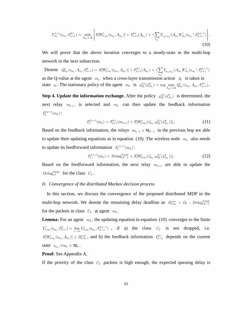
65
, , , 11,1 1 1( , ) min [ ( , )] ( ) ( ) ( ', )
h h h h h h m m h h hh hm hh
mh
b t b t b tt t tm m k m m m m s s m m mh h h
As
V s F EW s A F A T A V s Fγ −++ + +∈
= + +
∑ '
'A
.
(10)
We will prove that the above iteration converges to a steady-state in the multi-hop
network in the next subsection.
Denote , , 11 , 1 1( , , ) [ ( , )] ( ) ( ) ( ', )
h h h h h h h m m h h hh h
mh
b t b tt b t tm m m h k m m m m s s m m mh h
s
Q s A F EW s A F A T A V s Fγ −+ + += + + ∑ '
'
as the Q-value at the agent hm when a cross-layer transmission action hA is taken in state hs . The stationary policy of the agent hm is , ,
1( ) arg min ( , , )h h h h
m hh
d t b tt tm m m mkh h
AQ s A Fµ +∈
=A
L .
Step 4. Update the information exchange. After the policy , ( )h
d t tmkhµ L is determined, the
next relay 1hm + is selected and hm can then update the feedback information
, 1( )b thhF m+ :
, 1 , ,1 ,1( ) ( ) [ ( , ( ))]
h h h
b t b t d tt t th h k m m mh h khF m F m EW s µ+
++= + L , (11)
Based on the feedback information, the relays 1 1h hm − −∈ M in the previous hop are able
to update their updating equations as in equation (10). The wireless node hm also needs
to update its feedforward information , 1( )f thhF m+ :
, 1 ,, 1 ,( ) [ ( , ( ))]
h h h
f t d tPASS t t th k h k m m mh khF m Delay EW s µ+
−= + L . (12)
Based on the feedforward information, the next relay 1hm + are able to update the
,PASSk hDelay for the class kC .
D. Convergence of the distributed Markov decision process
In this section, we discuss the convergence of the proposed distributed MDP in the
multi-hop network. We denote the remaining delay deadline as , , 1h
rem PASSk m k k hD D Delay −= −
for the packets in class kC at agent hm .
Lemma: For an agent hm , the updating equation in equation (10) converges to the finite
, 1*, 1 , 1( , ) lim ( , )
h h h h
b tb tk m m h k m m h
tV s F V s F −
+ +→∞= , if a) the class kC is not dropped, i.e.
, ,[ ( , )]h h h h
t remk m m m k mEW s A D≤ , and b) the feedback information , 1
b thF + depends on the current
state ,hm h hs m∀ ∈ M .
Proof: See Appendix A.
If the priority of the class kC packets is high enough, the expected queuing delay is
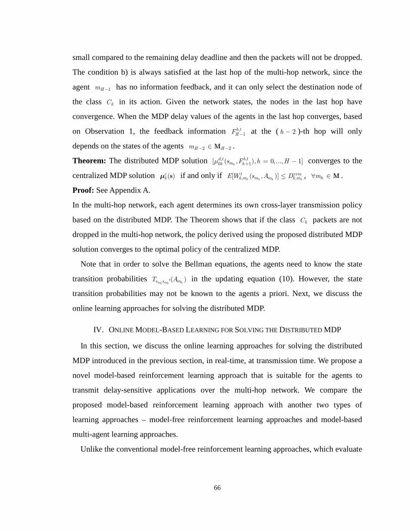
66
small compared to the remaining delay deadline and then the packets will not be dropped.
The condition b) is always satisfied at the last hop of the multi-hop network, since the
agent 1Hm − has no information feedback, and it can only select the destination node of
the class kC in its action. Given the network states, the nodes in the last hop have
convergence. When the MDP delay values of the agents in the last hop converges, based
on Observation 1, the feedback information , 1b tHF − at the ( 2h − )-th hop will only
depends on the states of the agents 2 2H Hm − −∈ M .
Theorem: The distributed MDP solution , ,1[ ( , ), 0,..., 1]
h
d t b tmkh hs F h Hµ + = − converges to the
centralized MDP solution ( )ck sµ if and only if , ,[ ( , )]
h h h h
t remk m m m k mEW s A D≤ , hm∀ ∈ M .
Proof: See Appendix A.
In the multi-hop network, each agent determines its own cross-layer transmission policy
based on the distributed MDP. The Theorem shows that if the class kC packets are not
dropped in the multi-hop network, the policy derived using the proposed distributed MDP
solution converges to the optimal policy of the centralized MDP.
Note that in order to solve the Bellman equations, the agents need to know the state
transition probabilities ( )m m hh hs s mT A' in the updating equation (10). However, the state
transition probabilities may not be known to the agents a priori. Next, we discuss the
online learning approaches for solving the distributed MDP.
IV. ONLINE MODEL-BASED LEARNING FOR SOLVING THE DISTRIBUTED MDP
In this section, we discuss the online learning approaches for solving the distributed
MDP introduced in the previous section, in real-time, at transmission time. We propose a
novel model-based reinforcement learning approach that is suitable for the agents to
transmit delay-sensitive applications over the multi-hop network. We compare the
proposed model-based reinforcement learning approach with another two types of
learning approaches – model-free reinforcement learning approaches and model-based
multi-agent learning approaches.
Unlike the conventional model-free reinforcement learning approaches, which evaluate

67
the optimal cross-layer transmission policy [ , 0,..., 1]dkh h Hµ = − without an explicit cost
model and state transition model, the proposed model-based reinforcement learning
approach adopts the priority queuing model ,[ ( , )]h h hk m m mEW s A for the cost and estimates
the state transition probabilities ( )m m hh hs s mT A' to solve the distributed MDP. Although the
computational complexity is high, we show that the proposed model-based learning
methods converge faster than the model-free learning approaches, since it takes less time
for the autonomic node to explore different states and correctly evaluate the Q values.
Such results are also discussed in [TO98] for more general learning settings. Compared to
the model-based multi-agent learning approaches, which directly model the behaviors of
the neighboring agents, the proposed model-based reinforcement learning approach
requires significantly smaller information exchange overheads, since an agent only needs
to model its own cost and state transition. Figure 3.4 provides a system block diagram of
the proposed online learning approach at the agent hm .
Fig. 3.4. System diagram of the proposed model-based online learning approach at the agent hm .
localInformation
Select an actionaccording to the
policy
Wirelessnetwork
Informationexchange
Packet transmission
Model the state
transition probability hm
A
Solve the modifiedBellman equation
Expected queuing delay estimation Autonomic node
hm
hmA
,[ ]hk mEW
'ˆh hs sT d
ikµ
1 1, fbh hF F+ −
, fbh hF F
hs
hmA

68
A. Model-free reinforcement learning
The model-free learning methods, e.g. Q-leaning [WD92] and TD-learning [Sut88],
can be applied at an agent hm to learn the next Q values 1[ ( , ), ]h h h h h
tm m m m mQ s A s+ ∀ ∈ X
without characterizing the state transition probabilities ( )h h hT As s ' . Taking Q-learning as an
example, given the feedback value , 1b thF + , the autonomic node hm updates the Q-value
using the following updating equation:
,1 1, 1( , ) (1 ) ( , ) ( ) min ( , )
h h h h h h h h h h hmh
b tt t t t t t tm m m t m m m t k m m m m mh
AQ s A Q s A Cost F A Q s Aρ ρ γ+ +
+= − + + + , (13)
where 0 1tρ< < represents the learning rate, and ttρ = ∞∑ and ( )
2ttρ < ∞∑ are
ensured for the convergence of the Q-value [WD92]. The , h
tk mCost represents the local
experienced cost (current queuing delay of sending packets in class kC ) and 1h
tms+
represents the next state after the agent hm takes the cross-layer transmission action
h
tmA . For exploration purposes, instead of following the optimal stationary policy
, ( ) arg min ( , )h h h h
m hh
d t tm m m mkh
As Q s Aµ
∈=
A, the next action is selected according to a soft-min policy.
Assume that ( , )h h
tkh m ms Aπ denotes the probability for agent hm to take the action hA
given the state hs . The soft-min policy , ( ) [ ( , ), ]h h h h
d t tm kh m m m hkh s s A Aµ π= ∀ ∈ A is defined
using the Boltzmann distribution [BBS95][TO98][WD92]:
'
exp( ( , )/ )( , )
exp( ( , )/ )h h h
h h
h h hh h
tm m m tt
kh m m tm m m tA
Q s As A
Q s A
τπ
τ∀ ∈
−=
−∑ A
, (14)
where τ is the temperature parameter. A small τ provides a greater probability
difference in selecting different actions. If 0τ → , the approach reduces back to
, ( )d thkh sµ = arg min ( , )
h h
th h h
AQ s A
∈A. On the other hand, a larger τ allows the agents to explore
various actions with higher probabilities. We provide detailed steps of the model-free
reinforcement learning in Algorithm 3.1 in Appendix B. Table 3.1 summarizes the
required local information, memory complexity, and computational complexity of the
model-free reinforcement learning approaches.

69
TABLE 3.1. COMPLEXITY SUMMARY OF THE MODEL-FREE REINFORCEMENT LEARNING
Required local information , ,, 1 1 , , , ,
h h h
f t b tt t tm m k m k h hs Cost C F F− += ∀L
Transmission policy State transition
model Q-value
Memory complexity
h hm m K× ×X A Not required h hm m K× ×X A
Computational complexity ( )h hm mO KX A
In each service interval, the model-free reinforcement learning approaches need to update
the Q-values of ,h hm m ks C∀ ∈ ∀X , and for each state, 1min ( , )
h h hmh
t tm m m
AQ s A+ over
h hm mA∀ ∈ A
is calculated. Hence, the computational complexity is ( )h hm mO KX A . Note that the
dynamics in the multi-hop network may change before the updated policy converges
when using a model-free learning approach. Hence, we consider alternative model-based
reinforcement learning in the next subsection, which is more suitable for the agents in the
multi-hop network due to a faster convergence rate.
B. Model-based reinforcement learning
In this section, we propose our model-based learning approach that enables the agent
hm to directly model the expected queuing delay ,[ ( , )]h h hk m m mEW s A and estimate the
state transition probabilities ( )m m hh hs s mT A' to solve the Bellman equation through value
iteration [Ber95]. Our approach is similar to the Adaptive-RTDP in [BBS95], where
maximum-likelihood state transition probabilities are adopted. Specifically, let
ˆ ( )hm mh h
tms sT A
' denote the estimated state transition probability at the service interval t . The
Q-value 1( , )h h h
t tm m mQ s A+ is updated at the agent hm as:
1
, 1, 1
'
( , ) (1 ) ( , )
ˆ [ ( , )] ( ) min ( ) ( , )
h h h h h h
h h h h h h h hm mh hm hhmh
t t t tm m m t m m m
b tt t t t t tt k m m m m m m m mh s s
As
Q s A Q s A
EW s A F A T A Q s A
ρ
ρ γ
+
++ ∈
= − +
+ +
∑ 'A
.
(15) 1h
tms+ represents the next state after the node hm takes the cross-layer transmission action
h
tmA . We provide detailed steps of the model-based reinforcement learning in Algorithm
3.2 in Appendix B.

70
The main differences between the model-based online learning approach and
model-free learning approaches are the following:
1) We model the expected queuing delay ,[ ( , )]h h h
t tk m m mEW s A with an action
h
tmA realized
from the policy ,d tkhµ using the preemptive-repeat priority M/G/1 queuing model as in the
previous chapter:
2, ,
1, , ,1
,, , , ,
1 1
[ ]
[ ], if [ ][ ( , )]
2 1 [ ] 1 [ ]
, otherwise
h h
h h h
h h h
h h h h
k
i m i m
i remk m k m k mk k
k m m mi m i m i m i m
i i
E X
E X EW DEW s A
E X E X
η
η η
=−
= =
+ ≤ = − − ∞
∑
∑ ∑
. (16)
From equation (16), we know that if the queuing time exceeds the remaining delay
deadline , h
remk mD , the expected queuing time ,[ ]
hk mEW becomes infinite, since the packets
will be useless (no utility gain) and they will be dropped at the agent hm .
2) Instead of using the Q-value of the next state 1h
tms+ at each service interval, the
maximum-likelihood state transition probabilities are updated and used. In Algorithm 3.2,
( )hm mh h
tms sn A
' represents the observed number of times before service interval t that the
action hm
A is taken when the state was in hm
s and made a transition to 'hm
s and
'( ) ( )
m h hm mh h hm mh h
t tm ms ss
n A n A∈
= ∑s 'X represents the observed number of times before service
interval t that the action hm
A is taken when the state was in hm
s . We apply the
maximum-likelihood state-transition probabilities [BBS95] in Algorithm 3.2 to update the
state transition probabilities ( )hm mh h
tms sT A
'.
3) Unlike regular value iteration, instead of updating the value 1( , )h h h
t tm m mQ s A+ for
h hm ms∀ ∈ X , we only update the value for states in a particular set hm
B . This procedure is
similar to the asynchronous DP in [Ber98]. According to Theorem in Section III, in order
to converge to a stationary policy, the following condition must hold
1
, 11
, ,, ( )
,, , 1
h h
h m mh hhh h
k m mk kremk m remgoodput x
k mk m m
TL LD
DT eζ δ
+
++
− −≤ ⇒ ≤
+ for any possible SINR
1,h hm mx+
at the agent
hm . Hence, the set hm
B is defined as

71
1
1
1
, , ,, : ln 1 h h h
h h h h
remk m m k m
m m m mk
T Ds x
L
ξδ +
+
= ≥ − − B , (17)
which depends on the physical layer parameters δ and ξ of the agent hm . We only
update the Q-values of the states h hm ms ∈ B in Algorithm 3.2. The rest of the states
h hm ms ∉ B have insufficient SINR values to keep the transmission time within the
remaining delay deadline , h
remk mD . Based on equation (16), these states will have an infinite
queuing delay and hence, they should never be selected as the next state. Table 3.2
summarizes the required local information, memory complexity, and computational
complexity of the proposed model-based reinforcement learning approach.
TABLE 3.2. COMPLEXITY SUMMARY OF THE MODEL-BASED REINFORCEMENT LEARNING
Required local information
, ,1 1 , ,
h h
f t b tt tm m h hs F F− +=L
Transmission policy State transition Q-value Memory complexity
h hm m K× ×B A h h hm m m K× × ×B B A
h hm m K× ×B A
Computational complexity ( )2
h hm mO K B A
The proposed model-based reinforcement learning approach has higher computational
complexity than model-free reinforcement learning approaches. For the proposed
model-based reinforcement learning approach, the Q-values of ,h hm m ks C∀ ∈ ∀B need to
be updated in each service interval, and for each state over h hm mA∀ ∈ A , the last term
1'
'
ˆmin ( ) ( , )h h h hm mh hm mh h
mh
t t tm m m ms sA
s
T A Q s A+
∈∑
A in equation (15) is calculated.
Hence, the computational complexity is ( )2
h hm mO K B A . Although the computational
complexity is significantly larger, the convergence rate of the proposed model-based
reinforcement learning approach is much faster than the model-free reinforcement
learning approaches. In Section V.B, we verify the convergence through extensive
simulation results.

72
C. Upper and lower bounds of the model-based learning approach
Since the maximum-likelihood state-transition probabilities ˆ ( )m m hh h
ts s mT A' are used in the
proposed model-based learning approach, there is no guarantee that the resulting MDP
delay value can converge to the optimal value *, 1( , )
h h
bk m m hV s F + in equation (7). In this
subsection, we investigate the accuracy of the proposed model-based learning in terms of
the resulting MDP delay value. Let , 1, 1( , )h h
t b tk m m hV s F −
+ and , 1, 1( , )
hh
b ttmk m hV s F −
+ denote the
upper and the lower bounds of the value, respectively, using ˆ ( )m m hh h
ts s mT A' in the proposed
model-based learning approach in service interval t . We define ε as the
(1 δ− )-confidence interval of the real MDP delay value (using the unknown ( )m m hh hs s mT A'
in Section III) in service interval t , i.e.
, 1 , 1, ,1 1Prob( ( , ) ( , ) ) 1h h h h
t b t b ttk m m k m mh hV s F V s F ε δ− −
+ +− ≥ ≤ − ( 0 1δ< < ).
Proposition: There exists a (1 δ− )-confidence interval ε , such that an agent hm can
update the upper bound of value , 1, 1( , )
h h
b ttk m m hV s F −
+ using
, , , 11, ,, 1 1 1
ˆ( , ) min [ ( , )] ( ) ( ) ( ', )h h h h h h h hh m mh h
m mh hmh
b t b t b tt t t tm k m m m m m k m mk m h h hs s
As
V s F EW s A F A T A V s Fγ ε−++ + +∈
= + + +
∑ '
'A
,(18)
and update the lower bound , 1, 1( , )
h h
b ttk m m hV s F −
+ using
, , , 11, ,, 1 1 1
ˆ( , ) min [ ( , )] ( ) ( ) ( ', )h h h h h h h hh m mh h
m mh hmh
b t b t b tt t t tm k m m m m m k m mk m h h hs s
As
V s F EW s A F A T A V s Fγ ε−++ + +∈
= + + −
∑ '
'A
,(19)
and the following two conditions are satisfied:
1) ( )2
max1( ) ln
2h h
m hh
m mts m
Vn A
δ ε
=
A B, where
,
max
max
1
h
remk m
kD
Vγ
=−
represents the largest
MDP delay value, h hm mA∀ ∈ A .
2) * * *, 1 , 1 , 1( , ) ( , ) ( , )
h h h h h h
b b bk m m h k m m h k m m hV s F V s F V s F+ + +≤ ≤ with probability at least 1 2δ− .
Proof: See Appendix A.
This proposition shows that the estimated values ,1, 1( , )
hh
b ttmk m hV s F+
+ become more accurate
as ( )m hh
ts mn A becomes larger than ( )
2max1
ln2
h hm m V
δ ε
A B. Moreover, the closer the
agent hm is to the destination node, the remaining path becomes shorter and provides a

73
smaller maxV and leads to a smaller requirement on ( )m hh
ts mn A . Hence, using the same
proposed model-based learning approach to accumulate ( )m hh
ts mn A , the learning approach
provides a more accurate MDP delay value for an agent that is closer to its destination
node, which is also verified in the simulation results in Section V.D.
V. SIMULATION RESULTS
In this section, two groups of delay-sensitive applications are sent with different
priorities ( 8K = ). The characteristic parameters of these delay-sensitive applications are
given in Table 3.3. In the simulation, the packet length kL is 1000 bytes for all classes.
The application delay deadline is set to 1kD = seconds for all packets in different
classes. We analyze the performance of our cross-layer transmission policy using the
proposed distributed MDP framework in terms of the discounted end-to-end delay of the
delay-sensitive applications.
TABLE 3.3. THE CHARACTERISTIC PARAMETERS OF THE DELAY-SENSITIVE APPLICATIONS.
A. Simulation results for different network topologies
We simulate the proposed model-based reinforcement learning for solving the
distributed MDP for the delay-sensitive applications in a 6-hop multi-hop network. The
network topology is shown in Figure 3.5 (a) with two ASs and 18 active ARs. Group 1
delay-sensitive applications are sent through the AS 1m to the destination node D1 and
group 2 delay-sensitive applications are sent from the other AS to its destination node D2.
The agents are assumed to be able to select a set of modulation and coding schemes that
support a transmission rate 1T = Mbps for all the transmission links in the network
[Kri02]. Each receiver of the transmission links receives a random SINR x that results
in a packet error rate ranging from 5% to 30%. We assume that the nodes are exchanging
hello messages (as in DSDV [PB94]) with the required information exchange every 10
Group 1 delay-sensitive applications 1V Group 2 delay-sensitive applications 2V
kC 1C 4C 6C 8C 2C 3C 5C 7C
kλ 0.0170 0.0064 0.0042 0.0031 0.0105 0.0064 0.0048 0.0042
kR (Kbps) 556 333 334 445 500 300 300 400

74
ms (each service interval is 10 ms). Figure 6(b) shows the MDP delay values from the
ASs to the destination nodes for the first 120 service intervals. Only the results of the first
five priority classes are shown. The higher priority traffic has a smaller MDP delay value
,tk mV . The results of centralized optimization are analytically computed by assuming that
the global network information is known by a central controller, which is unrealistic in
practice. On the other hand, the proposed model-based reinforcement learning determines
the cross-layer transmission policy at each agent based on local information. We set
0.75γ = , which is appropriate for highly time-varying multi-hop networks (after 10
service intervals, the future is only about 5% of the cost). Note that our model-based
learning provides the MDP delay values close to the centralized optimization results,
especially for the priority classes 1 2 3, ,C C C that satisfy the condition , ,[ ]h h
remk m k mEW D≤ .
These three priority classes converge to a steady state after 40t = , since their end-to-end
delays are within the delay deadline of the applications (the required performance level is
set as 1
1
41
ktk
t
DDγ
γ
∞−
=
= =−∑ when the delay deadline of each future service interval is
considered) and no packets are dropped. The results also show that the higher priority
traffic converges faster than the lower priority traffic. This is because the queuing delay
of the lower priority class traffic is impacted by the higher priority class traffic.
Fig. 3.5 (a) 6-hop network topology (b) MDP delay values of the first five priority classes.
0 20 40 60 80 100 120 140-10
0
10
20
30
40
50
60
70
80
90
100
x-axis (m)
y-ax
is (
m)
0 20 40 60 80 100 1200
5
V1,
m1
0 20 40 60 80 100 1200
5
V2,
m2
0 20 40 60 80 100 1200
50
V3,
m2
0 20 40 60 80 100 1200
50
service interval t
V4,
m1
0 20 40 60 80 100 1200
50
V5,
m2
(a) (b)
1m
2m 2D
1D
required performance level
Model-based learningCentralized optimization
0 20 40 60 80 100 120 140-10
0
10
20
30
40
50
60
70
80
90
100
x-axis (m)
y-ax
is (
m)
0 20 40 60 80 100 1200
5
V1,
m1
0 20 40 60 80 100 1200
5
V2,
m2
0 20 40 60 80 100 1200
50
V3,
m2
0 20 40 60 80 100 1200
50
service interval t
V4,
m1
0 20 40 60 80 100 1200
50
V5,
m2
(a) (b)
1m
2m 2D
1D
0 20 40 60 80 100 120 140-10
0
10
20
30
40
50
60
70
80
90
100
x-axis (m)
y-ax
is (
m)
0 20 40 60 80 100 1200
5
V1,
m1
0 20 40 60 80 100 1200
5
V2,
m2
0 20 40 60 80 100 1200
50
V3,
m2
0 20 40 60 80 100 1200
50
service interval t
V4,
m1
0 20 40 60 80 100 1200
50
V5,
m2
(a) (b)
1m
2m 2D
1D
required performance level
Model-based learningCentralized optimizationModel-based learningCentralized optimization

75
Next, we simulate a skewed network topology that has two clusters of nodes shown in
Figure 3.6 (a). Such network topology with clusters of nodes can be common in the
multi-hop network due to landscape requirements. The network connections between the
two clusters usually form a bottleneck to transmit the delay-sensitive applications. Figure
3.6 (b) shows that the discounted end-to-end delays ,tk mV of all the priority classes
increase. Only the first two priority classes converge to the steady state results and the
convergence rates decrease in the skewed network.
Fig. 3.6 (a) 2-cluster skewed network topology (b) MDP delay values of the first five priority classes.
B. Comparisons of the learning approaches
In this subsection, we compare the proposed model-based reinforcement learning
approach with Q-learning in [WD92] (a model-free reinforcement learning approach) and
the myopic self-learning approach in the previous chapter ( 0γ = ). We adopt the same
network conditions as the previous simulations and the network topology shown in
Figure 6(a). In Figure 8, the simulation results show that the proposed model-based
reinforcement learning approach outperforms the other two learning approaches in terms
of the MDP delay values for all the priority classes. Although Q-learning has the lowest
0 20 40 60 80 100 120 140 160 180-10
0
10
20
30
40
50
60
70
80
90
x-axis (m)
y-ax
is (
m)
0 20 40 60 80 100 1200
5
V1,
m1
0 20 40 60 80 100 1200
5
V2,
m2
0 20 40 60 80 100 1200
50
V3,
m2
0 20 40 60 80 100 1200
50
V4,
m1
0 20 40 60 80 100 1200
50
service interval t
V5,
m2
(a) (b)
1m
2m
1D
2D
required performance level
Model-based learningCentralized optimization
0 20 40 60 80 100 120 140 160 180-10
0
10
20
30
40
50
60
70
80
90
x-axis (m)
y-ax
is (
m)
0 20 40 60 80 100 1200
5
V1,
m1
0 20 40 60 80 100 1200
5
V2,
m2
0 20 40 60 80 100 1200
50
V3,
m2
0 20 40 60 80 100 1200
50
V4,
m1
0 20 40 60 80 100 1200
50
service interval t
V5,
m2
(a) (b)
1m
2m
1D
2D
required performance level
0 20 40 60 80 100 120 140 160 180-10
0
10
20
30
40
50
60
70
80
90
x-axis (m)
y-ax
is (
m)
0 20 40 60 80 100 1200
5
V1,
m1
0 20 40 60 80 100 1200
5
V2,
m2
0 20 40 60 80 100 1200
50
V3,
m2
0 20 40 60 80 100 1200
50
V4,
m1
0 20 40 60 80 100 1200
50
service interval t
V5,
m2
(a) (b)
1m
2m
1D
2D
0 20 40 60 80 100 120 140 160 180-10
0
10
20
30
40
50
60
70
80
90
x-axis (m)
y-ax
is (
m)
0 20 40 60 80 100 1200
5
V1,
m1
0 20 40 60 80 100 1200
5
V2,
m2
0 20 40 60 80 100 1200
50
V3,
m2
0 20 40 60 80 100 1200
50
V4,
m1
0 20 40 60 80 100 1200
50
service interval t
V5,
m2
(a) (b)
1m
2m
1D
2D
required performance level
Model-based learningCentralized optimizationModel-based learningCentralized optimization

76
computational complexity, it has the worst performance in terms of both the MDP delay
value ,tk mV and the convergence rate. The delay of the 1C traffic converges after 20t =
for the proposed model-based learning approach and converges only after 40t = for
Q-learning approach. The convergence is not guaranteed for the lower priority class
traffic, especially for the myopic self-learning solution. Moreover, although the myopic
approach has the fastest convergence rate, it results in a worse performance than the
proposed model-based reinforcement learning approach.
Fig 3.7. Comparisons of the MDP delay values using different learning approaches.
In addition to the discounted end-to-end delays ,tk mV , we directly compare the
undiscounted expected end-to-end delays [ ]tkE Delay of the delay-sensitive applications
0 20 40 60 80 100 1200
20
40
V1,
m1
0 20 40 60 80 100 1200
20
40
V2,
m2
0 20 40 60 80 100 1200
50
V3,
m2
0 20 40 60 80 100 1200
50
100
V4,
m2
0 20 40 60 80 100 1200
50
100
service interval t
V5,
m1
Model-based learningSelf-learningQ-learning
required performance level
0 20 40 60 80 100 1200
20
40
V1,
m1
0 20 40 60 80 100 1200
20
40
V2,
m2
0 20 40 60 80 100 1200
50
V3,
m2
0 20 40 60 80 100 1200
50
100
V4,
m2
0 20 40 60 80 100 1200
50
100
service interval t
V5,
m1
Model-based learningSelf-learningQ-learning
required performance level

77
from the ASs to the destination nodes. The acceptance level for [ ]tkE Delay is 1kD = . In
Figure 3.8, the simulation results show that by using the proposed model-based learning
approach, the multi-hop network is able to support up to three delay-sensitive
applications, since the end-to-end delay must be within the delay deadline of the
applications ( [ ]tk kE Delay D≤ ), while by using the other two learning approaches, the
network can only support two delay-sensitive applications.
Fig 3.8. Comparisons of the expected end-to-end delay using different learning approaches.
Next, we simulate the expected delay of different classes in a source variation scenario,
where the AS 1m disappears right after service interval 60t = . Figure 3.9 shows the
0 20 40 60 80 100 1200
20
40
E[D
elay
1]
0 20 40 60 80 100 1200
20
40
E[D
elay
2]
0 20 40 60 80 100 1200
20
40
E[D
elay
3]
0 20 40 60 80 100 1200
20
40
E[D
elay
4]
0 20 40 60 80 100 1200
20
40
service interval t
E[D
elay
5]
Model-based learningSelf-learningQ-learning
required performance level
0 20 40 60 80 100 1200
20
40
E[D
elay
1]
0 20 40 60 80 100 1200
20
40
E[D
elay
2]
0 20 40 60 80 100 1200
20
40
E[D
elay
3]
0 20 40 60 80 100 1200
20
40
E[D
elay
4]
0 20 40 60 80 100 1200
20
40
service interval t
E[D
elay
5]
Model-based learningSelf-learningQ-learning
required performance level

78
changes of expected delays over time for different classes using various learning
approaches. Since the AS 1m is the source node of packets in classes 1 4 6 8 , , , C C C C , the
expected delays 1[ ]E Delay and 4[ ]E Delay in Figure 3.8 vanish after 60t = . We can
observe that if the Q-learning is applied, before 60t = , only class 1C from 1m can be
delivered in time ( 1 1[ ]E Delay D≤ ). However, after 60t = , the class 2C from 2m can be
supported by the multi-hop network due to the alleviation of the traffic loading. By
applying the proposed model-based learning approach, before 60t = , both class 1 2,C C
from 1m and 2m can be delivered in time, and after 60t = , not only the class 2C but
also the class 3C from 2m can be supported by the multi-hop network. This shows that
the proposed model-based learning approach increases the capability of the agents in the
multi-hop network to support more delay-sensitive applications.
Fig 3.9. Source node of packets in class 1C , 4C disappears after 60t = .
0 20 40 60 80 100 1200
20
40
E[D
elay
1]
0 20 40 60 80 100 1200
20
40
E[D
elay
2]
0 20 40 60 80 100 1200
20
40
E[D
elay
3]
0 20 40 60 80 100 1200
20
40
E[D
elay
4]
0 20 40 60 80 100 1200
20
40
service interval t
E[D
elay
5]
Model-based learningSelf-learningQ-learning
required performance level
Source node disappears
Source node disappears
0 20 40 60 80 100 1200
20
40
E[D
elay
1]
0 20 40 60 80 100 1200
20
40
E[D
elay
2]
0 20 40 60 80 100 1200
20
40
E[D
elay
3]
0 20 40 60 80 100 1200
20
40
E[D
elay
4]
0 20 40 60 80 100 1200
20
40
service interval t
E[D
elay
5]
Model-based learningSelf-learningQ-learning
required performance level
Source node disappearsSource node disappears
Source node disappearsSource node disappears
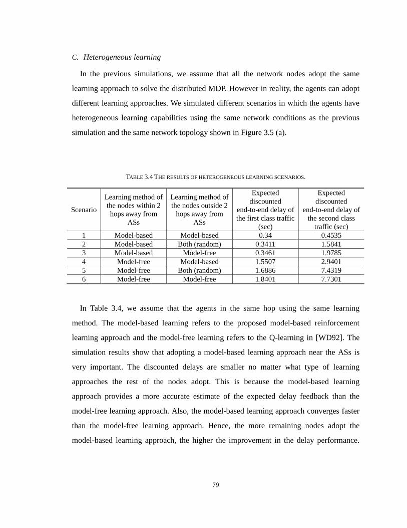
79
C. Heterogeneous learning
In the previous simulations, we assume that all the network nodes adopt the same
learning approach to solve the distributed MDP. However in reality, the agents can adopt
different learning approaches. We simulated different scenarios in which the agents have
heterogeneous learning capabilities using the same network conditions as the previous
simulation and the same network topology shown in Figure 3.5 (a).
TABLE 3.4 THE RESULTS OF HETEROGENEOUS LEARNING SCENARIOS.
In Table 3.4, we assume that the agents in the same hop using the same learning
method. The model-based learning refers to the proposed model-based reinforcement
learning approach and the model-free learning refers to the Q-learning in [WD92]. The
simulation results show that adopting a model-based learning approach near the ASs is
very important. The discounted delays are smaller no matter what type of learning
approaches the rest of the nodes adopt. This is because the model-based learning
approach provides a more accurate estimate of the expected delay feedback than the
model-free learning approach. Also, the model-based learning approach converges faster
than the model-free learning approach. Hence, the more remaining nodes adopt the
model-based learning approach, the higher the improvement in the delay performance.
Scenario
Learning method of the nodes within 2 hops away from
ASs
Learning method of the nodes outside 2
hops away from ASs
Expected discounted
end-to-end delay of the first class traffic
(sec)
Expected discounted
end-to-end delay of the second class
traffic (sec) 1 Model-based Model-based 0.34 0.4535 2 Model-based Both (random) 0.3411 1.5841 3 Model-based Model-free 0.3461 1.9785 4 Model-free Model-based 1.5507 2.9401 5 Model-free Both (random) 1.6886 7.4319 6 Model-free Model-free 1.8401 7.7301

80
Moreover, the discounted delays of the second priority class traffic vary more than the
first priority class. This shows that the learning methods adopted by the agents may not
impact the high priority delay-sensitive applications but can significantly impact the
delay-sensitive applications with low priorities. Importantly, the learning approaches also
impact the number of delay-sensitive applications supported by the multi-hop network.
D. Simulation results for the upper and the lower bounds
In this subsection, we provide simulation results to show the upper bound and the
lower bound of the model-based reinforcement learning. We adopt the same network
conditions and the 2-cluster network topology shown in Figure 3.6 (a). Figure 3.10 shows
the MDP delay values of the first priority class traffic at different hops. Since the real
delay is proven to be bounded between the upper and the lower bounds, the result shows
that the model-based reinforcement learning provides end-to-end delays that are more
and more accurate over time as well as when the agents are getting closer to the
destination nodes.
Fig. 3.10 The upper and the lower bounds of the MDP delay values for the first priority class traffic at
different hops.
0 20 40 60 80 100 120
0
2
4
V v
alue
s in
hop
1
0 20 40 60 80 100 120
0
2
4
V v
alue
s in
hop
2
0 20 40 60 80 100 120
0
2
4
service interval t
V v
alue
s in
hop
3
V value (discounted end-to-end delay)Upper bound of the V valueLower bound of the V value

81
VI. CONCLUSIONS
In this chapter, we investigate how the agents select optimal cross-layer transmission
actions in the multi-hop network to minimize the end-to-end delays of the delay-sensitive
applications. To consider both the spatial and temporal dependency in the multi-hop
network, we formulate the network delay minimization problem using MDP. We
decompose the centralized MDP into a distributed MDP framework that is suitable
delay-sensitive applications and prove that they converge asymptotically to the same
optimal policy. We propose an online model-based reinforcement learning approach for
solving the distributed MDP in practice. Unlike the model-free reinforcement learning
approaches, the proposed model-based reinforcement learning approach has a faster
convergence rate, since it takes less time for the autonomic node to explore different
states to evaluate the Q-values. Our simulation results verify that the proposed
model-based learning approach is more suitable for the autonomic nodes to support
delay-sensitive applications in the multi-hop network.
APPENDIX A
Proof of Lemma: For the higher priority class, if the condition , ,[ ]h h
remk m k mEW D≤ holds,
the packet will not be dropped in the network. Therefore, the updating equation (10) will
not be impacted by the information feedforward from the agents in the previous hops.
Based on this, we can write the updating equation (10) as a contraction mapping
,1,, 1( , , )
h hh
b tt t tm k mk m hV CM s F V+
+= . Define [ , ]hh m h hs s m= ∀ ∈ M as the states of the agents in the
h-th hop and , , hh h
t tk h k mmV V
∈= ∑ M
as the overall MDP delay value of the agents in the
h-th hop. The contraction mapping of the overall MDP delay value
, ,1, ,, 1 1( , , ) ( , , )
h hh h
b t b tt t t t tm k m h k hk h h hm
V CM s F V CM s F V++ +∈
= =∑ M can be constructed. Given that the
feedback information ,1
b thF + is a function of the current states ths , the feedback value can
then be regarded as part of the cost function. Based on this, equation (10) leads to a value
iteration update of a regular Bellman equation and hence, for hs∀ ,
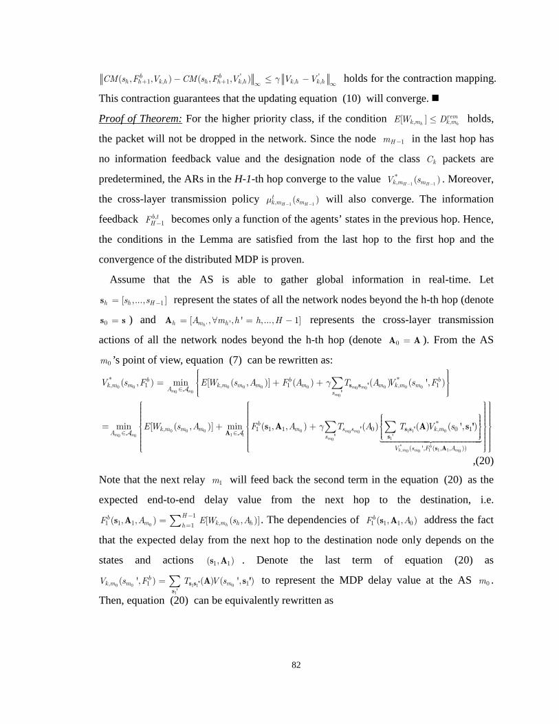
82
' '1 , 1 , , ,( , , ) ( , , )b b
h h k h h h k h k h k hCM s F V CM s F V V Vγ+ + ∞ ∞− ≤ − holds for the contraction mapping.
This contraction guarantees that the updating equation (10) will converge.
Proof of Theorem: For the higher priority class, if the condition , ,[ ]h h
remk m k mEW D≤ holds,
the packet will not be dropped in the network. Since the node 1Hm − in the last hop has
no information feedback value and the designation node of the class kC packets are
predetermined, the ARs in the H-1-th hop converge to the value 1 1
*, ( )
H Hk m mV s− −
. Moreover,
the cross-layer transmission policy 1 1, ( )
H H
tk m msµ
− − will also converge. The information
feedback ,1
b tHF − becomes only a function of the agents’ states in the previous hop. Hence,
the conditions in the Lemma are satisfied from the last hop to the first hop and the
convergence of the distributed MDP is proven.
Assume that the AS is able to gather global information in real-time. Let
1[ ,..., ]h h Hs s −=s represent the states of all the network nodes beyond the h-th hop (denote
0 =s s ) and ' '[ , , ' , ..., 1]hh m hA m h h H= ∀ = −A represents the cross-layer transmission
actions of all the network nodes beyond the h-th hop (denote 0 =A A ). From the AS
0m ’s point of view, equation (7) can be rewritten as:
0 0 0 0 0 0 0 0 00 00 0
0
0 0 0 0 1 1 00 01 10 0
1
* *, 1 , 1 , 1
*, 1 1 1 0 , 0 1
'
( , ) min [ ( , )] ( ) ( ) ( ', )
= min [ ( , )] min ( , , ) ( ) ( ) ( ', )
m mm m
m
m mm m
b b bk m m k m m m m m k m m
As
bk m m m m s s k m
A
V s F EW s A F A T A V s F
EW s A F A T A T V s
γ
γ
∈
∈ ∈
= + +
+ +
∑
∑
s s '
'
' s s 'A
s
s A A s '
A
A A0
*, 1 1 10 0 0( ', ( , , ))
m
bk m m m
s
V s F A
∑'
s A
,(20)
Note that the next relay 1m will feed back the second term in the equation (20) as the
expected end-to-end delay value from the next hop to the destination, i.e.
0
11 1 1 ,1( , , ) [ ( , )]
h
Hbm k m h hh
F A EW s A−
== ∑s A . The dependencies of 1 1 1 0( , , )bF As A address the fact
that the expected delay from the next hop to the destination node only depends on the
states and actions 1 1( , )s A . Denote the last term of equation (20) as
0 0 1 1 0
1
, 1 1'
( ', ) ( ) ( ', )bk m m mV s F T V s= ∑ s s '
s
A s ' to represent the MDP delay value at the AS 0m .
Then, equation (20) can be equivalently rewritten as

83
0 0
* *, ,( ) min [ ( , )] ( ) ( ')k m k k mV E Delay T Vγ
∈
= +
∑ ss'A
s'
s s A A sA
. (21)
We denote the Q-value of taking a cross-layer transmission action A at the state s as
0 0
*, ,( , ) [ ( , )] ( ) ( ')k m k k mQ E Delay T Vγ= + ∑ ss'
s'
s A s A A s . We define the centralized stationary
policy as 0,( ) argmin ( , )k k mQ
∈=
As s A
Aµ .
Note that for the agent hm , the cross-layer transmission policy , ( )h h
dk m msµ minimizes
' ' ' '
1
, ,' 0
[ ( , ( ))]h h h h
Ht t t d t
k m m k m m
h h t
r EW s sµ
− ∞
= =∑ ∑
' ' ' '
1
, ,0 '
[ ( , ( ))]h h h h
Ht t t d t
k m m k m m
t h h
r EW s sµ
∞ −
= =
= ∑ ∑ . Due to the principle
of the optimality [Ber95] the relay nodes selected from , ( )h h
dk m msµ must also lies on the
shortest route specified by the ( )k sµ . From equation (20), we can conclude that
' ' '
1
, ' ,0 ' 0 0
[ ( , ( ))] [ ( , ( ))]h h h h
Ht t t d t t t t t
k m m k m m k k
t h t
r EW s s r E Delayµ
∞ − ∞
= = =
=∑ ∑ ∑ s sµ . Hence, the distributed MDP
solution ,[ ( ), 0,..., 1]h h
dk m ms h Hµ = − converges to the same policy of the centralized MDP.
For the necessary condition, if the condition , ,[ ]h h
remk m k mEW D≤ does not hold for every
node in the route kσ , this results in an infinite ,[ ]hk mEW at the node hm and an infinite
feedback value , 1b thF
+ to notify the AS to reroute the packets and no convergence can be
guaranteed in this case.
Proof of Proposition: We apply Heoffding inequality [Hoe63] to obtain the confidence interval
ε , which basically states that given random variables 1 ,..., mX X in range max[0, ]X , the
inequality holds: 2
max2
1 1
1 1Prob( [ ] )
m mmX
i i
i i
X E X em m
ε
ε
−
= =
− ≥ ≤∑ ∑ . (22)
From the first condition, we have max
ln
2 ( )h h
m hh
m m
ts m
Vn A
δ
ε
− =
A B . Denote
, 1, 1
ˆ[ ( , )] ( ) ( ', )h h h h hm mh h
mh
b tt tm m m k m m hs s
s
EV s A T A V s F −+= ∑ '
'
as the average MDP delay upper bound based
on estimated ( )hm mh h
tms sT A
' evaluated whenever state
hms is visited and action
hmA is taken, and
denote , 1, 1[ ( , )] ( ) ( ', )
h h h h hm mh h
mh
b ttm m m k m m hs s
s
EV s A T A V s F −+= ∑ '
'
as the average expected MDP delay
value based on real ( )hm mh h
ms sT A'
. Similar to the proof of lemma 3.2 in [EMM03], equation (22)
can be rewritten as:

84
2
2
maxmax
ln1
2 ( )2 ( )
Prob( [ ( , )] [ ( , )] )
m mt h hs mm h th
s mm hh
h h h h
h h
n A VV n A
m m m mm m
EV s A EV s A e
δ
δε
− − − ≥ ≤ =
A B
A B.
(23)
Hence, , ,1 1, 1 , 1Prob( ( , ) ( , ) )
h hh h
b t b tt tm mk m h k m hV s F V s F ε δ+ +
+ +− ≥ ≤ for each state-action pair (the total
number of the state-action pairs is h hm mA B ). Similar proof can be applied to the lower bound.
Since ( )m hh
ts mn A in the last term of equations (18) and (19) goes to infinity as t → ∞ , we can
show that both the upper bound and the lower bound converge under the same conditions, i.e.
, ,* *, 1 , , 1 ,1 1( , ) lim ( , ) and ( , ) lim ( , )
h h h h h h h h
b t b tb t b tk m m h k m m k m m h k m mh h
t tV s F V s F V s F V s F+ ++ +→∞ →∞
= = . Due to the
symmetric structure of *, 1( , )
h h
bk m m hV s F + and *
, 1( , )h h
bk m m hV s F + , we apply the union bound as in
[EMM03] to show that the probability * *, 1 , 1Prob( ( , ) ( , ) ) 2
h h h h
b bk m m h k m m hV s F V s F ε δ+ +− ≥ ≤ and
complete the proof.

85
APPENDIX B Algorithm 3.1: Model-free reinforcement learning at node hm
Input: ,1 , b t
hF t+ ∀ , ,1 , f t
hF t− ∀ , γ , τ ; Output: , h
tk mµ , ,b t
hF , ,f thF ;
Initialization: 0, hk mµ , ,0
1bhF + , ,0
1fhF − , 0
hms ;
set 0t ← , 0, ( , ) 0, ,
h h h h h h hk m m m m m m mQ s A s A= ∀ ∈ ∀ ∈X A ;
Step 1: Verify the head of line packet class and the delay deadline. Get the class kC packet that has the highest priority in the queue, and check the packet header. If , 1
PASSk h kDelay D− > , drop the packet and repeat step 1, 1t t← + ; otherwise, go to step
2. Step 2: Select an action
h
tmA based on policy , h
tk mµ .
Randomly select the action h
tmA according to the probability distributions
,[ ( , ), ]h h h h h
t tk m m m m ms A Aπ ∀ ∈ A .
Step 3: Transmit the packet and observe the current cost , h
tk mCost and the new state 1
h
tms+
Step 4: Update the Q-value For
h hm ms∀ ∈ X , update the Q-values 1, ( , )
h hh
t tm mk mQ s A+ using equation (13).
Step 5: Update the policy For
h hm ms∀ ∈ X , update the policy 1, ( )
hh
tmk m sµ + using equation (14).
Step 6: Update the feedback values and exchange information with the neighboring nodes. Update , 1b t
hF+ and , 1f t
hF+ as in equation (11) and (12).
1t t← + ; go back to step 1.

86
Algorithm 3.2: Model-based reinforcement learning at node hm
Input: ,1 , b t
hF t+ ∀ , ,1 , f t
hF t− ∀ , γ , τ ; Output: , h
tk mµ , ,b t
hF , ,f thF ;
Initialization: 0, hk mµ , ,0
1bhF + , ,0
1fhF − , 0
hms ;
set 0t ← , 0, ( , ) 0, ,
h h h h h h hk m m m m m m mQ s A s A= ∀ ∈ ∀ ∈X A ;
Step 1: Verify the head of line packet class and the delay deadline. Get the class kC packet that has the highest priority in the queue, and check the packet
header. If , 1
PASSk h kDelay D− > , drop the packet and repeat step 1, 1t t← + ; otherwise, go to step
2. Step 2: Select an action
h
tmA based on policy , h
tk mµ .
Randomly select the action h
tmA according to the probability distributions
,[ ( , ), ]h h h h h
t tk m m m m ms A Aπ ∀ ∈ A .
Step 3: Transmit the packet, observe the new state 1h
tms+ , and update the number of state
transition. 1 1
1 ( ) ( ) 1t t t th hm m m mh h h h
t t t tm ms s s s
n A n A+ ++ = + ; 1'
( ) ( )t t th hm m mm mh h hh h
t t t tm ms s ss
n A n A+∈= ∑ X
.
1
1
( )ˆ ( )
( )
t t hm mh ht t
hm mh ht hmh
t tms st t
ms s t tms
n AT A
n A
+
+ = .
Step 4: Evaluate the local queuing delay Calculate ,[ ( , )]
h h h
t tk m m mEW s A using equation (16).
Step 5: Update the Q-value For
h hm ms∀ ∈ B , update the Q-values 1, ( , )
h hh
t tm mk mQ s A+ using equation (15).
Step 6: Update the policy For
h hm ms∀ ∈ B , update the policy 1, ( )
hh
tmk m sµ + using equation (14).
Step 7: Update the feedback values and exchange information with the neighboring nodes. Update , 1b t
hF+ and , 1f t
hF+ as in equation (11) and (12).
1t t← + ; go back to step 1.

87
Chapter 4
Adapting the Information Horizon – Risk-Aware
Scheduling for Multimedia Streaming
I. INTRODUCTION
As discussed in the previous chapter, the majority of the multimedia-centric research
focuses on a centralized optimization and optimizes the video streaming using purely
end-to-end metrics and does not consider the protection techniques available at the lower
layers of the protocol stack. Hence, they do not take advantage of the significant gains
provided by cross-layer design [SYZ05][BT05][WCZ05]. In [AMV06], an integrated
cross-layer optimization framework was proposed that considers the video quality impact
based on different information horizons. However, the proposed solution in [AMV06]
considers only the single user case, where a set of paths and transmission opportunities
are statically pre-allocated for each video application. This leads to a sub-optimal,
non-scalable solution for the multi-user case. Importantly, the overhead induced by the
various information horizons are not investigated in [AMV06], which have essential
impact for the delay-sensitive multimedia applications. To enable efficient distributed
multi-user video streaming over a wireless multi-hop infrastructure, nodes need to timely
collect and disseminate network information based on which, the various nodes can
collaboratively adapt their cross-layer transmission strategies. For instance, based on the
available information feedback, a network node can timely choose an alternate (less
congested) route for streaming the packets that have a higher contribution to the overall
distortion or a more imminent deadline.
Although the information feedback is essential to the cross-layer optimization, the cost

88
of collecting the information is seldom discussed in the literature. Due to the
informationally decentralized nature of the multi-hop wireless network, it is impractical
to assume that the global network information and the time-varying application
requirements can be relayed to the central (overlay) network manager in a timely manner.
Distributed suboptimal solutions that adapt the transmission strategies based on
well-designed localized information feedback should be adopted for the delay-sensitive
applications.
In summary, no integrated framework has been developed that explicitly considers the
impact of accurate and frequent network information feedback from various horizons,
when optimizing the resource allocation and the cross-layer transmission strategies for
multiple collaborating users streaming real-time multimedia over a wireless multi-hop
network. In this chapter, we investigate the impact of this information feedback on the
distributed cross-layer transmission strategies deployed by the multiple video users. We
assume a directed acyclic overlay network as the previous chapters that can be
superimposed over any wireless multi-hop network to convey the information feedback.
Our solution relies on the users’ agreement to collaborate by dynamically adapting the
quality of their multimedia applications to accommodate the flows/packets of other users
with a higher quality impact and/or higher probability to miss their decoding deadlines.
Unlike commercial multi-user systems, where the incentive to collaborate is minimal, we
investigate the proposed approach in an enterprise network setting where source and relay
nodes exchange accurate and trustable information about their applications and network
statistics.
To increase the number of users that can simultaneously share the same wireless
multi-hop infrastructure as well as to improve their performance given time-varying
network conditions, we deploy scalable video coding schemes [VAH06] that enable a
fine-granular adaptation to changing network conditions and a higher granularity in
assigning the packet priorities. We assume each receiving node performs polling-based

89
contention-free media access control (MAC) [IEE03] that dynamically reserves a
transmission opportunity interval in a service interval. The network topology and the
corresponding channel condition of each link are assumed to remain unchanged within
the service interval.
In this chapter, we discuss the required information/parameter exchange among
network nodes/layers for implementing a distributed solution for selecting the following
cross-layer transmission strategies at each intermediate node – the packet scheduling, and
the next-hop relay (node) selection based on routing policies similar to the Bellman-Ford
routing algorithm [BG87], and the retransmission limit at the MAC layer. In performing
the cross-layer adaptation, we explicitly consider the packet deadlines and the relative
priorities (based on the quality impact of the packets) encapsulated in the packet headers.
Each intermediate node maintains a queue of video packets from various users and
determines the cross-layer transmission strategies in a distributed fashion through the
information feedback from other intermediate nodes within a certain network horizon and
with a certain frequency. While a larger horizon/frequency can provide more accurate
network information, this also results in an increased transmission overhead that can have
a negative impact on the video performance. Hence, we aim at quantifying the video
quality benefit derived by the various users for different network conditions and video
application characteristics based on various information feedbacks.
Our chapter makes the following contributions:
• Decentralized information feedback driven cross-layer adaptation
In this chapter, we show how the various cross-layer strategies can be adapted based on
the information feedback. The solutions of centralized flow-based optimizations
[WZ02][SYZ05][AL94] have several limitations. First, the video bitstreams are changing
over time in terms of required rates, priorities and delays. Hence, it is difficult to timely
allocate the necessary bandwidths across the wireless network infrastructure to match
these time-varying application requirements. Second, the delay constraints of the various

90
packets are not explicitly considered in centralized solutions, as this information cannot
be relayed to a central resource manager in a timely manner. Third, the complexity of the
centralized approach grows exponentially with the size of the network and number of
video flows. Finally, the channel characteristics of the entire network (the capacity region
of the network) need to be known for this centralized, oracle-based optimization. This is
not practical as channel conditions are time-varying, and having accurate information
about the status of all the network links is not realistic.
Alternatively, we focus on a fully distributed packet-based solution, where timely
information feedback can efficiently drive the cross-layer adaptation for each individual
multimedia stream as well as the multi-user collaborations in sharing the wireless
infrastructure. To cope with the delay sensitivity of the video traffic, we explicitly
consider the delay deadlines of the various packets (packets are dropped whenever their
deadlines expire) and estimate the remaining transmission time based on the available
information feedback. This approach is better suited for the informationally decentralized
nature of the investigated multi-user video transmission problem over multi-hop
infrastructures.
• Impact of various information horizons/frequencies
We define the mechanism of information feedback conveyed through a multi-hop
overlay infrastructure and investigate the impact of different information
horizons/frequencies on the video quality derived by the various multimedia users. We
discuss the tradeoff between the increased transmission overhead and the benefit of larger
information horizons, which result in improved predictions of network conditions. More
information allows nodes in the network to better estimate the time for each packet to
reach its destination and hence, the chance of missing its deadline.
• Information feedback driven packet scheduling and retransmission strategies
We introduce the concept of risk estimation based on the available information
feedback that determines the probability that a packet will miss its delay deadline. Based

91
on the estimated risk and the quality impact of the video packet, we proposed novel
information feedback driven scheduling and retransmission strategies for each node in the
network.
The chapter is organized as follows. Section II defines the video and network
specification for multi-user video transmission over multi-hop wireless networks and
provides a cross-layer distributed optimization scheme based on the information feedback.
In Section III, we discuss the impact of the information feedback with different
information horizons and present an integrated cross-layer adaptation algorithm for the
real-time multi-user streaming problem. Section IV introduces a novel information
feedback driven scheduling algorithm that takes advantage of the larger information
horizons. Section V introduces our information feedback driven retransmission limit
calculation. In Section VI, we discuss the overheads of the information feedback of
various parameters. Simulation results are given in Section VII. Section VIII concludes
the chapter.
II. PROBLEM FORMULATION AND SYSTEM DESCRIPTION
We assume that V video users with distinct source and destination nodes are sharing
the same multi-hop wireless infrastructure. Similarly, we adopt an embedded 3D wavelet
codec [AMB04] as Chapter 2 and construct video classes by truncating the embedded
bitstream (see Chapter 3.II.A). Here we define that kN represents the number of packets
in the class kf in one GOP duration of the corresponding video sequence and hence,
k k kR N L= represents the rate requirement.
At the client side, the expected quality improvement for video v in one GOP can be
expressed as:
( ) ( )k
rec succv k k k k
f v
Q L N Pλ∈
= ⋅ ⋅ ⋅∑ , (1)
Here, we assume that the client implements a simple error concealment scheme, where
the lower priority packets are discarded whenever the higher priority packets are lost
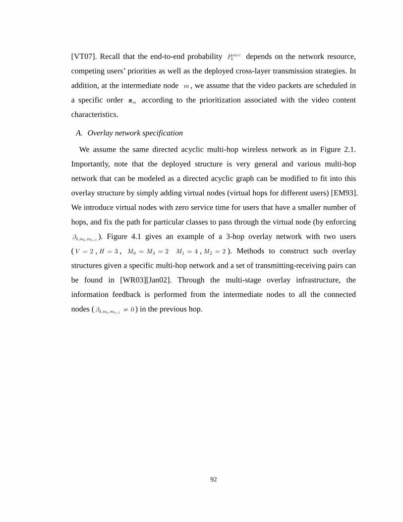
92
[VT07]. Recall that the end-to-end probability succkP depends on the network resource,
competing users’ priorities as well as the deployed cross-layer transmission strategies. In
addition, at the intermediate node m , we assume that the video packets are scheduled in
a specific order mπ according to the prioritization associated with the video content
characteristics.
A. Overlay network specification
We assume the same directed acyclic multi-hop wireless network as in Figure 2.1.
Importantly, note that the deployed structure is very general and various multi-hop
network that can be modeled as a directed acyclic graph can be modified to fit into this
overlay structure by simply adding virtual nodes (virtual hops for different users) [EM93].
We introduce virtual nodes with zero service time for users that have a smaller number of
hops, and fix the path for particular classes to pass through the virtual node (by enforcing
1, ,h hk m mβ+
). Figure 4.1 gives an example of a 3-hop overlay network with two users
( 2V = , 3H = , 0 3 2M M= = 1 4M = , 2 2M = ). Methods to construct such overlay
structures given a specific multi-hop network and a set of transmitting-receiving pairs can
be found in [WR03][Jan02]. Through the multi-stage overlay infrastructure, the
information feedback is performed from the intermediate nodes to all the connected
nodes (1, , 0
h hk m mβ+
≠ ) in the previous hop.

93
Fig. 4.1. The directed acyclic multi-hop overlay network for an exemplary wireless infrastructure. (a) Actual network topology that has 2 source-destination pairs, 5 relay nodes. (b) Overlay network
topology that has 2 source-destination pairs, 6 relay nodes (with one virtual node in the 1-hop intermediate nodes).
B. Centralized cross-layer optimization for multi-user wireless video transmission
We define hm
STR as the cross-layer transmission strategy vector for packets at the
node hm consisting of the packet scheduling policy πhm, the relay selecting parameters
1, ,h hk m mβ+
for routing, the MAC retransmission limit 1, ,h h
MAXk m mγ
+ per link, i.e.
hmSTR =
1 1, , , ,[ , , ]h h h h h
MAXm k m m k m m totβ γ
+ +∈π A . And tot APP NET MAC= × ×A A A A represents the
set including all the feasible cross-layer transmission strategy vector, where APPA is the
set of all feasible packet scheduling strategies, NETA is the set of all possible selections
of relays, and MACA is an integer set from 0 to the maximum retransmission limit
supported by the MAC protocol. Then, assuming the global information globalI is
available, the investigated multi-user wireless video transmission problem can be
S2
D1
r4
r5
r1
r2
r3
S1
D2
: Physical connections: Overlay connections
, 2, 5 , 2, 5,k S r k S rT p
, 4, 1 , 4, 1,k r D k r DT p
S2
D1
r4
r5
r1
r2
r3
S1
D2
: Physical connections: Overlay connections
S2
D1
r4
r5
r1
r2
r3
S1
D2
S2S2
D1D1
r4
r5
r1r1
r2
r3
S1
D2
: Physical connections: Overlay connections: Physical connections: Overlay connections
, 2, 5 , 2, 5,k S r k S rT p
, 4, 1 , 4, 1,k r D k r DT p
, 4, 1 , 4, 1,k r D k r DT p
S2
S1
r1
r2
r3
1rv
r4
r5
D1
D2
1-hop overlay intermediate nodes
2-hop overlay intermediate nodes
Virtual node
Source nodes Destination nodes
, 2, 5 , 2, 5,k S r k S rT p
, 4, 1 , 4, 1,k r D k r DT p
S2S2
S1S1
r1r1
r2r2
r3r3
1rv
r4r4
r5r5
D1D1
D2D2
1-hop overlay intermediate nodes
2-hop overlay intermediate nodes
Virtual node
Source nodes Destination nodes
, 2, 5 , 2, 5,k S r k S rT p
(a)
(b)

94
formulated as a centralized delay-driven cross-layer optimization:
1
1
arg max ( , )
= arg max ( , )
tot
totk
Vopt rec
v global
v
Vsucc
k k k k global
v f v
Q
L N Pλ
∈ =
∈ = ∈
= ∑
∑∑
M
M
STR
STR
STR STR
STR
A
A
I
I
, (2)
where [ | ]hm hSTR m= ∈STR M , and M represents the set of nodes at which the
transmission strategies decisions can be made for the video packets. 1
0
H
hhM
−
== ∑M is
the number of the nodes in M . Since the successfully received packets of each class kf
must have their end-to-end delay kD smaller than their corresponding delay deadline kd ,
the constraint of the optimization is ( ) , 1,..., .k kD d k K< =STR Due to the priority
queuing and the error concealment scheme, the optimal solution of equation (2) serves
the more important packets instead of transmitting as many packets as possible. Although
the centralized optimization provides optimal solution for the multi-user video streaming
problem, it suffers from the unrealistic assumption of collecting timely global
information across the multi-hop network for the delay-sensitive applications. Due to the
informationally decentralized nature of the multi-hop wireless networks, the centralized
solution is not practical for the multi-user video streaming problem. For instance, the
optimal solution depends on the delay incurred by the various packets across the hops,
which cannot be timely relayed to a central controller. Moreover, the complexity of the
centralized optimization grows exponentially with number of classes and nodes in the
network. Hence, the optimization might require a large amount of time to process and the
collected information might no longer be accurate by the time transmission decisions
need to be made.
C. Proposed distributed cross-layer adaptation based on information feedback
Instead of gathering the global information globalI , we propose a distributed
suboptimal solution that collects the local information feedback localI at the node hm
to maximize the expected quality of the various users sharing the same multi-hop
wireless infrastructure:

95
, at
arg max [ ( , )]h h h
totk h
opt succm k k k m k m local
STRf m
STR L N E P STRλ∈ ∀
= ∑A
I , (3)
where , hk mN represents the number of packets of class kf present in the queue at the
node hm .
In this chapter, we define localI with the following information feedback parameters:
• SINR , the SINR to calculate the channel conditions over each link of the overlay
network.
• , hk mP , the packet loss probability of the class kf through the intermediate node hm .
The parameter illustrates the bottleneck identification for various video classes. This
information can be used by the application layer to decide how many quality layers
are transmitted or to adapt its encoding parameters (in the case of real-time encoding)
to improve its video quality performance given the current number of users, priorities
of the competing streams and network conditions, but also, importantly, to alleviate
the network congestion.
• ,[ ]hk mE Delay , the expected delay from the intermediate node hm to the destination
node of the class kf to convey the congestion information of the network, which is
essential for the delay-sensitive applications.
Let us consider the simple example in Figure 4.2 that illustrates how information
feedback is deployed. The term information horizon will be defined in Section III. In this
example, node n1 is an intermediate node that needs to relay multiple video classes from
various users. In order for the relay n1 to determine the optimized cross-layer
transmission strategies, at least 1-hop information feedback is required. The network
status information can be disseminated at frequent intervals over the overlay
infrastructure, and it is considered to be known at the decision relay n1. However, in
certain cases, feedback information from some hops (beyond the information horizon)
may arrive with an intolerable delay, and may be unreliable due to the rapidly-changing
network conditions.

96
Fig. 4.2. Illustrative example of an application layer overlay network with information horizon 2h =
.
In this chapter, we make the following assumptions for performing the information
feedback and the delay estimation ,[ ]hk mE Delay . First, we assume a polling-based
contention-free media access (which is similar to the deployed IEEE 802.11e [IEE03]
and 802.11s [FWK06] standards) that dynamically reserves transmission opportunities
within a service interval SIt [IEE03], and the network status (such as the topology, the
transmission rate 1, ,h hk m mT
+and the packet error rate
1, ,h hk m mp+
for each link) remains
unchanged in SIt . Second, because of the retransmission in the MAC layer protection,
the effective packet transmission time can be formulated as a geometric distribution
[Kon80] with 1, ,h hk m mT
+,
1, ,h hk m mp+
, and packet length kL (as discussed in Section III.B).
Third, for simplification, the arrival of the packets at each intermediate node is regarded
as a Poisson arrival process, which is reasonable if the number of intermediate nodes is
large enough and the selection of paths is relatively balanced. Fourth, we assume that the
queue waiting time dominates the overall delay. Under these assumptions, we can
estimate the risk that packets from different priority classes will not arrive at their
Information horizon
n1
n2
n3
n4
n5
n6
n7
Hop h Hop h+1 Hop h+2
2h =
2 , 2
, 2
, ,
[ ]n k n
k n
SINR P
E Delay5 , 5
, 5
, ,
[ ]n k n
k n
SINR P
E Delay
3 , 3
, 3
, ,
[ ]n k n
k n
SINR P
E Delay
4 , 4
, 4
, ,
[ ]n k n
k n
SINR P
E Delay
6 , 6
, 6
, ,
[ ]n k n
k n
SINR P
E Delay
TX strategies:
TX strategies:
, 3, 6 , 3, 6, MAXk n n k n nβ γ
Video Sub-flowsfrom Multiple users
1 1 1 1, , ,d L Nλ
2 2 2 2, , ,d L Nλ
3 3 3 3, , ,d L Nλ
4 4 4 4, , ,d L Nλ
n8
1nπPacket scheduling, 3, 5 , 3, 5, MAXk n n k n nβ γ
: Video flows (With TX strategies): Information feedback of localI
Information horizon
n1
n2
n3
n4
n5
n6
n7n7
Hop h Hop h+1 Hop h+2
2h =
2 , 2
, 2
, ,
[ ]n k n
k n
SINR P
E Delay5 , 5
, 5
, ,
[ ]n k n
k n
SINR P
E Delay
3 , 3
, 3
, ,
[ ]n k n
k n
SINR P
E Delay
4 , 4
, 4
, ,
[ ]n k n
k n
SINR P
E Delay
6 , 6
, 6
, ,
[ ]n k n
k n
SINR P
E Delay
TX strategies:
TX strategies:
, 3, 6 , 3, 6, MAXk n n k n nβ γ
Video Sub-flowsfrom Multiple users
1 1 1 1, , ,d L Nλ1 1 1 1, , ,d L Nλ
2 2 2 2, , ,d L Nλ2 2 2 2, , ,d L Nλ
3 3 3 3, , ,d L Nλ3 3 3 3, , ,d L Nλ
4 4 4 4, , ,d L Nλ4 4 4 4, , ,d L Nλ
n8n8
1nπPacket scheduling 1nπPacket scheduling, 3, 5 , 3, 5, MAXk n n k n nβ γ
: Video flows (With TX strategies): Information feedback of localI: Video flows (With TX strategies): Information feedback of localI

97
destination before their decoding deadline expires (see Section IV for more detail). The
adaptation of πhm,
1, ,h h
MAXk m mγ
+, and the dynamic routing policies for
1, ,h hk m mβ+
can be
deployed in a distributed manner based on the information feedback. Next, we discuss the
mechanism of performing the information feedback through the directed acyclic overlay
network.
III. IMPACT OF ACCURATE NETWORK STATUS
Since the network conditions can rapidly vary in multi-hop network infrastructures,
the performance of any video streaming solution will significantly depend on the
availability of accurate network information. Three key aspects for multi-user video
streaming are influenced by the availability, accuracy and timeliness of this information
feedback.
• Decentralized decision making - network nodes can be implemented to improve their
adopted cross-layer strategies based on information feedback about the channel
conditions and regional network congestion to avoid unnecessary queuing delay and
hence, packet drops.
• Timely adaptation - information feedback enables timely adaptation to network
changes (e.g. nodes leaving or sources of interference appearing or disappearing),
which is essential for delay-sensitive multimedia transmission.
• Inter-user collaboration - based on information feedback, network resources can be
effectively managed and users are able to effectively collaborate to achieve the
desired global optimal utility. For instance, in the absence of such information, an
intermediate node may waste precious resources by allocating time to packets from
classes that will miss their deadlines, thereby preventing other classes which can
meet their delay constraint from being transmitted.
A. Information feedback frequencies and information horizon
The information feedback should be performed in a distributed (per hop) fashion that
explicitly considers the dissemination delay. We assume that the information feedback is
98
periodically transmitted to the previous hop every infot1 seconds during each SIt
( info0 SIt t< ≤ ). We define infof (1) as the frequency of the information feedback within
one hop:
infoinfo
1f (1)
t= . (4)
We also define the vector 1 2( , ,...., )Hb b b=b of the dissemination factors over the network.
Let info( )t h represent the time it takes for the information to be disseminated over h
hops:
info info( ) , where 1, for 1h ht h b t b h= × ≥ ≥ . (5)
Since the network information requires time to pass through the various hops, we have
1h hb b −> . We set 1 1b = . Because the information is conveyed hop by hop, info( )t h also
depends on the per-hop information feedback frequency infof (1) . We define infof ( )h as the
information feedback frequency when the information is conveyed over h hops in the
following way:
infoinfo
1f ( )
( ) SI h
ch
t h t b= =
×, (6)
where c is defined as infoSIt t . Since the network conditions are assumed to be
unchanged within the service interval SIt , we define the information horizon h
as the
number of hops from which the information feedback can be accurately disseminated
during SIt :
info
info
( , f (1)) maximize
subject to ( ) ,
1,..., .
SI
h h
t h t
h H
=
≤
=
b
(7)
In [AMV06][Kri02], the dissemination time for the information feedback is proportional
to the number of hops across which the information feedback is traversed, i.e.
(1,2, 3,...., 1, )p H H= −b , and if we assume that c is an integer, the relationship between h
and infof (1) becomes a linear function:
1 The time interval is not the time fraction for transmitting the information feedback in a service interval, but rather the time between two subsequent information feedbacks (which includes time for transmitting the video packet, the information feedback and also the protocol overheads).
99
info info( , f (1)) f (1)p SIh t c= × =b
. (8)
We focus on the impact of different information horizons directly on the video
qualities of multiple users sharing the same multi-hop wireless network. Note that infof (1)
can be converted into an information horizon based on equation (7), as long as the
information dissemination factors (i.e. b vector) are given. Thus, for simplicity, in the
remainder part of the chapter, we denote the information horizon info( , f (1))h b
by simply
h
. An example of 2h =
is shown in Figure 4.2. The local information feedback in
equation(3) for a larger information horizon becomes a vector
, , , 1 ,[ , , [ ] | ... , ]
h h hlocal m k m k m h k h k h hSINR P E Delay m k+ += ∈ ∪ ∪ ∀M M I , where , 1k h+M represents
a set of nodes in the h+1-th hop that feedback the information for the class kf traffic to
the decision nodes (e.g. node “n1” in the example in Figure 4.2).
B. The impact of various information horizons
With a larger information horizon, more accurate network status can be obtained,
which can be used to adapt the cross-layer transmission strategies at various layers. A
larger information horizon ensures that the information can be obtained in a timely
manner and network status can be estimated more accurately. For example, a better
routing decision can be determined to avoid the congested regions in the network. This
decreases the packet loss probability kP for each class, thus increasing the succkP for the
important classes and improving the received video qualities. However, the penalty of the
overhead is seldom jointly considered in the prior works. Let ,[ ( )]h
packetk mETime h
represent
the expected transmission time for a video packet in class kf at node hm to the next
hop with the information feedback of horizon horizonh . Based on the geometric
assumption, we can write:
( ),, 11
1
1
1 11
1
, ,, ,,
, , , ,1
1[ ( )]
1
MAXmk m hhh
h h
h hh
h h h hh
Mk m mpacket k header over
k m mk mk m m k m mm
p L LETime h Time h
p T
γ
β
+++
++ ++
+
=
− + = + − ∑
, (9)
which is calculated as an average transmission time over all the possible relays 1hm + in
the next hop. ( )overTime h
denotes the time overhead introduced by the various protocols
[IEE03] including the time of waiting for the MAC acknowledgements etc., and also the

100
information feedback. Consequently, a larger information horizon can induce larger
overheads for the packet transmission time, and hence increases the end-to-end delay kD ,
which can lead to higher packet losses kP as they can miss their deadline. In this chapter,
we assume that the time overhead is a known function of the information horizon and we
will discuss this in more detail in Section VII.
In general, the information horizon might be different for various users or classes and
also can vary per node, depending on its location, congestion level, etc. Thus, a scalable
information feedback can be implemented (e.g. the information horizon can depend on
class kf and node hm ). For instance, to reduce the overhead associated with the
information feedback, some less important classes can have smaller horizons. However,
for simplicity, the information horizon is assumed to be the same for all classes (users) in
the rest of the chapter. The topic of implementing the scalable information feedback and
the analysis of its impact form a topic of our future research.
C. Distributed cross-layer adaptation based on the information feedback with larger
information horizons
Instead of performing the exhaustive search for the distributed optimization in
equation (3), we present the following iterative cross-layer adaptation to solve the
multi-user video streaming problem. Based on the information feedback, the goal of the
distributed cross-layer adaptation is to determine an optimal packet present in the queue
(from πhm) to be transmitted through the optimal relay 1hm + (from
1, ,h hk m mβ+
) in the
next hop with the optimal retransmission limit (from 1, ,h h
MAXk m mγ
+).
1. To determine a packet of a specific class kf for transmission, the packet scheduling
policy πhm in the queue of the intermediate node hm is optimized to first transmit
the video packets with larger kλ , since they have a higher impact on the overall video
quality. With a larger information horizon, such packet scheduling can be improved as
we will discuss it in Section IV.
2. To solve the routing problem, we deploy a priority queuing approach based on the

101
information feedback and apply dynamic routing policies similar to the Bellman-Ford
routing algorithm [BG87]. We exploit the ,[ ]hk mE Delay in the local information
feedback localI . The selection of 1, ,h hk m mβ
+ is based on the
1,[ ]hk mE Delay+
value that
minimizes the end-to-end packet loss probability kP for the transmitted packet. We
will discuss the routing problem in detail in Section VI.
3. At the MAC layer, we choose the appropriate retransmission limit 1, ,h h
MAXk m mγ
+ per packet
based on the 1, ,h h
goodputk m mT
+ such that its delay constraint is satisfied. Based on our prior
results [VT07] in one-hop network, the optimal retransmission strategy is to send the
highest priority packet until it is successfully received by the next relay or until its
delay deadline expires. Specifically, let currd represent the current delay incurred by a
particular packet at the current nodehm . The maximum retransmission limit for the
packet of class kf over the link from hm to 1hm + is determined based on the delay
deadline kd (where ⋅ is the floor operation): ( )
1
1
, ,, , 1h h
h h
goodput currkk m mMAX
k m mk
T d d
Lγ +
+
− = −
. (10)
With a larger information horizon, the retransmission limit can be improved as we will
discuss it in Section V.
4. Then, we measure the SINR and estimate the corresponding ,[ ]hk mE Delay and , hk mP
for each class kf at the node hm and feed back this information to the nodes in the
previous hops within the information horizon h
.
IV. RISK-AWARE SCHEDULING FOR MULTIMEDIA STREAMING
At each intermediate node hm , in order to optimize the scheduling of the various
video packets, we determine the risk , hk mRisk ( ,0 1hk mRisk≤ ≤ ) that the packets of class
kf will miss their delay deadline, based on the probability that the estimated received
time at the destination is after their delay deadlines. Higher probabilities of packet loss
over the network (due to interference, congestion, nodes leaving etc.) will lead to higher
risks of packets missing their delay deadlines. Based on this risk, the scheduling of the

102
various packets of the different classes can be determined to ensure a maximized system
quality.
To compute the risk estimation for a packet, we need to consider both the delay
deadlines kd as well as the expected delay ,[ ]hk mE Delay in the information feedback
localI conveyed from the intermediate nodes within the information horizon h
. The
video packets at an intermediate node can be divided into three categories:
• Packets that will certainly be dropped (“dropped” packets).
• Packets that have very high probability to be dropped (“almost-dropped” packets).
• Packets that have low probability to be dropped (“seldom-dropped” packets).
“Dropped” packets are video packets with a current cumulative delay currd exceeding
their delay deadline (curr kd d> ). These packets will be dropped at the current node and
hence, there is no need to compute their risk. The “almost-dropped” packets have not yet
exceeded their delay deadline (curr kd d< ), but their current cumulative delay plus the
expected delay to reach the destination does exceed their delay deadline, i.e.
,[ ]h
currk m kd E Delay d+ > . We set the risks for these “almost-dropped” packets to be 0, as
they have a very high probability of being dropped and hence, they will unnecessarily
waste resources that could be used for the successful transmission of “seldom-dropped”
packets. The remaining video packets are “seldom-dropped” packets. Their current
cumulative delay plus the expected delay from the current node to the destination is lower
than the delay deadline, i.e. ,[ ]h
currk m kd E Delay d+ < . Hence, these packets have a high
probability of arriving at the destination on time and their scheduling needs to be
optimized to maximize the video quality across the various users. Next, we discuss how
to estimate the risk for these seldom-dropped packets.
A. Risk estimation based on priority queuing analysis
The risk estimation for the seldom dropped packets is determined based on the priority
queuing analysis, by using the approximation of the waiting time tail distribution. Let
, hk mW represent the queue waiting time for class kf at intermediate node hm . The

103
waiting time tail distribution can be approximated as [JTK01][ACW95]:
( ), ,
1, , ,
,1
[ ]
Prob [ ] exp( )[ ]
h h
h h h
h
k
i m i mki
k m i m i mk mi
E X
W t E X tEW
η
η =
=
> ≈ − ×
∑∑ , (11)
where , hk mη is the measured average input rate and ,[ ]hi mE X is the average service time
of class kf at the intermediate node hm . The expected average queue waiting time of
the priority queue is:
( )
2, ,
1, , 1
, , , ,1 1
[ ]
P rob [ ]
2 1 [ ] 1 [ ]
h h
h h
h h h h
k
i m i m
ik m k m k k
ti m i m i m i m
i i
E X
W t dt EW
E X E X
η
η η
∞=
−=−∞
= =
> = = − −
∑∫
∑ ∑. (12)
equation(12) is determined based on the Mean Value Analysis (MVA) of a
preemptive-priority M/G/1 queue [BG87]. Until now, we do not consider the interference
incurred in wireless multi-hop networks (orthogonal transmission channels are available
for adjacent wireless links), the average service time ,[ ]hk mE X is the average packet
transmission time ,[ ( )]h
packetk mETime h
in equation(9). If the influence of interference is
considered, the average service time ,[ ]hk mE X can be approximated using a virtual queue
analysis similar to the “service on vacation” concept in queuing theory [Kle75][BG87].
Using equation(11), the proposed risk estimation2 for the packets in class kf can be
computed as: I
,I
,
,
Prob( [ ]), if [ ] 0 (seldom-dropped packets)( )=
0 ,if [ ] 0 (almost-dropped packets)
=
h
h
left leftk m k k
k m leftk
i m
W Time E d E dRisk Time
E d
η
+ > > ≤
( ), ,
1 I,
,1
[ ]
[ ] exp [ ] , if [ ] 0 [ ]
0 , if
h h
h h
h
k
i m i mkleft lefti
i m k kk mi
E X
E X Time E d E dEW
E
η=
=
× − >
∑∑
[ ] 0 leftkd
≤
,
(13)
where ,[ ] [ ]h
left currk k mkE d d d E Delay= − − represents the expected time remaining after a
2 The higher risk packets should be sent earlier, since they are with high probability to exceed their deadlines. However, we do not want to waste our resources on those almost-drop packets, hence the risk estimation for these packets are set to zero.
104
packet reaches its destination. We can determine the probability that the waiting time
, hk mW plus a pre-determined time duration ITime , which is a general variable for risk
estimation, exceeds the expected time left [ ]leftkE d , and thus, that the packet will be lost.
The time duration ITime can be viewed as an extension of the waiting time for the
packet. Larger ITime values lead to higher risks. An example of the risk estimation is
given in Section IV.B. Note that the accuracy of computing the expected time left [ ]leftkE d
increases with a larger information horizon. Thus, the I, ( , )hk mRisk Time h
also depends on
the information horizon h
and can be better estimated given a larger h
.
B. Feedback-driven scheduling
In a priority queue, the packet scheduler at an intermediate node transmits first the
most important packets (i.e. the packets with the largest kλ ). Each packet is transmitted
until the packet is successfully received by the next hop node or until its deadline expires.
Assume that there are L total video packets at the intermediate node hm . Let the
application layer packet scheduling π 1( ,..., ,..., )hm l Lπ π π= , where lπ represents the
scheduling order for the video packet 1,....,l L∈ . The basic priority scheduling can be
written as:
( )I,1
1
argmax ,
subject to ( ,..., ,..., ),
, if , and
h h hmh
h
KPRIm k k m m k
k
m l L
currl k l k
N Time L
drop l f d d
πλ
π π π
π
=
= × =
= ∈ ≥
∑π
π π
π , (14)
where ( )I, ,h hk m mN Timeππ is the number3 of packets of the class kf that are transmitted
during a period of time ITimeπ using a specific packet scheduling πhm. The notation
l dropπ = indicates that the packet l is not scheduled due to its deadline expiration.
A packet could be dropped in the future hops, as its deadline is exceeded at these hops,
and the transmission time of this packet is wasted. This may results in the loss of other
packets that would have arrived on time at their destination. Thus, enabled by the
3 Packet loss is considered in this number due to the delay constraint that drops packets.

105
information feedback, an intermediate node gathers the network status and makes a
scheduling decision. Instead of always transmitting the most important packet in the
queue, some other video packets of the different users that are less important but have a
higher packet loss probability (risk) can be sent first. Based on this, we propose a novel
Information Feedback Driven packet Scheduling (IFDS). The system map of the IFDS
scheduling at an intermediate node is illustrated in Figure 4.3. The risk is estimated using
the information feedback ,[ ]hk mE Delay and the waiting time distribution (see equation
(13)).
Fig. 4.3 System map for the IFDS packet scheduling.
For the IFDS scheduling, the video packets ordered in h
IFDSmπ are transmitted for a
pre-determined period of time IntervalTimeπ . The IFDS scheduling is determined as:
I I, ,
1
1
( ) argmax ( , ) ( , )
subject to ( ,..., ,..., ),
, if , and
h h h hmh
h
KIFDSm k k m m k k m
k
m l L
currl k l k
h N Time L Risk Time h
drop l f d d
π πλ
π π π
π
=
= × × =
= ∈ ≥
∑
π
π π
π . (15)
As opposed to the priority queuing scheduling (equation (14)), the risk of losing a certain
class I, ( , )hk mRisk Time hπ
is considered jointly with the packet quality impact. The
scheduler sends the packets in the order that maximizes the output video quality weighted
Risk Estimation
InformationFeedback
Packet HeaderExtractor
TX StrategyDecisions
Service TimeAnalysis
Input RateAnalysis
Priority QueueWaiting Time
Analysis
IFDSScheduler
, hk mRisk
, ( )k kλ θ λ
,[ ]hk mEW
,[ ]hk mE Delay
,[ ]hk mE X
SINR
, hk mη
, ,k k kd Lλ
,γ β
πhm
, hk mP
Risk Estimation
InformationFeedback
Packet HeaderExtractor
TX StrategyDecisions
Service TimeAnalysis
Input RateAnalysis
Priority QueueWaiting Time
Analysis
IFDSScheduler
, hk mRisk
, ( )k kλ θ λ
,[ ]hk mEW
,[ ]hk mE Delay
,[ ]hk mE X
SINR
, hk mη
, ,k k kd Lλ
,γ β
πhm
, hk mP

106
by , hk k mRiskλ within the time interval ITimeπ . Since different traffic classes have
different packet transmission times ,[ ]h
packetk mETime (see equation (9)), the number of
packets being transmitted per class ( )I, ,h hk m mN Timeππ depends on which packets are sent
(scheduling decision). However, the I, ( , )hk mRisk Time hπ
remains constant and is
independent of the scheduling decision within ITimeπ . Recall that with a larger
information horizon h
, the risk is estimated more accurately because the node is able to
obtain more accurate information from nodes which are closer to the destination. Hence,
the packet scheduling policy h
IFDSmπ is more accurate and adaptive to the network
changes than the priority scheduling strategy of equation (14). Finally, the IFDS
scheduling has the following constraint: π
π1 ' '
' '
( ,..., ,..., ,..., ) | , =
only if , ' and ( )
h
h
IFDSm l l L l l
Finalm
k k k kl f l f
π π π π π π
λ θ λ
= ∈ ∈ >
, (16)
where the notation 'l lπ π represents that packet l is scheduled before packet 'l . If
kλ belongs to user v , the k( )θ λ is a class dependent threshold, which can be defined as:
1..
( user ) max | the same user k u uu k K
v f vθ λ λ∈ +
∈ = ∈ . (17)
Equation (17) provides a threshold for a particular class, which is the quality impact
value of the next important class of the same user. The reason for the constraint in
equation (16) is to avoid sending an unimportant class with high risk (i.e. for the classes
of the same user, packets with higher kλ must be sent first). This is important since the
less important classes depend on the more important classes of the same user and hence,
their distortion will be significantly impacted if the higher priority packets are lost
[VT07].
An example of the risk estimation at an intermediate node hm with fixed h
is given
in Figure 4.4 for a case of two users and four classes with the quality impact parameters
1 2 3 4λ λ λ λ> > > . User 2 (with classes 2f and 3f ) has a smaller expected time left
[ ]leftkE d than user 1 (having classes 1f and 4f ). Note that when I [ ]left
kTime E dπ ≥ ,
I, ( ) 1hk mRisk Timeπ = for all the classes, because they miss their deadlines after waiting for

107
ITimeπ . Let us now adopt the IFDS packet scheduling algorithm, and set the ITimeπ
between 1[ ]leftE d and 2[ ]leftE d . From Figure 4.4, we can observe that I2, ( ) 1
hmRisk Timeπ =
and I1, ( ) 0
hmRisk Timeπ ≅ . Hence, the packets of class 1f can wait for ITimeπ without
significantly increasing the packet loss, while the packets of class 2f that are less
important ( 2 1λ λ< ) are transmitted.
From the example, we see that the setting of ITimeπ affects the risk estimation and
hence the scheduling decision. Note that if we set ITimeπ larger than the maximum delay
deadline of all the users, the risk will be 1 for all the seldom-dropped packets, and thus
the information feedback driven scheduling will only depend on kλ . If ITimeπ is set too
small, the risk estimations will not affect the original priority decision. Thus, we define a
lower and an upper bound of the ITimeπ :
Imin [ ] max [ ], where [ ] 0 (for seldom-dropped packets)left left leftk k k
k kE d Time E d E dπ≤ ≤ > , (18)
since the risk estimations are large enough to take effect within this interval. For the
example in Figure 4.4, I3 1[ ] [ ]left leftE d Time E dπ≤ ≤ .
Fig. 4.4. Risk estimation vs. time interval for 2 users.
ITimeπ
1[ ]leftE d 3[ ]leftE d 2[ ]leftE d 4[ ]leftE d
ITimeπ for IFDS scheduling

108
V. RISK-AWARE MAC LAYER RETRANSMISSION STRATEGY
For protection over an error-prone wireless link, a retransmission scheme at the MAC
layer is adopted. In [VT07], it was shown that for the scalable video coders such as
[AMB04], the video packets should be retransmitted by the MAC until they are received
without error or their deadline expires in order to maximize the received video quality.
However, if a packet approaches its delay deadline, the risk that it will not reach its
destination increases. Hence, similarly to the application layer scheduling strategies
discussed in the previous section, we propose a MAC layer information feedback driven
retransmission strategy 1, , ( )
h h
IFDSk m m hγ
+
that explicitly considers the risk of losing a packet
based on the available information feedback localI .
Let retry be an integer variable that represents the number of retransmissions for a
packet. If the transmission of the packet repeatedly fails, the retransmission should last
only until another class of video packets starts to have a higher impact in terms of overall
video quality. In both scheduling policies in the previous section, the scheduler will send
packets of class kf having a larger , hk k mRiskλ value (see equation (15)). Therefore, the
information feedback driven retransmission limit becomes:
( ) ( )1
1
, ,
I I, ,
I, ,
( ) maximize
subject to , , , for all that ( )
( 1) , ,
h h
h h
h h
IFDSk m m
k k m j j m j k
packetk m m
h
Risk Time h Risk Time h j
Time Time
γ γ
γ
γ γ
λ λ λ θ λ
γ γ
+
+
=
≥ >
= + × ∈
N
, (19)
which states that the retransmission limit is the maximum number of retries such that the
transmitting packet (of class kf ) has a greater , hk k mRiskλ than other packets in the queue.
Due to the scheduling constraint in equation (16), we only need to check the classes that
have a quality impact value larger than the threshold ( )kθ λ in equation (19). Note that
the information feedback driven retransmission limit is always smaller than the
retransmission limit in equation (10) (1 1, , , ,h h h h
IFDS MAXk m m k m mγ γ
+ +≤ ), since when a packet
approaches the deadline, it will first belong to the “almost-dropped” packets class
( ,[ ]h
currk m kd E Delay d+ > ), for which , 0
hk mRisk = . Thus, another class of packets will be

109
transmitted, thereby terminating the retransmission of the current packet. Consequently, a
packet retransmission will first reach the information feedback driven retransmission
limit 1, ,h h
IFDSk m mγ
+ before the delay deadline. Thus, other packets that have a better chance to
reach the destinations could be sent earlier.
VI. OVERHEAD ANALYSIS FOR INFORMATION FEEDBACK
The information feedback can enable the cross-layer adaptation of video streaming
over a multi-hop network. As the information horizon increases, the network status can
be estimated more timely and accurately, and the cross-layer strategies can be improved
for the delay-sensitive applications. However, a larger information horizon also consumes
more network resources for video transmission and results in an increased time overhead
per packet transmission, ( )overkTime h
(see equation (9)). Various information feedback
parameters have different transmission overheads. In this chapter, we take the three
information feedback parameters illustrated in Figure 4.2 as examples.
Assuming a certain topology, let us perform a worst-case analysis to quantify the
maximum information feedback. We assume that the information feedback overheads are
[ ], ,SINR Ploss E DelayI I I for the three information feedback parameters, respectively. We
assume that the average number of nodes in one hop is M , the number of total classes is
K , and we set the information horizon as maxh
for all users (classes). The SINR
information is fed back from potential receivers to the transmitters to enable the link
adaptation as well as to facilitate the polling control signaling. Thus, an information
horizon of only 1 hop is sufficient for the adopted overlay infrastructure, and the
overhead in terms of the information feedback unit is 2SINRM I . As for the other two
information feedback parameters, the parameters are required across the whole
information horizon and different for all the classes. An aggregation scheme G can be
applied to reduce the repeated information (as in e.g. [KV04][KEW02]). The worst-case
overheads in terms of the information feedback unit are max max( , )Plossh KM I h⋅
G and
max max[ ]( , )E Delay
h KM I h⋅
G , respectively. max( , )PlossI h
G and max[ ]( , )E DelayI h
G represents the

110
functions of aggregated information feedback over maxh
hops for these two information
feedback parameters. In conclusion, the information feedback overhead increases with
the information horizon.
VII. SIMULATION RESULTS
To assess the importance of information feedback, we consider several multi-user
video transmission scenarios. Two video sequences, “Mobile” and “Coastguard” (16
frames per GOP, frame rate of 30 Hz, CIF format) compressed using a scalable video
codec [AMB04] are sent from distinct sources to their corresponding destinations
through the multi-hop wireless network shown in Figure 4.5. We consider four different
scenarios with various information horizons and information feedback overheads as
stated in Table 4.1. Each video sequence is divided into four classes ( 4, 8vC K= = ). The
quality impact parameters kλ and the number of packets kN in one group of picture for
each class are the same as the previous chapter in Table 3.1.
Fig. 4.5. Simulation settings of a 6-hop overlay network with 2 video sequences.
S1
S2
D1
D2
10Tm
10Tm
3Tm
3Tm
5Tm
5Tm4Tm
3Tm
3Tm4Tm
5Tm
5Tm 5Tm
5Tm
4Tm
3Tm
7Tm
4Tm
5Tm
5TmVideo: MobileDeadline = 500ms
Video: CoastguardDeadline = 300ms
Hop1 Hop2 Hop3 Hop4
n1
n3
n4
n5
n6
n7
n8
n2
3Tm
3Tm
Hop5
n9
n10
n11
n12
n13
Hop6
10Tm 10Tm
10Tm
10Tm
10Tm
3Tm
7Tm
10Tm
7Tm
10Tm
7Tm
10Tm
10Tm
10TmS1
S2
D1
D2
10Tm
10Tm
3Tm
3Tm
5Tm
5Tm4Tm
3Tm
3Tm4Tm
5Tm
5Tm 5Tm
5Tm
4Tm
3Tm
7Tm
4Tm
5Tm
5TmVideo: MobileDeadline = 500ms
Video: CoastguardDeadline = 300ms
Hop1 Hop2 Hop3 Hop4
n1
n3
n4
n5
n6
n7
n8
n2
3Tm
3Tm
Hop5
n9
n10
n11
n12
n13
Hop6
10Tm 10Tm
10Tm
10Tm
10Tm
3Tm
7Tm
10Tm
7Tm
10Tm
7Tm
10Tm
10Tm
10Tm

111
TABLE 4.1 DESCRIPTIONS FOR THE FOUR CASES OF THE SIMULATION RESULTS ( 100SIt = ms).
Scenario Information
horizon h
Information feedback interval
infot
Overhead per packet
( )overTime h
Equivalent overhead/packet
ratio of
“Coastguard”
Equivalent overhead/packet
ratio (Tm =300 Kbps)
c=1 1 hop 100ms 0.1 ms 82.1 10−× Tm 6.3/1000 c=2 2 hops 50ms 0.2 ms 84.2 10−× Tm 12.6/1000 c=3 3 hops 33ms 0.3 ms 86.3 10−× Tm 18.9/1000 c=4 4 hops 25ms 0.4 ms 88.4 10−× Tm 25.2/1000
In our simulation, we captured the packet-loss pattern under different channel
conditions (described in the chapter by the link SINR) using our wireless streaming
test-bed [KV04]. In this way, we can assess the efficiency of our system under real
wireless channel conditions and link adaptation mechanisms currently deployed in
state-of-the-art 802.11a/g wireless cards with 802.11e extension. Link adaptation selects
one appropriate physical-layer mode (modulation and channel coding) depending on the
link condition, in order to continuously maximize the experienced goodput [KV04].
Hence, each link in our network settings shown in Figure 4.5 is assigned with an
effective transmission rate measured from the test-bed. The parameter Tm represents
the streaming efficiency of the network. The various efficiency levels are represented by
varying the available time fraction for the contention-free period in the polling-based
MAC protocol, which induces the various available transmission rates for the video
packets over the links. In our event-driven simulation, these network efficiency levels
range from 300 Kbps to 500 Kbps. A larger Tm gives higher network efficiency. We
set 100SIt = ms, p=b b (see Section III) and h
varies from 1 to 4 for the four scenarios.
The information feedback overheads are set as ( ) /1000overSITime h t h= ×
for all the
classes. Note that the time overhead is limited, i.e. 2.5% of the average packet transmit
time when Tm =300 Kbps, and 4h =
.
Note that the effect of the IFDS scheduling depends on many factors, such as the
network topology, application characteristics, network transmission efficiency, and
congestion/interference conditions, etc. Here, we would like to assess the importance of
112
the risk consideration in resource-constrained networks. We set the application playback
delay deadlines are set to 500 ms and 300 ms for the classes of the two video sequences
respectively. The transmission rates of the links in the first hop are, relatively higher than
the subsequent links. Consequently, most of the packets of the various classes will be
queued at the specific intermediate nodes n1 and n2 (some of them will still be left in the
source queues), and the effect of risk can be highlighted for two streams with different
delay deadlines.
We adopt the IFDS scheduling and the retransmission limit algorithm in Section IV
and V for cases with larger information horizons ( 2h ≥
). In scenario 1, we make the
packet scheduling first transmit the packets with the highest quality impact parameter kλ
until the transmission success or delay deadline expiration (i.e. equation(14)). In scenario
2, the risk estimation is considered jointly with the quality impact parameters using
equation(15). In scenarios 3 and 4, larger information horizons are used in equation(15)
for risk estimation. However, with larger information horizon, the performance degrades
due to larger information feedback overheads. The simulation results of the packet loss
rate of each class at their destinations are shown in Table 4.2 under various network
transmission efficiencies. Since the delay deadline of the “Coastguard” sequence is
smaller, it has higher packet loss rate, especially in networks with low transmission
efficiency. However, it is shown that as the information horizon increases, the IFDS
scheduling sends more “Coastguard” packets to improve its video quality without
degrading significantly the video quality of the “Mobile” sequence.
To observe the impact of the various information horizons on the overall video quality,
the average Y-PSNR decoded at the destinations of the two sequences are shown in
Figure 4.6. It shows that the optimal choice of information horizon varies with the
network transmission efficiency. For networks with high transmission efficiency, a larger
information horizon ( 3h ≥
) makes the IFDS scheduling more efficient, and improves
the video qualities. However, for a network with low transmission efficiency that is more

113
congested, a shorter information horizon ( 2h ≤
) results in better performance since the
limited network resource can be focused on the video transmission (payload).
TABLE 4.2 SIMULATION RESULTS FOR IFDS SCHEDULING WITH VARIOUS INFORMATION HORIZONS AND
DIFFERENT NETWORK EFFICIENCIES. Mobile (1668 Kbps)
Packet loss probability kP (delay deadline 500mskd = ) for different Tm (Kbps)
Scenario 1 Scenario 2 Scenario 3 Scenario 4 kf
300 400 500 300 400 500 300 400 500 300 400 500 Opt.
Value
1f 0% 0.3% 0% 5.5% 2.0% 0% 7.8% 1.2% 0.2% 1.3% 0.8% 0% 0%
3f 21% 8.1% 3.3% 62% 18% 3.0% 68% 16% 4.1% 51% 18% 4.2% 0%
6f 79% 30% 12% 100% 69% 15% 100% 52% 19% 100% 55% 19% 0%
8f 100% 95% 83% 100% 100% 83% 100% 100% 82% 100% 100% 90% 0%
Y-PSNR (dB)
29.46 30.98 31.66 28.66 30.02 31.24 28.30 30.16 31.22 28.23 29.97 31.16 33.12
Coastguard (1500 Kbps)
Packet loss probability kP (delay deadline 300mskd = ) for different Tm (Kbps)
Scenario 1 Scenario 2 Scenario 3 Scenario 4 kf
300 400 500 300 400 500 300 400 500 300 400 500 Opt.
Value
2f 33% 10% 11% 7.9% 5.7% 1.7% 8.1% 4.8% 3.9% 8.0% 6.4% 1.2% 0%
4f 100% 96% 41% 95% 65% 51% 97% 67% 27% 99% 43% 38% 0%
5f 100% 100% 96% 100% 100% 100% 100% 100% 98% 100% 99% 96% 0%
7f 100% 100% 100% 100% 100% 100% 100% 100% 100% 100% 100% 100% 0%
Y-PSNR (dB)
28.51 29.35 30.34 29.92 30.49 31.13 29.81 30.76 31.84 29.73 30.68 31.67 35.61
Fig. 4.6 Y-PSNR vs. various information horizon cases under different network transmission efficiencies.
1 2 3 427
28
29
30
31
32
Information horizon
Y-P
SN
R (
dB)
coa ,Tm=300mob ,Tm=300average,Tm=300coa ,Tm=400mob ,Tm=400average,Tm=400coa ,Tm=500mob ,Tm=500average,Tm=500

114
VIII. CONCLUSIONS
In this chapter, we investigate the impact of information feedback with different
network horizons on the video quality of multiple users sharing the same multi-hop
wireless network. We illustrate how the various cross-layer strategies can be adapted to
take advantage of the available information feedback from a larger network horizon
through the proposed information feedback driven scheduling, retransmission limit and
the dynamic priority hybrid routing algorithm. Unlike the end-to-end feedback that exists
in today’s networking protocols (such as the rate control in TCP), the information
feedback is performed in a distributed (per hop) fashion that explicitly considers the
instantaneous delays, which is essential for supporting delay-sensitive multimedia
applications. We investigate the tradeoff between the increased transmission overhead
and the benefit of larger information horizons leading to an improved prediction of
network conditions. The results show that in a network with higher transmission
efficiency, a larger information horizon can lead to an improved performance in terms of
video quality, which leads to more than 2 dB improvement in video quality as a result of
balancing the effect of different delay deadline among users. However, with lower
transmission efficiency, smaller information horizon performs better by ensuring limited
overhead of the information feedback.

115
Chapter 5
Feedback-Driven Interactive Learning in Mobile
Ad Hoc Networks
I. INTRODUCTION
Power control is an important problem in wireless networks. Prior literature has
investigated such dynamic resource management jointly with routing [NMR05], time
sharing [KOG07], frequency channel selection [SB97][ZZY05], power allocation
[GKG07][YGC02][LZL07], etc. In this chapter, we focus on the non-cooperative
decentralized setting, where autonomous users make decisions on accessing resources
based on their current knowledge about their opponents as determined from information
feedback. Such information feedback is essential for decentralized dynamic resource
management, since in informationally-decentralized wireless networks, it is impossible
for a user to know the exact actions of the other users sharing the network. Hence, it is
important to investigate how users can dynamically adapt their current decisions to
maximize the expected utility based on available information feedback. We focus on the
joint power-spectrum allocation problem for dynamic resource management in wireless
network, since the interference at the physical layer results in a strong coupling between
the transmission actions (i.e. the power/frequency channel selections) of the competing
users. However, the proposed solution can also be used in other decentralized dynamic
resource management problems.
Joint power and spectrum resource allocation research has attracted a lot of attention in
recent years [YL06][YGC02][MCP06][GM00][SMG02][XSC03]. For the multi-user
case to maximize the overall throughput, the resource allocation problem becomes very
complicated since the wireless mutual interference among users results in a nonconvex

116
optimization problem [YL06]. The computational complexity of the centralized
approaches becomes prohibitive as the number of users grows. Moreover, the centralized
approaches require the propagation of global control information back and forth to a
common coordinator, thereby incurring heavy signaling overhead [GKG07]. Hence,
decentralized solutions, such as the “iterative water filling” approach [YGC02], are more
desirable in practice.
Recently, game-theoretic concepts have been applied to deal with the decentralized
resource allocation problem [MCP06][GM00][SMG02][XSC03][LZL07] using various
utility functions. For example, in [MCP06], non-cooperative power control games were
constructed where each user possesses an energy-efficient utility function. The existence
and uniqueness of Nash equilibrium in such non-cooperative game was extensively
studied. In [MCP06][GM00], other than maximizing the throughput, users maximize a
ratio of throughput over the transmitted power (measured in bits/joule). In
[SMG02][XSC03], a pricing mechanism was employed to provide Pareto-efficient
solutions by adopting an additional penalty term associated with the power consumption
in the utility function. In [LZL07], a reinforcement learning approach for the
non-cooperative game is proposed and the convergence property of the reinforcement
approach was studied.
In short, previous research mainly concentrates on studying the existence and
performance of Nash equilibrium in non-cooperative games or developing efficient
algorithms to approach the Pareto boundary. However, prior research does not consider
the users’ availability of information feedback from various users and ignores the
performance degradation when the actions of the other users are not accurately modeled.
Note that without a central coordinator, multiple users sharing the same wireless network
need to manage their local resources based on the available information feedback. Hence,
the best response strategy of a selfish user making decisions in the non-cooperative game
based on “limited” (incomplete) information feedback [GKG07] still needs to be

117
determined. Intuitively, a “foresighted” user with more information should be able to gain
more benefits in such a non-cooperative game. However, such information feedback is
not costless. In practical systems, heavy signaling overhead can degrade the users’
performance [SV07b]. Therefore, it is important to investigate what is the benefit that a
user can derive from gathering more information feedback, which allows it to better
model the competing wireless users, while explicitly considering the cost of feeding back
the information.
In this chapter, we investigate two types of information feedback for autonomous
self-interested users (transmitter-receiver pairs) in the power control problem. The
transmitters will select the transmitting power levels and the frequency channels by
maximizing the utility function based on two types of information feedback:
1) Private information feedback – To evaluate the utility function, transmitters actually
require their receivers to provide important channel state information, the
Signal-to-Interference-Noise Ratio (SINR). The SINR value contains the aggregate
effect of other users’ actions and this value can only be measured at the receiver side.
Such information needs to be fed back to the transmitter to make decisions. This
information feedback between the transmitter-receiver pair is referred to as the private
information feedback.
2) Public information feedback – When non-cooperative users have incentives to
exchange information (depending on the communication protocols, such as in [LS99]),
explicit information feedback about the other users’ actions enables a user to directly
model the other users efficiently and hence, improve the accuracy of the utility
evaluation resulting from taking different actions. Even when users are
non-cooperative, they can still reveal their action information to others in order to
maximize their own utilities [FL98]. This explicit information feedback among users is
referred to as the public information feedback.
Note that the private information feedback contains implicit information about the other
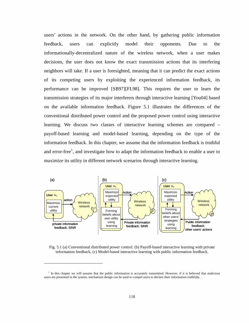
118
users’ actions in the network. On the other hand, by gathering public information
feedback, users can explicitly model their opponents. Due to the
informationally-decentralized nature of the wireless network, when a user makes
decisions, the user does not know the exact transmission actions that its interfering
neighbors will take. If a user is foresighted, meaning that it can predict the exact actions
of its competing users by exploiting the experienced information feedback, its
performance can be improved [SB97][FL98]. This requires the user to learn the
transmission strategies of its major interferers through interactive learning [You04] based
on the available information feedback. Figure 5.1 illustrates the differences of the
conventional distributed power control and the proposed power control using interactive
learning. We discuss two classes of interactive learning schemes are compared –
payoff-based learning and model-based learning, depending on the type of the
information feedback. In this chapter, we assume that the information feedback is truthful
and error-free1, and investigate how to adapt the information feedback to enable a user to
maximize its utility in different network scenarios through interactive learning.
Fig. 5.1 (a) Conventional distributed power control. (b) Payoff-based interactive learning with private
information feedback. (c) Model-based interactive learning with public information feedback.
1 In this chapter we will assume that the public information is accurately transmitted. However, if it is believed that malicious users are presented in the system, mechanism design can be used to compel users to declare their information truthfully.
User vm
Maximizecurrentutility
Wireless network
action
private informationfeedback: SINR
User vm
Maximizeexpected
utilityWireless network
Action
Private informationfeedback: SINR
Formingbeliefs about
own utilityusing
learning
User vm
Maximizeexpected
utility Wireless network
Action
Public information feedback:
other users’ actions
Forming beliefs aboutother users’strategies
using learning
(a) (b) (c)
User vmUser vm
Maximizecurrentutility
Wireless network
action
private informationfeedback: SINR
User vmUser vm
Maximizeexpected
utilityWireless network
Action
Private informationfeedback: SINR
Formingbeliefs about
own utilityusing
learning
User vmUser vm
Maximizeexpected
utility Wireless network
Action
Public information feedback:
other users’ actions
Forming beliefs aboutother users’strategies
using learning
(a) (b) (c)

119
We focus on the problem of delay-sensitive applications sharing the same wireless
network. Due to the delay sensitivity, the utility of a user is dramatically impacted by the
applications of other users. This provides the user an additional incentive to adopt a better
learning scheme, since it cannot wait a long time to transmit the packets. To cope with the
delay sensitivity, we need to consider not only the impact of the effective throughput over
the wireless network, but also the source traffic characteristics, including the source rates
and the delay deadlines of the applications.
In summary, this chapter aims to make the following contributions:
1) Feedback-driven interactive learning framework that outperforms the Nash
equilibrium performance. We develop a feedback-driven learning framework for
distributed power control of delay sensitive users that outperforms the Nash equilibrium
performance, which is achieved when users deploy myopic best response such as iterative
water filling [YGC02]. Note that the users are self-interested, meaning that they tend to
maximize their own utility in a fully distributed manner.
2) Cost-efficiency tradeoff of interactive learning. We consider learning solutions
based on both the private and public information feedback, and characterize the cost of
information feedback by explicitly considering – a) from whom (i.e. from which
transmitters or receivers) this information is obtained, and b) how often such information
is obtained (i.e. the frequency of getting feedback). We quantify the cost-efficiency
tradeoff when learning from different information feedback and show how to adapt the
information feedback to maximize the learning efficiency.
3) Analytical upper bounds based on interactive learning. We also quantify the utility
upper bounds that can be achieved by a user through learning based on private or public
information feedback.
The chapter is organized as follows. In Section II, we discuss the considered network
settings and formulate the studied informationally-decentralized dynamic resource
management problem among wireless users competing for resources with incomplete

120
information. In Section III, we characterize the information feedback and discuss the
cost-efficiency tradeoff of the information feedback. Based on the type of information
feedback, we introduce two classes of interactive learning solutions and discuss how to
adjust the information feedback to improve the learning efficiency. In Section IV,
payoff-based learning is discussed, which employs only private information feedback. In
Section V, we introduce model-based learning, which requires public information
feedback. Section VI presents simulation results and Section VII concludes the chapter.
II. NETWORK SETTINGS AND PROBLEM FORMULATION
A. Network settings
We assume that there are V users ( 1m ,…, Vm ) that are simultaneously transmitting
delay sensitive applications over the same wireless infrastructure. A network user vm is
composed of a source node svn (transmitter) and a destination node dvn (receiver) that
can establish a direct communication connection, i.e. , s dv v vm n n= . We assume that there
are multiple frequency channels for users to transmit their applications and F is the set
of all channels. An illustrative network example is depicted in Figure 5.2.
Fig. 5.2 System diagram of the dynamic joint power-spectrum resource allocation.
11 1 1( )G f P⋅1sn
sVn
1dn
dVn
( )VV V VG f P⋅
……
…
1 ( )V V VG f P⋅
1 1 1( )VG f P⋅
Mutualinterference
1γPrivate information feedback
VγPrivate information feedback
publicinformation feedback
VA
Decision maker
Decision maker
packet arrival
packet arrival11 1 1( )G f P⋅
1sn1sn
sVnsVn
1dn1dn
dVndVn
( )VV V VG f P⋅
……
…
1 ( )V V VG f P⋅
1 1 1( )VG f P⋅
Mutualinterference
1γPrivate information feedback
VγPrivate information feedback
publicinformation feedback
VA
Decision maker
Decision maker
packet arrival
packet arrival
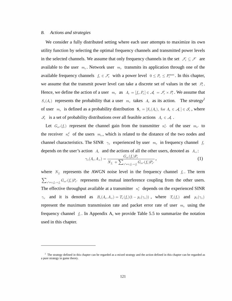
121
B. Actions and strategies
We consider a fully distributed setting where each user attempts to maximize its own
utility function by selecting the optimal frequency channels and transmitted power levels
in the selected channels. We assume that only frequency channels in the set v ⊆F F are
available to the user vm . Network user vm transmits its application through one of the
available frequency channels v vf ∈ F with a power level max0 v vP P≤ ≤ . In this chapter,
we assume that the transmit power level can take a discrete set of values in the set vP .
Hence, we define the action of a user vm as [ , ]v v v v v vA f P= ∈ = ×A F P . We assume that
( )v vS A represents the probability that a user vm takes vA as its action. The strategy2
of user vm is defined as a probability distribution [ ( ), for ]v v v v v vS A A= ∈ ∈S A S , where
vS is a set of probability distributions over all feasible actions v vA ∈ A .
Let '( )vv vG f represent the channel gain from the transmitter 'svn of the user 'vm to
the receiver dvn of the users vm , which is related to the distance of the two nodes and
channel characteristics. The SINR vγ experienced by user vm in frequency channel vf
depends on the user’s action vA and the actions of all the other users, denoted as -vA :
'
-' '' ,
( )( , )
( )v
v v
vv v vv v v
f vv v vv v f f
G f PA A
N G f Pγ
≠ =
=+ ∑
, (1)
where vf
N represents the AWGN noise level in the frequency channel vf . The term
'' '' ,( )
v vvv v vv v f f
G f P≠ =∑ represents the mutual interference coupling from the other users.
The effective throughput available at a transmitter svn depends on the experienced SINR
vγ and it is denoted as -( , ) ( )(1 ( ))v v v v v v vB A A T f p γ= − , where ( )v vT f and ( )v vp γ
represent the maximum transmission rate and packet error rate of user vm using the
frequency channel vf . In Appendix A, we provide Table 5.5 to summarize the notation
used in this chapter.
2 The strategy defined in this chapter can be regarded as a mixed strategy and the action defined in this chapter can be regarded as a pure strategy in game theory.
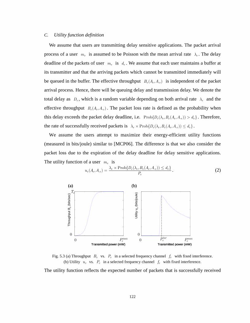
122
C. Utility function definition
We assume that users are transmitting delay sensitive applications. The packet arrival
process of a user vm is assumed to be Poisson with the mean arrival rate vλ . The delay
deadline of the packets of user vm is vd . We assume that each user maintains a buffer at
its transmitter and that the arriving packets which cannot be transmitted immediately will
be queued in the buffer. The effective throughput -( , )v v vB A A is independent of the packet
arrival process. Hence, there will be queuing delay and transmission delay. We denote the
total delay as vD , which is a random variable depending on both arrival rate vλ and the
effective throughput -( , )v v vB A A . The packet loss rate is defined as the probability when
this delay exceeds the packet delay deadline, i.e. -Prob ( , ( , )) v v v v v vD B A A dλ > . Therefore,
the rate of successfully received packets is -Prob ( , ( , )) v v v v v v vD B A A dλ λ× ≤ .
We assume the users attempt to maximize their energy-efficient utility functions
(measured in bits/joule) similar to [MCP06]. The difference is that we also consider the
packet loss due to the expiration of the delay deadline for delay sensitive applications.
The utility function of a user vm is -
-Prob ( , ( , ))
( , ) v v v v v v vv v v
v
D B A A du A A
P
λ λ× ≤= . (2)
Fig. 5.3 (a) Throughput vB vs. vP in a selected frequency channel vf with fixed interference.
(b) Utility vu vs. vP in a selected frequency channel vf with fixed interference.
The utility function reflects the expected number of packets that is successfully received
(a) (b)
vT
0
0 maxvP 0 max
vP
0
Transmitted power (mW) Transmitted power (mW)
Thr
ough
put B
v(b
its/s
ec)
Util
ity u
v(b
its/jo
ule)
tarvP
(a) (b)
vT
0
0 maxvP 0 max
vP
0
Transmitted power (mW) Transmitted power (mW)
Thr
ough
put B
v(b
its/s
ec)
Util
ity u
v(b
its/jo
ule)
tarvP

123
(rather than transmitted as in [MCP06]) per joule of energy consumed for delay sensitive
users. More details about how this utility function can be computed in a practical
communication setting can be found in Appendix B. Figure 5.3 illustrates the utility
function of a user vm using different power max0 v vP P≤ ≤ in a selected frequency
channel vf with fixed interference. We denote the power of user vm that maximizes the
utility function when transmitting in channel vf as ( )tarv vP f .
D. Problem formulation
Let myopv−A represent the latest actions of the other users observed by a user vm in the
network. Conventionally, the user vm adopts a myopic distributed optimization, which
can be formulated as: [ , ] arg max ( , )
v v
myop myop myop myopv v v v v v
AA f P u A −
∈= = A
A. (3)
In [MCP06], it was shown that the myopic best response myopvA converges to the Nash
equilibrium under certain conditions on channel gains. However, if a foresighted user vm
knows the exact response actions of other users ( )forsv vA−A , a better performance can be
achieved [FT91]. Let ( )forsv vA−A represent the actions of the other users given that the
action vA is taken by user vm . The optimization performed by a foresighted user can be
formulated as [FT91]: [ , ] arg max ( , ( ))
v v
fors fors fors forsv v v v v v v
AA f P u A A−
∈= = A
A. (4)
Let us assume that only one user is foresighted, and all the other users in the network still
adopt a myopic best response. Given the exact response actions ( )forsv vA−A , the foresighted
decision making based on the complete information of the other users will converge to
the Stackelberg equilibrium [FT91] and the optimal utility is denoted as
( ( )) max ( , ( ))v v
fors forsv v v v v v v
AU A u A A− −
∈=A A
A. (5)
However, due to the informationally-decentralized nature of the wireless networks, it is
impossible for each user to know in practice the exact response actions ( )forsv vA−A . Hence,
accurately modeling the actions ( )forsv vA−A based on the information feedback is
necessary.

124
Definition 1: Denote the information feedback of user vm at time slot t as tvI ,
regardless whether the information feedback is private or public. We define the observed
information history of user vm at time slot t as 1 , t t tv v vo o −= I .
Assume that the strategy of user vm at time slot t is denoted as tvS . We use the
notation v−M to indicate the set of all users except user vm . The strategy of all users in
the network except user vm is , for t tv u u vm− −= ∈S S M .
Definition 2: Since the exact response actions of other users forsv−A are not available to
user vm in real time, user vm estimates forsv−A by building a belief on the other users’
strategies tv−S . The belief of user vm is defined as
( ) ( | ), for all t tv v v v v v vA S A A A− − −= ∈S A , where ( | )t
v v vS A A− − 3 is the estimated strategies
of the other users given that user vm decides to take the action vA .
In other words, user vm estimates the other users’ strategies ( )tv vA−S
for each of its
action v vA ∈ A4.
Definition 3: Assume vΛ represents the interactive learning scheme adopted by user
vm . A learning scheme vΛ is defined as a method that allows user vm to build a belief
( )t tv v vo− = ΛS
5 based on the observed information history tvo , in order to estimate the
actions of the other users forsv−A .
Specifically, by learning from the observed information history tvo , user vm builds its
belief tv−S
on the other users’ strategies and determine its own best response strategy
tvS . Figure 5.4 illustrates how a delay sensitive user makes decisions based on the
observed information history tvo and the mutual interference coupling in the dynamic
wireless environment. The problem in equation (4) can be now reformulated as:
3 ( ) ( | ), for t tv v u u u v u vA A A m− −= ∈ ∈S S M A . ( | )t
u u u vA A∈S A [ ( | ), for ]tu u v u uS A A A= ∈ A
is the conditional probability distribution when user vm takes the action vA . 4 Based on different types of information feedback, user vm may implicitly model the other users by only estimating the
aggregate effect of the other users. See Section IV for more detail. 5 For representation convenience, we use the simplified notation fors
v−A to represent ( ),forsv v v vA A− ∈A A as the exact
response actions of other users. And also use tv−S
to represent ( )tv vA−S
in the rest of the chapter.

125
( , )( ) arg max [ ( , )]tv v
v v
t t tv v v v vE u
−− −
∈=
S SS
S S S S
S. (6)
Based on the determined tvS , user vm selects an action vA at time slot t .
Fig. 5.4 Interactions among users and the foresighted decision making based on information feedback.
E. Learning efficiency
The performance of an interactive learning approach depends on how accurate the
belief ( )t tv v vo− = ΛS can predict the actions forsv−A . A more accurate prediction of forsv−A
can lead to a better learning efficiency. We define the learning efficiency ( ( ))tv v vJ oΛ of
the learning approach vΛ (based on the observed information history tvo ) by
quantifying its impact on the expected utility, i.e.
( , )( ( )) [ ( , ( ))]t tv v
t t tv v v v v v vJ o E u o
−Λ Λ
S SS , where (7)
( , )[ ( , ( ))] ( ) ( | ) ( , )t tv v
V -1v v
t t t tv v v v v v v v v v v v
A A
E u o S A S A A u A A−
−
− − −∈ ∈
Λ = × × ∑ ∑S S
S
A A
. (8)
The notation ( | )tv v vS A A− − is used to represent the joint probability that the users
u vm −∈ M take actions vA− , given that user vm took the action vA .
Since the belief t v−S is only a prediction for fors
v−A , we define the Price of Imperfect
Belief (PIB) for using the learning scheme vΛ based on the observed information
history tvo as the performance difference between the Stackelberg equilibrium [FT91]
( )forsv vU −A (where the user vm knows the exact response of the other users) and the
practical learning efficiency ( ( ))tv v vJ oΛ , i.e.
( ( )) ( ) ( ( ))t fors tP v v v v v v vo U J o−∆ Λ − ΛA . (9)
Sourcecharacteristics
Strategy that maximizes
,v vdλ
User vm
Users v−M
tvS
1tv−
−SWireless network
environment
( )fG
tvI
1tv−
−I
Learning( )tv voΛ
tv−S
[ ]vE uSource
characteristics
Strategy that maximizes
,v vdλ
User vmUser vm
Users v−M
tvS
1tv−
−SWireless network
environment
( )fG
tvI
1tv−
−I
Learning( )tv voΛ
tv−S
[ ]vE u

126
In the next sections, we quantify the cost of the information feedback tvI and study
two classes of interactive learning approaches privvΛ and pub
vΛ based on different types
of information feedback.
III. INFORMATION FEEDBACK FOR INTERACTIVE LEARNING
A. Characterization of information feedback
In this chapter, we define the entire information history from all users until time slot t
as
, , , for 1,..., , 0,..., t s s sv v vh A v V s tγ= = =G . (10)
Note that a user vm observes only a subset of the entire history through information
feedback, i.e. t tvo h⊆ . The observed information history tvo can be characterized in
three distinct categories:
• Types of information feedback – As mentioned before, there are two types of
information that a user vm can observe at a certain time slot t , i.e. the private
information feedback , 1 t priv tv vγ
−=I or the public information feedback
, 1 1 , , for t pub t tv u u u vA m− −
− −= ∈G MI . Recall that 1 , t t tv v vo o −= I in Definition 1.
• Information zone – We define the information zone tvV as a set of users that are
able to feed back information to the transmitter of user vm at time slot t . In the
wireless communication networks, the information from further users is less
significant, since the effect of mutual interference coupling decreases ( 'vvG decreases
in equation (1)) as the distance increases [Rap02]. Hence, user vm can selectively
collect the information only from a set of neighboring (e.g. within an information
horizon as in the previous chapter) users tu vm ∈ V , i.e.
, 1 1 , , for t pub t t tv u u u vA m− −
− = ∈G VI . Since the information zone of the private
information feedback only contains user vm itself, we define 0tv =V for
, 1 t priv tv vγ
−=I .
• Information feedback frequency – In our problem formulation in equation (6), user
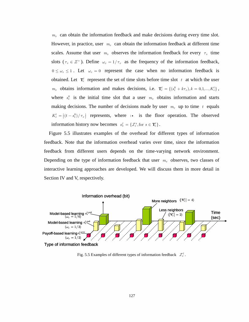
127
vm can obtain the information feedback and make decisions during every time slot.
However, in practice, user vm can obtain the information feedback at different time
scales. Assume that user vm observes the information feedback for every vτ time
slots ( vτ+∈ Z ). Define 1/v vω τ= as the frequency of the information feedback,
0 1vω≤ ≤ . Let 0vω = represent the case when no information feedback is
obtained. Let tvT represent the set of time slots before time slot t at which the user
vm obtains information and makes decisions, i.e. 0( ), 0,1,..., t tv v v vs k k Kτ= + =T ,
where 0vs is the initial time slot that a user vm obtains information and starts
making decisions. The number of decisions made by user vm up to time t equals
0( )/tv v vK t s τ = − represents, where i is the floor operation. The observed
information history now becomes , for t s tv v vo s= ∈ TI .
Figure 5.5 illustrates examples of the overhead for different types of information
feedback. Note that the information overhead varies over time, since the information
feedback from different users depends on the time-varying network environment.
Depending on the type of information feedback that user vm observes, two classes of
interactive learning approaches are developed. We will discuss them in more detail in
Section IV and V, respectively.
Fig. 5.5 Examples of different types of information feedback tvI .
Time (sec)
Information overhead (bit)
Type of information feedback
Model-based learning
Model-based learning
Payoff-based learning ,t privvo
,t pubvo
,t pubvo
More neighbors
Less neighbors
( 1/2)vω =
( 1/ 3)vω =
( 1/6)vω =
( 4)tv =V
( 2)tv =V
Time (sec)
Information overhead (bit)
Type of information feedback
Model-based learning
Model-based learning
Payoff-based learning ,t privvo
,t pubvo
,t pubvo
More neighbors
Less neighbors
( 1/2)vω =
( 1/ 3)vω =
( 1/6)vω =
( 4)tv =V
( 2)tv =V

128
B. Cost-efficiency tradeoff when adjusting the information feedback
Let us denote the information feedback overhead of user vm as ( , )v v vσ ω V6, which is
a function of the information feedback frequency vω and the number of the neighboring
users vV . In general, with more frequent information feedback (i.e. a larger vω ) or
feedback from more users (i.e. a larger vV ), a user can obtain more information from
the entire information history th and hence, this results in a more accurate belief. On the
other hand, a large information overheads ( , )v v vσ ω V can degrade the learning
efficiency ( ( ))tv v vJ oΛ . In this chapter, we assume that the packet transmission and the
information feedback are multiplexed in the same frequency channel. Hence, considering
the information overhead, the effective throughput can be represented as
( , , ) ( , ) ( )v v v v v v v vB A A B A Aσ θ σ− −′ = × , where 0 ( ) 1vθ σ< ≤ represents the fraction of time
dedicated to the packet transmission, and it is a decreasing function of vσ .
We now focus on how the learning efficiency ( ( ))tv v vJ oΛ in equation (7) changes with
different value of vσ . If vσ is large, the belief t v−S provides an accurate model on
forsv−A . Given fors
v−A , the utility function in equation (2) can be derived as (see Appendix C
for more detail): 1
(1 ), if ( , , )/( , ( , ))( , , )
0 , otherwise
vv v v v v v
v v v v v vv v v v
B A A LP F A Au A A
λσ λ
σ γσ−
−−
′− >=
, (11)
where ( , ( , )) exp( ( , ( , )) )vv v v v v v v v v v v v
v
dF A A B A A d
Lσ γ σ γ λ− −′≡ − . (12)
vL represents the average packet length of user vm . Note that both ( , , )v v v vB A Aσ −′ and
( , ( , ))v v v v vF A Aσ γ − are decreasing functions of vσ . Hence, the utility function is a
non-increasing function of vσ . In other words, the PIB P∆ is a non-decreasing function
of vσ when vσ is large. On the other hand, if vσ is small, the belief t v−S provides an
inaccurate model on forsv−A . By having more information t tvo h⊆ , increasing vσ can
improve the learning efficiency and hence, P∆ decreases. In other words, P∆ is a
6 Note that for private information feedback, the information overhead vσ only depends on vω ( vV =0).

129
non-increasing function of vσ when vσ is small. Note that this efficiency-cost tradeoff
occurs when adjusting either vω or vV .
Proposition 1: For a given learning scheme vΛ , there exists at least one optimal
information feedback overhead *vσ such that *( ) argmin ( ( ( )))tv v P v vo
σσ σΛ = ∆ Λ (13)
Proof: Note that minimizing P∆ is the same as maximizing ( ( ))tv v vJ oΛ . Since
0 ( ( )) ( )t forsv v v vJ o U −≤ Λ ≤ A is bounded, there must exist a minimum value with a certain
*vσ .
Based on Proposition 1, we propose an adaptive interactive learning that adapts the
information feedback parameters for user vm to improve its learning efficiency vJ .
Figure 5.6 presents the system block diagram of our adaptive interactive learning
framework. Due to the consideration of the source characteristics, the interactive learning
framework is operated at the application layer. The goal of user vm in the adaptive
interactive learning framework is to build the belief tv−S
based on tvo for determining
the best response strategy tvS and adjust the information feedback 1( )tv vσ
+I to improve
the learning efficiency ( ( ))tv v vJ oΛ . In the following sections, we will discuss the adaptive
interactive learning schemes based on different types of information feedback in more
details.
Fig. 5.6 System block diagram for the adaptive interactive learning for dynamic resource management.
Evaluate effectivethroughput
( , )vB f γ Select [ , ]t t tv v vA f P=
Application Layer
PHY/MAC Layer
User
Wireless networkcoupling( )fG
Observedinfo t
vo
Determinestrategy t
vS
EvaluatevJ
Utility evaluation
Adapt1( )t
v vσ+I
Wireless networkcoupling( )fG
vm
Source characteristics
1. Gather information2. Build belief throughlearning
3. Foresighted decisionmaking
Interactivelearning
,v vdλ
Evaluate effectivethroughput
( , )vB f γ Select [ , ]t t tv v vA f P=
Application Layer
PHY/MAC Layer
User
Wireless networkcoupling( )fG
Wireless networkcoupling( )fG
Observedinfo t
voObservedinfo t
voObservedinfo t
vo
Determinestrategy t
vS
EvaluatevJ
Utility evaluation
Adapt1( )t
v vσ+I
Wireless networkcoupling( )fG
Wireless networkcoupling( )fG
vm
Source characteristicsSource characteristics
1. Gather information2. Build belief throughlearning
3. Foresighted decisionmaking
Interactivelearning
,v vdλ

130
IV. INTERACTIVE LEARNING WITH PRIVATE INFORMATION FEEDBACK
In the case where user vm only observes the private information feedback ,t privvI , it
can only model the aggregate effect of other users’ actions through the experienced SINR
value vγ . Hence, it cannot model the exact response actions of the other users forsv−A
explicitly. Note that the observed information history in this case is
1( ) , ( )t s tv v v v vo sω γ ω−= ∈ T . Based on this observed information history ( )t
v vo ω , user vm
is aware of its past actions 1,s tv vA s− ∈ T and the past resulting utilities
1 1( , ),s s tv v v vu A sγ− − ∈ T . Let ( , ( ))t
v v v vu A o ω represent the estimated utility of user vm if the
action vA is taken. Instead of predicting the exact response actions forsv−A explicitly,
user vm builds a belief on the utility and determines its best strategy tvS based on its
past experienced action-utility pairs 1 1 1[ , ( , )],s s s tv v v v vA u A sγ− − − ∈ T . Hence, user vm does not
try to estimate the probability ( | )tv v vS A A− − in equation (8). Instead, user vm builds
directly its belief on what will be the average utility impact that it will experience if it
takes action vA , i.e. ( , ( ))tv v v vu A o ω substitutes the term ( | ) ( , )
V -1v
tv v v v v v
A
S A A u A A
−
− − −
∈
×∑
A
in equation (8).
Let ( ) ( ( ))t priv tv v v v voω ω= ΛS be the strategy of user vm at time slot t learned from the
observed information history ( )tv vo ω . From equation (7), the learning efficiency of user
vm is
( ( ( ))) ( ) ( , ( ))v
priv t t tv v v v v v v v v v
A
J o S A u A oω ω∈
Λ = ×∑ A
. (14)
To minimize P∆ in equation (9), the best response strategy is:
( ) arg max ( ) ( , ( ))v v
v
t tv v v v v v v v
A
S A u A oω ω∈
∈
= ×∑S
S S
A
. (15)
The payoff-based learning based on private information feedback can be represented
equation (15). After the strategy tvS is determined, the action of user vm at time slot t
is determined by
( )t tv vA Rand= S , (16)
where ( )tvRand S represents a random selection based on the probabilistic strategy

131
tv v∈S S . Payoff-based learning [You04] provides a method to learn the strategy tvS from
the past experienced action-utility pairs 1 1 1[ , ( , )],s s s tv v v v vA u A sγ− − − ∈ T . A simple example of
a payoff-based learning method will be provided in Section IV.A.
If the private information feedback is costless (i.e. v vB B′ = in equation (11)), the
utility upper bound of the payoff-based learning can be calculated based on the resulting
strategy * *[ ( ), for all ]v v v v vS A A= ∈S A at convergence.
Proposition 2 For a payoff-based learning with private information feedback, if the
information feedback is costless, the upper bound of the learning efficiency ( )privv vJ Λ is
(1 ( )) ( )priv forsv v v vUε −− Λ A , and 0 ( ) 1priv
v vε≤ Λ < .
1( ) ( ) ( , )
( )v
priv forsv v v v v vfors
v v A
g A u AU
ε −− ∈
Λ = ∑ AA A
, where *
*
1 ( ), for ( )
( ), otherwise
forsv v
v
S A A Ag A
S A
− == −
. (17)
Proof: By substituting equation (14) into equation (9), the PIB becomes
( ) ( ) ( )priv priv forsP v v v v vUε −∆ Λ = Λ A . Since ( , )fors
v v vu A −A has costless information feedback,
substituting ( , ( ))tv v v vu A o ω by ( , )fors
v v vu A −A provides a lower bound on ( )privP v∆ Λ , which
is ( ) ( , )v
forsv v v v
A
g A u A −∈∑ A
A
.
From equation (17), in order to decrease ( )privv vε Λ , user vm needs to increase the
accuracy of the best response strategy *vS such that it approaches forsvA . Next, let us give
a simple example using a well-known reinforcement learning solution [You04].
A. Reinforcement learning based on private information feedback
In this subsection, let us assume 1vω = . By applying typical reinforcement learning,
user vm models its best response strategy tvS as ( )
( )( )
v v
tv vt
v v tv v
A
r AS A
r A∈
=∑A
, (18)
where ( )tv vr A represents the propensity [You04] of user vm choosing an action vA at
time slot t . Let us define [ ( ), for ]t tv v v v vr A A= ∈r A as a vector of propensity of all
feasible actions. The user updates tvr based on the experienced utility, 1 1( , )t t
v v vu A γ− −
when the action 1tvA− is taken at time slot 1t − . Here, we adopt the cumulative payoff

132
matching [You04]:
1 1 1 1(1 ) ( , ) ( )t t t t tv v v v v vu A Aα α γ− − − −= × + − ×r r I , (19)
where α is the discount factor for the history value of the cumulative propensity.
( ) [ ( ), for ]t tv v vA I A A A= = ∈I A represents an indicator vector such that
1, if ( )
0, if
tv
tv t
v
A AI A A
A A
== = ≠
. (20)
B. Adaptive reinforcement learning
The reinforcement learning in the previous subsection fixes 1vω = , i.e. user vm
obtains information feedback at each time slot. From Proposition 1, we know that by
adjusting information feedback frequency vω to *vω , user vm can minimize its PIB
P∆ . Hence, we introduce the adaptive reinforcement learning that adjusts vω to
maximize the learning efficiency ( )privv vJ Λ . Specifically, for 1vω < , user vm will not
receive the private information feedback at each time slot with probability 1 vω− . If
there is no information feedback, user vm takes the baseline action basevA , which is the
past action that ever provides the best payoff value. Smaller vω means that the user is
more reluctant to deviate from its baseline action and leads to a lower information
feedback overhead. With probability vω , the user will receive the information feedback
and perform the same reinforcement learning as in the previous subsection. After user
vm selects an action tvA , it compares the payoff value vu and then updates the record of
the baseline action basevA and the baseline payoff value basevu :
1 1 1, if ( , )
, otherwise
t t t basev v v v v
basev base
v
A u A uA
A
γ− − − >=
. (21)
1 1max( , ( , ))base base t tv v v v vu u u A γ− −= . (22)
Finally, user vm evaluates the learning efficiency ( ( ))tv vJ oΛ and changes the
information feedback frequency vω by vω until the maximum ( ( ))tv vJ oΛ is found.
The details of the proposed adaptive reinforcement learning can be found in Algorithm
5.1 in Appendix D.

133
V. INTERACTIVE LEARNING WITH PUBLIC INFORMATION FEEDBACK
Unlike the payoff-based learning, when user vm observes public information
feedback , 1 1 , , for t pub t tv u u u vA m− −
− −= ∈G MI , the observed information history is
, , t s pub tv v vo s−= ∈ TI . Based on this, user vm can directly model the strategy of other
users and build belief t v−S on it explicitly.
Let ( ) ( ( ))t pub tv v v v voσ σ− = ΛS . From equation (7), the learning efficiency is
( ( ( ))) ( ) ( | ) ( , , )V -1
v v
pub t t tv v v v v v v v v v v v v
A A
J o S A S A A u A Aσ σ
−
− − −∈ ∈
Λ = × × ∑ ∑
A A
. (23)
To minimize the P∆ in equation (9), the best response strategy of user vm is to take
the action ( ( )t tv vA=S I ):
( ) arg max [ ( , ( ))]tv
v v
t tv v v v v v
AA E u Aσ σ
−−
∈=
SS
A. (24)
Model-based learning [You04] provides a method to build the belief on ( )tv vσ−S
of other
users’ actions from the past experienced public information 1,s tu vA s− ∈ T . We present the
action learning that performs equation (24) as an example in Section V.A.
Similarly, if the public information feedback is costless (i.e. v vB B′ = in equation (11)
), the utility upper bound of the model-based learning can be calculated as discussed
below.
Proposition 3 For the model-based learning based on the public information feedback, if
the information feedback is costless, the upper bound of the learning efficiency ( )pubv vJ Λ
is ( )forsv vU −A .
Proof: Substitute equation (24) into equation (23) and substitute ( , , )v v v vu A Aσ − by
( , )forsv v vu A −A . And this provides an upper bound on ( )pub
v vJ Λ , since
( , ) ( , , )forsv v v v v v vu A u A Aσ− −≥A . Equation (23) then becomes
max ( , ) ( | ) ( , ) ( )v v V -1
v
fors t fors fors forsv v v v v v v v v v v
AA
u A S A A u A U
−
− − − − −∈
∈
× = = ∑A A A
AA
.
(25)
The reason why the model-based learning with public information feedback has a
higher upper bound compared to the payoff-based learning with private information

134
feedback is because it enables the user to explicitly model the actions of other users and
hence, the user can directly choose the action that maximizes its expected utility. Next,
we provide a simple model-based learning – action learning, which is similar to the
well-known fictitious play [You04].
A. Action learning based on public information feedback
Recall that in order to build the belief t v−S from , , t s pub t
v v vo s−= ∈ TI , user vm
maintains a set of strategy vectors ( | ) ( | ), for t tv v v u u u v u vS A A S A A m− − −= ∈ ∈ M A for all
possible actions v vA ∈ A , where ( | ) [ ( | ), for ]t tu u u v u u v u uS A A S A A A∈ = ∈ A A represents
the estimated strategy of the user u vm −∈ M given that user vm taking action vA at
time slot t . Hence, in the action learning, whenever action vA is taken by the user vm ,
we set ( | )
( | )( | )
u
tu u vt
u u v tu v
A
r A AS A A
r A A∈
=∑
A
, (26)
where ( | )tu u vr A A is the propensity of user um at time t . The propensity represents the
number of times that user um takes action uA given that user vm took action vA .
Hence, whenever the action vA is taken by user vm , the vector
( | ) [ ( | ), for all ]t tu u u v u u v u uA A r A A A∈ = ∈r A A is updated by:
1 1( | ) ( | ) ( )t t tu u u v u u u v uA A A A A− −∈ = ∈ +r r IA A . (27)
Then, the probability ( | )tu u vS A A represents the empirical frequency that user um will
take an action u uA ∈ A given that user vm took an action vA .
Next, we show how to maximize [ ( , ( ))]tv
tv v v vE u A σ
−−SS in equation (24) analytically
given the belief t v−S . First, we show the necessary condition for user vm to maximize its
utility function.
Proposition 4: For a certain frequency channel f , in order to maximize ( )vu f , user
vm needs to transmit at the target SINR value ( )tarv fγ , which is the unique positive
solution of ( )( )
( ) 1v vv
v
B LF
d
γγ γ
γ
′∂= −
∂ ( ( )vF γ is in equation (12)).
Proof: See Appendix C.

135
Proposition 4 suggests that if user vm is using the frequency channel f , it should
adapt the target power level ( )tarvP f accordingly to the interference from the other users
using the same frequency channel to support the target SINR value ( )tarv fγ . Since the
power level in our setting is discrete, we choose the ( )tarv vP f ∈ P as the power that
provides the nearest SINR value to ( )tarv fγ . If the target SINR ( )tar
v fγ requires a power
higher than maxvP (when the interference in the channel is too high), set ( )tar
vP f to
maxvP .
Next, given the target ( )tarvP f , we further determine the optimal frequency channel
selection of the user vm .
Proposition 5: Let ( ) ( , ( ))tar tarv v vF f F f fγ= in equation (12). Given the corresponding
target ( )tarvP f , the optimal action *
vA of a user vm is
* ( )arg min ( )
( ) 1v
tarvtar
v v tarfv
F ff P f
F f∈= ×
−F and * *( )tar
v v vP P f= . (28)
Proof: From Proposition 4, maximizing 1(1 )vv
v vu P F
λ= − leads to equation (28).
In summary, user vm selects the frequency channel *vf and power level *vP to
support the target SINR *( )tarv vfγ , which maximizes the utility function in equation (2).
This requires user vm to estimate the interference from other users, which can be
computed by user vm based on its belief t v−Θ . Specifically, denote the estimated
interference of user vm as ( )v vAΩ , when the action vA is taken. Given t v−Θ , ( )v vAΩ
can be computed as: ( ) ( )[ ( | ) ( )]
u u
tv v uv v u u v u u
u v
A
A G f S A A P I f f≠∈
Ω = × × =∑
A
. (29)
Then, the resulting SINR value ( )v vAγ is ( [ , ]v v vA f P= ): ( )
( , )( )
v
vv v vv v v
f v v
G f Pf P
N Aγ =
+ Ω. (30)
By applying Proposition 4, we calculate the target power ( )tarvP f in different frequency
channels: ( ) min ( ) ( , )
v
tar tarv v v
PP f f f Pγ γ
∈= −
P. (31)
Then we apply Proposition 5 to determine * *[ , ]tv v vA f P= .

136
B. Adaptive action learning
For the action learning in the previous subsection, the public information feedback
, 1 1 , , t pub t tv u u u vA m− −
− −= ∈G MI is required from every user in the network, during each
time slot. This results in heavy information overhead. Moreover, the overall action
space 1V−A makes the computational complexity prohibitive to model all the users in
the network. To approach the upper bound ( )forsv vU −A of the model-based learning
efficiency, we need to adjust the information overhead ( , )v v vσ ω V by changing the
information feedback parameters vω and vV .
Hence, in our proposed active action learning, to reduce the overhead, we classify the
neighboring users of user vm into H groups (1 vH −≤ ≤ M ) and assign different
information feedback frequency ivω to different groups
(i.e. 1 21 ... 0Hv v vω ω ω≥ ≥ ≥ ≥ ≥ ). For the dynamic power/spectrum management problem
in this chapter, the neighboring users can be classified based on their average channel
gains uvG over the frequency channels, i.e. ( )1 ( )uv uvfG G f
∈= ∑ F
F (from the
transmitter of the neighboring user um to the receiver of the foresighted user vm ),
since these channel gains directly impact the user’s utility (see equation (1) and (2)). For
instance, a neighboring user um with a larger channel gain uvG will have more impact
on vu .
Let ivX represents the number of users in the group , 1,...,iH i H= . Assume the
neighboring users are relabeled according to its average channel gain value, i.e.
[1] [2] [ 1]...v v V vG G G −≥ ≥ ≥ . Then, 1
[ ]1 1
, iff [ ]i i
j ju i v v
j j
m H X u X
−
= =
∈ ≤ ≤∑ ∑ (32)
In Algorithm 5.2 in Appendix D, we provide our adaptive action learning approach
for the extreme case when 2H = as an example. In this case, we only need to adapt
vV ( 1v vX = V and 2 1v vX V= − − V ). If the neighboring users u vm ∈ V , we set
1vω = , otherwise, 0vω = . Meaning that user vm only needs to model the users in set
vV based on , 1 1( )
, , tv
t pub t tu u u vv
A m− −−
= ∈V
G VI . In Table 5.1, we compare the two
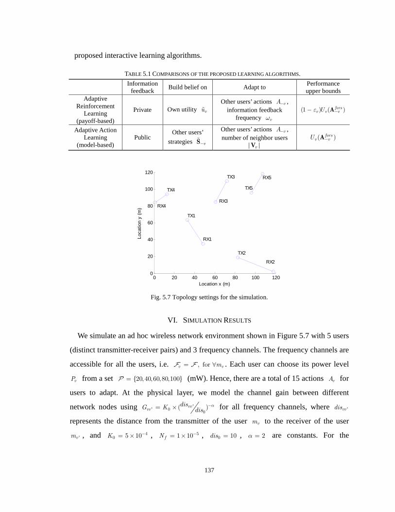
137
proposed interactive learning algorithms.
TABLE 5.1 COMPARISONS OF THE PROPOSED LEARNING ALGORITHMS.
Information
feedback Build belief on Adapt to
Performance upper bounds
Adaptive Reinforcement
Learning (payoff-based)
Private Own utility vu Other users’ actions vA− ,
information feedback frequency vω
(1 ) ( )forsv v vUε −− A
Adaptive Action Learning
(model-based) Public
Other users’
strategies v−S
Other users’ actions vA− , number of neighbor users
vV ( )forsv vU −A
Fig. 5.7 Topology settings for the simulation.
VI. SIMULATION RESULTS
We simulate an ad hoc wireless network environment shown in Figure 5.7 with 5 users
(distinct transmitter-receiver pairs) and 3 frequency channels. The frequency channels are
accessible for all the users, i.e. , for v vm= ∀F F . Each user can choose its power level
vP from a set 20,40,60,80,100=P (mW). Hence, there are a total of 15 actions vA for
users to adapt. At the physical layer, we model the channel gain between different
network nodes using '' 0
0( )vv
vvdisG K dis
α−= × for all frequency channels, where 'vvdis
represents the distance from the transmitter of the user vm to the receiver of the user
'vm , and 40 5 10K −= × , 51 10fN
−= × , 0 10dis = , 2α = are constants. For the
0 20 40 60 80 100 1200
20
40
60
80
100
120
TX1
RX1
TX2
RX2
TX3
RX3
TX4
RX4
TX5
RX5
Location x (m)
Loca
tion
y (m
)

138
application layer parameters, we set the average packet length vL = 1000 bytes, input
rate vR = 500 Kbps ( /v v vR Lλ = ), and delay deadline 200vd = msec for all the users.
The effective transmission rate ( ) (1 ( )) ( )v v v v v vB T pγ γ σ β′ = × − × , where ( )v vp γ
represents the packet error rate (see Appendix B).
A. Comparison among different learning approaches
We show the simulation results using five different schemes when the physical
transmission rate are T = 700 Kbps and 2100 Kbps in Table II and III, respectively. The
five schemes are – 1) the centralized optimal (CO) 2) the theoretical upper bound
( )vU −A (UB) 3) myopic best response without learning (NE), 4) user 1m adopting
adaptive reinforcement learning with private information feedback in Algorithm 1 (AR),
and 5) user 1m adopting adaptive action learning with public information feedback in
Algorithm 2 (AA). The CO scheme provides the global optimal results for the overall
utilities. In the NE scheme, each user attempt to maximize its current utility function
based on the actions they observe in the previous time slot as in equation (3). The UB is
computed from equation (4) for 1m given the exact response of the other four users
( 1 1( )forsu U −= A ). Since, the user 1m is in the middle of the topology, we select 1m to be
the foresighted user who learns from the information feedback. Each simulation result is
averaged over 500 time slots in the dynamic network settings with mutual interference in
equation (1).
Table 5.2 shows that user 1m stays in channel 1 in both the CO and UB scheme while
the other four users using the rest of two channels. However, since users are
self-interested, NE scheme shows that user 5m also attempts to transmit in channel 1
and hence, the utility 1u decreases and forces user 1m to increase its power level. If
user 1m becomes foresighted, as shown in the AR scheme, it will keep using the highest
power level to prevent user 5m from using its channel. The resulting utility 1u is higher
than the NE scheme. Using the AA scheme, users are able to exploit the spectrum more
efficiently, due to the ability that the users can better model the strategies of other

139
interference sources in the network. However, this requires significant information
overhead, which results in a worse performance at low bandwidth, i.e. when T = 700
Kbps. Note that although only user 1m is learning, the average utility of using
interactive learning schemes outperforms the myopic NE scheme. Even in a
non-cooperative setting, this foresighted user actually benefits the overall system
performance.
TABLE 5.2 SIMULATION RESULTS OF THE FIVE SCHEMES WHEN T = 700 KBPS.
T = 700 Kbps Actions [ , ]v v vA f P=
(or strategies vS ) vu (Kbit/joule)
5
1/5vv
u=∑
1m [1,3] 1022.8 2m [2,1] 0 3m [3,2] 1479.5 4m [2,1] 3096.7
1) Centralized Optimal (CO)
5m [2,2] 1499.8
1420.8
1m [1,3] 1( )forsvU −A =
1022.8 2m [2,4] 0 3m [2,4] 765.3 4m [3,1] 3100.8
2) Theoretical Upper Bound
(UB)
5m [3,2] 1536.1
1285.0
1m [1,3] x 65%, [1,5] x 35% 519.0 2m [2,5] x 65%, [3,5] x 35% 195.2 3m [3,2]x33%,[3,3]x33%,[3,5]x33% 530.6 4m [2,1]x65%, [3,1]x35% 2073.0
3) Myopic Best Response
(NE) 5m [2,2]x33%,[2,3]x33%,[1,3]x33% 1132.9
890.15
1m [1,5] 555.2 2m [2,5] 113.5 3m [3,5] 345.6 4m [2,1] 2830.2
4) Adaptive Reinforcement
Learning at 1m (AR)
5m [2,3] 1183.7
1005.6 ( vω = 0.7)
1m [1,3]x65%,[1,4]x27%,[1,5]x8% 529.3 2m [2,5] x 85%, [3,5] x 15% 445.6 3m [3,2]x45%,[3,3]x45%,[3,5]x10% 446.8 4m [2,1]x50%, [3,1]x50% 2771.2
5) Adaptive Action
Learning at 1m (AA)
5m [2,2]x10%,[2,3]x10%,[1,3]x80% 1003.3
1039.3 ( vV = 2)
When T = 2100 Kbps, Table 5.3 shows that users are now selecting a lower power
levels, since the physical transmission bandwidth is sufficient. Using the AR scheme,
user 1m again occupies channel 1 by using higher power level compared to the UB
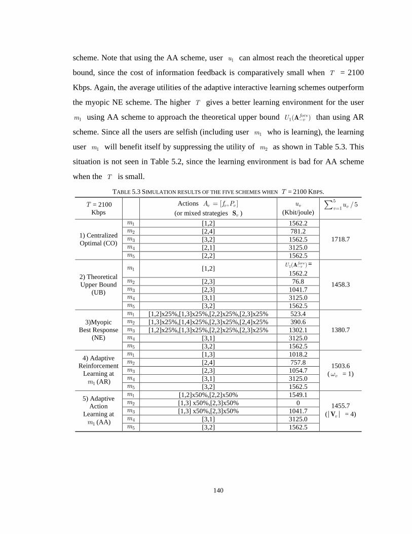
140
scheme. Note that using the AA scheme, user 1u can almost reach the theoretical upper
bound, since the cost of information feedback is comparatively small when T = 2100
Kbps. Again, the average utilities of the adaptive interactive learning schemes outperform
the myopic NE scheme. The higher T gives a better learning environment for the user
1m using AA scheme to approach the theoretical upper bound 1( )forsvU −A than using AR
scheme. Since all the users are selfish (including user 1m who is learning), the learning
user 1m will benefit itself by suppressing the utility of 2m as shown in Table 5.3. This
situation is not seen in Table 5.2, since the learning environment is bad for AA scheme
when the T is small.
TABLE 5.3 SIMULATION RESULTS OF THE FIVE SCHEMES WHEN T = 2100 KBPS.
T = 2100 Kbps
Actions [ , ]v v vA f P=
(or mixed strategies vS ) vu
(Kbit/joule)
5
1/5vv
u=∑
1m [1,2] 1562.2 2m [2,4] 781.2 3m [3,2] 1562.5 4m [2,1] 3125.0
1) Centralized Optimal (CO)
5m [2,2] 1562.5
1718.7
1m [1,2] 1( )forsvU −A =
1562.2 2m [2,3] 76.8 3m [2,3] 1041.7 4m [3,1] 3125.0
2) Theoretical Upper Bound
(UB)
5m [3,2] 1562.5
1458.3
1m [1,2]x25%,[1,3]x25%,[2,2]x25%,[2,3]x25% 523.4 2m [1,3]x25%,[1,4]x25%,[2,3]x25%,[2,4]x25% 390.6 3m [1,2]x25%,[1,3]x25%,[2,2]x25%,[2,3]x25% 1302.1 4m [3,1] 3125.0
3)Myopic Best Response
(NE) 5m [3,2] 1562.5
1380.7
1m [1,3] 1018.2 2m [2,4] 757.8 3m [2,3] 1054.7 4m [3,1] 3125.0
4) Adaptive Reinforcement
Learning at 1m (AR)
5m [3,2] 1562.5
1503.6 ( vω = 1)
1m [1,2]x50%,[2,2]x50% 1549.1 2m [1,3] x50%,[2,3]x50% 0 3m [1,3] x50%,[2,3]x50% 1041.7 4m [3,1] 3125.0
5) Adaptive Action
Learning at 1m (AA)
5m [3,2] 1562.5
1455.7 ( vV = 4)

141
B. Convergence of the learning appraoches
In order to show the convergence of the proposed learning approaches, in Figure 5.8,
we simulate the time plot of the two proposed learning algorithms (AR and AA) and the
best response scheme without learning (NE). The network settings are the same as Table
II when T = 700 Kbps. It is shown that both the two proposed learning schemes
outperform the myopic best response scheme in terms of the average utility. The
convergence speed of the AR scheme is about three times slower than the myopic best
response (which converges to Nash equilibrium in about 5 time slots), while the AA
scheme is about six times slower. The convergence speed of the AR scheme is faster than
the AA scheme, since the AR scheme only need to build belief on its own utility. The AA
scheme needs to build beliefs on its neighboring users’ strategies, which leads to a slower
convergence speed.
Fig. 5.8 Average utility vs. time slot of the proposed algorithms when T = 700 Kbps.
C. Adaptive reinforcement learning using different time scales
The reinforcement learning is very sensitive to the initial status of users’ actions.
Hence, in our simulations, we first train the user 1m ’s initial strategy by performing
0 15 30 45 60 75750
800
850
900
950
1000
1050
1100
1150
Time slot (sec)
Ave
rage
Util
ity (
Kbi
t/jo
ule)
Myopic Best Response (NE)Adaptive Reinforcement Learning (AR)Adaptive Action Learning (AA)

142
myopic best response in the first 20 time slots. Then, we simulate the reinforcement
learning with different values of vω in Figure 5.9 for different T . Since the input rates
of the applications are fixed to 500 Kbps, the utility will saturate as the bandwidth
increases. The UB scheme has another saturation when T becomes larger than 1.1
Mbps, since the larger bandwidth enables another set of actions for the users. Note that
when 1 1ω = , the reinforcement learning learns the transmission strategy 1tS at every
time slot. The simulation results show that the performance of 1 0.8ω = is better than
1 1ω = when the physical bandwidth is lower than 1Mbps, since learning at a slower
pace can reduce the overhead of the private information feedback. The results in Figure 9
show that the proposed adaptive reinforcement learning operates on the envelope of the
solutions obtained for different 1ω , with 1 [0.5,1]ω ∈ . Hence, the performance of user 1m
using the adaptive reinforcement learning becomes closer to the upper bound.
Fig. 5.9 Performance of user 1m adopting adaptive reinforcement learning with private information feedback using different 1ω .
0.4 0.6 0.8 1 1.2 1.4 1.6 1.8 2 2.2
x 106
0
200
400
600
800
1000
1200
1400
1600
Physical Transmission Rate, T (bit/sec)
Util
ity u
1 (K
bit/
joul
e)
UB SchemeReinforcement learning (wv=1)
Adaptive Reinforcement learningPayoff-based learning upperbound
wv = 1
wv=0.8
PIB

143
D. Adaptive action learning from different neighboring users
In Figure 5.10, we also simulate the case that the action learning models the strategy of
the nearest 2v =V users instead of 4v− =M users. With smaller vV , fewer
neighbors need to feed back information and hence, results in less information overhead.
The simulation results show that modeling users from public information feedback can
improve the performance for user 1m . However, when the physical transmission rate is
lower than 1.1 Mbps, the required information overhead degrades the performance
significantly and hence, it is essential to adapt the number of neighbors in the action
learning to model less users in the network. The results show that using the proposed
adaptive action learning, the performance of user 1m with public information feedback
becomes closer to the upper bound.
Fig. 5.10 Performance of user 1m adopting adaptive action learning with public information feedback
using different 1tV .
0.4 0.6 0.8 1 1.2 1.4 1.6 1.8 2 2.2
x 106
0
200
400
600
800
1000
1200
1400
1600
Physical Transmission Rate, T (bps)
Util
ity u
1 (K
bit/
joul
e)
Adaptive Action LearningUB Scheme (model-based learning upperbound)
|V1|=4 |V
1|=2
|V1|=2
PIB

144
E. Mobility effect on the interactive learning efficiency
In the previous subsections, all the simulation results are based on the fixed topology
shown in Figure 5.7. In this subsection, we simulate the case that all 5 receivers moves
according to a well-known mobility model “random walk” [CBD02] – receivers
randomly select a direction at each time slot and move at a fixed speed ν . Starting from
the topology in Figure 5.7, Figure 5.11 shows the learning efficiency over time of the AR,
AA, and NE schemes for ν =0.5, 1, 2 (meter/time slot) with T = 2100 Kbps. It is
shown that the AA scheme has higher learning efficiency on average, since user 1m is
able to obtain the channel gain information (which is directly affected by the mobility) of
the other users from the public information feedback. Moreover, as expected, as the
mobility increases, the learning efficiency decreases because the receivers are moving
further apart. Especially for the reinforcement learning without explicit channel gain
information, the results show that the performance can be worse than myopic best
response, since the learning cannot keep up with the topology changes and the user’s
belief about the other users becomes inaccurate when the mobility is high.
VII. CONCLUSIONS
In this chapter, we provide an adaptive interactive learning framework for delay
sensitive users to adapt their frequency channel selections and power levels in wireless
networks in a decentralized manner. We show that a foresighted user can improve its
utility significantly learning from the information feedback. We determine performance
upper bounds for the user’s utility when learning from private or public information
feedback, respectively. The simulation results show that the proposed adaptive interactive
learning can significantly improve the performance of delay sensitive users compared to
the myopic best response. It is shown that even when only one user learns from its
information feedback, the overall performance can be better than the Nash equilibrium
resulting from the myopic best response. Especially, if the available system bandwidth is
not limited, the proposed adaptive action learning with public information feedback
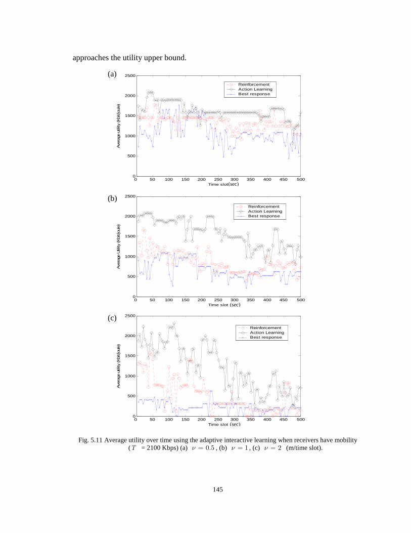
145
approaches the utility upper bound.
Fig. 5.11 Average utility over time using the adaptive interactive learning when receivers have mobility (T = 2100 Kbps) (a) 0.5ν = , (b) 1ν = , (c) 2ν = (m/time slot).
0 50 100 150 200 250 300 350 400 450 5000
500
1000
1500
2000
2500
Time slot
Ave
rage
util
ity (Kbi
t/jo
ule)
ReinforcementAction LearningBest response
0 50 100 150 200 250 300 350 400 450 5000
500
1000
1500
2000
2500
Time slot
Ave
rage
Util
ity (Kbi
t/jo
ule)
ReinforcementAction LearningBest response
0 50 100 150 200 250 300 350 400 450 5000
500
1000
1500
2000
2500
Time slot
Ave
rage
util
ity (Kbi
t/jo
ule)
ReinforcementAction LearningBest response
(a)
(b)
(c)
(sec)
(sec)
(sec)
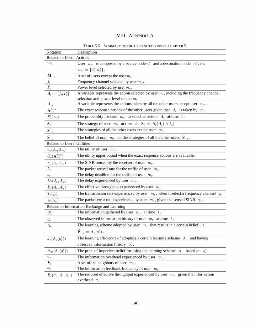
146
VIII. APPENDIX A
TABLE 5.5 SUMMARY OF THE USED NOTATIONS OF CHAPTER 5. Notation Description Related to Users’ Actions vm User vm is composed by a source nodesvn and a destination node svn , i.e.
, s dv v vm n n= .
v−M A set of users except the uservm .
vf Frequency channel selected by uservm .
vP Power level selected by uservm .
[ , ]v v vA f P= A variable represents the action selected by uservm , including the frequency channel selection and power level selection.
vA− A variable represents the actions taken by all the other users except user vm . forsv−A The exact response actions of the other users given that vA is taken by vm .
( )tv vS A The probability for user vm to select an action vA at time t . tvS The strategy of user vm at time t . [ ( ), ]t t
v v v vS A A= ∀S tv−S The strategies of all the other users except user vm .
tv−S
The belief of user vm on the strategies of all the other users t v−S .
Related to Users’ Utilities
-( , )v v vu A A The utility of user vm .
( )forsv vU −A The utility upper bound when the exact response actions are available.
-( , )v v vA Aγ The SINR sensed by the receiver of user vm .
vλ The packet arrival rate for the traffic of user vm .
vd The delay deadline for the traffic of user vm .
-( , )v v vD A A The delay experienced by user vm .
-( , )v v vB A A The effective throughput experienced by user vm .
( )v vT f The transmission rate experienced by user vm , when it select a frequency channel vf .
( )v vp γ The packet error rate experienced by user vm , given the sensed SINR vγ .
Related to Information Exchange and Learning tvI The information gathered by user vm at time t . tvo The observed information history of user vm at time t .
vΛ The learning scheme adopted by user vm that results in a certain belief, i.e.
( )t tv v vo− = ΛS .
( ( ))tv v vJ oΛ The learning efficiency of adopting a certain learning scheme vΛ and having
observed information history tvo .
( ( ))tP v vo∆ Λ The price of imperfect belief for using the learning scheme vΛ based on tvo .
vσ The information overhead experienced by user vm .
vV A set of the neighbors of user vm .
vω The information feedback frequency of user vm .
-( , , )v v v vB A Aσ′ The reduced effective throughput experienced by user vm given the information overhead vσ .

147
IX. APPENDIX B
Recall that vT and vp represent the maximum transmission rate and packet error rate
of user vm using the frequency channel vf . vT and vp are estimated by the
MAC/PHY layer link adaptation [Kri02], which can be modeled as sigmoid functions of
the SINR -( , )v v vA Aγ for user vm :
-( , ( , ))v v v v vp f A Aγ-
1
1 exp( ( ( , ) ))v v vA Aζ γ δ=
+ −, (33)
- -( , ) ( ) (1 ( , ( , )))v v v v v v v v v vB A A T f p f A Aγ= × − , (34)
- -( , , ) ( , ) ( )v v v v v v v vB A A B A Aσ θ σ′ = × , and ( , ) 1 ( 1)v v v v vσ ω ρω= − +V V , where ζ , δ , and
0ρ > are empirical constants corresponding to the modulation and coding schemes for a
given packet length.
Assume that a delay sensitive application is sent by the user vm through the network
with the average input rate vR (bits/sec). Assume that the user vm maintains a queue
with infinite buffer size in the application layer. We model the packet arrival process
using Poisson process. The packet arrival rate is assumed as /v v vR Lλ = (packet/sec).
Considering the packet protection scheme similar to the Automatic Repeat Request
protocol in IEEE 802.11 networks [IEE03], the transmission time of a packet can be
modeled as a geometric distribution. For simplicity, we approximate the queuing model
as M/M/1 queue with the service rate - -( , , ) ( , , )/v v v v v v v v vA A B A A Lµ σ σ′= (packet/sec).
Denote the delay of transmitting the delay sensitive application through the network as
-( , , )v v v vD A Aσ . The average delay can be obtained by
--
1[ ( , , )]
( , , )v v v vv v v v v
E D A AA A
σµ σ λ
=−
, for -( , , )v v v v vA Aµ σ λ> . (35)
Using the M/M/1 queuing model, the probability that the packet of the user vm can be
received before the delay deadline vd is
---
1 exp( ), for ( , , )[ ( , , )]Prob ( , , ) 0 , otherwise
vv v v v v
v v v vv v v v v
dA A
E D A AD A A dµ σ λ
σσ
− − >≤ =
, (36)
The utility function in (2) equals to 0 unless the transmitted power is high enough to

148
support a sufficient throughput -( , , ))/v v v v v vB A A Lσ λ′ > to keep the probability
-Prob ( , , ) 0v v v v vD A A dσ ≤ > (see Figure 2). Substituting equation (35) and (36) into
equation (2), we have equation (11). Since ( )v vB σ′ is a decreasing function of vσ , the
utility function is a non-increasing function of vσ .
X. APPENDIX C
Proof of Proposition 4: Given the channel model ( , )vB f γ for the frequency channel f
in equation (34), user vm , v fm ∈ Ω can apply queuing analysis with the application
characteristics vR , vL and vd . From equation (35) and (36), we have
1Prob 1
( )v vv v
D dF γ
≤ = − . The optimality condition of 0v
v
u
P
∂=
∂ becomes
1 11
( ) ( )vv v v v v
PP F Fγ γ
∂− × = −
∂. The left hand side can be derived as ( ) 1
( )v v v
vv v v v
B d
L F
γγ
γ γ
∂×
∂,
since vv v
v
PP
γγ
∂=
∂. By multiplying vF to both sides, we have the optimality condition in
Proposition 4 and the corresponding tarvγ that maximizes the utility function vu .

149
XI. APPENDIX D
Algorithm 5.1 Adaptive reinforcement learning with private information feedback For user vm at time slot t , assume (0,1)U represents a uniform distribution from 0 to 1.
Initialization: Set 0prevvJ = , 1vω = , 0.05vω = .
Step 1. If ( (0,1)) 1 vRand ω< −U , keep using action t basev vA A= , 1t t← + , and repeat Step 1,
otherwise go to Step 2. Step 2. Calculate 1 1( , )t t
v v vu A γ− − from previous action 1 1 1[ , ]t t tv v vA f P− − −= and the private
information feedback , 1 t priv tv vγ
−=I .
Step 3. Update the propensity tvr and the strategy t
vS .
Step 4. Determine the action from ( )t tv vA Rand= S .
Step 5. Update the baseline action basevA and baseline payoff value base
vu as in equation (21) and (22). Step 6. Evaluate vJ . If prev
v vJ J> , then If 0 ,v v v v vω ω ω ω ω− > ← − , else if 0v vω ω− ≤ , keep vω .
Otherwise, If 1 ,v v v v vω ω ω ω ω+ ≤ ← + , else if 1v vω ω− > , keep vω . Step 7. Set prev
v vJ J← , 1t t← + , and go back to Step 1.
Algorithm 5.2 Adaptive action learning (H =2) with public information feedback For user vm at time slot t , Initialization: Set 0prev
vJ = , v v−=V M , 1v =V .
Step 1. Observe the public information feedback , 1 1( ) , , v
t pub t tu u u vv
A m− −− = ∈V
G VI fed back from
the users u vm ∈ V .
Step 2. Update the propensity tur for users u vm ∈ V and calculate the strategy vector ( )t
v vA−S .
Step 3. Calculate the target power ( )tarvP f from equation (31) and find the action * *[ , ]t
v v vA f P= using Proposition 5.
Step 4. Evaluate vJ . If prevv vJ J> , then
If 0,v v v v v− > ← −V V V V V , else if 0v v− ≤V V , keep
vV . Otherwise,
If v v v−+ ≤V V M , v v v← +V V V , else if
v v v−+ >V V M , keep vV .
Step 5. Set prevv vJ J← , 1t t← + , and go back to Step 1.

150
Chapter 6
Resource Management in Single-Hop Cognitive
Radio Networks
I. INTRODUCTION
The demand for wireless spectrum has increased rapidly in recent years due to the
emergence of a variety of applications, such as wireless Internet browsing, file
downloading, streaming, etc. In the foreseeable future, the requirements for wireless
spectrum will increase even more with the introduction of multimedia applications such
as YouTube, peer to peer multimedia networks, and distributed gaming. However,
scanning through the radio spectrum reveals its inefficient occupancy [SW04] in most
frequency channels. Hence, the Federal Communications Commission (FCC) suggested
in 2002 [FCC02] improvements on spectrum usage to efficiently allocate frequency
channels to license-exempt users without impacting the primary licensees. This forms
cognitive radio networks that 1) enhance the spectrum usage of the traditional licensing
system, and 2) release more spectrum resources for the unlicensed allocations in order to
fulfill the required demand.
The emergence of cognitive radio networks have spurred both innovative research and
ongoing standards [CCB06][Hay05][MM99]. Cognitive radio networks have the
capability of achieving large spectrum efficiencies by enabling interactive wireless users
to sense and learn the surrounding environment and correspondingly adapt their
transmission strategies. Three main challenges arise in this context. The first problem is
how to sense the spectrum and model the behavior of the primary licensees. The second
problem is how to manage the available spectrum resources and share the resource to the
license-exempt users to satisfy their transmission requirements while not interfering with
151
the primary licensees. The third problem is how to maintain seamless communication
during the transition (hand-off) of selected frequency channels. In this chapter, we focus
on the second challenge and rely on the existing literature for the remaining two
challenges [ALV06][Bro05].
Prior research such as [CCB06][ZL06] focus on centralized solutions for the resource
management problem in cognitive radio networks. However, due to the
informationally-decentralized nature of wireless networks, the complexity of the optimal
centralized solutions for spectrum allocation is prohibitive [WP02] for delay-sensitive
multimedia applications. Moreover, the centralized solution requires the propagation of
private information back and forth to a common coordinator, thereby incurring delay that
may be unacceptable for delay-sensitive applications. Hence, it is important to implement
decentralized solutions for dynamic channel selection by relying on the wireless
multimedia users’ capabilities to sense and adapt their frequency channel selections.
Moreover, unlike most of the existing research on resource management in the cognitive
radio networks [TJ91][SCC05] that ignores the multimedia traffic characteristics in the
application layer and assumes that all competing users in the networks are of the same
type (applications, radio capabilities), we consider heterogeneous users in this chapter,
meaning that the users can have 1) different types of utility functions and delay deadlines,
2) different traffic priorities and rates, and 3) experience distinct channel conditions in
different frequency channels. For example, the multimedia users can differ in their
preferences of utility functions, priorities of accessing the frequency channels, traffic rate
requirements, capabilities of transmitting data in different frequency channels. Note that
in the informationally-decentralized wireless network, these utility functions, traffic
characteristics, and the channel conditions are usually considered as private information
of the users. Hence, the main challenge here is how to coordinate the spectrum sharing
among heterogeneous multimedia users in a decentralized manner.
To do this, information exchange across the multimedia users is essential. Since the
152
decisions of a user will impact and be impacted by the other users selecting the same
frequency channel, without explicit information exchange, the heterogeneous users will
consume additional resources and respond slower to the time-varying environment
[Luc06]. The key questions are what information exchanges are required, and how
autonomous users adapt their channel selections based on the limited information
exchange to efficiently maximize their private utilities. In this chapter, we propose a
novel priority virtual queue interface to abstract multimedia users’ interactions and
determine the required information exchange according to the priority queuing analysis.
Note that such information exchanges can rely on a dedicated control channel for all
users, or can use a group-based scheme without a common control channel [ZZY05].
In this chapter, we model the traffic of the users (including the licensed users and the
license-exempt users) and the channel conditions (e.g. Signal-to-Noise Ratio,
Bit-Error-Rate) by stationary stochastic models similar to [SCC05]. Our approach
endows the primary licensees with the priority to preempt the transmissions of the
license-exempt users in the same frequency channel. Based on the priority queuing
analysis, each wireless user can evaluate its utility impact based on the behaviors of the
users deploying the same frequency channel (including the primary licensees, to which
the highest priority is assigned). The behavior of a user is represented by its probability
profile for selecting different frequency channels, which is referred as the channel
selection strategy in this chapter. Based on the expected utility evaluation, we propose a
Dynamic Strategy Learning (DSL) algorithm for an autonomous multimedia user to adapt
its channel selection strategy.
In summary, our chapter addresses the following important issues:
a) Separation of the utility evaluation and channel selection using the priority
virtual queue interface.
We propose a novel priority virtual queue interface for each autonomous user to
exchange information and maximize its private utility in cognitive radio networks.

153
Through the interface, the user can model the strategies of the other users with higher
priorities and evaluates the expected utility of selecting a certain frequency channel.
Importantly, the interface provides a simple model that facilitates the user’s learning of
what is the best channel selection strategy.
b) Priority virtual queuing analysis for heterogeneous multimedia users.
Unlike prior works on cognitive radio networking, which seldom consider multimedia
traffic characteristics and delay deadlines in the application layer, our priority virtual
queue framework enables the autonomous multimedia users to consider 1) priorities of
accessing the frequency channels, 2) different traffic loads and channel conditions in
different frequency channels, and 3) heterogeneous preferences for various types of
utility functions based on the deployed applications. Note that the priority queuing model
allows the primary licensees to actively share the occupied channels instead of excluding
all the other wireless users. However, by assigning highest preemptive priorities to the
licensees, the unlicensed users do not impact the licensees.
c) DSL algorithm for dynamic channel selections by wireless stations.
Based on the expected utility evaluation from the interface, we propose a decentralized
learning algorithm that dynamically adapts the channel selection strategies to maximize
the private utility functions of users. Note that a frequency channel can be shared by
several users. A wireless user can also select multiple frequency channels for
transmission. Our learning algorithm addresses how multimedia users distribute traffic to
multiple available frequency channels to maximize their own utility functions.
The rest of this chapter is organized as follows. Section II provides the specification of
cognitive radio networks and models the dynamic resource management problem as a
multi-agent interaction problem. In Section III, we give an overview of our dynamic
resource management for the heterogeneous multimedia users, including the priority
virtual queue interface and the dynamic channel selection. In Section IV, we provide the
queuing analysis for the priority virtual queue interface and determine the required

154
information exchange. In Section V, we focus on the dynamic channel selection and
propose the DSL algorithm to adapt the channel selection strategy for the multimedia
users. Simulation results are given in Section VI. Section VII concludes the chapter.
II. MODELING THE COGNITIVE RADIO NETWORKS AS MULTI-AGENT INTERACTIONS
A. Agents in a cognitive radio network
In this chapter, we assume that the following agents interact in the cognitive radio
network:
Primary Users are the incumbent devices possessing transmission licenses for
specific frequency bands (channels). We assume that there are M channels in the
cognitive radio network, and that there are several primary users in each frequency
channel. These primary users can only occupy their assigned frequency channels.
Since the primary users are licensed users, they will be provided with an
interference-free environment [Hay05][ALV06].
Secondary Users are the autonomous wireless stations that perform channel sensing
and share the available spectrum holes [CCB06]. We assume that there are N
secondary users in the system. These secondary users are able to transmit their traffic
using various frequency channels. If multiple users select the same frequency channel,
they will time share the chosen frequency channel. Moreover, these secondary users
are license-exempt, and hence, they cannot interfere with the primary users.
In this chapter, we consider the users sharing a single-hop wireless ad-hoc network.
Figure 6.1 provides an illustration of the considered network model. We assume the
secondary users as transmitter-receiver pairs with information exchange among these
pairs. In order to maintain stationary property, we assume that these network agents are
static (i.e. we do not consider mobility effects). Next, we model the interaction among
secondary users accessing the same frequency channel.

155
Fig. 6.1 An illustration of the considered network model.
B. Models of the dynamic resource management problem
• Users: As indicated above, there are two sets of users – aggregate primary users in
each channel 1 ,..., MPU PU=PU1 and the secondary users 1 ,..., NSU SU=SU .
The priorities of users in cognitive radio networks are pre-assigned depending on
their Quality of Service (QoS) requirements and their right to access the frequency
channels.
• Resources: The resources are the frequency channels 1 ,..., MF F=F . Multiple users
can time share the same frequency channel. Note that even if the same time sharing
fraction is assigned to the users choosing the same frequency channel, their
experienced channel conditions may differ.
• Actions: The considered actions of the secondary users are the selection of the
frequency channel for each packet transmission. We denote the actions of a secondary
user iSU using 1 2[ , ,..., ] Mi i i iMa a a= ∈a A , where ija ∈ A ( = 0,1A ). 1ija =
indicates that iSU chooses the frequency channel jF . Otherwise, 0ija = . Let i−a
denote the actions of the other secondary users except iSU . Let
1 From the secondary users’ point of view, there is no need to differentiate different primary users in one frequency channel. Hence, we reduce the primary users in one frequency channel into one aggregate primary user. A secondary user needs to back-off and wait for transmission or select another frequency channel, once any of the primary users starts to transmit in the same frequency channel.
Information exchange
Multimedia flowSensing feedback (e.g. SINR)
1SU
2SU
1PU
1F
2PU
2F3PU
3F
Information exchange
Multimedia flowSensing feedback (e.g. SINR)
Information exchange
Multimedia flowSensing feedback (e.g. SINR)
1SU
2SU
1PU
1F
2PU
2F3PU
3F1SU
2SU
1PU
1F
1PU
1F
1PU
1F
2PU
2F
2PU
2F
2PU
2F3PU
3F
3PU
3F
3PU
3F

156
1[ , ..., ]T T M NN
×= ∈A a a A denote the total action profile across all secondary users.
• Strategies: A strategy of a secondary user iSU is a vector of probabilities
1 2[ , , ..., ] Mi i i iMs s s= ∈s S , where ijs ∈ S ( [0,1]∈S ) represents the probability of the
secondary user iSU to take the action ija (i.e. to choose the frequency channel jF ).
Hence, the summation over all the frequency channels is 1
1M
ijjs
==∑ . Note that ijs
can also be viewed as the fraction of data from iSU transmitted on frequency
channel jF , and hence, multiple frequency channels are selected for a secondary
users with 0ijs > . Let 1[ , ..., ]T T M NN
×= ∈S s s S denote the total strategy profile across
all secondary users.
• Utility functions: Each secondary user has its own utility function. Based on the
adopted actions of the secondary users, we denote the utility function of iSU as iu .
Conventionally, the utility function of a specific user is often modeled solely based on
its own action, i.e. ( )i iu a without modeling the other secondary users [WP02][VS05].
However, the utility function for multimedia users relates to the effective delay and
throughput that a secondary user can derive from the selected frequency channel,
which is coupled with the actions of other secondary users. Hence, the utility function
iu is also influenced by the action of other secondary users that select the same
frequency channel. In other words, the utility function can be regarded as ( , )i i iu −a a .
We will discuss this utility function in detail in Section III.C.
Expected utility function with dynamic adaptation: In an
informationally-decentralized cognitive wireless network that consists of
heterogeneous secondary users, the secondary user iSU may not know the exact
actions of other secondary users i−a . Moreover, even if all the actions are known, it
is unrealistic to assume that the exact action information can be collected timely to
compute and maximize the actual utility function ( , )i i iu −a a . Hence, a more practical
solution is to dynamically model the other secondary users’ behavior by updating
their probabilistic strategy profile of actions i−s based on the observed information,
157
and then compute the optimal channel selection strategy is that maximizes the
expected utility function of iSU , i.e.
( , )( , ) [ ( , )]i ii i i i i iU E u−− −= s ss s a a , (1)
where ( , )[ ( , )]i i i i iE u− −s s a a is the expected utility function, given a fixed strategy profile
( , )i i−=S s s . In the next section, we discuss how secondary users perform dynamic
resource management that maximizes the expected utility function ( , )i i iU −s s by
modeling the strategy (behavior) i−s of the other users in cognitive radio networks.
III. DYNAMIC RESOURCE MANAGEMENT FOR HETEROGENEOUS SECONDARY USERS
USING PRIORITY QUEUING
In this section, we provide our dynamic resource management solution using the
multi-agent interaction settings in the previous section. We first emphasize the
heterogeneity of the secondary users in cognitive radio networks and then introduce our
solution with the priority queuing interface and adaptive channel selection strategies.
A. Prioritization of the users
We assume that there are K priority classes of users in the system. The highest
priority class 1C is always reserved for the primary users PU in each frequency
channel. The heterogeneous secondary users SU can be categorized into the rest of
1K − priority classes (2, ..., KC C ) to access the frequency channels2. We assume that the
users in higher priority classes can preempt the transmission of the lower priority classes
to ensure an interference-free environment for the primary users [Kle75]. The priority of
a user affects its ability of accessing the channel. Primary users in the highest priority
class 1C can always access their corresponding channels at any time. Secondary users,
on the other hand, need to sense the channel and wait for transmission opportunities for
transmission (when there is no higher priority users using the channel) based on their
2 The prioritization of the secondary users can be determined based on their applications, prices paid for spectrum access, or other mechanism design based rules. In this chapter, we will assume that the prioritization was already performed.

158
priorities. We assume that there are kN users in each of the class kC . Hence, 1N M=
(number of aggregate primary users) and 2
K
kkN N
==∑ (number of secondary users).
Various multiple access control schemes can be adopted for the secondary users to
share the spectrum resource. For simplicity, in this chapter, we consider a MAC protocol
similar to IEEE 802.11e HCF [IEE03]3 to assign transmission opportunities (i.e. TXOP)
and ensure that a secondary users in the lower priority class will stop accessing the
channel and wait in the queue or change its action (channel selection) if a higher priority
user is using the frequency channel. Note that for secondary users, they not only can have
different priorities to access the frequency channels, but they can also have different
channel conditions and possess their own preferences for a certain type of utility function,
which is discussed in the following subsections.
B. Heterogeneous channel conditions
For a certain frequency channel jF , the secondary users can experience various
channel conditions for the same frequency channel. We denote ijT and ijp as the
resulting physical transmission rate and packet error rate for the secondary user iSU
transmitting through a certain frequency channel jF . Let [ , ]ij ij ijR T p= ∈R be the
channel conditions of the channel jF for the secondary user iSU . We denote the
channel condition matrix as [ ] M NijR ×= ∈R R . The expected physical transmission rate
and packet error rate can be approximated as sigmoid functions of measured
Signal-to-Interference-Noise-Ratio (SINR) and the adopted modulation and coding
scheme as in [Kri02]. Note that the expected ijT and ijp of the same frequency channel
can be different for various secondary users.
C. Goals of the heterogeneous secondary users
In general, the utility function iu is a non-decreasing function of the available
3 Either the polling-based HCCA or contention-based EDCA protocols can be applied, as long as the priority property of the users is provided. However, a more sophisticated MAC protocols can also be considered to deal with the spectrum heterogeneity (such as HD-MAC in [ZZY05]). Different MAC protocols will have different overheads including the time of waiting for the MAC acknowledgement, contention period, etc. that affect the service time distribution of the M/G/1 queuing model.

159
transmission rates. Several types of objectives for the secondary users can be considered
in practice, such as minimizing the end-to-end delay, loss probability, or maximizing the
received quality, etc. For simplicity, we assume only two types of utility functions4 in
this chapter.
• The delay-based utility for delay-sensitive multimedia applications.
Let ( , )i i iD −a a represent the end-to-end packet delay (transmission delay plus the
queuing delay) for the secondary user iSU . Let id represent the delay deadline of the
application of secondary user iSU . We consider this type of utility function as (as in
[JCO02]):
(1)( , ) Prob( ( , ) )i i i i i iiu D d− −= ≤a a a a , (2)
which depends on the end-to-end delay ( , )i i iD −a a and the delay deadline id imposed
by the application.
• The throughput-based utility for delay-insensitive applications.
Let effiT represent the effective available throughput for the secondary user iSU . The
second type of utility function is assumed to be directly related to the throughput (as in
[ZP05]). In this chapter, we define it as:
maxmax(2)
max
( , ), if ( , )
( , )
1 , if ( , )
effi i effi
i i iiii ii
effi i ii
TT T
Tu
T T
−−
−
−
≤= >
a aa a
a a
a a
, (3)
where maxiT is the physical throughput required by the secondary user iSU .
We assume that a secondary user can possess multiple applications that can be either
delay-sensitive multimedia traffic or delay-insensitive data traffic. Hence, we define the
utility function of a secondary user as a multi-criterion objective function (as in
[ZL06][TJZ03]) of these two types of utility functions. Different secondary users can
have different preferences iθ5 (0 1iθ≤ ≤ ). Specifically, the goal of a secondary user
4 This model can be easily extended to more types of utility functions. Moreover, our utility function can also be easily modified to a quality-type utility function using different priorities. For simplicity, we do not consider the quality impact of different multimedia packets in our utility function.
5 In this chapter, we assume that the preferences iθ are predetermined by the secondary users. The preferences iθ of the multi-criterion optimization can be determined based on the applications. See e.g. [SP85].
160
iSU is to maximize the following utility function:
(1) (2)( , ) = ( , ) (1 ) ( , )i i i i i i i i ii iu u uθ θ− − −⋅ + − ⋅a a a a a a . (4)
Note that, in this setting, 0 ( , ) 1i i iu −≤ ≤a a .
D. Example of three priority classes with different utility functions
Let kA be the action set of the secondary users in the classes 2,..., kC C , i.e.
| , 2,..., k i i lSU C l k= ∈ =A a . Note that 1k k− ⊆ ⊆A A A . Due to the priority queuing
structure, the actions of the secondary users with lower priority will not affect the users in
the higher priority class [BG87]. Hence, the decentralized optimizations are performed
starting from the higher priority classes to the lower priority classes. In other words, the
decentralized optimization of a secondary user in a lower priority class also needs to
consider the actions of the users in higher priority classes. For example, three classes can
be assumed ( 3K = ) – the first priority class is composed by the primary users whose
actions are fixed (no channel selection capability). The second priority class 2C is
composed by the secondary users transmitting delay-sensitive multimedia applications,
and the third priority class 3C is composed by the secondary users transmitting regular
data traffic, which requires throughput maximization. The objective function for each of
the secondary users in priority class 2C is ( 21, for i iSU Cθ = ∈ ): (1)
( , ) 2
maximize ( , )
maximize [Prob( ( ) ))]i i
i ii
i i
U
E D d−
−
⇒ ≤s s
s s
A
. (5)
Then, the objective function for the secondary users in the class 3C is
( 30, for i iSU Cθ = ∈ ): (2)
( , )
maximize ( , )
maximize [ ( )]i i
i ii
effi
U
E T−
−
⇒ s s
s s
A
, (6)
with the constraint that 2 ⊆A A are predetermined by (5). The effective transmission
rate of each secondary user can be expressed as:
( , )1
[ ( )] (1 )i i
Meff
ij ij ijij
E T s T p−
=
= −∑s s A . (7)
From the above three classes example, note that delay analysis is essential for the

161
heterogeneous secondary users with delay-sensitive applications in a cognitive radio
network.
To maximize the expected utility function as stated in equation (1), a secondary user
needs to consider the impact of the other secondary users. In order to efficiently regulate
the information exchange among heterogeneous users and efficiently provide expected
utility evaluation, a coordination interface must be developed. Based on this interface,
the secondary users can interact with each other in a decentralized manner. In the next
subsection, we propose a novel dynamic resource management with such an interface for
a secondary user iSU to adapt its frequency selection strategy is .
E. Priority virtual queue interface
The resource management for delay-sensitive multimedia applications over cognitive
radio networks needs to consider the heterogeneous wireless users having various utility
functions, priorities of accessing the channel, traffic rates, and channel conditions.
Specifically, the main challenge is how to coordinate the spectrum sharing among
competing users and select the frequency channel to maximize the utility functions in a
decentralized manner. For this, we propose a novel priority virtual queue interface.
Unlike prior research assuming that secondary users apply 2-state “spectrum holes”
(on-off model [SCC05]) for spectrum access [Hay05] in our priority virtual queue
interface, we allow secondary users to obtain transmission opportunities once the primary
user in a specific channel stops transmitting. The primary users have the highest priority,
thereby being able to preempt the transmission of the secondary users’ transmission.
The priority virtual queue interface has two main tasks – 1) determines the required
information exchange and 2) evaluates the utility impact from the wireless environment
as well as the competing users’ behaviors in the same frequency channel. In the priority
virtual queue interface of a user, the virtual queues are preemptive priority queues [Kle75]
for each of the frequency channels. They are emulated by each multimedia user to
estimate the delay of selecting a specific frequency channel for transmission. Figure 6.2

162
illustrates the architecture of the proposed dynamic resource management with priority
virtual queue interface that exchanges information and emulates the expected delay. Note
that these virtual queues are in fact distributed (physically located) at the secondary users.
Fig. 6.2 The architecture of the proposed dynamic resource management with priority virtual queue
interface.
The implementation of the dynamic resource management with priority virtual queue
interface of the secondary users is presented below:
1. Information exchange collection: The secondary user iSU collect the required
information from other secondary users through the priority virtual queue interface.
The required information exchange will be discussed in Section IV.D based on the
queuing analysis.
2. Priority queuing analysis: The interface estimates i−s and performs priority
queuing analysis based on the observed information to evaluate the expected utility
( , )i i iU −s s . The priority queuing analysis will be discussed in details in Section IV.
3. Dynamic strategy adaptation: Based on the expected utility ( , )i i iU −s s , the
Dynamic channel selection
Priority queuing performance analysis Dynamic channel
selectionPriority virtual queue
interfaceDynamic strategy
adaptation
1SU
1s
1U
Informationexchange
1... ...i NSU SU SU
1PU MPU
……
Heterogeneous traffic
Priority virtual queues for each of the wireless channels1F jF MF
……
Cognitive Radio Network
jPUTransmission opportunityfrom the MAC protocol
Dynamic channel selection
Priority queuing performance analysis
Dynamic channel selection
Dynamic channel selection
Priority queuing performance analysis Dynamic channel
selectionDynamic channel
selectionPriority virtual queue
interfaceDynamic strategy
adaptation
1SU
Priority virtual queueinterface
Dynamic strategyadaptation
Priority virtual queueinterface
Dynamic strategyadaptation
1SU
1s
1U
Informationexchange
1... ...i NSU SU SU
1PU1PU1PU MPU
……
Heterogeneous traffic
Priority virtual queues for each of the wireless channels1F jF MF
……
Cognitive Radio Network
jPUTransmission opportunityfrom the MAC protocol
163
secondary user adapts its channel selection strategy is . We propose a dynamic
strategy learning algorithm, which will be discussed in detail in Section V.
4. Assign actions for each packet based on the strategy: Based on current channel
selection strategy is , iSU can assign to each packet an action (select frequency
channel according to the probability profile). As the channel selection strategy adapts
to the network changes, the behavior of a secondary user selecting the frequency
channels for its packets will also change.
5. Wait for the transmission opportunity and transmit the packets: The packets wait
in queues to be transmitted. Based on the priorities of the users, the higher priority
secondary users will have a better chance to access the channel and transmit their
packets.
Note that the primary users will transmit whenever needed in their corresponding
frequency channels.
Next, we present the priority queuing analysis for delay-sensitive multimedia users to
evaluate ( , )i i iU −s s .
IV. PRIORITY QUEUING ANALYSIS FOR DELAY-SENSITIVE MULTIMEDIA USERS
In this section, we discuss the priority queuing analysis for delay-sensitive multimedia
applications. It is important to note that the packets of the competing wireless users are
physically waiting at different locations. Figure 6.3 gives an example of the physical
queues for the case of M frequency channels and N secondary users. Each secondary
user maintains M physical queues for the various frequency channels, which allows
users to avoid the well-known head-of-line blocking effect [WZF04]. The channel
selection decisions are based on the queuing analysis, which will be discussed in detail in
Section V. In this section, we focus on the priority queuing analysis from the perspective
of each secondary user to evaluate ( , )i i iU −s s .

164
Fig. 6.3 Actions of the secondary users ija and their physical queues for each frequency channel.
A. Traffic models
• Traffic model for primary users
We assume that the stationary statistics of the traffic patterns of primary users can be
modeled by all secondary users. The packet arrival process of a primary user is modeled
as a Poisson process with average packet arrival rate PUjλ for the primary user jPU
using the frequency channel jF . Note that the aggregation of Poisson processes of
primary users in the same frequency channel is still Poisson. We denote the mth moments
of the service time distribution of the primary user jPU in frequency channel jF as
[( ) ]PU mjE X . We adopt an M/G/1 model for the traffic descriptions. Note that this traffic
model description is more general than a Markov on-off model [SCC05], which is a
sub-set of our queuing model with an exponential idle period and an exponential busy
period.
• Traffic model for secondary users
1to F
2to F
to MF
1SU
1to F
2to F
to MF
2SU
1to F
2to F
to MF
NSU
1F 2F MF
11a 12a 1Ma
21a 22a 2Ma
1Na 2Na NMa
1ija =0ija =
Physical queues at the secondary users
Cognitive RadioNetwork1V
1js
2V2 js
NVNjs
Virtual queues for different frequency channels
1PU 2PU MPU
1to F
2to F
to MF
1SU
1to F
2to F
to MF
2SU1to F
2to F
to MF
2SU
1to F
2to F
to MF
NSU
1F 2F MF
11a 12a 1Ma
21a 22a 2Ma
1Na 2Na NMa
1ija =0ija =1ija =0ija =1ija =0ija =
Physical queues at the secondary users
Cognitive RadioNetwork1V
1js1V
1js
2V2 js
2V2 js
NVNjs
NVNjs
Virtual queues for different frequency channels
1PU 2PU MPU

165
We assume that the average rate requirement for the secondary user iSU is iB (bit/s).
Let ijλ denote the average packet arrival rate of the secondary user iSU using the
frequency channel jF . Since the strategy ijs represents the probability of the secondary
user iSU taking action ija (transmitting using the frequency channel jF ), we have i
ij iji
Bs
Lλ = , (8)
where iL denotes the average packet length of the secondary user iSU . If a certain
secondary user iSU can never use the frequency channel jF , we fix its strategy to
0ijs = , and hence, 0ijλ = . For simplicity, we also model the packet arrival process of
the secondary users using a Poisson process. Note that the average arrival rate is the only
sufficient statistics required to describe a Poisson process.
Since packet errors are unavoidable in a wireless channel, we assume that packets will
be retransmitted, if they are not correctly received. This can be regarded as a protection
scheme similar to the Automatic Repeat Request protocol in IEEE 802.11 networks
[IEE03]. Hence, the service time of the users can be modeled as a geometric distribution
[Kon80]. Let [ ]ijE X and 2[ ]ijE X denote the first two moments of the service time of the
secondary user iSU using the frequency channel jF . We have:
[ ](1 )i o
ijij ij
L LE X
T p
+=
−, (9)
22
2 2
( ) (1 )[ ]
(1 )
i o ijij
ij ij
L L pE X
T p
+ +=
−, (10)
where iL is the average packet length of the secondary user iSU and oL represents
the effective control overhead including the time for protocol acknowledgement6,
information exchange, and channel sensing delay, etc. (see [IEE03] for details). Let us
denote [ [ ] | 1,..., ]i ijE X j M= =X and 2 2[ [ ] | 1,..., ]i ijE X j M= =X . To describe the traffic
model, we define the traffic specification7 for the secondary user iSU as
2[ , , , , ], if i k i i i i i kC B L SU C= ∈TS X X . This information needs to be exchanged among the
6 Here we only consider retransmission due to channel errors. We consider the protocol overhead in the MAC layer including possible contention period, time for acknowledgement, etc. in the effective control overhead.
7 The traffic specification is similar to the TSPEC in current IEEE 802.11e [IEE03] for multimedia transmission.

166
secondary users, which will be discussed in detail in Section IV.D.
B. Priority virtual queuing analysis
In order to evaluate the expected utility ( , )i i iU −s s for delay-sensitive multimedia
applications, we need to calculate the distribution of the end-to-end delay ( , )i i iD −a a for
the secondary user iSU to transmit its packets. The expected end-to-end delay8 [ ]iE D
of the secondary user iSU can be expressed as:
1
[ ( , )] [ ( ( ))]M
i i i ij ij ij
j
E D s E D R−=
= ⋅∑a a A , (11)
where [ ( ( ))]ij ijE D R A is the average end-to-end delay if the secondary user iSU chooses
the frequency channel jF . Note that ijs is the strategy of the action ija in A .
Using the queuing model in Figure 6.3, each arriving packet of iSU will select a
physical queue to join (action ija ) according to the strategy ijs . Note that there are N
physical queues from N secondary users for a frequency channel jF . Only one of them
can transmit its packets at any time. Hence, we form a “virtual queue” for the same
frequency channel as illustrated in Figure 6.3. In a virtual queue, the packets of the
different secondary users wait to be transmitted. Importantly, the total sojourn time
(queue waiting time plus the transmission service time) of this virtual queue now
becomes the actual service time at each of the physical queues. The concept is similar to
the “service on vacation” [BG87] in queuing theory, and the waiting time of the virtual
queue can be regarded as the “vacation time”.
Since the number of the secondary users in a regular cognitive radio network is usually
large, we can approximate the virtual queue using prioritized M/G/1 queuing model (i.e.
when N → ∞ , the input traffic of the virtual queue can be modeled as a Poisson process).
The average arrival rate of the virtual queue of the frequency channel jF is 1
N
ijiλ
=∑ .
Let us denote the first two moments of the service time for the virtual queue of the
8 In order to simplify the notation, we use simple expectation notation [ ]E ⋅ instead of the expectation over the action strategies
( , )[ ]i iE
−⋅s s hereafter in this chapter.
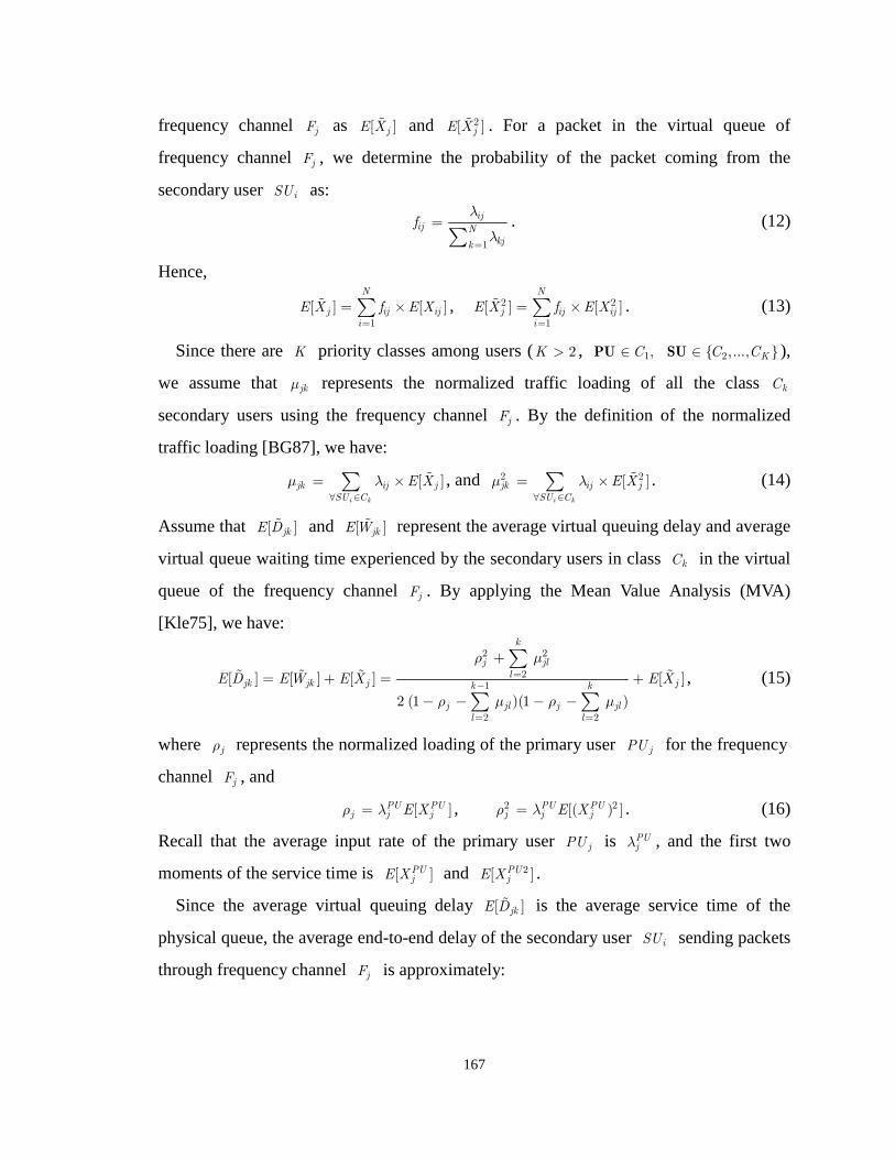
167
frequency channel jF as [ ]jE X and 2[ ]jE X . For a packet in the virtual queue of
frequency channel jF , we determine the probability of the packet coming from the
secondary user iSU as:
1
ijij N
kjk
fλ
λ=
=∑
. (12)
Hence,
1
[ ] [ ]N
j ij ij
i
E X f E X=
= ×∑ , 2 2
1
[ ] [ ]N
j ij ij
i
E X f E X=
= ×∑ . (13)
Since there are K priority classes among users ( 2K > , 1,C∈PU 2 ,..., KC C∈SU ),
we assume that jkµ represents the normalized traffic loading of all the class kC
secondary users using the frequency channel jF . By the definition of the normalized
traffic loading [BG87], we have:
[ ]i k
jk ij j
SU C
E Xµ λ∀ ∈
= ×∑ , and 2 2[ ]i k
jk ij j
SU C
E Xµ λ∀ ∈
= ×∑ . (14)
Assume that [ ]jkE D and [ ]jkEW represent the average virtual queuing delay and average
virtual queue waiting time experienced by the secondary users in class kC in the virtual
queue of the frequency channel jF . By applying the Mean Value Analysis (MVA)
[Kle75], we have:
2 2
21
2 2
[ ] [ ] [ ] [ ]
2 (1 )(1 )
k
j jl
ljk jk j jk k
j jl j jl
l l
E D EW E X E X
ρ µ
ρ µ ρ µ
=−
= =
+
= + = +
− − − −
∑
∑ ∑
, (15)
where jρ represents the normalized loading of the primary user jPU for the frequency
channel jF , and
[ ]PU PUj j jE Xρ λ= , 2 2[( ) ]PU PU
j j jE Xρ λ= . (16)
Recall that the average input rate of the primary user jPU is PUjλ , and the first two
moments of the service time is [ ]PUjE X and 2[ ]PU
jE X .
Since the average virtual queuing delay [ ]jkE D is the average service time of the
physical queue, the average end-to-end delay of the secondary user iSU sending packets
through frequency channel jF is approximately:

168
[ ][ ] , for [ ] 1,
1 [ ]
jkij ij jk i k
ij jk
E DE D E D SU C
E Dλ
λ= < ∈−
. (17)
Strategies ( , )i i−s s such that [ ] 1ij jkE Dλ ≥ will result in an unbounded delay [ ]ijE D ,
which is undesirable for delay-sensitive applications. The advantage of this
approximation is that once the average delay of the virtual queue [ ]jkE D is known by the
secondary user iSU , the secondary user can immediately calculate the expected
end-to-end delay [ ]ijE D of a packet transmitting using the frequency channel jF . Note
that in equation (17), we assume that once a packet selects a physical queue, it cannot
switch to another queue (change position to the other queues). However, by considering
current physical queue size ijq for user iSU using the frequency channel jF , a packet
can change its channel selection after it is put in the physical queue. The switching
probability from a longer queue iaq to a shorter queue ibq in a time interval t can be
defined as 1 exp( ( ))ia ibt q q− − × − . To evaluate such expected end-to-end delay [ ]ijE D , a
more sophisticated queuing model with jockey impatient customers [Koe66] needs to be
considered.
Let ( , )ij i iP s s− represent the probability of packet loss for the secondary user iSU
sending packets through frequency channel jF . By applying G/G/1 approximation based
on the work of [JTK01], we have: [ ]
[ ]exp( ), for [ ] 1, [ ]( , )
1, for [ ] 1
ij jk iij jk ij jk i k
ijij i i
ij jk
E D dE D E D SU C
E DP
E D
λλ λ
λ
−
× − < ∈= ≥
s s
. (18)
For a delay-sensitive secondary user iSU , the objective function in (5) becomes: (1)
1
1
maximize ( , )
maximize (1 ( , ))
[ ]minimize [ ]exp( ), for
[ ]
i
i
i
i ii
M
ij ij i i
j
Mij jk i
ij ij jk i kijj
U
s P
E D ds E D SU C
E D
λλ
−
−=
=
⇒ −
×⇒ − ∈
∑
∑
s
s
s
s s
s s
. (19)
C. Information overhead and the aggregate virtual queue effects
In the previous subsection, we calculate ( , )ij i iP s s− , the packet loss probability for a

169
packet of the secondary user iSU transmitting using the frequency channel jF . In a
general case, we can calculate the expected utility function of equation (4) as: (1) (2)
max1 1
1
[ ( , )] = (1 )
(1 ( , )) (1 ) (1 )/
[ ( , )]
i i i i ii i
M M
i ij ij i i i ij ij ij ij j
M
ij ij i ij
E u U U
s P s T p T
s EV
θ θ
θ θ
−
−= =
−=
⋅ + − ⋅
= ⋅ − + − −
= ⋅
∑ ∑
∑
a a
s s
a a
, (20)
where max[ ( , )] (1 ( , )) (1 ) (1 )/ij i i i ij i i i ij ij iEV P T p Tθ θ− −= − + − −a a s s . [ ( , )]ij i iEV −a a represents
the aggregate virtual queue effect for the secondary user iSU of class kC transmitting
using the frequency channel jF . Note that [ ( , )] 1ij i iEV − ≤a a .
The aggregate virtual queue effect [ ( , )]ij i iEV −a a can be regarded as a metric of the
dynamic wireless environment and the competing wireless users’ behaviors
[Hay05][MM99], which reflects the impact of the time-varying environment and the
impact of the other users (including the primary user and the other secondary users) on
the secondary user iSU in the specific frequency channels jF . To evaluate [ ( , )]ij i iEV −a a ,
modeling other secondary users is necessary9. Our priority virtual queue interface
requires the following information to compute jlµ and 2jlµ in (15):
1. Priority: the secondary users’ priorities.
2. Normalized loading: the secondary users’ normalized loading parameters [ ]ij jE Xλ × ,
which not only include the information of is , but also reflects the input traffic
loading and the expected transmission time using a specific frequency channel.
3. Variance statistics: the secondary users’ variance statistics with the normalized
parameter 2[ ]ij jE Xλ × .
To determine the above information, two kinds of information need to be exchanged:
Information exchange of other secondary users’ traffic specification i−TS (see
Section IV.A).
Information exchange of the action of the other secondary users i−a (to model the
9 Although we apply M/G/1 priority queuing analysis, more sophisticated queuing models can be applied for evaluating the aggregate virtual queue effects, if using different traffic model description.

170
strategies i−s ).
Since the traffic specification iTS only varies when the frequency channels change
dramatically (we do not consider mobility effects and this information exchange is
assumed to be truthfully revealed), the traffic specification can be exchanged only when a
secondary user joins the network to reduce the overhead. On the other hand, the action
information can be observed (sensed) more frequently (once per packet/service interval
[IEE03]). Note that since the users in the higher priority classes will not be affected by
the users in the lower priority classes, they do not need the information from the users in
a lower priority class. Hence, higher priority secondary users will have small information
exchange overhead and computational complexity. In conclusion, the information
overheads for higher importance secondary users are limited.
Based on the action information observation, the interface updates the strategies
( , )i i−s s and compute all the required information to evaluate the aggregate virtual queue
effect [ ( , )]ij i iEV −a a . Next, we discuss how to make use of [ ( , )]ij i iEV −a a to determine the
frequency channel selection.
V. DYNAMIC CHANNEL SELECTION WITH STRATEGY LEARNING
From Section III, we know that the goals of the secondary users are to maximize their
utility functions. We define the best response strategy for the decentralized optimization
by considering the strategy that yields the highest utility iU of the secondary user iSU .
To simplify the description, we now consider all the secondary users in one class10. The
decentralized optimization is: *
( , )arg max [ ( , )]i iM
i
i i i iE u− −
∈= s s
s
s a aS
. (21)
From equation (20), the decentralized optimization problem in equation (21) can be
written as:
10 For multiple priority classes’ case, the same algorithm can be applied consecutively from higher priority classes to lower priority classes without losing generality.

171
*
1
arg max [ ( , )]M
i
M
i ij ij i i
j
s EV −∈ =
= ⋅∑s
s a aS
. (22)
Based on the strategy *is , a secondary user can choose its action (frequency channel), and
then the secondary user models i−s based on the action information exchange revealed
by the other secondary users (i.e. i−a ) in order to evaluate a new [ ( , )]ij i iEV −a a . The
concept is similar to the fictitious play [FL98] in multi-agent learning in game theory.
The difference is that a user not only models the strategies of the other users, but also
explicitly calculates the aggregate virtual queue effect [ ( , )]ij i iEV −a a that directly impacts
the utility function. Based on the priority queuing analysis in Section IV, the aggregate
virtual queue effect [ ( , )]ij i iEV −a a can be evaluated using equation (20) by each of the
secondary users. The iterative learning algorithm based on [ ( , )]ij i iEV −a a can be written
as: *
1
( ) arg max ( , ( 1))
arg max [ ( ( 1), ( 1))]
Mi
Mi
i i i i
M
ij ij i i
j
n U n
s EV n n
−∈
−∈ =
= −
= ⋅ − −∑
s
s
s s s
a a
S
S
, (23)
where the initial stage is (0)is . We show the system diagram of a secondary user in
Figure 6.4. The optimal strategy *is can be determined by the secondary user iSU for a
given [ ( , )]ij i iEV −a a from the interface. Then, based on the best response strategy *( )i ns , a
packet of the secondary user iSU selects an action ( )i na .

172
Fig 6.4. The block diagram of the priority virtual queue interface and dynamic strategy learning of a
secondary user.
Let the frequency channel with the largest [ ( ( 1))]ijEV n −A be *( )F n , i.e.
*( ) argmax [ ( ( 1))]j i
ijF
F n EV n∈
= −F
A . Recall that ( 1) [ ( 1), ( 1)]i in n n−− = − −A a a . The solution
of (23) is: *
*1, if ( )
( ) .0, otherwise
ij j
i
ij
s F F nn
s
= == =
s (24)
For a specific frequency channel jF , even though the corresponding primary user’s
traffic is stationary, it is not guaranteed that the secondary users’ strategies will converge
to a steady state, since the secondary users mutually impact each other. Hence, our
solution adopts a multi-agent learning which resembles the gradient play [FL98] in game
theory. Our approach does not employ a best response strategy, but rather adjusts a
strategy in the direction of the perceived “better” response. In addition, due to the cost of
frequency hopping and the hardware limitations, only a limited set of selectable
frequency channels can be selected by a secondary user for transmission. Hence, we
assume that the selectable frequency channels for the secondary user iSU are in a set
i ⊆F F . Let us denote | 0i j ij iF s= > ⊆H F as the set of frequency channels with
0ijs > . The maximum number of selected frequency channel is iH , i.e. i iH≤F .
Note that changing the selected frequency channels requires channel sensing, control
signaling, and also additional incurred delays, etc. for the spectrum handoff [ALV06]. In
Dynamic learning
Relay and frequency channel selection based on strategy
Interactive learning
Application layertraffic specification
tis
iNode
Priority queue interface
Priority virtual queuing analysis
Real-time packettransmission
Strategy modeling for other nodes
Information exchange
1tio −−
tio
tia
ObservedInfo.
MAC/PHY cross-layer adaptation
Channel condition
1ti−−s
Selected actionDynamic learning
Relay and frequency channel selection based on strategy
Interactive learning
Application layertraffic specification
tis
iNode iNode
Priority queue interface
Priority virtual queuing analysis
Real-time packettransmission
Strategy modeling for other nodes
Information exchange
1tio −−
tio
tia
ObservedInfo.
MAC/PHY cross-layer adaptation
Channel condition
1ti−−s
Selected action

173
Appendix, we discuss the convergence properties of the proposed algorithm considering
the cost of changing the frequency selection strategy. We refer to this cost for the
secondary user iSU as ( )( ), ( 1)i i in nχ −s s , which is a function of the difference between
the selected strategy and the previous strategy (see Appendix for more detail). The utility
function of iSU now becomes
( )1
( ( ), ( 1)) ( ) [ ( ( 1))] ( ), ( 1)M
i i i ij ij i i ijU n n s n EV n n nχ− =
− = × − − −∑s s A s s .
The steps in our DSL algorithm are summarized below:
Algorithm 6.1 DSL algorithm
Step 1. Model the strategy matrix from the action information exchange:
The priority virtual queue interface collects the action information from the other users
and accordingly updates the strategy matrix.
Step 2. Calculate virtual queue effects:
Given the strategy matrix of the previous stage, ( 1) [ ( 1), ( 1)]i in n n−− = − −S s s and the
channel loading specification, we calculate the aggregate virtual queue effects
[ ( ( 1))]ijEV n −A based on equation (18) and (20).
Step 3. Determine the set of selected frequency channels:
Determine the set iH of selected frequency channels from iF :
( )( ) argmax [ ( ( 1))]i
j i
Hi ij
Fn EV n
∈= −
F
H A , (25)
where we denote the operation ( )max (X)N as the largest N choices from a set X .
Recall that the frequency channel with the largest [ ( ( 1))]ijEV n −A be *( )F n .
Step 4. Determine the channel selection strategies:
Based on ( )i nH , we determine the strategy ( )ijs n using the following policy:
*
*
*( )
max(0, ( 1) ) , if ( ), ( )
( ) 1 max(0, ( 1) ), if ( ), ( )
0 , if ( )
j
ij j i j
ij ij j i jF F n
j i
s n F n F F n
s n s n F n F F n
F n
σ
σ≠
− − ∈ ≠= − − − ∈ = ∉
∑
H
H
H
, (26)
where σ is a constant step size of changing the strategies such that the policy favors a
frequency channel leading to a larger ( ( 1))ijV n −S . Specifically, the policy concentrates

174
the traffic distribution to the frequency channel *( )F n from the other frequency channels
in iH , while learning from the previous strategy ( 1)ijs n − .
Step 5. Update the new strategy:
Update the new strategy ( )ijs n if the strategy ( )ijs n leads to an improved utility.
( ), if ( ( ), ( 1)) ( ( 1), ( 1))( )
( - 1), otherwise
ij i i i i i i
ijij
s n U n n U n ns n
s n
− − − > − −=
s s s s
. (27)
Step 6. Determine a frequency channel for packet transmissions based on the
strategy.
The proposed dynamic channel selection algorithm has the following advantages:
1. Decentralized decision making allows heterogeneous secondary users (in terms of
their priorities, utilities, source traffic and channel conditions) to optimize their own
utility functions based on the information exchanges.
2. Virtual queuing analysis provides the expected utility impacted by other users using
the same frequency channel and hence, simplifies the required information exchange.
3. The iterative algorithm provides real-time adaptation to the changing network
conditions and source traffic variations of the primary users or other secondary users.
VI. SIMULATION RESULTS
First, we simulate a simple network with two secondary users and three frequency
channels (i.e. 2N = , 3M = ) in order to show the results of our solution using a simple
example such that the behavior of the proposed cognitive radio model can be clearly
understood. We assume that each secondary user can choose all the frequency channels,
i.e. 3iH = . The two secondary users are in the same priority class. The simulation
parameters of the secondary users are presented in Table 6.1 including the channel
conditions [ , ]ij ij ijR T p= , and initial strategies (0)is , etc. The average packet lengths are
assumed to be 1000 bytes and the delay deadlines are assumed to be 0.5 sec for all users.
The normalized traffic statistics of the primary users are in Table 6.2. Given these
statistics, Figure 6.5 provides the analytical experienced delays [ ]ijE D (using equation

175
(17)) that are bounded by the delay deadlines for the two secondary users using different
strategy pairs 1 2( , )j js s in the three frequency channels. Importantly, a strategy pair
1 2( , )j js s that results in an unbounded [ ]ijE D will make the utility function drop abruptly
for delay-sensitive applications (see equation (2)), which is undesirable for these
secondary users. Hence, equation (17) provides the analytical operation points for the
strategy pairs. In the following subsection, each secondary user applies the proposed DSL
algorithm from a uniform traffic distribution over the three channels to find the channel
selection strategies.
TABLE 6.1 SIMULATION PARAMETERS OF THE SECONDARY USERS.
Physical transmission rate
ijT (Mbps)
Physical packet error rate
ijp
Initial strategy (0)ijs Secondary
users
1F 2F 3F 1F 2F 3F 1F 2F 3F
Satisfaction rate
max 3i iT B= (Mbps)
Rate requirement
iB (Mbps)
1SU 1.90 1.21 1.78 0.09 0.16 0.12 1/3 1/3 1/3 2.77 0.92
2SU 0.46 0.97 1.52 0.01 0.09 0.15 1/3 1/3 1/3 2.21 0.74
TABLE 6.2 SIMULATION PARAMETERS OF THE PRIMARY USERS.
Primary users Normalized loading jρ
Second moment normalized loading 2
jρ
1PU 0.2 41 10−× 2PU 0.1 41 10−× 3PU 0.3 41 10−×
A. Impact of the delay sensitivity preference of the applications
In this simulation, we show that the delay sensitivity preferences of the secondary
users affect the stability of utility and also the resulting channel selection strategies.
Figure 6.6 gives the strategies and the resulting utilities of the two secondary users with
two different iθ (applications that care less about delay with iθ = 0.2, 1,2i = in Figure
6.6 (a) and applications that care more about delay with iθ = 0.8, 1,2i = in Figure 6.6
(b)).

176
Fig. 6.5 Analytical expected delay of the secondary users with various strategies in different frequency
channels, shadow part represents a bounded delay below the delay deadline (stable region).
The delay-sensitive applications in Figure 6.6 (b) do not achieve a steady state, since
the small changes in the channel selection strategies can push the experienced delay over
the delay deadline and hence, impact the utility function dramatically. Moreover,
compared with the resulting strategies of the applications in Figure 6.6 (a), Figure 6.6 (b)
shows that the delay-sensitive applications prefer a channel without other secondary users
to transmit the data – 1SU transmits most of its data through channel 1F , while 2SU
transmits through 2F and 3F (i.e. 11 1s ≅ , 21 0s ≅ ). This is because for a secondary
user with delay sensitive applications, the utility function is more sensitive to the traffic
in a frequency channel. The data traffic from other secondary users can increase the
uncertainty of the channel, which makes such channel undesirable for the delay sensitive
applications. Moreover, the resulting utility is more unstable for the applications with a
larger iθ . The resulting strategy 11( , 0)s , 22(0, )s , and 23(0, )s of Figure 6.6 (b) are closer
to the region with unbounded delay for 11[ ]E D , 22[ ]E D , and 23[ ]E D (see Figure 6.5).
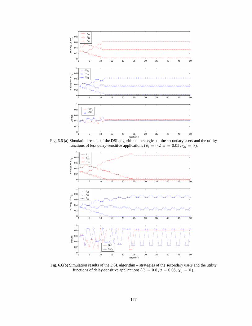
177
0 5 10 15 20 25 30 35 40 45 500
0.2
0.4
0.6
0.8
1
Str
ateg
y of
SU
1
0 5 10 15 20 25 30 35 40 45 500
0.2
0.4
0.6
0.8
1
Str
ateg
y of
SU
2
0 5 10 15 20 25 30 35 40 45 500
0.2
0.4
0.6
0.8
1
Iteration n
Util
ities
s11s12s13
s21s22s23
SU1SU2
0 5 10 15 20 25 30 35 40 45 500
0.2
0.4
0.6
0.8
1
Str
ateg
y of
SU
1
0 5 10 15 20 25 30 35 40 45 500
0.2
0.4
0.6
0.8
1S
trat
egy
of S
U2
0 5 10 15 20 25 30 35 40 45 500
0.2
0.4
0.6
0.8
1
Iteration n
Util
ities
s11s12s13
s21s22s23
SU1SU2
Fig. 6.6 (a) Simulation results of the DSL algorithm – strategies of the secondary users and the utility
functions of less delay-sensitive applications ( 0.2iθ = , 0.05σ = , 0ijχ = ).
Fig. 6.6(b) Simulation results of the DSL algorithm – strategies of the secondary users and the utility
functions of delay-sensitive applications ( 0.8iθ = , 0.05σ = , 0ijχ = ).

178
0.1 0.2 0.3 0.4 0.5 0.6 0.7 0.8 0.9 10
0.2
0.4
0.6
0.8
Str
ateg
y of
SU
1
0.1 0.2 0.3 0.4 0.5 0.6 0.7 0.8 0.9 10
0.2
0.4
0.6
0.8
Str
ateg
y of
SU
2
0.1 0.2 0.3 0.4 0.5 0.6 0.7 0.8 0.9 10
0.5
1
Normalized loading of PU1: ρ1
Util
ities
SU1
SU2
s21
s22s23
s11s
12s
13
B. Impact of the primary users
Next, we simulate the impact of the highest priority users – the primary users in Figure
6.7. We change the normalized traffic loading of 1PU in the frequency channel 1F from
0 to 1 and fix the normalized loading of the other two primary users as in Table II. Due to
the priority queuing, we know that once 1ρ reaches 1, frequency channel 1F is not
accessible for the secondary users. For different normalized loading of 1PU , Figure 6.7
shows the resulting strategies and the utilities of the two secondary users after
convergence. Both 11s and the utility value 1U decreases when the available resource
from 1F decreases (1 0.6ρ > ). Interestingly, even though 2SU does not utilize channel
1F ( 21 0s ≅ ) and the resulting strategies do not change with 1ρ , 2U also decreases. This
is because more traffic from 1SU will now be distributed to 2F and 3F . This simple
example illustrates that the traffic of a higher priority class user can still affect the utilities
of the secondary users in lower priority classes even when these secondary users avoid
selecting the same channels as the higher priority class user.
Fig. 6.7 Steady state strategies of the secondary users and the utility functions vs. the normalized loading
of 1PU for delay-sensitive applications ( 0.8iθ = , 0.05σ = , 0.02ijχ = ).

179
C. Comparison with other cognitive radio resource management solutions
In this subsection, we simulate a larger number of secondary users and a larger number
of frequency channels. First, we look at the case with 6 secondary users with video
streaming applications (“Coastguard”, frame rate of 30Hz, CIF format, delay deadline
500ms) sharing 10 frequency channels ( 6, 10N M= = , 1iθ = ). We compare our DSL
algorithm with other two resource allocation algorithms – the “Static Assignment” [TJ91]
and the “Dynamic Least Interference” [KP99]. In the “Static Assignment” algorithm, a
secondary user will statically select a frequency channel with the best effective
transmission rate without interacting with other secondary users. This work has the
drawback that it is merely a decentralized scheme without any information exchange. In
the “Dynamic Least Interference” algorithm, a secondary user will dynamically select a
single frequency channel that has the least interference from the other users (both
secondary users and primary users), which is also similar to the rule D in [ZC05]. This
work has the drawback of considering only the interference and the resulting throughput
in the physical layer. We simulate 100 different frequency channel conditions as well as
the traffic loadings and then compute the average the video PSNR and the standard
deviation of the PSNR over the one hundred cases in Table 6.3 for the 6 video
applications. Unlike the “Dynamic Least Interference” that only considers the
interference and the resulting throughput in the physical layer, our proposed multi-agent
learning algorithm tracks the strategies of the other users through information exchange
and adequately adapts the channel selection to maximize the multimedia utility in the
application layer. The results show that our DSL algorithm outperforms the other two
algorithms for delay-sensitive multimedia applications in terms of packet loss rate (PLR)
and video quality (PSNR).
Next, we simulate the case with 20 secondary users with video streaming applications
( 1iθ = ) mixed with r secondary users with delay insensitive ( 0iθ = ) applications.
These secondary users are in the same priority class and share 10 frequency channels.

180
The average ijT of the frequency channels is now set to 3 Mbps, instead of 1.25 Mbps
and 1 Mbps in the previous simulation. Table 6.4 shows the average packet loss rate and
the average PSNR over the 20 video streams (instead of over 100 different channel
conditions in the previous simulation) with different r for the three solutions. Larger r
reduces the available resources that can be shared by the video streams, and hence,
decreases the received video quality. The results show that the video streaming of the
“Static Assignment” is impacted severely by the different channel conditions to the
secondary users. The standard deviations of the “Static Assignment” are larger than the
results of the “Dynamic Least Interference” and our DSL algorithm. The results again
show that our DSL algorithm outperforms the other two algorithms for multimedia
applications in terms of packet loss rate and video quality.
TABLE 6.3 COMPARISONS OF THE CHANNEL SELECTION ALGORITHMS FOR DELAY-SENSITIVE APPLICATIONS
WITH 6, 10N M= = .
“Static Assignment – Largest Bandwidth”
“Dynamic Least Interference”
“Dynamic Learning Algorithm” Medium
bandwidth case: (average ijT =
1.25 Mbps) PLR
Average Y-PSNR
(dB)
Y-PSNR Standard Deviatio
n
PLR Average Y-PSNR
(dB)
Y-PSNR Standard Deviatio
n
PLR Average Y-PSNR
(dB)
Y-PSNR Standard Deviatio
n
1SU 15.24 % 32.93 3.92 17.44 % 32.55 3.49 7.61 % 34.17 1.52
2SU 25.38 % 31.48 4.31 19.80 % 32.20 3.45 8.74 % 33.97 1.82
3SU 21.34 % 32.03 4.24 15.45 % 32.86 3.50 11.85 % 33.44 2.28
4SU 20.38 % 32.17 4.35 12.98 % 33.26 3.40 8.22 % 34.06 1.77
5SU 27.17 % 31.21 4.29 20.56 % 32.09 3.55 12.61 % 33.32 2.21
6SU 19.26 % 32.32 4.33 12.86 % 33.27 3.61 9.38 % 33.86 2.27
“Static Assignment -Largest-Bandwidth”
“Dynamic Least Interference”
“Dynamic Learning Algorithm” Low
bandwidth case: (average ijT =
1 Mbps) PLR
Average Y-PSNR
(dB)
Y-PSNR Standard Deviatio
n
PLR Average Y-PSNR
(dB)
Y-PSNR Standard Deviatio
n
PLR Average Y-PSNR
(dB)
Y-PSNR Standard Deviatio
n
1SU 42.01 % 29.48 4.94 38.16 % 29.89 4.32 18.30 % 32.42 1.97
2SU 38.21 % 29.90 4.89 34.07 % 30.35 4.29 17.02 % 32.62 2.42
3SU 39.97 % 29.69 5.02 33.85 % 30.37 4.41 18.76 % 32.36 2.26
4SU 32.30 % 30.59 4.98 29.74 % 30.87 4.37 16.12 % 32.75 2.31
5SU 42.19 % 29.48 4.98 38.34 % 29.87 4.41 18.45 % 32.40 2.33
6SU 37.07 % 30.01 5.04 31.52 % 30.65 4.46 19.40 % 32.26 2.67

181
TABLE 6.4 COMPARISONS OF THE CHANNEL SELECTION ALGORITHMS FOR DELAY-SENSITIVE APPLICATIONS
WITH 20 , 10N r M= + = , WHERE r IS THE SECONDARY USERS WITH DELAY INSENSITIVE 0kθ =
APPLICATIONS. “Static Assignment
– Largest Bandwidth” “Dynamic Least
Interference” “Dynamic Learning
Algorithm” Average ijT
= 3 Mbps PLR Average Y-PSNR
(dB)
Y-PSNR Standard Deviatio
n
PLR Average Y-PSNR
(dB)
Y-PSNR Standard Deviatio
n
PLR Average Y-PSNR
(dB)
Y-PSNR Standard Deviatio
n 2r = 20.00% 28.49 14.24 12.64% 33.76 2.59 0.06% 35.60 0.0013 5r = 35.00% 23.15 16.98 15.81% 33.30 2.83 2.86% 35.23 1.64 10r = 50.00% 17.81 17.80 24.34% 32.32 3.36 8.12% 34.50 2.55
VII. CONCLUSIONS
In this chapter, we propose a priority virtual queue interface for heterogeneous
multimedia users in cognitive radio networks, based on which they can exchange
information and time share the various frequency channels in a decentralized fashion.
Based on the information exchange, the secondary users are able to evaluate the expected
utility impact from the dynamic wireless environment as well as the competing wireless
users’ behaviors and learn how to efficiently adapt their channel selection strategies. We
focus on delay-sensitive multimedia applications, and propose a dynamic learning
algorithm based on the priority queuing analysis. Importantly, unlike conventional
channel allocation schemes that select the least interfered channel merely based on the
channel estimation, the proposed multi-agent learning algorithm allows the secondary
users to track the actions of the other users and adequately adapt their own strategies and
actions to the changing multi-user environment. The results show that our proposed
solution outperforms the fixed channel allocation and the dynamic channel allocation that
selects the least interfered channel, in terms of video quality. Without primary users using
the highest priority class, the proposed approach can also be used to support QoS for
general multi-radio wireless networks. This situation also emerges in wireless systems
such as those discussed in [ALV06], where the secondary users are competing in the

182
unlicensed band (i.e. ISM band) and there is no primary user. The proposed DSL
algorithm can be implemented by the secondary users to switch channels,
suspend/resume channel operation, and add/remove channels, etc., while complying with
emerging MAC solutions for cognitive radio networks [CCB06].
VIII. APPENDIX
CONVERGENCE OF THE DECENTRALIZED APPROACH
If we consider the additional cost (penalty) ( ), ( 1)i i i nχ −s s when the channel selection
strategies are not the same, equation (23) can be rewritten as:
( )
*
1
( ) arg max ( , ( 1))
arg max [ ( ( 1))] , ( 1)
Mi
Mi
i i i i
M
ij ij i i i
j
n U n
s EV n nχ
−∈
∈ =
= −
= ⋅ − − − ∑
s
s
s s s
A s s
S
S
, (28)
For example, the penalty function can be
( )
, if ( 1) 0, 0
, ( 1) , if ( 1) 0, 0
0, otherwise
ij iji
i i i i ij ij
s n s
n s n s
χ
χ χ
+
−
− = >− = − > =
s s , (29)
where iχ+ and iχ
− represent the cost of selecting a new channel and the cost of hopping
away from a used frequency channel.
From equation (28), the secondary user iSU will keep updating its channel for
transmission, unless the utility difference of selecting a new strategy *( )i ns becomes
small. Hence, in the proposed DSL algorithm in Section V, assume the difference
between the estimated strategy ( )ijs n and the previous strategy ( 1)ijs n − is ( )ije n for
iSU using the frequency channel jF , i.e. ( ) ( ) ( 1)ij ij ije n s n s n= − − . Let
1( ) ( ) [ ( ( 1))]
Mdiffij iji j
U n e n EV n=
= × −∑ A be the utility difference between the estimated
strategy and the previous strategy.
Claim 1: If ( )ije n satisfies the following condition:
( )( ) ( ), ( 1)diffi i iiU n n nχ≤ −s s , (30)
for all the secondary users, the channel selection strategies converge to a steady state.

183
Proof: Equation (30) can be derived as: ( )
( )
1
1 1
( ), ( 1) ( ( ) ( 1)) [ ( ( 1))]
( 1) [ ( ( 1))] ( ) [ ( ( 1))] ( ), ( 1)
( ( 1), ( 1)) ( ( ), ( 1))
M
i i i ij ij ijj
M M
ij ij ij ij i i ij j
i i i i i i
n n s n s n EV n
s n EV n s n EV n n n
U n n U n n
χ
χ
=
= =
− −
− ≥ − − × −
⇒ − × − ≥ × − − −
⇒ − − ≥ −
∑
∑ ∑
s s A
A A s s
s s s s
From Step 5 of the DSL algorithm in Section V, the strategies will remain unchanged and
converge to a steady state.
Claim 2: If the penalty function ( ), ( 1)i i i nχ −s s is a convex function of is , when the
DSL algorithm converges to a steady state, the channel selection strategy *is is the best
response strategy that maximizes iU .
Proof: As long as the penalty function ( ), ( 1)i i i nχ −s s is a convex function of is , the
utility function ( , ( 1))i i iU n− −s s is a concave function, since for each iteration, the
[ ( ( 1))]ijEV n −A in equation (28) does not change with is . Hence, when the DSL
algorithm converges to a steady state, the local optimum in equation (28) converges to the
global optimum.

184
Chapter 7
Resource Management in Multi-hop Cognitive
Radio Networks
I. INTRODUCTION
The majority of the resource management research in cognitive radio networks has
focused on a single-hop wireless infrastructure [CCB06][ZTS07][NH07][HPR07]. In this
chapter, we focus on the resource management problem in the more general setting of
multi-hop cognitive radio networks. A key advantage of such flexible multi-hop
infrastructures is that the same infrastructure can be re-used and reconfigured to relay the
content gathered by various transmitting users (e.g. sources nodes) to their receiving
users (e.g. sinks nodes). These users may have different goals (application utilities etc.)
and may be located at various locations. For the multi-hop infrastructure, there are three
key differences as opposed to the single-hop case. First, the users have as available
network resources not only the vacant frequency channels (spectrum holes or spectrum
opportunities [Hay05][CCB06]) as in the single-hop case, but also the routes through the
various network relays to the destination nodes. Second, the transmission strategies will
need to be adapted not only at the source nodes, but also at the network relay nodes. In
cognitive radio networks, network nodes are generally capable of sensing the spectrum
and modeling the behavior of the primary users and thereby, identifying the available
spectrum holes. In multi-hop cognitive radio networks, the network nodes will also need
to model the behavior of the other neighbor nodes (i.e. other secondary users) in order to
successfully optimize the routing decisions. In other words, network relays also require a
learning capability in the multi-hop cognitive radio network. Third, to learn and
efficiently adapt their decisions over time, the wireless nodes need to possess accurate

185
(timely) information about the channel conditions, interference patterns and other nodes
transmission strategies. However, in a distributed setting such as a multi-hop cognitive
radio network, the information is decentralized, and thus, there is a certain delay
associated with gathering the necessary information from the various network nodes.
Hence, an effective solution for multi-hop cognitive radio networks will need to tradeoff
the “value” of having information about other nodes versus the transmission overheads
associated with gathering this information in a timely fashion across different hops, in
terms the utility impact.
In this chapter, we aim at learning the behaviors of interacting cognitive radio nodes
that use simple interference graph (similar to the spectrum holes used in
[CCB06][ZTS07]) to sequentially adjust and optimize their transmission strategies. We
apply a multi-agent learning algorithm – the fictitious play (FP) [FL98] to model the
behavior of neighbor nodes based on the information exchange among the network nodes.
We focus on delay-sensitive applications such as real-time multimedia streaming, i.e. the
receiving users need to get the transmitted information within a certain delay. Due to the
informationally decentralized nature of the multi-hop wireless networks, a centralized
resource management solution for these delay-constrained applications is not practical
[SV07b], since the tolerable delay does not allow propagating information back and forth
throughout the network to a centralized decision maker. Moreover, the complexity and
the information overhead of the centralized optimization grow exponentially with the size
of the network. The problem is further complicated by the dynamic competition for
wireless resources (spectrum) among the various wireless nodes (i.e. source nodes/relays).
The centralized optimization will require a large amount of time to process and the
collected information will no longer be accurate by the time transmission decisions need
to be made. Hence, a distributed resource management solution, which explicitly
considers the availability of information, the transmission overheads and incurred delays,
as well as the value of this information in terms of the utility impact is necessary.

186
The chapter is organized as follows. In Section II, we discuss the main challenges of
the dynamic resource management in multi-hop cognitive radio networks and the related
works. Section III provides the multi-hop cognitive radio network settings and strategies
and Section IV gives problem formulation of the distributed resource management for
delay sensitive transmission in such networks. In Section V, we determine how to
quantify the rewards and costs associated with various information exchanges in the
multi-hop cognitive radio networks. In Section VI, we propose our distributed resource
management algorithms with the information exchange and introduce the adopted
multi-agent learning approach – adaptive fictitious play in the proposed algorithms.
Simulation results are in Section VII. Finally, Section VIII concludes the chapter.
II. MAIN CHALLENGES AND RELATED WORKS
A. Main challenges in multi-hop cognitive radio networks
To design such a distributed resource management in multi-hop cognitive radio
networks, several main challenges need to be addressed:
• Dynamic adaptation to a time-varying network environment
Multi-hop cognitive radio networks are generally experiencing the following dynamics:
1) the primary users directly affect the spectrum opportunities available for the secondary
users, 2) the mobility of the network relays that affects the network topology, 3) the
traffic load variation due to multiple applications simultaneously sharing the same
network infrastructure, and 4) the time-varying wireless channel conditions. Given the
dynamic nature of the cognitive radio networks, wireless nodes need to learn,
dynamically self-organize and strategically adapt their transmission strategies to the
available resources without interfering the primary licensees. Due to these time-varying
dynamics, the outcomes of these interactions do not need to converge to an equilibrium,
i.e., disequilibrium and perpetual adaptation of strategies may persist, as long as the
performance of the delay sensitive application is maximized [FL98]. Hence, repeated

187
information exchange among network nodes is required for nodes to efficiently learn and
keep adapting to the changing network dynamics.
• Information availability in multi-hop infrastructures
Due to the informationally-decentralized nature of the multi-hop infrastructure, the
exchanged network information is only useful when it can be conveyed in time. The
timeliness constraint of the information exchange depends on the delay deadline of the
applications, the information overhead, and the condition of the network links, etc. Hence,
the value of information in terms of its impact on the users’ utilities will need to be
quantified for the different settings of the multi-hop cognitive radio network. This
information will impact the accuracy with which the wireless nodes can model the
behavior of other nodes (including the primary users) and hence, the efficiency with
which they can respond to this environment by adequately optimizing their transmission
strategies.
B. Related work
Distributed dynamic spectrum allocation is an important issue in cognitive radio
networks. Various approaches have been proposed in recent years. In [ZTS07], a
decentralized cognitive MAC protocols are proposed based on the theory of Partially
Observable Markov Decision Process (POMDP), where a secondary user is able to model
the primary users through Markovian state transition probabilities. In [NH07], the authors
investigated a game-theoretic spectrum sharing approach, where the primary users are
willing to share spectrum and provide a determined pricing function to the secondary
users. In [HPR07], a no-regret learning approach is proposed for dynamic spectrum
access in cognitive radio networks. However, these studies focus on dynamic spectrum
management for the single-hop network case.
Exploiting frequency diversity in wireless multi-hop networks has attracted enormous
interests in recent years. In [LL06], the authors propose a distributed allocation scheme of
sub-carriers and power levels in an orthogonal frequency-division multiple-access-based

188
(OFDMA) wireless mesh networks. They proposed a fair scheduling scheme that
hierarchically decouples the sub-carrier and power allocation problem based on the
limited local information that is available at each node. In [WYT06], the authors focus on
the distributed channel and routing assignment in heterogeneous multi-radio,
multi-channel, multi-hop wireless networks. The proposed protocol coordinates the
channel and route selection at each node, based on the information exchanged among
two-hop neighbor nodes. However, these studies are not suitable for cognitive radio
networks, since they ignore the dynamic nature of spectrum opportunities and users
(network nodes) need to estimate the behavior of the primary users for coexistence. To
the best of our knowledge, the dynamic resource management problem in multi-hop
cognitive radio networks has not been addressed in literature.
In summary, the chapter makes the following contributions.
a) We propose a dynamic resource management scheme in multi-hop cognitive radio
network settings based on periodic information exchange among network nodes. Our
approach allows each network nodes (secondary users and relays) to exchange their
spectrum opportunity information and select the optimal channel and next relay to
transmit delay sensitive packets.
b) We investigate the impact of the information exchange collected from various hops on
the performance of the distributed resource management scheme. We introduce the notion
of an “information cell” to explicitly identify the network nodes that can convey timely
information. Importantly, we investigate the case that the information cell does not cover
all the interfering neighbor nodes in the interference graph.
c) The proposed dynamic resource management algorithm applies FP, which allows
various nodes to learn their spectrum opportunity from the information exchange and
adapt their transmission strategies autonomously, in a distributed manner. Moreover, we
discuss the tradeoffs between the cost of the required information exchange and the
learning efficiency of the multi-agent learning approach in terms of the utility impact.

189
Next, we present our network settings of the multi-hop cognitive radio networks.
III. MULTI-HOP COGNITIVE RADIO NETWORK SETTINGS
A. Network entities
In this chapter, we assume that a multi-hop cognitive radio network involves the
following network entities and their interactions:
Primary Users (PUs) are the incumbent devices that possess transmission licenses
for specific frequency bands (channels). Without loss of generality, we assume that
there are M frequency channels in the considered cognitive radio network. We also
assume that the maximum number of primary users that can be present in the network
equals M . Note that these primary users can only occupy their assigned (licensed)
frequency channels and not other primary users’ channels. Since the primary users
are licensed users, they will be guaranteed an interference-free environment
[Hay05][ALV06]. When a primary user is not transmitting data using its assigned
frequency channel, a spectrum hole is formed at the corresponding frequency
channel.
Secondary Users (SUs) are the autonomous wireless stations that perform channel
sensing and access the existing spectrum holes in order to transmit their data. The
secondary users can occupy the spectrum holes available in the various frequency
channels. In this chapter, the secondary users are deploying delay sensitive
applications. Specifically, we assume that there are V delay sensitive applications
simultaneously sharing the cognitive radio network infrastructure, having unique
source and destination nodes. These secondary users are able to deploy their
applications across various frequency channels and routes.
Network Relays (NRs) are autonomous wireless nodes that perform channel sensing
and access the existing spectrum holes in order to relay the received data to one of its
neighboring nodes or SUs. Hence, unlike in the SUs case, there is no source or

190
destination present at the NRs. Note that multiple applications can use the same NR
using different frequency channels.
B. Source traffic characteristics
Let iV denote the delay sensitive application of the i -th SU. Assume that the
application iV consists of packets in iK priority classes. The total number of
applications is V . We assume that there are a total of 1
1V
iiK K
== +∑ priority classes
(i.e., 1, , KC C=C … ). The reason for adding an additional priority class is because the
highest priority class 1C is reserved for the traffic of the primary users. The rest of the
classes , 1kC k > can be characterized by:
kλ , the impact factor of a class kC . For example, this factor can be obtained based on
the money paid by a user (different service levels can be assigned for different SUs by
the cognitive radio network), based on the distortion impact experienced by the
application of each SU or based on the tolerated delay assigned by the applications.
The classes of the delay sensitive applications are then prioritized based on this
impact factor, such that 'k kλ λ≥ if ', 2,...,k k k K< = . The impact factor is
encapsulated in the header (e.g. RTP header) of each packet.
kD , the delay deadline of the packets in a class kC . In this chapter, a packet is
regarded useful for the delay sensitive applications only when it is received before its
delay deadline.
kL , the average packet length in the class kC .
A variety of delay sensitive applications can use the cognitive radio set-up discussed in
this chapter. Multimedia transmission such as video streaming or video conferencing can
be examples of such applications as discussed in the first three chapters. We assume in
this chapter that an application layer scheduler is implemented at each network node to
send the most important packet first based on the impact factor encapsulated in the packet
header.

191
C. Multi-hop cognitive radio network specification
We consider a multi-hop cognitive radio network, which is characterized by a general
topology graph ( , , )M N EG that has a set of primary users 1 ,..., Mm m=M , a set of
network nodes 1 ,..., Nn n=N (include SUs and NRs) and a set of network edges (links)
1 ,..., Le e=E (connecting the SUs and NRs). There are a total of N nodes and L
links in this network. Each of these N network nodes is either a secondary user (as a
source or a destination node) or a network relay.
We assume that 1 ,..., Mf f=F is the set of frequency channels in the network, where
M is the total number of the frequency channels. To avoid interference to the primary
users, the network nodes can only use spectrum holes for transmission. Hence, to
establish a link with its neighbor nodes, each network node n ∈ N can only use the
available frequency channels in a set n ⊆F F . Note that these wireless nodes in a
cognitive radio network will continuously sense the environment and exchange
information and hence, nF may change over time depending on whether the primary
users are transmitting in their assigned frequency channels.
The network resource for a network node n ∈ N of the multi-hop cognitive radio
network includes the routes composed by the various links and frequency channels. We
define the resource matrix [ ] 0,1L Mn ijR ×= ∈R for the network node n as follows:
1, if link is connected to the node
and the frequency channel is available.
0, otherwise.
i
jij
e n
fR
=
(1)
Whether or not the resource ijR is available to node n ∈ N depends not only on the
topology connectivity, but also on the interference from other traffic using the same
frequency channel. Next, we discuss the interference from other users (including the
primary users).
D. Interference characterization
Recall that the highest priority class 1C is always reserved in each frequency channel

192
for the traffic of the primary users. The traffic of the SUs can be categorized into 1K −
priority classes ( 2, ..., KC C ) for accessing frequency channels. The traffic priority
determines its ability of accessing the frequency channel. Primary users in the highest
priority class 1C can always access their corresponding channels at any time. The traffic
of the SUs can only access the spectrum holes for transmission. Hence, we define two
types of interference to the secondary users in the considered multi-hop cognitive radio
network:
1) Interference from primary users.
In practical cognitive networks, even though primary users have the highest priority,
secondary users will cause some level of interference to the primary users due to their
imperfect awareness (sensing) of the primary users. The primary users’ interference
depends on the location of the M primary users. We rely on methods such as in
[Bro05] that consider the power and location of the secondary users to ensure that the
secondary users do not exceed some critical interference level to the primary users. We
also assume that the spectrum opportunity map is available to the secondary users as in
[CCB06][HPR07]. Since the primary users will block all the neighbor links using its
frequency channel, a network node n will sense the channel and obtain the Spectrum
Opportunity Matrix (SOM) of the primary users:
1, if the primary user is occupying frequency channel
and the link can interfere with the primary user.[ ] 0,1 , with
0, otherwise.
j
L Min ij ij
f
eZ Z×= ∈ =Z
(2)
A simple example is illustrated in Figure 7.1, which indicates the SOM of the primary
users and the resource matrix of each network node in the multi-hop cognitive radio
network.

193
Fig. 7.1. A simple multi-hop cognitive radio network with three nodes and two frequency channels.
2) Interference from competing secondary users.
We define [ ] 0,1L Mk ijI
×= ∈I as the Interference Matrix (IM) for the traffic in
priority class , 2kC k ≥ .
1, if link using frequency channel can be
interfered by the traffic of priority class .
0, otherwise.
i j
kij
e f
CI
=
(3)
The interference caused by the traffic in priority class kC can be determined based on
the interference graph of the nodes that transmit the traffic (as in [HPR07]). The
interference graph is defined as the corresponding links that are interfered by the
transmission of the class kC traffic1. The IM can be computed by the information
exchange among the neighbor nodes.
The available resource matrix can be masked out by the SOM and IM of the higher
priority classes, i.e. ( )1 ...I
n k nnk −= ⊗ ⊗ ⊗R R I Z , where the notation ⊗ represents
1 In a wireless environment, the transmission of neighbor links can interfere with each other and significantly impact their effective transmission time. Hence, the action of a node can impact and be impact by the action of the other relay nodes. In order to coordinate these neighboring nodes, we construct the interference matrix with binary “1” and “0”.
Spectrum opportunitymatrix of the primaryusers:
Resource matrixat each node:
2n
1n 3n
1m
2m
1f
1 2
1 2 3
1 2 3
,
, ,
, ,
f f
n n n
e e e
=
=
=
F
N
E
1e
2e
3e
2n
1n 3n
1m
2m
1f
1 2
1 2 3
1 2 3
,
, ,
, ,
f f
n n n
e e e
=
=
=
F
N
E
1e
2e
3e
1
2 2
3
0 1
1 1
0 1
e
e
e
=
Z
1 2 f f
1
1 2
3
1 1
1 1
0 0
e
e
e
=
R
1 2 f f
1
2 2
3
1 1
0 0
1 1
e
e
e
=
R
1 2 f f
1
3 2
3
0 0
1 1
1 1
e
e
e
=
R
1 2 f f
Spectrum opportunitymatrix of the primaryusers:
Resource matrixat each node:
2n
1n 3n
1m
2m
1f
1 2
1 2 3
1 2 3
,
, ,
, ,
f f
n n n
e e e
=
=
=
F
N
E
1e
2e
3e
2n
1n 3n
1m
2m
1f
1 2
1 2 3
1 2 3
,
, ,
, ,
f f
n n n
e e e
=
=
=
F
N
E
1e
2e
3e
2n
1n 3n
1m
2m
1f
1 2
1 2 3
1 2 3
,
, ,
, ,
f f
n n n
e e e
=
=
=
F
N
E
1e
2e
3e
2n
1n 3n
1m
2m
1f
1 2
1 2 3
1 2 3
,
, ,
, ,
f f
n n n
e e e
=
=
=
F
N
E
1e
2e
3e
2n
1n 3n
1m
2m
1f
1 2
1 2 3
1 2 3
,
, ,
, ,
f f
n n n
e e e
=
=
=
F
N
E
1e
2e
3e
1
2 2
3
0 1
1 1
0 1
e
e
e
=
Z
1 2 f f
1
2 2
3
0 1
1 1
0 1
e
e
e
=
Z
1 2 f f
1
1 2
3
1 1
1 1
0 0
e
e
e
=
R
1 2 f f
1
1 2
3
1 1
1 1
0 0
e
e
e
=
R
1 2 f f
1
2 2
3
1 1
0 0
1 1
e
e
e
=
R
1 2 f f
1
2 2
3
1 1
0 0
1 1
e
e
e
=
R
1 2 f f
1
3 2
3
0 0
1 1
1 1
e
e
e
=
R
1 2 f f
1
3 2
3
0 0
1 1
1 1
e
e
e
=
R
1 2 f f

194
element-wise multiplication of the matrixes and I denotes the inverse operation, which
turns 1 into 0 and 0 into 1. The resulting resource matrix ( )InkR represents the available
resource around the network node n for the class kC traffic under the interference of
other higher priority traffic (classes). Next, we define the actions available to the network
nodes in a multi-hop cognitive radio network.
E. Actions of the nodes
We define the action of the network node n in order to relay the delay sensitive
application iV as ( , )n n nA e f= ∈ ∈E F . We assume that a network relay n can select a
set of links to its neighbor nodes (links connected to node n ) n ⊆E E . Corresponding to
the actions, we define the transmission strategy vector of the network node n as
s [ | ( , )]n A n ns A e f= = ∈ ∈E F , where As represent the probability that the network node
n will choose an action A . We refer to an action at a node n as a “feasible action” for
transmitting a class kC traffic, if ( , )A e f= is an “available resource” in ( )InkR (i.e.
element 1efR = in ( )InkR ), since in this case the selected link and frequency channel do
not interfere with the traffic in the higher priority classes. That is,
( )ˆ ( ) ( , ) | [ ] , 1I L Mn ef efnkk A e f R R×= = = =A R . (4)
We denote the set of all the feasible actions for node n as ˆ ( )n kA for class kC traffic.
We next determine the corresponding delay based on different actions, which considers
the deployed cross-layer transmission strategies in order to compute the Effective
Transmission Time (ETT) [DPZ04] over the transmission links.
Each network node n computes the ETT ( , ), with ,nk n nETT e f e f∈ ∈E F for
transmitting delay sensitive applications in priority class kC :
( , )( , ) (1 ( , ))
knk
n n
LETT e f
T e f p e f=
× −. (5)
( , )nT e f and ( , )np e f represent the transmission rate and the packet error rate of the
network node n using the frequency channel f over the link e . ( , )nT e f and ( , )np e f
can be estimated by the MAC/PHY layer link adaptation [Kri02]. Specifically, we
assume that the channel condition of each link-frequency channel pair can be modeled

195
using a continuous-time Markov chain [BG87] with a finite number of states ( , )ne fS . The
time a channel condition spends in state ( , )ne f
i ∈ S is exponentially distributed with
parameter iν (rate of transition at state i in transitions/sec). We assume that the
maximum transition rate2 of the network is ν and the variation of the channel
conditions in a time interval 1/τ ν≤ is regarded negligible.
Define the action vector [ | ]i n iA n= ∈A σ as the vector of the actions of all the
network relay nodes for transmitting iV . Assume that the i th delay sensitive application
iV are transmitted from the source node sin ∈ N to the destination node din ∈ N with a
total of iq packets. The routes of iV are denoted as | 1,..., i ij ij qσ= =σ , where ijσ
is the route of thej th packet in iV . A route ijσ is a set of link-frequency pairs that the
packets flow through, i.e.
( , ) | the th packet of flows through link using frequency channel ij ie f j V e fσ = . (6)
Note that if the action of a certain relay node changes, the corresponding route ( )ij iσ A of
relaying iV also changes. We denote the end-to-end delay of the packets transmitted
using the route ( )ij iσ A as ( ( ))ij ij id σ A . Based on the topology, each network relay node
receiving a packet can decide where to relay the packet to and using which frequency
channel, in order to minimize its end-to-end delay ( ( ))ij ij id σ A . Finally, to calculate
( ( ))ij ij id σ A , the source node need to obtain the delay information from other nodes
according to the actions taken by the relay nodes, i.e.
( ( )) ( ), for ij
ij ij i nk i i k
n
d ETT V Cσ
σ∈
= ∈∑A A . (7)
IV. RESOURCE MANAGEMENT PROBLEM FORMULATION
By examining the cumulated ETT values, the objective of a delay sensitive application
is to minimize its own end-to-end packet delay. The centralized and proposed distributed
2 In case that some of the channel conditions change severely in the network, a threshold thν can be set by protocols to avoid these fast-changing nodes and the ν is hence selected as the maximum transition rate below this threshold value.

196
problem formulations are subsequently provided.
• Centralized problem formulation with global information available at the
sources
If we assume that the global information3 iG is available to the source node sin for
the delay sensitive application iV , the route ( , )ij i iσ A G can be determined for each
packet j of iV . The centralized optimization can be performed at every source node in
order to maximize the utility iu . Hence, for application iV we have:
argmax ( , )
ˆ subject to for all
opti i ii
n i
u
A A
=
∈ ∈
A A
A A
G, (8)
where 1
( , ) Prob ( ( , )) iq
i i i ij ij ij i i ij
j
u d Dλ σ=
= ⋅ ≤∑A AG G ,
and ij k ij kD D λ λ= = if kj C∈ . (9)
However, due to the limited wireless network resource, the end-to-end delay constraint
( ( , ))ij ij i i kd Dσ ≤A G can make the optimization solution infeasible. Hence, a sub-optimal
greedy algorithms that perform optimizations sequentially from the highest priority class
to the lowest priority class are commonly adopted [CF06][SV07b]. Specifically, for class
kC , the following optimization is considered:
argmin ( ( , ))
subject to ( ( , )) ,
ˆ for all .
k
optij ij ik iik
j C
ij ij ik i k
n ik
d
d D
A A
σ
σ
∈
=
≤
∈ ∈
∑A A
A
A A
G
G , (10)
where [ | , ]ik n ij kA n j C= ∈ ∈A σ .
Due to the informationally decentralized nature of the multi-hop wireless networks, the
centralized solution is not practical for the multi-user delay sensitive applications, as the
tolerable delay does not allow propagating the global information iG back and forth
throughout the network to a centralized decision maker. For instance, the optimal solution
depends on the delay ijd incurred by the various packets across the hops, which cannot
3 The word “global information” means the information gathered from every node throughout the network. We discuss the required information in Section V.

197
be timely relayed to a source node. For instance, when the network environment is
time-varying, the gathered global information iG can be inaccurate due to the
propagation delay for this information. Moreover, the complexity of the centralized
optimization grows exponentially with the number of classes and nodes in the network.
The problem is further complicated by the dynamic adaptation of the transmission
strategies deployed by the wireless nodes, which impacts their spectrum access and hence,
implicitly, the performance of their neighbor nodes. The optimization will require a large
amount of time to process and the collected information might no longer be accurate by
the time transmission decisions need to be made.
In summary, in the studied dynamic cognitive radio network, the decisions on how to
adapt the aforementioned actions at sources and relays need to be performed in a
distributed manner due to these informational constraints. Hence, a “decomposition” of
the optimization problem into distributed strategic adaptation based on the available local
information is necessary.
• Proposed distributed problem formulation with local information at each
node:
Instead of gathering the entire global information iG at each source, we propose a
distributed suboptimal solution that collects the local information nL at node n to
minimize the expected delay of the various applications sharing the same multi-hop
wireless infrastructure. Note that at each node n , the end-to-end delay for sending a
packet kj C∈ in equation (10) can be decomposed as:
( ) ( ) [ ( , )]Pij ij n ij n ijd d E d kσ σ σ= + , (11)
where ( )Pn ijd σ represents the past delay that packet j has experienced before it arrives
at node n and [ ( , )]n ijE d k σ represents the expected delay from the node n to the
destination of the packet kj C∈ . The sending packet kj C∈ is determined by the
application layer scheduler according to the impact factor kλ . The information about kλ
can be encapsulated in the packet header and ( )Pn ijd σ can be calculated based on the

198
timestamp available in the packet header. The priority scheduler at each node ensures that
the higher priority classes are not influenced by the lower priority classes (see equation
(10)). Since at the node n the value of ( )Pn ijd σ is fixed, the optimization problem at the
node n becomes: argmin [ ( , ( , ))]
subject to [ ( , ( , ))] ( ) ,
ˆ
optn n ij n n
Pn ij n n k n ij k
n n
A E d k A
E d k A D d j C
A
σ
σ σ ρ
=
≤ − − ∈
∈ A
L
L , (12)
where [ ( , ( , ))]n ij n nE d k Aσ L represents the expected delay from the relay node n to the
destination of the packets in class kC . ρ represents a guard interval such that the
probability Prob [ ( , ( , ))] ( ) Pn ij n n n ij kE d k A d Dσ σ+ > L is small (as in [JF06]). To estimate
the expected delay [ ( , ( , ))]n ij n nE d k Aσ L in equation (12), each network node n maintains
an estimated transmission delay [ ( )]nE d k from itself to the destination for each class of
traffic using the Bellman-Ford shortest-delay routing algorithm [BG87]. We assume that
each node n maintains and updates a delay vector [ [ (2)],..., [ ( )]]n n nE d E d K=d (note that
the first priority class is reserved for the primary users) with elements for each priority
class. Each network node exchanges such information to its neighbor nodes and selects
the best action optnA for the highest priority packet in the buffer of the network node n .
We will discuss the minimum-delay routing/channel selecting algorithm in Section VI.
Note that a group of packets in the buffer of a node n can take the action nA , since the
action is determined based on local information nL . Since in the cognitive radio
networks, the available channel is time-variant, the information needs to be timely
conveyed to the network node for the distributed optimization. Compared to the
centralized approach in equation (8), the distributed resource management in equation (12)
can adapt better to the dynamic wireless environment by periodically gathering local
information. Next, we discuss the distributed resource management with information
constraints in more detail.
V. DISTRIBUTED RESOURCE MANAGEMENT WITH INFORMATION CONSTRAINTS

199
A. Considered medium access control
In this chapter, we assume that the required local information nL is exchanged using a
designated coordination control channel similar to [BRB05]. Such a coordination channel
can be selected from the existing ISM bands, since there is no primary licensee in these
bands to interfere with. The transmission is time slotted and the time slot structure of a
node is provided in Figure 7.2. We denote the time slot duration as It . The action nA
are selected at each node, during each time slot, after the coordination interval (that
includes the channel sensing for SOM and the information exchange for IM). We denote
the coordination interval at the network node n as ( )I nd L . The goal of the coordination
interval at each time slot is to provide the feasible action set nA for the channel access
and the relay selection of the packet transmission. We will discuss how to obtain nA
based on the SOM and the IM among the neighboring nodes when we introduce the
proposed algorithm, in Section VI.
Fig. 7.2. Transmission time line at the node n with local information nL .
Besides the SOM and IM, the information required in the coordination interval should
also include the delay vectors nd and the control messages for RTS/CTS coordination
[ZTS07][WYT06]. Note that the local information nL does not need to include all these
information in each time slot (except the control messages). For example, the SOM and
IM can be collected in a different period, depending on the sensing and information
exchange mechanism. Hence, the coordination duration ( )I nd L will vary for different
It
( )I nd L ( )I nd LDecision making
Packets transmission
Time slot
Coordination interval
Channel sensingIt
( )I nd L ( )I nd LDecision making
Packets transmission
Time slot
Coordination interval
Channel sensing

200
time slots, which will be discussed in more detail in Section V.C. Next, we investigate the
benefit of acquiring information from different h -hop neighbor nodes, which also affects
the duration of the coordination interval ( )I nd L .
B. Benefit of acquiring information and information constraints
For the network node n , the local information nL gathered from different network
nodes has different impact on decreasing the objective function [ ( , ( , ))]n ij n nE d k Aσ L in
equation (12). Let ( ) ( , ), , | x x x
nn k x n n n x xx n A A n= ∈I d NI denote the set of local
information gathered from the neighbor nodes, which is x hops away from node n ,
where nxN represents a set of nodes that is x hops away from node n . We define
( ) ( ) | 1,..., n nx l l x= =L I as the local information gathered from all of these neighbor
nodes. Given the local information ( )n xL , we define the optimal expected delay as
( , ) [ ( , ( , ( )))]optn n ij n nK k x E d k A xσ= L . The larger x will has a smaller expected delay ( , )nK k x .
The benefit (reward) of the information ( )n xI for the class kC traffic is denoted as
( , ( ))n nJ k xI . In a static network case, ( , ( ))n nJ k xI is defined as:
( , ( )) ( , 1) ( , ), if 1n n n nJ k x K k x K k x x− − >I . (13)
We define ( , (1)) ( ,1) n n nJ k K k=I since (1) (1)n n=L I . The reward of information
( , ( ))n nJ k xI can be regarded as the benefit (decrease of the expected delay) in terms of
the expected delay [ ( , )]n ijE d k σ if the information ( )n xI is received by node n . Note
that the optimal expected delay ( , )nK k x , given the information ( )n xL :
2
( , ) ( ,1) ( , ( ))x
n n n n
l
K k x K k J k l=
= −∑ I . (14)
Equation (14) states that the optimal expected delay is a decreasing function of x ,
meaning that smaller expected delays can be achieved as more information is gathered.
The improvement is quantified by the reward of the information ( , ( ))n nJ k lI . Here, we
ignore the cost of exchanging such information, which will be defined in the next
subsection. Figure 7.3 shows a simple illustrative example of reward of information at
node n , which is five hops away from the destination node of class kC traffic. The
more information ( )n xI available from nodes that is x hops away, the smaller optimal

201
1 2 3 4 50
100
200
1 2 3 4 50
100
200
1 2 3 4 50
100
200( )x
( )x
( , )nK k x
( , ( ))n nJ k xIStatic
( , ( ))dn nJ k xI
Dynamic
( )x
n2n
1n3n
4n
dn
(1)I(2)I
(3)I
(4)I
(5)I
1x =
2x =
3x = 4x =
( ) ( ) | 1,.., n nx l l x= =L I
(3)L
( ) ( , ), , x x xn k x n n nx n A A= I dI
5n
(msec)
(msec)
(msec)
1 2 3 4 50
100
200
1 2 3 4 50
100
200
1 2 3 4 50
100
200( )x
( )x
( , )nK k x
( , ( ))n nJ k xIStatic
( , ( ))dn nJ k xI
Dynamic
( )x
n2n
1n3n
4n
dn
(1)I(2)I
(3)I
(4)I
(5)I
1x =
2x =
3x = 4x =
( ) ( ) | 1,.., n nx l l x= =L I
(3)L
( ) ( , ), , x x xn k x n n nx n A A= I dI
5n
(msec)
(msec)
(msec)
expected delay ( , )nK k x can be obtained.
Fig. 7.3. Example of the static reward of information ( , ( ))n nJ k xI , dynamic reward of information
( , ( ))dn nJ k xI and optimal expected delay ( , )nK k x (where the information horizon ( , )nh k ν = 3, average
packet length kL =1000 bytes, and average transmission rate T = 6Mbps over the multi-hop network).
Let ( ) [ ( , ( )), for 1 ]n n n nk J k x x H= ≤ ≤J I denote the reward vector from 1 -hop
information to nH -hop information, where max , I dn n nH H H= . d
nH represents the
shortest hop counts from the node n to the destination node of the class kC traffic and
InH represents the interference range in terms of hop counts for node n . We also need to
consider the hop count InH in case that the destination node is close to the node n
within the interference range. We assume that the reward vector ( )n kJ is obtained when
the network is first deployed and only updated infrequently, when SUs join or leave the
network. Note that all the elements in ( )n kJ are nonnegative, i.e.
( , ( )) 0, for 1n n nJ k x x H≥ ≤ ≤I , due to the fact that knowing additional information
cannot increase the expected delay [ ( , )]n ijE d k σ in a static network. However, if we
consider the propagation delay of such information exchange across the network in the
dynamic network, the dynamic reward of information ( , ( ))dn nJ k xI decreases as the hop

202
count x increases. When the information of the further nodes reaches the decision node
n , the information is more likely to be out-of-date (i.e. the information cannot reflect the
exact network situation in a dynamic setting, since the network conditions and traffic
characteristics are time-varying). Once the information is out-of-date, ( , ( )) 0dn nJ k x =I ,
i.e. there is no benefit from gathering information that is out-of-date. Note that in a
dynamic network, once ( , ( )) 0dn nJ k x =I , ( , ( ')) 0d
n nJ k x =I for ' nx x H≤ ≤ .
Therefore, in the dynamic network, we define the information horizon ( , )h k ν such
that ( , ) argmax
subject to ( , ( )) ( , ),1
n
dn n n
h k x
J k x k x H
ν
φ ν> ≤ ≤
I. (15)
where ( , ) 0kφ ν ≥ represents a minimum delay variation specified by the application
which determines the minimum benefit of receiving local information for class kC
traffic. In fact, ( , )nh k ν depends on the variation speed ν of the wireless network
condition (i.e. the transition rate of the Markovian channel condition model, see Section
III. E). In a dynamic network with higher variation speeds ν (e.g. with high mobility), a
higher threshold ( , )kφ ν is needed to guarantee that the information ( )n xI is still
valuable and it should be exchanged. This results in a smaller information horizon
( , )nh k ν . We illustrate this mobility issue in Section VII. Note that the information horizon
( , )nh k ν varies for different classes of traffic at different locations in the network. Since
higher priority class traffic has more network resources than the lower priority class (i.e.
they are scheduled first for optimization in equation (12)), the threshold value
( , ) ( ', )k kφ ν φ ν≤ , if 'k k< and thereby, ( , ) ( ', )n nh k h kν ν≥ , if 'k k< . In other words, the
information horizon ( , )nh k ν of a higher priority class kC is larger than the information
horizon ( ', )nh k ν of a lower priority class 'kC .
Although the information horizon ( , )nh k ν can vary at different locations for different
priority classes depending on the applications, the complexity of such implementation is
high and the adaptation of the information horizon itself can be an interesting topic.
Hence, we will leave the information horizon adaptation problem to our future research.
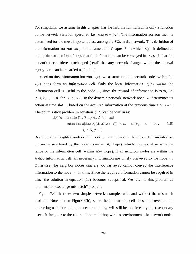
203
For simplicity, we assume in this chapter that the information horizon is only a function
of the network variation speed ν , i.e. ( , ) ( )nh k hν ν= . The information horizon ( )h ν is
determined for the most important class among the SUs in the network. This definition of
the information horizon ( )h ν is the same as in Chapter 3, in which ( )h ν is defined as
the maximum number of hops that the information can be conveyed in τ , such that the
network is considered unchanged (recall that any network changes within the interval
( ) 1/τ ν ν≤ can be regarded negligible).
Based on this information horizon ( )h ν , we assume that the network nodes within the
( )h ν hops form an information cell. Only the local information ( )n hL within the
information cell is useful to the node n , since the reward of information is zero, i.e.
( , ( )) 0n nJ k x =I for ( )x h ν∀ > . In the dynamic network, network node n determines its
action at time slot t based on the acquired information at the previous time slot 1t − .
The optimization problem in equation (12) can be written as: ( ) argmin [ ( , ( , ( , - 1)))]
subject to [ ( , ( , ( , - 1)))] ( ) ,
ˆ ( 1)
optn n ij n n
Pn ij n n k n ij k
n n
A t E d k A h t
E d k A h t D d j C
A t
σ
σ σ ρ
=
≤ − − ∈
∈ −A
L
L . (16)
Recall that the neighbor nodes of the node n are defined as the nodes that can interfere
or can be interfered by the node n (within InH hops), which may not align with the
range of the information cell (within ( )h ν hops). If all neighbor nodes are within the
h -hop information cell, all necessary information are timely conveyed to the node n .
Otherwise, the neighbor nodes that are too far away cannot convey the interference
information to the node n in time. Since the required information cannot be acquired in
time, the solution in equation (16) becomes suboptimal. We refer to this problem as
“information exchange mismatch” problem.
Figure 7.4 illustrates two simple network examples with and without the mismatch
problem. Note that in Figure 4(b), since the information cell does not cover all the
interfering neighbor nodes, the center node 2n will still be interfered by other secondary
users. In fact, due to the nature of the multi-hop wireless environment, the network nodes

204
that are far away from the node n have limited interference impact on node 2n . Hence,
even though the information horizon h does not match the interference range, the
performance degradation of the optimization problem in equation (16) using the local
information ( )n hL is limited.
Fig 7.4. (a) 2-hop information cell network without information exchange mismatch problem.
(b) 1-hop information cell network with information exchange mismatch problem.
C. Cost of information exchange
In the previous subsection, we discuss the reward of information in an h -hop
information cell while ignoring the negative impact of the information exchange. In this
section, we discuss the cost (increase of the expected delay) due to this information
exchange. Recall that the duration of the time slot is ( )It ν , which is also the interval
between the repeated information exchanges in the network. We define there are c time
slots in τ seconds, i.e. ( )
( )Itc
τ νν = . (17)
1n
3n
4n
1m
6n
5n
2n
1n
3n
4n
1m
6n
5n
2n
(a) (b)
6 6 6, ( ), [ ( )]n k kA n E d nI
1 1 1, ( ), [ ( )]n k kA n E d nI
5 5 5, ( ), [ ( )]n k kA n E d nI
3 3 3, ( ), [ ( )]n k kA n E d nI
4 4 4, ( ), [ ( )]n k kA n E d nI
3 3 3, ( ), [ ( )]n k kA n E d nI
4 4 4, ( ), [ ( )]n k kA n E d nI
1 1 1, ( ), [ ( )]n k kA n E d nI
Interference range of 2nInformation horizon
1n
3n
4n
1m
6n
5n
2n
1n
3n
4n
1m
6n
5n
2n
(a) (b)
1n1n
3n3n
4n4n
1m1m1m
6n6n
5n5n
2n2n
1n1n
3n3n
4n4n
1m1m1m
6n6n
5n5n
2n2n
(a) (b)
6 6 6, ( ), [ ( )]n k kA n E d nI
1 1 1, ( ), [ ( )]n k kA n E d nI
5 5 5, ( ), [ ( )]n k kA n E d nI
3 3 3, ( ), [ ( )]n k kA n E d nI
4 4 4, ( ), [ ( )]n k kA n E d nI
3 3 3, ( ), [ ( )]n k kA n E d nI
4 4 4, ( ), [ ( )]n k kA n E d nI
1 1 1, ( ), [ ( )]n k kA n E d nI
Interference range of 2nInformation horizon

205
c defines the frequency of the decision making as well as the learning process, which
will be discussed in detail in Section VI. Note that decisions can be made every It and
this time slot duration is short enough compared to τ . Hence, the network changes in It
is also negligible.
Recall that the coordination duration in a time slot for the network node n is
( ( ))I nd hL . Assume the information unit for the required information is ( )IU , ( )A
U , and
( )dU per class, respectively. Assume the average number of nodes in an h -hop
information cell is ( )N h . The information time overhead of ( )n hL is on average
( ) ( ) ( )( ( )) ( )[( 1)( ) ]d I AI nd h N h K U U U= − + +L .
Note that even though the information exchange is implemented in a designated
coordination channel [BRB05], a network node with a single antenna cannot transmit
both the data and the control signals at the same time. This information exchange time
overhead decreases the effective transmission rate at node n using the line e and
frequency channel f : ( ) ( ( ))
( , ) ( , )( )
I I nn n
I
t d hT e f T e f
t
ν
ν
−′ = ×
L . (18)
Hence, the effective transmission time at a node n using the link e and frequency
channel f to transmit a packet in class kC becomes: ( )
( , ) ( , )( ) ( ( ))
Ink nk
I I n
tETT e f ETT e f
t d h
ν
ν′ = ×
− L. (19)
In conclusion, the increase of the effective transmission time degrades the performance of
the delay sensitive applications. The degradation depends on the content of the local
information exchange ( )n hL , and the network variation speed ν . Hence, the benefit
( , ( ))dn nJ k xI in equation (15) will decrease due to this cost of the information. Hence, we
denote the value of information with this cost consideration as ( , ( ))cn nJ k xI :
( , ( )) ( , 1) ( , )
( ) ( ) ( , 1) ( , )
( ) ( ( 1)) ( ) ( ( ))
cn n n n
I In n
I I n I I n
J k x K k x K k x
t tK k x K k x
t d x t d x
ν ν
ν ν
′ ′= − −
= − × − ×− − −
I
L L
. (20)
And the optimal information horizon ( , )nh k ν in equation (15) also decreases due to
the cost. Next, we discuss the proposed distributed resource management algorithm based

206
on the information exchanges and learning capabilities to tackle the optimization problem
in equation (16).
VI. DISTRIBUTED RESOURCE MANAGEMENT ALGORITHMS
Figure 7.5 provides a system diagram of the proposed distributed resource
management. First, a packet kj C∈ is selected from the application scheduler at the
node n based on the impact factor kλ of the packet and an action nA is taken for that
packet. The application layer information including , ,k k kC L D is conveyed to the
network layer for this action decision. Network conditions ( , ), ( , )n nT e f p e f are then
conveyed from the MAC/PHY layer for computing the ETT values using equation (5).
Fig. 7.5. System diagram of the proposed distributed resource management.
In addition to the ( , ), ( , )n nT e f p e f , the action selection is impacted by the interference
induced from the action of these neighbor nodes and hence, the information received
from the neighbor nodes in the information cell. Recall that ( ) ( ) | 1,..., n nh l l h= =L I .
We use the notation ( )n h− to represent the set of the neighbor nodes of the network node
n in the h -hop information cell. Hence, the local information exchanged
( ) ( ) ( )( ) ( ( ), ), , n k n h n h n hh n h A A− − −= −I dL across the network nodes is required. Hence, the
MAC/PHY layer adaptation and channel sensing
Application layerpacket scheduling
Network layer minimum-delay route/channel selection
Packet transmission
Information exchange interface
, ,k k kC L D
nZ ( , ), ( , ), ,n nT e f p e f e f∈ ∈E F
( )( )Innk A−R nA
nNode
packets
Data transmission
Inter node information exchangeCross-layer message passing
[ ( )]kE d n−
i kV C∈
( )
( , ),
, [ ( )]
n
k n
n k
h
n A
A E d n
−
−
=
−
−
I
L
Upstreamnode
Downstream node
MAC/PHY layer adaptation and channel sensing
Application layerpacket scheduling
Network layer minimum-delay route/channel selection
Packet transmission
Information exchange interface
, ,k k kC L D
nZ ( , ), ( , ), ,n nT e f p e f e f∈ ∈E F
( )( )Innk A−R nA
nNodenNode
packets
Data transmission
Inter node information exchangeCross-layer message passing
Data transmission
Inter node information exchangeCross-layer message passing
[ ( )]kE d n−
i kV C∈
( )
( , ),
, [ ( )]
n
k n
n k
h
n A
A E d n
−
−
=
−
−
I
L
Upstreamnode
Downstream node
207
node n knows the estimated delay ( )n h−d from its neighbor nodes to the destinations,
so as the actions ( )n hA− of its neighbor nodes and their IM ( )( ( ), )k n hn h A−−I . Based on the
delay information from the neighbor nodes ( )n h−d , a network node can update its own
estimated delay to the various destinations and determine the minimum-delay action
based on Bellman-Ford algorithm [BG87].
We separate the distributed resource management into two blocks at the node n as in
Figure 7.5 – the information exchange interface block that regularly collects required
local information and the route/channel selection block to determine the optimal action.
We now discuss the role of the exchanged information and the two algorithms
implemented in these blocks, respectively.
A. Resource management algorithms
The next algorithm is performed at network node n at the information exchange
interface in Figure 7.5.
Algorithm 7.1. Periodic information exchange algorithm:
Step 1. Collect the required information – the node n first collects the required
information the SOM Z from channel sensing and
( ) ( ) ( )( ) ( ( ), ), , n k n h n h n hh n h A A− − −= −I dL from the neighbor nodes in the information cell.
Step 2. Learn the behavior of the neighbor nodes – by continuously monitoring the
actions of the neighbor nodes, node n can model the behavior of the neighbor nodes or
learn a better transmission strategy using strategy vectors
( ) [ ( ) | ( , )]A n nn s n A e f′ ′′ ′= = ∈ ∈s E F , ( )n n h′ ∈ − , where ( )As n ′ represents the probability
(strategy) of selecting an action A by the node n ′ , which will be discussed in the next
subsection.
Step 3. Estimate the resource matrix – from the SOM and the IM ( , )k nn A ′′I gathered
from the neighbor node n ′ , the resource matrix can be obtained for each class of traffic
by ( )1 ...I
n k nnk −= ⊗ ⊗ ⊗R R I Z , which will be explained in Section VI.A in more details.
Then the available resource ( )( )Innk A−R are provided to the network layer route/channel

208
selection block stated in the Algorithm 7.2.
Step 4. Update information ( , ), , k n n nn A AI d – based on the recently selected action
nA , the latest delay vector nd , and the IM ( , )k nn AI . Two types of interference model are
considered in this chapter when constructing the IM ( , )k nn AI from equation (3):
1) A network node can transmit and receive packets at the same time – Note that a node
cannot reuse a frequency channel nf ∈ F used by its neighbor nodes. If a frequency
channel is used by its neighbor nodes, all the elements in the column of the
interference ( , )k nn AI that is associated with the frequency channel are set to 1. Then
the IM is exchanged to the nodes within the pre-determined information horizon h .
2) A network node cannot transmit and receive packets at the same time – In this case, if
the frequency channel nf ∈ F is used, all the elements in the column of the IM
( , )k nn AI associated with the frequency channel are set to 1. In addition, if a network
link ne ∈ E is used by its neighbor nodes, all the elements of the IM ( , )k nn AI that is
associated with the node n are also set to 1, no matter what frequency channel it
uses. Then the IM is exchanged to the nodes within the pre-determined information
horizon h .
Step 5. Broadcast the information ( , ), , k n n nn A AI d and repeat the algorithm
periodically in every ( )It ν seconds.
The next algorithm is performed at the network node n at the network layer
minimum-delay route/channel selection block in Figure 7.5.
Algorithm 7.2. Minimum-delay route/channel selection algorithm:
Step 1. Determine the packet to transmit – based on the impact factor, one packet j
in the buffer at the node n is scheduled to be transmitted. Assume the packet kj C∈ ,
and the information of kC , kL , Pk nD d− are extracted or computed from the application
layer.
Step 2. Construct the feasible action set – construct the feasible action set ˆ ( )n kA from
the resource matrix ( )InkR given from the information exchange interface for the priority

209
class kC at the node n (see equation (4)).
Step 3. Estimate the channel condition – the transmission rate ( , )nT e f and packet error
rate ( , )np e f for each link-frequency channel pair ( , )n ne f∈ ∈E F are provided from the
PHY/MAC layer through link adaptation [Kri02].
Step 4. Calculate the expected delay toward the destination – for each action
ˆ ( )n nA k∈ A of the traffic class kC :
'( )ˆ[ ( , )] ( ) [ ( )], for ( )
nn n nk n n A n nE d k A ETT A E d k A k= + ∀ ∈ A , (21)
where '( )[ ( )]nn AE d k represents the corresponding element for the class kC in the delay
vector n−d from the neighbor node '( )nn A . ( )nk nETT A can be calculated based on kL ,
( , )nT e f , and ( , )np e f using equation (5).
Step 5. Check the delay deadline – if [ ( )] Pn k nE d k D d ρ≥ − − , drop the packet.
Step 6. Select the minimum delay action – if [ ( )] Pn k nE d k D d ρ< − − , find the
minimum-delay route and frequency channel selection, i.e. determine the optimal action
optnA from the feasible action set ˆ ( )n kA . In other words, the goal here is to solve equation
(16) at node n :
ˆ ( )arg min [ ( , )]
n n
optn n n
A kA E d k A
∈=
A
. (22)
Note that the feasible action set ˆ ( )n kA in equation (22) depends on the actions of other
neighbor nodes nA− . It is important for the network nodes to adopt learning approaches
for modeling the behaviors of these network nodes to decrease the complexity of the
dynamic adaptation. This will be discussed in the next subsection.
Step 7. Send RTS request – after determining the next relay and frequency channel,
send RTS request indicating the determined action information optnA to the next relay.
Step 8. Wait for CTS response and transmit the packets.
Step 9. Update the delay and the current action information – after selecting the
optimal action, update the estimated delay [ ( )]nE d k using exponential moving average
with a smoothing factor α :
[ ( )] [ ( )] (1 ) [ ( , )]old optn n n nE d k E d k E d k Aα α= × + − × , (23)

210
and provide the updated delay vector [ [ (2)],..., [ ( )]]n n nE d E d K=d to Algorithm 7.1 at the
information exchange interface. In Figure 7.6, we provide a block diagram of the
proposed distributed resource management. For the blocks that beyond the scope of this
chapter, we refer to [ALV06][Bro05] for channel sensing, [ZTS07][WYT06] for
RTS/CTS coordination, and [BG87] for the delay vectors.
Fig. 7.6. Block diagram of the proposed distributed resource management at network node n .
B. Adaptive fictitious play (AFP)
We now provide a learning approach for the SUs to learn the feasible action set ˆ ( )n kA
in equation (22) for our distributed resource management algorithms. Specifically, based
on the information exchange ( )n hL , the behaviors of the neighbor nodes in the
information cell can be learned (Step 2 of Algorithm 7.1) and based on the behaviors, the
feasible action set ( )n kA is determined. This motivates us to apply a well-known
Channel sensingfor primary users Determining
resource matrixusing AFP ( )I
nkR
Info.exchangeamongsecondaryusers
Interferencematrix
Delay vectors
RTS/CTScoordination
Minimum-delayRoute/channel selection
Select a feasible action that minimizes
Priority scheduledpacket buffer
Information update
RTS/CTScoordination
Packettransmission
nZ
( ),k nn A−−I
nA( )nRTS A
( )nCTS A
n−d
( , ), , k n n nn A AI d
kC
Periodic information exchange algorithm
Minimum-delayroute/channel selection algorithm
[ ( , )]n nE d k A
: blocks that are notcovered in this chapter
Channel sensingfor primary users Determining
resource matrixusing AFP ( )I
nkR
Info.exchangeamongsecondaryusers
Interferencematrix
Delay vectors
RTS/CTScoordination
Minimum-delayRoute/channel selection
Select a feasible action that minimizes
Priority scheduledpacket buffer
Information update
RTS/CTScoordination
Packettransmission
nZ
( ),k nn A−−I
nA( )nRTS A
( )nCTS A
n−d
( , ), , k n n nn A AI d
kC
Periodic information exchange algorithm
Minimum-delayroute/channel selection algorithm
[ ( , )]n nE d k A
Channel sensingfor primary usersChannel sensingfor primary users Determining
resource matrixusing AFP ( )I
nkR
Info.exchangeamongsecondaryusers
Interferencematrix
Delay vectors
RTS/CTScoordination
Info.exchangeamongsecondaryusers
Interferencematrix
Delay vectors
RTS/CTScoordination
Minimum-delayRoute/channel selection
Select a feasible action that minimizesMinimum-delayRoute/channel selection
Select a feasible action that minimizes
Priority scheduledpacket bufferPriority scheduledpacket buffer
Information update
RTS/CTScoordination
Packettransmission
nZ
( ),k nn A−−I
nA( )nRTS A
( )nCTS A
n−d
( , ), , k n n nn A AI d
kC
Periodic information exchange algorithm
Minimum-delayroute/channel selection algorithm
[ ( , )]n nE d k A
: blocks that are notcovered in this chapter

211
learning approach – fictitious play [FL98], applied when the SUs are willing4 to reveal
their current action information and thereby, they are able to model the behaviors
(strategies) of other SUs (a model-based learning [SPG07]). However, due to the
information constraint discussed in the previous section, only the information from the
neighbor nodes in the information cell is useful. Hence, we adapt the fictitious play
learning approach to our considered network setting. Figure 7.7(a) provides a block
diagram of the proposed distributed resource management algorithm using the adaptive
fictitious play.
Fig. 7.7 (a). Block diagram of the proposed distributed resource management algorithm using the AFP. (b). Impact of the network variation on the FP and the video performance.
4 If the action information is not provided by the other secondary users, a node can learn its own strategy from its action payoffs –
the estimated delay [ ( )]nE d k . The learning approach refers to the reinforcement learning (a model-free learning or a payoff-based
learning).
AdaptiveFictitious Play
Feasible action set
Best response (minimum-delay)action selectionin equation (22)
( )n hA−
(- ( )) k n hI
( )n h−d
( ( ))n h−s ˆ ( )n kA
optnA
Primary usersmodeling
nZ
AdaptiveFictitious Play
Feasible action set
Best response (minimum-delay)action selectionin equation (22)
( )n hA−
(- ( )) k n hI
( )n h−d
( ( ))n h−s ˆ ( )n kA
optnA
Primary usersmodeling
nZ(a)
(b
Networkvariation speed
Information accuracy
Horizonadaptation
Fictitious play for the users in the information cell
Videoperformancee.g. delay, packet loss
ν h
( )n h−
Adapt the horizon to optimize the performance
Networkvariation speed
Information accuracy
Horizonadaptation
Fictitious play for the users in the information cell
Videoperformancee.g. delay, packet loss
ν h
( )n h−
Adapt the horizon to optimize the performance

212
Note that only part of the SUs can be modeled via the learning approach depending on
the information horizon. Specifically, a node n maintains a strategy vector over time
( , ) [ ( , ) | ( , )]A n nn t s n t A e f′ ′′ ′= = ∈ ∈s E F for each of its neighbor nodes ( )n n h′ ∈ − in the
information cell. ( , )As n t′ represents the frequency selection strategy of the node n ′
making action A at time t , which is obtained using:
( , )
( , )( , )
( , )n n
AA
A
A
r n ts n t
r n t′ ′∈
′′ =
′∑E F
, (24)
where ( , )Ar n t′ is the propensity [You04] of node n ′ for taking action A at time t ,
which can be computed by:
( , ) ( , 1) ( ( ) )A A nr n t r n t I A t Aα ′′ ′= × − + = , (25)
where 1α < is a discount factor quantifying the importance of the history value.
( ( ) )nI A t A′ = represents an indicator function such that, 1, if the action of the node at time is
( ( ) )0, otherwise
n
n t AI A t A′
′= =
. (26)
Figure 7.7(b) shows how the network variation speed ν affects the size of the
information cell and ultimately, the video performance. We will consider the mobility of
the network relays to show this network variation impact in the next section.
As stated in Section III.E, ( , )As n t′ represent the probability that the network node n ′
will choose an action A . Hence, the probability ( , )As n t′ for modeling the node n ′
making an action A at time t will increase with the actual times that the action A is
selected. Based on the strategy ( , )As n t′ , the adaptive fictitious play provides the
estimated IM kI , and then the feasible action set ˆ ( )n kA can be computed.
From the gathered IM ( , )k nn A ′′I from the neighbor node ( )n n h′ ∈ − , the node n can
compute the expected IM from
( ) ( )
[ ] ( ) ( ) ( , )e ek ij k A k
An n k n n k
I n s n n A′ ′∈− ∈−
′ ′ ′= = =∑ ∑ ∑I I I . (27)
Then, the node n can estimate the IM kI for the traffic in class kC : 1, if
[ | ]0, if
eij
k ij ij eij
II I
I
µ
µ
≥= = <
I , (28)

213
where µ represents a threshold value that determines whether or not a
link-frequency-channel pair ( , )e f is considered to be occupied. Feasible action set
ˆ ( )n kA can hence be learned based on the resource matrix ( )1 ...I
n k nnk −= ⊗ ⊗ ⊗R R I Z
using equation (4). By learning the feasible action set ˆ ( )n kA , the best response actions
are computed using equation (22).
C. Information exchange overhead reduction
The fictitious play suffers from a large information overhead, since it requires all the
local information ( ) ( ) ( )( ) ( ( ), ), , n k n h n h n hh n h A A− − −= −I dL in the h –hop information cell.
From the cost of information exchange in equation (20), we know that the overhead can
increase the expected delay, especially when the network changes slowly (i.e. with a large
information cell). Hence, the overhead reduction is required to mitigate the performance
degradation.
(1) Reducing the information horizon.
Recall that the information overhead of ( )n hL is ( ) ( ) ( )( )[( 1)( ) ]d I AN h K U U U− + + in
average ( ( )N h is the average number of nodes in an h -hop information cell). With an
information horizon 'h h< , the overhead becomes ( ) ( ) ( )( ')[( 1)( ) ]d I AN h K U U U− + + ,
where ( ') ( )N h N h< . Note that it is not always beneficial to decrease the overhead by
reducing the information horizon. There exists a trade-off as discussed in Section V. The
reward of information ( , ( ))dn nJ k xI , x h< in equation (15) provides a metric to select
the most valuable information from the nodes within the information cell.
(2) Reducing the number of classes.
From equation (12), we know that the higher priority classes will not be influenced by
the lower priority classes. Hence, the information overhead can be reduced by ignoring
the information exchange of the lower priority classes. The overhead becomes
( ) ( ) ( )( )[( ' 1)( ) ]d I AN h k U U U− + + , 'k K< .
(3) Reducing the frequency of learning.
Although we divide c time slots in τ seconds, a network node n does not have to

214
learn in all these c time slots. In other words, the periodic learning process of the node
n does not have to be aligned with the information exchange (decision making). In order
to avoid simultaneous learning among network neighbors in a distributed manner, at each
time slot, the network node n updates the strategy vector ( , )As n t′ with probability
/n nb cε = ( nb c≤ ), and keeps the same strategy vector with probability 1 nε− . In other
words, the network node n chooses nb time slots out of c time slots in τ seconds to
model the behavior of other neighbor nodes. Note that the parameter nb characterize the
speed of learning at different network node n . The larger nb gives the network node n
faster learning capability. The information overhead of ( )n hL becomes
( ) ( ) ( )/ ( )[( 1)( ) ]d I Anb c N h K U U U× − + + .
VII. SIMULATION RESULTS
We simulate two video streaming applications that are transmitting videos 1V
“Coastguard” and 2V “Mobile” (16 frames per GOP, frame rate of 30Hz, CIF format)
over the same multi-hop cognitive radio network. Each video sequence is divided into
four priority classes ( 4, 9iK K= = ) with average packet length kL = 1000 bytes and
delay deadline kD = 500 millisecond. Although the first priority class 1C is reserved for
the primary users, let us first consider the case when there are no primary users, i.e. only
the SUs and NRs are transmitting. We assume that there are two frequency channels
(M =2). The wireless network topology is shown in Figure 7.8 in a 100x100 meters
region with N = 15 nodes and L = 22 links similar to the network settings in [KSV06]. A
link is established as long as the channel condition (described in the chapter by the link
SINR) is acceptable within the transmission distance (approximately 36 meters). Note
that this transmission distance is not aligned with the interference range InH . Neighbor
nodes that are beyond the transmission distance can still interfere with each other.

215
20 40 60 80 100 120 14020
40
60
80
100
120
140
1 2 3
4 56
7 8 9
1011 12
13 14 15
1V
2V
1dn
1sn
2sn
2dn
20 40 60 80 100 120 14020
40
60
80
100
120
140
1 2 3
4 56
7 8 9
1011 12
13 14 15
1V
2V
1dn
1sn
2sn
2dn
Fig. 7.8. Wireless network settings for the simulation of two video streams.
Fig.7.9. Reward dnJ and cost c
nJ of different information horizon at different node for video 1V .
1 2 30
100
200
1 2 30
0.2
0.4
1 2 30
0.2
0.4
1 2 30
100
200
300
1 2 30
0.2
0.4
0.6
1 2 30
0.2
0.4
0.6
Rew
ard
Jd n and
cos
t Jc n o
f th
e in
form
atio
n fo
r V 1 (
mse
c)
HIn=40m
n=1
HIn=40m
n=7
HIn=40m
n=13
HIn=80m
n=1
HIn=80m
n=7
HIn=80m
n=13
Information horizon h
Information horizon h
cost
reward
reward
cost
cost cost

216
A. Reward and cost of the information exchange
First, we simulate the impact of the information including the reward dnJ (see
equation (13)) and cost cnJ (see equation (20)) from the expected delay [ ]nE d using the
adaptive fictitious play in Section VII with different information horizons. Figure 7.9
shows the resulting reward and cost of information at different locations for streaming
video 1V (at noden = 1, 7, and 13 on one of the routes of video 1V ). The results show
that a 1-hop information cell is enough when the interference range is 40 meters, since
only the nodes that are 1 hop away can interfere with each other. If the interference range
is 80 meters, the information exchange mismatch problem (see Section V) occurs and the
appropriate information horizon for information exchange is then increased to 2.
B. Application layer performance with different information horizons and interference
ranges
We next compare the proposed dynamic resource management algorithm using
adaptive fictitious play (AFP) with two other resource management methods – AODV
[PR99] with load balancing over the two available frequency channels (AODV/LB) and
the Dynamic Least Interference Channel Selection [KP99] (DCS) extended to a network
setting. Table 7.1 and 7.2 show the results of the Y-PSNR of the two video sequences
using different approaches. The results show that the proposed algorithm using learning
from the nodes within the information cell outperforms the alternative approaches.
Especially, when the interference range is large (InH = 80 meters), the proposed AFP
approach significantly improves the video quality (X represents PSNR below 26 dB,
which is unacceptable for a viewer).
TABLE 7.1. Y-PSNR OF THE TWO VIDEO SEQUENCES USING VARIOUS APPROACHES ( InH = 40 METERS).
Y-PSNR (dB)
Network Bandwidth AODV/LB DCS
AFP (1-hop information
cell)
1V 32.47 35.21 35.61 Average T =5.5 Mbps 2V 31.70 33.32 33.32

217
TABLE 7.2. Y-PSNR OF THE TWO VIDEO SEQUENCES USING VARIOUS APPROACHES ( InH = 80 METERS).
Y-PSNR (dB)
Network Bandwidth AODV/LB DCS
AFP (1-hop information
cell)
AFP (2-hop information
cell)
1V X X 28.19 29.80 Average T =5.5 Mbps 2V X X 31.26 31.70
1V 30.47 34.46 35.61 35.61 Average T =10 Mbps 2V 31.92 33.08 33.32 33.32
For delay sensitive applications, we measure the packet loss rate (i.e. the probability
that the end-to-end delay exceeds the delay deadline) for different approaches in Figure
7.10(a). The results of both applications are shown. The AODV represents the on-demand
routing solution with only 1 frequency channel. The AODV/LB approach randomly
distributes packets over the two available frequency channels. The DCS approach with
cognitive ability selects a better frequency channel based on the link measurements and
hence, improves the performance opposed to the AODV/LB. The AFP further improves
the performance of both applications by learning the behaviors of the neighbor nodes.
Interestingly, the benefit brought by the learning capability decreases as the network
bandwidth increases. In other words, it is not worthy to be too intelligent in an
environment with plenty of resource. Moreover, as shown in Figure 7.10(b), the
improvement of 2-hop information cell is limited when the interference range is 40
meters. This is because the nodes that are two hops away have no impact on the current
node and their information is not valuable (i.e. it does not impact the utility).
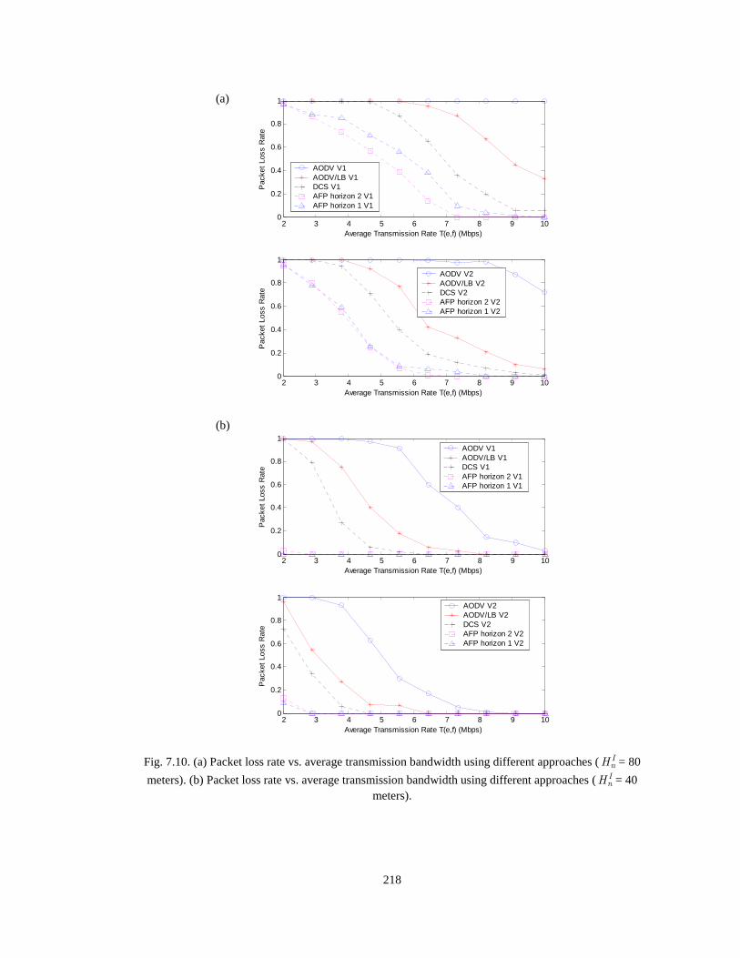
218
Fig. 7.10. (a) Packet loss rate vs. average transmission bandwidth using different approaches (InH = 80
meters). (b) Packet loss rate vs. average transmission bandwidth using different approaches (InH = 40 meters).
2 3 4 5 6 7 8 9 100
0.2
0.4
0.6
0.8
1
Average Transmission Rate T(e,f) (Mbps)
Pac
ket
Loss
Rat
e
2 3 4 5 6 7 8 9 100
0.2
0.4
0.6
0.8
1
Average Transmission Rate T(e,f) (Mbps)
Pac
ket
Loss
Rat
e
AODV V2AODV/LB V2DCS V2AFP horizon 2 V2AFP horizon 1 V2
AODV V1AODV/LB V1DCS V1AFP horizon 2 V1AFP horizon 1 V1
2 3 4 5 6 7 8 9 100
0.2
0.4
0.6
0.8
1
Average Transmission Rate T(e,f) (Mbps)
Pac
ket
Loss
Rat
e
2 3 4 5 6 7 8 9 100
0.2
0.4
0.6
0.8
1
Average Transmission Rate T(e,f) (Mbps)
Pac
ket
Loss
Rat
e
AODV V1AODV/LB V1DCS V1AFP horizon 2 V1AFP horizon 1 V1
AODV V2AODV/LB V2DCS V2AFP horizon 2 V2AFP horizon 1 V2
(a)
(b)

219
C. Reducing the frequency of learning
When the interference range is 40 meters, Figure 7.10(b) shows that the AFP with
1-hop information cell is better than with 2-hop information cell, since 1-hop information
cell has smaller cost of information exchange. In addition to reducing the information
horizon, reducing the frequency of learning /nb c at all the nodes can also reduce the
cost of information exchange. Figure 7.11 shows the packet loss rate of the two
applications with different information horizon when /nb c changing from 1 to 0.5. As
the learning frequency /nb c decreases, the packet loss rate decreases with the cost of
information exchange. However, it is shown that when /nb c < 0.6, the AFP becomes
inefficient and the packet loss rate starts increasing for both applications. In other words,
changing the frequency of learning will also lead to a trade-off between the learning
efficiency and the information overhead. The information overhead decreases when the
learning frequency /nb c decreases and hence, the packet loss rate decreases. However,
when the learning frequency is too slow (/nb c < 0.6), the learning efficiency decreases
and this results in an increasing packet loss rate.
Fig. 7.11. Packet loss rate vs. learning frequency /nb c (average T =5.5 Mbps, InH = 80 meters).
0.50.60.70.80.910.3
0.35
0.4
0.45
0.5
0.55
Learning frequency bn/c
Pac
ket
Loss
Rat
e
0.50.60.70.80.910
0.05
0.1
0.15
0.2
0.25
Learning frequency bn/c
Pac
ket
Loss
Rat
e
AFP horizon 2 V2AFP horizon 1 V2
AFP horizon 2 V1AFP horizon 1 V1

220
0 0.1 0.2 0.3 0.4 0.5 0.6 0.7 0.80.4
0.5
0.6
0.7
0.8
Primary user time fraction ρ
Pac
ket
loss
rat
e
AFP horizon 3 V1AFP horizon 2 V1AFP horizon 1 V1
0 0.1 0.2 0.3 0.4 0.5 0.6 0.7 0.80.1
0.15
0.2
0.25
0.3
0.35
Primary user time fraction ρ
Pac
ket
loss
rat
e
AFP horizon 3 V2AFP horizon 2 V2AFP horizon 1 V2
D. Impact of the primary users
The simulation implies that the reward of information is also impacted by the existence
of the primary users. Next, we consider the impact of the primary users, which always
have higher priority to access the pre-assigned frequency channels than the network
nodes in Figure 7.8. Assume that the frequency channel 1F is occupied by the primary
users with time fraction ρ =0%, 20%, 40%, 60%, and 80% around a certain congestion
region (network nodes n = 7, 11, 12) in Figure 7.8. Figure 7.12 shows the packet loss
rate for the two video streams using the AFP with various information horizons. The
average transmission rate is set to 5.5 Mbps, /nb c = 1, and the interference rage is 80
meters.
Fig. 7.12. Packet loss rate vs. time fraction ρ of the primary users occupying frequency channel 1F
around network node n = 7, 11, 12 (average T =5.5Mbps, /nb c = 1, InH = 80 meters).
The results show that as the time fraction ρ increases, the packet loss rates of both
applications increase, since fewer resources are available for the secondary users to
transmit the packets. As the simulation in the previous subsection, when the interference

221
rage is 80 meters, AFP with 2-hop information cell still performs better than 1-hop
information cell case. Interestingly, for application 1V , AFP with 3-hop information cell
performs even better in a large ρ case, even though more cost of information is needed.
This is because the congestion region are more likely to be discovered at the source node
n =1 and detour the packets through other routes. However, such advantage is not
exploited by the application 2V , since its destination node is affected by the primary
users and there is no way to detour the packets. Note that when there is no primary user
( ρ = 0), AFP with 3-hop information cell performs worse than 2-hop case due to the
larger cost of information exchange.
E. Impact of mobility
In this subsection, we consider the impact of mobility on the video performance. We
adopt a well-known mobility model, the “random walk” [CBD02], in which the relay
nodes (secondary users) shown in Figure 8 randomly select a direction at each time slot
and move at a fixed speed v . We simulate the speed v ranging from 0 to 1 meters/sec.
We assume that there is no primary user, i.e. 0ρ = . The average transmission rate is set
to 8 Mbps, /nb c = 1, and the interference rage is 80 meters. Figure 7.13 illustrates the
packet loss rate as the mobility changes for different information horizons. The results
show that the mobility degrades the performance of both applications. When the mobility
v is small, AFP with information horizon 2h = performs better than with information
horizon 1h = as in the previous simulations with InH = 80 meters. However, for video
2V , when the mobility exceeds 0.6 meters/sec, the best information horizon changes from
2h = to 1h = . This is because the increased mobility will decrease the information
accuracy and hence, the required information horizon also decreases. Note that for video
1V , the AFP with information horizon 2h = still performs better than with information
horizon 1h = . This is because the video 1V has a longer route and thus, modeling more
interfering neighbor nodes, using a larger information horizon, is still beneficial.

222
Fig. 7.13. Packet loss rate vs. mobility v of the secondary users (network relays)
(average T = 8Mbps, 0ρ = , /nb c = 1, InH = 80 meters).
VIII. CONCLUSIONS
In this chapter, we show that the distributed resource management solution using
adaptive fictitious play significantly improves the performance of delay sensitive
applications transmitted over a multi-hop cognitive radio network. We assume that the
autonomous secondary users are able to learn the spectrum opportunities based on the
information exchange. The proposed approach can also be used to support QoS for
general multi-radio wireless networks, when there is no primary user. This situation is
also brought up in [ALV06], when the secondary users are competing in the unlicensed
band (i.e. ISM band), where there is no primary user. Importantly, based on the value of
the obtained information (i.e. the impact on decreasing the expected end-to-end delay),
we define the information horizon in our adaptive fictitious play. In addition to the
reward, the cost of the information exchange is also considered in terms of transmission
0 0.2 0.4 0.6 0.8 1.00
0.2
0.4
0.6
0.8
Mobility v (meters/sec)P
acke
t lo
ss r
ate
0 0.2 0.4 0.6 0.8 1.00
0.1
0.2
0.3
0.4
Mobiliby v (meters/sec)
Pac
ket
loss
rat
e
AFP horizon 2 V2AFP horizon 1 V2
AFP horizon 2 V1AFP horizon 1 V1

223
time overheads. Various approaches of decreasing this time overhead are discussed, and
their performance impact is quantified. Our simulation results show that the benefit from
various information horizons can be different for distinct applications with various delays
and quality impacts, especially when primary users are present in the network at different
locations.

224
Chapter 8
Conjecture-Based Channel Selection in Multi-
Channel Wireless Networks
I. INTRODUCTION
In this chapter, we provide a fundamental view of channel selection in multi-channel
MAC protocols that aims to minimize the delays of delay-sensitive users transmitting
their packets through the multi-channel wireless network. Since the delay of a user is
impacted by the channel selection strategies of the other network users, it is important
that users consider the impact of these other users while determining their own channel
selection strategy. We endow the users with the ability to build beliefs about the
aggregate response of the other users to their actions (the aggregate response in this
chapter is the remaining capacity in each channel that can be measured based on the
throughput estimation method [SCN03]) and efficiently minimize their expected future
delays in a foresighted manner. Specifically, we model the multi-user interaction as a
channel selection game played by users who are capable of making conjectures about
how their transmission actions (i.e. their channel selection) will impact other users and
eventually impact their future performance. We investigate the performance of the
resulting ε -consistent conjectural equilibrium obtained when these users interact based
on their conjectures about the future remaining capacities when selecting channels. The
proposed ε -consistent conjectural equilibrium is a relaxed version of the conventional
conjectural equilibrium [Hah77], which allows us to characterize the equilibrium
obtained when network users are able to build near-accurate conjectures.
The channel selection problem was first studied in cellular networks. Various channel
assignment schemes have been proposed (see e.g. [KN96] for an excellent survey).

225
However, most of these channel assignment schemes are based on centralized solutions,
which do not scale to the network size and/or are not suitable for wireless networks
without a fixed infrastructure, such as ad hoc wireless networks. Moreover, centralized
approaches are especially not desirable for delay-sensitive applications as considered in
this chapter. The reason is that these centralized solutions require propagating control
messages back and forth to a network coordinator, thereby incurring delays that are often
unacceptable for delay-sensitive applications [SV08].
To cope with these challenges, distributed channel selection schemes without a network
manager have also been proposed in various types of wireless networks, such as wireless
ad hoc networks [NZD02][JDN01][SV04], wireless mesh networks [RC05], and
cognitive radio networks [CZ05][ZC05][HBH05][SV08], etc. For instance, in wireless ad
hoc networks, Nasipuri et al. [NZD02] proposed a multi-channel carrier sense multiple
access (CSMA) protocol that identifies the set of idle channels and selects the best
channel for transmission based on the channel condition observed at the transmitter side.
Jain et al. [JDN01] assumed a separate control channel and proposed an alternate multi-
channel CSMA protocol that selects the best channel based on the channel condition
observed at the receiver side. So and Vaidya [SV04] proposed a solution that allows users
to perform request-to-send (RTS)/clear-to-send (CTS) negotiation without a separate
control channel. However, these solutions are myopic, because the autonomous users
only adapt to their latest network measurement (e.g. idle channel set, channel condition).
These solutions can be inefficient, since the users only react to the latest contention
measurements experienced in the different wireless channels.
In emerging cognitive radio networks, a key challenge is how the secondary users can
select their transmission channels in order to optimize their performance. Zheng and Cao
[ZC05] provided five rule-based spectrum management schemes where users measure
local interference patterns and act independently according to the prescribed rules. J.
Huang et al. [HBH05] proposed a spectrum sharing scheme where users can select

226
multiple channels to transmit packets and exchange interference prices for each channel.
These distributed schemes assume that users cooperate in order to efficiently coordinate
their channel selection strategies. However, as discussed in e.g. [RHA04], users can
decide to deviate from the rules prescribed by the MAC protocols as long as they derive a
higher utility when deviating. That is, users in the network may not have incentives to
cooperate and maximize a network/system performance, because this would not
maximize their own utilities. Non-cooperative games were proposed to characterize and
analyze the performance of self-interested users interacting in different communication
systems. For example, Lee et al. [LTH07] showed that the current back-off based MAC
protocols can be modeled as a non-cooperative channel access game. The distributed
channel selection problem was studied by Felegyhazi et al. [FCB07], who showed that
users autonomously selecting channels in non-cooperative multi-channel wireless
networks converge to the Nash Equilibrium (NE). However, it is well-known that the NE
can often be Pareto-inefficient. For instance, it is possible that some of the selfish users
will improve their performance at the cost of degrading the system-wide performance. To
optimize the multi-user system utility, a Network Utility Maximization (NUM)
framework has been introduced in [LCC07]. It has been shown that by allowing users to
exchange messages, they can determine a wireless channel access strategy that reaches a
Pareto-efficient solution in a distributed manner. Similar concepts have been proposed in
[WZQ08] for distributed channel selection, where pricing has been deployed in order to
enable users to maximize the system throughput in a distributed manner. To determine
the resource price, message exchanges among users are necessary. However, such
message exchanges among users can be undesirable due to their increased computational
and communication overhead, or simply due to security issues, protocol limitations, etc.
Moreover, the incentives for the users to add a penalty term in their utility functions in
order to collaborate with each other are not addressed. Alternatively, a distributed
channel access scheme using simple random access algorithms without message

227
exchanges was discussed in [PYC08]. However, this solution can only achieve a near
optimal system-wise throughput if there are no message exchanges among the
participating users.
In this chapter, we develop a distributed channel selection scheme for multi-channel
wireless networks. We show that it is possible for users to achieve a system-wise optimal
solution without the need for message exchanges when users are able to make foresighted
decisions based on their future expected utilities. Their foresighted interaction also
provides them the necessary incentives to collaborate, because they can now determine
their own performance benefits resulting from their voluntary collaboration with the other
users. We investigate in this chapter the multi-user communication scenarios under which
a system-wise optimal solution can be reached by the autonomous users.
This chapter considers how autonomous users can transmit delay-sensitive traffic over
the same multi-channel wireless network. The autonomous users will dynamically select
the channels in which they should send their traffic in a distributed and strategic manner,
by estimating their expected utilities from taking various transmission actions based on
their available conjectures about the communication system. Specifically, we discuss two
new concepts that enable the network users to make strategic decisions and maximize
their own utilities in distributed wireless networks, without the need of message
exchanges with other users:
• Foresighted channel selection strategies. As mentioned previously, the users’
strategies are coupled in multi-user wireless environments since the channel selection
of a user impacts and is impacted by the other users. Thus, users need to select their
channels by considering not only the impact of their actions on their immediate
experienced utilities, but also on their long term utilities. For instance, a user’s
aggressive strategy may be rewarded in the short term, but this will trigger the other
users to adapt their own strategies, which will impact its long term reward. Hence,
foresighted users need to build accurate models (conjectures) about how their actions

228
are coupled with that of the other users and, based on these models, make foresighted
decisions on how to adapt their transmission strategies in real-time.
• Learning accurate coupling models based on local information. To build these
coupling models, the foresighted users can adopt interactive learning approaches to
update their beliefs about the expected response of the other users to their actions.
Specifically, we propose learning approaches for foresighted users to build their
beliefs in a distributed manner, given only their local information (i.e. their own
measurement history).
We provide foresighted channel selection strategies for the following two
communication scenarios – 1) when the system has only one foresighted user, and 2)
when the system has multiple foresighted users. We are able to analytically show that
when the system has only one foresighted user, this user can deploy a linear belief
function to model the aggregate response of the other users. In [WH98], a foresighted
user is assumed to model the market price also as a linear function of its desired demand.
However, we note that using the linear model is purely heuristic in [WH98]. In this
chapter, we will show that such a linear belief function is able to capture the specific
structure of the considered multi-user interaction. When there is only one foresighted user,
we investigate two different situations. We show that when the foresighted user is
altruistic (e.g. whenever it acts as a network leader), it can drive the system to the system-
wise Pareto optimal solution by modeling the reactions of the other myopic users.
Alternatively, if the foresighted user is self-interested, we show that this user will benefit
itself at the expense of (some of) the myopic users increased delays. If the system has an
increased number of foresighted users building beliefs simultaneously, these users’
beliefs will become inconsistent and users will experience performance degradation. To
enable multiple foresighted users to build consistent beliefs about each other, they need to
obey the rules prescribed by the MAC protocol. We also show how these autonomous
users can comply with the rule-based solution, such that the distributed channel selection
229
reaches the system-wise Pareto optimal solution when all users decide their channel
selection strategies in an autonomous manner.
The chapter is organized as follows. Section II discusses the considered wireless
network model and formulates the foresighted channel selection problem for autonomous
delay-sensitive users. In Section III, we define the conjecture-based channel selection
game for the foresighted users and the ε -consistent conjectural equilibrium of the game.
In Section IV, we investigate the case when there is only one foresighted user in the
network. We provide a learning algorithm for the foresighted user to update its belief. In
Section V, we further discuss the case when there are multiple foresighted users in the
network. The numerical results are shown in Section VI and Section VII concludes the
chapter.
II. PROBLEM FORMULATION FOR FORESIGHTED CHANNEL SELECTION
A. Network model
We assume that there are M autonomous network users sharing the same multi-
channel wireless network. Let , 1,..., iv i M= =V represent the set of these users. User iv
is composed by a source-destination pair, i.e. ( , )s di i iv v v= . We assume that there are N
non-overlapping channels for these users to transmit their delay-sensitive applications. Let
, 1,..., jr j N= =r represents the set of all these non-overlapping frequency channels.
We assume that each user iv wants to serve an application with traffic rate ix (bps).
Each frequency channel jr has a capacity jW1 (bps). In this chapter, we assume an
unsaturated network condition, in which the total capacity is more than the total traffic
rate of the users, i.e. 1 1
N M
j ij iW x
= =>∑ ∑ . Each wireless channel access can then be
modeled as a queue [CW05]. Such unsaturated condition can ensure that a user can
always find an unsaturated channel to transmit its traffic, and hence, the queuing delays
1 For simplicity, we assume that each virtual queue has the same capacity for every user. However, the analysis provided in this
chapter can be generalized to the case when each virtual queue has different capacities for different users by adopting a more sophisticated queuing model.

230
can be bounded. The network queuing model is illustrated in Figure 8.1. For each
wireless channel, the maximum channel service rate is /j jC W L= (packets/second),
where L is the average packet length. When more users access the same channel, the
channel service rate reduces due to the contention. The resulting service rate is measured
by user iv when accessing channel jr and it is referred to the remaining capacity ijC in
this chapter. This is regarded as the local information of user iv , e.g. the throughput
estimation method proposed in [SCN03], based on which it makes its channel selection
decision.
Fig. 8.1 Considered queuing model for multi-user channel access.
Next, we define the distributed wireless channel selection problem in more detail. An
autonomous wireless user needs to autonomously determine its traffic rate to transmit on
each frequency channel. We denote the probability of user iv to select the channel jr as
[0,1]ija ∈ . Let 1[ ,..., ] [0,1]Ni i iNa a= ∈a be the channel selection probability distribution of
user iv , where 1
1N
ijja
==∑ . The traffic rate from user iv through the channel jr is
denoted as ijλ (packet/second), where /ij i ijx a Lλ = and 1
/N
ij ijx Lλ
==∑ , and we denote
[ , 1,..., ]i ij j Nλ= =σ as the traffic distribution of user iv , and i−σ as the traffic
distribution for the other users except iv ( [ , ]i i−=σ σ σ ). The total traffic rate on the
1sv
sMv
1a
Ma
1r
2r
Nr
1W
2W
NW
1x
Mx
Channels
Sources
1dv
dMv
Destinations
1sv
sMv
1a
Ma
1r
2r
Nr
1W
2W
NW
1x
Mx
Channels
Sources
1dv
dMv
Destinations

231
channel jr is denoted as jλ and 1
M
j ijiλ λ
==∑ .
As in [CW05] we assume that each user deploys an application generating a Poisson
packet arrival. We assume that the delay through each frequency channel can be modeled
using an M/M/1 queuing model. The expected delay through the channel jr can then be
expressed as:
1, if
[ ], otherwise
j jj jj
CCE D
λλ
> −= ∞
. (1)
The delay of user iv is defined as:
1 1
( , ) [ ]( )
N Nij
i i i ij iji ij i ijj j
LU a E D
x C
λ
λ−
−= =
= =−∑ ∑σ σ
σ, (2)
where ( )ij iC −σ is the measured remaining capacity (an aggregate response of the other
users’ channel selection) for a specific user iv using channel jr . Since in a wireless
channel [ ] [ ]ij jE D E D= , following equation (1) and (2), we have ( )ij iC − =σ ''j i ji iC λ
≠−∑
2.
Note that in the considered network, there is no information exchange among the users.
We assume that if user iv changes its traffic ijλ in channel jr , another user 'iv can
measure the resulting changes in the remaining capacity of channel jr as
0' '( )i j ij i j ijC Cλ λ= − , where 0
'i jC is the remaining capacity when 0ijλ = .
Next, we first discuss how the multi-user multi-channel selection problem can be solved
using a conventional, centralized approach, which requires message exchanges (between
the users and a central network manager).
B. Conventional centralized decision making
In general, centralized resource management methods aim at implementing Pareto
efficient solutions, which optimize the “system welfare”, e.g. they minimize the weighted
summation of users’ utilities, i.e. 1
( ) ( )M
i iiU wU
==∑σ σ , where iw represents the weighting
2 We assume that this remaining capacity can be measured by user iv based on the throughput estimation method as in [SCN03].
This value is analytically true when the M/M/1 queuing model in each channel is valid.

232
parameters.
Definition 1: Pareto boundary. Given different users’ weights
1[ , 1,..., | 0, 1]
M
i i iiw i M w w
== = > =∑w , the Pareto boundary is formed by the solutions of
the following multi-user multi-channel selection problem:
10
1
( ) argmin ( )
s.t. / , for
MPi ii
N
ij i ij
wU
x L vλ
=≥
=
=
= ∀
∑
∑
wσ
σ σ
. (3)
In order to perform the above centralized optimization, the network manager needs to
collect the global network information [ , , , , , ]g j j i i i iC r x v w v= ∀ ∀ ∀I . Specifically, in
this chapter, we define the system-wise utility as
1
1 11
( ) ( )
MM N
ijfair ii i M
i j j iji
LU xU
C
λ
λ
=
= ==
= =−
∑∑ ∑
∑σ σ . Based on Little’s formula [Kle75], this utility
represents the total queue size of these N M/M/1 queues for the N channels.
Definition 2: System-wise Pareto optimal solution. The system-wise Pareto optimal
solution is then defined as:
0
1
argmin ( )
s.t. / , for
P fair
N
ij i ij
U
x L vλ
≥
=
=
= ∀∑
σσ σ
. (4)
The system-wise Pareto optimal solution is on the Pareto boundary where the users’
weights are proportional to the traffic rates of the users. However, such centralized
approach may be undesirable in many settings due to two reasons: a) high message
overhead required for exchanging the control information and b) users may not have
incentives to comply with the allocation solution Pσ imposed by the central manager.
These motivate the adoption of distributed resource management approaches, which do
not require any message exchanges.
C. Conventional distributed decision making
In a distributed resource management, the objective of a user iv is to minimize its

233
delay over all possible wireless channels that it chooses. The traffic distribution of the
other users i−σ may not be observable for user iv , but iv can measure the aggregate
response ( )ij iC −σ . To perform equation (5), user iv needs to observe the local
information [ , , , , i ij j j j iC r C r x= ∀ ∀I . Based on it, the following best response is
adopted by every user in the network:
0
1
( ) argmin ( , )
s.t. /
ii i i i i
N
ij ij
U
x L
π
λ
≥
=
=
=∑
I Iσ
σ
, (5)
where iπ represents the myopic policy for channel selection. The solution to the problem
in equation (5) will lead to a NE, as proven in [KLO97] for a network routing scenario,
similar to the considered channel selection setting. Based on [KLO97], the optimal
channel selection probability for user iv to transmit in channel jr can be expressed as
* * /ij ij ia L xλ= , and * max0, ij ij ij iC Rλ α= − , (6)
where /j i
i ij irR C x L
∈Ω= −∑ represents the overall remaining capacity after user iv
sends its traffic ix , iΩ represents the set of channels for which 0ijλ > , and
j i
ijij
ijr
C
Cα
∈Ω
=∑
represents the optimal fraction (in terms of minimizing iU ), based on
which iR is allocated to channel jr . The difference between the measured remaining
capacity ijC and ij iRα is the optimal *ijλ for user iv to put on channel jr .
Note that , j jC r∀ and ix is time-invariant, and , ij jC r∀ is time-variant. To reach the
NE, users repeatedly measure the remaining capacities , ij jC r∀ and interact with each
other using the best response in equation (5). Specifically, user iv will update its traffic
rate on the channel jr as:
1 1min0, ( ) t t tij ij ij ij iC C Rλ α− −= − ,
1
1
j i
tij
ijtijr
C
Cα
−
−∈Ω
=∑
. (7)
However, the resulting NE is Pareto inefficient [KLO95]. Hence, in this chapter, we
investigate how to improve the efficiency of the multi-user interaction to achieve the

234
system-wise Pareto optimal solution in a distributed manner. We endow users with the
ability to build belief functions ( )i iB σ on the remaining capacities ijC (instead of using
the latest measurement) for user iv to take into account the impact of iσ on ijC . We refer
to this approach as foresighted decision making because it enables users to predict how
their channel selection will impact the decision of the other users and thereby, impact the
future remaining capacities. Next, we discuss this distributed foresighted resource
management approach.
D. Foresighted decision making
By adopting a belief function ( )i iB σ , the distributed optimization in equation (5) is
formulated as
0
1
( , ) argmin ( , ( ), )
s.t. /
i
fi i i i i i ii
N
ij ij
U
x L
π
λ
≥
=
=
=∑
B BI Iσ
σ σ
, (8)
where ( )i iB σ represents the conjecture (belief) of user iv on the expected remaining
capacity over each frequency channel when the traffic distribution iσ is taken. This belief
is built based on the measurement history ( , ), 1,..., , 1,..., t t k t ki ij ijo C k S j Nλ − −= = = , where
S is the observation window size. In Figure 8.2, we provide a block diagram to highlight
the main differences between the myopic channel selection approaches and the proposed
foresighted channel selection. Comparing the optimal foresighted policy in equation (8)
and the policy in equation (5), there are two main differences.
1) Unlike in equation (5), the provided policy in equation (8) does not depend only on the
current remaining capacities 1 , 1,..., tijC j N− = . Alternatively, user iv can determine its
expected remaining capacities when it takes a certain traffic distribution iσ by learning
and updating its belief ( )i iB σ based on its measurement history tio .
2) The delays in equation (5) are based on the latest measurements of the remaining
capacities. Hence, instead of minimizing the delay in equation (5) in a myopic manner,
the expected delay ( , )i i iU Bσ , which is considered as the future delay, is minimized in

235
equation (8).
Fig. 8.2 Block diagram of the (a) myopic channel selection and (b) foresighted channel selection.
III. CONJECTURE-BASED CHANNEL SELECTION GAME AND THE CONJECTURAL
EQUILIBRIUM
In a network, there are users who adopt the myopic channel selection or adopt the
foresighted channel selection. We formalize the multi-user interaction in a multi-channel
network using the following repeated game.
Definition 3: Conjecture-based channel selection game. We consider the conjecture-
based channel selection game as a stage game represented by the following tuple
, , ,ΛV US .
• V is the set of players (users), and we assume that there are two types of users in the
network: a set of foresighted users in FV and a set of myopic users in MV , i.e.
, F M=V V V .
• Λ is the action space of the system, where 1 ... MΛ = Λ × ×Λ . The action of user iv is
defined as the traffic distribution [ , ]i ij j irλ= ∀ ∈ Λσ .
• S is the conjecture space of all the users, i.e. 1 2 ... M= × × ×S S S S . The conjecture of
Useriv
Delayminimization
Network
Latestmeasurement
iI
iv
iσ
(a)
Useriv
Delayminimization
NetworkLearn and determine
belief
iIiv
(b)
iB
Measurementhistory
iσ
UserivUseriv
Delayminimization
NetworkNetwork
Latestmeasurement
iI
iv
iσ
(a)
UserivUseriv
Delayminimization
NetworkNetworkLearn and determine
belief
iIiv
(b)
iB
Measurementhistory
iσ

236
user iv is defined as its belief about the expected remaining capacities
[ ( ), ]i ij ij j iC rλ= ∀ ∈B S . We will discuss how to construct the function ( )ij ijC λ in Section
IV. B. This function models the remaining capacities for user iv . Such models
implicitly provide the user iv with an aggregate belief regarding the coupling of its
actions to that of the other users.
• U is a delay vector of the users, i.e. [ ( , ), ]i i i iU v= ∀U Bσ .
The stage game is played repeatedly by the users with the following two types of belief
updating methods:
a) Myopic users: A myopic user iv will update its belief function using 1[ , ]t ti ij jC r−= ∀B in
the repeated game. As a result, user iv will select its new action tiσ based on the latest
measurements obtained about the remaining capacities, using the myopic best response in
equation (7).
b) Foresighted users: A foresighted user iv will update its belief function using
( ) [ ( ), ]t t t ti i ij ij jC rλ= ∀B σ in the repeated game and select its new action t
iσ using equation (8).
We will discuss how to learn the belief function ( )t tij ijC λ in Section IV.
Note that the actual (real) remaining capacities [ ( ), 1,..., ]ijC j N=σ depend on σ .
However, user iv ’s conjecture is the expected remaining capacities on the various
channels ( )ij iC σ given only iσ . Based on these conjectures, we can define the concept of
a Conjectural Equilibrium (CE) for the considered channel selection game. The CE was
first discussed by Hahn in the context of a market model [Hah77]. A general multi-agent
framework is proposed in [WH98] to study the existence of and the convergence to CE in
market interactions.
Definition 4: Conjectural equilibrium of the channel selection game. Following the
definition in [Hah77], the conjectural equilibrium (CE) is defined as * ∈ Λσ , if for each
user iv ∈ V , the following two conditions are satisfied:
(a) The expected remaining capacities at the equilibrium are the actual remaining
capacities, i.e. * * * *( ) ( ),ij i ij jC C r= ∀ σ σ .

237
(b) The action at the equilibrium *iσ minimizes * *( , ( ), 1,..., )i i ij iU C j N=σ σ .
The belief function ( )t ti iB σ may not be perfectly estimated at the equilibrium in practice.
However, a user can still keep selecting the same action with imperfect belief estimation,
as long as that action consistently minimizes the expected utility. For this, we define an
extension to the well-known CE, where users’ actions converge to the equilibrium based
on their “imperfect” beliefs.
Definition 5: ε -consistent conjectural equilibrium of the channel selection game. The ε -
consistent conjectural equilibrium (ε -CE) is defined as * ∈ Λσ , if for each user iv ∈ V ,
the following two conditions are satisfied:
(a) The expected remaining capacities at the equilibrium approximate the actual
remaining capacities, i.e.
( )2* * * *maxmax ( ) ( )
i j iij i ij
v r AC C ε
∈ ∈− ≤
V
σ σ . (9)
(b) The action at the equilibrium *iσ minimizes its expected delay *( , ( ))i i i iU Bσ σ .
Note that as the CE, ε -CE may not exist and, even if it exists, it may not be a unique
equilibrium. Next, we will discuss how a user should build its conjecture (belief) that
leads to the ε -CE and compare the resulting performance with the system-wise Pareto
optimal solution in various scenarios. In Section IV, we investigate the case when the
system has only one foresighted user and in Section V, the case when multiple
foresighted users interact.
IV. DISTRIBUTED CHANNEL SELECTION WHEN THERE IS ONLY ONE FORESIGHTED USER
A. Belief function when only one user is foresighted
In this subsection, we assume that only user 1v is foresighted and the other users are
myopic in the conjecture-based channel selection game. We then discuss how to
construct the belief function 1 1 1 1( ) [ ( ), 1,..., ]jC j N= =B σ σ in equation (8). Given the traffic
distribution of the user 1v , the channel selection game of the other myopic users will

238
reach NE. Note that when user 1v puts more traffic3 1jλ into channel jr , the lower
remaining capacity 'i jC will be measured by the other users, which leads to another NE.
Proposition 1: Linearity of the belief function in the case of one foresighted user. The
belief function 1 1 1 1( ) [ ( ), ]j j jC rλ= ∀B σ can be approximately modeled as a linear belief
function when there is only one foresighted user in the wireless network.
Proof: From equation (6), the remaining capacity ' 1
1 1 ' 1( ) ( )i
j j j i j j
v v
C Cλ λ λ≠
= − ∑ can be
expressed as:
( )'
' ' '
1 1 ' 1 ' 1 '
0' 1 ' 1 '
constant
( )= ( ) ( )
= + ( )
Mi
M M Mi i i
j j j i j j i j j i
v
j i j j i j j i
v v v
C C C R
C C R
λ λ α λ
λ α λ
∈
∈ ∈ ∈
− −
− +
∑
∑ ∑ ∑
V
V V V
.
Note that the last term can be written as follows using the Taylor expansion:
( )
' 1' 1 ' '
' ' ' 1'
22' '
' 1 ' 1 '21 1
( )( )
( )
(0) (0)...
i j ji j j i i
i j i j jj j
i j i ji j i j i
j j
CR R
C C
d dbR R R
a b d d
λα λ
λ
α αλ λ
λ λ
≠
=+
≅ + + ++
∑
,
where ' '' i jj ja C
≠=∑ , 0
'i jb C= . The magnitude of the second order term is bounded
as follows:
( )( )
( )
( )( )
22 2'
1 ' 1 '2 2 2 31
22 ' 1
1 '2 3 3
(0) 1 1
2 2 ( )
4( ) 4
i jj i j i
j
i jj i
d aR R
d b b a b a b
RaR
a b b ab
αλ λ
λ
λλ
= + + +
≅ ≤+
.
In our network settings, since the value of 3ab in the denominator is much larger than the
value of 'iR in the nominator, it can be shown that all the higher order terms of
' 1 '( )i j j iRα λ can be negligible and only the linear terms are significant.
Based on this, we define the linear belief function for the foresighted users.
3 1jλ can be set as the smallest difference of the foresighted user iv ’s traffic in channel jr when iv changing its belief
parameters ij i∈β B

239
Definition 6: Linear belief function for the foresighted user. The linear belief function on
the remaining capacities of a foresighted user iv can be expressed by a two-parameter
linear function:
(0) (1)( )ij ij ijij ijC λ β β λ= + , (10)
where (0) (1)[ , ]ij iij ijβ β= ∈β B and iB represents a finite set of positive parameters with
(1)0 1ijβ≤ < , (0)0 jij Cβ≤ ≤ .The condition (1)0 1ijβ≤ < implies that when the foresighted
user increases the traffic that it transmits through a certain channel ijλ , the other myopic
users will avoid using the same channel and move their traffic to other channels. This
increases the expected remaining capacity ijC for the foresighted user iv . In the next
subsection, we provide a reinforcement learning method for the foresighted user iv to
learn these parameters (0) (1)[ , ]ij ij ijβ β=β based on the measurement history tio .
B. Linear regression learning to model the belief function
The foresighted user iv repeatedly updates its belief function (0) (1)( )ij ij ijij ijC λ β β λ= + at
every time slot4. In this chapter, we make the foresighted user update the parameters
(0) (1)[ , ]t ttij iij ijβ β= ∈β B using the following update rule:
( ) 1
ˆarg min ,
ˆwhere 1 ( )
ij i
tij ij ij
t tij i ij i ij ijoρ ρ
∈
−
=
= − +
ββ β − β
β β β
B . (11)
iρ is the learning rate, which determines how rapidly a user is willing to change its belief
on the remaining capacities. (0) (1)( ) [ , ]tij ij ij ijo β β= β will be estimated based on the linear
regression from the samples tijo , where tijo represents the latest S measured remaining
capacities and input traffic pairs for a certain channel in tio (i.e. ( , ), 1,..., t k t kij ijC k Sλ− − = ).
For this, we can adopt standard least square error linear regression [KSH00]. To estimate
the error due to deploying a linear model, denote ( , )t k tij ije o− β as the residual error of the
linear regression at time slot t k− . The mean residual error is then defined as
4 Different time scale can be applied for the foresighted users to make sure that the measured remaining capacities tijC are the
stable results of the other myopic users played in the game.

240
1
1( , ) ( , )
St t k t
ij ij ij ij
k
e o e oS
−
=
= ∑ β β .
Proposition 2: Reaching the ε - CE using the linear regression learning. When there is
only one foresighted user, the linear regression learning results in ε - CE of the
conjecture-based channel selection game with max ( , )j
tij ij
re oε ≤ β .
Proof: The foresighted user can determine an optimal action based on the linear belief
function using the linear regression learning method. Given the optimal action of the
foresighted user, the other myopic users will reach their NE equilibrium. If ε is selected
as the worst case mean residual error, i.e. max ( , )j
tij ij
re oε ≤ β , the two conditions in
Definition 5 are satisfied. Hence, such equilibrium will be the ε -CE.
In the simulation section, we also verify that the mean residual error for the belief
function linearization is indeed very small, i.e. ( )
'
2' 1
3( , ) 0
4Mi
i jtij ij
v
Re o
ab
λ
∈
≤ ≅∑V
β , when
there is only one foresighted user in the network.
Next, we discuss in more detail the ε -CE in two different cases: when the foresighted
user is altruistic and when the foresighted user is self-interested.
C. Altrustic foresighted user
An altruistic foresighted user is usually the leader in a clustered network [CZ05], e.g.
the access point in IEEE 802.11 network, or the routing leader in a hierarchical ad hoc
network [Bel04]. An altruistic foresighted user will have an objective function that is
aligned with the system goal, ( )fairU σ . As the foresighted user iv ’s belief ( )ij ijC λ reflects
the aggregate traffic distribution of all the other users Mi
ijvλ
∈∑ V, ( )fairU σ can be
rewritten as:
1
1 11
(0) (1)
(0) (1)1
( )
( )
( , ( ))
MN Nij j ij ij iji
Mij ij ijj jj iji
Nj ij ijij ij fair
i i i
j ij ijij ij
C C
CC
CU
λ λ λ
λ λλ
β β λ λ
β β λ λ
=
= ==
=
− +=
−−
− − += ≡
+ −
∑∑ ∑
∑
∑ B
σ σ
. (12)
Then, the altruistic foresighted user iv performs the following optimization:

241
0
1
minimize ( , ( ))
s.t. /
i
fairi i i
N
ij ij
U
x Lλ
≥
==∑
Bσ
σ σ
, (13)
while the rest of the myopic users adopt equation (7). Note that only the system-wise
Pareto optimal solution on the Pareto boundary can be approached by the altruistic
foresighted user5. For the other solutions on the Pareto boundary, the foresighted user
needs to know the traffic rate ix as well as the weights iw of the other users. However, the
foresighted user adopts a linear belief function in Section IV.B, which provides an
imperfect belief by approximating the remaining capacities. There will be a performance
penalty (gap) experienced by the foresighted user between the resulting ε - CE *altσ and
the system-wise Pareto optimal solution Pσ based on the user’s perfect beliefs, which is
defined as:
( , ) ( ) ( )P fair fair Palt altGAP U U= −∗ ∗σ σ σ σ . (14)
Proposition 3: Reaching system-wise Pareto optimal solution when only one user is
foresighted. When there is only one altruistic foresighted user iv in the conjecture-based
channel selection game, the gap between the resulting ε - CE alt∗σ and the Pσ will be
bounded by:
( )2* *
, ,
( , )j i
jPalt
r ij alt ij alt
CGAP
Cε
λ∈Ω
≤−
∑∗σ σ , (15)
where iΩ represents a set of channels whose 0ijλ > .
Proof: Since the foresighted user can access all the channels, the foresighted user’s action
can directly influence all the other myopic users in the network. Since the foresighted
user will approximate ( )ij ijC λ to the actual remaining capacities to satisfy equation (9) at
the ε - CE alt∗σ , the worst case * * *( ) ( ) 'ij i ij altC C ε≥ − ∗σ σ ( 'ε ε= ) can be considered to
bound the ( , )PaltGAP ∗σ σ . The worst case gap is bounded by
5 For the solution of equation (13) to approach the system-wise Pareto optimal solution, the ratio of the traffic rate of the
foresighted user and the total traffic rate is required to be above a certain threshold, which is discussed in [KLO95]. In the following discussion, we assume that the ratio is above such threshold.

242
* * * *
* * * *
'( , )
'j j
j ij ij j ij ijPalt
r rij ij ij ij
C C C CGAP
C C
λ ε λ
λ ε λ∈Ω ∈Ω
+ − + + −≤ −
− − −∑ ∑∗σ σ . Let * *
ij j ij ijK C Cλ= + − and
* *ij ij ijJ C λ= − . For a small ε , the first term of the right hand side can be simplified as
( )2
''
'j i j i j i
ij ij ij ij
ij ijr r r ij
K K K J
J J J
εε
ε∈Ω ∈Ω ∈Ω
+ +≅ +
−∑ ∑ ∑ and the gap will be bounded by
( ) ( )2 2* *
( , ) ' 'j i j i
ij ij jPalt
r rij ij ij
K J CGAP
J Cε ε
λ∈Ω ∈Ω
+≤ =
−∑ ∑∗σ σ .
In other words, the foresighted user is able to drive alt∗σ to the system-wise Pareto optimal
solution for an arbitrary small ε . Proposition 3 also implies that given the same total
capacities, i.e. 1
N
jjC
=∑ is fixed, the uniform capacities among the frequency channels
will result in a minimum gap from the ε - CE to the system-wise Pareto optimal solution.
D. Self-interested foresighted user
Note that reaching the system-wise Pareto optimal solution will not minimize the delay
of the foresighted user itself (as will be shown in the Section VI). Thus, a self-interested
foresighted user has no incentive to optimize the system-wise delay. Importantly, the
foresighted users will have to sacrifice its own delay in order to minimize the system-
wise delay. Hence, we now consider the case when the foresighted user is self-interested
and only intends to minimize its own delay. If the foresighted user is self-interested, the
objective function of the foresighted user is then minimizing
( , ( ))i i i iU =Bσ σ1 ( )
Nij
i ij ij ijj
L
x C
λ
λ λ= −∑
. Specifically, with the linear belief functions, the self-
interested foresighted user iv performs:
(0) (1)10
1
minimize
s.t. /
i
N ij
jij ijij ij
N
ij ijx L
σ
λ
β β λ λ
λ
=≥
=
+ −
=
∑
∑
. (16)
The following proposition provides the optimal action for the self-interested foresighted
user.
Proposition 4: Solution of the self-interested foresighted user

243
Given the belief of the remaining capacity (0) (1)( )ij ij ijij ijC λ β β λ= + , with (1)0 1ijβ≤ < ,
(0)0 jij Cβ≤ ≤ , the optimal action that minimizes iU for the foresighted user to transmit on
channel jr is * * /ij ij ia L xλ= ,
( )* max0, / j i
fij ij ij iij
r
D D x Lλ α∈Ω
= − − ∑ , (17)
where ( )(0) (1)/ 1ij ij ijD β β= − . The portion ( )fijα now becomes /
jij ijrκ κ
∈Ω∑ , where
( )(0) (1)/ 1ij ij ijκ β β= − and iΩ represents the channels whose 0ijλ > .
Proof: See Appendix A.
While the other users are myopic, the best performance from the self-interested
foresighted user’s perspective is to achieve the Stackelberg Equilibrium (SE) Sσ [FL98].
Note that if the foresighted user is able to build a perfect belief on the remaining capacities
(i.e. 0ε = ), the resulting conjectural equilibrium is the same as the SE of the game, since
the foresighted user knows the exact reactions of the myopic users. Hence, we use the SE
Sσ instead of the system-wise Pareto optimal solution Pσ to benchmark the self-interested
foresighted user. Denoting the solution in Proposition 3 as *selfσ , the corresponding
performance gap is defined as ( , ) ( ) ( )S Sself i self iGAP U U= −∗ ∗σ σ σ σ .
Proposition 5: Reaching SE when only one user is foresighted. When there is only one
self-interested foresighted user iv in the conjecture-based channel selection game, the
gap between the resulting ε - CE and the SE will be bounded by:
( )2* *
, ,
1( , )
j i
Sself
r ij self ij self
GAPC
ελ∈Ω
≤−
∑∗σ σ , (18)
where iΩ represents a set of channels whose 0ijλ > .
Proof: The gap can be shown to be bounded using a similar proof as Proposition 3. Note
that the foresighted user is now minimizing its own delay instead of fairU in Proposition 3.
Hence, the ( , )SselfGAP ∗σ σ is calculated with respect to the foresighted user iv ’s delay iU ,
and the resulting upper bound changes accordingly.

244
In other words, the foresighted user is able to drive the ε - CE self∗σ to the SE Sσ for an
arbitrary small ε . Proposition 4 provides the optimal channel selection of the self-
interested foresighted user iv when applying a linear belief function as described in
equation (10) and Proposition 5 implies that the performance of the foresighted user at ε -
CE can be as good as the SE when the self-interested foresighted user can approximate the
future remaining capacities. In Appendix C, Algorithm 8.1 provides the channel selection
algorithm that will be followed by the self-interested foresighted user. An illustrative
example is given in Figure 8.3 for the solutions introduced in Section IV.C and IV.D in 2-
user case (iv is the foresighted user and iv− is the myopic user). Note that the SE Sσ
provides a smaller delay compared to Pσ for the foresighted user iv at the cost of
increasing the delay of the myopic user. This is because it selfishly minimizes its own
delay given that it knows the reaction of the other user, which is the best that a self-
interested foresighted user can achieve.
Fig. 8.3 An illustrative example of the solutions in the utility domain for a 2-user case ( iv is the foresighted user).
x
x
Pσ
Sσ*altσ
*selfσ
iU
iU−*( , )SselfGAP σ σ
*( , )PaltGAP σ σ
ε-CE region with self-interested leader
ε-CE region with altruistic leader
x
x
Pσ
Sσ*altσ
*selfσ
iU
iU−*( , )SselfGAP σ σ
*( , )PaltGAP σ σ
ε-CE region with self-interested leaderε-CE region with self-interested leader
ε-CE region with altruistic leaderε-CE region with altruistic leader

245
V. DISTRIBUTED CHANNEL SELECTION WHEN THERE ARE MULTIPLE FORESIGHTED
USERS
A. Performance degradation when multiple users learn
In this section, we investigate the case when multiple users are foresighted. Unlike in
Section IV, the coexistence of the multiple foresighted users now complicates the
prediction of the other users’ reaction (not only the myopic users). The linear belief
function in Section IV cannot accurately model the aggregate response of the other users.
Without a valid belief function, the ε - CE *σ does not exist. This is because the other
foresighted users will continuously modify their decisions and thus, the condition in
equation (9), which is necessary for reaching the ε - CE, will not be satisfied. Such
autonomous learning solution can result in users’ utility degradation as well as a system
utility degradation as shown in [WH98], and it is also illustrated in our simulation results
in Section VI. We quantify the performance degradation of a wireless system where
foresighted users are autonomously learning using a time average gap
([ , 1,..., ], )t PGAP t T=σ σ to the system-wise Pareto optimal solution, which is defined as:
1 1
([ , 1,..., ], )
1( ) ( )
t P
T Mt fair P
i i
t i
GAP t T
xU UT = =
=
= −∑ ∑
σ σ
σ σ, (19)
where tσ represents the traffic distribution of users at time slot t . We substitute the first
term in equation (14) by the time average delay of all the users in the network. This is
because in this setting, there is no guarantee that the system will converge to an
equilibrium.
To close the gap to the system-wise Pareto optimal solution, these foresighted users
cannot form their own beliefs independently [WH98]. Instead, they need to obey the
coordination rules prescribed by MAC protocol to specify their beliefs. Such rules can be
collaborative solutions derived from solving the centralized optimization in equation (4) or
using a NUM-type framework [WZQ08]. In this chapter, we assume that a self-interested

246
foresighted user will only choose to comply with such a prescribed rule when doing so is
more beneficial (in terms of delay) for itself than when not doing so. We will find the
sufficient condition for the collaboration/coordination among the users to be self-enforcing.
Next, we show how the foresighted users can collaboratively build beliefs according to the
rules to reach the system-wise Pareto optimal solution.
B. Reaching system-wise Pareto optimal solution when every user builds belief using a
prescribed rule
In this subsection, we propose an alternative rule-based belief function for the
foresighted users, other than the linear regression learning method proposed in Section
IV.B. We prove that this rule-based belief enables the foresighted users to reach the
system-wise optimal solution in a distributed manner, based on their local information.
Proposition 6: Rule-based solution that reaches the system-wise Pareto optimal solution.
A family of belief functions * * i ij i= ⊆βB B leads to the rule-based solution
* * , 1,..., , 1,..., rule ij i M j Nλ= = =σ , where * max0,
j i
jij ij i
jr
CC R
Cλ
∈Ω
= −∑
.
This solution satisfies the optimality conditions of minimizing ( )fairU σ and results in
*( , )PruleGAP σ σ = 0.
Proof: See Appendix B.
A straightforward example for the belief functions in Proposition 6 can be ( )
2*(0) ijij
j
CCβ = , *(1) 1 ij
ijj
CCβ = − for iv∀ ∈ V . By forcing the users to use this
*(0) *(1)* [ , ]ij ij ijβ β=β6 , the rule-based solution *ruleσ can be obtained by the users in one
iteration based on their current remaining capacities ijC .
So far, two different approaches are provided for a foresighted user to build belief
functions: 1) using (0) (1)[ , ]t ttij ij ijβ β=β that applies the linear regression learning in equation
6 Such rule-based solution is not a equilibrium of the channel selection game. It is derived as an optimal rate allocation using the
utility function defined in this chapter, where all users prefer to minimize the delays experienced from different queues. With other types of utility functions (e.g. users may have conflict of interests), such rule-based solution may not be derivable.

247
(11) and 2) using *(0) *(1)* [ , ]ij ij ijβ β=β that applies the rule-based solution. The reason why
we consider these two approaches is because of their low computational complexities and
because they act only on the local information. The first approach allows the foresighted
users to learn their beliefs using a linear model, which has only two parameters, and the
linear regression of these two parameters can be easily performed. The second approach
can reach the system-wise Pareto optimal solution by appropriately providing these two
parameters to the foresighted users. Importantly, there are two differences between these
two approaches:
a) The first approach allows the foresighted users to build their beliefs about the
aggregate response of the other users ( ijC in this chapter) based on only local
information. However, the second approach builds the beliefs for users to follow the
optimal rate allocation (in the sense of manipulating users’ utility functions, and done in
the NUM-type approaches in [WZQ08]), which results in minimizing the system’s utility.
b) As discussed in the previous subsection, the first approach is not suitable for the
scenario when multiple foresighted users build their beliefs simultaneously, because the
linear belief is no longer valid. The resulting delay minimization is inefficient. On the
contrary, applying the second approach is efficient, but only when all users comply with
the rule-based solution. Hence, it is important to investigate the incentives for the
foresighted users to comply with the rule-based solution.
To do this, we first consider the case where a new user joins a network and the other
users present in the network are already complying with the rules (choosing *ijβ ). The
following condition ensures that no users will have incentive to deviate from the rule-
based solution.
Proposition 7: Sufficient condition (incentive) for users to comply with the rule-based
solution. When all users in the network are foresighted, no users will deviate from the
rule-based solution *ruleσ , if the users are sharing all the channels, i.e. 0, ,ij i jv rλ > ∀ ∀ .
248
Proof: When the other users select the rule-based solution and all the channels are shared
by all the users (i.e. 0, ,ij i jv rλ > ∀ ∀ ), the fraction j i
ijij
ijr
C
Cα
∈Ω
=∑
in the user’s best
response (see equation (6)) will coincide with j i
j
jr
C
C∈Ω∑
. Hence, the rule-based solution
*ruleσ is the best response for user iv , for iv∀ ∈ V when the other users select the rule-
based solution.
In a more general case where some of the users will deviate from the rule-based
solution (when the condition in Proposition 7 is not satisfied), the foresighted users will
then select the alternative linear regression learning method (0) (1)[ , ]t ttij ij ijβ β=β to build their
beliefs and minimize autonomously their own delays, and end up having the undesirable
gap in equation (19). This is similar to the prisoner’s dilemma game [FT91], where users
also have two actions. In this case, an on-line coordination procedure will be needed for
the foresighted users to discover the benefit of using the rule-based solution *ruleσ , which
will be discussed in the next subsection. Importantly, message exchanges among the
users are still informationally inefficient and thus, undesirable, for the on-line procedure.
Instead of allowing the foresighted users to directly reveal their willingness to comply
with the rule-based solution, the on-line procedure only allows the foresighted users to
test and conjecture on the willingness of the other users by observing their own delay
performance, which can be computed based on their local information.
C. On-line coordination of the foresighted channel selection
We now discuss the on-line coordination procedure from a self-interested foresighted
user’s point of view. First, a foresighted user needs to identify whether or not it is the
only foresighted user in the network, in which case it should build its own belief by using
the linear regression learning method tijβ by applying the self-interested channel selection
in Algorithm 8.1. Second, if there are multiple foresighted users in the network, the
foresighted user needs to identify whether or not it should comply with the rule-based

249
belief *ijβ to enforce the rule-based solution *ruleσ . We propose the following procedures
for the self-interested foresighted user to identify these two conditions in two stages:
a) Stage 1: identify whether or not it is the only foresighted user in the network. To
identify whether or not the foresighted user is the only foresighted user present in the
network, we propose a probing approach to conjecture the existence of any other
foresighted users. Specifically, the foresighted user can deliberately deplete a certain
frequency channel jr (thereby making the remaining capacity equal to j ijC λ δ− = ,
where 1δ << ) and observe the change in the remaining capacity ijC . Depending on
whether the other users are foresighted or myopic, they will react to this action differently.
The myopic user will immediately avoid this channel, since the small remaining capacity
of that channel is undesirable for them to minimize their delays (since 1tijC δ− = in
equation (7)). If there exist any foresighted users 'iv in the network, its *'i jλ will be
determined according to the belief function parameter 'ti jβ . Note that for a foresighted
user, the parameters 'ti jβ will not immediately react to the channel depletion due to the
learning rate 'iρ in equation (11). Hence, the foresighted user 'iv will still put traffic into
the channel jr , i.e. *' 0i jλ > . By examining the change of the subsequent remaining
capacity ijC , user iv can conjecture whether or not there are other foresighted users in the
network. Note that a foresighted user can test this condition when it first joins the
network, and we assume that the probability that more than two foresighted users
simultaneously join the network is very small.
b) Stage 2: determine whether or not to comply with the prescribed rule. In the second
stage, if there are multiple foresighted users in the network, the foresighted user should
also identify whether or not complying with the rule-based solution can result in a better
delay performance for itself. Of course, the foresighted user would like to build its belief
autonomously to minimize its own delay. However, the autonomous learning solution can
result in undesired performance degradation when there are multiple foresighted users in
the network [WH98]. Hence, the coordinated rule-based solution can be a better choice

250
for the foresighted users. This is similar to the situation arising in the Prisoners’ dilemma,
where users will align their actions to maximize their payoffs if they can coordinate with
each other [FT91]. However, as discussed in Section V.B, if some of the foresighted
users deviate from the prescribed rule, the performance degradation can once again
provide incentives for these foresighted users to not comply with the rule. Hence, in this
stage, the foresighted users test the willingness of each other for complying with the rule-
based solution *ruleσ . Following the procedure, the foresighted users perform the rule-
based solution *ruleσ at the same time (immediately after a predetermined T time slots 7).
A foresighted user will be willing to comply with the rule-based solution only if the
resulting delay performance *( )i ruleU σ is better than the time average delay
1
1( )
TTA ti it
U UT =
= ∑ σ during the first T time slots, when the foresighted user selfishly
performs Algorithm 8.1 to optimize its own utility.
The detailed steps of the proposed procedure are provided in Algorithm 8.2. This
algorithm allows the foresighted user to test the resulting performance of different
channel selection solutions without any message exchange to notify what types of users it
is interacting with. These other users can be myopic users (who just myopically react to
the latest remaining capacity measurement) or other self-interested foresighted users who
do not want to comply with the coordinated rule-based solution (e.g. users who are not
satisfied with their resulting delays when complying with the prescribed rules). The
algorithm provides a method for the foresighted users who are willing to apply this
algorithm to discover which solution (the rule-based solution or the self-interested
solution in Algorithm 8.1) leads to the best performance in terms of their experienced
delay. Figure 8.4 provides a flowchart of the proposed on-line procedure. The procedure
can be deployed periodically at the beginning of each MAC super-frame [IEE03] in
current standards to test the abovementioned two conditions. Then, during the super-
7 Such T time slots directly related to the duration of the test procedures. The small T cannot guarantee that the time average
delay TAiU is representative enough. On the other hand, the large T results in a large protocol overhead for the test procedures,
which can be undesirable in the case where all users prefer coordinated rule-based solution.

251
frame, users can transmit their data using a particular solution (i.e. the coordinated rule-
based solution or the selfish foresighted solution). The protocol overhead of the
procedure can be set relatively small compared to the data transmission period in a MAC
super-frame.
Fig. 8.4 Flowchart of the on-line foresighted channel selection procedure.
VI. SIMULATION RESULTS
In this section, we simulate the conjecture-based channel selection game in two
network settings, which are shown in Table 8.1. We assume an asymmetric network
where the capacities of the channels are 1 8W = Mbps and 2iW = Mbps, 2,...,i N= . The
users are assumed to have traffic with Poission arrival rates 1x = 3.8 Mbps, 0.6ix =
Mbps, 2,...,i M= . The average packet length is L = 1000 bits.
TABLE 8.1. CONSIDERED NETWORK SETTINGS.
Network setting
Number of
channels N
Number of users M
Total channel
capacities (Mbps)
Total traffic rates
(Mbps) 1 (Large network) 10 30 26 21.2 2 (Small network) 2 8 10 8
Periodically testingat the beginning of each Superframe
Only one foresighted user?
Better performance when comply with the
prescribed rule?
Performingthe coordinated
rule-based solution
Yes
No
Yes No
Performingthe selfish
foresighted solution
Periodically testingat the beginning of each Superframe
Only one foresighted user?
Better performance when comply with the
prescribed rule?
Performingthe coordinated
rule-based solution
Yes
No
Yes No
Performingthe selfish
foresighted solution

252
A. Single foresighted user scenario
We first simulate the case when there is only one foresighted user. User 1v is assumed
to be the foresighted user, and the rest of the users are myopic users. Figure 8.5(a) shows
the evolution of user 1v ’s action 1a (i.e. its channel selection probabilities) until the
system reaching the NE in network setting 1 (the large network). Since channel 1r has a
larger capacity, more traffic will be distributed to channel 1r than to the other channels.
Using the learning method proposed in Section IV.B, the foresighted user 1v can
determine its belief functions on the remaining capacities. The circles in Figure 8.5(b)
represent the measured remaining capacities 11C at different channel selection probability
11a (the samples 1to ). The solid line represents the resulting linear regression. The
resulting parameters of the linear belief function are 11 [0.375, 4962]=β . The residual mean
square error is 0.051 and the computed bound is ( )
'
2'
310.85
4Mi
i ij
v
R
ab
λ
∈
≅∑V
, which are in
agreement with Proposition 1. Figure 8.5(c) shows similar results in channel 2r . Similarly
in network setting 2 (the small network), Figure 8.5(d) shows again the evolution of 1a in
a network. The channel selection converges faster in this setting, since the number of
users is smaller. The resulting parameters of the linear belief function are 11 [0.52, 4718]=β .
The residual mean square error is 0.012 and the computed bound is ( )
'
2'
34.34
4Mi
i ij
v
R
ab
λ
∈
≅∑V
, which are again in agreement with Proposition 1. Based on the
linear belief functions, user 1v can perform the foresighted channel selection.
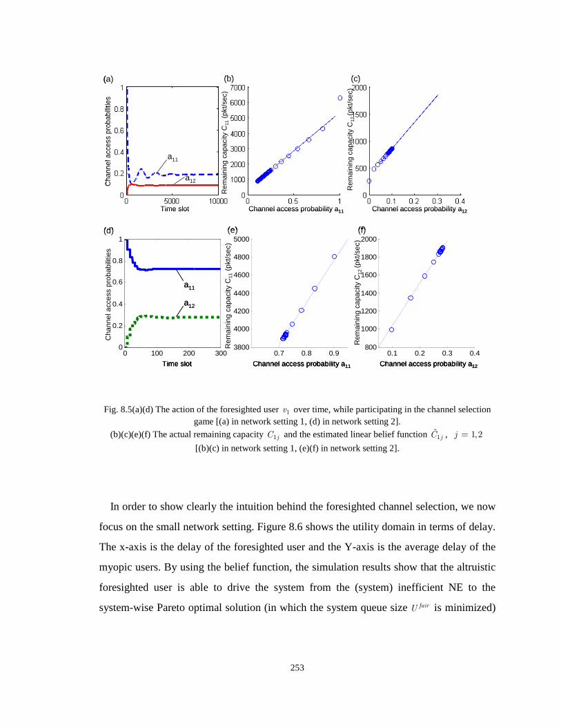
253
Fig. 8.5(a)(d) The action of the foresighted user 1v over time, while participating in the channel selection game [(a) in network setting 1, (d) in network setting 2].
(b)(c)(e)(f) The actual remaining capacity 1jC and the estimated linear belief function 1jC , 1,2j =
[(b)(c) in network setting 1, (e)(f) in network setting 2].
In order to show clearly the intuition behind the foresighted channel selection, we now
focus on the small network setting. Figure 8.6 shows the utility domain in terms of delay.
The x-axis is the delay of the foresighted user and the Y-axis is the average delay of the
myopic users. By using the belief function, the simulation results show that the altruistic
foresighted user is able to drive the system from the (system) inefficient NE to the
system-wise Pareto optimal solution (in which the system queue size fairU is minimized)
Time slot
Cha
nnel
acc
ess
prob
abili
ties
Rem
aini
ng c
apac
ity C
11(p
kt/s
ec)
(a) (b) (c)
Rem
aini
ng c
apac
ity C
12 (p
kt/s
ec)
Channel access probability a11 Channel access probability a12
a11
a12
Time slot
Cha
nnel
acc
ess
prob
abili
ties
Rem
aini
ng c
apac
ity C
11(p
kt/s
ec)
(a) (b) (c)
Rem
aini
ng c
apac
ity C
12 (p
kt/s
ec)
Channel access probability a11 Channel access probability a12
a11
a12
0 100 200 3000
0.2
0.4
0.6
0.8
1
0.7 0.8 0.93800
4000
4200
4400
4600
4800
5000
0.1 0.2 0.3 0.4800
1000
1200
1400
1600
1800
2000
a11a12
Time slot
Cha
nnel
acc
ess
prob
abili
ties
Rem
aini
ng c
apac
ity C
11(p
kt/s
ec)
(d) (e) (f)
Rem
aini
ng c
apac
ity C
12 (p
kt/s
ec)
Channel access probability a11 Channel access probability a12
a11
a12
a11
a12

254
by using the belief function. If the foresighted user is selfish, it will drive the system from
NE to SE. Table 8.2 shows the results at different equilibriums. When the foresighted
user is selfish, it puts more traffic into the efficient channel 1r and forces the other
myopic users to select the other channel, thereby benefiting its own utility. On the
contrary, if the foresighted user is altruistic, it puts less traffic into channel 1r and allows
the other users myopically select the efficient channel 1r , which will result in an optimal
system performance.
Fig 8.6. Reaching the system-wise Pareto optimal solution and the Stackelberg Equilibrium.
TABLE 8.2. RESULTS AT DIFFERENT EQUILIBRIUMS
Action of the
foresighted user 11a
Action of the
myopic user 1ia
Delay of the
foresighted user
Average delay of
the myopic users
System Performance
NE 0.72 0.97 0.955 ms 0.848 ms 7.19 SE 0.95 0.78 0.914 ms 0.947 ms 7.45
System-wise
optimal 0.66 1 1.011 ms 0.752 ms 7.00
Next, we highlight the impact in terms of delay for the foresighted user and the myopic
users, when different numbers of myopic users are active in the network. Figure 8.7
shows the delay of the foresighted user at different equilibriums when there are various
0.8 0.9 1 1.1 1.2 1.3 1.4 1.5
x 10-3
6
6.5
7
7.5
8
8.5
9
9.5
10x 10
-4
System-wise Pareto Optimal
Nash
Stackelberg
Delay of the foresighted user (sec)
Ave
rage
del
ay o
f the
myo
pic
user
s (s
ec)
System-wise Pareto Optimal
Nash Equilibrium
Stackelberg Equilibrium
0.8 0.9 1 1.1 1.2 1.3 1.4 1.5
x 10-3
6
6.5
7
7.5
8
8.5
9
9.5
10x 10
-4
System-wise Pareto Optimal
Nash
Stackelberg
Delay of the foresighted user (sec)
Ave
rage
del
ay o
f the
myo
pic
user
s (s
ec)
System-wise Pareto Optimal
Nash Equilibrium
Stackelberg Equilibrium

255
numbers of myopic users in the network. The results show that, as the number of myopic
users in the network increases, the altruistic foresighted user will have a higher delay
impact to reach the system-wise Pareto optimal solution. Beyond 10 myopic users, the
system-wise Pareto optimal solution is not reachable. This situation is also observed in
network setting 1 (large network setting). This is because the traffic ratio of the
foresighted user to the total traffic in the network is not sufficient enough to drive the
equilibrium to the system-wise Pareto optimal solution (as discussed in [KLO95]). On the
contrary, the foresighted user can benefit more in terms of delay when the number of the
myopic users in the network increases.
B. Multiple foresighted user scenario
In this subsection, we simulate the result when there are multiple foresighted users in
the network. We simulate the resulting delays of the conjecture-based channel selection
game using the small network setting in the previous subsection. The only difference is
that we now assume that the 8 users all have traffic with Poisson arrival rate 1ix = Mbps.
Hence, the total traffic rate is still 8 Mbps. These users can select three different channel
selection solutions: 1) the rule-based solution (RB) in Section V.B, 2) the self-interested
Fig. 8.7 Delay of the foresighted user at different equilibrium for various numbers of myopic users in the network.
5 6 7 8 90.5
1
1.5
2
2.5
3x 10
-3
Number of myopic users
Del
ay o
f th
e fo
resi
ghte
d us
er (
sec)
5 6 7 8 90.4
0.6
0.8
1
1.2
1.4
1.6
1.8
2
2.2
2.4x 10
-3
Number of myopic users
Ave
rage
del
ay o
f m
yopi
c us
ers
(sec
)
System-wise ParetoStackelbergNash
System-wise ParetoStackelbergNash
256
foresighted solution (SF) in Section IV.D, and 3) the myopic solution (MY) in Section
II.C. We discuss 8 different scenarios in Table 8.3. First, we simulate the case when all
users are myopic (scenario 1). As simulated in the previous subsection, a self-interested
foresighted user can have a smaller delay when the rest of the users are myopic. However,
when the number of these self-interested foresighted users is larger than 3, the average
delay of these selfish foresighted users can be even worse than the average delay which
they experience when they adopt a myopic channel selection strategy. Hence, this gives
incentives for these foresighted users to collaborate with each other by adhering to the
proposed Algorithm 8.2, which allows the users to test the rule-based solution. The rule-
based solution (scenario 5) provides the minimum average delay for all the foresighted
users and the minimum queue size of the system (minimum fairU ). However, we can see
that, once a selfish user deviates from the rule, both the delay of the selfish user as well as
the system queue size fairU increase (scenario 6). Thus, if a foresighted user joins a
network where the other users already comply with the rule-based solution, the users
should collaborate with each other for their own benefit. Hence, their collaboration is
self-enforcing rather than mandated by a protocol designer. Moreover, from scenario 3
and 8, we see that even when the rest of the users are myopic, the 3 foresighted users will
still have incentive to perform collaborated rule-based solution. However, the delay
performance degrades seriously when some foresighted users deliberately deviate from
the prescribed rules (we set 2 users to select SF in scenario 7). In this case, these
foresighted users will not have incentives to comply with the rule-based solution anymore.
They will all become self-interested and perform Algorithm 8.1 (as in scenario 4).

257
TABLE 8.3. NUMERICAL RESULTS IN DIFFERENT SCENARIOS
Scenarios Number of users using different
solutions
Average delay of the foresighted users (ms)
Normalized system queue
size ( fairU /total traffic rate)
GAP to the optimal system
performance 1 All MY 0.90 0.9 0.025 2 1 SF, 7 MY 0.852 0.91 0.035 3 3 SF, 5 MY 0.877 0.918 0.043 4 5 SF, 3 MY 0.933 0.953 0.078 5 All RB 0.80 0.875 0 6 1 SF, 7RB 1.00 1.00 0.125 7 3 RB, 2 SF, 3
MY 1.164 1.164 0.289
8 3 RB, 5 MY 0.864 0.911 0.034
VII. CONCLUSIONS
In this chapter, we study the distributed channel selection problem in multi-channel
wireless networks. Although we use a multi-channel wireless network setting, it is
important to note that the proposed method can be applied to other load balancing
resource sharing system. We model the multi-user interaction using a conjecture-based
channel selection game where myopic users and foresighted users coexist in the network.
Based on the analysis of the conjecture-based channel selection game, we investigate two
different operation scenarios. In the single foresighted user scenario, we find that
achieving the Pareto-efficient solution is possible without any message exchanges among
users, as long as the foresighted user is not selfish. In the scenario where multiple users
are foresighted, we show that the resulting performance degrades when users are learning
in an autonomous manner. Hence, we discuss a rule-based solution for the foresighted
users to collaboratively build the conjectures that optimize the system queue size in this
chapter. In order to benefit themselves, these foresighted users can either build their own
conjectures autonomously, based on their local information, or they can comply with a
prescribed rule-based solution. We propose an on-line procedure for the foresighted users
to select a solution to minimize their delay. The results show that in such multi-channel
network, delay-sensitive users can minimize their delays if there is only one self-
interested foresighted user managing the network. If multiple foresighted users are

258
present in the network, they benefit from complying with the rule prescribed by the MAC
protocols.
VIII. APPENDIX A
Proof of Proposition 4. First, we see that the objective function is a convex function,
given that (1)0 1ijβ≤ ≤ , (0) 0ijβ ≥ . Assume µ as the Lagrange multiplier. Forj ir F∀ ∈ , the
optimality conditions:
( )
(0)
2(0) (1)
1ijij ij ij
ij ijij ij
Dβ
µ λ κµβ β λ λ
= ⇒ = −+ −
. (20)
From the constraint 1
N
ij ijxλ
==∑ , we have
( )1/ / /j j
ij i ijr rD x Lµ κ
∈Ω ∈Ω= −∑ ∑ . (21)
By substituting equation (21) into equation (20), we have ( )( / )j
fij ij ij iij
r
D D x Lλ α∈Ω
= − −∑
for 0ijλ > case.
IX. APPENDIX B
Proof of Proposition 6 Denote the total traffic through jr as 1
M
j ijiλ λ
==∑ . Assume
[ , 1,..., ]i i Mµ= =µ as the Lagrange multipliers. The Lagrange function of equation (4)
can be written as:
1
1 1 11
( , ) ( / )
MN M N
ijii i ijM
j i jj iji
x LC
λµ λ
λ
=
= = ==
= + −−
∑∑ ∑ ∑
∑σ µL . (22)
For those 0ijλ > , the optimality conditions are:
( )2
, for j j
i j j iij j
C CC v
Cµ λ
µλ= ⇒ = − ∀ ∈
−V . (23)
Since we assume the non-saturated condition, the condition 1 1
/N M
j ij ix Lλ
= ==∑ ∑ holds.
Based on this, we can calculate the Lagrange multipliers:
( )1
, for j j
j
j jr r
ii jr
Cv
C
λ
µ
∈Ω ∈Ω
∈Ω
−= ∀∑ ∑
∑. (24)
Hence, the Pareto optimum solution will be:
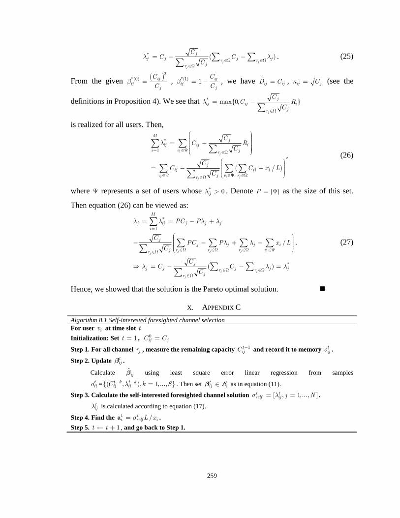
259
* ( )j j
j
jj j j jr r
jr
CC C
Cλ λ
∈Ω ∈Ω∈Ω
= − −∑ ∑∑
. (25)
From the given ( )
2*(0) ijij
j
C
Cβ = , *(1) 1
ijij
j
C
Cβ = − , we have ij ijD C= , ij jCκ = (see the
definitions in Proposition 4). We see that * max0,
j
jij ij i
jr
CC R
Cλ
∈Ω
= −∑
is realized for all users. Then,
*
1
( / )
ij
i i jj
Mj
ij ij i
i v jr
jij ij i
v v rjr
CC R
C
CC C x L
C
λ= ∈Ψ ∈Ω
∈Ψ ∈Ψ ∈Ω∈Ω
= −
= − −
∑ ∑∑
∑ ∑ ∑∑
, (26)
where Ψ represents a set of users whose * 0ijλ > . Denote P = Ψ as the size of this set.
Then equation (26) can be viewed as:
*
1
*
/
( )
j j j ij
j j
j
M
j ij j j j
i
jj j j i
r r r vjr
jj j j j jr r
jr
PC P
CPC P x L
C
CC C
C
λ λ λ λ
λ λ
λ λ λ
=
∈Ω ∈Ω ∈Ω ∈Ψ∈Ω
∈Ω ∈Ω∈Ω
= = − +
− − + −
⇒ = − − =
∑
∑ ∑ ∑ ∑∑
∑ ∑∑
. (27)
Hence, we showed that the solution is the Pareto optimal solution.
X. APPENDIX C
Algorithm 8.1 Self-interested foresighted channel selection For user iv at time slot t
Initialization: Set 1t = , 0ij jC C=
Step 1. For all channel jr , measure the remaining capacity 1tijC− and record it to memory t
ijo .
Step 2. Update tijβ .
Calculate ijβ using least square error linear regression from samples
tijo =( , ), 1,..., t k t k
ij ijC k Sλ− − = . Then set tij i∈β B as in equation (11).
Step 3. Calculate the self-interested foresighted channel solution [ , 1,..., ]t tself ij j Nσ λ= = .
tijλ is calculated according to equation (17).
Step 4. Find the /t ti self iL xσ=a .
Step 5. 1t t← + , and go back to Step 1.

260
Algorithm 8.2 On-line procedure of the foresighted channel selection For a self-interested foresighted user iv in the test period Stage 1: Identify whether or not there is only one foresighted user. Set ij jCλ δ= − to deplete the channel jr .
Measure the subsequent remaining capacity ijC .
If ijC δ= , there is only one foresighted user. Apply Algorithm 8.1 in the data transmission
period. Otherwise, go to Stage 2. Stage 2: Identify whether or not to comply with the rule-based solution
Step 1. Perform Algorithm 8.1 for T time slots and measure the time average delay TAiU .
Step 2. Perform the rule-based solution * *[ , 1,..., ]rule ij j Nσ λ= = as in Proposition 6. Measure the
resulting delay *( )iU σ .
Step 3. Compare the utilities. If *( ) TAi iU U≥σ , keep using the rule-based solution *ruleσ in the data
transmission period. Otherwise, apply Algorithm 8.1.

261
Chapter 9
Conclusions
This dissertation focused on developing mathematical tools, theoretical and statistical
analysis, and algorithms, to understand, improve, and preserve the performance of
delay-sensitive applications over multi-hop wireless networks. Current networks are
primarily designed to communicate delay-insensitive information– they are not designed
to handle delay-sensitive traffic. The goal of this dissertation was to study and propose
mechanisms that endow wireless networks with the ability to reconfigure and adjust
priorities in response to a time-varying network environment in order to deliver desired
levels of performance for delay-sensitive applications. System-theoretic and optimization
tools, as well as advanced networking, routing, communications, learning and
game-theoretic concepts were integrated in order to model and control the behavior of
complex interconnected wireless networks.
Most existing networking research aims at improving the goodput and robustness to
various attacks or vulnerabilities of multi-hop wireless networks by redesigning existing
transport, network or MAC protocols. However, such solutions are only successful if
these new protocols are widely adopted by both international standardization bodies and
industry. Also, such solutions often demand backwards compatibility and interoperability
with existing infrastructures. In contrast, the research in this dissertation focused on
improving the resilience and robustness of wireless networks, with minimal or no change
to existing protocols and network infrastructure. This objective was accomplished as
follows.
In order to fulfill stringent requirements of communicating delay-sensitive traffic over
a multi-hop network, nodes in a network should be able to learn the behavior and status

262
of neighboring nodes and, subsequently, self-organize and adapt their cross-layer
strategies in order to maximize the performance metrics and improve network
performance. The foundations in this dissertation therefore rely on recognizing and
exploiting the following three essential features: (A) the need to endow nodes in a
network with multi-agent interactive learning abilities; (B) the need for these cognitive
nodes to continuously adjust their operation in response to a dynamically changing (as
opposed to static or stationary) network environment, and (C) the need for the individual
nodes to adjust their own expectations in response to the state of the network by
assigning different risk levels to different portions of their data. The discussion in the
sequel expands on features (A)-(C), which were developed in this dissertation.
(A) Multi-agent interactive learning. To begin with, the individual nodes in a wireless
network must be endowed with adaptation and learning abilities in order to be able to
assess the conditions in their neighborhood on various levels such as (1) identifying
nodes that have been compromised due to node failure, or other effects, (2) identifying
node behavior and their history of resource usage, and (3) identifying nodes with poor
signal-to-noise or power conditions.
By adding a cognitive dimension to the nodes, a wireless network becomes better
enabled to evaluate the expected responses of neighboring nodes to various types of
interference. They also become better prepared to support delay-sensitive applications.
The “cognition” (i.e., learning of the environment and the actions from competing nodes)
will allow the network nodes to dynamically self-organize and strategically adapt their
transmission strategies to maximize the utility defined by the application and, more
importantly, be able to provide improved robustness to network attacks. The nodes will
be expected to behave as cognitive agents competing for resources within a stochastic
game formulation. Within this game, different levels of collaboration can be allowed
depending on the “smartness” and “risk” attitudes of the different wireless entities. The
cognitive nodes would be able to react to information collected from their neighbors and

263
compete for resources by adjusting their local cross-layer strategies in relation to dynamic
routing, transmission power, channel selection, scheduling, interference avoidance,
spectrum allocation, traffic shaping, source-level error resilience, etc. By doing so, the
nodes are able to deliver improved performance in terms of minimizing transmission
delay for delay-sensitive applications. These objectives can be achieved by developing
accurate queuing models for the various cross-layer transmission algorithms and
protocols, and by relying on sophisticated queuing concepts, such as service-on-vacation,
to accurately model interference effects among simultaneously transmitting nodes within
a unifying delay-aware framework.
(B) Adaptation to a dynamic heterogeneous network environment. Additionally, this
research recognizes that a wireless network is fundamentally a dynamic system as
opposed to a static interconnection of nodes. The states of the network, as well as its
topology, are continuously changing due, for example, to the varying levels of resources
that are available in the network. The dynamic nature of the wireless network is a strong
reason why individual nodes should be able to continuously adjust their operation in
response to a dynamically changing (as opposed to static or stationary) network
environment. In this manner, nodes are able to match available wireless resources and
successfully cope with network dynamics.
The merits of the proposed approaches can be understood from the perspective of
multi-agent learning versus single-agent learning. In existing cross-layer optimization
solutions, single agent learning is deployed whereby an agent repeatedly interacts with its
environment (in this case, the wireless medium). In the case of a stationary environment,
repeated interactions should ideally lead to a better model of the environment and, hence,
to the opportunity to optimize the agents’ strategy over the long run. In multi-agent
learning, on the other hand, the environment is composed of other agents, which are
simultaneously adapting their strategies [SL09]. Consequentially, from the perspective of
any single agent or wireless node, the environment appears to be non-stationary. Hence,

264
unlike conventional cross-layer solutions, the research will focus on how to exploit the
interactions among network entities with the objective of maximizing network and users’
utilities at reasonable complexity under a broad set of operating scenarios.
The merits of the approaches in this dissertation can also be examined from the
perspective of game theory. Earlier investigations on the application of game theory to
networking problems have concentrated on characterizing properties of equilibrium
conditions. However, an equilibrium operating condition reflects optimality from the
perspective of any single agent and it can lead to potential loss of efficiency. In contrast,
multi-agent learning leads to a dynamic network operating under non-stationary
conditions. As such, the interactions among the nodes need not lead to a state of
equilibrium for the network. Perpetual adaptation of strategies may persist, as long as the
performance of delay-sensitive applications is maximized. Critical questions that were
answered in this dissertation are how quickly conditions and behaviors can be learned
and estimated, and how to optimally manage resources and adapt given the speed of
change in the interferences, the channel conditions, and application-layer traffic
characteristics. For example, in multiple-access radio systems, one cannot change the
channel dynamics but, fortunately, one can heavily influence the interference dynamics
and the signal-to-interference ratio by adapting the cross-layer transmission strategies.
Thus, this research enabled modeling the various network dynamics in order to
strategically design adaptation strategies at the various layers of the protocol stack to
effectively respond and proactively counteract network dynamics.
(C) Dynamic risk and reward assessment. Adaptation and learning allows each
cognitive node to assess the network conditions based on information collected from its
neighborhood. Based on this assessment, the nodes can adjust their own utility functions.
This feature is particularly relevant under emergency situations since it enables nodes to
tag some parts of their data as more critical than others and to request different levels of
QoS for the partitioned data. For example, some parts of the data may need to experience

265
a much shorter delay than other parts. Allowing for such solutions for delay-sensitive
applications is an effective means to permit network survivability and resilience in
dynamically changing environments because of time-varying source characteristics,
wireless network conditions and infrastructure, and mission goals.
In the proposed framework, each node can estimate the risk that packets containing
delay-sensitive content of various priorities will not arrive on time at their destination.
Each node can also observe partial historic information of the outcome of the resource
allocation procedure, through which the nodes can estimate the expected rewards in the
future. Subsequently, the transmission strategies can be adapted to jointly consider the
estimated risk of losing the packets (or not receiving them on time), as well as the impact
in terms of content distortion based on the various mission goals. Preliminary results
show that such cross-layer transmission strategies and dynamic routing policies based on
information exchanges significantly outperform existing state-of-the-art on-demand
routing solutions designed for ad-hoc wireless networks.
Additionally, existing research on learning in games assumes that either everything
(the utility functions are fully known) or nothing (only the payoffs of each individual
player is known) about the utility functions is known. However, in the proposed
framework, a middle ground exists where there is partial knowledge of the functional
form of the utility function but subject to uncertain parameters that can be estimated
online. Existing approaches do not exploit the availability of such partial information.
In summary, the foundation of the research developed in this dissertation was to
investigate how the autonomic nodes interact with each other to compete for resources
and how and what the nodes can learn from their observed transmission history in order
to improve their own strategies to interact with other wireless users. The proposed
approach is to model the various wireless nodes as a collection of selfish, autonomous
agents that make their own decisions and strategically interact in order to acquire wireless
resources. A key aspect of the proposed solution for building robustness for
266
delay-sensitive applications is the decentralization of the decision-making process among
the participating autonomic nodes and their ability to comprehend and consciously
influence the wireless network dynamics based on the gathered information about other
network nodes.

267
Bibliography
[ACW95] J. Abate, G. L. Choudhury, and W. Whitt. “Exponential approximations for tail probabilities in queues I: Waiting times”, Operations Research, vol. 43, no. 5, pp 885-901, 1995.
[AMB04] Y. Andreopoulos, A. Munteanu, J. Barbarien, M. van der Schaar, J.
Cornelis, and P. Schelkens, “In-band Motion Compensated Temporal Filtering,” Signal Processing: Image Communication (Special Issue on “Subband/Wavelet Interframe Video Coding”), vol. 19, no. 7, pp. 653-673, Aug. 2004.
[AMV06] Y. Andreopoulos, N. Mastronarde, and M. van der Schaar, “Cross-layer
Optimized video Streaming over wireless multi-hop Mesh Networks,” IEEE Journal on Selected Areas in Communications, vol. 24, no. 11, Nov 2006, pp. 2104-2115.
[ALV06] I. F. Akyildiz, W. –Y. Lee, M. C. Vuran, and S. Mohanty, “NeXt
generation/dynamic spectrum access/cognitive radio wireless networks: a survey,” Computer Networks: The International Journal of Computer and Telecommunication Networking, vol. 50, no. 13, Sep 2006.
[AL94] B. Awerbuch and T. Leighton, “Improved Approximation Algorithms for
the Multi-commodity Flow Problem and Local Competitive Routing in Dynamic Networks,” Proc. 26th ACM Symposium on Theory of Computing, May 1994.
[BBS95] A. G. Barto, S. J. Bradtke and S. P. Singh, "Learning to act using real-time
dynamic programming", Artificial Intelligence, vol. 72, no. 1-2, Jan 1995, pp. 81-138.
[Bel04] E. M. Belding-Royer, “Multi-level Hierarchies for Scalable Ad Hoc
Routing,” ACM/Kluwer Wireless Networks (WINET), vol. 9, no. 5, Sept. 2004, pp. 461-478.
[Ber82] D. P. Bertsekas, “Distributed dynamic programming”, IEEE Trans. Autom.
Control, vol. 27, no. 3, pp. 610-616, Jun 1982. [Ber95] D. P. Bertsekas, Dynamic programming and Optimal Control. vol. I,
Belmont, MA: Athena Scientific, 1995. [BG87] D. Bertsekas, R. Gallager, Data Networks, Prentice Hall, Inc. Upper
Saddle River, NJ, 1987.

268
[BL94] J. A. Boyan and M. L. Littman, “Packet routing in dynamically changing networks: A reinforcement learning approach,” in Advances in NIPS 6, J. D. Cowan et al., Eds. San Francisco, CA: Morgan Kauffman, 1994, pp. 671–678.
[BRB05] V. Brik, E. Rozner, S. Banarjee, P. Bahl, “DSAP: a protocol for
coordinated spectrum access,” in Proc. IEEE DySPAN 2005, Nov. 2005, pp. 611-614.
[Bro05] T. X. Brown, “An analysis of unlicensed device operation in licensed
broadcast service bands,” in Proc. IEEE DySPAN 2005, Nov 2005, pp. 11-29.
[BT05] A. Butala, L. Tong, “Cross-layer Design for Medium Access Control in
CDMA Ad-hoc Networks,” EURASIP J. on Applied Signal Processing, vol. 2, pp. 129-143, 2005.
[CBD02] T. Camp, J. Boleng, V. Davies, “A survey of mobility models for ad hoc
network research,” in Wireless Communications and Mobile Computing (WCMC), vol. 2, no. 5, pp. 483-502, 2002.
[CCB06] C. Cordeiro, K. Challapali, D. Birru and S. Shankar N, “IEEE 802.22: An
Introduction to the First Wireless Standard based on Cognitive Radios,” Journal of Communications, Academy Publishers, vol. 1, no. 1, Apr 2006.
[CF06] J. Chakareski and P. Frossard, “Rate-Distortion Optimized Distributed
Packet Scheduling of Multiple Video Streams Over Shared Communication Resource,” IEEE Transactions on Multimedia, vol. 8, no. 2, Apr, 2006.
[CM06] P. A. Chou, and Z. Miao, “Rate-Distortion Optimized Streaming of
Packetized Media,” IEEE Transactions on Multimedia, vol. 8, no. 2, pp. 390-404. April 2006.
[CW05] S. T. Cheng, M. Wu, “Performance Evaluation of Ad-Hoc WLAN by
M/G/1 Queuing Model,” IEEE International Conference on Information Technology : Coding and Computing (ITCC’05), pp. 681-686, 2005.
[CZ00] G. Cheung, A. Zakhor, “Bit Allocation for Joint Source/Channel Coding of
Scalable Video,” IEEE Transactions on Image Processing, vol. 9, no. 3, pp. 340-356, Mar 2000.

269
[CZ05] L. Cao and H. Zheng, “Distributed Spectrum Allocation via Local Bargaining,” in 2nd Ann. IEEE Comm. Soc. Conf. On Sensor and Ad Hoc Comm. and Networks (SECON 2005), pp. 475-486, 2005.
[CZ06] P. A. Chou, and M. Zhourong, “Rate-distortion Optimized Streaming of
packetized media,” IEEE Transactions on Multimedia, vol. 8, no. 2, pp. 390-404. April 2006.
[DAB03] D. S. J. De Couto, D. Aguayo, J. Bicket, and R. Morris, “A High
Throughput Path Metric for Multi-hop Wireless Routing,” Proc. ACM Conf. Mob. Computing and Networking, MOBICOM, pp. 134-146, 2003.
[DCC05] J. Dowling, E. Curran, R. Cunningham, and V. Cahill, “Using Feedback in
Collaborative Reinforcement Learning to Adaptively Optimize MANET Routing,” IEEE Transactions on System, Man, and Cybernetics – Part A: Systems and Humans, vol. 35, no. 3, pp. 360-372, May 2005.
[DHP03] Y. Diao, J. L. Hellerstein, S. Parekh, J. P. Bigus, “Managing Web Server
Performance with Autotune Agens,” IBM System Journal, vol 42, no. 1, 2003.
[DPZ04] R. Draves, J. Padhye, and B. Zill, “Routing in multi-radio, multi-hop
wireless mesh networks,” in Proc. ACM Internat. Conf. on Mob. Computing and Networking (MOBICOM), 2004, pp. 114-128.
[EM93] J. R. Evans and E. Minieka, Optimization Algorithms for Networks and
Graphs, NY: Marcel Dekker, 1993. [EMM03] E. Even-Dar, S. Mannor, Y. Manour, “Action elimination and stopping
conditions for reinforcement learning,” Proc. Of the International Conference on Machine Learning (ICML 2003), 2003.
[FCB07] M. Felegyhazi, M. Cagalj, S. S. Bidokhti, and J.-P. Hubaux,
“Noncooperative multi-radio channel allocation in wireless networks,” in IEEE INFOCOM ’07, May 2007.
[FCC02] Federal Communications Commission (FCC), “Spectrum Policy Task
Force,” ET Docket no. 02-135, Nov 15, 2002. [FL98] D. Fudenberg and D.K. Levine, The Theory of Learning in Games, MIT
Press, Cambridge, MA, 1998. [FT91] D. Fudenberg and J. Tirole, Game Theory. MIT Press, Cambridge, MA,
1991.

270
[FV07] F. Fu and M. van der Schaar, "Non-collaborative resource management for wireless multimedia applications using mechanism design," IEEE Trans. Multimedia, vol. 9, no. 4, pp. 851-868, Jun. 2007.
[FWK06] S. M. Faccin, C. Wijting, J. Kenckt, A. Damle. “Mesh WLAN Networks:
Concept and System Design”, IEEE Wireless Communications Mag., pp. 10-17, Apr 2006.
[GJ07] P. Gupta and T. Javidi, "Towards Throughput and Delay-Optimal
Routing for Wireless Ad-Hoc Networks,'' Asilomar Conference on Signals, Systems and Computers, Nov. 2007.
[GFX01] Y. Guan, X. Fu, D. Xuan, P. U. Shenoy, R. Bettati, and W. Zhao,
“NetCamo: Camoufloging Network Traffic for QoS-Guaranteed Mission Critical Applications,” IEEE Transactions on System, Man, and Cybernetics – Part A: Systems and Humans, vol. 31, no. 4, pp. 253-265, July 2001.
[GKG07] D. Gesbert, S. G. Kiani, A. Gjendemsjo, and G. E. Oien, “Adaptation,
Coordination, and Distributed Resource Allocation in Interference-Limited Wireless Networks,” Proceeding of IEEE, vol. 95, no. 12, pp. 2393-2409, 2007.
[GM00] D. J. Goodman and N. B. Mandayam, “Power control for wireless data,”
IEEE Personal Communications, vol. 7, pp. 48-54, Apr 2000. [Hah77] F. H. Hahn, “Exercises in conjectural equilibrium analysis,” Scandinavian
Journal of Economics, vol. 79, pp. 210-226, 1977. [Hay05] S. Haykin, “Cognitive Radio: Brain-Empowered Wireless
Communications,” in IEEE Journal on Selected Areas in Communications, vol. 23, no. 2, Feb 2005.
[HBH05] J. Huang, R. A. Berry, M. L. Honig, “Spectrum Sharing with Distributed
Interference Compensation,” in Proc. IEEE DySPAN 2005, Nov. 2005, pp. 88-93.
[HHN08] Y. Huang, W. He, K. Nahrstedt, W. C. Lee, “Dos Resistant Broadcast
Authentication with Low End-to-end Delay,” IEEE INFOCOM 2008, April 2008.

271
[HPR07] Z. Han, C. Pandana, and K. J. Ray Liu, ``Distributive Opportunistic Spectrum Access for Cognitive Radio using Correlated Equilibrium and No-regret Learning", in Proceedings of IEEE Wireless Communications and Networking Conference, 2007.
[Hoe63] W. Hoeffding, “Probability inequalities for sums of bounded random
variables,” Journal of the American Statistical Association, vol. 58, no. 301, pp. 31-30, Mar. 1963.
[Hor01] P. Horn, “Autonomic Computing: IBM Perspective on the State of
Information Technology,” http://www.research.ibm.com/autonomic , Oct 2001.
[IEE03] IEEE 802.11e/D5.0, Draft Supplement to Part 11: Wireless Medium
Access Control (MAC) and physical layer (PHY) specifications: Medium Access Control (MAC) Enhancements for Quality of Service (QoS), June 2003.
[Jan02] J. Jannotti, “Network-layer support for overlay networks,” in Proc. IEEE
Conf. Open Architectures and Network Programming, NY, June 2002. [JB07] T. Jiang, J. S. Baras, “Fundamental Tradeoffs and Constrained Coalitional
Games in Autonomic Wireless Networks,” IEEE WiOpts, 2007. [JCO02] D. Julian, M. Chiang, D. O’Neill, and S. Boyd, “QoS and fairness
constrained convex optimization of resource allocation for wireless cellular and ad hoc networks,” IEEE INFOCOM 2002, pp. 477-486.
[JDN01] N. Jain, S. Das, and A. Nasipuri, “A multi-channel MAC protocol with
receiver based channel selection for multi-hop wireless networks,” ICCCN 2001, Oct. 2001.
[JF06] D. Jurca and P. Frossard, “Media Streaming with Conservative Delay on
Variable Rate Channels,” in Proceedings of IEEE international Conference on Multimedia and Expo (ICME, 2006), 2006.
[JF07] D. Jurca, P. Frossard, “Packet Selection and Scheduling for Multipath
video streaming,” IEEE Transactions on Multimedia, vol. 9, no. 2, Apr. 2007.
[JM96] D. B. Johnson, and D. A. Maltz, “Dynamic source routing in ad hoc
wireless networks,” Chapter in Mobile Computing, Kluwer Acad. Pub., 1996.

272
[JTK01] T. Jiang, C. K. Tham, and C. C. Ko, “An approximation for waiting time tail probabilities in multiclass systems”, IEEE Communications Letters, vol. 5, no. 4, pp 175-177. April 2001.
[KC03] J. O. Kephart and D. M. Chess, “The vision of autonomic computing,”
IEEE Computer Magazine, vol. 36, no.1, pp.41-50, 2003. [KEW02] B. Krishnamachari, D. Estrin, S. Wicker, “The Impact of Data
Aggregation in Wireless Sensor Networks,” IEEE Proc. of International Conference on Distributed Computing Systems Workshop, pp. 575-578, 2002.
[Kle75] L. Kleinrock, Queuing Systems Volume I: Theory, NY: Wiley-Interscience
Publication, 1975. [Koe66] E. Koenigsberg, “On jockeying in queues,” Manag. Sci. vol. 12, pp.
412–436, 1966. [Kon80] A. G. Konheim, “A Queuing Analysis of Two ARQ Protocols,” IEEE
Transactions on Communications, vol. com-28, no. 7, July 1980. [KOG07] S. G. Kiani, G. E. Oien, D. Gesbert, “Maximizing multi-cell capacity using
distributed power allocation and scheduling,” IEEE Wireless Communications and Networking Conference, WCNC 2007, pp. 1690-1694, Mar 2007.
[Kri02] D. Krishnaswamy, “Network-assisted Link Adaptation with Power Control
and Channel Reassignment in Wireless Networks,” 3G Wireless Conference, pp. 165-170, 2002.
[KLO95] Y. A. Korilis, A. A. Lazar, and A. Orda, “Architecting Noncooperative
Networks,” IEEE Journal on Selected Areas in Comm., vol. 13, no. 7, Sep 1995.
[KLO97] Y. A. Korilis, A. A. Lazar, and A. Orda, “Achieving Network Optima
Using Stackelberg Routing Strategies,” IEEE/ACM Transactions on Networking, vol. 5. no. 1, Feb 1997.
[KMT98] F. Kelly, A. Maulloo, and D. Tan, ”Rate control in communication
networks: shadow prices, proportional fairness and stability,” Journal of the Operational Research Society, vol. 49, no. 3, pp. 237–252, Mar. 1998.

273
[KN96] I. Katzela and M. Naghshineh, “Channel assignment schemes for cellular mobile telecommunications: A comprehensive survey,” IEEE Personal Communications, vol. 3, pp. 10-31, Jun. 1996.
[KP99] G. D. Kondylis and G. J. Pottie, “Dynamic Channel Allocation Strategies
for Wireless Packet Access,” IEEE VTC, Amsterdam, Sep 1999. [KSH00] T. Kailath, A. H. Sayed, and B. Hassibi, Linear Estimation, Prentice-Hall,
NJ, 2000. [KSV06] D. Krishnaswamy, H. –P. Shiang, J. Vincente, V. Govindan, W. S.
Conner, S. Rungta, W. Chan, K. Miao “A cross-layer cross-overlay architecture for proactive adaptive processing in mesh networks,” 2nd IEEE Workshop on Wireless Mesh Networks (WiMesh 2006), 2006. pp. 74-82.
[KV04] D. Krishnaswamy, and J. Vicente, “Scalable Adaptive Wireless Networks
for Multimedia in the Proactive Enterprise,” Intel Technology Journal, see online at: http://developer.intel.com/technology/itj/2004/volume08issue04/art04_scalingwireless/p01_abstract.htm, 2004.
[LCC07] J. W. Lee, M. Chiang, A. R. Calderbank, “Utility-Optimal Random-Access
Control,” IEEE Transactions on Wireless Comm., vol. 6, no. 7, pp. 2741-2750. July 2007.
[LL06] K.-D. Lee and V.C.M. Leung, "Fair Allocation of Subcarrier and Power in
an OFDMA Wireless Mesh Network", IEEE J. Sel. Areas in Commun., vol. 24, no. 11, pp. 2051-2060, Nov. 2006.
[Low03] S. H. Low, “A duality model of TCP and queue management algorithms,”
IEEE/ACM Transactions on Networking, vol. 11, no. 4, pp. 525–536, 2003.
[LS99] S. Lal, E. S. Sousa, “Distributed resource allocation for DS-CDMA-based
multimedia ad hoc wireless LANs,” IEEE J. Sel. Areas Commun.,vol. 17, no. 5, pp. 947-967, May 1999.
[LTH07] J. W. Lee, A. Tang, J. Huang, M. Chiang, A. R. Calderbank,
“Reverse-Engineering MAC: A Non-cooperative Game Model,” IEEE Journal on Selected Areas in Comm., vol. 25, no. 6, pp. 1135-1147, Aug 2007.
[Luc06] Robert W. Lucky, “Tragedy of the commons,” IEEE Spectrum, vol. 43
no.1, pp. 88, Jan 2006.

274
[LZL07] C. Long, Q. Zhang, B. Li, H. Yang, and X. Guan, “Non-cooperative power control for wireless ad hoc networks with repeated games,” IEEE Journal on Selected Areas in Communications (JSAC), vol. 25, no. 6 pp. 1101-1112, Aug. 2007.
[MCP06] F. Meshkati, M. Chiang, H. V. Poor, and S. C. Schwartz, “A
game-theoretic approach to energy-efficient power control in multi-carrier CDMA systems,” IEEE Journal on Selected Areas in Communications (JSAC), vol. 24, pp. 1115-1129, June 2006.
[MD01] M. K. Marina, S. R. Das, “Ad hoc on-demand multi-path distance vector
routing (AOMDV),” Proc. of International Conference on Network Protocols (ICNP), pp. 14-23, 2001.
[MGM05] M. Machado, O. Goussevskaia, R. Mini, C. G. Rezende, A. Loureiro, G.
Mateus, J. Nogueira, “Data Dissemination in Autonomic Wireless Sensor Networks,” IEEE J. Sel. Areas Commun., vol. 23, no. 12, pp. 2305-2319, Dec 2005.
[ML99] J. R. Moorman and J. W. Lockwood, “Implementation of the multiclass
priority fair queuing (MPFQ) algorithm for extending quality of service in existing backbones to wireless endpoints,” IEEE Global Telecommunications Conference, 1999, vol. 5, pp. 2752-2757.
[MM99] J. Mitola, G. Q. Maguire Jr., “Cognitive radio: Making software radios
more personal,” IEEE Pers. Commun., vol. 6, no. 4, pp. 13-18, Aug. 1999. [MTO04] D. Marsh, R. Tynan, D. O’Kane, G. M. P. O’Hare, “Autonomic Wireless
Sensor Networks,” Artificial Intelligence, vol. 17, pp. 741-748, 2004. [NMR05] M. J. Neely, E. Modiano, and C. E. Rohrs, “Dynamic Power Allocation
and Routing for Time-Varying Wireless Networks”, IEEE Journal on Selected Areas in Communications, vol. 23. no1, Jan 2005. pp. 89-103.
[NH07] D. Niyato and E. Hossain, "A game-theoretic approach to competitive
spectrum sharing in cognitive radio networks," in Proc. IEEE WCNC'07, Hong Kong, 11-15 March, 2007.
[NZD02] A. Nasipuri, J. Zhuang, and S. R. Das, “A multi-channel MAC protocol
with power control for multi-hop mobile ad hoc networks,” The Computer Journal, 45, 2002.

275
[NZT02] S. Nelakuditi, Z. Zhang, R. P. Tsang, D. H. C. Du, “Adaptive Proportional Routing: A Localized QoS Routing Approach,” IEEE/ACM Transactions on Networking, vol. 10, no. 6, pp. 790-804, Dec 2002.
[OR98] A. Ortega, and K. Ramchandran, “Rate-distortion Methods for Image and
Video Compression,” IEEE Signal Processing Mag., vol. 15, no. 6, pp. 23-50, Nov, 1998.
[PB94] C. E. Perkins, P. Bhagwat, “Highly Dynamic Destination-Sequenced
Distance-Vector Routing (DSDV) for Mobile Computers,” ACM SIGCOMM Computer Communication Review, vol. 24, no. 4, pp. 234-244, Oct. 1994.
[PR99] C. E. Perkins, E. M. Royer, “Ad hoc on-demand distance vector routing,”
in Proceedings of the 2nd IEEE Workshop on Mobile Computing Systems and Applications, pp. 90-100, Feb 1999.
[Put94] M. L. Puterman, Markov Decision Process: Discrete Stochastic Dynamic
Programming, John Wiley & Sons, Inc. New York, 1994. [PYC08] A. Proutiere, Y. Yi, M. Chiang, “Throughput of Random Access without
Message Passing,” CISS 2008, Mar. 2008, pp. 509-514. [QCS02] D. Qiao, S. Choi and K. G. Shin, “Goodput Analysis and Link Adaptation
for IEEE 802.11a Wireless LAN”, IEEE Transactions on Mobile Computing, vol.1, no. 4, 2002.
[Rap02] T. S. Rappaport. Wireless Communications: Principles and Practice.
Prentice Hall, 2002. [RC05] A. Raniwala, T. Chiueh, “Architecture and Algorithms for an IEEE
802.11-based Multi-channel Wireless Mesh Network”, INFOCOM 2005. [RE07] A. Rezgui and M. Eltoweissy, “Service-Oriented Sensor-Actuator
Networks,” IEEE Communications, vol. 45, no. 12, pp 92-100, Dec 2007. [RHA04] M. Raya, J. –P. Hubaux, and I. Aad, “DOMINO: a system to detect greedy
behavior in IEEE 802.11 hotspot,” in MobiSys’04, 2004. [RT02] T. Roughgarden, E. Tardos, “How Bad is Selfish Routing?” Journal of the
ACM, vol. 49, no. 2, pp. 236-259, March 2002.
276
[QCS02] D. Qiao, S. Choi and K. G. Shin, “Goodput Analysis and Link Adaptation for IEEE 802.11a Wireless LAN”, IEEE Transactions on Mobile Computing, vol.1, no. 4, 2002.
[SB97] S. Singh, D. Bertsekas, “Reinforcement learning for dynamic channel
allocation in cellular telephone systems,” In Advances in Neural Information Processing Systems, pp. 974-980, Cambridge MA, 1997.
[SCC05] S. Shankar, C. T. Chou, K. Challapali, and S. Mangold, “Spectrum agile
radio: capacity and QoS implementations of dynamic spectrum assignment,” Global Telecommunications Conference, Nov. 2005.
[SCN03] S. H. Shah, K. Chen, and K. Nahrstedt, “Available Bandwidth Estimation
in IEEE 802.11-Based Wireless Networks,” in ISMA/CAIDA 1st Bandwidth Estimation Workshop (BEst 2003), 2003.
[SL09] Y. Shoham, K. Leyton-Brown, Multi-Agent System: Algorithms,
Game-Theoretic, and Logical Foundations, Cambridge University Press, 2009.
[SMG02] C. U. Saraydar, N. B. Mandayam, and D. J. Goodman, “Efficient power
control via pricing in wireless data networks,” IEEE Trans. on Commun., vol. 50, no. 2, pp. 291-303, Oct 2002.
[SP85] S.Sabri and B. Prasada, “Video Conferencing Systems,” Proc. of the IEEE,
vol. 73, no. 4, pp. 671-688, 1985. [SPG07] Y. Shoham, R. Powers, and T. Grenager, “If multi-agent learning is the
answer, what is the question?” Artificial Intelligence, vol. 171, no. 7, pp. 365-377, May 2007.
[SPI05] C. Shen, D. Pesch, J. Irvine, “A Framework for Self-management of
Hybrid Wireless Networks using Autonomic Computing Principles,” IEEE Comm. Networks and Services Research Conference, pp. 261-266, May 2005.
[Sut88] R. S. Sutton, ”Learning to predict by the method of temporal differences,”
Machine Learning, vol. 3, no. 1, pp. 9-44, Aug. 1988. [SV04] J. So, N. H. Vaidya, “Multi-Channel MAC for Ad Hoc Networks:
Handling Multi-Channel Hidden Terminals using a Single Transceiver,” ACM International Symp. Mobile Ad Hoc Net. And Comp (MOBIHOC), May 2004, pp. 222-233.

277
[SV06] H. –P. Shiang, and M. van der Schaar, “Multi-user Video Straming over Multi-hop Wireless Networks: A Cross-layer Priority Queuing Approach,” in IEEE Conference on Intelligent Information Hiding and Multimedia Signal Processing (IIH-MSP 2006), pp. 255-258, Dec, 2006.
[SV07a] H. Shiang and M. van der Schaar, "Multi-user video streaming over
multi-hop wireless networks: A distributed, cross-layer approach based on priority queuing," IEEE J. Sel. Areas Commun., vol. 25, no. 4, pp. 770-785, May 2007.
[SV07b] H.-P. Shiang and M. van der Schaar, "Informationally Decentralized Video
Streaming over Multi-hop Wireless Networkss," IEEE Trans. Multimedia, vol. 9, no. 6, pp. 1299-1313, Sep 2007.
[SV08] H. P. Shiang and M. van der Schaar, "Queuing-Based Dynamic Channel
Selection for Heterogeneous Multimedia Applications over Cognitive Radio Networks," IEEE Trans. Multimedia, Vol. 10, no.5, pp. 896-909, Aug. 2008.
[SW04] G. Staple and K. Werbach, “The End of Spectrum Scarcity,” IEEE
Spectrum, vol. 41, no. 3, pp. 48-52, Mar 2004. [SYZ05] E. Setton, T. Yoo, X. Zhu, A. Goldsmith, and B. Girod, “Cross-layer
design of Ad hoc Networks for real-time video streaming,” IEEE Wireless Communications Mag., pp. 59-65, Aug 2005.
[TB00] H. Tong, T. X. Brown, “Adaptive Call Admission Control under Quality
of Service Constraints: A Reinforcement Learning Solution,” IEEE J. Sel. Areas Commun., vol. 18, no. 2, pp. 209-221, Feb 2000.
[TG03] S. Toumpis, A. J. Goldsmith, "Capacity Regions for wireless Ad Hoc
Network", IEEE Transactions on Wireless Communications, vol. 2, no. 4, pp. 736-748, July 2003.
[TJZ03] X. Tan, W. Jin, and D. Zhao, “The application of multi-criterion
satisfactory optimization in computer networks design,” IEEE Proc. of the 40th International Conference on Parallel and Distributed Computing, Applications and Technologies, Aug 2003, pp. 660-664.
[TL08] A. Tizghadam, A. Leon-Garcia, “On Congestion in Delay-sensitive
Networks,” IEEE INFOCOM 2008, April 2008. [TO98] P. Tadepalli and D. Ok, "Model-based average reward reinforcement
learning", Artificial Intelligence, vol. 100, no. 1-2, Jan 1998, pp. 177-224.
278
[TJ91] S. Tekinay and B. Jabbari, “Handover and Channel Assignment in Mobile Cellular Networks,” IEEE Communication Magazine, vol. 29, pp. 42-46, Nov 1991.
[VAH06] M. van der Schaar, Y. Andreopoulos, Z. Hu, “Optimized Scalable Video
Streaming over IEEE 802.11a/e HCCA Wireless Networks under Delay Constraints,” IEEE Trans. On Mobile Computing, vol. 5, no. 6, pp. 755 – 768, June 2006.
[VCS03] A. Vetro, C. Christopoulos, H. Sun, “Video Transcoding Architectures and
Techniques: An Overview,” IEEE Signal Processing Magazine, vol. 20, no. 2, pp. 18-29, Mar 2003.
[VT07] M. van der Schaar, D. S. Turaga, “Cross-layer Packetization and
Retransmission Strategies for Delay-sensitive wireless Multimedia Transmission,” IEEE Transactions on Multimedia, vol. 9, no. 1, pp. 185-197, Jan 2007.
[VS05] M. van der Schaar and S. Shankar, "Cross-layer wireless multimedia
transmission: challenges, principles, and new paradigms," IEEE Wireless Commun. Mag., vol. 12, no. 4, pp. 50-58, Aug. 2005.
[WCZ05] Y. Wu, P. A. Chou, Q. Zhang, K. Jain, W. Zhu, S.Y. Kung, "Network
Planning in Wireless Ad Hoc Networks: A Cross-Layer Approach", IEEE Journal on Selected Areas in Communications, vol. 23, no. 1, pp. 136-150, Jan. 2005.
[WD92] C. J. C. H. Watkins, P. Dayan, “Q-learning”, Machine Learning, vol. 8, no.
3-4, pp. 279-292, May 1992. [WH98] M. P. Wellman and J. Hu, "Conjectural equilibrium in multiagent
learning," Machine Learning, vol. 33, pp. 179-200, 1998. [WP02] C. C. Wang and G. J. Pottie, “Variable Bit Allocation for FH-CDMA
Wireless Communication Systems,” IEEE Transactions on Communications, vol.50, no. 6, Oct 2002.
[WPT03] R. Want, T. Pering, D. Tennenhouse, “Comparing autonomic and
proactive computing,” IBM Systems Journal, vol. 42, no. 1, 2003. http://www.research.ibm.com/journal/sj/421/want.html
[WR03] M. Waldvogel and R. Rinaldi. “Efficient Topology-Aware Overlay
Network, ” ACM SIGCOMM Computer Comm. Review, vol. 33, no. 1, pp. 101-106, Jan 2003.

279
[WV06] M. Wang and M. van der Schaar, “Operational Rate-Distortion Modeling for Wavelet Video Coders,” IEEE Transactions on Signal Processing, vol. 54, no. 9, pp. 3505-3517, Sep. 2006.
[WYT06] H. Wu, F. Yang, K. Tan, J. Chen, Q. Zhang, Z. Zhang, "Distributed
Channel Assignment and Routing in Multi-radio Multi-channel Multi-hop Wireless Networks", in IEEE JSAC special issue on multi-hop wireless mesh networks, vol. 24, no. 11, pp. 1972-1983, Nov 2006.
[WZ02] W. Wei, and A. Zakhor, “Multipath unicast and multicast video
communication over wireless ad hoc networks,” Proc. Int. Conf. Broadband Networks, Broadnets, pp. 496-505, 2002.
[WZF04] J. Wang, H. Zhai, and Y. Fang, “Opportunistic Packet Scheduling and
Media Access Control for Wireless LANs and Multi-hop Ad Hoc Networks,” IEEE Wireless Communications and Networking Conference, vol. 2, pp. 1234-1239, Mar 2004.
[WZQ08] F. Wu, S Zhong, C Qiao, “Globally optimal channel assignment for
non-cooperative wireless networks,” INFOCOM 2008, pp. 2216-2224. [XCR08] D. Xu, M. Chiang, and J. Rexford, “Link-state Routing with Hop-by-Hop
Forwarding Achieves Optimal Traffic Engineering”, Proc. IEEE INFOCOM, 2008.
[XJB04] L. Xiao, M. Johansson, S. P. Boyd, “Simultaneous Routing and Resource
Allocation Via Dual Decomposition,” IEEE Transactions on Communications, vol. 52, no. 7, pp. 1136-1144, July 2004.
[XSC03] M. Xiao, N. B. Shroff, and E. J. P. Chong, “A Utility-Based
Power-Control Scheme in Wireless Cellular Systems,” IEEE/ACM Transactions on Networking, vol. 11, pp. 210-221, Apr 2003.
[YGC02] W. Yu, G. Ginis, and J. M. Cilffi, “Distributed Multi-user Power Control
for Digital Subscriber Lines,” IEEE J. Sel. Areas Commun., vol. 20, no. 5, pp. 1105-1115, Jun. 2002.
[YL06] W. Yu, R. Lui, “Dual Methods for Nonconvex Spectrum Optimization of
Multi-carrier Systems,” IEEE Transactions on Communications, vol. 54, no. 7, July 2006.
[You04] H. P. Young, Strategic learning and its Limits, Oxford University Press,
NY 2004.

280
[ZC05] H. Zheng, and L. Cao, “Device-Centric Spectrum Management,” in Proc. IEEE DySPAN 2005, Nov. 2005, pp. 56-65.
[ZL06] S. A. Zekavat, and X. Li, “Ultimate Dynamic Spectrum Allocation via
User-central Wireless Systems,” Journal of Communications, Academy Publishers, vol. 1, no. 1, pp. 60-67, Apr 2006.
[ZP05] H. Zheng, and C. Peng, “Collaboration and Fairness in Opportunistic
Spectrum Access,” In Proc. 40th annual IEEE International Conference on Communications, Jun 2005.
[ZTS07] Q. Zhao, L. Tong, A. Swami, and Y. Chen, "Decentralized Cognitive
MAC for Opportunistic Spectrum Access in Ad Hoc Networks: A POMDP Framework" IEEE Journal on Selected Areas in Communications (JSAC): Special Issue on Adaptive, Spectrum Agile and Cognitive Wireles Networks, vol. 25, no. 3, pp. 589-600, April, 2007.
[ZZY05] J. Zhao, H. Zheng, G.-H. Yang, “Distributed Coordination in Dynamic
Spectrum Allocation Networks,” in Proc. IEEE DySPAN 2005, Nov 2005, pp. 259-268.