designing business samples used for surveys …
TRANSCRIPT

1 This paper reports the results of research and analysis undertaken by Census Bureau staff. It has undergone a more limited reviewby the Census Bureau than its official publications. This report is released to inform interested parties and to encourage discussion. We thankJames N. Burton, William C. Davie Jr., and Richard A. Moore Jr. for their helpful comments.
1325
DESIGNING BUSINESS SAMPLES USED FOR SURVEYS CONDUCTED BY THEUNITED STATES BUREAU OF THE CENSUS1
David L. Kinyon, Donna Glassbrenner, Jock Black, and Ruth E. Detlefsen, U.S. Bureau of the CensusDavid L. Kinyon, U.S. Bureau of the Census, SSSD, Room 2754-3, Washington, DC 20233, USA
ABSTRACT
The United States Bureau of the Census conducts periodic surveys of the retail, wholesale, and service trade areas to measuretotals and trends relevant to the economy. The samples used for these surveys are revised after the Economic Census isconducted. This paper will discuss the sample design procedures used to determine number of strata, strata bounds, andsample sizes. The procedures were complicated by the dynamic nature of the sampling frame, the use of annual data to designmonthly surveys, the absence of information on the characteristics of sampling units during the life of the revised samples,and the presence of outliers. This paper also discusses the method used to minimize sample overlap and possible areas forresearch.
Key Words: Economic Surveys, Sample Design, Stratification, Multiple Constraints, Outlier
1. INTRODUCTIONThe United States Bureau of the Census conducts monthly and annual surveys of the retail and wholesale trade
areas and annual surveys of the service trade area to measure totals and trends relevant to the economy, primarily thosepertaining to sales and inventories. While we usually design and select new samples for these surveys after the datafrom the quinquennial Economic Census is finalized, we accelerated the schedule for the 2000 Business SampleRevision (BSR-2K) to expedite replacement of the 1987 Standard Industrial Classification (SIC) system with the 1997North American Industry Classification System (NAICS). We will begin using the revised samples to conduct the 1999annual and 2001 monthly surveys.
This paper describes the methods used to minimize the effects of deficiencies in the sampling frame and todetermine sample design parameters, such as the number of strata, stratum bounds, and stratum sample sizes. Thispaper also discusses the method used to minimize overlap from the samples selected in the previous sample revision,the 1997 Business Sample Revision (BSR-97), and suggests possible areas for research that will assist in the planningof future sample revisions.
2. SAMPLE DESIGN FOR BSR-2KThere is a general similarity between the BSR-2K sample design and its predecessors. The new samples were
selected using a stratified random sample design. Strata were based on kind of business and size. The same kinds ofsampling units were used. Sample sizes were computed using standard formulas (Cochran 1977). Publication levelsand reliability constraints were similar.
Though the overall design was similar, we faced many challenges that resulted in changes to our procedures.Because strata were based on NAICS industries, little historical sample design information was available to assist inour sample design work. We computed sample design parameters in two phases and revised these parameters aftersignificant corrections were made to the data used to construct the sampling frame. We used a new algorithm tocalculate sample sizes to meet multiple reliability constraints. Also, we limited the amount of overlap with the BSR-97sample to distribute respondent burden among the smaller sampling units.
2.1. Constructing Preliminary and Final Sampling FramesThe sampling frame for BSR-2K was comprised of records for two types of sampling units - companies and
Employer Identification Numbers (EINs). Both companies and EINs are groups of one or more employer establishmentsunder common ownership. An employer establishment is the smallest business unit at which transactions take placeand payroll and employment records are kept. A company is comprised of all establishments under common ownership.An EIN is comprised of all establishments within a company that use the EIN to file payroll withholdings. In many

1326
cases, an EIN is identical to its parent company. For more information on the two types of sampling units, see U.S.Census Bureau (1999).
For each trade area, sampling units were formed by aggregating sales and payroll data for employerestablishments classified in the trade area. Thus, for a given company, the data from all employer establishmentsclassified in retail were aggregated to create one or more sampling units, the data from all employer establishmentsclassified in wholesale were aggregated to create one or more sampling units, and the data from all employerestablishments classified in service were aggregated to create one or more sampling units.
Each sampling unit was assigned a measure of size that estimated the unit’s annual sales at the time of samplingframe construction. Also, each sampling unit was assigned the kind of business, based on the most detailed NAICSindustry levels for which estimates were to be published, that accounted for most of the unit’s measure of size.
Using two types of sampling units is a compromise between data collection and maintenance for our samples.For data collection, the company is preferred because respondents usually have complete and up-to-date knowledge ofcompany activity, including information on new activities. For sample maintenance, the EIN is preferred because usingthe EIN-based administrative data system is the most cost-effective method of identifying new entities. Using bothcompany and EIN sampling units complicated our sample design work, as will be discussed in section 2.3.
Because of the time required to determine our sample design parameters, we used establishment data from the1997 Economic Census in the first phase of our sample design work to construct the preliminary sampling frame andto determine initial sample design parameters, as will be described in section 2.3. Unlike prior sample revisions, thedata from the Economic Census had not been fully edited. After significant corrections were made to data from theEconomic Census, we revised our designs -- sometimes significantly.
In the second phase of our design work, we used establishment data from the Census Bureau’s StandardStatistical Establishment List (SSEL) to create the final sampling frame and to determine final sample design parameters,as will be described in sections 2.3-2.5. The SSEL is a multi-relational database that contains a record for eachemployer establishment and is periodically updated with information from the Economic Census, the CompanyOrganization Survey (COS), and administrative data. The final sampling frame was comprised of records for samplingunits with business activity at the time this frame was constructed and included records for sampling units that becameknown to us only after the 1997 Economic Census. Because the SSEL had not been updated with fully edited data fromthe 1997 Economic Census or with information from the 1998 COS, we made corrections to the SSEL data and revisedthe final sampling frame and the final sample design parameters. After we determined our final sample designparameters, we minimized overlap of EINs selected in both BSR-97 and BSR-2K by removing EINs from the finalsampling frame, as will be described in section 2.6.
2.2. Forming Strata Based on Sample Design Requirements and Size We formed primary strata based on the most detailed NAICS industry levels for which estimates were to bepublished. These primary strata were comprised of 84 retail strata, 41 wholesale strata, and 351 service strata. The retailprimary strata were not used as part of the design of the sample used to produce estimates of monthly retail inventories,and the design of this sample will not be discussed in this paper.
Each primary stratum was then stratified by measure of size. These measure of size substrata were comprisedof a certainty substratum (or take-all substratum) of companies and three or more non-certainty substrata of EINs notassociated with companies in certainty substrata. While the companies in certainty substrata were to be selected withprobability one, a sample of EINs was to be selected among the non-certainty substrata. Thus, a given sampling framewas comprised of both a certainty sampling frame of companies and a non-certainty sampling frame of EINs.
For each primary stratum, we determined the number of substrata, substratum bounds, and substratum samplesizes required to meet our sample design requirements. These sample design requirements were NAICS-based industrylevels for which estimates were to be published; desired coefficients of variation (CVs) at publication levels on estimatesof total sales and total wholesale inventories; approximate total sample sizes for each of the retail, wholesale, and servicesamples based on budget constraints; and lists of companies that were expected to have a large influence on the precisionof our estimates and were to be selected with probability one.
2.3. Determining Substrata and Initial Sample Sizes for Each Primary StratumFor each primary stratum, we used only data from the Economic Census in the first phase of our design work
to determine the initial lower bound of the certainty substratum, the initial number of substrata, and initial substratumsample sizes. We used SSEL data in the second phase of our design work to determine final substrata and sample sizesrequired to meet the multiple CV constraints discussed in section 2.2.
1327
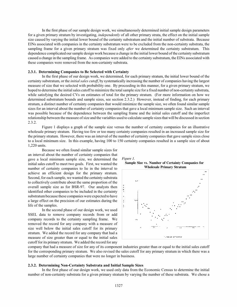
Figure 1. Sample Size vs. Number of Certainty Companies for
Wholesale Primary Stratum
In the first phase of our sample design work, we simultaneously determined initial sample design parametersfor a given primary stratum by investigating, independently of all other primary strata, the effect on the initial samplesize caused by varying the initial lower bound of the certainty substratum and the initial number of substrata. BecauseEINs associated with companies in the certainty substratum were to be excluded from the non-certainty substrata, thesampling frame for a given primary stratum was fixed only after we determined the certainty substratum. Thisdependence complicated our sample design work because a change in the initial lower bound of the certainty substratumcaused a change in the sampling frame. As companies were added to the certainty substratum, the EINs associated withthese companies were removed from the non-certainty substrata.
2.3.1. Determining Companies to Be Selected with CertaintyIn the first phase of our design work, we determined, for each primary stratum, the initial lower bound of the
certainty substratum, or the initial sales cutoff, by systematically increasing the number of companies having the largestmeasure of size that we selected with probability one. By proceeding in this manner, for a given primary stratum, wehoped to determine the initial sales cutoff to minimize the total sample size for a fixed number of non-certainty substrata,while satisfying the desired CVs on estimates of total for the primary stratum. (For more information on how wedetermined substratum bounds and sample sizes, see section 2.3.2.) However, instead of finding, for each primarystratum, a distinct number of certainty companies that would minimize the sample size, we often found similar samplesizes for an interval about the number of certainty companies that gave a local minimum sample size. Such an intervalwas possible because of the dependence between the sampling frame and the initial sales cutoff and the imperfectrelationship between the measure of size and the variables used to calculate sample sizes that will be discussed in section2.3.2.
Figure 1 displays a graph of the sample size versus the number of certainty companies for an illustrativewholesale primary stratum. Having too few or too many certainty companies resulted in an increased sample size forthe primary stratum. However, there was an interval of the number of certainty companies that gave sample sizes closeto a local minimum size. In this example, having 100 to 150 certainty companies resulted in a sample size of about1,220 units.
Because we often found similar sample sizes foran interval about the number of certainty companies thatgave a local minimum sample size, we determined theinitial sales cutoff to meet two goals. First, we wanted thenumber of certainty companies to lie in the interval toachieve an efficient design for the primary stratum.Second, for each sample, we wanted the certainty substratato collectively contribute about the same proportion of theoverall sample size as for BSR-97. Our analysts thenidentified other companies to be included in the certaintysubstratum because these companies were expected to havea large effect on the precision of our estimates during thelife of the samples.
In the second phase of our design work, we usedSSEL data to remove company records from or addcompany records to the certainty sampling frame. Weremoved the record for any company with a measure ofsize well below the initial sales cutoff for its primarystratum. We added the record for any company that had ameasure of size greater than or equal to the initial salescutoff for its primary stratum. We added the record for anycompany that had a measure of size for any of its component industries greater than or equal to the initial sales cutofffor the corresponding primary stratum. We also revised the sales cutoff for any primary stratum in which there was alarge number of certainty companies that were no longer in business.
2.3.2. Determining Non-Certainty Substrata and Initial Sample SizesIn the first phase of our design work, we used only data from the Economic Census to determine the initial
number of non-certainty substrata for a given primary stratum by varying the number of these substrata. We chose a

1328
design that resulted in the smallest sample size required to satisfy the desired CVs on estimates of total for the primarystratum, while guaranteeing that no EIN from a non-certainty substratum was selected with probability one and no morethan a few non-certainty substrata had sample sizes under Neyman (optimal) allocation that were less than three units.If these conditions were not met, we changed the design to make it more efficient. Specifically, if some EINs from non-certainty substrata were selected with probability one, we lowered the initial sales cutoff. Also, if the sample sizes formore than three non-certainty substrata were less than three, we reduced the number of non-certainty substrata fromtwelve in increments of three substrata until this did not occur.
We set non-certainty substratum bounds using a modification to the Dalenius-Hodges cumulative rule infwhich we used the cumulative 0.4th power of the frequency distribution of the measure of size to set substratum bounds.We used the cumulative 0.4th power of the frequency distribution because we found this gave slightly smaller samplesizes than the ones based on either the square root or cube root.
To compensate for using annual data to design samples that will be used to create more variable monthlyestimates and to control the influence of a given sampling unit on our estimates, we increased initial sample sizes.Controlling the influence of a given sampling unit on our estimates is important because the characteristics of a samplingunit can change during the life of the samples and affect the precision of our estimates.
We increased our initial sample sizes in two ways. First, for each non-certainty substratum, we includedminimum sample size and minimum sampling rate restrictions. For each non-certainty substratum, we required thesample size to be at least three units and to result in a sampling rate greater than or equal to a minimum sampling ratethat depended on the particular trade area. Second, instead of computing sample sizes for estimating total measure ofsize, we computed sample sizes for estimating a total that was assumed to be highly correlated with total measure of size.
For the retail, wholesale, and service samples, we computed sample sizes for estimating the total of a payroll-based regression estimate of annual sales at the time of sampling frame construction. We used a regression method(McNeil 1977) that modeled the relationship between payroll and sales establishment data from the 1997 EconomicCensus at the six-digit NAICS level. For each sampling unit, we then aggregated establishment-level regressionestimates that were formed by multiplying the appropriate regression coefficient by the most recent annual payrollestimate available. For the wholesale sample, we also computed sample sizes for estimating total 1997 end-of-yearinventories based on data from the 1997 Economic Census. We then determined the initial sample size for a givenwholesale primary stratum to be the maximum of the two sample sizes computed.
In the second phase of our design work, we used SSEL data to determine final substratum bounds and samplesizes. Before determining these sample design parameters, we removed from the non-certainty sampling frame therecords for all EINs associated with companies on the certainty sampling frame and reduced the number of substratafor primary strata in which the sample design was grossly inefficient.
2.4. Computing Final Sample Sizes to Meet Multiple Coefficient of Variation ConstraintsAs discussed in section 2.2, among our sample design requirements were desired CVs on estimates of total at
NAICS-based publication levels. In general, these publication levels exhibited a hierarchical, or nested, structure thatwas based on the six-digit coding system employed by NAICS. For example, estimates were desired for the followingretail industries: New Car Dealers (NAICS 441110), Automobile Dealers (NAICS 4411), Motor Vehicle and PartsDealers (NAICS 441), and Retail Trade (NAICS 44-45).
We computed final sample sizes required to satisfy desired CVs on estimates of total at publication levels usinga new method. First, for each publication level, we determined the sample sizes required to satisfy the desired CVs onestimates of total using the variables described in section 2.3.2. We then calculated the corresponding sample sizesunder Neyman (optimal) allocation for each non-certainty substratum that contributed to the publication level. Finally,for each non-certainty substratum, we took as the final sample size the maximum of the sample sizes for the substratumcomputed. For the wholesale sample, sample sizes were generally larger for estimating total 1997 end-of-yearinventories than for estimating total annual sales using the payroll-based estimate.
1329
Figure 2.
Table 1 illustrates the method used to determine samplesizes to meet multiple CV constraints on total annual salesestimates for one of the non-certainty substrata of the New CarDealers (NAICS 441110) retail primary stratum. In this table,the NAICS code for a given row is contained, or nested, in theNAICS codes of all rows that follow. Because the maximumsample size required for this substratum was 46.37, a sample ofsize 47 guaranteed that all CV constraints affecting thissubstratum were satisfied.
As discussed in section 2.3.2, we included minimumsample size and minimum sampling rate restrictions. Forsubstrata whose sample sizes were not determined from theserestrictions, we recomputed sample sizes afterremoving the contribution of the restricted substratafrom desired variances at publication levels. We didthis because, in the substrata that we “froze” by settingtheir sample sizes based on the restrictions, we selecteda larger sample than Neyman allocation required tomeet the desired CV constraints. Therefore, smallersample sizes were possible for substrata whose samplesizes were not determined from the restrictions.
An example of the sample size reductionsfound after “freezing” the sample sizes for restrictedsubstrata and recomputing sample sizes for all othersubstrata is shown in Table 2. In this example, thesample size for substratum 1 was increased from 6 to10 to satisfy the minimum sampling rate restriction.After recomputing sample sizes for substrata 2 through6 by removing the contribution of substratum 1 to thedesired variances at publication levels, the sample sizes for substrata 3 and 5 were each reduced by one.
2.5. Sample Design Changes Due to EIN OutliersIn the second phase of our design work, we discovered a relatively small number of EIN records on the final
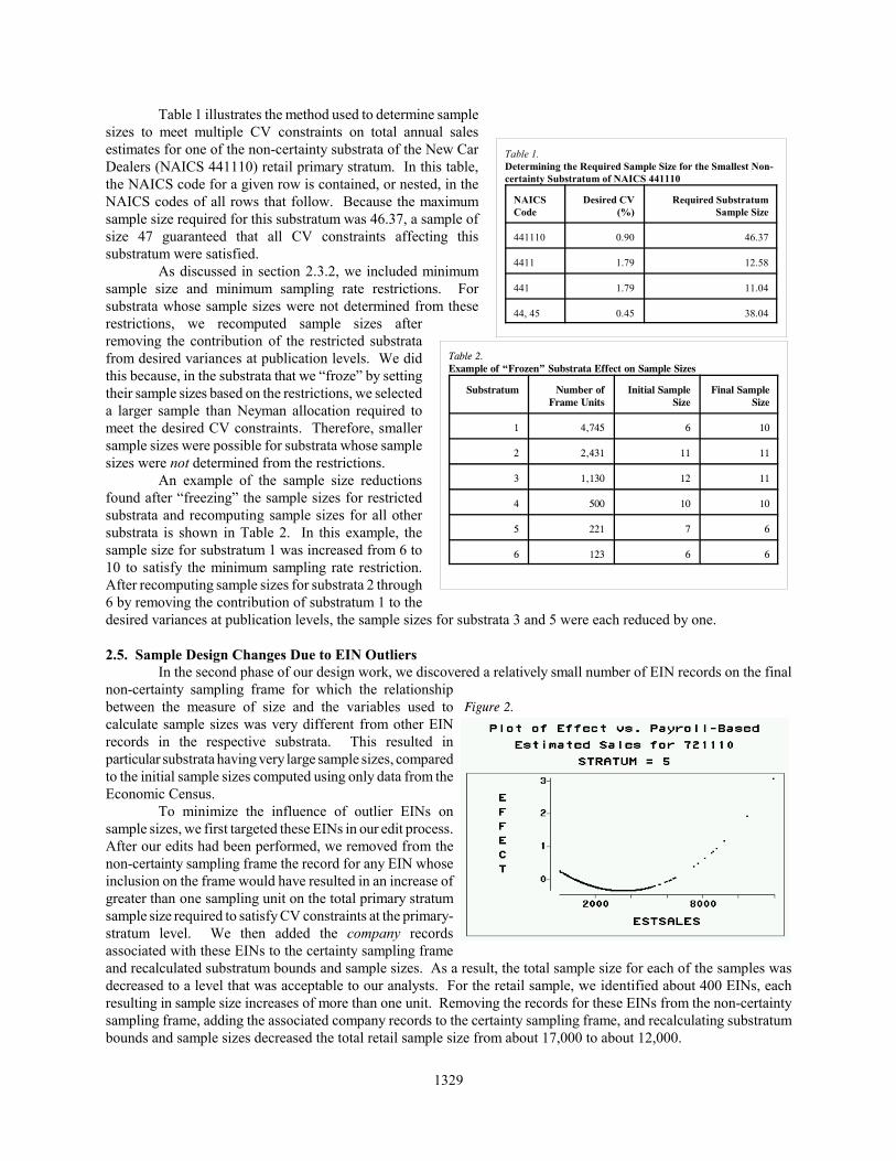
non-certainty sampling frame for which the relationshipbetween the measure of size and the variables used tocalculate sample sizes was very different from other EINrecords in the respective substrata. This resulted inparticular substrata having very large sample sizes, comparedto the initial sample sizes computed using only data from theEconomic Census.
To minimize the influence of outlier EINs onsample sizes, we first targeted these EINs in our edit process.After our edits had been performed, we removed from thenon-certainty sampling frame the record for any EIN whoseinclusion on the frame would have resulted in an increase ofgreater than one sampling unit on the total primary stratumsample size required to satisfy CV constraints at the primary-stratum level. We then added the company recordsassociated with these EINs to the certainty sampling frameand recalculated substratum bounds and sample sizes. As a result, the total sample size for each of the samples wasdecreased to a level that was acceptable to our analysts. For the retail sample, we identified about 400 EINs, eachresulting in sample size increases of more than one unit. Removing the records for these EINs from the non-certaintysampling frame, adding the associated company records to the certainty sampling frame, and recalculating substratumbounds and sample sizes decreased the total retail sample size from about 17,000 to about 12,000.
Table 1.Determining the Required Sample Size for the Smallest Non-certainty Substratum of NAICS 441110
NAICSCode
Desired CV(%)
Required SubstratumSample Size
441110 0.90 46.37
4411 1.79 12.58
441 1.79 11.04
44, 45 0.45 38.04
Table 2.Example of “Frozen” Substrata Effect on Sample Sizes
Substratum Number ofFrame Units
Initial SampleSize
Final SampleSize
1 4,745 6 10
2 2,431 11 11
3 1,130 12 11
4 500 10 10
5 221 7 6
6 123 6 6

1330
Figure 2 displays a graph of the primary stratum sample size increase (denoted by EFFECT) versus the variableused to compute sample sizes (denoted by ESTSALES) for EINs in an illustrative non-certainty substratum. In thisfigure, there were four EINs that resulted in an increase of greater than one unit on the primary stratum sample size.
2.6. Limiting Overlap of BSR-97 and BSR-2K SamplesTo distribute respondent burden among the smaller sampling units, we minimized overlap of non-certainty EINs
selected in both BSR-97 and BSR-2K by removing EINs from the final sampling frame for BSR-2K prior to sampleselection. Limiting overlap is especially important for EINs selected for our monthly surveys because we askrespondents to report monthly for the duration of the samples.
Application of the overlap minimization, or controlled non-selection, was subject to constraints on theprocedure’s contributions to the biases and variances of our estimates. We chose to include in the controlled non-selection only substrata for which the relative biases of our estimates of total at the primary-stratum level were less than0.5% in absolute value and for which the corresponding variances changed by less than 20%. We believed the biasrestriction would produce negligible biases in estimates of month-to-month change. Also, we included in the controllednon-selection only substrata with a sufficient number of EINs remaining after controlled non-selection to select a sampleof a pre-determined size as detailed in section 2.4.
Because future information on BSR-2K sampling units was, of course, not available to us, we based ourconstraints on the biases and variances of hypothetical estimates of total using the measure of size and the variables usedto calculate sample sizes described in section 2.3.2. By limiting the contributions, due to controlled non-selection, tothe biases and variances of these hypothetical estimates, we hoped to control the corresponding contributions to thebiases and variances of our future estimates.
3. FUTURE RESEARCHWe will continue to investigate improvements to the sample design methods used for our sample revisions.
This research will assist us in the planning of future sample revisions.We plan to investigate the methods used in BSR-2K to determine initial sample design parameters for each
primary stratum. We would like to automate these methods to reduce the time required to determine these parametersand to prevent variations in sample design caused by different designers. To accomplish this task, we must determineacceptable bounds for the number of substrata having sample sizes under Neyman allocation that are less than theminimum sample size, the increased sample size associated with lowering the initial sales cutoff below the cutoff thatgives a local minimum sample size, and the percent contribution of the certainty substratum to the total sample size.
We should revisit our method of sample size determination to meet multiple reliability constraints. We shouldconsider using the measure of size to allocate a given sample size to the substrata. Another adjustment to the currentmethod of sample size determination might be to determine the sample size for a given publication level by taking intoaccount the potentially larger sample sizes required for more detailed publication levels nested within the publicationlevel. This small adjustment would expand our method of “freezing” substrata and recomputing sample sizes that wasdiscussed in section 2.4.
4. REFERENCESCochran, W. (1977), Sampling Techniques, New York: John Wiley & Sons.Isaki, C., K. Wolter, T. Sturdevant, N. Monsour, and M. Trager (1976), “Sample Redesign of the Census Bureau’s Monthly Business Surveys,” Proceedings of the Business and Economic Statistics Section, American Statistical Association, pp. 90-98.McNeil, D. (1977), Interactive Data Analysis: A Practical Primer, New York: John Wiley & Sons.Sweet, E. and R. Sigman (1995), User Guide for the Generalized SAS Univariate Stratification Program, Technical Report #ESM-9504, Washington, DC: Bureau of the Census.U.S. Census Bureau (1999), Current Business Reports, Series BR/98-A, Annual Benchmark Report for Retail Trade: January 1989 to December 1998, Washington, DC.U.S. Office of Management and Budget (1998), North American Industry Classification System: United States, 1997, Lanham, MD: Bernan Press.

1331
ON REDESIGNING CANADA’S SERVICE INDUSTRIES SURVEYS
Serge Legault, Joseph Kresovic 1
In early 1997, Service Industries Division began a complete redesign of its annual survey program and made the transitionto probability sampling. The annual surveys estimate total revenue, expenses, value added and detailed characteristics. Thetimetable and operational constraints under which such a redesign took place made it necessary to accomplish several tasksand develop a survey infrastructure within a short period of time while maintaining an acceptable level of quality. Thispaper outlines the survey design and infrastructure, provides an assessment of the methodology and processes used anddiscusses the impact on the personnel involved.
KEY WORDS: Infrastructure, enhancement, evaluation, accuracy, attitudes towards change
1- INTRODUCTION
In early 1997, the Service Industries Division (SID) of Statistics Canada began a complete redesign of its annualsurvey program and made the transition to probability sampling. Starting from a small services program which hadsome gaps in coverage and some quality problems, a strategy to provide better information on the very largeCanadian services sector was developed. Several new surveys were added to the existing survey program that nowcomprise more than twenty surveys covering subjects such as publishing industries; rental and leasing services;professional, scientific, technical and business services; arts, entertainment and recreation; traveller accommodationand personal services. This changing environment was shaped by the Project to Improve Provincial EconomicStatistics (PIPES) and the new approach to the business statistics program that it brought, namely the UnifiedEnterprise Survey (UES).
The goal of the PIPES is to improve provincial economic statistics so that sales tax revenues can be fairly dividedbetween the federal government and the participating provincial governments. The Unified Enterprise Survey willgradually replace Statistics Canada’s individual annual business surveys over the next several years. However,because of the scale and magnitude of this initiative, it has to be implemented progressively. In the meantime,Service Industries Division has identified several industries not currently in-scope to the UES and proceeded toinclude them as part of their in-division survey program which is the object of this paper. The Service Industriessurvey program has rapidly become a reliable statistical program that now rests on solid foundations. To betterillustrate this reality, a brief overview of the former SID survey program is in order.
"Prior to 1996, virtually none of the surveys were scientifically based nor did they originate from thecentral business register (BR), but rather from a tax-based universe maintained separately andsupplemented with data from small panels of firms maintained within the division. Thus, we did not benefitfrom BR updates of births, deaths and classification changes. Survey processing was often unsophisticatedmatching the division's resource constraints. The sample sizes were very small – on average 5%. There wasa continual and often losing struggle to improve timeliness. (McMechan , et al 1999)"
Furthermore SID could not effectively assess the quality of the estimates being released since it was impossible tocompute sampling variances. These surveys excluded units with revenue less than $250,000 so only basic financialdata from the tax records were available for these firms – no extensive financial data, characteristics, inputs, outputs,geography, trade, types of services or client base. This was not a trivial shortcoming, given the industrial structure ofservices in which many industries are primarily composed of small firms, and given the evidence that smaller firmsin the services sector follow different market strategies than large firms. There were many challenges to overcome,not only technical, but also from an individual standpoint. Such important changes in the work environment maytrigger apprehensions among those most affected by the change. This will be discussed in more detail in section 3.
1 Serge Legault, Business Survey Methods Division, Statistics Canada, Ottawa, Ontario, Canada, K1A 0T6 Joseph Kresovic, Service Industries Division, Statistics Canada, Ottawa, Ontario, Canada, K1A 0T6

1332
2- THE REDESIGNED SURVEY
2.1 Redesign ConsiderationsSID is now entering its fourth year since it made the transition to the new survey program. The methodology andapproaches described here represent the current evolution of the program. Even though many improvements andadjustments were made to the original approach implemented for reference year 1996, the strategy and objectives ofthe program have basically remained unchanged.The following points were identified as key elements of the new strategy:
i) use the centrally maintained Business Register for the creation of the sampling frame and collection entitiesbased on the North American Industry Classification System (NAICS);
ii) adopt the statistical establishment as the sampling unit instead of the legal entity (Cuthill, 1990);iii) increase the coverage to include firms under $250,000 while minimizing response burden using
administrative information for very small firms;iv) use statistically sound methods for sampling, edit and imputation, data allocation and estimation;v) favour the use of easily re-usable generalized systems;vi) make available to users indicators of the quality of data being disseminated (in accordance with Statistics
Canada policy on informing users on Data Quality and Methodology);vii) provide reliable estimates of economic output, characteristics and components of value-added, both
nationally as well as provincially; andviii) try to achieve a 'soft transition’ to UES i.e. adopt practices and concepts used for the UES surveys.
In addition to the challenges of the statistical program, there were considerable managerial challenges facing SID.Entering this period of rapid growth and change, operational and systems infrastructures had to be developed alongwith effective internal communications and information-sharing processes. All of this happened as the work and theoutput were becoming more complex and multi-streamed.
2.2 Sampling Frame and Survey Population
The current annual Service Industries survey program consists of 89 NAICS6 industries grouped into 12 differentsurvey vehicles: Automotive Equipment Rental & Leasing; Consumer Goods Rental; Commercial & IndustrialMachinery; Personal Services; Arts Entertainment & Recreation; Travel Arrangements; Architects; TravellerAccommodation; Advertising; Engineering; On-line Information Providers and Computer Services. Even thoughthe basic objective is to produce estimates for the whole industry ---incorporated and unincorporated--- the portionof the population eligible for sampling (survey population) was defined as all incorporated establishments withrevenue above $50,000 for the reference year. Some exceptional unincorporated and government business unitswere also added to direct data collection if their contribution was deemed too significant to be ignored or if theywere part of a multi-establishment enterprise.
The main motivation for excluding some units from direct data collection was to achieve major reductions in theresponse burden of very small businesses at the expense of introducing a small amount of uncertainty in the finalestimates. Businesses below the exclusion thresholds are still part of the universe but their contribution is accountedfor in the final estimates through the use of administrative taxation records (section 2.7 will discuss the approachchosen to account for this portion). Using these exclusion criteria, the survey population of the SID programrepresents approximately 45% of the target population in terms of number of establishments but more than 90% interms of revenue.
The Business Register is the primary source for the identification and selection of units for sampling purposes. Assuch, it is extremely important that this file reflects the most up-to-date information from SID work andunderstanding of the industry. Thus, several activities were undertaken in order to enhance the list frame prior tosampling. The emphasis was on validating and correcting the industry coding and the revenue used for stratification.
2.3 Stratification and Sample Allocation
The Service Industries survey program is using a stratified one-phase sampling design. Different methods forperforming stratification and sample allocation have been used since the inception of the program. The current

1333
approach utilizes Statistics Canada's Generalized Sampling System (GSAM) which proved to be more efficient andeasier to set up than the customized approaches previously used. Moreover, GSAM is a SAS based application thatcan easily run on a microcomputer. The survey population was stratified by survey, province, NAICS level and size(revenue). Stratification by province was necessary in order to comply with one of the objectives of the program,that is, to provide reliable estimates at the provincial level. NAICS level is the pre-determined industrial level atwhich Services Division wished to produce reliable estimates within each of the 12 surveys. This varies from onesurvey to another but NAICS5 was the level most frequently used. The combination of survey, province and NAICSlevel defined the cells which were in turn stratified based on revenue. As a result, each cell was comprised of 4strata, that is, one take-all, two take-somes and one additional stratum consisting of multi-establishment firms.
The stratum boundaries were determined using the Dalenius-Hodges cumulative root f method. This method isderived from the formula for the variance of the estimated mean by assuming optimum allocation under stratifiedsimple random sampling. If �(y) represents the frequency distribution of variable y, then the new boundaries aredetermined by creating equal intervals on the cumulative square root f scale. The GSAM option of minimum costwas used to determine a sample allocation that minimized the total sample size subject to constraints on thecoefficients of variation (CV's) for the target variable (revenue). The target CV's were set at 5.5% per cell and theminimum sample size in each stratum was set at 5. Furthermore, cells with less than 15 units were subject tocomplete enumeration, maximum sampling weights were set at 40, and finally, inflation adjustments to the requiredsample size were made in order to compensate for non-response and deaths. The outcome of this procedure for the1999 Reference Year design was a sample of 18,239 establishments.
2.4 Data Collection
Although sampling is performed at the establishment level, the collection entity (CE) is a grouping of establishmentswithin a statistical company. It is assumed that the statistical company can report for all its establishments inindustries in-scope to the survey. Hence, this approach enables SID to further reduce the response burden on largefirms and reduce its survey costs at the same time. Only the Traveller Accommodation survey took exception to thisrule because it is a survey that covers a broad range of business activities that can only be collected at theestablishment level. For reference year 1999, the number of units to contact dropped to 14,683 which represents a20% reduction from the original sample size.
2.5 Pre-Grooming and Edit & Imputation
Several checks and corrections are performed during the Pre-grooming step. Survey response codes, provincialdistribution and outlier records are reviewed and, if necessary, corrections are made. The review process isfacilitated by the production of a series of standard reports. All corrections and updates are made using a customizedcorrection facility that provides easy access to the data.
Imputation is performed using a "nearest neighbour" procedure (donor imputation). Several reports are createdduring this process in order to assess and monitor the quality. They include summary tables indicating the conditionof the records coming out of the edit and imputation process, edit failure rates and the number of times a donor wasused. In addition to the donor imputation approach, imputation can also be done based on cold-deck procedures suchas historical imputation.
2.6 Data Allocation
Provincial data allocation is the process by which surveyed records, which are at the company level, are broken upinto provinces. This is done to enable estimation at the province level, a requirement of the survey program. As wediscussed in section 2.4, the questionnaire data represent all in-scope establishments within a statistical company forall of Canada. The goal of provincial data allocation is to disaggregate the questionnaire level data to respect theprovincial level of geography.
The goal of distributing the questionnaire level data to each province is achieved by using the data in a questionnairemodule that contains the provincial distribution grid. This questionnaire module includes the provincial distributionof the following data: number of locations, operating revenue, salaries, wages & benefits and number of employees(on a few surveys only).

1334
In general, the data in this table are used to develop ratios for each province which are then used in conjunction withthe questionnaire level data to produce the provincial based data. When this questionnaire module is not completedby the respondent, or is not edited by subject matter, then the provincial distribution grid is completed at the end ofthe E&I stage using information from the original sampling frame. The end result of this process is one record foreach province in which operations of a collection entity (CE) exist. Each of these records contains data related toone province only and each has the same sampling weight as the original entity. If a CE has operations in only oneprovince, then the resulting record's data equals the CE record's data.
2.7 Estimation
One of the main objectives of the Service Industries survey program is to reduce operating costs and respondentburden. This can be partially accomplished by utilizing data from administrative sources as proxy data for the firmsbelow the $50,000 threshold. Administrative information comes mainly from taxation sources and includes basicinformation such as revenue, salaries, wages and depreciation. SID conducted an evaluation of the administrativeinformation by comparing it with survey data for a sample of respondents. The conclusion was that taxation datarepresents a reasonable proxy for survey data but provides an inferior level of detail than its survey counterpart.Therefore, SID decided to produce "complete" estimates (i.e. survey + non-survey population) for basic variablessuch as total revenue, value-added components and total expenses. Detailed characteristics such as revenue by typeof service and detailed expense items are only produced for the survey population using the classic Horvitz-Thompson expansion estimator (Särndal et al., 1992) and are calculated using the Generalized Estimation System.
3. IMPACT OF CHANGE, ATTITUDES TOWARDS CHANGE
The magnitude of the survey redesign and the number of people affected by it were also issues to contend with. Assurvey designers, it was important to understand the factors that drive change and how people react to them. It ishuman nature to resist change and this holds true in the workplace especially when the security and identity that afamiliar job provides is subject to substantial changes. In addition, since the expansion of the work was more rapidthan the expansion of resources or staff, the added workload was also an important factor. For this reason manyempowerment principles were implemented. The survey tools were designed to provide survey managers with someflexibility in the manner in which they wanted to proceed but within some established guidelines. In other words, theintent was to create a working climate that enabled everyone to demonstrate their full potential. Given that theoverall objectives are clearly understood, this approach will encourage staff to be creative, show initiative andaccept more responsibilities because more decision power was given to them.
Throughout the redesign process, many training and information sessions were held in order to ensure that everyoneaffected by the change understood the new methodologies and procedures being implemented and draw out people'sconcerns about the change and discuss constructive ways to address them. Because the systems and interfaces weredeveloped using an evolutionary prototyping methodology, future users (i.e. survey analysts and support staff) hadan opportunity to interact with the prototype and provide direct feedback to the designers. The benefits of such adevelopment approach is that difficulties with the systems can be quickly revealed and if required, furtherexplanation of the underlying methodology and functionality can be provided. It was sometimes necessary to resortto alternative solutions and approaches not only based on time and resources but also taking into consideration thelevel of complexity being introduced. Overly complex survey functions are less conducive to understanding and thusnot likely to be fully accepted by all.
Review tools and manual interventions were designed to allow the analysts to perform verification and changes tothe data at different stages of survey processing. The amount of manual intervention was kept to a manageablelevel and mostly focused on extraordinary cases. Such a process is not only a safety net but also proved to be aneffective confidence builder. The analysts could, for example, review the outcome of imputation and find out thatthe actions taken were satisfactory the majority of the time. After a while, second thoughts about the methodologyand the processes were slowly dispelled.
4. QUALITY EVALUATION
Even though there is no standard definition of quality for official statistics (Statistics Canada, 1998), the quality ofdata must be defined and assured in the context of “fitness for use”. This in turn can be summarized as relevance,

1335
timeliness, accessibility, interpretability, coherence and accuracy. These elements of quality are overlapping andinterrelated—often in a confounding manner. Furthermore, there is no single measure of accuracy nor is there aneffective statistical model for bringing together all of the characteristics of quality into a single indicator. Therefore,each element of quality will be briefly assessed .
Relevance and Timeliness: The survey program was instituted in order to fill major data gap in the services sectorof the Canadian economy. Industries not covered in the past were added to the program and existing surveys wereredesigned using modern and sound methods. Even though all important deadlines for the release of the final resultswere met, the time required to process the survey took longer than anticipated. This is mostly due to the fact that thesurvey infrastructures and processes were developed in a very short time. SID made sure that timeliness would notbe achieved at the expense of reliability. Improvements in the timeliness are expected because the program has nowreached some stability and requires less development.
Accessibility and Interpretability: Each release is accompanied with a statement informing users on the data qualityand a description of the methodology.
Consistency: Internally, the consistency of the Service Industries survey program is indisputable since the concepts,definitions and approaches used do not vary from one survey to another. In addition, one of the objectives of thesurvey redesign was to achieve a 'soft transition’ to UES i.e. adopt practices and concepts used for the large scaleUES survey. This goal was attained and SID considers that the "in-division" products can be logically connectedwith other statistical survey programs.
Accuracy: In order to assess the degree to which the survey results correctly measure the statistical activity it wasdesigned to estimate, several indirect measurements quantifying the major elements of quality were produced.
i) Sampling errors
A common approach to assess the quality of a survey is to look at the error caused by observing a sample instead ofthe whole population i.e. the sampling error. The results for the revenue variable from the RY97 survey portionwere used to conduct this evaluation. Globally, the computed CV's are below 10% for the vast majority of the pre-specified NAICS levels which is considered to be very reliable. In order to obtain a more relevant indication of theefficiency of the sampling design, the observed CV's were compared with the target CV's. The results can be foundin table 1.
Table 1: Difference between the observed and target CV's (%)for the revenue variable in RY97
Distribution by range of CV difference (%) Percent(Observed CV - Target CV) <= 0 670 < (Observed CV - Target CV) <= 5 165 < (Observed CV - Target CV) <= 10 5(Observed CV - Target CV) >10 12
Table 1. shows that two-thirds of the pre-specified levels at which CV's were controlled have achieved equal orbetter results than predicted. On the other hand, the large observed CV's were found to be restricted to a fewindustries where high out of scope and/or poor response rates were observed during collection. This points out toframe deficiencies rather than inefficiency of the sampling design.
ii) Non-sampling errors
The results in Table 2. are an indication that the program is improving and reaching some stability. The decreasingpercentage of out of scope(O/S) and out of business (O/B) units demonstrate that the frame enhancement activitycombined with the survey feedback are resulting in a more up-to-date list frame. On the other hand, the unable tocontact and refusal rates seemed to have stabilized at very acceptable levels, that is, 20% and 1% respectively. Theunit response rate, calculated by excluding the O/S and O/B, is also climbing steadily at a rate of 3% per year from68% in RY96 to 74% in RY98. Finally, the weighted unit response rates by revenue, a refinement of unit response

1336
rates (Federal Committee on Statistical Methodology, 1988) but only available for RY97, resulted in a response rateof 82%. This means that data is being collected at a higher rate for the larger firms in the sample.
Table 2: Outcome of data collection for RY96, RY97 & RY98 for all surveys
RY96 RY97 RY98Fully or partially completed 41% 52% 59%Out of scope, out of business 40% 27% 20%Unable to contact 17% 20% 20%Refusal 2% 1% 1%
The impact of imputation was also assessed (table 3). Results for the revenue variables show that across all RY97surveys, 25.1% of the units were imputed for this field but the contribution of these units to the final revenueestimates was 20.6%. This indicates that smaller units tend to require more imputation than larger ones.
Table 3: Impact of imputation on final estimates for selected variables in RY97Variable % of records imputed % of estimate from imputationRevenue 25.1 20.6Expenses 25.6 25.1Salaries & Wages 26.4 27.1Employment 27.5 25.1
5. CONCLUDING REMARKS
The early re-development years of the Service Industries survey program have been in many ways a fast-trackexercise. Even though time and resources were often scarce, the objectives established at the beginning of theprocess have been successfully met. Now that the program has reached some maturity and stability in terms ofdesign and processing, it provides us with the opportunity to further assess its quality and consider possibleimprovements. Frame related issues remain the most important areas for continued improvements. A proposal for ayear long review of the list frame by the analysts in order to assess updates, classification and size variables is beingput forth. Streamlining of the survey feedback process and updating of the contact information will also continue tobe a priority. In the more technical area, different ways of accounting for the excluded portion of the population andthe possibility of using post-stratification to improve the quality of the estimates will be investigated. Thedetermination of an exclusion threshold using an approach that takes into account the revenue distribution withineach survey will also be examined. Finally, priority codes during collection will be instituted this year in order tooptimize and focus follow-up activities where it is most needed.
REFERENCES
Cuthill, I (1990), "The Statistics Canada Business Register", Proceedings of the 1989 Annual Research Conference of the U.S. Bureau of the Census
Federal Committee on Statistical Methodology (1988), Measurement of Quality in Establishments Surveys,Statistical Policy Paper 15, Washington, DC.
Särndal, C., Swensson, B. and Wretman, J. (1992), Model Assisted Survey Sampling, New York: Springer-Verlag
McMechan, J, (1999), Service Industries Programme Report, Ottawa: Internal Report
Statistics Canada Methodology Branch(1998), Statistics Canada Quality Guidelines. Catalogue 12-539-XIE

1337
THE REDESIGN OF THE CANADIAN QUARTERLY FINANCIAL SURVEY
Claude Nadeau, Margot Greenberg, Patricia Whitridge and Danielle Lalande, Statistics CanadaClaude Nadeau, Statistics Canada, R.H. Coats 11-F, Ottawa ON K1A 0T6, Canada, [email protected]
ABSTRACT
Statistics Canada’s quarterly and annual financial survey programs publish business financial statistics covering virtually all businesssectors. The Quarterly Financial Survey (QFS), which gathers information from the largest enterprises, has been the subject of amajor redesign effective in 1999. First of all, after a lengthy reconciliation process, a new sample frame (Statistics Canada’s BusinessRegister) was adopted. The entire sample design and processing methods were overhauled including the industrial classification,stratification methodology, model used to estimate for small enterprises, and finally the estimation methods. Additional changes weremade to the collection edits and the imputation methodology.
We discuss how and why the numerous changes were implemented. Naturally, the effects these changes have on the estimates needto be assessed. We discuss how this assessment was performed and we present the main findings. Fine-tuning done for referenceyear 2000 as well as more important modifications planned for the 2001 reference year are highlighted.
Key Words: Frame, Imputation, Industrial Classification, Coefficient of Variation, Stratification, Results Assessments
1. BACKGROUND
The Quarterly Financial Survey (QFS) yields information about investment activity, financing patterns, rates of return andother financial performance ratios, by industry, that are used by government departments, private industry and the academiccommunity. The target population is essentially all (non-government) enterprises with operations in Canada. The reallysmall enterprises (revenue < $30,000 and assets < $50,000) are excluded from the target population. The quarterly samplecovers all of the largest enterprises (Take-All), some of the medium-sized enterprises (Take-Some) and none of the smallenterprises (Take-None) although a model provides estimates for the latter in order to arrive at quarterly estimates for theentire population. This sampling strategy provided reasonably good estimates for a very large target population (close to 1million enterprises) with a relatively small sample that has slightly less than 6,000 units (the sample size we can afford).Prior to 1999, these statistics were published by industry groups based on the Canadian Standard Industrial Classificationsystem – Company level (SIC-C 1980).
A number of major changes (listed in further details in the next section) took place in 1999 such as the change of frame, thetransition from SIC-C to NAICS (North American Industry Classification System) industrial classification, expansion of thesurvey to meet the requirements for the Unified Enterprise Survey (survey pulling together existing surveys) and the draw ofthe new NAICS based sample as well as changes to the processing of the data. This impacted on all key aspects of thesurvey and more or less involved redesigning the survey in its entirety.
Before proceeding with the dissemination of the new estimates we felt it necessary to assess and validate the estimates bylooking into various factors which we feel are key in determining the overall quality of the estimates produced by the newsurvey and processing system. In Section 2 we present the nature and motivation of the changes made in 1999. In Section3 we compare the results obtained with the new methodology to those of the old system. We assess, in Section 4, thequality of the survey estimates. Section 5 presents some adjustments that we have made in 2000. Concluding remarks andfuture projects are found in Section 6.
2. CHANGES TO THE SURVEY METHODOLOGY
The following changes to the methodology were implemented for reference year 1999.
1) New frame: Prior to the redesign, the division in charge of the survey maintained its own frame (called QASF). It wasdecided that, from 1999 onwards, a new survey frame (Survey Universe File or SUF) would be extracted from the StatisticsCanada Business Register (BR) each quarter. The BR is Statistics Canada’s central register of all businesses in Canada. Itdescribes the businesses at four levels: enterprise, company, establishment and location. The Quarterly Financial Surveyuses the enterprise level. The SUF contains about 900,000 enterprises while the former frame (QASF) had about 1,000,000,

1338
but it contained many dead enterprises. In addition, there is a Supplemental file that contains “correct” values of assets andrevenue (usually from the QASF) for a sub-set of units for which the BR values are believed to be incorrect. In those cases,the values of the Supplemental file are used.
2) Stratification: The redesigned survey uses the NAICS Canada 1997 classification system. By aggregating NAICScodes, we formed 157 industry groups which were similar to the old SIC-C groupings. We call this the NAICS157“classification system”. The population is now stratified by industry group (NAICS157), country of control (Canada, USA,other) and size (large, medium or small). The size is based on assets and revenue information on the BR and determineswhether an enterprise is Take-All (sampled with certainty), Take-Some (sampled with some probability) or Take-None (noteligible to be sampled). Note that before the redesign, enterprises with country of control other than Canada that were notTake-None size were sampled with certainty, i.e. there was no Take-Some strata in this case (only Take-None or Take-All).
The general rule for a unit to be in the Take-None stratum is that it must have assets<$10M and revenue<$25M (or <$15Min some industries). Those boundaries are lower or equal to those used in the old design, thus leading to a larger surveyedpopulation and therefore a smaller Take-None population in some industries. Since the contribution of the Take-None to thetotal estimate (for given industry and country of control) comes from a model, we want to keep this small and try to have thebulk of the total estimate coming from the surveyed portion (Take-All/Take-Some). The number of enterprises in thesurveyed portion went from approximately 10,000 units to about 17,000. The Take-None portion now accounts for 11% oftotal assets and 26% of revenue. We had similar percentages before the redesign. However those numbers vary a lot byindustries. In half of the 157 industry groups, the Take-None accounts for less than 10% of the estimate for that industry.However there are industries where the Take-None still represents a very significant portion of the estimate. Thoseindustries, such as agriculture, contain mostly small enterprises (which are not sampled) which represent a high proportionof the overall industry. Lowering the Take-None threshold to bring down the Take-None contribution would inflatedrastically the number of units in the Take-Some and lead to a sample size that we cannot afford (if we want design weightsno larger than 10; see below).
Prior to the redesign, the Take-All/Take-Some thresholds were set without trying to achieve some kind of optimality. Withthe redesign, the Take-All/Take-Some thresholds were re-derived using the method developed by Lavallée and Hidiroglou(1988), which tries to achieve a target coefficient of variation (CV) while minimizing the sample size. To satisfy theUnified Enterprise Survey, some special rules were also put into place for mandatory Take-All: multi-legals withrevenue>=$25M, five census industry groups (e.g. banks), unincorporated joint-ventures and partnership with assets>=$100M. Let us mention again that the non-Canadian controlled enterprises are no longer necessarily Take-All or Take-None; they may now be Take-Some as well.
3) Allocation/Selection: A target CV for assets and revenue of 10% for the surveyed population within each industry groupby country of control level was specified in the redesign. We obtained Take-All/Take-Some thresholds (by industry groupand country of control) using the Lavallée-Hidiroglou method. The Take-None portion was totally ignored here when wecomputed the sample sizes required to meet the CV target. Since publications are made at the industry group level only, ourchances of not exceeding the 10% CV target are good. For the Take-Some strata, additional constraints of a minimumsample size of 4 units (to enable variance estimation) and a maximum weight of 10 were also specified. Before theredesign, design weights never exceeded 7 and the CV target was 8.5% (although observed CVs were never published).
A new sample was selected in the first quarter of 1999 and updated throughout 1999. In each quarter, births are identifiedand an additional sample is selected from these new enterprises. The selection of units is based on permanent randomnumbers implemented in GSAM (generalized sampling system developed at Statistics Canada). Prior to the redesign, onlythe very large (Take-All sized) births to the frame were added to the sample (we did not try to survey the Take-Some sizedbirths).
4) Imputation: Prior to the redesign, imputation was either manual or historical. Two imputation techniques were used inthe old system to handle non-response. The first one was known as “historical” imputation. In this case, a non-respondingenterprise in the current quarter was imputed using its data from the last quarter that was inflated (or deflated) by a growthfactor derived from responses of other enterprises in similar industries to take into account the changes in the economyduring the quarter. The other technique was “manual” imputation where the missing value was obtained from anothersource.
The redesign added two new strategies to the imputation toolbox.

1339
i) Three key variable imputation: For non-respondents, a follow-up is made to try to obtain at least 3 key variables(revenue, assets, profit). When data from previous quarters exist, historical imputation is used, but it is prorated to thereported values for the 3 key variables.ii) Donor imputation: This was put in place as drawing a new sample in Q1 1999 meant that many new units with nohistorical data would be in sample and possibly be in need of imputation. The donor strategy is two-fold. If the 3 keyvariables are reported, then a donor is identified using a nearest neighbour donor selection method with the three keyvariables used as matching fields and its data is copied to the recipient and then prorated to the 3 key variables. On theother hand, if the recipient has no reported data, a straight donor imputation is used. To find the closest donor, the BRvalues (or Supplemental file as explained earlier) are used.
5) Weighting: The weighting strategy now involves a post-stratification Survey Universe File (or Post-SUF). This Post-SUF is created about 2 months after the initial SUF and is simply a more up-to-date image of the SUF (at the same referencedate). Adjustments to the design (initial) weights are calculated so that final weights add up to the Post-SUF counts withineach stratum. With the old methodology, once design weights were calculated they were not altered throughout theestimation stage of the production cycle.
6) Take-None: Besides having a different Take-None population (lower thresholds), the model producing estimates for theTake-None was changed because the old one could not be used given the major changes to the design.. Now the model usesa regression model instead of a constant ratio model. For each of the three key variables and for each industry, there is a setof regression parameters that were estimated using historical data (1990 to 1997) converted from SIC-C to NAICS andadjusted for the lower Take-None thresholds. The output of the regression model is sometimes inadequate, so it is boundedby values that are function of the former Take-None model and the Take-None values found on the frame (BR or theSupplemental file).
3. IMPACT OF THE REDESIGN
Methodologically, the changes made to the Quarterly Financial Survey are significant and it is anticipated that they mightimpact on the financial statistics produced for the all industries totals in spite of the fact that the target population has notchanged and the same financial data is being collected.
Table 1 shows the results for the last quarter of 1998 (old methodology) and the first quarter of 1999 (redesignedmethodology). The increases that we observe in Table 1 are unusually large for the quarter. Within the non-financial sector,the increases are more substantial. So methodological changes to the Quarterly Financial Survey has resulted in a break inthe series between Q4 1998 and Q1 1999. Singling out which of the methodological changes gave rise to the break isdifficult. The 1988-1998 series will be re-released under the NAICS157 classification. At the same time, adjustments atthe industry level will be made to smooth the breaks between the old and new design results.
Table 1: Q4 1998 versus Q1 1999 estimates
Q4 1998 Q1 1999 IncreaseAssets 3,702 billion 3,857 billion 4.2 %Revenue 412 billion 466 billion 13.1 %Profits 34 billion 40 billion 17.6 %
Another means to assess the validity of the data produced by the new methodology is to compare it to other economic andindustrial indicators. We are currently reviewing results to ensure reasonableness and consistency with other publishedresults (e.g. National Accounts, Retail Trade, Wholesale Trade to name a few).
4. QUALITY OF SURVEY ESTIMATES PRODUCED UNDER THE NEW METHODOLOGY
We would also like to report on other important and useful common quality indicators of the new data: coefficients ofvariation, imputation rates and weighting factors. In this analysis, the Take-None are totally ignored; we focus only onthe surveyed portion. Out-of-scope records are also excluded. In Q1 1999, 900 out of the 5,684 sampled enterpriseswere out-of-scope (365 out of 960 in the financial industry). In Q2 1999, 816 out of the 5,637 sampled enterprises were out-

1340
of-scope (356 out of 1,002 in the financial industry). We should expect the out-of-scope rates to go down as the frameimproves as we have already begun to observe between Q1 1999 and Q2 1999.
4.1 Coefficients of variation
Coefficients of Variation (CV) were calculated for both Q1 and Q2 1999 on total assets and total operating revenue asindicators of how well the estimation procedure measured these variables from the sample. A comparison with the CVs ofQ4 1998 cannot be made since CVs were not calculated in the old system. The new 1999 sample was drawn in such a waythat, at the design stage, the CVs should not be higher than 10% for any industry/country of control combination. Actuallypublication is made at the industry level only (NAICS157) so we only care about CVs at this level. There are 113 industriesout of 157 for which our CV targets for both assets and revenue are met in Q1 1999; in Q2 1999, there are 114. On theother hand, there are 10 industries with high CVs (over 20%) for either assets or revenue in either Q1 or Q2 1999. This maybe attributable to either inefficient stratification due to inaccurate auxiliary information on the frame (SUF) or to a largenumber of out-of-scopes in some industries.
4.2 Imputation
Table 2 shows the imputation rates for the last quarter 1998 (under old system) and the first quarter of 1999 (under the newmethodology). Rates ignore out-of-scopes and are computed in terms of counts and weighted or unweighted assets.
Table 2: Imputation rates. Format of each cell is: all industries (financial industries ; non-financial industries).
Q4 1998 Q1 1999Any imputation Donor imputation Any imputation Donor imputation
Counts 52% (48% ; 53%) 0% (0% ; 0%) 45% (34% ; 46%) 45% (34% ; 46%)Unweighted Assets 32% (19% , 49%) 0% (0% ; 0%) 16% (8% ; 31%) 16% (8% ; 31%)Weighted Assets 32% (19% ; 48%) 0% (0% ; 0%) 20% (9% ; 36%) 20% (9% ; 36%)
Out of the 5,493 enterprises sampled in Q1 1999, approximately 2,400 were in the Q4 1998 sample while the other 3,100were sent questionnaires for the first time. The use of imputation was expected to be heavy for at least a few quarters untilthe new enterprises in the sample familiarized themselves with the questionnaire content and the quarterly deadlines. Table2 shows that, surprisingly, the imputation rates in Q1 1999 are smaller than those of Q4 1998. Operational setbacks in theprocessing of the redesigned data meant that surveyed enterprises had more time to respond. Also increased attention byoperations staff was given to data collection in Q1 1999 due to the new units in sample. Those two factors alleviated thedependency on donor imputation for the new enterprises in sample in Q1 1999.
The imputation rates based on counts are larger than those based on unweighted assets. From this we must conclude thatlarger enterprises are responding to the survey at a higher rate than relatively smaller enterprises (in a way this is notsurprising, since the largest units are given special attention). Imputation rates based on weighted assets are the mostrelevant as they represent the true impact of imputation on the total estimates.
Also note in Table 2 the substantially smaller imputation rates in financial industries. In general, the enterprises in thefinancial industries are large regulated entities that have a history of reporting. In some industries, the imputation rate is 0%since we get data from regulatory bodies to which enterprises must report (e.g. chartered banks), or from provincial sources(e.g. credit unions). Investment and holding companies is the only financial industry with high imputation rates (62% of theunweighted assets are imputed).
4.3 Weights
Due to the change in the Take-None threshold, the surveyed portion (Take-All/Take-Some) that we are estimating has moreunits (about 17,000) in 1999 compared to 1998 and earlier years (about 10,000). However, the total sample size is aboutthe same. Consequently we must expect to see larger weights.
Table 3 shows what proportion of the total assets estimate comes from units with weights in the following ranges: equal to1, between 1 and 5, between 5 and 10 or greater than 10. For instance, in Q4 1998, 96% of the assets estimates came fromunits with weight equal to 1. For the financial industries, that percentage is 98%. In the old system, weights were frequently

1341
equal to 1 and rarely exceeded 5, as seen in Table 3. In 1999, a larger proportion of the assets estimates comes from unitswith weights greater than one. Notice that there are weights greater than 10 despite the fact that the sample design tries toavoid this. This is due to the new estimation procedure where the final weights are altered by the post-stratification.
Table 3: Weight distribution of Total Assets estimates. Format of each cell is: all industries (financial industries ; non-financial industries). The Take-None and out-of-scope units are excluded.
W=1 1<W<5 5<=W<=10 W>10Q4 1998 96% (98% ; 92%) 3% (2% ; 5%) 1% (0% ; 3%) 0% (0% ; 0%)Q1 1999 83% (94% ; 67%) 8% (2% ; 17%) 3% (1% ; 5%) 6% (3% ; 11%)Q2 1999 81% (89% ; 68%) 10% (7% ; 16%) 2% (1% ; 4%) 7% (3% ; 12%)
Another thing to notice from Table 3 is that the assets estimates for the financial industries mostly come from units with aweight equal to 1 (compared to non-financial industries). This is due to the following industries where we do a census: trustcompanies, credit unions and chartered banks. These industries are comprised only of enterprises with weights of 1 andaccount for very high levels of assets.
5. SAMPLE ADJUSTMENT FOR QUARTER 1 2000
We have encountered some problems with the redesign that prompted us to do, in Q1 2000, some fine-tuning.
New auxiliary variables: As explained before, auxiliary variables either came from the BR or the Supplemental file.Investigations showed that information from Revenue Canada, which is available for about half of the universe, was morereliable than what is on the BR. The auxiliary variables (used for stratification and imputation among other things) are nowconstructed by picking the first non-missing value in the Supplemental file, Revenue Canada file or the BR.
High CVs: As mentioned in Section 4.1, we have encountered in 10 industries where CVs were higher than 20% for eitherassets or revenue in either Q1 or Q2 1999. In quarter 1 2000, we oversampled those industries by aiming for a CV of 5%(at the industry/country of control level) with maximum design weight of 5. For other industries we still aim for a CV of10% with maximum design weight of 10. We do not recalculate the Take-All/Take-Some boundaries (with Lavallée-Hidiroglou), but any threshold that was previously set at over $250M is capped at $250M to avoid having very large Take-Some enterprises. The fact that we will use better auxiliary revenue and assets information (tax data) will probably have apositive effect on the precision of estimates as there will be fewer records being assigned to the wrong stratum.
Mutual Funds: This industry was split into 8 new industries, therefore there are now 164 industry groups to estimate. Foreach of those 8 new industries, we computed new Take-All/Take-Some boundaries (with Lavallée-Hidiroglou) which werenot subject to the aforementioned $250M cap. A CV of 5% with maximum design weight of 5 were targeted in those newindustries..
The sample adjustment had to be done in such a way that there would be a substantial overlap between the Q4 1999 and theQ1 2000 samples. To achieve this, we performed the sample adjustment with GSAM (generalized sampling systemdeveloped by Statistics Canada) as it uses permanent random number and therefore is not too disruptive with respect tosampled units.
Table 4 summarizes the impact of the sample adjustment. We see that the sample size has increased from 5,184 (cell 15) to5,847 (cell 51) due to the sample adjustment. This is a good improvement as the sample had substantially eroded mainlybecause of the large number of out-of-scope or dead enterprises on the Q1 1999 sample. Meanwhile the quarterlypopulation has decreased in size from 17,371 (cells 25 and 15) to 16,377 (cells 52 and 51). This decrease is mainly due to thefact that 3,216 (cells 13 and 23) enterprises that were formerly in the quarterly population are now Take-None while only2,171 (cells 31 and 32) enterprises made the opposite trip. This is in line with our feelings that, due to inaccurate informationon the frame (SUF), there were many enterprises in the surveyed portion that did not belong there and, to a lesser extent,many enterprises not in the surveyed portion that should have been there. Regarding sample overlap, 4,238 (cell 11) of the5,184 enterprises in sample in Q4 1999 remained in sample for Q1 2000. There are 333 (cell 12) enterprises that were

1342
sampled in Q4 1999 that are not in sample in Q1 2000 even though they remain in the surveyed portion population. We feelthat this count is reasonably small. In normal circumstances (non “sample adjustment” quarters), this 12 cell should be 0. Onthe other hand, 1,029 (cell 21) enterprises that were formerly Take-Some not sampled are now in sample (as Take-Some orTake-All). This more than offsets the 333 enterprises that were dropped from the sample and constitutes the main reasonwe observe a larger sample size.
Table 4 Transition of enterprises between Q4 1999 and Q1 2000. Tiny superscripts on the right are cell labels.
Q1 2000Q4 1999
In sample In survey portionbut not sampled
Take-None Not on SUF Total
In sample 4,238 11 333 12 506 13 107 14 5,184 15
In survey not sampled 1,029 21 8,331 22 2,710 23 117 24 12,187 25
Take-None 489 31 1,682 32 870,649 33 12,983 34 885,803 35
Not on SUF 91 41 184 42 21,253 43 0 44 21,528 45
Total 5,847 51 10,530 52 895,118 53 13,207 54 924,702 55
6. CONCLUDING REMARKS The Quarterly Financial Survey has undergone numerous significant changes in Q1 1999 as well as some other adjustmentsin Q1 2000. We believe that the survey has improved as a result. We now produce CVs and most of them are below our10% target. Industries with high CVs are oversampled in 2000. We have increased the surveyed portion of the universe(from about 10,000 to about 17,000 units) to diminish our reliance on the Take-None estimates. Efficient stratification(Lavallée-Hidiroglou) allowed us to do this while maintaining the sample size below 6,000. Finally, the response rates arebetter in 1999 than they were before; a pleasant surprise as we were fearing the opposite.
Other changes are in the pipeline. The main one is the introduction of an annual sample rotation. A new sample will bedrawn in 2001 (year 0 of the rotation) with the first actual rotation taking place in the Q1 2002. We will also improve thepost-stratification weighting strategy. We want to automate confidentiality checks. Improving the Take-None model anddeveloping CV estimates that take into account its contribution to the total estimate is also on the agenda.
ACKNOWLEDGEMENTS
A large part of this paper is based on Dornan et al.. We wish to thank Chris Mohl, Jean-Pierre Simard and Trish Horricks forhelpful comments.
REFERENCES
Lavallée, P. and Hidiroglou, M. (1988). “On the Stratification of Skewed Populations,” Survey Methodology, 14, pp. 33-43.
Dornan, R., Greenberg, M., Lalande, D., Moreau, R., Potter, W., Paju, M. and Simard, J.-P. (2000), “Analyzing Macro-estimates Produced from the QFS Redesigned 2 System,” unpublished report, Ottawa, Canada: Statistics Canada.

1343
TAX DATA IN STATISTICS NEW ZEALAND’S MAIN ECONOMIC SURVEY:A TWO-PHASED REDESIGN
Frances Krsinich, Statistics New ZealandStatistics New Zealand, PO Box 2922, Wellington, New Zealand
ABSTRACT
Over the past two years a phased approach has been used to introduce some major changes into our main annual economic survey:• direct use of tax data (for a subset of the population)• use of tax data in stratification (including use of a two-dimensional size stratification)• a dual sample design and questionnaire approachThe gains in efficiency have been exploited by reducing the sample size (and hence the cost of the survey). Some gains have been re-invested into the survey by improving on the accuracies achieved for some key variables (including capital formation and total income).I will discuss what has been achieved and our future plans for the survey.
Key Words: Administrative Data, Two-Dimensional Stratification, Bi-Variate Stratification, Response Burden
1. INTRODUCTION
Statistics New Zealand recently redesigned the Annual Enterprise Survey (AES). This was done in two phases, withthe first phase of the redesign being implemented for the 1998 survey year (AES98), and the second for the 1999year (AES99). I will summarise what was achieved. I will focus on how we used tax data to improve the survey.Tax data was used in two ways - to directly replace surveying of small and simple respondents, and to improve thestratification of the sample. While many agencies plan to, or already, use administrative data to replace surveying ofsmall respondents, a less obvious use for administrative data is its incorporation into the sample design. In StatisticsNew Zealand’s case, using tax data to improve the stratification resulted in reductions in sample size comparable tothose resulting from the direct use of the tax data as a data source. This result may encourage other agencies to moreseriously consider how they can use administrative data for design purposes, as well as a data source.
I will also mention how we split the survey into two components to increase the information collected, without acorresponding increase in respondent burden.
2. THE ANNUAL ENTERPRISE SURVEY
New Zealand is a small country, with a population of approximately 4 million. There are around 340,000economically significant NZ businesses, and these are the target population of AES. Before the recent AES redesignthe agriculture industry was surveyed via Statistics New Zealand’s Agriculture Economic Survey, and of theremaining 240,000 businesses 32,000 were sampled for the Annual Enterprise Survey - an overall sampling fractionof 13%. (Although Agriculture is now included in the scope of AES, at this initial stage estimates are made solelyfrom the tax data).
New Zealand’s business survey population has a distribution typical of business populations - it has many smallbusinesses which individually contribute only a very small amount to the statistics of interest, and a few largebusinesses which contribute a lot. To illustrate: 60% of the population are classified as individuals or partnerships(these are the respondents we consider ‘small and simple’) and, collectively, they contribute just 10% to the estimateof value added (one of the key outputs of AES). In contrast, the largest 100 respondents (0.04% of the population)contribute 35% to the estimate of value added.
Prior to the redesign the AES sample was stratified by number of employees, with up to three strata for each ofapproximately 100 industries (92 in AES98 and 107 in AES99) – these are the subpopulations for which accurateestimates are required. Each industry has a full coverage strata for the large respondents, with up to two sampledstrata. Some very small industries are full coverage (in AES99, 37 of the 107 industries were full coverage).AES collects annual data on income, expenditure, capital formation and assets. The level and type of detail requiredis industry-specific, so questionnaires are tailored to the different industries.

1344
3. TAX DATA
In addition to the sample of businesses providing data to Statistics New Zealand for the Annual Enterprise Survey,most of the business population is also providing data to the Inland Revenue Department (IRD). Data provided tothe IRD includes tax return data (called IR10 data) and data relating to the Goods and Services Tax (GST data).IRD shares this data with Statistics New Zealand for statistical purposes. Over time, the provision of this data toStatistics New Zealand has become more timely, and Statistics New Zealand has begun to have more input intodefinitions etc, ensuring better comparability between the two data sources.
The IR10 form collects much of the same information collected in AES. For small and simple businesses the data isclosely comparable, and AES data items can be derived from IR10 data items. For larger and more complexbusinesses there is data required from AES which is not as easily derivable from the IR10 data.
4. SOURCING AES DATA FROM TAX DATA
The most obvious way to use IR10 data is as a data source for the small and simple businesses which fall into theAES sample. However, since we have IR10 data for the whole population, we can make even bigger savings on thepost out sample size by using IR10 data for all small and simple businesses.
As part of the process of designing the sample, we set explicit accuracy objectives for design variables for both theoverall population and the industry sub-populations. By using IR10 data for all the small and simple businesses,rather than just a sample, this part of the population doesn’t contribute any sampling error to the overall and industryestimates, so we have more sampling error to ‘spend’ on the rest of the population. So the post-out sample size canbe even further reduced.
Preliminary comparisons used a sample design achieving 1.5% relative sampling error (i.e. XX ˆ)ˆvar(96.1 × ) forvalue added at the overall population level. With no replacement of surveying by IR10 data, the sample requiredwas 36,000. Using IR10 as the data source for just those small businesses otherwise in the sample reduced the post-out sample size to 21,000 (a reduction of 42%). If IR10 data was used for all small businesses the post out samplesize was reduced further by 14% to 18,000, that is, an overall reduction of 50%.
The post out sample size is reduced, but the number of units being processed by the system is increased significantly(from 32,000 to approximately 200,000). This is because, for each small and simple population unit, the IR10 datais automatically transformed to the form of the AES data, and then batch-input into the processing system. Thesystem then processes the data in the same way as the respondents to the AES survey. Units whose data is derivedfrom IR10 data are flagged as such. Today, faster and more efficient computing resources make this a feasibleoption – five years ago it wouldn’t have been an option.
5. PREVIOUS STRATIFICATION OF AES
Before the redesign, the Annual Enterprise Survey was stratified by number of employees. Full time equivalentemployees, or FTE, is a variable held on Statistics New Zealand’s Business Frame. This is generally well correlatedwith the variables of interest that we are collecting, so it is a sensible way of stratifying the population into small,medium and large strata. Until recently, it was the only variable available for the whole population which could beused for stratification.
6. INCORPORATING TAX DATA INTO THE STRATIFICATION
For many industries, the 'sales' variable available from the Goods and Services Tax (GST) data is better correlatedwith the AES design variables than FTE. The design variables are the key variables of interest which accuracyobjectives are specified for. By incorporating this variable into the stratification we were able to make significantsample size savings by designing a more efficient sample. We incorporated GST into the stratification in twophases, corresponding to the two phases of the AES redesign.

1345
In the first phase we determined, for each industry, which of FTE or GST was a more efficient stratificationvariable. We did this by using our optimal stratification tool, STRAT (Hamilton and Lovatt 1989), to produceoptimal stratified samples for each industry using each of GST and FTE, and we then compared the resultant samplesizes. For 64 of the 71 sampled industries, GST was a more efficient stratification variable than FTE. Using GST asa stratifier for these industries enabled a reduction in sample size of 15% compared to the previous FTE-onlystratification.
In the second phase we used the newly developed STRAT2D (Briggs 2000) to incorporate both GST and FTE into a2-dimensional stratification scheme. This achieved a further 20% reduction in sample size. That is, the sample wasreduced by 32% from the original FTE-only stratification. Two-dimensional stratification made significantimprovements to the efficiency of the stratification, particularly for those industries which weren't already wellstratified by either FTE or GST alone.
7. IMPROVING ACCURACY
Before the redesign, value added was the only variable for which accuracy objectives were explicitly stated anddesigned for. Although many other variables are also important, their achieved accuracy under the old design wasdetermined by how well they were correlated with value added. This correlation varied across different industries.
Part of the redesign work in the first phase was the re-specification, by users, of what aspects of the data were mostimportant for their needs, expressed in terms of derived variables. The three identified derived variables to be usedas design variables were value added, total income, and gross fixed capital formation.
The achieved accuracy for value added at the industry level had been 9% under the old design. Although totalincome and gross fixed capital formation had not been designed for explicitly, their achieved relative samplingerrors had been in the ranges 3-18% (for total income) and 18-42% (for capital formation). Given this accuracyconstraint of 9% for value-added, the use of IR10 data to replace surveying for all small and simple units and the useof GST to improve stratification reduced the required post out-sample size from 32,000 to well under the targetsample size of 20,500. This meant we had sample size to 'spend' on improvements and, in the first phase of thedesign, this was used to introduce explicit accuracy constraints for total income and gross fixed capital formation,and to improve the accuracies for all three design variables. By the second phase of the redesign the achievedrelative sampling errors were: value added 5%, total income 6% and gross fixed capital formation 13%.
8. THE USE OF TWO COMPONENTS TO COLLECT MORE INFORMATION
Another requirement from the users was an increase in the amount of information collected. This was to enablecalculation of sector accounts. To avoid an increase in respondent burden corresponding to larger questionnaires,the information required was split into two components. These two components relate to 1. financial performanceand asset schedule (corresponding to the original design variables value added, total income and gross fixed capitalformation) and 2. financial position (corresponding to new design variables total assets and total liabilities).Effectively, two separate samples were designed, corresponding to each of these two components. The sampleswere then combined. The sample size of 20,500 was retained, with part of the population getting one of the twocomponents (with less information required than from the original 1-component survey), and the other part of thepopulation (generally the larger businesses) getting the two-component form (with more information required thanfrom the original 1-component survey). So, for part of the population, respondent burden was decreased and for theother part of the population respondent burden was increased, with the result that the total respondent burdenremained approximately the same but with smaller businesses getting less, and larger businesses getting more,response burden placed on them than previously.
The population can be classified into industries or institutional sectors. Another advantage of the two-componentdesign was the ability to explicitly target the design of the financial position component towards sector breakdownsonly. Accurate estimates of total assets and total liabilities were only required for the sector breakdowns. Althoughthere are 27 four-digit sectors in-scope for AES, most of them are very small and are therefore full coverage. Thereare only three large sectors (Private Corporate Producer Enterprises, Private Non-Corporate Producer Enterprises

1346
and Private Non Profit Organisations) which need to be sampled. Of these three sectors, high accuracies are onlyrequired for the two Producer Enterprise Sectors. Previously, in the one-component design, the accuracies werespecified for the industry breakdowns (these were the most important), with the resultant sector accuracies checkedafterwards. Introduction of the new design variables, total assets and total liabilities, into this one-component designwould not have been as efficient as in the two-component design where we could design directly for sectors. Muchsmaller overall sampling fractions are required to achieve high accuracies for just two relatively large sectorbreakdowns than for the 70 sampled industries in AES99.
9. SUMMARY OF IMPROVEMENTS
By using tax data as a data source and to improve stratification, and by splitting the survey into two components tomore effectively target the population for the different design variables, we were able to make significantimprovements to the AES survey.
We reduced respondent burden and operational cost by significantly reducing the post out sample size. The samplewas reduced from 32,000 in AES97 to 20,500 in AES99, a reduction of 36%.
The amount of information collected was increased, without a corresponding increase in average respondent burden.
We introduced extra design variable constraints. In AES97 the only accuracy constraint was for value added. InAES98 this was expanded to include total income and gross fixed capital formation, and in AES99 total assets andtotal liabilities were added.
We improved the accuracy significantly. In AES97 the achieved relative sampling errors at the industry level were9% (value added), 3-18% (total income) and 18-47% (gross fixed capital formation). By AES99 the achievedrelative sampling errors were 5% (value added), 6% (total income) and 13% (gross fixed capital formation), withsector accuracies of 3% (total assets) and 4% (total liabilities).
Relative Sampling Error (%)AES97 AES98 AES99
IndustriesValue Added 9 6 5Total Income (3-18) 9 6Gross Fixed CapitalFormation
(18-47) 16 13
SectorsTotal Assets - - 3Total Liabilities - - 4
Post Out Sample SizeAES97 AES98 AES9932,000 20,500 20,500
10. FUTURE PLANS
There is still a lot of scope for exploiting the potential of tax data. The data we have used so far (IR10 data and thesales variables from GST data) were those most obviously related to what is measured in AES. With moreinvestigation it is probable that further gains could be made in stratification by using other of the available taxvariables for particular industries - we could try an approach which combines what we did in the two phases of theredesign - using two-dimensional stratification but varying the two variables used for each industry. In terms ofutilising tax data to improve the estimates, we could incorporate tax data into estimation through the use of ratioestimation and imputation for non-respondents.

1347
There is also scope for improving the integration of AES with related sub-annual Statistics New Zealand surveys.There is room for improvement in the comparability of definitions of data collected and statistical units and theclassifications for which estimates are produced. Greater comparability would enable us to more seriously considercombining the detailed information available in AES with the monthly and quarterly movements in key variablesobtained from surveys like the Retail Trade Survey, the Wholesale Trade Survey and the Quarterly ManufacturingSurvey. It is also possible that data from the subannuals could give us extra information about the relationshipbetween frame and survey variables which we could use to improve the AES design, or that survey data fromsubannuals could be incorporated into imputation and/or estimation of AES (and vice versa - data from AES couldbe used to improve the design and estimation of subannual surveys).
11. CONCLUSION
I hope to have shown that, if processing power and per-unit costs of cleaning and concording tax data allow it, it isworth incorporating tax data not just for the sample that would have been directly surveyed otherwise, but for thewhole subpopulation for which this data is an acceptable replacement. This way, the sample error saved on this partof the population can be spent elsewhere.
In addition to using administrative data to replace surveying, it is well worth considering how it can be used toimprove the sample design. In the case of Statistics New Zealand's Annual Enterprise Survey, the gains madethrough incorporating tax data into, first, the 1-dimensional, and then the 2-dimensional, stratification, were almostas significant as those from using tax data to replace direct surveying. The potential for these gains is dependent onthe flexibility of the survey system so any generalised systems should be as flexible as possible.
If the survey collects a wide range of information, it is also worth considering whether it would be more efficient tosplit the information into relatively homogeneous subsets of information and design separate samples for these. Thiscan prevent an unnecessary increase in the average respondent burden on the whole population.
12. REFERENCES
Briggs, J and V. Duoba (2000), “STRAT2d: Optimal Bi-Variate Stratification System”, Research Report #8,Statistics New Zealand.
Briggs, J and V.Duoba (2000), “STRAT2d – An Optimal Bi-Variate Stratification System Developed by StatisticsNew Zealand”, Proceedings of the International Conference on Establishment Surveys II
Hamilton M, Lovatt D (1989), Optimal Stratification for Multivariate Sample Surveys, Masters Dissertation, hard-copy available from the author of this paper (Frances Krsinich).