designing the business of cpv/opv
TRANSCRIPT

Designing the Business of
CPV/OPV
Tara Scherder
Managing Director
Arlenda, Inc
26-May-2016
© 2016
Discussion
• Goal of CPV/OPV
• The Nature of Pharmaceutical Manufacturing Data
• State of Control
• Evolving Risk Based Approach to CPV
– Risk based approach to responding to statistical signals
– Risk based approach to monitoring frequency
– Risk based approach to choice of attributes and parameters
• Some Statistical Considerations
• It’s About the Patient

Continued Process Verification 2011 FDA Guidance on Process Validation
• Ongoing assurance is gained during routine production that the process remains in a state of control
• Manufacturers should:
– Understand the sources of variation
– Detect the presence and degree of variation
– Understand the impact of variation on the process and ultimately on product attributes
– Control the variation in a manner commensurate with the risk it represents to the process and product
Ongoing Process Verification EC ANNEX 15 Qualification and Validation
• Manufacturers should monitor product quality to ensure that a state of control is maintained throughout the product lifecycle with the relevant process trends evaluated

Design of a Monitoring Program
WHAT
Attributes and Parameters
WHEN
How Often
WHO
Statistician? Process SME?
HOW
Charts State of Control
If the elements are not designed and integrated well, monitoring can become very resource intensive, and seen as a large burden for a manufacturer, instead of a process improvement opportunity

736557494133251791
102
101
100
99
98
97
96
95
Observation
Ind
ivid
ua
l V
alu
e
_X=98.173
UCL=101.390
LCL=94.955
2
1
2
2
I Chart of Assay with shifts
Control Chartsthe VOICE of the PROCESS
(1) Also known as Shewhart rules, Western Electric rules, or trend rules
6
Lower and Upper Control Limits
Average
Results in time order
Red “signal” indicate patterns that are unexpected by random chance – likely due to a “special cause” (1)
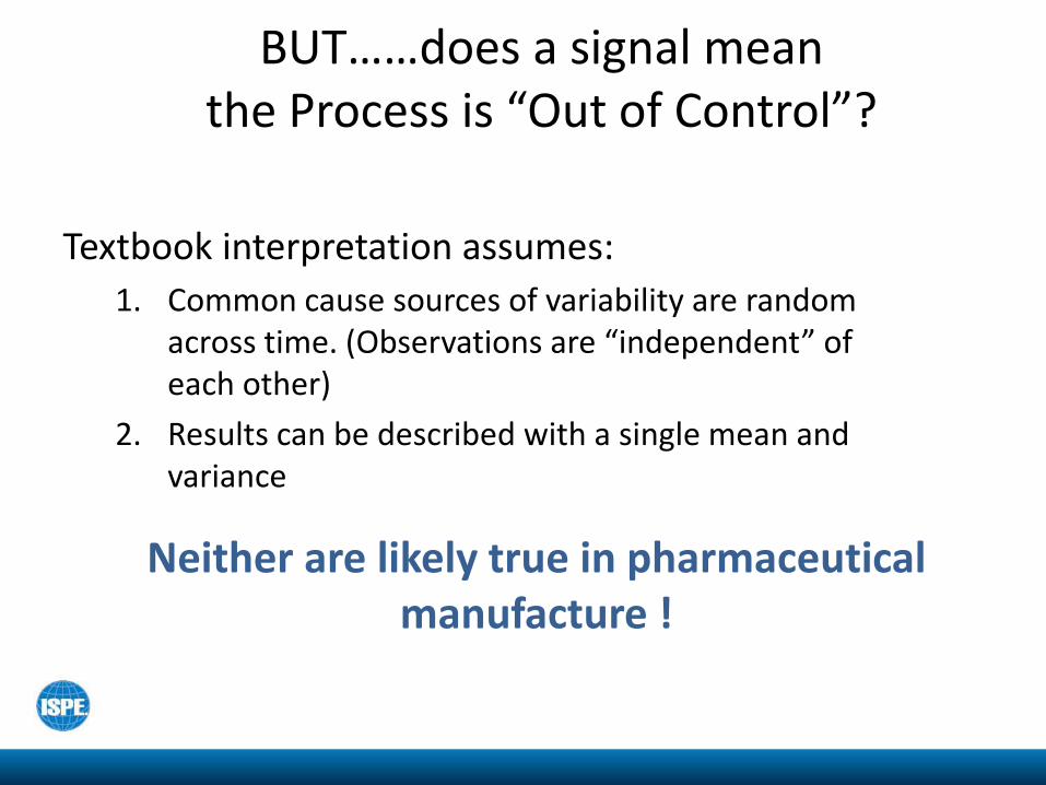
Textbook interpretation assumes:
1. Common cause sources of variability are random across time. (Observations are “independent” of each other)
2. Results can be described with a single mean and variance
BUT……does a signal meanthe Process is “Out of Control”?
Neither are likely true in pharmaceutical manufacture !
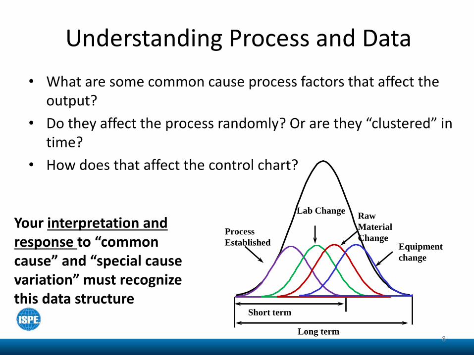
Understanding Process and Data
• What are some common cause process factors that affect the output?
• Do they affect the process randomly? Or are they “clustered” in time?
• How does that affect the control chart?
Short term
Long term
Process
Established
Lab ChangeRaw
Material
ChangeEquipment
change
Your interpretation and response to “common cause” and “special cause variation” must recognize this data structure
8
736557494133251791
102
101
100
99
98
97
96
95
Observation
Ind
ivid
ua
l V
alu
e
_X=98.173
UCL=101.390
LCL=94.955
2
1
2
2
I Chart of Assay with shifts
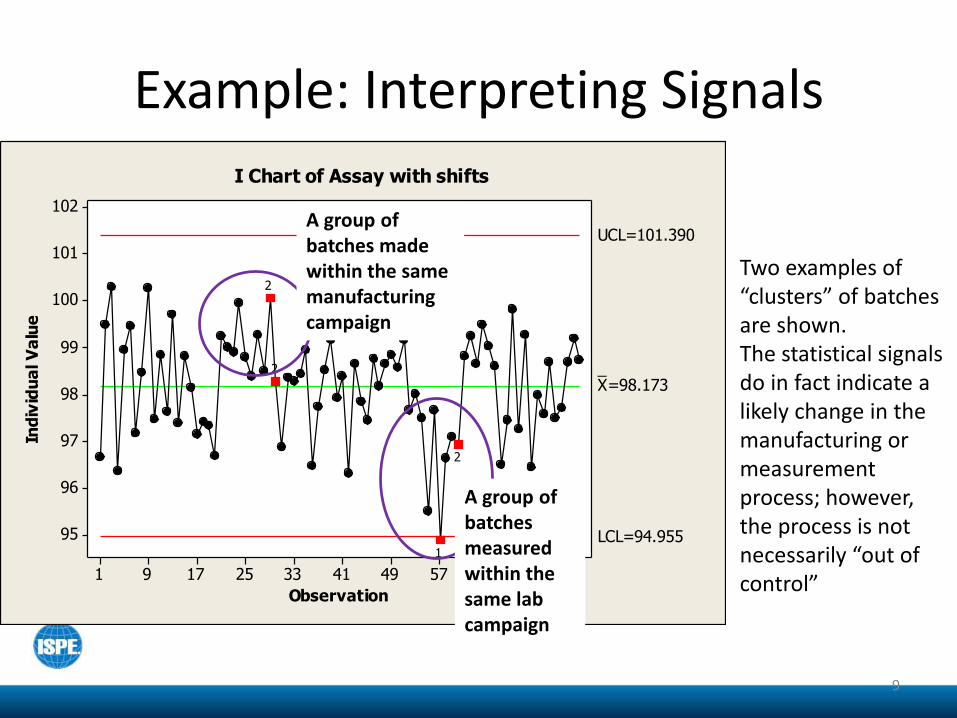
Example: Interpreting Signals
A group of batches made within the same manufacturing campaign
A group of batches measured within the same lab campaign
Two examples of “clusters” of batches are shown.The statistical signals do in fact indicate a likely change in the manufacturing or measurement process; however, the process is not necessarily “out of control”
9

Understanding “State of Control”
676601526451376301226151761
102.5
100.0
97.5
Observation
Ind
ivid
ua
l V
alu
e
_X=99.317
UCL=101.029
LCL=97.604
2
2
22222
2
11
2
6
11
6
1
1
151
6
66
6
6
4
22
26
6
2
2
22
2
2
22
2
2
11
2
2
2
222
2
22
22
26666
22
66
111
6
55
6
55
22
6666
2
2
22
2
2
6666
5
66
66
5
6
6
1
222
2
22222
1
2
2
22
2
1
6
6
6
1
222
I Chart of Content Uniformity
• It is CRITICAL that the typical operations inherent to pharmaceutical manufacturing , and the expected effect on control charts, be understood
• Expect to see “shift” signals in a process having this behavior• Some “special cause” variation is “expected”• Short term limits (used in default Shewhart charts) will reflect
within group variability, and will therefore typically be more narrow than long term limits
This is the “State of Control”
Typical Individuals Control Chart showing multiple statistical signals
Mindset Change – This is not real-time SPC
• Don’t let fear of signals trigger manipulation of data and charts. You may forfeit learning
• There is no requirement to initiate an investigation for statistical signals.
“..Not all signals are created equally.
“Magnitude of reaction depends on the severity of the signal…” (1)
• If red dots are always the enemy, consider changing the business process
(1) Alex Viehmann, FDA/CDER/OPQ, ISPE PV Statistician Forum April 2015
Risk Based Approach to Response to Statistical Signals
• Parameter severity
• Capability
• Magnitude of excursion
• Historical behavior
• Process and Measurement knowledge
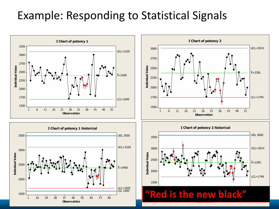
Example: Responding to Statistical Signals
51464136312621161161
3000
2750
2500
2250
2000
1750
1500
Observation
Ind
ivid
ua
l V
alu
e
_X=2381
UCL=3014
LCL=1749
2
1
2
22
2
I Chart of potency 2
918273645546372819101
3500
3000
2500
2000
1500
1000
Observation
Ind
ivid
ua
l V
alu
e
_X=2381
UCL=3014
LCL=1749
USL 3600
LSL 1200
2
1
2
22
2
1
2
2
2
I Chart of potency 2 historical
51464136312621161161
3250
3000
2750
2500
2250
2000
1750
1500
Observation
Ind
ivid
ua
l V
alu
e
_X=2400
UCL=3105
LCL=1695
222
2
I Chart of potency 1
8273645546372819101
3500
3000
2500
2000
1500
Observation
Ind
ivid
ua
l V
alu
e
_X=2400
UCL=3105
LCL=1695LSL 1600
USL 3500
222
2
I Chart of potency 1 historical
“Red is the new black”

Risk Based Approach to What to Monitor
Stage 3A of CPV: Establish State of Control
• Critical Quality Attributes
• Consider Process Parameters that vary, and can influence a quality attribute. Document justification to not monitor
• Establish tentative control limits until expected sources of variability have been incorporated
• Be careful with statistical evaluation of enhanced sampling, that is the methods to analyze the within and between batch variability and capability.
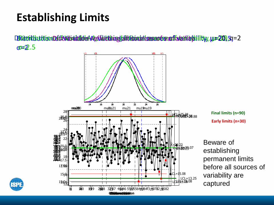
Early limits (n=30)
Final limits (n=90)
Observation
Ind
ivid
ua
l V
alu
e
8273645546372819101
28
26
24
22
20
18
16
14
12
_X=20.07
UCL=26.88
LCL=13.25
mu20 mu21 mu1926242220181614
LCL UCL
Distribution of variable A reflecting initial sources of variability, µ=20, σ=2Distribution of Variable A, with additional source of variability, µ=21.5, σ=2
Distribution of Variable A, with additional source of variability, µ=19, σ=2.5
Distribution reflecting all sources of variability
26242220181614
LCL UCL
26242220181614
LCL UCL
26242220181614
LCL UCL
Observation
Ind
ivid
ua
l V
alu
e
28252219161310741
25.0
22.5
20.0
17.5
15.0
_X=20.23
UCL=25.38
LCL=15.08
Observation
Ind
ivid
ua
l V
alu
e
554943373125191371
25.0
22.5
20.0
17.5
15.0
_X=20.23
UCL=25.38
LCL=15.08
mu20 mu211
Observation
Ind
ivid
ua
l V
alu
e
8273645546372819101
25.0
22.5
20.0
17.5
15.0
_X=20.23
UCL=25.38
LCL=15.08
mu20 mu21 mu19
6
1
5
1
1
Establishing Limits
Beware of
establishing
permanent limits
before all sources of
variability are
captured
Risk Based Approach to What to Monitor
Stage 3B of CPV: Ongoing Monitoring
• Critical Quality Attributes
• Process Parameters
– How much does it vary? The control strategy may limit the variability to a range that does not influence the critical quality attribute
– What attribute does it influence? What is the severity of that attribute? The performance of that attribute?
These are re-evaluated on an ongoing basis. If the state of control changes, adjustments to the CPV plan can be made based on a change in risk
Risk Based Approach to Monitoring Frequency
• Ideally, it is desirable to evaluate performance after a few results, after campaign, etc….; however, this is not always practical or necessary– The longer the time between evaluation, the more difficult to
uncover sources of variability• What is the performance of the quality attribute? How capable is it
to meet specification? What is the state of control?• Manufacturing Frequency (large vs small volume, by campaign, etc.) • “We don’t have the resources to review performance more than
once/year.” Don’t be constrained by a poorly designed business process, such as complex reporting and approvals
This is re-evaluated on an ongoing basis. If the state of control changes, adjustments to the CPV plan can be made based on a change in risk
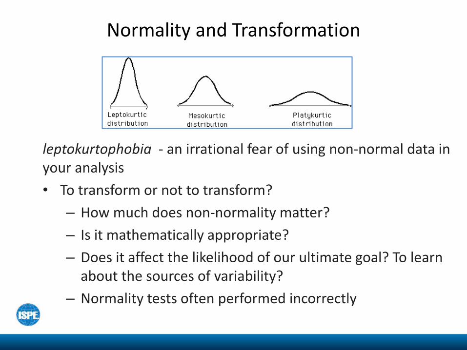
Normality and Transformation
leptokurtophobia - an irrational fear of using non-normal data in your analysis
• To transform or not to transform?
– How much does non-normality matter?
– Is it mathematically appropriate?
– Does it affect the likelihood of our ultimate goal? To learn about the sources of variability?
– Normality tests often performed incorrectly
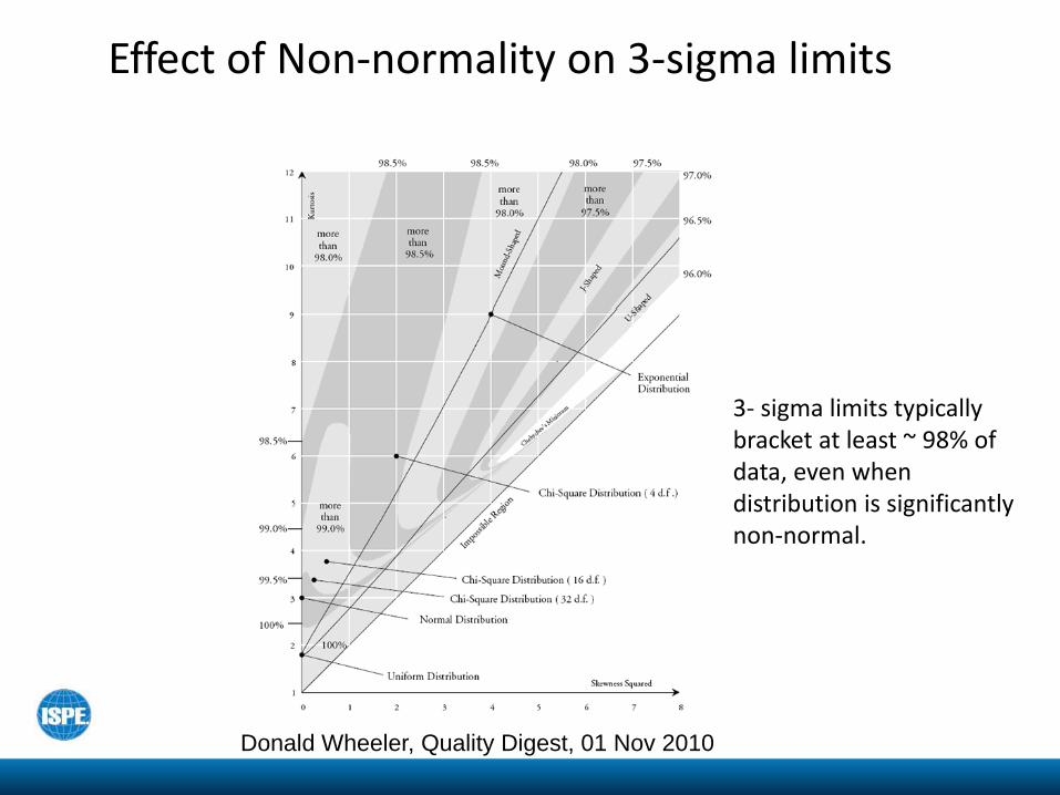
Effect of Non-normality on 3-sigma limits
Donald Wheeler, Quality Digest, 01 Nov 2010
3- sigma limits typically bracket at least ~ 98% of data, even when distribution is significantly non-normal.
Primary Question When Data Aren’t Normal
• Transform only when underlying distribution is normal (physical, chemical, etc.…)
– Observed distribution could be happenstance, not underlying. Transforming is over fitting current data
– Limited data in distribution tails to model accurately, so any transform could be inaccurate
– Negatively affect ease of interpretation
• Consider risk of non-normality
“Whenever you fit a model to your data you are assuming that those data are homogeneous. If they are not homogeneous, all of your statistics, all of your models, and all of your predictions are going to be wrong” (1)
(1) Donald Wheeler, Quality Digest, 30 July 2012
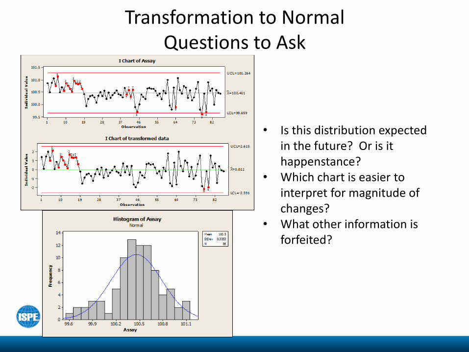
Transformation to Normal Questions to Ask
• Is this distribution expected in the future? Or is it happenstance?
• Which chart is easier to interpret for magnitude of changes?
• What other information is forfeited?
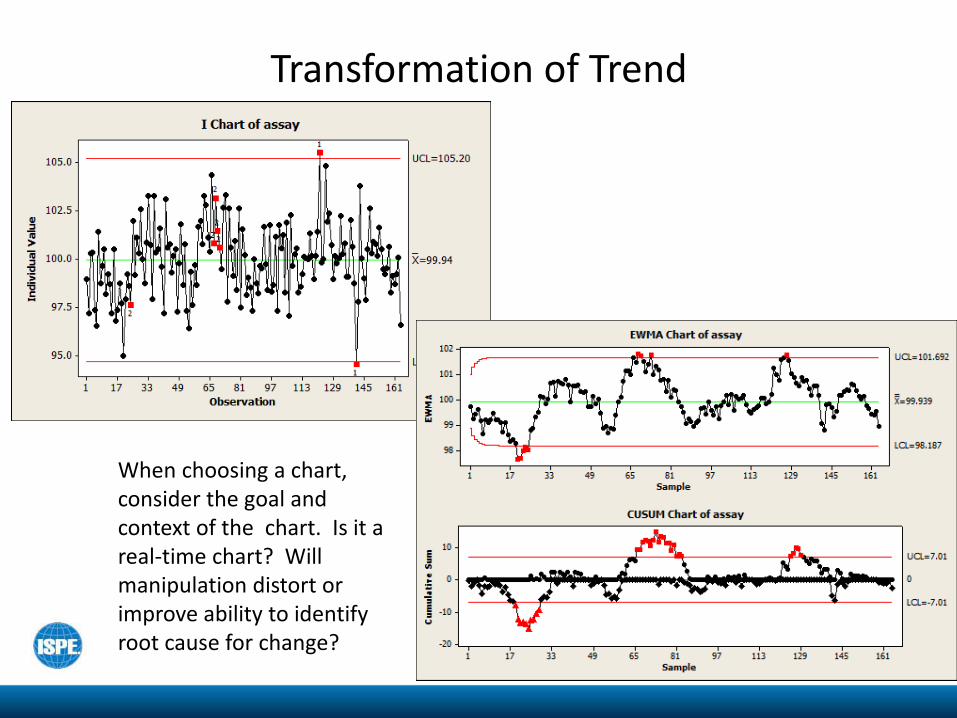
Transformation of Trend
When choosing a chart, consider the goal and context of the chart. Is it a real-time chart? Will manipulation distort or improve ability to identify root cause for change?
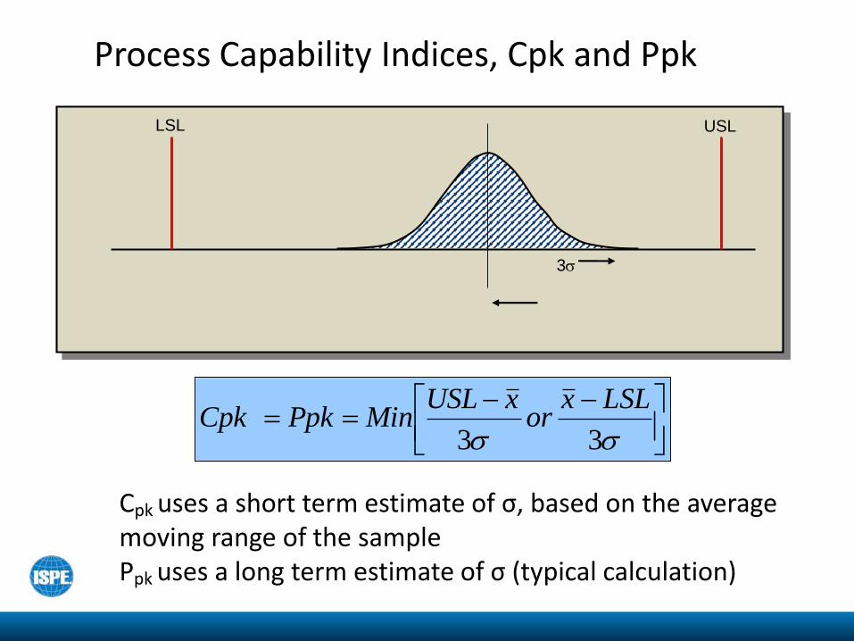
Process Capability Indices, Cpk and Ppk
3
LSL USL
33
LSLxor
xUSLMinPpkCpk
Cpk uses a short term estimate of σ, based on the average moving range of the sample Ppk uses a long term estimate of σ (typical calculation)

Cpk vs. PpkShort Term vs. Long Term
40136132128124120116112181411
101.5
100.5
99.5
98.5
97.5
96.5
Observation
Ind
ivid
ua
l V
alu
e
_X=99.281
UCL=101.118
LCL=97.444
6
111
5
6
6
22
6
2
2
222
2
2
2
2
222
2
2
22
2
2
2222
2
22
2
2
2
2
2
2
2
2
2
22
2
2
6
6
1
2
22
7
222
2
22222
2
2
2
22
2
1
6
6
6
6
2222
2
7
7
I Chart of Content Uniformity
10997857361493725131
11
10
9
8
7
6
5
4
Observation
Ind
ivid
ua
l V
alu
e
_X=7.684
UCL=10.967
LCL=4.402
I Chart of Acceptance Value
Cpk vs. PpkWhich should you use?
Ppk accounts for shifts in the mean that naturally occur over time. Cpk reflects what the capability could be without the shifts
Indeed, you would like the two to be equal; however, if your process is highly capable, it does not serve the interest of the business or patient to identify and eliminate the root cause of every shift in mean. Prioritization and action must be risk based
The difference between the two metrics can provide insight into your process, that is, the influence from sources of variability, such as raw materials, campaigns, equipment, analytical campaigns….
Process Capability Notes
• Textbook advice: Process must be in a “state of control” to calculate capability. Remember, process will often be “out of statistical control” because of non-independence. Interpret the consequence in context of use. (for example, predication of OOS vs level of response to signals)
• If data are non-normal, evaluate practical effect on interpretation use of capability (for example, is risk of failure more or less than what is expected from reported capability index)
• Be wary of combining within and between batch variance components
• Other statistical methods can provide likelihood of failure, e.g., Bayesian methods
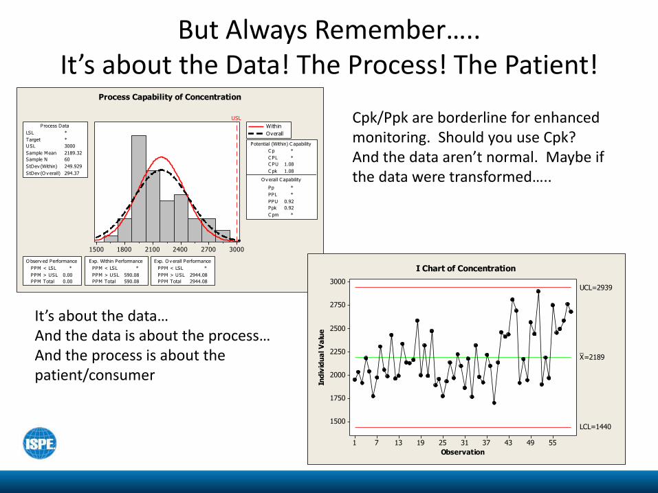
But Always Remember…..It’s about the Data! The Process! The Patient!
300027002400210018001500
USL
LSL *
Target *
USL 3000
Sample Mean 2189.32
Sample N 60
StDev (Within) 249.929
StDev (O v erall) 294.37
Process Data
C p *
C PL *
C PU 1.08
C pk 1.08
Pp *
PPL *
PPU 0.92
Ppk 0.92
C pm *
O v erall C apability
Potential (Within) C apability
PPM < LSL *
PPM > USL 0.00
PPM Total 0.00
O bserv ed Performance
PPM < LSL *
PPM > USL 590.08
PPM Total 590.08
Exp. Within Performance
PPM < LSL *
PPM > USL 2944.08
PPM Total 2944.08
Exp. O v erall Performance
Within
Overall
Process Capability of Concentration
554943373125191371
3000
2750
2500
2250
2000
1750
1500
Observation
Ind
ivid
ua
l V
alu
e
_X=2189
UCL=2939
LCL=1440
I Chart of Concentration
Cpk/Ppk are borderline for enhanced monitoring. Should you use Cpk? And the data aren’t normal. Maybe if the data were transformed…..
It’s about the data…And the data is about the process…And the process is about the patient/consumer
Summary
Ongoing assurance is gained during routine production that the process remains in a state of control
• Holistic integration of what, when, who and how
• Nature of the data and the State of Control
• Evolving Risk Based Approach to Monitoring
• Mindset Change | “Red is your friend, not your enemy”
• It’s about the data, the data is about the process, and the process is about the patient
