desired compensation adaptive robust contouring …byao/papers/dscc2009...email: qfw [email protected]...

DESIRED COMPENSATION ADAPTIVE ROBUST CONTOURING CONTROL OF ANINDUSTRIAL BIAXIAL PRECISION GANTRY SUBJECT TO COGGING FORCES ∗

Chuxiong Hu

The State Key Laboratory of Fluid

Power Transmission and ControlZhejiang University

Hangzhou, 310027, China

Email: [email protected]

Bin Yao†

School of Mechanical Engineering

Purdue UniversityWest Lafayette, Indiana, 47907

U.S.A


Qingfeng Wang

The State Key Laboratory of Fluid

Power Transmission and ControlZhejiang University

Hangzhou, 310027, China


ABSTRACT

To obtain a higher level of contouring motion control per-

formance for linear-motor-driven multi-axes mechanical systems

subject to significant nonlinear cogging forces, both coordinated

control of multi-axes motions and effective compensation of cog-

ging forces are necessary. In addition, the effect of unavoidable

velocity measurement noises needs to be carefully examined and

sufficiently attenuated. To solve these problems simultaneously,

in this paper, a discontinuous projection based desired compen-

sation adaptive robust contouring controller is developed by ex-

plicitly taking into account the specific characteristics of cogging

forces in the controller designs and employing the task coordi-

nate formulation for coordinated motion controls. Specifically,

based on the largely periodic nature of cogging forces with re-

spect to position, design models consisting of known sinusoidal

functions of positions corresponding to the main harmonics of

the force ripple waveforms with unknown weights are used to

approximate the unknown cogging forces. Theoretically, the re-

sulting controller achieves a guaranteed transient performance

and final contouring accuracy in the presence of both paramet-

ric uncertainties and uncertain nonlinearities. In addition, the

controller also achieves asymptotic output tracking when there

are parametric uncertainties only. Comparative experimental re-

sults obtained on a high-speed industrial biaxial precision gantry

driven by linear motors are presented to verify the excellent con-

touring performance of the proposed control scheme and the ef-

∗THE WORK IS SUPPORTED IN PART BY THE US NATIONAL SCI-

ENCE FOUNDATION (GRANT NO. CMS-0600516) AND IN PART BY THE

NATIONAL NATURAL SCIENCE FOUNDATION OF CHINA (NSFC) UN-

DER THE JOINT RESEARCH FUND FOR OVERSEAS CHINESE YOUNG

SCHOLARS (GRANT NO. 50528505).†Address all correspondence to this author.

fectiveness of the cogging force compensations.

1 Introduction

For an industrial biaxial gantry system driven by linear mo-

tors, the contouring performance is evaluated by the contouring

error which represents the geometric deviation from the actual

contour to the desired contour [1]. The degradation of contour-

ing performance could be mainly due to lacking coordination of

multi-axes motions [2] and effects of disturbances such as fric-

tion and cogging forces [3]. The former is referred to as the

coordinated contouring control problem and the later as the dis-

turbance rejection/compensation.

To address the contouring control problems, Koren [4] first

proposed the cross-coupled control (CCC) strategy in which cou-

pling actions was introduced in the servo controllers so that the

control of one axial servomechanism was affected by other ax-

ial servomechanisms involved in the motion and consequently

the coordination of axes was strengthened. Since then, many re-

search publications on CCC have been published [2, 5, 6]. But

these designs are based on the traditional control theories for lin-

ear time-invariant systems and cannot address the dynamic cou-

pling phenomena (e.g. Coriolis force) well when tracking curved

contours. Chiu and Tomizuka [7] formulated the contouring con-

trol problem in a task coordinate frame "attached" to the desired

contour. Under the task coordinate formulation, a control law

could be designed to assign different dynamics to the normal and

tangential directions relative to the desired contour. Since then

contouring control schemes based on task coordinate approaches

have been reported [1,8]. However, these control techniques can-

not explicitly deal with parametric uncertainties and uncertain

1 Copyright © 2009 by ASME

DSCC2009-2687

Proceedings of the ASME 2009 Dynamic Systems and Control Conference DSCC2009

October 12-14, 2009, Hollywood, California, USA

nonlinearities. As a result, they are often insufficient when strin-

gent contouring performance is of concern as actual systems are

always subjected to certain model uncertainties and disturbances.

To achieve higher precision motion control of linear-motor-

driven systems, the cogging force behavior should be clearly un-

derstood such that effective cogging force compensation can be

synthesized. Thus significant research efforts have been devoted

to the modeling and compensation of cogging force [3, 9, 10].

For example, in [10], the cogging force is assumed to be periodic

functions with respect to position so that Fourier expansion with

a few significant terms could be utilized to represent the cogging

force. Non-periodic effect is also considered in a recent publica-

tion [3]. It should be noted all these cogging force compensation

researches are done for single axis motion only.

In this paper, high-performance contouring motion control

of a biaxial linear-motor-driven precision gantry subject to sig-

nificant nonlinear cogging forces is studied. In order to achieve

effective cogging force compensations, the cogging force model

in [10] is utilized to formulate the overall system dynamics in

a task coordinate frame. The desired compensation adaptive ro-

bust control (DCARC) strategy [11] is then applied to develop a

coordinated ARC contouring controller in which the regressor is

calculated based on the desired contour information only. Theo-

retically, the proposed controller achieves certain guaranteed out-

put contouring transient performances and steady-state contour-

ing accuracies even in the presence both parametric uncertainties

and uncertain nonlinearities. In addition, when the actual system

is subjected to parametric uncertainties only, a much improved

steady-state tracking performance – asymptotic output tracking –

is achieved as well. Experimental results have also been obtained

on a high-speed Anorad industrial biaxial gantry driven by LC-

50-200 linear motors with a linear encoder resolution of 0.5 µm.

The results verify the excellent contouring performance of the

proposed DCARC controller in actual implementation in spite

of various parametric uncertainties and uncertain disturbances.

Comparative experimental results also demonstrate the effective-

ness of the cogging force compensations.

2 Problem Formulation

2.1 Task Coordinate Frame

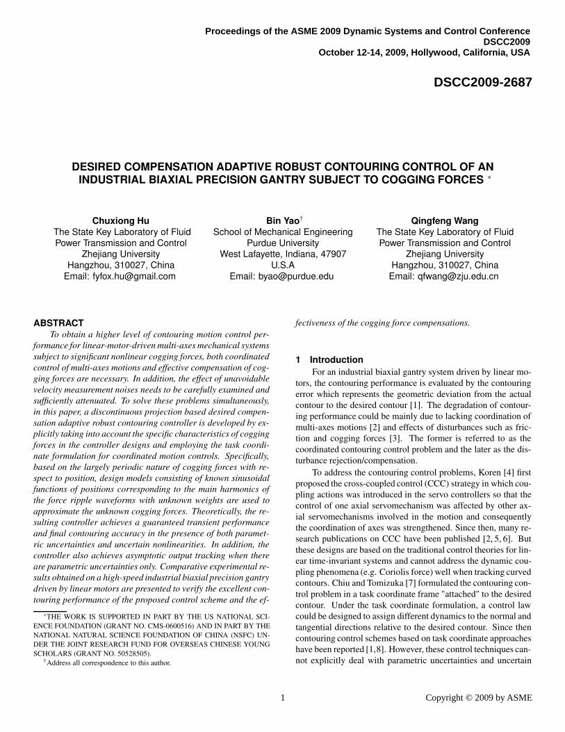
Figure 1 shows a popular approximation of contouring error

[5, 8]. Let x and y denote the horizontal and the vertical axes of

a biaxial gantry system. At any time instant, there are two points

Pd and Pa denoting the position of the reference command and

the actual position of the system, respectively. Tangential and

normal directions of the desired contour at the point Pd are used

to approximate the contouring error by the distance from Pa to

the tangential line. With this definition, the contouring error ε c

can be approximately computed by the normal error ε n as:

εc ≈ εn = −sinα · ex + cosα · ey (1)

Figure 1. An Approximate Contouring Error Model

where ex and ey denote the axial tracking errors of x and y axes,

i.e. ex = x−xd , ey = y−yd , and α denotes the angle between the

tangential line to the horizontal X-axis. In this model, if the ax-

ial tracking errors are comparatively small to the curvature of the

desired contour, then it yields a good approximation of the con-

touring error. The tangential error ε t in Figure 1 can be obtained

as

εt = cosα · ex + sinα · ey (2)

Then the tangential and the normal directions are mutually or-

thogonal and hence can be taken as the basis for the task coor-

dinate frame. Thus the physical (x,y) coordinates can be trans-

formed into the task coordinates of (εc,εt ) by a linear transfor-

mation

ε = Te (3)

where ε = [εc,εt ]T ; e = [ex,ey]

T , and the time-varying transfor-

mation matrix depends on the reference trajectories of the desired

contour only and is given by

T =

[−sinα cosαcosα sinα

](4)

The matrix T is always unitary for all values of α , i.e., TT = T

and T−1 = T.

2.2 System Dynamics

The biaxial linear-motor-driven gantry has the following dy-

namics [3]:

Mq+ Bq+ Fc(q)+ Fr(q) = u+ d; (5)

where q = [x(t),y(t)]T , q = [x(t), y(t)]T and q = [x(t), y(t)]T are

the 2× 1 vectors of the axis position, velocity and acceleration,

respectively; M = diag[M1,M2] and B = diag[B1,B2] are the


2× 2 diagonal inertia and viscous friction coefficient matrices,

respectively. Fc(q) is the 2×1 vector of Coulomb friction which

is modeled by Fc(q) = AfSf(q), where Af = diag[A f 1,A f 2] is the

2×2 unknown diagonal Coulomb friction coefficient matrix, and

Sf(q) is a known vector-valued smooth function used to approx-

imate the traditional discontinuous sign function sgn( q) used in

the traditional Coulomb friction modeling for effective friction

compensation in implementation [14]. F r(q) represents the 2×1

vector of position dependent cogging forces. u is the 2×1 vector

of control input, and d is the 2×1 vector of unknown nonlinear

functions due to external disturbances or modeling errors.

In this paper, it is assumed that the permanent magnets of

the same linear motor are all identical and are equally spaced at a

pitch of P. Thus, Fr(q) = [Fr(x),Fr(y)]T is a periodic function of

position q with a period of P, i.e., Fr(x+P) = Fr(x), Fr(y+P) =Fr(y) and it can be approximated quite accurately by the first

several harmonic functions of the positions, which is represented

by

Fr(x) = ∑mi=1(Sxisin( 2iπ

Px)+Cxicos( 2iπ

Px))

Fr(y) = ∑nj=1(Sy jsin( 2 jπ

Py)+Cy jcos( 2 jπ

Py))

(6)

where Sxi,Cxi,Sy j,Cy j are the unknown weights, m and n are the

numbers of harmonics used to approximate the cogging forces in

X-axis and Y-axis, respectively. The larger m and n are, the better

Fr(q) approximates the actual cogging forces, but the larger the

number of parameters need to be adapted. So a trade-off has to be

made based on the particular structure of a motor. For example,

in [12], it was experimentally observed that the first, the third,

and the fifth harmonics are the main harmonics in the force ripple

waveform.

With the above cogging force and friction modelling, the

linear motor dynamics (5) can be written as:

Mq+ Bq+ AfSf(q)+ Fr(q) = u+ dN + d (7)

where dN = [dN1,dN2]T is the nominal value of the lumped mod-

eling error and disturbance d l = d+ Fr(q)−Fr(q)+ AfSf(q)−

Fc(q), and d = dl − dN represents the time-varying portion of

the lumped uncertainties. For this dynamic system, we define

the tracking error as e = [ex,ey]T = [x(t)− xd(t),y(t)− yd(t)]

T

where qd(t) = [xd(t),yd(t)] is the reference trajectory describing

the desired contour. Then the system dynamics can be rewritten

as

Me+ Be+ AfSf(q)+ Fr(q)+Mqd + Bqd = u+ dN + d (8)

Noting (3) and (4) and the unitary property of T, the time deriv-

atives of the tracking error states can be derived as [8]

e = Tε + Tε, e = Tε + 2Tε + Tε (9)

Then the system dynamics can be represented in the task coordi-

nate frame as

Mtε + Btε + 2Ctε + Dtε + Mqqd+Bqqd

+AfqSf(q)+ Frq(q) = ut + dt + ∆(10)

where

Mt = TMT,Bt = TBT,Ct = TMT,

Dt = TMT+ TBT,ut = Tu,dt = TdN, ∆ = Td,Mq = TM,Bq = TB,Afq = TAf,Frq(q) = TFr(q)

(11)

It is well known that equation (10) has the following properties:

(P1) Mt is a symmetric positive definite (s.p.d.) matrix with

µ1I ≤ Mt ≤ µ2I (12)

where µ1 and µ2 are two positive scalars.

(P2) The matrix Nt = Mt −2Ct is a skew-symmetric matrix.

(P3) All modeled terms of the task space dynamics (10) can

be linearly parameterized by a set of parameters as follows

Mtε + Btε + 2Ctε + Dtε + Mqqd + Bqqd

+AfqSf(q)+ Frq(q)−dt = −ϕ(q, q, q,t)θ (13)

where ϕ is a 2 × (8 + 2m + 2n) matrix of known functions,

commonly referred to as the regressor, and θ is a vector

of unknown parameters defined as θ = [θ1, ...,θ8+2m+2n]T =

[M1,M2,B1,B2,A f 1,A f 2,Sx1,Cx1, ...,Sxm,Cxm,Sy1,Cy1, ...,Syn,Cyn,dN1,dN2]

T .

In general, the parameter vector θ cannot be known exactly.

For example, the payload of the biaxial gantry depends on tasks.

However, the extent of parametric uncertainties can be predicted.

Therefore, the following practical assumption is made: 1

Assumption 1. The extent of the parametric uncertainties and

uncertain nonlinearities is known, i.e.,

θ ∈ Ωθ ⇒θ : θmin ≤ θ ≤ θmax

∆ ∈ Ω∆ ⇒

∆ : ||∆|| ≤ δ∆

(14)

where θmin = [θ1min, ...,θ(8+2m+2n)min]T , and θmax =

[θ1max, ...,θ(8+2m+2n)max]T are known. δ∆ is a known func-

tion.

The control objective is to synthesize a control input u t such

that q = [x,y]T tracks the reference trajectory qd(t) = [xd ,yd ]T

describing the desired contour as closely as possible. qd(t) is

assumed to be of at-least second-order differentiable.

1For simplicity, the following notations are used: •i for the i-th component of

the vector •, •min for the minimum value of •, and •max for the maximum value

of •. The operation ≤ for two vectors is performed in terms of the corresponding

elements of the vectors.


3 Discontinuous ProjectionLet θ denote the estimate of θ and θ the estimation error

(i.e., θ = θ −θ ). In view of (14), the following adaptation law

with discontinuous projection modification can be used

˙θ = Pro j

θ(Γτ) (15)

where Γ > 0 is a diagonal matrix, τ is an adaptation function

to be synthesized later. The projection mapping Pro j θ (•) =

[Pro jθ1

(•1), ...,Pro jθp

(•p)]T is defined in [13] as

Pro jθi(•i) =

0 i f θi = θimax and •i > 0

0 i f θi = θimin and •i < 0

•i otherwise

(16)

It is shown that for any adaptation function τ , the projection

mapping used in (16) guarantees [13]

(P4) θ ∈ Ωθ ⇒

θ : θimin ≤ θ ≤ θimax

(P5) θ T (Γ−1Pro jθ(Γτ)− τ) ≤ 0, ∀τ

(17)

4 Adaptive Robust Control (ARC) Law Synthesis

Define a switching-function-like quantity as

s = ε + Λε (18)

where Λ > 0 is a diagonal matrix. Define a positive semi-definite

(p.s.d.) function

V (t)= 12sTMts (19)

Differentiating V yields

V = sT[ut + dt + ∆−Mqqd −Bqqd −AfqSf(q)

−Frq(q)−Btε −Ctε −Dtε + CtΛε + MtΛε ] (20)

where (P2) is used to eliminate the term 12sTMts. Furthermore,

viewing (P3), we can linearly parameterize the terms in (20) as

Mqqd + Bqqd + AfqSf(q)+ Frq(q)+ Btε + Ctε

+Dtε −CtΛε −MtΛε −dt = −Ψ(q, q,t)θ (21)

where Ψ is a 2×(8+2m+2n)matrix of known functions, known

as the regressor. Thus (20) can be rewritten as

V = sT[ut + Ψ(q, q,t)θ + ∆] (22)

Noting the structure of (22), the following ARC law is proposed:

ut = ua + us; ua = −Ψ(q, q, t)θ ; τ = ΨT(q, q,t)s (23)

where ua is the adjustable model compensation needed for

achieving perfect tracking and us is a robust control law to be

synthesized later. Substituting (23) into (22) and simplifying the

resulting expression lead to

V = sT[us −Ψ(q, q,t)θ + ∆] (24)

The robust control function us consists of two terms:

us = us1 + us2, us1 = −Ks (25)

where us1 is used to stabilize the nominal system, which is cho-

sen to be a simple proportional feedback with K being a symmet-

ric positive definite matrix for simplicity. And us2 is a feedback

used to attenuate the effect of model uncertainties for a guaran-

teed robust performance. Noting Assumption 1 and (P4) of (17),

there exists a us2 such that the following two conditions are sat-

isfied

i sT[us2 −Ψ(q, q, t)θ + ∆] ≤ ηii sTus2 ≤ 0

(26)

where η is a design parameter that can be arbitrarily small. One

smooth example of us2 satisfying (24) is given by us2 =− 14η h2s,

where h is a smooth function satisfying h ≥ ||θM||||Ψ(q, q,t)||+δ∆, and θM = θmax −θmin.

5 Desired Compensation ARC (DCARC)

In [11], the desired compensation ARC law in which the re-

gressor is calculated by desired trajectory information only to re-

duce the effect of measurement noise, has been proposed. In the

following, a DCARC law employing the cogging force model in

(6) is constructed and applied to the biaxial linear-motor-driven

gantry as well.

The proposed DCARC law and adaptation function have the

same form as (23), but with the regressor Ψ(q, q, t) substituted

by the desired regressor Ψd(qd(t), qd(t),t):

ut = ua + us; ua = −Ψdθ ; τ = ΨTd s (27)

Choose a positive semi-definite (p.s.d) function:

V (t) = 12sTMts+ 1

2εTKε ε (28)


where Kε is a diagonal positive definite matrix. Differentiating

V (t) and substituting (27) into the resulting expression yields

V = sT[us + Ψθ −Ψdθ + ∆]+ εTKε ε (29)

where Ψ = Ψ(q, q,t)−Ψd(qd, qd,t) is the difference between

the actual regression matrix and the desired regression matrix

formulations. As shown in [14], Ψ can be quantified as

||Ψθ || ≤ ζ1||ε||+ ζ2||ε||2 + ζ3||s||+ ζ4||s||||ε|| (30)

where ζ1,ζ2,ζ3 and ζ4 are positive bounding constants that de-

pend on the desired contour and the physical properties of the

biaxial gantry. Similar to (25), the robust control function u s

consists of two terms given by:

us = us1 + us2, us1 = −Ks−Kεε −Ka||ε||2s (31)

where the controller parameters K, Kε and Ka are s.p.d. matri-

ces satisfying σmin(Ka) ≥ ζ2 +ζ4 (σmin(·) denotes the minimum

eigenvalue of a matrix) and the following condition

Q =

[σmin(Kε Λ)− 1

4ζ2 − 1

2ζ1

− 12ζ1 σmin(K)− ζ3 −

14ζ4

]> 0 (32)

Specifically, it is easy to check that if

σmin(Kε Λ) ≥ 12ζ1 + 1

4ζ2, σmin(K) ≥ 1

2ζ1 + ζ3 + 1

4ζ4 (33)

the matrix Q defined in (32) is positive definite. The robust con-

trol term us2 is required to satisfy the following constrains similar

to (26),

i sT

us2 −Ψdθ + ∆≤ η

ii sTus2 ≤ 0(34)

One smooth example of us2 satisfying (34) is us2 = − 14η h2

ds,

where hd is any function satisfying hd ≥ ||θM||||Ψd||+ δ.

Theorem 1. [15] The desired compensation ARC law (27)

guarantees that:

A. In general, all signals are bounded. Furthermore, the

positive semi-definite function V (t) defined by (28) is bounded

above by

V (t) ≤ exp(−λ t)V(0)+ ηλ [1− exp(−λ t)] (35)

where λ =2σmin(Q)

max[µ2,σmax(Kε)] , and σmax(·) denotes the minimum

eigenvalue of a matrix.

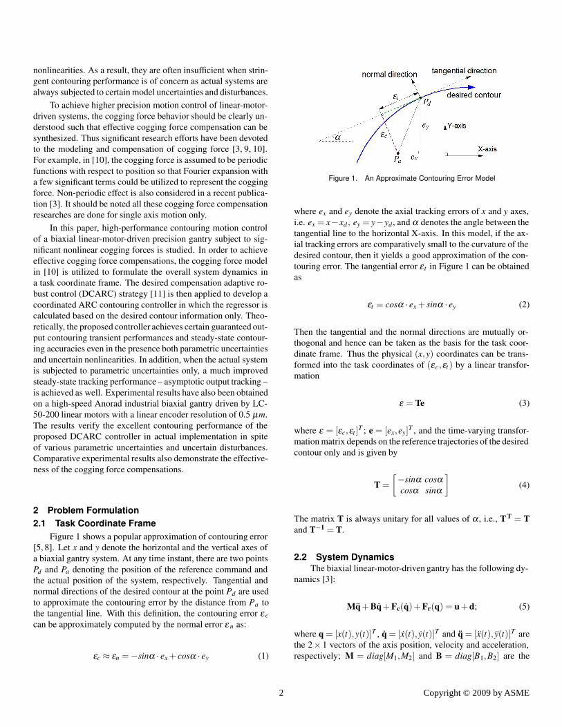
Figure 2. A Biaxial linear motor driven gantry system

B. Suppose that after a finite time t0 there exist parametric

uncertainties only, i.e., ∆ = 0, ∀t ≥ t0. Then, in addition to result

A, zero final tracking error is also achieved, i.e, ε → 0 and s → 0

as t → ∞.

6 Experimental Setup and Results

6.1 Experiment setup

A biaxial Anorad HERC-510-510-AA1-B-CC2 gantry from

Rockwell Automation is set up in Zhejiang University as a test-

bed. As shown in Figure 2, the two axes powered by Anorad

LC-50-200 iron core linear motors are mounted orthogonally

with X-axis on top of Y-axis. The position sensors of the gantry

are two linear encoders with a resolution of 0.5µm after quadra-

ture. The velocity signal is obtained by the difference of two

consecutive position measurements. Standard least-square iden-

tification is performed to obtain the parameters of the biaxial

gantry and it is found that nominal values of the gantry sys-

tem parameters without loads are M1 = 0.12(V/m/s2),M2 =0.64(V/m/s2),B1 = 0.166(V/m/s),B2 = 0.24(V/m/s),A f 1 =0.1(V),A f 2 = 0.36(V).

Explicit measurement of cogging force is then conducted for

both axes by blocking the motor and using an external force sen-

sor (HBM U10M Force Transducer with AE101 Amplifier) to

measure the blocking forces at zero input voltages. This mea-

surement is done for various positions with 1mm incremental

distance. Frequency domain analysis of the measured ripple

forces [3] indicates that the fundamental period corresponds to

the pitch of the magnets (P = 50mm) and that the harmonic terms

of cogging forces have significant values at frequencies corre-

sponding to i = 1,2,3 and j = 1,6,12 in (6). Thus the approxi-

mate cogging forces model (6) is chosen as

Fr(q) = [Sx1sin( 2πP

x)+Cx1cos( 2πP

x)+ Sx2sin( 4πP

x)

+Cx2cos( 4πP

x)+ Sx3sin( 6πP

x)+Cx3cos( 6πP

x),Sy1sin( 2π

Py)+Cy1cos( 2π

Py)+ Sy6sin( 12π

Py)

+Cy6cos( 12πP

y)+ Sy12sin( 24πP

y)+Cy12cos( 24πP

y)]T

(36)


The bounds of the parametric variations are chosen as:

θmin = [0.06,0.5,0.15,0.1,0.05,0.08,−0.2,−0.2,−0.2,−0.2,−0.2,−0.2,−0.2,−0.2,−0.2,−0.2,−0.2,−0.2,−0.5,−1]T

θmax = [0.20,0.75,0.35,0.3,0.15,0.5,0.2,0.2,0.2,0.2,0.2,0.2,0.2,0.2,0.2,0.2,0.2,0.2,0.5,1]T

(37)

6.2 Performance Indexes

The following performance indexes will be used to measure

the quality of each control algorithm:

⋄ ||εc||rms = ( 1T

´ T

0|εc|

2dt)1/2, the root-mean-square (RMS)

value of the contouring error, is used to measure average con-

touring performance, where T is the total running time;

⋄ εcM = maxt

|εc|, the maximum absolute value of the con-

touring error is used to measure transient performance;

⋄ ||ui||rms = ( 1T

´ T

0|ui|

2dt)1/2, the average control input of

each axis, is used to evaluate the amount of control effort.

6.3 Experimental Results

The control algorithms are implemented using a dSPACE

DS1103 controller board. The controller executes programs at

a sampling period of Ts = 0.2ms, resulting in a velocity mea-

surement resolution of 0.0025m/sec. The following control al-

gorithms are compared:

C1: DCARC without cogging force compensation.

The smooth functions S f (xd) and S f (yd) are chosen as2π arctan(9000xd) and 2

π arctan(9000yd). The design parameter

Λ is chosen as: Λ = diag[100,30]. us2 in (31) is given in Section

V. Theoretically, we should use the form of u s2 = −Ks2(q)swith Ks2(q) being a nonlinear proportional feedback gain as

given in [16] to satisfy the robust performance requirement

(34) globally. In implementation, a large enough constant

feedback gain Ks2 is used instead to simplify the resulting

control law. With such a simplification, though the robust

performance condition (34) may not be guaranteed globally,

the condition can still be satisfied in a large enough working

range which might be acceptable to practical applications as

done in [17]. With this simplification, noting (31), we choose

us = −Kss−Kεε −Ka||ε||2s in the experiments where Ks

represents the combined gain of K and K s2, and the controller

parameters are Ks = diag[100,60], Ka = diag[10000,10000],and Kε = diag[5000,5000]. The adaptation rates are set as Γ =diag[10,10,10,10,1,1,0,0,0,0,0,0,0,0,0,0,0,0,5000,5000].

The initial parameter estimates are chosen as: θ (0) =[0.1,0.55,0.20,0.22,0.1,0.15,0,0,0,0,0,0,0,0,0,0,0,0,0,0] T.

C2: DCARC with cogging force compensa-

tion. The same control law as the above DCARC

but with cogging force compensation, i.e., letting Γ =diag[10,10,10,10,1,1,500,500,500,500,500,500,500,500,500,500,500,500,5000,5000].

The following test sets are performed:

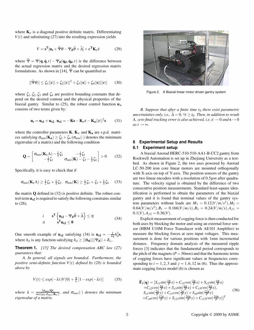
Table 1. Circular contouring results

Set 1 Set 2 Set 3

Controller C1 C2 C1 C2 C1 C2

||εc||rms(µm) 2.54 1.64 2.66 1.74 3.03 2.11

εcM(µm) 9.22 7.05 9.56 7.91 28.48 25.26

||ux||rms(V ) 0.26 0.26 0.26 0.26 0.26 0.26

||uy||rms(V ) 0.41 0.41 0.42 0.42 0.41 0.41

Set1 : To test the nominal contouring performance of the con-

trollers, experiments are run without payload;

Set2 : To test the performance robustness of the algorithms to pa-

rameter variations, a 5 kg payload is mounted on the gantry;

Set3 : A large step disturbance (a simulated 0.6 V electrical sig-

nal) is added to the input of Y axis at t=1.9 sec and removed

at t=4.9 sec to test the performance robustness of each con-

troller to disturbance.

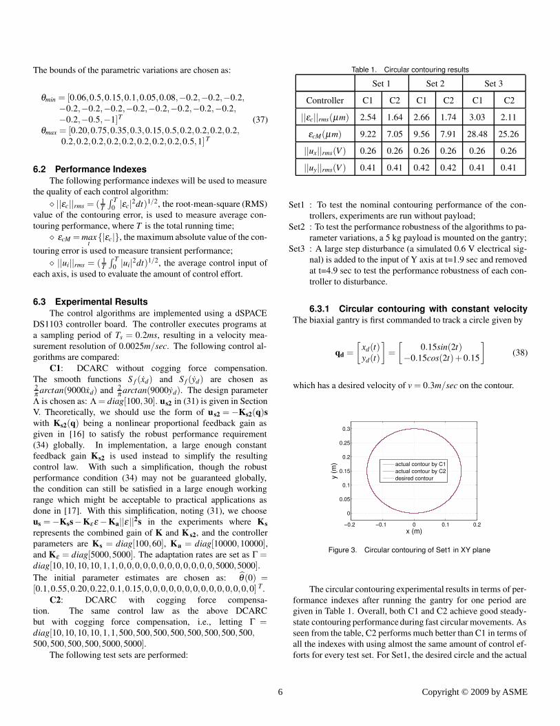
6.3.1 Circular contouring with constant velocity

The biaxial gantry is first commanded to track a circle given by

qd =

[xd(t)yd(t)

]=

[0.15sin(2t)

−0.15cos(2t)+ 0.15

](38)

which has a desired velocity of v = 0.3m/sec on the contour.

−0.2 −0.1 0 0.1 0.2

0

0.05

0.1

0.15

0.2

0.25

0.3

x (m)

y (

m) actual contour by C1

actual contour by C2

desired contour

Figure 3. Circular contouring of Set1 in XY plane

The circular contouring experimental results in terms of per-

formance indexes after running the gantry for one period are

given in Table 1. Overall, both C1 and C2 achieve good steady-

state contouring performance during fast circular movements. As

seen from the table, C2 performs much better than C1 in terms of

all the indexes with using almost the same amount of control ef-

forts for every test set. For Set1, the desired circle and the actual


0 5 10 15−1

−0.5

0

0.5

1x 10

−5

t (sec)

C1

: C

on

tou

rin

g E

rro

r (m

)

0 5 10 15−1

−0.5

0

0.5

1x 10

−5

t (sec)

C2

: C

on

tou

rin

g E

rro

r (m

)

Figure 4. Circular contouring errors of Set1 (no load)

0 5 10 15−1

−0.5

0

0.5

1x 10

−5

t (sec)

C1

: C

on

tou

rin

g E

rro

r (m

)

0 5 10 15−1

−0.5

0

0.5

1x 10

−5

t (sec)

C2

: C

on

tou

rin

g E

rro

r (m

)

Figure 5. Circular contouring errors of Set2 (loaded)

contours by C1 and C2 are shown in Figure 3, and the contouring

errors are given in Figure 4, demonstrating the good nominal per-

formance of DCARC controllers – the contour errors are mostly

within 5 µm. For Set2, the contouring errors are displayed in Fig-

ure 5 which shows that both controllers achieve good steady-state

contouring performance in spite of the change of inertia load,

verifying the performance robustness of the proposed DCARC

controllers to parameter variations. The contouring errors of Set3

are given in Figure 6. As seen from the figures, the added large

disturbances do not affect the contouring performance much ex-

cept the transient spikes when the sudden changes of the distur-

bances occur – even the transient tracking errors are within 26

µm for C2. These results demonstrate the strong performance

robustness of the DCARC schemes. Comparing C2 with C1, the

improvements of contouring performances in all three sets also

illustrate the effectiveness of the cogging force compensations.

0 5 10 15−4

−2

0

2

4x 10

−5

t (sec)

C1

: C

on

tou

rin

g E

rro

r (m

)

0 5 10 15−4

−2

0

2

4x 10

−5

t (sec)

C2

: C

on

tou

rin

g E

rro

r (m

)

Figure 6. Circular contouring errors of Set3 (disturbances)

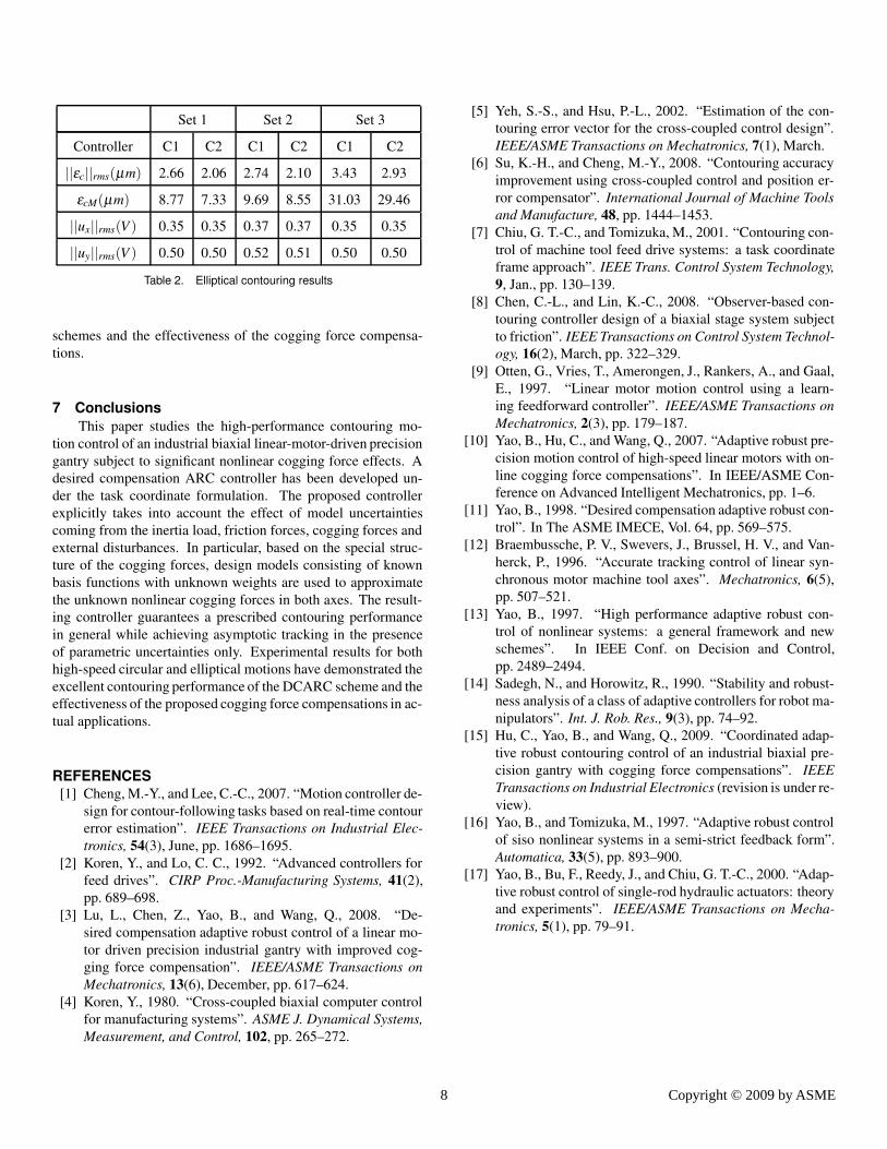
6.3.2 Elliptical contouring with constant angular

velocity The biaxial gantry is also commanded to track an el-

lipse described by

qd =

[xd(t)yd(t)

]=

[0.2sin(3t)

−0.1cos(3t)+ 0.1

](39)

which has an angular velocity of ω = 3rad/sec. The ellipti-

−0.2 −0.1 0 0.1 0.2−0.05

0

0.05

0.1

0.15

0.2

x (m)

y (

m) actual contour by C1

actual contour by C2

desired contour

Figure 7. Elliptical contouring of Set1 in XY plane

cal contouring experimental results in terms of performance in-

dexes after running the gantry for one period are given in Table

2. Overall, both C1 and C2 achieve good steady-state contouring

performance during the fast elliptical movements. As seen from

the table, C2 performs better than C1 in terms of all the indexes

with using almost the same amount of control efforts for every

test set. For Set1, the desired ellipse and the actual contours by

C1 and C2 are shown in Figure 6.3.2. All these results further

demonstrate the strong performance robustness of the proposed


Set 1 Set 2 Set 3

Controller C1 C2 C1 C2 C1 C2

||εc||rms(µm) 2.66 2.06 2.74 2.10 3.43 2.93

εcM(µm) 8.77 7.33 9.69 8.55 31.03 29.46

||ux||rms(V ) 0.35 0.35 0.37 0.37 0.35 0.35

||uy||rms(V ) 0.50 0.50 0.52 0.51 0.50 0.50

Table 2. Elliptical contouring results

schemes and the effectiveness of the cogging force compensa-

tions.

7 Conclusions

This paper studies the high-performance contouring mo-

tion control of an industrial biaxial linear-motor-driven precision

gantry subject to significant nonlinear cogging force effects. A

desired compensation ARC controller has been developed un-

der the task coordinate formulation. The proposed controller

explicitly takes into account the effect of model uncertainties

coming from the inertia load, friction forces, cogging forces and

external disturbances. In particular, based on the special struc-

ture of the cogging forces, design models consisting of known

basis functions with unknown weights are used to approximate

the unknown nonlinear cogging forces in both axes. The result-

ing controller guarantees a prescribed contouring performance

in general while achieving asymptotic tracking in the presence

of parametric uncertainties only. Experimental results for both

high-speed circular and elliptical motions have demonstrated the

excellent contouring performance of the DCARC scheme and the

effectiveness of the proposed cogging force compensations in ac-

tual applications.

REFERENCES

[1] Cheng, M.-Y., and Lee, C.-C., 2007. “Motion controller de-

sign for contour-following tasks based on real-time contour

error estimation”. IEEE Transactions on Industrial Elec-

tronics, 54(3), June, pp. 1686–1695.

[2] Koren, Y., and Lo, C. C., 1992. “Advanced controllers for

feed drives”. CIRP Proc.-Manufacturing Systems, 41(2),

pp. 689–698.

[3] Lu, L., Chen, Z., Yao, B., and Wang, Q., 2008. “De-

sired compensation adaptive robust control of a linear mo-

tor driven precision industrial gantry with improved cog-

ging force compensation”. IEEE/ASME Transactions on

Mechatronics, 13(6), December, pp. 617–624.

[4] Koren, Y., 1980. “Cross-coupled biaxial computer control

for manufacturing systems”. ASME J. Dynamical Systems,

Measurement, and Control, 102, pp. 265–272.

[5] Yeh, S.-S., and Hsu, P.-L., 2002. “Estimation of the con-

touring error vector for the cross-coupled control design”.

IEEE/ASME Transactions on Mechatronics, 7(1), March.

[6] Su, K.-H., and Cheng, M.-Y., 2008. “Contouring accuracy

improvement using cross-coupled control and position er-

ror compensator”. International Journal of Machine Tools

and Manufacture, 48, pp. 1444–1453.

[7] Chiu, G. T.-C., and Tomizuka, M., 2001. “Contouring con-

trol of machine tool feed drive systems: a task coordinate

frame approach”. IEEE Trans. Control System Technology,

9, Jan., pp. 130–139.

[8] Chen, C.-L., and Lin, K.-C., 2008. “Observer-based con-

touring controller design of a biaxial stage system subject

to friction”. IEEE Transactions on Control System Technol-

ogy, 16(2), March, pp. 322–329.

[9] Otten, G., Vries, T., Amerongen, J., Rankers, A., and Gaal,

E., 1997. “Linear motor motion control using a learn-

ing feedforward controller”. IEEE/ASME Transactions on

Mechatronics, 2(3), pp. 179–187.

[10] Yao, B., Hu, C., and Wang, Q., 2007. “Adaptive robust pre-

cision motion control of high-speed linear motors with on-

line cogging force compensations”. In IEEE/ASME Con-

ference on Advanced Intelligent Mechatronics, pp. 1–6.

[11] Yao, B., 1998. “Desired compensation adaptive robust con-

trol”. In The ASME IMECE, Vol. 64, pp. 569–575.

[12] Braembussche, P. V., Swevers, J., Brussel, H. V., and Van-

herck, P., 1996. “Accurate tracking control of linear syn-

chronous motor machine tool axes”. Mechatronics, 6(5),

pp. 507–521.

[13] Yao, B., 1997. “High performance adaptive robust con-

trol of nonlinear systems: a general framework and new

schemes”. In IEEE Conf. on Decision and Control,

pp. 2489–2494.

[14] Sadegh, N., and Horowitz, R., 1990. “Stability and robust-

ness analysis of a class of adaptive controllers for robot ma-

nipulators”. Int. J. Rob. Res., 9(3), pp. 74–92.

[15] Hu, C., Yao, B., and Wang, Q., 2009. “Coordinated adap-

tive robust contouring control of an industrial biaxial pre-

cision gantry with cogging force compensations”. IEEE

Transactions on Industrial Electronics (revision is under re-

view).

[16] Yao, B., and Tomizuka, M., 1997. “Adaptive robust control

of siso nonlinear systems in a semi-strict feedback form”.

Automatica, 33(5), pp. 893–900.

[17] Yao, B., Bu, F., Reedy, J., and Chiu, G. T.-C., 2000. “Adap-

tive robust control of single-rod hydraulic actuators: theory

and experiments”. IEEE/ASME Transactions on Mecha-

tronics, 5(1), pp. 79–91.


desired compensation adaptive robust contouring …byao/papers/dscc2009...email: qfw [email protected]...

Documents